ORIGINAL ARTICLE

doi:10.1111/j.1558-5646.2010.01018.x

LINEAGES THAT CHEAT DEATH: SURVIVINGTHE SQUEEZE ON RANGE SIZEAnthony Waldron1,2

1Department of Zoology, University of British Columbia, Vancouver, British Columbia, Canada, and Odum School of

Ecology, University of Georgia, Athens, Georgia 306022E-mail: anthonywaldron@hotmail.com

Received April 10, 2009

Accepted February 10, 2010

Evolutionary lineages differ greatly in their net diversification rates, implying differences in rates of extinction and speciation.

Lineages with a large average range size are commonly thought to have reduced extinction risk (although linking low extinction

to high diversification has proved elusive). However, climate change cycles can dramatically reduce the geographic range size of

even widespread species, and so most species may be periodically reduced to a few populations in small, isolated remnants of

their range. This implies a high and synchronous extinction risk for the remaining populations, and so for the species as a whole.

Species will only survive through these periods if their individual populations are “threat tolerant,” somehow able to persist in

spite of the high extinction risk. Threat tolerance is conceptually different from classic extinction resistance, and could theoretically

have a stronger relationship with diversification rates than classic resistance. I demonstrate that relationship using primates as a

model. I also show that narrowly distributed species have higher threat tolerance than widespread ones, confirming that tolerance

is an unusual form of resistance. Extinction resistance may therefore operate by different rules during periods of adverse global

environmental change than in more benign periods.

KEY WORDS: Climate change, diversification, extinction, fragmentation, geographic range size.

The diversity of species is the product of extinction and speciation

in evolutionary lineages. A classic puzzle is why some lineages

(e.g., families) are so much more species-rich than others (Stanley

1979; Marzluff and Dial 1991; Barraclough et al. 1998; Jablonski

2007). When two lineages are of the same age, differences in

their species-richness must indicate differences in their extinction

and speciation rates. It follows that any heritable trait influencing

extinction or speciation might help to explain lineage diversity.

Large geographic range size has been extensively associated

with reduced extinction risk, and more recently with a high di-

versification rate (Jablonski 1995; Gaston and Blackburn 1997;

McKinney 1997; Owens et al. 1999; Purvis et al. 2000; Cardillo

et al. 2003). However, range sizes fluctuate enormously over

short evolutionary time periods, especially in response to cy-

cles of global climate change (Overpeck et al. 1992; Webb and

Bartlein 1992; Cronin et al. 1996; FAUNMAP Working Group

1996; Davis and Shaw 2001). During environmentally adverse

periods of change such as glaciations, species can be reduced to

small remnant areas of habitat that are themselves broken up into

even smaller fragments (Vrba 1992; Webb and Bartlein 1992;

FAUNMAP Working Group 1996; Haffer 1997; Dynesius and

Jansson 2000; Davis and Shaw 2001; Bonaccorso et al. 2006),

with classic glacial “refugia” being an extreme example of this

process (Haffer 1997). However, fragmentation of geographic

range and confinement to small areas can commonly occur out-

side of glacial maxima as well (Vrba 1992; Jansson and Dynesius

2002).

Although refugial remnants were originally posited as oases

against extinction for the species occupying them (Haffer 1997),

species reduced to a few populations in small remnants during

periods of global environmental change must face significant ex-

tinction pressures. Species are generally range-restricted at such

2 2 7 8C© 2010 The Author(s). Journal compilation C© 2010 The Society for the Study of Evolution.Evolution 64-8: 2278–2292

LINEAGES THAT CHEAT DEATH

moments, whatever their time-averaged or time-point range sizes,

and range restriction increases extinction risk (Jablonski 1987;

McKinney 1997). In addition, it is now known that populations

confined to remnant habitat areas face a high risk of extinction

in ecological time, due to increased vulnerability to environmen-

tal stochasticity and local catastrophes (especially when restric-

tion to a small area also implies reduction to a small population

size) (MacArthur and Wilson 1967; Diamond 1984; Gilpin and

Soule 1986; Simberloff 1986b; Lande 1993; Lawton et al. 1994;

Newmark 1995; Cowlishaw 1999; Harcourt and Schwartz 2001).

Indeed, island biogeography theory (MacArthur and Wilson 1967)

has clearly demonstrated that if an area of habitat such as forest

is reduced in size and fragmented, then the remnant piece of

habitat must lose species over time in a process known as “relax-

ation” (Brown 1971; Diamond 1972; Simberloff and Abele 1975;

Terborgh and Winter 1980; Diamond 1984). Very small popula-

tions in remnants may even be at risk of extinction from loss of

genetic variation if the isolation is prolonged (Gilpin and Soule

1986).

The set of extinction pressures described above may occur

repeatedly as species’ distributions wax and wane, and so the

ability to survive temporary periods of high risk, here abbreviated

to “threat tolerance,” may have a significant influence on species’

longevity, and so on lineage diversity.

THREAT TOLERANCE AND CLASSIC EXTINCTION

RESISTANCE

Threat tolerance is conceptually different from the well-studied

type of extinction resistance associated with a widespread geo-

graphic distribution. In particular, the two types of extinction resis-

tance imply different relationships between population extinction

and species extinction, and large differences in population-level

susceptibility. In a widespread species, it is unlikely that all popu-

lations will be simultaneously threatened. The species as a whole

then persists because at least one population somewhere escapes

from each threat (remains untouched by it) (Simberloff 1986a).

Temporary population losses can later be replaced by immigra-

tion from other populations in nonthreatened areas (Brown and

Kodric-Brown 1977; Lomolino 1986). Individual populations can

therefore be highly susceptible to threat, but this is unimportant to

species persistence. I will refer to this type of extinction resistance

as “escape” or “classic extinction resistance.” Threat tolerance,

on the other hand, means that a population is under direct ex-

tinction pressure in situ but persists in the face of the danger,

rather than because it is far away from the danger. The species

persists because its individual populations have a surprisingly low

susceptibility to direct extinction threats.

For example, if widespread species A consists of 20 popu-

lations and narrowly distributed species B consists of two popu-

lations, then classic extinction resistance makes A less likely to

go extinct than B. However, if global change reduces both A and

B to a single small population in a limited area, then the species

better able to directly tolerate the consequently high extinction

threat will have the higher probability of persisting.

EXTINCTION RESISTANCE AND LINEAGE DIVERSITY

Intuitively, one might expect any mechanism that lowers extinc-

tion to lead to high species diversity in a lineage. But this is not

necessarily a robust assumption. Lineages that have low rates of

extinction also tend to have low rates of speciation (Stanley 1979),

and there is therefore no a priori reason to believe extinction-

resistant lineages should be more diverse than high-turnover lin-

eages. In general, no consistently strong link has been found

between classic extinction resistance and lineage diversity. In-

deed, the traits associated with classic extinction resistance, such

as large geographic range size and generalism, are often found

in species-poor, slowly diversifying lineages (Stanley 1979; Vrba

1992; Jablonski and Roy 2003; Hernandez Fernandez and Vrba

2005b). This is perhaps because the very traits that make species

extinction-resistant also potentially sabotage the speciation pro-

cess; for example, high dispersal (characteristic of widespread

species) and the occupation of many habitat types can make it dif-

ficult for one population to become reproductively isolated from

the rest of the species.

Tolerance could potentially have a much stronger relation-

ship to lineage diversity than classic extinction resistance does,

because it lowers extinction rates without a compensatory sab-

otaging of speciation rates. Reproductively isolated populations

that could become new species will often be small and (by def-

inition) spatially isolated. But if they are to achieve full species

status, these isolates must first survive thousands of years of the

very extinction risks implied by smallness and isolation (Stanley

1979; Glazier 1987; Allmon 1992). Tolerance will therefore raise

the effective rate of speciation (defined as the rate of creation

of reproductively isolated populations, multiplied by the rate at

which these reach full species status), by reducing population ex-

tinction rates. Indeed, tolerance should be seen as an extension of

the Stanley–Glazier–Allmon theory of selection on small founder

populations.

SCOPE OF THIS STUDY

Theoretically, there may be several types of tolerance to various

different extinction threats. I chose here to study tolerance of peri-

odic contraction and fragmentation of geographic range, because

this is one of the more widely documented extinction pressures

over prehistoric time and so likely to strongly influence extinc-

tion in lineages (Vrba 1992; Webb and Bartlein 1992; FAUNMAP

Working Group 1996; Haffer 1997; Dynesius and Jansson 2000;

Davis and Shaw 2001; Bonaccorso et al. 2006); because several

decades of ecological literature have made advances in working

EVOLUTION AUGUST 2010 2 2 7 9

ANTHONY WALDRON

out the extinction responses of populations in such a situation

(Brown 1971; Diamond 1972, 1984; Simberloff and Abele 1975;

Terborgh and Winter 1980); and because of its current relevance

to the anthropogenic climate change crisis.

This aspect of threat tolerance has been frequently addressed

at the population level by island biogeographers and conservation

ecologists (Diamond 1984; Henle et al. 2004). To my knowledge,

however, there has been no test for an evolutionary relationship

between tolerance and lineage diversity, and I test that relationship

in primates here. Nor has much attention been paid to the large

conceptual difference between the mechanisms of classic extinc-

tion resistance and the mechanisms of tolerance. I also show that

surprisingly, tolerance is higher in geographically rare species

than in widespread species, implying the underlying mechanisms

are indeed very different. The rules of extinction may therefore

change dynamically as planetary climate fluctuates, creating a

shifting balance in the selective advantages enjoyed by different

lineages.

MethodsAs described above, threat tolerance is likely to be a population-

level attribute, even though its effects may be detectable at the

level of species and lineages. As a model system to test threat tol-

erance in species that have been reduced to small habitat remnants

by climate change, I studied primate populations trapped on small

islands of habitat (“landbridge islands”) that became cut off from

the mainland coastal habitat ∼10,000 years ago, when climate

change caused the extensive melting of planetary ice and raised

sea levels over 100 m (Rohling et al. 1998). In other words, the

islands are small fragments of the formerly continuous mainland

coastal habitat that have suffered ∼10,000 years of isolation. The

trapped populations have been subjected to the multiple extinction

threats associated with limited range size and reduced population

size up to the present day (Lande 1993; Lawton et al. 1994), and

would also have been unable to migrate in response to environ-

mental change. I assume these extinction threats are reasonably

analogous to the threats faced by refuge or isolate populations dur-

ing other periods of range reduction and fragmentation, especially

that associated with climate change.

ASSESSING SPECIES’ POPULATION-LEVEL

TOLERANCE

I used primates as a model because global primate distributions on

both mainland and islands are well known. Also, postisolation re-

colonization of islands from the mainland would obscure patterns

of tolerance by reviving failed populations (Brown and Kodric-

Brown 1977; Lomolino 1986). Primates rarely cross ocean gaps,

and so minimize this potential confound (Heaney 1986; Abegg

and Thierry 2002). Finally, a complete, dated, modern phylogeny

exists for the primates (Vos and Mooers 2006), allowing compar-

ison of lineage tolerance with lineage diversification rates.

I searched the literature for landbridge islands that contain

at least one primate species (or that contained a species that has

recently been extirpated by man). Where one source recorded a

species on an island and another did not, I treated the species

as being present on the island. Macaca fascicularis was omitted

because it has been widely observed to cross ocean gaps, mixing

island and mainland populations (Abegg and Thierry 2002). The

decision as to whether Macaca assamensis and Hylobates con-

color were present on islands depends on a very limited number

of fairly old historical records (from early in the 20th century),

and so analyses were run with and without these two species’

lineages. I discarded any islands that lay close to river deltas,

because they probably do not have isolated populations (primates

would cross the intervening ocean on vegetation rafts swept down-

stream). I also discarded any islands less than 3 km offshore, to

further ensure that the islands contained well-isolated popula-

tions. I omitted the very large islands of Sri Lanka and Hainan:

Sri Lanka is so large as to have endemic species different from

mainland congeners, complicating assessment of extinction, and

Hainan (34,000 km2) was subjectively judged too large to repre-

sent meaningful range restriction. After these discards, a total of

62 primate-occupied landbridge islands remained (Table S1 and

Supporting Information).

It can reasonably be assumed that for a non–sea-crossing

taxon such as primates, species currently on the island today must

also have been present at the island’s moment of isolation from the

mainland, and have survived the intervening period. The island’s

modern-day species are therefore classified as “tolerant” of the

extinction pressures associated with prolonged restriction to a

small habitat remnant created by climate change. The next step is

to define the “intolerant” species that were originally trapped on

the islands but have since gone locally extinct and are no longer

found there today.

HOW MANY EXTINCTIONS OCCURRED ON EACH

ISLAND?

For most taxa including primates, fossil evidence is too incom-

plete to assess either the exact number or the identity of the species

that went extinct following landbridge island formation, and so a

model of local extinctions must be used instead (Diamond 1984;

Harcourt and Schwartz 2001). The pioneering and still widely

used model assumes that any species found on the mainland op-

posite the landbridge island, but not found on the island itself,

has gone extinct from the island (Brown 1971; Diamond 1984;

Harcourt and Schwartz 2001). However, critics have often pointed

out that a small area of land (the proto-island in this case) is

unlikely to have held every species present on the much larger

2 2 8 0 EVOLUTION AUGUST 2010

LINEAGES THAT CHEAT DEATH

mainland (Simberloff and Abele 1982; Haila and Jarvinen 1983;

Bolger et al. 1991).

I therefore took two approaches. The first, which will be

referred to as the “full species set analysis,” took the traditional

approach of assuming that all missing mainland species represent

local extinctions. The second, the “reduced species set analysis,”

sought to incorporate criticisms of this approach and assumed that

only some of the missing mainland species represent true local

extinctions. The reduced species set model calculates a reduced

number of extinction events for each island, by estimating the ini-

tial species richness on each island and subtracting the current-day

species richness. A reasonable first approximation of an island’s

initial species richness (at the moment it was cut off from the

mainland) is the number of species found in an island-sized area

of the mainland coast (Haila and Jarvinen 1983).

Unfortunately, however, surveys of several local mainland

plots at a scale relevant to the islands are almost never available.

The species–area information available with which to estimate the

original primate species richness on the island is usually limited to

counting the species that coarse-scale range maps indicate should

occur in the coastal area immediately opposite the island. Even

where the species richness of a few mainland communities is

known, the slope of the species–area relationship derived from

these communities may be subject to considerable uncertainty,

limiting its usefulness as a rigid model parameter (Simberloff and

Abele 1982; Boecklen and Simberloff 1986).

I therefore assumed that the unknown number of species in

an island-sized area of mainland coast can be estimated from

the known species richness of the region by using the estab-

lished mathematical species–area model, S = cAz (Preston 1962;

MacArthur and Wilson 1967; Soberon and Llorente 1993; Leitner

and Rosenzweig 1997). S is species richness, A is the area sampled

in square kilometers, and z is a coefficient typically taking val-

ues between 0.10 and 0.20 (Preston 1962; MacArthur and Wilson

1967; Leitner and Rosenzweig 1997).

The number of species statistically expected in a small area

Si can then be estimated as

Si = N × (Ai/M)z, (1)

where Si is the number of species on the island at the moment

of isolation, Ai is the area of the island, and N is the number of

species whose range maps overlap the mainland coastal point op-

posite the island. In sampling on the ground, a small area sample

at the coastal point will not contain all N species even though their

range maps suggest they should all be present. As one samples

an increasingly large area, the probability of all N species being

contained in the sample increases. M represents how big a sam-

pling quadrat would need to be empirically to be reasonably sure

that it included of all N species.

N and Ai are known (Ai is assumed to be similar to the value

in the present day), and I fitted models using z-values of 0.10,

0.12, 0.14, 0.16, and 0.18. If M were known for certain, equation

(1) would reduce to the equation developed by Pimm and Askins

(1995) to calculate expected species losses in a reduced area.

However, the size of quadrat M needed to capture all N species

is uncertain, and may be quite large because of the existence of

large “holes” of zero density in species’ distributions (Hurlbert

and Jetz 2007). Nevertheless, the value of M must be constrained

by biological realism, and this allows limiting conditions to be

set. As M becomes smaller, the model starts to predict that the

island originally had more species than the mainland does today.

This is highly improbable in a relaxing system, and the first con-

dition disallows any model in which this occurs. As M increases,

the model predicts that species richness has actually grown on

more and more islands—“negative extinction,” whereas species

richness should decrease or not change in a relaxing system.

(Stochastic variation in the original species richness of the island

may sometimes create this artifact empirically, but it is undesir-

able that the model should predict it in more than a few cases.) I

chose the minimum value of M, therefore, because this minimizes

the number of islands on which negative extinction is predicted.

I searched in increments of 500 km2 for the minimum value

of M for each z. M values used for each z in the basic model were

6000, 6500, 7000, 7500, and 8000 km2 (for z = 0.10, 0.12, 0.14,

0.16, and 0.18). This effectively means that only islands greater in

size than M (such as Bangka, 11,900 km2) can be assumed to have

originally contained all the species that range maps suggest should

be present in the area. For all islands smaller than M, the fraction

of missing species regarded as true extinctions can be seen for

each island size in Figure 1. The total number of local (island)

extinctions events predicted using equation (1) varied between 35

and 75 with variation in z.

I checked the sensitivity of the number of predicted extinc-

tions to variation in the value of M. Variability in M has little

impact on model outputs, because predictions for the number of

extinctions must be rounded to the nearest whole species. For

example, the median size of the islands used to calculate M is

290 km2, and the average mainland species richness (derived

from rangemaps) is five species. For a z value of 0.14, any M

value between 3800 and 40,000 predicts that the median-sized

island once contained three species.

It is possible that species have gone extinct from both the

mainland control areas and the islands (invisible extinctions). In

the model, this would mean that the number of extinction events

on islands was underestimated, potentially distorting the choice of

M and altering predicted values overall. I tried artificially incre-

menting mainland species richness by 33% and recalculating M.

This 33% change caused M values to be augmented by 1000 km2,

but this creates a difference of only 1–2% in the number of local

EVOLUTION AUGUST 2010 2 2 8 1

ANTHONY WALDRON

Figure 1. The proportion of missing mainland species assumed

to represent true extinctions on islands, as a function of island

size. The scenario shown is for z = 0.10. Islands where no extinc-

tions were predicted have been omitted from the figure because

a percentage of zero is undefined.

extinctions predicted (increasing to 4% for z = 0.10 only). Invisi-

ble extinctions will therefore have a minimal impact on predicted

number of extinctions (further effects of invisible extinctions on

hypothesis testing are addressed in the discussion).

The number of species predicted on an island from equa-

tion (1) is the statistical expectation only, that is, it assumes that

the island would represent a point lying directly on the regression

line from the species–area relationship. Microhabitat differences

between areas and chance will introduce scatter about this expec-

tation (Boecklen and Gotelli 1984). I added an error term to the

above model, yielding S = N ∗ (Ai/M)z + ε, and derived a different

species-richness prediction stochastically for each island in each

of 1000 runs of the model. The error term ε was drawn randomly

from a normal distribution with its mean set to the regression ex-

pectation, and where two standard deviations represented a 33.4%

variation from the mean. This level of variation is consistent with

empirical plots of error species/area sampling plots (Soberon and

Llorente 1993; Hill et al. 1994) and is large enough to create

variation in expected extinctions even for smaller low-diversity

islands (small diversity numbers require fairly large variation to

cause addition or subtraction of whole numbers of species after

rounding). Where the error term caused a prediction that exceeded

mainland species richness, the predicted species richness was set

as equal to mainland species richness. Negative predictions were

set to zero.

The overall assumption in the model is that, because land-

bridge islands at the moment of formation were parts of the main-

land coast, then they should have had similar habitat to the coast.

However, most primates are forest species, and area of forested

habitat may be a better predictor of species richness in a plot than

the gross size of the island itself. There is insufficient evidence

to estimate even roughly the area of forest habitat available on

each island 10,000 years ago, although forested area was proba-

bly reduced in the dry late Pleistocene/early Holocene (Meijaard

and van der Zon 2003; Bird et al. 2005). The larger z-values in

the model reduce the primate richness expected on each island

and so make the effective island size, that is, the forested area

smaller.

The tendency of most primate species to use forests will

create a further bias in effective island size. Small islands are

typically dominated by low-lying forested habitat in this study, but

large islands may have substantial areas containing habitats other

than moist lowland forest. This “habitat diversity effect” means

that island area generates a much greater overestimate of primate

habitat area for large islands than for small islands. The model will

therefore overestimate the predicted species richness of the large

islands. The majority of islands in this study are small (median

island area = 290 km2). For islands an arbitrary >1000 km2,

where habitat area could make a difference to predicted species

richness, I repeated the 1000 runs of the model three times more,

reducing island area to 60%, 75%, and 90% of the total area,

respectively. The precise arbitrary value is unimportant to model

outcomes: predictions of island species richness are rounded to the

nearest integer, and the percentage reductions in size do not alter

the expected species richness for any island <1000 km2 in size.

Which species went extinct?Each model scenario described above produces an estimated num-

ber of species extinctions for each island. Landbridge islands by

definition contain a subset of mainland species when they are

formed (Brown 1971; Diamond 1972), and so extinctions are as-

sumed to come from the species that are found on the mainland

immediately opposite to each island but are missing from the is-

land itself (Brown 1971; Diamond 1972; Wilcox 1978; Terborgh

and Winter 1980; Diamond 1984; Gotelli and Graves 1990). For

example, five mainland species may be missing from an island

and so class as “candidates” for extinction there, but the model

may suggest three extinctions. I therefore drew extinct species

from the list of candidates at random. (Islands >100 km2 off-

shore were excluded a priori because it was difficult to determine

accurately the “candidates” for them.) The probability of a species

occurring in a small area at the moment of isolation is positively

related to its population density, and so I weighted the probability

of drawing each species according to its population density. Some

species were missing from some islands but present on others. In

these cases, I classed species as intolerant if they had gone extinct

on >50% of islands (this percentage can be varied widely without

affecting the outcomes, see Supporting Information).

Each run of the model for each set of parameters made 1000

stochastic draws for both the number of extinctions on each island,

2 2 8 2 EVOLUTION AUGUST 2010

LINEAGES THAT CHEAT DEATH

and the identity of the species that went extinct. Models were run

1000 times for each set of parameters (five z-values, each with

three possible percentage size reductions to account for the habitat

diversity effect). The assumption is that, if observed relationships

between tolerance and species diversity, or between tolerance and

geographic range size, are robust to this fairly large degree of

stochastic variation in the inputs, then they can be regarded as

credible despite the empirical stochastic variation that occurs in

the identity and number of species found on islands.

Four possible changes of habitat may have occurred between

islands and mainland coasts over the past 10,000 years, causing

errors in the identification of intolerant species: (1) habitat has

disappeared from the island but not the mainland, for example,

due to deforestation, in which case extinction on the island is not a

risk but a certainty and it is meaningless to test tolerance; (2) new

habitat has appeared on the island; (3) habitat has disappeared

from the mainland coast but not the island, and so species that

used to be opposite to the island are no longer recognizable as

candidates; (4) new habitat has appeared on the mainland coast

but not on the island, causing a set of mainland species to spread to

the coast and falsely appear to be candidates for former presence

on the island.

To minimize potential errors under scenarios (1) or (4), I ex-

cluded a priori from the list of candidates any mainland species

for which the island contained no suitable habitat (see Supporting

Information). These exclusions also prevent species from being

erroneously counted as candidates in cases in which the island

has always had different habitat from the nearby coast. Scenario

(2), under which primate habitat was not present on the island

at the moment of insularization but subsequently develops there,

seems fairly unlikely to affect the analysis, not least because

primates could not have crossed the ocean postinsularization to

take advantage of the new habitat. Analyses could be affected if

the new habitat generated false candidates, especially if recent

island afforestation created the false expectation that mainland

forest-dwellers ought to have been present on the island since

its creation. However, it seems more likely that the gross forest

habitat required by nearly all primates in this study has been con-

tinuously present on the islands in most cases, perhaps because

maritime effects buffered climate fluctuations and provided mois-

ture (Cronk 1997). Any significant decrease in forest cover in the

past 10,000 years on already-tiny islands would almost certainly

cause the extinction of forest species, but even very small islands

typically retain forest-dwelling primate species today.

Scenario (3) requires the assumption that a primate not found

today on either mainland or island was once present on both.

Some studies have addressed this problem by using circles of a

fixed radius (ranging from hundreds to thousands of kilometers)

centered on each island to define the potential source pool of

species for the island (Gotelli and Graves 1990; Cardillo et al.

2008). I did not do this, because such circles would cut across

major geographic boundaries such as the Sanaga River in West

Africa, and would sometimes assume that species coexisted on

an island when they have significant allopatric separations on

the mainland. Instead, I checked each individual island to see

whether any species within the biogeographic region containing

the island lay near to the coastal point opposite to the island

but not directly on it. Where a species might only questionably

have been a candidate for one island, it was nearly always a

clear and unequivocal candidates for several other islands, and so

uncertainties about near-coastal distributions had a very limited

effect on the overall list of intolerant species. A few widespread

species today occupy no landbridge islands or coastal areas at all,

but may conceivably have once been landbridge island species.

I carried out sensitivity analyses to see whether these may have

affected results (see Supporting Information and Discussion), but

did not include them in the basic analysis.

Comparing tolerance and diversityI tested the main hypothesis—that lineages containing tolerant

species should have diversified more than lineages containing in-

tolerant species, by mapping tolerance and intolerance onto the

complete primate phylogeny (Vos and Mooers 2006). Diversifi-

cation rates are often measured from phylogenetic nodes (Isaac

et al. 2003). However, tolerance evolves fairly rapidly along the

phylogeny—lineages older than 2.2 million years begin to con-

tain mixtures of tolerant and intolerant species—and so it seemed

inappropriate to perform comparative analyses for tolerance over

branch lengths that sometimes extend to nodes several million

years older than this. I therefore adapted the standard diversi-

fication rate analysis by measuring diversification rates from a

consistent point in the recent past. I took a time slice through the

phylogeny at 2 Myr before present (slightly younger than the min-

imum time for tolerance to evolve between character states), such

that each branch emerging from the slice 2 Myr ago represents

one lineage. Each lineage has an equal random chance of diver-

sifying over the period between the time slice and the present.

The full species set had 31 threat-tolerant lineages and 22 threat-

intolerant lineages. The reduced species set, when entered into

stochastic analyses, retained all 31 tolerant lineages, but removed

a small number of intolerant lineages from analysis whenever a

stochastic run classified all species in a candidate lineage as false

extinctions. The average number of threat-intolerant lineages in

the reduced species set analyses was 18.

To check robustness to the 2-Myr parameter, I removed the

species that defined the date of the youngest split between tolerant

and intolerant lineages (Procolobus badius and P. pennantii) and

repeated the analysis for the new youngest split date of 2.8 Myr.

Diversification rate was calculated as ln(number of species in the

lineage/time) (Isaac et al. 2003).

EVOLUTION AUGUST 2010 2 2 8 3

ANTHONY WALDRON

Figure 2. Measuring diversification rates in threat-tolerant and

threat-intolerant lineages, based on a consistent point in the re-

cent past or “timeslice.” Each branch arising from the timeslice is

treated as a lineage, and the rate is calculated from how often the

branches diversify between the timeslice and the present. The date

of the timeslice is set so that all lineages have a single trait value

(tolerant or intolerant). Dashed lines = threat-intolerant species,

solid lines = threat-tolerant species. A small number of species

have unknown tolerance values (gray line), and these were as-

sumed to have the trait value common to all the known species in

the lineage.

Diversification rates of tolerant and intolerant lineages could

then be compared by a t-test. However, there was a strong phyloge-

netic signal in tolerance itself (see Results), indicating that a phy-

logenetically corrected statistic was more appropriate (Abouheif

1999). For each of the 1000 models runs, I carried out a phy-

logenetic regression of diversification rate on a binary variable

tolerance/intolerance (Grafen 1989), equivalent to a phylogenet-

ically corrected t-test, and recorded the P-values and direction

of the relationship. I then counted how many times out of one

thousand the P-value was significant at alpha < 0.05 (the random

expectation is 50 times).

When dividing lineages into tolerant and nontolerant, it was

usually possible to establish the trait value directly for every

species in the lineage (e.g., this was possible in 37/53 of the

2-Myr-old lineages in the full species set). Where a lineage con-

tained a species that was not island-associated and so had no

direct measure of tolerance (usually a single species case), the

tolerance trait value shared by all other members of the lineage

was assigned to the nontestable species (Fig. 2). Tolerance has a

significant phylogenetic signal (Supporting Information), with a

strong clustering of similar trait values in large clades such as the

Lorisidae (bushbabies and allies) and Hylobatidae (gibbons) (see

Table S2), and so in the very young clades used here, it seemed

reasonable to assume that the “unknown” species in a lineage

should share the tolerance trait value of the known species.

TESTING THE RELATIONSHIP BETWEEN TOLERANCE

AND GEOGRAPHIC RANGE SIZE

It is reasonably well established that large range size increases

the longevity of species (Koch 1980; Jablonski 1987, 1995;

McKinney 1997). If tolerance were positively correlated with

large range size, or with factors that cause species to have large

range size, then tolerance could appear to drive lineage diversity

simply because it was cocorrelated with an existing strong predic-

tor of extinction resistance. On the other hand, if tolerance is not

positively correlated with range size, this would suggest that it is

a different form of extinction resistance with a novel influence on

species diversity. I compared log-transformed range sizes of toler-

ant and intolerant species with a phylogenetically corrected t-test,

as before. Range sizes were calculated by digitizing published

range maps and using ArcGIS utilities (ESRI 2005) to calculate

the distributional area (Supporting Information).

The assumption here is that the relative range sizes of primate

species have remained broadly consistent in their relationships

to each other over the past 10,000 years (a period in which no

speciation events have occurred in the primates used), even if

the individual range sizes have fluctuated. That is to say, range

sizes that are big today have generally been bigger over the past

10,000 years than range sizes that are small today, for example,

the baboon Papio, with a modern range size of 13,460,000 km2,

has consistently had a wider distribution in the Holocene than

the guenon Cercopithecus preussi, with a modern range size of

80,800 km2.

POTENTIAL SOURCES OF ERROR

Population abundance has been theoretically linked with diver-

sification (Gavrilets 1999; Hubbell 2001) and has often been

identified as the major determinant of species survival in habi-

tat remnants as well (Diamond 1984; Harcourt and Schwartz

2001; Lindenmayer 2006). Any relationship between tolerance

and diversification could therefore occur because both are co-

correlated with abundance. I tested whether abundance (popula-

tion density) was a correlate of diversification rate, by regressing

diversification rate on the average log-transformed population

density of each 2-Myr-old lineage, using the phylogenetic regres-

sion (Grafen 1989). Population densities were means of values

taken from a wide search of the primate literature (see Supporting

Information). Population density has a surprisingly strong phylo-

genetic signal (lambda = 0.87 where 1.0 indicates the strongest

possible signal [Purvis et al. 2005]), and so it seems reasonable to

use modern-day densities in comparative evolutionary analysis.

I did not perform the same test for geographic range size: the

relationship between range size and diversification is a complex

topic in which the appropriate neontological methodology is still

being debated (Gaston and Blackburn 1997; Owens et al. 1999;

Cardillo et al. 2003; Losos and Glor 2003; Waldron 2007) and is

the subject of a forthcoming study (Waldron in preparation).

The primate phylogeny will not be completely accurate

and the taxonomic status of primate species is regularly de-

bated (Groves 2001). Groves (2001) lists 348 primate species

in comparison the 218 in Vos and Mooers (2006). I tested for

2 2 8 4 EVOLUTION AUGUST 2010

LINEAGES THAT CHEAT DEATH

Table 1. Statistical relationships between tolerance and (a) lineage diversification rate in 2-Myr-old lineages; (b) rate in 2.8-Myr-old

lineages; (c) geographic range size. Columns with Z-values show the stochastic reduced-species analysis, final column shows the all-

species analysis (see text). P-values in reduced-species analysis are medians of 1000 simulations, with values in brackets showing the

percentage of times the P-value fell below 0.05.

Z=0.10 Z=0.12 Z=0.14 Z=0.16 Z=0.18 All-species

(a) Tolerance and diversification rate (2 Myr) Positive Positive Positive Positive Positive PositiveP<0.001 P<0.001 P<0.001 P=0.001 P=0.001 P=0.012(100%) (100%) (100%) (100%) (100%)

(b) Tolerance and diversification rate (2.8 Myr) Positive Positive Positive Positive Positive PositiveP=0.017 P=0.016 P=0.013 P=0.023 P=0.023 P=0.010(100%) (100%) (99.7%) (99.8%) (99.2%)

(c) Tolerance and log (range size) Negative Negative Negative Negative Negative NegativeP=0.008 P=0.008 P=0.007 P=0.007 P=0.008 P=0.002(99.9%) (99.8%) (99.6%) (99.3%) (98.8%)

potential sensitivity to changes in taxonomy by counting how

many new species would be added to tolerant and intolerant

clades, respectively, by Groves (2001). To address the possibility

that changes in the phylogeny affect results, I updated the opera-

tional phylogeny with studies on individual clades that post-dated

the studies used to create the supertree, so long as such studies

provided a dated phylogeny of the clade (Cortes-Ortiz et al. 2003;

Collins 2004; Nieves et al. 2005; Tosi et al. 2005; Chatterjee 2006;

Chakraborty et al. 2007). Phylogenetic GLS-based analyses could

not strictly be performed on such a large compilation of separate

phylogenies without constructing a new supertree. I did, however,

perform a nonphylogenetic t-test on the diversification rates of

tolerant and intolerant clades in the updated phylogeny, and com-

pared this with a nonphylogenetic t-test on the Vos and Mooers

(2006) clades (see Supporting Information).

DATA SOURCES AND STATISTICAL SOFTWARE

Primate distributions on islands and mainlands were garnered

from a variety of published sources (Supporting Information).

Phylogenetic signal testing was carried out with Abouheif’s TFSI

and “Runs” programs (Abouheif 1999). Phylogenetic regressions,

model simulations, and t-tests were carried out in the R statisti-

cal environment (R Development Core Team 2005) using APE

(Paradis et al. 2004) for the phylogenetic regression.

ResultsTolerance had a strong correlation with lineage diversification

rates (Table 1). For example, intolerant lineages have not diver-

sified at all in the last 2 Myr under any stochastic model set of

parameters, compared to nearly half of tolerant lineages (Fig. 3).

Figure 3. Diversification rates in threat-tolerant and threat-intolerant lineages. Bars show the proportional frequency of three classes of

diversification rate (no diversification, one new extant species, >1 new species) over the past 2 Myr for the reduced species set analyses.

Frequencies do not vary with z. N = 31 tolerant lineages and an average of 17 intolerant lineages across the stochastic analyses.

EVOLUTION AUGUST 2010 2 2 8 5

ANTHONY WALDRON

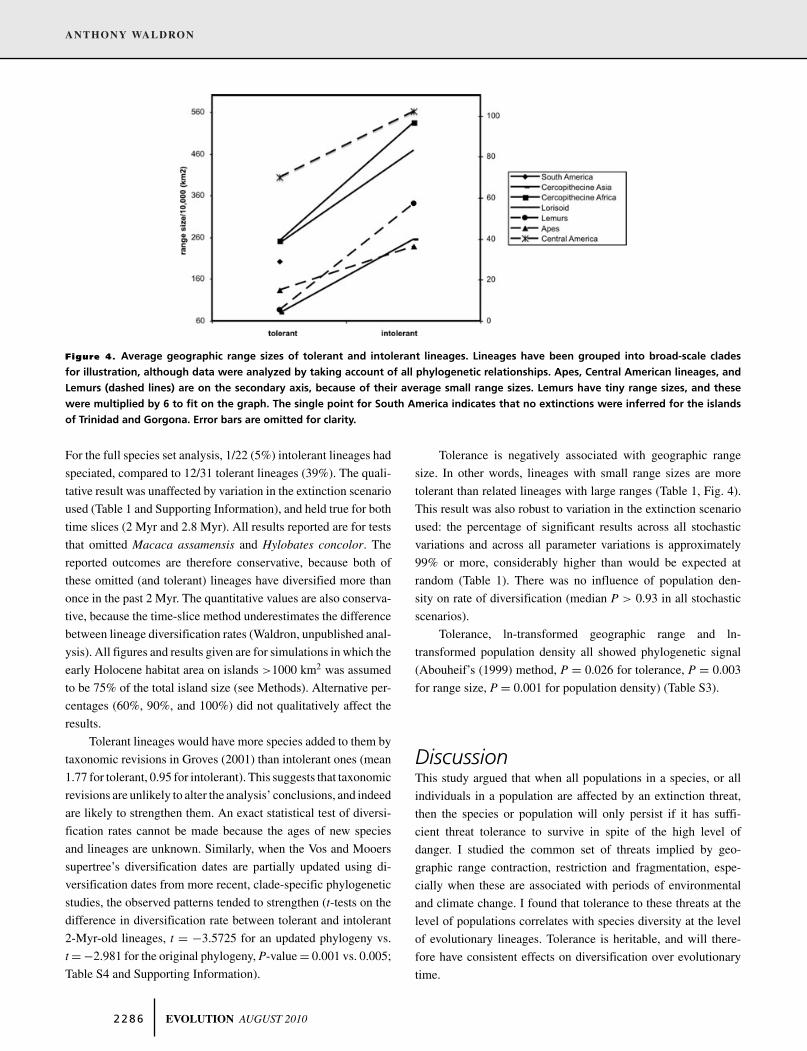
Figure 4. Average geographic range sizes of tolerant and intolerant lineages. Lineages have been grouped into broad-scale clades

for illustration, although data were analyzed by taking account of all phylogenetic relationships. Apes, Central American lineages, and

Lemurs (dashed lines) are on the secondary axis, because of their average small range sizes. Lemurs have tiny range sizes, and these

were multiplied by 6 to fit on the graph. The single point for South America indicates that no extinctions were inferred for the islands

of Trinidad and Gorgona. Error bars are omitted for clarity.

For the full species set analysis, 1/22 (5%) intolerant lineages had

speciated, compared to 12/31 tolerant lineages (39%). The quali-

tative result was unaffected by variation in the extinction scenario

used (Table 1 and Supporting Information), and held true for both

time slices (2 Myr and 2.8 Myr). All results reported are for tests

that omitted Macaca assamensis and Hylobates concolor. The

reported outcomes are therefore conservative, because both of

these omitted (and tolerant) lineages have diversified more than

once in the past 2 Myr. The quantitative values are also conserva-

tive, because the time-slice method underestimates the difference

between lineage diversification rates (Waldron, unpublished anal-

ysis). All figures and results given are for simulations in which the

early Holocene habitat area on islands >1000 km2 was assumed

to be 75% of the total island size (see Methods). Alternative per-

centages (60%, 90%, and 100%) did not qualitatively affect the

results.

Tolerant lineages would have more species added to them by

taxonomic revisions in Groves (2001) than intolerant ones (mean

1.77 for tolerant, 0.95 for intolerant). This suggests that taxonomic

revisions are unlikely to alter the analysis’ conclusions, and indeed

are likely to strengthen them. An exact statistical test of diversi-

fication rates cannot be made because the ages of new species

and lineages are unknown. Similarly, when the Vos and Mooers

supertree’s diversification dates are partially updated using di-

versification dates from more recent, clade-specific phylogenetic

studies, the observed patterns tended to strengthen (t-tests on the

difference in diversification rate between tolerant and intolerant

2-Myr-old lineages, t = −3.5725 for an updated phylogeny vs.

t = −2.981 for the original phylogeny, P-value = 0.001 vs. 0.005;

Table S4 and Supporting Information).

Tolerance is negatively associated with geographic range

size. In other words, lineages with small range sizes are more

tolerant than related lineages with large ranges (Table 1, Fig. 4).

This result was also robust to variation in the extinction scenario

used: the percentage of significant results across all stochastic

variations and across all parameter variations is approximately

99% or more, considerably higher than would be expected at

random (Table 1). There was no influence of population den-

sity on rate of diversification (median P > 0.93 in all stochastic

scenarios).

Tolerance, ln-transformed geographic range and ln-

transformed population density all showed phylogenetic signal

(Abouheif’s (1999) method, P = 0.026 for tolerance, P = 0.003

for range size, P = 0.001 for population density) (Table S3).

DiscussionThis study argued that when all populations in a species, or all

individuals in a population are affected by an extinction threat,

then the species or population will only persist if it has suffi-

cient threat tolerance to survive in spite of the high level of

danger. I studied the common set of threats implied by geo-

graphic range contraction, restriction and fragmentation, espe-

cially when these are associated with periods of environmental

and climate change. I found that tolerance to these threats at the

level of populations correlates with species diversity at the level

of evolutionary lineages. Tolerance is heritable, and will there-

fore have consistent effects on diversification over evolutionary

time.

2 2 8 6 EVOLUTION AUGUST 2010

LINEAGES THAT CHEAT DEATH

TOLERANCE AND CLASSIC EXTINCTION RESISTANCE

I also found that tolerance was unexpectedly correlated with small

range size. This suggests that tolerance represents a different type

of extinction-resistance from the resistance conferred by having a

large range size. Widespread species probably have low extinction

risk because threats are nearly always circumscribed in area, and

so some groups of individuals will lie outside the scope of each

passing threat (they “escape” threat). The implied mechanism

is that persistence occurs when threat levels are low, and threat

levels are always low for some population in a widespread species.

For tolerance, on the other hand, the implied mechanism is that

populations are surprisingly resistant when directly exposed to

threat, that is, when threat levels are high.

Tolerance and escape imply different relationships between

population extinction rates and species extinction risk. For es-

cape, individual population extinctions are largely irrelevant to

the overall persistence of the species, because other, unthreatened

populations exist elsewhere. For tolerance, population-level and

species-level persistence must be highly correlated, because it is

only the tolerance of populations that keeps the species afloat.

The link observed in this study between population persis-

tence and lineage diversity is most easily explained by a strong

correlation between the persistence of populations and species.

Global periods of hostile environmental change are likely to

tighten the relationship between population-level and species-

level persistence, because large numbers of species are reduced

to a few small and simultaneously threatened populations. During

more benign periods, the average global influence of escape on

species persistence may increase, and the influence of tolerance

may decrease.

High degrees of threat tolerance in rare lineages probably

represent the outcome of an evolutionary filter. Lineages that

have small (and fluctuating) range sizes will have been repeatedly

exposed to the dangers of range restriction throughout most of

their history. Geographically rare species also tend to consist of

several discrete populations (Maurer and Nott 1998) and to have

poor dispersal (Gaston 1994). Small populations, isolation, and

inability to migrate will therefore have been important parts of

the selective pressures experienced by most rare species, and rare

species unable to withstand these pressures should be pruned from

the tree of life. (See Stanley (1990) and Jablonski (2001) for a

similar idea that clades become more extinction-resistant over

time as more susceptible species are progressively pruned).

The precise ecological adaptations that allow rare species to

tolerate geographic restriction and isolation would be a topic for

future research. It seems possible that widespread, usually gen-

eralist species have high dispersal ability (Brown 1995) because

they must range widely in time and space to acquire resources.

Dispersal may also be an adaptive strategy responding more gen-

erally to unstable population dynamics, as has been shown in bee-

tles (Boer 1970; Glazier 1987). Species that experience extreme

variation in resource availability may be “obligate dispersers,” in

the sense that individuals must travel widely in ecological time

in order for the population to persist. Obligate dispersal may also

occur at the species level if species with unstable local popula-

tions depend upon high levels of dispersal in a metapopulation

structure to persist. Isolation in a small area would cause local

extinction in obligate-dispersing species.

DIVERSITY, LONGEVITY, AND EXTINCTION

Geographically rare species are short-lived in comparison to

widespread species (Jablonski 1987, 1995; Hunt et al. 2005).

Although tolerance must increase longevity, the small range size

of tolerant species therefore suggests that they are unlikely to

represent the longest-lived species in a taxon. However, species

diversity is the net difference between speciation events and ex-

tinction events, and so biological attributes that reduce extinction

rates relative to speciation rates will cause increases in lineage

diversity, whatever species life spans are in absolute terms. Ge-

ographical rarity is often associated with high speciation rates,

both for raw range size (Mayr 1963; Jackson 1974; Vrba 1980;

Stanley 1986; Vermeij 1987; Jablonski and Roy 2003), and for

the number of biomes used under Vrba’s resource-use hypoth-

esis (Vrba 1987, 1993; Hernandez Fernandez and Vrba 2005a;

Bofarull et al. 2008). However, the effect of this rapid specia-

tion on diversity may be nullified by the equally high species

extinction rates associated with rarity (Stanley 1979; Stanley

1986; Vrba 1992; McKinney 1997). A major impact of toler-

ance could be in reducing extinction rates in rare lineages, so that

their high speciation rates can become translated into high species

diversity.

More generally, tolerance of geographic restriction during

environmental change may allow species to persist long enough

to become widespread in the first place. Species tend to start

out with small range sizes (Vrba and DeGusta 2004; Liow and

Stenseth 2007; Waldron 2007). Species can later occupy large

geographic areas (Vrba and DeGusta 2004; Foote et al. 2007;

Liow and Stenseth 2007; Waldron 2007), but will need to survive

their potentially vulnerable early years to do so.

TOLERANCE AND THE SPECIATION PROCESS

Tolerance can bestow extinction resistance not only on newly

created species, but also on small, reproductively isolated popula-

tions that may go on to become new species. Peripatric speciation

involves the isolation of small populations as a mechanism of

speciation (Mayr 1963), and Stanley (1979), Glazier (1987), and

Allmon (1992) used the term “isolate selection” to describe the

idea that peripatrically speciating ancestor species would only

leave behind daughter species if those daughters could survive

the initial threat implied by smallness and isolation.

EVOLUTION AUGUST 2010 2 2 8 7

ANTHONY WALDRON

The overall importance of peripatric speciation to the ac-

cumulation of species diversity in lineages may be limited

(Barraclough and Vogler 2000). However, recent work suggests

that even the apparently dominant mode of allopatric speciation

(Barraclough and Vogler 2000; Phillimore et al. 2008) often splits

ancestral range so asymmetrically that it creates a daughter species

with a very small range size (Waldron 2007). The same is likely

to be true for sympatric speciation (Waldron 2007). Glazier’s and

Allmon’s ideas therefore apply to speciation in general. Indeed,

many modern species are thought to have arisen when species

became split into two small, isolated populations in fragmented

habitat refugia either during the Neogene (Vrba 1980, 1992, 1993;

Klicka and Zink 1997; Avise and Walker 1998; Weir and Schluter

2004).

Jansson and Dynesius (2002) have argued that range fluctu-

ations due to climate change are too short to trigger speciation,

because isolated populations will be reunited quickly when fur-

ther climate change causes the reexpansion of their ranges. Simi-

larly, Vrba (1992, 1995) indicates that full reproductive isolation

does not occur in all Milankovitch cycles, but only in the longest

ones. It is interesting to note that tolerance is associated here with

rare, probably low-dispersal species. Populations of low-dispersal

species may have so little gene flow between them that they re-

main isolated long after a glacial maximum ends and their ranges

begin to reexpand, as has been shown in birds (Price et al. 1997).

In addition, reproductive isolation can be the cumulative result of

repeated geographic isolations (Avise and Walker 1998), suggest-

ing that the frequency of the cycles and the rate at which species

reexpand their populations between cycles may be as important

as the duration of a single Milankovitch cycle.

POTENTIAL CONFOUNDS

The apparent link between tolerance and lineage diversity could

be artifactual, if tolerance were correlated with other factors

that independently increase diversification rates. However, the

traits generally believed to increase diversification in mammals—

generalism, high dispersal rates, and large range size itself are

positively correlated with geographic range size (Brown 1995;

Rosenzweig 1995; Gaston and Blackburn 1997; Owens et al.

1999; Cardillo et al. 2003; Isaac et al. 2003; Phillimore et al.

2006; Jablonski 2008). Tolerance, on the other hand, is negatively

correlated with range size in spite of its strong positive correlation

with diversification rate, suggesting its effect is independent of

other common factors that influence lineage diversity. In addi-

tion, the strongest general predictor of tolerance in the literature,

population abundance (Brown 1971; Diamond 1984; Laurance

et al. 2002; Lindenmayer 2006) has no relationship here with

diversification rate.

It is possible that some species populations go extinct from

landbridge islands for reasons that are unrelated to the extinction

pressures postulated here. For example, ground-nesting birds may

suffer higher rates of nest predation on the newly created island

that they did on the mainland (Karr 1982). These idiosyncratic

effects are unlikely to be consistently correlated with a low rate

of diversification across all species, and so would most probably

appear as error terms in the relationship between diversification

rate and tolerance.

A number of widespread species may have been on both

coast and island in the past, but have modern-day range limits a

few hundreds of kilometers short of the coast. If they had gone

extinct on islands, this would be undetectable from their present-

day distribution, and they would be wrongly omitted from the

list of intolerant species. Examples are Gorilla and Miopithecus

for Bioko, Symphalangus and Pongo for several of the Sunda

Shelf islands, Phaner and Avahi laniger in Madagascar (Harcourt

and Schwartz 2001; Meijaard and van der Zon 2003; Ganzhorn

et al. 2006). Although there is not enough evidence to confidently

state which of these species should and should not be included

as intolerants in formal analysis, none of these lineages have

diversified at all in the past 2 Myr (and some of them are indeed

among the slowest-diversifying of all primate lineages). Their

inclusion would only strengthen the conclusions found in this

study.

The geographic range size of species today may have been

dramatically altered by human influences, distorting the relation-

ship of range size and tolerance. For the observed patterns to

be an artifact of anthropogenic habitat reduction, human impacts

would need to universally cause dramatically bigger range col-

lapses in tolerant species than in intolerant species (see Fig. 4).

This seems an unlikely assumption, especially given that many

documented range collapses have occurred in intolerant species

such as gibbons and orangutan (this may in itself by an outcome

of their populations’ intolerance of reduced, fragmented habitat)

(Harcourt 1999; Geissman et al. 2000).

The phylogeny is not likely to be completely accurate, either

in its arrangement of species or in its diversification dates. This

could affect both the diversity of lineages, and the accuracy of

the timeslice method. However, modern taxonomic and phyloge-

netic revisions in species arrangement seem likely to strengthen

the diversity patterns observed (see Results and Supporting Infor-

mation). As regards dating errors, the diversification events for

most lineages occur millions of years away from the timeslice

dates chosen, especially in intolerant clades, and so the timeslices

for these lineages are likely to be robust to considerable error.

When dates do lie close to the timeslices, shifting those dates

will increase or decrease diversity almost exclusively in toler-

ant lineages. Date-shifted tolerant lineages will still have more

diversity on average than the universally monospecific intolerant

lineages, and so the overall conclusions are highly robust to dating

errors.

2 2 8 8 EVOLUTION AUGUST 2010

LINEAGES THAT CHEAT DEATH

It may be argued that large islands do not represent an ex-

tinction risk to all populations. Some populations may naturally

occupy areas less than, for example, the 11,900 km2 of the largest

island, and so insularization causes a mild threat at best via iso-

lation. There is surprisingly little information on the geographic

extent of primate populations that would permit measurement of

how much each population on each island has been truncated, but

the median size of islands is 290 km2, suggesting probable trun-

cation in many cases. I retested the correlations using only islands

of 2000 km2 or less, and again for 500 km2 or less, and found no

difference in the qualitative results. Nor are the tolerant species

somehow “island specialists”: they all have the great majority of

their distribution on the mainland.

Nevertheless, an alternative hypothesis to why some pop-

ulations persist in fragments is that these populations are less

truncated, and so suffer a lower level of threat (instead of hav-

ing a higher tolerance of threat). If the spatial extent of a species

correlates with the spatial extent of its individual populations (as

seems to be the case [Maurer and Nott 1998]), then geographi-

cally rare species will have less truncated populations in remnants

than widespread species. Rare species still have higher odds of

survival in remnants, but the main attribute causing differential

survival would be the natural geographic extent of a species’

populations.

RARITY HAS POSITIVE AND NEGATIVE EFFECTS

ON EXTINCTION RISK

A major implication of this study is that geographic rarity can have

both positive and negative effects on extinction risk. These effects

will depend on the severity and geographical extent of threats

themselves, and on the timescales involved. Rare species tolerate

range shrinkage better than common species (a positive impact of

rarity). On the other hand, tolerance can have no influence when

all habitat is wiped out, and such catastrophic destruction will

be experienced more often by rare species than by widespread

species (a negative impact of rarity). One implication is that toler-

ance may be a weaker influence at higher latitudes, where habitat

loss is more often catastrophic (Bennett et al. 1991; Jansson and

Dynesius 2002). I studied primates, whose tropical distribution

means they should often suffer habitat shrinkage rather than habi-

tat obliteration during climate change.

Similarly, it seems likely that few environmental changes

will be so widespread as to envelop every last population in a

widespread species. Species with large ranges therefore have their

tolerance tested only rarely, but may prove extinction-prone at the

population level when they are so tested. If environmental change

has been sufficiently severe to reduce a generally widespread

species to a few isolated populations, then the entire species has

a high risk of extinction because of its populations’ intolerance

of threat. Rare species, on the other hand, will frequently be en-

veloped by an extinction threat, but may prove extinction-resistant

so long as the threat is noncatastrophic.

Overall, the positive impacts of rarity on persistence seem

likely to operate over shorter timescales than the negative effects.

The results of this study suggest that the short-term effects last

long enough to leave a signature over the evolutionary timescales

associated with speciation and extinction. This is in keeping with

the observed periodicity of climate change over the past few mil-

lion years, with Milankovitch cycles occurring every 100,000 or

41,000 years, and as often as every 19,000–23,000 years (Berger

1988). Mammal species on average experience about 20 periods

of major climate change over their lifetimes (Vrba 1992), and it

would seem that this periodicity would certainly be rapid enough

to accord a significant role to tolerance.

The difference between the mechanisms of tolerance and

classic extinction resistance also suggests that as climate and en-

vironment cycles, there may be a shifting balance of selective

pressures on species. When habitat is widespread and continuous,

populations are much less fragmented, and generalists can dis-

perse in response to adverse local fluctuations. Classic extinction

resistance will have a strong influence on species persistence, and

widespread and generalist species will have low extinction risks.

But when climate change reduces habitat to small, isolated frag-

ments, tolerance becomes more important to species persistence,

and rare species may gain the persistence advantage (at least those

that lie within distributional reach of an environmental refuge).

Measurements of tolerance would also have clear usefulness

today in predicting the extinctions likely to result from anthro-

pogenic habitat loss, fragmentation, and climate change. Human

land use conversion has already caused habitat loss and fragmen-

tation to become the number one threat to species survival today

(Diamond 1984; Wilcove et al. 1998; Secretariat of the Conven-

tion on Biological Diversity 2006). Climate change will worsen

this situation, both because it will reduce some habitats further,

and because populations in isolated fragments cannot migrate in

response to environmental change. Tolerance will be a key deter-

minant of survival under such circumstances. But its unexpected

link with small range size suggests that some widely used pre-

dictors of extinction risk may be poor predictors of populations’

extinction risk in a hotter, more fragmented world.

ACKNOWLEDGMENTSThanks to D. Schluter, A. Mooers, S. Spade, J. Myers, J. Weir, P. Stephens,R. Hall, M. Hernandez Fernandez, and four anonymous referees for com-menting on previous versions of this manuscript, and to D. Schluter forassisting with the phylogenetic regression.

LITERATURE CITEDAbegg, C., and B. Thierry. 2002. Macaque evolution and dispersal in insular

south-east Asia. Biol. J. Linn. Soc. 75:555–576.Abouheif, E. 1999. A method for testing the assumption of phylogenetic

independence in comparative data. Evol. Ecol. Res. 1:895–909.

EVOLUTION AUGUST 2010 2 2 8 9

ANTHONY WALDRON

Allmon, W. D. 1992. A causal analysis of stages in allopatric speciation.Pp. 219–258 in D. J. Futuyma and J. Antonovics, eds. Oxford surveysin evolutionary biology. OUP, Oxford.

Avise, J. C., and D. Walker. 1998. Pleistocene phylogeographic effects onavian populations and the speciation process. P. R. Soc. Lond. B Biol.265:457–463.

Barraclough, T. G., and A. P. Vogler. 2000. Detecting the geographical patternof speciation from species-level phylogenies. Am. Nat. 155:419–434.

Barraclough, T. G., A. P. Vogler, and P. H. Harvey. 1998. Revealing the factorsthat promote speciation. Philos. T. R. Soc. B. 353:241–249.

Bennett, K. D., P. C. Tzedakis, and K. J. Willis. 1991. Quaternary Refugia ofNorth European Trees. J. Biogeogr. 18:103–115.

Berger, A. 1988. Milankovitch theory and climate. Rev. Geophys. 26:624–657.Bird, M. I., D. Taylor, and C. Hunt. 2005. Environments of insular Southeast

Asia during the Last Glacial Period: a savanna corridor in Sundaland?Quaternary Sci. Rev. 24:2228–2242.

Boecklen, W. J., and N. J. Gotelli. 1984. Island biogeographic theory andconservation practice – species-area or specious-area relationships. Biol.Conserv. 29:63–80.

Boecklen, W., and D. Simberloff. 1986. Area-based extinction models inconservation. Pp. 247–276 in D. K. Elliott, ed. Dynamics of extinction.John Wiley and Sons, New York.

Boer, P. J. D. 1970. On significance of dispersal power for populations ofCarabid-Beetles (Coleoptera, Carabidae). Oecologia 4:1–28.

Bofarull, A., A. Royo, M. Fernandez, E. Ortiz-Jaureguizar, and J. Morales.2008. Influence of continental history on the ecological specializationand macroevolutionary processes in the mammalian assemblage of SouthAmerica: differences between small and large mammals. BMC Evol.Biol. 8:97.

Bolger, D. T., A. C. Alberts, and M. E. Soule. 1991. Occurrence patternsof bird species in habitat fragments – sampling, extinction, and nestedspecies subsets. Am. Nat. 137:155–166.

Bonaccorso, E., I. Koch, and A. T. Peterson. 2006. Pleistocene fragmentationof Amazon species’ ranges. Divers Distrib. 12:157–164.

Brown, J. H. 1971. Mammals on mountaintops – nonequilibrium insular bio-geography. Am. Nat. 105:467–478.

———. 1995. Macroecology. University of Chicago Press, Chicago.Brown, J. H., and A. Kodric-Brown. 1977. Turnover rates in insular biogeog-

raphy: effect of immigration on extinction. Ecology 58:445–449.Cardillo, M., J. S. Huxtable, and L. Bromham. 2003. Geographic range size,

life history and rates of diversification in Australian mammals. J. Evol.Biol. 16:282–288.

Cardillo, M., J. L. Gittleman, and A. Purvis. 2008. Global patterns in thephylogenetic structure of island mammal assemblages. P. R. Soc. B.275:1549–1556.

Chakraborty, D., U. Ramakrishnan, J. Panor, C. Mishra, and A. Sinha. 2007.Phylogenetic relationships and morphometric affinities of the Arunachalmacaque Macaca munzala, a newly described primate from ArunachalPradesh, northeastern India. Mol. Phylogenet. Evol. 44:838–849.

Chatterjee, H. J. 2006. Phylogeny and biogeography of gibbons: a dispersal-vicariance analysis. Int. J. Primatol. 27:699–712.

Collins, A. C. 2004. Atelinae phylogenetic relationships: the trichotomy re-vived? Am. J. Phys. Anthropol. 124:285–296.

Cortes-Ortiz, L., E. Bermingham, C. Rico, E. Rodriguez-Luna, I. Sampaio,and M. Ruiz-Garcia. 2003. Molecular systematics and biogeography ofthe Neotropical monkey genus, Alouatta. Mol. Phylogenet. Evol. 26:64–81.

Cowlishaw, G. 1999. Predicting the pattern of decline of African primatediversity: an extinction debt from historical deforestation. Conserv. Biol.13:1183–1193.

Cronin, T. M., M. E. Raymo, and K. P. Kyle. 1996. Pliocene (3.2–2.4 Ma) os-

tracode faunal cycles and deep ocean circulation, North Atlantic Ocean.Geology 24:695–698.

Cronk, Q. C. B. 1997. Islands: stability, diversity, conservation. Biodivers.Conserv. 6:477–493.

Davis, M. B., and R. G. Shaw. 2001. Range shifts and adaptive responses toQuaternary climate change. Science 292:673–679.

Diamond, J. M. 1972. Biogeographic kinetics – estimation of relaxation-timesfor avifaunas of southwest pacific islands. Proc. Natl. Acad. Sci. USA69:3199–3203.

———. 1984. ‘Normal’ extinctions of isolated populations. Pp. 191–246 in

M. H. Nitecki, ed. Extinctions. University of Chicago Press, Chicago.Dynesius, M., and R. Jansson. 2000. Evolutionary consequences of changes

in species’ geographical distributions driven by Milankovitch climateoscillations. Proc. Natl. Acad. Sci. USA 97:9115–9120.

ESRI. 2005. ArcGIS 9.2. Environmental Systems Research Institute,Redlands, CA.

FAUNMAP Working Group. 1996. Spatial response of mammals to late Qua-ternary environmental fluctuations. Science 272:1601–1606.

Foote, M., J. S. Crampton, A. G. Beu, B. A. Marshall, R. A. Cooper, P. A.Maxwell, and I. Matcham. 2007. Rise and fall of species occupancy inCenozoic fossil mollusks. Science 318:1131–1134.

Ganzhorn, J. U., S. M. Goodman, S. Nash, and U. Thalmaan. 2006. Lemurbiogeography. Pp. 229–254 in S. M. Lehman and J. G. Fleagle, eds.Primate biogeography. Springer, New York.

Gaston, K. J. 1994. Rarity. Chapman and Hall, London.Gaston, K. J., and T. M. Blackburn. 1997. Age, area and avian diversification.

Biol. J. Linn. Soc. 62:239–253.Gavrilets, S. 1999. A dynamical theory of speciation on holey adaptive land-

scapes. Am. Nat. 154:1–22.Geissman, T., X. D. Nguyen, N. Lormee, and F. Momberg. 2000. Vietnam

primate conservation stauts review 2000: part 1, Gibbons. Fauna andFlora International, Indochina Programme, Hanoi.

Gilpin, M. E., and M. E. Soule. 1986. Minimum viable populations: theporcesses of species extinctions. Pp. 19–34 in M. Soule, ed. Conserva-tion biology: the science of scarcity and diversity. Sinauer Associates,Sunderland, MA.

Glazier, D. S. 1987. Toward a predictive theory of speciation – the ecology ofisolate selection. J. Theor. Biol. 126:323–333.

Gotelli, N. J., and G. R. Graves. 1990. Body size and the occurrence of avianspecies on land-bridge islands. J. Biogeogr. 17:315–325.

Grafen, A. 1989. The phylogenetic regression. Philos. T. R. Soc. B. 326:119–157.

Groves, C. 2001. Primate taxonomy. Smithsonian Institute Press, Washington.Haffer, J. 1997. Alternative models of vertebrate speciation in Amazonia: an

overview. Biodivers. Conserv. 6:451–476.Haila, Y., and O. Jarvinen. 1983. Land bird communities on a Finnish Island –

species impoverishment and abundance patterns. Oikos 41:255–273.Harcourt, A. H. 1999. Biogeographic relationships of primates on South-East

Asian islands. Global Ecol. Biogeogr. 8:55–61.Harcourt, A. H., and M. W. Schwartz. 2001. Primate evolution: a biology of

Holocene extinction and survival on the southeast Asian Sunda Shelfislands. Am. J. Phys. Anthropol. 114:4–17.

Heaney, L. R. 1986. Biogeography of mammals in Se Asia – estimates of ratesof colonization, extinction and speciation. Biol. J. Linn. Soc. 28:127–165.

Henle, K., D. B. Lindenmayer, C. R. Margules, D. A. Saunders, and C. Wissel.2004. Species survival in fragmented landscapes: where are we now?Biodivers. Conserv. 13:1–8.

Hernandez Fernandez, M., and E. Vrba. 2005a. Macroevolutionary processesand biomic specialization: testing the resource-use hypothesis. Evol.Ecol. 19:199–219.

2 2 9 0 EVOLUTION AUGUST 2010

LINEAGES THAT CHEAT DEATH

———. 2005b. Macroevolutionary processes and biomic specialization: test-ing the resource-use hypothesis. Evol. Ecol. 19:199–219.

Hill, J. L., P. J. Curran, and G. M. Foody. 1994. The effect of sampling on thespecies-area curve. Global Ecol. Biogeogr. Lett. 4:97–106.

Hubbell, S. P. 2001. The unified neutral theory of biodiversity and biogeogra-phy. Princeton University Press, Princeton, NJ.

Hunt, G., K. Roy, and D. Jablonski. 2005. Species-level heritability reaffirmed:a comment on “On the heritability of geographic range sizes”. Am. Nat.166:129–135.

Hurlbert, A. H., and W. Jetz. 2007. Species richness, hotspots, and the scaledependence of range maps in ecology and conservation. Proc. Natl.Acad. Sci. USA 104:13384–13389.

Isaac, N. J. B., P. M. Agapow, P. H. Harvey, and A. Purvis. 2003. Phyloge-netically nested comparisons for testing correlates of species richness: asimulation study of continuous variables. Evolution 57:18–26.

Jablonski, D. 1987. Heritability at the species level – analysis of geographicranges of cretaceous mollusks. Science 238:360–363.

———. 1995. Extinction in the fossil record. Pp. 25–44 in R. M. May andJ. H. Lawton, eds. Extinction rates. Oxford University Press, Oxford.

———. 2001. Lessons from the past: evolutionary impacts of mass extinc-tions. PNAS 98:5393–5398.

———. 2007. Scale and hierarchy in macroevolution. Palaeontology 50:87–109.

———. 2008. Species selection: theory and data. Annu. Rev. Ecol. Evol. S39:501–524.

Jablonski, D., and K. Roy. 2003. Geographical range and speciation infossil and living molluscs. Proc. R. Soc. Lond. B. Biol. 270:401–406.

Jackson, J. B. C. 1974. Biogeographic Consequences of Eurytopy and Steno-topy among Marine Bivalves and Their Evolutionary Significance. Am.Nat. 108:541–560.

Jansson, R., and M. Dynesius. 2002. The fate of clades in a world of recurrentclimatic change: milankovitch oscillations and evolution. Annu. Rev.Ecol. Syst. 33:741–777.

Karr, J. R. 1982. Avian extinction on Barro-Colorado Island, Panama – aReassessment. Am Nat 119:220–239.

Klicka, J., and R. M. Zink. 1997. The importance of recent ice ages in speci-ation: a failed paradigm. Science 277:1666–1669.

Koch, C. F. 1980. Bivalve species duration, areal extent and population-sizein a Cretaceous Sea. Paleobiology 6:184–192.

Lande, R. 1993. Risks of population extinction from demographic and envi-ronmental stochasticity and random catastrophes. Am. Nat. 142:911–927.

Laurance, W. F., T. E. Lovejoy, H. L. Vasconcelos, E. M. Bruna, R. K. Didham,P. C. Stouffer, C. Gascon, R. O. Bierregaard, S. G. Laurance, and E.Sampaio. 2002. Ecosystem decay of Amazonian forest fragments: a22-year investigation. Conserv. Biol. 16:605–618.

Lawton, J. H., G. Daily, and I. Newton. 1994. Population-Dynamic Principles.Philos. T. R. Soc. B 344:61–68.

Leitner, W. A., and M. L. Rosenzweig. 1997. Nested species-area curves andstochastic sampling: a new theory. Oikos 79:503–512.

Lindenmayer, D. B. A. F. J. 2006. Habitat fragmentation and landscape change.Island Press, Washington, DC.

Liow, L. H., and N. C. Stenseth. 2007. The rise and fall of species: implicationsfor macroevolutionary and macroecological studies. Proc. R. Soc. B.274:2745–2752.

Lomolino, M. V. 1986. Mammalian Community Structure on Islands – theImportance of Immigration, Extinction and Interactive Effects. Biol. J.Linn. Soc. 28:1–21.

Losos, J. B., and R. E. Glor. 2003. Phylogenetic comparative methods and thegeography of speciation. Trends Ecol. Evol. 18:220–227.

MacArthur, R. H., and E. O. Wilson. 1967. The Theory of Island Biogeogra-phy. Princeton University Press, Princeton, NJ.

Marzluff, J. M., and K. P. Dial. 1991. Life-History Correlates of TaxonomicDiversity. Ecology 72:428–439.

Maurer, B. A., and M. P. Nott. 1998. Geographic range fragmentation and theevolution of biological diversity. Pp. 31–50 in M. L. McKinney and J.A. Drake, eds. Biodiversity dynamics: turnover of populations, taxa andcommunities. Columbia University Press, New York.

Mayr, E. 1963. Animal species and evolution. Harvard University Press,Cambridge, MA.

McKinney, M. L. 1997. Extinction vulnerability and selectivity: combiningecological and paleontological views. Annu. Rev. Ecol. Syst. 28:495–516.

Meijaard, E., and A. P. M. Van Der Zon. 2003. Mammals of south-east Asianislands and their Late Pleistocene environments. J. Biogeogr. 30:1245–1257.

Newmark, W. D. 1995. Extinction of Mammal Populations in Western North-American National-Parks. Conserv. Biol. 9:512–526.

Nieves, M., M. S. Ascunce, M. I. Rahn, and M. D. Mudry. 2005. Phylogeneticrelationships among some Ateles species: the use of chromosomic andmolecular characters. Primates 46:155–164.

Overpeck, J. T., R. S. Webb, and T. Webb. 1992. Mapping Eastern North-American Vegetation Change of the Past 18 Ka – No-Analogs and theFuture. Geology 20:1071–1074.

Owens, I. P. F., P. M. Bennett, and P. H. Harvey. 1999. Species richness amongbirds: body size, life history, sexual selection or ecology? Proc. R. Soc.Lond. B Biol. 266:933–939.

Paradis, E., J. Claude, and K. Strimmer. 2004. APE: analyses of Phylogeneticsand Evolution in R language. Bioinformatics 20:289–290.

Phillimore, A. B., R. P. Freckleton, C. D. L. Orme, and I. P. F. Owens. 2006.Ecology predicts large-scale patterns of phylogenetic diversification inbirds. Am. Nat. 168:220–229.

Phillimore, A. B., C. D. L. Orme, G. H. Thomas, T. M. Blackburn, P. M.Bennett, K. J. Gaston, and I. P. F. Owens. 2008. Sympatric speciationin birds is rare: insights from range data and simulations. Am. Nat.171:646–657.

Pimm, S. L., and R. A. Askins. 1995. Forest losses predict bird extinctions ineastern north-america. Proc. Natl. Acad. Sci. USA 92:9343–9347.

Preston, F. W. 1962. Canonical Distribution of Commonness and Rarity.1.Ecology 43:185–215.

Price, T. D., A. J. Helbig, and A. D. Richman. 1997. Evolution of breed-ing distributions in the old world leaf warblers (genus Phylloscopus).Evolution 51:552–561.

Purvis, A., M. Cardillo, R. Grenyer, and B. Collen. 2005. Correlates ofextinction risk: phylogeny, biology, threat and scale. Pp. 295–316 in

A. Purvis, J. L. Gittleman, and T. Brooks, eds. Phylogeny and Conser-vation. Cambridge University Press, Cambridge.

Purvis, A., K. E. Jones, and G. M. Mace. 2000. Extinction. Bioessays 22:1123–1133.

R Development Core Team. 2005. R: 2.2.1: a language and environment forstatistical computing. R Foundation for Statistical Computing, Vienna.

Rohling, E. J., M. Fenton, F. J. Jorissen, P. Bertrand, G. Ganssen, andJ. P. Caulet. 1998. Magnitudes of sea-level lowstands of the past500,000 years. Nature 394:162–165.

Rosenzweig, M. L. 1995. Species diversity in space and time. CUP,Cambridge.

Secretariat of the Convention on Biological Diversity. 2006. Global Biodiver-sity Outlook. Montreal.

Simberloff, D. 1986a. The proximate causes of extinction. Pp. 259–276 in D.M. Raup and D. Jablonski, eds. Patterns and processes in the history oflife. Springer-Verlag, Berlin.

EVOLUTION AUGUST 2010 2 2 9 1

ANTHONY WALDRON

———. 1986b. The proximate causes of extinction. Pp. 259–276 in D. M.Raup and D. Jablonski, eds. Patterns and processes in the history of life.Springer-Verlag, Berlin.

Simberloff, D. S., and L. G. Abele. 1975. Island biogeography theory andconservation practice. Science 191:285–286.

Simberloff, D., and L. G. Abele. 1982. Refuge design and island biogeographictheory – effects of fragmentation. Am Nat 120:41–50.

Soberon, J., and J. Llorente. 1993. The use of species accumulation functionsfor the prediction of species richness. Conserv Biol 7:480–488.

Stanley, S. M. 1979. Macroevolution. Freeman, San Francisco.———. 1986. Population-size, extinction, and speciation – the fission effect

in Neogene Bivalvia. Paleobiology 12:89–110.———. 1990. Delayed recovery and the spacing of major extinctions. Paleo-

biology 16:401–114.Terborgh, J., and B. Winter. 1980. Some causes of extinction. Pp. 119–

133 in M. E. Soule and B. A. Wilcox, eds. Conservation biology: anevolutionary-ecological perspective. Sinauer, Sunderland, MA.

Tosi, A. J., K. M. Detwiler, and T. R. Disotell. 2005. X-chromosomal windowinto the evolutionary history of the guenons (Primates: Cercopithecini).Mol. Phylogenet. Evol. 36:58–66.

Vermeij, G. J. 1987. The Dispersal Barrier in the Tropical Pacific – Impli-cations for Molluscan Speciation and Extinction. Evolution 41:1046–1058.

Vos, R. A., and A. O. Mooers. 2006. A new dated supertree of the primates.Inferring large phylogenies: the big tree problem. PhD thesis. SimonFraser University.

Vrba, E. S. 1980. Evolution, species and fossils – how does life evolve. S. Afr.J. Sci. 76:61–84.

Vrba, E. 1987. Ecology in relation to speciation rates; some case histories ofMiocene-Recent mammal Clades. Evol. Ecol. 1:283–300.

Vrba, E. S. 1992. Mammals as a key to evolutionary-theory. J. Mammal73:1–28.

———. 1993. Turnover-pulses, the red queen, and related topics. Am. J. Sci.293A:418–452.

———. 1995. On the connections between paleoclimate and evolution. Pp.24–45 in E. S. Vrba, G. H. Denton, T. C. Partridge, and L. H. Burckle(eds.), Paleoclimate and Evolution, with Emphasis on Human Origins.Yale University Press, New Haven.

Vrba, E. S., and D. DeGusta. 2004. Do species populations really start small?New perspectives from the Late Neogene fossil record of African mam-mals. Philos. T. R. Soc. B 359:285–292.

Waldron, A. 2007. Null models of geographic range size evolution reaffirmits heritability. Am. Nat. 170:221–231.

Webb, T., and P. J. Bartlein. 1992. Global changes during the last 3 millionyears – climatic controls and biotic responses. Annu. Rev. Ecol. Syst.23:141–173.

Weir, J. T., and D. Schluter. 2004. Ice sheets promote speciation in borealbirds. Proc. R. Soc. Lond. B. Biol. 271:1881–1887.

Wilcove, D. S., D. Rothstein, J. Dubow, A. Phillips, and E. Losos. 1998.Quantifying threats to imperiled species in the United States. Bioscience48:607–615.

Wilcox, B. A. 1978. Super-saturated island faunas – species-age relationshipfor lizards on post-pleistocene land-bridge islands. Science 199:996–998.

Associate Editor: G. Hunt

Supporting InformationThe following supporting information is available for this article:

Table S1. Islands used, primates associated with them, and number of extinctions.

Table S2. Tolerance and biology of island primate species.

Table S3. Phylogenetic signal in traits used in this study.

Table S4. The effect of incorporating modern phylogenetic revisions on the outcome of a t-test comparing diversification rates

between tolerant and intolerant clades (full species set model).

Supporting Information may be found in the online version of this article.

Please note: Wiley-Blackwell is not responsible for the content or functionality of any supporting information supplied by the

authors. Any queries (other than missing material) should be directed to the corresponding author for the article.

2 2 9 2 EVOLUTION AUGUST 2010