Linear growth rate of structure in parametrized post-Friedmannian universes

arX

iv:1

003.

4231

v2 [

astr

o-ph

.CO

] 2

7 M

ay 2

010

The linear growth rate of structure in Parametrized Post Friedmannian Universes

Pedro G. Ferreira∗

Oxford Astrophysics, Physics, DWB, Keble Road, Oxford, OX1 3RH, UK

Constantinos Skordis†

School of Physics and Astronomy, University of Nottingham, University Park, Nottingham, NG7 2RD,UK

A possible solution to the dark energy problem is that Einstein’s theory of general relativityis modified. A suite of models have been proposed that, in general, are unable to predict thecorrect amount of large scale structure in the distribution of galaxies or anisotropies in the CosmicMicrowave Background. It has been argued, however, that it should be possible to constrain ageneral class of theories of modified gravity by focusing on properties such as the growing mode,gravitational slip and the effective, time varying Newton’s constant. We show that assuming certainphysical requirements such as stability, metricity and gauge invariance, it is possible to come up withconsistency conditions between these various parameters. In this paper we focus on theories whichhave, at most, 2nd derivatives in the metric variables and find restrictions that shed light on currentand future experimental constraints without having to resort to a (as yet unknown) complete theoryof modified gravity. We claim that future measurements of the growth of structure on small scales(i.e. from 1-200 h−1 Mpc) may lead to tight constraints on both dark energy and modified theoriesof gravity.

I. INTRODUCTION

The dark energy problem, i.e. the possibility that 70%of the Universe seems to be permeated by an invisiblefluid which behaves repulsively under gravity and doesnot cluster, has been the focus of research in cosmologyfor over decade. There are a host of proposals [1] and abattery of experiments are under way, or on the drawingboard, to characterize the nature of this elusive source ofenergy [2–5].

In recent years, an alternative possibility has emerged,that Einstein’s General theory of relativity is incorrecton cosmological scales and must be modified. Althoughthe idea that General Relativity is incomplete has beenaround since the early 1960s [6–9], there are now a num-ber of proposals for what this theory of modified grav-ity might be [10]. The Einstein-Hilbert action, Sg ∝∫

d4x√−gR (where g is the metric determinant and R

is the scalar curvature of a metric gab) can be replacedby a more general form Sg ∝

∫

d4x√−gF (R) where F

is an appropriately chosen function of R [11, 12]; thedynamics of the gravitational field can emerge from atheory in higher dimensions such as one might encounterin brane worlds [13]; a preferred reference frame mayemerge from the spontaneous symmetry breaking of localLorentz symmetry [14–17]; the metric which satisfies theEinstein equation is not necessarily the one that definesgeodesic motion [18] but is related to a second metricvia additional fields [19–21] or connections [22–24]; theEinstein-Hilbert action may be deformed by choosing asfundamental variables of gravity, SU(2) connections [25–27].

∗Electronic address: [email protected]†Electronic address: [email protected]

Many of these models have been successful in repro-ducing, for example, the observed relation between red-shift and luminosity distances from distant supernovae.They have, however, generally failed to reproduce theobserved clustering of galaxies on large scales as well asthe anisotropies in the Cosmic Microwave Background(CMB) unless the modified theory becomes effectivelyequivalent to general relativity (i.e. the Einstein-Hilbertaction and a cosmological constant), e.g. [28–30]. Thegeneral problem that seems to plague most theories isan excess of power on the very largest scales which man-ifests itself through the Integrated Sachs Wolfe (ISW)effect and a mismatch between the normalization of thepower spectrum of fluctuations on the largest and small-est scales. As yet, a truly compelling and viable modelof modified theory of gravity has yet to be but forwardwhich may resolve the dark energy problem.All is not lost, however, and progress can be made

in learning about potential modifications to gravity byextracting phenomenogical properties that can be com-pared to observation- the ”Parametrized Post Friedman-nian” approach [31]. In this paper we focus on a key ob-servable characterizing the evolution of large scale struc-ture: the growing mode of gravitational collapse.The time evolution of the density field can be a sen-

sitive probe of not only the expansion rate of the theUniverse but also its matter content. In a flat, matterdominated universe we have that δM , the density con-trast of matter, evolves as δM ∝ a where a is the scalefactor of the Universe. We can parametrize deviationsfrom this behaviour in terms of γ [32–35] through

γ ≡ln[

δMHδM

]

lnΩM

(1)

where ΩM is the fractional density of matter, H = aaand

overdots are derivatives with regards to conformal time,

http://arxiv.org/abs/1003.4231v2

mailto:[email protected]

mailto:[email protected]

2

τ . For standard growth in the presence of a cosmologicalconstant, one has that γ ≈ 6/11 to a very good approxi-mation. This is not true over a wide range of values forΩM . In fact, in Figure 1 we can see that γ deviates fromits early-universe asymptotic value as ΩM → 0. A natu-ral question to ask is how γ depends on different aspectsof the Universe and how might use it to constrain darkenergy and modifications to gravity. In this paper we willfocus on a few of these properties.

FIG. 1: The solid line is the growth parameter, γ, for a ΛCDMuniverse, as a function of ΩM . For small values of ΩΛ, γ is wellapproximated by 6/11 (dashed line) but there are deviationsas ΩΛ grows; we find errors of 0.7%, 3.3% and 4.2% whenΩM = 0.7, 0.3 and 0.05.

One important property of the Universe is the equationof state of dark energy, characterized by the constant (orfunction of time), w:

PE = wρE . (2)

PE and ρE are the pressure and energy densities of thedark energy. The function w may be time varying and isrelated to the adiabatic speed of sound c2a as

c2a = w − w

3H(1 + w)(3)

Another important property is gravitational slip, ζ,which is normally defined to be

Φ−Ψ ≡ ζΦ (4)

where we are taking a linearly perturbed metric in theconformal Newtonian gauge,

ds2 = −a2(1 + 2Ψ)dτ2 + a2(1− 2Φ)d~x2. (5)

Such a parametrization has been advocated in a numberof papers on modified gravity [36–42] and it has beenshown that it can lead to a number of observational ef-fects. Albeit simple, and appealing, such a parametriza-tion of slip is not necessarily general and, as we shall seein the next section, necessarily implies other non-trivialmodifications to the gravitational sector. Such modifi-cations are, in general, not explicitely acknowledged but

may correspond to unexpected assumptions about anyputative, underlying theory. Hence a more general as-sumption (at least within the context of 2nd order the-ories) would be that gravitational slip would depend on

Φ and Φ (this is explained in more detail in section-IIDand in [43])Finally, we can define an effective Newton’s constant in

the relativistic Newton-Poisson equation

∇2Φ = 4πa2Geff

∑

X

ρX [δX + 3(1 + wX)a

aθX ]

where δX is the density contrast and θX is the momentumof the cosmological fluid X which has an equation of statewX . We can define the dimensionless function

µ2 ≡ G

Geff

(6)

where G is the ”bare” Newton constant. It then makessense to try to constrain (γ, w, ζ and µ) in the hope thatit may be possible to shed light on a possible theory ofmodified gravity.Although there alternative proposals [44, 45], a num-

ber of groups have have pioneered the use of this simpleparametrization of modified gravity (in terms of ζ, µ2 orboth): in [36, 37] it was argued that gravitational slipmight be a generic prediction for modified theories ofgravity, in [38, 39] it was shown that it would be pos-sible to constrain it through cross correlations of theCMB with galaxy surveys and in [46] from the ISW ef-fect; weak lensing has been proposed as a possible routefor constraining these parameters [47–49] with a tenta-tive detection of modification being proposed in [41, 50].Much is expected from applying these methods to futureambitious experiments that will map out the large scalestructure of the Universe. Indeed constraints of GeneralRelativity are a core element of the science that could beextracted from the Euclid experiment [3].Given that such an approach is phenomenological, the

general attitude has been to leave these parameters com-pletely free. There is merit to such an approach in thatone isn’t restricting oneself to a particular theory andhence constraints will be general. It is true however thatis is possible to idenitfy (reasonably general) consistencyconditions for (γ, w, ζ and µ), contingent on specificphysical assumptions. In this paper we state these as-sumptions and present restrictions on (γ, w,ζ and µ).We shall use the formalism first proposed by one of us[43]which spells out how to build consistent modifications togravity.This paper is structured as follows. In Section II we re-

cap the formalism presented in [43] and relate it to the pa-rameters we wish to study phenomenologically. We dis-cuss how the consistency conditions reduce the freedomto choose arbitrary (γ, ζ, µ2). In Section III we imple-ment the consistency conditions and find a relationshipbetween the parameters by looking at the evolution equa-tion for the density contrast in matter for small wave-lengths. In doing so, we find find analytic expressions for

3

the relationships and briefly assess the range of scale towhich they are applicable. In Section IV we find analyticexpressions for γ to 2nd order for a general parametriza-tion which is consistent with the Parametrized Post New-tonian approximation on small scales.In Section V we dis-cuss the generality of the results and how they may beextended to other, more exotic models.

II. THE FORMALISM

We now summarize the formalism, the details of whichcan be found in the [43]: we present the field equations,the evolution equations for the fluid components and theconsistency conditions for modifications to the field equa-tions. We shall further assume a spatially flat universe,but our results can be easily generalized to include cur-vature.

A. The background cosmology

As discussed in [43], the background equations forany theory of gravity for which the metric is Friedman-Robertson-Walker (FRW) can be recast in the usual formused in GR. The Friedman equation simply reads

3H2 = 8πGa2∑

X

ρX (7)

In addition to the Friedman equation we also have theRaychaudhuri equation −2 a

a+ H2 = 8πGa2

∑

X PX .With the help of the Friedman equation, in a universecontaining only pressureless matter and dark energy (asis approximately the case in the late universe) the Ray-chaudhuri equation may be rewritten as

H = −1

2H2(1 + 3wΩE) (8)

The dark energy density ρE and w, may be in gen-eral a function of additional degrees of freedom, thescale factor a or H. For example, for F (R) one gets

ρE = 12 (RFR − F ) − 3H

a2 FR − 3H2

a2 FR. But this ex-plicit dependence of ρE (or of w) is irrelevant. Onemay always treat ρE as a standard fluid with a time-varying equation of state w subject to energy conserva-tion ρE + 3H(1 +w)ρE = 0 (but note that there may beadditional field equations that determine the time depen-dence of w). In a universe containing only pressurelessmatter and dark energy, the energy conservation equa-tion for dark energy can be rewritten as

ΩE = −3HwΩMΩE (9)

Our discussion above has one important consequence:that one cannot distinguish modifications of gravity fromordinary fluid dark energy using observables based onFRW alone. As discussed in [43], and further below,the situation changes drastically once we consider linearfluctuations.

B. The field equations.

The idea is to parameterize deviations from Einsteingravity at a linear level. Schematically we can write themodified Einstein equations in the form

δGmodµν = δGµν − δUµν = 8πGδTµν + 8πGδTDE

µν (10)

Note that for a tensor F we use δF to indicate a linearperturbation of F and we assume that δUab is made ofthe scalar metric perturbations and their derivatives. Letus also stress that the background tensor correspondingto Uab, i.e. Uab vanishes. We assume that ”normal mat-ter” (i.e. baryons, dark matter, neutrinos and photons)are contained in Tµν and that dark energy, or any nonmetric degrees of freedom that behave like dark energy(such as a scalar field- quintessence- or a dark fluid), arecontained in TDE

µν . In this paper we will restrict ourselvesto two fluids: Tµν is the energy-momentum tensor for apressureless fluid with density ρM , density contrast δMand momentum θM while TDE

µν is the energy momentumtensor of a fluid with density ρDE , density contrast δDE

and θDE which can be characterized defined in terms of(possibly time varying) equation of state and sound speed(we shall use the approach of [51] to model a quintessencelike fluid with a constant equation of state.The field equations can be rewritten in the following

form

− 2k2Φ = 8πGa2∑

X

ρX [δX + 3(1 + wX)HθX ]

+U∆ + 3HUθ (11)

2(Φ +HΨ) = 8πGa2∑

X

(ρX + PX)θX + Uθ (12)

d

dτ(Φ +HΨ) = 4πGa2ρEΠE +

1

6UP +

1

3∇2UΣ

−2H(Φ +HΨ) + (H2 − H)Ψ

Φ−Ψ = UΣ (13)

As advertised, the U terms contain modifications to grav-ity and we have used the notation from [43]: U∆ ≡−a2U0

0,~∇iUθ = −a2U0

i, UP = a2U ii and [~∇i~∇j −

13~∇2δij ]UΣ = a2(U i

j − 13U

kkδ

ij). Further, we have pa-

rameterized the dark energy pressure perturbation ΠE ≡δPE/ρE as

ΠE = c2sδE + 3(c2s − c2a)(1 + w)HθE (14)

For adiabatic fluids, as is the case of radiation and CDM,cs = ca and we get ΠE = c2sδE . In general, however,cs 6= ca and may in fact be a function of space as well astime.

C. The fluid equations.

It is convenient to define ∆X = δX − 3(1 + wX)Φ forX = M,DE. We then have that the equations of motion

4

for the fluids [51] are:

∆M = −k2θM

θM = −HθM +Ψ

∆E = 3H(w − c2s)∆E − (1 + w)k2θE

−9(1 + w)H(c2s − c2a) [Φ +HθE ]

θE = (3c2s − 1)HθE + c2s

(

1

1 + w∆E + 3Φ

)

+Ψ (15)

D. The consistency conditions.

In principle, one should be able to choose arbitrarycombinations of metric perturbations to go in the tensorU . Yet in [43] it was argued that by assuming a set ofgeneral properties, it is possible to restrict the form of U .For the purpose of this paper, we shall choose the generaltheory of gravity to satisfy the following restrictions:

1. The fundamental geometric degree of freedom is the

metric. This encompasses most modified theoriesof gravity including the first order Palatini (torsion-less) formulations (where the connection Γc

ab is in-dependent of the metric at the level of the action)or purely affine theories [52], provided a metric canbe defined.

2. The field equations are at most 2nd order. This doesrestrict the class of acceptable theories (for exam-ple F (R) theories have generally higher derivatives)but it has become clear that it is these higher or-der terms that lead (again) to instabilities in thegeneration of large scale structure.

3. The field equations are gauge-form invariant.

Gauge form-invariance is the linearized version ofthe full diffeomorphism invariance of any gravita-tional theory with a manifold structure. It is theunbroken symmetry of the field equations undergauge transformations. After a gauge transforma-tion, the field equations retain their exact form :they are f orm-invariant (see [53–56] for furtherdiscussion).

It is of course possible to relax some of these conditionsand we will discuss how in the conclusions.Armed with these conditions we can construct U in

Fourier space solely out of Φ and Φ such that: U∆ =k2AΦ, Uθ = kBΦ, UP = k2C1Φ + kC2Φ and UΣ =D1Φ + D2Φ/k. All operators above (e.g. A ) are di-

mensionless. Terms such as Φ, Ψ and Ψ (and higherderivatives) are forbidden while terms proportional to Ψare allowed but their coefficients vanish as a result of theBianchi identities. This last fact is a consequence of theconsistency conditions outlined above and the reader isreferred to [43] for a more thorough treatment.We can rearrange (11) in the form of (6) to immeadi-

ately read off

µ2 = 1 +A+ 3HkB

2.

where we let Hk ≡ H/k.Furthermore we have that the shear field equation be-

comes

Φ−Ψ = ζΦ +g

kΦ

where we have let ζ = D1 and g = D2.We see that the gravitational slip Φ − Ψ will gener-

ally depend on both Φ and its time derivative, Φ, andnot solely on Φ. Defining Φ = γPPFΨ as has been inproposed in [38, 39], we find that

γPPF [Φ] =1

1− ζ − gkd ln Φdτ

≈ 1 + ζ +g

k

d lnΦ

dτ(16)

Thus unless g = 0, γPPF is an explicit functional of Φ,introducing interesting enviromental dependance on thematter distribution. All parameterizations of the slipused so far, for which Φ − Ψ ∝ Φ, have ignored thispossibility which suggests that they were over simplistic(although see [31]).As shown in [43], as a result of the Bianchi identities

we have ∇aUab = 0, leading to a series of restrictions on

the coefficients:

A = H2Hkg + 2k(2H2k +

13 )g − 2Hζ

H − H2 − k2

3

B = − k

3HA− 2

3g

C1 =3

k(B + 2HB) + 2ζ = −A− 1

H [A+ kB]

C2 = − k

HA (17)

This means a consistent modification to the Einsteinequations is uniquely determined by two arbitrary freefunctions, ζ(τ, k) and g(τ, k).Finally we can combine the expression for A and B

appropriately to find that g has a simple interpretationas a perturbation of the effective gravitational constant :

µ2 = 1− Hkg (18)

Hence the consistency conditions lead to an importantrelationship between a generalized form of the gravita-tional slip. In particular, if we consider time variations

of the Newtonian potential, it is inconsistent to consider

a restricted parametrization of the gravitational slip of

the form Φ−Ψ = ζΦ on all scales. [66].

E. Parameterizing ζ and g

We are not assuming any particular underlying the-ory of modified gravity and hence do not have a specificmodel for ζ and g. Our interest is in theories that maymimic the behaviour of dark energy so we expect devi-ations from Einstein gravity to emerge as ΩE begins todiverge from 0. A simple assumption is to assume that

5

the gravitational slip is analytic at ΩE = 0 and Taylorexpand it:

ζ = ζ1ΩE + ζ2Ω2E +O(Ω3

E) (19)

We can do the same for g so that

g = g1ΩE + g2Ω2E +O(Ω3

E) (20)

In Section III we find how the growth depends on sucha parametrization and, in particular, determine analyticexpressions for γ.This way of parameterizing ζ and g has three major

advantages :

• It is in the spirit of the Parametrized Post-Newtonian (PPN) formalism where the PPN pa-rameters are isolated from the potentials which aredependent on the density profiles and thus the so-lutions; the role of the ”potential” in this case istaken by ΩE(τ) which depends on the backgroundcosmology.

• Expanding in powers of ΩE isolates the backgroundeffects of the dark energy from the genuine effectsof the perturbations. In particular, the dark en-ergy relative density Ω0E or the dark matter rela-tive density Ω0m would have no effect on the pa-rameters ζi and gi.

• This expansion makes mathematical sense for anyanalytic function, as the function ΩE(τ) is alwaysbounded to be 0 ≤ ΩE ≤ 1, i.e. it is a naturalysmall parameter.

Note that we have dropped any k dependence from thisparametrization. There are two ways that k-dependencecan enter, either relative to a fixed scale k0 (which may bepart of some theory of gravity) or relative to the Hubblescale H. If we wish to see how our results are affectedby a scale dependence relative to the temporal changesintroduced by the FRW background we can extend theparametrization to

ζ = ζ(0) + ζ(1)Hk

g = g(0) + g(1)Hk (21)

where, as above, we have

ζ(0) = ζ01ΩE +O(Ω2E)

ζ(1) = ζ11ΩE +O(Ω2E) (22)

and likewise with g(0) and g(1).It turns out that, if we attempt to, on one hand gen-

eralize our parametrization of ζ and g, but, on the otherhand pin it down so as to be consistent with PPN methodused on much smaller scales, we need to change our previ-ous approach. It is entirely possible that there are otherscales in the system. Furthermore, as we show in in Ap-pendix A, to leading order we may have g ∝ Hm

k wherem is negative. These can complicate the simple model

we considered above. For example, consider the func-tion f = eℓH where ℓ is a fixed scale. How does oneexpand this on small scales? One would be tempted towrite f = eℓkHk ≈ 1 + ℓkHk = 1 + ℓH but this clearlymakes no sense. The scale k was artificially introducedand leads to erroneous conclusions.In general we have a function ζ(τ, k). Since ζ is dimen-

sionless while τ and k are not, the functional dependenceon τ and k must come in dimensionless combinations.It is convinient to exchange τ with either τ(H) or withτ(ΩE). Thus the most general function ζ will have theform ζ = ζ(ΩE ,Hk, ℓH, k/k0) for constants ℓ and k0, andthere may be additional dimensionless parameters enter-ing. We can thus isolate the leading-order dependence ofζ on Hk and write

ζ = ζL(ΩE , k)Hnk (23)

for a constant n. We expand g in a similar way as

g = gL(ΩE , k)Hmk (24)

for a constant m. In Appendix A we show that a consis-tent PPN limit fixes n = 0 and m = −1.Thus we arrive at our general expansion of ζ and g in

the small scale limit, which is consistent with PPN:

ζ = ζ(0)

g = g(−1) 1

Hk

ζ(0) = ζ1ΩE + ζ2Ω2E + ζ3Ω

3E (25)

g(−1) = g1ΩE + g2Ω2E + g3Ω

3E (26)

The parameters ζi and gi may in principle be k-dependent, e.g. ζ1 ∝ (k/k0)

N for a fixed scale k0 andpower index N . We shall not investigate this furtherin this work but we stress it as a possibility and notethat our results would include these cases. In Section IVwe conclude by presenting and analysing the resultinggrowth rate due to such a parametrization.

III. THE GROWTH RATE ON SMALL SCALESFOR A SIMPLIFIED MODEL OF ζ AND g

The definition of γ originally arose when characteriz-ing the evolution of small scale density perturbations.We expect it to be particularly useful when characteriz-ing the growth of structure on small scales (by which wemean roughly between 1 and 200h−1 Mpc) as would beprobed by galaxy redshift surveys (through redshift mea-surements of the power spectrum, for example, or redshiftspace distortions [57–59]) and weak lensing surveys.In this section we focus on the behaviour of this sys-

tem in the limit in which Hk ≡ H/k ≪ 1, i.e. onscales deep inside the horizon. We can then assume that∆DE ≃ θDE ≃ 0. This is true for c2s ∼ O(1) or larger.Since in this paper we are concerned with modificationsof gravity rather than the speed of sound we will leave

6

the full treatment of small c2s for a future investigation.We shall, however, show the effect of small c2s numericallyfuther below.In what follows we will present a modified evolution

equation, find analytic expressions for the growth factorand compare to numerical results for the full system.

A. Evolution of density perturbations

Combining the fluid equations (15) in one 2nd orderequation, we find that ∆M obeys

∆M +H U ∆M − 3

2ΩMH2 V∆M = 0 (27)

with the damping coefficient modified by

U [ζ, g] = 1 +3ΩMHk

2(1−Hkg)

g

+3Hk [1− ζ − gB/2]

1−Hkg + 9H2kΩM/2

(28)

and the response term modified by.

V [ζ, g] =1− ζ − gB/2

(1−Hkg)(1 + 9H2kΩM/2−Hkg)

(29)

Specifying ζ and g completely fixes U and V .If we further take the provisional small scale limit

Hk ≪ 1 (i.e. without assuming anything about ζ andg) we find that

U [ζ, g] = 1 +3ΩMHk

2(1−Hkg)

g +3Hk [1− ζ − gB/2]

1−Hkg

(30)

and

V [ζ, g] =1− ζ − gB/2

(1−Hkg)2(31)

The full small scale limit, including ζ and g is presentedin appendix A.

B. Analytic expressions for the growing mode

We expect modifications of gravity to kick in when theexpansion rate starts to deviate from matter domination.In this section we will work with the parametrization ofζ and g proposed in equations (19) and (20). We canimmediately see from equations (30) and (31) that theeffects from g will only come in at orderHk. We shall alsorestrict ourselves to constant w and leave varying w forsection IV. In this section we shall present the derivationand result to first order in ΩE and then present the resultto second order in ΩE .The starting point is

∆M +H∆M − 3H2ΩM

2(1− ζ1ΩE)∆M = 0

Changing variables to ln a and defining ∆M = aY , wecan rewrite this equation as

Y ′′ +5− 3wΩE

2Y ′ +

3

2ΩE [1− w + ζ1ΩM ]Y = 0

where we have used the Raychauduri equation (8) andwhere we set ()′ = d

d ln a.

Changing variables to ΩE and using the 0th order fluidconservation equation, rewritten as Ω′

E = −3wΩMΩE wefind

3w2Ω2MΩ2

E

d2Y

dΩ2E

+w

2ΩMΩE [3w(2 − 3ΩE)− 5]

dY

dΩE

+1

2[ΩE(1− w) + ζ1ΩMΩE ]Y = 0 (32)

Equation (32) has a three regular singular points (atΩE = 0 and ΩE = 1) and can therefore be transformedinto the hypergeometric equation. We wish to find itsbehaviour around ΩE = 0 and do so by expanding Y ,Y = 1 + Y1ΩE to find (to lowest order in ΩE)

Y1 =1− w + ζ1w(5− 6w)

and hence

∆M = a

[

1 +1− w + ζ1w(5− 6w)

ΩE

]

Therefore to O(ΩE)

ln∆M = ln a+1− w + ζ1w(5− 6w)

ΩE

which we can use to find the logarithmic derivative of thegrowth factor f ≡ d ln∆M/d ln a:

f = 1− 3(1− w + ζ1)

5− 6wΩE

As stated above, we are parametrizing the growth factorusing f = Ωγ

M and so we have that

γ = γ0 =3(1− w + ζ1)

5− 6w(33)

where the subsciript 0 is due to the fact that this is thelowest order approximation.We can easily see that, for w = −1 and ζ1 = 0 we

retrieve γ = 6/11 ≃ 0.54545..., the approximation firstproposed in [32] and subsequently rederived and advo-cated in [60] and [33]. If we assume a more general (butconstant) equation of state, we improve on the approxi-mation advocated in [33].It is possible to further improve the approximation by

going to next order in ΩE . For this we need Y and ζ toO(Ω2

E), i.e. Y = 1+Y1ΩE+Y2Ω2E and ζ = ζ1ΩE+ζ2Ω

2E .

. We now have that

γ = γ0 + γ1ΩE (34)

7

where γ0 is as derived above and given in (33) and

γ1 =3w

2

[

−3Y1 − (2− 3w)Y 21 + 4Y2

]

(35)

where we have defined

Y2 =(1− w)(15w2 − 4w − 1) + ζ1(9w

2 + 2w − 2)

2w2(12w − 5)(5− 6w)

− ζ21 + w(5 − 6w)ζ22w2(12w − 5)(5− 6w)

(36)

In the case of w = −1 (i.e. the cosmological constant)and ζ = 0 we find that expression (35) reduces to

γ1 =15

2057

As stated above assuming that g can be parametrizedin the same way as ζ, independently of Hk, we find thatit does not affect the growth of structure on small scales.The situation is of course different if we consider expand-ing 1−µ2 = gHk in powers of ΩE with coefficients whichare Hk independent.

C. Comparison with numerical results

We can solve (13), (15) and (17) to assess the qual-ity of this analytic approximation. We first restrict our-selves to a dark energy like fluid with a large sound speed,c2s ∼ O(1), (such as a quintessence model or most otherfield like models) and assume no modifications to grav-ity. We see a number of features in Figure 2. First ofall, γ is very clearly not independent of ΩM as has beengenerally assumed. In fact as ΩM → 0, γ deviates sub-stantially from its asymptotic value at ΩM = 1. Never-theless, we find that (35) is a good aproximation to thetrue behaviour. In Figure 2 we plot the true and approx-imate behaviours of γ for w = −1, −0.8, −0.6 and −0.4:we find deviations of at most a ten percent for w = −0.4at ΩM = 0.1.We may relax the condition c2s = 1 substantially before

the dark energy perturbations affect the growing modein the density field. This is clearly illustrated in Figure 3where, for w = −0.6, three different values of the soundspeed are chosen: c2s = 5 × 10−4, c2s = 10−5 c2s = 10−6

and c2s = 0. For c2s = 5 × 10−4, the growth is still in-distinguishable from c2s = 1 and only once the jean scalefor the dark energy falls susbtantially below the cosmo-logical horizon is the effect noticeable. In particular ourresults hold for values cs such that cs > 10 ∼ Hk, whichapproximately translates to c2s >∼ 3× 10−4.We note in passing that the effects of the speed of

sound without modifications of gravity, have been studiedin [61–63]. In particular [63] have found fitting formulasfor γ which interpolate between cs = 0 and cs ∼ O(1).However, those fitting formulas do not account for modi-fications of gravity and are in fact quite model dependent(they depend on the background cosmology). The cur-rent constraints on the speed of sound do not rule out

FIG. 2: The growth parameter, γ, for a selection of dark en-ergy models, as a function of ΩM . The dashed curves are thenumerical results for w = −1, −0.8, −0.6 and −0.4 in ascend-ing order and the corresponding analytic approximations areplotted in solid line.

small values [64] and in fact they are consistent withcs = 0. Since this work concerns the effects of modi-fications of gravity rather than effects coming from thespeed of sound, however, we leave the case for small csfor a future investigation.

FIG. 3: The growth parameter, γ, for a selection of darkenergy models where w = −0.6 and the sound speed is chosento be c2s = 5 × 10−4, c2s = 10−5, c2s = 10−6 and c2s = 0 indescending order from the top of the figure, as a function ofΩM .Let us now introduce modifications to gravity and as-

sume a non-negligible gravitational slip. In Figures 4 and5 we show how well the analytic approximation fares incomparison to different values of ζ1 and ζ2 ( in these fig-ures we restrict ourselves to w = −1 but the agreementbetween the numerical and approximate estimates of γ

8

is generic). In Figure 4 we restrict ourselves to a gravi-tational slip which is linear in ΩE and identify the twomain effects. First of all, the quicker the onset of slip, themore effective the supression of growth due to the onsetof dark energy- γ0 increases with ζ1. Furthermore, thedependence of γ on ΩE , through γ1, changes sign so thatfor larger ζ1, γ becames smaller as ΩM decreases.

FIG. 4: The growth parameter, γ, for a selection of gravita-tional slip parameters of the form ζ = ζ1ΩE , as a function ofΩM . The dashed curves are the numerical results for ζ1 = 0,0.2, 0.4 and 0.6 in ascending order and the corresponding an-alytic approximations are plotted in solid line.

This last effect is further affected by ζ2. Indeed wefind that the slope of γ as function of ΩM can greatly beaffected by higher order terms in ζ.

FIG. 5: The growth parameter, γ, for a selection of gravi-tational slip parameters of the form ζ = ζ1ΩE + ζ2Ω

2

E , as afunction of ΩM . The dashed curves are the numerical resultsfor ζ1 = 0.2 and ζ2 = 0, 0.125, 0.2 and 0.4 and the corre-sponding analytic approximations are plotted in solid line.

D. Intermediate and large scales

While the γ parametrization is particularly useful onsmall scales where terms dependent on Hk can be dis-carded, this isn’t true once we look at horizon crossing,i.e. Hk ≃ 1. This regime will be of particular impor-tance for measurements of the cosmic microwave back-ground and using the Integrated Sachs-Wolfe effect tolook for the presence of dark energy or modified gravity[38, 39, 46, 65]. Let us now consider the parametrizationpresented in equations (21)We expand eq. (27) to include the first order term in

Hk which gives

∆M +H[

1 +3HkΩM

2g(0)

]

∆M − 3

2ΩMH2

1− ζ(0)

+Hk

[

g(0)(

2− ζ(0))

− ζ(1)]

∆M = 0 (37)

where the functions ζ(0), ζ(1)and g(0) are further ex-panded in powers of ΩE using equation (22). We applythe same techniques as in section III B above, and expandγ as

γ = γ(0) + γ(1)Hk

where the coefficients γ(0) and γ(1) are further expandedin powers of ΩE , i.e. γ(0) = γ00 + O(ΩE). Carryingthrough the expansion we find that

γ(0) = 31− w + ζ015− 6w

+O(ΩE) (38)

γ(1) =27

4

3ζ201 + 2ζ11 − 2g013w − 1

+O(ΩE) (39)

There are now 3 free modified gravity constants: ζ01, ζ11and g01. Notice how the first order correction in Hk to γonly depends on the modified gravity parameters and iszero for wCDM , i.e. corrections in Hk to γ for wCDMcome to second order.We find that scale dependent corrections in powers of

Hk are always subdominant compared with correctionsin powers of ΩE , or corrections with respect to a fixedscale, e.g. ∼ (ℓk)N . They are thus effectively negligible.We find that at k ∼ 0.04hMpc−1 corrections in powersof Hk are around 1% at redshift z = 1 for ζ11 = −0.6and become smaller at larger k (smaller scales), or lowerredshift (z ∼ 0). Hence, it perfectly reasonable to discardscale dependent corrections which come in powers of Hk.

IV. GENERAL EVOLUTION OF ζ AND g

We now wish to address a more realistic expansion ofthe ζ and g proposed in the Section II which is consistentwith the PPN approximation on small scales, namely (25)and (26). Having in mind our findings in section IIID onintermediate scales, we disregard any dependence of ∆M

(and hence of γ) on Hk, and therefore to this order wecan set ∆M = δM .

9

We perform the calculation in steps. First, we solve the2nd order differential equation obeyed by δ by applying aTaylor series expansion in ΩE , resulting in a set of coef-ficients Y1, Y2, Y3 which are functions of the expansioncoefficients of w, U and V . Then we relate the a perturba-tive expansion coefficients for δ, namely Y1, Y2, Y3, tothe γ parameter. Finally we relate Y1, Y2, Y3 for gen-eral U and V to the specific case of our gζCDM model.

A. Perturbative solution of the δ-equation

We start with the equation for the matter density con-trast in the absence of DE perturbations, namely

δM +HU δM − 3H2ΩM

2VδM = 0 (40)

Changing the independent variable from τ to ln a and thedependent variable from δM to Y defined by Y ≡ δM/a,we get

Y ′′ +

[

U +3

2(1− wΩE)

]

Y ′

+

[

U +1

2(1− 3wΩE)−

3ΩM

2V]

Y = 0 (41)

On small scales we may expand Y (k, τ) = Y (0)(k, τ) +Y (1)(k, τ)Hk +O(H2

k) (see appendix A), where the func-

tional coefficients Y (i)(k, τ) have no dependence on Hk

but may still be k or τ dependent through combinationsof the form ℓk or τ/ℓ (where ℓ is some scale, not neces-sarily the same scale for all such combinations). We areinterested in the small-scale limit Hk → 0, and we shallwork with Y (k, τ) = Y (0)(ℓk,ΩE) only. As discussedin section IIID above, at the scale of validity of the γparameterization Hk-corrections are always small and ir-relevant. Since time dependence only comes through τ/ℓfor some scale ℓ we may further exchange τ/ℓ with afunction of ΩE , thus we let Y (k, τ) = Y (k,ΩE).We now Taylor expand Y (k,ΩE) in powers of ΩE . To

get γ to O(Ω2E) we need to expand Y to O(Ω3

E) as

Y = 1 + Y1ΩE + Y2Ω2E + Y3Ω

3E (42)

We then use the above expansion (42) into (41) andmatch orders [67]. To be able to do that we need to ex-pand the functions w, U and V . Since w always appearsin the combination wΩE we only need it to O(Ω2

E). Thefunctions U and V , however, are needed to O(Ω3

E). Thuswe expand

w = w0 + w1ΩE + w2Ω2E (43)

U = 1 + U1ΩE + U2Ω2E + U3Ω

3E (44)

V = 1 + V1ΩE + V2Ω2E + V3Ω

3E (45)

While wi are constants, the Ui and Vi coefficients may bek-dependent, for example U1 = U01(

kk0

)N for some index

N and scale k0. Using the expansions (42), (43), (44)and (45) into (41) and equating orders in ΩE we find

Y1 =−1 + w0 + V1 − 2

3U1

w0(6w0 − 5)

Y2 =1

2w0(12w0 − 5)

w1 + V2 − V1 −2

3U2

+

[

− 1− 2

3U1 + V1 + 5w1

+w0(−4 + 2U1 + 15w0 − 18w1)

]

Y1

Y3 =1

3w0(18w0 − 5)

V3 −2

3U3 − V2 + w2

+

[

V2 −2

3U2 − V1 − 4w1 + 5w2 + 2w1 (U1 − 6w1)

+w0 (−2U1 + 2U2 − 9w0 + 42w1 − 24w2)

]

Y1

+

[

− 1− 2

3U1 + V1 − 9w0 + 10w1

+2w0 (2U1 + 27w0 − 30w1)

]

Y2

(46)

We notice that in general there are 9 initial coefficientsappearing in (40) that determine only 3 final coefficientsYi for the solution to (40).Having found the coefficients Yi we proceed to relate

them to γ.

B. From δ to γ

We can now use the definition of the logarithmicchange of the growth-rate f = d ln δ

d ln aand then get γ from

γ = ln f/ lnΩM . We find that γ is expanded as

γ = γ0 + γ1ΩE + γ2Ω2E (47)

where

γ0 = 3w0Y1

γ1 = −γ0

(

3

2+ Y1 −

1

2γ0

)

+ 3w1Y1 + 6w0Y2

γ2 = γ0

(

−11

6− 1

2γ0 +

1

3γ20

)

− 3

2γ1

+1

2

[

6w1γ0 + 6w2 − γ20 − 3γ0 − 2γ1

]

Y1

+ [−(1− 6w0)γ0 + 6w1]Y2 + 9w0Y3 (48)

Given a set of coefficients Y1, Y2, Y3, w0, w1, w2 wecan get γ(ΩE). Note that Y1, Y2, Y3 may be k-dependent, for example Y1 = Y01(

kk0

)N for some indexN and scale k0.One important point is in order. What we have done

so far is more general than the approach we discussed inthe main part of the article. In particular the derivation

10

of the γ coefficients in this appendix would hold for anytheory for which the density contrast obeys (40). Onesuch theory is DGP, even though strictly speaking DGPdoes not fit within our framework of the main part of thearticle.To connect the γ coefficients above with our framework

we must perform a third step : relate the Ui and Vi

coefficients with expansions of g and ζ.

C. Relating to the gζCDM model

As shown in the appendix A, to be consistent withultra-small scale quasistatic limit the functions ζ and gmust have the form ζ = ζ(0)+O(Hk) and Hkg = g(−1)+O(Hk). As discussed in the last part of section II E, wefurther expand ζ(0) and g(−1) as

ζ(0) = ζ1ΩE + ζ2Ω2E + ζ3Ω

3E (49)

and

g(−1) = g1ΩE + g2Ω2E + g3Ω

3E (50)

respectively, where the coefficients may once again be k-dependent. To lowest order in Hk we find

U1 =3

2g1

U2 =3

2

[

g2 − g1 + g21]

U3 =3

2

[

g3 − g2 + g21(g1 − 1) + 2g1g2]

V1 = 2g1 − ζ1

V2 = 2g2 + (2 + 3w0)g21 − g1ζ1 − ζ2

V3 = 2g3 + 2(1 + 3w0)g31 + (3w1 − 3w0 − ζ1)g

21

+g1g2(4 + 9w0)− g2ζ1 − g1ζ2 − ζ3 (51)

These expressions may then be used with (46) and (48)to find the γ coefficients.

D. Comparison with Numerical Results

The fitting formulas we have derived map theoreticalproperties of the gravitational field onto the observable,γ. This allows us to circumvent the use of a full cosmo-logical perturbation code when trying to observationallyconstrain the µ2, ζ and g via the growth of structure.We have already seen how well such an approach faresfor the simplified model we used in Section III. We nowbriefly show how the general framework fares- note thatthe model for g and ζ matches onto the PPN and we havefound the expansion of γ to second order in ΩE . Both ofthese properties should allow us to span a wide range ofpossible models.If we focus first on the gravitational slip, we can see

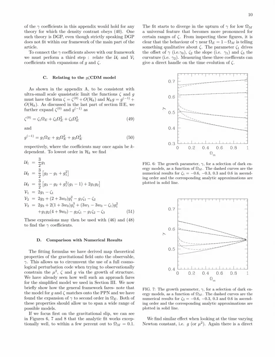
in Figures 6, 7 and 8 that the analytic fit works excep-tionally well, to within a few percent out to ΩM = 0.1.

The fit starts to diverge in the upturn of γ for low ΩM

a universal feature that becomes more pronounced forcertain ranges of ζ. From inspecting these figures, it isclear that the behaviour of γ near ΩE = 1−ΩM is tellingsomething qualitative about ζ. The parameter ζ1 drivesthe offset of γ (i.e.γ0), ζ2 the slope (i.e. γ1) and ζ3 thecurvature (i.e. γ2). Measuring these three coefficents cangive a direct handle on the time evolution of ζ.

FIG. 6: The growth parameter, γ, for a selection of dark en-ergy models, as a function of ΩM . The dashed curves are thenumerical results for ζ1 = −0.6, −0.3, 0.3 and 0.6 in ascend-ing order and the corresponding analytic approximations areplotted in solid line.


We find similar effect when looking at the time varyingNewton constant, i.e. g (or µ2). Again there is a direct

11


mapping between g1, g2 and g3 and γ0, γ1 and γ2. Theaccuracy of the approximation breaks down for smallervalues of ΩM yet is still excellent in the range of interestfor observational cosmology. For small values of ΩE heaccuracy is less than a percent and really only becomeslarge (of order 5− 10%) for ΩM < 0.1.

FIG. 9: The growth parameter, γ, for a selection of dark en-ergy models, as a function of ΩM . The dashed curves are thenumerical results for g1 = −0.4, −0.2, 0.2 and 0.4 in descend-ing order and the corresponding analytic approximations areplotted in solid line.



V. DISCUSSION

Let us briefly recap what we have done. The mainpoint of this paper is that, when introducing modifica-tions to gravity in linear perturbation theory, one musttake into account the consistency conditions in the fieldequations. These necessarily lead to restrictions in theform of the modifications that can be introduced. Mostnotably, and within the context of second order theories,this means that if one wishes to include modifications to

12

the Newton-Poisson equation, then one cannot consider

the simplified gravitational slip, Ψ = ζΦ, and must in-clude an extra term such that Ψ = ζΦ + (g/k)Φ wheregkH = 1 − Geff/G0. If we wish to construct a proper

”Parametrized Post Friedmanian” approach to modifiedgravity, any parameter we introduce must be independentof the environment or initial conditions in the perturba-tions. The only way to do this is to use the parametriza-tion we are advocating. To our knowledge, all attemptsat studying cosmological deviations from general relativ-ity have ignored this and hence it is unclear what class oftheories they map onto and which types of theories arebeing constrained.

Having taken this point on board, we have found theexpression for the growth parameter on small scales interms of both the gravitational slip, ζ and the modifiedNewton constant, µ2 = 1 − g

kH. Given a set of cosmo-

logical constraints on γ and its dependence on ΩM , it isnow straightforward to calculate constraints on ζ and g.The growth parameter is given by equation (47) whichcan be seen as a Taylor expansion in terms of 1 − ΩM .The coefficients in this expansion, γ0, γ1 and γ2 can beexpressed in terms of the equation of state, w (see Equa-tion 43), ζ (see Equation 25) and g (see Equation 26)by using equations (51), followed by equations (46) andfinally equations (48).

With these relations in hand, it is now possible to usecosmological observations to place constraints on the-ories of modified gravity. In this paper we have fo-cused on small scales (by which we mean between 1 and200h−1Mpc), scales that should be probed by redshiftspace distortion measurements, galaxy power spectra andweak lensing. Furthermore, we can now do this con-sistently, relating modifications in the growth rate withchanges in the gravitational slip. This is of particularimportance when considering weak lensing where obser-vations probe Φ + Ψ. It is also clear from our analysisthat we have come up against the limitations of the γparametrization: it is useful and effective on very smallscales but not on scales comparable to the cosmologicalhorizon. On those scales, one should be using the full setof field equations. We therefore do not advocate usingour fitting formula to the growth on larger scales such aswould be probed by the Integrated Sach-Wolfe.

How general is this method? We have declared fromthe outset, the class of theories that we are considering.They must be metric, with 2nd order equations and sat-isfy gauge form-invariance. From what we have learntabout modifications of gravity, these seem a reasonableset of conditions to apply- they lead to theories whichare less likely to be marred by gross instabilities either atthe classical or quantum level. We should point out thatall other attempts at developing such a parametrizationhave implicitely made these assumptions although havenot necessarily done so self-consistently. It is possible toextend this analysis beyond the scope of these theories.If we are to go beyond 2nd order, one must include termsin Φ or even higher. The Bianchi conditions will, again,

impose a set of constraints on the coefficients of theseterms and should allow a similar type of analysis.Two well studied theores are worth mentioning. F (R),

F (RµνRµν), etc, theories come with up-to four timederivatives in the field equations. Thus they do not falldirectly within the methods of this paper but do underthe general scheme outlined in [43]. In this case one

would have to include terms involving Φ, Φ, Ψ and Ψin to the G00 and G0i Einstein equations, while the Gij

equations would need...Φ and Ψ in addition. Theories with

higher derivatives are a subject that warrants further in-vestigation and have yet to be properly incorporated inany parametrized modifications of standard general rela-tivity.One other theory, studied extensively is the DGP the-

ory [13]. In this case, only two time derivatives arepresent in the field equations and just like our frame,DGP contains two non-metric dynamical degrees of free-dom, which can be effectively written ad δE and θE .However, our framework cannot encompass DGP becauseDGP cannot be written as a generalized fluid as we haveassumed of dark energy in this work (hence it is not a fail-ure of our use of δUab). Nevertheless, our γ parameteri-zation in powers of ΩE is still valid, and indeed needed.In the case of DGP we find that

γ =11

16+

7

5632ΩE − 93

4096Ω2

E (52)

gives an error on γ around 5% at ΩM < 0.1, droppingto 2% at ΩM ∼ 0.2 and < 1% for larger values of ΩM .The error on the corresponding density contrast at thosevalues of ΩM is < 2%, ∼ 1% and < 0.5% respectively.Notice how the coefficients are entirely fixed and do notdepend on the only free parameter of the theory, namelythe scale rc. Rather rc comes to play a role only throughΩE = 1

Hrc.

Acknowledgements

We are grateful to Tim Clifton, Tom Zlosnik and JoeZuntz. This work was supported by the BIPAC.

Appendix A: The quasistatic limit : connecting tothe Parametrized Post Newtonian (PPN) approach

We reduce our equations to small scales and slow ex-pansions. To make contact with the PPN expansion,we will write the Einstein equations in powers of the 3-velocity v. The 3-velocity is related to the 4-velocity byui = a−1vi. In this gauge, for scalar perturbations we get

ui = a−1~∇iθ, so that vi = ~∇iθ. Hence θ = −k−2~∇ivi.

Letting v =√vivi we get on dimensional grounds kθ = v.

The PPN order bookkeeping is k ∂∂τ

≡ ()′ ∼ O(v) and

Φ ∼ Ψ ∼ δρ ∼ O(v2). The same bookkeeping prescrip-tion holds in our case, and in addition, we also haveHk ∼ O(v) and ∆M ∼ δM ∼ O(0).We are now ready to find the small scale limit which

is consistent with PPN. We start from the operators A,

13

B, C1 and C2. Since H′k = − 1

2H2k(1 + 3wΩE) and Ω′

E =

−3HkwΩMΩE , and letting J = H2k(1 + wΩE) we get

A = −3Hk

2Hk(g′ − ζ) + 2(2H2

k +13 )g

1 + 92J

→ 6Hk

[

Hkζ −1

3g

]

B =2Hk(g

′ − ζ) +H2k(1− 3wΩE)g

1 + 92J

→ Hk [−2ζ + 2g′ +Hk(1 − 3wΩE)g]

C1 = −6Hk

1

1 + 92J

ζ′ +1

(1 + 92J)

2

2 + 9H2k(1 + 3wΩE)

−27H4k

[

1 + wΩE + 3w2ΩMΩE

]

ζ

+6Hk

1

1 + 92J

g′′ +3H2

k

(1 + 92J)

2

4− 6wΩE

+27H2k

[

1 + wΩE + w2ΩMΩE

]

g′

+3H3

k

(1 + 92J)

2

1− 6wΩE + 9w2ΩE

+9H2k

[

1− 2wΩE + 6w2ΩE − 9w2Ω2E

]

g

→ 2ζ + 3Hk

[

2g′′ + 2Hk(2 − 3wΩE)g′

+H2k(1 − 6wΩE + 9w2ΩE)g

]

and

C2 = 32Hk(g

′ − ζ) + 2(2H2k +

13 )g

1 + 92J

→ 6

[

−Hkζ +1

3g

]

where → denotes taking only the lowest order terms thatcan contribute to the small scale limit.

Now consider the Einstein equations. In the small scalelimit we get

−2k2Φ− 6H(Φ +HΨ) = 8πGa2ρδ

+6H[

Hζ − 1

3kg

]

Φ, (A1)

2(Φ +HΨ) = 8πGa2ρθ

+H [−2ζ + 2g′ +Hk(1− 3wΩE)g] Φ, (A2)

6d

dτ

(

Φ +HΨ)

+ 12H(Φ +HΨ) + 2k2(Φ−Ψ) =

−3(EF + ER)Ψ + k2

2ζ + 3Hk

[

2g′′

+H2k(1− 6wΩE + 9w2ΩE)g

]

+2Hk(2− 3wΩE)g′

Φ+ 2 [−3Hζ + kg] Φ, (A3)

and

Φ−Ψ = ζΦ +g

kΦ (A4)

As argued in Section II we expand ζ in powers of Hk

and write

ζ = ζL(ΩE , k)Hnk (A5)

to leading order. We expand g in a similar way as

g = gL(ΩE , k)Hmk (A6)

The goal now is to find the smallest powers m and n thatcan be consistent with the Einstein equations as Hk → 0.It is easily seen that ζ′ = ζ1Hn+1

k for some functionζ1(ΩE , k) which is found to be

ζL1 = −n

2(1 + 3wΩE)ζL − 3wΩMΩE

∂ζL∂ΩE

(A7)

Similarly we have g′ = gL1Hm+1k and g′′ = gL2Hm+2

k andsimilar expressions to (A7) can be found for gL1 and gL2.Consider again the Einstein equations and now keep

on the lowest orders for each variable. For example Φ isO(2) while (EF + ER)Ψ = O(4) and Φ = O(4) etc. Weget

−2k2Φ = 8πGa2ρδ + 6k2Hk

[

ζLHn+1k − 1

3gLHm

k

]

Φ,

(A8)

2(Φ +HΨ) = 8πGa2ρθ +H[

− 2ζLHnk + 2gL1Hm+1

k

+(1− 3wΩE)gLHm+1k

]

Φ, (A9)

and

Φ−Ψ =

ζLHnk + 3Hm+3

k

[

gL2 + (2− 3wΩE)gL1

+1

2(1− 6wΩE + 9w2ΩE)gL

]

Φ

+[

−3ζLHn+1k + gLHm

k

]

Φ′, (A10)

while the shear equation (A4) remains unchanged.Clearly the choice n = 0 and m = −1 is consistent withall of the above equations.

14

Let us investigate whether smaller numbers are pos-sible. Suppose that n < 0. Then the shear equation(A4) implies ζLHn

kΦ+ gLHmk Φ′ = 0, hence if n < 0 then

m < −1 and in particular m = n − 1. Note that thislast relation includes the choice n = 0 as a special case.If on the other hand m < −1 then the term gLHm

k Φ′ inthe shear equation (A4) is of order less than two whichforces automatically n < 0. Thus, without loss of gener-ality we may set m = n−1. With this choice the Einsteinequation (A8) becomes

−2k2Φ = 8πGa2ρδ + 6k2Hnk

[

ζLH2k − 1

3gL

]

Φ

Therefore if n < 0 we must have ζLH2k − 1

3gL = 0 andsince both ζL and gL are independent of Hk, this forcesζL = gL = 0. Thus, the only consistent leading-orderchoice is n = 0 and m = −1.To summarize, a consistent small scale limit imposes

the expansions

ζ = ζL(ΩE , k) +O(Hk) (A11)

g = gL(ΩE , k)1

Hk

+O(H0k) (A12)

Note that there may be additional constraints on thek-dependence of ζL and gL.One source of worry is the H−1

k term that persists inthe shear equation (A4). This is not a problem, how-ever. We may write the potentials in terms of the mattervariables in a way that no ambiguity arises. We find

Φ = − 4πGa2ρMk2(1 − gL)

δM , (A13)

Ψ =1− ζL + gL

(

ζL − gL + 3wΩMΩE∂gL∂ΩE

)

1− gLΦ

−3

2HΩM

gL1− gL

θM , (A14)

Φ =4πGa2ρM1− gL

θM −H[

1 +3wΩMΩE

∂gL∂ΩE

1− gL

]

Φ, (A15)

which are perfectly consistent equations.

Finally, (A14) has a further interesting reduction (in

this small scale limit). We replace θM by −δ/k2, then use

δM = HfδM and finally use (A13) to write Φ = γPPNΨwhere

1

γPPN

=1

1− gL

1− ζL − gL(1− gL)f

+gL

(

ζL − gL + 3wΩMΩE

∂gL∂ΩE

)

(A16)

while the measured Newton’s constant on the Earth, GN

is

GN =G

γPPN (1− gL)(A17)

Expanding ζL and gL in powers of ΩE we find

γPPN ≈ 1 + ζ1ΩE (A18)

and

GN

G≈ 1 + (g1 − ζ1)ΩE (A19)

hence

GN

GN

≈ −3w(g1 − ζ1)ΩEH (A20)

[1] E. J. Copeland, M. Sami, and S. Tsujikawa, Int. J. Mod.Phys. D15, 1753 (2006), hep-th/0603057.

[2] Square Kilometer Array (SKA),http://www.skatelescope.org/.

[3] A. Refregier et al. (2010), arXiv:1001.0061.[4] Dark Energy Survey (DES),

https://www.darkenergysurvey.org/.[5] Large Synoptic Survey Telescope (LSST),

http://www.lsst.org/lsst.[6] P. A. M. Dirac, Proc. Roy. Soc. A 165, 199 (1938).[7] P. Jordan, Nature (London) 164, 637 (1949).[8] C. Brans and R. H. Dicke, Phys. Rev. 124, 925 (1961).[9] A. D. Sakharov, Sov.Phys.Dokl. 12, 1040 (1968).

[10] P. G. Ferreira and G. D. Starkman, Science 326, 812(2009), 0911.1212.

[11] L. Amendola, R. Gannouji, D. Polarski, and S. Tsu-

jikawa, Phys. Rev. D 75, 083504 (2007), arXiv:gr-qc/0612180.

[12] T. P. Sotiriou and V. Faraoni, Rev. Mod. Phys. 82, 451(2010).

[13] G. R. Dvali, G. Gabadadze, and M. Porrati, Phys. Lett.B485, 208 (2000), hep-th/0005016.

[14] T. G. Zlosnik, P. G. Ferreira, and G. D. Starkman, Phys.Rev. D75, 044017 (2007), astro-ph/0607411.

[15] J. B. Jimenez and A. L. Maroto, Phys. Rev. D78, 063005(2008).

[16] K. Dimopoulos, M. Karciauskas, and J. M. Wagstaff,Phys. Rev. D81, 023522 (2010).

[17] T. Koivisto and D. F. Mota, JCAP 08, 021 (2008).[18] J. D. Bekenstein, Phys. Rev. D48, 3641 (1993), gr-

qc/9211017.[19] J. D. Bekenstein, Phys. Rev. D70, 083509 (2004), astro-

15

ph/0403694.[20] C. Skordis, Phys. Rev. D77, 123502 (2008), 0801.1985.[21] C. Skordis, Class. Quant. Grav. 26, 143001 (2009),

0903.3602.[22] M. Banados, Phys. Rev. D77, 123534 (2008), 0801.4103.[23] M. Banados, A. Gomberoff, D. C. Rodrigues, and C. Sko-

rdis, Phys. Rev. D79, 063515 (2009), 0811.1270.[24] M. Milgrom, Phys. Rev. D80, 123536 (2009).[25] J. F. Plebanski, J. Math. Phys. 18, 2511 (1977).[26] K. Krasnov, Class. Quant. Grav. 26, 055002 (2009),

0811.3147.[27] K. Krasnov and Y. Shtanov (2010), arXiv:1002.1210.[28] M. Banados, P. G. Ferreira, and C. Skordis, Phys. Rev.

D79, 063511 (2009), 0811.1272.[29] J. A. Zuntz, P. G. Ferreira, and T. G. Zlosnik, Phys. Rev.

Lett. 101, 261102 (2008), 0808.1824.[30] J. A. Zuntz et al. (2010), arXiv:1002.0849.[31] W. Hu and I. Sawicki, Phys. Rev. D76, 104043 (2007),

0708.1190.[32] P. J. E. Peebles, The Large Scale Structure of the Uni-

verse (Princeton University Press, 1980).[33] E. Linder, Phys. Rev. D72, 043529 (2005).[34] S. Lee and K. Ng, ArXiv e-prints (2009), 0907.2108.[35] S. Lee, ArXiv e-prints (2009), 0905.4734.[36] E. Bertschinger, Astrophys. J. 648, 797 (2006), astro-

ph/0604485.[37] E. Bertschinger and P. Zukin, Phys. Rev. D78, 024015

(2008), 0801.2431.[38] S. F. Daniel et al., Phys. Rev. D80, 023532 (2009).[39] S. F. Daniel et al. (2010), arXiv:1002.1962.[40] L. Pogosian, A. Silvestri, K. Koyama, and G.-B. Zhao

(2010), arXiv:1002.2382.[41] R. Bean (2009), arXiv:0909.3853.[42] R. Reyes, R. Mandelbaum, U. Seljak, T. Baldauf, J. E.

Gunn, L. Lombriser, and R. E. Smith, Nature (London)464, 256 (2010), 1003.2185.

[43] C. Skordis, Phys. Rev. D79, 123527 (2009), 0806.1238.[44] T. Koivisto and D. F. Mota, Phys. Rev. D 73, 083502

(2006), arXiv:astro-ph/0512135.[45] D. F. Mota, J. R. Kristiansen, T. Koivisto, and N. E.

Groeneboom, Mon. Not. R. Astron. Soc. 382, 793 (2007),

0708.0830.[46] W. Hu, Phys. Rev. D77, 103524 (2008), 0801.2433.[47] J.-P. Uzan and F. Bernardeau, Phys. Rev. 64, 083004

(2001).[48] P. Zhang, M. Liguori, R. Bean, and S. Dodelson, Phys.

Rev. Lett. 99, 141302 (2007), 0704.1932.[49] F. Schmidt, Phys. Rev. D80, 043001 (2009).[50] R. Bean and M. Tangmatitham (2010), 1002.4197.[51] W. Hu, Astrophys. J. 506, 485 (1998), astro-ph/9801234.[52] M. Banados and P. G. Ferreira (2010), to be submitted.[53] N. Straumann (2004), berlin, Germany: Springer-Verlag

( Texts and Monographs In Physics).[54] D. Giulini, Lect. Notes Phys. 721, 105 (2007), gr-

qc/0603087.[55] H. Westman and S. Sonego, Found. Phys. 38, 908 (2008),

0708.1825.[56] H. Westman and S. Sonego (2007), 0711.2651.[57] N. Kaiser, Mon. Not. R. Astron. Soc. 227, 1 (1987).[58] L. Guzzo et al., Nature 451, 541 (2008).[59] F. Simpson and J. A. Peacock, Phys. Rev. D 81, 043512

(2010), 0910.3834.[60] L. Wang and P. J. Steinhardt, Astrophys. J. 508, 483

(1998).[61] J. Weller and A. M. Lewis, Mon. Not. Roy. Astron. Soc.

346, 987 (2003), astro-ph/0307104.[62] R. Bean and O. Dore, Phys. Rev. D69, 083503 (2004),

astro-ph/0307100.[63] G. Ballesteros and A. Riotto, Phys. Lett. B668, 171

(2008), 0807.3343.[64] R. de Putter, D. Huterer, and E. V. Linder (2010),

1002.1311.[65] G. Crittenden, R. and N. G. Turok, Phys. Rev. Lett. 76,

575 (1996).[66] This may be acceptable on small scales, however, where

the additional contributions to Φ−Ψ may be recasted interms of Φ, thus, creating an effective Φ−Ψ = ζeffΦ

[67] We could have used a more general form Y (0) = Y0,however, Y0 can always be absorved into an overall nor-malization of δM .

Documents

Linear growth rate of structure in parametrized post-Friedmannian universes