Embed Size (px)
Citation preview

This page intentionally left blank
Linear Programming and Network Flows

This page intentionally left blank
Linear Programming and Network Flows
Fourth Edition
Mokhtar S. Bazaraa Agility Logistics
Atlanta, Georgia
John J. Jarvis Georgia Institute of Technology
School of Industrial and Systems Engineering Atlanta, Georgia
HanifD.Sherali Virginia Polytechnic Institute and State University
Grado Department of Industrial and Systems Engineering Blacksburg, Virginia
©WILEY A John Wiley & Sons, Inc., Publication

Copyright © 2010 by John Wiley & Sons, Inc. All rights reserved.
Published by John Wiley & Sons, Inc., Hoboken, New Jersey. Published simultaneously in Canada.
No part of this publication may be reproduced, stored in a retrieval system, or transmitted in any form or by any means, electronic, mechanical, photocopying, recording, scanning, or otherwise, except as permitted under Section 107 or 108 of the 1976 United States Copyright Act, without either the prior written permission of the Publisher, or authorization through payment of the appropriate per-copy fee to the Copyright Clearance Center, Inc., 222 Rosewood Drive, Danvers, MA 01923, (978) 750-8400, fax (978) 750-4470, or on the web at www.copyright.com. Requests to the Publisher for permission should be addressed to the Permissions Department, John Wiley & Sons, Inc., 111 River Street, Hoboken, NJ 07030, (201) 748-6011, fax (201) 748-6008, or online at http://www.wiley.com/go/permission.
Limit of Liability/Disclaimer of Warranty: While the publisher and author have used their best efforts in preparing this book, they make no representations or warranties with respect to the accuracy or completeness of the contents of this book and specifically disclaim any implied warranties of merchantability or fitness for a particular purpose. No warranty may be created or extended by sales representatives or written sales materials. The advice and strategies contained herein may not be suitable for your situation. You should consult with a professional where appropriate. Neither the publisher nor author shall be liable for any loss of profit or any other commercial damages, including but not limited to special, incidental, consequential, or other damages.
For general information on our other products and services or for technical support, please contact our Customer Care Department within the United States at (800) 762-2974, outside the United States at (317) 572-3993 or fax (317) 572-4002.
Wiley also publishes its books in a variety of electronic formats. Some content that appears in print may not be available in electronic format. For information about Wiley products, visit our web site at www.wiley.com.
Library of Congress Cataloging-in-Publication Data:
Bazaraa, M. S. Linear programming and network flows / Mokhtar S. Bazaraa, John J. Jarvis, Hanif D.
Sherali. — 4th ed. p. cm.
Includes bibliographical references and index. ISBN 978-0-470-46272-0 (cloth) 1. Linear programming. 2. Network analysis (Planning) I. Jarvis, John J. II. Sherali,
Hanif D., 1952- III. Title. T57.74.B39 2010 519.7'2—dc22 2009028769
Printed in the United States of America.
10 9 8 7 6 5 4 3

Dedicated to Our Parents

This page intentionally left blank
CONTENTS
Preface xi
ONE: INTRODUCTION 1 1.1 The Linear Programming Problem 1 1.2 Linear Programming Modeling and Examples 7 1.3 Geometric Solution 18 1.4 The Requirement Space 22 1.5 Notation 27
Exercises 29 Notes and References 42
TWO: LINEAR ALGEBRA, CONVEX ANALYSIS, AND POLYHEDRAL SETS 45 2.1 Vectors 45 2.2 Matrices 51 2.3 Simultaneous Linear Equations 61 2.4 Convex Sets and Convex Functions 64 2.5 Polyhedral Sets and Polyhedral Cones 70 2.6 Extreme Points, Faces, Directions, and Extreme
Directions of Polyhedral Sets: Geometric Insights 71 2.7 Representation of Polyhedral Sets 75
Exercises 82 Notes and References 90
THREE: THE SIMPLEX METHOD 91 3.1 Extreme Points and Optimality 91 3.2 Basic Feasible Solutions 94 3.3 Key to the Simplex Method 103 3.4 Geometric Motivation of the Simplex Method 104 3.5 Algebra of the Simplex Method 108 3.6 Termination: Optimality and Unboundedness 114 3.7 The Simplex Method 120 3.8 The Simplex Method in Tableau Format 125 3.9 Block Pivoting 134
Exercises 135 Notes and References 148
FOUR: STARTING SOLUTION AND CONVERGENCE 151 4.1 The Initial Basic Feasible Solution 151 4.2 The Two-Phase Method 154 4.3 The Big-MMethod 165 4.4 How Big Should Big-WBe? 172 4.5 The Single Artificial Variable Technique 173 4.6 Degeneracy, Cycling, and Stalling 175 4.7 Validation of Cycling Prevention Rules 182
Exercises 187 Notes and References 198
FIVE: SPECIAL SIMPLEX IMPLEMENTATIONS AND OPTIMALITY CONDITIONS 201 5.1 The Revised Simplex Method 201 5.2 The Simplex Method for Bounded Variables 220
vii
viii Contents
5.3 Farkas' Lemma via the Simplex Method 234 5.4 The Karush-Kuhn-Tucker Optimality Conditions 237
Exercises 243 Notes and References 256
SIX: DUALITY AND SENSITIVITY ANALYSIS 259 6.1 Formulation of the Dual Problem 259 6.2 Primal-Dual Relationships 264 6.3 Economic Interpretation of the Dual 270 6.4 The Dual Simplex Method 277 6.5 The Primal-Dual Method 285 6.6 Finding an Initial Dual Feasible Solution: The
Artificial Constraint Technique 293 6.7 Sensitivity Analysis 295 6.8 Parametric Analysis 312
Exercises 319 Notes and References 336
SEVEN: THE DECOMPOSITION PRINCIPLE 339 7.1 The Decomposition Algorithm 340 7.2 Numerical Example 345 7.3 Getting Started 353 7.4 The Case of an Unbounded Region X 354 7.5 Block Diagonal or Angular Structure 361 7.6 Duality and Relationships with other
Decomposition Procedures 371 Exercises 376 Notes and References 391
EIGHT: COMPLEXITY OF THE SIMPLEX ALGORITHM AND POLYNOMIAL-TIME ALGORITHMS 393 8.1 Polynomial Complexity Issues 393 8.2 Computational Complexity of the Simplex Algorithm 397 8.3 Khachian's Ellipsoid Algorithm 401 8.4 Karmarkar's Projective Algorithm 402 8.5 Analysis of Karmarkar's Algorithm: Convergence,
Complexity, Sliding Objective Method, and Basic Optimal Solutions 417
8.6 Affine Scaling, Primal-Dual Path Following, and Predictor-Corrector Variants of Interior Point Methods 428 Exercises 435 Notes and References 448
NINE: MINIMAL-COST NETWORK FLOWS 453 9.1 The Minimal Cost Network Flow Problem 453 9.2 Some Basic Definitions and Terminology
from Graph Theory 455 9.3 Properties of the A Matrix 459 9.4 Representation of a Nonbasic Vector in
Terms of the Basic Vectors 465 9.5 The Simplex Method for Network Flow Problems 466 9.6 An Example of the Network Simplex Method 475 9.7 Finding an Initial Basic Feasible Solution 475 9.8 Network Flows with Lower and Upper Bounds 478
Contents IX
9.9 The Simplex Tableau Associated with a Network Flow Problem 481
9.10 List Structures for Implementing the Network Simplex Algorithm 482
9.11 Degeneracy, Cycling, and Stalling 488 9.12 Generalized Network Problems 494
Exercises 497 Notes and References 511
TEN : THE TRANSPORTATION AND ASSIGNMENT PROBLEMS 513 10.1 Definition of the Transportation Problem 513 10.2 Properties of the A Matrix 516 10.3 Representation of a Nonbasic Vector in Terms
of the Basic Vectors 520 10.4 The Simplex Method for Transportation Problems 522 10.5 Illustrative Examples and a Note on Degeneracy 528 10.6 The Simplex Tableau Associated with a Transportation
Tableau 535 10.7 The Assignment Problem: (Kuhn's) Hungarian
Algorithm 535 10.8 Alternating Path Basis Algorithm for Assignment Problems..544 10.9 A Polynomial-Time Successive Shortest Path
Approach for Assignment Problems 546 10.10 The Transshipment Problem 551
Exercises 552 Notes and References 564
ELEVEN: THE OUT-OF-KILTER ALGORITHM 567 11.1 The Out-of-Kilter Formulation of a Minimal
Cost Network Flow Problem 567 11.2 Strategy of the Out-of-Kilter Algorithm 573 11.3 Summary of the Out-of-Kilter Algorithm 586 11.4 An Example of the Out-of-Kilter Algorithm 587 11.5 A Labeling Procedure for the Out-of-Kilter Algorithm 589 11.6 Insight into Changes in Primal and Dual Function Values 591 11.7 Relaxation Algorithms 593
Exercises 595 Notes and References 605
TWELVE: MAXIMAL FLOW, SHORTEST PATH, MULTICOMMODITY FLOW, AND NETWORK SYNTHESIS PROBLEMS 607 12.1 The Maximal Flow Problem 607 12.2 The Shortest Path Problem 619 12.3 Polynomial-Time Shortest Path Algorithms for Networks
Having Arbitrary Costs 635 12.4 Multicommodity Flows 639 12.5 Characterization of a Basis for the Multicommodity
Minimal-Cost Flow Problem 649 12.6 Synthesis of Multiterminal Flow Networks 654
Exercises 663 Notes and References 678
BIBLIOGRAPHY 681 INDEX 733

This page intentionally left blank
PREFACE
Linear Programming deals with the problem of minimizing or maximizing a linear function in the presence of linear equality and/or inequality constraints. Since the development of the simplex method by George B. Dantzig in 1947, linear programming has been extensively used in the military, industrial, governmental, and urban planning fields, among others. The popularity of linear programming can be attributed to many factors including its ability to model large and complex problems, and the ability of the users to solve such problems in a reasonable amount of time by the use of effective algorithms and modern computers.
During and after World War II, it became evident that planning and coordination among various projects and the efficient utilization of scarce resources were essential. Intensive work by the United States Air Force team SCOOP (Scientific Computation of Optimum Programs) began in June 1947. As a result, the simplex method was developed by George B. Dantzig by the end of the summer of 1947. Interest in linear programming spread quickly among economists, mathematicians, statisticians, and government institutions. In the summer of 1949, a conference on linear programming was held under the sponsorship of the Cowles Commission for Research in Economics. The papers presented at that conference were later collected in 1951 by T. C. Koopmans into the book Activity Analysis of Production and Allocation.
Since the development of the simplex method, many researchers and practitioners have contributed to the growth of linear programming by developing its mathematical theory, devising efficient computational methods and codes, exploring new algorithms and new applications, and by their use of linear programming as an aiding tool for solving more complex problems, for instance, discrete programs, nonlinear programs, combinatorial problems, stochastic programming problems, and problems of optimal control.
This book addresses linear programming and network flows. Both the general theory and characteristics of these optimization problems, as well as effective solution algorithms, are presented. The simplex algorithm provides considerable insight into the theory of linear programming and yields an effi-cient algorithm in practice. Hence, we study this method in detail in this text. Whenever possible, the simplex algorithm is specialized to take advantage of the problem structure, such as in network flow problems. We also present Khachian's ellipsoid algorithm and Karmarkar's projective interior point algorithm, both of which are polynomial-time procedures for solving linear programming problems. The latter algorithm has inspired a class of interior point methods that compare favorably with the simplex method, particularly for general large-scale, sparse problems, and is therefore described in greater detail. Computationally effective interior point algorithms in this class, including affine scaling methods, primal-dual path-following procedures, and predictor-corrector techniques, are also discussed. Throughout, we first present the fundamental concepts and the algorithmic techniques, then illustrate these by numerical examples, and finally provide further insights along with detailed mathematical analyses and justification. Rigorous proofs of the results are given
xi
xii Preface
without the theorem-proof format. Although some readers might find this unconventional, we believe that the format and mathematical level adopted in this book will provide an insightful and engaging discussion for readers who may either wish to learn the techniques and know how to use them, as well as for those who wish to study the theory and the algorithms at a more rigorous level.
The book can be used both as a reference and as a textbook for advanced undergraduate students and first-year graduate students in the fields of industrial engineering, management, operations research, computer science, mathematics, and other engineering disciplines that deal with the subjects of linear programming and network flows. Even though the book's material requires some mathematical maturity, the only prerequisite is linear algebra and elemen-tary calculus. For the convenience of the reader, pertinent results from linear algebra and convex analysis are summarized in Chapter 2.
This book can be used in several ways. It can be used in a two-course sequence on linear programming and network flows, in which case all of its material could be easily covered. The book can also be utilized in a one-semester course on linear programming and network flows. The instructor may have to omit some topics at his or her discretion. The book can also be used as a text for a course on either linear programming or network flows.
Following the introductory first chapter, the second chapter presents basic results on linear algebra and convex analysis, along with an insightful, geomet-rically motivated study of the structure of polyhedral sets. The remainder of the book is organized into two parts: linear programming and networks flows. The linear programming part consists of Chapters 3 to 8. In Chapter 3 the simplex method is developed in detail, and in Chapter 4 the initiation of the simplex method by the use of artificial variables and the problem of degeneracy and cycling along with geometric concepts are discussed. Chapter 5 deals with some specializations of the simplex method and the development of optimality criteria in linear programming. In Chapter 6 we consider the dual problem, develop several computational procedures based on duality, and discuss sensitivity analysis (including the tolerance approach) and parametric analysis (including the determination of shadow prices). Chapter 7 introduces the reader to the decomposition principle and large-scale optimization. The equivalence of several decomposition techniques for linear programming problems is exhibited in this chapter. Chapter 8 discusses some basic computational complexity issues, exhibits the worst-case exponential behavior of the simplex algorithm, and presents Karmarkar's polynomial-time algorithm along with a brief introduction to various interior point variants of this algorithm such as affine scaling methods, primal-dual path-following procedures, and predictor-corrector techniques. These variants constitute an arsenal of computationally effective approaches that compare favorably with the simplex method for large, sparse, generally structured problems. Khachian's polynomial-time ellipsoid algorithm is presented in the Exercises.
The part on network flows consists of Chapters 9 to 12. In Chapter 9 we study the principal characteristics of network structured linear programming problems and discuss the specialization of the simplex algorithm to solve these problems. A detailed discussion of list structures, useful from a terminology as well as from an implementation viewpoint, is also presented. Chapter 10 deals
Preface xiii
with the popular transportation and assignment network flow problems. Although the algorithmic justifications and some special techniques rely on the material in Chapter 9, it is possible to study Chapter 10 separately if one is sim-ply interested in the fundamental properties and algorithms for transportation and assignment problems. Chapter 11 presents the out-of-kilter algorithm along with some basic ingredients of primal-dual and relaxation types of algorithms for network flow problems. Finally, Chapter 12 covers the special topics of the maximal flow problem (including polynomial-time variants), the shortest path problem (including several efficient polynomial-time algorithms for this ubiquitous problem), the multicommodity minimal-cost flow problem, and a network synthesis or design problem. The last of these topics complements, as well as relies on, the techniques developed for the problems of analysis, which are the types of problems considered in the remainder of this book.
In preparing revised editions of this book, we have followed two princi-pal objectives. Our first objective was to offer further concepts and insights into linear programming theory and algorithmic techniques. Toward this end, we have included detailed geometrically motivated discussions dealing with the structure of polyhedral sets, optimality conditions, and the nature of solution algorithms and special phenomena such as cycling. We have also added examples and remarks throughout the book that provide insights, and improve the understanding of, and correlate, the various topics discussed in the book. Our second objective was to update the book to the state-of-the-art while keeping the exposition transparent and easy to follow. In keeping with this spirit, several topics have now been included, such as cycling and stalling phenomena and their prevention (including special approaches for network flow problems), numerically stable implementation techniques and empirical studies dealing with the simplex algorithm, the tolerance approach to sensitivity analysis, the equivalence of the Dantzig-Wolfe decomposition, Benders' partitioning method, and Lagrangian relaxation techniques for linear programming problems, computational complexity issues, the worst-case behavior of the simplex method, Khachian's and Karmarkar's polynomial-time algorithms for linear programming problems, various other interior point algo-rithms such as the affine scaling, primal-dual path-following, and predictor-corrector methods, list structures for network simplex implementations, a suc-cessive shortest path algorithm for linear assignment problems, polynomial-time scaling strategies (illustrated for the maximal flow problem), polynomial-time partitioned shortest path algorithms, and the network synthesis or design problem, among others. The writing style enables the instructor to skip several of these advanced topics in an undergraduate or introductory-level graduate course without any loss of continuity. Also, several new exercises have been added, including special exercises that simultaneously educate the reader on some related advanced material. The notes and references sections and the bibliography have also been updated.
We express our gratitude once again to Dr. Jeff Kennington, Dr. Gene Ramsay, Dr. Ron Rardin, and Dr. Michael Todd for their many fine suggestions during the preparation of the first edition; to Dr. Robert N. Lehrer, former director of the School of Industrial and Systems Engineering at the Georgia Institute of Technology, for his support during the preparation of this first edition; to Mr. Carl H. Wohlers for preparing its bibliography; and to Mrs. Alice
XIV Preface
Jarvis, Mrs. Carolyn Piersma, Miss Kaye Watkins, and Mrs. Amelia Williams for their typing assistance. We also thank Dr. Faiz Al-Khayyal, Dr. Richard Cottle, Dr. Joanna Leleno, Dr. Craig Tovey, and Dr. Hossam Zaki among many others for their helpful comments in preparing this manuscript. We are grateful to Dr. Suleyman Tufekci, and to Drs. Joanna Leleno and Zhuangyi Liu for, respectively, preparing the first and second versions of the solutions manual. A special thanks to Dr. Barbara Fraticelli for her painstaking reading and feedback on the third edition of this book, and for her preparation of the solutions manual for the present (fourth) edition, and to Ki-Hwan Bae for his assistance with editing the bibliography. Finally, our deep appreciation and gratitude to Ms. Sandy Dalton for her magnificent single-handed feat at preparing the entire electronic document (including figures) of the third and fourth editions of this book.
Mokhtar S. Bazaraa John J. Jarvis
Hanif D. Sherali
ONE: INTRODUCTION
Linear programming is concerned with the optimization (minimization or maximization) of a linear function while satisfying a set of linear equality and/or inequality constraints or restrictions. The linear programming problem was first conceived by George B. Dantzig around 1947 while he was working as a mathematical advisor to the United States Air Force Comptroller on developing a mechanized planning tool for a time-staged deployment, training, and logistical supply program. Although the Soviet mathematician and economist L. V. Kantorovich formulated and solved a problem of this type dealing with organization and planning in 1939, his work remained unknown until 1959. Hence, the conception of the general class of linear programming problems is usually credited to Dantzig. Because the Air Force refers to its various plans and schedules to be implemented as "programs," Dantzig's first published paper addressed this problem as "Programming in a Linear Structure." The term "linear programming" was actually coined by the economist and mathematician T. C. Koopmans in the summer of 1948 while he and Dantzig strolled near the Santa Monica beach in California.
In 1949 George B. Dantzig published the "simplex method" for solving linear programs. Since that time a number of individuals have contributed to the field of linear programming in many different ways, including theoretical developments, computational aspects, and exploration of new applications of the subject. The simplex method of linear programming enjoys wide acceptance because of (1) its ability to model important and complex management decision problems, and (2) its capability for producing solutions in a reasonable amount of time. In subsequent chapters of this text we shall consider the simplex method and its variants, with emphasis on the understanding of the methods.
In this chapter, we introduce the linear programming problem. The following topics are discussed: basic definitions in linear programming, assumptions leading to linear models, manipulation of the problem, examples of linear problems, and geometric solution in the feasible region space and the requirement space. This chapter is elementary and may be skipped if the reader has previous knowledge of linear programming.
1.1 THE LINEAR PROGRAMMING PROBLEM
We begin our discussion by formulating a particular type of linear programming problem. As will be seen subsequently, any general linear programming problem may be manipulated into this form.
Basic Definitions
Consider the following linear programming problem. Here, qxt + c2*2 + ■·· +
cnxn is the objective function (or criterion function) to be minimized and will
be denoted by z. The coefficients cj,c2,...,c„ are the (known) cost coefficients
and
1
2 Chapter 1
xl,x2,...,xn are the decision variables (variables, structural variables, or activity levels) to be determined.
Minimize qxj + c2x2
subject to α\\Χχ + αχ2χ2
α2\χ\ + «22^2
+· +·
+·
+·
+·
· + · +
■ +
· +
· +
...,
cnxn
a\nxn
a2nxn
Π X
Xyl
>
>
>
>
b\
h
bm
0.
am\x\ + am2x2
Χγ , Χ2 ,
The inequality Σ%\aijxj ^ fydenotes the rth constraint (or restriction or functional,
structural, or technological constraint). The coefficients a^ for;'= \,...,m,j= 1,..., «are
called the technological coefficients. These technological coefficients form the constraint matrix A.
A =
«11
«21
«12
«22
«1«
«2«
Ciyyiy, .«ml «m2
The column vector whose rth component is bt, which is referred to as the right-hand-side vector, represents the minimal requirements to be satisfied. The constraints X\, x2,... ,xn > 0 are the nonnegativity constraints. A set of values of
the variables x\,...,xn satisfying all the constraints is called a feasible point or a feasible solution. The set of all such points constitutes the feasible region or the feasible space.
Using the foregoing terminology, the linear programming problem can be stated as follows: Among all feasible solutions, find one that minimizes (or maximizes) the objective function.
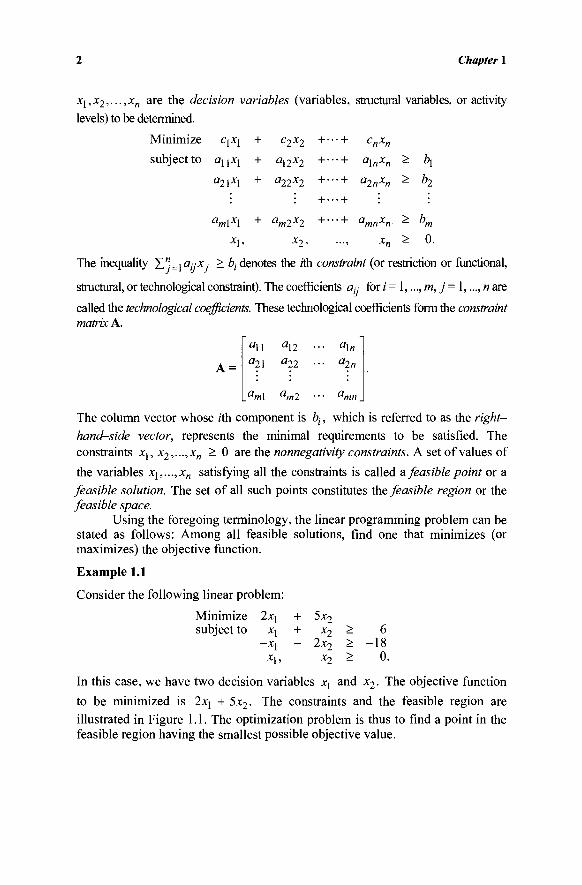
Example 1.1
Consider the following linear problem:
Minimize 2xj + subject to xj +
~x\ -X], x-> > 0 .
5x2 x2
2x2 x2
> > >
-U
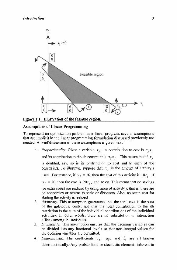
In this case, we have two decision variables χλ and x2. The objective function
to be minimized is 2xj + 5x2. The constraints and the feasible region are illustrated in Figure 1.1. The optimization problem is thus to find a point in the feasible region having the smallest possible objective value.
Introduction 3
Figure 1.1. Illustration of the feasible region.
Assumptions of Linear Programming
To represent an optimization problem as a linear program, several assumptions that are implicit in the linear programming formulation discussed previously are needed. A brief discussion of these assumptions is given next.
1. Proportionality. Given a variable x ·, its contribution to cost is ex.-
and its contribution to the rth constraint is ciyx,-. This means that if x ■
is doubled, say, so is its contribution to cost and to each of the constraints. To illustrate, suppose that x.- is the amount of activity j
used. For instance, if x. = 10, then the cost of this activity is 10c,. If
x ■ = 20, then the cost is 20c., and so on. This means that no savings
(or extra costs) are realized by using more of activity/; that is, there are no economies or returns to scale or discounts. Also, no setup cost for starting the activity is realized.
2. Additivity. This assumption guarantees that the total cost is the sum of the individual costs, and that the total contribution to the rth restriction is the sum of the individual contributions of the individual activities. In other words, there are no substitution or interaction effects among the activities.
3. Divisibility. This assumption ensures that the decision variables can be divided into any fractional levels so that non-integral values for the decision variables are permitted.
4. Deterministic. The coefficients c-, ay, and bl are all known
deterministically. Any probabilistic or stochastic elements inherent in
4 Chapter 1
demands, costs, prices, resource availabilities, usages, and so on are all assumed to be approximated by these coefficients through some deterministic equivalent.
It is important to recognize that if a linear programming problem is being used to model a given situation, then the aforementioned assumptions are implied to hold, at least over some anticipated operating range for the activities. When Dantzig first presented his linear programming model to a meeting of the Econometric Society in Wisconsin, the famous economist H. Hotelling critically remarked that in reality, the world is indeed nonlinear. As Dantzig recounts, the well-known mathematician John von Neumann came to his rescue by counter-ing that the talk was about "Linear" Programming and was based on a set of postulated axioms. Quite simply, a user may apply this technique if and only if the application fits the stated axioms.
Despite the seemingly restrictive assumptions, linear programs are among the most widely used models today. They represent several systems quite satis-factorily, and they are capable of providing a large amount of information besides simply a solution, as we shall see later, particularly in Chapter 6. Moreover, they are also often used to solve certain types of nonlinear optimization problems via (successive) linear approximations and constitute an important tool in solution methods for linear discrete optimization problems having integer-restricted variables.
Problem Manipulation
Recall that a linear program is a problem of minimizing or maximizing a linear function in the presence of linear inequality and/or equality constraints. By simple manipulations the problem can be transformed from one form to another equivalent form. These manipulations are most useful in linear programming, as will be seen throughout the text.
INEQUALITIES AND EQUATIONS
An inequality can be easily transformed into an equation. To illustrate, consider the
constraint given by Σ"ί=\αϋχί - V This constraint can be put in an equation form
by subtracting the nonnegative surplus or slack variable xn+i (sometimes denoted by
Sf) leading to Y,n;=\aijxj - xn+i = fy ^ d xn+i - 0· Similarly, the constraint
1L"J=\<*ÌJXJ ^ bt is equivalent to Σ/=ιβ(/*/ + xn+i = ty and xn+i > 0. Also, an
equation of the form ΥΓ;=\αηχί = ty can be transformed into the two inequalities
Z/=i%*y ^ fy and Σ / ^ ^ · * / ^ bh although this is not the practice.
NONNEGATIVITY OF THE VARIABLES
For most practical problems the variables represent physical quantities, and hence must be nonnegative. The simplex method is designed to solve linear programs where the variables are nonnegative. If a variable x,· is unrestricted in sign, then it
can be replaced by x'- - x"- where x'- > 0 and x"· > 0. If xx,...,xk are some A:
Introduction 5
variables that are all unrestricted in sign, then only one additional variable x" is needed in the equivalent transformation: x · = x'- - x" for j = 1, ..., k, where
x'l > 0 fory'= \,...,k, and x" > 0. (Here, -x" plays the role of representing the
most negative variable, while all the other variables x ■ are x'- above this value.)
Alternatively, one could solve for each unrestricted variable in terms of the other variables using any equation in which it appears, eliminate this variable from the problem by substitution using this equation, and then discard this equation from the problem. However, this strategy is seldom used from a data management and numerical implementation viewpoint. Continuing, if x > £ -, then the new
variable x'- = x ■ - £ ■ is automatically nonnegative. Also, if a variable x.- is
restricted such that x- < u.-, where we might possibly have w. < 0, then the
substitution X'I = u.- -x.- produces a nonnegative variable x'-.
MINIMIZATION AND MAXIMIZATION PROBLEMS
Another problem manipulation is to convert a maximization problem into a minimization problem and conversely. Note that over any region,
n n maximum X CJXJ = -minimum X ~cjxj-
Hence, a maximization (minimization) problem can be converted into a minimi-zation (maximization) problem by multiplying the coefficients of the objective function by - 1 . After the optimization of the new problem is completed, the objective value of the old problem is -1 times the optimal objective value of the new problem.
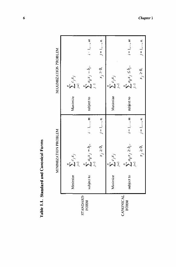
Standard and Canonical Formats
From the foregoing discussion, we have seen that any given linear program can be put in different equivalent forms by suitable manipulations. In particular, two forms will be useful. These are the standard and the canonical forms. A linear program is said to be in standard format if all restrictions are equalities and all variables are nonnegative. The simplex method is designed to be applied only after the problem is put in standard form. The canonical form is also useful, especially in exploiting duality relationships. A minimization problem is in canonical form if all variables are nonnegative and all the constraints are of the > type. A maximization problem is in canonical form if all the variables are nonnegative and all the constraints are of the < type. The standard and canonical forms are summarized in Table 1.1.
Linear Programming in Matrix Notation
A linear programming problem can be stated in a more convenient form using matrix notation. To illustrate, consider the following problem:
Tab
le 1
.1.
Sta
ndar
d an
d C
anon
ical
For
ms
ST
AN
DA
RD
F
OR
M
CA
NO
NIC
AL
F
OR
M
Min
imiz
e
subj
ect
to
Min
imiz
e
subj
ect
to
MIN
IMIZ
AT
ION
P
RO
BL
EM
« 7=1
n YJa
ijx j
=b i
, i=
\,.
7=1
xj*0
, 7
=1
,.
n Yuc ix j
7=1 n H
a ijx j*b i>
»'
=!>
·
7=1
xj>
0,
j=\,
.
., m
., n.
., m
., n.
Max
imiz
e
subj
ect
to
Max
imiz
e
subj
ect
to
MA
XIM
IZA
TIO
N
PR
OB
LE
M
n Σ°]
χ ] 7=
1 n Ha ijx j=
b i' »'
=!.
·■
7=1
Xj>
0,
y=
l,„
n Σνο-
7=1 n H
a ijx j-b i'
'=1
.··
7=1
Xj^
O,
j=i,.
. ., m
., «.
., m
., n.
f
Introduction 7
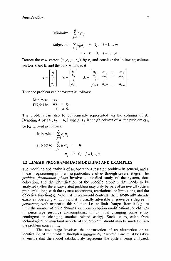
Minimize Σ c.-x.-7=1 n
subject to Σ ayxj = bj, i = l,...,m
Xj > 0, j = l,...,n.
Denote the row vector (cj,c2,...,cn) by c, and consider the following column
vectors x and b, and the m x n matrix A.
~ * l " x?
.•V
b = V b?
Pm_ A =
an an a2\ a 22
am\ am2
Then the problem can be written as follows:
«2K
Minimize subject to
ex Ax = b
x > 0.
The problem can also be conveniently represented via the columns of A. Denoting A by [aj,a2,...,a„] where a, is the /th column of A, the problem can
be formulated as follows:
Minimize Σ c.-x,· y=i
subject to Σ ax , · y'=l
XJ > 0, j = !,...,«.
1.2 LINEAR PROGRAMMING MODELING AND EXAMPLES
The modeling and analysis of an operations research problem in general, and a linear programming problem in particular, evolves through several stages. The problem formulation phase involves a detailed study of the system, data collection, and the identification of the specific problem that needs to be analyzed (often the encapsulated problem may only be part of an overall system problem), along with the system constraints, restrictions, or limitations, and the objective function(s). Note that in real-world contexts, there frequently already exists an operating solution and it is usually advisable to preserve a degree of persistency with respect to this solution, i.e., to limit changes from it (e.g., to limit the number of price changes, or decision option modifications, or changes in percentage resource consumptions, or to limit changing some entity contingent on changing another related entity). Such issues, aside from technological or structural aspects of the problem, should also be modeled into the problem constraints.
The next stage involves the construction of an abstraction or an idealization of the problem through a mathematical model. Care must be taken to ensure that the model satisfactorily represents the system being analyzed,
8 Chapter 1
while keeping the model mathematically tractable. This compromise must be made judiciously, and the underlying assumptions inherent in the model must be properly considered. It must be borne in mind that from this point onward, the solutions obtained will be solutions to the model and not necessarily solutions to the actual system unless the model adequately represents the true situation.
The third step is to derive a solution. A proper technique that exploits any special structures (if present) must be chosen or designed. One or more optimal solutions may be sought, or only a heuristic or an approximate solution may be determined along with some assessment of its quality. In the case of multiple objective functions, one may seek efficient or Pareto-optimal solutions, that is, solutions that are such that a further improvement in any objective function value is necessarily accompanied by a detriment in some other objective function value.
The fourth stage is model testing, analysis, and (possibly) restructuring. One examines the model solution and its sensitivity to relevant system parameters, and studies its predictions to various what-if types of scenarios. This analysis provides insights into the system. One can also use this analysis to ascertain the reliability of the model by comparing the predicted outcomes with the expected outcomes, using either past experience or conducting this test retroactively using historical data. At this stage, one may wish to enrich the model further by incorporating other important features of the system that have not been modeled as yet, or, on the other hand, one may choose to simplify the model.
The final stage is implementation. The primary purpose of a model is to interactively aid in the decision-making process. The model should never replace the decision maker. Often a "frank-factor" based on judgment and experience needs to be applied to the model solution before making policy decisions. Also, a model should be treated as a "living" entity that needs to be nurtured over time, i.e., model parameters, assumptions, and restrictions should be periodically revisited in order to keep the model current, relevant, and valid.
We describe several problems that can be formulated as linear programs. The purpose is to exhibit the varieties of problems that can be recognized and expressed in precise mathematical terms as linear programs.
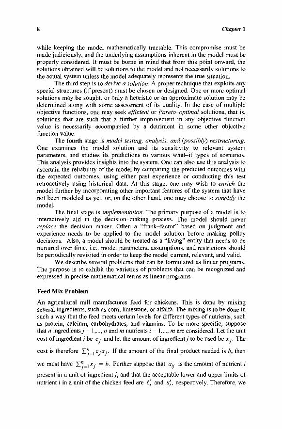
Feed Mix Problem
An agricultural mill manufactures feed for chickens. This is done by mixing several ingredients, such as corn, limestone, or alfalfa. The mixing is to be done in such a way that the feed meets certain levels for different types of nutrients, such as protein, calcium, carbohydrates, and vitamins. To be more specific, suppose that n ingredients y = 1,..., n and m nutrients / = 1,..., m are considered. Let the unit cost of ingredient j be c, and let the amount of ingrediente to be used be x,. The
cost is therefore Σ^=jC.-x,-. If the amount of the final product needed is b, then
we must have Z'Li*/ = b. Further suppose that a,·.- is the amount of nutrient i
present in a unit of ingrediente, and that the acceptable lower and upper limits of nutrient / in a unit of the chicken feed are l\ and u\, respectively. Therefore, we
Introduction 9
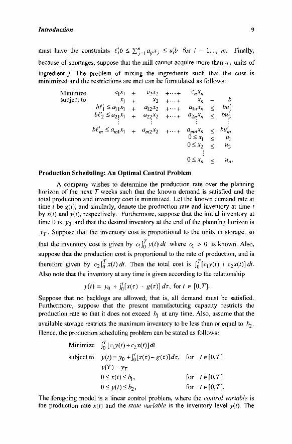
must have the constraints i\b < Z'Lifl//*; < u\b for / = 1,..., m. Finally,
because of shortages, suppose that the mill cannot acquire more than u · units of
ingredient j . The problem of mixing the ingredients such that the cost is minimized and the restrictions are met can be formulated as follows:
Minimize subject to
c\x\ xx
bi\ < a^ixi
bi\ < a2\X\
bi'm < amXxx
+ + + +
+
c2x2 x2
«12*2 a22*2
am2x2
+ ·· + -· + ·· + ··
+ -·
·· + ·· + ·· + ·· +
·· +
cnxn xn
a\nxn a2nxn
amnxn
0 < X 2
= < <
< < <
b bu[ bu'j
bu'm u\ u2
0<xn < un.
Production Scheduling: An Optimal Control Problem
A company wishes to determine the production rate over the planning horizon of the next T weeks such that the known demand is satisfied and the total production and inventory cost is minimized. Let the known demand rate at time / be g(t), and similarly, denote the production rate and inventory at time / by x(t) and y(t), respectively. Furthermore, suppose that the initial inventory at time 0 is _y0
a n ( i m a t m e desired inventory at the end of the planning horizon is yT. Suppose that the inventory cost is proportional to the units in storage, so
that the inventory cost is given by q }0 y(t) dt where q > 0 is known. Also,
suppose that the production cost is proportional to the rate of production, and is
therefore given by c2jQ x(t)dt. Then the total cost is J0 [c^y(t) + c2x(t)]dt.
Also note that the inventory at any time is given according to the relationship
y(t) = y0 + ί'0[χ(τ) - g(T)]dr, for? E [Ο,Γ].
Suppose that no backlogs are allowed; that is, all demand must be satisfied. Furthermore, suppose that the present manufacturing capacity restricts the production rate so that it does not exceed t\ at any time. Also, assume that the
available storage restricts the maximum inventory to be less than or equal to b2. Hence, the production scheduling problem can be stated as follows:
Minimize J0 [qy{t) + c2x(t)] dt
subject to y(t) = yo+i'0[x(T)-g(T)]dT, for ts[0,T]
y(T) = yT
0 < x ( / ) < q , for te[0,T]
0<y(t)<b2, for t e[0,T].
The foregoing model is a linear control problem, where the control variable is the production rate x(t) and the state variable is the inventory level y(t). The
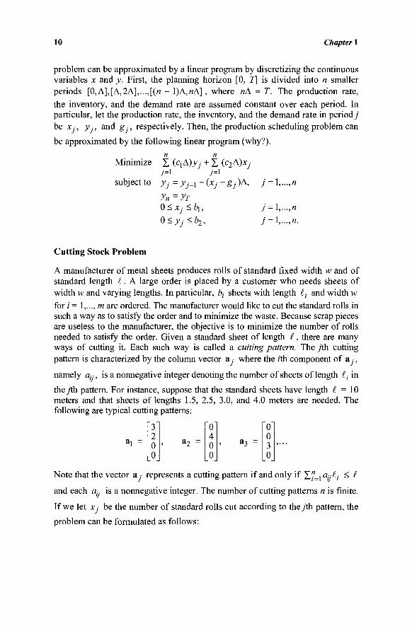
10 Chapter 1
problem can be approximated by a linear program by discretizing the continuous variables x and y. First, the planning horizon [0, 7] is divided into n smaller periods [0,Δ],[Δ,2Δ],...,[(« - 1)Δ,«Δ], where «Δ = T. The production rate, the inventory, and the demand rate are assumed constant over each period. In particular, let the production rate, the inventory, and the demand rate in period j be X:, y ■, and g ■, respectively. Then, the production scheduling problem can
be approximated by the following linear program (why?). n n
Minimize Σ (c\A)y ■ + Σ (c2A)x ■ 7=1 j=\
subject to yj = yj_x +(xj -gj)A, j = \,...,n
yn=yr 0<Xj<bi, 7 = 1,.··," 0<yj<b2, j = \,...,n.
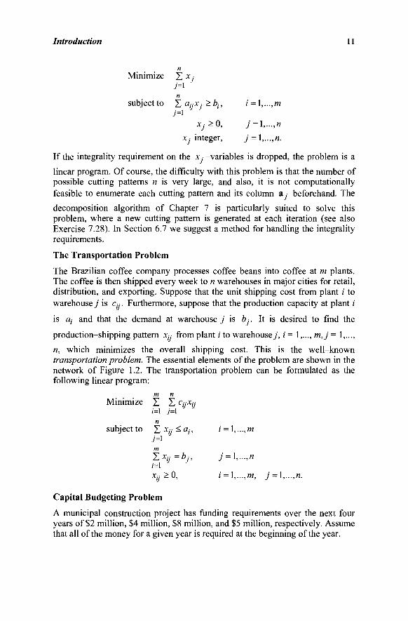
Cutting Stock Problem
A manufacturer of metal sheets produces rolls of standard fixed width w and of standard length £. A large order is placed by a customer who needs sheets of width w and varying lengths. In particular, bt sheets with length li and width w for / = 1,..., m are ordered. The manufacturer would like to cut the standard rolls in such a way as to satisfy the order and to minimize the waste. Because scrap pieces are useless to the manufacturer, the objective is to minimize the number of rolls needed to satisfy the order. Given a standard sheet of length £, there are many ways of cutting it. Each such way is called a cutting pattern. The j'th cutting pattern is characterized by the column vector a,- where the z'th component of a,,
namely a^, is a nonnegative integer denoting the number of sheets of length £j in
they'th pattern. For instance, suppose that the standard sheets have length £ = 10 meters and that sheets of lengths 1.5, 2.5, 3.0, and 4.0 meters are needed. The following are typical cutting patterns:
3 2 0 0
a2 =
0 4 0 0
a 3 =
0 0 3 0
Note that the vector a represents a cutting pattern if and only if YÀ"=iaij£i < I
and each α„ is a nonnegative integer. The number of cutting patterns n is finite.
If we let Xj be the number of standard rolls cut according to they'th pattern, the
problem can be formulated as follows:
Introduction 11
n Minimize Σ x.-
7=1 n
subject to YdaijXj>bi, i = \,...,m 7=1
Xj>0, j = l,...,n Xj integer, j = l,...,n.
If the integrality requirement on the Xj -variables is dropped, the problem is a
linear program. Of course, the difficulty with this problem is that the number of possible cutting patterns n is very large, and also, it is not computationally feasible to enumerate each cutting pattern and its column a, beforehand. The
decomposition algorithm of Chapter 7 is particularly suited to solve this problem, where a new cutting pattern is generated at each iteration (see also Exercise 7.28). In Section 6.7 we suggest a method for handling the integrality requirements.
The Transportation Problem
The Brazilian coffee company processes coffee beans into coffee at m plants. The coffee is then shipped every week to n warehouses in major cities for retail, distribution, and exporting. Suppose that the unit shipping cost from plant / to warehouse j is c«. Furthermore, suppose that the production capacity at plant ;
is Oj and that the demand at warehouse j is Z> · . It is desired to find the
production-shipping pattern JC,·.· from plant i to warehouse j , i = 1,..., m,j = 1,...,
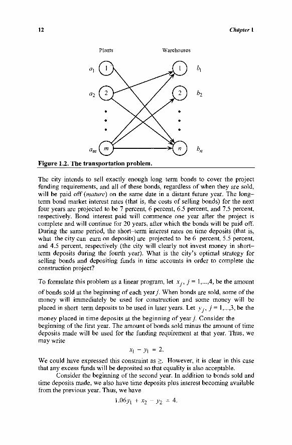
n, which minimizes the overall shipping cost. This is the well-known transportation problem. The essential elements of the problem are shown in the network of Figure 1.2. The transportation problem can be formulated as the following linear program:
Minimize
subject to
m n Σ Σ CjjXjj (=1 y=l n Σ Xy ^ah
7=1 m ΣΧη =bj, ;=1 χ ^ ο ,
i = \,..
j = l-
i = l,..
.,m
..,«
.,m. j = \,...,n.
Capital Budgeting Problem
A municipal construction project has funding requirements over the next four years of $2 million, $4 million, $8 million, and $5 million, respectively. Assume that all of the money for a given year is required at the beginning of the year.
12 Chapter 1
Plants Warehouses
Figure 1.2. The transportation problem.
The city intends to sell exactly enough long-term bonds to cover the project funding requirements, and all of these bonds, regardless of when they are sold, will be paid off {mature) on the same date in a distant future year. The long-term bond market interest rates (that is, the costs of selling bonds) for the next four years are projected to be 7 percent, 6 percent, 6.5 percent, and 7.5 percent, respectively. Bond interest paid will commence one year after the project is complete and will continue for 20 years, after which the bonds will be paid off. During the same period, the short-term interest rates on time deposits (that is, what the city can earn on deposits) are projected to be 6 percent, 5.5 percent, and 4.5 percent, respectively (the city will clearly not invest money in short-term deposits during the fourth year). What is the city's optimal strategy for selling bonds and depositing funds in time accounts in order to complete the construction project?
To formulate this problem as a linear program, let x ·, j = 1,...,4, be the amount
of bonds sold at the beginning of each year/. When bonds are sold, some of the money will immediately be used for construction and some money will be placed in short-term deposits to be used in later years. Let y -, j = 1,...,3, be the
money placed in time deposits at the beginning of year/ Consider the beginning of the first year. The amount of bonds sold minus the amount of time deposits made will be used for the funding requirement at that year. Thus, we may write
χ\ - y\ = 2.
We could have expressed this constraint as >. However, it is clear in this case that any excess funds will be deposited so that equality is also acceptable.
Consider the beginning of the second year. In addition to bonds sold and time deposits made, we also have time deposits plus interest becoming available from the previous year. Thus, we have
1.06>Ί +χ2 -y2 = 4.
Introduction 13
The third and fourth constraints are constructed in a similar manner. Ignoring the fact that the amounts occur in different years (that is, the
time value of money), the unit cost of selling bonds is 20 times the interest rate. Thus, for bonds sold at the beginning of the first year we have c\ = 20(0.07).
The other cost coefficients are computed similarly. Accordingly, the linear programming model is given as follows:
Minimize 20(0.07)^ + 20(0.06) x2 + 20(0.065) x3 + 20(0.075) x4
subject to x, - y\ = 2
1.067, + x2 - y2 = 4
1.055y2+ χτ, - y-i = 8
1.045^3 + x4 = 5
xx, x2, x3, x4, yx, y2, y3 > 0.
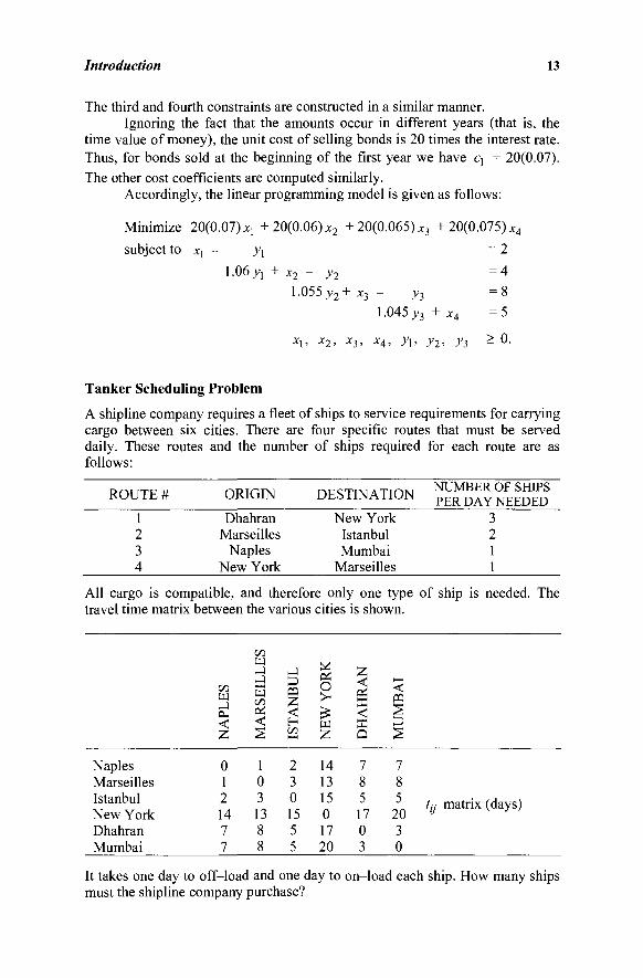
Tanker Scheduling Problem
A shipline company requires a fleet of ships to service requirements for carrying cargo between six cities. There are four specific routes that must be served daily. These routes and the number of ships required for each route are as follows:
ROUTE # ORIGIN DESTINATION NUMBER OF SHIPS PER DAY NEEDED
1 2 3 4
Dhahran Marseilles
Naples New York
New York Istanbul Mumbai
Marseilles
3 2 1 1
All cargo is compatible, and therefore only one type of ship is needed. The travel time matrix between the various cities is shown.
Naples Marseilles Istanbul New York Dhahran Mumbai
< Z,
0 1 2 14 7 7
OQ
w on
< 2
1 0 3 13 8 8
J
1 H t/3
2 3 0 15 5 5
^ O >
« Z
14 13 15 0 17 20
7,
X < X a 7 8 5 17 0 3
< pa
HJ
^
7 8 5
20 3 0
tjj matrix (days)
It takes one day to off-load and one day to on-load each ship. How many ships must the shipline company purchase?
14 Chapter 1
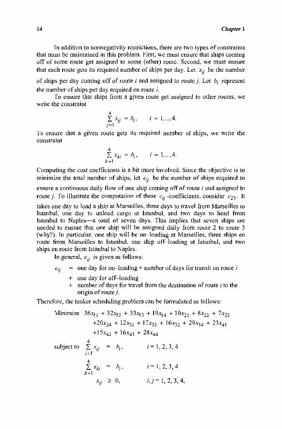
In addition to nonnegativity restrictions, there are two types of constraints that must be maintained in this problem. First, we must ensure that ships coming off of some route get assigned to some (other) route. Second, we must ensure that each route gets its required number of ships per day. Let x;y be the number
of ships per day coming off of route i and assigned to route j . Let ty represent the number of ships per day required on route ;'.
To ensure that ships from a given route get assigned to other routes, we write the constraint
4 Σ Xn = bh i = l , - ,4 .
7=1
To ensure that a given route gets its required number of ships, we write the constraint
4 Σ Xki = bi> ' = !>···,4·
Computing the cost coefficients is a bit more involved. Since the objective is to minimize the total number of ships, let c;y be the number of ships required to
ensure a continuous daily flow of one ship coming off of route / and assigned to route j . To illustrate the computation of these c(y -coefficients, consider c23. It
takes one day to load a ship at Marseilles, three days to travel from Marseilles to Istanbul, one day to unload cargo at Istanbul, and two days to head from Istanbul to Naples—a total of seven days. This implies that seven ships are needed to ensure that one ship will be assigned daily from route 2 to route 3 (why?). In particular, one ship will be on-loading at Marseilles, three ships en route from Marseilles to Istanbul, one ship off-loading at Istanbul, and two ships en route from Istanbul to Naples.
In general, c,·.· is given as follows:
% = one day for on-loading + number of days for transit on route i
+ one day for off-loading + number of days for travel from the destination of route / to the
origin of route j .
Therefore, the tanker scheduling problem can be formulated as follows:
Minimize 36xu + 32x[2 + 33x]3 + 19x]4 + 10x2i + 8x22 + 7*23
+20x24 + 12x31 + 17x32 + 16x33 + 29x34 + 23x41
+15x42 + 16x43 + 28x44
4 subject to X Xjj = bj, i= 1,2,3,4
4 Σ Xki = bi> «'=1,2,3,4
k=\ Xij * 0, U = 1,2,3,4,
Introduction 15
where l\ = 3, b2 = 2, b^ = 1 , and b4 = 1. It can be easily seen that this is another application of the transportation
problem (it is instructive for the reader to form the origins and destinations of the corresponding transportation problem).
Multiperiod Coal Blending and Distribution Problem
A southwest Virginia coal company owns several mines that produce coal at different given rates, and having known quality (ash and sulfur content) specifications that vary over mines as well as over time periods at each mine. This coal needs to be shipped to silo facilities where it can be possibly subjected to a beneficiation (cleaning) process, in order to partially reduce its ash and sulfur content to a desired degree. The different grades of coal then need to be blended at individual silo facilities before being shipped to customers in order to satisfy demands for various quantities having stipulated quality specifications. The aim is to determine optimal schedules over a multiperiod time horizon for shipping coal from mines to silos, cleaning and blending the coal at the silos, and distributing the coal to the customers, subject to production capacity, storage, material flow balance, shipment, and quality requirement restrictions, so as to satisfy the demand at a minimum total cost, including revenues due to rebates for possibly shipping coal to customers that is of a better quality than the minimum acceptable specified level.
Suppose that this problem involves i = 1,..., m mines,/= \,...,Jsilos, k = \,...,K customers, and that we are considering t= 1,..., Γ(> 3) time periods. Let pit be the production (in tons of coal) at mine i during period t, and let ait and
sit respectively denote the ash and sulfur percentage content in the coal
produced at mine / during period t. Any excess coal not shipped must be stored
at the site of the mine at a per-period storage cost of c, per ton at mine i,
where the capacity of the storage facility at mine i is given by M,-.
Let Ay denote the permissible flow transfer arcs (i,j) from mine i to silo
j , and let Ft = {j : (;', j) e Α^} and R: = {i : (/, j) e Αχ}. The transportation
cost per ton from mine i to siloy is denoted by c,y, for each (/,/) e Αγ. Each
siloj has a storage capacity of S.-, and a per-ton storage cost of c .■, per period.
Assume that at the beginning of the time horizon, there exists an initial amount
of q: tons of coal stored at siloj, having an ash and sulfur percentage content of
a, and s , respectively. Some of the silos are equipped with beneficiation or
cleaning facilities, where any coal coming from mine i to such a siloy is cleaned
at a cost of Cy per ton, resulting in the ash and sulfur content being respectively
attenuated by a factor of /L e (0,1] and γ^ e (0,1], and the total weight being
thereby attenuated by a factor of α^ ε (0,1] (hence, for one ton input, the

16 Chapter 1
output is ay tons, which is then stored for shipment). Note that for silos that do
not have any cleaning facilities, we assume that c = 0, and ay = /L = γ-y = 1.
Let A2 denote the feasible flow transfer arcs (j, k) from silo j to customer
k, and let FJ = {k : (j,k) e A2}, and R% = {j : (j,k) ε A2}. The transport-
tation cost per ton from silo y to customer k is denoted by Cjk, for each (j, k) e
A2. Additionally, if ty is the time period for a certain mine to silo shipment
(assumed to occur at the beginning of the period), and t2 is the time period for a
continuing silo to customer shipment (assumed to occur at the end of the
period), then the shipment lag between the two coal flows is given by t2 - fj. A
maximum of a three-period shipment lag is permitted between the coal production at any mine and its ultimate shipment to customers through any silo, based on an estimate of the maximum clearance time at the silos. (Actual shipment times from mines to silos are assumed to be negligible.) The demand placed (in tons of coal) by customer k during period / is given by dkt, with ash and sulfur percentage contents being respectively required to lie in the intervals defined by the lower and upper limits [#%,u%t] and [l\t, u\t]. There is also a revenue earned of rkt per-ton per-percentage point that falls below the maxi-mum specified percentage ukt of ash content in the coal delivered to customer k during period /.
To model this problem, we first define a set of principal decision
variables as yyt = amount (tons) of coal shipped from mine i to siloy in period
t, with continued shipment to customer k in period τ (where τ = t, t + 1, t + 2,
based on the three-period shipment lag restriction), and yβτ = amount (tons)
of coal that is in initial storage at silo/, which is shipped to customer k in period τ (where τ = 1,2,3, based on a three period dissipation limit). Controlled by these principal decisions, there are four other auxiliary decision variables defined as follows: xiS = slack variable that represents the amount (tons) of coal
remaining in storage at mine i during period δ;x.-g = accumulated storage
amount (tons) of coal in silo j during period δ; ζ%Τ = percentage ash content in
the blended coal that is ultimately delivered to customer k in period r, and ζ\τ = percentage sulfur content in the blended coal that is ultimately delivered to customer k in period τ. The linear programming model is then given as follows, where the objective function records the transportation, cleaning, and storage costs, along with the revenue term over the horizon \,...,T of interest. The respective sets of constraints represent the flow balance at the mines, storage capacity restrictions at the mines, flow balance at the silos, storage capacity restrictions at the silos, the dissipation of the initial storage at the silos, the
Introduction 17
demand satisfaction constraints, the ash content identities, the quality bound specifications with respect to the ash content, the sulfur content identities, the quality bound specifications with respect to the sulfur content, and the remaining logical nonnegativity restrictions. (All undefined variables and summation terms are assumed to be zero. Also, see Exercises 1.19-1.21.)
Minimize J T mm{t+2,T} , D . Σ Σ Σ Σ Σ [c\ + cfj + c%
7=1 Ì<ER) k<EFJ t=\ τ=ί
+ (T-t + \)ή}γ^ + Σ Σ cfxfs i=\ S=\
+ Σ Σ Σ c%y%T + Σ Σ c ^ j - Σ Σ y)kA 7=1 keFJ τ=\ j=\ t=\
K T
- Σ Σ («Ar - 4r)dkTrkT k=\ r=l
r<t keFf
subject to δ ΣΡίΐ t=\
t+2 .M xiS » Σ Σ Σ Σ Ϋψ
jeF> '=1 keFJ τ=ί
i = \,...,m,5 = \,...,T
0 < x $ <Mt, i = l,...,m,S = l,...,T
kx δ t+2
Σ Σ Σ Σ ayyij, ieRj keFJ /=max{l,<y-2} τ=δ
0 +[q)
min{5-l,3} 0 s
Σ Σ yjkri = XJS> kzFJ τ=1
j = l,...,J, δ - Ι,.,.,Τ
0<x]s<Sj, j = l,...,J,S = l,...,T
sr 4- 0 0 · , , Σ Σ yjkz = ijy J = !>···,./
k&F} τ=\ τ
Σ jeR% Ì&R) /=max{l,r-2} ye/{£
ayyyÌ + Σ 2 y%T = <4r>
k = Χ,.,.,Κ,τ = 1.....Γ
zkrdkT ~ Σ jeR% ie/fj i=max{l,r-2}
k = Ι,.,.,Κ,τ = Ι,.,.,Τ
1\τ <ζ%τ <uakT,k = l,...,K,T = l,...,T
η kz , ^ 0 0 °ufiijyijt + Σ ajyjkt,
18 Chapter 1
zkTdkr = Σ Σ Σ Sit/ijyijt + Σ 5 / ^ r . ye/?* ieRlj /=max{l,r-2} jeRJ
k = Ι,.,.,Κ,Τ = Ι,.,.,Τ
ί\τ <ζ{τ <4T,k = ì,...,K,T = l,...,T
y§ > 0,(i,j) e Aut = \,...,T,k = 1,...,*, τ = t,...,t + 2,
y% > 0,(Λ*) e ^2.*- = ! ' 2 ' 3 ·
1.3 GEOMETRIC SOLUTION
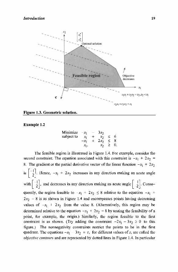
We describe here a geometrie procedure for solving a linear programming problem. Even though this method is only suitable for very small problems, it provides a great deal of insight into the linear programming problem. To be more specific, consider the following problem:
Minimize ex subject to Ax = b
x > 0.
Note that the feasible region consists of all vectors x satisfying Ax = b and x > 0. Among all such points, we wish to find a point having a minimal value of ex. Note that points having the same objective value z satisfy the equation ex = z,
that is, YTj=\cìxi = z- Since z is to be minimized, then the plane (line in a
two-dimensional space) Σ,"/=ι€ίχ/ = z m u s t be moved parallel to itself in the
direction that minimizes the objective the most. This direction is -c , and hence the plane is moved in the direction of -c as much as possible, while maintaining contact with the feasible region. This process is illustrated in Figure 1.3. Note
that as the optimal point x is reached, the line C\X\ + C2X2 = z , where z = c\x* + C2X2> cannot be moved farther in the direction -c = (-c, ,-c2), because this will only lead to points outside the feasible region. In other words, one
cannot move from x* in a direction that makes an acute angle with -c , i.e., a direction that reduces the objective function value, while remaining feasible. We
therefore conclude that x* is indeed an optimal solution. Needless to say, for a maximization problem, the plane ex = z must be moved as much as possible in the direction c, while maintaining contact with the feasible region.
The foregoing process is convenient for problems having two variables and is obviously impractical for problems with more than three variables. It is
worth noting that the optimal point x* in Figure 1.3 is one of the five corner points that are called extreme points. We shall show in Section 3.1 that if a linear program in standard or canonical form has a finite optimal solution, then it has an optimal corner (or extreme) point solution.
Introduction 19
Figure 1.3. Geometric solution.
Example 1.2
0.
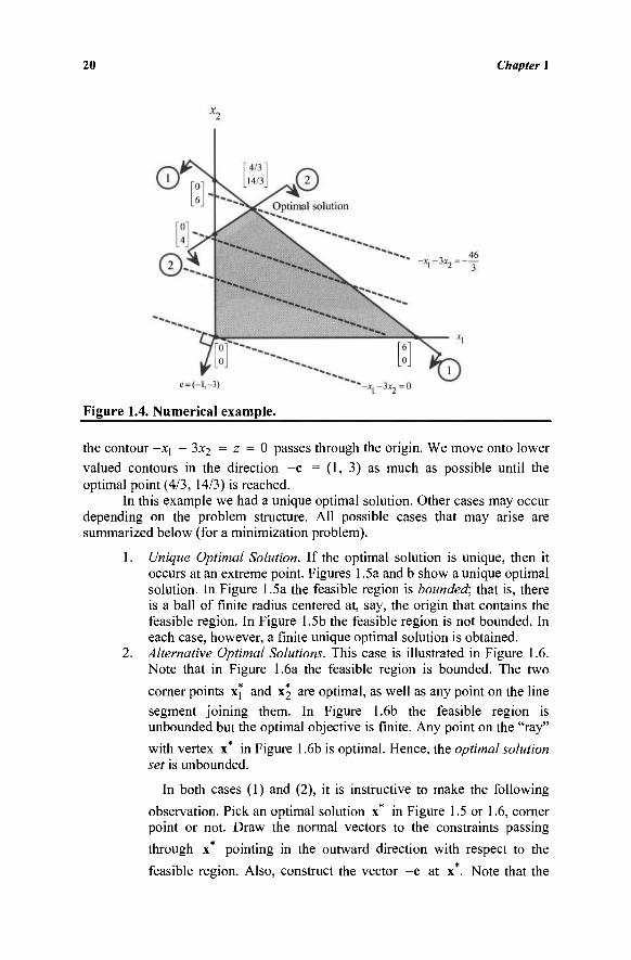
The feasible region is illustrated in Figure 1.4. For example, consider the second constraint. The equation associated with this constraint is -X] + 2x2
=
8. The gradient or the partial derivative vector of the linear function -xj + 2x2
Minimize subject to
-x, X,
- X ,
X\,
- 3x2 + x2
+ 2x2 x2
< < >
IS Hence, -xj + 2x2 increases in any direction making an acute angle
with -1 2 , and decreases in any direction making an acute angle 1
-2 . Conse-
quently, the region feasible to -Xj + 2x2 < 8 relative to the equation -xj + 2x2 = 8 is as shown in Figure 1.4 and encompasses points having decreasing values of -Xj + 2x2 from the value 8. (Alternatively, this region may be determined relative to the equation -xj + 2x2 = 8 by testing the feasibility of a point, for example, the origin.) Similarly, the region feasible to the first constraint is as shown. (Try adding the constraint -2x[ + 3x2 > 0 to this figure.) The nonnegativity constraints restrict the points to be in the first quadrant. The equations -X] - 3x2 = z, for different values of z, are called the objective contours and are represented by dotted lines in Figure 1.4. In particular
20 Chapter 1
Figure 1.4. Numerical example.
the contour -X] - 3x2 = z = 0 passes through the origin. We move onto lower valued contours in the direction -c = (1, 3) as much as possible until the optimal point (4/3, 14/3) is reached.
In this example we had a unique optimal solution. Other cases may occur depending on the problem structure. All possible cases that may arise are summarized below (for a minimization problem).
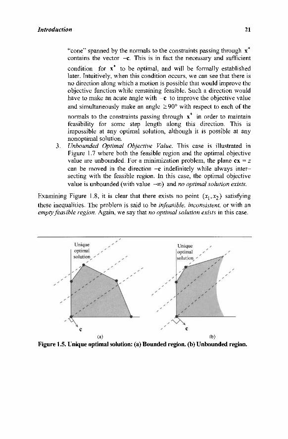
1. Unique Optimal Solution. If the optimal solution is unique, then it occurs at an extreme point. Figures 1.5a and b show a unique optimal solution. In Figure 1.5a the feasible region is bounded; that is, there is a ball of finite radius centered at, say, the origin that contains the feasible region. In Figure 1.5b the feasible region is not bounded. In each case, however, a finite unique optimal solution is obtained.
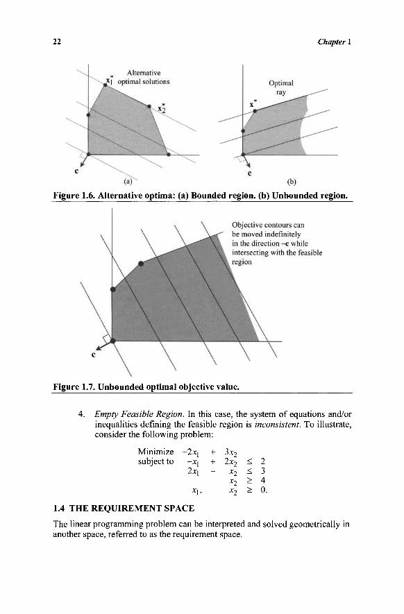
2. Alternative Optimal Solutions. This case is illustrated in Figure 1.6. Note that in Figure 1.6a the feasible region is bounded. The two
corner points x* and X;> are optimal, as well as any point on the line segment joining them. In Figure 1.6b the feasible region is unbounded but the optimal objective is finite. Any point on the "ray"
with vertex x* in Figure 1.6b is optimal. Hence, the optimal solution set is unbounded.
In both cases (1) and (2), it is instructive to make the following
observation. Pick an optimal solution x* in Figure 1.5 or 1.6, corner point or not. Draw the normal vectors to the constraints passing
through x* pointing in the outward direction with respect to the
feasible region. Also, construct the vector -c at x*. Note that the
Introduction 21
"cone" spanned by the normals to the constraints passing through x* contains the vector -c. This is in fact the necessary and sufficient
condition for x* to be optimal, and will be formally established later. Intuitively, when this condition occurs, we can see that there is no direction along which a motion is possible that would improve the objective function while remaining feasible. Such a direction would have to make an acute angle with -c to improve the objective value and simultaneously make an angle > 90° with respect to each of the
normals to the constraints passing through x* in order to maintain feasibility for some step length along this direction. This is impossible at any optimal solution, although it is possible at any nonoptimal solution.
3. Unbounded Optimal Objective Value. This case is illustrated in Figure 1.7 where both the feasible region and the optimal objective value are unbounded. For a minimization problem, the plane ex = z can be moved in the direction -c indefinitely while always inter-secting with the feasible region. In this case, the optimal objective value is unbounded (with value —oo) and no optimal solution exists.
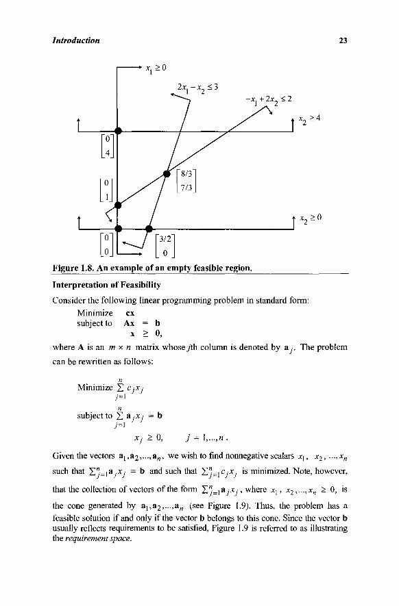
Examining Figure 1.8, it is clear that there exists no point (X],x2) satisfying these inequalities. The problem is said to be infeasible, inconsistent, or with an empty feasible region. Again, we say that no optimal solution exists in this case.
(a) (b)
Figure 1.5. Unique optimal solution: (a) Bounded region, (b) Unbounded region.
22 Chapter 1
Figure 1.6. Alternative optima: (a) Bounded region, (b) Unbounded region.
Figure 1.7. Unbounded optimal objective value.
Empty Feasible Region. In this case, the system of equations and/or inequalities defining the feasible region is inconsistent. To illustrate, consider the following problem:
Minimize subject to
-2x[
~x\ 2x]
X] ,
+ 3x2 + 2x2
- x2 x2 x2
< < > >
2 3 4 0,
1.4 THE REQUIREMENT SPACE
The linear programming problem can be interpreted and solved geometrically in another space, referred to as the requirement space.
Introduction 23
Figure 1.8. An example of an empty feasible region.
Interpretation of Feasibility
Consider the following linear programming problem in standard form:
Minimize ex subject to Ax = b
x > 0,
where A is an m χ η matrix whose7th column is denoted by a ,·. The problem
can be rewritten as follows:
Minimize Σ c.-x,· 7=1
subject to Σ &jXj 7=1
b
Xj > 0, j = Ι,.,.,η .
Given the vectors aj,a2,...,a„, we wish to find nonnegative scalare χλ, x2, —,xn
such that Jl"=]ajXj = b and such that Hnj-\CjXj is minimized. Note, however,
that the collection of vectors of the form X ^ = 1 a x - , where xx, x2,...,x„ > 0, is
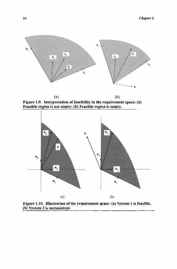
the cone generated by aj,a2,...,a„ (see Figure 1.9). Thus, the problem has a feasible solution if and only if the vector b belongs to this cone. Since the vector b usually reflects requirements to be satisfied, Figure 1.9 is referred to as illustrating the requirement space.
24 Chapter 1
Figure 1.9. Interpretation of feasibility in the requirement space: (a) Feasible region is not empty, (b) Feasible region is empty.
Figure 1.10. Illustration of the requirement space: (a) System 1 is feasible, (b) System 2 is inconsistent.
Introduction 25
Example 1.3
Consider the following two systems:
System 1 :
System 2:
2xi + X2 + X3 -X] + 3x 2
X], X2, X3,
2xi + X2 + X3 -X[ + 3x2
X], X2, X3,
+ x4 X4
+ x4 X4
= 2 = 3 > 0.
= -1 = 2 > 0.
Figure 1.10 shows the requirement space of both systems. For System 1, the
vector b belongs to the cone generated by the vectors 2 -1 5
1 3 1
1 0 , and
, and hence admits feasible solutions. For the second system, b does not
belong to the corresponding cone and the system is then inconsistent.
The Requirement Space and Inequality Constraints
We now illustrate the interpretation of feasibility for the inequality case. Consider the following inequality system:
n Σ a,x, < b
7=1
Xj > 0 , j= Ι,.,.,η.
Note that the collection of vectors Z ' L i 8 / * / , where x · > 0 fory = \,...,n, is
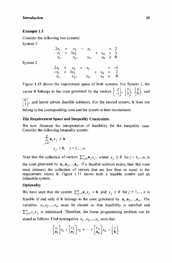
the cone generated by aj,a2,...,a„. If a feasible solution exists, then this cone must intersect the collection of vectors that are less than or equal to the requirement vector b. Figure 1.11 shows both a feasible system and an infeasible system.
Optimality
We have seen that the system H,n;=\*jXj = b and x,· > 0 for j = 1,..., n is
feasible if and only if b belongs to the cone generated by a!,a2,...,a„. The
variables X],x2,...,x„ must be chosen so that feasibility is satisfied and
Ji"i-\cjxj is minimized. Therefore, the linear programming problem can be
stated as follows. Find nonnegative x1; x2,...,x„ such that
*i + c 2 a2
x2 + · · · + z b
26 Chapter 1
Figure 1.11. Requirement space and inequality constraints: (a) System is feasible, (b) System is infeasible.
where the objective z is to be minimized. In other words we seek to represent the
vector z b
c2 a2
, for the smallest possible z, in the cone spanned by the vectors
. The reader should note that the price we must pay for
including the objective function explicitly in the requirement space is to increase the dimensionality from mtom+ 1.
Example 1.4
Minimize -2xj - 3x2
subject to X] + 2x2 ^ 2 Xj , x 2 - 0.
Add the slack variable JC3 > 0. The problem is then to choose χγ, x2, x^ > 0 such that
-2 1 X\ +
-3 2 x2 + 0
1 *3 = z 2
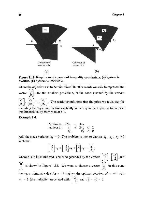
where z is to be minimized. The cone generated by the vectors
is shown in Figure 1.12. We want to choose a vector
-2 1
z 2
having a minimal value for z. This gives the optimal solution z '-2
1}and
in this cone
= -4 with 2 (the multiplier associated with
1 ) and x2 = x-} = 0.
Introduction 27
Example 1.5
Minimize -2xt - 3x2
subject to x, X ] ,
+ 2x2 > 2 > x2 > 0.
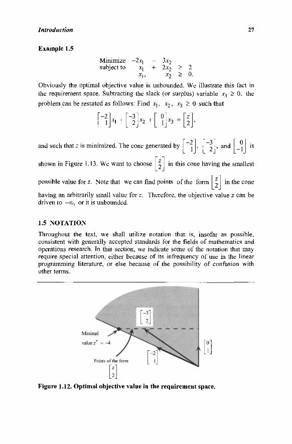
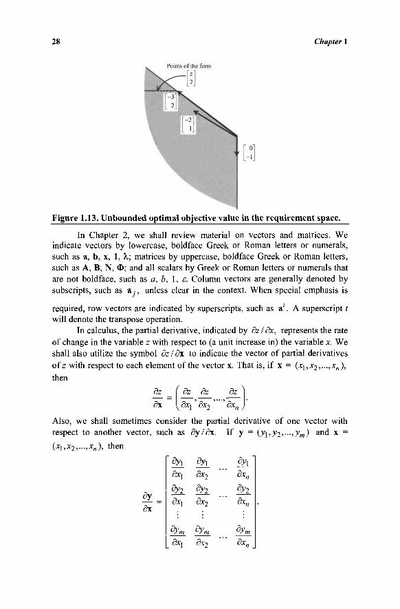
Obviously the optimal objective value is unbounded. We illustrate this fact in the requirement space. Subtracting the slack (or surplus) variable x3 > 0, the
problem can be restated as follows: Find xj, x2, x3 > 0 such that
-2 1 Xj +
-3 2 x2 + 0
-1 x3 =
z 2
and such that z is minimized. The cone generated by -3 2 , and
shown in Figure 1.13. We want to choose in this cone having the smallest
possible value for z. Note that we can find points of the form in the cone
having an arbitrarily small value for z. Therefore, the objective value z can be driven to -oo, or it is unbounded.
1.5 NOTATION
Throughout the text, we shall utilize notation that is, insofar as possible, consistent with generally accepted standards for the fields of mathematics and operations research. In this section, we indicate some of the notation that may require special attention, either because of its infrequency of use in the linear programming literature, or else because of the possibility of confusion with other terms.
Figure 1.12. Optimal objective value in the requirement space.
28 Chapter 1
Figure 1.13. Unbounded optimal objective value in the requirement space.
In Chapter 2, we shall review material on vectors and matrices. We indicate vectors by lowercase, boldface Greek or Roman letters or numerals, such as a, b, x, 1, λ; matrices by uppercase, boldface Greek or Roman letters, such as A, B, N, Φ; and all scalars by Greek or Roman letters or numerals that are not boldface, such as a, b, 1, ε. Column vectors are generally denoted by subscripts, such as a,, unless clear in the context. When special emphasis is
required, row vectors are indicated by superscripts, such as a'. A superscript t will denote the transpose operation.
In calculus, the partial derivative, indicated by dz/dx, represents the rate of change in the variable z with respect to (a unit increase in) the variable x. We shall also utilize the symbol dz/dx to indicate the vector of partial derivatives of z with respect to each element of the vector x. That is, if x = (xi,x2,...,xn), then
dz _\ dz dz dz
dx y dx\ dx2 dx„ /
Also, we shall sometimes consider the partial derivative of one vector with respect to another vector, such as dy I dx. If y = (y^,y2,...,ym) and x =
(xi,x2,...,x„), then
oy dx
3*1
dy2
3*i
dx\
dx2
dy2
dx2
dx2
dx„
dy2
dx„
dxn
Introduction 29
Note that if z is a function of the vector x = (xi,X2,.-,xn), then dz/δχ is called the gradient of z.
We shall, when necessary, use (a, b) to refer to the open interval a < x < b, and [a, b] to refer to the closed interval a < x < b. Finally we shall utilize the standard set operators u , n , c , and e to refer to union, intersection, set inclusion, and set membership, respectively.
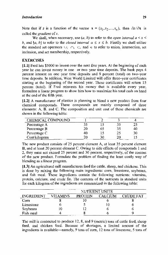
EXERCISES [1.1] Fred has $5000 to invest over the next five years. At the beginning of each year he can invest money in one- or two-year time deposits. The bank pays 4 percent interest on one-year time deposits and 9 percent (total) on two-year time deposits. In addition, West World Limited will offer three-year certificates starting at the beginning of the second year. These certificates will return 15 percent (total). If Fred reinvests his money that is available every year, formulate a linear program to show him how to maximize his total cash on hand at the end of the fifth year.
[1.2] A manufacturer of plastics is planning to blend a new product from four chemical compounds. These compounds are mainly composed of three elements: A, B, and C. The composition and unit cost of these chemicals are shown in the following table:
CHEMICAL COMPOUND Percentage A Percentage B Percentage C Cost/kilogram
1 35 20 40 20
2 15 65 15 30
3 35 35 25 20
4 25 40 30 15
The new product consists of 25 percent element A, at least 35 percent element B, and at least 20 percent element C. Owing to side effects of compounds 1 and 2, they must not exceed 25 percent and 30 percent, respectively, of the content of the new product. Formulate the problem of finding the least costly way of blending as a linear program. [1.3] An agricultural mill manufactures feed for cattle, sheep, and chickens. This is done by mixing the following main ingredients: corn, limestone, soybeans, and fish meal. These ingredients contain the following nutrients: vitamins, protein, calcium, and crude fat. The contents of the nutrients in standard units for each kilogram of the ingredients are summarized in the following table:
NUTRIENT UNITS INGREDIENT Corn Limestone Soybeans Fish meal
VITAMINS 8 6 10 4
PROTEIN 10 5 12 8
CALCIUM 6 10 6 6
CRUDE FAT 8 6 6 9
The mill is contracted to produce 12, 8, and 9 (metric) tons of cattle feed, sheep feed, and chicken feed. Because of shortages, a limited amount of the ingredients is available—namely, 9 tons of corn, 12 tons of limestone, 5 tons of
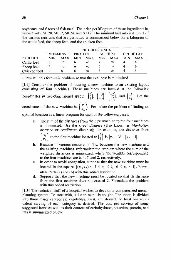
30 Chapter 1
soybeans, and 6 tons offish meal. The price per kilogram of these ingredients is, respectively, $0.20, $0.12, $0.24, and $0.12. The minimal and maximal units of the various nutrients that are permitted is summarized below for a kilogram of the cattle feed, the sheep feed, and the chicken feed.
PRODUCT Cattle feed Sheep feed Chicken feed
VITAMINS MIN MAX 6 6 4
oo OO
6
NUTRIENT UNITS PROTEIN MIN MAX 6 oo 6 oo 6 oo
CALCIUM MIN MAX 7 6 6
oo oo oo
CRUDE FAT MIN MAX 4 8 4 6 4 5
Formulate this feed-mix problem so that the total cost is minimized.
[1.4] Consider the problem of locating a new machine to an existing layout consisting of four machines. These machines are located at the following
coordinates in two-dimensional space: , , , , - 1 , and L . Let the
coordinates of the new machine be ' . Formulate the problem of finding an
optimal location as a linear program for each of the following cases:
a. The sum of the distances from the new machine to the four machines is minimized. Use the street distance (also known as Manhattan distance or rectilinear distance); for example, the distance from
1 to the first machine located at , I is |xj - 3| + |x2 - l|·
b. Because of various amounts of flow between the new machine and the existing machines, reformulate the problem where the sum of the weighted distances is minimized, where the weights corresponding to the four machines are 6,4, 7, and 2, respectively.
c. In order to avoid congestion, suppose that the new machine must be located in the square {(x1;x2) : -1 ^ *i ^ 2, 0 < x2 < 1}. Form-ulate Parts (a) and (b) with this added restriction.
d. Suppose that the new machine must be located so that its distance from the first machine does not exceed 2. Formulate the problem with this added restriction.
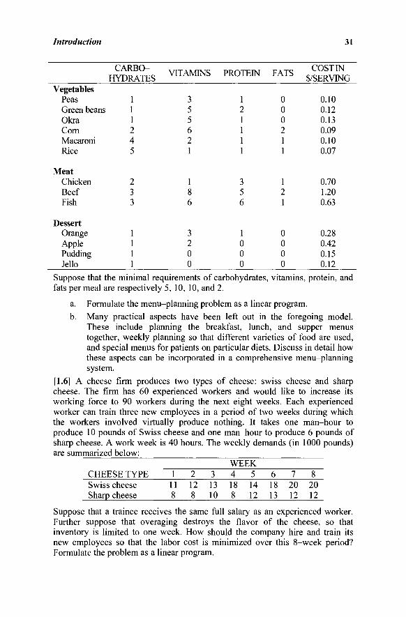
[1.5] The technical staff of a hospital wishes to develop a computerized menu-planning system. To start with, a lunch menu is sought. The menu is divided into three major categories: vegetables, meat, and dessert. At least one equi-valent serving of each category is desired. The cost per serving of some suggested items as well as their content of carbohydrates, vitamins, protein, and fats is summarized below:
Introduction 31
Vegetables Peas Green beans Okra Corn Macaroni Rice
Meat Chicken Beef Fish
Dessert Orange Apple Pudding Jello
CARBO-HYDRATES
1 1 1 2 4 5
2 3 3
1 1 1 1
VITAMINS
3 5 5 6 2 1
1 8 6
3 2 0 0
PROTEIN
1 2 1 1 1 1
3 5 6
1 0 0 0
FATS
0 0 0 2 1 1
1 2 1
0 0 0 0
COST IN $/SERVING
0.10 0.12 0.13 0.09 0.10 0.07
0.70 1.20 0.63
0.28 0.42 0.15 0.12
Suppose that the minimal requirements of carbohydrates, vitamins, protein, and fats per meal are respectively 5, 10, 10, and 2.
a. Formulate the menu-planning problem as a linear program.
b. Many practical aspects have been left out in the foregoing model. These include planning the breakfast, lunch, and supper menus together, weekly planning so that different varieties of food are used, and special menus for patients on particular diets. Discuss in detail how these aspects can be incorporated in a comprehensive menu-planning system.
[1.6] A cheese firm produces two types of cheese: swiss cheese and sharp cheese. The firm has 60 experienced workers and would like to increase its working force to 90 workers during the next eight weeks. Each experienced worker can train three new employees in a period of two weeks during which the workers involved virtually produce nothing. It takes one man-hour to produce 10 pounds of Swiss cheese and one man-hour to produce 6 pounds of sharp cheese. A work week is 40 hours. The weekly demands (in 1000 pounds) are summarized below:
CHEESE TYPE Swiss cheese Sharp cheese
1 11 8
2 12 8
3 13 10
WEEK 4 5 18 14 8 12
6 18 13
7 20 12
8 20 12
Suppose that a trainee receives the same full salary as an experienced worker. Further suppose that overaging destroys the flavor of the cheese, so that inventory is limited to one week. How should the company hire and train its new employees so that the labor cost is minimized over this 8-week period? Formulate the problem as a linear program.
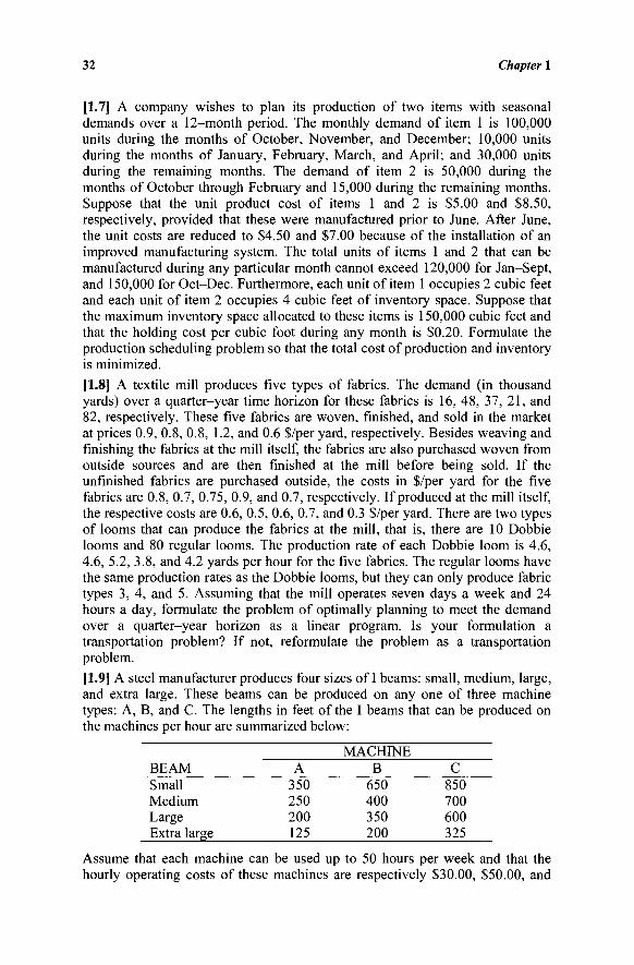
32 Chapter 1
[1.7] A company wishes to plan its production of two items with seasonal demands over a 12-month period. The monthly demand of item 1 is 100,000 units during the months of October, November, and December; 10,000 units during the months of January, February, March, and April; and 30,000 units during the remaining months. The demand of item 2 is 50,000 during the months of October through February and 15,000 during the remaining months. Suppose that the unit product cost of items 1 and 2 is $5.00 and $8.50, respectively, provided that these were manufactured prior to June. After June, the unit costs are reduced to $4.50 and $7.00 because of the installation of an improved manufacturing system. The total units of items 1 and 2 that can be manufactured during any particular month cannot exceed 120,000 for Jan-Sept, and 150,000 for Oct-Dec. Furthermore, each unit of item 1 occupies 2 cubic feet and each unit of item 2 occupies 4 cubic feet of inventory space. Suppose that the maximum inventory space allocated to these items is 150,000 cubic feet and that the holding cost per cubic foot during any month is $0.20. Formulate the production scheduling problem so that the total cost of production and inventory is minimized.
[1.8] A textile mill produces five types of fabrics. The demand (in thousand yards) over a quarter-year time horizon for these fabrics is 16, 48, 37, 21, and 82, respectively. These five fabrics are woven, finished, and sold in the market at prices 0.9, 0.8, 0.8, 1.2, and 0.6 $/per yard, respectively. Besides weaving and finishing the fabrics at the mill itself, the fabrics are also purchased woven from outside sources and are then finished at the mill before being sold. If the unfinished fabrics are purchased outside, the costs in $/per yard for the five fabrics are 0.8, 0.7, 0.75, 0.9, and 0.7, respectively. If produced at the mill itself, the respective costs are 0.6, 0.5, 0.6, 0.7, and 0.3 $/per yard. There are two types of looms that can produce the fabrics at the mill, that is, there are 10 Dobbie looms and 80 regular looms. The production rate of each Dobbie loom is 4.6, 4.6, 5.2, 3.8, and 4.2 yards per hour for the five fabrics. The regular looms have the same production rates as the Dobbie looms, but they can only produce fabric types 3, 4, and 5. Assuming that the mill operates seven days a week and 24 hours a day, formulate the problem of optimally planning to meet the demand over a quarter-year horizon as a linear program. Is your formulation a transportation problem? If not, reformulate the problem as a transportation problem.
[1.9] A steel manufacturer produces four sizes of I beams: small, medium, large, and extra large. These beams can be produced on any one of three machine types: A, B, and C. The lengths in feet of the I beams that can be produced on the machines per hour are summarized below:
BEAM Small Medium Large Extra large
A 350 250 200 125
MACHINE B
650 400 350 200
C 850 700 600 325
Assume that each machine can be used up to 50 hours per week and that the hourly operating costs of these machines are respectively $30.00, $50.00, and
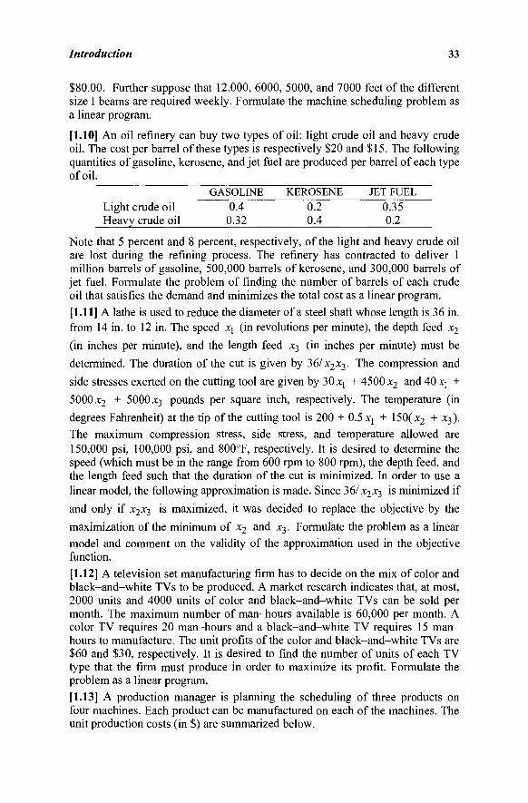
Introduction 33
$80.00. Further suppose that 12,000, 6000, 5000, and 7000 feet of the different size I beams are required weekly. Formulate the machine scheduling problem as a linear program.
[1.10] An oil refinery can buy two types of oil: light crude oil and heavy crude oil. The cost per barrel of these types is respectively $20 and $15. The following quantities of gasoline, kerosene, and jet fuel are produced per barrel of each type of oil.
GASOLINE KEROSENE JET FUEL Light crude oil 0.4 0.2 0.35 Heavy crude oil 032 04 0.2
Note that 5 percent and 8 percent, respectively, of the light and heavy crude oil are lost during the refining process. The refinery has contracted to deliver 1 million barrels of gasoline, 500,000 barrels of kerosene, and 300,000 barrels of jet fuel. Formulate the problem of finding the number of barrels of each crude oil that satisfies the demand and minimizes the total cost as a linear program.
[1.11] A lathe is used to reduce the diameter of a steel shaft whose length is 36 in. from 14 in. to 12 in. The speed X\ (in revolutions per minute), the depth feed x2
(in inches per minute), and the length feed x3 (in inches per minute) must be determined. The duration of the cut is given by 36/x2x3. The compression and side stresses exerted on the cutting tool are given by 30 xj + 4500 x2 and 40 X] + 5000 x2 + 5000 x3 pounds per square inch, respectively. The temperature (in degrees Fahrenheit) at the tip of the cutting tool is 200 + 0.5 jq + 150(x2 + x3). The maximum compression stress, side stress, and temperature allowed are 150,000 psi, 100,000 psi, and 800°F, respectively. It is desired to determine the speed (which must be in the range from 600 rpm to 800 rpm), the depth feed, and the length feed such that the duration of the cut is minimized. In order to use a linear model, the following approximation is made. Since 36/x2x3 is minimized if and only if x2x3 is maximized, it was decided to replace the objective by the maximization of the minimum of x2 and x3. Formulate the problem as a linear model and comment on the validity of the approximation used in the objective function.
[1.12] A television set manufacturing firm has to decide on the mix of color and black-and-white TVs to be produced. A market research indicates that, at most, 2000 units and 4000 units of color and black-and-white TVs can be sold per month. The maximum number of man-hours available is 60,000 per month. A color TV requires 20 man-hours and a black-and-white TV requires 15 man-hours to manufacture. The unit profits of the color and black-and-white TVs are $60 and $30, respectively. It is desired to find the number of units of each TV type that the firm must produce in order to maximize its profit. Formulate the problem as a linear program. [1.13] A production manager is planning the scheduling of three products on four machines. Each product can be manufactured on each of the machines. The unit production costs (in $) are summarized below.
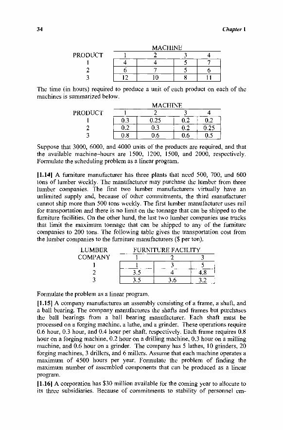
34 Chapter 1
MACHINE PRODUCT 1 2 3 4
4 6 12
4 7 10
5 5 8
7 6 11
The time (in hours) required to produce a unit of each product on each of the machines is summarized below.
MACHINE PRODUCT 1 2 3 4
0.3 0.2 0.8
0.25 0.3 0.6
0.2 0.2 0.6
0.2 0.25 0.5
Suppose that 3000, 6000, and 4000 units of the products are required, and that the available machine-hours are 1500, 1200, 1500, and 2000, respectively. Formulate the scheduling problem as a linear program.
[1.14] A furniture manufacturer has three plants that need 500, 700, and 600 tons of lumber weekly. The manufacturer may purchase the lumber from three lumber companies. The first two lumber manufacturers virtually have an unlimited supply and, because of other commitments, the third manufacturer cannot ship more than 500 tons weekly. The first lumber manufacturer uses rail for transportation and there is no limit on the tonnage that can be shipped to the furniture facilities. On the other hand, the last two lumber companies use trucks that limit the maximum tonnage that can be shipped to any of the furniture companies to 200 tons. The following table gives the transportation cost from the lumber companies to the furniture manufacturers ($ per ton).
LUMBER FURNITURE FACILITY COMPANY 1 2 3
1 3.5 3.5
3 4
3.6
5 4.8 3.2
Formulate the problem as a linear program. [1.15] A company manufactures an assembly consisting of a frame, a shaft, and a ball bearing. The company manufactures the shafts and frames but purchases the ball bearings from a ball bearing manufacturer. Each shaft must be processed on a forging machine, a lathe, and a grinder. These operations require 0.6 hour, 0.3 hour, and 0.4 hour per shaft, respectively. Each frame requires 0.8 hour on a forging machine, 0.2 hour on a drilling machine, 0.3 hour on a milling machine, and 0.6 hour on a grinder. The company has 5 lathes, 10 grinders, 20 forging machines, 3 drillers, and 6 millers. Assume that each machine operates a maximum of 4500 hours per year. Formulate the problem of finding the maximum number of assembled components that can be produced as a linear program.
[1.16] A corporation has $30 million available for the coming year to allocate to its three subsidiaries. Because of commitments to stability of personnel em-
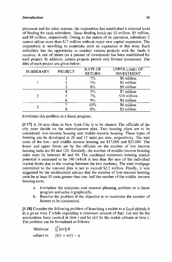
Introduction 35
ployment and for other reasons, the corporation has established a minimal level of funding for each subsidiary. These funding levels are $3 million, $5 million, and $8 million, respectively. Owing to the nature of its operation, subsidiary 2 cannot utilize more than $17 million without major new capital expansion. The corporation is unwilling to undertake such an expansion at this time. Each subsidiary has the opportunity to conduct various projects with the funds it receives. A rate of return (as a percent of investment) has been established for each project. In addition, certain projects permit only limited investment. The data of each project are given below:
SUBSIDIARY
1
2
3
PROJECT
1 2 3 4 5 6 7 8
RATE OF RETURN
7% 5% 8% 5% 7% 9% 10% 8%
UPPER LIMIT OF INVESTMENT
$6 million $5 million $9 million $7 million
$10 million $4 million $6 million $3 million
Formulate this problem as a linear program.
[1.17] A 10-acre slum in New York City is to be cleared. The officials of the city must decide on the redevelopment plan. Two housing plans are to be considered: low-income housing and middle-income housing. These types of housing can be developed at 20 and 15 units per acre, respectively. The unit costs of the low- and middle-income housing are $17,000 and $25,000. The lower and upper limits set by the officials on the number of low-income housing units are 80 and 120. Similarly, the number of middle-income housing units must lie between 40 and 90. The combined maximum housing market potential is estimated to be 190 (which is less than the sum of the individual market limits due to the overlap between the two markets). The total mortgage committed to the renewal plan is not to exceed $2.5 million. Finally, it was suggested by the architectural adviser that the number of low-income housing units be at least 50 units greater than one-half the number of the middle-income housing units.
a. Formulate the minimum cost renewal planning problem as a linear program and solve it graphically.
b. Resolve the problem if the objective is to maximize the number of houses to be constructed.
[1.18] Consider the following problem of launching a rocket to a fixed altitude b in a given time T while expending a minimum amount of fuel. Let u(t) be the acceleration force exerted at time t and let y(t) be the rocket altitude at time t. The problem can be formulated as follows:
Minimize J0 |w(?)|i#
subject to y(t) = u(t) - g
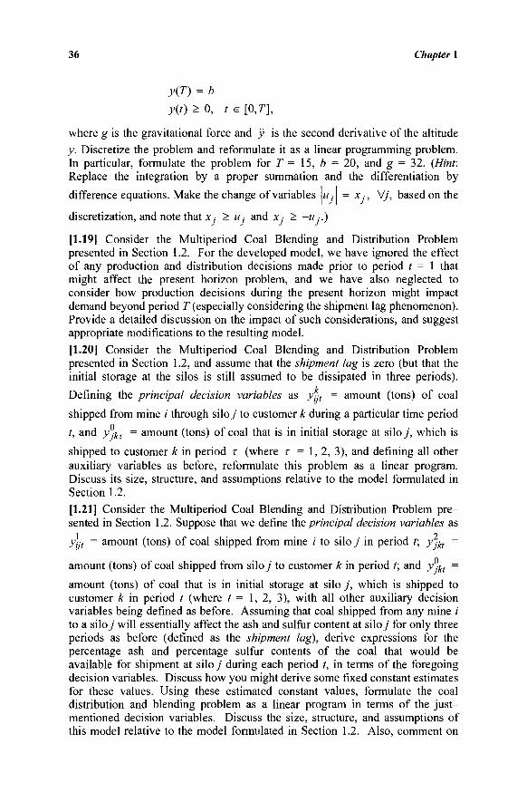
36 Chapter 1
y(T) = b y(t) > 0, / e [Ο,Γ],
where g is the gravitational force and y is the second derivative of the altitude y. Discretize the problem and reformulate it as a linear programming problem. In particular, formulate the problem for T = 15, b = 20, and g = 32. (Hint: Replace the integration by a proper summation and the differentiation by
difference equations. Make the change of variables M, = x ·, V/, based on the
discretization, and note that x- > u and x- > -w·.)
[1.19] Consider the Multiperiod Coal Blending and Distribution Problem presented in Section 1.2. For the developed model, we have ignored the effect of any production and distribution decisions made prior to period / = 1 that might affect the present horizon problem, and we have also neglected to consider how production decisions during the present horizon might impact demand beyond period T (especially considering the shipment lag phenomenon). Provide a detailed discussion on the impact of such considerations, and suggest appropriate modifications to the resulting model.
[1.20] Consider the Multiperiod Coal Blending and Distribution Problem presented in Section 1.2, and assume that the shipment lag is zero (but that the initial storage at the silos is still assumed to be dissipated in three periods).
Defining the principal decision variables as y^, = amount (tons) of coal
shipped from mine / through siloy to customer k during a particular time period
t, and yjkz = amount (tons) of coal that is in initial storage at silo j , which is
shipped to customer k in period r (where r = 1, 2, 3), and defining all other auxiliary variables as before, reformulate this problem as a linear program. Discuss its size, structure, and assumptions relative to the model formulated in Section 1.2.
[1.21] Consider the Multiperiod Coal Blending and Distribution Problem pre-sented in Section 1.2. Suppose that we define the principal decision variables as
1 *s
yijt = amount (tons) of coal shipped from mine i to silo j in period t; yjkt =
amount (tons) of coal shipped from siloy to customer k in period t; and y^ =
amount (tons) of coal that is in initial storage at silo j , which is shipped to customer k in period / (where / = 1, 2, 3), with all other auxiliary decision variables being defined as before. Assuming that coal shipped from any mine i to a silo j will essentially affect the ash and sulfur content at siloy for only three periods as before (defined as the shipment lag), derive expressions for the percentage ash and percentage sulfur contents of the coal that would be available for shipment at silo j during each period /, in terms of the foregoing decision variables. Discuss how you might derive some fixed constant estimates for these values. Using these estimated constant values, formulate the coal distribution and blending problem as a linear program in terms of the just-mentioned decision variables. Discuss the size, structure, and assumptions of this model relative to the model formulated in Section 1.2. Also, comment on
Introduction 37
the nature of the resulting model if we used the actual expressions for the ash and sulfur content of coal at each silo j during each period t, in lieu of the constant estimates. [1.22] A region is divided into m residential and central business districts. Each district is represented by a node, and the nodes are interconnected by links representing major routes. People living in the various districts go to their business in the same and/or at other districts so that each node attracts and/or generates a number of trips. In particular, let ay be the number of trips
generated at node / with final destination at node j and let by be the time to
travel from node i to node j . It is desired to determine the routes to be taken by the people living in the region.
a. Illustrate the problem by a suitable network. b. Develop some measures of effectiveness for this traffic assignment
problem, and for each measure, devise a suitable model.
[1.23] Consider the problem of scheduling court hearings over a planning horizon consisting of « periods. Let b- be the available judge-hours in period j ,
hy be the number of hearings of class ; arriving in period j , and ai be the
number of judge-hours required to process a hearing of class ;'. It is desired to determine the number of hearings Xy of class i processed in period/
a. Formulate the problem as a linear program. b. Modify the model in Part (a) so that hearings would not be delayed
for too long.
[1.24] Consider the following multiperiod, multiproduct Production-Inventory Problem. Suppose that we are examining T periods t = 1,..., T, and some n products / = 1,..., n. There is an initial inventory of yi0 that is available at hand for each product /, / = 1,..., n. We need to principally determine the level of production for each product i = 1,..., n during each of the periods / = 1,..., T, so as to meet the forecasted demand dit for each product / during each period /
when it occurs, at a minimal total cost. To take advantage of varying demands and costs, we are permitted to produce excess quantities to be stored for later use. However, each unit of product / consumes a storage space Sj, and incurs a storage cost of cit during period t, for / = 1,..., n, t = 1,..., T. The total storage space anticipated to be available for these n products during period /is St, t=\ ,..., T. Furthermore, each unit of product i requires /?, hours of labor to produce, where the labor cost per hour when producing a unit of product i during period t is given by iit, for / = 1,..., n, t = 1,..., T. The total number of labor hours
available to manufacture these n products during period t is given by Ht. Formulate a linear program to solve this production-inventory control system problem, prescribing production as well as inventory levels for each product over each time period.
38 Chapter 1
[1.25] Suppose that there are m sources that generate waste and n disposal sites. The amount of waste generated at source / is a,· and the capacity of site j is b-.
It is desired to select appropriate transfer facilities from among K candidate facilities. Potential transfer facility k has a fixed cost fk, capacity qk, and unit
processing cost ak per ton of waste. Let cik and cL be the unit shipping costs
from source i to transfer station k and from transfer station k to disposal site j , respectively. The problem is to choose the transfer facilities and the shipping pattern that minimize the total capital and operating costs of the transfer stations plus the transportation costs. Formulate this distribution problem. {Hint: Let yk
be 1 if transfer station k is selected and 0 otherwise.)
[1.26] A governmental planning agency wishes to determine the purchasing sources for fuel for use by n depots from among m bidders. Suppose that the maximum quantity offered by bidder i is at gallons and that the demand of depot/
is bj gallons. Let c,y be the unit delivery cost for bidder i to they'th depot.
a. Formulate the problem of minimizing the total purchasing cost as a linear program.
b. Suppose that a discount in the unit delivery cost is offered by bidder i if the ordered quantity exceeds the level ar;. How would you incorporate this modification in the model developed in Part (a)?
[1.27] The quality of air in an industrial region largely depends on the effluent emission from n plants. Each plant can use m different types of fuel. Suppose that the total energy needed at plant j is b- British Thermal Units per day and
that Cj- is the effluent emission per ton of fuel type i at plant j . Further suppose
that fuel type / costs c; dollars per ton and that each ton of this fuel type generates
ay British Thermal Units at plant j . The level of air pollution in the region is not
to exceed b micrograms per cubic meter. Finally, let γ ■ be a meteorological
parameter relating emissions at plant/ to air quality in the region.
a. Formulate the problem of determining the mix of fuels to be used at each plant.
b. How would you incorporate technological constraints that prohibit the use of certain mixes of fuel at certain plants?
c. How could you ensure equity among the plants?
[1.28] For some industry, let p(Q), Q > 0, be an inverse demand curve, that is,
p(Q) is the price at which a quantity Q will be demanded. L e t / ( 0 , Q > 0, be a supply or marginal cost curve, that is, fyQ) is the price at which the industry is willing to supply Q units of the product. Consider the problem of determining a
(perfect competition) equilibrium price and production quantity p* and Q* for
/>(·) and /(■) of the type shown in Figure 1.14 via the intersection of these

Introduction 39
supply and demand curves. Note that Q* is obtainable by finding that Q, which maximizes the area under the demand curve minus the area under the supply curve. Now, suppose that /( ·) is not available directly, but being a marginal cost curve, is given implicitly by
\®f(x)dx = min{cy: Ay = b, ay = Q,y > 0},
where A is m x n, a and c are 1 x «, and y is an «-vector representing a set of production activities. Further, suppose that the demand curve />(·) is approx-imated using the steps shown in the figure. (Let there be s steps used, each of height Hi and width Wi for / = 1,..., s.) With this approximation, formulate the problem of determining the price-quantity equilibrium as a linear program.
* Q
Figure 1.14. Supply demand equilibrium for Exercise 1.28
[1.29] Consider the following two-stage stochastic program with recourse. Suppose that in a time-stage process, we need to make some immediate decision ("here and now") that is represented by the decision variable vector x > 0. (For example, x might represent some investment or production decisions.) This decision must satisfy the constraints Ax = b. Subsequent to this, a random demand vector d, say, will be realized according to some probability distribution. Based on the initial decision x and the realization d, we will need to make a recourse decision y > 0 (e.g., some subsequent additional production decisions), such that the constraint Dx + Ey = d is satisfied. The total objective cost for this pair of decisions is given by q x + C2y. Assume that the random demand vector d can take on a discrete set of possible values dj , d2 , —, d„ with respective known
probabilities p\, p2,—,pq, where Σ Pr r=\
= 1, pr > 0, Vr = \,...,q. (Accord-
ingly, note that each realization dr will prompt a corresponding recourse decision yr.) Formulate the problem of minimizing the total expected cost subject to the initial and recourse decision constraints as a linear programming problem. Do you observe any particular structure in the overall constraint coefficient matrix with respect to the possible nonzero elements? (Chapter 7 explores ways for solving such problems.)
[1.30] Consider the following linear programming problem.
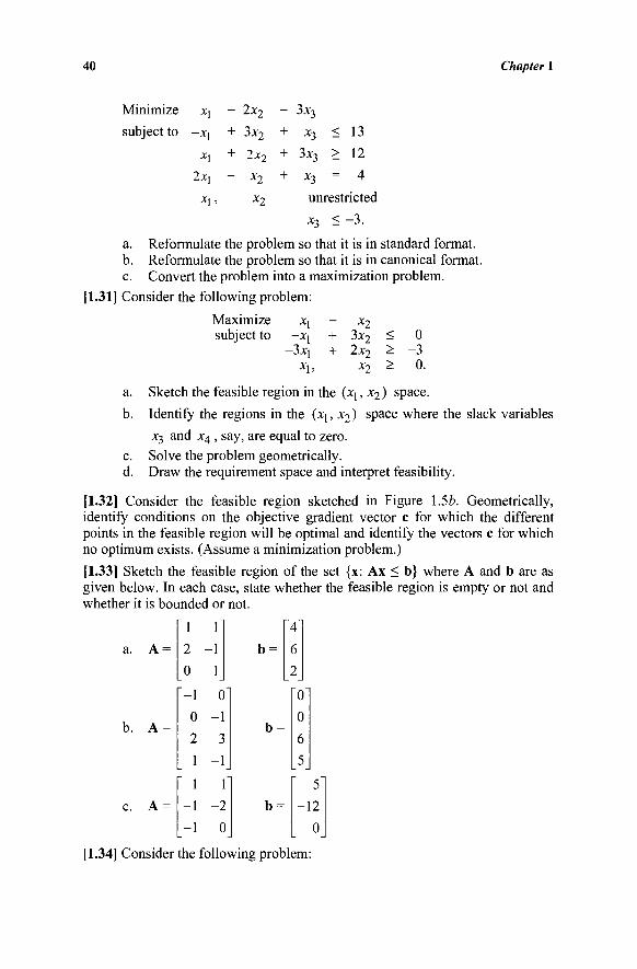
40 Chapter 1
Minimize
subject to - * i
x\
- 2x2
+ 3x2
+ 2x2
- * 2
- 3x3
+ x3 < 13
+ 3x3 > 12
+ x3 = 4
x2 unrestricted
x3 < - 3 .
a. Reformulate the problem so that it is in standard format. b. Reformulate the problem so that it is in canonical format. c. Convert the problem into a maximization problem.
[1.31] Consider the following problem:
Maximize subject to
x\ - j q
- 3 x j x{,
~ x2 + 3x2 + 2x2
x2
< > >
0 -3
0
a.
b.
Sketch the feasible region in the (X], Χ2 ) space.
Identify the regions in the (xj, x2) space where the slack variables
x3 and x4 , say, are equal to zero. Solve the problem geometrically. Draw the requirement space and interpret feasibility.
[1.32] Consider the feasible region sketched in Figure \.5b. Geometrically, identify conditions on the objective gradient vector c for which the different points in the feasible region will be optimal and identify the vectors c for which no optimum exists. (Assume a minimization problem.)
[1.33] Sketch the feasible region of the set {x: Ax < b} where A and b are as given below. In each case, state whether the feasible region is empty or not and whether it is bounded or not.
a.
b. A:
c.
"-1
0
2 1
0"
-1
3 -1
b =
"0"
0
6 5
1
-1
-1
f -2
0
b =
5"
-12
0
[1.34] Consider the following problem:
Introduction 41
a. b.
Maximize subject to
3X! -*1
Sketch the feasible region.
+ +
x2 2x2
x2 < <
0 4.
Verify that the problem has an unbounded optimal solution value.
[1.35] Consider the following problem:
Maximize subject to
2x\ *l
4xj Xj,
+ + +
3x2
x2
6x2 x2
< < >
2 9 0.
a. Sketch the feasible region. b. Find two alternative optimal extreme (corner) points. c. Find an infinite class of optimal solutions.
[1.36] Consider the following problem:
Maximize -xj - x2 + 2x3 + x4
subject to 2xj + x2 + x3 + x4 > 6 Xj + 2x2 - 2x3 + x4 < 4 X], x2 , x3, x4 > 0.
a. Introduce slack variables and draw the requirement space. b. Interpret feasibility in the requirement space. c. You are told that an optimal solution can be obtained by having at
most two positive variables while all other variables are set at zero. Utilize this statement and the requirement space to find an optimal solution.
[1.37] Consider the following problem:
Maximize subject to
3xj -*!
-2xj *1 Xj,
+ + + +
6x2 2x2
x2
2x2 x2
< < < >
2 0 4 0,
a. Graphically identify the set of all alternative optimal solutions to this problem.
b. Suppose that a secondary priority objective function seeks to maximize -3xj + x2 over the set of alternative optimal solutions identified in Part (a). What is the resulting solution obtained?
c. What is the solution obtained if the priorities of the foregoing two objective functions is reversed?
[1.38] Consider the problem: Minimize ex subject to Ax > b, x > 0. Suppose that one component of the vector b, say bt, is increased by one unit to 6, + 1.
a. What happens to the feasible region? b. What happens to the optimal objective value?
[1.39] From the results of the previous problem, assuming dz I dbj exists, is it < 0, = 0, or > 0?
42 Chapter 1
[1.40] Solve Exercises 1.38 and 1.39 if the restrictions Ax > b are replaced by Ax<b .
[1.41] Consider the problem: Minimize ex subject to Ax > b, x > 0 a new constraint is added to the problem.
a. What happens to the feasible region? b. What happens to the optimal objective value z ?
[1.42] Consider the problem: Minimize ex subject to Ax > b, x > 0 a new variable is added to the problem.
a. What happens to the feasible region? b. What happens to the optimal objective value z ?
[1.43] Consider the problem: Minimize ex subject to Ax > b, x > 0 a constraint, say constraint /, is deleted from the problem.
a. What happens to the feasible region? b. What happens to the optimal objective value z ?
[1.44] Consider the problem: Minimize ex subject to Ax > b, x > 0 a variable, say, xk, is deleted from the problem.
a. What happens to the feasible region? b. What happens to the optimal objective value z ?
NOTES AND REFERENCES
1. Linear programming and the simplex method were developed by Dantzig in 1947 in connection with military planning. A great deal of work has influenced the development of linear programming, including World War II operations and the need for scheduling supply and maintenance operations as well as training of Air Force personnel: Leontief s input-output model [1951], von Neumann's Equilibrium Model [1937], Koopmans' Model of Transportation [1949], the Hitchcock transportation problem [1941], the work of Kantorovich [1958], von Neumann-Morgenstern game theory [1944], and the rapid progress in electronic computing machines have also impacted the field of linear programming. The papers by Dantzig [1982] and by Albers and Reid [1986] provide good historical developments.
2. Linear programming has found numerous applications in the military, the government, industry, and urban engineering. See Swanson [1980], for example.
3. Linear programming is also frequently used as a part of general computational schemes for solving nonlinear programming problems, discrete programs, combinatorial problems, problems of optimal control, and programming under uncertainty.
4. Exercise 1.8 is derived from Camm et al. [1987], who discuss some modeling issues. For more detailed discussions, see Woolsey and Swanson [1975], Woolsey [2003], and Swanson [1980]. The Multiperiod Coal Blending and Distribution Problem discussed in Section 1.2, and Exercises 1.19-1.21, are adapted from Sherali and Puri [1993] (see also Sherali and Saifee [1993]). For a discussion on structured modeling and on computer-assisted/artificial intelligence approaches to linear
Suppose that
Suppose that
Suppose that
Suppose that
Introduction 43
programming modeling, see Geoffrion [1987], Greenberg [1983], and Murphy and Stohr [1986], for example.
5. For discussions on diagnosing infeasibilities and related Irreducible Infeasible System (IIS) issues, see Arnaldi et al. [2003], Greenberg [1996], Greenberg and Murphy [1991], and Parker and Ryan [1996].
6. For an excellent discussion on modeling issues and insights related to formulating and solving real-world problems, the reader is referred to Brown and Rosenthal [2008] (also, see the other references cited therein).

This page intentionally left blank
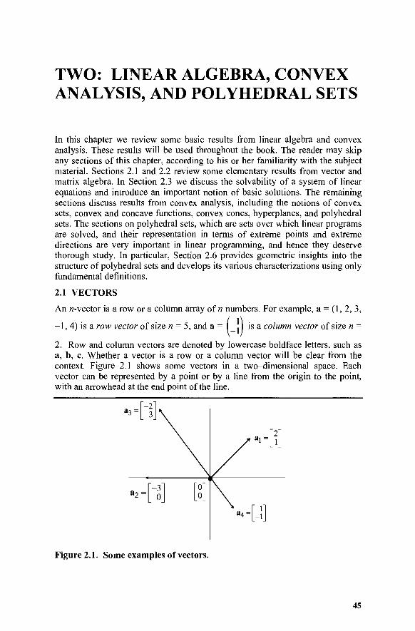
TWO: LINEAR ALGEBRA, CONVEX ANALYSIS, AND POLYHEDRAL SETS
In this chapter we review some basic results from linear algebra and convex analysis. These results will be used throughout the book. The reader may skip any sections of this chapter, according to his or her familiarity with the subject material. Sections 2.1 and 2.2 review some elementary results from vector and matrix algebra. In Section 2.3 we discuss the solvability of a system of linear equations and introduce an important notion of basic solutions. The remaining sections discuss results from convex analysis, including the notions of convex sets, convex and concave functions, convex cones, hyperplanes, and polyhedral sets. The sections on polyhedral sets, which are sets over which linear programs are solved, and their representation in terms of extreme points and extreme directions are very important in linear programming, and hence they deserve thorough study. In particular, Section 2.6 provides geometric insights into the structure of polyhedral sets and develops its various characterizations using only fundamental definitions.
2.1 VECTORS
An «-vector is a row or a column array of « numbers. For example, a = (1, 2, 3,
-!) -1, 4) is a row vector of size n = 5, and a is a column vector of size ,
2. Row and column vectors are denoted by lowercase boldface letters, such as a, b, c. Whether a vector is a row or a column vector will be clear from the context. Figure 2.1 shows some vectors in a two-dimensional space. Each vector can be represented by a point or by a line from the origin to the point, with an arrowhead at the end point of the line.
Figure 2.1. Some examples of vectors.
45
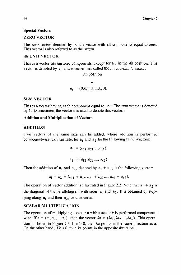
46 Chapter 2
Special Vectors
ZERO VECTOR
The zero vector, denoted by 0, is a vector with all components equal to zero. This vector is also referred to as the origin.
ith UNIT VECTOR
This is a vector having zero components, except for a 1 in the ith position. This vector is denoted by e; and is sometimes called the z'th coordinate vector.
rth position
i e,· = (0,0,...,1,...,0,0).
SUM VECTOR
This is a vector having each component equal to one. The sum vector is denoted by 1. (Sometimes, the vector e is used to denote this vector.)
Addition and Multiplication of Vectors
ADDITION
Two vectors of the same size can be added, where addition is performed componentwise. To illustrate, let aj and a2 be the following two «-vectors:
a l = (.an,a2\,...,anl),
a2 = (au,a22,...,an2).
Then the addition of aj and a2, denoted by aj + a2, is the following vector:
«l + a2 = (an + an,a2X + a22,...,anl + an2).
The operation of vector addition is illustrated in Figure 2.2. Note that aj + a2 is
the diagonal of the parallelogram with sides aj and a2. It is obtained by step-
ping along aj and then a2, or vice versa.
SCALAR MULTIPLICATION
The operation of multiplying a vector a with a scalar k is performed component-wise. I f a = {a\,a2,...,an), then the vector k& - (kax,ka2,...,kan). This opera-tion is shown in Figure 2.3. If k > 0, then k& points in the same direction as a. On the other hand, if k < 0, then ka points in the opposite direction.
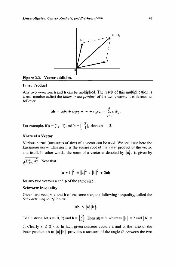
Linear Algebra, Convex Analysis, and Polyhedral Sets 47
Figure 2.2. Vector addition.
Inner Product
Any two «-vectors a and b can be multiplied. The result of this multiplication is a real number called the inner or dot product of the two vectors. It is defined as follows:
ab = αφχ + α·φι + ··· + anbn = Σ ajbj-
For example, if a = (1,-1) and b = , , then ab = - 3 .
Norm of a Vector
Various norms (measures of size) of a vector can be used. We shall use here the Euclidean norm. This norm is the square root of the inner product of the vector and itself. In other words, the norm of a vector a, denoted by llall, is given by
Σ"=ία). Note that
a + b Hall2 + ||b||2 + 2ab
for any two vectors a and b of the same size.
Schwartz Inequality
Given two vectors a and b of the same size, the following inequality, called the Schwartz inequality, holds:
|ab| < llall ||bj|.
To illustrate, let a = (0, 2) and b : . Then ab = 8, whereas llall = 2 and ||b|| =
5. Clearly 8 < 2 x 5. In fact, given nonzero vectors a and b, the ratio of the inner product ab to llall llbll provides a measure of the angle Θ between the two
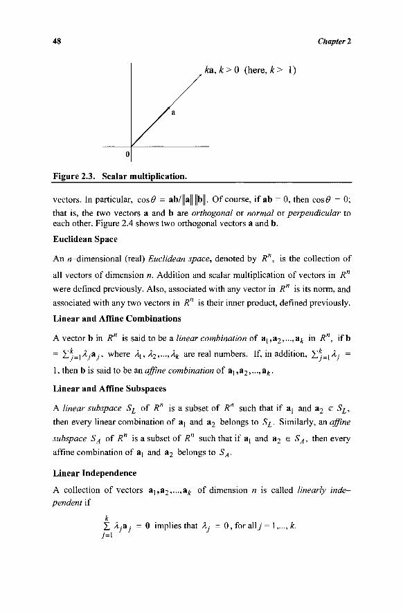
48 Chapter 2
k&, k>0 (here, k> 1)
Figure 2.3. Scalar multiplication.
vectors. In particular, cose? = a b / a b . Of course, if ab = 0, then cosi? = 0;
that is, the two vectors a and b are orthogonal or normal or perpendicular to each other. Figure 2.4 shows two orthogonal vectors a and b.
Euclidean Space
An «-dimensional (real) Euclidean space, denoted by R", is the collection of
all vectors of dimension n. Addition and scalar multiplication of vectors in R"
were defined previously. Also, associated with any vector in Rn is its norm, and
associated with any two vectors in Rn is their inner product, defined previously.
Linear and Affine Combinations
A vector b in R" is said to be a linear combination of a[,a2,...,a£ in Rn, if b
■\h = = X*.=jA.-a,·, where Aj, λ^,.,.,λ^ are real numbers. If, in addition, £*._
1, then b is said to be an affine combination of aj,a2,...,at.
Linear and Affine Subspaces
A linear subspace SL of Rn is a subset of R" such that if a! and a2 £ SL,
then every linear combination of aj and a2 belongs to SL. Similarly, an affine
subspace SA of Rn is a subset of R" such that if aj and a2 £ SA, then every
affine combination of aj and a2 belongs to SA.
Linear Independence
A collection of vectors aj,a2,...,a^ of dimension n is called linearly inde-pendent if
Σ l a - = 0 implies that A.- = 0, for ally = \,...,k.
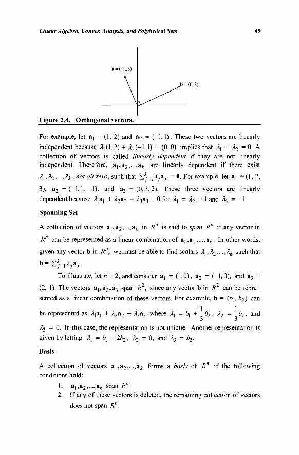
Linear Algebra, Convex Analysis, and Polyhedral Sets 49
a = (-1,3)
b = (6,2)
Figure 2.4. Orthogonal vectors.
For example, let aj = (1, 2) and a2 = (-1,1). These two vectors are linearly independent because A] (1,2) + ^(-1 ,1) = (0,0) implies that \ = Àq_ = 0. A collection of vectors is called linearly dependent if they are not linearly independent. Therefore, a1,a2,...,alt are linearly dependent if there exist
λχ,λχ,.,.,λ^, not all zero, such that γ}:χλ:&: = 0. For example, let a! = (1, 2,
3), a2 = (-1,1, - 1), and a3 = (0,3, 2). These three vectors are linearly
dependent because Ajaj + λ^Ά2 + A3a3 =0 for A] = λ^ — 1 and A3 = - 1 .
Spanning Set
A collection of vectors a1,a2,...,a/t in R" is said to span R" if any vector in
R" can be represented as a linear combination of &-i,&2,...,&k. In other words,
given any vector b in R", we must be able to find scalars λ^,λ^,.,.,λ^ such that
To illustrate, let n = 2, and consider aj = (1,0), a2 = (-1,3), and a3 =
(2, 1). The vectors ai,a2,a3 span R , since any vector b in R can be repre-
sented as a linear combination of these vectors. For example, b = (b\,b2) can
be represented as λχ&χ + A?_a2 + ^3a3 w n e r e A] = ^ Η—b2, Aq = ~^2» anc^
A3 = 0. In this case, the representation is not unique. Another representation is
given by letting \ = i\ - 2b2, λχ = 0, and A3 = b2.
Basis
A collection of vectors a1,a2,...,a/t forms a basis of R" if the following conditions hold:
1. a1?a2,...,a^ span R".
2. If any of these vectors is deleted, the remaining collection of vectors
does not span R".
50 Chapter 2
It can be shown that the foregoing conditions are equivalent to the following two requirements: k = n and a],a2,...,a„ are linearly independent. To illustrate,
and a2 consider the two vectors aj vh vl /
2 in R . These two vectors
2 form a basis of R since k = n = 2, and a! and a2 are linearly independent.
Given a basis of R", say ai,a2,...,a„, any vector b in R" is uniquely
represented in terms of this basis. If b = X"._jA,-a,- and also b = X"=jA'a ·,
then S'LiO^/ ~ Λ·/)8/ = 0> which implies thatyl · = λ': for each /, since
otherwise, we would violate the linear independence of aj,a2,...,a„.
Since a basis in R" must always have n vectors, then the dimension of a basis is unique, namely, n. But a basis itself is not unique, since any set of n
vectors that are linearly independent will form a basis in R".
Replacing a Vector in the Basis by Another Vector
In the simplex method discussed in Chapter 3, different bases will be generated, where one vector from the last basis is replaced by another vector. We have to be careful in choosing the vectors entering and leaving the basis, because otherwise, the new vectors may not be linearly independent, and hence will not form a basis. To illustrate, the vectors aj = (1, 2,1), a2 = (3, 0,1), and a3 =
(2, -2, 1) are linearly independent, and hence form a basis of R . We cannot replace a3 by (2, -2, 0), because aj, a2 , and (2, -2, 0) are linearly dependent and do not form a basis.
This leads to the following natural question: If we have a basis of R",
what is the condition that will guarantee that if a vector of the basis, say a ,·, is
replaced by another vector, say a, then the new set of vectors still forms a basis?
Let a1?a2,...,a„ form a basis of R". We want to replace a by a. Since
a] ,...,&„ form a basis, then a can be represented as a linear combination of these vectors, that is,
n a = Σ Xi&i.
i = l
Suppose that λ- Φ 0. We shall show that the vectors a1? a2,...,a ·_],
a, a,+1,...,a„ are linearly independent, and hence form a basis. Suppose that
there exist μ and //,·(/ Φ j), such that
Σ MM + //a = 0.
Linear Algebra, Convex Analysis, and Polyhedral Sets 51
Substituting a = Σ"=ιΛ'8ί> w e g e t
Σ MM + μ Σ Λ-a, = 0, i*j i=\
i.e., Σ (Mi + M ) a ; + Mj*j = 0.
But since al5 a2,...,a,,...,a„ are linearly independent, then μλ- = 0, and
μι + μλι = 0 for / Φ j . Since A, Φ 0 by assumption, then // = 0. But this
implies that //, = 0 for i Φ j . In other words, £ i ? t -//,-a,· + /ia = 0 is only
possible if μ = 0 and μ, = 0 for / Φ j , and hence, a and a, for / ^ _/ are linearly independent and must form a basis. From this discussion it is obvious that the condition A · Φ 0 is sufficient for the new set of vectors to be linearly
independent. Obviously, the condition is also necessary, because if A.- were
zero, then a - Σ/*/Λ3/ = 0> a nd hence, a and a,· for / Φ j would be linearly
dependent.
2.2 MATRICES
A matrix is a rectangular array of numbers. If the matrix has m rows and n columns, it is called an m χ η matrix (read "w by «"). Matrices will be denoted by capital boldface letters, such as A, B, C. An example of a 3 χ 2 matrix is given below:
1 2 3
-1 2 1
The entry in row / and column j is denoted by a;.·; for example, a]2 = -1 and
«3j = 3. An m χ « matrix A can be represented by its columns or by its rows. If
we denote the columns of A by a],a2,...,a„, then A = [aj,a2,...,a„]. Similarly,
A can be represented as
" A
where a , a ,...,am are the rows of A. Note that every vector is a matrix, but every matrix is not necessarily a vector.
52 Chapter 2
Addition of Matrices
The addition of two matrices of the same dimension is defined component-wise; that is, if A and B are m χ n matrices, then C = A + B is defined by letting Cjj = o,y + by, for i = 1,..., m and/ = 1,..., n.
Multiplication by a Scalar
Let A be an w x « matrix and let & be a scalar. Then /cA is an m χ η matrix whose ij entry is ka^.
Matrix Multiplication
Let A be an m χ n matrix and B be an n χ p matrix. Then the product AB is defined to be the m χ p matrix C with
n % = Y.aikbki, for/'=l,..., m and j=\,...,p.
k=\
In other words, the ij entry of C is determined as the inner product of the z'th row of A and they'th column of B. Let
"1 4 2
-1 1 -2 5
0 1 and B =
5 0 3 0 1 1
Then
"1 4 2
-1 1 -2 5
0 1
"5 0" 3 0 1 1
= " 3 f 19 5 11 1
The following points need to be emphasized. If A is an m χ n matrix and B is a p x q matrix, then:
1. AB is defined only iin=p. AB is then an m χ q matrix. 2. BA is defined only if q = m. BA is then ap χ η matrix. 3. Even if AB and BA are both defined (if m = n — p — q), then AB is
not necessarily equal to BA. Note that AB in the foregoing example is defined, but BA is not defined.
Special Matrices
ZERO MATRIX
An m x n matrix is called the zero matrix if each entry in the matrix is zero.
IDENTITY MATRIX
A square n χ η matrix is called the identity matrix, denoted by I (sometimes the notation I„ is used to denote its size), if it has entries equal to one on the
Linear Algebra, Convex Analysis, and Polyhedral Sets 53
diagonal and zero entries everywhere else. Note that AI„ = A and ImA = A for any m χ η matrix A.
TRIANGULAR MATRIX
A square n χ η matrix is called an upper triangular matrix if all the entries below the diagonal are zeros. Similarly, an n χ η matrix is called a lower triangular matrix if all elements above the diagonal are zeros.
Transposition
Given an m χ η matrix A with ay as its ij entry, the transpose of A, denoted by
A1, is an n x m matrix whose ij entry is α.Ί. In other words, A' is formed by
letting they'th column of A be they'th row of A' (similarly, by letting they'th row
of A be theyth column of A'). A square matrix A is called symmetric if A = A'
and skew-symmetric if A = -A' . The following results are obvious:
1. (A') ' = A.
2. If A and B have the same dimension, then (A + B)' = Α' + Β'.
3. If AB is defined, then (AB)' = Β Ά ' .
Partitioned Matrices
Given an m χ n matrix A, we can obtain a submatrix of A by deleting certain rows and/or columns of A. Hence, we can think of a matrix A as being partitioned into submatrices. For example, consider
«11
«21
«31
«41
«12
«22
«32
«42
«13
«23
«33
«43
«14
«24
«34
«44
Here A has been partitioned into four submatrices: A n , A12, A21, and A22; therefore
An A 2 1
A, 2
A 2 2
where
"«11
«21
.«31
«12
«22
«32 _
A 1 2 =
«13
«23
.«33
«14
«24
«34 .
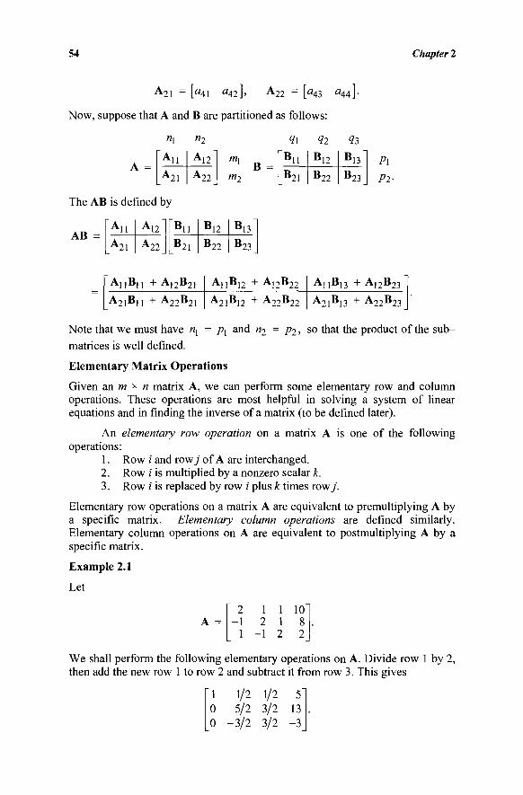
54 Chapter 2
A21 = [a4] a42], Α22 = [a43 a44].
Now, suppose that A and B are partitioned as follows:
[An A2 !
«2
Α12Ί
A22_ /W2
B [B11
B21
?2
B 1 2
B 2 2
ft B 1 3
B 2 3
The AB is defined by
AB = [An A21
A12
A 2 2 _
[B11 B 2 1
B12
B 2 2
B 13
B 2 3
P\
Pi-
Α,ιΒι, + Α,,Β H\a\\ 12D21
A91B11 + A99B l 2 1 D l l 22D21
A n B 1 2 + Α,,Β 12D22
A2iB12 + A22B22
AnB,3 + A]2B23
A T I B I T + A T O B l21D13 22D23
Note that we must have «j = ρχ and n2 = p2, so that the product of the sub-matrices is well defined.
Elementary Matrix Operations
Given an m * n matrix A, we can perform some elementary row and column operations. These operations are most helpful in solving a system of linear equations and in finding the inverse of a matrix (to be defined later).
An elementary row operation on a matrix A is one of the following operations:
1. Row i and rowy' of A are interchanged. 2. Row i is multiplied by a nonzero scalar k. 3. Row i is replaced by row / plus k times row/
Elementary row operations on a matrix A are equivalent to premultiplying A by a specific matrix. Elementary column operations are defined similarly. Elementary column operations on A are equivalent to postmultiplying A by a specific matrix.
Example 2.1
Let
A = 2 1 1
-1 2 1 1 -1 2
10
We shall perform the following elementary operations on A. Divide row 1 by 2, then add the new row 1 to row 2 and subtract it from row 3. This gives
1 0 0
1/2 5/2
-3/2
1/2 3/2 3/2
5 13 -3
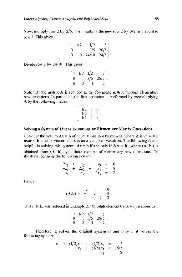
Linear Algebra, Convex Analysis, and Polyhedral Sets 55
Now, multiply row 2 by 2/5, then multiply the new row 2 by 3/2 and add it to row 3. This gives
1 1/2 1/2 5" 0 1 3/5 26/5 0 0 24/10 24/5
Divide row 3 by 24/10. This gives
"1 1/2 1/2 5" 0 1 3/5 26/5 0 0 1 2
Note that the matrix A is reduced to the foregoing matrix through elementary row operations. In particular, the first operation is performed by premultiplying A by the following matrix:
1/2 0 0 1/2 1 0
-1/2 0 1
Solving a System of Linear Equations by Elementary Matrix Operations
Consider the system Ax = b of m equations in n unknowns, where A is an m χ η matrix, b is an w-vector, and x is an «-vector of variables. The following fact is helpful in solving this system: Ax = b if and only if A'x = b', where (Α', b') is obtained from (A, b) by a finite number of elementary row operations. To illustrate, consider the following system:
Hence,
2xj + - X j +
xx -
(A,b)
*2 + 2x, +
Χ'χ + - **3
x3 =
*3 =
10
2.
1 1 10 2 1 8
- 1 2 2
This matrix was reduced in Example 2.1 through elementary row operations to
1 1/2 I/2 5
0 1 3/5 26/5 0 0 1 2
Therefore, x solves the original system if and only if it solves the following system:
xx + (l/2)x2 + (1/2)JC3 = 5 x2 + (3/5) x3 = 26/5
x3 = 2.
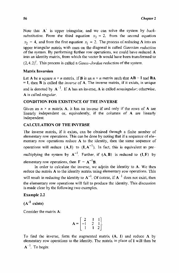
56 Chapter 2
Note that A' is upper triangular, and we can solve the system by back-substitution. From the third equation x3 = 2, from the second equation
x2 = 4, and from the first equation xl = 2. The process of reducing A into an upper triangular matrix with ones on the diagonal is called Gaussian reduction of the system. By performing further row operations, we could have reduced A into an identity matrix, from which the vector b would have been transformed to
(2,4,2)'. This process is called a Gauss-Jordan reduction of the system.
Matrix Inversion
Let A be a square n χ n matrix. If B is an n χ n matrix such that AB = I and BA = I, then B is called the inverse of A. The inverse matrix, if it exists, is unique
and is denoted by A" . If A has an inverse, A is called nonsingular; otherwise, A is called singular.
CONDITION FOR EXISTENCE OF THE INVERSE
Given an « x « matrix A, it has an inverse if and only if the rows of A are linearly independent or, equivalently, if the columns of A are linearly independent.
CALCULATION OF THE INVERSE
The inverse matrix, if it exists, can be obtained through a finite number of elementary row operations. This can be done by noting that if a sequence of ele-mentary row operations reduce A to the identity, then the same sequence of
operations will reduce (A, I) to (I, A - ). In fact, this is equivalent to pre-
multiplying the system by A~ . Further, if (A,B) is reduced to (I,F) by
elementary row operations, then F = A - B. In order to calculate the inverse, we adjoin the identity to A. We then
reduce the matrix A to the identity matrix using elementary row operations. This
will result in reducing the identity to A - . Of course, if A~ does not exist, then the elementary row operations will fail to produce the identity. This discussion is made clear by the following two examples.
Example 2.2
(A" exists)
Consider the matrix A:
A = 2 1 1
-1 2 1 1 -1 2
To find the inverse, form the augmented matrix (A, I) and reduce A by elementary row operations to the identity. The matrix in place of I will then be
A~ . To begin:
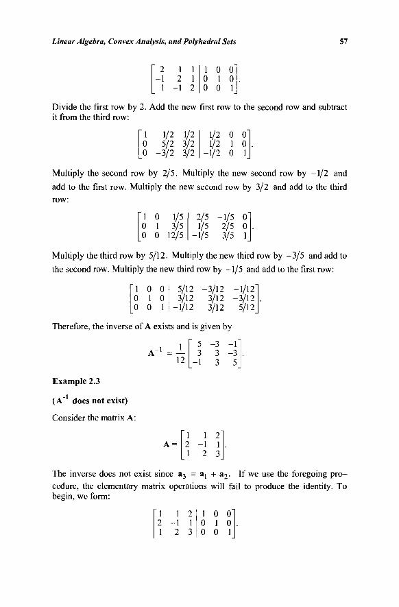
Linear Algebra, Convex Analysis, and Polyhedral Sets 57
2 1 1
1 1 2 1
-1 2
1 0 0 0 1 0 0 0 1
Divide the first row by 2. Add the new first row to the second row and subtract it from the third row:
1 1/2 1/2 0 5/2 3/2 0 -3/2 3/2
1/2 0 0 1/2 1 0
-1/2 0 1
Multiply the second row by 2/5. Multiply the new second row by -1/2 and
add to the first row. Multiply the new second row by 3/2 and add to the third
row:
1 0 1/5 0 1 3/5 0 0 12/5
2/5 -1/5 0 1/5 2/5 0
-1/5 3/5 1
Multiply the third row by 5/12. Multiply the new third row by -3/5 and add to
the second row. Multiply the new third row by -1/5 and add to the first row:
5/12 -3/12 -1/12' 3/12 3/12 -3/12
-1/12 3/12 5/12
Therefore, the inverse of A exists and is given by
1 0 0
0 1 0
0 0 1
A - » = - L 12
5 3
-1
Example 2.3
(A" does not exist)
Consider the matrix A:
1 2 1
1 2 -1 1 2 3
The inverse does not exist since a3 = aj + a2. If we use the foregoing pro-cedure, the elementary matrix operations will fail to produce the identity. To begin, we form:
1 2 1
1 2 -1 1 2 3
1 0 0 0 1 0 0 0 1
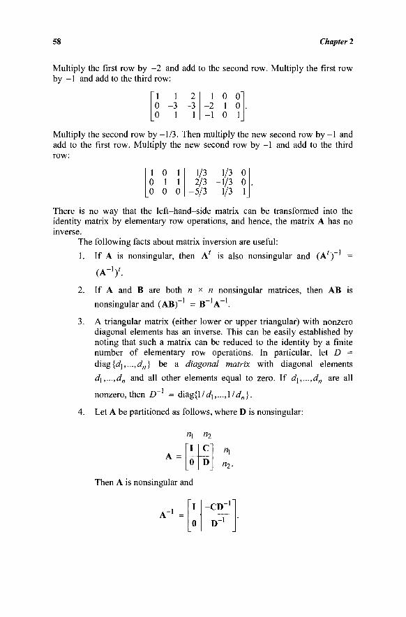
58 Chapter 2
Multiply the first row by -2 and add to the second row. Multiply the first row by -1 and add to the third row:
1 0 0
1 -3
1
2 -3
1
1 0 0 -2 1 0 -1 0 1
Multiply the second row by -1/3. Then multiply the new second row by -1 and add to the first row. Multiply the new second row by -1 and add to the third row:
1 0 1 0 1 1 0 0 0
1/3 2/3
-5/3
1/3 0 -1/3 0
1/3 1
There is no way that the left-hand-side matrix can be transformed into the identity matrix by elementary row operations, and hence, the matrix A has no inverse.
The following facts about matrix inversion are useful:
1. If A is nonsingular, then A' is also nonsingular and (A')~ =
(A"1)'.
2. If A and B are both n χ n nonsingular matrices, then AB is
nonsingular and (AB)~ = B~ A~ .
3. A triangular matrix (either lower or upper triangular) with nonzero diagonal elements has an inverse. This can be easily established by noting that such a matrix can be reduced to the identity by a finite number of elementary row operations. In particular, let D = diagli, . . . ,dn) be a diagonal matrix with diagonal elements d\,...,dn and all other elements equal to zero. If d\,...,dn are all
nonzero, then D~ = diag {1 / d\,..., 1 / dn}.
4. Let A be partitioned as follows, where D is nonsingular:
"l
"2·
«1
I
0
"2
c D
Then A is nonsingular and
A - ' = -CD"
D -1
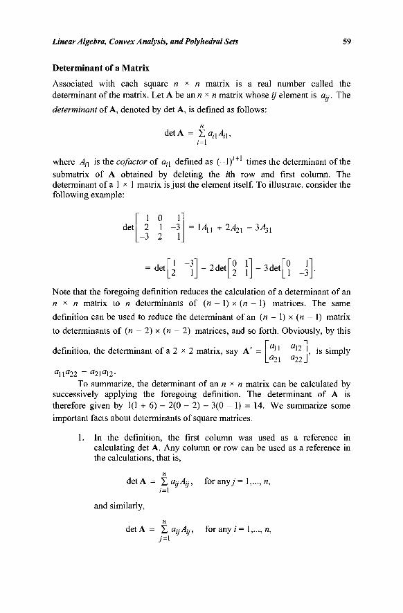
Linear Algebra, Convex Analysis, and Polyhedral Sets 59
Determinant of a Matrix
Associated with each square n χ η matrix is a real number called the determinant of the matrix. Let A be an n χ η matrix whose ij element is a^. The
determinant of A, denoted by det A, is defined as follows:
detA = Σ anA\,
Nl + l where ΑΛ is the cofactor of αΛ defined as (-1) times the determinant of the submatrix of A obtained by deleting the rth row and first column. The determinant of a 1 x 1 matrix is just the element itself. To illustrate, consider the following example:
det 1 0 1 2 1 -3
-3 2 1 141 + 2Λ71 - 3A *Ί1 ■21 31
det 2 det 0 1 2 1 -3de t
Note that the foregoing definition reduces the calculation of a determinant of an n x n matrix to n determinants of (n - 1) x (n - 1) matrices. The same
definition can be used to reduce the determinant of an (n - 1) x (n - 1) matrix
to determinants of (n - 2) x (n - 2) matrices, and so forth. Obviously, by this
definition, the determinant of a 2 χ 2 matrix, say A' a2\
an
«22
is simply
α11α22 ~ al\a\2-To summarize, the determinant of an « χ η matrix can be calculated by
successively applying the foregoing definition. The determinant of A is therefore given by 1(1 + 6) - 2(0 - 2) - 3(0 - 1) = 14. We summarize some important facts about determinants of square matrices.
1. In the definition, the first column was used as a reference in calculating det A. Any column or row can be used as a reference in the calculations, that is,
detA = Σ α ι /Λ; ' for any _/ = 1,..., n, i=\
and similarly,
detA = Σ OfjAy, for any /= 1,..., n, 7=1
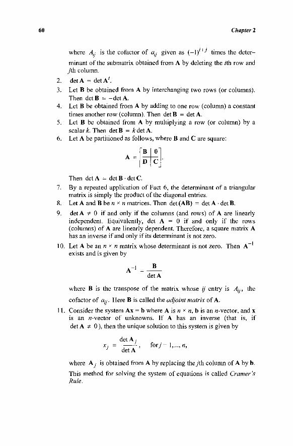
60 Chapter 2
where Ay is the cofactor of ay given as (-l)'+J times the deter-minant of the submatrix obtained from A by deleting the rth row and yth column.
2. detA = detA'. 3. Let B be obtained from A by interchanging two rows (or columns).
Then detB = -detA. 4. Let B be obtained from A by adding to one row (column) a constant
times another row (column). Then det B = det A. 5. Let B be obtained from A by multiplying a row (or column) by a
scalar k. Then det B = k det A. 6. Let A be partitioned as follows, where B and C are square:
B
D
0
c
Then detA = detB·detC. 7. By a repeated application of Fact 6, the determinant of a triangular
matrix is simply the product of the diagonal entries. 8. Let A and B be « χ n matrices. Then det (AB) = det A · det B.
9. detA Φ 0 if and only if the columns (and rows) of A are linearly independent. Equivalently, det A = 0 if and only if the rows (columns) of A are linearly dependent. Therefore, a square matrix A has an inverse if and only if its determinant is not zero.
10. Let A be an « x « matrix whose determinant is not zero. Then A~ exists and is given by
detA
where B is the transpose of the matrix whose ij entry is Ay, the
cofactor of ay. Here B is called the adjoint matrix of A.
11. Consider the system Ax = b where A is « χ n, b is an «-vector, and x is an «-vector of unknowns. If A has an inverse (that is, if det A Φ 0 ), then the unique solution to this system is given by
detA· X; = - , for/= 1,..., «, ; detA
where A .· is obtained from A by replacing they'th column of A by b.
This method for solving the system of equations is called Cramer's Rule.
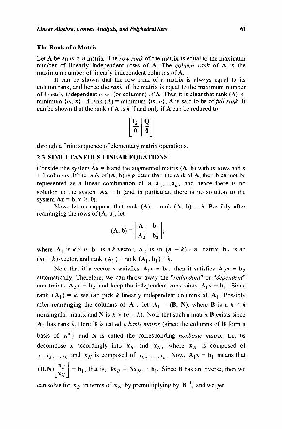
Linear Algebra, Convex Analysis, and Polyhedral Sets 61
The Rank of a Matrix
Let A be an m χ η matrix. The row rank of the matrix is equal to the maximum number of linearly independent rows of A. The column rank of A is the maximum number of linearly independent columns of A.
It can be shown that the row rank of a matrix is always equal to its column rank, and hence the rank of the matrix is equal to the maximum number of linearly independent rows (or columns) of A. Thus it is clear that rank (A) < minimum {m, «}. If rank (A) = minimum {m, «}, A is said to be offull rank. It can be shown that the rank of A is A: if and only if A can be reduced to
\h 0
Q 0
through a finite sequence of elementary matrix operations.
2.3 SIMULTANEOUS LINEAR EQUATIONS
Consider the system Ax = b and the augmented matrix (A, b) with m rows and n + 1 columns. If the rank of (A, b) is greater than the rank of A, then b cannot be represented as a linear combination of ai,a2,...,a„, and hence there is no solution to the system Ax = b (and in particular, there is no solution to the system Ax = b, x > 0).
Now, let us suppose that rank (A) = rank (A, b) = k. Possibly after rearranging the rows of (A, b), let
(A, b) =
where A] is k χ n, b] is a ^-vector, A2 is an (m - k) x n matrix, b 2 is an
(m - fc)-vector, and rank (Aj ) = rank (Aj, bt ) = k.
Note that if a vector x satisfies Ajx = bj, then it satisfies A2x = b 2
automatically. Therefore, we can throw away the "redundant" or "dependent" constraints A2x = b 2 and keep the independent constraints Ajx = bj. Since
rank (A; ) = k, we can pick k linearly independent columns of At. Possibly
after rearranging the columns of A], let A] = (B, N), where B is a k χ k
nonsingular matrix and N is k x (n - k). Note that such a matrix B exists since
Aj has rank k. Here B is called a basis matrix (since the columns of B form a
basis of R ) and N is called the corresponding nonbasic matrix. Let us
decompose x accordingly into xB and xN, where xB is composed of
xx,x2,..;Xii and xN is composed of xk+l,...,xn. Now, AjX = bj means that
(Β,Ν) Χί
l7V bi, that is, BxB + Nx^ = bj. Since B has an inverse, then we
can solve for xB in terms of xN by premultiplying by B , and we get
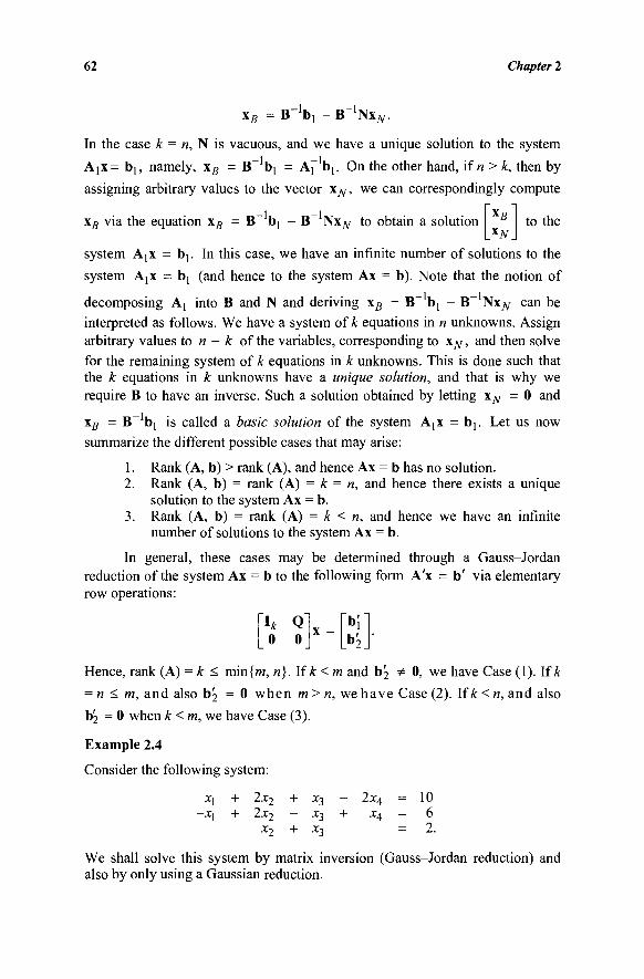
62 Chapter 2
xB = B \ - B l~NxN.
In the case k = n, N is vacuous, and we have a unique solution to the system
AjX= b], namely, xB = B~ bj = Aj" b). On the other hand, if n > k, then by
assigning arbitrary values to the vector xN, we can correspondingly compute
xB via the equation xB = B bj - B Nx y to obtain a solution XJV
to the
system Atx = b{. In this case, we have an infinite number of solutions to the
system Atx = b[ (and hence to the system Ax = b). Note that the notion of
decomposing At into B and N and deriving xB = B~ bj - B~ ΉχΝ can be interpreted as follows. We have a system of & equations in n unknowns. Assign arbitrary values to n - k of the variables, corresponding to x^ , and then solve for the remaining system of k equations in k unknowns. This is done such that the k equations in k unknowns have a unique solution, and that is why we require B to have an inverse. Such a solution obtained by letting xN = 0 and
xB = B~ bj is called a basic solution of the system AjX = bj. Let us now summarize the different possible cases that may arise:
1. Rank (A, b) > rank (A), and hence Ax = b has no solution. 2. Rank (A, b) = rank (A) = k = n, and hence there exists a unique
solution to the system Ax = b. 3. Rank (A, b) = rank (A) = k < n, and hence we have an infinite
number of solutions to the system Ax = b.
In general, these cases may be determined through a Gauss-Jordan reduction of the system Ax = b to the following form A'x = b' via elementary row operations:
0 0 bi b'2
Hence, rank (A) = k < min{w, «}. If k < m and b'2 Φ 0, we have Case (1). lik
= n < m, and also b^ = 0 when m> n, we have Case (2). lik < n, and also
b'2 = 0 when k<m,we have Case (3).
Example 2.4
Consider the following system:
+ 2 ^ 2 ~^~ -^3 — 2 x 4 =
+ ^-^2 — * 3 ~^~ ^4 ~ x2 + x 3
= 10 = 6 = 2
We shall solve this system by matrix inversion (Gauss-Jordan reduction) and also by only using a Gaussian reduction.
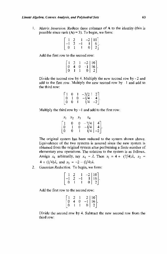
Linear Algebra, Convex Analysis, and Polyhedral Sets 63
1. Matrix Inversion. Reduce three columns of A to the identity (this is possible since rank (A) = 3). To begin, we form:
1 2 -1 2 0 1
1 -1
1
-2 1 0
10 6 2
Add the first row to the second row:
2 4 1
2 -1 0
10" 16 2
Divide the second row by 4. Multiply the new second row by -2 and add to the first row. Multiply the new second row by -1 and add to the third row:
1 0 1 -3/2 0 1 0 -1/4 0 0 1 1/4
2 4
-2
Multiply the third row by -1 and add to the first row:
X] Xo -^ - 4
1 0 0 -7 /4 0 1 0 0 0 1
-1/4 1/4
The original system has been reduced to the system shown above. Equivalence of the two systems is assured since the new system is obtained from the original system after performing a finite number of elementary row operations. The solution to the system is as follows. Assign x4 arbitrarily, say x4 = λ. Then xj = 4 + (7/4)A, x2 =
4 + (1/4)2, and x3 = -2 - (1/4)Λ. Gaussian Reduction. To begin, we form:
1 2 -1 2 0 1
1 -1
1
-2 1 0
10 16 2
Add the first row to the second row:
2 -1 0
10" 16 2
Divide the second row by 4. Subtract the new second row from the third row:
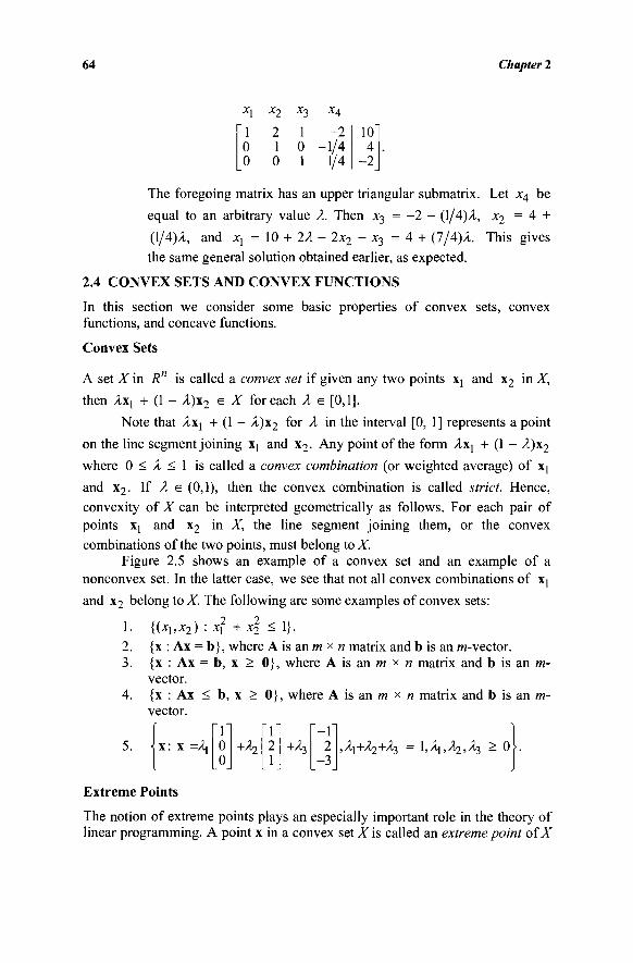
64 Chapter 2
XÌ X2 ·3 - 4
1 2 1 -2 0 1 0 -1/4 0 0 1 1 / 4
10 4
-2
The foregoing matrix has an upper triangular submatrix. Let x4 be
equal to an arbitrary value λ. Then x3 = -2 - (1/4)A, x2 = 4 +
(1/4)2, and ^ = 10 + 2A - 2x2 - *3 = 4 + (7/4)/l. This gives
the same general solution obtained earlier, as expected.
2.4 CONVEX SETS AND CONVEX FUNCTIONS
In this section we consider some basic properties of convex sets, convex functions, and concave functions.
Convex Sets
A set X in R" is called a convex set if given any two points xt and x2 in X,
then Axi + (1 - A)x2 e X for each λ e [0,1].
Note that λχ^ + (1 - A)x2 for A in the interval [0, 1] represents a point on the line segment joining X] and x2. Any point of the form Axj + (1 - A)\2
where 0 < λ < 1 is called a convex combination (or weighted average) of x}
and x2. If λ e (0,1), then the convex combination is called strict. Hence, convexity of X can be interpreted geometrically as follows. For each pair of points Xi and x2 in X, the line segment joining them, or the convex
combinations of the two points, must belong to X. Figure 2.5 shows an example of a convex set and an example of a
nonconvex set. In the latter case, we see that not all convex combinations of X[ and x2 belong to X. The following are some examples of convex sets:
1. 2. 3.
4.
5.
{(xt,x2) : x\ + x2 < 1}. {x : Ax = b}, where A is an m χ η matrix and b is an /«-vector. {x : Ax = b, x > 0}, where A is an m * n matrix and b is an m-vector. {x : Ax < b, x > 0}, where A is an m χ η matrix and b is an m-vector.
i x : x —ΛΛ
1 0 0
+/?2 1 2 1
+A, -1 2
-3 ,Ai+À2+À-} = ί,λ^,λζ,λτ, > 0>.
Extreme Points
The notion of extreme points plays an especially important role in the theory of linear programming. A point x in a convex set X is called an extreme point of X
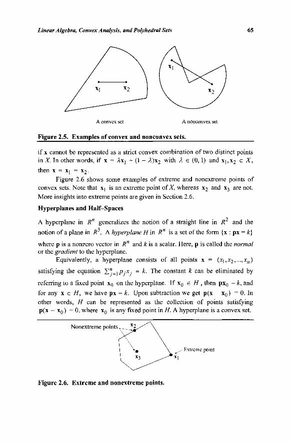
Linear Algebra, Convex Analysis, and Polyhedral Sets 65
x 2
A convex set A nonconvex set
Figure 2.5. Examples of convex and nonconvex sets.
if x cannot be represented as a strict convex combination of two distinct points in X. In other words, if x = Axj + (1 - A)x2 with λ e (0,1) and Xj, x2 e X,
then x = xj = x2. Figure 2.6 shows some examples of extreme and nonextreme points of
convex sets. Note that xj is an extreme point of X, whereas x2 and x3 are not. More insights into extreme points are given in Section 2.6.
Hyperplanes and Half-Spaces
A hyperplane in R" generalizes the notion of a straight line in R and the
notion of a plane in R . A hyperplane H in R" is a set of the form {x : px = k}
where p is a nonzero vector in R" and A: is a scalar. Here, p is called the normal or the gradient to the hyperplane.
Equivalently, a hyperplane consists of all points x = (xi,x2,...,x„)
satisfying the equation Y,"=xPjXj = k. The constant k can be eliminated by
referring to a fixed point x0 on the hyperplane. If x0 e H , then px0 = k, and for any x e H, we have px = k. Upon subtraction we get p(x - x0) = 0. In other words, H can be represented as the collection of points satisfying p(x - XQ) =0, where x0 is any fixed point in H. A hyperplane is a convex set.
Nonextreme points
Extreme point xl
Figure 2.6. Extreme and nonextreme points.
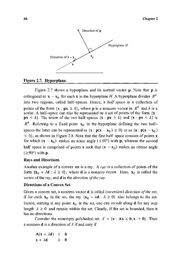
66 Chapter 2
\ Direction of p
\ ^^ Hyperplane H
Direction of x - x ^ ' χο
Figure 2.7. Hyperplane.
Figure 2.7 shows a hyperplane and its normal vector p. Note that p is
orthogonal to x - x0 for each x in the hyperplane H. A hyperplane divides R" into two regions, called half-spaces. Hence, a half-space is a collection of
points of the form {x : px > k}, where p is a nonzero vector in R" and & is a scalar. A half-space can also be represented as a set of points of the form {x : px < k}. The union of the two half-spaces {x : px > k} and {x : px < k} is
R". Referring to a fixed point x0 in the hyperplane defining the two half-spaces the latter can be represented as {x : p(x - x0 ) ^ 0} or as {x : p(x - x0 ) < 0}, as shown in Figure 2.8. Note that the first half-space consists of points x for which (x - x0) makes an acute angle (<90°) with p, whereas the second
half-space is comprised of points x such that (x - XQ ) makes an obtuse angle (> 90°) with p.
Rays and Directions
Another example of a convex set is a ray. A ray is a collection of points of the form {x0 + Ad : λ > 0}, where d is a nonzero vector. Here, x0 is called the vertex of the ray, and d is the direction of the ray.
Directions of a Convex Set
Given a convex set, a nonzero vector d is called (recession) direction of the set, if for each x0 in the set, the ray {x0 + λά : λ > 0} also belongs to the set.
Hence, starting at any point x0 in the set, one can recede along d for any step length λ > 0 and remain within the set. Clearly, if the set is bounded, then it has no directions.
Consider the nonempty polyhedral set X = {x : Ax < b,x > 0}. Then a nonzero d is a direction of X if and only if
A(x + Ad) < b x + Ad > 0
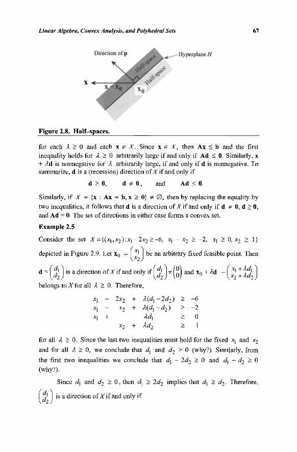
Linear Algebra, Convex Analysis, and Polyhedral Sets 67
Figure 2.8. Half-spaces.
for each λ > 0 and each x e X. Since x e X, then Ax < b and the first inequality holds for λ > 0 arbitrarily large if and only if Ad < 0. Similarly, x + Ad is nonnegative for λ arbitrarily large, if and only if d is nonnegative. To summarize, d is a (recession) direction ofXif and only if
d > 0, d Φ 0, and Ad < 0.
Similarly, if X = {x : Ax = b, x > 0} Φ 0 , then by replacing the equality by two inequalities, it follows that d is a direction of X if and only if d Φ 0, d > 0, and Ad = 0. The set of directions in either case forms a convex set.
Example 2.5
Consider the set X = {(x1,x2):x1-2x2 >-6, x{ - x2 > -2 , xx > 0, x2 > 1}
depicted in Figure 2.9. Let x0 = 1 be an arbitrary fixed feasible point. Then
d = f dJ 1 is a direction ofXif and only if f d} W n i and xn +/ld ={ Χχ +λΛ] 2 is a direction of X if and only if H 1 W \l and x0 + Ad = K / + Q
belongs to Sforali λ > 0. Therefore,
x\ - 2x2 + X(d\ - 2d2 ) > -6
X] - x2 + λ(άγ -d2) > -2 X] + λάλ > 0
x2 + λά2 > 1
for all λ > 0. Since the last two inequalities must hold for the fixed xj and x2
and for all λ > 0, we conclude that d\ and d2 > 0 (why?). Similarly, from
the first two inequalities we conclude that d\ - 2d2 ^ 0 and d\ - d2 > 0
(why?).
Since d] and d2 > 0, then c/j > 2d2 implies that d\ > d2. Therefore,
,' is a direction of X if and only if
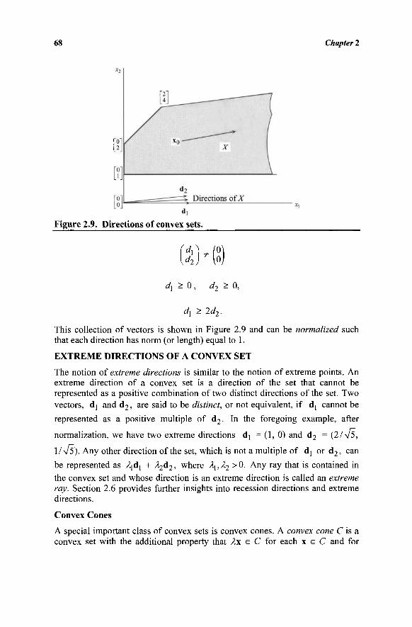
68 Chapter 2
Figure 2.9. Directions of convex sets.
(i)'(S) dl > 0 , c/2 > 0,
dl > 2d2.
This collection of vectors is shown in Figure 2.9 and can be normalized such that each direction has norm (or length) equal to 1.
EXTREME DIRECTIONS OF A CONVEX SET
The notion of extreme directions is similar to the notion of extreme points. An extreme direction of a convex set is a direction of the set that cannot be represented as a positive combination of two distinct directions of the set. Two vectors, dj and d2, are said to be distinct, or not equivalent, if dj cannot be represented as a positive multiple of d2- In the foregoing example, after normalization, we have two extreme directions dj =(1 ,0) and d2 = (2/ 1/V5). Any other direction of the set, which is not a multiple of dj or d2, can be represented as Ajdj + À^a2, where λχ,λ^ >0. Any ray that is contained in
the convex set and whose direction is an extreme direction is called an extreme ray. Section 2.6 provides further insights into recession directions and extreme directions.
Convex Cones
A special important class of convex sets is convex cones. A convex cone C is a convex set with the additional property that 2 i e C for each x e C and for
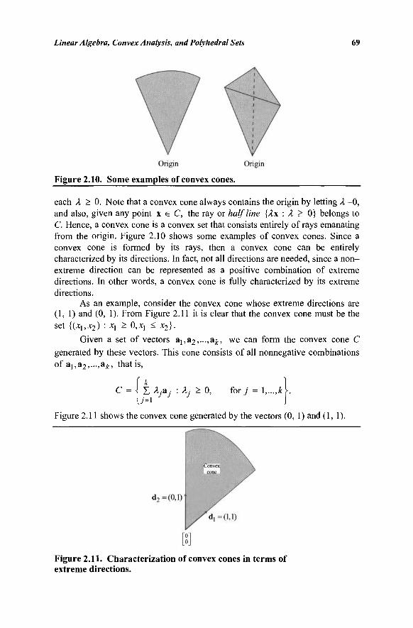
Linear Algebra, Convex Analysis, and Polyhedral Sets 69
Figure 2.10. Some examples of convex cones.
each λ > 0. Note that a convex cone always contains the origin by letting λ =0, and also, given any point x e C, the ray or half line {Ax : λ > 0} belongs to C. Hence, a convex cone is a convex set that consists entirely of rays emanating from the origin. Figure 2.10 shows some examples of convex cones. Since a convex cone is formed by its rays, then a convex cone can be entirely characterized by its directions. In fact, not all directions are needed, since a non-extreme direction can be represented as a positive combination of extreme directions. In other words, a convex cone is fully characterized by its extreme directions.
As an example, consider the convex cone whose extreme directions are (1, 1) and (0, 1). From Figure 2.11 it is clear that the convex cone must be the Set {{X\,Xj) '■ X\ ^ 0,Xj < X2}.
Given a set of vectors ai,a2,...,ayt, we can form the convex cone C generated by these vectors. This cone consists of all nonnegative combinations of a1,a2,...,a/t, that is,
C = \ Σ Aj*j : λ] > 0, for j = \,...,k\.
Figure 2.11 shows the convex cone generated by the vectors (0, 1) and (1, 1).
Figure 2.11. Characterization of convex cones in terms of extreme directions.
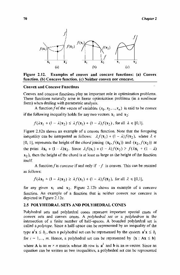
70 Chapter 2
/ ( x i ) /(x2)
/ ( * i ) .
x, x2
(a)
Figure 2.12. Examples of convex and concave functions: (a) Convex function, (b) Concave function, (c) Neither convex nor concave.
Convex and Concave Functions
Convex and concave functions play an important role in optimization problems. These functions naturally arise in linear optimization problems (in a nonlinear form) when dealing with parametric analysis.
A function/of the vector of variables (xj, x2,—,xn) is said to be convex
if the following inequality holds for any two vectors Xj and x2:
f{Axx + (1 " λ)χ2) < Af(xx) + (1 - Λ) / ( χ 2 ) , for all A e [0,1].
Figure 2.12a shows an example of a convex function. Note that the foregoing inequality can be interpreted as follows: Af(x{) + (1 - A)f{x2), where A e
[0, 1], represents the height of the chord joining (X],/(X])) and (x2 , / (x2)) at
the point Axx + (1 - A)x2. Since Af(xx) + (1 - A)f(x2) > f(Axx + (1 - λ)
x2), then the height of the chord is at least as large as the height of the function
itself. A function/is concave if and only if - / is convex. This can be restated
as follows:
f(Axx + (1 - /t)x2) > Af{xx) + (1 - A)f(x2), forali A e [0,1],
for any given X] and x2. Figure 2.12b shows an example of a concave function. An example of a function that is neither convex nor concave is depicted in Figure 2.12c.
2.5 POLYHEDRAL SETS AND POLYHEDRAL CONES
Polyhedral sets and polyhedral cones represent important special cases of convex sets and convex cones. A polyhedral set or a polyhedron is the intersection of a finite number of half-spaces. A bounded polyhedral set is called a polytope. Since a half-space can be represented by an inequality of the
type a'x < ty, then a polyhedral set can be represented by the system a'x < ty
for / = 1,..., m. Hence, a polyhedral set can be represented by {x : Ax < b}
where A is an m χ n matrix whose rth row is a' and b is an w-vector. Since an equation can be written as two inequalities, a polyhedral set can be represented
Linear Algebra, Convex Analysis, and Polyhedral Sets 71
by a finite number of linear inequalities and/or equations. As an example, consider the polyhedral set defined by the following inequalities:
-2xj + x2 < 4
X\ + %2 ^ 3
x, < 2
x, > 0
x2 > 0.
The intersection of these five half-spaces gives the shaded set of Figure 2.13. Clearly the set is a convex set. We can see a distinct difference between the first inequality and the remaining inequalities. If the first inequality is disregarded, the polyhedral set is not affected. Such an inequality is called (geometrically) redundant or irrelevant to the polyhedral set.
A special class of polyhedral sets is the set of polyhedral cones. A polyhedral cone is the intersection of a finite number of half-spaces, whose hyperplanes pass through the origin. In other words, C is a polyhedral cone if it can be represented as {x : Ax < 0}, where A is an m x n matrix. Note that the
rth row of the matrix A is the normal vector to the hyperplane defining the rth half-space. Figure 2.11 shows an example of a polyhedral cone.
2.6 EXTREME POINTS, FACES, DIRECTIONS, AND EXTREME DIRECTIONS OF POLYHEDRAL SETS: GEOMETRIC INSIGHTS
In Section 2.4 we discussed extreme points and directions of general convex sets, although we often used polyhedral sets for illustration. In this section, we will provide some geometric insights and equivalent definitions of extreme points and directions for polyhedral sets. We will assume that the polyhedral set under discussion in this section is of the form
X = {x : Ax < b,x > 0} (2.1)
where A is m χ n and b is an w-vector. As shown in Chapter 1, through suitable linear transformations, the feasible region of any linear programming problem can be put into this so-called canonical form.
Extreme Points
We have already seen that an extreme point of X is a point in X that cannot be made to lie in the interior of a line segment contained within X. We will now provide an equivalent geometric definition. Toward this end, consider the following simple but important observation. Let x e X and suppose that some constraint αχ < β of X is binding, or tight, or active, at x that is, αχ = β.
Suppose further that we can write x = λχ' + (1 - À)x", where 0 < λ < 1 and
where x' and x" e X. Then it must be also true that αχ' = β and αχ" = β,
that is, αχ < β must be binding at x' and at x" as well. This clearly follows
72 Chapter 2
Figure 2.13. Polyhedral set.
from the fact that αχ' < β and αχ" < β (since x', x" e X), but A(ax') +
(1 - λ)(αχ") = β (since ax = ytf ), where 0 < A < 1. An extreme point can now be defined as follows. Let the hyperplanes
associated with the (m + ri) defining half-spaces of Xbe referred to as defining hyperplanes of X. Furthermore, note that a set of defining hyperplanes are linearly independent if the coefficient matrix associated with this set of equations has full row rank. Then a point x e X is said to be an extreme point or a corner point, or a vertex of X if x lies on some n linearly independent defining hyperplanes of X If more than n defining hyperplanes pass through an extreme point, then such an extreme point is called a degenerate extreme point. The excess number of planes over n is called its order of degeneracy. A polyhedron with at least one degenerate extreme point is said to be a degenerate polyhedral set.
This definition of extreme points is readily seen to be equivalent to saying that x cannot be written as a strict convex combination of two distinct points in X. When x e X lies on some n linearly independent defining hyperplanes, then if we can write x = λχ' + (1 - λ)χ", where 0 < λ < 1 and χ',
x" e X, we have that both x' and x" also lie on these n hyperplanes. The solution to these n hyperplane equations, however, is unique. Hence, x = x' = x". Conversely, if the maximum number of linearly independent defining hyperplanes binding at x e X are r < n and are given by Gx = g, where G is r x n, let d Φ 0 be a solution to Gd = 0. Note that such a d exists (why?). Then there exists an ε > 0 such that x' = (x + εά) e X and x" = (x - ed) e X, since Gx' = g, Gx" = g and the constraints of X that are nonbinding at x remain satisfied provided ε > 0 is small enough. Consequently, since x = 0.5x' + 0.5x" and x', x" e X, we have that x is not an extreme point of X.
Referring to the polyhedral set in Figure 2.14, note how every extreme point is formed by some n = 3 linearly independent defining hyperplanes, and at every other point, fewer than n = 3 linearly independent defining hyperplanes are binding. Note also that at the indicated degenerate extreme point, four defining hyperplanes are binding. The order of degeneracy is one. In particular,
Linear Algebra, Convex Analysis, and Polyhedral Sets 73
/ - Degenerate extreme point
s' / \ \ ^ — Two-dimensional face
Adjacent extreme points
Figure 2.14. Extreme points and edges of X.
there is more than one choice of selecting n = 3 linearly independent hyperplanes that give this vertex as their unique intersection point. However, no defining hyperplanes or half-space can be omitted without changing the structure of this polyhedron. That is, there are no redundant constraints.
Faces, Edges, and Adjacent Extreme Points
We have seen that each extreme point x of X is a unique solution to some n linearly independent defining hyperplanes binding at x. In general, the set of points in X that correspond to some nonempty set of binding defining hyperplanes of X is called a face of X. Now, given any face F oiX, if r(F) is the maximum number of linearly independent defining hyperplanes that are binding at all points feasible to F, then the dimension ofF, denoted dim(F), is equal to n - r(F). In other words, each linearly independent binding hyperplane results
in the loss of one "degree of freedom." Consequently, extreme points are zero-dimensional faces ofX Similarly, an edge of X is a one-dimensional face of X, that is, it is the set of points in X formed by the intersection of some (« - 1) linearly independent defining hyperplanes (with some points in this set not having more than (n - 1) binding linearly independent hyperplanes). That is, an edge has one "degree of freedom" imparted by having one less than n linearly independent hyperplanes that are binding at all points. Similarly, if r(X) is
defined with respect to X itself, then although X is in R", it is actually of
dimension dim(X) = n - r{X). The set X is said to be full dimensional if
r(X) = 0, that is, dim(X) = n. Furthermore, the set X (when not full dimensional or viewed in a higher dimension) and the empty set are also sometimes called improper faces of X itself. The other faces are called proper faces. The highest dimensional proper face of X is of dimension dim(X) - 1
(when dim(X) > 1) and is called a facet of X. Finally, two extreme points of X are said to be adjacent if the line
segment joining them is an edge of X. Hence, adjacent extreme points have some (n - 1) common binding linearly independent defining hyperplanes. Figure 2.14 illustrates these definitions.
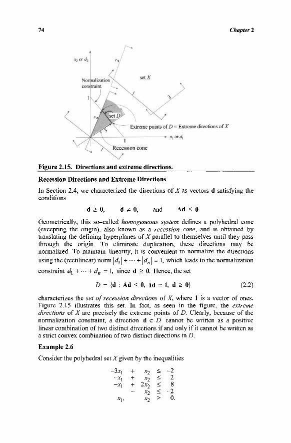
74 Chapter 2
Figure 2.15. Directions and extreme directions.
Recession Directions and Extreme Directions
In Section 2.4, we characterized the directions of X as vectors d satisfying the conditions
d > 0, d Φ 0, and Ad < 0.
Geometrically, this so-called homogeneous system defines a polyhedral cone (excepting the origin), also known as a recession cone, and is obtained by translating the defining hyperplanes of X parallel to themselves until they pass through the origin. To eliminate duplication, these directions may be normalized. To maintain linearity, it is convenient to normalize the directions using the (rectilinear) norm \άχ | H l· \dn | = 1, which leads to the normalization
constraint d\ + —v dn =1 , since d > 0. Hence, the set
D = {d : Ad < 0, Id = 1, d > 0} (2.2)
characterizes the set of recession directions of X, where 1 is a vector of ones. Figure 2.15 illustrates this set. In fact, as seen in the figure, the extreme directions of X are precisely the extreme points of D. Clearly, because of the normalization constraint, a direction d e f l cannot be written as a positive linear combination of two distinct directions if and only if it cannot be written as a strict convex combination of two distinct directions in D.
Example 2.6
Consider the polyhedral set X given by the inequalities
-3XJ + x2 ^ - 2 -X] + x2 < 2 -Xj + 2x2 < 8
- x2 < - 2 X], x2 - 0·
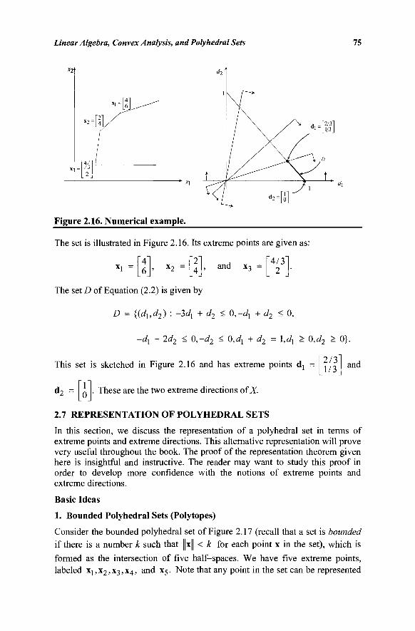
Linear Algebra, Convex Analysis, and Polyhedral Sets 75
x2
Figure 2.16. Numerical example.
The set is illustrated in Figure 2.16. Its extreme points are given as:
x2 = 4 , and x3
The set D of Equation (2.2) is given by
D = {(dhd2) : -3i/j + d2 < 0,-d{ + d2 < 0,
4/3 2
-dx + 2d2 < 0,-d2 < 0,dx + d2 = \,dx > 0,d2 > 0}.
This set is sketched in Figure 2.16 and has extreme points dj 2/3 1/3 and
d, = . These are the two extreme directions of X.
2.7 REPRESENTATION OF POLYHEDRAL SETS
In this section, we discuss the representation of a polyhedral set in terms of extreme points and extreme directions. This alternative representation will prove very useful throughout the book. The proof of the representation theorem given here is insightful and instructive. The reader may want to study this proof in order to develop more confidence with the notions of extreme points and extreme directions.
Basic Ideas
1. Bounded Polyhedral Sets (Polytopes)
Consider the bounded polyhedral set of Figure 2.17 (recall that a set is bounded if there is a number k such that |x|| < k for each point x in the set), which is formed as the intersection of five half-spaces. We have five extreme points, labeled X],x2,X3,X4, and X5. Note that any point in the set can be represented
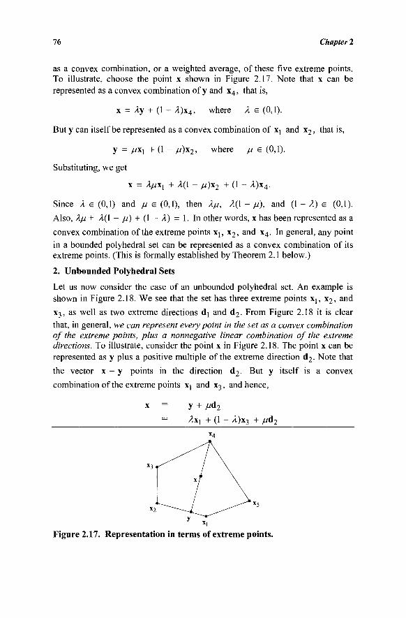
76 Chapter 2
as a convex combination, or a weighted average, of these five extreme points. To illustrate, choose the point x shown in Figure 2.17. Note that x can be represented as a convex combination of y and x4, that is,
x = Ay + (1 - λ)χ4, where λ e (0,1).
But y can itself be represented as a convex combination of Xj and x2, that is,
y = μχχ + (1 - μ)\2, where μ e (0,1).
Substituting, we get
x = λμχ\ + /l(l - μ)χ2 + (1 - λ)χ4.
Since λ e (0,1) and μ e (0,1), then λμ, λ{\ - μ), and (1 - λ) e (0,1).
Also, λμ + λ(1 - μ) + (1 - λ) = 1. In other words, x has been represented as a
convex combination of the extreme points xj, x2, and x4. In general, any point in a bounded polyhedral set can be represented as a convex combination of its extreme points. (This is formally established by Theorem 2.1 below.)
2. Unbounded Polyhedral Sets
Let us now consider the case of an unbounded polyhedral set. An example is shown in Figure 2.18. We see that the set has three extreme points Xj, x2, and x3, as well as two extreme directions dj and d2. From Figure 2.18 it is clear that, in general, we can represent every point in the set as a convex combination of the extreme points, plus a nonnegative linear combination of the extreme directions. To illustrate, consider the point x in Figure 2.18. The point x can be represented as y plus a positive multiple of the extreme direction d2. Note that
the vector x - y points in the direction d2. But y itself is a convex
combination of the extreme points Xj and x3, and hence,
x = y + μά2
= λχχ + (1 - λ)χ3 + μά2
Figure 2.17. Representation in terms of extreme points.
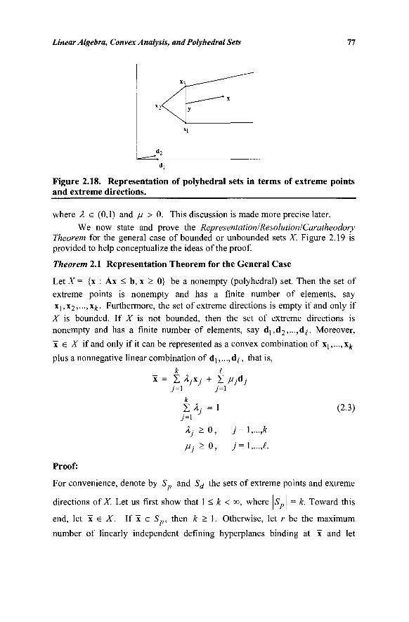
Linear Algebra, Convex Analysis, and Polyhedral Sets 77
Figure 2.18. Representation of polyhedral sets in terms of extreme points and extreme directions.
where λ e (0,1) and μ > 0. This discussion is made more precise later. We now state and prove the Representation!Resolution!Caratheodory
Theorem for the general case of bounded or unbounded sets X. Figure 2.19 is provided to help conceptualize the ideas of the proof.
Theorem 2.1 Representation Theorem for the General Case
Let X = {x : Ax < b, x > 0} be a nonempty (polyhedral) set. Then the set of extreme points is nonempty and has a finite number of elements, say Xj,X2,...,X;t. Furthermore, the set of extreme directions is empty if and only if
X is bounded. If X is not bounded, then the set of extreme directions is nonempty and has a finite number of elements, say d],d2,...,d^. Moreover, x e X if and only if it can be represented as a convex combination of Xj,...,x^. plus a nonnegative linear combination of dj,...,d^, that is,
k i
X = Σ AyXy + Σ Mjdj 7=1 j=\
Σλ.-=1 (2.3) 7=1
Àj>0, j=\,...,k
Mj>0, j=\,...,t
Proof:
For convenience, denote by S and Sj the sets of extreme points and extreme
directions of X. Let us first show that 1 < k < co, where \S„\ = k. Toward this
end, let x e X. If x e Sp, then k > 1. Otherwise, let r be the maximum
number of linearly independent defining hyperplanes binding at x and let
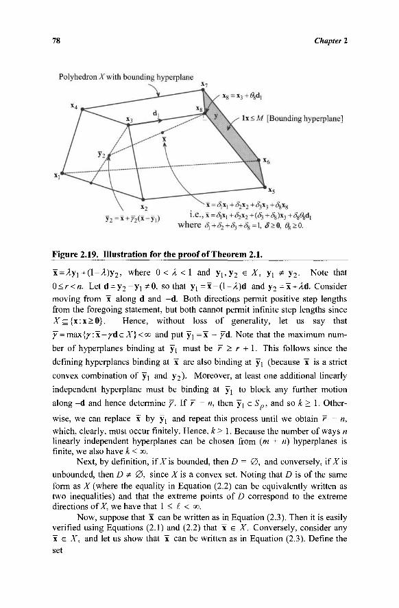
78 Chapter 2
Figure 2.19. Illustration for the proof of Theorem 2.1.
x = /lyi+(1-A)y2, where 0 < λ < 1 and yi,y2 e I , yt ΐ y2. Note that 0<r<n. Let d = y 2 - y i ^0 , so that yj =x - ( l -A)d and y2 =x + /ld. Consider moving from x along d and -d. Both directions permit positive step lengths from the foregoing statement, but both cannot permit infinite step lengths since ^ c { x : x > 0 } . Hence, without loss of generality, let us say that
f = max{/:x-/dsX}<<x> and put y{=x - yd. Note that the maximum num-
ber of hyperplanes binding at y"] must be 7 > r + 1. This follows since the
defining hyperplanes binding at x are also binding at yt (because x is a strict
convex combination of y and y2 ). Moreover, at least one additional linearly
independent hyperplane must be binding at yl to block any further motion
along -d and hence determine f. If 7 = n, then y"; eSp, and so k > 1. Other-
wise, we can replace x by yt and repeat this process until we obtain 7 = n, which, clearly, must occur finitely. Hence, k>l. Because the number of ways n linearly independent hyperplanes can be chosen from (m + ri) hyperplanes is finite, we also have k<x>.
Next, by definition, if X'\s bounded, then D = 0 , and conversely, if X is
unbounded, then D Φ 0, since X is a convex set. Noting that D is of the same form as X (where the equality in Equation (2.2) can be equivalently written as two inequalities) and that the extreme points of D correspond to the extreme directions of X, we have that 1 < £ < co.
Now, suppose that x can be written as in Equation (2.3). Then it is easily verified using Equations (2.1) and (2.2) that x e X. Conversely, consider any x € X, and let us show that x can be written as in Equation (2.3). Define the set
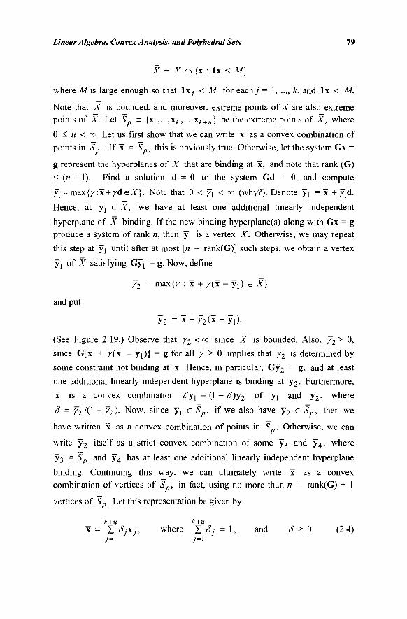
Linear Algebra, Convex Analysis, and Polyhedral Sets 79
X = X n {x : lx < M}
where Mis large enough so that lx < M for eachy = 1, ..., k, and lx < M.
Note that X is bounded, and moreover, extreme points of X are also extreme points of X. Let Sp = {xi,...,xìc,...,xìc+u} be the extreme points of X, where
0 < u < oo. Let us first show that we can write x as a convex combination of points in S If x e Sp, this is obviously true. Otherwise, let the system Gx =
g represent the hyperplanes of X that are binding at x, and note that rank (G)
< (n - 1). Find a solution d Φ 0 to the system Gd = 0, and compute
fl =max{/:x + d e X } . Note that 0 < γ~\ < oo (why?). Denote y"i = x + ;Fjd.
Hence, at yj e X, we have at least one additional linearly independent
hyperplane of X binding. If the new binding hyperplane(s) along with Gx = g
produce a system of rank n, then yt is a vertex X. Otherwise, we may repeat
this step at yj until after at most [n - rank(G)] such steps, we obtain a vertex
yj of X satisfying Gyj = g. Now, define
Ϋ2 = max{/ : x + y(x - yj) e X)
and put
y2 = x + f2(J-y\)-
(See Figure 2.19.) Observe that y2 < <» since X is bounded. Also, f2> 0,
since G[x + γ(χ - yj )] = g for all γ > 0 implies that γ2 is determined by
some constraint not binding at x. Hence, in particular, Gy2 = g, and at least
one additional linearly independent hyperplane is binding at y2. Furthermore,
x is a convex combination δγλ + (1 - S)y2 of yj and y2, where
δ = γ2 /(l + γ2). Now, since yj e Sp, if we also have y2 e S . , then we
have written x as a convex combination of points in Sp. Otherwise, we can
write y2 itself as a strict convex combination of some y3 and y^, where
y3 e Sp and y4 has at least one additional linearly independent hyperplane
binding. Continuing this way, we can ultimately write x as a convex combination of vertices of S , in fact, using no more than n - rank(G) + 1
vertices of S . Let this representation be given by
k+u k+u x = Σ SjXj, where Σδ]=\, and δ > 0. (2.4)
7=1 7=1
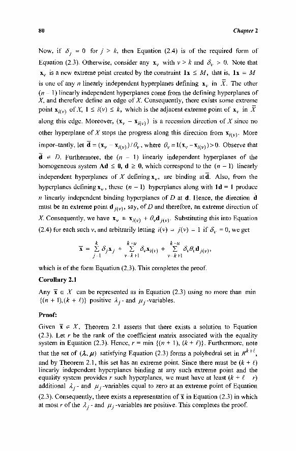
80 Chapter 2
Now, if δ'■ = 0 for j > k, then Equation (2.4) is of the required form of
Equation (2.3). Otherwise, consider any xv with v > k and δν > 0. Note that
xv is a new extreme point created by the constraint lx < M, that is, lx = M
is one of any n linearly independent hyperplanes defining xv in X. The other
(n - 1) linearly independent hyperplanes come from the defining hyperplanes of
X, and therefore define an edge of X. Consequently, there exists some extreme
point χ,·/νΛ of X, 1 < i(v) < k, which is the adjacent extreme point of xv in X
along this edge. Moreover, (xv - X,YV\) is a recession direction of X since no
other hyperplane of X stops the progress along this direction from Χ,-ΛΛ. More
impor-tantly, let d = (xv - χ;γν))/#ν, where θν =1(χν -χ,γν))>0. Observe that
d e D. Furthermore, the (n - 1) linearly independent hyperplanes of the homogeneous system Ad < 0, d > 0, which correspond to the (n - 1) linearly
independent hyperplanes of X defining xv, are binding at d. Also, from the
hyperplanes defining xv , these (« - 1) hyperplanes along with Id = 1 produce
n linearly independent binding hyperplanes of D at d. Hence, the direction d must be an extreme point d ,· /ν \ , say, of D and therefore, an extreme direction of
X. Consequently, we have xv = X,YV\ + θνά YV\. Substituting this into Equation
(2.4) for each such v, and arbitrarily letting i(v) = j(v) = 1 if δν =0, we get
k k+u k+u x = Σ Sj-Kj + Σ dvxi{v) + Σ δνθνάΛν),
j=\ v=k+\ v=k+\
which is of the form Equation (2.3). This completes the proof.
Corollary 2.1
Any x e X can be represented as in Equation (2.3) using no more than min {(« + ì),(k + £)} positive λ.- and //.-variables.
Proof:
Given x e X, Theorem 2.1 asserts that there exists a solution to Equation (2.3). Let r be the rank of the coefficient matrix associated with the equality system in Equation (2.3). Hence, r = min {(« + 1), (k + £)}. Furthermore, note
that the set of (λ, μ) satisfying Equation (2.3) forms a polyhedral set in R + , and by Theorem 2.1, this set has an extreme point. Since there must be (k + £) linearly independent hyperplanes binding at any such extreme point and the equality system provides r such hyperplanes, we must have at least (k + I - r) additional λ .■ - and μ .· -variables equal to zero at an extreme point of Equation
(2.3). Consequently, there exists a representation of x in Equation (2.3) in which at most r of the A.· - and μ .· -variables are positive. This completes the proof.
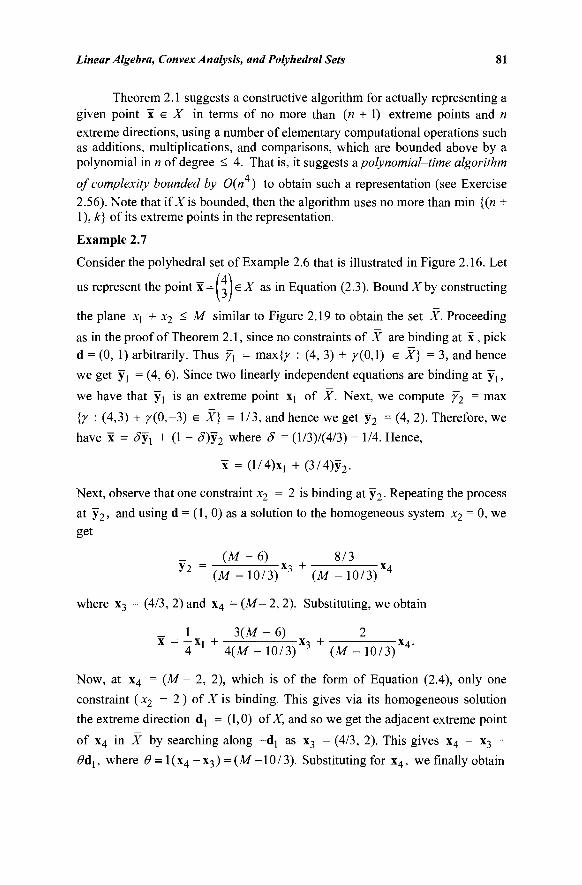
Linear Algebra, Convex Analysis, and Polyhedral Sets 81
Theorem 2.1 suggests a constructive algorithm for actually representing a given point x e X in terms of no more than (n + 1) extreme points and n extreme directions, using a number of elementary computational operations such as additions, multiplications, and comparisons, which are bounded above by a polynomial in n of degree < 4. That is, it suggests a. polynomial-time algorithm
of complexity bounded by 0(n ) to obtain such a representation (see Exercise 2.56). Note that ifXis bounded, then the algorithm uses no more than min {(« + 1), k} of its extreme points in the representation.
Example 2.7
Consider the polyhedral set of Example 2.6 that is illustrated in Figure 2.16. Let
us represent the point x = L e X as in Equation (2.3). Bound X by constructing
the plane x\ + x2 < M similar to Figure 2.19 to obtain the set X. Proceeding
as in the proof of Theorem 2.1, since no constraints of X are binding at x, pick
d = (0, 1) arbitrarily. Thus ;Fj = max{^ : (4, 3) + γ(0,\) e X} = 3, and hence
we get y"] = (4, 6). Since two linearly independent equations are binding at y1;
we have that yx is an extreme point \λ of X. Next, we compute γ2 = max
{/ : (4,3) + ^(0,-3) e X) = 1/3, and hence we get y2 = (4, 2). Therefore, we
have x = £y, + (1 - δ)γ2 where δ = (l/3)/(4/3) = 1/4. Hence,
x = (l/4)Xl + (3/4)y2.
Next, observe that one constraint x2 = 2 is binding at y2. Repeating the process
at y2, and using d = (1, 0) as a solution to the homogeneous system x2 = 0, we
get
(M - 6) 8/3 y2 = x-! + X4
(M - 10 /3 ) (M - 10 /3 ) 4
where x3 = (4/3, 2) and x4 = ( M - 2, 2). Substituting, we obtain
_ 1 3(M - 6) 2 X = —Xi H X-, + XA.
4 ' 4(M - 10/3) J (M - 10/3) 4
Now, at x4 = (M - 2, 2), which is of the form of Equation (2.4), only one
constraint ( x2 = 2 ) of X is binding. This gives via its homogeneous solution
the extreme direction dj = (1,0) of X, and so we get the adjacent extreme point
of x4 in X by searching along -dj as x3 = (4/3, 2). This gives x4 = x3 +
θύγ, where <9 = l(x4 - x 3 ) = (M-10/3). Substituting for x4, we finally obtain
82 Chapter 2
■x, + 3(M - 6)
4 ( M - 1 0 / 3 ) ' -x, + (M - 10/3) [x3 + (M - 10/3)d,]
or
X = —Xi
4 ' + -X-. + 2d,,
4 i '
which is of the required form of Equation (2.3). Note that this representation is not unique. Another representation for x is
- l ] ΊΛ
X = —X 7 H Xi H d i . 2 l 2 J 3 '
Note from Figure 2.18 that n = 2, k = 3, and I = 2 in this problem. Hence, min{(« + 1), (k + i )} = 3, and hence, both representations use the upper bound number of terms prescribed by Corollary 2.1. In this case, a lower bound on the number of terms required in any representation of x = (4, 3) also happens to be three.
Some Insights into the Equality Constrained Polyhedron
Consider the nonempty polyhedral set X = {x : Ax = b, x > 0} where A is m x n and rank(A) = m. Note that by equivalently replacing each equality constraint by two inequalities, all the discussion in this section continues to hold true for this case as well. In particular, consider the extreme points of X. As before, these are points in X formed by the intersection of n linearly independent hyperplanes. However, from the equality constraints, we know that m linearly independent hyperplanes are always binding at any feasible solution. Hence, at any extreme point x of X, there must be some (n - tri) additional hyperplanes binding from the nonnegativity constraints, say, xN = 0, which together with Ax = b pro-duce n linearly independent equations in n unknowns, thereby yielding x as the unique solution. Similarly, one can characterize edges and adjacent extreme points of X following Section 2.6, and note as before that extreme directions of X correspond to extreme points of
D = {d : Ad = 0,ld = l,d > 0}.
Finally, in light of the remark concerning extreme points of X, the reader may find it instructive to read through the proof of Theorem 2.1, thinking of Xas the equality constrained set.
EXERCISES
[2.1] Show that the vectors
a, = 0 , 1 and *3 -
ίίλ
vh
Linear Algebra, Convex Analysis, and Polyhedral Sets 83
form a basis for R . Supposing that a2 is replaced by
new set of vector still forms a basis of R .
indicate whether the
"1 ~l
[2.2] Which of the following collection of vectors form a basis of R , span R , or neither?
a. aj =
b. aj =
c. a! =
d. aj =
e. aj =
[2.3] Let
rn 2 lu (l) 3
f-1 2
I 3 rn 2 lu rn 4 w
a2 =
a2 =
\ a2 =
/
a2 =
a2 =
a l =
f-l> 2
l°v 5
f-n 0 ?
1-iJ f2i 0
(ολ 1
l°J f-3
-1
I 2 f-1 -4
l-i
\ 5
/ \
?
/
a2 = i3l 2
15J
a 3 =
a 3 =
a3 =
a3 =
, a3
foi 0
lu
fU 2
l3j ί 8
-1
I 7 ί°Ί
1 l°J
ΐ
λ
/
/
V
5/2Ì 3
5 J
^_3Λ 2
V 4y
Are these vectors linearly independent? Do they span R ?
[2.4] Let a1,a2,...,a/t form a basis for R". Show that a],a2,...,a^. are linearly independent. Also show that k = n.
[2.5] Does the following matrix have an inverse? If the answer is yes, find A~ :
"1 -4 4 0"
2 5 0 1
0 2 0 1
1 3 2 2_
[2.6] Find the inverse of the following triangular matrix:
"2 4 -3 -Λ
0 4 3 2
0 0 2 5
0 0 0 - 1
84 Chapter 2
[2.7] Let A be a 3 x 5 matrix. Consider the matrix C obtained by weighting the columns of A with scalars 1, 3/2, -2 , 4, and - 1 , respectively, and adding them up. Write C as a matrix product. Similarly, let D be the weighted sum of the rows of A, using weights 2, -2 , and 3/2, respectively. Write D as a matrix product. Likewise, let E be a matrix whose first row is the sum of the rows of A, whose second row is the third row of A, and whose third row is obtained by summing: thrice the first row of A, -5/2 times the second row of A, and twice the third row of A. Write E as a matrix product.
[2.8] Let B be an invertible matrix. Show that B" is unique.
[2.9] Suppose that &x,a2,...,&n form a basis of/?" and y = Ajaj +À2&2 + ·■· +
/L,a„ with Àj = 0. Prove that aj,...,a,-_j,y, a ,+1,...,a„ do not form a basis of R".
[2.10] Let
"B
T
0"
I
where B is an m χ m invertible matrix, I is a k x k identity matrix, 0 is an m x k zero matrix, and T is an arbitrary k x m matrix. Show that A has an inverse and that
A ' 1 = B-1
T B 1
0
I
[2.11] Show that if A and B are n χ η matrices that are both invertible, then
(AB)-1 = B_1A_1.
[2.12] Let A be an » x « invertible matrix. Show that A' has an inverse and that
(A')"1 = (A"1)'.
[2.13] Let B be an invertible matrix with nonnegative entries. Show that every
row of B~ has a least one positive entry.
[2.14] Let A = (a1,a2,...,a,-,...,a/„) be an invertible m χ m matrix. Show that
A ' a,· = e ,· where e ,■ is a vector of zeros except for a 1 at positiony.
[2.15] Let A be an « x « matrix. Suppose that B is an n χ n matrix such that AB = I. Is it necessarily true that A has an inverse? Is it necessarily true that B =
A"1?
[2.16] If the rth row of a square nonsingular matrix B is multiplied by a scalar
λ * 0, what changes would result in B~ ?
[2.17] If the rth column of a square nonsingular matrix B is multiplied by a
scalar λ Φ 0, what changes would result in B~ ?
Linear Algebra, Convex Analysis, and Polyhedral Sets 85
[2.18] Find the rank of the following matrices:
"1 0 1 - f
(i) A = 2 3 4 1
1 0 5 - 3
"-2 1 - 3 "
(ii) A = 2 4 - 2
4 3 1
[2.19] Find the determinants of the following matrices. " 1 0 f
2 2 - 1 a. A
b. A =
c.
0
1
-3
-2
1
'2
1
3
1
0
1
2
2
-2
3
-2
-2
-1
-1
2
ί -2
-3
[2.20] Solve the following system by Cramer's Rule:
2x, x2 5x, + 2xi
[2.21] Demonstrate by enumeration that every basis matrix of the following system is triangular:
Χγ + X-J + X4 —
~X\ "H X"2 ~^~ X$ =
— X2 ~ X4. =
- x-i =
tig system of equations:
Xj + 2x2 + X3 = x l + *2 - *3 =
X] + 3x2 + X3 =
4 2
-3 -2 .
1 3
-4
Without resolving the system, what is the solution if the right-hand-side of the first equation is changed from 1 to 2?
[2.23] Show that the determinant of a square triangular matrix is the product of the diagonal entries.
[2.24] Find all basic solutions of the following system:
86 Chapter 2
-X] + 2x2 + X3 + 3x4 - 2x5 = 4 xx - 2x2 + 2x4 + x5 = 2.
[2.25] Determine whether the following system possesses: (a) no solution, (b) a unique solution, or (c) many (how many?) solutions.
Xi + 3 x 2 + X3 — ΧΛ — 1
5x2 _ 6x3 + x4 = 0
X] - 2x2 + 4x3 = 2.
[2.26] Construct a general solution of the system Ax = b where A is an m χ η matrix with rank m. What is the general solution of the following system?
Xi — 2x2 + X3 = 2 -Xj + 3x2 + 2x3 = 6.
[2.27] Consider the system Ax = b where A = [a|,a2,...,a„] is an m χ η matrix
of rank m. Let x be any solution of this system. Starting with x, construct a basic
solution. (Hint: Suppose that xx,...,xp *0 and xp+x,...,xn = 0. If p > m, repre-
sent one of the columns a , fory = 1, ..., p, as a linear combination of the
remaining vectors. This results in a new solution having a smaller number of nonzero variables. Repeat the process.)
[2.28] Which of the following sets are convex and which are not?
a. {(xx,x2) : X\ + x2 > 3}.
b. {(xj,x2,X3) : xj + 2x2 < 1, xj - 2x3 < 2}.
c. {(xj,x2) : x2 - 3x] = 0}.
d. {(x],x2,x3) : x2 > Xj , X] + 2x2 + X3 < 4}.
e. {(xi,x2) : xi = 3 , |x2| < 4}.
f. {(x1;x2,x3) : x3 = |x2|, X! < 3}.
[2.29] Which of the following functions are convex, concave, or neither?
a. f(x) = x2.
b. / (x l 5 x 2 ) = e"*1"*2 + 2x,2 - 2xx.
c. f(xx, x2) = maximum{fx (xx,x2), f2 (xx,x2)} where / , (^, x2 ) = 3x2
"7 2 + x2
a n d f2Ìxl>x2) = ^xl _ 5*2-d- /(Xi,X2) = minimum { ^ ( x ^ ) , f2(x\*x2)} w h e r e Ai') a n d /2O
are defined in Part (c). 2 2 2
e. y (Xi,Χ7 >-*3) = — x\ ~~ X 2 ~ x3 ~^~ 2XjX2 ~~ %2X3 ~^~ 1 ~^~ 5x-\.
1. J (Xi , X2 ) — Xi + X2 — 2X]X2 + X 2 .
Linear Algebra, Convex Analysis, and Polyhedral Sets 87
[2.30] Consider the set {(xl5x2) : ~x\ + x2 - 2 , x\ + 2x2 -8> x\ - 0> x2 -0} ·
What is the minimum distance from (-3,4) to the set? What is the point in the
set closest to (-3,4)? Repeat with the point (6,4).
[2.31] Let a i = (^), a2 = (*), ^ = ( " i j , «4 = |_4), and a5 = ( ^ ) . Illus-
trate geometrically the collection of all convex combinations of these five points.
[2.32] Show that a hyperplane H = {x: px = k) and a half-space H+ = {x: px > k] are convex sets.
[2.33] Show that/is convex if and only if its epigraph ={(x,y) : x e R", y e
R, y > f(x)} is a convex set. Similarly, show that/is concave if and only if its
hypograph = {(x,y) : x e R", y e R , y < / (x)} is a convex set.
[2.34] Show that a differentiable function / is convex if and only if the
following inequality holds for each fixed point x0 in Rn: f(x) > /(XQ) +
V/(x0)'(x - XQ) for all x e R", where V/(x0) is the gradient vector off at x0
given by
> ( X Q ) df(x0) g/(x0)Y
cbcj ' 9x2 ' ' δχη J
[2.35] Show that the set of feasible solutions to the following linear program forms a convex set:
Minimize ex subject to Ax = b
x > 0 .
[2.36] Consider the set X = {{x\,xj) : x\ + x2 ^ 2, x2 < 4, xl5x2 > 0}.
Find a hyperplane / / such that X and the point (1,-2) are on different sides of
the hyperplane. Write the equation of the hyperplane.
[2.37] If 5 is an open set, show that the problem
Maximize ex
subject to x e S
where c Φ 0 possesses no optimal point. {Note: S is open if for each x0 e S,
there is an ε > 0 such that ||x - x 0 | < ε implies that x e S.)
[2.38] Show that C is a convex cone if and only if x and y e C imply that
λχ + //y e C for all λ > 0 and μ > 0.
[2.39] Show that if C is a convex cone, then C has at most one extreme point, namely, the origin.
88 Chapter 2
[2.40] Find the extreme points of the region defined by the following inequalities:
Xj + 2x2 + x3 < 5 —X\ + x2 + 2x3 < 6
Xi , Xo, X3 ^ 0.
(///«/: Consider n = 3 intersecting defining hyperplanes at a time.)
[2.41] Why does the following set have directions? Find all its extreme directions:
-Xj + 2x2 = 3 2x] - 2x2 - X3 < 2
x3 > 1 Xi, Xj , X3 — 0 .
(Hint: Enumerate the extreme points of its normalized set of directions. What else needs to be checked?)
[2.42] Find all extreme points of the following polyhedral set:
X= {(xi,x2,x3) : X\ - x2 + Χτ, ^ Ι,Λ Ι - 2x2 < 4,xl5x2,X3 > 0}.
Does X have any recession directions? Why?
[2.43] Let X= {x : Ax < b} c R" and let x0 e X be such that fewer than n
linearly independent hyperplanes defining X are active at x0. Show that x0
cannot be an extreme point of X.
[2.44] Prove in detail that a polyhedral set X is bounded if and only if it has no directions.
[2.45] Consider the nonempty polyhedral set X = {x : Ax = b, x > 0}. Show
directly by definition that d is a direction of the set if and only ifd * 0, Ad = 0,
andd > 0. Obtain analogous results if Ax = b is replaced byAjx = bj,
A2x > b2.
[2.46] Given a nonempty polyhedron X, a face F of X is also defined as the intersection of a supporting hyperplane of X with X itself. (A hyperplane supports Χ'ιΐX lies completely in one half-space defined by the hyperplane and the intersection of the hyperplane with X is nonempty.) Show the equivalence between this definition and the one given in Section 2.6.
[2.47] You are given the following polyhedral set. Identify the faces, extreme points, extreme directions, and extreme rays of the set.
Xj - x2 + x3 < 10 2χλ - x2 + 2x3 < 40 3xj - 2x2 + 3x3 < 50
Xi, X 2 , X3 ^ 0 .
Linear Algebra, Convex Analysis, and Polyhedral Sets 89
[2.48] Let X ={(xx,x2) : χλ - x2 < 3, -x1 + 3x2 < 3, xx > -3}. Find all extreme points of X and represent x = (0, 1) as a convex combination of the extreme points. [2.49] Answer the following questions and provide a brief explanation or illustration:
a. Is it possible for X in Equation (2.1) to be empty but D in Equation (2.2) to be nonempty?
b. Is there a relationship between redundancy and degeneracy of a polyhedral set?
c. Does degeneracy imply redundancy in two dimensions? d. If the intersection of a finite number of half-spaces is nonempty,
then this set has at least one extreme point. True or false? Explain. e. An unbounded «-dimensional polyhedral set can have at most n
extreme directions. True or false? Explain. f. What is the maximum (actual) dimension of X = {x : Ax = b, x
> 0}, where A is m x n of rank r, with r<m<rf!
[2.50] Find all extreme points and extreme directions of the following poly-hedral set:
X = \(X\ ,X2 5- -3 , %4 ) · —X\ "t" %2 ~~ 3 '
—2X] — Xy + 2%4 < 2, X],X2,X2,XQ ^ 0 } .
Represent x = (1, 1, 1, 2) as a convex combination of the extreme points of X plus a nonnegative combination of the extreme directions of X.
[2.51] Show that an unbounded polyhedral set of the form {x : Ax = b, x>0} has at least one extreme direction. In particular, using the normalized direction set D in lieu of Xin the proof of Theorem 2.1, show how you can start with any direction d in D and reduce it to an extreme direction.
[2.52] Consider the polyhedral set X = {x : px = k] where p is a nonzero vector and A: is a scalar. Show that X has neither extreme points nor extreme rays. How do you explain this in terms of the general Representation Theorem?
[2.53] LetX= {x : Ax = b,x > 0} where A is an w x « matrix with rank m. Show that d is an extreme direction of X if and only if d is a positive multiple of
the vector (-yy,0,0,...,l,0,...,0)' where the 1 appears in positionj, and where:
y7 = Β Λ 7 < Ο ,
A = [B, N] where B is an m x m invertible matrix a = a column of N.
(Hint: Consider extreme points of the normalized direction set.) Illustrate by the following system:
90 Chapter 2
X] - 3X2 + *3 = 0
-3x) + X2 + x 4 = 3
X i , X o , X3 , X4 ^ U.
[2.54] In the proof of Theorem 2.1, consider the direction d given by
(xv - x,(v))/(9v. Show how you would algebraically obtain d, given the
extreme point xv of X, v> k.
[2.55] Consider the polyhedral set X = {x : Qx < q}, where Q is m χ η. Mathematically characterize the statement that an entire line belongs to X. What does this imply about the rank of Q? Show that a nonempty polyhedron has extreme points if and only if it contains no lines.
[2.56] Based on Theorem 2.1 and its proof, construct a polynomial-time
algorithm of complexity bounded by 0{n ) in order to obtain a representation
of x e X in terms of no more than (n + 1) extreme points and n extreme directions of X. Show that the number of extreme points needed in the representation by this algorithm is no more than the bound provided by Corollary 2.1 when X is a bounded set.
NOTES AND REFERENCES
1. Sections 2.1 through 2.3 present a quick review of some relevant results of vector and matrix algebra.
2. Sections 2.4 and 2.5 give some basic definitions and properties of convex sets, convex cones, and convex functions. For more details the reader may refer to Eggleston [1958], Mangasarian [1969], Bazaraa, Sherali, and Shetty [2006], and Rockafellar [1970].
3. Correspondence between bases and extreme points is established in the next chapter in Section 3.2, and an algebraic characterization of extreme directions is presented in Exercise 2.53.
4. The representation theorem for polyhedral sets evolved from the work of Minkowski [1910] and Goldman and Tucker [1956]. The result is also true for (nonpolyhedral) convex sets that contain no lines. See Rockafellar [1970] and Bazaraa and Shetty [1976]. The geometric proof of Theorem 2.1 in Section 2.6 is taken from Sherali [1987b]. (Parts of the proof, parts of Example 2.7, and Figure 2.17 are reprinted from H. D. Sherali, "A Constructive Proof of the Representation Theorem for Polyhedral Sets Based on Fundamental Definitions," American Journal of Mathematical and Management Sciences, Vol. 7 (1987), 253-270, Copyright © 1987 by the American Sciences Press, Inc., 20 Cross Road, Syracuse, New York 13224. Reprinted by permission.) For further geometric insights, see Akgul [1988], Grunbaum [1967], Murty [1983, 1985], and Sommerville [1958].
THREE: THE SIMPLEX METHOD
In this chapter we begin to discuss Dantzig's simplex method, which was conceived in the summer of 1947 for solving linear programming problems. The first significant application of this method occurred soon after in the fall of 1947. J. Laderman solved a diet-planning linear program with nine equality constraints and 27 nonnegative variables at the National Bureau of Standards. Using desk calculators, this problem took 120 man-days to solve and the worksheets were laboriously glued together and spread out like a "table cloth." Today, using modern-age computer facilities and sophisticated implementations of the simplex method, linear programs having more than tens-of-thousands of constraints and variables are readily solvable. Although several variants of the simplex method have evolved and other new competing algorithms have been proposed (see Chapter 8), the simplex method remains a viable and popular tool for solving linear programming problems. It also provides further insights into the facial structure of polyhedral sets that define the underlying feasible region for linear programs.
We begin our discussion of the simplex method by showing that if an optimal solution exists, then an optimal extreme point also exists. Extreme points are then characterized in terms of basic feasible solutions. We then describe the simplex method for improving these solutions until optimality is reached, or else until we conclude that the optimal value is unbounded. Both geometric and algebraic descriptions are provided. The well-known tableau format of the simplex method is also discussed. This is a key chapter, fundamental to the development of many other chapters in the book.
3.1 EXTREME POINTS AND OPTIMALITY
We observed from Figure 1.3 that when an optimal solution of a linear programming problem exists, an optimal extreme point also exists. This observation is always true, as will be shown shortly.
Consider the following linear programming problem:
Minimize ex subject to Ax = b
x > 0 .
Let X], x2, ..., Xfr be the extreme points of the constraint set, and let dj, d2, ...,
de, be the extreme directions of the constraint set. Recall that any point x such that Ax = b and x > 0 can be represented as
k e x = Σ Α,.χ, + Σ Mjdj
where
91
92 Chapter 3
k
Σ λ} = 1 7=1
Ay > 0,
Mj > 0,
7=1 , . .
y= l , . .
.,*
. ,£
Therefore, the linear programming problem can be conceptually transformed into a problem in the variables λι,λ2,...,λΙι, μ],μ2,—,μι, result-ing in the following equivalent linear program:
k t Minimize Σ (cxy)Ay + Σ (cdy)/"y
7=1 7=1
it subject to Σ Aj: = 1
Ay > 0, y=l, . . . , A;
/ ^ • > 0 , 7=1, . . . ,^ .
Assume that & > 1. Since the // -variables can be made arbitrarily large, the
minimum is -oo if cd7 < 0 for some/ e {1,..., £}. If cd, > 0 for ally = 1,..., t,
then the corresponding μ · can be chosen as zero. Now, in order to minimize
£^=,(cxy)A,· over Al,À2,...,Àlc satisfying A > 0 for j = 1,..., k, and
Σ^=ι^ί = 1 » w e simply find the minimum ex -, say cx„, let X = 1, and set
all other A.- -variables equal to zero.
To summarize, given feasibility, the optimal value of the linear problem is finite if and only if cd, > 0 for all extreme directions. Furthermore, if this is
the case, then we can find a minimizing point by selecting a solution having the minimum objective value among all extreme points. This shows that if an optimal solution exists, we must be able to find an optimal extreme point solution. Of course, if the minimum ex, value occurs at more than one index,
then each corresponding extreme point is an optimal point and each convex combination of these points is an optimal solution (why?). In fact, the entire set of alternative optimal solutions is given by the set of convex combinations of such points plus a nonnegative linear combination of the extreme directions d,
that satisfy cd, = 0 (why?).
Example 3.1
Consider the region defined by the following constraints:
-Xj + %2 < 2
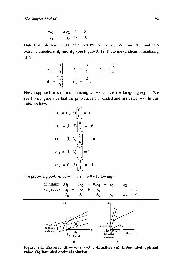
The Simplex Method 93
—jtj + 2 x 2 < 6
X\, x2 - 0.
Note that this region has three extreme points Xj, x2, and x3, and two
extreme directions dj and d2 (see Figure 3.1). These are (without normalizing
d2)
M
d, =
0] 0
Γ
u_
x2 =
d2 =
ΓοΊ _2_
"2"
[_ ij Now, suppose that we are minimizing X] - 3 x2 over the foregoing region. We see from Figure 3.1a that the problem is unbounded and has value -co. In this case, we have
ΓίΐΊ 0
= -6
CXj
cx2
cx3
cd!
cd2
= 0,-
= 0,
= (1.
= (1,
= (1,
-3)
-3)
-3)
-3)
-3)
"0" 0
"0" 2
~2
4
0 "2"
1
-10
= 1
The preceding problem is equivalent to the following:
Minimize 0/li - 6^2 - 10A3 + μ\ subject to \ + λχ + A3
\ , Àq_, A3, / / j ,
/"2 = 1
Ml > 0.
(a) (*) Figure 3.1. Extreme directions and optimality: (a) Unbounded optimal value, (b) Bounded optimal solution.
94 Chapter 3
Since cd2 = -1 < 0 and μ2 can be made arbitrarily large without violating
the foregoing constraints, the objective value can be made -co by letting μ2 =
co. Then μλ can be chosen equal to zero. Any set of nonnegative \ , λ%, λ^
adding to 1 satisfies the foregoing constraints, for example, \ = 1, λ^ = λ3 = 0. This illustrates the necessary and sufficient condition for unboundedness for a feasible linear program, namely, cd < 0 for some extreme direction d.
Now, consider the problem of minimizing Axx - x2 over the same
region. From Figure 3.1b the optimal solution is the extreme point x2 =
this case we have "ni
. In
CXi
cd,
cd->
= -2
= 4
(4,-1)
cx2 = (4,-1)
cx3 = (4,-1)
(4,-1)
: (4,-1)
This problem is therefore equivalent to the following:
7.
Minimize OAj
subject to A]
-2λχ
+ Λ2
*2>
+ +
4A3 + 4/4 +7μ2
tt> -"2
1
0.
Since the coefficients of μ\ and μ2 in the objective function are
positive, we let μλ = μ2 = 0. In order to minimize the expression 0/^ - 2λ2 +
4λ$ subject \α\+λζ+λί=\ and Aj, λχ, λ$ > 0, we let λ^ = 1 and λχ =
A3 = 0. This shows that the optimal solution is the extreme point x2 =
Minimizing ex corresponds to moving the plane ex = constant in the direction -c as far as possible. When c = (1, -3) we can move the plane indefinitely while always intersecting the feasible region, and hence the optimal value is -GO. When c = (4, -1) we cannot move the plane indefinitely in this fashion and we must stop at the point x2; otherwise, we will "leave" the feasible region.
3.2 BASIC FEASIBLE SOLUTIONS
We have developed, in the previous section, a necessary and sufficient condition for an unbounded solution. We also showed that if an optimal solution exists,
The Simplex Method 95
then an optimal extreme point also exists. The notion of an extreme point is a geometric notion, and an algebraic characterization of extreme points is needed before they can be utilized from a computational point of view.
In this section we introduce basic feasible solutions and show that they correspond to extreme points. This characterization will enable us to algebraically describe the simplex method.
Definition (Basic Feasible Solutions)
Consider the system Ax = b and x > 0, where A is an m χ n matrix and b is an w-vector. Suppose that rank (A, b) = rank (A) = m. After possibly rearranging the columns of A, let A = [B, N] where B is an m χ m invertible matrix and N is
X JV anmx(n-ff l ) matrix. The solution x to the equations Ax = b, where
xB = B_1b
and xN =0
is called a basic solution of the system. If \B > 0, then x is called a basic feasible solution of the system. Here B is called the basic matrix (or simply the basis) and N is called the nonbasic matrix. The components of xB are called
basic variables (or dependent variables) and the components of xN are called
nonbasic variables (or independent variables). If xg > 0, then x is called a
nondegenerate basic feasible solution, and if at least one component of x g is zero, then x is called a degenerate basic feasible solution.
The notion of a basic feasible solution is illustrated by the following two examples.
Example 3.2
[Basic Feasible Solutions)
Consider the polyhedral set defined by the following inequalities (and illustrated in Figure 3.2):
x\
X\,
+ x2 x2 x2
< 6 < 3 > 0.
By introducing the slack variables x3 and x4, the problem is put in the following standard format:
X\,
x2 x2 x2>
+ x3
x3,
= 6 + x4 = 3
x4 > 0.
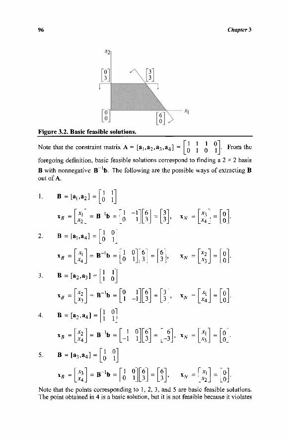
96 Chapter 3
Figure 3.2. Basic feasible solutions.
Note that the constraint matrix A = [a],a2,a3,a4] 1 1 1 0 0 1 0 1 From the
foregoing definition, basic feasible solutions correspond to finding a 2 χ 2 basis
B with nonnegative B~ b. The following are the possible ways of extracting B out of A.
2.
3.
4.
5.
B = [a!,a2] =
L*2
1 1 0 1
Β " ^ = 1 -1 0 1
ii,a4] =
~x{ X4
= E
"1 0" 0 1_
r'b = Ί 0" 0 1
"6" 3 =
"6" _3_
lJV
B = [a 2 ,a 3 ] =
Lx3.
1 1 1 0
ΒΛ = 0 1 1 - 1
x3
x2
x3
xx X4
B = [a2,a<
Χβ = ~x2
X4
l] =
= B
"1 0" 1 1
->b = 1 0"
- 1 1 "6" 3 =
" 6" - 3 > XN -
~x{ *3.
= 0 _0_
XR =
>3>a4] =
~x{ X4
= B
Ί 0" 0 1
lb = "1 0" 0 1
~6 3 =
~6 3_ KN x2
Note that the points corresponding to 1,2, 3, and 5 are basic feasible solutions. The point obtained in 4 is a basic solution, but it is not feasible because it violates
The Simplex Method 97
the normegativity restrictions. In other words, we have four basic feasible solutions, namely:
*i =
3 3 0
LoJ . x2 =
6 0 0
L3 . x3 =
0 3 3
LoJ
and
These points belong to R , since after introducing the slack variables we have
four variables. These basic feasible solutions, projected in R
(JCI,X2) space—give rise to the following four points:
that is, in the
3 3 »
6 0 1
0 3
and
These four points are illustrated in Figure 3.2. Note that these points are precisely the extreme points of the feasible region.
In this example, the possible number of basic feasible solutions is bounded by the number of ways of extracting two columns out of four columns to form the basis. Therefore the number of basic feasible solutions is less than or equal to
4!
2!2! = 6.
Out of these six possibilities, one point violates the nonnegativity of B b. Furthermore, aj and a3 could not have been used to form a basis, since aj = a3
are linearly dependent, and hence the matrix 1 1 0 0 does not qualify as
a basis. This leaves four basic feasible solutions. In general, the number of basic feasible solutions is less than or equal to
\m) m\(n — m)\
There is another intuitive way of viewing basic solutions and basic feasible solutions. (This is made more precise in the sequel.) Each constraint, including the nonnegativity constraints, can be associated uniquely with a certain variable. Thus x\ > 0 can be associated with the variable x^, and the line JCJ = 0 defines the boundary of the half-space corresponding to xj > 0. Also, jq + x2 ^ 6 can be associated with the variable x3, and x3 = 0 defines the boundary of the half-space corresponding to xl + x2 ^ 6. Figure 3.3 portrays graphically the boundaries of the various half-spaces defined by the constraints. Now, basic solutions correspond to the intersection of two lines in this graph. The lines
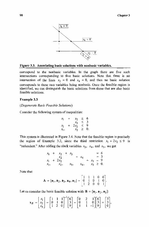
98 Chapter 3
Figure 3.3. Associating basic solutions with nonbasic variables.
correspond to the nonbasic variables. In the graph there are five such intersections corresponding to five basic solutions. Note that there is no intersection of the lines x2 = 0 and x4 = 0, and thus no basic solution corresponds to these two variables being nonbasic. Once the feasible region is identified, we can distinguish the basic solutions from those that are also basic feasible solutions.
Example 3.3
(Degenerate Basic Feasible Solutions)
Consider the following system of inequalities:
*1
X,
Xj ,
+
+
x2 x7.
2x2 x2
< < < >
6 ί 9 0.
This system is illustrated in Figure 3.4. Note that the feasible region is precisely the region of Example 3.2, since the third restriction xj + 2x2 < 9 is
"redundant." After adding the slack variables x3, x4, and x5, we get
Note that
x\
x\ X] ,
+
+
x2 x2
2x2
x2
x3
*3>
X4
X4
A = [a! ,a 2 ,a 3 , a 4 , a 5 ]
t
>
1 0 1
+
1 1 2
x5 x5
1 0 0
—
>
0 1 0
6 3 9 0.
0 0 1
Let us consider the basic feasible solution with B = [at, a2, a3 ]:
X,
x? x3
= 1 1 1 0 1 0 1 2 Oj
- 1 6" 3
L9 =
0 0 1
-2 1 1
i l 0 -1
[61 3 9
= Γ3Ί 3 0
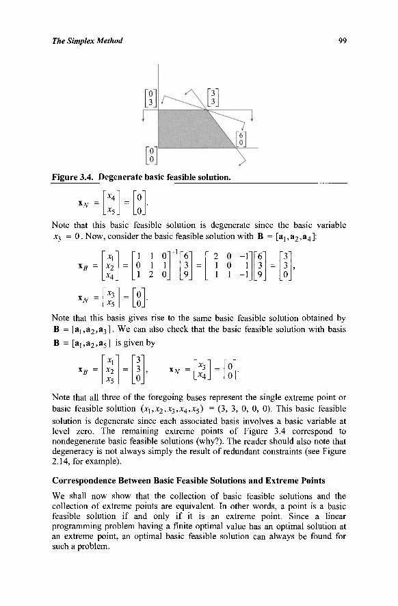
The Simplex Method 99
Figure 3.4. Degenerate basic feasible solution.
0
.0.'
Note that this basic feasible solution is degenerate since the basic variable x3 = 0. Now, consider the basic feasible solution with B = [aj,a2,a4]:
6^ 3 9
= 3 3 0
x3
_ X 5 . = 0
_0_
Note that this basis gives rise to the same basic feasible solution obtained by B = [at,a2,a3]. We can also check that the basic feasible solution with basis B = [a],a2,a5] is given by
~x3~ X4 = 0
.0.
Note that all three of the foregoing bases represent the single extreme point or basic feasible solution (xl ) = (3, 3, 0, 0, 0). This basic feasible solution is degenerate since each associated basis involves a basic variable at level zero. The remaining extreme points of Figure 3.4 correspond to nondegenerate basic feasible solutions (why?). The reader should also note that degeneracy is not always simply the result of redundant constraints (see Figure 2.14, for example).
Correspondence Between Basic Feasible Solutions and Extreme Points
We shall now show that the collection of basic feasible solutions and the collection of extreme points are equivalent. In other words, a point is a basic feasible solution if and only if it is an extreme point. Since a linear programming problem having a finite optimal value has an optimal solution at an extreme point, an optimal basic feasible solution can always be found for such a problem.
lN X4
x5
X,
x7 X4
= 1 1 0 0 1 1 1 2 0
—1 6 3 9
=
xl x7. x5
= 3 3 0
100 Chapter 3
Consider the following problem:
Minimize ex
subject to Ax = b
x > 0 , where A is an w x « matrix with rank m. Let x be an extreme point of the feasible region. We shall show that x is also a basic feasible solution of the system Ax = b, x > 0.
By the definition given in Section 2.6, there are some n linearly independent defining hyperplanes binding at x. Since Ax = b provides m linearly independent binding hyperplanes, there must be some p = n - m additional binding defining hyperplanes from the nonnegativity constraints that together with Ax = b provide n linearly independent defining hyperplanes binding at x. Denoting these p additional hyperplanes by x^ = 0, we therefore
conclude that the system Ax = b, xN = 0 has x as the unique solution. Now, let
N represent the columns of the variables xN in A, and let B be the remaining
columns of A with xB as the associated variables. Since Ax = b can be written
as Bxg + Nxw = b, this means that B is tn x tti and invcrtiblc, and moreover, \β
= B"'b > 0, since x — (xg, Xyy ) is a feasible solution. Therefore, x is a basic feasible solution.
Conversely, suppose that x is a basic feasible solution of the system Ax = b, x > 0. We want to show that x is an extreme point. By definition, x = (xB,
xN ) where correspondingly A = (B, N) such that xB = B~ b > 0 and xN = 0.
But this means that the n hyperplanes Ax = b, xN = 0 are binding at x and are
moreover linearly independent, since B~ exists. Hence, by the definition in Section 2.6, x is an extreme point. Therefore, we have shown that every basic feasible solution is an extreme point and vice versa. Exercise 3.15 asks the reader to construct an alternative proof for this characterization.
Every basic feasible solution is equivalent to an extreme point. However, there may exist more than one basis corresponding to the same basic feasible solution or extreme point. A case of this type can occur in the presence of degeneracy, as illustrated in Example 3.3. Referring to the preceding proof, this case corresponds to that of an extreme point at which some r> p = n- m defining hyperplanes from x > 0 are binding. Hence, for any associated basis, (r-p) of the x g -variables are also zero. Consequently, the number of positive variables is q =
m - (r - p) < m. In this case, each possible choice of a basis B that includes the columns of these q positive variables represents this point (why?).
Clearly, if there exists more than one basis representing an extreme point, then this extreme point is degenerate. However, the converse is not necessarily true. Consider the following example of a polyhedral set:
Xj + Xj ~t" ΧΛ = 1
—Xi + X7 + X3 = 1
X\, X2, x3 - 0 .
The Simplex Method 101
Consider the solution x = (0, 1, 0). Observe that this is an extreme point or a basic feasible solution with a corresponding basis having xy and x2 as basic variables. Moreover, this is a degenerate extreme point. There are four defining hyperplanes binding at x. Moreover, there are three ways of choosing three linearly independent hyperplanes from this set that yield x as the (unique) solution (how?). However, the basis associated with x is unique.
In this example, the constraints Ax = b imply that xj = 0. However, after
fixing X] = 0, we no longer have a full rank system. If this were not the case, then for any degenerate extreme point, there would be more than one corresponding basis. To see this, consider the system Ax = b, x > 0, where A is m χ η of rank m. Let x be a degenerate extreme point solution, and let xB and xN be a set of basic and nonbasic variables, respectively, corresponding to a particular basis. As usual, let B and N be the columns of A associated with the variables x g and xN, respectively. Then, the given system is equivalent to
B_1Nx^ + xB = B_1b = b
χΝ, xB > 0.
Consider a degenerate basic variable xB (with br = 0), which is such that Ax
= b does not necessarily imply that xB = 0. Given that such a variable exists,
we will construct another basis representing this point. Let xk be some
component of x^ that has a nonzero coefficient ΘΓ in the row corresponding to
xB . Note that xk exists. Then consider a new choice of (« - m) nonbasic
variables given by xB and Xjy-/t > where XJV_£ represents the components of
xN other than xk . Putting xB = 0 and x^r_^ = 0 above uniquely gives xk =
br/0r = 0 from row r, and so xB. = bt is obtained as before from the other
rows. Hence, this corresponds to an alternative basis that represents the same extreme point. Finally, note that if no degenerate basic variable xB of this type
exists, then there is only one basis that represents this extreme point.
Existence of Basic Feasible Solutions
Since a nonempty set X= {x: Ax = b, x > 0} has extreme points (from Theorem 2.1), we know that the system Ax = b, x > 0 has at least one basic feasible solution. In fact, starting from any feasible point x e X, the proof of Theorem 2.1 shows how to constructively obtain an extreme point, and hence a basic feasible solution o fX Assuming without loss of generality that rank (A) = m, we can examine the binding nonnegativity constraints at this extreme point, and select p = (n - m) of them to correspond to the variables xN, such that the system Ax = b, Xjy = 0 has rank n (how?). Calling the remaining m variables Χβ as basic variables, we obtain a corresponding basis.
102 Chapter 3
Summary of Results
Let us summarize some of the important facts about the following linear programming problem, where A is an m x n matrix with rank m.
Minimize ex
subject to Ax = b
x > 0 .
Theorem 3.1 The collection of extreme points corresponds to the collection of basic feasible solutions, and both are nonempty provided that the feasible region is not empty.
Theorem 3.2 Assume that the feasible region is nonempty. Then a finite optimal solution exists if and only if cd, > 0 fory = 1,..., I, where di,...,d^ are the extreme
directions of the feasible region. Otherwise, the optimal solution value is unbounded.
Theorem 3.3 If an optimal solution exists, then an optimal extreme point (or equivalently an optimal basic feasible solution) exists.
Theorem 3.4 For every extreme point (basic feasible solution) there is a corresponding basis (not necessarily unique), and, conversely, for every basis there is a correspond-ing (unique) extreme point. Moreover, if an extreme point has more than one basis representing it, then it is degenerate. Conversely, a degenerate extreme point has more than one basis representing it if and only if the system Ax = b itself does not imply that the degenerate basic variables corresponding to an associated basis are identically zero.
Now, since the extreme points may be enumerated by algebraically
enumerating all basic feasible solutions, which are bounded by \ \ , one may
think of simply listing all basic feasible solutions and picking the one having the minimal objective value. This is unsatisfactory, however, for a number of
reasons. First, the number of basic feasible solutions is bounded by \ \ , which
is large, even for moderate values of m and n. Second, this simple approach does not tell us if the problem has an unbounded optimal value, which may occur if the feasible region is unbounded. Last, if the feasible region is empty and if we apply the foregoing "simple-minded procedure," we shall discover that the feasible region is empty, only after all possible ways of extracting m columns out of n columns of the matrix A fail to produce a basic feasible solution, either
on the grounds that B does not have an inverse, or else that B~ b X 0. The simplex method is a clever procedure that moves from one extreme
point to another extreme point having a better (at least not worse) objective
The Simplex Method 103
value. It also discovers whether the feasible region is empty and whether the optimal objective value is unbounded. In practice, the method only enumerates a small portion of the extreme points of the feasible region. The key to this method is revealed next.
3.3 KEY TO THE SIMPLEX METHOD
The key to the simplex method lies in recognizing the optimality of a given extreme point solution based on local considerations without having to (globally) enumerate all extreme points or basic feasible solutions.
Consider the following linear programming problem:
LP: Minimize ex subject to Ax = b
x > 0 ,
where A is an m χ η matrix with rank m. Suppose that we have a basic feasible
solution n whose objective value z0 is given by
Z° = C ( B 0 b ) = {CB'CN){B~Qb) = Cz?B~lb· (3-1}
Now, let x g and x^ denote the set of basic and nonbasic variables for the
given basis. Then feasibility requires that xB >0,xN> 0, and that b = Ax =
B xB + Νχ^. Multiplying the last equation by B" and rearranging the terms, we get
say, (3.2)
where J is the current set of the indices of the nonbasic variables. Noting Equations (3.1) and (3.2) and letting z denote the objective function value, we get
B"'b
B"'b
b
- B~}mN
JeJ
- Z(y;)*;, JeJ
CX CBXB + CNXN
z 0
B_1b - Σ B"1»;*/
- Σ (2; - Cj)Xj
+ Σ CjXj jeJ
(3.3)
where z · = c#B a ,■ for each nonbasic variable.
104 Chapter 3
Using the foregoing transformations, the linear programming problem LP may be rewritten as:
Minimize z = z0 - £ (z ■ - c ) x · jeJ
subject to Σ (y / ) x / + XB ~ b (3-4)
Xj > 0, j e J, and χβ > 0.
Without loss of generality, let us assume that no row in Equation (3.4) has all zeros in the columns of the nonbasic variables x.-, j e J. Otherwise, the basic
variable in such a row is known in value, and this row can be deleted from the problem. Now, observe that the variables \B simply play the role of slack variables in Equation (3.4). Hence, we can equivalently write LP in the nonbasic variable space, that is, in terms of the nonbasic variables, as follows:
Minimize z = z0 - £ (z,- - c.)x ■ JzJ
subject to Z ( y y ) * y ^ b (3.5) jeJ
Xj > 0, j e J.
Note that the number of nonbasic variables is p = (n - ni), and so we have represented LP in some p-dimensional space. This is to be expected since there are p independent variables or p degrees of freedom in our constraint system. The values ( c ,■ - z ■ ) are referred to as reduced cost coefficients since they are
the coefficients of the (nonbasic) variables in this reduced space. The representation (3.4), in which the objective function z and the basic variables xB have been solved for in terms of the nonbasic variables, is referred to as a
representation of the basic solution in canonical form. The key result now simply says the following:
If (zj - Cj) < 0 for all j e J , then the current
basic feasible solution is optimal. (3.6)
This should be clear by noting that since z - c,· < 0 for all j e J, we have z
> z0 for any feasible solution; but for the current (basic) feasible solution, we
know thatz = z0, since x.- = 0 for all j e J.
3.4 GEOMETRIC MOTIVATION OF THE SIMPLEX METHOD
It is instructive to examine the foregoing operations geometrically. Observe that in the nonbasic variable space representation, the feasible region of LP is defined in terms of n intersecting half-spaces: m associated with the inequality constraints in Equation (3.5), and/? = n - m associated with the nonnegativity constraints. Associated with each of these half-spaces, there is a certain defining
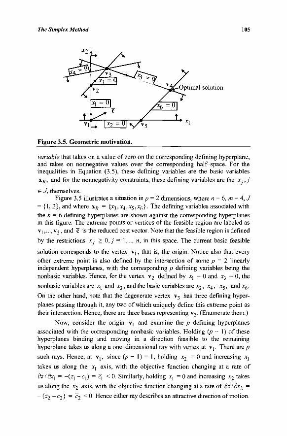
The Simplex Method 105
Figure 3.5. Geometric motivation.
variable that takes on a value of zero on the corresponding defining hyperplane, and takes on nonnegative values over the corresponding half-space. For the inequalities in Equation (3.5), these defining variables are the basic variables x g , and for the nonnegativity constraints, these defining variables are the Xj,j
e J, themselves. Figure 3.5 illustrates a situation in/? = 2 dimensions, where n = 6, m = 4, J
= {1, 2}, and where xB = {x3,x4,x5,x6}. The defining variables associated with the n = 6 defining hyperplanes are shown against the corresponding hyperplanes in this figure. The extreme points or vertices of the feasible region are labeled as Vj,...,v5, and ~c is the reduced cost vector. Note that the feasible region is defined
by the restrictions x,· > 0, j = 1,..., n, in this space. The current basic feasible
solution corresponds to the vertex Vj, that is, the origin. Notice also that every other extreme point is also defined by the intersection of some p = 2 linearly independent hyperplanes, with the corresponding p defining variables being the nonbasic variables. Hence, for the vertex v2 defined by xx = 0 and x3 = 0, the
nonbasic variables are xj and x3, and the basic variables are x2 , Χ4, x$, andx6. On the other hand, note that the degenerate vertex v3 has three defining hyper-planes passing through it, any two of which uniquely define this extreme point as their intersection. Hence, there are three bases representing v3. (Enumerate them.)
Now, consider the origin Vj and examine the p defining hyperplanes associated with the corresponding nonbasic variables. Holding (p - 1) of these hyperplanes binding and moving in a direction feasible to the remaining hyperplane takes us along a one-dimensional ray with vertex at vj. There are p
such rays. Hence, at vj, since (p — 1) = 1, holding x2 = 0 and increasing X]
takes us along the xj axis, with the objective function changing at a rate of
dzldxx = -(zj - q ) = q < 0. Similarly, holding X! = 0 and increasing x2 takes
us along the x2 axis, with the objective function changing at a rate of dz/dx2 =
-(z2-c2) = c2 < 0. Hence either ray describes an attractive direction of motion.
106 Chapter 3
Suppose that we choose the latter direction of motion. Because this is a feasible direction, it takes us along an edge of the feasible region (why?). Naturally, we would like to move as far as possible along this edge since dz/dx2 = c~2 is a negative constant. However, our motion is blocked by the hyperplane x3 = 0, since x3 has been driven to zero and moving any further would drive x3
negative. (Of course, if no such blocking hyperplane existed, then the optimal solution value would have been unbounded.) Furthermore, since (p - 1) linearly independent hyperplanes were binding all along and we were blocked by a new hyperplane, we now have/) linearly independent hyperplanes binding, and so we are at another extreme point of the feasible region. In fact, this is an adjacent extreme point with respect to the previous extreme point (why?). At v2 the nonbasic variables are X] and x3,and the remaining variables are basic. We have now completed one step known as an iteration or pivot of the simplex method. In this step, the variable x2 is called the entering variable since it
entered the set of basic variables, and the variable x3 is called the blocking variable, or the leaving variable, since it blocked our motion or left the set of basic variables with respect to Vj. The previous and the new basis differ in only one basic variable, and therefore, in only one nonbasic variable. Such bases are called adjacent bases.
Repeating this process at v2, we would of course not like to enter x3
into the basis, since it will only take us back along the reverse of the previous direction. However, holding x3 = 0 and increasing X] takes us along an improving edge (why?). Proceeding in this direction as shown in Figure 3.5, we notice that more than one hyperplane blocks our motion. Suppose that we arbitrarily choose one of these, namely, x4 = 0 as the blocking hyperplane. Hence, X4 is the leaving variable, and for current basis representing v3, we have that x3 and x4 are the nonbasic variables. Now, if we hold x4 = 0 and move in a direction along which x3 increases, the objective function value would decrease because this direction makes an acute angle with - c . However, this direction is not feasible. We are blocked by the hyperplane x5 = 0 even before we begin to move! That is, X5 leaves the basis giving x4 and x5 as our new nonbasic variables, while we are still at the same vertex v3. Such a step in which one basis is exchanged for an adjacent basis, both representing the same extreme point solution, is called a degenerate iteration or a degenerate pivot. While such a pivot is undesirable, it may not always be avoidable, unlike as in Figure 3.5 (how?). Certainly, we would not like to be stuck in an infinite loop at an extreme point while performing a sequence of degenerate pivots that takes us in a closed loop of bases, all representing the same extreme point, with the objective function therefore remaining a constant. Such a phenomenon is called cycling and, as shown in Chapter 4, it can indeed occur. Special precautions need to be taken for its prevention.
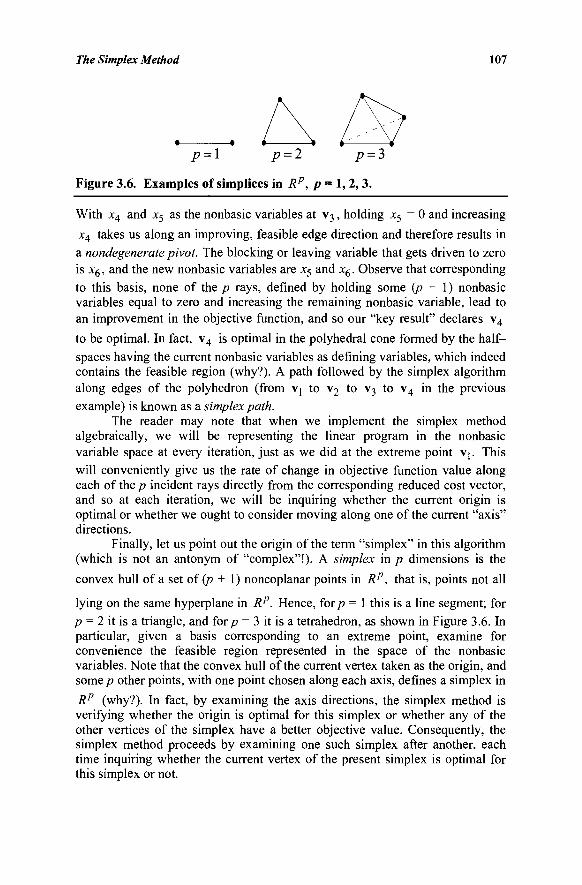
The Simplex Method 107
• · /? = 1 P = 2 P = 3
Figure 3.6. Examples of simplices in Rp, p = 1,2,3.
With x4 and x5 as the nonbasic variables at v3 , holding x5 = 0 and increasing x4 takes us along an improving, feasible edge direction and therefore results in a nondegenerate pivot. The blocking or leaving variable that gets driven to zero is x6, and the new nonbasic variables are x5 and JC6 . Observe that corresponding to this basis, none of the p rays, defined by holding some (p - 1) nonbasic variables equal to zero and increasing the remaining nonbasic variable, lead to an improvement in the objective function, and so our "key result" declares v4
to be optimal. In fact, v4 is optimal in the polyhedral cone formed by the half-spaces having the current nonbasic variables as defining variables, which indeed contains the feasible region (why?). A path followed by the simplex algorithm along edges of the polyhedron (from Vj to v2 to v3 to v4 in the previous
example) is known as a simplex path. The reader may note that when we implement the simplex method
algebraically, we will be representing the linear program in the nonbasic variable space at every iteration, just as we did at the extreme point V[. This
will conveniently give us the rate of change in objective function value along each of the p incident rays directly from the corresponding reduced cost vector, and so at each iteration, we will be inquiring whether the current origin is optimal or whether we ought to consider moving along one of the current "axis" directions.
Finally, let us point out the origin of the term "simplex" in this algorithm (which is not an antonym of "complex"!). A simplex in p dimensions is the
convex hull of a set of (p + 1) noncoplanar points in Rp, that is, points not all
lying on the same hyperplane in Rp. Hence, for/? = 1 this is a line segment; for p = 2 it is a triangle, and for p = 3 it is a tetrahedron, as shown in Figure 3.6. In particular, given a basis corresponding to an extreme point, examine for convenience the feasible region represented in the space of the nonbasic variables. Note that the convex hull of the current vertex taken as the origin, and some p other points, with one point chosen along each axis, defines a simplex in
Rp (why?). In fact, by examining the axis directions, the simplex method is verifying whether the origin is optimal for this simplex or whether any of the other vertices of the simplex have a better objective value. Consequently, the simplex method proceeds by examining one such simplex after another, each time inquiring whether the current vertex of the present simplex is optimal for this simplex or not.
108 Chapter 3
3.5 ALGEBRA OF THE SIMPLEX METHOD
We will now translate the geometric process described in the foregoing section into algebra. Toward this end, consider the representation of the linear program LP in the nonbasic variable space, written in equality form as in Equation (3.4). If (z ■ - c ■ ) < 0 for all j e J, then x ■ = 0 for j eJ and xB = b is optimal
for LP as noted in Equation (3.6). Otherwise, while holding (p - 1) nonbasic variables fixed at zero, the simplex method considers increasing the remaining variable, say, xk . Naturally, we would like zk - ck to be positive, and perhaps
the most positive of all the zj -cj, j e J. Now, fixing Xj = 0 for j e J - {k},
we obtain from Equation (3.4) that
z = zo-(zk-ck)xk (3.7)
and
XBX
XB2
xBr
XB m _
V b2
K
A i .
y\k
yik
yrk
Jmk_
xk. (3.8)
If )>% < 0, then xB. increases as xk increases, and so xB. continues to be non-
negative. If yjk > 0, then xB. will decrease as xk increases. In order to satisfy
nonnegativity, xk is increased until the first point at which some basic variable
xB drops to zero. Examining Equation (3.8), it is then clear that the first basic
variable dropping to zero corresponds to the minimum of ft, I yik for positive
yik. More precisely, we can increase xk until
xk = —^- = minimum <{ ^— :yik > 0 \. yrk \<i<m yik
lb, (3.9)
In the absence of degeneracy, br > 0, and hence xk = br I yrk > 0. From
Equation (3.7) and the fact that zk-ck > 0, it then follows that z < z0 and the
objective function strictly improves. As xk increases from level 0 to br I yrk, a
new feasible solution is obtained. Substituting xk = brlyrk in Equation (3.8) gives the following point:
The Simplex Method 109
XB -Dj Dr, i= \,...,m,
xk =■
yrk (3.10)
and all other x · -variables are zero.
From Equation (3.10), xB = 0 and hence, at most m variables are positive.
The corresponding columns in A are &Β,ΛΒ,...,ΛΒ, ak, aB ,...,& B . Note
that these columns are linearly independent since yrk Φ 0. (Recall that if &B ,...,
aB ,..., aB are linearly independent, and if ak replaces &B , then the new columns
are linearly independent if and only if yrk Φ 0; see Section 2.1.) Therefore, the point given by Equation (3.10) is a basic feasible solution.
To summarize, we have algebraically described an iteration, that is, the process of transforming from one basis to an adjacent basis. This is done by increasing the value of a nonbasic variable xk with positive zk - ck and
adjusting the current basic variables. In the process, the variable xB drops to
zero. The variable xk hence enters the basis and xB leaves the basis. In the
absence of degeneracy the objective function value strictly decreases, and hence the basic feasible solutions generated are distinct. Because there exists only a finite number of basic feasible solutions, the procedure would terminate in a finite number of steps.
Example 3.4
Minimize χλ + x2 subject to X\ + 2x2 ^ 4
x2 < 1 X[, x 2 - 0·
Introduce the slack variables x3 and x4 to put the problem in a standard form. This leads to the following constraint matrix A:
A= [a 1 , a 2 , a3 ,a 4 ] = 1 2 1 0 0 1 0 1
Consider the basic feasible solution corresponding to B = [aj, a2] . In other
words, Xj and x2 are the basic variables, while x3 and x4 are the nonbasic variables. The representation of the problem in this nonbasic variable space as in Equation (3.4) with J= {3,4} may be obtained as follows. First, compute:
B" Ί 2 0 1
-1 "1 0
-2 1 csB-'=(l, 1) = (i,-i).
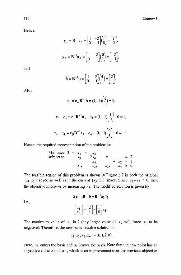
110 Chapter 3
Hence,
and
Also,
y3 =B 'a3 =
y 4 =B~ 1 a 4 =
"1 0
"l 0
-2 1
-2" 1
Ki)-
(!)■[
"Γ 0_|'
"-2" 1
b = B_1b =
z 0 =c / i B- 1 b = ( l , - l ) ^ ) = 3,
Z 3 " C 3 = C B B a 3 - C 3 = ( l , - l ) -0 = 1,
z4~c4 =cBB a 4 - c 4 = ( l , - l ) - 0 = - l .
Hence, the required representation of the problem is:
Minimize 3 - x3 + x4
subject to x3 Ζ,ΧΛ + X\ x4 x2, x3,
+ x2 = 1 x4 > 0.
The feasible region of this problem is shown in Figure 3.7 in both the original (xj,x2) space as well as in the current (x3,x4) space. Since z^-c^ > 0, then the objective improves by increasing x3. The modified solution is given by
i.e.,
xB =B ' b - B 'a3x3
*3· xx x2
= 2 1 - 1
0
The maximum value of x3 is 2 (any larger value of x3 will force xj to be negative). Therefore, the new basic feasible solution is
(x1,x2,x3,x4) = (0,1,2,0).
Here, x3 enters the basis and xj leaves the basis. Note that the new point has an objective value equal to 1, which is an improvement over the previous objective
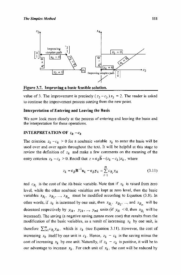
The Simplex Method 111
*2*
Improving simplex path
X4
1*2 = °l - N Improving simplex path
Figure 3.7. Improving a basic feasible solution.
value of 3. The improvement is precisely (z3 - c 3 ) x 3 = 2 . The reader is asked to continue the improvement process starting from the new point.
Interpretation of Entering and Leaving the Basis
We now look more closely at the process of entering and leaving the basis and the interpretation for these operations.
INTERPRETATION OF zk -ck
The criterion zk-ck > 0 for a nonbasic variable xk to enter the basis will be used over and over again throughout the text. It will be helpful at this stage to review the definition of zk and make a few comments on the meaning of the
entry criterion zk-ck > 0. Recall that z = Cgb - (zk - ck )x/c, where
zk = CBB H = CBy* = Σ cB yik (3.11)
and cB. is the cost of the z'th basic variable. Note that if xk is raised from zero
level, while the other nonbasic variables are kept at zero level, then the basic variables xB , xB , ..., xB must be modified according to Equation (3.8). In
other words, if xk is increased by one unit, then xB , xB ..., and xB will be
decreased respectively by y^k, y2k, ■■■, ymk units (if yik < 0, then xB. will be
increased). The saving (a negative saving means more cost) that results from the modification of the basic variables, as a result of increasing xk by one unit, is
therefore £i=ic5-.);iVt> which is zk (see Equation 3.11). However, the cost of
increasing xk itself by one unit is ck. Hence, zk - ck is the saving minus the
cost of increasing xk by one unit. Naturally, if zk - ck is positive, it will be to
our advantage to increase xk. For each unit of xk, the cost will be reduced by
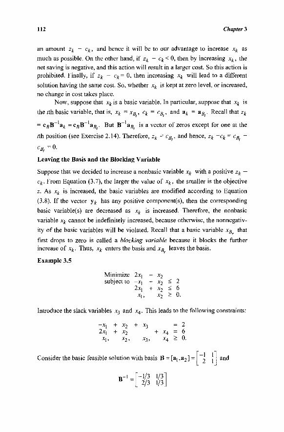
112 Chapter 3
an amount zk - ck, and hence it will be to our advantage to increase xk as much as possible. On the other hand, if zk - ck< 0, then by increasing xk, the net saving is negative, and this action will result in a larger cost. So this action is prohibited. Finally, if zk - ck= 0, then increasing xk will lead to a different
solution having the same cost. So, whether xk is kept at zero level, or increased, no change in cost takes place.
Now, suppose that xk is a basic variable. In particular, suppose that xk is
the /th basic variable, that is, xk = xB , ck = cB , and ak = aB . Recall that zk
= cgB~ ak = cgB~ ΆΒ . But B~ ag is a vector of zeros except for one at the
fth position (see Exercise 2.14). Therefore, zk = cB , and hence, zk ~ck = cB -
cBt = 0.
Leaving the Basis and the Blocking Variable
Suppose that we decided to increase a nonbasic variable xk with a positive zk —
ck. From Equation (3.7), the larger the value of xk, the smaller is the objective
z. As xk is increased, the basic variables are modified according to Equation
(3.8). If the vector y^ has any positive component(s), then the corresponding
basic variable(s) are decreased as xk is increased. Therefore, the nonbasic
variable xk cannot be indefinitely increased, because otherwise, the nonnegativ-
ity of the basic variables will be violated. Recall that a basic variable xB that
first drops to zero is called a blocking variable because it blocks the further increase of xk. Thus, xk enters the basis and xB leaves the basis.
Example 3.5
Minimize 2x\ subject to -jq
2x\ Xj,
- *2 + H + *2
x2
< < >
2 6 0.
Introduce the slack variables x3 and x4. This leads to the following constraints:
- * i 2xj
*1>
+ +
x2
x2 x2'
+ *3
*3>
+ X\
X$
= = >
2 6 0.
Consider the basic feasible solution with basis B = [a! ,a2] = -1 1 2 1
B _ I = -1/3 1/3" _ 2/3 1/3
and
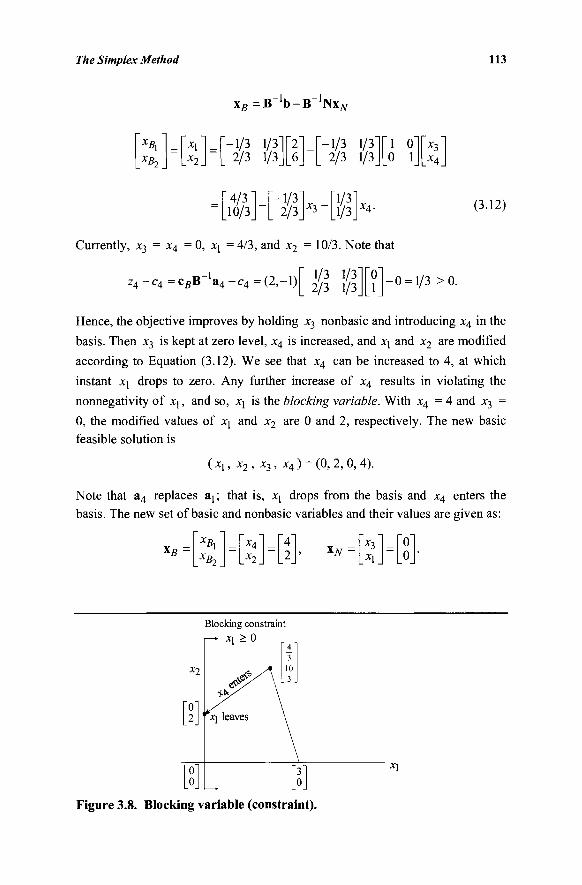
The Simplex Method 113
x^=B"1b-B"1NxA,
XBX
XB2
X,
x2_
"-1/3 _ 2/3
4/3 10/3
1/3] [2 1/3 J [6
- -Ψ 2/3
*3
1/3 2/3
1/3 1/3
1/3] 1/3.
X4.
Ί 0" 0 1
*3 _x4_
(3.12)
Currently, x3 = x4 = 0, xj = 4/3, and x2 = 10/3. Note that
Z4-C4 = c s B a 4 - c 4 = ( 2 , - i ) -1/3 1/3' 2/3 1/3 - 0 = 1/3 >0.
Hence, the objective improves by holding x3 nonbasic and introducing x4 in the
basis. Then x3 is kept at zero level, x4 is increased, and x\ and x2 are modified
according to Equation (3.12). We see that x4 can be increased to 4, at which
instant xj drops to zero. Any further increase of x4 results in violating the
nonnegativity of X], and so, X] is the blocking variable. With x4 = 4 and x3 =
0, the modified values of xj and x2 are 0 and 2, respectively. The new basic
feasible solution is
(x1 ; x2 , x3, x4 ) = (0, 2, 0, 4).
Note that a4 replaces a^ that is, χλ drops from the basis and x4 enters the basis. The new set of basic and nonbasic variables and their values are given as:
X R = XBX
XB2
= X4
-x2_ =
"4" 2
liV -
Blocking constraint
• xx > 0
Figure 3.8. Blocking variable (constraint).
114 Chapter 3
Moving from the old to the new basic feasible solution is illustrated in Figure
3.8 in the original (xl5 x2) space. Note that as x4 increased by one unit, xj
decreases by 1/3 unit and x2 decreases by 1/3 unit; that is, we move in the
direction (-1/3, -1/3) in the (x1? x2) space. This continues until we are blocked
by the nonnegativity restriction xj > 0. At this point xj drops to zero and leaves
the basis.
3.6 TERMINATION: OPTIMALITY AND UNBOUNDEDNESS
We have discussed a procedure that moves from one basis to an adjacent basis, by introducing one variable into the basis, and removing another variable from the basis. The criteria for entering and leaving are summarized below:
1. Entering: xk may enter if zk - ck > 0
2. Leaving: xs may leave if
*r ■ ■ \bi J —— = minimum^ —— :yjk > 0 >. yrk \<i<m [yik J
Two logical questions immediately arise. First, what happens if each nonbasic variable x,· has z - c, < 0? In this case, as seen by Equation (3.6),
we have obtained an optimal basic feasible solution. Second, suppose that zk - ck > 0, and hence xk is eligible to enter the basis, but we cannot find any
positive component yik, that is, y^ < 0. In this case, the optimal objective value is unbounded. These cases will be discussed in more detail in this section.
Termination with an Optimal Solution
Consider the following problem, where A is an m χ η matrix with rank m.
Minimize ex
subject to Ax = b
x > 0 .
Suppose that x* is a basic feasible solution with basis B; that is, x* = " " .
Let z* denote the objective of x*, that is, z* = csB~ b. Suppose further that
z - Cj < 0 for all nonbasic variables, and hence there are no nonbasic variables
that are eligible to enter the basis. Let x be any feasible solution with objective value z. Then from Equation (3.3) we have
z* -z= X (zj-Cj)Xj. (3.13)
The Simplex Method 115
Because z · - c,· < 0 and x,· > 0 for all variables, then z < z, and so, as in
Equation (3.6), x is an optimal basic feasible solution.
Unique and Alternative Optimal Solutions
We can get more information from Equation (3.13). If z--c , · < 0 for all
nonbasic components, then the current optimal solution is unique. To show this,
let x be any feasible solution that is distinct from x*. Then there is at least one
nonbasic component x ,· that is positive, because if all nonbasic components are
zero, x would not be distinct from x*. From Equation (3.13) it follows that z >
z*, and hence, x* is the unique optimal solution.
Now, consider the case where z · -c ■ < 0 for all nonbasic components,
but zk - ck = 0 for at least one nonbasic variable xk. As xk is increased, we
get (in the absence of degeneracy) points that are distinct from x* but have the same objective value (why?). If xk is increased until it is blocked by a basic variable (if it is blocked at all), we get an alternative optimal basic feasible solution. The process of increasing xk from level zero until it is blocked (if at all) generates an infinite number of alternative optimal solutions.
Example 3.6
Minimize -3xj + x2 subject to χχ + 2x2 + x3 = 4
—Xi + X 2 ~~ -^4 = 1 Xj , X2 5 X3 5 X4 ^ 0 .
Consider the basic feasible solution with basis B = [a, ,a4] =
. The corresponding point is given by 1 0 1 1
xs = Xj
X4 B ' b 1 0
1 1 XN -
x2
x3
1 0 -1 1 and B
and the objective value is -12. To see if we can improve the solution, calculate
z2 - c 2 and z3 - c3 as follows, noting that cgB~ = (-3, 0), where cB = (-3,
0):
z2-c2 =cBB a 2 - c 2 = ( - 3 , 0 ) - l = -7 ,
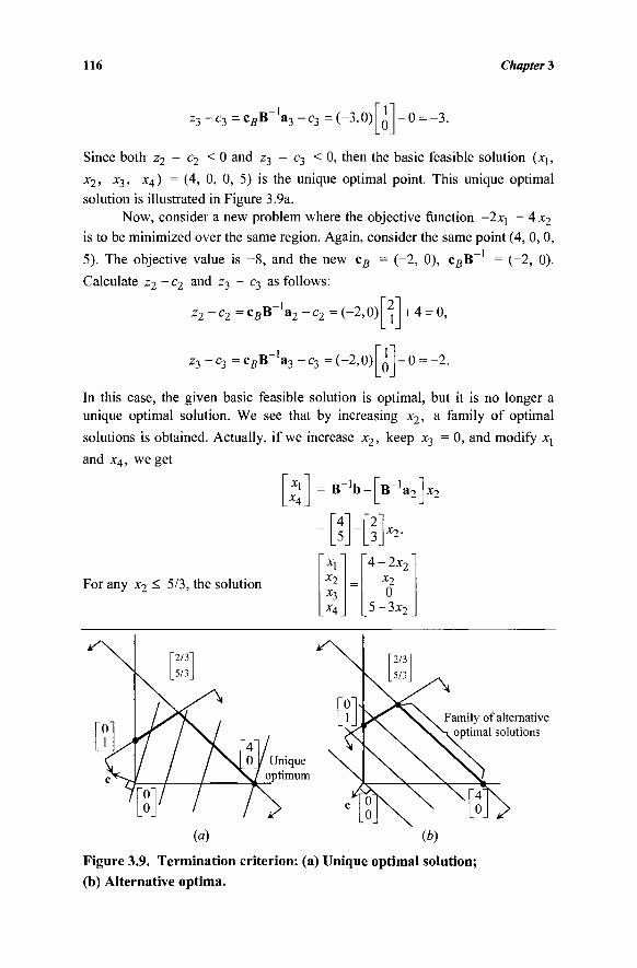
116 Chapter 3
z3-c3=CgB a3-c3=(-3,0) -0 = -3.
Since both z2 - c2 < 0 and z^ - c^ < 0, then the basic feasible solution (X],
x2, X3, X4) = (4, 0, 0, 5) is the unique optimal point. This unique optimal
solution is illustrated in Figure 3.9a. Now, consider a new problem where the objective function -2xt - 4 x2
is to be minimized over the same region. Again, consider the same point (4, 0, 0,
5). The objective value is - 8 , and the new cB = (-2, 0), c#B
Calculate z2 - c 2 and z3 - c3 as follows:
(-2, 0).
z2 " c2 = CBB a2 - c2 = (~2> 0)
z 3 -C3=c g B- 1 a 3 -C3=(-2 ,0 )
+ 4 = 0,
-0 =
In this case, the given basic feasible solution is optimal, but it is no longer a unique optimal solution. We see that by increasing x2, a family of optimal
solutions is obtained. Actually, if we increase x2, keep x3 = 0, and modify xj
and x4, we get
X4 =
=
B"
"4" 5
>b
- "2 3
B a2 x2
x2.
For any x2 < 5/3, the solution
xl x2 x3 X4
=:
"4-2x2" x2 0
5-3x2
Unique optimum
Figure 3.9. Termination criterion: (a) Unique optimal solution; (b) Alternative optima.
Family of alternative optimal solutions
The Simplex Method 117
is an optimal solution with objective value - 8 . In particular, if x2 = 5/3, we get an alternative basic feasible optimal solution, where x4 drops from the basis. This is illustrated in Figure 3.9b. Note that the new objective function contours are parallel to the hyperplane χχ + 2 x2 =4 corresponding to the first constraint. That is why we obtain alternative optimal solutions in this example. In general, whenever the optimal objective function contour contains a face of dimension greater than 0, we will have alternative optimal solutions.
Unboundedness
Suppose that we have a basic feasible solution of the system Ax = b, x > 0, with objective value z0. Now, let us consider the case when we find a corresponding
nonbasic variable xk with zk - ck > 0 and y^ < 0. This variable is eligible to enter the basis, since increasing it will improve the objective function value. From Equation (3.3) we have
Since we are minimizing the objective z and since zk - ck > 0, then it is to our benefit to increase xk indefinitely, which will make z go to -co. The reason that we were not able to do this before was that the increase in the value of xk was blocked by a basic variable. This puts a "ceiling" on xk beyond which a basic variable will become negative. But if blocking is not encountered, there is no reason why we should stop increasing xk. This is precisely the case when y^ < 0. Recall that from Equation (3.8) we have
xB=B-lb-[yk]xk
and so, if y^ < 0, then xk can be increased indefinitely without any of the basic
variables becoming negative. Therefore, the solution x (where \B = B~ b -
[v/fc]x/t> the nonbasic variable xk is arbitrarily large, and other nonbasic
variables are zero) is feasible and its objective value is z = ZQ-(Z/C-CJC)X!(,
which approaches -co as xk approaches oo.
To summarize, if we have a basic feasible solution with zk-ck > 0 for
some nonbasic variable xk, and meanwhile y^ < 0, then the optimal objective
value is unbounded, tending to -co. This is obtained by increasing xk
indefinitely and adjusting the values of the current basic variables, and is equivalent to moving along the ray:
118 Chapter 3
ÌVV 0
0
I Ò
+ **
"-y*"
0
i
ò
:xk>0
Note that the vertex of the ray is the current basic feasible solution
the direction of the ray is
B ' b and
0
j Ò
where the 1 appears in the Mi position. It may be noted that cd = (cB,cN)d = -cByk+ck =-zk+ck.
But ck-zk < 0 (because xk was eligible to enter the basis). Hence, cd < 0 for the recession direction d of the (nonempty) feasible region, which is the necessary and sufficient condition for unboundedness. In Exercise 3.52 we ask the reader to verify that d is indeed an (extreme) direction of the feasible region.
Example 3.7
( Unboundedness)
Minimize —JCJ subject to x\
-xl Χγ,
- 3JC2
- 2x2 ^ 4 + JC2 - 3
x2 > 0.
The problem, illustrated in Figure 3.10, clearly has an unbounded optimal objective value. After introducing the slack variables x3 and x4, we get the
constraint matrix A 1 -2
-1 1
solution whose basis B = [a3,a4]
1 0 0 1
1 0 0 1
Now, consider the basic feasible
Xn = *3 X4
1 0" 0 1
~4 3 =
"4" 3 XN -
xl x2
= "0" 0
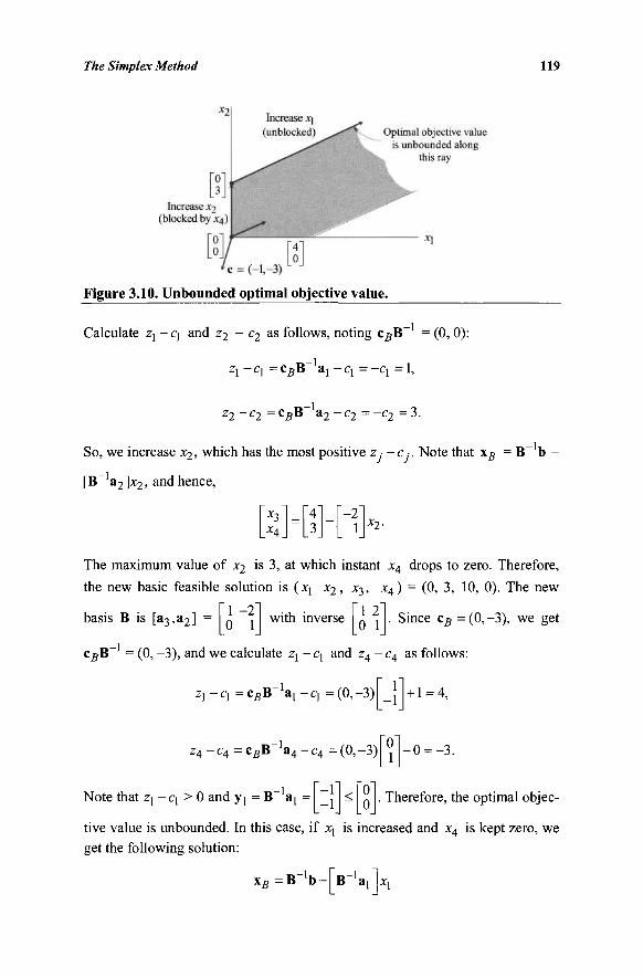
The Simplex Method 119
Figure 3.10. Unbounded optimal objective value.
i _ , Calculate zj - q and z2 - c2 as follows, noting c s B = (0, 0):
zl ~ c l = C B B a l ~ c l = _ c l = !»
Z 2 ~ C 2 = C B B a 2 - c 2 = - c 2 = 3 .
So, we increase x2, which has the most positive z · - c ■. Note that x# = B b
[B~ a2 ]x2, and hence,
*3 x4
= 4 3 - -2
1 x2.
The maximum value of x2 is 3, at which instant x4 drops to zero. Therefore,
the new basic feasible solution is (xj x2 , x3, x4) = (0, 3, 10, 0). The new
basis B is [a3,a2] 1 -2 0 1 with inverse 1 2
0 1 Since c g =(0,-3), we get
c s B = (0,-3), and we calculate zi -c\ and z4-c4 as follows:
z i - c i = c s B a i - c i = ( 0 , - 3 ) + 1 = 4,
z4-c4= c sB a4 - c4 = (0, -3) - 0 = -3 .
Note that zx - q > 0 and yj = B aj = -1 -1 . Therefore, the optimal objec-
tive value is unbounded. In this case, if xj is increased and x4 is kept zero, we get the following solution:
xR=B"'b B 'aj xx
120 Chapter 3
i.e..
*3 _x2.
= "10"
3 - "-Γ -1
x,= "10 + X!-
3 + xt
with X] > 0, and x4 = 0. Note that this solution is feasible for all x^ > 0. In particular,
X] -2x 2 + X3 =x\— 2(3 + X]) + (10 + Xj) = 4,
and
-χγ + x2 + X4 = -xi +(3 + xi) + 0 = 3.
Furthermore, z = - 9 - 4x1; which approaches -00 as xj approaches 00. Therefore, the optimal objective value is unbounded by moving along the ray
{(0,3,10,0)+ xx (1,1, 1,0): xx >0}.
Again, note that the necessary and sufficient condition for unboundedness holds; in particular,
cd = ( -1 , -3 , 0,0) -4<0.
3.7 THE SIMPLEX METHOD
All the machinery that is needed to describe the simplex algorithm and to prove its convergence in a finite number of iterations (in the absence of degeneracy) has been generated. Given a basic feasible solution and a corresponding basis, we can either improve it if zk - ck > 0 for some nonbasic variable xk, or stop with an optimal point if z ■ -c ■ < 0 for all nonbasic variables. If zk -ck > 0 and the vector y^ contains at least one positive component, then the increase in xk will be blocked by one of the current basic variables, which drops to zero and leaves the basis. On the other hand, if zk -ck > 0 and y^ < 0, then xk can
be increased indefinitely, and the optimal objective value is unbounded (-co). This discussion is precisely the essence of the simplex method.
We now give a summary of the simplex method for solving the following linear programming problem:
Minimize ex
subject to Ax = b x > 0 ,
where A is an m χ n matrix with rank m (the requirement that rank (A) = m will be relaxed in Chapter 4).
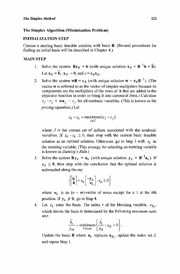
The Simplex Method 121
The Simplex Algorithm (Minimization Problem)
INITIALIZATION STEP
Choose a starting basic feasible solution with basis B. (Several procedures for finding an initial basis will be described in Chapter 4.)
MAIN STEP
1. Solve the system Bxg = b (with unique solution xB = B~ b = b).
Let xB = b, xN =0, andz = cBxB.
2. Solve the system wB = cB (with unique solution w = c5B~ ). (The vector w is referred to as the vector of simplex multipliers because its components are the multipliers of the rows of A that are added to the objective function in order to bring it into canonical form.) Calculate z ■ -Cj = wa - c ■ for all nonbasic variables. (This is known as the
pricing operation.) Let
zk-ck = maximum{z · - c . } jeJ
where J is the current set of indices associated with the nonbasic variables. If zk-ck < 0, then stop with the current basic feasible solution as an optimal solution. Otherwise, go to Step 3 with xk as the entering variable. (This strategy for selecting an entering variable is known as Dantzig 's Rule.)
3. Solve the system B y^ = ak (with unique solution y . = B~ ak). If
y^ < 0, then stop with the conclusion that the optimal solution is
unbounded along the ray
+ xk -Yk *k
:xk>0
where e^ is an (n - m)-vector of zeros except for a 1 at the Mi
position. If y^ X 0, go to Step 4.
Let xk enter the basis. The index r of the blocking variable, xB ,
which leaves the basis is determined by the following minimum ratio test:
b, • · \bi minimum < —^ : yik > 0
yrk \<i<m [yik
Update the basis B where zk replaces a g , update the index set J,
and repeat Step 1.
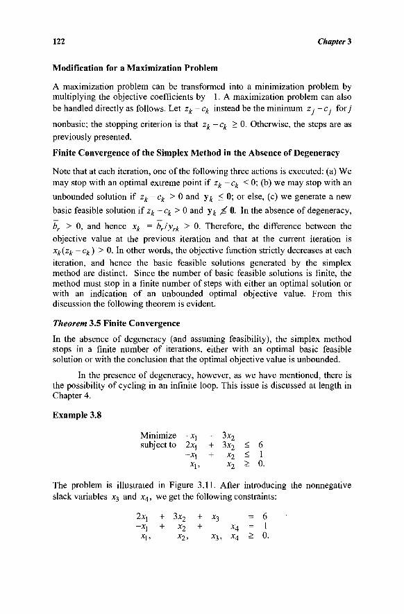
122 Chapter 3
Modification for a Maximization Problem
A maximization problem can be transformed into a minimization problem by multiplying the objective coefficients by - 1 . A maximization problem can also be handled directly as follows. Let zk -ck instead be the minimum z,- -c,· for/
nonbasic; the stopping criterion is that zk - ck > 0. Otherwise, the steps are as previously presented.
Finite Convergence of the Simplex Method in the Absence of Degeneracy
Note that at each iteration, one of the following three actions is executed: (a) We
may stop with an optimal extreme point if zk-ck < 0; (b) we may stop with an
unbounded solution if zk -ck > 0 and y^ < 0; or else, (c) we generate a new
basic feasible solution if zk - ck > 0 and y^ X 0. In the absence of degeneracy,
br > 0, and hence xk = brlyrk > 0. Therefore, the difference between the objective value at the previous iteration and that at the current iteration is xk(zk -ck) > 0. In other words, the objective function strictly decreases at each iteration, and hence the basic feasible solutions generated by the simplex method are distinct. Since the number of basic feasible solutions is finite, the method must stop in a finite number of steps with either an optimal solution or with an indication of an unbounded optimal objective value. From this discussion the following theorem is evident.
Theorem 3.5 Finite Convergence
In the absence of degeneracy (and assuming feasibility), the simplex method stops in a finite number of iterations, either with an optimal basic feasible solution or with the conclusion that the optimal objective value is unbounded.
In the presence of degeneracy, however, as we have mentioned, there is the possibility of cycling in an infinite loop. This issue is discussed at length in Chapter 4.
Example 3.8
Minimize -X] - 3x2 subject to 2xj + 3x2 ^ 6
-Χγ + X2 - 1 Xj, x 2 - 0·
The problem is illustrated in Figure 3.11. After introducing the nonnegative slack variables x3 and x4, we get the following constraints:
2xj + 3x2 + X3 = 6 —Xj + x 2 + X4 = 1
X\, X2, X3, X4 — 0.
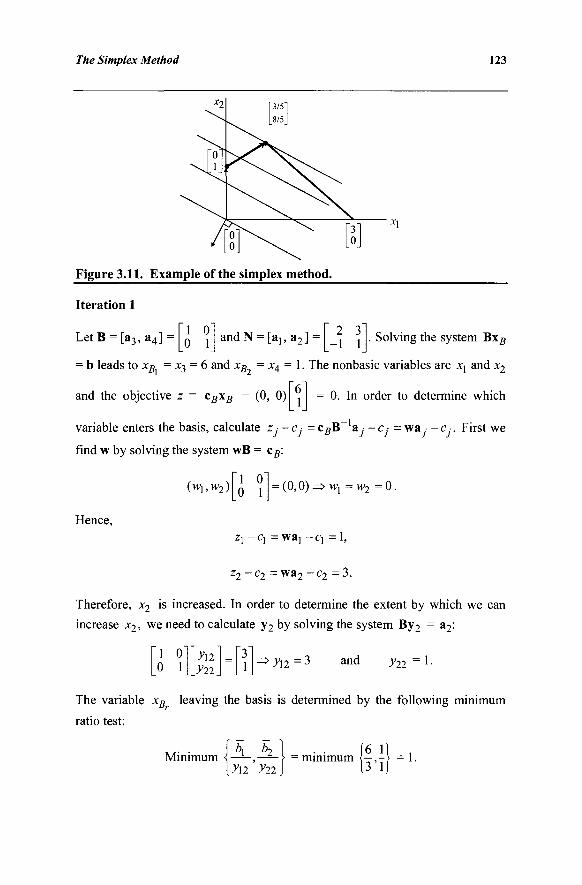
The Simplex Method 123
Figure 3.11. Example of the simplex method.
Iteration 1
LetB = [a3, a 4 ] : 1 0 0 1 and N = [a1? a2] 2 3
-1 1 . Solving the system Bxs
b leads to xB = x3 = 6 and xB = x4 = 1. The nonbasic variables are X] and x2
and the objective z = cB\B = (0, 0) 0. In order to determine which
variable enters the basis, calculate z ■ -c,- = cgB a , -c ■ = wa -c ·. First we
find w by solving the system wB = c#:
(wuw2) 1 0 0 1 = (0,0)=>Μ>! =w2 = 0 .
Hence, zx-cx = w a 1 - q =1,
z2-c2 = w a 2 - c 2 =3.
Therefore, x2 is increased. In order to determine the extent by which we can
increase x2, we need to calculate y2 by solving the system By2 = a2:
1 0 0 1
yu yn
■ yn = 3 and •V22 = !·
The variable xB leaving the basis is determined by the following minimum
ratio test:
Minimum «—*-,—— > = minimum {—,-} = 1. [yn yn] (3 ij
124 Chapter 3
Therefore, the index r = 2; that is, xB = x4 leaves the basis. This is also
obvious by noting that
xBl XB7
*3 X4
= 6 1 - 3
1 x2 (3.14)
and x4 first drops to zero when x2 = 1.
Iteration 2
The variable x2 enters the basis and x4 leaves the basis:
B = [a3,a2] 1 3 0 1 and N = [a1?a4] = 2 0
-1 1
Now, x g can be determined by solving BxB = b or simply by noting that x2
1 in Equation (3.14):
XBX XB2
The objective value is z = - 3 . Calculate w by wB = cB:
x3 x2
= 3 1 5
x\ x4 1
= 0 0
(wuw2) 1 3 0 1 ;(0,-3)=>W! =0 and w2 = -3 .
Hence,
z, - q = waj - c,
(0,-3) + 1 = 4.
The variable x4 left the basis in the previous iteration and cannot enter the basis
in this iteration (because z4-c4 < 0; see Exercise 3.35). Therefore, Xj is
increased. Solve the system Byj = a^
1 3 0 1
yu 721
2 -1 ■yu=5 and y2l = - 1 .
Since >>2i < 0, then xB = x3 leaves the basis as X! is increased. This is also
clear by noting that
x f t
Χβ, 2_
xi x7.
= 3 1 - 5
- 1
and x3 drops to zero when xl = 3/5.
The Simplex Method 125
Iteration 3
Here, xj enters the basis and x3 leaves the basis:
B = [a1;a2] 2 3 -1 1 and N = [a3,a4] 1 0
0 1
χ β , XB2
x2.
3/5' 8/5 ^N
X 3
X 4
The objective value is given by z = -27/5. Calculate w by wB = cB:
(w,,w2) 2 3 -1 1 = (-l,-3)=> wj -4/5 and w2 = -3 /5 .
The variable x3 left the basis in the last iteration and cannot enter the basis in
this iteration (because z3 - c3 < 0). Hence, we compute
z4-c4 = wa4 - c4
= (-4/5, - 3 /5 ) - 0 = - 3 / 5 .
Therefore, zj - c ,· < 0 for all nonbasic variables, and the current point is
optimal. The optimal solution is therefore given by
(x1 ;x2 ,x3 ,x4) = (3/5, 8/5, 0, 0)
with objective value -27/5. Figure 3.11 displays the simplex path, that is, the sequence of steps that the simplex method took to reach the optimal point.
3.8 THE SIMPLEX METHOD IN TABLEAU FORMAT
At each iteration, the following linear systems of equations need to be solved: BxB = b, wB = cB, and By^ = ak. Various procedures for solving and updating these systems will lead to different algorithms that all lie under the general framework of the simplex method described previously. In this section, we describe the simplex method in tableau format. In subsequent chapters we shall discuss several procedures for solving the preceding systems for general linear programs as well as for problems having special structures such as network flow problems.
Suppose that we have a starting basic feasible solution x with basis B. The linear programming problem can be represented as follows.
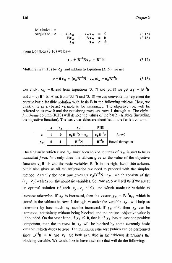
126 Chapter 3
Minimize z subject to z - cBxB - cNxN = 0
BxB + NxN = b xB, xN > 0.
(3.15) (3.16)
From Equation (3.16) we have
xB + B 'NXJV = B 'b. (3.17)
Multiplying (3.17) by cB and adding to Equation (3.15), we get
z + 0 x g + (csB"1N-cjV)xAr =CgB"'b. (3.18)
Currently, xN = 0, and from Equations (3.17) and (3.18) we get xB = B b
and z = csB~ b. Also, from (3.17) and (3.18) we can conveniently represent the current basic feasible solution with basis B in the following tableau. Here, we think of z as a (basic) variable to be minimized. The objective row will be referred to as row 0 and the remaining rows are rows 1 through m. The right-hand-side column (RHS) will denote the values of the basic variables (including the objective function). The basic variables are identified in the far left column.
z
1
0
*B
0
I
XN
C/jB-'N - Cjv
B !N
RHS
CfiB-'b
B-'b
RowO
Rows 1 through m
The tableau in which z and xB have been solved in terms of x^ is said to be in
canonical form. Not only does this tableau give us the value of the objective
function c#B~ b and the basic variables B~ b in the right-hand-side column,
but it also gives us all the information we need to proceed with the simplex
method. Actually the cost row gives us c#B~ N-cN, which consists of the
(z · —c ,·)-values for the nonbasic variables. So, row zero will tell us if we are at
an optimal solution (if each z - c. < 0), and which nonbasic variable to
increase otherwise. If xk is increased, then the vector y^ = B~ ak, which is
stored in the tableau in rows 1 through m under the variable xk, will help us
determine by how much xk can be increased. If y^ < 0, then xk can be
increased indefinitely without being blocked, and the optimal objective value is
unbounded. On the other hand, if y^ X 0, that is, if y^ has at least one positive
component, then the increase in xk will be blocked by some currently basic
variable, which drops to zero. The minimum ratio test (which can be performed
since B~ b = b and y^ are both available in the tableau) determines the
blocking variable. We would like to have a scheme that will do the following:
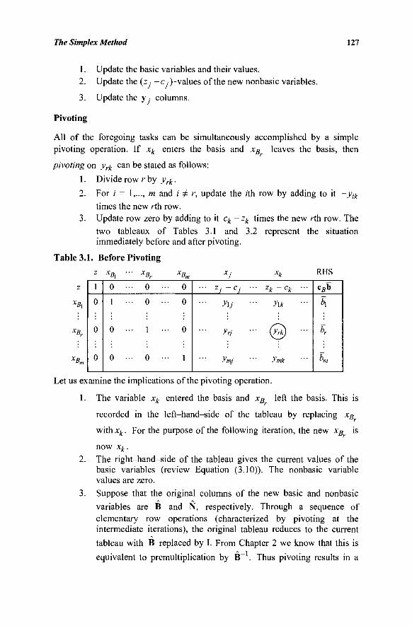
The Simplex Method 127
1. Update the basic variables and their values. 2. Update the (z -c.)-values of the new nonbasic variables.
3. Update the y.- columns.
Pivoting
All of the foregoing tasks can be simultaneously accomplished by a simple pivoting operation. If xk enters the basis and xB leaves the basis, then
pivoting on yrk can be stated as follows:
1. Divide row r by yrk.
2. For i = 1,..., m and i Φ r, update the rth row by adding to it -yik
times the new rth row. 3. Update row zero by adding to it ck -zk times the new rth row. The
two tableaux of Tables 3.1 and 3.2 represent the situation immediately before and after pivoting.
Table 3.1. Before Pivoting
z χΒχ ■■■ xBr xBm Xj xk RHS
z
xBi
XBm
Let us examine the implications of the pivoting operation.
1. The variable xk entered the basis and xB left the basis. This is
recorded in the left-hand-side of the tableau by replacing xB
with xk. For the purpose of the following iteration, the new xB is
now xk. 2. The right-hand-side of the tableau gives the current values of the
basic variables (review Equation (3.10)). The nonbasic variable values are zero.
3. Suppose that the original columns of the new basic and nonbasic variables are B and N, respectively. Through a sequence of elementary row operations (characterized by pivoting at the intermediate iterations), the original tableau reduces to the current
tableau with B replaced by I. From Chapter 2 we know that this is
equivalent to premultiplication by B~ . Thus pivoting results in a
1
0
0
0
0 ·
1
0 ·
0 ·
• 0
■ 0
• 1 ·
• 0 ·
• 0
• 0
• 0
• 1
- z i ~ c i ■
... yXj .
- yrj ■
ymj
■· zk ~ck - ·
y\k
■ @ -
ymk
cBb
\
br
K
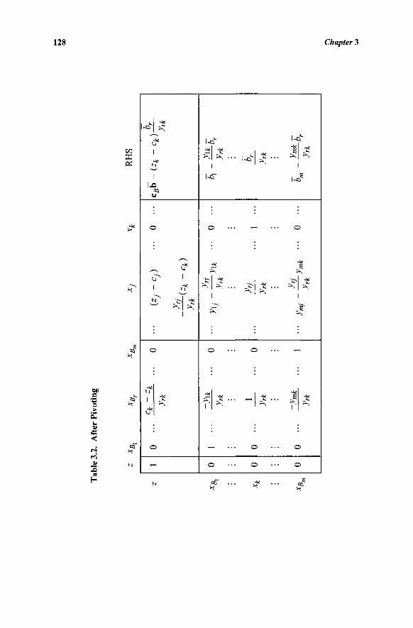
Tab
le 3
.2.
Afte
r Pi
votin
g
z χ Β
λ x B
r x B
ni
XB
,
x k
XD
1 0 0 0
0 ·
1 ·
0 ·
0 ·
c k -
zk
y rk
-y\k
y rk 1
y rk
-ymk
y rk
• 0
• 0
• 0
• 1
x k R
HS
- (z
y~
cy
) -
—(z k
~ c k)
y r
k k
yrj
IlL
yrk yr
j ■"
y m
j -
~~ym
k "
y rk
■
o ··
·
• 0
·■·
. i
...
• 0
···
c5
b-(
z/t
-c k)
rf-
y rk
bt
-—b r
y rk
Il_
yrk
b m
b r
y rk
f
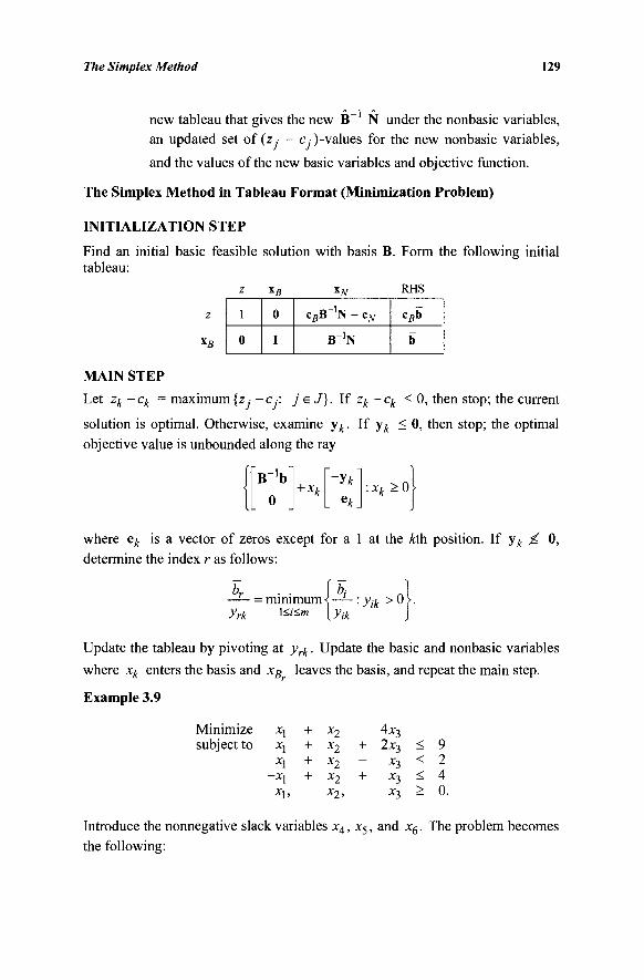
The Simplex Method 129
new tableau that gives the new B N under the nonbasic variables, an updated set of (z - c.)-values for the new nonbasic variables,
and the values of the new basic variables and objective function.
The Simplex Method in Tableau Format (Minimization Problem)
INITIALIZATION STEP
Find an initial basic feasible solution with basis B. Form the following initial tableau:
z
1
0
x s
0
I
XjV
c^B-'N - c^
B ' N
RHS
cBb
b
MAIN STEP
Let zk-ck = maximum {z,· -c, · : j eJ}. If zk -ck < 0, then stop; the current
solution is optimal. Otherwise, examine y^. If y^ < 0, then stop; the optimal objective value is unbounded along the ray
:xk>0\ B-V
0 + xk
"-y*"
ek_
where ek is a vector of zeros except for a 1 at the kth position. If y^ X 0, determine the index r as follows:
—— = minimum yrk \<i<m \iM
Update the tableau by pivoting at yrk. Update the basic and nonbasic variables
where xk enters the basis and xB leaves the basis, and repeat the main step.
Example 3.9
Minimize subject to
X,
*\ *\
~xl X],
+ + + +
Xo x2 x2 x2
x2,
- 4x3
+ 2x3
" *3 + x3
x3
< < < >
9 2 4 0.
Introduce the nonnegative slack variables x4, x5, and x6. The problem becomes the following:
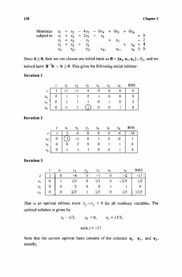
130 Chapter 3
Minimize - 4x3 + 0x4 + 0x5 + Ox6
subject to xj + x2 + 2x3 + X4
- X j
X j ,
+ x2 -+ x2 +
x2,
x3
*3 *3> X4,
*5
x5,
= 9 = 2
x6 = 4 x6 > 0.
Since b > 0, then we can choose our initial basis as B = [a4,a5,a6] = I3 , and we
indeed have B~ b = b > 0. This gives the following initial tableau:
Iteration 1
z
X4
X ,
H
z
1
0
0
0
X,
-1
1
1
-1
x2
-1
1
1
1
*3
4
2
-1
(J)
x4
0
1
0
0
*5
0
0
1
0
H 0
0
0
1
RHS
0
9
2
4
Iteration 2
z
H x5
x3
z
1
0
0
0
X,
3
© 0
-1
x2
-5
-1
2
1
*3
0
0
0
1
H 0
1
0
0
x5
0
0
1
0
x6
-A
-2
1
1
RHS
-16
1
6
4
Iteration 3
x\ x5
X3
z 1
0
0
0
xx
0
1
0
0
x2
-4
-1/3
2
2/3
*3
0
0
0
1
X4
-1
1/3
0
1/3
x5
0
0
1
0
x6
-2
-2 /3
1
1/3
RHS -17
1/3
6
13/3
This is an optimal tableau since z ■ - c, < 0 for all nonbasic variables. The
optimal solution is given by
X) = 1/3, x2 =0, x3 = 13/3,
withz = -17.
Note that the current optimal basis consists of the columns aj, a5, and a3, namely,
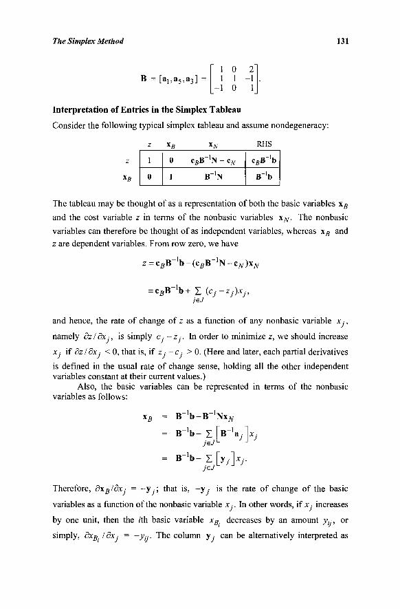
The Simplex Method 131
B = [a,,a5,a3] = 1 0 1 1
-1 0
Interpretation of Entries in the Simplex Tableau
Consider the following typical simplex tableau and assume nondegeneracy:
«fi
The tableau may be thought of as a representation of both the basic variables xB
and the cost variable z in terms of the nonbasic variables xN. The nonbasic
variables can therefore be thought of as independent variables, whereas xB and
z are dependent variables. From row zero, we have
z
1
0
*B
0
I
XN
CgB-'N - cN
B_1N
RHS
csB- 'b
B ' b
z = cBB ' b - ( c s B 1N-c i V)x N
= cgB b+ Σ (Cj-Zj)Xj,
and hence, the rate of change of z as a function of any nonbasic variable x ■ ,
namely dz/dx.-, is simply c. - z . In order to minimize z, we should increase
x · if dz/dx.- < 0, that is, if z · -c ■ > 0. (Here and later, each partial derivatives
is defined in the usual rate of change sense, holding all the other independent variables constant at their current values.)
Also, the basic variables can be represented in terms of the nonbasic variables as follows:
VB - B"1b-B~1NxA,
B ' b
B " b
" Σ [BV ■ Σ [yy]*r
Therefore, ΒχΒ/θχ,- = -y , · ; that is, -y,· is the rate of change of the basic
variables as a function of the nonbasic variable x,. In other words, if x, increases
by one unit, then the z'th basic variable xB. decreases by an amount yti, or
simply, dxB. I dx ■ = -yy. The column y · can be alternatively interpreted as
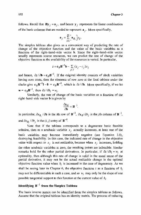
132 Chapter 3
follows. Recall that By = a , and hence y · represents the linear combination
of the basic columns that are needed to represent a . More specifically,
a7- = l[as.]yy.
The simplex tableau also gives us a convenient way of predicting the rate of change of the objective function and the value of the basic variables as a function of the right-hand-side vector b. Since the right-hand-side vector usually represents scarce resources, we can predict the rate of change of the objective function as the availability of the resources is varied. In particular,
z = c s B _ 1 b - X (Zj-Cj)Xj jeJ
and hence, dz/db = cBB~ . If the original identity consists of slack variables
having zero costs, then the elements of row zero at the final tableau under the
slacks give cBB~ 1-0 = csB~ , which is dz/db. More specifically, if we let
w= cgB~ , then dz/dty =wj·. Similarly, the rate of change of the basic variables as a function of the
right-hand-side vector b is given by
* S . = B-1. 5b
In particular, dxB. Idb is the z'th row of B~ , dxBl dbj is they'th column of B~ ,
and dxB. I dbj is the (/',_/) entry of B~ .
Note that if the tableau corresponds to a degenerate basic feasible solution, then as a nonbasic variable x ,· actually increases, at least one of the
basic variables may become immediately negative (see Equation 3.8), destroying feasibility. In this case, the indicated rate of change in the objective value with respect to x ,■ is not realizable, because when x .· increases, holding
the other nonbasic variables at zero, the resulting points are infeasible. Similar remarks hold for the other partial derivatives. In particular, if dz/dty = w,· at optimality, then although this rate of change is valid in the usual sense of the partial derivative, it may not be the actual realizable change in the optimal objective function value when bt is increased in the case of degeneracy. As we shall be seeing later in Chapter 6, the objective function z as a function of ty may not be differentiable in such a case, and so w,- may only be the slope of one possible tangential support to this function at the current value of bt.
Identifying B from the Simplex Tableau
The basis inverse matrix can be identified from the simplex tableau as follows. Assume that the original tableau has an identity matrix. The process of reducing
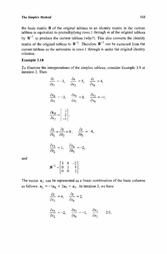
The Simplex Method 133
the basis matrix B of the original tableau to an identity matrix in the current tableau is equivalent to premultiplying rows 1 through m of the original tableau
by B~ to produce the current tableau (why?). This also converts the identity
matrix of the original tableau to B~ . Therefore B~ can be extracted from the current tableau as the submatrix in rows 1 through m under the original identity columns.
Example 3.10
To illustrate the interpretations of the simplex tableau, consider Example 3.9 at iteration 2. Then
-3, dz
dx-, = 5,
dx6
d*5 dxi
= 0, 5x3
dx6 1,
dx-j
dz _ dz dz = - 4 ,
dx5
'db,
dx4 _ 2
db3
and
B 1 0 -2 0 1 1 0 0 1
The vector a2 can be represented as a linear combination of the basic columns
as follows: a2 = - l a 4 + 2a5 + a3. At iteration 3, we have
f =<■ dx2
dx5 = _ 2 j
dx2
dz _
dx6
dx6
■2,
-1, 9x3
Sx7
= -2/3,
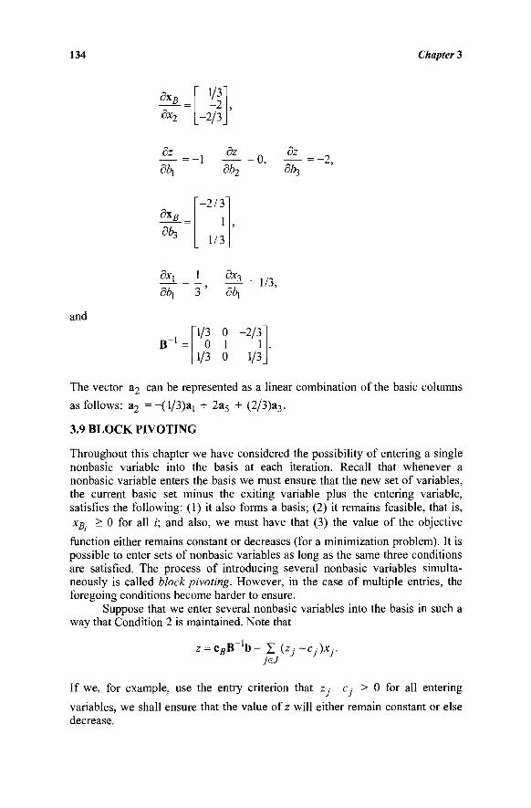
134 Chapter 3
3x2
1/3" -2
-2/3_
ÌL=-i A= 0 > A 9 ^ 9è2 9Z>j
= -2,
dxf
dbi
-2/3
1
1/3
and
5xj
<5òJ"
B
^ = 1/3, 36,
1/3 0 -2/3 0 1 1
1/3 0 1/3
The vector a2 can be represented as a linear combination of the basic columns
as follows: a2 =-(l/3)ai + 2a5 + (2/3)a3.
3.9 BLOCK PIVOTING
Throughout this chapter we have considered the possibility of entering a single nonbasic variable into the basis at each iteration. Recall that whenever a nonbasic variable enters the basis we must ensure that the new set of variables, the current basic set minus the exiting variable plus the entering variable, satisfies the following: (1) it also forms a basis; (2) it remains feasible, that is, Xg. > 0 for all i; and also, we must have that (3) the value of the objective
function either remains constant or decreases (for a minimization problem). It is possible to enter sets of nonbasic variables as long as the same three conditions are satisfied. The process of introducing several nonbasic variables simulta-neously is called block pivoting. However, in the case of multiple entries, the foregoing conditions become harder to ensure.
Suppose that we enter several nonbasic variables into the basis in such a way that Condition 2 is maintained. Note that
z = cBB ■ Z^j~Cj)Xj.
If we, for example, use the entry criterion that z · - c > 0 for all entering
variables, we shall ensure that the value of z will either remain constant or else decrease.
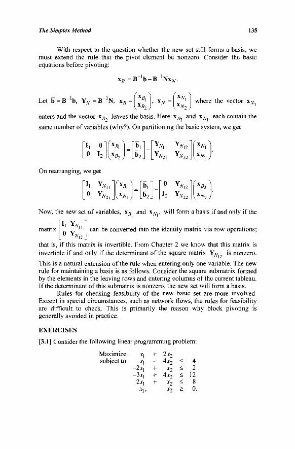
The Simplex Method 135
With respect to the question whether the new set still forms a basis, we must extend the rule that the pivot element be nonzero. Consider the basic equations before pivoting:
xg = B _ 1 b - B ' Ν Χ ^ .
Let b = B~1b, Y# =B- 1N, *B2
XjV,
*N2J
where the vector x JV,
enters and the vector xB leaves the basis. Here xB and \N each contain the
same number of variables (why?). On partitioning the basic system, we get
Il 0 0 I ,
V*B2J
lN, lNv
lN-22 XN2
On rearranging, we get
"li YJV,
0 Y; N7 \x"u b b 2
0 Y M 12
v22
XB-
VW-2 )
Now, the new set of variables, xB and \N , will form a basis if and only if the
matrix Il Υ*π
0 Y ΛΤι-
can be converted into the identity matrix via row operations;
that is, if this matrix is invertible. From Chapter 2 we know that this matrix is invertible if and only if the determinant of the square matrix Y y is nonzero.
This is a natural extension of the rule when entering only one variable. The new rule for maintaining a basis is as follows. Consider the square submatrix formed by the elements in the leaving rows and entering columns of the current tableau. If the determinant of this submatrix is nonzero, the new set will form a basis.
Rules for checking feasibility of the new basic set are more involved. Except in special circumstances, such as network flows, the rules for feasibility are difficult to check. This is primarily the reason why block pivoting is generally avoided in practice.
EXERCISES
[3.1] Consider the following linear programming problem:
Maximize subject to
x\ x\
-2xj -3xj
2xj X],
+ -+ + +
2x2 4x2
x2 4x2
x2 x2
< < < < >
4 2
12 8 0
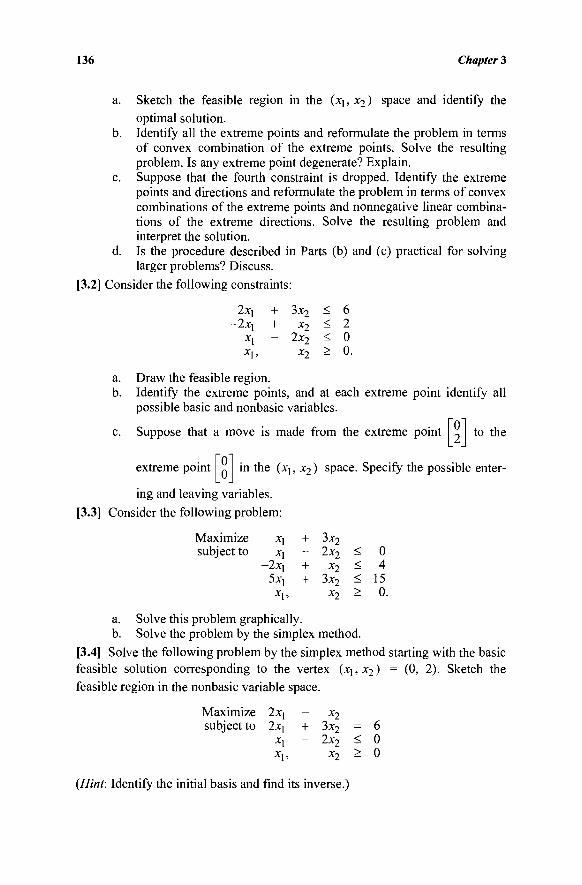
136 Chapter 3
a. Sketch the feasible region in the (X],x2) space and identify the optimal solution.
b. Identify all the extreme points and reformulate the problem in terms of convex combination of the extreme points. Solve the resulting problem. Is any extreme point degenerate? Explain.
c. Suppose that the fourth constraint is dropped. Identify the extreme points and directions and reformulate the problem in terms of convex combinations of the extreme points and nonnegative linear combina-tions of the extreme directions. Solve the resulting problem and interpret the solution.
d. Is the procedure described in Parts (b) and (c) practical for solving larger problems? Discuss.
[3.2] Consider the following constraints:
2xj 2xj
X,
Xj,
+ 3x2
+ x2 - 2x2
x2
< < < >
6 2 0 0.
a. Draw the feasible region. b. Identify the extreme points, and at each extreme point identify all
possible basic and nonbasic variables. "0"
c. Suppose that a move is made from the extreme point to the
extreme point in the (xj, x2) space. Specify the possible enter-
ing and leaving variables. [3.3] Consider the following problem:
Maximize subject to
x\ x\
-2xj 5X]
X] ,
+ 3x2 - 2x2
+ *2 + 3x2
x2
< 0 < 4 < 15 > 0.
a. Solve this problem graphically. b. Solve the problem by the simplex method.
[3.4] Solve the following problem by the simplex method starting with the basic feasible solution corresponding to the vertex (JCJ, X2) = (0, 2). Sketch the feasible region in the nonbasic variable space.
Maximize subject to
2xj 2x[
*1 X,,
" *2 + 3x2 - 2x2
*2
= 6 < 0 > 0
(Hint: Identify the initial basis and find its inverse.)
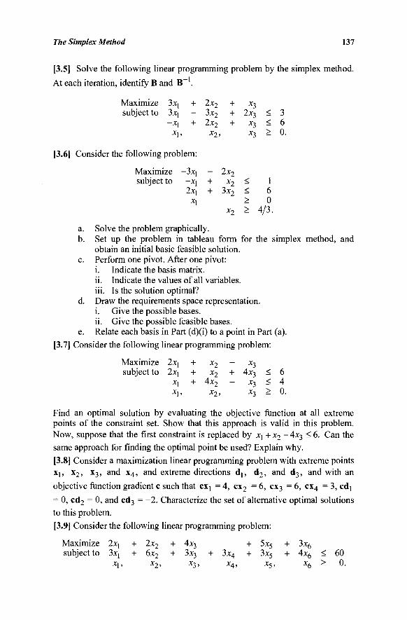
The Simplex Method 137
[3.5] Solve the following linear programming problem by the simplex method.
At each iteration, identify B and B - .
Maximize 3xj + 2x2 + x3 subject to 3xj - 3x2 + 2x3 < 3
-xj + 2x2 + x3 < 6 Xj, X 2 , Χ3 ^ 0 .
[3.6] Consider the following problem:
Maximize subject to
-3xi -x, 2xj
Xj
- 2x2 + x2 < + 3x2 <
> x2 >
1 6 0
4/3.
a. Solve the problem graphically. b. Set up the problem in tableau form for the simplex method, and
obtain an initial basic feasible solution. c. Perform one pivot. After one pivot:
i. Indicate the basis matrix. ii. Indicate the values of all variables, iii. Is the solution optimal?
d. Draw the requirements space representation, i. Give the possible bases. ii. Give the possible feasible bases.
e. Relate each basis in Part (d)(i) to a point in Part (a).
[3.7] Consider the following linear programming problem:
Maximize subject to
2x[ 2xj
x\ X[,
+ x2 + x2
+ 4x2 x2>
~ x3 + 4x3
- *3 *3
< 6 < 4 > 0,
Find an optimal solution by evaluating the objective function at all extreme points of the constraint set. Show that this approach is valid in this problem. Now, suppose that the first constraint is replaced by xj + x2 - 4x3 < 6. Can the same approach for finding the optimal point be used? Explain why. [3.8] Consider a maximization linear programming problem with extreme points Xl, x2, x3, and x4, and extreme directions dj, d2, and d3, and with an
objective function gradient c such that cxj = 4, cx2 = 6, cx3 = 6, cx4 = 3, cdj
= 0, cd2 = 0, and cd3 = -2 . Characterize the set of alternative optimal solutions
to this problem.
[3.9] Consider the following linear programming problem:
Maximize subject to
2x[ 3xj *1>
+ 2x2
+ 6x2
x2,
+ 4x3
+ 3x3
x3, + 3x4
X4,
+ 5x5 + 3x5
x5,
+ 3x6 + 4x6
*6
< >
60 0.
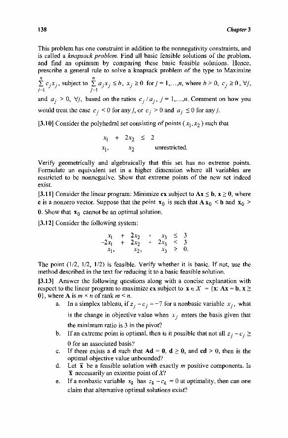
138 Chapter 3
This problem has one constraint in addition to the nonnegativity constraints, and is called a knapsack problem. Find all basic feasible solutions of the problem, and find an optimum by comparing these basic feasible solutions. Hence, prescribe a general rule to solve a knapsack problem of the type to Maximize n n
X CjXj, subject to Σ ajxj ^b, x,· > 0 for y = 1,...,n, where b > 0, c,· > 0, V/,
and a. > 0, V/, based on the ratios c.· la,, j = \,...,n. Comment on how you
would treat the case c ,· < 0 for any/, or c > 0 and a ■ < 0 for any/.
[3.10] Consider the polyhedral set consisting of points (x{,x2) such that
Χγ + 2x2 ^ 2
xj, x2 unrestricted.
Verify geometrically and algebraically that this set has no extreme points. Formulate an equivalent set in a higher dimension where all variables are restricted to be nonnegative. Show that extreme points of the new set indeed exist.
[3.11] Consider the linear program: Minimize ex subject to Ax < b, x > 0, where c is a nonzero vector. Suppose that the point x0 is such that A x0 < b and x0 >
0. Show that x0 cannot be an optimal solution.
[3.12] Consider the following system:
Xj + 2x2 + x3 < 3 -2xj + 2x2 + 2x3 < 3
xu x2, x-i > 0.
The point (1/2, 1/2, 1/2) is feasible. Verify whether it is basic. If not, use the method described in the text for reducing it to a basic feasible solution. [3.13] Answer the following questions along with a concise explanation with respect to the linear program to maximize ex subject to x e X = {x: Ax = b, x > 0}, where A is m χ η of rank m<n.
a. In a simplex tableau, if z ■ - c ,· = -7 for a nonbasic variable x ,·, what
is the change in objective value when x · enters the basis given that
the minimum ratio is 3 in the pivot? b. If an extreme point is optimal, then is it possible that not all z ,· - c,· >
0 for an associated basis? c. If there exists a d such that Ad = 0, d > 0, and cd > 0, then is the
optimal objective value unbounded? d. Let x be a feasible solution with exactly m positive components. Is
x necessarily an extreme point of XÌ e. If a nonbasic variable xk has Zjc~
ck = 0 a t optimality, then can one claim that alternative optimal solutions exist?
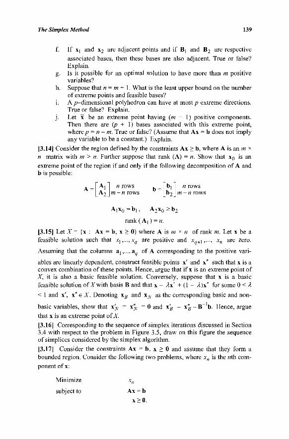
The Simplex Method 139
f. If X] and x2 are adjacent points and if Bj and B2 are respective associated bases, then these bases are also adjacent. True or false? Explain.
g. Is it possible for an optimal solution to have more than m positive variables?
h. Suppose that n = m+ 1. What is the least upper bound on the number of extreme points and feasible bases?
i. A/^-dimensional polyhedron can have at most/? extreme directions. True or false? Explain,
j . Let x be an extreme point having (m - 1) positive components. Then there are (p + 1) bases associated with this extreme point, where p = n-m. True or false? (Assume that Ax = b does not imply any variable to be a constant.) Explain.
[3.14] Consider the region defined by the constraints Ax > b, where A is an m x
n matrix with m > n. Further suppose that rank (A) = n. Show that x0 is an extreme point of the region if and only if the following decomposition of A and b is possible:
Ai n rows . _ m-n rows ~~ b2
n rows m-n rows
A 1 x 0 =b 1 , A 2 x 0 > b 2
rank ( Aj ) = n.
[3.15] Let X = {x : Ax = b, x > 0) where A is m χ n of rank m. Let x be a feasible solution such that χ^,.,.,χ are positive and x +1,..., xn are zero.
Assuming that the columns a[,...,a of A corresponding to the positive vari-ables are linearly dependent, construct feasible points x' and x" such that x is a convex combination of these points. Hence, argue that if x is an extreme point of X, it is also a basic feasible solution. Conversely, suppose that x is a basic feasible solution of X with basis B and that x = λχ' + (1 - λ)χ" for some 0 < λ < 1 and x', x" E X. Denoting xg and xN as the corresponding basic and non-basic variables, show that x'N = x"N = 0 and x'B = x"B = B~ b. Hence, argue that x is an extreme point of X.
[3.16] Corresponding to the sequence of simplex iterations discussed in Section 3.4 with respect to the problem in Figure 3.5, draw on this figure the sequence of simplices considered by the simplex algorithm.
[3.17] Consider the constraints Ax = b, x > 0 and assume that they form a bounded region. Consider the following two problems, where xn is the «th com-ponent of x:
Minimize
subject to
xn
Ax = b x>0 .
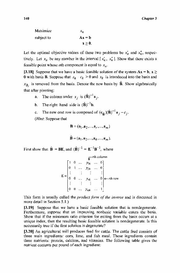
140 Chapter 3
Maximize subject to
xn
Ax = b x>0
Let the optimal objective values of these two problems be x'„ and x"n, respec-
tively. Let xn be any number in the interval [ x'n , x"n]. Show that there exists a
feasible point whose «th component is equal to xn.
[3.18] Suppose that we have a basic feasible solution of the system Ax = b, x > 0 with basis B. Suppose that zk - ck > 0 and xk is introduced into the basis and
xB is removed from the basis. Denote the new basis by B. Show algebraically
that after pivoting:
a. The column under x- is (B)~ a-.
b. The right-hand-side is (B)~ b.
c. The new cost row is composed of (c^ )(B)~ a · - c .·.
(Hint: Suppose that
B = (a1,a2,...,ar,...,am)
B = (a1,a2,...,aA,...,aOT).
First show that B = BE, and (B) l = E ' β \ where
E =
1 0 0 1
r-rth column
y\k - o y2k ... 0
0 0 ... yrk ... 0
0 0 ymk
■ rth row
This form is usually called the product form of the inverse and is discussed in more detail in Section 5.1.) [3.19] Suppose that we have a basic feasible solution that is nondegenerate. Furthermore, suppose that an improving nonbasic variable enters the basis. Show that if the minimum ratio criterion for exiting from the basis occurs at a unique index, then the resulting basic feasible solution is nondegenerate. Is this necessarily true if the first solution is degenerate?
[3.20] An agricultural mill produces feed for cattle. The cattle feed consists of three main ingredients: corn, lime, and fish meal. These ingredients contain three nutrients: protein, calcium, and vitamins. The following table gives the nutrient contents per pound of each ingredient:
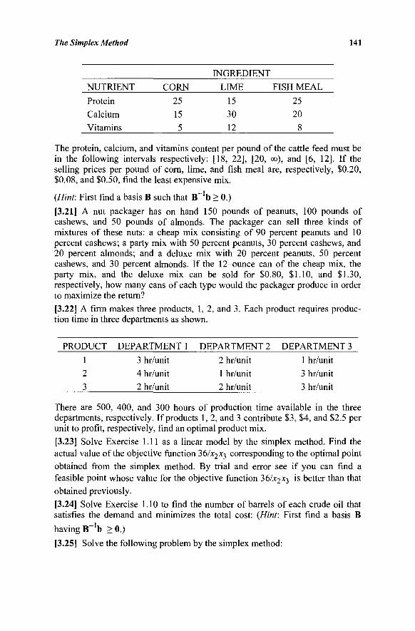
The Simplex Method 141
INGREDIENT
NUTRIENT
Protein Calcium
Vitamins
CORN
25
15
5
LIME
15
30 12
FISH MEAL
25 20
8
The protein, calcium, and vitamins content per pound of the cattle feed must be in the following intervals respectively: [18, 22], [20, oo), and [6, 12]. If the selling prices per pound of corn, lime, and fish meal are, respectively, $0.20, $0.08, and $0.50, find the least expensive mix.
(Hint: First find a basis B such that B_1b > 0.)
[3.21] A nut packager has on hand 150 pounds of peanuts, 100 pounds of cashews, and 50 pounds of almonds. The packager can sell three kinds of mixtures of these nuts: a cheap mix consisting of 90 percent peanuts and 10 percent cashews; a party mix with 50 percent peanuts, 30 percent cashews, and 20 percent almonds; and a deluxe mix with 20 percent peanuts, 50 percent cashews, and 30 percent almonds. If the 12-ounce can of the cheap mix, the party mix, and the deluxe mix can be sold for $0.80, $1.10, and $1.30, respectively, how many cans of each type would the packager produce in order to maximize the return?
[3.22] A firm makes three products, 1, 2, and 3. Each product requires produc-tion time in three departments as shown.
PRODUCT
1 2
3
DEPARTMENT 1
3 hr/unit
4 hr/unit 2 hr/unit
DEPARTMENT 2
2 hr/unit 1 hr/unit
2 hr/unit
DEPARTMENT 3
1 hr/unit 3 hr/unit
3 hr/unit
There are 500, 400, and 300 hours of production time available in the three departments, respectively. If products 1, 2, and 3 contribute $3, $4, and $2.5 per unit to profit, respectively, find an optimal product mix.
[3.23] Solve Exercise 1.11 as a linear model by the simplex method. Find the actual value of the objective function 36/x2x^ corresponding to the optimal point obtained from the simplex method. By trial and error see if you can find a feasible point whose value for the objective function 36/x2*3 is better than that obtained previously.
[3.24] Solve Exercise 1.10 to find the number of barrels of each crude oil that satisfies the demand and minimizes the total cost: (Hint: First find a basis B
having B^b >0.)
[3.25] Solve the following problem by the simplex method:
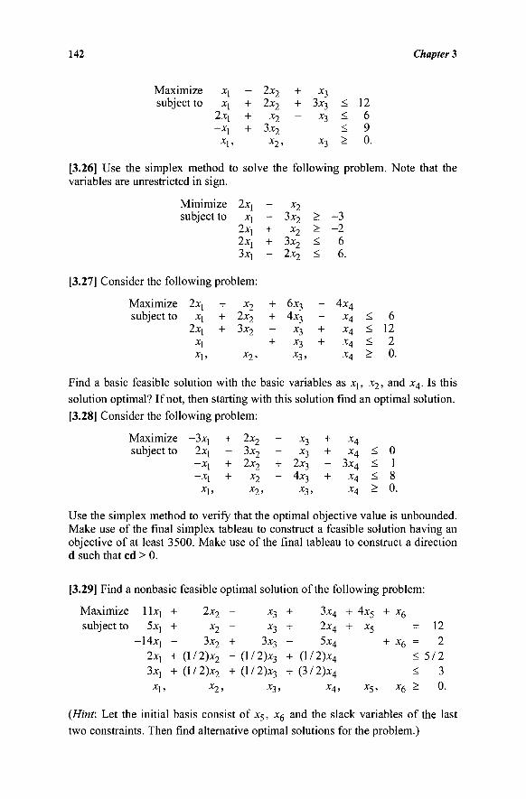
142 Chapter 3
Maximize subject to
X, x\
2x| -x,
Xj ,
- 2x2
+ 2x2 + x2
+ 3x2 x2,
+ + -
x3
3x3 x3
x3
< < < >
12 6 9 0.
[3.26] Use the simplex method to solve the following problem. Note that the variables are unrestricted in sign.
Minimize 2xj subject to xj
2x] 2xj 3x]
der the following problem:
Maximize 2x{ + x2
subject to xi + 2x2 2xj + 3x2
X,
X j , X 2 ,
--+ + —
+ + -+
x2 3x2
x2 3x2 2x2
6x3
4x3 x3 x3 x3>
> > < <
--+ +
-3 -2
6 6.
4x4
X4
X4
X4
X4
< < < >
6 12 2 0.
Find a basic feasible solution with the basic variables as xj, x2, and x4. Is this solution optimal? If not, then starting with this solution find an optimal solution. [3.28] Consider the following problem:
Maximize subject to
-3xj 2xj - X ,
-xx
xu
+ 2x2 - 3x2
+ 2x2 + x2
Λ 2 .
- x3
- x3 + 2x3 - 4x3
x3,
+ + -+
X4
X4
3x4 X4
X4
< < < >
0 1 8 0.
Use the simplex method to verify that the optimal objective value is unbounded. Make use of the final simplex tableau to construct a feasible solution having an objective of at least 3500. Make use of the final tableau to construct a direction d such that cd > 0.
[3.29] Find a nonbasic feasible optimal solution of the following problem:
Maximize llxj + 2x2 - x3
subject to 5xj + x2 - x3
-14xj - 3x2 + 3x3
2x, + (l/2)x2 - (l/2)x3
3x! + (l/2)x2 + (l/2)x3
Xj , X2 , X3 ,
(Hint: Let the initial basis consist of x5, x6 and the slack variables of the last two constraints. Then find alternative optimal solutions for the problem.)
+ 3x4
+ 2x4
— 3X4
+ (l/2)x4
+ (3/2)x4
X4,
+ +
4x5
*5
x5,
+ x6
= 12 + x6 = 2
< 5/2 < 3
x6 > 0.
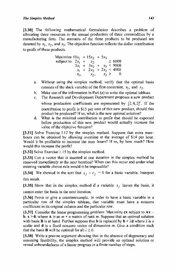
The Simplex Method 143
[3.30] The following mathematical formulation describes a problem of allocating three resources to the annual production of three commodities by a manufacturing firm. The amounts of the three products to be produced are denoted by xj, x2, and x3. The objective function reflects the dollar contribution to profit of these products.
Maximize lOxj + 15x2 + 5x3 subject to 2xj + x2 - 6000
3*! + 3x2 + x3 < 9000 X! + 2x2 + 2x3 < 4000 Xj, x 2 , x 3 ^ 0.
a. Without using the simplex method, verify that the optimal basis consists of the slack variable of the first constraint, x1; and x2.
b. Make use of the information in Part (a) to write the optimal tableau. c. The Research and Development Department proposes a new product
whose production coefficients are represented by [2,4,2]'. If the contribution to profit is $15 per unit of this new product, should this product be produced? If so, what is the new optimal solution?
d. What is the minimal contribution to profit that should be expected before production of this new product would actually increase the value of the objective function?
[3.31] Solve Exercise 1.12 by the simplex method. Suppose that extra man-hours can be obtained by allowing overtime at the average of $14 per hour. Would it be profitable to increase the man-hours? If so, by how much? How would this increase the profit?
[3.32] Solve Exercise 1.15 by the simplex method. [3.33] Can a vector that is inserted at one iteration in the simplex method be removed immediately at the next iteration? When can this occur and under what entering variable choice rule would it be impossible?
[3.34] We showed in the text that z.· - c,- = 0 for a basic variable. Interpret
this result.
[3.35] Show that in the simplex method if a variable x · leaves the basis, it
cannot enter the basis in the next iteration. [3.36] Prove or give a counterexample. In order to have a basic variable in a particular row of the simplex tableau, that variable must have a nonzero coefficient in its original column and the particular row.
[3.37] Consider the linear programming problem: Maximize ex subject to Ax = b, x > 0, where A is an m χ η matrix of rank m. Suppose that an optimal solution with basis B is at hand. Further suppose that b is replaced by b + Ad where A is a scalar and d is a fixed nonzero vector of dimension m. Give a condition such that the basis B will be optimal for all λ > 0. [3.38] Write a precise argument showing that in the absence of degeneracy and assuming feasibility, the simplex method will provide an optimal solution or reveal unboundedness of a linear program in a finite number of steps.
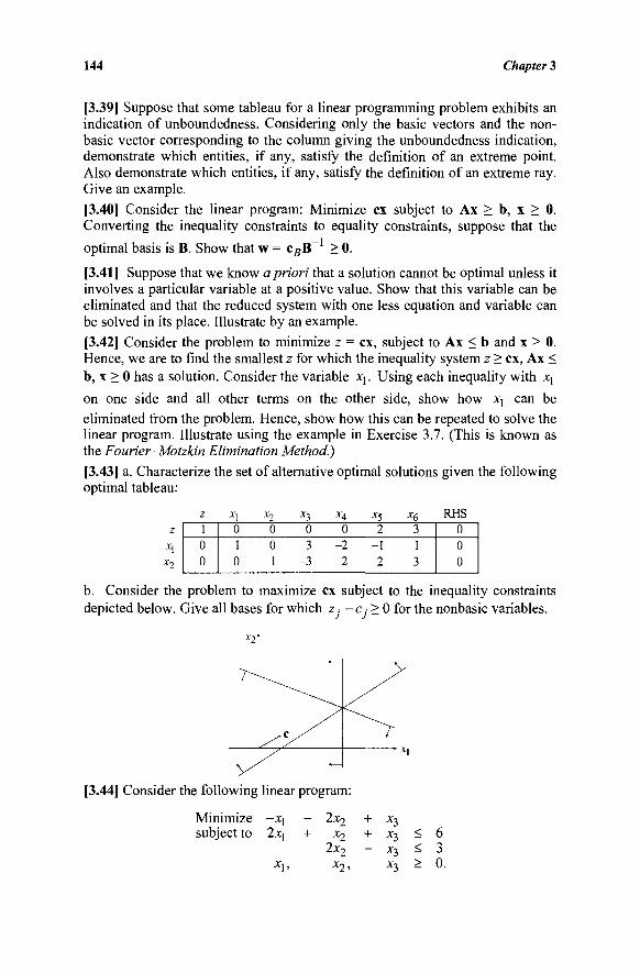
144 Chapter 3
[3.39] Suppose that some tableau for a linear programming problem exhibits an indication of unboundedness. Considering only the basic vectors and the non-basic vector corresponding to the column giving the unboundedness indication, demonstrate which entities, if any, satisfy the definition of an extreme point. Also demonstrate which entities, if any, satisfy the definition of an extreme ray. Give an example.
[3.40] Consider the linear program: Minimize ex subject to Ax > b, x > 0. Converting the inequality constraints to equality constraints, suppose that the
optimal basis is B. Show that w = c#B~ > 0.
[3.41] Suppose that we know a priori that a solution cannot be optimal unless it involves a particular variable at a positive value. Show that this variable can be eliminated and that the reduced system with one less equation and variable can be solved in its place. Illustrate by an example.
[3.42] Consider the problem to minimize z = ex, subject to Ax < b and x > 0. Hence, we are to find the smallest z for which the inequality system z > ex, Ax < b, x > 0 has a solution. Consider the variable χγ. Using each inequality with χλ
on one side and all other terms on the other side, show how xj can be
eliminated from the problem. Hence, show how this can be repeated to solve the linear program. Illustrate using the example in Exercise 3.7. (This is known as the Fourier-Motzkin Elimination Method?) [3.43] a. Characterize the set of alternative optimal solutions given the following optimal tableau:
Z Λ"| X2 X3 X4 Χς X(. RHS
1 0 0
0 0 0 0 2 3 1 0 3 - 2 - 1 1 0 1 - 3 2 2 3
0 0 0
b. Consider the problem to maximize ex subject to the inequality constraints depicted below. Give all bases for which z · -c,· > 0 for the nonbasic variables.
[3.44] Consider the following linear program:
Minimize -x\ - 2x2 + ^3 subject to 2x] + x2 + *3 - 6
2x2 - X3 < 3 X], x2, X3 ^ 0.
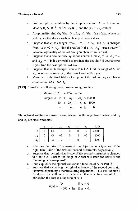
The Simplex Method 145
a. Find an optimal solution by the simplex method. At each iteration
identify B, N, B"1, B-1N, C B B ~ \ and the (zj - Cy)-values.
b. At optimality, find dxi /dx3, dx2 /Sx4, dz/dx5, dxB /dxN, where x4
and x5 are the slack variables. Interpret these values.
c. Suppose that q is changed from -1 to —1 + Aj, and c2 is changed
from -2 to -2 + Δ2. Find the region in the (Aj, Δ2) space that will
maintain optimality of the solution you obtained in Part (a).
d. Suppose that a new activity x6 is considered. Here c6 = -4 , a16 = 2,
and α26 = 4· Is it worthwhile to produce the activity? If your answer
is yes, find the new optimal solution. e. Suppose that i\ is changed from 6 to 6 + Δ. Find the range of Δ that
will maintain optimality of the basis found in Part (a). f. Make use of the final tableau to represent the column a3 as a linear
combination of aj and a2.
[3.45] Consider the following linear programming problem:
Maximize 2xj + 12x2 + 7x3
subject to xj + 3x2 + 2x3 < 10000
2xx + 2x2 + x3 < 4000
Xj, x 2 , x 3 > 0.
The optimal solution is shown below, where z is the objective function and x4
and x5 are slack variables:
a.
b.
c. d.
z
x4
x3
z
1
0
0
X,
12
-3
2
xl 2
-1
2
x3 0
0
1
X4
0
1
0
x5
7
-2
1
RHS
28000
2000
4000
What are the rates of increase of the objective as a function of the right-hand-side of the first and second constraints, respectively? Suppose that the right-hand-side of the second constraint is changed to 4000 + Δ. What is the range of A that will keep the basis of the foregoing tableau optimal? Find explicitly the optimal value z as a function of Δ for Part (b). Suppose that increasing the right-hand-side of the second constraint involved expanding a manufacturing department. This will involve a fixed cost as well as a variable cost that is a function of Δ. In particular, the cost as a function of Δ is
Α(Δ) io if A = 0
[4000 + 2Δ if Δ > 0.
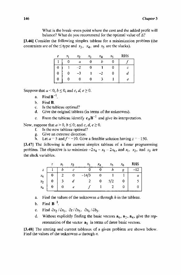
146 Chapter 3
What is the break-even point where the cost and the added profit will balance? What do you recommend for the optimal value of Δ?
[3.46] Consider the following simplex tableau for a minimization problem (the constraints are of the < type and x3, x4, and x5 are the slacks).
z
1
0
0
0
x\ 0
1
0
0
x2
a
-2
-3
0
x3
0
0
1
0
X4
b
1
-2
3
x5
0
0
0
1
RHS
/ c
d
e
Suppose that a < 0, b < 0, and c,d,e> 0.
a. FindB-1. b. Find B. c. Is the tableau optimal? d. Give the original tableau (in terms of the unknowns).
e. From the tableau identify cBB~ and give its interpretation.
Now, suppose that a > 0, b < 0; and c,d,e> 0. f. Is the new tableau optimal? g. Give an extreme direction. h. Let a = 5 and/= -10. Give a feasible solution having z = -150.
[3.47] The following is the current simplex tableau of a linear programming problem. The objective is to minimize -2x4 -x$- 2x6, and xj, x2, and x3 are the slack variables.
z
1
0
0
0
x\ b
2
3
0
x2
c
0
d
e
x3
0
-14/3
2
/
H 0
0
0
1
*5
h
1
5/2
2
x6
g 1
0
0
RHS
-12
a
5
0
z x6
x2
X4
a. Find the values of the unknowns a through h in the tableau.
b. Find B"1.
c. Find5x2/9xi, dz/dx5, dx^ldb^.
d. Without explicitly finding the basic vectors a6, a2, a4, give the rep-
resentation of the vector a5 in terms of these basic vectors.
[3.48] The starting and current tableaux of a given problem are shown below. Find the values of the unknowns a through n.
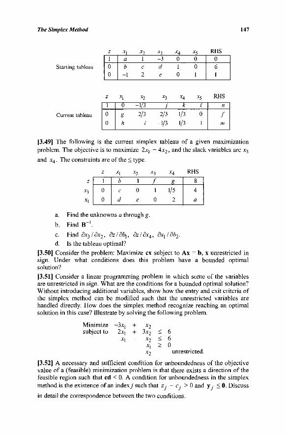
The Simplex Method 147
Starting tableau
Current tableau
z 1 0 0
z
1
0
0
x\ a b -1
x\ 0
8 h
x2
1 c 2
x2
-1/3
2/3
i
x3
-3 d e
x3
j 2/3
-1/3
x4
0 1 0
x4
k
1/3
1/3
x5 0 0 1
x5
£
0
1
RHS 0 6 1
RHS
n
f m
[3.49] The following is the current simplex tableau of a given maximization problem. The objective is to maximize 2*] - 4x2, and the slack variables are *3
and *4. The constraints are of the < type.
z
x3
x\
z 1
0
0
X,
b
c
d
x2
1
0
e
x3
f 1
0
X4
8
1/5
2
KHS 8
4
a
a. Find the unknowns a through g.
b. Find B~'.
c. Find 3*3/3*2, dz/dbi, dz/dx4, dxyldbz-d. Is the tableau optimal?
[3.50] Consider the problem: Maximize ex subject to Ax = b, x unrestricted in sign. Under what conditions does this problem have a bounded optimal solution?
[3.51] Consider a linear programming problem in which some of the variables are unrestricted in sign. What are the conditions for a bounded optimal solution? Without introducing additional variables, show how the entry and exit criteria of the simplex method can be modified such that the unrestricted variables are handled directly. How does the simplex method recognize reaching an optimal solution in this case? Illustrate by solving the following problem.
Minimize subject to
-3*i 2*i
*i
+ *2 + 3*2 - * 2
*i
* 2
< 6 < 6 > 0
unrestricted
[3.52] A necessary and sufficient condition for unboundedness of the objective value of a (feasible) minimization problem is that there exists a direction of the feasible region such that cd < 0. A condition for unboundedness in the simplex method is the existence of an index_/' such that z - c ,· > 0 and y, < 0. Discuss
in detail the correspondence between the two conditions.
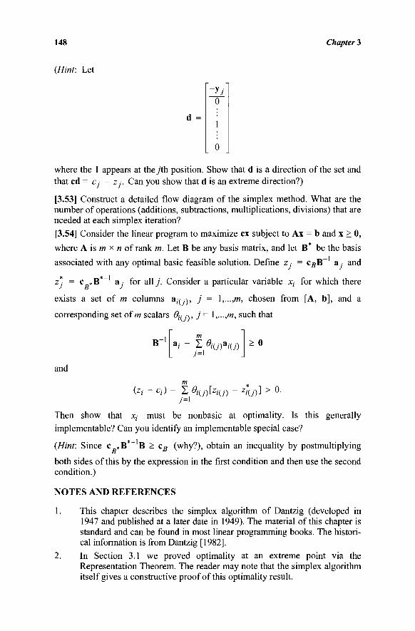
148 Chapter 3
{Hint: Let
d =
0
where the 1 appears at they'th position. Show that d is a direction of the set and that cd = Cj - zj. Can you show that d is an extreme direction?)
[3.53] Construct a detailed flow diagram of the simplex method. What are the number of operations (additions, subtractions, multiplications, divisions) that are needed at each simplex iteration?
[3.54] Consider the linear program to maximize ex subject to Ax = b and x > 0,
where A is m χ n of rank m. Let B be any basis matrix, and let B* be the basis
associated with any optimal basic feasible solution. Define Zj = c5B~ &j and
Z: = c „B a for ally. Consider a particular variable x, for which there
exists a set of m columns a,-(/), j = l,...,m, chosen from [A, b], and a
corresponding set of m scalars % , ) , j = \,...,m, such that
B~ m Σ ei<j)*i<j)
7=1 > o
and
(z,· -ct)- Σ OiU)[zi(j) - zi(y)] > °-7=1
Then show that x must be nonbasic at optimality. Is this generally implementable? Can you identify an implementable special case?
*—1
{Hint: Since c «B B > c^ (why?), obtain an inequality by postmultiplying both sides of this by the expression in the first condition and then use the second condition.)
NOTES AND REFERENCES
1. This chapter describes the simplex algorithm of Dantzig (developed in 1947 and published at a later date in 1949). The material of this chapter is standard and can be found in most linear programming books. The histori-cal information is from Dantzig [1982].
2. In Section 3.1 we proved optimality at an extreme point via the Representation Theorem. The reader may note that the simplex algorithm itself gives a constructive proof of this optimality result.
The Simplex Method 149
3. The material on block pivoting is from Tucker [1960b]. For further read-ing on block pivoting, see Dantzig [1963a], Lasdon [1970], and Cooper and Kennington [1979]. For a discussion on some nonadjacent extreme point methods for linear programs, see Sherali, Soyster, and Baines [1983], Sherali and Baines [1984], Murty and Fathi [1984], Murty [1986], and Sethi and Thompson [1984]. A host of nonlinear program-ming approaches to linear programming problems have been inspired by Khachian's [1979] and Karmarkar's [1984a, b] polynomial-time algo-rithms for linear programs (see Chapter 8).
4. Exercise 3.54 relates to Cheng's [1980] theoretical work (see also Brosius [1981]) on a priori recognizing basic or nonbasic variables at optimality.

This page intentionally left blank
FOUR: STARTING SOLUTION AND CONVERGENCE
In the previous chapter, we developed the simplex method with the assumption that an initial basic feasible solution is at hand. In many cases, such a solution is not readily available, and some work may be needed to get the simplex method started. In this chapter, we describe two procedures (the two-phase method and the big-Af method), both involving artificial variables, to obtain an initial basic feasible solution to a slightly modified set of constraints. The simplex method is used to eliminate the artificial variables and to then solve the original problem. We also discuss in more detail the difficulties associated with degeneracy. In particular we show that the simplex method converges in a finite number of steps, even in the presence of degeneracy, provided that a special rule for entering and/or exiting from the basis is adopted.
4.1 THE INITIAL BASIC FEASIBLE SOLUTION
Recall that the simplex method starts with a basic feasible solution and moves to an improved basic feasible solution, until the optimal point is reached or unboundedness of the objective function is verified. However, in order to
initialize the simplex method, a basis B with b = B b > 0 must be available. We shall show that the simplex method can always be initiated with a very simple basis, namely, the identity.
Easy Case
Suppose that the constraints are of the form Ax < b, x > 0 where A is an m χ η matrix and b is a nonnegative w-vector. By adding the slack vector xs, the
constraints can be put in the following standard form: Ax + xs = b, x > 0, xs > 0. Note that the new m x (m + n) constraint matrix (A, I) has rank m, and a basic feasible solution of this system is at hand, by letting x^ be the basic vector, and x be the nonbasic vector. Hence, at this starting basic feasible solution, we have xs = b and x = 0, and now the simplex method can be applied.
Some Bad Cases
In many situations, finding a starting basic feasible solution is not as straight-forward as the case just described. To illustrate, suppose that the constraints are of the form Ax < b, x > 0, but the vector b is not nonnegative. In this case, after introducing the slack vector xs, we cannot let x = 0, because xs = b violates the
nonnegativity requirement. Another situation occurs when the constraints are of the form Ax > b, x >
0, where b X 0. After subtracting the slack vector xs, we get Ax - xs= b, x >
151
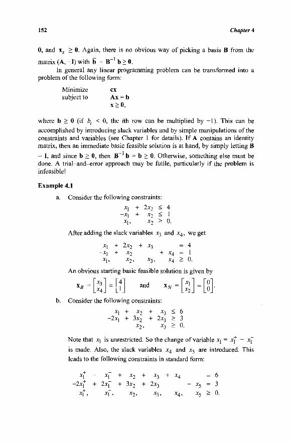
152 Chapter 4
0, and xs > 0. Again, there is no obvious way of picking a basis B from the
matrix (A, -I) with b = B"1 b > 0. In general any linear programming problem can be transformed into a
problem of the following form:
Minimize ex subject to Ax = b
x > 0 ,
where b > 0 (if ty < 0, the rth row can be multiplied by -1). This can be
accomplished by introducing slack variables and by simple manipulations of the constraints and variables (see Chapter 1 for details). If A contains an identity matrix, then an immediate basic feasible solution is at hand, by simply letting B
= I, and since b > 0, then B~ b = b > 0. Otherwise, something else must be done. A trial-and-error approach may be futile, particularly if the problem is infeasible!
Example 4.1
a. Consider the following constraints:
xj + 2x2 < 4 -X[ + x2 - 1
xu x2 > 0.
After adding the slack variables x3 and x4, we get
Xl + 2x2 + X3 = 4 —Xj + X2 + ΧΛ
= 1 X\ , X2 5 X3 5 XA — t).
An obvious starting basic feasible solution is given by
and xN
b. Consider the following constraints:
*3 X4
x, x2.
Xj + X2
-2xj + 3x2
x2,
+ ^3 + 2x3
x3
< > >
6 3 0.
Note that xj is unrestricted. So the change of variable Xj — Xj Xj
is made. Also, the slack variables x4 and x5 are introduced. This
leads to the following constraints in standard form:
Xi — Xi
-2x]+ + 2xf X[ , Xj ,
+ X2 + X3 + X4
+ 3x2 + 2x3
X2, Χ3, Χ4,
= 6 - x5 = 3
x5 > 0.
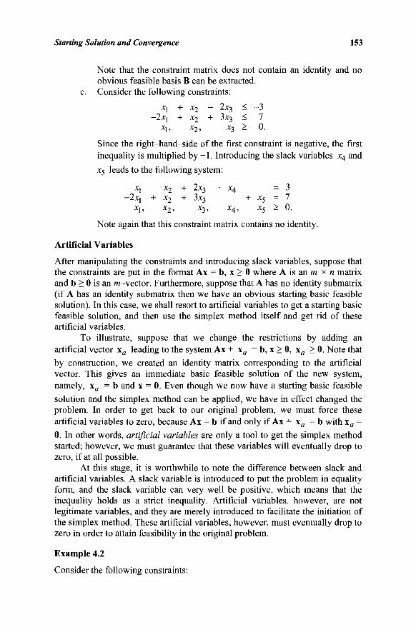
Starting Solution and Convergence 153
Note that the constraint matrix does not contain an identity and no obvious feasible basis B can be extracted,
c. Consider the following constraints: xl + x2 ~ 2*3 ^ -3
-2x\ + x2 + 3x3 < 7 X] , Χ'χ, X% — 0 .
Since the right-hand-side of the first constraint is negative, the first inequality is multiplied by - 1 . Introducing the slack variables x4 and
x5 leads to the following system:
~X\ — X2 + 2x3 — χ^ = 3 -2x] + x2 + 3x3 + x5 = 7
X] , X2, X3, X4 ? X5 — t)·
Note again that this constraint matrix contains no identity.
Artificial Variables
After manipulating the constraints and introducing slack variables, suppose that the constraints are put in the format Ax = b, x > 0 where A is an m x n matrix and b > 0 is an w-vector. Furthermore, suppose that A has no identity submatrix (if A has an identity submatrix then we have an obvious starting basic feasible solution). In this case, we shall resort to artificial variables to get a starting basic feasible solution, and then use the simplex method itself and get rid of these artificial variables.
To illustrate, suppose that we change the restrictions by adding an artificial vector xa leading to the system Ax + xa = b, x > 0, xa > 0. Note that
by construction, we created an identity matrix corresponding to the artificial vector. This gives an immediate basic feasible solution of the new system, namely, xa = b and x = 0. Even though we now have a starting basic feasible
solution and the simplex method can be applied, we have in effect changed the problem. In order to get back to our original problem, we must force these artificial variables to zero, because Ax = b if and only if Ax + xa = b with xa =
0. In other words, artificial variables are only a tool to get the simplex method started; however, we must guarantee that these variables will eventually drop to zero, if at all possible.
At this stage, it is worthwhile to note the difference between slack and artificial variables. A slack variable is introduced to put the problem in equality form, and the slack variable can very well be positive, which means that the inequality holds as a strict inequality. Artificial variables, however, are not legitimate variables, and they are merely introduced to facilitate the initiation of the simplex method. These artificial variables, however, must eventually drop to zero in order to attain feasibility in the original problem.
Example 4.2
Consider the following constraints:
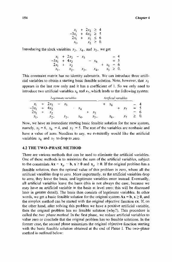
154 Chapter 4
- 3 x j 2x|
Xj,
ick variables x3,
X\ + 2x 2 --3*1 + 4 x 2
2xj + X2
Xj, X2 >
+ 2x2 + 4x2 + X2
x2
x4, and
" *3
x3,
> 4 > 5 < 6 > 0.
x5, we get
= 4 X4 = 5
+ x5 = 6 x4, x5 > 0.
This constraint matrix has no identity submatrix. We can introduce three artifi-cial variables to obtain a starting basic feasible solution. Note, however, that x5
appears in the last row only and it has a coefficient of 1. So we only need to introduce two artificial variables x6 and x7, which leads to the following system:
Legitimate variables Artificial variables
xx
■3xj 2xj
+ 2x2 + 4x2 + X2
x2
X3 + x6 = 4 X4 + Xj — 5
+ x5 = 6 X3, X4, X5, Χβ, Χη ^ 0.
Now, we have an immediate starting basic feasible solution for the new system, namely, x5 = 6, x6 = 4, and x7 = 5. The rest of the variables are nonbasic and have a value of zero. Needless to say, we eventually would like the artificial variables x6 and x7 to drop to zero.
4.2 THE TWO-PHASE METHOD
There are various methods that can be used to eliminate the artificial variables. One of these methods is to minimize the sum of the artificial variables, subject to the constraints Ax + xa = b, x > 0 and xa > 0. If the original problem has a
feasible solution, then the optimal value of this problem is zero, where all the artificial variables drop to zero. More importantly, as the artificial variables drop to zero, they leave the basis, and legitimate variables enter instead. Eventually, all artificial variables leave the basis (this is not always the case, because we may have an artificial variable in the basis at level zero; this will be discussed later in greater detail). The basis then consists of legitimate variables. In other words, we get a basic feasible solution for the original system Ax = b, x > 0, and the simplex method can be started with the original objective function ex. If, on the other hand, after solving this problem we have a positive artificial variable, then the original problem has no feasible solution (why?). This procedure is called the two-phase method. In the first phase, we reduce artificial variables to value zero or conclude that the original problem has no feasible solutions. In the former case, the second phase minimizes the original objective function starting with the basic feasible solution obtained at the end of Phase I. The two-phase method is outlined below:
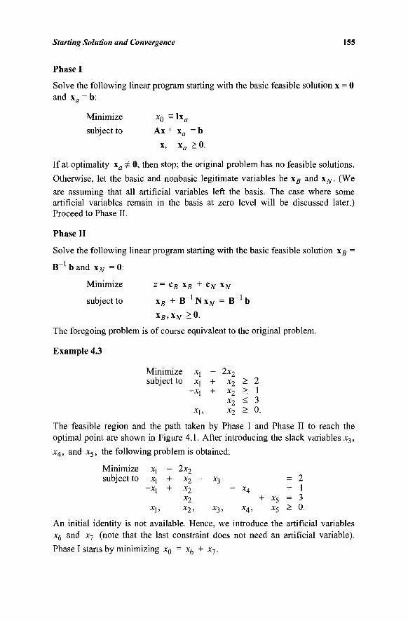
Starting Solution and Convergence 155
Phase I
Solve the following linear program starting with the basic feasible solution x = 0 and \a= b:
Minimize x0 = i\a
subject to Ax + \a = b
x, x a > 0 .
If at optimality χα Φ 0, then stop; the original problem has no feasible solutions.
Otherwise, let the basic and nonbasic legitimate variables be \B and xN. (We
are assuming that all artificial variables left the basis. The case where some artificial variables remain in the basis at zero level will be discussed later.) Proceed to Phase II.
Phase II
Solve the following linear program starting with the basic feasible solution \B =
B"1 b and xN = 0:
Minimize z= cB xB + cN \N
subject to x g + B~ NXJV = B~ b
XB,XJV >0.
The foregoing problem is of course equivalent to the original problem.
Example 4.3
Minimize xj - 2x2
subject to *i + *2 - 2 -Xj + x 2 > 1
x2 < 3 Xj , * 2 - 0·
The feasible region and the path taken by Phase I and Phase II to reach the optimal point are shown in Figure 4.1. After introducing the slack variables x3,
x4, and x5, the following problem is obtained:
Minimize Xj - 2x2 subject to xj + x2 - X3 = 2
—Xj + X2 — X4 — 1 X2 + X5 = 3
Xj, X2, X3, X4, Χ5 ^ 0.
An initial identity is not available. Hence, we introduce the artificial variables x6 and x7 (note that the last constraint does not need an artificial variable).
Phase I starts by minimizing x0 = x6 + x7.
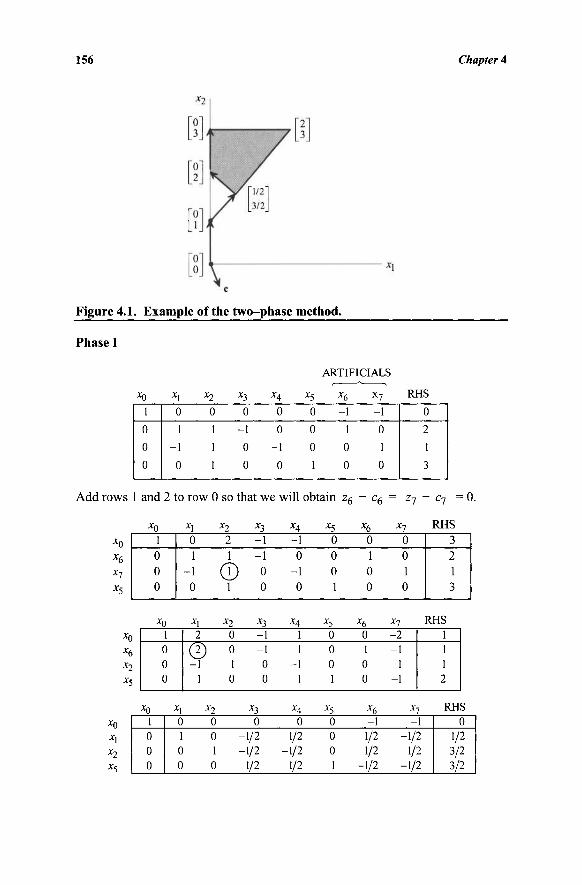
156 Chapter 4
Figure 4.1. Example of the two-phase method.
Phase I
ARTIFICIALS
Xn Xi Xy Xi ΧΛ X< Xf. X"7 Kfib
1
0
0
0
0
1
-1
0
0
1
1
1
0
-1
0
0
0
0
-1
0
0
0
0
1
-1
1
0
0
-1
0
1
0
0
2
1
3
Add rows 1 and 2 to row 0 so that we will obtain z6 - c6 = ζΊ - cj = 0.
Xr\ ΧΛ Λ"9 ΧΊ. ΧΛ ΧΖ Xfc Χη χντιΛ
1 0 0 0
0 1
-1 0
2 1
co 1
-1 -1 0 0
-1 0
-1 0
0 0 0 1
0 1 0 0
0 0 1 0
3 2 1 3
Χα XI X? - 3 " 4 * 5 * 6 " 7 KJ~lo
1 0 0 0
2
Θ -1 1
0 0 1 0
-1 -1 0 0
1 1
-1 1
0 0 0 1
0 1 0 0
-2 -1
1 -1
1 1 1 2
Χη Χι Χτ Χ3 ΧΑ - 5 " 6 " 7
RHS 1 0 0 0
0 1 0 0
0 0 1 0
0 -1/2 -1/2
1/2
0 1/2
-1/2 1/2
0 0 0 1
-1 1/2 1/2
-1/2
-1 -1/2
1/2 -1/2
0 1/2 3/2 3/2
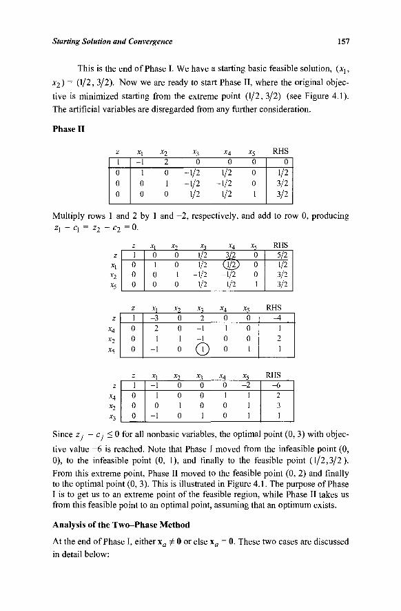
Starting Solution and Convergence 157
This is the end of Phase I. We have a starting basic feasible solution, {xx, xl) = (1/2> 3/2)· Now we are ready to start Phase II, where the original objec-
tive is minimized starting from the extreme point (1/2, 3/2) (see Figure 4.1).
The artificial variables are disregarded from any further consideration.
Phase II
z 1 0 0 0
x\ -1
1 0 0
x2
2 0 1 0
x3
0 -1/2 -1/2
1/2
X4
0 1/2
-1/2 1/2
XS
0 0 0 1
RHS 0
1/2 3/2 3/2
Multiply rows 1 and 2 by 1 and - 2 , respectively, and add to row 0, producing zl ~ c\ = z2 ~ c2 = °-
z x\ x2
x5
z x4
x2 x5
z X4
x? x3
z 1 0 0 0
z 1 0 0 0
z 1 0 0 0
x\ 0 1 0 0
X,
-3 2 1
-1
X,
-1 1 0
-1
x? 0 0 1 0
x2
0 0 1 0
x2
0 0 1 0
x3
1/2 -1/2 -1/2
1/2
*3 2
-1
0 x3
0 0 0 1
x4
3/2 (1/2) -1/2
1/2
X4
0 1 0 0
X4
0 1 0 0
x5 0 0 0 1
x5 0 0 0 1
*> -2
1 1 1
RHS -5/2
1/2 3/2 3/2
RHS ^t
1 2 1
RHS -6
2 3 1
Since z Cj < 0 for all nonbasic variables, the optimal point (0, 3) with objec-
tive value -6 is reached. Note that Phase I moved from the infeasible point (0, 0), to the infeasible point (0, 1), and finally to the feasible point (1/2,3/2).
From this extreme point, Phase II moved to the feasible point (0, 2) and finally to the optimal point (0, 3). This is illustrated in Figure 4.1. The purpose of Phase I is to get us to an extreme point of the feasible region, while Phase II takes us from this feasible point to an optimal point, assuming that an optimum exists.
Analysis of the Two-Phase Method
At the end of Phase I, either χα Φ 0 or else xa
in detail below:
: 0. These two cases are discussed
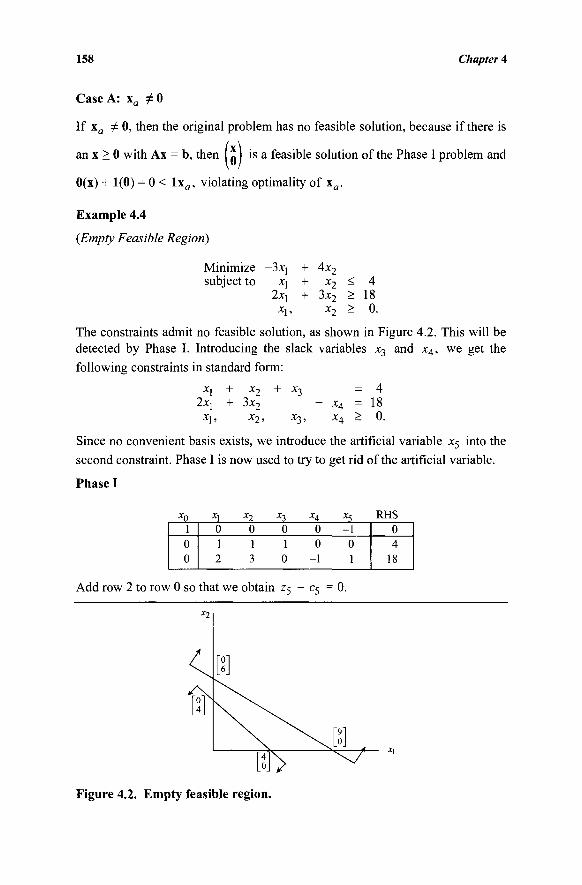
158 Chapter 4
Case A: xa φθ
If xa φ 0, then the original problem has no feasible solution, because if there is
an x > 0 with Ax = b, then I ft ) is a feasible solution of the Phase I problem and
0(x) + 1(0) = 0 < l x a , violating optimality of xa.
Example 4.4
(Empty Feasible Region)
Minimize -3xj + 4x2 subject to xj + x2 < 4
2x, + 3x2 > 18 X], *2 - 0·
The constraints admit no feasible solution, as shown in Figure 4.2. This will be detected by Phase I. Introducing the slack variables x3 and x4, we get the following constraints in standard form:
xl + x2 + x3 = 4 2x\ + 3x2 - x4 = 1 8
X\, X2> *3 ! X4 — 0 .
Since no convenient basis exists, we introduce the artificial variable x5 into the
second constraint. Phase I is now used to try to get rid of the artificial variable.
Phase I
Xa Xi X9 -^3 -^4 -*5 J v H o
1 0 0
0 0 0 0 - 1 1 1 1 0 0 2 3 0 - 1 1
0 4
18
Add row 2 to row 0 so that we obtain z5 - c5 = 0.
*2
Figure 4.2. Empty feasible region.
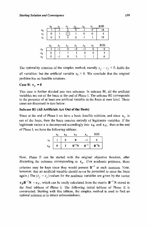
Starting Solution and Convergence 159
JCQ
*5
XQ
x0
1 0 0
x0
1 0 0
*1 2 1 2
X]
-1 1
-1
x2
3
® 3
x2
0 1 0
x3
0 1 0
*5 -3
1 -3
X4
-1 0
-1
X4
-1 0
-1
x5
0 0 1
x5
0 0 1
RHS 18 4
18
RHS 6 4 6
The optimality criterion of the simplex method, namely z · - c. < 0, holds for
all variables; but the artificial variable x5 > 0. We conclude that the original
problem has no feasible solutions.
Case B: \a = 0
This case is further divided into two subcases. In subcase Bl, all the artificial variables are out of the basis at the end of Phase I. The subcase B2 corresponds to the presence of at least one artificial variable in the basis at zero level. These cases are discussed in turn below:
Subcase Bl (All Artificials Are Out of the Basis)
Since at the end of Phase I we have a basic feasible solution, and since xa is out of the basis, then the basis consists entirely of legitimate variables. If the legitimate vector x is decomposed accordingly into \B and xN, then at the end of Phase I, we have the following tableau:
xo
XQ
1
0
XS
0
I
XN
0
B-1N
x a
-1
B 1
RHS
0
B ' b
Now, Phase II can be started with the original objective function, after discarding the columns corresponding to xa. (For academic purposes, these
columns may be kept since they would present B~ at each iteration. Note, however, that an artificial variable should never be permitted to enter the basis again.) The (z, - c. )-values for the nonbasic variables are given by the vector
cBB~ N - c^ , which can be easily calculated from the matrix B~ N stored in
the final tableau of Phase I. The following initial tableau of Phase II is constructed. Starting with this tableau, the simplex method is used to find an optimal solution or to detect unboundedness.
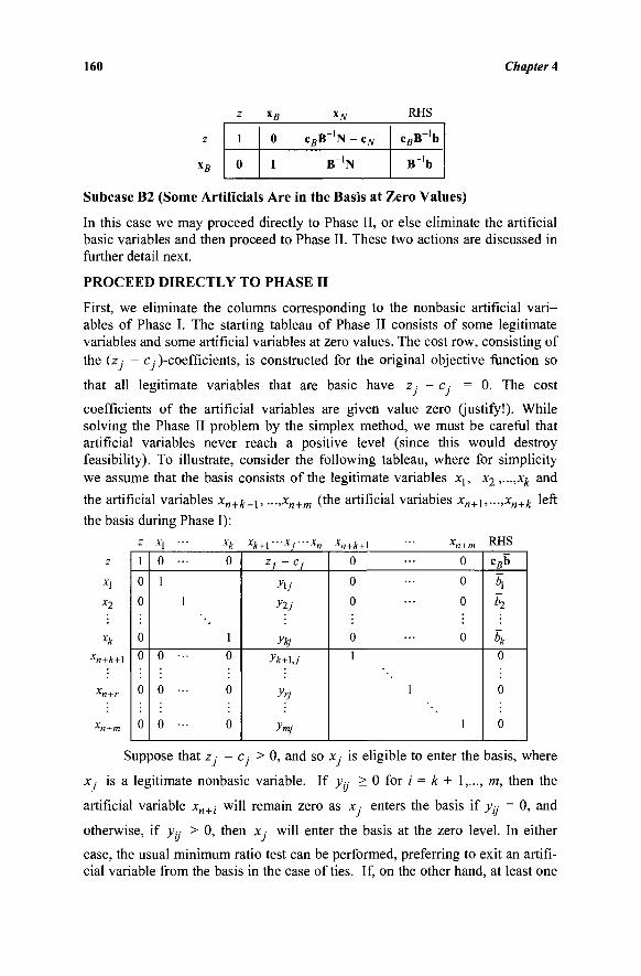
160 Chapter 4
z
1
0
χ β
0
I
xN
c B B- 'N - cN
B_1N
RHS
CfiB- 'b
B>b
Subcase B2 (Some Artificials Are in the Basis at Zero Values)
In this case we may proceed directly to Phase II, or else eliminate the artificial basic variables and then proceed to Phase II. These two actions are discussed in further detail next.
PROCEED DIRECTLY TO PHASE II
First, we eliminate the columns corresponding to the nonbasic artificial vari-ables of Phase I. The starting tableau of Phase II consists of some legitimate variables and some artificial variables at zero values. The cost row, consisting of the (z ■ - Cj^-coefficients, is constructed for the original objective function so
that all legitimate variables that are basic have z, - c, = 0. The cost
coefficients of the artificial variables are given value zero (justify!). While solving the Phase II problem by the simplex method, we must be careful that artificial variables never reach a positive level (since this would destroy feasibility). To illustrate, consider the following tableau, where for simplicity we assume that the basis consists of the legitimate variables xl5 x2 >-->xk an(^ the artificial variables x„+£+i, —,xn+m ( m e artificial variables xn+i,~;Xn+k left the basis during Phase I):
z x\ x2
xk
xn+k+l
xn+r
xn+m
z
1
0
0
0
0
0
0
X, · · ·
0 ···
1
1
0 ···
0 ···
0 ···
xk
0
1
0
0
0
xk+\ '"xj'"xn
zi - ci
y\j
yij
yq yk+ij
yrj
ymj-
xn+k+l
0
0
0
0
1
■*n+m
0
0
0
0
1
1
RHS
cBb
\ h
h 0
0
0
Suppose that z - c.- > 0, and so x, is eligible to enter the basis, where
Xj is a legitimate nonbasic variable. If >>,·. > 0 for i = k + 1,..., m, then the
artificial variable xn+i will remain zero as x ■ enters the basis if ytj = 0, and
otherwise, if >>,-. > 0, then x ■ will enter the basis at the zero level. In either
case, the usual minimum ratio test can be performed, preferring to exit an artifi-cial variable from the basis in the case of ties. If, on the other hand, at least one
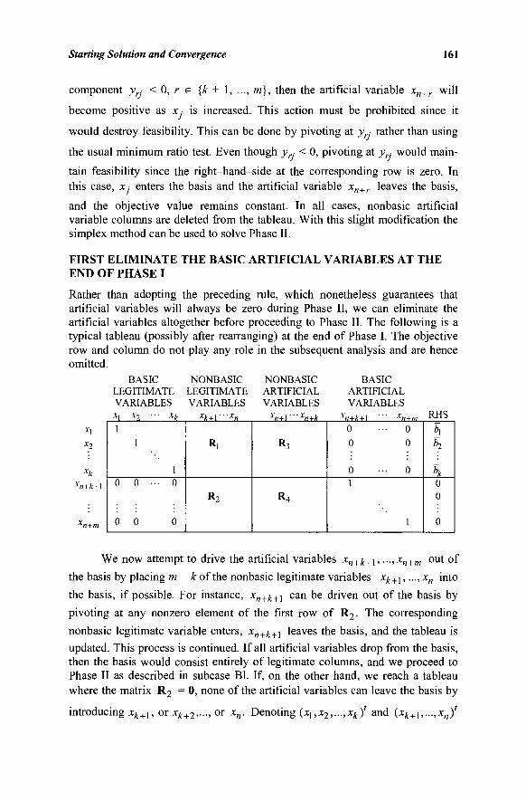
Starting Solution and Convergence 161
component y ■ < 0, r e {k + 1, ..., m}, then the artificial variable xn+r will
become positive as xj is increased. This action must be prohibited since it
would destroy feasibility. This can be done by pivoting at yr.- rather than using
the usual minimum ratio test. Even though y ■ < 0, pivoting at yr,- would main-
tain feasibility since the right-hand-side at the corresponding row is zero. In
this case, x.- enters the basis and the artificial variable xn+r leaves the basis,
and the objective value remains constant. In all cases, nonbasic artificial variable columns are deleted from the tableau. With this slight modification the simplex method can be used to solve Phase II.
FIRST ELIMINATE THE BASIC ARTIFICIAL VARIABLES AT THE END OF PHASE I
Rather than adopting the preceding rule, which nonetheless guarantees that artificial variables will always be zero during Phase II, we can eliminate the artificial variables altogether before proceeding to Phase II. The following is a typical tableau (possibly after rearranging) at the end of Phase I. The objective row and column do not play any role in the subsequent analysis and are hence omitted.
BASIC NONBASIC NONBASIC BASIC LEGITIMATE LEGITIMATE ARTIFICIAL ARTIFICIAL VARIABLES VARIABLES VARIABLES VARIABLES
X,
x?
xk xn+k+\
xn+m
X\ 1
0
0
x? ■
1
0 ·
0
• xk
1 • 0
0
xk+\"'xn
Ri
R2
xn+\"
R3
R4
'xn+k xn+k + \
0 0
0 1
xn+m
0 0
0
1
RHS
*i h
\ 0 0
0
We now attempt to drive the artificial variables x„+£+i, —,xn+m out of the basis by placing m - k of the nonbasic legitimate variables xk+\,..., xn into the basis, if possible. For instance, x„+£+i can be driven out of the basis by pivoting at any nonzero element of the first row of R2. The corresponding nonbasic legitimate variable enters, x„+£+i leaves the basis, and the tableau is updated. This process is continued. If all artificial variables drop from the basis, then the basis would consist entirely of legitimate columns, and we proceed to Phase II as described in subcase Bl. If, on the other hand, we reach a tableau where the matrix R2 = 0, none of the artificial variables can leave the basis by
introducing x#+1, οτ xk+2,..., or xn. Denoting (xl,x2,—,χ^)' and (xk+l,...,xn)'
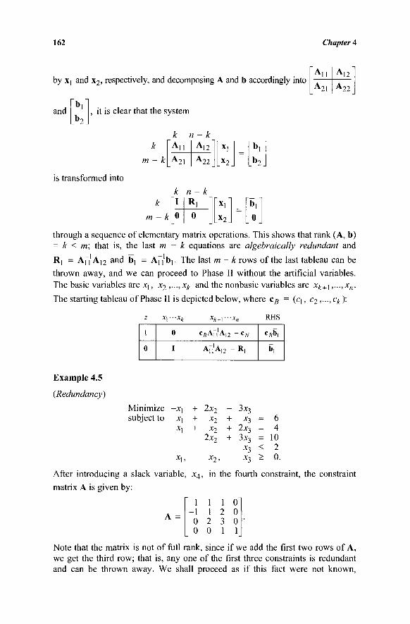
162 Chapter 4
by X[ and x2, respectively, and decomposing A and b accordingly into
and it is clear that the system
["An A21
A12
A22_
[An A 2 1
A12
A 2 2
~ΧΓ _ X 2 j
= V . b 2 .
is transformed into
I
0
Ri 1 0
~ x l ~
_x2_ = V
0
through a sequence of elementary matrix operations. This shows that rank (A, b) = k < m; that is, the last m - k equations are algebraically redundant and
R] = Afi AJ2 and bj = A^b]. The last m - k rows of the last tableau can be thrown away, and we can proceed to Phase II without the artificial variables. The basic variables tire Xj, X2 ,.. -, Xfc and the nonbasic variables are xk+\ ,...,x„.
The starting tableau of Phase II is depicted below, where cB = (q, c2,...,ck):
z
1
0
XyXjt
0
I
xk+\ "'xn
C B A U A 1 2 " eN
Α Π A12 = R l
RHS
c^b,
bi
Example 4.5
(Redundancy)
Minimize subject to
-Xj + 2x 2
xl
X | ,
x2
3x3 xi
~Xj + x2 + 2x^ —
2x2 + 3*3 x3
x2, x3
6 4
10 2 0.
After introducing a slack variable, x4, in the fourth constraint, the constraint
matrix A is given by:
" 1 1 1 0 - 1 1 2 0 0 2 3 0 0 0 1 1
Note that the matrix is not of full rank, since if we add the first two rows of A, we get the third row; that is, any one of the first three constraints is redundant and can be thrown away. We shall proceed as if this fact were not known,
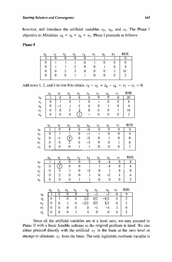
Starting Solution and Convergence 163
however, and introduce the artificial variables x5, x6, and x7. The Phase I
objective is: Minimize x0 = x5 + x6 + χη. Phase I proceeds as follows:
Phase I
XQ XI X1) XT XA X5 Xf. X 7 K.H S
1 0 0 0 0
0 1
-1 0 0
0 1 1 2 0
0 1 2 3 1
0 0 0 0 1
-1 1 0 0 0
-1 0 1 0 0
-1 0 0 1 0
0 6 4
10 2
Add rows 1, 2, and 3 to row 0 to obtain z5 - c5 = z6 - c6 = ζΊ - cj = 0.
XQ
XS
Χβ
*7
XA
XQ
1 0 0 0 0
X\ 0 1
-1 0 0
x2
4 1 1 2 0
*s 6 1 2 3
0)
x4
0 0 0 0 1
x5 0 1 0 0 0
x6 0 0 1 0 0
Χη
0 0 0 1 0
RHS 20 6 4 10 2
x0 1 0 0 0 0
X,
0 1
-1 0 0
x2 4 1
CO 2 0
*3 0 0 0 0 1
xA
-6 -1 -2 -3
1
x5
0 1 0 0 0
x6 0 0 1 0 0
X-l
0 0 0 1 0
RHS 8 4 0 4 2
XQ XI XT X3 X4 X5 X5 Xl KJ1S
1 0 0 0 0
4
(2) -1 2 0
0 0 1 0 0
0 0 0 0 1
2 1
-2 1 1
0 1 0 0 0
-4 -1
1 -2
0
0 0 0 1 0
8 4 0 4 2
XQ X] X2 -*3 X4 -£5 -g Χη Kxib
1 0 0 0 0
0 1 0 0 0
0 0 1 0 0
0 0 0 0 1
0 1/2
-3/2 0 1
-2 1/2 1/2 -1 0
-2 -1/2
1/2 -1 0
0 0 0 1 0
0 2 2 0 2
Since all the artificial variables are at a level zero, we may proceed to Phase II with a basic feasible solution to the original problem at hand. We can either proceed directly with the artificial x7 in the basis at the zero level or
attempt to eliminate x7 from the basis. The only legitimate nonbasic variable is
XQ
X5
x6
Χη
x3
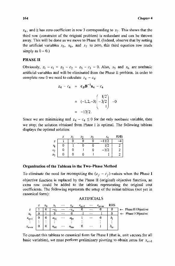
164 Chapter 4
x4, and it has zero coefficient in row 3 corresponding to x7. This shows that the third row (constraint of the original problem) is redundant and can be thrown away. This will be done as we move to Phase II. (Indeed, observe that by setting the artificial variables x5, x6, and x7 to zero, this third equation row reads simply as 0 = 0.)
PHASE II
Obviously, zj - c\ = z2 _ c2 = z3 _ c3 = 0. Also, x5 and x6 are nonbasic
artificial variables and will be eliminated from the Phase II problem. In order to complete row 0 we need to calculate z4 - c4:
^4 - c4 = c5B c4
( 1/21 - 3 / 2
I iJ = (-1,2,-3)
= -13/2.
Since we are minimizing and z4 - c4 < 0 for the only nonbasic variable, then
we stop; the solution obtained from Phase I is optimal. The following tableau displays the optimal solution:
z x\ x2
*3
z 1 0 0 0
*1 0 1 0 0
x2
0 0 1 0
x3
0 0 0 1
xA
-13/2 1/2
-3/2 1
RHS -4 2 2 2
Organization of the Tableau in the Two-Phase Method
To eliminate the need for recomputing the (ZJ - Cj)-values when the Phase I
objective function is replaced by the Phase II (original) objective function, an extra row could be added to the tableau representing the original cost coefficients. The following represents the setup of the initial tableau (not yet in canonical form):
ARTIFICIALS
xo xn+\
z 1 0 0
0
x0
0 1 0
0
*i · -c, · 0
«11 ·
am\ ■
■■ xn
■■ ~cn
0
■■ amn
xn+\ 0 -1 1
0
xn+m 0 -1 0
1
RHS 0 0
bm
Phase II Objective Phase I Objective
To convert this tableau to canonical form for Phase I (that is, unit vectors for all basic variables), we must perform preliminary pivoting to obtain zeros for xM+[
Starting Solution and Convergence 165
through xn+m in the x0 (Phase I objective) row. This is done by successively
adding every row (except the z row) to the x0 r o w ·
Once the initial tableau has been converted to canonical form, the simplex method is applied to the resulting tableau using the x0 row as the
(Phase I) objective function row until optimality is achieved. During Phase I the z row is transformed, just as any other row of the tableau would be, to maintain unit vectors for the basic variables. Note, however, that during Phase I, although the basis entry is solely determined by the entries in row x0, ties could be broken using the z row.
At the end of Phase I, if x0 is positive, then the problem is infeasible and the optimization process can be terminated. Otherwise, the x0 row and x0
column are deleted and Phase II is initiated (after possibly eliminating artificial variables), with the values in the z row being the correct values of z. - c ■
(why?) for the Phase II objective.
4.3 THE BIG-M METHOD
Recall that artificial variables constitute a tool that can be used to initiate the simplex method. However, the presence of artificial variables at a positive level, by construction, means that the current point is an infeasible solution of the original system. The two-phase method is one way to dispense with the artificial variables. However, during Phase I of the two-phase method the original cost coefficients are essentially ignored. Phase I of the two-phase method seeks any basic feasible solution, not necessarily a good one. Another possibility for eliminating the artificial variables is to assign coefficients for these variables in the original objective function in such away as to make their presence in the basis at a positive level very unattractive from the objective function point of view. To illustrate, suppose that we want to solve the following linear programming problem, where b > 0:
Minimize ex subject to Ax = b
x > 0.
If no convenient basis is known, we can introduce the artificial vector xa, which leads to the following system:
Ax + xa - b x,xa > 0.
The starting basic feasible solution is given by xfl = b and x = 0. In order to
reflect the undesirability of a nonzero artificial vector, the objective function is modified such that a large penalty is paid for any such solution. More specifi-cally consider the following problem:
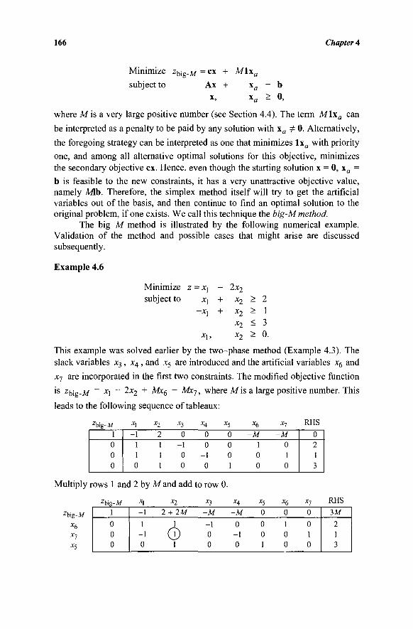
166 Chapter 4
Minimize zbig_M = c x + M\xa
subject to Ax + \a = b x, \a > 0,
where Mis a very large positive number (see Section 4.4). The term Mlxa can
be interpreted as a penalty to be paid by any solution with xa Φ 0. Alternatively,
the foregoing strategy can be interpreted as one that minimizes lx a with priority
one, and among all alternative optimal solutions for this objective, minimizes
the secondary objective cx. Hence, even though the starting solution x = 0, xa =
b is feasible to the new constraints, it has a very unattractive objective value, namely Mb. Therefore, the simplex method itself will try to get the artificial variables out of the basis, and then continue to find an optimal solution to the original problem, if one exists. We call this technique the big-M method.
The big-M method is illustrated by the following numerical example. Validation of the method and possible cases that might arise are discussed subsequently.
Example 4.6
Minimize z = χλ - 2x2
subject to xl + x2 - 2 - X j + x 2 - 1
x2 < 3
This example was solved earlier by the two-phase method (Example 4.3). The slack variables X3 , Χ4 , and x5 are introduced and the artificial variables x6 and
xj are incorporated in the first two constraints. The modified objective function
is Zbig-M = x\ ~ 2x2 + Mxe + M*l > w n e r e M is a large positive number. This
leads to the following sequence of tableaux:
Zbig-M x\ x2 x3 x4 x5 x6 xl
1 0 0 0
-1 1
-1 0
2 1 1 1
0 -1 0 0
0 0
-1 0
0 0 0 1
-M 1 0 0
-M 0 1 0
0 2 1 3
Multiply rows 1 and 2 by Mand add to row 0.
Zbig-M x\ *2 x3 H x5 x6 x7 RHS
1
0 0 0
-1
1 -1 0
2 + 2M
1
CO 1
-M
-1 0 0
-M
0 -1 0
0
0 0 1
0
1 0 0
0
0 1 0
3M
2 1 3
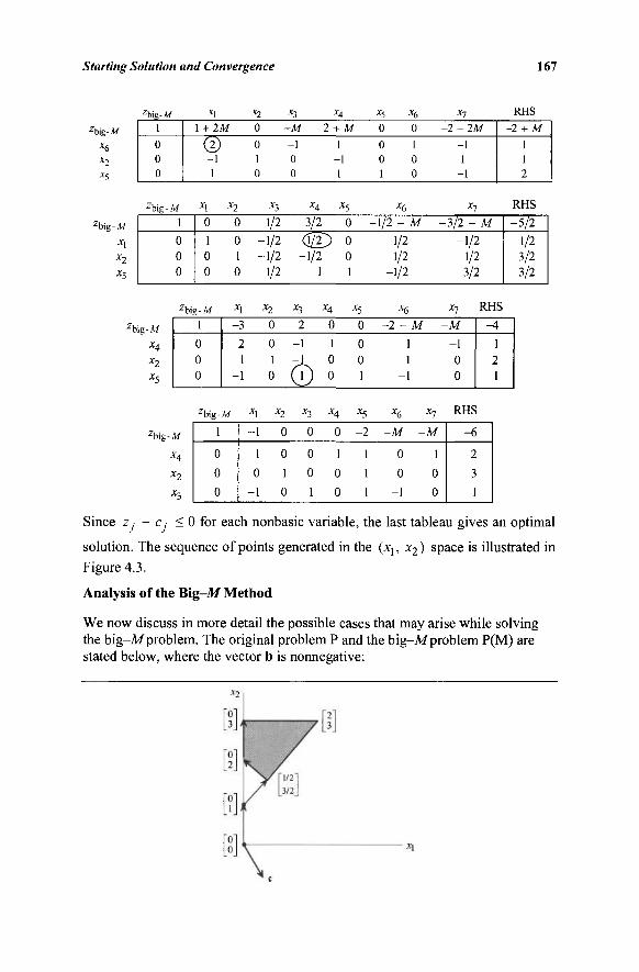
Starting Solution and Convergence 167
zbig-x6 x2 x5
Zbig
\1
-M x\
x2 x5
Zbig-M 1
0 0 0
xl 1 + 2M
(2) -1 1
x2 0
0 1 0
*3 -M
-1 0 0
x4
2 + M
1 -1 1
x5
0
0 0 1
*6 0
1 0 0
*7 - 2 - 2 M
-1 1
-1
RHS
-2 + M
1 1 2
Zbig-M
1
0 0 0
X[ x2
0 0
1 0 0 1 0 0
*3 1/2
-1/2 -1/2
1/2
X4 X5
3/2 0
a© 0 -1/2 0
1 1
*6
-1/2 - A/
1/2 1/2
-1/2
x7
-3 /2 - M
-1/2 1/2 3/2
RHS
-5 /2
1/2 3/2 3/2
2big-M
X4
* 2 X5
Zbig-M
1
0 0 0
*1
- 3
2 1
-1
X2 *3 -«4
0 2 0
0 -1 1 1 -1 0 0 Q 0
*5
0
0 0 1
·% -2 - M
1 1
-1
x7
-M
-1 0 0
RHS
-4
1 2 1
2big-M
X4
^2
x3
Zbig-M
1
0
0
0
x\ -1
1
0
- 1
x2
0
0
1
0
x3
0
0
0
1
X4
0
1
0
0
x5
-2
1
1
1
x6
-M
0
0
-1
x7
-Λ/
-1
0
0
RHS
- 6
2
3
1
Since z: -7 cy < 0 for each nonbasic variable, the last tableau gives an optimal
solution. The sequence of points generated in the (xj, x2) space is illustrated in
Figure 4.3.
Analysis of the Big-M Method
We now discuss in more detail the possible cases that may arise while solving the big-M problem. The original problem P and the big-M problem P(M) are stated below, where the vector b is nonnegative:
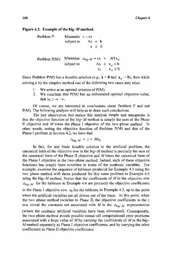
168 Chapter 4
Figure 4.3. Example of the big-M method.
Problem P: Minimize z = ex subject to Ax = b
x > 0.
Problem P(M): Minimize zbig.M = ex + Mlxa
subject to Ax + xa = b x, xa > 0.
Since Problem P(M) has a feasible solution (e.g., x = 0 and xa = b), then while
solving it by the simplex method one of the following two cases may arise:
1. We arrive at an optimal solution of P(M). 2. We conclude that P(M) has an unbounded optimal objective value,
that is, z —> -co.
Of course, we are interested in conclusions about Problem P and not P(M). The following analysis will help us to draw such conclusions.
The key observation that makes this analysis simple and transparent is that the objective function of the big-M method is simply the sum of the Phase II objective and M times the Phase I objective of the two-phase method. In other words, noting the objective function of Problem P(M) and that of the Phase I problem in Section 4.2, we have that
Zbig-M = z + MXQ.
In fact, for any basic feasible solution to the artificial problem, the canonical form of the objective row in the big-M method is precisely the sum of the canonical form of the Phase II objective and M times the canonical form of the Phase I objective in the two-phase method. Indeed, each of these objective functions has simply been rewritten in terms of the nonbasic variables. For example, examine the sequence of tableaux produced for Example 4.3 using the two-phase method with those produced for this same problem in Example 4.6 using the big-M method. Notice that the coefficients of M in the objective row Zbig-M f°r m e tableaux in Example 4.6 are precisely the objective coefficients
in the Phase I objective row x0 for the tableaux in Example 4.3, up to the point
when the artificial variables are all driven out of the basis. At this point, when the two-phase method switches to Phase II, the objective coefficients in the z row reveal the constants not associated with M in the zbig_M representation
(where the nonbasic artificial variables have been eliminated). Consequently, the two-phase method avoids possible round-off computational error problems associated with a large value of M by carrying the coefficients of M in the big-M method separately as Phase I objective coefficients, and by carrying the other coefficients as Phase II objective coefficients.
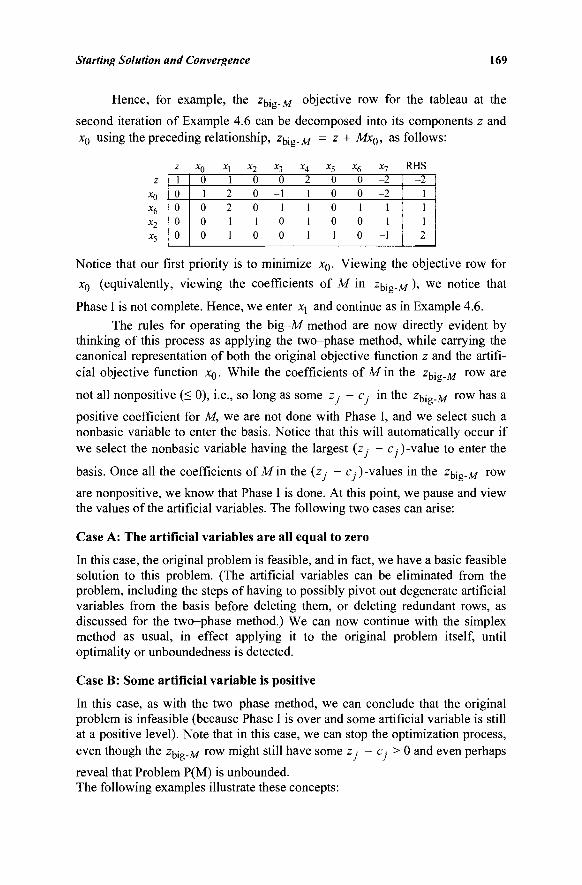
Starting Solution and Convergence 169
Hence, for example, the zbig.M objective row for the tableau at the
second iteration of Example 4.6 can be decomposed into its components z and XQ using the preceding relationship, zbig_M = z + Mx0, as follows:
Z X Q X\ XJ X3 ΧΛ -^5 Xf, Χ"7 RHS 1 0 0 0 0
0 1 0 0 0
1 2 2
-1 1
0 0 0 1 0
0 2 0 -1 -1 0 -0
1 0 1 0 1 0 1 1
0 0 1 0 0
-2 -2 -1
1 -1
-2 1 1 1 2
Notice that our first priority is to minimize x0. Viewing the objective row for
XQ (equivalently, viewing the coefficients of M in zbig_M ), we notice that
Phase I is not complete. Hence, we enter xj and continue as in Example 4.6. The rules for operating the big-M method are now directly evident by
thinking of this process as applying the two-phase method, while carrying the canonical representation of both the original objective function z and the artifi-cial objective function x0. While the coefficients of Min the zbi„_M row are
not all nonpositive (< 0), i.e., so long as some zj - cj in the zbig_M r o w n a s a
positive coefficient for M, we are not done with Phase I, and we select such a nonbasic variable to enter the basis. Notice that this will automatically occur if we select the nonbasic variable having the largest (z · - c.)-value to enter the
basis. Once all the coefficients of Min the (z · - c,)-values in the z^„M row
are nonpositive, we know that Phase I is done. At this point, we pause and view the values of the artificial variables. The following two cases can arise:
Case A: The artificial variables are all equal to zero
In this case, the original problem is feasible, and in fact, we have a basic feasible solution to this problem. (The artificial variables can be eliminated from the problem, including the steps of having to possibly pivot out degenerate artificial variables from the basis before deleting them, or deleting redundant rows, as discussed for the two-phase method.) We can now continue with the simplex method as usual, in effect applying it to the original problem itself, until optimality or unboundedness is detected.
Case B: Some artificial variable is positive
In this case, as with the two-phase method, we can conclude that the original problem is infeasible (because Phase I is over and some artificial variable is still at a positive level). Note that in this case, we can stop the optimization process, even though the Zbig-M r o w might still have some z · - c > 0 and even perhaps
reveal that Problem P(M) is unbounded. The following examples illustrate these concepts:
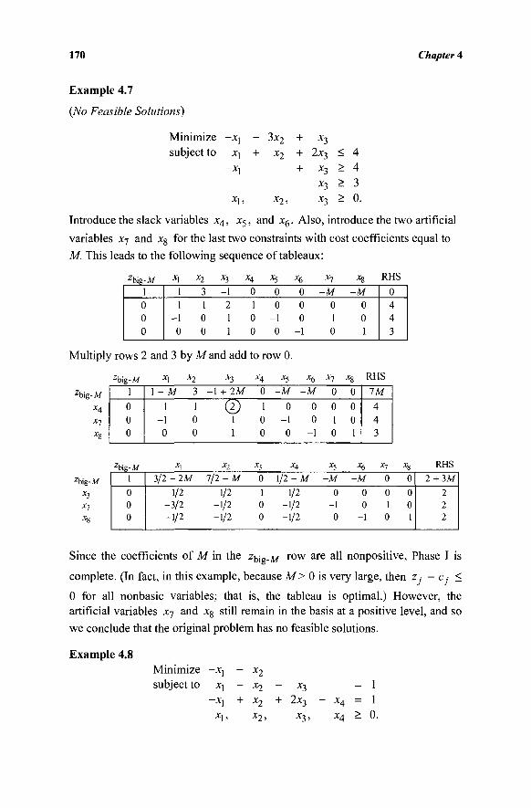
170 Chapter 4
Example 4.7
(No Feasible Solutions)
Minimize subject to
- * i
X,
-x1
X j ,
- 3x 2 + X3
+ x2 + 2x3
+ x3
*3 X 2 , X3
< 4 > 4 > 3 > 0
Introduce the slack variables and x6. Also, introduce the two artificial
variables x7 and x8 for the last two constraints with cost coefficients equal to
M. This leads to the following sequence of tableaux:
RHS Z b i g - M Λ"2 Χτ, Χ4 x6 Χη X%
1 0 0 0
1 1
-1 0
3 1 0 0
-1 2 1 1
0 1 0 0
0 0
-1 0
0 0 0
-1
-M 0 1 0
-M 0 0 1
0 4 4 3
Multiply rows 2 and 3 by M and add to row 0.
Zb\g-M
X4
*8
Z b i g - M
1
0 0 0
x\ \-M
1 -1
0
x2
3
1 0 0
x-i -1 + 2M
1 1
JC4
0
1 0 0
x5
-M
0 -1 0
x6 x7 x8
- M O O
0 0 0 0 1 0
-1 0 1
RHS
ΊΜ
4 4 3
Zbig-M
*8
Zbig-M
1
0 0 0
*\ 3/2 - 1M
1/2 -3/2 -1/2
x2
7 / 2 - M
1/2 -1/2 -1/2
*s 0
1 0 0
X4
1/2 - M
1/2 -1/2 -1/2
x5
-M
0 -1 0
X6
-M
0 0
-1
X-,
0
0 1 0
xs 0
0 0 1
RHS
2 + 3M
2 2 2
Since the coefficients of M in the ^big-M r o w a r e a n nonpositive, Phase I is
complete. (In fact, in this example, because M> 0 is very large, then z - c, <
0 for all nonbasic variables; that is, the tableau is optimal.) However, the artificial variables x7 and x8 still remain in the basis at a positive level, and so we conclude that the original problem has no feasible solutions.
Example 4.8 Minimize -xj - x2
subject to Xj - x2 - x3 = 1 —Xi + X2 "1~ ^X3 — ΧΛ ~ A
Xj, X 2 , Χ3, Χ4 > 0 .
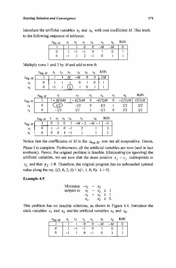
Starting Solution and Convergence 171
Introduce the artificial variables x5 and x6 with cost coefficient M. This leads
to the following sequence of tableaux: Zbig-M
1 0 0
x\ 1 1
-1
x2
1 -1
1
*3
0 -1 2
X^
0 0
-1
x5
-M 1 0
x6
-M 0 1
RHS 0 1 1
Multiply rows 1 and 2 by Mand add to row 0.
Zbig-M x\ x2 x3 x4 x5 x6 RHS Zbig-M
x6
1
0 0
1 1 M -M 0 0
1 - 1 - 1 0 1 0 -1 1 ( 2 ) -1 0 1
2AT
1 1
Zbig-M x 5 x 3
Zbig-M
1
0 0
X,
1 + (1/2)M
CMÌ) -1/2
x2 x3
- (1/2) Ai 0
-1/2 0 1/2 1
x4 x5
-(1/2)M 0
-1/2 1 -1/2 0
x6
-(1/2)M
1/2 1/2
RHS
(3/2)M 3/2 1/2
Zbig-M x\ x3
Zbig-M
1
0 0
X] X2 -^3 %4
0 2 0 1 1 - 1 0 - 1 0 0 1 - 1
*5
- M - 2 2 1
x6
-A/-1 1 1
RHS -3 3 2
Notice that the coefficients of M in the z^„M row are all nonpositive. Hence,
Phase I is complete. Furthermore, all the artificial variables are zero (and in fact nonbasic). Hence, the original problem is feasible. Eliminating (or ignoring) the artificial variables, we see now that the most positive z,· - c ■ corresponds to
xj and that y2 < 0. Therefore, the original program has an unbounded optimal
value along the ray {(3, 0, 2, 0) + λ(1, 1, 0, 0): λ > 0}.
Example 4.9
Minimize -χλ - x2
subject to X] - x2 > I -Xj + x 2 - 1
Xj, x 2 > 0.
This problem has no feasible solutions, as shown in Figure 4.4. Introduce the slack variables x3 and x4 and the artificial variables x5 and x6.
Zbig-M
1 0 0
*1
1 1
-1
x2
1 -1
1
*3
0 -1 0
x4
0 0
-1
*5
-M 1 0
x6
-M 0 1
RHS 0 1 1
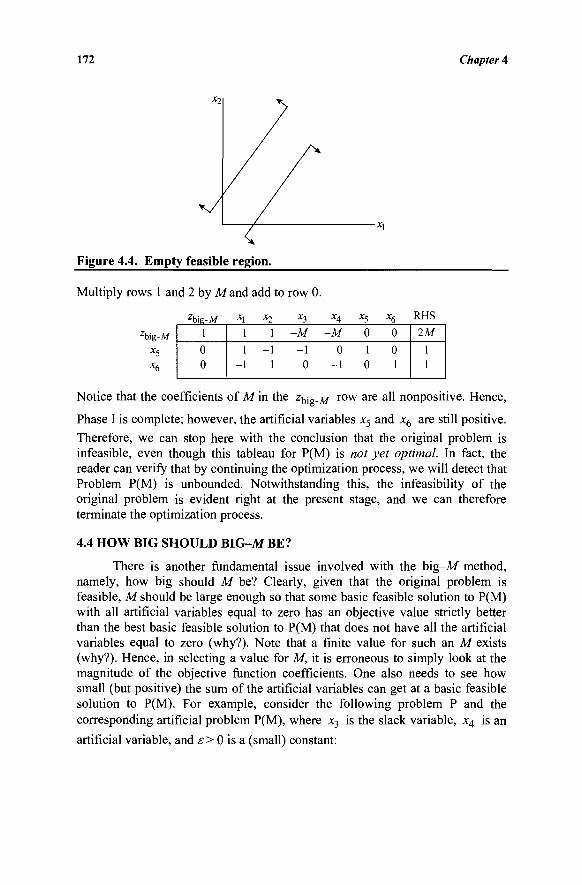
172 Chapter 4
Figure 4.4. Empty feasible region.
Zbif>-M
1
0 0
*1
1
1 -1
x2
1
-1 1
*3
-M
-1 0
X4
-M
0 -1
x5
0
1 0
H 0
0 1
RHS 2M
1 1
Multiply rows 1 and 2 by Mand add to row 0.
Zbig-M
X5
x6
Notice that the coefficients of Min the zbig.M row are all nonpositive. Hence,
Phase I is complete; however, the artificial variables x5 and x6 are still positive.
Therefore, we can stop here with the conclusion that the original problem is infeasible, even though this tableau for P(M) is not yet optimal. In fact, the reader can verify that by continuing the optimization process, we will detect that Problem P(M) is unbounded. Notwithstanding this, the infeasibility of the original problem is evident right at the present stage, and we can therefore terminate the optimization process.
4.4 HOW BIG SHOULD BIG-MBE?
There is another fundamental issue involved with the big-M method, namely, how big should M be? Clearly, given that the original problem is feasible, M should be large enough so that some basic feasible solution to P(M) with all artificial variables equal to zero has an objective value strictly better than the best basic feasible solution to P(M) that does not have all the artificial variables equal to zero (why?). Note that a finite value for such an M exists (why?). Hence, in selecting a value for M, it is erroneous to simply look at the magnitude of the objective function coefficients. One also needs to see how small (but positive) the sum of the artificial variables can get at a basic feasible solution to P(M). For example, consider the following problem P and the corresponding artificial problem P(M), where x3 is the slack variable, x4 is an
artificial variable, and ε> 0 is a (small) constant:
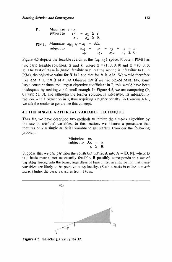
Starting Solution and Convergence 173
P : Minimize z = Xj subject to εχχ - x2 - ε
xj , x2 - 0.
P(M) : Minimize zbig_M = *i + M*4 subject to εχι - x2 - X3 + X4 = ε
Χγ, X2, Χ3, Χ\ ^ 0. Figure 4.5 depicts the feasible region in the (X], x2 ) space. Problem P(M) has two basic feasible solutions, x and x, where x = (1, 0, 0, 0) and x = (0, 0, 0, £·). The first of these is (basic) feasible to P, but the second is infeasible to P. In P(M), the objective value for x is 1 and that for x is εΜ. We would therefore like εΜ > 1, that is M> l/ε. Observe that if we had picked Mas, say, some large constant times the largest objective coefficient in P, this would have been inadequate by making ε> 0 small enough. In Figure 4.5, we are comparing (0, 0) with (1, 0), and although the former solution is infeasible, its infeasibility reduces with a reduction in ε, thus requiring a higher penalty. In Exercise 4.43, we ask the reader to generalize this concept.
4.5 THE SINGLE ARTIFICIAL VARIABLE TECHNIQUE
Thus far, we have described two methods to initiate the simplex algorithm by the use of artificial variables. In this section, we discuss a procedure that requires only a single artificial variable to get started. Consider the following problem:
Minimize ex subject to Ax = b
x > 0.
Suppose that we can partition the constraint matrix A into A = [B, N], where B is a basis matrix, not necessarily feasible. B possibly corresponds to a set of variables forced into the basis, regardless of feasibility, in anticipation that these variables are likely to be positive at optimality. (Such a basis is called a crash basis.) Index the basic variables from 1 to m.
Figure 4.5. Selecting a value for M.
174 Chapter 4
Multiplying the constraints by B , we get
Ixg + B ' N X J V = b
where b = B~ b. Suppose that b X 0 (if b > 0, we have a starting basic
feasible solution). To this system let us add a single artificial variable, xa, with a
coefficient o f -1 in each constraint that has bt < 0. Call this column ya. This
gives:
Ixg + B-'Nx^v + yaxa = b.
Now, introduce xa into the basis by selecting the pivot row r as follows:
br = minimum {è! . i:bj<0 l '
Note that br < 0. On pivoting in row r (that is, inserting xa and removing xr ),
we get the new right-hand-side values:
-br{>_0)
bt -br{> 0), ifo,· < 0 , i i r
bj(> 0), otherwise.
Thus by entering xa and exiting xr we have constructed a basic feasible solution
to the enlarged system (the one including the single artificial variable). Starting with this solution, the simplex method can be used with either the two-phase or the big-M method.
Note that the variable xa creates one extra dimension for this problem.
Its column is the sum of the artificial variable columns we would have added for the two-phase or the big-M method. Hence, effectively, if we further restrict all the artificial variables in the two-phase or big-M method to be equal to each other, we would obtain the single artificial variable technique. Empirically, it has been found that the single artificial variable technique is not as efficient as the other two methods, perhaps because of its foregoing restrictive nature, whereby a simplex path needs to be traced in which all violated constraints are simultaneously satisfied.
Example 4.10
Minimize 2xj + 3x2 subject to x\ + x2 > 3
-2x] + x2 > 2 Χγ, x2 - 0·
Subtracting the slack variables x3 and x4 and multiplying by - 1 , the structural
constraints become:
—X] — x2 + X3 — —3 λΧχ — X2 + ΧΛ = —2.
bI =
b\ =
b\ =
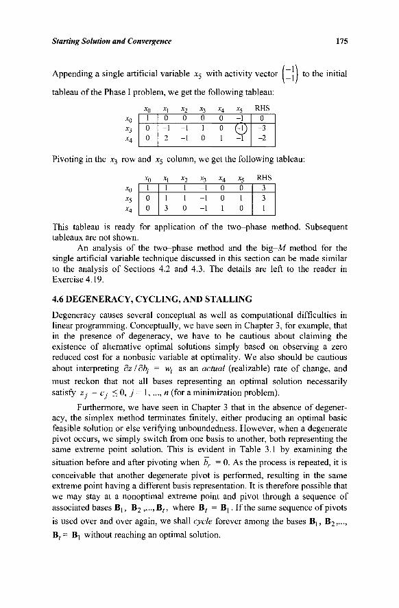
Starting Solution and Convergence 175
Appending a single artificial variable x5 with activity vector j _ . 1 to the initial
tableau of the Phase I problem, we get the following tableau:
Xn Xi X7 X3 X4 X5 RHS 1 0 0
0 0 0 0 - 1 - 1 - 1 1 0 (-1) 2 - 1 0 1 - 1
0 -3 -2
Pivoting in the x3 row and x5 column, we get the following tableau:
ΧΛ XI X2 X3 X4 X5 I v r l o
1 0 0
1 1 - 1 0 0 1 1 - 1 0 1 3 0 - 1 1 0
3 3 1
This tableau is ready for application of the two-phase method. Subsequent tableaux are not shown.
An analysis of the two-phase method and the big-M method for the single artificial variable technique discussed in this section can be made similar to the analysis of Sections 4.2 and 4.3. The details are left to the reader in Exercise 4.19.
4.6 DEGENERACY, CYCLING, AND STALLING
Degeneracy causes several conceptual as well as computational difficulties in linear programming. Conceptually, we have seen in Chapter 3, for example, that in the presence of degeneracy, we have to be cautious about claiming the existence of alternative optimal solutions simply based on observing a zero reduced cost for a nonbasic variable at optimality. We also should be cautious about interpreting dz I dty = W; as an actual (realizable) rate of change, and must reckon that not all bases representing an optimal solution necessarily satisfy Zj - Cj < 0, j = 1,..., n (for a minimization problem).
Furthermore, we have seen in Chapter 3 that in the absence of degener-acy, the simplex method terminates finitely, either producing an optimal basic feasible solution or else verifying unboundedness. However, when a degenerate pivot occurs, we simply switch from one basis to another, both representing the same extreme point solution. This is evident in Table 3.1 by examining the
situation before and after pivoting when br = 0. As the process is repeated, it is
conceivable that another degenerate pivot is performed, resulting in the same extreme point having a different basis representation. It is therefore possible that we may stay at a nonoptimal extreme point and pivot through a sequence of associated bases Bl5 B2 ,—,Β,, where B, = B[. If the same sequence of pivots
is used over and over again, we shall cycle forever among the bases B1; B2,...,
B, = Bj without reaching an optimal solution.
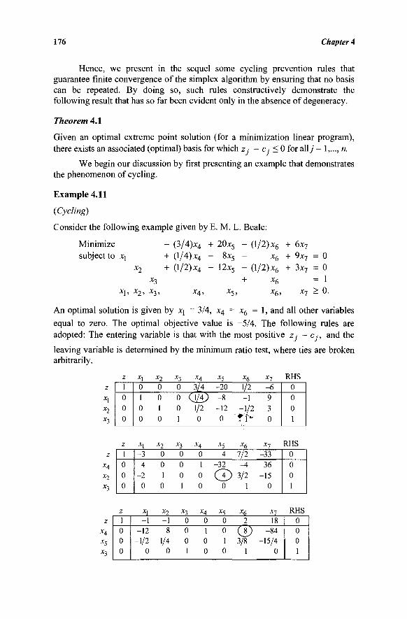
176 Chapter 4
Hence, we present in the sequel some cycling prevention rules that guarantee finite convergence of the simplex algorithm by ensuring that no basis can be repeated. By doing so, such rules constructively demonstrate the following result that has so far been evident only in the absence of degeneracy.
Theorem 4.1
Given an optimal extreme point solution (for a minimization linear program), there exists an associated (optimal) basis for which z ■ - c < 0 for ally = 1,..., n.
We begin our discussion by first presenting an example that demonstrates the phenomenon of cycling.
Example 4.11
{Cycling)
Consider the following example given by E. M. L. Beale:
Minimize - (3/4)x4
subject to xj + (1/4) x4
x2 + (1/2) x4
x3 x\> x2> x3> x4>
+ 20x5
- 8x5
- !2x5
*5>
- (1/2) x6 + 6x7
- x6 + 9x7
- (1/2) x6 + 3x7
+ x6
x6, x7
= 0 = 0 = 1 > 0
An optimal solution is given by Xj = 3/4, x4 = x6 = 1, and all other variables equal to zero. The optimal objective value is -5/4. The following rules are adopted: The entering variable is that with the most positive z ■ - c,·, and the
leaving variable is determined by the minimum ratio test, where ties are broken arbitrarily.
z x\ x2
x3
z x4
x2 x3
z x4
x5
xi
z 1 0 0 0
z 1 0 0 0
z 1 0 0 0
X,
0 1 0 0
X,
-3 4
-2 0
X,
-1 -12
-1/2 0
x2 0 0 1 0
x2
0 0 1 0
x2 -1 8
1/4 0
x3 x4
0 3/4 0 Q / 4 ; 0 1/2 1 0
X3 X^
0 0 0 1 0 0 1 0
x3 x4
0 0 0 1 0 0 1 0
x5 -20 -8 -12 0
xs 4
-32
© 0
*5 0 0 1 0
x6 1/2 -1
-1/2
x6
111 -A
3/2 1
x6 2
(5) 3/8
1
*7 -6 9 3 0
*7 -33 36
-15 0
x7
-18 -84
-15/4 0
RHS 0 0 0 1
RHS 0 0 0 1
RHS 0 0 0 1
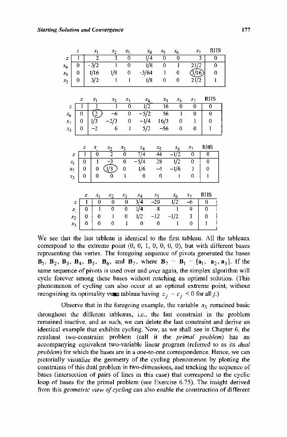
Starting Solution and Convergence 177
z
*6
*5
*3
z 1 0 0 0
x\ 2
-3/2 1/16 3/2
*2 -3
1 -1/8
-1
*3 0 0 0 1
x4
-1/4 1/8
-3/64 -1/8
x5 0 0 1 0
x6 0 1 0 0
X-j
3 -21/2 (5/16) 21/2
RHS 0 0 0 1
z
*6 x7
x3
z 1 0 0 0
X,
1
(2) 1/3 -2
x2 -1 -6
-2/3 6
x3 0 0 0 1
xA 1/2
-5/2 -1/4
5/2
x5 -16
56 16/3 -56
H 0 1 0 0
x7 0 0 1 0
RHS 0 0 0 1
z x\ x7
x3
z 1 0 0 0
X[ X2 X3
0 2 0 1 -3 0 0 (ί/Γ) 0 0 0 1
x4
7/4 -5/4
1/6 0
x5
-M 28
0
x6 -1/2
1/2 -1/6
1
x7
0 0 1 0
RHS 0 0 0 1
z xi x2
x3
z 1 0 0 0
xl 0 1 0 0
x2 0 0 1 0
*3 0 0 0 1
X^
3/4 1/4 1/2
0
x5 -20
-8 -12
0
H 1/2 -1
-1/2 1
*7 -6 9 3 0
RHS 0 0 0 1
We see that the last tableau is identical to the first tableau. All the tableaux correspond to the extreme point (0, 0, 1,0, 0, 0, 0), but with different bases representing this vertex. The foregoing sequence of pivots generated the bases B], B2 , B3, B 4 , B5, B6 , and B7, where B7 = Bj = [al5 a2, a3]. If the
same sequence of pivots is used over and over again, the simplex algorithm will cycle forever among these bases without reaching an optimal solution. (This phenomenon of cycling can also occur at an optimal extreme point, without recognizing its optimality via» tableau having z - c ■ < 0 for ally.)
Observe that in the foregoing example, the variable x3 remained basic
throughout the different tableaux, i.e., the last constraint in the problem remained inactive, and as such, we can delete the last constraint and derive an identical example that exhibits cycling. Now, as we shall see in Chapter 6, the resultant two-constraint problem (call it the primal problem) has an accompanying equivalent two-variable linear program (referred to as its dual problem) for which the bases are in a one-to-one correspondence. Hence, we can pictorially visualize the geometry of the cycling phenomenon by plotting the constraints of this dual problem in two-dimensions, and tracking the sequence of bases (intersection of pairs of lines in this case) that correspond to the cyclic loop of bases for the primal problem (see Exercise 6.75). The insight derived from this geometric view of cycling can also enable the construction of different
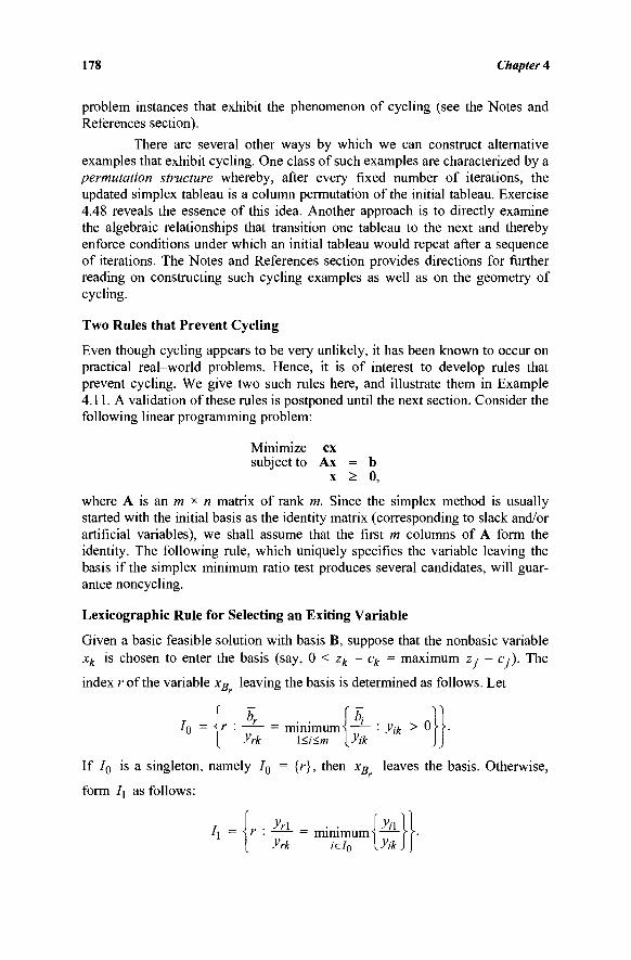
178 Chapter 4
problem instances that exhibit the phenomenon of cycling (see the Notes and References section).
There are several other ways by which we can construct alternative examples that exhibit cycling. One class of such examples are characterized by a permutation structure whereby, after every fixed number of iterations, the updated simplex tableau is a column permutation of the initial tableau. Exercise 4.48 reveals the essence of this idea. Another approach is to directly examine the algebraic relationships that transition one tableau to the next and thereby enforce conditions under which an initial tableau would repeat after a sequence of iterations. The Notes and References section provides directions for further reading on constructing such cycling examples as well as on the geometry of cycling.
Two Rules that Prevent Cycling
Even though cycling appears to be very unlikely, it has been known to occur on practical real-world problems. Hence, it is of interest to develop rules that prevent cycling. We give two such rules here, and illustrate them in Example 4.11. A validation of these rules is postponed until the next section. Consider the following linear programming problem:
Minimize ex subject to Ax = b
x > 0,
where A is an m χ η matrix of rank m. Since the simplex method is usually started with the initial basis as the identity matrix (corresponding to slack and/or artificial variables), we shall assume that the first m columns of A form the identity. The following rule, which uniquely specifies the variable leaving the basis if the simplex minimum ratio test produces several candidates, will guar-antee noncycling.
Lexicographic Rule for Selecting an Exiting Variable
Given a basic feasible solution with basis B, suppose that the nonbasic variable xk is chosen to enter the basis (say, 0 < zk - ck = maximum z ■ - c,·). The
index r of the variable xB leaving the basis is determined as follows. Let
Λ) = \ r '■ ~f- = minimumj-7- : y^ > °f f· [ yrk \<i<m [yik JJ
If IQ is a singleton, namely 70 = lrh m e n XB l e a v e s the basis. Otherwise,
form /] as follows:
T - \, ■ yn _ · · J ^ i l l l\ - \r . minimumi ft-[ yrk «e/0 {yik])
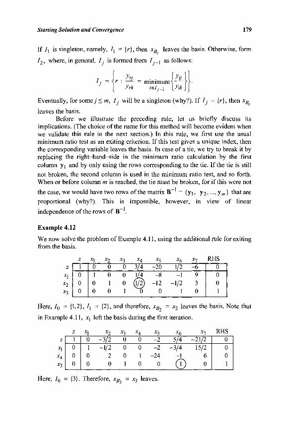
Starting Solution and Convergence 179
If /j is singleton, namely, /[ = {r}, then xB leaves the basis. Otherwise, form
I2, where, in general, / is formed from / _j as follows:
/ - i , · yV - ■ ■ i ^ ' l l J, - \r . minimumi >>■ J [ yrk ieij.i [yuc\\
Eventually, for somey < m, Ij will be a singleton (why?). If I j = {r}, then xB
leaves the basis. Before we illustrate the preceding rule, let us briefly discuss its
implications. (The choice of the name for this method will become evident when we validate this rule in the next section.) In this rule, we first use the usual minimum ratio test as an exiting criterion. If this test gives a unique index, then the corresponding variable leaves the basis. In case of a tie, we try to break it by replacing the right-hand-side in the minimum ratio calculation by the first column y\ and by only using the rows corresponding to the tie. If the tie is still
not broken, the second column is used in the minimum ratio test, and so forth. When or before column m is reached, the tie must be broken, for if this were not
the case, we would have two rows of the matrix B~ = (yx, y2, —,ym) that are
proportional (why?). This is impossible, however, in view of linear
independence of the rows of B~ .
Example 4.12
We now solve the problem of Example 4.11, using the additional rule for exiting from the basis.
Z ΧΛ XJ X3 ΧΛ Χς XA ΧΊ RHS 1 0 0 0
0 1 0 0
0 0 1 0
0 0 0 1
3/4 1/4
(1/2) 0
-20 -8
-12 0
1/2 -1
-1/2 1
-6 9 3 0
0 0 0 1
Here, I0 = {1,2}, Ιλ = {2}, and therefore, xB = x2 leaves the basis. Note that
in Example 4.11, x\ left the basis during the first iteration.
Z JCj X2 -£3 Xif X5 Xfr Xj RHS 1 0 0 0
0 1 0 0
-3/2 -1/2
2 0
0 0 0 1
0 0 1 0
-2 -2
-24 0
5/4 -3/4
-1
(1)
-21/2 15/2
6 0
0 0 0 1
Here, I0 = {3}. Therefore, xB = x3 leaves.
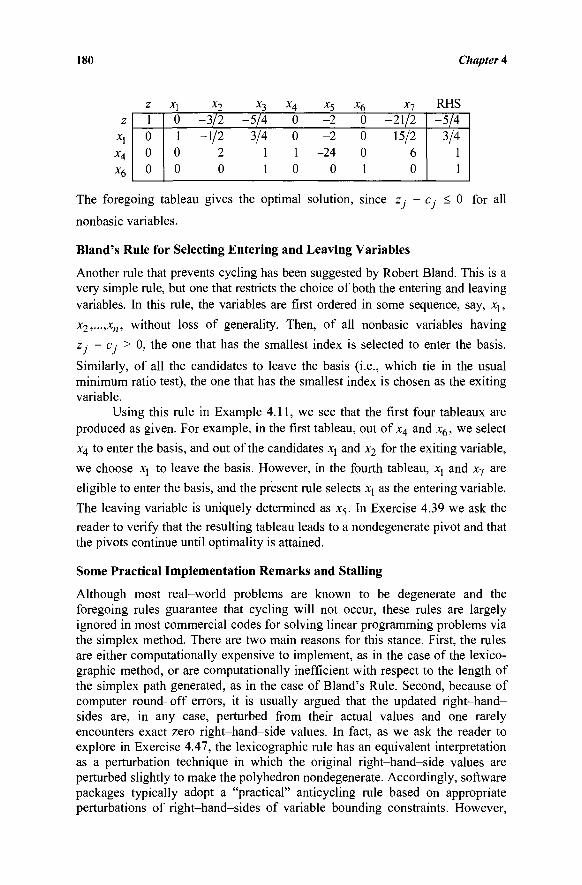
180 Chapter 4
Z X| X2 X3 X4 X5 Xf, Χη RHS 1 0 0 0
0 1 0 0
-3/2 -1/2
2 0
-5/4 3/4
1 1
0 0 1 0
-2 -2
-24 0
0 0 0 1
-21/2 15/2
6 0
-5/4 3/4
1 1
The foregoing tableau gives the optimal solution, since z .· - c .■ < 0 for all
nonbasic variables.
Bland's Rule for Selecting Entering and Leaving Variables
Another rule that prevents cycling has been suggested by Robert Bland. This is a very simple rule, but one that restricts the choice of both the entering and leaving variables. In this rule, the variables are first ordered in some sequence, say, x1?
x2,...,x„, without loss of generality. Then, of all nonbasic variables having z. - Cj > 0, the one that has the smallest index is selected to enter the basis.
Similarly, of all the candidates to leave the basis (i.e., which tie in the usual minimum ratio test), the one that has the smallest index is chosen as the exiting variable.
Using this rule in Example 4.11, we see that the first four tableaux are produced as given. For example, in the first tableau, out of x4 and x6, we select
x4 to enter the basis, and out of the candidates X\ and x2 for the exiting variable,
we choose xy to leave the basis. However, in the fourth tableau, X| and x7 are
eligible to enter the basis, and the present rule selects Xj as the entering variable.
The leaving variable is uniquely determined as x5. In Exercise 4.39 we ask the
reader to verify that the resulting tableau leads to a nondegenerate pivot and that the pivots continue until optimality is attained.
Some Practical Implementation Remarks and Stalling
Although most real-world problems are known to be degenerate and the foregoing rules guarantee that cycling will not occur, these rules are largely ignored in most commercial codes for solving linear programming problems via the simplex method. There are two main reasons for this stance. First, the rules are either computationally expensive to implement, as in the case of the lexico-graphic method, or are computationally inefficient with respect to the length of the simplex path generated, as in the case of Bland's Rule. Second, because of computer round-off errors, it is usually argued that the updated right-hand-sides are, in any case, perturbed from their actual values and one rarely encounters exact zero right-hand-side values. In fact, as we ask the reader to explore in Exercise 4.47, the lexicographic rule has an equivalent interpretation as a perturbation technique in which the original right-hand-side values are perturbed slightly to make the polyhedron nondegenerate. Accordingly, software packages typically adopt a "practical" anticycling rule based on appropriate perturbations of right-hand-sides of variable bounding constraints. However,
Starting Solution and Convergence 181
this is not guaranteed to obviate cycling (see the Notes and References section). It is important to note here that in the case of network structured linear programs, as we shall see later, neither of the foregoing reasons apply; however, cycling prevention rules are both easy to implement and are often computationally advantageous in this context.
There is another issue that needs to be mentioned at this point. Although the foregoing rules prevent cycling, it is entirely possible that the simplex algorithm may go through an exceedingly long (though finite) sequence of degenerate pivots. In particular, for some classes of problems having a certain structure, it may be possible that the algorithm performs a number of consecu-tive degenerate pivots that are exponential in the size (m and n) of the problem. This phenomenon is known as stalling. The term arises because with increasing problem size, the algorithm can spend an enormous (though finite) amount of time at a degenerate vertex before finally verifying optimality or moving off from that vertex. Besides preventing cycling, we would also like to obviate stalling by ensuring that the length of a sequence of degenerate pivots is bounded from above by some polynomial in m and n.
The key to preventing stalling appears to lie in what are known as stages. A stage is a sequence of degenerate pivots in which no nonbasic variable remains enterable throughout, with no strict subset of this sequence having the same property. We would like both the number of pivots in a stage, which is the length of a stage, and the number of stages in a sequence of degenerate pivots to be "small," that is, polynomially bounded. The first of these two conditions is easy to achieve. For example, consider the following rule for choosing an entering variable, which is sometimes referred to as the Least Recently Considered (LRC) variable choice rule. Suppose that we maintain a circular list of the variables and at any pivot, if a variable xk enters, then
suppose that the next entering variable is selected as the first eligible candidate (with zj - Cj > 0) from the list {xk+\,...,xn, x\,...,xk) where xn+l = JCJ. Then it
is clear that the length of a stage is no more than n, since no variable could have remained enterable and have been ignored throughout a sequence of n (or more) degenerate pivots. Such a rule, by its nature, is aptly called an affirmative action policy. Note that Bland's Rule is not an affirmative action strategy, since it "discriminates" in favor of variables having lower indices. In fact, there exist examples that demonstrate that Bland's Rule admits stalling (see the Notes and References section of this chapter). On the other hand, it is an open question whether the lexicographic rule plus Dantzig's Rule of entering the variable having the most positive z - c admits or prevents stalling for general linear
programs. (For network structured problems, this is known to prevent stalling.) The issue of ensuring a polynomial bound on the number of stages in a
sequence of degenerate pivots is harder to achieve. For general linear program-ming problems, a rule that provides such a guarantee has not as yet been discovered. However, as we shall see in Chapter 9, for network structured problems, a lexicographic cycling prevention rule does exist that is easy to implement, is computationally advantageous, and that prevents stalling when used in conjunction with an appropriate affirmative action entering rule.
182 Chapter 4
4.7 VALIDATION OF CYCLING PREVENTION RULES
In this section we show that the rules adopted in the previous section indeed prevent cycling. We do this by showing that none of the previous bases visited by the simplex method are repeated. In view of the finite number of bases, this automatically guarantees termination in a finite number of iterations. Lexicographic Rule In order to facilitate the proof of finite convergence under the lexicographic rule, consider the following notion of a lexicographically positive vector. A vector x is called lexicographically positive (denoted by x >- 0) if the following two require-ments hold:
1. x is not identically zero. 2. The first nonzero component of x is positive.
For example, (0, 2, - 1 , 3), (2, 1, - 3 , 1), and (0, 0, 1, -1) are lexicographically positive vectors, whereas ( -1 , 1,2, 3), (0, 0, 0, 0), and (0, 0, -2 , 1) are not. A lexicographically nonnegative vector, denoted by > 0, is either the zero vector or else a lexicographically positive vector. In order to prove that none of the bases generated by the simplex method is repeated, we first show that each row
of the m x (m + 1) matrix (b, B~ ) is lexicographically positive at each iteration,
where b = B~ b. Basic feasible solutions that satisfy this property are sometimes called strongly feasible solutions. Indeed, in the absence of degeneracy, we have
b > 0, and therefore, each row (b, B~ ) is clearly lexicographically positive.
First, recall that the original basis is I, and since b > 0, then each row of
the matrix (b, B~ ) = (b, I) is lexicographically positive. (If a feasible basis that
is different from the identity is available, we still have a starting solution that satisfies the lexicographic positive condition — see Exercise 4.41.) In view of this, the preceding result will be proved if we can show the following: If each
row of (b, B~ ) is >- 0, then each row of (b, B~ ) is >- 0 where B is the new
basis obtained after pivoting and b = B~ b. Consider the following two tableaux before and after entering xk, and recall that the first m columns (ignoring the z
column) in these tableaux represent B~ and B~ , respectively (since the first m columns of the original problem form the identity). Here, z denotes the objective value c#b before pivoting.
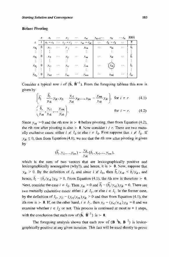
Starting Solution and Convergence 183
Before Pivoting
z
*? XB>
*B,
XB
Z
1
0
0
0
0
x\ 2 \ ~ c \ ■
y\\
Λ·ι
yr\
ym\ ■
■ XJ ■
■ ZJ ~ CJ ■
■ y\j ■
■ yy ■
■ yrj ■
ymj
xm zm ~ cm
y\m
yim
yrm
ymm
xm +1 " "" xk '"xn zk - c k ■■■
y\k
yjk
■ © ■■·
ymk
RHS
z
h
k
br
K
i-U Consider a typical row i of (b, B ). From the foregoing tableau this row is
given by
yrk
\yrk yrk
yik^i\
yrm
'""' yrk
yr\
yrk -yik'-->yim
yrm
yrk ■yik
\
for i Φ r
for / = r.
(4.1)
(4.2)
/
Since yrk > 0 and the rth row is >- 0 before pivoting, then from Equation (4.2),
the rth row after pivoting is also >■ 0. Now consider / Φ r. There are two mutu-
ally exclusive cases: either / g 70 or else / e 70. First suppose that i 0 IQ. If
yik < 0, then from Equation (4.1), we see that the rth row after pivoting is given
by
(bj,yiU...,yim) - ^(br,yrU...,yrm), yrk
which is the sum of two vectors that are lexicographically positive and lexicographically nonnegative (why?), and hence, it is >- 0. Now, suppose that
yij( > 0. By the definition of 70 a n d since / 0 70, then brlyrk < b^ly^, and
hence, bj - {brlyrk)yik > 0· From Equation (4.1), the rth row is therefore >- 0.
Next, consider the case i e 70. Then yik > 0 and bj - (brlyrk)yii<: = 0. There are
two mutually exhaustive cases: either i 0 I\, or else i e 7j. In the former case,
by the definition of I\, yn - {yr\lyrk)yìk > 0 an^ m u s from Equation (4.1), the
rth row is >- 0. If, on the other hand, / e Ιχ, then yn - {yr\lyrk)yìk = 0 and we
examine whether / e 72 or not. This process is continued at most m + 1 steps,
with the conclusion that each row of(b , B _ 1 ) is y 0.
The foregoing analysis shows that each row of (B" 'b , B"1) is lexico-
graphically positive at any given iteration. This fact will be used shortly to prove
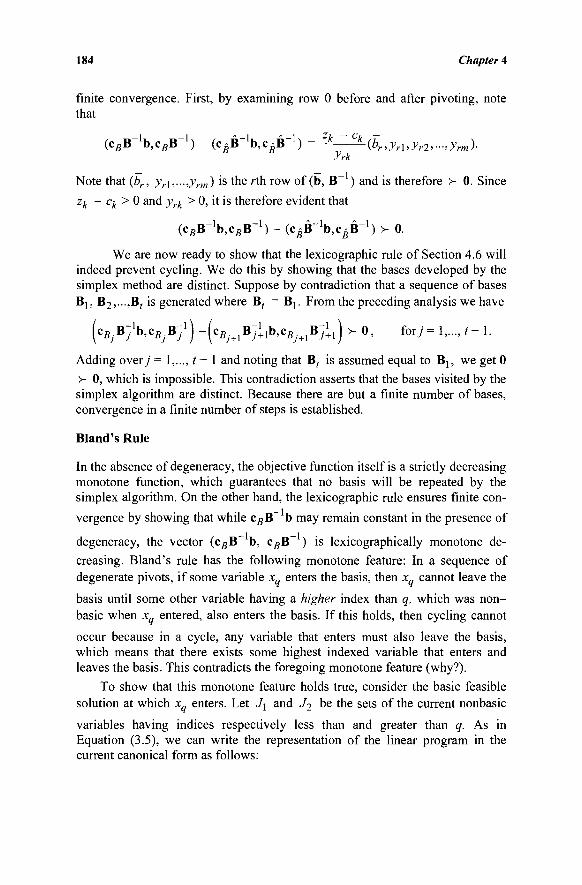
184 Chapter 4
finite convergence. First, by examining row 0 before and after pivoting, note that
( C J B - V B B - 1 ) - ( ( - B - V i - B - 1 ) = Zk ~Ck(br,yrUyr2,...,yrm). yrk
Note that {br, yr\,—,yrm) is the rth row of (b, B~ ) and is therefore >- 0. Since zk " ck > 0 and yrk > 0, it is therefore evident that
(cgB-'b.CgB-1) - ( c ^ b ^ B - 1 ) >- 0.
We are now ready to show that the lexicographic rule of Section 4.6 will indeed prevent cycling. We do this by showing that the bases developed by the simplex method are distinct. Suppose by contradiction that a sequence of bases B], B2,...,Br is generated where B, = B). From the preceding analysis we have
icB.B-\cBjBY) -{cBj+lBf+1b,cBj+lBY+l} y 0, for/= 1,..., * - 1.
Adding overy = 1,..., / - 1 and noting that B, is assumed equal to Bj, we get 0
>- 0, which is impossible. This contradiction asserts that the bases visited by the simplex algorithm are distinct. Because there are but a finite number of bases, convergence in a finite number of steps is established.
Bland's Rule
In the absence of degeneracy, the objective function itself is a strictly decreasing monotone function, which guarantees that no basis will be repeated by the simplex algorithm. On the other hand, the lexicographic rule ensures finite con-vergence by showing that while CgB~ b may remain constant in the presence of
degeneracy, the vector (cgB~ b, cgB~ ) is lexicographically monotone de-creasing. Bland's rule has the following monotone feature: In a sequence of degenerate pivots, if some variable xq enters the basis, then x„ cannot leave the
basis until some other variable having a higher index than q, which was non-basic when xq entered, also enters the basis. If this holds, then cycling cannot
occur because in a cycle, any variable that enters must also leave the basis, which means that there exists some highest indexed variable that enters and leaves the basis. This contradicts the foregoing monotone feature (why?).
To show that this monotone feature holds true, consider the basic feasible solution at which x„ enters. Let Jj and J2
De t n e sets of the current nonbasic
variables having indices respectively less than and greater than q. As in Equation (3.5), we can write the representation of the linear program in the current canonical form as follows:
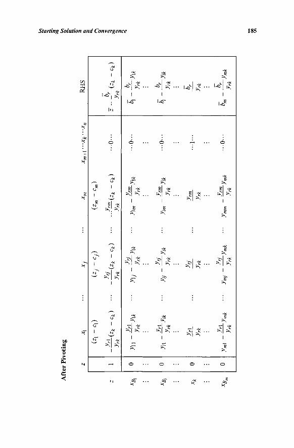
Starting Solution and Convergence 185
en
o
> fi i .
c
■Jl
c « -V K
~ ε H
S H
H
N
—* s I S
^ υ"1
1
N
^ <T 1
-* 1
'-Hk 1
IN
ό
1 -V N
1
9 1
N
* l is 1
1
•—1 -v
*k 1
-
i ^
1
©
-4s
iS
1 *.. 1 1
s
»s
ί| 3 -1
i \
vl -*
*k.. 1 is
o
•44
Ss
1 i<r
©
is
. 1 .. 1 1
ε is
is 'M is
■ i s | is ·· 1 ss
•V
i s T"l -4i
. *k.. 1 is
o
'*H 3 ··
"Γ
!| is ·· J\1 is
"ol IS .. i s | pi:
T| IS .. i s | i s
o
E iS
1
l<>£
Ó
-ΐ
ÌSS
il ί 1 1
ε s
δ
'c-l IS =M is
1
i s
δ
— 1 -ie
1
©
«3 ί
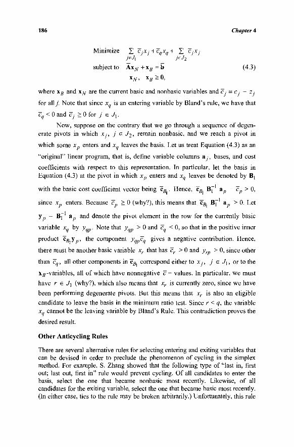
186 Chapter 4
Minimize Σ cjxj+cqxq+ Σ c.-x.-
subject to Ax^ + xB = b (4.3)
X iV> XB — ^>
where xB and xN are the current basic and nonbasic variables and c ■ = c, - z,
for ally. Note that since xq is an entering variable by Bland's rule, we have that
c' < 0 and c · > 0 for j e J j .
Now, suppose on the contrary that we go through a sequence of degen-erate pivots in which x-, j e J2, remain nonbasic, and we reach a pivot in
which some x„ enters and x„ leaves the basis. Let us treat Equation (4.3) as an
"original" linear program, that is, define variable columns a ·, bases, and cost
coefficients with respect to this representation. In particular, let the basis in Equation (4.3) at the pivot in which x„ enters and xq leaves be denoted by Bj
with the basic cost coefficient vector being ΈΒ . Hence, Cg Bj~ a - c > 0,
since xp enters. Because c" > 0 (why?), this means that cB Bf &p > 0. Let
y „ = Bf a and denote the pivot element in the row for the currently basic
variable xq by y . Note that y > 0 and c < 0, so that in the positive inner
product CD y„ , the component yqpCq gives a negative contribution. Hence,
there must be another basic variable xr that has cr > 0 and y > 0, since other
than ZL, all other components in cg correspond either to x ■, j e Jx, or to the
xg-variables, all of which have nonnegative Έ— values. In particular, we must
have r e Jj (why?), which also means that xr is currently zero, since we have
been performing degenerate pivots. But this means that xr is also an eligible
candidate to leave the basis in the minimum ratio test. Since r < q, the variable
xq cannot be the leaving variable by Bland's Rule. This contradiction proves the
desired result.
Other Anticycling Rules
There are several alternative rules for selecting entering and exiting variables that can be devised in order to preclude the phenomenon of cycling in the simplex method. For example, S. Zhang showed that the following type of "last in, first out; last out, first in" rule would prevent cycling. Of all candidates to enter the basis, select the one that became nonbasic most recently. Likewise, of all candidates for the exiting variable, select the one that became basic most recently. (In either case, ties to the rule may be broken arbitrarily.) Unfortunately, this rule
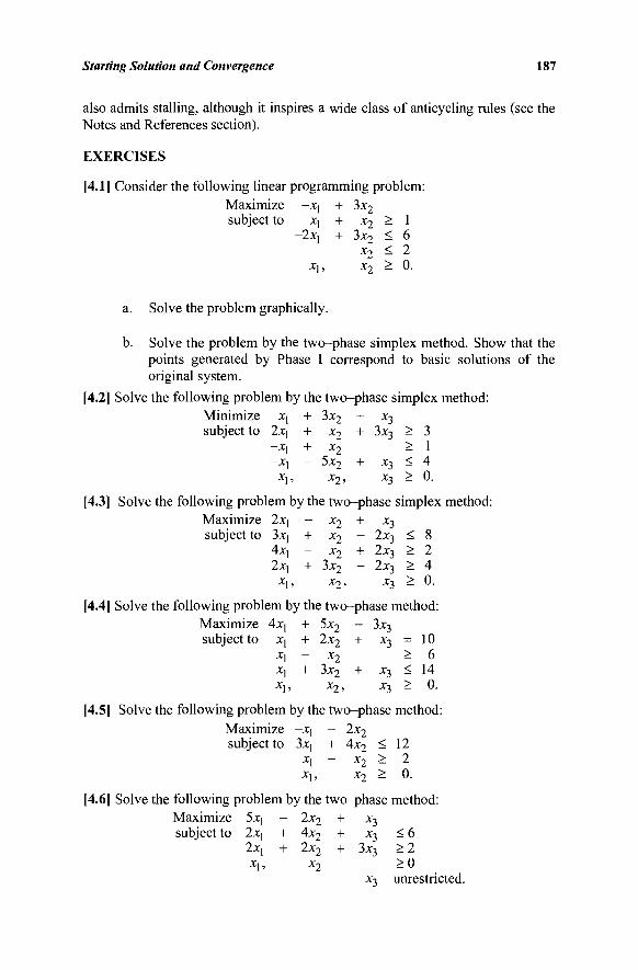
Starting Solution and Convergence 187
also admits stalling, although it inspires a wide class of anticycling rules (see the Notes and References section).
EXERCISES
[4.1] Consider the following linear programming problem: Maximize -xj + 3x2 subject to xj + x2 > 1
-2x\ + 3x2 < 6 x2 < 2
Xj, x2 - 0·
a. Solve the problem graphically.
b. Solve the problem by the two-phase simplex method. Show that the points generated by Phase I correspond to basic solutions of the original system.
[4.2] Solve the following problem by the two-phase simplex method: Minimize xj + 3x2 ~ *3 subject to 2x] + x2 + 3x3 > 3
-Xj + x2 > 1 -X[ - 5x2 + x3 < 4
X\, Χ 2 , Χ3 ^ t).
[4.3] Solve the following problem by the two-phase simplex method: Maximize 2xt - x2 + x3
subject to 3xj + x2 - 2x3 < 8 4xj - x2 + 2x3 > 2 2xj + 3x2 - 2x3 > 4
X\, X 2 , X3 ^ ϋ .
[4.4] Solve the following problem by the two-phase method: Maximize 4x, + 5x2 - 3x3
subject to X] + 2x2 + x3 = 10 X] - x2 > 6 Xj + 3x2 + x3 < 14 X], x2, x3 ^ 0.
[4.5] Solve the following problem by the two-phase method: Maximize -Xj - 2x2
subject to 3xj + 4x2 < 12 X] - x2 > 2 Xj, x2 > 0.
[4.6] Solve the following problem by the two-phase method: Maximize 5xj - 2x2 + x3
subject to 2x] + 4x2 + x3 < 6 2xj + 2x2 + 3x3 > 2 χ\, x2 > 0
x3 unrestricted.
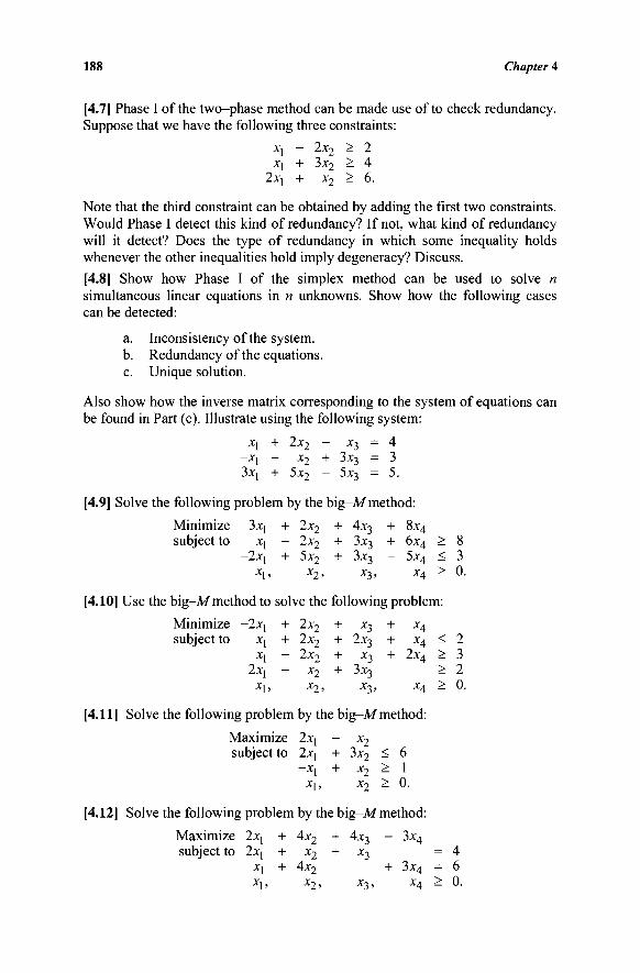
188 Chapter 4
[4.7] Phase I of the two-phase method can be made use of to check redundancy. Suppose that we have the following three constraints:
Xj - 2x2 > 2 xx + 3x2 > 4
2*1 + x2 > 6.
Note that the third constraint can be obtained by adding the first two constraints. Would Phase I detect this kind of redundancy? If not, what kind of redundancy will it detect? Does the type of redundancy in which some inequality holds whenever the other inequalities hold imply degeneracy? Discuss.
[4.8] Show how Phase I of the simplex method can be used to solve n simultaneous linear equations in n unknowns. Show how the following cases can be detected:
a. Inconsistency of the system. b. Redundancy of the equations. c. Unique solution.
Also show how the inverse matrix corresponding to the system of equations can be found in Part (c). Illustrate using the following system:
X\ + 2x2 - x3 = 4 ~X\ — X2 ~t" 3x3
= 3 3xj + 5x2 - 5x3 = 5.
[4.9] Solve the following problem by the b ig-M method:
Minimize 3x[ + 2x2 + 4x3 + 8x4
subject to xj - 2x2 + 3x3 + 6x4 > 8 -2x[ + 5x2 + 3x3 - 5x4 < 3
Xj, x2 , x3, x4 > 0.
[4.10] Use the b ig-M method to solve the following problem:
Minimize -2x[ + 2x2 + x3 + x4
subject to xj + 2x2 + 2x3 + x4 < 2 Xj - 2 x 2 + x 3 + 2 x 4 > 3
2x[ - x 2 + 3x3 > 2 X\, X2, X3, X4 ^ 0.
[4.11] Solve the following problem by the b ig-M method:
Maximize 2xj - x2
subject to 2*i + 3x2 < 6 -Xj + x2 > 1
Xj, x2 > 0.
[4.12] Solve the following problem by the b ig-M method:
Maximize 2xj + 4x2 + 4x3 - 3x4
subject to 2xj + x2 + x3 = 4 x\ + 4 x 2 + 3x 4 = 6 Xj, x 2 , x 3 , x 4 > 0.
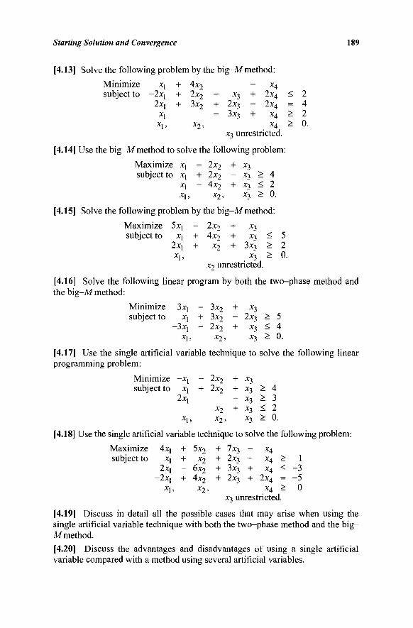
Starting Solution and Convergence 189
[4.13] Solve the following problem by the big-M method:
Minimize X| + 4x2 _ *4
subject to -2*1 + 2x2 - X3 + 2x4 < 2 2xj + 3x2 + 2x3 - 2x4 = 4
xj - 3x3 + x4 > 2 x\, x2, x4 > 0.
x3 unrestricted.
[4.14] Use the big-M method to solve the following problem:
Maximize xj - 2x2 + X3 subject to X] + 2x2 - x3 > 4
x\ ~ 4x2 + x3 < 2 X i , x 2 , Χ3 ^ 0.
[4.15] Solve the following problem by the big-M method:
Maximize 5xj - 2x2 + X3 subject to xj + 4x2 + x3 < 5
2xj + x2 + 3x3 > 2 Χγ, Χ3 - 0·
x2 unrestricted.
[4.16] Solve the following linear program by both the two-phase method and the big-M method:
Minimize 3xj - 3x2 + X3 subject to xi + 3x2 - 2x3 > 5
-3xt - 2x2 + x3 < 4 Xj, x2, X3 > 0.
[4.17] Use the single artificial variable technique to solve the following linear programming problem:
Minimize -X] - 2x2 + x3 subject to Xj + 2x2 + X3 > 4
2xj - x3 > 3 x2 + x3 < 2
Xj , X 2 , X3 ^ 0.
[4.18] Use the single artificial variable technique to solve the following problem:
Maximize 4x] + 5x2 + 7x3 - x4 subject to Xj + x2 + 2x3 - x4 > 1
2XJ - 6x2 + 3x3 + x4 < -3 -2xj + 4x2 + 2x3 + 2x4 = -5
Xj, x2, x4 ^ 0 x3 unrestricted.
[4.19] Discuss in detail all the possible cases that may arise when using the single artificial variable technique with both the two-phase method and the big-M method.
[4.20] Discuss the advantages and disadvantages of using a single artificial variable compared with a method using several artificial variables.
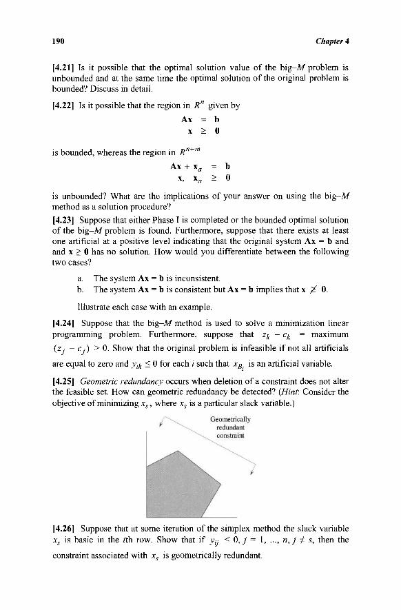
190 Chapter 4
[4.21] Is it possible that the optimal solution value of the big-M problem is unbounded and at the same time the optimal solution of the original problem is bounded? Discuss in detail.
[4.22] Is it possible that the region in R" given by
Ax = b x > 0
is bounded, whereas the region in Rn+m
Ax + xa = b x, xa > 0
is unbounded? What are the implications of your answer on using the big-M method as a solution procedure?
[4.23] Suppose that either Phase I is completed or the bounded optimal solution of the big-M problem is found. Furthermore, suppose that there exists at least one artificial at a positive level indicating that the original system Ax = b and and x > 0 has no solution. How would you differentiate between the following two cases?
a. The system Ax = b is inconsistent. b. The system Ax = b is consistent but Ax = b implies that x X 0.
Illustrate each case with an example.
[4.24] Suppose that the big-M method is used to solve a minimization linear programming problem. Furthermore, suppose that zk - ck = maximum
(z. - c ·) > 0. Show that the original problem is infeasible if not all artificials
are equal to zero and y^ < 0 for each i such that xB. is an artificial variable.
[4.25] Geometric redundancy occurs when deletion of a constraint does not alter the feasible set. How can geometric redundancy be detected? (Hint: Consider the objective of minimizing xs, where xs is a particular slack variable.)
[4.26] Suppose that at some iteration of the simplex method the slack variable xs is basic in the rth row. Show that if y^ < 0, j = 1, ..., n, j Φ s, then the
constraint associated with x is geometrically redundant.
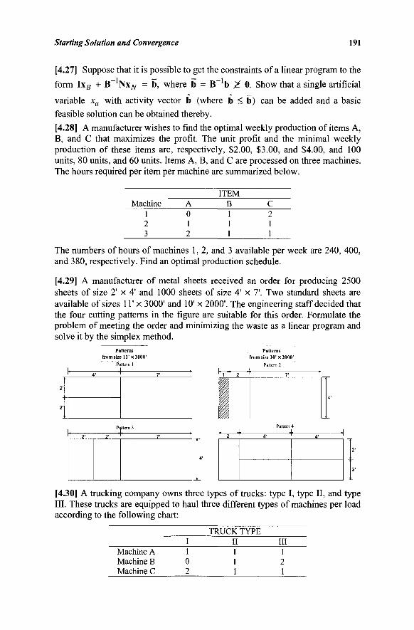
Starting Solution and Convergence 191
[4.27] Suppose that it is possible to get the constraints of a linear program to the i - l -U form \\B + B Nxjy = b, where b = B b ^ 0. Show that a single artificial
variable xa with activity vector b (where b < b) can be added and a basic
feasible solution can be obtained thereby.
[4.28] A manufacturer wishes to find the optimal weekly production of items A, B, and C that maximizes the profit. The unit profit and the minimal weekly production of these items are, respectively, $2.00, $3.00, and $4.00, and 100 units, 80 units, and 60 units. Items A, B, and C are processed on three machines. The hours required per item per machine are summarized below.
ITEM Machine
1 2 3
A 0 1 2
B 1 1 1
C 2 1 1
The numbers of hours of machines 1, 2, and 3 available per week are 240, 400, and 380, respectively. Find an optimal production schedule.
[4.29] A manufacturer of metal sheets received an order for producing 2500 sheets of size 2' x 4' and 1000 sheets of size 4' x 7'. Two standard sheets are available of sizes 1Γ x 3000' and 10' x 2000'. The engineering staff decided that the four cutting patterns in the figure are suitable for this order. Formulate the problem of meeting the order and minimizing the waste as a linear program and solve it by the simplex method.
Patterns from size 11' X 3000'
Pattern 1
+
Patterns from size 10'X 2000'
Pattern 2
I ' r l · z 'I' r "I
H^ ? + Ϊ ^
[4.30] A trucking company owns three types of trucks: type I, type II, and type III. These trucks are equipped to haul three different types of machines per load according to the following chart:
TRUCK TYPE I II III
Machine A Machine B Machine C
1 0 2
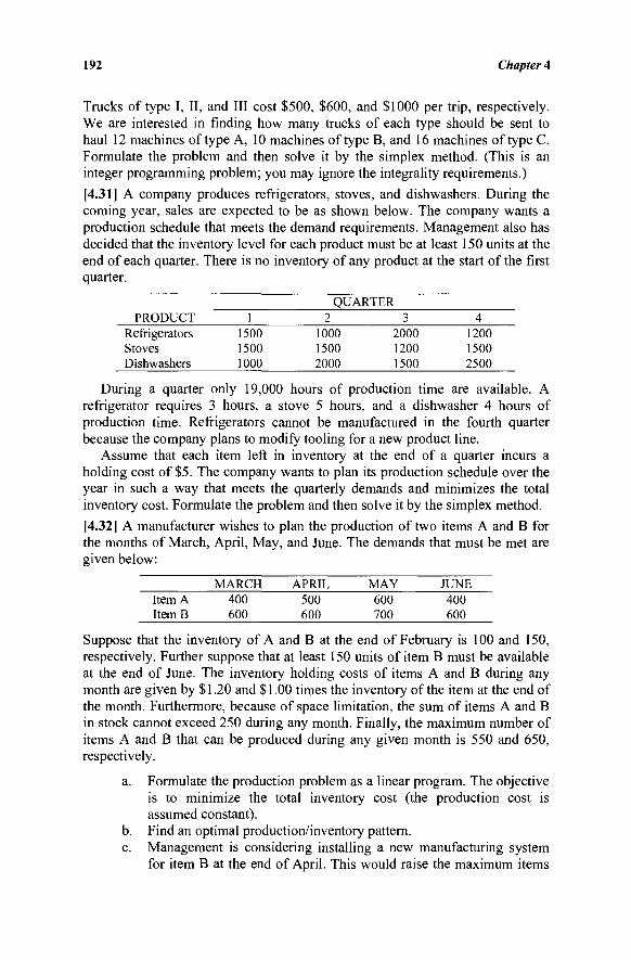
192 Chapter 4
Trucks of type I, II, and III cost $500, $600, and $1000 per trip, respectively. We are interested in finding how many trucks of each type should be sent to haul 12 machines of type A, 10 machines of type B, and 16 machines of type C. Formulate the problem and then solve it by the simplex method. (This is an integer programming problem; you may ignore the integrality requirements.)
[4.31] A company produces refrigerators, stoves, and dishwashers. During the coming year, sales are expected to be as shown below. The company wants a production schedule that meets the demand requirements. Management also has decided that the inventory level for each product must be at least 150 units at the end of each quarter. There is no inventory of any product at the start of the first quarter.
QUARTER PRODUCT
Refrigerators Stoves Dishwashers
1 1500 1500 1000
2 1000 1500 2000
3 2000 1200 1500
4 1200 1500 2500
During a quarter only 19,000 hours of production time are available. A refrigerator requires 3 hours, a stove 5 hours, and a dishwasher 4 hours of production time. Refrigerators cannot be manufactured in the fourth quarter because the company plans to modify tooling for a new product line.
Assume that each item left in inventory at the end of a quarter incurs a holding cost of $5. The company wants to plan its production schedule over the year in such a way that meets the quarterly demands and minimizes the total inventory cost. Formulate the problem and then solve it by the simplex method.
[4.32] A manufacturer wishes to plan the production of two items A and B for the months of March, April, May, and June. The demands that must be met are given below:
Item A ItemB
MARCH 400 600
APRIL 500 600
MAY 600 700
JUNE 400 600
Suppose that the inventory of A and B at the end of February is 100 and 150, respectively. Further suppose that at least 150 units of item B must be available at the end of June. The inventory holding costs of items A and B during any month are given by $ 1.20 and $ 1.00 times the inventory of the item at the end of the month. Furthermore, because of space limitation, the sum of items A and B in stock cannot exceed 250 during any month. Finally, the maximum number of items A and B that can be produced during any given month is 550 and 650, respectively.
a. Formulate the production problem as a linear program. The objective is to minimize the total inventory cost (the production cost is assumed constant).
b. Find an optimal production/inventory pattern. c. Management is considering installing a new manufacturing system
for item B at the end of April. This would raise the maximum items
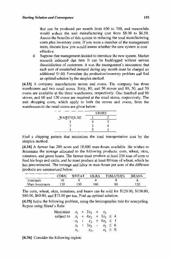
Starting Solution and Convergence 193
that can be produced per month from 650 to 700, and meanwhile would reduce the unit manufacturing cost from $8.00 to $6.50. Assess the benefits of this system in reducing the total manufacturing costs plus inventory costs. If you were a member of the management team, discuss how you would assess whether the new system is cost-effective.
d. Suppose that management decided to introduce the new system. Market research indicated that item B can be backlogged without serious dissatisfaction of customers. It was the management's assessment that each unit of unsatisfied demand during any month must be charged an additional $1.00. Formulate the production/inventory problem and find an optimal solution by the simplex method.
[4.33] A company manufactures stoves and ovens. The company has three warehouses and two retail stores. Sixty, 80, and 50 stoves and 80, 50, and 50 ovens are available at the three warehouses, respectively. One hundred and 90 stoves, and 60 and 120 ovens are required at the retail stores, respectively. The unit shopping costs, which apply to both the stoves and ovens, from the warehouses to the retail stores are given below:
STORE WAREHOUSE 1 2
1 4 5 2 2 4 3 5 3
Find a shipping pattern that minimizes the total transportation cost by the simplex method.
[4.34] A farmer has 200 acres and 18,000 man-hours available. He wishes to determine the acreage allocated to the following products: corn, wheat, okra, tomatoes, and green beans. The farmer must produce at least 250 tons of corn to feed his hogs and cattle, and he must produce at least 80 tons of wheat, which he has precontracted. The tonnage and labor in man-hours per acre of the different products are summarized below:
Tons/acre Man-hours/acre
CORN 10 120
WHEAT 4
150
OKRA 4
100
TOMATOES 8 80
BEANS 6
120
The corn, wheat, okra, tomatoes, and beans can be sold for $120.00, $150.00, $80.00, $60.00, and $75.00 per ton. Find an optimal solution.
[4.35] Solve the following problem, using the lexicographic rule for noncycling. Repeat using Bland's Rule:
Maximize xj + 2x2 + *3 subject to Χχ + 4x2 + 3x3 < 4
-jci + x2 + 4x3 < 1 x\ + 3x2 + x3 < 6 X], x 2 , x3 ^ 0.
[4.36] Consider the following region:
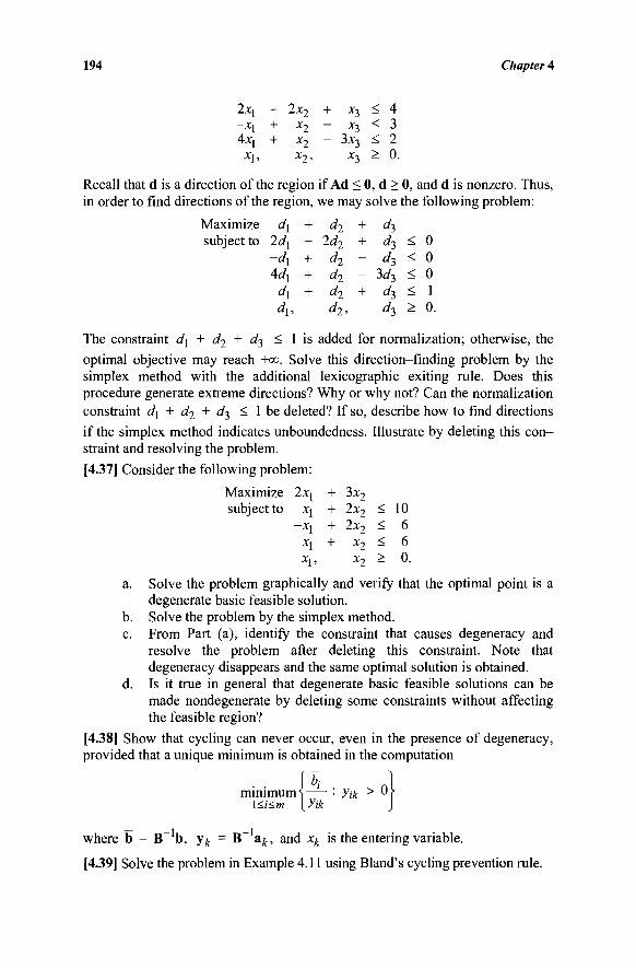
194 Chapter 4
2x| - 2x2 + X3 < 4 - X j + X2 - X3 < 3
4xj + x2 - 3x3 < 2 X i , x 2 5 -^3 — " ·
Recall that d is a direction of the region if Ad < 0, d > 0, and d is nonzero. Thus, in order to find directions of the region, we may solve the following problem:
Maximize c/j + d2 + c/3 subject to 2Ì/J - 2d2 + d$ < 0
-dx + d2 - d3 < 0 Adx + d2 - 3c/3 < 0
d\ + d2 + i/3 < 1 dy, d2, i/3 > 0.
The constraint d\ + d2 + <i3 < 1 is added for normalization; otherwise, the optimal objective may reach +co. Solve this direction-finding problem by the simplex method with the additional lexicographic exiting rule. Does this procedure generate extreme directions? Why or why not? Can the normalization constraint dx + d2 + c/3 < 1 be deleted? If so, describe how to find directions
if the simplex method indicates unboundedness. Illustrate by deleting this con-straint and resolving the problem.
[4.37] Consider the following problem:
Maximize 2xj + 3x2
subject to x\ + 2x2 < 10 -Xj + 2x2 < 6
Xj + x2 < 6 Xj, x2 > 0.
a. Solve the problem graphically and verify that the optimal point is a degenerate basic feasible solution.
b. Solve the problem by the simplex method. c. From Part (a), identify the constraint that causes degeneracy and
resolve the problem after deleting this constraint. Note that degeneracy disappears and the same optimal solution is obtained.
d. Is it true in general that degenerate basic feasible solutions can be made nondegenerate by deleting some constraints without affecting the feasible region?
[4.38] Show that cycling can never occur, even in the presence of degeneracy, provided that a unique minimum is obtained in the computation
m i n i m u m ^ — : y^ > 0> \<i<m [yik J
where b = B~ b, y^ = B~ a^, and xk is the entering variable.
[4.39] Solve the problem in Example 4.11 using Bland's cycling prevention rule.
Starting Solution and Convergence 195
[4.40] Suppose that we have an optimal extreme point of a minimization linear programming problem. In the presence of degeneracy, is it possible that this extreme point corresponds to a basic feasible solution such that z ■ - c .■ > 0 for at
least one nonbasic variable? If this were the case, are we guaranteed of another basic feasible solution corresponding to the same extreme point where z · - c <
0 for all nonbasic variables? Why or why not? Illustrate by a numerical example.
[4.41] In order to prove finite convergence of the simplex method using the lexicographic rule, we assumed that the first m columns of the constraint matrix form the identity. Show that this assumption can be relaxed provided that we have any basic feasible solution. (Hint: Let B be the starting basis and consider the following equivalent problem.)
Minimize 0xs + (c^ - cfiB~ N)xN
subject to Ixg + B_1NxAr = B"'b \B, xN > 0.
[4.42] We showed that the row vector (c#B~ b, cgB~ ) is lexicographically
decreasing from one iteration to another using the lexicographic rule. Give an
economic interpretation of this fact. (Hint: Note that z = c 5 B _ b and that
dz/db = cgB^].)
[4.43] LetX= {x: Ax = b, x > 0} be nonempty, where A is m χ η. Consider the preemptive priority multiple objective problem of maximizing q x over x e X,
and among all alternative optimal solutions, maximizing c2x, and among all
continuing alternative optimal solutions, maximizing c3x, and so on, until the
final problem of maximizing crx over continuing alternative optimal solutions.
Call any such resulting optimal solution x a preemptive optimal solution, and assume that one exists. Show that there exists a scalar MQ > 0 such that for any
M> MQ, a solution x* is a preemptive optimal solution if and only if it solves
the following problem:
Maximizes Σ Mr~'ci\ : x e X>.
[4.44] Suppose that a linear programming problem admits feasible points. Utilize the result of Exercise 4.43 to show that if Mis large enough, then a finite optimal solution of the big-M problem must have all artificials equal to zero. Give all details.
[4.45] Consider the linear programming problem to minimize ex subject to x e X = {x: Ax = b, x > 0}, where X is a nonempty, bounded polyhedral set in
R". Define 0X < θ2 <■·· < 9r as the distinct values taken on by ex over the
extreme points of X and let 5, be the set of extreme points of X for which the
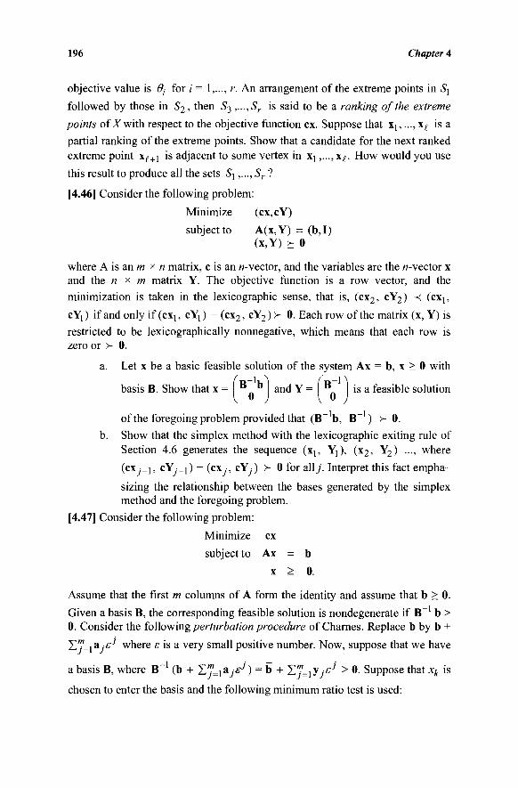
196 Chapter 4
objective value is 9i for i = 1,..., r. An arrangement of the extreme points in S\
followed by those in S2, then S^,...,Sr is said to be a ranking of the extreme
points of X with respect to the objective function ex. Suppose that \h...,\e is a
partial ranking of the extreme points. Show that a candidate for the next ranked
extreme point x i + 1 is adjacent to some vertex in Xj,..., xe. How would you use
this result to produce all the sets S\,..., Sr ?
[4.46] Consider the following problem:
Minimize (cx,cY)
subject to A(x,Y) = (b,I) (x,Y) > 0
where A is an m x n matrix, c is an «-vector, and the variables are the κ-vector x and the « x m matrix Y. The objective function is a row vector, and the
minimization is taken in the lexicographic sense, that is, (cx2, cY2) -< (exj,
cYj) if and only if (cxl5 cYi) - (cx2, cY2) >■ 0. Each row of the matrix (x, Y) is
restricted to be lexicographically nonnegative, which means that each row is zero or > 0.
a. Let x be a basic feasible solution of the system Ax = b, x > 0 with
basis B. Show that x = n and Y = " is a feasible solution
of the foregoing problem provided that (B~ b, B~ ) >- 0. b. Show that the simplex method with the lexicographic exiting rule of
Section 4.6 generates the sequence (xj, Yj), (x2, Y2) ..., where (cx,_i, cY,_!) - (ex ,·, cY.) >- 0 for ally. Interpret this fact empha-sizing the relationship between the bases generated by the simplex method and the foregoing problem.
[4.47] Consider the following problem:
Minimize ex
subject to Ax = b
x > 0.
Assume that the first m columns of A form the identity and assume that b > 0.
Given a basis B, the corresponding feasible solution is nondegenerate if B~ b > 0. Consider the following perturbation procedure of Charnes. Replace b by b +
Σ7=ι3/£''/ w n e r e ε is a very small positive number. Now, suppose that we have
a basis B, where B~' (b + ZJ= 1ay£7) = b + Σ"}^j£j > 0. Suppose that xk is
chosen to enter the basis and the following minimum ratio test is used:
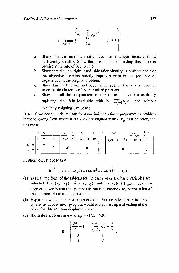
Starting Solution and Convergence 197
minimum \<i<m ytk
■ yik > °
a. Show that the minimum ratio occurs at a unique index r for a sufficiently small e Show that the method of finding this index is precisely the rule of Section 4.6.
b. Show that the new right-hand-side after pivoting is positive and that the objective function strictly improves even in the presence of degeneracy in the original problem.
c. Show that cycling will not occur if the rule in Part (a) is adopted. Interpret this in terms of the perturbed problem.
d. Show that all the computations can be carried out without explicitly
replacing the right-hand-side with b + Z 7 = i a / ^ an<i without
explicitly assigning a value to ε. [4.48] Consider an initial tableau for a maximization linear programming problem in the following form, where B is a 2 x 2 nonsingular matrix, cB is a 2-vector, and n is even:
z
xl
z
1
0
0
*i
0
1
0
*2
0
0
1
x3 x4
-CB
B
*5 *6
- c s ( I + B )
B2
*7 *8
- c „ ( I + B + B2)
B3
xn+\
-C S (I + B + B 2 +
*» + 2
•• + B2"1)
B2
RHS
0
0
0
Furthermore, suppose that
- + i -
B 2 =1 and -c B (I + B + B2 +··· + Β 2 ) = (0, 0).
(a) Display the form of the tableau for the cases when the basic variables are selected as (i) {x3, x4}; (ii) {x5, x6}, and finally, (iii) {xn+\, xn+2Ì- m
each case, verify that the updated tableau is a (block-wise) permutation of the columns of the initial tableau.
(b) Explain how the phenomenon observed in Part a can lead to an instance where the above linear program would cycle, starting and ending at the basic feasible solution displayed above.
(c) Illustrate Part b using n = 8, cB =(1/2,-7/20).
B 2
1 \2) 2
J_ 2
198 Chapter 4
and with the simplex cycle proceeding through the following closed loop of bases: {xu x2}, {x2, x^}, {*3> X4Ì> (x4> xs}> ix5> Χ(,},-·-Λχ9> XIO)>
{X], X\Q}, and back to {x^, x2}.
NOTES AND REFERENCES
1. The use of artificial variables to obtain a starting basic feasible solution was first published by Dantzig [1951a].
2. The single artificial variable technique of Section 4.5 can be viewed as the dual of a similar technique that adds a new row to obtain a starting basic dual feasible solution. The latter is discussed in Section 6.6. Com-putational results appear in Wolfe and Cutler [1963].
3. A general Phase I method in which the sum of infeasibilities is reduced without regard to the feasibility of individual variables has been sug-gested by Maros [1986].
4. The cycling example of Section 4.6 is due to Beale [1955]. The proof of the cycling prevention rule via lexicographic ordering was published by Dantzig, Orden, and Wolfe [1955]. The cycling prevention rule can also be interpreted as a perturbation technique, as briefly described in Exercise 4.47. This technique was independently devised by Charnes [1952].
5. Bland's cycling prevention rule [1977] is simple and elegant, although computationally unattractive. The notion of stages and an example of a network structured linear program for which Bland's rule admits stalling has been provided by Cunningham [1979]. The term "affirmative action" for entering variable selection strategies is from Fathi and Tovey [1986]. For stalling prevention in network flow problems using Dantzig's entering variable choice and the lexicographic cycling prevention rule, see Orlin [1985]. Marshall and Suurballe [1969] show that the smallest examples that can exhibit cycling have m = 2, n = 6, (n - ni) > 3, and cycle length equal to 6. Related results for network structured problems are studied by Cunningham [1979]. For a practical anticycling rule, see Gill et al. [1988]. Hall and McKinnon [2004] have shown, however, that this technique does not obviate cycling, using a class of simple examples. The LIFO (last-in-first-out) type of anticycling rule has been proposed by Zhang [1991], who also develops a wide class of cycling prevention rules that uphold certain consistent and well-preserved orderings of variable indices within the pivot rule.
6. The cycling examples based on a permutation structure as explained in Section 4.6 are due to Zornig [2008] (Exercise 4.48 provides some details of this concept based on this paper). Also, see Zornig [2006] for a discussion on constructing cycling examples using Dantzig's entry rule and the steepest edge entry rule (see Chapter 5) based on direct algebraic pivoting relationships. Lee [1997] illustrates the geometry in the requirement space (see Chapter 2) for the dual (see Chapter 6) to Hoffman's [1953] example of cycling. In fact, Hoffman's [1953] example
Starting Solution and Convergence 199
also conforms to the abovementioned permutation structure. Furthermore, Avis et al. [2008] discuss the geometry of cycling from the viewpoint of the sequence of bases for the dual problem (see Chapter 6 and Exercise 6.75) that correspond to the closed cyclic loop of bases in a given (primal) problem. This viewpoint also affords a mechanism for constructing examples that exhibit the phenomenon of cycling.
7. Exercise 4.43 addresses the notion of equivalent weights for preemptive priority multiple objective programs, as discussed in Sherali and Soyster [1983a] and in Sherali [1982].
8. Exercise 4.45 states the basic result of Murty [1968] used for ranking extreme points of polytopes. An alternative ranking technique appears in Sherali and Dickey [1986]. For the special case of ranking vertices of an assignment polytope, see Bazaraa and Sherali [1981]. Also, for related work on enumerating all vertices of polytopes, see Mattheiss [1973] and Mattheiss and Rubin [1980].

This page intentionally left blank
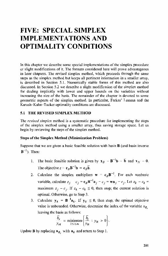
FIVE: SPECIAL SIMPLEX IMPLEMENTATIONS AND OPTIMALITY CONDITIONS
In this chapter we describe some special implementations of the simplex procedure or slight modifications of it. The formats considered here will prove advantageous in later chapters. The revised simplex method, which proceeds through the same steps as the simplex method but keeps all pertinent information in a smaller array, is described in Section 5.1. Numerically stable forms of this method are also discussed. In Section 5.2 we describe a slight modification of the simplex method for dealing implicitly with lower and upper bounds on the variables without increasing the size of the basis. The remainder of the chapter is devoted to some geometric aspects of the simplex method. In particular, Farkas' Lemma and the Karush-Kuhn-Tucker optimality conditions are discussed.
5.1 THE REVISED SIMPLEX METHOD
The revised simplex method is a systematic procedure for implementing the steps of the simplex method using a smaller array, thus saving storage space. Let us begin by reviewing the steps of the simplex method.
Steps of the Simplex Method (Minimization Problem)
Suppose that we are given a basic feasible solution with basis B (and basis inverse
B"1). Then:
1. The basic feasible solution is given by x g = B~ b = b and x^ = 0.
The objective z = c5B~ b = cgb.
2. Calculate the simplex multipliers w = cgB~ . For each nonbasic
variable, calculate z ■ - c,- = cgB~ a, - c,- = wa, - c.·. Let zk - ck =
maximum z ■ - c.·. If zk - ck < 0, then stop; the current solution is
optimal. Otherwise, go to Step 3.
3. Calculate y^ = B~ ak. If y^ < 0, then stop; the optimal objective
value is unbounded. Otherwise, determine the index of the variable xB
leaving the basis as follows:
K . . \bi yrk \<ì^m [ytk
Update B by replacing aB with &k and return to Step 1.
201
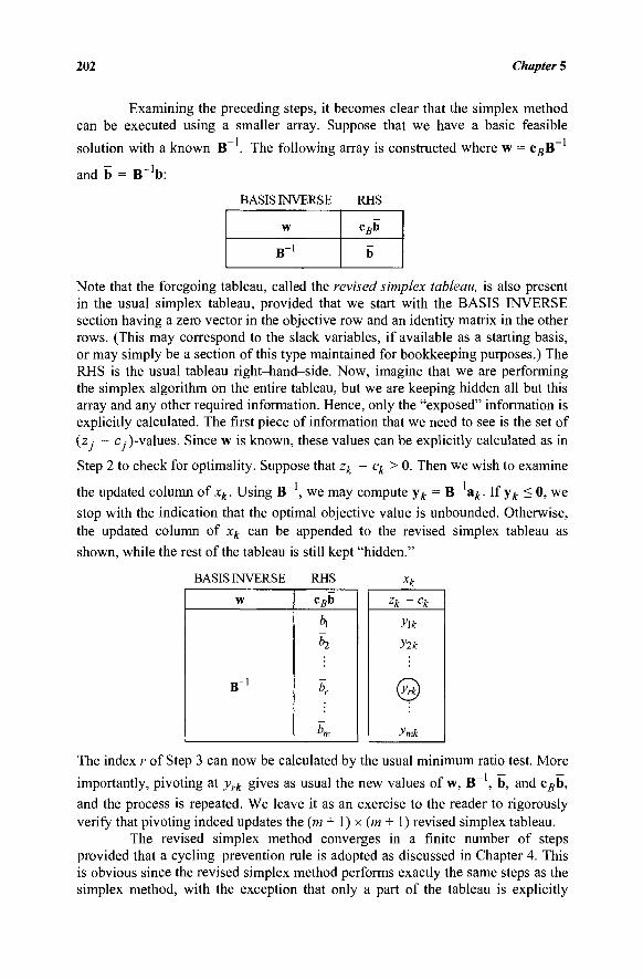
202 Chapter 5
Examining the preceding steps, it becomes clear that the simplex method can be executed using a smaller array. Suppose that we have a basic feasible
solution with a known B~ . The following array is constructed where w = cBB~
and b = B_1b:
BASIS INVERSE RHS
w
B 1
cBb
b
Note that the foregoing tableau, called the revised simplex tableau, is also present in the usual simplex tableau, provided that we start with the BASIS INVERSE section having a zero vector in the objective row and an identity matrix in the other rows. (This may correspond to the slack variables, if available as a starting basis, or may simply be a section of this type maintained for bookkeeping purposes.) The RHS is the usual tableau right-hand-side. Now, imagine that we are performing the simplex algorithm on the entire tableau, but we are keeping hidden all but this array and any other required information. Hence, only the "exposed" information is explicitly calculated. The first piece of information that we need to see is the set of (z - c,)-values. Since w is known, these values can be explicitly calculated as in
Step 2 to check for optimality. Suppose that zk - ck > 0. Then we wish to examine
the updated column of xk. Using B~ , we may compute y^ = B~ a^. If yk < 0, we stop with the indication that the optimal objective value is unbounded. Otherwise, the updated column of xk can be appended to the revised simplex tableau as shown, while the rest of the tableau is still kept "hidden."
BASIS INVERSE RHS xk
zk ~ck
y\k
yik
ymk
The index r of Step 3 can now be calculated by the usual minimum ratio test. More importantly, pivoting at yrk gives as usual the new values of w, B~ , b, and Cgb, and the process is repeated. We leave it as an exercise to the reader to rigorously verify that pivoting indeed updates the (m + 1) x (m + 1) revised simplex tableau.
The revised simplex method converges in a finite number of steps provided that a cycling-prevention rule is adopted as discussed in Chapter 4. This is obvious since the revised simplex method performs exactly the same steps as the simplex method, with the exception that only a part of the tableau is explicitly
w
B-1
cBb
h h
br
K
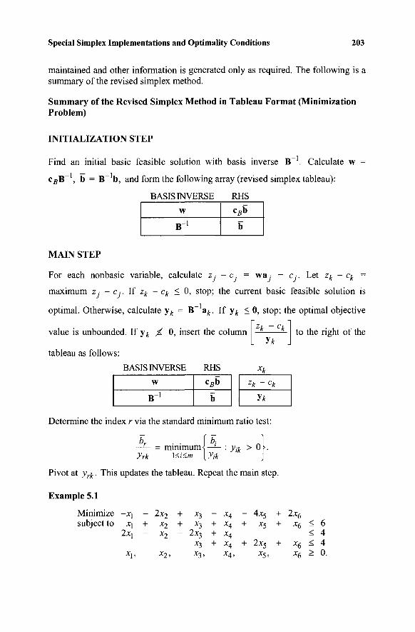
Special Simplex Implementations and Optimally Conditions 203
maintained and other information is generated only as required. The following is a summary of the revised simplex method.
Summary of the Revised Simplex Method in Tableau Format (Minimization Problem)
INITIALIZATION STEP
Find an initial basic feasible solution with basis inverse B~ . Calculate w =
cgB~ , b = B~ b, and form the following array (revised simplex tableau):
BASIS INVERSE RHS
w
B 1
cgb
b
MAIN STEP
For each nonbasic variable, calculate Zj - Cj = wa, - c,·. Let zk - ck =
maximum z,- - c ·. If zk - ck < 0, stop; the current basic feasible solution is
optimal. Otherwise, calculate y^ = B~ ak. If y^ < 0, stop; the optimal objective
value is unbounded. If y^ ^ 0, insert the column
tableau as follows:
BASIS INVERSE RHS
zk ~ck
xk
to the right of the
w
B 1
cBb
b
zk ~ck
y*
Determine the index r via the standard minimum ratio test:
yrk minimum-i—^- : yik > Ok
\<i<m [yik
Pivot at yrk. This updates the tableau. Repeat the main step.
Example 5.1
Minimize subject to
-x, X,
2X]
X,,
- 2x2
+ *2 ~ x2
x2,
+ x3
+ *3 - 2x3
x3 x3,
— x^ + x4 + x4
+ x4 X4,
- 4x5
+ x5
+ 2x5
^ 5 .
+ 2x6
+ x6
+ x6 x6
< 6 < 4 < 4 > U.
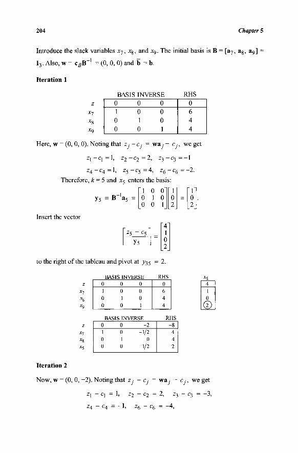
204 Chapter 5
Introduce the slack variables χη, x8, and x9. The initial basis is B = [a7, a8, a9]
I3. Also, w = c s B _ 1 = (0, 0, 0) and b = b.
Iteration 1
z
Χη
Xg
Xo
Here, w = (0, 0, 0). Noting that zj - Cj = way - Cj, we get
Z [ - C j = l , z 2 - C 2 = 2 , Z3—C3=—1
z 4 - c 4 = l , z 5 - c 5 = 4 , z 6 - c 6 = - 2 .
Therefore, k = 5 and x5 enters the basis:
BASIS INVERSE 0 0 0 1 0 0 0 1 0 0 0 1
RHS 0 6 4 4
ys B'a-: 1 0 ol 0 1 0 0 0 1
ΓΓ 0 2
= [ΊΊ 0 2
Insert the vector
zs ~cs
ys
[4] 1 0 2
to the right of the tableau and pivot at ^35 = 2.
BASIS INVERSE RHS
z
x7
*9
* 7
^8
^5
0 0 0 1 0 0 0 1 0 0 0 1
0 6 4 4
BASIS INVERSE RI 0 0 -2 1 0 -1/2 0 1 0 0 0 1/2
IS -8
4 4 2
x5
0
Iteration 2
Now, w = (0, 0, -2). Noting that zy - cj = wa · - Cj, we get
Z] - q = 1, Z2 _ c 2 = 2> z 3 ~ c 3 = ~3>
z4 - c4 = - 1 , z6 - c6 = -4,
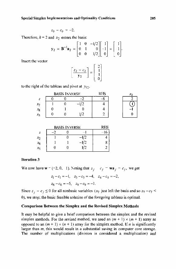
Special Simplex Implementations and Optimality Conditions 205
Z9 — c9 = —2.
Therefore, k = 2 and x2 enters the basis:
1 0 0 1 0 0
y2 = B a 2] 0 2_
Γ -1 0
= f
-1 0
Insert the vector
z2 ~c2 Y2
to the right of the tableau and pivot at y^·
z x7
x5
x2
Xg
x5
BASIS INVERSE 0 0 - 2 1 0 -1/2 0 1 0 0 0 1/2
BASIS INVERSE -2 0 -1
1 0 -1/2 1 1 -1/2 0 0 1/2
RHS -8 4 4 2
RHS -16
4 8 2
Iteration 3
We now have w = (-2, 0,-1). Noting that z ■ - c = wa, - c,·, we get
zl-cl=-\, z 3 - c 3 = - 4 , z4-c4=-2,
z 6 - c 6 = - 5 , z 9 - c 9 = - l .
Since z · - c < 0 for all nonbasic variables (x7 just left the basis and so z7 - c 7 <
0), we stop; the basic feasible solution of the foregoing tableau is optimal.
Comparison Between the Simplex and the Revised Simplex Methods
It may be helpful to give a brief comparison between the simplex and the revised simplex methods. For the revised method, we need an (m + 1) x (m + 1) array as opposed to an (m + 1) x (n + 1) array for the simplex method. If « is significantly larger than m, this would result in a substantial saving in computer core storage. The number of multiplications (division is considered a multiplication) and
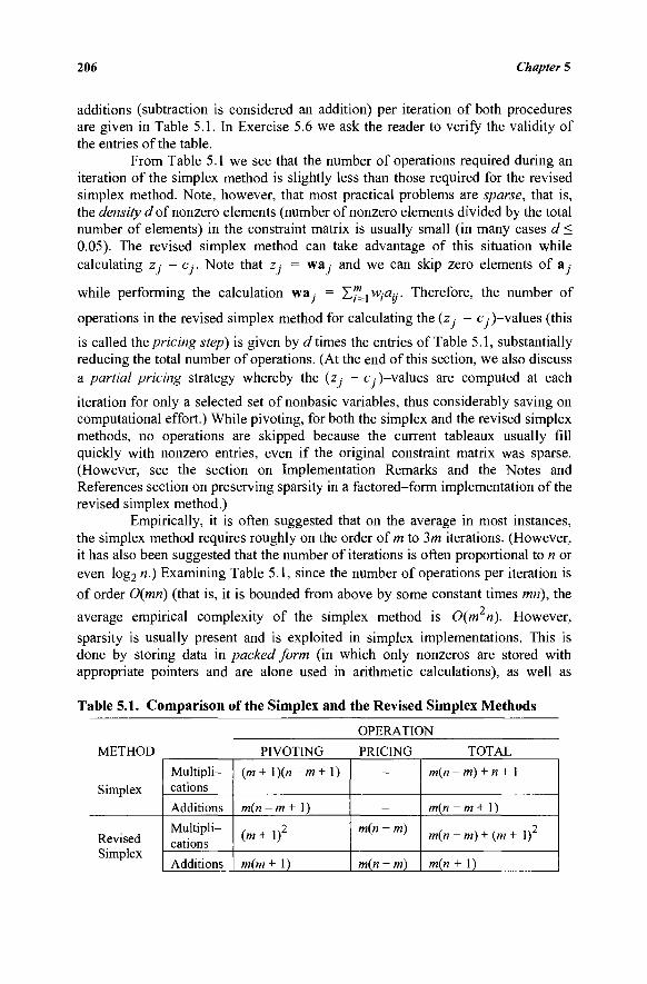
206 Chapter 5
additions (subtraction is considered an addition) per iteration of both procedures are given in Table 5.1. In Exercise 5.6 we ask the reader to verify the validity of the entries of the table.
From Table 5.1 we see that the number of operations required during an iteration of the simplex method is slightly less than those required for the revised simplex method. Note, however, that most practical problems are sparse, that is, the density d of nonzero elements (number of nonzero elements divided by the total number of elements) in the constraint matrix is usually small (in many cases d < 0.05). The revised simplex method can take advantage of this situation while calculating Zj - Cj. Note that z · = wa; and we can skip zero elements of ay
while performing the calculation wa, = Z^i^-a». Therefore, the number of
operations in the revised simplex method for calculating the (z · - c .· )-values (this
is called the pricing step) is given by d times the entries of Table 5.1, substantially reducing the total number of operations. (At the end of this section, we also discuss a partial pricing strategy whereby the (z,· - c,)-values are computed at each
iteration for only a selected set of nonbasic variables, thus considerably saving on computational effort.) While pivoting, for both the simplex and the revised simplex methods, no operations are skipped because the current tableaux usually fill quickly with nonzero entries, even if the original constraint matrix was sparse. (However, see the section on Implementation Remarks and the Notes and References section on preserving sparsity in a factored-form implementation of the revised simplex method.)
Empirically, it is often suggested that on the average in most instances, the simplex method requires roughly on the order of m to 3m iterations. (However, it has also been suggested that the number of iterations is often proportional to n or even log2 n.) Examining Table 5.1, since the number of operations per iteration is of order 0(mn) (that is, it is bounded from above by some constant times mn), the average empirical complexity of the simplex method is 0(m n). However, sparsity is usually present and is exploited in simplex implementations. This is done by storing data in packed form (in which only nonzeros are stored with appropriate pointers and are alone used in arithmetic calculations), as well as
Table 5.1. Comparison of the Simplex and the Revised Simplex Methods
OPERATION METHOD
Simplex
Revised
Simplex
Multipli-cations
Additions
Multipli-cations
Additions
PIVOTING
(m+ \)(n-m+ 1)
m(n-m + 1)
(m + l)2
m(m + 1)
PRICING
-
—
m{n - m)
m(n - m)
TOTAL
m(n - ni) + n + 1
m(n - m + 1 ) 9
m(n - m) + (m+ 1)
m(n + 1)
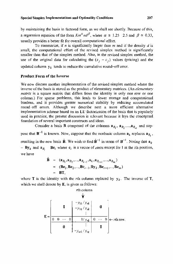
Special Simplex Implementations and Optimality Conditions 207
by maintaining the basis in factored form, as we shall see shortly. Because of this,
a regression equation of the form Kmand^, where a = 1.25 -2.5 and β = 0.33,
usually provides a better fit for overall computational effort. To summarize, if n is significantly larger than m and if the density d is
small, the computational effort of the revised simplex method is significantly smaller than that of the simplex method. Also, in the revised simplex method, the use of the original data for calculating the (zy - Cy)-values (pricing) and the
updated column yk tends to reduce the cumulative round-off error.
Product Form of the Inverse
We now discuss another implementation of the revised simplex method where the inverse of the basis is stored as the product of elementary matrices. (An elementary matrix is a square matrix that differs from the identity in only one row or one column.) For sparse problems, this leads to fewer storage and computational burdens, and it provides greater numerical stability by reducing accumulated round-off errors. Although we describe next a more efficient alternative implementation scheme based on an LU factorization of the basis that is popularly used in practice, the present discussion is relevant because it lays the conceptual foundation of several important constructs and ideas.
Consider a basis B composed of the columns aB , ag , . . . ,aB and sup-
pose that B~ is known. Now, suppose that the nonbasic column ak replaces aB ,
resulting in the new basis B. We wish to find B~ in terms of B~ . Noting that a^
= Byt and ag. = Be, where e,· is a vector of zeros except for 1 at the rth position,
we have
B = (aBl,a2,2,...,a/>r_1,afcja2,r+1)...,afiM)
= (Be1,Be2,...,Ber_1,ByA,Ber+1,...,Bem)
= BT,
where T is the identity with the rth column replaced by y^. The inverse of T,
which we shall denote by E, is given as follows: rth column
I I
0 0 ··· 0
0
-y\k !yrk
-yik 'yrk
l/yrk
-ymk iyrk
0
0 ··· 0
I
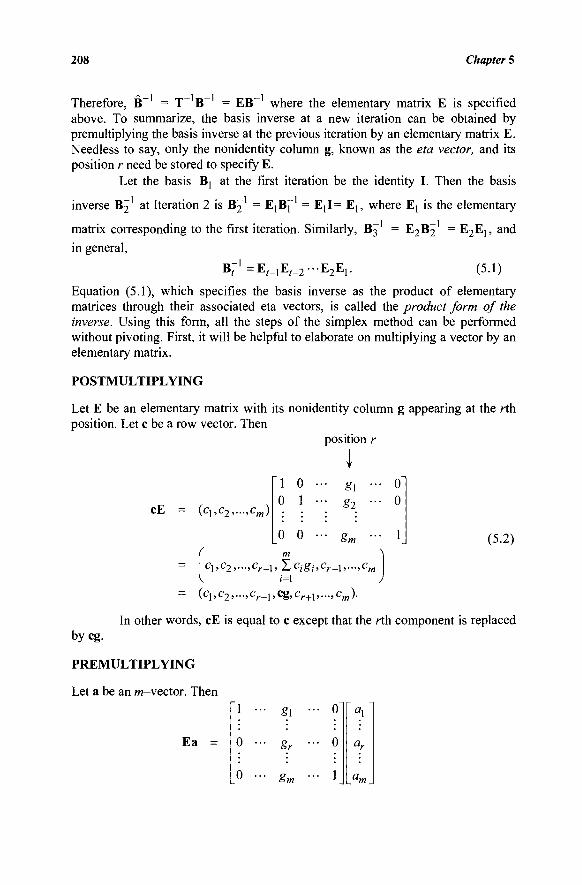
208 Chapter 5
Therefore, B - = T~ B~ = EB~ where the elementary matrix E is specified above. To summarize, the basis inverse at a new iteration can be obtained by premultiplying the basis inverse at the previous iteration by an elementary matrix E. Needless to say, only the nonidentity column g, known as the eta vector, and its position r need be stored to specify E.
Let the basis Bj at the first iteration be the identity I. Then the basis
inverse B2 at Iteration 2 is B2 = EjBJ" = Ejl= E1? where E! is the elementary
matrix corresponding to the first iteration. Similarly, B3 = E2B2 = E2Ej, and
in general,
B, = Εί_1Ε,_2···Ε2Ε1. (5.1)
Equation (5.1), which specifies the basis inverse as the product of elementary matrices through their associated eta vectors, is called the product form of the inverse. Using this form, all the steps of the simplex method can be performed without pivoting. First, it will be helpful to elaborate on multiplying a vector by an elementary matrix.
POSTMULTIPLYING
Let E be an elementary matrix with its nonidentity column g appearing at the rth position. Let c be a row vector. Then
position r
\ 1 0 ». gl ... 0" 0 1 ··· g2 ... 0
0 0 ··· gm ·■· 1 ( 5 2 )
( C j , C 2 , . . . , C w ) cE
C\,c2,..;Cr_x, Y1cigi,cr+X,...,cn
= (cl>c2>— >cr-l>cS>£T+l'—>c/n)·
In other words, cE is equal to c except that the rth component is replaced by eg.
PREMULTIPLYING
Let a be an w-vector. Then
Ea
1 S\ °Y°i 0 ... gr ... 0
0 - gm ... 1
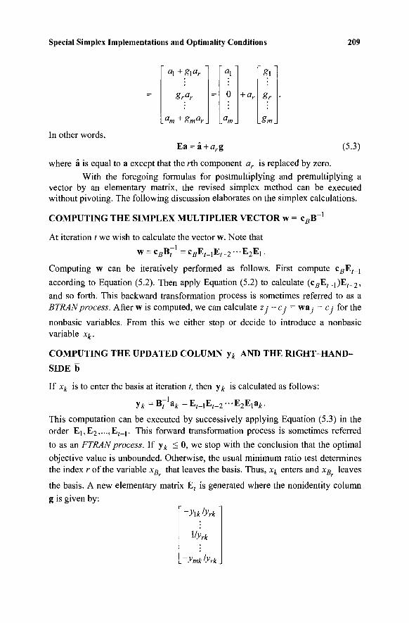
Special Simplex Implementations and Optimality Conditions 209
ax+gxar
Srar
_m £m®r _
=
ai 0
_<V
+ ar
E\~
Sr
_&m _
In other words, Ea = à + arg (5.3)
where a is equal to a except that the rth component ar is replaced by zero.
With the foregoing formulas for postmultiplying and premultiplying a vector by an elementary matrix, the revised simplex method can be executed without pivoting. The following discussion elaborates on the simplex calculations.
COMPUTING THE SIMPLEX MULTIPLIER VECTOR w = cgB_ 1
At iteration t we wish to calculate the vector w. Note that
w = csB71=CgEMEi_2---E2E1.
Computing w can be iteratively performed as follows. First compute c5E,_j according to Equation (5.2). Then apply Equation (5.2) to calculate (CgE/^])E/_25
and so forth. This backward transformation process is sometimes referred to as a BTRAN process. After w is computed, we can calculate zi -c ,· = wa - c; for the
nonbasic variables. From this we either stop or decide to introduce a nonbasic variable x^.
COMPUTING THE UPDATED COLUMN y* AND THE RIGHT-HAND-
SIDE b
If xk is to enter the basis at iteration t, then y^ is calculated as follows:
y * = B r 1 a t = E M E t _ 2 - E 2 E , a t .
This computation can be executed by successively applying Equation (5.3) in the order Ei,E2,...,E/_1. This forward transformation process is sometimes referred
to as an FTRAN process. If y^ < 0, we stop with the conclusion that the optimal objective value is unbounded. Otherwise, the usual minimum ratio test determines the index r of the variable xB that leaves the basis. Thus, xk enters and xB leaves
the basis. A new elementary matrix E, is generated where the nonidentity column
g is given by:
-yykfyrk
l/yrk
_-ymk!yrk.
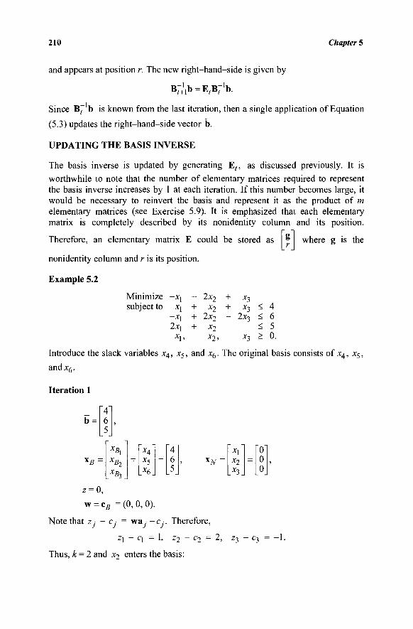
210 Chapter 5
and appears at position r. The new right-hand-side is given by
B ^ b = Ε , Β ^ .
Since BJ b is known from the last iteration, then a single application of Equation
(5.3) updates the right-hand-side vector b.
UPDATING THE BASIS INVERSE
The basis inverse is updated by generating E,, as discussed previously. It is
worthwhile to note that the number of elementary matrices required to represent the basis inverse increases by 1 at each iteration. If this number becomes large, it would be necessary to reinvert the basis and represent it as the product of m elementary matrices (see Exercise 5.9). It is emphasized that each elementary matrix is completely described by its nonidentity column and its position.
Therefore, an elementary matrix E could be stored as
nonidentity column and r is its position.
where g is the
Example 5.2
Minimize -xj subject to x\
-x{ 2xi
Xj,
- 2x2 + x2 + 2x2 + x2
x2,
+ x3
+ x3
- 2x3
x3
< 4 < 6 < 5 > 0
Introduce the slack variables and x6. The original basis consists of X4, Χ5,
andx6.
Iteration 1
= 4Ί
6 5
B ~
·>
XBX XB7
_-%_ —
X4
x5
_x6_ =
4 6 5
w = c B =(0,0,0).
*-N
X,
x2 x3
= 0 0 0
Note that z · - c ,· way - Cj. Therefore,
zj - q = 1, z2 - c2
Thus, k= 2 and x2 enters the basis:
z3 - c 3 = - 1 .
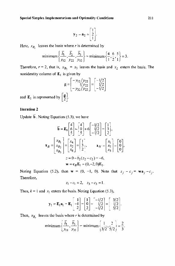
Special Simplex Implementations and Optimality Conditions 211
Y2=a2
minimum : minimum ml· Here, xB leaves the basis where r is determined by
b\ b2 b}
\y\i yn ^32.
Therefore, r = 2, that is, xB = x5 leaves the basis and x2 enters the basis. The
nonidentity column of E] is given by
-ynly il g = 1/ 22
-1/2 1/2
-1/2
and E] is represented by
Iteration 2
Update b . Noting Equation (5.3), we have
b = E,
XBX
XB2
*Bi _
=
4 6 5
X4 x2
3
=
=
4 0 5
+ 6 -1/2
1/2 -1/2
=
Γίΐ 3 , xN -_2J
1 3 2
x\ x5 x3
~
= -
0 0 0
χ β
z = 0-b2(z2 ~c2) = -6,
w ^ E , =(0 , -2 ,0 )^ .
Noting Equation (5.2), then w = (0, - 1 , 0). Note that z;· - c , = w a , - c ,
Therefore, z l - c l = 2 , z 3 - c 3 = l .
Thus, k = 1 and xt enters the basis. Noting Equation (5.3),
yx = Elal =Ei
Then, xB leaves the basis where r is determined by
f -1 2
= "Γ 0 2
--1/2Ί
1/2 -1/2
= 3/2
-1/2 5/2
1 U 63 ì . . r minimum i , >· = minimum <
h i y3iJ [3/2 5/2
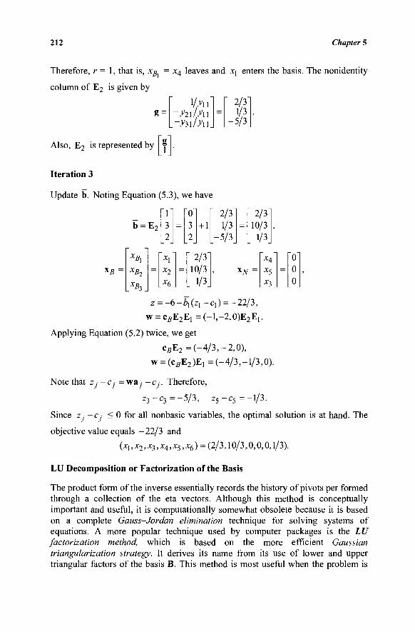
212 Chapter 5
Therefore, r = 1, that is, xB
column of E2 is given by
x4 leaves and jq enters the basis. The nonidentity
g
Also, E2 is represented by
1/Λΐ -yn/yu -yii/yn
2/3' 1/3
-5/3.
Iteration 3
Update b. Noting Equation (5.3), we have
b = E, "f 3 2
= "0" 3 2
+ 1 2/3" 1/3
_-5/3_ =
" 2/3" 10/3
. I/3.
χΒχ
XB2
XB3
= *\ x2
-x6_
=
" 2/3" 10/3
. 1/3. X/v —
X4
^5
_ x 3 _
= "0" 0 0
z = -<3-b\(zy —c\) = -22/3 ,
w = cBE2E1=(-l , -2,0)E2E1.
Applying Equation (5.2) twice, we get
cBE2 =( -4 /3 , -2 ,0 ) ,
w = (csE2)E1 =(-4/3,-1/3,0).
Note that z - c · = wa ,· - c .·. Therefore,
z 3 - c 3 = - 5 / 3 , z5-c5 =-1/3 .
Since z - c , < 0 for all nonbasic variables, the optimal solution is at hand. The
objective value equals -22/3 and
(x1,x2,x3,x4,x5,x6) = (2/3,10/3,0,0,0,1/3).
LU Decomposition or Factorization of the Basis
The product form of the inverse essentially records the history of pivots per formed through a collection of the eta vectors. Although this method is conceptually important and useful, it is computationally somewhat obsolete because it is based on a complete Gauss-Jordan elimination technique for solving systems of equations. A more popular technique used by computer packages is the LU factorization method, which is based on the more efficient Gaussian triangularization strategy. It derives its name from its use of lower and upper triangular factors of the basis B. This method is most useful when the problem is
Special Simplex Implementations and Optimality Conditions 213
large-scale and sparse, and it is accurate and numerically stable (round-off errors are controlled and do not tend to accumulate).
In implementing the simplex algorithm, the systems of equations that need to be solved are Bxg = b and wB = cB, and then Byfc = ak once an entering
variable xk is determined. The first of these equations gives the basic variable
values. Since the variable values are simply updated at every iteration, it only needs to be solved initially or whenever B is periodically refactored from scratch in order to maintain numerical accuracy. The second system computes the simplex multiplier vector w, which is used to price the nonbasic variables via the relationship z ■ -c ■ = wa. -c ·. Once a variable xk having zk - ck > 0 has been
chosen to enter the basis, its updated column y^ needs to be computed. This is
done via the third system of equations. The vector y^ provides the information on
how the basic variables change when xk is increased and determines the exiting
variable via the minimum ratio test. Hence, a new basis is obtained along with the (possibly) revised basic variable values. This process is then repeated.
Now, if B happens to be an upper triangular matrix, say, then the foregoing systems of equations can be solved easily and accurately. The systems BxB = b and By^ = ak can be solved by a backward substitution process in which
the last component of the solution vector is given directly by the last equation. This is substituted in the next to last equation to obtain the next to last component of the solution vector, and so on. The system wB = cB can be solved similarly by a forward substitution process in which the components of w are obtained sequentially in the order w\, w2,... wm.
On the other hand, if B is not (upper) triangular, then it can be made so through a series of row operations. Algebraically, this process can be represented as a premultiplication of B by a nonsingular, row-operation transformation matrix R such that RB = U, an upper triangular matrix. If this is done, then to solve the system By4 = &k, we can premultiply both sides by R to get RBy^ = Ra^, that is, Uy^ = ajj., where a'k = Rak. Hence, the upper triangular system Uy^ = a'k can now be solved by a backward substitution process. An identical strategy can be used to solve the system BxB = b. In order to solve the system wB = cB, consider
the affine transformation w = w'R. Then the foregoing system becomes w'RB = cB or w'U = cB, from which w' can be obtained via a forward substitution process. Knowing w', we can now compute w as w'R. Hence, if the row operations involved are not too computationally intensive and are well conditioned (do not involve divisions by small magnitude numbers, for instance), then the systems of equations can again be solved conveniently and accurately.
Observe that if the row operations required to upper triangularize B involve a simple row by row Gaussian reduction process, then R would be a lower triangular matrix. In other words, the first row of B would be left as is, the second row would have a multiple of the first row added to it in order to zero out the (2, 1) element of B, the third row of B would have a multiple of the first row and a multiple of the second row added to it in order to zero out the (3, 1) and the (3, 2)
214 Chapter 5
elements, and so on. In this case, we would have B = R U = LU, a product of a
lower triangular matrix L = R~ and an upper triangular matrix U. Hence, such a factorization is called an LU factorization, even in instances when R is not lower triangular.
Obtaining the LU Factorization of B
Typically, in addition to the Gaussian pivots or reductions, we also need to perform permutations of rows in the factorization in order to obtain desirable pivot elements. For example, to begin, we may wish to make that row the first row that has the largest absolute valued coefficient in the first column, so that the Gaussian pivots associated with zeroing out the first column under the (1, 1) element are numerically well conditioned. (Of course, if the starting (1,1) element in B is zero, then some such permutation is imperative.) Hence, the row operation matrix R may involve a (row interchange) permutation matrix Pj followed by a Gaussian reduction or pivot matrix G\ used to triangularize the first column (or the first nontriangular column), then possibly another permutation matrix P2 followed by a Gaussian triangularization matrix G2, and so on. Hence, if we use r such operations, we will have
R = (GrPr)-(G2P2)(G1P1) .
Accordingly, a forward transformation process called FTRAN is used to compute
a'k = Rak while solving the system By^ = ak by employing the operators (G;P;)
in the order \,...,r on &k. Similarly, a backward transformation process called
BTRAN is used to compute w = w'R while solving the system wB = c g by
postoperatively using G,P, on w' in the order r, r - 1,..., 1.
Now, let us discuss the construction of the operators defining R. Suppose that so far we have upper triangularized columns 1,..., k - 1 of B, and we are now considering the triangularization of a nontriangular column k using, for example, the operator G,P,. Let B^ be the current partially triangular matrix. Then we first determine the largest absolute valued element in rows k,k+\,...,mfor column k in Bk. If this happens to be the (k, k) element itself, then no row interchange
(permutation) is necessary, and in this case P; = I. Otherwise, if this happens to be
the element (/, k), then we need to interchange rows k and t. Hence, the permutation matrix that accomplishes this is given as follows, where the elements not shown are zeros:
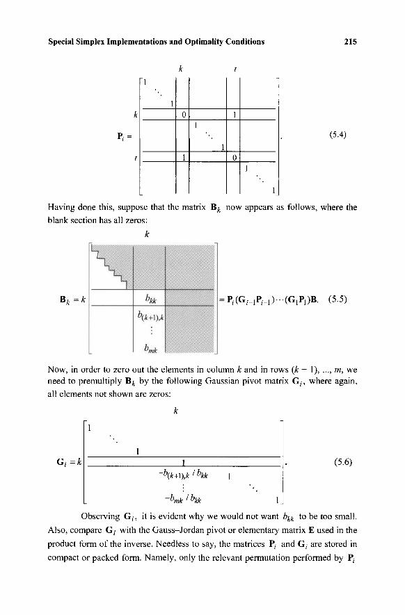
Special Simplex Implementations and Optimality Conditions 215
P,=
k
t
"1
1
k
0
1
1
1
t
1
0
-i
1
1
(5.4)
Having done this, suppose that the matrix Βλ now appears as follows, where the
blank section has all zeros:
k
Bk=k : P i ( G M P M ) - ( G 1 P , ) B . (5.5)
Now, in order to zero out the elements in column k and in rows (k + 1), ..., m, we need to premultiply B^ by the following Gaussian pivot matrix G;, where again, all elements not shown are zeros:
~\k+\),k lb> \k
'bmk I bkk 1.
(5.6)
Observing G;, it is evident why we would not want b^ to be too small.
Also, compare G,· with the Gauss-Jordan pivot or elementary matrix E used in the
product form of the inverse. Needless to say, the matrices P( and G, are stored in
compact or packed form. Namely, only the relevant permutation performed by P;·
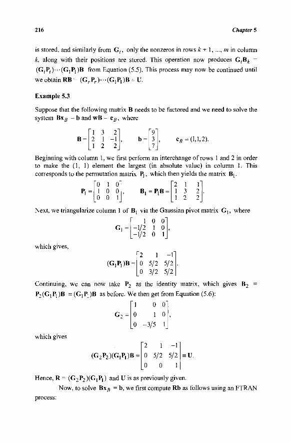
216 Chapter 5
is stored, and similarly from G,-, only the nonzeros in rows k + 1, ..., m in column
k, along with their positions are stored. This operation now produces G^B^ =
(G,P;)--(G1P])B from Equation (5.5). This process may now be continued until
we obtain RB= (GrPr)---(GIP1)B = U.
Example 5.3
Suppose that the following matrix B needs to be factored and we need to solve the system Βχβ = b and wB = cB, where
B 2
-1 2
c 5 =(1,1,2).
Beginning with column 1, we first perform an interchange of rows 1 and 2 in order to make the (1, 1) element the largest (in absolute value) in column 1. This corresponds to the permutation matrix Pj, which then yields the matrix Bj.
Β ^ Ρ , Β Pi = 0 1 0
1 0 0
0 0 1
Next, we triangularize column 1 of Bj via the Gaussian pivot matrix Gj, where
1 -1/2 -1/2
0 0 1 0 0 1
which gives,
(G!P,)B = 2 1 -1 0 5/2 5/2 0 3/2 5/2
Continuing, we can now take P2 as the identity matrix, which gives B2
P2(G1P1)B = (GjP^B as before. We then get from Equation (5.6):
G7 =
1
0
0
0 0
1 0
-3/5 1
which gives
(G2P2)(G1P1)B =
1 -1
0 5/2 5/2
0 0 1 = u.
Hence, R = (G2P2)(GjP1) and U is as previously given.
Now, to solve B\B = b, we first compute Rb as follows using an FTRAN
process:
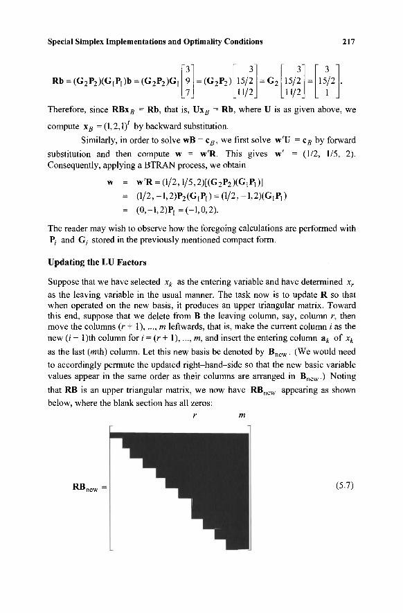
Special Simplex Implementations and Optimality Conditions 217
"3" 9 7
3" = (G2P2) 15/2
11/2 = G2
3" 15/2 11/2
= 3
15/2 1
Rb = (G2P2)(G,P1)b = (G2P2)G1
Therefore, since RBx5 = Rb, that is, Uxg = Rb, where U is as given above, we
compute xB =(1,2,1)' by backward substitution.
Similarly, in order to solve wB = cB, we first solve w'U = cB by forward
substitution and then compute w = w'R. This gives w' = (1/2, 1/5, 2). Consequently, applying a BTRAN process, we obtain
w = w'R = (l/2,l/5,2)[(G2P2)(G1P1)]
= (1/2, -1,2)P2(G,P,) = (1/2, - 1 ,2X0 ,^ )
= (0,-l ,2)P1=(-l ,0,2).
The reader may wish to observe how the foregoing calculations are performed with P, and G, stored in the previously mentioned compact form.
Updating the LU Factors
Suppose that we have selected x^ as the entering variable and have determined xr
as the leaving variable in the usual manner. The task now is to update R so that when operated on the new basis, it produces an upper triangular matrix. Toward this end, suppose that we delete from B the leaving column, say, column r, then move the columns (r + 1),..., m leftwards, that is, make the current column / as the new (/ - l)th column for i = (r + 1),..., m, and insert the entering column &k of xk
as the last (wth) column. Let this new basis be denoted by B n e w . (We would need to accordingly permute the updated right-hand-side so that the new basic variable values appear in the same order as their columns are arranged in Bnew.) Noting
that RB is an upper triangular matrix, we now have RBnew appearing as shown
below, where the blank section has all zeros:
RBnew - (5.7)
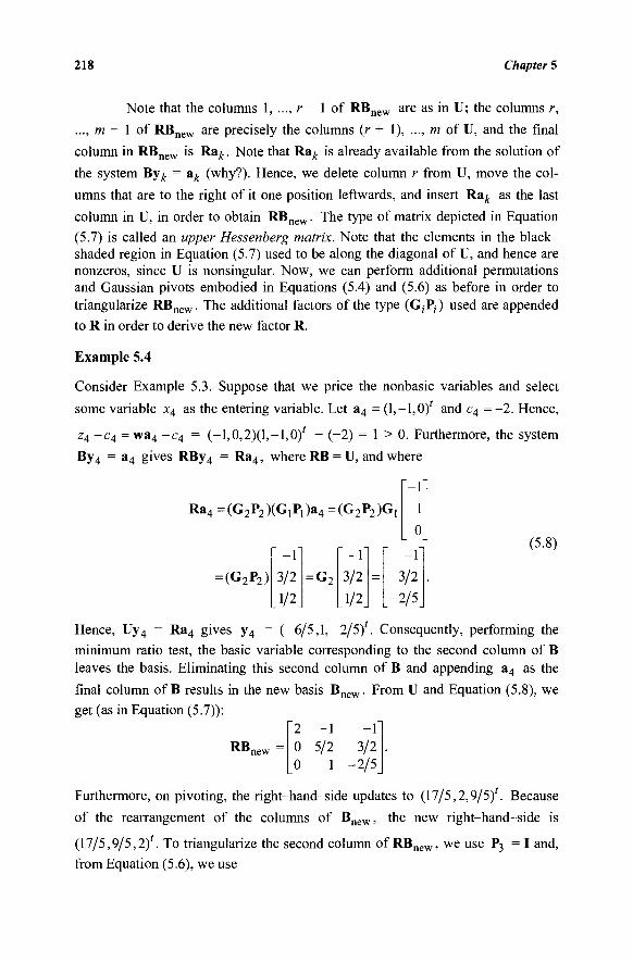
218 Chapter 5
Note that the columns 1, ..., r - 1 of RBn e w are as in U; the columns r,
..., m - 1 of RBnew are precisely the columns (r + 1), ..., m of U, and the final
column in RBn e w is Ra^. Note that Ra^ is already available from the solution of
the system By^ = ak (why?). Hence, we delete column r from U, move the col-
umns that are to the right of it one position leftwards, and insert Ra^ as the last
column in U, in order to obtain RBn e w. The type of matrix depicted in Equation
(5.7) is called an upper Hessenberg matrix. Note that the elements in the black-shaded region in Equation (5.7) used to be along the diagonal of U, and hence are nonzeros, since U is nonsingular. Now, we can perform additional permutations and Gaussian pivots embodied in Equations (5.4) and (5.6) as before in order to triangularize RBn e w. The additional factors of the type (G;P,) used are appended to R in order to derive the new factor R.
Example 5.4
Consider Example 5.3. Suppose that we price the nonbasic variables and select
some variable x4 as the entering variable. Let a4 = (1,-1,0)' and c4 = -2. Hence,
Z4-C4 = w a 4 - c 4 = (-1,0,2)(1,-1,0)' - (-2) = 1 > 0. Furthermore, the system
By4 = a4 gives RBy4 = Ra4, where RB = U, and where
Ra4 =(G2P2)(G1P,)a4 =(G2P2)Gi
= (G2P2)
" -f 3/2
.V 2 . = G2
" -f 3/2
.1/2.
=
- f 3/2
. "2 /5 .
(5.8)
Hence, Uy4 = Ra4 gives y4 = (-6/5,1,-2/5)'. Consequently, performing the minimum ratio test, the basic variable corresponding to the second column of B leaves the basis. Eliminating this second column of B and appending a4 as the
final column of B results in the new basis B n e w . From U and Equation (5.8), we
get (as in Equation (5.7)):
RB„ 2 -1 -1 0 5/2 3/2 0 1 -2 /5
Furthermore, on pivoting, the right-hand-side updates to (17/5,2,9/5)'. Because
of the rearrangement of the columns of B n e w , the new right-hand-side is
(17/5,9/5,2)'. To triangularize the second column of RBn e w , we use P3 = I and, from Equation (5.6), we use
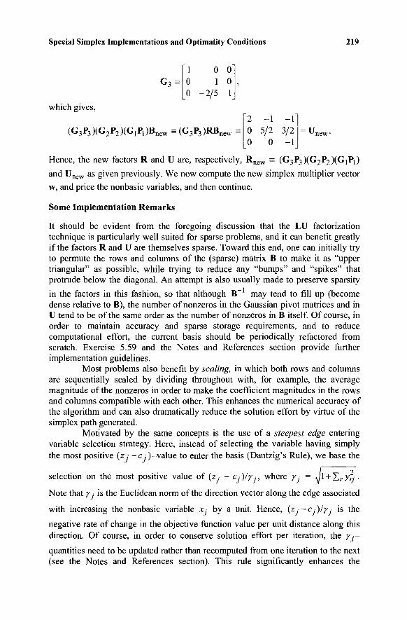
Special Simplex Implementations and Optimality Conditions 219
G3 = 1 0 0 0 1 0 0 -2/5 1
1
which gives,
(G3P3)(G2P2)(G1P,)Bnew = (G3P3)RBnew = ~2 -1 - Γ 0 5/2 3/2 0 0 - 1
— ^new
Hence, the new factors R and U are, respectively, Rnew = (G3P3)(G2P2)(G1P1)
and Unew as given previously. We now compute the new simplex multiplier vector
w, and price the nonbasic variables, and then continue.
Some Implementation Remarks
It should be evident from the foregoing discussion that the LU factorization technique is particularly well suited for sparse problems, and it can benefit greatly if the factors R and U are themselves sparse. Toward this end, one can initially try to permute the rows and columns of the (sparse) matrix B to make it as "upper triangular" as possible, while trying to reduce any "bumps" and "spikes" that protrude below the diagonal. An attempt is also usually made to preserve sparsity
in the factors in this fashion, so that although B~ may tend to fill up (become dense relative to B), the number of nonzeros in the Gaussian pivot matrices and in U tend to be of the same order as the number of nonzeros in B itself. Of course, in order to maintain accuracy and sparse storage requirements, and to reduce computational effort, the current basis should be periodically refactored from scratch. Exercise 5.59 and the Notes and References section provide further implementation guidelines.
Most problems also benefit by scaling, in which both rows and columns are sequentially scaled by dividing throughout with, for example, the average magnitude of the nonzeros in order to make the coefficient magnitudes in the rows and columns compatible with each other. This enhances the numerical accuracy of the algorithm and can also dramatically reduce the solution effort by virtue of the simplex path generated.
Motivated by the same concepts is the use of a steepest edge entering variable selection strategy. Here, instead of selecting the variable having simply the most positive (z; -c , ) -value to enter the basis (Dantzig's Rule), we base the
selection on the most positive value of (z ■ - cAly ,·, where γ= = Μ + ΣΓ);ή ·
Note that γ ■ is the Euclidean norm of the direction vector along the edge associated
with increasing the nonbasic variable x. by a unit. Hence, (z-c .-)//■ is the
negative rate of change in the objective function value per unit distance along this direction. Of course, in order to conserve solution effort per iteration, the γ.—
quantities need to be updated rather than recomputed from one iteration to the next (see the Notes and References section). This rule significantly enhances the
220 Chapter 5
performance of the simplex algorithm over the use of Dantzig's Rule, particularly on unsealed problems. (It has also been observed to assist more strongly with the dual simplex method that is discussed in Chapter 6.)
Another related strategy is partial pricing or suboptimization. Thus far, we have conducted a total pricing of all the nonbasic variables at each iteration. This is convenient and advantageous for problems having no more than 1000 or so variables. However, for larger-sized problems, such a total pricing operation can be computationally expensive. It is usually preferable to perform a partial pricing or a so-called suboptimization process. We describe here one particular implementation of this process using Dantzig's Rule for selecting an entering variable. To begin, all the nonbasic variables are priced and the largest (z; - c ,· )-value, say, zk -ck = Amax > 0,
is found. A list L is constructed of the current basic variables and those nonbasic variables for which Zj - Cj lies within some px percent of Amax. At this point, the
variables not in L are ignored, and the iterations continue by selecting the nonbasic variable having the most positive (z ; -c;)-value in L for entering the basis. However,
once the most positive (z ,· - c ,· ) -value falls below some p2 percent of Amax, or when
the simplex method goes through some N consecutive degenerate iterations, the list L is reconstructed. If this list were not reconstructed, then the algorithm would eventually solve the problem where the ignored nonbasic variables are permanently fixed at zero; hence the name "suboptimization" of this technique. Typical values of p\ and p2 are,
respectively, 0.8 and 0.67 for sparse problems (d < 0.05 - 0.1) and 0.7 and 0.4 for dense problems. (Here, d is the density of the matrix A.) A typical value of N is about 10-30.
Finally, we mention that for large-scale problems, it is useful to have a matrix generator program in order to automatically generate the constraints and the objective function based on the structure of the application instead of manually inputting the data. The software would then store the nonzero coefficients in packed form as noted earlier, and then use them appropriately to perform the foregoing computations. Many modeling languages are now available as user-friendly interfaces to enable the specifications of problems in algebraic symbolic format, rather than require a laborious construction of nonzero matrix coefficients in specified packed formats. The interested reader is referred to the Notes and References section for further discussions on these topics.
5.2 THE SIMPLEX METHOD FOR BOUNDED VARIABLES
In most practical problems the variables are usually bounded. A typical variable xj
is bounded from below by £ ■ and from above by u-, where i ■ < it-. If we
denote the lower and upper bound vectors by i and u, respectively, we get the following linear program with bounded variables:
Minimize ex
subject to Ax = b
^ < x < u .
Special Simplex Implementations and Optimality Conditions 221
By standard transformations, we can assume without loss of generality that £ is
finite for eachy = 1, ..., n (why?). If £ = 0, the usual nonnegativity restrictions are obtained. In fact, any lower bound vector can be transformed into the zero vector by using the change of variables x' = x — (. The most straightforward (and the least efficient) method of handling the constraints £ < x < u is to introduce the slack vectors Xj and x2, leading to the constraints x + xt = u and x - x2 = £■ This increases the number of equality constraints from m to m + In and the number of variables from n to 2>n. Even if £ = 0 or is transformed into 0, as discussed, the slack vector Xj is needed, which increases both the constraints and variables by n.
From the foregoing discussion it is clear that the problem size (and hence the computational effort) would increase significantly if the constraints £ < x < u are treated in the usual manner by introducing slack vectors. The simplex method with bounded variables handles these constraints implicitly in a fashion similar to that used by the simplex method to handle the constraints x > 0. Therefore, the so-called "working basis" remains of size m x m, and hence such a method is known as a compact basis method. As in the simplex method, the algorithm of this section moves from a basic feasible solution to an improved basic feasible solution of the system Ax = b, £ < x < u (at a nondegenerate pivot step), until optimality is reached or unboundedness is verified.
Now, observe that the feasible region of the foregoing problem is a
polyhedron in R", and as before, its extreme points are feasible points at which
some n linearly independent hyperplanes are binding. Since Ax = b gives m linearly independent hyperplanes that are binding at each feasible solution, we seek p = n- m appropriate additional binding hyperplanes from the inequalities £ < x < u in order to make up the required set of n linearly independent binding equations for defining each extreme point solution. (Throughout we only consider constraints having finite upper or lower bounds to be binding.) Consequently, there arep = n -m degrees of freedom remaining after imposing the constraints Ax = b, and so, the
given polyhedron is embedded in Rp. We therefore need to associate with an
extreme point some p {independent) nonbasic variables fixed either at their lower or their upper bounds such that the remaining m (dependent) basic variables are uniquely determined via the system Ax = b. If more than p, say, q, of the inequalities £ < x < u are binding at an extreme point, then such an extreme point is degenerate and has q - p > 1 of the associated basic variables at one of their bounds. Hence, we define a basic feasible solution as follows, so that a solution x is an extreme point if and only if it is a basic feasible solution. Details of the proof based on this exposition are very similar to the case of the set X = {x: Ax = b, x > 0} and are left to the reader in Exercise 5.17.
Definition (Basic Feasible Solutions)
Consider the system Ax = b and £ < x < u, where A is an m x n matrix of rank m. The solution x to the equations Ax = b is a basic solution of this system if A can be partitioned into [B, Nj, N2 ], where the (square) matrix B has rank m, such that with
222 Chapter 5
x partitioned accordingly as (xB, xN , x^ ) we have xN = £N , xN = uN , and
accordingly, xB = B~ b - B~ N ^ ^ - B^ N2u^ . Furthermore, if lB < xB <
uB, then x is said to be a basic feasible solution. The matrix B is called the
(working) basis, xB are the basic variables, and xN and x^ are the nonbasic
variables at their lower and upper limits, respectively. If, in addition, lB <xB <
uB, then x is called a nondegenerate basic feasible solution; otherwise, it is called
a degenerate basic feasible solution. The partition [B,Nj, N2] corresponding to a basic (feasible) solution is
said to be a basic (feasible) partition. Two basic (feasible) partitions are said to be adjacent if all but one nonbasic variable coincides in the two partitions, being fixed at the same bounds. Note that for a degenerate extreme point, x, each choice of p
= (n - m) defining hyperplanes from the set I < x < u that, along with the m constraints Ax = b, yield n linearly independent hyperplanes binding at x, corresponds to a basic feasible partition associated with x.
Example 5.5
Consider the region given by xx
-χϊ 0
-1
+ + < <
x2
2x2 X]
x2
< < < <
5 4 4 4
First introduce the slack variables x3 and x4. This gives the following system
(note that a close examination of the system shows that w3 and H4 can be replaced
by 6 and 10, respectively, if so desired): X[ +
- X [ + x2
2x2
+ x3
0 -1 0 0
+ < < < <
X4 x\
x2 x3 X4
= = < < < <
5 4 4 4
00
00
We would like to find all the basic feasible solutions of this system. This can be accomplished by extracting a basis of the first two constraints, solving the basic variables in terms of the nonbasic variables, and then fixing the nonbasic variables at their lower or upper bounds. To illustrate the method select, say, a2 and a4 as the basic vectors. Then
B = [a2,a4] =
;he first tw
right-hand-side, we get
1 0 2 1
and B"1 = 1 0 -2 1
Multiplying the first two constraints by B and transferring x{ and x3 to the
Special Simplex Implementations and Optimally Conditions 223
X2 — 5 — Xi — X3
x4 = -6 + 3xj + 2x3.
Now, fix X| at its lower or upper bound, x3 at its lower bound, and solve for x2
and x4:
1. xj = 0, x3 = 0 => x2 = 5, and x4 = -6 . Since x4 < 0, this basic solution
is not a basic feasible solution.
2. xl = 4, x3 = 0 => x2 = 1, and x4 = 6. Therefore, ( xj, χ2 , Χ3, x4 ) =
(4, 1, 0, 6) is a basic feasible solution.
The other basic solutions can be obtained in a similar manner. If all of the possible bases were enumerated, we would see that the basic feasible solutions are (2,3,0,0), (0,2,3,0), (4,1,0,6), (0, -1,6,6), and (4, -1,2,10). Projecting these points in the (xb
x2) space, we get the extreme points Vj, ..., v5 shown in Figure 5.1. In this example, n = 4, m = 2, and sop = n - m = 2. In fact, the representation shown in Figure 5.1 is in the p = 2-dimensional space corresponding to X] and x2 as the independent variables. Note how each extreme point is formed by some p = 2 linearly independent defining hyperplanes binding in this space. In particular, (x3 =
£3, x4= £4) gives V!, (xj = l\, x4= £Λ) gives v2, {χλ = ux, x3 = l3) gives v3, (x{
= i], x2= i2) gives v4, and (xt = MJ, X2 = £2) g i y e s v5· Hence, as noted previously, the basic feasible solutions and the extreme points coincide. Observe also that the extreme points v4 and v5 have the same working basis associated
with them, namely, the columns of the variables x3 and x4. However, they differ
in the bound values assigned to the (independent) nonbasic variables xj and x2, and
hence produce distinct basic feasible partitions and distinct basic feasible solutions. Furthermore, since all extreme points are nondegenerate here, each has a unique basic feasible partition associated with it, and the adjacent basic feasible partitions correspond to adjacent extreme points. We ask the reader to explore a generalization of this in Exercise 5.18 by imitating the analysis for the nonnegatively constrained case.
Improving a Basic Feasible Solution
We now know how to characterize a basic feasible solution. We also know that an optimal basic feasible solution exists provided that the feasible region is not empty and the optimum is finite (why?). Note, however, that the number of basic feasible
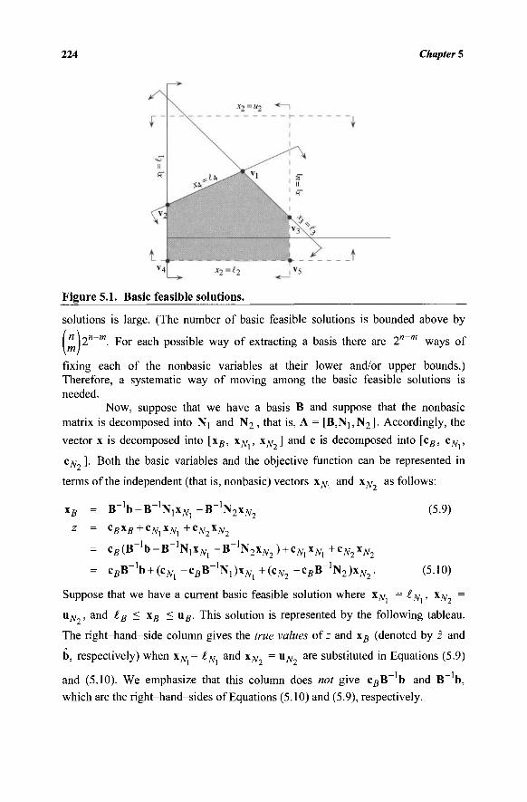
224 Chapter 5
Figure 5.1. Basic feasible solutions.
solutions is large. (The number of basic feasible solutions is bounded above by
n 2n~m_ For each possible way of extracting a basis there are 2n~m ways of
fixing each of the nonbasic variables at their lower and/or upper bounds.) Therefore, a systematic way of moving among the basic feasible solutions is needed.
Now, suppose that we have a basis B and suppose that the nonbasic
matrix is decomposed into Nj and N2 , that is, A = [B,Ni,N2]. Accordingly, the
vector x is decomposed into [xB, χ^ , xN ] and c is decomposed into [cB, cN ,
cN ]. Both the basic variables and the objective function can be represented in
terms of the independent (that is, nonbasic) vectors xN and xN as follows:
xB = B- 1 b-B- 1 N 1 x W l -B- 1 N 2 x^ 2 (5.9)
2 ~ cBxB+cNlxNl
+cN2XN2
= c ^ B ^ b - B " 1 ] * , ! ^ -B-]N2xN2) + cNixNl +cN2xN2
= CgB-1b + (c^-CgB-1N])xy V l+(ci V 2-CgB-1N2)xi V 2. (5.10)
Suppose that we have a current basic feasible solution where x^ = £N , xN =
uN , and lB < xB < uB. This solution is represented by the following tableau.
The right-hand-side column gives the true values of z and xB (denoted by z and
b, respectively) when x^ = £^ and x^ = uN are substituted in Equations (5.9)
and (5.10). We emphasize that this column does not give c^B~ b and B~ b, which are the right-hand-sides of Equations (5.10) and (5.9), respectively.
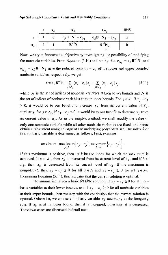
Special Simplex Implementations and Optimally Conditions 225
z \B χΝχ xNl RHS
1
0
0 c ^ B - ' N j - c ^ cBB-%-cN2
I B_1N! Β ~ ' Ν 2
z
b
Now, we try to improve the objective by investigating the possibility of modifying
the nonbasic variables. From Equation (5.10) and noting that c^ - c5B~ N[ and
cN - cgB~ N2 give the reduced costs Cj - z · of the lower and upper bounded
nonbasic variables, respectively, we get
z = cBBlb- Σ (zj~cj)xj- Σ (zj-cj)xj (5·11) jsJx jeJ2
where J\ is the set of indices of nonbasic variables at their lower bounds and J2 is
the set of indices of nonbasic variables at their upper bounds. For j e Jj if z ; - c ,·
> 0, it would be to our benefit to increase x- from its current value of £.-.
Similarly, for j e J2, if z ; - c ,· < 0, it would be to our benefit to decrease x.- from
its current value of « . As in the simplex method, we shall modify the value of
only one nonbasic variable while all other nonbasic variables are fixed, and hence obtain a movement along an edge of the underlying polyhedral set. The index k of this nonbasic variable is determined as follows. First, examine
maximum \ maximum iz.-cA, maximum {c ,· - z ,· H. { yw, l J) jeJ2
( J J>\
If this maximum is positive, then let k be the index for which the maximum is achieved. If k e J1; then xk is increased from its current level of £k, and if k e
J2, then xk is decreased from its current level of uk. If the maximum is
nonpositive, then zj - Cj < 0 for all j e Jx and z- - c- > 0 for all j GJ2.
Examining Equation (5.11), this indicates that the current solution is optimal.
To summarize, given a basic feasible solution, if z · - c ■ < 0 for all non-
basic variables at their lower bounds, and if z - c > 0 for all nonbasic variables at their upper bounds, then we stop with the conclusion that the current solution is optimal. Otherwise, we choose a nonbasic variable xk according to the foregoing
rule. If xk is at its lower bound, then it is increased; otherwise, it is decreased.
These two cases are discussed in detail next.
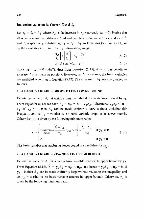
226 Chapter 5
Increasing xk from its Current Level lk
Let xk = £k + A k where A k is the increase in xk (currently A k = 0). Noting that
all other nonbasic variables are fixed and that the current value of \B and z are b
and z, respectively, substituting xk = (k + A k in Equations (5.9) and (5.11), or
by the usual dxB/dxk and dz/dxk information, we get
*B xk
b
h + Ai - y *
1 (5.12)
z = z + Ak[-(zk-ck)]. (5.13)
Since zk - ck > 0 (why?), then from Equation (5.13), it is to our benefit to
increase Δ^ as much as possible. However, as A k increases, the basic variables
are modified according to Equation (5.12). The increase in Δ^ may be blocked as
follows.
1. A BASIC VARIABLE DROPS TO ITS LOWER BOUND
Denote the value of A k at which a basic variable drops to its lower bound by γχ.
From Equation (5.12) we have iB < xB = b - Υ^Δ^. Therefore, y^A^ < b -
iB. If y k < 0, then Δ^ can be made arbitrarily large without violating this
inequality and so γ\ = <x> (that is, no basic variable drops to its lower bound).
Otherwise, γχ is given by the following minimum ratio:
lb-* minimum·^ L : Vc > 0 r ~ ~ i f y / t ^ O
Π=< \<i<m y yik J yrk (5.14)
co i f y y t ^ o .
The basic variable that reaches its lower bound is a candidate for xB .
2. A BASIC VARIABLE REACHES ITS UPPER BOUND
Denote the value of Δ^ at which a basic variable reaches its upper bound by γ2.
From Equation (5.12), b - y^A^ = \B < uB, and hence ~ykAk < u g - b . If
y^ > 0, then A k can be made arbitrarily large without violating this inequality, and
so Y2 =oo (that is, no basic variable reaches its upper bound). Otherwise, γ2 is
given by the following minimum ratio:
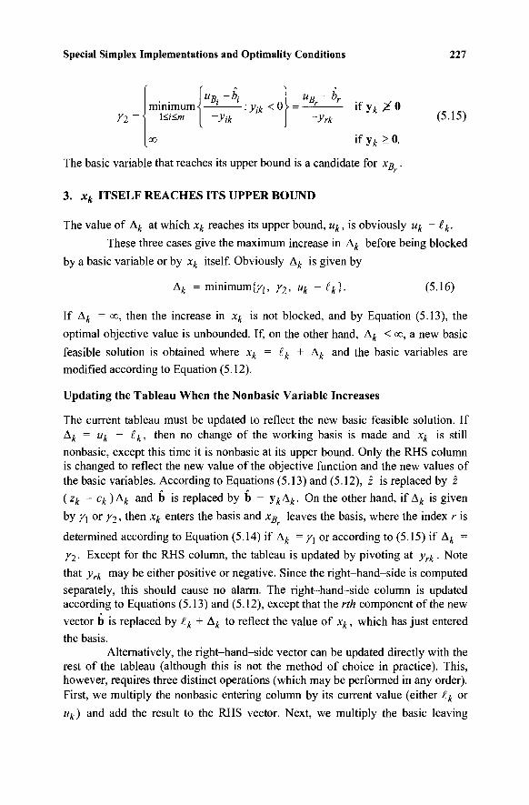
Special Simplex Implementations and Optimality Conditions 227
Ϊ2=\
uB. - bj uB -br minimum^ —i :yik<0\ = —r- i f y ^ X O
\<i<m -yik -yrk (5.15)
co if yk > 0.
The basic variable that reaches its upper bound is a candidate for xB .
3. xk ITSELF REACHES ITS UPPER BOUND
The value of Ak at which xk reaches its upper bound, uk, is obviously uk - £k.
These three cases give the maximum increase in Ak before being blocked
by a basic variable or by xk itself. Obviously Ak is given by
Δβ- = m i n i m u m ^ , γ2, uk - £k}. (5.16)
If Ak = co, then the increase in xk is not blocked, and by Equation (5.13), the
optimal objective value is unbounded. If, on the other hand, Δ^ < co, a new basic
feasible solution is obtained where xk = ik + Ak and the basic variables are
modified according to Equation (5.12).
Updating the Tableau When the Nonbasic Variable Increases
The current tableau must be updated to reflect the new basic feasible solution. If ^k = uk - £k, then no change of the working basis is made and xk is still
nonbasic, except this time it is nonbasic at its upper bound. Only the RHS column
is changed to reflect the new value of the objective function and the new values of
the basic variables. According to Equations (5.13) and (5.12), z is replaced by z -
(zk - ck )Ak and b is replaced by b - y^A^. On the other hand, if Ak is given
by γi or γ2, then xk enters the basis and xB leaves the basis, where the index r is
determined according to Equation (5.14) if Ak = yi or according to (5.15) if Δ^ =
/2 ■ Except for the RHS column, the tableau is updated by pivoting at yrk . Note
that yrk may be either positive or negative. Since the right-hand-side is computed
separately, this should cause no alarm. The right-hand-side column is updated according to Equations (5.13) and (5.12), except that the rth component of the new
vector b is replaced by £k + Ak to reflect the value of xk, which has just entered
the basis. Alternatively, the right-hand-side vector can be updated directly with the
rest of the tableau (although this is not the method of choice in practice). This, however, requires three distinct operations (which may be performed in any order). First, we multiply the nonbasic entering column by its current value (either £k or
uk) and add the result to the RHS vector. Next, we multiply the basic leaving
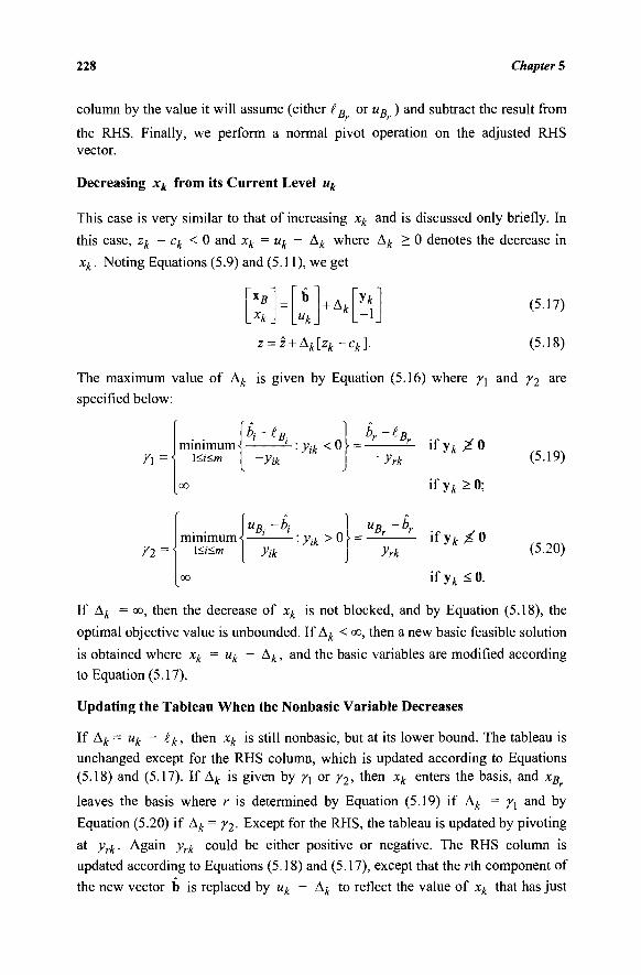
228 Chapter 5
column by the value it will assume (either lB or uB ) and subtract the result from
the RHS. Finally, we perform a normal pivot operation on the adjusted RHS vector.
Decreasing xk from its Current Level uk
This case is very similar to that of increasing xk and is discussed only briefly. In
this case, zk - ck < 0 and xk = uk - Ak where Ak > 0 denotes the decrease in
xk. Noting Equations (5.9) and (5.11), we get
(5.17)
(5.18)
~ x / .xk_
= b
.uk_ + Ak
~Yk~ -1
z = z + Ak[zk~ck].
The maximum value of Δ^ is given by Equation (5.16) where γ\ and γ2 a r e
specified below:
n
B: minimum < -
\<i<m -yik ■yik<o\
br -t.
-yrk i f y ^ X o
i f y ^ o ;
(5.19)
Ϊ2
\uB-bi uB -br
minimum \ ■yik>0\ = ify*X(> \<i<m y yik j yrk (5.20)
oo if yA < 0.
If Ak = oo, then the decrease of xk is not blocked, and by Equation (5.18), the
optimal objective value is unbounded. If Ak < oo, then a new basic feasible solution
is obtained where xk = uk - Ak, and the basic variables are modified according
to Equation (5.17).
Updating the Tableau When the Nonbasic Variable Decreases
If Ak = uk - ik, then xk is still nonbasic, but at its lower bound. The tableau is unchanged except for the RHS column, which is updated according to Equations (5.18) and (5.17). If Ak is given by γχ or γ2, then xk enters the basis, and xB
leaves the basis where r is determined by Equation (5.19) if Ak = γλ and by
Equation (5.20) if Ak = γ2· Except for the RHS, the tableau is updated by pivoting
at yrk. Again yrk could be either positive or negative. The RHS column is
updated according to Equations (5.18) and (5.17), except that the rth component of
the new vector b is replaced by uk - Ak to reflect the value of xk that has just
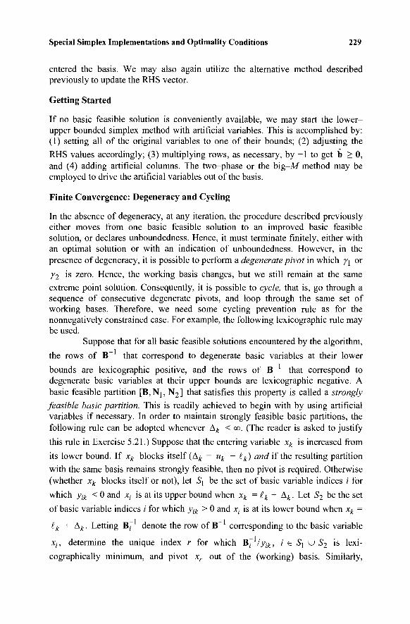
Special Simplex Implementations and Optimally Conditions 229
entered the basis. We may also again utilize the alternative method described previously to update the RHS vector.
Getting Started
If no basic feasible solution is conveniently available, we may start the lower-upper bounded simplex method with artificial variables. This is accomplished by: (1) setting all of the original variables to one of their bounds; (2) adjusting the
RHS values accordingly; (3) multiplying rows, as necessary, by -1 to get b > 0, and (4) adding artificial columns. The two-phase or the big-M method may be employed to drive the artificial variables out of the basis.
Finite Convergence: Degeneracy and Cycling
In the absence of degeneracy, at any iteration, the procedure described previously either moves from one basic feasible solution to an improved basic feasible solution, or declares unboundedness. Hence, it must terminate finitely, either with an optimal solution or with an indication of unboundedness. However, in the presence of degeneracy, it is possible to perform a degenerate pivot in which γ^ or
Yl is zero. Hence, the working basis changes, but we still remain at the same
extreme point solution. Consequently, it is possible to cycle, that is, go through a sequence of consecutive degenerate pivots, and loop through the same set of working bases. Therefore, we need some cycling prevention rule as for the nonnegatively constrained case. For example, the following lexicographic rule may be used.
Suppose that for all basic feasible solutions encountered by the algorithm,
the rows of B~ that correspond to degenerate basic variables at their lower
bounds are lexicographic positive, and the rows of B~ that correspond to degenerate basic variables at their upper bounds are lexicographic negative. A basic feasible partition [B, N1; N2] that satisfies this property is called a strongly
feasible basic partition. This is readily achieved to begin with by using artificial variables if necessary. In order to maintain strongly feasible basic partitions, the following rule can be adopted whenever Ak < oo. (The reader is asked to justify this rule in Exercise 5.21.) Suppose that the entering variable xk is increased from its lower bound. If xk blocks itself (Δ^ = uk - ik) and if the resulting partition with the same basis remains strongly feasible, then no pivot is required. Otherwise (whether xk blocks itself or not), let Sj be the set of basic variable indices / for
which yik < 0 and x,· is at its upper bound when xk = tk + Ak. Let S2 be the set
of basic variable indices i for which yik > 0 and x; is at its lower bound when xk =
lk + Δ^. Letting BJ~ denote the row of B^1 corresponding to the basic variable
xh determine the unique index r for which BJl/yjk, i e S] u S2 is lexi-
cographically minimum, and pivot xr out of the (working) basis. Similarly,
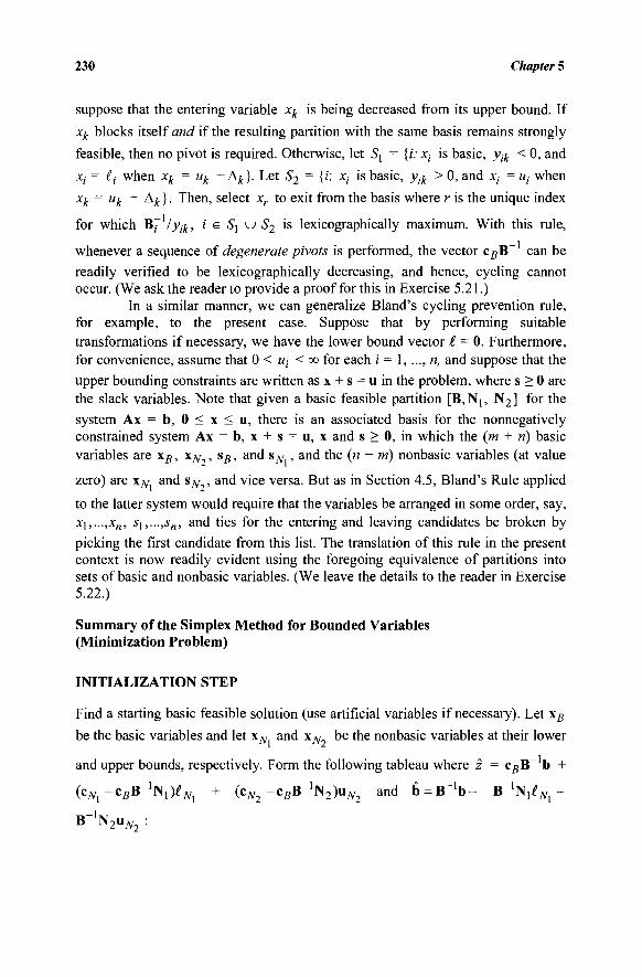
230 Chapter 5
suppose that the entering variable xk is being decreased from its upper bound. If
xk blocks itself and if the resulting partition with the same basis remains strongly
feasible, then no pivot is required. Otherwise, let S\ = {i: x; is basic, yik < 0, and
Xj = tj when xk = uk - Δ ^ } . Let S2 = {/: Xj is basic, yjk > 0, and JC,· = w,· when xk = uk ~ ^ki- Then, select xr to exit from the basis where r is the unique index
for which BJ lyik, i ε S^ u 52 is lexicographically maximum. With this rule,
whenever a sequence of degenerate pivots is performed, the vector cBB~ can be
readily verified to be lexicographically decreasing, and hence, cycling cannot occur. (We ask the reader to provide a proof for this in Exercise 5.21.)
In a similar manner, we can generalize Bland's cycling prevention rule, for example, to the present case. Suppose that by performing suitable transformations if necessary, we have the lower bound vector £ = 0. Furthermore, for convenience, assume that 0 < w,· < co for each i = 1,..., n, and suppose that the upper bounding constraints are written as x + s = u in the problem, where s > 0 are the slack variables. Note that given a basic feasible partition [B, Nj, N2] for the
system Ax = b, 0 < x < u, there is an associated basis for the nonnegatively constrained system Ax = b, x + s = u, x and s > 0, in which the (m + ri) basic variables are \B, χ^ , sB, and s^ , and the (n - rri) nonbasic variables (at value
zero) are x^ and sN , and vice versa. But as in Section 4.5, Bland's Rule applied
to the latter system would require that the variables be arranged in some order, say, xi,...,xn, s^,...,sn, and ties for the entering and leaving candidates be broken by
picking the first candidate from this list. The translation of this rule in the present context is now readily evident using the foregoing equivalence of partitions into sets of basic and nonbasic variables. (We leave the details to the reader in Exercise 5.22.)
Summary of the Simplex Method for Bounded Variables (Minimization Problem)
INITIALIZATION STEP
Find a starting basic feasible solution (use artificial variables if necessary). Let \B
be the basic variables and let \N and xN be the nonbasic variables at their lower
and upper bounds, respectively. Form the following tableau where z = cgB~ b +
(cNl-cBB-%)£Ni + (cN2 - c s B- 'N 2 )u W 2 and 6 = Β ~ ^ - B~%iNl~
B-'N2uW2 :
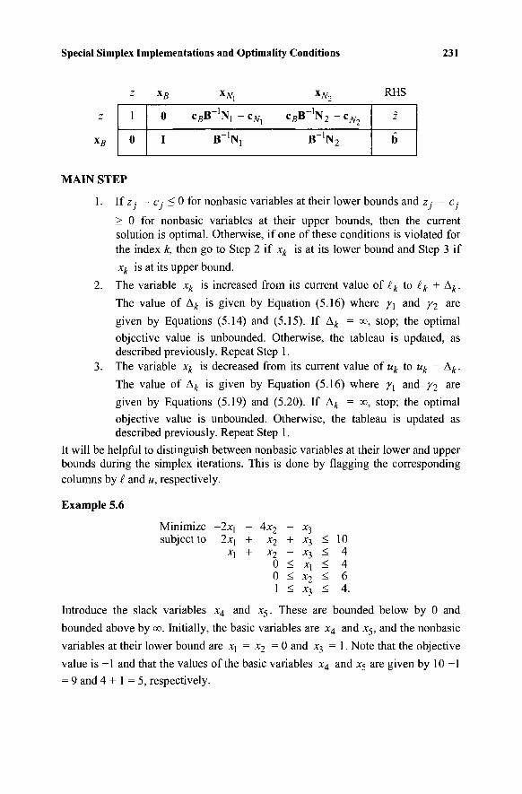
Special Simplex Implementations and Optimally Conditions 231
XB
z
1
0
XB
0
I
XJV,
CgB-'N! - c ^
B_1N!
XN2
cBB"1N2 - cN2
B_1N2
RHS
z
b
MAIN STEP
1. If; Cj < 0 for nonbasic variables at their lower bounds and z j J - J J
> 0 for nonbasic variables at their upper bounds, then the current solution is optimal. Otherwise, if one of these conditions is violated for the index k, then go to Step 2 if xk is at its lower bound and Step 3 if
xk is at its upper bound.
2. The variable xk is increased from its current value of £k to £k + Ak.
The value of Ak is given by Equation (5.16) where γ^ and γ2 a r e
given by Equations (5.14) and (5.15). If Ak = oo, stop; the optimal
objective value is unbounded. Otherwise, the tableau is updated, as described previously. Repeat Step 1.
3. The variable xk is decreased from its current value of uk to uk - Ak.
The value of Ak is given by Equation (5.16) where γ\ and γ2 are
given by Equations (5.19) and (5.20). If Ak = GO, stop; the optimal
objective value is unbounded. Otherwise, the tableau is updated as described previously. Repeat Step 1.
It will be helpful to distinguish between nonbasic variables at their lower and upper bounds during the simplex iterations. This is done by flagging the corresponding columns by £ and u, respectively.
Example 5.6
Minimize subject to
-2JC]
2XJ
*l
- 4 x 2 - *3 + X2 + *3
+ x2 ~ x3 0 < xx
0 < x2
1 < x3
< 10 < 4 < 4 < 6 < 4.
Introduce the slack variables x4 and x5. These are bounded below by 0 and
bounded above by oo. Initially, the basic variables are x4 and x5, and the nonbasic
variables at their lower bound = 0 and x3 = 1. Note that the objective
value is -1 and that the values of the basic variables x4 and x5 are given by 10 -1 = 9 and 4 + 1 = 5 , respectively.
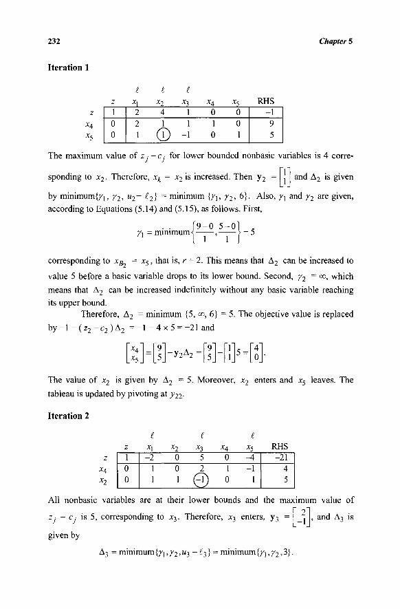
232 Chapter 5
Iteration 1
z 1 0 0
*1 2 2 1
*2 *3 4 1 1 1
© -i
X4
0 1 0
*s 0 0 1
RHS -1 9 5
z X4
x5
The maximum value of z ,· - c, for lower bounded nonbasic variables is 4 corre-
sponding to x2 · Therefore, xk = x2 is increased. Then y2 and Δ2 is given
by minimum{/], γ2, u2~ ί2) = minimum {γχ, γ2, 6}. Also, γ\ and γ2 are given,
according to Equations (5.14) and (5.15), as follows. First,
Ì 9 - 0 5 -0 ] γλ = minimum <- = 5
corresponding to xB = x5 , that is, r = 2. This means that Δ2 can be increased to
value 5 before a basic variable drops to its lower bound. Second, γ2 = co, which
means that Δ2 can be increased indefinitely without any basic variable reaching
its upper bound.
Therefore, Δ2 = minimum {5,00, 6} = 5. The objective value is replaced
by-1 ~{z2 -c2 )Δ2 = - 1 - 4 x 5 =-21 and
* 5 . -Υ2Δ2 =
9 5
- 1 1 5 = 4
0
The value of x2 is given by Δ2 = 5 . Moreover, x2 enters and x5 leaves. The
tableau is updated by pivoting at y22.
Iteration 2
z 1 0 0
xl -2
1 1
x2 0 0 1
*3 5 2
Θ
x4
0 1 0
x5
-4 -1
1
RHS -21
4 5
z x4 x2
All nonbasic variables are at their lower bounds and the maximum value of 2 zj - Cj is 5, corresponding to x3. Therefore, x3 enters, y3
:
given by
Δ3 = minimum{γ\,γ2,«3 - ^ 3 } = minimum{^1,^2,3}.
-1 , and Δ3 is
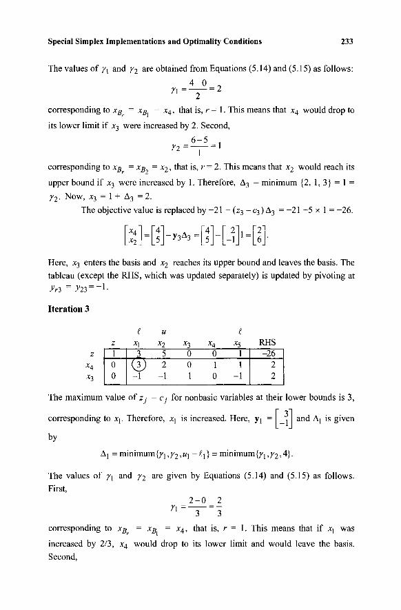
Special Simplex Implementations and Optimality Conditions 233
The values of γχ and γ2 are obtained from Equations (5.14) and (5.15) as follows:
4 - 0
corresponding to xB = xB = x4, that is, r = 1. This means that x4 would drop to
its lower limit if x3 were increased by 2. Second,
6 - 5 Ϊ2
1 1
corresponding to xB = xB = x2, that is, r = 2. This means that x2 would reach its
upper bound if x3 were increased by 1. Therefore, Δ3 = minimum {2, 1, 3} = 1 =
γ2 ■ Now, x3 = 1 + Δ3 = 2.
The objective value is replaced by -21 - (z3 - c3) Δ3 = - 2 1 - 5 x 1 = -26.
x4 x2.
- ν 3 Δ 3 = 4 5 - 2
-1 1 = 2 6
Here, x3 enters the basis and x2 reaches its upper bound and leaves the basis. The
tableau (except the RHS, which was updated separately) is updated by pivoting at
Iteration 3
z X4
x3
z 1 0 0
^ *1 3
( 3 ) -1
u x2
5 2
-1
x3
0 0 1
X4
0 1 0
I x5
1 1
-1
RHS -26
2 2
The maximum value of z - c ■ for nonbasic variables at their lower bounds is 3,
and Aj is given corresponding to Xj. Therefore, xj is increased. Here, yi =
by
Δ] = minimum {Y\,y2,u\-i\} = minimum {γ\,γ2Α}-
The values of γ\ and γ2 are given by Equations (5.14) and (5.15) as follows.
First,
2 - 0 2 7 l " = 3
corresponding to xB = xB = x4, that is, r = 1. This means that if x\ was
increased by 2/3, x4 would drop to its lower limit and would leave the basis. Second,
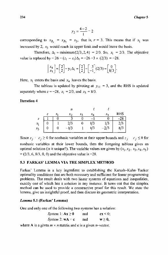
234 Chapter 5
corresponding to xB = xB = x3, that is, r = 3. This means that if x^ was
increased by 2, x3 would reach its upper limit and would leave the basis.
Therefore, Δ] =minimum{2/3,2,4} = 2/3. So, Xj = 2/3. The objective
value is replaced by - 26 - (zj - qJAj = -26 -3 x (2/3) = -28.
_ x 3 . =
"2" 2_ - y i A i =
~2 2_ -
' 3" -1 (2/3)= " 0 "
_8/3_
Here, xj enters the basis and x4 leaves the basis.
The tableau is updated by pivoting at yn = 3, and the RHS is updated
separately where z = -28, xj = 2/3, and x3 = 8/3.
Iteration 4
u £ I Z Χγ X~y X-7 XA X5 RHS 1 0 0
0 3 0 - 1 0 1 2/3 0 1/3 1/3 0 -1/3 1 1/3 -2/3
-28 2/3 8/3
Since zj - c,· > 0 for nonbasic variables at their upper bounds and z - c · < 0 for
nonbasic variables at their lower bounds, then the foregoing tableau gives an optimal solution (is it unique?). The variable values are given by (x\,X2, X3,X4,xs) = (2/3, 6, 8/3, 0, 0) and the objective value is -28.
5.3 FARKAS' LEMMA VIA THE SIMPLEX METHOD
Farkas' Lemma is a key ingredient to establishing the Karush-Kuhn-Tucker optimality conditions that are both necessary and sufficient for linear programming problems. The result deals with two linear systems of equations and inequalities, exactly one of which has a solution in any instance. It turns out that the simplex method can be used to provide a constructive proof for this result. We state the lemma, give an insightful proof, and then discuss its geometric interpretation.
Lemma 5.1 (Farkas' Lemma)
One and only one of the following two systems has a solution:
System 1 : Ax > 0 and ex < 0;
System 2: wA = c and w > 0 ,
where A is a given m x n matrix and c is a given «-vector.
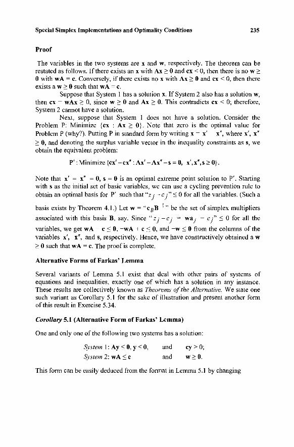
Special Simplex Implementations and Optimality Conditions 235
Proof
The variables in the two systems are x and w, respectively. The theorem can be restated as follows. If there exists an x with Ax > 0 and ex < 0, then there is no w > 0 with wA = c. Conversely, if there exists no x with Ax > 0 and ex < 0, then there exists a w > 0 such that wA = c.
Suppose that System 1 has a solution x. If System 2 also has a solution w, then ex = wAx > 0, since w > 0 and Ax > 0. This contradicts ex < 0; therefore, System 2 cannot have a solution.
Next, suppose that System 1 does not have a solution. Consider the Problem P: Minimize {ex : Ax > 0}. Note that zero is the optimal value for Problem P (why?). Putting P in standard form by writing x = x' - x", where x', x"
> 0, and denoting the surplus variable vector in the inequality constraints as s, we obtain the equivalent problem:
P' : Minimize {ex'-cx" : A x ' - Ax"-s = 0, x',x",s > 0}.
Note that x' = x" = 0, s = 0 is an optimal extreme point solution to P'. Starting with s as the initial set of basic variables, we can use a cycling prevention rule to obtain an optimal basis for P' such that "z ,· - c ,·" < 0 for all the variables. (Such a
basis exists by Theorem 4.1.) Let w = "c s B~ " be the set of simplex multipliers
associated with this basis B, say. Since "Z;-CJ = wa, - c , " < 0 for all the
variables, we get wA — c < 0, -wA + c < 0, and -w < 0 from the columns of the variables x', x", and s, respectively. Hence, we have constructively obtained a w > 0 such that wA = c. The proof is complete.
Alternative Forms of Farkas' Lemma
Several variants of Lemma 5.1 exist that deal with other pairs of systems of equations and inequalities, exactly one of which has a solution in any instance. These results are collectively known as Theorems of the Alternative. We state one such variant as Corollary 5.1 for the sake of illustration and present another form of this result in Exercise 5.34.
Corollary 5.1 (Alternative Form of Farkas' Lemma)
One and only one of the following two systems has a solution:
System 1 : Ay < 0, y < 0, and cy > 0;
System 2: wA < c and w > 0.
This form can be easily deduced from the format in Lemma 5.1 by changing
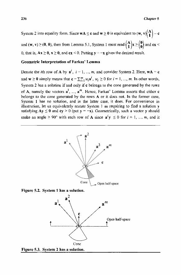
236 Chapter 5
System 2 into equality form. Since wA < c and w > 0 is equivalent to (w, v) . = c
and (w, v) > (0, 0), then from Lemma 5.1, System 1 must read - x > L and ex <
0, that is, Ax > 0, x > 0, and ex < 0. Putting y = -x gives the desired result.
Geometric Interpretation of Farkas' Lemma
Denote the rth row of A by a', / = 1, ..., m, and consider System 2. Here, wA = c
and w > 0 simply means that c = Σ™ι *^»', w,· > 0 for / = 1, ..., m. In other words,
System 2 has a solution if and only if c belongs to the cone generated by the rows
of A, namely the vectors a , ..., am. Hence, Farkas' Lemma asserts that either c belongs to the cone generated by the rows A or it does not. In the former case, System 1 has no solution, and in the latter case, it does. For convenience in illustration, let us equivalently restate System 1 as requiring to find a solution y satisfying Ay < 0 and cy > 0 (put y = -x). Geometrically, such a vector y should
make an angle > 90° with each row of A since a'y < 0 for i = 1, ..., m, and it
Figure 5.2. System 1 has a solution.
.2
Cone Figure 5.3. System 2 has a solution.
Open half-space
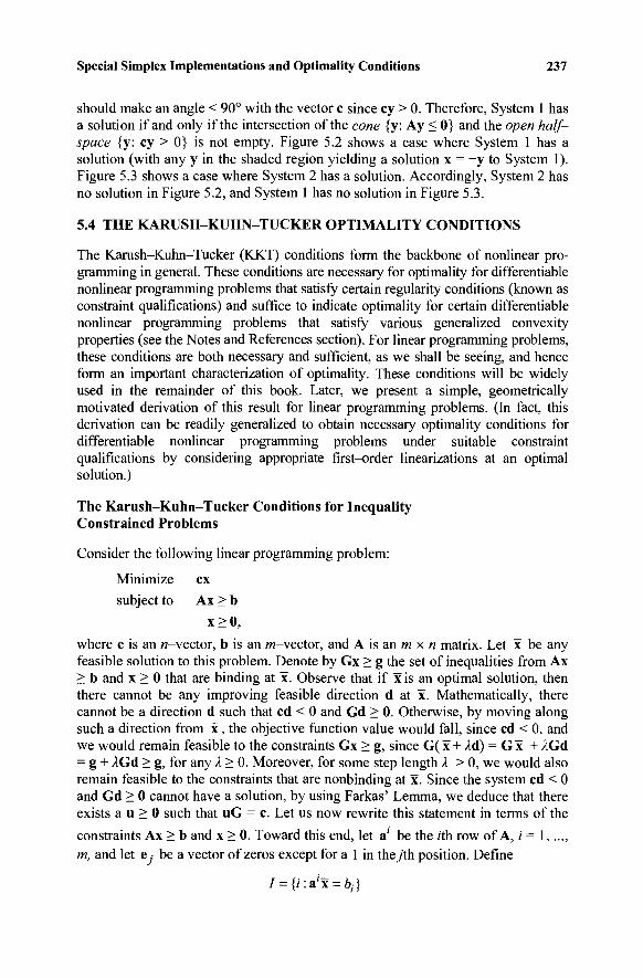
Special Simplex Implementations and Optimality Conditions 237
should make an angle < 90° with the vector c since cy > 0. Therefore, System 1 has a solution if and only if the intersection of the cone {y: Ay < 0} and the open half-space {y: cy > 0} is not empty. Figure 5.2 shows a case where System 1 has a solution (with any y in the shaded region yielding a solution x = -y to System 1 ). Figure 5.3 shows a case where System 2 has a solution. Accordingly, System 2 has no solution in Figure 5.2, and System 1 has no solution in Figure 5.3.
5.4 THE KARUSH-KUHN-TUCKER OPTIMALITY CONDITIONS
The Karush-Kuhn-Tucker (KKT) conditions form the backbone of nonlinear pro-gramming in general. These conditions are necessary for optimality for differentiable nonlinear programming problems that satisfy certain regularity conditions (known as constraint qualifications) and suffice to indicate optimality for certain differentiable nonlinear programming problems that satisfy various generalized convexity properties (see the Notes and References section). For linear programming problems, these conditions are both necessary and sufficient, as we shall be seeing, and hence form an important characterization of optimality. These conditions will be widely used in the remainder of this book. Later, we present a simple, geometrically motivated derivation of this result for linear programming problems. (In fact, this derivation can be readily generalized to obtain necessary optimality conditions for differentiable nonlinear programming problems under suitable constraint qualifications by considering appropriate first-order linearizations at an optimal solution.)
The Karush-Kuhn-Tucker Conditions for Inequality Constrained Problems
Consider the following linear programming problem:
Minimize ex
subject to Ax > b
x > 0 ,
where c is an «-vector, b is an w-vector, and A is an m x n matrix. Let x be any feasible solution to this problem. Denote by Gx > g the set of inequalities from Ax > b and x > 0 that are binding at x. Observe that if x is an optimal solution, then there cannot be any improving feasible direction d at x. Mathematically, there cannot be a direction d such that cd < 0 and Gd > 0. Otherwise, by moving along such a direction from x, the objective function value would fall, since cd < 0, and we would remain feasible to the constraints Gx > g, since G( x + 2d) = G x + IGd = g + AGd > g, for any λ > 0. Moreover, for some step length λ > 0, we would also remain feasible to the constraints that are nonbinding at x. Since the system cd < 0 and Gd > 0 cannot have a solution, by using Farkas' Lemma, we deduce that there exists a u > 0 such that uG = c. Let us now rewrite this statement in terms of the
constraints Ax > b and x > 0. Toward this end, let a' be the rth row of A, i = 1,..., m, and let e ,· be a vector of zeros except for a 1 in they'th position. Define
/ = {/:a'x = o;·}
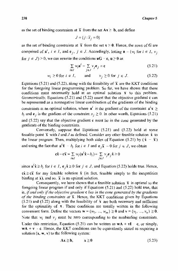
238 Chapter 5
as the set of binding constraints at x from the set Ax > b, and define
J = {j:xj=0)
as the set of binding constraints at x from the set x > 0. Hence, the rows of G are
comprised of a', i e / , and e ,·, j e J. Accordingly, letting u = (w; for / e / , v.-
for j e J ) > 0, we can rewrite the conditions uG = c, u > 0 as
Z w / a/ + Σ v 7 e y =c (5.21)
iel jeJ wt > 0 for i e I, and Vj > 0 for j e J. (5.22)
Equations (5.21) and (5.22), along with the feasibility of x are the KKT conditions for the foregoing linear programming problem. So far, we have shown that these conditions must necessarily hold at an optimal solution x to this problem. Geometrically, Equations (5.21) and (5.22) assert that the objective gradient c can be represented as a nonnegative linear combination of the gradients of the binding
constraints at an optimal solution, where a' is the gradient of the constraint a'x > bj and e, is the gradient of the constraint x · > 0. In other words, Equations (5.21)
and (5.22) say that the objective gradient c must lie in the cone generated by the gradients of the binding constraints.
Conversely, suppose that Equations (5.21) and (5.22) hold at some feasible point x with / and J as defined. Consider any other feasible solution x to the linear program. Then, multiplying both sides of Equation (5.21) by (x - x)
and using the fact that a'x = ty for / e / and e x = 0 for j e J, we obtain
c x - c x = X Wj(a'x-bj)+ X vjejx>0 iel jeJ
since a'x > bt for / e / , e x > 0 for j e J, and Equation (5.22) holds true. Hence,
ex > ex for any feasible solution x (in fact, feasible simply to the inequalities binding at x), and so, x is an optimal solution.
Consequently, we have shown that a feasible solution x is optimal to the foregoing linear program if and only if Equations (5.21) and (5.22) hold true, that is, if and only if the objective gradient c lies in the cone generated by the gradients of the binding constraints at x. Hence, the KKT conditions given by Equations (5.21) and (5.22) along with the feasibility of x are both necessary and sufficient for the optimality of x. These conditions are usually written in the following convenient form. Define the vectors w = (v^, ..., wm) > 0 and v = (vj, ..., vn) > 0. Note that w, and v must be zero corresponding to the nonbinding constraints.
Under this restriction, Equation (5.21) can be written as wA + vi = c, or simply, wA + v = c. Hence, the KKT conditions can be equivalently stated as requiring a solution (x, w, v) to the following system:
Ax > b, x > 0 (5.23)
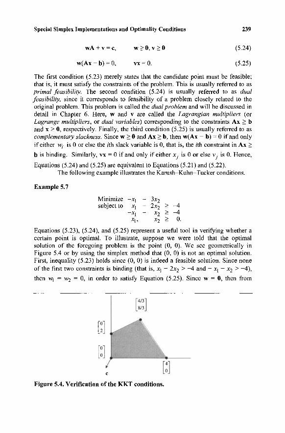
Special Simplex Implementations and Optimality Conditions 239
wA + v = c, w > 0, v > 0 (5.24)
w(Ax - b) = 0, vx = 0. (5.25)
The first condition (5.23) merely states that the candidate point must be feasible; that is, it must satisfy the constraints of the problem. This is usually referred to as primal feasibility. The second condition (5.24) is usually referred to as dual feasibility, since it corresponds to feasibility of a problem closely related to the original problem. This problem is called the dual problem and will be discussed in detail in Chapter 6. Here, w and v are called the Lagrangian multipliers (or Lagrange multipliers, or dual variables) corresponding to the constraints Ax > b and x > 0, respectively. Finally, the third condition (5.25) is usually referred to as complementary slackness. Since w > 0 and Ax > b, then w(Ax - b) = 0 if and only if either vv; is 0 or else the rth slack variable is 0, that is, the rth constraint in Ax >
b is binding. Similarly, vx = 0 if and only if either x- is 0 or else v, is 0. Hence,
Equations (5.24) and (5.25) are equivalent to Equations (5.21) and (5.22). The following example illustrates the Karush-Kuhn-Tucker conditions.
Example 5.7
Minimize -xj - 3x2 subject to JCJ - 2x2 ^ ~4
-Χγ - *2 - ~ 4 Xy, X2 - 0·
Equations (5.23), (5.24), and (5.25) represent a useful tool in verifying whether a certain point is optimal. To illustrate, suppose we were told that the optimal solution of the foregoing problem is the point (0, 0). We see geometrically in Figure 5.4 or by using the simplex method that (0, 0) is not an optimal solution. First, inequality (5.23) holds since (0, 0) is indeed a feasible solution. Since none of the first two constraints is binding (that is, Xj - 2x2 > -4 and - X\ - x2 > ~4), then W| = w2 = 0, in order to satisfy Equation (5.25). Since w = 0, then from
Figure 5.4. Verification of the KKT conditions.
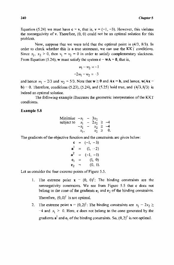
240 Chapter 5
Equation (5.24) we must have c = v, that is, v = (-1, -3). However, this violates the nonnegativity of v. Therefore, (0, 0) could not be an optimal solution for this problem.
Now, suppose that we were told that the optimal point is (4/3, 8/3). In order to check whether this is a true statement, we can use the KKT conditions. Since xx, x2 > 0, then vl = v2 = 0 in order to satisfy complementary slackness. From Equation (5.24), w must satisfy the system c - wA = 0, that is,
w\ -w 2 = -1
-2w[ - w2 = -3
and hence wx = 2/3 and w2 = 5/3. Note that w > 0 and Ax = b, and hence, w(Ax -
b) = 0. Therefore, conditions (5.23), (5.24), and (5.25) hold true, and (4/3,8/3) is
indeed an optimal solution. The following example illustrates the geometric interpretation of the KKT
conditions.
Example 5.8
Minimize -x\ - 3x2 subject to X! - 2x2 ^ _ 4
-X\ - x2 > -4 Xj, x2 > 0.
The gradients of the objective function and the constraints are given below:
c = (-1, -3)
a1 = (1, - 2 )
a2 = (-1, -1) ei = (1, 0) e2 = (0, 1).
Let us consider the four extreme points of Figure 5.5.
1. The extreme point x = (0, 0)': The binding constraints are the nonnegativity constraints. We see from Figure 5.5 that c does not belong to the cone of the gradients ej and e2 of the binding constraints.
Therefore, (0,0)' is not optimal.
2. The extreme point x = (0,2)': The binding constraints are xx - 2x2 >
-4 and xj > 0. Here, c does not belong to the cone generated by the
gradients a and e} of the binding constraints. So, (0,2)' is not optimal.
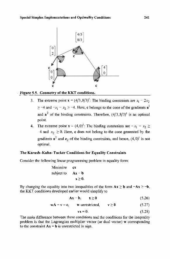
Special Simplex Implementations and Optimality Conditions 241
Figure 5.5. Geometry of the KKT conditions.
3. The extreme point x = (4/3,8/3)': The binding constraints are xx - 2x2
> -4 and -JCJ - x2 > -4 . Here, c belongs to the cone of the gradients a
and a of the binding constraints. Therefore, (4/3,8/3)' is an optimal
point.
4. The extreme point x = (4,0)': The binding constraints are ~X\ - x2 >
-4 and x2 > 0. Here, c does not belong to the cone generated by the
gradients a and e2 of the binding constraints, and hence, (4,0)' is not
optimal.
The Karush-Kuhn-Tucker Conditions for Equality Constraints
Consider the following linear programming problem in equality form:
Minimize ex
subject to Ax = b
x > 0 .
By changing the equality into two inequalities of the form Ax > b and -Ax > -b ,
the KKT conditions developed earlier would simplify to
Ax = b, x > 0 (5.26)
wA + v = c, w unrestricted, v > 0 (5.27)
vx = 0. (5.28) The main difference between these conditions and the conditions for the inequality problem is that the Lagrangian multiplier vector (or dual vector) w corresponding to the constraint Ax = b is unrestricted in sign.
242 Chapter 5
Optimally at a Basic Feasible Solution
Consider the following problem:
Minimize ex
subject to Ax = b
x > 0 .
Assume that rank (A) = m. Let us reinvestigate how the simplex method recognizes an optimal basic feasible solution. Suppose that we have a basic feasible solution x with basis B and let us examine conditions (5.26), (5.27), and (5.28). Obviously, (5.26) holds true. The condition c - wA - v = 0 can be rewritten as follows, where v is decomposed into \B and \N:
(cB, cN) - w(B, N) - (v s , yN) = (0, 0). (5.29)
To satisfy the complementary slackness condition vx = 0, since xN = 0, it suffices
to have \B = 0, so that vx = v#x s + v^x^ = 0. With vs = 0, Equation (5.29)
reduces to the following two equations:
cB - w B = 0
cN - w N - νΛτ=0.
From the first equation we get w = c5B~ , and from the second equation we get
vN = cN - wN = cN - cBB_1N.
To summarize, given a basic feasible solution, condition (5.26) automatically holds true. Equation (5.28) is satisfied by letting \B = 0, and the condition wA + v = c is
satisfied by letting w = cgB~ and \N = cN - cBB~ N. The only possible
source of violation of the Karush-Kuhn-Tucker conditions is that v^ might not be
nonnegative. Note, however, that vN consists of the (cj - zy)-values for the
nonbasic variables. Therefore, the nonnegativity of v^ in Equation (5.27) is
violated if c,· - z ■ < 0 for some nonbasic variable. Of course, if c .· - z,· > 0 for
each nonbasic variable, then \N > 0 and all the Karush-Kuhn-Tucker conditions
are met. These are precisely the simplex termination criteria.
Reinterpretation of the Simplex Method
From the previous discussion, the simplex method can be interpreted as a systematic procedure for approaching an optimal extreme point satisfying the Karush-Kuhn-Tucker conditions. At each iteration, feasibility (called primal feasibility) is satisfied, and hence, condition (5.26) always holds true. Also, complementary slackness is always satisfied, since either a variable x ■ is nonbasic
and has value zero, or else v.· = c.· - z = 0, and hence v · x = 0 for ally, i.e.,
Special Simplex Implementations and Optimality Conditions 243
vx = 0. Therefore, condition (5.28) is always satisfied during the simplex method. Condition (5.27) (called dual feasibility; more on this in Chapter 6) is partially violated during the iterations of the simplex method. Condition (5.27) has two portions, namely, wA + v = c and v > 0. The first portion always holds true by
letting w = CgB~ and v = (\B, \N) = (0, cN - c g B ~ N). However, the second
portion, namely nonnegativity of c^ - cgB~ N, which is part of dual feasibility, is
violated, until of course, an optimal basis is reached. To summarize, the simplex method always satisfies primal feasibility and complementary slackness. Dual feasibility is violated, and the violation is used to try and improve the objective function value by increasing the nonbasic variable having the most negative c ■ - Zj, for example, until dual feasibility is also satisfied.
Finding the Lagrangian Multipliers from the Simplex Tableau
We already know that \B = 0 and \N = cN - cgB~ N. Therefore, the Lagrangian
multiplier v corresponding to the constraint x ■ > 0 can be easily obtained from
row 0 of the simplex tableau. More precisely, v, is the negative of the z · - c,
entry in row 0 under the x, column.
Now, we turn to the Lagrangian vector w = cgB~ corresponding to the
constraints Ax = b. The method for obtaining w from the simplex tableau was discussed in Chapter 3. We shall elaborate on this further. Recall that row 0 of the simplex method consists of z,· - c · fory = 1,...,«, which is given by the vector
CgB~ A - c. If the matrix A has an identity matrix as a portion of its columns,
then in row 0 under these columns, we have csB~ I - c = w — c, where è is the part of the cost vector c corresponding to the identity columns in the original problem. By simply adding the vector c to w - c in row 0, we get w.
EXERCISES
[5.1] Solve the following linear program by the revised simplex method:
Minimize Xj + 4x2 - 7x3 + x4 + 5x5 subject to xj - (3/4)x2 + 2x3 - (1/4) x4 = 6
- (1/4) x2 + 3x3 - (3/4) x4 + x5 = 5 Xj, x 2 , x 3 , Χ4, Xj > 0.
[5.2] Solve the following linear program by the revised simplex method: Maximize - 2x2 + x3 subject to xj - 2x2 + x3 > -4
X] + x2 + x3 < 7 zxj — x2 — x3 s 5 x1; x2, x3 > 0.
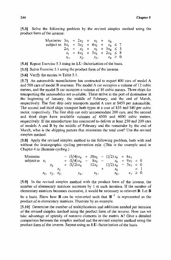
244 Chapter 5
[5.3] Solve the following problem by the revised simplex method using the product form of the inverse:
Maximize 3x{ + 2x2 + X3 + X4 subject to 8x[ + 3x2 + 4x3 + x4 < 7
2xj + x2 + X3 + 5 x 4 < 3 X\ + 4 x 2 + 5x3 + 2 x 4 < 8 X|, x 2 , Χ3, x 4 > 0.
[5.4] Repeat Exercise 5.3 using an LU-factorization of the basis.
[5.5] Solve Exercise 5.1 using the product form of the inverse.
[5.6] Verify the entries in Table 5.1.
[5.7] An automobile manufacturer has contracted to export 400 cars of model A and 500 cars of model B overseas. The model A car occupies a volume of 12 cubic meters, and the model B car occupies a volume of 16 cubic meters. Three ships for transporting the automobiles are available. These arrive at the port of destination at the beginning of January, the middle of February, and the end of March, respectively. The first ship only transports model A cars at $450 per automobile. The second and third ships transport both types at a cost of $35 and $40 per cubic meter, respectively. The first ship can only accommodate 200 cars, and the second and third ships have available volumes of 4500 and 6000 cubic meters, respectively. If the manufacturer has contracted to deliver at least 250 and 200 cars of models A and B by the middle of February and the remainder by the end of March, what is the shipping pattern that minimizes the total cost? Use the revised simplex method.
[5.8] Apply the revised simplex method to the following problem, both with and without the lexicographic cycling prevention rule. (This is the example used in Chapter 4 to illustrate cycling.)
Minimize - (3/4) x4 + 20x5 - (1/2) x6 + 6x7 subject to xj + (1/4) x4 - 8x5 - x6 + 9x7 = 0
x2 + (1/2) x4 - 12x5 - (1/2) x6 + 3x7 = 0 x3 + x6 = 1
Xj, x2, X3, x4, X5, x^, x7 ^ 0.
[5.9] In the revised simplex method with the product form of the inverse, the number of elementary matrices increases by 1 at each iteration. If the number of elementary matrices becomes excessive, it would be necessary to reinvert B. Let B
be a basis. Show how B can be reinverted such that B - is represented as the product of m elementary matrices. Illustrate by an example.
[5.10] Determine the number of multiplications and additions needed per iteration of the revised simplex method using the product form of the inverse. How can we take advantage of sparsity of nonzero elements in the matrix A? Give a detailed comparison between the simplex method and the revised simplex method using the product form of the inverse. Repeat using an LU-factorization of the basis.
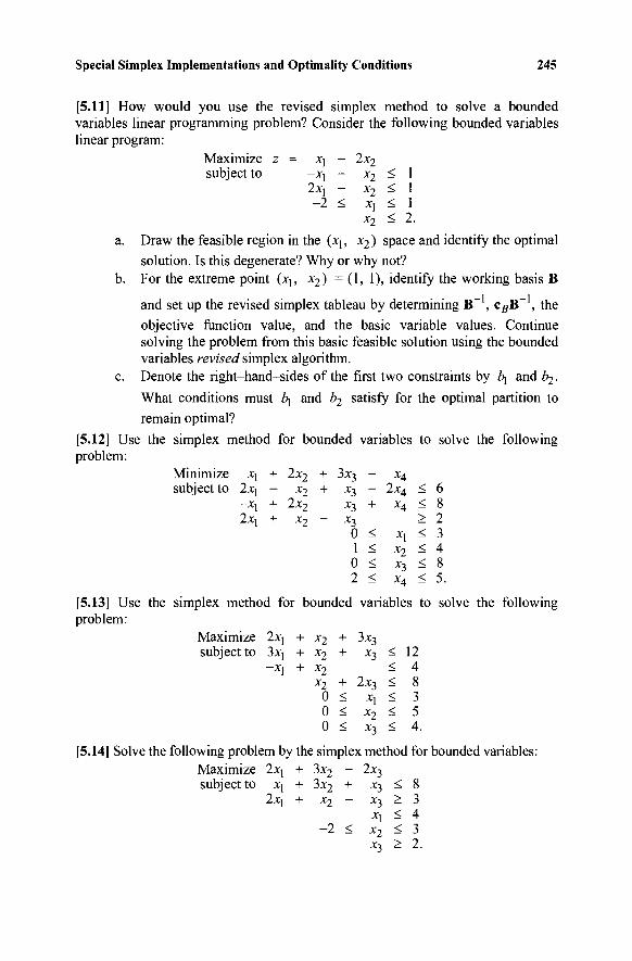
Special Simplex Implementations and Optimality Conditions 245
[5.11] How would you use the revised simplex method to solve a bounded variables linear programming problem? Consider the following bounded variables linear program:
Maximize z = X\ - 2x2 subject to -JCJ - x2 < 1
2xj - x2 < 1 -2 < X] < 1
x2 < 2.
a. Draw the feasible region in the (xj, x2) space and identify the optimal
solution. Is this degenerate? Why or why not? b. For the extreme point (xl5 x2) = (1, 1), identify the working basis B
and set up the revised simplex tableau by determining B~ , c5B~ , the
objective function value, and the basic variable values. Continue solving the problem from this basic feasible solution using the bounded variables revised simplex algorithm.
c. Denote the right-hand-sides of the first two constraints by i\ and b2.
What conditions must i\ and b2 satisfy for the optimal partition to
remain optimal?
[5.12] Use the simplex method for bounded variables to solve the following problem:
Minimize xt + 2x2 + 3x3 - x4 subject to 2xj - x2 + x3 - 2x4 < 6
—Xj + ZX2 — X3 + X4 S o
2xj + x2 - X3 > 2 0 < x{ < 3 1 < x2 < 4 0 < x3 < 8 2 < x4 < 5.
[5.13] Use the simplex method for bounded variables to solve the following problem:
Maximize 2xj + x2 + 3x3 subject to 3xj + x2 + x3 < 12
-Χχ + X2 < 4 x2 + 2x3 < 8
0 < xx < 3 0 < x2 < 5 0 < x3 < 4.
[5.14] Solve the following problem by the simplex method for bounded variables: Maximize 2x] + 3x2 - 2x3 subject to xj + 3x2 + x3 < 8
2x[ + x2 - x3 > 3 xt < 4
-2 < x2 < 3 x3 > 2.
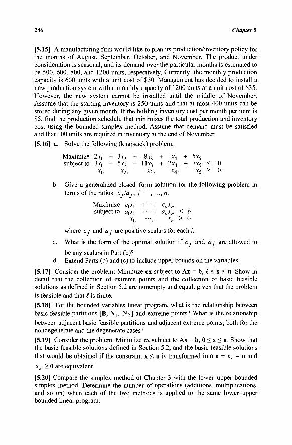
246 Chapter 5
[5.15] A manufacturing firm would like to plan its production/inventory policy for the months of August, September, October, and November. The product under consideration is seasonal, and its demand over the particular months is estimated to be 500, 600, 800, and 1200 units, respectively. Currently, the monthly production capacity is 600 units with a unit cost of $30. Management has decided to install a new production system with a monthly capacity of 1200 units at a unit cost of $35. However, the new system cannot be installed until the middle of November. Assume that the starting inventory is 250 units and that at most 400 units can be stored during any given month. If the holding inventory cost per month per item is $5, find the production schedule that minimizes the total production and inventory cost using the bounded simplex method. Assume that demand must be satisfied and that 100 units are required in inventory at the end of November.
[5.16] a. Solve the following (knapsack) problem.
Maximize 2xj + 3x2 + 8x3 + x4 + 5x5 subject to 3xj + 5x2 + 11*3 + ^x4 + ^x5 - ^
X[, x2, X3, X4, X5 St 0.
b. Give a generalized closed-form solution for the following problem in terms ofthe ratios c;la;, j= 1,..., n:
Maximize C]Xt +···+ cnxn
subject to ajX[ H l· anxn < b X[, · · · , xn > 0,
where c; and a; are positive scalars for each j .
c. What is the form of the optimal solution if cj and a ; are allowed to
be any scalars in Part (b)? d. Extend Parts (b) and (c) to include upper bounds on the variables.
[5.17] Consider the problem: Minimize ex subject to Ax = b, I < x < u. Show in detail that the collection of extreme points and the collection of basic feasible solutions as defined in Section 5.2 are nonempty and equal, given that the problem is feasible and that I is finite.
[5.18] For the bounded variables linear program, what is the relationship between basic feasible partitions [B, Ήχ, Ν2] and extreme points? What is the relationship between adjacent basic feasible partitions and adjacent extreme points, both for the nondegenerate and the degenerate cases?
[5.19] Consider the problem: Minimize ex subject to Ax = b, 0 < x < u. Show that the basic feasible solutions defined in Section 5.2, and the basic feasible solutions that would be obtained if the constraint x < u is transformed into x + xs = u and xs > 0 are equivalent.
[5.20] Compare the simplex method of Chapter 3 with the lower-upper bounded simplex method. Determine the number of operations (additions, multiplications, and so on) when each of the two methods is applied to the same lower-upper bounded linear program.
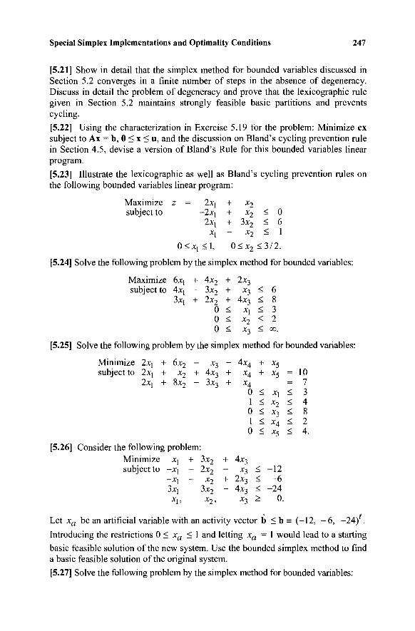
Special Simplex Implementations and Optimality Conditions 247
[5.21J Show in detail that the simplex method for bounded variables discussed in Section 5.2 converges in a finite number of steps in the absence of degeneracy. Discuss in detail the problem of degeneracy and prove that the lexicographic rule given in Section 5.2 maintains strongly feasible basic partitions and prevents cycling.
[5.22] Using the characterization in Exercise 5.19 for the problem: Minimize ex subject to Ax = b, 0 < x < u, and the discussion on Bland's cycling prevention rule in Section 4.5, devise a version of Bland's Rule for this bounded variables linear program.
[5.23] Illustrate the lexicographic as well as Bland's cycling prevention rules on the following bounded variables linear program:
Maximize z = 2xj subject to -2x[
2x[
*1
0 < xl < 1,
[5.24] Solve the following problem by the sim
Maximize 6xj + 4x2
subject to 4xj - 3x2
3xj + 2x2
0 0 0
+ + + -
x2 x2 <
3x2 < x2 <
; 0 ; 6 ; 1
0 < x 2 < 3 / 2 .
plex method for bounded variables:
+ + + < < <
2x3
x3 < 4x3 <
*1 * x2 < ^3 ^
6 8 3 2
00.
[5.25] Solve the following problem by the simplex method for bounded variables:
Minimize 2xt + 6x2 - X3 subject to 2xj + x2 + 4x3
2xj + ox2 — 5x-x
[5.26] Consider the following problem: Minimize xl + 3x2 subject to -xi - 2x2
—Xi — X 2
JXJ — 3x 2
X j , X 2 ,
-+ +
+ -+ -
4x4 + x4 + X4
0 < 1 < 0 < 1 < 0 <
4*3 x3 <
2x3 < 4x3 <
x3 >
*5 x5 =
= *1 ^ x2 < x3 < x4 < *5 ^
-12 -6
-24 0.
10 7 3 4 8 2 4.
Let xa be an artificial variable with an activity vector b < b = (-12, - 6 , -24) . Introducing the restrictions 0 < xa < 1 and letting xa = 1 would lead to a starting basic feasible solution of the new system. Use the bounded simplex method to find a basic feasible solution of the original system.
[5.27] Solve the following problem by the simplex method for bounded variables:
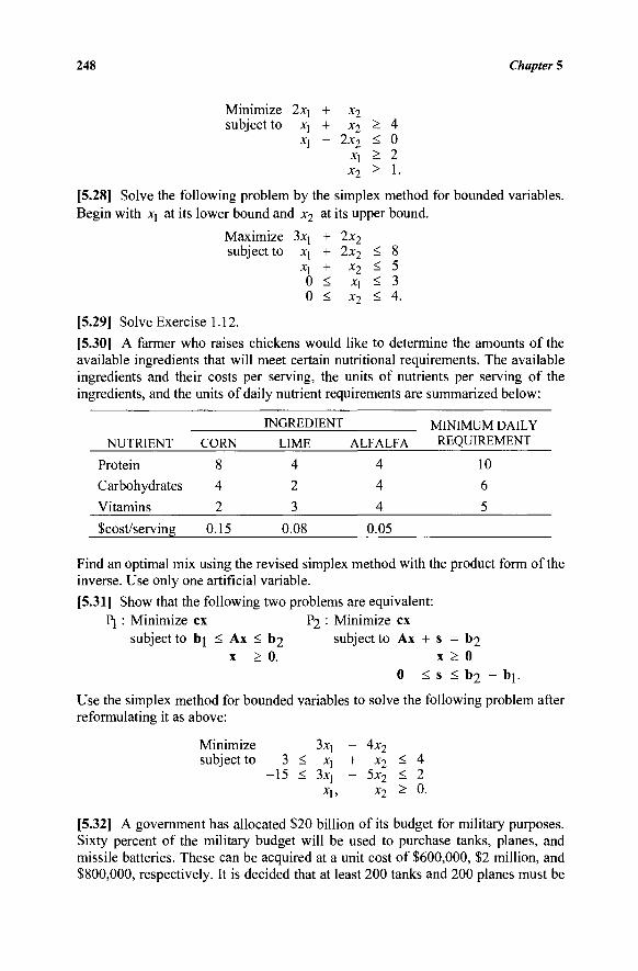
248 Chapter 5
Minimize 2xj + x2 subject to Xj + x2 > 4
X\ - 2x2 ^ 0 x, > 2 x2 > 1.
[5.28] Solve the following problem by the simplex method for bounded variables. Begin with xj at its lower bound and x2 at its upper bound.
Maximize 3xj + 2x2 subject to xl + 2x2 < 8
X[ + x 2 < 5 0 < χλ < 3 0 < x2 < 4.
[5.29] Solve Exercise 1.12.
[5.30] A farmer who raises chickens would like to determine the amounts of the available ingredients that will meet certain nutritional requirements. The available ingredients and their costs per serving, the units of nutrients per serving of the ingredients, and the units of daily nutrient requirements are summarized below:
NUTRIENT
Protein
Carbohydrates
Vitamins
$cost/serving
CORN
8
4
2
0.15
INGREDIENT LIME
4
2
3
0.08
ALFALFA
4
4
4
0.05
MINIMUM DAILY REQUIREMENT
10
6
5
Find an optimal mix using the revised simplex method with the product form of the inverse. Use only one artificial variable.
[5.31] Show that the following two problems are equivalent: P[ : Minimize ex P2 : Minimize ex
subject to bj < Ax < b2 subject to Ax + s = b2 x > 0. x > 0
0 < s < b2 - bj.
Use the simplex method for bounded variables to solve the following problem after reformulating it as above:
Minimize 3xj - 4x2 subject to 3 < xj + x2 < 4
-15 < 3xj - 5x2 < 2 Xl, x2 > 0.
[5.32] A government has allocated $20 billion of its budget for military purposes. Sixty percent of the military budget will be used to purchase tanks, planes, and missile batteries. These can be acquired at a unit cost of $600,000, $2 million, and $800,000, respectively. It is decided that at least 200 tanks and 200 planes must be
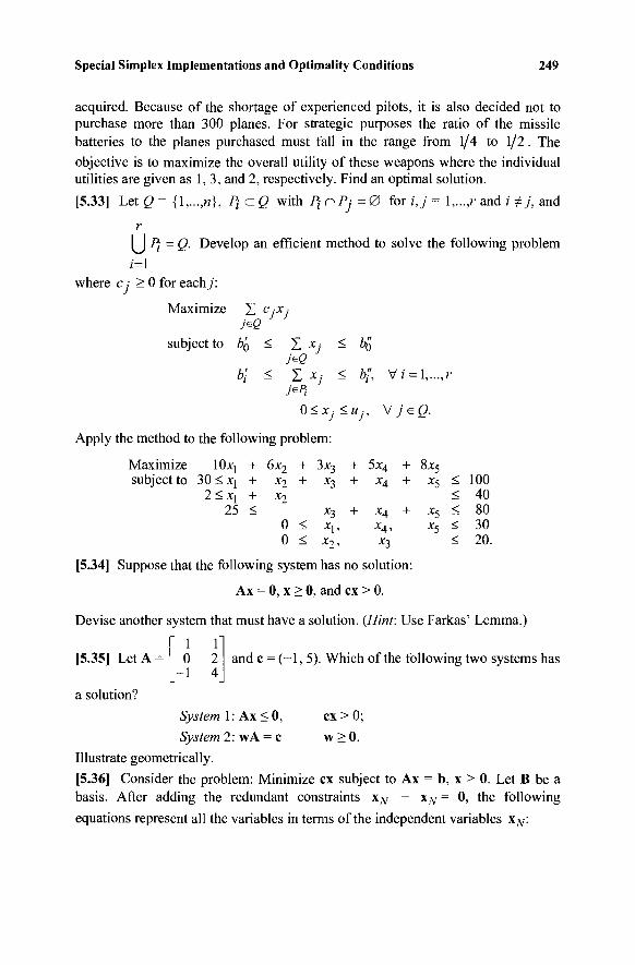
Special Simplex Implementations and Optimality Conditions 249
acquired. Because of the shortage of experienced pilots, it is also decided not to purchase more than 300 planes. For strategic purposes the ratio of the missile batteries to the planes purchased must fall in the range from 1/4 to 1/2. The objective is to maximize the overall utility of these weapons where the individual utilities are given as 1,3, and 2, respectively. Find an optimal solution.
[5.33] Let Q = {Ι,.,.,η}, Pj^Q with P, r\Pj = 0 for i,j = \,...,r and i +j, and
r U Pf = Q. Develop an efficient method to solve the following problem
/=1 where c ,· > 0 for each/:
Maximize Σ c.-x.-
subject to Z>Q < Σ Xj ^ o
b\ < Σ xj < b"h Vi = l,...,r
0<Xj<uj, VjeQ.
Apply the method to the following problem:
Maximize 10xj + 6x2 + 3x3 + 5x4 + 8x5 subject to 30 <X) + x2 + X3 + x 4 + x 5 < 100
2<x t + x2 < 40 25 < 80
0 < Xi, x4, x5 < 30 0 < x2, x3 < 20.
[5.34] Suppose that the following system has no solution:
Ax = 0, x > 0, and ex > 0.
Devise another system that must have a solution. {Hint: Use Farkas' Lemma.)
1 0
-1
f 2 4
[5.35] LetA= 0 2 and c = (- l , 5). Which of the following two systems has
a solution?
System 1 : Ax < 0, ex > 0;
System 2: wA = c w > 0 .
Illustrate geometrically.
[5.36] Consider the problem: Minimize ex subject to Ax = b, x > 0. Let B be a basis. After adding the redundant constraints xN - Χχ= 0, the following equations represent all the variables in terms of the independent variables xN:
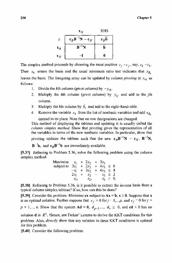
250 Chapter 5
\pj RHS
csB-1N - c^
B-1N
- I
cBb
b
0
The simplex method proceeds by choosing the most positive zj - cj , say, zk - ck.
Then xk enters the basis and the usual minimum ratio test indicates that xB
leaves the basis. The foregoing array can be updated by column pivoting at yrk as
follows: 1. Divide the Mi column (pivot column) by -yrk.
2. Multiply the Mi column (pivot column) by y ■ and add to the jth
column.
3. Multiply the Mi column by br and add to the right-hand-side.
4. Remove the variable xk from the list of nonbasic variables and add xs
instead in its place. Note that no row designations are changed. This method of displaying the tableau and updating it is usually called the column simplex method. Show that pivoting gives the representation of all the variables in terms of the new nonbasic variables. In particular, show that
pivoting updates the tableau such that the new cBB_1N - cN, B_1N,
B~ b, and csB~ b are immediately available.
[5.37] Referring to Problem 5.36, solve the following problem using the column simplex method:
Maximize Xj + 2x2 + 3x3 subject to 3x] + 2x2 + 4x3 < 6
-xj + 3x2 + 4x3 < 8 2xj + x2 - x3 < 2
X], χ 2 , Χ3 ^ 0.
[5.38] Referring to Problem 5.36, is it possible to extract the inverse basis from a typical column simplex tableau? If so, how can this be done?
[5.39] Consider the problem: Minimize ex subject to Ax = b, x > 0. Suppose that x is an optimal solution. Further suppose that Xj > 0 fory = l,...,p, and Xj = 0 fory =
p + 1,..., n. Show that the system Ad = 0, d +1,..., dn > 0, and cd < 0 has no
solution d in R". Hence, use Farkas' Lemma to derive the KKT conditions for this problem. Also, directly show that any solution to these KKT conditions is optimal for this problem.
[5.40] Consider the following problem:
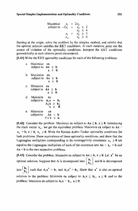
Special Simplex Implementations and Optimality Conditions 251
Maximize subject to
xj + 2JC2
-2x] + X2 x2
X\ + X2
Χγ, Χ2
< < < >
2 4 5 0
Starting at the origin, solve the problem by the simplex method, and exhibit that the optimal solution satisfies the KKT conditions. At each iteration, point out the source of violation of the optimality conditions. Interpret the KKT conditions geometrically at each extreme point encountered.
[5.41] Write the KKT optimality conditions for each of the following problems:
a. Maximize ex subject to Ax < b
x > 0.
b. Maximize ex subject to Ax > b
x > 0.
c. Minimize ex subject to Ax < b
x > 0.
d. Minimize ex subject to Ajx = b]
A2x > b2 x > 0.
e. Minimize ex subject to Ax = b
£<x < u.
[5.42] Consider the problem: Maximize ex subject to Ax < b, x > 0. Introducing the slack vector xs, we get the equivalent problem: Maximize ex subject to Ax + xs = b, x > 0, xs > 0. Write the Karush-Kuhn-Tucker optimality conditions for both problems. Show equivalence of these optimality conditions, and show that the Lagrangian multipliers corresponding to the nonnegativity constraints xs > 0 are
equal to the Lagrangian multipliers of each of the constraint sets Ax + xs = b and
Ax < b in the two respective problems.
[5.43] Consider the problem: Minimize ex subject to Ax > b, x > 0. Let x* be an
optimal solution. Suppose that A is decomposed into M
and b is decomposed
into bi b2
such that Ajx* = bj and A2x* > b 2 . Show that x* is also an optimal
solution to the problem: Minimize ex subject to Ajx > b[, x > 0, and to the
problem: Minimize ex subject to AyX = b1 ; x > 0.
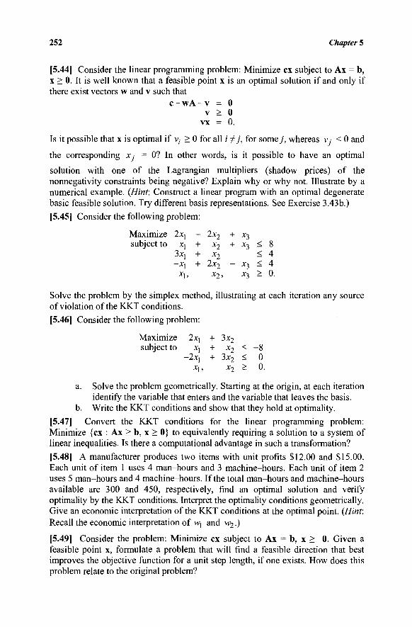
252 Chapter 5
[5.44] Consider the linear programming problem: Minimize ex subject to Ax = b, x > 0. It is well known that a feasible point x is an optimal solution if and only if there exist vectors w and v such that
c - w A - v = 0 v > 0
vx = 0.
Is it possible that x is optimal if v;· > 0 for all i Φ], for some j , whereas v < 0 and
the corresponding x,· = 0? In other words, is it possible to have an optimal
solution with one of the Lagrangian multipliers (shadow prices) of the nonnegativity constraints being negative? Explain why or why not. Illustrate by a numerical example. (Hint: Construct a linear program with an optimal degenerate basic feasible solution. Try different basis representations. See Exercise 3.43b.)
[5.45] Consider the following problem:
Maximize 2xj - 2x2 + X3 subject to X] + x2 + x3 < 8
3xi + x2 < 4 -xj + 2x2 - x3 < 4
X|, X7, X3 ^ 0.
Solve the problem by the simplex method, illustrating at each iteration any source of violation of the KKT conditions.
[5.46] Consider the following problem:
Maximize 2xj + 3x2 subject to xj + x2 < -8
-2xl + 3x2 < 0 xj, x2 > 0.
a. Solve the problem geometrically. Starting at the origin, at each iteration identify the variable that enters and the variable that leaves the basis.
b. Write the KKT conditions and show that they hold at optimality.
[5.47] Convert the KKT conditions for the linear programming problem: Minimize {ex : Ax > b, x > 0} to equivalently requiring a solution to a system of linear inequalities. Is there a computational advantage in such a transformation?
[5.48] A manufacturer produces two items with unit profits $12.00 and $15.00. Each unit of item 1 uses 4 man-hours and 3 machine-hours. Each unit of item 2 uses 5 man-hours and 4 machine-hours. If the total man-hours and machine-hours available are 300 and 450, respectively, find an optimal solution and verify optimality by the KKT conditions. Interpret the optimality conditions geometrically. Give an economic interpretation of the KKT conditions at the optimal point. (Hint: Recall the economic interpretation of w\ and w2.)
[5.49] Consider the problem: Minimize ex subject to Ax = b, x > 0. Given a feasible point x, formulate a problem that will find a feasible direction that best improves the objective function for a unit step length, if one exists. How does this problem relate to the original problem?
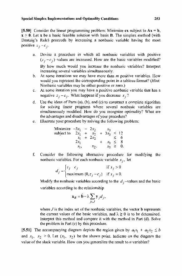
Special Simplex Implementations and Optimally Conditions 253
[5.50] Consider the linear programming problem: Minimize ex subject to Ax = b, x > 0. Let x be a basic feasible solution with basis B. The simplex method (with Dantzig's Rule) proceeds by increasing a nonbasic variable having the most positive z; - C:.
a. Devise a procedure in which all nonbasic variables with positive (z, -c,)-values are increased. How are the basic variables modified?
By how much would you increase the nonbasic variables? Interpret increasing several variables simultaneously.
b. At some iterations we may have more than m positive variables. How would you represent the corresponding point in a tableau format? (Hint: Nonbasic variables may be either positive or zero.)
c. At some iteration you may have a positive nonbasic variable that has a negative ZJ-CJ. What happens if you decrease x ?
d. Use the ideas of Parts (a), (b), and (c) to construct a complete algorithm for solving linear programs where several nonbasic variables are simultaneously modified. How do you recognize optimality? What are the advantages and disadvantages of your procedure?
e. Illustrate your procedure by solving the following problem:
Minimize subject to
-3x[ 2xj
x\ 2xj
xl>
— zx2 — X3 + x2 + 3x3
+ 2x2
+ x3 x2' x3
< < < >
12 6 8 0.
f. Consider the following alternative procedure for modifying the nonbasic variables. For each nonbasic variable x,·, let
(zj - e, if x · > 0 dJ maximum {0, Zj - cj} if Xj = 0.
Modify the nonbasic variables according to the d,· -values and the basic
variables according to the relationship
xB =b-\^y jdj,
where J is the index set of the nonbasic variables, the vector b represents the current values of the basic variables, and λ > 0 is to be determined. Interpret this method and compare it with the method in Part (d). Solve the problem in Part (e) by this procedure.
[5.51] The accompanying diagram depicts the region given by α^χ^ + α2χ2 < b
and xj, x2 > 0. Let (x1? x2) be the shown point. Indicate on the diagram the value of the slack variable. How can you generalize the result to n variables?
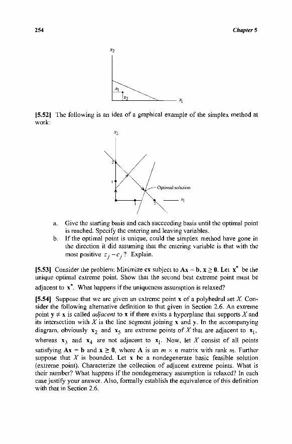
254 Chapter 5
χ2
i*2
[5.52] The following is an idea of a graphical example of the simplex method at work:
a.
Optimal solution
*1
Give the starting basis and each succeeding basis until the optimal point is reached. Specify the entering and leaving variables,
b. If the optimal point is unique, could the simplex method have gone in the direction it did assuming that the entering variable is that with the most positive z,· - c .· ? Explain.
[5.53] Consider the problem: Minimize ex subject to Ax = b, x > 0. Let x* be the unique optimal extreme point. Show that the second best extreme point must be
adjacent to x*. What happens if the uniqueness assumption is relaxed?
[5.54] Suppose that we are given an extreme point x of a polyhedral set X. Con-sider the following alternative definition to that given in Section 2.6. An extreme point y Φ x is called adjacent to x if there exists a hyperplane that supports X and its intersection with X is the line segment joining x and y. In the accompanying diagram, obviously x2 and x5 are extreme points of X that are adjacent to Xy, whereas x3 and x4 are not adjacent to x{. Now, let X consist of all points
satisfying Ax = b and x > 0, where A is an m x n matrix with rank m. Further suppose that X is bounded. Let x be a nondegenerate basic feasible solution (extreme point). Characterize the collection of adjacent extreme points. What is their number? What happens if the nondegeneracy assumption is relaxed? In each case justify your answer. Also, formally establish the equivalence of this definition with that in Section 2.6.
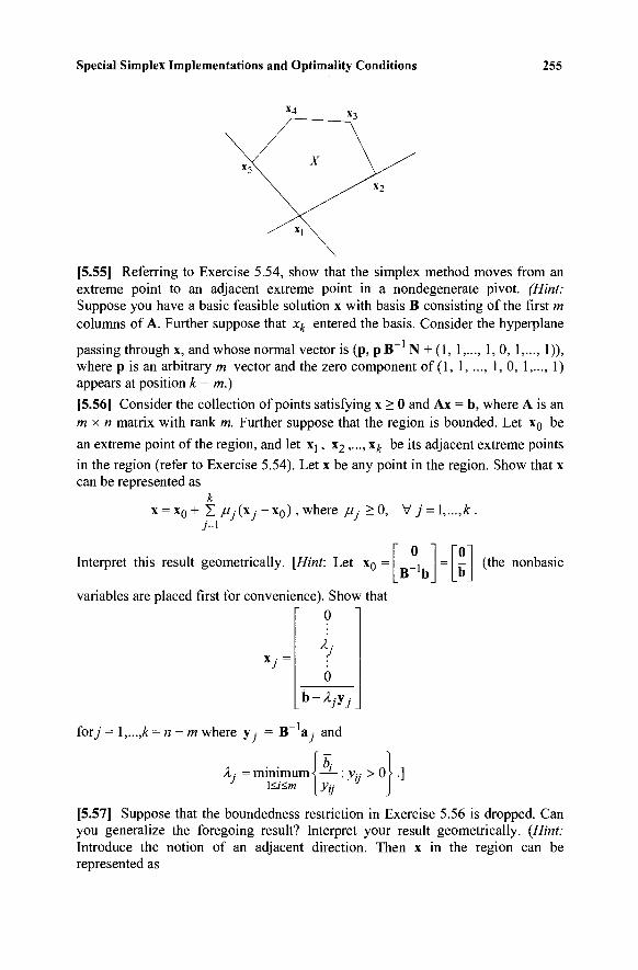
Special Simplex Implementations and Optimality Conditions 255
[5.55] Referring to Exercise 5.54, show that the simplex method moves from an extreme point to an adjacent extreme point in a nondegenerate pivot. (Hint: Suppose you have a basic feasible solution x with basis B consisting of the first m columns of A. Further suppose that xk entered the basis. Consider the hyperplane
passing through x, and whose normal vector is (p, pB~ N + (1, 1,..., 1, 0, 1,..., 1)), where p is an arbitrary w-vector and the zero component of (1, 1, ..., 1, 0, 1,..., 1) appears at position k - m.)
[5.56] Consider the collection of points satisfying x > 0 and Ax = b, where A is an m x n matrix with rank m. Further suppose that the region is bounded. Let x0 be
an extreme point of the region, and let Xj, x2,..., x^ be its adjacent extreme points in the region (refer to Exercise 5.54). Let x be any point in the region. Show that x can be represented as
k
x = *o+ Σ A / ( x / - X o ) > w n e r e Mi ^ ° . Vy = l,...,£.
Interpret this result geometrically. [Hint: Let x0 =
variables are placed first for convenience). Show that 0
0
B ' b (the nonbasic
minimum·; — : ytj > 0 >.] \<i<m \yu
[5.57[ Suppose that the boundedness restriction in Exercise 5.56 is dropped. Can you generalize the foregoing result? Interpret your result geometrically. {Hint: Introduce the notion of an adjacent direction. Then x in the region can be represented as
256 Chapter 5
χ = χ0 + Σ μ,·(χ/ -*ο)+ Σ Mjdj jel jeJ
where //.· > 0 for j e I u J, x for j GI are adjacent extreme points, and d for
j e J are adjacent extreme directions.)
[5.58] Show that an extreme point of a bounded polyhedral set has a minimal objective if and only if it has an objective that is smaller than or equal to that of any adjacent extreme point. Can you generalize the result to the unbounded case? (Hint: Use Exercises 5.56 and 5.57.)
[5.59] Given a basis B, consider an LU factorization such that PBQ = LU, where P and Q respectively permute the rows and columns of B, and where L and U are resultant lower and upper triangular factors. Show how each of the systems wB = cB for computing the simplex multiplier vector w, and By^ = &k for
determining the updated column of an entering variable xk can be solved via the
solution of two appropriate triangular equation systems.
NOTES AND REFERENCES
1. The revised simplex method was devised by Dantzig and Orchard-Hays [1953] (also see Dantzig and Orchard-Hays [1954] for the product form of the inverse). For further reading on this topic, refer to Dantzig [1963a].
2. The experimentation related to fitting the regression equation Kmand^ for computational effort in solving linear programs appears in Knolmayer [1982]. For information on theoretical bounds on computational effort using the simplex method, see Chapter 8.
3. The simplex method using the LU-factorization of the basis was introduced by Bartels and Golub [1969] and is said to employ the "elimination form of the inverse." For more information on this subject, see Gill et al. [1974] and Saunders [1976a, b]. For factorizations designed for use in a parallel computing environment, refer to Helgason et al. [1987]. In an alternative LU factorization approach, the rows and columns of B are suitably permuted (using permutation matrices P and Q), based on which the lower and upper triangular factors L and U, respectively, are computed such that PBQ = LU. In particular, when determining the simplex multiplier vector w via the system wB = c g , this entails solving two triangular systems (see Exercise 5.59). However, Hu and Pan [2008] show how the simplex multiplier vector can be updated from one iteration to the next based on updates to the LU factors such that only one triangular system is solved. This yields a computational advantage, particularly for dense problems.
4. The steepest edge variations of the rules for selecting entering variables are discussed in Harris [1975] and in Goldfarb and Reid [1977]. For problem scaling, see Kuhn and Quandt [1962], Tomlin [1975], and Sherali et al. [1983]. The concept of partial pricing or suboptimization discussed in Section 5.1 is standard and in widespread use. The particular description given here has been adapted from Frendewey and Glover's [1981] experiments on large-scale linear programs with embedded networks. Also,
Special Simplex Implementations and Optimality Conditions 257
see Gibbs et al. [1983]. For model and input/output management of large-scale linear programs, see Greenberg [1983] and Murphy and Stohr [1986]. Several modeling languages have been developed to enable a convenient input of a linear programming model into a solver, without requiring the user to manipulate the data into a particular packed-form representation as needed by the solver. Examples of commercial modeling languages include AMPL, OPL, GAMS, and LINGO. Examples of commercial solvers include CPLEX, OSL (see Forrest and Tomlin (1990)), and LINDO. (Refer to their respective online Web sites.)
5. In Chapter 7 we describe the use of the revised simplex method in solving large-scale problems in the context of decomposition by generating columns at each iteration.
6. The simplex method for bounded variables was developed by Dantzig [1955] at the RAND corporation to provide a shortcut routine for solving a problem of assigning personnel. The method was independently developed by Charnes and Lemke [1954].
7. The strongly feasible partition lexicographic cycling prevention rule for bounded variables linear programming problems was proposed by Cunningham [1976] and Murty [1978]. For further developments involving generalized upper bounds (GUBs) and variable upper bounds (VUBs), the interested reader is referred to Dantzig and Van Slyke [1965] and Schrage [1975, 1978].
8. The Karush-Kuhn-Tucker optimality conditions for nonlinear programs were developed independently by Karush [1939] in his master's thesis, and by Kuhn and Tucker [1950]. A specialization of these conditions for linear programs is given in Section 5.4. For further reading on the theorems of the alternative and the KKT conditions, the reader may refer to Bazaraa, Sherali, and Shetty [2006], Mangasarian [1969], and Zangwill [1969]. The KKT conditions for linear programming and the subject of duality are very closely associated. This fact will become apparent when the reader studies Chapter 6.

This page intentionally left blank

SIX: DUALITY AND SENSITIVITY ANALYSIS
For every linear program we solve, there is another associated linear program that we happen to be simultaneously solving. This new linear program satisfies some very important properties. It may be used to obtain the solution to the original program, and its variables provide extremely useful information about the set of optimal solutions to the original linear program.
This leads to rich economic interpretations related to the original linear programming problem. In fact, the roots of this problem lie in the characteriza-tion of the optimality conditions for the original linear program. For the sake of expository reference, we shall call the original linear programming problem the primal (linear programming) problem, and we shall call this related linear pro-gram the dual (linear programming) problem. Although the term "dual" comes from linear algebra, the term "primal" was suggested as an appropriate Latin antonym by Dantzig's father, Tobias Dantzig (who was a mathematician), to substitute for the cumbersome phrase, "the original problem of which this is the dual." Actually, the terms primal and dual for this related pair of linear pro-gramming problems are only relative, because the dual of the "dual" is the "primal" itself.
We shall begin by formulating this new dual (linear programming) problem and proceed to develop some of its important properties. These properties will lead to two new algorithms, the dual simplex method and the primal-dual algorithm, for solving linear programs. Finally, we shall discuss the effect of variations in the data, that is, the cost coefficients, the right-hand-side coefficients, and the constraint coefficients, on the optimal solution to a linear program.
6.1 FORMULATION OF THE DUAL PROBLEM
Associated with each linear programming problem there is another linear pro-gramming problem called the dual. The dual linear program possesses many important properties relative to the original primal linear program. There are two important forms (definitions) of duality: the canonical form of duality and the standard form of duality. These two forms are completely equivalent. They arise respectively from the canonical and the standard representation of linear programming problems.
Canonical Form of Duality
Suppose that the primal linear program is given in the (canonical) form:
P : Minimize ex subject to Ax > b
x > 0.
Then the dual linear program is defined by:
259
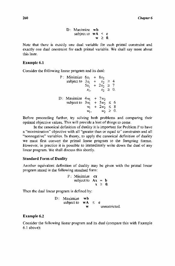
260 Chapter 6
D : Maximize wb subject to wA < c
w > 0.
Note that there is exactly one dual variable for each primal constraint and exactly one dual constraint for each primal variable. We shall say more about this later.
Example 6.1
Consider the following linear program and its dual:
P : Minimize 6x\ + 8x2 subject to 3xj + x2 - 4
5jq + 2x2 S 7 X[, x2 - 0.
D : Maximize 4wj + 7w2 subject to 3wj + 5w2 < 6
Wi + 2 w 2 < 8 Wj, w 2 > 0.
Before proceeding further, try solving both problems and comparing their optimal objective values. This will provide a hint of things to come.
In the canonical definition of duality it is important for Problem P to have a "minimization" objective with all "greater than or equal to" constraints and all "nonnegative" variables. In theory, to apply the canonical definition of duality we must first convert the primal linear program to the foregoing format. However, in practice it is possible to immediately write down the dual of any linear program. We shall discuss this shortly.
Standard Form of Duality
Another equivalent definition of duality may be given with the primal linear program stated in the following standard form:
P : Minimize ex subject to Ax = b
x > 0.
Then the dual linear program is defined by:
D : Maximize wb subject to wA < c
w unrestricted.
Example 6.2
Consider the following linear program and its dual (compare this with Example 6.1 above):
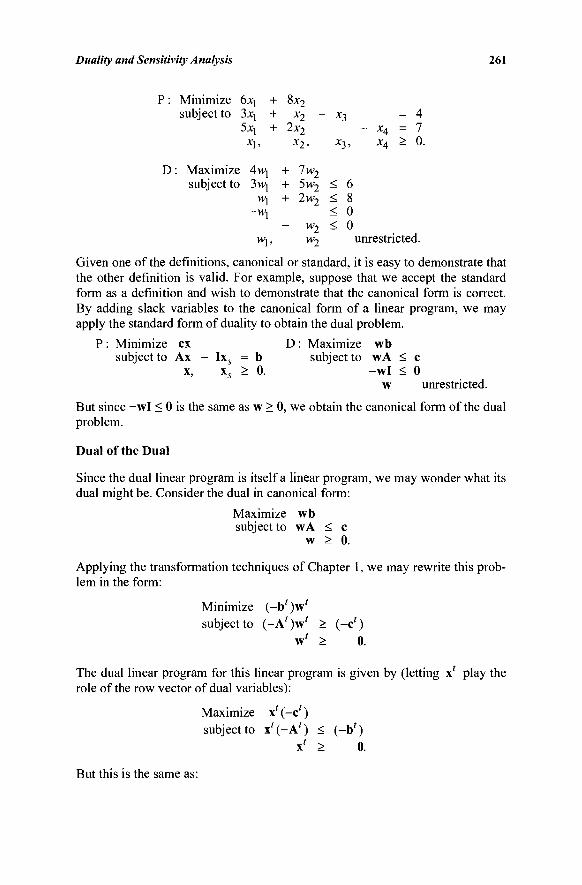
Duality and Sensitivity Analysis 261
P : Minimize 6xj + 8x2 subject to 3*i + x2 -
5xj + 2x2 Xj , X2,
D : Maximize 4wj + 7w2 subject to 3wj + 5w2
Wj + 2w2
- w2 Wj, W2
x3 = 4 - x4 = 7
x3, x4 > 0.
< 6 < 8 < 0 < 0
unrestricted.
Given one of the definitions, canonical or standard, it is easy to demonstrate that the other definition is valid. For example, suppose that we accept the standard form as a definition and wish to demonstrate that the canonical form is correct. By adding slack variables to the canonical form of a linear program, we may apply the standard form of duality to obtain the dual problem.
P : Minimize ex D : Maximize wb subject to Ax -
x, - Ixs = b
xs > 0. subject to wA < c
-w l < 0 w unrestricted.
But since -wl < 0 is the same as w > 0, we obtain the canonical form of the dual problem.
Dual of the Dual
Since the dual linear program is itself a linear program, we may wonder what its dual might be. Consider the dual in canonical form:
Maximize wb subject to wA < c
w > 0.
Applying the transformation techniques of Chapter 1, we may rewrite this prob-lem in the form:
Minimize (-b' )w' subject to (-A')w' > (-c')
w' > 0.
The dual linear program for this linear program is given by (letting x' play the role of the row vector of dual variables):
Maximize x' (-c' ) subject to x ' ( -A') < (-b')
x' > 0.
But this is the same as:
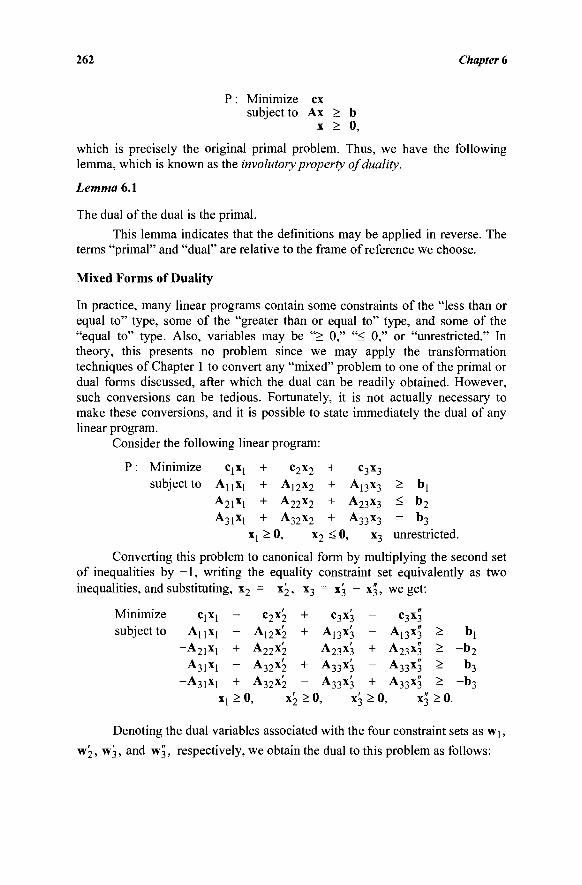
262 Chapter 6
P : Minimize ex subject to Ax > b
x > 0,
which is precisely the original primal problem. Thus, we have the following lemma, which is known as the involutory property of duality.
Lemma 6.1
The dual of the dual is the primal.
This lemma indicates that the definitions may be applied in reverse. The terms "primal" and "dual" are relative to the frame of reference we choose.
Mixed Forms of Duality
In practice, many linear programs contain some constraints of the "less than or equal to" type, some of the "greater than or equal to" type, and some of the "equal to" type. Also, variables may be "> 0," "< 0," or "unrestricted." In theory, this presents no problem since we may apply the transformation techniques of Chapter 1 to convert any "mixed" problem to one of the primal or dual forms discussed, after which the dual can be readily obtained. However, such conversions can be tedious. Fortunately, it is not actually necessary to make these conversions, and it is possible to state immediately the dual of any linear program.
Consider the following linear program:
P : Minimize CJXJ + c2X2 + c3x3
subject to AJJXJ + A12X2 + A n x 3 > bj A21x, + A22x2 + A23x3 < b 2 A3lxl + A32x2 + A33x3 = b3
Xj > 0, x2 < 0, x3 unrestricted.
Converting this problem to canonical form by multiplying the second set of inequalities by - 1 , writing the equality constraint set equivalently as two inequalities, and substituting, x2 = - x 2 , x3 = x3 - x!j, we get:
Minimize qxj - c2x2 + c3x3 - c3x^ subject to AJJXJ - A[2x2 + A13x3 - A13x^ > bj
-A21X! + A22x2 - A23x3 + A23x5 > - b 2 A31xl - A32x2 + A33x3 " A33x3 ^ b3
-A31xl + A32x2 " A33x3 + A33x3 ^ ~b3 Xj > 0, X2 > 0, X3 > 0, X3 > 0.
Denoting the dual variables associated with the four constraint sets as Wj,
w2, w3, and w3, respectively, we obtain the dual to this problem as follows:
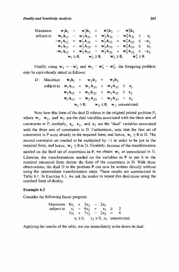
Duality and Sensitivity Analysis 263
w ^ j - w2b2 + w3b3 - w^b3
W 1 A 11 - W 2 A 2 1 + W 3 A 3 1 " W 3 A 3 1 ^ c l W 1 A 1 2 + W 2 A 2 2 - W 3 A 3 2 + W3A32 < - C 2
W 1 A 1 3 - W 2 A 2 3 + W 3 A 3 3 ~ W 3 A 3 3 ^ c 3 w,A13 + w2A2 3 - w3A33 + w5A33 < - c 3
w, > 0, w2 > 0, w3 > 0, W3 > 0.
Finally, using w2 = - w 2 and w3 = w3 - w^, the foregoing problem
may be equivalently stated as follows:
D : Maximize Wjb] + w2b2 + w3b3
subject to WJAJI + w2A2i + w3A31 < C[
WjA12 + w2A2 2 + w3A32 > c2
W1A13 + W2A23 + W3A33 = c3 Wi > 0, w2 < 0, w3 unrestricted.
Note how this form of the dual D relates to the original primal problem P, where Wj, w2, and w3 are the dual variables associated with the three sets of
constraints in P; similarly, Xj, x2, and x3 are the "dual" variables associated with the three sets of constraints in D. Furthermore, note that the first set of constraints in P were already in the required form, and hence, W] > 0 in D. The second constraint set needed to be multiplied by -1 in order to be put in the required form, and hence, w2 < 0 in D. Similarly, because of the transformation
needed on the third set of constraints in P, we obtain w3 as unrestricted in D.
Likewise, the transformations needed on the variables in P to put it in the required canonical form dictate the form of the constraints in D. With these observations, the dual D to the problem P can now be written directly without using the intermediate transformation steps. These results are summarized in Table 6.1. In Exercise 6.1, we ask the reader to repeat this derivation using the standard form of duality.
Example 6.3
Consider the following linear program:
Maximize Βχγ + 3x2 - 2x3 subject to JCJ - 6JC2 + x3 > 2
5xj + 7x2 - 2x3 = -4 Xj < 0, x2 > 0, x3 unrestricted.
Applying the results of the table, we can immediately write down its dual:
Maximize subject to
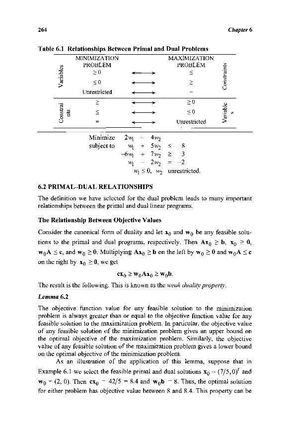
264 Chapter 6
Table 6.1 Relationships Between Primal and Dual Problems
i >
nj
u
MINIMIZATION PROBLEM
> 0
<o Unrestricted
>
<
* *
MAXIMIZATION PROBLEM
<
>
>o <o
Unrestricted
IS
C O
U
ce w
CO
>
Minimize subject to
2w|
-6w[
- 4w2
+ 5w2
+ 7w2
- 2w2
Wj < 0, w2
> 3 = -2 unrestricted.
6.2 PRIMAL-DUAL RELATIONSHIPS
The definition we have selected for the dual problem leads to many important relationships between the primal and dual linear programs.
The Relationship Between Objective Values
Consider the canonical form of duality and let x0 and w0 be any feasible solu-
tions to the primal and dual programs, respectively. Then Ax0 > b, x0 > 0,
w0A < c, and w0 > 0. Multiplying Ax0 > b on the left by w0 > 0 and w0A < c
on the right by x0 > 0, we get
cx0 > w0Ax0 > w0b.
The result is the following. This is known as the weak duality property.
Lemma 6.2
The objective function value for any feasible solution to the minimization problem is always greater than or equal to the objective function value for any feasible solution to the maximization problem. In particular, the objective value of any feasible solution of the minimization problem gives an upper bound on the optimal objective of the maximization problem. Similarly, the objective value of any feasible solution of the maximization problem gives a lower bound on the optimal objective of the minimization problem.
As an illustration of the application of this lemma, suppose that in
Example 6.1 we select the feasible primal and dual solutions x0 = (7/5,0)' and
w0 = (2, 0). Then cx0 = 42/5 = 8.4 and w0b = 8. Thus, the optimal solution
for either problem has objective value between 8 and 8.4. This property can be
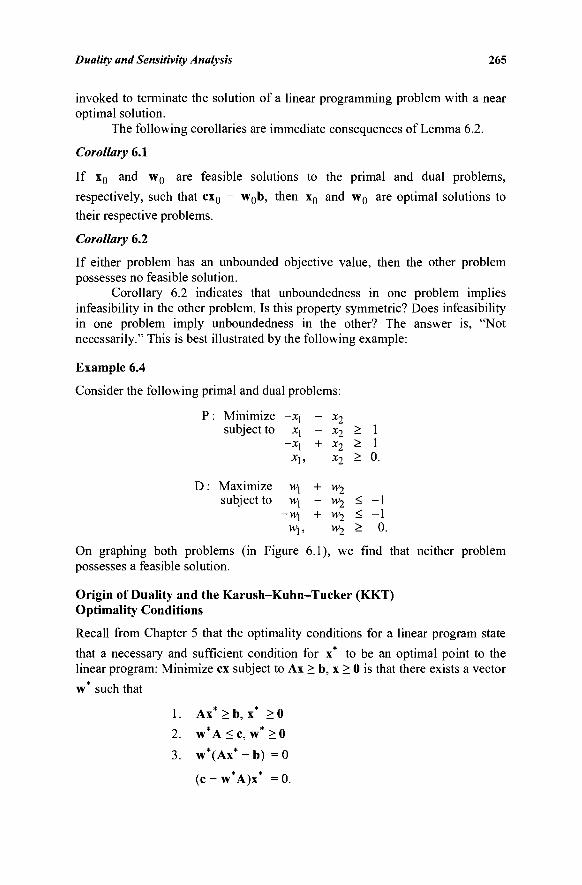
Duality and Sensitivity Analysis 265
invoked to terminate the solution of a linear programming problem with a near optimal solution.
The following corollaries are immediate consequences of Lemma 6.2.
Corollary 6.1
If x0 and w0 are feasible solutions to the primal and dual problems,
respectively, such that cx0 = w0b, then x0 and w0 are optimal solutions to
their respective problems.
Corollary 6.2
If either problem has an unbounded objective value, then the other problem possesses no feasible solution.
Corollary 6.2 indicates that unboundedness in one problem implies infeasibility in the other problem. Is this property symmetric? Does infeasibility in one problem imply unboundedness in the other? The answer is, "Not necessarily." This is best illustrated by the following example:
Example 6.4
Consider the following primal and dual problems:
P : Minimize —x\ — x2 subject to Xj - x2 > 1
-x\ + x2 > 1 X\, *2 - 0·
D : Maximize w\ + w2 subject to Wj - w2 < -1
-M\ + VV2 < -1 w\, vv2 > 0.
On graphing both problems (in Figure 6.1), we find that neither problem possesses a feasible solution.
Origin of Duality and the Karush-Kuhn-Tucker (KKT) Optimality Conditions
Recall from Chapter 5 that the optimality conditions for a linear program state
that a necessary and sufficient condition for x* to be an optimal point to the linear program: Minimize ex subject to Ax > b, x > 0 is that there exists a vector
w* such that
1. Ax*>b, x* >0
2. w*A<c, w*>0
3. w*(Ax* - b) = 0
(c - w*A)x* = 0.
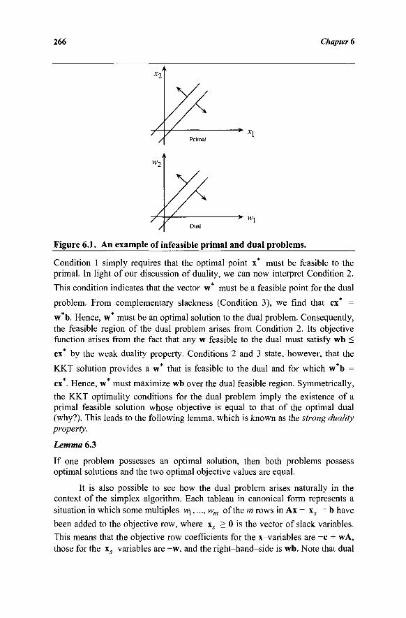
266 Chapter 6
*■ Wj
Figure 6.1. An example of infeasible primal and dual problems.
Condition 1 simply requires that the optimal point x* must be feasible to the primal. In light of our discussion of duality, we can now interpret Condition 2.
This condition indicates that the vector w* must be a feasible point for the dual
problem. From complementary slackness (Condition 3), we find that ex* =
w b. Hence, w must be an optimal solution to the dual problem. Consequently, the feasible region of the dual problem arises from Condition 2. Its objective function arises from the fact that any w feasible to the dual must satisfy wb <
ex* by the weak duality property. Conditions 2 and 3 state, however, that the
KKT solution provides a w* that is feasible to the dual and for which w*b =
ex*. Hence, w* must maximize wb over the dual feasible region. Symmetrically,
the KKT optimality conditions for the dual problem imply the existence of a primal feasible solution whose objective is equal to that of the optimal dual (why?). This leads to the following lemma, which is known as the strong duality property.
Lemma 6.3
If one problem possesses an optimal solution, then both problems possess optimal solutions and the two optimal objective values are equal.
It is also possible to see how the dual problem arises naturally in the context of the simplex algorithm. Each tableau in canonical form represents a situation in which some multiples w\,...,wm of the m rows in Ax - xs = b have
been added to the objective row, where xs > 0 is the vector of slack variables. This means that the objective row coefficients for the x-variables are -c + wA, those for the xs variables are -w, and the right-hand-side is wb. Note that dual
Duality and Sensitivity Analysis 267
feasibility (Condition 2) requires a set of these so-called simplex multipliers w such that the canonical objective row coefficients are nonpositive for all the x-and xs -variables. Indeed, if the primal problem has been solved to optimality,
then the available simplex multipliers w = cgB , where B is the optimal basis
matrix, satisfy these dual feasibility conditions. Moreover, if x is a primal optimal solution, its objective value ex* coincides with w*b, the right-hand-side value in the objective row of the optimal tableau. In view of the weak duality property of Lemma 6.2, we have that, at optimality, the simplex
multipliers w* must be a maximizing solution to wb subject to the constraints wA < c and w > 0, that is, to the so-called dual linear programming problem.
Lemma 6.3 provides an insightful result that is related to Corollary 6.2. For the linear program P: Minimize ex, subject to Ax > b, x > 0, consider the homogeneous form of its dual problem, namely, HD: Maximize wb, subject to wA < 0, w > 0. Note that the dual to HD has the same feasible region as P. Hence, if HD is unbounded, then by Corollary 6.2, P is infeasible. Conversely, if P is infeasible, then HD must be unbounded, or else, since HD is feasible (w = 0 is a feasible solution), it must have an optimal solution. But Lemma 6.3 tells us that the dual to HD then has an optimal solution; that is, P is feasible, a contra-diction. Therefore, we have the following result. We ask the reader to verify this using Example 6.4. It is insightful to note that the homogeneous form of the dual arises from the dual problem via a characterization of its recession directions as in Chapter 2.
Corollary 6.3
The primal problem is infeasible if and only if the homogeneous form of the dual problem is unbounded (and vice versa).
By utilizing the foregoing results we obtain two important basic theorems of duality. These two theorems will permit us to use the dual problem to solve the primal problem and, also, to develop new algorithms to solve both problems.
The Fundamental Theorem of Duality
Combining the results of the lemmas, corollaries, and examples of the previous section we obtain the following:
Theorem 6.1 (Fundamental Theorem of Duality)
With regard to the primal and dual linear programming problems, exactly one of the following statements is true:
1. Both possess optimal solutions x* and w* with ex* = w*b. 2. One problem has an unbounded optimal objective value, in which
case the other problem must be infeasible. 3. Both problems are infeasible.
268 Chapter 6
From this theorem we see that duality is not completely symmetric. The best we can say is that (here optimal means having a finite optimum, and un-bounded means having an unbounded optimal objective value):
P OPTIMAL O D OPTIMAL
P(D) UNBOUNDED =s> D(P) INFEASIBLE
P(D) INFEASIBLE => D(P) UNBOUNDED OR INFEASIBLE
P(D) INFEASIBLE <£> D(P) UNBOUNDED IN HOMOGENEOUS FORM
Complementary Slackness and the Supervisor's Principle
We have seen that if x and w are any pair of primal and dual feasible solutions to the linear program: Minimize ex, subject to Ax > b, x > 0, then they are both optimal to their respective problems if and only if they have the same objective value (that is, ex = wb). This is known as the supervisor's principle because it provides a simple check by which a "supervisor" can verify the (simultaneous) optimality of a pair of candidate primal and dual feasible solutions. The KKT conditions tell us that another equivalent supervisor's principle is to check for
the complementary slackness conditions (written as Condition 3). Indeed, if x*
and w* respectively satisfy primal and dual feasibility (Conditions 1 and 2),
then ex* = w*b, that is, w*(Ax* - b) + (c - w*A)x* = 0 holds true, if and only
if Condition 3 is satisfied, since w* > 0, Ax* - b > 0, c - w*A > 0, and x* > 0.
In expanded form, since w* > 0 and Ax* - b > 0, then w* (Ax - b) = 0 implies
w*(a'x* - bt) = 0 for / = 1,..., m. Similarly, (c - w*A)x* = 0 implies (c,—
w*ay· )x* = 0 fory = 1,..., n.
Thus, we have the following theorem:
Theorem 6.2 (Complementary Slackness Theorem)
Let x* and w* be any feasible solutions to the primal and dual problems in the canonical form. Then they are respectively optimal if and only if
(cj -w*ay)x* =0, j = ί,.,.,η
and
w*(a!x* -bi) = 0, i = l,...,m.
This is a very important theorem relating the primal and dual problems. It obviously indicates that at least one of the two terms in each expression must be zero. In particular,
Xj > 0 => w a ,· = Cj
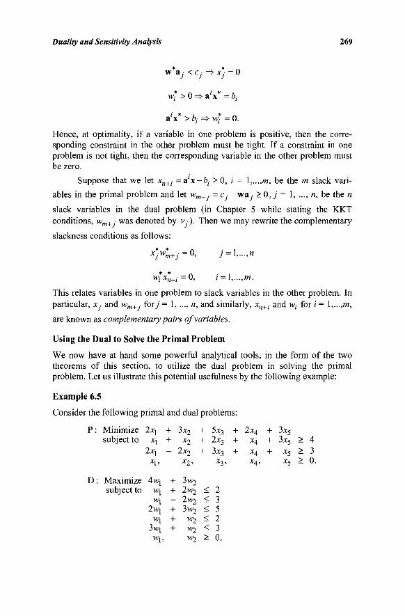
Duality and Sensitivity Analysis 269
w &j < Cj =>■ Xj = Ό
Wj > 0 = > a x =bi
ax >bt =Φ w,- =0.
Hence, at optimality, if a variable in one problem is positive, then the corre-sponding constraint in the other problem must be tight. If a constraint in one problem is not tight, then the corresponding variable in the other problem must be zero.
Suppose that we let xn+i = a i x - è / > 0, i = \,...,m, be the m slack vari-
ables in the primal problem and let wm+J- = c ■ - w a >0,j= 1, ..., n, be the n
slack variables in the dual problem (in Chapter 5 while stating the KKT conditions, wm+ .· was denoted by v, ). Then we may rewrite the complementary
slackness conditions as follows:
x*-w*m+j=°> j = l-,n
w;*x«+i= 0 ' i = \,...,m.
This relates variables in one problem to slack variables in the other problem. In particular, x ■ and wm+J- fory = 1,..., n, and similarly, xn+i and wt for i = l,...,m,
are known as complementary pairs of variables.
Using the Dual to Solve the Primal Problem
We now have at hand some powerful analytical tools, in the form of the two theorems of this section, to utilize the dual problem in solving the primal problem. Let us illustrate this potential usefulness by the following example:
Example 6.5
Consider the following primal and dual problems:
: Minimize 2x\ + 3x2
subject to xj + x2
2χγ - 2x2
X\, %2>
: Maximize 4w\ + 3w2
subject to Wj + 2w2 W] - 2w2
2wy + 3w2 Wj + W2
3>V] + W2
Wi, W2
+ 5x3
+ 2*3 + 3x3
x3,
< 2 < 3 < 5 < 2 < 3 > 0.
+ + +
2x4 X4
X4 X4,
+ 3x5 + 3x5
+ X5
x5
> > >
4 3 0.
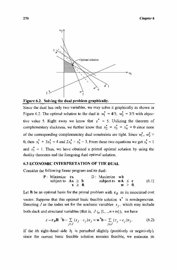
270 Chapter 6
Figure 6.2. Solving the dual problem graphically.
Since the dual has only two variables, we may solve it graphically as shown in
Figure 6.2. The optimal solution to the dual is w\ = 4/5, w\ = 3/5 with objec-
tive value 5. Right away we know that z* = 5. Utilizing the theorem of
complementary slackness, we further know that = 0 since none
of the corresponding complementary dual constraints are tight. Since w*, w^ >
0, then x* + 3x1 = 4 and 2xj + x5 = 3. From these two equations we get x* = 1
and X5 = 1. Thus, we have obtained a primal optimal solution by using the
duality theorems and the foregoing dual optimal solution.
6.3 ECONOMIC INTERPRETATION OF THE DUAL
Consider the following linear program and its dual:
P : Minimize ex D : Maximize wb subject to Ax > b subject to wA < c (6.1)
x > 0. w > 0.
Let B be an optimal basis for the primal problem with cB as its associated cost
vector. Suppose that this optimal basic feasible solution x* is nondegenerate. Denoting J as the index set for the nonbasic variables x ■, which may include
both slack and structural variables (that is, J £ {\,...,n + m}), we have
z = csB"'b - Σ (ZJ ~ Cj)Xj = w*b - Σ {Zj ~ Cj )xj. (6.2)
If the rth right-hand-side bt is perturbed slightly (positively or negatively),
since the current basic feasible solution remains feasible, we maintain its
Duality and Sensitivity Analysis 271
optimality. Hence, if z is the optimal objective function value and B, is the
rth column of B~ , we have
— = cBBJl=w*. (6.3) db,. '
Thus, w* is the rate of change of the optimal objective value with a unit
increase in the rth right-hand-side value, given that the current nonbasic vari-
ables are held at zero (regardless of feasibility). Because w* > 0, z* will increase
(respectively, decrease) or stay constant as b, increases (respectively, decreases).
Economically, we may think of w as a vector of shadow prices for the right-hand-side vector. To illustrate, if the rth constraint represents a demand for production of at least bt units of the rth product and ex represents the total
cost of production, then w,· is the incremental cost of producing one more unit
of the rth product. Put another way, w,· is Uve fair price we would pay to have an extra unit of the rth product.
We may also interpret the entire dual problem economically. Suppose that we engage a firm to produce specified amounts b\, b2,-.;bm of m outputs or goods. The firm may engage in any of n activities at varying levels to produce the outputs. Each activity j has its own unit cost c , and we agree to pay the
total cost of production. From our point of view, we would like to have control over the firm's operations so that we can specify the mix and levels of activities that the firm will engage in so as to minimize the total production cost. If ay-denotes the amount of product / generated by one unit of activity j , then Σ%\αϋχί represents the units of output i that are produced. These must be
greater than or equal to the required amount b,. Therefore, we wish to solve the
following problem, which is precisely the primal problem: n
Minimize X c.x,
» subject to Σ α,-,χ, > bh i-\,...,m
7=1 xj > 0, ; = 1,...,«.
Instead of trying to control the operation of the firm to obtain the most desirable mix of activities, suppose that we agree to pay the firm unit prices wj, w2,...,wm
for each of the m outputs. However, we also stipulate that these prices announced by the firm must be fair. Since a;y is the number of units of output i
produced by one unit of activity j and w· is the unit price of output i, then
272 Chapter 6
Σ*ιΙ\αϋ™ί c a n be interpreted as the unit price of activity j consistent with the
prices wj, w2,...,wm. Therefore, we tell the firm that the implicit price of activity
j , namely Σί=ι%*ί'/, should not exceed the actual cost c,-. Therefore, the firm
must observe the constraints T,1L\aijwi -cj f°rJ = U—>"· Within these con-
straints the firm would like to choose a set of prices that maximizes its return
Σ^ ι Wjbj. This leads to the following dual problem considered by the firm:
m Maximize Σ W/fy
(=1
m subject to Σ auwi - c/> j = \,...,n
Wj > 0, i = \,...,m.
The main duality theorem states that, provided an optimum exists, there is an equilibrium set of activities and set of prices where the minimal production cost is equal to the maximal return. That the two objectives are equal at optimality becomes intuitively clear by noting that they represent the fair charge to the customer, where the primal objective is derived by cost considerations and the dual objective is arrived at by a pricing mechanism. These shadow prices are often used by regulated industries, such as electric utilities, to set ana justify prices.
Observe that the complementary slackness theorem says that if, at opti-
mality, Σ/=!«(/**■ >t>i, then w* = 0, that is, if the optimal level of activities
that meets all demand requirements automatically produces an excess of product i, then the incremental cost associated with marginally increasing £,- is naturally
zero. Similarly, if T^a^w* <Cj, then x* = 0, that is, if the total revenue
generated via the items produced by a unit level of activity j is less than the associated production cost, then the level of activity j should be zero at optimality.
Interchanging the roles of the previous primal and dual problems, there is another interesting economic interpretation that can be given. Consider the following pair of dual problems, where the problems D and P have been rewritten as P and D, respectively:
n
P : Maximize Σ c.-x.-7=1 n
subject to Σ αϋχϊ - bj, iori = \,...,m 7=1
x > 0.
Duality and Sensitivity Analysis 273
m D : Minimize Σ biwi
i = l
m subject to Σ ajjWj > Cj, for j = \,...,n
i=\ w > 0.
Assume that problem P is a product-mix problem in which n products are being manufactured using some m types of resources. Here, x ■ represents the number
of units (per year) produced of product j , and bt represents the number of units available for resource / fory = 1,..., n and i = 1,..., m. A unit of product y' fetches a profit of c. units and consumes a;y units of resource i for i = 1,..., m.
As before, let w;- denote the shadow price or the imputed value or the
fair market price/rent for a unit of resource i. Then the dual constraints have the following interpretation. Observe that if the manufacturer considers renting out the m resources at unit prices W],...,wm instead of manufacturing the mix of products, then every unit of product/ not manufactured would result in a loss of profit of e,- units but would earn a rent of Z^ciyW,· units by virtue of the
resources this releases. The dual constraints ensure that this venture is at least as profitable as manufacturing the products. However, in order to maintain fair or competitive prices while guaranteeing this profitability, the dual objective seeks to minimize the total rent. The main duality result tells us that, provided an optimum exists, the resulting total rent will match the total optimal profit obtainable by manufacturing the products. Hence, w, imputes a value that the
manufacturer ascribes to a unit of the rth resource from the viewpoint of optimally operating the production process. In particular, at optimality, the complementary slackness theorem says that if not all available units of resource
/ are utilized, then the marginal worth w* of an extra unit of resource i is
naturally zero. Similarly, if the net value YJ^a^w* of the resources consumed
by a unit level of production of product j exceeds the realizable profit c., then
the optimal production level of product 7 should be zero.
Shadow Prices Under Degeneracy
Now, consider the pair of primal and dual problems given in Equation (6.1 ), and assume that we have a degenerate optimal basic feasible solution. Then, while
the derivative of z in Equation (6.2) with respect to bt remains w* in the usual
sense of the derivative where all other parameters bk, k* i, and x , j e J,
are held constant at their present values, this may not reflect the true "shadow
price." That is, Equation (6.3) may not be valid. In fact, as will be seen later, z*
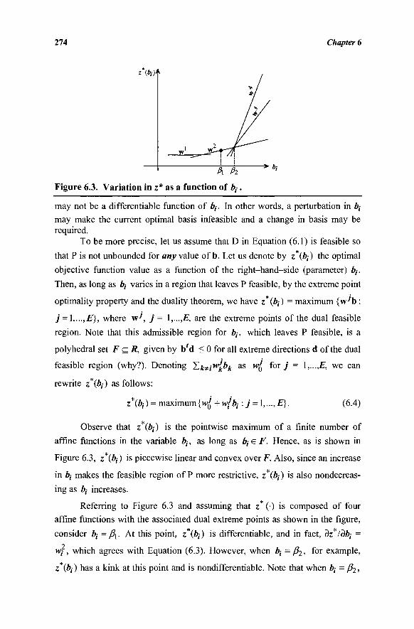
274 Chapter 6
z (*)\
β\ Pi
Figure 6.3. Variation in z* as a function of ft,·.
may not be a differentiable function of ft,·. In other words, a perturbation in ft,· may make the current optimal basis infeasible and a change in basis may be required.
To be more precise, let us assume that D in Equation (6.1) is feasible so
that P is not unbounded for any value of b. Let us denote by z (ft,·) the optimal
objective function value as a function of the right-hand-side (parameter) ft,·.
Then, as long as ft,· varies in a region that leaves P feasible, by the extreme point
optimality property and the duality theorem, we have z (ft,·) = maximum {wJb :
j = \,...,E}, where wJ, j = \,...,E, are the extreme points of the dual feasible
region. Note that this admissible region for ft,·, which leaves P feasible, is a
polyhedral set F c i , given by b'd < 0 for all extreme directions d of the dual
feasible region (why?). Denoting Yjk^iwJkbk as w^ for j = l,...,E, we can
rewrite z*(ft,·) as follows:
z*(b() = maximum{M^ + w/ft,· : j = Ι,.,.,Ε}. (6.4)
Observe that z (ft,·) is the pointwise maximum of a finite number of
affine functions in the variable ft,·, as long as ft,· e F. Hence, as is shown in
Figure 6.3, z*(ft,·) is piecewise linear and convex over F. Also, since an increase
in ft,· makes the feasible region of P more restrictive, z*(b;) is also nondecreas-
ing as ft,· increases.
Referring to Figure 6.3 and assuming that z* (·) is composed of four
affine functions with the associated dual extreme points as shown in the figure,
consider ft,· = β\. At this point, z*(ft,·) is differentiable, and in fact, 8z*/3ft,· =
w;, which agrees with Equation (6.3). However, when ft,· = β2, for example,
z (ft,·) has a kink at this point and is nondifferentiable. Note that when ft,· = /72>
Duality and Sensitivity Analysis 275
the dual has alternative optimal extreme point solutions w , w , and w . This
implies degeneracy at optimality in the primal problem, for if an optimal primal
basic feasible solution x* with basis B is nondegenerate, then by the comple-mentary slackness theorem, any dual optimal solution w must satisfy the dual constraints with respect to the basic variable columns as equalities, that is, wB =
c g must hold true. This gives w = c#B~ as the unique dual optimum, a con-
tradiction. In fact, since any optimal dual extreme point solution must be com-
plementary to x*, the dual constraints corresponding to the q < m positive basic
variables in x* must be binding. This gives q linearly independent binding hyperplanes at optimality in the dual from the (m + ri) inequalities defining the dual feasible region. Each choice of (m - q) additional (linearly independent) hyperplanes that gives some optimal dual extreme point corresponds to a choice of the (m - q) columns of the variables (structural or slacks) in P associated with these constraints. Therefore, because of the linear independence, this corresponds to a choice of a basis in P, and since the nonbasic variables for this
basis are zero in x*, this is a basis associated with x*. Hence, the alternative
optimal dual extreme point solutions all correspond to alternative bases associ-
ated with the primal degenerate vertex x . Now, from Equation (6.4), we can define the one-sided (right-hand and
left-hand) directional derivatives of z*(bj) with respect to bj. The right-hand
derivative, denoted d+z*/dbh gives the rate of change in z* with an increase in
bj. As evident from Equation (6.4) (see Figure 6.3), so long as P remains
feasible as bj increases marginally (else, the right-hand shadow price is infi-
nite), we have
d+z* = maximum!^ : w·7 is an optimal dual vertex at b{}. (6.5)
dbj
Similarly, the left-hand derivative, denoted d~z*/dbj, gives the negative of the
rate of change in z* as bj decreases. Again, from Equation (6.4), referring to
Figure 6.3, this is given by
d~z* = minimum{My : wJ is an optimal dual vertex at bt}. (6.6)
dbj
Equations (6.5) and (6.6) respectively give the right-hand and left-hand shadow
prices associated with the rth right-hand-side. Observe that if x* is nondegener-
ate, so that there is a unique dual optimal extreme point w*, we get d+z*ldbj =
d~z*ldbj = w*, as in Equation (6.3). Later, we shall comment on how these
right-hand and left-hand shadow prices can be easily computed in general via a parametric analysis.
276 Chapter 6
Example 6.6
Consider the (generic) instance of Problem P of Equation (6.1) as depicted in Figure 6.4. Here, m = 3; n = 2; x3, x4, and x5 are the slack variables associated
with the three primal constraints, and Aj, A2, and A3 denote the gradients of the three rows of A. Observe that since the feasible half-spaces are Ax > b, the normal vectors - Aj, - A2, and - A 3 are as shown in the figure. Note that each
dual basis has two basic variables.
First, consider Figure 6.4a This problem has a unique primal optimal
solution x*. The KKT conditions at x* require -c to be written as -wlAl -
w2A2, and hence, w^ andw2 are both positive and are uniquely determined. * —1
That is, there is a unique dual extreme point solution given by w = "cgB ".
(Here, wj and w2 are the basic variables, and w3, w4, and w5 are nonbasic,
where w4 and w5 are the slack variables for the two dual constraints.) Because
the maximum in Equation (6.4) is unique, Equation (6.3) holds and we have
dz*/di\ = w* > 0, dz*/db2 = w2 > 0, and dz* Idb?, = w3 = 0. It is instructive to
note that in the optimal tableau representing x*, <3z*/3r3 = - (z3 - c 3 ) = w*.
Note that the edge along which we move when we hold x4 = 0 and increase x3
is precisely the direction in which the optimal solution moves when i\ is
(marginally) increased.
Second, in Figure 6.4a, rotate -c so that it aligns with the vector - Aj. We
now have alternative optimal primal solutions, one of which is degenerate.
However, since x* is still optimal, and since by the KKT conditions, all optimal
dual solutions must be complementary to x*, we only need to examine any one
primal optimal solution, say, x*, in order to capture all dual optimal solutions.
Applying the KKT conditions at x*, we find that again there is only one dual optimal solution w* where w[ > 0 is a solution to - W] Aj = -c , and w2 = w3 =0. Hence, Equation (6.3) again holds true, although the primal problem has a degenerate optimum.
Finally, consider Figure 6.4b, where x* is the unique optimum. However, it is degenerate and there are two optimal bases, having either x3 and
x5 as nonbasic variables, or x4 and x5 as nonbasic variables. (Note that not all
z · -c ■ < 0 for the choice of nonbasic variables x3 and x4 ; in fact, for this
choice, z4-c4 > 0 (why?).) Hence, each of these two optimal bases gives a dual
optimal extreme point. The first basis gives a dual optimal vertex w in
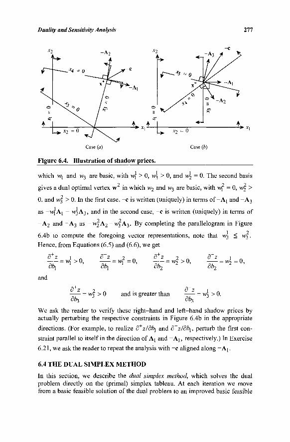
Duality and Sensitivity Analysis 277
>■ X]
Case (a)
Figure 6.4. Illustration of shadow prices.
Case (b)
which W[ and vv3 are basic, with M\ > 0, w3 > 0, and w2 = 0. The second basis 7 7 7
gives a dual optimal vertex w in which w2 and vv3 are basic, with w\ = 0, w2 >
0, and w3 > 0. In the first case, -c is written (uniquely) in terms of-Aj and - A 3
as -WjA! - w3A3, and in the second case, -c is written (uniquely) in terms of 7 7
- A 2 and - A 3 as - w 2 A 2 - w 3 A 3 . By completing the parallelogram in Figure 1 7
6.4b to compute the foregoing vector representations, note that w3 < H>3 .
Hence, from Equations (6.5) and (6.6), we get — - = w;>0, — - = wt=0, — = wj>0, — = w 2 = 0 , dt>i ot\ db2 002
and
<5 z 2 1 · ■ d~z 1 = w3 > 0 and is greater than = w3 > 0.
dlh, db^ We ask the reader to verify these right-hand and left-hand shadow prices by actually perturbing the respective constraints in Figure 6.4b in the appropriate
directions. (For example, to realize d+z/db] and d~z/dby, perturb the first con-
straint parallel to itself in the direction of Aj and - A ( , respectively.) In Exercise
6.21, we ask the reader to repeat the analysis with -c aligned along -A j .
6.4 THE DUAL SIMPLEX METHOD
In this section, we describe the dual simplex method, which solves the dual problem directly on the (primal) simplex tableau. At each iteration we move from a basic feasible solution of the dual problem to an improved basic feasible
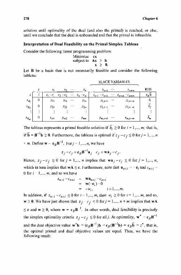
278 Chapter 6
solution until optimality of the dual (and also the primal) is reached, or else, until we conclude that the dual is unbounded and that the primal is infeasible.
Interpretation of Dual Feasibility on the Primal Simplex Tableau
Consider the following linear programming problem: Minimize ex subject to Ax > b
x > 0.
Let B be a basis that is not necessarily feasible and consider the following tableau:
SLACK VARIABLES
x2 xn+\ RHS 1
0
0
0
ζ , - q
y\\
yn
ym\
z2 - c 2 ·
Ά2 ■
yn ■
ymi ■
zn cn
y\n
yin
ymn
zn+\ cn+\
Λ,η+1 '
yi,n+\ ■
ym,n+\ ·
zn+m n+m
y\,n+m
y2,n+m
ym,n+tn
cBb
\
h
K
XB2
XD
The tableau represents a primal feasible solution if è,· > 0 for / = 1,..., m; that is,
if b = B~ b > 0. Furthermore, the tableau is optimal if z ,· - c ,· < 0 for/ = 1,..., n
+ m. Define w = csB~ . For/ = 1,..., n, we have
-1 Zi -c, =cRB a,· -c,- wa; -Ci. -j -j-^-B1* "j - / j V"·
Hence, zj-c; < 0 for/ = 1,..., n implies that wa, - c , < 0 for/ = 1,..., n,
which in turn implies that wA < c. Furthermore, note that a„+i = - e; and cn+i =
0 for /' = 1,..., m, and so we have
'«+! '-»+/ wa„ = w( -e ; ) -0
= -w(-, i = \,...,m.
In addition, if zn+i -cn+i < 0 for i = 1,..., m, then w(- > 0 for / = 1,..., m, and so,
w > 0. We have just shown that z ; -c; < 0 for/ = 1,..., n + m implies that wA
< c and w > 0, where w = c#B~ . In other words, dual feasibility is precisely
the simplex optimality criteria z ; -c ; < 0 for all/. At optimality, w* = cfiB~
and the dual objective value w*b = (cgB~ )b = c#(B- b) = cfib = z*, that is,
the optimal primal and dual objective values are equal. Thus, we have the following result:
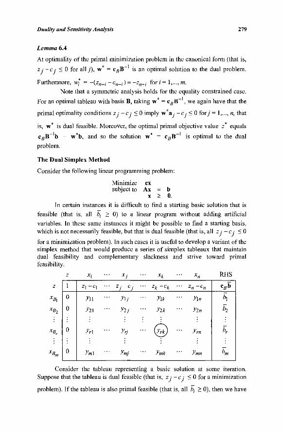
Duality and Sensitivity Analysis 279
Lemma 6.4
At optimality of the primal minimization problem in the canonical form (that is,
z; -c; < 0 for ally), w*
Furthermore, w* = - ( z n 4
-1 : c#B is an optimal solution to the dual problem.
c„+i) = -z„+i foTi=i,...,m.
Note that a symmetric analysis holds for the equality constrained case. * —1
For an optimal tableau with basis B, taking w = c B B , we again have that the
primal optimality conditions z ,· -c >· < 0 imply w*a - c · < 0 for 7 = I,..., n, that
is, w* is dual feasible. Moreover, the optimal primal objective value z* equals
problem.
w*b, and so the solution w* = c 5 B is optimal to the dual
The Dual Simplex Method
Consider the following linear programming problem:
Minimize ex subject to Ax = b
x > 0.
In certain instances it is difficult to find a starting basic solution that is
feasible (that is, all è, > 0) to a linear program without adding artificial
variables. In these same instances it might be possible to find a starting basis,
which is not necessarily feasible, but that is dual feasible (that is, all z ,· - c ,· < 0
for a minimization problem). In such cases it is useful to develop a variant of the simplex method that would produce a series of simplex tableaux that maintain dual feasibility and complementary slackness and strive toward primal feasibility.
Xy. -RHS x\ xk
1
0
0
0
0
z \ ~ c \ ■
y\\ ■
yi\ ■
JVi ·
ym\ ■
■ zj~cj ■
- y\j ■
■■ y2j ■
■ yrj ■
■■ ymj ■
■■ zk~ck ■
■■ y\k ■
■■ yik ■
■■ @ ■
ymk
zn cn
■■ yu
■■ yin
■ yrn
ymn
— Cgb
h h
br
K
z
xBl
XB2
xBr
XD
tJry7
Consider the tableau representing a basic solution at some iteration. Suppose that the tableau is dual feasible (that is, z ; —ci < 0 for a minimization
problem). If the tableau is also primal feasible (that is, all bj > 0), then we have
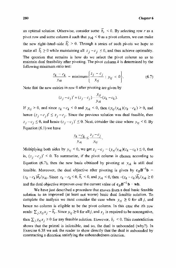
280 Chapter 6
an optimal solution. Otherwise, consider some br < 0. By selecting row r a s a
pivot row and some column k such that vr£ < 0 as a pivot column, we can make
the new right-hand-side b'r > 0. Through a series of such pivots we hope to
make all bi > 0 while maintaining all z ; -c; < 0, and thus achieve optimality.
The question that remains is how do we select the pivot column so as to maintain dual feasibility after pivoting. The pivot column k is determined by the following minimum ratio test:
— — = minimum-M J- : yrj < 0>. (6.7)
>7* [ yrj J J
Note that the new entries in row 0 after pivoting are given by
y„-(zj ~cji = ( z ; ~ cj ) (zk ~ ck )■
yrk
If yrj > 0, and since zk -ck < 0 and yrk < 0, then {yrjlyrk){zk -ck) > 0, and
hence (z —e.-)' < z ■ —e,-. Since the previous solution was dual feasible, then
z · - e.- < 0, and hence (z ,· - c, )' < 0. Next, consider the case where y ■ < 0. By
Equation (6.1) we have zAZ£L<zI—iL
yrk yrj
Multiplying both sides by _y · < 0, we get Zj -cj - (yrjlyrk){zk -ck) < 0, that
is, (z -Cj)' < 0. To summarize, if the pivot column is chosen according to
Equation (6.7), then the new basis obtained by pivoting at yrk is still dual
feasible. Moreover, the dual objective after pivoting is given by c#B- b -
(zk -ck)brlyrk. Since zk -ck<0,br< 0, and yrk < 0, then -(zk -ck)brlyrk > 0
and the dual objective improves over the current value of cBB~ b = wb.
We have just described a procedure that moves from a dual basic feasible solution to an improved (at least not worse) basic dual feasible solution. To complete the analysis we must consider the case when y > 0 for all j , and
hence no column is eligible to be the pivot column. In this case the /th row
reads: Σ/^w^/ = K- Since y ■ > 0 for ally, and x ■ is required to be nonnegative,
then YsjyyjXj > 0 for any feasible solution. However, br < 0. This contradiction
shows that the primal is infeasible, and so, the dual is unbounded (why?). In Exercise 6.38 we ask the reader to show directly that the dual is unbounded by constructing a direction satisfying the unboundedness criterion.
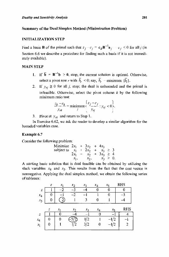
Duality and Sensitivity Analysis 281
Summary of the Dual Simplex Method (Minimization Problem)
INITIALIZATION STEP
>B"'a, Cj < 0 for ally (in Find a basis B of the primal such that z · - c = c g ~ „
Section 6.6 we describe a procedure for finding such a basis if it is not immedi-ately available).
MAIN STEP
1. If b = B~ b > 0, stop; the current solution is optimal. Otherwise,
select a pivot row r with br < 0; say, br = minimum {b,}.
2. If yr: > 0 for all j , stop; the dual is unbounded and the primal is
infeasible. Otherwise, select the pivot column k by the following minimum ratio test:
zk~ck 'ί-= minimum <; — — : y · < 0 >. yrk J
3. Pivot at yrk and return to Step 1.
In Exercise 6.62, we ask the reader to develop a similar algorithm for the bounded variables case.
Example 6.7
Consider the following problem: Minimize 2xj subject to xy
2X[ X,,
+ 3x2
+ 2x2
- x2 x2>
+ 4x3
+ x3 > 3 + 3x3 > 4
x3 > 0 A starting basic solution that is dual feasible can be obtained by utilizing the slack variables x4 and x5. This results from the fact that the cost vector is
nonnegative. Applying the dual simplex method, we obtain the following series of tableaux:
z X4
*5
z 1 0 0
xl
-2 -1
©
x2
-3 -2
1
x3
-4 -1 -3
X4
0 1 0
*5 0 0 1
RHS 0
-3 -4
z
X4
*1
z 1 0 0
xx
0 0 1
x2 -A
-1/2
x 3 -1
1/2 3/2
X4
0 1 0
*5 -1
-1/2 -1/2
RHS 4
-1 2
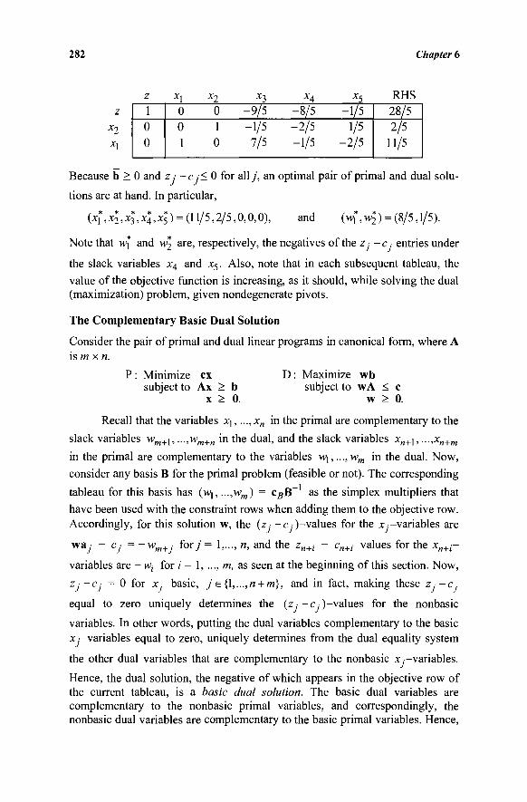
282 Chapter 6
z Xi X9 - 3 -*-4 - -5 RHS 1
0 0
0 0 -9/5 -8/5 -1/5 0 1 -1/5 -2/5 1/5 1 0 7/5 -1/5 -2/5
28/5 2/5
11/5
Because b > 0 and z ,· -c ,·< 0 for ally, an optimal pair of primal and dual solu-
tions are at hand. In particular,
{x{,x*2,xl,x*A,xl) = (11/5,2/5,0,0,0), and (w*, w\ ) = (8/5,1/5).
Note that wj and w\ are, respectively, the negatives of the z -c ■ entries under
the slack variables x4 and x5. Also, note that in each subsequent tableau, the
value of the objective function is increasing, as it should, while solving the dual (maximization) problem, given nondegenerate pivots.
The Complementary Basic Dual Solution
Consider the pair of primal and dual linear programs in canonical form, where A is m x n.
P : Minimize ex D : Maximize wb subject to Ax > b subject to wA < c
x > 0. w > 0.
Recall that the variables xj,..., x„ in the primal are complementary to the
slack variables wm+i, —,wm+n in the dual, and the slack variables x„+\, —,xn+m
in the primal are complementary to the variables w\,...,wm in the dual. Now,
consider any basis B for the primal problem (feasible or not). The corresponding
tableau for this basis has (M\, ...,wm) = cBW as the simplex multipliers that
have been used with the constraint rows when adding them to the objective row.
Accordingly, for this solution w, the (z -c.)-values for the x -variables are
wa, - Cj = —wm+j forj = 1,..., n, and the zn+j - cn+i values for the x„+;—
variables are - w;- for i = 1,..., m, as seen at the beginning of this section. Now,
Zj-Cj = 0 for x basic, j e{l,...,n + m}, and in fact, making these Zj-c.-
equal to zero uniquely determines the (z ■ -c )-values for the nonbasic
variables. In other words, putting the dual variables complementary to the basic x,-variables equal to zero, uniquely determines from the dual equality system
the other dual variables that are complementary to the nonbasic x.—variables.
Hence, the dual solution, the negative of which appears in the objective row of the current tableau, is a basic dual solution. The basic dual variables are complementary to the nonbasic primal variables, and correspondingly, the nonbasic dual variables are complementary to the basic primal variables. Hence,
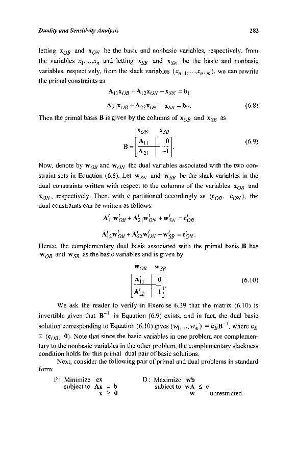
Duality and Sensitivity Analysis 283
letting \OB and xON be the basic and nonbasic variables, respectively, from
the variables x^,...,xn and letting xSB and xSN be the basic and nonbasic
variables, respectively, from the slack variables (x„+\, ...,x„+m), we can rewrite
the primal constraints as
A 1 1 x O S + A12XCW _ x SN
A 2 1 x O S + A22XCW ~XSB ~ b 2 -
Then the primal basis B is given by the columns of xOB an<^ XSB a s
B
xOB
ΓΑ„ _A21
XSB
0
- I
(6.8)
(6.9)
Now, denote by wOB and w0iy the dual variables associated with the two con-
straint sets in Equation (6.8). Let w ^ and wSB be the slack variables in the
dual constraints written with respect to the columns of the variables xOB and
χΟΛί, respectively. Then, with c partitioned accordingly as (c0B, cON), the
dual constraints can be written as follows:
Ai, I W U + A U L + W ' Μ1"ΌΒ L21WCW SN cOB
A l o W n o + A r " ' cON-Μ 2 " Ό β ">-A22wOiV +yvSB
Hence, the complementary dual basis associated with the primal basis B has v/OB and wSB as the basic variables and is given by
w OB
[Ai, _A'l2
0
I
(6.10)
We ask the reader to verify in Exercise 6.39 that the matrix (6.10) is
invertible given that B" in Equation (6.9) exists, and in fact, the dual basic
solution corresponding to Equation (6.10) gives (v^,..., wm) = cgB~ , where cB
= (c0B, 0). Note that since the basic variables in one problem are complemen-
tary to the nonbasic variables in the other problem, the complementary slackness
condition holds for this primal-dual pair of basic solutions. Next, consider the following pair of primal and dual problems in standard
form:
P : Minimize ex subject to Ax = b
x > 0.
D : Maximize wb subject to wA < c
w unrestricted.
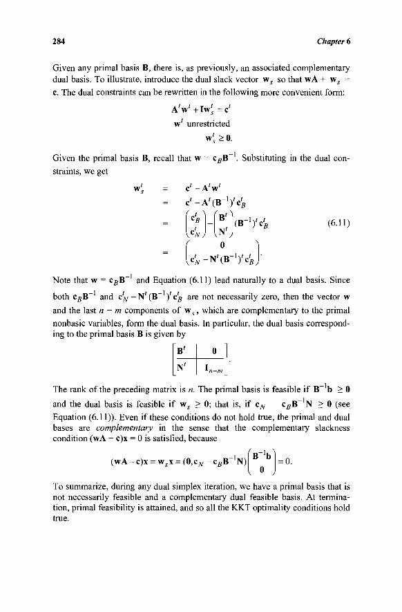
284 Chapter 6
Given any primal basis B, there is, as previously, an associated complementary dual basis. To illustrate, introduce the dual slack vector ws so that wA + ws = c. The dual constraints can be rewritten in the following more convenient form:
A V + I w ^ = C '
w' unrestricted
wl > 0.
Given the primal basis B, recall that w
straints, we get
>-i c#B . Substituting in the dual con-
c'-AV t
c
VCNJ f
N' 0
(B-Vei
-\\t j
(6.11)
Note that w = cBB~ and Equation (6.11) lead naturally to a dual basis. Since
both cgB~ and c'N -N ' (B~ )'C'B are not necessarily zero, then the vector w
and the last n - m components of w s , which are complementary to the primal
nonbasic variables, form the dual basis. In particular, the dual basis correspond-ing to the primal basis B is given by
B'
N'
0
ln-m
The rank of the preceding matrix is n. The primal basis is feasible if B b > 0 and the dual basis is feasible if ws > 0; that is, if cN - cBB~ N > 0 (see Equation (6.11)). Even if these conditions do not hold true, the primal and dual bases are complementary in the sense that the complementary slackness condition (wA - c)x = 0 is satisfied, because
(wA-c)x = wix = (0,cAr - c g B N) o
= 0.
To summarize, during any dual simplex iteration, we have a primal basis that is not necessarily feasible and a complementary dual feasible basis. At termina-tion, primal feasibility is attained, and so all the KKT optimality conditions hold true.
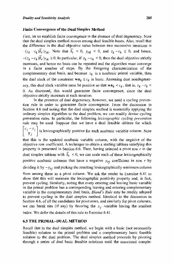
Duality and Sensitivity Analysis 285
Finite Convergence of the Dual Simplex Method
First, let us establish finite convergence in the absence of dual degeneracy. Note that the dual simplex method moves among dual feasible bases. Also, recall that the difference in the dual objective value between two successive iterations is
-{zk-ck)brlyrk. Note that br < 0, y^ < 0, and zk-ck < 0, and hence,
-(zk -ck)brlyrk > 0. In particular, if zk-ck < 0, then the dual objective strictly
increases, and hence no basis can be repeated and the algorithm must converge in a finite number of steps. By the foregoing characterization of the complementary dual basis, and because xk is a nonbasic primal variable, then the dual slack of the constraint wa^ < ck is basic. Assuming dual nondegener-acy, this dual slack variable must be positive so that wa^ < ck, that is, zk-ck<
0. As discussed, this would guarantee finite convergence, since the dual objective strictly increases at each iteration.
In the presence of dual degeneracy, however, we need a cycling preven-tion rule in order to guarantee finite convergence. From the discussion in Section 4.6 and noting that the dual simplex method is essentially applying the ordinary simplex algorithm to the dual problem, we can readily devise cycling prevention rules. In particular, the following lexicographic cycling prevention rule may be used. Suppose that we have a dual feasible tableau for which
CJ~ZJ is lexicographically positive for each nonbasic variable column. Note
that this is the updated nonbasic variable column, with the negative of the objective row coefficient. A technique to obtain a starting tableau satisfying this property is presented in Section 6.6. Then, having selected a pivot row r in the
dual simplex tableau with br < 0, we can scale each of these lexicographically
positive nonbasic columns that have a negative yr; coefficient in row r by
dividing it by -yr; and picking the resulting lexicographically minimum column
from among these as a pivot column. We ask the reader in Exercise 6.41 to show that this will maintain the lexicographic positivity property and, in fact, prevent cycling. Similarly, noting that every entering and leaving basic variable in the primal problem has a corresponding leaving and entering complementary variable in the complementary dual basis, Blond's Rule may be readily adapted to prevent cycling in the dual simplex method. Identical to the discussion in Section 4.6, of all the candidates for pivot rows, and similarly for pivot columns, we can break ties (if any) by favoring the x,· -variable having the smallest
index. We defer the details of this rule to Exercise 6.41.
6.5 THE PRIMAL-DUAL METHOD
Recall that in the dual simplex method, we begin with a basic (not necessarily feasible) solution to the primal problem and a complementary basic feasible solution to the dual problem. The dual simplex method proceeds by pivoting through a series of dual basic feasible solutions until the associated compie-
286 Chapter 6
mentary primal basic solution is feasible, thus satisfying all of the KKT optimality conditions.
In this section we describe a method, called the primal-dual algorithm, which is similar to the dual simplex method in that it begins with dual feasibility and proceeds to obtain primal feasibility while maintaining complementary slackness. However, an important difference between the dual simplex method and the primal-dual method is that the primal-dual algorithm does not require the dual feasible solution to be basic. Given a dual feasible solution, the primal variables that correspond to tight dual constraints (so that complementary slack-ness is satisfied) are determined. Using Phase I of the simplex method, we attempt to attain primal feasibility using only these variables. If we are unable to obtain primal feasibility, we change the dual feasible solution in such a way as to admit at least one new variable to the Phase I problem. This is continued until either the primal becomes feasible or the dual becomes unbounded.
Development of the Primal-Dual Method
Consider the following primal and dual problems in standard form where b > 0.
P : Minimize ex D : Maximize wb subject to Ax = b subject to wA < c
x > 0. w unrestricted.
Let w be an initial dual feasible solution, that is, wa < c ■ for a l l / By comple-
mentary slackness, if wa. = c·, then x■ is allowed to be positive and we
attempt to attain primal feasibility from among these variables. Let Q = {/': wa,·
- Cj = 0}, that is, Q is the set of indices of primal variables allowed to be positive. Then the Phase I problem that attempts to find a feasible solution to the primal problem among variables in the set Q becomes:
Minimize X Ox- + lxa
JeQ subject to X a x + xa = b
xj > 0 for j e g
xa > 0.
We utilize the artificial vector xa to obtain a starting basic feasible solution to
the Phase I problem. The Phase I problem is sometimes called the restricted primal problem.
Denote the optimal objective value of the foregoing problem by x0. At
optimality of the Phase I problem either x0 = 0 o r xo > 0- When x0
= 0, we have a feasible solution to the primal problem because all the artificial variables are zeros. Furthermore, we have a dual feasible solution, and the complementary slackness condition (way - CJ)XJ = 0 holds true because either j e Q, in which
case wa - c · = 0, or else j g Q, in which case x.- =0 . Therefore, we have an
Duality and Sensitivity Analysis 287
optimal solution of the overall problem whenever x0 = 0. If x0 > 0, primal
feasibility is not achieved and we must construct a new dual solution that admits a new variable to the restricted primal problem in such a way that x0 might be
decreased. We shall modify the dual vector w such that all the basic primal variables in the restricted problem remain in the new restricted primal problem, and in addition, at least one primal variable that did not belong to the set Q is passed to the restricted primal problem. Furthermore, this variable is such that it reduces x0 if introduced in the basis. In order to construct such a dual vector, consider the following dual of the Phase I problem:
Maximize vb subject to va < 0, j e Q
v < 1 v unrestricted.
Let v* be an optimal solution to the foregoing problem. Then, if an original variable x ■ is a member of the optimal basis for the restricted primal,
the associated dual constraint must be tight, that is, v*a ■ = 0. Also, the criterion
for basis entry in the restricted primal problem is that the associated dual
constraint be violated, that is, v*a · > 0. However, no variable currently in the
restricted primal has this property, since the restricted primal has been solved
optimally. For j £ Q, compute v*a,. If v*a, > 0, then if x■ could be passed
to the restricted primal problem it would be a candidate to enter the basis with the potential of a further decrease in x0 . Therefore, we must find a way to force
some variable x ,■ with v*a > 0 into the set Q.
Construct the following dual vector w', where θ> 0:
w' = w + #v*.
Then,
w 'a , -c , · = (w + #v*)a,· -c,· J J ' J 1 ( 6 12)
= ( w a y - c y ) + (9(v*a7·).
Note that wa, -c ■ = 0 and v*a,- < 0 for j eQ. Thus, Equation (6.12) implies
that w'a, —e.- < 0 for j e Q. In particular, if x with j eQ is a basic variable
in the restricted primal, then v a,· = 0 and w'a -c, = 0, permittingy in the new
restricted primal problem. If j fé Q and v*a < 0, then from Equation (6.12)
and noting that wa, - c , < 0, we have w'a -c ■ < 0. Finally, consider j 0 Q
with v*a, > 0. Examining Equation (6.12) and noting that wa -c ■ < 0 for
288 Chapter 6
j 0 Q, it is evident that we can choose a Θ > 0 such that w'a · - c . < 0 for
j & Q with at least one component equal to zero. In particular, define Θ as
follows:
Θ = " ( w a * ~°k) = minimum ~(W*y ~°j) : y \ > 0 > 0. (6.13)
\*&k J [ v*ay j
By the definition of Θ and from Equation (6.12), we see that w'aA -ck = 0.
Furthermore, for eachy with v*a .■ > 0, and noting Equations (6.12) and (6.13),
we have w ' a , - c · <0. To summarize, modifying the dual vector as detailed previously leads to a
new feasible dual solution where w'a,· -c ■ < 0 for ally. Furthermore, all the variables that belonged to the restricted primal basis are passed to the new restricted primal. In addition, a new variable xk that is a candidate to enter the basis, is passed to the restricted primal problem. Hence, we continue from the present restricted primal basis by entering xk, which leads to a potential reduc-tion in XQ.
Case of Unbounded Dual
The foregoing process is continued until either x0 = 0, in which case we have
an optimal solution, or else, x0 > 0 and v*a · < 0 for all j fé Q. In this case,
consider w' = w + θ\*. Since wa -c.· < 0 for ally and by assumption v*a < 0
for ally, then from Equation (6.12) w' is a dual feasible solution for all Θ > 0. Furthermore, the dual objective value is
w'b = (w + 9\*)b = wb + <9v*b.
Since v*b = x0 (why?) and the latter is positive, then w'b can be increased
indefinitely by choosing Θ arbitrarily large. Therefore the dual is unbounded and hence, the primal is infeasible. Alternatively, note that the total (usual) Phase I problem has the current restricted Phase I solution as an optimum (why?). Since x0 > 0, the primal is infeasible.
Summary of the Primal-Dual Algorithm (Minimization Problem)
INITIALIZATION STEP
Choose a vector w such that wa - c .■ < 0 for ally.
Duality and Sensitivity Analysis 289
MAIN STEP
1. Let Q = {/: wa · - c = 0} and solve the following restricted primal
problem:
Minimize Σ Ox,- + lxa
subject to X a ,x · + xa = b j*Q
x > 0 for j e g
xa > 0.
Denote the optimal objective value by x0. If x0 = 0, stop; an optimal
solution is obtained. Otherwise, let v* be the optimal dual solution to the foregoing restricted primal problem.
2. If v*a ,· < 0 for ally, then stop; the dual is unbounded and the primal
is infeasible. Otherwise, let
- ( w a - c . ) „ Θ = minimum·^ — : v a · > 0 > > 0,
j { v**j j
and replace w by w + θ\*. Repeat Step 1.
Example 6.8
Consider the following problem:
Minimize 3x( + 4x2 + 6x3 + 7x4 + x5 subject to 2xj - x2 + x3 + 6x4 - 5x5 - x6 = 6
X] + Χ-χ + 2 x 3 + X4 + 2X5 — Χη = 3
Xi , X 2 , Χ3, -^4> -£5 > -^6 ' ^7
The dual problem is given by the following:
Maximize 6wj + 3w2 subject to 2vV] + vv2 < 3
- w j + w 2 < 4 wj + 2 w 2 < 6
6wj + w 2 < 7 - 5 w [ + 2 w 2 < 1
-wx < 0 - w2 < 0
w\, w2 unrestricted.
An initial dual feasible solution is given by w = (\ν\,χν2) = (0,0). Substituting w in each dual constraint, we find that the last two dual constraints are tight so that Q = {6, 7}. Denoting the artificial variables by xg and x9, the restricted primal problem becomes as follows:
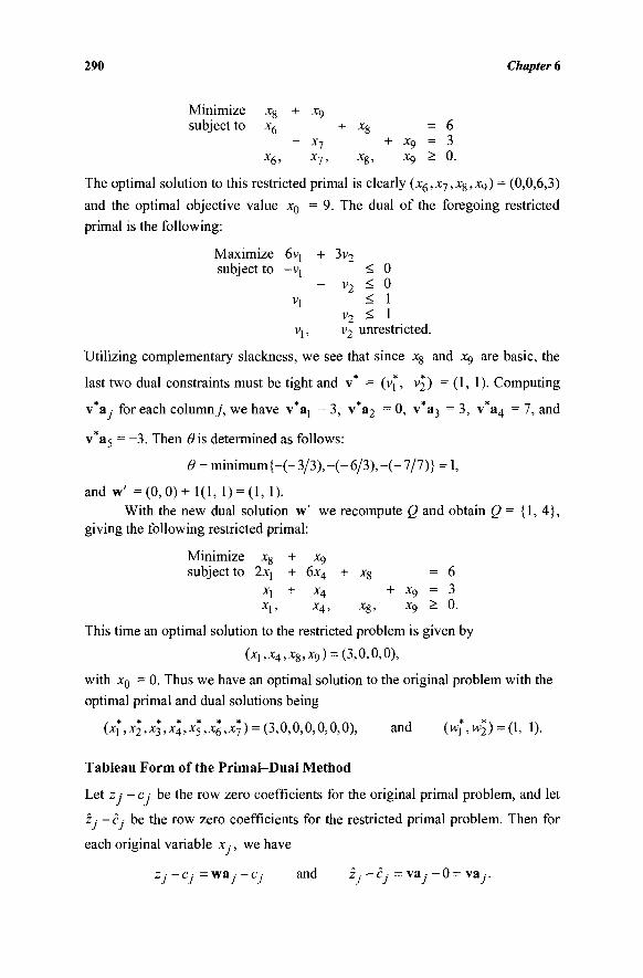
290 Chapter 6
Minimize Xg + Xg subject to -x 6 + xg = 6
— Χγ + Xg = 3 Xg, X7, Xg, Xg > 0.
The optimal solution to this restricted primal is clearly (x6,x7,xg,x9) = (0,0,6,3)
and the optimal objective value x0 = 9. The dual of the foregoing restricted
primal is the following:
Maximize 6vj + 3v2 subject to -vj < 0
- v2 < 0 vj < 1
v2 < 1 vj, v2 unrestricted.
Utilizing complementary slackness, we see that since x8 and Xg are basic, the
last two dual constraints must be tight and v* = (vj", v2) = (1, 1). Computing
v*a · for each column j , we have v*aj = 3, v*a2 =0, v a3 = 3, v a4 =7, and
v*a5 = - 3 . Then #is determined as follows:
Θ = minimum{-(-3/3),-(-6/3),-(-7/7)} = ^
and w' =(0 ,0)+1(1 , 1) = (1, 1). With the new dual solution w' we recompute Q and obtain Q = {1,4},
giving the following restricted primal:
Minimize Xg + Xo subject to 2xj + 6x4 + xg = 6
Xi + XA + Xg = 3 X], X4, Xg, X9 > 0.
This time an optimal solution to the restricted problem is given by
(χ!,Χ4,χ8,χ9) = (3,0,0,0),
with XQ = 0. Thus we have an optimal solution to the original problem with the
optimal primal and dual solutions being
(X]*,x2,X3,X4,x|,X6,X7) = (3,0,0,0,0,0,0), and (wj\w2) = (l, 1).
Tableau Form of the Primal-Dual Method
Let Zj-c; be the row zero coefficients for the original primal problem, and let
Zj -c,- be the row zero coefficients for the restricted primal problem. Then for
each original variable x · , we have
ZJ ~ CJ = w a i " CJ a n d ii ~ ÒJ = ™J ~ ° = v a i ·
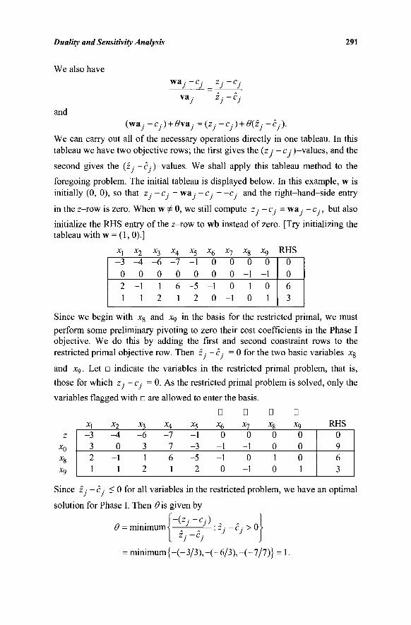
Duality and Sensitivity Analysis 291
We also have
wa, -CJ
va, Zj-Cj
and (way· -cj) + 9y&j = (zj -cj) + 0(zj - èj ) .
We can carry out all of the necessary operations directly in one tableau. In this tableau we have two objective rows; the first gives the (z ,· -c ,)-values, and the
second gives the (z - c. )-values. We shall apply this tableau method to the
foregoing problem. The initial tableau is displayed below. In this example, w is initially (0, 0), so that z · ■CJ ■■MfRj-Cj -c ■ and the right-hand-side entry
in the z-row is zero. When w Φ 0, we still compute z · - c = wa.· - c , but also
initialize the RHS entry of the z-row to wb instead of zero. [Try initializing the tableau with w = (1, 0).]
Xj Xn -£3 -£4 -£5 Xfo X~j Xg XQ RHS - 3 - 4 - 6
0 0 0 2 -1 1 1 1 2
-7 0 6 1
-1 0
-5 2
0 0
-1 0
0 0 0
-1
0 -1
1 0
0 -1 0 1
0 0 6 3
Since we begin with x8 and xq in the basis for the restricted primal, we must
perform some preliminary pivoting to zero their cost coefficients in the Phase I objective. We do this by adding the first and second constraint rows to the restricted primal objective row. Then z · - c = 0 for the two basic variables xg
and x9. Let G indicate the variables in the restricted primal problem, that is,
those for which z - c, = 0. As the restricted primal problem is solved, only the
variables flagged with o are allowed to enter the basis.
D D Q D
Xì Xn X"\ XA X$ X() XI XQ XQ RHS z
x 0
*8 Xq
Since ij - c ■ < 0 for all variables in the restricted problem, we have an optimal
solution for Phase I. Then Θis given by
Rz/-C/) - 1 Θ = minimum^ —-^—^— : z · - c ■ > 0 >
{ ZJ~CJ \ = minimum{-(-3/3),-(-6/3),-(-7/7)} = 1.
-3 3 2 1
-4 0
-1 1
-6 3 1 2
-7 7 6 1
-1 -3 -5 2
0 -1 -1 0
0 -1 0
-1
0 0 1 0
0 0 0 1
0 9 6 3
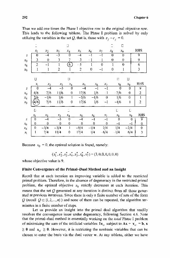
292 Chapter 6
Thus we add one times the Phase I objective row to the original objective row. This leads to the following tableau. The Phase I problem is solved by only utilizing the variables in the set Q, that is, those with z · - c . · = 0.
z
x0 xs X9
z x0 X4 x9
z x0 x4 x\
3 x\ x2 x3
D
*5 x6 x7
Ώ xs
□ x9 RHS
0 3 2 1
D X,
0 4/6 2/6
D x\ 0 0 0 1
-4 0
-1 1
*2 -4
7/6 -1/6
7/6
*2 -A
0 -3/4
7/4
- 3 3 1 2
*3 -3
11/6 1/6
11/6
*3 -3
0 -3/4 11/4
0 7
(è) 1
D X4
0 0 1 0
□ X4
0 0 1 0
-4 -3 -5
2
x5
^4 17/6 -5/6 17/6
x5
^1 0
-9/4 17/4
-1 -1 -1 0
*6 -1
1/6 -1/6
1/6
H -1 0
-1/4 1/4
-1 -1 0
-1
x7
-1 -1 0
-1
x7
-1 0
2/4 -6/4
0 0 0 0 1 0 0 1
D
*8 0
-7 /6 1/6
-1/6
D x8
0 -1
1/4 -1/4
9 9 6 3
D Xg RHS
0 0 0 1
9 2 1 2
D Xo -RH.S 0
-1 -2/4
6/4
9 0 0 3
Because x0 = 0, the optimal solution is found, namely:
(x1*,X2,X3,X4,X5,X6,X*) = (3,0,0,0,0,0,0)
whose objective value is 9.
Finite Convergence of the Primal-Dual Method and an Insight
Recall that at each iteration an improving variable is added to the restricted primal problem. Therefore, in the absence of degeneracy in the restricted primal problem, the optimal objective x0 strictly decreases at each iteration. This
means that the set Q generated at any iteration is distinct from all those gener-ated at previous iterations. Since there is only a finite number of sets of the form Q (recall g c {1,2,...,«}) and none of them can be repeated, the algorithm ter-minates in a finite number of steps.
Let us provide an insight into the primal-dual algorithm that readily resolves the convergence issue under degeneracy, following Section 4.6. Note that the primal-dual method is essentially working on the total Phase I problem of minimizing the sum of the artificial variables lxa subject to Ax + xa = b, x
> 0 and \a > 0. However, it is restricting the nonbasic variables that can be
chosen to enter the basis via the dual vector w. At any tableau, either we have
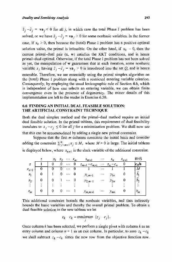
Duality and Sensitivity Analysis 293
z · -èj - va, < 0 for ally, in which case the total Phase I problem has been
solved, or we have z ,· - c · va, > 0 for some nonbasic variables. In the former
case, if XQ > 0, then because the (total) Phase I problem has a positive optimal
solution value, the primal is infeasible. On the other hand, if x0 = 0> then the
current primal-dual pair (x, w) satisfies the KKT conditions, and is hence primal-dual optimal. Otherwise, if the total Phase I problem has not been solved as yet, the manipulation of w guarantees that at each iteration, some nonbasic variable x,- having z. - c , = va > 0 is introduced into the set Q, and is hence
enterable. Therefore, we are essentially using the primal simplex algorithm on the (total) Phase I problem along with a restricted entering variable criterion. Consequently, by employing the usual lexicographic rule of Section 4.6, which is independent of how one selects an entering variable, we can obtain finite convergence even in the presence of degeneracy. The minor details of this implementation are left to the reader in Exercise 6.50.
6.6 FINDING AN INITIAL DUAL FEASIBLE SOLUTION: THE ARTIFICIAL CONSTRAINT TECHNIQUE
Both the dual simplex method and the primal-dual method require an initial dual feasible solution. In the primal tableau, this requirement of dual feasibility translates to z,· - c . < 0 for ally for a minimization problem. We shall now see
that this can be accommodated by adding a single new primal constraint. Suppose that the first m columns constitute the initial basis and consider
adding the constraint Σ":=ίη+χΧι < M, where M> 0 is large. The initial tableau
is displayed below, where x„+1 is the slack variable of the additional constraint.
z
xn+\ XX
X2
xm
Z
1 0 0
0
0
X,
0 0 1
0
0
x 2 ·
0 · 0 · 0 ·
1 ·
0 ·
xm ■ 0
• 0 • 0
• 0
• 1
xm+\ zm+\ ~cm+\
1
y\,m+\
yi,m+\
ym,m+l
xn
zn ~ cn 1
• y\n
■ yin
ymn
xn+l 0
1
0
0
0
RHS
c B b
M
h h
K
This additional constraint bounds the nonbasic variables, and thus indirectly bounds the basic variables and thereby the overall primal problem. To obtain a dual feasible solution in the new tableau we let
zk~ck = maximum {z ■ - c,-}. j
Once column k has been selected, we perform a single pivot with column k as an entry column and column n + 1 as an exit column. In particular, to zero zk - ck
we shall subtract zk -ck times the new row from the objective function row.
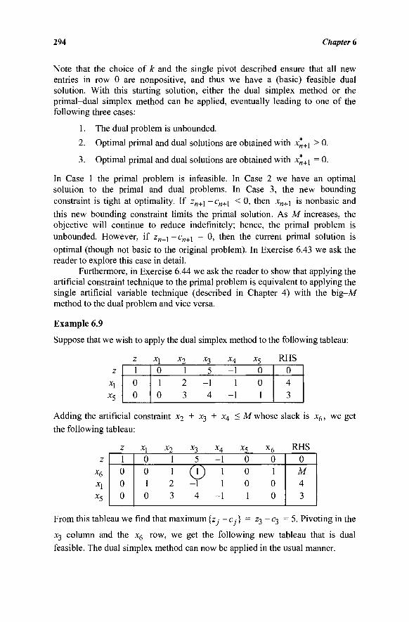
294 Chapter 6
Note that the choice of k and the single pivot described ensure that all new entries in row 0 are nonpositive, and thus we have a (basic) feasible dual solution. With this starting solution, either the dual simplex method or the primal-dual simplex method can be applied, eventually leading to one of the following three cases:
1. The dual problem is unbounded.
2. Optimal primal and dual solutions are obtained with x*+[ > 0.
3. Optimal primal and dual solutions are obtained with x*+1 = 0.
In Case 1 the primal problem is infeasible. In Case 2 we have an optimal solution to the primal and dual problems. In Case 3, the new bounding constraint is tight at optimality. If z„+1 -c„+ 1 < 0, then xn+l is nonbasic and
this new bounding constraint limits the primal solution. As M increases, the objective will continue to reduce indefinitely; hence, the primal problem is unbounded. However, if z„+1 - c„+1 = 0, then the current primal solution is
optimal (though not basic to the original problem). In Exercise 6.43 we ask the reader to explore this case in detail.
Furthermore, in Exercise 6.44 we ask the reader to show that applying the artificial constraint technique to the primal problem is equivalent to applying the single artificial variable technique (described in Chapter 4) with the big-M method to the dual problem and vice versa.
Example 6.9
Suppose that we wish to apply the dual simplex method to the following tableau:
Σ Xi Χ'γ X-5 ΧΛ X C RHS 1 0 0
0 1 5 - 1 0 1 2 - 1 1 0 0 3 4 - 1 1
0 4 3
Adding the artificial constraint x2 + x3 + x4 - M whose slack is x6, we get
the following tableau:
Z Xi Xo X3 ΧΛ Χζ Χ Α RHS 1 0 0 0
0 0 1 0
1 1 2 3
5
( ! ) -1 4
-1 1 1
-1
0 0 0 1
0 1 0 0
0 M 4 3
From this tableau we find that maximum {z .· - c ,■} = z^~c3 = 5· Pivoting in the
x3 column and the x6 row, we get the following new tableau that is dual
feasible. The dual simplex method can now be applied in the usual manner.
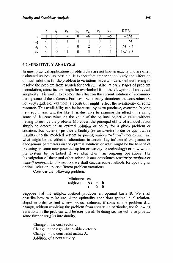
Duality and Sensitivity Analysis 295
Z Xi X2 X'X XA X$ ^ 6
RHS 1 0 0 0
0 0 1 0
-4 1 3
-1
0 1 0 0
-6 1 2
-5
0 0 0 1
-5 1 1
-4
-5M M
M + 4 - 4 M + 3
6.7 SENSITIVITY ANALYSIS
In most practical applications, problem data are not known exactly and are often estimated as best as possible. It is therefore important to study the effect on optimal solutions for the problem to variations in certain data, without having to resolve the problem from scratch for each run. Also, at early stages of problem formulation, some factors might be overlooked from the viewpoint of analytical simplicity. It is useful to explore the effect on the current solution of accommo-dating some of these factors. Furthermore, in many situations, the constraints are not very rigid. For example, a constraint might reflect the availability of some resource. This availability can be increased by extra purchase, overtime, buying new equipment, and the like. It is desirable to examine the effect of relaxing some of the constraints on the value of the optimal objective value without having to resolve the problem. Moreover, the principal utility of a model is not simply to determine an optimal solution or policy for a given problem or situation, but rather to provide a facility (or an oracle) to derive quantitative insights into the modeled system by posing various "what-if queries such as: what might be the effect of alterations in certain key influential exogenous or endogenous parameters on the optimal solution; or what might be the benefit of investing in some new potential option or activity or technology; or how would the system be perturbed if we shut down an ongoing operation? The investigation of these and other related issues constitutes sensitivity analysis or what-if analysis. In this section, we shall discuss some methods for updating an optimal solution under different problem variations.
Consider the following problem:
Minimize ex subject to Ax = b
x > 0.
Suppose that the simplex method produces an optimal basis B. We shall describe how to make use of the optimality conditions (primal-dual relation-ships) in order to find a new optimal solution, if some of the problem data change, without resolving the problem from scratch. In particular, the following variations in the problem will be considered. In doing so, we will also provide some further insights into duality.
Change in the cost vector c. Change in the right-hand-side vector b. Change in the constraint matrix A. Addition of a new activity.
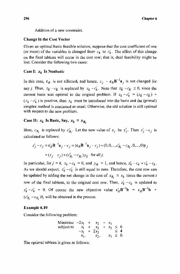
296 Chapter 6
Addition of a new constraint.
Change in the Cost Vector
Given an optimal basic feasible solution, suppose that the cost coefficient of one (or more) of the variables is changed from ck to c'k. The effect of this change on the final tableau will occur in the cost row; that is, dual feasibility might be lost. Consider the following two cases:
Case I: xk Is Nonbasic
In this case, cB is not affected, and hence, z ■ = cgB~ a. is not changed for
a n y / Thus, z£ - c£ is replaced by zk-c'k. Note that zfc-cfc < 0, since the
current basis was optimal to the original problem. If zk-c'k = (z# - c^ ) +
( ck - c'k ) is positive, then xk must be introduced into the basis and the (primal)
simplex method is continued as usual. Otherwise, the old solution is still optimal with respect to the new problem.
Case II: xk Is Basic, Say, xk = xB
Here, cB is replaced by c'B . Let the new value of z be z'·. Then z' -c,· is
calculated as follows:
z) -cj =cBB-1aj -CJ=(CBB-^J -Cj) + (0,0,...,cBt -cBt,0,...,0)yy·
= (zj -cj) + (c'Bt - cBf )ytJ for ally.
In particular, for j = k, zk~ck = 0, and ylk = 1 , and hence, z'k-ck =c'k -ck.
As we should expect, z'k - c'k is still equal to zero. Therefore, the cost row can
be updated by adding the net change in the cost of xB = xk times the current t
row of the final tableau, to the original cost row. Then, z'k - ck is updated to
z'k-c'k = 0. Of course the new objective value CgB~ b = c#B~ b +
(c'B - cB )bt will be obtained in the process.
Example 6.10
Consider the following problem:
Minimize -2xj + x2 - χτ, subject to X\ + x2 + Χτ, ^ 6
-xx + 2x2 ^ 4 Χγ, Χ2, Χ^ ^ U.
The optimal tableau is given as follows:
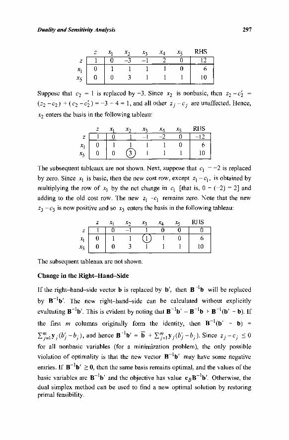
Duality and Sensitivity Analysis 297
z Xj X2 x3 x4 x5 RHS
1 0 0
0 -3 -1 -2 0 1 1 1 1 0 0 3 1 1 1
-12 6 10
Suppose that c2 = 1 is replaced by - 3 . Since x2 is nonbasic, then z2-c2 =
(z2-c2) + (c2 -c2) = -3 + 4 = 1, and all other z ■ -c,· are unaffected. Hence,
x2 enters the basis in the following tableau:
Z Xi X2 X 3 ΧΛ Χς RHS 1 0 0
0 1 - 1 - 2 0 1 1 1 1 0 0 0 1 1 1
-12 6 10
The subsequent tableaux are not shown. Next, suppose that q = -2 is replaced
by zero. Since x\ is basic, then the new cost row, except z\-c\, is obtained by
multiplying the row of X\ by the net change in q [that is, 0 - (-2) = 2] and
adding to the old cost row. The new z\ - q remains zero. Note that the new
z3 - c3 is now positive and so x3 enters the basis in the following tableau:
Z Xy X2 X3 X4 Xj RHS 1 0 0
0 - 1 1 0 0 i i (V) i o 0 3 1 1 1
0 6 10
The subsequent tableaux are not shown.
Change in the Right-Hand-Side
If the right-hand-side vector b is replaced by b', then B~ b will be replaced
by B_1b'. The new right-hand-side can be calculated without explicitly
evaluating B"V. This is evident by noting that B " V = B"'b + B_1(b' - b). If
the first m columns originally form the identity, then B~ (b' - b) =
ZJ=xyj{b'j -bj), and hence B ^ b ' = b + Z J ^ y / * / -* / ) · S i n c e ZJ ~CJ' - °
for all nonbasic variables (for a minimization problem), the only possible
violation of optimality is that the new vector B~ b' may have some negative
entries. If B~ b ' > 0, then the same basis remains optimal, and the values of the
basic variables are B~ b' and the objective has value csB~ b'. Otherwise, the
dual simplex method can be used to find a new optimal solution by restoring primal feasibility.
298 Chapter 6
Note that this case is similar to the previous case in that we are changing
the cost vector in the dual problem. Hence, if B~ b' > 0, then dual optimality is maintained. Otherwise, in the available dual basic feasible solution, the nonbasic dual variable complementary to a negative basic primal variable is enterable, and we proceed by applying the simplex algorithm to the dual as previously.
Example 6.11
Suppose that the right-hand-side of Example 6.10 is replaced by ! . . Note that
B 1 1 0 1 1 , and hence B b' = 1 0
1 1 } \ . Then, B " V > 0, and
hence the new optimal solution is Xj = 3, x5 = 7, x2 = χτ, = X4 = 0.
Change in the Constraint Matrix
We now discuss the effect of changing some of the entries of the constraint matrix A. Two cases, namely, changes involving nonbasic columns and changes involving basic columns are discussed. The dual operations of changing rows in A are also discussed.
Case I: Changes in Activity Vectors for Nonbasic Columns (Changes in Rows with Basic Slack Variables)
Suppose that the nonbasic column a,- is modified to a'-. Then, the new updated
column is B~ a' and z'· - c = c£B~ a'· - c ·. If z'· - c < 0, then the old solu-
tion is optimal; otherwise, the simplex method is continued, after column j of
the tableau is updated, by introducing the nonbasic variable x ,·.
Changing a nonbasic variable column in the primal corresponds to chang-ing a dual constraint for which the slack variable is basic. Hence, the dual operation for this case identifies with changing the row (in a "primal" problem) where the associated slack variable is basic. In this case, the new row simply replaces the old row and is then updated to bring the tableau into canonical form. If the slack variable is negative when this is accomplished, then we may continue by using the dual simplex algorithm, starting by pivoting on this row, and hence, entering the complementary dual variable into the basis.
Case II: Changes in Activity Vectors for Basic Columns (Changes in Rows with Nonbasic Slack Variables)
Suppose that a basic column a, is modified to a' . Now, it is possible that the
current set of basic vectors no longer form a basis after the change. Even if this does not occur, a change in the activity vector for a single basic column will
change B~ , and thus the entries in every column.
Duality and Sensitivity Analysis 299
This change is handled very easily in two steps. First, assume that a new
activity x'j is being added to the problem with column a'· (and objective coef-
ficient C;). Second, eliminate the old variable x · from the problem. The first
step is accomplished by computing y' = B~ a'· and z'· -c , · = cgB~ a'- - c,·,
where B is the current basis matrix. This gives the updated column for x'-. If the
element y'j- in the basic row for x ■ and the column of x'· is not zero, then x' can
be exchanged for x ■ in the basis and the column of the old variable x .■ can be
eliminated from the problem (why?). This pivot might destroy either or both primal and dual feasibility, but we can restore primal or dual feasibility using artificial variables if necessary and reoptimize. On the other hand, if y'j,- = 0,
then the current set of basic vectors with the new column for x no longer forms
a basis (why?). In this case, one way to eliminate x · from the problem is to treat
it as an artificial variable that is basic in that row and to resort to the two-phase or the big-M method.
The dual operation for this case is to change a row in the problem where the corresponding slack variable is nonbasic. Since several coefficients in the updated slack variable column can be nonzero, this row may have multiples of it added to several other rows. For convenience, let us refer to the slacks in the old and the new form of this rth constraint as xsi and x'si, respectively. Then the dual operations to the ones given previously are as follows: First, add this new row with x'si basic and update the tableau into canonical form. (Some related mathematical details are given later in the discussion on adding a new constraint.) If the element in this row and the column of xsi is nonzero, then exchange x'sj for xsi in the basis. (This corresponds to the case y'j- Φ 0 above.)
Delete the representation of xS(· in terms of the nonbasic variables from the problem, since the old form of the constraint is no longer needed. Otherwise, if the exchange of x'si for xsi in the basis is not possible, we can change the right-hand-side of the old (< type) constraint to a big-M value in order to make this old form of the constraint essentially redundant to the problem and continue the optimization by using the dual simplex method. This corresponds to the handling of the case y'jj = 0.
Example 6.12(a)
Suppose that in Example 6.10, a2 is changed from I ~ ) to I -1 . Then,
* - M . ?)(!)-(?)
300 Chapter 6
c B B - , a ^ - C 2 = ( - 2 , 0 ) ' 2 -l = - 5 .
Thus, the current optimal tableau remains optimal with column x2 replaced by
(-5,2,7/ .
Next, suppose that column a] is changed from I , ) to , . Then,
yi B ' a !
c B B- , a ; -c 1 =(-2 ,0)(_ ( })- ( -2) = 2.
Here, the entry in the Χχ row of yj is zero, and so the current basic columns no
longer span the space. Adding the column (2,0,-1)' of xj and making xj an
artificial variable in the basis with a big-A/penalty in the objective function, we get the following tableau:
z xx
x5
z 1 0 0
*1 -M
(!) 0
x[ 2 0
-1
x2
-3 1 3
*3 -1
1 1
x4
-2 1 1
x5
0 0 1
RHS -12
6 10
After preliminary pivoting at row xj and column X] to get zj - cj = 0, that is,
to get the tableau in canonical form, we can proceed with the big-M method.
-!) Finally, suppose that column aj is changed from (_.) to ( A Then,
* - " - ' « - ( ! ?)( c B B~ 1 a ; - C l =( -2 ,0) (3) - ( -2) = -4.
In this case, the entry in the xj row of yj is nonzero and so we add the column
(-4,3,9)' of x(, perform a pivot in the xj column and the row for xj in the
following tableau, and proceed with x\ eliminated:
z xx
x5
z 1 0 0
1
X,
-A
(1) 9
x2
-3 1 3
x3
-1 1 1
X/\
-2 1 1
x5 0 0 1
RHS -12
6 10
The subsequent tableaux are not shown.
Duality and Sensitivity Analysis 301
Example 6.12(b)
Suppose that in Example 6.10 the first constraint is changed to x2 — χτ, < 6.
Call the new slack variable x\ and add this constraint to the optimal tableau
with x\ basic in the new row. This gives the following tableau (in canonical
form):
Z Xi Xj X3 XA X5 XA RHS 1 0 0 0
0 1 0 0
-3 1 3 1
-1 1 1
-1
-2 1 1 0
0 0 1 0
0 0 0 1
-12 6
10 6
Note that the element in row x\ and column x4 is zero. (Otherwise, we could have pivoted on this element and deleted the resulting representation of x4 in terms of the nonbasic variables in the last row.) Hence, we change the right-hand-side of the old first (< type) constraint to M This makes the updated right-hand-side vector equal to (-2M, M, M + 4, 6). Note that we still have optimality in this case, with the objective value of order —M. (The old constraint is restricting the optimum with ZA-CA < 0.) Hence, the new problem is unbounded.
Adding a New Activity
Suppose that a new activity x„+1 with per-unit cost c„+] and consumption
column a„+1 is considered for possible inclusion within the model. Without
resolving the problem, we can easily determine whether involving x„+1 is
worthwhile. First, we calculate z„+1 - cn+1. If zn+l - cn+\ < 0 (for a
minimization problem), then x*+1 = 0 and the current solution is optimal. On
the other hand, if z„+] - cn+l > 0, then we introduce x„+1 into the basis and
use the simplex method to continue to find a new optimal solution.
Example 6.13
Consider Example 6.10. We wish to find a new optimal solution if a new
(-A activity x6 > 0 having c6 = 1 and a6 = is introduced. First, we calculate
z 6 - c 6 and y6:
z 6 " c 6 = w a 6 " c 6
= (-2,0)^]-l = l
ye = B a 6 = x , -1
1
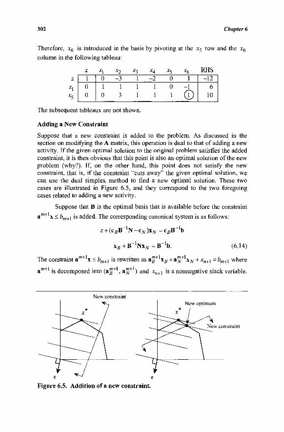
302 Chapter 6
Therefore, x6 is introduced in the basis by pivoting at the x5 row and the x6
column in the following tableau:
z
x5
z 1 0 0
xl 0 1 0
x2
-3 1 3
x3
-1 1 1
X4
-2 1 1
x5
0 0 1
x6 1
©
RHS -12
6 10
The subsequent tableaux are not shown.
Adding a New Constraint
Suppose that a new constraint is added to the problem. As discussed in the section on modifying the A matrix, this operation is dual to that of adding a new activity. If the given optimal solution to the original problem satisfies the added constraint, it is then obvious that this point is also an optimal solution of the new problem (why?). If, on the other hand, this point does not satisfy the new constraint, that is, if the constraint "cuts away" the given optimal solution, we can use the dual simplex method to find a new optimal solution. These two cases are illustrated in Figure 6.5, and they correspond to the two foregoing cases related to adding a new activity.
Suppose that B is the optimal basis that is available before the constraint
am+ x < bm+i is added. The corresponding canonical system is as follows:
z + (csB"1N-ci V)xi V =c s B _ 1 b
χ β + Β *Nx N B ' b . (6.14)
The constraint am+ x < bm+i is rewritten as a#+ \B +a^+ xN +xn+\ =bm+y where
am+1 is decomposed into (ag+ , a™+ ) and x„+] is a nonnegative slack variable.
New constraint New optimum
New constraint
Figure 6.5. Addition of a new constraint.
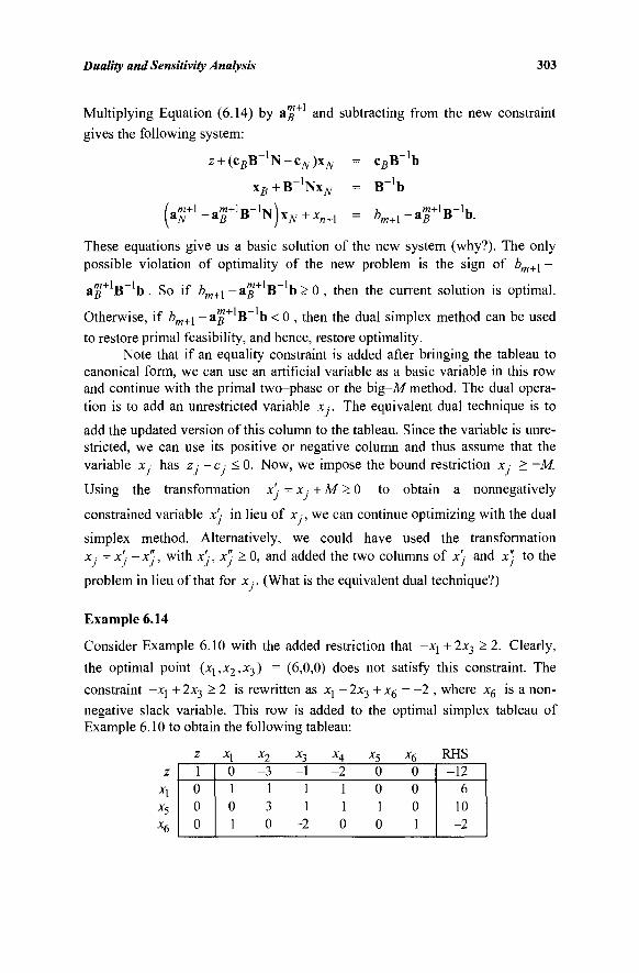
Duality and Sensitivity Analysis 303
,/K+l Multiplying Equation (6.14) by &B and subtracting from the new constraint
gives the following system:
(■ m+\ N '
z + (cfiB lN-cN)x
N
xB+B'lNxN
h
= CgB^'b
-H
, j»+l B ln)xN + X, n+l
B " b
è ^ - a ^ B - ' b .
These equations give us a basic solution of the new system (why?). The only possible violation of optimality of the new problem is the sign of bm+\ -
a£+1B_1b . So if bm+l -ag+1B 'b > 0 , then the current solution is optimal.
Otherwise, if èm+1 - a^ + 1 B 'b < 0 , then the dual simplex method can be used
to restore primal feasibility, and hence, restore optimality. Note that if an equality constraint is added after bringing the tableau to
canonical form, we can use an artificial variable as a basic variable in this row and continue with the primal two-phase or the big-M method. The dual opera-tion is to add an unrestricted variable x . The equivalent dual technique is to
add the updated version of this column to the tableau. Since the variable is unre-stricted, we can use its positive or negative column and thus assume that the variable x ,· has z ,· - c ,■ < 0. Now, we impose the bound restriction x · > —M.
Using the transformation x' = x · + M > 0 to obtain a nonnegatively
constrained variable x'- in lieu of x , we can continue optimizing with the dual
simplex method. Alternatively, we could have used the transformation x ■ = x'j - x"j, with x'j, x"j > 0, and added the two columns of x' and xj to the
problem in lieu of that for x ·. (What is the equivalent dual technique?)
Example 6.14
Consider Example 6.10 with the added restriction that -xj +2x3 >2. Clearly, the optimal point (xj,x2,X3) = (6,0,0) does not satisfy this constraint. The constraint -χχ + 2x3 > 2 is rewritten as χλ - 2x3 + x6 = -2 , where x6 is a non-negative slack variable. This row is added to the optimal simplex tableau of Example 6.10 to obtain the following tableau:
z X,
X,
x6
z 1 0 0 0
x\ 0 1 0 1
x2 -3
1 3 0
x3
-1 1 1
-2
• 4 -2
1 1 0
x5
0 0 1 0
x6 0 0 0 1
KH$ -12
6 10 -2
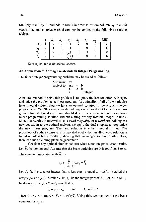
304 Chapter 6
Multiply row 1 by -1 and add to row 3 in order to restore column xj to a unit
vector. The dual simplex method can then be applied to the following resulting tableau:
2 Xi Xj X"l XA X$ X(\ RHS 1 0 0 0
0 1 0 0
-3 1 3
-1
-1 1
Θ
-2 1 1
-1
0 0 1 0
0 0 0 1
-12 6
10 -8
Subsequent tableaux are not shown.
An Application of Adding Constraints in Integer Programming
The linear integer programming problem may be stated as follows:
Minimize ex subject to Ax = b
x > 0. x integer.
A natural method to solve this problem is to ignore the last condition, x integer, and solve the problem as a linear program. At optimality, if all of the variables have integral values, then we have an optimal solution to the original integer program (why?). Otherwise, consider adding a new constraint to the linear pro-gram. This additional constraint should delete the current optimal noninteger linear programming solution without cutting off any feasible integer solution. Such a constraint is referred to as a valid inequality or a valid cut. Adding the new constraint to the optimal tableau, we apply the dual simplex to reoptimize the new linear program. The new solution is either integral or not. The procedure of adding constraints is repeated until either an all-integer solution is found or infeasibility results (indicating that no integer solution exists). How, then, can such a cutting plane be generated?
Consider any optimal simplex tableau when a noninteger solution results.
Let br be nonintegral. Assume that the basic variables are indexed from 1 to m.
The equation associated with br is
n _ xr+ Σ yrJXj=br.
j=m+l
Let Irj be the greatest integer that is less than or equal to yrj (Irj is called the
integer part of yrj). Similarly, let Ir be the integer part of br. Let Frj and Fr
be the respective fractional parts, that is,
Frj = yrj ~ !rj a n d Fr=br-Ir.
Then 0 < F ■ < 1 and 0 < Fr < 1 (why?). Using this, we may rewrite the basic
equation for xr as
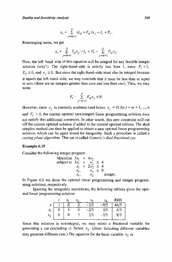
Duality and Sensitivity Analysis 305
xr+ Σ {Irj+Frj)Xj=Ir+Fr. j=m+\
Rearranging terms, we get n n
Xr "T 2 J rj j f I ^ Π j '
j=m+\ j=m+\
Now, the left-hand-side of this equation will be integral for any feasible integer solution (why?). The right-hand-side is strictly less than 1, since Fr < 1,
Frj > 0, and x .■ > 0. But since the right-hand-side must also be integral because
it equals the left-hand-side, we may conclude that it must be less than or equal to zero (there are no integers greater than zero and less than one). Thus, we may write
Fr- Σ FrjXj<0.
However, since x ■ is currently nonbasic (and hence x.· = 0) for/ = m + 1,..., n
and Fr > 0, the current optimal (noninteger) linear programming solution does
not satisfy this additional constraint. In other words, this new constraint will cut off the current optimal solution if added to the current optimal tableau. The dual simplex method can then be applied to obtain a new optimal linear programming solution, which can be again tested for integrality. Such a procedure is called a cutting plane algorithm. This cut is called Gomory's dual fractional cut.
Example 6.15
Consider the following integer program: Minimize 3xj + 4x2 subject to 3xj + x2 > 4
xx + 2x2 > 4 x\, x2 > 0 Xl, x2 integer.
In Figure 6.6 we show the optimal linear programming and integer program-ming solutions, respectively.
Ignoring the integrality restrictions, the following tableau gives the opti-mal linear programming solution:
Z Xj X 2 X-5 XA RHS 1 0 0
0 0 -2/5 -9/5 1 0 - 2 / 5 1/5 0 1 1/5 -3/5
44/5 4/5 8/5
Since this solution is nonintegral, we may select a fractional variable for generating a cut (including z). Select x2. (Note: Selecting different variables
may generate different cuts.) The equation for the basic variable x2 is
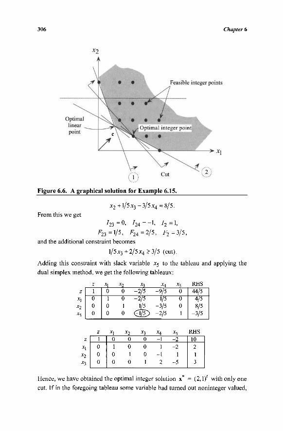
306 Chapter 6
Figure 6.6. A graphical solution for Example 6.15.
h = Pi
1, = 3/5,
x2+l /5x3 - 3/5 x4 = 8 / 5 · From this we get
723=0, 7 2 4 = - l ,
^23 =1/5, % =2/5, and the additional constraint becomes
l/5x3+2/5x4 >3/5 (cut).
Adding this constraint with slack variable x5 to the tableau and applying the
dual simplex method, we get the following tableaux:
z X] Xj x 3 x& Χς RMS
z X,
x2 x5
1 0 0 0
0 1 0 0
0 -2/5 0 -2/5 1 1/5 0 <£/?)
-9/5 1/5
-3/5 -2/5
0 0 0 1
44/5 4/5 8/5
-3/5
z x\
x7. x3
z 1 0 0 0
X)
0 1 0 0
x2
0 0 1 0
x3
0 0 0 1
X4
-1 1
-1 2
x5
-2 -2
1 -5
RHS 10 2 1 3
Hence, we have obtained the optimal integer solution x* = (2,1)' with only one
cut. If in the foregoing tableau some variable had turned out noninteger valued,
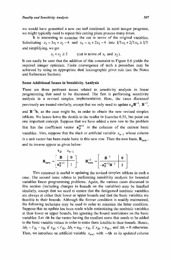
Duality and Sensitivity Analysis 307
we would have generated a new cut and continued. In most integer programs, we might typically need to repeat this cutting plane process many times.
It is interesting to examine the cut in terms of the original variables. Substituting x3 = 3xj + x2 - 4 and x4 = x\ + 2x2 - 4 into 1/5 x3 + 2/5 x4 > 3/5 and simplifying, we get
Xj + x2 > 3 (cut in terms of x\ and x2 ).
It can easily be seen that the addition of this constraint to Figure 6.6 yields the required integer optimum. Finite convergence of such a procedure may be achieved by using an appropriate dual lexicographic pivot rule (see the Notes and References Section).
Some Additional Issues in Sensitivity Analysis
There are three pertinent issues related to sensitivity analysis in linear programming that need to be discussed. The first is performing sensitivity analysis in a revised simplex implementation. Here, the cases discussed
previously are treated similarly, except that we only need to update c#B~ , B~ ,
and B~ b, as the case might be, in order to obtain the new revised simplex tableau. We hence leave the details to the reader in Exercise 6.55, but point out one important concept. Suppose that we have added a new row to the problem
that has the coefficient vector ag+ in the columns of the current basic
variables. Also, suppose that the slack or artificial variable x„+1 whose column
is a unit vector has been made basic in this new row. Then the new basis, B n e w ,
and its inverse appear as given below:
XB xn+\
B
a£+1
0
1
B '
-a£+ 1B-'
0
1
This construct is useful in updating the revised simplex tableau in such a case. The second issue relates to performing sensitivity analysis for bounded variables linear programming problems. Again, the various cases discussed in this section (including changes in bounds on the variables) may be handled similarly, except that we need to ensure that the designated nonbasic variables are always at either their lower or upper bounds and that the basic variables are feasible to their bounds. Although the former condition is readily maintained, the following technique may be used in order to maintain the latter condition. Suppose that an update has been made while maintaining the nonbasic variables at their lower or upper bounds, but ignoring the bound restrictions on the basic variables. Let Ab be the vector having the smallest norm that needs to be added to the basic variable values in order to make them feasible to their bounds. Hence, Afy =(-BÌ~xBi if xBi < ^Bh &bi = uBi ~xBi ^ xBi > uBi> an<^ A6,· = 0 otherwise. Then, we introduce an artificial variable x„+1 with -Ab as its updated column
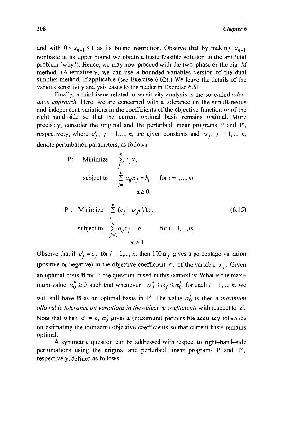
308 Chapter 6
and with 0 < x„+] < 1 as its bound restriction. Observe that by making x„+1
nonbasic at its upper bound we obtain a basic feasible solution to the artificial problem (why?). Hence, we may now proceed with the two-phase or the big-M method. (Alternatively, we can use a bounded variables version of the dual simplex method, if applicable (see Exercise 6.62).) We leave the details of the various sensitivity analysis cases to the reader in Exercise 6.61.
Finally, a third issue related to sensitivity analysis is the so-called toler-ance approach. Here, we are concerned with a tolerance on the simultaneous and independent variations in the coefficients of the objective function or of the right-hand-side so that the current optimal basis remains optimal. More precisely, consider the original and the perturbed linear programs P and P', respectively, where c-, j = 1,..., n, are given constants and a.-, j = 1,..., n, denote perturbation parameters, as follows:
n
P : Minimize X c -x· 7=1 «
subject to "L ciijXj -bj for; = l,...,m
x>0. n
P': Minimize Σ (cj +ajCj)Xj (6.15) y=i
n subject to Σ auXj =bt for i = 1,..., m
7=1
x>0.
Observe that if c' = c fory = 1,..., n, then 100a.· gives a percentage variation
(positive or negative) in the objective coefficient c, of the variable x ·. Given
an optimal basis B for P, the question raised in this context is: What is the maxi-
mum value CUQ > 0 such that whenever - « Q < a < CCQ for each/ = 1,..., n, we
will still have B as an optimal basis in P'. The value a$ is then a maximum
allowable tolerance on variations in the objective coefficients with respect to c'.
Note that when c' = c, a0 gives a (maximum) permissible accuracy tolerance
on estimating the (nonzero) objective coefficients so that current basis remains optimal.
A symmetric question can be addressed with respect to right-hand-side perturbations using the original and perturbed linear programs P and P', respectively, defined as follows:
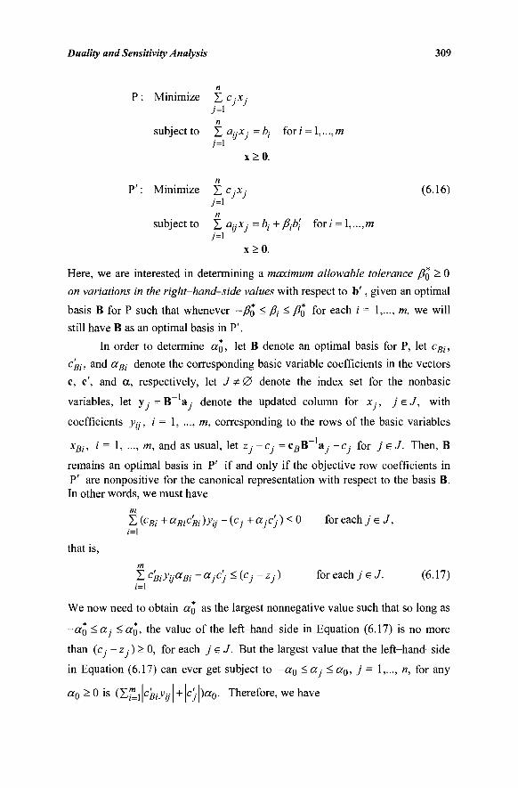
Duality and Sensitivity Analysis 309
Minimize Σ c X:
n subject to Σ a^Xj = ty for i = 1,.
x>0 .
P': Minimize Σ c,x,· (6.16)
subject to Σ ay* · = bj + /?,·£>/ for / = 1,...,m 7=1
x>0.
Here, we are interested in determining a maximum allowable tolerance /?0 ^ 0
o« variations in the right-hand-side values with respect to b ' , given an optimal
basis B for P such that whenever -β$ < /?, < β$ for each /' = 1,..., m, we will
still have B as an optimal basis in P'.
In order to determine «Q, let B denote an optimal basis for P, let cBj,
c'Bi, and aBi denote the corresponding basic variable coefficients in the vectors
c, c', and a, respectively, let J Ψ 0 denote the index set for the nonbasic
variables, let y · = B~ a · denote the updated column for x ■, j e J, with
coefficients y^, i = 1, ..., m, corresponding to the rows of the basic variables
xBi, i = 1, ..., m, and as usual, let zj -Cj = c#B~ ay -Cj for j e J. Then, B
remains an optimal basis in P' if and only if the objective row coefficients in P' are nonpositive for the canonical representation with respect to the basis B. In other words, we must have
m Σ (pBi + aBic'Bi )yiJ - (cj + aye} ) < 0 for each jeJ, i=\
that is,
Σ c'BiyyaBi - ccjc'j < (cj - zj ) for each jeJ. (6.17) i=\
We now need to obtain a$ as the largest nonnegative value such that so long as
-«o ^aj ^ « 0 ' m e v a l u e of the left-hand-side in Equation (6.17) is no more
than (c ~zj)- 0, for each j e J. But the largest value that the left-hand-side
in Equation (6.17) can ever get subject to - α 0 - aj - ao> J = 1>—> n> f°r anY
«0 > 0 is (Σ™ i \cBiyij \ + \c'j )a0· Therefore, we have
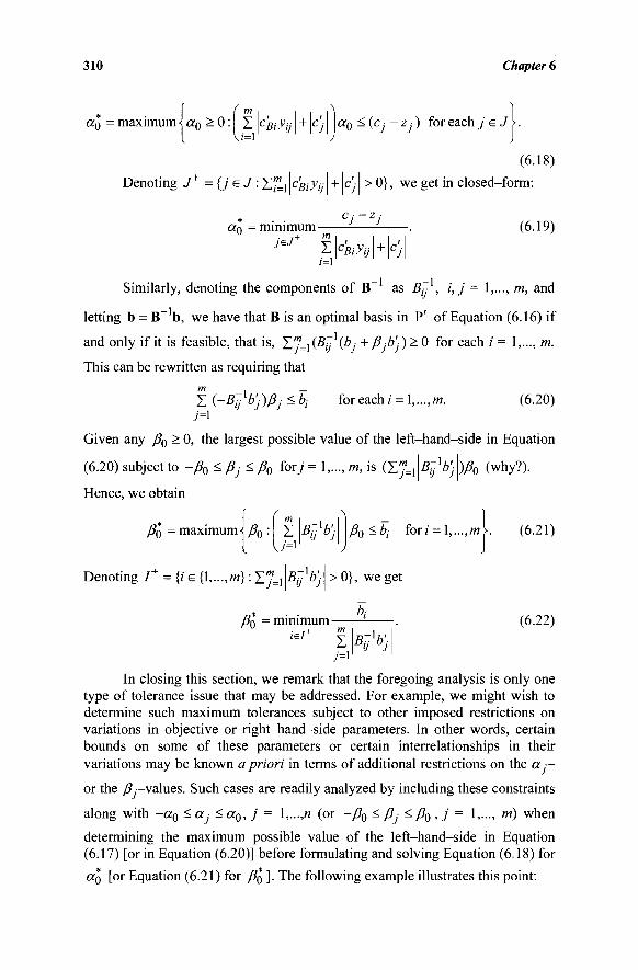
310 Chapter 6
I I I I
«0 = maximum<αΰ>0: Σ ks;>y·\ + \c'j\ a0 -(cj ~zj) f ° r e a c n 7 e-^ I V/=1 ) J
(6.18)
Denoting J+ ={j eJ : Y™= λ \ο'Βίγ^ + ìc'j > 0}, we get in closed-form:
«o = minimum-• r+ m I I I I
7ej ite+k (6.19)
i=l
Similarly, denoting the components of B as By , i,j = 1,..., m, and
letting b = B~ b, we have that B is an optimal basis in P' of Equation (6.16) if
- 1 , and only if it is feasible, that is, Σ"}={{Β1]ιψ]+β]ο)) > 0 for each / = 1,...,
This can be rewritten as requiring that
m.
7=1 for each i = \,...,m. (6.20)
Given any β0 > 0, the largest possible value of the left-hand-side in Equation
(6.20) subject to -β0 < β] < β0 fory = 1,..., m, is (Σ%
Hence, we obtain
BUbJ )β0 (why?).
β0 = maximum^ /?0 :
Denoting / + = {/ e {1,...,m) : £ J = ]
m
Σ U=i
B'-K v J
y90<è, for/= !,...,/« (6.21)
Bi'bJ
βθ = minimum
>0}, we get
k
Σ y=i
Btb'j
(6.22)
In closing this section, we remark that the foregoing analysis is only one type of tolerance issue that may be addressed. For example, we might wish to determine such maximum tolerances subject to other imposed restrictions on variations in objective or right-hand-side parameters. In other words, certain bounds on some of these parameters or certain interrelationships in their variations may be known a priori in terms of additional restrictions on the a —
or the β,—values. Such cases are readily analyzed by including these constraints
along with -a0 < <Xj < a0, j = \,...,n (or -β0 < fij < β0 , j = 1,..., m) when
determining the maximum possible value of the left-hand-side in Equation (6.17) [or in Equation (6.20)] before formulating and solving Equation (6.18) for
«0 [°r Equation (6.21) for β^ ]. The following example illustrates this point:
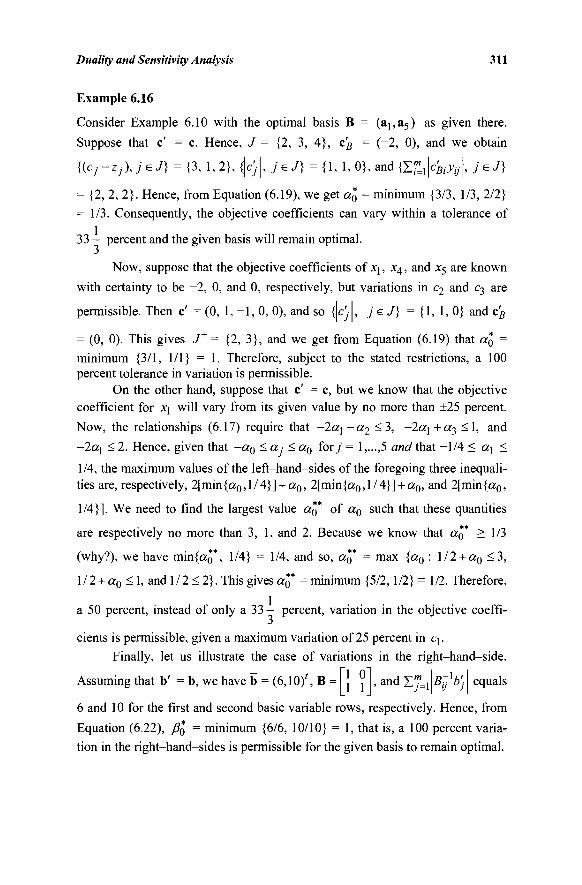
Duality and Sensitivity Analysis 311
Example 6.16
Consider Example 6.10 with the optimal basis B = (aj,a5) as given there.
Suppose that c' = c. Hence, J = {2, 3, 4}, c'B = (-2, 0), and we obtain
{(CJ-ZJ), jeJ} = {3, 1, 2}, {|C)|, jeJ} = {\, 1, 0}, and { Σ £ ι ^ 4 J e J}
= {2, 2, 2}. Hence, from Equation (6.19), we get α0 = minimum {3/3, 1/3, 2/2}
= 1/3. Consequently, the objective coefficients can vary within a tolerance of
33 — percent and the given basis will remain optimal.
Now, suppose that the objective coefficients of X] , Χ4, and x5 are known
with certainty to be -2 , 0, and 0, respectively, but variations in c2 and c3 are
permissible. Then c' = (0, 1, - 1 , 0, 0), and so Uc'ji, j e J} = {1, 1, 0} and c'B
= (0, 0). This gives J+ = {2, 3}, and we get from Equation (6.19) that a§ =
minimum {3/1, 1/1} = 1. Therefore, subject to the stated restrictions, a 100 percent tolerance in variation is permissible.
On the other hand, suppose that c' = c, but we know that the objective
coefficient for xj will vary from its given value by no more than ±25 percent.
Now, the relationships (6.17) require that -2«[ - a 2 ^ 3 , -2arj + a 3 <1, and
-2a\ < 2. Hence, given that - a 0 < a,· < a0 f°rJ = 1>-··>5 and that -1/4 < a\ <
1/4, the maximum values of the left-hand-sides of the foregoing three inequali-ties are, respectively, 2[πάη{α$,\Ι4}] + a$, 2[πήη{α0,1/4}] + α:0, and 2[min{«0>
1/4}]. We need to find the largest value a™ of a0 such that these quantities
are respectively no more than 3, 1, and 2. Because we know that «Q* — 1/3
(why?), we have min{«Q*, 1/4} = 1/4, and so, α " = m a x iao '■ l /2 + a0 ^ 3 ,
1 / 2 + a0 -1> a nd 1 / 2 < 2}. This gives «Q* = minimum {5/2,1/2} = 1/2. Therefore,
a 50 percent, instead of only a 33 — percent, variation in the objective coeffi-
cients is permissible, given a maximum variation of 25 percent in q. Finally, let us illustrate the case of variations in the right-hand-side.
Assuming that b' = b, we have b = (6,10)', B = 1 0 1 1
, and Σ7=1 Βϋ^ equals
6 and 10 for the first and second basic variable rows, respectively. Hence, from
Equation (6.22), β^ = minimum {6/6, 10/10} = 1, that is, a 100 percent varia-
tion in the right-hand-sides is permissible for the given basis to remain optimal.
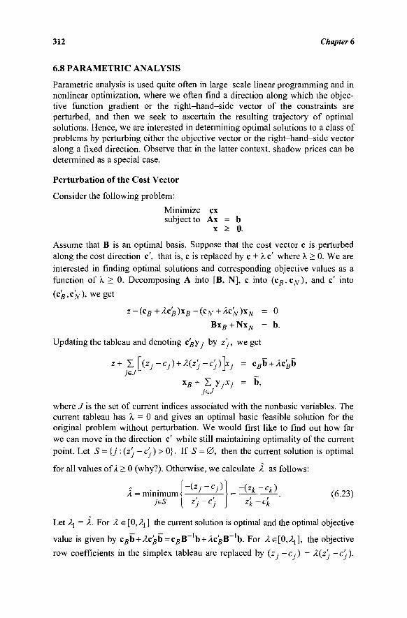
312 Chapter 6
6.8 PARAMETRIC ANALYSIS
Parametric analysis is used quite often in large-scale linear programming and in nonlinear optimization, where we often find a direction along which the objec-tive function gradient or the right-hand-side vector of the constraints are perturbed, and then we seek to ascertain the resulting trajectory of optimal solutions. Hence, we are interested in determining optimal solutions to a class of problems by perturbing either the objective vector or the right-hand-side vector along a fixed direction. Observe that in the latter context, shadow prices can be determined as a special case.
Perturbation of the Cost Vector
Consider the following problem:
Minimize ex subject to Ax = b
x > 0.
Assume that B is an optimal basis. Suppose that the cost vector c is perturbed along the cost direction c', that is, c is replaced by c + λ c' where λ > 0. We are interested in finding optimal solutions and corresponding objective values as a function of λ > 0. Decomposing A into [B, N], c into (c^c^y), and c' into
(CB,CV), we get
z-(cB+Àc'B)\B-(cN+Àc'N)xN = 0
Bxg + N\N = b.
Updating the tableau and denoting c^yy by z'j, we get
z+ Σ [(zj -cj) + À(z'j -c'ji^Cj = Cgb + Ac^b
*B + Σ yjXj = b, jeJ
where J is the set of current indices associated with the nonbasic variables. The current tableau has λ = 0 and gives an optimal basic feasible solution for the original problem without perturbation. We would first like to find out how far we can move in the direction c' while still maintaining optimality of the current point. Let S = {j : (ζ'- -c ■) > 0}. If S = 0 , then the current solution is optimal
for all values of 1 > 0 (why?). Otherwise, we calculate A as follows:
Ì = m i n i m u m J " ^ ' ^ 0 } = ±ίΐΞ*1. (6.23) jsS [ z'j-c'j J z'k-c'k
Let λχ = λ. For λ e [0, λ\ ] the current solution is optimal and the optimal objective
value is given by cgb + Ac5b = cgB~ b + CgB- b. For λ efO,/^], the objective
row coefficients in the simplex tableau are replaced by (z ■ - c . ) + A(z' -c ' · ) .
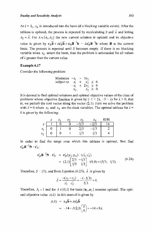
Duality and Sensitivity Analysis 313
At λ = λ], xk is introduced into the basis (if a blocking variable exists). After the
tableau is updated, the process is repeated by recalculating S and X and letting
À2 - A. For Λ, e [Λ-ι,/Ι2 ] the new current solution is optimal and its objective
value is given by cgb + Acgb = cgB~ b + Ac'BB~ b where B is the current basis. The process is repeated until S becomes empty. If there is no blocking variable when xk enters the basis, then the problem is unbounded for all values of λ greater than the current value.
Example 6.17
Consider the following problem:
Minimize -xl - 3x2 subject to X[ + x2 < 6
- X | + 2x 2 ^ 6 X], X2 > 0
It is desired to find optimal solutions and optimal objective values of the class of problems whose objective function is given by (-1 + 2λ, -3 + λ) for λ > 0; that is, we perturb the cost vector along the vector (2,1). First we solve the problem with λ = 0 where x3 and x4 are the slack variables. The optimal tableau for λ = 0 is given by the following:
z
x2
z 1 0 0
X]
0 1 0
x2
0 0 1
x3
-5/3 2/3 1/3
X4
-2/3 -1/3
1/3
RHS -14
2 4
In order to find the range over which this tableau is optimal, first find
c'nB-1N-c'w: cfl N-
c'BB_1N-c', N = c f i(y3>y4)-(c3>c4) "2/3 -1/3 _ 1/3 1/3 (2,1) (0,0) = (5/3,-1/3).
(6.24)
Therefore, 5= {3}, and from Equation (6.23), X is given by
-(z3-c3) -(-5/3) À-- = 1.
Z3 - C3 5/3
Therefore, λ\ = 1 and for λ e [0,1] the basis [a!,a2] remains optimal. The opti-
mal objective value ζ(λ) in this interval is given by
ζ(λ) = Cgb + /lcgb
= -14 + 2(2,1) -14 + 8A.
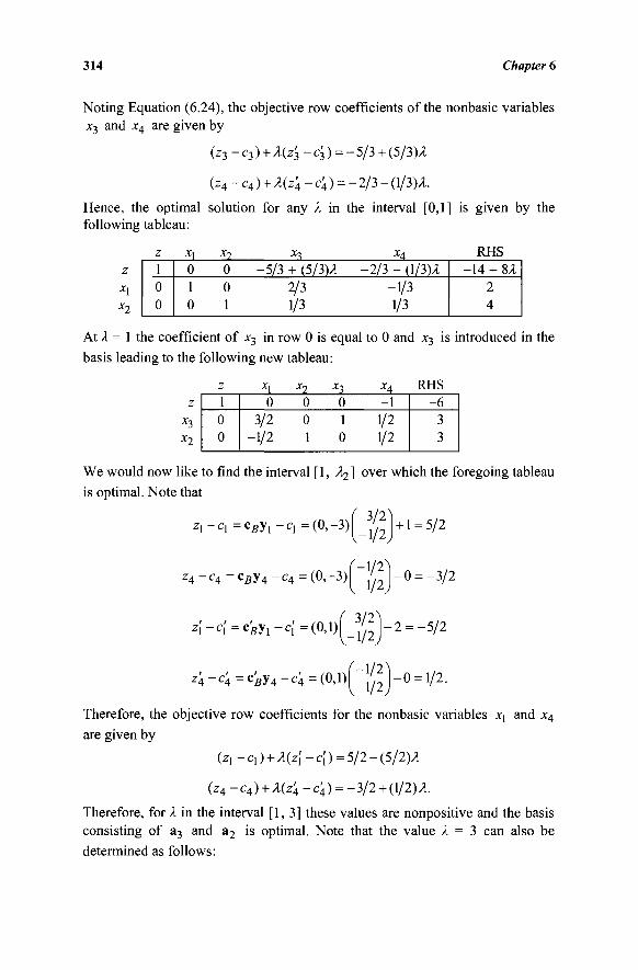
314 Chapter 6
Noting Equation (6.24), the objective row coefficients of the nonbasic variables x3 and x4 are given by
( z 3 - c 3 ) + l ( z 3 - c 3 ) = - 5 / 3 + (5/3)1
(z4 - c4 ) + λ(ζ\ - c\ ) = - 2/3 - (1/3)1.
Hence, the optimal solution for any λ in the interval [0,1] is given by the following tableau:
z x\ x2
At λ = 1 the coefficient of x3 in row 0 is equal to 0 and x3 is introduced in the
basis leading to the following new tableau:
z 1 0 0
X,
0 1 0
x? 0 0 1
x3
-5/3 + (5/3)1 2/3 1/3
Λ4
-2/3 - (1/3)1 -1/3 1/3
RHS -14 + 81
2 4
z x3
x2
z 1 0 0
X,
0 3/2
-1/2
x2 0 0 1
x3
0 1 0
x4
-1 -1/2
1/2
RHS -6
3 3
We would now like to find the interval [1, λ^] over which the foregoing tableau is optimal. Note that
3/2^ *i - ci = csy! - q = (0, -3) I _ ^ I + 1 = 5/2
-3/2 z4-c4=cBy4-c4 =(0,-3)1 / 2 J - 0 =
A -c[ = c'By{ -c[ = ( 0 , 1 ) [ _ ^ ] - 2 = - V 2
z 4 - c 4 = c ^ y 4 - c 4 = ( 0 , 1 ) ^ 1 ^ 1 - 0 = 1/2.
Therefore, the objective row coefficients for the nonbasic variables xx and x4
are given by
(z! - q ) + λ(ζ[ -c[) = 5/2-(5/2)1
(z4 - c4 ) + l (z 4 - c4 ) = - 3/2 + (1/2) 1.
Therefore, for /I in the interval [1, 3] these values are nonpositive and the basis consisting of a3 and a2 is optimal. Note that the value 1 = 3 can also be determined as follows:
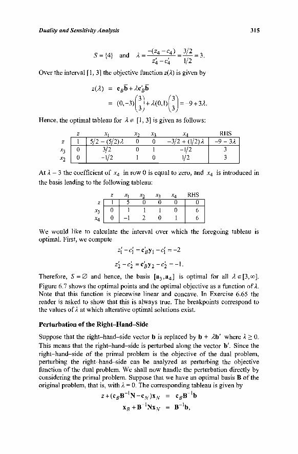
Duality! and Sensitivity Analysis 315
S = {4} and λ·-- ( z 4 - c 4 ) ^ 3 / 2
z4 - c4 1/2 :3.
Over the interval [1,3] the objective function z(X) is given by
ζ(λ) cgb +Acgb
(0,-3) '3 Ì (3^
3 J + A(0,1) -9 + 3A.
Hence, the optimal tableau for A e [1, 3] is given as follows:
z
x2
At A = 3 the coefficient of x4 in row 0 is equal to zero, and x4 is introduced in
the basis leading to the following tableau:
z 1 0 0
*1
5/2 - (5/2) λ 3/2
-1/2
*■>
0 0 1
*1 0 1 0
X4
-3 /2 + (1/2) λ -1/2 1/2
RHS -9 + 3/1
3 3
z x3
z 1 0 0
x\ -5
1 -1
*2 0 1 2
*3 0 1 0
X4
0 0 1
RHS 0 6 6
We would like to calculate the interval over which the foregoing tableau is optimal. First, we compute
-2 z l ~ c l =cByi~c\
-1. z 2 ~ c 2 = C S V 2 - C 2
Therefore, 5 = 0 and hence, the basis [a3,a4] is optimal for all λ e [3,co].
Figure 6.7 shows the optimal points and the optimal objective as a function of A. Note that this function is piecewise linear and concave. In Exercise 6.65 the reader is asked to show that this is always true. The breakpoints correspond to the values of A at which alterative optimal solutions exist.
Perturbation of the Right-Hand-Side
Suppose that the right-hand-side vector b is replaced by b + Ab' where A > 0. This means that the right-hand-side is perturbed along the vector b'. Since the right-hand-side of the primal problem is the objective of the dual problem, perturbing the right-hand-side can be analyzed as perturbing the objective function of the dual problem. We shall now handle the perturbation directly by considering the primal problem. Suppose that we have an optimal basis B of the original problem, that is, with A = 0. The corresponding tableau is given by
z + (csB'
"fl
N
+ B
cN)xN = 1
C g B _ 1 b
'Nx N = B ' b ,
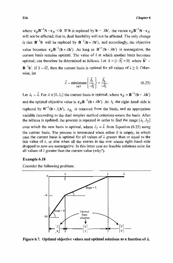
316 Chapter 6
where cgB N - c ^ < 0. If b is replaced by b + Ab', the vector c#B N-cN
will not be affected; that is, dual feasibility will not be affected. The only change
is that B~ b will be replaced by B~ (b + Ab'), and accordingly, the objective
value becomes cgB~ (b + Ab'). As long as B~ (b + Ab') is nonnegative, the
current basis remains optimal. The value of λ at which another basis becomes
optimal, can therefore be determined as follows. Let S = {/' : b\ < 0} where b' =
B~'b'. If S = 0 , then the current basis is optimal for all values of λ > 0. Other-wise, let
A = minimum < —=- > = —=-. ieS {-b'i} -b'r
(6.25)
Let A[ = A. For A e [0, Aj] the current basis is optimal, where χβ = B~ (b + Ab')
and the optimal objective value is cBB~ (b + Ab'). At Aj the right-hand-side is
replaced by B~ (b + Ajb'), xB is removed from the basis, and an appropriate
variable (according to the dual simplex method criterion) enters the basis. After the tableau is updated, the process is repeated in order to find the range \\,Xj\
over which the new basis is optimal, where λ^ = A from Equation (6.25) using
the current basis. The process is terminated when either S is empty, in which case the current basis is optimal for all values of λ greater than or equal to the last value of A, or else when all the entries in the row whose right-hand-side dropped to zero are nonnegative. In this latter case no feasible solutions exist for all values of 1 greater than the current value (why?).
Example 6.18
Consider the following problem:
Figure 6.7. Optimal objective values and optimal solutions as a function of A.
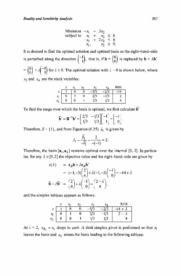
Duality and Sensitivity Analysis 317
Minimize -x{ - 3x2 subject to x\ + x2 < 6
-xj + 2x2 < 6
It is desired to find the optimal solution and optimal basis as the right-hand-side
is perturbed along the direction , , that is, if b = L- is replaced by b + Ab'
= I , I +A . for A > 0. The optimal solution with λ = 0 is shown below, where
x3 and x4 are the slack variables:
z
*1
*2
z 1 0 0
*1 0 1 0
x2
0 0 1
x3
-5/3 2/3 1/3
•*4 -2/3 -1/3
1/3
RHS -14
2 4
To find the range over which the basis is optimal, we first calculate b'
b' = B- 1b ' 2/3 -1/3' 1/3 1/3
Therefore, S= {1}, and from Equation (6.25) \ is given by
\ _ 2 A, ■ = 2.
Therefore, the basis [aj,a2] remains optimal over the interval [0, 2]. In particu-
lar, for any λ e [0,2] the objective value and the right-hand-side are given by
z{X) = c5b + l c B b ' f2
(-1,-3)| - | + A(-1,-3) -14 + Λ
b + /lb' = in: 2-λ 4
and the simplex tableau appears as follows:
z X,
x2
z 1 0 0
X,
0 1 0
x2
0 0 1
x3
-5/3 2/3 1/3
X4
-2 /3 -1/3
1/3
RHS -14 + 2
2- λ 4
At A = 2, χβ = X] drops to zero. A dual simplex pivot is performed so that xj
leaves the basis and x4 enters the basis leading to the following tableau:
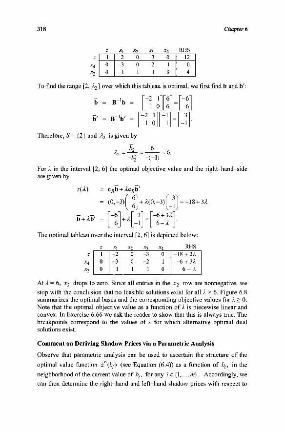
318 Chapter 6
z X4
x2
z 1 0 0
x\ -2 -3
1
x2 0 0 1
*3 -3 -2
1
X4
0 1 0
RHS -12
0 4
To find the range [2, λχ ] over which this tableau is optimal, we first find b and b':
b = B_1b =
b' = B V = Γ
"-2 1 1 0
-2 1"|
1 oj
T6" |_6
-Γ 1
"-6" 6
" 31 - 1
Therefore, S= {2} and λχ is given by
h-b2
h -b2 -(-1) 6.
For A in the interval [2, 6] the optimal objective value and the right-hand-side are given by
z(A) = c s b + /lcsb'
= (0,-3)MÌ + A(0>-3)ijjì = -18 + 3A
b + Ab' = - 6
6 + λ
3
- 1
- 6 + 3A
6-λ
1 0 0
-2 0 - 3 0 -3 0 - 2 1
1 1 1 0
-18 + 3/1 -6 + 3,1
6 - / 1
The optimal tableau over the interval [2, 6] is depicted below:
Z X] Xj X*i ΧΛ JxrlS
z x4 x2
At λ = 6, x2 drops to zero. Since all entries in the x2 r o w a r e nonnegative, we
stop with the conclusion that no feasible solutions exist for all λ > 6. Figure 6.8 summarizes the optimal bases and the corresponding objective values for λ > 0. Note that the optimal objective value as a function of λ is piecewise linear and convex. In Exercise 6.66 we ask the reader to show that this is always true. The breakpoints correspond to the values of A for which alternative optimal dual solutions exist.
Comment on Deriving Shadow Prices via a Parametric Analysis
Observe that parametric analysis can be used to ascertain the structure of the
optimal value function z (è,·) (see Equation (6.4)) as a function of bh in the
neighborhood of the current value of bj, for any / e {1,..., m). Accordingly, we
can then determine the right-hand and left-hand shadow prices with respect to
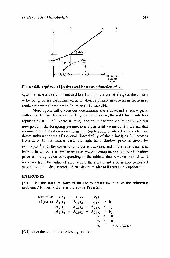
Duality and Sensitivity Analysis 319
Figure 6.8. Optimal objectives and bases as a function of λ.
ty as the respective right-hand and left-hand derivatives of z* (ty ) at the current
value of bt, where the former value is taken as infinity in case an increase in ό;·
renders the primal problem in Equation (6.1) infeasible. More specifically, consider determining the right-hand shadow price
with respect to bh for some ie{\,...,m}. In this case, the right-hand-side b is replaced by b + Ab', where b' = e;-, the rth unit vector. Accordingly, we can now perform the foregoing parametric analysis until we arrive at a tableau that remains optimal as λ increases from zero (up to some positive level) or else, we detect unboundedness of the dual (infeasibility of the primal) as λ increases from zero. In the former case, the right-hand shadow price is given by
Wj = (cgB~ ); for the corresponding current tableau, and in the latter case, it is infinite in value. In a similar manner, we can compute the left-hand shadow price as the w, value corresponding to the tableau that remains optimal as λ increases from the value of zero, where the right-hand-side is now perturbed according to b - Ae,·. Exercise 6.70 asks the reader to illustrate this approach.
EXERCISES
[6.1] Use the standard form of duality to obtain the dual of the following problem. Also verify the relationships in Table 6.1.
inimize CjX] + c2X2 bjectto A n x , + A|2X2
A21X! + A22x2
A 3 1 x l + A 3 2 x 2
+ C3X3
+ A13x3 > bj + A23x3 < b 2
+ A33x3 = b3
X! > 0
x2 < 0 x3 unrestricted
[6.2] Give the dual of the following problem:

320 Chapter 6
Maximize -2xj + 3x2 + subject to -2x] + x2 +
2x[ + -2x2 +
isider the following problem: Maximize -JCJ subject to 2xj
X,
X] ,
5x3 3x3 + x3
x3 +
x2,
+ 3x2 + 3x2
- 3x2 x2
x^
X4 x\ x3 X4
< > >
> 5 = 4 < 6 < 0 > 0
unrestricted
6 -3
0.
[6.3]
a. Solve the problem graphically. b. State the dual and solve it graphically. Utilize the theorems of duality
to obtain the values of all the primal variables from the optimal dual solution.
[6.4] Solve the following linear program by a graphical method: Maximize 3xj + subject to 6x[ +
3xj + X,,
(Hint: Utilize the dual problem.)
[6.5] Consider the following problem:
Maximize 10xj + 24x2 + subject to xj + x2 +
2xj + 4x2 + X\, *2'
3x2 9x2 2x2 x2,
20x3
2x3
3x3
*3>
+ 21x3 + 25x3 < 15 + 25x3 < 20
x3 > 0.
+ 20x4 + 25x5
+ 3x4 + 5x5
+ 2x4 + x5 X4, X5
< < >
19 57 0.
a. Write the dual problem and verify that (wj, w2 ) = (4, 5) is a feasible
solution. b. Use the information in Part (a) to derive an optimal solution to both
the primal and the dual problems.
[6.6] Consider the following problem:
Minimize subject to
2X] X,
- 2 x j
Xl,
+ 15x2 + 5x3 + 6x2 + 3x3 + 5x2 - 4x3
x2> x3'
+ 6X4 + X4 > + 3x4 <
x4 >
2 -3
0.
a. Give the dual linear problem. b. Solve the dual geometrically. c. Utilize information about the dual linear program and the theorems
of duality to solve the primal problem.
[6.7] Consider the following linear programming problem:
Maximize 2xj + 3x2 + 5x3 subject to Xj + 2x2 + 3x3 < 8
Xl - 2x2 + 2x3 < 6 Xj, Χ2, x3 — ^·
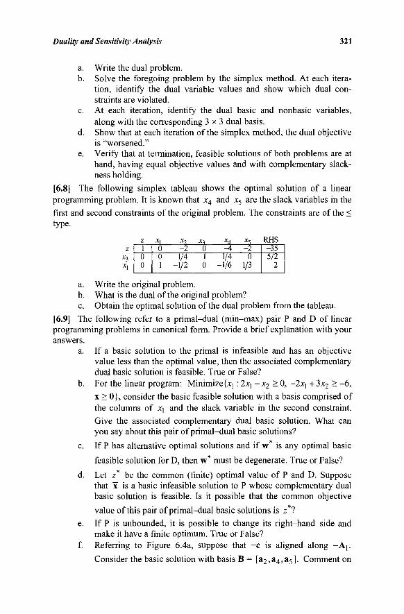
Duality and Sensitivity Analysis 321
a. Write the dual problem. b. Solve the foregoing problem by the simplex method. At each itera-
tion, identify the dual variable values and show which dual con-straints are violated.
c. At each iteration, identify the dual basic and nonbasic variables, along with the corresponding 3 x 3 dual basis.
d. Show that at each iteration of the simplex method, the dual objective is "worsened."
e. Verify that at termination, feasible solutions of both problems are at hand, having equal objective values and with complementary slack-ness holding.
[6.8] The following simplex tableau shows the optimal solution of a linear programming problem. It is known that x4 and x5 are the slack variables in the
first and second constraints of the original problem. The constraints are of the < type.
Z X] Xj X-^ ΧΛ Χ^ RHS 1 0 0
0 -2 0 - 4 - 2 0 1/4 1 1/4 0 1 -1/2 0 -1/6 1/3
-35 5/2
2
a. Write the original problem. b. What is the dual of the original problem? c. Obtain the optimal solution of the dual problem from the tableau.
[6.9] The following refer to a primal-dual (min-max) pair P and D of linear programming problems in canonical form. Provide a brief explanation with your answers.
a. If a basic solution to the primal is infeasible and has an objective value less than the optimal value, then the associated complementary dual basic solution is feasible. True or False?
b. For the linear program: Minimize {xj : 2xj - x 2 > 0, -2xj +3x2 > -6, x > 0}, consider the basic feasible solution with a basis comprised of the columns of Xj and the slack variable in the second constraint. Give the associated complementary dual basic solution. What can you say about this pair of primal-dual basic solutions?
c. If P has alternative optimal solutions and if w is any optimal basic
feasible solution for D, then w* must be degenerate. True or False?
d. Let z* be the common (finite) optimal value of P and D. Suppose that x is a basic infeasible solution to P whose complementary dual basic solution is feasible. Is it possible that the common objective
value of this pair of primal-dual basic solutions is z*?
e. If P is unbounded, it is possible to change its right-hand-side and make it have a finite optimum. True or False?
f. Referring to Figure 6.4a, suppose that -c is aligned along -Aj .
Consider the basic solution with basis B = [a2 ,a4 ,a5] . Comment on
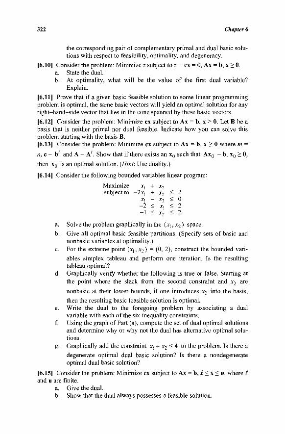
322 Chapter 6
the corresponding pair of complementary primal and dual basic solu-tions with respect to feasibility, optimality, and degeneracy.
[6.10] Consider the problem: Minimize z subject to z - ex = 0, Ax = b, x > 0. a. State the dual. b. At optimality, what will be the value of the first dual variable?
Explain.
[6.11] Prove that if a given basic feasible solution to some linear programming problem is optimal, the same basic vectors will yield an optimal solution for any right-hand-side vector that lies in the cone spanned by these basic vectors.
[6.12] Consider the problem: Minimize ex subject to Ax = b, x > 0. Let B be a basis that is neither primal nor dual feasible. Indicate how you can solve this problem starting with the basis B. [6.13] Consider the problem: Minimize ex subject to Ax = b, x > 0 where m =
n, c = b ' and A = A'. Show that if there exists an x0 such that Ax0 = b, x0 > 0,
then x0 is an optimal solution. (Hint: Use duality.)
[6.14] Consider the following bounded variables linear program:
Maximize subject to
X,
- 2 x j X,
-2 -1
+ x2 + x2
- x2 < X!
< x2
< < < <
2 0 2 2.
a. Solve the problem graphically in the (xj, x2) space.
b. Give all optimal basic feasible partitions. (Specify sets of basic and nonbasic variables at optimality.)
c. For the extreme point (xj, x2 ) = (0, 2), construct the bounded vari-ables simplex tableau and perform one iteration. Is the resulting tableau optimal?
d. Graphically verify whether the following is true or false. Starting at the point where the slack from the second constraint and x2 are nonbasic at their lower bounds, if one introduces x2 into the basis, then the resulting basic feasible solution is optimal.
e. Write the dual to the foregoing problem by associating a dual variable with each of the six inequality constraints.
f. Using the graph of Part (a), compute the set of dual optimal solutions and determine why or why not the dual has alternative optimal solu-tions.
g. Graphically add the constraint Xj + x2 < 4 to the problem. Is there a
degenerate optimal dual basic solution? Is there a nondegenerate optimal dual basic solution?
[6.15] Consider the problem: Minimize ex subject to Ax = b, £ < x < u, where ί and u are finite.
a. Give the dual. b. Show that the dual always possesses a feasible solution.
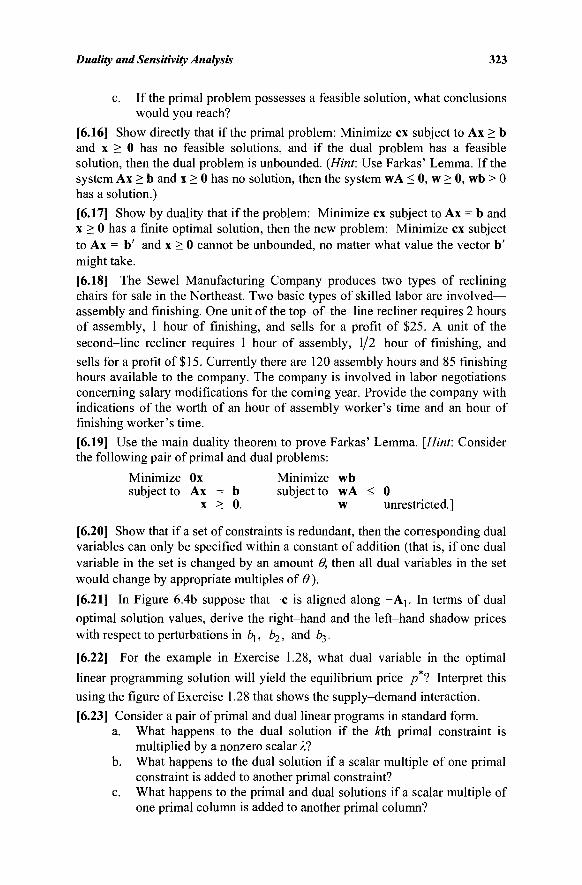
Duality and Sensitivity Analysis 323
c. If the primal problem possesses a feasible solution, what conclusions would you reach?
[6.16] Show directly that if the primal problem: Minimize ex subject to Ax > b and x > 0 has no feasible solutions, and if the dual problem has a feasible solution, then the dual problem is unbounded. {Hint: Use Farkas' Lemma. If the system Ax > b and x > 0 has no solution, then the system wA < 0, w > 0, wb > 0 has a solution.)
[6.17] Show by duality that if the problem: Minimize ex subject to Ax = b and x > 0 has a finite optimal solution, then the new problem: Minimize ex subject to Ax = b' and x > 0 cannot be unbounded, no matter what value the vector b' might take.
[6.18] The Sewel Manufacturing Company produces two types of reclining chairs for sale in the Northeast. Two basic types of skilled labor are involved— assembly and finishing. One unit of the top—of-the-line recliner requires 2 hours of assembly, 1 hour of finishing, and sells for a profit of $25. A unit of the second-line recliner requires 1 hour of assembly, 1/2 hour of finishing, and
sells for a profit of $15. Currently there are 120 assembly hours and 85 finishing hours available to the company. The company is involved in labor negotiations concerning salary modifications for the coming year. Provide the company with indications of the worth of an hour of assembly worker's time and an hour of finishing worker's time.
[6.19] Use the main duality theorem to prove Farkas' Lemma. [Hint: Consider the following pair of primal and dual problems:
Minimize Ox Minimize wb subject to Ax = b subject to wA < 0
x > 0. w unrestricted.]
[6.20] Show that if a set of constraints is redundant, then the corresponding dual variables can only be specified within a constant of addition (that is, if one dual variable in the set is changed by an amount Θ, then all dual variables in the set would change by appropriate multiples of Θ).
[6.21] In Figure 6.4b suppose that -c is aligned along - Ap In terms of dual optimal solution values, derive the right-hand and the left-hand shadow prices with respect to perturbations in l\, b2, and b^.
[6.22] For the example in Exercise 1.28, what dual variable in the optimal
linear programming solution will yield the equilibrium price p*l Interpret this
using the figure of Exercise 1.28 that shows the supply-demand interaction.
[6.23] Consider a pair of primal and dual linear programs in standard form. a. What happens to the dual solution if the Ath primal constraint is
multiplied by a nonzero scalar A? b. What happens to the dual solution if a scalar multiple of one primal
constraint is added to another primal constraint? c. What happens to the primal and dual solutions if a scalar multiple of
one primal column is added to another primal column?
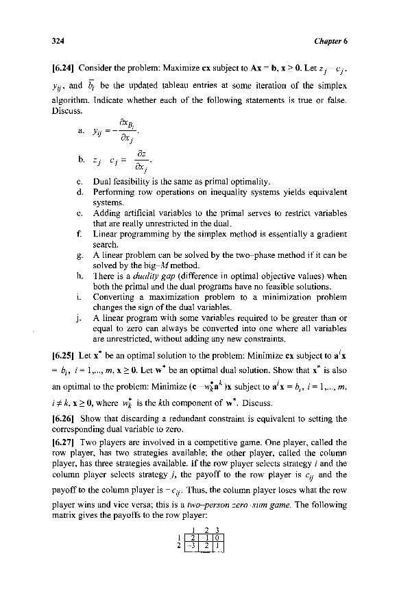
324 Chapter 6
[6.24] Consider the problem: Maximize ex subject to Ax = b, x > 0. Let z - c ,·,
yy, and bt be the updated tableau entries at some iteration of the simplex
algorithm. Indicate whether each of the following statements is true or false. Discuss.
a . y t j = -dxBj
dxj
u dz
b. Zj -Cj = . 1 J Bxj
c. Dual feasibility is the same as primal optimality. d. Performing row operations on inequality systems yields equivalent
systems. e. Adding artificial variables to the primal serves to restrict variables
that are really unrestricted in the dual. f. Linear programming by the simplex method is essentially a gradient
search. g. A linear problem can be solved by the two-phase method if it can be
solved by the big-M method. h. There is a duality gap (difference in optimal objective values) when
both the primal and the dual programs have no feasible solutions. i. Converting a maximization problem to a minimization problem
changes the sign of the dual variables. j . A linear program with some variables required to be greater than or
equal to zero can always be converted into one where all variables are unrestricted, without adding any new constraints.
[6.25] Let x* be an optimal solution to the problem: Minimize ex subject to a'x
= bj, i = 1,..., m, x > 0. Let w be an optimal dual solution. Show that x* is also
an optimal to the problem: Minimize (c -w£a )x subject to a'x = bh i = 1,..., m,
ίφ^χ>0, where w*k is the kth component of w*. Discuss.
[6.26] Show that discarding a redundant constraint is equivalent to setting the corresponding dual variable to zero.
[6.27] Two players are involved in a competitive game. One player, called the row player, has two strategies available; the other player, called the column player, has three strategies available. If the row player selects strategy i and the column player selects strategy j , the payoff to the row player is cy and the
payoff to the column player is -Cy. Thus, the column player loses what the row
player wins and vice versa; this is a two—person zero-sum game. The following matrix gives the payoffs to the row player:
1 2 3 1 2
2 -3
-1 2
0 1
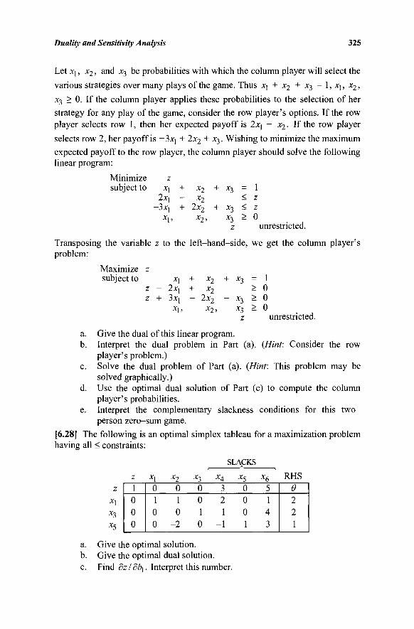
Duality and Sensitivity Analysis 325
Let Xj, x 2 , and x3 be probabilities with which the column player will select the
various strategies over many plays of the game. Thus xj + x2 + X3 = 1, X\, x2 ,
X3 > 0. If the column player applies these probabilities to the selection of her
strategy for any play of the game, consider the row player's options. If the row
player selects row 1, then her expected payoff is 2xi - x2. If the row player
selects row 2, her payoff is -3xl + 2x2 + x3. Wishing to minimize the maximum
expected payoff to the row player, the column player should solve the following linear program:
Minimize subject to
z X, + X2
zxi — x 2
-3xj + 2x2
*1> x2
x3
*3
= 1 < z < z
x3 > 0 unrestricted.
Transposing the variable z to the left-hand-side, we get the column player's problem:
Maximize z subject to x\
z - 2x\ z + 3x[
X|,
+ x2
+ *2 - 2x2
*2>
+ X3
- x3
x3
z
= > > >
1 0 0 0
unrestricted.
a. Give the dual of this linear program. b. Interpret the dual problem in Part (a). (Hint: Consider the row
player's problem.) c. Solve the dual problem of Part (a). (Hint: This problem may be
solved graphically.) d. Use the optimal dual solution of Part (c) to compute the column
player's probabilities. e. Interpret the complementary slackness conditions for this two-
person zero-sum game.
[6.28] The following is an optimal simplex tableau for a maximization problem having all < constraints:
SLACKS
Xi X7 X3 X4 X5 Xf.
~T~]
x3
x5
Give the optimal solution. Give the optimal dual solution. Find dzldb\. Interpret this number.
RHS 1 0 0 0
0 1 0 0
0 1 0
-2
0 0 1 0
3 2 1
-1
0 0 0 1
5 1 4 3
Θ 2 2 1
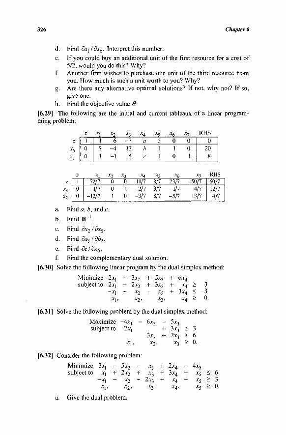
326 Chapter 6
d. Find 9xj / Sx6. Interpret this number. e. If you could buy an additional unit of the first resource for a cost of
5/2, would you do this? Why? f. Another firm wishes to purchase one unit of the third resource from
you. How much is such a unit worth to you? Why? g. Are there any alternative optimal solutions? If not, why not? If so,
give one. h. Find the objective value Θ.
[6.29] The following are the initial and current tableaux of a linear program-ming problem:
z x6 xl
z 1 0 0
*1 1 5 1
x2
6 -4 -1
x3 -1 13 5
X4
a b c
x5 5 1 1
x6 0 1 0
x7
0 0 1
RHS 0
20 8
z x3
x2
z 1 0 0
xl x2 x 3 72/7 0 0 -1/7 0 1
-12/7 1 0
X4 X5
11/7 8/7 -2/7 3/7 -3/7 8/7
x6 Till -1/7 -5/7
*7 -50/7
4/7 13/7
RHS 60/7 12/7 4/7
a. Find a, b, and c.
b. Find B_1.
c. Find dx21 dx5.
d. Find 9x3/9è2.
e. Find dz/dx6. f. Find the complementary dual solution.
[6.30] Solve the following linear program by the dual simplex method:
Minimize 2xj subject to 2x]
Xj,
3x2
2x2
x2
x 2 ,
+ 5x3
+ 3x3
- x3
x3 ,
6x4 X4
3x4
X4
> 3 < -3 > 0.
[6.31] Solve the following problem by the dual simplex method:
Maximize -4xt -subject to 2x]
X|,
[6.32] Consider the following problem:
5x-Minimize 3xj subject to Xj
Xj,
l2 + 2x2
- x2 X 2 ,
6x2
3x2
x 2 ,
x3 x3
2x3 x3,
5x3 3x3 > 3 2x3 > 6
x3 > 0.
2x4
3x4
X4 X4,
- 4x5
+ x5
- x5 x5
< 6 > 3 > 0.
a. Give the dual problem.
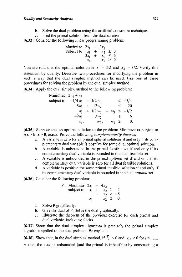
Duality and Sensitivity Analysis 327
b. Solve the dual problem using the artificial constraint technique. c. Find the primal solution from the dual solution.
[6.33] Consider the following linear programming problem:
Maximize 2x\ subject to Xj
3x| X j ,
- 3x2 + x2
+ x2 x2
> < >
3 6 0.
You are told that the optimal solution is xj = 3/2 and x2 = 3/2. Verify this
statement by duality. Describe two procedures for modifying the problem in such a way that the dual simplex method can be used. Use one of these procedures for solving the problem by the dual simplex method.
[6.34] Apply the dual simplex method to the following problem: Minimize 2w\ + W3 subject to 1/4 wx
8wi Wj
- 9 w j
Wy,
- 1/2 w2
+ 12w2
+ l/2w2 -- 3w2
w2,
< <
- W3 <
< W3 >
-3/4 20
-1/2 6 0.
[6.35] Suppose that an optimal solution to the problem: Minimize ex subject to Ax > b, x > 0, exists. Prove the following complementarity theorem.
a. A variable is zero for all primal optimal solutions if and only if its com-plementary dual variable is positive for some dual optimal solution.
b. A variable is unbounded in the primal feasible set if and only if its complementary dual variable is bounded in the dual feasible set.
c. A variable is unbounded in the primal optimal set if and only if its complementary dual variable is zero for all dual feasible solutions.
d. A variable is positive for some primal feasible solution if and only if its complementary dual variable is bounded in the dual optimal set.
[6.36] Consider the following problem:
: Minimize 2xj - 4x2 subject to xj + x2
- *2 x, x2
> > >
2 -5
0
a. Solve P graphically. b. Give the dual of P. Solve the dual graphically. c. Illustrate the theorem of the previous exercise for each primal and
dual variable, including slacks.
[6.37] Show that the dual simplex algorithm is precisely the primal simplex algorithm applied to the dual problem. Be explicit.
[6.38] Show that, in the dual simplex method, if br < 0 and yrj > 0 fory = 1,...,
n, then the dual is unbounded (and the primal is infeasible) by constructing a
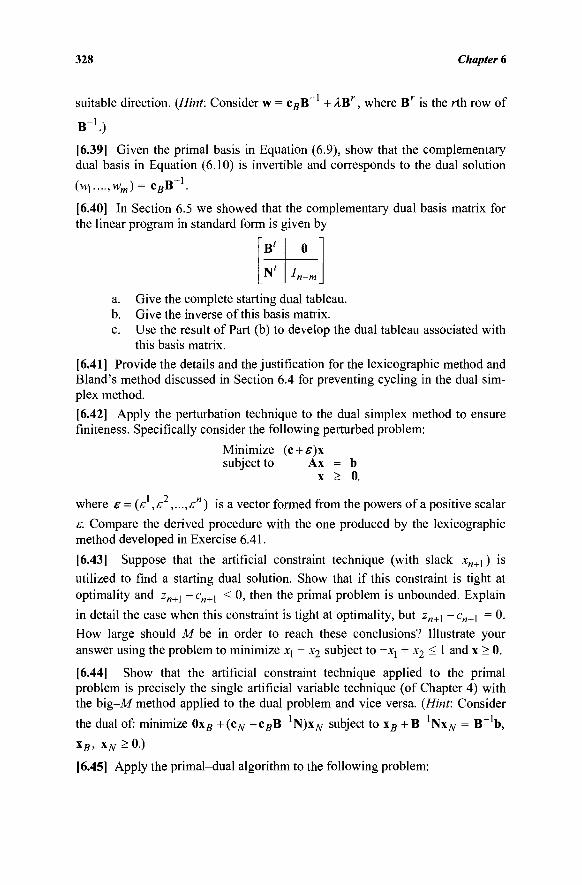
328 Chapter 6
suitable direction. (Hint: Consider w = cgB + ÀBr, where Br is the rth row of
B-1.)
[6.39] Given the primal basis in Equation (6.9), show that the complementary dual basis in Equation (6.10) is invertible and corresponds to the dual solution
(wl,...,wm)= c s B - 1 .
[6.40] In Section 6.5 we showed that the complementary dual basis matrix for the linear program in standard form is given by
B'
N'
0
*n-m
a. Give the complete starting dual tableau. b. Give the inverse of this basis matrix. c. Use the result of Part (b) to develop the dual tableau associated with
this basis matrix.
[6.41] Provide the details and the justification for the lexicographic method and Bland's method discussed in Section 6.4 for preventing cycling in the dual sim-plex method.
[6.42] Apply the perturbation technique to the dual simplex method to ensure finiteness. Specifically consider the following perturbed problem:
Minimize (c + e)x subject to Ax = b
x > 0.
where ε = (ε ,ε ,...,εη) is a vector formed from the powers of a positive scalar
ε. Compare the derived procedure with the one produced by the lexicographic method developed in Exercise 6.41.
[6.43] Suppose that the artificial constraint technique (with slack xn+\) is utilized to find a starting dual solution. Show that if this constraint is tight at optimality and z„+1 - c„+1 < 0, then the primal problem is unbounded. Explain
in detail the case when this constraint is tight at optimality, but zH+[ -c„+ 1 = 0. How large should M be in order to reach these conclusions? Illustrate your answer using the problem to minimize X] - x2 subject to -X] + x2 < 1 and x > 0.
[6.44] Show that the artificial constraint technique applied to the primal problem is precisely the single artificial variable technique (of Chapter 4) with the big-M method applied to the dual problem and vice versa. (Hint: Consider
the dual of: minimize 0xB + (cN - cgB~ N)xw subject to xB + B~ Nx^ = B~ b,
xB, xN>0.)
[6.45] Apply the primal-dual algorithm to the following problem:
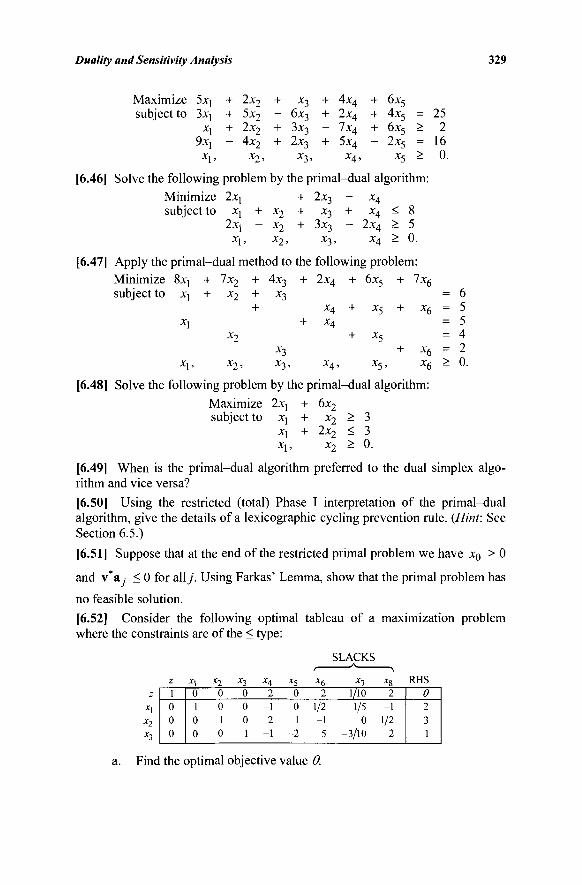
Duality and Sensitivity Analysis 329
Maximize 5xi subject to 3*1
x\ 9xl
X ] ,
+ 2x2 + X3 + 4x4 + 6x5
+ 5x2 - 6x3 + 2x4 + 4x5 = + 2x2 + 3x3 - 7x4 + 6x5 > - 4x2 + 2x3 + 5x4 - 2x5 =
Xo ί X"? i X4 5 X5 —
[6.46] Solve the following problem by the primal-dual algorithm:
Minimize 2xj + 2x3 - x4
subject to X] + x2 + X3 + X4
25 2
16 0.
x2
LX\ — X2 + JX3 — ^-X4 < > > X[, X 2 , X3, X4
[6.47] Apply the primal-dual method to the following problem:
Minimize subject to
8xj
Xj
X\,
7x2
x2
x2
x2,
4x 3 + 2 x 4 + 6x5
*3
*3 x3>
X4 X4
X4,
x5
x5,
7x 6
x6
x6 x6
6 5 5 4 2 0.
J6.48] Solve the fol lowing problem by the p r ima l -dua l a lgori thm:
Max imize 2xj + 6x 2
subject to xj + x 2 > 3 Xj + 2x 2 < 3 Xj, x 2 > 0.
[6.49] W h e n is the p r ima l -dua l a lgori thm preferred to the dual s implex a lgo-
r i thm and vice versa?
[6.50] Us ing the restricted (total) Phase I interpretation of the p r ima l -dua l
a lgori thm, g ive the details of a lexicographic cycl ing prevent ion rule. (Hint: See
Sect ion 6.5.)
[6.51] Suppose that at the end of the restricted pr imal p rob lem w e have x 0 > 0
and v*a ■ < 0 for al ly. Us ing Fa rkas ' L e m m a , show that the pr imal p rob lem has
n o feasible solution.
[6.52] Cons ider the fol lowing opt imal tableau o f a maximiza t ion p rob lem
where the constraints are of the < type:
SLACKS
z x\ *?
*3
z 1 0 0 0
x\ 0 1 0 0
*2 0 0 1 0
*3 0 0 0 1
X4
2 -1 2
-1
xs
0 0 1
-2
x6
2 1/2 -1 5
*7 1/10 1/5
0 -3/10
*8 2
-1 1/2
2
RHS Θ 2 3 1
a. Find the optimal objective value Θ.
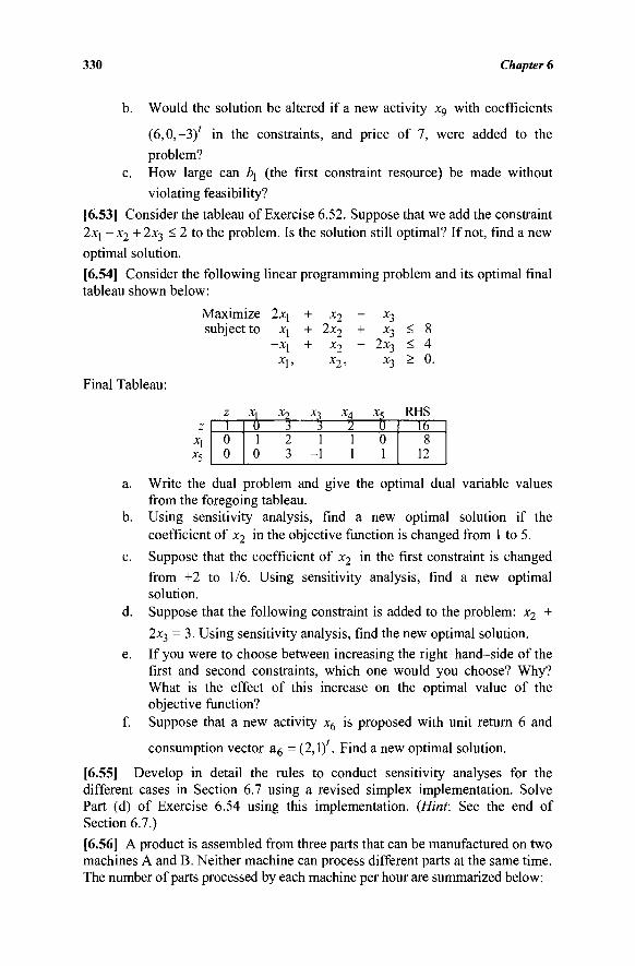
330 Chapter 6
b. Would the solution be altered if a new activity x9 with coefficients
(6,0,-3)' in the constraints, and price of 7, were added to the problem?
c. How large can t\ (the first constraint resource) be made without
violating feasibility? [6.53] Consider the tableau of Exercise 6.52. Suppose that we add the constraint 2x\ -x2+ 2x3 < 2 to the problem. Is the solution still optimal? If not, find a new optimal solution.
[6.54] Consider the following linear programming problem and its optimal final tableau shown below:
Final Tableau:
Maximize subject to
z x\ x5
z 1 0 0
\ 0 1 0
2*i x\
-*i X,,
x2
1 2 3
+ x2 -+ 2x2 + + x2 -
x2,
X-j X4
3 2 1 1
-1 1
*3 *3
2*3 x3
xl 0 0 1
< 8 < 4 > 0.
RHS 16 8
12
a.
b.
c.
d.
Write the dual problem and give the optimal dual variable values from the foregoing tableau. Using sensitivity analysis, find a new optimal solution if the coefficient of x2 in the objective function is changed from 1 to 5. Suppose that the coefficient of x2 in the first constraint is changed from +2 to 1/6. Using sensitivity analysis, find a new optimal solution. Suppose that the following constraint is added to the problem: x2 + 2x3 = 3. Using sensitivity analysis, find the new optimal solution.
If you were to choose between increasing the right-hand-side of the first and second constraints, which one would you choose? Why? What is the effect of this increase on the optimal value of the objective function? Suppose that a new activity x6 is proposed with unit return 6 and
consumption vector a6 = (2,1)'. Find a new optimal solution.
[6.55] Develop in detail the rules to conduct sensitivity analyses for the different cases in Section 6.7 using a revised simplex implementation. Solve Part (d) of Exercise 6.54 using this implementation. (Hint: See the end of Section 6.7.)
[6.56] A product is assembled from three parts that can be manufactured on two machines A and B. Neither machine can process different parts at the same time. The number of parts processed by each machine per hour are summarized below:
f.
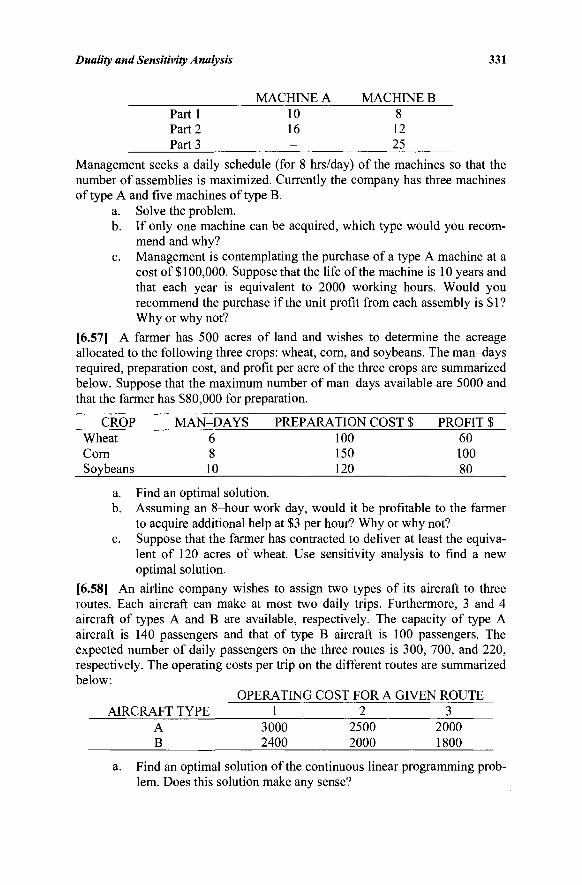
Duality and Sensitivity Analysis 331
MACHINE A MACHINE B Part 1 10 8 Part 2 16 12 Part 3 - 25
Management seeks a daily schedule (for 8 hrs/day) of the machines so that the number of assemblies is maximized. Currently the company has three machines of type A and five machines of type B.
a. Solve the problem. b. If only one machine can be acquired, which type would you recom-
mend and why? c. Management is contemplating the purchase of a type A machine at a
cost of $100,000. Suppose that the life of the machine is 10 years and that each year is equivalent to 2000 working hours. Would you recommend the purchase if the unit profit from each assembly is $ 1 ? Why or why not?
[6.57] A farmer has 500 acres of land and wishes to determine the acreage allocated to the following three crops: wheat, corn, and soybeans. The man-days required, preparation cost, and profit per acre of the three crops are summarized below. Suppose that the maximum number of man-days available are 5000 and that the farmer has $80,000 for preparation.
CROP MAN-DAYS PREPARATION COST $ PROFIT $ Wheat 6 100 60 Corn 8 150 100 Soybeans 10 120 80
a. Find an optimal solution. b. Assuming an 8-hour work day, would it be profitable to the farmer
to acquire additional help at $3 per hour? Why or why not? c. Suppose that the farmer has contracted to deliver at least the equiva-
lent of 120 acres of wheat. Use sensitivity analysis to find a new optimal solution.
[6.58] An airline company wishes to assign two types of its aircraft to three routes. Each aircraft can make at most two daily trips. Furthermore, 3 and 4 aircraft of types A and B are available, respectively. The capacity of type A aircraft is 140 passengers and that of type B aircraft is 100 passengers. The expected number of daily passengers on the three routes is 300, 700, and 220, respectively. The operating costs per trip on the different routes are summarized below:
OPERATING COST FOR A GIVEN ROUTE AIRCRAFT TYPE 1 2 3
A 3000 2500 2000 B 2400 2000 1800
a. Find an optimal solution of the continuous linear programming prob-lem. Does this solution make any sense?
332 Chapter 6
b. Using the cutting plane algorithm of Section 6.7, find an optimal integer solution.
[6.59] The tourism department of a certain country would like to decide which projects to fund during the coming year. The projects were divided into three main categories: religious, historical, and construction (hotels, roads, recreation centers, and so on). Three proposals A, B, and C for restoring religious sites are submitted, with estimated costs of $5, $7, and $4 million, respectively. Four proposals D, E, F, and G for the restoration of historical sites are submitted with respective estimated costs of $15, $12, $8, and $9 million. Finally, five proposals H, I, J, K, and L for constructing new facilities are submitted. These cost $2, $15, $22, $12, and $15 million, respectively. In order to determine the relative priority of these projects, experts from the tourism department developed a scoring model with the following scores for proposals A, B, C, D, E, F, G, H, I, J, K, L: 5, 6, 2, 7, 11, 1, 7, 2, 10, 9, 5, and 4, respectively. The department decides that at least one project of each category must be funded. Projects E and F represent a continuation of a plan that started during the previous year, and at least one of them must be funded. Furthermore, at most two historical and three construction projects can be chosen. Which projects should the tourism department fund in order to maximize the total score and not to exceed $90 million? (Hint: Suppose that project/ is chosen if x = 1 and is not chosen if x-
= 0. First solve the continuous linear program by the bounded simplex method and then add appropriate cuts.)
[6.60] Assuming c' = c and b' = b, find the maximum allowable tolerances CCQ
and /?Q on variations in the objective coefficients and on the right-hand-sides respectively, to maintain the (optimal) basis of Exercise 6.54 as optimal. Sup-pose it is known that the objective coefficient for xl can vary no more than ±30
percent. How does this affect α$ ? On the other hand, suppose it is known that
the variation βχ in the first constraint is no more than 50 percent of the variation
/?2 in the second constraint. How does this affect /?Q ?
[6.61] Develop in detail the rules to conduct sensitivity analyses for the differ-ent cases in Section 6.7 for the bounded variables simplex algorithm. Include the case of changing bounds on variables. To illustrate, consider Example 5.6 in
Section 5.2 and suppose that the column of x2 is changed from (1,1)' to (-1,-1)'. Update the optimal solution using sensitivity analysis on the given final tableau. Repeat assuming that the upper bound on x2 is changed from 6 to 1/2. (Hint: See the end of Section 6.7.)
[6.62] Develop the details of a dual simplex algorithm for the bounded variables simplex algorithm. Provide convergence arguments. Illustrate by using this algorithm to update the optimal solution for the sensitivity analysis in-stances of Exercise 6.61. (Hint: Choose a row of a basic variable that violates its upper or lower bound as the pivot row, and pick an appropriate pivot column where the change in the nonbasic variable upon pivoting improves the bound
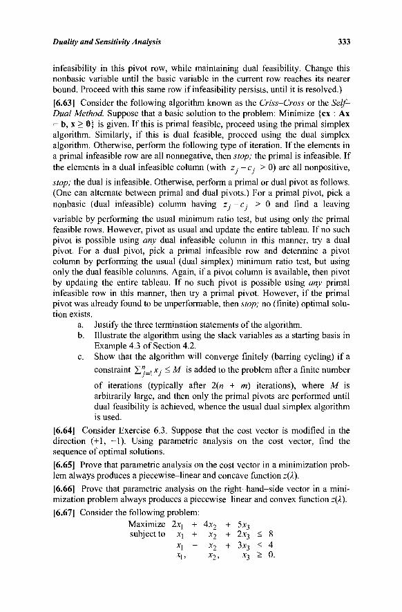
Duality and Sensitivity Analysis 333
infeasibility in this pivot row, while maintaining dual feasibility. Change this nonbasic variable until the basic variable in the current row reaches its nearer bound. Proceed with this same row if infeasibility persists, until it is resolved.)
[6.63] Consider the following algorithm known as the Criss-Cross or the Self-Dual Method. Suppose that a basic solution to the problem: Minimize {ex : Ax = b, x > 0} is given. If this is primal feasible, proceed using the primal simplex algorithm. Similarly, if this is dual feasible, proceed using the dual simplex algorithm. Otherwise, perform the following type of iteration. If the elements in a primal infeasible row are all nonnegative, then stop; the primal is infeasible. If the elements in a dual infeasible column (with z · - c , > 0) are all nonpositive,
stop; the dual is infeasible. Otherwise, perform a primal or dual pivot as follows. (One can alternate between primal and dual pivots.) For a primal pivot, pick a nonbasic (dual infeasible) column having z · - c > 0 and find a leaving
variable by performing the usual minimum ratio test, but using only the primal feasible rows. However, pivot as usual and update the entire tableau. If no such pivot is possible using any dual infeasible column in this manner, try a dual pivot. For a dual pivot, pick a primal infeasible row and determine a pivot column by performing the usual (dual simplex) minimum ratio test, but using only the dual feasible columns. Again, if a pivot column is available, then pivot by updating the entire tableau. If no such pivot is possible using any primal infeasible row in this manner, then try a primal pivot. However, if the primal pivot was already found to be unperformable, then stop; no (finite) optimal solu-tion exists.
a. Justify the three termination statements of the algorithm. b. Illustrate the algorithm using the slack variables as a starting basis in
Example 4.3 of Section 4.2. c. Show that the algorithm will converge finitely (barring cycling) if a
constraint ΣΓί=\ *; ^ M is added to the problem after a finite number
of iterations (typically after 2(w + m) iterations), where M is arbitrarily large, and then only the primal pivots are performed until dual feasibility is achieved, whence the usual dual simplex algorithm is used.
[6.64] Consider Exercise 6.3. Suppose that the cost vector is modified in the direction (+1, -1). Using parametric analysis on the cost vector, find the sequence of optimal solutions.
[6.65] Prove that parametric analysis on the cost vector in a minimization prob-lem always produces a piecewise-linear and concave function ζ(λ).
[6.66] Prove that parametric analysis on the right-hand-side vector in a mini-mization problem always produces a piecewise-linear and convex function z(X).
[6.67] Consider the following problem: Maximize 2xj + 4x2 + 5x3
subject to X] + x2 + 2x3 < 8 x\ - x2 + 3x3 < 4 X\, X2,
x3 - 0.
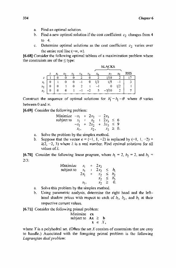
334 Chapter 6
a. b.
c.
Find an optimal solution. Find a new optimal solution if the cost coefficient c2 changes from 4 to-4 . Determine optimal solutions as the cost coefficient c2 varies over the entire real line (-co, co).
[6.68] Consider the following optimal tableau of a maximization problem where the constraints are of the < type:
SLACKS . * .
z
*l x2
*3
z 1 0 0 0
x\ 0 1 0 0
x2
0 0 1 0
*3 0 0 0 1
x4
2 -1 2
-1
x5 0 0 1
-2
*6 2
1/2 -1
5
x7 1/10
1/5 0
-3/10
*R 2
-1 1/2
2
RHS 17 3 1 7
ί\-θ where (9 varies Construct the sequence of optimal solutions for b{ ■
between 0 and co.
[6.69] Consider the following problem: Minimize -X[ subject to X[
- X )
* 1 >
a. Solve the problem by the simplex method. b. Suppose that the vector c = (-1, 1, -2) is replaced by (-1, 1, -2) +
λ(2, -2, 3) where λ is a real number. Find optimal solutions for all values of A.
[6.70] Consider the following linear program, where i\ = 2, b2 = 2, and th, =
2/3:
+ zx2 + x2 + 2x2
x2,
- zx3
+ 2x3
+ 3x3 x3
< < >
6 9 0.
Vlaximize subject to
*1 *1
2x[
Xj,
+ 2x2
+ 2x2
+ X2 x2 x2
< < < >
A| A* *3 0
a. Solve this problem by the simplex method. b. Using parametric analysis, determine the right-hand and the left-
hand shadow prices with respect to each of l\, Z , and b^ at their respective current values.
[6.71] Consider the following primal problem: Minimize ex subject to Ax > b
X G X,
where X is a polyhedral set. (Often the set X consists of constraints that are easy to handle.) Associated with the foregoing primal problem is the following Lagrangian dual problem:
Duality and Sensitivity Analysis 335
Maximize / (w) subject to w > 0
where flyv) = wb + minimumxe^· (c - wA)x.
a. Show that if x0 is feasible to the primal problem, that is, Ax0 > b
and x0 e X, and w0 is feasible to the Lagrangian dual problem, that
is, w0 >0, then cx0 > / (w 0 ) . b. Suppose that X is nonempty and bounded and that the primal
problem possesses a finite optimal solution. Show that
minimum ex = maximum f(w) Ax > b w > 0. xeX
[6.72] Consider the problem: Minimize xj+2x2 subject to 3x]+x 2 >6 ,
-X] + x2 ^ 2, jq + x2 < 8, and X\,x2 > 0. Let X = {x : - x \ + x2 ^ 2, xj + x2 < 8,
xu x2 >0}.
a. Formulate the Lagrangian dual problem, where w is the Lagrangian multiplier associated with the first constraint in the above problem.
b. Show thatflw) = 6w + minimum {0,4 - 2w, 13 - 14w, 8 - 24w}. (Hint: Examine the second term in fiw) in Exercise 6.71 and enumer-ate the extreme points of X graphically.)
c. Plot flw) as a function of w. d. From Part (c) locate the optimal solution to the Lagrangian dual
problem. e. From Part (d) find the optimal solution to the primal problem.
[6.73] Prove that if K is a skew symmetric matrix (that is, K = - Κ ' ), then the
system Kx > 0, x > 0
possesses at least one solution x such that Kx + x > 0. (Hint: Apply Farkas' Lemma to the system Kx > 0, x> 0, e.x > 0. Repeat for each j and combine
solutions by summing.)
[6.74] Apply the result of the previous problem to the system:
Ax-rb>0 , x > 0 -wA + re > 0, w > 0
w b - c x > 0 , r > 0 .
a. Use this result to derive the fundamental theorem of duality. b. Use this result to prove that at optimality there exists at least one pair of
primal and dual optimal points with the property that if a variable in one problem is zero, then the complementary variable in the other problem is positive. This is called the strong theorem of complementary slackness, or the strict complementary slackness property.
336 Chapter 6
c. Illustrate the strong theorem of complementary slackness geometri-cally. (Hint: Consider a linear program where the objective function contours are parallel to one of the constraints and alternative optimal solutions result.)
d. When must the solution to the strong complementary slackness theorem not occur at an extreme point? (Hint: Consider Part (c).)
[6.75] Consider Beale's example of cycling discussed in Chapter 4 (Example 4.11). Let P denote the problem in which the last constraint in this example is deleted.
a. Following Example 4.11, construct a sequence of tableaux for Problem P that exhibit cycling.
b. Write the dual D to Problem P and plot its constraints (in two dimensions). For each basic feasible solution for Problem P in the cycle of Part a, exhibit the corresponding complementary dual basis in your graphical plot.
c. Based on geometrical observations in Part b, devise appropriate rules by which a traversal of bases in the dual problem would correspond to cycling among a sequence of bases representing a given vertex in the primal problem. Discuss how you might use this geometric insight to construct alternative examples of linear programs that exhibit the phenomenon of cycling.
NOTES AND REFERENCES
1. John von Neumann is credited with having first postulated the existence of a dual linear program. His insights came through his work in game theory and economics together with a strong mathematical component. Many individuals have continued to develop and extend the basic duality theorems, notably Tucker [1960a] and A. C. Williams [1970]. Also, see Dantzig [1982] for his pioneering contributions to duality theory.
2. For more details on shadow prices and relationships with directional derivatives for nondifferentiable convex functions, see Akgul [1984] and Bazaraa et al. [2006]. For a related application to marginal cost pricing for an electric utility, where a closed form derivation for the dual variables is presented, see Sherali et al. [1984].
3. The dual simplex method was first developed by Lemke [1954]. 4. The primal-dual algorithm was developed by Dantzig, Ford, and Fulkerson
[1956]. This development was fostered out of the work of Kuhn [1955] on the assignment problem. Also, see Paparrizos et al. [2003] for recent improvements on this approach.
5. The cutting plane application in integer programming presented in Section 6.7 is mainly for illustration. For more up-to-date information on integer programming methods, see Schrijver [1986], Johnson et al. [1985], Crowder et al. [1983], and Nemhauser and Wolsey [1998].
6. The tolerance approach to sensitivity analysis presented in Section 6.7 is from Wendell [1984, 1985a, b]. Also, see Freund [1985] for sensitivity analysis involving simultaneous changes in constraint coefficients. For a
Duality and Sensitivity Analysis 337
discussion on using sensitivity analyses to handle the effect of uncertainty versus incorporating uncertainty directly within models, see Higle and Wallace [2003].
7. The Criss-Cross algorithm presented in Exercise 6.63 is from Zionts [1969, 1974].
8. Exercise 6.75 uses duality to provide insights into the geometry of cycling as motivated by Avis et al. [2008].

This page intentionally left blank
SEVEN: THE DECOMPOSITION PRINCIPLE
This chapter discusses the Dantzig-Wolfe decomposition technique and its relationships with Benders partitioning and Lagrangian relaxation techniques for dealing with large-scale and/or specially structured linear programming prob-lems. It is not unusual in a corporate management model or in a logistics model to produce a linear program having many thousands of rows and a seemingly unlimited number of columns. In such problems, some method must be applied to convert the large problems into one or more appropriately coordinated smaller problems of manageable size. The Dantzig-Wolfe, Benders, and Lagrangian relaxation techniques, which are all equivalent for linear program-ming problems, and which we simply refer to as applying the decomposition principle, do exactly this.
Even if a linear program is of manageable size, some of its constraints might possess a special structure that permits efficient handling. In such cases, we would like to partition the linear program into one part having a general structure and another part having a special structure in a manner such that a more efficient solution method can be devised. Again, the decomposition principle can be applied to such a linear program to achieve the desired effect.
The decomposition principle is a systematic procedure for solving large-scale linear programs or linear programs that contain specially structured constraints. The constraints are partitioned into two sets: general constraints (or complicating constraints) and constraints having a special structure. It will become apparent that it is not necessary for either set to have special structure, however, special structure, when available, enhances the efficiency of the procedure.
The strategy of the decomposition procedure is to operate on two separate linear programs: one over the set of general constraints and one over the set of special constraints. Information is passed back and forth between the two linear programs until an optimal solution to the original problem is achieved. The lin-ear program over the general constraints is called the master problem, and the linear program over the special constraints is called the subproblem. The master problem passes down a continually revised set of cost coefficients (or prices) to the subproblem, and receives from the subproblem a new column (or columns) based on these cost coefficients. For this reason, such a procedure is also known as a column generation method or & price directive algorithm.
We shall begin by assuming that the special constraint set is bounded. Once the decomposition principle is developed for this case and we have dis-cussed how to get started, we shall relax the boundedness assumption. We shall also extend the procedure to problems having multiple subproblems, and exhibit its relationship with other procedures.
339
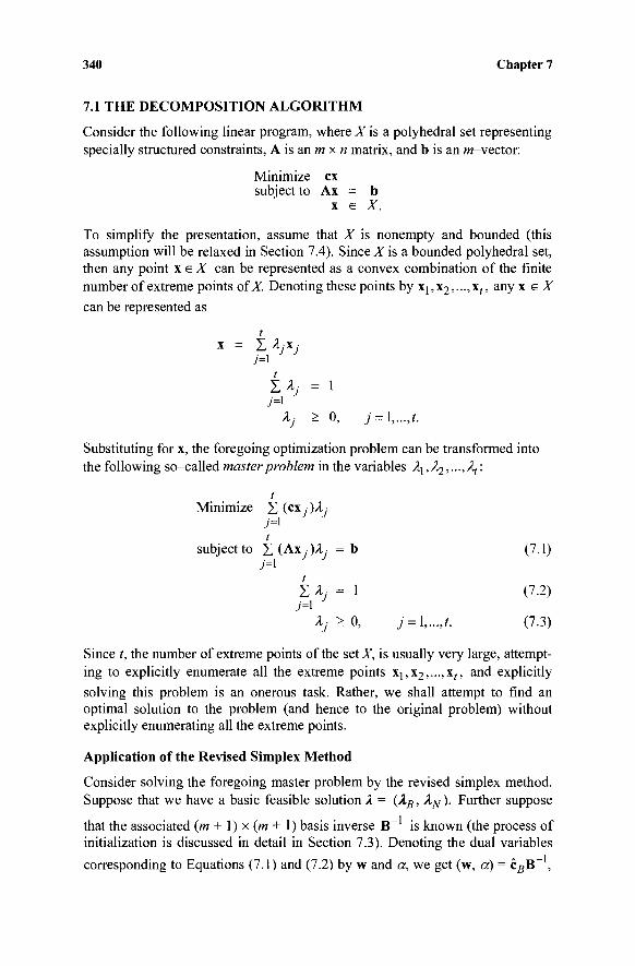
340 Chapter 7
7.1 THE DECOMPOSITION ALGORITHM
Consider the following linear program, where X is a polyhedral set representing specially structured constraints, A is an m x n matrix, and b is an w-vector:
Minimize ex subject to Ax = b
x e X.
To simplify the presentation, assume that X is nonempty and bounded (this assumption will be relaxed in Section 7.4). Since X is a bounded polyhedral set, then any point x e X can be represented as a convex combination of the finite number of extreme points ofX Denoting these points by Xj,x2,...,x(, any x e X can be represented as
t x = Σ Λ-.-χ,-
Σλ: = 1 7=1
Àj > 0, j = l,...,t.
Substituting for x, the foregoing optimization problem can be transformed into the following so-called master problem in the variables Aj, λ^,..., λ, :
t Minimize X( c x / )^ · /
7=1
subject to Σ (Axy)Ay = b (7.1) 7=1
Σ λ] = 1 (7.2) 7=1
Aj>0, j = l,...,t. (7.3)
Since t, the number of extreme points of the setX, is usually very large, attempt-ing to explicitly enumerate all the extreme points χ1,χ2,...,χ/, and explicitly solving this problem is an onerous task. Rather, we shall attempt to find an optimal solution to the problem (and hence to the original problem) without explicitly enumerating all the extreme points.
Application of the Revised Simplex Method
Consider solving the foregoing master problem by the revised simplex method. Suppose that we have a basic feasible solution λ = {λΒ, λΝ ). Further suppose
that the associated (m + 1) χ (m + 1) basis inverse B~ is known (the process of initialization is discussed in detail in Section 7.3). Denoting the dual variables
corresponding to Equations (7.1) and (7.2) by w and a, we get (w, a) = cgB~ ,
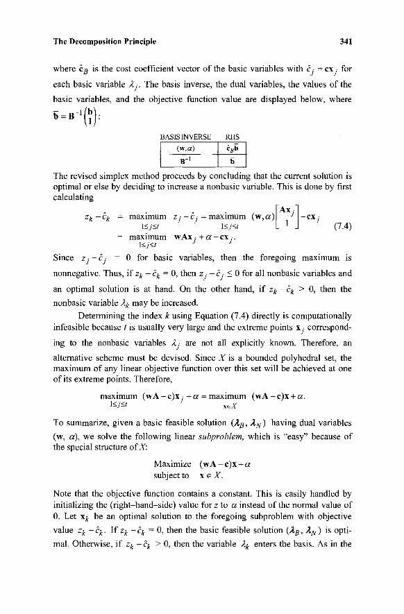
The Decomposition Principle 341
where cB is the cost coefficient vector of the basic variables with c ■ = ex · for
each basic variable λ .■. The basis inverse, the dual variables, the values of the
basic variables, and the objective function value are displayed below, where
S-»-'(ì): BASIS INVERSE RHS
(w,a)
B-1
ètfb
b
The revised simplex method proceeds by concluding that the current solution is optimal or else by deciding to increase a nonbasic variable. This is done by first calculating
TAX; zk-ck = maximum z ,· - c, = maximum (w,or)
\<j<t \<j<t
j
1 " c x ; (7.4)
= maximum w Ax. + « - ex.. \<j<t J J
Since zj —è: = 0 for basic variables, then the foregoing maximum is
nonnegative. Thus, if zk -ck = 0, then zj - Cj < 0 for all nonbasic variables and
an optimal solution is at hand. On the other hand, if zk-ck > 0, then the
nonbasic variable Xk may be increased.
Determining the index k using Equation (7.4) directly is computationally
infeasible because t is usually very large and the extreme points x,· correspond-
ing to the nonbasic variables A, are not all explicitly known. Therefore, an
alternative scheme must be devised. Since X is a bounded polyhedral set, the maximum of any linear objective function over this set will be achieved at one of its extreme points. Therefore,
maximum (wA - c)x .■ + a = maximum (wA - c)x + a.
To summarize, given a basic feasible solution {λΒ, λΝ ) having dual variables
(w, a), we solve the following linear subproblem, which is "easy" because of the special structure of X:
Maximize (wA - c)x + a subject to x e X.
Note that the objective function contains a constant. This is easily handled by initializing the (right-hand-side) value for z to a instead of the normal value of 0. Let \k be an optimal solution to the foregoing subproblem with objective value zk-ck. If zk-ck = 0, then the basic feasible solution {λΒ, λΝ ) is opti-mal. Otherwise, if zk-ck > 0, then the variable Xk enters the basis. As in the
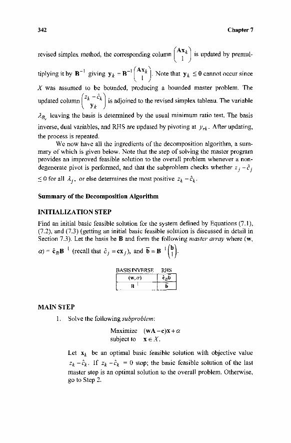
342 Chapter 7
revised simplex method, the corresponding column | * | is updated by premul-
tiplying it by B giving yk = B giving y^ = B * . Note that y^ < 0 cannot occur since
X was assumed to be bounded, producing a bounded master problem. The
updated column \ k k is adjoined to the revised simplex tableau. The variable
λΒ leaving the basis is determined by the usual minimum ratio test. The basis
inverse, dual variables, and RHS are updated by pivoting at yrk. After updating,
the process is repeated. We now have all the ingredients of the decomposition algorithm, a sum-
mary of which is given below. Note that the step of solving the master program provides an improved feasible solution to the overall problem whenever a non-degenerate pivot is performed, and that the subproblem checks whether z -c,-
< 0 for all A-, or else determines the most positive zk-ck.
Summary of the Decomposition Algorithm
INITIALIZATION STEP
Find an initial basic feasible solution for the system defined by Equations (7.1), (7.2), and (7.3) (getting an initial basic feasible solution is discussed in detail in Section 7.3). Let the basis be B and form the following master array where (w,
»-i a) = c#B (recall that èj = cxy ), and b = B 1
BASIS INVERSE RHS (w,a)
B '
c^b
b
MAIN STEP
1. Solve the following subproblem:
Maximize (wA-c)x + a subject to x e X.
Let \k be an optimal basic feasible solution with objective value zk-cic. If zk - ck = 0 stop; the basic feasible solution of the last master step is an optimal solution to the overall problem. Otherwise, go to Step 2.
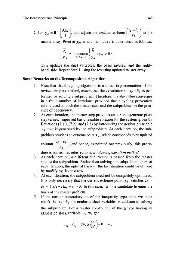
The Decomposition Principle 343
2. Let y t = B ] * , and adjoin the updated column * k to the
master array. Pivot at yrk where the index r is determined as follows:
br ■ ■ f bi Λ -1— = minimum < —— :yik > 0 >. yrk \<i<m+\ [yik J
This updates the dual variables, the basis inverse, and the right-hand-side. Repeat Step 1 using the resulting updated master array.
Some Remarks on the Decomposition Algorithm
1. Note that the foregoing algorithm is a direct implementation of the revised simplex method, except that the calculation of zk - ck is per-formed by solving a subproblem. Therefore, the algorithm converges in a finite number of iterations, provided that a cycling prevention rule is used in both the master step and the subproblem in the pres-ence of degeneracy.
2. At each iteration, the master step provides (at a nondegenerate pivot step) a new improved basic feasible solution for the system given by Equations (7.1 ), (7.2), and (7.3) by introducing the nonbasic variable Xk that is generated by the subproblem. At each iteration, the sub-problem provides an extreme point xk, which corresponds to an updated
column , and hence, as pointed out previously, this proce-zk~ck
yk dure is sometimes referred to as a column generation method. At each iteration, a different dual vector is passed from the master step to the subproblem. Rather than solving the subproblem anew at each iteration, the optimal basis of the last iteration could be utilized by modifying the cost row. At each iteration, the subproblem need not be completely optimized. It is only necessary that the current extreme point \k satisfies zk -
ck = (wA-c)x t + a > 0. In this case, Xk is a candidate to enter the basis of the master problem. If the master constraints are of the inequality type, then we must check the z ,· - c .· for nonbasic slack variables in addition to solving
the subproblem. For a master constraint i of the < type having an associated slack variable sh we get
zs,·-c*,· = ( * .« ) ( o ) - 0 = w / ·
344 Chapter 7
Thus, for a minimization problem, a slack variable associated with a < constraint is eligible to enter the basis if w, > 0. (Note that the
entry criterion is w, < 0 for constraints of the > type.)
It should be clear that if there are other variable columns that are explicitly maintained in the master problem in addition to the λ -variable columns or the slack columns, then like the latter, these columns also may be priced using the simplex multiplier vector (w, a) in the usual manner in order to test for their eligibility to enter the basis. (See Exercise 7.20.)
6. Assume that the original linear program is feasible and that A i s m x n of rank m, so that the master problem has basic feasible solutions with bases of size (m + 1) x (m + 1). Since there are m linearly independent constraints Ax = b binding at every feasible solution, we are searching for an optimum over some p = (n - m) dimensional
subset of X. Hence, at an optimal extreme point solution x* to the original linear program, (at least) some p linearly independent
constraints defining X must be binding. Consequently, x* lies on (at most) some (n - p) = m dimensional face of X. From the discussion of Chapter 2 it follows that since this face is itself (at most) an m-dimensional polytope with its vertices being a subset of the vertices
of X, we can manage to represent x using at most (m + 1) vertices of X. Hence, we will need at most (m + 1) positive λ-variables at optimality. This of course concurs with the size of the master problem basis.
On this (at most) m dimensional face of X, there may be several
ways of representing x* in terms of at most (m + 1) extreme points of X. Computationally, it so turns out that one can usually achieve a convex combination of a set of extreme points of X that brings the resulting solution to within 1-5 percent of optimality fairly quickly. However, it has been observed on many classes of problems that the tail-end convergence rate in obtaining a more exact representation for an optimal solution can be very slow. (The algorithm need not produce an extreme point optimal solution for the original problem when alternative optima exist.) Hence, in practice, the procedure is frequently terminated once it comes to within 1-5 percent of optimality. The next discussion provides a useful construct for implementing such a termination criterion. In addition, Exercises 7.42 and 7.43 describe certain stabilized column generation implementation techniques to improve the convergence behavior of the Dantzig-Wolfe decomposition method in particular, and of column generation procedures in general (also, see the Notes and References section).
The Decomposition Principle 345
Calculation and Use of Lower Bounds
Recall that the decomposition algorithm stops when maximum z ■ - c = 0.
Because of the enormous number of variables (λ\, λ^,..., \ ), continuing the compu-tations until this condition is satisfied may be exceedingly time-consuming for large problems.
We shall develop a lower bound on the objective value for any feasible solution to the overall problem, and hence, a lower bound on the optimal objective value. Since the decomposition algorithm generates feasible points having nonworsening objective values via the master problem, we have a sequence of nonincreasing upper bounds. Hence, we may stop when the difference between the objective value of the current feasible point and the available lower bound is within an acceptable tolerance. This may not give the true optimal solution, but will guarantee a good feasible solution, within any desired accuracy from the optimum. Consider the following subproblem:
Maximize (wA - c)x + a subject to x e X,
where w is the dual vector passed from the master step. Let the optimal objec-tive value of the foregoing subproblem be zk-ck. Now, let x be any feasible solution to the overall problem, that is, Ax = b and x e X. By the definition of zk-ck, and because x e X, we have
{wA-c)x + a<(zk-ck).
Noting that Ax = b, this inequality implies that
cx>v/Ax-(zk-ck) + a = yvb + a-(zk-ck) = cBb-(zk-ck).
Since this is true for each x e Xwith Ax = b, then
minimum ex > èBb - (zk - ck ). Ax=b
In other words, cBb-(zk -ck) is a lower bound on the optimal objective value for the overall problem. Note that cBb is the current best upper bound. How-ever, the lower bounds thus generated need not be monotone and we need to maintain the best (greatest) lower bound.
7.2 NUMERICAL EXAMPLE
Consider the following problem:
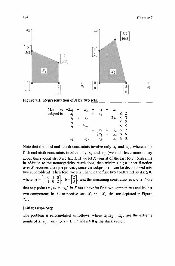
346 Chapter 7
Figure 7.1. Representation of Xby two sets.
Minimize subject to
- 2 x [ x\ x\ x\ x\
X\,
- x2
+ x2
+ 2x2
*2>
+ *3 x3
x3 2x3
x3,
+
+
+ +
X4
< 2 2x4 < 3
< 2 < 5
x4 < 2 x4 < 6 x4 > 0.
Note that the third and fourth constraints involve only xj and x2, whereas the
fifth and sixth constraints involve only x3 and x4 (we shall have more to say
about this special structure later). If we let X consist of the last four constraints in addition to the nonnegativity restrictions, then minimizing a linear function over X becomes a simple process, since the subproblem can be decomposed into two subproblems. Therefore, we shall handle the first two constraints as Ax < b,
where A = 1 0 1 0 1 1 0 2 , and the remaining constraints as x e X. Note
that any point (xj,x2,x3,x4) inXmust have its first two components and its last
two components in the respective sets Χχ and X2 that are depicted in Figure
7.1.
Initialization Step
The problem is reformulated as follows, where x],x2,...,x/, are the extreme
points ofX, è: = ex .· fory = \,...,t, and s > 0 is the slack vector:
The Decomposition Principle 347
Minimize Σ c -A ■ 7=1
t subject to Σ (Ax ,·)A ,· + s
7=1
Aj > 0,
s > 0.
b
1
j = \,-,t
Let the starting basis consist of s and λ\ where Xj = (0, 0, 0, 0) is an extreme
point of X with CX[ = 0. Therefore,
[Ί 0 0
0 1 0
0] 0 1
The vector (w,or) = c s B
B
0B _ 1 =0 , and b = B_ 1 This gives the
following tableau, where the first three columns give (wl,w2,a) in row 0 and
B in the remaining rows:
BASIS INVERSE RHS z
51 s2
\
0 1 0 0
0 0 1 0
0 0 0 1
0 2 3 1
Iteration 1
SUBPROBLEM
Solve the following subproblem:
Maximize (wA - c)x + a subject to x e X.
Here, {w^,w2) = (0, 0) from the foregoing array. Therefore, the subproblem is as follows:
Maximize 2xj + x2 + χτ, - x$ + 0 subject to x e X.
This problem is separable in the vectors (xi,x2) and (x3,x4) and can be solved geometrically. Using Figure 7.1, it is easily verified that the optimal solution is x2 = (2,3/2,3,0) with objective value z2 -c2 = 17/2. Since z2-c2= 17/2 > 0,
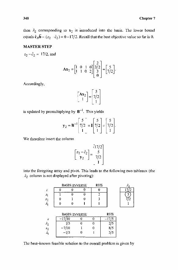
348 Chapter 7
then λχ corresponding to x2 is introduced into the basis. The lower bound
equals c5b - (z2 - c2 ) = 0 -17/2. Recall that the best objective value so far is 0.
MASTER STEP
z2 _^2 = 17/2, and
Ax7 1 0 1 0 1 1 0 2
Γ 2 " 3/2 3 0
5 7/2
Accordingly,
Ax2
1
-1
5 7/2
1
is updated by premultiplying by B . This yields
y 2 = B
We therefore insert the column
5 7/2
1 = 1
5 7/2
1 =
5 7/2
1
z 2 ~ c 2
. ?2 =
"17/2" 5
7/2 1
into the foregoing array and pivot. This leads to the following two tableaux (the À2 column is not displayed after pivoting):
BASIS INVERSE RHS A. z
*1 s2 4
z
s2
0 0 0 1 0 0 0 1 0 0 0 1
BASIS INVERSE -17/10 0
1/5 0 -7/10 1
-1/5 0
0 2 3 1
0 0 0 1
RHS -17/5
2/5 8/5 3/5
17/2
7/2
The best-known feasible solution to the overall problem is given by
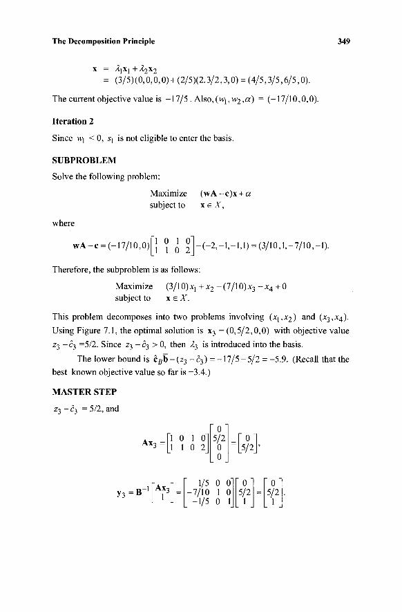
The Decomposition Principle 349
= (3/5) (0,0,0,0) + (2/5)(2,3/2,3,0) = (4/5,3/5,6/5,0).
The current objective value is -17/5 . Also,(w\,w2,a) = (-17/10,0,0).
Iteration 2
Since wj < 0, Sj is not eligible to enter the basis.
SUBPROBLEM
Solve the following problem:
Maximize (wA-c)x + « subject to x e X,
where
w A - c = (-17/10,0) 1 0 1 0 1 1 0 2 (-2,-1,-1,1) = (3/10,1,-7/10,-1).
Therefore, the subproblem is as follows:
Maximize (3/10) xx + x2 - (7/10) x3 - x4 + 0 subject to xeX.
This problem decomposes into two problems involving (x\,x2) and (x3,x4).
Using Figure 7.1, the optimal solution is x3 =(0,5/2,0,0) with objective value
z3 - c3 =5/2. Since Z3 - c3 > 0, then A3 is introduced into the basis.
The lower bound is cgb - (z3 - c3 ) = -17/5 - 5/2 = -5.9. (Recall that the best-known objective value so far is -3.4.)
MASTER STEP
z3 - c3 = 5/2, and
A x i Ì 0 1 0 1 1 0 2
" 0 " 5/2 0 0
" 0 5/2
y 3 = B Ax3
1
1/5 0 0" 7/10 1 0 -1/5 0 1
" 0 " 5/2
1 =
" 0 " 5/2
1
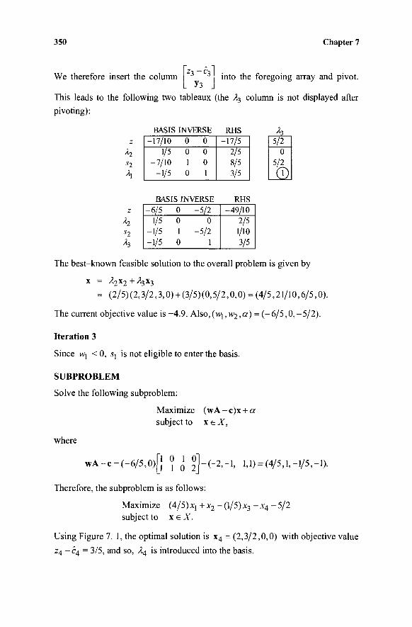
350 Chapter 7
We therefore insert the column into the foregoing array and pivot. Z3-C3
This leads to the following two tableaux (the A3 column is not displayed after
pivoting):
z
h s2
BASIS INVERSE RHS -17/10 0 0
1/5 0 0 -7/10 1 0
-1/5 0 1
-17/5 2/5 8/5 3/5
A. 5/2
0
BASIS INVERSE RHS -6/5 0
1/5 0 -1/5 1 -1/5 0
-5/2 0
-5/2 1
-49/10 2/5 1/10 3/5
z
h si
h The best-known feasible solution to the overall problem is given by
X = /l2X2+/Ì3X3
= (2/5) (2,3/2,3,0) + (3/5) (0,5/2,0,0) = (4/5,21/10,6/5,0).
The current objective value is -4.9. Also,{w\,w2,a) = (-6/5,0,-5/2).
Iteration 3
Since wj < 0, S\ is not eligible to enter the basis.
SUBPROBLEM
Solve the following subproblem:
Maximize (wA-c)x + a subject to x e X,
where
w A - c = (-6/5,0) 1 0 1 0 1 1 0 2 -(-2,-1,-1,1) = (4/5,1,-1/5,-1).
Therefore, the subproblem is as follows:
Maximize (4/5) xl+x2- (1/5) x3 - x4 - 5/2 subject to x e X.
Using Figure 7. 1, the optimal solution is x4 = (2,3/2,0,0) with objective value
Z4 - c 4 = 3/5, and so, A4 is introduced into the basis.
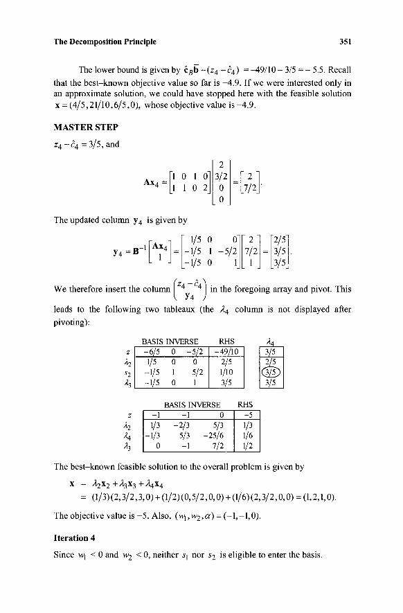
The Decomposition Principle 351
The lower bound is given by c s b - (z4 - c4 ) = —49/10 - 3/5 = - 5.5. Recall
that the best-known objective value so far is -4.9. If we were interested only in an approximate solution, we could have stopped here with the feasible solution x = (4/5,21/10,6/5,0), whose objective value is -4.9.
MASTER STEP
z4 - c 4 =3/5, and
Axd = Ì 0 1 0 1 1 0 2_
Γ2] 3/2 0 0
" 2 " _7/2_
The updated column y4 is given by
y 4 = B " Ax4
1
1/5 0 0 1/5 1 -5/2 1/5 0 1
2 7/2
1 =
2/5 3/5 3/5
We therefore insert the column 4 4 in the foregoing array and pivot. This
leads to the following two tableaux (the A4 column is not displayed after
pivoting):
z
s2
BASIS INVERSE -6/5 0 -5/2 1/5 0 0
-1/5 1 -5/2 -1/5 0 1
RHS -49/10
2/5 1/10 3/5
3/5 2/5
3/5
BASIS INVERSE -1 -1 0 1/3 -2/3 5/3
-1/3 5/3 -25/6 0 -1 7/2
RHS -5 1/3 1/6 1/2
h
The best-known feasible solution to the overall problem is given by
X — ^9X7 +Λ3Χ3 + / t 4 X 4
= (1/3) (2,3/2,3,0) + (1/2) (0,5/2,0,0) + (1/6) (2,3/2,0,0) = (1,2,1,0).
The objective value is - 5 . Also, (w\,w>2, ci) = (-1,-1,0).
Iteration 4
Since wj < 0 and w2 < 0, neither η nor s2 is eligible to enter the basis.
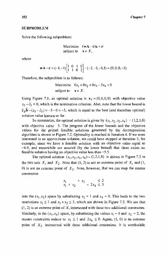
352 Chapter 7
SUBPROBLEM
Solve the following subproblem:
Maximize (wA - c)x + a subject to x e X,
where
w A - c = ( - l , - l ) 1 0 1 0 1 1 0 2 (-2,-1,-1,1) = (0,0,0,-3).
Therefore, the subproblem is as follows:
Maximize Oxj + 0x2 + 0x3 - 3x4 + 0
subject to x e X.
Using Figure 7.1, an optimal solution is x5 =(0,0,0,0) with objective value
z5-c5 = 0, which is the termination criterion. Also, note that the lower bound is
c s b - ( z 5 - c 5 ) = - 5 - 0 = -5 , which is equal to the best (and therefore optimal)
solution value known so far. To summarize, the optimal solution is given by (xi,x2,x3,x4) = (1,2,1,0)
with objective value - 5 . The progress of the lower bounds and the objective values for the primal feasible solutions generated by the decomposition algorithm is shown in Figure 7.2. Optimality is reached at Iteration 4. If we were interested in an approximate solution, we could have stopped at Iteration 3, for example, since we have a feasible solution with an objective value equal to -4.9, and meanwhile are assured (by the lower bound) that there exists no feasible solution having an objective value less than -5.5.
The optimal solution (x1;x2,X3,X4) = (1,2,1,0) is shown in Figure 7.3 in
the two sets X\ and X2. Note that (1, 2) is not an extreme point of X{ and (1,
0) is not an extreme point of X2. Note, however, that we can map the master
constraints
Xl + x3 < 2 x\ + x2 + 2x4 ^ 3
into the (xi,X2) space by substituting x3 = 1 and x4 = 0. This leads to the two
restrictions X\ < 1 and xj +x2 < 3, which are shown in Figure 7.3. We see that
(1, 2) is an extreme point of X\ intersected with these two additional constraints.
Similarly, in the (x3,x4) space, by substituting the values Xj = 1 and x2 = 2, the
master constraints reduce to x3 < 1 and 2x4 < 0. Again, (1, 0) is an extreme
point of X2 intersected with these additional constraints. It is worthwhile
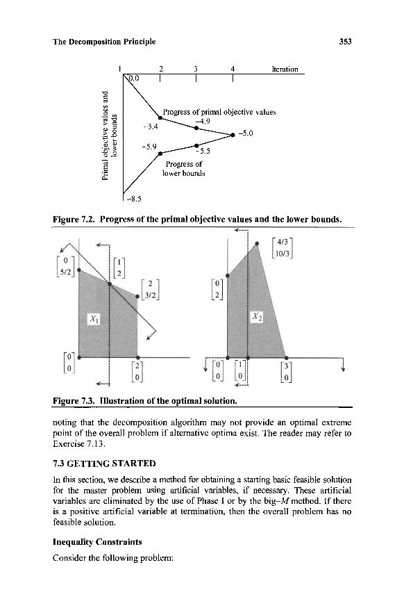
The Decomposition Principle 353
Iteration
Figure 7.2. Progress of the primal objective values and the lower bounds.
Figure 7.3. Illustration of the optimal solution.
noting that the decomposition algorithm may not provide an optimal extreme point of the overall problem if alternative optima exist. The reader may refer to Exercise 7.13.
7.3 GETTING STARTED
In this section, we describe a method for obtaining a starting basic feasible solution for the master problem using artificial variables, if necessary. These artificial variables are eliminated by the use of Phase I or by the big-M method. If there is a positive artificial variable at termination, then the overall problem has no feasible solution.
Inequality Constraints
Consider the following problem:
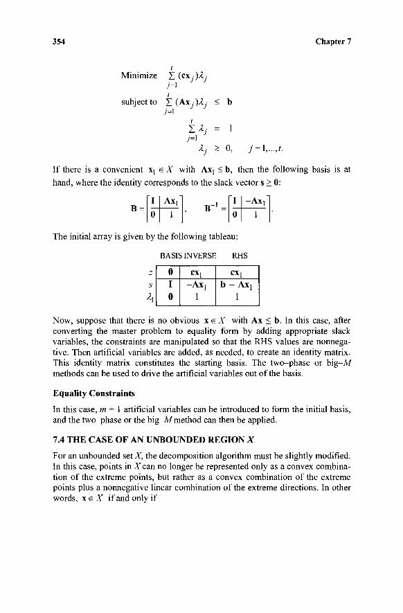
354 Chapter 7
Minimize £ (cx.)A,· 7=1 /
subject to X (Axj)Àj < b
Σ Α , = 1 7=1
A, > 0, j = l,...,t.
If there is a convenient Xj e X with Axj < b, then the following basis is at
hand, where the identity corresponds to the slack vector s > 0:
B "I
0
Axj
1 B" I
0
- A X ]
1
The initial array is given by the following tableau:
BASIS INVERSE RHS
z s
Now, suppose that there is no obvious x e X with Ax < b. In this case, after converting the master problem to equality form by adding appropriate slack variables, the constraints are manipulated so that the RHS values are nonnega-tive. Then artificial variables are added, as needed, to create an identity matrix. This identity matrix constitutes the starting basis. The two-phase or big-M methods can be used to drive the artificial variables out of the basis.
0 I 0
CXi
-Axj
1
» ! b - Axj
1
Equality Constraints
In this case, m + 1 artificial variables can be introduced to form the initial basis, and the two-phase or the big-Ai method can then be applied.
7.4 THE CASE OF AN UNBOUNDED REGION X
For an unbounded set X, the decomposition algorithm must be slightly modified. In this case, points in X can no longer be represented only as a convex combina-tion of the extreme points, but rather as a convex combination of the extreme points plus a nonnegative linear combination of the extreme directions. In other words, x e X if and only if
The Decomposition Principle 355
Σ X-jXj + Σ Mjdj
ΣΑ;=1
Ay>0,
^•>o, 7=1,··
7=1,·
.,?
.,*
where X],x2,...,x?, are the extreme points ofX, and d i ,d 2 , . ,d^ are the extreme directions of X. The primal problem can be transformed into a so-called master problem in the variables λ^,λι,.,.,λ, and μ^,μ^,—,μ^ as follows:
Minimize Σ (cxy)Ay + X (cdy)/^-7=1 7=1
t £ subject to Σ (AxyHy + Σ (Ady)//,· =b (7.5)
7=1 7=1
Σ Ay = 1 (7.6) 7=1
Ay>0, y = l,...,i
MjZO, j = \,...,L
Because t and i are usually very large, we shall attempt to solve the foregoing problem by the revised simplex method. Suppose that we have a basic feasible solution for the foregoing system with basis B, and let w and a be the dual vari-ables corresponding to Constraints (7.5) and (7.6), respectively. Hence, B~ ,
(w,a) = cgB~ (cg is the vector of cost coefficients for the basic variables), and
b = B~ , I are known, and are displayed below:
BASIS INVERSE RHS
(w,a)
B-1
cBb
b
Recall that the current solution is optimal to the overall problem if z ■ - c . < 0
for each variable. In particular, the following conditions must hold at optimality:
Xj nonbasic: 0 > z 7 7
(w,a) Ax J - ex · = wAx · + a - ex ■ (7.7)
μj nonbasic => 0 > z - c ■ = (w, a) Ad Q ; ] - c d , = w A d , - c d , . (7.8)
356 Chapter 7
Since the number of nonbasic variables is very large, checking Conditions (7.7) and (7.8) by generating the corresponding extreme points and directions is computationally intractable. However, we may determine whether or not these conditions hold by solving the following subproblem. More importantly, as this subproblem is solved, we shall see that if the Conditions (7.7) or (7.8) do not hold, then a nonbasic variable having a positive zk-ck, and hence eligible to enter the basis, will be found.
Maximize (wA - c)x + a subject to XGX.
First, suppose that the optimal objective value for this subproblem is unbounded. Recall that when this occurs, an extreme direction d^ is found such that
(wA-c)dj >0. This means that Condition (7.8) is violated. Moreover, zk -ck
= (wA-c)dj > 0 and μ/ί is eligible to enter the basis. In this case, * is
updated by premultiplying by B~ , and the resulting column k k is inserted in \ Vk )
the foregoing array and the revised simplex method is continued. Next, consider the case where the optimal solution value is bounded. A
necessary and sufficient condition for boundedness is that (wA - c)d · < 0 for
all extreme directions, and so, Condition (7.8) holds true. Now, we check whether Condition (7.7) holds true. Let xk be an optimal extreme point and
consider the optimal objective value, zk-ck, to the subproblem. If zk-ck < 0,
then by the optimality of xk, for each extreme point x ■ of X, we have
(wA-c)x,· + a<(wA-c)xk + a =zk-ck < 0,
and hence, Condition (7.7) holds true and we stop with an optimal solution to the overall problem. If, on the other hand, zk-ck > 0, then Ak is introduced
into the basis. This is done by inserting the column * * into the foregoing I y* )
array and pivoting, where yk = B~ k . Note that, as in the bounded case, if
the master problem includes slack or other explicitly present variables, then the (zj - e,- )-values for these variables must be (explicitly) checked before
deducing optimality. Also, the bounded subproblems yield lower bounds as for the previous case.
To summarize, solving the foregoing subproblem leads us either to terminate the algorithm with an optimal solution, or else to identify an entering nonbasic variable. We now have all the ingredients for a decomposition
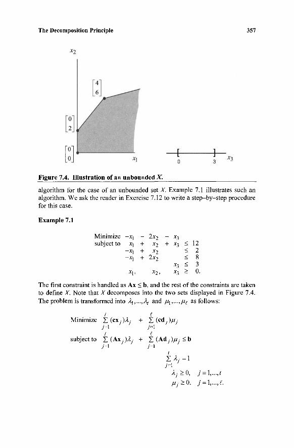
The Decomposition Principle 357
Figure 7.4. Illustration of an unbounded X.
algorithm for the case of an unbounded set X. Example 7.1 illustrates such an algorithm. We ask the reader in Exercise 7.12 to write a step-by-step procedure for this case.
Example 7.1
Minimize -x\ - 2x2 - XT, subject to xj + x2 + Xj ^ 12
-X\ + x2 < 2 -x, + 2x2 < 8
x3 < 3 X j , X2 5 X3 — U.
The first constraint is handled as Ax < b, and the rest of the constraints are taken to define X. Note that X decomposes into the two sets displayed in Figure 7.4. The problem is transformed into ^,.,.,λ, and μ\,...,μ( as follows:
/ i Minimize Σ (Cx/Hy + Σ (cdy)/^,·
y=i y=i
subject to Σ(Αχ7·)Α7· + Σ (Ad,)/^· <b 7=1 7=1
Σ ^ · = ΐ
Ay>o, 7 = 1,...,/ / iy>0, j = l,...J.
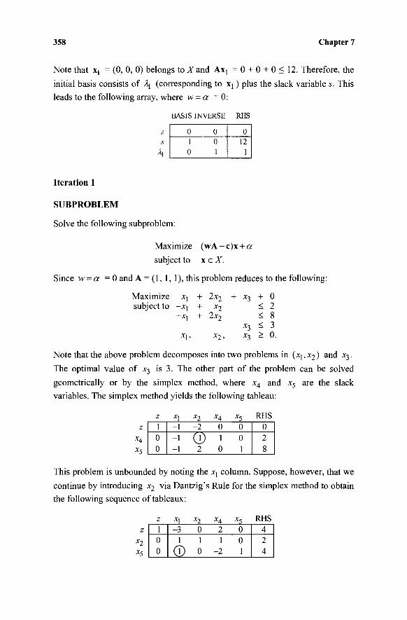
358 Chapter 7
Note that Xj = (0, 0, 0) belongs to X and Axj = 0 + 0 + 0 < 12. Therefore, the
initial basis consists of \ (corresponding to X[ ) plus the slack variable s. This
leads to the following array, where w = a =0:
BASIS INVERSE RHS
0 0 1 0 0 1
0 12
1
Iteration 1
SUBPROBLEM
Solve the following subproblem:
Maximize (wA - c)x + a
subject to x e X.
Since w = a = 0 and A = (1, 1, 1), this problem reduces to the following:
Maximize xj + 2x2 + x3 + 0 subject to -xj + x2 < 2
-x, + 2x2 < 8 x3 < 3
X], x 2 , Χ3 ^ 0.
Note that the above problem decomposes into two problems in (xl,x2) and x3.
The optimal value of x3 is 3. The other part of the problem can be solved
geometrically or by the simplex method, where x4 and x5 are the slack
variables. The simplex method yields the following tableau:
Z ΧΆ Xy XA XK RHS 1 0 0
- 1 - 2 0 0 -1 (1 ) 1 0 - 1 2 0 1
0 2 8
This problem is unbounded by noting the X] column. Suppose, however, that we
continue by introducing x2 via Dantzig's Rule for the simplex method to obtain
the following sequence of tableaux:
Z X] Xj XA Xs. RHS 1 0 0
- 3 0 2 0 - 1 1 1 0 0 0 - 2 1
4 2 4
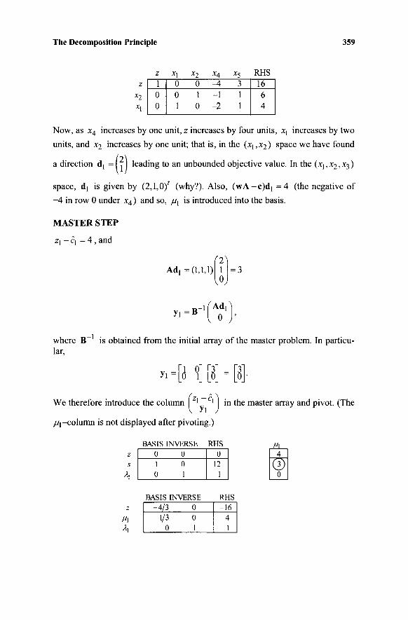
The Decomposition Principle 359
z x2 x\
z 1 0 0
x\ 0 0 1
x2 0 1 0
x^ -A -1 -2
x5
3 1 1
RHS 16 6 4
Now, as ;t4 increases by one unit, z increases by four units, x\ increases by two
units, and x2 increases by one unit; that is, in the (X],x2) space we have found
(2\ a direction d leading to an unbounded objective value. In the (xl,x2,x^)
space, d] is given by (2,1,0)' (why?). Also, (wA-c)dj =4 (the negative of
-4 in row 0 under x4) and so, μ\ is introduced into the basis.
MASTER STEP
zj - cj = 4 , and
Adj =(1,1,1) f^\
v«y
y i = fi-l i Ad,
0
-1 :„ where B is obtained from the initial array of the master problem. In particu-lar,
yi =
We therefore introduce the column | ' ' | in the master array and pivot. (The
"1 0" 0 1
"3" 0 =
"3" 0
//^column is not displayed after pivoting.)
BASIS INVERSE RHS
\
4
0 0 1 0 0 1
0 12
1
BASIS INVERSE Rl· -4/3 0
1/3 0 0 1
IS -16
4 1
£L 4
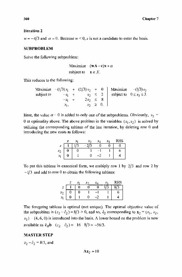
360 Chapter 7
Iteration 2
w = -4/3 and « = 0. Because w < 0, s is not a candidate to enter the basis.
SUBPROBLEM
Solve the following subproblem:
Maximize (wA - c)x + a
subject to x e X.
This reduces to the following:
Maximize -(l/3)X[ + (2/3) x2 + 0 subject to -Χ[ + x2 < 2
-X\ + 2 x 2 < 8 Χχ, Χ2 - 0·
Here, the value a = 0 is added to only one of the subproblems. Obviously, x3 =
0 at optimality above. The above problem in the variables (x1?x2) is solved by
utilizing the corresponding tableau of the last iteration, by deleting row 0 and introducing the new costs as follows:
Σ Xi Xy XA Χξ RHS 1 0 0
1/3 -2 /3 0 0 0 1 - 1 1 1 0 - 2 1
0 6 4
To put this tableau in canonical form, we multiply row 1 by 2/3 and row 2 by
-1/3 and add to row 0 to obtain the following tableau:
Z Xi X T XA X< RHS 1 0 0
0 0 0 1/3 0 1 - 1 1 1 0 - 2 1
8/3 6 4
The foregoing tableau is optimal (not unique). The optimal objective value of
the subproblem is (z2 - c 2 ) = 8/3 > 0, and so, λχ corresponding to x2 = {x\, x2,
x3 ) = (4, 6, 0) is introduced into the basis. A lower bound on the problem is now
available as c ^ b - ( z 2 - c 2 ) = -16 -8 /3= -56/3.
MASTER STEP
z2-C2= 8/3, and
Maximize -(1/3) x3
subject to 0 < x3 < 3.
Ax2 =10
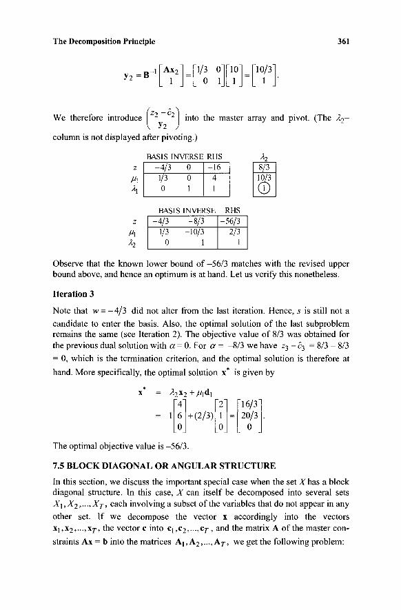
The Decomposition Principle 361
y 2 = B -1 Ax2
1 1/3 0"
0 1 10/3
1
We therefore introduce 2 2 into the master array and pivot. (The λ^-
column is not displayed after pivoting.)
BASIS INVERSE RHS
z Ml
Ml h
-4/3 0 1/3 0 0 1
-16 4 1
BASIS INVERSE RHS -4/3 -8/3
1/3 -10/3 0 1
-56/3 2/3
1
h 8/3
Observe that the known lower bound of -56/3 matches with the revised upper bound above, and hence an optimum is at hand. Let us verify this nonetheless.
Iteration 3
Note that w = -4 /3 did not alter from the last iteration. Hence, 5 is still not a
candidate to enter the basis. Also, the optimal solution of the last subproblem remains the same (see Iteration 2). The objective value of 8/3 was obtained for the previous dual solution with a = 0. For a - -8/3 we have Z3 - c3 = 8/3 - 8/3 = 0, which is the termination criterion, and the optimal solution is therefore at hand. More specifically, the optimal solution x* is given by
V; 4
1 6 0
+ Mdi
+ (2/3) 2 1 0
=
16/3 20/3
0
The optimal objective value is -56/3.
7.5 BLOCK DIAGONAL OR ANGULAR STRUCTURE
In this section, we discuss the important special case when the set X has a block diagonal structure. In this case, X can itself be decomposed into several sets Xl,X2,:.,Xr, each involving a subset of the variables that do not appear in any other set. If we decompose the vector x accordingly into the vectors Xj,x2,...,X7·, the vector c into Cj,C2,..-,Cy, and the matrix A of the master con-straints Ax = b into the matrices A], Α2,..., Α7·, we get the following problem:
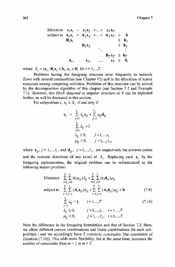
362 Chapter 7
+ C7-X7·
+ ATxT = b < bj
< b 2
X ] , X 2 , · · . , X7- > 0 ,
where X,· = {x, :B,x; <b ; ,x ; > 0} for i = \,...,T.
Problems having the foregoing structure arise frequently in network flows with several commodities (see Chapter 12) and in the allocation of scarce resources among competing activities. Problems of this structure can be solved by the decomposition algorithm of this chapter (see Section 7.2 and Example 7.1). However, this block diagonal or angular structure of X can be exploited further, as will be discussed in this section.
For subproblem i, x, ε Xt if and only if
'■■ Λ
X,· = Σ % x y + Σ ftijA,j
h Σ % = 1
7=1 %>0, j = l,...,tj
where xy, y = 1,...,/,, and d„·, j = !,...,£j, are respectively the extreme points
and the extreme directions (if any exist) of Xt. Replacing each x,· by the
foregoing representation, the original problem can be reformulated as the following master problem:
T ti T lt
Minimize Σ Σ ( c^ /Hy + Σ Σ (c,d; Λμί · ι=1 y=l i=\j=\
subject to Σ Σ (A;Xy )Xtj + Σ Σ (A;d,)M y = b (7.9) i=ij=i /=iy=i
Σ % = 1 i = l,...,T (7.10)
^j^ 0, J = \,...,ti, Ì = \,...,T
Mij>0, j = l,...,ti, i = l,...,T.
Note the difference in the foregoing formulation and that of Section 7.2. Here, we allow different convex combinations and linear combinations for each sub-problem i and we accordingly have T convexity constraints [the constraints of Equation (7.10)]. This adds more flexibility, but at the same time, increases the number of constraints from m + 1 to m + T.
Minimize CJXJ + c2x2 +··· subject to AjXi + A2x2 +...
BiXi B2x2
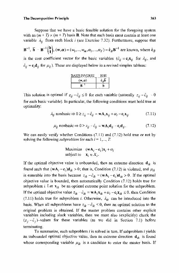
The Decomposition Principle 363
Suppose that we have a basic feasible solution for the foregoing system with an (m + T) x (m + T) basis B. Note that each basis must contain at least one variable L· from each block i (see Exercise 7.32). Furthermore, suppose that
B~ , b = B~ L , (•w,a) = (wl,...,wm,al,...,aT) = cBB~ are known, where cB
is the cost coefficient vector for the basic variables (£y = c;x;y for Ay, and
c,y = c,dy for //«). These are displayed below in a revised simplex tableau:
BASIS INVERSE RHS
(w,a)
B-1
c5b
b
This solution is optimal if z,,· - c,,· < 0 for each variable (naturally z,y - èy = 0
for each basic variable). In particular, the following conditions must hold true at optimality:
Ay nonbasic => 0 > z(y - èy = wA,-x,y + a,· - c,-x;y (7.11)
//,y nonbasic => 0 > z;,- - èy = wA,d,y - c,-d,y. (7.12)
We can easily verify whether Conditions (7.11) and (7.12) hold true or not by solving the following subproblem for each / = 1,..., T:
Maximize (wA;· - c;- )x,· + a ;
subject to Xj eXj.
If the optimal objective value is unbounded, then an extreme direction Aik is found such that (wA,· -c,-)d^ > 0; that is, Condition (7.12) is violated, and μ{ίί
is enterable into the basis because zjk -cik = (wA; -cf)aik > 0. If the optimal objective value is bounded, then automatically Condition (7.12) holds true for subproblem /'. Let \ik be an optimal extreme point solution for the subproblem.
If the optimal objective value zik -cik = \νΑ;χ;Α +α, -c,-x^ < 0, then Condition
(7.11) holds true for subproblem i. Otherwise, Àjk can be introduced into the
basis. When all subproblems have zik - cjk < 0, then an optimal solution to the
original problem is obtained. If the master problem contains other explicit variables including slack variables, then we must also (explicitly) check the (z,· - c )-values for these variables (as we did in Section 7.1) before
terminating. To summarize, each subproblem i is solved in turn. If subproblem / yields
an unbounded optimal objective value, then an extreme direction dik is found
whose corresponding variable μΛ is a candidate to enter the master basis. If
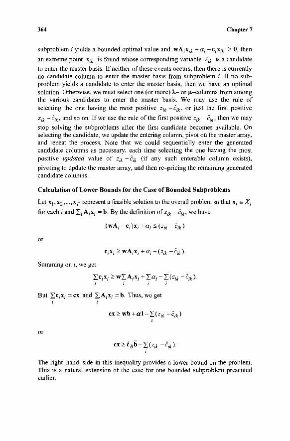
364 Chapter 7
subproblem i yields a bounded optimal value and wAj\ik +at -CjXjk > 0, then
an extreme point xjk is found whose corresponding variable Àjk is a candidate
to enter the master basis. If neither of these events occurs, then there is currently no candidate column to enter the master basis from subproblem i. If no sub-problem yields a candidate to enter the master basis, then we have an optimal solution. Otherwise, we must select one (or more) λ - or μ-columns from among the various candidates to enter the master basis. We may use the rule of selecting the one having the most positive zik -cjk, or just the first positive zik ~Cik> a n a s o o n · Ifwe use t n e mie of the first positive zik -cik, then we may stop solving the subproblems after the first candidate becomes available. On selecting the candidate, we update the entering column, pivot on the master array, and repeat the process. Note that we could sequentially enter the generated candidate columns as necessary, each time selecting the one having the most positive updated value of zik - cik (if any such enterable column exists), pivoting to update the master array, and then re-pricing the remaining generated candidate columns.
Calculation of Lower Bounds for the Case of Bounded Subproblems
Let X!,X2,...,X7· represent a feasible solution to the overall problem so that x; e Xt
for each i and Σ; A;x( = b. By the definition of zik -cik, we have
(wA; -c()x;- +α;· < (zik -cik)
or
c,·*,· > wAji; + «,· - (zik - cik ).
Summing on /', we get
XCjX; > wIAj-X,· + Σ « ; - Σ ( % ~Cìk). i i i i
But Zc ; x i =cx a n Q ΣΑ,-χ,- =b. Thus, we get I i
ex > wb + a\ - Σ (zik - cik ) i
or
cx>cBb-Z(zik-cik). i
The right-hand-side in this inequality provides a lower bound on the problem. This is a natural extension of the case for one bounded subproblem presented earlier.
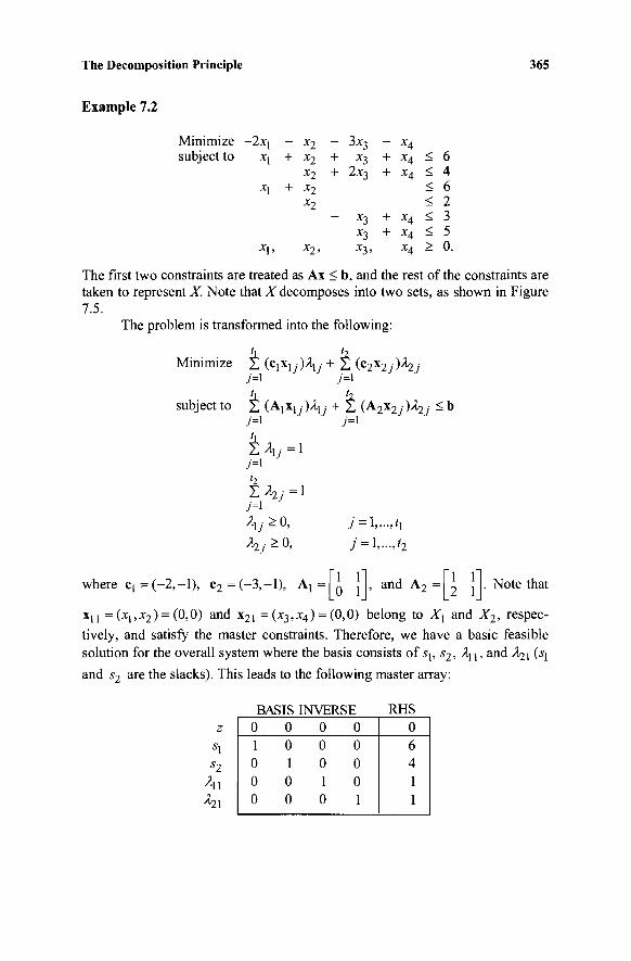
The Decomposition Principle 365
Example 7.2
Minimize subject to
- 2 x j x\
x\
X\,
- x2 + x2
x2
+ x2 x2
x2,
— + +
-
3*3 *3
2x3
x3 x3
*3>
— x4
+ x4 < 6 + x4 < 4
< 6 < 2
+ x4 < 3 + x4 < 5
x4 > 0.
The first two constraints are treated as Ax < b, and the rest of the constraints are taken to represent X. Note that X decomposes into two sets, as shown in Figure 7.5.
The problem is transformed into the following:
h h Minimize Σ {t\*\j)hj + Σ (£2*2j)h.j
7=1 7=1 Ί h
subject to Σ (AjXl7)/ll7- + Σ (A2X2j)h.j - b
7=1 j=\
Σλυ=\ 7=1
7=1
where q = (-2,-1), c 2 = ( - 3 , - l ) , A!
j = \,...,tl
j = l,...,t2
1 1 0 1 , and A2
1 1 2 1
. Note that
xu =(x!,x2) = (0,0) and x21 = (x3,x4) = (0,0) belong to X1 and X2, respec-tively, and satisfy the master constraints. Therefore, we have a basic feasible solution for the overall system where the basis consists of sh s2, λλ t , and λ^χ (jj and s2 are the slacks). This leads to the following master array:
s2 Al
BASIS INVERSE 0 0 0 0 1 0 0 0 0 1 0 0 0 0 1 0 0 0 0 1
RHS 0 6 4 1 1
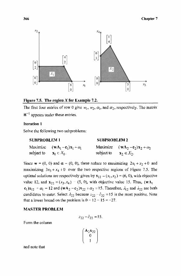
366 Chapter 7
Figure 7.5. The region X for Example 7.2.
The first four entries of row 0 give M\, W2, ah and a2, respectively. The matrix
B~ appears under these entries.
Iteration 1
Solve the following two subproblems:
SUBPROBLEM 1 SUBPROBLEM 2
Maximize ( w A j - c ^ x j + a i Maximize ( w A 2 - c 2 ) x 2 + « 2 subject to Xj e l i - subject to x2eX2.
Since w = (0, 0) and a = (0, 0), these reduce to maximizing 2xj + x2 + 0 and
maximizing 3x 3 +x 4 +0 over the two respective regions of Figure 7.5. The
optimal solutions are respectively given by x]2 = (xi,x2) = (6, 0), with objective
value 12, and x22 =(^3,^4) = (5, 0), with objective value 15. Thus, (wAj -cl)xl2 + «i = 12 and (wA2 -c2)x22 +a2 = 15. Therefore, A12 and λτ^ are both
candidates to enter. Select λχχ because z22 - c22 =15 is the most positive. Note
that a lower bound on the problem is 0 - 12 - 15 = -27.
MASTER PROBLEM
Form the column
and note that
z22-c22 =15.
A2x22
0 1
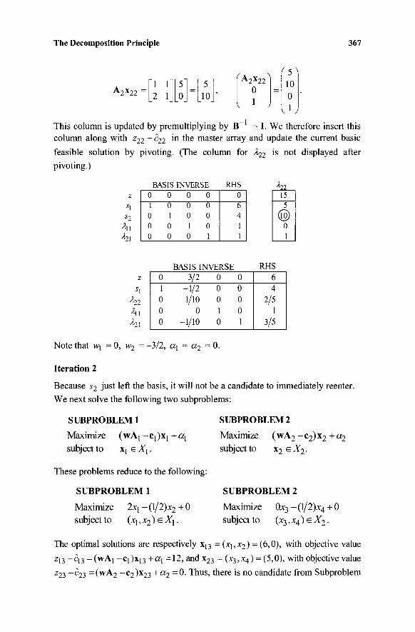
The Decomposition Principle 367
A2X22 = "1 f
2 1_
"5"
0 = ~5~
10 5
f A Y > A 2 X 2 2 0 =
(5) 10 0
»-i This column is updated by premultiplying by B = I. We therefore insert this column along with z22 - c22 in the master array and update the current basic feasible solution by pivoting. (The column for A^2 is not displayed after pivoting.)
À22_ BASIS INVERSE 0 0 0 0 1 0 0 0 0 1 0 0 0 0 1 0 0 0 0 1
RHS 0 6 4 1 1
15
é 0 1
hi
h\
Note that w\ = 0, w2 = -3/2, «j = a2 = 0.
0 1 0 0 0
BASIS INVERSE -3 /2 0 0 -1/2 0 0 1/10 0 0
0 1 0 -1/10 0 1
RHS -6
4 2/5
1 3/5
Iteration 2
Because s2 just left the basis, it will not be a candidate to immediately reenter.
We next solve the following two subproblems:
SUBPROBLEM 1
Maximize (wAj - c ^ + o ^ subject to Xj e Χ^.
These problems reduce to the following:
SUBPROBLEM 1
Maximize 2x\ -(l/2)x2 +0 subject to (*], x2 ) e X\.
SUBPROBLEM 2
Maximize ( wA2 - c2) x2 + «2 subject to x2 e X2.
SUBPROBLEM 2
Maximize 0x3 - (1/ 2)x4 + 0 subj ect to ( JC3, Χ4 ) e X2.
The optimal solutions are respectively X[3 = (x\,x2) = (6,0), with objective value Z13 - < Ì3 = ( W A i _ c i ) x i3 +a\ =12, and x23 = (x3,x4) = (5,0), with objective value z23 _^23 =(wA2 -C2)x23 + a 2 = 0· Thus, there is no candidate from Subproblem
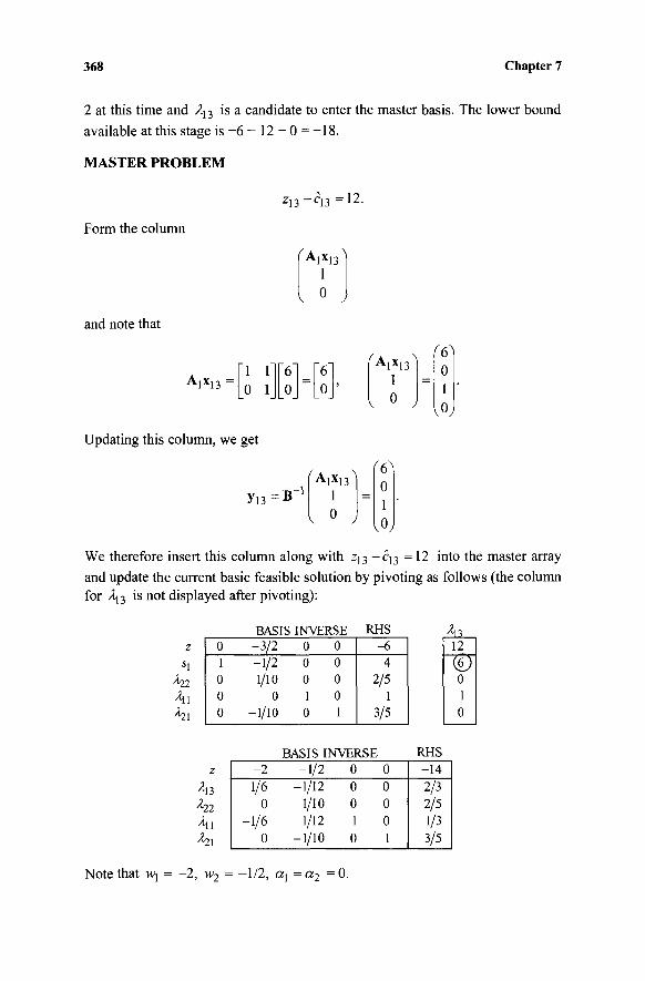
368 Chapter 7
2 at this time and Xu is a candidate to enter the master basis. The lower bound
available at this stage is -6 - 12 — 0 = —18.
MASTER PROBLEM
Form the column
z 1 3 -c 1 3 =12.
' A l X l 3 ^ 1
V ° J
and note that
Alx13 "1 f 0 1
"6n
0 = "6"
0 ί
fAiXn^ 1
I o J =
r 6 i 0
1
Updating this column, we get
y o = B - 1 Ά , χ ^
v 0 j
0 1
We therefore insert this column along with z^-c^ =12 into the master array and update the current basic feasible solution by pivoting as follows (the column for A]3 is not displayed after pivoting):
h.2
0 1 0 0 0
BASIS INVERSE -3/2 0 0 -1/2 0 0 1/10 0 0
0 1 0 -1/10 0 1
RHS -6 4
2/5 1
3/5
12
0 1 0
A13
-2 1/6
0 -1/6
0
BASIS INVERSE -1/2 0 0
-1/12 0 0 1/10 0 0 1/12 1 0
-1/10 0 1
RHS -14 2/3 2/5 1/3 3/5
Note that M\ = -2, w2 = -1/2, «j = a2 = 0.
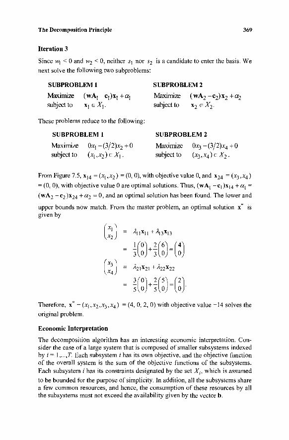
The Decomposition Principle 369
Iteration 3
Since wj < 0 and w2 < 0, neither jj nor s2 is a candidate to enter the basis. We
next solve the following two subproblems:
SUBPROBLEM 1 SUBPROBLEM 2
Maximize (wAj -CJ)XJ+a j Maximize ( w A 2 - c 2 ) x 2 + a 2
subject to X j e Z j . subject to x 2 e X 2 -
These problems reduce to the following:
SUBPROBLEM 1 SUBPROBLEM 2
Maximize 0x\ - (3/2)x2 + 0 Maximize 0x3 -(3/2)x4 +0
subject to (x],x2)^X\. subject to (x 3 ,x 4 ) eX 2 ·
From Figure 7.5, x14 = (x1?x2) = (0, 0), with objective value 0, and x24 = (x3,x4)
= (0, 0), with objective value 0 are optimal solutions. Thus, (wAj -Cj)x14 + «j =
(wA2 -c 2 )x 2 4 +cc2 =0 , and an optimal solution has been found. The lower and
upper bounds now match. From the master problem, an optimal solution x* is given by
χ I = Λΐχ11+/113χ13
3"loJ+3"loj = lvO = λ2Χ\2Χ +λ22χ22
- Kw-e Therefore, x* = (xi,x2,x3,x4) = (4, 0, 2, 0) with objective value -14 solves the
original problem.
Economic Interpretation
The decomposition algorithm has an interesting economic interpretation. Con-sider the case of a large system that is composed of smaller subsystems indexed by / = Ι,.,.,Τ. Each subsystem i has its own objective, and the objective function of the overall system is the sum of the objective functions of the subsystems. Each subsystem i has its constraints designated by the set Xj, which is assumed
to be bounded for the purpose of simplicity. In addition, all the subsystems share a few common resources, and hence, the consumption of these resources by all the subsystems must not exceed the availability given by the vector b.
370 Chapter 7
Recalling the economic interpretation of the dual variables (Lagrangian multipliers), w, is the rate of change of the objective as a function of 6;·. That is,
if bj is (marginally) replaced by ty+A, holding the current nonbasic variables in
the master problem at zero, then the objective value is modified by adding νν,-Δ.
Hence, -w,· can be thought of as the price of consuming one unit of the ith
common resource. Similarly, -α,- can be thought of as the price of consuming a
portion of the rth convexity constraint. With this in mind, the decomposition algorithm can be interpreted as
follows. With the current proposals of the subsystems, the superordinate (total system) obtains a set of optimal weights for these proposals and announces a set of prices for using the common resources. These prices are passed down to the subsystems, which modify their proposals according to these new prices. A typical subsystem / solves the following subproblem:
Maximize (wA; - c,·)x,· + «,· subject to Xj e Xh
or equivalently,
Minimize (c,· - wA; )x( - a;
subject to x; eXj.
The original objective function of subsystem / is c(x;. The term -ννΑ,-χ,· reflects the
indirect price of using the common resources. Note that A;x, is the amount of
the common resources consumed by the proposal x ; . Since the price of using
these resources is -w, then the indirect cost of using them is -wA,-x,·, and the
total cost is (c,· — wA,-)x,·. Note that the term -wA;x, makes proposals that use
much of the common resources unattractive from a cost point of view. Subsys-
tem i announces an optimal proposal xik. If this proposal is to be considered,
then the weight of the older Xy-proposals must decrease in order to "make
room" for this proposal; that is, Σ / % m u s t decrease from its present level of 1.
The resulting saving is precisely a,. If the cost of introducing the proposal xik
is less than the saving realized; that is, if (c; - wA; )xik - al < 0, or
(wA,· -c,-)x,-fc + a,· >0 , then the superordinate would consider this new pro-
posal. After all the subsystems introduce their new proposals, the superordinate
determines an optimal mix of these proposals and passes down new prices. The
process is repeated until none of the subsystems has a new attractive proposal;
that is, when (c,· - wA;)xJ/t - α · > 0 for each ;'.
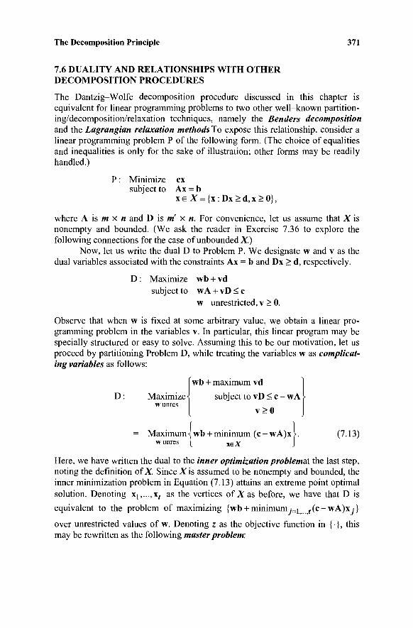
The Decomposition Principle 371
7.6 DUALITY AND RELATIONSHIPS WITH OTHER DECOMPOSITION PROCEDURES
The Dantzig-Wolfe decomposition procedure discussed in this chapter is equivalent for linear programming problems to two other well-known partition-ing/decomposition/relaxation techniques, namely the Benders decomposition and the Lagrangian relaxation methods To expose this relationship, consider a linear programming problem P of the following form. (The choice of equalities and inequalities is only for the sake of illustration; other forms may be readily handled.)
P : Minimize ex subject to Ax = b
X E J V E { X : D X > ( 1 , X > 0 } ,
where A is m x « and D is m x n. For convenience, let us assume that X is nonempty and bounded. (We ask the reader in Exercise 7.36 to explore the following connections for the case of unbounded X.)
Now, let us write the dual D to Problem P. We designate w and v as the dual variables associated with the constraints Ax = b and Dx > d, respectively.
D : Maximize wb + vd subject to wA + vD < c
w unrestricted, v > 0.
Observe that when w is fixed at some arbitrary value, we obtain a linear pro-gramming problem in the variables v. In particular, this linear program may be specially structured or easy to solve. Assuming this to be our motivation, let us proceed by partitioning Problem D, while treating the variables w as complicat-ing variables as follows:
wb + maximum vd
subject to vD < c - wA
v > 0 D: Maximize-
= Maximum-^ wb + minimum (c-wA)xk (7.13) wunres [ xeX J
Here, we have written the dual to the inner optimization problemat the last step, noting the definition of X. Since X is assumed to be nonempty and bounded, the inner minimization problem in Equation (7.13) attains an extreme point optimal solution. Denoting Χι,.,.,χ, as the vertices of Xas before, we have that D is
equivalent to the problem of maximizing {wb + minimumy-=1 ((c-wA)x,·}
over unrestricted values of w. Denoting z as the objective function in {■}, this may be rewritten as the following master problem.
372 Chapter 7
MP : Maximize z subjectto z < wb + (c-wA)x · fory = l,...,f (7.14)
z, w unrestricted.
Note that MP is inconvenient to solve directly because it typically has far too many constraints. Hence, we can adopt a relaxation strategy, in which only a few of the constraints in Equation (7.14) are explicitly maintained. Suppose that for such a relaxed master program we obtain an optimal solution (z\w). Then z" is an upper bound on the optimal value to the original problem (why?). Further-more, (z,w) is optimal for MP if and only if (z,w) is feasible to all constraints in Equation (7.14) (why?). Hence, in order to check if any constraint in Equation (7.14) is violated, we wish to check if z < wb + (c-wA)x,· for ally = 1,...,/, that
is, if z < wb + minimum J=1 ; /{(c-wA)xy}. However, the latter problem is
equivalent to the linear programming subproblem:
wb +minimum {(c-wA)x}. (7.15) xeX
If z is less than or equal to the optimal objective value in Equation (7.15), then we are done. (In fact, in this case, z will be equal to the optimal value in Equa-tion (7.15) since z is equal to wb + (c-wA)x for some je{\,...,t} in the
solution to the relaxed master program.) Otherwise, if \k solves Problem (7.15), we have z > wb + (c - wA)x^, and we can generate the constraint z<wb + (c-wA)xyt, and add it to the current (relaxed) master program and reoptimize. Observe that this new constraint cuts off or deletes the previous master problem solution (z, w). This process may be repeated until the solution
(z, w) to some relaxed master problem gives z equal to the optimal value in Equation (7.15). This must occur finitely since X has only a finite number of vertices.
The foregoing procedure is known as Benders partitioning or Benders decomposition technique. (Its generalization to nonlinear or discrete problem structures is addressed in Exercise 7.38 and in the Notes and References section.) Problem (7.14) (or its relaxation) is referred to as Benders {relaxed) master problem, its constraints are referred to as Benders constraints or Benders cuts (from their role of deleting previous master problem solutions), and Problem (7.15) is known as Benders subproblem. However, note that Problem (7.15) is also the subproblem solved by the Dantzig-Wolfe decomposition method, and that the Benders master program (7.14) is simply the dual to the Dantzig-Wolfe master problem with Constraints (7.1)—(7.3). (Here, the nonnegative dual multipliers associated with the constraints (7.14) are A., j =
\,...,t; these variables sum to unity by virtue of the column of the variable z in Problem MP.) Therefore, Benders algorithm is called a row generation technique in contrast with the Dantzig-Wolfe column generation procedure. It follows that if at the end of each relaxed master program solution, we maintain
The Decomposition Principle 373
only those generated rows in Equation (7.14) that have currently nonbasic slack variables, and so whose complementary dual variables A,· are basic, then the
resulting algorithm is precisely the same as the decomposition algorithm of Section 7.1. In particular, the starting solution technique of Section 7.3 provides an initial bounded Benders master program. Also, when Benders algorithm terminates, the available optimal primal solution may be computed as the sum of the products of the x,—solutions and the corresponding dual variables λ: that are
associated with the explicitly present constraints (7.14) in the final Benders relaxed master problem. (Note that this sum is a convex combination.) Furthermore, note that if we did not delete any of the constraints generated by Benders algorithm and solved each relaxed Benders master program to optimality, the equivalent implementation for the Dantzig-Wolfe method would be to optimize each master program over all the A,—variable columns generated
thus far. Observe that the foregoing discussion also indicates how to recover an
optimal set of dual multipliers (w , v ) for the Problem P after solving it using
the Dantzig-Wolfe decomposition algorithm. The vector w is directly available
as the optimal set of multipliers associated with the constraints (7.1). The corre-
sponding solution v* is obtainable from the first inner maximization problem in
Equation (7.13) after fixing w at w . Hence, if the second inner minimization
subproblem in Equation (7.13) is solved with w = w , then v* is obtained as the set of optimal dual multipliers associated with the constraints in X. For instance,
in the example of Section 7.2, we obtain (w>[ ,H>2) = (-1, -1). Furthermore, with
w = w fixed, the (final) subproblem solved is to maximize {-3*4 : xe X},
which yields an optimal set of dual multipliers v* = (0, 0, 0, 0) for the constraints 3, 4, 5, and 6 in the example.
It may also be noted that the Dantzig-Wolfe and the Benders decompo-sition methods are respectively classified as price directive and resource directive schemes. The former type of procedure conducts the coordination in the decomposition method by adjusting prices or objective function coefficients via Lagrangian multipliers. On the other hand, the latter type of procedure is dual to this scheme, and conducts this coordination by adjusting the common resource availabilities (right-hand-sides) by fixing certain variable values.
There is another general price-directive optimization strategy for P that finds an equivalence with the foregoing methods when solving linear program-ming problems, namely the Lagrangian relaxation technique (See Exercise 6.71.) Observe from Equation (7.13) that if we denote the function in {·}, which is a function of w, as θ(\ν), we can equivalently state D as the following problem:
Maximize {0(w) : w unrestricted} (7.16)
374 Chapter 7
where
#(w) = wb + minimum {(c - wA)x : x e X). (7.17)
Problem (7.16) is known as a Lagrangian dual to Problem P. Problem (7.17) is the associated Lagrangian subproblem. Note that in Problem (7.17), the con-straints Ax = b have been accommodated into the objective function of P via the Lagrangian multipliers w. By the foregoing discussion, it is evident that the maximum value in Problem (7.16) matches with the optimal objective value for P, and hence, 6>(w) provides a lower bound for this optimal value for any arbitrary w. This is why Problem (7.16) is called a "Lagrangian dual" problem. Furthermore, since #(w) = wb + minimum =[ !?{(c-wA)x,}, we have that
#(w) is a piecewise linear and concave function of w (why?). Hence, Problem
(7.16) seeks an unconstrained maximum for this function. Although several nonlinear search methods for nonsmooth optimization problems may be used to solve Problem (7.16), the Benders procedure is evidently one viable solution technique. This cutting plane or row generation scheme can be viewed as a tangential approximation method for solving Problem (7.16), in which only a few of the tangential supports or segments z < wb + (c-wA)x -,j = l,...,t that
describe θ( ·) are generated. Here, z is the value measured along the θ( -)-axis. Using this viewpoint, the relaxed master problem MP from Equation (7.14) employs an outer linearization of Problem (7.16), using only a subset of the tangential supports that actually describe the piecewise linear function #(·). If w solves this problem with objective value z, then z is an upper bound on the optimal value of Problem (7.16). However, if z=#(w) itself, then w is
optimal for Problem (7.16) (why?). Otherwise, z > # ( w ) = wb + minimum {(c-wA)x : x e X} = wb + (c-wA)x^, say, as produced by the Sub-problem (7.17), which coincides with the Benders subproblem (7.15). Hence, the tangential support z < wb + (c - wA)x^ is generated and included in the
outer-linearization of #(·), and the procedure is repeated until termination is obtained. At termination, the optimal primal solution may be recovered by weighting each x ■ in Equation (7.14) by the corresponding dual multiplier Àj, if
positive at optimality, and summing. Exercises 7.42 and 7.43 explore further refinements to accelerate the
convergence behavior of Benders and Lagrangian relaxation approaches using the boxstep method and its extensions, as well as the associated corresponding stabilized column generation implementation techniques for the Dantzig-Wolfe decomposition procedure.
Example 7.3
Consider the linear programming problem given in the example of Section 7.2. Denote the dual variables associated with the constraints as (\ν],%ν2,νί,ν2,ν^, v4) and write the dual as follows:
The Decomposition Principle 375
Maximize 2wx + 3H>2 + 2vj + 5v2 + 2v3 + 6v4
subject to w\ + n>2 + Vj + v2 < -2 w>2 + 2v2 < -1
ΜΊ - V3 + 2V4 < -1 2w>2 + v3 + v4 < 1
w < 0, v < 0.
Treating w as the complicating variables, we obtain the Benders master problem in this case as follows:
Maximize z subject to z < 2w>i + 3w>2 + x^ (-2 - H - M^)
+xj2(-l-w2) + xj3(-l-wi)+xj4(l-2»2) forj = l,...,t
z unrestricted, w < 0,
where x,· = (χβ,χ:2,χ:3,χ:4), j = 1,-, t, are the vertices of A" as defined in
Section (7.2). The corresponding Lagrangian dual problem is given as follows:
Maximize {#(w) : w < 0}
where, for a given w = (n^, w>2 ), we have
#(w) = 2m + 3w2 + minimum{(-2 - w\ - w2 )x\ + (-1 - W2 )x2 xeAT
+ (-l-W[)jC3 +(1-2M2)J«4}.
Note that evaluating #(w), given w, is precisely equivalent to solving the
Benders subproblem.
Suppose that as in Section 7.2 we begin with the vertex Xj = (0, 0, 0, 0)
of X. Hence, the relaxed Benders master problem is of the form:
Maximize z subject to z < 2w\ + 3w2
w<0.
The optimal solution is jf = 0 and w = (0, 0). Hence, using only the tangential
support z ^ 2ft\ +3w2 for θ( ·), we obtain w = (0, 0) as the maximizing solu-
tion. Solving the Benders subproblem with w = (0, 0), that is, computing θ(\ν),
we get #(w) = -17/2 , which is realized at x2 =(2,3/2,3,0). Since #(w)<z~,
we generate a second Benders cut or tangential support using x2:
z < 2wx +3w>2 + 2 ( - 2 - n \ - w2) + (3/2)(-1 - w2) + 3 ( - l - wx)
= -n/2-3wl-(l/2)w2.
This leads to the following relaxed Benders master program:
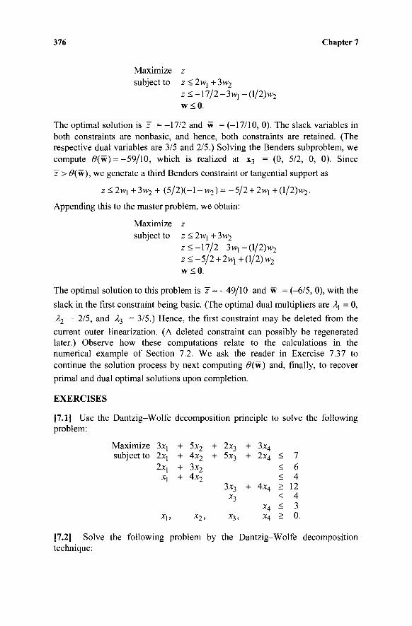
376 Chapter 7
Maximize z subject to z < 2wj + 3w2
z<-17/2-3w, - ( l /2 )w 2
w<0.
The optimal solution is I = -17/2 and w = (-17/10, 0). The slack variables in both constraints are nonbasic, and hence, both constraints are retained. (The respective dual variables are 3/5 and 2/5.) Solving the Benders subproblem, we compute #(w) = -59/10, which is realized at x3 = (0, 5/2, 0, 0). Since z > #(w), we generate a third Benders constraint or tangential support as
z<2wj + 3w2 + (5/2)(- l -w2) = -5 /2 + 2 wx +(l/2)w2.
Appending this to the master problem, we obtain:
Maximize z subject to z < 2w[ + 3w2
z <-17/2-3w,-(1/2) w2
z < - 5 / 2 + 2w1+(l/2)w2
w<0.
The optimal solution to this problem is z = -49/10 and w = (-6/5, 0), with the slack in the first constraint being basic. (The optimal dual multipliers are Aj = 0, À2 = 2/5, and A3 = 3/5.) Hence, the first constraint may be deleted from the current outer-linearization. (A deleted constraint can possibly be regenerated later.) Observe how these computations relate to the calculations in the numerical example of Section 7.2. We ask the reader in Exercise 7.37 to continue the solution process by next computing #(w) and, finally, to recover primal and dual optimal solutions upon completion.
EXERCISES
[7.1] Use the Dantzig-Wolfe decomposition principle to solve the following problem:
Maximize 3x] + 5x2 + 2x3 + 3x4
subject to 2xj + 4x2 + 5x3 + 2x4 < 7 2xj + 3x2 < 6
Xj + 4x2 < 4 3x3 + 4x4 > 12 x3 < 4
x4 < 3 Xj, x 2 , x 3 , x 4 ^ 0.
[7.2] Solve the following problem by the Dantzig-Wolfe decomposition technique:
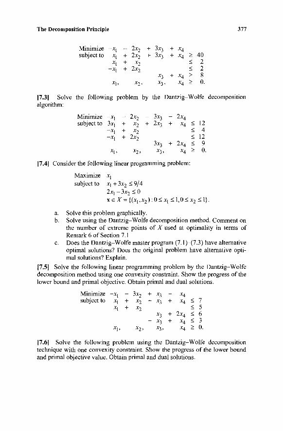
The Decomposition Principle 377
Minimize subject to
-x, X,
X,
-x,
x\,
- 2x2 + 2x2
+ x2 + 2x2
x2>
+ 3x3 + 3x3
*3 x3,
+ x4
+ x4
+ x4 X4
> < < > >
40 2 2 8 0.
[7.3] Solve the following problem by the Dantzig-Wolfe decomposition algorithm:
Minimize -xj - 2x2 - 3x3 - 2x4 subject to 3xj + x2 + 2x3 + x4 < 12
-X! + x2 < 4 -xt + 2x2 < 12
3x3 + 2x4 < 9
Xj, X2 5 ·*3 ' -*·4 — ^·
[7.4] Consider the following linear programming problem:
Maximize Xj subject to xj + 3x2 < 9/4
2xj - 3x2 < 0 x e X = {(x,,x2):0<x1 <1 ,0<χ 2 <1}.
a. Solve this problem graphically. b. Solve using the Dantzig-Wolfe decomposition method. Comment on
the number of extreme points of X used at optimality in terms of Remark 6 of Section 7.1
c. Does the Dantzig-Wolfe master program (7.1)—(7.3) have alternative optimal solutions? Does the original problem have alternative opti-mal solutions? Explain.
[7.5] Solve the following linear programming problem by the Dantzig-Wolfe decomposition method using one convexity constraint. Show the progress of the lower bound and primal objective. Obtain primal and dual solutions.
Minimize subject to
-x, *1 xx
X\,
— 3x2 + x3 + x2 + x3 + x2
x3 - x3
x2, x3,
— x4 + x4
+ 2x4 + x4
x4
< 7 < 5 < 6 < 3 > 0.
[7.6] Solve the following problem using the Dantzig-Wolfe decomposition technique with one convexity constraint. Show the progress of the lower bound and primal objective value. Obtain primal and dual solutions.
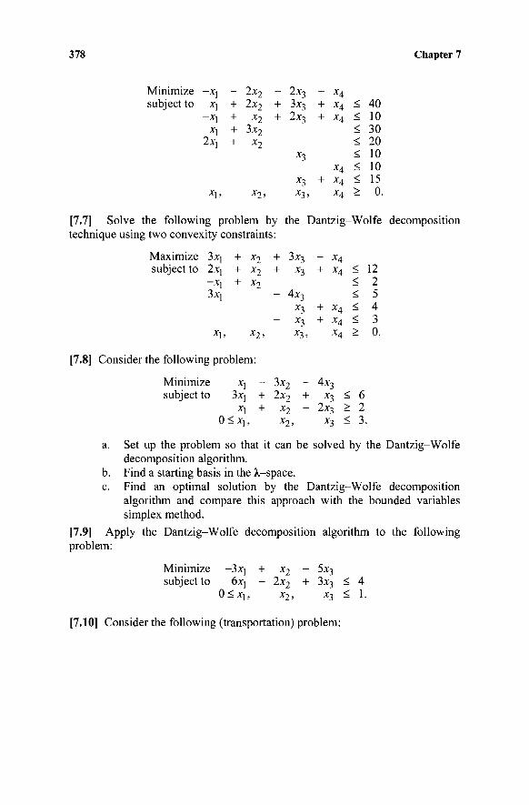
378 Chapter 7
Minimize -xj subject to xj
- * i xl
2xj
X j ,
- 2x2
+ 2x2
+ x2 + 3x2 + x2
*2>
-+ +
2x3
3x3 2x3
x3
x3 x3>
— X4
+ x4 < 40 + x4 < 10
< 30 < 20 < 10
x4 < 10 + x4 < 15
x4 > 0.
[7.7] Solve the following problem by the Dantzig-Wolfe decomposition technique using two convexity constraints:
Maximize 3xj + x2
subject to 2χγ + x2
~x\ + x2 3xi
X j , X 2 ,
Lie following problem:
Minimize Xj -subject to 3xj +
Xj +
0 < x b
+ 3x3
+ x3
- 4x3 x3
" x3 x3,
3x2 -2x2 +
x2 ~ x2>
— x4
+ x4 < 12 < 2 < 5
+ x4 < 4 + x4 < 3
x4 > 0.
4x3
x3 < 6 2x3 > 2
x3 < 3.
a. Set up the problem so that it can be solved by the Dantzig-Wolfe decomposition algorithm.
b. Find a starting basis in the λ-space. c. Find an optimal solution by the Dantzig-Wolfe decomposition
algorithm and compare this approach with the bounded variables simplex method.
[7.9] Apply the Dantzig-Wolfe decomposition algorithm to the following problem:
Minimize subject to
- 3 x j 6x[
0<xu
+ -
x2
2x2 x2,
-+
5x3
3x3
*3
< <
4 1.
[7.10] Consider the following (transportation) problem:
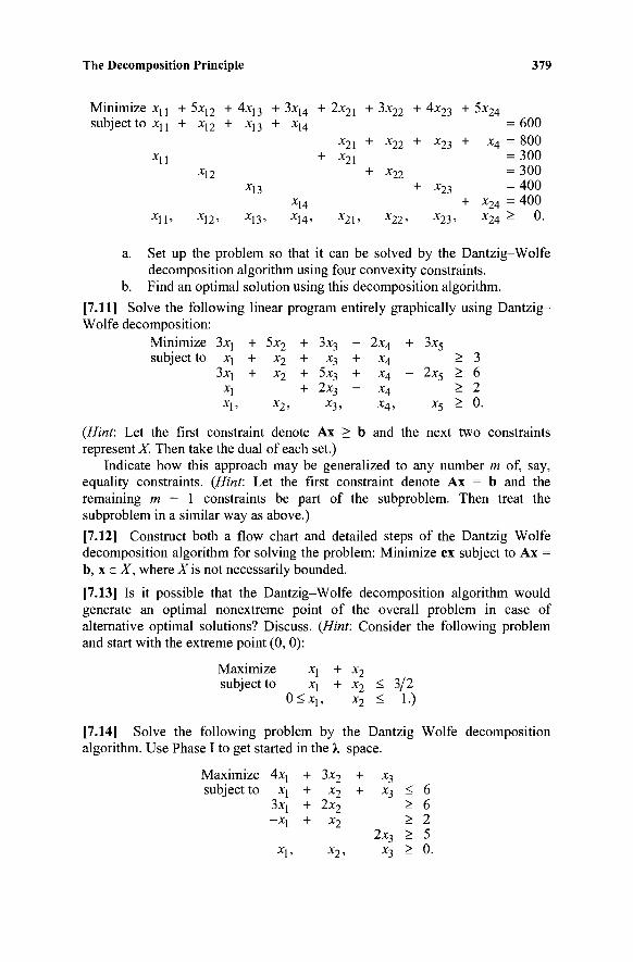
The Decomposition Principle 379
Minimize XJI + 5x12 + 4x;3 + 3x14 + 2x2[ + 3x22 + 4*23 + 5x24 subject to Xu + X]2 + X[3 + Xi4 =600
x21 + x22 + x23 + x4 ~ ^00 Χη + X2i = 300
X]2 + X22 = 300 x13 + x23 = 400
x14 + x24 = 400 X j l , X j 2 , X j3 , Xj4, X 2 J , X 2 2 , X 2 3 , X 2 4 > 0 .
a. Set up the problem so that it can be solved by the Dantzig-Wolfe decomposition algorithm using four convexity constraints.
b. Find an optimal solution using this decomposition algorithm.
[7.11] Solve the following linear program entirely graphically using Dantzig-Wolfe decomposition:
Minimize 3x] + 5x2 + 3x3 - 2x4 + 3x5 subject to X] + x2 + x3 + x4 > 3
3xj + x2 + 5x3 + x4 - 2x5 > 6 X[ + 2x3 - x4 > 2 Xi, X2 ; X 3 ? X-4? x 5 — ^ ·
{Hint: Let the first constraint denote Ax > b and the next two constraints represent X. Then take the dual of each set.)
Indicate how this approach may be generalized to any number m of, say, equality constraints. {Hint: Let the first constraint denote Ax = b and the remaining m - 1 constraints be part of the subproblem. Then treat the subproblem in a similar way as above.)
[7.12] Construct both a flow chart and detailed steps of the Dantzig-Wolfe decomposition algorithm for solving the problem: Minimize ex subject to Ax = b, x G X, where X is not necessarily bounded.
[7.13] Is it possible that the Dantzig-Wolfe decomposition algorithm would generate an optimal nonextreme point of the overall problem in case of alternative optimal solutions? Discuss. {Hint: Consider the following problem and start with the extreme point (0, 0):
Maximize x\ + x2 subject to X! + x2 < 3/2
0<x, , x2 < 1.)
[7.14] Solve the following problem by the Dantzig-Wolfe decomposition algorithm. Use Phase I to get started in the λ-space.
Maximize 4xj + 3x2 + X3 subject to X] + x2 + x3 < 6
3xj + 2x2 > 6 -Xi + x2 > 2
2x3 > 5 X\, Χ2 ■> ^3 — *J ■

380 Chapter 7
[7.15] An agricultural mill produces cattle feed and chicken feed. These prod-ucts are composed of three main ingredients, namely, corn, lime, and fish meal. The ingredients contain two main types of nutrients, namely, protein and cal-cium. The following table gives the nutrients' contents in standard units per pound of each ingredient:
NUTRIENT Protein Calcium
CORN 27 20
INGREDIENT LIME FISH MEAL
20 30 30 20
The protein content must lie in the interval [22, 25] per pound of cattle feed. Also the calcium content must be greater than or equal to 22 per pound of the cattle feed. Similarly, the protein content and the calcium content must be in the intervals [21, 24] and [21, 29], respectively, per pound of the chicken feed. Sup-pose that 3000, 2500, and 1000 pounds of corn, lime, and fish meal, respectively, are available. Also, suppose that it is required to produce 4000 and 2000 pounds of the cattle and chicken feed, respectively. Let the price per pound of the corn, lime, and fish meal be respectively $0.20, $0.15, and $0.25. Formulate the blending problem with an objective of minimizing the cost.
Solve the problem by the Dantzig-Wolfe decomposition algorithm using two convexity constraints. Extra corn and fish meal can be obtained but, because of shortages, at the higher prices of $0.22 and $0.27 per pound. Would you advise the mill to consider extra corn and fish meal and modify their blending at these prices? Why or why not?
[7.16] A company has two manufacturing facilities, one in Atlanta and one in Los Angeles. The two facilities produce refrigerators and washer/dryers. The production capacities of these items in Atlanta are 5000 and 7000, respectively. Similarly, the capacity of the Los Angeles facility is 8000 refrigerators and 4000 washer/dryers. The company delivers these products to three major customers in New York City, Seattle, and Miami. The customer's demand is given below:
DEMAND / CUSTOMER NEW YORK SEATTLE MIAMI Refrigerators 4000 5000 4000 Washer/dryers 3000 3000 4000
The items are transported from the manufacturing facilities to the customers via a railroad network. The unit transportation costs (no distinction is made between the two items) are summarized below. Also, because of limited space, the maximum number of refrigerators and/or washer/dryers that can be transported from a facility to a customer is given in the following table:
CUSTOMER FACILITY
Atlanta Unit shipping cost $ Max. number of units
NEW YORK 7
6000
SEATTLE 15
3000
MIAMI 8
8000 T . . Unit Shipping cost $ 15 Los Angeles — ,—°—~—: r—r
12 20 Max. number of units 3000 9000 3000

The Decomposition Principle 381
It is desired to find the shipping pattern that minimizes the total transportation cost.
a. Formulate the problem. b. Use the Dantzig-Wolfe decomposition technique with two convexity
constraints to solve the problem.
{Note: This problem is called a multicommodity transportation problem. The subproblem decomposes into two transportation problems. If you are familiar with the transportation algorithm, you can use it to solve the subproblems. Otherwise, use the simplex method to solve the subproblems.)
[7.17] A company owns two refineries in Dallas and New York. The company can purchase two types of crude oil: light crude oil, and heavy crude oil at the prices of $15 and $10 per barrel, respectively. Because of shortages, the maxi-mum amounts of these crudes that can be purchased are 3 million and 2 million barrels, respectively. The following quantities of gasoline, kerosene, and jet fuel are produced per barrel of each type of oil:
Light crude oil Heavy crude oil
GASOLINE 0.40 0.32
KEROSENE 0.20 0.40
JET FUEL 0.35 0.20
Note that 5 percent and 8 percent of the light and heavy crude are lost during the refining process, respectively. The company has contracted to deliver these products to three consumers in Kansas City, Los Angeles, and Detroit. The demands of these products are given below:
Kansas City Los Angeles Detroit
GASOLINE 300,000 600,000 900,000
KEROSENE 800,000 400,000 300,000
JET FUEL
800,000 500,000
It is desired to find the amounts that must be purchased by the company of each crude type at each of its refining facilities, and the shipping pattern of the products to Kansas City, Los Angeles, and Detroit that satisfy the demands and minimize the total cost (purchase plus shipping). The shipping and handling of a barrel of any finished product from the refineries to the consumers is given below:
KANSAS CITY LOS ANGELES DETROIT Dallas Refinery $0.70 $0.50 $0.70 New York Refinery $0.40 $0.90 $0.40
a. Formulate the problem. b. Suggest a decomposition scheme for solving the problem. c. Solve the problem using your scheme in Part (b).
[7.18] Assume that a linear program requires 3w/2 iterations for a solution. Also, assume that standard techniques of pivoting are used to update the basis inverse and RHS vector [together, these constitute an {m + 1) χ (m + 1) matrix if we ignore the z column]. If there is no special structure to the constraint matrix,
382 Chapter 7
then is there an optimal split for Dantzig-Wolfe decomposition? That is, find m\ + m2 = m s u c n m a t m e first m\ constraints form the master problem and the next TM2 constraints are subproblem constraints, and the total "effort" is
minimized. Let the "effort" be defined by the number of elementary operations (additions, subtractions, multiplications, and divisions).
[7.19] In the previous problem suppose that m\ and m2 are given and that the
second m2 constraints are of a special structure. Specifically, suppose that the
subproblem requires only 5 percent of the normal effort to yield a solution when treated by itself.
a. Should the problem be decomposed for efficiency? b. Is there a critical value of the percentage effort required?
[7.20] Develop the master and the subproblem using the Dantzig-Wolfe decomposition technique for the following linear programming problem. Assume that X is polyhedral and has a special structure. Formally state the decomposition algorithm for this case.
Maximize ex + dy subject to Ax + Dy < b
xeX.
[7.21] Consider the problem: Minimize ex subject to Ax = b, Dx = d, x > 0.
Suppose that w* and w2 are the optimal dual solution vectors associated with
the constraints Ax = b and Dx = d, respectively. Consider the problem:
Maximize (w*A -c)x subject to x e X = {x : Dx = d,x > 0}. Assume that X is
bounded. Let x*,x2,...,x£ be alternative optimal solutions of the foregoing
problem that are extreme points of the set X. Show that an optimal solution of the original problem can be represented as a convex combination of
Xj,x2,...,x£, that is,
X = Σ hjXj 7=1 k Σλ:=\ y=i Zj>0, j = i,...,k.
Is this true if Jf is unbounded? Prove this assertion or give a counterexample and modify the representation statement.
[7.22] Consider the feasible and bounded problem: Minimize ex subject to Ax
= b, x e X. Suppose that w A - c = 0 where w* is the optimal Lagrange multi-plier vector associated with the constraints Ax = b. Does this imply that there
exists an optimal solution x* that belongs to the interior of X? Is the converse of this implication true? Interpret your answers geometrically.
The Decomposition Principle 383
[7.23] Consider the problem: Minimize ex subject to Ax = b, x e X. Suppose that X has a block diagonal structure. The Dantzig-Wolfe decomposition algorithm can be applied by using either one convexity constraint or several convexity constraints, one for each subproblem. Discuss the advantages and disadvantages of both strategies. Which one would you prefer and why?
[7.24] Develop the derivation of a lower bound on the optimal objective value when using the Dantzig-Wolfe approach for the case of an unbounded sub-problem region.
[7.25] Suppose that the columns added during each master step of the Dantzig-Wolfe decomposition algorithm are stored. In particular, suppose that the master problem at iteration/? is as follows:
p Minimize Σ ( c x / )^ /
y=i p
subject to Σ (Ax.- )λ- = b
P
7=1 Aj>0, j = \,...,p,
where x1;...,x„ are the extreme points generated so far. Discuss the details of
such a decomposition procedure and compare this with that of Section 7.1. Illustrate by solving the problem of Section 7.2.
[7.26] Referring to Exercise 7.25, consider the following master problem:
p Minimize X (cx.)/L
y=l p
subject to Σ(Αχ,-)λ. =b
p Σ ^ · = ΐ
7=1 Xj >0, j = \,...,p.
Write the dual of this master problem. Suppose that the dual problem has been solved instead of this problem; how does the decomposition algorithm proceed? Give a detailed algorithmic statement and relate to the discussion in Section 7.6. Show convergence of the procedure and interpret it geometrically.
[7.27] Give a detailed analysis of the cases that may be encountered as artificial variables are used to find a starting basis of the master problem in Dantzig-Wolfe decomposition. Discuss both the two-phase method and the big-A/ method.
384 Chapter 7
[7.28] Consider the following cutting stock problem. We have standard rolls of length £, and an order is placed requiring bj units of length ih where i = 1,..., m. It is desired to find the minimum number of rolls that satisfy the order.
a. Formulate the problem. b. Apply the Dantzig-Wolfe decomposition algorithm to solve the
problem, neglecting integrality requirements. Discuss in detail. (Hint: Consider the column a, representing they'th cutting pattern. Here, a ,■
is a vector of nonnegative integers; ay, the z'th component, is the
number of rolls of length l-t in the y'th cutting pattern. Develop a
scheme for generating these a.—columns. What is the master
problem and the subproblem?)
[7.29] Consider the following problem:
+ C2X2 + ·■■+ CT\T
+ A2X2 + Minimize subject to
coxo D0
xo D l x 0
+ + +
Clx, A,x,
Bl* l
■ + ATxT
+ Μ$γΧγ xr
= b0
= b, = b2
= bj-
> 0.
D2X0 + I*2X2
D r x 0
x0> xl> x 2 '
Describe in detail how the Dantzig-Wolfe decomposition technique can be used to solve problems of the foregoing structure. (Hint: Let the first set of constraints be the constraints of the master problem. The subproblem consists of the remaining constraints. Take the dual of the subproblem and solve it by decomposition. This becomes a "three-level" algorithm. The subproblem is said to have a dual-angular structure.)
[7.30] Consider the following staircase structured linear program:
Minimize CJXJ + c2x2 + c3x3 + c4x4 + —l· cT\T
subject to Α , χ ι = bj
B,X! + A2x2 = b 2
B2x2 +A3X3 = b 3
B3X3 + A4x4 = b 4
Xj, x2, x3, x4, · · · , x7"-i, x r — 0·
a. Writing xi as a convex combination (with weights \j, j = \,...,Εγ)
of vertices in X\ ={x:A]X! =bj,Xi >0}, assumed to be nonempty
and bounded, use the Dantzig-Wolfe decomposition principle on the problem.
The Decomposition Principle 385
b. For the master program obtained in Part (a), define X2 as the set of
Z]j, j = l,...,E\ and x2 that satisfy the constraints involving only
these variables (that is, not involving the variables x 3 , . . . , x r . Use the
Dantzig-Wolfe decomposition principle on this master problem with
subproblems solved over X2 to obtain a second-level nested
decomposition of the problem. c. Continuing in this fashion, propose a multilevel nested decomposi-
tion algorithm for this problem.
[7.31] Solve the following generalized linear programming problem by decomposition:
Minimize -2xj + 5x2 - 4x3
subject to X] + 2x2 + 1X3 < 6 3xj - 6x2 + G2X3 - 3
3α] + 2a2 = 6 X] , Χ2, Χ3 , £2], #7 — ^ ·
[Hint: Let X = {(al,a2):3ai+ 2a2 = 6 , αγ,α2 > 0}.]
[7.32] Consider the following problem:
T Minimize Σ c
(x,·
i=\ T
subject to X Α,·χ,· = b i=\ Xj e l ; , i = l,...,T.
Show that any basis in the λ-space for the Dantzig-Wolfe master program having Tconvexity constraints must contain at least one L· for each i = Ι,.,.,Τ.
[7.33] Many options are available while solving the subproblem(s) and the master problem in Dantzig-Wolfe decomposition. These include the following:
a. The subproblem is terminated if an extreme point \ k is found with
zk~ck> 0. Then Àk is introduced in the master problem.
b. Several columns can be generated from the subproblem(s) at each iteration.
c. At least one additional column is added to the master problem while explicitly storing all the previously generated columns. In this case the master problem reduces to finding an optimal mix of all columns generated so far.
Discuss in detail the foregoing options and compare and contrast them. Elaborate on the advantages and disadvantages of each option.
[7.34] Consider the following problem:
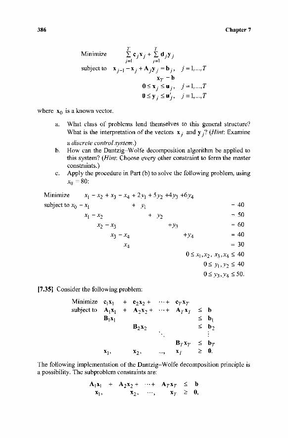
386 Chapter 7
τ τ Minimize Σ e ,-χ,- + Σ dyVy
7=1 7=1 subjectto χ ·_ι - χ ■ +Α y · =b ·, j = \,...,T
\T =b 0 < X j < u 7 - , j = l,...,T o<yy<u}, y = i,...,r
where x0 is a known vector.
a. What class of problems lend themselves to this general structure? What is the interpretation of the vectors xy and yy? (Hint: Examine
a discrete control system.) b. How can the Dantzig-Wolfe decomposition algorithm be applied to
this system? (Hint: Choose every other constraint to form the master constraints.)
c. Apply the procedure in Part (b) to solve the following problem, using x0 = 80:
Minimize χχ + x2 + χτ, + χ^ + 2γλ + 5y2 +4>>3 +6y4
subject to x0 - x{ + yx
xx-x2 + y2
x2 - x3 +y3
X3 — X4 +JV4
X4
0<
.35] Consider the following problem:
Minimize CjX] + C2X2 + —l" cT\T
subjectto AJXJ + A2x2+ ■■■+ ATxT
B,x, B2x2
Orr\rr
= 40
= 50
= 60
= 40
= 30
< 40
0< yx,y2 < 40
0 < ^ , ^ 4 < 5 0 .
< b < b, < b 2
< bT
X], x 2 , ..., x r > 0.
The following implementation of the Dantzig-Wolfe decomposition principle is a possibility. The subproblem constraints are:
A)X[ + A2x2 + —h AT\T < b x,, x2, ■·-, \T > 0,
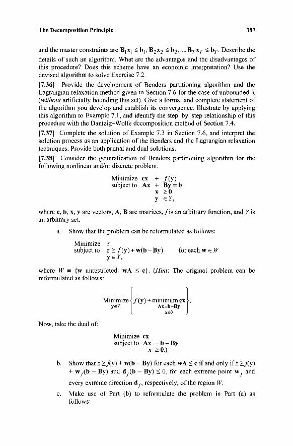
The Decomposition Principle 387
and the master constraints are B]Xj < b1; B2X2 - ^2'-'^τχτ - ^τ Describe the details of such an algorithm. What are the advantages and the disadvantages of this procedure? Does this scheme have an economic interpretation? Use the devised algorithm to solve Exercise 7.2.
[7.36] Provide the development of Benders partitioning algorithm and the Lagrangian relaxation method given in Section 7.6 for the case of unbounded X {without artificially bounding this set). Give a formal and complete statement of the algorithm you develop and establish its convergence. Illustrate by applying this algorithm to Example 7.1, and identify the step-by-step relationship of this procedure with the Dantzig-Wolfe decomposition method of Section 7.4.
[7.37] Complete the solution of Example 7.3 in Section 7.6, and interpret the solution process as an application of the Benders and the Lagrangian relaxation techniques. Provide both primal and dual solutions.
[7.38] Consider the generalization of Benders partitioning algorithm for the following nonlinear and/or discrete problem:
Minimize ex + / (y ) subject to Ax + By = b
x >0 y ey,
where c, b, x, y are vectors, A, B are matrices,/is an arbitrary function, and Y is an arbitrary set.
a. Show that the problem can be reformulated as follows:
Minimize z subject to z> / (y ) + w(b-By) for each w eW
y e F ,
where W = {w unrestricted: wA < c}. {Hint: The original problem can be reformulated as follows:
Minimize yeY
f{y) + minimum ex Ax=b-By
x>0
Now, take the dual of:
Minimize ex subject to Ax = b - By
x >0.)
b. Show that z >fiy) + w(b - By) for each wA < c if and only if z >Xy) + Wy(b - By) and dy(b - By) < 0, for each extreme point w,· and
every extreme direction d ,·, respectively, of the region W.
c. Make use of Part (b) to reformulate the problem in Part (a) as follows:
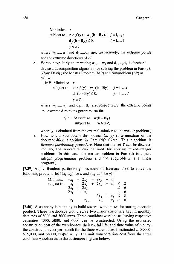
388 Chapter 7
Minimize z subjectto z > / ( y ) + wy-(b-By), j = \,...,t
d y ( b - B y ) < 0 , j = \,...,i
y e 7,
where Wi,...,wi and di,...,d^ are, respectively, the extreme points
and the extreme directions of W. d. Without explicitly enumerating W|,...,w, and dt,...,d^ beforehand,
devise a decomposition algorithm for solving the problem in Part (c). {Hint: Devise the Master Problem (MP) and Subproblem (SP) as below:
MP : Minimize z subjectto z > / ( y ) + w y (b-By) , j = \,...,t'
d 7 ( b - B y ) < 0 , j = \,...J'
yeY,
where Wj,...,w,' and d],...,d^ are, respectively, the extreme points
and extreme directions generated so far.
SP : Maximize w(b - By) subject to wA < c,
where y is obtained from the optimal solution to the master problem.) e. How would you obtain the optimal (x, y) at termination of the
decomposition algorithm in Part (d)? (Note: This algorithm is Benders partitioning procedure. Note that the set Y can be discrete, and so, the procedure can be used for solving mixed-integer problems. In this case, the master problem in Part (d) is a pure integer programming problem and the subproblem is a linear program.)
[7.39] Apply Benders partitioning procedure of Exercise 7.38 to solve the following problem [let ( (X), x2 ) be x and (x3, Χ4 ) be y] :
Minimize subject to
-x, X,
-3x ] 2x]
x\,
- 2x2 + 2x2
+ 2x2 + x2
x2>
— 3X3 — X4 + ZX3 + X4
3X3 + X4 X3, X4
< < < < >
12 6 6 8 0,
[7.40] A company is planning to build several warehouses for storing a certain product. These warehouses would serve two major customers having monthly demands of 3000 and 5000 units. Three candidate warehouses having respective capacities 4000, 5000, and 6000 can be constructed. Using the estimated construction cost of the warehouses, their useful life, and time value of money, the construction cost per month for the three warehouses is estimated as $9000, $15,000, and $8000, respectively. The unit transportation cost from the three candidate warehouses to the customers is given below:
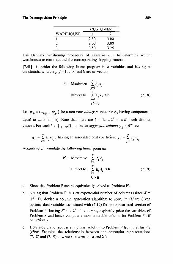
The Decomposition Principle 389
CUSTOMER WAREHOUSE 1 2 3
1 2 2.50 3.00 3.00 3.00 3.50 3.25
Use Benders partitioning procedure of Exercise 7.38 to determine which warehouses to construct and the corresponding shipping pattern.
[7.41] Consider the following linear program in n variables and having m constraints, where a , j = !,...,«, and b are w-vectors:
P : Maximize X c.-x.-7=1 n
subject to 'Σ, a.-Xj <b (7.18) 7=1 x>0.
Let w, = (w,.,...,w, ) be a non-zero binary «-vector (i.e., having components
equal to zero or one). Note that there are k = 1,...,2" - 1 = K such distinct
vectors. For each k e {\,...,K}, define an aggregate column g e Rm as:
n n g, = Σ a .w having an associated cost coefficient / = Σ c.w...
* , = ] J V * ;_[ 7 N
Accordingly, formulate the following linear program:
K P': Maximize Σ f,À,
k=\ h k
K subject to Σ g, A, <b (7.19)
k=\ k K
λ>0.
a. Show that Problem P can be equivalently solved as Problem P'.
b. Noting that Problem P' has an exponential number of columns (since K =
2" -1), devise a column generation algorithm to solve it. (Hint: Given
optimal dual variables associated with (7.19) for some restricted version of
Problem P' having K' « 2" - 1 columns, explicitly price the variables of Problem P and hence compute a most enterable column for Problem P', if one exists.)
c. How would you recover an optimal solution to Problem P from that for P'? {Hint: Examine the relationship between the constraint representations (7.18) and (7.19) to write x in terms of w and λ.)
390 Chapter 7
d. Extend the approach of Parts a-c to the case where Problem P has bounded variables of the form 0 < x. <\,j = \,...,n (possibly after scaling). (Hint:
Note that any solution x to this Problem P can be represented as a convex combination of the extreme points of the unit hypercube W = {w: 0 < w <
1} cJ?" , whose 2" extreme points are defined by all possible binary
vectors in R".)
[7.42] Consider the following pair of primal and dual linear programs P and D, where Aismx n and D is m' χ η:
P : Minimize ex D : Maximize wb + vd subject to Ax = b subject to wA + vD < c
x e X = {x : Dx > d, x > 0} w unrestricted, v > 0.
Let Problem BMP denote the Benders master problem defined by Equation (7.14).
a. Show that the dual to Problem BMP (call this DWMP) is the Dantzig-Wolfe master program given by Equations (7.1) - (7.3).
b. Now, suppose that in Problem BMP, we impose the bounds w~ < w < w+
on the w-variables, where the lower and upper bounds w~ and w+ are estimated to (possibly) capture an optimal set of values for the w-variables. Explain how this might help the Benders algorithm to converge faster to an optimal solution. (Hint: Examine the geometry of the tangential approximation or outer linearization interpretation of Benders (or the Lagrangian relaxation) procedure discussed in Section 7.6.)
c. Given the bounds in Part b, suppose that we find an optimal solution w
via Benders algorithm such that w~ < w* < w+. Show that w* is (part of) an optimal solution to Problem D.
d. In Part c, if the stated condition does not hold true, suggest how you might
adjust the bounds [w~,w+] and reiterate to optimally solve Problem D
using the Benders decomposition technique. (This is referred to as a boxstep method.)
e. For the Problem BMP in Part b to which we had added the bounding
constraints w~ < w < w+ (call this BMP'), designate y+ and y~ as the
dual variables associated with the constraints w < w + and - w < - w ~ , respectively, and write the corresponding dual problem (call this DWMP'). Compare the problems DWMP and DWMP' and comment on their relative structures.
f. Using Part e, extend the analysis of the modified Benders algorithm devised in Parts b-d to an equivalent modified implementation of the Dantzig-
The Decomposition Principle 391
Wolfe decomposition method (this is referred to as a stabilized column generation implementation).
[7.43] Consider the Problem BMP' defined in Exercise 7.42, and suppose that we further modify this to derive the following problem:
BMP+: Maximize ζ - π + δ + - π " δ " (7.20)
subject to z + w(Axy - b) < ex · fory = 1,...,/ (7.21)
w ' - π " < w < w + + 7 t + (7.22)
(z,w) unrestricted, (π+,π~) >0,
where π+ and π~ are variable vectors, and δ+ and δ~ are suitable corresponding objective coefficient vectors that penalize any deviation of w
outside the given bounds [w~,w+].
a. Discuss the relationship between Problems BMP' and BMP+. In particular, for what selection of parameter values δ+ and δ~ would BMP+ reduce to BMP'?
b. Extend your response to Parts c and d of Exercise 7.42 to the case of
Problem BMP+.
c. Associate dual variables A.-, j = l,...,t, y+ , and y~ with the respective
constraints (7.21), and the pair of bounding constraints w-π"1" < w+ and
- w - π " <-w~ in (7.22), and write the dual to Problem BMP+ (call this
DWMP+). Translate your analysis for the modified Benders approach in Part b to describe a corresponding modified Dantzig-Wolfe algorithm as
applied to Problem DWMP+. (This is a further extension of a stabilized column generation implementation with respect to that discussed in Exercise 7.42).
NOTES AND REFERENCES
1. The decomposition algorithm of this chapter is an adaptation of the Dantzig-Wolfe decomposition principle [1960, 1961]. The latter was inspired by the suggestions of Ford and Fulkerson [1958b] for solving the special case of multicommodity network flow problems.
2. The decomposition method presented in this chapter is closely associated with the concepts of generalized Lagrangian multipliers, tangential approxi-mation of the Lagrangian dual function, and the dual cutting plane algorithm, as discussed in Section 7.6. For further reading on these topics the reader may refer to Bazaraa, Sherali and Shetty [2006], Everett [1963], Geoffrion [1971], Lasdon [1970], Kelley [1960], and Zangwill
392 Chapter 7
[1969]. Exercise 7.41 describes a counterintuitive technique here to Oguz [2002], which creates an equivalent representation of a given general linear program by exponentially blowing up the number of variables and then applying column generation. This is shown to have some computational promise for the bounded-variables case.
3. In addition to the Dantzig-Wolfe and similar decomposition algorithms, the literature covers a plethora of other decomposition methods. These can be classified as price-directive and resource-directive algorithms. In the former, a direction for modifying the Lagrangian multipliers of the coupling constraints is found and then a suitable step size is taken along this direction. See, for example, Geoffrion [1970], Lasdon [1970], Grinold [1972], Balas [1966b], Held, Wolfe, and Crowder [1974], Bazaraa and Goode [1979], Minoux [1986], Lubbecke and Desrosiers [2002], and Desrosiers and Lubbecke [2005]. The resource-directive algorithms proceed by finding a direction for modifying the shares of the common resources among the subproblems and then determining the step size. The reader may refer to Geoffrion [1970, 1974], Lasdon [1970], Abadie [1963], Minoux [1986], and Guignard-Spielberg [2004].
4. In Exercise 7.38 we described the partitioning scheme of Benders [19621 that was specialized in Section 7.6. This scheme is particularly suited for solving mixed-integer programming problems.
5. For an in-depth geometric analysis of the Dantzig-Wolfe decomposition algorithm, see Todd [1983]. For implementation issues, see Ho and Loute [1981, 1983]. Birge [1985] provides some further insights into this proce-dure, and Wittrock [1985] applies it to the dual of the staircase structured problem of Exercise 7.30. (The approach sketched in Exercise 7.30 is from Glassey [1973].) For generalizations of Dantzig-Wolfe/Benders algo-rithms, see Geoffrion [1972] and Burkard et al. [1985].
6. Marsten [1975] and Marsten et al. [1975] describe the boxstep method for accelerating the convergence behavior of Benders algorithm. (Related ideas can also be used to improve Lagrangian relaxation procedures.) This has inspired duality-based concepts of stabilized column generation for markedly improving the computational behavior of column generation procedures in general, and Dantzig-Wolfe decomposition in particular. These ideas are briefly described in Exercises 7.42 and 7.43, and are discussed in greater detail in the papers by duMerle et al. [1999] and Desaulniers et al. [2001].
7. Column generation methods are also frequently combined with branch-and-price techniques for solving (specially structured) mixed-integer programming problems. The interested reader is referred to the papers by Barnhart et al. [1998] and Vanderbeck [2000], as well as to a general review paper by Wilhelm [2001].
EIGHT: COMPLEXITY OF THE SIMPLEX ALGORITHM AND POLYNOMIAL-TIME ALGORITHMS
In this chapter we discuss some fundamental computational complexity issues and theoretically efficient, that is to say, polynomial-time, algorithms for solving linear programming problems. We begin by discussing the issue of exponential versus polynomial-time algorithms based on a worst-case computational performance analysis. According to this classification scheme, the simplex algorithm is shown to be "bad," because it exhibits an exponential growth in effort on certain classes of problems as problem size increases. Fortunately, there are some average-case theoretical results that help resolve the discrepancy between the worst-case theoretical results and the observed practical efficiency of the simplex algorithm. However, there do exist theoretically efficient algorithms for linear programming problems that exhibit a growth in solution effort that is polynomial in the size of the problem. The two well-publicized algorithms of Khachian and Karmarkar fall in this category. Although Khachian's algorithm has failed to be of practical computational value, the underlying concept behind Karmarkar's algorithm is far more promising. We therefore relegate the development of Khachian's algorithm to the exercises (see Exercises 8.12-8.17), but treat Karmarkar's algorithm in detail in this chapter. We also comment on several interior point algorithmic variants that have been inspired by Karmarkar's algorithm, but that are computationally much more effective. Curiously, all of these algorithms are nonlinear approaches to linear programming problems. Although a preparation in nonlinear programming theory and algorithms will provide additional insights to the reader, we maintain a level of presentation, aided by geometric motivations, that will require a knowledge of only some basic linear algebra and calculus on the part of the reader. The reader is also encouraged to review the material in Chapter 2.
8.1 POLYNOMIAL COMPLEXITY ISSUES
As the field of Operations Research continued to develop following the birth of linear programming, a rich collection of different types of problems were intro-duced along with a host of competing solution algorithms. Consequently, there arose a need to be able to formally classify and compare problems and algorithms from the viewpoint of their computational tractability. To address this need, in the 1970s, computer scientists and operations research analysts introduced the issue of computational complexity of problems and algorithms. The idea here is to conduct an evaluation of the problem or algorithm based on its performance in a worst-case type of situation, with an aim to ascertain how difficult a problem is to solve in the worst case, or what is the growth in computational effort of an algorithm as a function of the size of the problem in the worst case. Such an analysis provides a performance guarantee for an algorithm that solves a given class of problems.
393
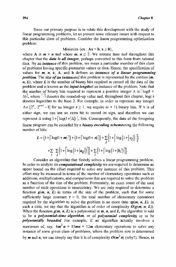
394 Chapter 8
Since our primary purpose is to relate this development with the study of linear programming problems, let us present some relevant issues with respect to this particular class of problems. Consider the linear programming optimization problem:
Minimize {ex : Ax = b, x > 0}, where A is m x « and where m, n > 2. We assume here and throughout this chapter that the data is all integer, perhaps converted to this form from rational data. By an instance of this problem, we mean a particular member of this class of problems having specific parameter values or data. Hence, the specification of values for m, n, c, A, and b defines an instance of a linear programming problem. The size of an instanceof this problem is represented by the entities (m, n, L), where L is the number of binary bits required to record all the data of the problem and is known as the input lengthof an instance of the problem. Note that the number of binary bits required to represent a positive integer Δ is l~log(l + Δ)1, where Γ1 denotes the rounded-up value and, throughout this chapter, log() denotes logarithm to the base 2. For example, in order to represent any integer
Δ Ε [2r, 2r+ -1] for an integer r > 1, we require (r + 1) binary bits. If Δ is of
either sign, we can use an extra bit to record its sign, and therefore we can
represent Δ using 1 +["logli+ |Δ|)Ί, bits. Consequently, the data of the foregoing
linear program can be recorded by a binary encoding schemeusing the following number of bits:
£ = {l + flog(l + m)l} + {l + flog(l+ii)l} + z{l + riog(l + |cJ-|)]} j
+Σ z{i+["iog(i+|a&.|)]}+z{i+[iog(i+|*/|)l}. J I
Consider an algorithm that finitely solves a linear programming problem. In order to analyze its computational complexity we are required to determine an upper bound on the effort required to solve any instance of this problem. This effort may be measured in terms of the number of elementary operations such as additions, multiplications, and comparisons that are required to solve the problem as a function of the size of the problem. Fortunately, an exact count of the total number of such operations is unnecessary. We are only required to determine a function g(m, n, L) in terms of the size of the problem, such that for some sufficiently large constant τ > 0, the total number of elementary operations required by the algorithm to solve the problem is no more than ig{m, n, L). In such a case, we say that the algorithm is of order of complexity 0(g(m, n, L)). When the function g(m, n, L) is a polynomial in m, n, and L, the algorithm is said to be a polynomial-time algorithm, or of polynomial complexity or to be polynomially bounded For example, if an algorithm actually involves a
maximum of, say, 6m n + I5mn + 12m elementary operations to solve any instance of some given class of problems, where the problem size is determined
by m and n, we can simply say that it is of complexity 0(m n) (why?). Hence, in
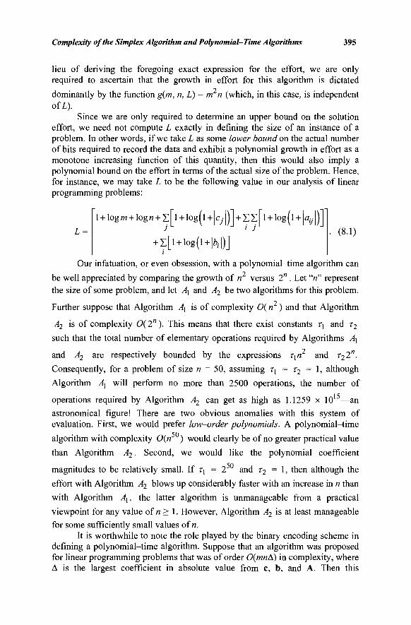
Complexity of the Simplex Algorithm and Polynomial-Time Algorithms 395
lieu of deriving the foregoing exact expression for the effort, we are only required to ascertain that the growth in effort for this algorithm is dictated
dominantly by the function g(m, n,L) = m n (which, in this case, is independent ofL).
Since we are only required to determine an upper bound on the solution effort, we need not compute L exactly in defining the size of an instance of a problem. In other words, if we take L as some lower bound on the actual number of bits required to record the data and exhibit a polynomial growth in effort as a monotone increasing function of this quantity, then this would also imply a polynomial bound on the effort in terms of the actual size of the problem. Hence, for instance, we may take L to be the following value in our analysis of linear programming problems:
L =
l + log/K + logn + x [ l + log(l + |cy|)] + Z Z [ l + log(l + |ay|)
+ Z[l + log(l + |ò;|)] (8.1)
Our infatuation, or even obsession, with a polynomial-time algorithm can
be well appreciated by comparing the growth of n versus 2n. Let "«" represent
the size of some problem, and let A\ and A2 be two algorithms for this problem.
Further suppose that Algorithm Ax is of complexity 0(n ) and that Algorithm
A2 is of complexity 0( 2" ). This means that there exist constants τ\ and τ2
such that the total number of elementary operations required by Algorithms A\
and A2 are respectively bounded by the expressions τ{η and τ22".
Consequently, for a problem of size n = 50, assuming η = r2 = 1, although
Algorithm Αγ will perform no more than 2500 operations, the number of
operations required by Algorithm A2 can get as high as 1.1259 x 10 —an
astronomical figure! There are two obvious anomalies with this system of evaluation. First, we would prefer low-order polynomials. A polynomial-time
algorithm with complexity 0(n ) would clearly be of no greater practical value
than Algorithm A2. Second, we would like the polynomial coefficient
magnitudes to be relatively small. If τ{ = 2 and τ2 — 1, then although the
effort with Algorithm A2 blows up considerably faster with an increase in n than
with Algorithm A\, the latter algorithm is unmanageable from a practical
viewpoint for any value of n > 1. However, Algorithm A2 is at least manageable
for some sufficiently small values of n. It is worthwhile to note the role played by the binary encoding scheme in
defining a polynomial-time algorithm. Suppose that an algorithm was proposed for linear programming problems that was of order 0(mnA) in complexity, where Δ is the largest coefficient in absolute value from c, b, and A. Then this
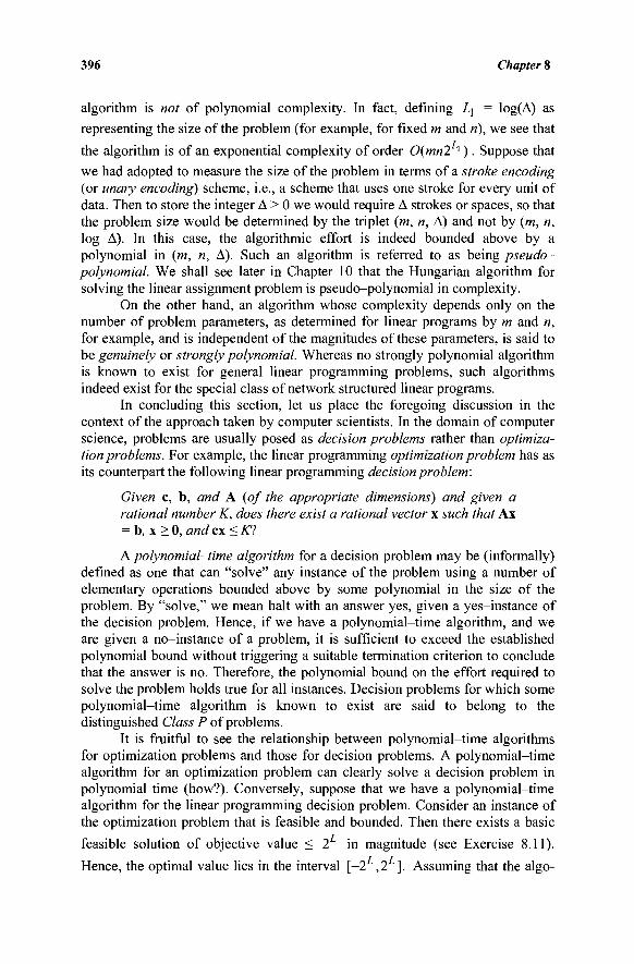
396 Chapter 8
algorithm is not of polynomial complexity. In fact, defining L\ = log(A) as representing the size of the problem (for example, for fixed m and ri), we see that the algorithm is of an exponential complexity of order 0(mn2^ ) . Suppose that we had adopted to measure the size of the problem in terms of a stroke encoding (or unary encoding) scheme, i.e., a scheme that uses one stroke for every unit of data. Then to store the integer Δ > 0 we would require Δ strokes or spaces, so that the problem size would be determined by the triplet (m, n, Δ) and not by (m, n, log Δ). In this case, the algorithmic effort is indeed bounded above by a polynomial in (m, n, Δ). Such an algorithm is referred to as being pseudo-polynomial. We shall see later in Chapter 10 that the Hungarian algorithm for solving the linear assignment problem is pseudo-polynomial in complexity.
On the other hand, an algorithm whose complexity depends only on the number of problem parameters, as determined for linear programs by m and n, for example, and is independent of the magnitudes of these parameters, is said to be genuinely or strongly polynomial. Whereas no strongly polynomial algorithm is known to exist for general linear programming problems, such algorithms indeed exist for the special class of network structured linear programs.
In concluding this section, let us place the foregoing discussion in the context of the approach taken by computer scientists. In the domain of computer science, problems are usually posed as decision problems rather than optimiza-tion problems. For example, the linear programming optimization problem has as its counterpart the following linear programming decision problem:
Given c, b, and A (of the appropriate dimensions) and given a rational number K, does there exist a rational vector x such that Ax = b, x > 0 , andcx<ICi
A polynomial-time algorithm for a decision problem may be (informally) defined as one that can "solve" any instance of the problem using a number of elementary operations bounded above by some polynomial in the size of the problem. By "solve," we mean halt with an answer yes, given a yes-instance of the decision problem. Hence, if we have a polynomial-time algorithm, and we are given a no-instance of a problem, it is sufficient to exceed the established polynomial bound without triggering a suitable termination criterion to conclude that the answer is no. Therefore, the polynomial bound on the effort required to solve the problem holds true for all instances. Decision problems for which some polynomial-time algorithm is known to exist are said to belong to the distinguished Class P of problems.
It is fruitful to see the relationship between polynomial-time algorithms for optimization problems and those for decision problems. A polynomial-time algorithm for an optimization problem can clearly solve a decision problem in polynomial time (how?). Conversely, suppose that we have a polynomial-time algorithm for the linear programming decision problem. Consider an instance of the optimization problem that is feasible and bounded. Then there exists a basic
feasible solution of objective value < 2 in magnitude (see Exercise 8.11).
Hence, the optimal value lies in the interval [-2 ,2 ]. Assuming that the algo-
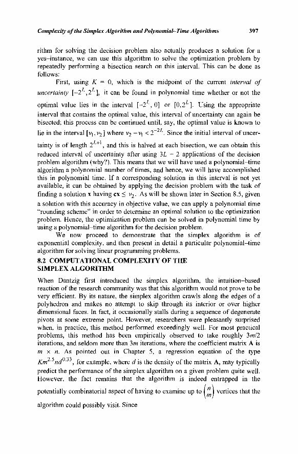
Complexity of the Simplex Algorithm and Polynomial-Time Algorithms 397
rithm for solving the decision problem also actually produces a solution for a yes-instance, we can use this algorithm to solve the optimization problem by repeatedly performing a bisection search on this interval. This can be done as follows:
First, using K = 0, which is the midpoint of the current interval of
uncertainty [-2 ,2 ], it can be found in polynomial time whether or not the
optimal value lies in the interval [-2 , 0] or [0,2 ]. Using the appropriate
interval that contains the optimal value, this interval of uncertainty can again be bisected; this process can be continued until, say, the optimal value is known to
—7 J
lie in the interval [vj, v2 ] where v2 - vj < 2 . Since the initial interval of uncer-tainty is of length 2 + , and this is halved at each bisection, we can obtain this reduced interval of uncertainty after using 3L + 2 applications of the decision problem algorithm (why?). This means that we will have used a polynomial-time algorithm a polynomial number of times, and hence, we will have accomplished this in polynomial time. If a corresponding solution in this interval is not yet available, it can be obtained by applying the decision problem with the task of finding a solution x having ex < v2. As will be shown later in Section 8.5, given a solution with this accuracy in objective value, we can apply a polynomial time "rounding scheme" in order to determine an optimal solution to the optimization problem. Hence, the optimization problem can be solved in polynomial time by using a polynomial-time algorithm for the decision problem.
We now proceed to demonstrate that the simplex algorithm is of exponential complexity, and then present in detail a particular polynomial-time algorithm for solving linear programming problems. 8.2 COMPUTATIONAL COMPLEXITY OF THE SIMPLEX ALGORITHM
When Dantzig first introduced the simplex algorithm, the intuition-based reaction of the research community was that this algorithm would not prove to be very efficient. By its nature, the simplex algorithm crawls along the edges of a polyhedron and makes no attempt to skip through its interior or over higher dimensional faces. In fact, it occasionally stalls during a sequence of degenerate pivots at some extreme point. However, researchers were pleasantly surprised when, in practice, this method performed exceedingly well. For most practical problems, this method has been empirically observed to take roughly 3m/2 iterations, and seldom more than 3m iterations, where the coefficient matrix A is m x n. As pointed out in Chapter 5, a regression equation of the type
Km ' nd ' , for example, where d is the density of the matrix A, may typically predict the performance of the simplex algorithm on a given problem quite well. However, the fact remains that the algorithm is indeed entrapped in the
potentially combinatorial aspect of having to examine up to I n vertices that the
algorithm could possibly visit. Since
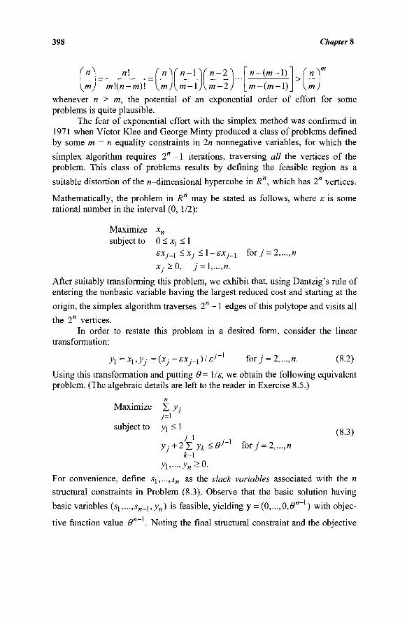
398 Chapter 8
ίη\ n\(n-\ n — (m — \)
m — (m — \) m\(n — rri)\ \m )\m-\)\m — 2/
whenever n > m, the potential of an exponential order of effort for some problems is quite plausible.
The fear of exponential effort with the simplex method was confirmed in 1971 when Victor Klee and George Minty produced a class of problems defined by some m = n equality constraints in 2n nonnegative variables, for which the simplex algorithm requires 2" -1 iterations, traversing all the vertices of the problem. This class of problems results by defining the feasible region as a
suitable distortion of the «-dimensional hypercube in R", which has 2" vertices.
Mathematically, the problem in R" may be stated as follows, where ε is some rational number in the interval (0, 1/2):
Maximize xn
subject to 0 < Xj < 1 εχ,·_ι <Xj < 1 - £Xj-\ for j = 2,..., n
Xj^O, j = \,...,n.
After suitably transforming this problem, we exhibit that, using Dantzig's rule of entering the nonbasic variable having the largest reduced cost and starting at the
origin, the simplex algorithm traverses 2" -1 edges of this polytope and visits all
the 2" vertices. In order to restate this problem in a desired form, consider the linear
transformation:
y].=xl>yj=(xj-£Xj-l)/£J'~1 foTj = 2,...,n. (8.2)
Using this transformation and putting θ= Ι/ε, we obtain the following equivalent problem. (The algebraic details are left to the reader in Exercise 8.5.)
n Maximize X y :
7=1 subject to y\ < 1
.£1 _ M (8.3)
) ' , · + 2 Σ Λ < ^ 1 for7- = 2,...,« k=l
yu...,y„>0.
For convenience, define sy,...,sn as the slack variables associated with the n
structural constraints in Problem (8.3). Observe that the basic solution having
basic variables {si,...,sn_\,yn) is feasible, yielding y = (Ο,.,.,Ο,ό'"- ) with objec-
tive function value θ"~ . Noting the final structural constraint and the objective
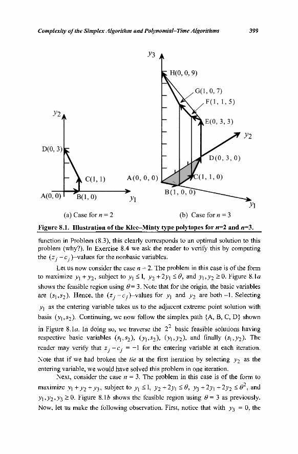
Complexity of the Simplex Algorithm and Polynomial-Time Algorithms 399
Figure 8.1. Illustration of the Klee-Minty type polytopes for n=2 and «=3.
function in Problem (8.3), this clearly corresponds to an optimal solution to this problem (why?). In Exercise 8.4 we ask the reader to verify this by computing the (z ■ - Cj )-values for the nonbasic variables.
Let us now consider the case n = 2. The problem in this case is of the form to maximize y\ + y2, subject to yx < 1, y2 + 2y\ <Θ, and y\,y2 ^ 0. Figure 8.1a shows the feasible region using θ=3. Note that for the origin, the basic variables are (sx,s2). Hence, the (z^·-c,)-values for yx and y2 are both-1. Selecting
j] as the entering variable takes us to the adjacent extreme point solution with
basis (y\,s2). Continuing, we now follow the simplex path {A, B, C, D} shown
in Figure 8.1a. In doing so, we traverse the 2 basic feasible solutions having respective basic variables (si,s2), (y\,s2), (y\,y2), and finally (s^,y2). The reader may verify that z,· -c ■ = -1 for the entering variable at each iteration.
Note that if we had broken the tie at the first iteration by selecting y2 as the
entering variable, we would have solved this problem in one iteration.
Next, consider the case n = 3. The problem in this case is of the form to
maximize y\+y2+yi,, subject to y\ < 1, y2 +2yx < Θ, y^ +2y^ +2y2 ^ θ , and
y\,y2,y-i ^0. Figure 8.1 b shows the feasible region using 0 = 3 as previously. Now, let us make the following observation. First, notice that with j 3 = 0, the
400 Chapter 8
extreme points in the (yx, y2 ) space obtained for the case n = 2 are still extreme
points in the present case; s3 is the third basic variable. The corresponding sets
of basic variables are (sx,s2,s3), (yx,s2,s3), (yx,y2,s3), and (-S], >>2,53 ). Second,
observe that in moving from each one of these bases to the next, the (z · - c,· ) -
value for the entering variable is -1 as for the case n = 2. The (z · - c )-value
for the new nonbasic variable y3 also remains at -1 throughout, since the last
component of the simplex multiplier vector cBB~ is zero for all these bases B. Hence, the simplex path {A, B, C, D} for the case n = 2 remains a simplex path for the case n = 3 under Dantzig's entering rule. Moreover, y3 remains enterable
throughout. Third, at the vertex D, we must enter y3, and because s3 and y3 can-
not both be basic, s3 must leave the basis. For the remaining iterations, y3
remains basic. Using the last equation to solve for y3 in terms of yx, y2, and s3
and eliminating y3 from the problem gives the same problem as for the case n =
2, except that the objective coefficients of yx and y2 are now - 1 . In other
words, it is as if the n = 2 problem has been changed from a maximization to a minimization problem at the end of its solution! Consequently, maintaining Dantzig's entering criterion, the simplex path simply reverses through the bases for the case n = 2, with y3 being the additional basic variable throughout. We now visit the vertices E, F, G, and H in Figure 8. lo, with respective sets of basic variables (sl,y2,y3), (y{,y2,y3), Oi ,s2 ,y3) , and (s:,s2,y3). Therefore, in solving
this problem, we have traversed 2 -1 edges and visited (all the) 2 extreme points in the process.
This is now readily generalized using an inductive argument. For example,
for the case n = 4, we first go through the set of 2 bases having basic variables (SUS2,S3,S4), (^,52,^3^4)' C V l ^ ' ^ ' ^ ) ' ( Λ , ^ ' ^ . ^ Χ ( W 2 * yì^4), {y\,y2,y^,s4), (yus2,y3,s4), and (sus2,y3,s4). This sequence is obtained by using the n = 3 case with s4 as the additional basic variable. Then, y4 enters and s4 leaves the basis, giving the set of basic variables (s^,s2, 73,^4). The sequence of pivots reverses with the maximization problem for the n = 3 case effectively turning into a minimization problem when y4 is held basic. We next
generate the 2 bases with basic variables (si,s2,y3,y4), (ylt s2,y3,y4),
Ο ι , ^ . Λ . ^ Χ (sx,y2,y3,y4), (sl,y2,s3,y4), (yl,y2,s3,y4), {yx, s2,s3,y4),
and (si,s2,s3,y4). This results in 2x2 =2 bases over 2 -1 pivots. The
construction of the formal inductive proof is now straightforward and is left to the reader in Exercise 8.6. It is interesting to observe that for the general case «,
all throughout the first 2"' basic feasible solutions, the variable yn remains enterable. Recall the definition of a stage from Chapter 4! Also, notice that at the
Complexity of the Simplex Algorithm and Polynomial-Time Algorithms 401
end of 2"~ pivots, the basic variables are (si,S2,—,sn_2, yn-\,yn)- If ^«-1 is entered at this pivot, then the optimum results. (This corresponds to going from E to H in Figure 8.le.) However, both yl and s„_! have zj -Cj = -1 here, and the
choice of entering y\ takes us through the reverse sequence of pivots.
Notice the exorbitant amount of effort as problem size increases. Assume
that the problem having n constraints in In nonnegative variables requires 0.25w elementary operations per pivot, and that each operation takes one nanosecond
(10~ sec) to perform. Then, the estimated computational effort for n = 50 is
22.3 years; for n = 60 it is over 328 centuries! One may argue that the simplex algorithm did have an opportunity to solve the foregoing problem in one iteration. In fact, by scaling the columns, for example, using the transformation
Yi = 2~' yt, we can eliminate the ties in the entering criterion at the first iteration
and thereby solve the problem in one iteration unarguably. Observe also that the rule of entering the variable that gives the maximum improvement in the objective function value also solves this problem unambiguously in one iteration. Moreover, this criterion is invariant with respect to scaling and problem representation, since it is intimately connected with the structure of the polytope itself. In 1973, however, Robert Jeroslow exhibited the existence of problem classes that yield an exponential effort with the maximum-improvement entering criterion as well. In fact, for some fixed integer r > 1, if one were to perform all r next pivots, and select the r-pivot simplex path that gives the best improvement in objective value, then the algorithm would still exhibit an exponential trend on some classes of problems. The root of the problem is therefore in the myopic or local viewpoint of the simplex algorithm whereby decisions are based on the local combinatorial structure of the polytope, and where the motion is restricted to an edge path.
8.3 KHACHIAN'S ELLIPSOID ALGORITHM
Confronted with the exponential worst-case behavior of the simplex algorithm, the question of whether there existed a polynomial-time algorithm for solving linear programming problems remained open until 1979, when it was answered affirmatively by L. G. Khachian. Khachian proposed a polynomial-time algorithm for determining a solution (if one exists) to the open set of linear inequalities S = {x : Gx < g}, where G is r x q with r and q > 2, and where G and g have all integer components. This algorithm either finds a solution in S, if one exists, or else concludes that S is empty. Its basic mode of operation is as follows:
First, the method defines a ball or sphere in Rq, centered at the origin and having a radius that is large enough to encompass a sufficiently large volume of S, assuming that S is nonempty. If the center of this ball is in S, then the algorithm terminates. Otherwise, the method proceeds to construct a suitable sequence of ellipsoids that are monotonically shrinking in volume, but all of which contain the region of S that was captured by the initial ball. Whenever the center of any ellipsoid is found to lie in S, the algorithm terminates. The principal
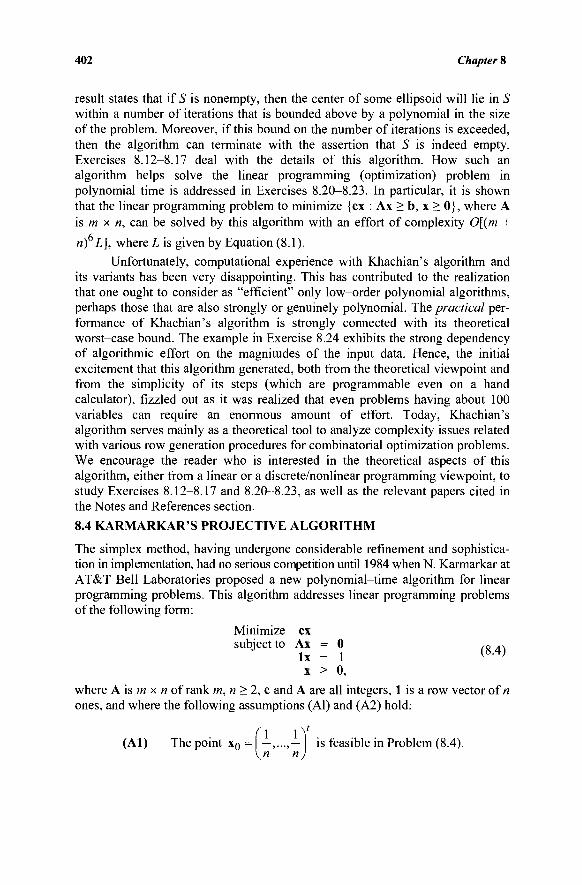
402 Chapter 8
result states that if S is nonempty, then the center of some ellipsoid will lie in S within a number of iterations that is bounded above by a polynomial in the size of the problem. Moreover, if this bound on the number of iterations is exceeded, then the algorithm can terminate with the assertion that S is indeed empty. Exercises 8.12-8.17 deal with the details of this algorithm. How such an algorithm helps solve the linear programming (optimization) problem in polynomial time is addressed in Exercises 8.20-8.23. In particular, it is shown that the linear programming problem to minimize {ex : Ax > b, x > 0}, where A is m x n, can be solved by this algorithm with an effort of complexity 0[(m +
ri) L], where L is given by Equation (8.1).
Unfortunately, computational experience with Khachian's algorithm and its variants has been very disappointing. This has contributed to the realization that one ought to consider as "efficient" only low-order polynomial algorithms, perhaps those that are also strongly or genuinely polynomial. The practical per-formance of Khachian's algorithm is strongly connected with its theoretical worst-case bound. The example in Exercise 8.24 exhibits the strong dependency of algorithmic effort on the magnitudes of the input data. Hence, the initial excitement that this algorithm generated, both from the theoretical viewpoint and from the simplicity of its steps (which are programmable even on a hand calculator), fizzled out as it was realized that even problems having about 100 variables can require an enormous amount of effort. Today, Khachian's algorithm serves mainly as a theoretical tool to analyze complexity issues related with various row generation procedures for combinatorial optimization problems. We encourage the reader who is interested in the theoretical aspects of this algorithm, either from a linear or a discrete/nonlinear programming viewpoint, to study Exercises 8.12-8.17 and 8.20-8.23, as well as the relevant papers cited in the Notes and References section.
8.4 KARMARKAR'S PROJECTIVE ALGORITHM
The simplex method, having undergone considerable refinement and sophistica-tion in implementation, had no serious competition until 1984 when N. Karmarkar at AT&T Bell Laboratories proposed a new polynomial-time algorithm for linear programming problems. This algorithm addresses linear programming problems of the following form:
Minimize ex subject to Ax = 0 ÌO ,s
lx = 1 ( 8-4 )
x > 0,
where A is m x n of rank m, n > 2, c and A are all integers, 1 is a row vector of « ones, and where the following assumptions (Al) and (A2) hold:
(\ lY (Al) The point x0 = —,...,— is feasible in Problem (8.4).
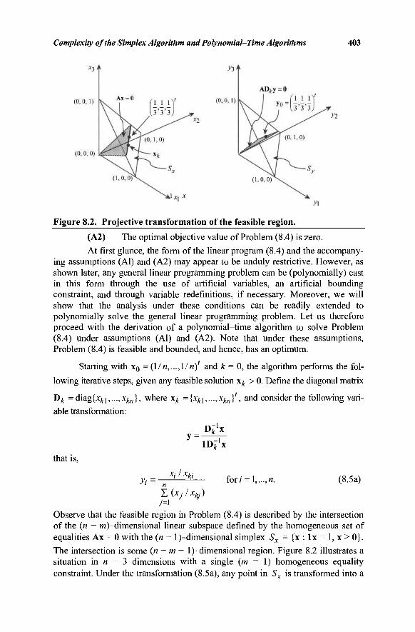
Complexity of the Simplex Algorithm and Polynomial-Time Algorithms 403
Figure 8.2. Projective transformation of the feasible region.
(A2) The optimal objective value of Problem (8.4) is zero.
At first glance, the form of the linear program (8.4) and the accompany-ing assumptions (Al) and (A2) may appear to be unduly restrictive. However, as shown later, any general linear programming problem can be (polynomially) cast in this form through the use of artificial variables, an artificial bounding constraint, and through variable redefinitions, if necessary. Moreover, we will show that the analysis under these conditions can be readily extended to polynomially solve the general linear programming problem. Let us therefore proceed with the derivation of a polynomial-time algorithm to solve Problem (8.4) under assumptions (Al) and (A2). Note that under these assumptions, Problem (8.4) is feasible and bounded, and hence, has an optimum.
Starting with x0 = (1/«,...,l/«)' and k = 0, the algorithm performs the fol-
lowing iterative steps, given any feasible solution x^ > 0. Define the diagonal matrix
D^ = axag{xk\,...,xkn}, where x^ = {xkl,...,x/m}1, and consider the following vari-able transformation:
Dl 'x y = —-—
ID*1* that is,
yt= nXi'Xki fori=l,...,«. (8.5a)
Observe that the feasible region in Problem (8.4) is described by the intersection of the (n - w)-dimensional linear subspace defined by the homogeneous set of equalities Ax = 0 with the (n - l)-dimensional simplex Sx = {x : lx = 1, x > 0}.
The intersection is some (n- m— l)-dimensional region. Figure 8.2 illustrates a situation in n = 3 dimensions with a single (m = 1) homogeneous equality constraint. Under the transformation (8.5a), any point in Sx is transformed into a
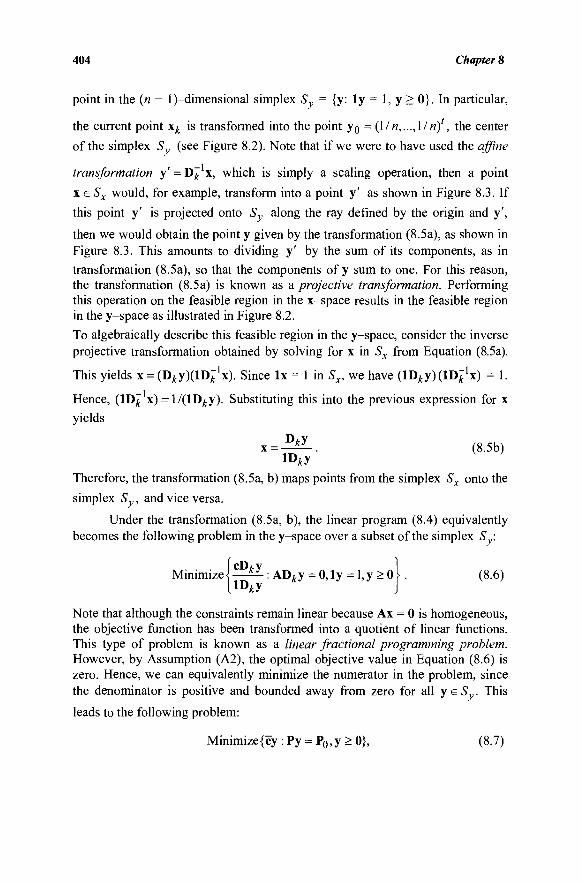
404 Chapter 8
point in the (n - l)-dimensional simplex Sy = {y: ly = 1, y > 0}. In particular,
the current point x^ is transformed into the point y0 = (1/«,..., 1/w)', the center
of the simplex Sy (see Figure 8.2). Note that if we were to have used the affine
transformation y' = D^ x, which is simply a scaling operation, then a point
x e Sx would, for example, transform into a point y' as shown in Figure 8.3. If
this point y' is projected onto Sy along the ray defined by the origin and y',
then we would obtain the point y given by the transformation (8.5a), as shown in Figure 8.3. This amounts to dividing y' by the sum of its components, as in
transformation (8.5a), so that the components of y sum to one. For this reason, the transformation (8.5a) is known as a projective transformation. Performing this operation on the feasible region in the x-space results in the feasible region in the y-space as illustrated in Figure 8.2.
To algebraically describe this feasible region in the y-space, consider the inverse projective transformation obtained by solving for x in Sx from Equation (8.5a).
This yields x = (D^yXlD^'x). Since lx = 1 in Sx, we have (lD/ty)(lD^1x) = 1.
Hence, (1D^ x) = l/(lD^y). Substituting this into the previous expression for x
yields
(8.5b) iD*y
Therefore, the transformation (8.5a, b) maps points from the simplex Sx onto the
simplex Sy, and vice versa.
Under the transformation (8.5a, b), the linear program (8.4) equivalently becomes the following problem in the y-space over a subset of the simplex Sy:
Minimize \ ^ 1 : AD^y = 0,ly = 1, y > 0 1 . (8.6) l 1 D * y J
Note that although the constraints remain linear because Ax = 0 is homogeneous, the objective function has been transformed into a quotient of linear functions. This type of problem is known as a linear fractional programming problem. However, by Assumption (A2), the optimal objective value in Equation (8.6) is zero. Hence, we can equivalently minimize the numerator in the problem, since the denominator is positive and bounded away from zero for all y e Sy. This
leads to the following problem:
Minimize{cy:Py = P0,y > 0}, (8.7)
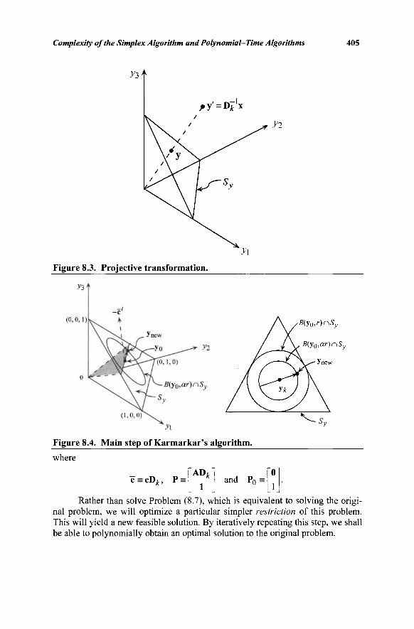
Complexity of the Simplex Algorithm and Polynomial-Time Algorithms 405
Figure 8.3. Projective transformation.
Figure 8.4. Main step of Karmarkar's algorithm.
B(y0,r)nSy
B(y0,ar)nSy
where
c ^ c D u P . AD,
1 and Pn =
Rather than solve Problem (8.7), which is equivalent to solving the origi-nal problem, we will optimize a particular simpler restriction of this problem. This will yield a new feasible solution. By iteratively repeating this step, we shall be able to polynomially obtain an optimal solution to the original problem.
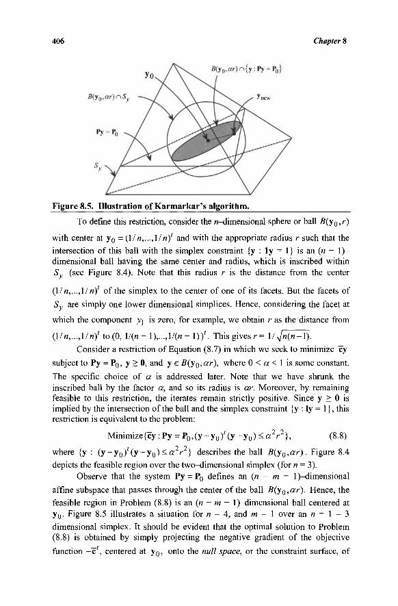
406 Chapter 8
Figure 8.5. Illustration of Karmarkar's algorithm.
To define this restriction, consider the «-dimensional sphere or ball 5(yo, r)
with center at y0 = (ì/η,...,Ι/ή)' and with the appropriate radius r such that the intersection of this ball with the simplex constraint {y : ly = 1} is an (n - 1)-dimensional ball having the same center and radius, which is inscribed within Sy (see Figure 8.4). Note that this radius r is the distance from the center
(l/n,...,l/n)' of the simplex to the center of one of its facets. But the facets of
Sy are simply one lower dimensional simplices. Hence, considering the facet at
which the component y^ is zero, for example, we obtain r as the distance from
(1/«,...,l/«)r to (0, 1 / ( / J - 1 ) , . . . , 1 / ( M - 1 ) ) ' . This gives r= l/yjn(n-l).
Consider a restriction of Equation (8.7) in which we seek to minimize cy
subject to Py = PQ, y > 0, and y e B(y0,ar), where 0 < a < 1 is some constant.
The specific choice of a is addressed later. Note that we have shrunk the inscribed ball by the factor a, and so its radius is ar. Moreover, by remaining feasible to this restriction, the iterates remain strictly positive. Since y > 0 is implied by the intersection of the ball and the simplex constraint {y : ly = 1}, this restriction is equivalent to the problem:
Minimize{cy : Py = P0,(y - y 0 ) ' ( y - y 0 ) * a2r2}, (8.8)
where {y : (y-yo) ( y ~ y o ) - a r } describes the ball B(yQ,ar). Figure 8.4 depicts the feasible region over the two-dimensional simplex (for n = 3).
Observe that the system Py = P0 defines an (» - m - l)-dimensional
affine subspace that passes through the center of the ball B(yQ,ar). Hence, the feasible region in Problem (8.8) is an (n - m - l)-dimensional ball centered at y0. Figure 8.5 illustrates a situation for n = 4, and m = 1 over an n - 1 = 3
dimensional simplex. It should be evident that the optimal solution to Problem (8.8) is obtained by simply projecting the negative gradient of the objective
function - c ' , centered at y0, onto the null space, or the constraint surface, of
Complexity of the Simplex Algorithm and Polynomial—Time Algorithms 407
Py = P0, and then moving from y0 along this projected direction to the
boundary of the ball B(y0,ar). (See Figures 8.4 and 8.5.) Observe that the
simplicity of this solution process is a consequence of the fact that we are optimizing a linear function over a ball, and that we are currently located at the
center of this ball. Denoting the projection of the gradient vector 'c' as (the column vector) c„ and the optimum to Problem (8.8) as yn e w, we get
C P
ynew ^ Ο - ^ Ϊ Γ Ί Ϊ · (8-9a) IM
[Note that if c„ = 0, then any feasible solution is optimal (why?), and we may
terminate with x^ as an optimal solution to Problem (8.4).] In order to calculate c„, observe that since c lies on the constraint
surface of Py = P0, the vector (c' - c „ ) is contained in the space spanned by the
gradients to Py =P0 . Hence, there exists a vector w such that P'w =Έ* - c _ .
Multiplying both sides by P, we get PP'w = Pc1, because Pc^ = 0 by definition.
Noting that A is of full row rank and that x^ > 0, the square matrix PP' is
invertible (see Exercise 8.25). This yields w = (PP')~ Vcl. Hence, we have
cp = ~c' - P'w given as
CP I - P ' ( P P ' ) - 1 p l c ' . (8.9b)
In Exercise (8.26), we ask the reader to use an alternative approach to show that the optimal solution to Problem (8.8) is given by Equations (8.9a, b). We remark here that the solution w is the solution to the least-squares problem
2 of minimizing P'w over w E R^m+ ' (see Exercise 8.27). Hence, in lieu of
explicitly computing c„ using Equation (8.9b), we may obtain c„ by deriving a
solution w to this problem by using any nonlinear search method, and then
setting c = c' - P ' w . In either case, the formula (8.9b) gives c„.
Given ynew in Equation (8.9a), the corresponding revised vector χ^+1 in
the x-space is obtained via the inverse transformation (8.5b) as
% . ^ . (8-10)
Observe that ynew > 0 since it lies in the interior of the (n - l)-dimensional
sphere inscribed in Sy. Hence, x i + 1 > 0 in Equation (8.10). This completes one
iteration. The process may now be repeated after incrementing k by one. As shown in Section 8.5, the objective value in Problem (8.4) of the sequence of
408 Chapter 8
iterates thus generated approaches the optimal objective value of zero in the limit as k -> oo, although not necessarily monotonically. Hence, for practical purposes, this process may be terminated when the objective value gets suffi-ciently close to zero.
For theoretical purposes, consider the following lower bound L on the input length for Problem (8.4):
L = l + log(l + |cy- max |) + log(|detmax|)
where c,· max is the largest numerical value of any cost coefficient c,·, and
|detmax| is the largest numerical value of the determinant of any basis for Prob-lem (8.4). It follows from a property of the determinants stated in Exercise 8.9 that L is indeed a lower bound on the input length for Problem (8.4), since
log(|detmax|) < log(l + ffi) + £;Z/k)g(l + U.. ). (Note that an alternative, although
larger, lower bounding value of L is given by replacing log(|detmax|) with the
latter term, as illustrated in Example 8.2.) In the next section, we shall demonstrate that by using a value of a = (n - l)/3«, the algorithm produces a
solution of objective value smaller than 2~ within lOnL iterations, with an
overall effort of polynomial complexity 0(n ' L). Once this occurs, an exact
extreme point optimal solution to Problem (8.4) may be obtained via the following polynomial-time procedure.
Starting with the final iterate \k obtained with objective value cxk < 2~L,
this procedure finds an extreme point solution with at least as good an objective value using the following method known as a purification scheme. If n linearly independent constraints are binding at x^, then it is already a basic feasible
solution. Otherwise, there exists a direction d Φ 0 lying in the null space of the binding constraints, that is, satisfying the homogeneous equality system corresponding to the binding constraints. The method now moves the current iterate along the direction d if cd < 0, and along the direction -d otherwise, until some constraint blocks any further motion by feasibility considerations. This motion must be blocked because the feasible region is bounded. Note that at the
new solution, the objective value is no more than cx^ < 2~ and at least one
additional linearly independent constraint is binding. Proceeding in this fashion, a basic feasible solution x to Problem (8.4) can be obtained having an objective
value strictly less than 2~ .
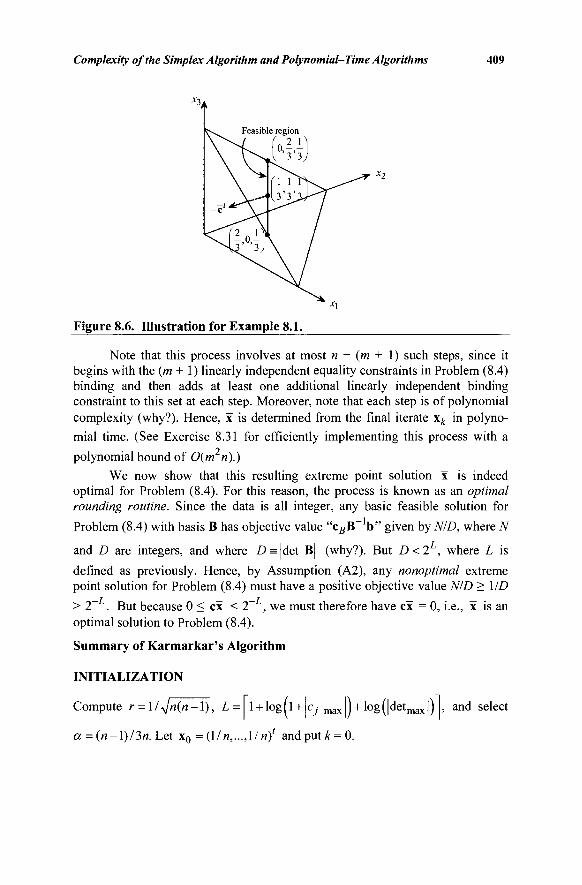
Complexity of the Simplex Algorithm and Polynomial-Time Algorithms 409
*3
Feasible region
'41,
Figure 8.6. Illustration for Example 8.1.
Note that this process involves at most n - (m + 1) such steps, since it begins with the (m + 1) linearly independent equality constraints in Problem (8.4) binding and then adds at least one additional linearly independent binding constraint to this set at each step. Moreover, note that each step is of polynomial complexity (why?). Hence, x is determined from the final iterate x^ in polyno-mial time. (See Exercise 8.31 for efficiently implementing this process with a polynomial bound of 0(m «).)
We now show that this resulting extreme point solution x is indeed optimal for Problem (8.4). For this reason, the process is known as an optimal rounding routine. Since the data is all integer, any basic feasible solution for
Problem (8.4) with basis B has objective value "c#B~ b " given by NID, where N
and D are integers, and where D = |det B| (why?). But D < 2 , where L is
defined as previously. Hence, by Assumption (A2), any nonoptimal extreme point solution for Problem (8.4) must have a positive objective value NID > \ID
> 2~ . But because 0 < ex < 2" , we must therefore have ex = 0, i.e., x is an optimal solution to Problem (8.4).
Summary of Karmarkar's Algorithm
INITIALIZATION
Compute r = l/yjn(n-l), L= l + logll + \cj max ) + log(|detmax|) , and select
a = («- l ) /3«. Let x0 = (!/«,.. . ,!/«/ and put k = 0.
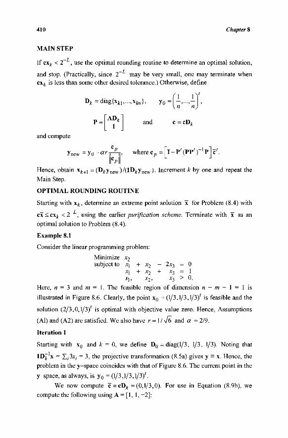
410 Chapter 8
MAIN STEP
If cx^ < 2" , use the optimal rounding routine to determine an optimal solution,
and stop. (Practically, since 2~ may be very small, one may terminate when c\k is less than some other desired tolerance.) Otherwise, define
Ok=diag{xk],...,xkn}, y 0 = |
~ADt
1 P '
n
'k and c = cDj.
and compute
vnew ■y0-ar^-r where c„ = Γ ΐ - Ρ ' ( Ρ Ρ ' ) _ 1 Ρ CP
Hence, obtain χ^+[ =(O)cynev/)/(lOjcynew). Increment k by one and repeat the
Main Step.
OPTIMAL ROUNDING ROUTINE
Starting with \k, determine an extreme point solution x for Problem (8.4) with
ex < cx^ < 2~ , using the earlier purification scheme. Terminate with x as an
optimal solution to Problem (8.4).
Example 8.1
Consider the linear programming problem:
Minimize x2
subject to X\ + x2 - 2x3 = 0 X] + X2 + X3 = 1
Χχ, Xji X^ — (J·
Here, n = 3 and m = 1. The feasible region of dimension n - m - 1 = 1 is
illustrated in Figure 8.6. Clearly, the point x0 = (1/3,1/3,1/3)' is feasible and the
solution (2/3,0,1/3)' is optimal with objective value zero. Hence, Assumptions
(Al) and (A2) are satisfied. We also have r = 1 / Λ/6 and a = 2/9.
Iteration 1
Starting with x0 and k = 0, we define D0 = diag(l/3, 1/3, 1/3). Noting that
1D^ x = Σ;3χ; = 3, the projective transformation (8.5a) gives y = x. Hence, the
problem in the y-space coincides with that of Figure 8.6. The current point in the
y-space, as always, is y0 = (1/3,1/3,1/3)'.
We now compute ~c=cOk =(0,1/3,0). For use in Equation (8.9b), we
compute the following using A = [1, 1,-2]:
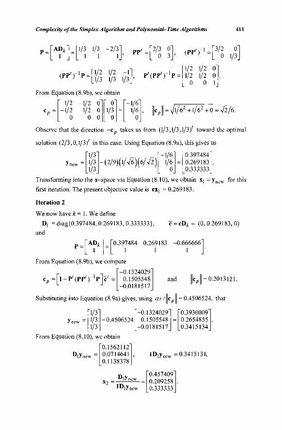
Complexity of the Simplex Algorithm and Polynomial-Time Algorithms 411
P = AD* 1
1/3 1/3 -2/3" 1 1 1
pp ' '2/3 0" 0 3
(ΡΡ'Γ1 '3/2 0' 0 1/3
(PP')_ 1P = 1/2 1/2 -1 1/3 1/3 l/3_
P ' (PP') _ 1P = 1/2 1/2 0" 1/2 1/2 0
0 0 1
From Equation (8.9b), we obtain
1/2 1/2
0
-1/2 0" 1/2 0
0 0
0" 1/3
0 =
Γ-1/6Ί 1/6
0 |cp I = Vl/62+l/62+0 = V2/6.
Observe that the direction -c„ takes us from (1/3,1/3,1/3)' toward the optimal
solution (2/3,0,1/3)' in this case. Using Equation (8.9a), this gives us
1/3 1/3 1/3
-(2/9)(l/V6-)(6/V2~) Γ-1/6Ί
1/6 0
= Γ0.397484" 0.269183 0.333333
Transforming into the x-space via Equation (8.10), we obtain Xj = ynew for this
first iteration. The present objective value is cxj = 0.269183.
Iteration 2
We now have k = 1. We define
Ό{ =diag {0.397484, 0.269183,0.333333}, c=cD* = (0,0.269183,0) and
P = AD* 1
0.397484 0.269183 -0.666666 1 1 1
From Equation (8.9b), we compute
i-p^pp'r 'pV = 0.1324029 0.1505548 0.0181517
and c J =0.2013121.
Substituting into Equation (8.9a) gives, using ari c J = 0.4506524, that
1/3 1/3 1/3
0.4506524 ynew
From Equation (8.10), we obtain
D i y n e w
-0.1324029 0.1505548
-0.0181517
0.3930009 0.2654855 0.3415134
0.1562112 0.0714641 0.1138378
x, = Diy„ l D i y lJnew
IDtfnew =0.3415131,
0.457409 0.209258 0.333333
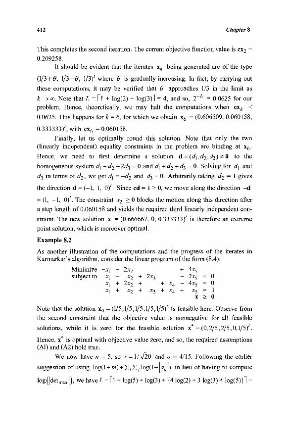
412 Chapter 8
This completes the second iteration. The current objective function value is cx2 =
0.209258. It should be evident that the iterates xk being generated are of the type
(1/3 + 6», 1/3-0, 1/3)' where Θ is gradually increasing. In fact, by carrying out
these computations, it may be verified that Θ approaches 1/3 in the limit as
k -> oo. Note that L = [Ί + log(2) + log(3)l = 4, and so, 2~L = 0.0625 for our
problem. Hence, theoretically, we may halt the computations when cxA <
0.0625. This happens for k=6, for which we obtain x6 = (0.606509, 0.060158,
0.333333)', with cx6 =0.060158.
Finally, let us optimally round this solution. Note that only the two (linearly independent) equality constraints in the problem are binding at x6.
Hence, we need to first determine a solution d = (di,d2,d^)^ 0 to the
homogeneous system d\ + d2 -2c/3 = 0 and di+d2+djl =0 . Solving for d\ and
i/3 in terms of d2, we get d\ = -d2 and d^ = 0. Arbitrarily taking d2 = 1 gives
the direction d = (-1, 1, 0)'. Since cd = 1 > 0, we move along the direction -d
= (1, - 1 , 0)'. The constraint x2 > 0 blocks the motion along this direction after
a step length of 0.060158 and yields the required third linearly independent con-
straint. The new solution x = (0.666667, 0, 0.333333)' is therefore an extreme
point solution, which is moreover optimal.
Example 8.2
As another illustration of the computations and the progress of the iterates in Karmarkar's algorithm, consider the linear program of the form (8.4):
Minimize -X] - 2x2 + 4x5
subject to x\ — %2 + 2*3 - 2x5 = 0 X] + 2x2 + + x4 - 4x5 = 0 Xj 4- X2 + X3 + X4 + X5 = 1
x > 0.
Note that the solution x0 =(1/5,1/5,1/5,1/5,1/5)' is feasible here. Observe from
the second constraint that the objective value is nonnegative for all feasible
solutions, while it is zero for the feasible solution x* =(0,2/5,2/5,0,1/5)'.
Hence, x* is optimal with objective value zero, and so, the required assumptions (Al) and (A2) hold true.
We now have n = 5, so r = l/V20 and a = 4/15. Following the earlier
suggestion of using log(l + w) + X;Z/log(l+ a,·, ) in lieu of having to compute
log(|detmax |), we have L = Γΐ + log(5) + log(3) + {4 log(2) + 3 log(3) + log(5)}l =
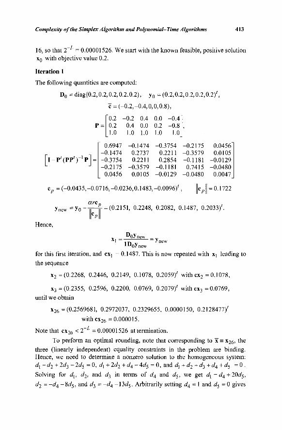
Complexity of the Simplex Algorithm and Polynomial-Time Algorithms 413
16, so that 2 = 0.00001526. We start with the known feasible, positive solution x0 with objective value 0.2.
Iteration 1
The following quantities are computed:
D0 = diag{0.2,0.2,0.2,0.2,0.2}, y0 = (0.2,0.2,0.2,0.2,0.2)',
c = (-0.2,-0.4,0,0,0.8),
0.2 -0.2 0.4 0.0 -0.4^ P = 0.2 0.4 0.0 0.2 -0.8
1.0 1.0 1.0 1.0 1.0
0.6947 -0.1474 -0.3754 -0.2175 0.0456 -0.1474 0.2737 0.2211 -0.3579 0.0105 -0.3754 0.2211 0.2854 -0.1181 -0.0129 -0.2175 -0.3579 -0.1181 0.7415 -0.0480 0.0456 0.0105 -0.0129 -0.0480 0.0047
I - P ' ( P P ' ) _ 1 P
c = (-0.0435,-0.0716,-0.0236,0.1483,-0.0096)' : : 0.1722
arc. : v 0 ' : (0.2151, 0.2248, 0.2082, 0.1487, 0.2033)'.
Hence, Doyn
1 1 Ι Λ * 11CW
1Doynew for this first iteration, and cxj = 0.1487. This is now repeated with Xj leading to the sequence
x 2 = (0.2268, 0.2446, 0.2149, 0.1078, 0.2059)' with cx2 = 0.1078,
x 3 = (0.2355, 0.2596, 0.2200, 0.0769, 0.2079)' with cx3 =0.0769, until we obtain
x 2 6 = (0.2569681, 0.2972037, 0.2329655, 0.0000150, 0.2128477)'
withcx26 =0.000015.
Note that cx26 < 2~L = 0.00001526 at termination.
To perform an optimal rounding, note that corresponding to x = x26, the
three (linearly independent) equality constraints in the problem are binding. Hence, we need to determine a nonzero solution to the homogeneous system: dx-d2 + 2^3 - 2d5 = 0, di + 2d2 +d4- 4d5 = 0, and dx+d2+d-i+d4+d5 = 0 . Solving for d\, d2, and i/3 in terms of d4 and d5, we get <ή =d4+20d5, d2 = -d4 - 8i/5, and i/3 = -d4 -13d5. Arbitrarily setting d4 = 1 and d5 = 0 gives
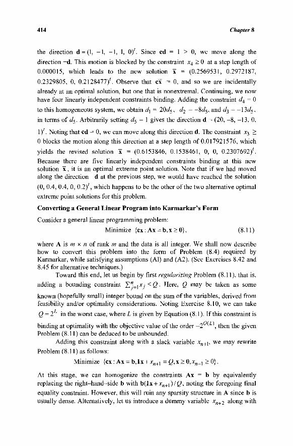
414 Chapter 8
the direction d = (1, - 1 , - 1 , 1, 0)'. Since cd = 1 > 0, we move along the
direction -d. This motion is blocked by the constraint x4 > 0 at a step length of
0.000015, which leads to the new solution x = (0.2569531, 0.2972187,
0.2329805, 0, 0.2128477)'. Observe that ex = 0, and so we are incidentally
already at an optimal solution, but one that is nonextremal. Continuing, we now
have four linearly independent constraints binding. Adding the constraint d4 = 0
to this homogeneous system, we obtain d\ = 20d5, of2 = ~8i/5, and d^ = -I3d5,
in terms of d5. Arbitrarily setting d5 = 1 gives the direction d = (20, -8 , -13, 0,
1 )'. Noting that cd = 0, we can move along this direction d. The constraint x3 >
0 blocks the motion along this direction at a step length of 0.017921576, which
yields the revised solution x = (0.6153846, 0.1538461, 0, 0, 0.2307692)'.
Because there are five linearly independent constraints binding at this new solution x, it is an optimal extreme point solution. Note that if we had moved along the direction -d at the previous step, we would have reached the solution
(0, 0.4, 0.4, 0, 0.2)', which happens to be the other of the two alternative optimal
extreme point solutions for this problem.
Converting a General Linear Program into Karmarkar's Form
Consider a general linear programming problem: Minimize {ex: Ax = b ,x>0}, (8.11)
where A is m x n of rank m and the data is all integer. We shall now describe how to convert this problem into the form of Problem (8.4) required by Karmarkar, while satisfying assumptions (Al) and (A2). (See Exercises 8.42 and 8.45 for alternative techniques.)
Toward this end, let us begin by first regularizing Problem (8.11), that is,
adding a bounding constraint X"-^x<Q. Here, Q may be taken as some
known (hopefully small) integer bound on the sum of the variables, derived from feasibility and/or optimality considerations. Noting Exercise 8.10, we can take
Q = 2 in the worst case, where L is given by Equation (8.1). If this constraint is
binding at optimality with the objective value of the order -2 ' ', then the given Problem (8.11) can be deduced to be unbounded.
Adding this constraint along with a slack variable xn+\, we may rewrite
Problem (8.11) as follows: Minimize {ex : Ax = b,lx + xn+l = Q, x > 0,xn+l > 0}.
At this stage, we can homogenize the constraints Ax = b by equivalently replacing the right-hand-side b with b(i\ + xn+l)/Q, noting the foregoing final equality constraint. However, this will ruin any sparsity structure in A since b is usually dense. Alternatively, let us introduce a dummy variable xn+2 along with
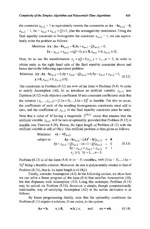
Complexity of the Simplex Algorithm and Polynomial-Time Algorithms 415
the constraint xn+2 = 1 to equivalently rewrite the constraints as Ax - bx„+2 = 0,
xn+2 = 1, lx + xn+] +x„+2 = 2 + U plus the nonnegativity restrictions. Using the
final equality constraint to homogenize the constraint xn+2 = 1, we can equiva-
lently write the problem as follows:
Minimize {ex : Ax - bx„+2 = 0, lx + x„+1 - Qxn+2 = 0,
lx + x„+1 +xn+2 = ( β + 1),χ>0,χ„+1 >0,x„+2 >0}.
Next, let us use the transformation x- = ( β + 1)>\, j = 1,...,« + 2, in order to
obtain unity as the right-hand-side of the final equality constraint above and hence derive the following equivalent problem:
Minimize {cy:Ay-by„+2 = 0,\y + yn+x -Qyn+2 =Q,ly + yn+l +yn+2 =1,
y>0,7„+ 1>0, j ;„+ 2>0}.
The constraints in Problem (8.12) are now of the form in Problem (8.4). In order to satisfy Assumption (Al), let us introduce an artificial variable yn+i into Equation (8.12) with objective coefficient Mand constraint coefficients such that the solution (yi,...,yn+i)-[l/(n + 3),...,\/(n + 3)]t is feasible. For this to occur, the coefficients of each of the resulting homogeneous constraints must add to zero, and the coefficient of yn+$ in the final equality constraint must be unity.
Note that a value of M having a magnitude 2 ^ ' exists that ensures that the artificial variable j>„+3 will be zero at optimality, provided that Problem (8.12) is
feasible (see Exercise 8.28). Hence, the input length of Problem (8.12) with the artificial variable is still of 0(L). This artificial problem is then given as follows:
Minimize cy + Μγη+^
subject to Ay-bj>„+2-[Al'-b]j>„+3 = 0 iy + + i - 2 y „ + 2 - ( « + i - 0 ^ + 3 = o (8.13)
ly+yn+i+yn+2+yn+3 = l
yj >0, V/ = l,...,« + 3.
Problem (8.13) is of the form (8.4) in (n + 3) variables, with [l/(n + 3),...,l/(« +
3)]' being a feasible solution. Moreover, its size is polynomially related to that of
Problem (8.11), that is, its input length is of 0(L). Finally, consider Assumption (A2). In the following section, we show how
we can solve a linear program of the form (8.4) that satisfies Assumption (Al), but that dispenses with Assumption (A2). Using this technique, Problem (8.11) may be solved via Problem (8.13). However, a simple, though computationally inadvisable, way of satisfying Assumption (A2) in the earlier derivation is as follows.
By linear programming duality, note that the optimality conditions for Problem (8.11) require a solution, if one exists, to the system
Ax = b, x > 0, wA<c, and cx = wb. (8.14)
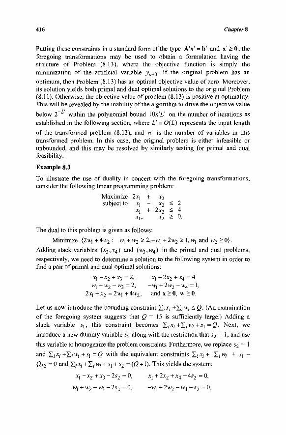
416 Chapter 8
Putting these constraints in a standard form of the type AY = b' and x' > 0, the foregoing transformations may be used to obtain a formulation having the structure of Problem (8.13), where the objective function is simply the minimization of the artificial variable y„+j. If the original problem has an
optimum, then Problem (8.13) has an optimal objective value of zero. Moreover, its solution yields both primal and dual optimal solutions to the original Problem (8.11). Otherwise, the objective value of problem (8.13) is positive at optimality. This will be revealed by the inability of the algorithm to drive the objective value
below 2~ within the polynomial bound lOn'L' on the number of iterations as established in the following section, where L' = O(L) represents the input length
of the transformed problem (8.13), and ri is the number of variables in this transformed problem. In this case, the original problem is either infeasible or unbounded, and this may be resolved by similarly testing for primal and dual feasibility.
Example 8.3
To illustrate the use of duality in concert with the foregoing transformations, consider the following linear programming problem:
Maximize 2xj + x2
subject to X\ — *2 - 2 xj + 2x2 < 4 Xj, *2 - 0·
The dual to this problem is given as follows:
Minimize {2wj + 4w2 : wj + w2 > 2,-w\ + 2w2 > 1, w\ and w2 > 0}.
Adding slack variables (x3,X4) and (TV},H>4) in the primal and dual problems, respectively, we need to determine a solution to the following system in order to find a pair of primal and dual optimal solutions:
Xj — x2 + X3 =2, Xj + zx2 + x4 = 4 *V[ + w2 — W3 = 2, —w\ + 2w2 - W4 = 1,
2xj + x2 = 2w] + 4w2, and x > 0, w > 0.
Let us now introduce the bounding constraint Χ,χ,- +Σ, w; < Q. (An examination
of the foregoing system suggests that Q = 15 is sufficiently large.) Adding a
slack variable s1( this constraint becomes Σ/*/+Σ;^,-+sj = 0 . Next, we
introduce a new dummy variable s2 along with the restriction that s2 = 1, and use
this variable to homogenize the problem constraints. Furthermore, we replace s2 = 1
and Σ,·χ;- +>ZÌWÌ +S\ =Q with the equivalent constraints Σί*/+ Σ/W; + *i -
Qs2 = 0 and Σ,*, +Σ; wi +S]+s2 =(Q + \). This yields the system:
Xj - x2 + x3 - 2s2 =0, Xj + 2x2 + X4 - 4s2 = 0,
M\ + w2 - H>3 - 2s2 = 0, -W[ + 2w2 - w4 - s2 =0,
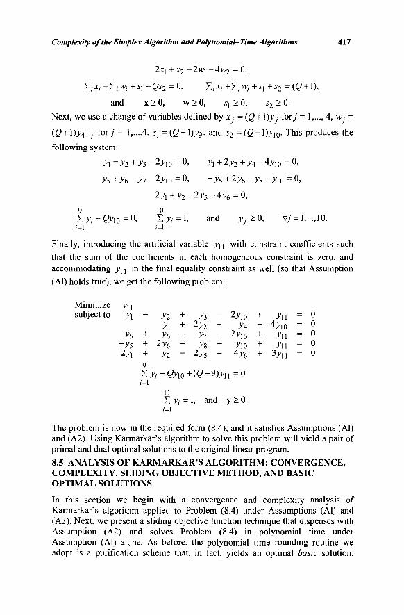
Complexity of the Simplex Algorithm and Polynomial-Time Algorithms 417
2x] + x2 - 2W[ - 4w2 = 0,
Σ,· *i +Σί W,· + Si - 0S2 = °. Σ/ *,· +Σί W; + i! + S2 = (Q + 1),
and x > 0, w > 0, sl > 0, s2 > 0.
Next, we use a change of variables defined by x · = (β + Ι)^, fory = 1,..., 4, H>7- =
(2 + 1)^4+7 fory = 1,...,4, ij = ( β + 1)>'9, and s2 = (ζ? + 1)>Ίο· This produces the
following system:
>Ί - ^ 2 + ^ 3 -2>Ίο = 0 ' yi + 2y2+y4-4yio = °>
^+^ό-^-^ιο =°. -ys + iye-ys-yio = 0'
Σ .V/- 2>Ίθ = °> Σ Λ = 1 , and j / , > 0, V/ = 1 10. ( = 1 1=1
Finally, introducing the artificial variable _yn with constraint coefficients such that the sum of the coefficients in each homogeneous constraint is zero, and accommodating j j j in the final equality constraint as well (so that Assumption (Al) holds true), we get the following problem:
Minimize y\ \ subject to yl - y2 + y3 - 2yl0
y\ + 2yi + y* ys + ye - yi - 2y\o
-ys + 2y6 - j 8 - yio 2yx + y2 - 2y5 - 4y6
;=1 11 Σ y, = 1, and y > 0. i = l
The problem is now in the required form (8.4), and it satisfies Assumptions (Al) and (A2). Using Karmarkar's algorithm to solve this problem will yield a pair of primal and dual optimal solutions to the original linear program.
8.5 ANALYSIS OF KARMARKAR'S ALGORITHM: CONVERGENCE, COMPLEXITY, SLIDING OBJECTIVE METHOD, AND BASIC OPTIMAL SOLUTIONS
In this section we begin with a convergence and complexity analysis of Karmarkar's algorithm applied to Problem (8.4) under Assumptions (Al) and (A2). Next, we present a sliding objective function technique that dispenses with Assumption (A2) and solves Problem (8.4) in polynomial time under Assumption (Al) alone. As before, the polynomial-time rounding routine we adopt is a purification scheme that, in fact, yields an optimal basic solution.
+ -+ + +
yn -■
4^0 = y\\ = Λι :
3 ^ i l :
= 0 = 0 = 0 = 0 = 0
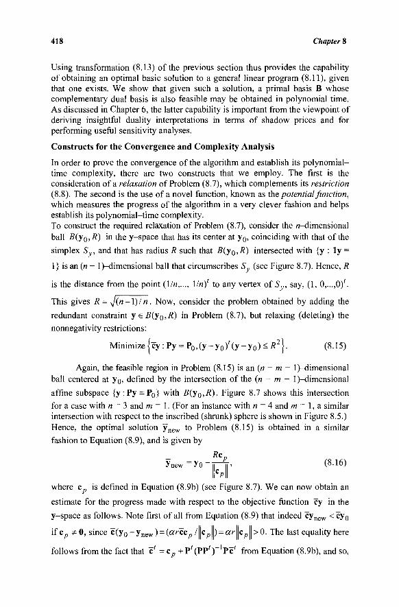
418 Chapter 8
Using transformation (8.13) of the previous section thus provides the capability of obtaining an optimal basic solution to a general linear program (8.11), given that one exists. We show that given such a solution, a primal basis B whose complementary dual basis is also feasible may be obtained in polynomial time. As discussed in Chapter 6, the latter capability is important from the viewpoint of deriving insightful duality interpretations in terms of shadow prices and for performing useful sensitivity analyses.
Constructs for the Convergence and Complexity Analysis
In order to prove the convergence of the algorithm and establish its polynomial-time complexity, there are two constructs that we employ. The first is the consideration of a relaxation of Problem (8.7), which complements its restriction (8.8). The second is the use of a novel function, known as the potential function, which measures the progress of the algorithm in a very clever fashion and helps establish its polynomial-time complexity. To construct the required relaxation of Problem (8.7), consider the «-dimensional ball B(yQ,R) in the y-space that has its center at y0, coinciding with that of the
simplex Sy, and that has radius R such that B(yQ,R) intersected with {y : ly =
1} is an (n - l)-dimensional ball that circumscribes Sy (see Figure 8.7). Hence, R
is the distance from the point (\/n,..., \ln)' to any vertex of Sy, say, (1, Ο,.,.,Ο)'.
This gives R = ^{n -1) /' n . Now, consider the problem obtained by adding the
redundant constraint y sB(y0,R) in Problem (8.7), but relaxing (deleting) the
nonnegativity restrictions:
Minimize {cy:Py = P 0 , ( y - y 0 ) / ( y - y 0 ) < / ? 2 } . (8.15)
Again, the feasible region in Problem (8.15) is an (n - m - l)-dimensional ball centered at y0, defined by the intersection of the (n - m - l)-dimensional
affine subspace {y:Py = P0} with B(y0,R). Figure 8.7 shows this intersection
for a case with n = 3 and m = 1. (For an instance with n = 4 and m = 1, a similar intersection with respect to the inscribed (shrunk) sphere is shown in Figure 8.5.) Hence, the optimal solution ynew to Problem (8.15) is obtained in a similar fashion to Equation (8.9), and is given by
R*p y n e w = y o - | i il' ( 8 · 1 6 )
hi where c„ is defined in Equation (8.9b) (see Figure 8.7). We can now obtain an
estimate for the progress made with respect to the objective function cy in the
y-space as follows. Note first of all from Equation (8.9) that indeed cynew <~cy0
if c„ * 0 , since ^(yo_ynew) = (ci:''^co I cp ) = a;r\\cp >0- The last equality here
follows from the fact that c~' = c p + P' (ΡΡ')"'Pc' from Equation (8.9b), and so,
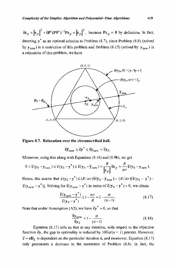
Complexity of the Simplex Algorithm and Polynomial-Time Algorithms 419
cc„ = c J + cP'(PP') Pc„ = c J , because Pc^, = 0 by definition. In fact,
denoting y* as an optimal solution to Problem (8.7), since Problem (8.8) (solved
by ynew) is a restriction of this problem and Problem (8.15) (solved by ynew ) is
a relaxation of this problem, we have
(0,0,1)
5(y0,tf)n{y:iy = i
B(y0,ar)nSy
(0 ,1 , 0)
Figure 8.7. Relaxation over the circumscribed ball.
cYnew ^cy*<;cynew <cy0.
Moreover, using this along with Equations (8.16) and (8.9b), we get
*\ - — 0 < c ( y 0 - y n e w ) < c ( y 0 - y ) < c ( y 0 - y n e w ) R
r cc . R
ar c(y o - y n ,)·
Hence, this asserts that c (y 0 -y* )< ( / e / a r ) c (y 0 -y n e w )= (R/ar)[c(y0- y*)-
c(ynew -y*)]· Solving for^(ynew -y*) in terms of c(y0 -y*) > 0, we obtain
c(y new y ) < i _ a r _ i a
c(y0-y*) R ("- 1 )
Note that under Assumption (A2), we have cy* = 0, so that
(8.17)
cy„ -<i- a < n ( 8 ' 1 8 )
cy0 (" - 1 ) Equation (8.17) tells us that at any iteration, with respect to the objective
function t:y, the gap to optimality is reduced by 100 a/(n - 1) percent. However, c = cDA is dependent on the particular iteration k, and moreover, Equation (8.17) only guarantees a decrease in the numerator of Problem (8.6). In fact, the
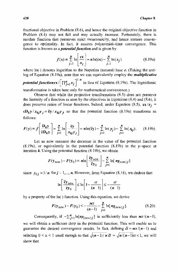
420 Chapter 8
fractional objective in Problem (8.6), and hence the original objective function in Problem (8.4) may not fall and may actually increase. Fortunately, there is another function that preserves strict monotonicity, and hence assures conver-gence to optimality. In fact, it assures polynomial-time convergence. This function is known as a potential function, and is given by
/ ( ι ) = Σ 1 η ex = «ln(cx)- Σ ln(*y) 7=1
(8.19a)
where ln() denotes logarithm to the Naperian (natural) base e. (Taking the anti-log of Equation (8.19a), note that we can equivalently employ the multiplicative
Γ lUn
potential function ex /' n'Li·*/ m n e u of Equation (8.19a). The logarithmic transformation is taken here only for mathematical convenience.)
Observe that while the projective transformation (8.5) does not preserve the linearity of a function as seen by the objectives in Equations (8.4) and (8.6), it does preserve ratios of linear functions. Indeed, under Equation (8.5), CX/JC,· =
cOky/xkjyj =Έγ/χίι:γy so that the potential function (8.19a) transforms as
follows:
F(y) = f o*y It
= Σ ΐ η 7=1
cy _ n n nln(cy)- Σ ln( j , · ) - Σ ln(jfc/).
7=1 7=1
(8.19b)
Let us now measure the decrease in the value of the potential function (8.19a), or equivalently in the potential function (8.19b) in the y-space at iteration k. Using the potential function (8.19b), we obtain
^ η ε ν ν ) - ^ θ ) = " 1 η cyn
cyo - Zln[«j(new)y]
7=1
since Jo; = l /« for/'= 1,..., n. However, from Equation (8.18), we deduce that
Cynew In cyo
<ln 1- a (»- l ) .
< — a («-1)
by a property of the ln() function. Using this equation, we derive
na " F(ynew)-F(y0)<- , ,. Σ ln[«J(new)y].
(«-1) y=i (8.20)
Consequently, if -H"i=i^[ny^new)j] is sufficiently less than nal(n-1),
we will obtain a sufficient drop in the potential function. This will enable us to guarantee the desired convergence results. In fact, defining a = nal(n-\) and
selecting 0 < a < 1 small enough so that ^{n-1)/ n a = ^nl{n-\)a < 1, we will show that
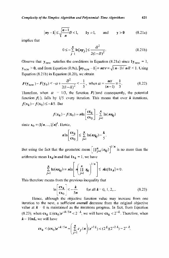
Complexity of the Simplex Algorithm and Polynomial-Time Algorithms 421
implies that
« y - 1 < a<\, ly = l, and
a2
y > 0
j=\ J 2(1-a)2
(8.21a)
(8.21b)
1, Observe that ynew satisfies the conditions in Equation (8.21a) since ly r
ynew > 0, and from Equation (8.9a), |«ynew _ l | = noer=-J(n—l)/ na < 1. Using
Equation (8.21b) in Equation (8.20), we obtain
1 F(ynew)-nyo)^-a+-
a2 1 _ na
— < — , when« = = —. >2 5 (n-1) 3
(8.22) 2(1 -ay
Therefore, when a = 1/3, the function F()and consequently, the potential function /(·), falls by 1/5 every iteration. This means that over k iterations,
/ ( x * ) - / ( * o ) ^ - # 5 . B u t
/ ( χ * ) - / ( χ ο ) = "1 η
since XQ = (\/n,...,l/n) . Hence,
«In
ex» CXn
- Σ ln(«%)
ex n k < Σ ln(iujy)—-.
cx0J j=l 5
Γ Ί " " But using the fact that the geometric mean FI'LiC**.·) is n o more than the arithmetic mean \\kln and that lxk = 1, we have
Σ ln(n^,·) = «In ( n ^
n Π *f u'=1
1/n
< iin[lxA] = 0.
This therefore means from the previous inequality that
In cxA
ex < for all A =0, 1,2,...
5« (8.23)
Hence, although the objective function value may increase from one iteration to the next, a sufficient overall decrease from the original objective value at k = 0 is maintained as the iterations progress. In fact, from Equation
(8.23), when c\k < (cx0)e~k/5n < 2~L, we will have cxk < 2~L. Therefore, when k = 10«L, we will have
ί .. \ cxk <(cx0)e -k/5n Σ Cjln {e~2L)<{2L){2~2L) = T'L.
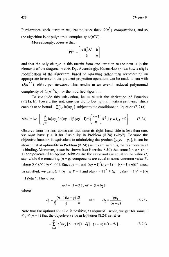
422 Chapter 8
Furthermore, each iteration requires no more than 0(n ) computations, and so
the algorithm is of polynomial complexity 0(n L).
More strongly, observe that
AD^A' 0
0 n PP'
and that the only change in this matrix from one iteration to the next is in the elements of the diagonal matrix Y)k. Accordingly, Karmarkar shows how a slight
modification of the algorithm, based on updating rather than recomputing an appropriate inverse in the gradient projection operation, can be made to run with
0(n ' ) effort per iteration. This results in an overall reduced polynomial
complexity of 0(n ' L) for the modified algorithm.
To conclude this subsection, let us sketch the derivation of Equation (8.21a, b). Toward this end, consider the following optimization problem, which
enables us to bound -YPj=i^[nyA subject to the conditions in Equation (8.21a):
Maximize j - £ ln[«y;· ] : (wy -1)'(«y -1) <( ^—ί- )a 2 , ly = l,y > o i . (8.24)
Observe from the first constraint that since its right-hand-side is less than one, we must have y > 0 for feasibility in Problem (8.24) (why?). Because the objective function is equivalent to minimizing the product [y\y2"-yni> it c a n be shown that at optimality in Problem (8.24) (see Exercise 8.30), the first constraint is binding. Moreover, it can be shown (see Exercise 8.30) that some 1 < q < (n -1) components of an optimal solution are the same and are equal to the value U, say, while the remaining (n - q) components are equal to some common value V,
where 0 < U< 1/ra < V< 1. Since ly = 1 and («y -1 ) ' («y -1) = [(« -1) / n]a2 must
be satisfied, we get qU + (n - q)V= 1 and q{nU'— 1 ) + (« - q){nV'- 1 ) = [(«
- \)ln]a . This gives
nU= (1-θι),ην= (l + <92)
where
(n-l)(n-q)a ^ _ _q^ {%^ \ q n (n-q)
Note that the optimal solution is positive, as required. Hence, we get for some 1 <q<(n~ 1) that the objective value in Equation (8.24) satisfies
- £ Hnyj 1 < -qln[l-^-(n-q)ln[l + θ2]. (8.26) 7=1
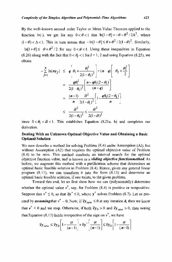
Complexity of the Simplex Algorithm and Polynomial-Time Algorithms 423
By the well-known second-order Taylor or Mean Value Theorem applied to the
function ln(), we get for any 0<6>< 1 that 1η[1-<?] = -<9-0 2 /2Δ 2 , where
( 1 - 0 ) < Δ < 1 . This in turn means that -\η[\-θ]<θ + θ212{\-θ)2. Similarly,
- ln[l + Θ] < -θ + Θ / 2 for any 0 < Θ < 1. Using these inequalities in Equation
(8.26) along with the fact that 0 < 0f < 1 for i = 1, 2 and using Equation (8.25), we
obtain
-ZHnyj] 7=1
£ 1 fl+-θί
2(i - ^ r + {n-q) -θ2 +
θί 1 2
Φ\ 2(1 -ΘΧΥ
(» - i )
η-φχ(2-θχ)
(n-q)
a n 2{\-θχΫ
1- ^ , ( 2 - ^ i )
a2 a
2(\-θχγ 2(1-ay since 0<θχ<α<l. This establishes Equation (8.21a, b) and completes our
derivation.
Dealing With an Unknown Optimal Objective Value and Obtaining a Basic Optimal Solution
We now describe a method for solving Problem (8.4) under Assumption (Al), but without Assumption (A2) that requires the optimal objective value of Problem (8.4) to be zero. This method conducts an interval search for the optimal objective function value, and is known as a sliding objective functionmethod. As before, we augment this method with a purification scheme that determines an optimal basic feasible solution to Problem (8.4). Hence, given any general linear program (8.11), we can transform it into the form (8.13) and determine an optimal basic feasible solution, if one exists, to the given problem.
Toward this end, let us first show how we can (polynomially) determine
whether the optimal value v , say, for Problem (8.4) is positive or nonpositive.
Suppose that v* < 0, so that cy* < 0, where y* solves Problem (8.7). Let us pro-
ceed by assumingthut v* = 0. Now, if cynew < 0 at any iteration k, then we know
that v* < 0 and we stop. Otherwise, if both cy0 > 0 and cynew > 0, then noting
that Equation (8.17) holds irrespective of the sign on v , we have
eyn ;cyo a
(n-1) + cy
a
(«-1) ^cy 0
1-- a («-!)
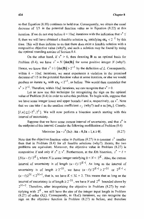
424 Chapter 8
so that Equation (8.18) continues to hold true. Consequently, we obtain the usual decrease of 1/5 in the potential function value as in Equation (8.22) at this
iteration. If we do not stop before k = lOraZ, iterations with the indication that v <
0, then we will have obtained a feasible solution \k satisfying cx^ < 2~ by this
time. This will then indicate to us that there does exist a feasible solution with a nonpositive objective value (why?), and such a solution may be found by using the optimal rounding routine of Section 8.4.
On the other hand, if v* > 0, then denoting B as an optimal basis for
Problem (8.4), we have v* =^7^61(8)) for some positive integer N (why?).
Hence, we know that v* > l/|det(B)| > 2~ by the definition of I . Consequently,
within k = \0nL iterations, we must experience a violation in the promised decrease of 1/5 in the potential function value at some iteration, or else we would
produce an iterate x^ with cx^ <2~ , as before. This would then contradict that
v* >2~ . Therefore, within lOnL iterations, we can recognize that v* > 0. Let us now use this technique for recognizing the sign on the optimal
value of Problem (8.4) in order to solve this problem. To begin with, suppose that
we have some integer lower and upper bounds I and u, respectively, on v*. Note that we can take I as the smallest coefficient c. (why?) and u as [cx0]. Clearly,
[£,u]c[-2L,2L]. We will now perform a bisection search starting with this
interval of uncertainty.
Suppose that we have some current interval of uncertainty, and that z* is the midpoint of this interval. Consider the following modification of Problem (8.4):
Minimize {cx-z*(lx): Ax = 0,lx = l,x> 0}. (8.27)
Note that the objective function value in Problem (8.27) is a constant z* smaller than that in Problem (8.4) for all feasible solutions (why?). Hence, the two problems are equivalent. Moreover, the objective value in Problem (8.27) is
nonpositive if and only if z* > v*. Furthermore, at the Ktìa. bisection, z* = I + K K
[N(u -1)12 ], where N is some integer satisfying 0<N< 2 . Also, the current K—1
interval of uncertainty is of length (u-l)l2 . A s long as the interval of
uncertainty is of length >2~2L, we have (u-£)/2K~l >2~2L or 2K~l <
(u-£)22L < 23L+1, that is, we have K < 3L + 2. This means that as long as the —9 J K
interval of uncertainty is of length > 2 , we have N and 2 bounded above by
2 + . Therefore, after integerizing the objective in Problem (8.27) by mul-is
tiplying with 2 , we still have the size of the integer input length in Problem (8.27) of order 0(L). Consequently, in 0(nL) iterations, we can recognize the sign on the objective function in Problem (8.27) as before, and therefore
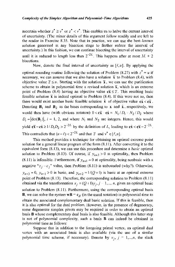
Complexity of the Simplex Algorithm and Polynomial-Time Algorithms 425
ascertain whether z* > v* or z* < v*. This enables us to halve the current interval of uncertainty. (The minor details of this argument follow readily and are left to the reader in Exercise 8.35. Note that in practice, we can use the best-known solution generated at any bisection stage to further reduce the interval of uncertainty.) In this fashion, we can continue bisecting the interval of uncertainty
—IT
until it is reduced to length less than 2 . This happens after at most 3L + 2 bisections.
Now, denote the final interval of uncertainty as [£,u]. By applying the optimal rounding routine following the solution of Problem (8.27) with z* = u if necessary, we can assume that we also have a solution x to Problem (8.4), with objective value z < u. Starting with the solution x, we can use the purification scheme to obtain in polynomial time a revised solution x, which is an extreme point of Problem (8.4) having an objective value c x < z . This resulting basic feasible solution x is indeed optimal to Problem (8.4). If this were not so, then there would exist another basic feasible solution x of objective value ex < ex . Denoting Bt and B2 as the bases corresponding to x and x, respectively, we would then have (with obvious notation) 0 < ex - ex = N] / D] - N2 ID2 where Dj =|det(B;)|, i = 1, 2, and where N] and N2 are integers. Hence, this would
—2/ —IT yield ex - ex > 1 / D\D2 > 2 by the definition of L, leading to ex < ex - 2 This contradicts that (u-l)<2 and that z and v e[£,u].
This method provides a technique for obtaining an optimal extreme point solution for a general linear program of the form (8.11). After converting it to the equivalent form (8.13), we can use this procedure and determine a basic optimal solution to Problem (8.13). Of course, if jv„+3 > 0 at optimality, then Problem
(8.11) is infeasible. Furthermore, if yn+i = 0 at optimality, being nonbasic with a
negative "z · - c " value, then Problem (8.11) is unbounded (why?). Otherwise,
>W3 = 0, yn+i > 0 is basic, and yn+2 = 1 l(Q +1) is basic at an optimal extreme point of Problem (8.13). Therefore, the corresponding solution to Problem (8.11) obtained via the transformation x = (Q + l)y,;j = 1,—, n, gives an optimal basic
solution to Problem (8.11). Furthermore, using the corresponding optimal basis B, we can solve the system wB = cB (in the usual notation) in polynomial time to
obtain the associated complementary dual basic solution. If this is feasible, then it is also optimal for the dual problem. However, in the presence of degeneracy, some degenerate simplex pivots may be required in order to obtain an optimal basis B whose complementary dual basis is also feasible. Although this latter step is not of polynomial complexity, such a basis B can indeed be obtained in polynomial time as follows:
Suppose that in addition to the foregoing primal vertex, an optimal dual vertex with an associated basis is also available (via the use of a similar polynomial-time scheme, if necessary). Denote by v , j = !,...,«, the slack
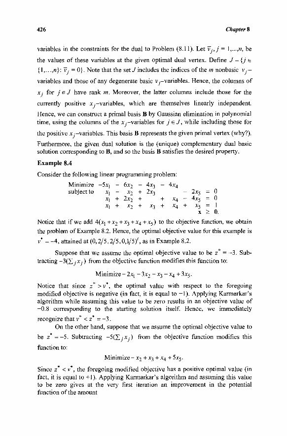
426 Chapter 8
variables in the constraints for the dual to Problem (8.11). Let v:,j = \,...,n, be
the values of these variables at the given optimal dual vertex. Define J = {j e
{Ι,.,.,η}: V: = 0}. Note that the set J includes the indices of the m nonbasic v . -
variables and those of any degenerate basic v,-variables. Hence, the columns of
x · for j e J have rank m. Moreover, the latter columns include those for the
currently positive x—variables, which are themselves linearly independent.
Hence, we can construct a primal basis B by Gaussian elimination in polynomial time, using the columns of the x.-variables for j e J, while including those for
the positive x —variables. This basis B represents the given primal vertex (why?).
Furthermore, the given dual solution is the (unique) complementary dual basic solution corresponding to B, and so the basis B satisfies the desired property.
Example 8.4
Consider the following linear programming problem:
Minimize -5xj - 6x2 - 4x3 - 4x4
subject to X{ ~ x2 + 2x3 - 2x5 = 0 X! + 2x2 + + x4 - 4x5 = 0 Xj + x2 + X3 + x4 + x5 = 1
x > 0.
Notice that if we add 4(xj +x2 +x3 + x4 + x5) to the objective function, we obtain
the problem of Example 8.2. Hence, the optimal objective value for this example is
v* = -4 , attained at (0,2/5,2/5,0,1/5)', as in Example 8.2.
Suppose that we assume the optimal objective value to be z = - 3 . Sub-tracting -3(X, x, ) from the objective function modifies this function to:
Minimize - 2xj - 3x2 - x3 - x4 + 3x5.
Notice that since z* >v*, the optimal value with respect to the foregoing modified objective is negative (in fact, it is equal to -1). Applying Karmarkar's algorithm while assuming this value to be zero results in an objective value of -0.8 corresponding to the starting solution itself. Hence, we immediately
recognize that v < z = - 3 .
On the other hand, suppose that we assume the optimal objective value to
be z* = - 5 . Subtracting -5(X x ) from the objective function modifies this
function to:
Minimize - x2 + x3 + x4 + 5x5.
Since z* < v*, the foregoing modified objective has a positive optimal value (in fact, it is equal to +1). Applying Karmarkar's algorithm and assuming this value to be zero gives at the very first iteration an improvement in the potential function of the amount
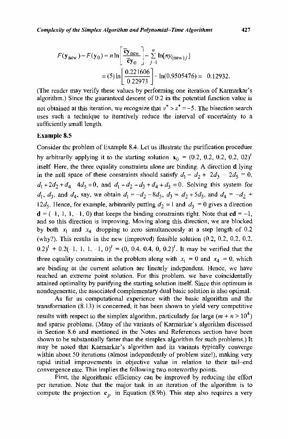
Complexity of the Simplex Algorithm and Polynomial-Time Algorithms 427
/ ? (ynew)-^(yo) = " l n
= (5) In
cyn
cyo
0.221606
Σ ln[^(new)y] 7=1
-ln(0.9505476) =-0.12932. 0.22973
(The reader may verify these values by performing one iteration of Karmarkar's algorithm.) Since the guaranteed descent of 0.2 in the potential function value is
not obtained at this iteration, we recognize that v* > z* = - 5 . The bisection search uses such a technique to iteratively reduce the interval of uncertainty to a sufficiently small length.
Example 8.5
Consider the problem of Example 8.4. Let us illustrate the purification procedure
by arbitrarily applying it to the starting solution x0 = (0.2, 0.2, 0.2, 0.2, 02)'
itself. Here, the three equality constraints alone are binding. A direction d lying
in the null space of these constraints should satisfy d\— d2 + 2d^ - 2d5 = 0,
dl+2d2+d4-4d5=0, and dx +d2 + d^ +d4 + d5 =0 . Solving this system for
d\, i/3, and d4, say, we obtain d\ = -d2 -8i/5, dj = d2 +5d5, and d4 = -d2 +
\2d5. Hence, for example, arbitrarily putting d2 = 1 and d5 = 0 gives a direction
d = (-1, 1, 1, - 1 , 0) that keeps the binding constraints tight. Note that cd = - 1 , and so this direction is improving. Moving along this direction, we are blocked by both x\ and x4 dropping to zero simultaneously at a step length of 0.2 (why?). This results in the new (improved) feasible solution (0.2, 0.2, 0.2, 0.2, 0.2)' + 0.2(-l, 1 , 1 , - 1 , 0 ) ' = (0, 0.4, 0.4, 0, 0.2)'. It may be verified that the three equality constraints in the problem along with xj = 0 and x4 = 0, which
are binding at the current solution are linearly independent. Hence, we have reached an extreme point solution. For this problem, we have coincidentally attained optimality by purifying the starting solution itself. Since this optimum is nondegenerate, the associated complementary dual basic solution is also optimal.
As far as computational experience with the basic algorithm and the transformation (8.13) is concerned, it has been shown to yield very competitive
results with respect to the simplex algorithm, particularly for large {m + n> 10 ) and sparse problems. (Many of the variants of Karmarkar's algorithm discussed in Section 8.6 and mentioned in the Notes and References section have been shown to be substantially faster than the simplex algorithm for such problems.) It may be noted that Karmarkar's algorithm and its variants typically converge within about 50 iterations (almost independently of problem size!), making very rapid initial improvements in objective value in relation to their tail-end convergence rate. This implies the following two noteworthy points.
First, the algorithmic efficiency can be improved by reducing the effort per iteration. Note that the major task in an iteration of the algorithm is to compute the projection c . in Equation (8.9b). This step also requires a very
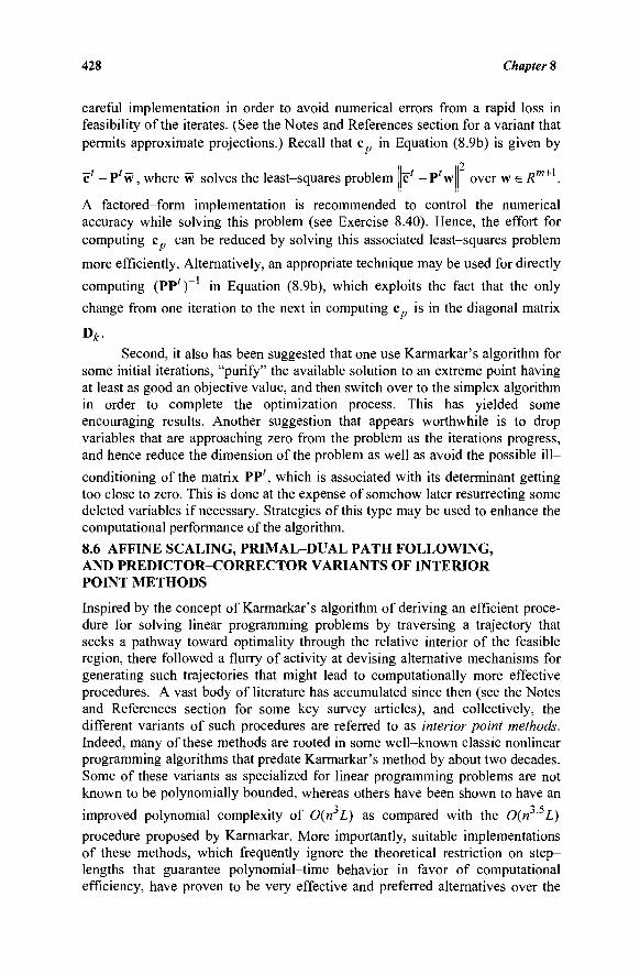
428 Chapter 8
careful implementation in order to avoid numerical errors from a rapid loss in feasibility of the iterates. (See the Notes and References section for a variant that permits approximate projections.) Recall that c„ in Equation (8.9b) is given by
2 C - F * W c' - P ' w , where w solves the least-squares problem o v e r w e 5 m + 1 .
A factored-form implementation is recommended to control the numerical accuracy while solving this problem (see Exercise 8.40). Hence, the effort for computing c„ can be reduced by solving this associated least-squares problem
more efficiently. Alternatively, an appropriate technique may be used for directly
computing (PP')~ in Equation (8.9b), which exploits the fact that the only
change from one iteration to the next in computing c is in the diagonal matrix
Ok.
Second, it also has been suggested that one use Karmarkar's algorithm for some initial iterations, "purify" the available solution to an extreme point having at least as good an objective value, and then switch over to the simplex algorithm in order to complete the optimization process. This has yielded some encouraging results. Another suggestion that appears worthwhile is to drop variables that are approaching zero from the problem as the iterations progress, and hence reduce the dimension of the problem as well as avoid the possible ill-conditioning of the matrix PP', which is associated with its determinant getting too close to zero. This is done at the expense of somehow later resurrecting some deleted variables if necessary. Strategies of this type may be used to enhance the computational performance of the algorithm.
8.6 AFFINE SCALING, PRIMAL-DUAL PATH FOLLOWING, AND PREDICTOR-CORRECTOR VARIANTS OF INTERIOR POINT METHODS
Inspired by the concept of Karmarkar's algorithm of deriving an efficient proce-dure for solving linear programming problems by traversing a trajectory that seeks a pathway toward optimality through the relative interior of the feasible region, there followed a flurry of activity at devising alternative mechanisms for generating such trajectories that might lead to computationally more effective procedures. A vast body of literature has accumulated since then (see the Notes and References section for some key survey articles), and collectively, the different variants of such procedures are referred to as interior point methods. Indeed, many of these methods are rooted in some well-known classic nonlinear programming algorithms that predate Karmarkar's method by about two decades. Some of these variants as specialized for linear programming problems are not known to be polynomially bounded, whereas others have been shown to have an
improved polynomial complexity of 0(n L) as compared with the 0(n ' L)
procedure proposed by Karmarkar. More importantly, suitable implementations of these methods, which frequently ignore the theoretical restriction on step-lengths that guarantee polynomial-time behavior in favor of computational efficiency, have proven to be very effective and preferred alternatives over the
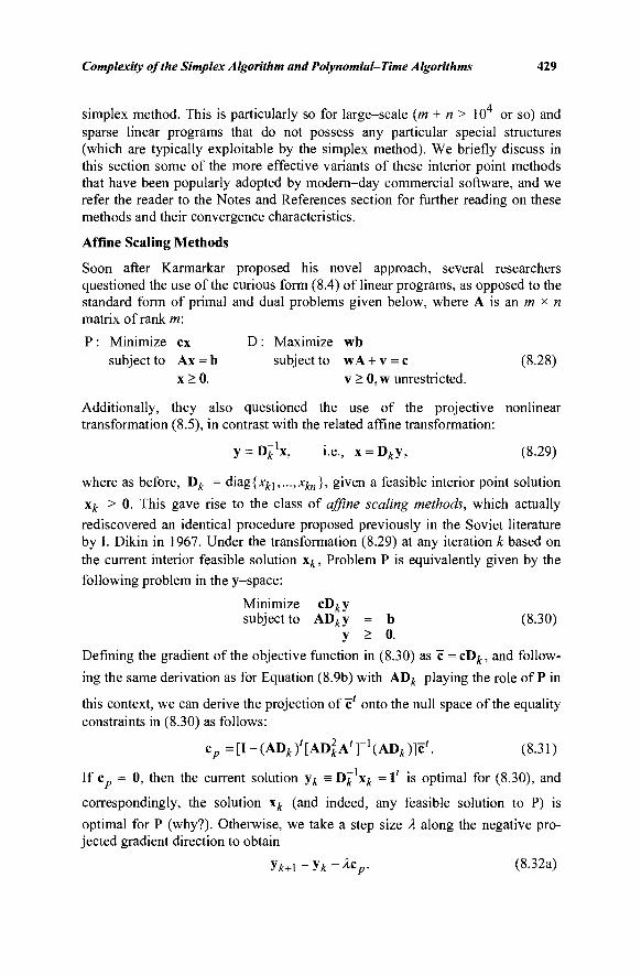
Complexity of the Simplex Algorithm and Polynomial-Time Algorithms 429
simplex method. This is particularly so for large-scale (m + n > 10 or so) and sparse linear programs that do not possess any particular special structures (which are typically exploitable by the simplex method). We briefly discuss in this section some of the more effective variants of these interior point methods that have been popularly adopted by modern-day commercial software, and we refer the reader to the Notes and References section for further reading on these methods and their convergence characteristics.
Affine Scaling Methods
Soon after Karmarkar proposed his novel approach, several researchers questioned the use of the curious form (8.4) of linear programs, as opposed to the standard form of primal and dual problems given below, where A is an m χ η matrix of rank m:
P : Minimize ex D : Maximize wb subject to Ax = b subject to wA + v = c (8.28)
x>0. v>0,w unrestricted.
Additionally, they also questioned the use of the projective nonlinear transformation (8.5), in contrast with the related affine transformation:
y = D^x, i.e., x = Oky, (8.29)
where as before, D^ = diaglx^j,...,*£„}, given a feasible interior point solution
xk > 0. This gave rise to the class of affine scaling methods, which actually
rediscovered an identical procedure proposed previously in the Soviet literature by I. Dikin in 1967. Under the transformation (8.29) at any iteration k based on the current interior feasible solution xk, Problem P is equivalently given by the following problem in the y~space:
Minimize cD^y subject to AD^y = b (8.30)
y > o. Defining the gradient of the objective function in (8.30) as c = cD^, and follow-
ing the same derivation as for Equation (8.9b) with AOk playing the role of P in
this context, we can derive the projection of c' onto the null space of the equality constraints in (8.30) as follows:
cp =[ I - (AD y t / [AD|A / r 1 (AD / t ) ]c ' . (8.31)
If c , = 0, then the current solution yk = Ό^ xk = l ' is optimal for (8.30), and
correspondingly, the solution xk (and indeed, any feasible solution to P) is
optimal for P (why?). Otherwise, we take a step size λ along the negative pro-jected gradient direction to obtain
y*+i = y * - ^ V (8.32a)
430 Chapter 8
Using (8.29), this translates to the following motion in the x-space upon premultiplying (8.32a) throughout by D^:
xi+i = xk - ÀDkcp = xk + Mk > (8.32b)
say, where d^ = -D^c Note that the maximum value Àmax of λ that would
maintain feasibility of x^+i is given by the usual "minimum ratio test" as:
λ—— = minimum^ —-— : dti < 0 >. (8.33) "max | _ ( ^ } kj |
Assuming that the feasible region is bounded (by using an artificial bounding constraint if necessary), we have ^ax < oo. However, in order to maintain the positivity of the iterates, we adopt a step-length that is short of the maximum step length, i.e., we take
/1 = «Λτιαχ. where 0 < α < 1 . (8.34)
(In practice, a is selected to lie in the interval 0.95-0.99.) This completes an iteration. Incrementing k by one, the foregoing process is repeated. It can be
shown that if this process generates a sequence { c„ } —> 0, then the corresponding
sequence of iterates {x^} approaches x*, an optimal solution to P, with the sequence
w^ = (AD^A')~ (ADfc)i' approaching an optimal dual solution. (Hence, a prac-
tical termination criterion is to stop the process whenever c J becomes suffi-
ciently small.) If both P and D are nondegenerate, this convergence can be shown
to hold true for any 0 < a < 1. However, under degeneracy, it has been exhibited
through an example that the procedure can fail to converge to an optimum
whenever a > 0.995, whereas one can prove in general that convergence (even
under degeneracy) holds true provided a < 2/3. Note that when convergence does
occur, we can optimally round the solution to an exact solution in a finite number
of iterations once the optimality gap becomes smaller than 2 , as before. However, this convergence process is not known to be polynomially bounded. In fact, it is suspected that by making a < 1 sufficiently large, the procedure can be contrived to follow a path close to the boundary that approximately parallels the simplex path described for the Klee-Minty example in Section 8.2, thereby portending an exponential worst-case complexity behavior. Nonetheless, this method is quite effective in practice. Finally, we comment that the foregoing procedure has been applied to P and is therefore called the primal affine scaling method; similar approaches adopted for D, or for both P and D simultaneously give rise to the respective classes of dual affine scaling, and primal-dual affine scaling methods.
Complexity of the Simplex Algorithm and Polynomial-Time Algorithms 431
Primal-Dual Path-Following Methods
Consider the pair of primal and dual linear programs in Equation (8.28) where the feasible region for P is nonempty and bounded (perhaps artificially so), and let us examine the following Barrier Problem BP, which is parametrized by a barrier parameter μ>0:
BP : Minimize \ β{\) = e x - / / £ ln(jcy) : Ax = b I. (8.35)
Observe that the nonnegativity constraints in Problem P of Equation (8.28) have been incorporated into the objective function in Problem (8.35) along with a "barrier term" that approaches oo if any x —value approaches zero (from the positive
side). It is well known from nonlinear programming (see the Notes and Refer-ences section) that given any desired level of accuracy ε > 0, there exists a μ > 0 small enough such that the corresponding optimal solution to Problem
(8.35) is positive and has an objective value in Problem (8.28) within ε of optimality. In fact, by the strict convexity of the objective function in Problem (8.35) and the stated assumptions on P, for every μ > 0, there exists a unique
optimum x say, to (8.35), where x^ approaches an optimum for P as μ -¥ 0+.
In fact, similar to the case of linear programs, the following Karush-Kuhn-Tucker (KKT) conditions for (8.35) are both necessary and sufficient for optimality, where the right-hand-side of Equation (8.36b) is the gradient of the objective function in Problem (8.35):
Ax = b (8.36a)
wA = c- / / [ l /x , , . . . , l /x„] . (8.36b)
To imitate the KKT conditions for P, and noting the form of D in Problem (8.28), let us substitute v = μ[\Ιχχ,...,\1χη] in Equation (8.36b). This yields the so-called perturbed KKT conditions (which are equivalent to Equation (8.36), but are specially designated because they admit algorithmic steps and related performance characteristics that would be quite different from applying similar techniques directly to Equation (8.36)):
Ax = b (8.37a)
wA + v = c (8.37b)
VjXj=M,Vj=l,.../i. (8.37c)
Note that given any μ > 0, and the corresponding unique optimum x„ > 0 to
Problem BP, Equation (8.37c) yields an associated unique value of v > 0, and
Equation (8.37b) then yields a unique value for w„, since A has full row rank
(note that a solution exists since these are necessary optimality conditions). Let us denote the triplet (x,w,v) by ξ, and accordingly, let ξμ = (x„ ,w„ ,v„ ) .
(Note that throughout, for notational convenience, x is a column vector whereas
432 Chapter 8
w and v are row vectors). The trajectory ξμ, generated as a function of μ as
μ —» 0+, is called the central path (motivated by the interiority of the solutions
thus produced). Observe that from Equations (8.37a)-(8.37c), we have that the optimality gap ex - wb is given by
n cx - wb = vx + wAx - wAx = Σ VJXJ = ημ. (8.38)
y=i
Hence, as μ —> 0+, the sequence of primal and dual feasible solutions x„ and
(w„, v„) respectively approach optimal solutions to P and D.
However, rather than follow the central path precisely (which would be computationally demanding), it turns out that it is sufficient to adopt a path that is close enough to the central path in a well-defined sense, in order to achieve (polynomial-time) convergence. More specifically, at any iteration k, suppose that we have a current solution ξίί = (x^,w^,v^), which is close enough to ξμ
for some current value of μ^ > 0 in that:
Ax£ =b,x/c > 0, W£ A + \k = c,\k > 0, (Wyj. is unrestricted), (8.39a)
and
Z(vkjxkj-Mk) <fyk, while Σ Vkjxki =nVk> (8.39b)
where 0 < Θ < 0.5 is a constant. Note that whereas Equation (8.37c) might hold true only approximately in the sense of Equation (8.39b), the second condition in (8.39b) asserts that the sum of the equations in Equation (8.37c) should hold true exactly. In particular then, by Equation (8.38), the duality gap cx^ -w A b equals
ημ^ We now reduce the value of μ to
A / t + i = M . (8-4°)
where 0 < β < 1, and accordingly, we derive a direction of motion d* =
(ax,Aw,dv) in the primal-dual space based on an attempt to satisfy Equation
(8.37) for this revised value of μ = μ^χ. Specifically, let us therefore examine
the system \(xk+ax) = b
( w j t + d w ) A + ( v A + d v ) = c
(vkj+dVj)(xkj+dXj) = Mk+l> Y / = 1.....M.
Noting Equation (8.39a), this reduces to the system
A d x = 0 (8.41a)
dwA + d v = 0 (8.41b)
Complexity of the Simplex Algorithm and Polynomial-Time Algorithms 433
vkjdxj+xkjdVj=Mk+\-vkfckj-d^dx, Y/=l,. . . ,n. (8.41c)
Observe that the system (8.41) is linear except for the quadratic product term dv.dx. in Equation (8.41c). Moreover, if we neglect this product term, then this
system yields a unique solution d i ={àx,Aw,av) (see Exercise 8.53). Indeed,
this direction turns out to be equivalent to that obtained by applying a single step of Newton's classic optimization method to the perturbed KKT system given in Equation (8.37). Adopting a unit step size along this (Newton) direction, we obtain the new iterate
&+!=&+<!£■ (8-42)
It can now be shown, noting Equations (8.39) and (8.40), that if we select <?
β = 1--η=, where δ = θ = 0.35, (8.43) v«
say, then the new iterate £A+1 thus obtained would be close enough to ξ„ on
the central path in the sense defined by Equation (8.39) (see Exercise 8.54). Hence, in particular, the optimality gap would be given by Equation (8.38). This means that for each iteration k, we would have that the optimality gap satisfies (noting (8.40) and assuming that v0x0 = ημ0 to start):
ak-*rkb = nuk = n!io0k=yoxQpk<\\\Q\\\\xo\\fl
k<22L/3k, (8-44)
where it can be shown that | x 0 | < 2 and ||v0| < 2 (see Exercise 8.10). There-
fore, this gap would be lesser than 2 , thereby permitting an optimal polynomial-
time rounding as in Section 8.4, whenever 22L /?* < 2~2L, i.e., k > 4Z,ln(2)/
[-In (/?)]. But from (8.43) and a property of the ln() function, we have
-ln(/?) = -ln(l—U>^=.
Therefore, by the iteration k > 4L ln(2) Ι[δ I v/i], that is, in iterations, we
would have the optimality gap being lesser than 2 . Similar to Karmarkar's
algorithm, the effort per iteration is 0(n ' ) (see Exercise 8.55), leading to an
overall 0(n L) algorithm.
Note that because the value of β is very close to unity, especially as n increases, the decay of//-values as controlled by Equation (8.40) can be very slow, leading to a painfully slow convergence process. Hence, a somewhat more aggressive strategy of decreasing μ is adopted in practice, thereby sacrificing the provable polynomial-time behavior in exchange for a highly improved empirical computational performance. For example, one strategy that has been successfully used is to let
434 Chapter 8
Mk+ì = Mk/n ifn ^ 5 0 0 0 ' a n d fk+\ = Mk/Jn i f " > 5 0 0 0 · (8·45)
In closing, we comment here that an application of an affine scaling strategy to the barrier problem BP defined in Equation (8.35), instead of to the original underlying linear program P, recovers the standard affine scaling method in the limit as μ -> 0. However, by holding μ > 0 but sufficiently small to enable an optimal rounding, the convergence of such an affine scaling process can be shown to hold for all values of the step-length parameter 0 < a < 1 analogous to Equation (8.34) (see Exercise 8.43), regardless of degeneracy.
Predictor-Corrector Algorithms
One of the most computationally effective interior point variants is a predictor-corrector approach, as applied to the foregoing primal-dual path-following algorithm. The basic idea behind this technique originates from the successive approximation methods implemented for the numerical solution of differential equations. Essentially, this method adopts steps along two successive directions at each iteration. The first is a predictor step that adopts a direction based on the system (8.41) under the ideal scenario of μ^+ι =0, but again neglecting the second-order term dv,dx,, V/ = Ι,.,.,κ. Let d'c be this direction obtained. A
tentative revised iterate |£+ 1 is computed as |£+ 1 =ξί(+λά'ξ, where the step-
length λ is taken close to the maximum step length λ^^ that would maintain
positivity of the x- and v-variables, similar to the mechanism of Equation (8.34).
(Here, we can take a = 0.95-0.99, say.) Then a revised value ^ + 1 of the
parameter μ is determined via a scheme of the type of Equation (8.45) or based on some suitable function of the optimality gap or complementary slackness violation (see Equation (8.38) and Exercise 8.57) at ξ^ and at ££+i · Using this value of //A+1 in Equation (8.41), but this time replacing the quadratic product term in Equation (8.41c) by the estimate d'v d'x , V/' = \,...,n, as determined by
ά'ξ, in lieu of simply neglecting this nonlinear term, a revised direction d; is
derived. (Note that because of the similarity of the systems that determine d;
and d;, factorizations developed to solve for the former direction can be
reutilized to obtain the latter direction.) The revised direction d; thus
determined is then used to take a step from ξ^ to give the new iterate ξίί+ί. This
correction toward the central path is known as a corrector step. Observe that the system (8.41) could be solved repeatedly in this manner by using the most recent direction components to estimate the quadratic term on the right-hand-side in Equation (8.41c), in order to obtain a more accurate estimate ^ + 1 corresponding
to the parameter μ^+\. Numerical results suggest that this might be a promising alternative to using a single corrector step.
Complexity of the Simplex Algorithm and Polynomial-Time Algorithms 435
EXERCISES
[8.1] Solve the problem to minimize 3 ^ + 2x2, subject to jq + 2x2 > 2 and x\ > 0, x2 > 0, using Karmarkar's algorithm by equivalently transforming the problem into the form (8.4) that satisfies Assumptions (Al) and (A2). Plot the iterates you generate in the ( jq ,x2 ) space.
[8.2] Consider the problem to minimize 3xj +2x2 subject to x\ +2x2 -X3 =2 ,
Xl +x2 +x3 +x4 = 4, x > 0. Transform this equivalently into the form (8.4) as in
Equation (8.13) that satisfies Assumption (Al), but not necessarily Assumption (A2). Use Karmarkar's sliding objective function method described in Section 8.5 to solve the resulting problem.
[8.3] Provide the details of an approach that uses a polynomial time algorithm for the linear programming decision problem in order to polynomially solve the linear programming optimization problem. What is the complexity of the latter in terms of the complexity of the former?
[8.4] With respect to the problem of Equation (8.3), show that the (z ■ -c )-values
corresponding to the basis with basic variables (sy,s2,..;Sn_i,yn) are all
nonnegative.
[8.5] Demonstrate that the transformation (8.2) reduces the Klee-Minty problem to the form in Problem (8.3).
[8.6] Following the arguments in Section 8.2, give a detailed proof by induction
that for Problem (8.3) in «-dimensions there exists a simplex path of length 2" -1 from the origin to the optimum using the most negative z .■ - C: entering rule
(Dantzig's Rule).
[8.7] Plot the (original) Klee-Minty polytope for n = 2 and n = 3. What is the relationship between these polytopes and the ones shown in Figure 8.1? Analogous to the statement of Exercise 8.6, what precise complexity assertion can you make with respect to the original Klee-Minty problem?
[8.8] Consider the linear programming problem to:
Maximize
subject to
Σ IO""'JC; y'=1
2 Σ l&~Jxj 7 = 1
J '
+ *,-<100M
Xj>0
for; = 1,..
fory = l,.
.,«
..,r
a. Demonstrate graphically for n = 2 and n = 3 that using (Dantzig's) most negative z - c,· entering rule, the simplex method can go
through 2" -1 pivots, starting at the origin. b. Provide a proof by induction for the statement in Part (a) for general
n.
436 Chapter 8
[8.9] Given a square matrix B with components By , i = 1,..., m,j = 1,..., m, show
by induction that |detB| < ΓΊ" =1 (1 + ÌBy ). (Hint: Use the column (row)-wise
expansion formula for det B.)
[8.10] In the usual notation, let x = (xB,xN) be a basic feasible solution of the
system Ax = b, x > 0, where A is m x n of rank m and where the data is all integer.
Show that the kth component xB of xB satisfies xB <2 l(mn), where
L = Γΐ + log m + log/? + Σ Σ [ Ι + log(l + ky|)l
+Σ[ι + ΐο8(ΐ+|6,-)|]1. i
Here, ay and ty are the components of A and b, respectively. Hence, show that
\\x\\<2L /n.
[8.11] For the linear programming problem to minimize ex subject to Ax = b, x > 0, where A is m x n and where the data is all integer, define L as in Equation (8.1). Using Exercise 8.10, and assuming the linear program to be feasible and bounded,
show that the optimal objective value lies in the interval [-2 ,2 ].
The following exercises 8.12-8.17 relate to Khachian's algorithm for determining in polynomial time if there exists an x belonging to the set
5 = { x : G x < g } or to conclude that S = 0 , where G is r x q, g is r x 1, with r and q > 2, and where the data is all integer: [8.12] Define
I = r i + logr + logg + I X [ l + log(l + |Gy|)]
+Z[i+iog(i+|g;.)|]l
and let EQ = {x : |x | < 2L}. Show that if S Φ 0 , then
v o l [ £ 0 n S ] > 2 - ( ? + 1 ) I
where νοΙ(Π) denotes the ^-dimensional volume. (Hint: The volume of a q-
dimensional simplex with vertices vi,...,v +) is given by
( l / 9 !) det 1 1 ·■■ 1
vi v2 ··· v9 + !
[8.13] (Khachian 's Main Step 1) Starting with k = 0, suppose that at iteration k, the ellipsoid Ek defined as follows is given:
Ek ={x:(x-xk)'Q-kl(x-xk)<l}
Complexity of the Simplex Algorithm and Polynomial-Time Algorithms 437
where xk is the center of the ellipsoid and Q^ is a q x q symmetric positive
definite matrix (that is, y 'Q/ty>0 for all y * 0 ) . In particular, det(Qyt)^ 0.
Given Ek, if xk e S, then halt. Otherwise, let the most violated constraint
defining S be G v x<g v . Hence, Gvxk>gv. Geometrically, translate the
hyperplane Gvx = gv parallel to itself in the (feasible) direction of -G'v until it
becomes tangential to the ellipsoid Ek at the point y^ (see Figure 8.8). Show
that
yk=xk+àk> where dA = Ì¥
Next, compute Y^ as the point on the hyperplane Gvx = gv obtained by moving
from xk in the direction d^. Hence, Y^ = xk + Akdk for some step length Xk.
Show that Xk = (gv -Gvxk)/(Gvdk) and that lk > 0. Also, show that if Àk > 1,
then S = 0 and the procedure can terminate.
[8.14] (Khachian's Main Step 2) Assuming that Zk < 1 in Exercise 8.13, let x i + 1
be the point on the line segment [Y^, y^ ] that divides this in the ratio 1 :q. Hence,
0+4?)., xk+\ 1 q
U+1; Y* +
1 |
U+U y* ■Xi. +-
(1 + 9)
Define the new ellipsoid Ek+\ = {x : (x - xk+l )' Qk+\ (x - x^+i ) ^ 1} with center at
xk+{ and with Q^+1 given by the following expression:
Q*+i = q2Q-4)
(<?2-i)
Q _ 2 0 ± ^ ) _ , (?+ 1X4+1)
Show that: a· Qk+\ ' s symmetric and positive definite (given that so is Q^).
b. The point y^ lies on the boundary of Ek+i.
c. The hyperplane Gvx = Gvy^ is tangential to Ek+^ at yk.
d. Ekn{x:Gvx<gv}^Ek+i where Ek = {x:(x-xk)'Q^(x-xk)<l}.
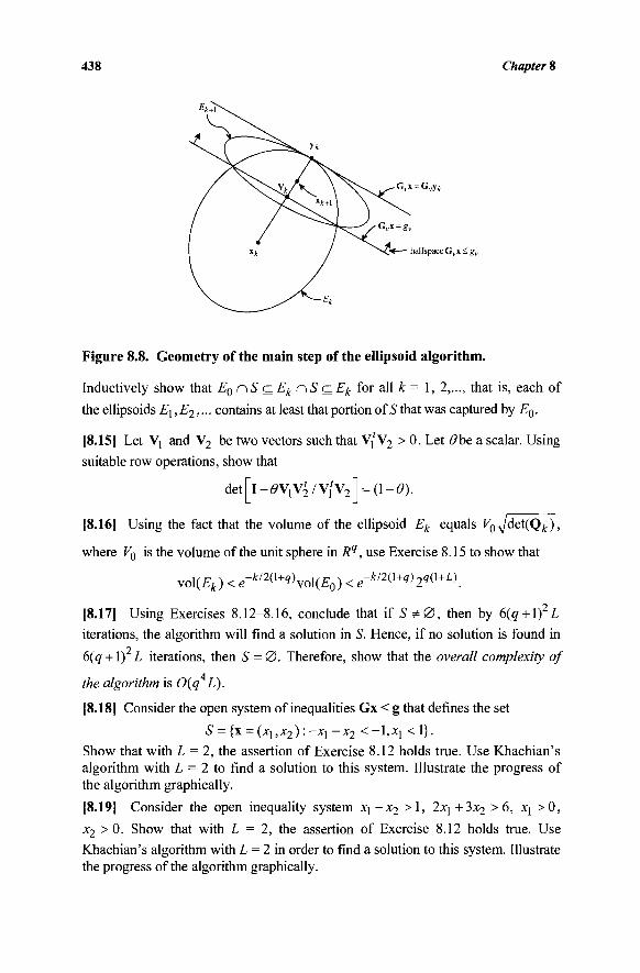
438 Chapter 8
G„x = Gvyt
Figure 8.8. Geometry of the main step of the ellipsoid algorithm.
Inductively show that E0r\S <^EknS cEk for all k = 1, 2,..., that is, each of
the ellipsoids Εχ, E2,... contains at least that portion of S that was captured by E0.
[8.15] Let V] and V2 be two vectors such that V/V2 > 0. Let 6>be a scalar. Using
suitable row operations, show that
det = (1-0). \-θ\λ\'2Ι\{\2
[8.16] Using the fact that the volume of the ellipsoid Ek equals K0A/det(Q^),
where V0 is the volume of the unit sphere in Rq, use Exercise 8.15 to show that
V 0 l ( ^ ) < e -* / 2 ^>VOl ( i s 0 ) < e-*/2(l+?)29(1+i>.
[8.17J Using Exercises 8.12-8.16, conclude that if S*0, then by 6{q + \)2L
iterations, the algorithm will find a solution in S. Hence, if no solution is found in
6{q + \) L iterations, then S = 0 . Therefore, show that the overall complexity of
the algorithm is 0{q L).
[8.18] Consider the open system of inequalities Gx < g that defines the set
S = {x = (x^,x2)'--X\ -x2 <-l ,*i <1}· Show that with L = 2, the assertion of Exercise 8.12 holds true. Use Khachian's algorithm with L = 2 to find a solution to this system. Illustrate the progress of the algorithm graphically.
[8.19] Consider the open inequality system X\-x2 >1, 2xt +3x2 > 6, jq >0 ,
x2 >0. Show that with L = 2, the assertion of Exercise 8.12 holds true. Use
Khachian's algorithm with L = 2 in order to find a solution to this system. Illustrate the progress of the algorithm graphically.
Complexity of the Simplex Algorithm and Polynomial-Time Algorithms 439
[8.20] In order to be able to use Khachian's algorithm for solving linear programming problems, one needs to be able to determine if the closed system of inequalities Gx < g has a solution, where G is r χ q, with r and q > 2, and G and g have all integer components. Toward this end, define S = {x : Gx < g} and consider the following open inequality system, where 1 is a row vector of r ones, and where L is defined in Exercise 8.12:
Gx < g + (2~L ) l ' , that is, (2L )Gx < (2L )g +1'.
Use Farkas' Lemma (see Chapter 5) to show that S is nonempty if and only if
this open inequality system has a solution. Show that the complexity of deter-
mining whether or not S is empty by Khachian's algorithm is 0(rq L).
[8.21] {Optimal Rounding Routine) Suppose that we are given a solution x to the
open inequality system Gx < g + (2~ )l ' , where L is defined as in Exercise 8.12.
Suppose that we are to determine from that a solution to the system Gx < g. Of
course, if Gx < g, then we are done. Otherwise, define s, (x) = g,- - G,x as the
slack in the rth constraint G,-x < g, corresponding to a given solution x. Note that
we have s(-(x) < 0 for some ;' e {1,..., r), but that s,(x) > —2~ for each i = 1,..., r. (This evidently means that only a small adjustment in x may be required to obtain s,(x)>0 for all i = 1,..., r; hence, the name of this routine.) Consider the operations of the following two steps:
Step 1. First, refine x to a solution xnew, which is such that (i) 5;(xnew)>min{0,ii(x)}, and (ii) every row of G can be written as a linear combination of the rows with index set V = {i: st (xnew ) ^ 0}. Show how this can be achieved in polynomial time. (Hint: If x does not satisfy these conditions, select a row Gk of G, with k ί V, which is not spanned by G,·, i e V, and find a
solution d(* 0) to the system of equations G;d = 0 for i e V, G^d = 1. Consider
the ray x = x + Ad,A>0, and take a suitable step along this ray. Repeat.)
Step 2. Given xnew from Step 1 along with the set V, find a maximal
linearly independent set of rows from the set G;, ieV. Let these rows be G,·,
ieJczV. Then show that any solution to the system G,-x = g, for i e J, yields
the desired solution to the system Gx < g.
Derive a polynomial complexity bound for this routine. ]8.22] This exercise describes an alternative approach to determining a solution to a closed system of inequalities via Khachian's algorithm. Consider the closed system of inequalities Gx < g, where G is r x q. Suppose that we have a solution x satisfying G ; x < g ( for i = 1,..., p, where p < r. Examine the open system of
inequalities G,x < g,·, for / = 1,..., p + 1, and suppose that this system is empty.
Show that G „+1x = g„+1 for all feasible solutions to Gx < g. By solving for some
variable in this equation in terms of the others, show how the system Gx < g can be
440 Chapter 8
reduced to an equivalent one with one fewer variable and constraint. How can you repeatedly use this process along with Khachian's algorithm to determine in polynomial time whether or not a closed system Gx < g (with integer data) has a feasible solution? What is the complexity of this procedure?
[8.23] Consider solving the following linear program in canonical form: Minimize ex, subject to Ax > b, x > 0, where A is m x n. Show that solving this problem is equivalent to determining a solution to a certain closed system of inequalities. How would you decide if the given linear program is infeasible or unbounded, given that the latter inequality system has no solution? Using Exercise 8.20, show that the
overall complexity of using Khachian's algorithm is 0[(m + n) L], where L is
given by Equation (8.1).
[8.24] Consider the open inequality system in R given by xl + 0x2 <1 + ί/θ and
-xl+0x2<-l, where # > 5 / V 2 . Let x0 = (1 + (V2 / 5), 0)' and define
EQ = { X : ( X - X 0 ) ' Q O ( x - x o ) ^ l } , where Q0 =21 so that EQ is a circle with
center at x0 and with radius V2. (Hence, this corresponds to "Z," = 1/2.) Using this
as a starting solution, apply Khachian's algorithm (Exercises 8.12-8.17) using Xk
= 0. (This corresponds to Khachian's original algorithm.) a. Give the geometric interpretation of using the formulas for \k+i and
Q;t+i of Exercise 8.14 with Xk = 0. Illustrate with a sketch similar to Figure 8.8.
b. Derive closed form expressions for x^ and Q^ as a function of iteration k.
c. Determine the smallest integer k such that xk satisfies the inequality
system. Show that by making Θ arbitrarily large, we can make the algorithm go through an arbitrarily large number of iterations before terminating. What does this say about the complexity of Khachian's algorithm using real data?
d. Suppose that Θ is an integer. Make the coefficients of the open inequality system to be integer-valued and determine L from Exercise 8.12. What does Part (c) say about the practical computational relationship of Khachian's algorithm with the quantity U!
[8.25] Show that the matrix PP' is invertible, where P is defined as in Equation (8.7), with A being m x n of rank m and with Ok =diag{x!ci,...,xim}, given x^ > 0.
[8.26] The Karush-Kuhn-Tucker optimality conditions for Problem (8.8) assert that the negative gradient of the objective function should be contained in the cone spanned by the gradients of the binding constraints. Use this fact to show that ynew defined by Equation (8.9) solves Problem (8.8).
Complexity of the Simplex Algorithm and Polynomial-Time Algorithms 441
- P ' w over w unrestricted in [8.27] Consider the problem of minimizing
sign. Show by setting the gradient of the objective function equal to zero that
w = (PPf)~ Pc* solves this problem.
[8.28] Use Exercise 8.10 to show that there exists a value of Mof magnitude 2 * ' such that the artificial variable j n + 3 in the problem of Equation (8.13) is zero at optimality, given that the problem in Equation (8.12) is feasible.
[8.29] Determine the value a of a that minimizes the expression -a + a I
2(1 - a) in Equation (8.22). Why does this not necessarily imply that the value a
is the best value for obtaining a maximum reduction in the potential function F(·)? How would you go about finding a better value of a from the viewpoint of reducing F(·)? (Hint Examine the derivation of the inequalities in Equations (8.20) and (8.21).)
[8.30] The Karush-Kuhn-Tucker optimality conditions for Problem (8.24), where the constraints are written as < inequalities, require the gradient of the objective function to lie in the cone spanned by the gradients of the binding constraints. Show that at optimality for Problem (8.24), the first constraint is binding and that y > 0. Using the stated optimality conditions, show that at optimality in Problem (8.24), some 1 < q < (n - 1) components of y are equal to a value U and the remaining components are equal to a value V, where U and V satisfy Equation (8.25).
[8.31] a. Using the procedure of Exercise 8.21, provide the details and the complexity analysis of an optimal rounding routine for Karmarkar's algorithm as applied to Problem (8.4) under Assumptions (Al) and (A2). In particular, define L as in Equation (8.1). Show that it is sufficient to determine a solution xk to Problem (8.4) with objective
function value cxk < 2~ in order to round this solution by using
Exercise 8.21 to an optimal solution to Problem (8.4) (with a zero objective function value) in polynomial time.
b. Illustrate the method of Part (a) by providing the details of optimally rounding the solution \26 obtained for Example 8.2.
c. What is the relationship of this procedure with the rounding routine given in Section 8.4?
d. Present a simplex pivot type of scheme for efficiently implementing the optimal rounding routine of Section 8.4. Show that this process
has a complexity bound of 0(m ri).
[8.32] Consider the potential function / (x) = ln[cx/lx]. Show how this trans-forms in the y-space under the projective transformation (8.5). Can this potential function be used to analyze the complexity of Karmarkar's algorithm? (Hint Examine the relationship between f(x) and ex for Problem (8.4).)
442 Chapter 8
[8.33] Analyze in detail the complexity of a single iteration of Karmarkar's algorithm for Problem (8.4).
[8.34] Using the development of Sections 8.4 and 8.5, show how you can use Karmarkar's algorithm to determine whether a given linear program is infeasible or whether it is unbounded.
[8.35] Provide the details of Karmarkar's algorithm and its complexity for solving Problem (8.4) via Problem (8.27) and the sliding objective method, under Assumption (Al) but treating the optimal objective value as unknown. Include an analysis of the optimal rounding via the purification step.
[8.36] Provide the complexity of solving the (general) linear programming problem (8.11) via Karmarkar's algorithm using the transformation of this problem into Problem (8.13) and the details of Exercise 8.35.
[8.37] Illustrate the procedure of Exercise 8.35 using Example 8.4 in Section 8.5
with the information that the optimal objective value v e [-6,0].
[8.38] Consider the linear assignment problem to minimize Σ™ ι Σ7=ι cijxij subject
to Σ™ι*// = 1 fory = l,.../n, Σ"}=χχ^ = 1 for i = 1,..., m, and x > 0. Suggest a suitable transformation to use Karmarkar's algorithm for solving this problem. Provide an algorithmic statement, including a suggested starting solution and any algorithmic specializations. In particular, how would you exploit the fact that the extreme points are integer valued? (Hint: With c integer, once a solution within a unit of optimality is found, it can be optimally rounded by purification.)
[8.39] Consider the linear transportation problem to minimize Σ ^ ι Σ Ϊ ^ , ν * / /
subject to Σ ^ Χ , ) ^ Si for i = 1,..., NS, Σ ^ ^ = dj for/ = 1,..., ND, and x > 0,
where NS is the number of sources with respective supplies s,-, i = l,...JVS, and
where ND is the number of sinks with respective demands d -, j = l,...JVD.
(Assume all integer data and that Z/Ifsj - Σ / ^ ^ / · ) Repeat the analysis of
Exercise 8.38 for this problem.
[8.40] Consider the following QR factorization method for obtaining the least-
c ' - P ' w in order to determine squares solution w to the problem of minimizing
c „ of Equation (8.9b) via c „ = ~c' - P'w . Given P' of full column rank, its QR
decomposition yields P' =QR, where Q is an n x n orthogonal matrix (that is,
QQ' = I) and R is an n x (m + 1) matrix of the form Ri 0
. Here, R] is (m + 1) χ
(m + 1), nonsingular, and upper triangular. (See the Notes and References section
for details on performing such a decomposition.) Denote Q c Cl
C2 with c
Complexity of the Simplex Algorithm and Polynomial-Time Algorithms 443
being of dimension (m + 1) and c2 being of dimension (n - m - 1). Using this
decomposition, show that w is given as the solution to the linear, triangular
system Rj w = Cj. Furthermore, show that c „ = Q
[8.41] Suppose that you use the techniques of Sections 8.4 and 8.5 to determine a basic solution to the primal-dual formulation in Equation (8.14). Does this necessarily yield an optimal primal basis whose complementary dual basis is dual feasible? If not, then under what conditions will this be obtained automatically, and what additional work may be required otherwise? Give the details of a polynomial-time scheme for finding such a basis. Explain the significance of being able to obtain such a basis.
[8.42] Consider the linear programming problem to minimize ex subject to Ax = b and x > 0, where A is m x n of rank m, the feasible region is bounded, and where
the data is all integer. Suppose that the optimal objective value v* and some (rational) feasible solution x > 0 to this problem are known.
a. Show that by using the transformation
1D-Ix + 1 I D ' x + l and by replacing the resulting fractional objective by the objective
function cDy-v* j 0 , one obtains an equivalent linear program of the
form (8.4). b. Establish the polynomial-time complexity of Karmarkar's algorithm
with respect to the original problem using this approach. c. Is the equivalence of Part (a) true if the feasible region of the original
problem is unbounded? d. Consider the following linear programming problem:
Minimize -Xj - 2x2 subject to X] - x2 + x-} = 1
X[ + 2 x 2 + x 4 = 2 Xj, x 2 , Χ3, Χ4 ^ 0.
Using x = (0.5, 0.5, 1, 0.5)' and v = -2 , show that this problem is
equivalent to that of Example 8.2. [8.43] Consider the linear programming problem P given in Equation (8.28), where A is m x n of rank m < n and where the data is all integer. Without loss of generality, assume that the feasible region is bounded and that a feasible solution x0 > 0 is known. (Show how one may use artificial variables and bounds, if
necessary, for this purpose.) Construct the so-called barrier function problem defined by Equation (8.35) for a given barrier parameter μ>0. Consider the
following Affine Scaling variant of Karmarkar's algorithm:
444 Chapter 8
Initialization. Let x0 be the given positive feasible solution, set k = 0, q = 0.97,
and select μ = min{2"2L_1 In, 10~12}, where L = Γΐ + Σ/Σ7·log(l + |ay |)Ί.
Step 1 (Dual estimates, projected gradient, and direction of motion, based on a
projected gradient step in the y-space, where y = D^ x. The latter transformation
gives the algorithm its name.) Given xk, define Ok = aiag{xki,...,xkr!}, ck = cDk,
and P^ = ADk. Compute the following:
Dual estimate: w^ = ( P ^ y ' p ^ c / -μΐ']
Reduced cost vector: R^ = c' -μΌ^ ΐ ' - A'w^
Projected gradient vector: cpk =[l-?tk(¥lcP
tk)~
lPk][c'k -μΐ']
Direction of motion: dk =-Okcpk.
Step 2 (Termination test). If w^ is dual feasible in Problem (8.28) and
cxk - b w j < 2 , then purify x^ to an extreme point of Problem (8.28) and
terminate. Otherwise, continue.
Step 3 (New iterate.) Set xk+ì =xk+Àkak, where the step length Àk is given by
; · · J ; O-g)2! Ak = minimum^ ^Anax > <· μ J
1 [ dkj ) where = maximum-^ —:j = l,...,n>.
Anax [ xkj J Increment k by one and return to Step 1.
a. Show that the algorithm generates a sequence of positive iterates χ .,
*= 0,1,2,.... b. Show that the algorithm either stops finitely with an optimal solution
xk to Problem (8.29) in case c„J = 0 for some k, or else, ignoring
the termination test at Step 2, an infinite sequence of primal-dual
iterates (xk,yvk) is generated such that the sequence jncpk }—>0.
Moreover, for any convergent subsequence {x^w^}^ indexed by K,
with limit point (x,w), show that x > 0 and that x solves Problem
(8.29). c. Show that w obtained in Part (b) is dual feasible to Problem (8.28).
Moreover, show that the duality gap between x and w in Problem
(8.28) is e x - b ' w = ημ.
d. Show that the reduced cost vector R^ approaches zero as k —» QO, and
that the dual iterate w^ becomes dual feasible in Problem (8.28) once
Complexity of the Simplex Algorithm and Polynomial-Time Algorithms 445
Rk is sufficiently close to zero. Hence, with μ defined as previously,
show that the algorithm terminates finitely at Step 2. e. Present a purification process for obtaining a pair of optimal primal
and dual extreme point solutions to Problem (8.28) after termination at Step 2.
f. Comment on the use of μ = 0. (This was the original affine scaling algorithm.)
[8.44] Consider the linear programming problem given in Exercise 8.42d. Starting
with the solution x0 = (0.5, 0.5, 1, 0.5)' apply the affine scaling algorithm of
Exercise 8.43 to solve this problem. Show the progress of the iterates with respect to feasibility and objective values in Problems P and D of Equation (8.28), and purify the resulting solution to a pair of optimal primal and dual extreme point solutions to Problems P and D, respectively.
[8.45] Suppose that the system Ax = b, x > 0 has a positive feasible solution. Consider the following Phase I problem, where x0 > 0 is arbitrarily chosen and λ is an artificial variable:
PI : Minimize{/t: A x - ( 2 - / l ) b - ( / l - l ) A x 0 = 0,x >0,A > 0}.
Note that (x,/t) = (x0,2) > 0 is a feasible, positive solution. Show that PI has an
optimal value that is strictly less than one. Also, show that for any feasible
solution (χ,Λ) to PI, where λ < 1, the solution χ = [(\-λ)χ0+χ]/(2-λ) is a
positive, feasible solution for the given linear system. Using Exercises 8.42 and 8.43, suggest a two-phase procedure for Karmarkar's algorithm, as well as for its affine scaling variant.
[8.46] Show that the dual iterate w^ for the affine scaling algorithm of Exercise
8.43 is the solution to a certain least-squares problem. Provide a geometric inter-pretation for this latter problem.
[8.47] Solve the problem of Exercise 8.2 using the affine scaling algorithm of Exercise 8.43, starting with the solution (x^,x2,x^,X4) = (1, 1, 1, 1). Repeat this using the affine scaling algorithm (with μ = 0) described in Section 8.6. [8.48] Consider the linear programming problem:
Minimize {ex : Ax = b, - 1 < x· < 1 for j = 1,...,«}, (8.46)
where A is m x n of rank m and where the data is all integer. Show how a problem having general lower and upper bounds i,- and M, on the x.-
variables, where —«><£ ■ <u,-<c0, can be put into this form. Assume (using
artificial variables if necessary) that there exists some known feasible solution
x0 to Problem (8.46) satisfying - l ' < x 0 < l ' . Analogous to Exercise 8.43,
construct the following barrier function problem for Problem (8.46) that uses a
barrier term to keep the variables strictly within their bounds:
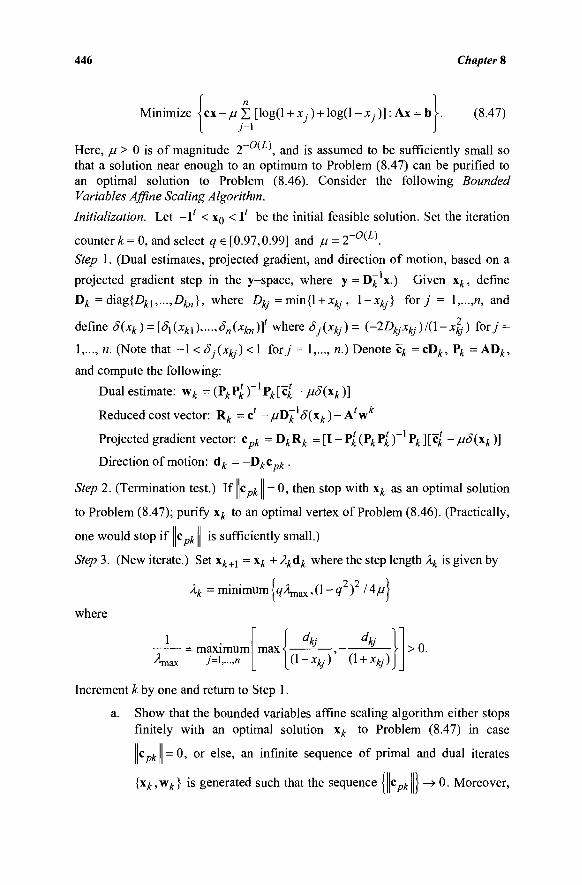
446 Chapter 8
Minimize ìcx-μΣ [log(l + Xj) + log(l-Xj)]:Ax = b>. (8.47)
Here, μ > 0 is of magnitude 2~ ' \ and is assumed to be sufficiently small so that a solution near enough to an optimum to Problem (8.47) can be purified to an optimal solution to Problem (8.46). Consider the following Bounded Variables Affine Scaling Algorithm.
Initialization. Let - l ' < x0 < l' be the initial feasible solution. Set the iteration
counter k = 0, and select q e [0.97,0.99] and μ = 2~~0{L\
Step 1. (Dual estimates, projected gradient, and direction of motion, based on a
projected gradient step in the y-space, where y = D^ x.) Given xk, define
Ok =diag{DA1,...,Dfoj}, where Dkj =mm{l + xkJ, \-xkj) for j = Ι,.,.,η, and
define S(xk) = [Si(xkl),...,S„(xkn)]t where Sj(xkj) = {-2Dkjxkj)l{\-xlj) for; =
1,..., n. (Note that -1 < Sj(xkj)< 1 for y = 1,..., n.) Denote \ = cD^, Vk = ADA,
and compute the following:
Dual estimate: w t = {PkYtky
XYk[c,k-μδ{χΙί)\
Reduced cost vector: R t = c' - μ ϋ ^ £(χΑ ) - A'w
Projected gradient vector: cpk = OkRk ^[l-Ptk(PkF
tky
iVk][c'k-MS(xk)]
Direction of motion: d^ = -Okcpk .
Step 2. (Termination test.) If c„J = 0, then stop with xk as an optimal solution
to Problem (8.47); purify x^ to an optimal vertex of Problem (8.46). (Practically,
one would stop if c ^ is sufficiently small.)
Step 3. (New iterate.) Set xk+l =xk+ Akdk where the step length lk is given by
Àk = minimum j qÀmsx, (1 - q2 )2 14μ
where
1 ■ = maximum
ΛΜΧ 7=l.-.n
dkj dkj max < >0.
β-Hj) (1 + ) J
Increment k by one and return to Step 1.
a. Show that the bounded variables affine scaling algorithm either stops finitely with an optimal solution xk to Problem (8.47) in case
c„J =0 , or else, an infinite sequence of primal and dual iterates
{x^w^} is generated such that the sequence j wcpk > -> 0. Moreover,
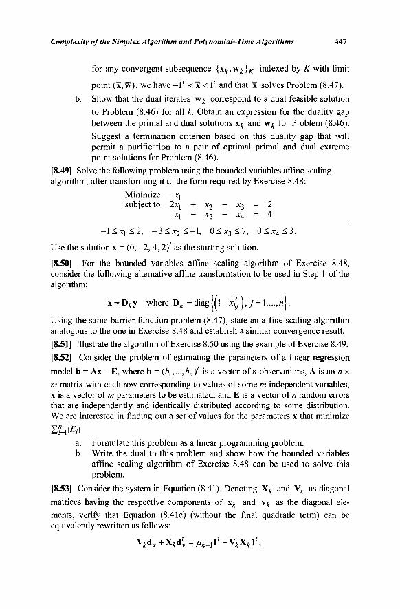
Complexity of the Simplex Algorithm and Polynomial-Time Algorithms 447
for any convergent subsequence {X£>WA;}A: indexed by K with limit point (x,w), we have - l ' < x < l ' and that x solves Problem (8.47).
b. Show that the dual iterates w^ correspond to a dual feasible solution to Problem (8.46) for all k. Obtain an expression for the duality gap between the primal and dual solutions x^ and w^ for Problem (8.46). Suggest a termination criterion based on this duality gap that will permit a purification to a pair of optimal primal and dual extreme point solutions for Problem (8.46).
[8.49] Solve the following problem using the bounded variables affine scaling algorithm, after transforming it to the form required by Exercise 8.48:
Minimize -xj subject to 2xj + x2 + X3 = 2
Xi — X2 + X4 = 4
-1<X!<2 , - 3 < x 2 < - l , 0 < x 3 < 7 , 0 < x 4 < 3 .
Use the solution x = (0, -2,4,2)' as the starting solution.
[8.50] For the bounded variables affine scaling algorithm of Exercise 8.48, consider the following alternative affine transformation to be used in Step 1 of the algorithm:
x = Dyty where D^ =d iag | | l - x | , J , y = l,...,«j.
Using the same barrier function problem (8.47), state an affine scaling algorithm analogous to the one in Exercise 8.48 and establish a similar convergence result.
[8.51] Illustrate the algorithm of Exercise 8.50 using the example of Exercise 8.49. [8.52] Consider the problem of estimating the parameters of a linear regression model b = Ax - E, where b = (oj,...,Z>„)' is a vector of « observations, A is an « x m matrix with each row corresponding to values of some m independent variables, x is a vector of m parameters to be estimated, and E is a vector of n random errors that are independently and identically distributed according to some distribution. We are interested in finding out a set of values for the parameters x that minimize
Y" ÌFÌ A=lp;|· a. Formulate this problem as a linear programming problem. b. Write the dual to this problem and show how the bounded variables
affine scaling algorithm of Exercise 8.48 can be used to solve this problem.
[8.53] Consider the system in Equation (8.41). Denoting X^ and V^ as diagonal matrices having the respective components of x^ and vk as the diagonal ele-ments, verify that Equation (8.41c) (without the final quadratic term) can be equivalently rewritten as follows:
V ^ + X ^ / ^ l ' - V ^ l ' ,
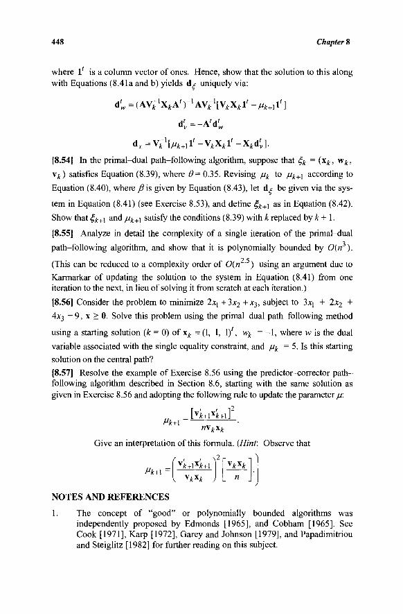
448 Chapter 8
where l i s a column vector of ones. Hence, show that the solution to this along with Equations (8.41a and b) yields dt uniquely via:
d'w=(Ay^xkAtylA\^[ykxki' - ^ + 1 i ' ]
d(, = -A'd'w
i ^ v i ' b w i ' - V A i ' - x X ] . [8.54] In the primal-dual path-following algorithm, suppose that ξίί = (xk, wk,
\k) satisfies Equation (8.39), where θ= 0.35. Revising μ/( to μ/ί+ί according to
Equation (8.40), where /?is given by Equation (8.43), let Αμ be given via the sys-
tem in Equation (8.41) (see Exercise 8.53), and define £*+i as in Equation (8.42).
Show that 4>+i and μλ+1 satisfy the conditions (8.39) with k replaced by k + 1.
[8.55] Analyze in detail the complexity of a single iteration of the primal-dual
path-following algorithm, and show that it is polynomially bounded by 0(n ).
2 5
(This can be reduced to a complexity order of 0(n · ) using an argument due to Karmarkar of updating the solution to the system in Equation (8.41) from one iteration to the next, in lieu of solving it from scratch at each iteration.)
[8.56] Consider the problem to minimize 2x\ +3x2 +*3, subject to 3x] + 2JC2 +
4x3 = 9, x > 0. Solve this problem using the primal-dual path-following method
using a starting solution (k = 0) of xk = (1, 1, 1)', wk = - 1 , where w is the dual
variable associated with the single equality constraint, and μί( = 5. Is this starting
solution on the central path? [8.57] Resolve the example of Exercise 8.56 using the predictor-corrector path-following algorithm described in Section 8.6, starting with the same solution as given in Exercise 8.56 and adopting the following rule to update the parameter μ:
_ [y'k+\x'k+\] Mk+\ ~ ·
mkxk
Give an interpretation of this formula. (Hint: Observe that
n \ )
NOTES AND REFERENCES
1. The concept of "good" or polynomially bounded algorithms was independently proposed by Edmonds [1965], and Cobham [1965]. See Cook [1971], Karp [1972], Garey and Johnson [1979], and Papadimitriou and Steiglitz [1982] for further reading on this subject.
i"*+l yk+lxk+\
yk*k
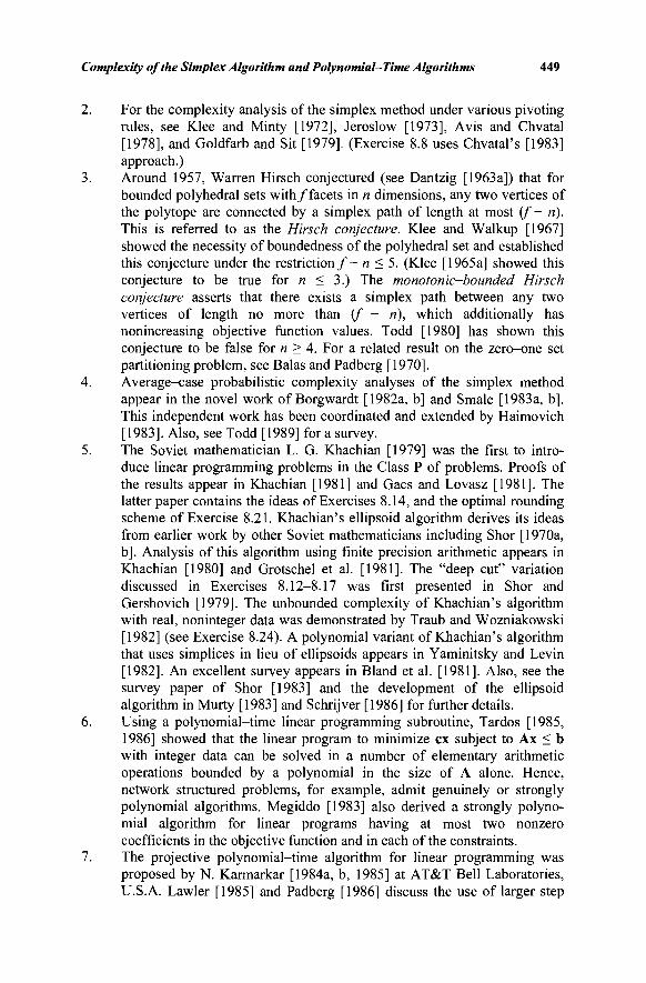
Complexity of the Simplex Algorithm and Polynomial-Time Algorithms 449
2. For the complexity analysis of the simplex method under various pivoting rules, see Klee and Minty [1972], Jeroslow [1973], Avis and Chvatal [1978], and Goldfarb and Sit [1979]. (Exercise 8.8 uses Chvatal's [1983] approach.)
3. Around 1957, Warren Hirsch conjectured (see Dantzig [1963a]) that for bounded polyhedral sets with/facets in n dimensions, any two vertices of the polytope are connected by a simplex path of length at most (f - ri). This is referred to as the Hirsch conjecture. Klee and Walkup [1967] showed the necessity of boundedness of the polyhedral set and established this conjecture under the restriction/- n < 5. (Klee [1965a] showed this conjecture to be true for n < 3.) The monotonic-bounded Hirsch conjecture asserts that there exists a simplex path between any two vertices of length no more than (f - ri), which additionally has nonincreasing objective function values. Todd [1980] has shown this conjecture to be false for n > 4. For a related result on the zero-one set partitioning problem, see Balas and Padberg [1970].
4. Average-case probabilistic complexity analyses of the simplex method appear in the novel work of Borgwardt [1982a, b] and Smale [1983a, b]. This independent work has been coordinated and extended by Haimovich [1983]. Also, see Todd [1989] for a survey.
5. The Soviet mathematician L. G. Khachian [1979] was the first to intro-duce linear programming problems in the Class P of problems. Proofs of the results appear in Khachian [1981] and Gacs and Lovasz [1981]. The latter paper contains the ideas of Exercises 8.14, and the optimal rounding scheme of Exercise 8.21. Khachian's ellipsoid algorithm derives its ideas from earlier work by other Soviet mathematicians including Shor [1970a, b]. Analysis of this algorithm using finite precision arithmetic appears in Khachian [1980] and Grotschel et al. [1981]. The "deep cut" variation discussed in Exercises 8.12-8.17 was first presented in Shor and Gershovich [1979]. The unbounded complexity of Khachian's algorithm with real, noninteger data was demonstrated by Traub and Wozniakowski [1982] (see Exercise 8.24). A polynomial variant of Khachian's algorithm that uses simplices in lieu of ellipsoids appears in Yaminitsky and Levin [1982]. An excellent survey appears in Bland et al. [1981]. Also, see the survey paper of Shor [1983] and the development of the ellipsoid algorithm in Murty [1983] and Schrijver [1986] for further details.
6. Using a polynomial-time linear programming subroutine, Tardos [1985, 1986] showed that the linear program to minimize ex subject to Ax < b with integer data can be solved in a number of elementary arithmetic operations bounded by a polynomial in the size of A alone. Hence, network structured problems, for example, admit genuinely or strongly polynomial algorithms. Megiddo [1983] also derived a strongly polyno-mial algorithm for linear programs having at most two nonzero coefficients in the objective function and in each of the constraints.
7. The projective polynomial-time algorithm for linear programming was proposed by N. Karmarkar [1984a, b, 1985] at AT&T Bell Laboratories, U.S.A. Lawler [1985] and Padberg [1986] discuss the use of larger step
Chapter 8
sizes, and Goldfarb and Mehrotra [1988] and Anstreicher [1986a] validate techniques using approximate projection operations. An alternative to using the sliding objective function/bisection scheme is presented in Todd and Burrell [1986] and Anstreicher [1985]. Charnes et al. [1984] exhibited a worst-case linear convergence rate for Karmarkar's algorithm. However, Iri and Imai [1986] developed a modification that is quadratically convergent. For additional analyses on superlinearly convergent primal-dual path-following methods, see Mehrotra [1993], Tapia et al. [1995], Ye et al. [1993], Zhang et al. [1992], and Zhang and Tapia [1993]. Implementation suggestions and transformations for solving general linear programs by Karmarkar's method appear in Tomlin [1985] and Shanno and Marsten [1985], in particular. The two-phase approach of Exercise 8.45 is from Kojima [1986]. For factorizations in solving the least-squares problem accurately, see Dongarra et al. [1979], Heath [1982], George and Heath [1980], and Todd and Burrell [1986]. Relationships of Karmarkar's algorithm to projected Newton barrier methods have been shown by Gill et al. [1986], and to the ellipsoid algorithm have been demonstrated by Todd [1989] and Ye [1987]. For computational experience using linear assignment problems, see Aronson et al. [1985]. The purification scheme first found its elements in Charnes et al. [1965]. Also, see Kortanek and Jishan [1988]. Sherali et al. [1988] showed how to use such a scheme for optimally rounding to a basic feasible solution. Ye [1987] also discusses how to obtain an optimal basis via Karmarkar's algorithm, and Ye and Kojima [1987] discuss how to recover dual solutions. Variants and discussions related to Karmarkar's projective algorithm appear in Anstreicher [1986b, e], Asie et al. [1986], Blair [1986], Blum [1985], Chang and Murty [1987], de Ghellinck and Vial [1986], Gay [1987], Gonzaga [1985, 1987b], Kojima [1986], Lustig [1985], Megiddo [1985, 1986a, b], Murty [1985], Nazareth [1986], Rinaldi [1986], Ye [1985a, b], and Chiù and Ye [1985b], among others. (See Note 8 for the affine scaling and the path-following variants.) For exploiting special structures using a variant of Karmarkar's projective algorithm, see Todd [1988]. Anstreicher [1997], Freund and Mizuno [1996], and Monma [1987], provide survey articles; see also Martin [1999], Saigal [1995], Terlaky [1998], and Vanderbei [1996].
The affine scaling variant of Karmarkar's algorithm finds its origin in Dikin [1967, 1974], but was rediscovered independently by Barnes [1986], Vanderbei et al. [1986] and Cavalier and Soyster [1985], follow-ing Karmarkar's algorithm. Barnes [1986], Vanderbei et al. [1986], Kortanek and Shi [1987], and Sherali [1987] prove convergence under various conditions. Sherali et al. [1988] have presented an assumption-free convergence analysis of a perturbation of this algorithm. (Exercises 8.43, 8.48, and 8.50 are derived from this paper.) For exploiting special structures using this variant, see Chandru and Kochar [1986]. Adler et al. [1986] and Monma and Morton [1987] have also independently developed dual affine variants of Karmarkar's algorithm. Megiddo and Shub [1987] have exhibited a worst-case exponential behavior for the affine scaling
Complexity of the Simplex Algorithm and Polynomial-Time Algorithms 451
algorithm with infinitesimal steps (continuous trajectory) on the Klee-Minty [1972] polytope by starting the algorithm close enough to a vertex. See Saigal [1995] and Vanderbei [1996] for detailed analyses regarding the convergence of the affine scaling method under degeneracy. By adopting an additional step that centers the iterate within the polytope, Barnes [1987] has derived a polynomial-time variant of the affine scaling algorithm. This centering amounts to increasing the denominator of Karmarkar's multiplicative potential function, while the usual gradient-based step is aimed at reducing the numerator of this potential function. Hence, we obtain a polynomial-time behavior. This approach falls under the category of path-following algorithms. These algorithms have been
motivated by the work of Megiddo [1986b], and include the 0(n L)
algorithms of Ben Daya and Shetty [1988], Gonzaga [1987a], Monteiro and Adler [1989a, b], Renegar [1988], Vaidya [1987], and Ye and Todd [1987], among others (see Terlaky [1998] and Martin [1999] for further references and discussions). In particular, McShane et al. [1988] provide implementation details and computations using the primal-dual path-following method of Monteiro and Adler [1989a], which is discussed in Section 8.6. The work of Gonzaga [1987a, b] also motivates a bidirectional search in the y-space based on the projection of the vector 1, in addition to that of the vector -cD^, onto the null space of P^ = AD^ in
the context of the affine scaling method. Gonzaga [1988] also shows how to derive a polynomial-time affine scaling variant through a potential function minimization process. For a polynomial-time primal-dual affine scaling variant of Karmarkar's algorithm, see Monteiro et al. [1990]. The popular predictor-corrector variants of primal-dual path-following algorithms were introduced by Mehrotra [1991, 1992], and computationally implemented by Lustig et al. [1992a, b]. Kojima et al. [1993] (see implementation aspects in Lustig et al. [1994a, b]), and Zhang and Zhang [1995] provide convergence analyses and polynomial complexity proofs for such variants. Carpenter et al. [1993] explore higher-order variants of predictor-corrector methods. For extensions of interior point methods to quadratic and convex nonlinear programs, see the exposition given in den Hertog [1994], Nesterov and Nemirovskii [1993], and Yudin and Nemirovskii [1976].
9. Similar to Khachian's [1979] algorithm, Dunagan and Vempala [2008] discuss an algorithm to solve linear programs by finding a solution to a
system of linear inequalities. Given m linear inequalities in R", assumed to contain a ball of radius p 0 , they devise a randomized perceptron-like algorithm (from machine learning) based on a periodic re-scaling technique to find a feasible solution with probability (1 - δ), where 0 < S<
1, in polynomial time with complexity 0{mn log(«)log(l//?0) +
mn log(«)log(l/<5)).

This page intentionally left blank
NINE: MINIMAL COST NETWORK FLOWS
In this chapter, we present a specialization of the simplex algorithm to network structured linear programming problems. This specialization, known as the net-work simplex algorithm, performs the simplex operations directly on the graph or the network itself. We also discuss appropriate data structures that facilitate the implementation of such a graph-theoretic procedure on the computer. The overall efficiency with which such a procedure operates enables one to solve problems 200-300 times faster than with a standard simplex approach that ignores any inherent special structures other than sparsity. Hence, very large problems can be solved with a reasonable amount of effort. Note that the network simplex algorithm has been shown to exhibit worst-case exponential behavior on certain classes of transportation problems, although new polynomial-time variants are emerging. Moreover, there exist (strongly) polynomial-time algorithms for network flow problems based on an iterative scaling method or on an implementation of a dual simplex method, as well as specialized types of polynomial-time primal simplex algorithms. Also, Khachian's and Karmarkar's polynomial-time algorithms could be used, specialized to exploit the coefficient matrix form and sparsity. However, the algorithms discussed in this chapter and in Chapter 11 are by far the most effective in practice. Furthermore, this chapter lays the foundation for studying polynomial-time dual-simplex algorithms, as well as more advanced topics dealing with generalized networks, extracting network or generalized network structures or substructures from given linear programming problems, and solving network flow problems with side-constraints and/or side-variables. We refer the reader to the Notes and References section for reading material on these topics.
We begin our discussion by introducing network structured linear pro-grams and some associated concepts from graph theory that are relevant to our study. Next, we present an important property possessed by the coefficient matrix that gives this problem its special structure, and we characterize a basis matrix in graph-theoretic terms. This leads us into developing the network sim-plex algorithm for the nonnegatively constrained as well as for the bounded variables problem. Thereafter, we examine data structures for representing the basis matrix that enable us to implement simplex types of algorithms on the computer. This discussion includes terminology and concepts that are important in educating the reader sufficiently to study much of the modern literature on network flow programming.
9.1 THE MINIMAL COST NETWORK FLOW PROBLEM
Consider a directed network or a digraph G, consisting of a finite set of nodes (vertices or points) < / = {1,2,..., m) and a set of directed arcs (links, branches, edges, or lines). ' / = {(i,j), (k, £),...,(s, t)} joining pairs of nodes in /. Arc (/,
453
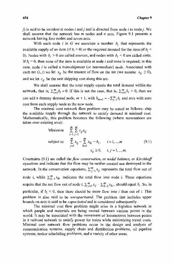
454 Chapter 9
j) is said to be incident at nodes i andj and is directed from node / to nodey. We shall assume that the network has m nodes and n arcs. Figure 9.1 presents a network having four nodes and seven arcs.
With each node i in G we associate a number bt that represents the
available supply of an item (iffy > 0) or the required demand for the item (if ty <
0). Nodes with bj > 0 are called sources, and nodes with bt < 0 are called sinks.
Iffy = 0, then none of the item is available at node / and none is required; in this
case, node /' is called a transshipment (or intermediate) node. Associated with
each arc (i,j) we let x,·. be the amount of flow on the arc (we assume x,y > 0),
and we let c,·.· be the unit shipping cost along this arc.
We shall assume that the total supply equals the total demand within the
network, that is, Σ™ i fy = 0. If this is not the case, that is, Σ™ i bj > 0, then we
can add a dummy demand node, m + 1, with bm+x = -Σ/uify and arcs with zero
cost from each supply node to the new node. The minimal-cost network flow problem may be stated as follows: ship
the available supply through the network to satisfy demand at minimal cost. Mathematically, this problem becomes the following (where summations are taken over existing arcs):
m m Minimize Σ Σ Ci/Xy
m m subject to Σ xij - Σ x/ci = fy> ' = h---,m (9.1)
j=\ k=\ χί/·^°> i,j = l,-,m.
Constraints (9.1) are called the flow conservation, or nodal balance, or Kirchhoff equations and indicate that the flow may be neither created nor destroyed in the
network. In the conservation equations, Σ?=ι % represents the total flow out of
node /, while Σ^=ι*& indicates the total flow into node i. These equations
require that the net flow out of node i, Σ^=] Xy - Σ™=\ *ki > should equal bt. So, in
particular, if bt < 0, then there should be more flow into / than out of i. This problem is also said to be uncapacitated. The problem that includes upper bounds on arcs is said to be capacitated and is considered subsequently.
The minimal cost flow problem might arise in a logistics network in which people and materials are being moved between various points in the world. It may be associated with the movement of locomotives between points in a railroad network to satisfy power for trains while minimizing travel costs. Minimal cost network flow problems occur in the design and analysis of communication systems, supply chain and distribution problems, oil pipeline systems, tanker scheduling problems, and a variety of other areas.
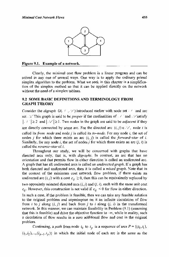
Minimal Cost Network Flows
ς< Figure 9.1. Example of a network.
Clearly, the minimal cost flow problem is a linear program and can be solved in any one of several ways. One way is to apply the ordinary primal simplex algorithm to the problem. What we seek in this chapter is a simplifica-tion of the simplex method so that it can be applied directly on the network without the need of a simplex tableau.
9.2 SOME BASIC DEFINITIONS AND TERMINOLOGY FROM GRAPH THEORY
Consider the digraph G(, I ',■'/) introduced earlier with node set, / and arc
set, V This graph is said to be proper if the cardinalities of / and · ^satisfy
|. / | ^ 2 and |. V | > 1. Two nodes in the graph are said to be adjacent if they
are directly connected by some arc. For the directed arc (i, j) e · "/, node i is
called its from-node and nodej is called its to-node. For any node i, the set of nodes j for which there exists an arc (i, j) is called the forward-star of /. Similarly, for any node /, the set of nodes j for which there exists an arc (/', i) is called the reverse-star of /.
Throughout our study, we will be concerned with graphs that have directed arcs only, that is, with digraphs. In contrast, an arc that has no orientation and that permits flow in either direction is called an undirected arc. A graph that has all undirected arcs is called an undirected graph. If a graph has both directed and undirected arcs, then it is called a mixed graph. Note that in the context of the minimum cost network flow problem, if there exists an undirected arc (i,j) with a cost q, > 0, then this can be equivalently replaced by
two oppositely oriented directed arcs (/',_/) and (J, i), each with the same unit cost Cj-. However, this construction is not valid if c,y < 0 for flow in either direction.
In such a case, if the problem is feasible, then we can take any feasible solution to the original problem and superimpose on it an infinite circulation of flow from i to j along (;', f) and back from j to i along (j, i) in the transformed network. In this manner, we can maintain feasibility in Problem (9.1) (assuming that this is feasible) and drive the objective function to -oo, while in reality, such a circulation of flow results in a zero additional flow and cost in the original problem.
Continuing, a path from node i0 to /_ is a sequence of arcs P = {(/0, /] ),
(il,Ì2%—Àip-iJp)} m which the initial node of each arc is the same as the
459
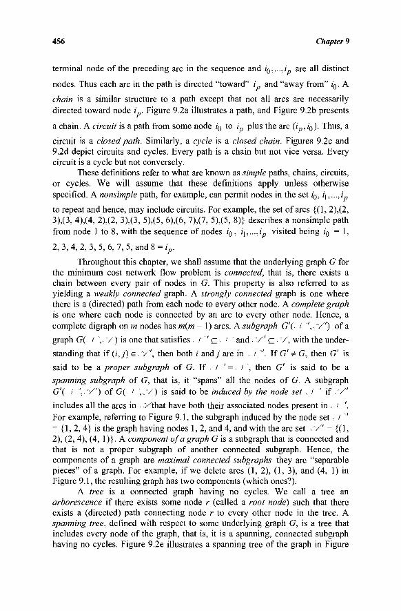
456 Chapter 9
terminal node of the preceding arc in the sequence and ί0,...,ί are all distinct
nodes. Thus each arc in the path is directed "toward" i„ and "away from" i0. A
chain is a similar structure to a path except that not all arcs are necessarily directed toward node ip. Figure 9.2a illustrates a path, and Figure 9.2b presents
a chain. A circuit is a path from some node ;0 to i plus the arc (i ,i0). Thus, a
circuit is a closed path. Similarly, a cycle is a closed chain. Figures 9.2c and 9.2d depict circuits and cycles. Every path is a chain but not vice versa. Every circuit is a cycle but not conversely.
These definitions refer to what are known as simple paths, chains, circuits, or cycles. We will assume that these definitions apply unless otherwise specified. A nonsimple path, for example, can permit nodes in the set z0, i\,...,ip
to repeat and hence, may include circuits. For example, the set of arcs {(1, 2),(2, 3),(3, 4),(4, 2),(2, 3),(3, 5),(5, 6),(6, 7),(7, 5),(5, 8)} describes a nonsimple path from node 1 to 8, with the sequence of nodes i0, i\,...,ip visited being i0 = 1,
2, 3, 4, 2, 3, 5, 6, 7, 5, and 8 = ip.
Throughout this chapter, we shall assume that the underlying graph G for the minimum cost network flow problem is connected, that is, there exists a chain between every pair of nodes in G. This property is also referred to as yielding a weakly connected graph. A strongly connected graph is one where there is a (directed) path from each node to every other node. A complete graph is one where each node is connected by an arc to every other node. Hence, a complete digraph on m nodes has m(m - 1) arcs. A subgraph G'( I ' , " / ' ) of a
graph G( / ,·."/) is one that satisfies . / ' c / and ■ V c ■ "/, with the under-standing that if (i,j) e . / ' , then both / andj are in , / ". If G' Φ G, then G' is said to be a proper subgraph of G. If ,. / ' =, / , then G' is said to be a spanning subgraph of G, that is, it "spans" all the nodes of G. A subgraph G'( I ','/') of G( l , " / ) is said to be induced by the node set , / ' if ."/ ' includes all the arcs in , Xthat have both their associated nodes present in . / '. For example, referring to Figure 9.1, the subgraph induced by the node set,. / " = {1,2, 4} is the graph having nodes 1, 2, and 4, and with the arc set . V = {(1, 2), (2, 4), (4, 1)}. A component of a graph G is a subgraph that is connected and that is not a proper subgraph of another connected subgraph. Hence, the components of a graph are maximal connected subgraphs-they are "separable pieces" of a graph. For example, if we delete arcs (1, 2), (1, 3), and (4, 1) in Figure 9.1, the resulting graph has two components (which ones?).
A tree is a connected graph having no cycles. We call a tree an arborescence if there exists some node r (called a root node) such that there exists a (directed) path connecting node r to every other node in the tree. A spanning tree, defined with respect to some underlying graph G, is a tree that includes every node of the graph, that is, it is a spanning, connected subgraph having no cycles. Figure 9.2e illustrates a spanning tree of the graph in Figure
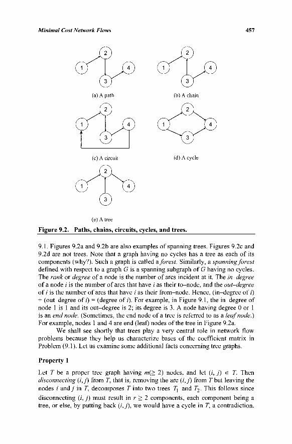
Minimal Cost Network Flows
(a) A path (b) A chain
(c) A circuit (d) A cycle
(e) A tree
Figure 9.2. Paths, chains, circuits, cycles, and trees.
9.1. Figures 9.2a and 9.2b are also examples of spanning trees. Figures 9.2c and 9.2d are not trees. Note that a graph having no cycles has a tree as each of its components (why?). Such a graph is called a forest. Similarly, a spanning forest defined with respect to a graph G is a spanning subgraph of G having no cycles. The rank or degree of a node is the number of arcs incident at it. The in-degree of a node i is the number of arcs that have i as their to-node, and the out-degree of ; is the number of arcs that have / as their from-node. Hence, (in-degree of i) + (out-degree of/) = (degree of/). For example, in Figure 9.1, the in-degree of node 1 is 1 and its out-degree is 2; its degree is 3. A node having degree 0 or 1 is an end node. (Sometimes, the end node of a tree is referred to as a leaf node.) For example, nodes 1 and 4 are end (leaf) nodes of the tree in Figure 9.2a.
We shall see shortly that trees play a very central role in network flow problems because they help us characterize bases of the coefficient matrix in Problem (9.1). Let us examine some additional facts concerning tree graphs.
Property 1
Let T be a proper tree graph having m(> 2) nodes, and let (/, j) e T. Then disconnecting (i,j) from T, that is, removing the arc (i,j) from T but leaving the nodes / andj in T, decomposes T into two trees 7j and T2. This follows since disconnecting (/, j) must result in r > 2 components, each component being a tree, or else, by putting back (/, j), we would have a cycle in T, a contradiction.
459
458 Chapter 9
Because putting back (/', J) can connect no more than two components by definition, and because Tis connected, we must have r = 2.
Property 2
A proper tree graph has at least two end nodes. This is clearly true for a tree having only two nodes. By induction, suppose that this is true for a tree having 2,...,(m - 1) nodes, and let us show that it is true for a tree having m nodes, where m>3. Select some (i,j) e Tand disconnect it from T, creating two trees 7j and T2, each having no more than (m - 1) nodes. If 7] or T2 has only one
node, then by the induction hypothesis, the total number of end nodes in 7j and
T2 is at least 3 (why?). Moreover, by putting back (/,/), we can lose at most one
of these end nodes. Hence, Trias at least two end nodes. Otherwise, if both 7]
and T2 have at least two nodes, then they have at least four end nodes in total,
and putting back (/, j) can result in a loss of at most two end nodes. This again shows that Thas at least two end nodes.
Property 3
A tree having m nodes has (m - 1) arcs. This is clearly true for m = 1 or 2. By induction, assume that this property holds for a tree having (m - 1) nodes and consider a tree with m nodes, m > 3. By Property 2, an end node i exists. Disconnect the (unique) arc incident at the end node and obtain two trees 7] and
T2 (by Property 1), where 7j = {/}. Hence, 7j has zero arcs, and T2 has (m -
1) nodes. By the induction hypothesis, it has (m - 2) arcs. Therefore, Thas (m -2)+ 1 = (m- 1) arcs.
These fundamental properties help establish several equivalent characteri-zations of a tree graph.
Equivalent Characterizations of a Tree Graph T
(a) T is connected and has no cycles. (b) T is connected and has (m - 1) arcs. (c) T has (m - 1) arcs and has no cycles. (d) T is connected, but disconnecting any arc from T results in two
components. (e) T has no cycles, but adding any new arc to T results in a graph
having exactly one cycle. (Such a graph is called a one-tree.) (f) T has a unique chain connecting each pair of its nodes.
Observe that Statements (a), (b), and (c) assert that any two of the three characteristics of being connected, having no cycles, and having (m - 1) arcs implies the third. Furthermore, we shall see later that Statements (d) and (f) play a role in computing and updating dual and primal variables. Statement (e) pertains to the representation of a nonbasic variable column in terms of the basic variable columns.
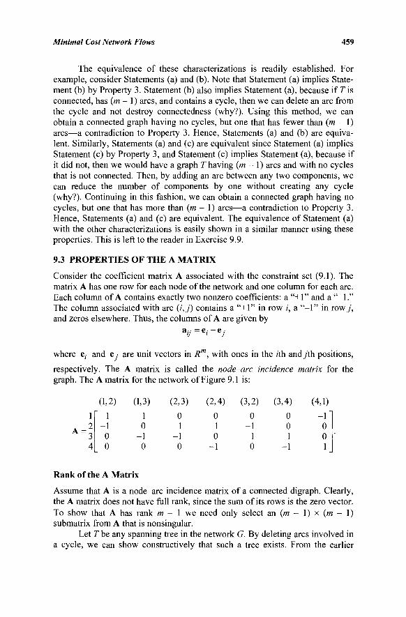
Minimal Cost Network Flows 459
The equivalence of these characterizations is readily established. For example, consider Statements (a) and (b). Note that Statement (a) implies State-ment (b) by Property 3. Statement (b) also implies Statement (a), because if T is connected, has (m - 1) arcs, and contains a cycle, then we can delete an arc from the cycle and not destroy connectedness (why?). Using this method, we can obtain a connected graph having no cycles, but one that has fewer than (m - 1) arcs—a contradiction to Property 3. Hence, Statements (a) and (b) are equiva-lent. Similarly, Statements (a) and (c) are equivalent since Statement (a) implies Statement (c) by Property 3, and Statement (c) implies Statement (a), because if it did not, then we would have a graph T having (m - 1) arcs and with no cycles that is not connected. Then, by adding an arc between any two components, we can reduce the number of components by one without creating any cycle (why?). Continuing in this fashion, we can obtain a connected graph having no cycles, but one that has more than (m - 1) arcs—a contradiction to Property 3. Hence, Statements (a) and (c) are equivalent. The equivalence of Statement (a) with the other characterizations is easily shown in a similar manner using these properties. This is left to the reader in Exercise 9.9.
9.3 PROPERTIES OF THE A MATRIX
Consider the coefficient matrix A associated with the constraint set (9.1). The matrix A has one row for each node of the network and one column for each arc. Each column of A contains exactly two nonzero coefficients: a "+1" and a " - 1 . " The column associated with arc (/,_/) contains a "+1" in row /, a " - 1 " in row/, and zeros elsewhere. Thus, the columns of A are given by
au=ei-ej
where e; and e,· are unit vectors in Rm, with ones in the rth andy'th positions,
respectively. The A matrix is called the node-arc incidence matrix for the graph. The A matrix for the network of Figure 9.1 is:
A = :
Rank of the A Matrix
Assume that A is a node-arc incidence matrix of a connected digraph. Clearly, the A matrix does not have full rank, since the sum of its rows is the zero vector. To show that A has rank m - 1 we need only select an (m - 1) x (m - 1) submatrix from A that is nonsingular.
Let T be any spanning tree in the network G. By deleting arcs involved in a cycle, we can show constructively that such a tree exists. From the earlier
1 2 3 4
0,2) 1
-1 0 0
(1,3)
1 0
-1 0
(2,3)
0 1
-1 0
(2,4)
0 1 0
-1
(3,2)
0 -1
1 0
(3,4)
0 0 1
-1
(4,1)
-1 0 0 1
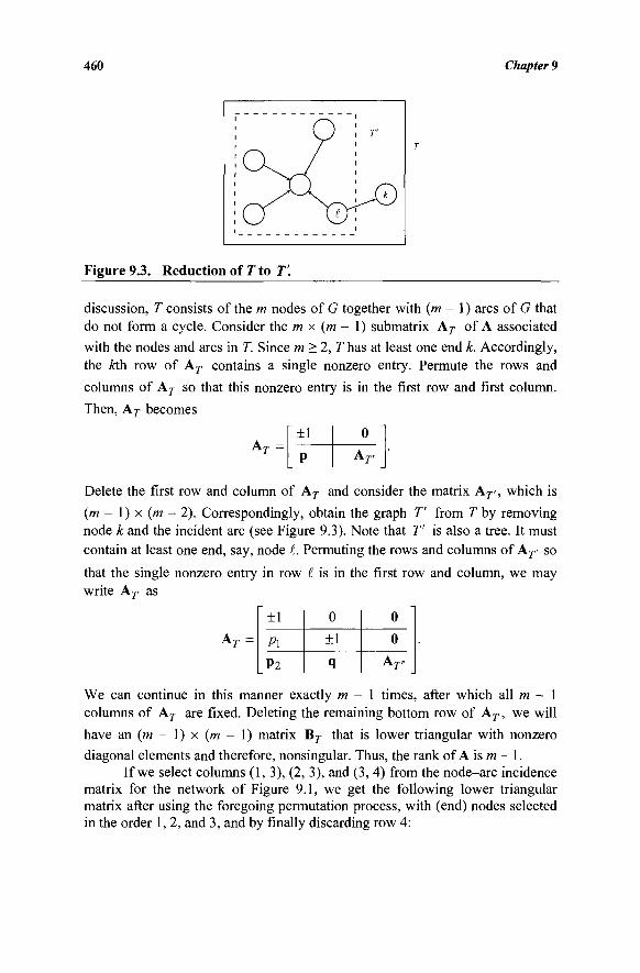
460 Chapter 9
Figure 9.3. Reduction of 7to T.
discussion, T consists of the m nodes of G together with (m - 1) arcs of G that do not form a cycle. Consider the m x (m - 1) submatrix AT of A associated with the nodes and arcs in T. Since m>2,T has at least one end k. Accordingly, the Ath row of AT contains a single nonzero entry. Permute the rows and
columns of AT so that this nonzero entry is in the first row and first column.
Then, A7- becomes
~±1
P
0
Aji AT =
Delete the first row and column of AT and consider the matrix A τ · , which is
(m - 1) x (m - 2). Correspondingly, obtain the graph 7" from T by removing node k and the incident arc (see Figure 9.3). Note that T' is also a tree. It must contain at least one end, say, node i. Permuting the rows and columns of Ατ· so
that the single nonzero entry in row I is in the first row and column, we may write AT as
±1
P\
P2
0
±1
q
0
0
A r _
We can continue in this manner exactly m - 1 times, after which all m - 1 columns of AT are fixed. Deleting the remaining bottom row of AT, we will
have an (m - 1) x (m - 1) matrix Bj- that is lower triangular with nonzero
diagonal elements and therefore, nonsingular. Thus, the rank of A is m - 1. If we select columns (1,3), (2, 3), and (3, 4) from the node-arc incidence
matrix for the network of Figure 9.1, we get the following lower triangular matrix after using the foregoing permutation process, with (end) nodes selected in the order 1, 2, and 3, and by finally discarding row 4:
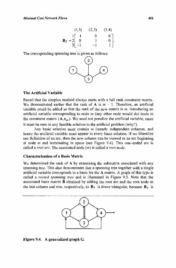
Minimal Cost Network Flows 461
(1,3) (2,3) (3,4)
1 B r =2
1 0
-1
0 1
-1
0 0 1
The corresponding spanning tree is given as follows:
©X© The Artificial Variable
Recall that the simplex method always starts with a full rank constraint matrix. We demonstrated earlier that the rank of A is m - 1. Therefore, an artificial variable could be added so that the rank of the new matrix is m. Introducing an artificial variable corresponding to node m (any other node would do) leads to the constraint matrix (A,em). We need not penalize the artificial variable, since
it must be zero in any feasible solution to the artificial problem (why?). Any basic solution must contain m linearly independent columns, and
hence the artificial variable must appear in every basic solution. If we liberalize our definition of an arc, then the new column can be viewed as an arc beginning at node m and terminating in space (see Figure 9.4). This one-ended arc is called a root arc. The associated node (m) is called a root node.
Characterization of a Basis Matrix
We determined the rank of A by examining the submatrix associated with any spanning tree. This also demonstrates that a spanning tree together with a single artificial variable corresponds to a basis for the A matrix. A graph of this type is called a rooted spanning tree and is illustrated in Figure 9.5. Note that the associated basis matrix B obtained by adding the root arc and the root node as the last column and row, respectively, to B r is lower triangular, because BT is
Figure 9.4. A generalized graph G.
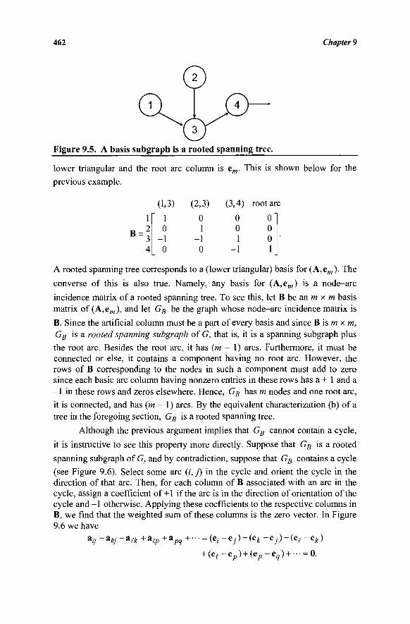
462 Chapter 9
Figure 9.5. A basis subgraph is a rooted spanning tree.
lower triangular and the root arc column is e,„. This is shown below for the
previous example.
1 2 3 4
(1,3)
1 0
-1 0
(2,3)
0 1
-1 0
(3,4)
0 0 1
-1
root arc
0" 0 0 1
B =
A rooted spanning tree corresponds to a (lower triangular) basis for (A,em). The
converse of this is also true. Namely, any basis for (A,em) is a node-arc
incidence matrix of a rooted spanning tree. To see this, let B be an m x m basis matrix of (A,em), and let GB be the graph whose node-arc incidence matrix is
B. Since the artificial column must be a part of every basis and since B is m x m, GB is a rooted spanning subgraph of G, that is, it is a spanning subgraph plus
the root arc. Besides the root arc, it has (m - 1) arcs. Furthermore, it must be connected or else, it contains a component having no root arc. However, the rows of B corresponding to the nodes in such a component must add to zero since each basic arc column having nonzero entries in these rows has a + 1 and a -1 in these rows and zeros elsewhere. Hence, GB has m nodes and one root arc, it is connected, and has (m - 1) arcs. By the equivalent characterization (b) of a tree in the foregoing section, GB is a rooted spanning tree.
Although the previous argument implies that GB cannot contain a cycle,
it is instructive to see this property more directly. Suppose that GB is a rooted
spanning subgraph of G, and by contradiction, suppose that GB contains a cycle
(see Figure 9.6). Select some arc (i,j) in the cycle and orient the cycle in the direction of that arc. Then, for each column of B associated with an arc in the cycle, assign a coefficient of+1 if the arc is in the direction of orientation of the cycle and -1 otherwise. Applying these coefficients to the respective columns in B, we find that the weighted sum of these columns is the zero vector. In Figure 9.6 we have
ay -Hj -*ek+aip +&Pq +··■ = (e,· -e_,-)-(et -ej)-(e( -ek)
+ (e^-e„) + (e„-e„) + --- = 0.
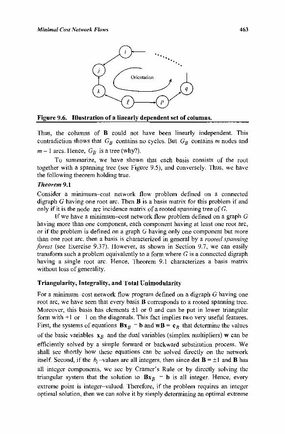
Minimal Cost Network Flows 463
Figure 9.6. Illustration of a linearly dependent set of columns.
Thus, the columns of B could not have been linearly independent. This contradiction shows that GB contains no cycles. But GB contains m nodes and m - 1 arcs. Hence, GB is a tree (why?).
To summarize, we have shown that each basis consists of the root together with a spanning tree (see Figure 9.5), and conversely. Thus, we have the following theorem holding true.
Theorem 9.1
Consider a minimum-cost network flow problem defined on a connected digraph G having one root arc. Then B is a basis matrix for this problem if and only if it is the node-arc incidence matrix of a rooted spanning tree of G.
If we have a minimum-cost network flow problem defined on a graph G having more than one component, each component having at least one root arc, or if the problem is defined on a graph G having only one component but more than one root arc, then a basis is characterized in general by a rooted spanning forest (see Exercise 9.37). However, as shown in Section 9.7, we can easily transform such a problem equivalently to a form where G is a connected digraph having a single root arc. Hence, Theorem 9.1 characterizes a basis matrix without loss of generality.
Triangularity, Integrality, and Total Uniniodulariry
For a minimum-cost network flow program defined on a digraph G having one root arc, we have seen that every basis B corresponds to a rooted spanning tree. Moreover, this basis has elements ±1 or 0 and can be put in lower triangular form with +1 or -1 on the diagonals. This fact implies two very useful features. First, the systems of equations BxB = b and wB = cB that determine the values
of the basic variables xB and the dual variables (simplex multipliers) w can be
efficiently solved by a simple forward or backward substitution process. We shall see shortly how these equations can be solved directly on the network itself. Second, if the ty -values are all integers, then since det B = ±1 and B has all integer components, we see by Cramer's Rule or by directly solving the triangular system that the solution to Bxg = b is all integer. Hence, every
extreme point is integer-valued. Therefore, if the problem requires an integer optimal solution, then we can solve it by simply determining an optimal extreme
464 Chapter 9
point solution to the linear programming network flow problem obtained by ignoring the integrality restrictions.
There is a richer property that the matrix A satisfies, namely, that of total unimodularity. A matrix A is said to be totally unimodular if every square submatrix of A has determinant +1, - 1 , or 0. In the case of the node-arc incidence matrix A, since all entries are ±1 or 0, every l x l submatrix has determinant ±1 or 0. Hence, by induction, suppose that this property is true for every square submatrix of size (k - 1) x (k - 1), and let A^ be any k χ k submatrix of A, where k > 2. We must show that det Ak = ±1 or 0. Note that each column of A^ has either all zeros or only a single nonzero entry that is +1 or - 1 , or it has exactly two nonzero entries, namely a +1 and a - 1 . If any column of A^ is zero, then det Ak = 0. If any column of A^ has a single nonzero entry, then expanding the determinant of A^ by the minors of that column, we get det A^ = ± det A^_i, where A^_i is a square submatrix of size (k-l) x (k - 1). By the induction hypothesis, det Ak_\ = ±1 or 0, and hence det Ak = ±1 or 0. Otherwise, every column of A^ must have a +1 and a - 1 . In this case, since the rows of Ak add up to the zero vector, we have that det A^ = 0. Hence, A is totally unimodular.
Note that this proof holds true even if we delete rows or columns from A, or more importantly, if we add ± unit vector columns to A. These columns may correspond to slack or surplus or artificial variable columns. The resulting coefficient matrix in such cases continues to be totally unimodular. Conse-quently, det B = ±1 for all bases B, and every extreme point is integer-valued
for integer right-hand-sides b. For any basis B, the inverse matrix B~ is also comprised of elements that are ±1 or 0 (why?). Furthermore, the updated column y(y in any canonical representation (simplex tableau) of a basic solution
is comprised of ±1 or 0 elements. To see this, note that y;.· is given by the
system By,y = a,-.·. Hence, the kth element yyk of y; is given by Cramer's Rule as
_ detBA
where Bk is obtained from B by replacing its Mi column with a;y. Hence, B^
is a square submatrix of A, and so det Bk - ±1 or 0. Because det B = ±1, it
follows that yij!c = ±1 or 0. Hence, any column a,-.· can be obtained by the
simple addition and subtraction of basic variable columns. (We shall also see this fact constructively later.)
To summarize, we have shown that the matrix A , comprised of the
node-arc incidence matrix of a graph along with ± unit vector columns, is
totally unimodular. Hence, for any basis B of A0, B and B~ have elements
that are ±1 or 0, det B = det B~ = ±1, the extreme points of {x : A x = b, x >
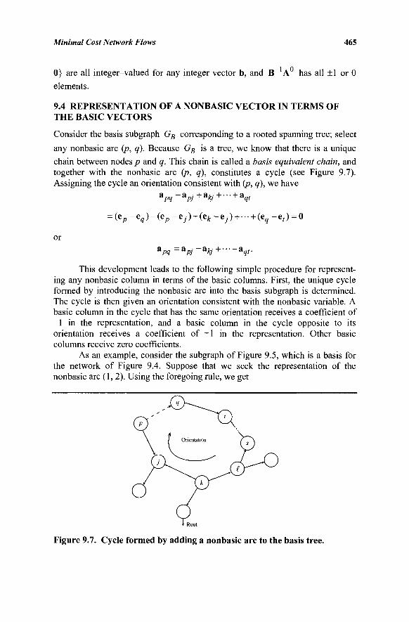
Minimal Cost Network Flows 465
0} are all integer-valued for any integer vector b, and B A has all ±1 or 0 elements.
9.4 REPRESENTATION OF A NONBASIC VECTOR IN TERMS OF THE BASIC VECTORS
Consider the basis subgraph GB corresponding to a rooted spanning tree; select
any nonbasic arc (p, q). Because Gs is a tree, we know that there is a unique
chain between nodes p and q. This chain is called a basis equivalent chain, and together with the nonbasic arc (p, q), constitutes a cycle (see Figure 9.7). Assigning the cycle an orientation consistent with (p, q), we have
apq ~ apj + akj H h aqt
= (ep-eq)-(ep-ej) + (ek-ej) + --- + (eq-et) = Q
or apq =apj-akj+----aqf
This development leads to the following simple procedure for represent-ing any nonbasic column in terms of the basic columns. First, the unique cycle formed by introducing the nonbasic arc into the basis subgraph is determined. The cycle is then given an orientation consistent with the nonbasic variable. A basic column in the cycle that has the same orientation receives a coefficient of -1 in the representation, and a basic column in the cycle opposite to its orientation receives a coefficient of +1 in the representation. Other basic columns receive zero coefficients.
As an example, consider the subgraph of Figure 9.5, which is a basis for the network of Figure 9.4. Suppose that we seek the representation of the nonbasic arc (1, 2). Using the foregoing rule, we get
Figure 9.7. Cycle formed by adding a nonbasic arc to the basis tree.
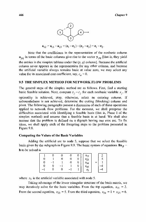
466 Chapter 9
J©
l12 l13 *23 : ( e 1 - e 3 ) - ( e 2 - e 3 ) = e 1 - e 2 .
Note that the coefficients in the representation of the nonbasic column a„„ in terms of the basic columns give rise to the vector y [that is, they yield
the entries in the simplex tableau under the (p, q) column]. Because the artificial column never appears in the representation for any other column, and because the artificial variable always remains basic at value zero, we may select any value for its associated cost coefficient, say, ca = 0.
9.5 THE SIMPLEX METHOD FOR NETWORK FLOW PROBLEMS
The general steps of the simplex method are as follows. First, find a starting basic feasible solution. Next, compute zj -cj for each nonbasic variable x-. If
optimality is achieved, stop; otherwise, select an entering column. If unboundedness is not achieved, determine the exiting (blocking) column and pivot. The following paragraphs present a discussion of each of these operations applied to network flow problems. For the moment, we shall postpone the difficulties associated with identifying a feasible basis (that is, Phase I of the simplex method) and assume that a feasible basis is at hand. We shall also assume that the problem is defined on a digraph having one root arc. To fix ideas, we shall apply each of the foregoing steps to the problem presented in Figure 9.8.
Computing the Values of the Basic Variables
Adding the artificial arc to node 5, suppose that we select the feasible basis given by the subgraph in Figure 9.9. The basic system of equations BxB = b to be solved is
1 0 0 0
-1
0 1
-1 0 0
0 0 1
-1 0
0 0 0 1
-1
0 0 0 0 1
xls
*23
*34
*45 X5
2 5 1
-4 -4
where x5 is the artificial variable associated with node 5.
Taking advantage of the lower triangular structure of the basis matrix, we may iteratively solve for the basic variables. From the top equation, xl5 =2.
From the second equation, x23 =5 . From the third equation, x34 = 1 + x23 = 6.
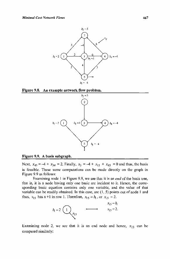
Minimal Cost Network Flows 467
*!=2 ί 1 bA=-A
Figure 9.8. An example network flow problem.
* !=2 ( 1 bA=-H
Figure 9.9. A basis subgraph.
Next, x45 = -4 + x34 = 2. Finally, x5 = -4 + x15 + x45 = 0 and thus, the basis
is feasible. These same computations can be made directly on the graph in Figure 9.9 as follows:
Examining node 1 in Figure 9.9, we see that it is an end of the basis tree, that is, it is a node having only one basic arc incident to it. Hence, the corre-sponding basic equation contains only one variable, and the value of that variable can be readily obtained. In this case, arc (1, 5) points out of node 1 and thus, X]5 has a +1 in row 1. Therefore, x15 = i\ , or x15 =2.
*15= h by=2 ( 1 ) * * x,,=2.
*15
Λ15 ■
Examining node 2, we see that it is an end node and hence, x23 can be computed similarly:
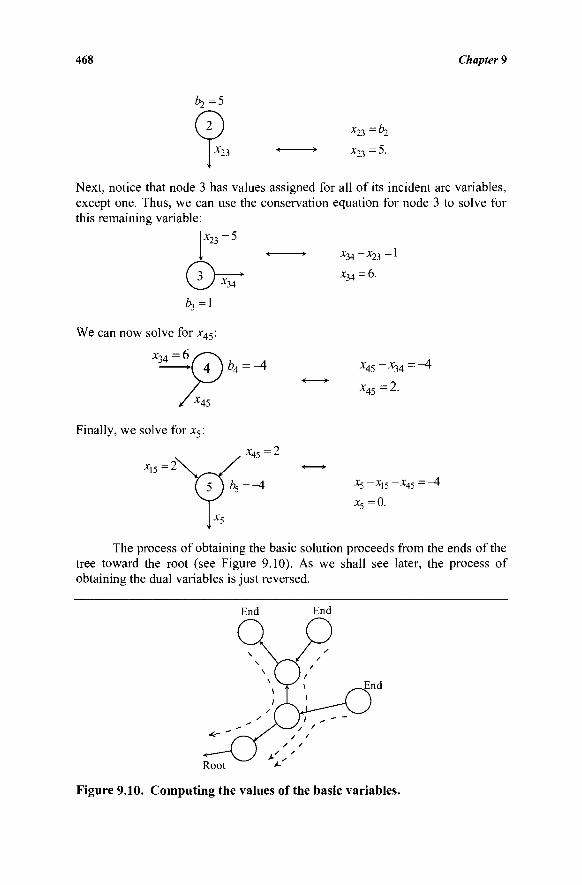
468 Chapter 9
Ò2=5
Θ *23
Χ 2 3 -ì>2
X2Ì=5.
Next, notice that node 3 has values assigned for all of its incident arc variables, except one. Thus, we can use the conservation equation for node 3 to solve for this remaining variable:
v23 ■
Θ = 1
x34
xv,~xn - 1
x34 = 6.
We can now solve for x45:
/ x45
Finally, we solve for x5:
*45=2
x^=2\^y Ϊ5 )b5=-4 V
. x5
« *
*—"
*45 -X34 — 4
X45 — 2.,
x5-x15-x45 =-A x5=0.
The process of obtaining the basic solution proceeds from the ends of the tree toward the root (see Figure 9.10). As we shall see later, the process of obtaining the dual variables is just reversed.
End End
Root
Figure 9.10. Computing the values of the basic variables.
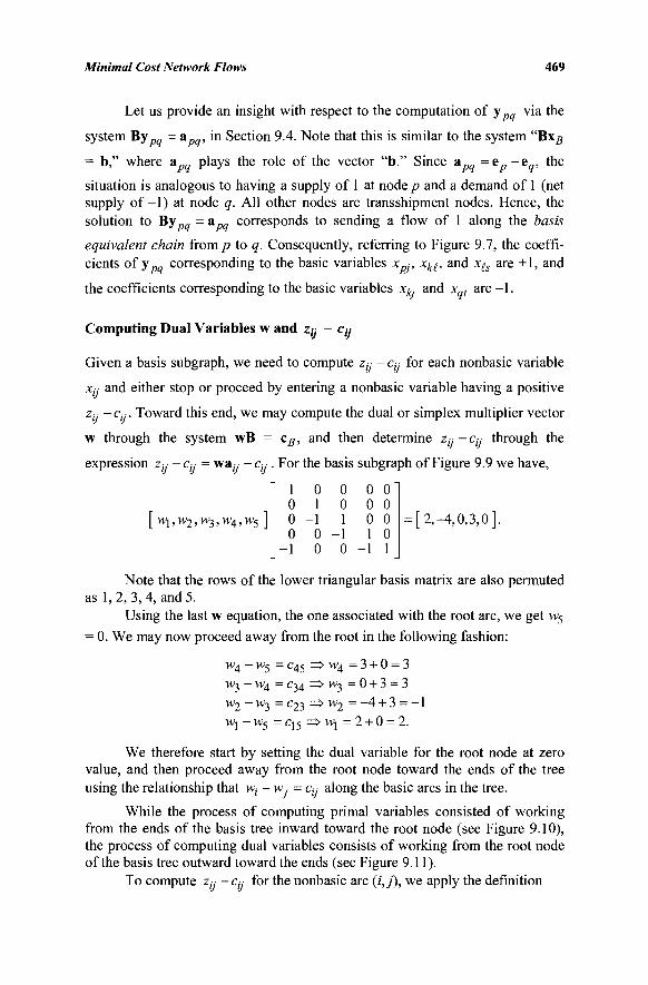
Minimal Cost Network Flows 469
Let us provide an insight with respect to the computation of y pq via the
system By _. = a „„, in Section 9.4. Note that this is similar to the system "Βχβ
= b," where &pq plays the role of the vector "b." Since apq -ep-eq, the
situation is analogous to having a supply of 1 at node p and a demand of 1 (net supply of-1) at node q. All other nodes are transshipment nodes. Hence, the solution to By „9 = a _. corresponds to sending a flow of 1 along the basis
equivalent chain from/? to q. Consequently, referring to Figure 9.7, the coeffi-cients of y corresponding to the basic variables x j , xkf, and xts are +1, and
the coefficients corresponding to the basic variables xkj- and xqt are-1.
Computing Dual Variables w and ztj - c,y
Given a basis subgraph, we need to compute z„ - c„ for each nonbasic variable
xq and either stop or proceed by entering a nonbasic variable having a positive
z„ - c,y. Toward this end, we may compute the dual or simplex multiplier vector
w through the system wB = cB, and then determine z„· - c„ through the
expression z„· -c„· = wa„· -c« . For the basis subgraph of Figure 9.9 we have,
[ W ] , VV2 , W3 , W4 , W5
1 0 0 0
-1
0 1
-1 0 0
0 0 1
-1 0
0 0 0 0 0 0 1 0
-1 1
= [2,-4,0,3,0].
Note that the rows of the lower triangular basis matrix are also permuted as 1,2, 3, 4, and 5.
Using the last w equation, the one associated with the root arc, we get vv5
= 0. We may now proceed away from the root in the following fashion:
w4 - w 5 = c45 =>w4 =3 + 0 = 3 W3 -W4 = C34 =>W} = 0 + 3 = 3 w2 ~ w3 = c23 =* w2 = -4 + 3 = -1 Wj - w5 = Cj5 => Wj =2 + 0 = 2.
We therefore start by setting the dual variable for the root node at zero value, and then proceed away from the root node toward the ends of the tree using the relationship that wi - w = c„ along the basic arcs in the tree.
While the process of computing primal variables consisted of working from the ends of the basis tree inward toward the root node (see Figure 9.10), the process of computing dual variables consists of working from the root node of the basis tree outward toward the ends (see Figure 9.11).
To compute z„ - c„ for the nonbasic arc (i,j), we apply the definition
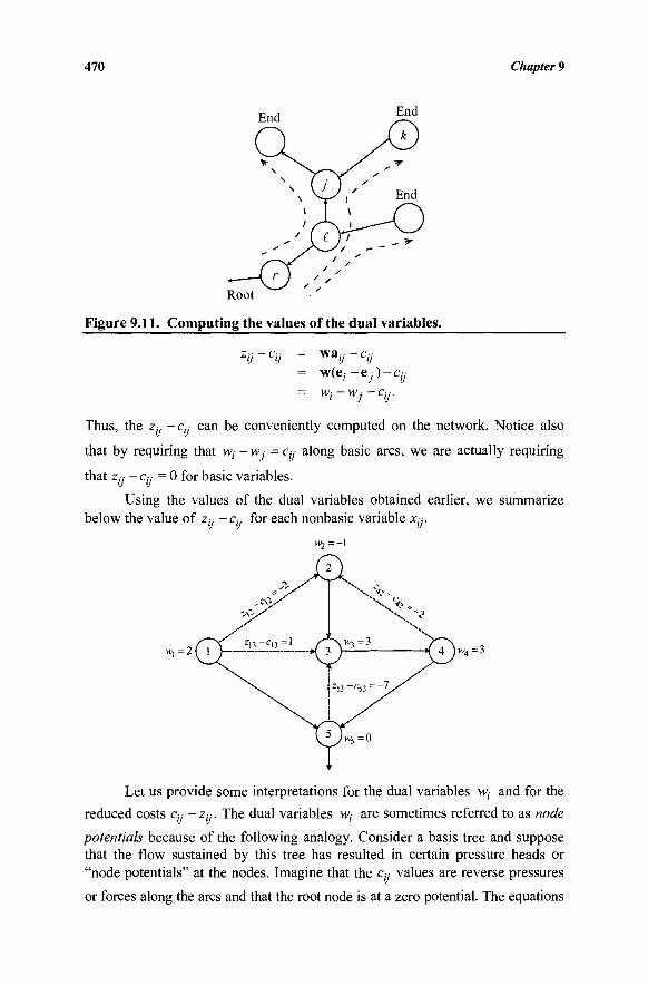
470 Chapter 9
Root
Figure 9.11. Computing the values of the dual variables.
zij~cij = w a i / - c y = w(e;-ey)-c / ; / · = Wi-Wj-Cjj.
Thus, the zy -ct- can be conveniently computed on the network. Notice also
that by requiring that w; - w- = ci;- along basic arcs, we are actually requiring
that z,·,· - c„ = 0 for basic variables. u u Using the values of the dual variables obtained earlier, we summarize
below the value of z« -c« for each nonbasic variable Xy.
vw =2
Let us provide some interpretations for the dual variables w,· and for the
reduced costs c„ -z,·,·. The dual variables w,· are sometimes referred to as node v U l
potentials because of the following analogy. Consider a basis tree and suppose that the flow sustained by this tree has resulted in certain pressure heads or "node potentials" at the nodes. Imagine that the Cy values are reverse pressures or forces along the arcs and that the root node is at a zero potential. The equations
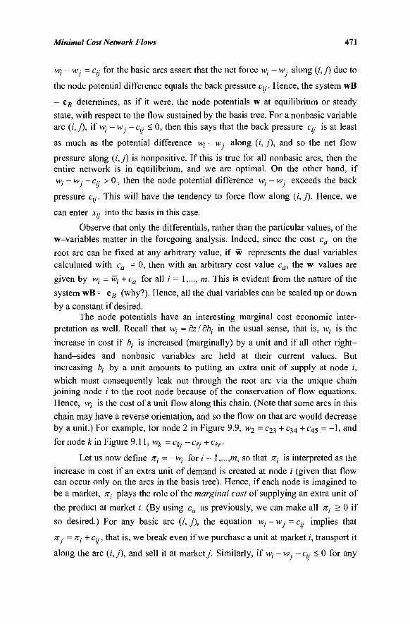
Minimal Cost Network Flows 471
Wj - w: = Cy for the basic arcs assert that the net force w,· - w, along (i,j) due to
the node potential difference equals the back pressure Cy. Hence, the system wB
= cB determines, as if it were, the node potentials w at equilibrium or steady state, with respect to the flow sustained by the basis tree. For a nonbasic variable arc (i,j), if Wj - w- -Cy < 0, then this says that the back pressure Cy is at least
as much as the potential difference w, - w, along (z, j), and so the net flow
pressure along (i, j) is nonpositive. If this is true for all nonbasic arcs, then the entire network is in equilibrium, and we are optimal. On the other hand, if Wj - Wj - CJ: > 0, then the node potential difference w; - w ,· exceeds the back
pressure Cy. This will have the tendency to force flow along (i, j). Hence, we
can enter Xy into the basis in this case.
Observe that only the differentials, rather than the particular values, of the w-variables matter in the foregoing analysis. Indeed, since the cost ca on the root arc can be fixed at any arbitrary value, if w represents the dual variables calculated with ca = 0, then with an arbitrary cost value ca, the w-values are given by w,· = w, +ca for all i = 1,..., m. This is evident from the nature of the system wB = cB (why?). Hence, all the dual variables can be scaled up or down
by a constant if desired. The node potentials have an interesting marginal cost economic inter-
pretation as well. Recall that wt =dz/ db{ in the usual sense, that is, w; is the increase in cost if ty is increased (marginally) by a unit and if all other right-hand-sides and nonbasic variables are held at their current values. But increasing è, by a unit amounts to putting an extra unit of supply at node i, which must consequently leak out through the root arc via the unique chain joining node i to the root node because of the conservation of flow equations. Hence, wt is the cost of a unit flow along this chain. (Note that some arcs in this chain may have a reverse orientation, and so the flow on that arc would decrease by a unit.) For example, for node 2 in Figure 9.9, w2 = c23 +c34 +c4 5 = - 1 , and
for node k in Figure 9.11, wk = % - cy + cfr.
Let us now define Kt = -w,· for i = \,...,m, so that ττ,- is interpreted as the increase in cost if an extra unit of demand is created at node / (given that flow can occur only on the arcs in the basis tree). Hence, if each node is imagined to be a market, π, plays the role of the marginal cost of supplying an extra unit of
the product at market i. (By using ca as previously, we can make all /rz· > 0 if
so desired.) For any basic arc (/, j), the equation w, - w,· = c^ implies that
π j = πι + Cy, that is, we break even if we purchase a unit at market /, transport it
along the arc (i,j), and sell it at market j . Similarly, if w,· - w -Cy < 0 for any
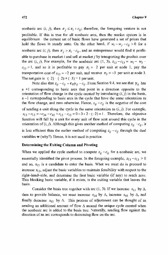
472 Chapter 9
nonbasic arc (/, j), then π- <TT;-+C«; therefore, the foregoing venture is not
profitable. If this is true for all nonbasic arcs, then the market system is in equilibrium—the current set of basic flows have generated a set of prices that hold the flows in steady state. On the other hand, if w, - w .■ - Cy > 0 for a
nonbasic arc (i, j), then π ■ > πί + Cy, and an entrepreneur would find it profit-
able to purchase in market i and sell at market y by transporting the product over
the arc (/, J). For example, for the nonbasic arc (1, 3), z13 - c 1 3 = wx - w3 -
c13 =1 , and so it is profitable to pay πχ =-2 per unit at node 1, pay the
transportation cost of c13 = -2 per unit, and receive ;r3 = -3 per unit at node 3.
The net gain is -(-2) - (-2) + (-3) = 1 per unit. Note also that zy -Cy = cfiy,y -Cy. From Section 9.4, we see that y,y has
a +1 corresponding to basic arcs that point in a direction opposite to the orientation of flow change in the cycle created by introducing (i, j) in the basis, a -1 corresponding to basic arcs in the cycle that have the same orientation as the flow change, and zero otherwise. Hence, zy - Cy is the negative of the cost
of sending a unit along the cycle in the same orientation as (i, j). For example, zi 3 ~ ci 3 = _c34 ~C45+C15_C13 = 0 - 3 + 2 - (-2) = 1. Therefore, the objective function will fall by a unit for every unit of flow sent around this cycle in the orientation of (/,_/). Although this gives another method of computing zy - c« , it
is less efficient than the earlier method of computing zy - Cy through the dual
variables w (why?). Hence, it is not used in practice.
Determining the Exiting Column and Pivoting
When we applied the cycle method to compute zy - Cy for a nonbasic arc, we
essentially identified the pivot process. In the foregoing example, z13 - q 3 > 0
and so, x13 is a candidate to enter the basis. What we must do is proceed to
increase x13, adjust the basic variables to maintain feasibility with respect to the
right-hand-side, and determine the first basic variable (if any) to reach zero. This blocking basic variable, if it exists, is the exiting variable that leaves the basis.
Consider the basis tree together with arc (1, 3). If we increase x13 by Δ,
then to provide balance, we must increase x34 by Δ, increase x45 by Δ, and
finally decrease x\ 5 by Δ. This process of adjustment can be thought of as sending an additional amount of flow Δ around the unique cycle created when the nonbasic arc is added to the basis tree. Naturally, sending flow against the direction of an arc corresponds to decreasing flow on the arc.
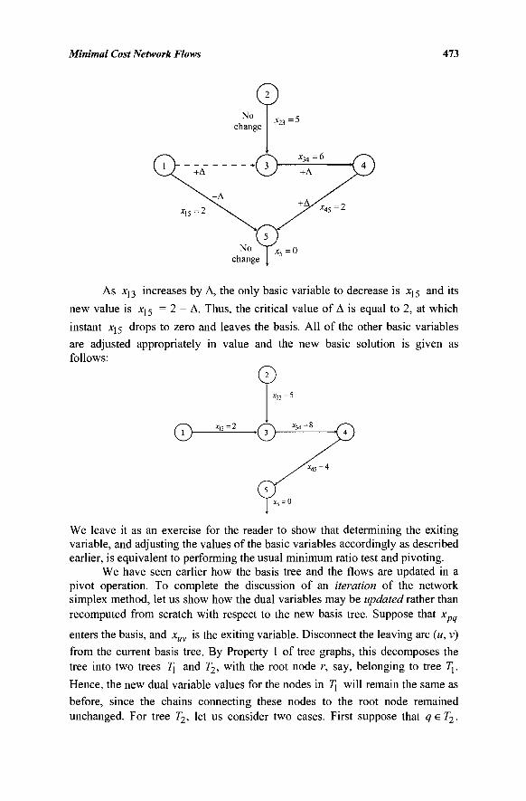
Minimal Cost Network Flows 473
change
As XJ3 increases by Δ, the only basic variable to decrease is xJ5 and its new value is x15 = 2 - Δ. Thus, the critical value of Δ is equal to 2, at which instant xl5 drops to zero and leaves the basis. All of the other basic variables are adjusted appropriately in value and the new basic solution is given as follows:
We leave it as an exercise for the reader to show that determining the exiting variable, and adjusting the values of the basic variables accordingly as described earlier, is equivalent to performing the usual minimum ratio test and pivoting.
We have seen earlier how the basis tree and the flows are updated in a pivot operation. To complete the discussion of an iteration of the network simplex method, let us show how the dual variables may be updated rather than recomputed from scratch with respect to the new basis tree. Suppose that xpq
enters the basis, and xuv is the exiting variable. Disconnect the leaving arc (w, v) from the current basis tree. By Property 1 of tree graphs, this decomposes the tree into two trees 7] and T2, with the root node r, say, belonging to tree 7]. Hence, the new dual variable values for the nodes in 7] will remain the same as before, since the chains connecting these nodes to the root node remained unchanged. For tree T2, let us consider two cases. First suppose that q eT2.
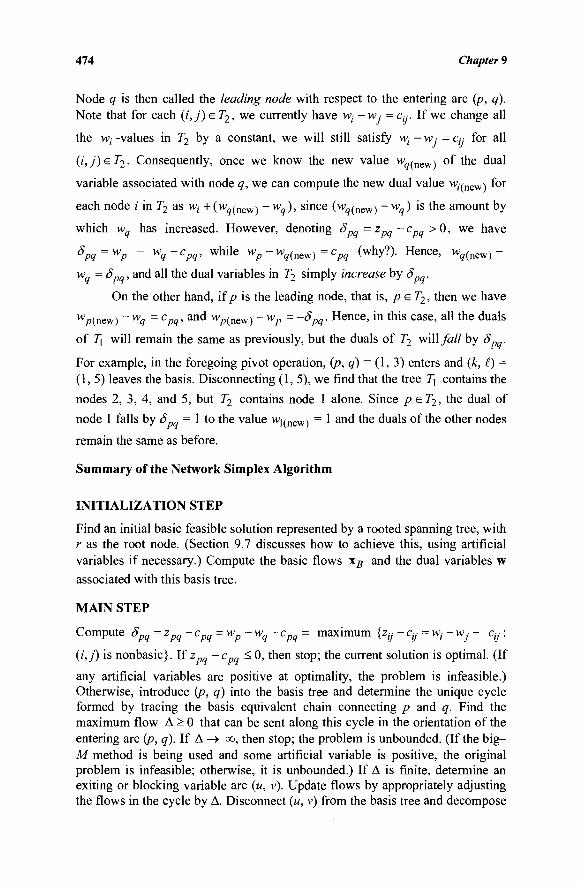
474 Chapter 9
Node q is then called the leading node with respect to the entering arc (p, q). Note that for each (i,j) eT2, we currently have vv(- - w,■ = Cy. If we change all
the Wj -values in T2 by a constant, we will still satisfy w, - w ■ = Cy for all
(i,j)eT2. Consequently, once we know the new value w„(new) of the dual
variable associated with node q, we can compute the new dual value w(vnew) for
each node i in T2 as wi + (wq/new^ -wq), since (w„(new) -w„) is the amount by
which wq has increased. However, denoting Spq=zpq-cpq>Q, we have
Spq=Wp ~ wq~cpq> w h i l e wp ~ ^ ( n e w ) = cpq ( w n y ? ) · H e n c e > ^ ( n e w ) ~
wq = 5pq, and all the dual variables in T2 simply increase by Spq.
On the other hand, ifp is the leading node, that is, peT2, then we have
WpCnew) - wq = cPq, a n d wp(new) ~ W
P = ~δPq- Hence, in this case, all the duals
of 7] will remain the same as previously, but the duals of T2 will fall by Spq.
For example, in the foregoing pivot operation, (p, q) = (1, 3) enters and (k, i) = (1,5) leaves the basis. Disconnecting (1,5), we find that the tree 7] contains the
nodes 2, 3, 4, and 5, but T2 contains node 1 alone. Since ρεΤ2, the dual of
node 1 falls by δ = 1 to the value >%new) = 1 and the duals of the other nodes
remain the same as before.
Summary of the Network Simplex Algorithm
INITIALIZATION STEP
Find an initial basic feasible solution represented by a rooted spanning tree, with r as the root node. (Section 9.7 discusses how to achieve this, using artificial variables if necessary.) Compute the basic flows xB and the dual variables w associated with this basis tree.
MAIN STEP
Compute 5pq = zpq - cpq =Wp-wq- cpq = maximum {zy - Cij = w, - Wj - Cy :
(i,j) is nonbasic}. If z -cpq < 0, then stop; the current solution is optimal. (If
any artificial variables are positive at optimality, the problem is infeasible.) Otherwise, introduce (p, q) into the basis tree and determine the unique cycle formed by tracing the basis equivalent chain connecting p and q. Find the maximum flow Δ > 0 that can be sent along this cycle in the orientation of the entering arc (p, q). If Δ —> co, then stop; the problem is unbounded. (If the big— M method is being used and some artificial variable is positive, the original problem is infeasible; otherwise, it is unbounded.) If Δ is finite, determine an exiting or blocking variable arc («, v). Update flows by appropriately adjusting the flows in the cycle by Δ. Disconnect (u, v) from the basis tree and decompose
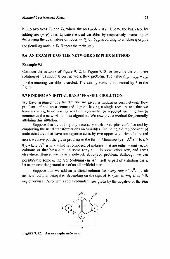
Minimal Cost Network Flows 475
it into two trees 7j and T2, where the root node r e 7J. Update the basis tree by adding arc (p, q) to it. Update the dual variables by respectively increasing or decreasing the dual values of nodes in T2 by δ , according to whether q οτρ is
the (leading) node in T2. Repeat the main step.
9.6 AN EXAMPLE OF THE NETWORK SIMPLEX METHOD
Example 9.1
Consider the network of Figure 9.12. In Figure 9.13 we describe the complete solution of this minimal cost network flow problem. The value Spq = zpq - cpq
for the entering variable is circled. The exiting variable is denoted by * in the figure.
9.7 FINDING AN INITIAL BASIC FEASIBLE SOLUTION
We have assumed thus far that we are given a minimum cost network flow problem defined on a connected digraph having a single root arc and that we have a starting basic feasible solution represented by a rooted spanning tree to commence the network simplex algorithm. We now give a method for generally attaining this situation.
Suppose that by adding any necessary slack or surplus variables and by employing the usual transformations on variables (including the replacement of undirected arcs that have nonnegative costs by two oppositely oriented directed
arcs), we have put the given problem in the form: Minimize {ex : A x = b, x >
0}, where A is m x n and is composed of columns that are either ± unit vector columns or that have a +1 in some row, a -1 in some other row, and zeros elsewhere. Hence, we have a network structured problem. Although we can
possibly use some of the arcs (columns) in A itself as part of a starting basis, let us present the general use of an all artificial start.
Suppose that we add an artificial column for every row of A0, the rth artificial column being ± e, depending on the sign of è, (that is, + e;- if bt > 0;
-e;· otherwise). Also, let us add a redundant row given by the negative of the sum
Figure 9.12. An example network.
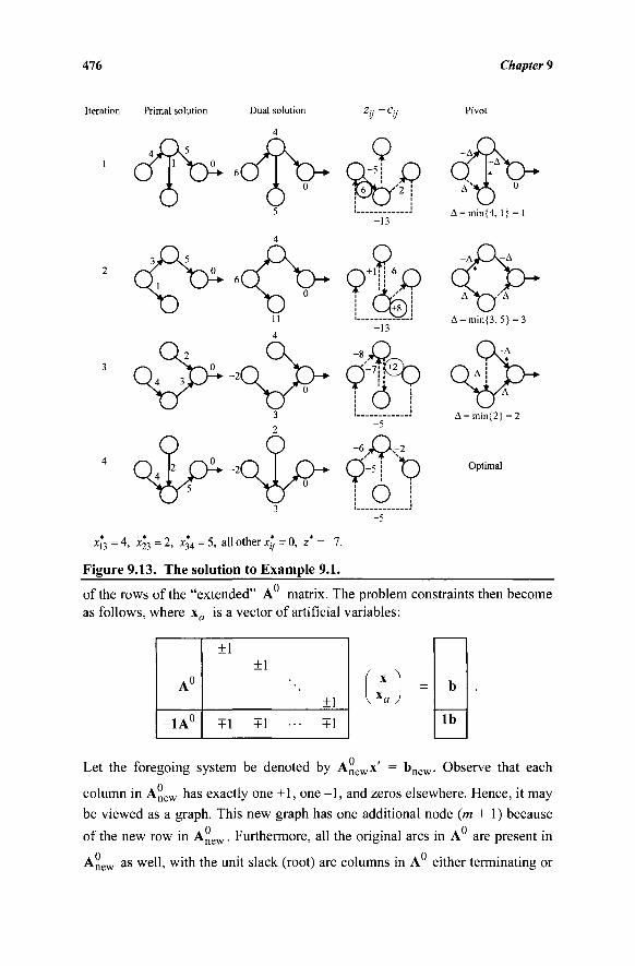
476 Chapter 9
Iteration Primal solution Dual solution
4
Pivot
1 dTtA o
o
δ °
11
4
o 0 2 ( J-+ -2(
9 l6Jr> '2
-13
£>
«CT\> φχρ
%5^<\)> ?fv -5
O '
A = min{4, 1} = 1
A = min{2} = 2
Optimal
x,*3 = 4, *23 = 2, X34 = 5, all other x*- = 0 , z* = - 7 .
Figure 9.13. The solution to Example 9.1. ■» * o of the rows of the "extended" A matrix. The problem constraints then become
as follows, where xa is a vector of artificial variables:
A0
-1A°
±1
+1
+1
+1 ■
+1
• +1
" Ì -x« )
^ ~ "new
b
lb
Obs erve that each Let the foregoing system be denoted by Anewx'
column in Anew has exactly one +1, one - 1 , and zeros elsewhere. Hence, it may
be viewed as a graph. This new graph has one additional node (m + 1) because
of the new row in An e w. Furthermore, all the original arcs in A are present in
Anew as well, with the unit slack (root) arc columns in A either terminating or
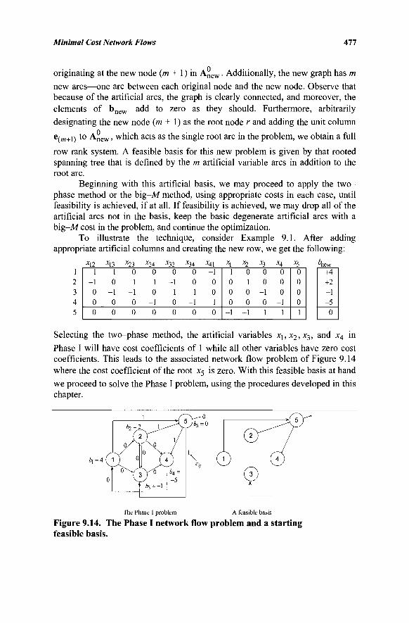
Minimal Cost Network Flows 477
originating at the new node (m + 1) in An e w. Additionally, the new graph has m new arcs—one arc between each original node and the new node. Observe that because of the artificial arcs, the graph is clearly connected, and moreover, the elements of b n e w add to zero as they should. Furthermore, arbitrarily designating the new node (m+ 1 ) as the root node r and adding the unit column e(m+l) t 0 ^new > which acts as the single root arc in the problem, we obtain a full
row rank system. A feasible basis for this new problem is given by that rooted spanning tree that is defined by the m artificial variable arcs in addition to the root arc.
Beginning with this artificial basis, we may proceed to apply the two-phase method or the big-M method, using appropriate costs in each case, until feasibility is achieved, if at all. If feasibility is achieved, we may drop all of the artificial arcs not in the basis, keep the basic degenerate artificial arcs with a big-Mcost in the problem, and continue the optimization.
To illustrate the technique, consider Example 9.1. After adding appropriate artificial columns and creating the new row, we get the following:
x12 x13 x23 x24 x32 x34 x41 x l x2 x3 x4 *5 4ew 1
-1 0 0 0
1 0
-1 0 0
0 1
-1 0 0
0 1 0
-1 0
0 -1
1 0 0
0 0 1
-1 0
-1 0 0 1 0
1 0 0 0
-1
0 1 0 0
-1
0 0
-1 0 1
0 0 0
-1 1
0 0 0 0 1
Selecting the two-phase method, the artificial variables xj,x2>x3> a n Q x4 m
Phase I will have cost coefficients of 1 while all other variables have zero cost coefficients. This leads to the associated network flow problem of Figure 9.14 where the cost coefficient of the root x5 is zero. With this feasible basis at hand
we proceed to solve the Phase I problem, using the procedures developed in this chapter.
The Phase 1 problem A feasible basis
Figure 9.14. The Phase I network flow problem and a starting feasible basis.
478 Chapter 9
Example 9.2
As another example, consider the following problem:
Minimize Xj2 + 2x13 + 3x23 - 2x24 + 4x34 subject to x12 + Xj3 < 6
-X12 + X23 + *24 S 4
- x13 - x23 + X34 < -2 - x24 - X34 < -5
X]2, X13, X23, *24> x34 - 0-
This problem states that no more than six and four units of supply are available at nodes 1 and 2, respectively. At least two and five units of demand also must be absorbed at nodes 3 and 4, respectively, with additional units being permissible if this is profitable. We now add slack variables η, s2, S3, and s4
with zero costs and add appropriate artificial variables and x4 with
big-M costs to the problem. Creating a new row equal to the negative of the sum of the other rows and including the artificial root-arc variable x5 with a zero cost yields the following system of equations:
*12 x13 x 23 x 2 4 ^34 s\ s2 53 ^4 x\ x2 x3 XA XS 1
-1 0 0 0
1 0
-1 0 0
0 1
-1 0 0
0 1 0
-1 0
0 0 1
-1 0
1 0 0 0
-1
0 1 0 0
-1
0 0 1 0
-1
0 0 0 1
-1
1 0 0 0
-1
0 1 0 0
-1
0 0
-1 0 1
0 0 0
-1 1
0 0 0 0 1
We now ask the reader to draw the graph corresponding to this system, to construct the starting artificial basis tree, and to optimize using the big-M method (see Exercise 9.14).
Note also that we could have used the slacks sy and s2 in lieu of the artifi-
cial variables x\ and x2, respectively in the starting basis. This use of an all-
artificial start is only for illustrative purposes.
9.8 NETWORK FLOWS WITH LOWER AND UPPER BOUNDS
It is simple and straightforward to make the transition from the ordinary simplex method for network flow problems to the bounded variables simplex method for network flow problems. We briefly review the essential changes required to effect such an extension to this method.
Getting Started and Computing the Flows
Via standard transformations, including the method of Section 9.7, we can assume without loss of generality that the given problem is in the form:
Minimize {ex : A x = b,£ < x < u}
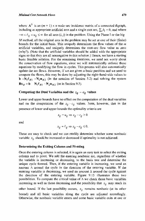
Minimal Cost Network Flows 479
where A is an (m + 1) x n node-arc incidence matrix of a connected digraph, including m appropriate artificial arcs and a single root arc, Σ,-ο,- =0 , and where
-co < £■■ < Uj- < co for all arcs (i,j) in the problem. Using the Phase I or the big-Ai method, all the original arcs in the problem may be set at one of their (finite) bounds for the initial basis. This uniquely determines the flow values of the m artificial variables, and uniquely determines the root-arc flow value as zero (why?). (Note that the artificial variables should be added with the appropriate signs so that they are all nonnegative in this solution.) Hence, we have a starting basic feasible solution. For the remaining iterations, we need not worry about the conservation of flow equations, since we will automatically enforce these equations by modifying the flow in cycles. This process will also automatically update the arc flows. However, if we are given a basic partition and we need to compute the flows, this may be done by adjusting the right-hand-side values to b -N\tNX -N2UJV2 (in the notation of Section 5.2) and solving the system
Βχβ = b - Nj-fjyi -^2nN2 (as m Section 9.5).
Computing the Dual Variables and the zy - c^ values
Lower and upper bounds have no effect on the computation of the dual variables and on the computation of the z,·.· - Cy values. Note, however, that in the
presence of lower and upper bounds the optimality criteria are
and
These are easy to check and we can readily determine whether some nonbasic variable Xy should be increased or decreased if optimality is not achieved.
Determining the Exiting Column and Pivoting
Once the entering column is selected, it is again an easy task to select the exiting column and to pivot. We add the entering nonbasic arc, regardless of whether the variable is increasing or decreasing, to the basis tree and determine the unique cycle formed. Then, if the entering variable is increasing, we send an amount Δ around the cycle in the direction of the entering variable. If the entering variable is decreasing, we send an amount Δ around the cycle against the direction of the entering variable. Figure 9.15 illustrates these two possibilities. To compute the critical value of Δ we check those basic variables increasing as well as those decreasing and the possibility that xy may reach its
other bound. If the last possibility occurs, x,y remains nonbasic (at its other
bound) and all basic variables along the cycle are adjusted accordingly. Otherwise, the nonbasic variable enters and some basic variable exits at one or
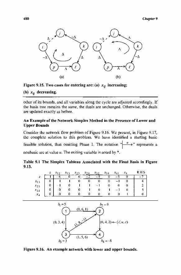
480 Chapter 9
k
/-A
P ) -Δ
(a)
Figure 9.15. Two cases for entering are: (a) xy increasing;
(b) Xjj decreasing.
other of its bounds, and all variables along the cycle are adjusted accordingly. If the basis tree remains the same, the duals are unchanged. Otherwise, the duals are updated exactly as before.
An Example of the Network Simplex Method in the Presence of Lower and Upper Bounds
Consider the network flow problem of Figure 9.16. We present, in Figure 9.17, the complete solution to this problem. We have identified a starting basic
u feasible solution, thus omitting Phase 1. The notation "
nonbasic arc at value u. The exiting variable is noted by *.
->" represents a
Table 9.1 The Simplex Tableau Associated with the Final Basis in Figure 9.13.
z x 13 x 2 3 X34
X4
z 1 0 0 0 0
* 1 2 - 6
1 - 1
0 0
* 1 3 0 1 0 0 0
x 2 3
0 0 1 0 0
X24
-2 0 1 1 0
*3 2
- 5 0
- 1 0 0
JC34
0 0 0 1 0
x 4 1
- 5 - 1
0 - 1
0
X4
0 0 0 0 1
R H S - 7
4 2 5 0
(0,3,4) (0,4, 2) <- {/, u, c)
(1,5,6) Z>3=3 64 =-8
Figure 9.16. An example network with lower and upper bounds.
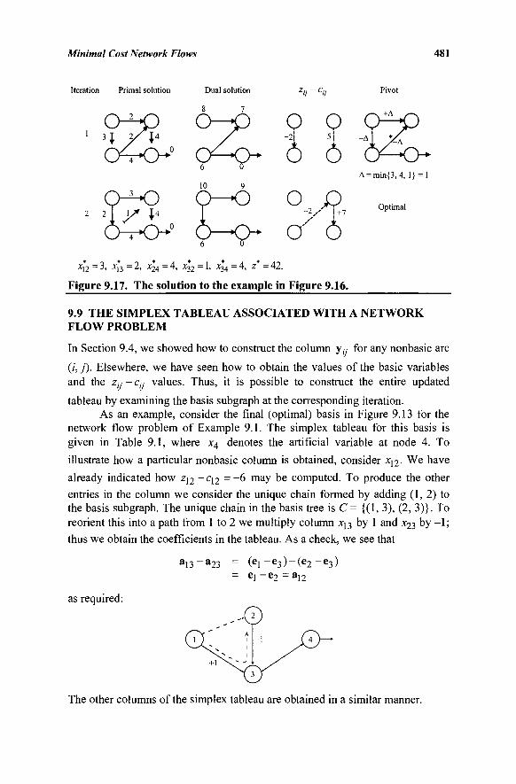
Minimal Cost Network Flows 481
Iteration Primal solution Dual solution Pivot
6 0
0 0 0 +Δ
5i
Ò Ó
O D - 2 / ; + 7
a" ó xl2 = 3, *13 = 2, Λ24 = 4, x32 = 1, X34 = 4, z = 42.
Figure 9.17. The solution to the example in Figure 9.16.
A = min{3,4, 1} = 1
Optimal
9.9 THE SIMPLEX TABLEAU ASSOCIATED WITH A NETWORK FLOW PROBLEM
In Section 9.4, we showed how to construct the column y,y for any nonbasic arc
(/', j). Elsewhere, we have seen how to obtain the values of the basic variables and the zy - Cy values. Thus, it is possible to construct the entire updated
tableau by examining the basis subgraph at the corresponding iteration. As an example, consider the final (optimal) basis in Figure 9.13 for the
network flow problem of Example 9.1. The simplex tableau for this basis is given in Table 9.1, where x4 denotes the artificial variable at node 4. To illustrate how a particular nonbasic column is obtained, consider x12. We have already indicated how z12 -Cj2 = - 6 may be computed. To produce the other entries in the column we consider the unique chain formed by adding (1, 2) to the basis subgraph. The unique chain in the basis tree is C= {(1, 3), (2, 3)}. To reorient this into a path from 1 to 2 we multiply column xj3 by 1 and x23 by - 1 ; thus we obtain the coefficients in the tableau. As a check, we see that
l 1 3 ~ a 2 3 = (e l ~ e 3 ) - ( e 2 ~ e 3 >
= e l - e 2 = a 1 2
as required:
The other columns of the simplex tableau are obtained in a similar manner.
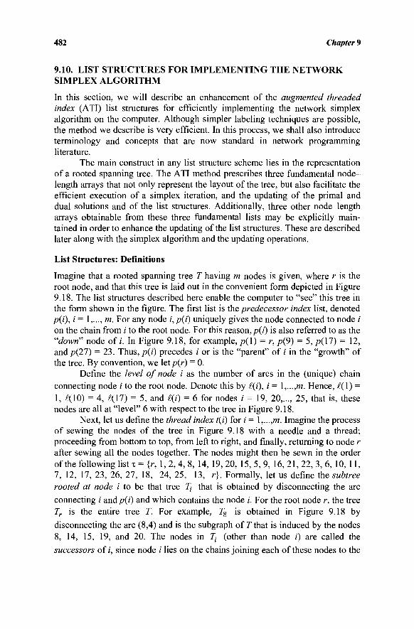
482 Chapter 9
9.10. LIST STRUCTURES FOR IMPLEMENTING THE NETWORK SIMPLEX ALGORITHM
In this section, we will describe an enhancement of the augmented threaded index (ATI) list structures for efficiently implementing the network simplex algorithm on the computer. Although simpler labeling techniques are possible, the method we describe is very efficient. In this process, we shall also introduce terminology and concepts that are now standard in network programming literature.
The main construct in any list structure scheme lies in the representation of a rooted spanning tree. The ATI method prescribes three fundamental node-length arrays that not only represent the layout of the tree, but also facilitate the efficient execution of a simplex iteration, and the updating of the primal and dual solutions and of the list structures. Additionally, three other node-length arrays obtainable from these three fundamental lists may be explicitly main-tained in order to enhance the updating of the list structures. These are described later along with the simplex algorithm and the updating operations.
List Structures: Definitions
Imagine that a rooted spanning tree T having m nodes is given, where r is the root node, and that this tree is laid out in the convenient form depicted in Figure 9.18. The list structures described here enable the computer to "see" this tree in the form shown in the figure. The first list is the predecessor index list, denoted p(i), i = 1,..., m. For any node i,p(i) uniquely gives the node connected to node i on the chain from / to the root node. For this reason, />(/) is also referred to as the "down" node of i. In Figure 9.18, for example, p(l) = r, p(9) = 5, p{\7) = 12, and p(21) = 23. Thus, p(i) precedes /' or is the "parent" of / in the "growth" of the tree. By convention, we \etp(r) = 0.
Define the level of node i as the number of arcs in the (unique) chain connecting node / to the root node. Denote this by i(i), i = Ι,...,/w. Hence, ^(1) = 1, ^(10) = 4, £(\7) = 5, and £(i) = 6 for nodes / = 19, 20,..., 25, that is, these nodes are all at "level" 6 with respect to the tree in Figure 9.18.
Next, let us define the thread index t(i) for i = ί,.,.,τη. Imagine the process of sewing the nodes of the tree in Figure 9.18 with a needle and a thread; proceeding from bottom to top, from left to right, and finally, returning to node r after sewing all the nodes together. The nodes might then be sewn in the order of the following list τ = {r, 1, 2,4, 8, 14, 19,20, 15, 5, 9, 16, 21, 22, 3, 6, 10, 11, 7, 12, 17, 23, 26, 27, 18, 24, 25, 13, r}. Formally, let us define the subtree rooted at node i to be that tree 7} that is obtained by disconnecting the arc connecting / and p(i) and which contains the node /. For the root node r, the tree Tr is the entire tree T. For example, Γ8 is obtained in Figure 9.18 by disconnecting the arc (8,4) and is the subgraph of T that is induced by the nodes 8, 14, 15, 19, and 20. The nodes in 7} (other than node i) are called the
successors of i, since node i lies on the chains joining each of these nodes to the
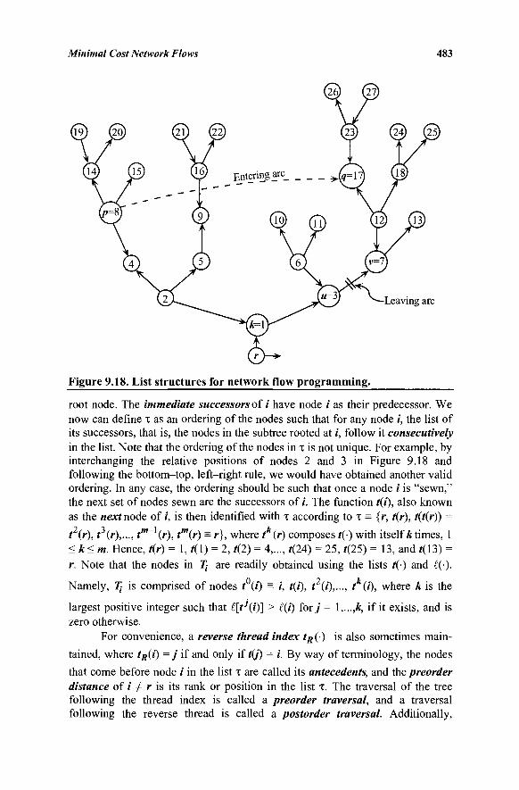
Minimal Cost Network Flows 483
Figure 9.18. List structures for network flow programming.
root node. The immediate successors of i have node i as their predecessor. We now can define τ as an ordering of the nodes such that for any node i, the list of its successors, that is, the nodes in the subtree rooted at i, follow it consecutively in the list. Note that the ordering of the nodes in τ is not unique. For example, by interchanging the relative positions of nodes 2 and 3 in Figure 9.18 and following the bottom-top, left-right rule, we would have obtained another valid ordering. In any case, the ordering should be such that once a node i is "sewn," the next set of nodes sewn are the successors of i. The function t{i), also known as the «ex* node oft, is then identified with τ according to τ = {r, t(r), t(t(r)) =
t2{r), ^(r),..., tm~X{r), tm(r) = r}, where tk(r) composes *(■) with itself A times, 1 < k< m. Hence, t(r) = 1, f(l) = 2, t(2) = 4,..., i(24) = 25, t(25) = 13, and f(13) = r. Note that the nodes in 3J are readily obtained using the lists t(-) and £(■).
Namely, 7J· is comprised of nodes t (i) = i, t{i), t (/),..., t (i), where k is the
largest positive integer such that £[tJ(i)] > l(i) for/' = \,...,k, if it exists, and is zero otherwise.
For convenience, a reverse thread index tR() is also sometimes main-
tained, where tR(i) =j if and only if t(j) = i. By way of terminology, the nodes that come before node i in the list t are called its antecedents, and the preorder distance of i Φ r is its rank or position in the list τ. The traversal of the tree following the thread index is called a preorder traversal, and a traversal following the reverse thread is called a postorder traversal. Additionally,
484 Chapter 9
another useful list both conceptually as well as computationally i s / / ) , the final
ofnode i for / = l,...,m. Given that 2} is comprised of the nodes t (/) = /,...,/ (/),
k> 0, the node//) = / (/) is the final node threaded in T{. Loosely speaking,//) is the "final or last successor" of / in the list τ. Note that if i is an end node, then T[ = i and fij) = i. Let us also denote another list «(/) as the number of nodes in
Th i = \,...,m. Thus,//) = t[n{i)'\i). In Figure 9.18, for example,/8) = 15, w(8)
= 5, /9) = 22, «(9) = 4 , /7 ) = 13, «(7) = 10./21) = 21, «(21) = 1,/r) = 13, and «(r) = 28.
Initialization
The foregoing lists are readily constructed for the all artificial basis in which the tree is comprised of arcs connecting each node and the root node. For this tree, we have/>(/) = r for all ΐφτ andp(r) = 0, £{i) = 1 for all /Φ r, and £(r) = 0, t(r) = 1, t(l) = 2, t{2) = 3,...,t(m - 1) = r (assuming that node "#«" is the root r). Also,
fj) = i and «(/) = 1 for all / Φ r, while fir) = m - 1 and «(/·) = m. On the other hand, if a certain advanced basis is available, then these lists
may be initialized as follows. (Use the example of Figure 9.18 while reading this procedure.) Pick some node as the root node r. Let S(r) be the immediate successors of r determined by finding the basic arcs incident at r. Then, p{i) = r and £(i) = 1 for all ie S(r). Pick some node ye S(r), put t(r) =j, and removey from S(r). Similarly, construct S(j) as the set of all nodes other than node r that are adjacent to nodey for some basic arc. Assume that SXj) φ 0 . Then/j(/) =j and i(f) = £(j) + 1 for all / e S(f). Pick some node A e S(j), put t(j) = k, and remove k from S (/). Continue in this manner until some node e is reached for which S(e) = 0 . Hence, e is an end node of the basis tree T. In this case, follow the predecessor index to come down the tree until a node q is reached for which S(q) Φ 0 . In this event, pick some £e S(q), put t(e) = £, and remove £ from
S(q). While coming down the tree, each node / that is crossed over downwards, including node e itself, gets node e as its final successor node f\i). Also, the number of new nodes labeled between threading / and giving node / its /(■}-value yields «(/). The process can now be continued by constructing S(£) and proceeding "up" the tree again. The procedure stops at the point when following the chain down from some end e, it reaches node r and finds S(r) = 0 , whereupon, in particular, among other labels, it sets/r) = e and t(e) = r.
Simplex Operations
Observe that each arc in the problem is uniquely identified with some node via its predecessor index. That is, for each node / Φ r, there is an associated, uniquely identified arc connecting i andp(t). This arc may be [/,/>(/)] or [p(/), /]. Hence, a node-length array ORIENT(-) may be carried to record the orientation of the basic arcs, having a + 1 in one case and a - 1 in the other case, respectively. For example, for node 20, the associated arc is \p(20), 20] = (14, 20)
Minimal Cost Network Flows 485
and ORIENT(20) = - 1 , while for node 8, the associated arc is [8,/>(8)] = (8, 4) and ORIENT(8) = 1. Consequently, the basic arc flow vector can be stored in a node-length array FLOW(-), where FLOW(/) is the flow on the arc connecting / and p(t). Let DUAL(i) represent the dual variable associated with node /. The arrays DUAL(-) and FLOW(-) are readily initialized via a preorder traversal and a postorder traversal, respectively. For example, in Figure 9.18, the dual values may be determined in the order of the nodes r, 1, 2, 4, 8, 14, 19, 20, 15,... as they appear in τ, based on the arc connecting each node / and its predecessor p(i), since the dual of p(i) is already computed for each / in this order. Similarly, the flows may be computed by following the nodes i in the reverse thread order 13, 25, 24, 18, 27, 26, 23, 17, 12,..., and determining the flow on the arc connecting / and /»(/). This is based on the nodal balance equation for node i in this order, since the flow on at most one incident arc is unknown in each case.
Suppose that by following the usual pricing scheme, we determine an entering arc (p, q). The basis equivalent chain may be traced by coming down from p and q following the predecessor index list />(·) until a first intersection point k is reached. Note that node k may be p or q itself. Hence, if £(p) > £(q), say, then we can come down from/» until we reach the level of q, from where it is known whether or not k = q. If not, then we can come down simultaneously one level at a time along the two chains until they intersect. While doing this, a minimum ratio test can be conducted simultaneously (how?), so that the leaving arc is known once the basis equivalent chain has been traced. Let the leaving arc connect nodes « and v, where u = p(y) (see Figure 9.18). Note that the actual leaving arc may be («, v) or (v, «). When the leaving arc is disconnected from T, the tree not containing the root is the subtree Tv. Let us also assume that q is the
leading node in Tv—the entering arc may actually be (p, q) or (q,p).
Updating Operations
The flows are updated as usual on the basis equivalent chain by tracing down from p and q to k after determining the flow change Δ. The predecessor index p() changes only on the q —> v chain, also known as the stem, simply reversing or inverting on this chain withp(q) =p. Hence, in Figure 9.18, we get/?(v) = 12, />(12) = 17, and/>(17) = 8, with p(i) as before, otherwise. Accordingly, the tree arcs that are associated with the nodes on the stem q —» v through the predecessor index change in this reversal process, and so the ORIENT() and FLOW(-) vectors should be appropriately updated. For example, FLOW(12) now corresponds to the flow on arc (12, 17) and ORIENT(12) = 1. The dual values in T- Tv remain
the same, while the dual values in Tv all increase by Spq = zpq ~cpq ^{ρ, <l) is
the entering arc, and decrease by δ^ =tqp~ cqp if (#> P) is m e entering arc.
Hence, the dual values can be updated by following the thread index from v t o / (v). (Notice how n (v) helps in this respect.)
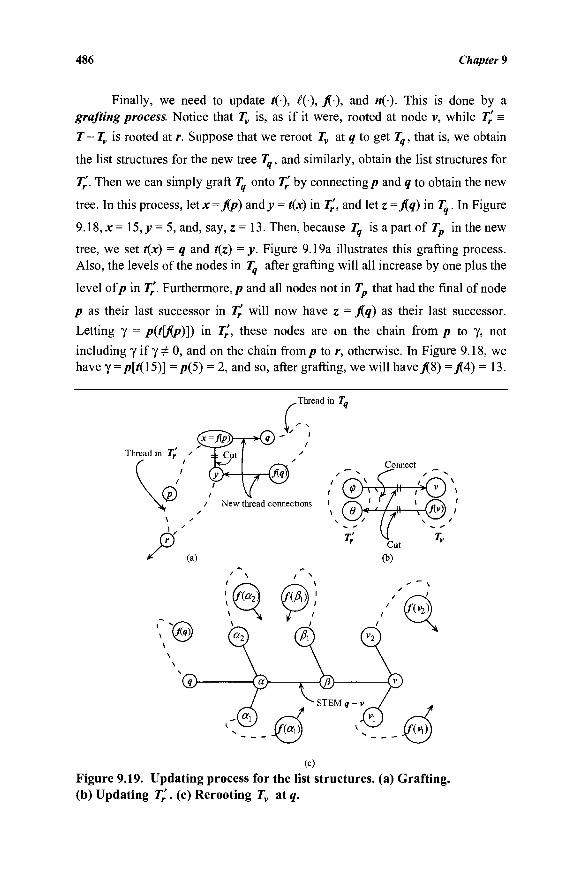
486 Chapter 9
Finally, we need to update /(·), £(■), / · ) , and «(·). This is done by a grafting process. Notice that Tv is, as if it were, rooted at node v, while Tr =
T- Tv is rooted at r. Suppose that we reroot Tv at q to get Tq, that is, we obtain
the list structures for the new tree Tq, and similarly, obtain the list structures for
2J.'. Then we can simply graft 21 onto Tr by connecting/» and q to obtain the new
tree. In this process, let x =fip) and y = t(x) in Tr, and let z =Αθ) in 21. In Figure
9.18, x= 15, y= 5, and, say, z= 13. Then, because 21 isapar tof21 in the new
tree, we set t(x) = q and t(z) = y. Figure 9.19a illustrates this grafting process. Also, the levels of the nodes in 21 after grafting will all increase by one plus the
level ofp in T'r. Furthermore,/» and all nodes not in 21 that had the final of node
/» as their last successor in 2J.' will now have z = fi,q) as their last successor.
Letting γ = p(t\fip)]) in T'r, these nodes are on the chain from p to γ, not
including γif γ ^ 0, and on the chain from/» to r, otherwise. In Figure 9.18, we
have J = p[t(l5)] =/»(5) = 2, and so, after grafting, we will have_/(8) =β4) = 13.
(c)
Figure 9.19. Updating process for the list structures, (a) Grafting, (b) Updating T'r . (c) Rerouting Tv at q.
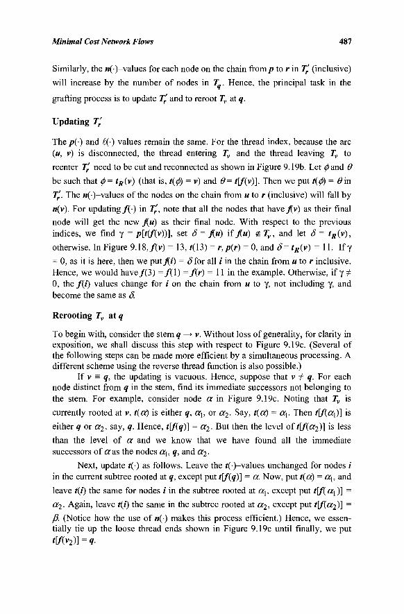
Minimal Cost Network Flows 487
Similarly, the «(-)-values for each node on the chain from/» to r in Tr (inclusive)
will increase by the number of nodes in Tq. Hence, the principal task in the
grafting process is to update T'r and to reroot Tv at q.
Updating T'r
The p(·) and £(■) values remain the same. For the thread index, because the arc (w, v) is disconnected, the thread entering Tv and the thread leaving Tv to
reenter T'r need to be cut and reconnected as shown in Figure 9.19b. Let ^and Θ
be such that φ = tR(v) (that is, ί(φ) = v) and θ= t[f(v)]. Then we put ί(φ) = (9in
Tr. The «(-)-values of the nodes on the chain from u to r (inclusive) will fall by
n(v). For updating/(·) in Tr, note that all the nodes that have/v) as their final
node will get the new fili) as their final node. With respect to the previous
indices, we find γ = p[t(f(v))], set δ = fili) if fiu) <£ Tv, and let δ = tR{v),
otherwise. In Figure 9.18,/(v) = 13, i(13) = r,p(r) = 0, and δ= tR{v) = 11. If γ
= 0, as it is here, then we put fii) = δίοτ all / in the chain from u to r inclusive. Hence, we would have/(3) = / ( l ) =f(r) = 11 in the example. Otherwise, if γ Φ 0, the f{i) values change for / on the chain from « to γ, not including γ, and become the same as δ
Rerooting Tv at q
To begin with, consider the stem q —> v. Without loss of generality, for clarity in exposition, we shall discuss this step with respect to Figure 9.19c. (Several of the following steps can be made more efficient by a simultaneous processing. A different scheme using the reverse thread function is also possible.)
If v = q, the updating is vacuous. Hence, suppose that v Φ q. For each node distinct from q in the stem, find its immediate successors not belonging to the stem. For example, consider node a in Figure 9.19c. Noting that Tv is
currently rooted at v, t(a) is either q, ah or «2- Say, t(d) = (X\. Then t\f{a{)] is either q or a2, say, q. Hence, t[f(q)] = a2- But then the level of i[/"(or2)] is le s s
than the level of a and we know that we have found all the immediate successors of eras the nodes cc\, q, and a2-
Next, update t() as follows. Leave the f(-)-values unchanged for nodes t in the current subtree rooted at q, except put t[f(q)] = a. Now, put t(a) = «j, and
leave t{i) the same for nodes t in the subtree rooted at a^, except put t\f{(X\)] =
a2. Again, leave t(i) the same in the subtree rooted at a2, except put t\f(a2)] =
β. (Notice how the use of «(■) makes this process efficient.) Hence, we essen-tially tie up the loose thread ends shown in Figure 9.19c until finally, we put
t[f(v2)] = q-
488 Chapter 9
The levels £(■) of the nodes that are shown explicitly in Figure 9.19c are obviously available. The levels of the other nodes in subtrees rooted at the nodes q, oc\, a2, β\, Vj, and v2 change by the same amounts as the levels of these corresponding nodes.
As far as /(■) and «(·) are concerned, these stay the same for nodes that are not on the stem. For nodes / on the stem, we have/(j) = / ( v2 ). Also, « (v) =
1 + «(vj) + n(v2), η(β) = 1 + «(/?,) + n(v), n(a) = 1 + n(a{) + n(a2) + η(β), and
n(q) equals the total number of nodes in Tv (the old w(v)).
In conclusion, we mention one important expedient. Note that instead of the foregoing grafting procedure, we could alternatively have left Tv rooted at v, rerooted Tr at p to get Tp, and then grafted Tp onto Tv by connecting p and q.
Then node v would have become the new root node. This process can be done exactly as previously. The tree that is rerooted at p or q is called the upper tree, while the other is called the lower tree. The decision as to which tree to make the upper tree depends on the ease with which the rerouting of the "upper" tree can be effected. Since this effort is directly related to the length of the stem, the tree having the shorter stem q-v or p-r may be chosen as the upper tree.
9.11 DEGENERACY, CYCLING, AND STALLING
In the absence of degeneracy, the network simplex algorithm converges in a finite number of iterations as in Chapter 3. (By degeneracy, we mean a basic arc other than the root arc has a zero flow value; the root arc flow is zero for all feasible solutions) However, simple examples (see Exercise 9.50) have been constructed that show that the network simplex algorithm can cycle, that is, infinitely loop through a sequence of degenerate pivots. Hence, cycling preven-tion rules need to be employed. It turns out that a special lexicographic type of rule for the network simplex algorithm is not only easy to implement with no significant overheads, but is computationally beneficial for highly degenerate problems as, for example, the linear assignment problem.
The prescribed cycling prevention rule is based on maintaining what are known as strongly feasible bases. A strongly feasible (basis) tree (SFI) for Problem (9.1) (including the root arc) is a feasible rooted spanning tree in which all degenerate arcs (if any) are pointing toward the root A directed arc (i, j) is said to be "pointing toward the root" if j =/>(/), that is, if/' lies on the chain from i to the root node r. It is instructive to identify the connection between strongly
feasible and "lexicographically positive" bases of Chapter 4. The fth row of B~
is given as the solution Rf to the system R,B = ej. Observe that this is similar to
the system "wB = cB." Hence, R; may be found by giving the fth basic arc a
cost of 1, the other arcs a cost of zero, and computing the dual variables. If the
nh arc is a root arc, then R; has all ones (why?). If the fth arc is not a root arc,
then from Section 9.5, the component of R(· corresponding to node/' is zero if
the fth arc does not lie on the chain from/' to the root. Otherwise, it is +1 if the
Minimal Cost Network Flows 489
rth arc is pointing toward the root, and is -1 if the z'th arc is pointing away from the root. In particular, for a basis corresponding to a strongly feasible tree, the
row of B~ corresponding to a degenerate arc has all components equal to 0 or 1. In fact, the foregoing argument shows that a basis B has lexicographic
positive rows in [B~ b, B~ ] if and only if it corresponds to a strongly feasible tree (why?). Hence, from Chapter 4 we are guaranteed finiteness if we maintain strongly feasible trees.
Obtaining an Initial Strongly Feasible Basis
If an all-artificial starting basis is used, then by simply defining the artificial arc connected to a transshipment node as being directed toward the (dummy (m + 1)5/) root node, we will have a strongly feasible starting basis. On the other hand, if some advanced starting basis is given, then consider the spanning graph formed by the arcs having positive flows and let some node be designated as the root node. This graph is a spanning forest. If it is connected, then it is a strongly feasible tree. Otherwise, one at a time, connect a component tree not containing the root node to the one containing the root node, using any arc in the problem that is pointing from a node in the former tree to one in the latter tree. Such an arc must of course be degenerate. Notice that if at any stage there are no arcs pointing from the se tX= {/' : node / is not as yet connected to the root} to the complement set X, then the problem is separable over the node sets X and X. This follows because we must have Ziexfy -T,iexfy = 0, and the flow on any
arc from a node in X to a node in X must be zero for all feasible solutions (why?). Hence, we may solve these separable problems independently. Note that we already have a strongly feasible tree for the node set X. Alternatively, we can connect any node in X to the root node via a degenerate artificial arc and continue this process.
Maintaining Strongly Feasible Trees
Given a strongly feasible basis tree at the beginning of an iteration, and given an entering arc (p, q), the following simple rule for selecting a leaving variable arc (w, v) ensures that we maintain a strongly feasible tree. Trace the basis equivalent chain by tracing the unique chains from p and q to the root node r until they intersect at some common node k. Figure 9.20a depicts the situation generically. Note that k can coincide with p and/or r or with q and/or r. Define the cycle C(e) created as having the orientation of the flow along (p, q) and commencing at node k, proceeding first along the k —► p chain, then including arc (p, q), and finally proceeding along the q —► k chain. Determine the exiting variable in C(e), breaking ties (if any) by selecting the last blocking arc in C(e). For example, in Figure 9.20b, when (4,7) enters, we havep = 4,q = 7, and k = 5, and of the blocking arcs (4, 3) and (6, 7), we select (6, 7) as the leaving variable arc.
It is easy to see following Figure 9.20a that this rule maintains strongly feasible bases. Note that any degenerate arc not involved in the cycle C(e) is still
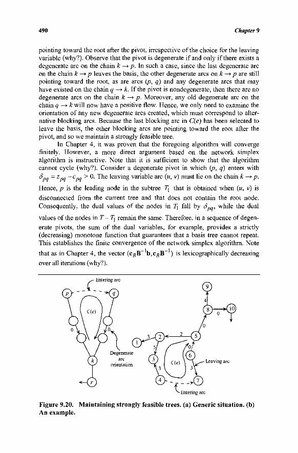
490 Chapter 9
pointing toward the root after the pivot, irrespective of the choice for the leaving variable (why?). Observe that the pivot is degenerate if and only if there exists a degenerate arc on the chain k —► p. In such a case, since the last degenerate arc on the chain k—*p leaves the basis, the other degenerate arcs on k —► p are still pointing toward the root, as are arcs (p, q) and any degenerate arcs that may have existed on the chain q —* k. If the pivot is nondegenerate, then there are no degenerate arcs on the chain k —* p. Moreover, any old degenerate arc on the chain q^>k will now have a positive flow. Hence, we only need to examine the orientation of any new degenerate arcs created, which must correspond to alter-native blocking arcs. Because the last blocking arc in C(e) has been selected to leave the basis, the other blocking arcs are pointing toward the root after the pivot, and so we maintain a strongly feasible tree.
In Chapter 4, it was proven that the foregoing algorithm will converge finitely. However, a more direct argument based on the network simplex algorithm is instructive. Note that it is sufficient to show that the algorithm cannot cycle (why?). Consider a degenerate pivot in which (p, q) enters with
cpq > 0. The leaving variable arc (u, v) must lie on the chain k—>p. pq PI
Hence, p is the leading node in the subtree 7] that is obtained when (u, v) is disconnected from the current tree and that does not contain the root node. Consequently, the dual values of the nodes in 7] fall by Spq, while the dual
values of the nodes in T- 7] remain the same. Therefore, in a sequence of degen-erate pivots, the sum of the dual variables, for example, provides a strictly (decreasing) monotone function that guarantees that a basis tree cannot repeat. This establishes the finite convergence of the network simplex algorithm. Note
that as in Chapter 4, the vector (c#B
over all iterations (why?).
b,cgB ) is lexicographically decreasing
Entering arc
Figure 9.20. Maintaining strongly feasible trees, (a) Generic situation, (b) An example.
Minimal Cost Network Flows 491
This cycling prevention rule is readily extended to the bounded variables network simplex algorithm. A strongly feasible basis tree may be defined here as one in which the basic arcs that are degenerate at their lower bounds are pointing toward the root and those basic and degenerate at their upper bounds are pointing away from the root. Then, the same leaving variable rule (which includes the case of the entering arc blocking itself) maintains strong feasibility and guarantees finite convergence. We leave the details to the reader in Exercise 9.38.
Stalling and its Prevention
Although the foregoing technique guarantees finite convergence, it is still entirely possible that the algorithm may stall at an extreme point, that is, go through a number of consecutive degenerate pivots that, although finite, is exponential in m and ». For example, if b = 0 in Problem (9.1), then all possible bases represent the same extreme point, namely, the origin, and there may be an expo-nential number of such bases that one may enumerate before terminating with Zj; - Cjj < 0 for all nonbasic variables. In fact, there exist examples exhibiting
this phenomenon (see the Notes and References section). In any case, it seems desirable to devise a rule that would guarantee that the number of consecutive degenerate pivots is bounded above by a polynomial in m and n.
As seen in Chapter 4, a key to preventing stalling is to keep the length as well as the number of stages small. Recall that a stage is a sequence of degener-ate pivots in which no nonbasic variable remains enterable throughout and no strict subset of this sequence has the same property. The length of a stage may be controlled by adopting an appropriate "affirmative action" rule for selecting an entering variable. For example, the Least Recently Considered (LRC) vari-able choice rule discussed in Chapter 4 guarantees that the number of pivots in a stage is no more than n. It turns out that independent of the rule for choosing an entering variable, if we maintain strongly feasible basis trees as previously, then the number of stages in a sequence of consecutive degenerate pivots is no more than the number of degenerate basic variables at the current extreme point. Hence, the number of stages in a sequence of degenerate pivots is bounded above by m, so that the number of consecutive degenerate pivots using strongly feasible bases in conjunction with the LRC entering rule, for example, is bounded above by the polynomial mn. This underscores the relevance of main-taining strongly feasible bases.
To establish the preceding bound on the number of stages, let Γ0, T\,...,TM
be the basis trees in a sequence of consecutive degenerate pivots such that either optimality is recognized at TM or the pivot executed on TM is nondegenerate.
Notice that the nondegenerate basic arcs are common in all of the trees T0,
Τγ,...,ΤΜ (why?). Consider the spanning graph formed by these nondegenerate
basic arcs. Let this graph have (tree) components Gl5 G2,...,Gp, where P < m. In
each of the trees TQ,...,TM, these components Gy,...,Gp are connected to each
other via some P-l degenerate arcs. In particular, let TM be as shown in Figure
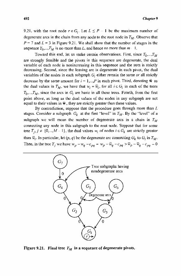
492 Chapter 9
9.21, with the root node r&G\. Let L < P - 1 be the maximum number of degenerate arcs in the chain from any node to the root node in TM. Observe that P = 7 and L = 3 in Figure 9.21. We shall show that the number of stages in the sequence TQ,...,TM is no more than L, and hence no more than m - 1.
Toward this end, let us make certain observations. First, since T0,...,TM
are strongly feasible and the pivots in this sequence are degenerate, the dual variable of each node is nonincreasing in this sequence and the sum is strictly decreasing. Second, since the leaving arc is degenerate in each pivot, the dual variables of the nodes in each subgraph G, either remain the same or all strictly decrease by the same amount for i = \,...,P in each pivot. Third, denoting w as the dual values in TM, we have that wt = wt, for all i e G{ in each of the trees T0,...,TM, since the arcs in G] are basic in all these trees. Fourth, from the first point above, as long as the dual values of the nodes in any subgraph are not equal to their values in w, they are strictly greater than these values.
By contradiction, suppose that the procedure goes through more than L stages. Consider a subgraph Gk at the first "level" in TM. By the "level" of a
subgraph we will mean the number of degenerate arcs in a chain in TM
connecting any node in this subgraph to the root node. Suppose that for some tree T-,j e {Ο,.,.,Μ- 1}, the dual values w, of nodes i e G^ are strictly greater
than Wj. In particular, let (p, q) be the degenerate arc connecting G^ to Gj in TM.
Then, in the tree T- we have wp - wq - cpq = w„-wq- cpq > wp - w - cpq = 0
Figure 9.21. Final tree TM in a sequence of degenerate pivots.
Minimal Cost Network Flows 493
(why?). As long as the dual values in Gk are not equal to those in w, arc (p, q) remains enterable and a stage persists. By the time the first stage is over within the sequence T0,...,TM, we will have w,· = w, for all i^Gk. This equality holds in every tree after this stage.
Inductively, assume that the procedure has gone through some I > 1
stages and the dual values of nodes in subgraphs at levels i or lower are all at
their corresponding values in w. Consider a subgraph Gk at level (£ + 1) and let
(p, q) be the first degenerate arc encountered in the chain from any node in Gk
to the root node. If κ>;· > iv,· for i e Gk in any tree following stage i, then as
before, in this tree we have wp -wq -cpq = wp-wq -cpq > wp - wq - cpq = 0
so that arc (p, q) is enterable. As long as the dual values in Gk are not fixed at
their corresponding values in w, (p, q) remains enterable and stage (I + 1) per-
sists. When stage (i + 1) is completed within the sequence TQ,...,TM, the dual
values of nodes in subgraphs at level (I + 1 ) are all at their values in w. Conse-quently, the number of stages in the sequence T0,...,TM, cannot be more than L. This establishes the required result.
Another Useful Entering Variable Choice Rule that Prevents Stalling
Besides the partial pricing rule for selecting an entering variable described in Chapter 3 and the LRC rule described in this chapter, there is another competi-tive entering variable selection rule that is well suited to how data are customarily stored. Suppose that the arcs in the problems are stored in a one-dimensional array with arcs having node 1 as their from-node appearing first, then arcs having node 2 as their from-node, and so on. Consider the following rule. Suppose that an arc having node j at its from-node has just entered. (Assume _/' = 1 to initialize.) Then the next entering variable is chosen as the best enterable arc with node j again as its from-node, and if none exists, then the best enterable arc having nodey + 1 as its from-node, and so on, considering arcs having nodes/ + 2,..., m, 1, 2,..., and nodey- 1 as their from-node, in this order. Then, we show that the maximum number of consecutive degenerate pivots
using strongly feasible basis trees is no more than mL, which is less than m . Note that the use of strongly feasible basis trees ensures that the number
of stages in a sequence of degenerate pivots is no more than L, independent of the rule for choosing an entering variable. To show that the length of a stage is no more than m, consider a tree 7\ in the sequence TQ,...,TM_\ that leads to a
degenerate pivot. Let w be the dual values in T-. Suppose that arc (p, q) enters,
say, where p e Gk. Referring to Figure 9.21 (assuming that this represents tree
Tj and not TM), note that the pivot will be degenerate if and only if q does not
lie in Gk or in its "successors," that is, if and only if the basis equivalent chain
includes the degenerate arc (w, v), which is defined as the first degenerate arc
494 Chapter 9
encountered by tracing from any node in G^ to the root node. Moreover, by the
rule for breaking ties for the leaving variable (see Figure 9.20a), the arc (w, v) must be the leaving variable arc. Consequently, if (p, q) enters degenerately, then the dual values of nodes in Gk and its successors reduce by δρ„ = z „ -cpq
> 0, while those of the other nodes remain the same. Let these revised dual
variables in 7\+1 be called w'. Because the set of nodes in Gk or in its succes-
sors have been unaffected by the pivot, for any node £ not in this set, we have w'p ~we ~cpl = (wp -5pq)-™l ~cpl = (wp ~wi 'CpU'Spq ^ ° s i n c e 8pq w a s
the most positive zpt -cpt value among all arcs of the type (p, t). If some arc
having node p as its from-node is now enterable, the resulting pivot must be nondegenerate. Consequently, if the next pivot is degenerate, the from-node cannot be node p, which means that in a sequence of degenerate pivots the length of a stage is < m. This establishes the required bound. In Exercise 9.49 we ask the reader to consider another variation of this rule.
9.12 GENERALIZED NETWORK PROBLEMS
Consider a linear programming problem of the form:
Minimize ex subject to Ax = b
x > 0,
where the matrix A is m x n of rank m and where each column a of A has at
most two nonzero entries. Then one may conceptualize the constraints Ax = b as a set of generalized nodal flow balance equations on a graph G(. / , "/) that is constructed as follows. Let / be the set of m nodes {l,...,m}, with node / being associated with the rth row of A. For each column a · of A having two nonzero
entries, occurring, say, in rows p and q, construct an undirected link L .■ between
nodes/) and q. For each column a of A having a single nonzero entry, occurring,
say, in row p, construct an undirected link L .■ incident at node p. Let ' / denote
the set of these links, and let x.- denote the flow associated with link L·.
Additionally, for each node p, examine the links that are incident at p and associate with each such link L- at the point of incidence at p a multiplier equal
to the coefficient in column a and row p. Then the nodal balance equations
assert that at each node p, the sum of the weighted flows on the incident links, where the weights equal the corresponding incident multipliers, must equal b„.
Because of this interpretation of modified flows, this type of problem is called a generalized network or a network flow with gains problem. Problems of this type are used to model a variety of situations involving a gain or loss in flow or the transformation of one type of product to another in a network-based system. (See Exercises 9.54 - 9.55.)
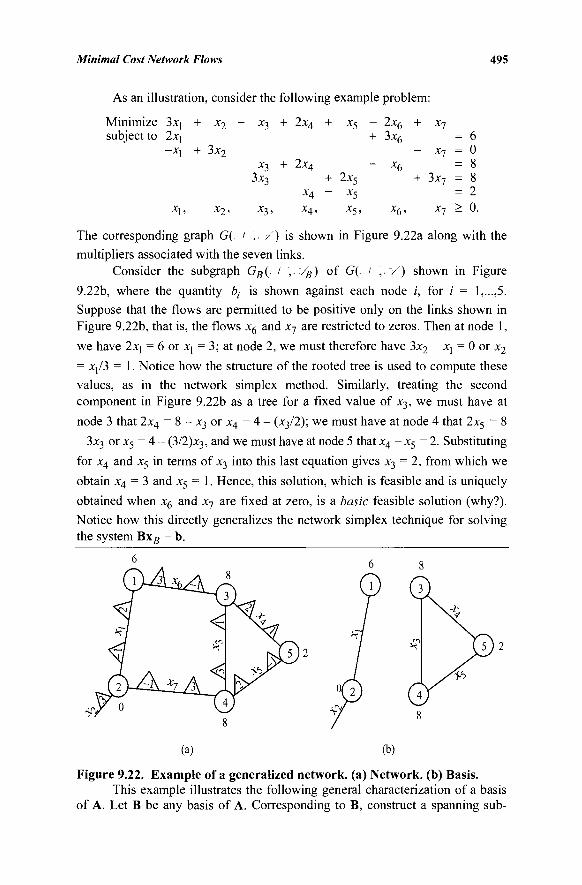
Minimal Cost Network Flows 495
As an illustration, consider the following example problem:
Minimize 3xj subject to 2x]
- * i
X] ,
+ *2
+ 3x2
x2,
- x3
x3 3x3
x3,
+ 2x4
+ 2x4
X4
X4,
+ x5
+ 2x5
- x5 x5,
- 2x6 + 3x6
- x6
x 6 '
+ Χη = 6
- x7 = 0 = 8
+ 3x7 = 8 = 2
x7 > 0
The corresponding graph G(- / , ·"/) is shown in Figure 9.22a along with the
multipliers associated with the seven links. Consider the subgraph GB( l ,'/β) of G( I , ·"/) shown in Figure
9.22b, where the quantity bt is shown against each node i, for /' = 1,...,5. Suppose that the flows are permitted to be positive only on the links shown in Figure 9.22b, that is, the flows x6 and x7 are restricted to zeros. Then at node 1,
we have 2xj = 6 or x\ = 3; at node 2, we must therefore have 3x2 - x\ = 0 or x2
= X]/3 = 1. Notice how the structure of the rooted tree is used to compute these
values, as in the network simplex method. Similarly, treating the second
component in Figure 9.22b as a tree for a fixed value of x3, we must have at
node 3 that 2x4 = 8 - x3 or x4 = 4 - (x3/2); we must have at node 4 that 2x5 = 8
- 3x3 or x5 = 4 - (3/2)x3, and we must have at node 5 that x4 - x5 = 2. Substituting
for x4 and x5 in terms of x3 into this last equation gives x3 = 2, from which we
obtain x4 = 3 and x5 = 1. Hence, this solution, which is feasible and is uniquely
obtained when x6 and x7 are fixed at zero, is a basic feasible solution (why?).
Notice how this directly generalizes the network simplex technique for solving
the system Bxg = b.
(a) (b)
Figure 9.22. Example of a generalized network, (a) Network, (b) Basis. This example illustrates the following general characterization of a basis
of A. Let B be any basis of A. Corresponding to B, construct a spanning sub-
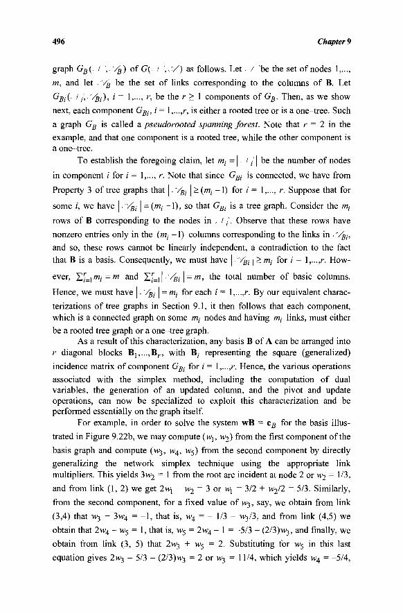
496 Chapter 9
graph GB(, I ,'/B) of G( l ,-"/) as follows. Let / be the set of nodes 1,...,
m, and let ■ YB be the set of links corresponding to the columns of B. Let
GBi{- I ,·,. Vg,), / = 1,..., r, be the r > 1 components of GB. Then, as we show
next, each component GBi, i = \,...,r, is either a rooted tree or is a one-tree. Such
a graph GB is called a pseudorooted spanning forest. Note that r = 2 in the
example, and that one component is a rooted tree, while the other component is a one-tree.
To establish the foregoing claim, let mi = |. / , | be the number of nodes
in component / for / = 1,..., r. Note that since GBi is connected, we have from
Property 3 of tree graphs that |. YBi | > (m,- -1) for i = 1,..., r. Suppose that for
some /, we have | YBi | = (w, -1) , so that GBi is a tree graph. Consider the Th-
rows of B corresponding to the nodes in . / ,·'. Observe that these rows have
nonzero entries only in the (w; -1) columns corresponding to the links in · ~/Bi,
and so, these rows cannot be linearly independent, a contradiction to the fact
that B is a basis. Consequently, we must have | -/Bi | > mi for i = l,...,r. How-
ever, Z / = i w i = w a nd Σ/=ι | S/Bi | = m > m e t o t a l number of basic columns.
Hence, we must have |,~/Bi | = w; for each / = l,...,r. By our equivalent charac-
terizations of tree graphs in Section 9.1, it then follows that each component,
which is a connected graph on some /w;- nodes and having w; links, must either be a rooted tree graph or a one-tree graph.
As a result of this characterization, any basis B of A can be arranged into r diagonal blocks Bl v . . ,Br , with B( representing the square (generalized)
incidence matrix of component GBi for / = 1,...,/-. Hence, the various operations
associated with the simplex method, including the computation of dual variables, the generation of an updated column, and the pivot and update operations, can now be specialized to exploit this characterization and be performed essentially on the graph itself.
For example, in order to solve the system wB = cB for the basis illus-
trated in Figure 9.22b, we may compute {y\\, w2) from the first component of the
basis graph and compute (w^, w4, w5) from the second component by directly
generalizing the network simplex technique using the appropriate link
multipliers. This yields 3w2 = 1 from the root arc incident at node 2 or w2 = 1/3,
and from link (1, 2) we get 2w[ - w2 = 3 or vv = 3/2 + w2/2 = 5/3. Similarly,
from the second component, for a fixed value of w3, say, we obtain from link
(3,4) that vv3 + 3w4 = - 1 , that is, w4 = - 1/3 - w3/3, and from link (4,5) we
obtain that 2w4 - w5 = 1, that is, w5 = 2H>4 - 1 = -5/3 - (2/3)w3, and finally, we
obtain from link (3, 5) that 2w3 + w5 = 2. Substituting for w5 in this last
equation gives 2w3 - 5/3 - (2/3)w3 = 2 or w3 = 11/4, which yields w4 = -5/4,
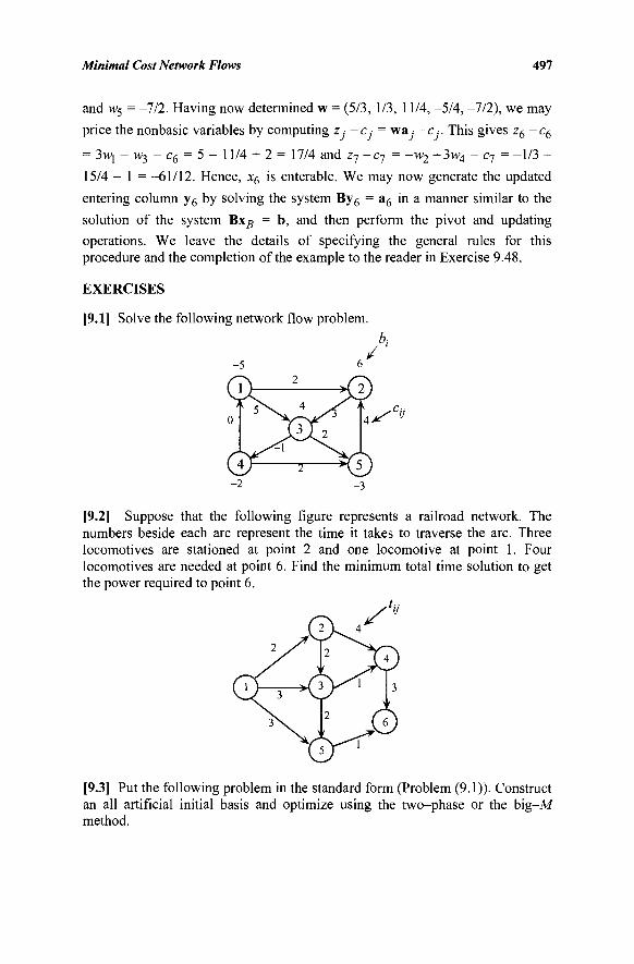
Minimal Cost Network Flows 497
and w5 = -7/2. Having now determined w = (5/3, 1/3, 11/4, -5/4, -7/2), we may
price the nonbasic variables by computing z,· -c ■ = wa · - c ·. This gives z6 - c 6
= 3w| - w3 - c6 = 5 - 11/4 + 2 = 17/4 and z7 -c7 = -w2 +3w4 — c-j — -1/3 -
15/4 - 1 = -61/12. Hence, x6 is enterable. We may now generate the updated
entering column y6 by solving the system By6 = a6 in a manner similar to the
solution of the system B\B = b, and then perform the pivot and updating
operations. We leave the details of specifying the general rules for this procedure and the completion of the example to the reader in Exercise 9.48.
EXERCISES
[9.1] Solve the following network flow problem.
[9.2] Suppose that the following figure represents a railroad network. The numbers beside each arc represent the time it takes to traverse the arc. Three locomotives are stationed at point 2 and one locomotive at point 1. Four locomotives are needed at point 6. Find the minimum total time solution to get the power required to point 6.
[9.3] Put the following problem in the standard form (Problem (9.1)). Construct an all artificial initial basis and optimize using the two-phase or the big-M method.
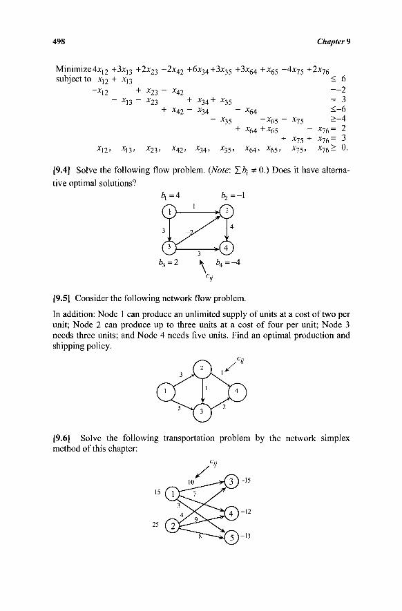
498 Chapter 9
Minimize4xj2 +3xj3 +2*23 ~2x4 2 +6x34+3x35 +3x64 +x^ -4χγ5 +2x75 subject to Xj2 + X]3 ^ 6
-X12 + X23 - *42 = - 2 ~~ x13 ~ x23 + x34 + x35 = 3
+ X42 - X34 - X64 < -6 ~ x35 ~x65 - x75 ^ ~ 4
+ x64 +x65 - x76= 2 + x75 + x76= 3
X12, X13, X23' x42> x34> x35> x64' x65> x75' x76 - °-
[9.4] Solve the following flow problem. {Note: Σέ,- * 0.) Does it have alterna-
tive optimal solutions?
£,=2 ^ b4=-4 CU
[9.5] Consider the following network flow problem.
In addition: Node 1 can produce an unlimited supply of units at a cost of two per unit; Node 2 can produce up to three units at a cost of four per unit; Node 3 needs three units; and Node 4 needs five units. Find an optimal production and shipping policy.
[9.6] Solve the following transportation problem by the network simplex method of this chapter:
/ * 10
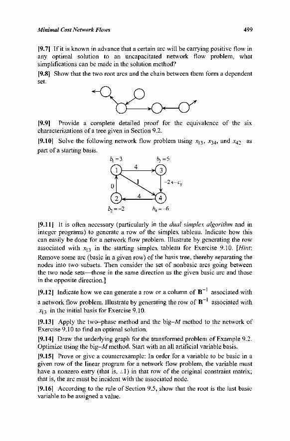
Minimal Cost Network Flows 499
[9.7] If it is known in advance that a certain arc will be carrying positive flow in any optimal solution to an uncapacitated network flow problem, what simplifications can be made in the solution method?
[9.8] Show that the two root arcs and the chain between them form a dependent set.
o-<f [9.9] Provide a complete detailed proof for the equivalence of the six characterizations of a tree given in Section 9.2.
[9.10] Solve the following network flow problem using x13, x34, and x42 as
part of a starting basis. él =3 6,=5
■2<-c;;
&j=-2
[9.11] It is often necessary (particularly in the dual simplex algorithm and in integer programs) to generate a row of the simplex tableau. Indicate how this can easily be done for a network flow problem. Illustrate by generating the row associated with x[3 in the starting simplex tableau for Exercise 9.10. [Hint:
Remove some arc (basic in a given row) of the basis tree, thereby separating the nodes into two subsets. Then consider the set of nonbasic arcs going between the two node sets—those in the same direction as the given basic arc and those in the opposite direction.]
-1 associated with
associated with
[9.12] Indicate how we can generate a row or a column of B
a network flow problem. Illustrate by generating the row of B~ X|3 in the initial basis for Exercise 9.10.
[9.13] Apply the two-phase method and the big-M method to the network of Exercise 9.10 to find an optimal solution.
[9.14] Draw the underlying graph for the transformed problem of Example 9.2. Optimize using the big-M method. Start with an all artificial variable basis.
[9.15] Prove or give a counterexample: In order for a variable to be basic in a given row of the linear program for a network flow problem, the variable must have a nonzero entry (that is, ±1) in that row of the original constraint matrix; that is, the arc must be incident with the associated node.
[9.16] According to the rule of Section 9.5, show that the root is the last basic variable to be assigned a value.
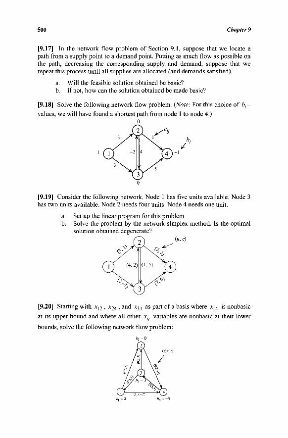
500 Chapter 9
[9.17] In the network flow problem of Section 9.1, suppose that we locate a path from a supply point to a demand point. Putting as much flow as possible on the path, decreasing the corresponding supply and demand, suppose that we repeat this process until all supplies are allocated (and demands satisfied).
a. Will the feasible solution obtained be basic? b. If not, how can the solution obtained be made basic?
[9.18] Solve the following network flow problem. (Note; For this choice of 6,·-
values, we will have found a shortest path from node 1 to node 4.)
[9.19] Consider the following network. Node 1 has five units available. Node 3 has two units available. Node 2 needs four units. Node 4 needs one unit.
a. Set up the linear program for this problem. b. Solve the problem by the network simplex method. Is the optimal
solution obtained degenerate?
[9.20] Starting with xj2 , *24 > a nd *3i as part of a basis where x14 is nonbasic
at its upper bound and where all other Xy variables are nonbasic at their lower
bounds, solve the following network flow problem:
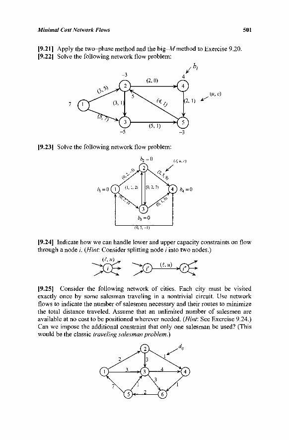
Minimal Cost Network Flows 501
[9.21] Apply the two-phase method and the big-Mmethod to Exercise 9.20. [9.22] Solve the following network flow problem:
(u,c)
[9.23] Solve the following network flow problem:
fr,=0
6, =0
y,u,c)
h=o
(0, 5, -1)
[9.24] Indicate how we can handle lower and upper capacity constraints on flow through a node i. (Hint: Consider splitting node / into two nodes.)
(l,u)
yùg ^ΤΜ^ΜΕ^
[9.25] Consider the following network of cities. Each city must be visited exactly once by some salesman traveling in a nontrivial circuit. Use network flows to indicate the number of salesmen necessary and their routes to minimize the total distance traveled. Assume that an unlimited number of salesmen are available at no cost to be positioned wherever needed. (Hint: See Exercise 9.24.) Can we impose the additional constraint that only one salesman be used? (This would be the classic traveling salesman problem.)
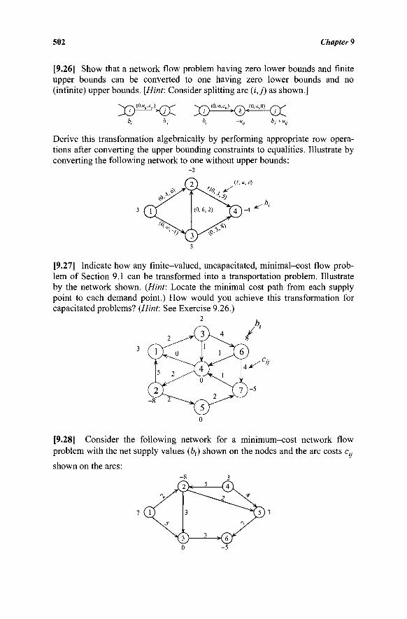
502 Chapter 9
[9.26] Show that a network flow problem having zero lower bounds and finite upper bounds can be converted to one having zero lower bounds and no (infinite) upper bounds. [Hint: Consider splitting arc (i,j) as shown.]
b, bj b, -uv bj+^j
Derive this transformation algebraically by performing appropriate row opera-tions after converting the upper bounding constraints to equalities. Illustrate by converting the following network to one without upper bounds:
[9.27] Indicate how any finite-valued, uncapacitated, minimal-cost flow prob-lem of Section 9.1 can be transformed into a transportation problem. Illustrate by the network shown. (Hint: Locate the minimal cost path from each supply point to each demand point.) How would you achieve this transformation for capacitated problems? (Hint: See Exercise 9.26.)
[9.28] Consider the following network for a minimum-cost network flow problem with the net supply values (è,·) shown on the nodes and the arc costs c,y
shown on the arcs:
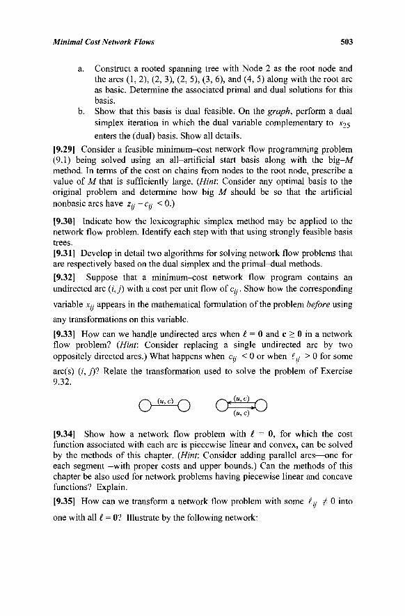
Minimal Cost Network Flows 503
a. Construct a rooted spanning tree with Node 2 as the root node and the arcs (1, 2), (2, 3), (2, 5), (3, 6), and (4, 5) along with the root arc as basic. Determine the associated primal and dual solutions for this basis.
b. Show that this basis is dual feasible. On the graph, perform a dual simplex iteration in which the dual variable complementary to x25 enters the (dual) basis. Show all details.
[9.29] Consider a feasible minimum-cost network flow programming problem (9.1) being solved using an all-artificial start basis along with the big-M method. In terms of the cost on chains from nodes to the root node, prescribe a value of M that is sufficiently large. (Hint: Consider any optimal basis to the original problem and determine how big M should be so that the artificial nonbasic arcs have Zy - Cy < 0.)
[9.30] Indicate how the lexicographic simplex method may be applied to the network flow problem. Identify each step with that using strongly feasible basis trees. [9.31] Develop in detail two algorithms for solving network flow problems that are respectively based on the dual simplex and the primal-dual methods.
[9.32] Suppose that a minimum-cost network flow program contains an undirected arc (i,j) with a cost per unit flow of ci}·. Show how the corresponding
variable Xy appears in the mathematical formulation of the problem before using
any transformations on this variable.
[9.33] How can we handle undirected arcs when £ = 0 and c > 0 in a network flow problem? (Hint: Consider replacing a single undirected arc by two oppositely directed arcs.) What happens when Cy < 0 or when £y > 0 for some
arc(s) (/, _/)? Relate the transformation used to solve the problem of Exercise 9.32.
[9.34] Show how a network flow problem with £ = 0, for which the cost function associated with each arc is piecewise linear and convex, can be solved by the methods of this chapter. (Hint: Consider adding parallel arcs—one for each segment—with proper costs and upper bounds.) Can the methods of this chapter be also used for network problems having piecewise linear and concave functions? Explain.
[9.35] How can we transform a network flow problem with some ly Φ 0 into
one with all £ = 0? Illustrate by the following network:
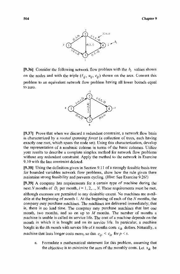
504 Chapter 9
[9.36] Consider the following network flow problem with the 6,· -values shown
on the nodes and with the triple (£y, Uy, c,y) shown on the arcs. Convert this
problem to an equivalent network flow problem having all lower bounds equal to zero.
[9.37] Prove that when we discard a redundant constraint, a network flow basis is characterized by a rooted spanning forest (a collection of trees, each having exactly one root, which spans the node set). Using this characterization, develop the representation of a nonbasic column in terms of the basic columns. Utilize your results to describe a complete simplex method for network flow problems without any redundant constraint. Apply the method to the network in Exercise 9.10 with the last constraint deleted.
[9.38] Using the definition given in Section 9.11 of a strongly feasible basis tree for bounded variables network flow problems, show how the rule given there maintains strong feasibility and prevents cycling. (Hint: See Exercise 9.26!)
[9.39] A company has requirements for a certain type of machine during the next N months of Dt per month, i = 1, 2,..., N. These requirements must be met,
although excesses are permitted to any desirable extent. No machines are avail-able at the beginning of month 1. At the beginning of each of the N months, the company may purchase machines. The machines are delivered immediately; that is, there is no lead time. The company may purchase machines that last one month, two months, and so on up to M months. The number of months a machine is usable is called its service life. The cost of a machine depends on the month in which it is bought and on its service life. In particular, a machine bought in the rth month with service life of A: months costs cilc dollars. Naturally, a machine that lasts longer costs more, so that cjp < cjs for/? < s.
a. Formulate a mathematical statement for this problem, assuming that the objective is to minimize the sum of the monthly costs. Let xik be
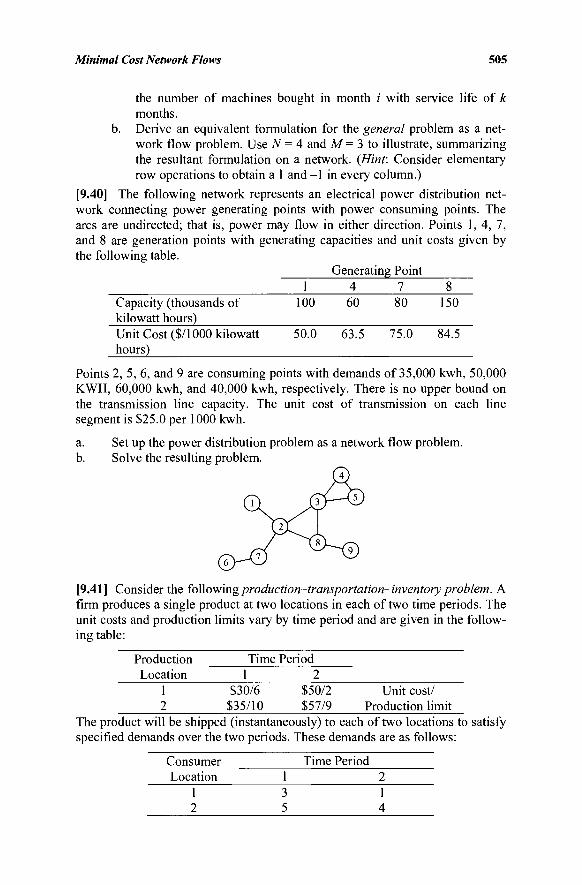
Minimal Cost Network Flows 505
the number of machines bought in month / with service life of k months,
b. Derive an equivalent formulation for the general problem as a net-work flow problem. Use N = 4 and M = 3 to illustrate, summarizing the resultant formulation on a network. (Hint: Consider elementary row operations to obtain a 1 and -1 in every column.)
[9.40] The following network represents an electrical power distribution net-work connecting power generating points with power consuming points. The arcs are undirected; that is, power may flow in either direction. Points 1,4, 7, and 8 are generation points with generating capacities and unit costs given by the following table.
Generating Point 1 4 7 8
Capacity (thousands of kilowatt hours) Unit Cost ($/1000 kilowatt hours)
100
50.0
60
63.5
80
75.0
150
84.5
Points 2, 5, 6, and 9 are consuming points with demands of 35,000 kwh, 50,000 KWH, 60,000 kwh, and 40,000 kwh, respectively. There is no upper bound on the transmission line capacity. The unit cost of transmission on each line segment is $25.0 per 1000 kwh.
a. Set up the power distribution problem as a network flow problem. b. Solve the resulting problem.
[9.41] Consider the following production-transportation-inventory problem. A firm produces a single product at two locations in each of two time periods. The unit costs and production limits vary by time period and are given in the follow-ing table:
Production Location
1 2
Time Period 1 2
$30/6 $50/2 $35/10 $57/9
Unit cost/ Production limit
The product will be shipped (instantaneously) to each of two locations to satisfy specified demands over the two periods. These demands are as follows:
Consumer Time Period Location 1 2
1 3 1 2 5 4
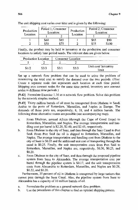
506 Chapter 9
The unit shipping cost varies over time and is given by the following:
Production Location
1 2
Period 1 ; Consumer Location:
1 2 $60 $65 $50 $75
Production Location
1 2
Period 2; Consumer Location:
1 2 $65 $90 $75 $100
Finally, the product may be held in inventory at the production and consumer locations to satisfy later period needs. The relevant data are given below.
Production Location 1 2
$1/2 $3/3
Consumer Location 1 2
,«- ,. ς , „ Unit cost/ Inventory limit
Set up a network flow problem that can be used to solve the problem of minimizing the total cost to satisfy the demand over the two periods. (Hint: Create a separate node that represents each location at each time period. Shipping arcs connect nodes for the same time period; inventory arcs connect nodes in different time periods.)
[9.42] Formulate Exercise 1.16 as a network flow problem. Solve this problem by the network simplex method.
[9.43] Thirty million barrels of oil must be transported from Dhahran in Saudi Arabia to the ports of Rotterdam, Marseilles, and Naples in Europe. The demands of these ports are, respectively, 8, 18, and 4 million barrels. The following three alternative routes are possible (see accompanying map).
a. From Dhahran, around Africa (through the Cape of Good Hope) to Rotterdam, Marseilles, and Naples. The average transportation and han-dling cost per barrel is $2.20, $2.40, and $2.45, respectively.
b. From Dhahran to the city of Suez, and then through the Suez Canal to Port Said. From Port Said the oil is shipped to Rotterdam, Marseilles, and Naples. The average transportation and handling cost from Dhahran to the city of Suez is $0.35 and the additional unit cost of transporting through the canal is $0.25. Finally, the unit transportation costs from Port Said to Rotterdam, Marseilles, and Naples are, respectively, $0.30, $0.23, and $0.20.
c. From Dhahran to the city of Suez, and then through the proposed pipeline system from Suez to Alexandria. The average transportation cost per barrel through the pipeline system is $0.17, and the unit transportation costs from Alexandria to Rotterdam, Marseilles, and Naples are $0.28, $0.22, and $0.20.
Furthermore, 35 percent of oil in Dhahran is transported by large tankers that cannot pass through the Suez Canal. Also, the pipeline system from Suez to Alexandria has a capacity of 10 million barrels of oil.
a. Formulate the problem as a general network flow problem. b. Use the procedures of this chapter to find an optimal shipping pattern.
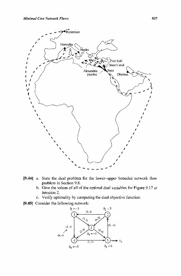
Minimal Cost Network Flows 507
„ — —>**Rotterdam
/ « / I / I / 1 / \ i \i 1 \ \ \
\ \
Marseilles f X / ^ ^ \
; Naples L t - ^ ^ s
j . "^ϊ>^. -l·/ Port Said
"~ ^ ,-Suez Canal Alexandria y"*sSuez
pipeline "
[9.44] a. State the dual problem for the lower-upper bounded network flow problem in Section 9.8.
b. Give the values of all of the optimal dual variables for Figure 9.17 at iteration 2.
c. Verify optimality by computing the dual objective function.
[9.45] Consider the following network:
(8, -3)
(«, e)
"CD—**a bA=-5 & = 6
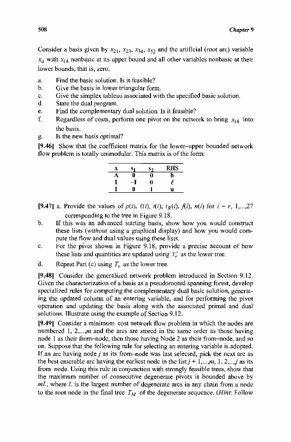
508 Chapter 9
Consider a basis given by x2i> x23> x34> x52 an^ m e artificial (root arc) variable
xa with x14 nonbasic at its upper bound and all other variables nonbasic at their
lower bounds, that is, zero.
a. Find the basic solution. Is it feasible? b. Give the basis in lower triangular form. c. Give the simplex tableau associated with the specified basic solution. d. State the dual program. e. Find the complementary dual solution. Is it feasible? f. Regardless of costs, perform one pivot on the network to bring x14 into
the basis. g. Is the new basis optimal?
[9.46] Show that the coefficient matrix for the lower-upper bounded network flow problem is totally unimodular. This matrix is of the form:
X
A I I
sl 0 - I 0
s2 0 0 I
RHS b £ u
[9.47] a. Provide the values of p(i), £{i), t{f), tR{i),f{i), η{ΐ) for i = r, 1 27 corresponding to the tree in Figure 9.18.
b. If this was an advanced starting basis, show how you would construct these lists {without using a graphical display) and how you would com-pute the flow and dual values using these lists.
c. For the pivot shown in Figure 9.18, provide a precise account of how these lists and quantities are updated using T'r as the lower tree.
d. Repeat Part (c) using Tv as the lower tree.
[9.48] Consider the generalized network problem introduced in Section 9.12. Given the characterization of a basis as a pseudorooted spanning forest, develop specialized rules for computing the complementary dual basic solution, generat-ing the updated column of an entering variable, and for performing the pivot operation and updating the basis along with the associated primal and dual solutions. Illustrate using the example of Section 9.12.
[9.49] Consider a minimum-cost network flow problem in which the nodes are numbered 1, 2,...,m and the arcs are stored in the same order as those having node 1 as their from-node, then those having Node 2 as their from-node, and so on. Suppose that the following rule for selecting an entering variable is adopted. If an arc having node/ as its from-node was last selected, pick the next arc as the best enterable arc having the earliest node in the listy + l,...,m, 1, 2,...j as its from-node. Using this rule in conjunction with strongly feasible trees, show that the maximum number of consecutive degenerate pivots is bounded above by mL, where L is the largest number of degenerate arcs in any chain from a node to the root node in the final tree TM of the degenerate sequence. {Hint: Follow
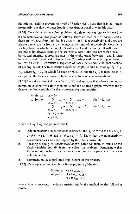
Minimal Cost Network Flows 509
the original stalling prevention proof of Section 9.11. Note that it is no longer necessarily true that the stage length is less than or equal to m in this case.)
[9.50] Consider a network flow problem with three vertices that each have è, =
0 and with twelve arcs given as follows. Between each pair of nodes / and j , there are two arcs from i toy having costs +1 and - 1 , respectively, and there are also two reverse arcs fromy to / having costs +1 and - 1 , respectively. Consider a starting basis in which the arc (1, 2) with cost 1 and the arc (2, 3) with cost -1 are basic. By always keeping one arc with a cost 1 and one arc with a cost -1 basic, and entering appropriate arcs in the cyclic order between 1 and 3, then between 2 and 3, and next between 1 and 2, starting with the entering arc from 1 to 3 with a cost - 1 , construct a sequence of bases that exhibits the phenomenon of cycling. (Hint: Try to construct a cycle of length 12, that is, trees TQ, T{,...Tn,
7]2, where 7]2 - 7b, in which for each i = 0, 1,...,5, the tree 7J+6 is identical to 7J-
except that the two basic arcs of the same cost have reverse orientations.)
[9.51] Consider a directed graph G(. / ",·."/) and suppose that a two-commodity
minimum-cost network flow problem is defined on this digraph, where x and y denote the flow variables for the two respective commodities.
Minimize ex + dy subject to X xy - X xki=^li fori = \,...,m
j:(i,j)€.Y k:(k,i)e.V Σ yy- Σ yki=b2i fori = l,...,m
j:(ij)e./ k:(k,i)e.Y θιχ<γ< θ2χ x,y>o,
where 0 < θ\ < θ2 are given constants.
a. Add nonnegative slack variable vectors Sj and s2 to write #]X<y<#2x
as i^x-y + Sj = 0 and y - # 2 x + s2 = 0. Show that the nonnegativity
constraints on x and y are implied by the other constraints. b. Treating x and y as unrestricted above, solve for them in terms of the
slack variables and eliminate them from the problem. Demonstrate that the resulting problem is a network flow problem separable in the vari-ables Sj ands2.
c. Comment on the algorithmic implications of this strategy.
[9.52] Develop a method to solve a linear program of the form:
Minimize ex + cn+lxn+l
subject to Ax + a„+1x„+1 = b x>0,x„ + 1 >0,
where A is a node-arc incidence matrix. Apply the method to the following problem:
510 Chapter 9
Minimize 5xj + 3x2 + 4x3 + 3x4 + 5x5 + x6
subject to X] + x2 + x6 = 2 —Xj + X3 4- X4 — 2ΧΛ
= 3 - x2 - X3 + x5 + 2x6 = - 1
- x4 - x5 - x6 = - 4 Xj, X2, X3, X4, X5, - δ - 0·
[9.53] Can the results of Exercise 9.52 be generalized to the case where the constraint matrix is of the form (A, D), where A is a node-arc incidence matrix and D is any arbitrary matrix? Apply the method to the previous problem with
the additional column x7 having a7 = ( 1 , - 6 , 2 , 0 ) ' and c7 = - 4 .
[9.54] Consider the investment problem presented in Exercise 1.1. Construct a generalized network to represent this flow with gains problem. Solve this problem using the algorithm discussed in Section 9.12.
[9.54] In the copper market, copper ore is mined at different mines i = \,...,M, having respective supplies st tons, i = Ι,.,.,Μ, and shipped to various smelters y
= l,...JS, where it is processed to produce blister copper, which is then sent to
different refineries, k = \,...,K, which produce high purity copper. This final
product is used to satisfy demands d(, 1= \,...,L, occurring in some L end-use
markets. There also exist predominantly copper-based scrap metal markets r =
l,...,R, having respective supplies ar tons, r= \,...,R, which feed back copper
into the system by shipping this copper-based scrap metal to the refineries for
purification. Assume that a ton of ore sent from mine / to smeltery will produce
ccjj e (0,1) tons of blister copper at smelter j at a total mining, transportation,
and smelting cost of Cy per ton; a ton of blister copper sent from smelter j to
refinery k will produce ββ e (0,1) tons of refined copper at a total
transportation and refining cost of C:k per ton; a ton of scrap metal sent from
scrap metal market r to refinery k will produce yrìi e (0,1) tons of refined
copper at a total transportation and refining cost of crk per ton; and that the
distribution cost from each refinery k to end-use market I is ck( per ton of
refined copper. For this simplified single period description of the copper market, construct a generalized network of the form depicted in Figure 9.22a to find a least cost copper processing and distribution solution, displaying the Z>; -
values at the nodes, and the A-matrix elements and cost coefficients on the edges. Define your decision variables associated with the different types of edges. Discuss how you might extend this model to a multi-period situation. (Soyster and Sherali (1981) describe a more sophisticated multi-period model for the U.S. copper market.)
[9.55] Consider the linear program LP to minimize ex subject to Ax = b, x > 0, where A is an m x n matrix of rank m < n. Consider any column a of A
Minimal Cost Network Flows 511
associated with the variable x-. For example, let a ,■ = (3, 2, -4, 6, 0,...,0)', and
suppose that we write
[*j]xj =
" 3 "
2
0
0
χβ +
0"
0
-4
6
0
0
xy2, where we additionally impose Χβ = χ / · 2 ( = χ / ) -
(This technique is called variable splitting based on its operation, and the relationship of the type x ·] = x -2 is referred to as an equal-flow constraint.)
Show how the general linear program LP can thus be converted to a generalized network flow problem with equal-flow side-constraints. Referring to the Lagrangian relaxation decomposition strategy in Chapter 7, discuss how you might exploit this induced structure to solve LP.
NOTES AND REFERENCES
1. The simplex method for general network flow problems is a natural exten-sion of the work on the transportation problem and the work of Koopmans [1949] relating linear programming bases for transportation problems and trees in a graph. On this subject, also see Ahuja et al. [1993] and Bertsekas [1991, 1998].
2. Computational experience with the network simplex algorithm, as reported by Glover et al. [1974a, b], Langley and Kennington [1973], Ali et al. [1978], and others, indicates that this algorithm compares favorably with several other procedures for solving network flow problems. However, recent work by Bertsekas [1985] and Bertsekas and Tseng [1988a, b; 1994] has resulted in a primal-dual type of algorithm (see Chapter 11) that appears to dominate the primal simplex algorithm. The codes RELAX and RELAXT based on this algorithm solve the standard NETGEN benchmark test problems (Klingman et al. [1974]) two-four times faster than the primal simplex code RNET written at Rutgers University. All commercial LP solvers have a specialized option to solve network structured problems (e.g., the popular software CPLEX has the NETOPT option based on the network simplex algorithm). For an application of interior point methods to network flow problems, see Mehrotra and Wang [1996].
3. Zadeh [1973] has exhibited the worst-case exponential behavior of the primal simplex and the primal-dual network algorithm among others, using a class of modified transportation problems. Edmonds and Karp [1972] were the first to propose a polynomial-time algorithm for network flow problems. Their procedure is based on a scaling technique that solves a sequence of network flow problems with modified (scaled)
512 Chapter 9
right-hand-side values, where the solution to each problem is obtained from the previous one via at most m shortest path problems, and where the first problem is a shortest path problem. Tardos [1985] and Orlin [1984] showed how this algorithm can be modified to derive strongly polynomial dual simplex types of algorithms for minimum cost network flow programming problems. A first polynomial-time primal simplex type of network flow algorithm is presented in Orlin [1997]. (Also, see Sokkalingham et al. [2000].)
4. The discussion of list structures in Section 9.10 is based on the enhancements to the augmented threaded index (ATI) method of Glover et al. [1974a] as discussed in Barr et al. [1979]. (See Barr et al. [1979] for a discussion on rerooting Tv at q based on reverse threads as an alternative
to the technique presented here.) Glover and Klingman [1982] present some computational comparison studies. For an alternative to perform tree-based operations using a data structure called dynamic trees, see Sleator and Tarjan [1983, 1985].
5. The strongly feasible bases of Section 9.11 were introduced by Cunningham [1976]. Their equivalence with lexicographic positivity was exhibited by Orlin [1985]. The instance of cycling in Exercise 9.50 is from Cunningham [1979]. Cunningham [1979] also exhibits the occur-rence of stalling and discusses its prevention. Orlin [1985] has shown that using Dantzig's entering criterion along with the lexicographic cycling prevention rule, the maximum number of consecutive degenerate (primal simplex) pivots for the minimum cost network flow problem is bounded
by 0(m n log m). 6. A general technique for converting linear programs to network flow
problems wherever possible via elementary row operations and variable scal-ing (i.e., finding hidden networks) is presented in Bixby and Cunningham [1980] (see Exercise 9.39). See also Klingman [1977]. Cunningham [1983] shows an instance in which the elimination of unrestricted variables can help in such a conversion process. In cases where a com-plete conversion is not possible, methods for exploiting network substruc-tures are discussed in Glover et al. [1978], Glover and Klingman [1981], and Frendewey and Glover [1981]. Also see Patty [1987] for a survey.
7. Section 9.12 (also see Exercise 9.48) discusses the extension of the models of this chapter to the flow with gains or the generalized network models. Jewell [1962] first solved this problem by a primal-dual method. Ellis Johnson [1965], Langley [1973], and others have since treated the problem via the simplex method. For further reading on this subject, see McBride [1981], Elam et al. [1979], Glover et al. [1974b], Kennington and Helgason [1980], and Bertsekas and Tseng [1988a, b; 1994]. Goldfarb and Lin [2002] discuss interior point methods for this class of problems.
TEN: THE TRANSPORTATION AND ASSIGNMENT PROBLEMS
Transportation and assignment problems are important network structured linear programming problems that arise in several contexts and that have deservedly received a great deal of attention in the literature. Although these problems are special cases of network flow problems, we have seen in the previous chapter that any finite-valued, capacitated or uncapacitated, minimum-cost network flow problem can be transformed into an equivalent (uncapacitated) transporta-tion problem (see Exercise 9.27). In fact, although the assignment problem is itself a special case of the transportation problem, any transportation problem, and hence any (capacitated) minimum-cost network flow problem, can be equivalently transformed into an assignment problem, as shown in Section 10.7. However, this is computationally inadvisable. Nonetheless, this feature is one reason for the interest generated by this pair of problems.
Algorithmically, the uncapacitated or the capacitated transportation problem may be solved using the techniques of the previous chapter. Some specialization in implementation is possible, but for the most part, the basic technique remains the same. For the sake of exposition, we will present some of these specializations in the context of the transportation tableau, which is customarily used to pedagogically present the network simplex algorithm for transportation problems. Although we will rely on the previous chapter for justi-fications and proofs, and we will exhibit the relationships of the method presented here with the general techniques of the foregoing chapter, the discussion in the present chapter is more or less self-contained.
On the other hand, because of its very special structure, a host of specialized algorithms have been proposed for the assignment problem. The well-known and instructive Hungarian algorithm, which led to the development of a general primal-dual algorithm for linear programming problems, is pre-sented here. We also comment on a specialization of the strongly feasible network simplex algorithm for assignment problems, known as the alternating basis algorithm, which yields a competitive solution procedure. Another algo-rithm that runs up to seven times faster than the latter algorithm is based on a successive shortest-path procedure. We present this method here, but postpone the actual solution of the shortest-path subproblems to Chapter 12.
10.1 DEFINITION OF THE TRANSPORTATION PROBLEM
Consider m origin points, where origin i has a supply of s·,· units of a particular
item (commodity). In addition, suppose that there are n destination points, where
513
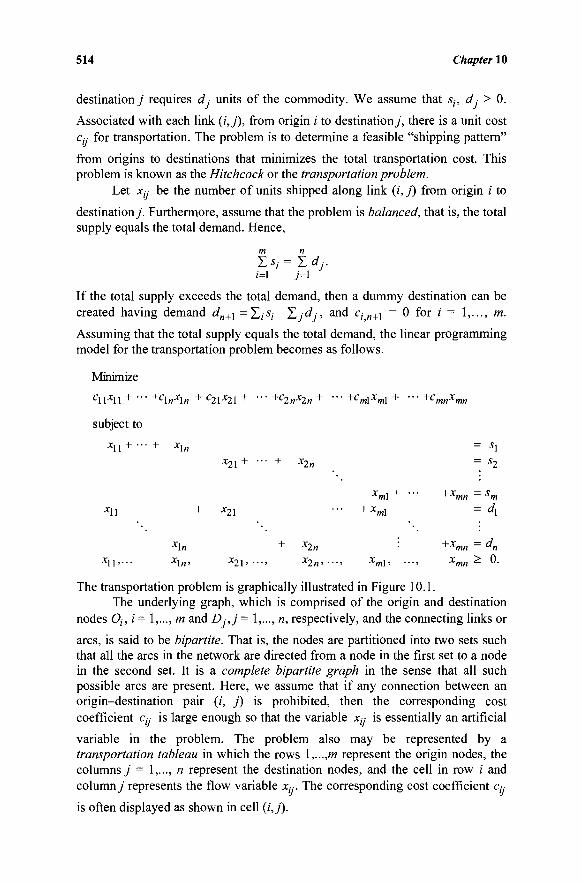
514 Chapter 10
destination j requires dj units of the commodity. We assume that sh d, > 0.
Associated with each link (i,j), from origin /' to destination y, there is a unit cost Cjj for transportation. The problem is to determine a feasible "shipping pattern"
from origins to destinations that minimizes the total transportation cost. This problem is known as the Hitchcock or the transportation problem.
Let Xj- be the number of units shipped along link (i, j) from origin i to
destination j . Furthermore, assume that the problem is balanced, that is, the total supply equals the total demand. Hence,
m n
Σ*; = Σ d:.
If the total supply exceeds the total demand, then a dummy destination can be created having demand dn+\ = Z ; 5 , - Σ , ά , - , and cin+l = 0 for i = 1,..., m.
Assuming that the total supply equals the total demand, the linear programming model for the transportation problem becomes as follows.
Minimize c l l * l l + ·■· +c\nx\n + c21*21 + - +c2r,x2n +
subject to
xn + ■■■ + xln
x2l+ ■■■ + x2n
' +cm\xm\ + '
xm\ + ' + xm\
' xm\ '
·· +C
·,
mnxmn
4-r
+xmn xmn
= s\ = s2
= sm = dx
= dn > 0.
xn + x2\
x\n + x2n Xn,... X] n, ^21 ' · · ·» x2n>
The transportation problem is graphically illustrated in Figure 10.1. The underlying graph, which is comprised of the origin and destination
nodes Oh i = 1,..., m and Dj,j = 1,..., n, respectively, and the connecting links or
arcs, is said to be bipartite. That is, the nodes are partitioned into two sets such that all the arcs in the network are directed from a node in the first set to a node in the second set. It is a complete bipartite graph in the sense that all such possible arcs are present. Here, we assume that if any connection between an origin-destination pair (/, j) is prohibited, then the corresponding cost coefficient c(y is large enough so that the variable % is essentially an artificial
variable in the problem. The problem also may be represented by a transportation tableau in which the rows l,...,m represent the origin nodes, the columns j = 1,..., n represent the destination nodes, and the cell in row i and column j represents the flow variable Xj-. The corresponding cost coefficient c,-.
is often displayed as shown in cell (i,j).
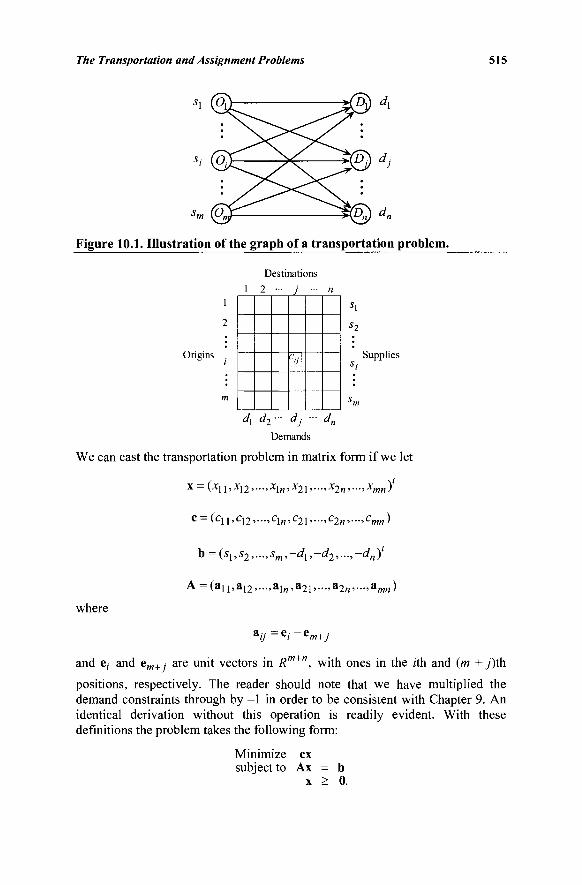
The Transportation and Assignment Problems 515
Figure 10.1. Illustration of the graph of a transportation problem.
Destinations . 1 2 - 3
1
2
Origins ciJ Supplies
d\ d2 - dj - dn
Demands
We can cast the transportation problem in matrix form if we let
x = \x\l>x\2>--->x\n>x2i>--->x2n>--->xmn)
c = (.cU'cl2'—'c\n'c2i'—'c2n'—'cmn)
b = (shs2,...,sm,-dl,-d2,...,-dn)'
A = (a11,a]2,...,a1„,a2i,...,a2„,...,am„)
where
a(/ — ei ~ em+j
and e,· and em +. are unit vectors in Rm+", with ones in the z'th and (m +j)th
positions, respectively. The reader should note that we have multiplied the demand constraints through by -1 in order to be consistent with Chapter 9. An identical derivation without this operation is readily evident. With these definitions the problem takes the following form:
Minimize ex subject to Ax = b
x > 0.
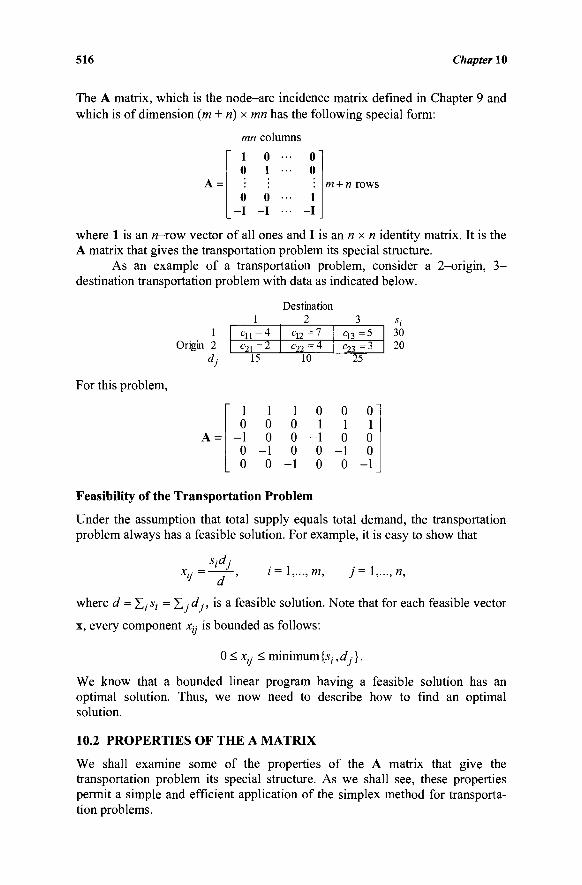
516 Chapter 10
The A matrix, which is the node-arc incidence matrix defined in Chapter 9 and which is of dimension (m + ri) x mn has the following special form:
A =
mn colum 1 0 0 1
0 0 · - I - I
ins 0 Ί
• 0
1 - I
m + n rows
where 1 is an «-row vector of all ones and I is an n x n identity matrix. It is the A matrix that gives the transportation problem its special structure.
As an example of a transportation problem, consider a 2-origin, 3 -destination transportation problem with data as indicated below.
1 Origin 2
1 c„=4 c21=2
Destination 2
c12=7 c22=4
3 c13=5 c 2 3 = 3
15 10 25
30 20
For this problem,
A =
1 1 1 0 0 0 0 0 0 1 1 1
- 1 0 0 - 1 0 0 0 - 1 0 0 - 1 0 0 0 - 1 0 0 - 1
Feasibility of the Transportation Problem
Under the assumption that total supply equals total demand, the transportation problem always has a feasible solution. For example, it is easy to show that
Xjj Sidj
i=\,...,m, j=l,...,n,
where d = X;-5; = ILjdj, is a feasible solution. Note that for each feasible vector
x, every component xt- is bounded as follows:
0 < Xj- < minimum{s;,d.·}.
We know that a bounded linear program having a feasible solution has an optimal solution. Thus, we now need to describe how to find an optimal solution.
10.2 PROPERTIES OF THE A MATRIX
We shall examine some of the properties of the A matrix that give the transportation problem its special structure. As we shall see, these properties permit a simple and efficient application of the simplex method for transporta-tion problems.
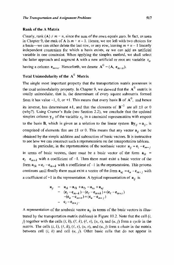
The Transportation and Assignment Problems 517
Rank of the A Matrix
Clearly, rank (A) φ m + n, since the sum of the rows equals zero. In fact, as seen in Chapter 9, the rank of A is m + n - 1. Hence, we are left with two choices for a basis—we can either delete the last row, or any row, leaving m + n - 1 linearly independent constraints for which a basis exists, or we can add an artificial variable in one constraint. When applying the simplex method, we shall select the latter approach and augment A with a new artificial or root arc variable xa
having a column em+„. Henceforth, we denote A = (A, em+n ).
Total Unimodularity of the A Matrix
The single most important property that the transportation matrix possesses is
the total unimodularity property. In Chapter 9, we showed that the A matrix is totally unimodular, that is, the determinant of every square submatrix formed
from it has value - 1 , 0, or +1. This means that every basis B of A , and hence
its inverse, has determinant ±1, and that the elements of B~ are all ±1 or 0 (why?). Using Cramer's Rule (see Section 2.2), we conclude that the updated simplex column y;y of the variable χ„- in a canonical representation with respect
to the basis B, which is given as a solution to the linear system By,y = a;y, is
comprised of elements that are ±1 or 0. This means that any vector a,y can be
obtained by the simple addition and subtraction of basic vectors. It is instructive to see how we can construct such a representation on the transportation tableau.
In particular, in the representation of the nonbasic vector a,y = e,· - eOT+ ,·
in terms of basic vectors, there must be a basic vector of the form Aik = ei ~em+k w i m a coefficient of +1. Then there must exist a basic vector of the
form a t t = e( -cm+!c with a coefficient of-1 in the representation. This process
continues until finally there must exist a vector of the form a · = e„ - e m + ,■ with
a coefficient of+1 in the representation. A typical representation of &„■ is
aij = aik ~ aik + a & ~ aus + auj
= ( ei -
em + * ) - ( e ^ - e w + / t ) + ( e ^ - e m + i )
\eu ~ em+s ) + (eH — em+j )
~~ e i — em+7 ·
A representation of the nonbasic vector a(y in terms of the basic vectors is illus-trated by the transportation matrix (tableau) in Figure 10.2. Note that the cell (/, j) together with the cells (i, k), (£, k), (i, s), (u, s), and (u,j) form a cycle in the matrix. The cells (/, k), (£, k), (I, s), («, 5), and («,/) form a chain in the matrix between cell (/, k) and cell («, j). Other basic cells that do not appear in
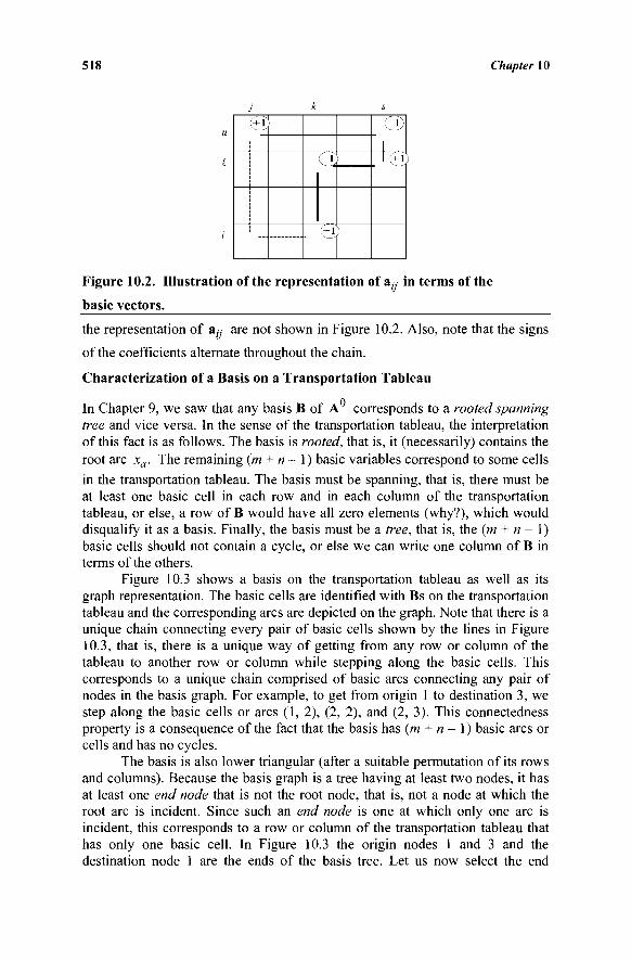
518 Chapter 10
j k
(+Γ
(zi
H
1
M
Figure 10.2. Illustration of the representation of a(y in terms of the
basic vectors.
the representation of a;y are not shown in Figure 10.2. Also, note that the signs
of the coefficients alternate throughout the chain.
Characterization of a Basis on a Transportation Tableau
In Chapter 9, we saw that any basis B of A corresponds to a rooted spanning tree and vice versa. In the sense of the transportation tableau, the interpretation of this fact is as follows. The basis is rooted, that is, it (necessarily) contains the root arc xa. The remaining (m + n~ 1) basic variables correspond to some cells
in the transportation tableau. The basis must be spanning, that is, there must be at least one basic cell in each row and in each column of the transportation tableau, or else, a row of B would have all zero elements (why?), which would disqualify it as a basis. Finally, the basis must be a tree, that is, the (m + n - 1) basic cells should not contain a cycle, or else we can write one column of B in terms of the others.
Figure 10.3 shows a basis on the transportation tableau as well as its graph representation. The basic cells are identified with Bs on the transportation tableau and the corresponding arcs are depicted on the graph. Note that there is a unique chain connecting every pair of basic cells shown by the lines in Figure 10.3, that is, there is a unique way of getting from any row or column of the tableau to another row or column while stepping along the basic cells. This corresponds to a unique chain comprised of basic arcs connecting any pair of nodes in the basis graph. For example, to get from origin 1 to destination 3, we step along the basic cells or arcs (1, 2), (2, 2), and (2, 3). This connectedness property is a consequence of the fact that the basis has (m + n- 1) basic arcs or cells and has no cycles.
The basis is also lower triangular (after a suitable permutation of its rows and columns). Because the basis graph is a tree having at least two nodes, it has at least one end node that is not the root node, that is, not a node at which the root arc is incident. Since such an end node is one at which only one arc is incident, this corresponds to a row or column of the transportation tableau that has only one basic cell. In Figure 10.3 the origin nodes 1 and 3 and the destination node 1 are the ends of the basis tree. Let us now select the end
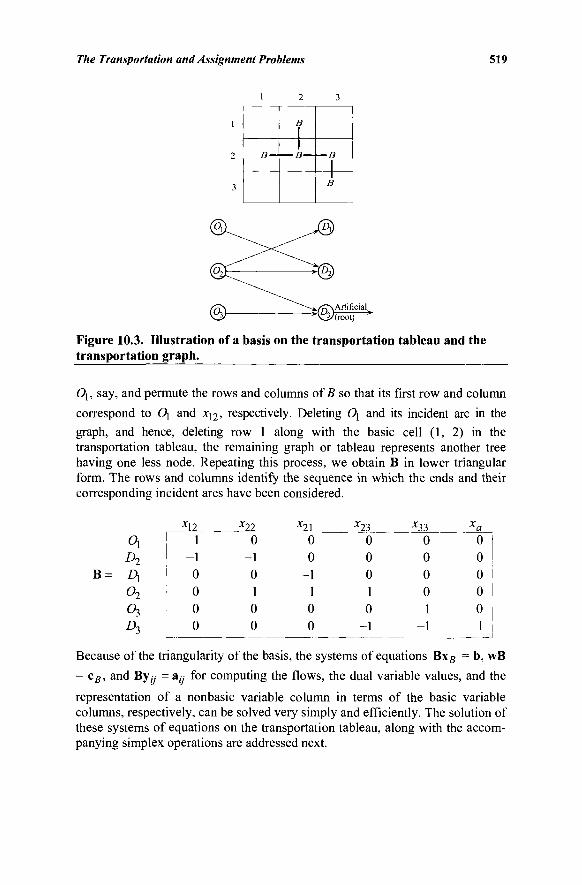
The Transportation and Assignment Problems 519
B —
B
1 1
B—
—B
1 1
B
Figure 10.3. Illustration of a basis on the transportation tableau and the transportation graph.
0[, say, and permute the rows and columns of B so that its first row and column
correspond to Οχ and x12, respectively. Deleting Ογ and its incident arc in the
graph, and hence, deleting row 1 along with the basic cell (1, 2) in the transportation tableau, the remaining graph or tableau represents another tree having one less node. Repeating this process, we obtain B in lower triangular form. The rows and columns identify the sequence in which the ends and their corresponding incident arcs have been considered.
0\ D2
= A o2 03 D3
xu
1
! - 1 1 0 1 0 ί 0
0
x22 0
-1 0 1 0 0
x21 0 0
-1 1 0 0
x23 0 0 0 1 0
-1
x33 0 0 0 0 1
-1
xa 0 0 0 0 0 1
Because of the triangularity of the basis, the systems of equations Bxg = b, wB
= cB, and By,y = a;y for computing the flows, the dual variable values, and the
representation of a nonbasic variable column in terms of the basic variable columns, respectively, can be solved very simply and efficiently. The solution of these systems of equations on the transportation tableau, along with the accom-panying simplex operations are addressed next.
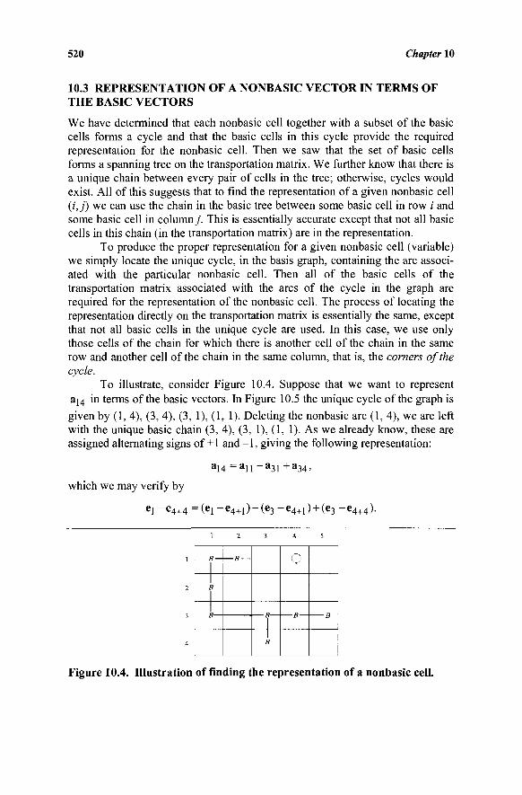
520 Chapter 10
10.3 REPRESENTATION OF A NONBASIC VECTOR IN TERMS OF THE BASIC VECTORS
We have determined that each nonbasic cell together with a subset of the basic cells forms a cycle and that the basic cells in this cycle provide the required representation for the nonbasic cell. Then we saw that the set of basic cells forms a spanning tree on the transportation matrix. We further know that there is a unique chain between every pair of cells in the tree; otherwise, cycles would exist. All of this suggests that to find the representation of a given nonbasic cell (/,_/) we can use the chain in the basic tree between some basic cell in row i and some basic cell in column /. This is essentially accurate except that not all basic cells in this chain (in the transportation matrix) are in the representation.
To produce the proper representation for a given nonbasic cell (variable) we simply locate the unique cycle, in the basis graph, containing the arc associ-ated with the particular nonbasic cell. Then all of the basic cells of the transportation matrix associated with the arcs of the cycle in the graph are required for the representation of the nonbasic cell. The process of locating the representation directly on the transportation matrix is essentially the same, except that not all basic cells in the unique cycle are used. In this case, we use only those cells of the chain for which there is another cell of the chain in the same row and another cell of the chain in the same column, that is, the corners of the cycle.
To illustrate, consider Figure 10.4. Suppose that we want to represent a14 in terms of the basic vectors. In Figure 10.5 the unique cycle of the graph is
given by (1, 4), (3, 4), (3, 1), (1, 1). Deleting the nonbasic arc (1, 4), we are left with the unique basic chain (3, 4), (3, 1), (1, 1). As we already know, these are assigned alternating signs of+1 and-1, giving the following representation:
a 1 4 = a n - a 3 1 + a 3 4 ,
which we may verify by
ei - e4+4 = (β! - e4+1 ) - (e3 - e4+1 ) + (e3 - e4+4 ).
1 2 3 4 5
B —
B
1
— B - -
1
B
-<?
Figure 10.4. Illustration of finding the representation of a nonbasic cell.
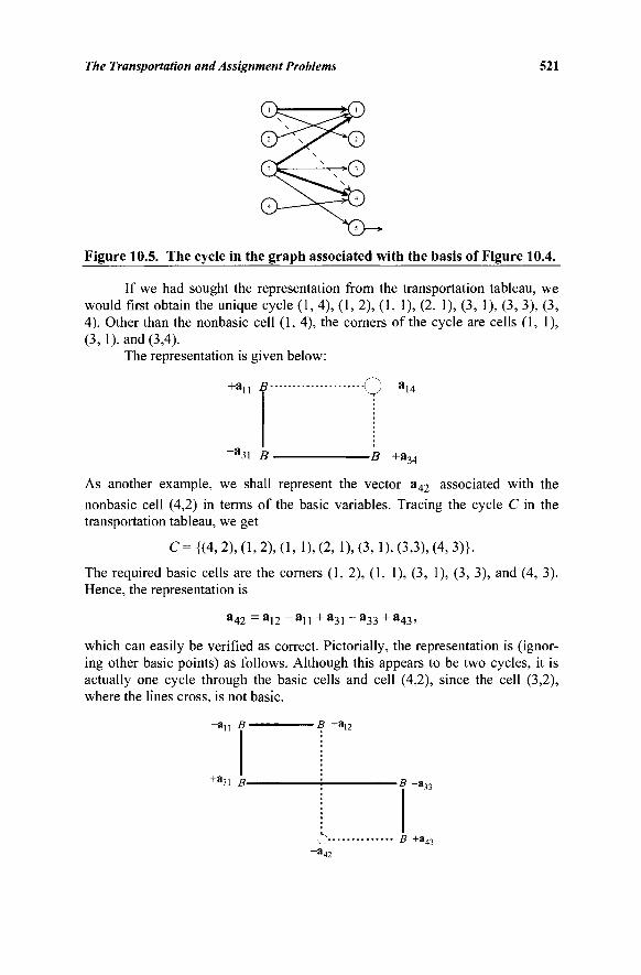
The Transportation and Assignment Problems 521
Figure 10.5. The cycle in the graph associated with the basis of Figure 10.4.
If we had sought the representation from the transportation tableau, we would first obtain the unique cycle (1, 4), (1, 2), (1, 1), (2, 1), (3, 1), (3, 3), (3, 4). Other than the nonbasic cell (1,4), the corners of the cycle are cells (1, 1), (3,1), and (3,4).
The representation is given below:
+a,i B
"31 B
"14
B +a 34
As another example, we shall represent the vector a42 associated with the
nonbasic cell (4,2) in terms of the basic variables. Tracing the cycle C in the transportation tableau, we get
C= {(4, 2), (1, 2), (1, 1), (2, 1), (3, 1), (3,3), (4, 3)}.
The required basic cells are the corners (1, 2), (1, 1), (3, 1), (3, 3), and (4, 3). Hence, the representation is
a 42= a 12- a l l+ a 31- a 33+ a 43>
which can easily be verified as correct. Pictorially, the representation is (ignor-ing other basic points) as follows. Although this appears to be two cycles, it is actually one cycle through the basic cells and cell (4,2), since the cell (3,2), where the lines cross, is not basic.
-a,, B
+a31 B
B +al:
B -a ,
O B +a43
-a4 2
522 Chapter 10
The Role of the Artificial Variable in the Transportation Problem
We note that the representation of a nonbasic vector involves only basic vectors associated with the unique chain through the basic cells. In particular, the artificial vector never becomes involved in any representation, and therefore, the artificial variable will always remain zero. This fact will allow us essentially to ignore the artificial variable in the application of the simplex method to transportation problems.
10.4 THE SIMPLEX METHOD FOR TRANSPORTATION PROBLEMS
The general steps in the application of the simplex method to a linear program are as follows:
1. Find a starting basic feasible solution.
2. Compute z - c for each nonbasic variable. Stop or select an enter-
ing column. 3. Determine an exiting column. 4. Obtain the new basic feasible solution and repeat Step 2.
We shall show how each of these steps can be carried out directly on the transportation tableau.
Finding a Starting Basic Feasible Solution
In Section 10.2 we produced a feasible solution for the transportation problem. However, the solution was not basic. While it would not be difficult to convert that solution into a basic feasible solution, we shall consider another procedure for obtaining a basic feasible solution. This method is called the northwest corner rule. During its process, as a variable % is assigned a value, we reduce
the corresponding s, and dj by that value. Let the reduced values of s, and dj be
denoted by st and dj, respectively. In particular, to start with, s,· = s,- and dj = dj.
Assuming that the total supply equals the total demand, beginning in cell (1, 1) we let
xj i = minimum {S], d\}
and replace ij by ij -x\\ and d\ by d\ -x\\. Then, if ij > 0, we move to cell (1,2), let
X\2= minimum {ij, d2}
and replace ij by ή -X\2 and d2 by d2 — JC12- However, if ή = 0, then we move to cell (2, 1), let
x21 = minimum {s2, d\}
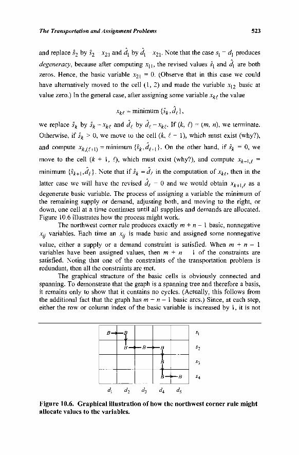
The Transportation and Assignment Problems 523
and replace s2 by s2 -x2\ and d\ by d] — JC2I- Note that the case η = rfj produces
degeneracy, because after computing xu, the revised values fj and <ή are both
zeros. Hence, the basic variable x2i = 0. (Observe that in this case we could
have alternatively moved to the cell (1,2) and made the variable x\2 basic at
value zero.) In the general case, after assigning some variable xkl the value
xki = minimum {sk,df},
we replace sk by sk -xk( and df by df -xk(. If {k, I) = (m, ri), we terminate.
Otherwise, if sk > 0, we move to the cell (k, i + 1), which must exist (why?),
and compute xk<g+n = minimum {sk,de+i}. On the other hand, if sk = 0, we
move to the cell (k + 1, i), which must exist (why?), and compute xk+\j =
minimum {sk+\,d^}. Note that if sk = dg in the computation of xke, then in the
latter case we will have the revised d( = 0 and we would obtain xk+ì e as a
degenerate basic variable. The process of assigning a variable the minimum of the remaining supply or demand, adjusting both, and moving to the right, or down, one cell at a time continues until all supplies and demands are allocated. Figure 10.6 illustrates how the process might work.
The northwest corner rule produces exactly m + n - 1 basic, nonnegative jc;. variables. Each time an JC,·,· is made basic and assigned some nonnegative
value, either a supply or a demand constraint is satisfied. When m + n - 1 variables have been assigned values, then m + n - 1 of the constraints are satisfied. Noting that one of the constraints of the transportation problem is redundant, then all the constraints are met.
The graphical structure of the basic cells is obviously connected and spanning. To demonstrate that the graph is a spanning tree and therefore a basis, it remains only to show that it contains no cycles. (Actually, this follows from the additional fact that the graph has m + n - 1 basic arcs.) Since, at each step, either the row or column index of the basic variable is increased by 1, it is not
B-) Ί 1
B—·.
~-B — «—5 1 1 L —B
άχ ί/2 ^3 " 4 <^5
Figure 10.6. Graphical illustration of how the northwest corner rule might allocate values to the variables.
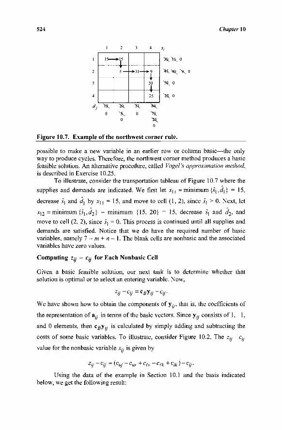
524 Chapter 10
1
2
3
4
1
15—
2
Ί * 5 —
3
-»·31—
4
->9
ι ♦ 50
1 25
χ χ o
Χ χ χ ο
X 0
X 0
dj X X o χ
0
X 0 X
X 0
Figure 10.7. Example of the northwest corner rule.
possible to make a new variable in an earlier row or column basic—the only way to produce cycles. Therefore, the northwest corner method produces a basic feasible solution. An alternative procedure, called Vogel's approximation method, is described in Exercise 10.25.
To illustrate, consider the transportation tableau of Figure 10.7 where the
supplies and demands are indicated. We first let x n = minimum {s\,d\} = 15,
decrease S\ and d\ by x^ = 15, and move to cell (1, 2), since ή > 0. Next, let
xn = minimum {η, d2} = minimum {15, 20} = 15, decrease η and d2, and move to cell (2, 2), since ·?} = 0. This process is continued until all supplies and
demands are satisfied. Notice that we do have the required number of basic variables, namely 7 = m + n - 1. The blank cells are nonbasic and the associated variables have zero values.
Computing zy - c^ for Each Nonbasic Cell
Given a basic feasible solution, our next task is to determine whether that solution is optimal or to select an entering variable. Now,
zij cij ■cBy ij cij-
We have shown how to obtain the components of y,y, that is, the coefficients of
the representation of a,·.· in terms of the basic vectors. Since y,y consists of 1, - 1 ,
and 0 elements, then cBy,y is calculated by simply adding and subtracting the
costs of some basic variables. To illustrate, consider Figure 10.2. The zy -Cy
value for the nonbasic variable Xy is given by
Zjj — Cy — (Cuj — Cus + C(s — Cgfc + Cjfc ) — Cjj.
Using the data of the example in Section 10.1 and the basis indicated below, we get the following result:
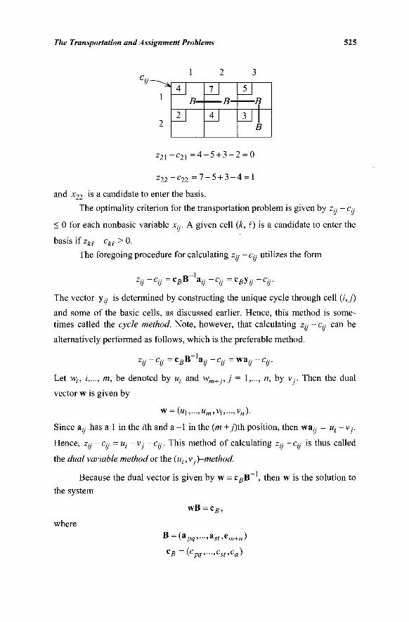
The Transportation and Assignment Problems 525
4 n
2
7
4
5
3 1 B
1
2
z 2 1 - c 2 1 = 4 - 5 + 3 - 2 = 0
*22~c22 = 7 - 5 + 3 - 4 = 1
and x22 is a candidate to enter the basis.
The optimality criterion for the transportation problem is given by zy - Cy
< 0 for each nonbasic variable Xy. A given cell (k, (!) is a candidate to enter the
basis if zki - Cfci > 0. The foregoing procedure for calculating zy - cy utilizes the form
Zij CU C D B a.-f-C;;
The vector y(y is determined by constructing the unique cycle through cell (i,j)
and some of the basic cells, as discussed earlier. Hence, this method is some-times called the cycle method. Note, however, that calculating Zy - Cy can be
alternatively performed as follows, which is the preferable method.
2 · - — C·· V V
CBB a y - c / , = w ay ' - c i / · ·
Since &y has a 1 in the rth and a -1 in the (m +/)th position, then wa,y = w, ,j.
Hence, zy - Cy - ui - v ■ - c, •y. This method of calculating zy „, ■
Let wh /,..., m, be denoted by w; and wm+j,j = 1,..., n, by v.-. Then the dual
vector w is given by
w = («i,...,wm,v1,...,v„).
VJ cu is thus called
the ί/κα/ variable method or the (w;, vA-method.
Because the dual vector is given by w = cgB~ , then w is the solution to
the system
wB = cB,
where
" = ( a w " ' a i f >em+n)
CB = (cpq>-">cst>ca)
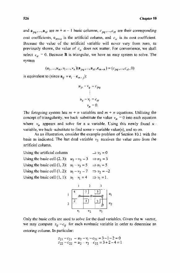
526 Chapter 10
and Λ ,&st are m + n - 1 basic columns, c ,cst are their corresponding w
cost coefficients, em+n is the artificial column, and ca is its cost coefficient. Because the value of the artificial variable will never vary from zero, as previously shown, the value of ca does not matter. For convenience, we shall
select ca = 0. Because B is triangular, we have an easy system to solve. The
system
(itl,...,um,vl,...,vn)(apq,...,ast,em+n) = (cpq,...,cst,0)
is equivalent to (since a,y = e, -em+J):
up ~ vg ~ cpq
v„=0.
The foregoing system has m + n variables and m + n equations. Utilizing the concept of triangularity, we back-substitute the value vn = 0 into each equation
where v„ appears and solve for a M-variable. Using this newly found in-
variable, we back-substitute to find some v^-variable value(s), and so on. As an illustration, consider the example problem of Section 10.1 with the
basis as indicated. The last dual variable v3 receives the value zero from the artificial column.
Using the artificial column
Using the basic cell (2, 3)
Using the basic cell (1,3)
Using the basic cell (1,2)
Using the basic cell (1,1)
"2
« l -«i -
" 1 -
= > v 3 = 0
- v3 = 3 => «2 = 3
- v3 = 5 => «i = 5
- v 2 = 7 = > v 2 = - 2
- vj = 4 => vj = 1.
1
Al B-
1]
2
il B-
A}
3
_5J
1 B
v, v2 v3
Only the basic cells are used to solve for the dual variables. Given the w-vector , we may compute zy - cy for each nonbasic variable in order to determine an
entering column. In particular:
z21_c21 = u2 ~vl ~c2\ = 3 - 1 - 2 = 0 z22~c22 = « 2 - v 2 - c 2 2 =3 + 2 - 4 = 1
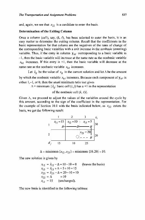
The Transportation and Assignment Problems 527
and, again, we see that x22 is a candidate to enter the basis.
Determination of the Exiting Column
Once a column (cell), say, (k, I), has been selected to enter the basis, it is an easy matter to determine the exiting column. Recall that the coefficients in the basic representation for that column are the negatives of the rates of change of the corresponding basic variables with a unit increase in the nonbasic (entering) variable. Thus, if the entry in column y ^ corresponding to a basic variable is - 1 , then the basic variable will increase at the same rate as the nonbasic variable xki increases. If this entry is +1, then the basic variable will decrease at the
same rate as the nonbasic variable xk( increases.
Let L· be the value of xt- in the current solution and let Δ be the amount
by which the nonbasic variable xy increases. Because each component of yke is
either 1,-1, or 0, then the usual minimum ratio test gives Δ = minimum {χψ basic cell (i,j) has a +1 in the representation
of the nonbasic cell (k, £)}.
Given Δ, we proceed to adjust the values of the variables around the cycle by this amount, according to the sign of the coefficient in the representation. For the example of Section 10.1 with the basis indicated below, as x22 enters the basis, we get the following result:
x n =15
B-
= 10 x13=5
B 30
20 Ó *23=20
B
15 10 25
Δ = minimum {χ\2,χ2ΐ) = minimum {10,20} = 10.
The new solution is given by
x\2 = x\2 - Δ = 10-10 = 0 (leaves the basis) X13 x23
X22
xu
χ 1 2 - Δ = 10-10 = 0 χ 1 3 +Δ = 5 + 10 = 15 χ 2 3 - Δ = 20-10 = 10 Δ =10 15 (unchanged).
The new basis is identified in the following tableau:
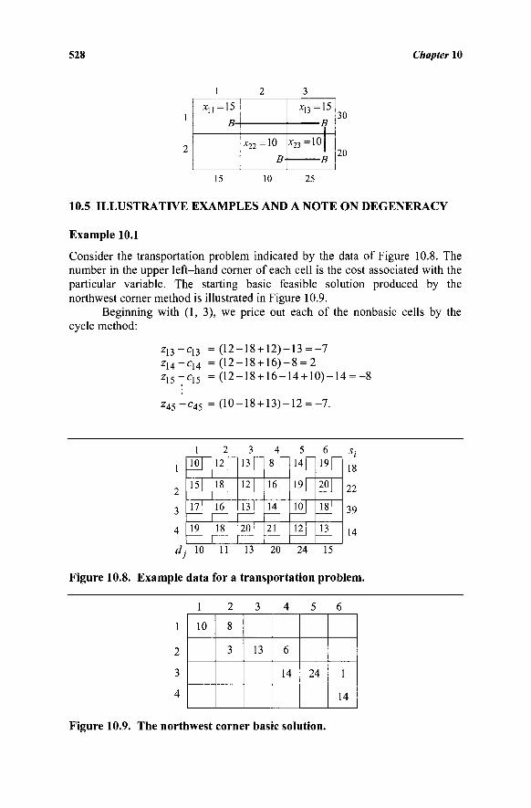
528 Chapter 10
xu=15 B-
XJ7 =10 Λ,22
B-
x13=15
x23=10 - 5
30
20
15 10 25
10.5 ILLUSTRATIVE EXAMPLES AND A NOTE ON DEGENERACY
Example 10.1
Consider the transportation problem indicated by the data of Figure 10.8. The number in the upper left-hand corner of each cell is the cost associated with the particular variable. The starting basic feasible solution produced by the northwest corner method is illustrated in Figure 10.9.
Beginning with (1, 3), we price out each of the nonbasic cells by the cycle method:
Z13~C13 =(12-18 + 12)-13 = -7 z i4 -c i 4 = (12-18 + 16)-8 = 2 z15-c15 =(12-18 + 16-14 + 10)-14 = -8
Z45-C45 =(10-18 + 13)-12 = -7 .
1
2
3
4
1
ioj 15]
17|
19
2 12
18
16
18
3
rJ
12
13 1
20 Γ""
4
1\ \e\ 14
2jJ
5
ill J9j 10
n\
6 19
20
18l
13 |
dj 10
22
39
14
11 13 20 24 15
Figure 10.8. Example data for a transportation problem.
1
2
3
4
1
10
2
8
3
3
13
4
6
14
5
24
6
1
14
Figure 10.9. The northwest corner basic solution.
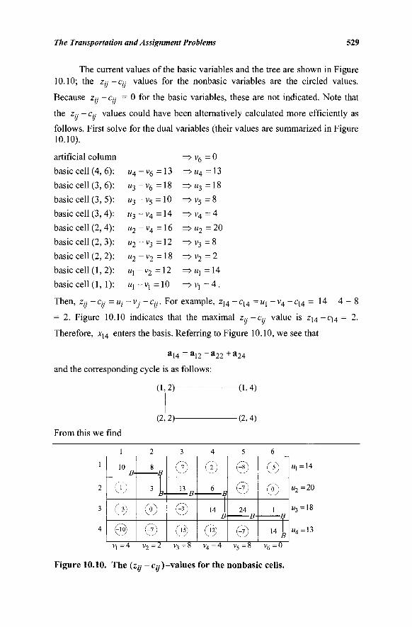
The Transportation and Assignment Problems 529
The current values of the basic variables and the tree are shown in Figure 10.10; the Zy—Cj.- values for the nonbasic variables are the circled values.
Because z„· - c„ = 0 for the basic variables, these are not indicated. Note that
the z„ - Cjj values could have been alternatively calculated more efficiently as
follows. First solve for the dual variables (their values are summarized in Figure 10.10).
artificial column
basic cell (4, 6)
basic cell (3, 6)
basic cell (3, 5)
basic cell (3, 4)
basic cell (2, 4)
basic cell (2, 3)
basic cell (2, 2)
basic cell (1,2)
basic cell (1, 1)
«4
"3"
"3"
"3"
u2
"2
«2
«,-
" l -
~ v 6
~v6
'v5
- V 4
- V 4
~ v 3
-v2
-v2 =
- V j =
= 13
= 18
= 10
= 14
= 16
= 12
= 18
= 12
= 10
^v6
= > W4
= > W3
^v5
=>v4
= > M 2
=> v3
=> v2
=>«,=
=>V! =
= 0
= 13
= 18
= 8
= 4
= 20
= 8
= 2
= 14
= 4 .
Then, Zjj -c„- = «,· - v · -c„·. For example, zj4 - q 4 = »! - v 4 - c 1 4 = 1 4 - 4 - 8
= 2. Figure 10.10 indicates that the maximal z„ -c„ value is zi4-cy4 = 2.
Therefore, x14 enters the basis. Referring to Figure 10.10, we see that
a 1 4 = a 1 2 - a 2 2 + a 2 4
and the corresponding cycle is as follows:
(1,2) 0,4)
(2, 2)- -(2,4)
From this we find
10 B-
CO
Θ Θ
8
3
0 Gì)
PT)
13 D
Θ Θ
(j)
6 „
14 B
Θ
® i?)
24
ί?)
Pi')
® 1
γ 4 w = 4 = 2 v, v6=0
Figure 10.10. The (z,y -c^-values for the nonbasic cells.
«,=14
«2=20
«3=18
«4 =13
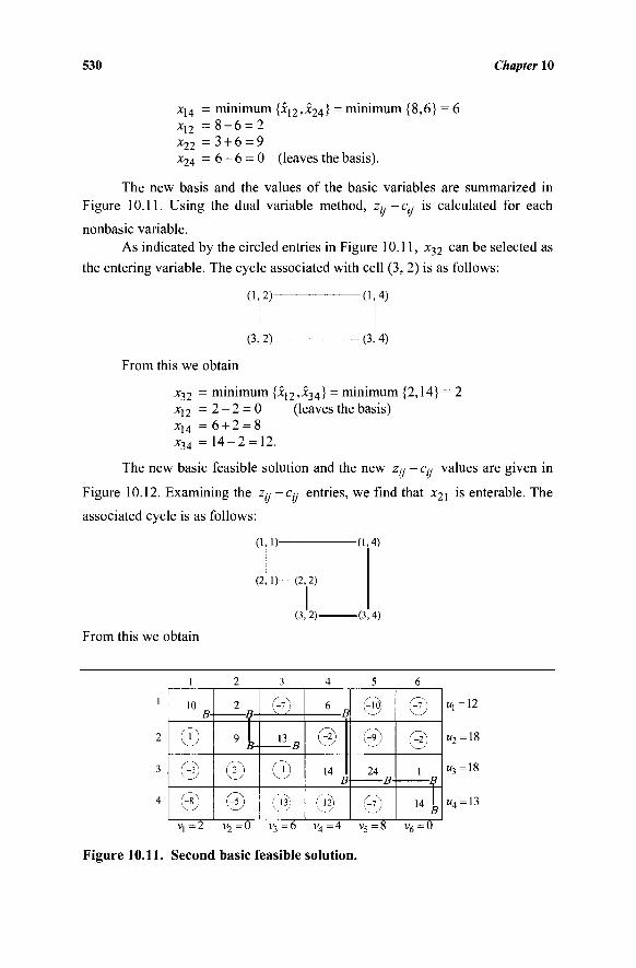
530 Chapter 10
*ΐ4 = minimum {Χ\2,Χ2Λ) = minimum {8,6} = 6 xn = 8 - 6 = 2 x22 = 3 + 6 = 9 x24 = 6 - 6 = 0 (leaves the basis).
The new basis and the values of the basic variables are summarized in Figure 10.11. Using the dual variable method, Zy-Cy is calculated for each
nonbasic variable. As indicated by the circled entries in Figure 10.11, x32 can be selected as
the entering variable. The cycle associated with cell (3, 2) is as follows:
0,2) -
(3, 2)
-0 ,4 )
■ (3, 4)
From this we obtain x32 = minimum {x\2>x34Ì = minimum {2,14} = 2 X]2 = 2 - 2 = 0 (leaves the basis) x14 = 6 + 2 = 8 x34 = 1 4 - 2 = 12.
The new basic feasible solution and the new z,-,· - c„ values are given in U v
Figure 10.12. Examining the z-y -cy entries, we find that χ2ι ·δ enterable. The
associated cycle is as follows: (1,1) (1,4)
( 2 , 1 ) - - ( 2 , 2)
(3,2) (3,4)
From this we obtain
1
2
3
4
1
10
0 (~*)
Θ
2 3
2
9 *
Θ @
R 13 rr
Θ Θ
4
6 „ (r*)
14 B
Gi\
5
0 Θ 24
Cn)
6
Θ Θ
1
Y 4
«,=12
«2=18
«3=18
«4 =13
V| = 2 v2 = 0 v3 = 6 v4 = 4 v5 = 8 v6 = 0
Figure 10.11. Second basic feasible solution.
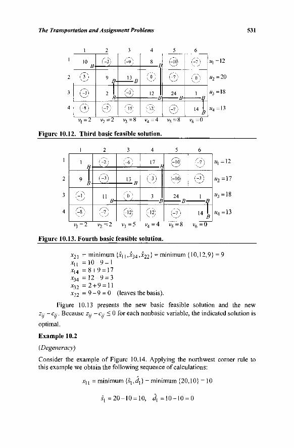
The Transportation and Assignment Problems 531
10
Θ © ®
© 9 p_
2
@
© 1 3 D
© i-is)
8 „ ®
12
©
© @
24
©
© ©
1
γ 4
t/j =12
w2=20
M 3 = 1 8
w4 = 1 3
Vj = 2 v2 = 2 v3 = 8 v4 = 4 v5 ^
Figure 10.12. Third basic feasible solution.
v6=0
1
9 i
© Θ
! -2 ^ V ©
© 11
©
© 1 3 D
© ©
17 j9
© 3
©
(ίθ;
Θ 24
©
Θ ©
1
Y 4
Mj = 1 2
a 9 =17
M3= li
«4 =13
V] = 2 v2 = 2 v3 = 5 v4 = 4 v5 :
Figure 10.13. Fourth basic feasible solution.
v 6 =0
x2i = minimum {ή ] , x3 4 , x2 2} = minimum {10,12,9} = 9 jcn = 1 0 - 9 = 1 x14 = 8 + 9 = 17 x34 = 1 2 - 9 = 3 x32 = 2 + 9 = 11 x22 = 9 - 9 = 0 (leaves the basis).
Figure 10.13 presents the new basic feasible solution and the new z„ - cu. Because z„ - c,·,· < 0 for each nonbasic variable, the indicated solution is
y y y y
optimal.
Example 10.2
(Degeneracy)
Consider the example of Figure 10.14. Applying the northwest corner rule to this example we obtain the following sequence of calculations:
*n = minimum {s^,^} = minimum {20,10} = 10
η = 2 0 - 1 0 = 10, c/j = 1 0 - 1 0 = 0
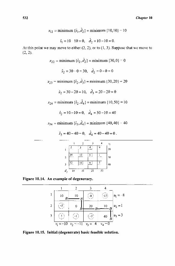
532 Chapter 10
x12 = minimum {s\,d2} = minimum {10,10} = 10
sx =10-10 = 0, d2 =10-10 = 0.
At this point we may move to either (2, 2), or to (1, 3). Suppose that we move to (2, 2).
x22 = minimum {s2,d2} = minimum {30,0} = 0
s2 = 3 0 - 0 = 30, d2 = 0 - 0 = 0
JC23 = minimum {s2,d^} = minimum {30,20} = 20
s2 = 3 0 - 2 0 = 10, i?3 = 2 0 - 2 0 = 0
x24 = minimum {s2,d4} = mmimum {10,50} = 10
s2 =10-10 = 0, d4 =50-10 = 40
X34 = minimum {53,d4} = minimum {40,40} = 40
s3 = 4 0 - 4 0 = 0, ^ 4 = 4 0 - 4 0 = 0.
2 i : 3
Γ _14j
12
12
nl
JT
1Λ
l]
9 ]
1
3 |
4 s,
20
30
40
dj 10 10 20 50
Figure 10.14. An example of degeneracy.
1
2
3
1
10 B-
Θ
CO
2
10
0
Θ
3
@
20
Pl\
4
© 10
40 1 B
tt] = — 0
u2 =1
«3=3
Vj=-10 v2 = —11 v 3 =^l v4=0
Figure 10.15. Initial (degenerate) basic feasible solution.
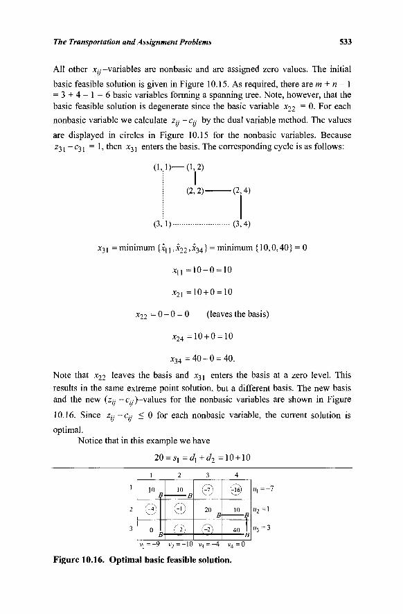
The Transportation and Assignment Problems 533
All other xi}—variables are nonbasic and are assigned zero values. The initial
basic feasible solution is given in Figure 10.15. As required, there are m + n - 1 = 3 + 4 - 1 = 6 basic variables forming a spanning tree. Note, however, that the basic feasible solution is degenerate since the basic variable x22
= 0· F°r each nonbasic variable we calculate z/; - ci;- by the dual variable method. The values
are displayed in circles in Figure 10.15 for the nonbasic variables. Because z3l _ c3 l = 1 > m e n x3i enters the basis. The corresponding cycle is as follows:
(1,1)—(1,2)
(2, 2)- •(2,4)
(3,1)- (3,4)
x31 = minimum {jcj j ,x 2 2 > 34} = minimum {10,0,40} = 0
xu = 1 0 - 0 = 10
JC21 =10 + 0 = 10
x22 = 0 - 0 = 0 (leaves the basis)
x24 =10 + 0 = 10
x34 = 4 0 - 0 = 40.
Note that x22 leaves the basis and x31 enters the basis at a zero level. This results in the same extreme point solution, but a different basis. The new basis and the new (z,y -c«)-values for the nonbasic variables are shown in Figure
10.16. Since z,-;-c,·,· < 0 for each nonbasic variable, the current solution is y y
optimal. Notice that in this example we have
20 = ^ =dx+d2 =10 + 10
10 10
^>
20 10
40
u2 = 1
Figure 10.16. Optimal basic feasible solution.
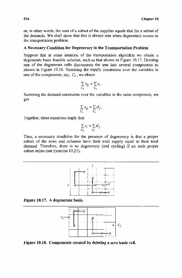
534 Chapter 10
or, in other words, the sum of a subset of the supplies equals that for a subset of the demands. We shall show that this is always true when degeneracy occurs in the transportation problem.
A Necessary Condition for Degeneracy in the Transportation Problem
Suppose that at some iteration of the transportation algorithm we obtain a degenerate basic feasible solution, such as that shown in Figure 10.17. Deleting one of the degenerate cells disconnects the tree into several components as shown in Figure 10.18. Summing the supply constraints over the variables in one of the components, say, Cj, we obtain
C, c,
Summing the demand constraints over the variables in the same component, we get
Σχ» =Zdj. c, c.
Together, these equations imply that
Σ«; =ΣίΛ·-c, c,
Thus, a necessary condition for the presence of degeneracy is that a proper subset of the rows and columns have their total supply equal to their total demand. Therefore, there is no degeneracy (and cycling) if no such proper subset exists (see Exercise 10.21).
Figure 10.17. A degenerate basis.
3
1
!
\l
l i
3
Ì- —B—
1 1
1 1
-B i
c,
Figure 10.18. Components created by deleting a zero basic cell.
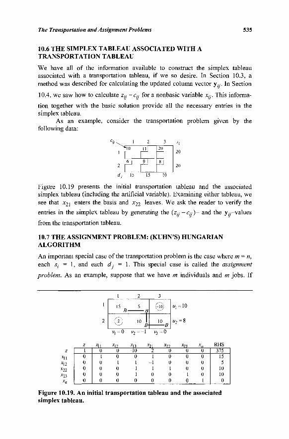
The Transportation and Assignment Problems 535
10.6 THE SIMPLEX TABLEAU ASSOCIATED WITH A TRANSPORTATION TABLEAU
We have all of the information available to construct the simplex tableau associated with a transportation tableau, if we so desire. In Section 10.3, a method was described for calculating the updated column vector y;y. In Section
10.4, we saw how to calculate zy -Cy for a nonbasic variable Xy. This informa-tion together with the basic solution provide all the necessary entries in the simplex tableau.
As an example, consider the transportation problem given by the following data:
1 2 3 s,
■10
6 |
nj 12a
9] L dj 15 15 10
Figure 10.19 presents the initial transportation tableau and the associated simplex tableau (including the artificial variable). Examining either tableau, we see that x2i enters the basis and x22 leaves. We ask the reader to verify the entries in the simplex tableau by generating the (z,-. -c,·.·)- and the y,-.—values from the transportation tableau.
10.7 THE ASSIGNMENT PROBLEM: (KUHN'S) HUNGARIAN ALGORITHM
An important special case of the transportation problem is the case where m = n, each Sj = 1, and each d.- = 1. This special case is called the assignment
problem. As an example, suppose that we have m individuals and m jobs. If
1 2 3
15 B
Θ
5
10 B
(AOJ
10
V]=0 v 2 = - l v 3 = 0
z *11 x\2 X22 χΊλ
*a
z 1 0 0 0 0 0
*11 0 1 0 0 0 0
*12 0 0 1 0 0 0
*13 -10
0 1
-1 1 0
*21 2 1
-1 1 0 0
x22 0 0 0 1 0 0
*23 0 0 0 0 1 0
*a 0 0 0 0 0 1
RHS 375
15 5
10 10 0
Figure 10.19. An initial transportation tableau and the associated simplex tableau.
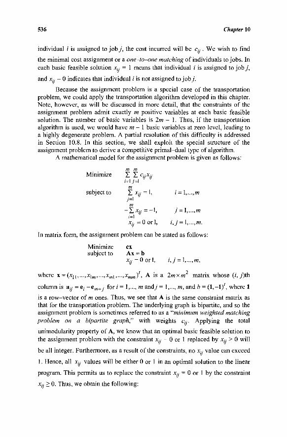
536 Chapter 10
individual / is assigned to job/ , the cost incurred will be c„ . We wish to find
the minimal cost assignment or a one-to-one matching of individuals to jobs. In each basic feasible solution x„- = 1 means that individual / is assigned to job/ ,
and Xy = 0 indicates that individual / is not assigned to job/.
Because the assignment problem is a special case of the transportation problem, we could apply the transportation algorithm developed in this chapter. Note, however, as will be discussed in more detail, that the constraints of the assignment problem admit exactly m positive variables at each basic feasible solution. The number of basic variables is 2m - 1. Thus, if the transportation algorithm is used, we would have m - 1 basic variables at zero level, leading to a highly degenerate problem. A partial resolution of this difficulty is addressed in Section 10.8. In this section, we shall exploit the special structure of the assignment problem to derive a competitive primal-dual type of algorithm.
A mathematical model for the assignment problem is given as follows:
m m Minimize Σ Σ <?„·*„·
1=17=1 m
subject to X x(;- = 1, i = l,...,m 7=1
m - Σ * ί / = - 1 , j = \,...,m
!=1 x„· = 0 ori, / , / = \,...,m.
In matrix form, the assignment problem can be stated as follows:
Minimize ex subject to Ax = b
Xy = 0 ori, / , / = \,...,m,
where x = (xjj,...,xlw,...,xmi,...,xmm), A is a 2mxm matrix whose (/', /)th
column is a„· = e;- - e m + , for i = 1,..., m and/ = 1,..., m, and b = (1,-1)', where 1
is a row-vector of m ones. Thus, we see that A is the same constraint matrix as that for the transportation problem. The underlying graph is bipartite, and so the assignment problem is sometimes referred to as a "minimum weighted matching problem on a bipartite graph" with weights c„. Applying the total
unimodularity property of A, we know that an optimal basic feasible solution to the assignment problem with the constraint x(. = 0 or 1 replaced by x„ > 0 will
be all integer. Furthermore, as a result of the constraints, no x„- value can exceed
1. Hence, all xy· values will be either 0 or 1 in an optimal solution to the linear
program. This permits us to replace the constraint x„ = 0 or 1 by the constraint
X// > 0. Thus, we obtain the following:
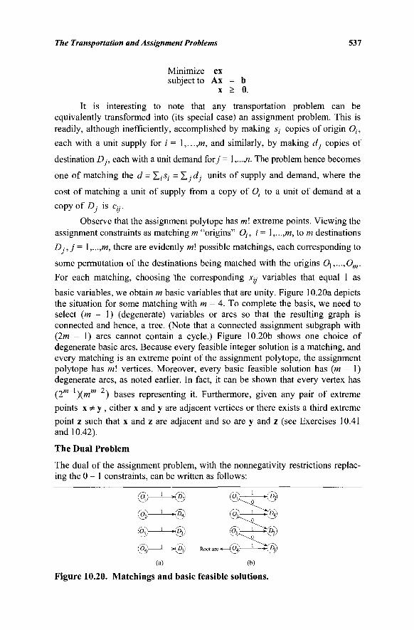
The Transportation and Assignment Problems 537
Minimize ex subject to Ax = b
x > 0.
It is interesting to note that any transportation problem can be equivalently transformed into (its special case) an assignment problem. This is readily, although inefficiently, accomplished by making s,· copies of origin Oh
each with a unit supply for / = \,...,m, and similarly, by making d ■ copies of
destination Dj, each with a unit demand for/ = \,...,n. The problem hence becomes
one of matching the d = Σ,-s,· = Σ dj units of supply and demand, where the
cost of matching a unit of supply from a copy of 0, to a unit of demand at a
copy of Dj is Cj-.
Observe that the assignment polytope has ml extreme points. Viewing the assignment constraints as matching m "origins" Oh i = \,...,m, to m destinations
Dj,j = \,...,m, there are evidently m\ possible matchings, each corresponding to
some permutation of the destinations being matched with the origins 0\,...,Om.
For each matching, choosing the corresponding x„- variables that equal 1 as
basic variables, we obtain m basic variables that are unity. Figure 10.20a depicts the situation for some matching with m = 4. To complete the basis, we need to select (m - 1) (degenerate) variables or arcs so that the resulting graph is connected and hence, a tree. (Note that a connected assignment subgraph with (2m - 1) arcs cannot contain a cycle.) Figure 10.20b shows one choice of degenerate basic arcs. Because every feasible integer solution is a matching, and every matching is an extreme point of the assignment polytope, the assignment polytope has ml vertices. Moreover, every basic feasible solution has (m - 1) degenerate arcs, as noted earlier. In fact, it can be shown that every vertex has
(2m~ )(mm~ ) bases representing it. Furthermore, given any pair of extreme
points x Φ y , either x and y are adjacent vertices or there exists a third extreme
point z such that x and z are adjacent and so are y and z (see Exercises 10.41 and 10.42).
The Dual Problem
The dual of the assignment problem, with the nonnegativity restrictions replac-ing the 0 - 1 constraints, can be written as follows:
© L^@ @\o—*® (pi) L_HS) @l > ? ®
(a) (b)
Figure 10.20. Matchings and basic feasible solutions.
538 Chapter 10
m m Maximize Σ ui - Σ v.-
i=\ j=\ subject to Uj-Vj <Cjj, i,j = \,...,m
w(,v unrestricted, i,j = \,...,m.
The complementary slackness conditions are given by
{cij-ui+vj)xij=<d, i,j=\,...,m.
Thus, if we can find a set of feasible values for the x, u, v, variables that satisfy complementary slackness, the resulting primal-dual solution will be optimal.
A feasible dual solution is given by
ùj = minimum {ci;}, i = \,...,m \<j<m
V;· = -minimum {c, - « , } , j = \,...,m. \<i<m
From this we see that w,· is the minimum c;, in row i and v, is the negative of the
minimum c„ - z5; in column/
The Reduced Matrix
Consider a reduced cost coefficient matrix where c„- is replaced by c„- = c„- -
Uj + v ■. In other words, the reduced cost matrix is obtained by first subtracting
from each row the minimum in that row, and then on the resulting matrix subtracting from each column the minimum in that column. The reduced matrix will have a zero in every row and column, and all of its entries will be nonnegative. The reduced matrix is actually the matrix of dual slack variables (why?).
Suppose that we can find a feasible set of x„-variables such that each
Xj- with value 1 is associated with a zero cell of the reduced matrix. Then, by
complementary slackness, we can conclude that we have an optimal solution. What, then, constitutes a set of feasible x„ -values? Reviewing the constraints
of the assignment problem, it is clear that we must have exactly one x„ in each
row equal to 1 and exactly one x„- in each column equal to 1. Thus, in a feasible
solution, there will be exactly m of the xy -variables equal to 1, the rest being
zero. Let us illustrate the foregoing ideas with an example. Consider the
following cost coefficient matrix for an assignment problem:
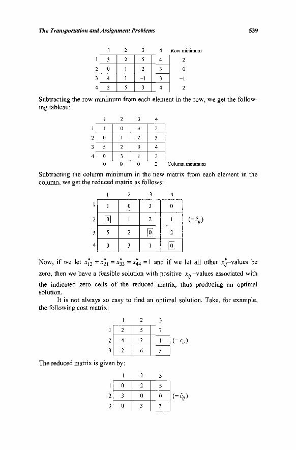
The Transportation and Assignment Problems 539
3
0
4
2
2
1
1
5
5
2
-1
3
4
3
3
4
Row minimum
2
0
-1
2
Subtracting the row minimum from each element in the row, we get the follow-ing tableau:
1
1 ! 1
2
3j 4L
0
5
0
2
0
1
2
3
3
3
2
0
1
4
2
3
4
2
Column minimum
Subtracting the column minimum in the new matrix from each element in the column, we get the reduced matrix as follows:
(=^)
1
2
3
4
1
1
0 5
0
2
0 1
2
3
3
3
2
0 1
4
0
1
2
0 Now, if we let x12 = *2i = x33 = x44 = 1 a ° d if we let all other x^—values be
zero, then we have a feasible solution with positive x,-, -values associated with
the indicated zero cells of the reduced matrix, thus producing an optimal solution.
It is not always so easy to find an optimal solution. Take, for example, the following cost matrix:
2 5 7
4 2 1
2 6 5
i=cy)
The reduced matrix is given by:
0
3
0
2
0
3
5
0
3
(=*?)
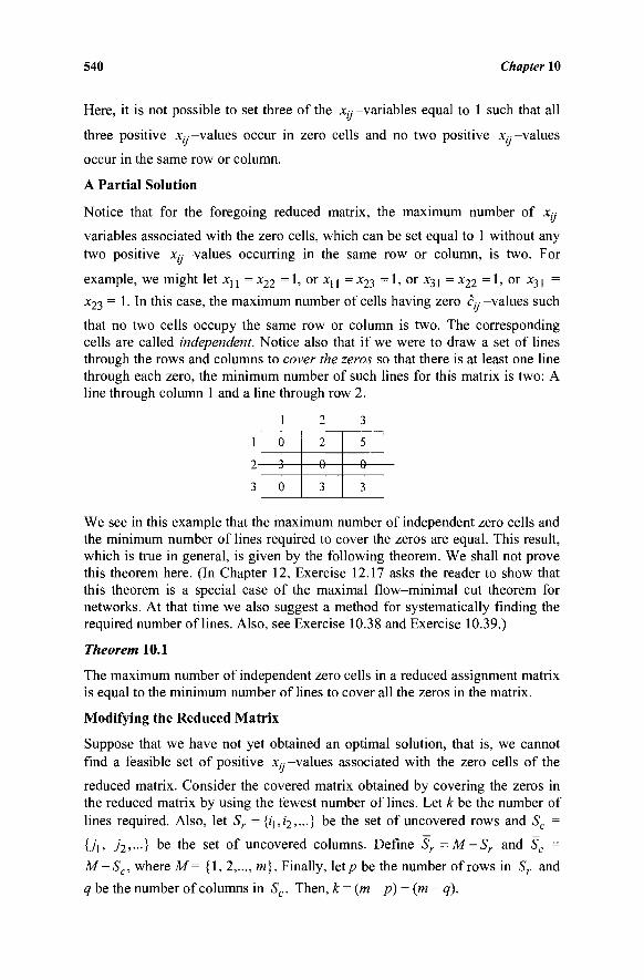
540 Chapter 10
Here, it is not possible to set three of the x„- -variables equal to 1 such that all
three positive xy-values occur in zero cells and no two positive x^-values
occur in the same row or column.
A Partial Solution
Notice that for the foregoing reduced matrix, the maximum number of xy
variables associated with the zero cells, which can be set equal to 1 without any two positive x„-values occurring in the same row or column, is two. For
example, we might let xj j = x22 = 1, or xj | = X23 = 1, or X31 = x22 = 1, or x31 =
X23 = 1. In this case, the maximum number of cells having zero c„· -values such
that no two cells occupy the same row or column is two. The corresponding cells are called independent. Notice also that if we were to draw a set of lines through the rows and columns to cover the zeros so that there is at least one line through each zero, the minimum number of such lines for this matrix is two: A line through column 1 and a line through row 2.
1 2 3
1[_ Φ
3
-Θ-
We see in this example that the maximum number of independent zero cells and the minimum number of lines required to cover the zeros are equal. This result, which is true in general, is given by the following theorem. We shall not prove this theorem here. (In Chapter 12, Exercise 12.17 asks the reader to show that this theorem is a special case of the maximal flow-minimal cut theorem for networks. At that time we also suggest a method for systematically finding the required number of lines. Also, see Exercise 10.38 and Exercise 10.39.)
Theorem 10.1
The maximum number of independent zero cells in a reduced assignment matrix is equal to the minimum number of lines to cover all the zeros in the matrix.
Modifying the Reduced Matrix
Suppose that we have not yet obtained an optimal solution, that is, we cannot find a feasible set of positive x„ -values associated with the zero cells of the
reduced matrix. Consider the covered matrix obtained by covering the zeros in the reduced matrix by using the fewest number of lines. Let k be the number of lines required. Also, let Sr ={/j,/2,...} be the set of uncovered rows and Sc =
{j\, 72,...} be the set of uncovered columns. Define Sr =M-Sr and Sc =
M -Sc, where M= {1, 2,..., m). Finally, \tip be the number of rows in Sr and
q be the number of columns in Sc. Then, k = {m -p) + {m- q).
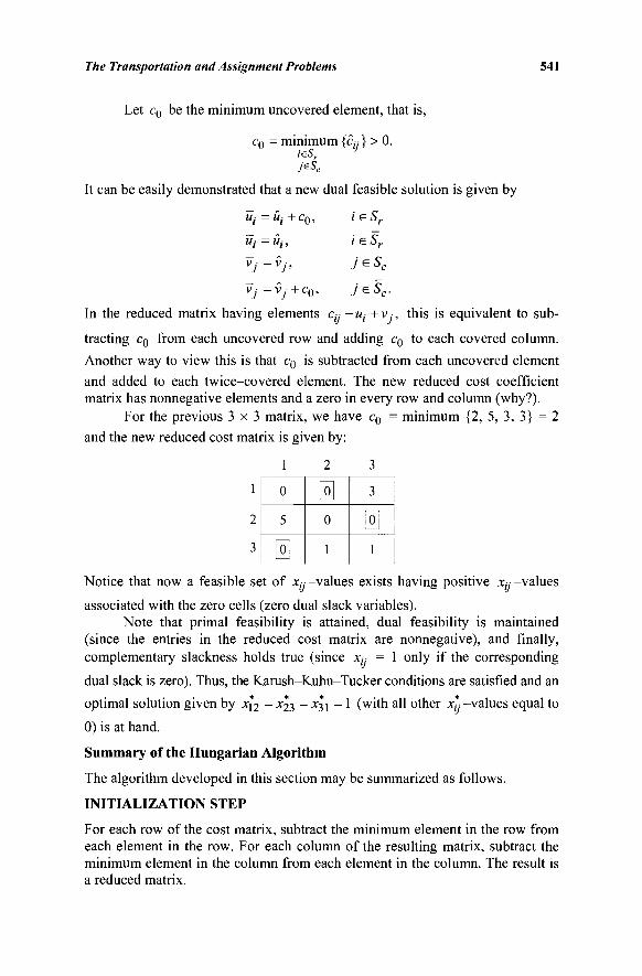
The Transportation and Assignment Problems 541
Let c0 be the minimum uncovered element, that is,
c0 = minimum {c.·,·} > 0. ìeSr
J
JcSc
It can be easily demonstrated that a new dual feasible solution is given by
uj = ùj + CQ , i eSr
uj = ùj, i e.Sr
V/=vy·, jeSc
Vj=Vj+c0, jeSc.
In the reduced matrix having elements Cy -ut + v,, this is equivalent to sub-
tracting c0 from each uncovered row and adding c0 to each covered column.
Another way to view this is that c0 is subtracted from each uncovered element
and added to each twice-covered element. The new reduced cost coefficient matrix has nonnegative elements and a zero in every row and column (why?).
For the previous 3 x 3 matrix, we have c0 = minimum {2, 5, 3, 3} = 2
and the new reduced cost matrix is given by:
1 2 3
0
5
H
L0]
0
1
3
m 1
Notice that now a feasible set of x,.--values exists having positive χί;·-values
associated with the zero cells (zero dual slack variables). Note that primal feasibility is attained, dual feasibility is maintained
(since the entries in the reduced cost matrix are nonnegative), and finally, complementary slackness holds true (since xy = 1 only if the corresponding
dual slack is zero). Thus, the Karush-Kuhn-Tucker conditions are satisfied and an
optimal solution given by xj*2 = XJT, = x^\ =1 (with all other x* -values equal to
0) is at hand.
Summary of the Hungarian Algorithm
The algorithm developed in this section may be summarized as follows.
INITIALIZATION STEP
For each row of the cost matrix, subtract the minimum element in the row from each element in the row. For each column of the resulting matrix, subtract the minimum element in the column from each element in the column. The result is a reduced matrix.
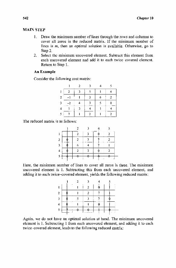
542 Chapter 10
MAIN STEP
2.
Draw the minimum number of lines through the rows and columns to cover all zeros in the reduced matrix. If the minimum number of lines is m, then an optimal solution is available. Otherwise, go to Step 2. Select the minimum uncovered element. Subtract this element from each uncovered element and add it to each twice-covered element. Return to Step 1.
An Example
Consider the following cost matrix:
1
2
3
4
5
The reduced matrix is as follows:
2
-1
-2
1
7
3
1
4
3
1
5
3
3
4
2
1
6
5
1
1
4
2
0
4
2
Here, the minimum number of lines to cover all zeros is three. The minimum uncovered element is 1. Subtracting this from each uncovered element, and adding it to each twice-covered element, yields the following reduced matrix:
Again, we do not have an optimal solution at hand. The minimum uncovered element is 1. Subtracting 1 from each uncovered element, and adding it to each twice-covered element, leads to the following reduced matrix:
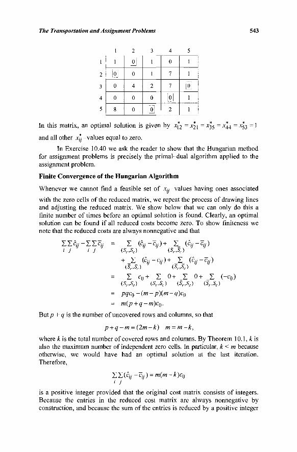
The Transportation and Assignment Problems 543
1 2 3 4 5
1
0 0
0
8
Έ 0
4
0
0
1
1
2
0
\o\
0
7
7
0 2
1
1
0 1
1
In this matrix, an optimal solution is given by *i2 = *2l = *35 = *44 = *53 =1
and all other x*-values equal to zero.
In Exercise 10.40 we ask the reader to show that the Hungarian method for assignment problems is precisely the primal-dual algorithm applied to the assignment problem.
Finite Convergence of the Hungarian Algorithm
Whenever we cannot find a feasible set of x„-values having ones associated
with the zero cells of the reduced matrix, we repeat the process of drawing lines and adjusting the reduced matrix. We show below that we can only do this a finite number of times before an optimal solution is found. Clearly, an optimal solution can be found if all reduced costs become zero. To show finiteness we note that the reduced costs are always nonnegative and that
Σ (èy-Cy) + Σ_ (Cy-Cy) (Sr,Sc) (Sr,Sc)
+ _Σ (Cij-Cij)+ _Σ_ (Cy-Cy) (Sr,Sc) (Sr,Sc) Σ c0+ Σ 0+ Σ 0+ _Σ_ (-c0)
(Sr,Sc) (Sr,Sc) (Sr,Sc) (Sr,Sc)
pqc0-(m-p)(m-q)c0
m(p + q-m)c0.
Butp + q is the number of uncovered rows and columns, so that
p + q-m = (2m -k)-m = m-k, where k is the total number of covered rows and columns. By Theorem 10.1, £ is also the maximum number of independent zero cells. In particular, k < m because otherwise, we would have had an optimal solution at the last iteration. Therefore,
ZZ(Cy -Cy) = m(m- k)c0
i J
is a positive integer provided that the original cost matrix consists of integers. Because the entries in the reduced cost matrix are always nonnegative by construction, and because the sum of the entries is reduced by a positive integer
ΣΣ%-ΣΣ^· » j ' j
544 Chapter 10
at each iteration, the algorithm stops in a finite number of steps. At termination we have an optimal solution since the Karush-Kuhn-Tucker conditions hold true.
As a final insight with respect to the Hungarian method, consider the following variation in the method. Suppose that at each step of covering the zeros of the reduced matrix, in lieu of using the fewest number of lines k, we
cover the zeros using some k < m lines, if possible (else, an optimal solution is at hand). As before, then, let c0 be the minimum resultant uncovered element
and suppose that we perform the same type of reduction operation. From the foregoing discussion or the corresponding dual solution adjustment, we have that the difference between the new and the previous dual objective values is given by
[ I w i - I v y l - E w i - I v y ] ' J · J
= c0\Sr | - c 0 | S c | = c 0 ( w - | 5 ^ j - | s c \) = c0(m-k)>l.
Hence, we obtain a dual ascent by at least a unit, and since the dual objective value is bounded above, we will converge in a finite number of iterations. Observe, however, that in order to maximize the dual ascent at each iteration, it
is not simply sufficient to select the minimum number of lines k = k to cover the zeros of the reduced matrix because the value CQ is also governed by this covering process. That is, we can try and devise a mechanism to cover the zeros using k <m lines, whenever possible, such that the resultant product c0 (m - k )
is maximized in order to accelerate the convergence process. The Notes and References section cites some improved modifications of the Hungarian method conducted along these lines.
10.8 ALTERNATING PATH BASIS ALGORITHM FOR ASSIGNMENT PROBLEMS
We have seen that every basic feasible solution to the assignment problem has degeneracy of order (m - 1). In fact, it has been empirically observed that typically 90 percent of the pivots used to solve the assignment problem by the usual primal simplex algorithm are degenerate when m > 500. This should not be surprising since we know that every non-optimal vertex is either adjacent to an optimal vertex or is adjacent to a neighbor of this optimal vertex. Hence, it stands to reason that if we devise a primal simplex algorithm that circumvents a sizeable portion of the degenerate pivots, then a significant savings in computational effort will result. The alternating path basis algorithm is a step in this direction. This algorithm is a special case of the strongly feasible network simplex algorithm discussed in Chapter 9, in which we additionally designate an origin node as the root node. For the assignment problem, a strongly feasible basis that has an origin node as a root node is called an alternating path basis. Because the algorithm encounters only strongly feasible bases, that is, bases in which all degenerate arcs point toward the root, it automatically circumvents
The Transportation and Assignment Problems 545
several bases representing the extreme points of the assignment polytope. As a result, this procedure yields about a 25% savings in pivots over the usual network simplex algorithm.
Figure 10.20b shows an alternating path basis that is a chain graph. Such a basis can always be used to initialize the algorithm, given any choice of a starting one-to-one matching. (Exercise 10.47 indicates why this may be an advantageous starting point in the absence of any other information.) Figure 10.21a displays a typical alternating path basis. Figure 10.21b exhibits a basis representing this same extreme point that is not an alternating path basis (why?). Note that the name "alternating path" arises from the fact that the arcs having flows of one and zero alternate on the chain from any node to the root node. These arcs are respectively called one-arcs and zero—arcs. Observe, however, that not any feasible basis having an origin node as a root node and having one-arcs and zero-arcs alternating is an alternating path basis. For example, consider the basis obtained (with m = 5) in Figure 10.21b by removing 03, £>3, Οη, and
D-j along with their incident arcs. In fact, it can be easily shown (see Exercise
10.45) that a feasible basis is an alternating path basis if and only if all one-arcs are pointing away from the root. This holds if and only if an origin node is a root node having one incident basic arc (other than the root arc), and all other origin nodes have exactly two incident arcs. This gives a special structure to an alternating path basis that can be algorithmically exploited.
The algorithm using alternating path bases follows exactly the strongly feasible tree network simplex procedure of Chapter 9. However, some speciali-zations are possible. For example, observe that a pivot with entering arc (Oj,D ·) is nondegenerate if and only if D is a successor of Oh that is, O, lies
on the chain from £>,■ to the root node. Whether the pivot is degenerate or not,
the leaving arc, by the strongly feasible tree rule, is the one incident at 0, in the
basis equivalent chain or in the cycle that is formed by adding (Oj,DA to the
basis graph. By noting that each origin node has a unique immediate successor, which is the destination node assigned to it, the tree may be stored by considering each such origin-destination pair as a single "married" unit, thereby reducing the storage and updating requirements by roughly one-half. We ask the reader to explore these specializations in Exercise 10.50.
Computationally, the primal-dual algorithm of the previous section dominates the alternating path basis algorithm for totally dense problems when the cost parameters are in the range 0-100. However, unlike the primal-simplex-based approaches, the primal-dual algorithm is quite sensitive to ranges in cost coefficients, as evident from its computational complexity. (It is also instructive to examine its finite convergence arguments.) Hence, the primal-simplex-based approaches dominate this algorithm for cost ranges exceeding 0-1000. Nonetheless, as the papers cited in the Notes and References section indicate, primal-dual types of algorithms do provide competitive alternatives to primal-simplex-based approaches for the assignment problem.
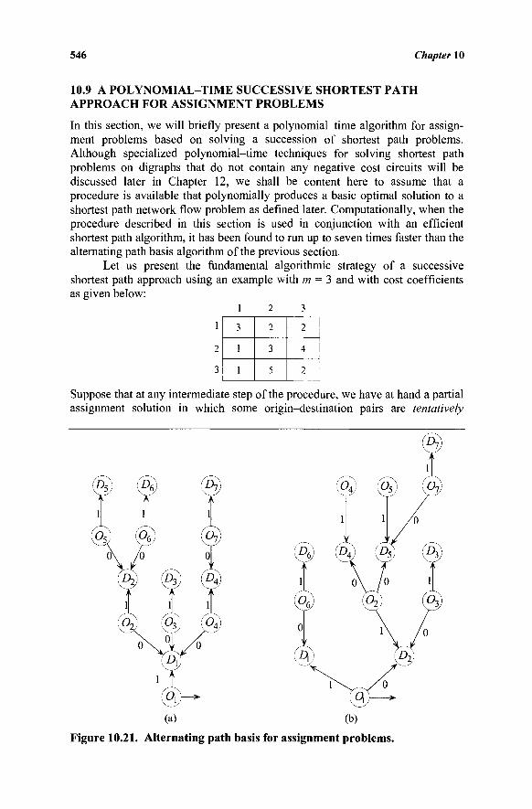
546 Chapter 10
10.9 A POLYNOMIAL-TIME SUCCESSIVE SHORTEST PATH APPROACH FOR ASSIGNMENT PROBLEMS
In this section, we will briefly present a polynomial-time algorithm for assign-ment problems based on solving a succession of shortest path problems. Although specialized polynomial-time techniques for solving shortest path problems on digraphs that do not contain any negative cost circuits will be discussed later in Chapter 12, we shall be content here to assume that a procedure is available that polynomially produces a basic optimal solution to a shortest path network flow problem as defined later. Computationally, when the procedure described in this section is used in conjunction with an efficient shortest path algorithm, it has been found to run up to seven times faster than the alternating path basis algorithm of the previous section.
Let us present the fundamental algorithmic strategy of a successive shortest path approach using an example with m = 3 and with cost coefficients as given below:
1 2 3
1
2
3
3
1
1
2
3
5
2
4
2
Suppose that at any intermediate step of the procedure, we have at hand a partial assignment solution in which some origin-destination pairs are tentatively
Figure 10.21. Alternating path basis for assignment problems.
The Transportation and Assignment Problems 547
matched. Let the sets UO and UD, respectively, contain the unassigned or active
origin and destination nodes, and let UO and UD be their respective
complements. To begin with, UO and UD are both empty. Let x denote the present partial assignment solution. Hence, x = 0 at the initialization step, and whenever an origin-destination assignment is made, the corresponding component of x will be set equal to one. Also, assume that currently | UO | = | UD | > 1 so that x is infeasible to the assignment problem.
Given a partial solution x, we first execute the shortest path step. For this purpose, let us construct a special network from the assignment graph as follows. For convenience, let the origin node 0, be indexed as /' for / = \,...,m, and let the destination node £>,· be indexed as m + j for/ = 1,..., m. Create an
additional dummy root node 0 and connect this to each origin node in UO using a zero cost arc. (Let the flow on this arc be represented by the nonnegative variable z,·, for /' e UO.) For each (Oj,Dj) pair for which xy is currently unity,
create the reverse arc (m +j, i) and let the cost on this arc be -Cy. (Let the flow
on this arc be represented by the nonnegative variable y^ = 1 - JC,· ; note that
currently, we therefore have y^ = 0.) All the other (OhDA arcs in the
assignment graph for which xy = 0 are present as the usual arcs (/, m +j) in this
new graph with the same variable x,y and cost cy. Next, place a supply of | UD |
= | UO | at node 0, and place a demand of one unit at each of the destination
nodes m+j for £),· e UD. Let all the other nodes be transshipment nodes. The
resulting network flow problem can be solved as the shortest path problem SP(x), which seeks a shortest path from node 0 to all the origin and destination
nodes in this network (not just to D e UD). Exercises 10.53 asks the reader to
show that SP(x) actually results from relaxing the assignment problem by
aggregating the unassigned origin node constraints; using the transformation yt-
= 1 - Xj- for each (0 ; ,D ■ ) pair for which χ,- = 1 ; and tentatively relaxing the
nonnegativity restriction on the latter x^—variables (i.e., not imposing y^ < 1 in
SP(x)).
Note that -ST^x) is feasible, (i.e., a path exists from node 0 to each of the origin and destination nodes in the underlying network for SP(x)), since we are considering a complete bipartite assignment network problem. (For a problem on a non-complete bipartite graph, if SP(x) is infeasible, then so is the original
assignment problem—see Exercise 10.46.) Hence, if SP(x) is not unbounded, that is, it does not contain any circuit having a total negative cost, then it has an optimal solution. This is clearly so for the starting problem SP(x) with x = 0, since the graph for this problem has all the original assignment graph arcs, and
548 Chapter 10
has a supply of m at the root node 0 and a demand of one at each of the destination nodes m +j,j = I,..., m. This is depicted in Figure 10.22a, where the supplies and demands are shown against each node and the costs are shown on the respective arcs. In fact, an optimal basic feasible solution here has basic arcs (0, i), i = 1,..., m, and (k■, m +j),j = I,..., m, where kj e argmin {cy\ / = 1,...,
m}. Figure 10.22b shows an optimal basis for the example problem, where the optimal dual variables are shown against the nodes. Later, we show that the primal feasible problem SP(\) is always dual feasible as well, and hence always
has an optimal solution. In this case, efficient polynomial-time algorithms described in Chapter 12 may be used to obtain a basic optimal solution. Let T(x) represent the corresponding optimal basis tree, which will, in fact, be an
arborescence with node 0 as the root node (e.g., see Figures 10.22b and 10.22d). The next step of the algorithm is the flow augmentation step. In particular, the basis tree T(x) obtained at the previous step gives shortest paths from node 0
through some unassigned origin nodes, to all the unassigned destination nodes. Let us pick any such destination node m +j (which has a unit demand) and trace the chain (reverse path) to the root node 0. This chain must finally pass through some unassigned origin node /', say, before reaching the root node 0. Along the corresponding path from / to m + j , let us complement the partial assignment values. Note that since the origin and destination nodes alternate on this path, as do the zero and one partial assignment values, the origin and destination nodes
in UO or UD on this path remain in these respective sets. Additionally, we have
/ e UO and (m +j) e UD, so that the cardinality of UO (and hence, UD) falls by one. Observe that, in effect, this amounts to sending a unit of flow along this path (from node 0), where the Xy-variables on this path go from xy = 0 to xy =
1, and the yy—variables on this path also go from yy = 0 to J« = 1, i.e., the
corresponding Xy-variables transition from Xy = 1 to Xy = 0; hence, the
complementation process. If there is another chain (reverse path) from another unassigned destination node to the root node 0 that goes through some other origin node in the updated UO set, then this step is repeated with respect to this path. This is carried out sequentially until the final updated graph contains no such path. Note that any two paths considered sequentially at this step must be disjoint since the basis tree has no cycles. If UD (and hence, UO) is empty at the end of this step, then as shown later, the current assignment x is optimal. Otherwise, we return to the shortest path step and repeat the procedure. Since | UD | drops by at least one at each iteration, we can loop through these two steps
at most m times, which yields an 0(m ) polynomial-time algorithm (assuming "3
that the complexity of the shortest path algorithm is 0(m )-see Chapter 12).
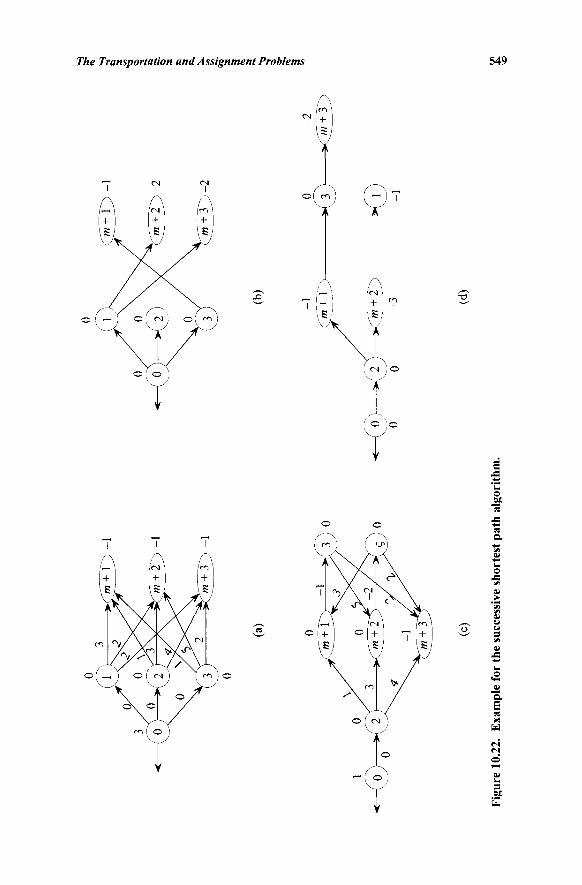
The Transportation and Assignment Problems 549
E -** o en
I
!
s tZ
550 Chapter 10
For the example problem, we can trace a path {0, 3, m + 1} to destination node 1 in Figure 10.22b at the flow augmentation step. This gives x3j = 1, UO = {1,2}, and UD = {2, 3}. A second path to destination 2 can be traced as {0, 1, m + 2}, which yields x12 = 1, UO = {2}, and UD = {3}. No additional disjoint
paths can be traced, and so currently we have the partial assignment solution x]2
= jc3l = 1, and Xj- = 0 otherwise.
Repeating the shortest path step, the new SP(x) graph obtained is shown
in Figure 10.22c. An optimal basis tree (arborescence) T(x) for this problem is
shown in Figure 10.22d. At the flow augmentation step, we trace the path {0, 2, m + 1, 3, m + 3} from node 0 to the unassigned destination node m + 3. Note that currently, x21
= 0> *3i = 1 0-e-> 731 = 0)> ar,d JÉ33 = 0 alternate on this path. Complementing these values, we get x2i
= 1> *3i = 0 0-e·' 731 = 1)' a n ^ S33 = 1· The value x12 = 1 remains unaffected. Hence, the resulting assignment solution is x12 = X21 = X33 = 1, and Xy = 0 otherwise, with UO = UD = 0 . We therefore
terminate, claiming this solution to be optimal, with the corresponding optimal dual solution to the assignment problem being given by the optimal dual solution to the final shortest path problem SP(x) solved, as shown against the nodes in Figure 10.22d.
To justify this algorithm, consider an optimal basis tree T(x) for the
shortest path problem SP(\) at some iteration. Note that, as shown above, an
optimal solution exists for SP(x) at the initial step when x = 0. Presently,
assume that an optimum exists for the current shortest path problem SP(x)
corresponding to the given partial assignment x, and we shall inductively verify
later than an optimum must then exist for the subsequent shortest path problem
in case there remain unassigned origins and destinations. Accordingly, let
w = (W],...,wm,wm+i,...,wm+m) be the associated set of optimal dual multipliers
for SP(x). Note that if Xy = 0, then arc (/, m + j) is present in the problem
SP(x) and we have w;- -vvm+ < c,·., with this constraint holding as an equality
if the arc (/, m +f) belongs to T(x). On the other hand, if Xy = 1, then arc (m +j,
i) is present in the problem SP(x) with a cost -c,·,· and, moreover, this arc must
belong to the shortest path tree T(x) since this is the only arc coming into node /'
e UO. Therefore, we have wm+j - wt = -Cy or w;· - wm+j = Cy. Consequently,
w is dual feasible to the assignment problem: Minimize {ex : Ax = b, x > 0} and is complementary slack with respect to x (why?). Moreover, the tree T(x)
also contains the arcs (0, i), V i e UO, because these are the only arcs coming into the respective unassigned origin nodes. Hence, we also have w, = 0, V i e UO.
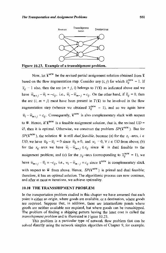
The Transportation and Assignment Problems 551
_ Transshipment , , .· ,. Sources , r Destinations
Figure 10.23. Example of a transshipment problem.
Now, let xnew be the revised partial assignment solution obtained from x
based on the flow augmentation step. Consider any (i,j) for which 3c^ew = 1. If
XJ: = 1 also, then the arc (m +j, i) belongs to T(x) as indicated above and we
have wm+j -w,· = -Cy, i.e., wt -wm+- = Cy. On the other hand, if Xy = 0, then
the arc (/', m + j) must have been present in T(x) to be involved in the flow
augmentation step (whence we obtained xyev/ = 1), and so we again have
Wj -wm+- =Cy. Consequently, xnew is also complementary slack with respect
to w. Hence, if xnew is a feasible assignment solution, that is, the revised UD =
0 , then it is optimal. Otherwise, we construct the problem SP(xnev/ ). But for
SP(xnev/), the solution w is still dual feasible, because (a) for the z;-arcs, / e
UO, we have w0 ~ ™i = 0 since w0 = 0, and wt = 0, V i e UO from above; (b)
for the jc,y—arcs we have w, - wm+ ,· < Cy since w is dual feasible to the
assignment problem; and (c) for the yy-arcs (corresponding to xjjev/ = 1), we
have wm+j -wi =-Cy, i.e., Wj-wm+j =Cy since xnew is complementary slack
with respect to w from above. Hence, SP(xnew ) is primal and dual feasible;
therefore, it has an optimal solution. The algorithmic process can now continue, and after at most m iterations, we achieve optimality.
10.10 THE TRANSSHIPMENT PROBLEM
In the transportation problem studied in this chapter we have assumed that each point is either an origin, where goods are available, or a destination, where goods are required. Suppose that, in addition, there are intermediate points where goods are neither available nor required, but where goods can be transshipped. The problem of finding a shipping pattern having the least cost is called the transshipment problem and is illustrated in Figure 10.23.
This problem is a particular type of network flow problem that can be solved directly using the network simplex algorithm of Chapter 9, for example.
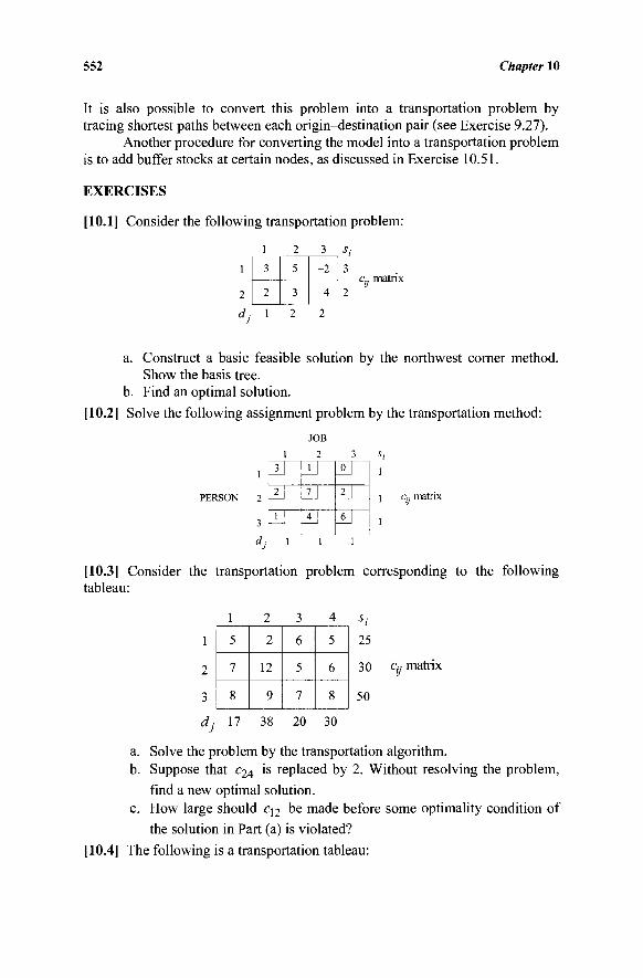
552 Chapter 10
It is also possible to convert this problem into a transportation problem by tracing shortest paths between each origin-destination pair (see Exercise 9.27).
Another procedure for converting the model into a transportation problem is to add buffer stocks at certain nodes, as discussed in Exercise 10.51.
EXERCISES
[10.1] Consider the following transportation problem:
1 2 3 J,·
3
2 d
3 5 - 2
2 3 4
a. Construct a basic feasible solution by the northwest corner method. Show the basis tree.
b. Find an optimal solution.
[10.2] Solve the following assignment problem by the transportation method:
PERSON
JOB
2
1] 2
j j
±\ 1\
±1
j>J 2
_6j
[10.3] Consider the transportation problem corresponding to the following tableau:
5
7
8
2
12
9
6
5
7
5
6
8
25
30
50
Cj- matrix
17 38 20 30
a. Solve the problem by the transportation algorithm. b. Suppose that c24 is replaced by 2. Without resolving the problem,
find a new optimal solution.
c. How large should q 2 be made before some optimality condition of
the solution in Part (a) is violated? [10.4] The following is a transportation tableau:
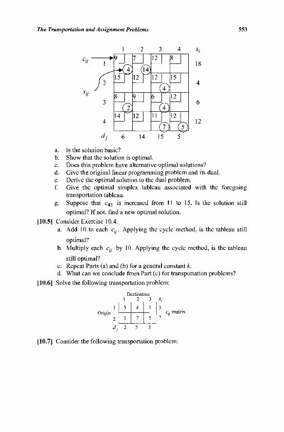
The Transportation and Assignment Problems 553
1
/
3
4
1
->to 15
8
a 14
2
/
12
9
12
3 1 0
12
to 6
to 11
to
4 o
15
12
12
& 12
14 15
a. Is the solution basic? b. Show that the solution is optimal. c. Does this problem have alternative optimal solutions? d. Give the original linear programming problem and its dual. e. Derive the optimal solution to the dual problem. f. Give the optimal simplex tableau associated with the foregoing
transportation tableau. g. Suppose that c43 is increased from 11 to 15. Is the solution still
optimal? If not, find a new optimal solution.
[10.5] Consider Exercise 10.4. a. Add 10 to each ctj. Applying the cycle method, is the tableau still
optimal? b. Multiply each c,y by 10. Applying the cycle method, is the tableau
still optimal? c. Repeat Parts (a) and (b) for a general constant k. d. What can we conclude from Part (c) for transportation problems?
[10.6] Solve the following transportation problem:
Origin
Destination 1 2 3
5
1
2
4
7
5
1
5
3
·*/ 3
Cjj matrix 7
[10.7] Consider the following transportation problem:
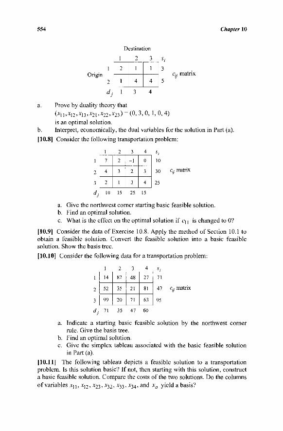
554 Chapter 10
Origin 1
2
</,·
Destination
1 2
2
1
1
1
4
3
3
1
4
4
3
5
c,y matrix
a. Prove by duality theory that
(x1 ] ,x1 2 ,x13,x2 1 ,x22,x23) = ((). 3>°> 1,0,4)
is an optimal solution. b. Interpret, economically, the dual variables for the solution in Part (a).
[10.8] Consider the following transportation problem:
7
4
2
2
3
1
-1
2
3
0
3
4
10
30
25
Cjj matrix
10 15 25 15
a. Give the northwest corner starting basic feasible solution. b. Find an optimal solution. c. What is the effect on the optimal solution if q j is changed to 0?
[10.9] Consider the data of Exercise 10.8. Apply the method of Section 10.1 to obtain a feasible solution. Convert the feasible solution into a basic feasible solution. Show the basis tree.
[10.10] Consider the following data for a transportation problem:
1
2
3
1
14
52
99
2
87
35
20
3
48
21
71
4
27
81
63
71
47
95
c« matrix
dj 71 35 47 60
a. Indicate a starting basic feasible solution by the northwest corner rule. Give the basis tree.
b. Find an optimal solution. c. Give the simplex tableau associated with the basic feasible solution
in Part (a).
[10.11] The following tableau depicts a feasible solution to a transportation problem. Is this solution basic? If not, then starting with this solution, construct a basic feasible solution. Compare the costs of the two solutions. Do the columns of variables X] j , x12, x 2 3 , X32 > x33 > x34 > a n ^ xa yield a basis?
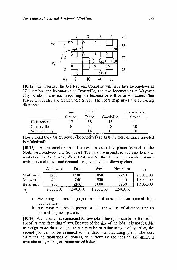
The Transportation and Assignment Problems 555
XU
1
/ 2
3
6
3
8
3
5,
6
8
(io) 1
2
8
& 9
(18)
7
( 2
20
(io 15
35
42
23
α7 20 10 40 30
[10.12] On Tuesday, the GT Railroad Company will have four locomotives at IE Junction, one locomotive at Centerville, and two locomotives at Wayover City. Student trains each requiring one locomotive will be at A-Station, Fine Place, Goodville, and Somewhere Street. The local map gives the following distances:
A-Station
Fine Place Goodville
Somewhere Street
IE Junction Centerville Wayover City
15 6 17
38 61 14
45 18 6
11 30 10
How should they assign power (locomotives) so that the total distance traveled is minimized?
[10.13] An automobile manufacturer has assembly plants located in the Northwest, Midwest, and Southeast. The cars are assembled and sent to major markets in the Southwest, West, East, and Northeast. The appropriate distance matrix, availabilities, and demands are given by the following chart.
Southwest East West Northeast
Northwest Midwest Southeast
1200 400 800
8500 800
1200
1850 900
1000
2250 1400 1100
2,500,000 1,800,000 1,600,000
dj 2,000,000 1,500,000 1,200,000 1,200,000
a. Assuming that cost is proportional to distance, find an optimal ship-ment pattern.
b. Assuming that cost is proportional to the square of distance, find an optimal shipment pattern.
[10.14] A company has contracted for five jobs. These jobs can be performed in six of its manufacturing plants. Because of the size of the jobs, it is not feasible to assign more than one job to a particular manufacturing facility. Also, the second job cannot be assigned to the third manufacturing plant. The cost estimates, in thousands of dollars, of performing the jobs in the different manufacturing plants, are summarized below.
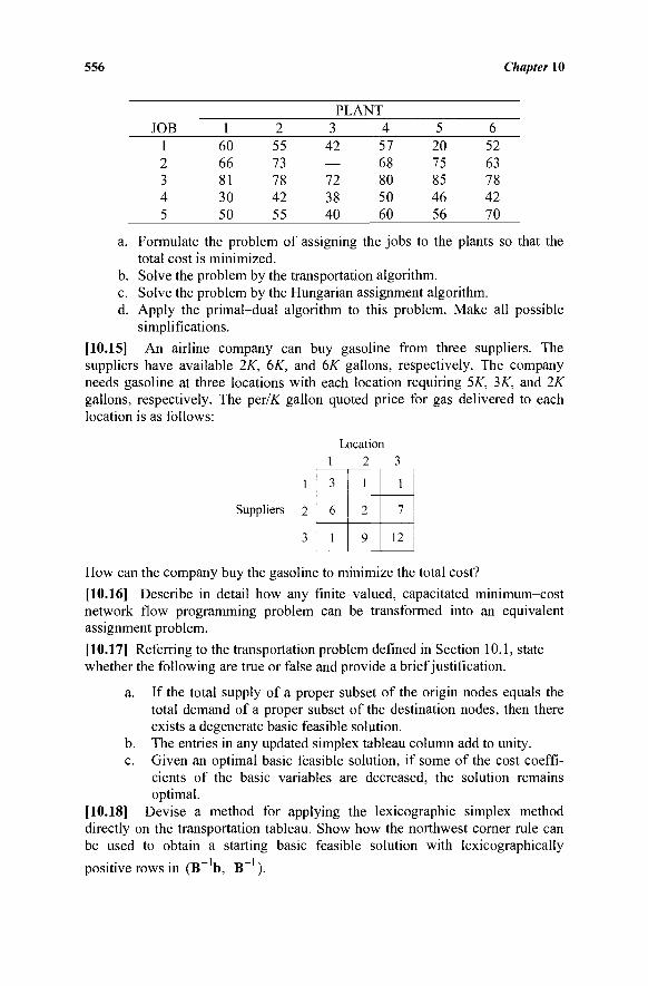
556 Chapter 10
PLANT JOB 1 2 3 4 5
1 60 66 81 30 50
2 55 73 78 42 55
3 42 — 72 38 40
4 57 68 80 50 60
5 20 75 85 46 56
6 52 63 78 42 70
a. Formulate the problem of assigning the jobs to the plants so that the total cost is minimized.
b. Solve the problem by the transportation algorithm. c. Solve the problem by the Hungarian assignment algorithm. d. Apply the primal-dual algorithm to this problem. Make all possible
simplifications.
[10.15] An airline company can buy gasoline from three suppliers. The suppliers have available 2K, 6K, and 6K gallons, respectively. The company needs gasoline at three locations with each location requiring 5K, 3K, and 2K gallons, respectively. The per/A^ gallon quoted price for gas delivered to each location is as follows:
Location 1 2 3 3
6
1
1
2
9
1
7
12
How can the company buy the gasoline to minimize the total cost? [10.16] Describe in detail how any finite-valued, capacitated minimum-cost network flow programming problem can be transformed into an equivalent assignment problem.
[10.17] Referring to the transportation problem defined in Section 10.1, state whether the following are true or false and provide a brief justification.
a. If the total supply of a proper subset of the origin nodes equals the total demand of a proper subset of the destination nodes, then there exists a degenerate basic feasible solution.
b. The entries in any updated simplex tableau column add to unity. c. Given an optimal basic feasible solution, if some of the cost coeffi-
cients of the basic variables are decreased, the solution remains optimal.
[10.18] Devise a method for applying the lexicographic simplex method directly on the transportation tableau. Show how the northwest corner rule can be used to obtain a starting basic feasible solution with lexicographically
positive rows in (B~ b, B~ ).
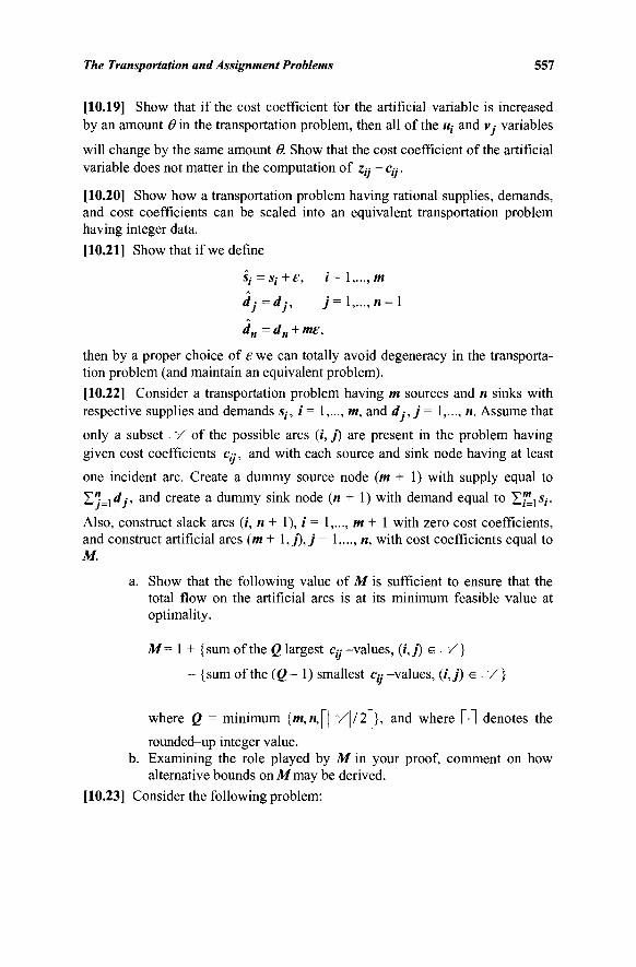
The Transportation and Assignment Problems 557
[10.19] Show that if the cost coefficient for the artificial variable is increased by an amount #in the transportation problem, then all of the ut and v.- variables
will change by the same amount Θ. Show that the cost coefficient of the artificial variable does not matter in the computation of Zy - Cy.
[10.20] Show how a transportation problem having rational supplies, demands, and cost coefficients can be scaled into an equivalent transportation problem having integer data.
[10.21] Show that if we define
S; =$;+£·, i= 1,..., Iti
dj=dj, j=l,...,n-l
d„=d„ + m£,
then by a proper choice of ε we can totally avoid degeneracy in the transporta-tion problem (and maintain an equivalent problem).
[10.22] Consider a transportation problem having m sources and n sinks with respective supplies and demands s,·, / = 1,..., m, and d:,j = 1,..., «. Assume that
only a subset . ~/ of the possible arcs (i, f) are present in the problem having given cost coefficients c«, and with each source and sink node having at least
one incident arc. Create a dummy source node (m + 1) with supply equal to
Y?i=\dj, and create a dummy sink node (n + 1) with demand equal to Σ™ι*/·
Also, construct slack arcs (i, n + 1), i = 1,..., m + 1 with zero cost coefficients, and construct artificial arcs (m + l,j),j= 1,..., n, with cost coefficients equal to M.
a. Show that the following value of M is sufficient to ensure that the total flow on the artificial arcs is at its minimum feasible value at optimality.
M= 1 + {sum of the Q largest c« -values, (i,f) e , /}
~ {sum of the {Q- 1) smallest cy -values, (/,_/') e -" /}
where Q = minimum {m,«,Π.~/|/2|}, and where Γ-Ί denotes the
rounded-up integer value. b. Examining the role played by M in your proof, comment on how
alternative bounds on Mmay be derived.
[10.23] Consider the following problem:
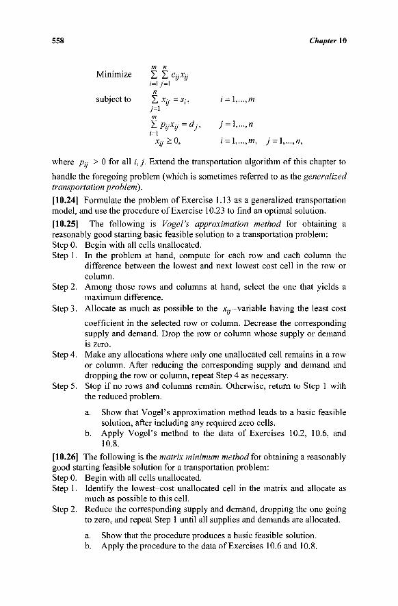
558 Chapter 10
Minimize Σ Σ c,·,*,-.· ,=iy=l n
subject to Σ % = si > / = 1,...,m 7=1 m
Y,pijxij=dj, j = \,...,n
Xjj>0, i = \,...,m, j-\,...,n,
where p^ > 0 for all /, j . Extend the transportation algorithm of this chapter to
handle the foregoing problem (which is sometimes referred to as the generalized transportation problem).
[10.24] Formulate the problem of Exercise 1.13 as a generalized transportation model, and use the procedure of Exercise 10.23 to find an optimal solution.
[10.25] The following is Vogel's approximation method for obtaining a reasonably good starting basic feasible solution to a transportation problem: Step 0. Begin with all cells unallocated. Step 1. In the problem at hand, compute for each row and each column the
difference between the lowest and next lowest cost cell in the row or column.
Step 2. Among those rows and columns at hand, select the one that yields a maximum difference.
Step 3. Allocate as much as possible to the xi-variable having the least cost
coefficient in the selected row or column. Decrease the corresponding supply and demand. Drop the row or column whose supply or demand is zero.
Step 4. Make any allocations where only one unallocated cell remains in a row or column. After reducing the corresponding supply and demand and dropping the row or column, repeat Step 4 as necessary.
Step 5. Stop if no rows and columns remain. Otherwise, return to Step 1 with the reduced problem.
a. Show that Vogel's approximation method leads to a basic feasible solution, after including any required zero cells.
b. Apply Vogel's method to the data of Exercises 10.2, 10.6, and 10.8.
[10.26] The following is the matrix minimum method for obtaining a reasonably good starting feasible solution for a transportation problem: Step 0. Begin with all cells unallocated. Step 1. Identify the lowest-cost unallocated cell in the matrix and allocate as
much as possible to this cell. Step 2. Reduce the corresponding supply and demand, dropping the one going
to zero, and repeat Step 1 until all supplies and demands are allocated.
a. Show that the procedure produces a basic feasible solution. b. Apply the procedure to the data of Exercises 10.6 and 10.8.
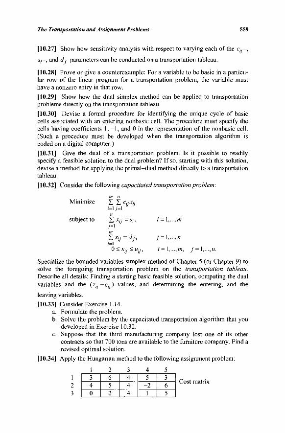
The Transportation and Assignment Problems 559
[10.27] Show how sensitivity analysis with respect to varying each of the cy-,
Sj-, and d -parameters can be conducted on a transportation tableau.
[10.28] Prove or give a counterexample: For a variable to be basic in a particu-lar row of the linear program for a transportation problem, the variable must have a nonzero entry in that row.
[10.29] Show how the dual simplex method can be applied to transportation problems directly on the transportation tableau.
[10.30] Devise a formal procedure for identifying the unique cycle of basic cells associated with an entering nonbasic cell. The procedure must specify the cells having coefficients 1,-1, and 0 in the representation of the nonbasic cell. (Such a procedure must be developed when the transportation algorithm is coded on a digital computer.)
[10.31] Give the dual of a transportation problem. Is it possible to readily specify a feasible solution to the dual problem? If so, starting with this solution, devise a method for applying the primal-dual method directly to a transportation tableau.
[10.32] Consider the following capacitated transportation problem:
Minimize
subject to
2J L cijxij
n }_, Xjj — Sj,
7=1 m ΣΧη =dj, i=\
0<Xij<Uij,
i = \,...,m
j = \,...,n
i = \,...,m, j = !,...,«.
Specialize the bounded variables simplex method of Chapter 5 (or Chapter 9) to solve the foregoing transportation problem on the transportation tableau. Describe all details: Finding a starting basic feasible solution, computing the dual variables and the (ZJ- - c^)-values, and determining the entering, and the
leaving variables.
[10.33] Consider Exercise 1.14. a. Formulate the problem. b. Solve the problem by the capacitated transportation algorithm that you
developed in Exercise 10.32. c. Suppose that the third manufacturing company lost one of its other
contracts so that 700 tons are available to the furniture company. Find a revised optimal solution.
[10.34] Apply the Hungarian method to the following assignment problem:
1 3 4 0
6 5 2
4 4 4
5 -2 1
3 6 5
Cost matrix
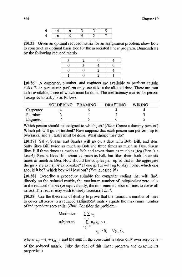
560 Chapter 10
4 6 3 3 5 6 4 5 2 7
4 5
[10.35] Given an optimal reduced matrix for an assignment problem, show how to construct an optimal basis tree for the associated linear program. Demonstrate by the following reduced matrix:
3 0 0 1
2 3 0 0
0 4 2 2
4 0 4 1
[10.36] A carpenter, plumber, and engineer are available to perform certain tasks. Each person can perform only one task in the allotted time. There are four tasks available, three of which must be done. The inefficiency matrix for person / assigned to tasky is as follows:
SOLDERING FRAMING DRAFTING WIRING Carpenter Plumber Engineer
4 2 6
Which person should be assigned to which job? {Hint: Create a dummy person.) Which job will go unfinished? Now suppose that each person can perform up to two tasks, and all tasks must be done. What should they do?
[10.37] Sally, Susan, and Sandra will go on a date with Bob, Bill, and Ben. Sally likes Bill twice as much as Bob and three times as much as Ben. Susan likes Bill three times as much as Bob and seven times as much as Ben (Ben is a loser!). Sandra likes Bob about as much as Bill, but likes them both about six times as much as Ben. How should the couples pair up so that in the aggregate the girls are as happy as possible? If one girl is willing to stay home, which one should it be? Which boy will lose out? (You guessed it!)
[10.38] Describe a procedure suitable for computer coding that will find, directly on the reduced matrix, the maximum number of independent zero cells in the reduced matrix (or equivalently, the minimum number of lines to cover all zeros). The reader may wish to study Exercise 12.17.
[10.39] Use the theorems of duality to prove that the minimum number of lines to cover all zeros in a reduced assignment matrix equals the maximum number of independent zero cells. {Hint: Consider the problem:
Maximize
subject to
ΣΣ-Xy ' j
c,=0
Xij>0, V(i,7),
where a;y = e, + em+ .· and the sum in the constraint is taken only over zero cells
of the reduced matrix. Take the dual of this linear program and examine its properties.)
The Transportation and Assignment Problems 561
[10.40] Compare the Hungarian method for the assignment problem with the primal-dual method applied to the assignment problem.
[10.41] Show that every vertex of the assignment polytope of Section 10.7 has
(2m~ ){mm~ ) bases representing it.
[10.42] Referring to the assignment polytope of Section 10.7, show that two extreme points x ^ y are adjacent if and only if P(x)u/>(y) contains exactly
one cycle, where P(x), for a given vertex x, is the subgraph of the assignment graph that contains only the positive flow arcs (see Figure 10.20a, for example). Show that given any pair of extreme points x Φ y of the assignment polytope,
either x and y are adjacent or there exists an extreme point z such that x and z as well as y and z are adjacent. (Hint: Recall that x and y are adjacent if and only if they have bases representing them such that the union of the respective spanning tree graphs contains exactly one cycle.)
[10.43] Show that each new dual solution in the assignment procedure specified in Section 10.7 is feasible.
[10.44] Show how one can construct the simplex tableau associated with an optimal assignment matrix.
[10.45] a. Show that a feasible basis for an assignment problem is an alternating path basis if and only if all one-arcs are pointing away from the root, which is also equivalent to having an origin node as the root node, with a single arc incident at the root node, and with all other origin nodes having exactly two incident arcs,
b. Give equivalent definitions of "alternating path bases" by designat-ing a demand node as the root node.
[10.46] Consider an assignment problem for which the underlying bipartite graph is not complete. Suppose that we construct the shortest path problem SP(x) for some partial solution x, as in the successive shortest path algorithm of
Section 10.9. Show that if SP(x) is infeasible, then so is the original assignment
problem. (Hint: Show that based on a feasible assignment, if one exists, a (reverse) path can be constructed from any unassigned destination node to the root node 0 in SP(x).)
[10.47] Show that given any basis representing an extreme point of the assignment polytope, the maximum number of potential nondegenerate pivots on this basis graph is m(m - l)/2, and the minimum number is (m - 1). Show that the maximum number is achieved if and only if the basis tree is a chain graph (see Figure 10.20b) and the minimum number is achieved on a basis in which all the degenerate arcs originate at some node or all terminate at some node. Can both types of bases be alternating path bases?
[10.48] Is it true that a feasible basis for an assignment problem in which some origin node is the root node, and in which the one-arcs and the zero-arcs alter-nate on the chain from any node to the root node is an alternating path basis?
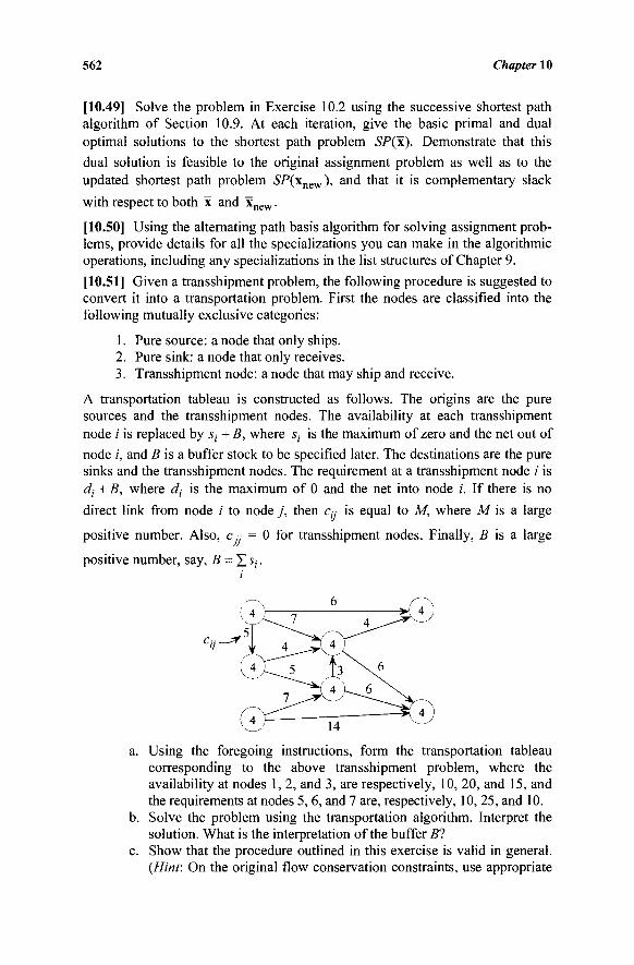
562 Chapter 10
[10.49] Solve the problem in Exercise 10.2 using the successive shortest path algorithm of Section 10.9. At each iteration, give the basic primal and dual optimal solutions to the shortest path problem SP(x). Demonstrate that this dual solution is feasible to the original assignment problem as well as to the updated shortest path problem £P(xnew), and that it is complementary slack
with respect to both x and xnew.
[10.50] Using the alternating path basis algorithm for solving assignment prob-lems, provide details for all the specializations you can make in the algorithmic operations, including any specializations in the list structures of Chapter 9.
[10.51] Given a transshipment problem, the following procedure is suggested to convert it into a transportation problem. First the nodes are classified into the following mutually exclusive categories:
1. Pure source: a node that only ships. 2. Pure sink: a node that only receives. 3. Transshipment node: a node that may ship and receive.
A transportation tableau is constructed as follows. The origins are the pure sources and the transshipment nodes. The availability at each transshipment node / is replaced by s,· + B, where st is the maximum of zero and the net out of
node /, and B is a buffer stock to be specified later. The destinations are the pure sinks and the transshipment nodes. The requirement at a transshipment node i is dj + B, where di is the maximum of 0 and the net into node i. If there is no
direct link from node / to node j , then % is equal to M, where M is a large
positive number. Also, c = 0 for transshipment nodes. Finally, B is a large
positive number, say, B - Σ·?,··
a. Using the foregoing instructions, form the transportation tableau corresponding to the above transshipment problem, where the availability at nodes 1, 2, and 3, are respectively, 10, 20, and 15, and the requirements at nodes 5, 6, and 7 are, respectively, 10,25, and 10.
b. Solve the problem using the transportation algorithm. Interpret the solution. What is the interpretation of the buffer Bl
c. Show that the procedure outlined in this exercise is valid in general. {Hint: On the original flow conservation constraints, use appropriate
The Transportation and Assignment Problems 563
substitutions of the type where a new variable equals B minus the sum of some variables.)
d. Convert the problem into a transportation problem using the least cost method discussed in Section 10.10. Apply the transportation algorithm and interpret your solution.
[10.52] If it is known in advance that a certain variable will be positive in any optimal solution to a transportation problem, what simplifications can result in the solution method?
m m [10.53] Consider the assignment problem AP to minimize Σ Σ c//xi/> subject
m m to Σ x„- =1 for each origin i = l,...,m; - X f c = _ ' f°r e a c n destination j =
7=1 ;=1
\,...,m, and x > 0. Suppose that we are applying the successive shortest path algorithm to solve this problem, where at a certain main step in this procedure,
we are given a partial assignment x having |UO | = |UD \ = q>\ and UO =
UD = m - q > 1. Accordingly, construct a relaxation of Problem AP as
follows:
(i) Aggregate the unassigned origin constraints to obtain m m
Σ Σ Xy = <?· Now, define zi = Σ x„-, \/i ε UO, and ieUOj=l j=\
rewrite this equation as the following set of constraints:
Σ Zi=q
ieUO
m
Σ Χ , 7 - Ζ , · = 0 , Vi e UO. 7=1
(ii) For each (/,_/) such that x; = 1, use a change of variables y„- =
1 - Xjj, and impose yy- > 0 (but not yt- < 1, i.e., relax xy > 0 for
these x(y-variables). a. Show that the resulting relaxed problem is a minimum cost network
flow program that is defined as SP(x) in Section 10.9. b. Explain how the flow augmentation step of the successive shortest
path algorithm ensures that the relaxed nonnegativity constraints in the transformation (ii) above are not violated when revising x to
564 Chapter 10
NOTES AND REFERENCES
1. Hitchcock [1941] is credited with the first formulation and discussion of a transportation model. Dantzig [1951c] adapted his simplex method to solve transportation problems. Charnes and Cooper [1954] developed an intuitive presentation of Dantzig's procedure through what is called the "stepping stone" method. In this chapter, we called this the "cycle method."
2. Koopmans [1949] was the first to note the relationship between basic solutions in the transportation problem and the tree structure of a graph. Other good discussions are provided by Dantzig [1963a] and Johnson [1965].
3. The bound on the value of M in Exercise 10.22 is derived in Sherali [1988].
4. A good study of the properties of the assignment polytope appears in Balinski and Russakoff [1974]. In addition to the results in Exercises 10.41 and 10.42, they show that the assignment polytope is of dimension
7 9
(m - 1) , has m facets, and has a simplex path linking any two vertices of length no more than 2m - 1. Therefore, the Hirsch conjecture (see the Notes and References section of Chapter 8) holds for this polytope.
5. The Hungarian method for the assignment problem was developed by Kuhn [1955]. This method finds its roots in the work of the Hungarian mathematician Egervàry [1931], hence its name. Kuhn's paper led to the
general primal-dual method for linear programs in the following year. 6. McGinnis [1983] presents a computational comparison between the
Hungarian algorithm and the primal simplex alternating path basis algo-rithm. For improvements and variations in the Hungarian algorithm, see Bertsekas [1981], Carpenito and Toth [1980], Redlack and Huang [1987], Jonker and Volgenant [1986], and Sherali and Driscoll [2003]. In particular, the last two papers examine alternatives to simply covering the zeros in the reduced matrix using the fewest number of lines versus focusing on a maximal dual improvement. Balinski [1984, 1985] provides an excellent study of the dual polyhedra of transportation and assignment problems, and exhibits why dual-based simplex approaches may be more suitable for these problems than primal procedures.
7. The alternating path basis algorithm was developed by Barr et al. [1977]. This algorithm turns out to be a special case of the strongly feasible tree algorithm of Cunningham [1976] that was independently developed for general network flow problems. The results in Exercises 10.45 and 10.50 are from the former paper. The result in Exercise 10.47 is from Bazaraa and Sherali [1982].
8. The successive shortest path algorithm for assignment problems dis-cussed in Section 10.9 is from Glover et al. [1986]. The threshold shortest path subroutine is used to derive a computationally very efficient algorithm. For another successive shortest path algorithm, see Engquist [1982]. Other polynomial algorithms for the assignment problem appear
The Transportation and Assignment Problems 565
in Akgul [1986a], Balinski [1985] (see Goldfarb [1985] for an improvement of this "signature algorithm"), Balinski [1986], and Hung [1983]. Also, see Orlin [1985] for some relevant discussions.
9. The reader interested in a further study of transportation problems involving aggregation and disaggregation methods for large-scale prob-lems is referred to Balas [1965], Zipkin [1980], and Zipkin and Raimer [1983].

This page intentionally left blank
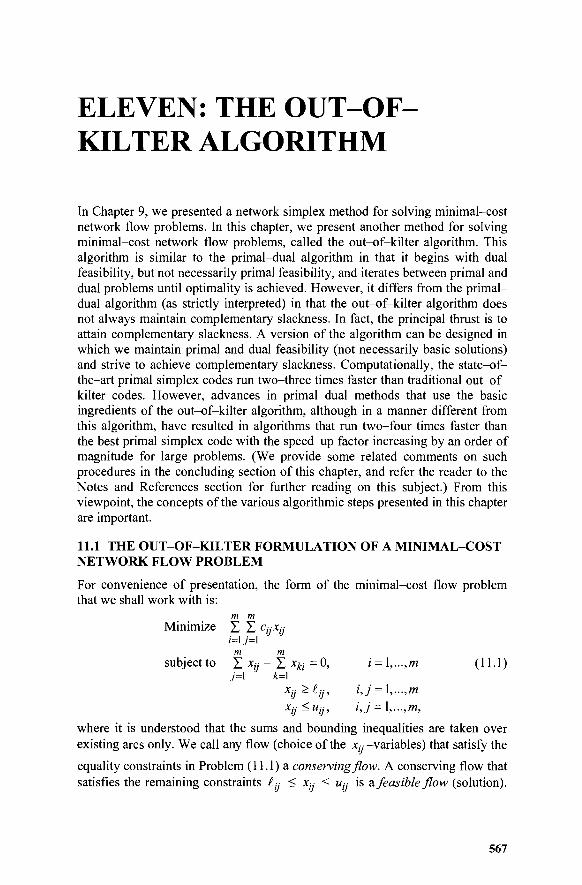
ELEVEN: THE OUT-OF-KILTER ALGORITHM
In Chapter 9, we presented a network simplex method for solving minimal-cost network flow problems. In this chapter, we present another method for solving minimal-cost network flow problems, called the out-of-kilter algorithm. This algorithm is similar to the primal-dual algorithm in that it begins with dual feasibility, but not necessarily primal feasibility, and iterates between primal and dual problems until optimality is achieved. However, it differs from the primal-dual algorithm (as strictly interpreted) in that the out-of kilter algorithm does not always maintain complementary slackness. In fact, the principal thrust is to attain complementary slackness. A version of the algorithm can be designed in which we maintain primal and dual feasibility (not necessarily basic solutions) and strive to achieve complementary slackness. Computationally, the state-of-the-art primal simplex codes run two-three times faster than traditional out-of-kilter codes. However, advances in primal-dual methods that use the basic ingredients of the out-of-kilter algorithm, although in a manner different from this algorithm, have resulted in algorithms that run two-four times faster than the best primal simplex code with the speed-up factor increasing by an order of magnitude for large problems. (We provide some related comments on such procedures in the concluding section of this chapter, and refer the reader to the Notes and References section for further reading on this subject.) From this viewpoint, the concepts of the various algorithmic steps presented in this chapter are important.
11.1 THE OUT-OF-KILTER FORMULATION OF A MINIMAL-COST NETWORK FLOW PROBLEM
For convenience of presentation, the form of the minimal-cost flow problem that we shall work with is:
m m Minimize X Σ %%
/=iy=i m m
subjectto Σ Xjj ~ Σ Xki = ®> i = \,...,m (H-l) 7=1 k=\
Xy^iij, i,j = \,...,m Xij^uy, i,j = \,...,m,
where it is understood that the sums and bounding inequalities are taken over existing arcs only. We call any flow (choice of the x;- -variables) that satisfy the
equality constraints in Problem (11.1) a conserving flow. A conserving flow that satisfies the remaining constraints ί^ < Xy < u^ is & feasible flow (solution).
567
568 Chapter 11
We shall assume that cy, £y, and Uy are integers and that -oo < iy < Uy < oo.
Since all right-hand-side values of the flow conservation equations in Problem (11.1) are zero, we conclude that the flow in the network does not have a starting point or an ending point, but circulates continuously throughout the network. Thus a conserving flow in the network will involve flows along cir-cuits (directed cycles). For this reason, the representation in Problem (11.1) is known as a circulatory network flow problem.
The foregoing formulation is completely equivalent to the formulation of the minimal-cost network flow problem presented in Chapter 9. This is readily seen by noting that a minimum cost network flow problem can be first of all put in the form (11.1) with a general (integer) right-hand-side vector b instead of a zero vector in the flow conservation constraints, and in particular, with 0 < iy <
Uy < co for all (i,j). Here, we assume that the variables Xy that are unbounded
from above are artificially bounded by using Uy = M, where M is sufficiently
large. By replacing each right-hand-side magnitude |è; | with a variable yi, where
yt is bound restricted as |6,·| < yt < |è,|, it is readily seen how we can transform
the given problem into the form (11.1) (see Exercise 11.1). Hence, in particular, note that we may possibly have some ly = Uy in Problem (11.1).
We emphasize here that the homogeneous form in Problem (11.1) is only for the sake of convenience. The same algorithm discussed in the sequel is applicable with a general right-hand-side vector and with -oo < ly < Uy < oo,
given a starting solution that is flow-conserving (perhaps to an artificial net-work). More specifically, consider a bounded variables network flow problem in the following general form as discussed in Chapter 9.
Minimize {cy : Ay = b, £ < y < u},
where A is a node-arc incidence matrix, and where -co < L· < uy < co, for all
arcs (i, j). Now let y be any arbitrary flow-conserving solution that satisfies
Ay = b, and consider the transformation
x = y - y , i.e., y = y + x. Under this transformation, the preceding problem becomes:
Minimize {c(y + x) : Ay + Ax = b, ^ - y < x < u - y } .
Dropping the constant term cy from the objective function, using the fact that
Ay = b, and defining £ = £ - y and u = ΰ - y , this problem is equivalent to:
Minimize {ex : Ax = 0,£ < x < u},
where -co < £■■ < uy < co. This problem is now in the form (11.1). Note that in
this form, x can be interpreted as the modification in the given flow y that is
required to achieve an optimal solution (if one exists). Hence, Problem (11.1) can essentially be viewed as a flow augmentation formulation of a minimal-cost
The Out-of-Kilter Algorithm 569
network flow program. We ask the reader to explore this concept further in Exercises 11.2 and 11.3.
The Dual of the Circulatory Network Flow Problem and Its Properties
If we associate a dual variable w; with each node's flow conservation equation
in Problem (11.1), a dual variable hy with the constraint Xy < uy (which is
treated as -Xy > -uy for the purpose of taking the dual), and a dual variable Vy
with the constraint Xy > iy , the dual of the out-of-kilter formulation for the
minimal-cost network flow problem is given by: mm mm
Maximize Σ Σ tyVy - Σ Σ Uyhy i=l y'=i '=l y=l
subject to Wj - W: + Vy - hy = Cy, i, j = 1,..., m fc,-,v,·,· > 0, /', / = \,...,m
IJ IJ J
Wj unrestricted, / = 1,...,/», where the summations and the constraints are taken over existing arcs. The dual problem has a very interesting structure. Suppose that we select any set of up-values (we shall assume throughout the development that the w, -values are integers). Then the dual constraint for arc (i,j) becomes
Vij ~ kij = Cij ~ Wi + Wj . hij * 0, Vy > 0,
and is satisfied by letting Vy - maximum {0, Cy - w,· + w .·}
hy = maximum {0,-{cy - w,· + w ■ )}.
Thus, the dual problem always possesses a feasible solution given any set of Wj -values. In fact, the choices of Vy and hy just given yield optimal values
of Vy and hy for a fixed set of Wj -values (why?).
The Complementary Slackness Conditions
The complementary slackness conditions for optimality of the out-of-kilter formulation are (review the Karush-Kuhn-Tucker optimality conditions) the following:
Oty-%)vi/=0> i,j=\,...,m (11.2)
(uy -Xij)hy = 0 , /,; = 1,..., m. (11.3)
Define Zy -Cy = Wj - w- - c« . Then by the definition of Vy and hy we get
Vy = maximum {0,-(zy -Cy)} (11.4)
hy = maximum {0, zy -Cy}. ( 11.5)
Note that z;,-c,·,- would be the familiar coefficient of JC,·,· in the objective y y y J
function row of the lower-upper bounded simplex tableau if we had a basic
570 Chapter 11
solution to the primal problem. However, we need not have a basic solution here, and no such implication of a basis is being made here by this notation.
Given a set of w,· -values, we can compute Zy -Cy = wi-W; -Cy.
Noting Equations (11.4) and (11.5), the complementary slackness conditions (11.2) and (11.3) hold only if
Zy - Cy < 0 => Vy > 0 => Xy = £y, l,j = 1,..., W
Zy ~ Cy > 0 => hy > 0 => Xy = Uy , Ì,j=\,..., ÌYI.
Conversely, if Xy = iy for all (i,j) such that zy -Cy < 0, and if Xy = Uy
for all (/,/) such that zy -c« > 0, then defining Vy and /^· as in Equations (11.4) and (11.5), respectively, we have complementary slackness holding true. Hence, we obtain the following key result that embodies the optimality conditions of Problem (11.1), as well as the principal thrust of the out-of-kilter algorithm.
Theorem 11.1
Let x be any conserving flow, and let w = (w\,...,wm) be any integer vector.
Then x and w are, respectively, primal and dual optimal solutions to Problem (11.1) if and only if for all (i,j) Zy-Cy < 0 implies Xy = iy,
Zy - Cy > 0 implies Xy = Uy ,
Zy -Cy = 0 implies iy < Xy < Uy,
where ( Zy - ci} ) = w,· - Wj - Cy for all (/,/).
The problem then is to search over values of the w; -variables and flow
conserving Xy -variables until the three conditions of Theorem 11.1 are
satisfied. Consider Figure 11.1a. Selecting a set of starting w, -values, say, each
Wj = 0, and a conserving flow, say, each xy = 0, we can check for optimality.
Figure 11.1b displays the values for Zy-Cy, Xy, and w, for the network of
Figure 11.1a. In Figure 11.1b we see that z12 -C)2 = - 2 and xJ2 = 0 (=^12)' a n ^
thus arc (1, 2) is said to be in-kilter, that is, well. On the other hand, z23 ~c23 = ^ a nd *23 = 0 (< «23), and thus arc (2, 3) is said to be out-of-kilter, that is, unwell or in improper condition. Hence, the name out-of-kilter.
To bring arc (2,3) into kilter we must either increase x23 o r decrease
z23_ c23 by changing the w,—values. This is exactly what the out-of-kilter algorithm attempts to do. During the primal phase of the out-of-kilter algorithm we shall be changing the x^-values in an attempt to bring arcs into kilter.
During the dual phase we change the w;· -values in an attempt to reach an in-
kilter state.
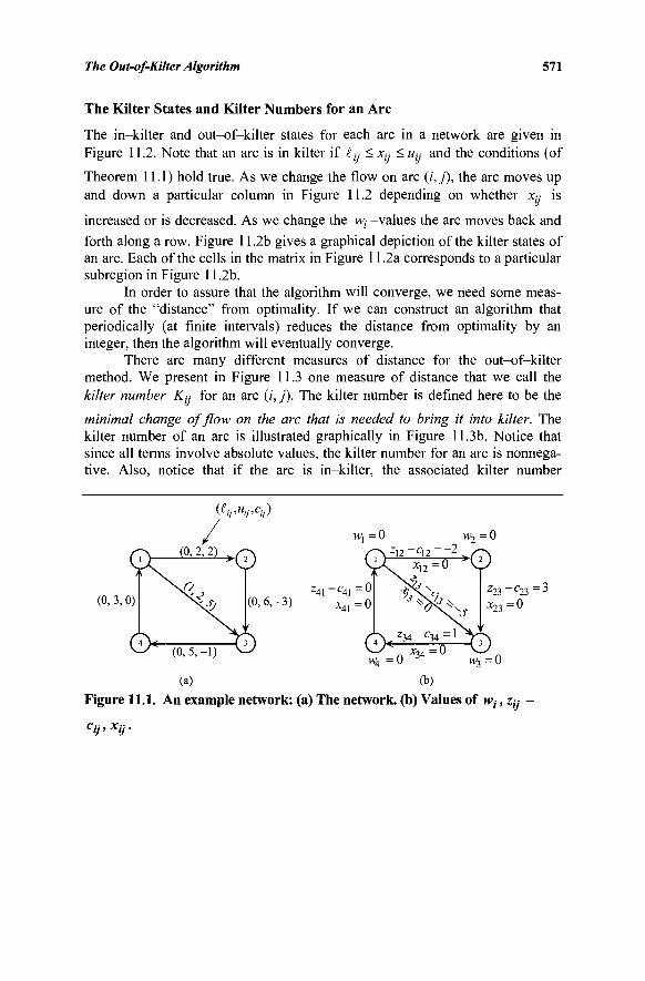
The Out-of-Kilter Algorithm 571
The Kilter States and Kilter Numbers for an Arc
The in-kilter and out-of-kilter states for each arc in a network are given in Figure 11.2. Note that an arc is in kilter if ί^ < χ^ < Uy and the conditions (of
Theorem 11.1) hold true. As we change the flow on arc (i,j), the arc moves up and down a particular column in Figure 11.2 depending on whether x^ is
increased or is decreased. As we change the w, -values the arc moves back and
forth along a row. Figure 11.2b gives a graphical depiction of the kilter states of an arc. Each of the cells in the matrix in Figure 11.2a corresponds to a particular subregion in Figure 11.2b.
In order to assure that the algorithm will converge, we need some meas-ure of the "distance" from optimality. If we can construct an algorithm that periodically (at finite intervals) reduces the distance from optimality by an integer, then the algorithm will eventually converge.
There are many different measures of distance for the out-of-kilter method. We present in Figure 11.3 one measure of distance that we call the kilter number Ky for an arc (i, j). The kilter number is defined here to be the
minimal change of flow on the arc that is needed to bring it into kilter. The kilter number of an arc is illustrated graphically in Figure 11.3b. Notice that since all terms involve absolute values, the kilter number for an arc is nonnega-tive. Also, notice that if the arc is in-kilter, the associated kilter number
(fpUpCy)
(0, 3, 0)
M\ = 0 W2 = 0
^41-c41 - ° (0.6.-3) x4 1=0
z23~c23 - 3
(0,5,-1)
(a) (b)
Figure 11.1. An example network: (a) The network, (b) Values of wt, zy -
(*·· V · ·
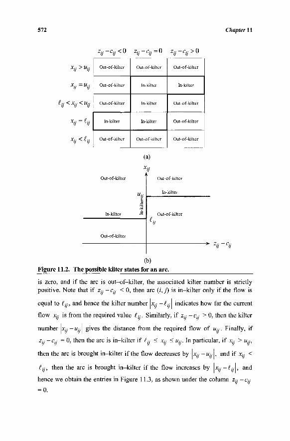
572 Chapter 11
Zy-Cy<0 Zy~Cy=0 Zy - Cy > 0
Xy>Uy
xu=uy
iy<Xy<Uy
X- =?■■
X- <(■■
Out-of-kilter
Out-of-kilter
Out-of-kilter
In-kilter
Out-of-kilter
Out-of-kilter
In-kilter
In-kilter
In-kilter
Out-of-kilter
Out-of-kilter
In-kilter
Out-of-kilter
Out-of-kilter
Out-of-kilter
(a)
xij
Out-of-kilter
In-kilter
Out-of-kilter
Out-of-kilter
In-kilter
Out-of-kilter
—>■ 2·- — C--
(b) Figure 11.2. The possible kilter states for an arc.
is zero, and if the arc is out-of-kilter, the associated kilter number is strictly positive. Note that if Zy - Cy < 0, then arc (/, j) is in-kilter only if the flow is
equal to £y, and hence the kilter number \Xy -ty\ indicates how far the current
flow Xy is from the required value iy. Similarly, if Zy -c« > 0, then the kilter
number \xy - w J gives the distance from the required flow of Uy. Finally, if
Zy -Cy = 0, then the arc is in-kilter if (y < Xy < Uy. In particular, if Xy > Uy,
then the arc is brought in-kilter if the flow decreases by \xy -Uy\, and if Xy <
iy, then the arc is brought in-kilter if the flow increases by * ; y-^J» and
hence we obtain the entries in Figure 11.3, as shown under the column zy -cy
= 0.
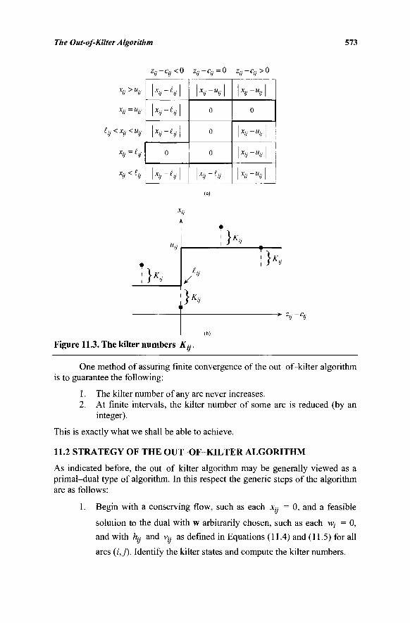
The Out-of-Kilter Algorithm 573
z ! / - c ! / < ° zij-cy=0 zij-cij>0
x- =£■■
1 jr.. _ / . . 1 \ 9 >l\
Γ xij - (-ij
0
1 X- -(■■
XiJ~U'j\
0
0
0
xij -ij
\XiJ~UV
0
xij-«y
xìj~uìj
xij-uìj
(a)
K
}KV
rK„
}Kv
(b)
Figure 11.3. The kilter numbers JT«.
One method of assuring finite convergence of the out-of-kilter algorithm is to guarantee the following:
1. The kilter number of any arc never increases. 2. At finite intervals, the kilter number of some arc is reduced (by an
integer).
This is exactly what we shall be able to achieve.
11.2 STRATEGY OF THE OUT-OF-KILTER ALGORITHM
As indicated before, the out-of-kilter algorithm may be generally viewed as a primal-dual type of algorithm. In this respect the generic steps of the algorithm are as follows:
1. Begin with a conserving flow, such as each jc,y = 0, and a feasible
solution to the dual with w arbitrarily chosen, such as each w, = 0,
and with L· and vy as defined in Equations (11.4) and (11.5) for all
arcs (/',/)· Identify the kilter states and compute the kilter numbers.
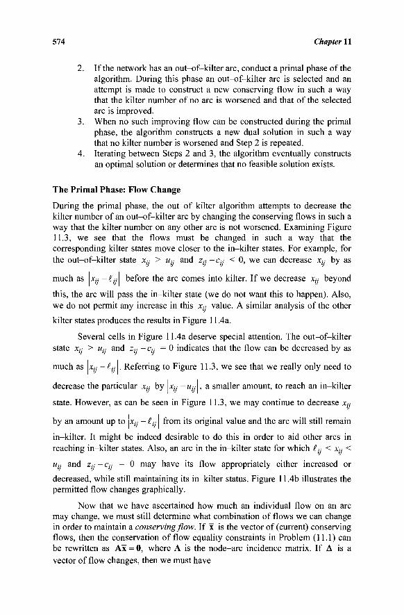
574 Chapter 11
2. If the network has an out-of-kilter arc, conduct a primal phase of the algorithm. During this phase an out-of-kilter arc is selected and an attempt is made to construct a new conserving flow in such a way that the kilter number of no arc is worsened and that of the selected arc is improved.
3. When no such improving flow can be constructed during the primal phase, the algorithm constructs a new dual solution in such a way that no kilter number is worsened and Step 2 is repeated.
4. Iterating between Steps 2 and 3, the algorithm eventually constructs an optimal solution or determines that no feasible solution exists.
The Primal Phase: Flow Change
During the primal phase, the out-of-kilter algorithm attempts to decrease the kilter number of an out-of-kilter arc by changing the conserving flows in such a way that the kilter number on any other arc is not worsened. Examining Figure 11.3, we see that the flows must be changed in such a way that the corresponding kilter states move closer to the in-kilter states. For example, for the out-of-kilter state χ„- > u„- and z« - c„- < 0, we can decrease χ„- by as
much as ixy -(-A before the arc comes into kilter. If we decrease jc,·.· beyond
this, the arc will pass the in-kilter state (we do not want this to happen). Also, we do not permit any increase in this x„- value. A similar analysis of the other
kilter states produces the results in Figure 11.4a.
Several cells in Figure 11.4a deserve special attention. The out-of-kilter state X:,- > «,·,· and z„ - c„ = 0 indicates that the flow can be decreased by as
much as % -i„· . Referring to Figure 11.3, we see that we really only need to
decrease the particular x„- by ixy -« , · / , a smaller amount, to reach an in-kilter
state. However, as can be seen in Figure 11.3, we may continue to decrease χ„-
by an amount up to \χ„- — tA from its original value and the arc will still remain
in-kilter. It might be indeed desirable to do this in order to aid other arcs in reaching in-kilter states. Also, an arc in the in-kilter state for which £y < x„- <
Ujj and Zjj - Cy = 0 may have its flow appropriately either increased or
decreased, while still maintaining its in-kilter status. Figure 11.4b illustrates the permitted flow changes graphically.
Now that we have ascertained how much an individual flow on an arc may change, we must still determine what combination of flows we can change in order to maintain a conserving flow. If x is the vector of (current) conserving flows, then the conservation of flow equality constraints in Problem (11.1) can be rewritten as Ax = 0, where A is the node-arc incidence matrix. If Δ is a vector of flow changes, then we must have
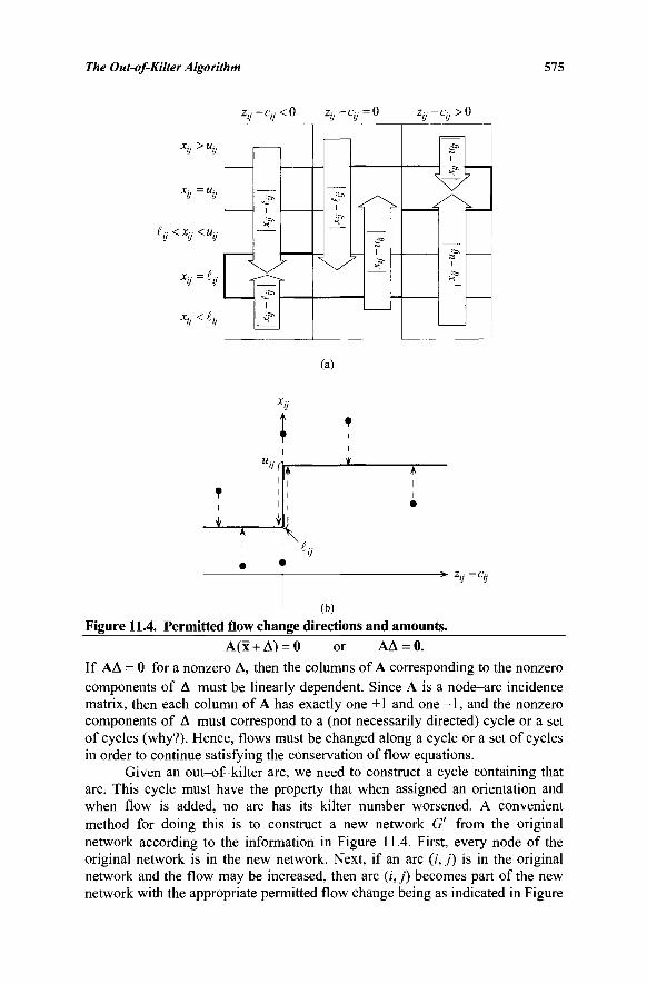
The Out-of-Kilter Algorithm 575
Zy-CyKO Zij-Cij=0
Xy>Uy
X- <(■■
(a)
(b)
Figure 11.4. Permitted flow change directions and amounts. Α(χ + Δ) = 0 or ΑΔ = 0.
If ΑΔ = 0 for a nonzero Δ, then the columns of A corresponding to the nonzero components of Δ must be linearly dependent. Since A is a node-arc incidence matrix, then each column of A has exactly one +1 and one - 1 , and the nonzero components of Δ must correspond to a (not necessarily directed) cycle or a set of cycles (why?). Hence, flows must be changed along a cycle or a set of cycles in order to continue satisfying the conservation of flow equations.
Given an out-of-kilter arc, we need to construct a cycle containing that arc. This cycle must have the property that when assigned an orientation and when flow is added, no arc has its kilter number worsened. A convenient method for doing this is to construct a new network G' from the original network according to the information in Figure 11.4. First, every node of the original network is in the new network. Next, if an arc (i, j) is in the original network and the flow may be increased, then arc (i, j) becomes part of the new network with the appropriate permitted flow change being as indicated in Figure
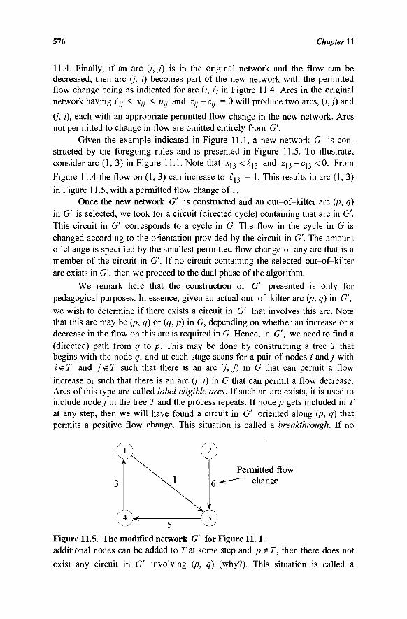
576 Chapter 11
11.4. Finally, if an arc (;', j) is in the original network and the flow can be decreased, then arc (/', i) becomes part of the new network with the permitted flow change being as indicated for arc (i, j) in Figure 11.4. Arcs in the original network having £y < χ(- < Uy and Zj- -cy = 0 will produce two arcs, (i,j) and
(j, i), each with an appropriate permitted flow change in the new network. Arcs not permitted to change in flow are omitted entirely from G'.
Given the example indicated in Figure 11.1, a new network G' is con-structed by the foregoing rules and is presented in Figure 11.5. To illustrate, consider arc (1, 3) in Figure 11.1. Note that x13 < i1 3 and z(3 - c 1 3 < 0. From
Figure 11.4 the flow on (1, 3) can increase to ^13 = 1. This results in arc (1, 3)
in Figure 11.5, with a permitted flow change of 1. Once the new network G' is constructed and an out-of-kilter arc (p, q)
in G' is selected, we look for a circuit (directed cycle) containing that arc in G'. This circuit in G' corresponds to a cycle in G. The flow in the cycle in G is changed according to the orientation provided by the circuit in G'. The amount of change is specified by the smallest permitted flow change of any arc that is a member of the circuit in G'. If no circuit containing the selected out-of-kilter arc exists in G', then we proceed to the dual phase of the algorithm.
We remark here that the construction of G' presented is only for pedagogical purposes. In essence, given an actual out-of-kilter arc (p, q) in G', we wish to determine if there exists a circuit in G' that involves this arc. Note that this arc may be (p, q) or (q, p) in G, depending on whether an increase or a decrease in the flow on this arc is required in G. Hence, in G', we need to find a (directed) path from q to p. This may be done by constructing a tree T that begins with the node q, and at each stage scans for a pair of nodes i andy with i e T and j £ T such that there is an arc (z, j) in G that can permit a flow
increase or such that there is an arc (j, i) in G that can permit a flow decrease. Arcs of this type are called label eligible arcs. If such an arc exists, it is used to include nodey in the tree Tand the process repeats. If node/» gets included in T at any step, then we will have found a circuit in G' oriented along (p, q) that permits a positive flow change. This situation is called a breakthrough. If no
(T) 0 Permitted flow
6 -*r—"" change
<i> j {ì) Figure 11.5. The modified network G' for Figure 11.1. additional nodes can be added to Tat some step and piT, then there does not
exist any circuit in G' involving (p, q) (why?). This situation is called a
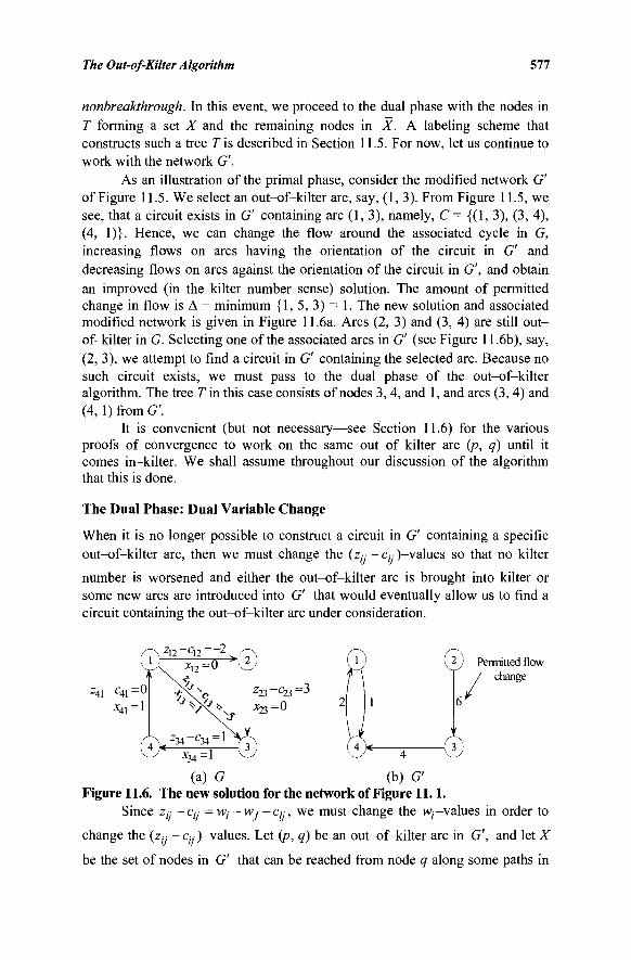
The Out-of-Kilter Algorithm 577
nonbreakthrough. In this event, we proceed to the dual phase with the nodes in T forming a set X and the remaining nodes in X. A labeling scheme that constructs such a tree T is described in Section 11.5. For now, let us continue to work with the network G'.
As an illustration of the primal phase, consider the modified network G' of Figure 11.5. We select an out-of-kilter arc, say, (1, 3). From Figure 11.5, we see, that a circuit exists in G' containing arc (1, 3), namely, C = {(1, 3), (3, 4), (4, 1)}. Hence, we can change the flow around the associated cycle in G, increasing flows on arcs having the orientation of the circuit in G' and decreasing flows on arcs against the orientation of the circuit in G', and obtain an improved (in the kilter number sense) solution. The amount of permitted change in flow is Δ = minimum {1, 5, 3) = 1. The new solution and associated modified network is given in Figure 11.6a. Arcs (2, 3) and (3, 4) are still out-of-kilter in G. Selecting one of the associated arcs in G' (see Figure 11.6b), say, (2, 3), we attempt to find a circuit in G' containing the selected arc. Because no such circuit exists, we must pass to the dual phase of the out-of-kilter algorithm. The tree Tin this case consists of nodes 3,4, and 1, and arcs (3, 4) and (4, l)fromG'.
It is convenient (but not necessary—see Section 11.6) for the various proofs of convergence to work on the same out-of-kilter arc (p, q) until it comes in-kilter. We shall assume throughout our discussion of the algorithm that this is done.
The Dual Phase: Dual Variable Change
When it is no longer possible to construct a circuit in G' containing a specific out-of-kilter arc, then we must change the (z^ -c,y)-values so that no kilter
number is worsened and either the out-of-kilter arc is brought into kilter or some new arcs are introduced into G' that would eventually allow us to find a circuit containing the out-of-kilter arc under consideration.
. /
Permitted flow change
x34-l
(a) G (b) G Figure 11.6. The new solution for the network of Figure 11.1.
Since Zjj -q.· = Wj -w.- —Cy, we must change the w;—values in order to
change the (z,·.· -c-)-values. Let (p, q) be an out-of-kilter arc in G', and let X
be the set of nodes in G' that can be reached from node q along some paths in
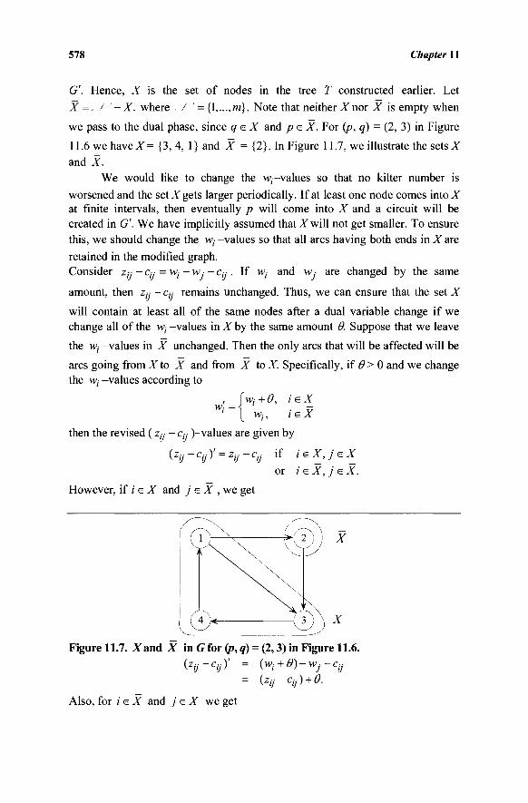
578 Chapter 11
G'. Hence, X is the set of nodes in the tree T constructed earlier. Let
X = , / -X. where / ' = {\,...,m). Note that neitherXnor X is empty when
we pass to the dual phase, since q e X and peX. For (p, q) = (2, 3) in Figure
11.6 we haveX = {3, 4, 1} and X = {2}. In Figure 11.7, we illustrate the setsX
and X. We would like to change the w,—values so that no kilter number is
worsened and the set X gets larger periodically. If at least one node comes intoX at finite intervals, then eventually p will come into X and a circuit will be created in G'. We have implicitly assumed that X will not get smaller. To ensure this, we should change the W; -values so that all arcs having both ends in X are retained in the modified graph. Consider zy- - cy· = w; - Wj - ctj . If w,· and wj are changed by the same
amount, then zy - cy remains unchanged. Thus, we can ensure that the set X
will contain at least all of the same nodes after a dual variable change if we change all of the w; -values in X by the same amount Θ. Suppose that we leave
the Wj -values in X unchanged. Then the only arcs that will be affected will be
arcs going fromXto X and from X toX. Specifically, if θ> 0 and we change the Wj -values according to
, _\wi+6, ÌGX W ' - { wh ieX
then the revised ( zy - c« )-values are given by
(zij ~ cij )' = zij ~ cij i f ' e xj J e x_ or i e X, j e X.
However, if / e X and j e X , we get
Figure 11.7. Xand X in G for (p, q) = (2,3) in Figure 11.6.
(zij ~ cij )' = (wi +θ)~ wj ~ cij = (Zij-Cij)+ Θ.
Also, for i e X and j e X we get
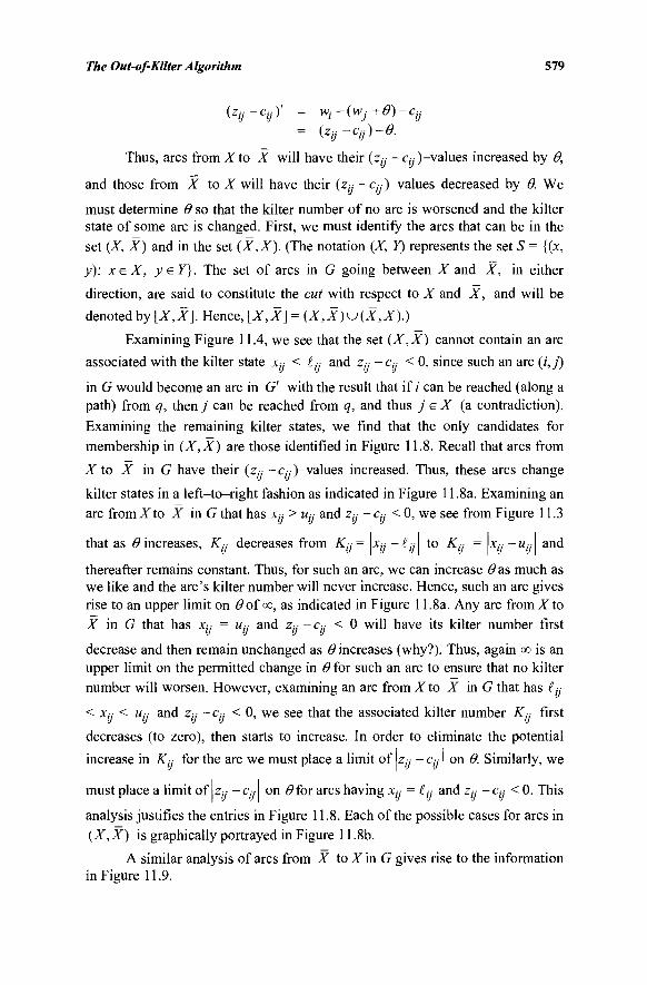
The Out-of-Kilter Algorithm 579
(zij~cij)' = wi-(\Vj+e)-ciJ
= ^ij-Cij)-e.
Thus, arcs from X to X will have their (zy- -cy)-values increased by Θ,
and those from X to X will have their (z„- - c„· )-values decreased by Θ. We
must determine Θ so that the kilter number of no arc is worsened and the kilter state of some arc is changed. First, we must identify the arcs that can be in the set (X, X) and in the set (X,X). (The notation (X, Y) represents the set S = {(x,
y): l e i , y^Y}· The set of arcs in G going between X and X, in either
direction, are said to constitute the cut with respect to X and X, and will be
denoted by [X,X]. Hence, [X,X] = (X,X)u(X,X).)
Examining Figure 11.4, we see that the set (X, X) cannot contain an arc
associated with the kilter state Xy < iy and Zy -cy < 0, since such an arc (/',/)
in G would become an arc in G' with the result that if i can be reached (along a path) from q, then j can be reached from q, and thus j e X (a contradiction). Examining the remaining kilter states, we find that the only candidates for membership in (X,X) are those identified in Figure 11.8. Recall that arcs from X to X in G have their (z„--c„)-values increased. Thus, these arcs change
kilter states in a left-to-right fashion as indicated in Figure 11.8a. Examining an arc from X to X in G that has Xy > Uy and z„- -c„ < 0, we see from Figure 11.3
that as # increases, Ky decreases from Ky= \xy -tyl to Ky = \xy -w„- and
thereafter remains constant. Thus, for such an arc, we can increase Θ as much as we like and the arc's kilter number will never increase. Hence, such an arc gives rise to an upper limit on #of cc, as indicated in Figure 11.8a. Any arc from X to X in G that has Xy = Uy and zy - Cy < 0 will have its kilter number first
decrease and then remain unchanged as Θ increases (why?). Thus, again co is an upper limit on the permitted change in Θ for such an arc to ensure that no kilter number will worsen. However, examining an arc from X to X in G that has iy
< Xy < Uy and z„ - c„- < 0, we see that the associated kilter number Ky first
decreases (to zero), then starts to increase. In order to eliminate the potential
increase in Ky for the arc we must place a limit of \zy -Cy\ on Θ. Similarly, we
must place a limit of z„· -c„· on #for arcs having Xy = iy and z„- -c„- < 0. This
analysis justifies the entries in Figure 11.8. Each of the possible cases for arcs in (X, X) is graphically portrayed in Figure 11.8b.
A similar analysis of arcs from X to X in G gives rise to the information in Figure 11.9.
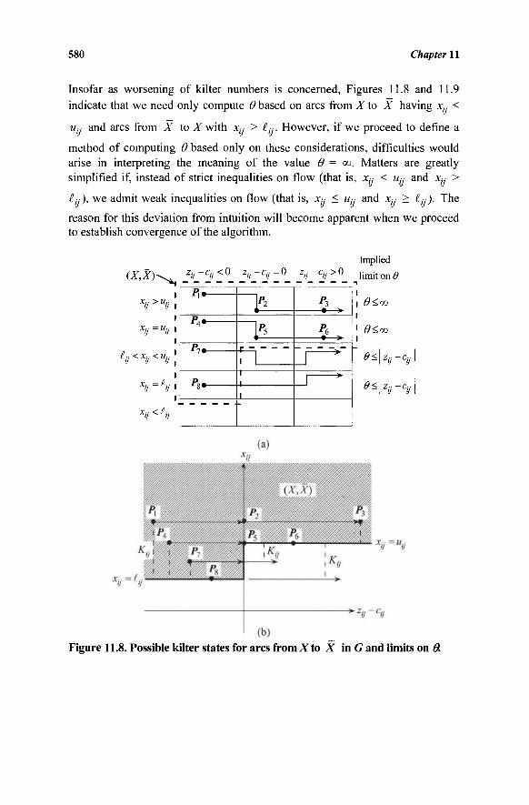
580 Chapter 11
Insofar as worsening of kilter numbers is concerned, Figures 11.8 and 11.9 indicate that we need only compute Θ based on arcs from X to X having x; <
Ujj and arcs from X to X with Xy > £y. However, if we proceed to define a
method of computing Θ based only on these considerations, difficulties would arise in interpreting the meaning of the value Θ = co. Matters are greatly simplified if, instead of strict inequalities on flow (that is, Xy < Uy and Xy >
£y), we admit weak inequalities on flow (that is, Xy < Uy and Xy > (y). The
reason for this deviation from intuition will become apparent when we proceed to establish convergence of the algorithm.
(X,X)^
Xy>Uy ,
xij=uij I
ii<x<i<ua\
X- -(.■■ i Λ*7 ιν 1
x- <(■■
zv-C{j<Q zij- - c , = 0 Zii~Cy>0
P:· rl*
p m rA*
P , . rT
P „ .
Pi
Ps
1
1
PJ .
p6
1 * J y
-
Γ
Implied limit on Θ
6><oo
<9<oo
θψν-ΰ·ί\
e*\*i-cy
Figure 11.8. Possible kilter states for arcs from AT to X in G and limits on Θ.
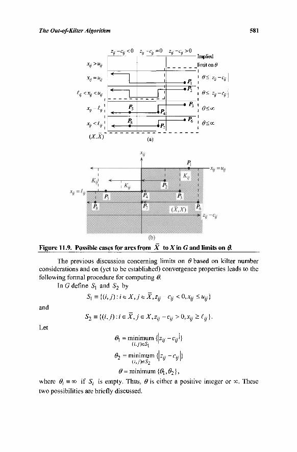
The Out-of-Kilter Algorithm 581
xij>uij
xij=uij
ij < xij < uij f
x - =!■■ ' V V 1
x <(■■ i
h -Cij< 0
Ps
%
zff-cii = 0
,P " 4
.*
Zy-Cy>0
• P t / * W X Z
• P ■ ri
t P ■ * t >
limit on Θ
\ *Φ*-<ν I H2*"^
] #<oo
1 <9<oo
(Χ,Χ) (a)
Figure 11.9. Possible cases for arcs from X to Xin G and limits on Θ.
The previous discussion concerning limits on Θ based on kilter number considerations and on (yet to be established) convergence properties leads to the following formal procedure for computing Θ.
In G define S\ and S2 by
S\ = {(*', j) :ieXJs X, z^ - ctj < 0,xtj < utj}
and
Let
S2={(i,j):ieX,jeX,zij- ctj >0,χϋ>ί y}.
9\ = minimum {\zu - c,-,·} (Uj)eSl
l J Ji
θ2 = minimum {z„ - c - } (z,/)eS2 ' 7 |
# = minimum {θ\,θ2},
where #,· = co if S, is empty. Thus, # is either a positive integer or oo. These
two possibilities are briefly discussed.
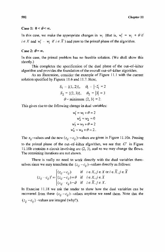
582 Chapter 11
Case l : O<0<oo.
In this case, we make the appropriate changes in w,· (that is, w\ = w,· + Θ if
i e X and w\ = vv; if / ε X ) and pass to the primal phase of the algorithm.
Case 2: θ=<χ>.
In this case, the primal problem has no feasible solution. (We shall show this shortly.)
This completes the specification of the dual phase of the out-of-kilter algorithm and provides the foundation of the overall out-of-kilter algorithm.
As an illustration, consider the example of Figure 11.1 with the current solution specified by Figures 11.6 and 11.7. Here,
S, ={(1,2)}, θχ=\-2\=2
S2={(2,3)}, 0 2 = | 3 | = 3
θ= minimum {2, 3} = 2.
This gives rise to the following change in dual variables:
w{ = Wj + Θ = 2 w2 = w2 = 0
W3 = W3 + Θ = 2
w\ = w4 + Θ = 2.
The Xj— values and the new (z^ -c,-.-)-values are given in Figure 11.10a. Passing
to the primal phase of the out-of-kilter algorithm, we see that G' in Figure 11.10b contains a circuit involving arc (2, 3), and so we may change the flows. The remaining iterations are not shown.
There is really no need to work directly with the dual variables them-selves since we may transform the (z,·.- - c;y )-values directly as follows:
(Zj-Cj) if is X,j sXorie X,j ε X
izij-cij)' = \{zij-cij) + e i f ieX,jeX (zy -Cy)-e if isX,jeX.
In Exercise 11.18 we ask the reader to show how the dual variables can be recovered from these (z^ - c„- ) -values anytime we need them. Note that the
(z„ - Cjj ) -values are integral (why?).
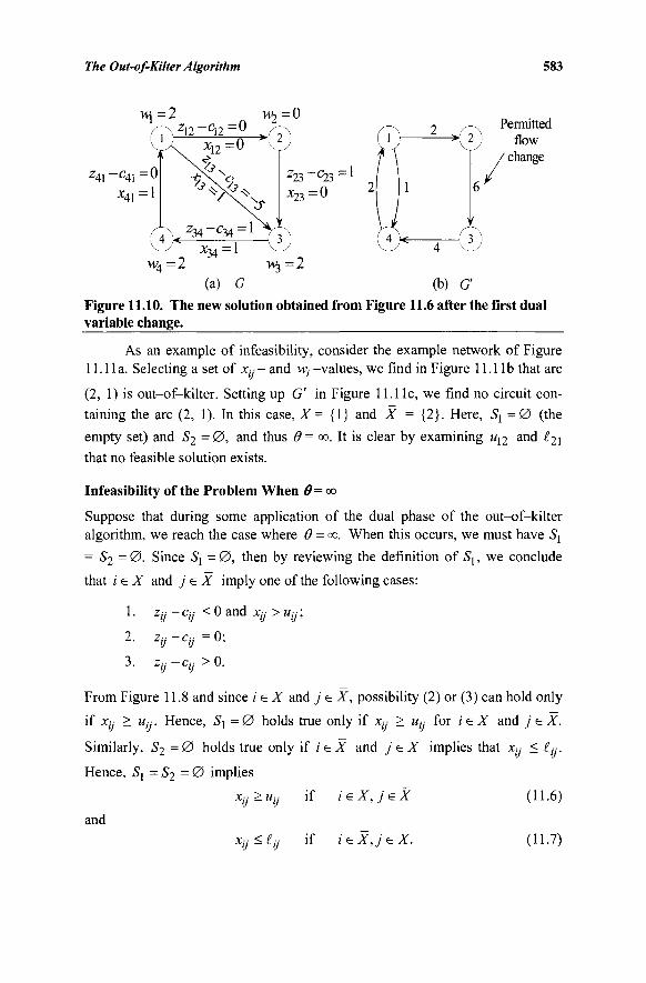
The Out-of-Kilter Algorithm 583
M\ = 2 w,=0
Z41~c41 - 0 x41:
Permitted flow
change
(a) G (b) G
Figure 11.10. The new solution obtained from Figure 11.6 after the first dual variable change.
As an example of infeasibility, consider the example network of Figure 11.11a. Selecting a set of xy- and wi -values, we find in Figure 11.1 lb that arc
(2, 1) is out-of-kilter. Setting up G' in Figure 11.11c, we find no circuit con-
taining the arc (2, 1). In this case, X= {1} and X = {2}. Here, Sx=0 (the
empty set) and S2 = 0, and thus θ= <x>. It is clear by examining w12 and i2i
that no feasible solution exists.
Infeasibility of the Problem When θ= οο
Suppose that during some application of the dual phase of the out-of-kilter algorithm, we reach the case where Θ = co. When this occurs, we must have S\
= S2 = 0 . Since Si = 0 , then by reviewing the definition of S\, we conclude
that i e X and j e X imply one of the following cases:
1. ZJ: - Cy < 0 and % > u^ ;
zy-cy =0;
zij-cv > 0 ·
From Figure 11.8 and since / e X and j ε X, possibility (2) or (3) can hold only
if Xj- > Uy. Hence, S^ = 0 holds true only if x,y > Uy for / e X and j e X.
Similarly, S2 - 0 holds true only if / e X and j e X implies that x^ < (.y.
Hence, Sl = S2 = 0 implies
ieXJeX (11.6)
and x - <(■■
Xy -Uy
if
if ieXJsX. (11.7)
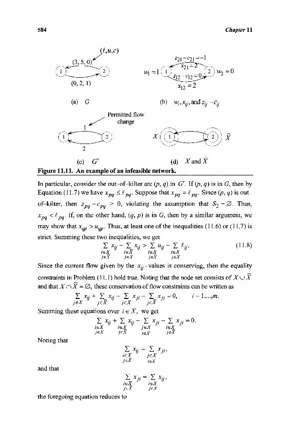
584 Chapter 11
(£,u,c)
VM
(a) G
1
Permitted flow change
ccz^
(b) wi,xij,SDàzij-ci v ' — v v
(c) G' (d) J i andX Figure 11.11. An example of an infeasible network.
In particular, consider the out-of-kilter arc (p, q) in G'. lf(p, q) is in G, then by Equation (11.7) we have x
of-kilter, then z PI ■ pq
. Suppose that x PI -pq
. Since (p, q) is out-
pq - cpq > 0, violating the assumption that 52 = 0 . Thus,
xpq ^lpq If, on the other hand, (q, p) is in G, then by a similar argument, we
may show that x„ > uqp. Thus, at least one of the inequalities (11.6) or (11.7) is
strict. Summing these two inequalities, we get
ieZ ieX ieX jeX jeX jeX
Since the current flow given by the x„· -values is conserving, then the equality
constraints in Problem ( 11.1 ) hold true. Noting that the node set consists of X u X and that X n X = 0 , these conservation of flow constraints can be written as
i= \,...,m.
Σ xu ieX jzX
2- xy "*" 2._ ·*« 2. x/i 2._ *// — u, yejr ;ex ye* y6x
Summing these equations over i e X, we get
Σ xs
Noting that
and that
2. Χη ' L xij 2 . % ji ieX ieX jeX ieX jaX j&X jex jeX
2_, Xy 2_ Xjj, ieX jeX
= 0.
Lu X ji 2J xii > i<=X jeX
ieX jeX
the foregoing equation reduces to
The Out-of-Kilter Algorithm 585
Σ * 0 - Σ * « = Ο . (11.9) ieX ieX
jeX JEX
Substituting in Equation (11.8), we get 0 > Σ « , ν - Σ Λ - (11-10)
ieX ÌGX j&X jeX
Suppose by contradiction that there is a feasible flow represented by L· for i,j
= \,...,m. Therefore, uy > Xy and -£y > -L·, and so, Equation (11.10) gives o> Σ « ι ? - Σ ^ · > Σ % - Σ % - (ii . l i)
;eX ieX / e * ieX JeX JeX jzX j^X
But since the L· -values represent a feasible flow, they must be conserving. In a
fashion similar to Equation (11.9), it is clear that the right-hand-side of the inequality in ( 11.11 ) is equal to zero. Therefore, Equation (11.11) implies that 0 > 0, which is impossible. This contradiction shows that if Θ = co, there could be no feasible flow.
Note that if we had defined S{ and S2 by strict inequalities on Xy (namely,
Xy < Uy and Xy > ly, respectively), we could not have produced the strict
inequality needed in Equation (11.8).
Convergence of the Out-of-Kilter Algorithm
For the purpose of the following finite convergence argument we make the assumption that the vectors £, u, and c are integer-valued.
In developing a finite convergence argument for the out-of-kilter algorithm, there are several properties of the algorithm that should be noted. First, every time a circuit is constructed in G' containing an out-of-kilter arc, the kilter number of that arc and of the total network is reduced by an integer (why?). We can construct only a finite number of circuits containing out-of-kilter arcs before an optimal solution is obtained (why?). Second, after each dual variable change, the kilter state of each arc in G that has both ends in X remains unchanged. Hence, if (p, q) is not in kilter, then after a dual variable change, each node in X before the change is in X after the change. Two possibilities exist. One possibility is that a new node k may be brought into X by virtue of an arc being added in G' from some node in Xto node k. Each time this occurs the set X grows by at least one node. This can occur at most a finite number of times before node/? becomes a member of Xand a circuit is created containing (p, q). Thus, if the algorithm is not finite, it must be the case that an infinite number of dual variable changes take place without the set X increasing or Θ equalling co. We shall show that this cannot occur.
Suppose that after a dual variable change, no new node becomes a member of X; that is, Xdoes not increase. Then, upon passing to the next dual phase, we have the same sets X and X and the same xit -values. In addition, each arc
586 Chapter 11
from X to X has had its Zy - Cy increased and each arc from X to X has had
its z,y - cy decreased. Thus, after the dual variable change, the new sets S{ and
S2 satisfy
S{ c S} and S2 c S2
(why?). Furthermore, by the choice of the (finite) value of Θ, at least one arc has been dropped from either Sj or S2. Thus, at least one of the foregoing inclusions
is proper. Now, Sl and S2 may decrease at most a finite number of times before
SiuS2 = 0 and Θ = 00 occurs, in which case the algorithm stops.
This completes a finiteness argument for the out-of-kilter algorithm. We now summarize the algorithm and present an example.
11.3 SUMMARY OF THE OUT-OF-KILTER ALGORITHM
The complete algorithm consists of three phases: the initialization phase, the primal phase, and the dual phase.
Initialization Phase
Begin with a conserving (integer) flow, say, each Xy = 0, and an initial set of
(integral) dual variables, say, each w;· = 0. Compute ζ(- -Cy = w,· - w- -Cy.
Primal Phase
Determine the kilter state and the kilter number for each arc. If all arcs are in kilter, stop; an optimal solution has been obtained. Otherwise, select or continue with a previously selected out-of-kilter arc. From the network G construct a new network G' according to Figure 11.4. For each arc (z, j) in G that is in a kilter state that permits a flow increase, place an arc (i,j) in G' with a permitted flow increase, as indicated in Figure 11.4. For any arc (i,j) in G that is in a kilter state that permits a flow decrease, place an arc (/', /') in G' with the permitted flow as indicated in Figure 11.4. For those arcs in G that are members of states that permit no flow change, place no arc in G'. In G\ attempt to construct a circuit containing the selected out-of-kilter arc (p, q). If such a circuit is available, we have a breakthrough. Determine a flow change Δ equal to the minimum of the permitted flow changes on arcs of the circuit. Change the flow on each arc of the associated cycle in G by the amount Δ using the orientation specified by the circuit as the direction of increase. In particular, let x'y = Xy +
A if (i, j) was a member of the circuit in G'; let x'y = Xy - A if (j, i) was a
member of the circuit in G'; let x'y = Xy otherwise. Repeat the primal phase. If
no circuit containing arc (p, q) is available in G', we have a nonbreakthrough, and we pass to the dual phase. (Note that the construction of the tree T described in Section 11.2 can be used to detect breakthroughs or a nonbreakthrough, in lieu of actually constructing the graph G'.)
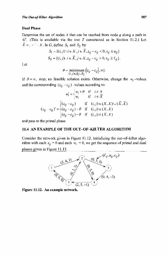
The Out-of-Kilter Algorithm 587
Dual Phase
Determine the set of nodes X that can be reached from node q along a path in G'. (This is available via the tree T constructed as in Section 11.2.) Let X =._ / -X. In G, define Sx and S2 by
5, = {(/, j) :ieX,je X, zy - Cy < 0, Xy < Uy}
S2 = {(}, j) :ieX,je X, zy ~ Cy > 0,Xy >£y}.
Let
Θ = minimum {z· - c,·,· , °o}. (i,j)^SluS2 ' J 7 |
If θ = κ>, stop; no feasible solution exists. Otherwise, change the w, -values
and the corresponding (z« - <:,%■ ) -values according to:
w,· +6* if ieX
(zii-cii)' =
if / e l
(^■-c^·) if (i,j)e(X,X)v(X,X)
(zy-Cy) + 9 if (/ ,7)e(X,X) (zy-Cy)-O if 0,7) e ( * , * )
and pass to the primal phase.
11.4 AN EXAMPLE OF THE OUT-OF-KILTER ALGORITHM
Consider the network given in Figure 11.12. Initializing the out-of-kilter algo-rithm with each xy = 0 and each
phases given in Figure 11.13.
: 0, we get the sequence of primal and dual
^(^ij'Uij'Cij)
(0, 4, -3)
(2,5,-1) Figure 11.12. An example network.
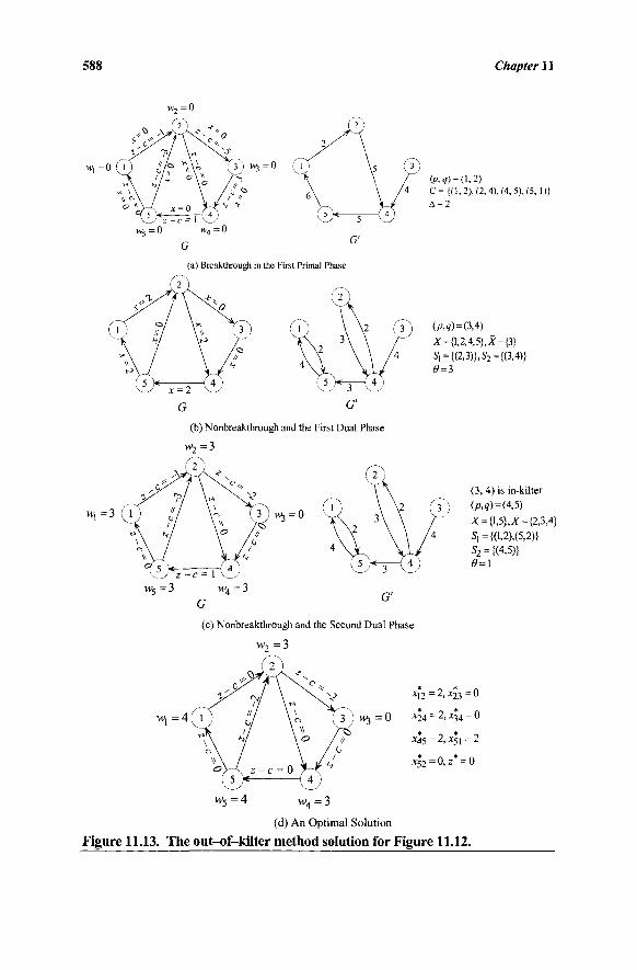
588 Chapter 11
w7 - 0
»i =0 (7
(b) Nonbreakthrough and the First Dual Phase
H>2 =3
3 j ^ 5 = 0
(c) Nonbreakthrough and the Second Dual Phase
w = 4 ( l )
(p,?) = (l,2) C= {(1,2), (2, 4), (4, 5), (5,1)) Δ = 2
(A?)=(3,4) _ X = {l,2,4,5},A- = {3} S,={(2,3)},S2 = {(3,4)} 0 = 3
(3, 4) is in-kilter (/>,<j-)=(4,5)
Χ = {1,5},Α' = {2,3,4} Sj = {(l,2),(5,2)} S2 = {(4,5)} 0 = 1
* O * Λ %? xi2-AJC23=U
3^)^3=0 24 = 2^34=0
X45 — z, X5 ] — Z
X52=0,z* = 0
4 '
w 4 = 3
(d) An Optimal Solution
Figure 11.13. The out-of-kilter method solution for Figure 11.12.
The Out-of-Kilter Algorithm 589
11.5 A LABELING PROCEDURE FOR THE OUT-OF-KILTER ALGORITHM
Either for hand or computer calculations there are simple and convenient ways to maintain the information required to solve a minimal-cost flow problem by the out-of-kilter algorithm. Suppose that we associate with each node j a label L(j) = (+/, Aj ). A label (/, Aj ) indicates that the flow on arc (z, j) could be
increased by an amount Δ ,· without worsening the kilter number of any arc. A
label (-;', Δ ) indicates that the flow on arc (j, /) could be decreased by an
amount Δ without worsening the kilter number of any arc. Note that Δ repre-
sents the current estimate of the amount of flow change that can take place along
some cycle containing an out-of-kilter arc and either arc (/', j) or (j, i) in such a
way that the kilter number of no arc is increased. The labeling algorithm
becomes as follows.
INITIALIZATION STEP
Select a conserving flow, for example, each xy = 0, and a set of dual variables,
such as each w,- =0.
Main Step
1. If all arcs are in kilter according to Figure 11.2, stop; an optimal solution is obtained. Otherwise, select (or continue with a previously selected) out-of-kilter arc, say (s, t). Erase all labels. If (s, t) is in one of the states where a flow increase, Δ^, is required according to Figure 11.4, then set q = t,p = s,
and L(q) = (+p,Ast). Otherwise, if (s, i) is in one of the states where a flow
decrease, Δ^ , is required according to Figure 11.4, then set q = s, p = t,
and L(q)= (-p,As,)-2. If node / has a label, nodey has no label, and flow may be increased by an
amount Δ,·.· along arc (/,_/) according to Figure 11.4, then assign nodey' the
label L(j) = (+ /, Δ ) where Δ ■ = minimum {Δ,, Δ,γ}. If node i has a label,
node/ has no label, and flow may be decreased by an amount Δ ,-,· along arc
(J, i) according to Figure 11.4, then give nodey the label L(J) = (-ϊ,Δ,·)
where Δ = minimum (Δ;·,Δ 7) . Repeat Step 2 until either node/? is labeled
or until no more nodes can be labeled. If node/? is labeled, go to Step 3 (a breakthrough has occurred); otherwise, go to Step 4 (a nonbreakthrough has occurred and the labeled nodes are in the tree 7).
590 Chapter 11
3. Let Δ = Δ„. Change flow along the identified cycle as follows. Begin at
node/?. If the first entry in L(p) is +k, then add Δ to x^. Otherwise, if the
first entry in L(p) is -k, then subtract Δ from xplc. Backtrack to node k and
repeat the process until node p is reached again in the backtracking process. Go to Step 1.
4. Let X be the set of labeled nodes and let X = = / -X. Define Sj = {(i,j):
iel,jeX, zy -cy < 0, Xy <uy) and S2 = {(/,/): ieX, jeX, zy -ci}
> 0, xy ^iy}. Let Θ = minimum Uzy - Cy , co: (z, j) e S\ u S2} ■ If Θ = co,
stop; no feasible solution exists. Otherwise, let [WÌ+Θ if ieX
(zg-Ci,)'--
Wi \Wi if ieX
and
\zy-cy) if (i,j)e(X,X)u(X,X) (zy-cy) + e if (i,j)e(X,X) (zy-cy)-e if (i,j)e(X,X)
and return to Step 1.
An Example of the Labeling Algorithm
We shall illustrate the labeling method for the out-of-kilter algorithm by performing the first two iterations represented in Figure 11.13a and b. From Figure 11.13a we find that arc (1, 2) is an out-of-kilter arc whose flow must be increased.
The sequence of operations of the labeling algorithm are as follows:
1. (s,/) = (1, 2), 4 = 2,/? =1,1(2) = (+1,2). 2. L(4) = (+2,2). 3. Z(5) = (+4,2). 4. Z(l) = (+5,2). 5. Breakthrough: Δ = 2.
6. Li(l) =+5 => x'5l =x5l +Δ = 2.
7. Li(5) = +4=>x^5 = χ 4 5 + Δ = 2.
8. I , (4) = +2 => χ'24 = χ24 + Δ = 2.
9. Z1(2) = +l=>x{2 =x\2+A = 2-10. Erase all labels, (s, t) = (3,4),q = 4,p = 3, L{4) = (+ 3, 4). 11. 1(5) = (+4, 3). 12.1(1) = (+5, 3). 13.L(2) = (-4,2). 14. Nonbreakthrough: X= {1, 2,4, 5}, X = {3}, θ= 3. 15. Wy = W2 = W4 = W5 = 3, H>3 = 0.
The Out-of-Kilter Algorithm 591
Since arc (3, 4) is now in-kilter, we select another out-of-kilter arc, erase all labels, and continue.
11.6 INSIGHT INTO CHANGES IN PRIMAL AND DUAL FUNCTION VALUES
It is instructive to see how the primal (penalty) and dual objective function values change in the primal and dual phases of the out-of-kilter algorithm. Not only does this provide an alternative convergence argument in which we need not necessarily work on the same out-of-kilter arc until it comes in kilter, but it also provides an insight into other acceptable ways of modifying primal and dual solutions.
First, consider the primal phase. Define for each arc (/, J) in G a function jR.· (Xjj) that measures the infeasibility of a conserving flow x as follows:
Pjj (xij ) = maximum {0, iy - x-.·} + maximum {0, Xy - if,·}.
Note that Py(xy) = 0 if and only if ly < x;: < Uy, and is positive otherwise.
Construct a primal penalty functionfix) defined for any conserving flow x as follows:
/ (x) = a + M Z f t ( * ) (H.12a) (U)
where M i s sufficiently large (for example, M>2 Σ c^-piax {«iy- iy, \uy , (ij)
k,y }, assuming that -°° < ly < uy < °° and that the algorithm is initialized with Xlj = 0 for all (/,/). Observe that the function fix) composes the original objec-tive function with a penalty term and is similar to the big-M objective function. For x restricted to be flow-conserving, we have Ax = 0 and so, wAx = 0. Subtracting wAx = 0 from the expression in Equation (11.12a) and noting that (c - wA) has components (cy -Zy), we can equivalently rewrite this function as
/(x) = Σ icy -zy^j + ΜΣ Ifj(xij) (11.12b)
for any conserving flow x. Whenever we have a breakthrough in the primal phase, we modify the flow in a cycle in G such that no kilter number worsens, and the kilter number of at least one arc strictly reduces. In particular, no Pu^xy)
term increases (why?). If any such term decreases (by an integer), then since M is large enough, so does the value of./(■). On the other hand, if no Py(xy) term
decreases in the cycle, then we must have £y < xy < uy for all arcs (/,/) in this
cycle (why?). Thus, the penalty term in Equation (11.12) remains constant during the flow change. However, from Figure 11.4 and the foregoing fact, if any arc (i,j) in the cycle satisfies Zy -Cy < 0, then we must have ly < XJ: < uy
and Xy must be decreasing in the breakthrough. Similarly, if zy — c« > 0 for any
592 Chapter 11
arc (/,/) in the cycle, then we must have iy < xy < Uy and X;: must be increasing
in the breakthrough. In either event, the first term in Equation (11.12b) strictly falls. Because we cannot have Zy ~ Cy = 0 for all arcs (/, j) in the cycle in this
case (why?), we again obtain a strict decrease in_/(■). Therefore,_/()falls by an integer at every primal breakthrough.
Next, consider the dual phase. Note from Equations (11.4) and (11.5) that hjj - v« - ( z» - c« ) = 0 for all (/, j). Using the current primal flow x, we can
equivalently rewrite the dual objective function as follows:
Σ Xy(cy-Zy) + Σ {tij-Xij>ij+ Σ (Xij-Uij)hj- (11-13) (hj) ('■>./) i'J)
During the dual phase, assuming that θ< °°, we note that Zjj ~Cy increases by Θ
for all (i,j) e (Χ,Χ), and decreases by θΐοτ all (i,j)e (X,X). Hence, from
Equation (11.9), the first term in Equation (11.13) remains constant (why?).
Next, consider an arc (i , /)e {X,X). Referring to Equations (11.4) and (11.5)
and Figure 11.8, suppose that cjy = zy - c« < 0. Since cy increases by Θ, we have
that vy decreases by Θ and h» remains zero in case iy < Xy < uy, and v,y
decreases by min {Θ, \cy\} and h» increases by max {0, Θ-icy } in case x^ >
uy. Therefore, the corresponding term (ly - Xjj)vy + (xy - ui\)^hj in Equation
(11.13) remains unchanged if and only if Xjj = iy, that is, arc (i,j) is in-kilter,
and increases by a positive integer otherwise. Furthermore, if zy - Cy > 0, then
hy increases by Θ, Vy remains zero, and we have Xy > Uy. Consequently, the
corresponding term in Equation (11.13) remains unchanged if and only if Xjj =
Uy, that is, arc (/, j) is in-kilter, and increases by a positive integer otherwise.
Similarly, consider (i,y)e (X,X). lfcy=Zy - c« > 0, then hy falls by ^and Vy
remains zero in case £y < Xf: < uy, and Z ·.· falls by min {Θ, cy) and vy increases
by max {0, Θ-Cy} in case Xjj < iy. On the other hand, if zy -Cy < 0, then vy
increases by Θ and /%,· remains zero, while we have Λ · < iy. Again, the
corresponding term in Equation (11.13) remains unchanged if and only if (/,/) is in kilter, and increases by a positive integer otherwise. Because the out-of-kilter arc (p, q) is either in (X, X) or (X, X) in G, we obtain a strict increase (by an integer) in the dual objective value during any iteration of the dual phase.
Because the primal penalty function _/(·) in Equation (11.12) falls by an integer in a primal breakthrough, and the dual objective function (11.13) increases by an integer in every dual phase iteration, the difference given by the primal minus the dual function values (call it the duality gap) falls by an integer every iteration. Hence, if 5j = 0 and S2-0 is not realized, the duality gap
The Out-of-Kilter Algorithm 593
must become nonpositive finitely. In this event, if PAxy) = 0 for all (/,/), that
is, we have feasibility, then the current solution (x, w) is primal-dual optimal. On the other hand, if some PAxy) is positive, then since it is an integer, we
have from Equation (11.12a) that the dual value is > ex + M >
Σ(/ ,·)icy max {My , \tjj\}· This exceeds any possible feasible value realizable in
Problem (11.1). Hence, the dual is unbounded and the primal is infeasible, and so we may terminate.
For the illustrative example of Section 11.4, we compute M> 2(4 + 6 + 5 + 15 + 12) = 84, say, M= 85. For the starting solution (x,w) = (0, 0), we have
flO) = M(2 + 2) = AM= 340 and the dual objective value is 2 - 5 - 1 2 = - 1 5 from Equations (11.12) and (11.13), respectively. After the first breakthrough, the primal penalty function value becomes 2(1) + 2(-l) + M(0) = 0. Note that feasibility is achieved and will be maintained by the algorithm henceforth (why?). After the first dual phase, the dual objective value becomes 1(2 - 5) = - 3 , which is an increase of 12 units from -15. After the second (consecutive) dual phase, the dual objective value also becomes zero. Thus, we achieve optimality.
Observe that by keeping track of the duality gap, we need not work with the same out-of-kilter arc until it comes in-kilter in order to guarantee finite convergence. Furthermore, any algorithmic scheme that ensures that the duality gap decreases from its previous lowest value (not necessarily monotonically) by an integer at finite intervals, is guaranteed to converge finitely.
11.7 RELAXATION ALGORITHMS
We close our discussion in this chapter by providing some elements of another highly competitive class of primal-dual methods, known as relaxation algo-rithms, for solving minimal-cost network flow programming problems. (Actu-ally, this technique can be extended to solve general linear programming problems as well.) The approach adopted by this algorithm is to maintain dual feasibility, along with complementary slackness with respect to a pseudoflow, where the latter satisfies the flow-bounding constraints but not necessarily the flow conservation equations. The method then strives to attain primal feasibility via suitable flow augmentations, and in the event of a specific type of primal nonbreakthrough following certain flow adjustments, it modifies the dual variables in order to obtain a dual ascent.
To elucidate somewhat further, consider a minimal-cost network flow problem that is cast in the following form:
Minimize {ex: Ax = b,0< x<u} (1114) m
where A is an m x n node-arc incidence matrix of a connected digraph, Σ ty = 0,
and where 0<«y <co, V(i,_/). Examining (7.16) and (7.17), we can write the
Lagrangian dual to Problem (11.14) as follows: Maximize {#(w) : w unrestricted} (11.15a)
where
594 Chapter 11
θ(\ν) = wb + minimum {(c -wA)x:0<x<u} (11.15b)
= wb - maximum {(wA - c)x : 0 < x < u}.
Note that if we define c^ =z^ -cy· =-w; -Wj -cy-,V0',/), as before, we can sim-
plify the computation of #(w) in Equation (11.15b) as:
0(^0 = wb-ZIw / y max {0,^·}. (11.15c) (ij)
Now, suppose that we have a current dual solution w. (To begin with, we can use w = 0, or estimate some advanced-start solution.) Let x evaluate #(w) via Equation (11.15b). If this pseudoflow x is a "flow," i.e., it also satisfies Ax = b, then x is a primal feasible solution for which <9(w) = wb +(c - wA)x = ex + w(b - Ax) = ex. Hence, the dual and primal objective values match, and so,
x and w are respectively optimal to the primal and dual problems. Otherwise, we compute the net excess function e(/) = Z>,-A,-x at each node / = 1,..., m,
m m where A,· is the rth row of A. Note that since Σ ty = 0 and Σ A; = 0 (why?), we
i=l i=l m _
have that X e(i) = 0. However, since Ax Φ b at this point, some nodes have a i = l
net excess resident supply (e(i) > 0), and some other nodes have a net unsatis-
fied demand requirement (e(r') < 0). Observe also that in the solution of the
subproblem (11.15b), if c„· > 0, then we must have x},- =«„·, and if c,-.· < 0, then
we must have x„· = 0. However, if c„· = 0, then we have the flexibility of select-
ing any value for x„· e[0,w„]. The relaxation algorithm (so-called because of
this Lagrangian relaxation framework employed) consequently attempts to begin
with some node t having e(t) > 0, and examines if this excess net supply can be
dissipated from node / along an incident arc (t, j) that has % = 0, or in the
reverse direction along an incident arc (/', t) that has c,·, = 0. If saturating these
arcs (i.e., making the maximum permissible flow augmentations along these arcs) yet leaves an excess supply, then a single-node nonbreakthrough results. In this event, the dual variable value wt of this node can be increased to obtain a dual ascent, thereby indicating that w was indeed a non-optimal dual solution (see Exercise 11.35; in fact, it is the frequent occurrence and the efficiency of such single-node dual ascent steps that are largely responsible for the computational effectiveness of this method.) Naturally, if this dual ascent leads to an indication of unboundedness of the dual problem, then we can declare the primal problem to be infeasible and terminate the algorithm. Otherwise, in case all the excess e{t) can possibly be dissipated, the procedure dissipates this excess only in a fashion such that the receiving node/ has e(j) < 0. In this manner, the resultant primal breakthrough improves the overall feasibility of the current primal solution x (while maintaining it optimal for Problem (11.15 b)), without
The Out-of-Kilter Algorithm 595
worsening any excess function values (i.e., without driving any of these values further away from zero). If e(t) gets reduced to zero, then we select another node that has a positive excess (if it exists; else we have achieved optimality), and we repeat this process. On the other hand, if e(t) is still positive, then we begin growing a tree T comprised of nodes having nonnegative excess values and connecting arcs that have zero (f -values and that have positive residual capacities (i.e., would permit a flow change leading away from node t). In this process, treating the nodes in T as a supernode of the type / in the foregoing single-node case, and treating the cut [T,T] as the arcs incident at this supernode, we again seek a similar type of dual ascent, or a primal breakthrough, or else, grow the tree further. Therefore, while the dual solution is not yet optimal, because the excess function imbalances do not worsen and the
m
total imbalance Σ | e(01 strictly falls finitely often while the dual solution
remains unchanged, we finitely obtain a dual ascent by at least a unit amount. Hence, either a dual ascent leads to dual unboundedness (thereby establishing primal infeasibility), or we attain dual optimality finitely. Thereafter, we must obtain a sequence of primal breakthroughs, resulting in a finite convergence to a pair of primal and dual optimal solutions. We refer the reader to the Notes and References section for further details on this algorithm. Also, see Exercise 11.43 for some related dual ascent concepts.
EXERCISES
[11.1] Show by manipulating the constraint equations mathematically that any minimal-cost network flow problem of the type discussed in Chapter 9 can be transformed into the out-of-kilter form (11.1) with, in particular, 0 < £y < Uy <
oo, V(/, _/'), by adding an additional node and at most m additional arcs. Explain
how you would compute, and use in this context, upper bounds on the values that the variables can attain at extreme point solutions.
[11.2] Consider the minimal-cost network flow problem: Minimize ex subject to Ax = b, i < x < u, where A is a node-arc incidence matrix. Define a conserving flow to be any x satisfying Ax = b (the conservation equations). Show that without transforming the network to the out-of-kilter form, the out-of-kilter algorithm can be applied directly on the original network with a starting conserving flow to solve the problem.
[11.3] Referring to Exercise 11.2, suppose further that we initialize the algo-rithm with a (possibly artificial) conserving flow that is also feasible to the bounds. Develop in detail the primal and dual phases of the algorithm. State the possible cases that may arise in this specialization. Also, show directly that the primal and dual objective values strictly improve during a (primal) breakthrough and during a dual phase, respectively.
[11.4] Solve the following problem by the out-of-kilter algorithm:
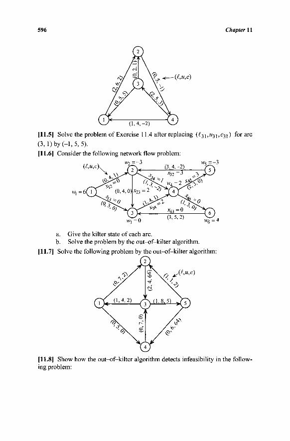
596 Chapter 11
(i,u,c)
(1,4,-2)
[11.5] Solve the problem of Exercise 11.4 after replacing (^31,«31,c31 ) for arc
(3,1) by (-1,5, 5).
[11.6] Consider the following network flow problem:
(l,u,c\
a. Give the kilter state of each arc. b. Solve the problem by the out-of-kilter algorithm.
[11.7] Solve the following problem by the out-of-kilter algorithm:
,u,c)
[11.8] Show how the out-of-kilter algorithm detects infeasibility in the follow-ing problem:
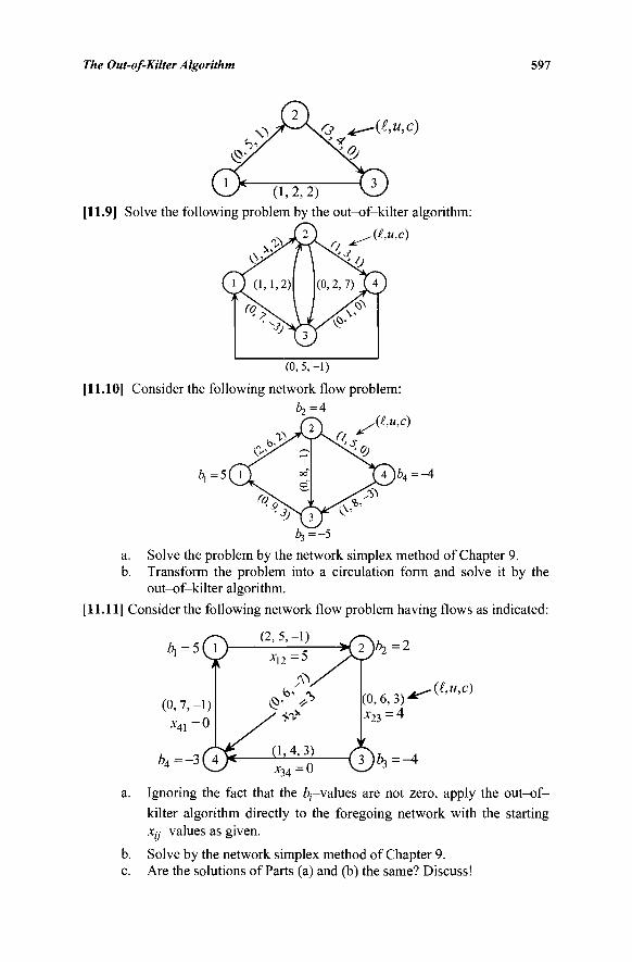
The Out-of-Kilter Algorithm 597
(i,u,c)
(1,2,2) [11.9] Solve the following problem by the out-of-kilter algorithm:
2) Al,u,c)
(0,5,-1)
[11.10] Consider the following network flow problem:
2 (i,u,c)
ò, =5f 1 4 ) b d = ^
Z>3=-5
a. Solve the problem by the network simplex method of Chapter 9. b. Transform the problem into a circulation form and solve it by the
out-of-kilter algorithm.
[11.11] Consider the following network flow problem having flows as indicated:
(2,5,-1) 2 > 2 = 2
(0,6,3)' ■ (£,u,c)
x34 = 0 :^4
a. Ignoring the fact that the fy-values are not zero, apply the out-of-kilter algorithm directly to the foregoing network with the starting x;-.-values as given.
b. Solve by the network simplex method of Chapter 9. c. Are the solutions of Parts (a) and (b) the same? Discuss!
598 Chapter 11
[11.12] Show that after each dual phase we can replace each new w; by w,· -wk, where k is some arbitrary node, and the out-of-kilter algorithm remains unaffected. (In a computer implementation, we might do this to force one dual variable, such as wk, to remain zero and keep all of the dual variables from getting too large.)
[11.13] How can alternative optimal solutions be detected in the out-of-kilter algorithm?
[11.14] Explain in detail the data and list structures you would use in order to efficiently implement the out-of-kilter algorithm. Compare your storage require-ment with that for a primal (network) simplex implementation.
[11.15] In the primal phase of the out-of-kilter algorithm, suppose that we need to find a (directed) path from q to p (in G'), given an out-of-kilter arc (p, q).
Consider the construction of the usual flow change tree T described in Sections 11.2 and 11.5. Recall that starting with T= {q}, each node that is included in T receives a label equal to the (positive) flow it can receive from q. Suppose that at each step we add to T that node, which among all candidates that can be connected to nodes already in T, can receive the largest flow change label. Show that if p e T, then this procedure will have found the maximum flow change
path from q top in G'.
[11.16] Is there any difficulty with the out-of-kilter algorithm when tj- = w;-
for some (i, j)l Carefully work through the development of the out-of-kilter algorithm for this case!
[11.17[ Suppose that we have a feasible solution to Problem (11.1). Assuming that the selected arc remains out-of-kilter, is it possible for no new node to come into Xafter a dual variable change? Discuss!
[11.18] Suppose that we work only with the (z,·.· - c,-, )-values after the initial
dual solution and never bother to change the w;-values. Show how the up-
values can be recovered anytime we want them. {Hint: The w;-values are not
unique. Set any one wi = 0.)
[11.19] Interpret the dual of the out-of-kilter formulation of Problem (11.1) from a marginal-cost viewpoint.
[11.20] Show that the dual solution given in Section 11.1 is optimal for a fixed set of Wj -values.
[11.21] Demonstrate directly that the dual objective function value is unbounded as Θ —* oo when S\ = 0 and S2 = 0 during the dual phase of the out-of-kilter
algorithm.
[11.22] Considering the out-of-kilter problem, show that a feasible solution exists if and only if for every choice of X and X = * / ' — X we have
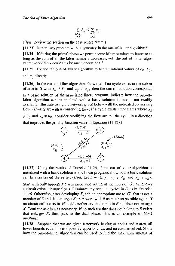
The Out-of-Kilter Algorithm 599
Σ tij < Σ Uij ieX ieX
jeX jeX
(Hint: Review the section on the case where θ= οο.)
[11.23] Is there any problem with degeneracy in the out-of-kilter algorithm? [11.24] If during the primal phase we permit some kilter numbers to increase as long as the sum of all the kilter numbers decreases, will the out-of-kilter algo-rithm work? How could this be made operational?
[11.25] Extend the out-of-kilter algorithm to handle rational values of Cy, iy,
and Uj- directly.
[11.26] In the out-of-kilter algorithm, show that if no cycle exists in the subset of arcs in G with Xy Φ ty and Xy Φ Uy, then the current solution corresponds
to a basic solution of the associated linear program. Indicate how the out-of-kilter algorithm can be initiated with a basic solution if one is not readily available. Illustrate using the network given below with the indicated conserving flow. (Hint: Start with a conserving flow. If a cycle exists among arcs where Xy
Φ £y and Xy Φ Uy, consider modifying the flow around the cycle in a direction
that improves the penalty function value in Equation (11.12).)
r?\ (4>7>4) , y r \
/ (i,u,c)
(0,4,2) x23=\
v_y x34 -1 v_y
[11.27] Using the results of Exercise 11.26, if the out-of-kilter algorithm is initialized with a basic solution to the linear program, show how a basic solution can be maintained thereafter. (Hint: Let E = {(/, j): Xy Φ ly and Xy Φ uy).
Start with only appropriate arcs associated with E as members of G'. Whenever a circuit exists, change flows. Eliminate any residual cycles in E, as in Exercise 11.26. Otherwise, after developing X, add an appropriate arc to G' that is not a member of E and that enlarges X; then work with E as much as possible again. If no circuit still exists in G', add another arc that is not in E but does not enlarge X. Continue as often as necessary. If no such arc that does not belong to E exists that enlarges X, then pass to the dual phase. This is an example of block pivoting.)
[11.28] Suppose that we are given a network having m nodes and n arcs, all lower bounds equal to zero, positive upper bounds, and no costs involved. Show how the out-of-kilter algorithm can be used to find the maximum amount of
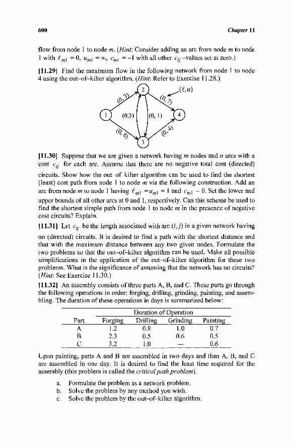
600 Chapter 11
flow from node 1 to node m. {Hint: Consider adding an arc from node m to node 1 with £ml = 0, umX = oo, cml = -1 with all other c^ -values set at zero.)
[11.29] Find the maximum flow in the following network from node 1 to node 4 using the out-of-kilter algorithm. (Hint: Refer to Exercise 11.28.)
[11.30] Suppose that we are given a network having m nodes and n arcs with a cost Cjj for each arc. Assume that there are no negative total cost (directed)
circuits. Show how the out-of-kilter algorithm can be used to find the shortest (least) cost path from node 1 to node m via the following construction. Add an arc from node m to node 1 having £ml =um\ = 1 and cm] = 0. Set the lower and upper bounds of all other arcs at 0 and 1, respectively. Can this scheme be used to find the shortest simple path from node 1 to node m in the presence of negative cost circuits? Explain.
[11.31] Let Cjj be the length associated with arc (i,j) in a given network having
no (directed) circuits. It is desired to find a path with the shortest distance and that with the maximum distance between any two given nodes. Formulate the two problems so that the out-of-kilter algorithm can be used. Make all possible simplifications in the application of the out-of-kilter algorithm for these two problems. What is the significance of assuming that the network has no circuits? (Hint: See Exercise 11.30.)
[11.32] An assembly consists of three parts A, B, and C. These parts go through the following operations in order: forging, drilling, grinding, painting, and assem-bling. The duration of these operations in days is summarized below:
Part A B C
Forging 1.2 2.3 3.2
Duration of Operation Drilling Grinding
0.8 1.0 0.5 0.6 1.0 —
Painting 0.7 0.5 0.6
Upon painting, parts A and B are assembled in two days and then A, B, and C are assembled in one day. It is desired to find the least time required for the assembly (this problem is called the critical path problem).
a. Formulate the problem as a network problem. b. Solve the problem by any method you wish. c. Solve the problem by the out-of-kilter algorithm.
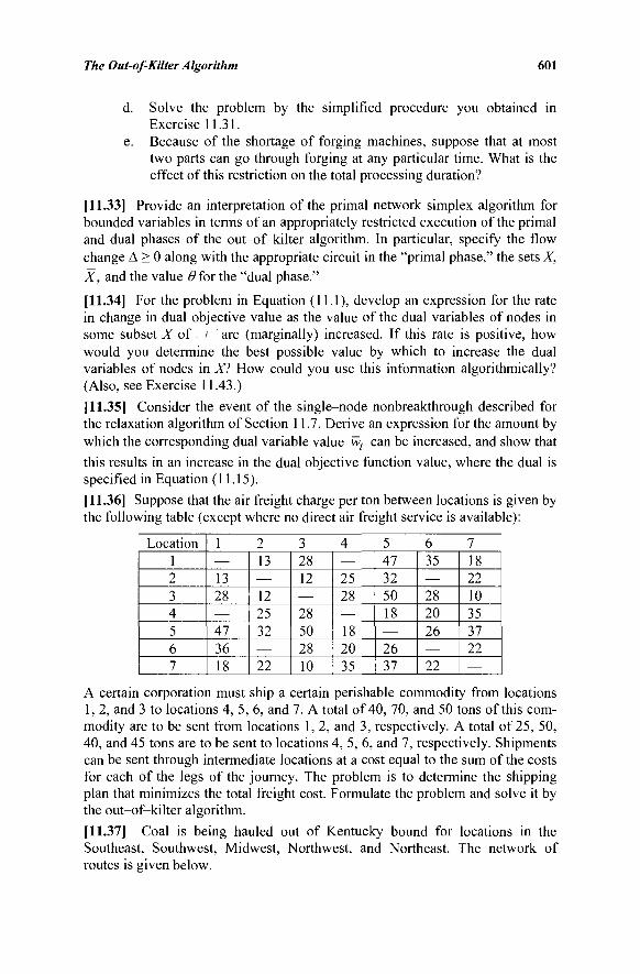
The Out-of-Kilter Algorithm 601
d. Solve the problem by the simplified procedure you obtained in Exercise 11.31.
e. Because of the shortage of forging machines, suppose that at most two parts can go through forging at any particular time. What is the effect of this restriction on the total processing duration?
[11.33] Provide an interpretation of the primal network simplex algorithm for bounded variables in terms of an appropriately restricted execution of the primal and dual phases of the out-of-kilter algorithm. In particular, specify the flow change Δ > 0 along with the appropriate circuit in the "primal phase," the sets X, X, and the value θΐοτ the "dual phase."
[11.34] For the problem in Equation (11.1), develop an expression for the rate in change in dual objective value as the value of the dual variables of nodes in some subset X of ■ / are (marginally) increased. If this rate is positive, how would you determine the best possible value by which to increase the dual variables of nodes in X? How could you use this information algorithmically? (Also, see Exercise 11.43.)
[11.35] Consider the event of the single-node nonbreakthrough described for the relaxation algorithm of Section 11.7. Derive an expression for the amount by which the corresponding dual variable value wt can be increased, and show that
this results in an increase in the dual objective function value, where the dual is specified in Equation (11.15).
[11.36] Suppose that the air freight charge per ton between locations is given by the following table (except where no direct air freight service is available):
Location 1 2 3 4 5 6 7
1 — 13 28 — 47 36 18
2 13 — 12 25 32 — 22
3 28 12 — 28 50 28 10
4 — 25 28 — 18 20 35
5 47 32 50 18 — 26 37
6 35 — 28 20 26 — 22
7 18 22 10 35 37 22 —
A certain corporation must ship a certain perishable commodity from locations 1, 2, and 3 to locations 4, 5, 6, and 7. A total of 40, 70, and 50 tons of this com-modity are to be sent from locations 1, 2, and 3, respectively. A total of 25, 50, 40, and 45 tons are to be sent to locations 4, 5, 6, and 7, respectively. Shipments can be sent through intermediate locations at a cost equal to the sum of the costs for each of the legs of the journey. The problem is to determine the shipping plan that minimizes the total freight cost. Formulate the problem and solve it by the out-of-kilter algorithm.
[11.37] Coal is being hauled out of Kentucky bound for locations in the Southeast, Southwest, Midwest, Northwest, and Northeast. The network of routes is given below.
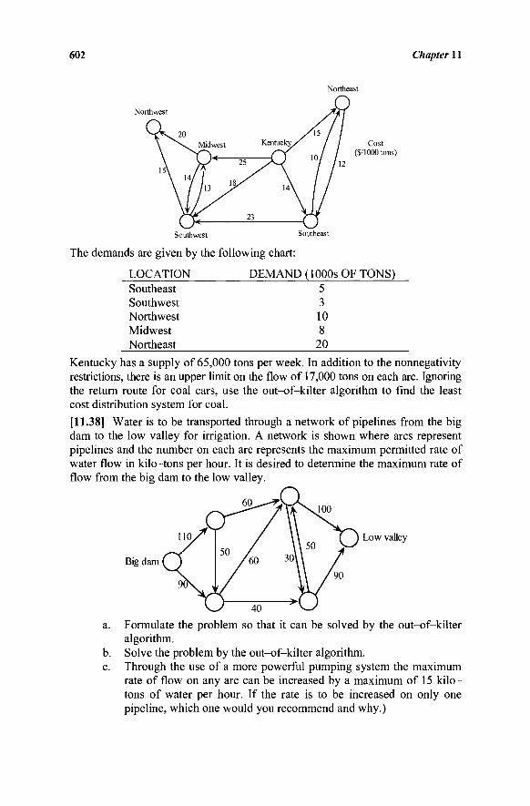
602 Chapter 11
Northeast
Northwest
Southwest Southeast
The demands are given by the following chart:
LOCATION DEMAND (1000s OF TONS) Southeast Southwest Northwest Midwest Northeast
5 3 10 8
20 Kentucky has a supply of 65,000 tons per week. In addition to the nonnegativity restrictions, there is an upper limit on the flow of 17,000 tons on each arc. Ignoring the return route for coal cars, use the out-of-kilter algorithm to find the least cost distribution system for coal.
[11.38] Water is to be transported through a network of pipelines from the big dam to the low valley for irrigation. A network is shown where arcs represent pipelines and the number on each arc represents the maximum permitted rate of water flow in kilo-tons per hour. It is desired to determine the maximum rate of flow from the big dam to the low valley.
Big dam
Low valley
a.
b. c.
Formulate the problem so that it can be solved by the out-of-kilter algorithm. Solve the problem by the out-of-kilter algorithm. Through the use of a more powerful pumping system the maximum rate of flow on any arc can be increased by a maximum of 15 kilo-tons of water per hour. If the rate is to be increased on only one pipeline, which one would you recommend and why.)
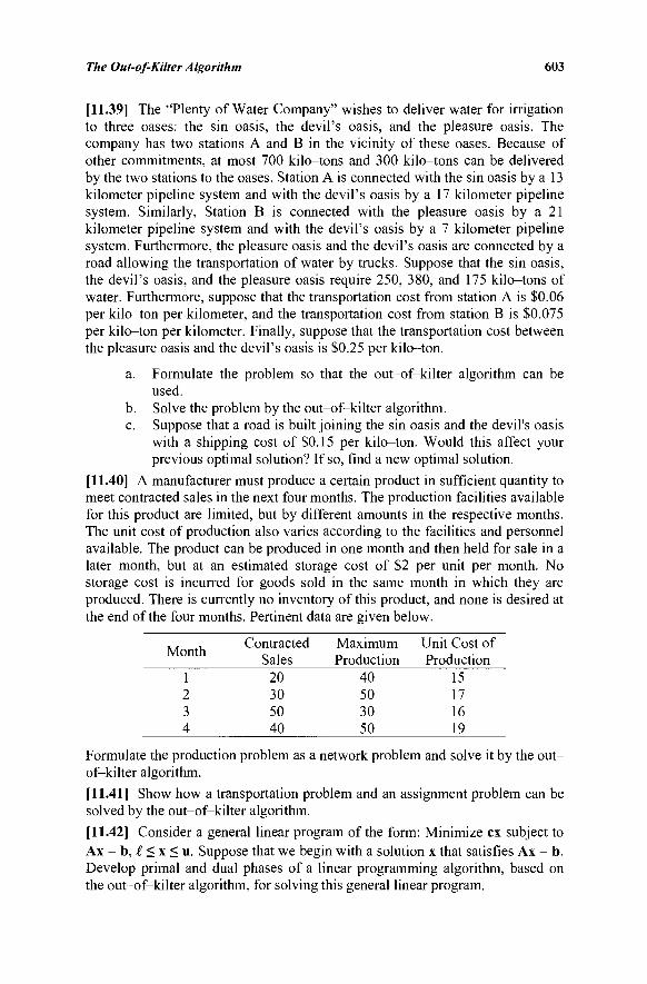
The Out-of-Kilter Algorithm 603
[11.39] The "Plenty of Water Company" wishes to deliver water for irrigation to three oases: the sin oasis, the devil's oasis, and the pleasure oasis. The company has two stations A and B in the vicinity of these oases. Because of other commitments, at most 700 kilo-tons and 300 kilo-tons can be delivered by the two stations to the oases. Station A is connected with the sin oasis by a 13 kilometer pipeline system and with the devil's oasis by a 17 kilometer pipeline system. Similarly, Station B is connected with the pleasure oasis by a 21 kilometer pipeline system and with the devil's oasis by a 7 kilometer pipeline system. Furthermore, the pleasure oasis and the devil's oasis are connected by a road allowing the transportation of water by trucks. Suppose that the sin oasis, the devil's oasis, and the pleasure oasis require 250, 380, and 175 kilo-tons of water. Furthermore, suppose that the transportation cost from station A is $0.06 per kilo-ton per kilometer, and the transportation cost from station B is $0,075 per kilo-ton per kilometer. Finally, suppose that the transportation cost between the pleasure oasis and the devil's oasis is $0.25 per kilo-ton.
a. Formulate the problem so that the out-of-kilter algorithm can be used.
b. Solve the problem by the out-of-kilter algorithm. c. Suppose that a road is built joining the sin oasis and the devil's oasis
with a shipping cost of $0.15 per kilo-ton. Would this affect your previous optimal solution? If so, find a new optimal solution.
[11.40] A manufacturer must produce a certain product in sufficient quantity to meet contracted sales in the next four months. The production facilities available for this product are limited, but by different amounts in the respective months. The unit cost of production also varies according to the facilities and personnel available. The product can be produced in one month and then held for sale in a later month, but at an estimated storage cost of $2 per unit per month. No storage cost is incurred for goods sold in the same month in which they are produced. There is currently no inventory of this product, and none is desired at the end of the four months. Pertinent data are given below.
Month
1 2 3 4
Contracted Sales
20 30 50 40
Maximum Production
40 50 30 50
Unit Cost of Production
15 17 16 19
Formulate the production problem as a network problem and solve it by the out-of-kilter algorithm. [11.41] Show how a transportation problem and an assignment problem can be solved by the out-of-kilter algorithm.
[11.42] Consider a general linear program of the form: Minimize ex subject to Ax = b, i < x < u. Suppose that we begin with a solution x that satisfies Ax = b. Develop primal and dual phases of a linear programming algorithm, based on the out-of-kilter algorithm, for solving this general linear program.
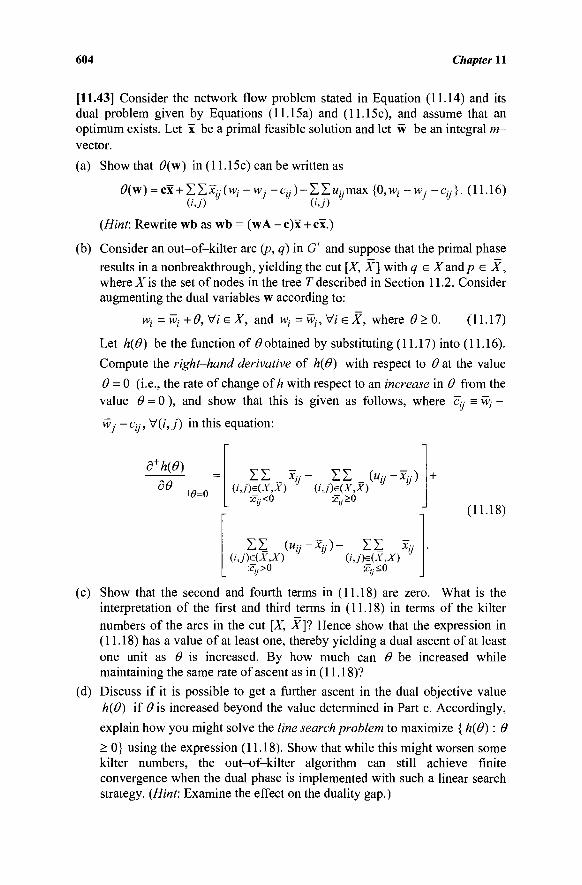
604 Chapter 11
[11.43] Consider the network flow problem stated in Equation (11.14) and its dual problem given by Equations (11.15a) and (11.15c), and assume that an optimum exists. Let x be a primal feasible solution and let w be an integral m-vector.
(a) Show that #(w) in (11.15c) can be written as
#(w) = ex + Σ Σ Xji (WJ ■Wj -Cy)-ZZMy-max {0,w;· -w,· -Cy}. (11.16) (ij)
(Hint: Rewrite wb as wb = (wA - c)x + ex.)
(b) Consider an out-of-kilter arc (p, q) in G' and suppose that the primal phase
results in a nonbreakthrough, yielding the cut [X, X] with q e Xand/? e X, where X is the set of nodes in the tree T described in Section 11.2. Consider augmenting the dual variables w according to:
Wj = Wj + Θ, Vi e X, and w;· = wh Vi e X, where Θ > 0. (11.17)
Let h(0) be the function of # obtained by substituting (11.17) into (11.16).
Compute the right-hand derivative of h(0) with respect to Θ at the value
Θ = 0 (i.e., the rate of change of h with respect to an increase in Θ from the
value Θ = 0 ), and show that this is given as follows, where c"« = wt -
W; -Cjj,V(i,j) in this equation:
d+h(0)
ΘΘ 0=0
(iJ)e(X,X) (i,j)e(X,X) *S<0
Σ Σ (liy-Xy)- Σ Σ (UMx,x)
XyX) (UMX,x)
:^.<0
(11.18)
(c) Show that the second and fourth terms in (11.18) are zero. What is the interpretation of the first and third terms in (11.18) in terms of the kilter numbers of the arcs in the cut [X, X]7 Hence show that the expression in (11.18) has a value of at least one, thereby yielding a dual ascent of at least one unit as Θ is increased. By how much can Θ be increased while maintaining the same rate of ascent as in (11.18)?
(d) Discuss if it is possible to get a further ascent in the dual objective value h(0) if é?is increased beyond the value determined in Part c. Accordingly, explain how you might solve the line search problem to maximize {h(G) : Θ
> 0} using the expression (11.18). Show that while this might worsen some kilter numbers, the out-of-kilter algorithm can still achieve finite convergence when the dual phase is implemented with such a linear search strategy. (Hint: Examine the effect on the duality gap.)
The Out-of-Kilter Algorithm 605
(e) If the cut [X, X] is not necessarily determined as a consequence of a nonbreakthrough in the primal phase, but is arbitrarily selected with both X and X being nonempty, verify that (11.18) still holds true. Hence, discuss how you might perform coordinate ascent steps or single-node ascent steps (see Section 11.17) in the present context when either X or X is a singleton. How would you incorporate such ascent steps within the overall framework of the out-of-kilter algorithm, and what is the potential advantage of employing such a strategy?
NOTES AND REFERENCES
1. Fulkerson [1961a] developed the out-of-kilter algorithm for network flow problems. For a slightly different development of the out-of-kilter algorithm, see Ford and Fulkerson [1962], and for a specialization, see Kennington and Helgason [1980].
2. The presentation of the out-of-kilter algorithm in this chapter follows that of Clasen [1968], especially the division of states according to values of flows x„ and reduced costs z.-.-c,·,-.
v y y
3. The spirit of the out-of-kilter algorithm can be extended to a procedure for general linear programs. This has been done by Jewell [1967]. The corresponding steps in the general case require the solution to linear programming subproblems instead of finding cycles or changing dual variables in a simple way.
4. Barr et al. [1974] provide a streamlined implementation scheme for the out-of-kilter algorithm along with computational results. Another implemen-tation scheme is described in Singh [1986]. Computational experience and comparisons are also provided by Glover and Klingman [1978] and Hatch [1975].
5. Bertsekas and Tseng [1988b] describe a primal-dual network flow relaxation algorithm that operates two-three times faster on the NETGEN benchmark test problems compared with RNET, an effective primal sim-plex code developed at Rutger's University by Professor Grigoriadis and Professor Hsu. This algorithm is discussed briefly in Section 11.7. Its version RELAX-IV, and extension to solve generalized networks are respectively described in Bertsekas and Tseng [1988b, 1994]. The principal computational advantage comes from the quick dual ascent steps using cuts based on single nodes as opposed to determining steepest ascent cuts (see Exercises 11.34 and 11.43). All modern-day commercial software have specialized routines to solve network structured problems that are being continually refined (e.g., the popular software CPLEX has an efficient network simplex code, NETOPT). For extensions to handle convex-arc costs, see Bertsekas et al. [1987], and for the design of relaxa-tion methods for general linear programs (see Tseng and Bertsekas [1987]). Also, for specializations of interior point methods to solve network flow problems and computational comparisons with simplex and relaxation methods, see Mehrotra and Wang [1996].

This page intentionally left blank
TWELVE: MAXIMAL FLOW, SHORTEST PATH, MULTICOMMODITY FLOW, AND NETWORK SYNTHESIS PROBLEMS
Two special and important network flow problems are the maximal flow prob-lem and the shortest path problem. Both of these problems can be solved by either the network simplex method of Chapter 9 or the out-of-kilter algorithm of Chapter 11. However, their frequent occurrence in practice and the specialized, more efficient procedures that can be developed for handling these two problems provide a strong case for considering them separately.
We also include in this chapter an introduction to the class of network flow problems called multicommodity network flows. In Chapters 9, 10, and 11 we have considered network flow problems in which it was not necessary to distinguish among the units flowing in the networks. There was essentially a single commodity or type of unit. There are network flow problems in which different types of units must be treated. In these instances, supplies and demands are by commodity type, and the distinction among the commodities must be maintained. We shall examine this multicommodity flow problem, consider the difficulty in dealing with it, and present a decomposition-based procedure for solving it.
Another topic that we introduce is network synthesis. The network flow problems considered thus far are analysis problems. A network is given, and some analysis is performed on it. On the other hand, the network synthesis problem requires one to construct an optimal network (in some defined sense) that satisfies certain specifications. Several of the tools developed in this book, including network analysis and decomposition methods, can be used to study such problems.
12.1 THE MAXIMAL FLOW PROBLEM
We begin by presenting Ford and Fulkerson's labeling method for solving maximal flow problems. This method is simply a specialization of the out-of-kilter algorithm applied to the maximal flow problem. Specialized primal sim-plex implementations have been found to be significantly faster than this method (with a speed-up factor of 1.5-5) and require only one-third of the amount of storage. However, this method does provide useful insights, and as with the general out-of-kilter algorithm, improved primal-dual implementa-tions can make it more competitive. In fact, at the end of this section, we briefly
607
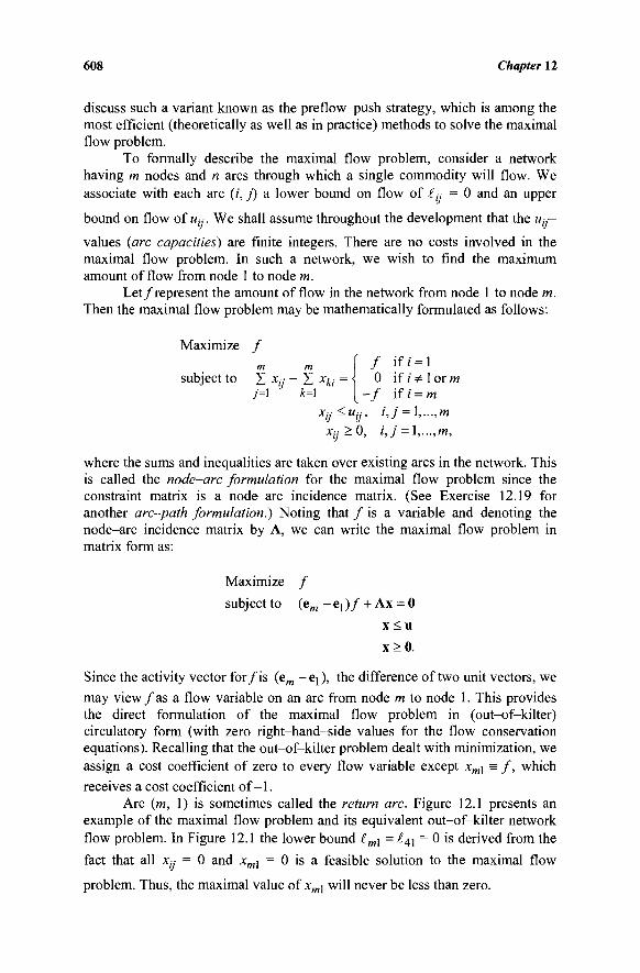
608 Chapter 12
discuss such a variant known as the preflow-push strategy, which is among the most efficient (theoretically as well as in practice) methods to solve the maximal flow problem.
To formally describe the maximal flow problem, consider a network having m nodes and n arcs through which a single commodity will flow. We associate with each arc (/', j) a lower bound on flow of ί^ = 0 and an upper
bound on flow of «,·.·. We shall assume throughout the development that the «(y-
values (arc capacities) are finite integers. There are no costs involved in the maximal flow problem. In such a network, we wish to find the maximum amount of flow from node 1 to node m.
Let/represent the amount of flow in the network from node 1 to node m. Then the maximal flow problem may be mathematically formulated as follows:
Maximize / m m ί / if/' = l
subject to X xtj - Σ xki = < 0 if i Φ1 or m 7=1 *=l [-/ if i = m
Xy^Uy, i,j = l,...,m
Xij>0, i,j = l,...,m,
where the sums and inequalities are taken over existing arcs in the network. This is called the node-arc formulation for the maximal flow problem since the constraint matrix is a node-arc incidence matrix. (See Exercise 12.19 for another arc-path formulation.) Noting that / is a variable and denoting the node-arc incidence matrix by A, we can write the maximal flow problem in matrix form as:
Maximize /
subject to (em - β] ) / + Ax = 0
x < u
x>0.
Since the activity vector for/is (em -e j ) , the difference of two unit vectors, we
may view fas a flow variable on an arc from node m to node 1. This provides the direct formulation of the maximal flow problem in (out-of-kilter) circulatory form (with zero right-hand-side values for the flow conservation equations). Recalling that the out-of-kilter problem dealt with minimization, we assign a cost coefficient of zero to every flow variable except xm\ = f, which receives a cost coefficient of -1 .
Arc (m, 1) is sometimes called the return arc. Figure 12.1 presents an example of the maximal flow problem and its equivalent out-of-kilter network flow problem. In Figure 12.1 the lower bound lmi = £4i = 0 is derived from the fact that all Xy = 0 and xml = 0 is a feasible solution to the maximal flow problem. Thus, the maximal value of xwl will never be less than zero.
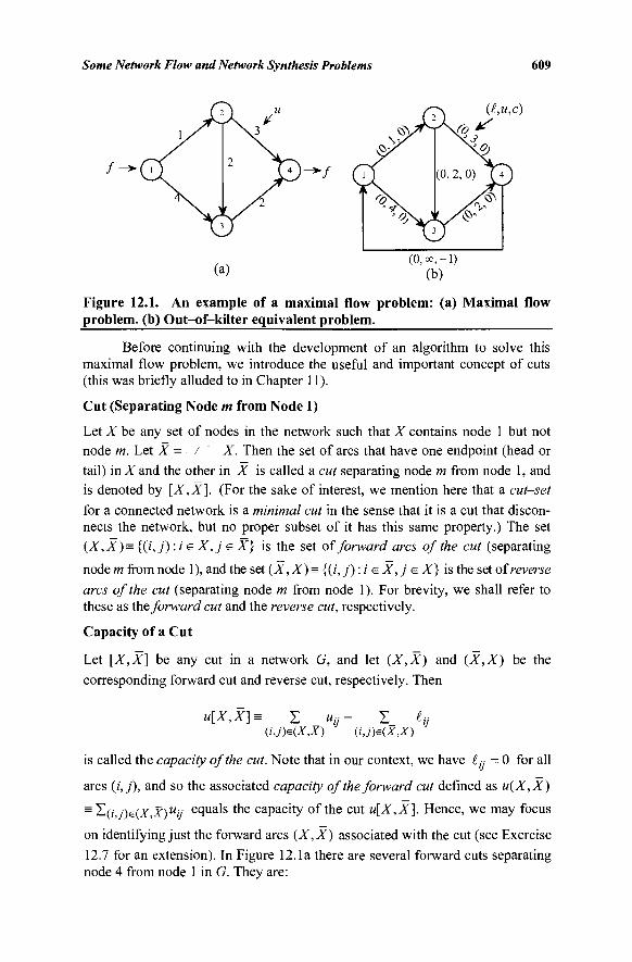
Some Network Flow and Network Synthesis Problems 609
<SV
r<l· oy
(i,u,c)
(0, 2, 0)
^ ^
(a) (0, oo, -1)
(b)
Figure 12.1. An example of a maximal flow problem: (a) Maximal flow problem, (b) Out-of-kilter equivalent problem.
Before continuing with the development of an algorithm to solve this maximal flow problem, we introduce the useful and important concept of cuts (this was briefly alluded to in Chapter 11).
Cut (Separating Node m from Node 1)
Let X be any set of nodes in the network such that X contains node 1 but not node m. Let X =. / -X. Then the set of arcs that have one endpoint (head or tail) in X and the other in X is called a cut separating node m from node 1, and is denoted by [X,X]. (For the sake of interest, we mention here that a cut-set
for a connected network is a minimal cut in the sense that it is a cut that discon-nects the network, but no proper subset of it has this same property.) The set (X, X) = {(/, j) : i e X, j e X} is the set of forward arcs of the cut (separating
node m from node 1), and the set (X, X)= {(/, y) : i e X,j e X} is the set oireverse arcs of the cut (separating node m from node 1). For brevity, we shall refer to these as the forward cut and the reverse cut, respectively.
Capacity of a Cut
Let [X,X] be any cut in a network G, and let (X,X) and (X,X) be the
corresponding forward cut and reverse cut, respectively. Then
u[X,X]= Σ _utj- Σ_ t,j
(ujtex,x) (i,mx,x) is called the capacity of the cut. Note that in our context, we have iy =0 for all
arcs (/,/), and so the associated capacity of the forward cut defined as u(X,X)
= ^(i,j)e(X,X)uij e c lu a l s m e capacity of the cut u[X,X]. Hence, we may focus
on identifying just the forward arcs (X, X) associated with the cut (see Exercise 12.7 for an extension). In Figure 12.1a there are several forward cuts separating node 4 from node 1 in G. They are:
610 Chapter 12
X = {1}, X = {2,3,4} (A",*) = {(1,2), (1,3)}, u(X,X) = 5 A" = {1,2}, ^ = {3,4} (X,X) = {(1,3),(2,3),(2,4)}, « ( * , * ) = 9 A" = {1,3}, * = {2,4} (X,X) = {(1,2),(3,4)}, u(X,X) = 3 X = {1,2,3}, X = {4} ( * , * ) = {(2,4), (3,4)}, W(*,X) = 5.
Let [A~,X] be any cut separating node m from node 1 in G. Summing the flow
conservation equations of the maximal flow problem over nodes in X, the flow variables that have both ends in X cancel and we get
Σ * ΐ , · - Σ *(, ·=/. (12.1) ieX i&X
Using Xy > ijj = 0 and xy < uy, we get
f< Σ _Uij- Σ iij= Σ _uy. (12.2) (U)e(X,x) (UMX,X) (UMX,X)
This leads to the following.
Lemma 12.1
The value / o f any (feasible) flow is less than or
any cut (separating node m from node 1).
The Dual of the Maximal Flow Problem
Consider the dual of the maximal flow problem:
m m Minimize Σ Σ Uyhy
i=l 7=1 subject to wm - W] = 1
Wj - Wj + hy > 0, i,j = l,...,m hij>Q, i,j = l,...,m,
where w is associated with the flow conservation equations and h is associated with the constraints x < u. Note that the first dual constraint is associated with the flow / whose column is ew - β]. A typical column a . of the node-arc
incidence matrix A has +1 in the rth position and -1 in they'th position, which leads to the dual constraints Wj - w- + L·- > 0.
Let [A", A"] be any cut and consider the foregoing dual problem. If we let
(0 if ieX Wi=\\ if isX
h J \ if (i,j) e (X,X) lJ \ 0 otherwise,
equal to the capacity u[X, X] of
Some Network Flow and Network Synthesis Problems 611
then this particular choice of w and h provides a feasible solution to the dual problem (why?) whose dual objective is equal to the capacity of the cut.
Thus, Lemma 12.1 also follows from the duality theorem, which states that any feasible solution to a minimization problem has an objective value greater than or equal to that of the associated maximization problem. As the reader may suspect, we shall show that the capacity of a minimal cut (i.e., one having a minimal capacity) is equal to the value of the maximal flow. We shall prove this constructively. We ask the reader to prove this result in Exercise 12.8 using the earlier duality relationship.
An Algorithm for the Maximal Flow Problem
From Lemma 12.1, if we are able to find a flow and a cut such that w[X,X] = /
we will have the maximal flow (and the minimal cut). We shall do this constructively by simply specializing the out-of-kilter algorithm to this problem.
Suppose that we start with any feasible (integer) flow in G, say, each Xy
= 0. From G, we construct G' as follows:
1. If arc (/,_/) is in G and % < uy, then we place arc (i,j) in G' along
with a permitted flow change value Δ,ν = w,·, - %.
2. If arc (i,j) is in G and Xj- > 0, then we place arc (/, i) in G' with a
permitted flow change value Δ ·,· = Xy.
Now, in G', two possibilities exist:
Case 1
A path P exists, in G', from node 1 to node m.
Case 2
No path exists, in G', from node 1 to node m.
In Case 1, we may construct a new feasible flow having a greater objec-tive value. Let Δ be equal to the minimum permitted flow change on the path P from node 1 to node m in G', that is, Δ = minimum {Δ# : (/,_/') is in the path}.
Note that Δ is a positive integer (why?). Consider the associated chain P' (undirected path) in G. Construct a new flow as follows. Add Δ to flows on arcs of the associated chain in G that have the same direction as the path in G', subtract Δ from flows on arcs of the associated chain in G that are against the direction of the path in G', and leave all other arc flows unchanged. The new flow is feasible (why?). The value of the new flow is / ' = / + Δ (why?).
Assuming that the capacities are finite, Case 1 can occur only a finite number of times before Case 2 occurs (why?). When Case 2 occurs, let X be the set of nodes in G' that can be reached along some path in G' from node 1. Let
612 Chapter 12
X =,/ -X and note that node m belongs to X (why?). Consider the cut
[X,X], i.e., the arcs in G between X and X. First, every arc (/,/) in G from Xto
X must have Xy = Uy\ otherwise, there would be an arc (i,j) in G' andy would
be a member of X (a contradiction). Second, every arc (i,j) in G from X to X must have Xy = 0; otherwise, there would be an arc (/', i) in G' and i would be a
member of X(a contradiction). Substituting in Equation (12.1), we get
Σ u,--0 = f, or u[X,X) = u(X,X) =f. ieX
Thus, we must have the maximal flow at hand by noting Equation (12.2). Hence, we have constructively proved the following. (See Exercise 12.7 for a direct generalization when £y Φ0.)
Theorem 12.1 (Maximal Flow-Minimal Cut Theorem)
The value of the maximal flow in G is equal to the capacity of the minimal cut in G.
Summary of the Maximal Flow Algorithm
The constructive proof of the maximal flow-minimal cut theorem leads to the following maximal flow algorithm.
INITIALIZATION STEP
Select a set of feasible (integer) flows, say, each Xy = 0.
MAIN STEP
From G construct G' as follows:
1. All of the nodes in G are in G'.
2. If Xj- < Uy in G, place (/,/) in G' with the permitted flow change on
(/,;) of Ay = uy - xy.
3. If Xy > 0 in G, place (/, /') in G' with the permitted flow change on
(/, 0 Of Αβ = Xy.
Note that arc (i,j) in G will give rise to two arcs in G' if 0 < Xy < uy. Attempt to locate a path P in G' from node 1 to node m. If no such path exists, stop; an optimal solution is at hand. Otherwise, let Δ be the minimum permitted flow change on P in G'. Add Δ to the flows on arcs of the associated chain in G that have the same direction as the path in G', subtract Δ from the flows on arcs of the associated chain in G that are against the direction of the path in G', and leave all other arc flows unchanged. Repeat the main step.
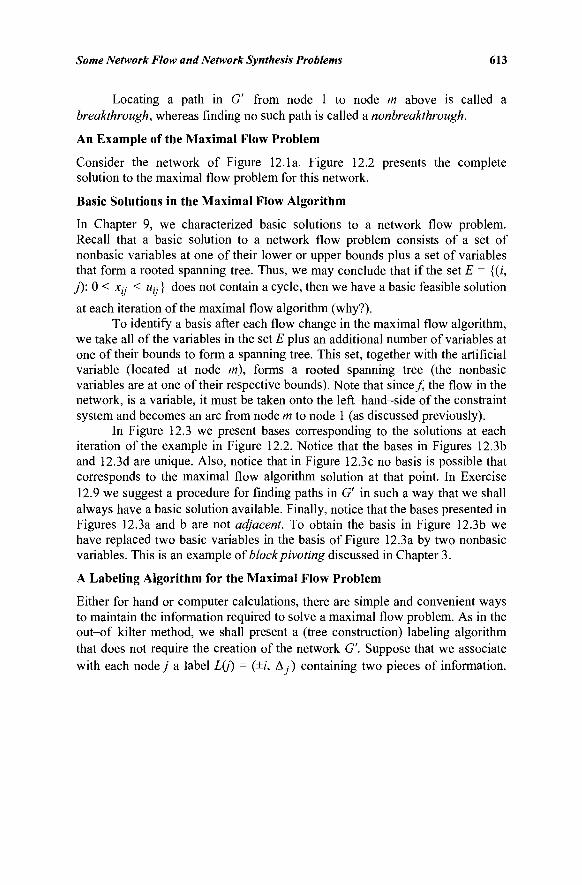
Some Network Flow and Network Synthesis Problems 613
Locating a path in G' from node 1 to node m above is called a breakthrough, whereas finding no such path is called a nonbreakthrough.
An Example of the Maximal Flow Problem
Consider the network of Figure 12.1a. Figure 12.2 presents the complete solution to the maximal flow problem for this network.
Basic Solutions in the Maximal Flow Algorithm
In Chapter 9, we characterized basic solutions to a network flow problem. Recall that a basic solution to a network flow problem consists of a set of nonbasic variables at one of their lower or upper bounds plus a set of variables that form a rooted spanning tree. Thus, we may conclude that if the set E = {(i, j): 0 < Xy < Uy} does not contain a cycle, then we have a basic feasible solution
at each iteration of the maximal flow algorithm (why?). To identify a basis after each flow change in the maximal flow algorithm,
we take all of the variables in the set E plus an additional number of variables at one of their bounds to form a spanning tree. This set, together with the artificial variable (located at node tri), forms a rooted spanning tree (the nonbasic variables are at one of their respective bounds). Note that since/ the flow in the network, is a variable, it must be taken onto the left-hand-side of the constraint system and becomes an arc from node m to node 1 (as discussed previously).
In Figure 12.3 we present bases corresponding to the solutions at each iteration of the example in Figure 12.2. Notice that the bases in Figures 12.3b and 12.3d are unique. Also, notice that in Figure 12.3c no basis is possible that corresponds to the maximal flow algorithm solution at that point. In Exercise 12.9 we suggest a procedure for finding paths in G' in such a way that we shall always have a basic solution available. Finally, notice that the bases presented in Figures 12.3a and b are not adjacent. To obtain the basis in Figure 12.3b we have replaced two basic variables in the basis of Figure 12.3a by two nonbasic variables. This is an example ofblock pivoting discussed in Chapter 3.
A Labeling Algorithm for the Maximal Flow Problem
Either for hand or computer calculations, there are simple and convenient ways to maintain the information required to solve a maximal flow problem. As in the out-of-kilter method, we shall present a (tree construction) labeling algorithm that does not require the creation of the network G'. Suppose that we associate with each node y a label L(j) = (±i, Δ ,·) containing two pieces of information.
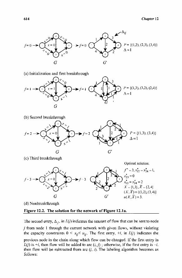
614 Chapter 12
/ = 0 /=o
G
P= {(1,2), (2,3), (3,4)} Δ = 1
(a) Initialization and first breakthrough
7\ P= {(1,3), (3,2), (2,4)}
Δ = 1
(b) Second breakthrough
/ = 2
(c) Third breakthrough
/ = 3
►/=2
►/=3
G'
P= {(1,3), (3,4)}
Δ = 1
Optimal solution:
/ = 3, X[2 = x24 = 1 >
^23=0 * — * _ T
*13 _Ji :34-_f A-=|1,3},X = {2,4} (jr,Jf) = {(1.2), (3,4)} u(X,X) = 3.
(d) Nonbreakthrough
Figure 12.2. The solution for the network of Figure 12.1a.
The second entry, Δ ·, in L(J) indicates the amount of flow that can be sent to node
j from node 1 through the current network with given flows, without violating the capacity constraints 0 < xy< Uy. The first entry, ±i, in L(j) indicates the
previous node in the chain along which flow can be changed. If the first entry in L(J) is +;', then flow will be added to arc (i,j) ; otherwise, if the first entry is -/, then flow will be subtracted from arc (/', /). The labeling algorithm becomes as follows:
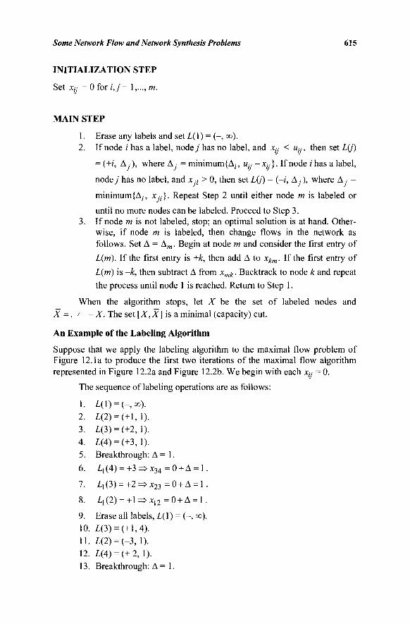
Some Network Flow and Network Synthesis Problems 615
INITIALIZATION STEP
Set Xjj = 0 for i,j = 1,..., m.
MAIN STEP
1. Erase any labels and set L( 1 ) = (-, co).
2. If node i has a label, nodey has no label, and xy < uy, then set L(j)
= (+/, Δ ·), where Δ = minimum{A;, Uy - % } · If node i has a label,
nodey has no label, and x ■,· > 0, then set L(j) = (-/, Δ ·), where Δ =
minimum^,-, x 7 } . Repeat Step 2 until either node m is labeled or
until no more nodes can be labeled. Proceed to Step 3. 3. If node m is not labeled, stop; an optimal solution is at hand. Other-
wise, if node m is labeled, then change flows in the network as follows. Set Δ = Am. Begin at node m and consider the first entry of L(m). If the first entry is +k, then add Δ to xkm. If the first entry of
L(m) is —k, then subtract Δ from xmk. Backtrack to node k and repeat
the process until node 1 is reached. Return to Step 1.
When the algorithm stops, let X be the set of labeled nodes and X = , / -X. The set [X, X] is a minimal (capacity) cut.
An Example of the Labeling Algorithm
Suppose that we apply the labeling algorithm to the maximal flow problem of Figure 12.1a to produce the first two iterations of the maximal flow algorithm represented in Figure 12.2a and Figure 12.2b. We begin with each xy = 0.
The sequence of labeling operations are as follows:
1. 1(1) = (- ,») . 2. L(2) = (+i,l). 3. 1(3) = (+2,1). 4. 1(4) = (+3,1). 5. Breakthrough: Δ = 1.
6. L,(4) = +3=>x34 =0 + Δ = 1.
7. Ζ1(3) = +2=>χ 2 3 =0 + Δ = 1.
8. Ll(2) = +l=>xn =0 + Δ = 1.
9. Erase all labels, 1(1) = (-,oo). 10. 7,(3) = (+1,4). 11. 1(2) = (-3,1). 12. 1(4) = (+2,1). 13. Breakthrough: Δ = 1.
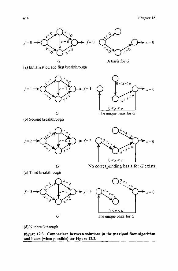
616 Chapter 12
/=o Ο~ > χ = ο
(a) Initialization and first breakthrough
7=1-
(b) Second breakthrough
7=2
(c) Third breakthrough
7=3-
The unique basis for G
7=2 x = 0
No corresponding basis for G exists
7=3 x = 0
The unique basis for G
(d) Nonbreakthrough
Figure 12.3. Comparison between solutions in the maximal flow algorithm and bases (when possible) for Figure 12.2.
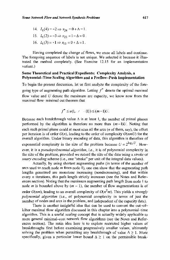
Some Network Flow and Network Synthesis Problems 617
14. L,(4) = +2=>x24 =0 + Δ = 1.
15. Z!(2) = -3=>x2 3 = 1 - Δ = 0.
16. Z!(3) = +l=>x13 =0 + Δ = 1.
Having completed the change of flows, we erase all labels and continue. The foregoing sequence of labels is not unique. We selected it because it illus-trated the method completely. (See Exercise 12.15 for an implementation variant.)
Some Theoretical and Practical Expedients: Complexity Analysis, a Polynomial-Time Scaling Algorithm and a Preflow-Push Implementation
To begin the present discussion, let us first analyze the complexity of the fore-
going type of augmenting path algorithm. Letting / * denote the optimal maximal
flow value and U denote the maximum arc capacity, we know now from the maximal flow-minimal cut theorem that
f* <u(l,, / -{\})<{m-\)U.
Because each breakthrough value Δ is at least 1, the number of primal phases performed by the algorithm is therefore no more than {m-\)U. Noting that
each such primal phase could at most scan all the arcs (n of them, say), the effort per iteration is of order 0(n), leading to the order of complexity 0(nmU) for the overall algorithm. Under binary encoding of data, this algorithm is therefore of
exponential complexity in the size of the problem because U = 2log2 u. How-ever, it is a pseudopolynomial algorithm, i.e., it is of polynomial complexity in the size of the problem, provided we record the size of the data using a stroke or unary encoding scheme (i.e., one "stroke" per unit of the integral data values).
Actually, by using shortest augmenting paths (in terms of the number of arcs used to reach node m from node 1), one can show that the augmenting path lengths generated are monotone increasing (nondecreasing), and that within every n iterations, this path length strictly increases (see the Notes and Refer-ences section). Noting that the maximum augmenting path length from node 1 to node m is bounded above by (m - 1), the number of flow augmentations is of order 0(nm), leading to an overall complexity of 0{n rri). This yields a strongly polynomial algorithm (i.e., of polynomial complexity in terms of just the number of nodes and arcs in the problem, and independent of the capacity data).
There is another insightful idea that can be used to convert the out-of-kilter maximal flow algorithm discussed in this chapter into a polynomial-time algorithm. This is a useful scaling concept that is actually widely applicable to more general minimal-cost network flow algorithms (see the Notes and Refer-ences section). The main idea here is to explore restricted higher values of breakthroughs first before examining progressively smaller values, ultimately solving the problem when permitting any breakthrough of value Δ > 1. More specifically, given a particular lower bound Δ > 1 on the permissible break-
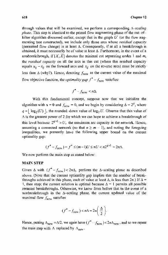
618 Chapter 12
through values that will be examined, we perform a corresponding A-scaling phase. This step is identical to the primal flow augmenting phase of the out-of-kilter algorithm discussed earlier, except that in the graph G' (or the flow aug-menting tree constructed), we include only those arcs whose residual capacity (permitted flow change) is at least Δ. Consequently, if at all a breakthrough is obtained, it must necessarily be of value at least Δ. Furthermore, in the event of a nonbreakthrough, if [X, X] denotes the minimal cut separating nodes 1 and m, the residual capacity on all the arcs in this cut (where this residual capacity equals Uy - Xy on the forward arcs and Xy on the reverse arcs) must be strictly
less than Δ (why?). Hence, denoting / n o w as the current value of the maximal
flow objective function, the optimality gap f - / n o w satisfies:
/ * "/now < " Δ ·
With this fundamental concept, suppose now that we initialize the
algorithm with x = 0 and / n o w = 0, and we begin by considering Δ = 2q, where
q = [ log2 (U) J, the rounded-down value of log2 U. Observe that this value of
Δ is the greatest power of 2 for which we can hope to achieve a breakthrough of
this level because 2q+i
> U, the maximum arc capacity in the network. Hence, assuming a connected network (so that n > m - 1), and noting the foregoing inequalities, we presently have the following upper bound on the current optimality gap:
(/* " /now ) = f<(m-\)U<nU< «2?+1 = 2κΔ.
We now perform the main step as stated below: MAIN STEP
Given Δ with (/* - fnow ) < 2«Δ, perform the Δ-scaling phase as described
above. (Note that the current optimality gap implies that the number of break-throughs achieved in this phase, each of value at least Δ, is less than 2«.) If Δ = 1, then stop; the current solution is optimal because Δ = 1 permits all possible remnant breakthroughs. Otherwise, we know from before that in the event of a nonbreakthrough in the Δ-scaling phase, the current updated value of the maximal flow / n o w satisfies
(/*-/now)<"A = 2«
Hence, putting Δηενν = Δ/2, we again have (/* - / n o w ) < 2«Δηενν, and so we repeat
the main step with Δ replaced by Anew.
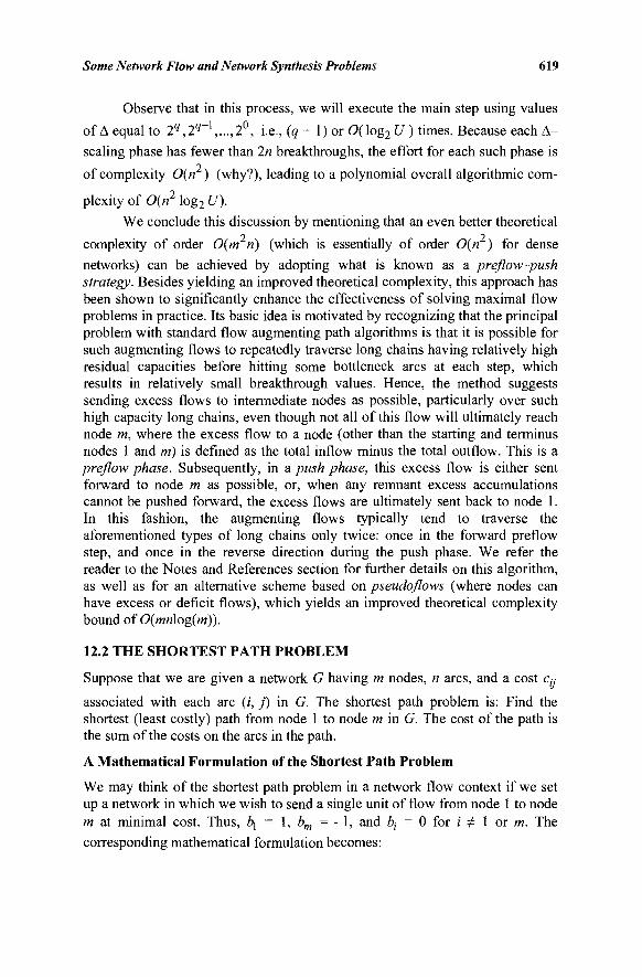
Some Network Flow and Network Synthesis Problems 619
Observe that in this process, we will execute the main step using values
of Δ equal to 2?,29_1,...,2°, i.e., (q + 1) or 0(log2 U ) times. Because each Δ-
scaling phase has fewer than In breakthroughs, the effort for each such phase is
of complexity 0(n ) (why?), leading to a polynomial overall algorithmic com-
plexity of 0(n log2 U).
We conclude this discussion by mentioning that an even better theoretical 9 · 9
complexity of order 0(m n) (which is essentially of order 0(n ) for dense networks) can be achieved by adopting what is known as a preflow-push strategy. Besides yielding an improved theoretical complexity, this approach has been shown to significantly enhance the effectiveness of solving maximal flow problems in practice. Its basic idea is motivated by recognizing that the principal problem with standard flow augmenting path algorithms is that it is possible for such augmenting flows to repeatedly traverse long chains having relatively high residual capacities before hitting some bottleneck arcs at each step, which results in relatively small breakthrough values. Hence, the method suggests sending excess flows to intermediate nodes as possible, particularly over such high capacity long chains, even though not all of this flow will ultimately reach node m, where the excess flow to a node (other than the starting and terminus nodes 1 and m) is defined as the total inflow minus the total outflow. This is a preflow phase. Subsequently, in a push phase, this excess flow is either sent forward to node m as possible, or, when any remnant excess accumulations cannot be pushed forward, the excess flows are ultimately sent back to node 1. In this fashion, the augmenting flows typically tend to traverse the aforementioned types of long chains only twice: once in the forward preflow step, and once in the reverse direction during the push phase. We refer the reader to the Notes and References section for further details on this algorithm, as well as for an alternative scheme based on pseudoflows (where nodes can have excess or deficit flows), which yields an improved theoretical complexity bound of 0(mn\og{m)).
12.2 THE SHORTEST PATH PROBLEM
Suppose that we are given a network G having m nodes, n arcs, and a cost Cy
associated with each arc (i, j) in G. The shortest path problem is: Find the shortest (least costly) path from node 1 to node m in G. The cost of the path is the sum of the costs on the arcs in the path.
A Mathematical Formulation of the Shortest Path Problem
We may think of the shortest path problem in a network flow context if we set up a network in which we wish to send a single unit of flow from node 1 to node m at minimal cost. Thus, i\ = 1, bm = —1, and bt = 0 for i Φ 1 or m. The corresponding mathematical formulation becomes:
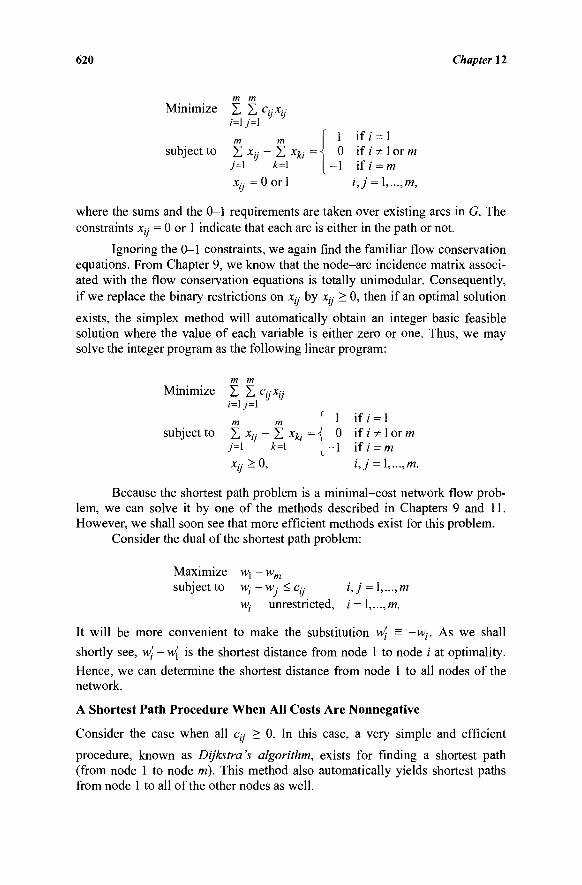
620 Chapter 12
vlinimize
iubject to
m m
L· L· cijxij i=\j=l
m m Σ Xy ~ Σ Xki = \
j=\ k=\ |
Xy = 0 or 1
0 - 1
if i = 1 if / Φ 1 or m if i = m
i,j = \,...,m,
where the sums and the 0-1 requirements are taken over existing arcs in G. The constraints Xy = 0 or 1 indicate that each arc is either in the path or not.
Ignoring the 0-1 constraints, we again find the familiar flow conservation equations. From Chapter 9, we know that the node-arc incidence matrix associ-ated with the flow conservation equations is totally unimodular. Consequently, if we replace the binary restrictions on Xy by Xy > 0, then if an optimal solution
exists, the simplex method will automatically obtain an integer basic feasible solution where the value of each variable is either zero or one. Thus, we may solve the integer program as the following linear program:
Minimize X Σ CyXy i=\j=\
subject to
Because the shortest path problem is a minimal-cost network flow prob-lem, we can solve it by one of the methods described in Chapters 9 and 11. However, we shall soon see that more efficient methods exist for this problem.
Consider the dual of the shortest path problem:
Maximize subject to
W]
wt
Wj
— w ¥Vm -Wj<Cy
unrestricted,
i,j = \,...,m
i = l,...,m.
It will be more convenient to make the substitution w\ = -w,·. As we shall shortly see, w\ - w{ is the shortest distance from node 1 to node / at optimality. Hence, we can determine the shortest distance from node 1 to all nodes of the network.
A Shortest Path Procedure When All Costs Are Nonnegative
Consider the case when all Cy > 0. In this case, a very simple and efficient
procedure, known as Dijkstra's algorithm, exists for finding a shortest path (from node 1 to node m). This method also automatically yields shortest paths from node 1 to all of the other nodes as well.
Some Network Flow and Network Synthesis Problems 621
INITIALIZATION STEP
Set w{ =Oandle tX={l} .
MAIN STEP
Let X = - / -X and consider the arcs in the set (X,X) = {(i,j):ie X,
jeXj.Let
w' +c = minimum {w· +c·.·}. P m (iJMX,X) J
Set w'q = w'p + cpq and place node q in X. Repeat the main step exactly m - 1
times (including the first time) and then stop; an optimal solution is at hand. (Because of the fact that whenever the label of a node q is set at w' = w' + cpq
as above, then this turns out to be the distance of the shortest path from node 1 to node q as established next, we refer to such a procedure as a labelingsetting algorithm.)
Validation of the Algorithm
We now prove that the algorithm produces an optimal solution. Assume, inductively, that each w- for ; e X represents the cost of a shortest path from node 1 to node i. This is certainly true for i = 1 (why?). Consider the algorithm at some point when a new node q is about to be added to X. Suppose that
w' +cna = minimum {w- +c ■}. (12.3) p pq (iJMX,x) J
We shall show that a shortest path from node 1 to node q has length w' = w'p + cpq and can be constructed iteratively as the available shortest path
from node 1 to node/? plus the arc (p, q). Let P be any path from node 1 to node q. It suffices to show that the length of P is at least w'. Since node 1 is in X and
node q is currently in X, then P must contain an arc (i,j) where i e Xanàj e X (here, / and j could be p and q, respectively). The length of the path P is thus equal to the sum of the following:
1. The length from node 1 to node i\ 2. The length of arc (i,j), that is, c,·.· ;
3. The length from j to q.
By the induction hypothesis, the length from node 1 to node / is greater than or equal tow,'. Because the costs of all arcs are nonnegative by assumption, then the length in Part 3 is nonnegative. Therefore, the length of P is greater than or equal to w\ + cu. In view of Equation (12.3), and since w' = w' +cpq, it is clear
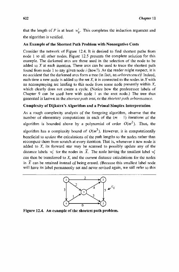
622 Chapter 12
that the length of P is at least w . This completes the induction argument and
the algorithm is verified.
An Example of the Shortest Path Problem with Nonnegative Costs
Consider the network of Figure 12.4. It is desired to find shortest paths from node 1 to all other nodes. Figure 12.5 presents the complete solution for this example. The darkened arcs are those used in the selection of the node to be added to X at each iteration. These arcs can be used to trace the shortest path found from node 1 to any given node / (how?). As the reader might suspect, it is no accident that the darkened arcs form a tree (in fact, an arborescencef. Indeed, each time a new node is added to the set^f, it is connected to the nodes in X with an accompanying arc leading to this node from some node presently within X, which clearly does not create a cycle. (Notice how the predecessor labels of Chapter 9 can be used here with node 1 as the root node.) The tree thus generated is known as the shortest path tree, or the shortest path arborescence.
Complexity of Dijkstra's Algorithm and a Primal Simplex Interpretation
As a rough complexity analysis of the foregoing algorithm, observe that the number of elementary computations in each of the (m - 1) iterations of the
algorithm is bounded above by a polynomial of order 0{m ). Thus, the
algorithm has a complexity bound of 0(m ). However, it is computationally
beneficial to update the calculations of the path lengths to the nodes rather than recompute them from scratch at every iteration. That is, whenever a new node is added to X, its forward star may be scanned to possibly update any of the distance labels w\ for the nodes in X. The node having the smallest label w\ can then be transferred to X, and the current distance calculations for the nodes in X can be retained instead of being erased. (Because this smallest label node will have its label permanently set and never revised again, we still refer to this
Figure 12.4. An example of the shortest path problem.
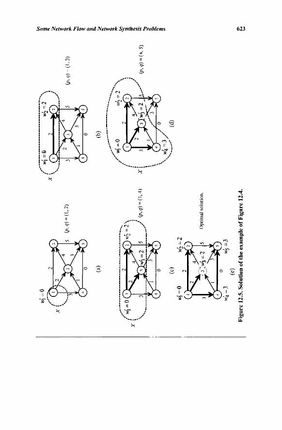
X
wj =
0
X
5 (P
, ?)
= (
!, 2)
(a)
/«i=
0(i
5 /
(P. ?
) =
0, 4
)
w'4
=3
w5
=3
(e)
Fig
ure
12.5
. Sol
utio
n of
the
exa
mp
le o
f F
igu
re 1
2.4.
f >
=0
x\
H^
=2
\
(P,i
) =
(l,
3)
(b)
/Ήί=
ο M<
7 =
2
^9 ;
(p,?
) =
(4,5
)
•v «
4=
3/
(d)
S
! ! Ì
624 Chapter 12
procedure as a label-setting algorithm.) In this manner, each iteration is of
complexity 0{m), and the algorithm is of complexity 0(m ). Observe also by
the foregoing inductive validation of the algorithm that at each (nonnull) step of the algorithm, the procedure determines a shortest path from node 1 to the selected minimal labeled node i. In fact, if at any iteration (< m - 1 ) of the algorithm, it turns out that the arc set (X, X) is empty, then the unlabeled nodes
in X are all obviously unreachable from node 1 and the nodes in X have their shortest paths from node 1 identified by the current shortest path tree. If all nodes are reachable from node 1, the algorithm will find the shortest paths from node 1 to all the nodes at the end of iteration (m - 1).
It turns out that the foregoing algorithm is actually an implementation of the primal simplex method. To see this relationship, assume for convenience that all nodes are reachable from node 1. Consider a minimum-cost network flow problem in which a supply of (m - 1) is placed at node 1 and each of the other nodes has a demand of one unit (i.e., b\ =(/w-l)and bt = - 1 , Vz = 2,...,m).
Suppose that we start with an all artificial basis, by designating node 1 as the root node, and constructing artificial arcs having big-M cost coefficients to directly connect node 1 with each of the nodes i = 2,..., m. Then, it is easy to verify that the first simplex iteration using the rule of entering the variable having the most positive zy - Cj- value is identical to the first iteration of
Dijkstra's algorithm. In fact, this is true for all the iterations. To see this, suppose that at some stage, we have a set of nodes still connected to node 1 via the artificial arcs, while the remaining nodes are connected to node 1 by (directed) paths in the current shortest path (sub)tree. Let X be a set that contains the latter nodes, and let X contain the former nodes. Note that the dual variables w( for
nodes / e X are all -M, while the dual variables w; for the nodes i e X are
equal to the negative of the total cost on the arcs in the respective paths connecting the nodes to node 1 in the current basis tree. Hence, we currently have Wj = -w\, as given by Dijkstra's algorithm. Note that the maximum (z;%- -
Cy)-value is realized for an arc (i,j) having i e Xandj e X (why?). Therefore,
the value max {Zj- - Cj-} = max {wt - w- - c,y :ieX,jsX} (Uj)
= - min {-M + w'j + c^ :i eX,j e X} (ij)
is realized by the same arc (p, q) as in Dijkstra's algorithm (why?). When the arc (p, q) enters the basis, the only reverse arc in the resulting cycle is the artificial arc, which therefore leaves the basis. Moreover, the subtree of the resulting basis tree induced by the nodes i n l u { q } is identical to the current
shortest path tree constructed by Dijkstra's algorithm. Hence, this algorithm coincides with a primal simplex implementation and produces an optimal basis tree for the previously-mentioned network flow problem at termination. This is verified by the foregoing validation of Dijkstra's algorithm (why?).
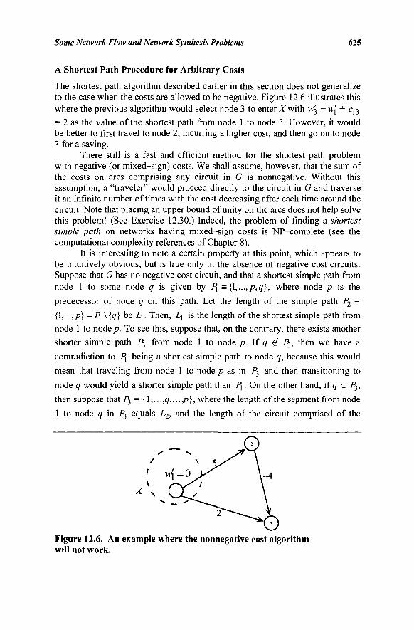
Some Network Flow and Network Synthesis Problems 625
A Shortest Path Procedure for Arbitrary Costs
The shortest path algorithm described earlier in this section does not generalize to the case when the costs are allowed to be negative. Figure 12.6 illustrates this where the previous algorithm would select node 3 to enter X with w3 = w[ + c13
= 2 as the value of the shortest path from node 1 to node 3. However, it would be better to first travel to node 2, incurring a higher cost, and then go on to node 3 for a saving.
There still is a fast and efficient method for the shortest path problem with negative (or mixed-sign) costs. We shall assume, however, that the sum of the costs on arcs comprising any circuit in G is nonnegative. Without this assumption, a "traveler" would proceed directly to the circuit in G and traverse it an infinite number of times with the cost decreasing after each time around the circuit. Note that placing an upper bound of unity on the arcs does not help solve this problem! (See Exercise 12.30.) Indeed, the problem of finding a shortest simple path on networks having mixed-sign costs is NP-complete (see the computational complexity references of Chapter 8).
It is interesting to note a certain property at this point, which appears to be intuitively obvious, but is true only in the absence of negative cost circuits. Suppose that G has no negative cost circuit, and that a shortest simple path from node 1 to some node q is given by Py ={\,...,p,q}, where node p is the
predecessor of node q on this path. Let the length of the simple path P2 =
{Ι,.,.,ρ} = P\\{q} be L\. Then, Z,j is the length of the shortest simple path from
node 1 to node p. To see this, suppose that, on the contrary, there exists another
shorter simple path P3 from node 1 to node p. If q 0 P^, then we have a
contradiction to Pl being a shortest simple path to node q, because this would
mean that traveling from node 1 to node p as in P3 and then transitioning to
node q would yield a shorter simple path than Px. On the other hand, if q e P3,
then suppose that P}= {l,...,q,...,p}, where the length of the segment from node
1 to node q in P3 equals L^, and the length of the circuit comprised of the
Figure 12.6. An example where the nonnegative cost algorithm will not work.
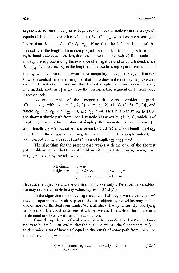
626 Chapter 12
segment of P^ from node q to node p, and then back to node q via the arc (p, q),
equals C. Hence, the length of P^ equals L^ +C-cpq, which we are asserting is
lesser than L], i.e., L2+C<L\+cpq. Note that the left-hand-side of this
inequality is the length of a nonsimple path from node 1 to node q, whereas the right-hand-side equals the length of the shortest simple path P\ from node 1 to node q, thereby portending the existence of a negative cost circuit. Indeed, since L\ + cpq < Li because L2 is the length of a particular simple path from node 1 to
node q, we have from the previous strict inequality that Lq+C < Ζ^, or that C <
0, which contradicts our assumption that there does not exist any negative cost circuit. By induction, therefore, the shortest simple path from node 1 to any intermediate node in P\ is given by the corresponding segment of Pl from node
1 to that node. As an example of the foregoing discussion, consider a graph
G(. / ,. - / ) with / ■ = {1, 2, 3}, . -/= {(1, 2), (1, 3), (2, 3), (3, 2)}, and
where q 2 = 2, C]3 ~ 5, c23 = 1, and c32 = —4. Then it is readily verified that the shortest simple path from node 1 to node 3 is given by {1, 2, 3}, which is of length cj2 +
c23 = 3, but the shortest simple path from node 1 to node 2 is not {1, 2} of length c12 = 2, but rather, it is given by {1, 3, 2} and is of length q 3 + c32
= 1. Hence, there must exist a negative cost circuit in this graph; indeed, the loop formed by the arcs (2, 3) and (3, 2) is of length c23 +c32 = - 3 .
The algorithm for the present case works with the dual of the shortest path problem. Recall that the dual problem with the substitution w[ = - w; for i = \,...,m is given by the following:
Maximize w'm - w\ subject to w'j - w'i < Cy i,j = \,...,m
w'j unrestricted, i = l,...,m.
Because the objective and the constraints involve only differences in variables, we may set one variable to any value, say w{ = 0 (why?).
In the algorithm for mixed-sign costs we shall begin with a choice of w' that is "superoptimal" with respect to the dual objective, but which may violate one or more of the dual constraints. We shall show that by iteratively modifying w' to satisfy the constraints, one at a time, we shall be able to terminate in a finite number of steps with an optimal solution.
Considering the set of nodes reachable from node 1 and assuming these nodes to be i = 2,..., m, and noting the dual constraints, the fundamental task is to determine a set of labels w'j equal to the length of some path from node 1 to node / for / = 2,..., m such that
w'· = minimum {W'+q·} for ally = 2,..., m. (12.4) i:{i,j) exists
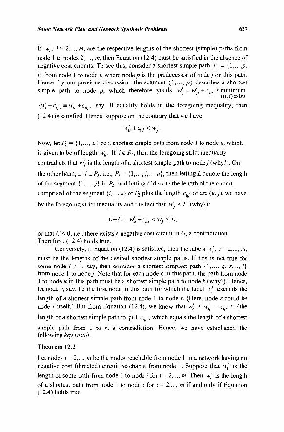
Some Network Flow and Network Synthesis Problems 627
If w\, i = 2,..., m, are the respective lengths of the shortest (simple) paths from node 1 to nodes 2,..., m, then Equation (12.4) must be satisfied in the absence of negative cost circuits. To see this, consider a shortest simple path P{ = {Ι,.,.,ρ,
j) from node 1 to node j , where node/7 is the predecessor of nodey on this path. Hence, by our previous discussion, the segment {Ι,.,.,ρ} describes a shortest simple path to node p, which therefore yields w'- =w'+ c „.· > minimum
i'.(i,j) exists
{w'i + Cjj} = w'u + cuj, say. If equality holds in the foregoing inequality, then
(12.4) is satisfied. Hence, suppose on the contrary that we have
w'u+cuj<w'j.
Now, let P2 = {1,..., u} be a shortest simple path from node 1 to node u, which
is given to be of length w'u. If j g P2, then the foregoing strict inequality
contradicts that w'· is the length of a shortest simple path to nodey (why?). On
the other hand, if j sP2, i.e., P2 = {l,...,j,... u}, then letting! denote the length
of the segment {1,...,_/} in P2, and letting Cdenote the length of the circuit
comprised of the segment {/,..., u} ofP2 plus the length c · of arc (uj), we have
by the foregoing strict inequality and the fact that w'· < L (why?):
L + C = w'u+cuj<w'j<L,
or that C < 0, i.e., there exists a negative cost circuit in G, a contradiction. Therefore, (12.4) holds true.
Conversely, if Equation (12.4) is satisfied, then the labels w·, i = 2,..., m, must be the lengths of the desired shortest simple paths. If this is not true for some nodey' Φ 1, say, then consider a shortest simplest path {1,..., q, r,...,j} from node 1 to nodey. Note that for each node k in this path, the path from node 1 to node k in this path must be a shortest simple path to node k (why?). Hence, let node r, say, be the first node in this path for which the label w'r exceeds the length of a shortest simple path from node 1 to node r. (Here, node r could be nodey itself.) But from Equation (12.4), we know that w'r < w' + cqr = (the
length of a shortest simple path to q) + cqr, which equals the length of a shortest
simple path from 1 to r, a contradiction. Hence, we have established the following key result.
Theorem 12.2
Let nodes / = 2,..., m be the nodes reachable from node 1 in a network having no negative cost (directed) circuit reachable from node 1. Suppose that w\ is the length of some path from node 1 to node i for / = 2,..., m. Then w\ is the length of a shortest path from node 1 to node i for i = 2,..., m if and only if Equation (12.4) holds true.
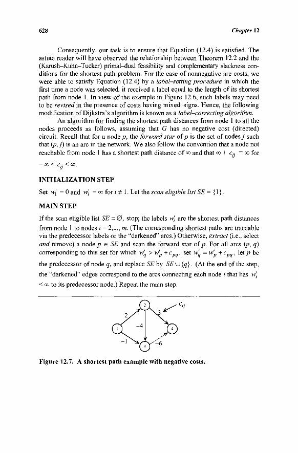
628 Chapter 12
Consequently, our task is to ensure that Equation (12.4) is satisfied. The astute reader will have observed the relationship between Theorem 12.2 and the (Karush-Kuhn-Tucker) primal-dual feasibility and complementary slackness con-ditions for the shortest path problem. For the case of nonnegative arc costs, we were able to satisfy Equation (12.4) by a label-setting procedure in which the first time a node was selected, it received a label equal to the length of its shortest path from node 1. In view of the example in Figure 12.6, such labels may need to be revised in the presence of costs having mixed-signs. Hence, the following modification of Dijkstra's algorithm is known as a label-correcting algorithm.
An algorithm for finding the shortest path distances from node 1 to all the nodes proceeds as follows, assuming that G has no negative cost (directed) circuit. Recall that for a node/7, the forward star ofp is the set of nodes y such that (p,j) is an arc in the network. We also follow the convention that a node not reachable from node 1 has a shortest path distance of oo and that co + c;y = <x> for
— 00 < Cjj < CO.
INITIALIZATION STEP
Set w{ = 0 and w\ = co for /' Φ 1. Let the scan eligible list SE = {1}.
MAIN STEP
If the scan eligible list SE = 0 , stop; the labels w\ are the shortest path distances from node 1 to nodes / = 2,..., m. (The corresponding shortest paths are traceable via the predecessor labels or the "darkened" arcs.) Otherwise, extract (i.e., select and remove) a node p e SE and scan the forward star of p. For all arcs (p, q) corresponding to this set for which w'q > w'p + cpq, set w'q=w'p+ cpq, let p be
the predecessor of node q, and replace SE by SE u {q}. (At the end of the step,
the "darkened" edges correspond to the arcs connecting each node / that has w\
< co to its predecessor node.) Repeat the main step.
Figure 12.7. A shortest path example with negative costs.
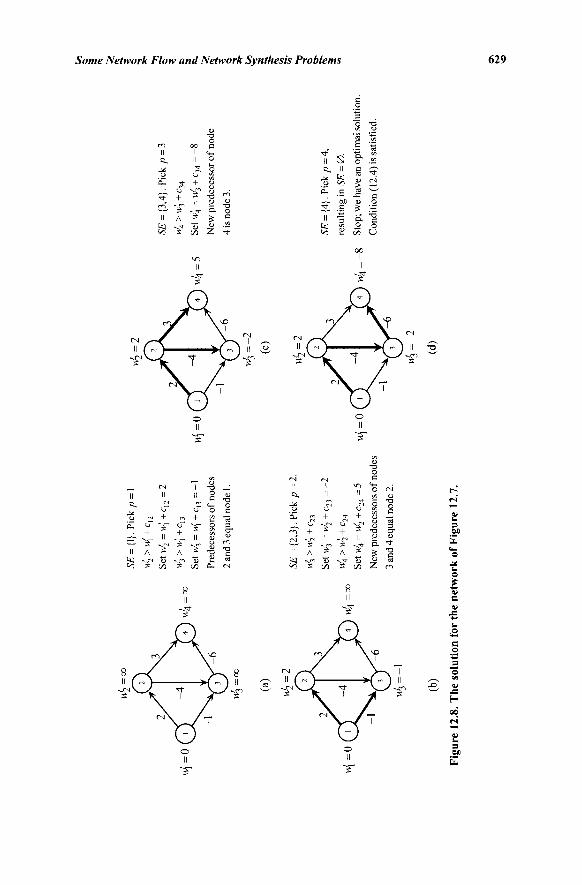
w[=
0
u{=
0
Μ^
=0
0
U$
=-l
(b)
SE =
{\}
. Pic
k p
= l
vif 4
= C
O
W2
> W
] +
C1
2
Set w
2 =
w\ +
c 12
=2
w>3
> w
j +
c 13
Set w
j = w
[ +
C| 3
=-1
1-
^=
0
Pred
eces
sors
of
node
s
2 an
d 3
equa
l nod
e 1.
SE =
{2,
3}. P
ick
p =
2.
w,
> w
-, +
cr
w4
> w
2 +
c24
Set
vf 4 =
w' 2
+ c 2
4 =
5
New
pre
dece
ssor
s of
nod
es
3 an
d 4
equa
l nod
e 2.
wj
=0
wA_
=2
H>2
=2
5£ =
{3,
4}.P
ickp
= 3
Vf 4
> W
3 +
C34
Set i
v 4 =
W3
+ c 3
4 =
-8
New
pre
dece
ssor
of
node
4 is
nod
e 3.
S£
= {4
}.P
ickp
= 4
,
resu
lting
in S
E =
0.
_g
Stop
; we
have
an
optim
al s
olut
ion.
Con
ditio
n (1
2.4)
is s
atis
fied
.
3 ft 3 ft.
5;
Fig
ure
12.
8. T
he
solu
tion
for
th
e n
etw
ork
of F
igu
re 1
2.7.
ve
630 Chapter 12
An Example of the Shortest Path Algorithm for Arbitrary Costs
Consider the network of Figure 12.7 where we wish to find the shortest path from node 1 to all the nodes. In Figure 12.8 we present the complete solution of the example by the previous algorithm. There is no required order in which the nodes must be selected from SE at each stage for the algorithm to converge. However, as we shall see subsequently, the choice of selecting the next node from SE does affect both the theoretical and practical efficiency of the algorithm. When the algorithm stops, Figure 12.8d gives the shortest paths and their values w\, along with the shortest path tree or arborescence. Arcs (/',_/) along the shortest path (i.e., belonging to the shortest path tree) have w'j -w'j = Cy. For any arc (i,j) in the shortest path tree at any stage, where / is
the predecessor of j , if we have the property w' = w\ + Cy holding true, we say
that the corresponding labels are sharp with respect to this arc. Hence, the foregoing statement asserts that the w'-labels are sharp with respect to the shortest path tree arcs at termination of the algorithm. We shall provide more rigor and insights into this observation in the discussion that follows next.
Verification of the Algorithm for Arbitrary Costs
We shall first show that when w[ < oo, this value represents the cost of some
path (not necessarily simple) from node 1 to node i. We note that in computing the cost of a (not necessarily simple) path, we must count the cost of an arc as many times as the arc appears in the path. Thus, for a nonsimple path P = {(1, 3), (3, 4), (4, 5), (5, 3), (3, 4), (4, 6)} the associated cost would be c]3 +c34 + c45 + c53 +c34 +c46· As w e s ^ a " see> nonsimple paths play a part in the algo-rithm only when there is a negative cost circuit in G.
We shall demonstrate that w'j (< oo) represents the cost of a path from
node 1 to node i at every iteration of the procedure. Now, since we start with w{ = 0 and w'j = oo for i'Φ 1, the result is true at
the first iteration. This is so because w[ = 0 represents the cost of the (empty)
path, which contains no arcs, from node 1 to node 1. Assume that the result is true at iteration t; that is, suppose that w- (< oo)
represents the cost of some (not necessarily simple) path from node 1 to node i. Consider iteration t+ \. Suppose that for i e SE, we find that w'j + Cy < w'j, in
which case, we set w' = w'j + Cy. By assumption, there exists a path Pt from
node 1 to node / at iteration t having cost w\. Consider the path Pj = P,; u {(i,j)}.
This path has a cost of w'j + Cy = w'- and the result is true at iteration t + 1. Thus,
if w'k < GO, then there exists a (not necessarily simple) path P from node 1 to
node k along which Σ(/ /)ejp% = w'k.
If there is no negative cost circuit in G, then the cost of any nonsimple path is greater than or equal to the cost of the corresponding simple path after
Some Network Flow and Network Synthesis Problems 631
eliminating the circuits in this path (why?). Hence, in the absence of negative cost circuits, w'j is bounded from below by the cost of a shortest simple path,
and thus by a finite integer (why?). Finally, treating <x> as a large integer, since 0 < \SE\ < m — 1, and since the two-tuple {T.iw'i, \$E\} lexicographically decreases by a positive integer at each iteration (why?), the shortest path algorithm will stop in a finite number of steps if G has no negative cost circuit. Moreover, at termination, if any w\ = oo, then it is readily verified that node i is unreachable from node 1, and vice versa.
Let us show that at termination, the labels w\ are the corresponding
shortest path distances. From Theorem 12.2, it is sufficient to show that Equation (12.4) holds true for the nodes reachable from node 1. Consider any node q Φ 1, and let node u be the predecessor of node q at termination. Then we must have w' =w'u+ cu„ i.e., the w' -labels must be sharp for the arc (u, q). To
see this, note that this is true when w' was finally set at its terminal (minimal)
value with node u being its predecessor. If, on the contrary, the label w'u was
subsequently revised (and therefore lowered), then node u would have entered SE and, when selected for scanning, would have subsequently revised the label of node q to a lower value, which contradicts the final setting of the label of q. Hence, we have,
K = w'u + cuq ^ minimum {w\ + ciq } = w'p+cpq, say. i:(i,q) exists
If equality holds in the foregoing inequality, then (12.4) is satisfied for this (arbitrary) node q. Hence, on the contrary, suppose that w'q > w'p + cpq.
However, after w'p < oo was set for the final time in the algorithm and was later
selected from SE for the final time, we should have relabeled node q since w'„ >w'p + cpq. Hence, we have a contradiction and therefore, the algorithm
produces the required shortest paths. In fact, at termination, the predecessor labels produce a shortest path tree (actually, an arborescence). To see this, note that we commence with an arborescence having node 1 as the root node being directly connected to each of the nodes 2,..., m via artificial big-M(virtually, infinite cost) arcs. Inductively, suppose that we have an arborescence at any given stage when we scan the forward star of some node p e SE, and discover a node q in this set having w' > w'p + c ,
based on which, we revise the label w'„ to equal w'p + cpq and we set the
predecessor of node q to node/?. If node q already had node/? as its predecessor, this would not alter the current arborescence (this step would only serve the purpose of making the labels sharp with respect to the arc (p, q)). Otherwise, suppose that we trace the chains (reverse paths) from nodes p and q to the root node 1, and let k be the first common node encountered on these chains. First, suppose that k Φ q (we might have k = p or k = 1). In this case, let u Φ ρ be the
632 Chapter 12
previous predecessor of node q (which belongs to the non-null chain from q to k). When we change just the predecessor of node q from u top, this is equivalent to adding the arc (p, q) to the current arborescence and removing the arc (w, q). The resulting graph is also an arborescence (why?). Observe that this is akin to performing a primal network simplex type tree update. However, it is insightful to note at this point that we are not executing a full dual update because we only revise the label of node q alone to the lower value, and do not simultaneously decrease by the same amount the labels of all the nodes in the subtree Tq
containing q that is obtained by deleting arc (w, q) in the current tree, as we would in a network simplex iteration. Hence, although the node labels are sharp at termination for the arcs in the final tree, they are not necessarily sharp for all the arcs in intermediate trees. Hence, unlike as for Dijkstra's algorithm for the nonnegative cost case, the present scheme differs from a standard network simplex implementation.
On the other hand, suppose that q = k. In this case, the current arborescence contains a path P = {1,..., u, q,...,p] from node 1 to node p. By revising the predecessor label of q from u to p, i.e., by adding the arc (p, q) to the current arborescence and removing the arc («, q), we would create a circuit comprised of the segment {q,...,p} in the path P, plus the return arc (p, q). Let C be the length of this circuit. As one might guess, it must be the case that C < 0, i.e., we have a negative cost circuit in G, which would contradict our standing assumption. To verify this, let L be the length of the segment {q,..., p} in the path P, so that C = L + cpq. Note that if the w' -labels were sharp with respect
to all the arcs in the path segment {<?,..., p} within P, we would have w' =w'+L (why?). However, as discussed above, we may not have this
sharpness property holding true for all the arcs in the path segment {q,...,p} of P. Hence, in general, we have W > w' +L > w' +cpq +L, or that C = L +
cp < 0, a contradiction.
Assuming that all nodes are reachable from node 1 (via big-M artificial arcs, if necessary), the reader may now observe that the final resulting shortest path tree (arborescence) produced is primal feasible for the corresponding minimum cost network flow program that has b\=m-\ and £,·=-!,
Vi = 2,...,m. Moreover, the dual solution w; = -w\, i = 1,..., m, is dual feasible and is complementary slack with respect to this solution. Hence, this tree yields an optimal basis.
We also have at hand a way to determine whether the network contains a negative cost circuit reachable from node 1. If no negative cost circuit exists, then c0 = Zc,.<oci/ is a lower bound on the w' -labels (why?). Thus, if any w\
falls below c0 during the algorithm, a negative cost circuit must exist and we
can then terminate the shortest path algorithm.
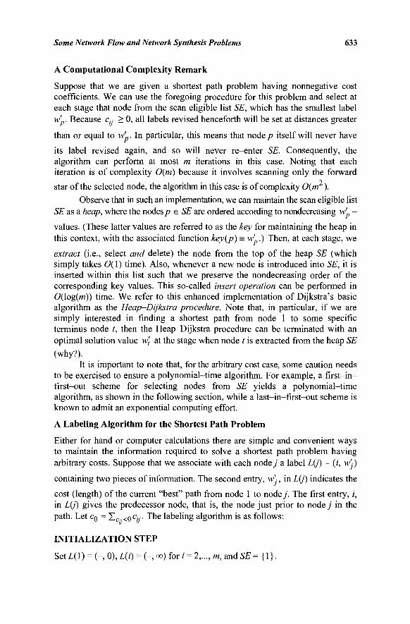
Some Network Flow and Network Synthesis Problems 633
A Computational Complexity Remark
Suppose that we are given a shortest path problem having nonnegative cost coefficients. We can use the foregoing procedure for this problem and select at each stage that node from the scan eligible list SE, which has the smallest label w'p. Because Cy > 0, all labels revised henceforth will be set at distances greater
than or equal to w' . In particular, this means that node p itself will never have
its label revised again, and so will never re-enter SE. Consequently, the algorithm can perform at most m iterations in this case. Noting that each iteration is of complexity 0(m) because it involves scanning only the forward
star of the selected node, the algorithm in this case is of complexity 0(m ).
Observe that in such an implementation, we can maintain the scan eligible list SE as a heap, where the nodes/» e SE are ordered according to nondecreasing w' -
values. (These latter values are referred to as the key for maintaining the heap in this context, with the associated function key(p) = w' .) Then, at each stage, we
extract (i.e., select and delete) the node from the top of the heap SE (which simply takes 0(1) time). Also, whenever a new node is introduced into SE, it is inserted within this list such that we preserve the nondecreasing order of the corresponding key values. This so-called insert operation can be performed in 0(\og{m)) time. We refer to this enhanced implementation of Dijkstra's basic algorithm as the Heap-Dijkstra procedure. Note that, in particular, if we are simply interested in finding a shortest path from node 1 to some specific terminus node t, then the Heap-Dijkstra procedure can be terminated with an optimal solution value w't at the stage when node t is extracted from the heap SE
(why?). It is important to note that, for the arbitrary cost case, some caution needs
to be exercised to ensure a polynomial-time algorithm. For example, a first-in-first-out scheme for selecting nodes from SE yields a polynomial-time algorithm, as shown in the following section, while a last-in-first-out scheme is known to admit an exponential computing effort.
A Labeling Algorithm for the Shortest Path Problem
Either for hand or computer calculations there are simple and convenient ways to maintain the information required to solve a shortest path problem having arbitrary costs. Suppose that we associate with each node/ a label L(j) = (/, w')
containing two pieces of information. The second entry, w', in L(J) indicates the
cost (length) of the current "best" path from node 1 to node j . The first entry, i, in L(J) gives the predecessor node, that is, the node just prior to node j in the path. Let c0 = Zc..<oc!y· The labeling algorithm is as follows:
INITIALIZATION STEP
Set L(l) = (-, 0), L(i) = (-, oo) for i = 2,..., m, and SE = {1}.
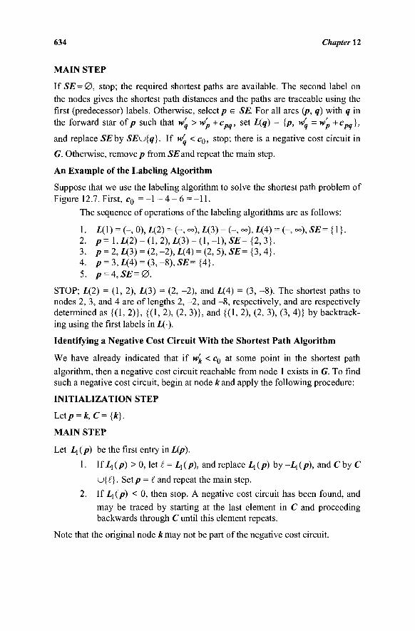
634 Chapter 12
MAIN STEP
If SE=0, stop; the required shortest paths are available. The second label on the nodes gives the shortest path distances and the paths are traceable using the first (predecessor) labels. Otherwise, select p e SE. For all arcs (p, q) with q in the forward star of p such that w' > w' +c„„, set L(q) = {p, w'= w' +cpq),
and replace SE by SEu{q}. If w < c0, stop; there is a negative cost circuit in
G. Otherwise, remove/; from SE and repeat the main step.
An Example of the Labeling Algorithm
Suppose that we use the labeling algorithm to solve the shortest path problem of Figure 12.7. First, c0 = -1 - 4 - 6 = -11.
The sequence of operations of the labeling algorithms are as follows:
1. L(l) = (-, 0),U2) = (-, oo),L{3) = (- =.), L(4) = (-, oo),SE={\}. 2. p=l,L(2) = (l,2),L(3) = (l,-\),SE={2,3}-3. p = 2, L(3) = (2, -2), 1(4) = (2, 5), SE= {3, 4}. 4. p = 3,L(4) = (3,-8),SE={4}. 5. p = 4,SE=0.
STOP; 1(2) = (1, 2), L(3) = (2, -2), and 1(4) = (3, -8). The shortest paths to nodes 2, 3, and 4 are of lengths 2, -2 , and -8 , respectively, and are respectively determined as {(1, 2)}, {(1, 2), (2, 3)}, and {(1, 2), (2, 3), (3, 4)} by backtrack-ing using the first labels in L(-).
Identifying a Negative Cost Circuit With the Shortest Path Algorithm
We have already indicated that if w'k < c0 at some point in the shortest path
algorithm, then a negative cost circuit reachable from node 1 exists in G. To find such a negative cost circuit, begin at node k and apply the following procedure:
INITIALIZATION STEP
Letp = k,C={k}.
MAIN STEP
Let Ly{p) be the first entry in Lip).
1. If Ly (p) > 0, let I = Z·! (/>), and replace L} (p) by ^ (p), and C by C
u{i}. Set/» = I and repeat the main step.
2. If L\(p) < 0, then stop. A negative cost circuit has been found, and may be traced by starting at the last element in C and proceeding backwards through C until this element repeats.
Note that the original node £ may not be part of the negative cost circuit.
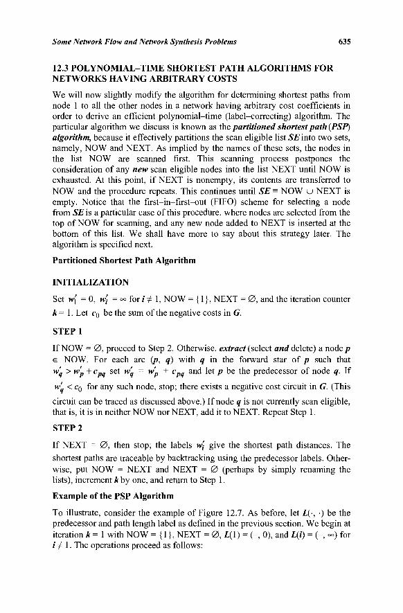
Some Network Flow and Network Synthesis Problems 635
12.3 POLYNOMIAL-TIME SHORTEST PATH ALGORITHMS FOR NETWORKS HAVING ARBITRARY COSTS
We will now slightly modify the algorithm for determining shortest paths from node 1 to all the other nodes in a network having arbitrary cost coefficients in order to derive an efficient polynomial-time (label-correcting) algorithm. The particular algorithm we discuss is known as the partitioned shortest path (PSP) algorithm, because it effectively partitions the scan eligible list SE into two sets, namely, NOW and NEXT. As implied by the names of these sets, the nodes in the list NOW are scanned first. This scanning process postpones the consideration of any new scan eligible nodes into the list NEXT until NOW is exhausted. At this point, if NEXT is nonempty, its contents are transferred to NOW and the procedure repeats. This continues until SE = NOW u NEXT is empty. Notice that the first-in-first-out (FIFO) scheme for selecting a node from SE is a particular case of this procedure, where nodes are selected from the top of NOW for scanning, and any new node added to NEXT is inserted at the bottom of this list. We shall have more to say about this strategy later. The algorithm is specified next.
Partitioned Shortest Path Algorithm
INITIALIZATION
Set w\ = 0, w'i = °° for i Φ 1, NOW = {1}, NEXT = 0 , and the iteration counter
k = 1. Let CQ be the sum of the negative costs in G.
STEP1
If NOW = 0 , proceed to Step 2. Otherwise, extract (select and delete) a node/» e NOW. For each arc (p, q) with q in the forward star of p such that w' > w' + cpq set w' = w'p + cpq and let p be the predecessor of node q. If
w' < CQ for any such node, stop; there exists a negative cost circuit in G. (This
circuit can be traced as discussed above.) If node q is not currently scan eligible, that is, it is in neither NOW nor NEXT, add it to NEXT. Repeat Step 1.
STEP 2
If NEXT = 0 , then stop; the labels w\ give the shortest path distances. The shortest paths are traceable by backtracking using the predecessor labels. Other-wise, put NOW = NEXT and NEXT = 0 (perhaps by simply renaming the lists), increment k by one, and return to Step 1.
Example of the PSP Algorithm
To illustrate, consider the example of Figure 12.7. As before, let L(-, ■) be the predecessor and path length label as defined in the previous section. We begin at iteration k = 1 with NOW = {1}, NEXT = 0 , L(\) = (-, 0), and L(i) = (-, °°) for ι Φ 1. The operations proceed as follows:
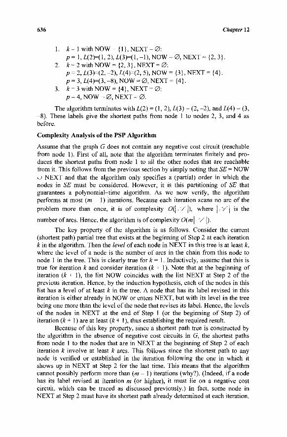
636 Chapter 12
1. k=\ with NOW = {1}, NEXT = 0 : p = 1, L(2)=( 1, 2), L(3)=( 1,-1), NOW = 0 , NEXT ={2,3}.
2. A: = 2 with NOW ={2, 3}, NEXT = 0 : p = 2, Z,(3)=(2, -2), I(4)=(2, 5), NOW = {3}, NEXT = {4}. p = 3, i(4)=(3, -8), NOW = 0 , NEXT = {4}.
3. A: = 3 with NOW ={4}, NEXT = 0 : p = 4, NOW = 0 , NEXT = 0 .
The algorithm terminates with 1(2) = (1,2), 1(3) = (2, -2), and L(4) = (3, -8). These labels give the shortest paths from node 1 to nodes 2, 3, and 4 as before.
Complexity Analysis of the PSP Algorithm
Assume that the graph G does not contain any negative cost circuit (reachable from node 1). First of all, note that the algorithm terminates finitely and pro-duces the shortest paths from node 1 to all the other nodes that are reachable from it. This follows from the previous section by simply noting that SE = NOW u NEXT and that the algorithm only specifies a (partial) order in which the nodes in SE must be considered. However, it is this partitioning of SE that guarantees a polynomial-time algorithm. As we now verify, the algorithm performs at most (m - 1) iterations. Because each iteration scans no arc of the problem more than once, it is of complexity 0( | . ' /1), where \-"/\ is the
number of arcs. Hence, the algorithm is of complexity 0(m\ Y |).
The key property of the algorithm is as follows. Consider the current (shortest path) partial tree that exists at the beginning of Step 2 at each iteration k in the algorithm. Then the level of each node in NEXT in this tree is at least k, where the level of a node is the number of arcs in the chain from this node to node 1 in the tree. This is clearly true for k = 1. Inductively, assume that this is true for iteration k and consider iteration (k + 1). Note that at the beginning of iteration {k + 1), the list NOW coincides with the list NEXT at Step 2 of the previous iteration. Hence, by the induction hypothesis, each of the nodes in this list has a level of at least k in the tree. A node that has its label revised in this iteration is either already in NOW or enters NEXT, but with its level in the tree being one more than the level of the node that revises its label. Hence, the levels of the nodes in NEXT at the end of Step 1 (or the beginning of Step 2) of iteration (k + 1 ) are at least (k+ 1 ), thus establishing the required result.
Because of this key property, since a shortest path tree is constructed by the algorithm in the absence of negative cost circuits in G, the shortest paths from node 1 to the nodes that are in NEXT at the beginning of Step 2 of each iteration k involve at least k arcs. This follows since the shortest path to any node is verified or established in the iteration following the one in which it shows up in NEXT at Step 2 for the last time. This means that the algorithm cannot possibly perform more than (m - 1) iterations (why?). (Indeed, if a node has its label revised at iteration m (or higher), it must lie on a negative cost circuit, which can be traced as discussed previously.) In fact, some node in NEXT at Step 2 must have its shortest path already determined at each iteration.
Some Network Flow and Network Synthesis Problems 637
This follows because the current list NEXT becomes the list NOW for the next iteration, and since all nodes relabeled from this point onward must have a node in this list on the chain to node 1, we cannot possibly have all the nodes in this list repeating or else we would have a cycle.
For the foregoing example, at the end of iteration k = 1, node 2 e NEXT has its shortest path determined, and at the end of iteration k = 2, node 4 e NEXT has its shortest path determined. Node 3 shows up in NEXT for the last time at (the end of) iteration k = 1 and has its shortest path determined during iteration k = 2. The levels of nodes 2, 3, and 4 in the final shortest path tree are 1, 2, and 3, respectively.
As far as computational implementation strategies are concerned, note that we could maintain the list NEXT as a heap, where the nodes are arranged in nondecreasing order of the labels w\ (which serve as the key for the heap).
Hence, each time a new node q is introduced into NEXT (or the label of an existing node q is revised within NEXT), it is inserted (or re-inserted) into NEXT to preserve the nondecreasing order of the labels w\. Then, once NEXT
is transferred to NOW at the end of any iteration, the nodes are subsequently extracted one at a time from NOW from the top of the list. However, in spite of its efficiency, this strategy turns out to be computationally expensive relative to a simple FIFO procedure because of the relative ease with which shortest path problems are solved using Algorithm PSP. On the other hand, a slight modification to the FIFO strategy yields an empirical advantage. In this strategy, letting w'j be the label of the node that is currently at the top of the list
NEXT, whenever a new node q having the label w' is inserted into NEXT, then
this node q is added to the top of the list NEXT if w' < w' , and otherwise, it
is inserted to the bottom of this list. The following section discusses a somewhat more sophisticated variation of this concept of maintaining an approximate heap that turns out to be even more effective in practice.
Threshold Partitioned Shortest Path Algorithm
A noteworthy computationally efficient variant of the PSP algorithm, particu-larly for nonnegative cost coefficients, has been designed to operate as follows. At the end of every iteration k, a suitable threshold value t is computed. Instead of transferring the entire list NEXT into NOW, only those nodes i e NEXT are placed in NOW that have w\ < t. The value t is tuned heuristically based on the network structure, but of course always satisfies t > minimum {w\: i e NEXT}.
Additionally, at Step 1 of the PSP algorithm, whenever a node q has its label updated and q is not a member of NOW, it is checked whether or not the revised w'q exceeds the current threshold value /. If w' > t, then node q is added to
NEXT as before. Otherwise, node q is added to a separate list NOW' (unless it is already there) and it is removed from NEXT if it happens to be there. Then, when NOW becomes empty, the contents of NOW' are transferred to NOW and the process repeats by scanning the nodes in NOW as before, until both NOW
638 Chapter 12
and NOW are empty. At this point, if we also have NEXT = 0 , then the method terminates. Otherwise, an appropriate revised threshold value t is computed, and all nodes i in NEXT that have their label values wj < t are
transferred to NOW, while the remaining nodes are retained in the list NEXT. The algorithm then resumes processing the nodes in NOW as before.
Observe that when all costs are nonnegative, the nodes having the small-est w'j -labels in the list NOW' or NEXT that are transferred into NOW have their shortest path distances already determined, and so will not show up in any subsequent set. Hence, there can be no more than (m - 1) total transfers from NOW' or NEXT into NOW. Because the effort involved between each such transfer is of complexity 0(\ ■'/1), the algorithm is of complexity 0(m\ .r/1).
Computationally, any new nodes added to NOW' or NEXT can either be appended to the bottom of these lists, or can be inserted into these lists as suggested for Algorithm PSP. Nodes are typically extracted from the top of the list NOW for scanning next, but it has also been suggested that nodes from NOW be selected in a last-in-first-out order. Empirically, the threshold partitioned shortest path algorithm has been found to be computationally superior on several types of networks, particularly, having nonnegative costs (see the Notes and References section).
Some Extensions of Shortest Path Problems
We conclude this section by indicating several interesting variants of shortest path problems that have been analyzed in the literature. One such variant is the time-dependent shortest path problem, which frequently arises in transportation networks that are subject to traffic congestion. Here, the duration required to traverse any arc (the arc cost) can be time-dependent, i.e., in general, it can be a function of the time that this arc is entered via its from-node. One can concep-tualize such networks in an expanded time—space representation in which each node i is replicated for all possible times t that it can be entered, and accord-ingly, it is represented by the two-tuple (i, t). An arc connects node (i, t\ ) to a
node (j, /2) in this network whenever there exists an arc (i,j) in the original
network for which the time to traverse this arc when entering node i at time ίχ
equals (t2 - t \ ). The "cost" on this arc is therefore simply a constant equal to
(t2 -1\ ). By conceptualizing the problem over this time-space network either
explicitly or implicitly, depending on the nature of the traversal time functions, the various algorithms discussed for the standard shortest path problem can be extended to such time-dependent problems. In particular, if the arc traversal times possess a first-in-first-out property, i.e., entering an arc at a relatively earlier time ensures exiting it also at a relatively earlier time, then this time-dependent shortest path problem is solvable in polynomial time as for the standard case. Otherwise, in general, the problem is known to be NP-hard (see the Notes and References section for definitions and details). Further extensions of this problem have also been considered in which arcs additionally have par-ticular labels (e.g., designating modes of transportation), and one is required to
Some Network Flow and Network Synthesis Problems 639
determine a time-dependent shortest path for which the corresponding sequence of labels belongs to a set of acceptable strings of labels. For instance, in a mul-timodal network having various modes of transportation such as cars, buses, trains, and even walking or biking, a user might specify various admissible strings such as, e.g., walk —* train —> bus —► walk, from an origin to a destina-tion. Here, each specified mode can be repeated several consecutive times via the arc labels in the prescribed shortest path solution. This is known as a label-constrained {time-dependent) shortest path problem. Other extensions include problems where the traversal time on any arc (/, J) might also depend on the previous arc leading to node i (in order to represent, e.g., left turns versus straight crossings into arc (/, j) at traffic road intersections), or the traversal times might be random variables. The former class of problems are called approach-dependent shortest path problems (and can also be label-constrained and time-dependent), whereas the latter class of problems are known as stochastic shortest path problems, or as dynamic stochastic shortest path problems in the case when the actual traversal cost on an arc is (stochastically) realized when reaching the entering node of the particular arc. We refer the reader to the Notes and References section for further details and information regarding these problems.
12.4 MULTICOMMODITY FLOWS
In all of the flow problems we have considered to this point, it has not been necessary to distinguish among the units flowing in the network. This class of network flow problems is called single-commodity flow problems. There is also a class of network flow problems called multicommodity flow problems in which it is necessary to distinguish among the flows in the network.
The most natural example of multicommodity flows occurs in rush hour traffic in any metropolitan city. If the area is divided into zones, then there are a number of people in zone / who must travel to work in zoney. There are also a number of people who must travel from zonej to work in zone i. The locations at which people originate inherit a corresponding supply (b > 0), and where they wish to go, we obtain a corresponding demand (b < 0). If we treat the problem as a single-commodity flow problem, a minimal-cost flow procedure (network simplex or out-of-kilter) would use the supply of people in a given zone to satisfy the demand in the same zone. This is an unacceptable solution. In this problem and ones like it, we must distinguish between the different types of flow and be careful to retain their identity and flow pattern throughout the optimization procedure. That is, we must essentially have a different flow vector and a set of conservation equations for each commodity.
As we shall see, multicommodity flow problems do not enjoy the same special properties as single-commodity flow problems. As an example, consider the network of Figure 12.9. Suppose that there are three commodities that flow through the network. The source for commodity 1 is node 1, and the sink for commodity 1 is node 3. That is, commodity 1 must originate only at node 1 and terminate only at node 3. Similarly, let the source and sink for commodity 2 be nodes 2 and 1, respectively. Finally, the source and sink for commodity 3 are nodes 3 and 2, respectively. With the restriction that the sum of all commodities
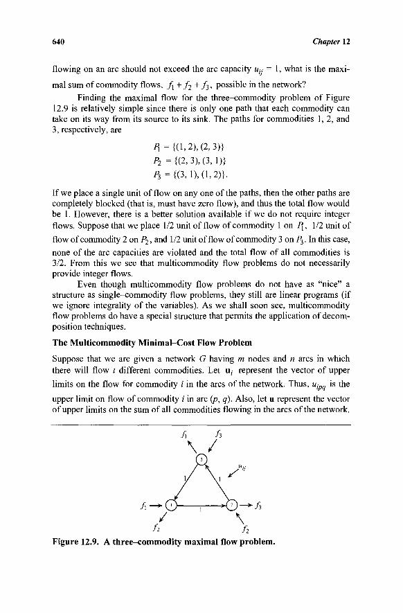
640 Chapter 12
flowing on an arc should not exceed the arc capacity Uy = 1, what is the maxi-
mal sum of commodity flows, f\+ f2+ fi, possible in the network? Finding the maximal flow for the three-commodity problem of Figure
12.9 is relatively simple since there is only one path that each commodity can take on its way from its source to its sink. The paths for commodities 1, 2, and 3, respectively, are
/>!={(1,2),(2,3)}
P2={(2,3),(3,1)}
F3={(3,1),(1,2)}.
If we place a single unit of flow on any one of the paths, then the other paths are completely blocked (that is, must have zero flow), and thus the total flow would be 1. However, there is a better solution available if we do not require integer flows. Suppose that we place 1/2 unit of flow of commodity 1 on fj, 1/2 unit of
flow of commodity 2 on P2, and 1/2 unit of flow of commodity 3 on P3. In this case,
none of the arc capacities are violated and the total flow of all commodities is 3/2. From this we see that multicommodity flow problems do not necessarily provide integer flows.
Even though multicommodity flow problems do not have as "nice" a structure as single-commodity flow problems, they still are linear programs (if we ignore integrality of the variables). As we shall soon see, multicommodity flow problems do have a special structure that permits the application of decom-position techniques.
The Multicommodity Minimal-Cost Flow Problem
Suppose that we are given a network G having m nodes and n arcs in which there will flow t different commodities. Let u, represent the vector of upper
limits on the flow for commodity i in the arcs of the network. Thus, uipq is the
upper limit on flow of commodity ;' in arc (p, q). Also, let u represent the vector of upper limits on the sum of all commodities flowing in the arcs of the network.
/ i -
h f2
Figure 12.9. A three-commodity maximal flow problem.
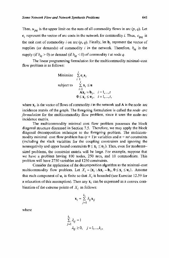
Some Network Flow and Network Synthesis Problems 641
Then, u is the upper limit on the sum of all commodity flows in arc (p, q). Let
c; represent the vector of arc costs in the network for commodity /. Thus, cipq is
the unit cost of commodity / on arc (p, q). Finally, let b, represent the vector of
supplies (or demands) of commodity / in the network. Therefore, biq is the
supply (if bj > 0) or demand (iibig < 0) of commodity i at node q.
The linear programming formulation for the multicommodity minimal-cost flow problem is as follows:
t Minimize Σ c
;x,'
;=1
subject to X x , < u
A x ; = b ; , i = l,...,t 0 < x ; < u ; , i = l,...,t,
where x;- is the vector of flows of commodity /' in the network and A is the node-arc
incidence matrix of the graph. The foregoing formulation is called the node-arc formulation for the multicommodity flow problem, since it uses the node-arc incidence matrix.
The multicommodity minimal-cost flow problem possesses the block diagonal structure discussed in Section 7.5. Therefore, we may apply the block diagonal decomposition technique to the foregoing problem. The multicom-modity minimal-cost flow problem has (t + \)n variables and n + mt constraints (including the slack variables for the coupling constraints and ignoring the nonnegativity and upper bound constraints 0 < x, < u,·). Thus, even for moderate-sized problems, the constraint matrix will be large. For example, suppose that we have a problem having 100 nodes, 250 arcs, and 10 commodities. This problem will have 2750 variables and 1250 constraints.
Consider the application of the decomposition algorithm to the minimal-cost
multicommodity flow problem. Let X{ ={x(· : Ax,· = b ; , 0 < x ; <u,·}. Assume
that each component of u, is finite so that X, is bounded (see Exercise 12.59 for
a relaxation of this assumption). Then any x, can be expressed as a convex com-
bination of the extreme points of Xt as follows:
_ ki
where
Σ % = ι
4 > o , j = i,...,kh
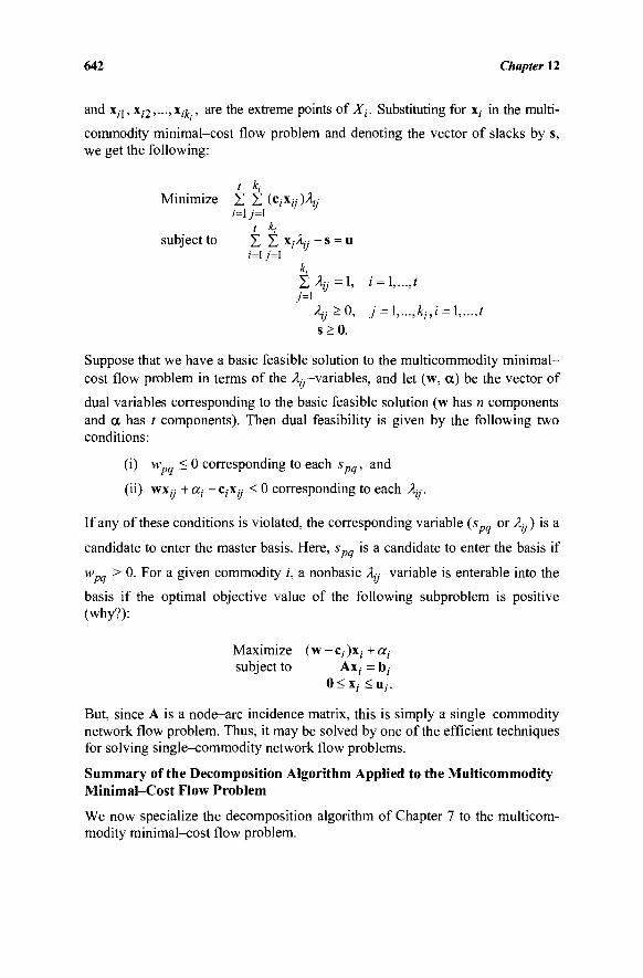
642 Chapter 12
and χ;·|, χ(·2,...,χ,·£., are the extreme points of Xt. Substituting for x, in the multi-commodity minimal-cost flow problem and denoting the vector of slacks by s, we get the following:
t K Minimize Σ Σ (c/x//)%
1=1 y=i
subject to Σ Σ *,·-% + s = u
ki
Z % = 1 > i = \,...,t 7=1
λ^>0, j = l,...,khi = l,...,t s>0.
Suppose that we have a basic feasible solution to the multicommodity minimal-cost flow problem in terms of the /L-variables, and let (w, a) be the vector of
dual variables corresponding to the basic feasible solution (w has n components and a has / components). Then dual feasibility is given by the following two conditions:
(i) wpq < 0 corresponding to each spq, and
(ii) wx,y + a, - CjXy < 0 corresponding to each L·.
If any of these conditions is violated, the corresponding variable {spq or L·) is a
candidate to enter the master basis. Here, spq is a candidate to enter the basis if
w > 0. For a given commodity i, a nonbasic ^ -variable is enterable into the
basis if the optimal objective value of the following subproblem is positive (why?):
Maximize (w - c; )x(· + a, subject to Ax;- = b,
0 < x , < U i ,
But, since A is a node-arc incidence matrix, this is simply a single-commodity network flow problem. Thus, it may be solved by one of the efficient techniques for solving single-commodity network flow problems.
Summary of the Decomposition Algorithm Applied to the Multicommodity Minimal-Cost Flow Problem
We now specialize the decomposition algorithm of Chapter 7 to the multicom-modity minimal-cost flow problem.
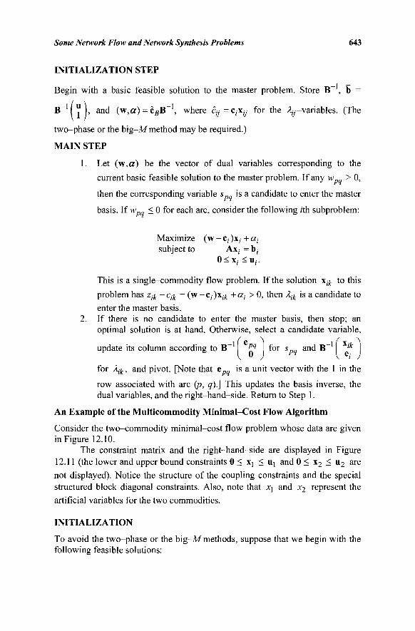
Some Network Flow and Network Synthesis Problems 643
INITIALIZATION STEP
Begin with a basic feasible solution to the master problem. Store B~ , b =
B~ I "? I, and (w,a) = cBB~ , where c,y =c,-xiy for the Ay—variables. (The
two-phase or the big-M method may be required.)
MAIN STEP
1. Let (w,a) be the vector of dual variables corresponding to the
current basic feasible solution to the master problem. If any wpq > 0,
then the corresponding variable sp is a candidate to enter the master
basis. If Wpq < 0 for each arc, consider the following rth subproblem:
Maximize (w - c,- )x;- + a,-subject to Ax,· = b(
0 < x ; <uf .
This is a single-commodity flow problem. If the solution xik to this
problem has zik -cik = (w-c,)x,£ +«/ > 0, then Àiìc is a candidate to
enter the master basis. 2. If there is no candidate to enter the master basis, then stop; an
optimal solution is at hand. Otherwise, select a candidate variable,
update its column according to B | ξ^ for s and B~ ' '*
for Xik, and pivot. [Note that epq is a unit vector with the 1 in the
row associated with arc (p, q).] This updates the basis inverse, the dual variables, and the right-hand-side. Return to Step 1.
An Example of the Multicommodity Minimal-Cost Flow Algorithm
Consider the two-commodity minimal-cost flow problem whose data are given in Figure 12.10.
The constraint matrix and the right-hand-side are displayed in Figure 12.11 (the lower and upper bound constraints 0 < xt < Uj and 0 < x2 < u2 are not displayed). Notice the structure of the coupling constraints and the special structured block diagonal constraints. Also, note that X] and x2 represent the artificial variables for the two commodities.
INITIALIZATION
To avoid the two-phase or the big-M methods, suppose that we begin with the following feasible solutions:
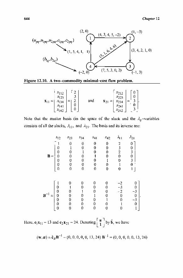
644 Chapter 12
(2.0) / (1, -3) (4, 3, 4, 5, -2) • - *
-H 2 \Upq >U\pq> U2pq ' C\pq ' C2pq )
(hqAq)
Figure 12.10. A two-commodity minimal-cost flow problem.
(3, 4, 2, 1, 0)
Xn =
x112 x123 x134 x141
_ X 1 4 2 _
=
2 3 2 U
u J
and x21 =
x212 x223 x234 x241
. *242 .
=
0
u 3 υ
[3 J
Note that the master basis (in the space of the slack and the ,Ί^-variables
consists of all the slacks, λη, and À%\- The basis and its inverse are:
B
s\2
1 0 0 0 0 0 0
s27,
0 1 0 0 0 0 0
s34
0 0 1 0 0 0 0
s4l
0 0 0 1 0 0 0
s42
0 0 0 0 1 0 0
λη
2 3 2 0 0 1 0
0" 0 3 0 3 0 1
B"
1 0 0 0 0 0 0
0 1 0 0 0 0 0
0 0 0 0 1 0 0
0 0
-3 0
-3 0 1
Here, C[Xu = 13 and c2x2i = 24. Denoting by b, we have
(w,a) = cBB_ 1 = (0, 0, 0, 0, 0, 13, 24) B_ 1 = (0, 0, 0, 0, 0, 13, 24)
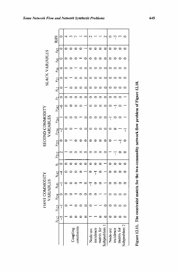
Figu
re 1
2.11
. T
he c
onst
rain
t m
atri
x fo
r th
e tw
o-co
mm
odity
net
wor
k fl
ow p
robl
em o
f F
igur
e 12
.10.
£ ?
FIR
ST C
OM
MO
DIT
Y
VA
RIA
BL
ES
SEC
ON
D C
OM
MO
DIT
Y
VA
RIA
BL
ES
SLA
CK
VA
RIA
BL
ES
Cou
plin
g co
nstr
aint
s
Nod
e-ar
c in
cide
nce
mat
rix
for
Sub
prob
lem
1
Nod
e-ar
c in
cide
nce
mat
rix
for
Sub
prob
lem
2 x 11
2 -5 1 0 0 0 0 1
-1 0 0 0 0 0 0
x 123 -1 0 1 0 0 0 0 1
-1 0 0 0 0 0
x 134 0 0 0 1 0 0 0 0 1
-1 0 0 0 0
x 141 -1 0 0 0 1 0 -1 0 0 1 0 0 0 0
x 142 -4 0 0 0 0 1 0 -1 0 1 0 0 0 0
x x 0 0 0 0 0 0 0 0 0 1 0 0 0 0
x 212 2 1 0 0 0 0 0 0 0 0 1
-1 0 0
x22
3 0 0 1 0 0 0 0 0 0 0 0 1 -1
0
x 234 -2 0 0 1 0 0 0 0 0 0 0 0 1
-1
x 241 1 0 0 0 1 0 0 0 0 0 -1
0 0 1
x 242 -6 0 0 0 0 1 0 0 0 0 0 -1 0 1
x 2 0 0 0 0 0 0 0 0 0 0 0 0 0 1
*12 0 1 0 0 0 0 0 0 0 0 0 0 0 0
s 23 0 0 1 0 0 0 0 0 0 0 0 0 0 0
s 34 0 0 0 1 0 0 0 0 0 0 0 0 0 0
s 41 0 0 0 0 1 0 0 0 0 0 0 0 0 0
s 42 0 0 0 0 0 1 0 0 0 0 0 0 0 0
RH
S 0 4 3 7 1 5 2 1 -1
-2
0 -3 3 0
s ft. s- ft
<Ji
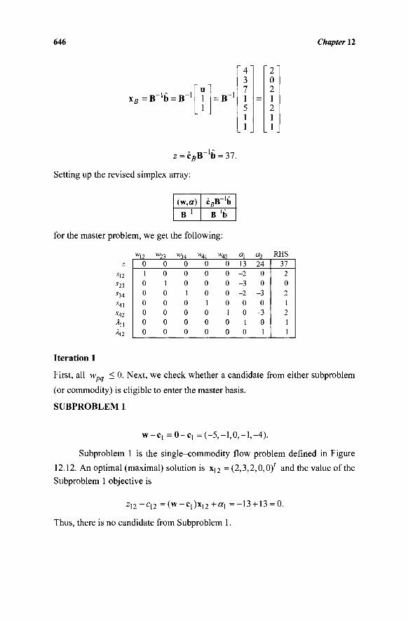
646 Chapter 12
B~'b = B"1 u 1 1 j
= B - '
[4 3 7 1 5 1 1
=
[2 1 0 2 1 2 1 1
z = cgB- 1b = 37.
Setting up the revised simplex array:
(w,a) B 1
c B B ' b
B'b
for the master problem, we get the following:
■*12
·*23
ί 4 1
s42
Iteration 1
First, all wpq < 0. Next, we check whether a candidate from either subproblem
(or commodity) is eligible to enter the master basis.
SUBPROBLEM 1
w\2
0 1 0 0 0 0 0 0
w„ 0 0 1 0 0 0 0 0
VK,4
0 0 0 1 0 0 0 0
w41
0 0 0 0 1 0 0 0
w42
0 0 0 0 0 1 0 0
a, 13 -2 -3 -2
0 0 1 0
«2 24
0 0
-3 0
-3 0 1
RHS 37
2 0 2 1 2 1 1
w-Cj =0-C! =(-5,-1,0,-1,-4).
Subproblem 1 is the single-commodity flow problem defined in Figure
12.12. An optimal (maximal) solution is x12 = (2,3,2,0,0)' and the value of the
Subproblem 1 objective is
z12 -C[2 =(w-Cj)Xj2 +«i =-13 + 13 = 0.
Thus, there is no candidate from Subproblem 1.
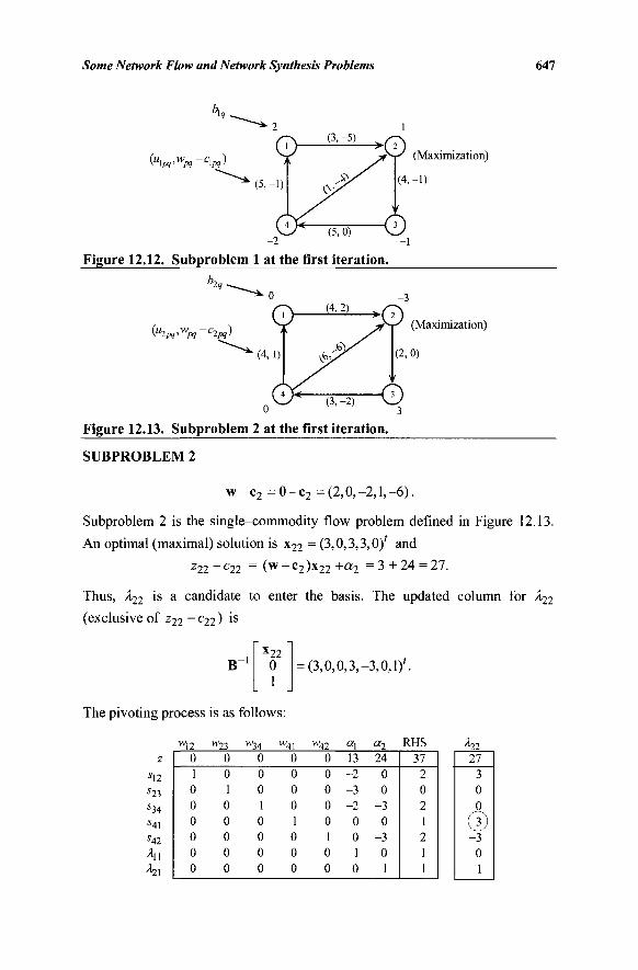
Some Network Flow and Network Synthesis Problems 647
0 W W « - C 1 M ) (Maximization)
(4, -1)
(5,0)
Figure 12.12. Subproblem 1 at the first iteration.
(U2n>Wpq -C2pc)
(Maximization)
(2,0)
- (3, -2) 0 3
Figure 12.13. Subproblem 2 at the first iteration.
SUBPROBLEM 2
w - c 2 = 0 - c 2 =(2,0,-2,1,-6).
Subproblem 2 is the single-commodity flow problem defined in Figure 12.13.
An optimal (maximal) solution is x22 = (3,0,3,3,0)' and z22 ~c22 = (w -c 2 )x 2 2 +a2 = 3 + 24 = 27.
Thus, λ^ is a candidate to enter the basis. The updated column for λχ2
(exclusive of z22 - c22 ) is
B x22
0 1
= (3,0,0,3,-3,0,1/.
The pivoting process is as follows:
w\2 w23 w34 w4\ w42 " l «2 RHS
s12
■*23
s42
\\
0 1 0 0 0 0 0 0
0 0 1 0 0 0 0 0
0 0 0 1 0 0 0 0
0 0 0 0 1 0 0 0
0 0 0 0 0 1 0 0
13 -2 -3 -2
0 0 1 0
24 0 0
-3 0
-3 0 1
37 2 0 2 1 2 1 1
^22 27
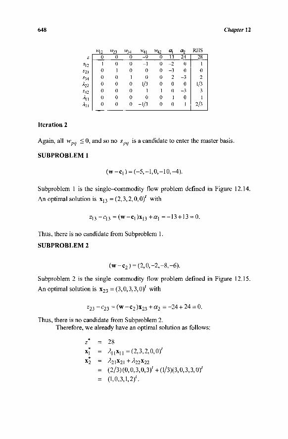
648 Chapter 12
z
*12
*23 S34
hi s42
/l | |
h.\
wu
0 1 0 0 0 0 0 0
H-23
0 0 1 0 0 0 0 0
WJ4
0 0 0 1 0 0 0 0
w41
-9 -1 0 0
1/3 1 0
-1/3
w42
0 0 0 0 0 1 0 0
_A_ _13_
-2 -3 -2
0 0 1 0
«2
24 0 0
-3 0
-3 0 1
RHS 28
1 0 2
1/3 3 1
2/3
Iteration 2
Again, all wpg < 0, and so no spq is a candidate to enter the master basis.
SUBPROBLEM 1
( w - C l ) = (-5,-1,0,-10,-4).
Subproblem 1 is the single-commodity flow problem defined in Figure 12.14.
An optimal solution is x]3 =(2,3,2,0,0)' with
z13 _c13 = ( w _ c l ) x 1 3 +a\ =-13 + 13 = 0.
Thus, there is no candidate from Subproblem 1.
SUBPROBLEM 2
( w - c 2 ) = (2,0,-2,-8,-6).
Subproblem 2 is the single-commodity flow problem defined in Figure 12.15.
An optimal solution is x23 = (3,0,3,3,0)' with
z23~c23 = (w -C 2 ) x 2 3+«2 =-24 + 24 = 0.
Thus, there is no candidate from Subproblem 2. Therefore, we already have an optimal solution as follows:
z* = 28
x* = ληχη =(2,3,2,0,0)'
X2 = ^21X21 + ^ 2 2 x 2 2
= (2/3) (0,0,3,0,3/ + (1/3X3,0,3,3,0)' = (1,0,3,1,2)'.
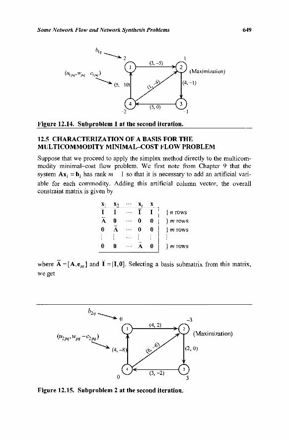
Some Network Flow and Network Synthesis Problems 649
(U\pq>Wpq-C\pq) (Maximization)
(4,-1)
-2 -1
Figure 12.14. Subproblem 1 at the second iteration.
12.5 CHARACTERIZATION OF A BASIS FOR THE MULTICOMMODITY MINIMAL-COST FLOW PROBLEM
Suppose that we proceed to apply the simplex method directly to the multicom-modity minimal-cost flow problem. We first note from Chapter 9 that the system Ax, = b, has rank m - 1 so that it is necessary to add an artificial vari-able for each commodity. Adding this artificial column vector, the overall constraint matrix is given by
} n rows } m rows } m rows
} m rows
x1 I A 0
0
*?. · I 0 A ·
0
• xr I
• 0 • 0
• A
X
I
o •
o
where A =[A,eOT] and I =[1,0]. Selecting a basis submatrix from this matrix,
we get
("ipq'Wpq -C2pq) (Maximization)
(2,0)
- (3, -2) 0 3
Figure 12.15. Subproblem 2 at the second iteration.
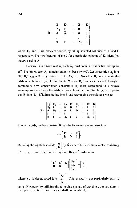
650 Chapter 12
B =
E,
A, 0
0
E2 ·
0
A2 ·
0
- E, 0
■· 0
- A,
E
0
0
0
where E,· and E are matrices formed by taking selected columns of I and I,
respectively. The row location of the 1 for a particular column of E,· identifies
the arc used in A,-.
Because B is a basis matrix, each A, must contain a submatrix that spans
Rm. Therefore, each A;· contains an m x m basis (why?). Let us partition A,· into
[B;· | D,·] where B,· is a basis matrix for Ax; = b ; . Note that B; must contain the
artificial column (why?). From Chapter 9, since B; is a basis for a set of single-
commodity flow conservation constraints, B, must correspond to a rooted
spanning tree in G with the artificial variable as the root. Similarly, let us parti-
tion E,· into [E'j | E"]. Substituting into B and rearranging the columns, we get
E; B, 0
E 7 .
0 B2
·· E; . 0 . 0
E,* Dl 0
E? . 0 D2
.. E;
.. 0
.. 0
E 0 0
0 0 B, 0 0 D, 0
In other words, the basis matrix B has the following general structure:
B = E' E" E B D 0
Denoting the right-hand-side by b (where b is a column vector consisting
of bj,b2,..., and bt), the basic system Bxg =b reduces to
F; B
E" D
ΕΊ 0
x F
*D
lsB j —
II b
where xB is decomposed into xF
*B This system is not particularly easy to
solve. However, by utilizing the following change of variables, the structure in the system can be exploited, as we shall outline shortly:
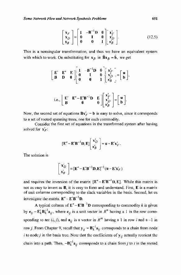
Some Network Flow and Network Synthesis Problems 651
X F
X D SB
I 0 0
- B ' D o I 0 0 I
~ X F ~ xb
JB . (12.5)
This is a nonsingular transformation, and thus we have an equivalent system
with which to work. On substituting for xB in Bxg = b, we get
E' E" E B D 0
I 0 0
-B_1D 0 I 0 0 I
"x>" X D s 5
u h
L J
i.e., E' E"-E'B_ 1D E B O O
\x'F-f
X D
LS'B . —
u b
■ J
Now, the second set of equations B\'F = b is easy to solve, since it corresponds to a set of rooted spanning trees, one for each commodity.
Consider the first set of equations in the transformed system after having solved for \'F:
The solution is
[E"-E'B_1D,E] l D = u - E ' x > .
XD = [E"-E'B"1D,E]"I(u-E'x>)
and requires the inversion of the matrix [E"-E'B D,E]. While this matrix is
not as easy to invert as B, it is easy to form and understand. First, E is a matrix of unit columns corresponding to the slack variables in the basis. Second, let us
- l i
»-i
investigate the matrix E"-E'B- 1D.
A typical column of E"-E'B_ 1D corresponding to commodity k is given
by e,·.· -E^B^ a,y, where e,y is a unit vector in Rn having a 1 in the row corre-
sponding to arc (i,j), and a,·.· is a vector in Rm having a 1 in row ; and a -1 in
row/. From Chapter 9, recall that y,y = B~f a,·.· corresponds to a chain from node
i to node/ in the basis tree. Note that the coefficients of y;y actually reorient the
chain into a path. Then, -B~f a/; corresponds to a chain fromy to i in the rooted
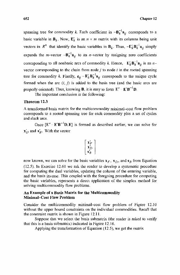
652 Chapter 12
spanning tree for commodity k. Each coefficient in -B£ a,y corresponds to a
basic variable in B^. Now, E^ is an n x m matrix with its columns being unit
vectors in R" that identify the basic variables in B^. Thus, -E^B^ a,y simply
expands the m-vector -B~f a,y to an «-vector by assigning zero coefficients
corresponding to all nonbasic arcs of commodity k. Hence, -E^B^ a,y is an n-
vector corresponding to the chain from node j to node i in the rooted spanning
tree for commodity k. Finally, e;y -EJ^B^ a;y corresponds to the unique cycle
formed when the arc (/, j) is added to the basis tree (and the basic arcs are
properly oriented). Thus, knowing B, it is easy to form E" - E ' B - D. The important conclusion is the following:
Theorem 12.3
A transformed basis matrix for the multicommodity minimal-cost flow problem corresponds to a rooted spanning tree for each commodity plus a set of cycles and slack arcs.
Once [E"-E'B~ D,E] is formed as described earlier, we can solve for
x'D and s'B. With the vector
L»i J now known, we can solve for the basic variables xF, xD, and s g from Equation
(12.5). In Exercise 12.61 we ask the reader to develop a systematic procedure for computing the dual variables, updating the column of the entering variable, and the basis inverse. This coupled with the foregoing procedure for computing the basic variables, represents a direct application of the simplex method for solving multicommodity flow problems.
An Example of a Basis Matrix for the Multicommodity Minimal-Cost Flow Problem
Consider the multicommodity minimal-cost flow problem of Figure 12.10 without the upper bound constraints on the individual commodities. Recall that the constraint matrix is shown in Figure 12.11.
Suppose that we select the basis submatrix (the reader is asked to verify that this is a basis submatrix) indicated in Figure 12.16.
Applying the transformation of Equation (12.5), we get the matrix
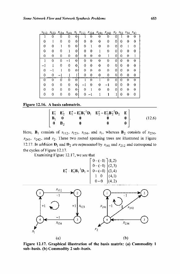
Some Network Flow and Network Synthesis Problems 653
■M12 1 0 0 0 0 1
-1 0 0 0 0 0 0
x123 0 1 0 0 0 0 1
-1 0 0 0 0 0
x134 0 0 1 0 0 0 0 1
-1 0 0 0 0
*141 x\ 0 0 0 0 0 0 1 0 0 0
-1 0 0 0 0 0 1 1 0 0 0 0 0 0 0 0
x212 1 0 0 0 0 0 0 0 0 1
-1 0 0
x234 x241 x242 x2 0 0 0 0 0 0 0 0 1 0 0 0 0 1 0 0 0 0 1 0 0 0 0 0 0 0 0 0 0 0 0 0 0 0 0 0 0 - 1 0 0 0 0 - 1 0 1 0 0 0
- 1 1 1 1
s12 1 0 0 0 0 0 0 0 0 0 0 0 0
Ì34 542
0 0 0 0 1 0 0 0 0 1 0 0 0 0 0 0 0 0 0 0 0 0 0 0 0 0
Figure 12.16. A basis submatrix.
E; B, 0
E ?
0
Bo
EJ' -EjBf'D! 0 0
E$ — IL^BO * 2
0 0
E
0 0
(12.6)
Here, Bj consists of x112, -M23, - 134, and xj, whereas B2 consists of *234> x24l> x242' a nd x2- These two rooted spanning trees are illustrated in Figure
12.17. In addition Ό\ and D2 are represented by x14] and x2i2 anc^ correspond to
the cycles of Figure 12.17. Examining Figure 12.17, we see that
(1.2) . . (2,3)
Ef-EÌBj-'D^ O-(-l) (3,4) (4,1) (4,2)
" 0 -0 -0 -
1
0
■(-i)l (-1) (-1) - 0
- 0
Ml 2
+1
o M34
Θ M23
Θ
(a) (b) Figure 12.17. Graphical illustration of the basis matrix: (a) Commodity 1 sub-basis, (b) Commodity 2 sub-basis.
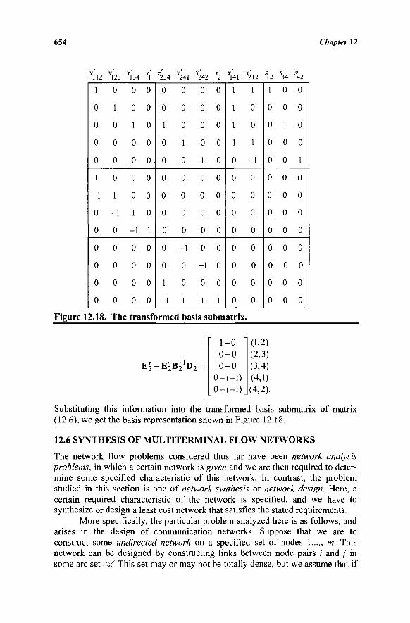
654 Chapter 12
X112
1
0
0
0
0
1
-1
0
0
0
0
0
0
X123
0
1
0
0
0
0
1
-1
0
0
0
0
0
X134
0
0
1
0
0
0
0
1
-1
0
0
0
0
xx 0
0
0
0
0
0
0
0
1
0
0
0
0
X234
0
0
1
0
0
0
0
0
0
0
0
1
-1
•*241
0
0
0
1
0
0
0
0
0
-1
0
0
1
■*242
0
0
0
0
1
0
0
0
0
0
-1
0
1
h 0
0
0
0
0
0
0
0
0
0
0
0
1
Ì 4 1
1
1
1
1
0
0
0
0
0
0
0
0
0
h\i
1
0
0
1
-1
0
0
0
0
0
0
0
0
\ l
1
0
0
0
0
0
0
0
0
0
0
0
0
^ 4 542
0 0
0 0
1 0
0 0
0 1
0 0
0 0
0 0
0 0
0 0
0 0
0 0
0 0
Figure 12.18. The transformed basis submatrix.
ÌLn ~~ J^2 2
1-0 0-0 0-0
0-(-l) 0-(+l)
(1,2) (2,3) (3,4) (4,1) (4,2).
Substituting this information into the transformed basis submatrix of matrix (12.6), we get the basis representation shown in Figure 12.18.
12.6 SYNTHESIS OF MULTITERMINAL FLOW NETWORKS
The network flow problems considered thus far have been network analysis problems, in which a certain network is given and we are then required to deter-mine some specified characteristic of this network. In contrast, the problem studied in this section is one of network synthesis or network design. Here, a certain required characteristic of the network is specified, and we have to synthesize or design a least cost network that satisfies the stated requirements.
More specifically, the particular problem analyzed here is as follows, and arises in the design of communication networks. Suppose that we are to construct some undirected network on a specified set of nodes 1,..., m. This network can be designed by constructing links between node pairs / and j in some arc set. "■/ This set may or may not be totally dense, but we assume that if
Some Network Flow and Network Synthesis Problems 655
all the potential arcs in · ' / are constructed, then the resulting network will be connected. In addition to selecting the arcs from "4 we have the freedom of designing the capacities of these arcs. If arc (/, j) is constructed with capacity Ujj, then a corresponding cost of c^ > 0 per unit capacity will be incurred.
The constructed network must independently sustain a certain maximal flow requirement ry > 0 between each pair of nodes or terminals i and/ (hence,
the name of this problem). Note that the requirements η- are specified between
each pair of nodes i and j , and not only for (/, j) e / The problem may be mathematically stated as follows, where L· denotes the maximum flow between
node pair i andy and is, of course, a function of the constructed network.
Minimize { X q.-Uy '■ fh- ^ fy for each / = 1,..., m - 1 ,j - i + \,...,m, (ij')e- ' /
and Uj- > 0 for (i,j) e " / } .
Before proceeding to solve this problem, there are two manipulations that we need to perform. First, we do not need all the m(m - l)/2 structural constraints in this problem. Intuitively, it should be evident that if the maximal flow requirements are satisfied for certain key node pairs, then the other flow requirements ought to be also automatically satisfied. In fact, these key node pairs turn out to be associated with a certain tree Tr known as the dominant requirement tree. Only the particular node pairs associated with the (m ~ 1) arcs in Tr need to have their flow requirement constraints explicitly represented. The second manipulation involves the representation of the constraints themselves. The quantities L· are functions of the variables Uu. This translation must be
made in order for us to be able to solve the problem mathematically. Note that this is readily done using the maximal flow-minimal cut theorem. Namely, for any node pair (/, j), fy > η- if and only if the capacity of each cut separating
nodes i andy' exceeds η- (why?). (Note that since the network is undirected, we
deal with the cut here, and there is no forward or reverse cut in this context.) Let k = 1,..., Kjj index the possible cuts separating nodes i andy. For each such k e
Kjj, define a column vector a ^ having | ■"/1 components, one corresponding to
each arc in Ύ, with the component corresponding to arc (p, q) being 1 if this arc belongs to the cut and zero otherwise. Then, for any node pair (i,j), we may replace fy > η- by the constraints
K * ) ' u > ^ · for*=l,.. . , K,j,
656 Chapter 12
where u is the vector (uy, (i, j) e ■"/). Before we consider the first
manipulation, let us introduce an example problem.
An Example for the Synthesis Problem
Consider the potential network shown in Figure 12.19a, where m = 5, |..Ύ \ =6
with the permissible arcs as shown, and the corresponding costs c,·. per unit
capacity as indicated against the arcs. Additionally, the requirements r^ are as
follows: r\2 = 3> 13 = 5> r\4 = 3> 15 = 2> r23 = 6>
r24 = 7, r25 = 5, r34 = 8, r35 = 1, r45 = 12.
Dominant Requirement Tree Tr
To define the dominant requirement tree Tr, construct a complete graph Gr on the node set 1,..., m, with the (undirected) arc between each node pair i and/ having a weight equal to the requirement η.-. Then, Tr is defined as the maximum
spanning tree for Gr, that is, it is a spanning tree for Gr that has the maximum total weight.
The process of constructing Tr involves a simple one-pass procedure and
may be done as follows. Suppose that the "weights" r^ are sorted from largest to smallest in a list L. (A complete sort is not necessary.) Select arcs for inclusion in Tr by proceeding in the order of list L. Skip any arc that results in a cycle with
respect to the arcs already selected. Stop when (m - 1) arcs have been selected. For the example problem, we would select and skip arcs as follows: select (4, 5), select (3, 4), select (2, 4), skip (2, 3) (why?), skip (2, 5), select (1,3), and stop. The resulting tree Tr is shown in Figure 12.19b.
The fact that this "greedy" procedure produces a maximal spanning tree
Tr may be verified as follows. Suppose that the tree T* is some maximal
spanning tree. We will show that the total weight of T* and the constructed tree Tr are the same. Toward this end, proceed down the list L and find the first arc
(p, q) that belongs to Tr but is not in T*. Add (p, q) to T* and examine the
(unique) cycle formed by (p, q) and the chain C connecting p and q in T*. Note
that ry > rpq for all (i,j) e C since T is maximal. If any (/,/) e C satisfies η-
> rpq, then (i,f) e Tr. If not, then because (i,j) appears before (p, q) in L and it
was not selected for inclusion in Tr, it must have formed a cycle with the arcs
selected for Tr before (/,/)· B u t a ' l s u c r i a r c s a r e a l s o m T* by the definition of (p, q). Hence, we have a contradiction (why?). But all the arcs in C cannot also be in Tr since (p, q) e Tr. Hence, there exists an arc (s, t) e C, (s, t) <£ Tr, such
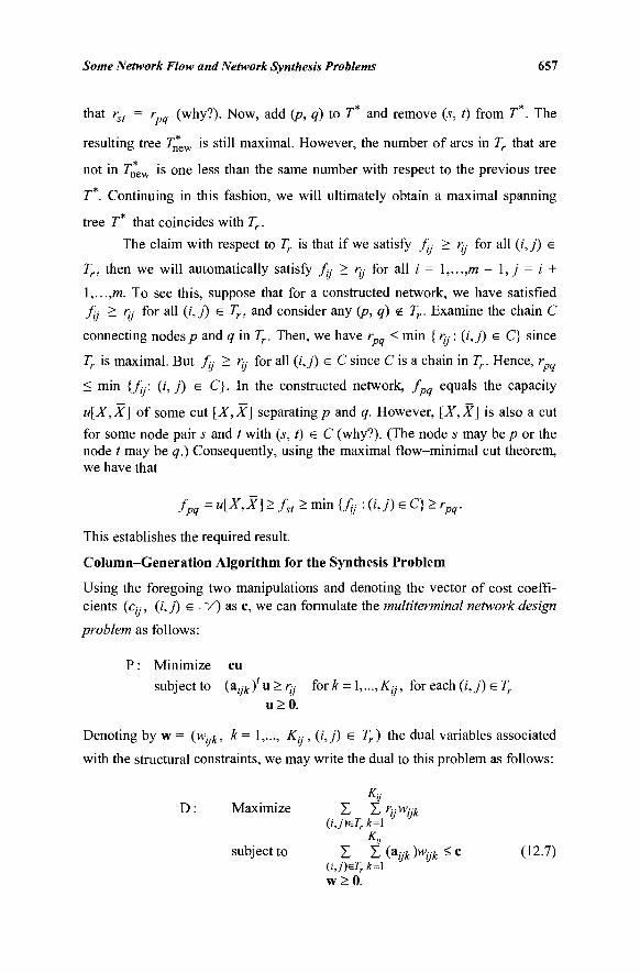
Some Network Flow and Network Synthesis Problems 657
that rst = r (why?). Now, add (p, q) to T* and remove (s, t) from T*. The
resulting tree T*ew is still maximal. However, the number of arcs in Tr that are
not in Tn*ew is one less than the same number with respect to the previous tree
T*. Continuing in this fashion, we will ultimately obtain a maximal spanning
tree T that coincides with Tr.
The claim with respect to Tr is that if we satisfy fy > ry for all (i, j) e
Tr, then we will automatically satisfy fy > ry for all i = l,...,m - \,j = i +
\,...,m. To see this, suppose that for a constructed network, we have satisfied fij > fy for all (i,j) e Tr, and consider any (p, q) g Tr. Examine the chain C
connecting nodes/) and q in Tr. Then, we have rpq < min {ri;- : (i,j) e C} since
Tr is maximal. But fy > η,- for all (i,f) e C since C is a chain in Tr. Hence, r
< min {fy. (i, j) ε C}. In the constructed network, / equals the capacity
w[X,X] of some cut [X,X] separating/) and q. However, [X,^Q is also a cut
for some node pair s and / with (s, t) e C (why?). (The node s may be p or the node / may be q.) Consequently, using the maximal flow-minimal cut theorem, we have that
fpq = u[X, X] > fst > min {fy : (i, j) e C} > rpq.
This establishes the required result.
Column-Generation Algorithm for the Synthesis Problem
Using the foregoing two manipulations and denoting the vector of cost coeffi-cients (cy, (/, j) e . V) as c, we can formulate the multiterminal network design
problem as follows:
P : Minimize cu
subject to ( a p )' u > ry for k = 1,..., Ky, for each (2, j) e Tr
u>0 .
Denoting by w = (w^, k= 1,..., Ky, (i,j) e Tr) the dual variables associated
with the structural constraints, we may write the dual to this problem as follows:
Ka D : Maximize Σ Σ rywijk
(U)eTrk=\ K.J
subject to Σ Σ (»/,*Η* ^ c (12-7) (i,j)eTr *=1 w>0.
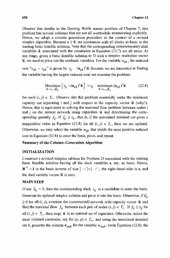
658 Chapter 12
Observe that similar to the Dantzig-Wolfe master problem of Chapter 7, this problem has several columns that are not all worthwhile enumerating explicitly. Hence, we adopt a column generation procedure in the context of a revised simplex algorithm. Because c > 0, we commence with all slacks as basic in the starting basic feasible solution. Note that the corresponding complementary dual variables Π associated with the constraints in Equation (12.7) are all zeros. At any stage, given a basic feasible solution to D with a simplex multiplier vector u, we need to price out the nonbasic variables. For the variable Wyk, the reduced
cost " cp - Zjjk" is given by ry- - ( a ^ / u . Because we are interested in finding
the variable having the largest reduced cost, we examine the problem:
Maximize j r„- - (a y A . /u | = ry■ - minimum ( a ^ / u (12.8) ft —· 1 j . . . , / v ,',■ ft — 1, . . . y Λ ,■-■
for each (i,j) e Tr. Observe that this problem essentially seeks the minimum capacity cut separating i andy with respect to the capacity vector u (why?). Hence, this is equivalent to solving the maximal flow problem between nodes / and j on the current network using capacities u and determining the corre-sponding quantity fy. If fy > ry, that is, if the associated minimal cut gives a
nonpositive value in Equation (12.8) for all (ì,j) e Tr, then we are optimal.
Otherwise, we may select the variable Wyk that yields the most positive reduced
cost in Equation (12.8) to enter the basis, pivot, and repeat.
Summary of the Column-Generation Algorithm
INITIALIZATION
Construct a revised-simplex tableau for Problem D associated with the starting basic feasible solution having all the slack variables s, say, as basic. Hence,
B~ = I is the basis inverse of size | ■ ' /1x | ■"/1, the right-hand-side is c, and
the dual variable vector u is zero.
MAIN STEP
If any uy < 0, then the corresponding slack sy is a candidate to enter the basis.
Generate its updated simplex column and pivot it into the basis. Otherwise, if uy
> 0 for all (/, j), examine the (constructed) network with capacity vector ΰ and find the maximal flow fy between each pair of nodes (i,j) e Tr. If fy > ry for
all (/,/) e Tr, then stop; ΰ is an optimal set of capacities. Otherwise, select the
most violated constraint, say for (p, q) e Tr, and using the associated minimal
cut k, generate the column a k for the variable w k. From Equation (12.8), the
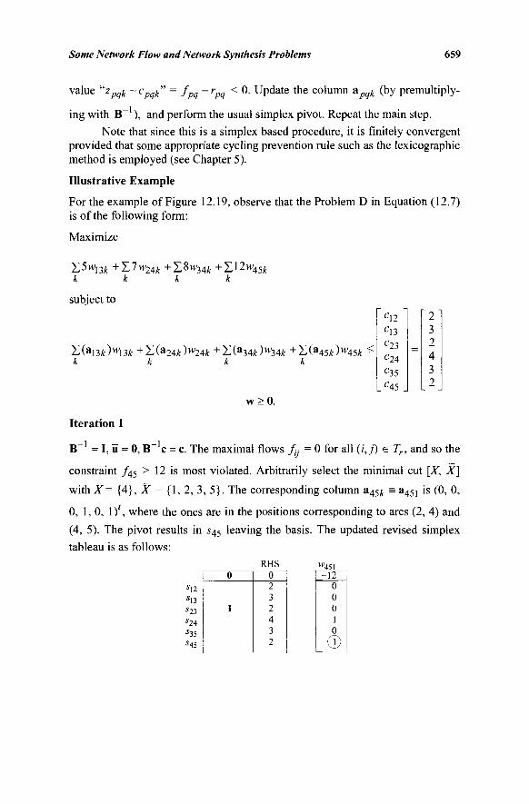
Some Network Flow and Network Synthesis Problems 659
value "Zpqk ~cpqlc" = fpq -rpq < 0. Update the column apgk (by premultiply-
ing with B~ ), and perform the usual simplex pivot. Repeat the main step.
Note that since this is a simplex based procedure, it is finitely convergent provided that some appropriate cycling prevention rule such as the lexicographic method is employed (see Chapter 5).
Illustrative Example
For the example of Figure 12.19, observe that the Problem D in Equation (12.7) is of the following form:
Maximize
Σ5>η3Α + I 7 w m +Z8w34A: +Z12w45yt k k k k
subject to
I ( a 1 3 A ) w m + Z ( a 2 4 i t ) w 2 4 f c +Σ(33 4 ί : )>ν34£ + Σ (»45Α: )W45A ^ k k k k
w>0.
' c12 '
Cl3 c23 C24
c35 _ C 4 5
' 2' 3 2 4 3
L2J
Iteration 1
B~ = I, u = 0, B~ c = c. The maximal flows fy = 0 for all (i,j) e Tr, and so the
constraint / 4 5 > 12 is most violated. Arbitrarily select the minimal cut [X, X]
with X= {4}, X = {1, 2, 3, 5}. The corresponding column a4 5 i = a45i is (0, 0,
0, 1,0, 1)', where the ones are in the positions corresponding to arcs (2, 4) and
(4, 5). The pivot results in s45 leaving the basis. The updated revised simplex
tableau is as follows:
*12 *Π s21 S24
^ s45
0
I
RHS 0 2 3 2 4 3 2
w451
-12 0 0 0 1 0
Ci)
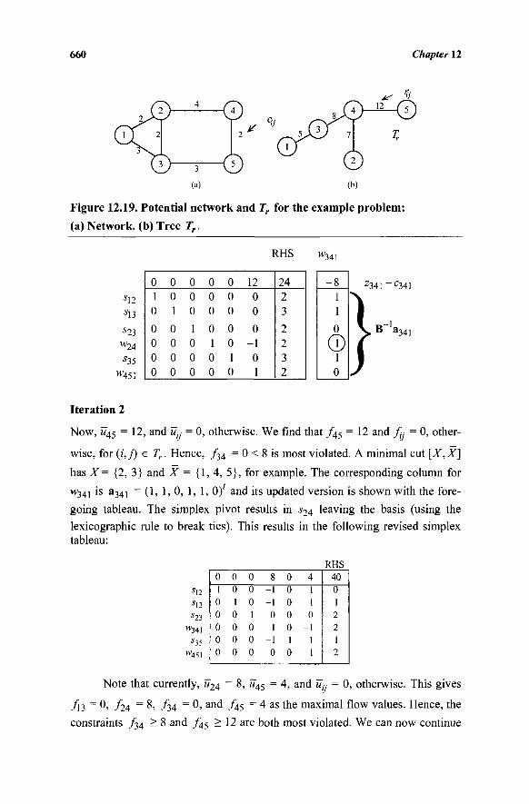
660 Chapter 12
Figure 12.19. Potential network and Tr for the example problem:
(a) Network, (b) Tree Tr.
RHS νν341
sn sn s23 w24
s35
*4M
0 1 0
0 0 0 0
0 0 1
0 0 0 0
0 0 0
1 0 0 0
0 0 0
0 1 0 0
0 0 0
0 0 1 0
12 0 0
0 -1
0 1
24 2 3
2 2 3 2
© 0
z341 _ c 341
Iteration 2
Now, M45 = 12, and Uy = 0, otherwise. We find that / 4 5 = 12 and L· = 0, other-
wise, for (i,j) e Tr. Hence, / 3 4 = 0 < 8 is most violated. A minimal cut [X, X]
has X= {2, 3} and X = {1, 4, 5}, for example. The corresponding column for
w34j is a341 = (1, 1, 0, 1, 1, 0)' and its updated version is shown with the fore-
going tableau. The simplex pivot results in s24 leaving the basis (using the
lexicographic rule to break ties). This results in the following revised simplex tableau:
RHS
s\2
■ 13
*23 w 341
•535 w4 5 1
Note that currently, M24 = 8, u45 = 4, and w,y = 0, otherwise. This gives
/]3 =0 , /24 = 8, / 3 4 = 0, and / 4 5 = 4 as the maximal flow values. Hence, the
constraints / 3 4 > 8 and / 4 5 > 12 are both most violated. We can now continue
0 1 0 0 0 0 0
0
0 1 0 0 0 0
0
0 0 1 0 0 0
8 -1 -1 0 1
-1 0
0 0 0 0 0 1 0
4 1 1 0
-1 1 1
40 0 1 2 2 1 2
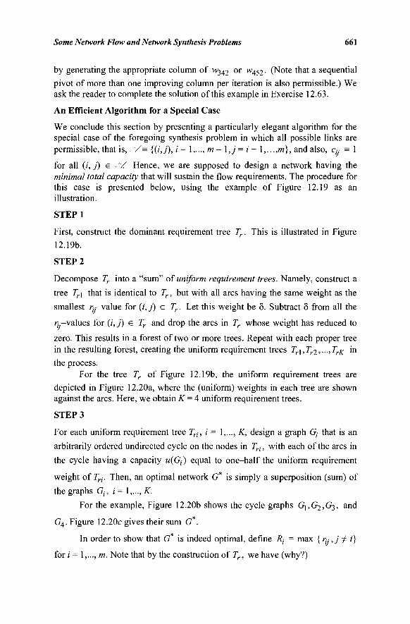
Some Network Flow and Network Synthesis Problems 661
by generating the appropriate column of w342 or w452- (Note that a sequential
pivot of more than one improving column per iteration is also permissible.) We ask the reader to complete the solution of this example in Exercise 12.63.
An Efficient Algorithm for a Special Case
We conclude this section by presenting a particularly elegant algorithm for the special case of the foregoing synthesis problem in which all possible links are permissible, that is,. ~/= {(i,j), i= 1,..., m-\,j = i+ \,...,m), and also, Cy = 1
for all (/, j) e . ~/ Hence, we are supposed to design a network having the minimal total capacity that will sustain the flow requirements. The procedure for this case is presented below, using the example of Figure 12.19 as an illustration.
STEP1
First, construct the dominant requirement tree Tr. This is illustrated in Figure
12.19b.
STEP 2
Decompose Tr into a "sum" of uniform requirement trees. Namely, construct a
tree Trj that is identical to Tr, but with all arcs having the same weight as the
smallest ry value for (i, j) e Tr. Let this weight be δ. Subtract δ from all the
A;·.—values for (i,j) e Tr and drop the arcs in Tr whose weight has reduced to
zero. This results in a forest of two or more trees. Repeat with each proper tree in the resulting forest, creating the uniform requirement trees Tr\,Tr2,—,TrK in the process.
For the tree Tr of Figure 12.19b, the uniform requirement trees are depicted in Figure 12.20a, where the (uniform) weights in each tree are shown against the arcs. Here, we obtain K = 4 uniform requirement trees.
STEP 3
For each uniform requirement tree Trj, i = 1,..., K, design a graph G;- that is an
arbitrarily ordered undirected cycle on the nodes in Tri, with each of the arcs in
the cycle having a capacity w(G() equal to one-half the uniform requirement
weight of Trj. Then, an optimal network G* is simply a superposition (sum) of
the graphs G,, i= \,...,K.
For the example, Figure 12.20b shows the cycle graphs Gj,G2,G3, and
G4. Figure 12.20c gives their sum G .
In order to show that G* is indeed optimal, define Rt = max {ry,j φ i}
for i = 1,..., m. Note that by the construction of Tr, we have (why?)
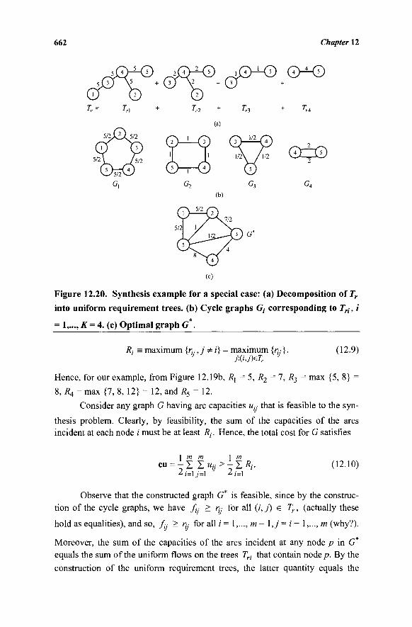
662 Chapter 12
(a)
(c)
Figure 12.20. Synthesis example for a special case: (a) Decomposition of Tr
into uniform requirement trees, (b) Cycle graphs G,· corresponding to Tri, i
= l,...,K=4. (c) Optimal graph G*.
Rj = maximum {rtj,j Φ /} = maximum {?]y}. (12.9) j:(i,j)eTr
Hence, for our example, from Figure 12.19b, R\ = 5, R2 = 7, R3 = max {5, 8} =
8, R4 = max {7, 8, 12} = 12, and R5 = 12.
Consider any graph G having arc capacities Uj- that is feasible to the syn-
thesis problem. Clearly, by feasibility, the sum of the capacities of the arcs
incident at each node /' must be at least Rj. Hence, the total cost for G satisfies
] m m \ m ο ι = - Σ Σ « ^ - Σ Λ , - (12.10)
Observe that the constructed graph G* is feasible, since by the construc-tion of the cycle graphs, we have fj- > η- for all (/, f) e Tr, (actually these
hold as equalities), and so, fy > η,- for all i = 1,..., m- \,j= i+ 1,..., m (why?).
Moreover, the sum of the capacities of the arcs incident at any node p in G* equals the sum of the uniform flows on the trees Tri that contain node/?. By the construction of the uniform requirement trees, the latter quantity equals the
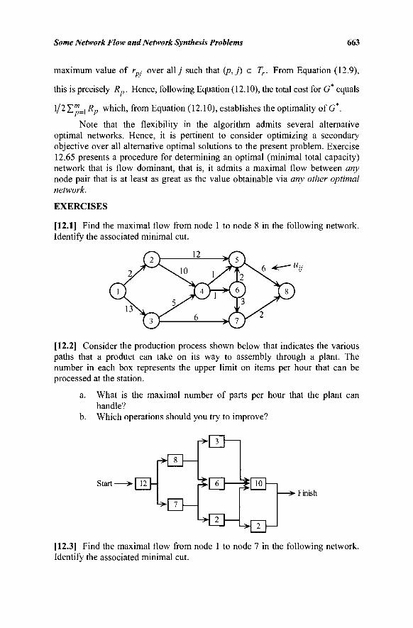
Some Network Flow and Network Synthesis Problems 663
maximum value of r over ally" such that (p,j) e Tr. From Equation (12.9),
this is precisely Rp. Hence, following Equation (12.10), the total cost for G* equals
l/2£p=i^?_ which, from Equation (12.10), establishes the optimality of G*.
Note that the flexibility in the algorithm admits several alternative optimal networks. Hence, it is pertinent to consider optimizing a secondary objective over all alternative optimal solutions to the present problem. Exercise 12.65 presents a procedure for determining an optimal (minimal total capacity) network that is flow dominant, that is, it admits a maximal flow between any node pair that is at least as great as the value obtainable via any other optimal network.
EXERCISES
[12.1] Find the maximal flow from node 1 to node 8 in the following network. Identify the associated minimal cut.
[12.2] Consider the production process shown below that indicates the various paths that a product can take on its way to assembly through a plant. The number in each box represents the upper limit on items per hour that can be processed at the station.
a. What is the maximal number of parts per hour that the plant can handle?
b. Which operations should you try to improve?
Start- 12
8
^ 7
3
% 6
2
L*-5
10
2
• Finish
[12.3] Find the maximal flow from node 1 to node 7 in the following network. Identify the associated minimal cut.
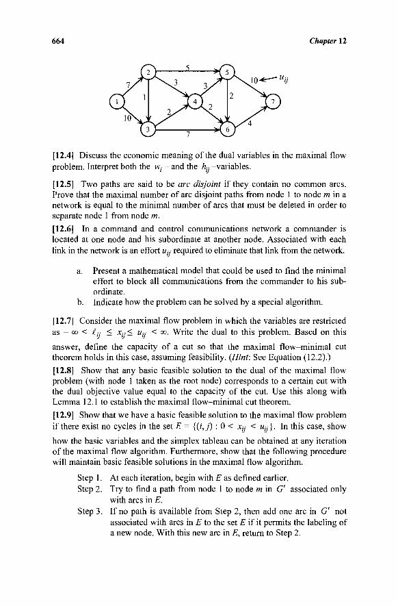
664 Chapter 12
[12.4] Discuss the economic meaning of the dual variables in the maximal flow problem. Interpret both the w,· - and the L· -variables.
[12.5] Two paths are said to be arc disjoint if they contain no common arcs. Prove that the maximal number of arc disjoint paths from node 1 to node m in a network is equal to the minimal number of arcs that must be deleted in order to separate node 1 from node m.
[12.6] In a command and control communications network a commander is located at one node and his subordinate at another node. Associated with each link in the network is an effort uy required to eliminate that link from the network.
a. Present a mathematical model that could be used to find the minimal effort to block all communications from the commander to his sub-ordinate.
b. Indicate how the problem can be solved by a special algorithm.
[12.7] Consider the maximal flow problem in which the variables are restricted as - » < 1-- < Xj-< uy < co. Write the dual to this problem. Based on this
answer, define the capacity of a cut so that the maximal flow-minimal cut theorem holds in this case, assuming feasibility. {Hint See Equation (12.2).)
[12.8] Show that any basic feasible solution to the dual of the maximal flow problem (with node 1 taken as the root node) corresponds to a certain cut with the dual objective value equal to the capacity of the cut. Use this along with Lemma 12.1 to establish the maximal flow-minimal cut theorem.
[12.9] Show that we have a basic feasible solution to the maximal flow problem if there exist no cycles in the set E = {(i,j) : 0 < x^ < Uj.}. In this case, show
how the basic variables and the simplex tableau can be obtained at any iteration of the maximal flow algorithm. Furthermore, show that the following procedure will maintain basic feasible solutions in the maximal flow algorithm.
Step 1. At each iteration, begin with E as defined earlier. Step 2. Try to find a path from node 1 to node m in G' associated only
with arcs in E. Step 3. If no path is available from Step 2, then add one arc in G' not
associated with arcs in E to the set E if it permits the labeling of a new node. With this new arc in E, return to Step 2.
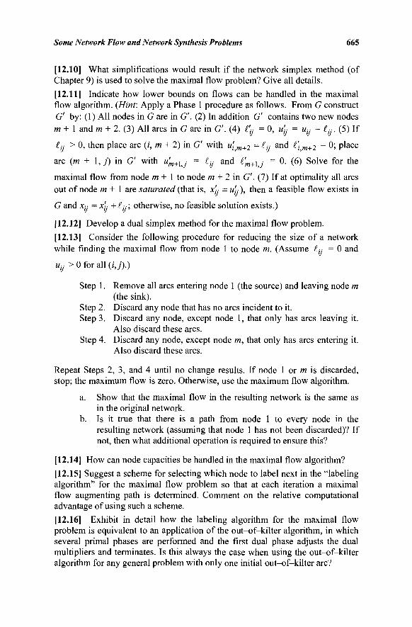
Some Network Flow and Network Synthesis Problems 665
[12.10] What simplifications would result if the network simplex method (of Chapter 9) is used to solve the maximal flow problem? Give all details.
[12.11] Indicate how lower bounds on flows can be handled in the maximal flow algorithm. (Hint: Apply a Phase 1 procedure as follows. From G construct G' by: (1) All nodes in G are in G'. (2) In addition G' contains two new nodes m + 1 and m + 2. (3) All arcs in G are in G'. (4) i'y = 0, u'y = Uy - ly. (5) If
ly > 0, then place arc (/, m + 2) in G' with w-m+2 = ly and t'im+2 = 0; place
arc (m + \, j) in G' with u'm+ìj = ly and l'm+\,- = 0. (6) Solve for the
maximal flow from node m + 1 to node m + 2 in G'. (7) If at optimality all arcs out of node m + 1 are saturated (that is, x'y = u'y ), then a feasible flow exists in
G and x-y = x'y + ly; otherwise, no feasible solution exists.)
[12.12] Develop a dual simplex method for the maximal flow problem.
[12.13] Consider the following procedure for reducing the size of a network while finding the maximal flow from node 1 to node m. (Assume ly = 0 and
uy > 0 for all (/,/).)
Step 1. Remove all arcs entering node 1 (the source) and leaving node m (the sink).
Step 2. Discard any node that has no arcs incident to it. Step 3. Discard any node, except node 1, that only has arcs leaving it.
Also discard these arcs. Step 4. Discard any node, except node m, that only has arcs entering it.
Also discard these arcs.
Repeat Steps 2, 3, and 4 until no change results. If node 1 or m is discarded, stop; the maximum flow is zero. Otherwise, use the maximum flow algorithm.
a. Show that the maximal flow in the resulting network is the same as in the original network.
b. Is it true that there is a path from node 1 to every node in the resulting network (assuming that node 1 has not been discarded)? If not, then what additional operation is required to ensure this?
[12.14] How can node capacities be handled in the maximal flow algorithm?
[12.15] Suggest a scheme for selecting which node to label next in the "labeling algorithm" for the maximal flow problem so that at each iteration a maximal flow augmenting path is determined. Comment on the relative computational advantage of using such a scheme.
[12.16] Exhibit in detail how the labeling algorithm for the maximal flow problem is equivalent to an application of the out-of-kilter algorithm, in which several primal phases are performed and the first dual phase adjusts the dual multipliers and terminates. Is this always the case when using the out-of-kilter algorithm for any general problem with only one initial out-of-kilter arc?
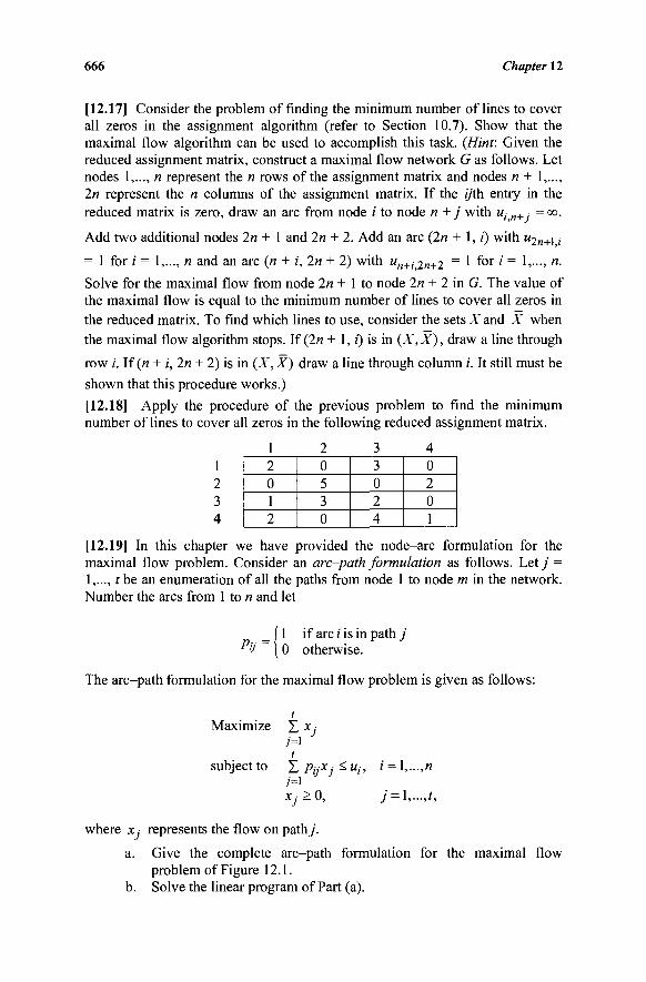
666 Chapter 12
[12.17] Consider the problem of finding the minimum number of lines to cover all zeros in the assignment algorithm (refer to Section 10.7). Show that the maximal flow algorithm can be used to accomplish this task. {Hint: Given the reduced assignment matrix, construct a maximal flow network G as follows. Let nodes 1,..., n represent the n rows of the assignment matrix and nodes n + 1,..., 2« represent the n columns of the assignment matrix. If the yth entry in the reduced matrix is zero, draw an arc from node i to node n + j with uin+ · = <x>.
Add two additional nodes 2n + 1 and In + 2. Add an arc (2ra + 1, /') with u2n+\i
= 1 for i = 1,..., n and an arc (« + i, 2n + 2) with un+i 2n+2 = 1 f°r i = ' , - , «·
Solve for the maximal flow from node In + 1 to node In + 2 in G. The value of the maximal flow is equal to the minimum number of lines to cover all zeros in the reduced matrix. To find which lines to use, consider the sets X and X when the maximal flow algorithm stops. If (2« + 1, i) is in (X, X), draw a line through
row /'. If (n + i, 2n + 2) is in (X,X) draw a line through column /. It still must be
shown that this procedure works.)
[12.18] Apply the procedure of the previous problem to find the minimum number of lines to cover all zeros in the following reduced assignment matrix.
1 2 3 4 2 0 1 2
0 5 3 0
3 0 2 4
0 2 0 1
[12.19] In this chapter we have provided the node-arc formulation for the maximal flow problem. Consider an arc-path formulation as follows. Let j = 1,..., / be an enumeration of all the paths from node 1 to node m in the network. Number the arcs from 1 to n and let
_ 11 if arc / is in path j P'j ~ ( 0 otherwise.
The arc-path formulation for the maximal flow problem is given as follows:
Maximize Σ x.-7=1
t subject to Σ PyXj ^ Hi,
7=1
Xj>0, where x. represents the flow on path/.
a. Give the complete arc-path formulation for the maximal flow problem of Figure 12.1.
b. Solve the linear program of Part (a).
i = \,...,n
j = l,...,t,
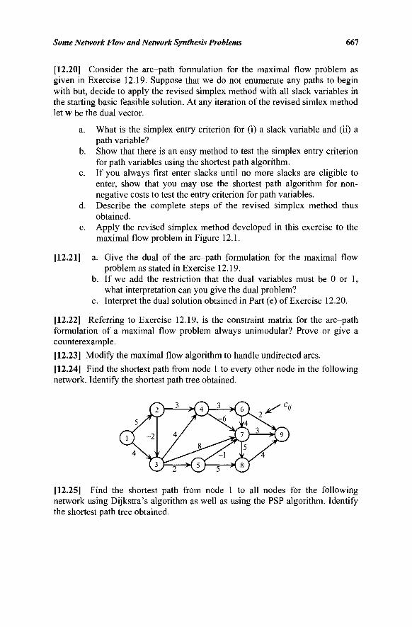
Some Network Flow and Network Synthesis Problems 667
[12.20] Consider the arc-path formulation for the maximal flow problem as given in Exercise 12.19. Suppose that we do not enumerate any paths to begin with but, decide to apply the revised simplex method with all slack variables in the starting basic feasible solution. At any iteration of the revised simlex method let w be the dual vector.
a. What is the simplex entry criterion for (i) a slack variable and (ii) a path variable?
b. Show that there is an easy method to test the simplex entry criterion for path variables using the shortest path algorithm.
c. If you always first enter slacks until no more slacks are eligible to enter, show that you may use the shortest path algorithm for non-negative costs to test the entry criterion for path variables.
d. Describe the complete steps of the revised simplex method thus obtained.
e. Apply the revised simplex method developed in this exercise to the maximal flow problem in Figure 12.1.
[12.21] a. Give the dual of the arc-path formulation for the maximal flow problem as stated in Exercise 12.19.
b. If we add the restriction that the dual variables must be 0 or 1, what interpretation can you give the dual problem?
c. Interpret the dual solution obtained in Part (e) of Exercise 12.20.
[12.22] Referring to Exercise 12.19, is the constraint matrix for the arc-path formulation of a maximal flow problem always unimodular? Prove or give a counterexample.
[12.23] Modify the maximal flow algorithm to handle undirected arcs.
[12.24] Find the shortest path from node 1 to every other node in the following network. Identify the shortest path tree obtained.
[12.25] Find the shortest path from node 1 to all nodes for the following network using Dijkstra's algorithm as well as using the PSP algorithm. Identify the shortest path tree obtained.
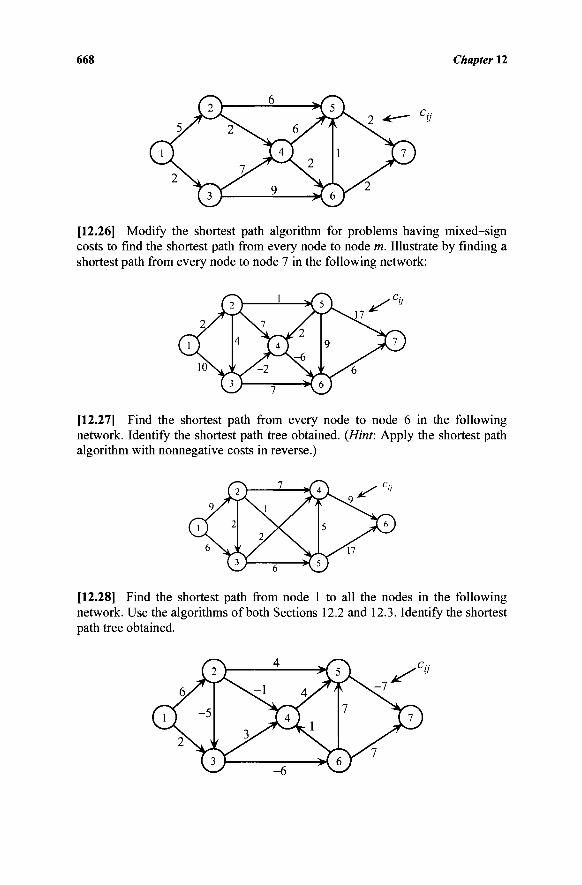
668 Chapter 12
[12.26] Modify the shortest path algorithm for problems having mixed-sign costs to find the shortest path from every node to node m. Illustrate by finding a shortest path from every node to node 7 in the following network:
[12.27] Find the shortest path from every node to node 6 in the following network. Identify the shortest path tree obtained. (Hint: Apply the shortest path algorithm with nonnegative costs in reverse.)
[12.28] Find the shortest path from node 1 to all the nodes in the following network. Use the algorithms of both Sections 12.2 and 12.3. Identify the shortest path tree obtained.
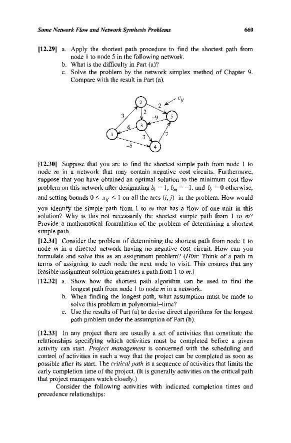
Some Network Flow and Network Synthesis Problems 669
[12.29] a. Apply the shortest path procedure to find the shortest path from node 1 to node 5 in the following network.
b. What is the difficulty in Part (a)? c. Solve the problem by the network simplex method of Chapter 9.
Compare with the result in Part (a).
[12.30] Suppose that you are to find the shortest simple path from node 1 to node m in a network that may contain negative cost circuits. Furthermore, suppose that you have obtained an optimal solution to the minimum cost flow problem on this network after designating b\ = 1, bm = - 1 , and bt = 0 otherwise, and setting bounds 0 < Xu < 1 on all the arcs (i,j) in the problem. How would
you identify the simple path from 1 to m that has a flow of one unit in this solution? Why is this not necessarily the shortest simple path from 1 to ml Provide a mathematical formulation of the problem of determining a shortest simple path.
[12.31] Consider the problem of determining the shortest path from node 1 to node m in a directed network having no negative cost circuit. How can you formulate and solve this as an assignment problem? (Hint: Think of a path in terms of assigning to each node the next node to visit. This ensures that any feasible assignment solution generates a path from 1 to m.)
[12.32] a. Show how the shortest path algorithm can be used to find the longest path from node 1 to node m in a network.
b. When finding the longest path, what assumption must be made to solve this problem in polynomial-time?
c. Use the results of Part (a) to devise direct algorithms for the longest path problem under the assumption of Part (b).
[12.33] In any project there are usually a set of activities that constitute the relationships specifying which activities must be completed before a given activity can start. Project management is concerned with the scheduling and control of activities in such a way that the project can be completed as soon as possible after its start. The critical path is a sequence of activities that limits the early completion time of the project. (It is generally activities on the critical path that project managers watch closely.)
Consider the following activities with indicated completion times and precedence relationships:
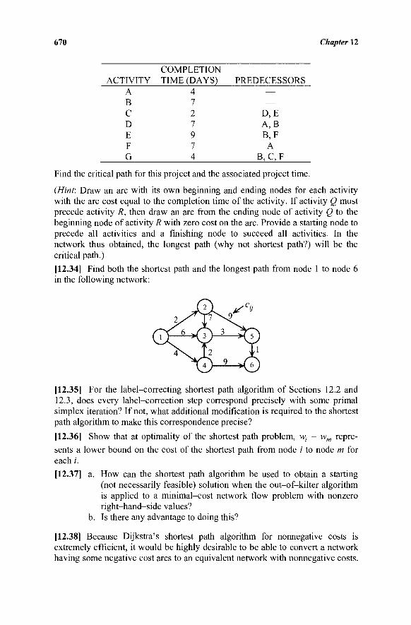
670 Chapter 12
COMPLETION ACTIVITY TIME (DAYS) PREDECESSORS
A 4 — B 7 — C 2 D, E D 7 A, B E 9 B,F F 7 A G 4 B, C,F
Find the critical path for this project and the associated project time.
(Hint: Draw an arc with its own beginning and ending nodes for each activity with the arc cost equal to the completion time of the activity. If activity Q must precede activity R, then draw an arc from the ending node of activity Q to the beginning node of activity R with zero cost on the arc. Provide a starting node to precede all activities and a finishing node to succeed all activities. In the network thus obtained, the longest path (why not shortest path?) will be the critical path.)
[12.34] Find both the shortest path and the longest path from node 1 to node 6 in the following network:
[12.35] For the label-correcting shortest path algorithm of Sections 12.2 and 12.3, does every label-correction step correspond precisely with some primal simplex iteration? If not, what additional modification is required to the shortest path algorithm to make this correspondence precise?
[12.36] Show that at optimality of the shortest path problem, w, - wm repre-sents a lower bound on the cost of the shortest path from node i to node m for each /.
[12.37] a. How can the shortest path algorithm be used to obtain a starting (not necessarily feasible) solution when the out-of-kilter algorithm is applied to a minimal-cost network flow problem with nonzero right-hand-side values?
b. Is there any advantage to doing this?
[12.38] Because Dijkstra's shortest path algorithm for nonnegative costs is extremely efficient, it would be highly desirable to be able to convert a network having some negative cost arcs to an equivalent network with nonnegative costs.
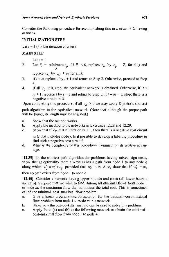
Some Network Flow and Network Synthesis Problems 671
Consider the following procedure for accomplishing this in a network G having m nodes.
INITIALIZATION STEP
Let t = 1 (/ is the iteration counter).
MAIN STEP
1. Let/ '=1. 2. Let c, = minimum Cy. If Έι < 0, replace c„- by Cy - c} for ally and
replace cki by cki + c} for all k.
3. If i < m replace / by / + 1 and return to Step 2. Otherwise, proceed to Step 4.
4. If all e,-, > 0, stop; the equivalent network is obtained. Otherwise, if t <
m + 1, replace / by / + 1 and return to Step 1 ; if / = m + 1, stop; there is a negative circuit in G.
Upon completing this procedure, if all c„· > 0 we may apply Dijkstra's shortest
path algorithm to the equivalent network. (Note that although the proper path will be found, its length must be adjusted.)
a. Show that the method works. b. Apply the method to the networks in Exercises 12.28 and 12.29. c. Show that if c„ < 0 at iteration m + 1, then there is a negative cost circuit
in G that includes node/. Is it possible to develop a labeling procedure to find such a negative cost circuit?
d. What is the complexity of this procedure? Comment on its relative advan-tage.
[12.39] In the shortest path algorithm for problems having mixed-sign costs, show that at optimality there always exists a path from node 1 to any node k along which w' = w[ + c„ provided that w'k < GO. Also, show that if Wk = oo,
then no path exists from node 1 to node k.
[12.40] Consider a network having upper bounds and costs (all lower bounds are zero). Suppose that we wish to find, among all maximal flows from node 1 to node m, the maximum flow that minimizes the total cost. This is sometimes called the minimal-cost-maximal flow problem. a. Give a linear programming formulation for the minimal-cost-maximal
flow problem from node 1 to node m in a network. b. Show how the out-of-kilter method can be used to solve this problem. c. Apply Parts (a) and (b) to the following network to obtain the minimal-
cost-maximal flow from node 1 to node 4:
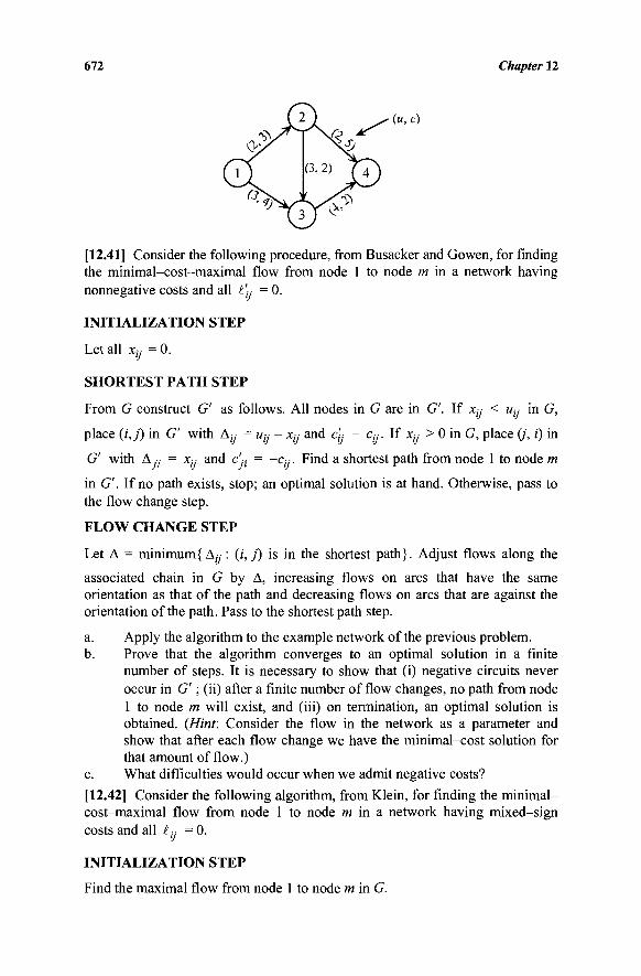
672 Chapter 12
[12.41] Consider the following procedure, from Busacker and Gowen, for finding the minimal-cost-maximal flow from node 1 to node m in a network having nonnegative costs and all l'y = 0.
INITIALIZATION STEP
Let all Xy = 0.
SHORTEST PATH STEP
From G construct G' as follows. All nodes in G are in G'. If Xy < Uy in G,
place (j,j) in G' with Δ,-.- = Uy - Xy and c'y = Cy. If Xy > 0 in G, place (/, i) in
G' with Aβ = Xy and c'( = -Cy. Find a shortest path from node 1 to node m
in G'. If no path exists, stop; an optimal solution is at hand. Otherwise, pass to the flow change step.
FLOW CHANGE STEP
Let Δ = minimum{Δ,γ : (i,j) is in the shortest path}. Adjust flows along the
associated chain in G by Δ, increasing flows on arcs that have the same orientation as that of the path and decreasing flows on arcs that are against the orientation of the path. Pass to the shortest path step.
a. Apply the algorithm to the example network of the previous problem. b. Prove that the algorithm converges to an optimal solution in a finite
number of steps. It is necessary to show that (i) negative circuits never occur in G' ; (ii) after a finite number of flow changes, no path from node 1 to node m will exist, and (iii) on termination, an optimal solution is obtained. (Hint: Consider the flow in the network as a parameter and show that after each flow change we have the minimal-cost solution for that amount of flow.)
c. What difficulties would occur when we admit negative costs?
[12.42] Consider the following algorithm, from Klein, for finding the minimal-cost-maximal flow from node 1 to node m in a network having mixed-sign costs and all iy = 0.
INITIALIZATION STEP
Find the maximal flow from node 1 to node m in G.
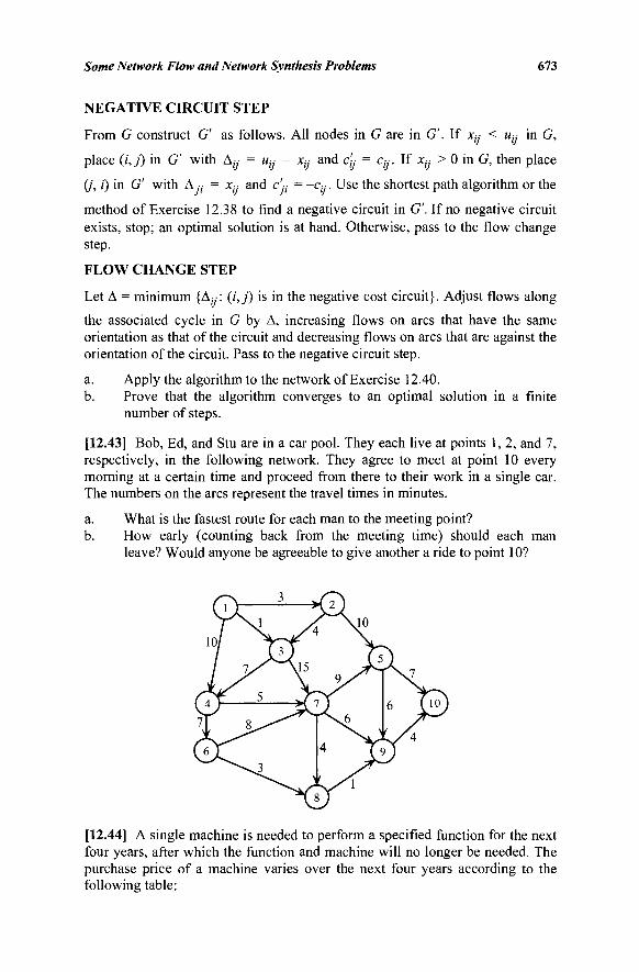
Some Network Flow and Network Synthesis Problems 673
NEGATIVE CIRCUIT STEP
From G construct G' as follows. All nodes in G are in G'. If x„ < «,-,· in G,
place (/,_/) in C with Δ^ = w„- - x„- and c„ = c„. If x„ > 0 in G, then place
(/, /') in G' with Δ ·,· = Xjj and Cy;· = -Cy. Use the shortest path algorithm or the
method of Exercise 12.38 to find a negative circuit in G'. If no negative circuit exists, stop; an optimal solution is at hand. Otherwise, pass to the flow change step.
FLOW CHANGE STEP
Let Δ = minimum {Δ„: (/,/) is in the negative cost circuit}. Adjust flows along
the associated cycle in G by Δ, increasing flows on arcs that have the same orientation as that of the circuit and decreasing flows on arcs that are against the orientation of the circuit. Pass to the negative circuit step.
a. Apply the algorithm to the network of Exercise 12.40. b. Prove that the algorithm converges to an optimal solution in a finite
number of steps.
[12.43] Bob, Ed, and Stu are in a car pool. They each live at points 1, 2, and 7, respectively, in the following network. They agree to meet at point 10 every morning at a certain time and proceed from there to their work in a single car. The numbers on the arcs represent the travel times in minutes.
a. What is the fastest route for each man to the meeting point? b. How early (counting back from the meeting time) should each man
leave? Would anyone be agreeable to give another a ride to point 10?
[12.44] A single machine is needed to perform a specified function for the next four years, after which the function and machine will no longer be needed. The purchase price of a machine varies over the next four years according to the following table:
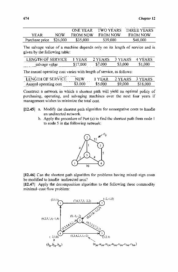
674 Chapter 12
YEAR NOW ONE YEAR FROM NOW
TWO YEARS FROM NOW
THREE YEARS FROM NOW
Purchase price $26,000 $35,000 $39,000 $48,000
The salvage value of a machine depends only on its length of service and is given by the following table:
LENGTH OF SERVICE 1 YEAR 2 YEARS 3 YEARS 4 YEARS salvage value $17,000 $7,000 $3,000 $1,000
The annual operating cost varies with length of service, as follows:
LENGTH OF SERVICE NEW 1 YEAR 2 YEARS 3 YEARS Annual operating cost $3,000 $5,000 $9,000 $18,000
Construct a network in which a shortest path will yield an optimal policy of purchasing, operating, and salvaging machines over the next four years if management wishes to minimize the total cost.
[12.45] a. Modify the shortest path algorithm for nonnegative costs to handle an undirected network,
b. Apply the procedure of Part (a) to find the shortest path from node 1 to node 5 in the following network:
[12.46] Can the shortest path algorithm for problems having mixed-sign costs be modified to handle undirected arcs? [12.47] Apply the decomposition algorithm to the following three commodity minimal-cost flow problem:
(3,1,11
(6,2,5,1,0,-1,4)
(7,4,3,7,3,-2,2)
(-2,1,0)
(VW
(-2,-1,0)
1,2,1)
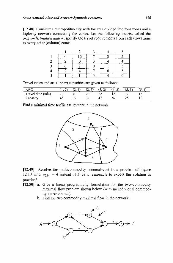
Some Network Flow and Network Synthesis Problems 675
[12.48] Consider a metropolitan city with the area divided into four zones and a highway network connecting the zones. Let the following matrix, called the origin-destination matrix, specify the travel requirements from each (row) zone to every other (column) zone:
1 2 3 4 5
Travel times and arc (upper) capacities are given as follows:
1 0 2 6 2 1
2 10 0 2 4 1
3 7 3 0 7 3
4 8 4 1 0 4
5 5 4 5 5 0
ARC (1,2) (2,4) (2,5) (3,2) (4,3) (5,1) (5,4) Travel time (min) Capacity
20 45
40 39
20 37
22 47
12 36
17 25
13 12
Find a minimal time traffic assignment in the network.
[12.49] Resolve the multicommodity minimal-cost flow problem of Figure 12.10 with M234 = 4 instead of 3. Is it reasonable to expect this solution in
practice? [12.50] a. Give a linear programming formulation for the two-commodity
maximal flow problem shown below (with no individual commod-ity upper bounds),
b. Find the two commodity maximal flow in the network.
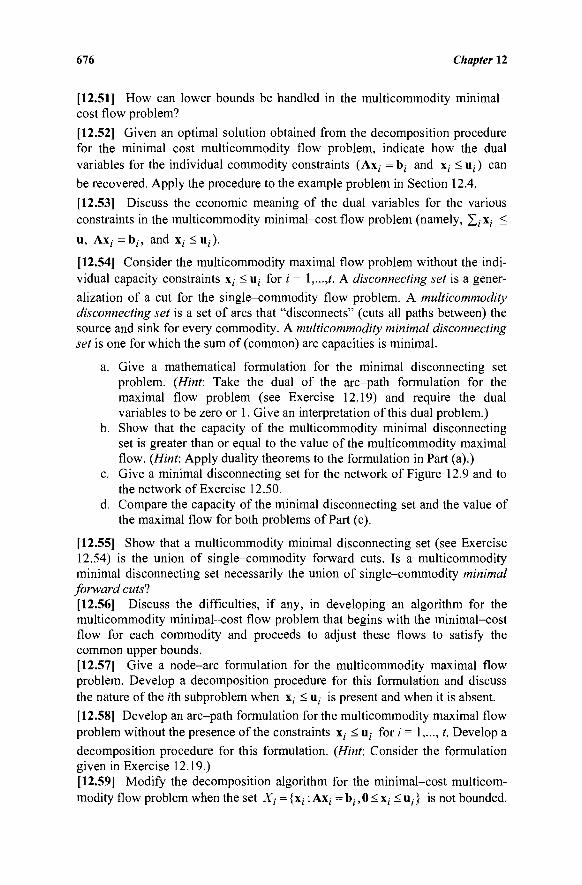
676 Chapter 12
[12.51] How can lower bounds be handled in the multicommodity minimal-cost flow problem?
[12.52] Given an optimal solution obtained from the decomposition procedure for the minimal-cost multicommodity flow problem, indicate how the dual variables for the individual commodity constraints (Ax,· = b; and x,- <u ; ) can be recovered. Apply the procedure to the example problem in Section 12.4. [12.53] Discuss the economic meaning of the dual variables for the various constraints in the multicommodity minimal-cost flow problem (namely, £,· x,· <
u, Ax, = b;, and x;· <u;).
[12.54] Consider the multicommodity maximal flow problem without the indi-vidual capacity constraints x; < u, for i = l,...,t. A disconnecting set is a gener-alization of a cut for the single-commodity flow problem. A multicommodity disconnecting set is a set of arcs that "disconnects" (cuts all paths between) the source and sink for every commodity. A multicommodity minimal disconnecting set is one for which the sum of (common) arc capacities is minimal.
a. Give a mathematical formulation for the minimal disconnecting set problem. (Hint: Take the dual of the arc-path formulation for the maximal flow problem (see Exercise 12.19) and require the dual variables to be zero or 1. Give an interpretation of this dual problem.)
b. Show that the capacity of the multicommodity minimal disconnecting set is greater than or equal to the value of the multicommodity maximal flow. (Hint: Apply duality theorems to the formulation in Part (a).)
c. Give a minimal disconnecting set for the network of Figure 12.9 and to the network of Exercise 12.50.
d. Compare the capacity of the minimal disconnecting set and the value of the maximal flow for both problems of Part (c).
[12.55] Show that a multicommodity minimal disconnecting set (see Exercise 12.54) is the union of single-commodity forward cuts. Is a multicommodity minimal disconnecting set necessarily the union of single-commodity minimal forward cuts! [12.56] Discuss the difficulties, if any, in developing an algorithm for the multicommodity minimal-cost flow problem that begins with the minimal-cost flow for each commodity and proceeds to adjust these flows to satisfy the common upper bounds. [12.57] Give a node-arc formulation for the multicommodity maximal flow problem. Develop a decomposition procedure for this formulation and discuss the nature of the /th subproblem when x; < u; is present and when it is absent. [12.58] Develop an arc-path formulation for the multicommodity maximal flow problem without the presence of the constraints x, < u( for i = 1,..., t. Develop a
decomposition procedure for this formulation. (Hint: Consider the formulation given in Exercise 12.19.) [12.59] Modify the decomposition algorithm for the minimal-cost multicom-modity flow problem when the set Xi = {x; : Ax, = b, , 0 < x, < u,} is not bounded.
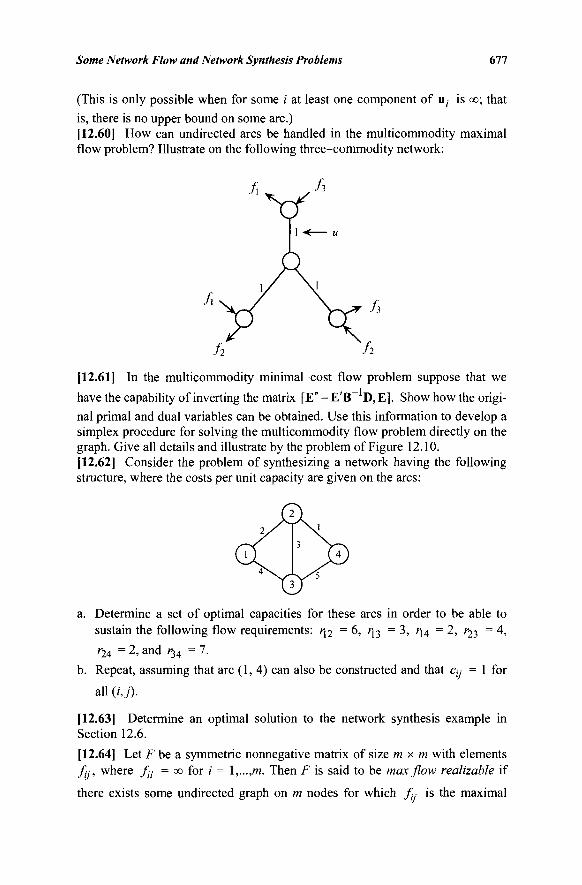
Some Network Flow and Network Synthesis Problems 677
(This is only possible when for some i at least one component of u; is oo; that
is, there is no upper bound on some arc.) [12.60] How can undirected arcs be handled in the multicommodity maximal flow problem? Illustrate on the following three-commodity network:
[12.61] In the multicommodity minimal-cost flow problem suppose that we have the capability of inverting the matrix [E"-E'B~ D,E]· Show how the origi-nal primal and dual variables can be obtained. Use this information to develop a simplex procedure for solving the multicommodity flow problem directly on the graph. Give all details and illustrate by the problem of Figure 12.10. [12.62] Consider the problem of synthesizing a network having the following structure, where the costs per unit capacity are given on the arcs:
a. Determine a set of optimal capacities for these arcs in order to be able to sustain the following flow requirements: ri2 = 6, r13 = 3, r]4 = 2, r23 = 4,
r24 = 2, and r34 = 7.
b. Repeat, assuming that arc (1, 4) can also be constructed and that Cy = 1 for
all (i,j).
[12.63] Determine an optimal solution to the network synthesis example in Section 12.6.
[12.64] Let F be a symmetric nonnegative matrix of size m x m with elements fu, where fu = oo for i = l,...,m. Then F is said to be max flow realizable if
there exists some undirected graph on m nodes for which /J is the maximal
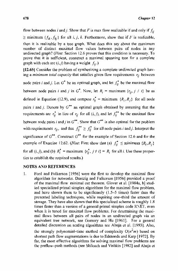
678 Chapter 12
flow between nodes / andy. Show that F is max flow realizable if and only if fy
> minimum {/^,/Η} f°r a u Uj, k. Furthermore, show that if F is realizable,
then it is realizable by a tree graph. What does this say about the maximum number of distinct maximal flow values between pairs of nodes in any undirected graph? {Hint: Section 12.6 proves that this condition is necessary. To prove that it is sufficient, construct a maximal spanning tree for a complete graph with each arc (i,j) having a weight fy.)
[12.65] Consider the problem of synthesizing a complete undirected graph hav-ing a minimum total capacity that satisfies given flow requirements r^ between
node pairs / andy. Let G* be an optimal graph, and let ff- be the maximal flow
between node pairs / and j in G*. Now, let Rj = maximum {η, j φ i) be as
defined in Equation (12.9), and compute η- = minimum {Rj,R:} for all node
pairs i and y. Denote by G** an optimal graph obtained by assuming that the
requirements are r*j in lieu of /■« for all (i,j), and let f** be the maximal flow
between node pairs i andy in G**. Show that G** is also optimal for the problem
with requirements r^, and that f** > f*; for all node pairs i andy. Interpret the
significance of G**. Construct G** for the example of Section 12.6 and for the
example of Exercise 12.62. (Hint: First show that (a) f*= < minimum {RhRj}
for all (i,j), and (b) R* = maximum {r*-, j Φ i) = Rj for all /. Use these proper-
ties to establish the required results.)
NOTES AND REFERENCES
1. Ford and Fulkerson [1956] were the first to develop the maximal flow algorithm for networks. Dantzig and Fulkerson [1956] provided a proof of the maximal flow-minimal cut theorem. Glover et al. [1984a, b] stud-ied specialized primal simplex algorithms for the maximal flow problem, and have shown them to be significantly (1.5-5 times) faster than the presented labeling techniques, while requiring one-third the amount of storage. They have also shown that this specialized scheme is roughly 1.8 times faster than a version of a general primal simplex code RNET, even when it is tuned for maximal flow problems. For determining the maxi-mal flows between all pairs of nodes in an undirected graph via an equivalent tree network, see Gomory and Hu [1961]. For a general detailed discussion on scaling algorithms see Ahuja et al. [1993]. Also,
the strongly polynomial-time method of complexity 0(« m) based on shortest path flow augmentations is due to Edmonds and Karp [1972]. By far, the most effective algorithms for solving maximal flow problems are the preflow-push methods (see Shiloach and Vishkin [1982] and Ahuja et
Some Network Flow and Network Synthesis Problems 679
al. [1993]. Wherease preflow algorithms permit flow imbalances only of the type where the excess given by the inflow minus the outflow is nonnegative, a more recent algorithm due to Hochbaum [2008] is based on pseudoflows where nodes can have excess or deficit (negative excess) flows. This algorithm, which is of complexity 0(mn\og(m)), first determines a minimal cut through an equivalent blocking-cut problem, and then recovers the maximal flow (with additional complexity 0(n log(m))).
2. The first algorithms for shortest path problems were developed by Bellman [1958], Dijkstra [1959], Dantzig [1960], Whiting and Hiller [1960], and Floyd [1962]. A good comparison of these procedures appears in Dreyfus [1969]. More efficient methods have been developed by Glover et al. [1985a, b]. Computer implementations of these algorithms are described by Klingman and Schneider [1986]. A comprehensive computational study appears in Glover et al. [1984a, b] and Hung and Divoky [1988], where it is shown that threshold based partitioned shortest path algorithms dominate other procedures. (Also, see Bertsekas [1993].) A good exposition on the complexity behavior of some shortest path implementations is given by Shier and Witzgall [1981]. Sherali [1991] presents relationships between the partitioned shortest path algorithm and a dynamic programming routine. Also, see Fredman and Tarjan [1984] for improved implementations using Fibonacci heaps. (Additional discussion on heap implementations appears in Ahuja et al. [1993].) For the use of decomposition techniques in solving large-scale shortest path problems on special networks, see Hu [1968], Shier [1973], and Jarvis and Tufekci [1981]. For a more detailed exposition on the relationship between shortest path algorithms and the simplex method, see Akgul [1986b], Dial et al. [1979], and Zadeh [1979]. The procedure of Exercise 12.38 was developed by Bazaraa and Langley [1974], and is based on ideas presented by Nemhauser [1972]. For generalizations of label setting and label correcting algorithms for bicriteria shortest path problems, see the survey paper by Skriver [2000]; for characterizing Pareto optimal (non-dominated) solutions to bicriteria/multi-criteria shortest path problems see Muller-Hannemann and Weihe [2006]; for time-dependent shortest path problems see Cook and Halsey [1966], Dreyfus [1969], Halpern [1977], Orda and Rom [1990], and Sherali et al. [1998]; for label-constrained and approach-dependent variants of this problem see Barrett et al. [2001] and Sherali et al. [2003, 2006]; for stochastic shortest path problems see Orda et al. [1993], Polychronopoulos and Tsitsiklis [1996], and Hutson and Shier [2009]; for complexity and algorithmic analyses of robust shortest paths under uncertainty, see Montemanni et al. [2004], Yu and Yang [1998], and Zielinski [2004]; and for dynamic and dynamic stochastic shortest path problems, see Psaraftis and Tsitsiklis [1993] and Cheung [1998a, b], respectively. Pallottino and Scutella [2003] discuss sensitivity analysis issues under changing arc costs for shortest path problems. Zhang and Yixun [2003] describe the reverse shortest path problem of finding a least
680 Chapter 12
cost decrement in link costs in order to achieve a specified target objective value. Also, Sherali and Hill [2009] discuss a time-restricted reverse shortest path problem of determining a reverse shortest path under time-restricted arc availabilities and given a specified lower bound on the start-time. (Such problems arise in air traffic management.)
3. Ford and Fulkerson [1958b] first proposed a column generation procedure for the multicommodity maximal flow problem. This was the forerunner to the Dantzig-Wolfe decomposition procedure for general linear programs. Hartmand and Lasdon [1972] proposed a procedure based on the simplex method for solving multicommodity flow problems. For the various exercises on multicommodity maximal flow problems, see Robacker [1956], Ford and Fulkerson [1958b], Bellmore et al. [1970], Grigoriadis and White [1972a, b], Hartman and Lasdon [1972], and Jarvis and Keith [1974]. A good discussion and survey on multicom-modity flow problems appears in Kennington and Helgason [1980], and Jones et al. [1993]. Lustig and Li [1992] provide excellent implementa-tion concepts.
4. The network synthesis problem described in Section 12.6 is from Gomory and Hu [1962]. Also, see Ford and Fulkerson [1962].
BIBLIOGRAPHY
Abadie, J., On the Decomposition Principle, ORC Report 63-20, Operations Research Center, University of California, Berkeley, CA, August 1963.
Abadie, J., and A. C. Williams, "Dual and Parametric Methods in Decomposition," in R. Graves and P. Wolfe (eds.), Recent Advances in Mathematical Programming, McGraw-Hill Book Co., NY, 1963.
Adler, I., M. G. C. Resende, and G. Veiga, "An Implementation of Karmarkar's Algorithm for Linear Programming," Operations Research Center, Report 86-8, University of California at Berkeley, May 1986.
Advani, S., "A Linear Programming Approach to Air-Cleaner Design," Operations Research, 22(2), pp. 295-297, March-April, 1974.
Aggarwal, S. P., "A Simplex Technique for a Particular Convex Programming Problem," Canadian Operational Research Society Journal, 4(2), pp. 82-88, July 1966.
Ahuja, R. K., T. L. Magnanti, and J. B. Orlin, Network Flows: Theory, Algorithms, and Applications, Prentice-Hall, Englewood Cliffs, NJ, 1993.
Ahuja, R. K., J. B. Orlin, P. Sharma, and P. T. Sokkalingham, "A Network Simplex Algorithms with 0(n) Consecutive Degenerate Pivots," Operations Research Letters, 30(3), pp. 141-148, 2002.
Akgul, M., "Topics in Relaxation and Ellipsoidal Methods," Ph.D. Dissertation, Department of Combinatorics and Optimization, University of Waterloo, Waterloo, Ontario, Canada, 1981.
Akgul, M., "A Note on Shadow Prices in Linear Programming," Journal of the Operational Research Society, 35(5) pp. 425-431, 1984.
Akgul, M., "An Algorithmic Proof of the Polyhedral Decomposition Theorem," Naval Research Logistics Quarterly, 35, pp. 463-472, 1988.
Akgul, M., "A Genuinely Polynomial Primal Simplex Algorithm for the Assignment Problem," Department of Computer Science and Operations Research, North Carolina State University, Raleigh, NC, 1986a.
Akgul, M., "Shortest Paths and the Simplex Method," Working Paper, Department of Computer Science, North Carolina State University, Raleigh, NC, 1986b.
Albers, D. J., and C. Reid, "An Interview with George B. Dantzig: The Father of Linear Programming," The College Mathematics Journal, 17(4), pp. 292-314, September 1986.
Ali, A., R. Helgason, J. Kennington, and H. Lall, "Primal-Simplex Network Codes: State-of-the-Art Implementation Technology," Networks, 8, pp. 315-339, 1978.
Ali, A., R. Helgason, J. Kennington, and H. Lall, "Computational Comparison Among Three Multicommodity Network Flow Algorithms," Operations Research, 28(4), pp. 995-1000, 1980.
Arnaldi, E., M. E. Pfetsch, and L. E. Trotter, Jr., "On the Maximum Feasible Subsystem Problems, IISs and IIS - Hypgraphics," Mathematical Programming {Series A), 95(3), pp. 533-554, 2003.
681
682 Bibliography
Anstreicher, K. M., "Analysis of a Modified Karmarkar Algorithm for Linear Programming," Working Paper Series B#84, Yale School of Organization and Management, Box IA, New Haven, CT, 1985.
Anstreicher, K. M., "A Strengthened Acceptance Criterion for Approximate Projection in Karmarkar's Algorithm," Operations Research Letters, 5(4), pp. 211-214, 1986a.
Anstreicher, K. M., "A Monotonie Projective Algorithm for Fractional Linear Programming," Algorithmica, 1, pp. 483-498, 1986b.
Anstreicher, K. M., "A Combined 'Phase I — Phase 11 ' Projective Algorithm for Linear Programming (To appear in Mathematical Programming), Technical Report, Yale School of Organization and Management, New Haven, CT, 1986c.
Anstreicher, K. M., "Interior Point Methods in Theory and Practice," Mathematical Programming, Series B, 76(1-2), pp. 1-263, 1997.
Arinal, J. C , "Two Algorithms for Hitchcock Problem," Revue Frangaise de Recherche Qpéationnelle (France), 33, pp. 359-374, 1964.
Aronofsky, J. S., and A. C. Williams, "The Use of Linear Programming and Mathematical Models in Underground Oil Production," Management Science, 8(4), pp. 394-407, July 1962.
Aronson, J., R. Barr, R. Helgason, J. Kennington, A Loh, and H. Zaki, "The Projective Transformation Algorithm by Karmarkar: A Computational Experiment with Assignment Problems," Technical Report 85-OR-3, Department of Operations Research, Southern Methodist University, and Department of Industrial Engineering, University of Houston, Houston, 1985.
Arrow, K. J., L. Hurwicz, and H. Uzawa (eds.), Studies in Linear and Nonlinear Programming, Stanford University Press, Stanford, CA, 1958.
Asher, D. T., "A Linear Programming Model for the Allocation of R and D Efforts," IEEE Transactions on Engineering Management, EM-9 (4), pp. 154-157, December 1962.
Asie, M., V. V. Kovacevic-Vujcic, and M. D. Radosavljevic-Nikolic, "Asymptotic Behavior and Numerical Stability of Karmarkar's Method for Linear Programming," University of Belgrade, Belgrade, Yugoslavia, 1986.
Aspvall, B., and R. E. Stone, " Khachiyan's Linear Programming Algorithm," Journal of Algorithms, l ,pp. 1-13, 1980.
Assad, A. A., "Multicommodity Network Flows: A Survey," Networks, 8(1), pp. 37-92, 1978.
Aucamp, D. C , and D. I. Steinberg, "The Computation of Shadow Prices in Linear Programming," Journal of the Operational Research Society, 33, pp. 557-565, 1982.
Au, T., and T. E. Stelson, Introduction to Systems Engineering, Deterministic Models, Addison-Wesley, Reading, Mass., 1969.
Avis, D., and V. Chvatal, "Notes on Bland's Pivoting Rule," Mathematical Programming Study, 8, pp. 24-34, 1978.
Bibliography 683
Avis, D., B. Kaluzny and D. Titley-Peloquin, "Visualizing and Constructing Cycles in the Simplex Method," Operations Research, 56(2), pp. 512-518,2008.
Azpeitia, A. G., and D. J. Dickinson, "A Decision Rule in the Simplex Method that Avoids Cycling," Numerisene Mathematik, 6, pp. 329-331, 1964.
Balas, E., "Solution of Large Scale Transportation Problems Through Aggregation," Operations Research, 13, pp. 82-93, 1965.
Balas, E., "The Dual Method for the Generalized Transportation Problem," Management Science, 12, pp. 555-568, 1966a.
Balas, E., "An Infeasibility Pricing Decomposition Method for Linear Programs," Operations Research, 14, pp. 847-873, 1966b.
Balas, E., and P. L. Ivanescu, "On the Generalized Transportation Problem," Management Science, 11, pp. 188-203, 1964.
Balas, E., and M. W. Padberg, "On the Set Covering Problem," Management Sciences Research Report #197, Carnegie Mellon University, 1970.
Balinski, M. L., "Integer Programming: Methods, Uses, Computation," Management Science, 12(3), pp. 253-313, November 1965.
Balinski, M. L., "An Algorithm for Finding all Vertices of Convex Polyhedral Sets," SIAM Journal on Applied Mathematics IX, pp. 72-88, 1961.
Balinski, M. L., "The Hirsch Conjecture for Dual Transportation Polyhedra," Mathematics of Operations Research, 1984.
Balinski, M. L., "Signature Methods for the Assignment Problem," Operations Research, 33(3), pp. 527-536, 1985.
Balinski, M. L., "A Competitive (Dual) Simplex Method for the Assignment Problem," Mathematical Programming, 34(2), pp. 125-141, 1986.
Balinski, M. L., and R. E. Gomory, "A Mutual Primal-Dual Simplex Method," in R. L. Graves and P. Wolfe (eds.), Recent Advances in Mathematical Programming, pp. 17-26, McGraw-Hill Book Co., NY, 1963.
Balinski, M. L., and R. E. Gomory, "A Primal Method for the Assignment and Transportation Problems," Management Science, 10(3), pp. 578-593, April 1964.
Balinski, M. L., and A. Russakoff, "On the Assignment Polytope," SIAM Review, 16(4), pp. 516-525, 1974.
Barnes, E. R., "A Variation on Karmarkar's Algorithm for Solving Linear Programming Problems," Mathematical Program-ming, 36, pp. 123-134, 1986.
Barnes, E. R., "A Polynomial Time Version of the Affine Scaling Algorithm," Presented at the Joint National ORSA/TIMS Meeting, St. Louis, October 1987.
Barnes, J. W., and R. M. Crisp, "Linear Programming: A Survey of General Purpose Algorithms," AIIE Transactions, 8(1), pp. 212-221, September 1975.
Barnett, S., "Stability of the Solution to a Linear Programming Problem," Networks, 13(3), pp. 219-228, September 1962.
Barnett, S., "A Simple Class of Parametric Linear Programming Problems," Operations Research, 16(6), pp. 1160-1165, November-December 1968.
684 Bibliography
Barnhart, C , E. L. Johnson, G. L. Nemhauser, M. W. P. Savelsbergh, and P. H. Vance, "Branch-and-Price: Column Generation for Solving Huge Integer Programs," Operations Research, 46(3), pp. 316-329, 1998.
Barr, R. S., F. Glover, and D. Klingman, "An Improved Version of the Out-of-Kilter Method and a Comparative Study of Computer Codes," Mathematical Programming, 7(1), pp. 60-86, 1974.
Barr, R. S., F. Glover, and D. Klingman, "The Alternating Basis Algorithm for Assignment Problems," Mathematical Programming, 13(1), pp. 1-13, 1977.
Barr, R. S., F. Glover, and D. Klingman, "The Generalized Alternating Path Algorithm for Transportation Problems," European Journal of Operational Research, 2, pp. 137-144, 1978.
Barr, R. S., F. Glover, and D. Klingman, "Enhancements of Spanning Tree Labelling Procedures for Network Optimization," INFOR, 17(1), pp. 16-34, 1979.
Barrett, C , R. Jacob, and M. V. Marathe, "Formal Language Constrained Path Problems," SIAM Journal on Computing, 30(3), pp. 809-837,2001.
Bartels, R. H., and G. H. Golub, "The Simplex Method of Linear Programming Using LU-Decomposition," Communications of the ACM, 12, pp. 266-268 and 275-278, 1969.
Battersby, A., Network Analysis for Planning and Scheduling, St. Martin's Press, NY, 1964.
Bazaraa, M. S., and R. W. Langley, "A Dual Shortest Path Algorithm," SIAM Applied Mathematics, 26(3), pp. 496-501, May 1974.
Bazaraa, M. S., and J. J. Goode, "A Survey of Various Tactics for Generating Lagrangian Multipliers in the Context of Lagrangian Duality," European Journal of Operational Research, 3, 322-338, 1979.
Bazaraa, M. S., and H. D. Sherali, "A Versatile Scheme for Ranking the Extreme Points of an Assignment Polytope," Naval Research Logistics Quarterly, 28(4), pp. 545-558, 1981.
Bazaraa, M. S., and H. D. Sherali, "A Property of Degenerate Pivots for Linear Assignment Networks," Networks, 12(4), pp. 469-474, 1982.
Bazaraa, M. S., H. D. Sherali, and C. M. Shetty, Nonlinear Programming: Theory and Algorithms, John Wiley & Sons, Inc., third edition, 2006.
Bazaraa, M. S., and C. M. Shetty, Foundations of Optimization, Springer Verlag,NY, 1976.
Beale, E. M. L., "Cycling in the Dual Simplex Algorithm," Naval Research Logistics Quarterly, 2(4), pp. 269-276, December 1955.
Beale, E. M. L., "An Algorithm for Solving the Transportation Problem When the Shipping Cost Over Each Route is Convex," Naval Research Logistics Quarterly, 6(1), pp. 43-56, March 1959.
Bell, E. J., "Primal-Dual Decomposition Programming," U.S.G.R.& D.R. Order AD-625 365 from CFSTI, Operations Research Center, University of California, Berkeley, CA, August 1965.
Bellman, R., "On a Routing Problem," Quarterly Applied Mathematics, 16(1), pp. 87-90, April 1958.
Bibliography 685
Bellmore, M., H. J. Greenberg, and J. J. Jarvis, "Multicommodity Disconnecting Sets," Management Science, 16, pp. B427-B433, 1970.
Bellmore, M., and R. Vemuganti, " On Multicommodity Maximal Dynamic Flows," Operations Research, 21, pp. 10-21, 1973.
Ben Daya, M., and C. M. Shetty, "Polynomial Barrier Function Algorithms for Linear Programming," School of Industrial and Systems Engineering, Georgia Institute of Technology, Atlanta, GA, 1988.
Benders, J. F., "Partitioning Procedures for Solving Mixed Variables Programming Problems," Numerisene Methamatik, 4, pp. 238-252, 1962.
Benichoi, M., J. M. Gauthier, G. Hentges, and G. Ribiere, "The Efficient Solution of Large-Scale Linear Programming Problems — Some Algorithmic Techniques and Computational Results," Mathematical Programming, 13, pp. 280-322, December 1977.
Ben-Israel, A., and A. Charnes, "An Explicit Solution of a Special Class of Linear Programming Problems," Operations Research, 16(6), pp. 1160-1175, November-December 1968.
Ben-Israel, A., and P. D. Robers, "A Decomposition Method for Interval Linear Programming," Management Science, 16(5), pp. 374-387, January 1970.
Bennett, J. M., and D. R. Green, "An Approach to Some Structured Linear Programming Problems," Operations Research, 17(4), pp. 749-750, July-August 1969.
Berge, C, and A. Ghouila-Houri, Programming, Games and Transportation Networks, John Wiley & Sons, NY, 1965.
Bertsekas, D. P., "A New Algorithm for the Assignment Problem," Mathematical Programming, 21, pp. 152-171, 1981.
Bertsekas, D. P., "A Unified Framework for Primal-Dual Methods in Minimum Cost Network Flow Problems," Mathematical Programming, 32, pp. 125-145, 1985.
Bertsekas, D. P., "A Distributed Asynchronous Relaxation Algorithm for the Assignment Problem," Proceedings of the 24th IEEE Conference on Decision and Control, Ft. Lauderdale, FL, pp. 1703-1704, December 1985.
Bertsekas, D. P., "Distributed Relaxation Methods for Linear Network Flow Problems," Proceedings of the 25th IEEE Conference on Decision and Control, Athens, Greece, pp. 2101-2106, 1986.
Bertsekas, D. P., "The Auction Algorithm: A Distributed Relaxation Method for the Assignment Problem," Report LIDS-P-1653, March 1987.
Bertsekas, D. P., Linear Network Optimization: Algorithms and Codes, MIT Press, Boston, MA, 1991.
Bertsekas, D. P., "A Simple and Fast Label Correcting Algorithm for Shortest Paths," Networks, 23, pp. 703-709, 1993.
Bertsekas, D. P., Network Optimization: Continuous and Discrete Models, Athena Scientific, 1998.
Bertsekas, D. P., and J. Eckstein, "Distributed Asychronous Relaxation Methods for Linear Network Flow Problems," Report LIDS-P-1606, Proceedings of IFAC '87, Munich, Germany, Pergamon Press, Oxford, England, July 1987.
686 Bibliography
Bertsekas, D. P., and D. El Baz, "Distributed Asynchronous Relaxation Methods for Convex Network Flow Problems," LIDS Report P-1417, SIAM Journal on Control and Optimization, 25, pp. 74-85, 1987.
Bertsekas, D. P., P. Hosein, and P. Tseng, "Relaxation Methods for Network Flow Problems with Convex Arc Costs," SIAM Journal on Control and Optimization, 25, pp. 1219-1243, 1987.
Bertsekas, D. P., and P. Tseng, "The RELAX Codes for Linear Minimum Cost Network Flow Problems," in FORTRAN Codes for Network Optimization, Annals of Operations Research (ed. B. Simeone), 13(1), pp. 125-190, 1988a (LIDS Report P-1469, MIT, 1986).
Bertsekas, D. P., and P. Tseng, "Relaxation Methods for Minimum Cost Ordinary and Generalized Network Flow Problems," Operations Research, 36(1), pp. 93-114, 1988b.
Bertsekas, D. P. and P. Tseng, "RELAX-IV: A Faster Version of the RELAX Code for Solving Minimum Cost Flow Problems," Technical Report, Department of Computer Science, MIT, Boston, MA, November 1994.
Best, M. J., and K. Ritter, Linear Programming Active Set Analysis and Computer Programs, Prentice-Hall, Inc., Englewood Cliffs, New Jersey, 1985.
Bialy, H., "An Elementary Method for Treating the Case of Degeneracy in Linear Programming," Unternehmensforschung (Germany), 10(2), pp. 118-123,1966.
Birge, J. R., "A Dantzig-Wolfe Decomposition Variant Equivalent to Basis Factorization," Mathematical Programming Study 24, ed. R. W. Cottle, pp. 43-64, 1985.
Birge, J. R., and L. Qi, "Solving Stochastic Linear Programs Via a Variant of Karmarkar's Algorithm," Technical Report 85-12, University of Michigan, College of Engineering, Ann Arbor, Michigan, 1985.
Bitran, G. R., and A. G. Novaes, "Linear Programming with a Fractional Objective Function," Operations Research, 21(1), pp. 22-29, January-February 1973.
Bixby, R. E., and W. H. Cunningham, "Converting Linear Programs to Network Problems," Mathematics of Operations Research, 5(3), pp. 321-357, 1980.
Blair, C. E., "The Iterative Step in the Linear Programming Algorithm of N. Karmarkar," Algorithmica, 1(4), pp. 537-539, 1986.
Bland, R. G., "New Finite Pivoting Rules for the Simplex Method," Mathematics of Operations Research, 2, pp. 103-107, May 1977.
Bland, R. G., D. Goldfarb, and M. J. Todd, "The Ellipsoid Method: A Survey," Operations Research, 29(6), pp. 1039-1091, November/December 1981.
Blum, L., "Towards an Asymptotic Analysis of Karmarkar's Algorithm," Mills College, Oakland, CA, and the Department of Mathematics, University of California, Berkeley, 1985.
Boldyreff, A. W., "Determination of the Maximal Steady State Flow of Traffic Through a Railroad Network," Operations Research, 3(4), pp. 443-465, November 1955.
Bibliography 687
Borgwardt, K. H., "Some Distribution Independent Results About the Asymptotic Order of the Average Number of Pivot Steps in the Simplex Method," Mathematics of Operations Research, 7(3), pp. 441-462, August 1982a.
Borgwardt, K. H., "The Average Number of Pivot Steps Required by the Simplex Method is Polynomial," Zeitschrift fur Operations Research, 26, pp. 157-177, 1982b.
Borgwardt, K. H., "A Probabilistic Analysis of the Simplex Method," Habilitation Thesis, Kaiserslautern, October 1984.
Borgwardt, K. H., The Simplex Method: A Probabilistic Analysis, Algorithms and Combinatorics 1, Springer-Verlag, 268 p., 1987.
Boulding, K. E., and W. A. Spivey, Linear Programming and the Theory of the Firm, The Macmillan Company, NY, 1960.
Bouska, J., and M. Cerny, "Decomposition Methods in Linear Programming," Ekonomicko-matematicky Obzor (Czechoslovakia), 1(4), pp. 337-369, 1965.
Bowman, E. H., "Production Scheduling by the Transportation Method of Linear Programming," Operations Research, 4(1), pp. 100-103, 1956.
Bowman, E. H., "Assembly-Line Balancing by Linear Programming," Operations Research, 8, pp. 385-389, 1960.
Boyer, D. D., A Modified Simplex Algorithm for Solving the Multicommodity Maximum Flow Problem, Technical Memorandum TM-14930, The George Washington University, Washington, D.C., 1968.
Bradley, G. H., "Survey of Deterministic Networks," AIIE Transactions, 7(3), pp. 222-234, September 1975.
Bradley, G. H., G. G. Brown, and G. W. Graves, "Design and Implementation of Large-Scale Primal Transshipment Algorithms," Management Science, 24(1), pp. 1-34, 1977.
Bramucci, F., "The Inversion Algorithm in Linear Programming," Metra (France), 6(2), pp. 357-381, June 1967.
Briggs, F. E. A., "A Dual Labeling Method for the Hitchcock Problem," Operations Research, 10(4), pp. 507-517, July-August 1962.
Brosius, L., "Comment on a Paper by M. C. Cheng," Mathematical Programming, 21, pp. 229-232, 1981.
Brown, G. G. and R. E. Rosenthal, "Optimization Tradecraft: Hard-Won Insights from Real-World Decision Support," Interfaces, 38(5), pp. 356-366, 2008.
Brown, G. W., and T. C. Koopmans, "Computational Suggestions for Maximizing a Linear Function Subject to Linear Inequalities," in T. C. Koopmans (ed.), Activity Analysis of Production and Allocation, John Wiley & Sons, NY, pp. 377-380, 1951.
Burdet, C. A., "Generating all the Faces of a Polyhedron," SIAM Journal on Applied Mathematics XXVI, pp. 479-489, 1974.
Burkard, R. E., H. W. Hamacher, and J. Tind, "On General Decomposition Schemes in Mathematical Programming," Mathematical Programming, 24, pp. 238-252, 1985.
688 Bibliography
Burrell, B. P., and M. J. Todd, "The Ellipsoid Method Generates Dual Variables," Mathematics of Operations Research, 10, pp. 688-700, 1985.
Busacker, R. G., and P. J. Gowen, A Procedure for Determining a Family of Minimal-Cost Network Flow Patterns, ORO Technical Report 15, Operations Research Office, Johns Hopkins University, 1961.
Busacker, R. G., and T. L. Saaty, Finite Graphs and Networks: An Introduction with Applications, McGraw-Hill Book Co., NY, 1965.
Cabot, A. V., R. L. Francis, and M. A. Stary, "A Network Flow Solution to a Rectilinear Distance Facility Location Problem," AIIE Transactions, 2(2), pp. 132-141, June 1970.
Cahn, A. S., "The Warehouse Problem," Bulletin of American Mathematical Society, 54, p. 1073, 1948.
Caiman, R. F., Linear Programming and Cash Management, CASH ALPHA, The M.I.T. Press, Cambridge, Mass., 1968.
Carnion, P., "Characterization of Totally Unimodular Matrices," Proceedings of American Mathematical Society, 16, pp. 1068-1073, 1965.
Camm, J. D., P. M. Dearing, and S. K. Tadisina, "The Calhoun Textile Mill Case: An Exercise on the Significance of Linear Programming Model Formulation," HE Transactions, 19(1), pp. 23-28, March 1987.
Caratheodory, C , "Uber den Variabilitatsbereich der Koeffizienten von Potenzreihen, die Gegebene Werte Nicht Annehmen," Mathematische Annalen, 64, pp. 95-115, 1007.
Carpenito, G., and L. Toth, "Algorithm 548 ~ Solution of the Assignment Problem," A CM Transactions on Mathematical Software, 6(1), 1980.
Carpenter, T. J., I. J. Lustig, M. M. Mulvey, and D. F. Shanno, "Higher Order Predictor-Corrector Interior Point Methods with Application to Quadratic Objectives," SIAM Journal on Optimization, 3, pp. 696-725, 1993.
Catchpole, A. R., "The Application of Linear Programming to Integrated Supply Problems in the Oil Industry," Networks, 13(2), pp. 161-169, June 1962.
Cavalier, T. M., and A. L. Soyster, "Some Computational Experience and a Modification of the Karmarkar Algorithm," Presented at the 12th International Symposium on Mathematical Programming, Massachusetts Institute of Technology, Cambridge, Massachusetts, August 1985.
Cederbaum, I., "Matrices All of Whose Elements and Subdeterminants are 1, - 1 , or 0," Journal of Mathematics and Physics, 36, pp. 351-361, 1958.
Chadda, S. S., "A Decomposition Principle for Fractional Programming," Opsearch, 4(3), pp. 123-132, 1967.
Chandrascharan, R., "Total Unimodularity of Matrices," SIAM Journal of Applied Mathematics, 17, pp. 1032-1034, 1969.
Chandru, V., and B. S. Kochar, "Exploiting Special Structures Using a Variant of Karmarkar's Algorithm," Research Memorandum 86-10, School of Industrial Engineering, Purdue University, West Lafayette, Indiana 47907, 1986.
Chandru, V., and B. S. Kochar. "A Class of Algorithms for Linear Programming," Research Memorandum 85-14, School of Industrial Engineering, Purdue University, West Lafayette, Indiana 47907, 1985 (revised June 1986).
Bibliography 689
Chandy, K. M., and T. Lo, "The Capacitated Minimum Spanning Tree," Networks, 3(2), pp. 173-181, 1973.
Chang, S. Y., and K. G. Murty, "The Steepest Descent Gravitational Method for Linear Programming," Technical Report #87-14, Department of Industrial and Operations Engineering, The University of Michigan, Ann Arbor, Michigan 48109-2117, 1987.
Charnes, A., "Optimality and Degeneracy in Linear Programming," Econometrica, 20(2), pp. 160-170, 1952.
Charnes, A., and W. W. Cooper, "The Stepping Stone Method of Explaining Linear Programming Calculations in Transportation Problems," Management Science, 1(1), pp. 49-69, 1954.
Charnes, A., and W. W. Cooper, Management Models and Industrial Applications of Linear Programming, John Wiley & Sons, NY, 1961.
Charnes, A., and W. W. Cooper, "Programming with Linear Fractional Functionals," Naval Research Logistics Quarterly, 9, pp. 181-186, 1962.
Charnes, A., and W. W. Cooper, "On Some Works of Kantorovich, Koopmans, and Others," Management Science, 8(3), pp. 246-263, April 1962.
Charnes, A., W. W. Cooper, and A. Henderson, An Introduction to Linear Programming, John Wiley & Sons, NY, 1953.
Charnes, A., W. W. Cooper, and R. Mellon, "Blending Aviation Gasoline: A Study in Programming Interdependent Activities in an Integrated Oil Company," Econometrica, 20(2), pp. 135-159, 1952.
Charnes, A., W. W. Cooper, and G. L. Thompson, "Some Properties of Redundant Constraints and Extraneous Variables in Direct and Dual Linear Programming Problems," Operations Research, 10, pp. 711-723, 1962.
Charnes, A., and K. O. Kortanek, "An Opposite Sign Algorithm for Purification to an Extreme Point Solution," Office of Naval Research, Memorandum No. 84, Northwestern University, Evanston, 1963.
Charnes, A., K. O. Kortanek, and W. Raike, "Extreme Point Solutions in Mathematical Programming: An Opposite Sign Algorithm, Systems Research Memorandum No. 129, Northwestern University, Evanston, 1965.
Charnes, A., and C. E. Lemke, A Modified Simplex Method for Control of Round-off Error in Linear Programming, Carnegie Institute of Technology, Pittsburgh, PA, 1952.
Charnes, A., and C. E. Lemke, "Minimization of Nonlinear Separable Convex Functionals," Naval Research Logistics Quarterly, 1(4), pp. 301-312, December 1954.
Charnes, A., and C. E. Lemke, Computational Theory of Linear Programming, 1: The Bounded Variables Problem, ONR Research Memorandum 10, Graduate School of Industrial Administration, Carnegie Institute of Technology, Pittsburgh, Pennsylvania, January 1954.
Charnes, A., and W. M. Raike, "One Pass Algorithms for Some Generalized Network Problems," Operations Research, 14, pp. 914-924,1966.
Charnes, A., T. Song, and M. Wolfe, "An Explicit Solution Sequence and Convergence of Karmarkar's Algorithm," Research Report CCS 501,
690 Bibliography
College of Business Administration 5.202, The University of Texas at Austin, Austin, Texas 78712-1177, 1984.
Cheng, M. C, "New Criteria for the Simplex Algorithm," Mathematical Programming, 19, pp. 230-236, 1980.
Cheung, R. K., "Iterative Methods for Dynamic Stochastic Shortest Path Problems," Department of Industrial Engineering and Engineering Management, Hong Kong University of Science and Technology, Clear Water Bay, Kowloon, Hong Kong, 1998.
Cheung, R. K. "Iterative Methods for Dynamic Shortest Path Problems," Naval Research Logistics, Vol. 45, pp. 769-789, 1998.
Chester, L. B., Analysis of the Effect of Variance on Linear Programming Problems. U.S.G.R.& D.R. Order AD-611 273 from Clearinghouse, Air Force Institute of Technology, Wright-Patterson AFB, Washington, D.C., August 1964.
Chien, R. T., "Synthesis of a Communication Net," IBM Journal of Research and Development, 4(3), pp. 311-320, 1960.
Chinneck, J. W., "An Effective Polynomial-time Heuristic for the Minimum-Cardinality IIS Set-Covering Problem," Annals of Mathematics and Artificial Intelligence, 17(1), pp. 127-144, 1996.
Chisman, J. A., "Using Linear Programming to Determine Time Standards," Journal of Industrial Engineering, 17'(4), pp. 189-191, April 1966.
Chiù, S. S., and Y. Ye, "Recovering the Shadow Price in Projection Methods of Linear Programming," Engineering-Economics Systems Department, Stanford University, Stanford, CA 94305, 1985.
Chiù, S. S., and Y. Ye, "Simplex Method and Karmarkar's Algorithm: A Unifying Structure," Engineering-Economic Systems Department, Stanford University, Stanford, CA 94305, 1985.
Christofides, N., Graph Theory: An Algorithmic Approach, Academic Press, NY, 1975.
Chung, A., Linear Programming, Charles E. Merrill Books, Columbus, Ohio, 1963.
Chvatal, V., Linear Programming, W. H. Freeman and Company, NY/San Francisco, 1983.
Clark, C. E., "The Optimum Allocation of Resources Among the Activities of a Network," Journal of Industrial Engineering, 12(1), pp. 11-17, January-February 1961.
Clasen, R. J., The Numerical Solution of Network Problems Using Out-of-Kilter Algorithm, RAND Report RM-5456 PR, March 1968.
Clements, R. A., "Linear Programming for Multiple Feed Formulation," NZOR (New Zealand), 2(2), pp. 100-107, July 1974.
Cline, R. E., "Representations for the Generalized Inverse of Matrices Partitioned as A = [U, V]," in R. Graves and P. Wolfe (eds.), Recent Advances in Mathematical Programming, pp. 37-38, McGraw-Hill Book Co., NY, 1963.
Cobham, A., "The Intrinsic Computational Difficulty of Functions," Proceedings of the 1964 International Congress for Logic, Methodology,
Bibliography 691
and Philosophy of Science, Y. Bar-Hille, (ed.), North-Holland, Amsterdam, pp. 24-30, 1965.
Commoner, F. G., "A Sufficient Condition for a Matrix to be Totally Unimodular," Networks, 3, pp. 351-365, 1973.
Cook, S. A., "The Complexity of Theorem-Proving Procedures," Proceedings of the Third Annual ACM Symposium on Theory of Computing, Association for Computing Machinery, NY, pp. 151-158, 1971.
Cook, K. L., and E. Halsey, "The Shortest Route Through a Network with Time-Dependent Intermodal Transit Times," Journal of Mathematical Analysis and Application, 14, pp. 493-498, 1966.
Cooper, L., and J. Kennington, "Non-Extreme Point Solution Strategies for Linear Programs," Naval Research Logistics Quarterly, 26(3), pp. 447-461, 1979.
Courtillot, M., "On Varying All the Parameters in a Linear Programming Problem and Sequential Solution of a Linear Programming Problem," Operations Research, 10(4), pp. 471-475, 1962.
Craven, B. D., "A Generalization of the Transportation Method of Linear Programming," Networks, 14(2), pp. 157-166, June 1963.
Crowder, H., and J. M. Hattingh, "Partially Normalized Pivot Selection," Mathematical Programming Study, Number 4, pp. 12-25, December 1975.
Crowder, FL, E. L. Johnson, and M. Padberg, "Solving Large-Scale Zero-One Linear Programming Problems," Operations Research, 31(5), pp. 803-834, 1983.
Cunningham, W. H., "A Network Simplex Method," Mathematical Programming, 11(2), pp. 105-116, 1976.
Cunningham, W. H., "Theoretical Properties of the Network Simplex Method," Mathematics of Operations Research, 4(2), pp. 196-208, 1979.
Cunningham, W. H., "A Class of Linear Programs Convertible to Network Problems," Operations Research, 31(2), pp. 387-390, 1983.
Curtis, F. H., "Linear Programming the Management of a Forest Property," Journal of Forestry, 61(9), pp. 611-616, September 1962.
Dantzig, G. B., Programming in a Linear Structure, Comptroller, United States Air Force, Washington, D.C., February 1948.
Dantzig, G. B., "Programming of Interdependent Activities, 11, Mathematical Model," in T. C. Koopmans; (ed.), Activity Analysis of Production and Allocation, John Wiley & Sons, NY, 1951, also published in Econometrica, 17(3-4), pp. 200-211, July-October 1949.
Dantzig, G. B., "Maximization of a Linear Function of Variables Subject to Linear Inequalities," in T. C. Koopmans (ed.), Activity Analysis of Production and Allocation, John Wiley & Sons, NY, pp. 339-347, 1951a.
Dantzig, G. B., "A Proof of the Equivalence of the Programming Problem and the Game Problem," in T. C. Koopmans (ed.), Activity Analysis of Production and Allocation, John Wiley & Sons, NY, pp. 359-373, 1951b.
Dantzig, G. B., "Application of the Simplex Method to a Transportation Problem," in T. C. Koopmans (ed.), Activity of Production and Allocation, John Wiley & Sons, NY, pp. 359-373, 1951c.
692 Bibliography
Dantzig, G. B., Computational Algorithm of the Revised Simplex Method, RAND Report RM-1266, The Rand Corporation, Santa Monica, CA, 1953.
Dantzig, G. B., Notes on Linear Programming, Part VII. The Dual Simplex Algorithm, RAND Report RM-1270, The Rand Corporation, Santa Monica, CA, July 1954.
Dantzig, G. B., Notes on Linear Programming, Part XI, Composite Simplex-Dual Simplex Algorithm-1, Research Memorandum RM-1274, The Rand Corporation, Santa Monica, CA, April 1954.
Dantzig, G. B., Notes on Linear Programming: Parts VIII, IX, X - Upper Bounds, Secondary Constraints, and Block Triangularity in Linear Programming, Research Memorandum RM-1367, The Rand Corporation, Santa Monica, CA, October 1954, also published in Econometrica, 23(2), pp. 174-183, April 1955.
Dantzig, G. B., "Discrete Variable Extremum Problems," Operations Research, 5(2), pp. 266-277, April 1957.
Dantzig, G. B., On the Significance of Solving Linear Programming Problems with Some Integer Variables, RAND Report P-1486, The Rand Corporation, Santa Monica, CA, September 1958.
Dantzig, G. B., On the Shortest Route Through a Network, RAND Report P-1345, The Rand Corporation, Santa Monica, CA, April 1958. Also, Management Science, 6(2), pp. 187-190, 1960.
Dantzig, G. B., Linear Programming and Extensions, Princeton University Press, Princeton, NJ, 1963a.
Dantzig, G. B., "Compact Basis Triangularization for the Simplex Method," in R. Graves and P. Wolfe (eds.), Recent Advances in Mathematical Programming, pp. 125-132, McGraw-Hill Book Co., NY, 1963b.
Dantzig, G. B., Optimization in Operations Research: Some Examples, U.S.G.R.& D.R. Order AD-618 748, Operations Research Center, University of California, Berkeley, CA, April 1965.
Dantzig, G. B., All Shortest Routes in a Graph, Technical Report 66-3, Operations Research House, Stanford University, Stanford, CA, November 1966.
Dantzig, G. B., "Reminiscences About the Origins of Linear Programming," Operations Research Letters, 1(2), pp. 43-48, April 1982.
Dantzig, G. B., W. D. Blanttner, and M. R. Rao, All Shortest Routes from a Fixed Origin in a Graph, Technical Report 66-2, Operations Research House, Stanford University, Stanford, CA, November 1966.
Dantzig, G. B., L. R. Ford, and D. R. Fulkerson, "A Primal-Dual Algorithm for Linear Programs," in H. W. Kuhn and A. W. Tucker (eds.), Linear Inequalities and Related Systems, Annals of Mathematics Study No. 38, Princeton University Press, Princeton, NJ, pp. 171-181, 1956.
Dantzig, G. B., and D. R. Fulkerson, "Minimizing the Number of Tankers to Meet a Fixed Schedule," Naval Research Logistics Quarterly, 1(3), pp. 217-222, September 1954.
Dantzig, G. B., and D. R. Fulkerson, "Computation of Maximal Flows in Networks," Naval Research Logistics Quarterly, 2(4), 1955.
Bibliography 693
Dantzig, G. B., and D. R. Fulkerson, "On the Max-Flow Min-Cut Theorem of Networks," in H. W. Kuhn and A. W. Tucker (eds.), Linear Inequalities and Related Systems, Annals of Mathematics Study No. 38, Princeton University Press, Princeton, NJ, pp. 215-221, 1956.
Dantzig, G. B., D. R. Fulkerson, and S. M. Johnson, "Solution of a Large-Scale Traveling-Salesman Problem," Operations Research, 2(4), pp. 393-410, November 1954.
Dantzig, G. B., D. R. Fulkerson, and S. M. Johnson, On a Linear Programming Combinatorial Approach to the Traveling Salesman Problem, RAND Report P-1281, The Rand Corporation, Santa Monica, CA, April 1958.
Dantzig, G. B., R. Harvey, and R. McKnight, Updating the Product Form of the Inverse for the Revised Simplex Method, ORC Report 64-33, Operations Research Center, University of California, Berkeley, CA, December 1964.
Dantzig, G. B., and D. L. Johnson, "Maximum Payloads Per Unit Time Delivered Through an Air Network," Operations Research, 12(2), March-April 1964.
Dantzig, G. B., S. Johnson, and W. White, A Linear Programming Approach to the Chemical Equilibrium Problem, RAND Report P-1060, The Rand Corporation, Santa Monica, CA, April 1958.
Dantzig, G. B., and A. Orden, Notes on Linear Programming: Part II - Duality Theorems, Research Memorandum RM-1265, The Rand Corporation, Santa Monica, CA, October 1953.
Dantzig, G. B., A. Orden, and P. Wolfe, "The Generalized Simplex Method for Minimizing a Linear Form Under Linear Inequality Restraints," Pacific Journal of Mathematics, 5(2), pp. 183-195, June 1955.
Dantzig, G. B., and W. Orchard-Hays, Notes on Linear Programming: Part V -Alternate Algorithm for the Revised Simplex Method Using Product Form for the Inverse, Research Memorandum RM-1268, The RAND Corporation, Santa Monica, CA, November 1953.
Dantzig, G. B., and W. Orchard-Hays, "The Product Form for the Inverse in the Simplex Method," Mathematical Tables and Aids to Computation, 8(46), pp. 64-67, 1954.
Dantzig, G. B., and R. M. Van Slyke, Generalized Upper Bounded Techniques for Linear Programming 1, 11, ORC reports 64-17 (1964), 64-18 (1965), Operations Research Center, University of California, Berkeley, CA.
Dantzig, G. B. and P. Wolfe, "Decomposition Principle for Linear Programs," Operations Research, 8(1), pp. 101-111, January-February 1960.
Dantzig, G. B., and P. Wolfe, "The Decomposition Algorithm for Linear Programs," Econometrica, 29(4), pp. 767-778, October, 1961.
Dantzig, G. B., and P. Wolfe, Linear Programming in a Markov Chain. Notes on Linear Programming and Extensions. Part 59, Research Memorandum RM2957-PR, The Rand Corporation, Santa Monica, CA, April 1962.
de Ghellinck, G., and J.-P. Vial, "A Polynomial Newton Methods for Linear Programming," Algorithmica, 1(4), pp. 425-454, 1986.
694 Bibliography
de Ghellinck, G., and J. Vial, "An Extension of Karmarkar's Algorithm for Solving a System of Linear Homogeneous Equations on the Simplex," Mathematical Programming, 39(1), pp. 79-92, 1987.
Denardo, E. V., "On Linear Programming in a Markov Decision Problem," Management Science, 16(5), pp. 281-288, January 1970.
Dennis, J. B., Mathematical Programming and Electrical Networks, John Wiley & Sons, NY, 1959.
Dennis, J. E., A. M. Morshedi, and K. Turner, "A Variable-Metric Variant of the Karmarkar Algorithm for Linear Programming," Mathematical Programming, 39(1), pp. 1-30, 1987.
Dent, J. B., and H. Casey, Linear Programming and Animal Nutrition, J. B. Lippincott Co., Philadelphia, PA, 1968.
Desaulniers, G., J. Desrosiers, and M. M. Solomon, "Accelerating Strategies in Column Generation Methods for Vehicle Routing and Crew Scheduling Problems," In C. C. Ribeiro and P. Hansen, Eds., Essays and Surveys in Metaheuristics, pp. 309-324, Boston, Kluwer, 2001.
Desrosiers, J. and M. E. Lubbecke, "A Primer in Column Generation," in Column Generation, G. Desaulniers, J. Desrosiers, and M. M. Solomon, Eds., pp. 1-32, Springer, New York, NY, 2005.
Dial, R., F. Glover, D. Karney, and D. Klingman, "A Computational Analysis of Alternative Algorithms and Labeling Techniques for Finding Shortest Path Trees," Networks, 9, pp. 215-248, 1979.
Dickson, J. C, and F. P. Frederick, "A Decision Rule for Improved Efficiency in Solving Linear Programming Problems with the Simplex Algorithm," Communications oftheACM, 3, pp. 509-512, 1960.
Dijkstra, E. W., "A Note on Two Problems in Connection with Graphs," Numerical Mathematics, 1, pp. 269-271, 1959.
Dikin, I. I., "Iterative Solution of Problems of Linear and Quadratic Programming," Soviet Mathematics Doklady, 8, pp. 674-675, 1967.
Dikin, I. I., "On the Speed of an Iterative Process," Upraulyaemye Sistemi, 12, pp. 54-60, 1974.
Doig, A. G., "The Minimum Number of Basic Feasible Solutions to a Transportation Problem," Journal of the Operational Research Society, 14(4), pp. 387-391, 1963.
Doig, A. G., and A. H. Land, "An Automatic Method of Solving Discrete Programming Problems," Econometrica, 28, pp. 497-520, 1960.
Dongarra, J. J., C. B. Moler, J. R. Bunch, and G. W. Stewart, "LINPACK User's Guide," SIAM, Philadelphia, PA, 1979.
Dorfman, R., Application of Linear Programming to the Theory of the Firm, University of California Press, Berkeley, CA, 1951.
Dorfman, R., P. A. Samuelson, and R. M. Solow, Linear Programming and Economic Analyses, McGraw-Hill Book Co., NY, 1958.
Dreyfus, S. E., "An Appraisal of Some Shortest Path Algorithms," Operations Research, 17(3), pp. 395-412, 1969.
du Merle, O., D. Villeneuve, J. Desrosiers, and P. Hansen, "Stabilized Column Generation," Discrete Mathematics, 194, pp. 229-237, 1999.
Bibliography 695
Duffin, R. J., "Infinite Programs," in H. W. Kuhn and A. W. Tucker (eds.), Linear Inequalities and Related Systems, Annals of Mathematics Study No. 38, pp. 157-170, Princeton University Press, Princeton, NJ, 1956.
Duffin, R. J., The Extremal Length of a Network, Office of Technical Services, Document No. AD-253 665, 1961.
Duffin, R. J., "Dual Programs and Minimum Costs," Journal of the Society for Industrial and Applied Mathematics, 10, pp. 119-123, 1962.
Duffin, R. J., "Convex Analysis Treated by Linear Programming," Mathematical Programming (Netherlands), 4(2), pp. 125-143, April 1973.
Dunagan, J. and S. Vempala, "A Simple Polynomial-Time Rescaling Algorithm for Solving Linear Programs," Mathematical Programming, Series A, 114, pp. 101-114,2008.
Dyer, M. E., and L. G. Proli, "An Algorithm for Determining all Extreme Points of a Convex Polytope," Mathematical Programming, 12, pp. 81-96, 1977.
Eckhardt, U., "Theorems on the Dimension of Convex Sets," Linear Algebra and its Applications, 12, pp. 63-76, 1975.
Edmonds, J., "Paths, Trees, and Flowers," Canadian Journal of Mathematics, pp. 449-467, 1965.
Edmonds, J., and R. M. Karp, "Theoretical Improvements in Algorithmic Efficiency for Network Flow Problems," Journal of the ACM, 19(2), pp. 248-264, April 1972.
Egervàry, E., "On Combinatorial Properties of Matrices (1931)," translated by H. W. Kuhn, Paper No. 4, George Washington University Logistics Research Project, 1954.
Eggleston, H. G., Convexity, Cambridge University Press, NY, 1958. Eisemann, K., "The Primal-Dual Method for Bounded Variables," Operations
Research, 12(1), pp. 110-121, January-February 1964. Elam, J., F. Glover, and D. Klingman, "A Strongly Convergent Primal-Simplex
Algorithm for Generalized Networks," Mathematics of Operations Research, 4(1), pp. 39-59, 1979.
Elmaghraby, S. E., "Sensitivity Analysis of Multiterminal Flow Networks," Operations Research, 12(5), pp. 680-688, September-October 1964.
Elmaghraby, S. E., "The Theory of Networks and Management Science. Part I," Management Science, 17(1), pp. 1-34, September 1970.
Elmaghraby, S. E., "The Theory of Networks and Management Science. Part II," Management Science, 17(2), pp. B54-1171, October 1970.
Engquist, M., "A Successive Shortest Path Algorithm for the Assignment Problem," INFOR, 20(4), pp. 370-384, 1982.
Eriksson, J. R., "An Iterative Primal-Dual Algorithm for Linear Programming," Report LITH-MAT-R-1985-10, Institute of Technology, Linkoping University, S-581 83 Linkoping, Sweden, 1985.
Evans, J. R., "A Combinatorial Equivalence Between a Class of Multicommodity Flow Problems and the Capacitated Transportation Problem," Mathematical Programming, 10(3), pp. 401-404, 1976.
Even, S., Graph Algorithms, Computer Science Press, Maryland, 1979.
696 Bibliography
Everett, H., "Generalized Lagrange Multiplier Method for Solving Problems of Optimum Allocation of Resources," Operations Research, 11, pp. 399-417, 1963.
Falk, J. E., "Lagrange Multipliers and Nonlinear Programming," Journal of Mathematical Analysis and Applications, 19, pp. 141-159, 1967.
Farbey, B. A., A. H. Lard, and J. D. Murchland, "The Cascade Algorithm for Finding All Shortest Distances in a Directed Graph," Management Science, 14(1), pp. 19-28, September 1967.
Farkas, J., " Uber die Theorie der einfachen Ungleichungen," Journal Flir die Reine und Angewandte Mathematik, 124, pp. 1-27, 1901.
Fathi, Y., and C. Tovey, "Affirmative Action Algorithms," Mathematical Programming, 34, pp. 292-301, 1986.
Ferguson, A. R., and G. B. Dantzig, Notes on Linear Programming: Part XVI -The Problem of Routing Aircraft - a Mathematical Solution, Research Memorandum, RM-1369, also RAND Paper P-561, 1954, also Aeronautical Engineering Review, 14(4), pp. 51-55, April 1955.
Ferguson, A. R., and G. B. Dantzig, "The Allocation of Aircraft to Routes — An Example of Linear Programming Under Uncertain Demand," Management Science, 3(1), pp. 45-73, October 1956.
Fisher, F. P., "Speed Up the Solution to Linear Programming Problems," Journal of Industrial Engineering, 12(6), pp. 412-416, November-December 1961.
Fletcher, R., and M. J. D. Powell, "On the Modification of LDLT Factorizations," Mathematics of Computation, pp. 1067-1087, 1974.
Flood, M. M., "On the Hitchcock Distribution Problem," Pacific Journal of Mathematics,^!), 1953.
Flood, M. M., "Application of Transportation Theory to Scheduling a Military Tanker Fleet," Operations Research, 2(2), pp. 150-162, 1954.
Flood, M. M., "An Alternative Proof of a Theorem of Konig as an Algorithm for the Hitchcock Distribution Problem," in R. Bellman and M. Hall (eds.), Proceedings of Symposia in Applied Mathematics, American Mathematical Society, Providence, RI, pp. 299-307, 1960.
Flood, M. M., "A Transportation Algorithm and Code," Naval Research Logistics Quarterly, 8(3), pp. 257-276, September 1961.
Florian, M., and P. Robert, "A Direct Search Method to Locate Negative Cycles in a Graph," Management Science, 17(5), pp. 307-310, January 1971.
Floyd, R. W., "Algorithm 97: Shortest Path," Communications of the ACM, 5(6), p. 345, 1962.
Ford, L. R., and D. R. Fulkerson, "Maximal Flow Through a Network," Canadian Journal of Mathematics, 8(3), pp. 399-404, 1956.
Ford, L. R., and D. R. Fulkerson, "A Simple Algorithm for Finding Maximal Network Flows and an Application to the Hitchcock Problem," Canadian Journal of Mathematics, 9(2), pp. 210-218, 1957.
Ford, L. R., and D. R. Fulkerson, "Solving the Transportation Problem," Management Science, 3(1), pp. 24-32, 1956.
Bibliography 697
Ford, L. R., and D. R. Fulkerson, "A Primal-Dual Algorithm for the Capacitated. Hitchcock Problem," Naval Research Logistics Quarterly, 4(1), pp. 47-54, 1957.
Ford, L. R., and D. R. Fulkerson, "Constructing Maximal Dynamic Flows from Static Flows," Operations Research, 6(3), pp. 419-433, 1958a.
Ford, L. R., and D. R. Fulkerson, "Suggested Computation of Maximal Multi-Commodity Network Flows," Management Science, 5(1), pp. 97-101, October 1958b.
Ford, L. R., and D. R. Fulkerson, Flows in Networks, Princeton University Press, Princeton, NJ, 1962.
Forrest, J. J. H., and J. Tomlin, "Implementing Interior Point Linear Programming Methods in the Optimization Subroutine Library," Mathematical Programming Systems RJ 7400 (69202), IBM, 1990.
Forrest, J. J. H., and J. A. Tomlin, "Updating Triangular Factors of the Basis to Maintain Sparsity in the Product Form Simplex Method," Mathematical Programming, 2, pp. 263-278, 1972.
Fox, B., "Finding Minimal Cost-Time Ratio Circuits," Operations Research, 17(3), pp. 546-551, May-June 1969.
Frank, H., and I. T. Frisch, Communication, Transmission, and Transportation Networks, Addison-Wesley, Reading, Mass., 1971.
Francis, R. L., and J. A. White, Facility Layout and Location, Prentice-Hall, Englewood Cliffs, NJ, 1974.
Frazer, R. J., Applied Linear Programming, Prentice-Hall, Englewood Cliffs, NJ, 1968.
Fredman, M. L., and R. E. Tarjan, "Fibonacci Heaps and their Uses in Improved Network Optimization Algorithms," Proceedings of the 25th IEEE Symposium on the Foundations of Computer Science, pp. 338-346, 1984.
Frendewey, J., and F. Glover, "Improved Algorithmic and Computational Procedures for Large Scale Embedded Network Linear Programming Problems," ORSA/TIMS Meeting, Houston, TX, October 1981.
Freund, R. M., "Postoptimal Analysis of a Linear Program under Simultaneous Changes in Matrix Coefficients," Mathematical Programming Study 24, ed. R. W. Cottle, pp. 1-13, 1985.
Freund, R. M. and S. Mizuno, "Interior Point Methods: Current Status and Future Directions," OPTIMA, 51, pp. 1-9, October 1996.
Frisch, K. R., "The Logarithmic Potential Method of Convex Programming," Memorandum of May 13, 1955, University Institute of Economics, Oslo, 1955.
Frisch, R., "The Multiplex Method for Linear Programming," Memorandum of Social Economic Institute, University of Oslo, Oslo, Norway, 1955.
Fulkerson, D. R., "A Network Flow Feasibility Theorem and Combinatorial Applications," Canadian Journal of Mathematics, 11(3), pp. 440-451, 1959.
Fulkerson, D. R., "Increasing the Capacity of a Network, the Parametric Budget Problem," Management Science, 5(4), pp. 472-483, July 1959.
Fulkerson, D. R., "On the Equivalence of the Capacity-Constrained Transshipment Problem and the Hitchcock Problem," Research
698 Bibliography
Memorandum RM2480, The Rand Corporation, Santa Monica, CA, 1960.
Fulkerson, D. R., "An Out-of-Kilter Method for Minimal Cost Flow Problems," Journal of the Society for Industrial and Applied Mathematics, 9(1), pp. 18-27, 1961a.
Fulkerson, D. R., "A Network Flow Computation for Project Cost Curves," Management Science, 7(2), pp. 167-178. January 1961b.
Fulkerson, D. R., "Flow Networks and Combinatorial Operations Research," The American Mathematical Monthly, 73(2), pp. 115-138, February 1966.
Fulkerson, D. R., "Networks, Frames, and Blocking Systems," Mathematics of the Decision Sciences, Part 1, Lectures in Applied Mathematics, 11 (eds. G. B. Dantzig and A. F. Veinott), American Mathematical Society, pp. 304-334,1968.
Fulkerson, D. R., and G. B. Dantzig, "Computations of Maximal Flows in Networks," Naval Research Logistic Quarterly, 2(4), pp. 277-283, December 1955.
Gacs, P., and L. Lovasz, "Khacian's Algorithm for Linear Programming," Mathematical Programming Study 14, North-Holland, Amsterdam, The Netherlands, pp. 61-68, January 1981.
Gal, T., "Shadow Prices and Sensitivity Analysis Under Degeneracy," OR Spektrum, 8, pp. 59-71, 1986.
Gale, D., "Neighboring Vertices on a Convex Polyhedron," in H. W. Kuhn and A. W. Tucker (eds.), Linear Inequalities and Related Systems, Annals of Mathematics Study No. 38, Princeton University Press, Princeton, NJ, pp. 255-263, 1956.
Gale, D., "A Theorem on Flows in Networks," Pacific Journal of Mathematics, 7, pp. 1073-1082,1957.
Gale, D., Transient Flows in Networks, Research Memorandum RM-2158, The Rand Corporation, Santa Monica, CA, 1958.
Gale, D., The Theory of Linear Economic Models, McGraw-Hill Book Co., NY, 1960.
Gale, D., On the Number of Faces of a Convex Polytope, Technical Report No. 1, Department of Mathematics, Brown University, 1962.
Gale, D., H. W. Kuhn, and A. W. Tucker, "Linear Programming and the Theory of Games," Chapter 19 of T. C. Koopmans (ed.), Activity Analysis of Production and Allocation, Cowles Commission Monograph 13, John Wiley & Sons, NY, 1951.
Garey, M. R., and D. S. Johnson, Computers and Intractability: A Guide to the Theory of ΉΡ-Completeness, Freeman, San Francisco, 1979.
Garfinkel, R. S., and G. L. Nemhauser, Integer Programming, John Wiley & Sons, NY, 1972.
Garvin, W. W., Introduction to Linear Programming, McGraw-Hill Book Co., NY, 1960.
Garvin, W. W., H. W. Crandall, J. B. John, and R. A. Spellman, "Application of Linear Programming in the Oil Industry," Management Science, 3(4), pp. 407-430, July 1957.
Bibliography 699
Gass, S. I., "A First Feasible Solution to the Linear Programming Problem," in H. Antosiewicz (ed.), Proceedings of the Second Symposium in Linear Programming, Vols. 1 and 2, DCS/Comptroller, Headquarters, U.S. Air Force, Washington, D.C., pp. 495-508, January, 1955.
Gass, S. I., Linear Programming: Methods and Applications, 4th ed., McGraw-Hill, NY, 1975.
Gass, S. I., The Dualplex Method for Large-scale Linear Programs, ORC Report 66-15, Operations Research Center, University of California, Berkeley, CA, June 1966.
Gass, S. I., and T. Saaty, "The Computational Algorithm for the Parametric Objective Function," Naval Research Logistics Quarterly, 2(1-2), pp. 39-45, 1955.
Gass, S. I., and T. L. Saaty, "Parametric Objective Function. Part II: Generalization," Operations Research, 3(4), pp. 395-401, 1955.
Gassner, Betty J., "Cycling in the Transportation Problem," Naval Research Logistics Quarterly, 11(1), pp. 43-58, March 1964.
Gay, D. M., "Electronic Mail Distribution of Linear Programming Test Problems," COAL Newsletter, 13, pp. 10-12, 1985.
Gay, D. M., "A Variant of Karmarkar's Linear Programming Algorithms for Problems in Standard Form," Mathematical Programming, 37, pp. 81 -90, 1987.
Geary, R. C , and M. C. McCarthy, Elements of Linear Programming, with Economic Applications, Charles Griffin & Co., London, 1964.
Geoffrion, A. M., "Primal Resource-Directive Approaches for Optimizing Nonlinear Decomposable Systems," Operations Research, 18(3), pp. 375-403, May-June 1970.
Geoffrion, A. M., "Duality in Nonlinear Programming: A Simplified Applications-Oriented Development," SIAM Review, 13, pp. 1-37, 1971.
Geoffrion, A. M., "Generalized Benders Decomposition," Journal of Optimization Theory and Applications, 10, pp. 237-260, 1972.
Geoffrion, A. M., "Lagrangean Relaxation for Integer Programming," Mathematical Programming Study, Number 2, pp. 82-114, 1974.
Geoffrion, A. M., "The Purpose of Mathematical Programming is Insight, Not Numbers," Interfaces, 7(1), pp. 81-92, 1976.
Geoffrion, A. M., "An Introduction to Structural Modeling," Management Science, 33(5), pp. 547-588, 1987.
George, J. A., and M. T. Heath, "Solution of Sparse Linear Least Squares Problems Using Givens Rotations," Linear Algebra and Its Applications, 34, pp. 69-83, 1980.
Gibbs, D., F. Glover, D. Klingman, and M. Mead, "A Comparison of Pivot Selection Rules for Primal Simplex Based Network Codes," Operations Research Letters, 2(5), pp. 199-202, 1983.
Gill, P. E„ G. H. Golub, W. Murray, and M. A. Saunders, "Methods for Modifying Matrix Factorizations," Mathematics of Computation, 28, pp. 505-535, 1974.
Gill, P. E., and W. Murray, "A Numerical Investigation of Ellipsoid Algorithms for Large-Scale Linear Programming," Technical Report SOL 80-27,
700 Bibliography
Systems Optimization Laboratory, Stanford University, Stanford, CA, October 1980.
Gill, P. E., W. Murray, M. A. Saunders, J. A. Tomlin, and M. H. Wright, "On Projected Newton Barrier Methods for Linear Programming and an Equivalence to Karmarkar's Projective Method," Mathematical Programming, 36, pp. 183-209, 1986.
Gill, P. E., W. Murray, M. A. Saunders, and M. H. Wright, "A Note on Nonlinear Approaches to Linear Programming," Technical Report SOL 86-7, Department of Operations Research, Stanford University, Stanford, CA 94305, 1986.
Gill, P. E., W. Murray, M. A. Saunders, and M. H. Wright, "Practical Anti-Cycling Procedure for Linear and Nonlinear Programming," Technical Report SOL 88-4, Systems Optimization Laboratory, Department of Operations Research, Stanford University, Stanford, CA 94305, July 1988.
Gilmore, P. C , and R. E. Gomory, "A Linear Programming Approach to the Cutting Stock Problem-Part 1," Operations Research, 9, pp. 849-859, 1961.
Gilmore, P. C, and R. E. Gomory, "A Linear Programming Approach to the Cutting Stock Problem - Part 2," Operations Research, 11(6), pp. 863-887, 1963.
Glassey, C. R., "Nested Decomposition and Multi-Stage Linear Programs," Management Science, 20(3), pp. 282-292, November 1973.
Glickman, T., and H. D. Sherali, "Large-Scale Network Distribution of Pooled Empty Freight Cars Over Time, With Limited Substitution and Equitable Benefits," Transportation Research, B (Methodology), 19(2), pp. 85-94, 1985.
Glicksman, M. A., Linear Programming and Theory of Games, John Wiley & Sons, NY, 1963.
Glover, F., "A New Foundation for a Simplified Primal Integer Programming Algorithm," Operations Research, 16(4), pp. 727-740, July-August, 1968.
Glover, F., R. Glover, and D. Klingman, "Threshold Assignment Algorithm," Mathematical Programming Study 26, pp. 12-37, 1986.
Glover, F., D. Karney, and D. Klingman, "The Augmented Predecessor Index Method for Locating Stepping-Stone Paths and Assigning Dual Prices in Distributions Problems," Transportation Science, 6, pp. 171-180, 1972.
Glover, F., D. Karney, and D. Klingman, "Implementation and Computational Comparisons of Primal, Dual and Primal-Dual Computer Codes for Minimum Cost Network Flow Problems," Networks, 4(3), pp. 191-212, 1974a.
Glover, F., D. Karney, D. Klingman, and A. Napier, "A Computational Study on Start Procedures, Basis Change Criteria, and Solution Algorithms for Transportation Problems," Management Science, 20(5), pp. 793-813, 1974b.
Bibliography 701
Glover, F., D. Karney, D. Klingman, and R. Russell, "Solving Singly Constrained Transshipment Problems," Transportation Science, 12(4), pp. 277-297, 1978.
Glover, F., and D. Klingman, "Comments on Note by Hatch on Network Algorithms," Operations Research, 29(2), pp. 370-373, 1978.
Glover, F., and D. Klingman, "The Simplex SON Algorithm for LP/Embedded Network Problems," Mathematical Programming Study, 15, pp. 148-176, 1981.
Glover, F., and D. Klingman, "Recent Developments in Computer Implementa-tion Technology for Network Flow Algorithms," INFOR, 20(4), pp. 433-452, 1982.
Glover, F., and D. Klingman, "Basic Dual Feasible Solutions for a Class of Generalized Networks," Operations Research, 20, pp. 126-136, 1972.
Glover, F., D. Klingman, and R. S. Barr, "An Improved Version of the Out-of-Kilter Method and a Comparative Study of Computer Codes," Report CS-102, Center for Cybernetic Studies, University of Texas, Austin, TX, 1972.
Glover, F., D. Klingman, M. Mead, and J. Mote, "A Note on Specialized Versus Unspecialized Methods for Maximum-Flow Problems," Naval Research Logistics Quarterly, 31, pp. 63-65, 1984b.
Glover, F., D. Klingman, J. Mote, and D. Whitman, "A Primal Simplex Variant for the Maximum-Flow Problem," Naval Research Logistics Quarterly, 31, pp. 41-61, 1984a.
Glover, F., D. Klingman, and N. Phillips, "A New Polynomially Bounded Shortest Path Algorithm," Operations Research, 33(1), pp. 65-73,1985a.
Glover, F., D. D. Klingman, N. V. Phillips, and R. F. Schneider, "New Polynomial Shortest Path Algorithms and Their Computational Attributes," Management Science, 31(9), pp. 1106-1128, 1985b.
Glover, F., D. Klingman, and J. Stutz, "Augmented Threaded Index Method for Network Optimization," INFOR, 12(3), pp. 293-298, 1974.
Glover, F., D. Klingman, and J. Stutz, "Extensions of the Augmented Predecessor Index Method to Generalized Network Problems," Transportation Science, 7(4), pp. 377-384, 1974.
Golden, B. L., and T. L. Magnanti, "Deterministic Network Optimization: A Bibliography," Networks, 7(2), pp. 149-183, 1977.
Goldfarb, D., "Efficient Dual Simplex Algorithms for the Assignment Problem," Mathematical Programming, 33, pp. 187-203,1985.
Goldfarb, D., J. Hao, and S. Kai, "Anti-stalling Pivot Rules for the Network Simplex Algorithms," Networks, 20, pp. 79-91, 1990.
Goldfarb, D., and Y. Lin, "Combinatorial Interior Point Methods for Generalized Network Flow Problems," Mathematical Programming {Series A), 93(2), pp. 227-246, 2002.
Goldfarb, D., and S. Mehrotra, "A Relaxed Version of Karmarkar's Method," Mathematical Programming, 40(3), pp. 289-316, 1988.
Goldfarb, D., and J. K. Reid, "A Practicable Steepest-Edge Simplex Algorithm," Mathematical Programming, 12, pp. 361-371, 1977.
702 Bibliography
Goldfarb, D., and W. Y. Sit, "Worst Case Behavior of Steepest Edge Simplex Method," Discrete Applied Mathematics, 1, pp. 277-285, 1979.
Goldman, A. J., "Resolution and Separation Theorems for Polyhedral Convex Sets," in H. W. Kuhn and A. W. Tucker (eds.), Linear Inequalities and Related Systems, Annals of Mathematics Study No. 38, Princeton University Press, Princeton, NJ, pp. 41-51, 1956.
Goldman, A. J., and D. Kleinman, "Examples Relating to the Simplex Method," Operations Research, 12(1), pp. 159-161, 1964.
Goldman, A. J., and A. W. Tucker, "Theory of Linear Programming," in H. W. Kuhn and A. W. Tucker (eds.), Linear Inequalities and Related Systems, Annals of Mathematics Study, Number 38, Princeton University Press, Princeton, NJ, pp. 53-98, 1956.
Goldman, A. J., and A. W. Tucker, "Polyhedral Convex Cones," in H. W. Kuhn and A. W. Tucker (eds.), Linear Inequalities and Related Systems, Annals of Mathematics Study, Number 38, Princeton University Press, Princeton, NJ,pp. 19-39, 1956.
Golomski, W. A., "Linear Programming in Food Blending," Annual Convention Transactions, 17th Annual Convention, American Society for Quality Control, pp. 147-152, 1963.
Golub, G. H., and C. F. Van Loan, Matrix Computations, Johns Hopkins University Press, 1983.
Gomory, R. E., An Algorithm for the Mixed Integer Problem, Research Memorandum RM-2597, The Rand Corporation, Santa Monica, CA, 1960.
Gomory, R. E., "An Algorithm for Integer Solutions to Linear Programs," in R. L. Graves and P. Wolfe (eds.), Recent Advances in Mathematical Programming, McGraw-Hill Book Co., NY, pp. 269-302, 1963a.
Gomory, R. E., "All-Integer Integer Programming Algorithm," in J. F. Muth and G. L. Thompson (eds.), Industrial Scheduling, Prentice-Hall, Englewood Cliffs, NJ, pp. 193-206,1963b.
Gomory, R. E., and W. J. Baumol, "Integer Programming and Pricing," Econometrica, 28(3), pp. 521-550, 1960.
Gomory, R. E., and T. C. Hu, "Multi-Terminal Network Flows," SIAM, 9(4), pp. 551-570,1961.
Gomory, R. E., and T. C. Hu, "An Application of Generalized Linear Programming to Network Flows," SIAM, 10(2), pp. 260-283, 1962.
Gomory, R. E., and T. C. Hu, "Synthesis of a Communication Network," SIAM 12(2), pp. 348-369, June 1964.
Goncalves, A. S., "Basic Feasible Solutions and the Dantzig-Wolfe Decomposition Algorithm," Operations Research Quarterly, 19(4), pp. 465-469, December 1968.
Gonzaga, C. C , "A Conical Projection Algorithm for Linear Programming," Memo No. UCB/ERL M85/61, Electronics Research Laboratory, College of Engineering, University of California, Berkeley, CA 94720, 1985.
Gonzaga, C, "An Algorithm for Solving Linear Programming Problems in
0 ( « 3 I ) Operations," Memo No. UCB/ERL M87/10, Electronics
Bibliography 703
Research Laboratory, College of Engineering, University of California, Berkeley, CA 94720,1987a.
Gonzaga, C. C , "Search Directions for Interior Linear Programming Methods," Memo #UCB/ERL M87/44, Electronics Research Laboratory, College of Engineering, University of California, Berkeley, CA 94720, 1987b.
Gonzaga, C. D., "Polynomial Affine Algorithms for Linear Programming," Department of Systems Engineering and Computer Science, COPPE-Federal University of Rio de Janeiro, Caixa Postal 6811, 21941 Rio de Janeiro, RJ, Brazil, ES-139/88, 1988.
Gorham, W., "An Application of a Network Flow Model to Personnel Planning," IEEE Transactions on Engineering Management, 10(3), pp. 121-123, September 1963.
Gould, F. J., "Proximate Linear Programming: A Variable Extreme Point Method," Mathematical Programming, 3(3), pp. 326-338, December 1972.
Granot, F., and D. Klingman, "Editorial: Some Recent Advances in the Theory, Computation, and Applications of Network Flow Models," INFOR, 20(4), pp. 285-286, 1982.
Graves, R. L., and P. Wolfe (eds.), Recent Advances in Mathematical Programming, McGraw-Hill Book Co., NY, 1963.
Greenberg, H., "Modification of the Primal-Dual Algorithm for Degenerate Problems," Operations Research, 16(6), pp. 1227-1230, November-December 1968.
Greenberg, H. J., "A Functional Description of ANALYZE: A Computer-Assisted Analysis System for Linear Programming Models," A CM Transactions on Mathematical Software, 9(1), pp. 18-56, 1983.
Greenberg, H. J., "An Analysis of Degeneracy," Naval Research Logistics Quarterly, 33, pp. 635-656, 1986.
Greenberg, H. J., "Consistency, Redundancy, and Implied Equalities in Linear Systems," Annals of Mathematics and Artificial Intelligence, 17, pp. 37-83, 1996.
Greenberg, H. J., and F. H. Murphy, "Approaches to Diagnosing Infeasible Linear Program," ORSA Journal on Computing, 3, pp. 253-261, 1991.
Grigoriadis, M. D., "A Dual Generalized Upper Bounding Technique," Management Science, 17(5), pp. 269-284, January 1971.
Grigoriadis, M. D., and W. W. White, "A Partitioning Algorithm for the Multicommodity Network Flow Problem," Mathematical Programming, 3(1), pp. 157-177, 1972a.
Grigoriadis, M. D., and W. W. White, "Computational Experience with a Multicommodity Network Flow Algorithm," in R. Cottle and J. Krarup (eds.), Optimization Methods for Resource Allocation, English University Press, 1972b.
Grinold, R. C, "A Multicommodity Max-Flow Algorithm," Operations Research, 16, pp. 1234-1238, 1968.
Grinold, R. C , "A Note on Multicommodity Max-Flow Algorithm," Operations Research, 17, p. 755, 1969.
704 Bibliography
Grinold, R. C , "Calculating Maximal Flows in a Network with Positive Gains," working paper WP CP-337, Center for Research in Management Science, University of California, Berkeley, CA, 1971.
Grinold, R. C, "Steepest Ascent for Large Scale Linear Programs," SIAM Review, 14, pp. 447-464, 1972.
Gross, O., "The Bottleneck Assignment Problem," Paper P-1630, The Rand Corporation, Santa Monica, CA, March 1959.
Gross, O., "A Linear Program of Prager's. Notes on Linear Programming and Extensions," Part 60, Research Memorandum RM-2993-PR, The Rand Corporation, Santa Monica, CA, April 1962.
Grotschel, M., L. Lovasz, and A. Schrijver, "The Ellipsoid Method and its Consequences in Combinatorial Optimization," Combinatorica, pp. 169-197, 1981.
Grotschel, M., L. Lovasz, and A. Schrijver, The Ellipsoid Method and Combinatorial Optimization, Springer, Berlin, 1986.
Grunbaum, B., Convex Polytopes, John Wiley & Sons, New York, NY, 1967. Guignard, M., "Lagrangean Relaxation," In M. Resende and P. Pardalos, Eds.,
Handbook of Applied Optimization, Oxford University Press, 2004. Gunther, P., "Use of Linear Programming in Capital Budgeting," Operations
Research, 3(2), pp. 219-224, May 1955. Gutnik, L. A., "On the Problem of Cycling in Linear Programming," Dokl. A.
SSR (USSR), 170(1), pp. 53-56, 1966. Hadley, G., Linear Algebra, Addison-Wesley, Reading, MA, 1961. Hadley, G., Linear Programming, Addison-Wesley, Reading, MA, 1962. Hadley, G., and M. A. Simonnard, "A Simplified Two-Phase Technique for the
Simplex Method," Naval Research Logistics Quarterly, 6(3), pp. 221-226, 1959.
Hagelschuer, P. B., Theory of Linear Decomposition, Springer-Verlag, NY, 1971.
Haimovich, M., "The Simplex Method is Very Good! — On the Expected Number of Pivot Steps and Related Properties of Random Linear Programs," Columbia University Press, New York, NY, 1983.
Hakimi, S. L., "On Simultaneous Flows in a Communication Network," Document No. AD-267 090, Office of Technical Services, 1961.
Haley, K. B., "The Existence of a Solution to the Multi-Index Problem" Operational Research Quarterly, 16(4), pp. 471-474, December, 1965.
Halmos, P. R., and H. E. Vaughan, "The Marriage Problem," American Journal of Mathematics, 72(1), pp. 214-215, January 1950.
Halpern, H. J., "Shortest Route with Time Dependent Length of Edges and Limited Delay Possibilities in Nodes," Zeitschrift fur Operations Research,!!,??. 117-124, 1977.
Harris, M. Y., "A Mutual Primal-Dual Linear Programming Algorithm," Naval Research Logistics Quarterly, 17(2), pp. 199-206, June 1970.
Harris, P M. J., "Pivot Selection Methods of the Devex LP Code," Mathematical Programming Study, 4, pp. 30-57, 1975. (Also, see Mathematical Programming, 5, pp. 1-28, 1973.)
Bibliography 705
Hartman, J. K., and L. S. Lasdon, "A Generalized Upper Bounding Algorithm for Multicommodity Network Flow Problems," Networks, 1, pp. 333-354, 1972.
Hatch, R. S., "Benchmarks Comparing Transportation Codes Based on Primal Simplex and Primal-Dual Algorithms," Operations Research, 23(6), pp. 1167-1171,1975.
Haverly, C. A., "Results of a New Series of Case Runs Using the Karmarkar Algorithm," Haverly Systems, Inc., Denville, NJ, 1985a.
Haverly, C. A., "Number of Simplex Iterations for Four Model Structures," Haverly Systems, Inc., Denville, NJ, 1985b.
Haverly, C. A., "Studies on Behavior of the Karmarkar Method," Haverly Systems, Inc., Denville, NJ, 1985c.
Heady, E. O., and W. Candler, Linear Programming Methods, Iowa State College Press, Ames, IA, 1958.
Heath, M., "Some Extensions of an Algorithm for Sparse Linear Least Squares Problems," SIAM Journal on Scientific and Statistical Computing, 3, pp. 233-237, 1982.
Held, M., P. Wolfe, and H. D. Crowder, "Validation of Subgradient Optimization," Mathematical Programming, 6, pp. 62-68, 1974.
Helgason, R. V., J. L. Kennington, and H. A. Zaki, "A Parallelization of the Simplex Method," Department of Operations Research, Southern Methodist University, Dallas, TX, 1987.
Heller, I., "Constraint Matrices of Transportation-Type Problems," Naval Research Logistics Quarterly, 4, pp. 73-78, 1957.
Heller, I., "On Linear Programs Equivalent to the Transportation Problem," SIAM, 12(1), pp. 31-42, March 1964.
Heller, I., and C. B. Tompkins, "An Extension of a Theorem of Dantzig's," in H. W. Kuhn and A. W. Tucker (eds.), Linear Inequalities and Related Systems, Annals of Mathematics Study No. 38, Princeton University Press, Princeton, NJ, pp. 247-254, 1956.
Hertog, D. den, Interior Point Approach to Linear, Quadratic and Convex Programming Algorithms and Complexity, Kluwer Academic Publishers, Dordrecht, The Netherlands, 1994.
Higle, J. L. and S. W. Wallace, "Sensitivity Analysis and Uncertainty in Linear Programming," Interfaces, 33(4), pp. 53-66, 2003.
Hillier, F. S., and G. J. Lieberman, Introduction to Operations Research, 4th ed., Holden-Day, Inc., San Francisco, CA, 1986.
Himmelblau, D., A Decomposition of Large Scale Problems, North-Holland, Amsterdam, 1973.
Hitchcock, F. L., "Distribution of a Product from Several Sources to Numerous Localities," Journal of Mathematical Physics, 20, pp. 224-230, 1941.
Ho, J. K., and E. Loute, "An Advanced Implementation of the Dantzig-Wolfe Decomposition Algorithm for Linear Programming," Mathematical Programming, 20, pp. 303-326, 1981.
Ho, J. K., and E. Loute, "Computational Experience with Advanced Implementation of Decomposition Algorithms for Linear Programming," Mathematical Programming, 27(3), pp. 283-290, 1983.
706 Bibliography
Hochbaum, D. S., "The Pseudoflow Algorithm: A New Algorithm for the Maximum-Flow Problem," Operations Research, 56(4), pp. 992-1009, 2008.
Hoffman, A. J., "How to Solve a Linear Program," in H. Antosiewicz (ed.), Proceedings of the Second Symposium in Linear Programming, Vols. 1 and 2, DCS/Comptroller, Headquarters U.S. Air Force, Washington, DC, pp. 397-424, January, 1955.
Hoffman, A. J., "Cycling in the Simplex Algorithm," Report No. 2974, National Bureau of Standards, Washington, DC, 1953.
Hoffman, A. J., and J. B. Kruskal, "Integral Boundary Points of Convex Polyhedra," in H. W. Kuhn and A. W. Tucker (eds.), Linear Inequalities and Related Systems, Annals of Mathematics Study, Number 38, Princeton University Press, Princeton, NJ, pp. 233-246, 1956.
Hoffman, A., N. Mannos, D. Sokolowsky, and N. Wiegmann, "Computational Experience in Solving Linear Programs," Journal of the Society for Industrial and Applied Mathematics, 1 (1), pp. 17-33, 1953.
Hu, J-F. and P-Q. Pan, "An Efficient Approach to Updating Simplex Multipliers in the Simplex Algorithm," Mathematical Programming, Series A, 114, pp. 235-248, 2008.
Hu, T. C, "The Maximum Capacity Route Problem," Operations Research, 9(6), pp. 898-900, November-December 1961.
Hu, T. C, "Multi-Commodity Network Flows," Operations Research, 11(3), pp. 344-360, May-June 1963.
Hu, T. C , "On the Feasibility of Multicommodity Flows in a Network," Operations Research, 12, pp. 359-360, 1964.
Hu, T. C , "Multi-Terminal Shortest Paths," U.S.G.R.& D.R. Order AD-618 757 from Clearinghouse, Operations Research Center, University of California, Berkeley, CA, April 1965.
Hu, T. C , "Minimum Convex Cost Flows," Naval Research Logistics Quarterly, 13(1), pp. 1-9, March 1966.
Hu, T. C , "Revised Matrix Algorithms for Shortest Paths in a Network," SIAM, 15(1), pp. 207-218, January 1967.
Hu, T. C , "Laplace Equation and Network Flows," Operations Research, 15(2), pp. 348-356, April 1967.
Hu, T. C, "Decomposition Algorithm for Shortest Paths in a Network," Operations Research, 16(1), pp. 91-102, January-February 1968.
Hu, T. C , Integer Programming and Network Flows, Addison-Wesley, Reading, MA, 1969.
Hung, M. S., "A Polynomial Simplex Method for the Assignment Problem," Operations Research, 31, pp. 595-600, 1983.
Hung, A S., and J. J. Divoky, "A Computational Study of Efficient Shortest Path Algorithms," Computers and Operations Research, 15(6), pp. 567-576, 1988.
Hung, M. S., and W. O. Rom, "Solving the Assignment Problem by Relaxation," Operations Research, 28(4), pp. 969-982, 1980.
Bibliography 707
Hutson, K. R. and D. R. Shier, "Extended Dominance and a Stochastic Shortest Path Problem," Computers and Operations Research, 36(2), pp. 584-596, 2009.
Hwang, C. L., and A. S. Masud, Multiple Objective Decision Making Methods and Applications: A State of the Art Survey, Springer, NY, 1979.
Iri, M., "A New Method of Solving Transportation Network Problems," Journal of the Operations Research Society of Japan, 3(1-2), pp. 27-87, October 1960.
Iri, M., "An Extension of the Maximum-Flow Minimum-Cut Theorem to Multicommodity Networks," Journal of the Operations Research Society of Japan, 5(4), pp. 697-703, 1967.
Iri, M., and H. Imai, "A Multiplicative Barrier Function Method for Linear Programming," Algorithmica, 1(4), pp. 455-482, 1986.
Jacobs, W. W., "The Caterer Problem," Naval Research Logistics Quarterly, 1(2), pp. 154-165, 1954.
Jarvis, J. J., "On the Equivalence Between the Node-Arc and Arc-Chain Formulations for the Multicommodity Maximal Flow Problem," Naval Research Logistics Quarterly, 16, pp. 515-529, 1969.
Jarvis, J. J., and A. M. Jezior, "Maximal Flow with Gains Through a Special Network," Operations Research, 20, pp. 678-688, 1972.
Jarvis, J. J., and P. D. Keith, "Multicommodity Flows with Upper and Lower Bounds," School of Industrial and Systems Engineering, Georgia Institute of Technology, Atlanta, GA, 1974.
Jarvis, J. J., and J. B. Tindall, "Minimum Disconnecting Sets in Directed Multi-Commodity Networks," Naval Research Logistics Quarterly, 19, pp. 681-690, 1972.
Jarvis, J. J., and S. Tufekci, "A Decomposition Algorithm for Locating a Shortest Path Between Two Nodes in a Network," Networks, 12, pp. 161-172,1981.
Jensen, P. A., and J. W. Barnes, Network Flow Programming, Wiley, NY, 1980. Jeroslow, R. G., "The Simplex Algorithm with the Pivot Rule of Maximizing
Criterion Improvement," Discrete Mathematics, 4, pp. 367-378, 1973. Jewell, W. S., "Optimal Flow through Networks," Interim Technical Report No.
8, M.I.T. Project, Fundamental Investigations in Methods of Operations Research, 1958.
Jewell, W. S., "Optimal Flow through Networks with Gains," Operations Research, 10(4), 1962.
Jewell, W. S., "A Primal-Dual Multicommodity Flow Algorithm," ORC Report 66-24, University of California, Berkeley, CA, 1966.
Jewell, W. S., "Multi-Commodity Network Solutions," Research Report ORC 66-23, Mathematical Science Division, Operations Research Center, University of California, Berkeley, CA, September 1966.
Jewell, W. S., "A Complex, Complementary Slackness, Out-of-Kilter Algorithm for Linear Programming," ORC 67-6, University of California, Berkeley, CA, 1967.
John, F., "Extremum Problems with Inequalities as Subsidiary Conditions," in Studies and Essays, Wiley Interscience, NY, pp. 187-204, 1948.
708 Bibliography
Johnson, E. L., "Programming in Networks and Graphs," Research Report ORC 65-1, University of California, Berkeley, CA, 1965.
Johnson, E. L., "Networks and Basic Solutions," Operations Research, 14, pp. 619-623, 1966.
Johnson, E. L., M. M. Kostreva, and U. H. Suhl, "Solving 0-1 Integer Programming Problems Arising from Large-Scale Planning Models," Operations Research, 33(4), pp. 803-819, 1985.
Jones, K. L., Lustig, I. J., Farvolden, J. M., and Powell W.B., "Multicommodity Network Flows: Impact of Formulation on Decomposition," Mathematical Programming, 62, 95-117, 1993.
Jones, W. G., and C. M. Rope, "Linear Programming Applied to Production Planning," Networks, 15(4), December 1964.
Jonker, R., and T. Volgenant, "Improving the Hungarian Assignment Algorithm," Operations Research Letters, 5(4), pp. 171-175, 1986.
Kahle, R. V., "Application of Linear Programming for Industrial Planning," Proceedings of the American Institute of Industrial Engineers, 1962.
Kalaba, R. E., and M. L. Juncosa, "Optimal Design and Utilization of Communication Networks," Management Science, 3(1), pp. 33-44, 1956.
Kantorovich, L., "Mathematical Methods in the Organization and Planning of Production," Publication House of the Leningrad State University, 1939. Translated in Management Science, 6, pp. 366-422, 1958.
Kantorovich, L., "On the Translocation of Masses," Compt. Rend. Academy of Sciences, U.R.S.S., 37, pp. 199-201, 1942. Translated in Management Science, 5(1), pp. 1-4, 1958.
Kantorovich, L. V., and M. K. Gavurin, "The Application of Mathematical Methods to Problems of Freight Flow Analysis," Akademii Nauk SSSR, Moscow-Leningrad, pp. 110-138, 1949.
Kapur, J. N., "Linear Programming in Textile Industry," Journal of National Productivity Council (India), 4(2), pp. 296-302, April-June 1963.
Karlin, S., Mathematical Methods and Theory in Games, Programming and Economics, 1-2, Addison-Wesley, Reading, MA, 1959.
Karmarkar, N., "A New Polynomial-Time Algorithm for Linear Programming," Combinatorica, 4, pp. 373-395, 1984a.
Karmarkar, N., "Some Comments on the Significance of the New Polynomial Time Algorithm for Linear Programming," AT&T Bell Laboratories, Murray Hill, NJ, 1984b.
Karmarkar, N., "Recent Developments in New Approaches to Linear Programming," Presented at the SIAM Conference on Optimization, Houston, May 1987.
Karp, R. M., "Reducibility Among Combinatorial Problems," in R. E. Miller and J. W. Thatcher (Eds.), Complexity of Computer Computations, pp. 85-103, Plenum, NY, 1972.
Karush, W., "Minima of Functions of Several Variables with Inequalities as Side Constraints," M.S. Thesis, Department of Mathematics, University of Chicago, 1939.
Karush, W., "Duality and Network Flow," Report TM-1042-201-00, System Development Corporation, Document No. AD-402 643, March 1963.
Bibliography 709
Kelley, J. E., "Parametric Programming and the Primal-Dual Algorithm," Operations Research, 7(3), pp. 327-334, 1959.
Kelley, J. E., "The Cutting Plane Method for Solving Convex Programs," SIAM, 8(4), pp. 703-712, December 1960.
Kelley, J. E., "Critical-Path Planning and Scheduling, Mathematical Basis," Operations Research, 9(2), pp. 296-320, May 1961.
Kennington, J. L., "Multicommodity Network Flows: A Survey," Technical Report CP74015, Department of Computer Science and Operations Research, Southern Methodist University, 1974.
Kennington, J. F., and R. V. Helgason, Algorithms for Network Programming, Wiley-Interscience, NY, 1980.
Khachian, L. G., "A Polynomial Algorithm in Linear Programming," Soviet Mathematics Doklady, 20, pp. 191-194, 1979.
Khachian, L. G., "Polynomial Algorithms in Linear Programming," USSR Computational Mathematics and Mathematical Physics, 20, pp. 53-72, 1980.
Khachian, L. G., "Polynomial Algorithms in Linear Programming," Zhurnal Vichislitel'noi Matematiki i Matematicheskoi Fiziki (in Russian), 20(1), pp. 51-68, 1980. See also Gacs, P., and L. Lovasz, "Khachian's Algorithm for Linear Programming," Mathematical Programming Study, Number 14, North-Holland, Amsterdam, The Netherlands, pp. 61-68, 1981.
Klee, V. L., "A String Algorithm for Shortest Paths in a Directed Network," Operations Research, 12(3), pp. 428-432, May-June 1964.
Klee, V., "A Class of Linear Programming Problems Requiring a Large Number of Iterations," Numerische Mathematik, 7, pp. 313-321, 1965a.
Klee, V., "Paths on Polyhedra I," Journal of the Society of Industrial and Applied Mathematics, 13, pp. 946-956,1965b.
Klee, V., and G. J. Minty, "How Good is the Simplex Algorithm?" in O. Shisha (Ed.), Inequalities III, Academic, NY, pp. 159-175,1972.
Klee, V., and D. W. Walkup, "The d-Step Conjecture for Polyhedra of Dimension d< 6," Acta Mathematica, 117, pp. 53-78, 1967.
Klein, M., "A Primal Method for Minimal Cost Flows," Management Science, 14(3), pp. 205-220, November 1967.
Kleitman, D. J., "An Algorithm for Certain Multi-Commodity Flow Problems," Networks, 1, 75-90, 1971.
Klingman, D., "Finding Equivalent Network Formulations for Constrained Network Problems," Management Science, 23(7), pp. 737-744, 1977.
Klingman, D., A. Napier, and J. Stutz, "NETGEN: A Program for Generating Large Scale Capacitated Assignment, Transportation, and Minimum Cost Flow Network Problems," Management Science, 20(5), pp. 814-821, 1974.
Klingman, D., and R. Russell, "Solving Constrained Transportation Problems," Operations Research, 23, pp. 91-106, 1975.
Klingman, D. D., and R. F. Schneider, "Microcomputer-Based Algorithms for Large Scale Shortest Path Problems," Discrete Applied Mathematics, 13, pp. 183-206, 1986.
710 Bibliography
Knolmayer, G., "Computational Experiments in the Formulation of Linear Product-Mix and Non-Convex Production-Investment Models," Computers and Operations Research, 9(3), pp. 207-219, 1982.
Kobayashi, T., "On Maximal Flow Problem in a Transportation Network with a Bundle," Journal of the Operations Research Society of Japan, 10(3-4), pp. 69-75, June 1968.
Koch, J. V., "A Linear Programming Model of Resource Allocation in a University," Decision Sciences, 4(4), pp. 494-504, October 1973.
Koenigsberg, E., "Some Industrial Applications of Linear Programming," Operations Research Quarterly, 12(2), pp. 105-114, June 1961.
Kojima, M., "Determining Basic Variables of Optimal Solutions in Karmarkar's New LP Algorithm," Algorithmica, 1(4), pp. 499-516, 1986.
Kojima, M., N. Megiddo, and S. Mizuno, "A Primal-Dual Infeasible-Interior-Point Algorithm for Linear Programming," Mathematical Programming, 61, pp. 263-280, 1993.
Kondor, Y., "Linear Programming of Income Tax Rates," Israel Journal of Technology (Israel), 6(5), pp. 341-354, November-December 1968.
Koopmans, T. C, "Optimum Utilization of the Transportation System," Econometrica, 17(3-4), pp. 136-146, 1949.
Koopmans, T. C. (ed.), Activity Analysis of Production and Allocation, Cowles Commission Monograph 13, John Wiley & Sons, NY, 1951.
Koopmans, T. C, and S. Reiter, "A Model of Transportation," in T. C. Koopmans (ed.), Activity Analysis of Production and Allocation, John Wiley & Sons, NY, pp. 222-259, 1951.
Kortanek, K. O., and Z. Jishan, "New Purification Algorithms for Linear Programming," Naval Research Logistics Quarterly, 35, pp. 571-583, 1988.
Kortanek, K. O., and M. Shi, "Convergence Results and Numerical Experiments on a Linear Programming Hybrid Algorithm," European Journal of Operational Research, 32(1), pp. 47-61, 1987.
Kortanek, K. O., and H. M. Strojwas, "An Application of the Charnes-Kortanek-Raike Purification Algorithm to Extreme Points and Extreme Directions," Department of Mathematics, Carnegie-Mellon University, Pittsburgh, PA, 1984.
Kotiah, T. C. T., and D. I. Steinberg, "On the Possibility of Cycling with the Simplex Method," Operations Research, 26(2), pp. 374-376, 1978.
Kozlov, A. and L. W. Black, "Berkeley Obtains New Results with the Karmarkar Algorithm," Progress Report in SIAM News, 3(19), pp. 3 and 20, 1986.
Kruskal, J. B., "On the Shortest Spanning Subtree of a Graph and the Traveling Salesman Problem," Proceedings of the American Mathematical Society, 7, pp. 48-50, 1956.
Kuhn, H. W., "The Hungarian Method for the Assignment Problem," Naval Research Logistics Quarterly, 2(1-2), pp. 83-97, March-June 1955.
Kuhn, H. W., and R. E. Quandt, "An Experimental Study of the Simplex Method," Proceedings of the Symposia in Applied Mathematics, Vol. XV, pp. 107-124, American Mathematical Society, 1962.
Bibliography 711
Kuhn, H. W., and A. W. Tucker, "Nonlinear Programming," in J. Neyman (ed.). Proceedings of the Second Berkeley Symposium on Mathematical Statistics and Probability, University of California Press, Berkeley, CA, pp. 481-492, 1950.
Kuhn, H. W. and A. W. Tucker (eds.), Linear Inequalities and Related Systems, Annals of Mathematics Study, Number 38, Princeton University Press, Princeton, NJ, 1956.
Kunzi, H. P., and K. Kleibohm, "The Triplex Method," Unternehmensforschung (Germany), 12(3), pp. 145 -154, 1968.
Kunzi, H. P., and W. Krelle, Nonlinear Programming, Blaisdell, Waltham, Mass., 1966.
Lagernan, J. J., "A Method for Solving the Transportation Problem," Naval Research Logistics Quarterly, 14(1), pp. 89-99, March 1967.
Land, A. H., and A. G. Doig, "An Automatic Method for Solving Discrete Programming Problems," Econometrica, 28, pp. 497-520, 1960.
Land, A. H., and S. W. Stairs, "The Extension of the Cascade Algorithm to Large Graphs," Management Science, 14(1), pp. 29-33, September 1967.
Langley, R. W., "Continuous and Integer Generalized Flow Problems," Ph.D. Dissertation, Georgia Institute of Technology, Atlanta, GA, 1973.
Langley, R. W., and J. L. Kennington, "The Transportation Problem: A Primal Approach," 43rd ORSA National Meeting, May 1973.
Larionov, B. A., "Abridgement of the Number of Operations in the Solution of the Transportation Problem of Linear Programming," Trudy Tashkentskogo Instituta Inzhenernogozheleznodorognogo Transporta (USSR), 29, pp. 211-214, 1964.
Lasdon, L. S., "Duality and Decomposition in Mathematical Programming," IEEE Transactions on Systems Science and Cybernetics, 4(2), pp. 86-100, 1968.
Lasdon, L. S., Optimization Theory for Large Systems, Macmillan, NY, 1970. Lavallee, R. S., "The Application of Linear Programming to the Problem of
Scheduling Traffic Signals," Operations Research, 3(4), pp. 562, Item D5 (Abstract), 1955.
Lawler, E. G., Combinatorial Optimization: Networks and Matroids, Holt, Rinehart and Winston, NY, 1976.
Lawler, E. G., "Is Karmarkar's Algorithm for Real?," Presented at the EURO VII Congress on Operations Research, Bologna, Italy, 1985.
Lee, J., "Hoffman's Circle Untangled," SIAM Review, 39(1), pp. 98-105, 1997. Lee, S. M., Goal Programming for Decision Analysis, Auerbach, Philadelphia,
PA, 1972. Lemke, C. E., "The Dual Method of Solving the Linear Programming Problem,"
Naval Research Logistics Quarterly, 1(1), pp. 36-47, 1954. Lemke, C. E., "The Constrained Gradient Method of Linear Programming,"
SIAM, 9(1), pp. 1-17, March 1961. Lemke, C. E., and T. J. Powers, "A Dual Decomposition Principle," Document
No. AD-269 699, 1961. Leontief, W. W., The Structure of the American Economy, 1919-1939, Oxford
University Press, NY, 1951.
712 Bibliography
Liebling, T. M., "On the Number of Iterations of the Simplex Method," Operations Research Verfahren (Germany), 17, pp. 248-264, 1973.
Liebling, T. M., "On the Number of Iterations of the Simplex Method," Methods of Operations Research, XVII, V Oberwolfach-Tagung uber Operations Research, 13(19), pp. 248-264, August 1977.
Llewellyn, R. W., Linear Programming, Holt, Rinehart and Winston, NY, 1964. Lombaers, H. J. M., Project Planning by Network Analysis, North-Holland
Publishing Co., Amsterdam, 1969. Lourie, J. R., "Topology and Computation of the Generalized Transportation
Problem," Management Science, 11(1), September 1964. Lovasz, L., "A New Linear Programming Algorithm — Better or Worse than the
Simplex Method?" The Mathematical Intelligencer 2, 3, pp. 141-146, 1980.
Lubbecke, M. E. and J. Desrosiers, "Selected Topics in Column Generation," Operations Research, 53(6), pp. 1007-1023, 2005.
Luenberger, D. G., Introduction to Linear and Non-Linear Programming, Second Edition, Addison-Wesley, Reading, MA, 1984.
Lustig, I. J., "A Practical Approach to Karmarkar's Algorithm," Technical Report Sol 85-5, Department of Operations Research, Stanford University, Stanford, CA, 1985.
Lustig, I. J., and G. Li, "An Implementation of a Parallel Primal-Dual Interior Point Method for Multicommodity Flow Problems," Computational Optimization and its Applications, 1(2), pp. 141-161, 1992.
Lustig, I. J., R. Marsten, and D. F. Shanno, "Computational Experience with a Globally Convergent Primal-Dual Predictor-Corrector Algorithm for Linear Programming," Mathematical Programming, 66, pp. 123-135, 1992a.
Lustig, I. J., R. E. Marsten, and D. F. Shanno, "On Implementing Mehrotra's Predictor-Corrector Interior-Point Method for Linear Programming, SIAM Journal on Optimization, 2, pp. 435-449, 1992b.
Lustig, I. J., R. Marsten, and D. F. Shanno, "Interior Point Methods for Linear Programming: Computational State of the Art," ORSA Journal on Computing 6(1), pp. 1-14, 1994a.
Lustig, I. J., R. Marsten, and D. F. Shanno, "The Last Word on Interior Point Methods for Linear Programming - For Now, Rejoinder," ORSA Journal on Computing 6(1), pp. 35, 1994b.
Maier, S. F., Maximal Flows Using Spanning Trees, Report 71-14, Operations Research House, Stanford University, Stanford, CA, 1971.
Malek-Zavarei, M., and J. K. Aggarwal, "Optimal Flow in Networks with Gains and Costs," Networks, 1(4), pp. 355-365, 1972.
Mandi, C , Applied Network Optimization, Academic Press, NY, 1979. Mangasarian, O. L., Non-Linear Programming, McGraw-Hill Book Co., NY,
1969. Manne, A. S., "Notes on Parametric Linear Programming," RAND Report P-
468, The Rand Corporation, Santa Monica, CA, 1953. Manne, A. S., Scheduling of Petroleum Refinery Operations, Harvard Economic
Studies, Number 48, Harvard University Press, Cambridge, MA, 1956.
Bibliography 713
Markowitz, H. M., "The Elimination Form of the Inverse and its Application to Linear Programming," Management Science, 3(3), pp. 255-269, 1957.
Markowitz, H. M., and A. S. Manne, "On the Solution of Discrete Programming Problems," Econometrica, 25(1), p. 19, January 1957.
Maros, I. G., "A General Phase-I Method in Linear Programming," European Journal of Operational Research, 23(1), 64-77, 1986.
Marshall, C. W., Applied Graph Theory, Wiley-Interscience, NY, 1971. Marshall, K. T., and J. W. Suurballe, "A Note on Cycling in the Simplex
Method," Naval Research Logistics Quarterly, 16, pp. 121-137, 1969. Marsten, R. E., "The Use of the Boxstep Method in Discrete Optimization,"
Mathematical Programming ,SWy, Number 3, pp. 127-144, 1975. Marsten, R. E., W. W. Hogan, and J. W. Blankenship, "The Boxstep Method for
Large-scale Optimization," Operations Research, 23, pp. 389-405, 1975. Martin, R. K., Large Scale Linear and Integer Optimization: A Unified
Approach, Kluwer Academic Publishers, Boston, MA, 1999. Masse, P., and R. Gibrat, "Applications of Linear Programming to Investments
in the Electric Power Industry," Management Science, 3(1), pp. 149-166, January 1957.
Mattheiss, T. H., "An Algorithm for Determining Irrelevant Constraints and all Vertices in Systems of Linear Inequalities," Operations Research, 1(1), pp. 247-260, 1973.
Mattheiss, T. H., and D. S. Rubin, "A Survey and Comparison of Methods for Finding all Vertices of Convex Polyhedral Sets," Mathematics of Operations Research, 5(2), pp. 167-185, May 1980.
Mattheiss, T. H., and B. K. Schmidt, "Computational Results on an Algorithm for Finding all Vertices of a Polytope," Mathematical Programming, 18, pp. 308-329, 1980.
Maurras, J. F., "Optimization of the Flow Through Networks with Gains," Mathematical Programming, 3, pp. 135-144, 1972.
Maurras, J. F., K. Truemper, and M. Akgul, "Polynomial Algorithms for a Class of Linear Programs," Mathematical Programming, 21, pp. 121-136, 1981.
Mayeda, W., and M. E. Van Valkenburg, "Set of Cut Sets and Optimum Flow," U.S.G.R.& D.R. Order AD-625 200 from CFSTI, Coordinated Science Laboratory, Illinois University, Urbana, IL, November 1965.
McBride, R. D., "Efficient Solution of Generalized Network Problems," Finance and Business Economics Department, School of Business Administration, University of Southern California, April 1981.
McGinnis, L. F., "Implementation and Testing of a Primal-Dual Algorithm for the Assignment Problem," Operations Research, 31(2), pp. 277-291, 1983.
Mclntosh, P. T., "Initial Solutions to Sets of Related Transportation Problems," Networks, 14(1), pp. 65-69, March 1963.
McKeown, P. G., "A Vertex Ranking Procedure for Solving the Linear Fixed Charge Problem," Operations Research, 23(6), pp. 1183-1191, 1975.
McMullen, P., "The Maximum Number of Faces of a Convex Polytope," Mathematika, 17, pp. 179-184, 1970.
714 Bibliography
McShane, K. A., C. L. Monma, and D. Shanno, "An Implementation of a Primal-Dual Interior Point Method for Linear Programming," School of Operations Research and Industrial Engineering, Cornell University, Ithaca, NY 14853, 1988.
Megiddo, N., "Is Binary Encoding Appropriate for the Problem-Language Relationship," Theoretical Computer Science, 19, pp. 1-5, 1982.
Megiddo, N., "Toward a Genuinely Polynomial Algorithm for Linear Programming," SIAM Journal of Computing, 12, pp. 347-353, 1983.
Megiddo, N., "A Variation on Karmarkar's Algorithm," Preliminary Report, IBM Research Laboratory, San Jose, CA 95193, 1985.
Megiddo, N., "Introduction: New Approaches to Linear Programming," Algorithmica, 1(4), pp. 387-394, 1986a.
Megiddo, N., "Pathways to the Optimal Set in Linear Programming," Research Report RJ 5295, IBM Almaden Research Center, San Jose, CA, 1986b.
Megiddo, N., and M. Shub, "Boundary Behavior of Interior Point Algorithms in Linear Programming," Presented at the Joint National TIMS/ORSA Meeting, New Orleans, LA, May 1987.
Mehrotra, S., "A Self Correcting Version of Karmarkar's Algorithm," Department of Industrial Engineering and Operations Research, Columbia University, New York, NY, 1986.
Mehrotra, S., "On Finding a Vertex Solution Using Interior Point Methods," Linear Algebra and its Applications, 152, pp. 233-253, 1991.
Mehrotra, S., "On the Implementation of a Primal-Dual Interior Point Method," SIAM Journal on Optimization, 2, pp. 575-601, 1992.
Mehrotra, S., "Quadratic Convergence in a Primal-Dual Method," Mathematics of Operations Research, 18, pp. 741-751, 1993.
Mehrotra, S. and J. S. Wang, "Conjugate Gradient Based Implementations of Interior Point Methods for Network Flow Problems," Chapter 11 in AMS Summer Conference Proceedings, SIAM, L. Adams and J. L. Nazareth, eds.,pp. 124-142,1996.
Metzger, R. W., and R. Schwarzbeck, "A Linear Programming Application to Cupola Charging," Journal of Industrial Engineering, 12(2), pp. 87-93, March-April 1961.
Mifflin, R., "On the Convergence of the Logarithmic Barrier Function Method," Numerical Methods of Nonlinear Optimization, Academic Press, NY, pp. 367-369, 1972.
Miller, R. E., "Alternative Optima, Degeneracy and Imputed Values in Linear Programs," Journal of Regional Science, 5(1), pp. 21-39, 1963.
Mills, G., "A Decomposition Algorithm for the Shortest-Route Problem," Operations Research, 14(2), pp. 279-291, March-April 1966.
Minieka, E., "Optimal Flow in a Network with Gains," INFOR, 10, pp. 171-178, 1972a.
Minieka, E., "Parametric Network Flows," Operations Research, 20(6), pp. 1162-1170, November-December 1972b.
Minieka, E., Optimization Algorithms for Networks and Graphs, Marcel Dekker,NY, 1978.
Minkowski, H., Geometry der Zahlen, Teubner, Leipzig, 2nd ed., 1910.
Bibliography 715
Minoux, M., Mathematical Programming: Theory and Algorithms, John Wiley & Sons, Inc., New York, NY, 1986.
Minty, G. J., "On an Algorithm for Solving Some Network-Programming Problems," Operations Research, 10(3), pp. 403-405, May-June 1962.
Mitra, G., M. Tamiz, J. Yadegar, and K. Darby-Dowman, "Experimental Investigation of an Interior Search Algorithm for Linear Programming," Mathematical Programming Symposium, Boston, 1985.
Monma, C. L., "Recent Breakthroughs in Linear Programming Methods," Bell Communications Research, Morristown, NJ, 1987.
Monma, C , and A. J. Morton, "Computational Experience with a Dual Affine Variant of Karmarkar's Method for Linear Programming," Bell Communications Research, Morristown, NJ, 1987.
Monteiro, R. D. C , and I. Adler, "Interior Path-Following Primal-Dual Algorithms - Part 1 : Linear Programming," Mathematical Programming, 44, pp. 27-42, 1989a.
Monteiro, R. D. C , and I. Adler, "Interior Path-Following Primal-Dual Algorithms - Part II: Convex Quadratic Programming," Mathematical Programming, 44, pp. 43-66, 1989b.
Monteiro, R. D. C , I. Adler, and M. G. C. Resende, "A Polynomial-Time Primal-Dual Affine Scaling Algorithm for Linear and Convex Quadratic Programming and its Power Series Extension," Mathematics of Operations Research, 15(2), pp. 191-214, 1990.
Montemanni, R., L. M. Gambardella, and A. V. Donati, "A Branch and Bound Algorithm for the Robust Shortest Path Problem with Interval Data," Operations Research Letters, 32(3), pp. 225-232, 2004.
Moore, E. F., "The Shortest Path Through a Maze," Proceedings of the International Symposium on the Theory of Switching, Part II, April 2-5, 1957, The Annals of the Computation Laboratory of Harvard University, Vol. 30, pp. 285-292, Harvard University Press, 1959.
Motzkin, T. S., "Beitràge zur Theorie der Linearen Ungleichungen," Ph.D. Dissertation, University of Zurich, 1936.
Motzkin, T. S., "The Multi-index Transportation Problem," Bulletin of American Mathematical Society, 58(4), p. 494, 1952.
Motzkin, T. S., "The Assignment Problem," Proceedings of the 6th Symposium in Applied Mathematics, McGraw-Hill Book Co., NY, pp. 109-125, 1956.
Motzkin, T. S., and I. G. Schoenberg, "The Relaxation Method for Linear Inequalities," Canadian Journal of Mathematics, 6, pp. 393-404, 1954.
Mueller, R. K., and L. Cooper, "A Comparison of the Primal Simplex and Primal-dual Algorithms in Linear Programming," Communications of the ACM, 18(11), pp. 682-686, November 1965.
Mueller-Merbach, H., "An Approximation Method for Finding Good Initial Solutions for Transportation Problems," Elektronische Datenverar-beitung (Germany), 4(6), pp. 255-261, November-December 1962.
Mueller-Merbach, H., "Several Approximation Methods for Solving the Transportation Problem," IBM-Form 78 106, IBM-Fachbibliothek (Germany), November 1963.
716 Bibliography
Mueller-Merbach, H., "The Method of Direct Decomposition in Linear Programming," Ablauf- und Planungsforschung (Germany), 6(2), pp. 306-322, April-June 1965.
Mueller-Merbach, H., "An Improved Starting Algorithm for the Ford-Fulkerson Approach to the Transportation Problem," Management Science, 13(1), pp. 97-104, September 1966.
Meuller-Merbach, H., "Optimal Acceleration of Projects by Parametric Linear Programming," Elektronische Datenverarbeitung (Germany), 9(1), pp. 33-39, January 1967.
Muller-Hannemann, M. and K. Weihe, "On the Cardinality of the Pareto Set in Bicriteria Shortest Path Problems," Annals of Operations Research, 147, pp. 269-286, 2006.
Mulvey, J. M., "Pivot Strategies for Primal-Simplex Network Codes," Journal of the Association for Computing Machinery, 25, pp. 266-270, 1978.
Munkres, J., "Algorithms for the Assignment and Transportation Problems," SIAM, 5(1), pp. 32-38, March 1957.
Murchland, J. D., "A New Method for Finding All Elementary Paths in a Complete Directed Graph," Report LSE-TNT-22, Transport Network Theory Unit, London School of Economics, London, England, October 1965.
Murchland, J. D., "The Once-Through Method of Finding All Shortest Distances in a Graph from a Single Origin," Report LBS-TNT-56, Transport Network Theory Unit, London School of Economics, London, England, August 1967.
Murphy, F. H., and E. A. Stohr, "An Intelligent System for Formulating Linear Programs," Decision Support Systems, 2(1), pp. 39-47, 1986.
Murtagh, B. A., Advanced Linear Programming, McGraw-Hill, NY, 1981. Murtagh, B. A., and M. A. Saunders, "MINOS-5.0 Users Guide," Report SOL
83-20, Department of Operations Research, Stanford University, CA, 1983.
Murty, K. G., "Solving the Fixed Charge Problem by Ranking the Extreme Points," Operations Research, 16, pp. 268-279, 1968.
Murty, K. G., Linear and Combinatorial Programming, John Wiley & Sons, Inc., NY, 1976.
Murty, K. G., "Resolution of Degeneracy in the Bounded Variable Primal Simplex Algorithm," Technical Report 78-1, Department of Industrial Engineering and Operations Research, University of Michigan, Ann Arbor, Michigan, 1978.
Murty, K. G., Linear Programming, John Wiley & Sons, Inc. NY, 1983. Murty, K. G., "Faces of a Polyhedron," Mathematical Programming Study, pp.
1-13,1985. Murty, K. G., "The Gravitational Method for Linear Programming," Opsearch,
23, pp. 206-214, 1986. Murty, K. G. and Y. Fathi, "A Feasible Direction Method for Linear
Programming," Operations Research Letters, 3(3), 121-127, 1984. Naniwada, M., "Multicommodity Flows in a Communication Network,"
Electronics Communications of Japan, 52, pp. 34-40, 1969.
Bibliography 717
Nazareth, J. L., "Homotopy Techniques in Linear Programming," Algorithmica, 1(4), pp. 529-536, 1986.
Nemhauser, G. L., "A Generalized Permanent Labeling Setting Algorithm for the Shortest Path Between Specified Nodes," Journal of Mathematical Analysis and Applications, 38, pp. 328-334, 1972.
Nemhauser, G. L., and L. A. Wolsey, Integer and Combinatorial Optimization, second edition, John Wiley & Sons, Inc., New York, NY, 1998.
Nesterov, Y., and A. Nemirovskii, Interior-Point Polynomial Algorithms in Convex Programming, SIAM, Philadelphia, PA, 1993.
Nicholson, T. A. J., "Finding the Shortest Route Between Two Points in a Network," The Computer Journal, 9(3), pp. 275-280, November 1966.
Nickels, W., W. Rodder, L. Xu, and H.-J. Zimmermann, "Intelligent Gradient Search in Linear Programming," European Journal of Operational Research, 22, pp. 293-303, 1985.
Oguz, O., "Generalized Column Generation for Linear Programming," Management Science, 48(3), pp. 444-452, 2002.
Ohtsuka, M., "Generalization of the Duality Theorem in the Theory of Linear Programming," Journal of Science of the Hiroshima University, Ser. A-I (Japan), 30(1), pp. 31-39, July 1966.
Ohtsuka, M., "Generalized Capacity and Duality Theorems in Linear Programming," Journal of Science of the Hiroshima University, Ser. A-I (Japan), 30(1), pp. 45-56, July 1966.
Onaga, K., "Optimum Flows in General Communications Networks," Journal of the Franklin Institute, 283, pp. 308-327, 1967.
Onaga, K., "A Multicommodity Flow Theorem," Electronics Communications of Japan, 53, pp. 16-22, 1970.
Orchard-Hays, W., "A Composite Simplex Algorithm-II," Research Memorandum RM-1275, The Rand Corporation, Santa Monica, CA, May 1954a.
Orchard-Hays, W., "Background, Development and Extensions of the Revised Simplex Method," Research Memorandum RM-1433, The Rand Corporation, Santa Monica, CA, 1954b.
Orchard-Hays, W., "Elimination and the Simplex Method," Report, CEIR, Inc., Bethesda, MD, 1961.
Orda, A., and R. Rom, "Shortest-Path and Minimum-Delay Algorithms in Networks with Time-Dependent Edge-Lengths," Journal of the Association for Computing Machinery, 37, pp. 607-625, 1990.
Orda, A., R. Rom, and M. Sidi, "Minimum Delay Routing in Stochastic Networks," IEEE/ACM Transactions on Networking, 1, pp. 187-198, 1993.
Orden, A., "A Procedure for Handling Degeneracy in the Transportation Problem," Mimeograph, DCS/Comptroller, Headquarters U.S. Air Force, Washington, DC, 1951.
Orden, A., "The Transshipment Problem," Management Science, 2(3), pp. 276-285, 1956.
Orden, A., "A Step Toward Probabilistic Analysis of Simplex Method Convergence," Mathematical Programming, 19(1), pp. 3-13, July 1980.
718 Bibliography
Orlin, J. B., "A Polynomial-Time Parametric Simplex Algorithm for the Minimum Cost Network Flow Problem," Sloan W. P. #1484-83, MIT, Cambridge, MA, 1983.
Orlin, J. B., "Genuinely Polynomial Simplex and Non-Simplex Algorithms for the Minimum Cost Flow Problem," Sloan W. P. #1615-84, MIT, Cambridge, MA, 1984.
Orlin, J. B., "On the Simplex Algorithm for Network and Generalized Networks," Mathematical Programming, 24, pp. 166-178, 1985.
Orlin, J. B., "A Polynomial Time Primal Network Simplex Algorithm for Minimum Cost Flows," Mathematical Programming, Series B, 78(2), pp. 109-129, 1997.
Osborne, M. R., "Dual Barrier Functions with Superfast Rates of Convergence for the Linear Programming Problem," Report, Department of Statistics, Research School of Social Sciences, Australian National University, 1986.
Padberg, M., "Solution of a Nonlinear Programming Problem Arising in the Projective Method," New York University, NY 10003, 1985.
Padberg, M., "A Different Convergence Proof of the Projective Method for Linear Programming," Operations Research Letters, 4, pp. 253-257, 1986.
Paige, C. C, and M. A. Saunders, "An Algorithm for Sparse Linear Equations and Sparse Least-Squares," ACM Transactions on Mathematical Software, 8, pp. 43-71, 1982.
Pallottino, S., and M. G. Scutella, "A New Algorithm for Reoptimizing Shortest Paths when Arc Costs Change," Operations Research Letters, 31(3), pp. 149-160, 2003.
Papadimitriou, C. FL, and K. Steiglitz, Combinatorial Optimization, Algorithms and Complexity, Prentice-Hall, Englewood Cliffs, NJ, 1982.
Paparrizos, K., N. Samaras, and G. Stephanides, "A New Efficient Primal Dual Simplex Algorithm," Computers and Operations Research, 30(9), pp. 1383-1400,2003.
Paranjape, S. R., "The Simplex Method: Two Basic Variables Replacement," Management Science, 12(1), pp. 135-141, September 1965.
Parker, M., and J. Ryan, "Finding the Minimum Weight IIS Cover of an Infeasible System of Linear Inequalities," Annals of Mathematics and Artificial Intelligence, 17, pp. 107-126, 1996.
Patty, B. W., "The Networks with Side Constraints Problem," Working Paper 87-04, University of Southern California, Department of ISE, 1987.
Perold, A. F., "A Degeneracy Exploiting LU-Factorization for the Simplex Method," Mathematical Programming, 19(3), pp. 239-254, November 1980.
Phillips, D. T., and P. A. Jensen, "The Out-of-Kilter Algorithm," Industrial Engineering, 6, pp. 36-44, 1974.
Phillips, D. T., A. Ravindran, and J. Solberg, Operations Research: Principles and Practice, John Wiley & Sons, Inc., NY, 1976.
Picard, J.-C. and M. Queyranne, "Selected Applications of Minimum Cuts in Networks" INFOR, 20(4), pp. 394-422, 1982.
Bibliography 719
Pickel, P. F., "Approximate Projections for the Karmarkar Algorithm," Manuscript, Polytechnique Institute of NY, Farmingdale, NY, 1985.
Pierskalla, W. P., "The Multidimensional Assignment Problem," Operations Research, 16, pp. 422-431, 1968.
Pollack, M., and G. Wallace, "Methods for Determining Optimal Traffic Routes in Large Communication Networks," U.S.G.R.R. Document Number AD-434 856, Stanford Research Institute, Menlo Park, CA, June 1962.
Polyak, B. T., and N. V. Tretiyakov, "Concerning an Iterative Method for Linear Programming and its Economic Interpretation," Economics and Mathematical Methods, 8, (in Russian), pp. 740-751, 1972.
Polychronopoulos, G. H., and J. N. Tsitsiklis, "Stochastic Shortest Path Problems with Recourse," Networks, 27, pp. 133-143, 1996.
Potts, R. B., and R. M. Oliver, Flows in Transportation Networks, Academic Press, NY, 1972.
Prager, W., "On the Caterer Problem," Management Science, 3(1), pp. 15-23, October 1956.
Prager, W., "A Generalization of Hitchcock's Transportation Problem," Journal of Mathematical Physics (M.I.T.), 36(2), pp. 99-106, July 1957.
Psaraftis, H. N., and J. N. Tsitsiklis, "Dynamic Shortest Paths in Acyclic Networks with Markovian Arc Costs," Operations Research, 41, pp. 91-101, 1993.
Pshchenichnii, B. M., "The Connection Between Graph Theory and the Transportation Problem," Dopovidi Akademii Nauk URSR (USSR), 4, pp. 427-430, 1963.
Quandt, R. E., and H. W. Kuhn, "On Upper Bounds for the Number of Iterations in Solving Linear Programs," Operations Research, 12(1), pp. 161-165, 1964.
Ravi, N., and R. E. Wendell, "The Tolerance Approach to Sensitivity Analysis of Matrix Coefficients in Linear Programming: General Perturbations," Journal of the Operational Research Society, 36(10), pp. 943-950, 1985.
Ravindran, A., and T. W. Hill, "A Comment on the Use of Simplex Method for Absolute Value Problems," Management Science, 19(5), pp. 581-582, January 1973,
Reban, K. R., "Total Unimodularity and the Transportation Problem: A Generalization," Linear Algebra and Its Applications, 8, pp. 11-24, 1974.
Redlack, A. and C. C. Huang, "The Assignment Problem: A New Look at an Old Problem," TIMS/ORSA Joint National Meeting, WA 11.3, New Orleans, May 4-6, 1987.
Reid, J. K., "A Sparsity-Exploiting Variant of the Bartels-Golub Decomposition for Linear Programming Bases," Mathematical Programming, 24, pp. 55-69, 1982.
Renegar, J., "A Polynomial-Time Algorithm Based on Newton's Method for Linear Programming," Mathematical Programming, 40, pp. 59-93, 1988.
Riesco, A., and M. E. Thomas, "A Heuristic Solution Procedure for Linear Programming Problems with Special Structure," AIIE Transactions, 1(2), pp. 157-163, June 1969.
720 Bibliography
Riley, V., and S. I. Gass, Linear Programming and Associated Techniques: A Comprehensive Bibliography on Linear, Nonlinear and Dynamic Programming, Johns Hopkins Press, Baltimore, MD, 1958.
Rinaldi, G., "A Projective Method for Linear Programming with Box-Type Constraints," Algorithmica, 1(4), pp. 517-528, 1986.
Ritter, K., "A Decomposition Method for Linear Programming Problems with Coupling Constraints and Variables," MRC Report No. 739, Mathematics Research Center, U.S. Army, University of Wisconsin, Madison, WI, April 1967.
Robacker, J. T., "Concerning Multicommodity Networks," Research Memorandum RM-1799, The Rand Corporation, Santa Monica, CA, 1956.
Robinson, S. M., "A Characterization of Stability in Linear Programming," Operations Research, 23(3), pp. 435-447, May/June 1977.
Rockafeller, R. T., Convex Analysis, Princeton University Press, Princeton, NJ, 1970.
Rockafellar, R. T., Network Flows and Monotropic Optimization, John Wiley & Sons, NY, NY, 1984.
Ronde, F. V., "Bibliography on Linear Programming," Operations Research, 5(1), pp. 45-62, 1957.
Roos, C , "On Karmarkar's Projective Method for Linear Programming," Report 85-23, Department of Mathematics and Informatics, Delft University of Technology, 2600 AL Delft, 1985a.
Roos, C , "A Pivoting Rule for the Simplex Method Which is Related to Karmarkar's Potential Function," Department of Mathematics and Informatics, Delft University of Technology, P.O. Box 356, 2600 AJ Delft, The Netherlands, 1985b.
Rosen, J. B., "The Gradient Projection Method for Nonlinear Programming: Part I -Linear Constraints," SIAM, 8(1), pp. 181-217, 1960.
Rosen, J. B., "The Gradient Projection Method for Nonlinear Programming: Part II," SIAM, 9(4), pp. 514-532, 1961.
Rosen, J. B., "Primal Partition Programming for Block Diagonal Matrices," Numerical Mathematics, 6, 250-260, 1964.
Rothchild, B., and A. Whinston, "On Two-Commodity Network Flows," Operations Research, 14(3), pp. 377-388, May-June 1966a.
Rothchild, B., and A. Whinston, "Feasibility of Two-Commodity Network Flows," Operations Research, 14, p. 1121-1129, 1966b.
Rothchild, B., and A. Whinston, "Maximal Two-Way Flows," SIAM, 15(5), pp. 1228-1238, September 1967.
Rothfarb, B., N. P. Shein, and I. T. Frisch, "Common Terminal Multicommodity Flow," Operations Research, 16, pp. 202-205, January-February 1968.
Rothfarb, B., and I. T. Frisch, "On the Three-Commodity Flow Problem," SIAM, 17, pp. 46-58, 1969.
Roy, B., "Extremum Paths," Gestion (France), 5, pp. 322-335, May 1966. Russel, A. H., "Cash Flows in Networks," Management Science, 16(5), pp. 357-
373, January 1970.
Bibliography 721
Rutenberg, D. P., "Generalized Networks," Generalized Upper Bounding and Decomposition of the Convex Simplex Method," Management Science, 16(5), pp. 388-401, January 1970.
Saaty, T. L., "The Number of Vertices of a Polyhedron," American Mathematical Monthly, 62(4), pp. 326-331, 1955.
Saaty, T. L., "Coefficient Perturbation of a Constrained Extremum," Operations Research, 7(3), pp. 294-302, May-June 1959.
Saaty, T. L., "A Conjecture Concerning the Smallest Bound on the Iterations in Linear Programs," Operations Research, 11, pp. 151-153, 1963.
Saaty, T. L., and S. I. Gass. "The Parametric Objective Function, Part I," Operations Research, 2(3), pp. 316-319, 1954.
Saigal, R., "Multicommodity Flows in Directed Networks," ORC Report 67-38, University of California, Berkeley, CA, 1967.
Saigal, R., "A Constrained Shortest Route Problem," Operations Research, 16(1), pp. 205-209, January-February 1968.
Saigal, R., "On the Modularity of a Matrix," Linear Algebra and Its Applications, 5, pp. 39-48, 1972.
Saigal, R., Linear Programming: A Modern Integrated Analysis, Kluwer Academic Publishers, Boston, MA, 1995.
Sakarovitch, M., "The Multi-Commodity Maximum Flow Problem," ORC Report 66-25, University of California, Berkeley, CA, 1966.
Sakarovitch, M., and R. Saigal, "An Extension of Generalized Upper Bounding Techniques for Structured Linear Programs," SIAM, 15(4), pp. 906-914, July 1967.
Saunders, M. A., "The Complexity of LU Updating in the Simplex Method," The Complexity of Computational Problem Solving, R. S. Anderssen and R. P. Brent, eds., Queensland: Queensland University Press, pp. 214-230, 1976a.
Saunders, M. A., "A Fast, Stable Implementation of the Simplex Method Using the Bartels-Golub Updating," in J. R. Bunch and D. J. Rose (eds.), Sparse Matrix Computations, Academic Press, New York, NY, pp. 213-226, 1976b.
Sandor, P. E., "Some Problems of Ranging in Linear Programming," Journal of the Canadian Operational Research Society, 2(1), pp. 26-31, June 1964.
Schrage, L., "Implicit Representation of Variable Upper Bounds in Linear Programming," Mathematical Programming Study, 4, pp. 118-132, 1975.
Schrage, L., "Implicit Representation of Generalized Variable Upper Bounds in Linear Programming," Mathematical Programming, 14(1), pp. 11-20, 1978.
Schrijver, A., "The New Linear Programming Method of Karmarkar," CWI Newsletter, 8, Centre for Mathematics and Computer Science, P.O. Box 4079, 1009 AB Amsterdam, The Netherlands, 1985.
Schrijver, A., Theory of Linear and Integer Programming, Wiley-Interscience, John Wiley and Sons, Inc., 1986.
Scoins, H. I., "The Compact Representation of a Rooted Tree and the Transportation Problem," Presented at the International Symposium on Mathematical Programming, London, 1964.
722 Bibliography
Seiffart, E., "An Algorithm for Solution of a Parametric Distribution Problem," Ekonomicko-matematicky Obzor (Czechoslovakia), 2(3), pp. 263-283, August 1966.
Sengupta, J. K., and T. K. Kumar, "An Application of Sensitivity Analysis to a Linear Programming Problem," Unternehmensforschung (Germany), 9(1), pp. 18-36, 1965.
Seshu, S., and M. Reed, Linear Graphs and Electrical Networks, Addison-Wesley, Reading, MA, 1961.
Sethi, A. P., and G. L. Thompson, "The Pivot and Probe Algorithm for Solving a Linear Program," Mathematical Programming, 29(2), pp. 219-233, 1984.
Shanno, D. F., "A Reduced Gradient Variant of Karmarkar's Algorithm," Working Paper 85-10, Graduate School of Administration, University of California, Davis, CA 95616, 1985.
Shanno, D. F., "Computing Karmarkar Projections Quickly," Mathematical Programming, 4(1), pp. 61-72, 1988.
Shanno, D. F., and R. E. Marsten, "On Implementing Karmarkar's Method," Working Paper 85-1, Graduate School of Administration, University of California at Davis, CA, 1985.
Shanno, D. F. and R. L. Weil, "Linear Programming With Absolute Value Functionals," Management Science, 16(5), p. 408, January 1970.
Shapley, L. S., "On Network Flow Functions," Research Memorandum RM-2338, The Rand Corporation, Santa Monica, CA, 1959.
Shapiro, J. F., "A Note on the Primal-Dual and Out-of-Kilter Algorithms for Network Optimization Problems," Networks, 7(1), pp. 81-88, 1977.
Sherali, H. D., "Equivalent Weights for Lexicographic Multiple Objective Programs: Characterizations and Computations," European Journal of Operational Research, 11(4), pp. 367-379, 1982.
Sherali, H. D., "An Insightful Marginal Cost Analysis for an Electric Utility Capacity Planning Problem," HE Transactions, 17(4), pp. 378-387, 1985.
Sherali, H. D., "Algorithmic Insights and a Convergence Analysis for a Karmarkar-type Algorithm for Linear Programs," Naval Research Logistics Quarterly, 34, pp. 399-416, 1987.
Sherali, H. D., "A Constructive Proof of the Representation Theorem for Polyhedral Sets Based on Fundamental Definitions," American Journal of Mathematial and Management Sciences, 7(3/4), pp. 253-270, 1987.
Sherali, H. D., "Bounds on Penalties for Dummy Arcs in Transportation Networks," European Journal of Operational Research, 36(3), pp. 353-359, 1988.
Sherali, H. D. On the Equivalence Between Some Shortest Path Algorithms, Operations Research Letters, 10(2), pp. 61-65, 1991.
Sherali, H. D., and C. G. Baines, "Advanced Basis or Block Pivoting Methods for Network Structured Linear Programs," Aligarh Journal of Statistics, 3(1), pp. 17-35, 1984.
Sherali, H. D., and S. E. Dickey, "A Extreme Point Ranking Algorithm for the Extreme Point Mathematical Programming Problem," Computers and Operations Research, 13(4), pp. 465-475, 1986.
Bibliography 723
Sherali, H. D., and P. J. Driscoll, "The Hungarian Algorithm Revisited," Manuscript, Department of Industrial and Systems Engineering, Virginia Polytechnic Institute and State University, Blacksburg, VA, 2003.
Sherali H. D., and J. M. Hill, "Generating Reverse Time-Restricted Shortest Paths with Application to Air Traffic Management," Transportation Research, to appear, 2009.
Sherali, H. D., A. G. Hobeika, and S. Kangwalklai, "Time-dependent Label-constrained Shortest Path Problems with Applications," Transportation Science, 37(3), pp. 278-293, 2003.
Sherali, H. D., C. Jeenanunta, C, and A. G. Hobeika, "The Approach-Dependent, Time-dependent, Label-constrained Shortest Path Problem," Networks, 48(2), pp. 57-67,2006.
Sherali, H. D., K. Ozbay, and S. Subramanian, "The Time-dependent Shortest Pair of Disjoint Paths Problem: Complexity, Models, and Algorithms," Networks, 31(4), pp. 259-272, 1998.
Sherali, H. D., and R. Puri, "Models for a Coal Blending and Distribution Problem," OMEGA - The International Journal of Management Science, 21(2), pp. 235-243, 1993.
Sherali, H. D., and Q. J. Saifee, "Strategic and Tactical Models and Algorithms for the Coal Industry Under the 1990 Clean Air Act," Network Optimization Problems: Algorithms, Applications and Complexity, Series on Applied Mathematics, eds. D.-Z. Du and P. M. Pardalos, World Scientific Publishing Company, 2, pp. 233-262, 1993.
Sherali, H. D., and C. M. Shetty, "A Primal Simplex Based Solution Procedure for the Retilinear Distance Multifacility Location Problem," Network, 29(4), pp. 373-381, 1978.
Sherali, H. D., and B. O. Skarpness, and B. Kim, "An Assumption-Free Convergence Analysis for a Perturbation of the Scaling Algorithm for Linear Programs, with Application to the Lu Estimation Problem," Naval Research Logistics Quarterly, 35, pp. 473-492, 1988.
Sherali, H. D., and A. L. Soyster, "Preemptive and Nonpreemptive Multi-Objective Programs: Relationships and Counter Examples," Journal of Optimization Theory and Applications, 39(2), pp. 173-186, 1983a.
Sherali, H. D., and A. L. Soyster, "Analysis of Network Structured Models for Electric Utility Capacity Planning and Marginal Cost Pricing Problems," Energy Models and Studies: Studies in Management Science and Systems Series, pp. 113-134, edited by Benjamin Lev, North-Holland Publishing Company, 1983b.
Sherali, H. D. A. L. Soyster, and C. G. Baines, "Non-Adjacent Extreme Point Methods for Solving Linear Programs," Naval Research Logistics Quarterly, 30(1), pp. 145-162, 1983.
Sherali, H. D., A. L. Soyster, F. H. Murphy, and S. Sen, "Linear Programming Based Analysis of Marginal Cost Pricing in Electric Utility Capacity Expansion," European Journal of Operational Research, 11, pp. 349-360, 1982.
724 Bibliography
Sherali, H. D., A. L. Soyster, F. H. Murphy, and S. Sen, "Intertemporal Allocation of Capital Costs in Electric Utility Capacity Expansion Planning Under Uncertainty," Management Science, 30(1), pp. 1-19, 1984.
Shetty, C. M., "A Solution to the Transportation Problem with Nonlinear Costs," Operations Research, 7(5), pp. 571-580, September-October 1959a.
Shetty, C. M., "Solving Linear Programming Problems with Variable Parameters," Journal of Industrial Engineering, 10(6), pp. 433-438, 1959b.
Shetty, C. M., "On Analyses of the Solution to a Linear Programming Problem," Networks, 12(2), pp. 89-104, June 1961.
Shier, D. R., "A Decomposition Algorithm for Optimality Problems in Tree Structured Networks," Discrete Mathematics, 6, pp. 175-189, 1973.
Shier, D., and C. Witzgall, "Properties of Labeling Methods for Determining Shortest Path Trees," Journal of Research National Bureau of Standards, 86, pp. 317-330, 1981.
Shiloach, Y., and U. Vishkin, "An 0(n2 log n) Parallel Max-flow Algorithm," Journal of Algorithms, 3, pp. 128-146, 1982.
Shor, N. Z., "Utilization of the Operation of Space Dilation in the Minimization of Convex Functions," Kibernetika, 6(1), pp. 6-12, 1970a, (English translation in Cybernetics, 6(1), pp. 7-15, 1970a).
Shor, N. Z., "Convergence Rate of the Gradient Descent Method with Dilatation of the Space," Kibernetika, 2, pp. 80-85, 1970b. (English translation in Cybernetics, 6, pp. 102-108, 1970b.)
Shor, N. Z., " Cut-off Method with Space Extension in Convex Programming Problems," Kibernetika, 1, pp. 94-95, 1977. (English translation in Cybernetics, 13, pp. 94-96, 1977.)
Shor, N. Z., "Generalized Gradient Methods of Nondifferentiable Optimization Employing Space Dilation Operators," In Bachem, A., M. Grotschel, and B. Korte, Mathematical Programming: The State of the Art, pp. 501-529, Springer-Verlag, Bonn, 1983.
Shor, N. Z., and V. 1. Gershovich, "Family of Algorithms for Solving Convex Programming Problems," Kibernetika, 15(4), pp. 62-67, 1979. (English translation in Cybernetics, 15(4), pp. 502-507, 1979.)
Simonnard, M. A., "Transportation-Type Problems," Interim Technical Report No. 11, Massachusetts Institute of Technology, Cambridge, Mass., 1959.
Simonnard, M. A., "Structure des Bases dans les Problèmes de Transport," Rev. Fr.Rech. Op., 12,1959.
Simonnard, M. A., Linear Programming, Prentice-Hall, Englewood Cliffs, NJ, 1966.
Simonnard, M. A., and G. F. Hadley, "Maximum Number of Iterations in the Transportation Problem," Naval Research Logistics Quarterly, 6(2), pp. 125-129, 1959.
Singh, S., "Improved Methods for Storing and Updating Information in the Out-of-Kilter Algorithm," Journal of the Association for Computing Machinery, 33(3), pp. 551-567, 1986.
Bibliography 725
Skriver, A. J. V., "A Classification of Bicriterion Shortest Path (BSP) Algorithms," Asia-Pacific Journal of Operations Research, 17, pp. 199-212,2000.
Sleator, D. D. and R. E. Tarjan, "A Data Structure for Dynamic Trees," Journal of Computer System Science, 24, pp. 362-391, 1983.
Sleator, D. D. and R. E. Tarjan, "Self-Adjusting Binary Search Trees," Journal oftheACM, 32, pp. 652-686, 1985.
Smale, S., "On the Average Speed of the Simplex Method of Linear Programming," Mathematical Programming, 27(3), pp. 241-262, 1983a.
Smale, S., "The Problem of the Average Speed of the Simplex Method," Mathematical Programming, The State of the Art-Bonn 1982, (eds.) A. Bachem, M. Grotschel, and B. Korte, Springer, Berlin, pp. 530-539, 1983b.
Smith, C. W., "Maximal Flow at Minimal Cost Through a Special Network with Gains," Thesis, School of Industrial and Systems Engineering, Georgia Institute of Technology, Atlanta, GA, 1971.
Smith, D. M., and W. Orchard-Hays, "Computational Efficiency in Product Form LP Codes," in R. Graves and P. Wolfe (eds.), Recent Advances in Mathematical Programming, pp. 211-218, McGraw-Hill Book Co., NY, 1963.
Sokkalingham, P. T., R. K. Ahuja, and J. B. Orlin, "New Polynomial-Time Cycle-Canceling Algorithms for Minimum Cost Flows," NetworL·, 36, pp. 53-63, 2000.
Sommerville, D. M. Y., An Introduction to the Geometry of n-Dimensions, Dover, NY, 1958.
Soyster, A. L. and H. D. Sherali, "On the Influence of Market Structure in Modeling the U.S. Copper Industry," OMEGA - The International Journal of Management Science, 9(4), pp. 381-388, 1981.
Spivey, W. A., Linear Programming, Macmillan, NY, 1963. Srinivasan, V., and G. L. Thompson, "Accelerated Algorithms for Labeling and
Relabeling of Trees with Applications to Distribution Problems," Journal oftheACM, 19, pp. 712-726, 1972.
Srinivasan, V., and G. L. Thompson, "Benefit-Cost Analysis of Coding Techniques for the Primal Transportation Algorithm," Journal of the Association for Computing Machinery, 20, pp. 194-213, 1973a.
Staffurth, C. (ed.), Project Cost Control Using Networks, The Operational Research Society and the Institute of Cost and Works Accountants, London, 1969.
Stevens, B. H., "Linear Programming and Location Rent," Journal of Regional Science, 3(2), pp. 15-26, 1961.
Stoinova-Penkrova, N., "The Simplex Method without Fractions," Trudove Vissh Ikonomicheshi Institute Sofia (Bulgaria), 1, pp. 357-370, 1964.
Stokes, R. W., "A Geometric Theory of Solution of Linear Inequalities," Transactions of the American Mathematical Society, 33, pp. 782-805, 1931.
Strang, G., " Karmarkar's Algorithm in a Nutshell," SIAM News, 18, p. 13, 1985.
726 Bibliography
Stroup, J. W., "Allocation of Launch Vehicles to Space Missions: A Fixed-Cost Transportation Problem," Operations Research, 15(6), pp. 1157-1163, November-December 1967.
Strum, J. E., Introduction to Linear Programming, Holden Day, San Francisco, 1972.
Swanson, L. W., Linear Programming, Basic Theory and Application, McGraw-Hill Publishing Company, New York, NY, 1980.
Swart, E. R., "A Modified Version of the Karmarkar Algorithm," Department of Mathematics and Statistics, University of Guelph, Guelph, Ontario, Canada, 1985.
Swarup, K., "Duality for Transportation Problem in Fractional Programming," CCERO (Belgium), 10(1), pp. 46-54, March 1968.
Symonds, G. H., Linear Programming. The Solution of Refinery Problems, Esso Standard Oil Company, NY, 1955.
Takahashi, I., "Tree Algorithm for Solving Resource Allocation Problems," Operations Research Society of Japan, 8, pp. 172-191, 1966.
Tamir, A., "On Totally Unimodular Matrices," Networks, 6, pp. 373-382, 1976. Tan, S. T., "Contributions to the Decomposition of Linear Programs,"
Unternehmensforschung (Germany), 10(3-4), pp. 168-189, 247-268, 1966.
Tang, D. T., "Bipath Networks and Multicommodity Flows," IEEE Transactions, 11, pp. 468-474,1964.
Tapia, R. A., Y. Zhang, and Y. Ye, "On the Convergence of the Iteration Sequence in Primal-Dual Interior-Point Methods, Mathematical Programming, 68, pp. 141-154, 1995.
Tardos, E., "A Strongly Polynomial Minimum Cost Circulation Algorithm," Combinatorica, 5, pp. 247-255, 1985.
Tardos, E., "A Strongly Polynomial Algorithm to Solve Combinatorial Linear Programs," Operations Research, 34(2), pp. 250-256, 1986.
Terlaky, T., Interior Point Methods of Mathematical Programming, Kluwer Academic Publishers, Boston, MA, 1998.
Thompson, G. L., F. M. Tonge, and S. Zionts, "Techniques for Removing Nonbinding Constraints and Extraneous Variables from Linear Programming Problems," Management Science, 12(7), pp. 588-608, March 1966.
Thrall, R. M., "The Mutual Primal-Dual Simplex Algorithm," Report No. 6426-27, University of Michigan Engineering Summer Conferences on Operations Research, Summer 1964.
Todd, M. J., "The Monotonie Bounded Hirsch Conjecture is False for Dimension at Least 4," Mathematics of Operations Research, 5(4), pp. 599-601, November 1980.
Todd, M. J., "Large-Scale Linear Programming: Geometry, Working Bases and Factorizations," Mathematical Programming, 26, pp. 1-20,1983.
Todd, M. J., "Exploiting Special Structure in Karmarkar's Linear Programming Algorithm," Mathematical Programming, 41(1), pp. 97-114, 1988.
Todd, M. J., "Recent Developments and New Directions in Linear Programming," in Mathematical Programming: Recent Developments
Bibliography 727
and Applications, M. Iri and K. Tanabe, eds., KTK Science Publications, Tokyo, Japan, pp. 109-157, 1989.
Todd, M. J., and B. P. Burrell, "An Extension of Karmarkar's Algorithm for Linear Programming Using Dual Variables," Algorithmica, 1(4), pp. 409-424, 1986.
Tomizawa, N., "On Some Techniques Useful for Solution of Transportation Network Problems," Networks, l ,pp. 173-194,1971.
Tomlin, J. A., "Minimum-Cost Multi-Commodity Network Flows," Operations Research, 14(1), pp. 45-51, February 1966.
Tomlin, J. A., "On Scaling Linear Programming Problems," Mathematical Programming Study, Number 4, pp. 146-166, December 1975.
Tomlin, J. A., "An Experimental Approach to Karmarkar's Projective Method for Linear Programming," Ketron, Inc., Mountain View, CA 94040, 1985.
Tompkins, C. B., "Projection Methods in Calculation," in H. A. Antosiewicz (ed.), Proceedings of the Second Symposium in Linear Programming, 2, pp. 425-448, National Bureau of Standards, 1955.
Tompkins, C. B., "Some Methods of Computational Attack on Programming Problems Other Than the Simplex Method," Naval Research Logistics Quarterly, 4(1), pp. 95-96, March 1957.
Torng, H. C , "Optimization of Discrete Control Systems Through Linear Programming," Journal of the Franklin Institute, 278, (1), pp. 28-44, July 1964.
Traub, J., and H. Wozniakowski, H., "Complexity of Linear Programming," Operations Research Letters, 1, pp. 59-62, 1982.
Truemper, K., "An Efficient Scaling Procedure for Gain Networks," Networks, 6(2), pp. 151-160,1976.
Truemper, K., "Unimodular Matrices of Flow Problems with Additional Constraints," Networks, 7(4), pp. 343-358, 1977.
Treumper, K., "Algebraic Characterizations of Unimodular Matrices," SIAM Journal of Applied Mathematics, 35, pp. 328-332, 1978.
Tseng, P., and D. P. Bertsekas, "Relaxation Methods for Linear Programs," Mathematics of Operations Research, 12, pp. 569-596, 1987.
Tucker, A. W., "Linear Programming and Theory of Games," Econometrica, 18(2), p. 189, April 1950.
Tucker, A. W., "Linear Inequalities and Convex Polyhedral Sets," in H. A. Antosiewicz (ed.), Proceedings of the 2nd Symposium in Linear Programming, 2, National Bureau of Standards, pp. 569-602, 1955.
Tucker, A. W., "Linear and Nonlinear Programming," Operations Research, 5(2), pp. 244-257, April 1957.
Tucker, A. W., "Dual Systems of Homogeneous Linear Relations," in H. W. Kuhn and A. W. Tucker (eds.), Linear Inequalities and Related Systems, Annals of Mathematics, Number 38, Princeton University, Princeton, NJ, pp. 3-18, 1960a.
Tucker, A. W., "Solving a Matrix Game by Linear Programming," IBM Journal of Research and Development, 4(5), pp. 507-517, November 1960b.
728 Bibliography
Tucker, A. W., "On Directed Graphs and Integer Programs," Technical Report, IBM Mathematical Research Project, Princeton University, Princeton, NJ, 1960c.
Tucker, A. W., "Combinatorial Theory Underlying Linear Programs," in R. Graves and P. Wolfe (eds.), Recent Advances in Mathematical Programming, McGraw-Hill Book Co., NY, 1963.
Tufekci, S., "Decomposition Algorithms for Finding the Shortest Path Between a Source Node and a Sink Node of a Network," Naval Research Logistics Quarterly, 30(3), pp. 387-396, 1983.
Tyndall, W. F., "An Extended Duality Theorem for Continuous Linear Programming Problems," SIAM, 15(5), pp. 1294-1298, September 1967.
Vaidya, P., "An Algorithm for LP Which Requires 0[((M + N)N + (M N)**(\.5))NL] Operations," Presented at the Joint National ORSA/TIMS Meeting, St. Louis, MO, October 1987.
Vajda, S., The Theory of Games and Linear Programming, John Wiley & Sons, New York, NY, 1956.
Vajda, S., Readings in Linear Programming, John Wiley & Sons, New York, NY, 1958.
Vajda, S., Mathematical Programming, Addison-Wesley, Reading, Mass., 1961. Van de Panne, C, Linear Programming and Related Techniques, North-
Holland/ American Elsevier, NY, 1971. Van de Panne, C , and A. Whinston, "The Simplex and Dual Method for
Quadratic Programming," Operations Research Quarterly, 15(4), pp. 355-388, December 1964.
Van de Panne, C, and A. Whinston, "An Alternative Interpretation of the Primal-Dual Method and Some Related Parametric Methods," U.S.G.R.& D.R. Order AD-624 499, University of Virginia, Charlottesville, VA, August 1965.
Vanderbeck, F., "On Dantzig-Wolfe Decomposition in Integer Programming and Ways to Perform Branching in a Branch-and-Price Algorithm," Operations Research, 48(1), pp. 111-128, 2000.
Vanderbei, R. J., Linear Programming: Foundations and Extensions, Kluwer Academic Publishers, Boston, MA, 1996.
Vanderbei, R. J., M. S. Meketon, and B. A. Freedman, "A Modification of Karmarkar's Linear Programming Algorithm," Algorithmica, 1(4), pp. 395-408, 1986.
Veinott, A. F., and H. M. Wagner, "Optimum Capacity Scheduling, I and II," Operations Research, 10, pp. 518-546, 1962.
Verkhovskii, B. S., "The Existence of a Solution of a Multi-Index Linear Programming Problem," Doklady Akademii Nauk SSSR (USSR), 158(4), pp. 763-766, 1964.
Von Neumann, J., "Uber ein Okonomisches Gleichungssystem und eine Verallgemeinerung des Brouwerschen Fixpunktsatzes," Ergebnisse eines Mathematischen Kolloquiums, 8, pp. 73-83, 1937.
Von Neumann, J., "On a Maximization Problem," Manuscript, Institute for Advanced Studies, Princeton, NJ, 1947.
Bibliography 729
Von Neumann, J., "A Certain Zero-Sum Two-Person Game Equivalent to the Optimal Assignment Problem" in H. W. Kuhn and A. W. Tucker (eds.), Contributions to the Theory of Games, 2, Annals of Mathematics Study No. 28, Princeton University Press, Princeton, NJ, pp. 12-15, 1953.
Von Neumann, J., and O. Morgenstern, Theory of Games and Economic Behavior, Princeton University Press, Princeton, NJ, 1944.
Votaw, D. F., and A. Orden, "Personal Assignment Problem," in A. Orden and L. Goldstein (eds.), Symposium on Linear Inequalities and Programming, 10, Planning Research Division, Director of Management Analysis Service, Comptroller, U.S. Air Force, Washington, DC, pp. 155-163, 1952.
Wagner, H. M., "A Linear Programming Solution to Dynamic Leontief Type Models," Research Memorandum RM-1343, The Rand Corporation, Santa Monica, CA, 1954.
Wagner, H. M., "A Two-Phase Method for the Simplex Tableau," Operations Research, 4(4), pp. 443-447, 1956.
Wagner, H. M., "A Comparison of the Original and Revised Simplex Methods," Operations Research, 5(3), pp. 361-369,1957a.
Wagner, H. M., "A Supplementary Bibliography on Linear Programming," Operations Research, 5(4), pp. 555-563, 1957b.
Wagner, H. M., "On the Distribution of Solutions in Linear Programming Problems," Journal of the American Statistical Association, 53, pp. 161-163, 1958a.
Wagner, H. M., "The Dual Simplex Algorithm for Bounded Variables," Naval Research Logistics Quarterly, 5(3), pp. 257-261, September 1958b.
Wagner, H. M., "On the Capacitated Hitchcock Problem," Technical Report No. 54, Stanford University, Stanford, CA, 1958c.
Wagner, H. M., "Linear Programming Techniques for Regression Analysis," Journal of the American Statistical Association, 54(285), pp. 206-212, March 1959.
Walker, W. E., "A Method for Obtaining the Optimal Dual Solution to a Linear Program Using the Dantzig-Wolfe Decomposition," Operations Research, 17(2), pp. 368-370, March-April 1969.
Walkup, D. W., "The Hirsch Conjecture Fails for Triangulated 27-Spheres," Mathematics of Operations Research, 3, pp. 224-230, 1978.
Waugh, F. V., "The Minimum Cost Dairy Feed," Journal of Farm Economics, 33(3), pp. 299-310, August 1951.
Wendell, R. E., "A Preview of the Tolerance Approach to Sensitivity Analysis in Linear Programming," Discrete Mathematics, 38, pp. 121-124, 1982.
Wendell, R. E., "Using Bounds on the Data in Linear Programming: The Tolerance Approach to Sensitivity Analysis," Mathematical Programming, 29, pp. 304-322, 1984.
Wendell, R. E., "The Tolerance Approach to Sensitivity Analysis in Linear Programming," Management Science, 31, pp. 564-578, 1985a.
Wendell, R. E., "Goal Programming Sensitivity Analysis: The Tolerance Approach," Decision Making with Multiple Objectives, Springer-Verlag, NY, pp. 300-307, 1985b.
730 Bibliography
White, D. J., "A Linear Programming Analogue, a Duality Theorem, and a Dynamic Algorithm," Management Science, 21(1), pp. 47-59, September 1974.
White, W. C, M. B. Shapiro, and A. W. Pratt, "Linear Programming Applied to Ultraviolet Absorption Spectroscopy," Communications of the ACM, 6(2), pp. 66-67, February 1963.
Whiting, P., and J. Hillier, "A Method for Finding the Shortest Routing Through a Road Network," Networks, 11, pp. 37-40, 1960.
Wilhelm, W. E., "A Technical Review of Column Generation in Integer Programming," Optimization and Engineering, 2, pp. 159-200, 2001.
Williams, A. C , "A Treatment of Transportation Problems by Decomposition," SIAM, 10(1), pp. 35-48, January-March 1962.
Williams, A. C , "Marginal Values in Linear Programming," SIAM, 11(1), pp. 82-94, March 1963.
Williams, A. C , "Complementary Theorems for Linear Programming," SIAM Review, 12(1), pp. 135-137, January 1970.
Williamson, J., "Determinants Whose Elements are 0 and 1," American Mathematical Monthly, 53, pp. 427-434, 1946.
Wittrock, R. J., "Dual Nested Decomposition of Staircase Linear Programs," Mathematical Programming Study, Number 24, ed. R. W. Cottle, pp. 65-86, 1985.
Wolfe, P., "An Extended Composite Algorithm for Linear Programming," Paper P-2373, The Rand Corporation, Santa Monica, CA, 1961.
Wolfe, P., "A Technique for Resolving Degeneracy in Linear Programming," Journal of SIAM, 11, pp. 205-211, 1963.
Wolfe, P., "The Composite Simplex Algorithm," SIAM Review, 7(1), pp. 42-54, 1965a.
Wolfe, P., "The Product Form of the Simplex Method," U.S.G.R.& D.R. Order AD-612 381, The Rand Corporation, Santa Monica, CA, 1965b.
Wolfe, P., and L. Cutler, "Experiments in Linear Programming," Recent Advances in Mathematical Programming, R. L. Graves and P. Wolfe (Eds.), McGraw-Hill, NY, pp. 177-200, 1963.
Wolfe, P., and G. B. Dantzig, "Linear Programming in a Markov Chain," Operations Research, 10, pp. 702-710, 1962.
Wollmer, R., "Removing Arcs from a Network," Operations Research, 12(6), pp. 934-940, November-December 1964.
Wollmer, R., "Maximizing Flow Through a Network with Node and Arc Capacities," Transportation Science, 2(3), pp. 213-232, August 1968.
Wollmer, R., "The Dantzig-Wolfe Decomposition Principle and Minimum Cost Multicommodity Network Flows," Paper P-4191, The Rand Corporation, Santa Monica, CA, 1969.
Wollmer, R., "Multicommodity Networks with Resource Constraints: The General Multicommodity Flow Problem," Report TM393-50, Jet Propulsion Laboratory, CA Institute of Technology, Pasadena, CA, 1971.
Woolsey, R. E. D., The Woolsey Papers, ed. R. L. Hewitt, Lionheart Publishing, Marietta, GA, 2003.
Bibliography 731
Woolsey, R. E. D., and H. S. Swanson, Operations Research for Immediate Application: A Quick and Dirty Manual, Harper and Row, NY, 1975.
Yadin, D. B., and A. S. Nemirovskii, "Informational Complexity and Efficient Methods for the Solution of Convex Extremal Problems," Ekonomika i Mathematicheskie Metody, 12, pp. 357-369, 1976. (English translation in Matekon, 13(3), pp. 25-45, 1977.)
Yaminitsky, B., and L. A. Levin, "An Old Linear Programming Algorithm Runs in Polynomial Time," in Proceedings 23rd Annual Symposium on Foundations of Computer Science, IEEE Computer Society, Long Beach, CA,pp. 327-328, 1982.
Yaspan, A., "On Finding a Maximal Assignment," Operations Research, 14(4), pp. 646-651, July-August 1966.
Ye, Y., "Barrier Projection and Sliding Current Objective Method for Linear Programming," Presented at 12th Mathematical Programming Symposium, Boston, Engineering Economic Systems Department, Stanford University, Stanford, CA 94305, 1985a.
Ye, Y., "Cutting-Objective and Scaling Methods — A Polynomial Algorithm for Linear Programming," Engineering-Economic Systems Department, Stanford University, Stanford, CA 94305, August 1985b.
Ye, Y., "Recovering Optimal Basis in Karmarkar's Polynomial Algorithm for Linear Programming," Department of Engineering-Economic Systems, Stanford University, Stanford, CA, 1987.
Ye, Y., "Karmarkar's Algorithm and the Ellipsoid Method," Operations Research Letters, 6, pp. 177-182, 1987.
Ye, Y., O. Giiler, R. A. Tapia, and Y. Zhang, "A Quadratically Convergent
O(yfnl)—Iteration Algorithm for Linear Programming," Mathematical Programming, 59, pp. 151-162,1993.
Ye, Y. and M. Kojima, "Recovering Optimal Dual Solutions in Karmarkar's Polynomial Algorithm for Linear Programming," Mathematical Programming, 39(3), pp. 305-318, 1987.
Ye, Y., and M. J. Todd, "Containing and Shrinking Ellipsoids in the Path-Following Algorithm," Department of Engineering-Economic Systems, Stanford University, Stanford, CA, 1987.
Yoshida, M., "Some Examples Related to the Duality Theorem in Linear Programming," Journal of Science of the Hiroshima University, Series A-I (Japan), 30(1), pp. 41-43, July 1966.
Young, R. D., "A Primal (All-Integer) Integer Programming Algorithm," Journal of Research — National Bureau of Standards: B, Mathematics and Mathematical Physics, 69(3), pp. 213-250, July-September 1965.
Young, R. D., "A Simplified Primal (All Integer) Integer Programming Algorithm," Operations Research, 16(4), pp. 750-782, July-August 1968.
Yu, G. and J. Yang, "On the Robust Shortest Path Problem," Computers and Operations Research, 25(6), pp. 457-468, 1998.
Yudin, D. B., and A. B. Nemirovski, "Informational Complexity and Efficient Methods for the Solution of Convex Extremal Problems," Ekonomika i Matematicheskie Metody, 12, pp. 357-369, 1976 (in Russian; English Translatioon in: Maketon 13(3), pp. 25-45, 1977).
732 Bibliography
Zadeh, N., "A Bad Network Problem for the Simplex Method and Other Minimum Cost Flow Algorithms," Mathematical Programming, 5, pp. 255-266, 1973.
Zadeh, N., "Near-Equivalence of Network Flow Algorithms," Technical Report No. 26, Department of Operations Research, Stanford University, Stanford, CA, 1979.
Zangwill, W. I., "The Convex Simplex Method," Management Science, 14(3), pp. 221-238, November 1967.
Zangwill, W. I., "Minimum Convex Cost Flows in Certain Networks," Management Science, 14(7), pp. 429-450, March 1968.
Zangwill, W. I., Nonlinear Programming: A Unified Approach, Prentice-Hall, Englewood Cliffs, NJ, 1969.
Zeleny, M., Linear Multiobjective Programming, Springer, NY, 1974. Zhang, S., "On Anti-cycling Pivoting Rules for the Simplex Method,"
Operations Research Letters, 10(4), pp. 189-192, 1991. Zhang, Y., and R. A. Tapia, "A Superlinearly Convergent Polynomial Primal-
Dual Interior-Point Algorithm for Linear Programming," SIAM Journal on Optimization, 3, pp. 118-133, 1993.
Zhang, Y., R. A. Tapia, and J. E. Dennis, "On the Superlinear and Quadratic Convergence of Primal-Dual Interior Point Linear Programming Algorithms," SIAM Journal on Optimization, 2, pp. 304-324, 1992.
Zhang, J., and L. Yixun, "Computation of the Reverse Shortest Path Problem," Journal of Global Optimization, 25(3), pp. 243-261, 2003.
Zhang, Y., and D. Zhang, "On Polynomiality of the Mehrotra-Type Predictor-Corrector Interior-Point Algorithms," Mathematical Programming, 68, pp. 303-318, 1995.
Zielinski, P., "The Computational Complexity of the Relative Robust Shortest Path Problem with Interval Data," European Journal of Operational Research, 158(3), pp. 570-576, 2004.
Zionts, S., "The Criss-Cross Method for Solving Linear Programming Problems," Management Science, 15(7), pp. 426-445, March 1969.
Zionts, S., Linear and Integer Programming, Prentice-Hall, Englewood Cliffs, NJ, 1974.
Zipkin, P., "Bounds for Aggregating Nodes in Network Problems," Mathematical Programming, 19, pp. 155-177, 1980.
Zipkin, P., and K. Raimer, "An Improved Disaggregation Method for Transportation Problems," Mathematical Programming, 26(2), pp. 238-242, 1983.
Zornig, P., Systematic Construction of Examples for Cycling in the Simplex Method," Computers and Operations Research, 33(8), pp. 2247-2262, 2006.
Zornig, P., "A Note on Cycling LP Examples with Permutation Structure," Computers and Operations Research, 35, pp. 994-1002, 2008.
Zoutendijk, G., Methods of Feasible Directions, Elsevier, NY, 1960.
INDEX
Active constraint, binding, tight, 71 Active nodes, 547 Activity level, 2 Adding:
new activity, 301 new constraint, 302
Addition: Matrices, 52 Vectors, 46
Additivity assumption, 3 Adjacent:
bases, 106,222,613 extreme directions, 255 extreme points, 73, 254 nodes, 455
Adjoint matrix, 60 Affine:
combination, 48 subspace, 48 transformation, 404 scaling algorithm, 444, 429, 430,
451 Affine scaling methods, 429, 430, 431,
444,445,451 Affirmative action rule, 181, 198, 491 Aggregation method, 389, 563 Aircraft assignment problem, 331 Air quality problem, 37 Algebra of simplex method, 108 Algebraically redundant, 162 Algorithm:
affine scaling, 429, 430, 431, 444, 445,451
assignment: alternating basis, 544, 564 Kuhn's Hungarian, 535, 541,
564 successive shortest path, 546,
564 Benders, 371,372, 388 bounded simplex, 220, 230, 478 bounded variables affine scaling,
446 Busacker-Gowen, 672 column generation, 339, 343 criss-cross, 333 cutting plane, 305, 372 Dantzig-Wolfe, 340, 680 decomposition, 340, 642 Dijkstra, 620
dual simplex, 499 Fourier-Motzkin, 144 generalized network simplex, 494,
512 good, 449 heap Dijkstra, 633 interior point methods, 429 Karmarkar, 402, 409 Khachian,401,437,450 Klein, 672 labeling, 482, 589, 613, 633 Lagrangian relaxation, 371, 373 maximal flow, 611, 678 multicommodity flows, 639 negative circuit, 632, 634 network simplex, 453, 474 network synthesis, 607, 654, 680 out-of-kilter, 570, 573, 586, 605 partitioned shortest path, 635 path-following, 431 predictor-corrector, 435 primal-dual path following, 431 primal-dual simplex, 285 projective, 402, 450 revised simplex, 202 self-dual, 333 shortest path, 546, 564, 620, 625,
639, 679 simplex, 91, 120,466,522 threshold partitioned shortest path,
637 transportation, 522
Alternative optimal solutions, 20, 92, 115
Algebra of the simplex method, 108 Algebraically redundant, 162 Alternating path basis algorithm, 544,
564 Analysis:
big-M method, 165, 172 convex, 45 parametric, 312 postoptimality (sensitivity), 295 two-phase method, 154
Angular structure, 361, 362 Antecedent nodes, 483 Anticycling rules, 186 Applications of linear programming:
aircraft assignment problem, 331 air quality problem, 37
733
734 Index
assignment problem, 535 capital budgeting, 11 copper market, 510 coal blending and distribution, 15,
36 cutting stock, 10, 191,384 discrete control problem, 386 distribution problem, 37 equilibrium problems, 38, 324 facility location problem, 30 feed-mix, 8, 29 game theory problems, 41, 324 housing renewal planning problem,
34 investment problem, 29, 31, 34 maximal flow problem, 607 menu planning problem, 30 minimal-cost maximal flow
problem, 672 minimal-cost network flow
problem, 453 multicommodity flow problem, 639 personnel training problem, 30 production scheduling, 9, 31, 33 production inventory, 37 production-transportation-
inventory problem, 505 project management problem, 669 project selection problem, 34 rocket launching problem, 35 scheduling problems, 9, 31, 32, 33,
36 tanker scheduling, 13 tourism problem, 332 traffic assignment problem, 37, 675 transportation problem, 11, 32, 513 two-stage stochastic problem with
recourse, 39 warehouse location problem, 388
Approach-dependent shortest path problem, 639, 679
Arborescence, 456, 622, 631 Arc:
capacities, 608 definition, 453 in-kilter/out-of-kilter, 561 label eligible, 569 one-arcs, 545 zero-arcs, 539
Arc disjoint paths, 664 Arc-path formulation, 608, 666 Artificial intelligence modeling
approach, 42 Artificial technique:
single constraint, 293 single variable, 173
Artificial variable, 153, 198, 522 Assignment problem:
alternating basis, 544, 564 covering, 540, 560, 666 definition, 535 dual problem, 537 finite convergence, 543, 550 independent cells, 540, 560, 666 (Kuhn's) Hungarian algorithm
modifying dual variables, 540 partial solution, 540 polytope, 537, 561, 564 problem, 535 reduced matrix, 538 successive shortest path, 546
Assumptions in linear programming, 3 Augmented matrix, 56, 61 Augmented threaded index, See also
Data structures, 482 Average-case complexity, 449
Back substitution, 56 Balanced transportation problem, 514 Barrier function, 444 Barrier problem, 431 Basic feasible partition, 222 Basic feasible solution:
bounded variables, 222 definition, 62, 94, 95 degenerate, 95, 98, 222 existence, 101 improving, 111, 223 initial, 129, 151, 293, 475, 489, 522 nondegenerate, 95, 222 number of, 97, 224 optimal, 21, 104,225 relationship to extreme points, 99
Basic dual solution, 282 Basic solution, 62, 95 Basic variables, 95, 222 Basis:
adjacent, 106 alternating path, 544, 564 assignment problem, 561 compact, 221 complementary dual, 282 crash, 173 definition, 49, 61, 95 entry criterion, 106, 111, 121, 178,
180,225,493 exit criterion, 112, 121, 178, 180,
479, 527
Index 735
generalized network, 494, 512 Karmarkar's algorithm, 424 matrix, 61, 95 maximal flow problem, 613 multicommodity flow problem, 649 network flow problem, 461, 504 number of, 97, 224 optimal, 21, 104,225 relationship to trees in networks,
461,463,518 transportation, 518 triangularity of in networks, 463,
518 working, 221
Basis equivalent chain, 465, 469 Benders' partitioning procedure, 371,
372, 388 Bidirectional search, 452 Big-M method:
analysis, 167 comparison with two-phase
method, 168 description, 165, 172
Binary encoding, 394 Binding constraints, active, tight, 71 Bipartite graph, 514, 536 Bland's cycling prevention rule, 180,
184,198,230 Block diagonal constraint matrix, 361,
362 Blocking hyperplane, constraint, 106 Blocking variable, 106, 112 Block pivoting, 134, 599, 613 Bounded set, 20, 75 Bounded variable, 220, 478 Bounded variables affine scaling
algorithms, 446 Boxstep method, 374, 390, 392 Branch-and-price, 392 Breakthrough, 576, 586, 594 BTRAN, 209 Bumps, 219 Busacker-Gowen algorithm, 672
Canonical form: of duality, 259 of linear program, 5, 71, 104 of simplex tableau, 126
Capacitated network, 454 Capacitated transportation problem,
559 Capacity:
arc, 478, 608 cut, 609
disconnecting set, 676 forward cut, 609
Capital budgeting problem, 11 Caratheodory theorem, 77 Central path, 432 Chain:
basis equivalent, 465, 469 in graph, 456 in transportation tableau, 517
Change: in basis, 50, 109 of constraint coefficients, 298 of cost vector, 296 of right-hand-side, 297
Chord, 70 Circuit, 456, 634 Circulatory network flow problem, 568 Circulation, 568 Class P of problems, 396 Closed chain, 456 Closed interval, 29 Closed path, 456 Closed system, 439 Cofactor, 59 Column generation scheme, 339, 343,
372, 657, 658, 680 Column generation, stabilized, 344,
374,391,392 Column pivoting, 250 Column rank, 61 Column simplex method, 250 Column vector, 45 Combination:
convex, 64 linear, 48
Communication network, 654 Compact basis, 221 Compact form, 214 Comparison:
of simplex and revised simplex, 205
Complementarity theorem, 327 Complementary
basic dual solution, 282 pair of variables, 269 slackness conditions, 239, 268, 538,
569 slackness theorems, 268, 336
Complete graph, 456, 514 Complexity:
average-case, 449 computational, definition, 81, 394 genuinely (strongly) polynomial,
396,450,617
736 Index
of Karmarkar's algorithm, 418 of Khachian's algorithm, 437 order, 394 polynomial, 394 ofPSP algorithm, 636 of shortest path problem, 617, 622,
633 of simplex method, 397 strongly (genuinely) polynomial,
396,450,617 Complicating constraints, 339 Complicating variables, 371 Computational complexity, 394, 397,
418 Component of graph, 456 Concave function, 70 Cone:
convex, 68, 237 generated by vectors, 69 polyhedral, 71 recession, 74
Connected graph: strongly, 456 weakly, 456
Conserving flow, 567, 595 Constraint:
active, binding, tight, 71 artificial, 293 complicating, 339 coupling, 386 definition, 2 functional, 2 matrix, 2 nonnegativity, 2
Construction of basic feasible solutions, 94
Consumption column, 301 Control variable, 9 Convergence:
assignment algorithms, 543, 552 bounded variable simplex method,
229 dual simplex method, 285 interior point methods, 429 Karmarkar's algorithm, 418 Khachian's algorithm, 439 maximal flow algorithm, 611 out-of-kilter algorithm, 585, 591 primal-dual method, 292 shortest path algorithms, 622, 630,
633 simplex method, 122, 181
Convex: analysis, 45
arc costs, 605 combination, 64 cone, 68 function, 64, 70 set, 64
Convexity constraint, 362 Coordinate ascent, 605 Coordinate vector, 46 Corner point, 72 Corners of cycle in transportation
tableau, 517, 520 Corrector step, 435 Cost coefficient, 1 Court scheduling problem, 36 Covering in assignment problem, 540,
560, 666 CPLEX, 511,605 Cramer's Rule, 60 Criss-cross algorithm, 333 Criterion function, 1 Critical path problem, 600, 669 Cut, 305, 372, 609 Cut-set, 609 Cutting plane algorithms, 305, 372 Cutting stock problem, 10, 191, 384 Cycle:
in graph, 456, 575, 634 in transportation tableau, 517, 520
Cycle method for computing z ,·, - c,·,·, 525, 564
Cycling: example, 175 geometry, 177, 199, 337 in networks, 482, 509 phenomenon, 106,229 practical prevention rule, 180, 198 prevention rules, 178 validation of prevention rules, 182
Dantzig's Rule, 121 Dantzig-Wolfe decomposition method,
340, 642, 680 Data structures, for network flows:
antecedents, 483 augmented threaded index, 482 down, 482 DUAL vector, 485 final of node, 484 grafting, 486 FLOW vector, 485 immediate successor, 483 last successor, 484 list structures, 482 level, 482
Index 737
lower tree, 488 next, 483 ORIENT vector, 484 postorder traversal, 483 predecessor, 482 preorder distances, 483 preorder traversal, 483 reverse thread, 483 subtree rooted at node, 482 successors, 482 thread, 482 upper tree, 488
Decision problem, 396, 436 Decision variables, 2 Decomposition algorithm:
algorithm/principle, 339 block diagonal structure, 361 economic interpretation, 369 getting started, 353 lower bound on objective function,
345, 364 multicommodity network flow
problem, 641 nested, 384, 385 network synthesis problem, 607,
654, 680 unbounded subproblem region, 354
Defining: hyperplane, 72 variable, 104
Degeneracy: in assignment problem, 537 in basic feasible solutions, 72, 95,
98,221,222,229 in networks, 488 order, 72 relationship
to cycling, 175 to shadow prices, 273
in transportation problems, 523, 528,531
Degenerate iteration/pivot, 106, 229, 230
Degree of node: definition, 457 in-degree, 457 out-degree, 457
Degrees of freedom, 104 Density, 206 Dependent:
constraints, 61 variables, 95, 221 vectors, 49
Destination in transportation problems, 513
Determinant of matrix, 59 Deterministic assumption, 3 Digraph, 453, 455 Dijkstra's algorithm, 620 Dimension:
of basis, 50 of Euclidean space, 48 full, 73 of matrix, 51 of set (region), 73 of vector, 45
Directed: arc, 453 cycle, 456 network, 453
Direction: associated with unbounded
solution, 118 of convex set, 66 distinct, 68 extreme, 68, 71 of polyhedral set, 66 of ray, 66, 118 recession, 66, 71
Disconnecting an arc, 457 Disconnecting set, 676 Discrete control problem, 386 Discrete optimization, 4 Distribution problem, 38 Divisibility assumption, 3 Dominant requirement tree, 655, 656 Dot product, 47 Dual:
affine scaling, 431 angular structure, 384 canonical form, 259 complementary basis, 282 feasibility and primal optimality,
239, 243 formulation, 259 mixed forms, 262 of assignment problem, 537 of circulatory network-flow
problems, 569 of dual, 261 of maximal flow problem, 610 of out-of-kilter formulation, 569 phase, 577, 587 problem, 239 relationship with primal problem,
264 simplex method, 279
738 Index
standard form, 260 variables, 239, 260, 269
Duality: Fundamental theorem, 267 and Karush-Kuhn-Tucker
conditions, 265 and Lagrangian multipliers, 239,
243,371 economic interpretation, 270 gap, 324, 592 involutory property, 262 origin, 265 strong, 266 supervisor's principle, 268 theorems, 267, 268 weak, 264
Dual feasibility, 239, 278 Dual simplex method:
bounded variables, 333 development, 277, 499 finite convergence, 285 getting started, 293 summary, 279, 281
Dual variable method, 525 Dynamic shortest path problems, 679 Dynamic stochastic shortest path
problems, 639, 679 Dynamic trees, 512
Economic interpretation: of decomposition, 369 of duality, 270
Edge of polyhedron, 73 of graph, 454
Efficient solutions, 8 Elementary matrix, 207 Elementary matrix operations, 54 Elimination form of the inverse, 256 Empty feasible region, 22 Encoding:
binary, 394 stroke, 396, 617
End node of a tree, 457, 518 Entry criterion, 106, 111, 121, 178,
180,225,493 Epigraph, 87 Equal flow constraint, 511 Equality constrained polyhedron, 82 Equilibrium, 39 Equivalent weights, 199 Eta vector, 208 Euclidean norm, 47 Euclidean space, 48
Excess flow, 679 Excess function, 594 Exit criterion, 112, 121, 178, 180,479,
527 Extreme direction, 68, 71, 74 Extreme point:
adjacent, 73, 254 definition, 64, 71,72 optimality at, 91, 114 relationship to basic feasible
solutions, 99 representation theorem, 75, 76
Extract a node/arc, 628, 633, 635 Extreme ray, 68, 71, 74
Face: improper, 73 proper, 71, 73
Facility location, 30 Factorization:
interior point methods, 450 LU, 212 QR, 443
Fair market price, 271, 273 Farkas' Lemma, 234, 235 Feasible:
flow, 567 region/space, 2 solution, 2 system, 23
Feed mix problem, 8, 29 Fibonacci heaps, 679 Final node, 484 Finite convergence, see Convergence Finite optimal solution, 91, 114 First-in-first-out, 635, 638 Flow:
in arc, 454 augmentation, 548, 568 conservation equations, 454 excess, 679 maximal, 607 minimal-cost, 454 multicommodity, 639 with gains, 510, 512
Forest graph, 457 Forward arcs of a cut, 609 Forward cut, 609 Forward-star, 455, 628 Fourier-Motzkin elimination method,
144 Fractional part, 304 From-node, 455 FTRAN, 209
Index 739
Full dimensional, 73 Full rank matrix, 61 Functional constraint, 2 Fundamental theorem of duality, 267
Game theory, 42, 324 Gaussian reduction, 56, 63, 214 Gaussian reduction matrix, 214 Gaussian triangularization, 212 Gauss-Jordan reduction, 56, 62, 212 Generalized linear programming
problem, 385 Generalized networks, 512, 494 Generalized transportation problem,
558 Generalized upper bounding, 257 General solution of linear equations, 62 Genuinely (strongly) polynomial, 396,
450, 617 Geometric interpretation:
Farkas' lemma, 236 Karush-Kuhn-Tucker conditions,
237 Geometric redundancy, 71, 190 Geometric solution of linear programs,
18, 104 Geometry of cycling, 177, 199, 337 Gomory's dual fractional cut, 305 Gradient, 29, 65 Grafting, 486 Graph:
bipartite, 514, 536 complete, 456, 514 component, 456 connected, strongly, weakly, 456 definition, 455 digraph, 455 forest, 457 mixed, 455 proper, 455 tree, 456 undirected, 455
Half line, 69 Half-space, 65, 66 Heap Dijkstra procedure, 633 Heap implementation, 633, 637, 679 Hidden networks, 512 Hirsch conjecture, 449, 564 Hitchcock (transportation) problem, 42,
514 Homogeneous system, 74, 267 Housing renewal planning problem, 34
Hungarian (Kuhn's) method, 535, 541, 564
Hyperplane: definition, 65 normal (gradient) to, 65
Hypograph, 87 Identity matrix, 52 Immediate successor, 483 Improving basic feasible solutions,
111,223 Inputed values, 273 Inactive constraint, 71 Incident, 454 Inconsistent system, 21, 22, 190 Incremental cost, 271 In-degree of node, 457 Independent cells in assignment
problem, 540, 560, 666 Independent variables, 95, 221 Independent vectors, 48 Induced by node set, 456 Infeasible, 21 Initial basic feasible solution, 129, 151,
293, 475, 489, 522 In-kilter, 570 Inner optimization problem, 371 Inner product, 47 Input length of problem, 394 Input-output management, 259 Insert operations, 633 Instance of problem, 394 Integer part of coefficient, 304 Integer programming problem, 304,
536 Integer property:
in assignment problems, 536 in network flow problems, 463 in transportation problems, 517
Integer variable, 304 Interior point methods, 429, 605 Intermediate node, 454 Interval:
closed, 29 open, 29 of uncertainty, 397
Inverse matrix: calculation, 56 condition for existence, 56 definition, 56 from simplex tableau, 132 product form, 140,207
Investment problem, 29, 31, 34 Involutory property, 262 Irreducible infeasible system, 43
740 Index
Irrelevant constraint, 71 Iteration, 106, 109,473
Karmarkar's (projective) algorithm: complexity analysis, 418 convergence, 418 description, 402 determining an optimal basis, 424 form of linear program, 414 potential function, 420 sliding objective method, 424
Karush-Kuhn-Tucker conditions: for equality constraints, 241 geometric interpretation, 237 for inequality constraints, 237 optimality conditions, 265 perturbed, 432 proof, 237 relationship to:
duality, 265 simplex method, 242
Key for heaps, 633 Khachian's algorithm, 401, 437, 450 Kilter:
number, 571 state, 571,572
Kirchhoff equations, 454 Klee-Minty polytope, 398, 399 Klein's algorithm, 672 Knapsack problem, 138, 246 Kuhn's Hungarian algorithm, 537
Label-correcting algorithm, 628 Label eligible arc, 576 Labeling algorithm:
maximal flow, 613 network simplex, 482 out-of-kilter, 589 shortest path, 633
Label-constrained shortest path problem, 679
Labeling method, 607 Label-setting algorithm, 621, 624, 628 Lagrangian dual problem, 335, 374 Lagrangian multipliers, 239, 243, 371 Lagrangian relaxation, 371, 373 Lagrangian subproblem, 374 Last successor, 484 Leading node, 474 Leaf node, 457 Least-recently-considered rule, 181,
491 Least squares problem, 407 Leaving variable, 106
Left-hand shadow price, 275 Legitimate variables, 153 Length of a stage, 181 Leontief input-output model, 42 Level index, 482 Lexicographically nonnegative vector,
182 Lexicographic ordering, 198 Lexicographically positive vector, 182 Lexicographic cycling prevention rule,
178,285 Linear:
dependence, 49 independence, 48 subspace, 48
Linear combination, 48 Linear equations:
basic solution, 62 Gaussian reduction, 56, 63 general solution, 62 number of solutions, 62 redundant, dependent, 61
Linear fractional program, 404 Linear inequalities, 2, 4 Linear programming problem:
assumptions in, 3 canonical form, 5, 6 examples, 7 formulation, 7 generalized, 385 geometry, 18 standard form, 5, 6
Linear subspace, 48 Linear transformation, 404, 652 Line belonging to set, 90 Line search problem, 604 Line segment, 64 Link (arc), 453 List structures, see Data structures Longest path problem, 669 Low-order polynomial bound, 395 Lower bounds:
on objective function, 345, 364 on variables, 220, 478, 655
Lower tree, 488 Lower triangular matrix, 53 LU decomposition/factorization, 212
Machine location problem, 29 Machine scheduling problem, 31, 33 Manhattan distance, 30 Manipulation of linear program, 4 Marginal cost, 471 Master array, 342
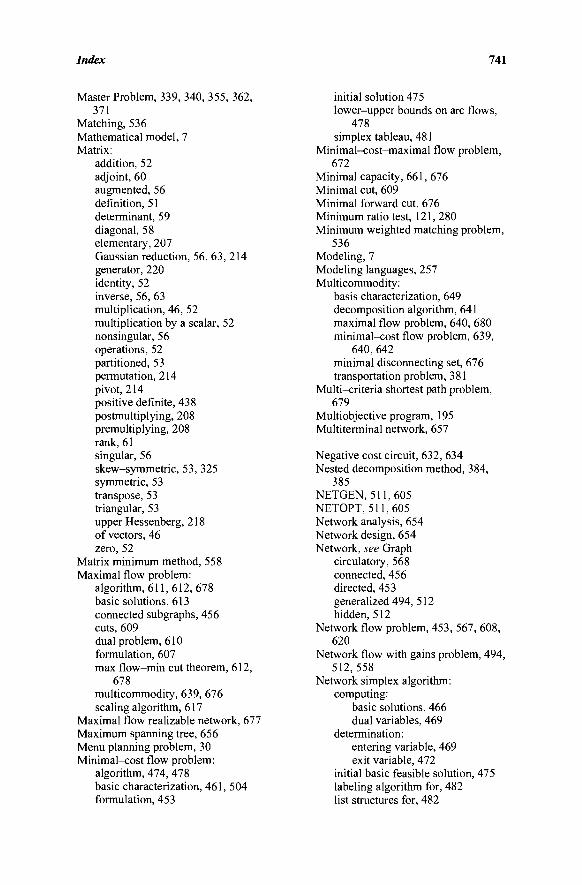
Index 741
Master Problem, 339, 340, 355, 362, 371
Matching, 536 Mathematical model, 7 Matrix:
addition, 52 adjoint, 60 augmented, 56 definition, 51 determinant, 59 diagonal, 58 elementary, 207 Gaussian reduction, 56, 63, 214 generator, 220 identity, 52 inverse, 56, 63 multiplication, 46, 52 multiplication by a scalar, 52 nonsingular, 56 operations, 52 partitioned, 53 permutation, 214 pivot, 214 positive definite, 438 postmultiplying, 208 premultiplying, 208 rank, 61 singular, 56 skew-symmetric, 53, 325 symmetric, 53 transpose, 53 triangular, 53 upper Hessenberg, 218 of vectors, 46 zero, 52
Matrix minimum method, 558 Maximal flow problem:
algorithm, 611,612, 678 basic solutions, 613 connected subgraphs, 456 cuts, 609 dual problem, 610 formulation, 607 max flow-min cut theorem, 612,
678 multicommodity, 639, 676 scaling algorithm, 617
Maximal flow realizable network, 677 Maximum spanning tree, 656 Menu planning problem, 30 Minimal-cost flow problem:
algorithm, 474, 478 basic characterization, 461, 504 formulation, 453
initial solution 475 lower-upper bounds on arc flows,
478 simplex tableau, 481
Minimal-cost-maximal flow problem, 672
Minimal capacity, 661, 676 Minimal cut, 609 Minimal forward cut, 676 Minimum ratio test, 121, 280 Minimum weighted matching problem,
536 Modeling, 7 Modeling languages, 257 Multicommodity:
basis characterization, 649 decomposition algorithm, 641 maximal flow problem, 640, 680 minimal-cost flow problem, 639,
640, 642 minimal disconnecting set, 676 transportation problem, 381
Multi-criteria shortest path problem, 679
Multiobjective program, 195 Multiterminal network, 657
Negative cost circuit, 632, 634 Nested decomposition method, 384,
385 NETGEN, 511,605 NETOPT, 511,605 Network analysis, 654 Network design, 654 Network, see Graph
circulatory, 568 connected, 456 directed, 453 generalized 494, 512 hidden, 512
Network flow problem, 453, 567, 608, 620
Network flow with gains problem, 494, 512,558
Network simplex algorithm: computing:
basic solutions, 466 dual variables, 469
determination: entering variable, 469 exit variable, 472
initial basic feasible solution, 475 labeling algorithm for, 482 list structures for, 482
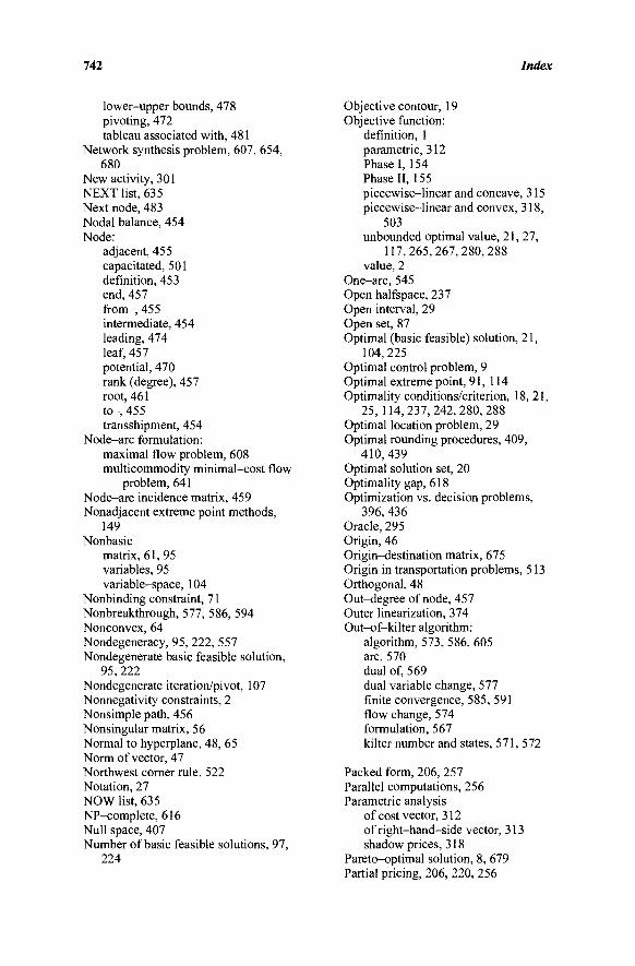
742 Index
lower-upper bounds, 478 pivoting, 472 tableau associated with, 481
Network synthesis problem, 607, 654, 680
New activity, 301 NEXT list, 635 Next node, 483 Nodal balance, 454 Node:
adjacent, 455 capacitated, 501 definition, 453 end, 457 from-, 455 intermediate, 454 leading, 474 leaf, 457 potential, 470 rank (degree), 457 root, 461 to-, 455 transshipment, 454
Node-arc formulation: maximal flow problem, 608 multicommodity minimal-cost flow
problem, 641 Node-arc incidence matrix, 459 Nonadjacent extreme point methods,
149 Nonbasic
matrix, 61, 95 variables, 95 variable-space, 104
Nonbinding constraint, 71 Nonbreakthrough, 577, 586, 594 Nonconvex, 64 Nondegeneracy, 95, 222, 557 Nondegenerate basic feasible solution,
95, 222 Nondegenerate iteration/pivot, 107 Nonnegativity constraints, 2 Nonsimple path, 456 Nonsingular matrix, 56 Normal to hyperplane, 48, 65 Norm of vector, 47 Northwest corner rule, 522 Notation, 27 NOW list, 635 NP-complete, 616 Null space, 407 Number of basic feasible solutions, 97,
224
Objective contour, 19 Objective function:
definition, 1 parametric, 312 Phase I, 154 Phase II, 155 piecewise-linear and concave, 315 piecewise-linear and convex, 318,
503 unbounded optimal value, 21, 27,
117,265,267,280,288 value, 2
One-arc, 545 Open halfspace, 237 Open interval, 29 Open set, 87 Optimal (basic feasible) solution, 21,
104, 225 Optimal control problem, 9 Optimal extreme point, 91, 114 Optimality conditions/criterion, 18, 21,
25, 114, 237, 242, 280, 288 Optimal location problem, 29 Optimal rounding procedures, 409,
410,439 Optimal solution set, 20 Optimality gap, 618 Optimization vs. decision problems,
396, 436 Oracle, 295 Origin, 46 Origin-destination matrix, 675 Origin in transportation problems, 513 Orthogonal, 48 Out-degree of node, 457 Outer linearization, 374 Out-of-kilter algorithm:
algorithm, 573, 586, 605 arc, 570 dual of, 569 dual variable change, 577 finite convergence, 585, 591 flow change, 574 formulation, 567 kilter number and states, 571, 572
Packed form, 206, 257 Parallel computations, 256 Parametric analysis
of cost vector, 312 of right-hand-side vector, 313 shadow prices, 318
Pareto-optimal solution, 8, 679 Partial pricing, 206, 220, 256
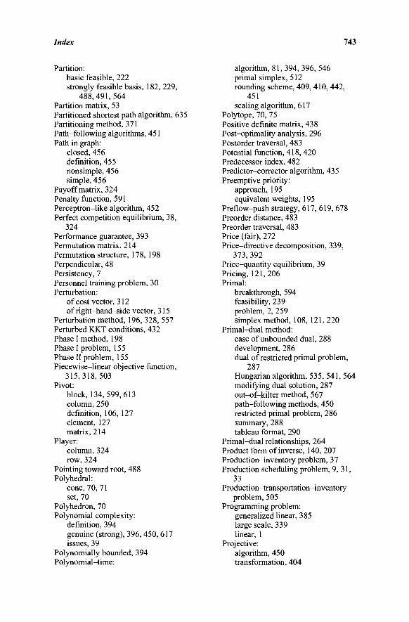
Index 743
Partition: basic feasible, 222 strongly feasible basis, 182, 229,
488,491,564 Partition matrix, 53 Partitioned shortest path algorithm, 635 Partitioning method, 371 Path-following algorithms, 451 Path in graph:
closed, 456 definition, 455 nonsimple, 456 simple, 456
Payoff matrix, 324 Penalty function, 591 Perceptron-like algorithm, 452 Perfect competition equilibrium, 38,
324 Performance guarantee, 393 Permutation matrix, 214 Permutation structure, 178, 198 Perpendicular, 48 Persistency, 7 Personnel training problem, 30 Perturbation:
of cost vector, 312 of right-hand-side vector, 315
Perturbation method, 196, 328, 557 Perturbed KKT conditions, 432 Phase I method, 198 Phase I problem, 155 Phase II problem, 155 Piecewise-linear objective function,
315,318,503 Pivot:
block, 134,599,613 column, 250 definition, 106, 127 element, 127 matrix, 214
Player: column, 324 row, 324
Pointing toward root, 488 Polyhedral:
cone, 70, 71 set, 70
Polyhedron, 70 Polynomial complexity:
definition, 394 genuine (strong), 396, 450, 617 issues, 39
Polynomially bounded, 394 Polynomial-time :
algorithm, 81,394, 396, 546 primal simplex, 512 rounding scheme, 409, 410, 442,
451 scaling algorithm, 617
Polytope, 70, 75 Positive definite matrix, 438 Post-optimality analysis, 296 Postorder traversal, 483 Potential function, 418, 420 Predecessor index, 482 Predictor-corrector algorithm, 435 Preemptive priority:
approach, 195 equivalent weights, 195
Preflow-push strategy, 617, 619, 678 Preorder distance, 483 Preorder traversal, 483 Price (fair), 272 Price-directive decomposition, 339,
373,392 Price-quantity equilibrium, 39 Pricing, 121, 206 Primal:
breakthrough, 594 feasibility, 239 problem, 2, 259 simplex method, 108, 121, 220
Primal^dual method: case of unbounded dual, 288 development, 286 dual of restricted primal problem,
287 Hungarian algorithm, 535, 541, 564 modifying dual solution, 287 out-of-kilter method, 567 path-following methods, 450 restricted primal problem, 286 summary, 288 tableau format, 290
Primal-dual relationships, 264 Product form of inverse, 140, 207 Production-inventory problem, 37 Production scheduling problem, 9, 31,
33 Production-transportation-inventory
problem, 505 Programming problem:
generalized linear, 385 large scale, 339 linear, 1
Projective: algorithm, 450 transformation, 404
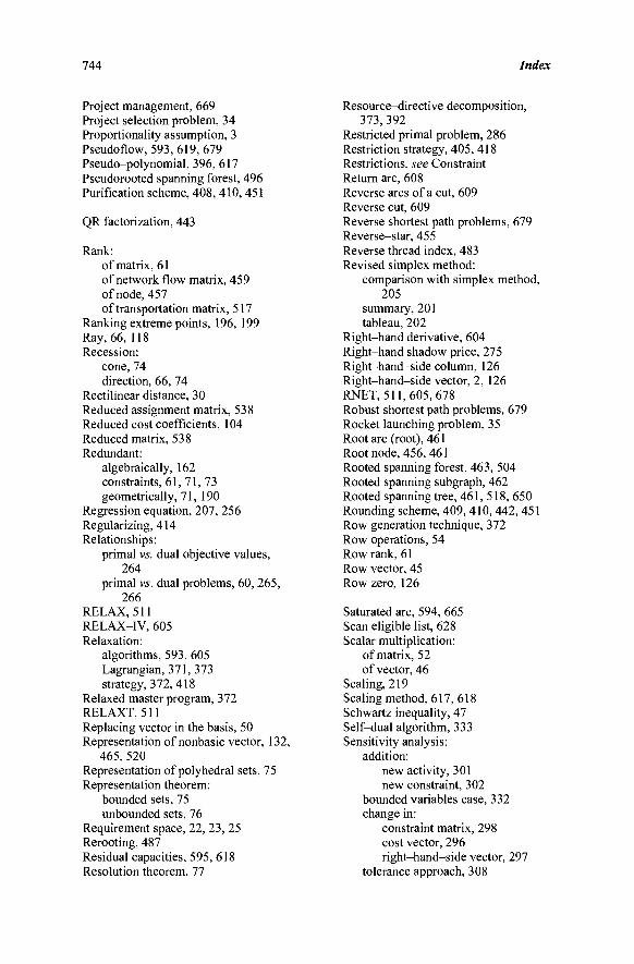
744 Index
Project management, 669 Project selection problem, 34 Proportionality assumption, 3 Pseudoflow, 593, 619, 679 Pseudo-polynomial, 396, 617 Pseudorooted spanning forest, 496 Purification scheme, 408, 410, 451
QR factorization, 443
Rank: of matrix, 61 of network flow matrix, 459 of node, 457 of transportation matrix, 517
Ranking extreme points, 196, 199 Ray, 66, 118 Recession:
cone, 74 direction, 66, 74
Rectilinear distance, 30 Reduced assignment matrix, 538 Reduced cost coefficients, 104 Reduced matrix, 538 Redundant:
algebraically, 162 constraints, 61, 71, 73 geometrically, 71, 190
Regression equation, 207, 256 Regularizing, 414 Relationships:
primal vs. dual objective values, 264
primal vs. dual problems, 60, 265, 266
RELAX, 511 RELAX-IV, 605 Relaxation:
algorithms, 593, 605 Lagrangian, 371, 373 strategy, 372, 418
Relaxed master program, 372 RELAXT, 511 Replacing vector in the basis, 50 Representation of nonbasic vector, 132,
465, 520 Representation of polyhedral sets, 75 Representation theorem:
bounded sets, 75 unbounded sets, 76
Requirement space, 22, 23, 25 Rerooting, 487 Residual capacities, 595, 618 Resolution theorem, 77
Resource-directive decomposition, 373, 392
Restricted primal problem, 286 Restriction strategy, 405, 418 Restrictions, see Constraint Return arc, 608 Reverse arcs of a cut, 609 Reverse cut, 609 Reverse shortest path problems, 679 Reverse-star, 455 Reverse thread index, 483 Revised simplex method:
comparison with simplex method, 205
summary, 201 tableau, 202
Right-hand derivative, 604 Right-hand shadow price, 275 Right-hand-side column, 126 Right-hand-side vector, 2, 126 RNET, 511,605,678 Robust shortest path problems, 679 Rocket launching problem, 35 Root arc (root), 461 Root node, 456, 461 Rooted spanning forest, 463, 504 Rooted spanning subgraph, 462 Rooted spanning tree, 461, 518, 650 Rounding scheme, 409, 410, 442, 451 Row generation technique, 372 Row operations, 54 Row rank, 61 Row vector, 45 Row zero, 126
Saturated arc, 594, 665 Scan eligible list, 628 Scalar multiplication:
of matrix, 52 of vector, 46
Scaling, 219 Scaling method, 617, 618 Schwartz inequality, 47 Self-dual algorithm, 333 Sensitivity analysis:
addition: new activity, 301 new constraint, 302
bounded variables case, 332 change in:
constraint matrix, 298 cost vector, 296 right-hand-side vector, 297
tolerance approach, 308
Index 745
bounded, 20, 75 convex, 64 operations, 29
Shadow prices, 271, 273 under degeneracy, 273 right-hand/left-hand, 275 via parametric analysis, 318
Sharp labels, 630 Shortest path:
algorithm: arbitrary costs, 625, 630, 633,
635 nonnegative costs, 620
approach-dependent, 639, 679 arborescence, 622 bicriteria, 679 complexity analysis, 622, 630, 633 dynamic problems, 679 dynamic stochastic problems, 639,
679 extensions, 639 flow augmentations, 679 interpretation of primal simplex,
622, 632 label-constrained, 639, 679 multi-criteria, 679 partitioned method, 635 polynomial-time algorithms, 635 problem, 547, 600,617,679 reverse path problem, 679 robust problem, 679 stochastic, 639, 679 time-dependent, 639, 679 time-restricted reverse problem,
680 threshold partitioned method, 637,
679 tree, 622, 637, 679
Signature algorithm, 565 Simple path, chain, circuit, cycle, 456 Simplex method:
bounded, 220, 230 column method, 250 complexity, 397 dual, 279 finite convergence, 122, 181, 285 implementation remarks, 180, 219 initial solution, 129, 151, 293, 475,
489, 522 interpretation through KKT
conditions, 242 network, 466 optimality criterion, 104, 225, 280
pivoting, 127 polynomial-time, 512 primal, 108, 121 primal-dual, 288 revised, 202 tableau format, 125, 129 transportation, 522
Simplex multipliers, 121, 267 Simplex path, 107 Simplex set:
definition, 107 volume, 437
Simplex tableau: bounded, 225 dual, 279 interpretation of entries, 131 network, 481 primal, 125 transportation, 535
Simultaneous equations, see System of linear equations
Single artificial constraint technique, 293
Single artificial variable technique, 173, 198
Single commodity flow problems, 639 Single node ascent step, 605 Single node breakthrough, 594 Singular matrix, 56 Sink, 454 Size of an instance, 394 Skew-symmetric matrix, 53, 335 Slack variable, 4 Sliding objective method, 424 Solution:
basic feasible, 62, 95 efficient, 8 feasible, 2 optimal, 18 Pareto-optimal, 8 space, 18
Solvers, commercial, 257 Source, 454 Space:
Euclidean, 48 requirement, 22, 23, 25 solution, 18
Spanning: forest, 457 set, 49 subgraph, 456 tree, 456, 518
Sparse, 206, 219 Special structures, 339
746 Index
Spikes, 219 Stabilized column generation, 344,
374,391,392 Stage, 181,491 Staircase structure, 384 Stalling:
definition, 175, 180, 181 in networks, 488, 493 prevention rules, 491 stages, 181,491
Standard form: of dual, 260 of linear program, 5, 6
State variable, 9 Steepest edge selection, 219, 256 Stepping stone method, 564 Street distance, 30 Strict complementary slackness
property, 336 Strict convex combination, 64 Stroke encoding, 396, 617 Strong duality, 266 Strongly feasible basic partition, 182,
229, 488, 489 Strongly feasible trees, 489, 491, 564 Strongly (genuinely) polynomial, 396,
450,617 Strong theorem of complementary
slackness, 336 Structural:
constraints, 2 variables, 2
Subgraph: definition, 456 induced by node set, 456 maximal connected, 456 proper, 456 spanning, 456
Submatrix, 53 Suboptimization, 220, 256 Subproblem, 339, 342, 356, 363, 372 Subtree rooted at a node, 482 Successive linear approximation, 4 Successive shortest path algorithm,
546, 562 Successor nodes, 482 Sum vector, 46 Supervisor's principle, 268 Supporting hyperplane, 88 Surplus variable, 4 Symmetric matrix, 53 Synthesis problem, 607, 654, 680 System of linear equations:
basic solution, 62
dependent, 61 Gaussian reduction, 56, 63 Gauss-Jordan reduction, 56, 62,
212 general solution, 62 number of solutions, 62 redundant, 61 solving, 55
Tableau: assignment, 538 bounded simplex, 225 dual simplex, 279 primal-dual, 290 revised simplex, 202 simplex, 125,481,535 transportation, 514 two-phase, 164
Tangential approximation method, 374 Tangential support, 374 Tanker scheduling problem, 13 Technological coefficients and
constraints, 2 Termination criterion:
infeasibility, 21, 22, 24, 155, 169, 170,280,288
optimality, 18, 19, 114, 169, 242, 280, 288
unboundedness, 21, 27, 92, 117, 169,231,280,288
Theorems of the alternative, 235 Thread index, 482 Threshold partitioned shortest path
algorithm, 637, 679 Tie breaking rule, 178 Tight constraint, binding, active, 71 Time-space network representation,
638 Tolerance sensitivity approach, 308 To-node, 455 Totally unimodular matrix, 463, 464,
517 Tourism problem, 332 Traffic assignment problem, 37, 675 Transposition of matrix, 53 Transportation problem:
algorithm, 522 balanced, 514 characterization of basis for, 518 corners of cycle in tableau, 517,
520 definition, 11,513 degeneracy in, 528, 534 properties of constraint matrix, 516
Index 747
rank of matrix, 517 representation of nonbasic vector,
520 simplex tableau associated with,
535 starting solution, 522, 558 tableau, 514
Transshipment: node, 454 problem, 551, 562
Traveling salesman problem, 501 Tree:
correspondence to basis in network flows, 461,463, 518
definition, 456 dominant requirement, 655, 656 end node, 457, 518 equivalent characterizations, 458 maximum spanning tree, 656 one-, 458 properties, 457, 458 rooted, 461, 518, 650 spanning, 456, 518, 650 strongly feasible, 489, 491, 564 uniform requirement, 661
Triangularity of basis in network flows, 463,518
Triangularization, 212 Triangular matrix, 53 Two-person zero-sum game, 324 Two-phase method:
analysis, 157 comparison with big-M method,
168 description, 154
Two-stage stochastic program with recourse, 39
Unary encoding, 396, 617 Unbounded:
optimal value, 21, 27, 92, 117, 169, 231,265,267,280,288
polyhedral set, 21, 76 subproblem region in
decomposition algorithms, 354 Uncapacitated problem, 454 Undirected graph, 455, 654 Uniform requirement tree, 661 Unimodularity, 517 Unique:
optimal solution, 20, 114 solution, 62
Unit vector, 46 Unrestricted variables, 4, 147
Updated: basis inverse, 208, 307 column vector, 209, 342 LU factors, 217 network list structures, 485 tableau, 128, 227, 228, 307
Upper bounds on variables, 220, 478 Upper Hessenberg matrix, 218 Upper tree, 488 Upper triangular, 53 Valid cut, 304 Valid inequality, 304 Variable:
artificial, 153, 198,522 basic, 95 blocking, 106, 112 bounded, 220, 478 definition, 2 dual, 239, 260, 269 entering basis, 106, 121, 178,225,
493 flow, 454 integer, 304 leaving basis, 112, 121, 178,479,
527 legitimate, 153 nonbasic, 95 slack, 4 surplus, 4 unrestricted, 4, 147
Variable splitting technique, 511 Variable upper bounding, 257 Vector:
basic, 49 definition, 45 dependent, 49 direction, 66, 71 eta, 208 Euclidean space, 48 independent, 48 lexicographically nonnegative, 182 lexicographically positive, 182 norm, 47 normal, 48, 67 operations, 46 sum, 46 unit, 46 zero, 46
Vertex, 72 Vertex of ray, 66, 118 Vogel's approximation method, 524,
558 Volume of simplex, 437

748 Index
Warehouse location problem, 388 Weak duality, 264 Zero: Weak theorem of complementary matrix, 52
slackness, 268 vector, 46 Weighted average, 64 Zero-arcs, 545 What-if analysis, 295 Zero-sum game, 324 Working basis, 221


