Linear scale-space

Journal of Mathematical Imaging and Vision, 4, 325-351 (IYY4) @ 1994 Kluwer Academic Publishers, Boston. Manufactured in T h e Netherlands.

Linear Scale-Space

L.M.J. FLORACK, B.M. ter HAAR ROMENY, J.J. KOENDERINK, AND M.A. VIERGEVER email: [email protected]

3 0 Computer Vision Research Group, Utrecht University Hospital, Room E02.222, Heidelberglaan 100, 3584 CX Utrecht. The Netherlands

Abstract. The formulation of a front-end or “early vision” system is addressed, and its connection with scale-space is shown. A front-end vision system is designed to establish a convenient format of some sampled scalar field, which is suited for postprocessing by various dedicated routines. The emphasis is on the motivations and implications of symmetries of the environment; they pose natural, a priori constraints on the design of a front-end.

The focus is on static images, defined on a multidimensional spatial domain, for which it is assumed that there are no a priori preferred points, directions, or scales. In addition, the front-end is required to be linear. These requirements are independent of any particular image geometry and express the front-end’s pure syntactical, “bottom up” nature.

It is shown that these symmetries suffice to establish the functionality properties of a front-end. For each location in the visual field and each inner scale it comprises a hierarchical family of tensorial apertures, known as the Gaussian family, the lowest order of which is the normalised Gaussian. The family can be truncated at any given order in a consistent way. The resulting set constitutes a basis for a local jet bundle.

Note that scale-space theory shows up here without any call upon the “prohibition of spurious detail”, which, in some way or another, usually forms the basic starting point for “diffusion-like’’ scale-space theories.

Keywords. scaled differential operators, front-end vision, Gaussian family, local jet bundle, scale invariance, scale-space

1 Introduction

Scale-space is by now a well-established concept in computer vision and image analysis. A historical contribution to scale-space theory is the introduction of the pyramid [4]. Though based on a rather ad hoc method, this model does capture the crucial observation of the in- herently multiscale nature of image structure. However, despite the continuous nature inherent to scaling, the pyramid model only comprises a finite number of preferred scales and suffers from various other deficiencies. In particular, it does not prevent discretisation effects from propagating all the way up to the top of the pyramid. A fundamental approach has been adopted by Witkin [47] and Koenderink [HI, who have formulated a causality constraint: no

“spurious resolution” should be generated when increasing scale. This, together with some weak symmetry considerations, establishes the normalised Gaussian as the only sensible scale-space filter. Scale-space theory then gains an increasing interest as it is further developed by Badaud et al. [l], Yuille and Poggio [51, 521, and several others [3, 14, 23, 24, 25, 27, 30, 29, 42, 41, 10, 91.

Thus the process of increasing scale appears to be governed by the isotropic diffusion equation, which captures the a priori constraints and whose Green’s function happens to be the Gaussian. For an actual scale-space computation, one has to discretise either the kernel, or the underlying diffusion equation. The latter approach has been adopted by Lindeberg [27, 281 who has formulated a scale-space for discrete signals defined on a regular grid, compris-

326 Florack, Romeny, Koenderink, and Viergever

ing a continuous scale parameter. The kernel of the discretised diffusion equation turns out to be related to the modified Bessel functions of integer order, normalised by an exponen- tially decreasing scaling factor. But either way, sufficiently large scale behaviour is of an intrinsically continuous nature and both methods of spatial discretisation indeed turn out to be equivalent in this limit. In all the abovemen- tioned approaches to scale-space theory, one in- variably encounters a fundamental assumption concerning the “prohibition of spurious detail”, formulated in one way or another. A consistent way of quantifying detail that generalises to multidimensional images has been proposed by Koenderink [18], who has formulated the requirement that local extrema must not be en- hanced, in other words, that the scale-space isosurfaces should be convex upward (only in the 1D case this corresponds to a monotonic decrease of the number of local extrema with scale; see the 2D example in [25], and also the discussion in [27] on this matter). This, together with some weak symmetry requirements, unambiguously establishes the diffusion equation as the scale-space generating equation.

A major contribution to scale-space theory has been given by Koenderink and Van Doorn in [24], in which they presenit a taxonomy of several complete, hierarchically ordered families of scale-space filters in various representations, and emphasise their equivalence (the paper in fact reformulates some of their earlier results obtained in [23] in a more systematic way).

In the present paper we consider the physical representation of scalar field measurements (images), which will be referred to as the front- end. Given the intrinsically finite aperture of any physical observation, and some fundamental front-end symmetries, essentially stat- ing that the front-end should have no built- in bias with respect to locations, orientations or scales, we will arrive at the Gaussian filter family without the explicit need of a causality requirement.

The Gaussian family is shown to correspond to the physical counterparts of mathematical differential operators in a precise sense, the

zeroth order member being the physical “identity” operator. Moreover, the tensorial nature of this family is explained, revealing its coordinate- independent nature. The infinite hierarchy can be consistently truncated at any order so as to yield a basis for a so-called local jet bundle. This provides a physical motivation and a clear mathematical basis for a multiscale representation, and for the goal of a front-end visual system: the manifest invariant representation of measurement data.

The major aim of this paper, however, is not to review well-established scale-space theory, but to give a detailed motivation of all its underlying premisses, i.e. the front-end symmetries. Scale- space theory ultimately relies on these premisses, which are often either taken for granted - as we did in [9] for the sake OF brevity; the emphasis in this paper was on the differential structure of images, see also [10]--or rejected without a solid motivation. This issue, however, is not whether to accept or re.ject scale-space theory (and any other solid theory for that matter), but to appreciate exactly where it fits in, and where it does not.

The article is organised as follows. In section 2 we propose a functional definition of a front-end by formulating a set of fundamental postulates, with an in-depth motivation for each of these. Here, we also review the problem of ill-posed differentiation and its solution. Section 3 elaborates on the central concept of scale. One has to realize that the action of scaling on a scene without proper scaling of the physical apertures by which that scene is observed will not lead to a scale-invariant measurement. For this reason one needs the ability to scale the apertures, and it is shown that the scale-ensemble of apertures thus obtained is related to a semigroup. It is then shown how to arrive at the Gaussian family as the complete solution to the front-end requirements.

Four appendices have been added to discuss in detail various concepts oE central importance to this paper: linearity (appendix A), scale invariance (as a conventional group invariance; see appendix B), the notions of homogeneity and isotropy (appendix C), and well-posed differentiation (appendix D).

Linear Scale-Space 327

2 Front-End Symmetries

The front-end, or “early vision system”, generally denotes the primary stage of a (biological or artificial) vision system. We will define the front-end as a purely syntactical, “bottom up” system, designed to establish a representation of a physical measurement in a format that can be easily read out by a variety of semantic routines (which are themselves not considered part of the front-end; cf. the “sensorium” in [23]). These dedicated routines can freely ad- dress the front-end, read it out selectively, and provide their own interpretation to the data. The front-end itself is an unbiased, read-only databank, collecting all the “evidence” obtained through measurements of the state of the physical environment.

We argue that the front-end is naturally constrained by a priori symmetries of its environment. In this context, an environment symmetry is a group of transformations that affect the environment in a way that is considered a priori irrelevant for visual processing. To avoid over- head caused by a representation of irrelevant details (which would put the cumbersome task of eliminating them with all the higher level routines!), it is quite natural to impose appropriate symmetry constraints on the front-end.

So in order to constrain the front-end, we must decide on its physical environment. We will take this to be a multidimensional, homogeneous, isotropic, “flat” space, for which we assume that there are no a priori preferred reference points, directions, or spatial scales. To incorporate this a priori knowledge about the environment into the front-end system, we propose the following functional constraints: A front-end system has to be able to generate a complete, homogeneous, isotropic, and scale invariant representation of its input data.

We are inclined to define the front-end by a complete, well-behaved solution satisfying the following front-end postulates:

Front-End Vision Postulates:

0 linearity 0 spatial scale invariance

0 spatial homogeneity 0 spatial isotropy

Paradoxically, it will turn out that this yields a seemingly redundant data representation. If mere representation of data were the sole issue, then indeed it is highly redundant (in that case it is appropriate to resort to data compression schemes), but if there are higher level visual routines addressing the front-end, dictating a common set of symmetries, then this truly is an optimal representation in the sense that the a priori symmetries are already qanifest in the data. Of course, the way in which the higher level routines access the front-end very much depends on their task and is certainly nontrivial. This, however, is beyond the scope of the paper.

We will proceed with a motivation for each of the front-end symmetries. In addition, we will comment on the necessary condition of well- posedness.

2.1 Linearity

Let pi be any signal labelled by i = 1 , . . . , n. Clearly, we may equally well take any other (sufficiently smooth) reparametrisation 4’ = d~’(4) instead of 8 itself, as long as it is unambiguous, i.e., one-to-one (det a@/aqY # 0). Because of isomorphism, there seems to be no “natural” choice for a particular representation. This seems to justify the linearity constraint imposed on the front-end transfer functions.

However, the representation of a physical observable (in particular, the linearity constraint) is not merely a matter of mathematical convenience. There is a more compelling, physical consideration to be taken into account, related to the intrinsically finite resolution of a physical system. A physically relevant observable is ideally represented in such a way that its intrinsic resolution is independent of its value. Then its “inner scale” may serve as an implicit unit of reference (or “hidden scale parameter”: see section 2.2) for the observable. This means that all signals become a priori equally important, and that there is no need to store the signal-independent inner scales. Let 68 be the inner scale for such a “natural” representation


#. Since 6~~ = a$’/a@b@, a natural representation is preserved by aflne transformations only (here, and henceforth, the Einstein summation convention is in effect).

We will henceforth assume that our observable (that quantity which the image intensity is intended to represent) has the “right representation”, disregarding the linear isation step. The linearisation step itself serves to define the relevant observable and hence depends on the physical details of the imaging process. See appendix A for a more detailed discussion on linearity.

2.2 Scale Invariance

Let L(x) represent some image grey value depending on d variables (spatial coordinates, time,. .. , etc.) x = (q,. .. ,Q). From a pure mathematical point of view there is no restriction whatsoever on the form of the function L(x). The physical requirement of scale invariance, however, imposes a restriction on the form of L(x): only those functions are allowed that “scale properly”. Already the great mathemati- cian Fourier pointed out this important difference between physics and “pure” mathematics in his treatise “ThCorie Analytiqui: de la Chaleur”, first published in Paris in 1822. This work has become famous for its contribution on Fourier analysis, but contains a second major contribution that has been greatly underestimated €or quite some time, viz. on the use of dimensions for physical quantities.

To appreciate the meaning of scale invariance it is necessary to understand the physical concept of hidden scale parameters, i.e. arbitrary parameters used in a theory as independent reference measures for physical quantities (units). These are intrinsically free parameters: physical quantities are always measured relative to these, no absolute values can be assigned to them. The law of scale invariance expresses the freedom to rescale these parameters at will. Note that scaling in this “conventional” sense is a group operation. For a rigorous formulation of conventional scale invariance, the reader is referred to appendix B. See also [12, pp. 126-1301 and [32, 35, 36, 371.

It is important to realize that the action of scaling on a physical scene without proper scal-

ing of the physical apertures by which that scene is observed will not lead to a scale-invariant measurement. A proper way of scaling takes into account everything that depends on the “hidden scale parameter”, i.e. spatial scale (see the Pi theorem in appendix B). In particular, one needs the ability to rescale the apertures in a conjugate fashion in order to restore overall scale-invariance, and to this end one needs to introduce an additional measurement parameter that accounts for the aperture’s width or inner scale. This inner scale is a property of the front- end. Provided one takes all scaling quantities, including the inner scale, into account, the measurement will be scale-invariant in the conventional group-theoretical sense. In order to un- confound the front-end from the measurement data, the inner scale apparently has to be afree parameter, at least at the level of the front-end.

The ability to independently scale the inner scale parameter leads to a multiresolution representation of the image; see [21, section 2.71. Incorporating this resolution degree of freedom into the front-end makes sense, considering the multiresolution semantics of an image (if you do not incorporate it in the common front-end, you inevitably need to introduce it in all higher level visual routines). A measurement data independent scaling of the inner scale is not a group operation, since it is generally impossible to obtain high resolution data from low resolution data (ill-posed ‘,deblurring’’), see also [16, 15, 341. Apart from this, it does share the other group defining properties. Such a set of irreversible, group-like operations constitutes a so-called semigroup (a precise formulation of this will be given later on).

Although we will be a bit sloppy with the ter- minology of “scaling”, let us state here once and for all that scale invariance in the context of this paper implies both a unit and resolution invariant representation of image structure, thus referring to both group as well as semigroup invariances.

2.3 Homogeneity and lsotropy

Translation and rotation invariance are implied by the assumptions of homogeneity and isotropy. Homogeneity means that all locations within the


field of view are a priori equivalent. Isotropy indicates the absence of a priori preferred directions in each point. In Cartesian coordinates the translation-rotation group is given by transformations of the type

.i? = f . r ’ 1 - a’. (1)

The rotation matrix ri is subject to the orthog- onality condition

(In a Cartesian frame upper and lower indices play no particular role.)

It is well-known that a homogeneous and isotropic spatial hypersurface must have a line element of the form ( r2 = ziz i , see [26])

with E = O,f l ,a an arbitrary length unit or inner scale parameter (this convention will make the line element dimensionless), and rg some constant with the same dimension as r. The symbol R generically denotes the coordinates of the unit hypersphere, with surface element do.

We shall consider only the case of aJEat metric space, in which case E = 0. This means that only the trivial Euclidean metric remains. In a Cartesian coordinate system the line element is then given by the familiar Pythagorean rule

de2 = q I 7 d z ’ d x J , (4)

with the covariant metric tensor qij given by

(5 ) - 9

r ] lJ = * 6 ! J ,

5,, being the familiar Kronecker symbol (i.e. 1 if i = j, and 0 otherwise).

Note that the homogeneity condition is rather restrictive. In fact, it is often unrealisable to treat all points in the visual field on equal foot- ing; this is certainly the case for an active vision system that needs to operate in real-time. For such a system it makes sense to focus in on a location of interest in the visual field, and to dedicate a significant part of its processing capacity to a “foveal subimage” only. At the

same time, it is desirable to maintain a (low- resolution) representation of the context.

Clearly, such a foveal front-end must be in- homogeneous, which seems a bit awkward for a system operating in a homogeneous environment. But this need not be a problem if one introduces an extra degree of freedom for ex- ploration: the ability to shift the foveal point relative to the scene. For further details the reader is referred to appendix C.

2.4 Well-Posedness

Well-posedness is an important requirement for any physical system. It usually refers to functionals, but has in fact the same meaning as continuity for ordinary functions. It is an obvious requirement if one does not allow insignificant perturbations of input (“noise” or quantisation errors) to have a significantly disturbing effect on the output.

Local image structure is captured by the spatial derivatives [10, 113. But note that a differential operator is an ill-posed functional. Hence it makes no sense to try and differentiate an image in the conventional way.

One usually attempts to circumvent this problem by applying some regularisation or smooth- ing scheme prior to differentiation. A derivative is then approximated by a difference quo- tient, involving a comparison of neighbouring pixels. This, however, does not really solve the ill-posed nature of differentiation, because ill- posedness has nothing to do with smoothness of the operands! It is not the image that needs regularisation but rather the operations performed on it, i.e. the differential operators (asking for a derivative of an image in the conventional sense simply amounts to posing a wrong question). Besides this problem, the choice of a regularisation scheme poses a fundamental problem. Clearly, the choice of a particular class of well- posed operators must be based on physical considerations beyond mere regularisation.

For a detailed discussion of well-posed differentiation, both from the mathematical point of view (in the context of tempered distributions) as well as from the physical point of view (linear filters), the reader is referred to appendix D.


In the sequel it will appear that taking into account the physical notion of scale is formally equivalent to the mathematica.1 theory of well- posed differentiation based on tempered distributions (with an appropriately constrained Schwartz space of test functions).

3 Scale and Resolution

Since local image structure crucially depends on resolution, the observable of interest must be sampled on all spatial scales sirnultaneously. As with all front-end symmetries, scale invariance cannot hold indefinitely. Because of the limited scale range determined by sampling characteristics and field of view, we have to decide on the proper scale range.

The smallest scale of interest will be called the inner scale, whereas the largest scale of interest will be called the outer scale. These are to be distinguished from the scale limitations posed by the acquisition device, i.e. the grid size and the field of view, respectively. Ideally, the scale- range of interest should be fairly within these fundamental device limits, but often economical or technical limitations tend to prevent this.

3.1 Inner Scale and Grid Size

Strictly speaking, when we are interested in image structure near voxel-scale1, we are facing an apparent undersampling problem, from which there is only one clean escape: zooming in on the scene, or resorting to a higher resolution acquisition. There is a serious problem with image structure analysis near voxel scale, since all features below this scale will have been destroyed in an intrinsically irreversible (and device dependent) way. Therefore we cannot expect reliable image structure within a certain boundary layer near voxel scale; there will be a confounding of device characteristics and data.

It pays off to study our own front-end visual system and see how Nature has designed this astonishingly well performing system, having time-polished it by evolution over many millions of years [13]. Indeed, the human visual front- end appears to ignore a small scale boundary

Fig. 1. The notorious boundary problem arises from the unrealisable desire to extract “large-scale” information near image boundaries; a proper formulation of the problem is scale-independent though.

layer by focussing on scales fairly larger than its smallest aperture: the typical separation of neighbouring rods or cones. Our retina typically has 108 rods and cones. It is not the output of individual rods and cones that is transferred, only a weighted sum over local ensembles of these is passed, making up a receptive field (RF). The profile of such a RF has to take care of the small-scale “spurious detail” generated by the individual rods and cones by scaling up to a larger inner scale in a very specific way. Nu- merous physiological and psychophysical results support the theory that the cortical RF profiles can be modelled by Gaussian filters (or linear derivatives of these) of various widths [48, 49,

In the Gaussian model, the variable width of the Gaussian kernel accounts for the spatial scaling degree of freedom. As far as the arguments in the next subsection are concerned, however, all that we need is a fair intuitive notion of the concept of inner scale, so one may think of any other, functionally similar model as well.

50, 21.

3.2 Outer Scale and Field of View

The finite extent of an image limits the accuracy of a scale-space analysis near the image’s boundary (we disregard a priori knowledge of image structure beyond the boundary), cf. Figure 1.

The problem seems to become more severe with increasing scale. It should be stressed, however, that the boundary problem is really scale-


independent. The actual problem consists of quantifying a scale-accuracy measure when trun- cating the infinite scale kernel. One (ad hoc) possibility is to truncate the tails such that a fixed fraction of the kernel’s weight is preserved. This, of course, requires a proper normalisation.

Suppose that y(x) is a basic, smooth kernel (in one dimension, for the sake of argument), normalised to unit weight according to

s:” dxy(x) = 1, (6)

and having the property that y(x) + 0 for 11x11 --+ CO sufficiently fast. Then all derivatives m ( x ) = d“r(x)/dz” are normalised to unit weight as well, in the following sense:

(7) 2”

n. I” d x ( - l ) y 7 , ( x ) = 1

p x ( - l ) t 1 7 y 7 , ( x ) x7’ = 1 - E

(which is easily proven by induction using partial integration). A possible truncation scheme then presents itself: if 0 < E < 1, truncate at x = f a , such that

(8) n.

(in such a scheme, a depends both on the error E as well as on the order n). Scaling x = Zu will yield compact u-neighbourhoods of total extent 2Eu in this case (with E scale-independent).

Given a certain tolerance, we can pack the image domain with (overlapping) compact u- neighbourhoods and use their midpoint values for a sampling rate reduction, see Figure 2. Note that a fixed sampling rate across scales runs counter to the very idea of scale invariance. In order to retain manifest scale invariance, the relative overlap or spatial density distribution of these neighbourhoods must be constant across scales. There is ample proof from physiology supporting these ideas of sampling rate reduction and fixed overlap. We know that the rods and cones in the retina are not to be regarded as the basic sampling apertures, as they are grouped into receptive fields of various scales (the output of individual rods and cones is ignored as such), thus accomplishing multiple scaling and consistent sampling rate reduction.

Fig. 2. The boundary problem does not arise when using sampling rate reduction in the appropriate way, keeping the relative overlap of local neighbourhoods fixed. Within the central region a distance .(U) 0: U away from the boundary this overlap is kept constant, but towards the boundary it necessarily decreases. Nevertheless, all points at the given scale are accurately represented within the image and there is no overlap with the image boundaries, hence no significant “boundary problem”.

Physiological data indicate a nearly fixed -and fairly large-relative overlap of RF’s, see e.g. [2, 8, 451.

The scale parameter u provides a natural length unit on the corresponding level of resolution. If we parametrise scale u by a dimensionless “zooming” parameter T , then scale- invariance or self-similarity implies that du/dr must be proportional to u (see Pi theorem in appendix B). Without loss of generality we can take du/dr = u , u ~ ~ = ~ = E. Note that this parametrisation effectively removes the artificial singularity at the fictitious level u = 0:

DEFINITION 1 (Natural Scale Parameter). A natural, dimensionless scale parameter r is obtained by the following reparametrisation of u:

u = EeT (r ER) .

Note that, on dimensional grounds, we are forced to introduce a “hidden scale” E, carrying the dimension of a length. It is unnatural to relate this parameter to the scale-space kernel (scale invariance), so it must be a property of the imaging modality. An intrinsic scale inherent to any imaging device that present itself is the sampling width or voxel size2.


Fig. 3. “Elliptic patchcs”, calculated for a typical 2.56 x 2.56 NMR image (first image) at several scales: T = 1 Sd, 2.2.5,3.00, corresponding to U = 4.48,9.49,20.09 pixels, respectively. An elliptic patch is defined as the connected set of pixels in which (a2L/a?-2)(a2L/ay2) -- (a*L/a.ray)2 :. 0.

For a given overlap of U-neighbourhoods, the number of samples on scale level U as com- pared to another level q) is given by N(u) = N(co)(uo/u)~ or, in terms of the natural scale parameter:

(9)

On the highest scale represented, the image domain has actually shrunk to a single point.

Intuitively, when measuring structures relative to the natural distance unit, a generic multiscale image (one in which, roughly speaking, all scales within its scale range are equally represented) is not likely to gain or loose a significant amount of structure per natural volume element, implying that the density of “generic lociil features” NF(T) will be proportional to the number of samples N(T), so:

Note that sampling rate reduction depends on the dimension. See Figure 3 and Figure 4 for an experimental verification of this typical behaviour for the “elliptic patches” of an NMR image in D = 2 (cf. also [30] for an experimental verification in D = 1). Of course, this will only hold on a scale range fairly within the fundamental upper and lower limits, at which there is a substantial, inevitable deviation from this natural behaviour. Its accuracy also depends on the iigenericity” of the image (an artificial, perfectly noise-free Gaussian blob provides a highly singular example, because of its “self-similarity”: upon blurring, it merely scales

5-

4-

3-

2- .--

. ,

. . . 11 I I I I I I I I

0 1 2 s r 4

Fig. 4. The logarithm of the number of elliptic patches, In N , as a function of the natural scale parameter T, calculated for the NMR image of Figure 3. The graph verifies the expected linear relationship with slope -dln ;VF/dT = 2.08 M 2 in the medium-scale region indicated by the dashed box, corresponding to inner scales between 3.5 and 20 pixels.

but does not change form; note that its singular “zero-dimensional’’ or “point-like” behaviour also shows up in the remarkable property that one can actually deblur it). See Figure 5.

If we take E to be the sampling width, then T = 0 corresponds to a resolution for which the width of the blurring kernel is of the same order of magnitude as the voxel size E of the original image. This sets a practical lower limit to the kernel widths, at which discretisation effects .will start to contribute to a significant degree [27]. The range T E (-w,O) corresponds to subvoxel scales that are not represented in the image iind in which all structure has beeen averaged out.


lr

5 1

0 1 2 3 7 . 4

Fig. 5. The logarithm of the number of elliptic patches, In N , as a function of the natural scale parameter T, calculated for an artificial, 2.56 x 2.56 Gaussian blob, both for the noisefree case (lower points) and for the case of a perturbative, pixel-uncorrelated. additive Gaussian noise with a standard deviation equal to one tenth of the peak value (upper points). Even though the image is a self-similar Gaussian blob and the perturbation owing to the noise is relatively small, both in correlation width as well as in dynamic range, the slope of the graph for the noisy data is close to (though slightly larger than) the generic value of 2 over the entire interior scale range: -dln N F / d r = 2.49 in the medium-scale region indicated by the dashed box.

When building up a scale-space in a self- similar way we must use an equidistant sampling of T [lS, 38, 301. By inspection of (9) we can interpret the sampling width 57 in terms of the rate of fusion of “points”, allowing for a corresponding sampling rate reduction. Without any form of sampling rate reduction, the volumetric overlap or sample density TZ(T) of spherical (7-neighbourhoods would be proportional to the inverse of N(r ) , so we would have:

d n d r

Diz = 0 - -

The sampling rate reduction scheme given by (9) is chosen precisely so as to maintain a fixed density of neighbouring “points”:

d n - _ - 0 d r

3.3 Scale-Space

In this section we will derive the unique scaling strategy for D-dimensional images (D > l),

using its semigroup nature in combination with the front-end vision symmetries.

Linear shift invariance implies that a rescaled image must be a convolution of the original image by some kernel G(.‘;u), so3:

L(.‘; (7) = {Lo * G(. ; U)}(.‘; U ) . (13)

It is especially attractive to consider this property in the Fourier domain, in which the kernel becomes diagonal: (13) then becomes an algebraic relation:

The Pi theorem (see appendix B) states that, because of conventional scale invariance, there are only two independent dimensionless variables in this case. We may take these to be B = C / L O and n = a;. Let us therefore define: + def

DEFINITION 2 (Natural Coordinates). Natural frequency coordinates are defined as the dimensionless numbers d associated with the frequency coordinates w’ at scale-space level (7 > 0 through:

+ n = (7;.

Similarly, natural spatial coordinates are defined as the dimensionless numbers 2 associated with the spatial coordinates 1 at scale-space level U > 0 through:

- + x U

x = - *

The Jacobian of the spatial scaling in Defini- tion 2 relates an ordinary spatial volume element to the natural volume element on a given scale (7:

According to the Pi theorem we may write the kernel B(w’;u) as a function of d:

B(w’;u) = C/LC, ef B(8) . (16)

For a scalar function (which we are looking for), spatial isotropy implies that B depends


only on the magnitude (Euclidean length) of the vector 6:

The consistency requirement that there is a one-to-one correspondence y(c) H n manifests itself mathematically by the existence of an iso-

B(6) = B(0) with 0 Ef m. (17) morphism { y ( a ) ; o } N .(Ri;$}, i.e. a one-to- one map between these two semigroups pre- serving the semigroup structure: Let us choose U to be such that, for fixed w,

the hypothetical zero-scale limit will leave the initial image unscaled, so: y(c) 0 y(Z) = T(“ @ 5). (20)

This means that we include the identity as a limiting, zero-scale kernel. Also, we require the infinite-scale limit to give us i i complete spatial averaging of the initial image:

Performing several rescalings in succession should be consistent with performing a single, effective rescaling. More specifically, if ~71 , 02 are the scale parameters associated with two rescalings B(01), G(02) respectively, then the concatenation of these should be a rescaling B(03) corresponding to an effective scale parameter u3 = a 2 $ 01, in which the additive operator “$” relates the effective scale parameter u3 to the parameters ul, 02. It is important to note that “$” need not correspond to ordinary addition. All that consistency requires is that the set {Rt; $} constitutes a commutative semigroup isomorphic to the commutative semigroup of image rescalings:

DEFINITION 3 (Commutative Semigroup). The set {R:; @} equipped with the (binary operation @ constitutes a commutative semigroup if the following conditions hold:

This isomorphism poses a very strong constraint on the form of the scale-space kernels.

We will now derive an explicit formula for the semigroup operation $. On dimensional grounds (manifest scale invariance), any allowable reparametrisation of n must be homogeneous, i.e. it must have the form 0 H A d ’ for some dimensionless parameters X > 0 and p # 0. Without loss of generality we may put X = 1. So any allowable reparametrisation of the scale-parameter (T can be realized by an automorphism P:

P: {Ri ; @} --$ {Xi; +}: U H d. (21)

Its inverse is given by:

P-l: (Ri; +} 4 {R,f; e}: cr H d p . (22)

If we assume that ordinary addition applies to {R;; +}, then the following identity holds (see (20)):

y(g) o y(Z) = y(P-’(Pa + PZ)). (23)

Note, however, that (23) still makes sense in the limiting case p 4 4~03, for which (21) and (22) by themselves have no meaning. It is easy to see that this singular case corresponds to the singular idempotent semigroups {Rt ; max} and {RL; min} defined by:

def u1 $ 02 = min(a1, U Z ) Val, u2 E R i , (24) def semigroup V a l , u2 3u3 = a 2 @ nl,

operation:

associativity: and:

Vg,, n2, u3n3 $ (c2 @ al) def

01 @ ~ 7 2 = max(gl, a2) Va l , c2 E RL, (25)

null element: 3 c q V ~ U @ go = a0 U respectively, which emerge as limiting cases from = ( 0 3 @ 02) @ 0 1 ,

the regular monotonic semigroup defined by = U,

(26) def commutativity: Val , CQ u1 $ c2 = (‘z $ oI. U1 $ 0 2 = (n; + o p .


We stress the fact that the null elements of these semigroups correspond to hypothetical, non-physical limits: for p < 0 we have ug = 03,

whereas for p > 0 we have = 0. Note that we have already decided no the null element ug = 0 by our limiting requirement (18), hence only positive p-values will be of interest to us4.

We now turn to the derivation of scale-space kernels compatible with (23). It is convenient to consider the frequency representation; if we define

def - G ( q = B(Qf’), we get from (23):

i7(Q)i7(6) = G(f-2 + 6). The general solution to this constraint is a normalised exponential function

i 7 ( ~ ) = exp(ao), (29)

or:

in which o is an arbitrary, negative constant (see (19)), whose absolute value can be absorbed into the definition of the scale parameter.

For the limiting case we have G(Q) = limf,+m &Ql’), i.e. c(0) if 0 5 f2 < 1 and @03) if 0 > 1. Together with the limiting conditions (18) and (19) (and taking G(1) Ef limnrlG(12) for defi- niteness), we thus find the following idempotent kernel:

G(Q) = exp(aQf’), (30)

in which X I is the indicator function defined by:

1 i f s E I

0 i f x @ I . XI(.) ef { (32)

In dimensionful coordinates this becomes:

G ( 4 .-I = X[O. I/a](4, (33)

i.e. an ideal low-pass filter with cut-off frequency w = l/a. In his article, Mallat proposes such an idempotent semigroup requirement as a starting point for a so-called “multiresolution approxi- mation” [33]; the operator which approximates a given signal at a resolution U is a linear projection, satisfying (20) and (24).

The general, regular case comprises a so- called (strongly) continuous semigroup of operators for each value of p , as opposed to the idempotent semigroup (33):

g(Z; (T) = e x p ( a d d ) . (34)

To single out a unique scale-space kernel, we need a final constraint on the parameter p . For a consistent interpretation of G(f2) as a spatial rescaling it is natural to impose the condition of separability in D > 1 dimensions:

i=l (35)

in which Qi is given by the magnitude of the projection vector (6 . %)k?i. This condition states that an isotropic rescaling can be obtained either directly through G(o) or through a concatenation of rescalings G(Qi) by the same amount in each of the independent spatial directions ei, i = 1 . - . D separately. Indeed, only in this way we can think of (T as a natural length unit in an isotropic space. The separability requirement fixes p = 2, so s = u2, not .- itself, is the “additive” parameter:

h

def

u @ Z = m. (36)

Note that the idempotent kernel (31) is not separable. A convenient choice for a is obtained by letting scale coincide with Gaussian width in the spatial domain, so that a = -1/2.

So we have finally established the unique scale-space kernel. In the Fourier domain it is given by:

or, in dimensionful coordinates:

B(w;rr) = exp ( - -u ,’,) w .

(37)

In the spatial domain it is given by the convolution kernel:

1 G(z;a) =

d Z z D


Note that in the spatial domain the Gaussian kernel G ( 3 a ) has a scale-dependent amplitude. It has the dimension of an inverse D- dimensional volume: we may write it as a product of an explicit volume factor and a dimensionless, scaled Gaussian:

with

Therefore (cf. (15)):

d D z G ( X ) = dDZCC:(x; a) , (42)

is a scale invariant measure. The prefix semi in “semigroup” expresses the

intrinsically irreversible nature of rescaling. Put differently, rescaling gives rise to irreversible catastrophes in the topological structure of the original image. In “forward direction”, i.e. when increasing scale, there are no “acausal” bifurcations (no creation of spurious detail).

It is important to stress that filtering a given image with G(1;a) does not yield an image with an inner scale a, but with an inner scale a @ ao, if a0 is the inner scale of the original image. Each layer L ( 3 a ) in scale-space can in turn be regarded as an initial image with an inner scale equal to a CB ao, and it is only when a >> a. that the inner scale of L ( 3 a ) approximately equals a. This observation is especially important if one is interested in scales only slightly larger than one voxel, for we can at most associate some “effective” inner scale a0 with the originally sampled image, but we cannot expect the scale-space requirements to be nicely fulfilled near voxel scale.

Having defined natural length units it seems rather trivial to remark that we now have a natural distance measure for the separation of two points on a given level a:

d t2 = dX,dX‘ = a-2dx,dxi. (43)

Note its singularity at the highest (fictitious) resolution a = 0. When viewed with an infinite resolution, two distinct points are always

“infinitely” far apart, since there can be an ar- bitrarily large amount of structure inbetween.

In this section we have derived the unique scalar scale-space kernel that satisfies all our front-end vision symmetries as well as some additional constraints, noticeably the concatenation or semigroup requirement (20) and the separability condition (35). But it is important to note that the very assumption that it has to be a scalar subject to these scaling properties has been explicitly added by our desire to find a filter that merely scales its input, but is not part of our fundamental front-end vision requirements. Indeed, it is only by virtue of these extra constraints that we were able to single out the Gaussian as the unique solution.

Although something so remarkably simple as isotropy poses such remarkably strong costraints, it should be stressed that the isotropy argument only reveals its costraining power in multidimensional spaces, for which the rotation group is nontrivial. This limitation is inherent to our starting point based or1 symmetries, which always tend to be more powerful when there are more “gauge” degrees of freedom. For D = 1, one may be tempted to use an argument of “dimensional reduction”’, and this seems quite legitimate if the 1-dimensional space of interest can be embedded in a multidimensional, isotropic space; simply suppress the scales for all but one of the independent directions. This would still imply, however, that we would be unable to predict the scaling rules for an intrinsically 1-dimensional case, such as a time scaling, since time cannot be embedded into a multidimensional, isotropic space. For an alternative derivation of scaling that also takes into account the 1-dimensional case we refer to the literalure (see [47, 18, 271).

The uniqueness of Gaussian scale-space gives rise to a paradox when considering a (real) time system, since the positive-time tail of a Gausisian kernel always violates temporal causality. This paradox is solved in [2Q], in which it is shown that the incompatibility of Gaussian scale-space and the requirement of temporal causality is a problem of time parametrisation: by mapping “ordinary” time t to “operational” time ,L: in a one-to-one way, such that the present mo-


ment always corresponds to infinity (indeed an intuitively appealing parametrisation!), temporal causality becomes manifest and time scaling proceeds as usual in the new parametrisation. The non-trivial problem solved in [20] consists of formulating those physical principles that unambiguously establish the “correct” time representation. Recall a similar observation made in section 2.1 and appendix A concerning the linear representation of the image values.

In the next section we will show that the Gaussian scale-space kernel is merely the lowest order member of a complete, hierurchi- cally ordered family of scale-space filters, all of which are compatible with our front-end vision requirements.

3.4 Higher Order Operutors

Although in prirciple the one-parameter Gaus- sian kernel is all one needs to generate a scale- space, it is highly insufficient for a complete, local description of image structure. In fact, this filter is the physical counterpart of the trivial mathematical identity operator in the sense that it merely extracts a scaled copy from the input data. Its mathematical analogue is trivial (it yields an exact copy), reflecting the absence of “hidden scales” in pure mathematical functions.

In this section we will show that the front- end vision requirements sec admit many more local scale-space operations beyond mere scaling. We will derive a complete, hierarchically ordered family of n-th order tensorial scale-space filters { T I , ( c ) } ~ = O , (in both spatial and Fourier representation) and discuss their role in front- end vision. The previously established Gaussian scale-space kernel naturally fits into this family as just the zeroth order, scalar member y = 70, albeit this very fact makes it a rather special one in its own right.

Using (93) (see appendix D) in connection with the unique, Gaussian scale-space filter (39), we can write down such a complete family of convolution kernels in the spatial domain in one go:

def ix) { G, ,... , ,8($ 0) = 3, ,... ,,<G($ o)} , (44) 71=0

with n = 0,1,2 ,... , and i k = l , . . . ,D for k =

1,. . . , 71. In the frequency domain it corresponds to a multiplicative family:

A few notes are to be made at this point. Firstly, with regard to our front-end symmetries it is convenient to talk about objects like scalars, vectors and tensors, which are the natural entities in a context of symmetries. These tensorial quantities can be represented with respect to an arbitrary Cartesian basis by means of a number of free indices, each of which can assume values in the range 1,. . . , D. The number of indices determines the order of the tensor. So 2’ e.g. refers to the i-th component of the vector (i.e. a 1-tensor) 5 relative to some unspeci- fied Cartesian coordinate system. Secondly, the nice property of completeness breaks down with the unrealisability of applying an infinite set of filters. Even worse, such a truncation may well destory isotropy too, if not done carefully. Therefore the notion of completeness cannot be maintained in the strict sense and we have to relax it somewhat, while at the same time insist- ing on strict isotropy. This consideration leads us to introduce equivalence classes of images for each inner scale, defined by an admissible truncation of the kernel family (i.e. one compatible with the front-end requirements) and captured conveniently by the concept of a local jet [39]. A local jet represents a complete, local description of an image within an equivalence class, is compatible with our front-end symmetries and only requires a finite (typically small) number of kernels.

But first we will give an alternative derivation of (44) and ( 4 9 , such that our front-end symmetries are seen to be manifestly incorporated. Since allowable kernels are diagonal in the Fourier domain, it is easiest to consider their Fourier representations.

It is a common misconception to think that rotational invariance of the kernels implies that they only depend on the length IlW’ll of the vector 3. This only holds for scalar kernels. It is easy to construct other, tensorial kernels within the isotropy constraint. In fact, any kernel must necessarily be a function of tensors 3”, i.e. the tensor product containing n factors 3, with


n = 0,1,2.. ., since w’ is the only independent vector available. Putting in it scalar multiplier G(G; a) to account for proper :scale fixing we can formulate the following proposition:

PROPOSITION 1 (Gaussian Family). A complete, hierarchically ordered family of multiplicative scale-space kernels is given in the Fourier representation by the set:

or alternatively: in the spatial representation by the corresponding convolution filters:

{ Gn($ a) = ?‘’G(<

The two families in Proposition 1 are merely different representations of one and the same basic family of tensor operators:

{%(a) = v ’ ” Y ( ~ ) )%. (46)

This means that for each rotation R there exists a matrix A, describing the transformation of the components of yTL, such that to each product of rotations R3 = R2Rl there belongs the corresponding product matrix A3 = A2Al. In a Cartesian coordinate system, this representation becomes especially simple: if rj denotes a rotation matrix in D dimensions, then we have

for each vector v’ (the so called adjoint representation, see (2)).

Tensors (“multi-component” objects) can be contracted so as to yield scalars (“single- component” entities). For details, the reader is referred to a basic course book on tensor calculus and invariants theory, e.g. [46, 31, 401 or, in the context of this paper, to an elaborate explanation in [9, 42, 101. Let us suffice here by giving a simple example. Consider the second order kernel

Note that in this representation, the zeroth or- 7 2 2 {U? j y } f J = 1. (50) der kernel y is the only scalar kernel. All higher order kernels are tensorial quantities. They can be represented with respect to a Cartesian coordinate system by a set of D” tensor components:

Its indices i and j can be contracted to yield the following scalar, second order kernel (tr denotes the trace of a 2-tensor):

(47) try2 = u2y, (51) h D

-Yn={7fz1 . . . %Y)i* ..<,=I ,

in which ui either denotes iui (see (45)) or & (see (44)). However, since the tensors yn are symmetric, not all of these are actually independent: a symmetric n-tensor in D dimensions can be represented with respect to an arbitrary Cartesian coordinate system by means of

n + D - - l D - 1 #YlI = ( )

so-called essential components yi, ... in. Care must be taken when using the Cartesian

coordinate representation (or any other coordinate representation for that matter), since except for the single component of y = 70, the individual kernel components are not rotationally invariant and thus meaningless. Isotropy resides in the fact that the transformation properties of the components yi, ...i,, of the n-tensor yn form a so called representation of the rotation group.

i.e. in Fourier space:

and, the spatial domain:

trGz(z;a) = AG(%a), (53)

which is the familiar, scaled Laplacean.

is given by: The generalisation of (20) to arbitrary orders

with the concatenation operator o depending on the representation space. In the spatial domain we have a convolution:


and in the Fourier representation a multiplica- tion:

Having manifestly incorporated isotropy, let us now review the precise definition of a local jet:

DEFINITION 4 (Local Jet of Order N). The local jet of order N of a smooth function f at the point 2, denoted by JN[f](2), is the equivalence class of all smooth functions that share the same truncated Taylor expansion of order N at 2.

Note that f(.;o) ‘kf f~ * G(.;a) is a smooth function for all 0 > 0, and all initial data f ~ . The leading parts of the Taylor expansions of all N-jet members coincide, so if g E J N [ f ] ( 2 ) , then gN(2) = f~(2):

n = O

The N-jet may serve as a descriptor of local structure at 2 up to 0(JN+’), and is compatible with all front-end symmetries. The local N-jet JN[f]($ 0) represents the image’s local structure at 2 and at fixed scale c up to any desired order N , and is complete by definition. By completeness, the array of N-jets, { J N [ f ] } converges to a formal limit Jm[f], containing f as its single member. Moreover, each essential kernel component in the family corresponds to an independent degree of freedom. Thus it is also a minimal set.

The following identity shows how to obtain image derivatives operationally:

It states that, in order to obtain any Cartesian partial derivative of order n of a rescaled image f($a), one only needs to convolve the original image f”(2) with the corresponding partial derivative of the zeroth-order Gaussian G($ a). Although in theory, n-th order derivatives of a scaled image are all well-defined by virtue of smoothness, the operations of differentiation and scaling are inseparable in practice. An effi- cient way of differentiating a scaled image f is

by exploiting the diagonality of differential operators in Fourier space. If jc denotes a Fourier transform and fo is the input image, then:

8i1...inf($ a) = F-1[F[fO]gi* ...jn](Z a). (59)

Taking the formal limit of vahishing scale will map scaled local neighbourhoods onto infinitesimal (or “zero-scale”) neighbourhoods. In a precise, operational sense this means that the Cartesian family constitutes the physical, scaled counterpart of a complete family of mathematical linear differential operators. Indeed, we have:

An alternative, but equivalent way of looking at the completeness and minimality of this set of filters has been given by Koenderink and Van Doorn [24], who took the isotropic diffusion equation as a fundamental starting point for the derivation of the complete family of scale-space filters or local neighbourhood operators, since this equation uniquely prohibits the generation of “spurious detail” in scale-space [18]. The evolution parameter in this parabolic equation is just the additive scale parameter s = U*. As the authors show, one may solve the equation for various representations of its complete solution. Their proof of Proposition 1 boils down to the observation that, in the spatial domain, after extracting a “window” function and a suitable constant for proper scaling and normalisation, one ends up with a Sturm-Liouville eigenvalue problem, well known from quantum mechanics, in which this same problem shows up as the time-independent Schrodinger equation for an isotropic, D-dimensional harmonic oscillator. Sturm-Liouville problems are known to possess a complete, orthonormal set of eigenfunctions, i.e. the Hermite functions. For further details, see [24].

The interpretation of scaling as a diffusion process nicely separates the “physical surplus” (i.e. the evolution parameter representing scale) from “pure mathematics” (i.e. the initial conditions) and links them through the diffusion equation. E.g., the complete Cartesian family

def


naturally evolves from the complete family of Cartesian partial differential operators:

or, in the frequency domain, from the complete set of homogeneous Gartesian tensor polynomials:

Other representations simply follow from this scheme by transforming the initial conditions to another coordinate representation, such as spherical or cylindrical coordinates.

Note the implicit, scale dependent amplitude of the higher order kernels in Proposition 1, arising from the fact that the Gaussian kernel is actually a function of a single variable 2 = 2/0 or 0 = uw:

+

&(3; U ) = U + ” ( i d ) V ( 0), (64) Gn($ O ) = u-~V- ’ (O)~?”G(X) . (65)

4 Conclusion

In this paper, we have reached the conclusion that the basic front-end requirements of linearity, scale invariance, homogeneity and isotropy, admit a hierarchical and complete set of filters, known as the Gaussian family. It is unique when viewed appropriately as an ordered set of (coordinate-independent) tensors, the orders of which quite literally correspond to orders of differentiation. In this paper we have discussed its Cartesian representation.

We conclude this paper by summarising several of its properties:

0 The operationally defined, scaled differential operators are robust, in the sense of being well-posed versions of their corresponding classical counterparts, the “zero-scale’’ differential operators. They are apt for differentiating images even when heavily polluted by noise [3].

0 Each member of the Cartesian family is char- acterised by a discrete label, its order. One may truncate the infinite hierarchy at any order N , thus obtaining a finite family of operators that captures the notion of a local jet of order N . This local concept gives rise to equivalence classes of “metamerical” images that share a common structure up to some order [22].

0 The family enjoys firm support from psy- chophysics and physiology. This may not come as a surprise, since many mammalians have to operate in an environment for which the front-end symmetries are a quite reason- able a priori choice.

0 The Cartesian members can be implemented easily and efficiently on a regular grid (particularly in Fourier space).

0 The family admits a straightforward appli- cation of the powerful and well-established results from the theories of algebraic and ge- ometrical diflerential invariants. Less straightforward are the complications following from the extra scaling degree of freedom (the image’s “deep structure”). These form a major topic in many recent efforts in scale-space theory, Catastrophe theory and singularity theory seem to provide some clues as to what happens when varying scale, but these have to be studied in the context of the constraints imposed by the diffusion equation [28, 71.

Appendix A: Linearity

In this appendix we propose to consider the state of a physical observable as a point on an abstract manifold. The idea is to consider a physical measurement as a (local) parametrisation of that manifold, i.e. an assignment of a set of numbers to each point of the manifold (a chart). We argue that this manifold can be endowed with a natural metric related to the intrinsic resolution by which the observable can be numerically represented using a measurement device. We do not claim that this picture is always appropriate, nor that its mathematical basis is firmly established for the general case. Suf- fice it to say that there exist instances for which


it is appropriate, and for which one can provide the necessary mathematical details. Here, the emphasis is on the motivation of a linear representation of an observable as a “canoni- cal” one induced by the resolving power of the measurement device.

Let d be some physical observable, with @ generically denoting both discrete and continuous components (if any) with respect to some (Hilbert space) basis. This condensed index notation is frequently employed in theoretical physics, and is very convenient in the present context. If desirable, one may split up the index i into its discrete and continuous components by making the formal identification i 2 ( x ; m ) with x E 0 c Rd and m E 1 c Z’. So @

The condensed notation may considerably simplify theoretical observations without loss of generality. For example, the Einstein summation convention applied to a condensed index entails a summation over its discrete part as well as an integration over its continuous part. Furthermore, a function of 8 corresponds to a functional of &(x), a partial derivative with respect to @ to a functional derivative with respect to q5111(x), etc. The continuous part, if present, usually labels the observable’s spatiotemporal (or Fourier) components. In that case the observable is usually called a field, or signal. We will assume that the observables in this context are true fields, and are elements of some Hilbert space 3-1. To summarise:

&(x).

DEFINITION 5 (Condensed Index Notation). Let i 2 (x;rn) and j 2 (y;n) denote condensed indices, each comprising a continuous label x , y E 0 c R“ as well as a discrete label m,n E I c Z’, then the following conventions apply:

The following example illustrates the use of condensed indices.

Example 1 (Condensed Index Notation). Make the following identifications:

i = y E R, C W ~ ( Z ; n) E R x z,+, & 2 d ( x ) E 3-1, ..

d“ dxn

R,i 2 -S(x - y) E L(3-1,”).

Here, the indices i and a refer to the components with respect to Hilbert space 3-1 and B’, respectively, and L(3-1, 3-1’) denotes the linear space of linear transformations 3-1 -+ 3-1’. Then the linear transformation

corresponds to the differential operator

The simplicity of the condensed index notation may be deceptive. The thing to keep in mind is that things may not be “as finite as they look”; in this example, the Euclidean norm bij#qY corresponds to an L2-norm, hence requires a nontrivial restriction to a proper Hilbert space, 3-1 = L 2 ( 0 ) say. But even with such a restriction, the operator norm of the linear operator Fa, or the matrix norm of R,i, is ill-defined. Hence, contrary to the finite dimensional case, linear operators are not automatically continuous. It is easy to see that the linear differential operators in Example 1 are discontinuous, and in some sense the discontinuity gets “worse” as the order n increases. This is just the problem of ill-posedness of differentiation (this includes the zeroth order case!).

Since well-posedness is an obvious physical necessity, we will insist on continuity of all physically meaningful functionals of 4. This excludes conventional differential operators.

Let M($) = {@ I i = 1, ... ,n} E R” be a set of point measurements. In principle, any other realisation M($) that is in a one-to-one relation with M(q5) provides an equally valid description of the underlying physical scene, were it not for resolution limitations, as we will argue below.

An intrinsic property of each measurement value 8 is its inner scale (inaccuracy or inverse resolution), 6@ say. Generically, the inner scale S@ is a functional of 4. One could call this functional the representation of the underlying physical system M it is intended to describe. A given field may be measured in various representations (possibly existing in parallel) depending


on what one wants to use it for. Different representations may put different emphasis (i.e. a bias) on values #. There is an obvious freedom of representation; in practice one needs to single out a particular one by means of a gauge condition.

A natural gauge is obtained from the requirement that the inner scale be independent of the measurement value (or rather, that the inner scale be an independent parameter). If $ corresponds to such a fixed-resolution representation, this means that 68 can be considered as an overall constant. The collection of all possible point measurements i:M(q5) I q5 E R“} can then be given the structure of an intrinsically flat metric space (only then the numbers q ! ~ ~ actually acquire a meaning, since their relative significance can be judged by the metric). Any particular realisation M ( q ) provides a coordinate system for this space, and in particular M(&) corresponds to rectilinear coordinates.

DEFINITION 6 (Resolution Induced Metric). Let # be a parametrisation of a physical system M, and let 64 be its inner scale. Let @ be a reparametrisation of q9, such that its inner scale 6$ = $6@ is an independentparamete6 then the inner scale 68 induces a metric on M defined by

in which qij is constant over M. Alternatively, in terms of an arbitrary parametrisation q9:

of the metric tensor qij is preserved by an aJgine transformation

The metric tensor ;iij with respect to the parametrisation 8 is given by:

Reversely, any pair of flat metric tensor qij, ;liij is related by such an afine transformation.

(The proof is straightforward.) The effect of an affine transformation on the inner scale 64 is given by 6& = ~ f 6 & . An example of such an “unbiased”, affine reparametrisation is a Fourier transformation:

Example 2 (Fourier Transformation). Consider a scalar image +(z) in one dimension. Let the Fourier transformation be defined by

so that its inverse is given by

Make the following identifications:

h

i = 2, CYfLv’, q9 f 4(2),@ &U),

which is indeed of the type described in This definition is ambiguous, because we did Proposition 2. Note that Ri,RfRtRT = 6;, not specify qij. However, the ambiguity is of a since executing two consecutive Fourier trans- simple nature: formations amounts to a spatial parity rever-

sal x H --2.

PROPOSITION 2 (Metric Ambiguity). The ambiguity of the metric of Definition 6 corresponds to DEFINITION 7 (Metric Affinity). Same notation afine transformations of 4, i.e. the constancy as in Definition 6. The metric afinity I’b($),


induced by the parametrisation @, and defined by

is given in terms of the parametrisation by

Switching from a natural representation 8 (see Definition 6 ) to a nonlinear representation 4 will make the inner scale SqY’ depend on the data qV, thus inducing a “bias” c$($). This is much like the sensation of gravity induced in an accelerating elevator in empty space, solely due to a transition from a “natural” coordinate system (a frame of inertia) to another.

Now the question may arise of how to obtain a natural representation of a signal 4, given its intrinsic scale 6qY‘ as a functional of 4 (indeed, this functional is the defining property of a natural representation!).

DEFINITION 8 (Measurements, Sources, and De- tectors). Let C$ = 0 correspond to the vacuum (“no signal”) state of M, and let 4 be the components of a source (or signal) corresponding to an excursion ji-om this vacuum in any representation. A detector may be defined as a real map

J” : M --+ R”’ : 4 H J“(#) (CY = 1 , . . . , m),

defined on a neighbourhood of the vacuum state of M. A measurement of @ corresponds to the image J“(#).

A detector is designed to evoke a response when exposed to a source configuration. Different source configurations can be distinguished by virtue of different responses in a (collection of) detector(s). In practice this means that it makes sense to subdivide the domain of all possible source configurations M into equivalence classes or metamers that yield the same output upon detection. A further subdivision has no operational significance (unless one adds at least

one independent detector), so the metamerical classes are like structureless “points” to the observing system.

By definition of inner scale, source fluctua- tions within a S@-neighbourhood are irrelevant. Ideally, the detector should therefore make no distinction between such configurations (it should not detect “spurious detail”), but should neither merge different 64-neighbourhoods into the same metamerical class (it should discrimi- nate meaningful differences in the signal). The inner scale set by the source data thus naturally transfers to the detector, and hence to the measurements; source and detector inner scales are intrinsically related. The relationship is most conveniently expressed in the natural J-gauge of Definition 6 (no bias: = 0):

DEFINITION 9 (Sensorium). The sensorium is a realisation of a detector defined in an arbitrary parameterisation 4 by

in which the xh.s. is evaluated in the natural representation 8 of Definition 6.

PROPOSITION 3 (Sensorium in Arbitrary Para- metrisation). The sensorium J”(-) of Definition 9 is defined in an arbitrary parametrisation @ by the vanishing of the second order covariant derivative with respect to @

05 in terms of ordinary (functional) derivatives and the metrical afinity:

Substituting the explicit form of the afinity from Definition 7 and using Definition 6 yields:

Proof 1 (Proposition 3). The proof of Proposi- tion 3 is simple: note that the r.h,s. of the defining equation in Definition 9 is linear with respect to p, so its second derivative with respect


to $ vanishes identically. Replacing ordinary derivatives by covariant ones (which correspond to ordinary derivatives in the 3-representation) yields a parametrisation-independent result.

The significance of Proposition 3 is that it tells us how to implement a good detector for a given source field 4' of interest, given its inner scale 6 8 as a functional of &. A final example may illustrate this in a situation of some practical interest.

Example 3 (Multiplicative Noise). Consider a physical observable @' whose intrinsic scale is determined by "multiplicative noise", i.e. for which we have 158 = @'6A (with 6X an irrelevant hidden scale parameter). The defining equation for a natural representation J"(q5) according to Proposition 3 reads:

The general solution is

~ " ( 4 ) = A"(R) In + B~R), in which A"(f2) and B"(R) are arbitrary functions of the n-dimensional unit hypersphere Q, the parameters of which can be chosen as

-,[A' IjY' f2:u7 - (i = 1) ..., n),

with 7; satisfying ~ i $ = 15;. Note that u,u7 = 1, so there are actually only n - 1 independent angular parameters P ( u = 1,. . . ) n - 1) for 0, as it should. The complementary n-th parameter is the magnitude p = &T of the field. This example shows that a natural representation of a signal 4' with presumed multiplicative uncertainty has the following properties:

0 a logarithmic compression of the L2-nonn of

0 an arbitrary parametrisation of its comple- the field @',

mentary degrees of freedom.

Some special (trivial) cases are the following:

0 11 Q is an empty index; J = I n &@, i.e. the order of magnitude of the signal (cf. proportional and Geiger-Muller counters),

h

0 if a = i, i.e. a refers to the same degree of freedom as the field label i : J i = u ; @ ' / m , i.e. a linear filtering of the normalised signal.

The natural representation J" is defined mod- ulo affine transformations J" H p;J" + Y".

Appendix B: Scale Invariance

In this appendix we take a closer look at the constraints imposed by the physical law of scale invariance. Let F be some physical observable depending on D other observable q , . . . ,213 (x in short):

F = F(x). (66)

Let us take the independent "hidden scale" parameters to be E ~ , ... ,EN. The law of scale invariance expresses the freedom of reparametrisation:

PROPOSITION 4 (Law of Scale Invariance). Phys- ical laws must be independent of the choice of fundamental parameters.

If we rescale E/,, --+ with p = 1 ,... , N labelling the hidden scales involved, a physical observable will, by its dependence on these fundamental parameters, be rescaled as well. We can consider the effect of rescaling all hidden scale parameters in relation (66). For the sake of clarity, let us rescale only one of the parameters qL and omit the index p. One may repeat the argument for each of the N parameters and thus obtain N constraints similar to the one we are about to derive. If we rescale:

then all quantities generally acquire a scale factor which is some power of A, revealing their dependence on the fundamental scale parameter E, say:

xi --+ A"'z~, F --+ A"F,

for some ai and a. The law of scale invariance as stated above now reflects itself in a constraint on the form of F(x), viz.:


PROPOSITION 5 (Form Covariance Constraint). A function relating physical obsewables must be form covariant under rescaling of fundamental parameters:

a dimensional unit with each physical quantity, consistent with its hidden scale dependence, and requiring a consistent use of units throughout:

PROPOSITION 6 (Dimensional Analysis). A relation between physical obsewables must be independent of the choice of dimensional units.

,lfVF = F(Xfv’xl 3 . . . ? X“DxD) , (6*)

i.e. the relation expressing F in terms of the x, should remain valid afteran arbitrary rescaling of the underlying “hidden scales’’. The term “covariance” is used here rather than “invariance” because F generally acquires a non-trivial multiplier (a # 0 in general), reflecting the fact that F is itself a physical observable just like the x i it depends on. One sometimes encounters the constraint (68) in differential form:

It can be obtained from (68) by differentiation with respect to X and then putting X = 1. Some of the exponents (I, (or a ) may vanish identically. If so, let us rearrange the corresponding variables x , in such a way that the first d - 1 of them correspond to non-scaling variables, for which a, = 0, and the remainder to non-trivially scaling variables, for which ai # 0. One can then solve (68) or (69) and find the general solution to be a linear combination of monomials nL,l xyi. The non-vanishing coefficients in this linear combination may be arbitrary functions of the scale-independent 71, . . . ,2,1-1:

* D

l l ~ “ ‘ l l ~ ) i=d

The scaling constraint poses the following restriction on these monomials: only those monomials are allowed for which:

n * : (Y = a&.

1 = d

All coefficients f , ~ , , . . . , , r ~ ( x ~ , . . . , xd-l) with indices that do not satisfy (71) must vanish identically. This restriction is indicated by the “*” stacked on top of the summation symbol in (70).

An equivalent but more familiar way of incorporating the constraint (71) is by associating

So simple dimensional analysis will reveal scale invariance. Remember, though, that it is the very notion of scale, in relation to the law of scale invariance, that justifies the use of dimensional units and the method of dimensional analysis. The rigorous way of formulating dimensional analysis is through the Pi theorem; if we take into account the rescaling of all independent hidden scales involved, then we may reformulate the dimensionality constraint as fol- IOWS [37, pp. 218-2211:

PROPOSITION 7 (Pi Theorem). Let z/,,p = 1 . . . N, be independent fundamental physical quantities, which scale according to

z/, I-+ x,,z/, p = 1 * . * N ,

and let x , , i = 1 . . . D, be derived quantities, scaling according to

N

x, H n X F x , i = l . . . D ,

for some N x D matrix of constants A = (apr), prescribed by the physical dependence of the quantities x , on the fundamental units labelled by the index p. Let R be the rank of this matrix A. Then there exist D - R independent dimensionless monomials

/1=1

D T a = n x f a a = ~ . . . D - R ,

with the property that any other dimensionless quantity can be written as a function of the T,.

The D x ( D - R) matrix B = (p,,) satisfies the linear system:

i= l

AB = 0. (72)

So if we rewrite (66) in the more general form:

G ( x ~ , . . . , XD) = 0, (73)


then there exists an equivalent relation: - G(T1, . . . , TD - R ) 0. (74)

For a proof and some illustrating examples, the reader is referred to [37].

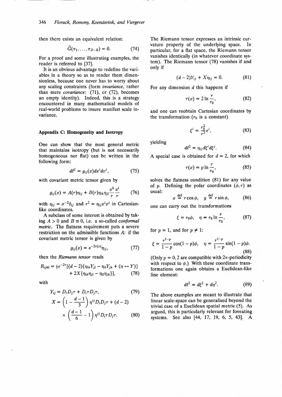
It is an obvious advantage to redefine the variables in a theory so as to render them dimensionless, because one never has to worry about any scaling constraints (form invariance, rather than mere covariance: (71), or (72), becomes an empty identity). Indeed, this is a strategy encountered in many mathematical models of real-world problems to insure manifest scale invariance.

The Riemann tensor expresses an intrinsic cur- vature property of the underlying space. In particular, for a flat space, the Riemann tensor vanishes identically (in whatever coordinate system). The Riemann tensor (78) vanishes if and only if

( d - 2)E;:j + X ~ i j = 0. (81)

For any dimension d this happens if r

ro r ( x ) = 21n - l

and one can reobtain Cartesian coordinates by the transformation (ro is a constant)

2

(83)

(84)

P - ~ O i - - p l Appendix C: Homogeneity and Isotropy

One can show that the most general metric that maintains isotropy (but is not necessarily homogeneous nor flat) can be written in the following form:

r

yielding

A special case is obtained for d = 2, for which

de2 = q i jd t id t j .

-

de2 = g < j ( x ) d x i d d l (75)

with covariant metric tensor given by

xk x1 gij(x) = A ( r ) ~ i j + B(r)qik~jl-- r r (76)

with qij = C T - ~ S ~ ~ and r2 = q;jxixj in Cartesian- like coordinates.

A subclass of some interest is obtained by taking A > 0 and B z 0, i.e. a so-called conformal metric. The flatness requirement puts a severe restriction on the admissible functions A: if the covariant metric tensor is given by

(77)

solves the flatness condition (81) for any value of p . Defining the polar coordinates (4 , r ) as usual:

(86) def def

x = rcos4, y - rs in4,

one can carry out the transformations r

TO = rO4, q = ro In -,

for p = 1, and for p # 1:

..l -n -1-v ‘f- * 8r- r

E = -cos(l -p)(b, q = - sin(1 - p)4 . 1 - P 1-P

(Only p = 0,2 are compatible with 2~-periodicity with respect to 4.) With these coordinate transformations one again obtains a Euclidean-like line element:

with de2 = d t 2 + dq2. (89) Yzj = DiDjr + DirDjr ,

X = (1 - y) ~ f j D i D j ~ + ( d - 2)

x (y - 1) qijD;.rDjr.

(79) The above examples are meant to illustrate that linear scale-space can be generalised beyond the trivial case of a Euclidean spatial metric (5 ) . As argued, this is particularly relevant for foveating

(80) systems. See also [44, 17, 19, 6, 5, 431. A


coordinate system in which the metric reduces to (89) is most suited for a sampling scheme based on a usual, regular grid.

Appendix D: Well-Posed Differentiation

The process of differentiation as defined in the standard way is known to be ill-posed in the sense of Hadamard. As a consequence, the process lacks the necessary robustness for practical implementations. But also in pure mathematics one has found the desire to be able to define, in some well-posed sense, derivatives of (possibly non-smooth) functions.

To see how this problem has been solved in mathematics, let us consider the class of functions of polynomial growth. This class of (piece- wise continuous, but generally non-smooth) functions is sufficient for most physical applications, and more specifically, for most image analysis and computer vision purposes:

DEFINITION 10 (Function of Polynomial Growth). A function g : R" + R is said to be of polynomial growth, if 3c > 0 m 2 0 such that:

For later convenience, let us also introduce the multi-index notation in d dimensions:

DEFINITION 11 (Multi-Index). With the multi- index notation n we mean any set of d non-negative integers, with n denoting its norm, i.e. the sum of all these integers:

i = l

We will henceforth use the notation D, to denote the n-th order linear partial differential operator dl'/ldz;' s ' 827, X" to denote the homogeneous polynomial of degree n, z;' . . x?, etc.

For the class of functions of polynomial growth one now proceeds as follows in order to define a well-posed linear differentiation: for each such function g one introduces a functional Tg, called a regular tempered distribution. This functional is defined so as to operate on the class of real, smooth test functions, called G(Rd) (the fact that

we consider the carrier Rd is not essential to the issue). A linear derivative D,g of g is then likewise associated with a regular tempered distribution, whose action on a test function 4 is expressed in terms of the action of Tg on the corresponding derivative 0.4 of 4 (which is well- defined by definition). Here is how it works:

DEFINITION 12 (Class of Smooth Test Func- tions). The class of smooth test functions, G(Rd), is defined by:

4 E G(Rd> * 4 E cm(Rd) A sup ]x"Dm&(x)] < 00,

z€Rd

for all multi-indices m and n.

In other words, it contains all smooth functions that decrease "sufficiently fast" at the boundaries.

DEFINITION 13 (Tempered Distribution). A linear functional T : G(Rd) + E% is called a tempered distribution if 3c > 0 and multi-indices m, n such that:

IT(4)I I CSUP IX'DmmI. X€Rd

DEFINITION 14 (Regular Tempered Distribu- tion). Let g be a function of polynomial growth, then its associated regular tempered distribution Tg is defined by the tempered distribution:

Tg : 8(Rd) + R : 4 dxg(x)+(x). s One may easily verify that a regular tempered distribution as defined by Definition 14 is indeed a tempered distribution according to the previous Definition 13. The space of all tempered distributions is a linear space over E% (with the usual definition of addition and scalar multipli- cation) and is denoted here by c(Rd). Often, and for obvious reasons, a regular tempered distribution Tg is identified with the function g, and in this sense one may easily define the derivative of g by identifying it with the derivative of its corresponding regular tempered distribution IT$:


DEFINITION 15 (Derivative of a Tempered Dis- tribution). The derivative D,T of a tempered distribution T is defined by:

(D, T)( d) gf (-) "T( D, 4).

The reason for the conventional minus sign is that in the subspace G(R") of smooth functions, the above definition essentially boils down to the classical definition of differentiation, which can readily be verified by repeated partial integra- tions. The test functions are irrelevant dummy variables then and there is no need for dis- tinguishing between a smooth function and its regular tempered distribution.

For the purpose of regularisation (i.e. turn- ing ill-posed differentiation into a well-posed problem), the restriction to a small subclass of test functions would be sufficient, but at this point this would be an ad hoc choice. That ex- plains why, from the strict mathematical point of view, the above operational definition of well- posed differentiation is a very natural one. For the physicist, however, who finds himself con- fronted with a new set of operands (the test functions), the above method is not quite sat- isfactory, since it refrains from constraining the new degrees of freedom introduced by the infinite dimensional class G(Rd) to any manageable proportion. Moreover, he is inclined to interpret a derivative of some observable as yet another observable. In other words, he would want to select a particular test function 4 (or at least a particular, parametrised subclass of test- functions) for each point of the image's domain and then "freeze" it into the functional. In this way, the arbitrary test function is promoted to the status of a linear filter. However, the choice of a particular filter or parametrised filter family must be based upon physical considerations beyond mere regularisation!

It is the purpose of this article to reconcile this physical point of view with the theory of regular tempered distributions. In principle, this is very simple: just take a parametrised subclass &(. ; x) of test functions for each point x of the image's domain (s denotes a set of parameters and x is the extra spatial label), and define a robust derivative of an image L(x) that continuously

depends on the image data, as follows:

DnLs(x) Ef (-)"TL(Dnqq. ; x)) r

(The operator D, is understood to apply to the first argument y of the test function.)

A typical example of an additional physical requirement is linear shift invariance, motivated by the notion that there is no a priori preferred point within the observable's field of view. It poses a strong restriction on the form of allowable test functions, viz.

4s(Y;x) = @S(X - Y)I (91)

from which we get

Anyway, once we have established the form of the kernels &(y; x), we are automatically provided with a complete family of operationally defined kernels, viz.

This family is complete in the following sense:

def Ls(x + a) = m 4 s c . ;x + a))

In other words, we only need to have access to the image's local functional values for the family q&(.;x) at the point x in order to reveal the global structure of the regularised function L.

This still leaves the central question of how to choose Qs and how to interpret it. Indeed, this is a question that cannot be solved from mathematical considerations only; one has 'to decide on physical grounds on the nature of the underlying physical parameters and on how 'to single out a unique filter class.

Acknowledgment

This work has been carried out as part of the national priority research programme "3D Com- puter Vision", supported by the Netherlands


Ministries of Economic Affairs and Education & Science through a SPIN grant. The support from the participating industrial companies is gratefully acknowledged.

Notes

1. A voxel is the D-dimensional analogue of a pixel. 2. For readers familiar with Lie groups, note that Defini-

tion 1 is just the exponentiated form of an infinitesimal rescaling of the inner scale: E H &(I + 67).

3. The vector notation for ,? and 2 is legitimate, once having chosen an arbitrary, fiducial origin for reference.

4. This is not a restriction: a reflection p ++ - p merely amounts to an interchange of the complementary concepts of scale and resolution, i.e. inverse scale.

References

1 . J. Babaud, A.P. Witkin, M. Baudin, and R.O. Duba, “Uniqueness of the gaussian kernel for scale-space filtering,” IEEE Trans. Pattern Analysis and Machine Intelligence, 8(1):26-33, 1986.

2. Piet Bijl, Aspects of Visual Contrast Detection. PhD thesis, University of Utrecht, The Netherlands, May 1991.

3. J. Blom, B.M. ter Haar Romeny, A. Bel, and J.J. Koen- derink, “Spatial derivatives and the propogation of noise in gaussian scale-space,” J. of Vis. Comm. and Im. R e p , 4(l):l-l3, March 1993.

4. P.J. Burt, T.H. Hong, and A. Rosenfeld, “Segmentation and estimation of image region properties through coop- erative hierarchical computation,” IEEE Trans. Systems, Man, and Cybernetics, 11(12):802-825, 1981.

5. J.L. Crowley, “Towards continuously operating integrated vision systems for robotics applications,” In Peter Johnsen and Smen Olsen, editors, Proc. 7th Scand. Con$ on Image Analysis, pages 494-505, Aalborg, DK, August 13-16 1991.

6.

7.

8.

9.

10.

J.L. Crowley, A. Chehikian, and F. Veillon, “Definition of image primitives,” VAP Tech. Rep. IR.A.3.1, LIFIA (1MAG)-I.N.P., Grenoble, France, 1990. James Damon, “Local Morse theory for solutions to the heat equation and Gaussian blurring,” Internal report De- partment of Mathematics. University of North Carolina, Chapel Hill, North Carolina, USA, 1990. Burkart Fischer, “Overlap of receptive field centers and representation of the visual field in the cat’s optic tract,” Vision Research, 13:2113-2120, 1973. L.M.J. Florack, B.M. ter Haar Romeny, J.J. Koenderink, and M.A. Viergever, “Scale and the differential structure of iamges,” Image and Vision Computing, 10(6):376-388, JulyIAugust 1992. L.M.J. Florack, B.M. ter Haar Romeny, J.J. Koenderink, and M.A. Viergever, “Cartesian differential invariants in scale-space,” Journal of Mathematical Imaging and Vision, 3(4):327-348, November 1993.

11.

12.

13.

14.

15.

16.

17.

18.

19.

20.

21.

22.

L.M.J. Florack, B.M. ter Haar Romeny, J.J. Koenderink, and M.A. Viergever, “General intensity transformations and differential invariants,” Journal of Mathematical Imag- ing and Vision, 1993. Accepted. Joseph Fourier. The Analytical Theory of Heat. Dover Pub- lications, Inc. New York, 1955. Replication of the English translation that first appeared in 1878 with previous corri- genda incorporated into the text, by Alexander Freeman, M.A. Original work: “Theorie Analytique de la Chaleur,“ Paris, 1822. David H. Hubel. Eye, Brain and Vision, volume 22 of Sci- entific American Library, Scientific American Press, New York, 1988. R.A. Hummel and B.C. Gidas, “Zero crossings and the heat equation,” Technical Report 1 1 1 , New York Univ. Courant Institute of Math. Sciences, Computer Science Division, 1984. R.A. Hummel, B.B. Kimia, and S.W. Zucker, “Deblurring Gaussian blur,” Computer Vision, Graphics, and Image Processing, 38:66-80, 1987. B.B. Kimia, Debluning gaussian blul; continuous and discrete approaches, Master’s thesis, McGill University, Elec- trical Eng. Dept., Montreal, Canada, 1986. J.J. Koenderink, “The concept of local sign,” in A.J. vanDoorn, W.A. van de Grind, and J.J. Koenderink, editors, Limits in Perception, pages 495-547. VNU Science Press, Utrecht, 1984. J.J. Koenderink, “The structure of images,” Biol. Cybern.,

J.J. Koenderink, “The structure of the visual field,” in W. Giittinger, and G. Dangelmayr, editors, The Physics of Structure Formation, Theory and Simulation. Springer- Verlag, 1986. Proceedings of an International Sympo- sium, tiibingen, Fed. Rep. of Germany, October 27- November 2. J.J. Koenderink, “Scale-time,’’ Biol. Cybern., 58:159-162, 1988. J.J. Koenderink, Solid Shape, MIT Press, Cambridge, Mass., 1990. J.J. Koenderink, “Local image structure,” in Proc. Scand Con$ on Image Analysis, pages 1-7, Aalborg, DK, August 1991.

50~363-370, 1984.

23. J.J.Koenderink and A.J. van Doorn, “Representation of local geometry in the visual system,” Biol. Cybern., 55:367- 375, 1987.

24. J.J. Koenderink and A.J. van Doorn, “Receptive field families,” Biol. Cybern., 63:291-298, 1990.

25. L.M. Lifshitz and S.M. Pizer, “A multiresolution hierarchical approach to image segmentation based on intensity extrema,“ IEEE Trans. Pattern Analysis and Machine In- teligence, 12(6):529-541, 1990.

26. Alan P. Lightman, William H. Press, Richard H. Price, and Saul A. Teukolsky, Problem Book in Relativity and Gravitation, Princeton University Press, Princeton, New Jersey, 1975.

27. T. Lindeberg, “Scale-space for discrete signals,” IEEE Trans. Pattern Analysis and Machine Intelligence, 12(3):234- 245, 1990.


28. T Lindeberg, Discrete Scale-Space Theory and the Scale- Space Primal Sketch, PhD thesis, Royal Institute of Tech- nology, Department of Numerical Analysis and Com- puting Science, Royal Institute of Technology, S-100 44 Stockholm, Sweden, May 1991.

29. T Lindeberg and J.O. Eklundh, “Guiding early visual processing with a scale-space primal sketch,” Technical Re- port CVAP-72, Royal Institute of Technology, University of Stockholm, Dept. of Numerical Analysis and Computing Science, Stockholm, Sweden, 1990.

30. T. Lindeberg and J.O. Eklundh, “On the computation of a scale-space primal sketch,” Technical Report CVAP-68, Royal Institute of Technology, University of Stockholm, Dept. of Numerical Analysis and Computing Science, Stockholm, Sweden, 1990.

31. M.M. Lipschutz, Differential Geometry, Schaum’s Outline Series. McGraw Hill, New York, 1969.

32. Lord Rayleigh, “The principle of similitude,” Nature, XCV66-68, 644, March 1915.

33. S.G. Mallat, “A theory of multiresolution signal decomposition: The wavelet representation,” IEEE Trans. Pattern Analysis and Machine Intelligence, 11 (7):674-694, 1989.

34. J.B. Martens, “Deblurring digital images by means of polynomial transforms,” Computer Vision, Graphics, and Image and Stochastic Processing, 50:157-176, 1990.

35. H.E. Moses and A.E Quesada, “The expansion of physical quantities in terms of the irreducible representations of the scale-euclidean group and applications to the construction of the scale-invariant correlation functions,” Arch. Rat. Mech. Anal., 44:217-248. 1971, Part I. Con- cepts. One-Dimensional Problems, Communicated by J. Meixner.

36. H.E. Moses and A.F. Quesada, “The expansion of physical quantities in terms of the irreducible representations of the scale-euclidean group and applications to the construction of scale-invariant correlation functions,” Arch. Rat. Mech. Anal., 50:194-236, 1973. Part 11. Three- Dimensional Problems; Generalizations of the Helmholtz Vector Decomposition Theorem, Communicated by J. Meixner.

37. P.J. Olver, Applications of Lie Groups to Differential Equa- tions, volume 107 of Graduate Texts in Mathematics, Springer-Verlag, 1986.

38. S.M. Pizer, J.J. Koenderink, L.M. Lifshitz, L. Helmink, and A.D.J. Kaasjager, “An image description for object defintion, based on extremal regions in the stack,” Infor- mation Processing in Medical Imaging, Proceedings of the 8th conference, pages 24-37, 1985.

39. T. Poston and I. Steward, Catastrophe Theory and its Ap- plications, Pitman, London, 1978.

40. M. Spivak, A Comprehensive Introduction to Differenrial Geometry, volume I-V, Publish or Perish, Inc., Houston, Texas, 1970.

41. B.M. ter Haar Romeny and L.M.J. Florack, “A multiscale geometric model of human vision, “In William R. Hendee and Peter N.T. Wells, editors, Perception of Visual Infor- mation, chapter 4, pages 73-1 14. Springer-Verlag. Berlin, 1993.

42. B.M. ter Haar Romeny and L.M.J. Florack, J.J. Koen- derink, and M.A. Viergever, “Scale-space: Its natural operators and differential invariants,” in A.C.E Colchester and D.J. Hawkes, editors, Information Processing in Med- ical Imaging, volume 511 of Lecture Notes in Computer Science, pages 239-255, Berlin, July 1991, Springer-Verlag.

43. Massimo Tistarelli and Giulio Sandini, Dynamic aspects in active vision,” CVGIP: Image Understanding, 56( 1):108- 129, July 1992.

44. A.J. van Door, J.J. Koenderink, and M.A. Bouman, “The influence of the retinal inhomogeneity on the perception of spatial patterns,” Kybernetik, 10:223-230, 1972.

45. H. Wassle, U. Griinert, J. Rohrenbeck, and B. Boycott, “Retina1 ganglion cell density and cortical magnification factor in the primat,” Vision Research, 30:1897-1911,1990.

46. H. Weyl, The Classical Groups, their Invariants and Rep- resentations, Princeton University Press, Princeton, NJ, 1946.

47. A.P. Witkin. “Scale space filtering,” in Proc. International Joint Conference on Artificial Intelligence, pages 101 9-1023, Karlsruhe, W. Germany, 1983.

48. R.A. Young. The Gaussian derivative theory of spatial vision: Analysis of cortical cell receptive field line-weighting profiles. Publication gmr-4920, General Motors Research Labs, Computer Science Dept., 30500 Mound Road, Box 9055, Warren, Michigan 48090-9055, May 28 1985.

49. R.A. Young, “The Gaussian derivative model for machine vision: Visual cortex simulation,“ Journal of the Optical Society of America, July 1986.

50. R.A. Young, “Simulation of human retinal function with the Gaussian derivative model,” in Proc. IEEE CVPR CH2290-5, pages 564-569, Miami, Fla. 1986.

51. A.L. Yuille and TA. Poggio, “Scaling theorems for zero- crossings,” IEEE Trans. Pattern Analysis and Machine In- telligence, 8: 15-25, 1986.

52. A.L. Yuille and TA. Paggio, “Scaling and fingerprint theorems for zero-crossings,” in C. Brown, editor, Advances in Computer Vision, pages 47-78. Lawrence Erlbaum, 1988.

=


Luc Florack received his M.Sc. degree in theoretical physics, with a thesis on the quantization of gauge field theories, from the University of Utrecht, The Netherlands, in 1989. He is currently a Ph.D. student in the Computer Vision Research Group, a member of the Utrecht Biophysics Re- search Institute. His primary research interest in computer vision is the representation of scalar image structure and, in particular, scale-space methods.

Jan Koenderink received the MSc. degree in physics and mathematics in 1967 and the Ph.D. degree in 1972 from the University of Utrecht, The Netherlands. He was an associate professor of experimental psychology at Groningen University until 1974, when he returned to Utrecht, where he presently holds a chair in the department of physics and astronomy. He is currently scientific director of the Utrecht Biophysics Research Institute, in which multidisci- plinary work in biology, medicine, physics, and computer science is coordinated. His research interests include opti- cally guided behavior, computational neuroscience, differential geometry, and image processing and interpretation.

Dr. Koenderink received an honorary (D.Sc.) degree in medicine from the University of Leuven and is a fellow of the Royal Netherlands Academy of Arts and Sciences. He participates on the editorial boards of several scientific journals.

Bart M. ter Haar Romeny received an M.Sc. degree in applied physics from Delft University of Technology in 1978 and a Ph.D. degree from the University of Utrecht, The Netherlands, in 1983. After being the principal physicist of Utrecht University Hospital Department of Radiology, he joined the University of Utrecht 3D Computer Vision Research Group as an associate researcher in 1989. His interests are mathematical aspects of front-end vision, particularly linear and nonlinear scale-space theory, medical computer-vision applications, picture archiving and commu- nication systems, differential geometry and perception, and cross-fertilization among these fields. He is the author of several papers and book chapters on these issues and is involved in (and initiated) a number of international collab- orations on these subjects.

Max Viergever received the M.Sc. degree in applied mathematics in 1972 and the D.Sc. degree with a thesis on cochlear mechanics in 1980, both from Delft University of Technology, The Netherlands. From 1972 to 1988 he was assistant professor and then associate professor of applied mathematics of Delft University. Since 1988 he has been professor of medical image processing and head of the Com- puter Vision Research Group at the University of Utrecht. He is the author of over 100 scientific papers on biophysics and medical image processing and is the author or editor of nine books. His research interests comprise all aspects of computer vision and image processing, including image reconstruction, compression, multimodality integration, multiresolution segmentation, and volumetric visualization. Dr. Viergever is at present associate editor of IEEE Transactions of Medical Imaging.

Documents

Linear scale-space