1

2

Abstract

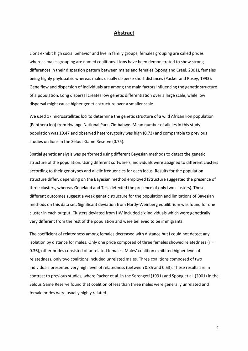
Lions exhibit high social behavior and live in family groups; females grouping are called prides

whereas males grouping are named coalitions. Lions have been demonstrated to show strong

differences in their dispersion pattern between males and females (Spong and Creel, 2001), females

being highly phylopatric whereas males usually disperse short distances (Packer and Pusey, 1993).

Gene flow and dispersion of individuals are among the main factors influencing the genetic structure

of a population. Long dispersal creates low genetic differentiation over a large scale, while low

dispersal might cause higher genetic structure over a smaller scale.

We used 17 microsatellites loci to determine the genetic structure of a wild African lion population

(Panthera leo) from Hwange National Park, Zimbabwe. Mean number of alleles in this study

population was 10.47 and observed heterozygosity was high (0.73) and comparable to previous

studies on lions in the Selous Game Reserve (0.75).

Spatial genetic analysis was performed using different Bayesian methods to detect the genetic

structure of the population. Using different software’s, individuals were assigned to different clusters

according to their genotypes and allelic frequencies for each locus. Results for the population

structure differ, depending on the Bayesian method employed (Structure suggested the presence of

three clusters, whereas Geneland and Tess detected the presence of only two clusters). These

different outcomes suggest a weak genetic structure for the population and limitations of Bayesian

methods on this data set. Significant deviation from Hardy-Weinberg equilibrium was found for one

cluster in each output. Clusters deviated from HW included six individuals which were genetically

very different from the rest of the population and were believed to be immigrants.

The coefficient of relatedness among females decreased with distance but I could not detect any

isolation by distance for males. Only one pride composed of three females showed relatedness (r =

0.36), other prides consisted of unrelated females. Males’ coalition exhibited higher level of

relatedness, only two coalitions included unrelated males. Three coalitions composed of two

individuals presented very high level of relatedness (between 0.35 and 0.53). These results are in

contrast to previous studies, where Packer et al. in the Serengeti (1991) and Spong et al. (2001) in the

Selous Game Reserve found that coalition of less than three males were generally unrelated and

female prides were usually highly related.

3

Although population density in the lion population in Hwange National Park is lower than in other

areas (Bauer and Van Der Merwe, 2004) I did not find reduced levels of genetic diversity. Females

are more territorial, staying close to their natal territory when dispersing, while males might travel

longer distances and therefore, may be responsible for the gene flow over this large area. Individuals

grouping differ from previous studies with prides being mostly unrelated and coalitions being more

related. Weak population structure and long distances dispersion suggests that the genetic structure

of this population seems to be under the influence of immigrants coming from outside the study area

rather than dispersal of sub-adults.

4

Contents

Introduction ……………………………………………………………………………………………………………………………6

Methods …………………………………………………………………………………………………………………………….…….9

Study area ………………………………………………………………………………………………………………….9

Collection and storage of samples……………………………………………………………………………..10

DNA extraction………………………………………………………………………………………………….……….11

Microsatellite genotyping………………………………………………………………………………………….11

Data analysis………………………………………………………………………………………….………………….12

Population genetic analysis ……………………………………………………………………………….12

Spatial genetic analysis ……………………………………………………………..12

STRUCTURE approach and parameters values…………………………..13

GENELAND approach and parameters values……………………………13

TESS approach and parameters values……………………………………..13

Population genetic analysis on the assumed units………………………………….…………14

Relatedness and isolation by distance……………………………………………………………….14

Results……………………………………………………………………………………………………………………………….……15

Population genetic analysis on the whole population………………………………………………………..15

Genetic structure analysis …………………………………………………………………………………………………15

STRUCTURE……………………………………………………………………………………………………….15

GENELAND………………………………………………………………………………………………………..16

TESS…………………………………………………………………………………………………………………..17

For all individuals…………………………………………………………………..….17

For males and females……………………………………………………………..18

Genetic diversity and genetic differentiation among the clusters……………………………….19

Following STRUCTURE results ……………………………………………………19

Following TESS results…………………………………………………………….…20

Relatedness ………………………………………………………………………………………………………………..20

Differences between males and females dispersion and relatedness……………..20

Relatedness within prides ……………………………………………………………………………….21

Discussion……………………………………………………………………………………………………………………….………23

Acknowledgement……………………………………………………………………………………………………………….…28

Literature………………………………………………………………………………………………………………………………..29

5

Introduction

Conservation genetics has grown out of population genetics applying genetic and molecular methods

as a tool for conservation of small endangered populations (O’Brien, 1994). As such, population

structures can be deduced which increases the amount of knowledge available on any population,

groups or individuals, limiting the risk of injurious conservation management decisions (O’Brien,

1994). One of the aspects of conservation genetics is thus investigating the level of relatedness

between individuals in a given population. Furthermore, population size, survival, reproductive rates,

dispersal and inbreeding can also be explored when using DNA data (Arrendal, 2007). As a result,

conservation genetics and molecular tools allows a deeper understanding and knowledge of the

driving forces behind any decline of endangered populations and the establishment of management

plans before further negative events take place (Saccheri et al., 1998).

In their seminal paper Manel et al. (2003) provided the first definition of landscape genetics stating

that this field ‘aims at providing information’s about the interaction between landscape features and

micro-evolutionary processes such as gene flow, genetic drift and selection’. In summary, landscape

genetics uses tools from different subject such as population genetics, landscape ecology and spatial

statistics to understand the movements behind the population genetic structure (Storfer et al.,

2007). Besides, the rise of landscape genetics only became possible on the strength of advances in

molecular markers, geographical tools and new spatial statistical tools (Guillot et al., 2005).

Landscape genetics have been revealed through the increase of genetic markers among the genomes

and the accessibility to a new range of spatial data. Researchers are now able to study the effects of

many landscape features (such as altitude, topography and vegetation) on the structure of

populations and their genetic variation (Storfer et al., 2007).

In the past, many conservation genetics studies of plants and animals have used microsatellites

(Höglund, 2009). Microsatellites, short tandem repeats of 1-6 base pairs, are commonly used for

kinship analyses because of their neutrality and high mutation rate which reveal recent changes in

the population structure (Schlötterer, 2000). Also, polymorphic microsatellite markers are a suitable

method for determining intra- and intergenetic variation and can therefore be used to evaluate

relatedness between individuals and between groups.

Social behavior, reflected in mating systems, dispersion and cooperation, greatly influence the

genetic structure of a population (Ross, 2001). Consequently genetic studies of population dynamics

6

and structure are needed for a deeper understanding of social interactions between individuals

(Storz, 1999). Genetic data can, to some extent, produce more reliable data than behavioral studies

(Sugg et al., 1996). For instance, before the appearance of molecular tools, behavioural studies of

lions aimed to look at their diet diversity (Schaller, 1972; Scheel, 1993) and to understand the

reproductive biology (Rudnai, 2008) and the relatedness links among individuals within their prides

(Bertram, 1976; Van Orsdol et al., 1985). Packer et al. (1991) argued that parental links were

observable for female lions, whereas paternal filiations could not be deduced through observational

studies.

The social behavior of individuals within a group often depends on their relatedness (Queller and

Goodnight, 1989). Therefore, knowledge of relatedness between individuals is needed to understand

social structure and behavior within groups. African lions live in fission-fusion groups consisting of a

group of related females and their offspring (Packer et al., 1990). They exhibit a complex social

structure and show cooperative behavior (Packer et al., 1991). African lions exhibit differences in

male and female dispersion. Females are philopatric, and females are generally incorporated into

their natal pride when they reach adulthood, or form new prides close to their old territory (Pusey

and Packer, 1994); whereas males disperse and are usually, transient to the pride and form coalitions

of related or unrelated males (Schaller, 1972; Waser, 1996). Several species of birds and mammals

exhibit sex difference in dispersal distance (Pusey, 1987). Sex-biased dispersal affects the life history

evolution of the species but also the genetic structure of a population (Goudet et al., 2002). As a

result, male dispersal is of great importance to avoid inbreeding in populations (Pusey and Packer,

1987). However, dispersal time and space should be minimal, as it involves high risk of mortality

(Spong and Creel, 2001). Sub adult lions, mainly males, have to disperse in order to gain access to a

territory to fulfill their needs for reproduction and prey. Before establishing a territory, young males

have to kill or exclude the resident individuals (Pusey and Packer, 1987). Studies of the Serengeti lion

population have demonstrated that females tend to disperse to avoid mating with their father or

because they have been evicted by a new coming male (Pusey and Packer, 1987). However

dispersing females suffer from higher mortality and a later start for breeding (Pusey and Packer,

1987).

Hwange National Park presents a setting ideal for a population genetic study of lions, it is the largest

national park in Zimbabwe (14,600km2) and the study area covers around 5000 km2. At 2.5 lions per

100 km2, lion density in Hwange is lower than in any of the previous studied areas (Bauer and Van

Der, 2004). Therefore we may expect social behavior and relatedness to be different due to the

differences in population structure.

7

The aim of my research is to extend the understanding of lion population structure and the evolution

of social behavior. A related aim is to provide a deeper knowledge of lion ecology, which may provide

important resources for future conservation management plans.

I focused on the following issues:

Assessment of the genetic diversity of the Hwange National Park lion population

Evaluation of the genetic structure and differentiation among putative genetic groups

To understand the mechanisms leading to the dispersion of sub-adult lions (relatedness

among lions within and among groups).

8

Methods

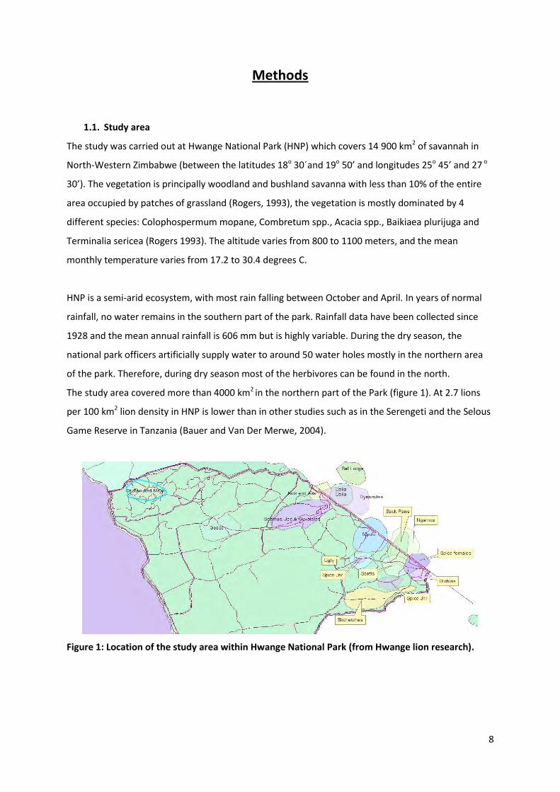
1.1. Study area

The study was carried out at Hwange National Park (HNP) which covers 14 900 km2 of savannah in

North-Western Zimbabwe (between the latitudes 18o 30´and 19o 50’ and longitudes 25o 45’ and 27 o

30’). The vegetation is principally woodland and bushland savanna with less than 10% of the entire

area occupied by patches of grassland (Rogers, 1993), the vegetation is mostly dominated by 4

different species: Colophospermum mopane, Combretum spp., Acacia spp., Baikiaea plurijuga and

Terminalia sericea (Rogers 1993). The altitude varies from 800 to 1100 meters, and the mean

monthly temperature varies from 17.2 to 30.4 degrees C.

HNP is a semi-arid ecosystem, with most rain falling between October and April. In years of normal

rainfall, no water remains in the southern part of the park. Rainfall data have been collected since

1928 and the mean annual rainfall is 606 mm but is highly variable. During the dry season, the

national park officers artificially supply water to around 50 water holes mostly in the northern area

of the park. Therefore, during dry season most of the herbivores can be found in the north.

The study area covered more than 4000 km2 in the northern part of the Park (figure 1). At 2.7 lions

per 100 km2 lion density in HNP is lower than in other studies such as in the Serengeti and the Selous

Game Reserve in Tanzania (Bauer and Van Der Merwe, 2004).

Figure 1: Location of the study area within Hwange National Park (from Hwange lion research).

9

1.2. Collection and storage of samples.

The project was conducted in collaboration with Hwange lion research (HLR), which is part of Oxford

University, WildCRU. HLR has been monitoring lions since 1999, primarily to address levels of trophy

hunting of lions in the areas surrounding HNP, Zimbabwe. Currently, HLR is monitoring over 200 lions

in 40 prides with 50 collars in the field.

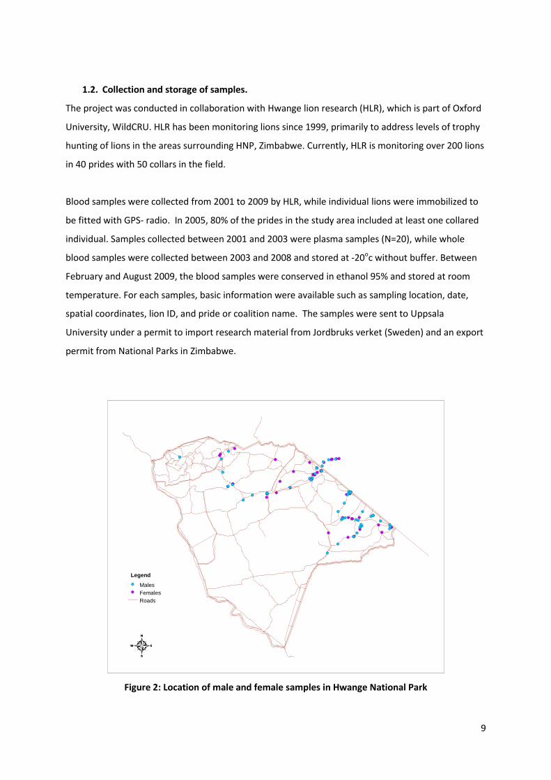
Blood samples were collected from 2001 to 2009 by HLR, while individual lions were immobilized to

be fitted with GPS- radio. In 2005, 80% of the prides in the study area included at least one collared

individual. Samples collected between 2001 and 2003 were plasma samples (N=20), while whole

blood samples were collected between 2003 and 2008 and stored at -20oc without buffer. Between

February and August 2009, the blood samples were conserved in ethanol 95% and stored at room

temperature. For each samples, basic information were available such as sampling location, date,

spatial coordinates, lion ID, and pride or coalition name. The samples were sent to Uppsala

University under a permit to import research material from Jordbruks verket (Sweden) and an export

permit from National Parks in Zimbabwe.

Figure 2: Location of male and female samples in Hwange National Park

Legend Males Females Roads

4

10

1.3. DNA extraction.

DNA extraction was carried out on 91 samples in total using different methods (high salt purification

protocol, Genemol or QIAGEN kits). Every sample was first extracted using a high salt purification

and the concentration and purity of the DNA was controlled. When the concentration was fairly low,

other extraction methods were tested to increase the amount of DNA.

High salt purification protocol: A small amount of blood (approx 10µL) was placed in a 1.5mL tube

with 350 µL of Set buffer, 19.4 µL of 20% SDS and 12.5 µL of proteinase K. After vortexing, the

samples were incubated overnight in an oven at 55°. 300µL of NaCl (6M) was added to each sample.

The solution was centrifuged for 10 minutes at 13000rpm, and then 600 µL of the supernatant was

transferred to a new tube and mixed with 150 µL of TRIS (0.01 M, pH 8.0). The samples were left

overnight with 750µL 99.5% EtOH stored at -20°. The tubes were centrifuged for 15 minutes at

10700rpm before to be washed with 1 mL freezer cold 70% EtOH, then centrifuged and left to dry

approximately 5 hours. To finish, the pellet was dissolved into 100 µL of Te-buffer (pH 7.6).

Ten samples, which had low concentration of DNA or impurity, were extracted again using a

GeneMole automated nucleic acid extraction instrument (Mole Genetics, Norway) according to the

manufacturer's guide. The quality was controlled but it was concluded that the quality was too low to

carry on any further analysis.

DNA was extracted from the 45 samples remaining using the blood and tissue QIAGEN extraction kit

following the manufacturer’s instructions. For the plasma samples we used the low DNA blood kit

(QIAGEN) to extract and followed the manufacturer’s instructions. For the remaining blood samples,

we used the blood and tissue extraction kit (QIAGEN) following the manufacturer’s instructions.

1.4. Microsatellite genotyping

A large number of polymorphic microsatellite markers have been identified for the domestic cat

(Marilyn Menotti-Raymond et al., 1999) and are suitable for genetic work on African lions. 29

different microsatellite markers were amplified with the Polymerase Chain Reaction (PCR). The

markers were labelled with fluorescent dyes (HEX, NED or FAM) and were divided into four

multiplexes according to their size. Multiplex PCR reactions were run in 10 µL volumes containing 1

µL of each multiplex mix, 1 µL of diluted DNA, 5 µL of PCR mastermix and 3 µL of Rnase free water.

PCR conditions were an initial denaturation cycle at 95ºC for 15mins, followed by 35 cycles at 94ºC

11

for 30s, annealing at 62ºC for 90s and 72ºC for 90s. PCRs then had a final extension at 72ºC for

10mins.

PCR products from each population were then analyzed using a MegaBace run. The plate was

composed of 2 µL of dilute 10 times PCR products, 7.8 µL H2O, 0.2 µL of MegaBace size standard.

Genotypes for each sample were scored using the software Fragment Profiler (Fragment Profiler 1.2,

Amersham Biosciences, 2003). A peak filter was used for the scoring (table 1), but peak scoring was

done manually.

1.5. Data analysis

A total of 91 individuals were genotyped for this study, however 4 individuals failed to amplify for

more than three loci and were therefore removed from the study. The following analyses were

performed on the 87 individuals remaining.

1.5.1. Population genetic analysis

I used GENEPOP on the web (http://genepop.curtin.edu.au/) to test for deviation from Hardy–

Weinberg equilibrium (HWE) for each locus and a global test for heterozygote deficit or excess

considering every locus for each individual.

Also, using the same software, I tested for genotypic linkage disequilibrium for each pair of loci. The

null hypothesis was that genotypes at any locus are inherited independently from the genotypes at

other loci. Mean number of alleles, allele frequencies for each locus, observed (Ho)and expected(He)

heterozygosity levels were calculated using the GENETIX 4.02 software package to evaluate the level

of genetic variation (available at http://www.univ-montp2.fr/∼genetix/genetix.htm). Also, I

calculated the Weir&Cockerham’s estimates of FIS (1984) for each locus and also globally using the

same software. Factorial component analysis was performed using the AFC 2D option implemented

in GENETIX (Belkhir et al. 2003) on the matrix of individual genotypes to visualize individuals and how

the genetic characteristics of each individual are organized in a multidimensional space based on

allelic data.

1.5.2. Spatial genetic analysis

First, I used the STRUCTURE software developed by Pritchard et al. (2000) (available at

http://pritch.bsd.uchicago.edu/ software.html.). This software represents a first step to define

different genetic units. It assigns the individuals within different clusters according to their genotypes

12

and deduces the structure of the populations. Each cluster represents a sample of individuals

characterized by a set of allelic frequencies for each locus.

In a second part, I used two similar spatial Bayesian methods (GENELAND and TESS), to provide a

deeper understanding and an improved definition of genetic units by incorporating the spatial

coordinates of the samples.

1.5.2.1 STRUCTURE approach and parameters values.

STRUCTURE assigns individuals to populations on the basis of Hardy-Weinberg equilibrium and

linkage disequilibrium (Falush et al., 2007). I ran STRUCTURE without any prior information on the

population and the samples. For this program, the user provides a range of K’s, the number of

clusters, and the method consists of running multiple MCMC with different values of K. I ran ten

independent replicates with K varying from 1 to 10. Every run consisted of 100 000 burn-in-steps,

500 000 Markov Chain Monte Carlo (MCMC) iteration (following the suggestions of the authors

Pritchard and Wen, 2003). I used the admixture model, which assumes correlation between the

allele’s frequencies from the different population and used the approach suggested by Evanno et al.

(2005) and the delta K method to infer the most likely number of clusters, K.

1.5.2.2 GENELAND approach and parameters values

GENELAND (Guillot et al. 2005) is an R package. It also uses a Bayesian clustering method to define

population structure and find genetic boundaries using a MCMC method and incorporating the

spatial coordinates of each sample. The main assumption of this software is that individuals belong

to a population which is at Hardy-Weinberg equilibrium. We ran GENELAND allowing the number of

clusters to vary from 1 to 10. We followed the authors’ recommendations for the parameter values.

1.5.2.3 TESS approach and parameters values

TESS version 2.3 uses a Bayesian clustering algorithm for spatial population genetic studies (Chen et

al. 2007, François et al. 2006). As in STRUCTURE, admixture and no-admixture models are available.

This software defines population structure using multilocus genotypes samples and incorporating

their geographical locations but does not presuppose any defined population (François et al. 2006).

TESS 2.3 was run specifying a MCMC model with an estimated number of clusters between 1 and 10,

500000 sweeps and a burn in period of 100000. 100 runs were performed for each model (the 10%

highest runs were used for each values of K). K was then deduced from the value of the replicate with

13

the highest likelihood as described by Chen et al. (2007). Population structure was deduced for all the

individuals and for males and females separately.

1.5.3 Population genetic analysis on the assumed units

I divided the individuals into clusters according to the STRUCTURE and the TESS output and then

performed the same standard population genetic analysis as above (section 1.5.1).

1.5.4 Relatedness and isolation by distance

I used the program SPAGEDI to look for genetic relatedness, differentiation between

individuals/populations and their spatial genetic structure. This program detects isolation by distance

and can be used to estimate gene dispersal (Hardy and Vekemans, 2002).

The isolation by distance between every individual was conducted using SPAGEDI on geographical

location and genetic distance, looking at males and females separately. I performed pair wise

estimates of genetic distance between every possible pair of individuals and correlated it against

geographical distances (Rousset, 1997). I carried out a Mantel test using 1000 permutations to

assess the significance of any correlation between genetic distance and geographical distance. In

these analyses I included 43 females and 47 males.

Individuals were also separated into prides and coalitions, and I calculated the pair wise

RELATIONSHIP coefficients (Queller & Goodnight, 1989) to estimate relatedness between individuals

within these units using the software GENETIX (Belkhir et al. 2001).

14

Results

2.1 Population genetic analysis on the whole population

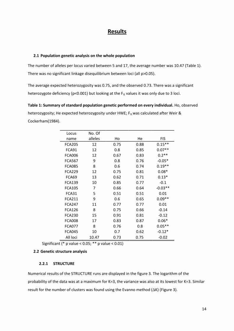
The number of alleles per locus varied between 5 and 17, the average number was 10.47 (Table 1).

There was no significant linkage disequilibrium between loci (all p>0.05).

The average expected heterozygosity was 0.75, and the observed 0.73. There was a significant

heterozygote deficiency (p<0.001) but looking at the FIS values it was only due to 3 loci.

Table 1: Summary of standard population genetic performed on every individual. Ho, observed

heterozygosity; He expected heterozygosity under HWE; FIS was calculated after Weir &

Cockerham(1984).

Locus name

No. Of alleles Ho He FIS

FCA205 12 0.75 0.88 0.15**

FCA91 12 0.8 0.85 0.07**

FCA006 12 0.67 0.83 0.2**

FCA567 9 0.8 0.76 -0.05*

FCA085 8 0.6 0.74 0.19** FCA229 12 0.75 0.81 0.08*

FCA69 13 0.62 0.71 0.13* FCA139 10 0.85 0.77 -0.1

FCA105 7 0.66 0.64 -0.03** FCA31 5 0.51 0.51 0.01

FCA211 9 0.6 0.65 0.09** FCA247 11 0.77 0.77 0.01 FCA126 8 0.75 0.66 -0.14

FCA230 15 0.91 0.81 -0.12 FCA008 17 0.83 0.87 0.06*

FCA077 8 0.76 0.8 0.05**

FCA045 10 0.7 0.62 -0.12*

All loci 10.47 0.73 0.75 -0.02

Significant (* p value < 0.05; ** p value < 0.01)

2.2 Genetic structure analysis

2.2.1 STRUCTURE

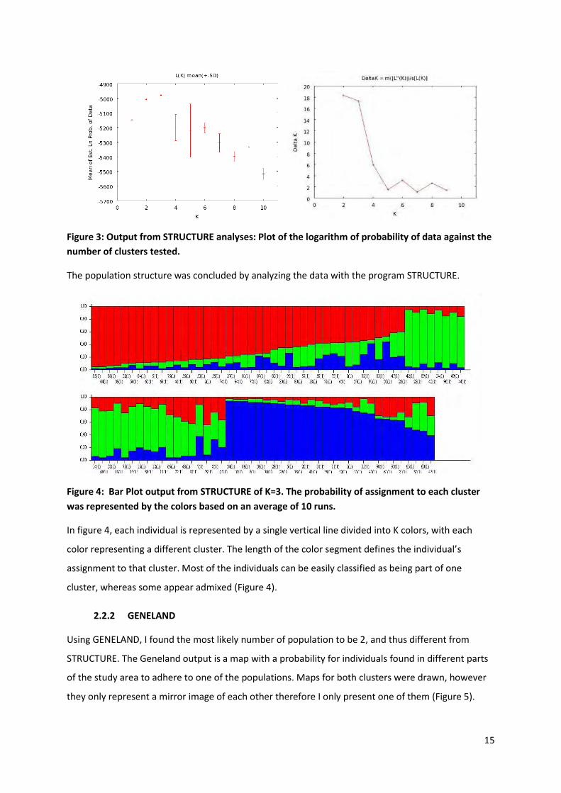
Numerical results of the STRUCTURE runs are displayed in the figure 3. The logarithm of the

probability of the data was at a maximum for K=3, the variance was also at its lowest for K=3. Similar

result for the number of clusters was found using the Evanno method ( K) (Figure 3).

15

Figure 3: Output from STRUCTURE analyses: Plot of the logarithm of probability of data against the

number of clusters tested.

The population structure was concluded by analyzing the data with the program STRUCTURE.

Figure 4: Bar Plot output from STRUCTURE of K=3. The probability of assignment to each cluster

was represented by the colors based on an average of 10 runs.

In figure 4, each individual is represented by a single vertical line divided into K colors, with each

color representing a different cluster. The length of the color segment defines the individual’s

assignment to that cluster. Most of the individuals can be easily classified as being part of one

cluster, whereas some appear admixed (Figure 4).

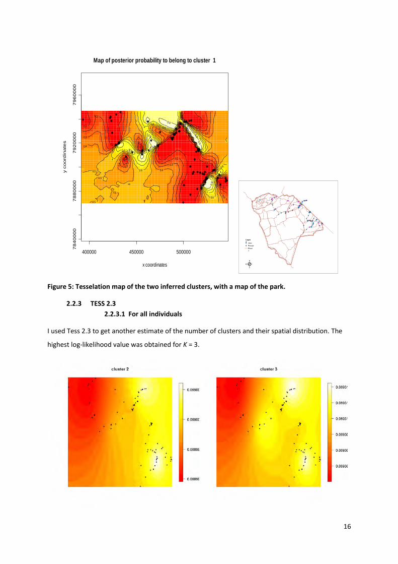
2.2.2 GENELAND

Using GENELAND, I found the most likely number of population to be 2, and thus different from

STRUCTURE. The Geneland output is a map with a probability for individuals found in different parts

of the study area to adhere to one of the populations. Maps for both clusters were drawn, however

they only represent a mirror image of each other therefore I only present one of them (Figure 5).

16

400000 450000 500000

78

40

00

07

88

00

00

79

20

00

07

96

00

00

x coordinates

y c

oo

rdin

ate

sMap of posterior probability to belong to cluster 1

0.1

0.1

0.1

0.1

0.1

0.2

0.2

0.2

0.2

0.2

0.2

0.3

0.3 0.3

0.3

0.3

0.4

0.4

0.4

0.4

0.4

0.4

0.5

0.5

0.5

0.5

0.5

0.5

0.6

0.6

0.6

0.7

0.7

0.7

0.7

0.8

0.8

0.8

0.8

0.8

0.9

0.9

0.9

0.9

Figure 5: Tesselation map of the two inferred clusters, with a map of the park.

2.2.3 TESS 2.3

2.2.3.1 For all individuals

I used Tess 2.3 to get another estimate of the number of clusters and their spatial distribution. The

highest log-likelihood value was obtained for K = 3.

Legen

d Male

s Female

s Road

s

4

17

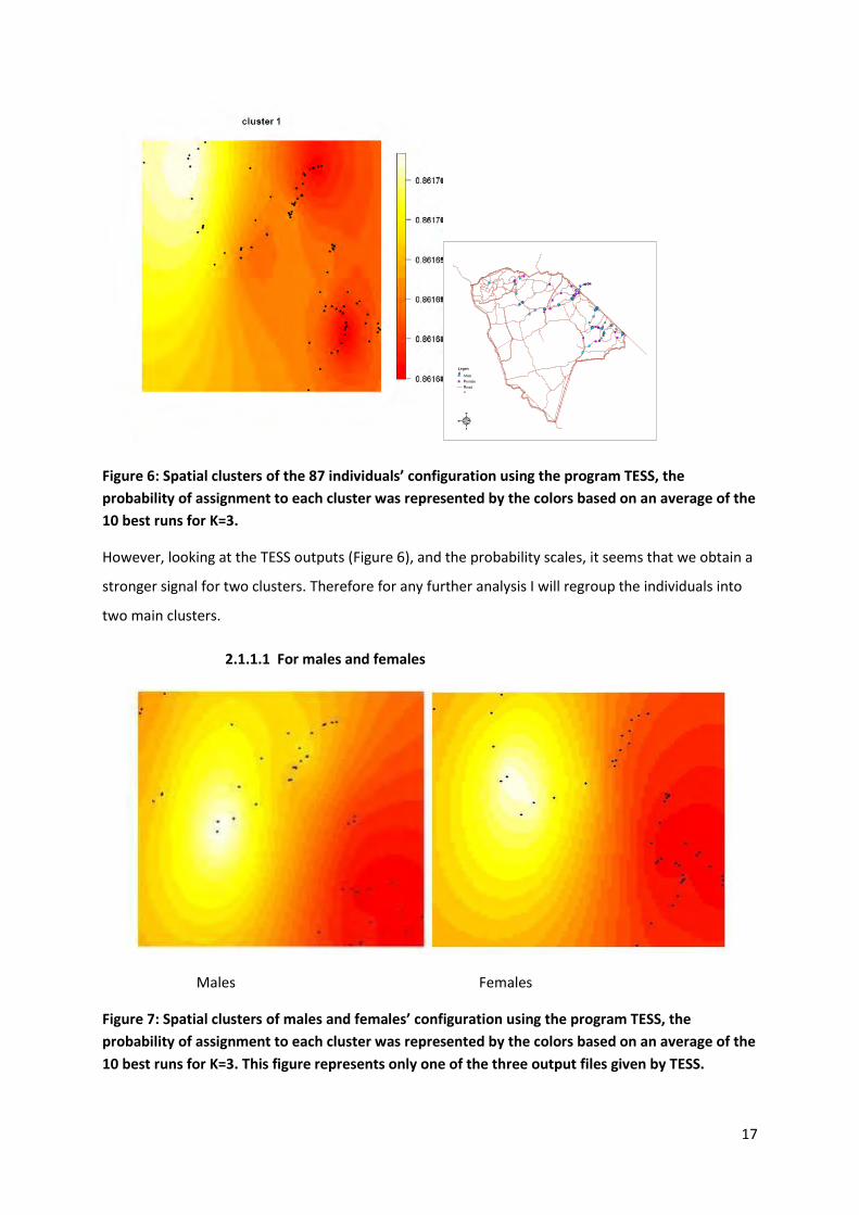
Figure 6: Spatial clusters of the 87 individuals’ configuration using the program TESS, the

probability of assignment to each cluster was represented by the colors based on an average of the

10 best runs for K=3.

However, looking at the TESS outputs (Figure 6), and the probability scales, it seems that we obtain a

stronger signal for two clusters. Therefore for any further analysis I will regroup the individuals into

two main clusters.

2.1.1.1 For males and females

Males Females

Figure 7: Spatial clusters of males and females’ configuration using the program TESS, the

probability of assignment to each cluster was represented by the colors based on an average of the

10 best runs for K=3. This figure represents only one of the three output files given by TESS.

Legen

d Male

s Female

s Road

s

4

18

The pattern of males and females clusters over the study area is comparable. Males and females

present a very similar spatial configuration according to the TESS output (Figure 7).

2.3 Genetic diversity and genetic differentiation among the clusters

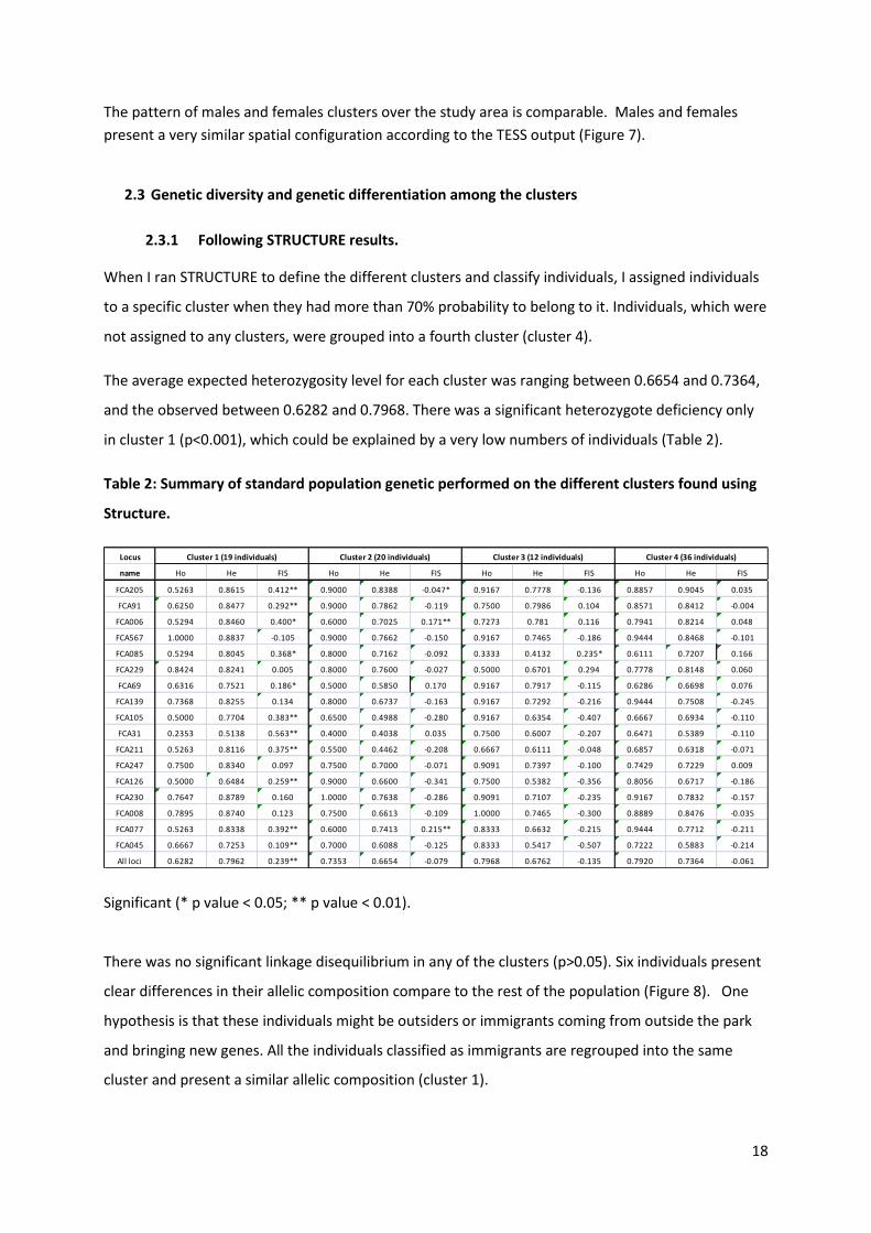
2.3.1 Following STRUCTURE results.

When I ran STRUCTURE to define the different clusters and classify individuals, I assigned individuals

to a specific cluster when they had more than 70% probability to belong to it. Individuals, which were

not assigned to any clusters, were grouped into a fourth cluster (cluster 4).

The average expected heterozygosity level for each cluster was ranging between 0.6654 and 0.7364,

and the observed between 0.6282 and 0.7968. There was a significant heterozygote deficiency only

in cluster 1 (p<0.001), which could be explained by a very low numbers of individuals (Table 2).

Table 2: Summary of standard population genetic performed on the different clusters found using

Structure.

Locus

name Ho He FIS Ho He FIS Ho He FIS Ho He FIS

FCA205 0.5263 0.8615 0.412** 0.9000 0.8388 -0.047* 0.9167 0.7778 -0.136 0.8857 0.9045 0.035

FCA91 0.6250 0.8477 0.292** 0.9000 0.7862 -0.119 0.7500 0.7986 0.104 0.8571 0.8412 -0.004

FCA006 0.5294 0.8460 0.400* 0.6000 0.7025 0.171** 0.7273 0.781 0.116 0.7941 0.8214 0.048

FCA567 1.0000 0.8837 -0.105 0.9000 0.7662 -0.150 0.9167 0.7465 -0.186 0.9444 0.8468 -0.101

FCA085 0.5294 0.8045 0.368* 0.8000 0.7162 -0.092 0.3333 0.4132 0.235* 0.6111 0.7207 0.166

FCA229 0.8424 0.8241 0.005 0.8000 0.7600 -0.027 0.5000 0.6701 0.294 0.7778 0.8148 0.060

FCA69 0.6316 0.7521 0.186* 0.5000 0.5850 0.170 0.9167 0.7917 -0.115 0.6286 0.6698 0.076

FCA139 0.7368 0.8255 0.134 0.8000 0.6737 -0.163 0.9167 0.7292 -0.216 0.9444 0.7508 -0.245

FCA105 0.5000 0.7704 0.383** 0.6500 0.4988 -0.280 0.9167 0.6354 -0.407 0.6667 0.6934 -0.110

FCA31 0.2353 0.5138 0.563** 0.4000 0.4038 0.035 0.7500 0.6007 -0.207 0.6471 0.5389 -0.110

FCA211 0.5263 0.8116 0.375** 0.5500 0.4462 -0.208 0.6667 0.6111 -0.048 0.6857 0.6318 -0.071

FCA247 0.7500 0.8340 0.097 0.7500 0.7000 -0.071 0.9091 0.7397 -0.100 0.7429 0.7229 0.009

FCA126 0.5000 0.6484 0.259** 0.9000 0.6600 -0.341 0.7500 0.5382 -0.356 0.8056 0.6717 -0.186

FCA230 0.7647 0.8789 0.160 1.0000 0.7638 -0.286 0.9091 0.7107 -0.235 0.9167 0.7832 -0.157

FCA008 0.7895 0.8740 0.123 0.7500 0.6613 -0.109 1.0000 0.7465 -0.300 0.8889 0.8476 -0.035

FCA077 0.5263 0.8338 0.392** 0.6000 0.7413 0.215** 0.8333 0.6632 -0.215 0.9444 0.7712 -0.211

FCA045 0.6667 0.7253 0.109** 0.7000 0.6088 -0.125 0.8333 0.5417 -0.507 0.7222 0.5883 -0.214

All loci 0.6282 0.7962 0.239** 0.7353 0.6654 -0.079 0.7968 0.6762 -0.135 0.7920 0.7364 -0.061

Cluster 1 (19 individuals) Cluster 2 (20 individuals) Cluster 3 (12 individuals) Cluster 4 (36 individuals)

Significant (* p value < 0.05; ** p value < 0.01).

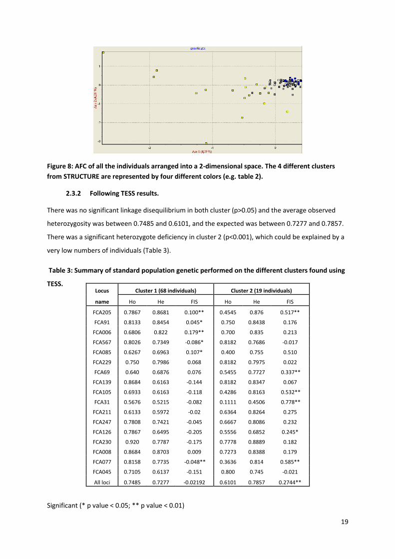
There was no significant linkage disequilibrium in any of the clusters (p>0.05). Six individuals present

clear differences in their allelic composition compare to the rest of the population (Figure 8). One

hypothesis is that these individuals might be outsiders or immigrants coming from outside the park

and bringing new genes. All the individuals classified as immigrants are regrouped into the same

cluster and present a similar allelic composition (cluster 1).

19

Figure 8: AFC of all the individuals arranged into a 2-dimensional space. The 4 different clusters

from STRUCTURE are represented by four different colors (e.g. table 2).

2.3.2 Following TESS results.

There was no significant linkage disequilibrium in both cluster (p>0.05) and the average observed

heterozygosity was between 0.7485 and 0.6101, and the expected was between 0.7277 and 0.7857.

There was a significant heterozygote deficiency in cluster 2 (p<0.001), which could be explained by a

very low numbers of individuals (Table 3).

Table 3: Summary of standard population genetic performed on the different clusters found using

TESS.

Significant (* p value < 0.05; ** p value < 0.01)

Locus Cluster 1 (68 individuals) Cluster 2 (19 individuals)

name Ho He FIS Ho He FIS

FCA205 0.7867 0.8681 0.100** 0.4545 0.876 0.517**

FCA91 0.8133 0.8454 0.045* 0.750 0.8438 0.176

FCA006 0.6806 0.822 0.179** 0.700 0.835 0.213

FCA567 0.8026 0.7349 -0.086* 0.8182 0.7686 -0.017

FCA085 0.6267 0.6963 0.107* 0.400 0.755 0.510

FCA229 0.750 0.7986 0.068 0.8182 0.7975 0.022

FCA69 0.640 0.6876 0.076 0.5455 0.7727 0.337**

FCA139 0.8684 0.6163 -0.144 0.8182 0.8347 0.067

FCA105 0.6933 0.6163 -0.118 0.4286 0.8163 0.532**

FCA31 0.5676 0.5215 -0.082 0.1111 0.4506 0.778**

FCA211 0.6133 0.5972 -0.02 0.6364 0.8264 0.275

FCA247 0.7808 0.7421 -0.045 0.6667 0.8086 0.232

FCA126 0.7867 0.6495 -0.205 0.5556 0.6852 0.245*

FCA230 0.920 0.7787 -0.175 0.7778 0.8889 0.182

FCA008 0.8684 0.8703 0.009 0.7273 0.8388 0.179

FCA077 0.8158 0.7735 -0.048** 0.3636 0.814 0.585**

FCA045 0.7105 0.6137 -0.151 0.800 0.745 -0.021

All loci 0.7485 0.7277 -0.02192 0.6101 0.7857 0.2744**

20

2.4 Relatedness

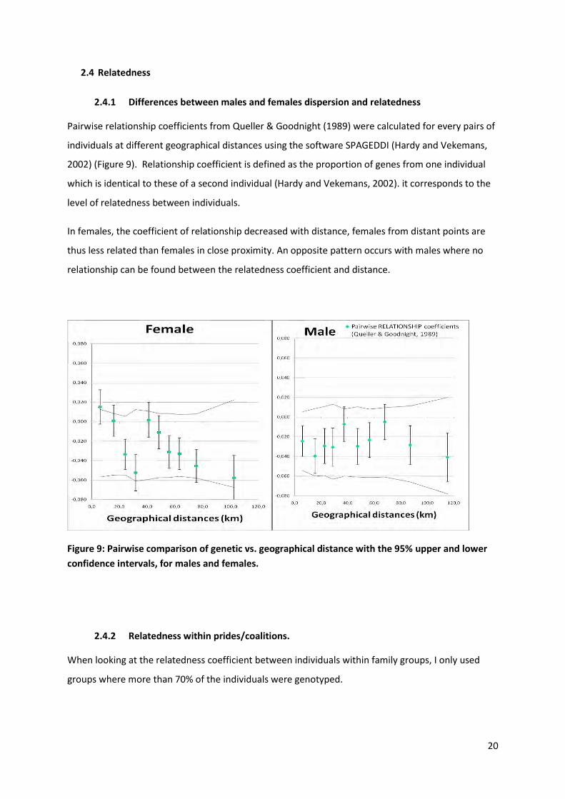
2.4.1 Differences between males and females dispersion and relatedness

Pairwise relationship coefficients from Queller & Goodnight (1989) were calculated for every pairs of

individuals at different geographical distances using the software SPAGEDDI (Hardy and Vekemans,

2002) (Figure 9). Relationship coefficient is defined as the proportion of genes from one individual

which is identical to these of a second individual (Hardy and Vekemans, 2002). it corresponds to the

level of relatedness between individuals.

In females, the coefficient of relationship decreased with distance, females from distant points are

thus less related than females in close proximity. An opposite pattern occurs with males where no

relationship can be found between the relatedness coefficient and distance.

Figure 9: Pairwise comparison of genetic vs. geographical distance with the 95% upper and lower

confidence intervals, for males and females.

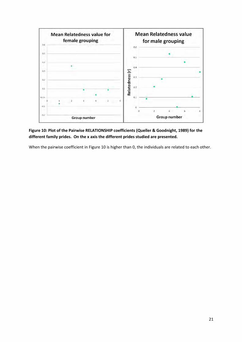
2.4.2 Relatedness within prides/coalitions.

When looking at the relatedness coefficient between individuals within family groups, I only used

groups where more than 70% of the individuals were genotyped.

21

Figure 10: Plot of the Pairwise RELATIONSHIP coefficients (Queller & Goodnight, 1989) for the

different family prides. On the x axis the different prides studied are presented.

When the pairwise coefficient in Figure 10 is higher than 0, the individuals are related to each other.

22

Discussion

In the past, traditional population genetics studies were limited in their ability to detect spatial

patterns; however landscape genetics now provide new horizons to test the influence of environment

features on genetic discontinuities, gene flow, and genetic population structure (Manel et al., 2003).

Population structure

To look for genetic structure of this wild African lion population I employed three different softwares,

to identify genetic clusters and the position of eventual genetic barriers, using the Bayesian methods

implemented in the softwares STRUCTURE (Pritchard et al., 2000), TESS (François et al., 2006) and

GENELAND (Guillot et al., 2005). Bayesian clustering algorithms are new tools developed to bring new

insights into the area of population genetic and molecular ecology (Beaumont and Rannala, 2004). As

such, they employ individual genetic information and/or spatial information to discern population

structure without assuming predefined populations. Chen et al. (2007) recommended combining

results from STRUCTURE and TESS to address inference of spatial population structure. It has also

been demonstrated that GENELAND was able to detect weak spatial genetic structure and is

therefore, highly efficient for detecting newly founded populations. Newly founded populations are

often established from a small number of individuals and therefore, are likely to be away from gene-

flow equilibrium (Coulon et al., 2006).

I obtained slightly different results regarding the population structure and more precisely regarding

the number of clusters when using the different softwares. The results generated by STRUCTURE and

TESS suggested the presence of three clusters within the population. For STRUCTURE, when K was

higher than 3, the variance was much higher which suggested unreliable data; this may suggest that

the true number of clusters inferred from STRUCTURE may actually be three. GENELAND always

suggested the presence of only two clusters.

Even though TESS suggested three clusters; it seems that I may have obtained stronger evidence for

two clusters. The third cluster is internal to the second one which suggests the presence of a so called

ghost cluster, of within the group clustering. Thus, I only used two clusters for further population

analysis using the TESS outputs, and merged the clusters 2 and 3.

The number of clusters obtained differs between 2 and 3 depending on the Bayesian methods used,

therefore based on these differences; it is complicated and contradictory to give a definitive and exact

number of clusters. Different results suggested either a weak genetic structure of the population or

the existence of severe limitations of Bayesian methods on my data set.

23

However some facts, listing below, support the presence of two clusters instead of three:

As suggested by Guillot et al (2005) and Coulon et al. (2006), when using GENELAND, 100

runs were achieved and ranking was made to only use the 10 best runs. This method

contributes to attain high level of consistency among the best runs.

The STRUCTURE output arranged individuals as being part of one of these three clusters,

however many individuals could not be classified as part of any clusters in particular, but

instead being a mix of clusters suggesting a weak population structure when using three

clusters.

The border between inferred populations using TESS coincides with field observations. This

border separate individuals from the western part of the park with the rest. There are strong

observational evidences that individuals coming from the northern part of the park were

occasionally mixing with southern individuals. However, there are few records that

individuals from the western part of the park dispersed and successfully established a

territory into the eastern and southern part of the park. Thus gene flow is somehow limited

between these two areas.

It has been demonstrated through observational and molecular data that only around 20% of

females’ lions disperse away from their natal pride (Spong and Creel, 2001). Female lions are

phylopatric, therefore their social behaviour is affecting the population structure. As a result, most of

the population structure of lion populations can be attributed to male dispersal. Because they

disperse, sometimes far from their natal range, male lions provide the whole population with new

genes. There was no significant difference in the structure of the population when comparing males

and females. Packer and Pusey (1993) described the dispersal distances as being either forced by an

adult male or to avoid inbreeding in their natal pride. However, they also demonstrated, along with

Spong and Creel (2001), that dispersal distances for males were relatively short. This contradicts the

weak population structure we observed in Hwange national Park. If male lions disperse relatively

short distances, the gene flow over the whole area would be somehow limited, and would contribute

to the formation of very distinct family cluster. However, I detected the presence of only two main

clusters over 40 prides, which illustrates that gene flow, might be more significant than in previous

studies.

Gene flow can be explained by movement of individuals to a new area or by a movement of gametes

over a large area (Slatkin, 1995). Gene flow have positive effects on the genetic structure of the

population, the introduction of new genes can allow the population to adapt to new environmental

conditions, and movement of individuals between groups can prevent them from deviating into

24

different populations (Slatkin, 1995). However, geographical features have been demonstrated to

influence genetic movement between populations in a large number of studies. Examples of such are

mountains limiting dispersion of individuals over a larger scale or rivers being a barrier to dispersal.

Dispersal of mature individuals between populations can sometimes be diminished by landscape

characteristics, and dispersal might be the main determinant of the genetic structure of the

population (Coulon et al., 2006).

Based on the factorial component analysis, there are strong evidences that 6 individuals (three males

and three females) are genetically distinct from the rest of the population. The males were sampled

between 2001 and 2002, whereas the females were sampled between 2007 and 2008. One main

hypothesis would be that these individuals could be considered as immigrants. Looking at

STRUCTURE clusters, all the individuals classified as immigrants are regrouped into the same cluster

(cluster 1) which could be explained by the arrival of new genes from a single or multiple individuals.

Dispersal of male lions occurs when they reach maturity, usually when the dominant male on this

territory chased them away (Pusey and Packer, 1987). Nonetheless, Packer and Pusey (1993)

determined that 69% of males which did enter the area during their study were coming from

elsewhere.

Regarding the location of Hwange National Park and the population structure uncovered with TESS

and GENELAND, I can assume that outsider males could arrive from Botswana which is located on the

western side of Hwange National Park. HNP does not have any barriers to prevent animals from going

inside or outside the park. Using telemetry data, it has been attested that at least one sub-adult male,

coming from inside HNP, during its dispersal period went twice into Botswana (personal observation).

Dispersal of males from Botswana could have entered HNP and established a new territory, bringing

new genes into the population.

Genetic diversity

My study reveals that level of genetic diversity in this Zimbabwean lion population is similar to the

level accessed in the Selous Game Reserve by Spong et al. (2002). The levels of genetic diversity are

not completely comparable between the two populations because, we did not employ exactly the

same primers pairs. However, four loci were used in common in both studies and the levels of genetic

diversity (number of alleles and Fis) were highly similar at those loci.

The overall level of expected heterozygosity 0.75 was slightly, but not significantly, higher than the

25

observed level 0.73 when looking at 17 loci, and suggested that despite a low density within HNP, this

lion population do not suffer from a loss of genetic diversity. I did not find a significant Fis (deviation

from Hardy Weinberg expectations) in the overall sample, highlighting the low level of inbreeding

over the whole population.

We found evidence for at least two genetic clusters. When looking at these two genetic cluster

regarding the TESS output, one of the cluster show a Fis significantly different from zero (0.2744). Such

a high value of Fis might be mostly due to the very low number of individuals’ presents in this sampled

group (only 19). Also, I suspect that at least one immigrant established a territory, bringing a new set

of genes in the pool. Regarding to this hypothesis, individuals belonging to this cluster might all be

descendants from a single outsider, and therefore the level of relatedness within that cluster would

be significant, showing a deviation from Hardy-Weinberg equilibrium.

A similar situation appears when looking at more than two clusters as suggested by the STRUCTURE

output. Only one of the clusters had a significant Fis, the one which comprise the supposed

immigrants. In this cluster, individuals are genetically all very different from the rest of the

population.

Relatedness estimates

Our results confirm expectations derived from previous study (Spong and Packer YEAR), and theory

about sex biased dispersal in mammals (Pusey, 1987). However, I found also some differences with

previous findings about relatedness within prides.

In females, the coefficient of relationship decreased with distance, females from distant points are

thus less related than females in close proximity. This might indicate that females stay closer to their

natal territory. A different pattern occur with males where no relationship can be found between the

relatedness coefficient and distance suggesting that males might travel longer distances from their

natal territory. This sex biased dispersal was highly expected as it has been demonstrated by Spong

and Creel (2001) and Packer and Pusey (1993). According to my data, females within 20 Km radians

were correlated to each others, which would suggest that females’ dispersion would be highly

limited. Lions prides exhibit a relatively complex social behaviour, within a pride cooperative hunting

(Schaller, 1972), group territorial defence (Mccomb et al, 1994) and rearing offspring (Pusey and

Packer, 1987).

However, there was no clear pattern between distance and male relatedness. Male lions are

presumed to disperse to avoid inbreeding (Packer and Pusey, 1987); but I could not detect any

isolation by distance pattern. Two previous studies have looked into relatedness between and within

social groups in African lions, resulting in different outcomes. Packer et al. (1991) described the social

26

structure and group composition of lions in the Serengeti National Park, using field observations and

minisatellite band sharing techniques. The Serengeti study covered 2000 km2, with a lion density of

around 13.6 lions per 100 km2 (Packer et al., 1991). They found that coalitions with less than four

individuals were usually unrelated whereas coalitions of four or more were usually composed of first

degree related individuals and that prides were composed of related females. More recently, Spong

et al. (2001) examined the genetic structures of a lion population in the Selous game reserve

(Tanzania), using microsatellite analyses, and sampled 70 individuals in 14 different groups. Selous is

the largest game reserve in Africa and lion density is fairly similar to that of the Serengeti study, with

8 to 13 individuals per 100 km2. Spong and Creel detected greater genetic diversity within coalitions,

and found some unrelated prides members. They discussed that differences between the studies

could be due to a range of different factors (sport hunting on males and different environmental

conditions than in previous lion studies) (Spong and Creel, 2001).

I looked at relatedness within prides and coalition when genetic data was available for at least 75% of

the individuals present at the same time in the pride or coalition. The results were surprising and

differ greatly from these two previous studies. Only one of the 6 female prides presented significant

level of relatedness (r= 0.36), whereas 5 out of 7 male coalitions presented significant level of

relatedness (with r comprised between 0.20 and 0.53). Females have previously never been observed

to live in the same pride as unrelated females (Spong et al., 2002) and thus my finding is of great

importance. Unrelated prides will lack of all the advantages of kinship pairing (such as cooperative

hunting and nursing), and therefore could become weaker to intrusions from dispersing individuals,

or new males attacking their offspring.

Female lions are philopatric and would therefore remain in their natal pride, increasing the chances

of unrelated siblings staying together. Every unrelated male in a coalition may reproduce with any

females on their territory. As a consequence, this increases the genetic difference among offspring.

Furthermore, if a new male intrudes a territory, he will also contribute to add new set of genes and

unrelated siblings into female prides.

Six of the males coalitions sampled in my study were formed by two individuals and three of them

was composed of highly related individuals (from r= 0.35 to 0.53). Using DNA fingerprint techniques,

Packer et al. (1991) demonstrated that groups of males composed of less than three individuals were

usually unrelated. In our study, half of the groups with only two males seem to be highly related, and

one duo present siblings (with r>0.5). Relatedness within coalitions reinforce the assumption that

sub-adults males are more likely to disperse with siblings for protection and strength to obtain a new

territory.

27

Conservation implications

It is important for conservation biologists to fully understand the structure of the populations and to

identify units for the population management (Coulon et al., 2006). Another important feature of

populations is their dispersal rate. This rate diverges according to the environment and the habitat

types, and as a result landscape features can have a conclusive control on the degree of genetic

divergence between populations (VanDongen et al., 1998). Identifying the barriers and the direction

of gene flow across the landscape provide researchers with valuable knowledge on features

influencing movement. As suggested by Coulon et al. (2006) such movements are often hard to

identify using basic ecological studies such as telemetry and capture-recapture studies. However,

gene flow can also be measured indirectly by measuring dispersal distances using radio-tracking

(Koenig et al., 1996).

Low lion density can highly impact the population structure within the park. There is no evidence

looking at the molecular data that this lion population has experienced any high level of inbreeding

which could lead to disastrous consequences. However, Packer et al (1991) demonstrated that in the

Serengeti Park, males avoid to reside in a territory if there is a large number of a mature daughter. In

that case, males would disperse to avoid inbreeding. Despite of this, with a low density of lions in

HNP, the opportunity for males to disperse to a territory with unrelated individual becomes highly

limited. Male territories in HNP are large and can contain several female prides (Personal

observations). Males will reproduce with any females present on their territories. As a result, sub

adults males will have to disperse longer distances to avoid inbreeding. Both Spong et al. (2002) in the

Selous game reserve, and Packer and Pusey in the Serengeti, have demonstrated short dispersal

distances for male sub-adults. Long dispersal distances can cause severe damages to the population

and involves higher risk of mortality, late reproduction, and high energy consumption (Perrin and

Mazalov, 1999). Although, lion territories have greatly expanded in HNP, which became highly

saturated, leaving very few opportunities for young male to disperse and establish a new territory.

Field data have also highlighted a high number of young siblings dispersing together and offspring

bounding with their father, this may all be due to the lack of territories available.

More knowledge about lion dispersal is necessary in order to promote long-term conservation and

management plans. For instance, specific data about speed and distance, along with data about

dispersal behaviour when encountering physical barriers (such as mountains or rivers) (Eizirik et al,

2001) will help in this endeavour.

28

Acknowledgements

I would firstly like to thank my supervisor Jacob Höglund for his support, his understanding and for

always having your door open to answers my questions. Thanks to have believed in this project since

the day I introduced it to you and to have given me the chance to make this project works despites

the obstacles.

I would also like to thank the Lion Research Team to have shared with me their amazing knowledge

about lions and their enthusiasm for Zimbabwean wildlife in general. Great thanks also to Hwange

National Park staffs for their help on the field and with the daily life in Hwange.

Big thanks to everybody at the Population Biology department, particularly to Gunilla for answering

countless questions in the lab and Vendela for showing me around in the first place. Thanks to Peter

for helping me scoring alleles and many other things; Magnus, Massa, Candice, Lynn, Biao and

Mohanad for their daily good mood.

Outside of the lab I would like to thank Kristina, Jenna, Lubov, Maike and Marius to have been such

good friends since the first day I started this master.

A special and extra thank to Gernot for helping me and showing me all the different softwares and

making “nasty” comments on the many versions of this thesis.

Last, but most important, huge thanks to my family for believing in me, letting me go away for so

long to achieve my dreams and to make me feel at home every time I come back to Toulouse. Merci

maman, Yank, Auré et Cels.

29

Literature

Arrendal J. 2007. Conservation Genetics of the Eurasian Otter in Sweden. [Ph.D. thesis]: Uppsala university, 60p. Bauer H, Van Der Merwe S. 2004. Inventory of free-ranging lions Panthera leo in Africa. Oryx 38: 26-31 Beaumont MA, Rannala B. 2004. The Bayesian revolution in genetics. Nature Reviews. Genetics

5:251–261

Belkhir K, Borsa P, Chikhi L, Raufaste N, Bonhomme F. 2001. Genetix 4.02, logiciel sous Windows TM

pour la génétique des population . Laboratoire Génome, Populations, Interactions: CNRS UMR 5000,

Université de Montpellier II, Montpellier, France.

Bowcock AM, Ruiz-Linares A, Tomfohrde J, Minch E, Kidd JR, Cavalli-Sforza LL. High resolution of

human evolutionary trees with polymorphic microsatellites. Nature 368: 455–457.

Chen C, Durand E, Forbes F, François O. 2007. Bayesian Clustering Algorithms Ascertaining Spatial

Population Structure: A New Computer Program and a Comparison Study. Molecular Ecology Notes

7: 747–756.

Coulon A, Guillot G, Cosson J et al. 2006. Genetic structure is influenced by lansdcape features.

Empirical evidence from a roe deer population. Molecular Ecology 15: 1669–1679.

Eizirik E, Kim JH, Menotti-Raymond M, Crawshaw PGJr, O’Brien SJ, Johnson WE. 2001.

Phylogeography, population history and conservation genetics of jaguar (Panthera onca, Mammalia,

Felidae). Molecular Ecology 10:65-79.

Evanno G, Regnaut S, Goudet J. 2005. Detecting the number of clusters of individuals using the

software STRUCTURE: a simulation study. Molecular Ecology 14: 2611–2620

François O, Ancelet S, Guillot G. 2006. Bayesian Clustering Using Hidden Markov Random Fields in

Spatial Population Genetics. Genetics 174, 805–816.

Gauffre B, Estoup A, Bretagnolle V, Cosson JF. 2008. Spatial genetic structure of a small rodent in a

heterogeneous. Molecular ecology 17: 4619-4629.

Guillot G, Estoup A, Mortier F, Cosson J. 2005. A spatial statistical model for landscape genetics.

Genetics 170:1261-1280.

Goudet J, Perrin N, Wasser P. 2002. Tests for sex-biased dispersal using bi-parentally inherited

genetic markers. Molecular Ecology 11: 1103–1114.

30

Hardy OJ, Vekemans X. 2002. SPAGeDi : a versatile computer program to analyse spatial genetic

structure at the individual or population levels. Molecular Ecology Notes 2: 618-620.

Höglund J. 2009. Evolutionary Conservation Genetics. Oxford University Press.

Koenig W D,VanVuren D, Hooge PN. 1996 Detectability, philopatry, and the distribution of dispersal

distances in vertebrates. Trends Ecol. Evol 11: 514-517.

Loveridge AJ, Searle AW, Murindagomo F, Macdonald DW. 2007. The impact of sport-hunting on the

lion population in a protected area. Biological Conservation 134:548–558.

Manel S, Schwartz MK, Luikart G, Taberlet P. 2003. Landscape genetics: combining landscape

ecology and population genetics. Trends Ecol. Evol 18: 189–197.

McComb K, Packer C, Pusey AE. 1994. Roaring and numerical assessment in contests between groups

of female lions, Panthera leo. Animal Behavior 47:379–387

Morin PA, Moore J.J, Chakraborty r. 1994. Kin selection, social structure, gene flow, and the evolution of chimpanzees. Science 265:1193-1201. O’Brien S.J. 1994. A role for molecular genetics in biological conservation. Proc. Natl. Acad. Sci. 91:5748-5755. Packer C, Scheel D, Pusey AE. 1990. Why Lions Form Groups: Food is Not Enough. The American

Naturalist 1:11-19.

Packer C, Gilbert DA, Pusey AE, O’Brien SJ. 1991. A molecular genetic analysis of kinship and cooperation in African lions. Nature 351:562-565. Packer C, Pusey AE. 1987. The evolution of sex-biased dispersal in lions. Behaviour 101:275-310. Packer C, Pusey AE. 1993. Dispersal, kinship and inbreeding in African lions. N.W. Thornhill editor, 375-391. The natural history of inbreeding and outbreeding: theoretical and empirical perspectives. University of Chicago Press, Chicago, Illinois. Perrin, N. and V. Mazalov. 2000. Local competition, inbreeding, and the evolution of sex-biased dispersal. American Naturalist, 155:116–127. Pusey AE. 1987. Sex-biased dispersal and inbreeding avoidance in birds and mammals, Trends Ecol. Evo. 2: 295–299.

Pusey AE, Packer C. 1987. The evolution of sex-biased dispersal in lions. Behaviour 101:275-310.

Pusey AE, Packer C. 1994. Infanticide in lions: consequences and counterstrategies. In: Infanticide

and parental care (Parmigiani S, vom Saal F, eds). London: Harwood Academic Publishers 277- 299.

Pritchard JK, Wen W. 2003. Documentation for STRUCTURE software: Version 2. Available from

http://www.pritch.bsd. uchicago.edu

31

Pritchard J, Stephens M, Donnelly P. 2000. Inference of population structure using multilocus

genotype data. Genetics 155: 945–959.

Queller DC, Goodnight KF. 1989. Estimating relatedness using genetic markers. Evolution 43: 258–

275.

Queller DC, Strassmann JE, Hughes CR. 1993. Microsatellites band kinship. Trends in Ecology and

Evolution 8: 285–288.

Raymond M, Rousset F. 1995. GENEPOP Version 1.2: Population genetics software for exat tests and

ecumenicism. Heredity 248–249

Rogers CML. 1993. A woody vegetation survey of Hwange National Park. Dept of National Parks and

Wildlife Management, Zimabwe.

Ross KG. 2001. Molecular ecology of social behaviour: analyses of breeding systems and genetic structure. Molecular Ecology 10:265–284.

Rousset F. 1997. Genetic differentiation and estimation of gene flow from Fstatistics under isolation

by distance. Genetics 145: 1219–1228.

Rudnai J. 2008. Reproductive biology of lions (Panthera leo massaica Neumann) in Nairobi National

Park. African Journal of Ecology 11:241-253.

Saccheri I, Kuussaari M, Kankare M, Vikman P. Fortelius W, Hanski I. 1998. Inbreeding and extinction in a butterfly metapopulation. Nature 392:491-494.

Sahlsten J, Thörngren H, Höglund J. 2008. Inference of hazel grouse population structure using

multilocus data: a landscape genetic approach. Heredity 1-8.

Scheel D. 1993. Profitability, encounter rates, and prey choice of African lions. Behavioral Ecology

4:90–97.

Schlötterer C. 2000. Evolutionary dynamics of microsatellite DNA. Chromosoma 109:365-371.

Shaller GB. 1972. The Serengeti lion. University of Chicago Press, Chicago. Slatkin MA. 1985. Gene flow in natural populations. Ann. Rev. Eco 16:393-430.

Slatkin MA. 1995. A measure of population subdivision based on microsatellite allele frequencies.

Genetics 139: 457–462.

Spong G, Creel S. 2001. Deriving dispersal distances from genetic data. Proceedings of the Royal

Society of London Series Biology Sciences 268: 2571–2574.

32

Spong G, Stone J, Creel S, Björklund M. 2001. Genetic structure of lions (Panthera leo L.) in the Selous Game Reserve: implications for the evolution of sociality. Evolutionary biology 15: 945-953. Spong G, Creel S, Stone J, Björklund M. 2002. Genetic structure of lions (Panthera leo L.) in the Selous Game Reserve: implications for the evolution of sociality. J Evol Biol 15:945–953.

Storfer A, Murphy MA, Evans JS, Goldberg CS, Robinson S, et al. 2007. Putting the ‘landscape’ in

landscape genetics. Heredity 98: 128–42.

Storz JF. 1999. Genetic consequences of mammalian social structure. Journal of mammology 80:553-569. Sugg DW, Chesser RK, Dobson FS, Hoogland JL. 1996. Population genetics meets behavioral ecology. Trends Ecol Evol 11:338–342. Van Dongen S, Backeljau T, Matthysen E, Dhondt AA. 1998. Genetic population structure of the winter moth (Operophtera brumata L.) (Lepidoptera, Geometridae) in a fragmented landscape. Heredity 80:92-100. Van Orsdol KG, Hanby JP, Bygott JD. 1985. Ecological correlates of lion social organization (Panthera leo). Journal of Zoology London 206: 97–112. Waser PM. 1996. Patterns and consequences of dispersal in gregarious carnivores. Conservation

behavior, ecology and evolution. (Ed. By J.L. Gittleman), pp. 267-295. Cornell University Press,

London.

Weir BS, Cockerham CC. 1984. Estimating F-statistics for the analysis of population structure.

Evolution 38: 1358–1370.

Wright S. 1965. The interpretation of population structure by F-statistics with special regard to

systems of mating. Evolution 19: 358-420.