Embed Size (px)
Citation preview

THE JOURNAL OF CHEMICAL PHYSICS 134, 184505 (2011)
Liquid-solid transition in fully ionized hydrogen at ultra-high pressuresElisa Liberatore,1,a) Carlo Pierleoni,2,b) and D. M. Ceperley3,c)
1Department of Physics, University of Rome “La Sapienza,” P.le A. Moro 2, 00185, Rome Italy2CNISM and Department of Physics, University of L’Aquila, Via Vetoio 10, I-67010 L’Aquila, Italy3Department of Physics, National Center of Supercomputer Applications, University of Illinois atUrbana-Champaign, Illinois 61801, USA
(Received 21 December 2010; accepted 12 April 2011; published online 11 May 2011)
We study the phase diagram of an effective ion model of fully ionized hydrogen at ultra-high pressure.We assume that the protons interact with a screened Coulomb potential derived from a static linearresponse theory. This model accurately reproduces the physical properties of hydrogen for densitiesgreater than ρm = 10 g/cm3 corresponding to the range of the coupling parameter rs � 0.6. Thepressure range, P � 20T Pa, is well beyond present experimental limitations. Assuming classicalprotons, we find that the zero temperature enthalpy of the perfect bcc crystal is slightly lower thanfor other structures at ρm = 12.47 g/cm3 while the fcc structure gains stability at higher density.Using Monte Carlo calculations, we compute the free energy of various phases and locate the meltingtransition versus density. We find that on melting, bcc is energetically favored with respect to fcc overthe entire range investigated. In the solid phase the system undergoes a structural transition from bccat higher temperature to fcc at lower temperature. The free energy difference between these twostructures is very small so that obtaining a quantitative estimate of this second transition line requiresaccuracy beyond that provided by our method. We estimate the effect of proton zero point motionon the bcc melting line for hydrogen, deuterium, and tritium by a path integral Monte Carlo method.Although zero point effects on hydrogen are large, since the two competing phases (bcc and liquid)have locally similar environments, the effect on the melting line is small; the melting temperature forhydrogen is lowered by about 10% with respect to the classical value. © 2011 American Institute ofPhysics. [doi:10.1063/1.3586808]
I. INTRODUCTION
Because hydrogen is the simplest and most abundant el-ement in the universe, its physical properties are of greatinterest both because of its place in the periodic table andfor its relevance to planetary physics and inertial fusionapplications.1–7 At low pressures and temperatures, hydro-gen behaves as a halogen, forming an insulating phase ofdiatomic molecules. Upon increasing pressure, well beyondthe metallization pressure of 0.25 GPa predicted in 1935,6 arich phase diagram has been observed with three differentinsulating molecular phases2, 10 and a metallic liquid phaseat higher temperature.7 Our current knowledge of the hy-drogen phase diagram, based on limited experimental dataand on theoretical predictions, e.g., ab initio simulations,is that at low temperature, below 500–800 K, solid hydro-gen remains insulating and in the molecular phase up to≈ 400 GPa.8 This pressure is slightly above the present limi-tation of modern experimental high-pressure static compres-sion techniques.9 Upon increasing temperature, the freelyrotating molecular hcp crystal melts to an insulating molec-ular liquid. The melting temperature increases with pres-sure up to P � 100 GPa to a value of T � 800 K and then
a)Electronic mail: [email protected])Electronic mail: [email protected])Electronic mail: [email protected].
apparently decreases. At temperatures above the meltingline, a liquid-liquid phase transition is predicted to oc-cur between an insulating, mostly, molecular liquid and aconducting, mostly, atomic liquid.11–20 There has been along-standing debate whether this process occurs in a contin-uous or through a first order transition. Indeed, the first Car-Parrinello simulations11, 12 as well as calculations based onsemi-empirical models15–19 showed the evidence of a discon-tinuous liquid-liquid transition, at variance with early Born-Oppenheimer molecular dynamics (BOMD) simulations andquantum Monte Carlo (QMC) investigations21 that found thisprocess continuous. There is recent experimental evidence ofa sharp conductivity rise.22 Moreover, the most recent and ac-curate ab initio QMC (Ref.20) and BOMD (Refs. 13 and 20)calculations agree with the presence of a first order liquid-liquid transition. The QMC investigation by Morales et al.20
predicts that the liquid-liquid transition terminates in a crit-ical point at T � 2000 K, above which the metallization andthe molecular dissociation with pressure occur in a continuousfashion. In the (P,T) plane, both the melting line and the metal-lization line have negative slopes and are predicted to meet atT � 550 K and P � 290 GPa.20 Qualitatively similar resultsare obtained by ab initio molecular dynamics simulations20
which locate the intersection of the melting line with the met-allization line at lower T � 700 K and P � 220 GPa. A pre-vious estimate of such intersection point by Car-Parrinellomolecular dynamics was reported to be T � 400 K and P� 300 GPa.12
0021-9606/2011/134(18)/184505/11/$30.00 © 2011 American Institute of Physics134, 184505-1
Author complimentary copy. Redistribution subject to AIP license or copyright, see http://jcp.aip.org/jcp/copyright.jsp

184505-2 Liberatore, Pierleoni, and Ceperley J. Chem. Phys. 134, 184505 (2011)
At higher pressure, well beyond metallization and dis-sociation, hydrogen will be a metal of protons and delo-calized electrons. Knowledge of the melting temperature ofthe atomic crystal is needed to understand the high pressurephase diagram. However, the stable crystal structures as afunction of pressure and temperature are not known. Groundstate quantum Monte Carlo investigations23–25 have estimatedthe transition from molecular to atomic crystal at rs = 1.31(P = 300 GPa)23 and predicted a diamond structure to be themost stable at this density. Ab initio molecular dynamics withclassical protons26 have found that at high density (rs ≤ 0.6)and low temperature close packed structures such as fcc andhcp are dynamically stable while bcc to be dynamically sta-ble at lower density (0.6 ≤ rs ≤ 1.2). Moreover, the bcc phasewas found to be the most stable phase at higher tempera-ture and hence the phase that melts into the liquid. The melt-ing temperature, estimated by Lindemann ratio criterium, wasfound to be Tm = 2200 K at rs = 0.5 and Tm = 350 K at rs
= 1. In addition, it was suggested that linear response theoryshould be quantitatively correct for rs � 0.5, since it providesan accurate prediction for the electronic density around aproton.
A very recent calculation used27 random structure search-ing to find the optimal zero temperature structure withinthe assumed DFT energy functional. Several novel structureswere found at intermediate densities. For example, I41/amdwas found to be stable for rs > 1.0 and the R − 3m structureat higher density. For rs < 0.92 fcc was found to be the moststable structure. Estimates were made for the contribution ofphonons and finite temperature, indicating that although zeropoint effects can shift the transition densities, these structures,or closely related ones, should remain stable. Since the densi-ties considered in this work are even higher, we only considersimple structures in this work.
The intermediate pressure region between the low pres-sure molecular phase and the high pressure, fully ionizedphase, should present very interesting physics: molecular dis-sociation and metallization in the crystal phase, competitionbetween crystal and liquid phases, and possible exotic liquidphases.28 This region is still largely unknown since it is par-ticularly challenging for both ab initio simulation techniquesand experiment.
In this paper we study the melting of hydrogen at ultra-high density, corresponding to 0.6 ≥ rs ≥ 0.3. In our model,the ion-ion interaction is given by a screened Coulomb repul-sion. We determine the melting line by calculating the freeenergy, both for classical and quantum protons and for theother isotopes of hydrogen. As suggested in Ref. 26, we finda competition between fcc and bcc structures below the melt-ing temperature.
The paper is organized as follows. In Sec. II, we describethe model adopted in our study. Section III is devoted to thedetails of our calculations, in particular to the free energymethod. We find a very small volume jump across the meltingtransition requiring a novel thermodynamic integration proce-dure described in the last part of Sec. III. In Sec. IV we derivethe quantum correction to the free energy of the classical sys-tem and present our results. Finally, in Sec. V, we draw ourconclusions and give some perspectives.
II. THE SCREENED COULOMB PLASMA MODEL
The screened coulomb plasma model has beenintroduced29 as a model for a fully ionized plasma atweak coupling (high density). Its full derivation can be foundin Ref. 30. Here we summarize the main steps and limitourselves to the case of hydrogen. Consider a system of non-relativistic Np protons and Ne = Np electrons in a volumeV. The ionic (electronic) density is n p = ne = n = N/V .Denoting the coordinates of protons by {R1, . . . , RN } and thecoordinates of electrons by {r1, . . . , rN }, the Hamiltonian ofthe system is
H = HOC P + Heg + Vint , (1)
HOC P = Kp + 1
2V
∑k �=0
v(k)[ρ
pk ρ
p−k − N
], (2)
Heg = Ke + 1
2V
∑k �=0
v(k)[ρe
kρe−k − N
], (3)
Vint = − 1
2V
∑k �=0
v(k)[ρ
pk ρe
−k + c.c.], (4)
where k = |k|, v(k) = 4π/k2 is the Fourier transformof the Coulomb potential, ρ
pk = e
∑Ni=1 exp(ik · Ri ), ρe
k
= −e∑N
i=1 exp(ik · ri ) are the Fourier components of thecharge density of protons and electrons, respectively, andKp and Ke are the kinetic energy operators for protons andelectrons, respectively. HOC P is the Hamiltonian of the onecomponent plasma (OCP),31 a system of protons in a rigidbackground of negative neutralizing charge, Heg is the Hamil-tonian of the electron gas (jellium),32, 33 a system of electronsin a rigid background of positive neutralizing charge and Vint
is the interaction term between the two species (c.c. in Eq. (4)indicates complex conjugation). At high density Vint becomesa weak coupling between the two systems.
We reduce the two component system to an effective onecomponent system of pseudo-ions30 by assuming the elec-tronic degrees of freedom are in their instantaneous groundstate for fixed ionic positions. If the coupling term is small,one can use linear response theory to express the electroniccharge density in terms of the instantaneous ionic charge den-sity; it is given by charge susceptibility of the homogeneouselectron gas χ (k)
⟨ρe
k
⟩e= −v(k)χ (k)ρ p
k =(
1
ε(k)− 1
)ρ
pk , (5)
where 〈. . .〉e is the average over the electronic ground stateand ε(k) is the dielectric function of the homogeneous elec-tron gas. Using Eq. (5) in Eq. (1) gives the effective Hamilto-nian for the ions
Heff =HOC P+ 1
2V
∑k �=0
v(k)
(1
ε(k)−1
)[ρ
pk ρ
p−k − N
]+Eeg(n)
= Kp + 1
2V
∑k �=0
v(k)
ε(k)
[ρ
pk ρ
p−k − N
] + Eeg(n)
= Kp + 1
2
∑i, j �=i
veff(|Ri j |; n) + Eeg(n), (6)
Author complimentary copy. Redistribution subject to AIP license or copyright, see http://jcp.aip.org/jcp/copyright.jsp
184505-3 Liquid-solid transition in hydrogen J. Chem. Phys. 134, 184505 (2011)
where Eeg(n) is the ground state energy of the homogeneouselectron gas with electronic density n, and veff(R; n) is theFourier transform of [v(k)/ε(k)]. Note that Heff depends onthe density through both the volume term Eeg(n) and the ef-fective pair potential, veff(R; n).
The energy and dielectric function of the homogeneouselectron gas are well characterized.33 Its ground state en-ergy has been computed by quantum Monte Carlo methods32
and parameterized by several authors. We adopt the form ofPerdew and Zunger,33, 34 which at high density can be writtenas
Eeg(rs)
N� 1.105
r2s
−0.468
rs+ A ln(rs) + B + Crsln(rs) + Drs,
(7)where energy is in atomic units (1 a.u. = 27.2 ev = 315.79× 10³ K) and rs is the electron sphere radius (the radius ofthe sphere containing one electron, in units of the Bohr ra-dius a0) defined as rs = (3/4πn)(1/3). In Eq. (7) the first twoterms are the Hartree-Fock contributions to the energy whilethe remaining terms represent the correlation energy εc(rs).The values of the parameters are33, 34 A = 0.031, B = −0.048,C = 0.002, D = −0.0116. The dielectric function is givenby33
ε−1(k) = 1 + v(k)L(k)
1 − v(k)L(k)(1 − G(k)), (8)
where L(k) is the static Lindhard function, i.e., the suscep-tibility of the ideal Fermi gas. The local field factor G(k)is proportional, through the interaction potential v(k), to theFourier transform of the second functional derivative of thecorrelation energy functional with respect to the density.35
Using quantum Monte Carlo methods, G(k) has been com-puted in a range of density corresponding to 2 ≤ rs ≤ 10 andparameterized.33, 35, 36 Since our system is at higher density,i.e., at lower correlation, we expect that the local density ap-proximation (LDA) form of G(k) be accurate enough for ourpurpose37
G(q) = q2
[1 − π
3
(4
9π
)1/3 (r3
s
d2εc
dr2s
− 2r2s
dεc
drs
)],
(9)where εc is the correlation energy (i.e., the last 4 terms inEq. (7)), q = k/(2kF ) and kF is the Fermi wave vector.
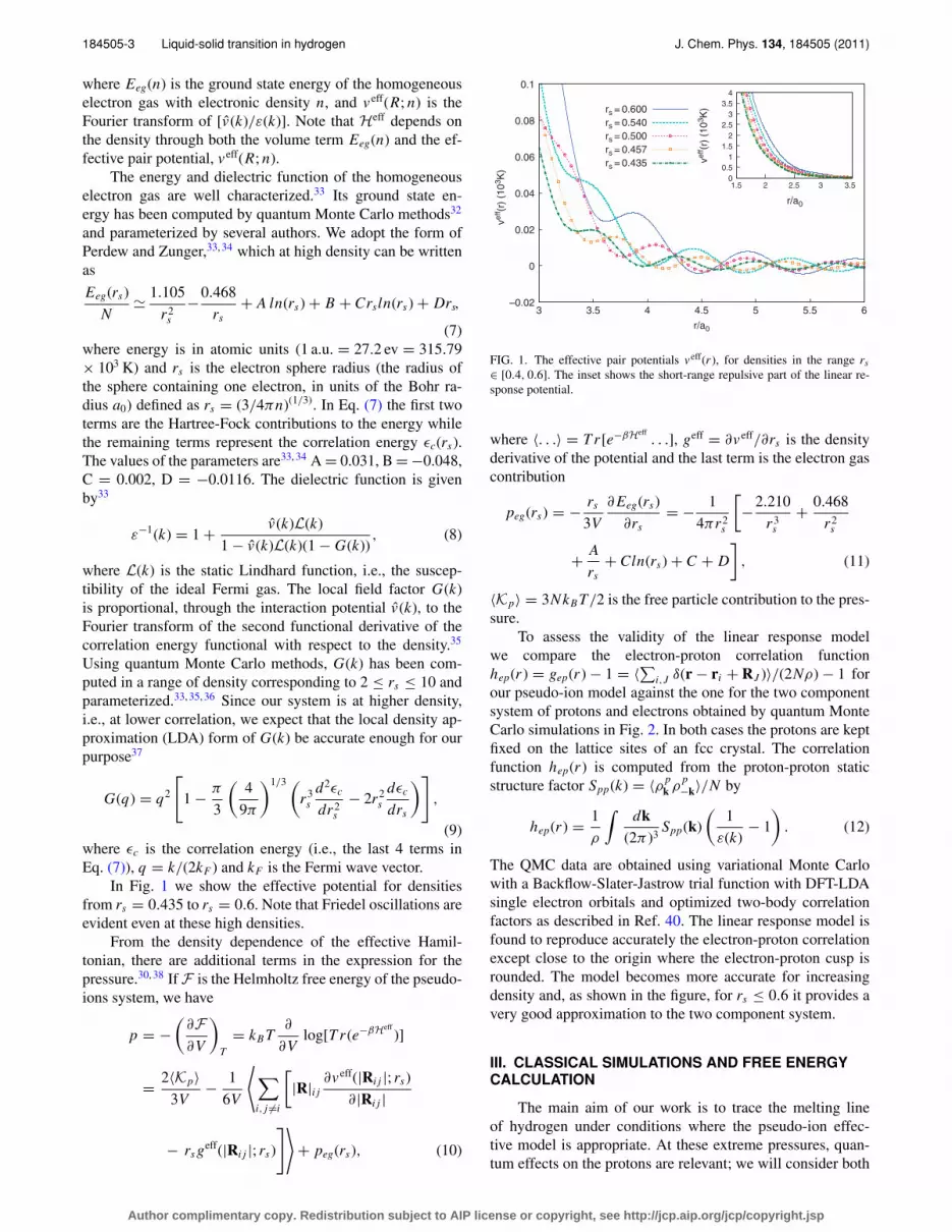
In Fig. 1 we show the effective potential for densitiesfrom rs = 0.435 to rs = 0.6. Note that Friedel oscillations areevident even at these high densities.
From the density dependence of the effective Hamil-tonian, there are additional terms in the expression for thepressure.30, 38 If F is the Helmholtz free energy of the pseudo-ions system, we have
p = −(
∂F∂V
)T
= kB T∂
∂Vlog[T r (e−βHeff
)]
= 2〈Kp〉3V
− 1
6V
⟨∑i, j �=i
[|R|i j
∂veff(|Ri j |; rs)
∂|Ri j |
− rs geff(|Ri j |; rs)
]⟩+ peg(rs), (10)
–0.02
0
0.02
0.04
0.06
0.08
0.1
3 3.5 4 4.5 5 5.5 6
ve
ff(r
) (1
03K
)
veff(r
) (1
03K
)
r/a0
r/a0
rs = 0.600
rs = 0.540
rs = 0.500
rs = 0.457
rs = 0.435
0
0.5
1
1.5
2
2.5
3
3.5
4
1.5 2 2.5 3 3.5
FIG. 1. The effective pair potentials veff(r ), for densities in the range rs
∈ [0.4, 0.6]. The inset shows the short-range repulsive part of the linear re-sponse potential.
where 〈. . .〉 = T r [e−βHeff. . .], geff = ∂veff/∂rs is the density
derivative of the potential and the last term is the electron gascontribution
peg(rs) = − rs
3V
∂ Eeg(rs)
∂rs= − 1
4πr2s
[−2.210
r3s
+ 0.468
r2s
+ A
rs+ Cln(rs) + C + D
], (11)
〈Kp〉 = 3NkB T/2 is the free particle contribution to the pres-sure.
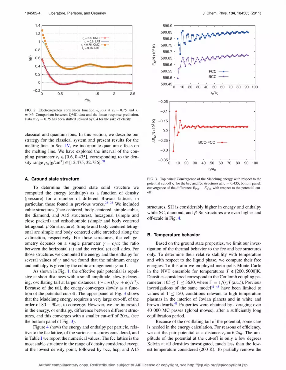
To assess the validity of the linear response modelwe compare the electron-proton correlation functionhep(r ) = gep(r ) − 1 = 〈∑i,J δ(r − ri + RJ )〉/(2Nρ) − 1 forour pseudo-ion model against the one for the two componentsystem of protons and electrons obtained by quantum MonteCarlo simulations in Fig. 2. In both cases the protons are keptfixed on the lattice sites of an fcc crystal. The correlationfunction hep(r ) is computed from the proton-proton staticstructure factor Spp(k) = 〈ρ p
k ρp−k〉/N by
hep(r ) = 1
ρ
∫dk
(2π )3Spp(k)
(1
ε(k)− 1
). (12)
The QMC data are obtained using variational Monte Carlowith a Backflow-Slater-Jastrow trial function with DFT-LDAsingle electron orbitals and optimized two-body correlationfactors as described in Ref. 40. The linear response model isfound to reproduce accurately the electron-proton correlationexcept close to the origin where the electron-proton cusp isrounded. The model becomes more accurate for increasingdensity and, as shown in the figure, for rs ≤ 0.6 it provides avery good approximation to the two component system.
III. CLASSICAL SIMULATIONS AND FREE ENERGYCALCULATION
The main aim of our work is to trace the melting lineof hydrogen under conditions where the pseudo-ion effec-tive model is appropriate. At these extreme pressures, quan-tum effects on the protons are relevant; we will consider both
Author complimentary copy. Redistribution subject to AIP license or copyright, see http://jcp.aip.org/jcp/copyright.jsp
184505-4 Liberatore, Pierleoni, and Ceperley J. Chem. Phys. 134, 184505 (2011)
–0.2
0
0.2
0.4
0.6
0.8
1
1.2
1.4
0 0.5 1 1.5 2 2.5
h(r
)
r/a0
rs = 0.6, QMC r
s = 0.6, LRT
rs = 0.75, QMC
rs = 0.75, LRT
FIG. 2. Electron-proton correlation function hep(r ) at rs = 0.75 and rs
= 0.6. Comparison between QMC data and the linear response prediction.Data at rs = 0.75 has been shifted upward by 0.4 for the sake of clarity.
classical and quantum ions. In this section, we describe ourstrategy for the classical system and present results for themelting line. In Sec. IV, we incorporate quantum effects onthe melting line. We have explored the interval of the cou-pling parameter rs ∈ [0.6, 0.435], corresponding to the den-sity range ρm[g/cm3] ∈ [12.475, 32.736].58
A. Ground state structure
To determine the ground state solid structure wecomputed the energy (enthalpy) as a function of density(pressure) for a number of different Bravais lattices, inparticular, those found in previous works.23–25 We includedcubic structures (face-centered, body-centered, simple cubic,the diamond, and A15 structures), hexagonal (simple andclose packed) and orthorhombic (simple and body centeredtetragonal, β-Sn structure). Simple and body centered tetrag-onal are simple and body centered cubic stretched along thez-direction, respectively. For those structures, the cell ge-ometry depends on a single parameter γ = c/a: the ratiobetween the horizontal (a) and the vertical (c) cell sides. Forthose structures we computed the energy and the enthalpy forseveral values of γ and we found that the minimum energyand enthalpy is given by the cubic arrangement: γ = 1.
As shown in Fig. 1, the effective pair potential is repul-sive at short distances with a small amplitude, slowly decay-ing, oscillating tail at larger distances: (∼ cos(k f r + φ)/r3).Because of the tail, the energy converges slowly as a func-tion of the potential cut-off. The upper panel of Fig. 3 showsthat the Madelung energy requires a very large cut-off, of theorder of 80 − 90a0, to converge. However, we are interestedin the energy, or enthalpy, difference between different struc-tures, and this converges with a smaller cut-off of 20a0. (seethe bottom panel of Fig. 3).
Figure 4 shows the energy and enthalpy per particle, rela-tive to the fcc lattice, of the various structures considered, andin Table I we report the numerical values. The fcc lattice is themost stable structure in the range of density considered exceptat the lowest density point, followed by bcc, hcp, and A15
599.45
599.5
599.55
599.6
599.65
599.7
599.75
599.8
599.85
599.9
0 10 20 30 40 50 60 70 80 90 100
EM
/N (
10
3 K
)ΔE
M/N
(10
3 K
)
rc/a0
0 10 20 30 40 50 60 70 80 90 100
rc/a0
FCC
BCC
–0.35
–0.3
–0.25
–0.2
–0.15
–0.1
–0.05
BCC-FCC
FIG. 3. Top panel: Convergence of the Madelung energy with respect to thepotential cut-off rc for the bcc and fcc structures at rs = 0.435; bottom panel:convergence of the difference Ebcc − E f cc with respect to the potential cut-off.
structures. SH is considerably higher in energy and enthalpywhile SC, diamond, and β-Sn structures are even higher andoff-scale in Fig. 4.
B. Temperature behavior
Based on the ground state properties, we limit our inves-tigation of the thermal behavior to the fcc and bcc structuresonly. To determine their relative stability with temperatureand with respect to the liquid phase, we compute their freeenergies. To this aim we employed metropolis Monte Carloin the NVT ensemble for temperatures T ∈ [200, 5000]K.Densities considered correspond to the Coulomb coupling pa-rameter: 105 ≤ � ≤ 3630, where � = 1/(rs T (a.u.)). Previousinvestigations of the same model41–45 have been limited tovalues of � ≤ 150, conditions relevant to high temperatureplasmas in the interior of Jovian planets and in white andbrown dwarfs.41 Properties were obtained by averaging over40 000 MC passes (global moves), after a sufficiently longequilibration period.
Because of the oscillating tail of the potential, some careis needed in the energy calculation. For reasons of efficiency,we cut the pair potential at a distance rc = 6.2a0. The am-plitude of the potential at the cut-off is only a few degreesKelvin at all densities investigated, much less than the low-est temperature considered (200 K). To partially remove the
Author complimentary copy. Redistribution subject to AIP license or copyright, see http://jcp.aip.org/jcp/copyright.jsp

184505-5 Liquid-solid transition in hydrogen J. Chem. Phys. 134, 184505 (2011)
–0.5
0
0.5
1
1.5
2
2.5
–0.5
0
0.5
1
1.5
2
2.5
10 15 20 25 30 35
EM
/N (
10
3K
)H
/N (
10
3K
)
ρ (g/cm3)
BCC
SH
HCP
A15
FCC
BCC
SH
HCP
A15
FCC
20 40 60 80 100 120 140
P (TPA)
FIG. 4. Madelung energies (upper panel) and zero temperature enthalpies(lower panel) for different perfect lattices. Values are relative to the fcc phase.Data for less favorable structures (as β-Sn or diamond) are off the scale.
effect of the cutoff, we correct the energy by adding the dif-ference between the converged value of the Madelung energyand that with the cut-off. In the liquid phase the standard tailcorrection,47 obtained assuming g(r ) = 1 for r > rc is used.
In order to use this cut-off radius and still work with asmall number of ions in the simulation cell, we sum over in-teractions between particles in the primary simulation box aswell as the 26 nearest images. With this strategy we are ableto use N ∼ 250 ions as compared with several thousands ofions if the box size were to be fixed at L = 2rc. This pro-cedure limits the maximum density that can be investigated
0
0.5
1
1.5
2
2.5
0.5 1 1.5 2 2.5
g(r
)
r/a0
N = 250N = 5324
0
0.5
1
1.5
2
2.5
3
0 5 10 15 20
S(k
)
ka0
N = 250N = 5324
FIG. 5. Comparison between structural properties of small (256) and large(5324) systems: radial distribution function g(r ) (left) and structure factorS(k) (right) at T = 4000 K and rs = 0.445.
to ρ � 40gr/cm3 which corresponds to rs � 0.41. For higherdensities (and lower rs) we would need to use larger systemsor sum over more neighboring boxes or to switch to the Ewaldmethod. However, the use of the standard Ewald breakup forthe linear response potential turns out not to be effective. Weare presently investigating a different breakup, which will beemployed in future studies. To check the effect of the artificialperiodicity imposed by the nearest box images summation, wecompare in Table II and Fig. 5, thermodynamic and structuralproperties computed with 256 particles in the liquid phase atT = 4000 K and different densities with those for a larger sys-tem (N = 5324) with box size � 2rc. We found a very goodagreement for the radial distribution function, the structurefactor, and the energies, but a small difference (≈ 0.1%) inthe pressure at higher densities. However, as explained in thefollowing, the estimation of the transitions is based on the in-ternal energy and not on the pressure.
C. Free energy calculations
A precise location of the melting line can be obtainedfrom the Helmholtz free energy using the common-tangentconstruction:46 it consists in plotting the isothermal free en-ergy of the two competing phases as a function of the spe-cific volume and finding pairs of points belonging to the
TABLE I. Converged Madelung energies for several crystalline structures as a function of density.
ρm (g/cm3) bcc fcc SC A15 DIAM hcp SH
12.4753 258.813 258.961 263.856 259.707 276.966 259.143 260.77014.7049 303.489 303.364 307.130 303.919 322.686 303.649 305.66217.1130 343.393 343.274 349.423 344.064 364.410 343.995 345.91519.1645 381.034 380.319 387.246 381.576 403.618 381.019 384.27121.5574 423.440 422.495 427.607 423.421 447.825 423.623 426.83023.7668 455.850 455.917 463.008 456.628 481.713 456.471 459.89025.9999 496.124 495.991 503.589 496.813 522.661 496.378 500.25928.2330 530.119 529.977 536.258 530.720 557.527 530.513 533.66530.5792 566.214 566.138 573.469 567.185 594.810 566.590 570.06132.7369 599.669 599.848 608.699 600.416 628.853 600.248 604.070
Author complimentary copy. Redistribution subject to AIP license or copyright, see http://jcp.aip.org/jcp/copyright.jsp

184505-6 Liberatore, Pierleoni, and Ceperley J. Chem. Phys. 134, 184505 (2011)
TABLE II. Comparison of energies per particle and pressures between a small system size (N = 256) summingover nearest box images, versus a large system size (N = 5324) with the minimum image convention. Calcula-tions were for a liquid state at T = 4000 K and at various densities.
rs ρm (g/cm3) E256(103K) E5324(103K) P256V (103K) P5324V (103K)
0.600 12.5 268.22(1) 268.237(2) 60.217(3) 60.210(1)0.540 17.0 352.73(1) 352.730(2) 76.616(2) 76.614(1)0.500 21.5 429.64(1) 429.647(2) 90.576(2) 90.6587(9)0.484 23.7 466.40(1) 466.408(3) 98.969(2) 98.972(2)0.468 26.3 503.42(1) 503.425(4) 107.225(2) 107.232(1)0.457 28.2 539.02(2) 539.110(5) 112.818(1) 112.830(1)0.445 30.5 575.84(2) 575.845(5) 118.392(3) 118.501(1)0.435 32.7 609.09(1) 609.096(3) 126.032(2) 126.128(3)
different curves but lying on a common tangent. The abscissaof those points represents the specific volume of each phase atcoexistence, while the slope of the tangent is the coexistencepressure. This procedure relies on hysteresis; in a simulationwith a finite number of particles and a finite number of MonteCarlo steps, one can work in a metastable phase, since near afirst order phase transition, there is a barrier for conversion ofthe MC random walk from a liquid configuration to a crystalconfiguration or vice versa.
Alternatively, the location of the transition can be ob-tained from the crossing point of the isothermal Gibbs freeenergy curves of the competing phases plotted against pres-sure. These curves can be obtained from the behavior of theHelmholtz free energy and the pressure as a function of vol-ume. The dependence of the Gibbs free energy on pressuremust be inferred by inverting the equation of state, a proce-dure which can introduce systematic errors, so that we pre-ferred to use the Helmholtz free energy with the common tan-gent construction.
For each phase, the Helmholtz free energy can be ob-tained by thermodynamic integration47 from a reference state,e.g., a coupling constant integration: one introduces a ficti-tious Hamiltonian dependent on a parameter λ ∈ [0, 1] whichcouples the original system to a reference system of known(or easy-to-compute) free energy. If Hλ = H1λ + H0(1 − λ),where H1 is the Hamiltonian of the reference system and H0
the Hamiltonian of the original system, we have
F(0) = F(1) +∫ 1
0dλ〈H0 − H1〉λ, (13)
where 〈. . .〉λ indicates an average with respect to e−βHλ . In thesolid phase, a suitable reference system is an Einstein crystalof the same structure, in which each particle is attached to alattice site with a spring (Frenkel-Ladd technique).47, 48 Forthe liquid phase, we used the coupling parameter λ to switchoff the interaction between the pseudo-ions Vλ = (1 − λ)Veff.This is equivalent to increasing the temperature up to theideal gas limit. The integrals over λ are estimated with aGauss-Legendre quadrature scheme with 12 points for thesolid phases and 20 points for the liquid phase. In the lat-ter case, where the integrand has a cusp as λ approaches 1, acorrection accounting for the inability of the Gauss-Legendreinterpolants to follow the behavior of the integrand has beenadded to the estimate of the integral.49
Thermodynamic integrations along isochores are carriedout for each density and for the three phases by (1) comput-ing the internal energies on a grid of temperatures, (2) fit-ting the energy data with a cubic polynomial in T , U (T, ρ)= ∑3
n=0 an(ρ)T n , and (3) performing the integration of thefitting function. We have integrated from 6000 K for the liquidphase and from 500 K for the solid phases. Numerical valuesfor the fitting parameters an are reported in Table III. Alongisotherms, the density dependence of the excess Helmholtzfree energy can be fit with a second order polynomial in ρm .We obtain the pressure with small errors by differentiation.
Inset (a) of Fig. 6 shows an example of the excessHelmholtz free energies along the isotherm at T = 2500 Kfor the three phases: liquid, bcc, and fcc. The three curves arevery close to each other and only slightly convex. In orderto enhance their curvature, and to help in constructing a com-mon tangent, we have subtracted from all curves the same lin-ear behavior κv; this does not affect the tangent construction.An example is given in the main panel of Fig. 6. A crossingpoint between the liquid and the bcc curves is now visible be-tween v = 0.45a3
0 and v = 0.46a30 . Even with this subtraction
the common tangent construction is particularly hard to ap-ply. Although our error bars on the free energy are very small(∼ 0.003%), the free energy curves are so close to each otherthat an estimate of the volume change at coexistence is verydifficult.
We interpreted this as an indication that the change ofvolume at coexistence is very small. A first order phase tran-sition with no volume change does occur in the one compo-nent plasma because any volume discontinuity will cost aninfinite energy due to the infinite range of the interaction po-tential and to the presence of a rigid neutralizing background.The linear response potential does have a finite range becauseof the polarizing background, so that a volume discontinuityis in principle possible, but probably very small. Assuminga negligible specific volume discontinuity at the coexistencebetween two phases α and β, the difference in Helmholtz freeenergy, �Fα,β and the difference in Gibbs free energy �Gα,β
both vanish
�Gαβ(T, P)=Fα(T, P(Vα)) − Fβ(T, P(Vβ )) + P(Vα − Vβ)
= �Fαβ(T, P(V )) = 0. (14)
As a consequence, a transition is given by the intersectionof the Helmholtz free energy curves, either along isotherms
Author complimentary copy. Redistribution subject to AIP license or copyright, see http://jcp.aip.org/jcp/copyright.jsp

184505-7 Liquid-solid transition in hydrogen J. Chem. Phys. 134, 184505 (2011)
TABLE III. Values of the parameters used to fit the internal energy of the bcc, the fcc, and the liquid phase, and the reference free energy.
ρ(g/cm3) 12.5 17.0 21.5 23.7 26.3 28.2 30.5 32.7
f Liq0 (103 K) 283.963 369.807 447.776 484.973 522.443 558.328 595.599 629.097
aLiq0 (103 K) 261.106 344.778 421.768 458.798 494.198 536.023 567.483 599.164
aLiq1 (−) 2.59492 3.02028 2.66867 2.36179 3.71206 −1.15905 2.79676 3.95242
aLiq2 (10−3 K−1) −0.28690 −0.36262 −0.22277 −0.13043 −0.49238 0.74571 −0.05808 0.07058
aLiq3 (10−8 K−2) 2.02837 2.62222 1.1955 0.40000 3.5556 −6.66667 2.26667 3.54815
f f cc0 (103 K) 265.192 349.350 425.924 462.543 499.655 535.112 571.897 604.990
a f cc0 (103 K) 261.155 345.007 421.300 457.972 495.242 530.686 567.417 600.403
a f cc1 (−) 1.35851 1.15098 2.11172 1.82019 1.45954 1.396 1.46372 1.44968
a f cc2 (10−3 K−1) 0.10355 0.32446 −0.40172 −0.18129 0.04134 0.08474 0.03438 0.14450
a f cc3 (10−8 K−2) 1.24273 −6.39716 10.4001 5.26667 0.58979 −0.39457 0.673656 −2.98644
f bcc0 (103 K) 265.042 349.214 425.941 462.584 499.650 535.153 571.938 605.039
abcc0 (103 K) 261.032 345.108 421.513 457.977 495.277 530.863 567.907 600.478
abcc1 (−) 1.42007 1.10833 1.72589 2.02952 1.50003 1.16169 1.5467 1.51647
abcc2 (10−3K −1) −0.02345 0.34584 −0.13167 −0.33069 −0.02288 0.23754 −0.29343 −0.51038
abcc3 (10−8K−2) 5.87915 −6.67735 4.16266 8.05108 2.18527 −3.81446 2.49272 −1.24264
or isochores, taking care to verify a posteriori that the pres-sure at coexistence is equal for the two phases. In panel (b) ofFig. 6 and in Fig. 7 we show an example of detecting a co-existence point along an isotherm and along an isochore, re-spectively.
In Fig. 8 we report our data for the melting line, to-gether with the melting line of the one component plasma(� = 178).50 As expected, we find that in the solid phase thebcc is more stable than the fcc at coexistence with the liquidand that the melting line is slightly concave with a meltingtemperature between 1500 and 3000 K in the explored densityrange. Numerical data for the melting line are summarized inTable IV together with the pressure for the solid and the liq-uid phases. On melting, the pressure for the two coexistingphases obtained from the density derivative of the free energy
474
474.5
475
475.5
476
0.43 0.44 0.45 0.46 0.47 0.48
F/N
-κv (
10
3K
)
F/N
-κv (
10
3K
)
ΔF/N
(10
3K
)
v/a03
v/a0
3
250
300
350
400
450
500
550
600
650
0.4 0.6 0.8 1
(a)
–0.1–0.05
0 0.05
0.1 0.15
0.2
0.4 0.5 0.6(b)
FIG. 6. Comparison of the Helmholtz free energy curves, as a functionof the specific volume v , for bcc (red triangles), fcc (magenta squares)and liquid (blue diamonds) phases, along the isotherm T = 2500 K. To en-hance the curvature of the free energy lines, a linear term l(v) = −κv , withκ = 3.9 × 10⁶ K/a3
0 , has been added to each curve. A common tangent be-tween the bcc and the liquid curves passes very near to their intersection, atv ≈ 0.453a3
0 , but the construction is sensitive to errors. In inset (a) the be-havior of the isothermal free energies is shown. In inset (b) fcc and liquidfree energies relative to the bcc phase are plotted in order to highlight thedifferences.
at constant temperature are found to be in agreement withinerror bars, supporting the assumption that the transition oc-curs with a very small volume discontinuity.
Using the same procedure, we can make predictions forthe bcc-fcc transition line. Indeed from the Madelung ener-gies in Sec. III A, we expect that fcc becomes more favor-able than bcc at low enough temperature. This is confirmedfrom the free energy curves along isochores which cross atlow temperature. The resulting transition points are reportedin Fig. 8. At variance with the bcc-liquid case, the free energydifference is now much smaller and statistical errors larger.Moreover, the transition points are more scattered with den-sity than observed for the liquid-bcc transition, most probablybecause of the truncation of the potential adopted in our sim-ulations which become more important at lower temperature.Nonetheless, our data indicate unambiguously the presenceof a structural phase transition line with T between 250 and1000 K in the density range ρm(g/cm3) ∈ [12.475, 32.736].
–0.8–0.6–0.4–0.2
0 0.2 0.4 0.6 0.8
1
0.5 1 1.5 2 2.5 3
ΔF/N
(10
3K
)
T (103K)
coexistence
462
463
464
465
466
467
468
469
0.5 1 1.5 2 2.5 3 3.5 4
F/N
(10
3K
)
T (103K)
FIG. 7. Free energies per particle of the liquid (blue diamonds), fcc (ma-genta squares), and bcc (red triangles) phases, along the isochore at ρm
= 23.7 g/cm3. Assuming a small volume discontinuity at transition, the coex-istence points can be easily recognized as the intersection between the curves.Inset: free energies relative to the bcc phase. Errors are smaller than the sizeof the symbols.
Author complimentary copy. Redistribution subject to AIP license or copyright, see http://jcp.aip.org/jcp/copyright.jsp

184505-8 Liberatore, Pierleoni, and Ceperley J. Chem. Phys. 134, 184505 (2011)
0
0.5
1
1.5
2
2.5
3
3.5
4
4.5
10 15 20 25 30 35
Tc (
10
3K
)
ρ (g/cm3)
Liquid
BCC
FCCTd
TOCP
FIG. 8. Coexistence points for the liquid-bcc transition (red squares) and forthe bcc-fcc transition (blue stars). Data points are obtained assuming no vol-ume change between the two phases at the transition. The OCP melting line(� = 178) is represented by the orange line and the degeneracy temperaturefor protons (see Sec. IV) by the green line.
Finally we have investigated finite size effects on the tran-sition, by computing internal energies versus N for the threephases considered. For both crystalline phases we have foundthat the specific free energy rises by roughly 30 K, whilefor the liquid phase size effects are negligible. As a conse-quence our estimate of the fcc-bcc transition is unaffected bysize effects while the bcc-liquid temperature is lowered by anamount which is within the statistical uncertainties.
IV. NUCLEAR QUANTUM EFFECTS ON THE MELTINGTRANSITION
So far we have considered the ions to be classical parti-cles. However, at high density the quantum effects for protonsmight be relevant to the precise location of the transition lines.The relevance of quantum delocalization and statistics can bequalitatively understood by comparing to the degeneracy tem-perature Td = ¯2
m pkBn2/3, the temperature at which the thermal
deBroglie wavelength equals the interparticle distance; m p isthe proton mass. As seen in Fig. 8, the degeneracy temper-ature is much lower than the melting temperature. In crystalphases, strong correlation between atomic motions typicallyreduces exchange effects by three or more orders of magni-tude; effects of fermi or bose statistics should be negligible forthe temperatures considered here. The quantum effects on the
TABLE IV. Estimates for the melting temperature Tm and pressure in theliquid (Pl ) and bcc (Pbcc) phases.
ρm (g/cm3) Tm (103K) Pl (T Pa) Pbcc(T Pa)
12.5 1.68(4) 24.5(2) 24.7(2)17.0 2.03(2) 42.1(2) 42.3(2)21.5 2.33(3) 65.2(3) 65.5(3)23.7 2.48(3) 81.0(4) 81.4(4)26.3 2.57(3) 92.3(4) 92.8(4)28.2 2.65(4) 103.3(4) 103.9(4)30.5 2.78(6) 119.5(4) 120.1(4)32.7 2.82(6) 136.3(4) 136.8(4)
phase transitions can only be due to zero point motion. Quan-tum effects on melting have been estimated for the quantumone component plasma and for a model of quantum protonsinteracting through a Thomas-Fermi potential.51, 52 Since ourpresent estimate of the fcc-bcc line is only qualitative, we willcompute quantum correction to the melting line only.
A. Formalism
In order to determine the effect of zero point motion onthe melting transition one can integrate the inverse mass λ
= ¯2/2m starting from the classical free energy, where λ = 0.The free energy derivative with respect to λ is given by39
∂Fλ
∂λ= 1
λ〈K〉λ, (15)
where 〈K〉λ = 〈−λ∇2〉λ is the average kinetic energy of thequantum system of Hamiltonian Hλ = −λ∇2 + V . The freeenergy of a system with given λ at a given thermodynamiccondition (T, ρ), can then be obtained from the free energy ofanother system at the same thermodynamic point, with samepotential energy but different mass, corresponding to λ0, bythe integration formula
F(λp) = F(λ0) +∫ λp
λ0
dλ
λ〈K〉λ. (16)
When λ0 becomes sufficiently small, the reference system canbe approximated with its classical limit. By splitting the ki-netic energy into a ideal and an excess part, we can rewritethe integration as
F(λp) = F(λ0) + 3
2N K B T ln
(λp
λ0
)
+∫ λp
0
dλ
λ
[〈K〉λ − 3
2N K B T
]
= Fcl(λp) +∫ λp
0
dλ
λ
[〈K〉λ − 3
2N K B T
], (17)
where Fcl(λp) is the free energy of the classical system withthe actual value of λp = ¯2/2m p. The lower bound of the in-tegral has been extended to 0 since quantum deviation in thekinetic energy goes linearly with λ and cancels the divergenceof the integrand at λ = 0. This procedure provides the quan-tum free energy for all isotopes at once.
In order to compute the quantum corrections[Eq. (17)] to the melting curve, we carried out path integralMC (PIMC) simulations in the NVT ensemble. The pathintegral formalism is based on the factorization exp(−βH)= [exp(−βH/M)]M of the density matrix ρβ = exp(−βH)in the coordinate representation
〈R| ρβ
∣∣R′⟩ = ρ(R, R′|β) =∫ M−1∏
i=1
dRi
M∏i=1
ρ(Ri−1, Ri |τ ),
(18)where R0 = R and RM = R′. The integral is over all thepossible paths of M intermediate steps and total length β;τ = β/M is called the time slice. The advantage of this fac-torization is that for small enough τ it is possible to ob-tain accurate approximate expressions of the density matrices
Author complimentary copy. Redistribution subject to AIP license or copyright, see http://jcp.aip.org/jcp/copyright.jsp

184505-9 Liquid-solid transition in hydrogen J. Chem. Phys. 134, 184505 (2011)
0
0.5
1
1.5
2
2.5
3
0.5 1 1.5 2
g(r
)
r/a0
λp
λp/2
λp/3
λp/5
λp/10
λp/50
λp
λp/2
λp/3
λp/5
λp/10
λp/50
0.5 1 1.5 2
r/a0
FIG. 9. Dependence of the radial distribution function on λ, for the liquid(left panel) and the bcc solid (right panel), near the classical melting temper-ature. ρm = 30.5 g/cm3 (corresponding to rs = 0.445), T = 2780 K. At thesmaller value of λ, λ = λp/50, the g(r ) of the system is identical within er-rorbars to the g(r ) of the classical system. For quantum particles, the g(r )becomes less structured and the height of the first peak is largely reducedwith respect to the classical limit.
ρ(Ri−1, Ri |τ ). For systems with a pair potential v(r ), an accu-rate form of ρ(Ri−1, Ri |τ ), rapidly convergent with the timeslice, is given by the pair density matrix.39
We carried out a series of PIMC simulations at differentdensities in the range ρm ∈ [12, 33]g/cm3, corresponding tors ∈ [0.435, 0.6]. Since we expected the quantum effects onthe melting temperature to be small, at each density ρm weonly calculated the corrections to the free energies for threetemperatures around the classical melting temperature T cl
m (ρ),for both the bcc and the liquid phases. We used systems of 250protons with a potential cut-off radius of rc = 6.2a0. Both po-tential energy and pair actions have been obtained by con-sidering each particle and its 26 nearest images. We usedM = 32 time slices, which, according to tests, gives a satis-factory convergence (≤3%) of the kinetic energy over the en-tire density range. Properties were averaged over 40 000 MCpasses, after equilibration.
Figure 9 shows an example of the dependance of the ra-dial distribution function g(r ) on λ, for both the bcc solid andthe liquid phase. In both phases, the g(r ) peaks broaden asλ is increased and for λ = λp the height of the first peak is60% smaller than the classical one. In addition, the rise of theg(r ) is less steep and begins at shorter distances than does theclassical system.
To estimate the integral over λ in Eq. (17), we use a gridof six values from λp down to λp/20 below which the kineticenergy follows the semiclassical linear behavior53, 54
⟨K
⟩λ
− 3
2kB T ≈ λ
π
3
ρ
K B T
∫ ∞
0r2gcl(r )
×[
d2veff(r )
dr2+ 2
r
dveff(r )
dr
]dr + O(λ2), (19)
where the gcl(r ) is the radial distribution function of the clas-sical system. The behavior of the integrand with λ, illustratedin Fig. 10, can be accurately fit with a cubic polynomial in λ:〈K〉λ − 3
2 kB T = κ1λ + κ2λ2 + κ3λ
3, which is then integratedto obtain the free energy of the quantum system. As we did
0
2
4
6
8
10
0 0.02 0.04 0.06 0.08
ΔK (
10
3 K
)
λ (103 K a02)
ρ = 32.7g/cm3
T = 2.83 103 K
ρ = 12.5g/cm3
T = 1.68 103 K
FIG. 10. Quantum contribution to the kinetic energies per particle of theliquid (triangles) and the bcc crystal (squares), as a function of λ, for thelowest density (ρm = 12.5 g/cm3, green lines) and the highest density (ρm
= 32.7 g/cm3, red lines) considered, at the times classical melting temper-ature (Tm = 1.68 × 10³ K and Tm = 2.82 103 K, respectively). The straightlines show the semiclassical behavior valid at low λ from Eq. (19).
for classical melting, we assume that the volume disconti-nuities at coexistence can be neglected, so that the meltingtemperature at fixed density occurs when free energies of thetwo phases becomes equal. These values are summarized inTable V and illustrated in Fig. 11. Quantum effects on themelting are negligible (≤2%) over the entire range of densi-ties for tritium (T) and quite small (≤4%) for deuterium (D),as shown in the inset of Fig. 11. For hydrogen, its melting tem-perature are lowered by as much as 10%; the melting curve isflattened at the highest densities considered.
We note that in the limit of high density, zero point ef-fects will eventually cause the hydrogen lattice to melt, evenat T = 0. At sufficiently high density the electron screeningis ineffective so that ε(k) = 1 in Eq. (6), and the protons in-teract with the bare coulomb interaction. Since the proper-ties of any one-component system are only determined by thedimensionless coupling parameter, we can use the result of
1.6
1.8
2
2.2
2.4
2.6
2.8
3
10 15 20 25 30 35
T (
10
3 K
)
ρ (g/cm3)
CLHDT
0
2
4
6
8
10
12
10 15 20 25 30 35
ΔT (
%)
ρ (g/cm3)
FIG. 11. Melting lines for hydrogen (H, green triangles), deuterium (D, bluesquares) and tritium (T, magenta squares), and the classical melting curve(CL, red diamonds). Dashed lines show the polynomial fit of the data points.The inset shows differences in the melting temperatures between the classicaland the quantum system.
Author complimentary copy. Redistribution subject to AIP license or copyright, see http://jcp.aip.org/jcp/copyright.jsp

184505-10 Liberatore, Pierleoni, and Ceperley J. Chem. Phys. 134, 184505 (2011)
TABLE V. The bcc-liquid transition temperature, as a function of the density, for classical protons (T (cl)m ), tritium
(T (T )m ), deuterium (T (D)
m ), and hydrogen (T (H )m ).
rs ρm (g/cm3) T (cl)m (103K) T (T )
m (103K) T (D)m (103K) T (H )
m (103K)
0.600 12.5 1.68(4) 1.68(4) 1.68(4) 1.67(4)0.540 17.0 2.03(2) 2.03(2) 2.03(2) 2.00(2)0.500 21.5 2.33(3) 2.32(3) 2.32(3) 2.27(3)0.484 23.7 2.48(3) 2.46(3) 2.45(3) 2.41(3)0.457 28.2 2.65(4) 2.63(4) 2.60(4) 2.50(4)0.445 30.5 2.78(6) 2.75(6) 2.70(6) 2.54(6)0.435 32.7 2.82(6) 2.76(6) 2.71(6) 2.56(6)
QMC calculations of the 3D Wigner crystallization of elec-trons for spin 1/2 fermions. It has been found32, 55 that thecritical density is r∗
s (e) = 106. Scaling this value using the ra-tio of electron to proton mass we find r∗
s (p) = (me/m p)r∗s (e)
= 0.0578(6). A rough estimate of the effect of including someelectronic screening suggests that the zero temperature highdensity melting transition could occur at a somewhat lowerdensity: r∗
s = 0.1.56 Further calculations are needed to firmup this estimate.
V. CONCLUSION
In this paper we have investigated fully ionized hydro-gen in a range of densities between 12 g/cm3 and 32 g/cm3
corresponding to the range of electronic Coulomb couplingparameter rs ∈ [0.43, 0.6] and the range of pressure 24T Pa≤ p ≤ 140T Pa where the electrons are weakly coupled to theproton charges and screen the bare proton-proton repulsion.In these conditions the interaction is accurately described bylinear response theory. We have investigated the phase transi-tions occurring at relatively low temperature. For the groundstate of classical protons, the fcc structure has been foundto be the most favorable among several cubic and non-cubicstructures, the bcc structure is only slightly higher in energy(or enthalpy) and found to be the stable crystal structure nearmelting. The melting and the fcc-bcc lines have been com-puted by free energy methods and located between 1500–3000 K and 200–1000 K, respectively. Our estimate of melt-ing is in rough agreement with previous predictions based onthe Lindemann criterium and ab initio Molecular Dynamicssimulation of the electron-proton system.10 Quantum correc-tions to the melting transition have been computed by integra-tion of the excess kinetic energy with respect to the inversemass using kinetic energies obtained by PIMC. The meltingline of hydrogen is barely affected by proton zero point mo-tion at low density while the melting temperature is loweredby as much as 10% at the highest density considered. Quan-tum effects on the fcc-bcc transition line have not been con-sidered because of the qualitative character of this prediction.
Our present results are relevant to the determination ofthe phase diagram of high pressure hydrogen, a system stilllargely unknown. In particular, the crystal structure of hy-drogen in a region of phase diagram between 200 GPa ≤ p≤ 25 T Pa and T ≤ 2000 K, where several interesting physi-cal phenomena occur (melting, molecular dissociation, metal-lization) is far from clear. Even the ground state structure and
its evolution with density from molecular to atomic hydrogenand beyond are unknown. A comprehensive search for lowerenergy/entropy structures, as has been recently reported27 forprotons interacting with DFT forces. In the present paper wehave shown that even a simple pseudo-ion model containsa solid-solid phase transition. Our present results representa starting point to trace the melting line and the solid-solidphase transition lines of atomic hydrogen from the high den-sity side into the interesting lower density region. Work to ex-tend at lower density the transition lines by coupled electron-ion Monte Carlo Method57 is in progress.
ACKNOWLEDGMENTS
We have the pleasure to thank G. Ciccotti for his invalu-able support, and S. Prestipino-Giarritta and F. Saija for use-ful discussions about the ground state structures. Computerresources were provided by CASPUR (Italy) within the Com-petitive HPC Initiative, Grant No.: cmp09-837, and by theDEISA Consortium (www.deisa.eu), co-funded through theEU FP6 project RI-031513 and the FP7 project RI-222919,through the DEISA Extreme Computing Initiative (DECI2009). CP is supported by the MIUR, project PRIN2007(Grant No. fw3mjx_004) and by IIT, project SEED n.259-SIMBEDD. DMC is supported by DOE Grant No. DE-FG52-09NA29456.
1I. F. Silvera, Rev. Mod. Phys. 52, 393 (1980).2H. K. Mao and R. J. Hemley, Rev. Mod. Phys. 66, 671 (1994).3E. G. Maksimov and Yu I. Silov, Phys. Usp. 42, 1121 (1999).4T. Guillot, Annu. Rev. Earth Planet Sci. 33, 493 (2005).5P. Loubeyre, F Occelli, and R. LeToullec, Nature (London) 416, 613(2002).
6E. Wigner and H. B. Huntington, J. Chem. Phys. 3, 764 (1935).7T. Weir, A. C. Mitchell, and W. J. Nellis, Phys. Rev. Lett. 76, 1860 (1996).8M. Städele and R. M. Martin, Phys. Rev. Lett. 84, 6070 (2000).9I. Goncharenko and P. Loubeyre, Nature (London) 435, 1206 (2005).
10J. Kohanoff, J. Low Temp. Phys. 122, 297 (2001)11S. Scandolo, Proc. Natl. Acad. Sci. U.S.A. 100, 3051 (2003).12S. A. Bonev, E. Schwegler, T. Ogitsu, and G. Galli, Nature (London) 431,
669 (2004).13I. Tamblyn and S. A. Bonev, Phys. Rev. Lett. 104, 065702 (2010).14W. Magro, D. M. Ceperley, C. Pierleoni, and B. Bernu, Phys. Rev. Lett. 76,
1240 (1996)15D. Saumon and G. Chabrier, Phys. Rev. A 46, 2084 (1992).16W. Ebeling and W. Richert, Phys. Rev. A 108, 80 (1985).17H. Kitamura and S. Ichimaru, J. Phys. Soc. Jpn. 67, 950 (1998).18D. Beule, W. Ebeling, A. Förster, H. Juranek, R. Redmer, and G. Röpke,
Phys. Rev. B 59, 14177 (1999).19G. Chabrier, D. Saumon, and C. Winisdoerffer, Astrophys. Space Sci. 307,
263 (2007).
Author complimentary copy. Redistribution subject to AIP license or copyright, see http://jcp.aip.org/jcp/copyright.jsp

184505-11 Liquid-solid transition in hydrogen J. Chem. Phys. 134, 184505 (2011)
20M. A. Morales, C. Pierleoni, E. Schwegler, and D. M. Ceperley, Proc. Natl.Acad. U.S.A. 107, 12799 (2010).
21K. T. Delaney, C. Pierleoni, and D. M. Ceperley, Phys. Rev. Lett. 97,235702 (2006).
22V. E. Fortov, R. I. Ilkaev, V. A. Arinin, V. V. Burtzev, V. A. Golubev, I. L.Iosilevskiy, V. V. Khrustalev, A. L. Mikhailov, M. A. Mochalov, V. Ya.Ternovoi, and M. V. Zhernokletov, Phys. Rev. Lett. 99, 185001 (2007).
23D. M. Ceperley and B. J. Alder, Phys. Rev. E 36, 2092 (1987).24V. Natoli, R. M. Martin, and D. M. Ceperley, Phys. Rev. Lett. 70, 1952
(1993).25V. Natoli, R. M. Martin, and D. M. Ceperley, Phys. Rev. Lett. 74, 1601
(1995).26J. Kohanoff and J. P. Hansen, Phys. Rev. E 54, 768 (1996).27J. M. McMahon and D. M. Ceperley, Phys. Rev. Lett. 106, 165302 (2011).28E. Babaev, A Sudbøand, and N. W. Ashcroft, Nature London 431, 666
(2004).29J. Hammerberg and N. W. Ashcroft, Phys. Rev. B 9, 409 (1974).30J. P. Hansen and I. R. McDonald, Theory of Simple Liquids (Academic,
London, 1986).31S. Ichimaru, H. Iyetomi, and S. Tanaka, Phys. Rep. 149, 91 (1987);
M. Baus and J. P. Hansen, Phys. Rep. 59, 1 (1980).32D. M. Ceperley and B. J. Alder, Phys. Rev. Lett. 45, 566 (1980).33G. Giuliani and G. Vignale, Quantum Theory of Electron Liquids
(Cambridge University Press, Cambridge, 2005).34J. Perdew and A. Zunger, Phys. Rev. B 23, 5048 (1981).35S. Moroni, D. M. Ceperley, and G. Senatore, Phys. Rev. Lett. 69, 1837
(1992).36M. Corradini, R. Del Sole, G. Onida, and M. Palummo, Phys. Rev. B 57,
14569 (1998).37K. S. Singwi and M. P. Tosi, Solid State Phys. 36 177 (1981).38P. Ascarelli and R. Harrison, Phys. Rev. Lett. 22, 285 (1969).
39D. M. Ceperley, Rev. Mod. Phys. 67, 279 (1995).40C. Pierleoni, K. T. Delaney, M. A. Morales, D. M. Ceperley, and
M. Holzmann, Comput. Phys. Commun. 179, 89 (2008).41W. B. Hubbard and W. L. Slattery, Astrophys. J. 168, 131 (1971).42S. Galam and J. P. Hansen, Phys. Rev. 148, A816 (1976).43M. Ross, H. E. DeWitt, and W. B. Hubbard, Phys. Rev. A 24, 1016
(1981).44H. Xu and J. P. Hansen, Phys. Rev. E 57, 211 (1998).45G. Chabrier, J. Phys. (France) 51, 1607 (1990).46M. Baus and C. F. Tejero, Equilibrium Statistical Physics: Phases of Matter
and Phase Transitions (Springer, New York, 2008).47D. Frenkel and B. Smit, Understanding Molecular Simulation, 2nd ed.
(Academic, London, 2002).48D. Frenkel and A. J. C. Ladd, J. Chem. Phys. 81, 3188 (1984).49See the appendix of G. D’Adamo and C. Pierleoni, J. Chem. Phys. 133,
204902 (2010).50G. S. Stringfellow, H. E. DeWitt, and W. L. Slattery, Phys. Rev. A 41, 1105
(1990) and references therein.51M. D. Jones and D. M. Ceperley, Phys. Rev. Lett. 76, 4572 (1996).52B. Miltzer and R. L. Graham, J. Phys. Chem. Solids 67, 2136 (2006).53C. Filippi and D. M. Ceperley, Phys. Rev. B 57, 252 (1998).54E. Wigner, Phys. Rev. 40, 749 (1932); J. G. Kirkwood, Phys. Rev. 44, 31
(1933).55N. D. Drummond, M. D. Towler, and R. J. Needs, Phys. Rev. B 69, 085116
(2004).56D. M. Ceperley, in Simple Molecular Systems at Very High Pressure, edited
by A. Polian, P. Loubeyre, and N. Boccara (Plenum, 1988), p. 477.57E. Liberatore, M. A. Morales, C. Pierleoni, and D. M. Ceperley (in
preparation).58in the case of hydrogen, the mass density in g/cm3 is related to the param-
eter rs by: ρm (g/cm3) = 2.6946/r3s .
Author complimentary copy. Redistribution subject to AIP license or copyright, see http://jcp.aip.org/jcp/copyright.jsp