Embed Size (px)
Citation preview
HAL Id: tel-01816972https://tel.archives-ouvertes.fr/tel-01816972
Submitted on 15 Jun 2018
HAL is a multi-disciplinary open accessarchive for the deposit and dissemination of sci-entific research documents, whether they are pub-lished or not. The documents may come fromteaching and research institutions in France orabroad, or from public or private research centers.
L’archive ouverte pluridisciplinaire HAL, estdestinée au dépôt et à la diffusion de documentsscientifiques de niveau recherche, publiés ou non,émanant des établissements d’enseignement et derecherche français ou étrangers, des laboratoirespublics ou privés.
Liquidity in the banking sectorLaurent Salé
To cite this version:Laurent Salé. Liquidity in the banking sector. Business administration. Université Panthéon-Sorbonne- Paris I, 2016. English. �NNT : 2016PA01E002�. �tel-01816972�
1
ECOLE DOCTORALE DE MANAGEMENT PANTHÉON-SORBONNE
ESCP Europe Ecole Doctorale de Management Panthéon-Sorbonne
ED 559 Liquidity in the banking sector
THESE En vue de l’obtention du
DOCTORAT ÈS SCIENCES DE GESTION Par
Laurent SALÉ Membre du LabexReFi
Soutenance : 24/11/2016
JURY
Directeur de Recherche : M. Franck BANCEL, Professeur - ESCP Europe.
Membres du jury
M. Hervé ALEXANDRE, Professeur des Universités, Université de Paris IX Dauphine (rapporteur).
M. Alexis COLLOMB, Professeur des Universités, Conservatoire National des Arts et Métiers (rapporteur).
M. Jean Paul LAURENT, Professeur des Universités, Université Paris I Panthéon Sorbonne.
M. Laurent QUIGNION, Head of Economie Bancaire, Group Economic Research, BNP Paribas.
.

1
L’Université n’entend donner aucune approbation ou improbation aux opinions émises
dans les thèses. Ces opinions doivent être considérées comme propres à leurs auteurs.

2
Remerciements
Les trois années passées au sein de l’école doctorale de l’ESCP-Europe sont un
marqueur dans ma vie et je souhaite vivement et sincèrement remercier toutes les personnes
qui m’auront stimulé et encouragé à aller jusqu’au bout de cette aventure.
Mes premiers remerciements vont à mon Directeur de thèse, le professeur Franck
Bancel, que je remercie pour sa patience, sa grande disponibilité, son esprit critique et son
aide. Je me rappellerai de ses conseils toujours judicieux qui m’ont permis d’achever cette
thèse. Je souhaite également remercier les professeurs du département Finance de l’ESCP
pour leurs commentaires et leurs conseils.
Je tiens à remercier chaleureusement les professeurs Hervé Alexandre et Alexis
Collomb pour avoir accepté d’être rapporteurs de ma thèse, les professeurs Jean Paul Laurent
ainsi que Mr Laurent Quignon, Senior économiste à BNP Paribas pour être membres du jury.
Sans le soutien de l’Ecole Doctoral de Management Panthéon-Sorbonne, du
programme doctoral de l’ESCP-Europe et le Laboratoire d’Excellence de la Régulation
Financière, il ne m’aurait pas été possible de mener à bien cette thèse. Je souhaite remercier
Le Directeur du programme de l’école doctorale Hervé Laroche pour son soutien et d’avoir
apporté à ce programme l’ensemble des éléments permettant aux doctorants de réaliser leur
projet.
Enfin, je souhaite remercier la personne qui accompagne ma vie ainsi que ma famille
pour leurs encouragements et de m’avoir soutenu dans ce projet.

3
Sommaire
PREAMBULE SUR L’ORIGINE DE LA THESE : UN ETONNEMENT, UNE INTERROGATION...................................... 7
INTRODUCTION .................................................................................................................................................. 9
AN OVERVIEW OF THE EVOLUTION OF CONCEPTS OF LIQUIDITY ....................................................................... 9
A CHANGE IN THE STATUS OF LIQUIDITY IN THE LITERATURE ......................................................................... 13
FUNDAMENTAL PROPERTIES OF LIQUIDITY AND DEFINITIONS ........................................................................ 15
WHAT WE DO NOT KNOW ABOUT LIQUIDITY ............................................................................................ 17
LIQUIDITY IN THE BANKING SECTOR: WHAT IS AT STAKE? ............................................................................ 22
THE THREE ISSUES STUDIED AND THE METHODOLOGY USED IN THIS THESIS ...................................................... 24
CHAPTER 1. WHY DO BANKS HOLD CASH? ...................................................................................................... 27
1.1 ABSTRACT, KEYWORDS AND JEL CLASSIFICATION ........................................................................... 27
1.2 INTRODUCTION ..................................................................................................................... 27
1.3 THEORETICAL CONSIDERATIONS AND ECONOMETRICAL PROXIES ........................................................ 30
1.3.1 What are the possible motives for banks to hold cash? ................................................ 32
1.3.2 What other factors might influence cash holding behavior? ........................................ 36
1.4 DATA AND DESCRIPTIVE STATISTICS ............................................................................................ 38
1.4.1 Bank sample ................................................................................................................ 38
1.4.2 Evolution of cash holding per geographical zone and type of bank .............................. 39
1.4.2.1 Cash ratio .................................................................................................................................... 39
1.4.2.2 Aggregated cash holdings .......................................................................................................... 42
1.5 METHODOLOGY AND EMPIRICAL RESULTS .................................................................................... 44
1.5.1 Variable definition and model specification ................................................................. 44
1.5.2 Regression results ........................................................................................................ 47
1.5.3 Dynamic model estimates with GMM .......................................................................... 50
1.6 CONCLUSIONS ...................................................................................................................... 53
1.7 TABLES ............................................................................................................................... 55

4
CHAPTER 2. DOES AN INCREASE IN CAPITAL NEGATIVELY IMPACT BANKING LIQUIDITY CREATION? ............ 71
2.1 ABSTRACT, KEYWORDS AND JEL CLASSIFICATION ........................................................................... 71
2.2 INTRODUCTION ..................................................................................................................... 72
2.3 LITERATURE REVIEW ON LIQUIDITY CREATION ............................................................................... 74
2.3.1 Litterature review ........................................................................................................ 74
2.3.2 Determinants of liquidity creation ............................................................................... 78
2.3.2.1 Specific bank factors include the following. ............................................................................. 78
2.3.2.2 Environmental factors include the following. ........................................................................... 80
2.4 METHODOLOGY USED TO ESTIMATE LIQUIDITY CREATION ................................................................ 82
2.5 EVOLUTION OF LIQUIDITY CREATION OVER A 34YEAR PERIOD .......................................................... 85
2.5.1 Bank sample ................................................................................................................ 86
2.5.2 Descriptive statistics .................................................................................................... 89
2.6 ECONOMETRIC MODEL ............................................................................................................ 93
2.6.1 Determinants of liquidity creation ............................................................................... 94
2.6.2 Bank typologies that generate more liquidity per geographic zone .............................. 97
2.6.3 Sensitivity analysis ..................................................................................................... 102
2.7 CONCLUSIONS .................................................................................................................... 105
2.8 TABLES AND FIGURES ............................................................................................................ 107
CHAPTER 3. POSITIVE EFFECTS OF BASEL III ON BANKING LIQUIDITY CREATION .......................................... 122
3.1 ABSTRACT, KEYWORDS AND JEL CLASSIFICATION ......................................................................... 122
3.2 INTRODUCTION ................................................................................................................... 122
3.3 LITERATURE REVIEW ON THE EFFECTS OF THE BANKING REGULATION ON BANK’S LIQUIDITY CREATION AND
BRIEF PRESENTATION OF BASEL III ....................................................................................................................... 125
3.3.1 Literature review on the effects of banking regulation on liquidity creation by banks 125
3.3.2 Summary of Basel III .................................................................................................. 127
3.3.2.1 From Basel I to Basel III, a brief history ................................................................................... 127
3.3.2.2 Brief presentation of the Components of Basel III ................................................................. 128

5
3.4 BANK SAMPLE, METHODOLOGY AND ECONOMETRIC MODEL ........................................................... 130
3.4.1 Bank sample and the fraction of the market covered ................................................. 131
3.4.2 Methodology and econometric model ....................................................................... 132
3.4.2.1 Measuring banking liquidity creation ..................................................................................... 132
3.4.2.2 Measuring the effects of a policy ............................................................................................ 134
3.5 DESCRIPTIVE STATISTICS ........................................................................................................ 138
3.6 ESTIMATION OF THE EFFECTS OF BASEL III ON BANKING LIQUIDITY CREATION ..................................... 139
3.6.1 Estimation by DinD .................................................................................................. 139
3.6.2 Robustness tests and estimation with additional methods ......................................... 143
3.6.2.1 Actuarial ................................................................................................................................... 144
3.6.2.2 Cox regression and comparison of banks’ propensity to create liquidity ............................. 145
3.7 CONCLUSIONS .................................................................................................................... 147
3.8 TABLES AND FIGURES ............................................................................................................ 148
CONCLUSION .................................................................................................................................................. 161
TABLES DES GRAPHES, DES TABLES, DES EQUATIONS ET REFERENCES BIBLIOGRAPHIQUES .......................... 165
TABLES DES GRAPHES ....................................................................................................................... 165
TABLE DES TABLES ........................................................................................................................... 166
TABLE DES EQUATIONS ..................................................................................................................... 168
REFERENCES BIBLIOGRAPHIQUES......................................................................................................... 169
6
Finally, we have learned that for regulators to make accurate predictions requires a
comprehensive picture of capital flows, liquidity and risks throughout the system. But
coordination among regulators, which is so important, is enormously difficult in the current
Balkanized regulatory system.
Alan Greenspan, Chairman of the Federal Reserve of the United States from 1987 to
2006. October 23rd 2008 testimony before the U.S. House of Representatives, 110th Congress.
7
Préambule sur l’origine de la thèse : Un étonnement, une interrogation
La présente thèse a pour origine l’étonnement de la crise financière de 2007/2008 et
de son ampleur. En tant que cadre au sein d’une grande banque Française, j’ai en effet été
témoin de la suite d’évènements qui a abouti à ce qui est reconnu comme la plus grave crise
financière depuis 1929. Cette crise du système financier a largement remis en cause la vision
selon laquelle les banques étaient solides et résilientes mais aussi l’hypothèse implicite que la
liquidité est disponible à tout moment sur les marchés dans les économies modernes. Il faut
rappeler que cette crise trouve ses racines dans la rupture de la traçabilité des risques des
actifs, en particulier via les mécanismes de titrisation (Gorton and Metrick (2012)). Les
premières banqueroutes pour cause de manque de liquidité, en particulier celles de Northern
Rock en 2007, de Bear Sterns en 2008 ainsi que des organismes américains de refinancement
du crédit immobilier Fannie Mae et Freddie Mac, des prêteurs Countrywide et Indyman et de
l'assureur AIG, ont contribué à montrer l’ampleur de cette opacification. L’arrêt brutal de la
liquidité disponible sur les marchés et qui permet en temps normal le refinancement des
banques à court terme et d’ajuster ainsi leur risque idiosyncratique a conduit à un scénario
dont l’amplitude est comparable à celle de 1929. L’exemple le plus saillant est celui de la
faillite de la banque Lehmann Brothers en 2008 qui détenait une dette de 619 milliards de
dollar et employait 25 000 personnes, alors qu’en février 2007 cette banque avait un cours
historique de 85,80$ et une capitalisation d’environ 60 milliards de dollars. L’impact
systémique de ces faillites et sa contamination auprès des marchés a causé leurs blocages
(Iyer, Lopes, Peydro and Schoar (2010) ; Acharya and Merrouche (2013)).

8
Cette suite d’évènements m’a amené à m’interroger sur la liquidité dans le secteur
bancaire et d’en explorer ses différentes facettes. Etant de par mon activité professionnelle au
cœur des problématiques de la liquidité dans le secteur bancaire, j’ai souhaité en rédigeant
cette thèse empirique1 par articles apporter de nouveaux éclairages et contribuer ainsi à
améliorer la compréhension du concept de liquidité dans ce secteur.
1 Afin d’assurer la reproduction des résultats, l’ensemble des calculs présentés ont été effectués avec
STATA®. Les do-files et fichiers log constitués sont disponibles sur demande.

9
Introduction
As one determinant of a bank’s survival during the financial crisis of 2007-2008,
liquidity in the banking sector presents a challenge for the financial and academic
communities and has recently become a central point of interest. The three articles presented
in this thesis focus on the two main facets of liquidity in the banking sector: the holding of
liquid assets (i.e., cash and assimilated resources) and the process of liquidity-creation in
banks used to fund loans. As will be discussed in the articles, these two aspects of liquidity
can be viewed as two sides of the same coin. I acknowledge that liquidity in banking is linked
to the creation of money; however, this thesis focuses on the aforementioned two aspects of
liquidity.
First, this section presents how ideas about liquidity in the banking sector have
evolved in mainstream economic thought. Second, it considers the revival of cash-holding
that has been observed since the financial crisis of 2007-2008. Third, it discusses the
properties of liquidity. Fourth, it explores what we do not know about liquidity. Fifth, it
identifies the fundamental issues analyzed in the three articles. Finally, it presents the
methodology used in the articles to address these issues.
An overview of the evolution of concepts of liquidity
This section provides an overview of the evolution of mainstream economic thought
regarding the status of liquidity. It first discusses the status of cash holdings and finishes with
a consideration of the latest concepts of liquidity in the banking sector.
10
a) Prior to the neoclassical tradition
Neither mercantilism nor the classical economic thought of such theorists as Adam
Smith (1723-1790), Thomas Malthus (1766-1831), David Ricardo (1772-1823) and Jean-
Baptiste Say (1762-1832) attended to agents’ motives for cash holding: money was primarily
used in physical form, composed of different valuable metals. One of the important features
of precious commodities in this era was that they served as a standard of value that was
immune to various risks, such as inflation. The first attempt to conceptualize money dates to
the classical period, during which money was considered to be a “simple vehicle of
transaction” (Say and Say (1803 )). In this view, cash-holding was driven mainly by
transactional motives, intended to further an individual’s objective of maximizing his own
satisfaction while minimizing his effort. At the beginning of the 19th century, the Quantity
Theory of Money of Say and Say (1803) was augmented by Fisher (1911) famous equation.2
The neoclassical tradition, which emerged in the second half of the 19th century with the
works of Léon Walras (1834-1910), Wilfredo Pareto (1848-1923) and Alfred Marshall (1842-
1924), completed the classical view and provided a framework to explain economic
phenomena at the individual level. As an alternative approach to the classical Quantity Theory
of Money, the well-known Cambridge3 equation shed new light on cash-holding, particularly
2 M*v = P*Y, where M is the Quantity of Money (stock of money present in the economy); v is the
speed at which the money circulates; p is the price index; and Y is the total volume of transactions performed in
that period.
3 Attributed to the common works of A. Marshall, A.C. Pigou and John Maynard Keynes: M=k.p.Y,
where M is the Supply of Money; Y is the total resources; p is the price of the good; and k is the proportion of
revenue that the agents want to hold in the form of money.
11
through its conceptualization of the factor k, representing the amount of money that agents
wish to hold. None of these equations, however, provided a comprehensive framework of the
factors causing agents to hold cash.
b) Keynesianism and motives for holding cash
In response to comments on The General Theory of Employment, Interest and Money
(Keynes (1936)), John Maynard Keynes, in The general theory of employment (Keynes
(1937)), completed his hypothesis regarding the preference for liquidity, positing four motives
for holding cash: transaction, precaution, speculation and financing. To these four motives,
the author added a degree of agents’ preference for liquidity, corresponding to the degree of
agents’ confidence in the development of the economy.
c) Monetarists and the reduction of banking regulation
The Chicago school of economics, and particularly the Monetarists led by M.
Friedman (1912-2006), observed inefficiencies in public policies, and in response, questioned
the effects of government intervention (Friedman and Friedman (1980)). This school of
economic thought demonstrated the complexity of implementing policies to stabilize the
economy, leading them to argue for minimal governmental intervention (Friedman and
Schwartz (2008)). Regarding financial stability, this view supported the deregulation of
banking activity and was largely supported by the Federal Reserve until the financial crisis of
2007-2008. In his 2008 testimony before the House of Representatives (110th Congress), Alan
12
Greenspan4 admitted to having put too much faith in the self-correcting power of the free
market. In essence, his testimony argued for a unified framework of banking regulations
needed to reduce market friction and minimize the biases generated by existing heterogeneous
regulations. It also stressed the importance of better understanding liquidity in the banking
sector, among other things. The Basel III regulatory framework has since been approved by
the G20 countries.
d) A revival of the concept of liquidity: The relationship between liquidity created by
banks and their structural fragility
The idea of liquidity in the banking sector was revived with the works of Bryant
(1980) and Diamond and Dybvig (1983), which provided a framework for establishing the
relationship between liquidity and the intrinsic fragility of banks. Liquidity is created when
liquid liabilities (i.e., deposits) are transformed into illiquid assets (i.e., loans). Once this
transformation occurs, however, a disconnection of maturities is also created: the expected
inflows from loan reimbursements – which are, by nature, scheduled - may be desynchronized
with potential depositor outflows, which can occur at any time. Under stressed conditions,
depositors may “run” to the banks and withdraw their deposits, generating massive bank runs.
This shortage of liquidity becomes the main trigger forcing banks into bankruptcy. Despite
this issue, the creation of liquidity is the cornerstone of banking activity; however, it also
accounts for their structural fragility (Diamond and Rajan (2001); Kashyap, Rajan and Stein
(2002)). The financial crisis of 2007-2008, which entailed serial bankruptcies of major banks,
4 Alan Greenspan, October 23rd 2008, testimony before the U.S. House of Representatives, 110th
Congress.
13
has validated this theoretical framework (Shin (2008); Goldsmith-Pinkham and Yorulmazer
(2010)).
A change in the status of liquidity in the literature
This section analyzes the evolution of the status of liquidity in the literature over the
last decades, considering liquidity first in non-financial firms and second in banks.
a) Corporations
During the 1990s, a sharp increase in corporate cash-holding was observed. This
unexpected increase challenged the academic community to account for the causes of this
excessive stockpiling of cash (Ferreira and Vilela (2004); Saddour (2006); Fritz Foley,
Hartzell, Titman and Twite (2007); Bates, Kahle and Stulz (2009)); Frésard and Salva
(2010)). In addition to these studies, which mainly focused on the motives for cash-holding,
other authors examined whether cash-holding is adjusted over time and hence whether it is
subject to optimality (Venkiteshwaran (2011); Akbari, Rahmani, Ahmadi and Shababi (2014);
Martínez-Sola, García-Teruel and Martínez-Solano (2013); Subramaniam, Tang, Yue and
Zhou (2011); Ozkan and Ozkan (2004)), beyond which agency effects could be detected.
14
b) Banks
Following the work of Bernanke and Gertler (1995), who established the importance
of interest rate structure on loan creation, other authors have analyzed liquidity created by
banks, proposing their own metrics. For example, Deep and Schaefer (2004) propose the “LT
Gap.” Berger and Bouwman (2009) offer a three-step procedure for constructing
measurements based on the category of product (CAT) or on their maturities (MAT), with off-
balance-sheet information (FAT) or without (NONFAT). Fungáčová, Weill and Zhou (2010)
offer a measurement derived from the latter, and Brunnermeier, Gorton and Krishnamurthy
(2014) offer a method to measure the risks of illiquidity by taking into account its endogenous
nature and the stochastic movements of the market.
Since the introduction of these metrics, other studies have been produced that
measure liquidity-creation in different countries and periods or estimate the effects of certain
factors, such as a new regulatory framework, on liquidity-creation. For instance, Berger and
Bouwman (2009) studied the creation of liquidity in the US between 1993 and 2003;
Hackethal, Rauch, Steffen and Tyrell (2010) in Germany between 1997 and 2006; Lakštutienė
and Krušinskas (2010) in Lithuania from 2004 to 2008; Berger, Bouwman, Kick and Schaeck
(2011) in Germany between 1999 and 2009; Fungáčová and Well (2012) in Russia between
1999 and 2007; Al-Khouri (2012) in GCC countries between 1998 and 2008; Horváth, Seidler
and Weill (2014) in the Czech Republic between 2000 and 2010; and Lei and Song (2013) in
China between 1988 and 2009. All of these studies, conducted in various countries at different
periods, provide a mosaic of views on banking liquidity-creation, sometimes offering
contradictory results (Bancel and Salé (2016)).
15
Fundamental properties of liquidity and definitions
Liquidity is an ambiguous concept that holds two fundamental properties: immediacy
and transferability (Diamond and Rajan (2005)). From these properties, it is possible to define
liquidity for each type of intermediation.
a) Financial intermediation
The liquidity of financial intermediation refers to the speed at which securities can be
traded (Myers and Rajan (1998)). This is traditionally conducted through investment banking.
The speed of exchange ensures the fluidity of the market, enabling an optimal balance
between the supply of capital and the demand for it. Moreover, this form of liquidity has an
endogenous property caused by the behavior of agents: under stressed conditions, loss
aversion tends to lead agents to strongly prefer avoiding losses over pursuing gains. Given the
interactions between funding and market liquidity (Brunnermeier and Pedersen (2009)) and
also given capital and liquidity problems (Allen and Gale (2004)), this aversion to the
prospect of loss is multiplied; it can lead to a loop effect, in which agents sell their positions
because they witness everyone else doing the same. The level of liquidity is measured by the
spread between selling and buying prices as well as by the volume of transactions. A high
spread indicates that the security is not liquid, which also contributes to reducing the volume
of transactions.
b) Balance-sheet intermediation

16
The liquidity of balance-sheet intermediation refers to the transformation effected by
the traditional banking model. Deposits (liquid liabilities) are transformed into loans (illiquid
assets), the maturation of which varies from middle- to long-term. Although different
measures have been created - as detailed in the second article presented in this thesis – the
liquidity created can be (roughly) summarized as the difference between liquid liabilities and
illiquid assets.
It should be noted that the functional separation of investment banking from
traditional banking is, in the context of liquidity, porous. Traditionally, money is created
when a bank grants a loan, under the condition that compulsory reserves are set aside in the
central bank (Le Bourva (1962)). In addition to this classical scheme, banks can sell or pledge
securities that they hold to obtain cash to fund loans. Consequently, investment banking
provides additional services to customers, such as guarantees and currency coverage, and
directly supports the traditional banking business. As a result of the complexity of the
relationship between investment banking and traditional banking businesses and to mitigate
market friction, banking groups tend to develop their own internal capital markets (Houston,
James and Marcus (1997); Campello (2002)).
These different concepts of liquidity are related, however: as examined in the second
article, liquid assets reduce the quantity of liquidity-creation performed in traditional banking.
While holding cash and assimilated resources improves the liquidity ratio, it also reduces
resources that could be allocated to illiquid assets (i.e., loans), hence reducing liquidity
creation. Overall, liquidity in the banking sector can take various forms that interact,
17
ultimately requiring the bank manager to make complex trade-offs. The complexity of these
interactions and constraints, added to the fact that illiquidity risk may contribute to the
creation of an intense financial crisis, has attracted the scrutiny of the academic community.
What we do not know about liquidity
Although cash can be considered as a trivial question for practitioners, there remain
theoretical aspects that are not fully understood. This section presents what we do not really
know about liquidity. Because the list of what we do not know about liquidity could be never-
ending, I briefly discuss the most important issues that relate to liquidity in banking sector.
There are several facets of the liquidity that are not yet fully understood.
The first is how to value the liquidity service of cash. For instance, unlike holding T-
bills, holding cash does not provide interest. Cash, however, is more liquid than T-bills.
Hence, it can be assumed that holding cash provides an additional service that offsets the loss
of interest that the T-bills provide. Said differently and in a state of equilibrium, the marginal
value of additional liquidity equals the interests of the T-bills. Theoretically, there are two
possibilities for banks to hold cash and cover against the lack of synchronicity between inflow
and outflows. The first is to finance this shortfall on the market. This “finance as you go”
strategy assumes that cash is available at any point of time and thus implies that the markets
are perfect or “agency-cost-free.” The other way around is to hoard cash to reducing the moral
hazard of market imperfections. For the latter case, it implies that holding cash beyond an
optimal level is triggered by two potential causes. The first is strategic. Agents may anticipate
a sudden recession and a dramatic fall of the capital markets, making it difficult to find cash.
18
By holding cash, non-distressed banks effectively force their competitors to sell assets at fire
prices. Banks that anticipate a financial crisis and decide to accumulate cash may buy assets at
fire prices and then hold a dominant position (Acharya, Shin and Yorulmazer (2011 )). Thus,
by building such a dominant position, cash holding can create value to a bank. In that sense,
the additional value of liquidity is composed of a predatory motive that can be assimilated to
an option or more precisely a call on the assets of competitors underlain by the freeze of the
capital market. The second is agency. Jensen (1986) argues that in the context of poor
investment opportunities, anchored managers are likely to keep cash instead of paying
dividends out to shareholders. Harford, Mansi and Maxwell (2008) document that managers
tend to stockpile excess cash and spend it quickly. To sum up this aspect: holding cash
beyond the minimum required to hedge against the idiosyncratic risk can be caused by
predatory or agency motives. In both cases, the additional liquidity is valued more than the
interest that could be provided if this cash were invested in T-bills. Holding liquidity for a
strategic (or predatory) motive can finally be assimilated to an option. It poses the question of
how to value this option: does it mean that the value of liquidity service of cash is
countercyclical?
The second facet is a matter of degree that is composed of two aspects. The first is
the degree of liquidity of the assets. Even if the T-bill is less liquid than cash, it is still more
liquid than corporate bonds, which are more liquid than other types of assets, such as
specialized machinery. In this view, an asset is liquid if the transaction cost for buying the
asset is low. The second is the degree of market liquidity, which is commonly measured by
the difference between the bid and ask, the market depth that corresponds to the volume of the
transactions and the market resilience that indicates the speed at which the prices revert to
19
their equilibrium level (Bervas (2006)). In this view, the market is liquid because three
indicators indicate there is a quasi-absence of transaction costs on the capital market. To
summarize this dimension, the transaction cost lies at the heart of liquidity. Even very illiquid
assets, however, can be converted into cash if the holder accepts the need to keep this asset a
certain amount of time and pay for the transaction cost that the selling of such illiquid asset
implies. In this vein, holding an excess of cash can be viewed as a way to hedge against
transactions costs. This poses the question of whether the excess of liquidity held corresponds
to the sum of the transaction costs. Further, if there is an excess of cash, what is the optimal
amount of cash for banks to hold?
The third dimension is the close relationship between liquidity and the value of an
asset. In the liquidity-asset-pricing-model (LAPM), Holmström and Tirole (2001) have
documented that the value of the assets is not only triggered by the consumer sector but also
by the corporate demand for stores of values. As a driver of asset valuation, the liquidity
constraint measures the level of confidence of the agents in the future and in market
uncertainties. This liquidity-risk dimension poses the question of how close the relationship is
between liquidity and confidence of the economy. This interrogation is particularly echoed by
the endogenous property of liquidity. Under stressed conditions, liquidity shortfall acts as a
loop that amplifies the negative effects of market falls. The prospect of loss generates the
freeze of the liquidity, which contributes to the panic. Is there any limit to this endogenous
effect beyond which the confidence of the market is reestablished? It finally poses the
question of how the governments can mitigate the effect of the erosion of liquidity to stabilize
the financial system.
20
The fourth dimension concerns the effect of public policy on liquidity. The close
relationship between market liquidity and financial stability has obliged governments to
impose various regulations on the financial sector. The first issue with regulation is to define a
proper objective, and the second issue is whether adequacy between the goal and the measures
is reached. There is a large strand of literature on the effect of regulation on liquidity, but
fundamentally there are three views. The first contends that the regulation has a negative
effect, or can create more harm than good. For example, and under this view, the lender-of-
last-resort mechanism reduces the incentive for banks to self-insure against payment shocks,
which weakens overall financial stability. The second view contends that the regulation has a
positive effect and is thus necessary to stabilize the market and reduce the social cost that
such instability generates. The third view contends that regulation is not a matter of thresholds
that enforces minima or maxima or mechanisms that imply a governmental intervention.
Under this view, regulations and supervisory practices that force accurate information
disclosure, empower private-sector corporate control of banks and foster incentives for private
agents to exert corporate control work best to promote bank development, performance and
stability (Sharma (2012)). The blurred distinction between liquidity and solvability
complicates the story. An insolvent bank can quickly become illiquid and an illiquid bank
insolvent. Is the solvability the cause of the liquidity issue or is it the opposite? How exactly
do they interact? The fact that the Basel III regulatory framework has enforced liquidity ratios
within the banking sector tends to demonstrate that the solvability ratios enforced with the
previous versions of Basel were not sufficient to stabilize the financial sector. It finally poses
the question of what are the effects of the Basel III regulatory framework on the liquidity
created by banks.
21
Indeed, the fifth and final dimension is the liquidity created by banks. The central
role of banks is to create liquidity (Diamond and Dybvig (1983)). Despite the existence of
empirical studies on banking liquidity creation, there is no homogeneous data on banking
liquidity creation over a long period of time and across several regions. The lack of such
comprehensive observations reduces our vision on liquidity created by banks. How much has
been created over a long period of time? Which regions have created most? Do European
banks perform better than their peers from Asia or North America?
From these different facets, different definitions of liquidity can be established.
Liquidity can first be viewed as a measure at which an asset can be sold without significant
transaction costs. Liquidity can also be regarded as a measure of the health of the financial
sector. Additionally, the value of the liquidity of cash has a value can be assimilated to an
option that is countercyclical. Liquidity creation as the central role of banking activity is also
its structural weakness that obliges governments to regulate banks and thereby stabilize the
financial sector. Consequently, liquidity in the banking sector is at the core of the complexity
of the financial system where conflicting objectives cohabitate. As a central point of financial
crisis, is the liquidity the cause, the effect or the symptom of the financial crisis? Finally, all
of these interrogations are linked to one crucial point: the absence of a comprehensive theory
on liquidity.
The next sections explain which issues this thesis explores and what methodologies
have been used.
22
Liquidity in the banking sector: What is at stake?
This section considers the most important questions at the center of the financial and
academic communities’ discussions of liquidity in the banking sector. I present first how the
agency effects could potentially hamper the efficient transmission of monetary policy and
then discuss the effects of regulation on liquidity.
a) Determining the existence of agency effects that may hamper the efficient
transmission of monetary policy.
Agents in the banking sector are bounded by a number of constraints, making it
difficult to identify their preferences and therefore to optimize their utility. Additional effects,
such as game theory (Thakor (1991)) and market signaling theory ((Ross (1977); Campbel
and Kracaw (1980)), complicate the story: the open market acts as a peer-to-peer surveillance
system for competitors (Mosebach (1999)), informing banks of the financial situations of their
peers. Under conditions of stress, the banks may eventually use that information to force their
competitors to sell assets at fire-sale prices, thus acquiring a dominant position (Acharya,
Shin and Yorulmazer (2011)). The paradox of liquidity results from this complexity;
deviations from value-maximizing are difficult to detect because of potential agency effects
(Myers and Rajan (1998)). Overall, the financial crisis of 2007-2008 has shed light on the
risks of illiquidity, with the systemic risk it implies. The crisis finally forced the academic
community to question the nature of liquidity: are the fundamental properties of liquidity
(transferability and immediacy) (Diamond and Rajan (2005)) completely understood? Given
the bounded rationality of cash-holding, is the utility function of cash subject to optimality? If
that is the case, are there agency effects (Jensen (1986))?
23
b) What are the effects of the regulatory framework on banking liquidity-creation?
The financial crisis has also challenged policymakers in addressing liquidity created
by banks, which exists for the purpose of financing the economy. The inherent fragility of
banks (Diamond and Rajan (2001)) forces authorities to impose a regulatory framework to
reduce it. The ultimate objective of the regulatory framework is to mitigate systemic risk,
which represents a social cost that governments - and by extension taxpayers - do not wish to
face. Regulatory constraints may also generate negative effects, however, or even increase the
probability of bank failures (Wagner (2007). Because there is no consensus on whether
regulation has positive (or negative) effects on the banking sector (Bancel and Salé (2016)), it
is thus important to determine the effects of increasing levels of capital and banking
regulations on liquidity created by banks. If liquidity creation is reduced by constraints (such
as an increase of capital or liquidity ratios) that mobilize resources instead of using them to
fund projects (Alexandre and Buisson-Stéphan (2014), it may potentially obstruct the path to
economic recovery and ultimately contribute to greater financial fragility. Consequently, is
increasing capital the appropriate response? How does the new regulatory framework affect
banking liquidity-creation? All of these questions place banking liquidity creation at the
center of the debate on financial stability, and ultimately raise questions about the most
appropriate method of regulation.
24
The three issues studied and the methodology used in this thesis
This thesis, composed of three articles,5 uses an empirical approach to address some
of the issues discussed above. In the article “Why do banks hold cash?”, I examine bank cash-
holding over a long period (35 years) to determine if the liquidity held by banks is subject to
agency issues (Jensen (1986)). To achieve this aim, I use advanced econometric models to
determine whether cash optimality exists in the banking sector. This question is of concrete
importance: in the case that banks hold cash beyond this optimality, this idle money would
not only represent an opportunity cost for the bank (Baumol (1952); Whalen (1966)) but also
would not be used to fund the economy, hence representing an overall cost to society.
The second article, “Does an increase in capital negatively impact banking liquidity-
creation?”, explores liquidity created by banks in several countries over a period of 35 years
for the purpose of determining which hypothesis prevails, the “crowding out” or the “risk
absorption” hypothesis. It is the first study offering a unified vision of banking liquidity-
creation over a long period of time and encompassing Asian & Pacific, European and North
American banks. It uses advanced econometric models that enable us to identify the types of
banks that create the most liquidity versus those that create less. Furthermore, these models
allow us to estimate the effect of increasing levels of capital on liquidity created by banks.
5 Although unpublished, none of the articles have been desk rejected. They all have been subject to blind review and have received comments of reviewers from the following journals, respectively: the JFQA (Journal of Financial and Qualitative Analysis), the JBF (Journal of Banking and Finance) and the JOEF (Journal of Empirical Finance). In addition, the second article has been presented to the 33rd International Symposium on Money, Banking and Finance on 7-8 July 2016 at Clermont-Ferrand and the third article to the Labex Refi doctoral college on June 22nd 2016. All the articles integrate the comments of the reviewers of theaforementioned journals or public presentations.

25
The new Basel III regulatory framework, however, is not only about the increase of
capital. It is composed of several components, some of which aim to reduce risk in the
banking sector. Considering all of these components, what effects will Basel III have on
banking liquidity-creation? To address this issue, the third article, “Positive effects of Basel III
on banking liquidity creation”, uses advanced econometric models, such as the “D-in-D,”6 life
table and semi-parametric regressions, to estimate these effects.
The three articles presented in this thesis will contribute to increasing our
understanding of how specific banking factors affect the transmission of monetary policy and
the efficiency of regulatory constraints.
Overall, this thesis is composed of the following three axes of research:
The first axis of my research examines the two main facets of liquidity. The first
is cash and assimilated, the main purpose of which is to hedge against the risk of
illiquidity. This aspect is explored in article 1, “Why do banks hold cash?”. The
second aspect relates to liquidity creation, which is the primary purpose of banks.
This aspect of liquidity is studied in article 2, “Does an increase in capital
negatively impact banking liquidity creation?”, which studies banking liquidity
creation over a long period of 35 years and across several countries.
The second axis of my research explores the effects of regulation in the banking
sector. For instance, the third article estimates the effects of Basel III on banking
liquidity creation.
6 “Difference in difference”

26
The third axis of my research is based on empirical observations that may
challenge existing theories. Each article in this thesis uses datasets and advanced
econometric tools to elaborate robust estimates and provide solid evidence, i.e.,
GMM, semi-parametric regressions, survival functions, sensitivity analysis and
D-in-D.
27
Chapter 1. Why do banks hold cash?
1.1 Abstract, keywords and JEL classification
This paper investigates the determinants of bank cash holding by using international
data for the period 1981-2014. The results do not seem to provide support for the
substitutability hypothesis regarding the substitutive relation between cash and debt levels.
Further, using the GMM-system estimation method, we find no support for the dynamic
optimal cash model, suggesting that cash management in the banking sector is bounded by
number of constraints that make it difficult for the agents to optimize their utility.
Keywords: Banks; Cash holding motives; GMM
JEL Classifications: C3 - Econometric Methods: Multiple/Simultaneous Equation
Models; C53 -Forecasting and Other Model Applications; G21 - Banks; Other Depository
Institutions; Mortgages.
1.2 Introduction
Cash has a value that is more complex than what is commonly accepted: as
part of its liquidity, cash has properties of transferability and immediacy (Diamond and Rajan
(2005) ) that can not only generate wealth in specific situations but also annihilate value
because of the related agency costs or tendency of banks to stockpile cash during stressful
market conditions. This dilemma has attracted the scrutiny of nonbanking firm researchers
28
and, more recently, those studying banks. Moreover, the recent global financial crisis has
demonstrated that cash holding is a major determinant in banks’ chances of survival; for
example, the Bear Stearns collapse in 2008 publicly revealed that banks at the time were
unable to fulfill liquidity stress test requirements and that both secured and unsecured funding
could vanish very quickly.
The classical theoretical view is that an optimal point exists beyond which holding
cash generates an opportunity cost (Baumol (1952); Whalen (1966)). Hence, if agents act
rationally, they should not stockpile cash, meaning that cash should be available at any point
in time in the market. However, this paper documents a secular increase in bank cash holding
over a 35-year period and examines the reasons why banks have to hold cash if they can meet
the financial demands thrown at them by whatever economic conditions they might face.
Overall, why is such an examination important? First, it examines whether an
optimal level of cash holding financing structure exists. If the existence (or otherwise) of cash
optimality can be determined, any excess of cash can be established, facilitating an
assessment of the existence of agency problems (Jensen (1986)). Second, it is important to
understand the factors that influence banks’ cash holding decisions. Indeed, current studies
document that precautionary holdings of cash substantially increased during the recent
financial crises. Thus, banks’ lending to households and corporations exhibited substantial
stagnation. During times in which banks show extreme precautionary hoarding of liquidity,
central banks’ transmission mechanisms of monetary policy could ultimately diminish their
effectiveness. This paper thus aims to improve our understanding of how banks decide about
their cash holdings in an international context and thus to contribute to a better transmission
mechanism of monetary policy.

29
With regards to banking sector, causes of cash holding have recently drawn the
attention of the academic community. For instance, Acharya and Skeie (2011) explore the
relation between cash holding and counterparty risk by modelling three states ranging from
“normal” to “market with liquidity hoarding” and by addressing causes of cash holding in the
context of financial crises. Moreover, Acharya and Merrouche (2013) show that a regime shift
occurred in 2007 that forced banks to hold cash mainly for precautionary measures, which in
turn generated spillover effects. These studies show that an increase in counterparty risk was
the main reason explaining banks’ cash holding and that stressful conditions create a
favorable environment that encourages banks to hold important buffers (Ashcraft,
McAndrews and Skeie (2011)). This significant increase in aggregate liquidity aims to ensure
that banks have the ability to face unpredictable payment shocks; however, the authors’ data
requirements restrict their sample size to limited periods (2007-2009), rendering
generalization of their results difficult. In addition, Ashcraft, McAndrews and Skeie (2011)
acknowledge that reasons other than precautionary motives could play a role in cash holding.
Hence, what motivates banks to hold cash, and how persistent are these motives over a long
period of time?
To fill this research gap, the present article first explores the determinants of
bank cash holding, and following Opler, Pinkowitz, Stulz and Williamson (1999), I present
variables in this respect. The results reveal that the regulatory and institutional framework,
bank size, government monetary policy and the macroeconomic environment exert a
significant influence over cash holding by banks. Additionally, for specific cases, the spread
that measures the difference between interbank loans over 3 months and T-bills over 3
months and that proxies for interbank liquidity shocks also plays a role in banks’ cash
30
holding. The findings also do not support the substitutability hypothesis regarding the
substitutive relation between cash holding and leverage ratios. Second, I test for the existence
of cash optimality. For robustness considerations, I follow Ozkan and Ozkan (2004) and
adopt the generalized moment of method (GMM) approach, which accounts for the dynamic
behavior of cash optimality. I find evidence that the dynamic nature of cash optimality is
rejected in the banking industry. These findings contrast with nonbanking sector where the
dynamic nature of cash optimality is observed (Ozkan and Ozkan (2004); Venkiteshwaran
(2011); Subramaniam, Tang, Yue and Zhou (2011)).
By defining variables tailored to the banking industry and by using data from a
large panel of 943 listed banks, this paper documents the evolution of cash holding in the
banking sector over a 35-year period. This cross-country research helps to identify the main
driving forces that induce each type/category of bank to hold cash. Considering the particular
risk that major banks created during the liquidity crisis, I separate banks based on their asset
size. The paper is organized as follows. The first part of the paper analyses the related
literature on the causes and implications of cash holding in the banking sector by focusing on
bank cash holding as part of banking liquidity. The second part describes the methodology
and data used in this research and presents the evolution of cash holding by Asian and Pacific,
European and North American listed banks over a 35-year period. The third part presents the
main results of the regression and GMM models, and the conclusion sums up the findings.
1.3 Theoretical considerations and econometrical proxies
This section reviews the literature on bank cash holding and its determinants.
31
Why do banks hold cash? Although a large strand of empirical research on
corporate cash holding (Kim, Mauer and Sherman (1998); Opler, Pinkowitz, Stulz and
Williamson (1999); Bates, Kahle and Stulz (2009)) that validates trade-off theory exists,
research on the determinants of cash holding in the banking sector is relatively recent, and
studies in this area have focused ostensibly on specific periods, such as the financial crisis
(Acharya and Skeie (2011); Acharya and Merrouche (2013); Ashcraft, McAndrews and Skeie
(2011)) and cash flow risks. On the one hand, trade-off theory argues for debt optimality. This
is mainly supported by the trade-off between benefits and costs of debt (Scott (1976)) and by
trade-off between tax benefits with expected distress costs or personal tax costs (Miller
(1977)). Similarly to debt, cash holding, produces costs and benefits. The two main costs
associated with cash holding depend on whether managers’ interests are in line with
shareholders’ interests: if managers maximize shareholder profits, the cost is a lower return
relative to another investment with a similar risk profile; if, however, managers do not
maximize shareholder profits, they tend to increase the size of assets under their control to
broaden their managerial discretion (Jensen (1986). The only benefit to holding cash is
therefore to obtain a safety buffer, which helps to finance growth opportunities while avoiding
increases in external funds or the liquidation of existing assets. Given the trade-off between
costs and benefits, there is no rationale for holding cash beyond this optimal cash point, apart
from rationale related to agency. On the other hand, the POH of Myers and Majluf (1984)
posits that no optimal debt level exists. Because increases in financing costs are positively
correlated with information asymmetry, issuing new equities is costly; hence, firms finance
their projects by following a preference hierarchy that is (1) using internal funds, (2) indebting
and (3) issuing new equity. Under this view, cash holding results from financing and
32
investment decisions, and it is utilized as a buffer between retained earnings and investment
needs.
But including capital markets frictions and financial constraints complicates
the story. The market frictions that are caused by taxes, transaction costs and information
asymmetries (between lenders and borrowers) can make external funding sources more
expensive than internal funding source. From these market imperfections external funding
sources is not equally available or in favorable terms to all. This shortage of internal sources
of funding causes constraints on investments and oblige banking group to develop internal
capital market (Houston, James and Marcus (1997)). If a bank identifies activity sector with
growth opportunities that would rise its value and finds itself being short of resources to
finance these investments, it may loses some of these investment opportunities. Consequently,
the level of internal funding is potentially an important determinant of growth opportunities.
1.3.1 What are the possible motives for banks to hold cash?
The first motive is precautionary, whereby a bank aim to ensure that its level of
cash holding complies with the level of risk that it assumes. As part of this motive, the
transactional motive is included, where the high volume of transactions within payment
systems and cash management complexity are also sources of additional uncertainty
(Armakola and Laurent (2015). Both transactional and precautionary motives concern the cost
of illiquidity; thus, banks are likely to retain extra cash as a guarantee to ensure smooth
payment capabilities against cash in- and outflow shock waves, also known as “idiosyncratic
risk”. In this vein, banking groups establish internal capital markets. As shown by Cetorelli
and Goldberg (2012), the internal capital market within a banking group is a function of bank
33
size and the distance between the headquarters and its subsidiaries and branches. By
establishing an internal capital market, banks aim to reduce the cost of external financing and
of idiosyncratic risk within their banking group, especially during periods of interbank
liquidity shocks. What proxy can best measure a bank’s cash flow risk? In this paper, bank
risk is measured by using the approach of Laeven and Levine (2009), who use the ROA
through the z-score (as originally proposed by Roy (1952)). One disadvantage in using equity
volatility as a measure of risk reduces the sample of 50 banks in average per year. To account
for that risk and for robustness reason, I also included the non-performing loans banking
variable that indicates an increase of the credit risk and accumulation of the bank's reserves.
The second motive is regulatory compliance, as banking regulatory
frameworks oblige banks to hold cash for liquidity ratio requirements. As Berger, Bouwman,
Kick and Schaeck (2011) argues, risk taking is affected by the applicable supervisory regime.
Moreover, as highlighted by Acharya, Gromb and Yorulmazer (2011), differences in the
institutional framework between central banks may have implications for bank reserve
balances because such institutional differences affect the interbank market competition and,
by extension, banks’ cash holdings. To control for the differences, I have built a supervisory
index similar to that used by Shehzad, de Haan and Scholtens (2010), which is composed as
follows: Before the deployment of the Basel regulatory framework (1997), I use the data from
La Porta, Lopez-De-Silanes, Shleifer and Vishny (1997), who find a positive relationship
between capital market development and legal enforcement. A grade is provided for the level
of property rights protection from 0 to 4 corresponding to not protective to most protective,
respectively. After the deployment of the Basel regulatory framework (1998), I use the data of
Barth, Caprio Jr and Levine (2001); Barth, Caprio and Levine (2004); Barth, Caprio and
Levine (2008); Barth, Caprio Jr and Levine (2013), which made it possible to measure the
34
effect of the legal environment and institutional differences on liquidity requirements per
period. I have computed these data and averaged the capital stringency as well as capital
activity and restrictiveness per period and per country. Tight regulations and scrutiny from
regulatory agencies oblige banks to reduce their risk exposure and to thus manage their
liquidity needs more efficiently. Because a decrease in risk implies a reduction in the liquidity
ratio, the relation between cash holding and the legal environment is expected to be negative.
The third motive is signaling. In the context of non-cooperative players, such
as those modelled by Thakor (1991), cash holding can be viewed as a signal. During
downturn periods, banks in severe need of cash submit unusually high refinancing rates to the
central bank, thus revealing the need to fund their liquidity risk. The interbank market, which
plays a role in liquidity insurance during normal periods, is then totally frozen because no
bank is willing to lend to other banks. As a result, an open market with a central bank is the
only place to find cash, and this market adjudication procedure provides information on
counterparty risk (Acharya and Merrouche (2013 )). The open market also acts as a peer
scrutinizer for competitors (Mosebach (1999)), whereby non-cooperative players are informed
of the financial situation of their competitors. This observation is reinforced by market
signaling theory (Campbel and Kracaw (1980 )), according to which insiders in a bank have
information to which the market does not have access. What metric could proxy this motive?
Ohlson (1995) conclude that dividends paid out provide information to the market that is then
reflected in the market price of stocks. If, by generating income that serves to establish the
dividend paid to shareholders, a bank gives a positive signal to the market about its financial
health, the bank is thus viewed as less risky and is more likely to have better access to
external finance. In this paper, the net income (before extraordinary items) that is used to
calculate earnings per share is used as a proxy to measure the signaling motive. The measure
35
is scaled over assets, and the relationship between this variable and cash holding is expected
to be negative.
The fourth motive is strategic, and it has two dimensions. The first dimension
involves cash holding to avoid value destruction. Tensions in financial markets can be
amplified and can lead to a major financial crisis when liquidity fades away. Diamond and
Rajan (2001) establish that liquidity is a major element of value destruction, while Carlson,
Mitchener and Richardson (2011) demonstrate that the liquidity problem exacerbates
solvency issues, thereby generating massive bank runs. This shortage of liquidity was the
main trigger that forced the British bank Northern Rock into bankruptcy and that led to
widespread banking panic. Such a shortage was repeated on a larger scale in 2008, during the
collapse of Lehman Brothers, AIG, Freddie Mac and Fannie Mae. The second dimension is a
predatory motive. By holding cash, nondistressed banks effectively force their competitors to
sell assets at fire prices. Banks that anticipate a banking crisis and that decide to accumulate
cash may buy assets at fire prices and then hold a dominant position (Acharya, Shin and
Yorulmazer (2011)). Thus, by building a dominant position, cash holding can create value for
a bank. Two hypotheses model the funding deficit and substitutability between debt, equity
and internal funding sources. The first hypothesis is the POH from Myers and Majluf (1984),
which models the funding deficit and substitutability between debt, equity and internal
funding sources. The second hypothesis is the trade-off theory, which implies that an optimal
debt ratio exists. In both cases, the leverage ratio is the metric used to determine this
substitutability effect. Following Bates, Kahle and Stulz (2009) and Graham and Harvey
(2001), this paper uses the commonly accepted leverage ratio, that is, the debt over equity
ratio, to measure a bank’s preference for indebtedness and its strategic motive. In trade-off
theory, the substitutability between cash and debt implies a negative relationship. However, if

36
the relationship is positive or if the sign is not constant over time, trade-off theory must be
rejected. Because banks are financially constrained, the substitutability between various
sources of financing is more sensitive when growth opportunities arise. These growth
opportunities are proxied by two metrics: first, the loan growth that represents a bank’s ability
to invest, in line with Caprio, Laeven and Levine (2007), and second, the market-to-book
ratio, whereby a low ratio indicates weak growth opportunities (Tobin (1969)).
The fifth motive is agency. Jensen (1986) argues that if poor investment
opportunities exist, anchored managers are likely to keep cash instead of paying dividends out
to shareholders. Harford, Mansi and Maxwell (2008), for instance, document that managers
tend to stockpile excess cash and then spend it quickly. Because entrenched managers tend to
avoid paying dividends and to spend cash quickly, the dividend paid to shareholders over the
shareholders’ equity ratio is the proxy that measures this motive in this paper. This research
follows Opler, Pinkowitz, Stulz and Williamson (1999), who document that the expected
relations between dividends paid and cash holding is expected to be positive. A negative and
significant coefficient can reveal that banks engage in profitable investment opportunities,
which in turn diminishes cash holding and thereby engender a negative relationship.
1.3.2 What other factors might influence cash holding behavior?
First, the size of the bank may influence cash holding behavior because,
depending on their size, banks behave differently; for instance, larger banks are more likely to
have a high volume of transactions and thus a higher risk of in- and outflow cash mismatches.
Hence, a bank’s size affects its precautionary motive. Additionally, as documented by
Houston, James and Marcus (1997), larger banks are more likely than smaller banks to
develop internal capital markets. Finally, as argued by Myers and Rajan (1998), the more
37
liquid assets a bank hold, the more likely it will face agency costs. Demirgüç-Kunt and
Huizinga (2011) consider the log of total assets to be an acceptable proxy for bank size. In
this paper, the relationship between bank size and cash holding is expected to be positive, in
that larger banks are expected to be more likely to hold cash than smaller banks. Furthermore,
three types of banks are defined: small banks (when an asset size lower than $US 50 billion),
medium banks (with an asset size between $US 50 billion and $US 250 billion), and large
banks (with an asset size higher than $US 250 billion).
Second, government monetary policy may influence cash holding behavior.
The close relationship between liquidity creation and monetary policy has been established by
Bernanke and Gertler (1995), in that a relatively low government-set interest rate encourages
credit supply, which ultimately positively increases bank liquidity capabilities. A positive
relationship between government monetary policy and cash holding is expected whereby
banks will tend to hold more government bonds when government bond rates are high. These
bonds are liquid and are hence equated to cash.
Finally, the macroeconomic environment may influence cash holding behavior,
as cash holding may also depend on where the bank is located and its economic perspectives.
GDP growth measures the economic growth rate of a bank’s locale. In addition, access to the
interbank market might be subject to liquidity shocks, which could play an important role in
banks’ cash holding decisions. For instance, during the recent financial crisis, interbank
markets froze, and banks increased their precautionary cash holdings once they were cut from
interbank markets. To control for the “interbank liquidity shock effect”, I follow Cornett,
McNutt, Strahan and Tehranian (2011) and use the TED spread indicator. A positive relation
between this indicator and cash holding is expected whereby a higher spread indicates a
greater cash stockpile.
38
1.4 Data and descriptive statistics
This section begins with a short description of the data sources, and the next
section undertakes a descriptive analysis of bank cash holding.
1.4.1 Bank sample
Accounting and market data for the banks were extracted from the Thomson
Reuters (Bankscope) database on an annual basis for the last 35 years. Data on foreign
exchange rates and GDP growth, at closing end of year since 1981, were derived from the
IMF. From the original number of listed bank identifiers available from Thomson Reuters, I
found 943 unique institutions. Each bank has a minimum of five reporting years, and the
number of banks varies per year because newcomers come in and closed banks move out
every year.
Because the panel data set is composed uniquely of listed banks, it is
dominated by US banks that represent 60% of the number of banks toward the end of the
sample period. However, 95 % of the US banks have a small size of less than $10 bln and
represent around 15% of the sum of assets of all US banks (figures not displayed). Besides,
the coverage of the initial year is rather limited to 60 banks in 1981. This coverage is much
improved in 2000 with 687 banks. As a result, the results are broken down per geographical
zones (Asia & Pacific, Europe and North America) per period and types bank (small, medium
and large).
Following Berger and Bouwman (2008), I include data from consolidated
financial statement of mother companies, which includes the financial statement of branches
and subsidiaries but eliminates intragroup activities. By excluding subsidiaries and branches, I
39
avoid double counting the cash hold by banks that belong to the same group, which would
have inflated the results otherwise. But this exclusion does not obstruct the results because the
panel is sufficiently representative. As can be observed in the table 2 below, the panel dataset
indeed covers a substantial fraction of Asia & Pacific, European and US market.
Table 1 shows a breakdown of the number of banks by geographical zone,
country and year.
Insert Table 1.
To provide a better view on the fraction of the market covered by the sample
used in this study, table 2 compares the total amount of deposits of loans of the database vs.
that of each country for the year 2011 (except for Canada, for which the year is 2013). Data
were extracted from local or regional bankers associations, when available. Overall, the
sample in this study covers 55% and 54% of the total deposits and loans, respectively, of the
banks in Asian, European and North American countries.
Insert Table 2.
1.4.2 Evolution of cash holding per geographical zone and type of bank
This section documents the evolution of first the cash ratio and second of the
aggregated cash holding in amount in the banking sector.
1.4.2.1 Cash ratio
This section shows the evolution of cash holding in the banking sector,
documenting the evolution of the cash to net asset ratio and of the aggregated cash holding of
40
banks per geographical zone. This dissociation per geographical zone is justified by the
potential effect of differences in accounting rules and bank size against the cash ratio. As
shown by a study initiated by the ISDA in 20127 on height major banks, the magnitude of the
difference between US GAAP and IFRS accounting netting rules substantially affects the
amount of total assets, thereby generating bias in comparisons of these institutions. Banks
using US GAAP net more than their peers using IFRS. Because of this netting effect, the cash
ratio is mechanically higher for banks using IFRS than for those using US GAAP.
The table below compares the evolution of cash and assimilates the evolution
of cash over assets, cash paid out over equity and leverage (total debts over common equities)
ratios per geographical zone, bank type and period. The type of bank corresponds to banks’
asset size, whereby small banks are those with total assets below US $50bln, medium-sized
banks are those with total assets between US $50bln and US $250bln and large banks are
those with total assets equating to greater than US $250bln. The four periods correspond to
the Basel regulatory framework deployment: before Basel I (from 1981 to 1988), Basel I
(between 1989 and 2007), Basel II (between 2008 and 2010) and Basel III (from 2011 to
2014). In addition to the Basel periods, I have established ten-year periods (1981-1990, 1991-
2000, 2001-2010, and 2010-2014). Because the banks are financially constrained and heavily
regulated, it intuitively justifies a breakdown of the Basel periods. To control for the potential
7 The ISDA reported the effects of differences in accounting rules between US GAAP and IFRS
based on eight major banks. Based on financial reporting data as of the end of the year 2009, the report indicates
that the three major US banks JP Morgan, Citi Bank and Bank of America would have had to gross up,
respectively, US $1,485, US $600 and US $1,414 billion of their total assets if they had followed the IFRS
accounting netting framework. Source: “Reported gross assets and effects of offsetting derivatives, 2012”.
41
implications of regulatory changes on banks’ cash holding decisions, OLS and GMM models
are computed on both the Basel and the ten-year periods.
Insert Tables 3 and 4.
Between regions and periods, the cash and leverage ratios show different
trends that do not provide strong evidence supporting the substitutability between cash
holding and leverage. The medians follow the same trends as the average terms presented
below, but they are not reported here for brevity. For small banks (columns 2-13), between
1981 and 2013, the cash ratio increased from 30% to 39% for Asian and Pacific banks,
whereas it decreased from 35% to 26% and from 41% to 19% for European and North
American banks, respectively. Moreover, the leverage ratio decreased from 115% to 89%,
from 1,761% to 343% and from 168% to 85% for Asian and Pacific, European and North
American banks, respectively. For medium-sized banks (columns 14-25), the cash ratio
remained stable at approximately 38% and 25% for Asian and Pacific and North American
banks, respectively, whereas it increased from 26% to 34% for European banks. In addition,
the leverage ratio decreased from 1,559% to 160% and from 1,680% to 431% for Asian and
Pacific and European banks, while it varied between 119% and 256% for North American
banks. For large banks (columns 26-37), the cash ratio remained relatively stable at
approximately 39% for Asian and Pacific banks, whereas it varied from 41% to 46% and from
35% to 40% for European and North American banks, respectively. Further, the leverage ratio
decreased from 562% to 368%, from 1,093% to 725% and from 327% to 187% for Asian and
Pacific, European and North American banks, respectively. The paid out shareholders’ equity
ratio varied between +0% and +6% for all types of banks, with higher ratios for North
American banks.
42
1.4.2.2 Aggregated cash holdings
This section documents the evolution of cash holding in the amount counter
valued in US$ billions based on the IMF foreign exchange rate at the end of each year. Given
that the bank size effect relates to several motives, the banks are divided into three types:
small, medium and large banks. The type of bank corresponds to the asset size, where small
banks are those with total assets below US $50bln, medium banks are those with total assets
between US $50bln and US $250bln and large banks are those with total assets greater than
US $250blblnn.
Insert Table 5.
The observations demonstrate that the evolution of cash holding is
heterogeneous and that European banks tend to stockpile more cash than their peers,
confirming the necessity to better understand the motives for banks to hold cash. However,
two types of causes for cash holding explain the observed differences: structural and
conjectural causes. The conjectural causes can be linked to the conjectural circumstances that
oblige banks to increase their cash holdings to cover against the cash flow risk. For instance,
in 2005, the European Constitutional Treaty was rejected in France after a referendum. In
addition, the oil commodity price rose by 40% for the first nine months of 2015. This
generated significant inflation, which in turn obliged the FED to increase its funding rate.
Consequently, the foreign exchange rate of €/US$ in Europe changed from 0.73 to 0.84 at the
end of 2014 and 2015, respectively. Coupled with a significant variation in the rate €/US$,
this referendum rejection obliged French banks to increase substantially their cash holdings
43
from US $0.7bln to US $1.9bn between 2004 and 2005. The structural causes of this
heterogeneity are further discussed in the regression section, which shows the significance of
cash holding motives.
For all regions aggregated (columns 26-27), cash holdings increased steadily
from US $104bln in 1981 to US $3 304bln in 2002. The amount of cash holdings then
increased from US $4 399bln to US $14 071bln between 2003 and 2012, and in 2013, this
figure decreased to US $11 255bln. For Asian and Pacific (columns 2-9) small banks, the
amount of cash holdings between 1981 and 1998 increased progressively from US $17bln to
US $146bln. Then, in 1999, it decreased sharply to US $79bln. Between 2000 and 2013, cash
holdings increased steadily from US $191bln to US $442bln, and finally, in 2014, small banks
aggregated US $284bln. For medium banks, the amount of cash holdings between 1982 and
1990 increased from US $6bln to US $162bln, and between 1991 and 1993, it decreased from
US $135bln to US $68bln. In 1994, the amount of increased to US $229bln, and from 1995 to
2000, it varied between US $158bln and US $ 107bln on the cusp of the Asian crisis. Between
2001 and 2011, the amount of then increased from US $123bln to US $715bln, and it started
to decrease sharply between 2012 and 2014 from US $675bln to US $375bln. For large banks,
the amount of cash holdings between 1991 and 1993 increased from US $32bln to US
$123bln, but it decreased sharply to US $53bln in 1994. Between 1995 and 1998, the amount
of cash holdings varied hieratically between US $99bln and US $172bln. In 1999, at the edge
of the Asian financial crisis, it fell to less than US $0.1bln. Between 2000 and 2012, the
amount of cash holdings then increased from US $113bln to US $2,996bln, and between 2012
and 2013, it decreased from US $2,996bln to US $2,315bln. For all European banks (columns
16-17), between 1981 and 2007, the amount of cash holdings increased from US $59bln to
US $9,597bln, and between 2008 and 2014, it decreased from US $8,874bln to US $5,131bln.
44
For all North American banks (columns 24-25), between 1981 and 2012, the amount of cash
holdings increased from US $28bln to US $2,046bln, and between 2012 and 2013, it
decreased from US $1,979bln to US $1,901bln. In the next section, which analyses the
motives for cash holding by banks, I analyze the structural causes of these differences.
1.5 Methodology and empirical results
This section presents the model specification, the results of the regression
model that computes the determinants of bank cash holding and of the GMM estimate that
analyses cash holding from a dynamic perspective.
1.5.1 Variable definition and model specification
From the literature review, an exhaustive list of explicative variables was
established, in which the cash-to-assets ratio is the variable explained in detail. Different
alternatives to the cash ratio, such as cash to assets, cash to net assets (Opler, Pinkowitz, Stulz
and Williamson (1999 )) or the log of cash to net assets (Fritz Foley, Hartzell, Titman and
Twite (2007 )), are proposed by the literature. In this sample, one independent variable is
used: cash and the assimilated ratio over assets, which comprises treasury securities, trading
account securities and cash due from banks. This definition is conceptually similar to that of
liquid assets (see Berger and Bouwman (2009)).
The model is constructed as follows. I use the dependent variable cash holding
assets, and the explanatory variables are (1) the standard deviation of ROA, a proxy for the
bank’s precautionary motive (Laeven and Levine (2009)); (2) the loan growth and market-to-
45
book ratios, proxies for the bank’s growth perspectives (Caprio, Laeven and Levine (2007)
and Tobin (1969)) ; (3) the legal and institutional environment in which the bank is located, a
proxy for regulatory compliance and the capital/liquidity stringency motive (La Porta, Lopez-
De-Silanes, Shleifer and Vishny (1997) and Barth, Caprio and Levine (2004); (4) net income
over assets, a proxy for the bank’s signaling motive (Ohlson (1995)); (5) the leverage ratio, a
proxy for the bank’s strategic motive (Bates, Kahle and Stulz (2009)); and (6) the dividend
paid out over the equity ratio, a proxy for the bank’s agency motive (Jensen and Meckling
(1976)). Moreover, five additional variables suggested by the literature review are added to
the model: The first three are considered independent, as they may substantially affect the
dependent variable, while the last three variables are control variables: (i) bank size, as small
banks may behave differently from large banks; (ii) the 10-year government bond per country
in which the bank is located, a proxy for government monetary policy; (iii) GDP growth in
the country in which the bank is located, a proxy for the economic environment (Beck,
Demirgüç-Kunt and Levine (2006)); (iv) the TED in which the bank is located, a proxy for
interbank liquidity shocks (Cornett, McNutt, Strahan and Tehranian (2011)); (v) Jensen
(1968) excess returns, a proxy for the risk profile of the bank; and (vi) nonperforming loans
over the total loans ratio, a proxy for the bank’s risk management efficiency (Acharya, Hasan
and Saunders (2006)). Consequently, the model can be notated as follows:
Equation 1:
Cash Holdingi = β0 + β1 Standard deviation of ROAi + β2 Legal environmentj + β3
Net income over asset ratioi + β4 Leverage ratioi + β5 Loan growthi
+ β6 Market-to-book ratioi + β7 Dividend paid out over equityi
+ β8 Bank sizei + β9 Government 10-year bond ratej+ β10 GDP Growthj +
β11 Control1_TEDj + β12 Control2_Excess returni,j +
46
β13 Control3_Nonperforming Loans over total loans ratioi + µ i
Tables 6 and 7 below list the explained explicative and control variables that
are used in the regression model.
Insert Tables 6 and 7
This chapter examines banks’ cash holding motives based on robust (Massart,
Kaufman, Rousseeuw and Leroy (1986 )) regression models that control for
heteroscedasticity. Based on observations noted in the descriptive statistics, the following
combination of test elements were established systematically for each model presented in
order to ensure the solidity of the regression models: endogeneity, omitted variables,
colinearity and size effect. For endogeneity, the control variables test the nonperforming loans
ratio, the excess returns and the TED. By including Jensen (1986) excess returns in the control
variables, I avoid endogenous biases linked to strategic effects or unobserved factors. For
omitted variables, a time-fixed effect test is computed to check average variances in cash
holding across years that would not be taken into account by the former exogenous variables
and to lessen threats related to serial correlation. They results show p-values below 0.001,
with Eta² or Omega² below 0.3, while the results of Student t-tests show p-values below
0.001.
47
1.5.2 Regression results
The table below displays the results of the regression model for all banks per
geographical zone and period (Basel and ten-year) to control for the effect of the deployment
of the Basel regulatory framework on banks’ cash holding motives.
Insert Tables 8 to 15.
The findings reveal significant heterogeneity in relation to banks’ cash holding
motives. This disparate nature of motives suggests that cash holding is sensitive to various
parameters that depend on the environment in which a bank is located. Below, the
standardized coefficients are presented to scale the cash holding motives and thus enable a
comparison between heterogeneous regions.
The following observations can be drawn. Mainly composed of developed countries
with lower starting point, on economic point of view, the banks in APAC have enjoyed a
stronger economic growth than in Europe or North America over the last decades. Also, the
regulatory framework in APAC region has been less constraining as shown by Barth, Caprio
Jr and Levine (2001). Over the period studied, the banks in US have taken advantage of a
common currency and more homogenous fiscal and regulatory framework than their
European peers. In addition, the legal environment in the US favors the business risk takers.
Consequently the US banks have benefited of a stable regulatory environment, even if the US
has been hurt by different economic downturns. In contrast, the European banks had to face a
lower economic growth, fiscal instability, heterogeneous regulatory frameworks and monetary
policies. These differences in Europe have started to be reduced, with the implementation of
the common euro currency. The necessity for a greater convergence has been largely
discussed, in particular since the last 5 years and after the budget crisis of 2010 that was
48
mainly triggered by Greece. The recent vote for Brexit in UK may accelerate this global
convergence, enabling a more stable environment for the banking system in Europe. This
difference of environments explains why the motives for holding cash and assimilated liquid
assets differ between regions.
For Asian and Pacific banks (table 10, column 4), the GDP growth, interbank
liquidity shock, precautionary and signaling motives explain Asian and Pacific banks’ cash
holding behavior, with standardized coefficients of 0.25***, 0.21***, 0.18*** and 0.16***,
respectively. These motives vary over time, as can be observed in columns 5 to 7, which show
the unstandardized coefficient per Basel period, or in columns 8 to 11 (table 10), which show
the unstandardized coefficient per ten-year period. The leverage ratio, which tests the
substitutability between cash holding and external funding, is relatively low and
nonsignificant, and the sign changes over the different periods, suggesting that the trade-off
theory does not apply for these types of banks.
For European banks (table 12, column 4), the bank size, precautionary motive,
interbank liquidity shock and regulatory compliance motives explain European banks’ cash
holding behavior, with standardized coefficients of 0.40***, 0.27***, 0.16***, and -0.11***,
respectively. The negative sign of the regulatory motive is expected. The significance of bank
size and interbank liquidity shocks remain relatively stable over the various periods presented
(table 12, columns 5 to 11); however, the regulatory compliant motive is less significant after
the Basel I period, suggesting that the regulatory and institutional changes marginally affected
the cash holding decisions of the banks after the deployment of Basel I.

49
For North American banks (table 14, column 4), the 10-year bond yield, bank size,
strategic and regulatory compliance motives explain North American banks’ cash holding
behavior, with standardized coefficients of 0.32***, 0.17***, -0.12***, and -0.10***,
respectively. The findings indicate that the leverage ratio has a significant predictive value but
that this predictive standardized coefficient (not reported in the tables for brevity) tends to
decrease over time, with values of -0.18***, -0.09** and -0.07*** for the Basel I, Basel II,
and Basel III periods, respectively. The negative sign in table 5 “Summary of variables – part
1” is expected.
Overall, the findings confirm that the leverage ratio does not have a significant
predictive value, has a varying sign, or has a predictive value that decreases over time, which
does not lend support to the substitutability hypothesis regarding the substitutive relation
between cash and debt. Thus, the trade-off hypothesis may not apply in the banking sector. To
determine precisely whether the trade-off theory has to be rejected, I have established a
dynamic and optimal cash holding model.
50
1.5.3 Dynamic model estimates with GMM
This section analyses cash holding from a dynamic perspective. If an optimal
level of cash holding indeed exists, this level could differ over time and across banks.
Therefore, an appropriate estimation technique will enable lags in adjustments, as well as
systematic changes in the determinants of optimal cash levels. The GMM8 estimation,
developed by Arellano and Bond (1991), helps to estimate unbiased partial adjustments and
makes it possible to control not only for endogeneity in bank-specific variables but also for
the dynamic nature of cash holding. To build a model consistent with the trade-off hypothesis,
which implies that banks have an optimal level of cash holding, I follow the protocols
8 Usually attributed to Hansen, Lars Peter, 1982, Large sample properties of generalized method of
moments estimators, Econometrica 1029-1054., the GMM is the most appropriate tool for controlling
unobserved effects. First, the cash holding at time t-1 may have an autoregressive effect. Second, Hansen
showed that every instrumental variables estimator, in nonlinear or linear models, with cross-section, panel data
or time series, could be conceived as a GMM estimator. Considered as a unifying framework for inference in
econometrics, this estimation has the advantage of being robust to the distribution of errors, and it is considered
more efficient than 2SLS (Hall, Alastair R, 2005. Generalized method of moments (Oxford University Press
Oxford).. Most commonly tool used when there is endogeneity threat between the dependent variables, the
GMM instruments them with a lagged dependent variable. In this article, the independent variables act as control
variables, with regards to liquidity created at t+1. Also, at lag 2, the GMM coefficient measures the degree of
mean reversion and thus (1-λ) is interpreted as the coefficient of persistence of the explicative variable Yt-1 for
each bank. Refer to proof of evidence in art. 1 “Why do banks hold cash?”, equation 4 on how to interpret the lag
2 coefficient 1-λ.
51
elaborated by Ozkan and Ozkan (2004) and Venkiteshwaran (2011). Because this level might
vary over time and between banks, the optimal cash ratio obtained is:
Equation 2
Suppose the unobserved target cash ratio: Cash*i,t
Cash* i,t = Σk βXi,t + µ i,t
Where
Cash is the cash ratio (cash over total assets)
Banks = i:from 1 to n
Time = t, from 1 to t
Xi,t is the vector of bank-specific determinants.
β is the estimated coefficient vector, and it corresponds to the propensity to
revert to cash holding.
Banks adjust their current cash ratio to reach the target ratio. It ultimately
forces the banks to establish a partial adjustment mechanism. This standard partial adjustment
model for cash holding can be written, where cash optimal* – cash (actual) = excess of cash.
Equation 3
Cash*i,t - Cashi,t-1 = λ (Cash*i,t – Cash i,t-1)
where coefficient λ varies between 0 and 1 and captures the fraction of the gap
between the target and the actual level of cash, said differently the ability for banks to adjust
to their target ratio.
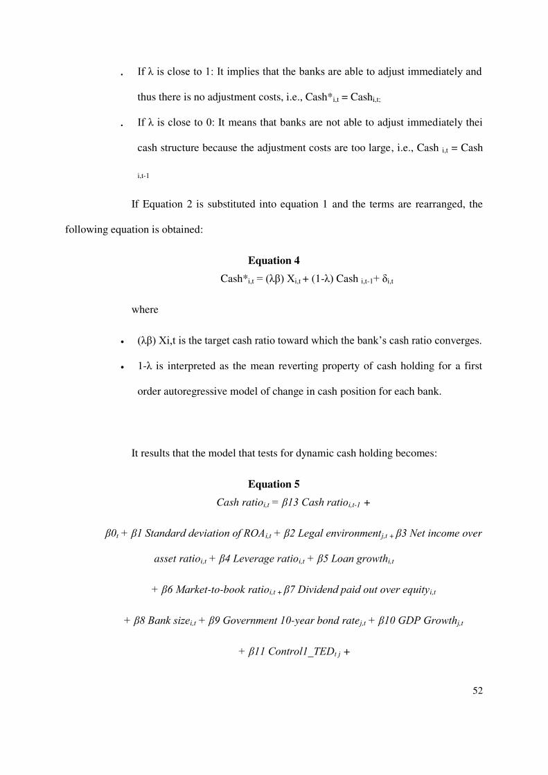
52
If λ is close to 1: It implies that the banks are able to adjust immediately and
thus there is no adjustment costs, i.e., Cash*i,t = Cashi,t;
If λ is close to 0: It means that banks are not able to adjust immediately thei
cash structure because the adjustment costs are too large, i.e., Cash i,t = Cash
i,t-1
If Equation 2 is substituted into equation 1 and the terms are rearranged, the
following equation is obtained:
Equation 4
Cash*i,t = (λβ) Xi,t + (1-λ) Cash i,t-1+ δi,t
where
(λβ) Xi,t is the target cash ratio toward which the bank’s cash ratio converges.
1-λ is interpreted as the mean reverting property of cash holding for a first
order autoregressive model of change in cash position for each bank.
It results that the model that tests for dynamic cash holding becomes:
Equation 5
Cash ratioi,t = β13 Cash ratioi,t-1 +
β0t + β1 Standard deviation of ROAi,t + β2 Legal environmentj,t + β3 Net income over
asset ratioi,t + β4 Leverage ratioi,t + β5 Loan growthi,t
+ β6 Market-to-book ratioi,t + β7 Dividend paid out over equityi,t
+ β8 Bank sizei,t + β9 Government 10-year bond ratej,t + β10 GDP Growthj,t
+ β11 Control1_TEDt j +

53
+ β12 Control2_Nonperforming Loans over total loans ratioi,t + µ i,t
The tables below report the results of the estimation. The results of Sargan &
Hansen’s J tests indicate that the instruments utilized in the GMM estimation do not correlate
with the error terms and that there are no overidentifying restrictions.
Insert Table 16.
Table 16, which reports the coefficient of the propensity to revert to cash
holding (1-λ) per geographical zone and bank size, confirms that the dynamic nature of the
cash holding model in the banking sector can be rejected. For the Asian and Pacific, European
and North American zones, the coefficients are 0.07 (1-0.93***), 0.28 (1-0.716***) and 0.13
(1-0.871***), respectively. For small, medium and large banks, the coefficients are 0.37 (1-
0.631***), 0.03 (1-0.968***) and 0.02 (1-0.978***), respectively.
Overall, these findings provide strong evidence that the dynamic nature of the
optimal cash model in the banking sector is rejected.
1.6 Conclusions
In this paper, I examined the hypothesis that cash optimality exists in the
banking sector. To determine the excess of the cash coefficient, I first identified the
determinants of cash holding. In contrast to previous studies, this paper explored the empirical
determinants of cash holding for a large sample of listed banks and over a long period of 35
years. I did not find any evidence that might support a substitutive relationship between cash
holding and the leverage ratio. Second, I integrated the dynamic nature of cash holding over
54
time to test whether banks adjust their level of cash to an optimal level. By using the GMM
protocol, I could establish this optimal cash level per bank while controlling for endogeneity
and measurement errors. Finally, the findings provide evidence that the dynamic nature of the
optimal cash model in the banking sector is rejected, in contrast to the nonbanking sector
(Ozkan and Ozkan (2004); Venkiteshwaran (2011) Akbari, Rahmani, Ahmadi and Shababi
(2014)); Subramaniam, Tang, Yue and Zhou (2011)). This paper yields several important
features that provide additional insights into not only what causes a bank to hold significant
amounts of cash but also how banks differ from corporations in regard to cash management.
Additionally, the Basel III regulatory framework—particularly with respect to liquidity
ratios—may oblige banks to adapt their financing models and, by extension, may change the
relationship between cash holding and debt levels. Further research on the impact of Basel III
on liquidity creation would be useful in this respect.
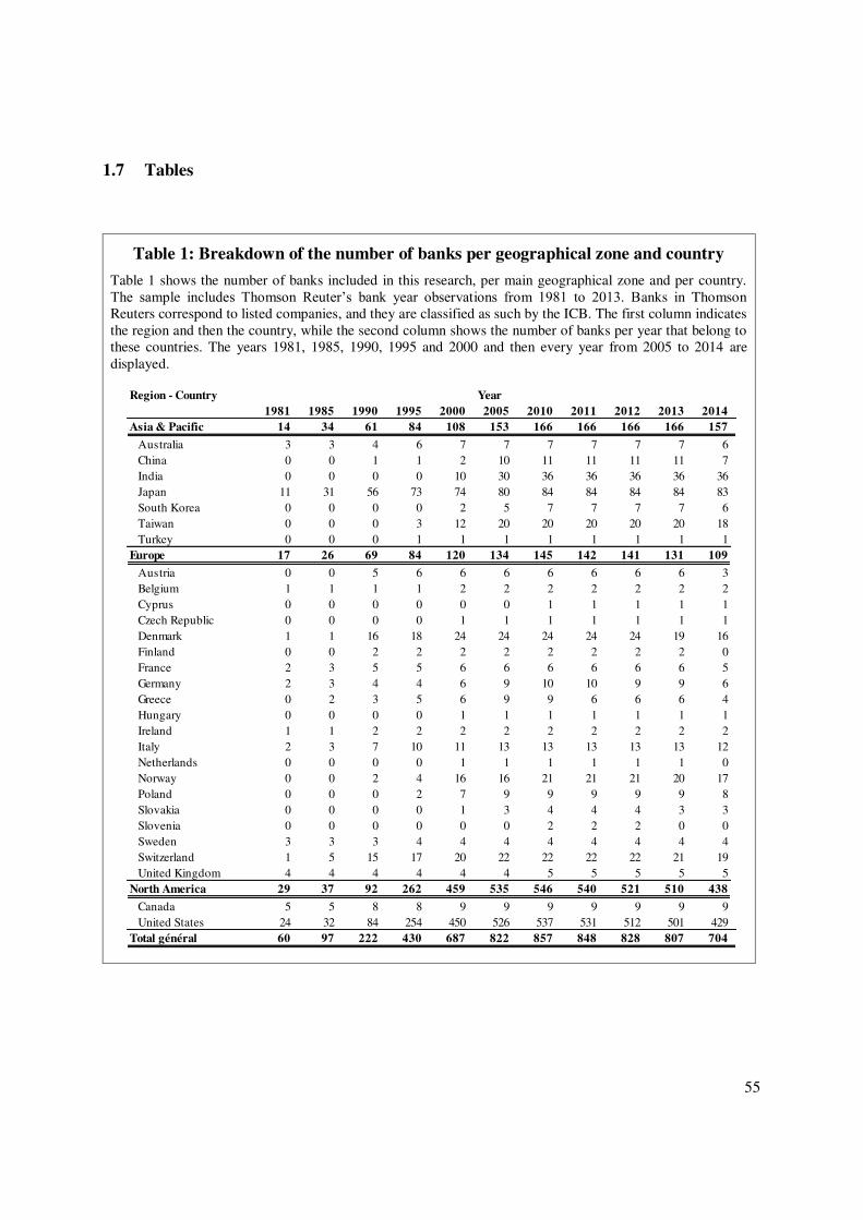
55
1.7 Tables
Table 1: Breakdown of the number of banks per geographical zone and country
Table 1 shows the number of banks included in this research, per main geographical zone and per country. The sample includes Thomson Reuter’s bank year observations from 1981 to 2013. Banks in Thomson Reuters correspond to listed companies, and they are classified as such by the ICB. The first column indicates the region and then the country, while the second column shows the number of banks per year that belong to these countries. The years 1981, 1985, 1990, 1995 and 2000 and then every year from 2005 to 2014 are displayed.
Region - Country1981 1985 1990 1995 2000 2005 2010 2011 2012 2013 2014
Asia & Pacific 14 34 61 84 108 153 166 166 166 166 157
Australia 3 3 4 6 7 7 7 7 7 7 6China 0 0 1 1 2 10 11 11 11 11 7India 0 0 0 0 10 30 36 36 36 36 36Japan 11 31 56 73 74 80 84 84 84 84 83South Korea 0 0 0 0 2 5 7 7 7 7 6Taiwan 0 0 0 3 12 20 20 20 20 20 18Turkey 0 0 0 1 1 1 1 1 1 1 1
Europe 17 26 69 84 120 134 145 142 141 131 109
Austria 0 0 5 6 6 6 6 6 6 6 3Belgium 1 1 1 1 2 2 2 2 2 2 2Cyprus 0 0 0 0 0 0 1 1 1 1 1Czech Republic 0 0 0 0 1 1 1 1 1 1 1Denmark 1 1 16 18 24 24 24 24 24 19 16Finland 0 0 2 2 2 2 2 2 2 2 0France 2 3 5 5 6 6 6 6 6 6 5Germany 2 3 4 4 6 9 10 10 9 9 6Greece 0 2 3 5 6 9 9 6 6 6 4Hungary 0 0 0 0 1 1 1 1 1 1 1Ireland 1 1 2 2 2 2 2 2 2 2 2Italy 2 3 7 10 11 13 13 13 13 13 12Netherlands 0 0 0 0 1 1 1 1 1 1 0Norway 0 0 2 4 16 16 21 21 21 20 17Poland 0 0 0 2 7 9 9 9 9 9 8Slovakia 0 0 0 0 1 3 4 4 4 3 3Slovenia 0 0 0 0 0 0 2 2 2 0 0Sweden 3 3 3 4 4 4 4 4 4 4 4Switzerland 1 5 15 17 20 22 22 22 22 21 19United Kingdom 4 4 4 4 4 4 5 5 5 5 5
North America 29 37 92 262 459 535 546 540 521 510 438
Canada 5 5 8 8 9 9 9 9 9 9 9United States 24 32 84 254 450 526 537 531 512 501 429
Total général 60 97 222 430 687 822 857 848 828 807 704
Year
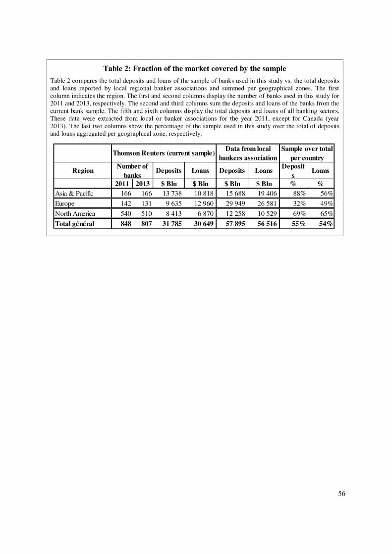
56
Table 2: Fraction of the market covered by the sample
Table 2 compares the total deposits and loans of the sample of banks used in this study vs. the total deposits and loans reported by local regional banker associations and summed per geographical zones. The first column indicates the region. The first and second columns display the number of banks used in this study for 2011 and 2013, respectively. The second and third columns sum the deposits and loans of the banks from the current bank sample. The fifth and sixth columns display the total deposits and loans of all banking sectors. These data were extracted from local or banker associations for the year 2011, except for Canada (year 2013). The last two columns show the percentage of the sample used in this study over the total of deposits and loans aggregated per geographical zone, respectively.
Region Deposits Loans Deposits LoansDeposit
sLoans
2011 2013 $ Bln $ Bln $ Bln $ Bln % %Asia & Pacific 166 166 13 738 10 818 15 688 19 406 88% 56%
Europe 142 131 9 635 12 960 29 949 26 581 32% 49%
North America 540 510 8 413 6 870 12 258 10 529 69% 65%
Total général 848 807 31 785 30 649 57 895 56 516 55% 54%
Sample over total per country
Thomson Reuters (current sample)
Number of banks
Data from local bankers association
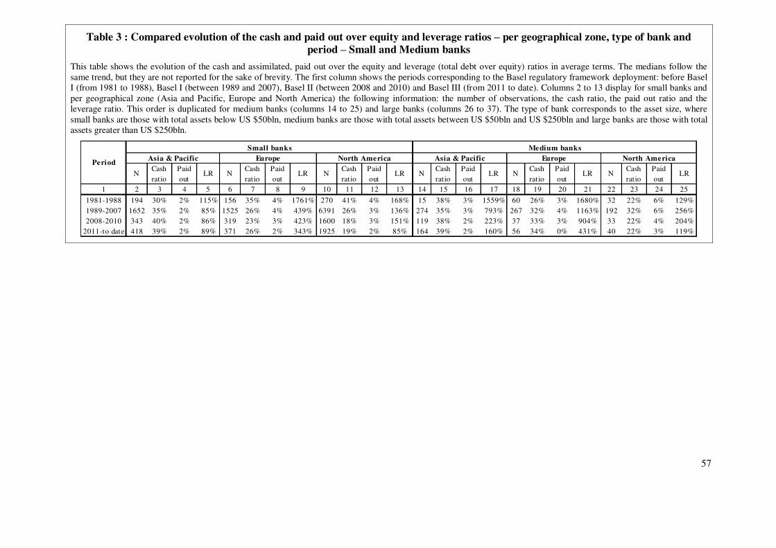
57
Table 3 : Compared evolution of the cash and paid out over equity and leverage ratios – per geographical zone, type of bank and period – Small and Medium banks
This table shows the evolution of the cash and assimilated, paid out over the equity and leverage (total debt over equity) ratios in average terms. The medians follow the same trend, but they are not reported for the sake of brevity. The first column shows the periods corresponding to the Basel regulatory framework deployment: before Basel I (from 1981 to 1988), Basel I (between 1989 and 2007), Basel II (between 2008 and 2010) and Basel III (from 2011 to date). Columns 2 to 13 display for small banks and per geographical zone (Asia and Pacific, Europe and North America) the following information: the number of observations, the cash ratio, the paid out ratio and the leverage ratio. This order is duplicated for medium banks (columns 14 to 25) and large banks (columns 26 to 37). The type of bank corresponds to the asset size, where small banks are those with total assets below US $50bln, medium banks are those with total assets between US $50bln and US $250bln and large banks are those with total assets greater than US $250bln.
NCash ratio
Paid out
LR NCash ratio
Paid out
LR NCash ratio
Paid out
LR NCash ratio
Paid out
LR NCash ratio
Paid out
LR NCash ratio
Paid out
LR
1 2 3 4 5 6 7 8 9 10 11 12 13 14 15 16 17 18 19 20 21 22 23 24 25
1981-1988 194 30% 2% 115% 156 35% 4% 1761% 270 41% 4% 168% 15 38% 3% 1559% 60 26% 3% 1680% 32 22% 6% 129%1989-2007 1652 35% 2% 85% 1525 26% 4% 439% 6391 26% 3% 136% 274 35% 3% 793% 267 32% 4% 1163% 192 32% 6% 256%2008-2010 343 40% 2% 86% 319 23% 3% 423% 1600 18% 3% 151% 119 38% 2% 223% 37 33% 3% 904% 33 22% 4% 204%
2011-to date 418 39% 2% 89% 371 26% 2% 343% 1925 19% 2% 85% 164 39% 2% 160% 56 34% 0% 431% 40 22% 3% 119%
Period
Small banks Medium banksAsia & Pacific Europe North America Asia & Pacific Europe North America
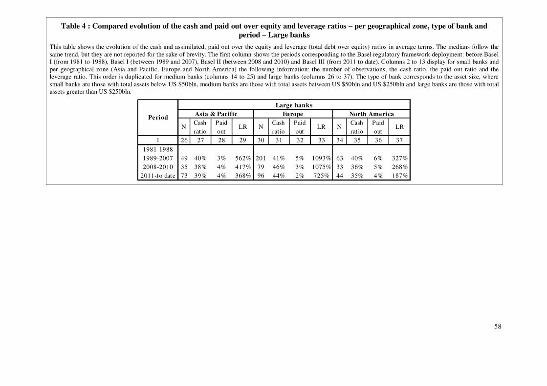
58
Table 4 : Compared evolution of the cash and paid out over equity and leverage ratios – per geographical zone, type of bank and period – Large banks
This table shows the evolution of the cash and assimilated, paid out over the equity and leverage (total debt over equity) ratios in average terms. The medians follow the same trend, but they are not reported for the sake of brevity. The first column shows the periods corresponding to the Basel regulatory framework deployment: before Basel I (from 1981 to 1988), Basel I (between 1989 and 2007), Basel II (between 2008 and 2010) and Basel III (from 2011 to date). Columns 2 to 13 display for small banks and per geographical zone (Asia and Pacific, Europe and North America) the following information: the number of observations, the cash ratio, the paid out ratio and the leverage ratio. This order is duplicated for medium banks (columns 14 to 25) and large banks (columns 26 to 37). The type of bank corresponds to the asset size, where small banks are those with total assets below US $50bln, medium banks are those with total assets between US $50bln and US $250bln and large banks are those with total assets greater than US $250bln.
NCash ratio
Paid out
LR NCash ratio
Paid out
LR NCash ratio
Paid out
LR
1 26 27 28 29 30 31 32 33 34 35 36 37
1981-19881989-2007 49 40% 3% 562% 201 41% 5% 1093% 63 40% 6% 327%2008-2010 35 38% 4% 417% 79 46% 3% 1075% 33 36% 5% 268%
2011-to date 73 39% 4% 368% 96 44% 2% 725% 44 35% 4% 187%
Europe North AmericaLarge banks
Asia & PacificPeriod
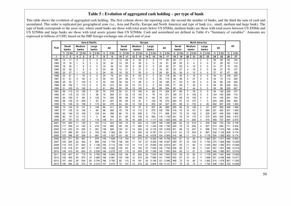
59
Table 5 : Evolution of aggregated cash holding – per type of bank
This table shows the evolution of aggregated cash holding. The first column shows the reporting year, the second the number of banks, and the third the sum of cash and assimilated. This order is replicated per geographical zone (i.e., Asia and Pacific, Europe and North America) and type of bank (i.e., small, medium and large bank). The type of bank corresponds to the asset size, where small banks are those with total assets below US $50bln, medium banks are those with total assets between US $50bln and US $250bln and large banks are those with total assets greater than US $250bln. Cash and assimilated are defined in Table 4’s “Summary of variables”. Amounts are expressed in billions of USD, based on the IMF foreign exchange rate of each end of year.
N $ Bln N $ Bln N $ Bln N $ Bln N $ Bln N $ Bln N $ Bln N $ Bln N $ Bln N $ Bln N $ Bln N $ Bln N $ Bln
1 2 3 4 5 6 7 8 9 10 11 12 13 14 15 16 17 18 19 20 21 22 23 24 25 26 27
1981 14 17 0 0 0 0 14 17 12 28 5 32 0 0 17 59 26 21 3 7 0 0 29 28 60 104
1982 15 18 1 6 0 0 16 24 12 25 6 36 0 0 18 61 28 25 3 4 0 0 31 29 65 114
1983 18 25 1 9 0 0 19 34 14 26 6 36 0 0 20 62 27 25 4 12 0 0 31 37 70 132
1984 22 30 1 8 0 0 23 38 13 21 6 31 0 0 19 52 30 27 4 10 0 0 34 37 76 127
1985 33 37 1 12 0 0 34 50 19 33 7 50 0 0 26 83 33 34 4 12 0 0 37 47 97 180
1986 33 61 1 16 0 0 34 76 24 55 8 63 0 0 32 118 36 45 4 16 0 0 40 61 106 255
1987 31 61 3 40 0 0 34 101 24 58 11 115 0 0 35 173 39 48 5 27 0 0 44 75 113 349
1988 28 55 7 104 0 0 35 160 38 82 11 98 0 0 49 180 51 53 5 33 0 0 56 86 140 425
1989 48 102 7 113 0 0 55 214 50 92 13 141 0 0 63 233 77 49 7 45 0 0 84 95 202 542
1990 51 102 10 162 0 0 61 264 52 59 13 163 4 82 69 304 85 54 7 44 0 0 92 98 222 667
1991 59 113 10 135 1 32 70 279 54 51 13 190 4 83 71 324 87 65 7 78 0 0 94 143 235 747
1992 61 115 10 131 1 38 72 284 57 52 13 145 4 75 74 271 125 57 9 103 0 0 134 160 280 716
1993 64 129 8 68 2 123 74 320 59 58 12 128 5 46 76 231 131 58 10 135 0 0 141 193 291 744
1994 68 145 12 229 1 53 81 427 59 59 12 91 7 123 78 273 222 61 10 167 1 0 233 228 392 929
1995 70 148 12 158 2 172 84 479 64 80 12 104 8 353 84 537 251 68 9 153 2 46 262 267 430 1 283
1996 74 144 10 121 2 146 86 411 65 84 12 97 9 507 86 688 285 64 10 148 2 57 297 269 469 1 368
1997 77 135 10 126 1 99 88 360 79 78 14 110 9 570 102 758 318 70 10 121 3 260 331 452 521 1 569
1998 83 146 10 109 1 104 94 358 86 73 16 209 9 716 111 998 374 72 10 152 3 225 387 449 592 1 805
1999 82 79 13 115 1 0 96 194 91 85 15 148 10 920 116 1 153 421 76 10 175 3 275 434 526 646 1 873
2000 97 191 10 107 1 113 108 411 93 78 16 228 11 1 117 120 1 423 444 63 11 200 4 473 459 737 687 2 570
2001 101 200 11 123 2 101 114 424 100 75 16 223 12 1 297 128 1 595 466 64 12 219 4 446 482 730 724 2 749
2002 117 309 14 140 2 216 133 665 98 65 17 280 13 1 445 128 1 790 494 70 12 222 4 557 510 849 771 3 304
2003 114 333 19 205 5 391 138 929 100 91 14 245 16 2 123 130 2 459 501 68 12 247 5 696 518 1 010 786 4 399
2004 117 386 22 274 6 723 145 1 383 99 91 16 300 16 2 781 131 3 171 513 61 13 204 6 897 532 1 162 808 5 716
2005 123 396 25 339 5 691 153 1 427 101 92 17 394 16 4 878 134 5 364 516 66 11 141 8 1 176 535 1 383 822 8 174
2006 123 371 29 381 7 876 159 1 628 110 104 15 210 21 6 393 146 6 708 532 67 10 90 9 1 460 551 1 617 856 9 953
2007 123 365 32 450 9 894 164 1 709 108 105 11 167 27 9 325 146 9 597 549 57 12 104 9 1 763 570 1 924 880 13 229
2008 119 372 37 603 9 1 136 165 2 112 108 110 10 114 27 8 650 145 8 874 541 53 11 84 11 1 445 563 1 582 873 12 568
2009 118 418 37 607 11 1 397 166 2 422 104 83 14 160 27 7 550 145 7 793 535 62 11 92 11 1 647 557 1 801 868 12 016
2010 106 410 45 630 15 2 239 166 3 279 107 110 13 204 25 7 336 145 7 650 524 60 11 81 11 1 848 546 1 990 857 12 918
2011 103 407 47 715 16 2 782 166 3 904 103 99 15 202 24 7 534 142 7 834 519 59 10 83 11 1 778 540 1 921 848 13 659
2012 102 409 45 675 19 2 996 166 4 081 103 139 12 219 26 7 586 141 7 945 500 67 10 91 11 1 888 521 2 046 828 14 071
2013 107 442 39 554 20 2 794 166 3 790 92 115 15 181 24 5 190 131 5 486 489 72 10 65 11 1 842 510 1 979 807 11 255
2014 106 284 33 375 18 2 315 157 2 974 73 107 14 219 22 4 804 109 5 131 417 75 10 74 11 1 752 438 1 901 704 10 006
Large
banksYear
Asia & Pacific Europe North America
AllSmall
banks
Medium
banks
Large
banksAll
Small
banksAll
Medium
banks
Large
banksAll
Small
banks
Medium
banks

60
Table 6: Summary of variables (part 1)
This table sums up the discussion above and shows the exhaustive list of variables used in this research. The first column indicates the motive, the second the variable name, the third the corresponding code used in the regression models, the fourth whether the variable has been scaled under a Siegel-Tukey test, the fifth the predictive sign and the sixth how the variable has been computed (Thomson Reuters’ code).
Motive Variable nameVariable name in
the OLS
Tukey' scale type
Predictive sign
How this variable is computed
1 2 3 4 5 6
Explained variable 1 Cash and assimilated over assets Y (Sqrt) NACash and Assimilated over Assets = Treasury Securities (item WC02205) + Trading account Securities (item WC02208) + Cash and due from banks (item WC2004) over Total Assets (item WC02999)
Explained variable 2 (GMM) Cash and assimilated over assets year +1 NA NA Δ cash holding = [Cash holding(y) - Cash holding(y-1) / Cash holding(y-1)]
1. Precautionary Standard deviation of returns on assets X1SdRoa Y (Log) +
Standard deviation of RoA = Net Income Total (item WC01751) / Total assets (item WC02999). The standard deviation require at least three observations, is rolling and computed every year (step of maximum 5 years).Net Income Total (WC01751)NET INCOME TOTAL represents the net income the company. It is before extraordinary items.
2. Effect of regulatory environment
Liquidity creation may depend on local regulatory constraints.
X2Legal NA -
To measure the effect of the legal environment and institutional differences on liquidity creation, an index has been established as follow : (1) before Basel I : I start first from La Porta et al. (1997) who established legal zones to measure the effect of the legal environment on the development of the capital market. To measure the effect of the legal environment on liquidity creation, a similar mapping is utilized in this paper, where a grade is provided to the level of property right protection from 0 to 4 corresponding from not protective to most protective, respectively. (2) from Basel I to II, (3) from Basel II to III, and (4) since Basel III : The regulatory environment mapping of banks is elaborated from Barth et al. (2008); Barth et al. (2001) for the three last periods corresponding respectively to Basel regulatory frameworks deployments. It is a summary that averages the capital stringency as well as capital activity and restrictiveness per periods.
3. Signaling Net income over assets X3Incoa NA -IncoA: Net Income Total (item WC01751) / Total Assets (item WC02999)Net Income Total (item WC01751) represents the net income the company uses to calculate its earnings per share. It is before extraordinary items.
4. Strategic - Funding source substitutability
Leverage ratio X4LR NA - Total Debt / Equity : The ratio is calculated as follow : Total debts (item WC03255) /Common equities (item WC03501)
4. Strategic - Growth opportunities
Loan growth X5LnGwth NA +Loan growth is a proxy for bank's growth opportunity. It is the variation of total loans over one reporting yearLnGwth : (Loans Total Y of bank i- Loans total Y-1 of bank i) / Loans total Y-1 of bank 1 - [Where Loans total is item WC02271]
4. Strategic - Growth opportunities
Market-to-book ratio X6MktBkR NA +This ratio is calculated as follow in this research: Market value per share (item WC05001) over Book value per share (item WC05476).
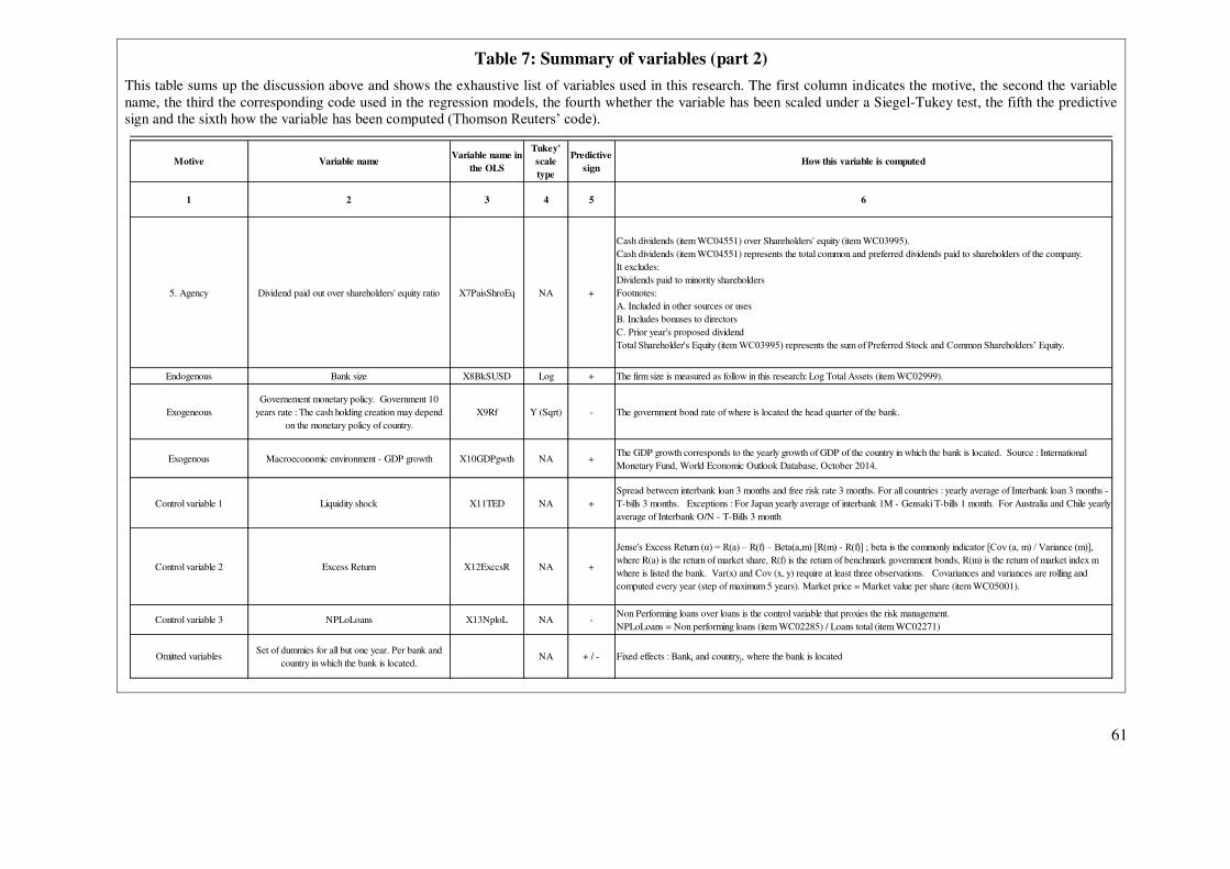
61
Table 7: Summary of variables (part 2)
This table sums up the discussion above and shows the exhaustive list of variables used in this research. The first column indicates the motive, the second the variable name, the third the corresponding code used in the regression models, the fourth whether the variable has been scaled under a Siegel-Tukey test, the fifth the predictive sign and the sixth how the variable has been computed (Thomson Reuters’ code).
Motive Variable nameVariable name in
the OLS
Tukey' scale type
Predictive sign
How this variable is computed
1 2 3 4 5 6
5. Agency Dividend paid out over shareholders' equity ratio X7PaisShroEq NA +
Cash dividends (item WC04551) over Shareholders' equity (item WC03995).Cash dividends (item WC04551) represents the total common and preferred dividends paid to shareholders of the company.It excludes:Dividends paid to minority shareholdersFootnotes:A. Included in other sources or usesB. Includes bonuses to directorsC. Prior year's proposed dividendTotal Shareholder's Equity (item WC03995) represents the sum of Preferred Stock and Common Shareholders’ Equity.
Endogenous Bank size X8BkSUSD Log + The firm size is measured as follow in this research: Log Total Assets (item WC02999).
ExogeneousGovernement monetary policy. Government 10
years rate : The cash holding creation may depend on the monetary policy of country.
X9Rf Y (Sqrt) - The government bond rate of where is located the head quarter of the bank.
Exogenous Macroeconomic environment - GDP growth X10GDPgwth NA +The GDP growth corresponds to the yearly growth of GDP of the country in which the bank is located. Source : International Monetary Fund, World Economic Outlook Database, October 2014.
Control variable 1 Liquidity shock X11TED NA +Spread between interbank loan 3 months and free risk rate 3 months. For all countries : yearly average of Interbank loan 3 months - T-bills 3 months. Exceptions : For Japan yearly average of interbank 1M - Gensaki T-bills 1 month. For Australia and Chile yearly average of Interbank O/N - T-Bills 3 month
Control variable 2 Excess Return X12ExccsR NA +
Jense's Excess Return (α) = R(a) – R(f) – Beta(a,m) [R(m) - R(f)] ; beta is the commonly indicator [Cov (a, m) / Variance (m)],
where R(a) is the return of market share, R(f) is the return of benchmark government bonds, R(m) is the return of market index m where is listed the bank. Var(x) and Cov (x, y) require at least three observations. Covariances and variances are rolling and computed every year (step of maximum 5 years). Market price = Market value per share (item WC05001).
Control variable 3 NPLoLoans X13NploL NA -Non Performing loans over loans is the control variable that proxies the risk management.NPLoLoans = Non performing loans (item WC02285) / Loans total (item WC02271)
Omitted variablesSet of dummies for all but one year. Per bank and
country in which the bank is located.NA + / - Fixed effects : Banki and countryj, where the bank is located
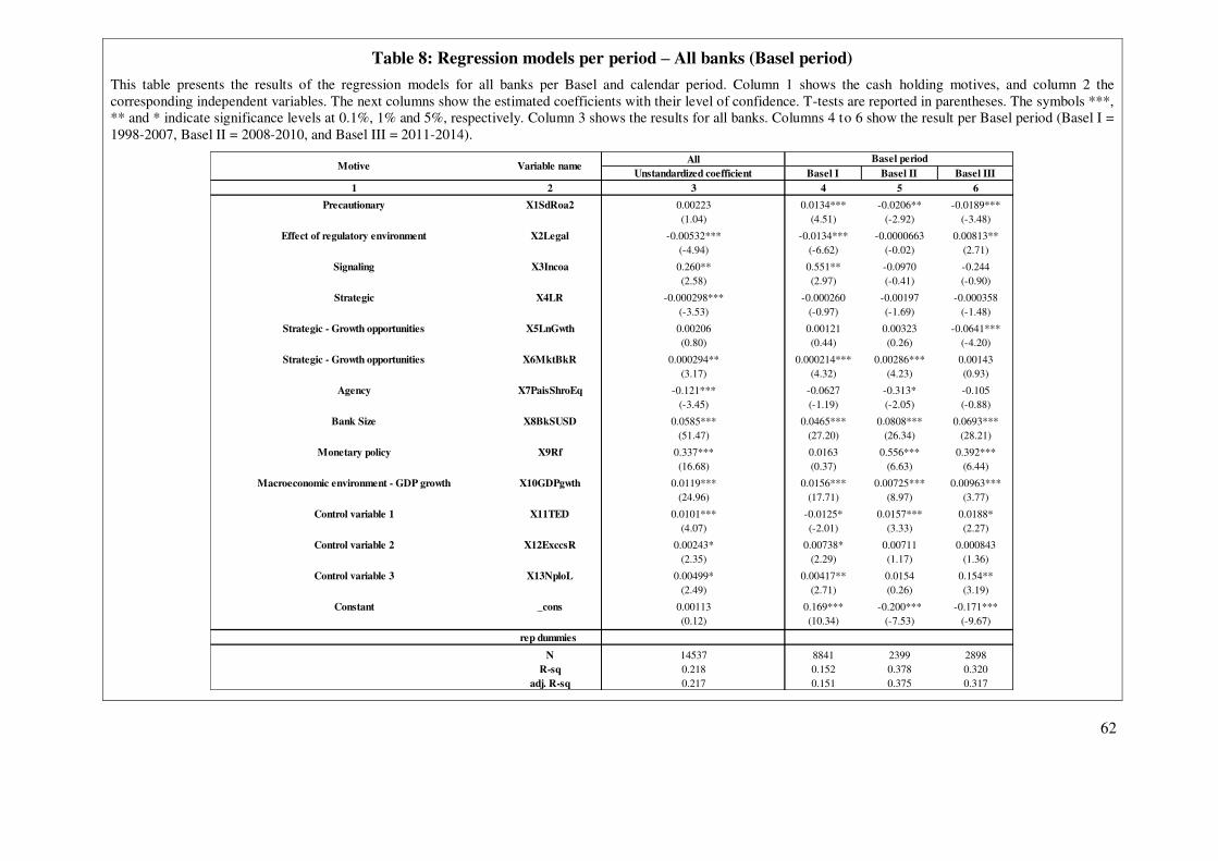
62
Table 8: Regression models per period – All banks (Basel period)
This table presents the results of the regression models for all banks per Basel and calendar period. Column 1 shows the cash holding motives, and column 2 the corresponding independent variables. The next columns show the estimated coefficients with their level of confidence. T-tests are reported in parentheses. The symbols ***, ** and * indicate significance levels at 0.1%, 1% and 5%, respectively. Column 3 shows the results for all banks. Columns 4 to 6 show the result per Basel period (Basel I = 1998-2007, Basel II = 2008-2010, and Basel III = 2011-2014).
AllUnstandardized coefficient Basel I Basel II Basel III
1 2 3 4 5 6
Precautionary X1SdRoa2 0.00223 0.0134*** -0.0206** -0.0189***(1.04) (4.51) (-2.92) (-3.48)
Effect of regulatory environment X2Legal -0.00532*** -0.0134*** -0.0000663 0.00813**(-4.94) (-6.62) (-0.02) (2.71)
Signaling X3Incoa 0.260** 0.551** -0.0970 -0.244(2.58) (2.97) (-0.41) (-0.90)
Strategic X4LR -0.000298*** -0.000260 -0.00197 -0.000358(-3.53) (-0.97) (-1.69) (-1.48)
Strategic - Growth opportunities X5LnGwth 0.00206 0.00121 0.00323 -0.0641***(0.80) (0.44) (0.26) (-4.20)
Strategic - Growth opportunities X6MktBkR 0.000294** 0.000214*** 0.00286*** 0.00143(3.17) (4.32) (4.23) (0.93)
Agency X7PaisShroEq -0.121*** -0.0627 -0.313* -0.105(-3.45) (-1.19) (-2.05) (-0.88)
Bank Size X8BkSUSD 0.0585*** 0.0465*** 0.0808*** 0.0693***(51.47) (27.20) (26.34) (28.21)
Monetary policy X9Rf 0.337*** 0.0163 0.556*** 0.392***(16.68) (0.37) (6.63) (6.44)
Macroeconomic environment - GDP growth X10GDPgwth 0.0119*** 0.0156*** 0.00725*** 0.00963***(24.96) (17.71) (8.97) (3.77)
Control variable 1 X11TED 0.0101*** -0.0125* 0.0157*** 0.0188*(4.07) (-2.01) (3.33) (2.27)
Control variable 2 X12ExccsR 0.00243* 0.00738* 0.00711 0.000843(2.35) (2.29) (1.17) (1.36)
Control variable 3 X13NploL 0.00499* 0.00417** 0.0154 0.154**(2.49) (2.71) (0.26) (3.19)
Constant _cons 0.00113 0.169*** -0.200*** -0.171***(0.12) (10.34) (-7.53) (-9.67)
rep dummies
N 14537 8841 2399 2898R-sq 0.218 0.152 0.378 0.320
adj. R-sq 0.217 0.151 0.375 0.317
Motive Variable nameBasel period

63
Table 9: Regression models per period – All banks (ten-years period and fixed effect)
This table presents the results of the regression models for all banks per Basel and calendar period. Column 1 shows the cash holding motives, and column 2 the corresponding independent variables. The next columns show the estimated coefficients with their level of confidence. T-tests are reported in parentheses. The symbols ***, ** and * indicate significance levels at 0.1%, 1% and 5%, respectively. Column 3 shows the results for all banks. Columns 4 to 6 show the result per Basel period (Basel I = 1998-2007, Basel II = 2008-2010, and Basel III = 2011-2014). Columns 7-10 show the results per ten-year period (1981-1990, 1991-2000, 2001-2010, and 2011-2014). Columns 11 and 12 show the fixed-effects results, where bank and country are the variables that control for unobserved heterogeneity. Robustness tests include endogeneity with instrumented variables and omitted variables with fixed effects. All the results show F values greater than 10, with P(F) less than 0.0001 and P(t) less than 0.0001.
1981-1990 1991-2000 2001-2010 2011-2014 Per bank Per country1 2 7 8 9 10 11 12
Precautionary X1SdRoa2 0.00683 0.00192 0.00848* -0.0189*** 0.00620** 0.0120***(0.64) (0.41) (2.23) (-3.48) (2.83) (5.56)
Effect of regulatory environment X2Legal 0.0699*** -0.0171** 0.000300 0.00813** 0.00881*** 0.00541**(7.26) (-3.09) (0.15) (2.71) (5.41) (2.75)
Signaling X3Incoa 3.707*** 2.124*** -0.134 -0.244 0.156 0.425***(3.63) (5.56) (-0.73) (-0.90) (1.92) (4.51)
Strategic X4LR 0.000758 -0.0000639 -0.00511*** -0.000358 -0.0000828 -0.000306***(1.21) (-0.46) (-4.98) (-1.48) (-1.31) (-4.02)
Strategic - Growth opportunities X5LnGwth 0.0133 0.000158 0.00876 -0.0641*** -0.00287 -0.00378(0.51) (0.05) (1.15) (-4.20) (-1.54) (-1.66)
Strategic - Growth opportunities X6MktBkR -0.0168*** 0.0000635 0.00454** 0.00143 -0.0000409 0.000209*(-5.86) (1.50) (3.19) (0.93) (-0.25) (2.54)
Agency X7PaisShroEq -0.679** -0.0383 -0.143* -0.105 -0.00442 0.172***(-2.95) (-0.46) (-2.12) (-0.88) (-0.14) (5.17)
Bank Size X8BkSUSD -0.00672 0.0222*** 0.0734*** 0.0693*** -0.0629*** 0.0306***(-0.98) (7.74) (34.75) (28.21) (-12.69) (21.95)
Monetary policy X9Rf 0.378*** -0.102 0.240*** 0.392*** 0.0866** 0.0307(4.81) (-1.78) (4.42) (6.44) (3.18) (0.92)
Macroeconomic environment - GDP growth X10GDPgwth -0.00154 0.000912 0.0110*** 0.00963*** 0.00714*** 0.00634***(-0.50) (0.59) (17.83) (3.77) (11.27) (7.99)
Control variable 1 X11TED 0.0383*** 0.0319** -0.0178*** 0.0188* 0.0405*** 0.0433***(3.87) (3.28) (-5.08) (2.27) (13.68) (11.74)
Control variable 2 X12ExccsR 0.000939 0.00900 0.0137** 0.000843 -0.000410 0.000750(0.08) (1.65) (3.07) (1.36) (-0.53) (0.80)
Control variable 3 X13NploL 0.118 0.152 0.00392* 0.154** 0.00105 0.00165(0.40) (1.61) (2.56) (3.19) (0.69) (0.92)
Constant _cons 0.0649 0.287*** -0.0241 -0.171*** 0.394*** 0.207***(0.88) (8.77) (-1.23) (-9.67) (20.15) (9.76)
rep dummies Yes Yes
N 650 3641 7348 2898 14537 14537R-sq 0.358 0.049 0.312 0.320 0.106 0.136
adj. R-sq 0.344 0.046 0.311 0.317 0.043 0.131
Motive Variable nameCalendar period Fixed effects
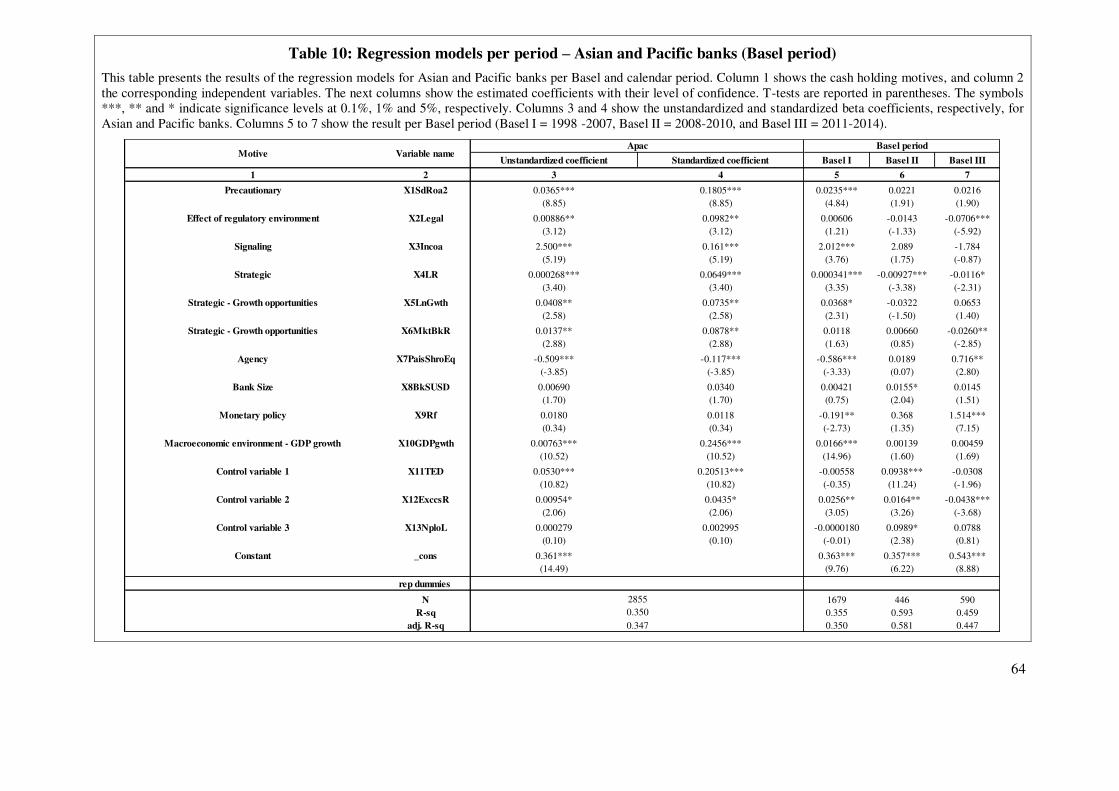
64
Table 10: Regression models per period – Asian and Pacific banks (Basel period)
This table presents the results of the regression models for Asian and Pacific banks per Basel and calendar period. Column 1 shows the cash holding motives, and column 2 the corresponding independent variables. The next columns show the estimated coefficients with their level of confidence. T-tests are reported in parentheses. The symbols ***, ** and * indicate significance levels at 0.1%, 1% and 5%, respectively. Columns 3 and 4 show the unstandardized and standardized beta coefficients, respectively, for Asian and Pacific banks. Columns 5 to 7 show the result per Basel period (Basel I = 1998 -2007, Basel II = 2008-2010, and Basel III = 2011-2014).
Unstandardized coefficient Standardized coefficient Basel I Basel II Basel III
1 2 3 4 5 6 7
Precautionary X1SdRoa2 0.0365*** 0.1805*** 0.0235*** 0.0221 0.0216(8.85) (8.85) (4.84) (1.91) (1.90)
Effect of regulatory environment X2Legal 0.00886** 0.0982** 0.00606 -0.0143 -0.0706***(3.12) (3.12) (1.21) (-1.33) (-5.92)
Signaling X3Incoa 2.500*** 0.161*** 2.012*** 2.089 -1.784(5.19) (5.19) (3.76) (1.75) (-0.87)
Strategic X4LR 0.000268*** 0.0649*** 0.000341*** -0.00927*** -0.0116*(3.40) (3.40) (3.35) (-3.38) (-2.31)
Strategic - Growth opportunities X5LnGwth 0.0408** 0.0735** 0.0368* -0.0322 0.0653(2.58) (2.58) (2.31) (-1.50) (1.40)
Strategic - Growth opportunities X6MktBkR 0.0137** 0.0878** 0.0118 0.00660 -0.0260**(2.88) (2.88) (1.63) (0.85) (-2.85)
Agency X7PaisShroEq -0.509*** -0.117*** -0.586*** 0.0189 0.716**(-3.85) (-3.85) (-3.33) (0.07) (2.80)
Bank Size X8BkSUSD 0.00690 0.0340 0.00421 0.0155* 0.0145(1.70) (1.70) (0.75) (2.04) (1.51)
Monetary policy X9Rf 0.0180 0.0118 -0.191** 0.368 1.514***(0.34) (0.34) (-2.73) (1.35) (7.15)
Macroeconomic environment - GDP growth X10GDPgwth 0.00763*** 0.2456*** 0.0166*** 0.00139 0.00459(10.52) (10.52) (14.96) (1.60) (1.69)
Control variable 1 X11TED 0.0530*** 0.20513*** -0.00558 0.0938*** -0.0308(10.82) (10.82) (-0.35) (11.24) (-1.96)
Control variable 2 X12ExccsR 0.00954* 0.0435* 0.0256** 0.0164** -0.0438***(2.06) (2.06) (3.05) (3.26) (-3.68)
Control variable 3 X13NploL 0.000279 0.002995 -0.0000180 0.0989* 0.0788(0.10) (0.10) (-0.01) (2.38) (0.81)
Constant _cons 0.361*** 0.363*** 0.357*** 0.543***(14.49) (9.76) (6.22) (8.88)
rep dummies
N 1679 446 590R-sq 0.355 0.593 0.459
adj. R-sq 0.350 0.581 0.447
ApacMotive Variable name
28550.3500.347
Basel period
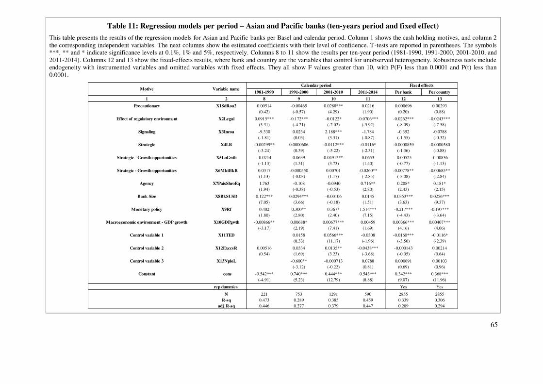
65
Table 11: Regression models per period – Asian and Pacific banks (ten-years period and fixed effect)
This table presents the results of the regression models for Asian and Pacific banks per Basel and calendar period. Column 1 shows the cash holding motives, and column 2 the corresponding independent variables. The next columns show the estimated coefficients with their level of confidence. T-tests are reported in parentheses. The symbols ***, ** and * indicate significance levels at 0.1%, 1% and 5%, respectively. Columns 8 to 11 show the results per ten-year period (1981-1990, 1991-2000, 2001-2010, and 2011-2014). Columns 12 and 13 show the fixed-effects results, where bank and country are the variables that control for unobserved heterogeneity. Robustness tests include endogeneity with instrumented variables and omitted variables with fixed effects. They all show F values greater than 10, with P(F) less than 0.0001 and P(t) less than 0.0001.
1981-1990 1991-2000 2001-2010 2011-2014 Per bank Per country
1 2 8 9 10 11 12 13
Precautionary X1SdRoa2 0.00514 -0.00465 0.0288*** 0.0216 0.000696 0.00293(0.42) (-0.57) (4.29) (1.90) (0.20) (0.88)
Effect of regulatory environment X2Legal 0.0915*** -0.172*** -0.0122* -0.0706*** -0.0262*** -0.0243***(5.31) (-4.21) (-2.02) (-5.92) (-8.09) (-7.58)
Signaling X3Incoa -9.330 0.0234 2.188*** -1.784 -0.352 -0.0788(-1.81) (0.03) (3.31) (-0.87) (-1.55) (-0.32)
Strategic X4LR -0.00299** 0.0000686 -0.0112*** -0.0116* -0.0000859 -0.0000580(-3.24) (0.39) (-5.22) (-2.31) (-1.36) (-0.88)
Strategic - Growth opportunities X5LnGwth -0.0714 0.0639 0.0491*** 0.0653 -0.00525 -0.00836(-1.13) (1.51) (3.73) (1.40) (-0.77) (-1.13)
Strategic - Growth opportunities X6MktBkR 0.0317 -0.000550 0.00701 -0.0260** -0.00778** -0.00685**(1.13) (-0.03) (1.17) (-2.85) (-3.08) (-2.84)
Agency X7PaisShroEq 1.763 -0.108 -0.0940 0.716** 0.208* 0.181*(1.94) (-0.38) (-0.53) (2.80) (2.43) (2.15)
Bank Size X8BkSUSD 0.122*** 0.0294*** -0.00106 0.0145 0.0353*** 0.0256***(7.05) (3.66) (-0.18) (1.51) (3.63) (9.37)
Monetary policy X9Rf 0.402 0.300** 0.367* 1.514*** -0.217*** -0.197***(1.80) (2.80) (2.40) (7.15) (-4.43) (-3.64)
Macroeconomic environment - GDP growth X10GDPgwth -0.00866** 0.00688* 0.00677*** 0.00459 0.00366*** 0.00407***(-3.17) (2.19) (7.41) (1.69) (4.16) (4.06)
Control variable 1 X11TED 0.0158 0.0566*** -0.0308 -0.0160*** -0.0116*(0.33) (11.17) (-1.96) (-3.56) (-2.39)
Control variable 2 X12ExccsR 0.00516 0.0334 0.0135** -0.0438*** -0.000143 0.00214(0.54) (1.69) (3.23) (-3.68) (-0.05) (0.64)
Control variable 3 X13NploL -0.600** -0.000713 0.0788 0.000691 0.00103(-3.12) (-0.22) (0.81) (0.69) (0.96)
Constant _cons -0.542*** 0.740*** 0.444*** 0.543*** 0.342*** 0.368***(-4.91) (5.23) (12.79) (8.88) (9.07) (11.96)
rep dummies Yes Yes
N 221 753 1291 590 2855 2855R-sq 0.473 0.289 0.385 0.459 0.339 0.306
adj. R-sq 0.446 0.277 0.379 0.447 0.289 0.294
Fixed effectsMotive Variable name
Calendar period
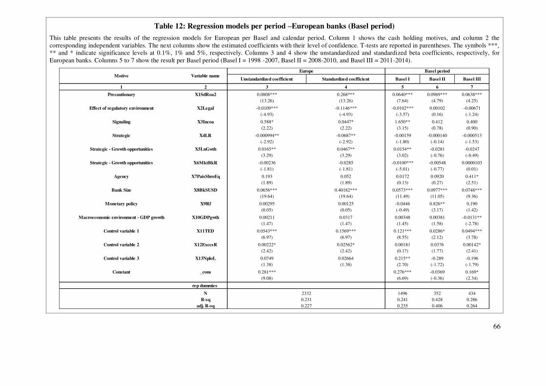
66
Table 12: Regression models per period –European banks (Basel period)
This table presents the results of the regression models for European per Basel and calendar period. Column 1 shows the cash holding motives, and column 2 the corresponding independent variables. The next columns show the estimated coefficients with their level of confidence. T-tests are reported in parentheses. The symbols ***, ** and * indicate significance levels at 0.1%, 1% and 5%, respectively. Columns 3 and 4 show the unstandardized and standardized beta coefficients, respectively, for European banks. Columns 5 to 7 show the result per Basel period (Basel I = 1998 -2007, Basel II = 2008-2010, and Basel III = 2011-2014).
Unstandardized coefficient Standardized coefficient Basel I Basel II Basel III
1 2 3 4 5 6 7
Precautionary X1SdRoa2 0.0808*** 0.268*** 0.0640*** 0.0989*** 0.0638***(13.26) (13.26) (7.64) (4.79) (4.25)
Effect of regulatory environment X2Legal -0.0109*** -0.1146*** -0.0102*** 0.00102 -0.00671(-4.93) (-4.93) (-3.57) (0.16) (-1.24)
Signaling X3Incoa 0.588* 0.0447* 1.650** 0.412 0.400(2.22) (2.22) (3.15) (0.78) (0.90)
Strategic X4LR -0.000994** -0.0687** -0.00159 -0.000140 -0.000513(-2.92) (-2.92) (-1.80) (-0.14) (-1.53)
Strategic - Growth opportunities X5LnGwth 0.0165** 0.0467** 0.0154** -0.0281 -0.0247(3.29) (3.29) (3.02) (-0.76) (-0.49)
Strategic - Growth opportunities X6MktBkR -0.00236 -0.0285 -0.0100*** -0.00548 0.0000103(-1.81) (-1.81) (-5.01) (-0.77) (0.01)
Agency X7PaisShroEq 0.193 0.052 0.0172 0.0920 0.411*(1.89) (1.89) (0.13) (0.27) (2.51)
Bank Size X8BkSUSD 0.0656*** 0.40182*** 0.0573*** 0.0977*** 0.0748***(19.64) (19.64) (11.49) (11.05) (9.36)
Monetary policy X9Rf 0.00295 0.00125 -0.0446 0.826** 0.190(0.05) (0.05) (-0.49) (3.17) (1.42)
Macroeconomic environment - GDP growth X10GDPgwth 0.00211 0.0317 0.00348 0.00381 -0.0131**(1.47) (1.47) (1.45) (1.58) (-2.78)
Control variable 1 X11TED 0.0543*** 0.1569*** 0.121*** 0.0286* 0.0494***(6.97) (6.97) (8.55) (2.12) (3.78)
Control variable 2 X12ExccsR 0.00222* 0.02562* 0.00181 0.0376 0.00142*(2.42) (2.42) (0.17) (1.77) (2.41)
Control variable 3 X13NploL 0.0749 0.02664 0.215** -0.289 -0.196(1.38) (1.38) (2.70) (-1.72) (-1.79)
Constant _cons 0.281*** 0.276*** -0.0369 0.169*(9.08) (6.69) (-0.36) (2.34)
rep dummies
N 1496 352 434R-sq 0.241 0.428 0.286
adj. R-sq 0.235 0.406 0.264
EuropeMotive Variable name
23320.2310.227
Basel period

67
Table 13: Regression models per period –European banks (ten-years period and fixed effect)
This table presents the results of the regression models for European per Basel and calendar period. Column 1 shows the cash holding mot ives, and column 2 the corresponding independent variables. The next columns show the estimated coefficients with their level of confidence. T-tests are reported in parentheses. The symbols ***, ** and * indicate significance levels at 0.1%, 1% and 5%, respectively. Columns 8 to 11 show the results per ten-year period (1981-1990, 1991-2000, 2001-2010, and 2011-2014). Columns 12 and 13 show the fixed-effects results, where bank and country are the variables that control for unobserved heterogeneity. Robustness tests include endogeneity with instrumented variables and omitted variables with fixed effects. They all show F values greater than 10, with P(F) less than 0.0001 and P(t) less than 0.0001.
1981-1990 1991-2000 2001-2010 2011-2014 Per bank Per country
1 2 8 9 10 11 12 13
Precautionary X1SdRoa2 0.00921 0.0526*** 0.0826*** 0.0638*** 0.00821 0.0532***(0.20) (4.81) (7.89) (4.25) (1.22) (8.69)
Effect of regulatory environment X2Legal -0.0109 -0.0238* 0.00487 -0.00671 0.00662 0.00372(-0.23) (-2.25) (1.57) (-1.24) (1.71) (0.89)
Signaling X3Incoa 7.785* 1.356* 0.290 0.400 -0.525* -0.277(2.03) (2.09) (0.59) (0.90) (-2.04) (-1.05)
Strategic X4LR -0.00403 -0.00261 -0.00147 -0.000513 -0.000444 -0.000646*(-1.70) (-1.87) (-1.78) (-1.53) (-1.73) (-2.35)
Strategic - Growth opportunities X5LnGwth 0.105 0.0130** 0.0135 -0.0247 -0.00513 0.00226(1.16) (2.84) (1.11) (-0.49) (-0.99) (0.39)
Strategic - Growth opportunities X6MktBkR -0.0108 -0.0135*** -0.0102 0.0000103 0.000812 -0.00137(-0.42) (-5.93) (-1.87) (0.01) (0.61) (-0.95)
Agency X7PaisShroEq -0.250 -0.132 0.109 0.411* 0.0881 0.190**(-0.48) (-0.69) (0.73) (2.51) (1.31) (2.68)
Bank Size X8BkSUSD -0.0404 0.0328*** 0.0964*** 0.0748*** 0.0547** 0.0652***(-1.75) (4.73) (16.58) (9.36) (3.25) (16.55)
Monetary policy X9Rf 0.00958 -0.340** 1.202*** 0.190 -0.380*** -0.384***(0.08) (-2.95) (7.45) (1.42) (-6.00) (-5.36)
Macroeconomic environment - GDP growth X10GDPgwth -0.00244 0.00167 0.00625*** -0.0131** 0.00181 0.000318(-0.27) (0.51) (3.88) (-2.78) (1.07) (0.17)
Control variable 1 X11TED 0.0629 0.0957*** 0.0441*** 0.0494*** 0.0286*** 0.0322***(0.95) (6.04) (3.64) (3.78) (3.92) (3.86)
Control variable 2 X12ExccsR 0.0104 0.00273 0.00553 0.00142* 0.000432 0.000856(0.41) (0.20) (0.44) (2.41) (0.35) (0.61)
Control variable 3 X13NploL 0.461 0.499* 0.0129 -0.196 -0.0867 -0.188**(0.24) (2.27) (0.16) (-1.79) (-1.58) (-3.21)
Constant _cons 0.587** 0.473*** -0.164** 0.169* 0.0881 0.227***(2.77) (9.02) (-2.75) (2.34) (1.19) (3.94)
rep dummies Yes Yes
N 86 737 1075 434 2332 2332R-sq 0.360 0.261 0.390 0.286 0.107 0.182
adj. R-sq 0.245 0.248 0.383 0.264 0.036 0.159
Fixed effectsMotive Variable name
Calendar period
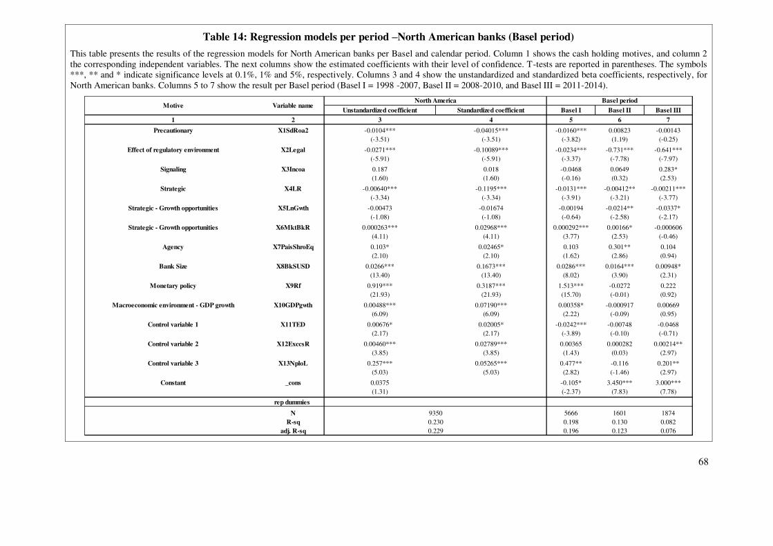
68
Table 14: Regression models per period –North American banks (Basel period)
This table presents the results of the regression models for North American banks per Basel and calendar period. Column 1 shows the cash holding motives, and column 2 the corresponding independent variables. The next columns show the estimated coefficients with their level of confidence. T-tests are reported in parentheses. The symbols ***, ** and * indicate significance levels at 0.1%, 1% and 5%, respectively. Columns 3 and 4 show the unstandardized and standardized beta coefficients, respectively, for North American banks. Columns 5 to 7 show the result per Basel period (Basel I = 1998 -2007, Basel II = 2008-2010, and Basel III = 2011-2014).
Unstandardized coefficient Standardized coefficient Basel I Basel II Basel III
1 2 3 4 5 6 7
Precautionary X1SdRoa2 -0.0104*** -0.04015*** -0.0160*** 0.00823 -0.00143(-3.51) (-3.51) (-3.82) (1.19) (-0.25)
Effect of regulatory environment X2Legal -0.0271*** -0.10089*** -0.0234*** -0.731*** -0.641***(-5.91) (-5.91) (-3.37) (-7.78) (-7.97)
Signaling X3Incoa 0.187 0.018 -0.0468 0.0649 0.283*(1.60) (1.60) (-0.16) (0.32) (2.53)
Strategic X4LR -0.00640*** -0.1195*** -0.0131*** -0.00412** -0.00211***(-3.34) (-3.34) (-3.91) (-3.21) (-3.77)
Strategic - Growth opportunities X5LnGwth -0.00473 -0.01674 -0.00194 -0.0214** -0.0337*(-1.08) (-1.08) (-0.64) (-2.58) (-2.17)
Strategic - Growth opportunities X6MktBkR 0.000263*** 0.02968*** 0.000292*** 0.00166* -0.000606(4.11) (4.11) (3.77) (2.53) (-0.46)
Agency X7PaisShroEq 0.103* 0.02465* 0.103 0.301** 0.104(2.10) (2.10) (1.62) (2.86) (0.94)
Bank Size X8BkSUSD 0.0266*** 0.1673*** 0.0286*** 0.0164*** 0.00948*(13.40) (13.40) (8.02) (3.90) (2.31)
Monetary policy X9Rf 0.919*** 0.3187*** 1.513*** -0.0272 0.222(21.93) (21.93) (15.70) (-0.01) (0.92)
Macroeconomic environment - GDP growth X10GDPgwth 0.00488*** 0.07190*** 0.00358* -0.000917 0.00669(6.09) (6.09) (2.22) (-0.09) (0.95)
Control variable 1 X11TED 0.00676* 0.02005* -0.0242*** -0.00748 -0.0468(2.17) (2.17) (-3.89) (-0.10) (-0.71)
Control variable 2 X12ExccsR 0.00460*** 0.02789*** 0.00365 0.000282 0.00214**(3.85) (3.85) (1.43) (0.03) (2.97)
Control variable 3 X13NploL 0.257*** 0.05265*** 0.477** -0.116 0.201**(5.03) (5.03) (2.82) (-1.46) (2.97)
Constant _cons 0.0375 -0.105* 3.450*** 3.000***(1.31) (-2.37) (7.83) (7.78)
rep dummies
N 5666 1601 1874R-sq 0.198 0.130 0.082
adj. R-sq 0.196 0.123 0.076
North AmericaMotive Variable name
93500.2300.229
Basel period
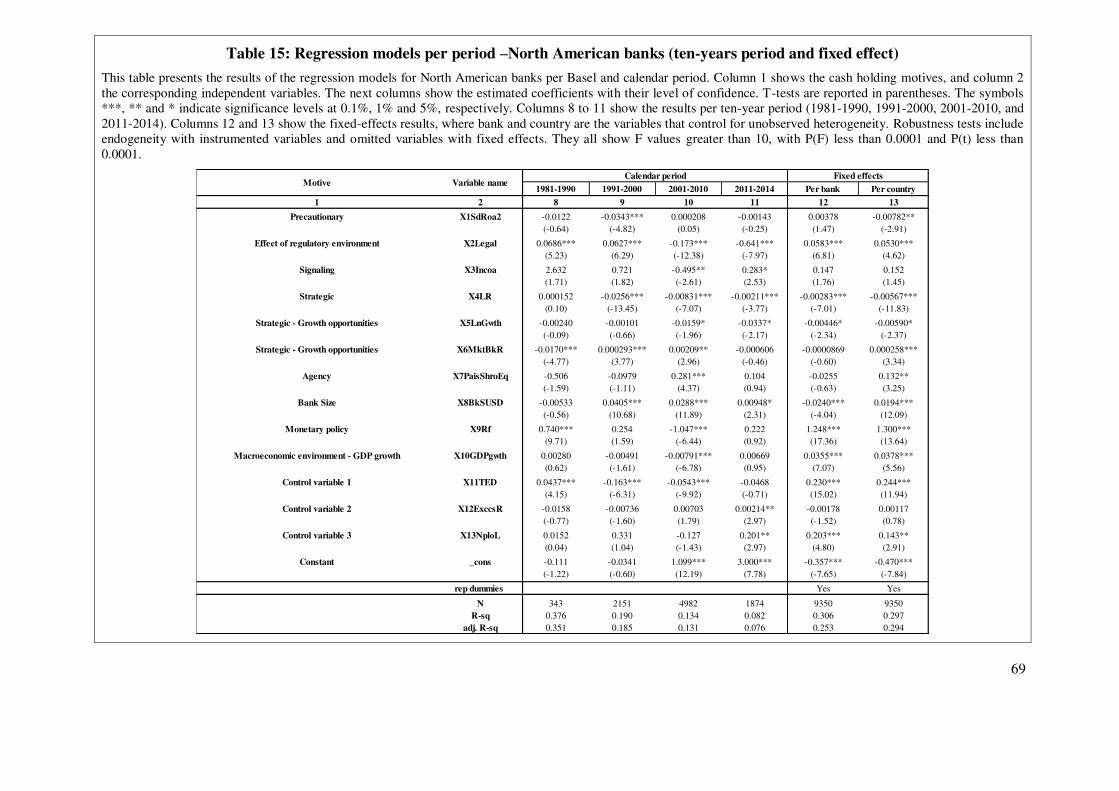
69
Table 15: Regression models per period –North American banks (ten-years period and fixed effect)
This table presents the results of the regression models for North American banks per Basel and calendar period. Column 1 shows the cash holding motives, and column 2 the corresponding independent variables. The next columns show the estimated coefficients with their level of confidence. T-tests are reported in parentheses. The symbols ***, ** and * indicate significance levels at 0.1%, 1% and 5%, respectively. Columns 8 to 11 show the results per ten-year period (1981-1990, 1991-2000, 2001-2010, and 2011-2014). Columns 12 and 13 show the fixed-effects results, where bank and country are the variables that control for unobserved heterogeneity. Robustness tests include endogeneity with instrumented variables and omitted variables with fixed effects. They all show F values greater than 10, with P(F) less than 0.0001 and P(t) less than 0.0001.
1981-1990 1991-2000 2001-2010 2011-2014 Per bank Per country
1 2 8 9 10 11 12 13
Precautionary X1SdRoa2 -0.0122 -0.0343*** 0.000208 -0.00143 0.00378 -0.00782**(-0.64) (-4.82) (0.05) (-0.25) (1.47) (-2.91)
Effect of regulatory environment X2Legal 0.0686*** 0.0627*** -0.173*** -0.641*** 0.0583*** 0.0530***(5.23) (6.29) (-12.38) (-7.97) (6.81) (4.62)
Signaling X3Incoa 2.632 0.721 -0.495** 0.283* 0.147 0.152(1.71) (1.82) (-2.61) (2.53) (1.76) (1.45)
Strategic X4LR 0.000152 -0.0256*** -0.00831*** -0.00211*** -0.00283*** -0.00567***(0.10) (-13.45) (-7.07) (-3.77) (-7.01) (-11.83)
Strategic - Growth opportunities X5LnGwth -0.00240 -0.00101 -0.0159* -0.0337* -0.00446* -0.00590*(-0.09) (-0.66) (-1.96) (-2.17) (-2.34) (-2.37)
Strategic - Growth opportunities X6MktBkR -0.0170*** 0.000293*** 0.00209** -0.000606 -0.0000869 0.000258***(-4.77) (3.77) (2.96) (-0.46) (-0.60) (3.34)
Agency X7PaisShroEq -0.506 -0.0979 0.281*** 0.104 -0.0255 0.132**(-1.59) (-1.11) (4.37) (0.94) (-0.63) (3.25)
Bank Size X8BkSUSD -0.00533 0.0405*** 0.0288*** 0.00948* -0.0240*** 0.0194***(-0.56) (10.68) (11.89) (2.31) (-4.04) (12.09)
Monetary policy X9Rf 0.740*** 0.254 -1.047*** 0.222 1.248*** 1.300***(9.71) (1.59) (-6.44) (0.92) (17.36) (13.64)
Macroeconomic environment - GDP growth X10GDPgwth 0.00280 -0.00491 -0.00791*** 0.00669 0.0355*** 0.0378***(0.62) (-1.61) (-6.78) (0.95) (7.07) (5.56)
Control variable 1 X11TED 0.0437*** -0.163*** -0.0543*** -0.0468 0.230*** 0.244***(4.15) (-6.31) (-9.92) (-0.71) (15.02) (11.94)
Control variable 2 X12ExccsR -0.0158 -0.00736 0.00703 0.00214** -0.00178 0.00117(-0.77) (-1.60) (1.79) (2.97) (-1.52) (0.78)
Control variable 3 X13NploL 0.0152 0.331 -0.127 0.201** 0.203*** 0.143**(0.04) (1.04) (-1.43) (2.97) (4.80) (2.91)
Constant _cons -0.111 -0.0341 1.099*** 3.000*** -0.357*** -0.470***(-1.22) (-0.60) (12.19) (7.78) (-7.65) (-7.84)
rep dummies Yes Yes
N 343 2151 4982 1874 9350 9350R-sq 0.376 0.190 0.134 0.082 0.306 0.297
adj. R-sq 0.351 0.185 0.131 0.076 0.253 0.294
Fixed effectsMotive Variable name
Calendar period
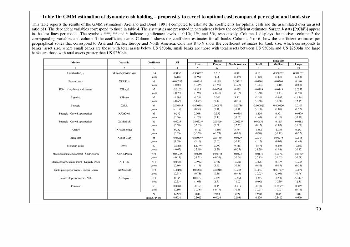
70
Table 16: GMM estimation of dynamic cash holding – propensity to revert to optimal cash compared per region and bank size
This table reports the results of the GMM estimation (Arellano and Bond (1991)) computed to estimate the coefficients for optimal cash and the assimilated over an asset ratio of t. The dependent variables correspond to those in table 4. The z statistics are presented in parentheses below the coefficient estimates. Sargan J-stats [P(Chi²)] appear in the last lines per model. The symbols ***, ** and * indicate significance levels at 0.1%, 1%, and 5%, respectively. Column 1 displays the motives, column 2 the corresponding variables and column 3 the coefficient name. Column 4 shows the coefficient estimates for all banks. Columns 5 to 6 show the coefficient estimates per geographical zones that correspond to Asia and Pacific, Europe and North America. Columns 8 to 9 show the coefficient estimates for bank size, which corresponds to banks’ asset size, where small banks are those with total assets below US $50bln, small banks are those with total assets between US $50bln and US $250bln and large banks are those with total assets greater than US $250bln.
Apac Europe North America Small Medium Large1 2 3 4 5 6 7 8 9 10
Cash holdingi,t-1 YCaaoA previous year b14 0.915* 0.930*** 0.716 0.871 0.631 0.968*** 0.978***_cons (2.18) (5.97) (1.06) (1.07) (1.83) (4.87) (7.52)
Precautionary X1SdRoa b1 -0.00782 -0.0310 -0.118 0.597** -0.0701 -0.0364 0.140_cons (-0.08) (-0.49) (-1.90) (3.22) (-0.43) (-1.10) (0.88)
Effect of regulatory environment X2Legal b2 -0.0163 0.115 -0.00794 0.438 -0.0189 -0.0143 0.0353_cons (-0.76) (1.95) (-0.48) (1.12) (-0.50) (-1.43) (1.90)
Signaling X5Incoa b3 -1.994 -1.764 0.546 3.501 -5.104 -0.965 -11.36*_cons (-0.66) (-1.77) (0.14) (0.36) (-0.58) (-0.30) (-2.15)
Strategic X6LR b4 -0.000445 0.000301 0.000875 -0.00786 -0.000926 0.000626 0.0107_cons (-1.19) (0.50) (0.18) (-1.18) (-0.08) (1.09) (1.92)
Strategic - Growth opportunities X5LnGwth b5 0.392 0.0634 0.352 -0.0508 1.456 0.371 -0.0379_cons (0.36) (1.20) (0.41) (-0.09) (1.47) (1.10) (-0.16)
Strategic - Growth opportunities X6MktBkR b6 0.0223 -0.0632** 0.00469 -0.00233* 0.00631 0.115 -0.0882_cons (0.68) (-3.05) (0.08) (-2.33) (0.12) (1.83) (-1.60)
Agency X7PaisShroEq b7 0.232 -0.729 -1.456 5.784 1.352 -1.353 0.283_cons (0.33) (-0.69) (-1.77) (0.95) (0.99) (-1.41) (0.22)
Bank Size X8BkSUSD b8 0.0322 0.0309** 0.00130 -0.0129 0.0304 0.00275 0.0515_cons (1.59) (3.16) (0.05) (-0.11) (1.12) (0.07) (1.49)
Monetary policy X9Rf b9 -0.0268 -1.137** 0.790 9.115 -0.471 0.440 -0.160_cons (-0.07) (-2.99) (1.20) (0.35) (-1.29) (1.88) (-0.42)
Macroeconomic environment - GDP growth X10GDPgwth b10 -0.00225 -0.0209 -0.00344 -0.0423 -0.0175 -0.00723 -0.00499_cons (-0.11) (-1.21) (-0.39) (-0.06) (-0.83) (-1.05) (-0.69)
Macroeconomic environment - Liquidity shock X11TED b11 0.0423 0.0922 0.427 -0.287 0.0643 0.109 0.0258_cons (0.86) (1.15) (1.65) (-0.16) (0.86) (0.87) (0.33)
Banks profit performance - Excess Return X12ExccsR b12 0.00458 0.00687 0.00210 0.0216 -0.00101 0.00193* -0.172_cons (0.58) (0.78) (0.59) (0.43) (-0.03) (2.06) (-0.96)
Banks risk performance - NPL X13NploL b13 0.795 0.00350 2.823 -2.651 1.385 -0.537 -5.342*_cons (0.53) (1.65) (1.71) (-1.02) (0.90) (-0.50) (-2.31)
Constant b0 0.0288 -0.160 -0.351 -1.719 -0.107 -0.00567 0.349_cons (0.10) (-0.46) (-0.77) (-0.45) (-0.21) (-0.03) (0.76)
N 14229 2842 2163 9224 12585 1096 548Sargan J P(chi²) 0.6031 0.3063 0.6056 0.6031 0.676 0.3402 0.699
Bank sizeMotive Variable Coefficient All
Region
71
Chapter 2. Does an increase in capital negatively impact banking liquidity creation?
2.1 Abstract, keywords and JEL classification
From a dataset composed of a panel of 940 listed banks based in European,
American and Asian countries, this paper documents the evolution of bank liquidity creation
over a 35-year period (1981-2014).
The empirical evidence confirms that risk and equity levels play a significant and
negative role. Overall, the negative effects of equity increases on bank liquidity creation are
more significant than corresponding positive effects on risk management, suggesting that
capital requirements imposed to support financial stability negatively affect liquidity creation.
These findings have broad implications for policymakers.
Keywords: Liquidity creation, sensitivity analysis, GMM, Cox regression
JEL Classifications: C3 - Econometric Methods: Multiple/Simultaneous Equation
Models; C53 -Forecasting and Other Model Applications; G21 - Banks; Other Depository
Institutions; Mortgages.
72
2.2 Introduction
Throughout modern finance theory, and according to Diamond and Dybvig (1983) in
particular, there has been a consensus that the primary purpose of banks is to create liquidity.
Two main facets of banks represent their inherent characteristics, but these two elements can
also be a source of weakness: By transforming liquid liabilities into illiquid assets, banks
expose themselves to liquidity mismatching, which in turn results in structural fragility.
Nonetheless, do banks create liquidity and if so, what types of banks achieve this
goal? In addition, how has this pattern of liquidity creation evolved over time? Finally, do any
increases in equity have a positive effect overall? Although liquidity creation is acknowledged
as the primary goal of banks, paradoxically, only a few empirical studies have attempted to
address such questions, and these have only focused on limited periods and countries. The
first attempt in this respect, by Deep and Schaefer (2004), is based on a panel of 200 US
commercial banks over a period of four years (Q2 1997 to Q2 2001). Their work presents
clues to the determinants of liquidity creation and concludes that credit risk inhibits the
liquidity creation process. The second study, by Berger and Bouwman (2009), which
examines a panel of 9,095 US banks over 11 years (1993-2003), shows that bank size plays a
positive role in the process. A third work focuses on German banks over a period of 10 years
(1999-2009) and attempts to determine the impact of banking regulation on liquidity creation
(Berger, Bouwman, Kick and Schaeck (2011)).
Several studies have examined banking liquidity creation in other countries, such as
Lei and Song (2013) in reference to China; Pana (2012) in reference to Japan; Lakštutienė and
Krušinskas (2010) in reference to Lithuania; Al-Khouri (2012) in reference to Bahrain,
73
Kuwait, Oman, Qatar, Saudi Arabia and the United Arab Emirates; Hackethal, Rauch, Steffen
and Tyrell (2010) in reference to Germany; Fungáčová, Weill and Zhou (2010) and
Fungáčová and Well (2012) in reference to Russia; Esterhuysen, Vuuren and Styger (2012) in
reference to South Africa; and Horváth, Seidler and Weill (2014) in reference to the Czech
Republic. All of these authors measure bank liquidity creation and test the effects of certain
factors on it. Capital, risk, and macroeconomic factors are nearly always considered in these
studies. Performing the analyses presented in this paper on an international sample of banks is
therefore not new.
While these works shed valuable light on banking liquidity creation, they still
perform analyses of specific countries and for limited periods (typically over ten years).
However, a review of the literature review indicates that no empirical research has undertaken
a unified and large cross-country analysis of liquidity creation over a period of more than 10
years. Given the potential effects of exogenous variables – such as economic recession and
monetary policy – on bank liquidity creation, an examination of a shorter period of less than
10 years and of only one country may influence a study’s determinants substantially.
To address this gap, I examine liquidity creation over a period of 35 years and across
the following geographic zones: Asia-Pacific, Europe, and North America. Additionally, I
attempt to determine whether capital increases positively affect liquidity creation.
To address this question, this paper is organized as follows. The first section reviews
the literature on liquidity creation, and the second section shows how the various
methodologies employed to compute liquidity creation levels have been adapted to this
dataset. A dataset of 940 listed banks extracted from Thomson Reuters has been established
that gathers financial and market data from 29 countries over more than three decades. These
74
data have been supplemented with macroeconomic data from the Bank of International
Settlement and from the International Monetary Fund.
The results demonstrate that the evolution of liquidity creation is somehow
heterogeneous across the examined regions. The last section of this paper is composed of
three parts as follows. First, a model for identifying determinants and liquidity creation
processes is presented. To address issues of endogeneity, I employ a multivariate dynamic
panel model using a GMM (Generalized Method of Moment) estimator as established by
Arellano and Bover (1995). In addition, OLS with a fixed effects estimator is presented to
ensure that it is not affected by omitted variables or other biases that would otherwise weaken
it. Second, a Cox regression (Cox (1972)) is used to establish a hazard model, which makes it
possible to determine a bank’s propensity to create liquidity. This makes it possible to
construct a profile of banks that create more liquidity than others based on inherent
characteristics such as size, risk level and equity level. Finally, a sensitivity analysis is
conducted to extend the core results and to estimate the marginal effect of an equity increase
on liquidity creation and risk management performance. General implications are presented
for policymakers in the conclusion.
2.3 Literature review on liquidity creation
This section reviews the literature on bank liquidity creation and its determinants.
2.3.1 Litterature review
Although Smith (1776) was the first to emphasize the role of banks in financing the
economy, the mainstream literature on bank liquidity creation dates back to the 1980s with the
75
work of Diamond and Dybvig (1983). Indeed, the model developed by the authors provides
the most comprehensive theoretical explanation regarding why it is important for banks to
hold a mix of illiquid loans and liquid assets. In addition, it helps practitioners to understand
that banks create liquidity by funding illiquid assets, such as loans with liquid liabilities, such
as deposits. It also shows that the fragile capital structures of banks are caused precisely by
this liquidity mismatch. Moreover, this liquidity creation process cannot be disassociated
from the risk transformation process, whereby banks transform risk by issuing riskless
deposits to fund risky loans (Ramakrishnan and Thakor (1984); Boyd and Prescott (1986)).
By issuing short-term deposits while lending against a medium- or long-term horizon, banks
expose themselves to interest rate fluctuations and counterparty defaults on payments. This
transformation, coupled with risk management (Diamond and Rajan (2001 )), is thus the
defining characteristic of banks.
Thus, do equity level increases contribute to the creation or destruction of liquidity?
Two opposing views address this subject; the first, “risk absorption hypothesis” (Berger and
Bouwman (2009)), contends that equity levels have a moderator or buffer effect on risk. With
increases in the probability of defaults arising as loans increase (Allen and Santomero
(1997)), increases in equity levels enable banks to absorb risks (Repullo (2005); Coval and
Thakor (2005)). In this respect, this risk-buffer effect favors liquidity creation. In other words,
an increase in equity levels reduces risk, making it possible to increase bank loan capacities
and thus liquidity creation. The second view, “financial fragility-crowding out hypothesis”
(Berger and Bouwman (2009)), contends that a bank’s level of equity contributes to the
destruction of liquidity, i.e., as deposits are immediately available, they offer more insurance
for short-term investors than illiquid equities (Gorton and Winton (2000)). As a result, and
because equities are illiquid, capital providers are more reluctant to fund banks (Diamond and
76
Rajan (2001); Diamond and Rajan (2000)); thus, this view assumes that liquidity is a form of
indirect insurance for depositors and that equilibrium is to be found by investors in short-term
(deposits) and medium- to long-term (equity) investments. If equities are preferred, it is to the
detriment of deposits, which mechanically decreases the capacity of banks to create liquidity.
In essence, there is an arbitrage effect between the preference for illiquid liabilities (equities)
and liquid liabilities (deposits) within a context of limited resources.
Other factors may contribute to liquidity creation. According to Kashyap, Rajan and
Stein (2002), both sides of a bank’s assets cannot be dissociated due to their mutual synergies.
These synergies between deposits and loan commitments create a form of liquidity provision
that contributes to liquidity creation (Kashyap, Rajan and Stein (2002). In addition,
supervisory regimes and regulatory stringency may also affect whether banks decide to
consider risk (Berger, Bouwman, Kick and Schaeck (2011).
Two approaches to measuring liquidity creation have been identified. The first,
proposed by Deep and Schaefer (2004), defines liquidity as a gap between liquid liabilities
and liquid assets, i.e., it shows the amount of transformed liquidity over total assets. The
second approach, created by Berger and Bouwman (2009), proposes a protocol that makes it
possible to construct a comprehensive measure of liquidity. It essentially dissociates liquid
assets/liabilities from illiquid assets/liabilities and establishes a three-step protocol for
computing liquidity creation, which can be summarized as follows: (1) classify asset
liabilities and off-balance sheet items with a certain degree of liquidity based on two types of
criteria (category or maturity), (2) assign to them three types of weight (+0.5; 0 or -0.5) and
(3) combine these two steps. The use of weights is justified by the “dollar-for-dollar adding
up constraints” argument, which is as follows. Assume that a bank holds $1 in liquid
liabilities, such as deposit claims, and that it uses this $1 to finance a loan, which is an illiquid
77
asset. The weighted protocol ensures that liquidity creation is indeed $1, where half of the $1
of liquid liability + half of the $1 of illiquid asset = $1 of created liquidity. In effect, $1 is
created when the bank transforms $1 of a deposit into a $1 loan. Similar reasoning is applied
to cases of liquidity destruction.
An additional measure presented by Fungáčová, Weill and Zhou (2010) is a gross
measure that has the advantage of providing an overall understanding of liquidity creation. By
applying assumptions that are less strict than other measures, it does not use detailed
categories or maturity classifications of different balance sheets items. On the assets side, total
loans are assumed to be illiquid, and current account and securities investments are assumed
to be liquid. On the liabilities side, total deposits are treated as liquid liabilities and equity is
treated as illiquid liabilities.
Another measure of liquidity exists, that is the Liquidity Mismatch Index
(Brunnermeier, Gorton and Krishnamurthy (2014). Because this index measures the
difference between the “asset price in times of crisis relative to the maturity structure of the
liabilities”, it takes into account the fact that liquidity of assets is endogenous: there is indeed
an interaction between funding and market liquidity (Brunnermeier and Pedersen (2009)) and
also between capital and liquidity problems (Allen and Gale (2004). This interaction can
generate a loop effect when the financial sector runs into liquidity problem, leading to further
asset price reduction, which in turns worsens the liquidity of the markets. This index thus
measures the risk for banks to be short of liquidity in adverse scenario, whereas the liquidity
measures of Deep and Schaefer (2004), Berger and Bouwman (2008) and Fungáčová, Weill
and Zhou (2010) measure the liquidity created by banks.
78
2.3.2 Determinants of l iquidity creation
Which elements determine liquidity creation? Different variables may interact within
liquidity creation processes. Based on the literature review, the effect of bank size and the
relationship between a bank’s role as a risk transformer and liquidity creator were identified
as the elements that are most likely to substantially interfere with liquidity creation.
Additional parameters, such as the level of equity, monetary policy and the legal environment,
are also explored. The determinants can be categorized into two sets of indicators: specific
and environmental bank factors.
2.3.2.1 Specific bank factors include the following.
Four bank specific factors have been identified: (1) bank size, (2) level of risk, (3)
level of equity and (4) bank performance.
Bank size: The relation between bank size and liquidity creation is due to several
factors. For instance, Houston, James and Marcus (1997) demonstrate that capital market
imperfections oblige banking group to put in place internal capital markets. Consequently,
bigger banks reduce their transaction cost, which enable them to optimize the allocation of
funding sources among their branches and subsidiaries. Given the empirical evidence
presented by Kashyap, Rajan and Stein (2002) that highlighted the synergy between deposit
taking and lending, as well as the relationship between bank size and transaction deposits, the
size of a bank may have a significant effect on liquidity creation. Following Demirgüç-Kunt
and Huizinga (2011), the log of total assets is a proxy for the size of a bank.
Level of equity: The role of equity levels in liquidity creation is documented by
Gorton and Winton (2000) and Diamond and Rajan (2001), who establish that higher capital
levels diminish liquidity creation as they negate deposit collection. Berger and Bouwman
79
(2009) elaborate two hypotheses to offer explanation for the substitution relationship between
liquidity creation and the level of capital. The first posits that given the limited access to
resources, if level of equity increases it is at the detriment of liquid assets and thus reduces the
liquidity creation. The second posits that increase of capital, reduces the risk, which provides
more resources allocated to loans, thus augments the liquidity creation. In this paper, the
equity variable is scaled over the assets. I acknowledge that the bank capital structure plays an
important role in the risk management (Laeven and Levine (2009)). Also, the bank capital
structure reflects not only its own characteristics, but also the environment in which it
operates (De Jonghe and Öztekin (2015)). Because bank capital structure is not available in
Thomson Reuters database, the level of risk is used to take into consideration the effect of
bank capital structure on risk management (see below). In addition, I have also accounted for
the exogenous factors that may influence the capital of banks in the section “Environmental
factors”.
Level of risk: The role of banks as risk transformers is examined widely in the
literature. According to Diamond (1984) and Ramakrishnan and Thakor (1984), banks finance
risky loans by issuing riskless deposits. However, the strength of the relationship between
liquidity creation and risk transformation has not been explored fully, and there is no evidence
that they vary in perfect parallel to one another. Reliance on performance indicators such as
RoE are a key incentive to excessive risk-taking in banks, as shown by Moussu and Petit-
Romec (2014). In this paper, bank risk is measured using approach, namely, the standard
deviation of RoE. For robustness and following Imbierowicz and Rauch (2014), I add the
credit risk level typically calculated by non-performing loans over loans and bank stability
risk or z-scores (as originally proposed by Roy (1952)).
80
Bank performance: Following Hackethal, Rauch, Steffen and Tyrell (2010), I include
a set of similar indicators, such as operating income (before taxes and exceptional profits or
losses), but also commonly used indicators to proxy bank performance, such as dividends
paid over equity, loan growth, Jensen’s excess return (as originally proposed by Jensen
(1968)) and the market price of the bank shares.
2.3.2.2 Environmental factors include the following.
Two environmental factors have been identified: (1) institutional regulatory
framework and (2) macro-economic factors.
Institutional regulatory framework: As argued by Berger, Bouwman, Kick and
Schaeck (2011), the supervisory regime can affect bank risk taking. To control this effect, and
because regulations in this regard vary across countries and over time, I have created a
supervisory index similar to that used by Shehzad, de Haan and Scholtens (2010). However,
the World Bank’s 2007 Regulation and Supervisory Database (Barth, Caprio and Levine
(2008)) has been maintained over a relatively short period of time. For this reason, the index
has been drawn from two sources and calculated for four periods corresponding to the
following: (1) before Basel I, (2) from Basel I to II, (3) from Basel II to III and (4) since Basel
III. For the before Basel I period, I follow La Porta, Lopez-De-Silanes, Shleifer and Vishny
(1997), who established legal zones for measuring the effect of the legal environment on
capital market development. To measure the effect of the legal environment on liquidity
creation, I use a similar mapping exercise whereby a grade is used to represent the level of
property rights protection (0 to 4, corresponding to “not protective” to “most protective”).
Second, the regulatory environment mapping of banks is adapted from Barth, Caprio and
Levine (2008)); Barth, Caprio Jr and Levine (2001) for the last three periods corresponding to
81
the Basel regulatory framework deployment (Barth, Caprio and Levine (2008). This summary
averages out capital stringency and capital activity and restrictions for each period. When
banks are subjected to high levels of scrutiny from regulatory agencies, they tend to lower
their risk exposure while managing their liquidity needs more efficiently. The relationship
between tight supervisory control and bank risk-taking behavior is expected to be negative. A
decrease in risk implies that less liquidity destruction is present, and this in turn contributes to
liquidity creation. Thus, a positive regulatory framework coefficient is predicted with regard
to liquidity creation.
Macroeconomic factors: Following Imbierowicz and Rauch (2014), Hackethal,
Rauch, Steffen and Tyrell (2010) and Lei and Song (2013), I include GDP and the
unemployment rate. Government monetary policy effects are also considered in this paper and
are supported by two traits. As Bernanke and Gertler (1995) established, a relatively low
government-set interest rate encourages credit supply. Furthermore, Hackethal, Rauch,
Steffen and Tyrell (2010) established the close relationship between liquidity and risk
transformation. A relaxed monetary policy ends by positively increasing bank liquidity and
risk transformation capabilities. The relationship between monetary policy and liquidity
creation is thus in opposition in that a decrease in the interest rate is expected to increase
liquidity creation. Because the money supply is typically ensured by the government interest
rate, in this paper, the 10-year government bond rate and the LT-ST spread are used to assess
the effect of a country’s monetary policy on liquidity creation in the banking sector. The use
of this metric is justified by the sensitivity of bank lending/borrowing to this maturity yield
and by the effect of the ST-LT spread structure on a bank’s profit margin (Bernanke, Gertler
and Gilchrist (1999)). In addition, to control for the “interbank liquidity shock effect,” I
follow Cornett, McNutt, Strahan and Tehranian (2011) and for each country use the TED

82
spread indicator, which is the spread between interbank loans and government bonds with
maturities of 3 months or thereabouts. Other macroeconomic metrics are also utilized: GDP
growth and the unemployment rate, which assumes that a positive economic context
encourages investment, which in turn triggers loan demand. To control for market
competition and following Lei and Song (2013), I include the bank-level Herfindahl market
competition index (HHI). Based on the loan market share for each country where bank
headquarters are located, this variable proxies for market concentration. As shown by Beck,
Demirguc-Kunt and Maksimovic (2004), market concentration impacts the availability of
credit and therefore may affect liquidity creation.
The tables below summarize the determinants for estimating liquidity creation and
how they have been computed.
Insert Tables 17 and 18.
2.4 Methodology used to estimate liquidity creation
Based on three approaches, this section describes the proxies to estimate liquidity
creation and compares the liquidity measures with those utilized by their authors, to check for
their correctness.
Note that the dataset is composed of variables extracted from a Thomson Reuters
database and they do not correspond fully with those used by the authors. Because Thomson
Reuters defines assets and liabilities according to their accounting classification, information
on customer types and off balance sheets are non-existent. Thus, I adopted the following three
measures:
83
Liquidity transformation (LT) gap as established by Deep and Schaefer
(2004), calculated as (liquid liabilities minus liquid assets) / total assets. In
this article, this measure is abbreviated as “LTGap”.
Gross liquidity creation measure (LGM) as established by Fungáčová, Weill
and Zhou (2010). A simple measure that classifies all loans as illiquid and all
deposits as liquid. In this article, this measure is abbreviated as “LGM”.
BB-MatNonFat as established by Berger and Bouwman (2009). This measure
calculates liquidity creation using a 3‐step procedure: it first classifies bank
activities as liquid / semi‐liquid / illiquid using information on both product
category and maturity of each activity, except that for loans only maturity
information is used (due to data limitations); it then applies a weighting
scheme to these activities; finally, it calculates the dollar amount of liquidity
created by an individual bank by multiplying the dollar amounts in the
different buckets by the weights and summing the weighted amounts. In this
article, this measure is abbreviated as “BB-MatNonFat”, where Mat means
that the balance sheet items have categorized by maturity and NonFat means
that the off balance sheet is excluded because of Thomson Reuter’s
limitations that do not have these data.
Because of Thomson Reuters’ limitations on maturity, I followed Distinguin, Roulet
and Tarazi (2013) to compute the liquidity measures. As a result, for US banks, the deposits
were weighted at 33%, whereas for other banks, they were weighted at 80%. The net loans are
all weighted at 85%. All amounts were deflated by the IMF inflation index (base 2005). The
table below shows how these three measures were proxied and presents the Thomson Reuters
items that were used to compute them. Notice that the time-series data are inflation adjusted
84
(base 2005) from the IMF inflation index for each country and are counter evaluated in US$
at the IMF foreign exchange rate for each end of calendar year.
Insert Table 19.
Overall, these liquidity creation measures are consistent with those utilized by the
works described above, although the dataset established herein helps to construct metrics for a
larger range of countries and for a longer period of time.
Insert Table 20.
For a similar period (1997-2001) and US banks, the LT gap computed with the
protocol aforementioned has a mean of 0.17, a median of 0.19 and a standard deviation of
0.08, whereas the same metric computed by the authors Deep and Schaefer (2004) records a
mean of 0.20, a median of 0.19 and a standard deviation of 0.16. The difference of the
standard is due to the fact that the authors of the LT Gap used quarterly data, whereas I used
annual data.
For a similar period (1993-2003) and US banks, the MatNonFat measure computed
with the aforementioned protocol has a mean of 0.25 in 1993 and of 0.27 in 2003, whereas the
CatNonFat9 measure computed by the authors Berger and Bouwman (2009) record 0.22 and
0.26 respectively. Note that the authors do show only means of CatNonFat measures, making
it difficult to conduct a strict comparison. Median and standard were not indicated in their
article.
9 Where Mat means that the balance sheet items have categorized by maturity, whereas Cat means
that the balance sheet have been categorized by category of products; Fat means that the off balance sheet is
included, whereas NonFat means that the off balance sheet data are excluded.
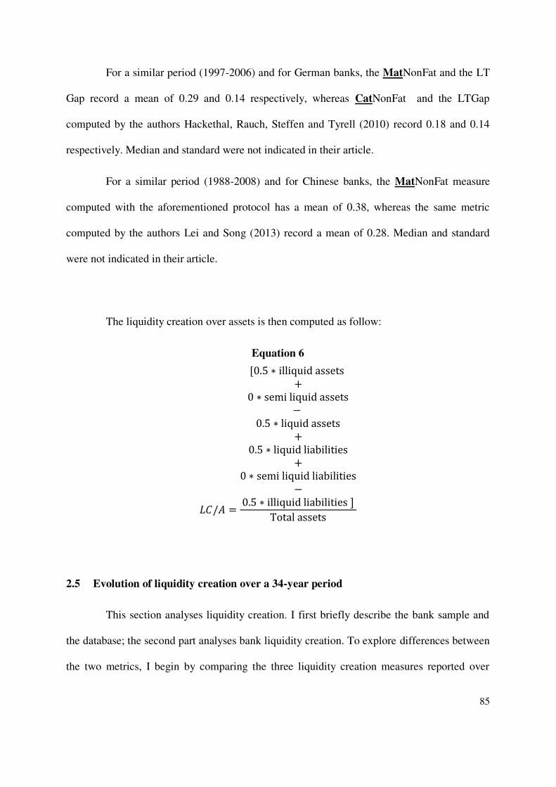
85
For a similar period (1997-2006) and for German banks, the MatNonFat and the LT
Gap record a mean of 0.29 and 0.14 respectively, whereas CatNonFat and the LTGap
computed by the authors Hackethal, Rauch, Steffen and Tyrell (2010) record 0.18 and 0.14
respectively. Median and standard were not indicated in their article.
For a similar period (1988-2008) and for Chinese banks, the MatNonFat measure
computed with the aforementioned protocol has a mean of 0.38, whereas the same metric
computed by the authors Lei and Song (2013) record a mean of 0.28. Median and standard
were not indicated in their article.
The liquidity creation over assets is then computed as follow:
Equation 6
��/� =
[0.5 ∗ illiquid assets
+
0 ∗ semi liquid assets−
0.5 ∗ liquid assets
+
0.5 ∗ liquid liabilities
+
0 ∗ semi liquid liabilities−0.5 ∗ illiquid liabilities ]
Total assets
2.5 Evolution of liquidity creation over a 34-year period
This section analyses liquidity creation. I first briefly describe the bank sample and
the database; the second part analyses bank liquidity creation. To explore differences between
the two metrics, I begin by comparing the three liquidity creation measures reported over
86
assets. The second section presents liquidity creation levels valued in billions of US dollars
per year and per geographic zone, and the final section compares the evolution of liquidity
creation and risk to the equity level for each period. The following four periods are examined:
(1) before Basel I (1981-1988), (2) from Basel I to II (1989-2007), (3) from Basel II to III
(2008-2010) and (4) since Basel III (2011 to date). My use of these periods is intuitive and is
justified by the effect of the institutional and regulatory framework that surrounds banking
activity, thus legitimizing my examination of the evolution of banking liquidity creation based
on this timeframe.
2.5.1 Bank sample
This section begins with a short description of the data sources and of the panel
representativeness.
Thomson Reuters referential data have the advantage of providing a somehow
homogeneous set of information, making it possible to create a database of banks with
common items and for a long period of time. To avoid double counting various banks that fall
under the same group, I have carefully selected unique bank values and excluded their
subsidiaries or branches. As shown by Cetorelli and Goldberg (2012), banking groups tend to
establish internal capital markets, and this may skew overall measures of liquidity creation.
Banks selected in the Thomson Reuters database correspond to those classified in ICB
industry sector 800 as “Banks providing a broad range of financial services, including retail
banking, loans and money transmissions,” which may aggregate different lines of business
corresponding to various banking activities (e.g., M&A, commercial banks) or banks with
state involvement (partially state-owned banks, fully private banks). As the aforementioned
87
breakdown was not provided, I followed Imbierowicz and Rauch (2014) and based the bank
typologies on three inherent characteristics: bank size, risk level and the level of capital.
The original number of unique listed banks extracted from Thomson Reuters is 940,
with the minimum and maximum numbers of years ranging from five to 35. The table below
shows a breakdown of the number of banks per geographic zone, country and year, with the
highest number of banks (857) recorded in 2010. North American listed banks include 537
US banks and nine Canadian banks, the latter of which represent a minor portion of this
geographic zone. A total of 166 Asia-Pacific banks are listed, with Japan, India, Taiwan and
China accounting for 84, 36, 20 and 11 listed banks, respectively. A total of 145 are European
banks, with Denmark, Switzerland and Norway accounting for 24, 22 and 21 listed banks,
respectively.
Because the panel data set is composed uniquely of listed banks, it is
dominated by US banks that represent 60% of the number of banks toward the end of the
sample period. However, 95 % of the US banks have a small size of less than $10 bln and
represent around 15% of the sum of assets of all US banks (figures not displayed). Besides,
the coverage of the initial year is rather limited to 60 banks in 1981. This coverage is much
improved in 2000 with 687 banks. The results are thus broken down per geographical zones
(Asia & Pacific, Europe and North America) per period and types bank (small, medium and
large).
Following Berger and Bouwman (2008), I include data from consolidated
financial statement of mother companies, which includes the financial statement of branches
and subsidiaries but eliminates intragroup activities. By excluding subsidiaries and branches, I
avoid double counting the liquidity created by banks and for banks that belong to the same
group, which would have inflated the results otherwise. But this exclusion does not obstruct
88
the results because the panel is sufficiently representative. As can be observed in the table 21
below, the panel dataset indeed covers a substantial fraction of Asia & Pacific, European and
US market.
Table 22 shows a breakdown of the number of banks by geographical zone,
country and year.
Insert Table 21.
Accounting and market data were extracted from the Thomson Reuters data source
on an annual basis for the last 35 years. Foreign exchange rates, GDP growth and the inflation
index have been provided by the IMF at closing end of year since 1981.
Although I acknowledge that this dataset is composed of 94010 listed banks,
excluding small banks, the panel is representative enough as shown in the table below, which
presents the fraction of the market covered per geographical zone by this panel dataset.
Insert Table 22.
10 The number of banks varies per year. This variation is attributable to the fact that newly listed
banks appear in the Thomson Reuter’s database, while merged, delisted or bankrupt banks are omitted.
89
2.5.2 Descriptive statistics
The first table shows the evolution of the three liquidity creation metrics scaled to the
total asset level for each period and geographic zone, thereby making a comparison between
them possible.
Insert Table 23.
Table 23 illustrates the evolution of each period and geographic zone for the three
liquidity creation measures “LTGap,” “LGM” and “BB-MatNonFat” – such as defined in the
section “2.4 Methodology used to estimate liquidity creation” – and scaled over assets. Major
disparities between the geographic zones can be observed. The cause of such disparities is
also due to different factors that compose the structural environment of the banks. In terms of
liquidity creation, the APAC region has created most. Triggered by a strong GDP growth,
which itself is linked to the low economic starting point of the different countries in this
region, such increase is not surprising. This region has also benefited of less compelling
regulatory framework, enabling the banks in this region to allocate their resource on illiquid
assets, and hence finance the economic growth. Developed countries have a higher starting
point, in terms of economic development. Therefore, the liquidity created in North America
and Europe is lower than in APAC region. But US banks have enjoyed a common currency
on their market, whereas European banks had to face different monetary policies until the
euro currency was implemented in 2000. Additionally, the heterogeneous regulatory
framework in Europe has complicated the story for the banks, until the implementation of
Basel III. The budget crisis mainly triggered by Greece in 2010 has brought to light the
necessity for the European countries to converge their budget, legal and fiscal frameworks.
The recent vote for Brexit in UK may accelerate this convergence. The sections below show
these differences.
90
For LTGap (column 4). In the Asia-Pacific region, liquidity creation ratios decreased
from 48% to 44% between 1981 and 2014, with a peak of 50% occurring during the period
1991-2000, which corresponds to the economic boom of the APAC zone. For Europe and
North America, liquidity creation ratios increased steadily from 16% to 26% and from 14% to
22%, respectively, between 1981 and 2014. Median values follow the same trend.
For LGM (column 7). In the Asia-Pacific region, this measure decreased from 57%
to 50%, with a peak of 59% occurring during the period 1991-2000. For Europe, this measure
decreased from 45% to 41%, with a peak of 45% occurring during the period 1991-2000. For
North America, the measure remained relatively stable at 36%, with a peak of 39% occurring
during the period 2001-2010. The median follows the same trend.
For BB-MatNonFat (column 11). In the Asia-Pacific region, this measure decreased
from 51% to 46%, with a peak of 53% occurring during the period 1991-2000. In Europe, the
measure increased from 33% to 37% between 1981-1990 and 1991-2000 and then steadily
decreased to 34% until the period 2011-2014. For North America, the measure remained
relatively stable at approximately 29%.
These findings show that liquidity creation varies significantly across countries and
over time. The figure below illustrates the evolution of liquidity creation for each year and
geographic zone as established by the LGM and BB-MatNonFat measures. Values are
expressed in US$ billion, counter valued at the end-of-year IMF foreign exchange rate and
deflated based on the IMF inflation index (base 2005).
Insert Figure 1.
91
For the Asia-Pacific region (data not reported but indicated in Figure 1), liquidity
creation steadily increased from $153bln to $1 873bln and from $116 to $1 570bln between
1981 and 1999 for the LGM and BB-MatNonFat measures, respectively. In 2000, with the
onset of the Asian Financial crisis, liquidity creation declined and fell to $1 542bln and
$1 293bln for the LGM and BB-MatNonFat measures, respectively. Between 2001 and 2012,
liquidity creation dramatically increased from $2 345bln and $2 030bln to $7 364bln and
$6 411bln for the LGM and BB-MatNonFat measures, respectively. These values started to
decline in 2013 and 2014, falling to $6 780bln and $5 728bln for the LGM and BB-
MatNonFat measures, respectively. Over this period, liquidity creation levels increased 44-
and 49-fold for the LGM and BB-MatNonFat measures, respectively.
In Europe (data not reported but indicated in Figure 1), liquidity creation between
1981 and 2004 increased steadily from $775bln and $632bln to $4 244bln and $2 928bln for
the LGM and BB-MatNonFat measures, respectively. However, in 2005-2006, liquidity
creation suddenly decreased to $3 143bln and $1 622bln. This diminution occurred as a result
of the conjunction of two main factors. First, the EUR/USD rate reached a historical low of
1.16 in December of 2005. The rejection of a referendum on the EC Constitution by France
and the Netherlands, the suspension of the UK’s entry into the euro zone and the increase of
200 basis points to the FED funds rate may explain this rate variance. Second, French banks
hoarded a substantial amount of cash and assimilated in 2005; between 2004 and 2005, cash
and assimilated holdings increased from €572bln to €1 610bln (not shown in the tables). This
substantial increase in liquid assets on the balance sheets of the French banks caused a sudden
upsurge in liquidity destruction, and both the effect of the exchange rate and the relative
increase in liquidity destruction largely explain the overall decline in liquidity creation in
92
Europe in 2005-2006. Between 2007 and 2012, liquidity creation varied from $5 015bln and
$2 511bln to $6 243bln and $3 584bln for the LGM and BB-MatNonFat measures,
respectively. Between 2013 and 2014, signals of financial recovery appeared to be somehow
present with increases to $6 104bln and $3 842bln in 2013, but decreases to $5 162bln and
$3 176bln in 2015 for the LGM and BB-MatNonFat measures, respectively. Over this period,
liquidity creation multiplied seven- and five-fold for the LGM and BB-MatNonFat measures,
respectively.
In North America (data not reported but indicated in Figure 1), between 1981 and
1997, liquidity creation steadily increased from $485bln and $436bln to $1 051bln and
$788bln for the LGM and BB-MatNonFat measures, respectively. Between 1998 and 2013,
this steady increase accelerated from $1 341bln and $1 010bln to $3 324bln and $2 394bln for
the LGM and BB-MatNonFat measures, respectively. In 2014, liquidity creation declined to
$3 250bln and $2 329.bln for the LGM and BB-MatNonFat measures, respectively. Over this
period, liquidity creation levels multiplied seven- and five-fold for the LGM and BB-
MatNonFat measures, respectively.
The next table compares the evolution of liquidity creation to the level of capital and
risk over four periods: (1) before Basel I (1981-1988), (2) from Basel I to II (1989-2007), (3)
from Basel II to III (2008-2010) and (4) since Basel III (2011-present).
Insert Table 24.
While an increase in equity levels is observable across all regions, this was not
followed by a significant decrease in the standard deviation of RoE. In the Asia-Pacific
93
region, from 1981-1988 to 1989-2007, the std. dev. of RoE increased from 2% to 24%. From
2008-2010 to 2011-2014, this measure sharply decreased from 8% to 6%. In Europe, from
1981-1988 to 2011-2014, the std. dev. of RoE steadily increased from 7% to 14%. In North
America, between 1981-1988 and 1989-2007, the std. dev. of RoE remained stable at 5%.
From 2008-2010 to 2011-2014, this variable increased from 11 to 13%.
The median values follow the same trends, though these are again not reported for
the sake of brevity. It can be concluded that an increase in equity may reduce liquidity
creation, but this is not necessarily accompanied by better risk performance.
The following section examines the determinants of liquidity creation and presents a
sensitivity analysis of the effect of marginal increases in equity levels on liquidity creation
and risk performance.
2.6 Econometric model
This section presents the results of the regression model that computes the
determinants of liquidity creation. To establish a profile of banks that generate liquidity
following Pagano, Röell and Zechner (2002) approach for predicting the probability of a
European company listing abroad, a Cox regression is also used. This section concludes with
a sensitivity analysis that compares the marginal effect of an increase in capital levels on both
liquidity creation and risk diminution measures.
94
2.6.1 Determinants of l iquidity creation
Following Berger and Bouwman (2009) and Imbierowicz and Rauch (2014), to
address endogeneity issues, I have constructed a model for estimating a multivariate dynamic
panel model using a GMM11estimator ((Arellano and Bover (1995); Berger and Bouwman
(2009) and Imbierowicz and Rauch (2014); Distinguin, Roulet and Tarazi (2013)).
This model can be notated as follows:
Equation 7
Eq1: Liquidity created over assets i,t = β0 + β18 Liquidity created over assetsi,t-1 +
11 Usually attributed to Hansen, Lars Peter, 1982, Large sample properties of generalized method of
moments estimators, Econometrica 1029-1054., the GMM is the most appropriate tool for controlling
unobserved effects, with regards to liquidity created by banks. First, the liquidity created at time t-1 may have an
autoregressive effect. The autoregressive effect can be intuitively attributed to traditional banking model
contributions to the stable structure of commercial banks: When a loan is granted to a customer, it is typically
allocated for a number of years. The customer may repatriate extra resources that are deposited and may open a
current account, which may in turn be used to finance new loans for the same customer or for other customers.
Second, Hansen showed that every instrumental variables estimator, in nonlinear or linear models, with cross-
section, panel data or time series, could be conceived as a GMM estimator. Considered as a unifying framework
for inference in econometrics, this estimation has the advantage of being robust to the distribution of errors, and
it is considered more efficient than 2SLS (Hall, Alastair R, 2005. Generalized method of moments (Oxford
University Press Oxford). Most commonly tool used when there is endogeneity threat between the dependent
variables, the GMM instruments them with a lagged dependent variable. In this article, the independent variables
act as control variables, with regards to liquidity created at t+1. Also, at lag 2, the GMM coefficient measures the
degree of mean reversion and thus (1-λ) is interpreted as the coefficient of persistence of the explicative variable
Yt-1 for each bank. Refer to proof of evidence in article 1 “Why do banks hold cash?”, equation 4 on how to
interpret the lag 2 coefficient 1-λ.
95
β1 Bank size i,t + β2 Std. dev. RoE i,t + β3 Equity scaled over asset i,t + β4 Non
performing loans over loans i,t + β5 Z-score i,t + β6 cash dividend paid over shareholder’s
equityi,t + β7 Loan growthi,t + β8 Jensen’s excess return i,t + β9 Operating income over assets
i,t + β10 Market value per share i,t + β11 10-years bond yield j,t + β12 Institutional regulatory
framework j,t + β13 GDP growth j,t + β14 HHI market concentration index j,t + β15 LT-ST
yield curve spread j,t + β16 Unemployment rate j,t + β17 Interbank liquidity shock TEDj,t + µ
where the variables are those discussed in the first (literature review) section and
listed in Table 1.
In addition to the GMM models, OLS regressions were conducted using the standard
robust approach and by clustering banks to control for heteroskedasticity. For the omitted
variables, a time-fixed effect test was conducted to check for average variances in liquidity
creation across years that would not be accounted for by the former exogenous variables and
to diminish serial correlation threats. In addition, the regression models were tested to ensure
that no collinearity or size effects were present. They show p-values of less than 0.001 with
Eta² or Omega² values of less than 0.4. Student tests show p-values of less than 0.001. A
correlation matrix is displayed in the table below.
Insert Table 25.
The results of the GMM and OLS regressions are shown in the tables below. Given
the correlations with the z-score and the std. dev. of RoE or operating income, the results are
first presented without the z-scores but with the std. dev. of RoE or operating income and
second with the z-scores but without the std. dev. of RoE or operating income.
Insert Tables 26, 27 and 28.
96
The results of the GMM estimators for the European banks are remarkably similar to
those presented by Hackethal, Rauch, Steffen and Tyrell (2010), although their study focused
only on German banks during the period 1997-2006. For instance, they found that the
liquidity creation estimator at the 2nd correlation had a coefficient of 0.842*** and of
0.938*** for the LTGap and BB (not indicated whether MatNonFat or CatNonFat),
respectively, whereas I found European peers coefficients of 0.910*** and 0.906*** for the
LTGap and BBMatNonFat, respectively. The results for other countries are also similar to
these coefficients, with 0.864*** and 0.809*** found for LTGap values and with 0.910***
and 0.878*** found for BBMatNonFat values for the Asia-Pacific region and North America,
respectively (table 26, columns 6-8). Overall, this indicates that liquidity created at time t-1
has an autoregressive effect. The autoregressive effect can be intuitively attributed to
traditional banking model contributions to the stable structure of commercial banks: When a
loan is granted to a customer, it is typically allocated for a number of years. The customer
may repatriate extra resources that are deposited and may open a current account, which may
in turn be used to finance new loans for the same customer or for other customers. However,
this autoregressive effect remains relatively low and below 0.5 for all regions (i.e., 1-0.910
and 1-0.906 for LTGap and BBMatNonFat of European banks, respectively)12. It results that
this autoregressive effect is not sufficient to harm the OLS specification. Table 28 shows the
coefficient of the other variables for the standard OLS. Monetary policy plays a significant
role in liquidity creation. The 10-year bond yield significantly affects the LTGap, with
expected negative coefficients of -1.256***, -0.619*** and -0.815*** found for the Asia-
Pacific region, Europe and North America, respectively (table 28, columns 4, 6 and 8). The
12 At lag 2, the GMM coefficient measures the degree of mean reversion and thus (1-λ) is interpreted
as the coefficient of persistence of the explicative variable Yt-1 for each bank.
97
unemployment rate, always significant, also affects negatively the liquidity creation. This
confirms that an increase in economic activity results in investment growth, which in turn
triggers loan demand. Bank size and equity levels both play a negative and significant role.
These results confirm the views of Gorton and Winton (2000) and Diamond and Rajan
(2001), according to which higher capital diminishes liquidity creation, i.e., the larger the size
of the bank, the lower the probability of liquidity creation. As larger banks enjoy broader
access to national and international markets, they may finance their loans through
indebtedness rather than by collecting deposits. Conversely, small banks may tend to prefer
collecting deposits in order to fund loans. Finally, the results reported in both the OLS and
fixed effects estimator, which tests for variance between countries, show that bank size and
equity level coefficients are not affected by fixed effects biases, confirming that the
econometric model presented generates accurate estimates. The descriptive statistics and
econometric model provide some evidence of a relationship between equity levels and
banking liquidity creation. However, to compare the explanatory power of the competing
hypotheses and eliminate spurious correlations, I employ a duration analysis to determine
which specific bank characteristics predict the variation in liquidity creation.
2.6.2 Bank typologies that generate more liquidity per geographic zone
This section describes the bank profiles that generate more liquidity than others
based on the Cox regression. Though typically used for survival analysis, I use the Cox
proportional hazard model because it is suited to the prediction of events in a panel setting,
hence to the estimation of distances to liquidity creation. This model reports the hazard rate
98
h(t) (that is, the probability of creating liquidity at time t conditional on not creating liquidity)
for a set of explicative variables:
Equation 8
h(t) = h0(t) exp (X’β)
where h0(t) is the baseline hazard rate at time t for the covariate vector set at 0 and β
is a vector coefficient. The Cox hazard regression is a semi-parametric model, which does not
require assumptions about the baseline hazard. The table below presents the exponentiated
coefficients ((exp(β1), exp (β2),…) rather than the coefficients (β1, β2,…). Exponentiated
coefficients can be interpreted as the effect of a unit change in the explanatory variable on the
hazard ratio h(t) = h0(t). For instance, a coefficient of 1.098 implies that a unit change in the
dependent variable increases the relative hazard by 9.8 percent.
To achieve this goal, I created a survivor function that corresponds with the
derivative of the three following liquidity creation measures: LTGap, LGM and BB-
MatNonFat. Note that the measures are deflated values drawn from the IMF inflation index
(base 2005) for each country. If the function is negative (i.e., if liquidity creation over assets
decreases over two reporting years), it is considered a failure. If the function is positive (i.e., if
liquidity creation over assets increases over two reporting years), it is considered a success.
The table below shows the results and the hazard ratio for specific bank characteristics, bank
sizes, risk levels and equity levels. These explicative variables have been layered to satisfy the
proportional-hazards assumption. For risk levels, the stratification corresponds to the quintile,
where IStratSDRoE_2 corresponds to q1 (less than or equal to 25%); IStratSDRoE_3
corresponds to q2 (less than or equal to 50%) and IStratSDRoE_4 corresponds to q3 (less than
or equal to 75%). In regards to bank size, small banks are those with total assets of less than
99
$US 50bln; medium banks are those with total assets of more than or equal to $US 50bln and
of less than $US 250bln; and large banks are those with total assets of more than or equal to
$US 250bln. Note that the total asset values have been deflated based on the IMF index
inflation rate for each country (base 2005) and then counter revaluated at each end-of-year
US$ IMF foreign exchange rate. For level of equity, stratification values vary from 0%
(“_IStratEqoA_0”) to 17.5% (“_IStratEqoA_5”) with a regular increase of 2.5bp with each
step. Overall, the Wilcoxon tests for the equality of survivor functions for the three liquidity
measures generate a p(χ²) of less than 0.000, demonstrating that the hypothesis of survivor
function equality is not rejected. As the Wilcoxon test gives more weight to tables at earlier
failure times, this test is preferred to the log-rank test when hazard functions are believed to
vary in ways other than proportionally; this is a reasonable assumption given that this paper
focuses on liquidity creation over a period of 35 years.
Insert Table 29.
Although level of risk, bank size and level of equity have a large impact on banking
liquidity creation, the effects vary among the three factors. The results indicate that for the
transformation from liquid liabilities to illiquid assets, the liquidity that generates liquidity
creation is closely linked to risk. The hazard ratio estimated shows a regular increase when
the std. dev. of RoE moves to a higher quintile.
For instance, the estimate decreases but with negative coefficients from -0.249***, -
0.406***, .0568*** for the LTGap and LGM, respectively, in the Asia-Pacific region
(column 4) when the std. dev. of RoE changes from q1 to q3. However, for Europe, the
coefficients are not significant to extrapolate the effects of increase of risk on banking
100
liquidity creation with regard to the semi parametric regression method. However, in North
America, an increase in risk level is followed by a decrease in the estimate. The coefficients
steadily decreases with negative coefficients from -0.176 *** to -0.578*** for the LTGap
when the std. dev. of RoE changes from q1 to q3. Only the LTGap shows significant
coefficients for all regions and for the risk level criteria. The results suggest that Asia-Pacific
and North American banks tend to generate liquidity for less risky projects than those of their
European counterparts.
Bank size plays a role in the Asia-Pacific region and in Europe but does not
significantly affect the liquidity creation process in North America. For the Asia-Pacific
region, when the bank size increases, the hazard ratio decreases as well. The estimate
decreases from 0.556*** to 0.464** between small and medium banks for the LTGap
(column 4). For Europe, the opposite is observed. The estimate increases from 0.313*** to
0.575*** for the LTGap (column 7). A similar comparison for North America is not possible
given the absence of highly significant coefficients, and thus, over a long period of time, there
is no clear evidence for the real effect of bank size on liquidity creation.
The effect of equity level increases also exhibits heterogeneous evolutions between
regions and across liquidity creation measures. For the Asia-Pacific region, between Equity
level 1 (5-7.5%) and Equity level 3 (10%-12.5%), the estimates decrease with negative
coefficients from -1.357*** to -1.496*** for the LTGap (column 4). The estimates decrease
from -1.786*** to -1.818*** between Equity level 1 (5-7.5%) and Equity level 2 (7.5-10%)
and increase to -1.416*** at Equity level 3 (10-12.5%) for the BB-MatNonFat (column 6).
There is strong evidence that for this region, regular equity increases are accompanied by
liquidity creation decline.
101
For Europe, the LGM (column 8) and BB-MatNonFat (column 9) provide significant
coefficients, enabling comparisons with different equity levels. For LGM (column 8),
between Equity level 1 (5-7.5%) and Equity level 2 (7.5-10%), estimates decrease from
-0.838*** to -0.871*** but increase to -0.592* at Equity level 3 (10-12.5%). For BB-
MatNonFat (column 9) between Equity level 1 (5-7.5%) and Equity level 2 (7.5-10%),
estimates decrease from -0.566*** to -0.613** but increase to 0.450** at Equity level 3 (10-
12.5%).
For North America, the estimates follow very different patterns depending on the
liquidity creation measure. Between Equity level 1 (5-7.5%) and Equity level 3 (10-12.5%),
this value decreases from 0.212** to -0.31*** and then increases to -0.29*** at Equity level 4
(12.5-15%) and decreases to-0.360** at Equity level 5 (15-17.5%) for the LTGap (column
10). Between Equity level 2 (7.5-10%) and Equity level 4 (12.5-15%), the estimates decrease
steadily from -0.351*** to -0.508*** and increase to -0.340** at Equity level 5 (15-17.5%)
for the LGM (column 11). Between Equity level 2 (7.5-10%) and Equity level 4 (12.5-15%),
the estimates decrease steadily from -0.463*** to -0.612*** and increase to -0.548*** at
Equity level 5 (15-17.5%) for the BB-MatNonFat (column 12).
These results may also leave the real effects of equity level increases on liquidity
creation measures unclear. However, it can be observed that between Equity level 1 (5-7.5%)
and Equity level 2 (7.5-10%), the hazard ratio tends to decrease for all liquidity creation
measures and regions, indicating that liquidity creation risks tend to increase in parallel with
equity level increases. However, the results strongly suggest that optimality effects are
important: Beyond a certain point, the variation in liquidity creation may change, suggesting
that liquidity creation is subject to marginal effects. To further this analysis, I have conducted
102
a sensitivity analysis of the effects of a marginal increase in equity levels on liquidity creation
and risk performance for each region.
2.6.3 Sensitivity analysis
This section presents the results of the marginal effect that a change on a regressor
has on those quantities computed and after estimation. As a convenient way used in
understanding the response of supply and demand in a market, the elasticity analysis enables
to observe the effect of changing level of equity on level of risk vs. liquidity creation, hence to
determine if the “risk absorption hypothesis prevails to the “crowding out hypothesis”. This
model reports the marginal effect of an increase of level of equity over the risk (i.e. Std Dev
of RoE, z-score) and liquidity creation (i.e. LTGap, LGM, BB-MatNOnFat) measures, hence
to compare these effects.
The figure below shows the sensitivity analysis for the LTGap, LGM and BB-
MatNonFat measures and for the std dev. of RoE and z-score risk performance measures for a
regular increase in equity level from 4% to 16%. The data are presented within the figures.
All of the data have p(t) values of less than 0.000 (not reported for purposes of brevity).
Insert Figure 2.
The sensitivity analysis shows that over the study period, an increase in equity levels
is accompanied by a decrease in liquidity creation levels. For the Asia-Pacific region and
North America, an increase in equity levels is regularly accompanied by higher declines in
liquidity creation measures than declines in risk. For Europe, only the LGM is less affected

103
and shows lower declines than risk. The other liquidity creation measures follow an identical
trend to those of the Asia-Pacific region and North America.
Each 2bp increase in the level of equity is followed by a regular decrease in liquidity
creation and by a slower decrease in the std dev. of the RoE, z-score and non-performing loan
ratio. The diminution of non-performance is not reported, as it has a P(t) of more than 5% and
can thus be ignored. Nevertheless, these findings demonstrate that a marginal increase in the
level of equity has at best a relatively neutral impact on both liquidity creation and risk
reduction. At worst, it reduces liquidity creation more than it reduces risk performance.
Strikingly, the decrease of liquidity creation is a curve for Asia & Pacific region, whereas it
has a form of a slope or Europe and North America, suggesting that this marginal effect is
higher for Asia & Pacific banks. In addition, I have compared the trends of the slopes of
liquidity vs. risk. The findings show that for increase of equity over assets from 4% to 16%
For Asian & Pacific banks, the slopes of LTGap, LGM and BB-MatNonFat
measures are of-0.89, -0.49 and -0.63, respectively, whereas the slope of the
risk (RoE) is of -0.02 (not reported for purposes of brevity).
For European banks the slopes of LTGap, LGM and BB-MatNonFat
measures are of -0.0003, -0.0414 and -0.0097, respectively, whereas the slope
of the risk (RoE) is of -0.0020 (not reported for purposes of brevity).
NAR the slopes of LTGap, LGM and BB-MatNonFat measures are of -0.06, -
0.10 and -0.15, respectively, whereas the slope of the risk (RoE) is of -0.05
(not reported for purposes of brevity).
104
This sensitivity analysis demonstrates that the liquidity creation decreases more that
the risks for Asian & Pacific and North American banks suggesting that over a long period of
time, the “financial fragility-crowding out hypothesis” prevails for these banks. However, the
liquidity tends to decrease less that the risk for European banks, suggesting that over a long
period of time, the “risk absorption” hypothesis prevails for these banks.
To summarize the findings that can be extrapolated from the standard and Cox
regressions and from the sensitivity analysis carried out in this section, banks with lower
equity and that take more risks, create more liquidity. These outcomes confirm that over a
long period of time, the negative effect of high levels of equity that Gorton and Winton (2000)
and Diamond and Rajan (2001) indicated for. Within a context of scarce resources, the
allocation of liquid liabilities to illiquid liabilities mechanically increases liquidity
destruction. These results complement those of Fungáčová, Weill and Zhou (2010); Horváth,
Seidler and Weill (2014) and Lei and Song (2013), who show that more stringent bank capital
requirements implemented to support financial stability among Russian, Czech and Chinese
banks, respectively, have harmed liquidity creation. This effect is however more pronounced
for Asian & Pacific and North American banks than their European peers. The heterogeneity
of the banking regulation and the implementation of Basel I and II, is a factor explaining
potentially this difference.
The finding that bank size plays a significant role in liquidity creation processes also
echoes the results of previous studies. Two main factors may oblige larger banks to hold more
liquid assets than their smaller counterparts: first, as documented by Allen and Gale (2000),
idiosyncratic and systemic risk are closely related. Given the high volumetric nature of
payments, the larger the bank, the more likely it is to hold cash to avoid internal cash-in and
outflow shocks. Second, larger banks hold cash not only for idiosyncratic constraint reasons
105
but also to establish an internal market (see Houston, James and Marcus (1997)). Banks may
also hold cash for other reasons, as explored in the first article. However, the effect is not
necessarily negative; it may also play a positive role, in particular for European banks.
2.7 Conclusions
This study yields results with respect to three factors. First, it is the only cross-
national, empirical study that documents bank liquidity creation over a period of 35 years.
Second, over this period, bank liquidity creation has increased from $1 413bln and $1 185bln
to $15 194bln and $11 234bln for the LGM and BB-MatNonFat measures, respectively. This
pattern may vary across regions; for example, liquidity creation increases in Asia and Europe
have multiplied 44- and 49-fold for the LGM and BB-MatNonFat measures, respectively,
although those measures for Europe and North America have increased seven- and five-fold
for the LGM and BB-MatNonFat measures, respectively. Third, this study shows that
liquidity creation is not only determined by monetary policy, macro-economic environment,
but also by endogenous factors of banks such as bank size, equity levels and risk
performances.
The results may have implications in regards to policy issues, particularly pertaining
to banking regulations and transmission of monetary policy. The results of this study highlight
that an increase in equity levels has two consequences. The first is positive, i.e., risk
reduction, and the second is negative and involves a decline in liquidity creation. The results
indicate that at best, the positive effects are equal to the negative effects; at worst, risk
reduction is lower than the decline in liquidity creation. This overall negative effect of an
increase in the level of equity may present medium- and long-term consequences for banking
106
industry of Asia & Pacific and North America. This sensitivity analysis demonstrates that the
liquidity creation decreases more that the risks for Asian & Pacific and North American banks
suggesting that over a long period of time, the “financial fragility-crowding out hypothesis”
prevails for these banks. However, the liquidity tends to decrease less that the risk for
European banks, suggesting that over a long period of time, the “risk absorption” hypothesis
prevails for these banks. This finding ultimately poses the question the effect of inappropriate
regulations (Morris and Shin (2004)). In a context of homogenization of the banking
regulation, in particular with Basel III deployment, further study on the effect of this new
regulatory framework on banking liquidity creation could be useful. Finally, the results
suggest that to reduce inefficiencies of monetary policy transmission, the conventional “bank
lending channel” needs to be completed with a model that would include bank specific factors
such as bank size, capital structure (Van den Heuvel (2002); (Shehzad, de Haan and Scholtens
(2010 ))) and risk performances.

107
2.8 Tables and figures
Table 17: Summary of variables (part 1)
The table below lists the explained and explicative variables, including the control variables used for the robustness tests in the regression model established herein. The first column lists the typology of the variable; the second lists the variable name; the third lists the shorthand variable name used in the GMM, OLS and Cox regressions; the fourth indicates whether a variable was scaled; the fifth lists the expected relationship to liquidity creation and the last column shows how the variable was computed.
Variable typology Variable nameVariable name
in the OLSTukey'
scale typePredictive
signHow this variable is computed and Thomson Reuters definitions
Liquidity creation variable 1
LTGapY1LTGap at t and t+1 (for
GMM)NA
LT gap as proposed by Deep and Schaefer (2004). Deflated based on the IMF inflation index (2005=100)
Liquidity creation variable 2
LGMY2GLC at t and t+1 (for GMM)
Squaled over assets
Gross Liquidity creation as measured by Fungáčová, Weill and Zhou (2010). Deflated
based on the IMF inflation index (2005=100).Liquidity creation
variable 3BB-MatNonFat
Y3NLC at t and t+1 (for GMM)
Squaled over assets
Liquidity created as measured by the BB-measure, which proxies the "MatNonFat". Deflated based on the IMF inflation index (2005=100)
Bank characteristics
Bank size X1BkSizeUSD Log +The firm size is measured as follow in this research: Log Total Assets (item WC02999).
Bank risk typologyStandard deviation
of returns on assetsX2SdRoe1 Log +
RoE1 = Operating income (item WC01250) / Shareholder's equities [Total Shareholder's Equity (item WC03995)]If Equity is empty, then calculated as follow : Total Liabilities & Shareholder's Equities (WC03999) - Total Liabilities (WC03351)], Operating income (WC01250)OPERATING INCOME represents the difference between sales and total operating expensesFootnotes: Net of income taxes
Shareholder's equities (WC03995)TOTAL SHAREHOLDERS’ EQUITY represents the sum of Preferred Stock and
Common Shareholders’ Equity.
Bank characteristics
Level of equity X3EQoA NA -Common equities (item WC03501) / Total assets (item WC02999)
Bank risk typologyCredit risk : NPL
over LoansX4NPLoLoans NA -
Non Performing loans over loans is the control variable that proxies the risk management.NPLoLoans = Non performing loans (item WC02285) / Loans total (item WC02271).
Bank risk typologyBank stability risk : z-
scoreX5Z Log +
The z-score as proposed originally by Roy (1952): RoA+ Equity over Asset divided by standard deviation of RoA. This bank risk indicator measures the bank's distance to insolvency. Inversely related to the probability of default, the sign is expected to be positive. - Standard deviation of RoA = Net Income Total (item WC01751) / Total assets (item WC02999). Tthe standard deviation requires at least three observations, is rolling and is computed every year (step of maximum 5 years).
Bank characteristics
Agency : Dividend paid out over
shareholders' equity ratio
X6PayShldrsoEq NA +
Cash dividends (item WC04551) over Shareholders' equity (item WC03995).Cash dividends (item WC04551) represents the total common and preferred dividends paid to shareholders of the company.It excludes:Dividends paid to minority shareholdersFootnotes:A. Included in other sources or usesB. Includes bonuses to directorsC. Prior year's proposed dividendTotal Shareholder's Equity (item WC03995) represents the sum of Preferred Stock and Common Shareholders’ Equity.
Bank performance Loan growth X7LnGwth NA +
Loan growth is a proxy for bank's growth opportunity. It is the variation of total loans over one reporting yearLnGwth : (Loans Total Y of bank i- Loans total Y-1 of bank i) / Loans total Y-1 of bank 1 - [Where Loans total is item WC02271]
Bank performance Excess Return X8ExcssR NA +
Jense's Excess Return (α) = R(a) – R(f) – Beta(a,m) [R(m) - R(f)] ; beta is the
commonly indicator [Cov (a, m) / Variance (m)], where R(a) is the return of market share, R(f) is the return of benchmark government bonds, R(m) is the return of market index m where is listed the bank. Var(x) and Cov (x, y) require at least three observations. Covariances and variances are rolling and computed every year (step of maximum 5 years). Market price = Market value per share (item WC05001).

108
Table 18: Summary of variables (part 2)
The table below lists the explained and explicative variables, including the control variables used for the robustness tests in the regression model established herein. The first column shows the typology of the variable; the second lists the variable name; the third lists the shorthand variable name used in the GMM, OLS and Cox regressions; the fourth indicates whether a variable was scaled; the fifth lists the expected relationship to liquidity creation and the last column shows how the variable was computed.
Variable typology Variable nameVariable name
in the OLSTukey'
scale typePredictive
signHow this variable is computed and Thomson Reuters definitions
Bank performanceOperating income
over assetsX9OpIncoA NA -
Operating Income (item WC01250) / Total Assets (item WC02999)OPERATING INCOME represents the difference between sales and total operating expenses. It is before extraordinary and tax items.
Bank performance Market share value X10MktPrice Market value per share (item WC05001).
Macro environment
Governement monetary policy. Government 10 years rate : The
cash holding creation may depend on the
monetary policy of country.
X11Rf Sqrt -
The government bond rate of where is located the head quarter of the bank.
Macro environmentInstitutional regulatory framework
X12Legal NA -
To measure the effect of the legal environment and institutional differences on liquidity creation, an index has been established as follow : (1) before Basel I : I start first from La Porta et al. (1997) who established legal zones to measure the effect of the legal environment on the development of the capital market. To measure the effect of the legal environment on liquidity creation, a similar mapping is utilized in this paper, where a grade is provided to the level of property right protection from 0 to 4 corresponding from not protective to most protective, respectively. (2) from Basel I to II, (3) from Basel II to III, and (4) since Basel III : The regulatory environment mapping of banks is elaborated from Barth et al. (2008); Barth et al. (2001) for the three last periods corresponding respectively to Basel regulatory frameworks deployments. It is a summary that averages the capital stringency as well as capital activity and restrictiveness per periods.
Macro environmentGDP growth per
countryX13GDPgwth NA +
The GDP growth corresponds to the yearly growth of GDP of the country in which the bank is located. Source : International Monetary Fund, World Economic Outlook Database, October 2014.
Macro environment
Hirshman-Herfindhal Index of
market concentration
X14HHI NA +
Computed as follow : HHI = Squared [Loan market share = Total (item WC02271) countervalued in KUSD / Total loan (BIS data) in KUSD per country where the bank is located]. Yearly Foreign exchange rate is that of IMF, closing end of year.
Macro environment Yield curve spread X15YieldSpread NA +Interest rate spread between 3-months and 10 year government bond. Source : Thomson Reuters.
Macro environment Unemployment X16UnmpRate Sqrt +Unemployment rate per country of where the bank is located. Source : IMF.
Interbank liquidity shock
Interbank liquidity shock
X17TED NA +
Spread between interbank loan 3 months and free risk rate 3 months. For all countries : yearly average of Interbank loan 3 months - T-bills 3 months. Exceptions : For Japan yearly average of interbank 1M - Gensaki T-bills 1 month. For Australia, yearly average of Interbank O/N - T-Bills 3 month.
Omitted variables
Set of dummies for all but one year. Per bank and country in which the bank is
located.
NA NA + / -
Fixed effects : countryj, where the bank is located.
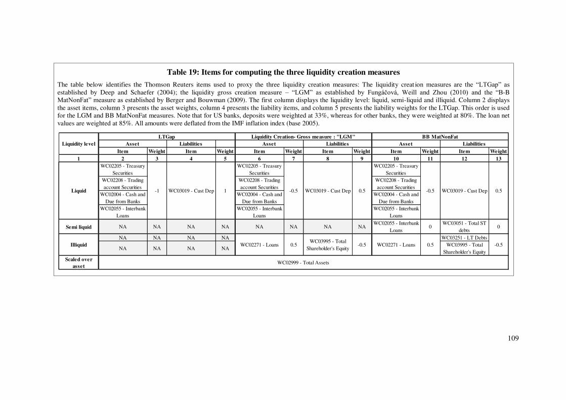
109
Table 19: Items for computing the three liquidity creation measures
The table below identifies the Thomson Reuters items used to proxy the three liquidity creation measures: The liquidity creat ion measures are the “LTGap” as established by Deep and Schaefer (2004); the liquidity gross creation measure – “LGM” as established by Fungáčová, Weill and Zhou (2010) and the “B-B MatNonFat” measure as established by Berger and Bouwman (2009). The first column displays the liquidity level: liquid, semi-liquid and illiquid. Column 2 displays the asset items, column 3 presents the asset weights, column 4 presents the liability items, and column 5 presents the liability weights for the LTGap. This order is used for the LGM and BB MatNonFat measures. Note that for US banks, deposits were weighted at 33%, whereas for other banks, they were weighted at 80%. The loan net values are weighted at 85%. All amounts were deflated from the IMF inflation index (base 2005).
LiabilitiesItem Weight Item Weight Item Weight Item Weight Item Weight Item Weight
1 2 3 4 5 6 7 8 9 10 11 12 13WC02205 - Treasury
SecuritiesWC02205 - Treasury
SecuritiesWC02205 - Treasury
SecuritiesWC02208 - Trading account Securities
WC02208 - Trading account Securities
WC02208 - Trading account Securities
WC02004 - Cash and Due from Banks
WC02004 - Cash and Due from Banks
WC02004 - Cash and Due from Banks
WC02055 - Interbank Loans
WC02055 - Interbank Loans
WC02055 - Interbank Loans
Semi liquid NA NA NA NA NA NA NA NAWC02055 - Interbank
Loans0
WC03051 - Total ST debts
0
NA NA NA NA WC03251 - LT Debts
NA NA NA NAWC03995 - Total
Shareholder's Equity
Scaled over asset
WC02999 - Total Assets
-1 1 -0.5 0.5 -0.5 0.5WC03019 - Cust Dep WC03019 - Cust Dep WC03019 - Cust Dep
WC02271 - LoansWC02271 - Loans 0.5
Liquidity level
WC03995 - Total Shareholder's Equity
BB MatNonFatAsset Asset Liabilities Asset Liabilities
Liquidity Creation- Gross measure : "LGM"LTGap
-0.50.5 -0.5Illiquid
Liquid
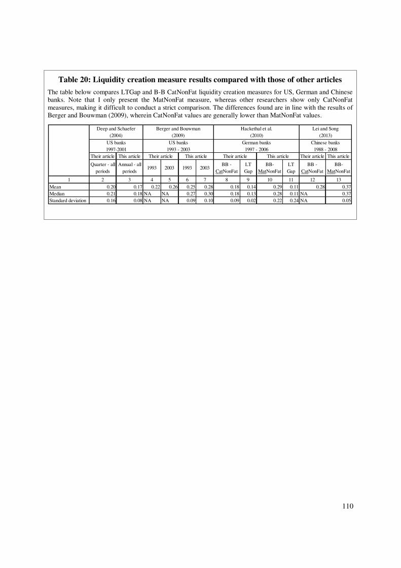
110
Table 20: Liquidity creation measure results compared with those of other articles
The table below compares LTGap and B-B CatNonFat liquidity creation measures for US, German and Chinese banks. Note that I only present the MatNonFat measure, whereas other researchers show only CatNonFat measures, making it difficult to conduct a strict comparison. The differences found are in line with the results of Berger and Bouwman (2009), wherein CatNonFat values are generally lower than MatNonFat values.
Their article This article Their article This article
Quarter - all periods
Annual - all periods
1993 2003 1993 2003BB -
CatNonFatLT Gap
BB-MatNonFat
LT Gap
BB - CatNonFat
BB-MatNonFat
1 2 3 4 5 6 7 8 9 10 11 12 13
Mean 0.20 0.17 0.22 0.26 0.25 0.28 0.18 0.14 0.29 0.11 0.28 0.37Median 0.21 0.18 NA NA 0.27 0.30 0.18 0.13 0.28 0.11 NA 0.37Standard deviation 0.16 0.08 NA NA 0.09 0.10 0.09 0.02 0.22 0.24 NA 0.05
US banks 1997-2001
Lei and Song (2013)
Chinese banks 1988 - 2008
Their article This article Their article This article
Deep and Schaefer (2004)
Hackethal et al. (2010)
Berger and Bouwman (2009)
US banks 1993 - 2003
German banks 1997 - 2006
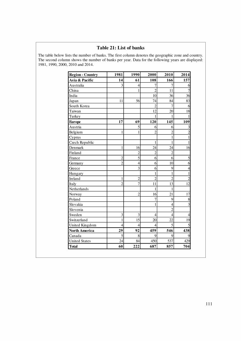
111
Table 21: List of banks
The table below lists the number of banks. The first column denotes the geographic zone and country. The second column shows the number of banks per year. Data for the following years are displayed: 1981, 1990, 2000, 2010 and 2014.
Region - Country 1981 1990 2000 2010 2014Asia & Pacific 14 61 108 166 157Australia 3 4 7 7 6China 1 2 11 7India 10 36 36Japan 11 56 74 84 83South Korea 2 7 6Taiwan 12 20 18Turkey 1 1 1Europe 17 69 120 145 109Austria 5 6 6 3Belgium 1 1 2 2 2Cyprus 1 1Czech Republic 1 1 1Denmark 1 16 24 24 16Finland 2 2 2France 2 5 6 6 5Germany 2 4 6 10 6Greece 3 6 9 4Hungary 1 1 1Ireland 1 2 2 2 2Italy 2 7 11 13 12Netherlands 1 1Norway 2 16 21 17Poland 7 9 8Slovakia 1 4 3Slovenia 2Sweden 3 3 4 4 4Switzerland 1 15 20 22 19United Kingdom 4 4 4 5 5North America 29 92 459 546 438Canada 5 8 9 9 9United States 24 84 450 537 429Total 60 222 687 857 704
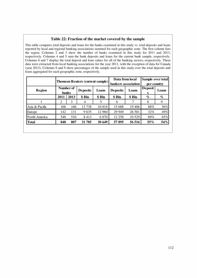
112
Table 22: Fraction of the market covered by the sample
This table compares total deposits and loans for the banks examined in this study vs. total deposits and loans reported by local and regional banking associations summed for each geographic zone. The first column lists the region. Columns 2 and 3 show the number of banks examined in this study for 2011 and 2013, respectively. Columns 4 and 5 sum the bank deposits and loans for the current bank sample, respectively. Columns 6 and 7 display the total deposit and loan values for all of the banking sectors, respectively. These data were extracted from local banking associations for the year 2011, with the exception of data for Canada (year 2013). Columns 8 and 9 show percentages of the sample used in this study over the total deposits and loans aggregated for each geographic zone, respectively.
Region Deposits Loans Deposits LoansDeposit
sLoans
2011 2013 $ Bln $ Bln $ Bln $ Bln % %1 2 3 4 5 6 7 8 9
Asia & Pacific 166 166 13 738 10 818 15 688 19 406 88% 56%
Europe 142 131 9 635 12 960 29 949 26 581 32% 49%
North America 540 510 8 413 6 870 12 258 10 529 69% 65%
Total 848 807 31 785 30 649 57 895 56 516 55% 54%
Sample over total per country
Thomson Reuters (current sample)
Number of banks
Data from local bankers association
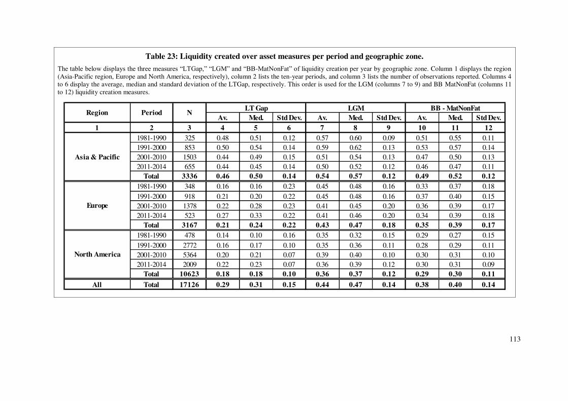
113
Table 23: Liquidity created over asset measures per period and geographic zone.
The table below displays the three measures “LTGap,” “LGM” and “BB-MatNonFat” of liquidity creation per year by geographic zone. Column 1 displays the region (Asia-Pacific region, Europe and North America, respectively), column 2 lists the ten-year periods, and column 3 lists the number of observations reported. Columns 4 to 6 display the average, median and standard deviation of the LTGap, respectively. This order is used for the LGM (columns 7 to 9) and BB MatNonFat (columns 11 to 12) liquidity creation measures.
Av. Med. Std Dev. Av. Med. Std Dev. Av. Med. Std Dev.1 2 3 4 5 6 7 8 9 10 11 12
1981-1990 325 0.48 0.51 0.12 0.57 0.60 0.09 0.51 0.55 0.111991-2000 853 0.50 0.54 0.14 0.59 0.62 0.13 0.53 0.57 0.142001-2010 1503 0.44 0.49 0.15 0.51 0.54 0.13 0.47 0.50 0.132011-2014 655 0.44 0.45 0.14 0.50 0.52 0.12 0.46 0.47 0.11
Total 3336 0.46 0.50 0.14 0.54 0.57 0.12 0.49 0.52 0.121981-1990 348 0.16 0.16 0.23 0.45 0.48 0.16 0.33 0.37 0.181991-2000 918 0.21 0.20 0.22 0.45 0.48 0.16 0.37 0.40 0.152001-2010 1378 0.22 0.28 0.23 0.41 0.45 0.20 0.36 0.39 0.172011-2014 523 0.27 0.33 0.22 0.41 0.46 0.20 0.34 0.39 0.18
Total 3167 0.21 0.24 0.22 0.43 0.47 0.18 0.35 0.39 0.171981-1990 478 0.14 0.10 0.16 0.35 0.32 0.15 0.29 0.27 0.15
1991-2000 2772 0.16 0.17 0.10 0.35 0.36 0.11 0.28 0.29 0.112001-2010 5364 0.20 0.21 0.07 0.39 0.40 0.10 0.30 0.31 0.102011-2014 2009 0.22 0.23 0.07 0.36 0.39 0.12 0.30 0.31 0.09
Total 10623 0.18 0.18 0.10 0.36 0.37 0.12 0.29 0.30 0.11
All Total 17126 0.29 0.31 0.15 0.44 0.47 0.14 0.38 0.40 0.14
Asia & Pacific
Europe
North America
LT Gap LGM BB - MatNonFatPeriod NRegion
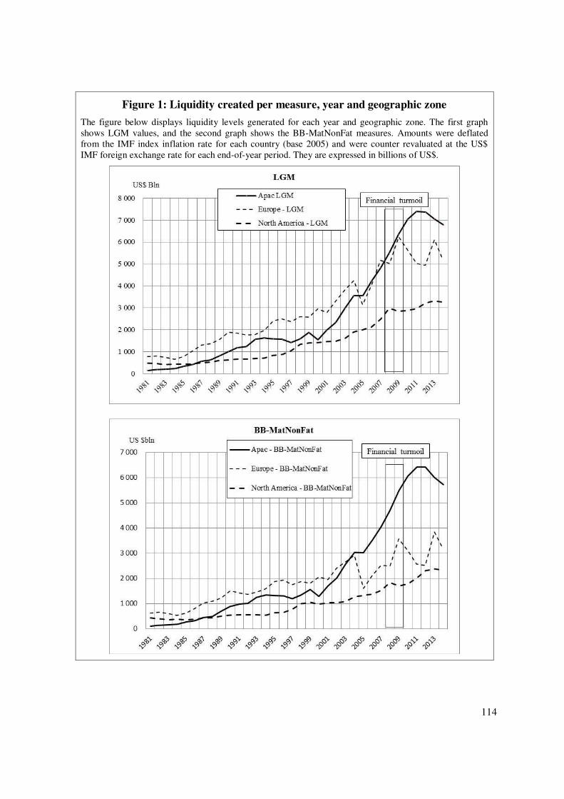
114
Figure 1: Liquidity created per measure, year and geographic zone
The figure below displays liquidity levels generated for each year and geographic zone. The first graph shows LGM values, and the second graph shows the BB-MatNonFat measures. Amounts were deflated from the IMF index inflation rate for each country (base 2005) and were counter revaluated at the US$ IMF foreign exchange rate for each end-of-year period. They are expressed in billions of US$.
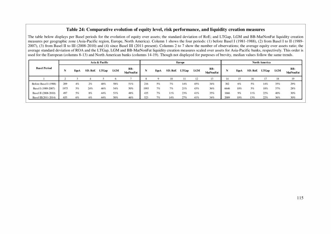
115
Table 24: Comparative evolution of equity level, risk performance, and liquidity creation measures
The table below displays per Basel periods for the evolution of equity over assets; the standard deviation of RoE; and LTGap, LGM and BB-MatNonFat liquidity creation measures per geographic zone (Asia-Pacific region, Europe, North America). Column 1 shows the four periods: (1) before Basel I (1981-1988), (2) from Basel I to II (1989-2007), (3) from Basel II to III (2008-2010) and (4) since Basel III (2011-present). Columns 2 to 7 show the number of observations; the average equity over assets ratio; the average standard deviation of ROA and the LTGap, LGM and BB-MatNonFat liquidity creation measures scaled over assets for Asia-Pacific banks, respectively. This order is used for the European (columns 8-13) and North American banks (columns 14-19). Though not displayed for purposes of brevity, median values follow the same trends.
N EqoA SD. RoE LTGap LGMBB-
MatNonFatN EqoA SD. RoE LTGap LGM
BB-MatNonFat
N EqoA SD. RoE LTGap LGMBB-
MatNonFat
1 2 3 4 5 6 7 8 9 10 11 12 13 14 15 16 17 18 19
Before Basel I (1988) 209 4% 2% 48% 58% 51% 216 5% 7% 14% 45% 34% 302 6% 5% 14% 35% 29%
Basel I (1989-2007) 1975 5% 24% 46% 54% 50% 1993 7% 7% 21% 43% 36% 6646 10% 5% 18% 37% 28%
Basel II (2008-2010) 497 5% 8% 44% 51% 48% 435 7% 11% 23% 41% 35% 1666 9% 11% 22% 40% 30%
Basel III(2011-2014) 655 6% 6% 44% 50% 46% 523 7% 14% 27% 41% 34% 2009 10% 13% 22% 36% 30%
Asia & Pacific Europe North America
Basel Period
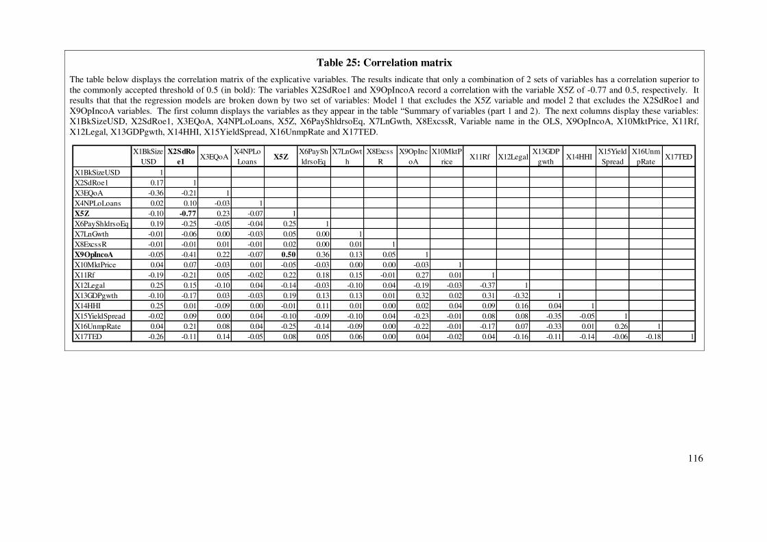
116
Table 25: Correlation matrix
The table below displays the correlation matrix of the explicative variables. The results indicate that only a combination of 2 sets of variables has a correlation superior to the commonly accepted threshold of 0.5 (in bold): The variables X2SdRoe1 and X9OpIncoA record a correlation with the variable X5Z of -0.77 and 0.5, respectively. It results that that the regression models are broken down by two set of variables: Model 1 that excludes the X5Z variable and model 2 that excludes the X2SdRoe1 and X9OpIncoA variables. The first column displays the variables as they appear in the table “Summary of variables (part 1 and 2). The next columns display these variables: X1BkSizeUSD, X2SdRoe1, X3EQoA, X4NPLoLoans, X5Z, X6PayShldrsoEq, X7LnGwth, X8ExcssR, Variable name in the OLS, X9OpIncoA, X10MktPrice, X11Rf, X12Legal, X13GDPgwth, X14HHI, X15YieldSpread, X16UnmpRate and X17TED.
X1BkSizeUSD
X2SdRoe1
X3EQoAX4NPLoLoans
X5ZX6PayShldrsoEq
X7LnGwth
X8ExcssR
X9OpIncoA
X10MktPrice
X11Rf X12LegalX13GDP
gwthX14HHI
X15YieldSpread
X16UnmpRate
X17TED
X1BkSizeUSD 1X2SdRoe1 0.17 1X3EQoA -0.36 -0.21 1X4NPLoLoans 0.02 0.10 -0.03 1X5Z -0.10 -0.77 0.23 -0.07 1X6PayShldrsoEq 0.19 -0.25 -0.05 -0.04 0.25 1X7LnGwth -0.01 -0.06 0.00 -0.03 0.05 0.00 1X8ExcssR -0.01 -0.01 0.01 -0.01 0.02 0.00 0.01 1X9OpIncoA -0.05 -0.41 0.22 -0.07 0.50 0.36 0.13 0.05 1X10MktPrice 0.04 0.07 -0.03 0.01 -0.05 -0.03 0.00 0.00 -0.03 1X11Rf -0.19 -0.21 0.05 -0.02 0.22 0.18 0.15 -0.01 0.27 0.01 1X12Legal 0.25 0.15 -0.10 0.04 -0.14 -0.03 -0.10 0.04 -0.19 -0.03 -0.37 1X13GDPgwth -0.10 -0.17 0.03 -0.03 0.19 0.13 0.13 0.01 0.32 0.02 0.31 -0.32 1X14HHI 0.25 0.01 -0.09 0.00 -0.01 0.11 0.01 0.00 0.02 0.04 0.09 0.16 0.04 1X15YieldSpread -0.02 0.09 0.00 0.04 -0.10 -0.09 -0.10 0.04 -0.23 -0.01 0.08 0.08 -0.35 -0.05 1X16UnmpRate 0.04 0.21 0.08 0.04 -0.25 -0.14 -0.09 0.00 -0.22 -0.01 -0.17 0.07 -0.33 0.01 0.26 1X17TED -0.26 -0.11 0.14 -0.05 0.08 0.05 0.06 0.00 0.04 -0.02 0.04 -0.16 -0.11 -0.14 -0.06 -0.18 1
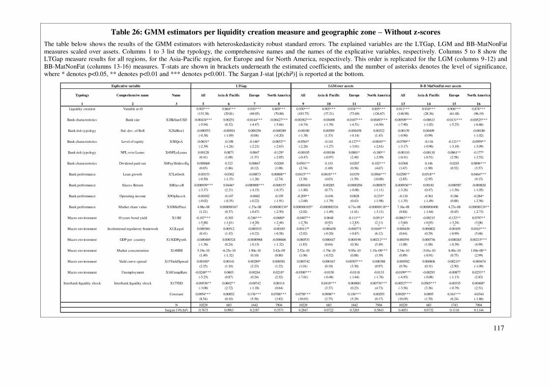
117
Table 26: GMM estimators per liquidity creation measure and geographic zone – Without z-scores
The table below shows the results of the GMM estimators with heteroskedasticity robust standard errors. The explained variables are the LTGap, LGM and BB-MatNonFat measures scaled over assets. Columns 1 to 3 list the typology, the comprehensive names and the names of the explicative variables, respectively. Columns 5 to 8 show the LTGap measure results for all regions, for the Asia-Pacific region, for Europe and for North America, respectively. This order is replicated for the LGM (columns 9-12) and BB-MatNonFat (columns 13-16) measures. T-stats are shown in brackets underneath the estimated coefficients, and the number of asterisks denotes the level of significance, where * denotes p<0.05, ** denotes p<0.01 and *** denotes p<0.001. The Sargan J-stat [p(chi²)] is reported at the bottom.
Typology Comprehensive name Name All Asia & Pacific Europe North America All Asia & Pacific Europe North America All Asia & Pacific Europe North America
1 2 3 5 6 7 8 9 10 11 12 13 14 15 16Liquidity creation Variable at t0 0.903*** 0.864*** 0.910*** 0.809*** 0.930*** 0.905*** 0.934*** 0.895*** 0.911*** 0.910*** 0.906*** 0.878***
(133.38) (29.81) (69.05) (70.80) (183.75) (37.21) (73.69) (126.67) (148.98) (28.36) (61.48) (96.19)
Bank characteristics Bank size X1BkSizeUSD -0.00434*** 0.00251 -0.0144*** -0.00427*** -0.00382*** -0.00498 -0.0107*** -0.00493*** -0.00509*** -0.00613 -0.0131*** -0.00525***(-5.94) (0.32) (-4.47) (-5.66) (-6.74) (-1.39) (-4.51) (-6.90) (-7.90) (-1.02) (-5.25) (-6.86)
Bank risk typology Std. dev. of RoE X2SdRoe1 -0.000553 -0.00924 0.000256 -0.000289 -0.00180 0.00589 -0.000458 0.00322 -0.00139 0.00409 -0.00180(-0.38) (-1.09) (0.06) (-0.20) (-1.38) (1.53) (-0.14) (1.43) (-0.90) (0.99) (-1.02)
Bank characteristics Level of equity X3EQoA -0.0631* -0.198 -0.146* -0.0652** -0.0563* -0.141 -0.127** -0.0810** -0.0790** -0.116 -0.121** -0.0959**(-2.39) (-1.24) (-2.21) (-2.63) (-2.26) (-1.27) (-3.01) (-2.61) (-3.17) (-0.96) (-3.18) (-3.09)
Bank risk typology NPL over Loans X4NPLoLoans 0.00128 0.0873 0.0847 -0.129* -0.00105 -0.00186 0.0801* -0.180** -0.00110 -0.00118 0.0861** -0.177*(0.41) (1.08) (1.37) (-2.05) (-0.47) (-0.97) (2.40) (-2.99) (-0.41) (-0.51) (2.58) (-2.52)
Bank characteristics Dividend paid out X6PayShldrsoEq 0.000668 0.322 0.00667 0.0269 0.0501** 0.110 0.0207 0.102*** 0.0368 0.146 0.0245 0.0896***(0.03) (1.86) (0.12) (1.08) (2.74) (1.69) (0.56) (4.67) (1.67) (1.90) (0.52) (3.57)
Bank performance Loan growth X7LnGwth -0.00153 -0.0362 -0.00873 0.00808** 0.0415*** 0.0618*** 0.0159 0.0566*** 0.0298** 0.0518** 0.0464***(-0.50) (-1.33) (-1.26) (2.74) (3.30) (4.03) (1.59) (10.88) (2.85) (2.95) (9.15)
Bank performance Excess Return X8ExcssR -0.000939*** 0.0446* -0.000908*** -0.000157 -0.000410 0.00285 -0.0000294 -0.000875 -0.000936** 0.00181 -0.000587 -0.000820(-3.37) (2.21) (-4.15) (-0.37) (-1.80) (0.77) (-0.08) (-1.11) (-3.26) (0.47) (-1.56) (-1.05)
Bank performance Operating income X9OpIncoA -0.00182 -0.147 -0.0602 -0.195 -0.209** -0.436 0.0828 -0.233* -0.110 -0.361 0.186 -0.284*(-0.02) (-0.35) (-0.22) (-1.91) (-2.60) (-1.79) (0.43) (-1.98) (-1.35) (-1.49) (0.88) (-2.56)
Bank performance Market share value X10MktPrice 4.08e-08 0.000000167 -1.53e-08 -0.00000134* 0.000000105* -0.000000316 6.71e-08 -0.00000118** 7.16e-08 -0.000000400 4.27e-08 -0.00000124**(1.21) (0.37) (-0.47) (-2.50) (2.02) (-1.49) (1.41) (-3.11) (0.84) (-1.64) (0.45) (-2.73)
Macro environment 10 years bond yield X11Rf -0.107*** -0.303 -0.246*** -0.0680* -0.0407** 0.0648 -0.111** 0.0511* -0.0863*** -0.00215 -0.132** 0.0797**(-5.88) (-1.61) (-4.20) (-2.44) (-2.76) (0.92) (-2.83) (2.11) (-5.60) (-0.03) (-3.24) (3.06)
0 0 0 0 0 0 0 0 0 0 0 0Macro environment Institutional regulatory framework X12Legal 0.000360 0.00512 -0.000315 -0.00185 0.00117* -0.000458 -0.000771 0.0169*** 0.000430 0.000802 -0.00105 0.0163***
(0.41) (1.42) (-0.22) (-0.58) (2.02) (-0.20) (-0.87) (6.12) (0.64) (0.29) (-0.99) (5.68)
Macro environment GDP per country X13GDPgwth -0.000469 0.000324 -0.0000968 -0.000606 0.000531 0.000447 0.000190 0.00212*** 0.000391 0.000736 -0.000263 0.00215***(-1.36) (0.24) (-0.13) (-1.32) (1.83) (0.64) (0.36) (5.49) (1.08) (1.00) (-0.39) (4.99)
Macro environment Market concentration X14HHI 5.19e-10 -6.25e-10 1.90e-10 3.42e-09 2.52e-10 -1.79e-10 9.95e-10 1.15e-08*** 2.34e-10 -3.01e-10 8.40e-10 1.09e-08**(1.49) (-1.32) (0.10) (0.80) (1.06) (-0.52) (0.88) (3.39) (0.89) (-0.91) (0.75) (2.99)
Macro environment Yield curve spread X15YieldSpread 0.00100* 0.00141 0.00289* 0.000581 0.000742 0.000167 0.00307*** 0.000388 0.000582 0.000606 0.00215* -0.000474(2.25) (1.10) (2.23) (1.22) (1.01) (0.10) (3.30) (0.97) (0.76) (0.31) (2.50) (-1.09)
Macro environment Unemployment X16UnmpRate -0.0248*** 0.0603 0.00244 0.0218* -0.0300*** -0.0150 -0.0118 -0.0133 -0.0199*** -0.00293 -0.00877 0.0253**(-5.25) (0.87) (0.24) (2.52) (-7.61) (-0.48) (-1.64) (-1.76) (-4.93) (-0.08) (-1.13) (2.83)
Interbank liquidity shock Interbank liquidity shock X17TED -0.00536** 0.0602** -0.00742 0.00114 0.0418*** 0.000881 0.00776*** -0.00527*** 0.0565*** -0.00335 0.00468*(-3.08) (2.72) (-1.18) (0.64) (3.37) (0.23) (4.73) (-3.56) (3.36) (-0.79) (2.51)
Constant 0.0954*** 0.00852 0.176*** 0.0788*** 0.0758*** 0.0998** 0.136*** 0.00293 0.0928*** 0.0895 0.161*** -0.0341(8.54) (0.10) (5.56) (3.82) (10.03) (2.75) (5.29) (0.17) (10.05) (1.70) (6.24) (-1.86)
N 10229 683 1642 7904 10229 683 1642 7904 10229 683 1743 7904
Sargan J P(chi²) 0.7675 0.0963 0.2187 0.3571 0.2847 0.0722 0.3265 0.5843 0.4051 0.0732 0.1116 0.1144
Explicative variable LTGap LGM over assets B-B MatNonFat over assets
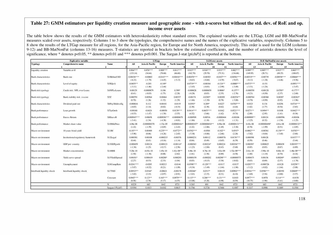
118
Table 27: GMM estimators per liquidity creation measure and geographic zone - with z-scores but without the std. dev. of RoE and op. income over assets
The table below shows the results of the GMM estimators with heteroskedasticity robust standard errors. The explained variables are the LTGap, LGM and BB-MatNonFat measures scaled over assets, respectively. Columns 1 to 3 show the typologies, the comprehensive names and the names of the explicative variables, respectively. Columns 5 to 8 show the results of the LTGap measure for all regions, for the Asia-Pacific region, for Europe and for North America, respectively. This order is used for the LGM (columns 9-12) and BB-MatNonFat (columns 13-16) measures. T-statistics are reported in brackets below the estimated coefficients, and the number of asterisks denotes the level of significance, where * denotes p<0.05, ** denotes p<0.01 and *** denotes p<0.001. The Sargan J-stat [p(chi²)] is reported at the bottom.
Typology Comprehensive name Name All Asia & Pacific Europe North America All Asia & Pacific Europe North America All Asia & Pacific Europe North America1 2 3 5 6 7 8 9 10 11 12 13 14 15 16
Liquidity creation Variable at t0 0.904*** 0.876*** 0.909*** 0.811*** 0.915*** 0.918*** 0.933*** 0.882*** 0.909*** 0.905*** 0.915*** 0.865***(133.14) (34.64) (70.68) (66.60) (162.70) (29.70) (75.31) (134.68) (149.95) (28.71) (69.25) (100.07)
Bank characteristics Bank size X1BkSizeUSD -0.00436*** -0.00802 -0.0143*** -0.00416*** -0.00470*** -0.00303 -0.0107*** -0.00581*** -0.00519*** -0.00739 -0.00938*** -0.00660***(-6.22) (-1.79) (-4.45) (-5.13) (-8.63) (-0.60) (-4.59) (-9.67) (-8.12) (-1.28) (-4.46) (-9.56)
Bank characteristics Level of equity X3EQoA -0.0655** -0.203 -0.149* -0.0719*** -0.00184 -0.124** -0.0880*** -0.0737*** -0.151 -0.0951***(-3.11) (-1.46) (-2.44) (-3.43) (-0.01) (-2.99) (-3.49) (-3.31) (-1.24) (-3.47)
Bank risk typology Credit risk : NPL over Loans X4NPLoLoans 0.00129 -0.0000879 0.106 0.399* -0.000628 0.0000659 0.0806* -0.157** -0.000550 -0.00120 0.0785* -0.177**(0.41) (-0.03) (1.75) (2.28) (-0.28) (0.03) (2.55) (-2.76) (-0.21) (-0.50) (2.37) (-2.68)
Bank risk typology Bank stability risk : z-score X5Z 0.000791 0.00564 0.00464 0.00337 -0.00174 -0.0385* 0.00209 -0.00354** -0.000764 -0.00368 0.00287 -0.00263*(0.70) (1.26) (1.32) (1.29) (-1.66) (-2.30) (0.78) (-3.00) (-0.70) (-0.99) (0.92) (-1.96)
Bank characteristics Dividend paid out X6PayShldrsoEq -0.000616 0.112 0.00101 -0.0119 0.0393* 0.209* 0.0227 0.0783*** 0.0323 0.134 0.0256 0.0734***(-0.03) (1.14) (0.02) (-0.33) (2.38) (2.38) (0.62) (4.44) (1.62) (1.77) (0.54) (3.83)
Bank performance Loan growth X7LnGwth -0.00160 -0.0424 -0.00930 0.0139*** 0.0414*** 0.0655*** 0.0162 0.0521*** 0.0271** 0.0494** 0.0108 0.0442***(-0.53) (-1.47) (-1.30) (3.55) (4.52) (3.66) (1.62) (9.74) (2.89) (2.95) (1.41) (9.36)
Bank performance Excess Return X8ExcssR -0.000943*** 0.00658 -0.000936*** -0.00000679 -0.000509 0.00516 -0.0000444 -0.00106 -0.000909** 0.00124 -0.000596 -0.00106(-3.41) (1.34) (-4.38) (-0.01) (-1.86) (1.18) (-0.12) (-1.31) (-3.25) (0.32) (-1.54) (-1.25)
Bank performance Market share value X10MktPrice 4.08e-08 -0.000000378 -1.53e-09 -0.00000161* 0.000000107* -0.000000654** 6.90e-08 -0.00000131*** 6.65e-08 -0.000000498* 4.81e-08 -0.00000132**(1.22) (-1.59) (-0.05) (-2.43) (2.22) (-2.86) (1.49) (-3.30) (0.78) (-1.99) (0.51) (-2.85)
Macro environment 10 years bond yield X11Rf -0.107*** 0.00469 -0.235*** -0.0772** -0.0702*** -0.0584 -0.102** 0.0547* -0.0882*** -0.00361 -0.130*** 0.0783**(-5.96) (0.06) (-4.26) (-2.65) (-5.38) (-0.86) (-2.66) (2.28) (-5.82) (-0.04) (-3.40) (3.00)
Macro environment Institutional regulatory framework X12Legal 0.000381 0.00108 -0.000215 -0.00376 0.0000231 0.00112 -0.000576 0.0176*** 0.000398 0.00128 0.0157***(0.44) (0.41) (-0.16) (-1.14) (0.04) (0.49) (-0.65) (6.39) (0.59) (0.46) (5.44)
Macro environment GDP per country X13GDPgwth -0.000459 0.00124 -0.000121 -0.00114* -0.000363 -0.00224* 0.000224 0.00194*** 0.000307 0.000625 0.000438 0.00193***(-1.34) (1.25) (-0.17) (-2.56) (-1.23) (-2.06) (0.43) (5.40) (0.85) (0.83) (0.67) (4.89)
Macro environment Market concentration X14HHI 5.20e-10 -6.03e-10 1.45e-10 1.41e-08** 4.48e-10 6.76e-10 1.01e-09 1.52e-08*** 2.61e-10 -3.90e-10 8.60e-10 1.48e-08***(1.50) (-1.38) (0.08) (2.82) (1.81) (1.58) (0.89) (4.58) (1.00) (-1.19) (0.70) (4.16)
Macro environment Yield curve spread X15YieldSpread 0.00101* 0.000419 0.00288* 0.000293 0.0000159 -0.000202 0.00298*** -0.00000575 0.000475 0.00136 0.00269* -0.000471(2.27) (0.53) (2.33) (1.04) (0.03) (-0.15) (3.36) (-0.02) (0.63) (0.69) (2.57) (-1.78)
Macro environment Unemployment X16UnmpRate -0.0241*** -0.0205 0.00213 -0.0144 -0.0398*** -0.128*** -0.0117 -0.0137 -0.0207*** -0.000726 -0.0128 0.0258**(-5.07) (-0.52) (0.21) (-1.09) (-9.34) (-3.49) (-1.64) (-1.90) (-5.12) (-0.02) (-1.64) (3.08)
Interbank liquidity shock Interbank liquidity shock X17TED -0.00523** 0.0344* -0.00621 -0.00178 -0.00246* 0.0317* 0.00119 0.00902*** -0.00541*** 0.0596*** -0.00350 0.00609***(-3.02) (2.22) (-0.97) (-0.91) (-2.01) (2.15) (0.31) (6.10) (-3.69) (3.54) (-0.80) (3.57)
Constant 0.0945*** 0.123** 0.165*** 0.0979*** 0.115*** 0.206*** 0.131*** 0.0103 0.0977*** 0.0978 0.114*** -0.0150(8.56) (2.76) (5.17) (4.55) (13.06) (5.28) (4.98) (0.59) (10.75) (1.90) (5.41) (-0.80)
N 10229 683 1642 8721 11265 801 1642 8721 10229 683 1642 8721Sargan J P(chi²) 0.9394 0.1013 0.6102 0.0615 0.1766 0.2726 0.5466 0.1007 0.3217 0.0986 0.1069 0.1504
Explicative variable LTGap LGM over assets B-B MatNonFat over assets
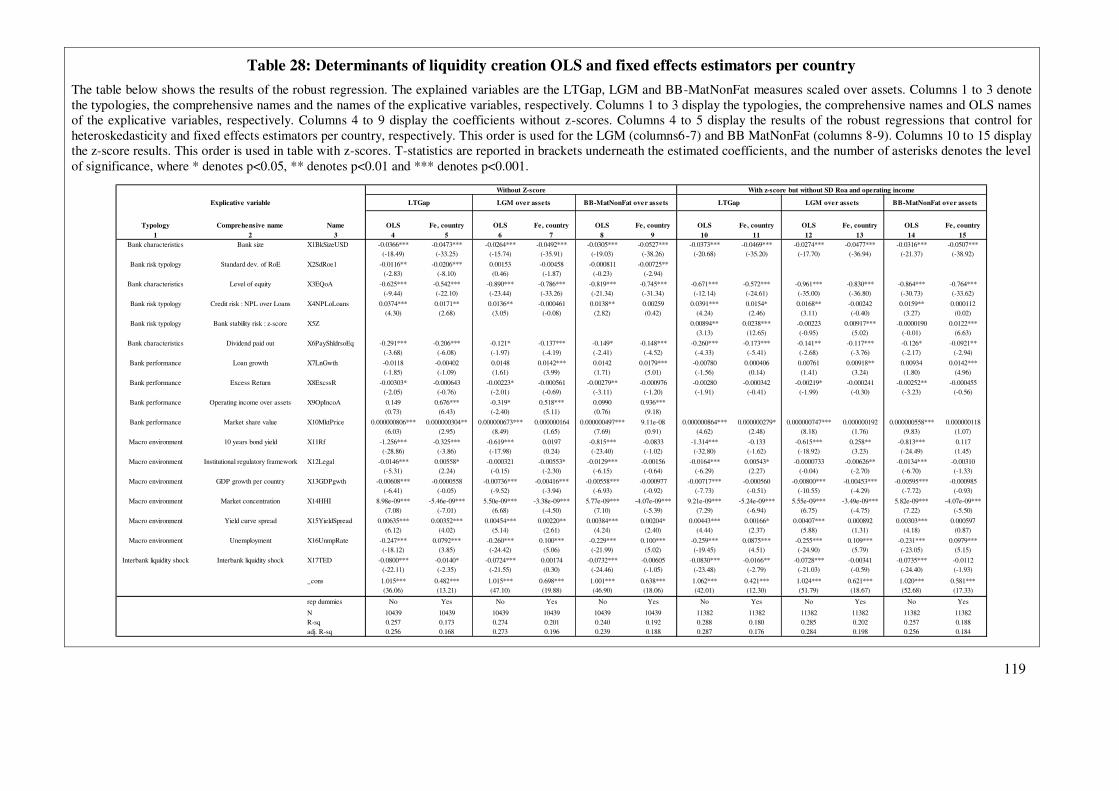
119
Table 28: Determinants of liquidity creation OLS and fixed effects estimators per country
The table below shows the results of the robust regression. The explained variables are the LTGap, LGM and BB-MatNonFat measures scaled over assets. Columns 1 to 3 denote the typologies, the comprehensive names and the names of the explicative variables, respectively. Columns 1 to 3 display the typologies, the comprehensive names and OLS names of the explicative variables, respectively. Columns 4 to 9 display the coefficients without z-scores. Columns 4 to 5 display the results of the robust regressions that control for heteroskedasticity and fixed effects estimators per country, respectively. This order is used for the LGM (columns6-7) and BB MatNonFat (columns 8-9). Columns 10 to 15 display the z-score results. This order is used in table with z-scores. T-statistics are reported in brackets underneath the estimated coefficients, and the number of asterisks denotes the level of significance, where * denotes p<0.05, ** denotes p<0.01 and *** denotes p<0.001.
Typology Comprehensive name Name OLS Fe, country OLS Fe, country OLS Fe, country OLS Fe, country OLS Fe, country OLS Fe, country1 2 3 4 5 6 7 8 9 10 11 12 13 14 15
Bank characteristics Bank size X1BkSizeUSD -0.0366*** -0.0473*** -0.0264*** -0.0492*** -0.0305*** -0.0527*** -0.0373*** -0.0469*** -0.0274*** -0.0477*** -0.0316*** -0.0507***(-18.49) (-33.25) (-15.74) (-35.91) (-19.03) (-38.26) (-20.68) (-35.20) (-17.70) (-36.94) (-21.37) (-38.92)
Bank risk typology Standard dev. of RoE X2SdRoe1 -0.0116** -0.0206*** 0.00153 -0.00458 -0.000811 -0.00725**(-2.83) (-8.10) (0.46) (-1.87) (-0.23) (-2.94)
Bank characteristics Level of equity X3EQoA -0.625*** -0.542*** -0.890*** -0.786*** -0.819*** -0.745*** -0.671*** -0.572*** -0.961*** -0.830*** -0.864*** -0.764***(-9.44) (-22.10) (-23.44) (-33.26) (-21.34) (-31.34) (-12.14) (-24.61) (-35.00) (-36.80) (-30.73) (-33.62)
Bank risk typology Credit risk : NPL over Loans X4NPLoLoans 0.0374*** 0.0171** 0.0136** -0.000461 0.0138** 0.00259 0.0391*** 0.0154* 0.0168** -0.00242 0.0159** 0.000112(4.30) (2.68) (3.05) (-0.08) (2.82) (0.42) (4.24) (2.46) (3.11) (-0.40) (3.27) (0.02)
Bank risk typology Bank stability risk : z-score X5Z 0.00894** 0.0238*** -0.00223 0.00917*** -0.0000190 0.0122***(3.13) (12.65) (-0.95) (5.02) (-0.01) (6.63)
Bank characteristics Dividend paid out X6PayShldrsoEq -0.291*** -0.206*** -0.121* -0.137*** -0.149* -0.148*** -0.260*** -0.173*** -0.141** -0.117*** -0.126* -0.0921**(-3.68) (-6.08) (-1.97) (-4.19) (-2.41) (-4.52) (-4.33) (-5.41) (-2.68) (-3.76) (-2.17) (-2.94)
Bank performance Loan growth X7LnGwth -0.0118 -0.00402 0.0148 0.0142*** 0.0142 0.0179*** -0.00780 0.000406 0.00761 0.00918** 0.00934 0.0142***(-1.85) (-1.09) (1.61) (3.99) (1.71) (5.01) (-1.56) (0.14) (1.41) (3.24) (1.80) (4.96)
Bank performance Excess Return X8ExcssR -0.00303* -0.000643 -0.00223* -0.000561 -0.00279** -0.000976 -0.00280 -0.000342 -0.00219* -0.000241 -0.00252** -0.000455(-2.05) (-0.76) (-2.01) (-0.69) (-3.11) (-1.20) (-1.91) (-0.41) (-1.99) (-0.30) (-3.23) (-0.56)
Bank performance Operating income over assets X9OpIncoA 0.149 0.676*** -0.319* 0.518*** 0.0990 0.936***(0.73) (6.43) (-2.40) (5.11) (0.76) (9.18)
Bank performance Market share value X10MktPrice 0.000000806*** 0.000000304** 0.000000673*** 0.000000164 0.000000497*** 9.11e-08 0.000000864*** 0.000000279* 0.000000747*** 0.000000192 0.000000558*** 0.000000118(6.03) (2.95) (8.49) (1.65) (7.69) (0.91) (4.62) (2.48) (8.18) (1.76) (9.83) (1.07)
Macro environment 10 years bond yield X11Rf -1.256*** -0.325*** -0.619*** 0.0197 -0.815*** -0.0833 -1.314*** -0.133 -0.615*** 0.258** -0.813*** 0.117(-28.86) (-3.86) (-17.98) (0.24) (-23.40) (-1.02) (-32.80) (-1.62) (-18.92) (3.23) (-24.49) (1.45)
Macro environment Institutional regulatory framework X12Legal -0.0146*** 0.00558* -0.000321 -0.00553* -0.0129*** -0.00156 -0.0164*** 0.00543* -0.0000733 -0.00626** -0.0134*** -0.00310(-5.31) (2.24) (-0.15) (-2.30) (-6.15) (-0.64) (-6.29) (2.27) (-0.04) (-2.70) (-6.70) (-1.33)
Macro environment GDP growth per country X13GDPgwth -0.00608*** -0.0000558 -0.00736*** -0.00416*** -0.00558*** -0.000977 -0.00717*** -0.000560 -0.00800*** -0.00453*** -0.00595*** -0.000985(-6.41) (-0.05) (-9.52) (-3.94) (-6.93) (-0.92) (-7.73) (-0.51) (-10.55) (-4.29) (-7.72) (-0.93)
Macro environment Market concentration X14HHI 8.98e-09*** -5.46e-09*** 5.50e-09*** -3.38e-09*** 5.77e-09*** -4.07e-09*** 9.21e-09*** -5.24e-09*** 5.55e-09*** -3.49e-09*** 5.82e-09*** -4.07e-09***(7.08) (-7.01) (6.68) (-4.50) (7.10) (-5.39) (7.29) (-6.94) (6.75) (-4.75) (7.22) (-5.50)
Macro environment Yield curve spread X15YieldSpread 0.00635*** 0.00352*** 0.00454*** 0.00220** 0.00384*** 0.00204* 0.00443*** 0.00166* 0.00407*** 0.000892 0.00303*** 0.000597(6.12) (4.02) (5.14) (2.61) (4.24) (2.40) (4.44) (2.37) (5.88) (1.31) (4.18) (0.87)
Macro environment Unemployment X16UnmpRate -0.247*** 0.0792*** -0.260*** 0.100*** -0.229*** 0.100*** -0.259*** 0.0875*** -0.255*** 0.109*** -0.231*** 0.0979***(-18.12) (3.85) (-24.42) (5.06) (-21.99) (5.02) (-19.45) (4.51) (-24.90) (5.79) (-23.05) (5.15)
Interbank liquidity shock Interbank liquidity shock X17TED -0.0800*** -0.0140* -0.0724*** 0.00174 -0.0732*** -0.00605 -0.0830*** -0.0166** -0.0728*** -0.00341 -0.0735*** -0.0112(-22.11) (-2.35) (-21.55) (0.30) (-24.46) (-1.05) (-23.48) (-2.79) (-21.03) (-0.59) (-24.40) (-1.93)0 0 0 0 0 0 0 0 0 0 0 0
_cons 1.015*** 0.482*** 1.015*** 0.698*** 1.001*** 0.638*** 1.062*** 0.421*** 1.024*** 0.621*** 1.020*** 0.581***(36.06) (13.21) (47.10) (19.88) (46.90) (18.06) (42.01) (12.30) (51.79) (18.67) (52.68) (17.33)
rep dummies No Yes No Yes No Yes No Yes No Yes No Yes0 0 0 0 0 0 0 0 0 0 0 0N 10439 10439 10439 10439 10439 10439 11382 11382 11382 11382 11382 11382R-sq 0.257 0.173 0.274 0.201 0.240 0.192 0.288 0.180 0.285 0.202 0.257 0.188adj. R-sq 0.256 0.168 0.273 0.196 0.239 0.188 0.287 0.176 0.284 0.198 0.256 0.184
Explicative variable
Without Z-score With z-score but without SD Roa and operating income
LTGap LGM over assets BB-MatNonFat over assets LTGap LGM over assets BB-MatNonFat over assets
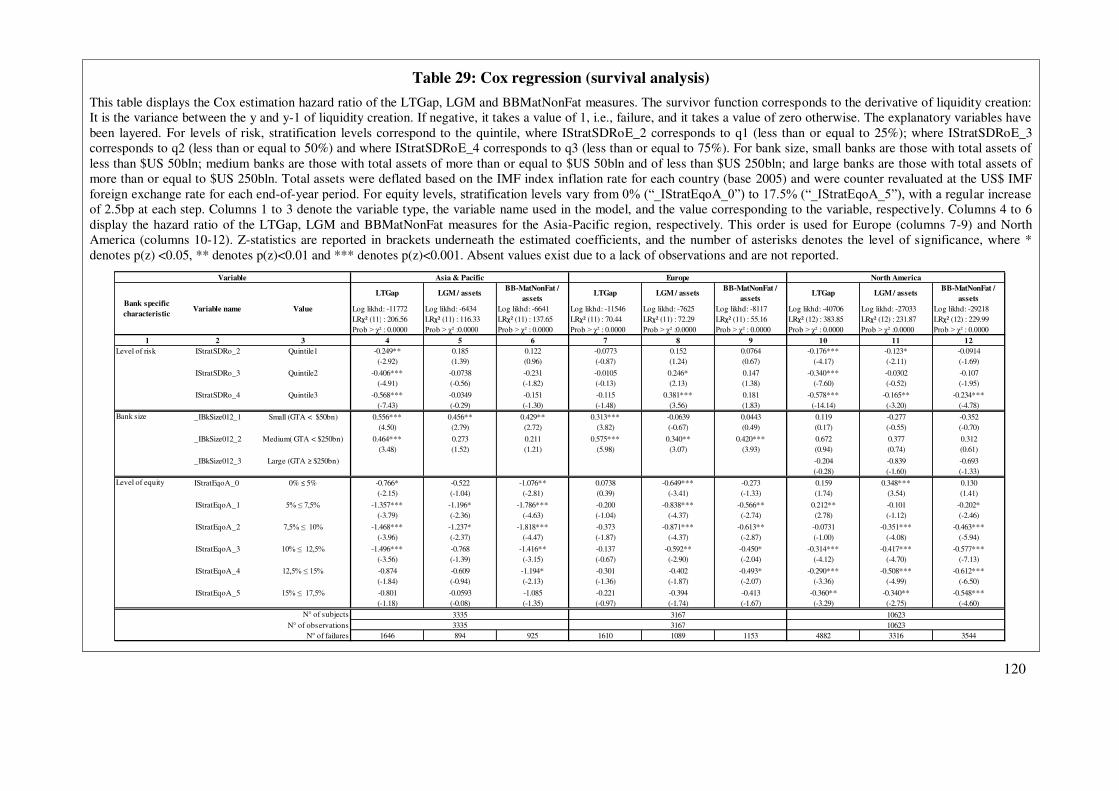
120
Table 29: Cox regression (survival analysis)
This table displays the Cox estimation hazard ratio of the LTGap, LGM and BBMatNonFat measures. The survivor function corresponds to the derivative of liquidity creation: It is the variance between the y and y-1 of liquidity creation. If negative, it takes a value of 1, i.e., failure, and it takes a value of zero otherwise. The explanatory variables have been layered. For levels of risk, stratification levels correspond to the quintile, where IStratSDRoE_2 corresponds to q1 (less than or equal to 25%); where IStratSDRoE_3 corresponds to q2 (less than or equal to 50%) and where IStratSDRoE_4 corresponds to q3 (less than or equal to 75%). For bank size, small banks are those with total assets of less than $US 50bln; medium banks are those with total assets of more than or equal to $US 50bln and of less than $US 250bln; and large banks are those with total assets of more than or equal to $US 250bln. Total assets were deflated based on the IMF index inflation rate for each country (base 2005) and were counter revaluated at the US$ IMF foreign exchange rate for each end-of-year period. For equity levels, stratification levels vary from 0% (“_IStratEqoA_0”) to 17.5% (“_IStratEqoA_5”), with a regular increase of 2.5bp at each step. Columns 1 to 3 denote the variable type, the variable name used in the model, and the value corresponding to the variable, respectively. Columns 4 to 6 display the hazard ratio of the LTGap, LGM and BBMatNonFat measures for the Asia-Pacific region, respectively. This order is used for Europe (columns 7-9) and North America (columns 10-12). Z-statistics are reported in brackets underneath the estimated coefficients, and the number of asterisks denotes the level of significance, where * denotes p(z) <0.05, ** denotes p(z)<0.01 and *** denotes p(z)<0.001. Absent values exist due to a lack of observations and are not reported.
LTGap LGM / assetsBB-MatNonFat /
assetsLTGap LGM / assets
BB-MatNonFat / assets
LTGap LGM / assetsBB-MatNonFat /
assetsLog likhd: -11772 Log likhd: -6434 Log likhd: -6641 Log likhd: -11546 Log likhd: -7625 Log likhd: -8117 Log likhd: -40706 Log likhd: -27033 Log likhd: -29218LRχ² (11) : 206.56 LRχ² (11) : 116.33 LRχ² (11) : 137.65 LRχ² (11) : 70.44 LRχ² (11) : 72.29 LRχ² (11) : 55.16 LRχ² (12) : 383.85 LRχ² (12) : 231.87 LRχ² (12) : 229.99Prob > χ² : 0.0000 Prob > χ² :0.0000 Prob > χ² : 0.0000 Prob > χ² : 0.0000 Prob > χ² :0.0000 Prob > χ² : 0.0000 Prob > χ² : 0.0000 Prob > χ² :0.0000 Prob > χ² : 0.0000
1 2 3 4 5 6 7 8 9 10 11 12Level of risk IStratSDRo_2 Quintile1 -0.249** 0.185 0.122 -0.0773 0.152 0.0764 -0.176*** -0.123* -0.0914
(-2.92) (1.39) (0.96) (-0.87) (1.24) (0.67) (-4.17) (-2.11) (-1.69)
IStratSDRo_3 Quintile2 -0.406*** -0.0738 -0.231 -0.0105 0.246* 0.147 -0.340*** -0.0302 -0.107(-4.91) (-0.56) (-1.82) (-0.13) (2.13) (1.38) (-7.60) (-0.52) (-1.95)
IStratSDRo_4 Quintile3 -0.568*** -0.0349 -0.151 -0.115 0.381*** 0.181 -0.578*** -0.165** -0.234***(-7.43) (-0.29) (-1.30) (-1.48) (3.56) (1.83) (-14.14) (-3.20) (-4.78)
Bank size _IBkSize012_1 Small (GTA < $50bn) 0.556*** 0.456** 0.429** 0.313*** -0.0639 0.0443 0.119 -0.277 -0.352(4.50) (2.79) (2.72) (3.82) (-0.67) (0.49) (0.17) (-0.55) (-0.70)
_IBkSize012_2 Medium( GTA < $250bn) 0.464*** 0.273 0.211 0.575*** 0.340** 0.420*** 0.672 0.377 0.312(3.48) (1.52) (1.21) (5.98) (3.07) (3.93) (0.94) (0.74) (0.61)
_IBkSize012_3 Large (GTA ≥ $250bn) -0.204 -0.839 -0.693(-0.28) (-1.60) (-1.33)
Level of equity IStratEqoA_0 0% ≤ 5% -0.766* -0.522 -1.076** 0.0738 -0.649*** -0.273 0.159 0.348*** 0.130(-2.15) (-1.04) (-2.81) (0.39) (-3.41) (-1.33) (1.74) (3.54) (1.41)
IStratEqoA_1 5% ≤ 7,5% -1.357*** -1.196* -1.786*** -0.200 -0.838*** -0.566** 0.212** -0.101 -0.202*(-3.79) (-2.36) (-4.63) (-1.04) (-4.37) (-2.74) (2.78) (-1.12) (-2.46)
IStratEqoA_2 7,5% ≤ 10% -1.468*** -1.237* -1.818*** -0.373 -0.871*** -0.613** -0.0731 -0.351*** -0.463***(-3.96) (-2.37) (-4.47) (-1.87) (-4.37) (-2.87) (-1.00) (-4.08) (-5.94)
IStratEqoA_3 10% ≤ 12,5% -1.496*** -0.768 -1.416** -0.137 -0.592** -0.450* -0.314*** -0.417*** -0.577***(-3.56) (-1.39) (-3.15) (-0.67) (-2.90) (-2.04) (-4.12) (-4.70) (-7.13)
IStratEqoA_4 12,5% ≤ 15% -0.874 -0.609 -1.194* -0.301 -0.402 -0.493* -0.290*** -0.508*** -0.612***(-1.84) (-0.94) (-2.13) (-1.36) (-1.87) (-2.07) (-3.36) (-4.99) (-6.50)
IStratEqoA_5 15% ≤ 17,5% -0.801 -0.0593 -1.085 -0.221 -0.394 -0.413 -0.360** -0.340** -0.548***(-1.18) (-0.08) (-1.35) (-0.97) (-1.74) (-1.67) (-3.29) (-2.75) (-4.60)
1646 894 925 1610 1089 1153 4882 3316 3544N° of failures
N° of subjects 3335 3167 10623N° of observations 3335 3167 10623
Variable Asia & Pacific Europe North America
Bank specific characteristic
Variable name Value
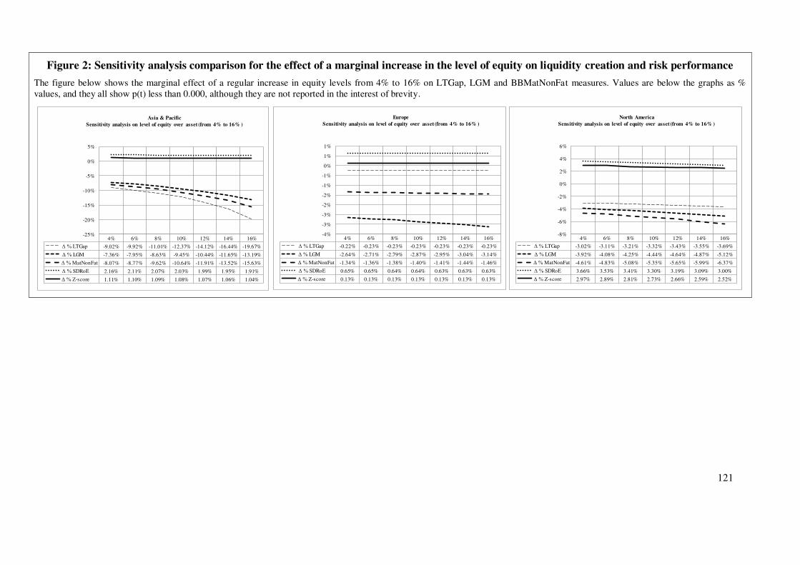
121
Figure 2: Sensitivity analysis comparison for the effect of a marginal increase in the level of equity on liquidity creation and risk performance
The figure below shows the marginal effect of a regular increase in equity levels from 4% to 16% on LTGap, LGM and BBMatNonFat measures. Values are below the graphs as % values, and they all show p(t) less than 0.000, although they are not reported in the interest of brevity.
4% 6% 8% 10% 12% 14% 16%
Δ % LTGap -3.02% -3.11% -3.21% -3.32% -3.43% -3.55% -3.69%
Δ % LGM -3.92% -4.08% -4.25% -4.44% -4.64% -4.87% -5.12%
Δ % MatNonFat -4.61% -4.83% -5.08% -5.35% -5.65% -5.99% -6.37%
Δ % SDRoE 3.66% 3.53% 3.41% 3.30% 3.19% 3.09% 3.00%
Δ % Z-score 2.97% 2.89% 2.81% 2.73% 2.66% 2.59% 2.52%
-8%
-6%
-4%
-2%
0%
2%
4%
6%
North AmericaSensitivity analysis on level of equity over asset (from 4% to 16% )
4% 6% 8% 10% 12% 14% 16%
Δ % LTGap -0.22% -0.23% -0.23% -0.23% -0.23% -0.23% -0.23%
Δ % LGM -2.64% -2.71% -2.79% -2.87% -2.95% -3.04% -3.14%
Δ % MatNonFat -1.34% -1.36% -1.38% -1.40% -1.41% -1.44% -1.46%
Δ % SDRoE 0.65% 0.65% 0.64% 0.64% 0.63% 0.63% 0.63%
Δ % Z-score 0.13% 0.13% 0.13% 0.13% 0.13% 0.13% 0.13%
-4%
-3%
-3%
-2%
-2%
-1%
-1%
0%
1%
1%
EuropeSensitivity analysis on level of equity over asset (from 4% to 16% )
4% 6% 8% 10% 12% 14% 16%
Δ % LTGap -9.02% -9.92% -11.01% -12.37% -14.12% -16.44% -19.67%
Δ % LGM -7.36% -7.95% -8.63% -9.45% -10.44% -11.65% -13.19%
Δ % MatNonFat -8.07% -8.77% -9.62% -10.64% -11.91% -13.52% -15.63%
Δ % SDRoE 2.16% 2.11% 2.07% 2.03% 1.99% 1.95% 1.91%
Δ % Z-score 1.11% 1.10% 1.09% 1.08% 1.07% 1.06% 1.04%
-25%
-20%
-15%
-10%
-5%
0%
5%
Asia & PacificSensitivity analysis on level of equity over asset (from 4% to 16% )
122
Chapter 3. Positive effects of Basel III on banking liquidity creation
3.1 Abstract, keywords and JEL classification
This paper estimates the effect of the Basel III regulatory framework on banking
liquidity creation. The results are based on a panel data set of U.S. banks that represent
approximately 60% of U.S. loans and deposits over a 7-year period (from 2009 to 2015) in
addition to difference-in-difference and standard survival methods. All components of Basel
III taken together, there is empirical evidence that Basel III has a positive effect on banking
liquidity creation in the US market in particular for major banks. These findings have broad
implications for policy makers.
Key words: Difference-in-difference, Cox, Survival, GMM, Basel III, Banking
liquidity.
JEL Classifications: C3 - Econometric Methods: Multiple/Simultaneous Equation
Models; C53 -Forecasting and Other Model Applications; G21 - Banks; Other Depository
Institutions; Mortgages.
3.2 Introduction
This paper estimates the effect of the new banking regulatory framework –
commonly referred to as Basel III – on banks’ liquidity creation. Because the liquidity crisis
of the banking sector was the cause of the 2007/2008 financial crisis, regulators have
tightened banking liquidity ratios. Indeed, under the BIS (Bank of International Settlement)
requirement and, in particular, Basel III, the LCR (liquidity coverage ratio) and NSFR (net
stable funding ratio) have been created. The former underpins the short-term resilience of a
123
bank’s liquidity risk profile, whereas the latter covers medium- and long-term liquidity
capabilities. The LCR regulatory framework has been prioritized and will be deployed in an
orderly fashion within a common timeframe among a significant majority of countries13.
Although the deployment of the LCR will begin in 2015 and be completed in 2019, it will be
subject to a transitional arrangement before reaching full implementation on 1 January 2019.
In addition, certain requirements, such as the increase in tier 1 and core tier 1 capital, started
in 2013.
In January 2014, the Basel Committee issued the final requirement for bank LCR-
related disclosures; the regulatory and supervisory agencies required the banks belonging to
their jurisdictions to disclose the LCR on 1 January 2014. For instance, calculation and
reporting requirements have been applicable since 1 January 2014 in the EU14. In Switzerland,
all banks reported the Basel III leverage ratio for Q3 2014. In the US, the leverage ratio
included in the final Basel III rule was approved in July 2013 and has been in effect since 1st
January 2014. To comply with this regulatory framework and as a potential signal addressed
to the market, banks have started to anticipate these liquidity constraints.
What will the effects of such regulation be? Will the treatment (the Basel III
regulatory framework) be positive, or will it ultimately weaken the banking sector? Overall,
there is no consensus within the academic community on whether the effects will be positive
or negative (Bancel and Salé (2016)). On one hand, by providing a cushion layer of extra
13 An exhaustive list of countries that have signed the Basel III regulatory framework is available on the BIS web
site. This list includes not only the G20 and EU countries but also Chile, Norway, the Republic of Korea, the
Republic of China (Taiwan), and Switzerland. Additional information is available at :
“http://www.bis.org/fsi/fsipapers.htm”. 14 Articles 451 and 521 of Regulation (EU) N° 575/2013.
124
liquidity, many experts estimate that this regulation will strengthen the banking sector against
a liquidity crisis without additional social costs and will have overall positive effects. On the
other hand, other authors wish to highlight the risk that inappropriate regulation can generate
for liquidity creation; by obliging banks to allocate fewer available resources to fund their
activity, the regulation reduces liquidity creation. From this perspective, the regulation
ultimately weakens the macroeconomic environment, encourages shadow banking, and
weakens the banking system.
Because banks began progressively implementing the required liquidity constraint
before the official deadline of 1 January 2015, this paper proposes estimating the effect of this
treatment on banking liquidity creation. To achieve this objective, two sets of methods have
been used. The first, is Card and Krueger (1994), who use the difference-in-difference (D-in-
D) method to estimate the effect of a wage increase policy on the fast food industry. Since
their publication, this method has been broadly used by most econometricians to estimate a
policy’s effect. For robustness, the effect by using other methods, in particular, life table and
Cox regression methods were analyzed. These methods offer additional insights into the
policy effects and complete the analysis of the D-in-D estimation.
This paper is organized as follows: Section 1 reviews the literature on the effects of
banking regulation on liquidity creation. It also provides a brief summary of the components
of the Basel III regulatory framework. Section 2 describes the bank sample and the
methodology and models applied to estimate the effects of Basel III. Section 3 estimates the
effects of Basel III, using a set of methods that includes the D-in-D and additional methods

125
for robustness. Concluding remarks are drawn from these empirical findings and directed
toward policy makers.
3.3 Literature review on the effects of the banking regulation on bank’s liquidity
creation and brief presentation of Basel III
The first part of this section reviews the literature on the effects of the banking
regulation on the liquidity creation by banks. The second and last part presents the
components of the Basel III regulatory framework.
3.3.1 Literature review on the effects of banking regulation on liquidity
creation by banks
The effect of regulation on the banking sector has been the subject of debate for
decades, and there is an extensive strand of the literature that addresses these effects (Admati,
DeMarzo, Hellwig and Pfleiderer (2010)), in particular since the financial crisis. This
literature first poses questions regarding the proper objective of financial regulation and
sufficient measures to achieve the goal (Morris and Shin (2008)). For instance, Repullo
(2005) shows that the existence of the lender-of-last-resort mechanism has both positive and
negative effects: although it improves the safety of the financial system, it reduces the
incentive for banks to self-insure against payment shocks. As a result, a liquidity buffer is
necessary and must be supported by a regulatory framework. However, it is difficult to
anticipate the effects of a regulation. Indeed, Morris and Shin (2004) suggest that
inappropriate regulations can be the source of liquidity shortages, and Wagner (2007) shows
126
that an augmentation of liquid assets unexpectedly increases the instability of banks and the
probability of failure. It is the inherent fragility of banks – that is, liquidity creation and the
risk transformation process (Diamond and Rajan (1999)); Diamond and Rajan (2001)) – that
motivates policy makers to establish regulatory constraints as a means to protect against
banking fragility and to limit the spillover effects when a bank defaults. Ultimately, regulatory
constraints may in turn reduce banking liquidity creation (Berger, Bouwman, Kick and
Schaeck (2011).
Finally, at least one consensus can be reached. Given the complexity of the
interconnection between the banking sector and the macroeconomic environment, it is
necessary to measure the amplitude of the effect of Basel III on banking liquidity creation.
How can the effect of the regulation be measured? Several surveys have attempted to
study the effect of banking regulation on liquidity. From a liquidity perspective, Berger,
Bouwman, Kick and Schaeck (2011) assess the impact of regulatory interventions and capital
support banking regulation in Germany on a panel of 2789 banks between 1999 and 2009;
Horváth, Seidler and Weill (2014) examine the effect of Basel III on 31 Slovakian banks
between 2000 and 2010, and Lei and Song (2013) study its effect on the capital structure of
135 Chinese banks between 1998 and 2009; Lakštutienė, Krušinskas and Rumšaitė (2011)
explore the effect of deposit insurance systems on 8 Lithuanian banks between 1995 and
2008; and Fungáčová, Weill and Zhou (2010) study the implementation of deposit insurance
by Russian banks between 1999 and 2007. Therefore, evaluating a regulatory framework’s
effects on banking activity is not new. However, based on the literature review, there is no
study that estimates the effects of all component taken together of the Basel III regulatory
framework on banking liquidity creation based on a broad set of methods.
127
By analyzing the impact of Basel III on a panel of US listed banks between 2009 and
2015 and by using a set of various methods to estimate the effect of a policy or a treatment,
this paper addresses this gap. The set of methods used is detailed in the next section.
3.3.2 Summary of Basel III
This section discusses summarizes the Basel III regulatory framework. The first part
summarizes the historical background of Basel III, the second and last part presents the
components of Basel III.
3.3.2.1 From Basel I to Basel III , a brief history
At the onset of the 1980s, many American Latin countries were not able to pay their
foreign debt. This “Latin American debt crisis” deteriorated the capital and generated
systemic risk for the US banks, which triggered the regulators of the central banks to establish
common standards in all important financial marketplaces. As a result, the G10 countries
signed the 1988 accord that called for a minimum capital ratio of capital to risk-weighted
assets of 8%. This accord evolved over time to entail precise definitions such as general
provisions or general loan-loss reserves included in the capital adequacy calculation or rules
on netting in derivative products. Finally, this framework was extended to all other countries
with active international banks (Basel I). Despite these attempts to improve this regulatory
framework, Basel I had a structural weakness. It did not provide the appropriate method to
accurately compute the underlying risks. For this reason, the revised capital framework of

128
Basel II was released in June 2004; it had three objectives, also named the “three pillars”: (1)
developing and expanding the standardized rules established in Basel I by imposing minimum
capital requirements on all; (2) establishing a common supervisory review framework on
institutions’ capital adequacy and internal assessment process; and (3) strengthening market
discipline and encouraging sound practices by enforcing higher disclosure standards for the
banking sector. However, the collapse of Lehman Brothers in September 2008 demonstrated
that the combination of poor governance and risk management with excessively leveraged
activities and insufficient liquidity buffers were the basements for misprices of credit and
liquidity risk. To respond to these risks, in November 2010, the G20 Summit in Seoul
established the new capital and liquidity standards, referred as Basel III.
3.3.2.2 Brief presentation of the Components of Basel III
This section presents briefly the main components of the new Basel III regulatory
framework.
The Basel III regulatory framework has several facets, i.e., increasing tier 1 and core
tier 1 capital, in terms of both quality and amount; imposing limits on leveraged activities;
obliging banks to create cushions against liquidity risk; and promoting the development of
organized markets for derivatives. The table below summarizes these components.
Insert Table 30.
From a broad liquidity perspective, the objective of this new regulatory framework is
to ensure that banks hold sufficient liquid assets to protect against unpredictable payment
129
shocks (Ashcraft, McAndrews and Skeie (2011 )), the contagious effects of which may lead to
a global financial crisis. Thus, the principle is straightforward: banks must hold a certain
amount of high-quality liquid assets (HQLA) to be able to potentially cover their liquidity
needs for a certain number of days. Therefore, the liquidity risk is expected to decrease among
the banks. The number of days depends mainly on the bank size in order to mitigate systemic
risk. The table below summarizes the types of banks that are subject to the liquidity
requirements of the new banking regulation. I acknowledge that there are multiple size
thresholds in Basel III, and their application is not a simple function of bank size 15. However,
the observation indicates that 95% of US banks have a size of less than $10 bln (see section
“3.4.1 Bank sample and the fraction of the market covered”). Consequently, it can be
estimated that the population identified as untreated is virtually not concerned by the liquidity
ratios. It enables to break down two types of population, i.e., untreated vs. treated, hence to
tests the effects of the treatment i.e. the Basel III regulatory framework.
15 With respect to the liquidity coverage ratio (LCR), here is a summary of the thresholds from the
Federal Register (source: Federal reserve System, 12 CFR Part 249, Regulation WW; Docket No. 1525) “The
final rule applies to large and internationally active banking organizations, generally, bank holding companies,
certain savings and loan holding companies, and depository institutions with $250 billion or more in total assets
or $10 billion or more in on-balance sheet foreign exposure and to their consolidated subsidiaries that are
depository institutions with $10 billion or more in total consolidated assets. The final rule focuses on these
financial institutions because of their complexity, funding profiles, and potential risk to the financial system.
Therefore, the agencies do not intend to apply the final rule to community banks. In addition, the Board is
separately adopting a modified minimum liquidity coverage ratio requirement for bank holding companies and
savings and loan holding companies without significant insurance or commercial operations that, in each case,
have $50 billion or more in total consolidated assets but that are not internationally active. The final rule is
effective January 1, 2015, with transition periods for compliance with the requirements of the rule.”
130
Insert Table 31.
By obliging banks to hold a certain amount of cash as insurance against liquidity
shocks, it forces banks to internalize the cost of a financial crisis. Because the consequences
of financial crises generate social costs, by internalizing this social cost within the banking
sector, the liquidity ratios can finally be viewed as Pigouvian taxes.
However, does this new banking regulation affect the banking sector on a global
basis and are the effects equally distributed? In the desire to ensure that all of the main players
follow the same rules and to avoid distortions between competitors, the G20 countries
(including all EU member states) and Chile, Norway, the Republic of Korea, the Republic of
China (Taiwan), and Switzerland have agreed to adopt Basel III16. Equality of treatment is
also ensured by the progressive deployment schedule of the Basel III LCR requirements, as
shown in the table below.
Insert Table 32.
3.4 Bank sample, methodology and econometric model
This section begins with a short description of the data sources and of the panel
representativeness. The second part presents the methodology used to estimate the effect of
16 The BIS regularly edits a progress report on the adoption of the Basel regulatory framework. See
the BIS website for the Basel committee publication : “http://www.bis.org/bcbs/publications.htm”.
131
Basel III on bank liquidity creation. The third and last part is a descriptive statistics of the
liquidity creation of the listed banks in the US market from 2009 to 2015.
3.4.1 Bank sample and the fraction of the market covered
This section shows the fraction of the market covered by the sample used in this
research. The data were extracted from Thomson Reuters. Based on the original number of
listed bank identifiers available in Thomson Reuters, 55517 listed banks have been selected.
From 2009 to 2014, the table below shows the number of banks per year.
Insert Table 33.
Because the panel data set is uniquely composed of listed banks, it is
dominated by small banks. However, 95% of US banks have a small size of less than $10 bln
and represent approximately 15% of the sum of assets of all US banks (figures not displayed),
neutralizing the effect size of the number of small banks.
Following Berger and Bouwman (2008), I include data from the consolidated
financial statements of mother companies, which include the financial statements of branches
and subsidiaries but eliminate intragroup activities. I have carefully selected unique values for
each bank and excluded their subsidiaries or branches. As shown by Cetorelli and Goldberg
(2012) and Houston, James and Marcus (1997), banking groups tend to establish internal
capital markets. Thus, if the liquidity creation of each bank belonging to the same group is
summed, the total liquidity created is inflated. Therefore, to avoid double counting liquidity
17 The number of banks varies per year because, every year, newcomers are in and closed banks are
out.

132
creation, the banks selected exclude subsidiaries and branches. Additionally, foreign banks
and their branches and subsidiaries are excluded. Therefore, each selected bank is a unique
unit that corresponds to the mother company of a banking group. I acknowledge that these
data are composed of 555 listed banks, excluding small banks. However, this exclusion does
not obstruct the results because the panel is sufficiently representative. As shown in the table
below, the panel data set indeed covers a substantial fraction of the US market.
Insert Table 34.
The banks selected in Thomson Reuters correspond to those classified in ICB
industry sector 800 as “banks providing a broad range of financial services, including retail
banking, loans and money transmissions,” which may aggregate different business lines that
correspond to various banking activities (e.g., M&A, commercial banks) or banks with state
involvement (partially state-owned banks, fully private banks). Observe that the sample
covers 61% and 60% of the deposits and loans, respectively, of the US market. Thus, the
panel elaborated can be considered representative of the US market.
3.4.2 Methodology and econometric model
This section presents the results of the econometrics used to estimate the effect of
Basel III on banking liquidity creation.
3.4.2.1 Measuring banking liquidity creation
This section describes the main measures used to estimate the banking liquidity
creation and justifies why these measures were used.
133
To determine the impact on banking liquidity creation, I have first calculated
liquidity creation based on the most common measures established: the LTGap and the BB-
MatNonFat18 established by Deep and Schaefer (2004) and by Berger and Bouwman (2009),
respectively. Given that Thomson Reuters does not provide off-balance sheet data or offer the
category of loans, only the BB-MatNonFat could be calculated. The table below shows how
these two measures have been proxied and also details which Thomson Reuters items were
used to compute them.
Because of Thomson Reuters’ limitations on maturity, I followed Distinguin, Roulet
and Tarazi (2013) to compute the liquidity measures. As a result, for US banks, the deposits
were weighted at 33%, whereas for other banks, they were weighted at 80%. The net loans are
all weighted at 85%. All amounts were deflated by the IMF inflation index (base 2005).
Insert Table 35.
18 As per as defined in Chapter 2 (Article 2) p.83 : the Liquidity transformation (LT) is calculated as
(liquid liabilities minus liquid assets) / total assets. In this article, this measure is abbreviated as “LTGap” The
BB-MatNonFat”, calculates liquidity creation using a 3‐step procedure: it first classifies bank activities as liquid
/ semi‐liquid / illiquid using information on both product category and maturity of each activity, except that for
loans only maturity information is used (due to data limitations); it then applies a weighting scheme to these
activities; finally, it calculates the dollar amount of liquidity created by an individual bank by multiplying the
dollar amounts in the different buckets by the weights and summing the weighted amounts. Where Mat means
that the balance sheet items have categorized by maturity and NonFat means that the off balance sheet is
excluded because of Thomson Reuter’s limitations that do not have these data. In this article, this measure is
abbreviated as “BB-MatNonFat”,
134
To check for correctness, I have compared the results of the measures computed in
this research with those from the aforementioned authors and for similar periods. The table
below demonstrates that, overall, these liquidity creation measures are consistent with those
utilized by several authors.
Insert Table 36.
3.4.2.2 Measuring the effects of a policy
This section explains the models used to estimate the effect of Basel III on liquidity
creation of banks: D-in-D and additional models used for robustness, i.e actuarial and Cox
regression.
The main principle of the D-in-D method to assess the impact of a regulatory change
on banks is similar to the survival models used in medical science to estimate the effects of a
medical treatment on a population: it compares 2 populations – one is subject to the treatment,
and the other is not –in two periods – before the treatment and after. In this paper, Basel III is
considered to be the treatment, and the banking population is divided into 2 types of banks:
those subject to Basel III (“treated”) and those that are not (“untreated”). Following section
3.4, which summarizes the Basel III regulatory framework, the treated vs. untreated
populations are divided based on their asset size ($50 billion).
The time series are between 2009 and 2015, where 2013 is the starting year of the
implementation of the liquidity constraints. The organizational challenges implied by such a
deployment for banks and the time given by regulators to banks to adjust to new capital
requirements (Kashyap, Stein and Hanson (2010)) indicate that the banks started to prepare
some years in advance to satisfy the first deadline requirements. In addition, two major
135
components of Basel III were implemented in 2013 : (1) the Leverage ratio disclosure and (2)
the Minimum common equity capital ratio (3.5%). Thus, it is reasonable to assume that the
effects of Basel III on liquidity creation started before the official deployment of liquidity
ratios. I acknowledge that this estimation could be re-assessed at various stages in the future.
However, this paper presents estimations that provide the first insights into the effects of
Basel III on banking liquidity creation. For purposes of robustness and to complete the D-in-
D estimation19, a set of additional tools have been used to estimate the effects of the policy.
Data before 2013 are considered as being before the deployment of the Basel III liquidity
constraints, whereas data from 2013 are considered as being after this deployment. Given the
potential interactions of the different components of Basel III on liquidity creation, this article
estimates the effect of all components taken together, rather than estimating the effects of a
particular component.
19 However, the D-in-D method is concerned with analyzing the time to occurrence of an event, and
though this method is robust, it also relies on key assumptions. The problem with using a linear regression to
analyze liquidity creation lies with the assumption that a common trend affects equally both treated and
untreated population. This assumption is weakened in particular when the treatment is spread out over time, as is
the case for the Basel III deployment for which the time duration turns out to be long. In particular, the
underlying causes of changes that do not relate to policy modification have evolved in the same way among the
treated and untreated population. As a result, the D-in-D estimation is potentially challenged by the duration of
the Basel III deployment, which occurs over several years. Because the key assumption of the D-in-D is
weakened over a long period, additional methods have been established that address non-normal distribution of
time to pre-estimate the effects of Basel III on banking liquidity creation. These methods also provide
complementary perspectives. Additionally, and for robustness, the bank characteristics, bank risk typology, bank
performance and macro environmental variables where used in the D-in-D as control variables, as shown in the
columns 5 and 9 of Table 40.
136
The table below shows how the two population types – treated and untreated – have
been elaborated.
Insert Table 37.
Categorization as treated vs. untreated is a function of bank size, where untreated
banks are banks for which total assets are below 50 bln. A large strand of the literature shows
that small and large banks behave differently. Although, from a theoretical perspective, the
fundamental function of liquidity creation does not depend on the bank size, Berger and
Bouwman (2009) document that large and small banks create liquidity in different ways when
using a measure that includes the off-balance sheet balances. Thus, I have compared the
averages, medians and standard deviations of liquidity creation per population and do not find
large differences. For the untreated population, the average, median and standard deviation
are 0.22, 0.23 and 0.06 for LT Gap and 0.30, 0.32 and 0.09 for MatNonFat scaled over assets,
respectively. For the treated population, the average, median and standard deviation are 0.16,
0.19 and 0.10 for LT Gap and 0.23, 0.26 and 0.12 for MatNonFat scaled over assets,
respectively (these figures are displayed in the table 38 and are shown in Figure 3). In
addition, to estimate the degree of heterogeneity between the untreated and treated
populations, I have computed the propensity score matching (Rosenbaum and Rubin (1983)).
The PSM (Propensity Score Matching) is an estimate of the likelihood that any given
individual would be in a treatment group, given a set of measures characteristics. Ranging
from 0 to 1, the PSM is commonly notated as follow:
Equation 9
Pr (Tr =1 | x1, x2, …xn)
137
Where:
Pr indicates the likelihood that any given individual would be a treatment group
Xi, represent the set of variables or characteristics used to compare both population
To compute the distance between the two populations, the following bank-specific
characteristics were aggregated:earnings per share, leverage ratio , standard deviation of RoE,
equity over asset ratio; non-performing loans, z-score, paid shareholders over equity, loan
growth, net income over assets and market price per bank. Windsorized at 5%, the rate of on
support over total number of observations equals 96.55% (2971 over 3077; not displayed in
the tables for brevity) for both LTGap and BB- BB-MatNonFat, providing strong evidence
that, on liquidity creation perspective, both treated and untreated populations are nearly
perfectly comparable, given the aforementioned set of inherent characteristics of banks.
Additional methods that estimate the Basel III effect on banking liquidity creation
have been used for robustness. The first method is actuarial and the second method is the Cox
regression method. For both the actuarial and the semi-parametric regression, the derivative of
liquidity creation was used: it is the variance between y and y-1 of the liquidity creation from
the LTGap and BB-MatNonFat. If the function is negative – liquidity creation over assets
decreases between 2 reporting years – then it is considered to be a failure. If the function is
positive – liquidity creation over assets increases between 2 reporting years – then it is
considered to be a success. In addition, the log-rank tests for equality of derivative functions
have been used to determine whether the differences in the functions differ significantly
between treated and untreated samples and for both the LTGap and the BB-MatNonFat
measures.
138
3.5 Descriptive statistics
The table below describes the liquidity creation indicators for the treated and
untreated banks. The first indicator is LTGap, and the second is BB-MatNonFat scaled over
assets and in US$ billions. Figure 3 shows the data displayed in Table 39 and depicts the
evolution of the banking liquidity creation measures.
Insert Figure 3 and Table 38.
Two main observations can be drawn, as discussed below.
First, the 15 treated banks, which represent 3% of the total banks, amount to 70% of
the liquidity created in the US, implying that Basel III affects a small number of banks but a
significant portion of the liquidity created.
For liquidity creation measures scaled over assets:
Average LTGap of untreated banks is stable at 0.22 between 2009 and
2015. For treated banks, the LTGap increased from 0.14 to 0.17 between
2009 and 2012, but decreased from 0.16 to 0.15 between 2013 and 2014
and then increased to 0.16 in 2015(columns 3 and 11). The medians follow
the same trends.
Average BB-MatNonFat over asset of untreated banks is stable at 0.30
between 2009 and 2014. For treated banks, BB-MatNonFat over asset
increased from 0.20 to 0.24 between 2009 and 2013, but decreased to 0.22
in 2015 (columns 6 and 14). The medians follow the same trends.

139
For the liquidity creation measures in US$ billions (BB-MatNonFat, columns 9 and
17): liquidity creation by untreated banks steadily increased from US$342 bln to US$412 bln
between 2009 and 2014 but decreased to US$410 bln in 2015. These figures are to be
reconciled with the sharp decrease of small US banks as observed in table 4. For treated
banks, liquidity creation increased from US$621 bln to US$899 bln between 2009 and 2013,
then decreased to US$810 bln in 2014. It has sharply increased to US$923 bln in 2015,
whereas the number of treated banks has remained stable to 15 banks (table 38).
Second, the observed negative evolution of banking liquidity creation among treated
banks in 2014 is very small and is contradicted by an increase of liquidity creation in 2015.
Based on the trends displayed in Figure 3, extrapolating the effects of Basel III on banking
liquidity creation is difficult. Hence, the next section estimates the effects of Basel III with
more sophisticated approaches.
3.6 Estimation of the effects of Basel III on banking liquidity creation
This section presents the results of the models that estimate the effect of Basel III on
bank liquidity creation.
3.6.1 Estimation by D-in-D
This section shows the results of the D-in-D estimator. To estimate the policy effect,
I have specified the model as follows:
Equation 10
Δ Liquidity created over assets i,tn = β0 + β1G1 + β2R2 + β3(G · R) +ε.
140
Where:
G equals 1 if the bank is treated; otherwise, 0.
R equals 1 if the subject was observed in the second period, otherwise 0.
G · R is the interaction term between G and R.
To control for endogeneity, I established a multivariate dynamic panel model
GMM20 estimator ((Arellano and Bover (1995); Berger and Bouwman (2009) and
Imbierowicz and Rauch (2014); Distinguin, Roulet and Tarazi (2013)).
This GMM is itself based on an OLS model that is based on the determinants of
liquidity creation from the literature review. Several studies have examined banking liquidity
creation in other countries, such as Lei and Song (2013) in reference to China; Pana (2012) in
reference to Japan; Lakštutienė and Krušinskas (2010) in reference to Lithuania; Al-Khouri
(2012) in reference to Bahrain, Kuwait, Oman, Qatar, Saudi Arabia and the United Arab
Emirates; Hackethal, Rauch, Steffen and Tyrell (2010) in reference to Germany; Fungáčová,
Weill and Zhou (2010) and Fungáčová and Well (2012) in reference to Russia; Esterhuysen,
Vuuren and Styger (2012) in reference to South Africa; and Horváth, Seidler and Weill (2014)
in reference to the Czech Republic. All of these authors measure banking liquidity creation
and test the effects of specific factors on it. Capital, risk, and macroeconomic factors are
nearly always considered in these studies.
20 Please refer to the note # 11 p.94 chapter 2 (article2) of the present thesis.
141
Based on the literature review, the model is constructed as follows. I use the
dependent variable of liquidity creation (the LTGap and BB-MatNonFat scaled over assets),
and the explanatory variables are (1) bank size, given that small banks may behave differently
from large banks; (2) equity over assets, which is a proxy that measures the risk absorption
effect (Repullo (2005); Coval and Thakor (2005)); (3) nonperforming loans over the total
loans ratio, which is a proxy for the bank’s risk management efficiency and credit risk profile
(Acharya, Hasan and Saunders (2006)); (4) z-score, which is a proxy for bank strength
originally proposed by Roy (1952); (5) the dividend paid out over the equity ratio, (6) loan
growth, (7) Jensen (1968)’s alpha for excess returns, and (8) the market share value, which all
proxy for bank performance (Hackethal, Rauch, Steffen and Tyrell (2010)); (9) the LT-ST
spread, which is used to assess the effect of a country’s monetary policy on liquidity creation
in the banking sector; the use of this metric is justified by the sensitivity of bank
lending/borrowing to the LT maturity yield and by the effect of the ST-LT spread structure on
a bank’s profit margin (Bernanke, Gertler and Gilchrist (1999)); (10) GDP growth and (11)
the unemployment rate, which are proxies for the economic environment (Beck, Demirgüç-
Kunt and Levine (2006), Imbierowicz and Rauch (2014), Hackethal, Rauch, Steffen and
Tyrell (2010) and Lei and Song (2013)); and (12) the bank-level Herfindahl market
competition index (HHI), which controls for market competition (Lei and Song (2013)). This
variable is a proxy for market concentration; as shown by Beck, Demirguc-Kunt and
Maksimovic (2004), market concentration impacts the availability of credit and, therefore,
may affect liquidity creation.
Consequently, the model can be notated as follows:
Equation 11
Liquidity created over assets i,t = β0 + β18 Liquidity created over assetsi,t-1 +
142
β1 Bank size i,t + β2 Equity scaled over asset i,t + β3 cash dividend paid over
shareholder’s equityi,t + β4 Non performing loans over loans i,t + β5 Z-score i,t + β6 Loan
growthi,t + β7 Jensen’s excess return i,t + β8 Market value per share i,t + β9 LT-ST yield curve
spread j,t + β10 GDP growth j,t + β11 Unemployment rate j,t + β12 HHI market concentration
index j,t +ε
The table below shows the items selected to compute the aforementioned
determinants.
Insert table 39.
OLS regressions were conducted by using the standard robust approach and by
clustering banks to control for heteroskedasticity. For the omitted variables, a time fixed-
effect test was conducted to check for average variances in liquidity creation across years that
would not be accounted for by the former exogenous variables and to diminish the risk of
serial correlation. In addition, the regression models were tested to ensure that no collinearity
or size effects were present. They show p-values of less than 0.001 with Eta² or Omega²
values of less than 0.4. Student tests show p-values of less than 0.001.
The table below displays the results of the aforementioned econometric model and
they indicate that the model is robust to endogeneity and fixed effects. The table below shows
also the results of the D-in-D estimator for both the LTGap and BB-MatNonFat measures.
Insert Table 40
For the LTGap, the results show that the interaction term is 0.28** (columns 4). This
interaction term, controlled by the determinants of liquidity creation, remains very significant

143
at 0.24** (column 5). For BB-MatNonFat, the interaction term has a coefficient of 0.28**
(column 8). Controlled by the determinants of banking liquidity creation, the interaction term
remains significant at 0.25*.
Based on the findings of the D-in-D analysis, it can be concluded that Basel III has a
positive effects on banking liquidity creation, for both LTGap and BB-MatNonFat scaled over
asset measures.
3.6.2 Robustness tests and estimation with additional methods
This section presents the results of additional models used to estimate the effects of
Basel III on bank liquidity creation, for robustness: actuarial model and semi parametric
regression.
For both the actuarial and the semi-parametric regression, I use the derivative of
liquidity creation: it is the variance between y and y-1 of the liquidity creation from the
LTGap and BB-MatNonFat. If the function is negative – liquidity creation over assets
decreases between 2 reporting years – then it is considered to be a failure. If the function is
positive – liquidity creation over assets increases between 2 reporting years – then it is
considered to be a success. In addition, the log-rank tests for equality of derivative functions
have been used to determine whether the differences in the functions differ significantly
between treated and untreated samples and for both the LTGap and the BB-MatNonFat
measures.
144
3.6.2.1 Actuarial
The results of the actuarial method are displayed in the graph below and demonstrate
that Basel III has little effect on banking liquidity creation. The data are sourced from the
actuarial life table that has been calculated.
Insert Figure 4 and Table 41
The evolution of the curves of the untreated and treated banks shows that there are no
substantial differences between these two types of bank. From the actuarial perspective,
between 2008 and 2013, the results indicate that the new banking regulation did not affect
substantially the liquidity creation of the banking sector. The curve, however, indicates that
the survival function, which was lower for untreated banks, crosses the curve of treated banks
in 2011 and is higher in 2015 for both measures. The life table below shows the results of this
actuarial estimation and indicates that the liquidity creation for treated population becomes
higher than untreated population. It suggests that the cure enables the treated banks to create
more liquidity than their untreated peers, which is consistent with the D-in-D.
145
3.6.2.2 Cox regression and comparison of banks’ propensity to create
l iquidity
The Cox regression provides additional clues on the propensity of banks to create
liquidity. This model reports the hazard rate h(t) (that is, the probability of creating liquidity at
time t conditional on not creating liquidity) for a set of explicative variables:
Equation 12
h(t) = h0(t) exp (X’β)
where h0(t) is the baseline hazard rate at time t for the covariate vector set at 0, and β is a
vector coefficient. The Cox hazard regression is a semi-parametric model that does not
require assumptions about the baseline hazard. The table below presents the exponentiated
coefficients ((exp(β1), exp (β2),…) rather than the coefficients (β1, β2,…) and also shows the
results and the hazard ratio for specific bank characteristics, including bank size, risk level
and equity level. These explicative variables have been layered to satisfy the proportional-
hazards assumption. For the risk levels, the stratification corresponds to the quintile, where
level of risk_2 corresponds to quintile 1 of the std. dev. of RoE less than or equal to 25%,
level of risk _3 corresponds to quintile 2 of the std. dev. of RoE less than or equal to 50%, and
level of risk_4 corresponds to quintile 3 of the std. dev. of RoE less than or equal to 75%.
With regard to bank size, small banks are those with total assets of less than $US50 bln,
medium banks are those with total assets of between $US50 bln and $US250 bln, and large
banks are those with total assets of $US250 bln or more.
Insert Table 42.
The results indicate that liquidity creation is closely linked to risk. The estimated
hazard ratio exhibits a regular increase when the standard deviation of RoE moves to a higher
146
quintile. For instance, between quintile 2 and 4 the estimates increase from 1.313*** and
1.282*** to 1.625*** and 2.510*** for the LTGap and BB-MatNonFat, respectively. The
coefficients of bank size are not significant, which makes it difficult to extrapolate the effects
by the bank size category. It also indicates that on liquidity perspective, the bank size does
not make the difference, which is consistent with the PSM tests.
The hazard ratio estimates tend to decrease when the level of equity is augmented.
For instance, at the lower level of equity over assets of less than or equal to5% (IStratEqoA0),
the coefficient is 1.155 and 1.516** for the LTGap and BB-MatNonFat, respectively. At the
level of equity less than 5% to 7.5% (IStratEqoA1), the coefficient is 1.271 and 1.097 for the
LTGap and BB-MatNonFat, respectively. At the level of equity less than 7.5 % to 10%
(IStratEqoA2), the coefficient is 0.937and 0.762* for the LTGap and BB-MatNonFat,
respectively. At the level of equity less than 10 % to 12.5% (IStratEqoA3), the coefficient is
0.865 and 0.748* for the LTGap and BB-MatNonFat, respectively. At the level of equity less
than 12.5 % to 15% (IStratEqoA3), the coefficient is 0.845and 0.740* for the LTGap and BB-
MatNonFat, respectively.
This finding is evidence that as the risk profile of the bank increases, the probability
of failure with regard to liquidity creation for both the LTGap and the BB-MatNonFat
measures increases. The results also confirm that, increase of capital contributes to increase
the probability of liquidity creation.
However, unlike the LTGap measure, the BB-MatNonFat measure is observably
sensitive to changes in the funding structure. Berger and Bouwman (2009) highlight this

147
endogeneity issue and view it as a correlation matter instead of a causal relationship. As
pointed out by (Distinguin, Roulet and Tarazi (2013)), they address this endogeneity using
instrumental variable regressions.
3.7 Conclusions
Although the primary focus of this paper has been to determine the effects of Basel
III on banking liquidity creation, the results presented herein have broader applicability for
policy makers. First, the choice of the measure is not neutral either. Because the BB-
MatNonFat measure is constructed with funding structure data, it is more sensitive to the
effects of Basel III. It can be concluded that the LTGap measure is more appropriate for
measuring the effects of Basel III on liquidity creation, although the BB-MatNonFat measure
and its variants offer considerable advantages when estimating liquidity creation in terms of
volume.
Though the deployment of the Basel III will be fully in place in 2019, the results are
significant and robust. The empirical results of this research indicate that, all components of
Basel III taken together, the positive effects are higher than the negative effects. It implies that
the synergies of the different component create an overall positive effect (for instance risk
reduction and stabilization of the financial sector) that is superior to the negative effects that
some components taken individually may have on liquidity creation. These findings have
broad implications for policy makers.

148
3.8 Tables and figures

149
Table 30: Key aspects of Basel III
This table summarizes the Basel III key components (source: the Bank for International Settlements (BIS) and the US Federal Reserve). Column 1 displays the key components of Pillar1 –Capital, column 2 for pillar 1 – risk coverage, the column 3 for pillar 1- Containing leverage; column 4 pillar 2 -Risk management and supervision, column 5 pillar 3 – market discipline and column 6 – liquidity. The row at the bottom makes a special note for systemically important financial institutions (SIFIs).
LiquidityPillar 2 Pillar 3
Capital Risk coverage Containing leverage Risk management and supervision Market discipline Global liquidity standard and supervisory monitoring
Quality and level of capital - Greater focus on common equity. - The minimum will be raised to 4.5% of riskweighted assets, after deductions.
Securitisations- Strengthens the capital treatment for certain complex securitisations. - Requires banks to conduct more rigorous credit analyses of externally rated securitisation exposures.
Capital loss absorption at the point of non-viability - Contractual terms of capital instruments will include a clause that allows – at the discretion of
the relevant authority – write-off or conversion to
common shares if the bank is judged to be non-viable. - This principle increases the contribution of the private sector to resolving future banking crises and thereby reduces moral hazard.
Trading book- Significantly higher capital for trading and derivatives activities, as well as complex securitisations held in the trading book.- Introduction of a stressed value-at-risk framework to help mitigate procyclicality. - A capital charge for incremental risk that estimates the default and migration risks of unsecuritised credit products and takes liquidity into account.
Capital conservation buffer Comprising common equity of 2.5% of risk-weighted assets, bringing the total common equity standard to 7%. Constraint on a bank’s
discretionary distributions will be imposed when banks fall into the buffer range.
Counterparty credit riskSubstantial strengthening of the counterparty credit risk framework. Includes: more stringent requirements for measuring exposure; capital incentives for banks to use central counterparties for derivatives; and higher capital for inter-financial sector exposures.
Principles for Sound Liquidity Risk Management and SupervisionThe Committee’s 2008 guidance Principles for Sound Liquidity Risk
Management and Supervision takes account of lessons learned during the crisis and is based on a fundamental review of sound practices for managing liquidity risk in banking organisations.
Countercyclical buffer Imposed within a range of 0-2.5% comprising common equity, when authorities judge credit growth is resulting in an unacceptable build up of systematic risk.
Bank exposures to central counterparties (CCPs)The Committee has proposed that trade exposures to a qualifying CCP will receive a 2% risk weight and default fund exposures to a qualifying CCP will be capitalised according to a risk-based method that consistently and simply estimates risk arising from such default fund.
Supervisory monitoringThe liquidity framework includes a common set of monitoring metrics to assist supervisors in identifying and analysing liquidity risk trends at both the bank and system-wide level
SiFis
All banks
In addition to meeting the Basel III requirements, global systemically important financial institutions (SIFIs) must have higher loss absorbency capacity to reflect the greater risks that they pose to the financial system. The Committee has developed a methodology that includes both quantitative indicators and qualitative elements to identify global systemically important banks (SIBs). The additional loss absorbency requirements are to be met with a progressive Common Equity Tier 1 (CET1) capital requirement ranging from 1% to 2.5%, depending on a bank’s systemic importance. For banks facing the highest
SIB surcharge, an additional loss absorbency of 1% could be applied as a disincentive to increase materially their global systemic importance in the future. A consultative document was published in cooperation with the Financial Stability Board, which is coordinating the overall set of measures to reduce the moral hazard posed by global SIFIs.
CapitalPillar 1
Supplemental Pillar 2 requirements.Address firm-wide governance and risk management; capturing the risk of off-balance sheet exposures and securitisation activities; managing risk concentrations; providing incentives for banks to better manage risk and returns over the long term; sound compensation practices; valuation practices; stress testing; accounting standards for financialinstruments; corporate governance; and supervisory colleges.
Leverage ratioA non-risk-based leverage ratio that includes off-balance sheet exposures will serve as a backstop to the risk-based capital requirement. Also helps contain system wide build up of leverage.
Revised Pillar 3 disclosures requirementsThe requirements introduced relate to securitisation exposures and sponsorship of off-balance sheet vehicles. Enhanced disclosures on the detail of the components of regulatory capital and their reconciliation to the reported accounts will be required, including a comprehensive explanation of how a bank calculates its regulatory capitalratios
Liquidity coverage ratioThe liquidity coverage ratio (LCR) will require banks to have sufficient highquality liquid assets to withstand a 30-day stressed funding scenario that is specified by supervisors. The Liquidity Coverage Ratio applies to U.S. banks as follow:1- Large Bank Holding Companies (BHC) – those with over $250
billion in consolidated assets, or more in on-balance sheet foreign exposure, and to SiFis : 30 days,2 - Regional banks, whose gross total asset is between $50 and $250 billion : 21 days3 - Small banks, whoc gross total asset is lower than $50 billion : reprieve
Net stable funding ratioThe net stable funding ratio (NSFR) is a longer-term structural ratio designed to address liquidity mismatches. It covers the entire balance sheet and provides incentives for banks to use stable sources of funding.
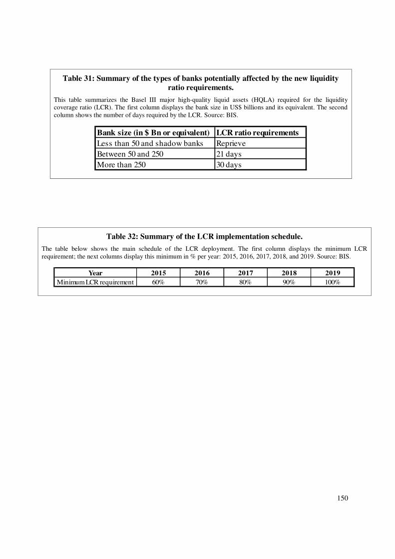
150
Table 31: Summary of the types of banks potentially affected by the new liquidity ratio requirements.
This table summarizes the Basel III major high-quality liquid assets (HQLA) required for the liquidity coverage ratio (LCR). The first column displays the bank size in US$ billions and its equivalent. The second column shows the number of days required by the LCR. Source: BIS.
Table 32: Summary of the LCR implementation schedule.
The table below shows the main schedule of the LCR deployment. The first column displays the minimum LCR requirement; the next columns display this minimum in % per year: 2015, 2016, 2017, 2018, and 2019. Source: BIS.
Bank size (in $ Bn or equivalent) LCR ratio requirementsLess than 50 and shadow banks ReprieveBetween 50 and 250 21 daysMore than 250 30 days
Year 2015 2016 2017 2018 2019Minimum LCR requirement 60% 70% 80% 90% 100%
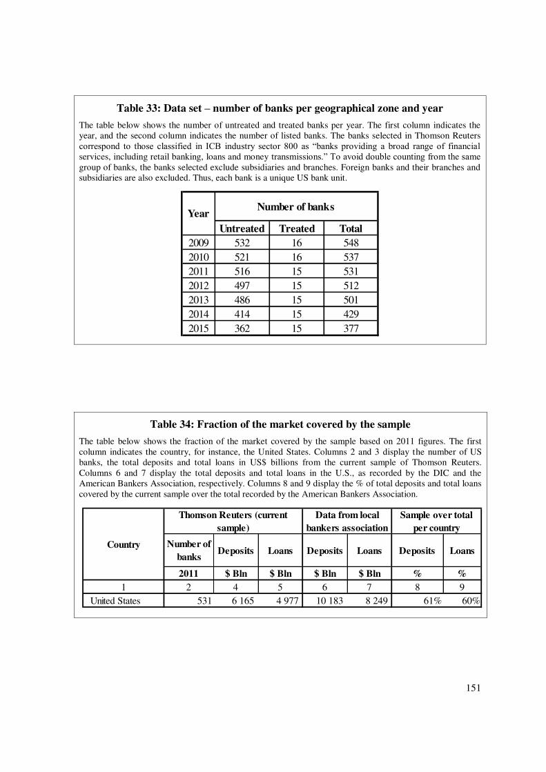
151
Table 33: Data set – number of banks per geographical zone and year
The table below shows the number of untreated and treated banks per year. The first column indicates the year, and the second column indicates the number of listed banks. The banks selected in Thomson Reuters correspond to those classified in ICB industry sector 800 as “banks providing a broad range of financial services, including retail banking, loans and money transmissions.” To avoid double counting from the same group of banks, the banks selected exclude subsidiaries and branches. Foreign banks and their branches and subsidiaries are also excluded. Thus, each bank is a unique US bank unit.
Table 34: Fraction of the market covered by the sample
The table below shows the fraction of the market covered by the sample based on 2011 figures. The first column indicates the country, for instance, the United States. Columns 2 and 3 display the number of US banks, the total deposits and total loans in US$ billions from the current sample of Thomson Reuters. Columns 6 and 7 display the total deposits and total loans in the U.S., as recorded by the DIC and the American Bankers Association, respectively. Columns 8 and 9 display the % of total deposits and total loans covered by the current sample over the total recorded by the American Bankers Association.
Untreated Treated Total2009 532 16 5482010 521 16 5372011 516 15 5312012 497 15 5122013 486 15 5012014 414 15 4292015 362 15 377
YearNumber of banks
Number of banks
Deposits Loans Deposits Loans Deposits Loans
2011 $ Bln $ Bln $ Bln $ Bln % %1 2 4 5 6 7 8 9
United States 531 6 165 4 977 10 183 8 249 61% 60%
Sample over total per country
Thomson Reuters (current sample)
Data from local bankers association
Country

152
Table 35: Items for computing the liquidity creation measures
The table below identifies the Thomson Reuters items used to proxy the liquidity creation measures: the “LTGap” measure, as established by Deep and Schaefer (2004), and the “B-B MatNonFat” measure, as established by Berger and Bouwman (2009). The first column displays the level of liquidity: liquid, semi-liquid and illiquid. Column 2 displays the asset items; column 3, the asset weight; column 4, the liabilities item; and column 5, the liabilities weight for the LTGap measure. This order is replicated for the BB MatNonFat measures. Observe that, for US banks, the deposits were weighted at 33%, whereas for other banks, they were weighted at 80%. The net loans are all weighted at 85%. All amounts were deflated by the IMF inflation index (base 2005).
Table 36: The results of the liquidity creation measures compared with other articles
The table below compares the LTGap and BB-CatNonFat liquidity creation measures for US, German and Chinese banks. Note that I only present the MatNonFat measure, whereas other researchers show only the CatNonFat measures, which makes it difficult to conduct a strict comparison. The differences found are in line with the results of Berger and Bouwman (2009), who find that CatNonFat values are generally lower than MatNonFat values
LiabilitiesItem Weight Item Weight Item Weight Item Weight
1 2 3 4 5 6 7 8 9
WC02205 - Treasury Securities
WC02205 - Treasury Securities
WC02208 - Trading account Securities
WC02208 - Trading account Securities
WC02004 - Cash and Due from Banks
WC02004 - Cash and Due from Banks
WC02055 - Interbank Loans
WC02055 - Interbank Loans
Semi liquid NA NA NA NAWC02055 - Interbank
Loans0
WC03051 - Total ST debts
0
NA NA NA NA WC03251 - LT Debts
NA NA NA NAWC03995 - Total
Shareholder's Equity
Scaled over asset
Liquidity levelBB MatNonFat
Asset Asset LiabilitiesLTGap
-0.5Illiquid
Liquid
WC02999 - Total Assets
-1 1 -0.5 0.5WC03019 - Cust Dep WC03019 - Cust Dep
WC02271 - Loans 0.5
Their article This article Their article This article
Quarter - all periods
Annual - all periods
1993 2003 1993 2003BB -
CatNonFatLT Gap
BB-MatNonFat
LT Gap
BB - CatNonFat
BB-MatNonFat
1 2 3 4 5 6 7 8 9 10 11 12 13
Mean 0.20 0.17 0.22 0.26 0.25 0.28 0.18 0.14 0.29 0.11 0.28 0.37Median 0.21 0.18 NA NA 0.27 0.30 0.18 0.13 0.28 0.11 NA 0.37Standard deviation 0.16 0.08 NA NA 0.09 0.10 0.09 0.02 0.22 0.24 NA 0.05
US banks 1997-2001
Lei and Song (2013)
Chinese banks 1988 - 2008
Their article This article Their article This article
Deep and Schaefer (2004)
Hackethal et al. (2010)
Berger and Bouwman (2009)
US banks 1993 - 2003
German banks 1997 - 2006

153
Table 37: Definition of population treated vs. population untreated
The table below identifies the types of banks that are affected by Basel III LCR requirements (“treated”) and those that are not (“untreated”). The first column indicates the bank size in US$ billions or equivalent, the second column indicates whether the bank is subject to Basel III, and the last column indicates whether the bank is considered to be “treated” or “untreated.”
Bank size (in $ Bn or equivalent) Banking regulation Treated / UntreatedLess than 50 and shadow banks Reprieve UntreatedMore than 50 Impacted Treated
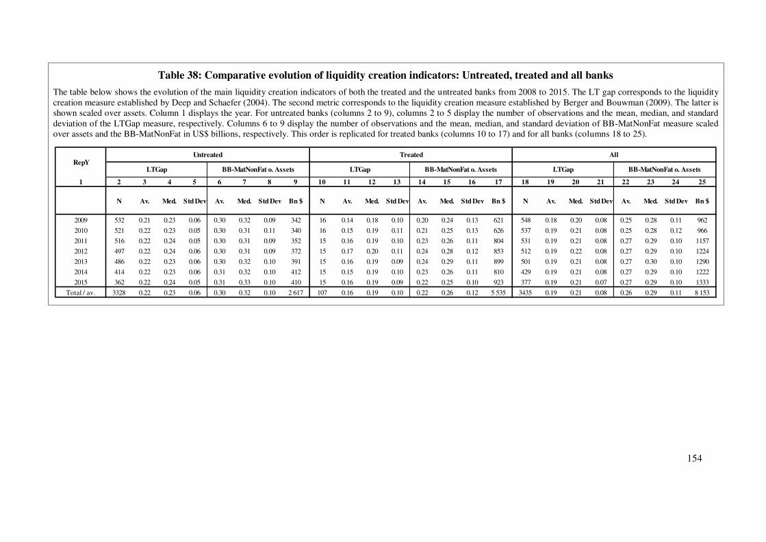
154
Table 38: Comparative evolution of liquidity creation indicators: Untreated, treated and all banks
The table below shows the evolution of the main liquidity creation indicators of both the treated and the untreated banks from 2008 to 2015. The LT gap corresponds to the liquidity creation measure established by Deep and Schaefer (2004). The second metric corresponds to the liquidity creation measure established by Berger and Bouwman (2009). The latter is shown scaled over assets. Column 1 displays the year. For untreated banks (columns 2 to 9), columns 2 to 5 display the number of observations and the mean, median, and standard deviation of the LTGap measure, respectively. Columns 6 to 9 display the number of observations and the mean, median, and standard deviation of BB-MatNonFat measure scaled over assets and the BB-MatNonFat in US$ billions, respectively. This order is replicated for treated banks (columns 10 to 17) and for all banks (columns 18 to 25).
1 2 3 4 5 6 7 8 9 10 11 12 13 14 15 16 17 18 19 20 21 22 23 24 25
N Av. Med. Std Dev Av. Med. Std Dev Bn $ N Av. Med. Std Dev Av. Med. Std Dev Bn $ N Av. Med. Std Dev Av. Med. Std Dev Bn $
2009 532 0.21 0.23 0.06 0.30 0.32 0.09 342 16 0.14 0.18 0.10 0.20 0.24 0.13 621 548 0.18 0.20 0.08 0.25 0.28 0.11 962
2010 521 0.22 0.23 0.05 0.30 0.31 0.11 340 16 0.15 0.19 0.11 0.21 0.25 0.13 626 537 0.19 0.21 0.08 0.25 0.28 0.12 966
2011 516 0.22 0.24 0.05 0.30 0.31 0.09 352 15 0.16 0.19 0.10 0.23 0.26 0.11 804 531 0.19 0.21 0.08 0.27 0.29 0.10 1157
2012 497 0.22 0.24 0.06 0.30 0.31 0.09 372 15 0.17 0.20 0.11 0.24 0.28 0.12 853 512 0.19 0.22 0.08 0.27 0.29 0.10 1224
2013 486 0.22 0.23 0.06 0.30 0.32 0.10 391 15 0.16 0.19 0.09 0.24 0.29 0.11 899 501 0.19 0.21 0.08 0.27 0.30 0.10 1290
2014 414 0.22 0.23 0.06 0.31 0.32 0.10 412 15 0.15 0.19 0.10 0.23 0.26 0.11 810 429 0.19 0.21 0.08 0.27 0.29 0.10 1222
2015 362 0.22 0.24 0.05 0.31 0.33 0.10 410 15 0.16 0.19 0.09 0.22 0.25 0.10 923 377 0.19 0.21 0.07 0.27 0.29 0.10 1333
Total / av. 3328 0.22 0.23 0.06 0.30 0.32 0.10 2 617 107 0.16 0.19 0.10 0.22 0.26 0.12 5 535 3435 0.19 0.21 0.08 0.26 0.29 0.11 8 153
RepYUntreated Treated All
LTGap BB-MatNonFat o. Assets LTGap BB-MatNonFat o. Assets LTGap BB-MatNonFat o. Assets
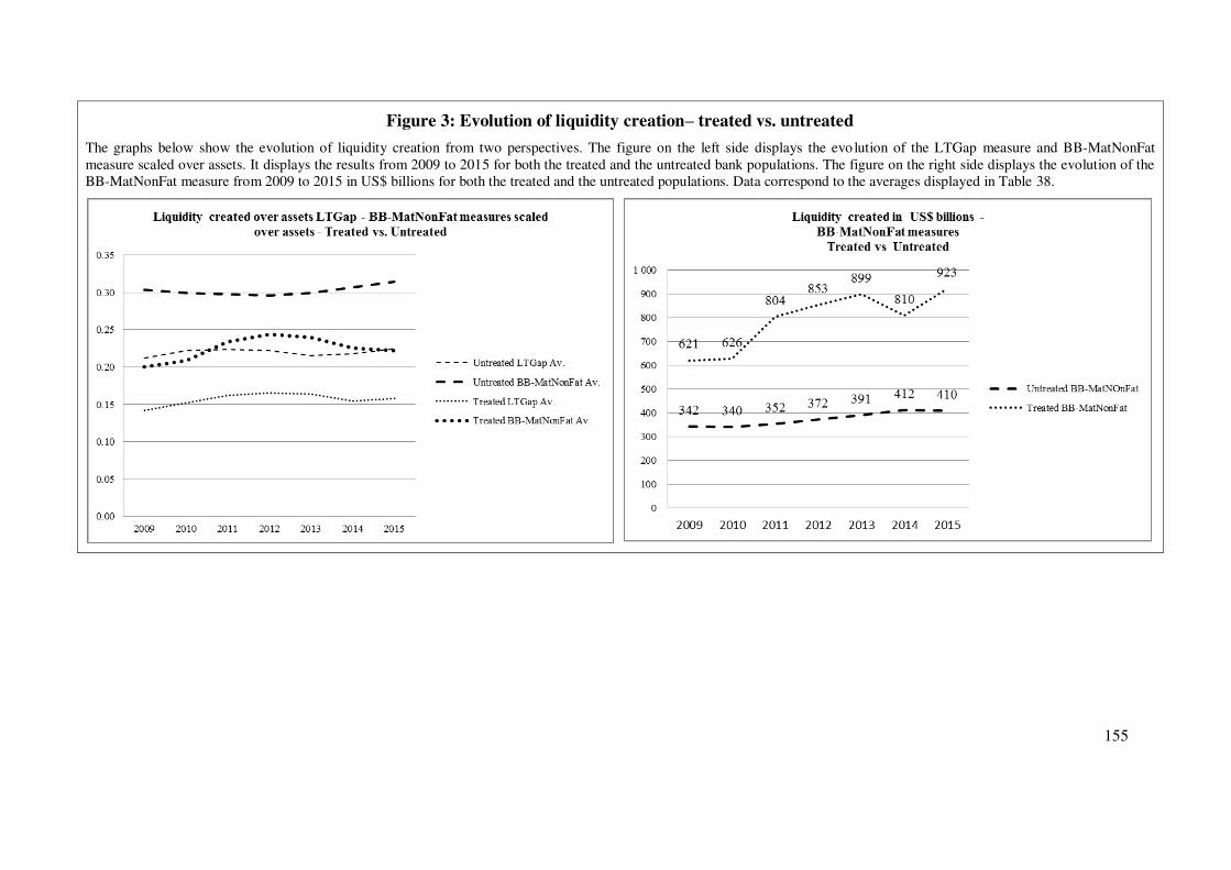
155
Figure 3: Evolution of liquidity creation– treated vs. untreated
The graphs below show the evolution of liquidity creation from two perspectives. The figure on the left side displays the evo lution of the LTGap measure and BB-MatNonFat measure scaled over assets. It displays the results from 2009 to 2015 for both the treated and the untreated bank populations. The figure on the right side displays the evolution of the BB-MatNonFat measure from 2009 to 2015 in US$ billions for both the treated and the untreated populations. Data correspond to the averages displayed in Table 38.

156
Table 39: List of variables that affect liquidity creation
The table below lists the explained and explicative variables, including the control variables used for the robustness tests in the regression model established herein. The first column shows the typology of the variable; the second lists the variable name; the third lists the shorthand variable name used in the GMM, OLS and Cox regressions; the fourth indicates whether a variable was scaled; the fifth lists the expected relationship with liquidity creation; and the last column shows how the variable was calculated.
Variable typology Variable nameVariable name in
the OLSTukey'
scale typePredictive
signHow this variable is computed and Thomson Reuters definitions
1 2 3 4 5 6
Liquidity creation variable 1
LTGapY1LTGap at t and
t+1 (for GMM)NA
LT gap as proposed by Deep and Schaefer (2004). Deflated based on the IMF inflation index (2005=100)
Liquidity creation variable 3
BB-MatNonFatY2NLC at t and t+1
(for GMM)Scaled over
assetsLiquidity created as measured by the BB-measure, which proxies the "MatNonFat". Deflated based on the IMF inflation index (2005=100)
Bank size X1BkSizeUSD Log +Firm size is measured as follows in this research: Log Total Assets (item WC02999).
Level of equity X2EQoA NA - Common equities (item WC03501) / Total assets (item WC02999)
Agency : Dividend paid out over shareholders' equity ratio
X3PayShldrsoEq NA +
Cash dividends (item WC04551) over Shareholders' equity (item WC03995). Cash dividends (item WC04551) represents the total common and preferred dividends paid to shareholders of the company.Total Shareholder's Equity (item WC03995) represents the sum of Preferred Stock and Common Shareholders’ Equity.
Credit risk : NPL over Loans X4NPLoLoans NA -
Non Performing loans over loans is the control variable that proxies the risk management.NPLoLoans = Non performing loans (item WC02285) / Loans total (item WC02271).
Bank stability risk : z-score X5Z Log +
The z-score as proposed originally by Roy (1952): RoA+ Equity over Asset divided by standard deviation of RoA. This bank risk indicator measures the bank's distance to insolvency. Inversely related to the probability of default, the sign is expected to be positive. - Standard deviation of RoA = Net Income Total (item WC01751) / Total assets (item WC02999). Tthe standard deviation requires at least three observations, is rolling and is computed every year (step of maximum 5 years). - Net Income Total (WC01751) , represents the net income of the company, before extraordinary items.
Loan growth X6LnGwth NA +
Loan growth is a proxy for bank's growth opportunity. It is the variation of total loans over one reporting yearLnGwth : (Loans Total Y of bank i- Loans total Y-1 of bank i) / Loans total Y-1 of bank 1 - [Where Loans total is item WC02271]
Excess Return X7ExcssR NA +
Jense's Excess Return (α) = R(a) – R(f) – Beta(a,m) [R(m) - R(f)] ; beta is the
common indicator [Cov (a, m) / Variance (m)], where R(a) is the return of market share, R(f) is the return of benchmark government bonds, R(m) is the return of the market index for the market where the bank is listed. Var(x) and Cov (x, y) require at least three observations. Covariances and variances are rolling and computed every year (step of maximum 5 years). Market price = Market value per share (item WC05001).
Market share value X8MktPrice Market value per share (item WC05001).
Monetary policy Yield curve spread X9YieldSpread NA +Interest rate spread between 3-months and 10 year government bond. Source : Thomson Reuters.
GDP growth per country X10GDPgwth NA +The GDP growth corresponds to the yearly growth of GDP of the country in which the bank is located. Source : International Monetary Fund, World Economic Outlook Database, October 2014.
Unemployment X11UnmpRate Sqrt +Unemployment rate for the country where the bank is located. Source : IMF.
Hirshman-Herfindhal Index of market concentration
X12HHI NA +
Computed as follows : HHI = Squared [Loan market share = Total (item WC02271) countervalued in KUSD / Total loan (BIS data) in KUSD per country where the bank is located]. Yearly Foreign exchange rate is that of IMF, closing end of year.
Omitted variablesSet of dummies for all but one year.
Per bank.NA NA + / - Fixed effects : countryj, where the bank is located.
Macro environment
Bank risk typology
Bank performance
Bank characteristics
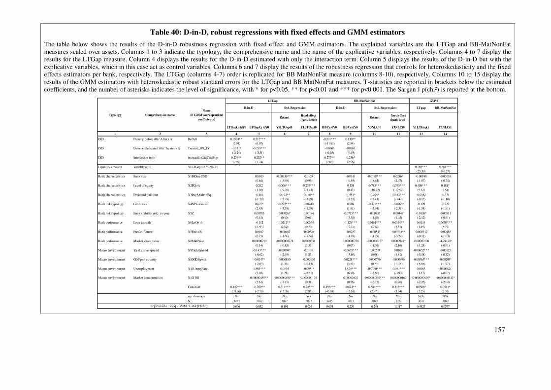
157
Table 40: D-in-D, robust regressions with fixed effects and GMM estimators
The table below shows the results of the D-in-D robustness regression with fixed effect and GMM estimators. The explained variables are the LTGap and BB-MatNonFat measures scaled over assets. Columns 1 to 3 indicate the typology, the comprehensive name and the name of the explicative variables, respectively. Columns 4 to 7 display the results for the LTGap measure. Column 4 displays the results for the D-in-D estimated with only the interaction term. Column 5 displays the results of the D-in-D but with the explicative variables, which in this case act as control variables. Columns 6 and 7 display the results of the robustness regression that controls for heteroskedasticity and the fixed effects estimators per bank, respectively. The LTGap (columns 4-7) order is replicated for BB MatNonFat measure (columns 8-10), respectively. Columns 10 to 15 display the results of the GMM estimators with heteroskedastic robust standard errors for the LTGap and BB MatNonFat measures. T-statistics are reported in brackets below the estimated coefficients, and the number of asterisks indicates the level of significance, with * for p<0.05, ** for p<0.01 and *** for p<0.001. The Sargan J p(chi²) is reported at the bottom.
Robustfixed effect (bank level)
Robustfixed effect (bank level)
LTGapCrtdY0 LTGapCrtdY0 Y1LTGapt0 Y1LTGapt0 BBCrtdY0 BBCrtdY0 Y3NLCt0 Y3NLCt0 Y1LTGapt1 Y3NLCt1
1 2 3 4 5 6 7 8 9 10 11 13 14
DID Dummy before (0) / After (1) BefAft 0.0524** 0.317*** -0.201*** 0.130**(2.94) (6.07) (-11.91) (2.84)
DID Dummy Untreated (0) / Treated (1) Treated_0N_1Y -0.131* -0.219*** -0.0606 -0.0681(-2.24) (-3.31) (-0.95) (-0.93)0 0 0 0
DID Interaction term interactionLiqCrtdPop 0.279** 0.252** 0.277** 0.256*(2.97) (2.74) (2.80) (2.56)
Liquidity creation Variable at t0 Y1LTGapt0 / Y3NLCt0 0.785*** 0.861***(25.39) (40.27)
Bank characteristics Bank size X1BkSizeUSD 0.0109 -0.00936*** 0.0105 -0.0141 -0.0198*** 0.0246* -0.00198 -0.00138(0.64) (-5.98) (0.96) (-0.93) (-8.64) (2.07) (-1.07) (-0.74)
Bank characteristics Level of equity X2EQoA 0.242 -0.366*** -0.237*** 0.158 -0.715*** -0.593*** 0.408*** 0.181*(1.02) (-9.70) (-5.43) (0.47) (-10.72) (-12.52) (5.32) (2.51)
Bank characteristics Dividend paid out X3PayShldrsoEq -0.481 -0.192** -0.140** -1.551* -0.295* -0.183*** -0.0382 -0.374(-1.20) (-2.78) (-2.89) (-2.57) (-2.43) (-3.47) (-0.12) (-1.18)
Bank risk typology Credit risk X4NPLoLoans 0.627* -0.222*** -0.0440 0.989 -0.371*** -0.0866* -0.139 -0.222(2.45) (-3.58) (-1.39) (1.81) (-3.94) (-2.51) (-1.54) (-1.91)
Bank risk typology Bank stability risk : z-score X5Z 0.00783 0.000267 0.00184 -0.0715*** -0.00735 0.00447 -0.0126* -0.00511(0.41) (0.10) (0.65) (-3.58) (-1.69) (1.45) (-2.12) (-0.91)0 0 0 0 0 0
Bank performance Loan growth X6LnGwth -0.112 0.0212** 0.00354 -1.129*** 0.0451*** 0.0154** 0.0114 0.0605***(-1.93) (2.82) (0.70) (-9.72) (3.52) (2.81) (1.45) (5.79)0 0 0 0 0 0
Bank performance Excess Return X7ExcssR 0.0167 -0.00487 -0.00324 -0.0257 -0.00543 -0.00743** -0.000312 -0.00485(0.71) (-1.66) (-1.56) (-1.18) (-1.29) (-3.29) (-0.11) (-1.63)0 0 0 0 0 0
Bank performance Market share value X8MktPrice 0.00000219 -0.000000778 0.0000534 0.000000758 -0.00000127 0.0000941* -0.00000108 -4.78e-09(0.14) (-0.85) (1.33) (0.07) (-1.08) (2.16) (-1.24) (-0.01)
Macro environment Yield curve spread X9YieldSpread -0.143*** -0.00394* 0.0101 -0.0678*** 0.00209 0.0109 -0.00652*** -0.00125(-6.62) (-2.49) (1.83) (-3.69) (0.98) (1.81) (-3.58) (-0.72)
Macro environment GDP per country X10GDPgwth -0.0147* 0.000880 -0.000101 0.0228*** 0.000776 -0.000996 -0.00565*** -0.00203*(-2.03) (1.31) (-0.13) (3.51) (0.79) (-1.15) (-5.06) (-1.97)
Macro environment Unemployment X11UnmpRate 1.563*** 0.0194 -0.0951* 1.524*** -0.0760*** -0.161*** 0.0163 -0.000821(5.03) (1.28) (-2.51) (6.10) (-3.60) (-3.90) (1.57) (-0.07)
Macro environment Market concentration X12HHI 0.00000455** -0.00000268*** 0.000000175 0.00000122 -0.00000265*** 0.000000162 -0.000000495* -0.000000442*(2.61) (-7.11) (0.31) (0.56) (-6.77) (0.26) (-2.26) (-2.04)
Constant 0.422*** -0.789** 0.314*** 0.225** 0.496*** -0.624** 0.584*** 0.313*** 0.0566* 0.0511*(38.76) (-2.70) (15.38) (2.85) (45.08) (-2.61) (20.70) (3.64) (2.25) (2.37)
rep dummies No No No Yes No No No Yes N/A N/A
N 3427 3077 3077 3077 3435 3077 3077 3077 3077 3077
0.006 0.032 0.191 0.034 0.038 0.259 0.248 0.117 0.4427 0.0577
Typology Comprehensive nameName
(if GMM correspondent coefficients)
GMM
LTgap BB-MatNonFat
Regressions : R-Sq - GMM : J-stat [P(chi²)]
LTGap BB-MatNonFat
Std. RegressionD-in-DStd. RegressionD-in-D
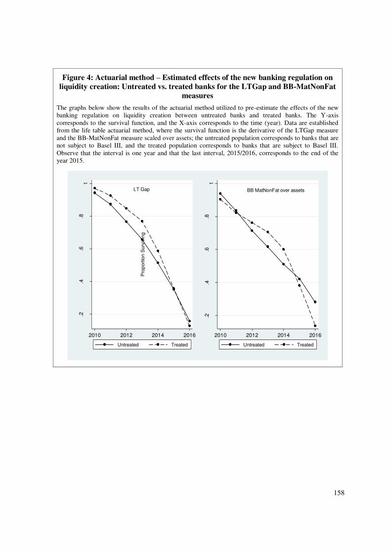
158
Figure 4: Actuarial method – Estimated effects of the new banking regulation on liquidity creation: Untreated vs. treated banks for the LTGap and BB-MatNonFat
measures
The graphs below show the results of the actuarial method utilized to pre-estimate the effects of the new banking regulation on liquidity creation between untreated banks and treated banks. The Y-axis corresponds to the survival function, and the X-axis corresponds to the time (year). Data are established from the life table actuarial method, where the survival function is the derivative of the LTGap measure and the BB-MatNonFat measure scaled over assets; the untreated population corresponds to banks that are not subject to Basel III, and the treated population corresponds to banks that are subject to Basel III. Observe that the interval is one year and that the last interval, 2015/2016, corresponds to the end of the year 2015.
LT Gap
.2.4
.6.8
1
2010 2012 2014 2016
Untreated Treated
BB MatNonFat over assets
.2.4
.6.8
1
Pro
port
ion S
urv
ivin
g
2010 2012 2014 2016
Untreated Treated
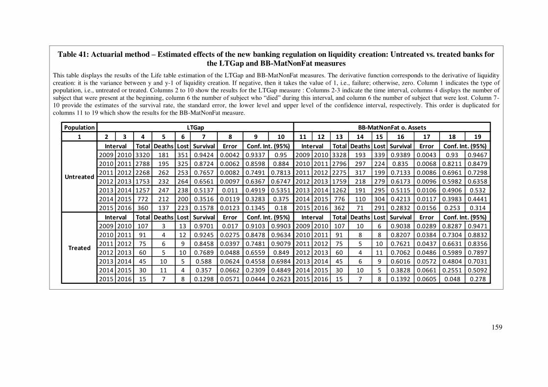
159
Table 41: Actuarial method – Estimated effects of the new banking regulation on liquidity creation: Untreated vs. treated banks for the LTGap and BB-MatNonFat measures
This table displays the results of the Life table estimation of the LTGap and BB-MatNonFat measures. The derivative function corresponds to the derivative of liquidity creation: it is the variance between y and y-1 of liquidity creation. If negative, then it takes the value of 1, i.e., failure; otherwise, zero. Column 1 indicates the type of population, i.e., untreated or treated. Columns 2 to 10 show the results for the LTGap measure : Columns 2-3 indicate the time interval, columns 4 displays the number of subject that were present at the beginning, column 6 the number of subject who “died” during this interval, and column 6 the number of subject that were lost. Column 7-10 provide the estimates of the survival rate, the standard error, the lower level and upper level of the confidence interval, respectively. This order is duplicated for columns 11 to 19 which show the results for the BB-MatNonFat measure.
Population
1 2 3 4 5 6 7 8 9 10 11 12 13 14 15 16 17 18 19
Total Deaths Lost Survival Error Total Deaths Lost Survival Error
2009 2010 3320 181 351 0.9424 0.0042 0.9337 0.95 2009 2010 3328 193 339 0.9389 0.0043 0.93 0.9467
2010 2011 2788 195 325 0.8724 0.0062 0.8598 0.884 2010 2011 2796 297 224 0.835 0.0068 0.8211 0.8479
2011 2012 2268 262 253 0.7657 0.0082 0.7491 0.7813 2011 2012 2275 317 199 0.7133 0.0086 0.6961 0.7298
2012 2013 1753 232 264 0.6561 0.0097 0.6367 0.6747 2012 2013 1759 218 279 0.6173 0.0096 0.5982 0.6358
2013 2014 1257 247 238 0.5137 0.011 0.4919 0.5351 2013 2014 1262 191 295 0.5115 0.0106 0.4906 0.532
2014 2015 772 212 200 0.3516 0.0119 0.3283 0.375 2014 2015 776 110 304 0.4213 0.0117 0.3983 0.4441
2015 2016 360 137 223 0.1578 0.0123 0.1345 0.18 2015 2016 362 71 291 0.2832 0.0156 0.253 0.314
Total Deaths Lost Survival Error Total Deaths Lost Survival Error
2009 2010 107 3 13 0.9701 0.017 0.9103 0.9903 2009 2010 107 10 6 0.9038 0.0289 0.8287 0.9471
2010 2011 91 4 12 0.9245 0.0275 0.8478 0.9634 2010 2011 91 8 8 0.8207 0.0384 0.7304 0.8832
2011 2012 75 6 9 0.8458 0.0397 0.7481 0.9079 2011 2012 75 5 10 0.7621 0.0437 0.6631 0.8356
2012 2013 60 5 10 0.7689 0.0488 0.6559 0.849 2012 2013 60 4 11 0.7062 0.0486 0.5989 0.7897
2013 2014 45 10 5 0.588 0.0624 0.4558 0.6984 2013 2014 45 6 9 0.6016 0.0572 0.4804 0.7031
2014 2015 30 11 4 0.357 0.0662 0.2309 0.4849 2014 2015 30 10 5 0.3828 0.0661 0.2551 0.5092
2015 2016 15 7 8 0.1298 0.0571 0.0444 0.2623 2015 2016 15 7 8 0.1392 0.0605 0.048 0.278
Untreated
Treated
Conf. Int. (95%)
Interval Conf. Int. (95%)
LTGap BBMatNonFat o. Assets
Interval Conf. Int. (95%)
Interval Conf. Int. (95%)
Interval
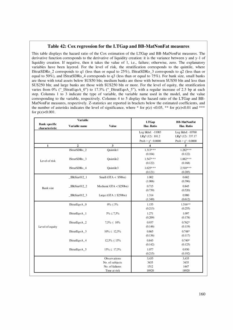
160
Table 42: Cox regression for the LTGap and BB-MatNonFat measures
This table displays the hazard ratio of the Cox estimation of the LTGap and BB-MatNonFat measures. The derivative function corresponds to the derivative of liquidity creation: it is the variance between y and y-1 of liquidity creation. If negative, then it takes the value of 1, i.e., failure; otherwise, zero. The explanatory variables have been layered. For the level of risk, the stratification corresponds to the quintile, where IStratSDRo_2 corresponds to q1 (less than or equal to 25%), IStratSDRo_3 corresponds to q2 (less than or equal to 50%), and IStratSDRo_4 corresponds to q3 (less than or equal to 75%). For bank size, small banks are those with total assets below $US50 bln; medium banks are those with between $US50 bln and less than $US250 bln; and large banks are those with $US250 bln or more. For the level of equity, the stratification varies from 0% (“_IStratEqoA_0”) to 17.5% (“_IStratEqoA_5”), with a regular increase of 2.5 bp at each step. Columns 1 to 3 indicate the type of variable, the variable name used in the model, and the value corresponding to the variable, respectively. Columns 4 to 5 display the hazard ratio of the LTGap and BB-MatNonFat measures, respectively. Z-statistics are reported in brackets below the estimated coefficients, and the number of asterisks indicates the level of significance, where * for p(z) <0.05, ** for p(z)<0.01 and *** for p(z)<0.001.
Bank specific characteristic
Variable name Value
Log likhd: -11083 Log likhd: -10760LRχ² (12) : 101.2 LRχ² (12) : 337.17
Prob > χ² : 0.0000 Prob > χ² : 0.0000
1 2 3 4 5IStratSDRo_2 Quintile1 1.313*** 1.282***
(0.104) (0.122)
IStratSDRo_3 Quintile2 1.547*** 1.882***(0.122) (0.168)
IStratSDRo_4 Quintile3 1.625*** 2.510***(0.121) (0.205)
_IBkSize012_1 Small (GTA < $50bn) 1.002 0.682(1.006) (0.396)
_IBkSize012_2 Medium( GTA < $250bn) 0.715 0.845(0.739) (0.520)
_IBkSize012_3 Large (GTA ≥ $250bn) 1.314 0.980(1.349) (0.612)
IStratEqoA_0 0% ≤ 5% 1.155 1.516**(0.213) (0.255)
IStratEqoA_1 5% ≤ 7,5% 1.271 1.097(0.209) (0.178)
IStratEqoA_2 7,5% ≤ 10% 0.937 0.762*(0.146) (0.119)
IStratEqoA_3 10% ≤ 12,5% 0.865 0.748*(0.136) (0.117)
IStratEqoA_4 12,5% ≤ 15% 0.845 0.740*(0.142) (0.125)
IStratEqoA_5 15% ≤ 17,5% 1.077 0.930(0.215) (0.192)
Observations 3,435 3,435No. of subjects 3435 3435No. of failures 1512 1447
Time at risk 18920 18920
LTGapHaz. Ratio
BB-MatNonFatHaz. Ratio
Level of risk
Bank size
Level of equity
Variable

161
Conclusion
This thesis has focused on liquidity in the banking sector. As one of the cornerstones
of banking, liquidity is a concept that can be viewed from two primary, related angles. The
first refers to the cash or assimilated resources that banks hold to meet immediate or short-
term needs. They provide security in the face of unforeseen risks and have proven essential to
banks’ survival under conditions of stress. The second refers to the classical maturity process,
through which resources undergo a transformation that ranges from short-term to long-term
and contributes to financing the economy.
The first article, “Why do banks hold cash?”, examined the hypothesis that cash
optimality exists in the banking sector. To reach this goal, I first explored the empirical
determinants of cash-holding for a large sample of listed banks over a period of 35 years.
Using the GMM-system estimation method, this study provides evidence that, in contrast to
the nonbanking sector, there is no support for the dynamic optimal cash model in the banking
industry. It confirms that agents in the banking sector face difficulties in determining their
preferences and optimizing their utility. These results provide new insights into cash
management in the banking sector and how it fundamentally differs from that of non-financial
industries, offering additional clues as to how banks differ from non-banks.
The next articles focus on liquidity-creation by banks. The article, “Does an increase
in capital negatively impact banking liquidity-creation?”, isolates the effect of increasing
levels of capital to determine which of the “risk absorption” or “crowding out” hypotheses
162
(Berger and Bouwman (2009)) prevails. The next and final article, “Positive effects of Basel
III on banking liquidity creation”, discusses the overall effects of Basel III on liquidity-
creation.
The article, “Does an increase in capital negatively impact banking liquidity-
creation?” yields several results. First, it is the only cross-national, empirical study
documenting bank liquidity-creation over a period of 35 years and providing a unified view of
banking liquidity-creation. Second, it confirms results presented in previous studies, which
show that liquidity-creation is determined not only by exogenous factors, such as monetary
policy, but also by endogenous factors, such as bank size, equity levels and risk performance.
These findings have broad applications for policy, particularly for reducing inefficiencies in
monetary policy transmission. Third, it confirms that an increase in equity levels has two
consequences. The first is positive: risk reduction. The second is negative, involving a decline
in liquidity-creation. However, taken alone, there is an overall negative effect from an
increase in the level of equity.
The primary focus of the last article, “Positive effects of Basel III on banking
liquidity creation” was to estimate the overall effects of Basel III, considering all components
together. The primary method used to estimate the effects of Basel III is the “D-in-D” method,
which, for robustness, has been complemented by additional analyses. The results indicate
that during the period studied, all things being equal, the Basel III regulatory framework has
not negatively impacted banking liquidity-creation in the U.S.
163
Overall, this thesis highlights the following key points:
The Basel III regulatory framework can be assimilated to a Pigouvian tax because it
internalizes the social costs of financial instability to banks.
Liquidity in the banking sector can be defined as a function for optimal asset
structure when bank managers face the dilemma of having to choose between allocating
resources to liquid assets to reduce the costs of illiquidity or allocating resources to illiquid
assets to finance projects and generate income. Given the market and regulatory constraints
that banks face, this arbitrage on the asset side is a complex process that is not yet fully
understood. Likely caused by the complexity and interdependence of constraints, the absence
of a dynamic optimal cash model may indicate that bank managers use models that are similar
to a “pecking order” approach, that is, by order of preference. This process echoes the
“pecking order hypothesis” of Myers and Majluf (1984), though the latter focuses on the
liability side of corporations. For the sake of future financial stability, further studies on this
issue should be conducted.
Finally, cash-holding and liquidity-creation by banks are affected by endogenous
factors of banks, such as bank size, level of equity or risk performance. In this regard, this
project has demonstrated that specific bank factors play a significant role in the transmission
of monetary policy. How could a monetary policy account for these factors appropriately?
This question lies ahead to be addressed by future studies.
But exogenous variables such as regulatory frameworks affect the motives for banks
to hold liquid assets or to create liquidity. A balkanized legal and fiscal environment may lead
the banks to arbitrate their decisions, based on these differences and ultimately select
countries which legal and fiscal frameworks is less compelling. In that sense, the results

164
presented in the articles in this thesis argue in favor of more integrated legal and fiscal
frameworks in Europe to mitigating these tradeoff effects.
Looking ahead to the next years, it is likely that the current liquidity ratios will be
amended to include the endogeneity property and the stochastic movements of the market as
proposed by the Liquidity Mismatch Measurement of Brunnermeier, Gorton and
Krishnamurthy (2014).
165
Tables des graphes, des tables, des équations et références bibliographiques
Tables des graphes
FIGURE 1: LIQUIDITY CREATED PER MEASURE, YEAR AND GEOGRAPHIC ZONE ...................................................................... 114
FIGURE 2: SENSITIVITY ANALYSIS COMPARISON FOR THE EFFECT OF A MARGINAL INCREASE IN THE LEVEL OF EQUITY ON LIQUIDITY
CREATION AND RISK PERFORMANCE................................................................................................................. 121
FIGURE 3: EVOLUTION OF LIQUIDITY CREATION– TREATED VS. UNTREATED ........................................................................ 155
FIGURE 4: ACTUARIAL METHOD – ESTIMATED EFFECTS OF THE NEW BANKING REGULATION ON LIQUIDITY CREATION: UNTREATED VS.
TREATED BANKS FOR THE LTGAP AND BBMATNONFAT MEASURES ....................................................................... 158
166
Table des tables
TABLE 1: BREAKDOWN OF THE NUMBER OF BANKS PER GEOGRAPHICAL ZONE AND COUNTRY ................................................... 55
TABLE 2: FRACTION OF THE MARKET COVERED BY THE SAMPLE ......................................................................................... 56
TABLE 3 : COMPARED EVOLUTION OF THE CASH AND PAID OUT OVER EQUITY AND LEVERAGE RATIOS – PER GEOGRAPHICAL ZONE, TYPE
OF BANK AND PERIOD – SMALL AND MEDIUM BANKS ............................................................................................ 57
TABLE 4 : COMPARED EVOLUTION OF THE CASH AND PAID OUT OVER EQUITY AND LEVERAGE RATIOS – PER GEOGRAPHICAL ZONE, TYPE
OF BANK AND PERIOD – LARGE BANKS ............................................................................................................... 58
TABLE 5 : EVOLUTION OF AGGREGATED CASH HOLDING – PER TYPE OF BANK ........................................................................ 59
TABLE 6: SUMMARY OF VARIABLES (PART 1) ................................................................................................................ 60
TABLE 7: SUMMARY OF VARIABLES (PART 2) ................................................................................................................ 61
TABLE 8: REGRESSION MODELS PER PERIOD – ALL BANKS (BASEL PERIOD) ........................................................................... 62
TABLE 9: REGRESSION MODELS PER PERIOD – ALL BANKS (TENYEARS PERIOD AND FIXED EFFECT) ............................................. 63
TABLE 10: REGRESSION MODELS PER PERIOD – ASIAN AND PACIFIC BANKS (BASEL PERIOD) .................................................... 64
TABLE 11: REGRESSION MODELS PER PERIOD – ASIAN AND PACIFIC BANKS (TENYEARS PERIOD AND FIXED EFFECT) ....................... 65
TABLE 12: REGRESSION MODELS PER PERIOD –EUROPEAN BANKS (BASEL PERIOD) ................................................................ 66
TABLE 13: REGRESSION MODELS PER PERIOD –EUROPEAN BANKS (TENYEARS PERIOD AND FIXED EFFECT) .................................. 67
TABLE 14: REGRESSION MODELS PER PERIOD –NORTH AMERICAN BANKS (BASEL PERIOD) ...................................................... 68
TABLE 15: REGRESSION MODELS PER PERIOD –NORTH AMERICAN BANKS (TENYEARS PERIOD AND FIXED EFFECT) ........................ 69
TABLE 16: GMM ESTIMATION OF DYNAMIC CASH HOLDING – PROPENSITY TO REVERT TO OPTIMAL CASH COMPARED PER REGION AND
BANK SIZE ................................................................................................................................................... 70
TABLE 17: SUMMARY OF VARIABLES (PART 1) ............................................................................................................ 107
TABLE 18: SUMMARY OF VARIABLES (PART 2) ............................................................................................................ 108
TABLE 19: ITEMS FOR COMPUTING THE THREE LIQUIDITY CREATION MEASURES .................................................................. 109
TABLE 20: LIQUIDITY CREATION MEASURE RESULTS COMPARED WITH THOSE OF OTHER ARTICLES ............................................ 110
TABLE 21: LIST OF BANKS ...................................................................................................................................... 111
167
TABLE 22: FRACTION OF THE MARKET COVERED BY THE SAMPLE ..................................................................................... 112
TABLE 23: LIQUIDITY CREATED OVER ASSET MEASURES PER PERIOD AND GEOGRAPHIC ZONE. ................................................. 113
TABLE 24: COMPARATIVE EVOLUTION OF EQUITY LEVEL, RISK PERFORMANCE, AND LIQUIDITY CREATION MEASURES .................... 115
TABLE 25: CORRELATION MATRIX ............................................................................................................................ 116
TABLE 26: GMM ESTIMATORS PER LIQUIDITY CREATION MEASURE AND GEOGRAPHIC ZONE – WITHOUT ZSCORES..................... 117
TABLE 27: GMM ESTIMATORS PER LIQUIDITY CREATION MEASURE AND GEOGRAPHIC ZONE WITH ZSCORES BUT WITHOUT THE STD.
DEV. OF ROE AND OP. INCOME OVER ASSETS ..................................................................................................... 118
TABLE 28: DETERMINANTS OF LIQUIDITY CREATION OLS AND FIXED EFFECTS ESTIMATORS PER COUNTRY .................................. 119
TABLE 29: COX REGRESSION (SURVIVAL ANALYSIS)....................................................................................................... 120
TABLE 30: KEY ASPECTS OF BASEL III ........................................................................................................................ 149
TABLE 31: SUMMARY OF THE TYPES OF BANKS POTENTIALLY AFFECTED BY THE NEW LIQUIDITY RATIO REQUIREMENTS. ................. 150
TABLE 32: SUMMARY OF THE LCR IMPLEMENTATION SCHEDULE. .................................................................................... 150
TABLE 33: DATA SET – NUMBER OF BANKS PER GEOGRAPHICAL ZONE AND YEAR ................................................................. 151
TABLE 34: FRACTION OF THE MARKET COVERED BY THE SAMPLE ..................................................................................... 151
TABLE 35: ITEMS FOR COMPUTING THE LIQUIDITY CREATION MEASURES ........................................................................... 152
TABLE 36: THE RESULTS OF THE LIQUIDITY CREATION MEASURES COMPARED WITH OTHER ARTICLES ........................................ 152
TABLE 37: DEFINITION OF POPULATION TREATED VS. POPULATION UNTREATED .................................................................. 153
TABLE 38: COMPARATIVE EVOLUTION OF LIQUIDITY CREATION INDICATORS: UNTREATED, TREATED AND ALL BANKS .................... 154
TABLE 39: LIST OF VARIABLES THAT AFFECT LIQUIDITY CREATION ..................................................................................... 156
TABLE 40: DIND, ROBUST REGRESSIONS WITH FIXED EFFECTS AND GMM ESTIMATORS ..................................................... 157
TABLE 41: ACTUARIAL METHOD – ESTIMATED EFFECTS OF THE NEW BANKING REGULATION ON LIQUIDITY CREATION: UNTREATED VS.
TREATED BANKS FOR THE LTGAP AND BBMATNONFAT MEASURES ....................................................................... 159
TABLE 42: COX REGRESSION FOR THE LTGAP AND BBMATNONFAT MEASURES ................................................................ 160
168
Table des équations
EQUATION 1: ........................................................................................................................................................ 45
EQUATION 2 ......................................................................................................................................................... 51
EQUATION 3 ......................................................................................................................................................... 51
EQUATION 4 ......................................................................................................................................................... 52
EQUATION 5 ......................................................................................................................................................... 52
EQUATION 6......................................................................................................................................................... 85
EQUATION 7 ......................................................................................................................................................... 94
EQUATION 8 ......................................................................................................................................................... 98
EQUATION 9 ....................................................................................................................................................... 136
EQUATION 10 ..................................................................................................................................................... 139
EQUATION 11 ..................................................................................................................................................... 141
EQUATION 12 ..................................................................................................................................................... 145
169
Références bibliographiques
References
Acharya, Viral V, Denis Gromb, and Tanju Yorulmazer, 2011, Imperfect competition in the interbank market for liquidity as a rationale for central banking, Federal Reserve Bank of New York.
Acharya, Viral V., Iftekhar Hasan, and Anthony Saunders, 2006, Should banks be diversified? Evidence from individual bank loan portfolios, Journal of Business 79, 1355-1412.
Acharya, Viral V., and Ouarda Merrouche, 2013, Precautionary hoarding of liquidity and interbank markets: Evidence from the subprime crisis, Review of Finance 17, 107-160.
Acharya, Viral V., Hyun Song Shin, and Tanju Yorulmazer, 2011, Crisis resolution and bank liquidity, Review of Financial Studies 24, 2166-2205.
Acharya, Viral V., and David Skeie, 2011, A model of liquidity hoarding and term premia in inter-bank markets, Journal of Monetary Economics 58, 436-447.
Admati, Anat R, Peter M DeMarzo, Martin Hellwig, and Paul Pfleiderer, 2010, Fallacies, irrelevant facts, and myths in the discussion of capital regulation: Why bank equity is not expensive, Preprints of the Max Planck Institute for Research on Collective Goods.
Akbari, Mir Askari, Samira Rahmani, Reza Ahmadi, and Hooman Shababi, 2014, Deviation from optimal level of cash holdings and cumulative abnormal returns, Universal Journal of Accounting and Finance 2, 88-96.
Al-Khouri, Ritab, 2012, Bank characteristics and liquidity transformation: The case of gcc banks, International Journal of Economics and Finance 4, p114.
Alexandre, Hervé, and Hélène Buisson-Stéphan, 2014, Impact of the 2008 crisis on credit rationing for french smes, Revue internationale P.M.E. : économie et gestion de la petite et moyenne entreprise 27, 95-113.
Allen, Franklin, and Douglas Gale, 2000, Financial contagion, Journal of political economy 108, 1-33.
Allen, Franklin, and Douglas Gale, 2004, Financial intermediaries and markets, Econometrica 1023-1061.
Allen, Franklin, and Anthony M. Santomero, 1997, The theory of financial intermediation, Journal of Banking & Finance 21, 1461-1485.
Arellano, Manuel, and Stephen Bond, 1991, Some tests of specification for panel data: Monte carlo evidence and an application to employment equations, The review of economic studies 58, 277-297.
Arellano, Manuel, and Olympia Bover, 1995, Another look at the instrumental variable estimation of error-components models, Journal of Econometrics 68, 29-51.
170
Armakola, Angela, and Jean Paul Laurent, 2015, Ccp resilience and clearing membership, Available at SSRN.
Ashcraft, Adam, James McAndrews, and David Skeie, 2011, Precautionary reserves and the interbank market, Journal of Money, Credit and Banking 43, 311-348.
Bancel, Franck, and Laurent Salé, 2016, Focus on basel 3 and bank liquidity creation, Bankers, Markets and Investors 143, 46-54
Barth, James R, Gerard Caprio, and Ross Levine, 2004, Bank regulation and supervision: What works best?, Journal of Financial intermediation 13, 205-248.
Barth, James R, Gerard Caprio, and Ross Levine, 2008, Bank regulations are changing: For better or worse ?, Comparative Economic Studies 50, 537-563.
Barth, James R, Gerard Caprio Jr, and Ross Levine, 2001, The regulation and supervision of banks around the world, The World Bank Policy Research.
Barth, James R, Gerard Caprio Jr, and Ross Levine, 2013, Bank regulation and supervision in 180 countries from 1999 to 2011, Journal of Financial Economic Policy 5, 111-219.
Bates, Thomas W., Kathleen M. Kahle, and RenÉ M. Stulz, 2009, Why do u.S. Firms hold so much more cash than they used to?, The Journal of Finance 64, 1985-2021.
Baumol, William J, 1952, The transactions demand for cash: An inventory theoretic approach, The Quarterly Journal of Economics 545-556.
Beck, Thorsten, Asli Demirgüç-Kunt, and Ross Levine, 2006, Bank concentration, competition, and crises: First results, Journal of Banking & Finance 30, 1581-1603.
Beck, Thorsten, Asli Demirguc-Kunt, and Vojislav Maksimovic, 2004, Bank competition and access to finance: International evidence, Journal of Money, Credit, and Banking 36, 627-648.
Berger, Allen N, and Christa HS Bouwman, 2008, Financial crises and bank liquidity creation, White paper.
Berger, Allen N, Christa HS Bouwman, Thomas Kick, and Klaus Schaeck, 2011. Bank risk taking and liquidity creation following regulatory interventions and capital support (Tilburg University).
Berger, Allen N., and Christa HS Bouwman, 2009, Bank liquidity creation, Review of Financial Studies 22, 3779-3837.
Bernanke, Ben S, and Mark Gertler, 1995, Inside the black box: The credit channel of monetary policy transmission, (National bureau of economic research).
Bernanke, Ben S, Mark Gertler, and Simon Gilchrist, 1999, The financial accelerator in a quantitative business cycle framework, Handbook of macroeconomics 1, 1341-1393.
Bervas, Arnaud, 2006, Market liquidity and its incorporation into risk management, Financial Stability Review 8, 63-79.
Boyd, John H, and Edward C Prescott, 1986, Financial intermediary-coalitions, Journal of Economic Theory 38, 211-232.
Brunnermeier, Markus K, Gary B Gorton, and Arvind Krishnamurthy, 2014, Liquidity mismatch measurement, Available at SSRN.
171
Brunnermeier, Markus K., and Lasse Heje Pedersen, 2009, Market liquidity and funding liquidity, Review of Financial Studies 22, 2201-2238.
Bryant, John, 1980, A model of reserves, bank runs, and deposit insurance, Journal of banking & finance 4, 335-344.
Campbel, Tim S., and William A. Kracaw, 1980, Information production, market signalling, and the theory of financial intermediation, The Journal of Finance 35, 863-882.
Campello, Murillo, 2002, Internal capital markets in financial conglomerates: Evidence from small bank responses to monetary policy, The Journal of Finance 57, 2773-2805.
Caprio, Gerard, Luc Laeven, and Ross Levine, 2007, Governance and bank valuation, Journal of Financial Intermediation 16, 584-617.
Card, David, and Alan B. Krueger, 1994, Minimum wages and employment: A case study of the fast-food industry in new jersey and pennsylvania, American Economic Review 84, 772-793.
Carlson, Mark, Kris James Mitchener, and Gary Richardson, 2011, Arresting banking panics: Federal reserve liquidity provision and the forgotten panic of 1929, Journal of Political Economy 119, 889-924.
Cetorelli, Nicola, and Linda S Goldberg, 2012, Liquidity management of us global banks: Internal capital markets in the great recession, Journal of International Economics 88, 299-311.
Cornett, Marcia Millon, Jamie John McNutt, Philip E. Strahan, and Hassan Tehranian, 2011, Liquidity risk management and credit supply in the financial crisis, Journal of Financial Economics 101, 297-312.
Coval, Joshua D, and Anjan V Thakor, 2005, Financial intermediation as a beliefs-bridge between optimists and pessimists, Journal of Financial Economics 75, 535-569.
Cox, David R, 1972, Regression models and life-tables, Journal of the Royal Statistical Society. Series B (Methodological) 187-220.
De Jonghe, Olivier, and Özde Öztekin, 2015, Bank capital management: International evidence, Journal of Financial Intermediation 24, 154-177.
Deep, A, and G Schaefer, 2004, Are banks liquidity transformers?, harvard university facultyresearch, in Harvard University Press, ed.: Working paper.
Demirgüç-Kunt, A, and Harry P Huizinga, 2011, Do we need big banks? Evidence on performance, strategy and market discipline, Working paper.
Diamond, Douglas W, and Philip H Dybvig, 1983, Bank runs, deposit insurance, and liquidity, The journal of political economy 401-419.
Diamond, Douglas W, and Raghuram G Rajan, 1999, Liquidity risk, liquidity creation and financial fragility: A theory of banking, (National Bureau of Economic Research).
Diamond, Douglas W, and Raghuram G Rajan, 2001, Banks and liquidity, The American Economic Review 91, 422-425.
Diamond, Douglas W., 1984, Financial intermediation and delegated monitoring, The Review of Economic Studies 51, 393-414.
172
Diamond, Douglas W., and Raghuram G. Rajan, 2000, A theory of bank capital, The Journal of Finance 55, 2431-2465.
Diamond, Douglas W., and Raghuram G. Rajan, 2001, Liquidity risk, liquidity creation, and financial fragility: A theory of banking, Journal of Political Economy 109, 287.
Diamond, Douglas W., and Raghuram G. Rajan, 2005, Liquidity shortages and banking crises, The Journal of Finance 60, 615-647.
Distinguin, Isabelle, Caroline Roulet, and Amine Tarazi, 2013, Bank regulatory capital and liquidity: Evidence from us and european publicly traded banks, Journal of Banking & Finance 37, 3295-3317.
Esterhuysen, Ja'Nel, Gary Van Vuuren, and Paul Styger, 2012, Liquidity creation in south african banks under stressed economic conditions, South African Journal of Economics 80, 106-122.
Ferreira, Miguel A., and Antonio S. Vilela, 2004, Why do firms hold cash? Evidence from emu countries, European Financial Management 10, 295-319.
Fisher, Irving, 1911. The purchasing power of money (Editura MacMillan, New York).
Frésard, Laurent, and Carolina Salva, 2010, The value of excess cash and corporate governance: Evidence from us cross-listings, Journal of Financial Economics 98, 359-384.
Friedman, Milton, and Rose Friedman, 1980. Free to choose: A personal statement (Harcourt Brace Jovanovich, New York).
Friedman, Milton, and Anna Jacobson Schwartz, 2008. A monetary history of the united states, 1867-1960 (Princeton University Press).
Fritz Foley, C., Jay C. Hartzell, Sheridan Titman, and Garry Twite, 2007, Why do firms hold so much cash? A tax-based explanation, Journal of Financial Economics 86, 579-607.
Fungáčová, Zuzana, Laurent Weill, and Mingming Zhou, 2010, Bank capital, liquidity creation and deposit insurance, Bank of Finland BOFIT Discussion.
Fungáčová, Zuzana, and Laurent Well, 2012, Bank liquidity creation in russia, Eurasian Geography & Economics 53, 285-299.
Goldsmith-Pinkham, Paul, and Tanju Yorulmazer, 2010, Liquidity, bank runs, and bailouts: Spillover effects during the northern rock episode, Journal of Financial Services Research 37, 83-98.
Gorton, Gary, and Andrew Metrick, 2012, Securitized banking and the run on repo, Journal of Financial Economics 104, 425-451.
Gorton, Gary, and Andrew Winton, 2000, Liquidity provision, bank capital, and the macroeconomy, in University of Minnesota, ed.: Working paper.
Graham, John R., and Campbell R. Harvey, 2001, The theory and practice of corporate finance: Evidence from the field, Journal of Financial Economics 60, 187-243.
Hackethal, A, C Rauch, S Steffen, and M Tyrell, 2010, Determinants of bank liquidity creation, Working paper.
Hall, Alastair R, 2005. Generalized method of moments (Oxford University Press Oxford).
173
Hansen, Lars Peter, 1982, Large sample properties of generalized method of moments estimators, Econometrica 1029-1054.
Harford, Jarrad, Sattar A. Mansi, and William F. Maxwell, 2008, Corporate governance and firm cash holdings in the us, Journal of Financial Economics 87, 535-555.
Holmström, Bengt, and Jean Tirole, 2001, Lapm: A liquidity-based asset pricing model, The Journal of Finance 56, 1837-1867.
Horváth, Roman, Jakub Seidler, and Laurent Weill, 2014, Bank capital and liquidity creation: Granger-causality evidence, Journal of Financial Services Research 45, 341-361.
Houston, Joel, Christopher James, and David Marcus, 1997, Capital market frictions and the role of internal capital markets in banking, Journal of Financial Economics 46, 135-164.
Imbierowicz, Björn, and Christian Rauch, 2014, The relationship between liquidity risk and credit risk in banks, Journal of Banking & Finance 40, 242-256.
Iyer, Rajkamal, Samuel Lopes, Jose-Luis Peydro, and Antoinette Schoar, 2010, Interbank liquidity crunch and the firm credit crunch: Evidence from the 2007-2009 crisis, in MA MIT Cambridge, ed.: Working paper.
Jensen, Michael C, 1968, The performance of mutual funds in the period 1945–1964, The Journal of finance 23, 389-416.
Jensen, Michael C, 1986, Agency costs of free cash flow, corporate finance, and takeovers, The American Economic Review 76, 323-329.
Jensen, Michael C., and William H. Meckling, 1976, Theory of the firm: Managerial behavior, agency costs and ownership structure, Journal of Financial Economics 3, 305-360.
Kashyap, Anil K, Jeremy C Stein, and Samuel Hanson, 2010, An analysis of the impact of ‘substantially heightened’capital requirements on large financial institutions, Booth School of Business, University of Chicago, mimeo.
Kashyap, Anil K., Raghuram Rajan, and Jeremy C. Stein, 2002, Banks as liquidity providers: An explanation for the coexistence of lending and deposit-taking, The Journal of Finance 57, 33-73.
Keynes, J. M., 1936. The general theory of employment, interest, and money (Harcourt, Brace, New York).
Keynes, J. M., 1937, The general theory of employment, Quarterly Journal of Economics 51, 209-223.
Kim, Chang-Soo, David C Mauer, and Ann E Sherman, 1998, The determinants of corporate liquidity: Theory and evidence, Journal of financial and quantitative analysis 33.
La Porta, Rafael, Florencio Lopez-De-Silanes, Andrei Shleifer, and Robert W. Vishny, 1997, Legal determinants of external finance, Journal of Finance 52, 1131-1150.
Laeven, Luc, and Ross Levine, 2009, Bank governance, regulation and risk taking, Journal of Financial Economics 93, 259-275.
174
Lakštutienė, Aušrinė, and Rytis Krušinskas, 2010, Lithuanian banks liquidity creation in 2004 - 2008, Economics & Management 986-991.
Lakštutienė, Aušrinė, Rytis Krušinskas, and Dalia Rumšaitė, 2011, Effect of depositor panic on the financial stability of banks, Economics & Management 16, 1154-1163.
Le Bourva, Jacques, 1962, Création de la monnaie et multiplicateur du crédit, Revue économique 29-56.
Lei, Adrian C. H., and Zhuoyun Song, 2013, Liquidity creation and bank capital structure in china, Global Finance Journal 24, 188-202.
Martínez-Sola, Cristina, Pedro J García-Teruel, and Pedro Martínez-Solano, 2013, Corporate cash holding and firm value, Applied Economics 45, 161-170.
Massart, Desire L., Leonard Kaufman, Peter J. Rousseeuw, and Annick Leroy, 1986, Least median of squares: A robust method for outlier and model error detection in regression and calibration, Analytica Chimica Acta 187, 171-179.
Miller, Merton H, 1977, Debt and taxes, the Journal of Finance 32, 261-275.
Morris, Stephen, and Hyun Song Shin, 2004, Liquidity black holes, Review of Finance 8, 1-18.
Morris, Stephen, and Hyun Song Shin, 2008, Financial regulation in a system context, Brookings papers on economic activity 2008, 229-274.
Mosebach, Michael, 1999, Market response to banks granting lines of credit, Journal of Banking & Finance 23, 1707-1723.
Moussu, Christophe, and Arthur Petit-Romec, 2014, Roe in banks: Myth and reality, SSRN Scholarly Paper, Social Science Research Network, Rochester, NY.
Myers, Stewart C., and Nicholas S. Majluf, 1984, Corporate financing and investment decisions when firms have information that investors do not have, Journal of Financial Economics 13, 187-221.
Myers, Stewart C., and Raghuram G. Rajan, 1998, The paradox of liquidity, The Quarterly Journal of Economics 113, 733-771.
Ohlson, James A., 1995, Earnings, book values, and dividends in equity valuation, Contemporary Accounting Research 11, 661-687.
Opler, Tim, Lee Pinkowitz, René Stulz, and Rohan Williamson, 1999, The determinants and implications of corporate cash holdings, Journal of Financial Economics 52, 3-46.
Ozkan, Aydin, and Neslihan Ozkan, 2004, Corporate cash holdings: An empirical investigation of uk companies, Journal of Banking & Finance 28, 2103-2134.
Pagano, Marco, Ailsa A Röell, and Josef Zechner, 2002, The geography of equity listing: Why do companies list abroad?, The Journal of Finance 57, 2651-2694.
Pana, Elisabeta, 2012, Qep and bank liquidity creation: Evidence from japan, Working paper.
Ramakrishnan, Ram TS, and Anjan V Thakor, 1984, Information reliability and a theory of financial intermediation, The Review of Economic Studies 51, 415-432.
Repullo, Rafael, 2005, Liquidity, risk-taking and the lender of last resort, Working paper.
175
Rosenbaum, Paul R., and Donald B. Rubin, 1983, The central role of the propensity score in observational studies for causal effects, Biometrika 70, 41-55.
Ross, Stephen A, 1977, The determination of financial structure: The incentive-signalling approach, The Bell Journal of Economics 23-40.
Roy, A. D., 1952, Safety first and the holding of assets, Econometrica 20, 431-449.
Saddour, Khaoula, 2006, Pourquoi les entreprises françaises détiennent-elles de la trésorerie?, ED 543, Sciences de gestion (Université Paris IX Dauphine).
Say, Jean Baptiste, and Horace Say, 1803. [2e édition 1846] traité d'économie politique: Ou simple exposition de la manière dont se forment, se distribuent et se consomment les richesses (Guillaumin).
Scott, James H., 1976, A theory of optimal capital structure, The Bell Journal of Economics 7, 33-54.
Sharma, Meera, 2012, Evaluation of basel iii revision of quantitative standards for implementation of internal models for market risk, IIMB Management Review 24, 234-244.
Shehzad, Choudhry Tanveer, Jakob de Haan, and Bert Scholtens, 2010, The impact of bank ownership concentration on impaired loans and capital adequacy, Journal of Banking & Finance 34, 399-408.
Shin, Hyun Song, 2008, Reflections on modern bank runs: A case study of northern rock, Princeton University 8.
Smith, Adam, 1776. An inquiry into the nature and causes of the wealth of nations (ed. E.Cannan).
Subramaniam, Venkat, Tony T Tang, Heng Yue, and Xin Zhou, 2011, Firm structure and corporate cash holdings, Journal of Corporate Finance 17, 759-773.
Thakor, Anjan V, 1991, Game theory in finance, Financial Management 71-94.
Tobin, James, 1969, A general equilibrium approach to monetary theory, Journal of Money, Credit and Banking 1, 15-29.
Van den Heuvel, Skander J, 2002, The bank capital channel of monetary policy, The Wharton School, University of Pennsylvania, mimeo.
Venkiteshwaran, Vinod, 2011, Partial adjustment toward optimal cash holding levels, Review of Financial Economics 20, 113-121.
Wagner, Wolf, 2007, The liquidity of bank assets and banking stability, Journal of Banking & Finance 31, 121-139.
Whalen, Edward L., 1966, A rationalization of the precautionary demand for cash, Quarterly Journal of Economics 80, 314-624.