Marine Micropaleontology 123 (2016) 29–40

Contents lists available at ScienceDirect

Marine Micropaleontology

j ourna l homepage: www.e lsev ie r .com/ locate /marmicro

Living coccolithophore assemblages in the Yellow and East China Seas inresponse to physical processes during fall 2013

Qingshan Luan a, Sumei Liu b, Feng Zhou c, Jun Wang a,d,⁎a Key Laboratory of Sustainable Development of Marine Fisheries, Ministry of Agriculture, Yellow Sea Fisheries Research Institute, Chinese Academy of Fishery Sciences, Qingdao 266071, Chinab Key Laboratory of Marine Chemistry Theory and Technology, Ministry of Education, Ocean University of China/Qingdao Collaborative Innovation Center of Marine Science and Technology,Qingdao 266100, Chinac State Key Laboratory of Satellite Ocean Environment Dynamics, Second Institute of Oceanography, State Oceanic Administration, Hangzhou 310012, Chinad Function Laboratory for Marine Ecology and Environmental Sciences, Qingdao National Laboratory for Marine Science and Technology, Qingdao 266071, China

⁎ Corresponding author at: Yellow Sea Fisheries ResearRoad, Qingdao 266071, Shandong, China.

E-mail addresses: luanqs@ysfri.ac.cn (Q. Luan), sumeilzhoufeng@sio.org.cn (F. Zhou), wangjun@ysfri.ac.cn (J. W

http://dx.doi.org/10.1016/j.marmicro.2015.12.0040377-8398/© 2015 Published by Elsevier B.V.

a b s t r a c t

a r t i c l e i n f o

Article history:Received 10 February 2015Received in revised form 14 December 2015Accepted 26 December 2015Available online 29 December 2015

Living coccolithophore assemblages collected at discrete depths (0–490 m) from eleven stations across the shelfand slope regions of the Yellow and East China Seas (YECS) during fall 2013were analyzed using a scanning elec-tron microscope. A total of 32 taxa were recorded, and the predominant taxa were Emiliania huxleyi,Gephyrocapsa spp., Syracosphaera spp. and Algirosphaera robusta. The body coccoliths of A. robusta exhibited anunusual morphology with incomplete hoods, which were recorded in nearly half of the samples and may repre-sent a new variety. In addition, an agglutination relationshipwas observed between Gephyrocapsa coccoliths andthe tintinnid Dictyocysta lepida in oligotrophic waters. Total coccolithophores reached a maximum cell abun-dance of 252 × 103 cells/l (on average 27.8 × 103 cells/l), with the contribution of Gephyrocapsa ericsonii,E. huxleyi and Gephyrocapsa oceanica accounting for 36.4%, 29.6% and 15.3%, respectively, of the total abundance.Coccolithophore assemblages in the YECSwere amixture of coastal, shelf and subtropical taxa, with the diversitydecreasing in a radial direction from theOkinawa Trough to the inner shelves. Distinct deep-waterflora existed inthe Kuroshio slope waters (100–490 m), which was precisely reflected by the cluster analysis, illustrating verylow percent similarity (48.1%) with the other groups. The occurrence of subtropical taxa in the coccolithophoreassemblages can be used as benign warmer water signals. In the bottom turbid layers, the coccolithophore as-semblages were largely composed of free coccoliths (84.3%), implying complex processes, such as cell death, re-suspension and lateral advection, in the sandy and detrital waters. To clarify the relationship between the speciesdistribution and ambient environments, a redundancy analysis (RDA) was applied to distinguish howmuch thevariation in the taxon composition could be attributed to changes in the environmental conditions. Conclusively,salinity and temperature, which to some extent could reflect the physical properties of water stability and strat-ification, were key factors in driving the distribution patterns of living coccolithophores in the study areas.

© 2015 Published by Elsevier B.V.

Keywords:Living coccolithophoreVertical distributionMultivariate analysisThe Yellow and East China Seas

1. Introduction

In general, living coccolithophores are a group of marine calcifyingunicellular phytoplankton that are usually small in size (~20 μm).They are recognized as playing a crucial role in the global carbon cyclethrough the production and export of organic carbon and calcite (Rostand Riebesell, 2004). As primary producers, the contribution ofcoccolithophores to the total primary production was assessed at~20% (~7 PgC y−1) on a global scale (Rousseaux and Gregg, 2014). Ascalcifiers, theymake a great contribution to the global budget of biogen-ic carbonate. Using time-series sediment trap samples, the coccolith

ch Institute, CAFS, 106 Nanjing

iu@ouc.edu.cn (S. Liu),ang).

contribution to the total carbonate flux was quantified as rangingfrom 20% to 80% in different marine settings, with an average of 60%(Honjo et al., 2008). Due to their biogeochemical significance,coccolithophores have attracted considerable interdisciplinary interestin extensive studies of taxonomy, biogeography, ecology andpaleoceanography (Jordan and Winter, 2000; Andruleit and Rogalla,2002; Young et al., 2003; Balch et al., 2011).

Research on coccolithophores in the China Seas increased greatlyfrom the beginning of this century, covering the East China Sea (ECS,Yang et al., 2001, 2004; Tanaka, 2003), the South China Sea (SCS, Chenet al., 2007; Fernando et al., 2007) and the Yellow Sea (YS, Wang et al.,2012; Luan et al., 2013). These researches provided valuable informa-tion on the biogeographic distribution of this calcifying phytoplanktongroup based on the samples collected in seawaters, mooring traps andsurface sediments. Although the qualitative and quantitative studies ofcoccolithophores from the China Seas were extensively carried out,

30 Q. Luan et al. / Marine Micropaleontology 123 (2016) 29–40

there is still a lack of understanding of the link between the species dis-tribution and ambient environment.

As k-strategists, coccolithophores possess a high affinity for nutri-ents and commonly inhabit well-stratified waters (Iglesias-Rodríguezet al., 2002). A model organism, Emiliania huxleyi, can reach high densi-ties both in laboratory and in situ environments, irrespective of nutrientconcentrations and nitrate to phosphate ratios (Egge and Aksnes, 1992;Fernández et al., 1993; van derWal et al., 1994). Yang et al. (2004) sug-gested that the presence of malformed coccolithophores in the ECS wasmainly caused by the nitrate deficiency in ambient waters. Chen et al.(2007) considered that the coccolithophore abundance was closely re-lated to surface nitrate availability and monsoons in the northern SCS.Luan et al. (2013) noted that the increasing seawater temperature, incombination with the water column stability, determined the high cellabundance and habitat preferential distribution of coccolithophores inthe southern YS.

Based on a 973-program supported cruise investigation in fall 2013,we studied the biogeographic distribution of coccolithophores acrossthe shelf and slope regions of the Yellow and East China Seas (YECS).Sampling was conducted in offshore waters, and the deepest sampleswere taken from the shelf edge/break area with water depths N300 m.We described an interesting morphology of Algirosphaera robusta(with incomplete hoods, different from Probert et al., 2007), whichwas consistently present in the samples and may be a new variety. Ad-ditionally, we observed an agglutination relationship betweencoccoliths and the tintinnid Dictyocysta lepida. To clarify the species-specific demands of coccolithophores for environments, a multivariateordination method of redundancy analysis (RDA) was applied to thiswork, which provided meaningful explanations with respect to envi-ronmental controls on the species distribution of these calcifyingorganisms.

2. Regional setting

The Yellow and East China Seas are located on the broad continentalshelf of China's coast, in conjunction with the rim of the northwesternPacific Ocean through the Okinawa Trough and Ryukyu Archipelago(Fig. 1A). The Kuroshio, originating from the oligotrophic equatorialwa-ters, carries heat and salt. It flows to the northeast of Taiwan Island andpasses the shelf break regions of the ECS before changing its direction tothe east at Tokara Strait (Su, 1998; Hsueh, 2000; Zhou et al., 2015). TheTaiwan Warm Current (TWC) maintains its path northeastward fromthe Taiwan Strait and intrudes into the bottom water of the inner ECS

Fig. 1. Sampling locations and regional backgrounds in the Yellow and East China Seas during thYuan and Hsueh, 2010; TWC, the TaiwanWarm Current; TSWC, the Tsushima Warm Current;perature in Oct. 2013, MODIS/AQUA monthly average datasets from the NASA ocean color serv

shelf before rising and uniting with the Changjiang Diluted Water(Katoh et al., 2000). The Yellow Sea Warm Current (YSWC), whichcarries anomalously warm and saline water into the trough during thecold months (Guan, 1994; Yuan and Hsueh, 2010), is generally thoughtto be a branch of the Tsushima Warm Current (TSWC, originates fromKuroshio, west of Kyushu). In addition, a permanent upwelling also ex-ists off northeast Taiwan as a result of the impingement of the Kuroshioonto the ECS continental shelf (Chern et al., 1990).

Biological processes in the YECS were subjected to circulation dy-namics and the associated nutrient behaviors. Higher phytoplanktonabundances were found in the Changjiang plume and coastal upwellingregions, followed by intermediate and lower values in themid-shelf andshelf break areas (Ning et al., 1988). Seasonal and inter-annual varia-tions of satellite-derived sea surface chlorophyll-a (Chl-a) also revealedthe close link between phytoplankton biomass and Changjiang dis-charge (Yamaguchi et al., 2012). Due to the existence of ‘excess nitrate’in surface waters (Wong et al., 1998), primary production in a signifi-cant portion of the ECS may be phosphate-limiting rather thannitrogen-limiting, in contrast to the open ocean in general. However,the excessive phosphorus from upwelling can stimulate phytoplanktongrowth and, consequently, consume the excessive nitrogen from riverdischarges (Chen et al., 2004).

MODIS/AQUA monthly average datasets of sea surface temperatureand chlorophyll-a during the current work (Oct. 2013) were in accor-dance with the distribution patterns of the bathymetry of the YECS(Fig. 1B, C). The coastal waters (b50m)were characterized by low tem-peratures (19–25 °C) and high Chl-a concentrations (2–5 μg/l), whilethe offshore waters (N50 m) had high temperatures (25–28 °C) andlow Chl-a concentrations (0–2 μg/l).

3. Material and methods

3.1. Cruise track and sampling

An interdisciplinary cruise investigation was carried out in the Yel-low and East China Seas in fall 2013 (from 13th Oct. to 6th Nov.). Duringthis cruise, we were able to sample the deep shelf waters and the slopearea adjoining the Okinawa Trough (Fig. 1A). A total of 57 filter samplesfrom 11 stations (9 over the shelf, 2 over the slope) were taken at dis-crete depths, with the deepest sample at 490 m (Table 1).

For coccolithophore sampling, seawater samples were collectedusing a Sea-Bird 25 CTD sampler equipped with a rosette of twelve 5-liter Go-Flo bottles. Immediately onboard, 1 l subsamples were filtered

e cruise. (A) Sampling sites superimposed on the topographical map; current sketch afterYSWC, the Yellow Sea Warm Current, cold months. (B) Satellite-derived sea surface tem-er http://oceancolor.gsfc.nasa.gov/. (C) Satellite chlorophyll-a in Oct. 2013.

Table 1Baseline information on the sampling of living coccolithophores during the cruise. Sampling depths within the brackets are above the thermoclines. Sampling depths in black fonts arewithin the bottom turbid layers.

Station Date (d/m/y) Time Latitude (N) Longitude (E) Bottom depth (m) Sampling depth (m)

M7 13.10.2013 02:21 33.23 124.03 62.8 (2, 16, 30), 40, 61A7 18.10.2013 12:39 32.15 125.61 67.7 (2, 36, 50), 63A8 18.10.2013 21:46 32.40 127.01 114.1 (2, 30, 50), 80, 110B7 19.10.2013 06:54 30.94 127.03 100.9 (2, 30, 50), 80, 97B6 19.10.2013 14:16 31.03 125.77 62.6 (2, 30, 60)C8 28.10.2013 22:44 28.97 125.65 108.4 (2, 30, 55), 72, 105C12 29.10.2013 12:28 28.12 127.07 440 (2, 45, 100), 200, 300, 428D7 30.10.2013 04:03 27.64 125.05 102.5 (2, 30, 55), 75, 98D5 30.10.2013 14:15 28.36 123.87 79.2 (2, 20, 40, 60), 76F6 06.11.2013 02:45 25.97 121.96 104.1 (2, 15, 35), 55, 75, 97F8 06.11.2013 16:27 25.52 122.59 505 (2, 50, 105), 180, 260, 330, 400, 490

31Q. Luan et al. / Marine Micropaleontology 123 (2016) 29–40

onto 0.4-μm pore-size (25 mm in diameter) isopore polycarbonatemembrane filters (Millipore Corporation) using a vacuum pumpunder low pressure (b100mmHg). Eachmembranewith filtered parti-cles was then transferred to a plastic petri dish and frozen at−20 °C inthe refrigerator for preservation until analysis.

Temperature and salinity were recorded with the onboard real-timeCTD facility. Samples for themeasurements of dissolved inorganic nutri-ents (nitrate, nitrite, ammonium, phosphate and silicate)were taken si-multaneously, and the concentrations were determined within onemonth after the cruise.

3.2. Coccolithophore analysis

Upon return to the laboratory, the samples were defrosted at roomtemperature. Subsequently, the filters were dried for 24 h at 40 °C inthe oven. To obtain cell and coccolith counts, a piece of the membrane(~0.5 cm2) was cut and attached to a stub using conductive double-sided adhesive tape, followed by coating with platinum using amagnetron sputter (MSP-1S, Shinkuu). Qualitative and quantitative in-spections for coccolithophores were performed under 2000× magnifi-cation by a tabletop scanning electron microscope (TM3000, Hitachi).

Species taxonomywas based on themorphological characteristics ofcoccoliths and coccospheres that were previously described (Winterand Siesser, 1994; Young et al., 2003). For statistical stability, a totalnumber of at least 500 coccoliths and 100 coccospheres were countedout from the arbitrarily selected scopes. The number of coccoliths percoccosphere was achieved by doubling the visible coccoliths of an intactcoccosphere (for taxa encountered only in coccolith form, refer to YangandWei, 2003). The cell abundances of each taxonwere then calculatedfollowing the formula (Bollmann et al., 2002):

C ¼ F � NA � V

where C is the cell abundance (cells/l); F is the effective filtration area;Nis the total number of cells counted; A is the analyzedfilter area; andV isthe filtered water volume (l).

3.3. Data analysis

The coccolithophore diversity was evaluated by three indices of spe-cies richness (dMa, Margalef, 1958), Shannon–Weaver Index (H′,Shannon and Weaver, 1949) and the Dominance (Y, Dufrene andLegendre, 1997). An Independent-Samples t-test (IBM SPSS Statistics20) was performed to compare themeans. Coccolithophore communitysimilaritywas determined by cluster analysiswith theunweighted pair-group method with arithmetic means (UPGMA), using the MVSP 3.13nsoftware. Whittaker's index of percent similarity (PS) was calculatedfrom the percent cell abundance for each taxon (Whittaker, 1952).

The RDA, a constrained ordination of the linear method, was used toestimate how much the variation in the taxon composition (response

variables) could be attributed to changes in the environmental condi-tions (explanatory variables). Before the RDA, a detrended correspon-dence analysis (DCA) was conducted to assess the lengths of thegradients in species data and to make the decision between unimodaland linearmethods. The RDAwas probably a better choice if the longestgradient was shorter than 3.0 (Lepš and Šmilauer, 2003). Taxa with agood species fit were incorporated in the RDA independently, accordingto the percentage of variability in taxon abundance explained by thefirst canonical axis in the ordination. These multivariate methods re-quired the log10(x + 1)-transformed datasets of taxon abundance andenvironmental parameters. The RDA and DCA were both realized inthe CANOCO 4.5 software.

4. Results

4.1. Physico-chemical environments

The ambient seawater temperature during the cruise varied be-tween 9.8 °C and 25.7 °C (mean ± SD, 21.3 ± 4.4 °C), while salinityranged from 31.8 to 34.8 (34.1 ± 0.7). A thermocline and haloclineexisted at most of the sampling stations, except for B6, where thewhole water column was well mixed (Fig. 2). A sharp decline of watertemperature (10.2 °C) with depthwas detected atM7 andwas confinedto a very thinwater layer (30–40m). A relatively low salinity (b34)wasrecorded atM7 andA7,with awater column average salinity of 32.2 and33.7, respectively.

The vertical distribution of dissolved inorganic nutrients dependedlargely on the thermocline depth (Fig. 2). Nitrate and phosphateconcentrations above the thermocline averaged 1.62 (0.10–8.96)μmol/l and 0.30 (0.02–1.13) μmol/l, respectively, while values belowthe thermocline were 10.2 (1.28–21.4) μmol/l and 0.89 (0.30–1.75)μmol/l, respectively. In the waters above the thermocline, A7 and M7were characterized by relatively nutrient-rich waters, with averagesof 4.21 μmol/l and 4.81 μmol/l for nitrate, and 0.42 μmol/l and0.72 μmol/l for phosphate, respectively. Only 7 of the ambient nutrientsamples at discrete depths had N:P ratios (sum of nitrate, nitrite andammonium to phosphate) N16, all other samples had N:P ratios b16.

4.2. Taxon composition

A total of 32 taxawere recorded from the samples collected at differ-ent depths (Table 2). According to the dominance index (Y), the pre-dominant taxa in coccolithophore assemblages were Gephyrocapsaericsonii, E. huxleyi, G. oceanica, Syracosphaera spp., A. robusta,Helladosphaera cornifera, Calciopappus rigidus, and Oolithotus antillarum.

An interesting morphology of A. robusta (with incomplete hoods,Fig. 3) was recorded in nearly one half of the samples. Two types ofcoccoliths were discriminated from the apical view of the coccosphere(Fig. 3C, D), body coccoliths and circumflagellar coccoliths surroundingthe flagellar opening. The marked morphological difference of this

Fig. 2. Vertical profiles of the seawater physico-chemical parameters (temperature, salinity, nitrate and phosphate).

32 Q. Luan et al. / Marine Micropaleontology 123 (2016) 29–40

Table 2Taxonomic list of coccolithophores in the samples (following Young et al., 2003; Jordanet al., 2004).

Taxa Frequency of occurrence(fi, %)

Dominance(Y)

CoccolithalesCalcidiscus leptoporus sensu stricto 38.6 –Hayaster perplexus 5.3 –Oolithotus antillarum 54.4 0.002Pleurochrysis carterae var. carterae 5.3 –Umbilicosphaera anulus 22.8 –Umbilicosphaera foliosa 38.6 –Umbilicosphaera sibogae 77.2 0.001

IsochrysidalesEmiliania huxleyi 100 0.206Gephyrocapsa ericsonii 100 0.245Gephyrocapsa oceanica 100 0.106

SyracosphaeralesAcanthoica quattrospina 1.8 –Algirosphaera robusta 49.1 0.009Calciopappus rigidus 19.3 0.002Calciosolenia brasiliensis 1.8 –Calciosolenia murrayi 42.1 –Discosphaera tubifera 28.1 –Michaelsarsia adriaticus 38.6 0.001Palusphaera vandelii 8.8 –Rhabdosphaera clavigera 24.6 –Syracosphaera lamina 17.5 0.001Syracosphaera nodosa 96.5 0.015Syracosphaera prolongata 40.4 –Syracosphaera pulchra 31.6 –

ZygodiscalesHelicosphaera carteri 22.8 –Helicosphaera wallichii 71.9 –Genera incertae sedisAlisphaera gaudii heterococcolith phase 1.8 –Umbellosphaera irregularis 15.8 –Umbellosphaera tenuis type I 49.1 –Umbellosphaera tenuis type IV 14.0 –Holococcolith-bearing taxaCalyptrolithophora papillifera 3.5 –Helladosphaera cornifera 12.3 0.002Homozygosphaera vercellii 1.8 –

Nannolith-bearing genera incertae sedisFlorisphaera profunda var. elongata 1.8 –

33Q. Luan et al. / Marine Micropaleontology 123 (2016) 29–40

variety in the YECS was the incomplete nature of the body coccolithhoods, where the central cavity was not fully covered by the tile-likeelements.

4.3. Coccolithophore abundance

The average cell abundance of the total coccolithophores was27.8 × 103 cells/l, with a maximum of 252 × 103 cells/l in the surfacewater at M7. High abundances (N200 × 103 cells/l) were presentabove the thermocline atM7 (0–30m),where the obvious stratificationof coccolithophores was recorded in the vertical profile (Fig. 4). Cellabundances at the slope stations F8 and C12 were characterized bylow levels, with averages of only 1.3 × 103 cells/l and 1.8 × 103 cells/lat N300 m, respectively.

Interestingly, in the sandy bottom turbid layers and the deepest wa-ters at the slope stations, coccolithophore assemblages were largely oc-cupied by free coccoliths, and intact coccospheres were rare. Theaverage coccolithophore abundance above the thermocline(42.1 × 103 cells/l) was markedly higher (t-test, p b 0.01) than thatbelow the thermocline (8.0 × 103 cells/l).

Standing crops of coccolithophores varied between 1.0 × 109 cells/m2

(B7) and 7.5 × 109 cells/m2 (M7), averaging 2.4 × 109 cells/m2.

4.3.1. Emiliania huxleyiThe average abundance of E. huxleyi was 8.6 × 103 cells/l in the

whole water column, with a maximum of 46.4 × 103 cells/l in the sur-face water at M7, followed by the subsurface water (44.0 × 103 cells/l)at A8. In the bottom water at B7, E. huxleyi existed primarily in theform of free coccoliths, accounting for 96.2% (coccolith-convertedpart) of the cell abundance of this species.

On average, E. huxleyi represented 29.6% of the total assemblage,with a maximum of 94.6%. The standing crops of E. huxleyi rangedfrom 0.24 × 109 cells/m2 (D7) to 1.8 × 109 cells/m2 (B6), accountingfor an average of 34.4% of the total assemblage.

4.3.2. Gephyrocapsa spp.Two species of Gephyrocapsa, G. ericsonii and G. oceanica, were pre-

dominant in the coccolithophore assemblages. The average abundancesof G. ericsonii and G. oceanicawere 9.0 × 103 cells/l and 6.7 × 103 cells/l,respectively, with the highest densities of 80.7 × 103 cells/l and95.3 × 103 cells/l, respectively. On average, G. ericsonii and G. oceanicaaccounted for 36.4% and 15.3%, respectively, of the total coccolithophoreassemblage.

The contributions of G. ericsonii and G. oceanica to the totalcoccolithophore abundance in the waters above the thermocline at M7were, on average, 35.7% and 33.7%, respectively, with their combinedtotal averaging 69.4%. A great number of intact coccospheres ofGephyrocapsa spp. can be seen in Fig. 5A. In addition, an agglutination re-lationship between coccoliths and tintinnidswas recorded at 45mat C12,where the tintinnidD. lepida covered its test with coccoliths of G. ericsoniiand G. oceanica (Fig. 5B). The average standing crops of G. ericsonii andG. oceanicawere 0.77 × 109 cells/m2 and 0.51 × 109 cells/m2, respectively,with maxima of 2.7 × 109 cells/m2 and 2.5 × 109 cells/m2, respectively, atM7.

4.3.3. Syracosphaera spp.Syracosphaera spp. are a group of common coccolithophores with

diversified forms in the study areas. Four species of Syracosphaeraspp. were recorded, with S. nodosa as the dominant form. The aver-age abundances were 1.05 × 103 cells/l (Syracosphaera nodosa),0.127 × 103 cells/l (Syracosphaera lamina), 0.042 × 103 cells/l(Syracosphaera prolongata) and 0.013 × 103 cells/l (Syracosphaerapulchra), with a maximum of 18.7 × 103 cells/l (16 m at M7),2.2 × 103 cells/l (35 m at F6), 0.88 × 103 cells/l (45 m at C12) and0.44 × 103 cells/l (45 m at C12), respectively. The contribution ofSyracosphaera spp. to the total coccolithophore abundance averaged4.4%, with high contributions of these taxa at slope stations F8 (9.9%on average) and C12 (8.6% on average). The standing crop ofSyracosphaera spp. averaged 0.12 × 109 cells/m2, and a maximumof 0.46 × 109 cells/m2 was detected at M7.

4.3.4. A. robustaAlthough A. robusta was recorded in only 49.1% of the samples, the

distribution of this species covered all of the water layers from the seasurface to 260 m deep waters in the form of an intact coccosphere.The average contribution of A. robusta was 3.2% of the totalcoccolithophore abundance, and the highest abundance was3.6 × 103 cells/l in the surface water at D7. The average standing cropof this species was 0.063 × 109 cells/m2 in the study areas, and highvalues were present at stations D7 (0.19 × 109 cells/m2), F8(0.14 × 109 cells/m2) and C12 (0.10 × 109 cells/m2).

4.3.5. Other dominant taxaOther dominant taxa in the coccolithophore assemblages in this

study included H. cornifera, C. rigidus, and O. antillarum. The highestcell densities of these three species were 10.6 × 103 cells/l,4.1 × 103 cells/l at 16 m at M7 and 3.1 × 103 cells/l at 300 m at C12, re-spectively. Umbilicosphaera spp. and Helicosphaera spp. were also fre-quently present in the assemblages, but primarily in the form of free

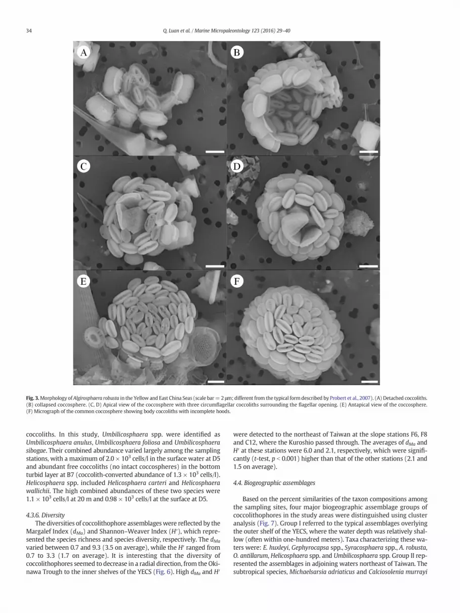
Fig. 3.Morphology of Algirosphaera robusta in the Yellow and East China Seas (scale bar= 2 μm; different from the typical formdescribed by Probert et al., 2007). (A) Detached coccoliths.(B) collapsed coccosphere. (C, D) Apical view of the coccosphere with three circumflagellar coccoliths surrounding the flagellar opening. (E) Antapical view of the coccosphere.(F) Micrograph of the common coccosphere showing body coccoliths with incomplete hoods.

34 Q. Luan et al. / Marine Micropaleontology 123 (2016) 29–40

coccoliths. In this study, Umbilicosphaera spp. were identified asUmbilicosphaera anulus, Umbilicosphaera foliosa and Umbilicosphaerasibogae. Their combined abundance varied largely among the samplingstations, with a maximum of 2.0 × 103 cells/l in the surface water at D5and abundant free coccoliths (no intact coccospheres) in the bottomturbid layer at B7 (coccolith-converted abundance of 1.3 × 103 cells/l).Helicosphaera spp. included Helicosphaera carteri and Helicosphaerawallichii. The high combined abundances of these two species were1.1 × 103 cells/l at 20 m and 0.98 × 103 cells/l at the surface at D5.

4.3.6. DiversityThe diversities of coccolithophore assemblageswere reflected by the

Margalef Index (dMa) and Shannon–Weaver Index (H′), which repre-sented the species richness and species diversity, respectively. The dMa

varied between 0.7 and 9.3 (3.5 on average), while the H′ ranged from0.7 to 3.3 (1.7 on average). It is interesting that the diversity ofcoccolithophores seemed to decrease in a radial direction, from the Oki-nawa Trough to the inner shelves of the YECS (Fig. 6). High dMa and H′

were detected to the northeast of Taiwan at the slope stations F6, F8and C12, where the Kuroshio passed through. The averages of dMa andH′ at these stations were 6.0 and 2.1, respectively, which were signifi-cantly (t-test, p b 0.001) higher than that of the other stations (2.1 and1.5 on average).

4.4. Biogeographic assemblages

Based on the percent similarities of the taxon compositions amongthe sampling sites, four major biogeographic assemblage groups ofcoccolithophores in the study areas were distinguished using clusteranalysis (Fig. 7). Group I referred to the typical assemblages overlyingthe outer shelf of the YECS, where the water depth was relatively shal-low (often within one-hundred meters). Taxa characterizing these wa-ters were: E. huxleyi, Gephyrocapsa spp., Syracosphaera spp., A. robusta,O. antillarum, Helicosphaera spp. and Umbilicosphaera spp. Group II rep-resented the assemblages in adjoining waters northeast of Taiwan. Thesubtropical species, Michaelsarsia adriaticus and Calciosolenia murrayi

Fig. 4.Vertical distribution of the coccolithophore abundances at the sampling stations. The solid lines indicate the bottomdepths. Samples collected below the dashed linewerewithin thebottom turbid layers.

35Q. Luan et al. / Marine Micropaleontology 123 (2016) 29–40

(Jordan, 2011), also frequently occurred in these waters, in addition toE. huxleyi and Gephyrocapsa spp. Group III depicted the assemblagesabove the thermocline of M7, where Gephyrocapsa spp. and E. huxleyi

almost completely dominated the waters. Group IV clustered the as-semblages in deep Kuroshio waters, usually with sampling depthsover one-hundred meters. Coccolithophores in these waters were

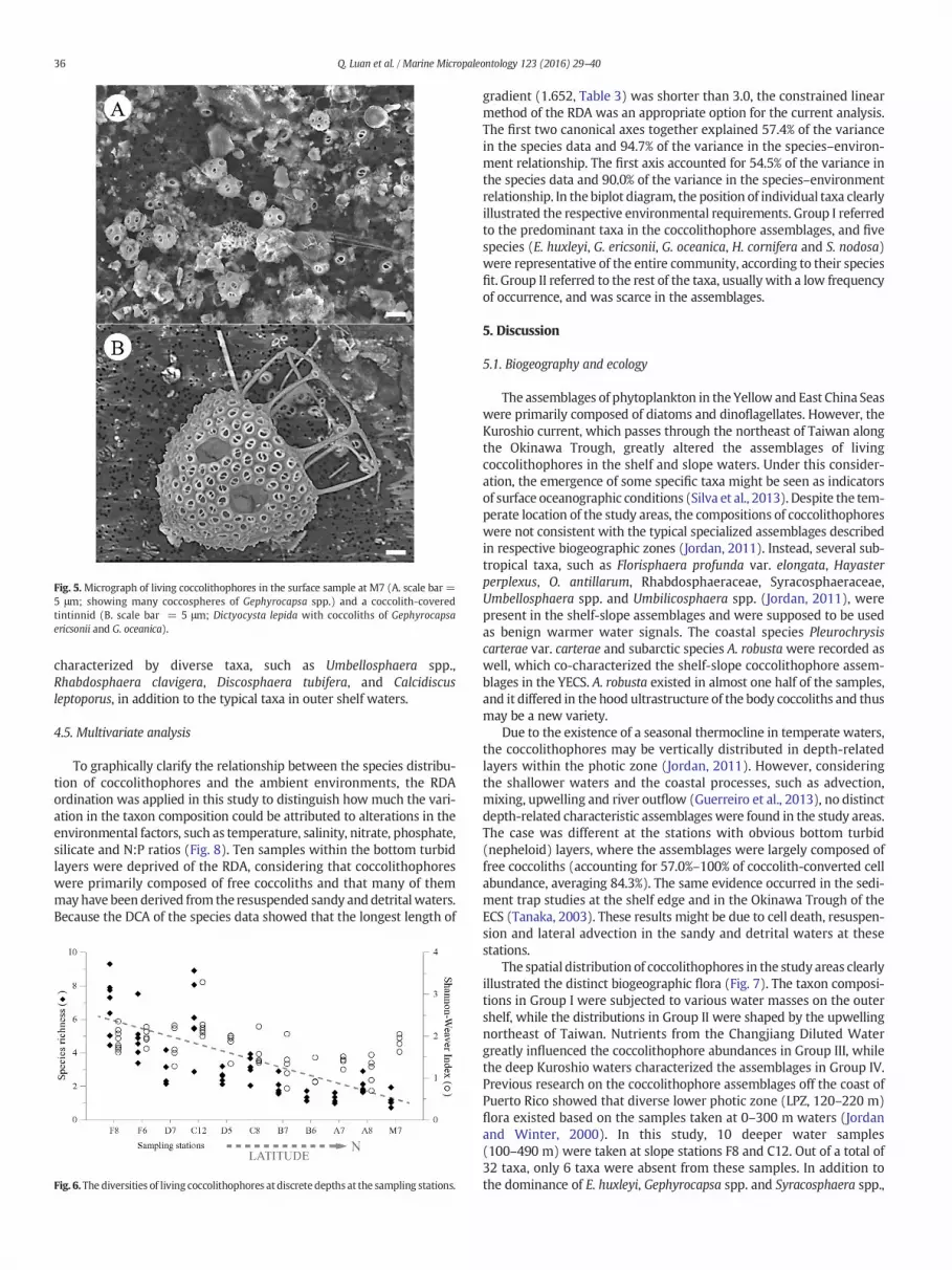
Fig. 5. Micrograph of living coccolithophores in the surface sample at M7 (A. scale bar =5 μm; showing many coccospheres of Gephyrocapsa spp.) and a coccolith-coveredtintinnid (B. scale bar = 5 μm; Dictyocysta lepida with coccoliths of Gephyrocapsaericsonii and G. oceanica).

36 Q. Luan et al. / Marine Micropaleontology 123 (2016) 29–40

characterized by diverse taxa, such as Umbellosphaera spp.,Rhabdosphaera clavigera, Discosphaera tubifera, and Calcidiscusleptoporus, in addition to the typical taxa in outer shelf waters.

4.5. Multivariate analysis

To graphically clarify the relationship between the species distribu-tion of coccolithophores and the ambient environments, the RDAordination was applied in this study to distinguish how much the vari-ation in the taxon composition could be attributed to alterations in theenvironmental factors, such as temperature, salinity, nitrate, phosphate,silicate and N:P ratios (Fig. 8). Ten samples within the bottom turbidlayers were deprived of the RDA, considering that coccolithophoreswere primarily composed of free coccoliths and that many of themmayhave been derived from the resuspended sandy anddetritalwaters.Because the DCA of the species data showed that the longest length of

Fig. 6.The diversities of living coccolithophores at discrete depths at the sampling stations.

gradient (1.652, Table 3) was shorter than 3.0, the constrained linearmethod of the RDA was an appropriate option for the current analysis.The first two canonical axes together explained 57.4% of the variancein the species data and 94.7% of the variance in the species–environ-ment relationship. The first axis accounted for 54.5% of the variance inthe species data and 90.0% of the variance in the species–environmentrelationship. In the biplot diagram, the position of individual taxa clearlyillustrated the respective environmental requirements. Group I referredto the predominant taxa in the coccolithophore assemblages, and fivespecies (E. huxleyi, G. ericsonii, G. oceanica, H. cornifera and S. nodosa)were representative of the entire community, according to their speciesfit. Group II referred to the rest of the taxa, usually with a low frequencyof occurrence, and was scarce in the assemblages.

5. Discussion

5.1. Biogeography and ecology

The assemblages of phytoplankton in the Yellow and East China Seaswere primarily composed of diatoms and dinoflagellates. However, theKuroshio current, which passes through the northeast of Taiwan alongthe Okinawa Trough, greatly altered the assemblages of livingcoccolithophores in the shelf and slope waters. Under this consider-ation, the emergence of some specific taxa might be seen as indicatorsof surface oceanographic conditions (Silva et al., 2013). Despite the tem-perate location of the study areas, the compositions of coccolithophoreswere not consistent with the typical specialized assemblages describedin respective biogeographic zones (Jordan, 2011). Instead, several sub-tropical taxa, such as Florisphaera profunda var. elongata, Hayasterperplexus, O. antillarum, Rhabdosphaeraceae, Syracosphaeraceae,Umbellosphaera spp. and Umbilicosphaera spp. (Jordan, 2011), werepresent in the shelf-slope assemblages and were supposed to be usedas benign warmer water signals. The coastal species Pleurochrysiscarterae var. carterae and subarctic species A. robusta were recorded aswell, which co-characterized the shelf-slope coccolithophore assem-blages in the YECS. A. robusta existed in almost one half of the samples,and it differed in the hood ultrastructure of the body coccoliths and thusmay be a new variety.

Due to the existence of a seasonal thermocline in temperate waters,the coccolithophores may be vertically distributed in depth-relatedlayers within the photic zone (Jordan, 2011). However, consideringthe shallower waters and the coastal processes, such as advection,mixing, upwelling and river outflow (Guerreiro et al., 2013), no distinctdepth-related characteristic assemblages were found in the study areas.The case was different at the stations with obvious bottom turbid(nepheloid) layers, where the assemblages were largely composed offree coccoliths (accounting for 57.0%–100% of coccolith-converted cellabundance, averaging 84.3%). The same evidence occurred in the sedi-ment trap studies at the shelf edge and in the Okinawa Trough of theECS (Tanaka, 2003). These results might be due to cell death, resuspen-sion and lateral advection in the sandy and detrital waters at thesestations.

The spatial distribution of coccolithophores in the study areas clearlyillustrated the distinct biogeographic flora (Fig. 7). The taxon composi-tions in Group I were subjected to various water masses on the outershelf, while the distributions in Group II were shaped by the upwellingnortheast of Taiwan. Nutrients from the Changjiang Diluted Watergreatly influenced the coccolithophore abundances in Group III, whilethe deep Kuroshio waters characterized the assemblages in Group IV.Previous research on the coccolithophore assemblages off the coast ofPuerto Rico showed that diverse lower photic zone (LPZ, 120–220 m)flora existed based on the samples taken at 0–300 m waters (Jordanand Winter, 2000). In this study, 10 deeper water samples(100–490 m) were taken at slope stations F8 and C12. Out of a total of32 taxa, only 6 taxa were absent from these samples. In addition tothe dominance of E. huxleyi, Gephyrocapsa spp. and Syracosphaera spp.,

Fig. 7. Biogeographic distribution of four living coccolithophore assemblages based on cluster analysis. Left panel: dendrogram showing the percent similarities of the coccolithophorecomposition at the sampling sites (UPGMA: unweighted pair-group method with arithmetic means; I–IV: four distinct assemblage groups of living coccolithophores); Right panel:spatial distribution of the assemblages.

37Q. Luan et al. / Marine Micropaleontology 123 (2016) 29–40

which were consistently present in the surface waters, O. antillarum,Umbellosphaera spp.,Umbilicosphaera spp. and A. robustawere relativelyabundant in the deep-water assemblages. This distinct biogeographicflora was precisely reflected in the former cluster analysis by GroupIV, which was in very low percent similarity (48.1%) with the othergroups.

In temperatewaters, coccolithophores exhibitedmarked seasonalityby reaching high cell densities in summer, especially when nutrientswere almost exhausted and decreased to low levels of concentrations(Jordan and Winter, 2000; Jordan, 2011) after the spring bloom of dia-toms (e.g., Xuan et al., 2011). After comparing historical data on the as-semblages of coccolithophores from other works and this study incoastal China Seas and the neighboring Pacific (Table 4), we foundthat the seasonal cell abundance of coccolithophores in coastal ChinaSeas was far below the level of blooms, although sporadic bloomswith cell densities N1000 × 103 cells/l were recorded in theNE subarcticPacific (Lipsen et al., 2007). The number of common taxa in coastalChina Seas ranged from10 to 40 (although over a hundred in the Pacific,Hagino et al., 2000; Jordan et al., 2000), with the seasonal abundanceof ca. 0–100 × 103 cells/l (scarcely N100 × 103 cells/l). In additionto the ubiquitous distribution of E. huxleyi and Gephyrocapsa spp.,

Syracosphaera spp. and Umbellosphaera spp. also dominated in the as-semblages in coastal China Seas and the adjoining Pacific.

5.2. Environmental controls on the distribution of living coccolithophores

Basically, bottom-up control factors, such as light, temperature andmacronutrients, were important for regulating the growth and calcifica-tion of living coccolithophores (Zondervan, 2007). In this paper, themultivariate method of RDA was applied to evaluate the effects ofthese environmental parameters on the coccolithophore distributionin the study areas. After the Monte Carlo permutation tests of signifi-cance, the independent explanation of species variation by salinity andtemperature reached up to 51.6% (F = 47.954, p b 0.01) and 11.8%(F = 6.027, p b 0.01), respectively, in contrast with the low contribu-tions by phosphate (3.6%) and nitrate (3.4%). Thus, salinity and temper-ature, which to some extent could reflect the physical properties ofwater stability and stratification, were the key factors in controllingthe distribution of living coccolithophores in the outer shelf and slopeof the YECS. The demands for inorganic macronutrients (e.g., nitrateand phosphate) were low for growth and proliferation. Becausecoccolithophores possess a high affinity for nutrients (Iglesias-

Fig. 8. RDA biplot showing the relationship between the species distribution of livingcoccolithophores and environmental factors. F and p values in the brackets refer to thesignificance of environmental variables by Monte Carlo permutation tests under thereduced model. Only the predominant taxa were labeled in the ordination chart.

38 Q. Luan et al. / Marine Micropaleontology 123 (2016) 29–40

Rodríguez et al., 2002), exceptional P-acquisition capacity (Riegmanet al., 2000), and combined abilities to use non-nitrate N (Palenik andHenson, 1997), they could reach high cell densities at both high andlow nutrient concentrations and N:P ratios (Egge and Aksnes, 1992).Mesocosm experiments also showed that different nutrient regimeshad no influence on the gross growth rate of E. huxleyi populations(van der Wal et al., 1994). Field observations further confirmed thatthe blooms of E. huxleyi almost always occurred in areas where nitrateand phosphate concentrations were very low (Fernández et al., 1993).

The recruitment of dissolved inorganic nutrients in the surface oceandepended largely on thewater stratification. The existence of a seasonalthermocline in temperate shallow seas greatly impeded the penetrationof nutrients from deeper waters. However, in well-stratified waters,rapid proliferation often occurred in some taxa, such as E. huxleyi andGephyrocapsa spp., in association with their low nutrient requirements.In this situation, a slight increase of element concentrations in thesurface waters could have triggered the rapid growth of livingcoccolithophores (even mesoscale blooms) when extra nutrients wereavailable (Jordan, 2011). This could bewhyextremely high cell densities(221 × 103 cells/l) existed above the thermocline at M7. First, the spe-cies responsible were those ubiquitous coccolithophores of G. ericsonii(35.7%), G. oceanica (33.7%) and E. huxleyi (18.5%). Second, a verysharp drop in the vertical temperature (10.2 °C, from 22.9 °C to12.7 °C) occurred in a 10-meter water layer (from 30 m to 40 m),which created well-stratified waters above the thermocline. The cold

Table 3Multivariate analysis of species data of living coccolithophores with ambient environmen-tal parameters.

Axes 1 2 3 4

DCA resultsEigenvalues 0.216 0.134 0.088 0.047Lengths of gradient 1.652 1.592 1.430 1.300Cumulative percentage variance of speciesdata

14.9 24.2 30.3 33.5

RDA resultsEigenvalues 0.545 0.028 0.017 0.006Species–environment correlations 0.912 0.615 0.588 0.411Cumulativepercentage variance

Of species data 54.5 57.4 59.1 59.7Ofspecies–environmentrelation

90.0 94.7 97.5 98.5

water was derived from the notable Yellow Sea Cold Water Mass,which had not completely vanished during fall (strong in summer, dis-appeared inwinter; Su, 1998). Third, the depth of the thermocline atM7(~30m)was shallower than that of the other shelf stations (~60m) anddeeper stations (~100 m), which favored the utilization of sunlight bycoccolithophores in theupper photic zone. Finally, stationM7was locat-ed at the plume frontal zone with a relative high Chl-a concentration(north branch extension, see Fig. 1C), where new nutrients enteredthe surface waters by the Changjiang discharge and transportation (ni-trate, 3.89 μmol/l; phosphate, 0.80 μmol/l). Under these considerations,the shallow, dynamic andwell-stratified surface seawaters, in combina-tion with the extra inputs of nutrients (inorganic/organic) from theChangjiang outflow, promoted the formation of high cell abundancesabove the thermocline at station M7.

The influence of cold eddies on the distributions of coccolithophoreswas verified by the samples collected near the center of the East ChinaSea Cold Eddy. Although the center of the cold eddy was not so obviousand strong during early fall, a synthesis of a 44-year long datasetshowed that the center was located in the waters of 32.0 °N, 125.7 °Eand varied seasonally (Wang et al., 2010). Interestingly, a bloom ofG. oceanica developed in the ECS during June 2011, which was not pre-viously reported (Jin et al., 2013). The bloom area located near the cen-ter of the East China Sea Cold Eddy, and the highest cell density reachedasmany as 620 × 103 cells/l. Most of the coccolithophores located in theChangjiang River plume area and the upwelling, which was induced bythe cold eddy, facilitated the bloom (Jin et al., 2013). Our results showedsimilar findings that the average coccolithophore abundance in thewater column (not including samples in the bottom turbid layers) atB6 and A7 (near the center of cold eddy, Fig. 1A) reached high valuesof 48.0 × 103 cells/l and 23.0 × 103 cells/l, respectively, which werehigher than that of the other stations (except for M7). Thus, physicalprocesses, such as the thermocline, cold eddies and frontal systems,played crucial roles in the biogeographic dynamics of coccolithophoresin the study areas. Further studies need to be conducted on the couplingof physical, chemical and biological processes in association with thecoccolithophores in coastal China Seas.

6. Conclusions

1. A total of 32 taxa of living coccolithophores were recorded from 57samples taken at discrete depths (0–490 m) at 11 stations acrossthe shelf and slope regions of YECS, with E. huxleyi, Gephyrocapsaspp., Syracosphaera spp. and A. robusta as the predominant forms.

2. An interesting morphology of A. robusta (incomplete hood ultra-structure of body coccoliths), which may be a new variety, was re-corded in nearly one half of the samples. An agglutinationrelationship was observed between Gephyrocapsa coccoliths andthe tintinnid D. lepida in oligotrophic waters.

3. The cell abundance of total coccolithophores reached a maximum of252×103 cells/l (on average 27.8× 103 cells/l), with the contributionof G. ericsonii, E. huxleyi and G. oceanica accounting for 36.4%, 29.6%and 15.3%, respectively, of the total assemblages.

4. Coccolithophore assemblages in the YECS were a mixture of coastal,shelf and subtropical taxa due to the coastal processes and Kuroshiotransportation. Decreasing diversity of coccolithophores in a radialdirection was found in this study, from the Okinawa Trough toinner shelves of the YECS.

5. Distinct deep-water flora existed in the Kuroshio slope waters(100–490 m), which was precisely reflected by the cluster analysis,illustrating very low percent similarity (48.1%) with the othergroups.

6. The occurrence of subtropical taxa in the assemblages can be used asbenign warmer water signals. In bottom turbid layers, the assem-blages were largely (84.3%) composed of free coccoliths, implyingcomplex processes, such as cell death, resuspension and lateral ad-vection, in the sandy and detrital waters.

Table 4Comparison of historical data on the assemblages of living coccolithophores by other works and this study in coastal China Seas and the Pacific.

Survey periodsa Sampling regionsb Total numberof taxa(analysismethods)

Abundance (×103 cells/l) Dominant taxa

1968 (Oct., Nov.)1 YECS Not clear(PM)

14–23 E. huxleyi, G. oceanica, S. pulchra

1990 (Nov.–Dec.), 1992(Sep.–Oct.)2

Equatorial western-centralPacific Ocean

111 (SEM) 3.7–44 E. huxleyi, G. ericsonii, G. oceanica, O. antillarum,U. irregularis

1992 (summer), 1997(winter)3

ECS 10 (SEM) 0–64.5 (summer), 0–56.4 (winter) E. huxleyi, G. oceanica

1996 (Mar. and Oct.)4 SCS (northeastern andcentral)

31 (SEM) 25–31 (0–25 m), 12–62 (150 m) E. huxleyi, F. profunda, G. oceanica, P. vandelii,Syracosphaera spp., Umbellosphaera spp.

1996 (summer)5 Northeastern Taiwan 41 (SEM) 11.5–19.7 (absolute coccospheres) C. murrayi, E. huxleyi, G. oceanica, P. vandelii,Umbellosphaera spp.

1997 (summer)6 western subarctic Pacific,western Bering Sea

35 (SEM) 0–15 E. huxleyi, Coccolithus pelagicus, C. pelagicus f. hyalinus

1998 (Feb.) to 2000(Sep.)7

NE subarctic Pacific Not clear(PM)

Average 40–552 (sporadic blooms N1000)

E. huxleyi, G. oceanica, Syracosphaera spp.

2002 (Mar.) to 2003(Jul.)8

Northern SCS 28 (SEM) 2.0–127.4 D. tubifera, E. huxleyi, G. ericsonii, G. oceanica,U. irregularis, U. tenuis

2010 (spring), 2011(winter)9

YS 9 (PM) 0–85.5 (spring, average 15.4), 0–22.5(winter, average 2.5)

E. huxleyi, G. oceanica

2011 (summer)10 ECS Not clear(SEM)

2.5–7.5 (bloom of 620) G. oceanica

2011 (summer,winter)11

YECS 20 (PM) 0–176.4 (summer, average 8.5), 0–71.7(winter, average 13.9)

A. robusta, E. huxleyi, G. oceanica, H. carteri

2013 (fall)12 YECS 32 (SEM) 0–252 (average 27.8) A. robusta, E. huxleyi, G. ericsonii, G. oceanica,Syracosphaera spp.

a Literatures: 1Okada andHonjo, 1975; 2Hagino et al. (2000); 3Yang et al. (2004); 4Yang et al. (2003); 5Yang et al. (2001); 6Hattori et al. (2004); 7Lipsen et al. (2007); 8Chen et al. (2007);9Luan et al. (2013); 10Jin et al. (2013); 11Sun et al. (2014); 12this study.

b Abbreviation: YECS, Yellow and East China Seas; YS, Yellow Sea; ECS, East China Sea; SCS, South China Sea; SEM, scanning electron microscope; PM, polarizing microscope.

39Q. Luan et al. / Marine Micropaleontology 123 (2016) 29–40

7. The RDAordination of the species distributionwith ambient environ-ments showed that salinity and temperature, which to some extentcould reflect the physical properties of water stability and stratifica-tion, were key factors in driving the distribution patterns of livingcoccolithophores in the study areas.

Acknowledgments

The authors would like to thank H. Zhai for his assistance in thesample collecting, M. Niu for her help in dealing with the satellitedatasets, and J.R. Young and R.W. Jordan for their suggestions on theidentification of Algirosphaera robusta. We are grateful to the twoanonymous reviewers for their comments on the accepted manuscript.This research was supported by the National Basic Research Programof China (grant numbers 2011CB409805 and 2015CB453303) and theNSFC-Shandong Joint Fund for Marine Science Research Centers (grantnumber U1406403).

References

Andruleit, H., Rogalla, U., 2002. Coccolithophores in surface sediments of the Arabian Seain relation to environmental gradients in surface waters. Mar. Geol. 186, 505–526.

Balch, W.M., Drapeau, D.T., Bowler, B.C., Lyczskowski, E., Booth, E.S., Alley, D., 2011. Thecontribution of coccolithophores to the optical and inorganic carbon budgets duringthe southern ocean gas exchange experiment: new evidence in support of the “GreatCalcite Belt” hypothesis. J. Geophys. Res. 116, C00F06. http://dx.doi.org/10.1029/2011JC006941.

Bollmann, J., Cortés, M.Y., Haidar, A.T., Brabec, B., Close, A., Hofmann, R., Palma, S., Tupas,L., Thierstein, H.R., 2002. Techniques for quantitative analyses of calcareous marinephytoplankton. Mar. Micropaleontol. 44, 163–185.

Chen, Y.-L.L., Chen, H.-Y., Gong, G.-C., Lin, Y.-H., Jan, S., Takahashi, M., 2004. Phytoplanktonproduction during a summer coastal upwelling in the East China Sea. Cont. Shelf Res.24, 1321–1338.

Chen, Y.-L.L., Chen, H.-Y., Chung, C.-W., 2007. Seasonal variability of coccolithophoreabundance and assemblage in the northern South China Sea. Deep-Sea Res. II 54,1617–1633.

Chern, C.-S., Wang, J., Wang, D.-P., 1990. The exchange of Kuroshio and East China Seashelf water. J. Geophys. Res. 95, 16017–16023.

Dufrene, M., Legendre, P., 1997. Species assemblages and indicator species: the need for aflexible asymmetrical approach. Ecol. Monogr. 67, 345–366.

Egge, J.K., Aksnes, D.L., 1992. Silicate as regulating nutrient in phytoplankton competition.Mar. Ecol. Prog. Ser. 83, 281–289.

Fernández, E., Boyd, P., Holligan, P.M., Harbour, D.S., 1993. Production of organic and inor-ganic carbon within a large-scale coccolithophore bloom in the northeast AtlanticOcean. Mar. Ecol. Prog. Ser. 97, 271–285.

Fernando, A.G.S., Peleo-Alampay, A.M., Wiesner, M.G., 2007. Calcareous nannofossils insurface sediments of the eastern and western South China Sea. Mar. Micropaleontol.66, 1–26.

Guan, B., 1994. Patterns and structures of the currents in Bohai, Huanghai and East ChinaSeas. In: Zhou, D., Liang, Y.B., Zeng, C.K. (Eds.), Oceanology of China Seas. Kluwer Ac-ademic Publishers, Dordrecht, pp. 17–26.

Guerreiro, C., Oliveira, A., de Stigter, H., Cachão, M., Sã, C., Borges, C., Cros, L., Santos, A.,Fortuño, J., Rodrigues, A., 2013. Late winter coccolithophore bloom off centralPortugal in response to river discharge and upwelling. Cont. Shelf Res. 59, 65–83.

Hagino, K., Okada, H., Matsuoka, H., 2000. Spatial dynamics of coccolithophore assem-blages in the Equatorial Western-Central Pacific Ocean. Mar. Micropaleontol. 39,53–72.

Hattori, H., Koike, M., Tachikawa, K., Saito, H., Nagasawa, K., 2004. Spatial variability of liv-ing coccolithophore distribution in theWestern Subarctic Pacific andWestern BeringSea. J. Oceanogr. 60 (2), 505–515.

Honjo, S., Manganini, S.J., Krishfield, R.A., Francois, R., 2008. Particulate organic carbonfluxes to the ocean interior and factors controlling the biological pump: a synthesisof global sediment trap programs since 1983. Prog. Oceanogr. 76, 217–285.

Hsueh, Y., 2000. The Kuroshio in the East China Sea. J. Mar. Syst. 24, 131–139.Iglesias-Rodríguez, M.D., Brown, C.W., Doney, S.C., Kleypas, J., Kolber, D., Kolber, Z., Hayes,

P.K., Falkowski, P.G., 2002. Representing key phytoplankton functional groups inocean carbon cycle models: coccolithophorids. Glob. Biogeochem. Cycles 16, 1100.http://dx.doi.org/10.1029/2001GB001454.

Jin, X., Liu, C., Liang, D., 2013. Distribution and malformation of extent coccolithophores inthe East China Sea in summer, 2011. J. Nannoplankton Res. 33 (special issue), 68.

Jordan, R.W., 2011. Coccolithophores. In: Schaechter, M. (Ed.), Eukaryotic Microbes. Aca-demic Press, San Diego, pp. 235–247.

Jordan, R.W., Winter, A., 2000. Assemblages of coccolithophorids and other living micro-plankton off the coast of Puerto Rico during January–May 1995. Mar. Micropaleontol.39, 113–130.

Jordan, R.W., Broerse, A., Hagino, K., Kinkel, H., Sprengel, C., Takahashi, K., Young, J.R.,2000. Taxon lists for modern nannoplankton. Mar. Micropaleontol. 39 (1–4),309–314.

Jordan, R.W., Cros, L., Young, J.R., 2004. A revised classification scheme for livinghaptophytes. Micropaleontology 50 (Suppl. 1), 55–79.

Katoh, O., Morinaga, K., Nakagawa, N., 2000. Current distributions in the southern EastChina Sea in summer. J. Geophys. Res. 105, 8565–8573.

Lepš, J., Šmilauer, P., 2003. Multivariate Analysis of Ecological Data Using CANOCO. Cam-bridge University Press, Cambridge.

Lipsen, M.S., Crawford, D.W., Gower, J., Harrison, P.J., 2007. Spatial and temporal variabil-ity in coccolithophore abundance and production of PIC and POC in the NE subarcticPacific during El Niño (1998), La Niña (1999) and 2000. Prog. Oceanogr. 75, 304–325.

40 Q. Luan et al. / Marine Micropaleontology 123 (2016) 29–40

Luan, Q., Sun, J., Niu, M., Wang, J., 2013. Warm currents affecting the spring and winterdistributions of living coccolithophores in the yellow sea, China. Oceanol. Hydrobiol.Stud. 42 (4), 431–441.

Margalef, R., 1958. Information theory in ecology. Gen. Syst. 3, 36–71.Ning, X., Vaulot, D., Liu, Z., Liu, Z., 1988. Standing stock and production of phytoplankton

in the estuary of the Changjiang (Yangtse River) and the adjacent East China Sea. Mar.Ecol. Prog. Ser. 49, 141–150.

Okada, H., Honjo, S., 1975. Distribution of coccolithophores in marginal seas along thewestern Pacific Ocean and in the Red Sea. Mar. Biol. 31, 271–285.

Palenik, B., Henson, S.E., 1997. The use of amides and other organic nitrogen sources bythe phytoplankton Emiliania huxleyi. Limnol. Oceanogr. 42, 1544–1551.

Probert, I., Fresnel, J., Billard, C., Geisen, M., Young, J.R., 2007. Light and electron micro-scope observations of Algirosphaera robusta (Prymnesiophyceae). J. Phycol. 43,319–332.

Riegman, R., Stolte, W., Noordeloos, A.A.M., Slezak, D., 2000. Nutrient uptake and alkalinephosphate (EC 3:1:3:1) activity of Emiliania huxleyi (Prymnesiophyceae) duringgrowth under N and P limitation in continuous cultures. J. Phycol. 36, 87–96.

Rost, B., Riebesell, U., 2004. Coccolithophores and the biological pump: response to envi-ronmental changes. In: Thierstein, H.R., Young, J.R. (Eds.), Coccolithophores — FromMolecular Processes to Global Impact. Springer, Berlin, pp. 99–127.

Rousseaux, C.S., Gregg, W.W., 2014. Interannual variation in phytoplankton primary pro-duction at a global scale. Remote sensing. 6 pp. 1–19.

Shannon, C.E., Weaver, W., 1949. TheMathematical Theory of Communication. Universityof Illinois Press, Urbana.

Silva, A., Brotas, V., Valente, A., Sá, C., Diniz, T., Patarra, R.F., Álvaro, N.V., Neto, A.I., 2013.Coccolithophore species as indicators of surface oceanographic conditions in the vi-cinity of Azores islands. Estuar. Coast. Shelf Sci. 118, 50–59.

Su, J.L., 1998. Circulation dynamics of the China seas: north of 18°N. In: Robinson, A.R.,Brink, K. (Eds.), The Sea. The Global Coastal Ocean: Regional Studies and Synthesesvol. 11. Wiley, New York, pp. 483–506.

Sun, J., Gu, X.Y., Feng, Y.Y., Jin, S.F., Jiang, W.S., Jin, H.Y., Chen, J.F., 2014. Summer and win-ter living coccolithophores in the Yellow Sea and the East China Sea. Biogeosciences11, 779–806.

Tanaka, Y., 2003. Coccolith fluxes and species assemblages at the shelf edge and in theOkinawa Trough of the East China Sea. Deep-Sea Res. II 50 (2), 503–511.

van der Wal, P., van Bleijswijk, J.D.L., Egge, J.K., 1994. Primary productivity and calcifica-tion rate in blooms of the coccolithophorid Emiliania huxleyi (Lohmann) Hay etMohler developing in mesocosms. Sarsia 79, 401–408.

Wang, G., Lan, J., Sun, S., 2010. A preliminary study of the center's location andinterseasonal variabilities of the cold eddy in East China Sea. Adv. Earth Sci. 25 (2),184–192 (in Chinese, with English Abstr.).

Wang, J., Luan, Q., Zuo, T., Chen, R., Sun, J., 2012. Taxonomic composition of marine-livingcoccolithophores in the Yellow Sea and East China Sea—new records and a specieslist. Mar. Biodivers. Rec. 5 (e114). http://dx.doi.org/10.1017/S1755267212001005.

Whittaker, R.H., 1952. A study of summer foliage insect communities in the Great SmokyMountains. Ecol. Monogr. 22, 1–44.

Winter, A., Siesser, W.G., 1994. Atlas of living coccolithophores. In: Winter, A., Siesser,W.G. (Eds.), Coccolithophores. Cambridge University Press, Cambridge, pp. 107–160.

Wong, G.T.F., Gong, G.-C., Liu, K.-K., Pai, S.-C., 1998. ‘Excess nitrate’ in the East China Sea.Estuar. Coast. Shelf Sci. 46, 411–418.

Xuan, J.-L., Zhou, F., Huang, D.-J., Wei, H., Liu, C.-G., Xing, C.-X., 2011. Physical processesand their role on the spatial and temporal variability of the spring phytoplanktonbloom in the central Yellow Sea. Acta Ecol. Sin. 31, 61–70.

Yamaguchi, H., Kim, H.-C., Son, Y.B., Kim, S.W., Okamura, K., Kiyomoto, Y., Ishizaka, J.,2012. Seasonal and summer interannual variations of SeaWiFS chlorophyll a in theYellow Sea and East China Sea. Prog. Oceanogr. 105, 22–29.

Yang, T.-N., Wei, K.-Y., 2003. How many coccoliths are there in a coccosphere of the ex-tant coccolithophorids? A compilation. J. Nannoplankton Res. 25, 7–15.

Yang, T.-N., Wei, K.-Y., Gong, G.-C., 2001. Distribution of coccolithophorids and coccolithsin surface ocean off northeastern Taiwan. Bot. Bull. Acad. Sinica 42, 287–302.

Yang, T.-N.,Wei, K.-Y., Chen, L.-L., 2003. Occurrence of coccolithophorids in the Northeast-ern and Central South China Sea. Taiwania 48 (1), 29–45.

Yang, T.-N., Wei, K.-Y., Chen, M.-P., Ji, S.-J., Gong, G.-C., Lin, F.-J., Lee, T.Q., 2004. Summerand winter distribution and malformation of coccolithophores in the East ChinaSea. Micropaleontology 50, 157–170.

Young, J.R., Geisen, M., Cros, L., Kleijne, A., Sprengel, C., Probert, I., Østergaard, J., 2003. Aguide to extant coccolithophore taxonomy. J. Nannoplankton Res. 25 (special issue1), 1–125.

Yuan, D., Hsueh, Y., 2010. Dynamics of the cross-shelf circulation in the Yellow and EastChina Seas in winter. Deep-Sea Res. II 57 (19–20), 1745–1761.

Zhou, F., Xue, H., Huang, D., Xuan, J., Ni, X., Xiu, P., Hao, Q., 2015. Cross-shelf exchange inthe shelf of the East China Sea. J. Geophys. Res. http://dx.doi.org/10.1002/2014JC010567.

Zondervan, I., 2007. The effects of light, macronutrients, trace metals and CO2 on the pro-duction of calcium carbonate and organic carbon in coccolithophores—a review.Deep-Sea Res. II 54, 521–537.