Embed Size (px)
Citation preview
Livi
ngdo
cum
ent
Q&U Bolometric Interferometer for Cosmology
Technical Design Report
The QUBIC Collaboration
Version 1.0May 12, 2017
arX
iv:1
609.
0437
2v2
[as
tro-
ph.I
M]
11
May
201
7
Livi
ngdo
cum
ent
QUBIC Technical Design ReportThe QUBIC collaboration
J. Aumont7, S. Banfi13, P. Battaglia14, E.S. Battistelli17, A. Baù13, B. Bélier8, D.Bennett15, L.Bergé5, J.Ph. Bernard9, M. Bersanelli14, M.A. Bigot-Sazy1, N. Bleurvacq1, G. Bordier1, J.
Brossard1, E.F. Bunn16, D. Buzi17, A. Buzzelli18, D. Cammilleri1, F. Cavaliere14, P. Chanial1, C.Chapron1, G. Coppi12, A. Coppolecchia17, F. Couchot11, R. D’Agostino18, G. D’Alessandro17, P.de Bernardis17, G. De Gasperis18, M. De Petris17, T. Decourcelle1, F. Del Torto14, L. Dumoulin5,A. Etchegoyen10, C. Franceschet13, B. Garcia10, A. Gault18, D. Gayer15, M. Gervasi13, A. Ghribi1,
M. Giard9, Y. Giraud-Héraud1, M. Gradziel15, L. Grandsire1, J.Ch. Hamilton1, D. Harari3, V.Haynes12, S. Henrot-Versillé11, N. Holtzer5, J. Kaplan1, A. Korotkov2, L. Lamagna17, J. Lande5,
S. Loucatos1, A. Lowitz19, V. Lukovic18, B. Maffei7, S. Marnieros5, J. Martino7, S. Masi17, A.May12, M. McCulloch12, M.C. Medina6, S. Melhuish12, A. Mennella14, L. Montier9, A. Murphy15,
D. Néel5, M.W. Ng12, C. O’Sullivan15, A. Paiella17, F. Pajot9, A. Passerini13, A.Pelosi17, C.Perbost1, O. Perdereau11, F. Piacentini17, M. Piat1, L. Piccirillo12, G. Pisano4, D. Prêle1, R.
Puddu17, D. Rambaud9, O. Rigaut5, G.E. Romero6, M. Salatino17, A. Schillaci17, S. Scully15, M.Stolpovskiy1, F. Suarez10, A. Tartari1, P. Timbie19, M. Tristram11, G. Tucker2, D. Viganò14, N.
Vittorio18, F. Voisin1, B. Watson12, M. Zannoni13 and A. Zullo17
1APC, Paris, France2Brown University, Providence, RI, USA
3Centro Atomico Bariloche, CNEA, Argentina4Cardiff University, Cardiff, UK
5CSNSM, Orsay, France6IAR-CONICET, CCT-La Plata, UNLP, Argentina
7IAS, Orsay, France8IEF, Orsay, France
9IRAP, Toulouse, France10ITeDA, CNEA, CONICET, UNSAM, Argentina
11LAL, Orsay, France12University of Manchester, Manchester, UK
13Universitá degli Studi di Milano-Bicocca, Milano, Italy14Universitá Degli Studi di Milano, Milano, Italy
15NUIM, Maynooth, Ireland16Richmond University, Richmond, VA, USA
17Universitá di Roma La Sapienza, Roma, Italy18Universitá di Roma Tor Vergata, Roma, Italy19University of Wisconsin, Madison, WI, USA
May 12, 2017
2
Livi
ngdo
cum
ent
Table Of Contents
Preface 5
1 Science Case 61.1 Context: the Quest for primordial B-modes . . . . . . . . . . . . . . . . . . . . . . . . . . . . . . . . 6
1.1.1 Primordial Universe, Inflation and the CMB Polarization . . . . . . . . . . . . . . . . . . . . . 61.1.2 A major observational challenge . . . . . . . . . . . . . . . . . . . . . . . . . . . . . . . . . . 71.1.3 Ongoing and planned projects . . . . . . . . . . . . . . . . . . . . . . . . . . . . . . . . . . . 7
1.2 Bolometric Interferometry and QUBIC . . . . . . . . . . . . . . . . . . . . . . . . . . . . . . . . . . . 91.2.1 The QUBIC design . . . . . . . . . . . . . . . . . . . . . . . . . . . . . . . . . . . . . . . . . 91.2.2 The QUBIC synthesized beam and map-making . . . . . . . . . . . . . . . . . . . . . . . . . 101.2.3 Self-calibration and the systematic effects mitigation with QUBIC . . . . . . . . . . . . . . . . 11
1.3 QUBIC sensitivity to B modes . . . . . . . . . . . . . . . . . . . . . . . . . . . . . . . . . . . . . . . 131.3.1 E/B power spectra from realistic simulations . . . . . . . . . . . . . . . . . . . . . . . . . . . 131.3.2 QUBIC Sensitivity to B-Modes . . . . . . . . . . . . . . . . . . . . . . . . . . . . . . . . . . . 13
2 Overall Description of QUBIC 152.1 Main characteristics of the Instrument . . . . . . . . . . . . . . . . . . . . . . . . . . . . . . . . . . . 152.2 Cryogenic systems . . . . . . . . . . . . . . . . . . . . . . . . . . . . . . . . . . . . . . . . . . . . . 22
2.2.1 Cryostat design / Mechanic architecture and CAD . . . . . . . . . . . . . . . . . . . . . . . . 222.2.2 Cryostat vacuum . . . . . . . . . . . . . . . . . . . . . . . . . . . . . . . . . . . . . . . . . . 222.2.3 Main Cryostat Cooling System . . . . . . . . . . . . . . . . . . . . . . . . . . . . . . . . . . 242.2.4 1K-box . . . . . . . . . . . . . . . . . . . . . . . . . . . . . . . . . . . . . . . . . . . . . . . 242.2.5 1 K System . . . . . . . . . . . . . . . . . . . . . . . . . . . . . . . . . . . . . . . . . . . . . 282.2.6 sub-K systems . . . . . . . . . . . . . . . . . . . . . . . . . . . . . . . . . . . . . . . . . . . 302.2.7 Heat Switches . . . . . . . . . . . . . . . . . . . . . . . . . . . . . . . . . . . . . . . . . . . 33
2.3 Optical chain . . . . . . . . . . . . . . . . . . . . . . . . . . . . . . . . . . . . . . . . . . . . . . . . 342.3.1 Window . . . . . . . . . . . . . . . . . . . . . . . . . . . . . . . . . . . . . . . . . . . . . . . 352.3.2 Half Wave plate . . . . . . . . . . . . . . . . . . . . . . . . . . . . . . . . . . . . . . . . . . . 352.3.3 Filters / Polarizer /Dichroïc . . . . . . . . . . . . . . . . . . . . . . . . . . . . . . . . . . . . . 382.3.4 Horns . . . . . . . . . . . . . . . . . . . . . . . . . . . . . . . . . . . . . . . . . . . . . . . . 422.3.5 Switches . . . . . . . . . . . . . . . . . . . . . . . . . . . . . . . . . . . . . . . . . . . . . . 492.3.6 Optical combiner . . . . . . . . . . . . . . . . . . . . . . . . . . . . . . . . . . . . . . . . . . 522.3.7 Cold stop / internal screening . . . . . . . . . . . . . . . . . . . . . . . . . . . . . . . . . . . 552.3.8 Optical Simulations . . . . . . . . . . . . . . . . . . . . . . . . . . . . . . . . . . . . . . . . . 56
2.4 Detection chain . . . . . . . . . . . . . . . . . . . . . . . . . . . . . . . . . . . . . . . . . . . . . . . 622.4.1 TES . . . . . . . . . . . . . . . . . . . . . . . . . . . . . . . . . . . . . . . . . . . . . . . . . 622.4.2 Cold electronics . . . . . . . . . . . . . . . . . . . . . . . . . . . . . . . . . . . . . . . . . . 652.4.3 SQUIDs . . . . . . . . . . . . . . . . . . . . . . . . . . . . . . . . . . . . . . . . . . . . . . . 682.4.4 ASIC . . . . . . . . . . . . . . . . . . . . . . . . . . . . . . . . . . . . . . . . . . . . . . . . 722.4.5 Warm electronics . . . . . . . . . . . . . . . . . . . . . . . . . . . . . . . . . . . . . . . . . . 742.4.6 QUBIC Studio, readout and control software . . . . . . . . . . . . . . . . . . . . . . . . . . . 762.4.7 Data storage . . . . . . . . . . . . . . . . . . . . . . . . . . . . . . . . . . . . . . . . . . . . 802.4.8 Detection chain: validation of a quarter of focal plane and readout system . . . . . . . . . . . 80
2.5 Mount System and Baffling . . . . . . . . . . . . . . . . . . . . . . . . . . . . . . . . . . . . . . . . . 822.5.1 Mount system . . . . . . . . . . . . . . . . . . . . . . . . . . . . . . . . . . . . . . . . . . . 822.5.2 External Baffling . . . . . . . . . . . . . . . . . . . . . . . . . . . . . . . . . . . . . . . . . . 84
2.6 Technological demonstrator . . . . . . . . . . . . . . . . . . . . . . . . . . . . . . . . . . . . . . . . 90
3 Calibration, Operation Modes and data processing 913.1 Instrument testing and calibration operations . . . . . . . . . . . . . . . . . . . . . . . . . . . . . . . 92
3.1.1 Cryogenic measurements and functional tests . . . . . . . . . . . . . . . . . . . . . . . . . . 923.1.2 Detector characteristics determination . . . . . . . . . . . . . . . . . . . . . . . . . . . . . . 923.1.3 With the calibration setup . . . . . . . . . . . . . . . . . . . . . . . . . . . . . . . . . . . . . 93
3.2 Modes of operations . . . . . . . . . . . . . . . . . . . . . . . . . . . . . . . . . . . . . . . . . . . . 94
3
Livi
ngdo
cum
ent
QUBIC TDR Version 1.0 (May 12, 2017)
3.2.1 Self-calibration mode . . . . . . . . . . . . . . . . . . . . . . . . . . . . . . . . . . . . . . . . 943.2.2 Observation mode . . . . . . . . . . . . . . . . . . . . . . . . . . . . . . . . . . . . . . . . . 94
3.3 Self-calibration . . . . . . . . . . . . . . . . . . . . . . . . . . . . . . . . . . . . . . . . . . . . . . . 963.3.1 The self-calibration procedure . . . . . . . . . . . . . . . . . . . . . . . . . . . . . . . . . . . 963.3.2 Self-calibration sources . . . . . . . . . . . . . . . . . . . . . . . . . . . . . . . . . . . . . . 973.3.3 Self-calibration sources support . . . . . . . . . . . . . . . . . . . . . . . . . . . . . . . . . . 973.3.4 Full beam calibration source . . . . . . . . . . . . . . . . . . . . . . . . . . . . . . . . . . . . 97
4 Operation site 994.1 Sites comparison . . . . . . . . . . . . . . . . . . . . . . . . . . . . . . . . . . . . . . . . . . . . . . 994.2 San Antonio de los Cobres, Argentina . . . . . . . . . . . . . . . . . . . . . . . . . . . . . . . . . . . 104
5 Organisation 1055.1 Management . . . . . . . . . . . . . . . . . . . . . . . . . . . . . . . . . . . . . . . . . . . . . . . . 105
5.1.1 Management of the collaboration . . . . . . . . . . . . . . . . . . . . . . . . . . . . . . . . . 1055.1.2 Collaboration Agreement (CA) / Memorandum of Understanding (MoU) . . . . . . . . . . . . 1065.1.3 Publication policy . . . . . . . . . . . . . . . . . . . . . . . . . . . . . . . . . . . . . . . . . . 106
5.2 Organization . . . . . . . . . . . . . . . . . . . . . . . . . . . . . . . . . . . . . . . . . . . . . . . . 1085.2.1 Product Breakdown Structure (PBS) . . . . . . . . . . . . . . . . . . . . . . . . . . . . . . . 1085.2.2 Works Breakdown Structure / Works packages . . . . . . . . . . . . . . . . . . . . . . . . . . 108
5.3 Development plan . . . . . . . . . . . . . . . . . . . . . . . . . . . . . . . . . . . . . . . . . . . . . . 1085.3.1 Heritage and first R&D works . . . . . . . . . . . . . . . . . . . . . . . . . . . . . . . . . . . 1085.3.2 Validation of the detection chain . . . . . . . . . . . . . . . . . . . . . . . . . . . . . . . . . . 1105.3.3 Validation of a technological demonstrator . . . . . . . . . . . . . . . . . . . . . . . . . . . . 1115.3.4 Construction and implementation of the first module . . . . . . . . . . . . . . . . . . . . . . . 111
5.4 Schedule . . . . . . . . . . . . . . . . . . . . . . . . . . . . . . . . . . . . . . . . . . . . . . . . . . 1125.4.1 Construction and test of the technological demonstrator . . . . . . . . . . . . . . . . . . . . . 1125.4.2 Construction of and test the first module instrument . . . . . . . . . . . . . . . . . . . . . . . 112
5.5 Costs and funding . . . . . . . . . . . . . . . . . . . . . . . . . . . . . . . . . . . . . . . . . . . . . . 1125.5.1 Costs an funding for R&D and validation of the detection chain . . . . . . . . . . . . . . . . . 1125.5.2 Costs and funding for construction and test of the technological demonstrator . . . . . . . . . 1125.5.3 Cost and funding for the construction of the first module . . . . . . . . . . . . . . . . . . . . . 1125.5.4 Cost and funding for the implementation on site of the first module . . . . . . . . . . . . . . . 112
5.6 QUBIC Evolution to a CMB Stage IV experiment . . . . . . . . . . . . . . . . . . . . . . . . . . . . . 112
List of Figures 115
List of Tables 119
6 References 121
A Annexe: Experiment location in Dome C 124A.1 Studies of the deployment of a QUBIC module at Dome C, Antarctica . . . . . . . . . . . . . . . . . . 124
A.1.1 Implementation issues at Dome C . . . . . . . . . . . . . . . . . . . . . . . . . . . . . . . . . 125A.1.2 Milestones . . . . . . . . . . . . . . . . . . . . . . . . . . . . . . . . . . . . . . . . . . . . . 125A.1.3 Materials transportation . . . . . . . . . . . . . . . . . . . . . . . . . . . . . . . . . . . . . . 125A.1.4 Resume of logistics costs . . . . . . . . . . . . . . . . . . . . . . . . . . . . . . . . . . . . . 125
A.2 Possible implementation at Dome C . . . . . . . . . . . . . . . . . . . . . . . . . . . . . . . . . . . . 128
B ATRIUM-77335 134
Page 4
Livi
ngdo
cum
ent
QUBIC TDR Version 1.0 (May 12, 2017)
Preface
QUBIC, now in its construction phase, is dedicated to the exploration of the inflation age of the Universe. By de-tecting and characterizing the Cosmic Microwave Background B-mode polarization, QUBIC will contribute to find the“smoking gun” of inflation and to discriminate among the numerous models consistent with current data. The pri-mordial B-modes (as opposed to E-modes) is the unique direct observational signature of the inflationary phase thatis thought to have taken place in the early Universe, generating primeval perturbations, producing Standard Modelelementary particles and giving its generic features to our Universe (flatness, homogeneity. . . ).
Recent results from the BICEP2 and the Planck collaborations have brought the importance of the quest for B-modes to the attention of a wide audience well beyond the cosmology community. The original claim from BICEP2,contradicted by Planck later on has also shown how challenging the search for primordial B-mode polarization is,because of many difficulties: smallness of the expected signal, instrumental systematics that could possibly inducepolarization leakage from the large E signal into B, brighter than anticipated polarized foregrounds (dust) reducingto zero the initial hope of finding sky regions clean enough to have a direct primordial B-modes observation.
QUBIC is designed to address all aspects of this challenge with a novel kind of instrument, a Bolometric Inter-ferometer , combining the background-limited sensitivity of Transition-Edge-Sensors and the control of systematicsallowed by the observation of interference fringe patterns, while operating at two frequencies to disentangle polarizedforegrounds from primordial B mode polarization.
QUBIC is the only European ground based B-mode project with the scientific potential of discovering and mea-suring B-modes. It is the natural project for the European CMB community to continue at the edge-cutting level it hasreached with Planck.
With the measurement of the Cosmic Microwave B-mode Polarization in two bands at 150 and 220 GHz, withtwo years of continuous observations from Alto Chorillos near San Antonio de los Cobres, Argentina, the first QUBICmodule would be able to constrain the ratio of the primordial tensor to scalar perturbations power spectra amplitudeswith a conservative projected uncertainty of σ(r) = 0.02, while having a good control of foregrounds contaminationthanks to its dual band nature.
Depending on the scientific and technological results of the first module we could envidage to construct moreQUBIC modules operating at three frequencies (90, 150 and 220 GHz) that could feature design upgrades in or-der to achieve a higher sensitivity, and could preferentially be deployed in Antartica to take benefit of its exquisiteatmospheric conditions. These could include different detectors (eg MKIDs), larger horn arrays or number of detec-tors, different optical combiner design, ... QUBIC is therefore a project dedicated to grow and could be a EuropenStage-IV CMB Polarization experiment.
QUBIC has been and will be implemented through successive steps:
1. R&D to design the instrument (now finalized)
2. Validation of the detections chain (now finalized)
3. Validation of the technological demonstrator (less detectors and horns than the final instrument, but in thenominal cryostat). This will occur in the course of 2017.
4. Construction and operations of the of the first module which will happen in the second half of 2017.
5. Optionaly, construction and operations of a number of additional modules to complete the QUBIC observatory.
More details can be found on the QUBIC website : http://qubic.in2p3.fr/QUBIC/Home.html
Page 5
Livi
ngdo
cum
ent
QUBIC TDR Version 1.0 (May 12, 2017)
1 Science Case
1.1 Context: the Quest for primordial B-modes
1.1.1 Primordial Universe, Inflation and the CMB Polarization
Our understanding of the origin and evolution of the Universe has made remarkable progress during the last twodecades, thanks in particular to the observations of the Cosmic Microwave Background (CMB). The diverse andmore and more numerous probes, such as CMB anisotropies, SNIa, BAO (...) give complementary informations,enabling consistency tests of the standard cosmological model (aka ΛCDM model). This concordance model isbased on General Relativity and is parameterized, in its simplest form, with six parameters. From the determinationof those cosmological parameters using the observations, we have learned that the Universe is spatially flat, containsa large fraction of dark matter, and experiences accelerated expansion. The latter can be accommodated within theFriedman-Lemaître framework through the presence of a mysterious dark energy Λ (or cosmological constant).
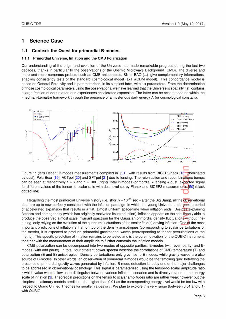
Figure 1: (left) Recent B-modes measurements compiled in [21], with results from BICEP2/Keck [18] (dominatedby dust), PolarBear [19], ACTpol [20] and SPTpol [21] due to lensing. The reionisation and recombinations bumpscan be seen at respectively ` ' 7 and ` ' 100. (right) Total B-modes (primordial + lensing + dust) expected signalfor different values of the tensor-to-scalar ratio with dust level set by Planck and BICEP2 measurements [50] (blackdotted line).
Regarding the most primordial Universe history (i.e. shortly – 10-38 sec – after the Big Bang), all the observationaldata are up to now perfectly consistent with the inflation paradigm in which the young Universe undergoes a periodof accelerated expansion that results in a flat, almost uniform space-time when inflation ends. Besides explainingflatness and homogeneity (which has originally motivated its introduction), inflation appears as the best theory able toproduce the observed almost scale invariant spectrum for the Gaussian primordial density fluctuations without fine-tuning, only relying on the evolution of the quantum fluctuations of the scalar field(s) driving inflation. One of the mostimportant predictions of inflation is that, on top of the density anisotropies (corresponding to scalar perturbations ofthe metric), it is expected to produce primordial gravitational waves (corresponding to tensor perturbations of themetric). This specific prediction of inflation remains to be tested and is the core motivation for the QUBIC instrument,together with the measurement of their amplitude to further constrain the inflation models.
CMB polarization can be decomposed into two modes of opposite parities: E-modes (with even parity) and B-modes (with odd parity). In total, four different power spectra describe the correlations of CMB temperature (T) andpolarization (E and B) anisotropies. Density perturbations only give rise to E modes, while gravity waves are alsosource of B-modes. In other words, an observation of primordial B-modes would be the “smoking gun” betraying thepresence of primordial gravity waves generated by inflation. B-mode detection is today one of the major challengesto be addressed in observational cosmology. This signal is parameterized using the tensor-to-scalar amplitude ratior which value would allow us to distinguish between various inflation scenarios and is directly related to the energyscale of inflation [3]. Theoretical predictions on the tensor to scalar amplitudes ratio are rather weak however but thesimplest inflationary models predict r to be higher than 0.01 as the corresponding energy level would be too low withrespect to Grand Unified Theories for smaller values or r. We plan to explore this very range (between 0.01 and 0.1)with QUBIC.
Page 6
Livi
ngdo
cum
ent
QUBIC TDR Version 1.0 (May 12, 2017)
1.1.2 A major observational challenge
Unfortunately, B-modes appear to be very difficult to detect because of their small amplitude: a tensor-to-scalarratio of 0.01 corresponds to polarization fluctuations of the CMB of a few nK while the well observed temperaturefluctuations are around 100 microK. Even if such a sensitivity can be achieved using background limited detectorssuch as bolometers from low-atmospheric emission suborbital locations or from a satellite, the challenge to face forthis detection remains huge because of two main reasons: instrumental systematics and foregrounds.
Instrumental systematic effects of usual telescopes (sidelobes, cross-polarization) may become too large to bedisentangled from a small primordial B-mode signal. Indeed any instrument, even designed with care, exhibits cross-polarization, beam mismatch, inter calibration uncertainties, cross-talk, . . . All of these instrumental systematics mixthe electric fields in the two orthogonal directions inducing a mixing between the Stokes parameters Q and U andpossibly a leakage from intensity into polarization. This induces leakage from I and E into B-modes that, given thesmallness of the primordial B-modes, may completely overcome those B-modes. A new generation of instrumentsachieving an unprecedented level of control of instrumental systematics is therefore needed for the B-mode quest.QUBIC was precisely designed with this objective.
B-modes anisotropies are also produced by foregrounds (summarized in the right panel of Figure 1):
1. The lensing of the B-modes by intervening large scale structure in the Universe converts part of the E-modes into B-modes, mostly at small scales(` & 300). The spectrum of those lensing B-modes however hasa well defined shape and has been detected recently by PolarBear [19], ActPol [20] and SPTpol [21] (seeFigure 1, left panel). This contribution is not expected to affect the primordial B-modes detectability on thelarge scales observed by QUBIC (around the so-called recombination peak at l=100) if the tensor-to-scalarratio is sufficiently high, but would become a strong limitation if r is below ∼ 0.01.
2. Thermal emission from dust grains in the Galaxy is expected (and measured) to be linearly polarized due tothe elongated shape of the grains which align along the magnetic field. The dust e.m. spectrum is differentfrom the CMB one so that multiple frequencies (above 150 GHz) can be used to remove it and obtain cleanedmaps of the CMB B-modes. This was the motivation for adding a 220 GHz channel in QUBIC besides theinitial 150 GHz one.
3. Synchrotron emission from electrons swirling around magnetic fields in the Galaxy is also expected to produceB-modes. The synchrotron EM spectrum is falling with frequency so that it can be monitored with channels atlower frequencies that the CMB ones the same way as dust. Synchrotron polarization is not expected to behighly significant at 150 nor at 220 GHz, the QUBIC operation frequencies [1] [41].
4. For ground based observations, atmosphere is also a possible source of contamination. However, the maineffect of atmosphere is to increase the loading on the detectors in a time-variable manner that increases thevariance of the data. A recent study with PolarBear data [35] has shown that the polarization induced byatmosphere remains at a small level when observing from the Atacama plateau, which is known to be worsethan in South Pole.
Searching for B-modes in the Cosmic Microwave Background polarization is therefore a major challenge that re-quires instruments observing at multiple frequencies with high sensitivity and unprecedented control of instrumentalsystematics. The current best upper-limit on r is r < 0.07 at 95% C.L. [50] and is obtained by combining BICEP2,Keck Array and Planck data.
1.1.3 Ongoing and planned projects
Two kinds of instruments have been used so far in the Cosmic Microwave Background polarization observations:
• Imagers where an optical system (reflective as in Planck or refractive as in BICEP2) allows us to form theimage of the sky on a focal plane equipped with high sensitivity total power detectors. Bolometers have beensuccessfully used because their intrinsic noise is lower than the photon noise of the observed radiation (so-called «background limited»). This is achieved by cooling the bolometers down to sub-Kelvin temperatures.The detection principle is that incoming radiation heats the bolometers whose temperature is being monitoredthrough the variation of a resistance (resistively or using the normal-superconducting transition). Recently,Kinetic Inductance Detectors (KIDs) have been developped, they present the advantage of an easier fabricationprocess and natural ability for multiplexed readout (a major issue at cryogenic temperatures). Imagers directly
Page 7
Livi
ngdo
cum
ent
QUBIC TDR Version 1.0 (May 12, 2017)
Project Country Location Status Frequencies ` range σ(r) goal
(GHz) value Ref. no fg. with fg.
QUBIC France Argentina 150,220 30-200 0.006 0.01
Bicep3/Keck U.S.A. Antartica Running 95, 150, 2201 50-250 [22] 2.5 10−3 0.013
CLASS U.S.A. Atacama ≥ 2016 38, 93, 148, 217 2-100 [29] 1.4 10−3 0.003
SPT3G U.S.A. Antartica 2017 95, 148, 223 50-3000 [23] 1.7 10−3 0.005
AdvACT U.S.A. Atacama Starting 90, 150, 230 60-3000 [24] 1.3 10−3 0.004
Simons Array U.S.A. Atacama ≥ 2017 90, 150, 220 30-3000 [25] 1.6 10−3 0.005
LSPE Italy Artic 2017 43, 90, 140, 220, 245 3-150 [30] 0.03∗
EBEX10K U.S.A. Antartica ≥ 2017 150, 220, 280, 350 20-2000 [28] 2.7 10−3 0.007
SPIDER U.S.A. Antartica Running 90, 150 20-500 [26] 3.1 10−3 0.012
PIPER U.S.A. Multiple ≥ 2016 200, 270, 350, 600 2-300 [27] 3.8 10−3 0.008
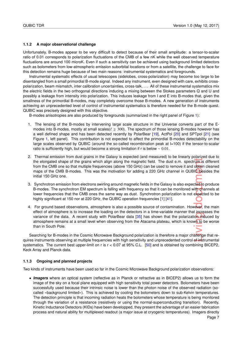
Table 1: Summary of the main ground and balloon projects aiming at measuring B-modes. The label “fg” or “no fg”corresponds to the assumption on the foregrounds, numbers have been extracted from [31]. [∗] The LSPE value isan upper limit at 99.7%CL. [1] Ref. [31] did not include this frequency..
measure the temperature on the sky in a given direction (with a resolution given by that of the telescope andhorns) and therefore allow building maps of the CMB Stokes parameters I, Q, and U that further enables us toreconstruct T, E and B power spectra.
• Interferometers where the correlation between two receivers allows us to directly access the Fourier modes(known as visibilities) of the Stokes parameters I, Q and U without producing maps. The observation ofinterference fringes with an interferometer allows for an extra control of systematic effects in comparison withan imager. That explains why interferometers were used for the first measurements of sub-degree temperatureanisotropies (with VSA [38]) and E-mode polarization (with CBI [40] and DASI [39]). However, they sufferedfrom a degraded sensitivity due to their heterodyne nature: signals at the frequency of the CMB (from a fewGHz to a few hundreds of GHz) need to be amplified and down-converted to lower frequencies before beingdetected. This amplification process adds an irreducible amount of noise that prevents such interferometersfrom being background limited. Furthermore, the complexity of traditional CMB interferometers (based onmultiplicative interferometry, making the correlation by pairs of detectors) prevent them from growing to thelarge number of receivers that is now required to achieve the sensitivity needed for the B-mode quest (if Nis the number of channels, their complexity increases as N2 while that of an imager grows as N). This is thereason why, despite their better ability to handle instrumental systematics, interferometers have no longer beenconsidered, until QUBIC, for CMB polarization observations.
Most of the on-going or planned projects are lead by U.S. teams. They are all based on the concept of a traditionalimager with a broad variety of technical choices regarding the modulation of the polarization, the optical setup,the detector technology, the frequency coverage or the instrument location. They also use different instrumentalapertures, that sets the angular accuracy hence the multipole coverage and therefore are optimized for differentscience goals: high angular resolution instruments are better suited for the lensing B-modes study (allowing oneto constrain neutrino masses for instance), and have published results on this (PolarBear, SPTpol, ACTpol) whilelow resolution suborbital instruments aim at detecting the recombination peak of the primordial B-modes at l=100.Satellite missions are considered by the community and aim at covering both science goals with the additionaladvantage of a full sky coverage allowing one to search for the reionization peak at l=7. However, no such missionhas been selected up to now by Space agencies, neither in the U.S.A. nor in Europe. LiteBird is a possible missionto be flown in the early 2020 by the Japanese Space Agency (JAXA) and would be an extremely sensitive project(targeting r=0.001) with low angular resolution, therefore only focused on primordial B-modes.
Table 1 summarizes the situation in terms of competitors for QUBIC. We know since the BICEP2/Planck con-troversy that foregrounds cannot be neglected. This is why, when the foreground-free forecasted sensitivity of theQUBIC first module, from Argentina, is σ(r) = 0.01, we can only achieve σ(r) = 0.02 when accounting for real-istic foregrounds. The observation efficiency is taken to be 30% in those QUBIC sensitivity forecasts. Besides
Page 8
Livi
ngdo
cum
ent
QUBIC TDR Version 1.0 (May 12, 2017)
BICEP/Keck [50] on the ground and the ballon-borne SPIDER experiment [59] which has already taken data in thesame multipole range as QUBIC (namely targeting the recombination peak at ` ∼ 100), it is clear from this tablethat QUBIC is competitive and timely with respect to other competitors with the same target. High resolution ex-periments are more suited to the measurement of the lensing B-modes which should provide very exciting neutrinoconstraints. Although these projects claim they will measure primordial B-modes, this is not their primary goal andthat they focus on the smaller angular scales because large angular scales are harder to reconstruct due to 1/fnoise (from electronics and/or atmosphere). As a matter of fact, these experiments have never published data, evenwith temperature only, below a multipole of ∼ 300. While having comparable sensitivity with the other experiments,QUBIC will offer this improved control of instrumental systematics that may be a decisive factor when reaching verylow tensor-to-scalar ratio sensitivity.
1.2 Bolometric Interferometry and QUBIC
Most of the current projects aiming at detecting the B-mode radiation are based on the architecture of an imagerbecause of its simplicity and the high sensitivity allowed by bolometers. However, imagers do not allow for the samelevel of control of instrumental systematics and could potentially reach a sensitivity floor because of E-modes leakinginto B-modes. Bolometric Interferometry is a novel concept combining the advantages of bolometric detectors interms of sensitivity with those of interferometers in terms of control for systematics. It was initially proposed in 2001by Peter Timbie (University of Wisconsin) and Lucio Piccirillo (University of Manchester). Two collaborations on bothsides of the Atlantic (BRAIN in Europe and MBI in the U.S.A.) started to develop the concept and decided to mergetheir efforts in the QUBIC project in 2008. The QUBIC collaboration now includes six laboratories in France, allmembers of the CNRS (APC in Paris, LAL, IAS and CSNSM in Orsay and IRAP in Toulouse), three Universitiesin Italy (Universitá di Roma – La Sapienza, Universitá Milano Bicocca and Statale in Milano), Manchester andCardiff Universities in the UK and NUI/Maynooth in Ireland, three universities in the USA (University of Wisconsin atMadison, WI ; Brown University at Providence, RH ; Richmond University, VI). NIKHEF (Netherlands) have joinedQUBIC in 2014.
1.2.1 The QUBIC design
QUBIC will observe interference fringes formed altogether by a large number of receiving horns with two arrays ofbolometric detectors (operating at 150 and 220 GHz) at the focal planes of an optical combiner. The image on eachfocal plane is a synthesized image in the sense that only specific Fourier modes are selected by the array of receivinghorns. A bolometric interferometer is therefore a synthetic imager whose beam is the synthesized beam formed bythe array of receiving horns. The interferometric nature of this synthesized beam allows us to use a specific self-calibration technique that permits to determine the parameters of the systematic effects channel by channel withan unprecedented accuracy [16] [36]. As a comparison, an imager can only measure the effective beam of eachchannel. We therefore have an extra-level of systematics control. The use of bolometric detectors allows us to reacha sensitivity comparable to that of an imager with the same number of receivers [17].
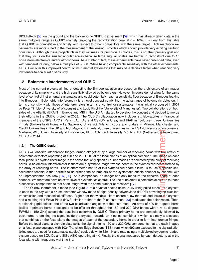
The QUBIC instrument is made (see Figure 2) of a cryostat cooled down to 4K using pulse-tubes. The cryostatis open to the sky with a 45 cm diameter window made of high-density polyethylene (HDPE) providing an excellenttransmission and mechanical stiffness. Right after the window, filters ensure a low thermal load inside the cryostatand a rotating Half-Wave-Plate (HWP) similar to that of the Pilot instrument [33] modulates the polarization. Then,a polarizing grid selects one of the two polarization angles w.r.t the instrument. An array of 400 corrugated horns(called « primary horns » designed to be efficient throughout the 150 and 220 GHz bands with a ≈ 13 degreesFWHM at 150 GHz) selects the baselines observed by QUBIC. These primary horns are immediately followed byback-horns re-emitting the signal inside the cryostat towards an « optical combiner » which is simply a telescopethat combines on the focal plane the images of each of the secondary horns in order to form interference fringes.Before the focal plane, a dichroic plate splits the signal into its 150 and 220 GHz components that are each imagedon a focal plane equipped with 1024 Transition-Edge-Sensors (TES) from which 992 are exposed to the sky radiation(blind ones are used for systematics studies) cooled down to 320 mK and read using a multiplexed cryogenic readoutsystem based on SQUIDs and SiGe ASIC operating at 4K. Finally, the signal measured by each detector p at in thefocal plane with frequency ν at time t is:
R(p, ν, t) = S I(p, ν) + cos[4ϕHPW(t)
]S Q(p, ν) + sin
[4ϕHPW(t)
]S U(p, ν) (1)
Page 9
Livi
ngdo
cum
ent
QUBIC TDR Version 1.0 (May 12, 2017)
< 1K
320 mK
~1K
Cryostat
Sky~40 cm
~4K
bolometer array ( 992 TES)150 GHz
Filters
Primary horns
Secondary horns
Switches
Half-wave plate
bolometer array (992 TES)
220 GHz
Dichroic
< 1K
~4K
~4K
~4K
Polarizing Grid ~4K
Figure 2: Sketch of QUBIC (see text for explanation)
where ϕHWP(t) is the angle of the HWP at time t , S I/Q/U the sky signal at frequency ν convolved with the syn-thesized beam (see Figure 3). With a scanning strategy offering a wide range of polarization angles on the sky andthanks to the HWP rotation, one can recover1 the synthesized images of each of the three Stokes parameters I, Qand U. In contrast with traditional interferometry, the observables of QUBIC are not the visibilities (Fourier Transformof the observed sky for modes corresponding to the baselines), but the synthesized image, which is nothing elsebut the observed sky filtered to the modes corresponding to the baselines allowed by our instrument. This particularfeature is a crucial one in QUBIC as each of these modes can be calibrated separately using the « self calibration »procedure (see section 1.2.3 and [36]) allowing QUBIC to reach an unprecedented level of instrumental systematicscontrol.
One important aspect of the QUBIC design is the presence of the polarizing grid right after the half-wave plate,ie very close to the sky. It may appear undesirable from the sensitivity point of view to reject half of the photons atthe entrance of the instrument. However, this a very nice feature from the point of view of polarization systematicsbecause this is associated with bolometers that are not polarization sensitive: the rejection of the undesideredpolarization with the polarizing grid is very efficient and whatever the cross-polarization of the rest of the instrument,the detectors will measure the polarized sky signal modulated by the HWP. This means that we expect a very lowlevel of instrumental cross-polarization for QUBIC.
1.2.2 The QUBIC synthesized beam and map-making
In QUBIC, each primary horns pair defines a baseline (a Fourier mode on the sky) that is transmitted through theinstrument and forms an interference fringe on the focal planes. In the standard « sky observing » mode, the fringesformed by all the baselines are coherently combined on the focal and form a synthesized image of the sky, whichis the sky image convolved by the QUBIC synthesized beam than can be calculated from the combination of allbaselines.
The QUBIC horn array and synthesized beams are shown in Figure 3. As can be seen on this Figure (left1It is worth noting that given the approximate cost of 5 k€ for a traditional correlator, a 400 elements traditional interferometer would require
˜80000 of them (one per baseline) and would therefore cost the amazing price of ˜400 M€. Using an optical combiner as in QUBIC thereforeappears as a very cheap way (by a factor ˜100) of performing interferometry with a large number of channels, leading to a better sensitivity thanksto the use of bolometers.
Page 10
Livi
ngdo
cum
ent
QUBIC TDR Version 1.0 (May 12, 2017)
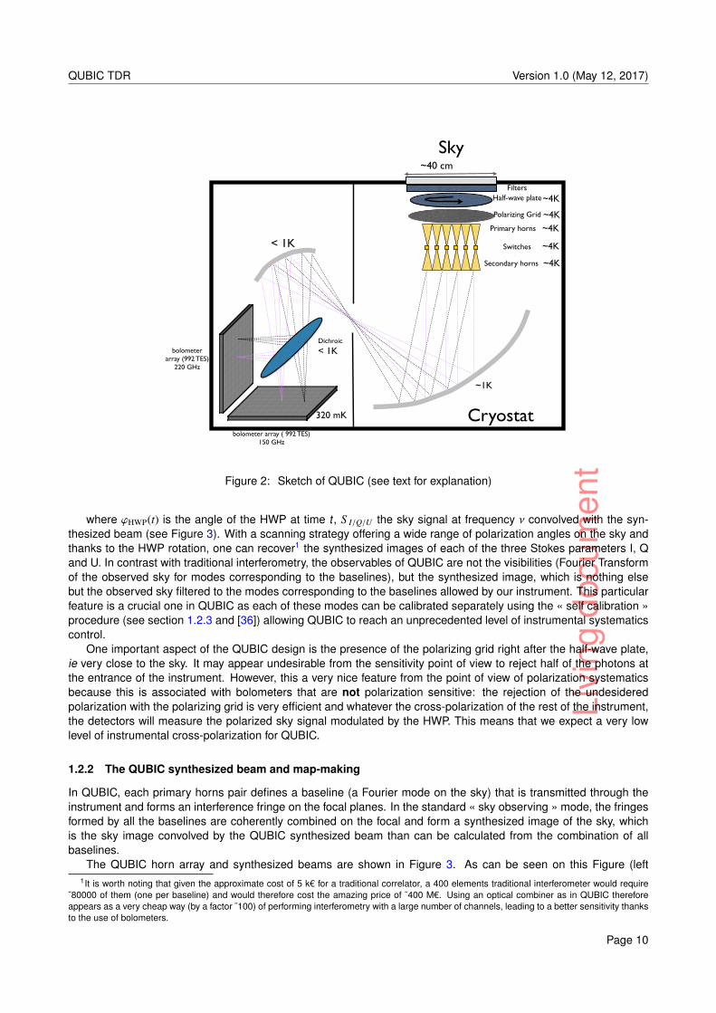
Figure 3: QUBIC primary horn array and corresponding beam on the sky for the central detector of any of the twofocal planes.
panel), the horn array, although enclosed in a circle to optimize the window occupation, respects a regular squaregrid pattern that has been shown to ensure a coherent summation of redundant baselines which is the key aspectoffering to a bolometric interferometer a comparable sensitivity to an imager [17] [16].
The synthesized beams shape is significantly different from the beam offered by a classical imager and typicalof that of an interferometer: it has a central peak, with 0.54° FWHM and has replications around, damped by theprimary 14° FWHM that are due to the fact that the primary horn array has finite extension. These replications are notsidelobes as they are a desired feature of an interferometer that only observes well defined and well « calibrable »baselines (see Sect. 3.3.1). It however makes the map-making procedure much more complicated than with animager as it involves partial deconvolution to disentangle the small contamination by secondary peaks with respectto the main one.
We have shown that using super-calculators and a specific map-making algorithm based on « inverse problemsolving » [32], one can recover the input I, Q and U maps provided the fact that the scanning strategy offers a wideenough variety of polarization angles on the sky (which is ensured by the combination of sweeps in azimuth withconstant elevation and the rotation of the Half-Wave-Plate, cf. Figure 4 and Figure 5).
1.2.3 Self-calibration and the systematic effects mitigation with QUBIC
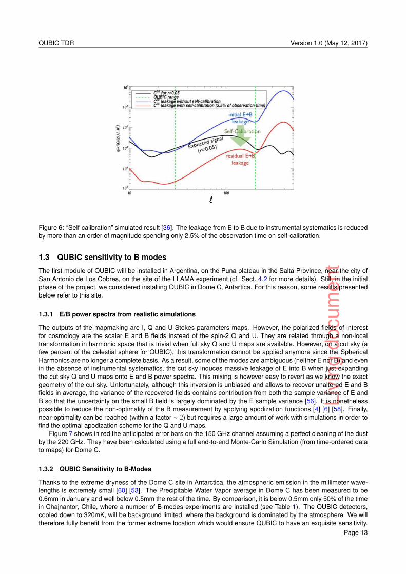
Interferometry is known [2] to offer an improved control of instrumental systematics with respect to direct imagingthanks to the observation of individual interference fringes that can be calibrated individually. This feature is con-served with bolometric interferometry, in QUBIC, thanks to the presence of electromagnetic switches between theprimary and secondary horns (cf. sections 2.3.4 and 2.3.5). This apparatus consists in a waveguide that is closedor open using a cold (4K) shutter operated by solenoid magnets. In the self-calibration mode, pairs of horns aresuccessively shut when observing an artificial partially polarized source (we do not need to know its polarization).As a result, we can reconstruct the signal measured by each individual pairs of horns in the array and compare them.As redundant baselines correspond to the same mode of the observed field, a different signal between them canonly be due to photon noise or instrumental systematics. Using a detailed model of the instrument incorporating allpossible systematics (through the use of Jones matrices for each optical component), we have shown that we canfully recover all of these parameters through a non-linear inversion involving hundreds of parameters (horn locationsand beams, components cross-polarization, detector inter calibration, . . . ). The updated model of the instrumentcan then be used to reconstruct the synthesized beam and improve the map-making, reducing the leakage betweenStokes parameters. We have shown in [36] that with 2.5% of the observing time, we can reduce the impact ofthe instrument systematics on the E to B leakage to a level allowing us to measure the B modes down to r=0.05(see Figure 6). No such feature exists with a usual imager justifying the fact that QUBIC will have extra-control oninstrumental systematics with respect to all the other running or planned instruments listed in Table 1.
Page 11
Livi
ngdo
cum
ent
QUBIC TDR Version 1.0 (May 12, 2017)
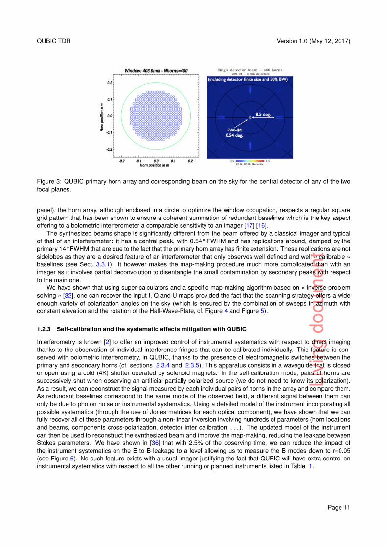
Figure 4: (left) Current results with the QUBIC mapmaking under the Gaussian peaks assumption. First row showsthe input I,Q and U maps in the region observed by QUBIC, second row shows the recovered maps using the fullsimulation pipeline, last row shows the residuals w.r.t. the input maps.
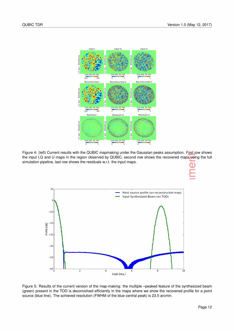
Figure 5: Results of the current version of the map-making: the multiple –peaked feature of the synthesized beam(green) present in the TOD is deconvolved efficiently in the maps where we show the recovered profile for a pointsource (blue line). The achieved resolution (FWHM of the blue central peak) is 23.5 arcmin.
Page 12
Livi
ngdo
cum
ent
QUBIC TDR Version 1.0 (May 12, 2017)
l
Figure 6: “Self-calibration” simulated result [36]. The leakage from E to B due to instrumental systematics is reducedby more than an order of magnitude spending only 2.5% of the observation time on self-calibration.
1.3 QUBIC sensitivity to B modes
The first module of QUBIC will be installed in Argentina, on the Puna plateau in the Salta Province, near the city ofSan Antonio de Los Cobres, on the site of the LLAMA experiment (cf. Sect. 4.2 for more details). Still, in the initialphase of the project, we considered installing QUBIC in Dome C, Antartica. For this reason, some results presentedbelow refer to this site.
1.3.1 E/B power spectra from realistic simulations
The outputs of the mapmaking are I, Q and U Stokes parameters maps. However, the polarized fields of interestfor cosmology are the scalar E and B fields instead of the spin-2 Q and U. They are related through a non-localtransformation in harmonic space that is trivial when full sky Q and U maps are available. However, on a cut sky (afew percent of the celestial sphere for QUBIC), this transformation cannot be applied anymore since the SphericalHarmonics are no longer a complete basis. As a result, some of the modes are ambiguous (neither E nor B) and evenin the absence of instrumental systematics, the cut sky induces massive leakage of E into B when just expandingthe cut sky Q and U maps onto E and B power spectra. This mixing is however easy to revert as we know the exactgeometry of the cut-sky. Unfortunately, although this inversion is unbiased and allows to recover unaltered E and Bfields in average, the variance of the recovered fields contains contribution from both the sample variance of E andB so that the uncertainty on the small B field is largely dominated by the E sample variance [56]. It is nonethelesspossible to reduce the non-optimality of the B measurement by applying apodization functions [4] [6] [58]. Finally,near-optimality can be reached (within a factor ∼ 2) but requires a large amount of work with simulations in order tofind the optimal apodization scheme for the Q and U maps.
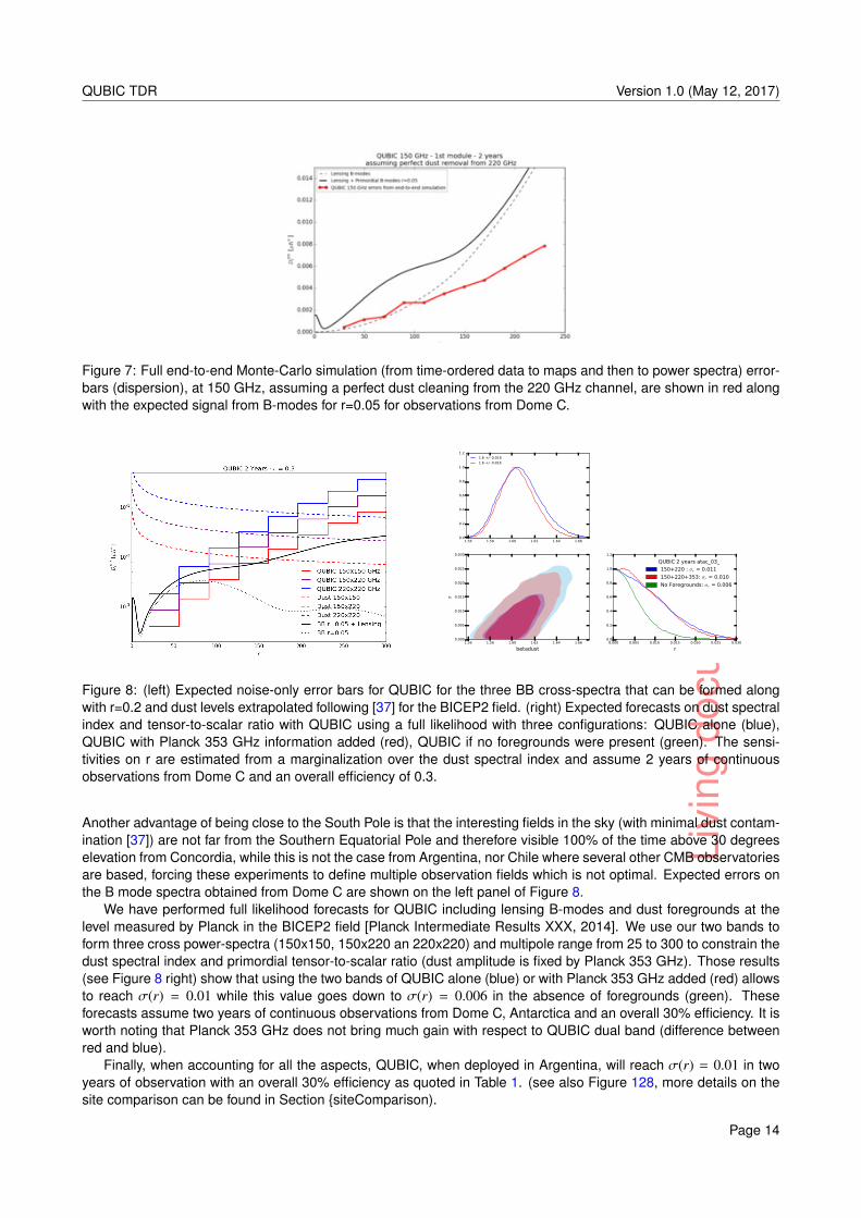
Figure 7 shows in red the anticipated error bars on the 150 GHz channel assuming a perfect cleaning of the dustby the 220 GHz. They have been calculated using a full end-to-end Monte-Carlo Simulation (from time-ordered datato maps) for Dome C.
1.3.2 QUBIC Sensitivity to B-Modes
Thanks to the extreme dryness of the Dome C site in Antarctica, the atmospheric emission in the millimeter wave-lengths is extremely small [60] [53]. The Precipitable Water Vapor average in Dome C has been measured to be0.6mm in January and well below 0.5mm the rest of the time. By comparison, it is below 0.5mm only 50% of the timein Chajnantor, Chile, where a number of B-modes experiments are installed (see Table 1). The QUBIC detectors,cooled down to 320mK, will be background limited, where the background is dominated by the atmosphere. We willtherefore fully benefit from the former extreme location which would ensure QUBIC to have an exquisite sensitivity.
Page 13
Livi
ngdo
cum
ent
QUBIC TDR Version 1.0 (May 12, 2017)
Figure 7: Full end-to-end Monte-Carlo simulation (from time-ordered data to maps and then to power spectra) error-bars (dispersion), at 150 GHz, assuming a perfect dust cleaning from the 220 GHz channel, are shown in red alongwith the expected signal from B-modes for r=0.05 for observations from Dome C.
1.56 1.58 1.60 1.62 1.64 1.660.0
0.2
0.4
0.6
0.8
1.0
1.21.6 +/- 0.018
1.6 +/- 0.016
1.56 1.58 1.60 1.62 1.64 1.66
betadust
0.000
0.005
0.010
0.015
0.020
0.025
0.030
r
0.000 0.005 0.010 0.015 0.020 0.025 0.030
r
0.0
0.2
0.4
0.6
0.8
1.0
1.2
QUBIC 2 years atac_03_
150+220 : σr = 0.011
150+220+353: σr = 0.010
No Foregrounds: σr = 0.006
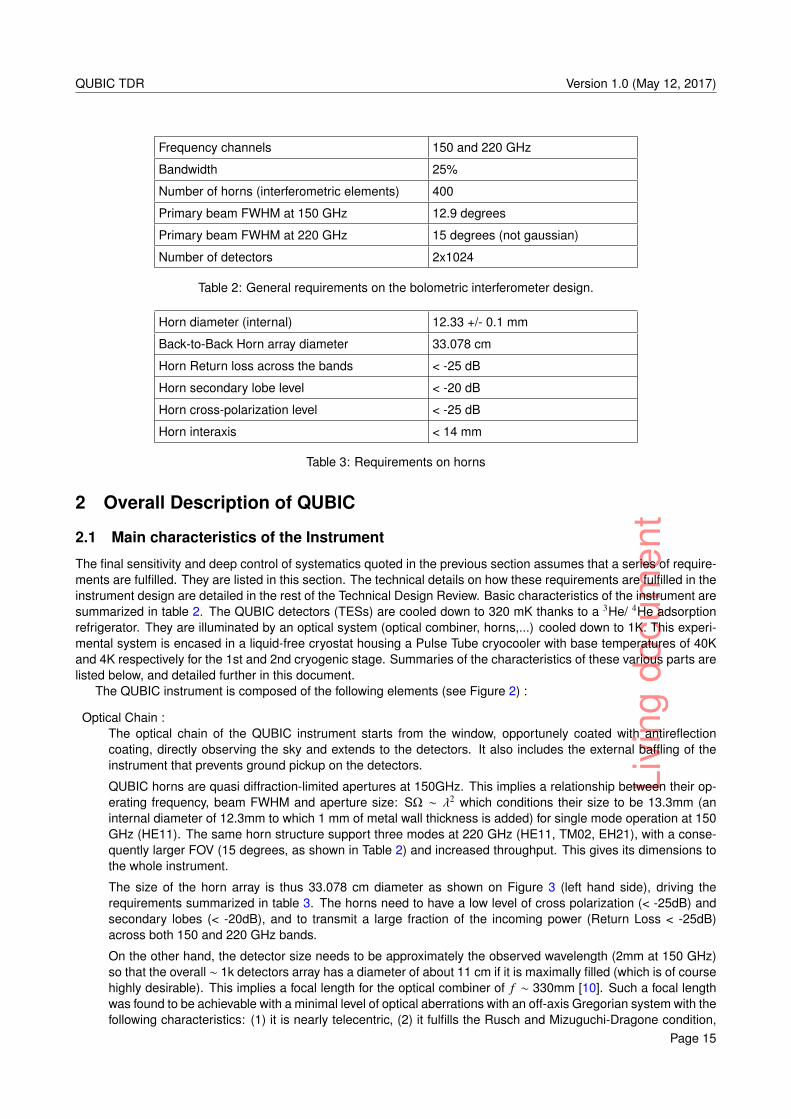
Figure 8: (left) Expected noise-only error bars for QUBIC for the three BB cross-spectra that can be formed alongwith r=0.2 and dust levels extrapolated following [37] for the BICEP2 field. (right) Expected forecasts on dust spectralindex and tensor-to-scalar ratio with QUBIC using a full likelihood with three configurations: QUBIC alone (blue),QUBIC with Planck 353 GHz information added (red), QUBIC if no foregrounds were present (green). The sensi-tivities on r are estimated from a marginalization over the dust spectral index and assume 2 years of continuousobservations from Dome C and an overall efficiency of 0.3.
Another advantage of being close to the South Pole is that the interesting fields in the sky (with minimal dust contam-ination [37]) are not far from the Southern Equatorial Pole and therefore visible 100% of the time above 30 degreeselevation from Concordia, while this is not the case from Argentina, nor Chile where several other CMB observatoriesare based, forcing these experiments to define multiple observation fields which is not optimal. Expected errors onthe B mode spectra obtained from Dome C are shown on the left panel of Figure 8.
We have performed full likelihood forecasts for QUBIC including lensing B-modes and dust foregrounds at thelevel measured by Planck in the BICEP2 field [Planck Intermediate Results XXX, 2014]. We use our two bands toform three cross power-spectra (150x150, 150x220 an 220x220) and multipole range from 25 to 300 to constrain thedust spectral index and primordial tensor-to-scalar ratio (dust amplitude is fixed by Planck 353 GHz). Those results(see Figure 8 right) show that using the two bands of QUBIC alone (blue) or with Planck 353 GHz added (red) allowsto reach σ(r) = 0.01 while this value goes down to σ(r) = 0.006 in the absence of foregrounds (green). Theseforecasts assume two years of continuous observations from Dome C, Antarctica and an overall 30% efficiency. It isworth noting that Planck 353 GHz does not bring much gain with respect to QUBIC dual band (difference betweenred and blue).
Finally, when accounting for all the aspects, QUBIC, when deployed in Argentina, will reach σ(r) = 0.01 in twoyears of observation with an overall 30% efficiency as quoted in Table 1. (see also Figure 128, more details on thesite comparison can be found in Section siteComparison).
Page 14
Livi
ngdo
cum
ent
QUBIC TDR Version 1.0 (May 12, 2017)
Frequency channels 150 and 220 GHz
Bandwidth 25%
Number of horns (interferometric elements) 400
Primary beam FWHM at 150 GHz 12.9 degrees
Primary beam FWHM at 220 GHz 15 degrees (not gaussian)
Number of detectors 2x1024
Table 2: General requirements on the bolometric interferometer design.
Horn diameter (internal) 12.33 +/- 0.1 mm
Back-to-Back Horn array diameter 33.078 cm
Horn Return loss across the bands < -25 dB
Horn secondary lobe level < -20 dB
Horn cross-polarization level < -25 dB
Horn interaxis < 14 mm
Table 3: Requirements on horns
2 Overall Description of QUBIC
2.1 Main characteristics of the Instrument
The final sensitivity and deep control of systematics quoted in the previous section assumes that a series of require-ments are fulfilled. They are listed in this section. The technical details on how these requirements are fulfilled in theinstrument design are detailed in the rest of the Technical Design Review. Basic characteristics of the instrument aresummarized in table 2. The QUBIC detectors (TESs) are cooled down to 320 mK thanks to a 3He/ 4He adsorptionrefrigerator. They are illuminated by an optical system (optical combiner, horns,...) cooled down to 1K. This experi-mental system is encased in a liquid-free cryostat housing a Pulse Tube cryocooler with base temperatures of 40Kand 4K respectively for the 1st and 2nd cryogenic stage. Summaries of the characteristics of these various parts arelisted below, and detailed further in this document.
The QUBIC instrument is composed of the following elements (see Figure 2) :
Optical Chain :The optical chain of the QUBIC instrument starts from the window, opportunely coated with antireflectioncoating, directly observing the sky and extends to the detectors. It also includes the external baffling of theinstrument that prevents ground pickup on the detectors.
QUBIC horns are quasi diffraction-limited apertures at 150GHz. This implies a relationship between their op-erating frequency, beam FWHM and aperture size: SΩ ∼ λ2 which conditions their size to be 13.3mm (aninternal diameter of 12.3mm to which 1 mm of metal wall thickness is added) for single mode operation at 150GHz (HE11). The same horn structure support three modes at 220 GHz (HE11, TM02, EH21), with a conse-quently larger FOV (15 degrees, as shown in Table 2) and increased throughput. This gives its dimensions tothe whole instrument.
The size of the horn array is thus 33.078 cm diameter as shown on Figure 3 (left hand side), driving therequirements summarized in table 3. The horns need to have a low level of cross polarization (< -25dB) andsecondary lobes (< -20dB), and to transmit a large fraction of the incoming power (Return Loss < -25dB)across both 150 and 220 GHz bands.
On the other hand, the detector size needs to be approximately the observed wavelength (2mm at 150 GHz)so that the overall ∼ 1k detectors array has a diameter of about 11 cm if it is maximally filled (which is of coursehighly desirable). This implies a focal length for the optical combiner of f ∼ 330mm [10]. Such a focal lengthwas found to be achievable with a minimal level of optical aberrations with an off-axis Gregorian system with thefollowing characteristics: (1) it is nearly telecentric, (2) it fulfills the Rusch and Mizuguchi-Dragone condition,
Page 15
Livi
ngdo
cum
ent
QUBIC TDR Version 1.0 (May 12, 2017)
Window diameter 39.9 cm
Filters diameters 39.2 cm
Polarizer diameter 32.6 cm
Half-Wave plate diameter 32.7 cm
Half-Wave plate, filters and polarizer transmis-sion
-0.2 dB
Half-Wave plate, filters and polarizer cross-polarization
-20 dB
Table 4: Requirements on cold optics chain
Optical combiner focal length 30 cm
Number of mirrors 2
M1 shape and diameter 480mm x 600mm -
M2 shape and diameter 600mm x 500mm -
Optical combiner sensitivity loss from aberra-tions
< 10%
Table 5: Requirements on mirrors and optical properties
(3) it features a field of view largely diffraction limited with with Strehl ratio >0.8 within +/- 4.9 degrees [5]. Therequirement for the amount of optical aberrations was that the sensitivity loss is less than 10% when calculatedby the ratio of the synthesized beam with and without optical aberrations. Requirements on cold optics andmirrors are summarized on Tables 4 and 5.
The different diameters have been calculated assuming that 95% of the power goes through the aperture, butsimilar values have been calculated to get 99% of the power.
The possibility to monitor departure from idealities is provided by the self-calibration procedure. This procedure(see Sect. 3.3.1) is indeed one of the main advantages of QUBIC with respect to other more traditional designs(see Sect. 1.1.3). In order to perform it efficiently, one needs to be able to switch on and off some of the hornswhile observing a calibration source. This requires waveguide switches placed in between the back-to-backhorns. Such switches need to be closed enough when in off position (-80 dB) while open enough when setto the on position (-0.1 dB). Both of these criteria need to be fulfilled simultaneously across the 150 and 220GHz bands. The switches also need to have low cross talk between neighbouring switches. The switchingbetween on and off needs to dissipate minimal power at the 4K stage (60 mW) in order not to heat this stageand perturb observations. Such requirements are summarized on Table 6
External shields are required to prevent ground pickup in the detectors and make sure that photons comingfrom a large angle with respect to the optical axis are absorbed or reflected before entering the cryostat. Thisis achieved thanks to:
• a cylindrical forebaffle attached to the cryostat with a 1m length and a 14 deg opening angle. This allowsto reduce by more than 20dB the radiation coming from 20deg < θ < 40deg from the optical axis, and bymore than 40dB beyond.
• an external shield around the instrument mount or the experiment module’s roof (therefore fixed with
Switches OFF transmission -80 dB
Switches ON transmission -0.1 dB
Switches Cross-talk -40 dB
Table 6: Requirements on switches
Page 16
Livi
ngdo
cum
ent
QUBIC TDR Version 1.0 (May 12, 2017)
Baffling reduction 20deg < θ < 40deg -20 dB
Baffling reduction 40deg < θ < 80deg -40 dB
Baffling reduction θ > 80deg -80 dB
Table 7: Requirements on the external shields
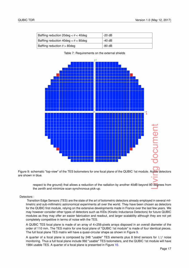
Figure 9: schematic "top-view" of the TES bolometers for one focal plane of the QUBIC 1st module. Active detectorsare shown in blue.
respect to the ground) that allows a reduction of the radiation by another 40dB beyond 80 degrees fromthe zenith and minimize scan synchronous pick-up.
Detectors :Transition Edge Sensors (TES) are the state of the art of bolometric detectors already employed in several mil-
limetric and sub-millimetric astronomical experiments all over the world. They have been chosen as detectorsfor the QUBIC first module, relying on the extensive developments made in France over the last few years. Wemay however consider other types of detectors such as KIDs (Kinetic Inductance Detectors) for future QUBICmodules as they may offer an easier fabrication and readout, and larger scalability although they are not yetcompletely competitive in terms of noise with the TES.
A QUBIC TES focal plane is made of an array of 4×256-pixels arrays disposed in an overall diameter of theorder of 110 mm. The TES matrix for one focal plane of "QUBIC 1st module" is made of four identical pieces.The full focal plane TES matrix will have a quasi-circular shape as shown in Figure 9.
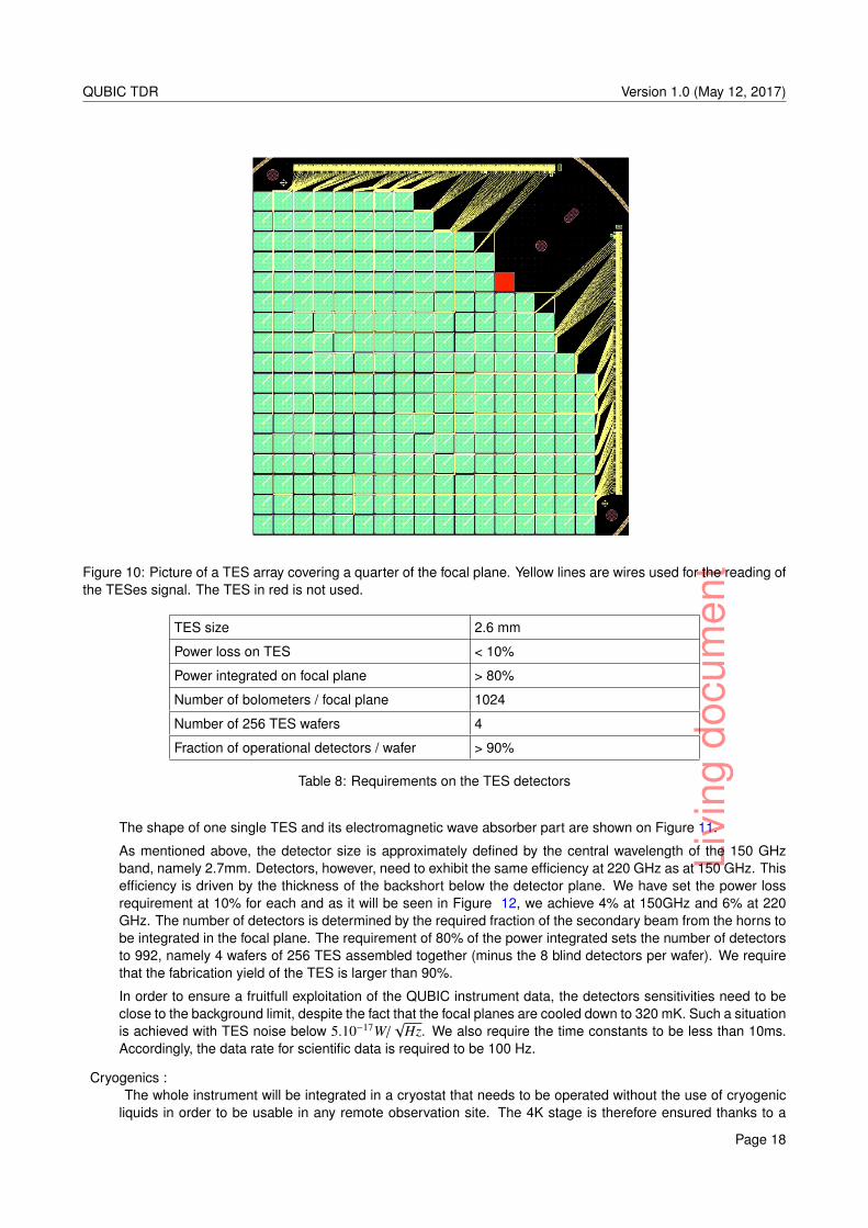
A quarter of a focal plane is composed by 248 "usable" TES elements plus 8 blind sensors for 1/ f noisemonitoring. Thus a full focal plane include 992 "usable" TES bolometers, and the QUBIC 1st module will have1984 usable TES. A quarter of a focal plane is presented in Figure 10.
Page 17
Livi
ngdo
cum
ent
QUBIC TDR Version 1.0 (May 12, 2017)
Figure 10: Picture of a TES array covering a quarter of the focal plane. Yellow lines are wires used for the reading ofthe TESes signal. The TES in red is not used.
TES size 2.6 mm
Power loss on TES < 10%
Power integrated on focal plane > 80%
Number of bolometers / focal plane 1024
Number of 256 TES wafers 4
Fraction of operational detectors / wafer > 90%
Table 8: Requirements on the TES detectors
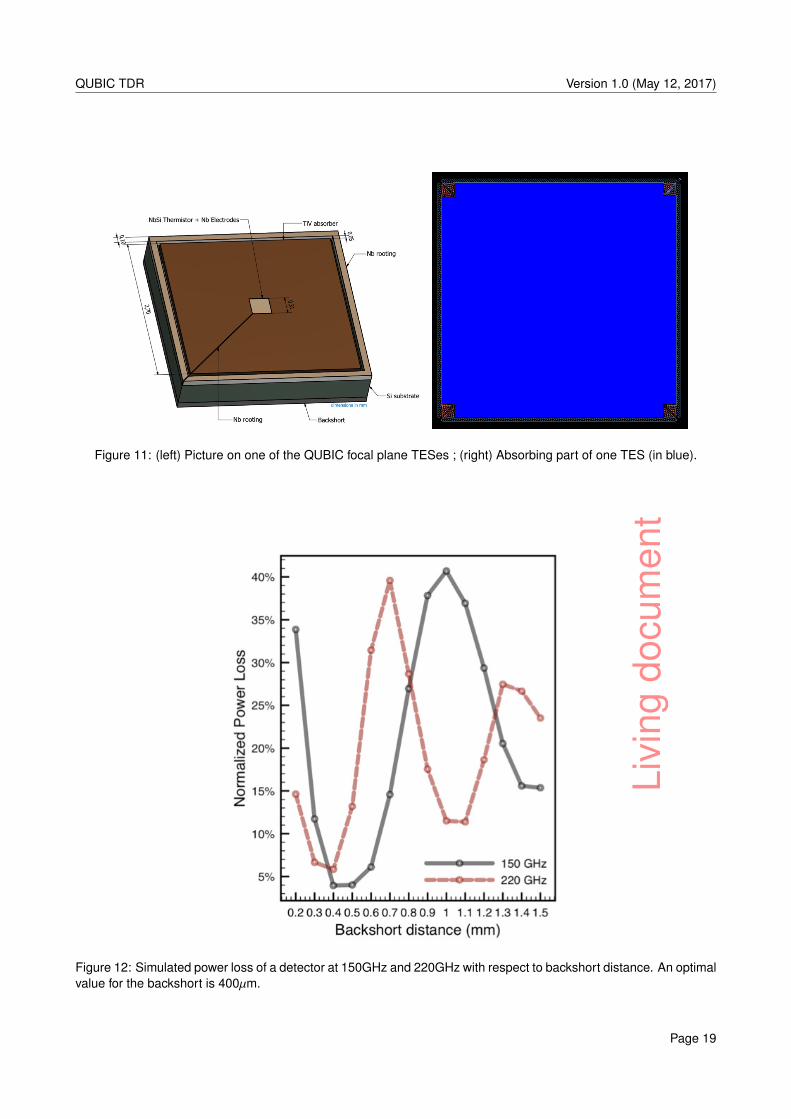
The shape of one single TES and its electromagnetic wave absorber part are shown on Figure 11.
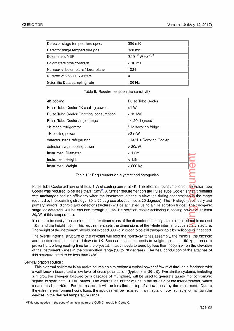
As mentioned above, the detector size is approximately defined by the central wavelength of the 150 GHzband, namely 2.7mm. Detectors, however, need to exhibit the same efficiency at 220 GHz as at 150 GHz. Thisefficiency is driven by the thickness of the backshort below the detector plane. We have set the power lossrequirement at 10% for each and as it will be seen in Figure 12, we achieve 4% at 150GHz and 6% at 220GHz. The number of detectors is determined by the required fraction of the secondary beam from the horns tobe integrated in the focal plane. The requirement of 80% of the power integrated sets the number of detectorsto 992, namely 4 wafers of 256 TES assembled together (minus the 8 blind detectors per wafer). We requirethat the fabrication yield of the TES is larger than 90%.
In order to ensure a fruitfull exploitation of the QUBIC instrument data, the detectors sensitivities need to beclose to the background limit, despite the fact that the focal planes are cooled down to 320 mK. Such a situationis achieved with TES noise below 5.10−17W/
√Hz. We also require the time constants to be less than 10ms.
Accordingly, the data rate for scientific data is required to be 100 Hz.
Cryogenics :The whole instrument will be integrated in a cryostat that needs to be operated without the use of cryogenic
liquids in order to be usable in any remote observation site. The 4K stage is therefore ensured thanks to a
Page 18
Livi
ngdo
cum
ent
QUBIC TDR Version 1.0 (May 12, 2017)
Figure 11: (left) Picture on one of the QUBIC focal plane TESes ; (right) Absorbing part of one TES (in blue).
Figure 12: Simulated power loss of a detector at 150GHz and 220GHz with respect to backshort distance. An optimalvalue for the backshort is 400µm.
Page 19
Livi
ngdo
cum
ent
QUBIC TDR Version 1.0 (May 12, 2017)
Detector stage temperature spec. 350 mK
Detector stage temperature goal 320 mK
Bolometers NEP 5.10−17W.Hz−1/2
Bolometers time constant < 10 ms
Number of bolometers / focal plane 1024
Number of 256 TES wafers 4
Scientific Data sampling rate 100 Hz
Table 9: Requirements on the sensitivity
4K cooling Pulse Tube Cooler
Pulse Tube Cooler 4K cooling power >1 W
Pulse Tube Cooler Electrical consumption < 15 kW
Pulse Tube Cooler angle range +/- 20 degrees
1K stage refrigerator 4He sorption fridge
1K cooling power >2 mW
detector stage refrigerator 3He/4He Sorption Cooler
detector stage cooling power > 20µW
Instrument Diameter < 1.6m
Instrument Height < 1.8m
Instrument Weight < 800 kg
Table 10: Requirement on cryostat and cryogenics
Pulse Tube Cooler achieving at least 1 W of cooling power at 4K. The electrical consumption of the Pulse TubeCooler was required to be less than 15kW2. A further requirement on the Pulse Tube Cooler is that it remainswith unchanged cooling efficiency when the instrument is tilted in elevation during observations in the rangerequired by the scanning strategy (30 to 70 degrees elevation, so ± 20 degrees). The 1K stage (secondary andprimary mirrors, dichroic and detector structure) will be achieved using a 4He sorption fridge. The cryogenicstage for detectors will be ensured through a 3He/4He sorption cooler achieving a cooling power of at least20µW at this temperature.
In order to be easily transported, the outer dimensions of the diameter of the cryostat is required not to exceed1.6m and the height 1.8m. This requirement sets the dimensions of the whole internal cryogenic architecture.The weight of the instrument should not exceed 800 kg in order to be still transportable by helicopters if needed.
The overall internal structure of the cryostat will hold the horns+switches assembly, the mirrors, the dichroicand the detectors. It is cooled down to 1K. Such an assemble needs to weight less than 150 kg in order toprevent a too long cooling time for the cryostat. It also needs to bend by less than 400µm when the elevationof the instrument varies in the observation range (30 to 70 degrees). The heat conduction of the attaches ofthis structure need to be less than 2µW.
Self-calibration source :This external calibrator is an active source able to radiate a typical power of few mW through a feedhorn with
a well-known beam, and a low level of cross-polarisation (typically < -30 dB). Two similar systems, includinga microwave sweeper followed by a cascade of multipliers, will be used to generate quasi- monochromaticsignals to span both QUBIC bands. The external calibrator will be in the far-field of the interferometer, whichmeans at about 40m. For this reason, it will be installed on top of a tower nearby the instrument. Due tothe extreme environment conditions, the sources will be installed in an insulation box, suitable to maintain thedevices in the desired temperature range.
2This was needed in the case of an installation of a QUBIC module in Dome C.
Page 20
Livi
ngdo
cum
ent
QUBIC TDR Version 1.0 (May 12, 2017)
Internal Structure weight < 150 kg
Internal Structure temperature spec. <1.4K
Internal Structure temperature goal 1 K
Internal Structure bending for +/- 20 deg. < 400µm
Internal Structure attaches heat conduction < 2µW
Internal Structure rotation < 0.2°
Table 11: Requirements on instrument internal structure
Frequency coverage 110-170 GHz & 170-260 GHz
power output spec. 5 mW
power output goal 1 mW
Operation modes CW + amplitude modulation
Polarisation Linear
Cross-polarisation ≤ -30 dB
Weight (estim., including insulation box) 10 kg
Table 12: Requirements on calibration sources
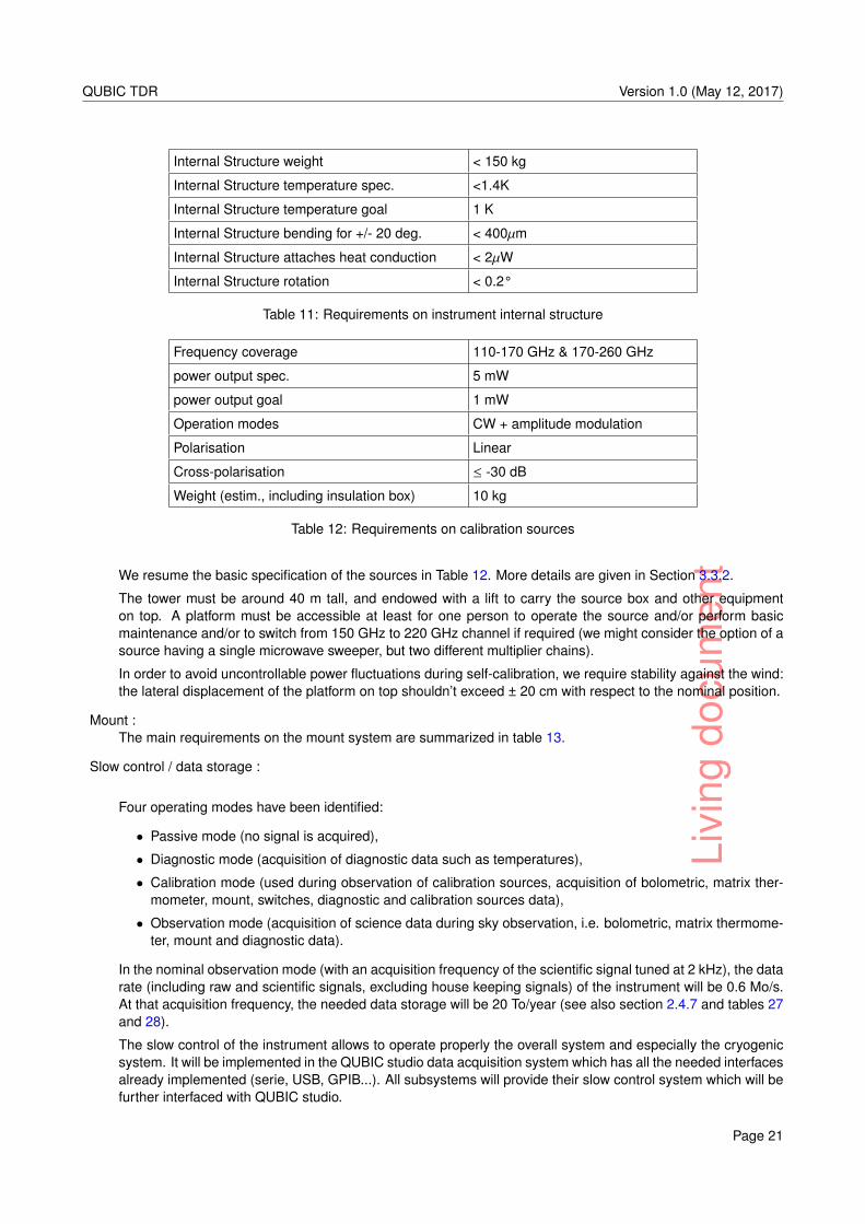
We resume the basic specification of the sources in Table 12. More details are given in Section 3.3.2.
The tower must be around 40 m tall, and endowed with a lift to carry the source box and other equipmenton top. A platform must be accessible at least for one person to operate the source and/or perform basicmaintenance and/or to switch from 150 GHz to 220 GHz channel if required (we might consider the option of asource having a single microwave sweeper, but two different multiplier chains).
In order to avoid uncontrollable power fluctuations during self-calibration, we require stability against the wind:the lateral displacement of the platform on top shouldn’t exceed ± 20 cm with respect to the nominal position.
Mount :The main requirements on the mount system are summarized in table 13.
Slow control / data storage :
Four operating modes have been identified:
• Passive mode (no signal is acquired),
• Diagnostic mode (acquisition of diagnostic data such as temperatures),
• Calibration mode (used during observation of calibration sources, acquisition of bolometric, matrix ther-mometer, mount, switches, diagnostic and calibration sources data),
• Observation mode (acquisition of science data during sky observation, i.e. bolometric, matrix thermome-ter, mount and diagnostic data).
In the nominal observation mode (with an acquisition frequency of the scientific signal tuned at 2 kHz), the datarate (including raw and scientific signals, excluding house keeping signals) of the instrument will be 0.6 Mo/s.At that acquisition frequency, the needed data storage will be 20 To/year (see also section 2.4.7 and tables 27and 28).
The slow control of the instrument allows to operate properly the overall system and especially the cryogenicsystem. It will be implemented in the QUBIC studio data acquisition system which has all the needed interfacesalready implemented (serie, USB, GPIB...). All subsystems will provide their slow control system which will befurther interfaced with QUBIC studio.
Page 21
Livi
ngdo
cum
ent
QUBIC TDR Version 1.0 (May 12, 2017)
Maximal diameter 2500 mm
Maximal height 2500 mm
Mass (without the instrument) < 2300 kg
Mass to be supported by the mount 700 kg
Diameter of the instrument 1600 mm
Height of the instrument with forebaffle 1800 mm
Electrical consumption of the mount < 1 kW
Rotation in azimuth -220 / +220
Rotation in elevation +30 / +70
Rotation around the optical axis -30/ +30
Pointing accuracy (all axis) < 20 arcsec
Angular speed (all axis) Adjustable between 0 and 5/s with steps < 0.2/s
Table 13: General requirements on the mount system.
2.2 Cryogenic systems
2.2.1 Cryostat design / Mechanic architecture and CAD
The cryogenic system of QUBIC aims at cooling the detector arrays at 0.3K, the beam combiner optics at 1K, andthe rotating HWP, the polarizing analyzer, the horn array, and the switches at 4K. It is based on:
• A self-contained 3He refrigerator cooling the detector arrays
• A self-contained 4He refrigerator pre-cooling the 3He fridge and cooling a large 1K shield surrounding theoptical system (the beam combiner optic)
• Two 1W pulse-tube (PT) refrigerators working in parallel and cooling the experiment volume at 3K and thesurrounding radiation shield at 40K respectively
• A large vacuum jacket surrounding the entire system, including a large (50 cm) optical window
• Heat switches, Heaters, Thermometers, Control Electronics to run the system.
In the following we describe the basic design choices, and the dimensions and interfaces of the cryogenic system.
2.2.2 Cryostat vacuum
The purpose of the outer shell of the cryostat is to allow the setup ot operate under high-vacuum conditions in theinternal volume of the cryostat, to support all the internal elements, and to permit mm-wave radiation under studyto reach the cryogenic part of the instrument through the optical window. The size of the outer shell of the cryostatis driven by the volume of the cryogenic instrument, which includes the polarization modulator, the horns array,the beam combiner mirrors, and the focal plane assembly, for a total volume of the order of 1 m3. The cryostathas been designed around the cryogenic instrument, and its dimensions are a trade-off between the total size limitimposed by the transportation and the need for sufficient thermal insulation between the cryogenic instrument andthe room-temperature shell.
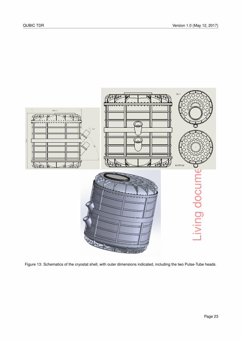
The resulting vacuum shell has a diameter of 1.4m and a height of 1.55m. Its shape and structure has beenoptimized for withstanding the stress from atmospheric pressure outside and vacuum inside, with sufficient safetyfactors. The structure is made out of Aluminium alloy sheets, roll-bent and welded, reinforced by a stiffening ribsstructure. The vacuum jacket is obtained by closing a vertical cylinder with two flanges (using indium seals) asshown in Figure 13. The axes of the two PTs are tilted by 40 deg with respect to the vertical, to allow optimalelevation coverage during the observations of the sky at the latitude of operation, while maintaining the Pulse Tubehead close to the vertical position where its operational performance are maximized.
Figure 13 also shows the two pulse-tube (PT) heads, mounted on dedicated flanges on the cylinder. The topflange differs from the bottom one because it includes the vacuum window.
Page 22
Livi
ngdo
cum
ent
QUBIC TDR Version 1.0 (May 12, 2017)
Figure 13: Schematics of the cryostat shell, with outer dimensions indicated, including the two Pulse-Tube heads.
Page 23
Livi
ngdo
cum
ent
QUBIC TDR Version 1.0 (May 12, 2017)
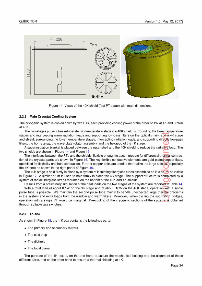
Figure 14: Views of the 40K shield (first PT stage) with main dimensions.
2.2.3 Main Cryostat Cooling System
The cryogenic system is cooled down by two PTs, each providing cooling power of the order of 1W at 4K and 30Wmat 40K.
The two-stages pulse tubes refrigerate two temperature stages: a 40K shield, surrounding the lower temperaturestages and intercepting warm radiation loads and supporting low-pass filters on the optical chain, and a 4K stageand shield, surrounding the lower temperature stages, intercepting radiation loads, and supporting directly low-passfilters, the horns array, the wave-plate rotator assembly, and the hexapod of the 1K stage.
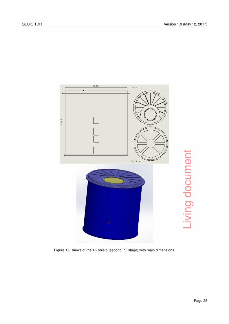
A superinsulation blanket is placed between the outer shell and the 40K shield to reduce the radiative load. Thetwo shields are shown in Figure 14 and Figure 15.
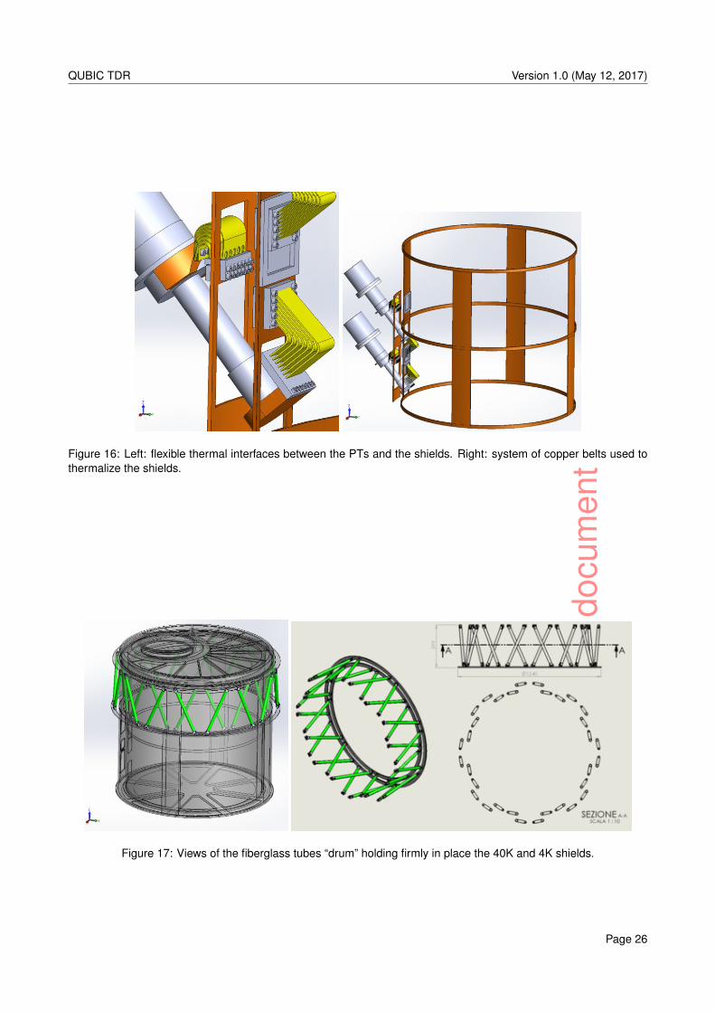
The interfaces between the PTs and the shields, flexible enough to accommodate for differential thermal contrac-tion of the cryostat parts are shown in Figure 16. The key flexible conductive elements are gold-plated copper flaps,optimized for flexibility and heat conduction. Further copper belts are used to thermalize the large shields (especiallythe 4K one) as shown in the right panel of Figure 16.
The 40K stage is held firmly in place by a system of insulating fiberglass tubes assembled as in a drum, as visiblein Figure 17. A similar drum is used to hold firmly in place the 4K stage. The support structure is completed by asystem of radial fiberglass straps mounted on the bottom of the 40K and 4K shields.
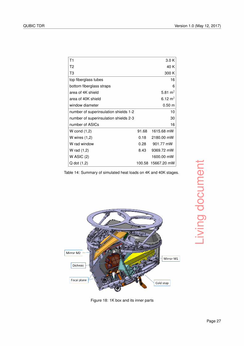
Results from a preliminary simulation of the heat loads on the two stages of the system are reported in Table 14.With a total load of about 0.1W on the 3K stage and of about 16W on the 40K stage, operation with a single
pulse tube is possible. We maintain the second pulse tube mainly to handle unexpected large thermal gradientsin the system and extra loads from the window and warm filters. Moreover, when cycling the sub-Kelvin fridges,operation with a single PT would be marginal. Pre-cooling of the cryogenic sections of the systems is obtainedthrough suitable gas switches.
2.2.4 1K-box
As shown in Figure 18, the 1 K box contains the followings parts:
• The primary and secondary mirrors
• The cold stop
• The dichroic
• The focal plane
The purpose of the 1K box is, on the one hand to assure the mechanical holding and the alignment of thesedifferent parts, and on the other hand to ensure a thermal shielding at 1K.
Page 24
Livi
ngdo
cum
ent
QUBIC TDR Version 1.0 (May 12, 2017)
Figure 15: Views of the 4K shield (second PT stage) with main dimensions.
Page 25
Livi
ngdo
cum
ent
QUBIC TDR Version 1.0 (May 12, 2017)
Figure 16: Left: flexible thermal interfaces between the PTs and the shields. Right: system of copper belts used tothermalize the shields.
Figure 17: Views of the fiberglass tubes “drum” holding firmly in place the 40K and 4K shields.
Page 26
Livi
ngdo
cum
ent
QUBIC TDR Version 1.0 (May 12, 2017)
T1 3.0 K
T2 40 K
T3 300 K
top fiberglass tubes 16
bottom fiberglass straps 6
area of 4K shield 5.81 m2
area of 40K shield 6.12 m2
window diameter 0.50 m
number of superinsulation shields 1-2 10
number of superinsulation shields 2-3 30
number of ASICs 16
W cond (1,2) 91.68 1615.68 mW
W wires (1,2) 0.18 2180.00 mW
W rad window 0.28 901.77 mW
W rad (1,2) 8.43 9369.72 mW
W ASIC (2) 1600.00 mW
Q dot (1,2) 100.58 15667.20 mW
Table 14: Summary of simulated heat loads on 4K and 40K stages.
Figure 18: 1K box and its inner parts
Page 27
Livi
ngdo
cum
ent
QUBIC TDR Version 1.0 (May 12, 2017)
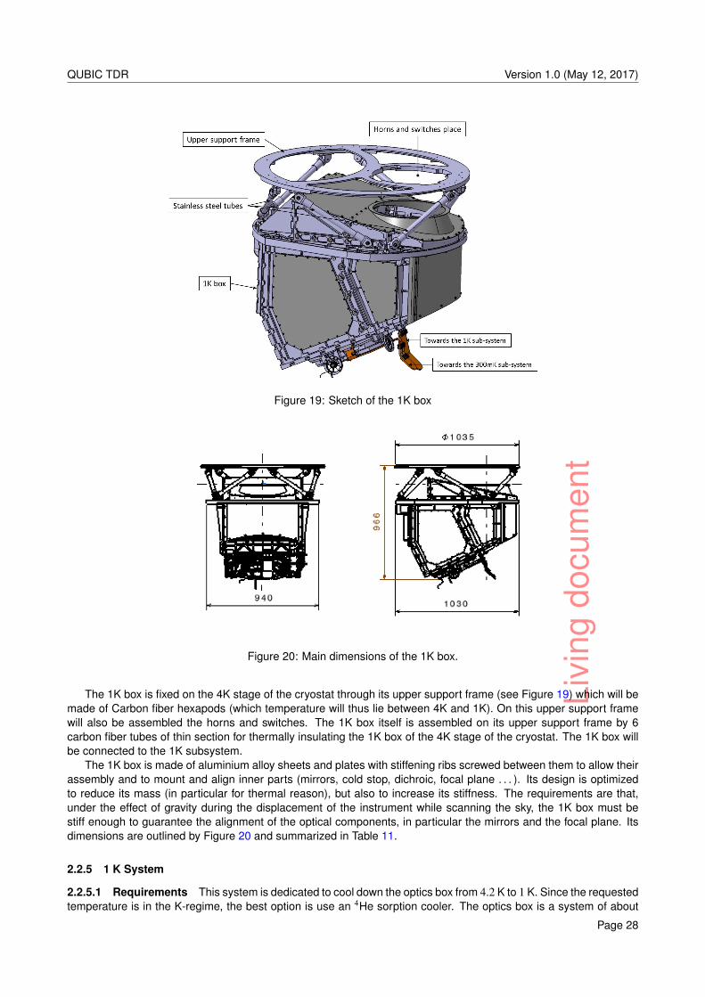
Figure 19: Sketch of the 1K box
Figure 20: Main dimensions of the 1K box.
The 1K box is fixed on the 4K stage of the cryostat through its upper support frame (see Figure 19) which will bemade of Carbon fiber hexapods (which temperature will thus lie between 4K and 1K). On this upper support framewill also be assembled the horns and switches. The 1K box itself is assembled on its upper support frame by 6carbon fiber tubes of thin section for thermally insulating the 1K box of the 4K stage of the cryostat. The 1K box willbe connected to the 1K subsystem.
The 1K box is made of aluminium alloy sheets and plates with stiffening ribs screwed between them to allow theirassembly and to mount and align inner parts (mirrors, cold stop, dichroic, focal plane . . . ). Its design is optimizedto reduce its mass (in particular for thermal reason), but also to increase its stiffness. The requirements are that,under the effect of gravity during the displacement of the instrument while scanning the sky, the 1K box must bestiff enough to guarantee the alignment of the optical components, in particular the mirrors and the focal plane. Itsdimensions are outlined by Figure 20 and summarized in Table 11.
2.2.5 1 K System
2.2.5.1 Requirements This system is dedicated to cool down the optics box from 4.2 K to 1 K. Since the requestedtemperature is in the K-regime, the best option is use an 4He sorption cooler. The optics box is a system of about
Page 28
Livi
ngdo
cum
ent
QUBIC TDR Version 1.0 (May 12, 2017)
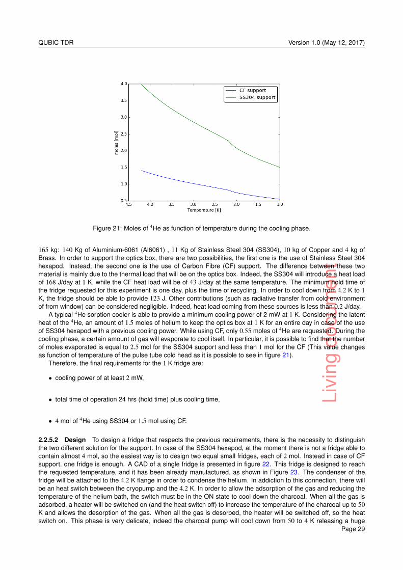
Figure 21: Moles of 4He as function of temperature during the cooling phase.
165 kg: 140 Kg of Aluminium-6061 (Al6061) , 11 Kg of Stainless Steel 304 (SS304), 10 kg of Copper and 4 kg ofBrass. In order to support the optics box, there are two possibilities, the first one is the use of Stainless Steel 304hexapod. Instead, the second one is the use of Carbon Fibre (CF) support. The difference between these twomaterial is mainly due to the thermal load that will be on the optics box. Indeed, the SS304 will introduce a heat loadof 168 J/day at 1 K, while the CF heat load will be of 43 J/day at the same temperature. The minimum hold time ofthe fridge requested for this experiment is one day, plus the time of recycling. In order to cool down from 4.2 K to 1K, the fridge should be able to provide 123 J. Other contributions (such as radiative transfer from cold environmentof from window) can be considered negligible. Indeed, heat load coming from these sources is less than 0.2 J/day.
A typical 4He sorption cooler is able to provide a minimum cooling power of 2 mW at 1 K. Considering the latentheat of the 4He, an amount of 1.5 moles of helium to keep the optics box at 1 K for an entire day in case of the useof SS304 hexapod with a previous cooling power. While using CF, only 0.55 moles of 4He are requested. During thecooling phase, a certain amount of gas will evaporate to cool itself. In particular, it is possible to find that the numberof moles evaporated is equal to 2.5 mol for the SS304 support and less than 1 mol for the CF (This value changesas function of temperature of the pulse tube cold head as it is possible to see in figure 21).
Therefore, the final requirements for the 1 K fridge are:
• cooling power of at least 2 mW,
• total time of operation 24 hrs (hold time) plus cooling time,
• 4 mol of 4He using SS304 or 1.5 mol using CF.
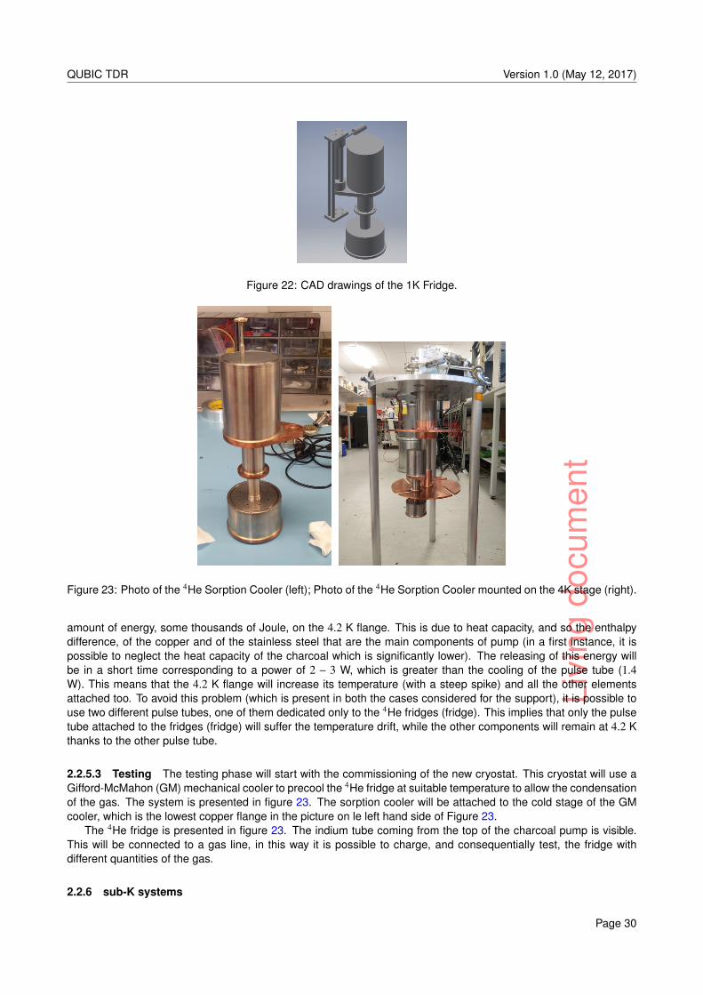
2.2.5.2 Design To design a fridge that respects the previous requirements, there is the necessity to distinguishthe two different solution for the support. In case of the SS304 hexapod, at the moment there is not a fridge able tocontain almost 4 mol, so the easiest way is to design two equal small fridges, each of 2 mol. Instead in case of CFsupport, one fridge is enough. A CAD of a single fridge is presented in figure 22. This fridge is designed to reachthe requested temperature, and it has been already manufactured, as shown in Figure 23. The condenser of thefridge will be attached to the 4.2 K flange in order to condense the helium. In addiction to this connection, there willbe an heat switch between the cryopump and the 4.2 K. In order to allow the adsorption of the gas and reducing thetemperature of the helium bath, the switch must be in the ON state to cool down the charcoal. When all the gas isadsorbed, a heater will be switched on (and the heat switch off) to increase the temperature of the charcoal up to 50K and allows the desorption of the gas. When all the gas is desorbed, the heater will be switched off, so the heatswitch on. This phase is very delicate, indeed the charcoal pump will cool down from 50 to 4 K releasing a huge
Page 29
Livi
ngdo
cum
ent
QUBIC TDR Version 1.0 (May 12, 2017)
Figure 22: CAD drawings of the 1K Fridge.
Figure 23: Photo of the 4He Sorption Cooler (left); Photo of the 4He Sorption Cooler mounted on the 4K stage (right).
amount of energy, some thousands of Joule, on the 4.2 K flange. This is due to heat capacity, and so the enthalpydifference, of the copper and of the stainless steel that are the main components of pump (in a first instance, it ispossible to neglect the heat capacity of the charcoal which is significantly lower). The releasing of this energy willbe in a short time corresponding to a power of 2 − 3 W, which is greater than the cooling of the pulse tube (1.4W). This means that the 4.2 K flange will increase its temperature (with a steep spike) and all the other elementsattached too. To avoid this problem (which is present in both the cases considered for the support), it is possible touse two different pulse tubes, one of them dedicated only to the 4He fridges (fridge). This implies that only the pulsetube attached to the fridges (fridge) will suffer the temperature drift, while the other components will remain at 4.2 Kthanks to the other pulse tube.
2.2.5.3 Testing The testing phase will start with the commissioning of the new cryostat. This cryostat will use aGifford-McMahon (GM) mechanical cooler to precool the 4He fridge at suitable temperature to allow the condensationof the gas. The system is presented in figure 23. The sorption cooler will be attached to the cold stage of the GMcooler, which is the lowest copper flange in the picture on le left hand side of Figure 23.
The 4He fridge is presented in figure 23. The indium tube coming from the top of the charcoal pump is visible.This will be connected to a gas line, in this way it is possible to charge, and consequentially test, the fridge withdifferent quantities of the gas.
2.2.6 sub-K systems
Page 30
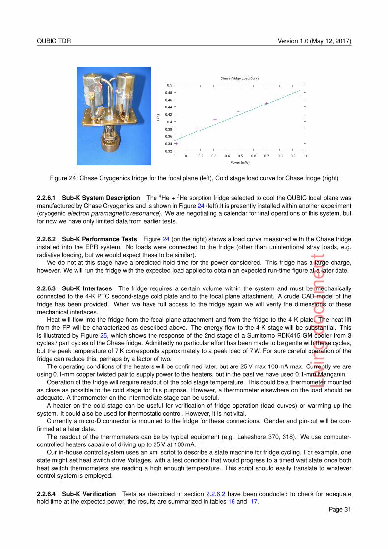
Livi
ngdo
cum
ent
QUBIC TDR Version 1.0 (May 12, 2017)
0.32
0.34
0.36
0.38
0.4
0.42
0.44
0.46
0.48
0.5
0 0.1 0.2 0.3 0.4 0.5 0.6 0.7 0.8 0.9 1T
(K)
Power (mW)
Chase Fridge Load Curve
Figure 24: Chase Cryogenics fridge for the focal plane (left), Cold stage load curve for Chase fridge (right)
2.2.6.1 Sub-K System Description The 4He + 3He sorption fridge selected to cool the QUBIC focal plane wasmanufactured by Chase Cryogenics and is shown in Figure 24 (left).It is presently installed within another experiment(cryogenic electron paramagnetic resonance). We are negotiating a calendar for final operations of this system, butfor now we have only limited data from earlier tests.
2.2.6.2 Sub-K Performance Tests Figure 24 (on the right) shows a load curve measured with the Chase fridgeinstalled into the EPR system. No loads were connected to the fridge (other than unintentional stray loads, e.g.radiative loading, but we would expect these to be similar).
We do not at this stage have a predicted hold time for the power considered. This fridge has a large charge,however. We will run the fridge with the expected load applied to obtain an expected run-time figure at a later date.
2.2.6.3 Sub-K Interfaces The fridge requires a certain volume within the system and must be mechanicallyconnected to the 4-K PTC second-stage cold plate and to the focal plane attachment. A crude CAD model of thefridge has been provided. When we have full access to the fridge again we will verify the dimensions of thesemechanical interfaces.
Heat will flow into the fridge from the focal plane attachment and from the fridge to the 4-K plate. The heat liftfrom the FP will be characterized as described above. The energy flow to the 4-K stage will be substantial. Thisis illustrated by Figure 25, which shows the response of the 2nd stage of a Sumitomo RDK415 GM cooler from 3cycles / part cycles of the Chase fridge. Admittedly no particular effort has been made to be gentle with these cycles,but the peak temperature of 7 K corresponds approximately to a peak load of 7 W. For sure careful operation of thefridge can reduce this, perhaps by a factor of two.
The operating conditions of the heaters will be confirmed later, but are 25 V max 100 mA max. Currently we areusing 0.1-mm copper twisted pair to supply power to the heaters, but in the past we have used 0.1-mm Manganin.
Operation of the fridge will require readout of the cold stage temperature. This could be a thermometer mountedas close as possible to the cold stage for this purpose. However, a thermometer elsewhere on the load should beadequate. A thermometer on the intermediate stage can be useful.
A heater on the cold stage can be useful for verification of fridge operation (load curves) or warming up thesystem. It could also be used for thermostatic control. However, it is not vital.
Currently a micro-D connector is mounted to the fridge for these connections. Gender and pin-out will be con-firmed at a later date.
The readout of the thermometers can be by typical equipment (e.g. Lakeshore 370, 318). We use computer-controlled heaters capable of driving up to 25 V at 100 mA.
Our in-house control system uses an xml script to describe a state machine for fridge cycling. For example, onestate might set heat switch drive Voltages, with a test condition that would progress to a timed wait state once bothheat switch thermometers are reading a high enough temperature. This script should easily translate to whatevercontrol system is employed.
2.2.6.4 Sub-K Verification Tests as described in section 2.2.6.2 have been conducted to check for adequatehold time at the expected power, the results are summarized in tables 16 and 17.
Page 31
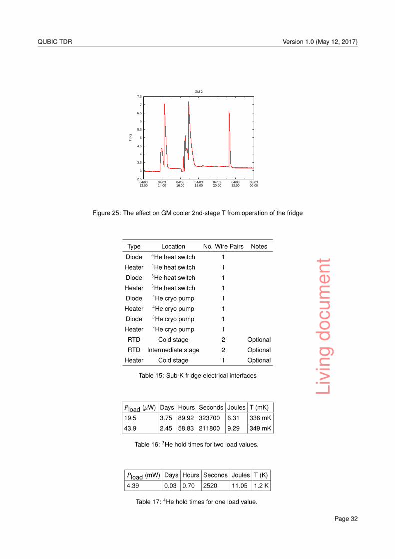
Livi
ngdo
cum
ent
QUBIC TDR Version 1.0 (May 12, 2017)
2.5
3
3.5
4
4.5
5
5.5
6
6.5
7
7.5
04/0312:00
04/0314:00
04/0316:00
04/0318:00
04/0320:00
04/0322:00
05/0300:00
T (
K)
GM 2
Figure 25: The effect on GM cooler 2nd-stage T from operation of the fridge
Type Location No. Wire Pairs Notes
Diode 4He heat switch 1
Heater 4He heat switch 1
Diode 3He heat switch 1
Heater 3He heat switch 1
Diode 4He cryo pump 1
Heater 4He cryo pump 1
Diode 3He cryo pump 1
Heater 3He cryo pump 1
RTD Cold stage 2 Optional
RTD Intermediate stage 2 Optional
Heater Cold stage 1 Optional
Table 15: Sub-K fridge electrical interfaces
Pload (µW) Days Hours Seconds Joules T (mK)
19.5 3.75 89.92 323700 6.31 336 mK
43.9 2.45 58.83 211800 9.29 349 mK
Table 16: 3He hold times for two load values.
Pload (mW) Days Hours Seconds Joules T (K)
4.39 0.03 0.70 2520 11.05 1.2 K
Table 17: 4He hold times for one load value.
Page 32
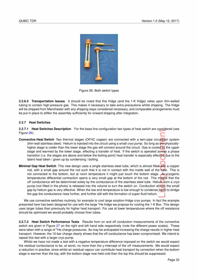
Livi
ngdo
cum
ent
QUBIC TDR Version 1.0 (May 12, 2017)
Figure 26: Both switch types
2.2.6.5 Transportation Issues It should be noted that this fridge (and the 1-K fridge) relies upon thin-walledtubing to contain high-pressure gas. This makes it necessary to take extra precautions whilst shipping. The fridgewill be shipped from Manchester with any shipping stays considered necessary, and comparable arrangements mustbe put in place to stiffen the assembly sufficiently for onward shipping after integration.
2.2.7 Heat Switches
2.2.7.1 Heat Switches Description For the base-line configuration two types of heat switch are considered (seeFigure 26):
Convective Heat Switch Two thermal stages (OFHC copper) are connected with a twin-pipe circulation system(thin-wall stainless steel). Helium is injected into the circuit using a small cryo pump. So long as the physically-higher stage is colder than the lower stage the gas will convect around the circuit. Gas is cooled by the upperstage and warmed by the lower stage, effecting a transfer of heat. If the switch is operated across a phasetransition (i.e. the stages are above and below the boiling point) heat transfer is especially effective due to thelatent heat taken / given up by condensing / boiling.
Minimal Gap Heat Switch This new design uses a single stainless-steel tube, which is almost filled with a copperrod, with a small gap around the rod such that it is not in contact with the inside wall of the tube. This isnot connected to the bottom, but at room temperature it might just touch the bottom stage. At cryogenictemperatures differential contraction opens a very small gap at the bottom of the rod. This means that theoff conductance will be determined solely by the conductance of the stainless steel tube. Helium from a cryopump (not fitted in the photo) is released into the volume to turn the switch on. Conduction across the smallgap by helium gas is very effective. When the low end temperature is low enough to condense liquid to bridgethe gap the conductance rises further, and further still with the formation of super-fluid helium.
We use convective switches routinely, for example to cool large sorption-fridge cryo pumps. In fact the examplepresented here has been designed for use with the large 4He fridge we propose for cooling the 1-K Box. This designuses larger tubes than previously for higher heat transport. For use at lower temperatures where the off resistanceshould be optimized we would probably choose finer tubes.
2.2.7.2 Heat Switch Performance Tests Results from on and off conduction measurements of the convectiveswitch are given in Figure 27 on the right and left hand side respectively (note the different power scales). Thesewere taken with a range of 4He charge pressures. As may be anticipated increasing the charge results in higher heattransport. However, the 10-bar charge clearly shows that the off conductance has been compromised. We intend torepeat this test with a larger cryo pump.
Whilst we have not made a test with a negative temperature difference imposed on the switch we would expectthe residual conductance to be, at worst, no more than the y-intercept of the off measurements. We would expecta reduction in practise, since whilst an residual vapour can contribute heat transport by convection when the bottomstage is warmer than the top, with the bottom stage now held cold than the top this should be suppressed.
Page 33
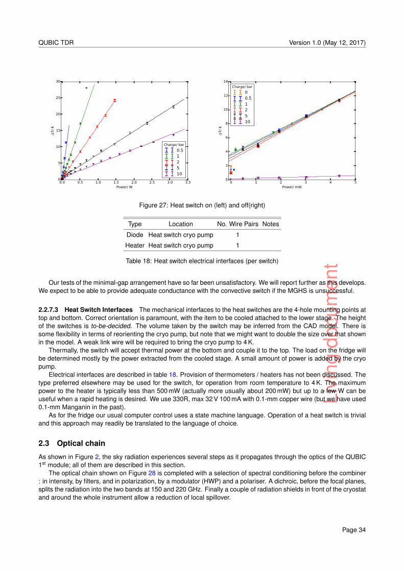
Livi
ngdo
cum
ent
QUBIC TDR Version 1.0 (May 12, 2017)
0.0 0.5 1.0 1.5 2.0 2.5 3.0 3.5Power/ W
0
5
10
15
20
25
30
∆T/
K
Charge/ bar
0.512510
0 1 2 3 4 5Power/ mW
0
2
4
6
8
10
12
14
∆T/
K
Charge/ bar
00.512510
Figure 27: Heat switch on (left) and off(right)
Type Location No. Wire Pairs Notes
Diode Heat switch cryo pump 1
Heater Heat switch cryo pump 1
Table 18: Heat switch electrical interfaces (per switch)
Our tests of the minimal-gap arrangement have so far been unsatisfactory. We will report further as this develops.We expect to be able to provide adequate conductance with the convective switch if the MGHS is unsuccessful.
2.2.7.3 Heat Switch Interfaces The mechanical interfaces to the heat switches are the 4-hole mounting points attop and bottom. Correct orientation is paramount, with the item to be cooled attached to the lower stage. The heightof the switches is to-be-decided. The volume taken by the switch may be inferred from the CAD model. There issome flexibility in terms of reorienting the cryo pump, but note that we might want to double the size over that shownin the model. A weak link wire will be required to bring the cryo pump to 4 K.
Thermally, the switch will accept thermal power at the bottom and couple it to the top. The load on the fridge willbe determined mostly by the power extracted from the cooled stage. A small amount of power is added by the cryopump.
Electrical interfaces are described in table 18. Provision of thermometers / heaters has not been discussed. Thetype preferred elsewhere may be used for the switch, for operation from room temperature to 4 K. The maximumpower to the heater is typically less than 500 mW (actually more usually about 200 mW) but up to a few W can beuseful when a rapid heating is desired. We use 330R, max 32 V 100 mA with 0.1-mm copper wire (but we have used0.1-mm Manganin in the past).
As for the fridge our usual computer control uses a state machine language. Operation of a heat switch is trivialand this approach may readily be translated to the language of choice.
2.3 Optical chain
As shown in Figure 2, the sky radiation experiences several steps as it propagates through the optics of the QUBIC1st module; all of them are described in this section.
The optical chain shown on Figure 28 is completed with a selection of spectral conditioning before the combiner: in intensity, by filters, and in polarization, by a modulator (HWP) and a polariser. A dichroic, before the focal planes,splits the radiation into the two bands at 150 and 220 GHz. Finally a couple of radiation shields in front of the cryostatand around the whole instrument allow a reduction of local spillover.
Page 34
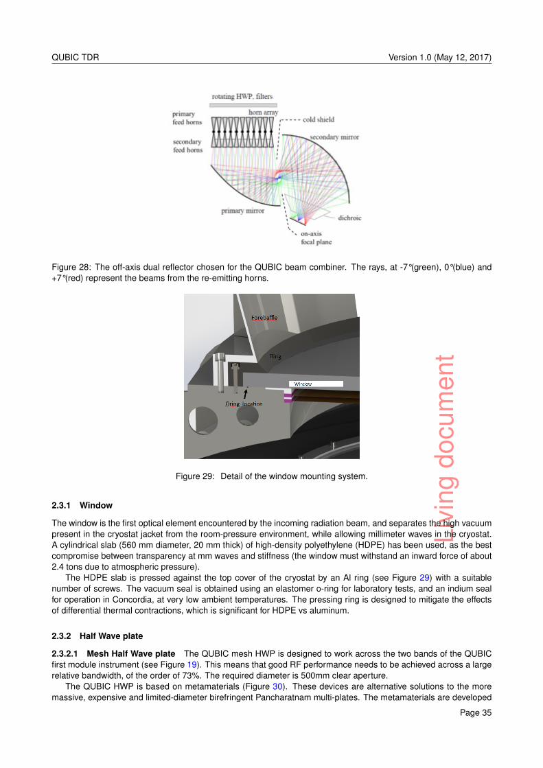
Livi
ngdo
cum
ent
QUBIC TDR Version 1.0 (May 12, 2017)
Figure 28: The off-axis dual reflector chosen for the QUBIC beam combiner. The rays, at -7°(green), 0°(blue) and+7°(red) represent the beams from the re-emitting horns.
Figure 29: Detail of the window mounting system.
2.3.1 Window
The window is the first optical element encountered by the incoming radiation beam, and separates the high vacuumpresent in the cryostat jacket from the room-pressure environment, while allowing millimeter waves in the cryostat.A cylindrical slab (560 mm diameter, 20 mm thick) of high-density polyethylene (HDPE) has been used, as the bestcompromise between transparency at mm waves and stiffness (the window must withstand an inward force of about2.4 tons due to atmospheric pressure).
The HDPE slab is pressed against the top cover of the cryostat by an Al ring (see Figure 29) with a suitablenumber of screws. The vacuum seal is obtained using an elastomer o-ring for laboratory tests, and an indium sealfor operation in Concordia, at very low ambient temperatures. The pressing ring is designed to mitigate the effectsof differential thermal contractions, which is significant for HDPE vs aluminum.
2.3.2 Half Wave plate
2.3.2.1 Mesh Half Wave plate The QUBIC mesh HWP is designed to work across the two bands of the QUBICfirst module instrument (see Figure 19). This means that good RF performance needs to be achieved across a largerelative bandwidth, of the order of 73%. The required diameter is 500mm clear aperture.
The QUBIC HWP is based on metamaterials (Figure 30). These devices are alternative solutions to the moremassive, expensive and limited-diameter birefringent Pancharatnam multi-plates. The metamaterials are developed
Page 35
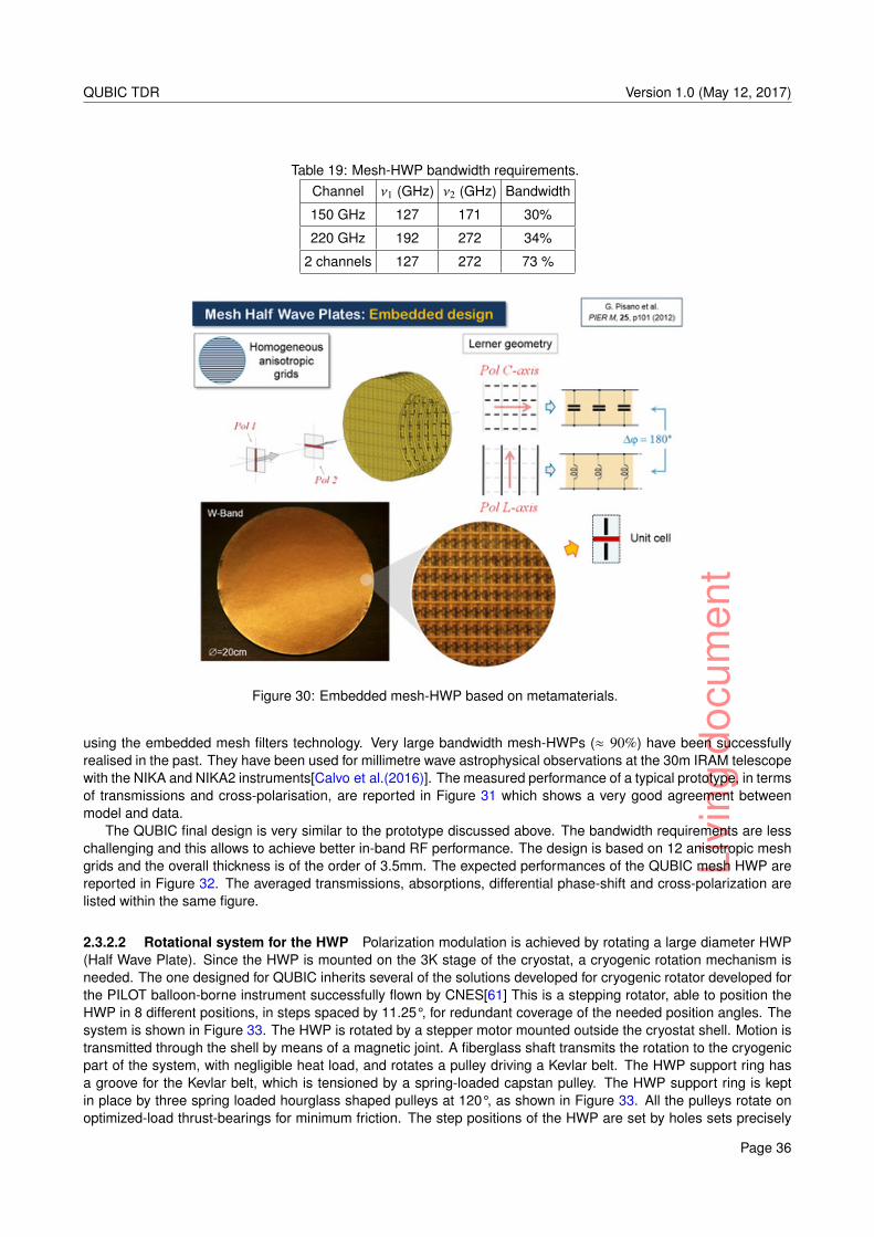
Livi
ngdo
cum
ent
QUBIC TDR Version 1.0 (May 12, 2017)
Table 19: Mesh-HWP bandwidth requirements.Channel ν1 (GHz) ν2 (GHz) Bandwidth
150 GHz 127 171 30%
220 GHz 192 272 34%
2 channels 127 272 73 %
Figure 30: Embedded mesh-HWP based on metamaterials.
using the embedded mesh filters technology. Very large bandwidth mesh-HWPs (≈ 90%) have been successfullyrealised in the past. They have been used for millimetre wave astrophysical observations at the 30m IRAM telescopewith the NIKA and NIKA2 instruments[Calvo et al.(2016)]. The measured performance of a typical prototype, in termsof transmissions and cross-polarisation, are reported in Figure 31 which shows a very good agreement betweenmodel and data.
The QUBIC final design is very similar to the prototype discussed above. The bandwidth requirements are lesschallenging and this allows to achieve better in-band RF performance. The design is based on 12 anisotropic meshgrids and the overall thickness is of the order of 3.5mm. The expected performances of the QUBIC mesh HWP arereported in Figure 32. The averaged transmissions, absorptions, differential phase-shift and cross-polarization arelisted within the same figure.
2.3.2.2 Rotational system for the HWP Polarization modulation is achieved by rotating a large diameter HWP(Half Wave Plate). Since the HWP is mounted on the 3K stage of the cryostat, a cryogenic rotation mechanism isneeded. The one designed for QUBIC inherits several of the solutions developed for cryogenic rotator developed forthe PILOT balloon-borne instrument successfully flown by CNES[61] This is a stepping rotator, able to position theHWP in 8 different positions, in steps spaced by 11.25°, for redundant coverage of the needed position angles. Thesystem is shown in Figure 33. The HWP is rotated by a stepper motor mounted outside the cryostat shell. Motion istransmitted through the shell by means of a magnetic joint. A fiberglass shaft transmits the rotation to the cryogenicpart of the system, with negligible heat load, and rotates a pulley driving a Kevlar belt. The HWP support ring hasa groove for the Kevlar belt, which is tensioned by a spring-loaded capstan pulley. The HWP support ring is keptin place by three spring loaded hourglass shaped pulleys at 120°, as shown in Figure 33. All the pulleys rotate onoptimized-load thrust-bearings for minimum friction. The step positions of the HWP are set by holes sets precisely
Page 36
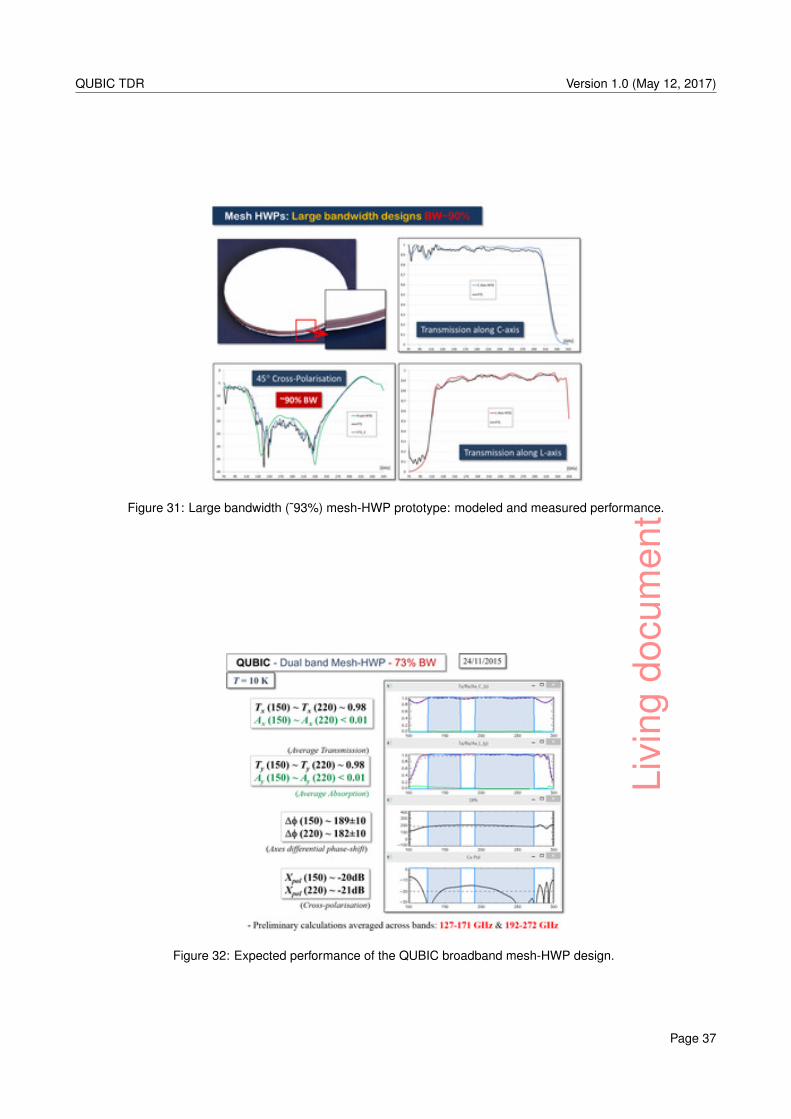
Livi
ngdo
cum
ent
QUBIC TDR Version 1.0 (May 12, 2017)
Figure 31: Large bandwidth (˜93%) mesh-HWP prototype: modeled and measured performance.
Figure 32: Expected performance of the QUBIC broadband mesh-HWP design.
Page 37
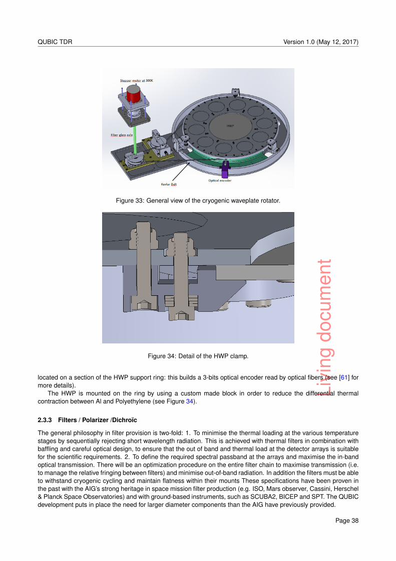
Livi
ngdo
cum
ent
QUBIC TDR Version 1.0 (May 12, 2017)
Figure 33: General view of the cryogenic waveplate rotator.
Figure 34: Detail of the HWP clamp.
located on a section of the HWP support ring: this builds a 3-bits optical encoder read by optical fibers (see [61] formore details).
The HWP is mounted on the ring by using a custom made block in order to reduce the differential thermalcontraction between Al and Polyethylene (see Figure 34).
2.3.3 Filters / Polarizer /Dichroïc
The general philosophy in filter provision is two-fold: 1. To minimise the thermal loading at the various temperaturestages by sequentially rejecting short wavelength radiation. This is achieved with thermal filters in combination withbaffling and careful optical design, to ensure that the out of band and thermal load at the detector arrays is suitablefor the scientific requirements. 2. To define the required spectral passband at the arrays and maximise the in-bandoptical transmission. There will be an optimization procedure on the entire filter chain to maximise transmission (i.e.to manage the relative fringing between filters) and minimise out-of-band radiation. In addition the filters must be ableto withstand cryogenic cycling and maintain flatness within their mounts These specifications have been proven inthe past with the AIG’s strong heritage in space mission filter production (e.g. ISO, Mars observer, Cassini, Herschel& Planck Space Observatories) and with ground-based instruments, such as SCUBA2, BICEP and SPT. The QUBICdevelopment puts in place the need for larger diameter components than the AIG have previously provided.
Page 38
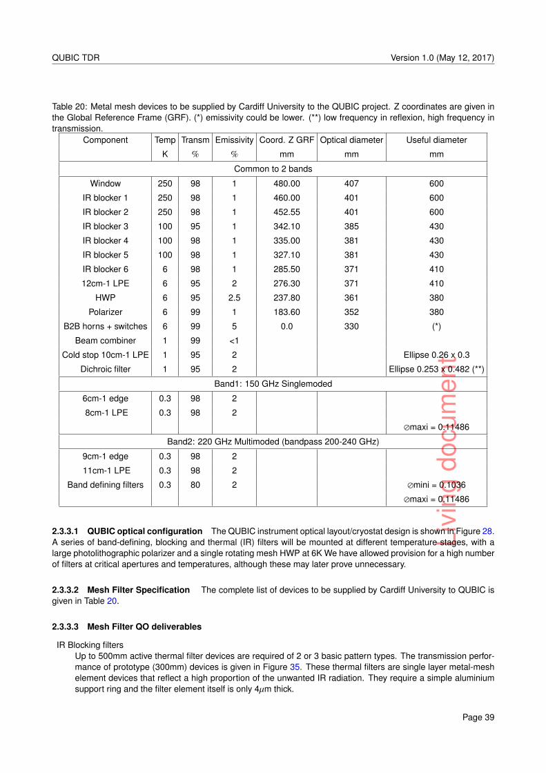
Livi
ngdo
cum
ent
QUBIC TDR Version 1.0 (May 12, 2017)
Table 20: Metal mesh devices to be supplied by Cardiff University to the QUBIC project. Z coordinates are given inthe Global Reference Frame (GRF). (*) emissivity could be lower. (**) low frequency in reflexion, high frequency intransmission.
Component Temp Transm Emissivity Coord. Z GRF Optical diameter Useful diameter
K % % mm mm mm
Common to 2 bands
Window 250 98 1 480.00 407 600
IR blocker 1 250 98 1 460.00 401 600
IR blocker 2 250 98 1 452.55 401 600
IR blocker 3 100 95 1 342.10 385 430
IR blocker 4 100 98 1 335.00 381 430
IR blocker 5 100 98 1 327.10 381 430
IR blocker 6 6 98 1 285.50 371 410
12cm-1 LPE 6 95 2 276.30 371 410
HWP 6 95 2.5 237.80 361 380
Polarizer 6 99 1 183.60 352 380
B2B horns + switches 6 99 5 0.0 330 (*)
Beam combiner 1 99 <1
Cold stop 10cm-1 LPE 1 95 2 Ellipse 0.26 x 0.3
Dichroic filter 1 95 2 Ellipse 0.253 x 0.482 (**)
Band1: 150 GHz Singlemoded
6cm-1 edge 0.3 98 2
8cm-1 LPE 0.3 98 2
maxi = 0.11486
Band2: 220 GHz Multimoded (bandpass 200-240 GHz)
9cm-1 edge 0.3 98 2
11cm-1 LPE 0.3 98 2
Band defining filters 0.3 80 2 mini = 0.1036
maxi = 0.11486
2.3.3.1 QUBIC optical configuration The QUBIC instrument optical layout/cryostat design is shown in Figure 28.A series of band-defining, blocking and thermal (IR) filters will be mounted at different temperature stages, with alarge photolithographic polarizer and a single rotating mesh HWP at 6K We have allowed provision for a high numberof filters at critical apertures and temperatures, although these may later prove unnecessary.
2.3.3.2 Mesh Filter Specification The complete list of devices to be supplied by Cardiff University to QUBIC isgiven in Table 20.
2.3.3.3 Mesh Filter QO deliverables
IR Blocking filtersUp to 500mm active thermal filter devices are required of 2 or 3 basic pattern types. The transmission perfor-mance of prototype (300mm) devices is given in Figure 35. These thermal filters are single layer metal-meshelement devices that reflect a high proportion of the unwanted IR radiation. They require a simple aluminiumsupport ring and the filter element itself is only 4µm thick.
Page 39
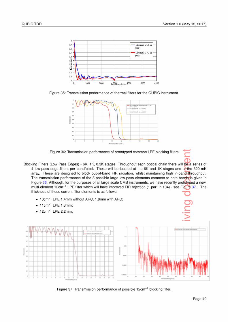
Livi
ngdo
cum
ent
QUBIC TDR Version 1.0 (May 12, 2017)
Figure 35: Transmission performance of thermal filters for the QUBIC instrument.
Figure 36: Transmission performance of prototyped common LPE blocking filters
Blocking Filters (Low Pass Edges) - 6K, 1K, 0.3K stages Throughout each optical chain there will be a series of4 low-pass edge filters per band/pixel. These will be located at the 6K and 1K stages and at the 320 mKarray. These are designed to block out-of-band FIR radiation, whilst maintaining high in-band throughput.The transmission performance of the 3 possible large low-pass elements common to both bands is given inFigure 36. Although, for the purposes of all large scale CMB instruments, we have recently prototyped a new,multi-element 12cm−1 LPE filter which will have improved FIR rejection (1 part in 104) - see Figure 37. Thethickness of these current filter elements is as follows:
• 10cm−1 LPE 1.4mm without ARC, 1.8mm with ARC;
• 11cm−1 LPE 1.3mm;
• 12cm−1 LPE 2.2mm;
Figure 37: Transmission performance of possible 12cm−1 blocking filter.
Page 40
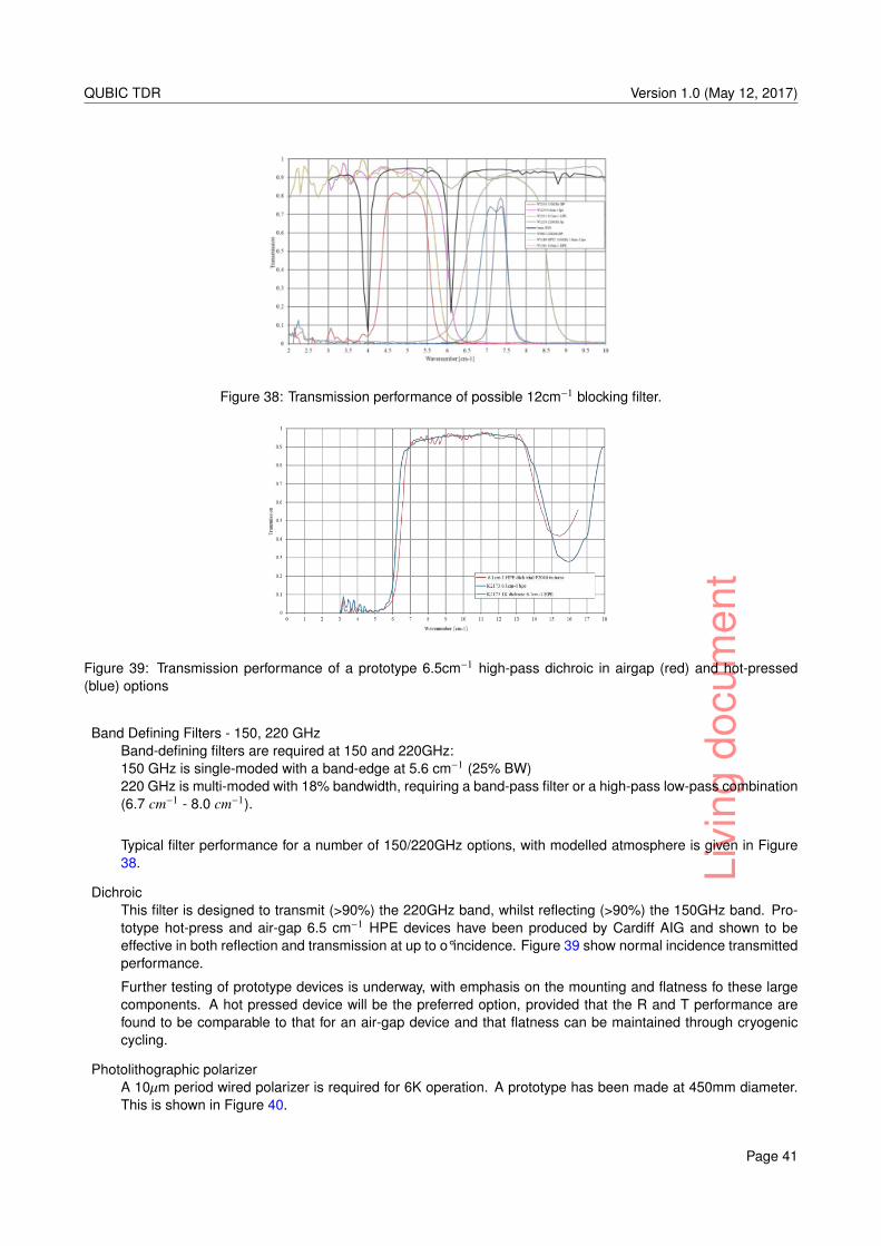
Livi
ngdo
cum
ent
QUBIC TDR Version 1.0 (May 12, 2017)
Figure 38: Transmission performance of possible 12cm−1 blocking filter.
Figure 39: Transmission performance of a prototype 6.5cm−1 high-pass dichroic in airgap (red) and hot-pressed(blue) options
Band Defining Filters - 150, 220 GHzBand-defining filters are required at 150 and 220GHz:150 GHz is single-moded with a band-edge at 5.6 cm−1 (25% BW)220 GHz is multi-moded with 18% bandwidth, requiring a band-pass filter or a high-pass low-pass combination(6.7 cm−1 - 8.0 cm−1).
Typical filter performance for a number of 150/220GHz options, with modelled atmosphere is given in Figure38.
DichroicThis filter is designed to transmit (>90%) the 220GHz band, whilst reflecting (>90%) the 150GHz band. Pro-totype hot-press and air-gap 6.5 cm−1 HPE devices have been produced by Cardiff AIG and shown to beeffective in both reflection and transmission at up to o°incidence. Figure 39 show normal incidence transmittedperformance.
Further testing of prototype devices is underway, with emphasis on the mounting and flatness fo these largecomponents. A hot pressed device will be the preferred option, provided that the R and T performance arefound to be comparable to that for an air-gap device and that flatness can be maintained through cryogeniccycling.
Photolithographic polarizerA 10µm period wired polarizer is required for 6K operation. A prototype has been made at 450mm diameter.This is shown in Figure 40.
Page 41
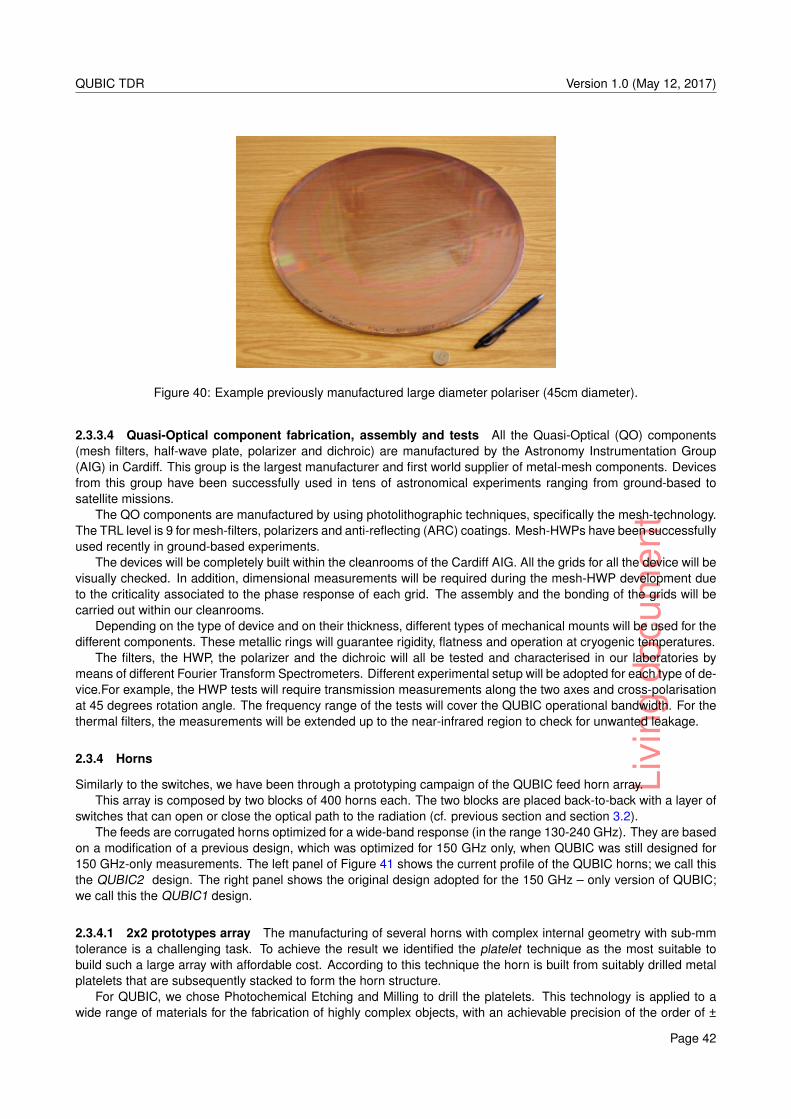
Livi
ngdo
cum
ent
QUBIC TDR Version 1.0 (May 12, 2017)
Figure 40: Example previously manufactured large diameter polariser (45cm diameter).
2.3.3.4 Quasi-Optical component fabrication, assembly and tests All the Quasi-Optical (QO) components(mesh filters, half-wave plate, polarizer and dichroic) are manufactured by the Astronomy Instrumentation Group(AIG) in Cardiff. This group is the largest manufacturer and first world supplier of metal-mesh components. Devicesfrom this group have been successfully used in tens of astronomical experiments ranging from ground-based tosatellite missions.
The QO components are manufactured by using photolithographic techniques, specifically the mesh-technology.The TRL level is 9 for mesh-filters, polarizers and anti-reflecting (ARC) coatings. Mesh-HWPs have been successfullyused recently in ground-based experiments.
The devices will be completely built within the cleanrooms of the Cardiff AIG. All the grids for all the device will bevisually checked. In addition, dimensional measurements will be required during the mesh-HWP development dueto the criticality associated to the phase response of each grid. The assembly and the bonding of the grids will becarried out within our cleanrooms.
Depending on the type of device and on their thickness, different types of mechanical mounts will be used for thedifferent components. These metallic rings will guarantee rigidity, flatness and operation at cryogenic temperatures.
The filters, the HWP, the polarizer and the dichroic will all be tested and characterised in our laboratories bymeans of different Fourier Transform Spectrometers. Different experimental setup will be adopted for each type of de-vice.For example, the HWP tests will require transmission measurements along the two axes and cross-polarisationat 45 degrees rotation angle. The frequency range of the tests will cover the QUBIC operational bandwidth. For thethermal filters, the measurements will be extended up to the near-infrared region to check for unwanted leakage.
2.3.4 Horns
Similarly to the switches, we have been through a prototyping campaign of the QUBIC feed horn array.This array is composed by two blocks of 400 horns each. The two blocks are placed back-to-back with a layer of
switches that can open or close the optical path to the radiation (cf. previous section and section 3.2).The feeds are corrugated horns optimized for a wide-band response (in the range 130-240 GHz). They are based
on a modification of a previous design, which was optimized for 150 GHz only, when QUBIC was still designed for150 GHz-only measurements. The left panel of Figure 41 shows the current profile of the QUBIC horns; we call thisthe QUBIC2 design. The right panel shows the original design adopted for the 150 GHz – only version of QUBIC;we call this the QUBIC1 design.
2.3.4.1 2x2 prototypes array The manufacturing of several horns with complex internal geometry with sub-mmtolerance is a challenging task. To achieve the result we identified the platelet technique as the most suitable tobuild such a large array with affordable cost. According to this technique the horn is built from suitably drilled metalplatelets that are subsequently stacked to form the horn structure.
For QUBIC, we chose Photochemical Etching and Milling to drill the platelets. This technology is applied to awide range of materials for the fabrication of highly complex objects, with an achievable precision of the order of ±
Page 42
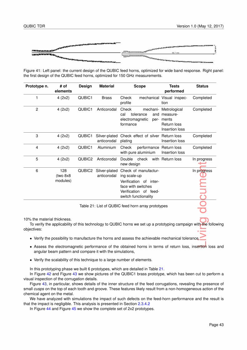
Livi
ngdo
cum
ent
QUBIC TDR Version 1.0 (May 12, 2017)
Figure 41: Left panel: the current design of the QUBIC feed horns, optimized for wide band response. Right panel:the first design of the QUBIC feed horns, optimized for 150 GHz measurements.
Prototype n. # ofelements
Design Material Scope Testsperformed
Status
1 4 (2x2) QUBIC1 Brass Check mechanicalprofile
Visual inspec-tion
Completed
2 4 (2x2) QUBIC1 Anticorodal Check mechani-cal tolerance andelectromagnetic per-formance
Metrologicalmeasure-mentsReturn lossInsertion loss
Completed
3 4 (2x2) QUBIC1 Silver-platedanticorodal
Check effect of silverplating
Return lossInsertion loss
Completed
4 4 (2x2) QUBIC1 Aluminium Check performancewith pure aluminium
Return lossInsertion loss
Completed
5 4 (2x2) QUBIC2 Anticorodal Double check withnew design
Return loss In progress
6 128(two 8x8modules)
QUBIC2 Silver-platedanticorodal
Check of manufactur-ing scale-upVerification of inter-face with switchesVerification of feed-switch functionality
In progress
Table 21: List of QUBIC feed horn array prototypes
10% the material thickness.To verify the applicability of this technology to QUBIC horns we set up a prototyping campaign with the following
objectives:
• Verify the possibility to manufacture the horns and assess the achievable mechanical tolerance,
• Assess the electromagnetic performance of the obtained horns in terms of return loss, insertion loss andangular beam pattern and compare it with the simulations,
• Verify the scalability of this technique to a large number of elements.
In this prototyping phase we built 6 prototypes, which are detailed in Table 21.In Figure 42 and Figure 43 we show pictures of the QUBIC1 brass prototype, which has been cut to perform a
visual inspection of the corrugation details.Figure 43, in particular, shows details of the inner structure of the feed corrugations, revealing the presence of
small cusps on the top of each tooth and groove. These features likely result from a non-homogeneous action of thechemical agent on the metal.
We have analyzed with simulations the impact of such defects on the feed-horn performance and the result isthat the impact is negligible. This analysis is presented in Section 2.3.4.2
In Figure 44 and Figure 45 we show the complete set of 2x2 prototypes.
Page 43
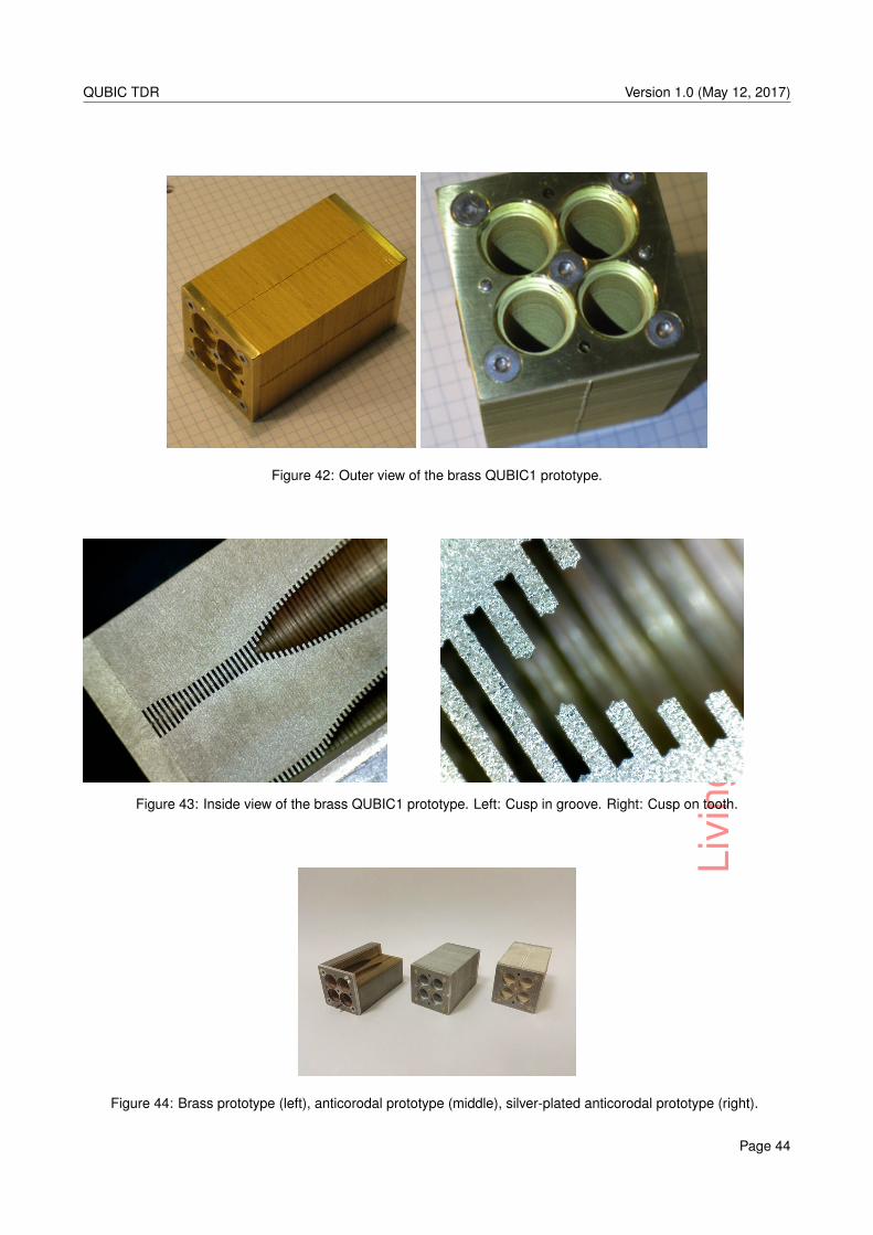
Livi
ngdo
cum
ent
QUBIC TDR Version 1.0 (May 12, 2017)
Figure 42: Outer view of the brass QUBIC1 prototype.
Figure 43: Inside view of the brass QUBIC1 prototype. Left: Cusp in groove. Right: Cusp on tooth.
Figure 44: Brass prototype (left), anticorodal prototype (middle), silver-plated anticorodal prototype (right).
Page 44
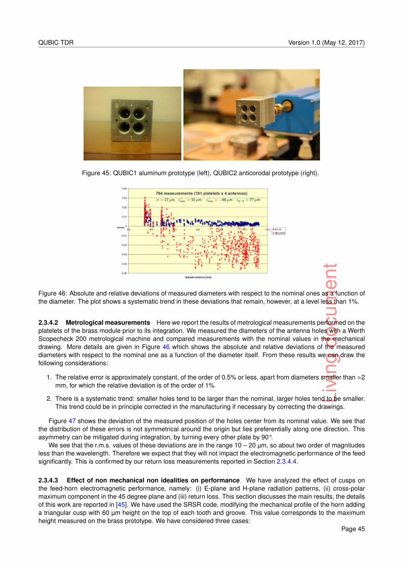
Livi
ngdo
cum
ent
QUBIC TDR Version 1.0 (May 12, 2017)
Figure 45: QUBIC1 aluminum prototype (left), QUBIC2 anticorodal prototype (right).
Figure 46: Absolute and relative deviations of measured diameters with respect to the nominal ones as a function ofthe diameter. The plot shows a systematic trend in these deviations that remain, however, at a level less than 1%.
2.3.4.2 Metrological measurements Here we report the results of metrological measurements performed on theplatelets of the brass module prior to its integration. We measured the diameters of the antenna holes with a WerthScopecheck 200 metrological machine and compared measurements with the nominal values in the mechanicaldrawing. More details are given in Figure 46 which shows the absolute and relative deviations of the measureddiameters with respect to the nominal one as a function of the diameter itself. From these results we can draw thefollowing considerations:
1. The relative error is approximately constant, of the order of 0.5% or less, apart from diameters smaller than ≈2mm, for which the relative deviation is of the order of 1%
2. There is a systematic trend: smaller holes tend to be larger than the nominal, larger holes tend to be smaller.This trend could be in principle corrected in the manufacturing if necessary by correcting the drawings.
Figure 47 shows the deviation of the measured position of the holes center from its nominal value. We see thatthe distribution of these errors is not symmetrical around the origin but lies preferentially along one direction. Thisasymmetry can be mitigated during integration, by turning every other plate by 90°.
We see that the r.m.s. values of these deviations are in the range 10 – 20 µm, so about two order of magnitudesless than the wavelength. Therefore we expect that they will not impact the electromagnetic performance of the feedsignificantly. This is confirmed by our return loss measurements reported in Section 2.3.4.4.
2.3.4.3 Effect of non mechanical non idealities on performance We have analyzed the effect of cusps onthe feed-horn electromagnetic performance, namely: (i) E-plane and H-plane radiation patterns, (ii) cross-polarmaximum component in the 45 degree plane and (iii) return loss. This section discusses the main results, the detailsof this work are reported in [45]. We have used the SRSR code, modifying the mechanical profile of the horn addinga triangular cusp with 60 µm height on the top of each tooth and groove. This value corresponds to the maximumheight measured on the brass prototype. We have considered three cases:
Page 45
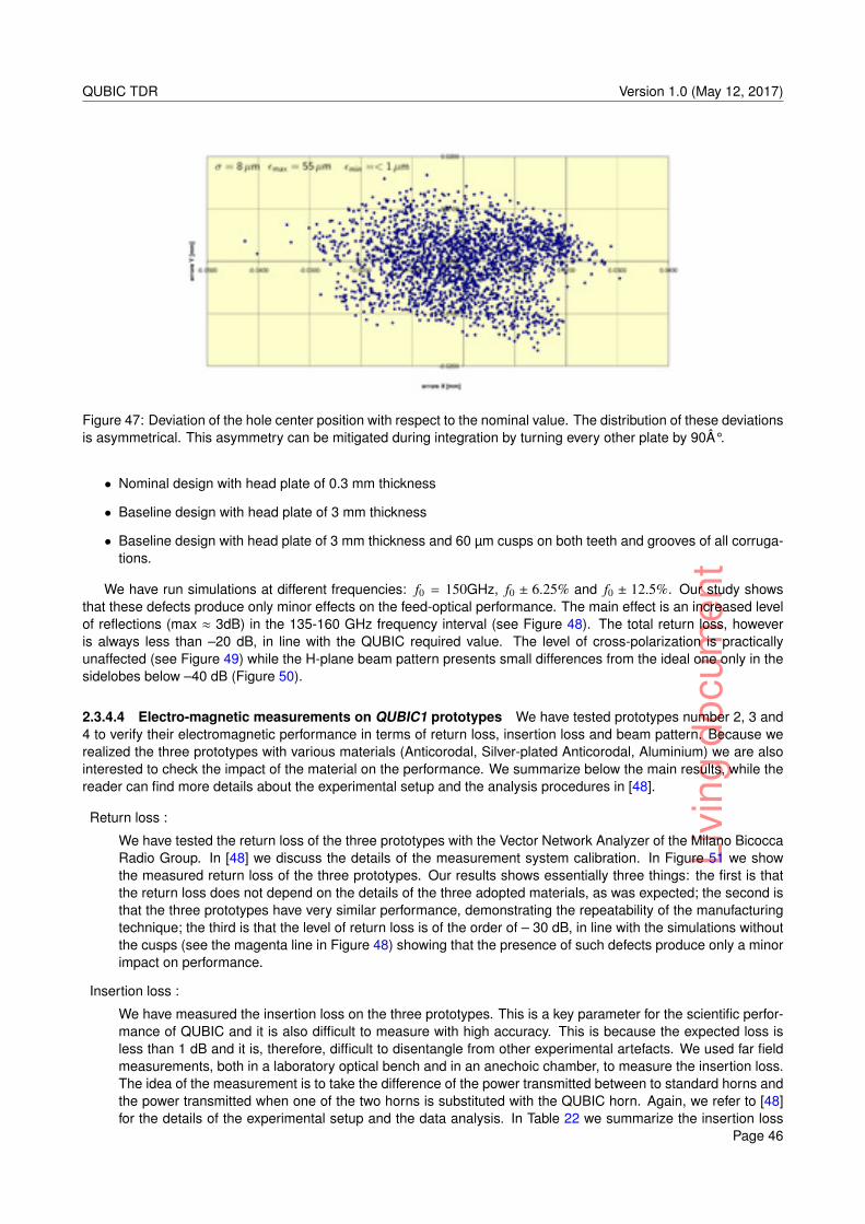
Livi
ngdo
cum
ent
QUBIC TDR Version 1.0 (May 12, 2017)
Figure 47: Deviation of the hole center position with respect to the nominal value. The distribution of these deviationsis asymmetrical. This asymmetry can be mitigated during integration by turning every other plate by 90°.
• Nominal design with head plate of 0.3 mm thickness
• Baseline design with head plate of 3 mm thickness
• Baseline design with head plate of 3 mm thickness and 60 µm cusps on both teeth and grooves of all corruga-tions.
We have run simulations at different frequencies: f0 = 150GHz, f0 ± 6.25% and f0 ± 12.5%. Our study showsthat these defects produce only minor effects on the feed-optical performance. The main effect is an increased levelof reflections (max ≈ 3dB) in the 135-160 GHz frequency interval (see Figure 48). The total return loss, howeveris always less than –20 dB, in line with the QUBIC required value. The level of cross-polarization is practicallyunaffected (see Figure 49) while the H-plane beam pattern presents small differences from the ideal one only in thesidelobes below –40 dB (Figure 50).
2.3.4.4 Electro-magnetic measurements on QUBIC1 prototypes We have tested prototypes number 2, 3 and4 to verify their electromagnetic performance in terms of return loss, insertion loss and beam pattern. Because werealized the three prototypes with various materials (Anticorodal, Silver-plated Anticorodal, Aluminium) we are alsointerested to check the impact of the material on the performance. We summarize below the main results, while thereader can find more details about the experimental setup and the analysis procedures in [48].
Return loss :
We have tested the return loss of the three prototypes with the Vector Network Analyzer of the Milano BicoccaRadio Group. In [48] we discuss the details of the measurement system calibration. In Figure 51 we showthe measured return loss of the three prototypes. Our results shows essentially three things: the first is thatthe return loss does not depend on the details of the three adopted materials, as was expected; the second isthat the three prototypes have very similar performance, demonstrating the repeatability of the manufacturingtechnique; the third is that the level of return loss is of the order of – 30 dB, in line with the simulations withoutthe cusps (see the magenta line in Figure 48) showing that the presence of such defects produce only a minorimpact on performance.
Insertion loss :
We have measured the insertion loss on the three prototypes. This is a key parameter for the scientific perfor-mance of QUBIC and it is also difficult to measure with high accuracy. This is because the expected loss isless than 1 dB and it is, therefore, difficult to disentangle from other experimental artefacts. We used far fieldmeasurements, both in a laboratory optical bench and in an anechoic chamber, to measure the insertion loss.The idea of the measurement is to take the difference of the power transmitted between to standard horns andthe power transmitted when one of the two horns is substituted with the QUBIC horn. Again, we refer to [48]for the details of the experimental setup and the data analysis. In Table 22 we summarize the insertion loss
Page 46
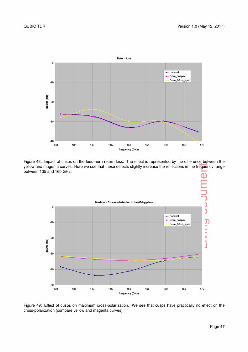
Livi
ngdo
cum
ent
QUBIC TDR Version 1.0 (May 12, 2017)
Figure 48: Impact of cusps on the feed-horn return loss. The effect is represented by the difference between theyellow and magenta curves. Here we see that these defects slightly increase the reflections in the frequency rangebetween 135 and 160 GHz.
Figure 49: Effect of cusps on maximum cross-polarization. We see that cusps have practically no effect on thecross-polarization (compare yellow and magenta curves).
Page 47
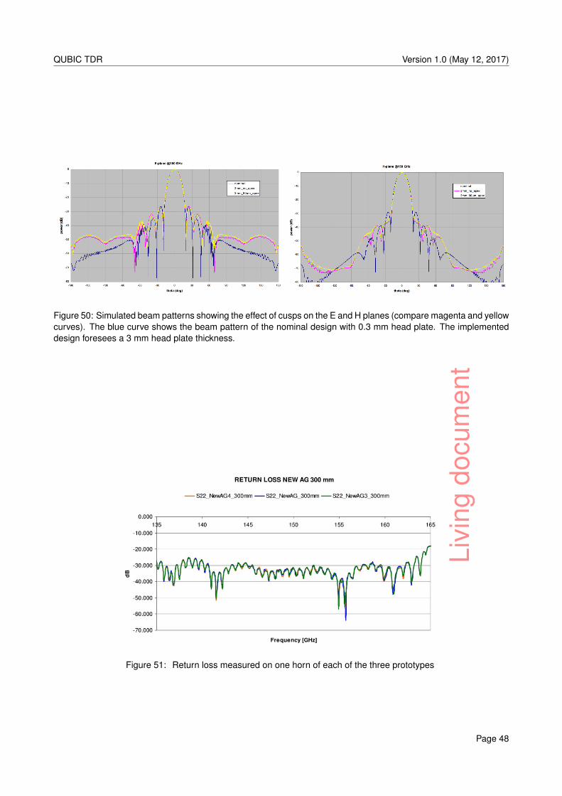
Livi
ngdo
cum
ent
QUBIC TDR Version 1.0 (May 12, 2017)
Figure 50: Simulated beam patterns showing the effect of cusps on the E and H planes (compare magenta and yellowcurves). The blue curve shows the beam pattern of the nominal design with 0.3 mm head plate. The implementeddesign foresees a 3 mm head plate thickness.
Figure 51: Return loss measured on one horn of each of the three prototypes
Page 48
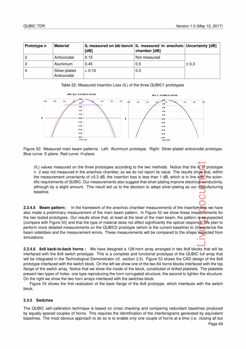
Livi
ngdo
cum
ent
QUBIC TDR Version 1.0 (May 12, 2017)
Prototype n Material IL measured on lab bench[dB]
IL measured in anechoicchamber [dB]
Uncertainty [dB]
2 Anticorodal 0.15 Not measured
3 Aluminium 0.45 0.5 ± 0.3
4 Silver-platedAnticorodal
< 0.10 0.3
Table 22: Measured Insertion Loss (IL) of the three QUBIC1 prototypes
Figure 52: Measured main beam patterns. Left: Aluminum prototype. Right: Silver-plated anticorodal prototype.Blue curve: E-plane. Red curve: H-plane.
(IL) values measured on the three prototypes according to the two methods. Notice that the IL of prototypen. 2 was not measured in the anechoic chamber, so we do not report its value. The results show that, withinthe measurement uncertainty of ±0.3 dB, the insertion loss is less than 1 dB, which is in line with the scien-tific requirements of QUBIC. Our measurements also suggest that silver-plating improve electrical conductivity,although by a slight amount. This result led us to the decision to adopt silver-plating as our manufacturingbaseline.
2.3.4.5 Beam pattern: In the framework of the anechoic chamber measurements of the insertion loss we havealso made a preliminary measurement of the main beam pattern. In Figure 52 we show these measurements forthe two tested prototypes. Our results show that, at least at the level of the main beam, the pattern is as expected(compare with Figure 50) and that the type of material does not affect significantly the optical response. We plan toperform more detailed measurements on the QUBIC2 prototype (which is the current baseline) to characterize thebeam sidelobes and the measurement errors. These measurements will be compared to the shape expected fromsimulations.
2.3.4.6 8x8 back-to-back horns : We have designed a 128-horn array arranged in two 8x8 blocks that will beinterfaced with the 8x8 switch prototype. This is a complete and functional prototype of the QUBIC full array thatwill be integrated in the Technological Demonstrator (cf. section 2.6). Figure 53 shows the CAD design of the 8x8prototype interfaced with the switch block. On the left we show one of the two 64 horns blocks interfaced with the topflange of the switch array. Notice that we show the inside of the block, constituted of drilled platelets. The plateletspresent two types of holes: one type reproducing the horn corrugated structure, the second to lighten the structure.On the right we show the two horn arrays interfaced with the switches block.
Figure 54 shows the first realization of the back flange of the 8x8 prototype, which interfaces with the switchblock.
2.3.5 Switches
The QUBIC self-calibration technique is based on cross checking and comparing redundant baselines producedby equally spaced couples of horns. This requires the identification of the interferograms generated by equivalentbaselines. The most obvious approach to do so is to enable only one couple of horns at a time (i.e. closing all but
Page 49
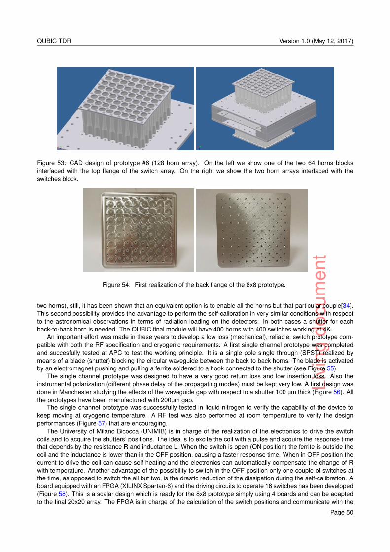
Livi
ngdo
cum
ent
QUBIC TDR Version 1.0 (May 12, 2017)
Figure 53: CAD design of prototype #6 (128 horn array). On the left we show one of the two 64 horns blocksinterfaced with the top flange of the switch array. On the right we show the two horn arrays interfaced with theswitches block.
Figure 54: First realization of the back flange of the 8x8 prototype.
two horns), still, it has been shown that an equivalent option is to enable all the horns but that particular couple[34].This second possibility provides the advantage to perform the self-calibration in very similar conditions with respectto the astronomical observations in terms of radiation loading on the detectors. In both cases a shutter for eachback-to-back horn is needed. The QUBIC final module will have 400 horns with 400 switches working at 4K.
An important effort was made in these years to develop a low loss (mechanical), reliable, switch prototype com-patible with both the RF specification and cryogenic requirements. A first single channel prototype was completedand succesfully tested at APC to test the working principle. It is a single pole single through (SPST) realized bymeans of a blade (shutter) blocking the circular waveguide between the back to back horns. The blade is activatedby an electromagnet pushing and pulling a ferrite soldered to a hook connected to the shutter (see Figure 55).
The single channel prototype was designed to have a very good return loss and low insertion loss. Also theinstrumental polarization (different phase delay of the propagating modes) must be kept very low. A first design wasdone in Manchester studying the effects of the waveguide gap with respect to a shutter 100 µm thick (Figure 56). Allthe prototypes have been manufactured with 200µm gap.
The single channel prototype was successfully tested in liquid nitrogen to verify the capability of the device tokeep moving at cryogenic temperature. A RF test was also performed at room temperature to verify the designperformances (Figure 57) that are encouraging.
The University of Milano Bicocca (UNIMIB) is in charge of the realization of the electronics to drive the switchcoils and to acquire the shutters’ positions. The idea is to excite the coil with a pulse and acquire the response timethat depends by the resistance R and inductance L. When the switch is open (ON position) the ferrite is outside thecoil and the inductance is lower than in the OFF position, causing a faster response time. When in OFF position thecurrent to drive the coil can cause self heating and the electronics can automatically compensate the change of Rwith temperature. Another advantage of the possibility to switch in the OFF position only one couple of switches atthe time, as opposed to switch the all but two, is the drastic reduction of the dissipation during the self-calibration. Aboard equipped with an FPGA (XILINX Spartan-6) and the driving circuits to operate 16 switches has been developed(Figure 58). This is a scalar design which is ready for the 8x8 prototype simply using 4 boards and can be adaptedto the final 20x20 array. The FPGA is in charge of the calculation of the switch positions and communicate with the
Page 50
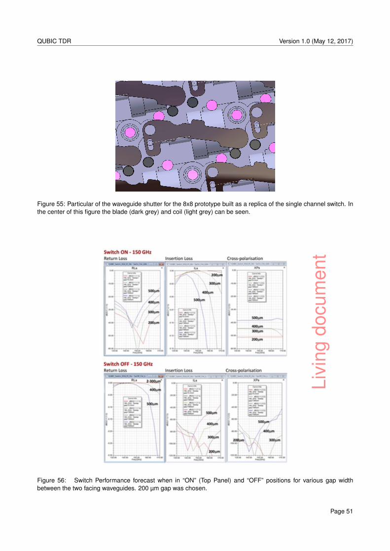
Livi
ngdo
cum
ent
QUBIC TDR Version 1.0 (May 12, 2017)
Figure 55: Particular of the waveguide shutter for the 8x8 prototype built as a replica of the single channel switch. Inthe center of this figure the blade (dark grey) and coil (light grey) can be seen.
Figure 56: Switch Performance forecast when in “ON” (Top Panel) and “OFF” positions for various gap widthbetween the two facing waveguides. 200 µm gap was chosen.
Page 51
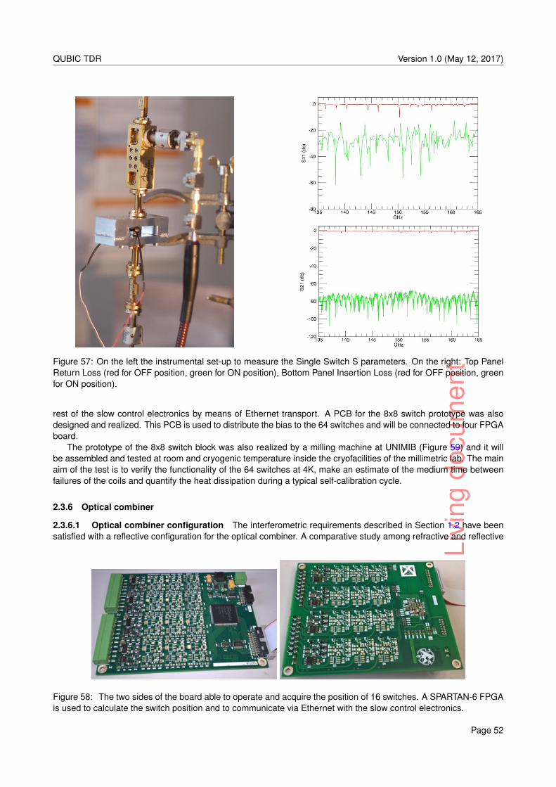
Livi
ngdo
cum
ent
QUBIC TDR Version 1.0 (May 12, 2017)
Figure 57: On the left the instrumental set-up to measure the Single Switch S parameters. On the right: Top PanelReturn Loss (red for OFF position, green for ON position), Bottom Panel Insertion Loss (red for OFF position, greenfor ON position).
rest of the slow control electronics by means of Ethernet transport. A PCB for the 8x8 switch prototype was alsodesigned and realized. This PCB is used to distribute the bias to the 64 switches and will be connected to four FPGAboard.
The prototype of the 8x8 switch block was also realized by a milling machine at UNIMIB (Figure 59) and it willbe assembled and tested at room and cryogenic temperature inside the cryofacilities of the millimetric lab. The mainaim of the test is to verify the functionality of the 64 switches at 4K, make an estimate of the medium time betweenfailures of the coils and quantify the heat dissipation during a typical self-calibration cycle.
2.3.6 Optical combiner
2.3.6.1 Optical combiner configuration The interferometric requirements described in Section 1.2 have beensatisfied with a reflective configuration for the optical combiner. A comparative study among refractive and reflective
Figure 58: The two sides of the board able to operate and acquire the position of 16 switches. A SPARTAN-6 FPGAis used to calculate the switch position and to communicate via Ethernet with the slow control electronics.
Page 52
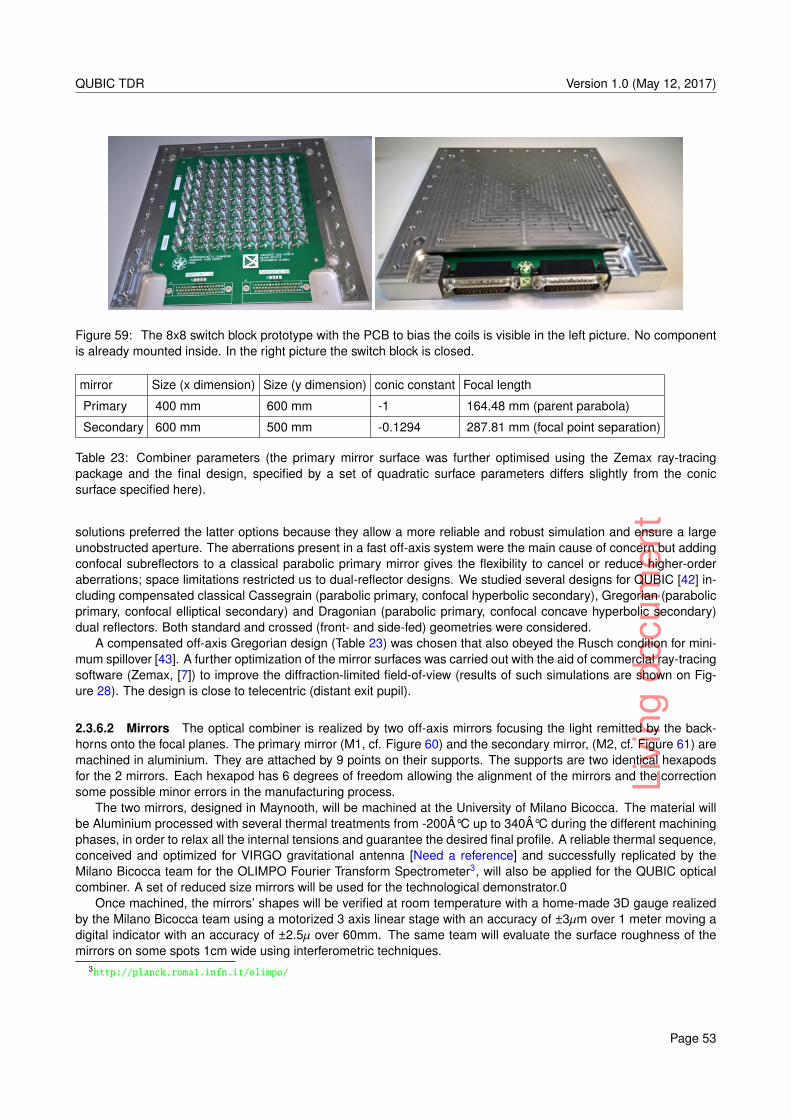
Livi
ngdo
cum
ent
QUBIC TDR Version 1.0 (May 12, 2017)
Figure 59: The 8x8 switch block prototype with the PCB to bias the coils is visible in the left picture. No componentis already mounted inside. In the right picture the switch block is closed.
mirror Size (x dimension) Size (y dimension) conic constant Focal length
Primary 400 mm 600 mm -1 164.48 mm (parent parabola)
Secondary 600 mm 500 mm -0.1294 287.81 mm (focal point separation)
Table 23: Combiner parameters (the primary mirror surface was further optimised using the Zemax ray-tracingpackage and the final design, specified by a set of quadratic surface parameters differs slightly from the conicsurface specified here).
solutions preferred the latter options because they allow a more reliable and robust simulation and ensure a largeunobstructed aperture. The aberrations present in a fast off-axis system were the main cause of concern but addingconfocal subreflectors to a classical parabolic primary mirror gives the flexibility to cancel or reduce higher-orderaberrations; space limitations restricted us to dual-reflector designs. We studied several designs for QUBIC [42] in-cluding compensated classical Cassegrain (parabolic primary, confocal hyperbolic secondary), Gregorian (parabolicprimary, confocal elliptical secondary) and Dragonian (parabolic primary, confocal concave hyperbolic secondary)dual reflectors. Both standard and crossed (front- and side-fed) geometries were considered.
A compensated off-axis Gregorian design (Table 23) was chosen that also obeyed the Rusch condition for mini-mum spillover [43]. A further optimization of the mirror surfaces was carried out with the aid of commercial ray-tracingsoftware (Zemax, [7]) to improve the diffraction-limited field-of-view (results of such simulations are shown on Fig-ure 28). The design is close to telecentric (distant exit pupil).
2.3.6.2 Mirrors The optical combiner is realized by two off-axis mirrors focusing the light remitted by the back-horns onto the focal planes. The primary mirror (M1, cf. Figure 60) and the secondary mirror, (M2, cf. Figure 61) aremachined in aluminium. They are attached by 9 points on their supports. The supports are two identical hexapodsfor the 2 mirrors. Each hexapod has 6 degrees of freedom allowing the alignment of the mirrors and the correctionsome possible minor errors in the manufacturing process.
The two mirrors, designed in Maynooth, will be machined at the University of Milano Bicocca. The material willbe Aluminium processed with several thermal treatments from -200°C up to 340°C during the different machiningphases, in order to relax all the internal tensions and guarantee the desired final profile. A reliable thermal sequence,conceived and optimized for VIRGO gravitational antenna [Need a reference] and successfully replicated by theMilano Bicocca team for the OLIMPO Fourier Transform Spectrometer3, will also be applied for the QUBIC opticalcombiner. A set of reduced size mirrors will be used for the technological demonstrator.0
Once machined, the mirrors’ shapes will be verified at room temperature with a home-made 3D gauge realizedby the Milano Bicocca team using a motorized 3 axis linear stage with an accuracy of ±3µm over 1 meter moving adigital indicator with an accuracy of ±2.5µ over 60mm. The same team will evaluate the surface roughness of themirrors on some spots 1cm wide using interferometric techniques.
3http://planck.roma1.infn.it/olimpo/
Page 53
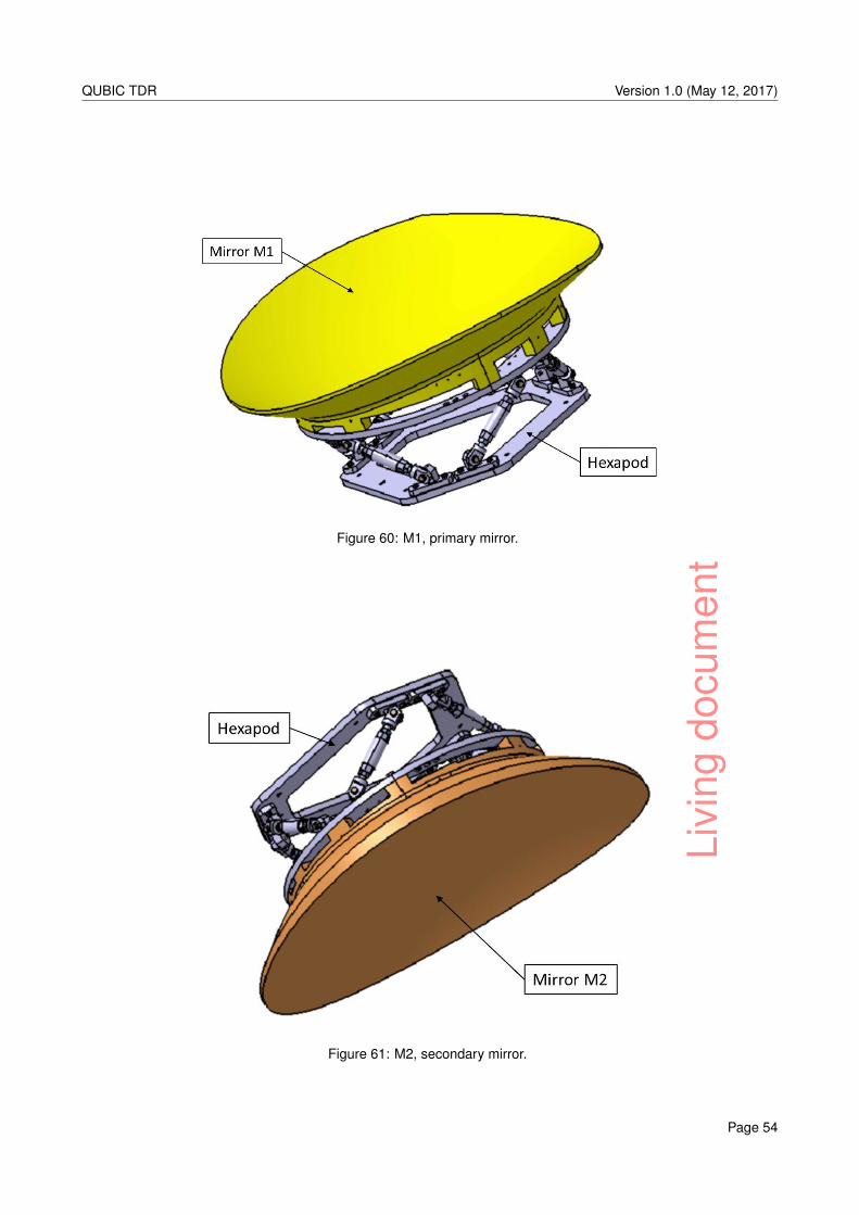
Livi
ngdo
cum
ent
QUBIC TDR Version 1.0 (May 12, 2017)
Figure 60: M1, primary mirror.
Figure 61: M2, secondary mirror.
Page 54
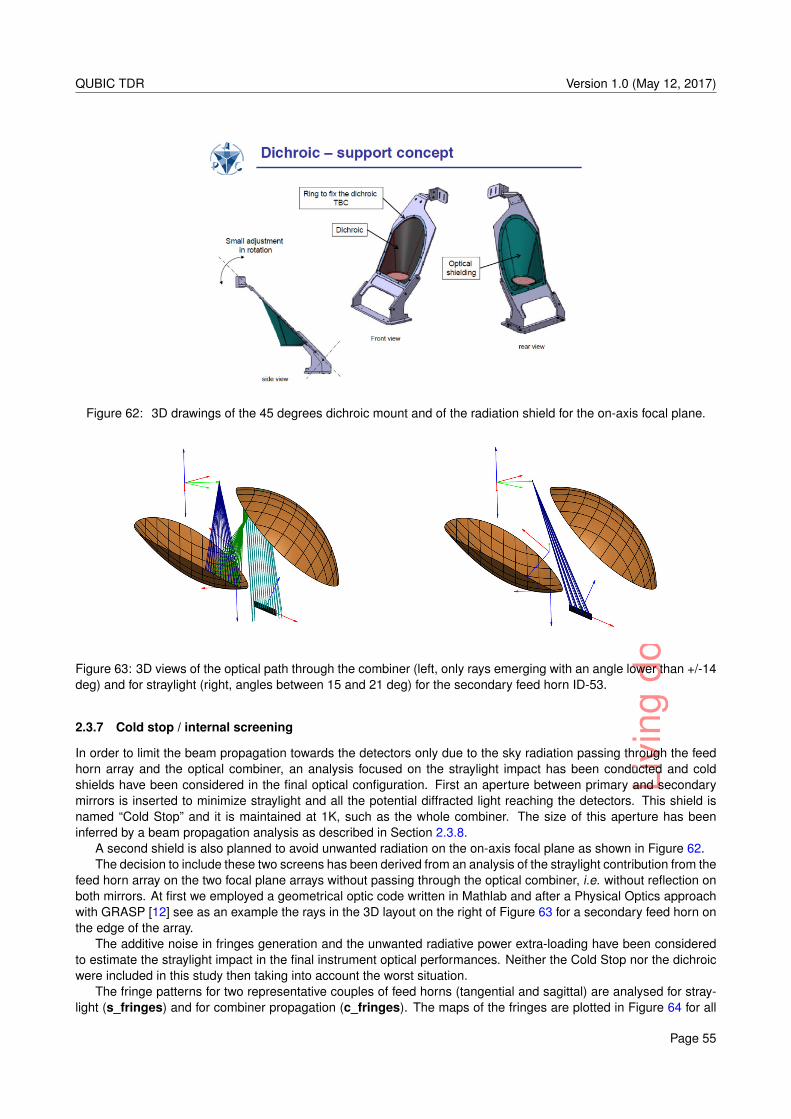
Livi
ngdo
cum
ent
QUBIC TDR Version 1.0 (May 12, 2017)
Figure 62: 3D drawings of the 45 degrees dichroic mount and of the radiation shield for the on-axis focal plane.
Figure 63: 3D views of the optical path through the combiner (left, only rays emerging with an angle lower than +/-14deg) and for straylight (right, angles between 15 and 21 deg) for the secondary feed horn ID-53.
2.3.7 Cold stop / internal screening
In order to limit the beam propagation towards the detectors only due to the sky radiation passing through the feedhorn array and the optical combiner, an analysis focused on the straylight impact has been conducted and coldshields have been considered in the final optical configuration. First an aperture between primary and secondarymirrors is inserted to minimize straylight and all the potential diffracted light reaching the detectors. This shield isnamed “Cold Stop” and it is maintained at 1K, such as the whole combiner. The size of this aperture has beeninferred by a beam propagation analysis as described in Section 2.3.8.
A second shield is also planned to avoid unwanted radiation on the on-axis focal plane as shown in Figure 62.The decision to include these two screens has been derived from an analysis of the straylight contribution from the
feed horn array on the two focal plane arrays without passing through the optical combiner, i.e. without reflection onboth mirrors. At first we employed a geometrical optic code written in Mathlab and after a Physical Optics approachwith GRASP [12] see as an example the rays in the 3D layout on the right of Figure 63 for a secondary feed horn onthe edge of the array.
The additive noise in fringes generation and the unwanted radiative power extra-loading have been consideredto estimate the straylight impact in the final instrument optical performances. Neither the Cold Stop nor the dichroicwere included in this study then taking into account the worst situation.
The fringe patterns for two representative couples of feed horns (tangential and sagittal) are analysed for stray-light (s_fringes) and for combiner propagation (c_fringes). The maps of the fringes are plotted in Figure 64 for all
Page 55
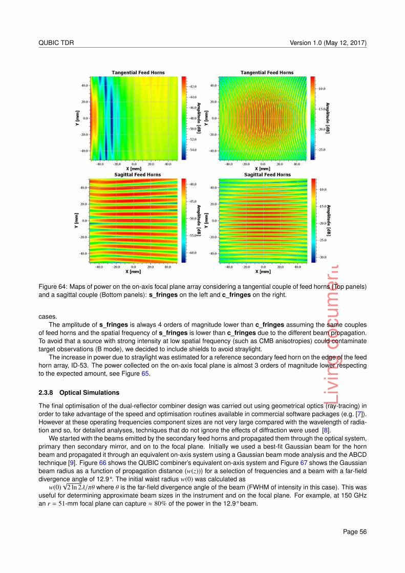
Livi
ngdo
cum
ent
QUBIC TDR Version 1.0 (May 12, 2017)
Figure 64: Maps of power on the on-axis focal plane array considering a tangential couple of feed horns (Top panels)and a sagittal couple (Bottom panels): s_fringes on the left and c_fringes on the right.
cases.The amplitude of s_fringes is always 4 orders of magnitude lower than c_fringes assuming the same couples
of feed horns and the spatial frequency of s_fringes is lower than c_fringes due to the different beam propagation.To avoid that a source with strong intensity at low spatial frequency (such as CMB anisotropies) could contaminatetarget observations (B mode), we decided to include shields to avoid straylight.
The increase in power due to straylight was estimated for a reference secondary feed horn on the edge of the feedhorn array, ID-53. The power collected on the on-axis focal plane is almost 3 orders of magnitude lower respectingto the expected amount, see Figure 65.
2.3.8 Optical Simulations
The final optimisation of the dual-reflector combiner design was carried out using geometrical optics (ray-tracing) inorder to take advantage of the speed and optimisation routines available in commercial software packages (e.g. [7]).However at these operating frequencies component sizes are not very large compared with the wavelength of radia-tion and so, for detailed analyses, techniques that do not ignore the effects of diffraction were used [8].
We started with the beams emitted by the secondary feed horns and propagated them through the optical system,primary then secondary mirror, and on to the focal plane. Initially we used a best-fit Gaussian beam for the hornbeam and propagated it through an equivalent on-axis system using a Gaussian beam mode analysis and the ABCDtechnique [9]. Figure 66 shows the QUBIC combiner’s equivalent on-axis system and Figure 67 shows the Gaussianbeam radius as a function of propagation distance (w(z))) for a selection of frequencies and a beam with a far-fielddivergence angle of 12.9°. The initial waist radius w(0) was calculated as
w(0)√
2 ln 2λ/πθ where θ is the far-field divergence angle of the beam (FWHM of intensity in this case). This wasuseful for determining approximate beam sizes in the instrument and on the focal plane. For example, at 150 GHzan r = 51-mm focal plane can capture ≈ 80% of the power in the 12.9° beam.
Page 56
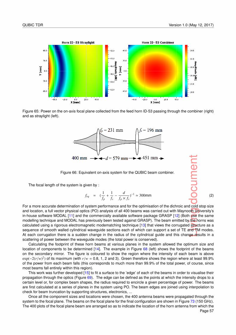
Livi
ngdo
cum
ent
QUBIC TDR Version 1.0 (May 12, 2017)
Figure 65: Power on the on-axis focal plane collected from the feed horn ID-53 passing through the combiner (right)and as straylight (left).
Figure 66: Equivalent on-axis system for the QUBIC beam combiner.
The focal length of the system is given by :
feq = (1fp
+1fs−
dfp × fs
)−1 ' 300mm (2)
For a more accurate determination of system performance and for the optimisation of the dichroic and cold stop sizeand location, a full vector physical optics (PO) analysis of all 400 beams was carried out with Maynooth University’sin-house software MODAL [11] and the commercially available software package GRASP [12] (Both use the samemodelling technique and MODAL has previously been tested against GRASP). The beam emitted by the horns wascalculated using a rigorous electromagnetic modematching technique [13] that views the corrugated structure as asequence of smooth walled cylindrical waveguide sections each of which can support a set of TE and TM modes.At each corrugation there is a sudden change in the radius of the cylindrical guide and this change results in ascattering of power between the waveguide modes (the total power is conserved).
Calculating the footprint of these horn beams at various planes in the system allowed the optimum size andlocation of components to be determined [14]. The example in Figure 68 (left) shows the footprint of the beamson the secondary mirror. The figure is coloured to show the region where the intensity of each beam is aboveexp(−2(r/w)2) of its maximum (with r/w = 0.8, 1, 2 and 3). Green therefore shows the region where at least 99.9%of the power from each beam falls (this corresponds to much more than 99.9% of the total power, of course, sincemost beams fall entirely within this region).
This work was further developed [15] to fit a surface to the ’edge’ of each of the beams in order to visualise theirpropagation through the optics (Figure 69). The edge can be defined as the points at which the intensity drops to acertain level or, for complex beam shapes, the radius required to encircle a given percentage of power. The beamsare first calculated at a series of planes in the system using PO. The beam edges are joined using interpolation tocheck for beam truncation by supporting structures, electronics, ...
Once all the component sizes and locations were chosen, the 400 antenna beams were propagated through thesystem to the focal plane. The beams on the focal plane for the final configuration are shown in Figure 73 (150 GHz).The 400 plots of the focal plane beam are arranged so as to indicate the location of the horn antenna from which the
Page 57
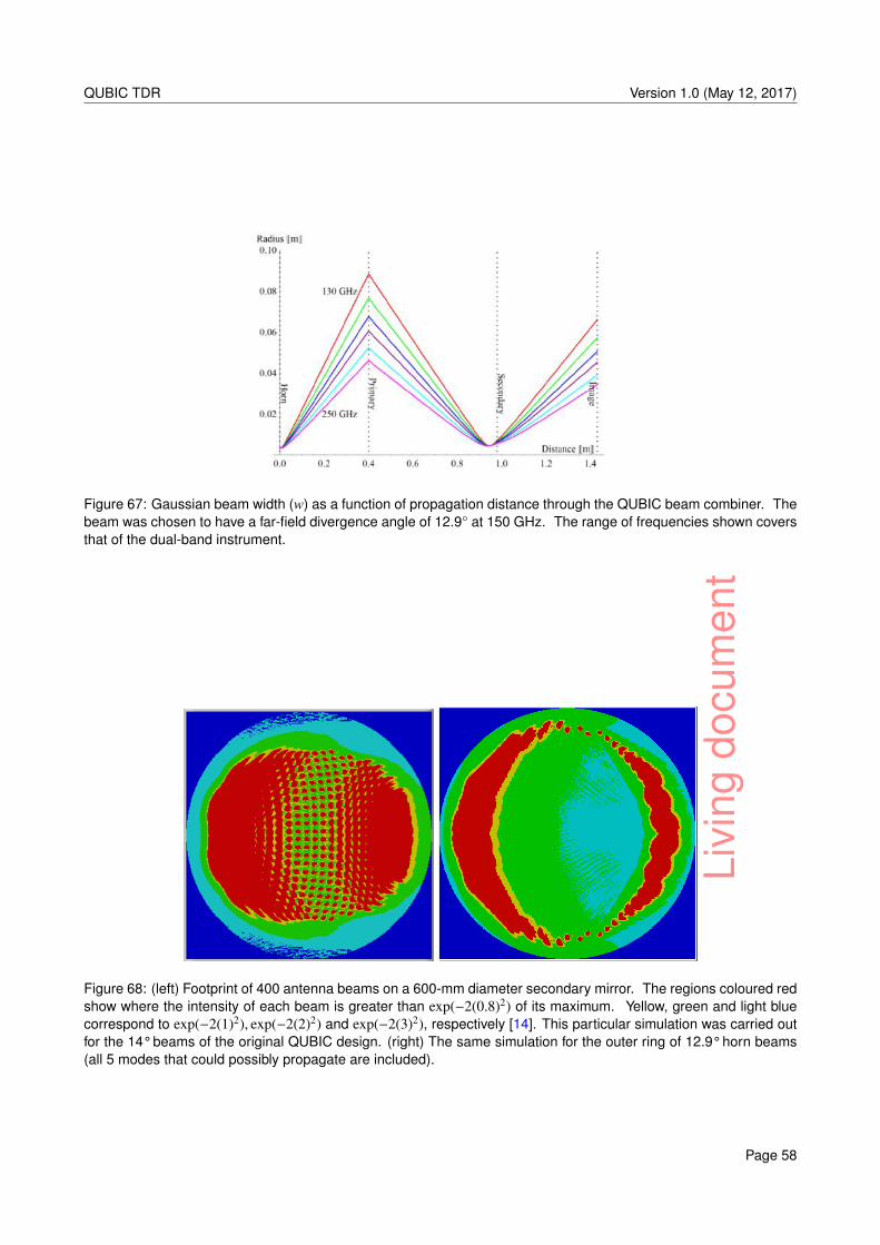
Livi
ngdo
cum
ent
QUBIC TDR Version 1.0 (May 12, 2017)
Figure 67: Gaussian beam width (w) as a function of propagation distance through the QUBIC beam combiner. Thebeam was chosen to have a far-field divergence angle of 12.9° at 150 GHz. The range of frequencies shown coversthat of the dual-band instrument.
Figure 68: (left) Footprint of 400 antenna beams on a 600-mm diameter secondary mirror. The regions coloured redshow where the intensity of each beam is greater than exp(−2(0.8)2) of its maximum. Yellow, green and light bluecorrespond to exp(−2(1)2), exp(−2(2)2) and exp(−2(3)2), respectively [14]. This particular simulation was carried outfor the 14° beams of the original QUBIC design. (right) The same simulation for the outer ring of 12.9° horn beams(all 5 modes that could possibly propagate are included).
Page 58
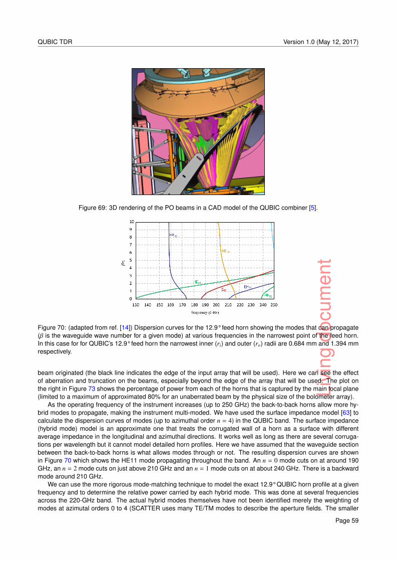
Livi
ngdo
cum
ent
QUBIC TDR Version 1.0 (May 12, 2017)
Figure 69: 3D rendering of the PO beams in a CAD model of the QUBIC combiner [5].
Figure 70: (adapted from ref. [14]) Dispersion curves for the 12.9° feed horn showing the modes that can propagate(β is the waveguide wave number for a given mode) at various frequencies in the narrowest point of the feed horn.In this case for for QUBIC’s 12.9° feed horn the narrowest inner (ri) and outer (ro) radii are 0.684 mm and 1.394 mmrespectively.
beam originated (the black line indicates the edge of the input array that will be used). Here we can see the effectof aberration and truncation on the beams, especially beyond the edge of the array that will be used. The plot onthe right in Figure 73 shows the percentage of power from each of the horns that is captured by the main focal plane(limited to a maximum of approximated 80% for an unaberrated beam by the physical size of the bolometer array).
As the operating frequency of the instrument increases (up to 250 GHz) the back-to-back horns allow more hy-brid modes to propagate, making the instrument multi-moded. We have used the surface impedance model [63] tocalculate the dispersion curves of modes (up to azimuthal order n = 4) in the QUBIC band. The surface impedance(hybrid mode) model is an approximate one that treats the corrugated wall of a horn as a surface with differentaverage impedance in the longitudinal and azimuthal directions. It works well as long as there are several corruga-tions per wavelength but it cannot model detailed horn profiles. Here we have assumed that the waveguide sectionbetween the back-to-back horns is what allows modes through or not. The resulting dispersion curves are shownin Figure 70 which shows the HE11 mode propagating throughout the band. An n = 0 mode cuts on at around 190GHz, an n = 2 mode cuts on just above 210 GHz and an n = 1 mode cuts on at about 240 GHz. There is a backwardmode around 210 GHz.
We can use the more rigorous mode-matching technique to model the exact 12.9° QUBIC horn profile at a givenfrequency and to determine the relative power carried by each hybrid mode. This was done at several frequenciesacross the 220-GHz band. The actual hybrid modes themselves have not been identified merely the weighting ofmodes at azimutal orders 0 to 4 (SCATTER uses many TE/TM modes to describe the aperture fields. The smaller
Page 59
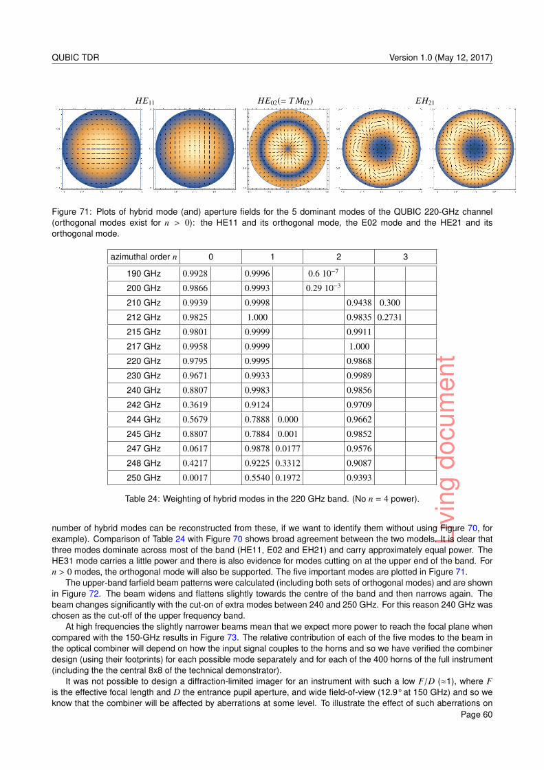
Livi
ngdo
cum
ent
QUBIC TDR Version 1.0 (May 12, 2017)
HE11 HE02(= T M02) EH21
Figure 71: Plots of hybrid mode (and) aperture fields for the 5 dominant modes of the QUBIC 220-GHz channel(orthogonal modes exist for n > 0): the HE11 and its orthogonal mode, the E02 mode and the HE21 and itsorthogonal mode.
azimuthal order n 0 1 2 3
190 GHz 0.9928 0.9996 0.6 10−7
200 GHz 0.9866 0.9993 0.29 10−3
210 GHz 0.9939 0.9998 0.9438 0.300
212 GHz 0.9825 1.000 0.9835 0.2731
215 GHz 0.9801 0.9999 0.9911
217 GHz 0.9958 0.9999 1.000
220 GHz 0.9795 0.9995 0.9868
230 GHz 0.9671 0.9933 0.9989
240 GHz 0.8807 0.9983 0.9856
242 GHz 0.3619 0.9124 0.9709
244 GHz 0.5679 0.7888 0.000 0.9662
245 GHz 0.8807 0.7884 0.001 0.9852
247 GHz 0.0617 0.9878 0.0177 0.9576
248 GHz 0.4217 0.9225 0.3312 0.9087
250 GHz 0.0017 0.5540 0.1972 0.9393
Table 24: Weighting of hybrid modes in the 220 GHz band. (No n = 4 power).
number of hybrid modes can be reconstructed from these, if we want to identify them without using Figure 70, forexample). Comparison of Table 24 with Figure 70 shows broad agreement between the two models. It is clear thatthree modes dominate across most of the band (HE11, E02 and EH21) and carry approximately equal power. TheHE31 mode carries a little power and there is also evidence for modes cutting on at the upper end of the band. Forn > 0 modes, the orthogonal mode will also be supported. The five important modes are plotted in Figure 71.
The upper-band farfield beam patterns were calculated (including both sets of orthogonal modes) and are shownin Figure 72. The beam widens and flattens slightly towards the centre of the band and then narrows again. Thebeam changes significantly with the cut-on of extra modes between 240 and 250 GHz. For this reason 240 GHz waschosen as the cut-off of the upper frequency band.
At high frequencies the slightly narrower beams mean that we expect more power to reach the focal plane whencompared with the 150-GHz results in Figure 73. The relative contribution of each of the five modes to the beam inthe optical combiner will depend on how the input signal couples to the horns and so we have verified the combinerdesign (using their footprints) for each possible mode separately and for each of the 400 horns of the full instrument(including the the central 8x8 of the technical demonstrator).
It was not possible to design a diffraction-limited imager for an instrument with such a low F/D (≈1), where Fis the effective focal length and D the entrance pupil aperture, and wide field-of-view (12.9° at 150 GHz) and so weknow that the combiner will be affected by aberrations at some level. To illustrate the effect of such aberrations on
Page 60
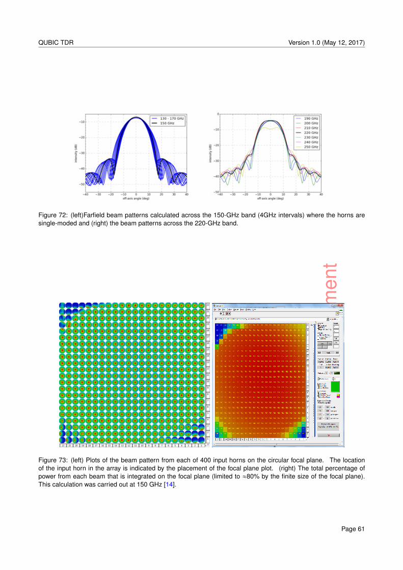
Livi
ngdo
cum
ent
QUBIC TDR Version 1.0 (May 12, 2017)
Figure 72: (left)Farfield beam patterns calculated across the 150-GHz band (4GHz intervals) where the horns aresingle-moded and (right) the beam patterns across the 220-GHz band.
Figure 73: (left) Plots of the beam pattern from each of 400 input horns on the circular focal plane. The locationof the input horn in the array is indicated by the placement of the focal plane plot. (right) The total percentage ofpower from each beam that is integrated on the focal plane (limited to ≈80% by the finite size of the focal plane).This calculation was carried out at 150 GHz [14].
Page 61
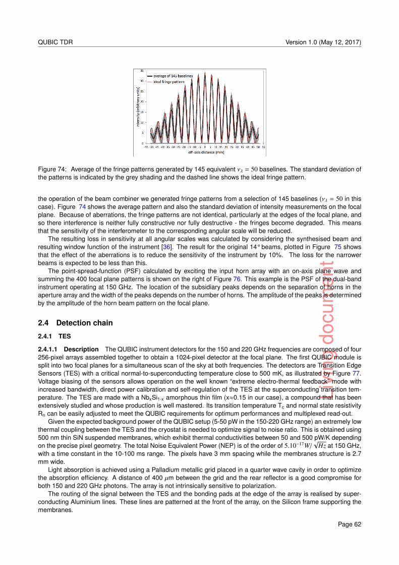
Livi
ngdo
cum
ent
QUBIC TDR Version 1.0 (May 12, 2017)
Figure 74: Average of the fringe patterns generated by 145 equivalent νλ = 50 baselines. The standard deviation ofthe patterns is indicated by the grey shading and the dashed line shows the ideal fringe pattern.
the operation of the beam combiner we generated fringe patterns from a selection of 145 baselines (νλ = 50 in thiscase). Figure 74 shows the average pattern and also the standard deviation of intensity measurements on the focalplane. Because of aberrations, the fringe patterns are not identical, particularly at the edges of the focal plane, andso there interference is neither fully constructive nor fully destructive - the fringes become degraded. This meansthat the sensitivity of the interferometer to the corresponding angular scale will be reduced.
The resulting loss in sensitivity at all angular scales was calculated by considering the synthesised beam andresulting window function of the instrument [36]. The result for the original 14° beams, plotted in Figure 75 showsthat the effect of the aberrations is to reduce the sensitivity of the instrument by 10%. The loss for the narrowerbeams is expected to be less than this.
The point-spread-function (PSF) calculated by exciting the input horn array with an on-axis plane wave andsumming the 400 focal plane patterns is shown on the right of Figure 76. This example is the PSF of the dual-bandinstrument operating at 150 GHz. The location of the subsidiary peaks depends on the separation of horns in theaperture array and the width of the peaks depends on the number of horns. The amplitude of the peaks is determinedby the amplitude of the horn beam pattern on the focal plane.
2.4 Detection chain
2.4.1 TES
2.4.1.1 Description The QUBIC instrument detectors for the 150 and 220 GHz frequencies are composed of four256-pixel arrays assembled together to obtain a 1024-pixel detector at the focal plane. The first QUBIC module issplit into two focal planes for a simultaneous scan of the sky at both frequencies. The detectors are Transition EdgeSensors (TES) with a critical normal-to-superconducting temperature close to 500 mK, as illustrated by Figure 77.Voltage biasing of the sensors allows operation on the well known “extreme electro-thermal feedback” mode withincreased bandwidth, direct power calibration and self-regulation of the TES at the superconducting transition tem-perature. The TES are made with a NbxSi1-x amorphous thin film (x≈0.15 in our case), a compound that has beenextensively studied and whose production is well mastered. Its transition temperature Tc and normal state resistivityRn can be easily adjusted to meet the QUBIC requirements for optimum performances and multiplexed read-out.
Given the expected background power of the QUBIC setup (5-50 pW in the 150-220 GHz range) an extremely lowthermal coupling between the TES and the cryostat is needed to optimize signal to noise ratio. This is obtained using500 nm thin SiN suspended membranes, which exhibit thermal conductivities between 50 and 500 pW/K dependingon the precise pixel geometry. The total Noise Equivalent Power (NEP) is of the order of 5.10−17W/
√Hz at 150 GHz,
with a time constant in the 10-100 ms range. The pixels have 3 mm spacing while the membranes structure is 2.7mm wide.
Light absorption is achieved using a Palladium metallic grid placed in a quarter wave cavity in order to optimizethe absorption efficiency. A distance of 400 µm between the grid and the rear reflector is a good compromise forboth 150 and 220 GHz photons. The array is not intrinsically sensitive to polarization.
The routing of the signal between the TES and the bonding pads at the edge of the array is realised by super-conducting Aluminium lines. These lines are patterned at the front of the array, on the Silicon frame supporting themembranes.
Page 62
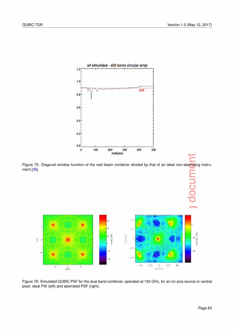
Livi
ngdo
cum
ent
QUBIC TDR Version 1.0 (May 12, 2017)
Figure 75: Diagonal window function of the real beam combiner divided by that of an ideal non-aberrating instru-ment [36].
Figure 76: Simulated QUBIC PSF for the dual band combiner, operated at 150 GHz, for an on-axis source or centralpixel: ideal PSf (left) and aberrated PSF (right).
Page 63
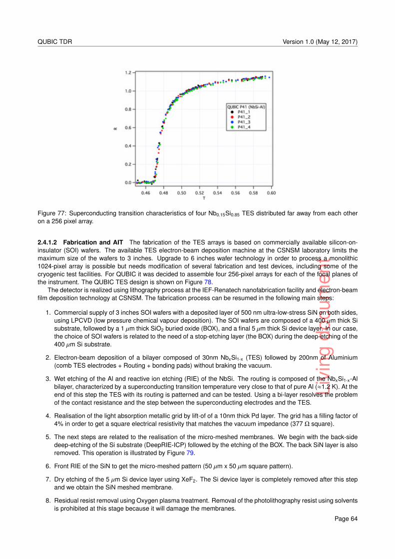
Livi
ngdo
cum
ent
QUBIC TDR Version 1.0 (May 12, 2017)
Figure 77: Superconducting transition characteristics of four Nb0.15Si0.85 TES distributed far away from each otheron a 256 pixel array.
2.4.1.2 Fabrication and AIT The fabrication of the TES arrays is based on commercially available silicon-on-insulator (SOI) wafers. The available TES electron-beam deposition machine at the CSNSM laboratory limits themaximum size of the wafers to 3 inches. Upgrade to 6 inches wafer technology in order to process a monolithic1024-pixel array is possible but needs modification of several fabrication and test devices, including some of thecryogenic test facilities. For QUBIC it was decided to assemble four 256-pixel arrays for each of the focal planes ofthe instrument. The QUBIC TES design is shown on Figure 78.
The detector is realized using lithography process at the IEF-Renatech nanofabrication facility and electron-beamfilm deposition technology at CSNSM. The fabrication process can be resumed in the following main steps:
1. Commercial supply of 3 inches SOI wafers with a deposited layer of 500 nm ultra-low-stress SiN on both sides,using LPCVD (low pressure chemical vapour deposition). The SOI wafers are composed of a 400 µm thick Sisubstrate, followed by a 1 µm thick SiO2 buried oxide (BOX), and a final 5 µm thick Si device layer. In our case,the choice of SOI wafers is related to the need of a stop-etching layer (the BOX) during the deep-etching of the400 µm Si substrate.
2. Electron-beam deposition of a bilayer composed of 30nm NbxSi1-x (TES) followed by 200nm of Aluminium(comb TES electrodes + Routing + bonding pads) without braking the vacuum.
3. Wet etching of the Al and reactive ion etching (RIE) of the NbSi. The routing is composed of the NbxSi1-x-Albilayer, characterized by a superconducting transition temperature very close to that of pure Al (≈1.2 K). At theend of this step the TES with its routing is patterned and can be tested. Using a bi-layer resolves the problemof the contact resistance and the step between the superconducting electrodes and the TES.
4. Realisation of the light absorption metallic grid by lift-of of a 10nm thick Pd layer. The grid has a filling factor of4% in order to get a square electrical resistivity that matches the vacuum impedance (377 Ω square).
5. The next steps are related to the realisation of the micro-meshed membranes. We begin with the back-sidedeep-etching of the Si substrate (DeepRIE-ICP) followed by the etching of the BOX. The back SiN layer is alsoremoved. This operation is illustrated by Figure 79.
6. Front RIE of the SiN to get the micro-meshed pattern (50 µm x 50 µm square pattern).
7. Dry etching of the 5 µm Si device layer using XeF2. The Si device layer is completely removed after this stepand we obtain the SiN meshed membrane.
8. Residual resist removal using Oxygen plasma treatment. Removal of the photolithography resist using solventsis prohibited at this stage because it will damage the membranes.
Page 64
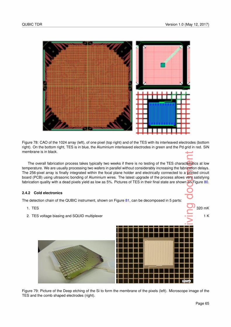
Livi
ngdo
cum
ent
QUBIC TDR Version 1.0 (May 12, 2017)
Figure 78: CAO of the 1024 array (left), of one pixel (top right) and of the TES with its interleaved electrodes (bottomright). On the bottom right, TES is in blue, the Aluminium interleaved electrodes in green and the Pd grid in red. SiNmembrane is in black.
The overall fabrication process takes typically two weeks if there is no testing of the TES characteristics at lowtemperature. We are usually processing two wafers in parallel without considerably increasing the fabrication delays.The 256-pixel array is finally integrated within the focal plane holder and electrically connected to a printed circuitboard (PCB) using ultrasonic bonding of Aluminium wires. The latest upgrade of the process allows very satisfyingfabrication quality with a dead pixels yield as low as 5%. Pictures of TES in their final state are shown on Figure 80.
2.4.2 Cold electronics
The detection chain of the QUBIC instrument, shown on Figure 81, can be decomposed in 5 parts:
1. TES 320 mK
2. TES voltage biasing and SQUID multiplexer 1 K
Figure 79: Picture of the Deep etching of the Si to form the membrane of the pixels (left). Microscope image of theTES and the comb shaped electrodes (right).
Page 65
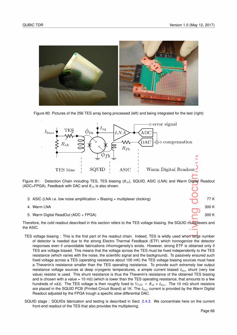
Livi
ngdo
cum
ent
QUBIC TDR Version 1.0 (May 12, 2017)
Figure 80: Pictures of the 256 TES array being processed (left) and being integrated for the test (right)
Figure 81: Detection Chain including TES, TES biasing (Rsh), SQUID, ASIC (LNA) and Warm Digital Readout(ADC+FPGA). Feedback with DAC and R f b is also shown.
3. ASIC (LNA i.e. low noise amplification + Biasing + multiplexer clocking) 77 K
4. Warm LNA 300 K
5. Warm Digital ReadOut (ADC + FPGA) 300 K
Therefore, the cold readout described in this section refers to the TES voltage biasing, the SQUID multiplexers andthe ASIC.
TES voltage biasing : This is the first part of the readout chain. Indeed, TES is wildly used when large numberof detector is needed due to the strong Electro Thermal Feedback (ETF) which homogenize the detectorresponses even if unavoidable fabrications inhomogeneity’s exists. However, strong ETF is obtained only ifTES are voltage biased. This means that the voltage across the TES must be fixed independently to the TESresistance (which varies with the noise, the scientific signal and the background). To passively ensured suchfixed voltage across a TES (operating resistance about 100 mK) the TES voltage biasing sources must havea Thevenin’s resistance smaller than the TES operating resistance. To provide such extremely low outputresistance voltage sources at deep cryogenic temperatures, a simple current biased Ibias shunt (very lowvalue) resistor is used. This shunt resistance is thus the Thevenin’s resistance of the obtained TES biasingand is chosen with a value = 10 mΩ (which is lower than the TES operating resistance, that amounts to a fewhundreds of mΩ). The TES voltage is then roughly fixed to VT ES = Rsh × Ibias. The 10 mΩ shunt resistorsare placed in the SQUID PCB (Printed Circuit Board) at 1K. The Ibias current is provided by the Warm DigitalReadout adjusted by the FPGA trough a specific slow differential DAC.
SQUID stage : SQUIDs fabrication and testing is described in Sect. 2.4.3. We concentrate here on the currentfront-end readout of the TES that also provides the multiplexing.
Page 66
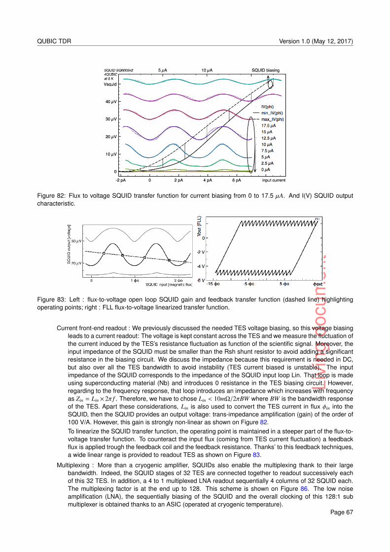
Livi
ngdo
cum
ent
QUBIC TDR Version 1.0 (May 12, 2017)
Figure 82: Flux to voltage SQUID transfer function for current biasing from 0 to 17.5 µA. And I(V) SQUID outputcharacteristic.
Figure 83: Left : flux-to-voltage open loop SQUID gain and feedback transfer function (dashed line) highlightingoperating points; right : FLL flux-to-voltage linearized transfer function.
Current front-end readout : We previously discussed the needed TES voltage biasing, so this voltage biasingleads to a current readout: The voltage is kept constant across the TES and we measure the fluctuation ofthe current induced by the TES’s resistance fluctuation as function of the scientific signal. Moreover, theinput impedance of the SQUID must be smaller than the Rsh shunt resistor to avoid adding a significantresistance in the biasing circuit. We discuss the impedance because this requirement is needed in DC,but also over all the TES bandwidth to avoid instability (TES current biased is unstable). The inputimpedance of the SQUID corresponds to the impedance of the SQUID input loop Lin. That loop is madeusing superconducting material (Nb) and introduces 0 resistance in the TES biasing circuit. However,regarding to the frequency response, that loop introduces an impedance which increases with frequencyas Zin = Lin × 2π f . Therefore, we have to chose Lin < 10mΩ/2πBW where BW is the bandwidth responseof the TES. Apart these considerations, Lin is also used to convert the TES current in flux φin into theSQUID, then the SQUID provides an output voltage: trans-impedance amplification (gain) of the order of100 V/A. However, this gain is strongly non-linear as shown on Figure 82.To linearize the SQUID transfer function, the operating point is maintained in a steeper part of the flux-to-voltage transfer function. To counteract the input flux (coming from TES current fluctuation) a feedbackflux is applied trough the feedback coil and the feedback resistance. Thanks’ to this feedback techniques,a wide linear range is provided to readout TES as shown on Figure 83.
Multiplexing : More than a cryogenic amplifier, SQUIDs also enable the multiplexing thank to their largebandwidth. Indeed, the SQUID stages of 32 TES are connected together to readout successively eachof this 32 TES. In addition, a 4 to 1 multiplexed LNA readout sequentially 4 columns of 32 SQUID each.The multiplexing factor is at the end up to 128. This scheme is shown on Figure 86. The low noiseamplification (LNA), the sequentially biasing of the SQUID and the overall clocking of this 128:1 submultiplexer is obtained thanks to an ASIC (operated at cryogenic temperature).
Page 67
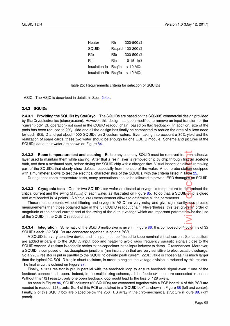
Livi
ngdo
cum
ent
QUBIC TDR Version 1.0 (May 12, 2017)
Heater Rh 300-500 Ω
SQUID Rsquid 100-200 Ω
Rfb Rfb 300-500 Ω
Rin Rin 10-15 kΩ
Insulation In Rsq/in > 10 MΩ
Insulation Fb Rsq/fb > 40 MΩ
Table 25: Requirements criteria for selection of SQUIDs
ASIC : The ASIC is described in details in Sect. 2.4.4.
2.4.3 SQUIDs
2.4.3.1 Providing the SQUIDs by StarCryo The SQUIDs are based on the SQ600S commercial design providedby StarCryoelectronics (starcryo.com). However, this design has been modified to remove an input transformer (for“current-lock” CL operation) not used in the QUBIC readout chain (based on flux feedback). In addition, size of thepads has been reduced to 200µ side and all the design has finally be compacted to reduce the area of silicon needfor each SQUID and put about 4000 SQUIDs on 2 custom wafers. Even taking into account a 80% yield and therealization of spare cards, these two wafer should be enough for one QUBIC module. Scheme and pictures of theSQUIDs aand their wafer are shown on Figure 84.
2.4.3.2 Room temperature test and cleaning Before any use, any SQUID must be removed from an adhesivelayer used to maintain them while sawing. After that a resin layer is removed chip by chip through first an acetonebath, and then a methanol bath, before drying the SQUID chip with a nitrogen flux. Visual inspection allows removingpart of the SQUIDs that clearly show defects, especially from the side of the wafer. A test probe-station equippedwith a multimeter allows to test the electrical characteristics of the SQUIDs, with the criteria listed in Table 25.
During these room temperature tests, many precautions should be followed to prevent ESD damages on SQUID.
2.4.3.3 Cryogenic test: One or two SQUIDs per wafer are tested at cryogenic temperature to determined thecritical current and the swing (∆Vsquid) of each wafer, as illustrated on Figure 85. To do that, a SQUID chip is gluedand wire bonded in “4 points”. A single V(φ) measurement allows to determine all the parameters.
These measurements without filtering and cryogenic ASIC are very noisy and give significantly less precisemeasurements than those obtained later in the full QUBIC readout chain. Nevertheless, this test gives an order ofmagnitude of the critical current and of the swing of the output voltage which are important parameters for the useof the SQUID in the QUBIC readout chain.
2.4.3.4 Integration Schematic of the SQUID multiplexer is given in Figure 86. It is composed of 4 columns of 32SQUIDs each. 32 SQUIDs are connected together using one PCB.
A SQUID is a very sensitive device and its input must be filtered to keep nominal critical current. So, capacitorsare added in parallel to the SQUID, input loop and heater to avoid radio frequency parasitic signals close to theSQUID washer. A resistor is added in series to the capacitors in the input inductor to damp LC resonances. Moreover,a SQUID is composed of two Josephson junctions (nm insulators) that are very sensitive to electrostatic discharge.So a 220Ω resistor is put in parallel to the SQUID to deviate peak current. 220Ω value is chosen as it is much largerthan the typical 2Ω SQUID fragile shunt resistors, in order to neglect the voltage division introduced by this resistor.The final circuit is oulined on Figure 87.
Finally, a 10Ω resistor is put in parallel with the feedback loop to ensure feedback signal even if one of thefeedback connection is open. Indeed, in the multiplexing scheme, all the feedback loops are connected in series.Without this 10Ω resistor, only one open feedback loop would lead to the loss of 128 pixels.
As seen in Figure 86, SQUID columns (32 SQUIDs) are connected together with a PCB board. 4 of this PCB areneeded to readout 128 pixels. So, 4 of this PCB are staked in a “SQUID box” as shown in Figure 88 (left and center).Finally, 2 of this SQUID box are placed below the 256 TES array in the cryo-mechanical structure (Figure 88, rightpanel).
Page 68
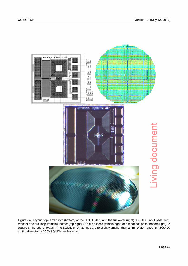
Livi
ngdo
cum
ent
QUBIC TDR Version 1.0 (May 12, 2017)
Figure 84: Layout (top) and photo (bottom) of the SQUID (left) and the full wafer (right). SQUID: input pads (left),Washer and flux loop (middle), heater (top right), SQUID access (middle right) and feedback pads (bottom right). Asquare of the grid is 100µm. The SQUID chip has thus a size slightly smaller than 2mm. Wafer: about 54 SQUIDson the diameter -> 2000 SQUIDs on the wafer.
Page 69
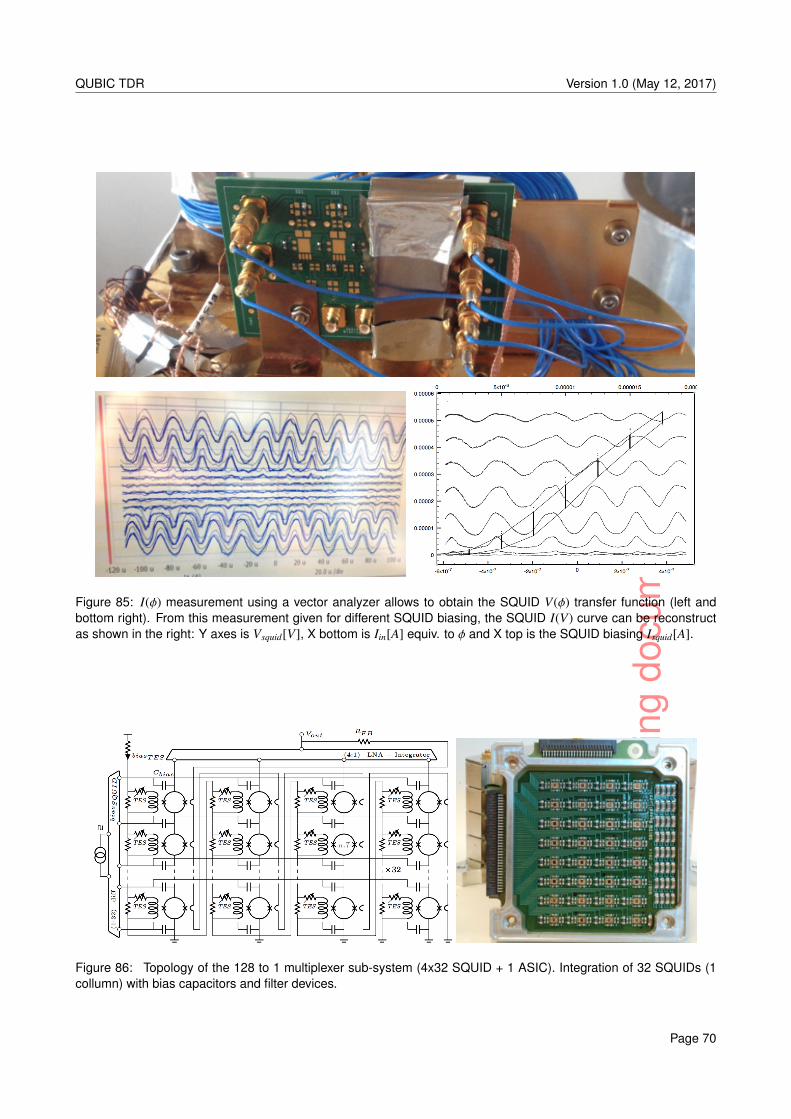
Livi
ngdo
cum
ent
QUBIC TDR Version 1.0 (May 12, 2017)
Figure 85: I(φ) measurement using a vector analyzer allows to obtain the SQUID V(φ) transfer function (left andbottom right). From this measurement given for different SQUID biasing, the SQUID I(V) curve can be reconstructas shown in the right: Y axes is Vsquid[V], X bottom is Iin[A] equiv. to φ and X top is the SQUID biasing Isquid[A].
Figure 86: Topology of the 128 to 1 multiplexer sub-system (4x32 SQUID + 1 ASIC). Integration of 32 SQUIDs (1collumn) with bias capacitors and filter devices.
Page 70
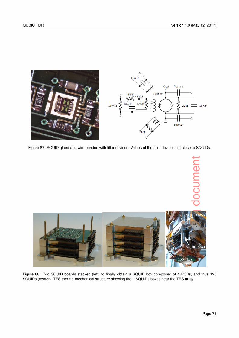
Livi
ngdo
cum
ent
QUBIC TDR Version 1.0 (May 12, 2017)
Figure 87: SQUID glued and wire bonded with filter devices. Values of the filter devices put close to SQUIDs.
Figure 88: Two SQUID boards stacked (left) to finally obtain a SQUID box composed of 4 PCBs, and thus 128SQUIDs (center). TES thermo-mechanical structure showing the 2 SQUIDs boxes near the TES array.
Page 71
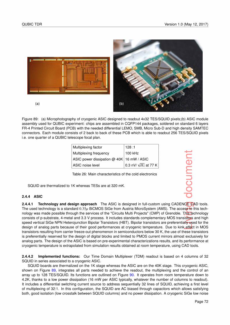
Livi
ngdo
cum
ent
QUBIC TDR Version 1.0 (May 12, 2017)
Figure 89: (a) Microphotography of cryogenic ASIC designed to readout 4x32 TES/SQUID pixels;(b) ASIC moduleassembly used for QUBIC experiment: chips are assembled in CQFP144 packages, soldered on standard 6 layersFR-4 Printed Circuit Board (PCB) with the needed differential LEMO, SMB, Micro Sub-D and high density SAMTECconnectors. Each module consists of 2 back to back of these PCB which is able to readout 256 TES/SQUID pixelsi.e. one quarter of a QUBIC telescope focal plan.
Multiplexing factor 128 :1
Multiplexing frequency 100 kHz
ASIC power dissipation @ 40K 16 mW / ASIC
ASIC noise level 0.3 nV/√
Hz at 77 K
Table 26: Main characteristics of the cold electronics
SQUID are thermalized to 1K whereas TESs are at 320 mK.
2.4.4 ASIC
2.4.4.1 Technology and design approach The ASIC is designed in full-custom using CADENCE CAD tools.The used technology is a standard 0.35µ BiCMOS SiGe from Austria MicroSystem (AMS). The access to this tech-nology was made possible through the services of the "Circuits Multi Projects" (CMP) of Grenoble. This technologyconsists of p-substrate, 4-metal and 3.3 V process. It includes standards complementary MOS transistors and highspeed vertical SiGe NPN Heterojunction Bipolar Transistors (HBT). Bipolar transistors are preferentially used for thedesign of analog parts because of their good performances at cryogenic temperature. Due to kink effect in MOStransistors resulting from carrier freeze-out phenomenon in semiconductors below 30 K, the use of these transistorsis preferentially reserved for the design of digital blocks and limited to PMOS current mirrors almost exclusively foranalog parts. The design of the ASIC is based on pre-experimental characterizations results, and its performance atcryogenic temperature is extrapolated from simulation results obtained at room temperature, using CAD tools.
2.4.4.2 Implemented functions: Our Time Domain Multiplexer (TDM) readout is based on 4 columns of 32SQUID in series associated to a cryogenic ASIC.
SQUID boards are thermalized on the 1K stage whereas the ASIC are on the 40K stage. This cryogenic ASIC,shown on Figure 89, integrates all parts needed to achieve the readout, the multiplexing and the control of anarray up to 128 TES/SQUID. Its functions are outlined on Figure 90. It operates from room temperature down to4.2K, thanks to a low power dissipation (16 mW per ASIC typically, whatever the number of columns to readout).It includes a differential switching current source to address sequentially 32 lines of SQUID, achieving a first levelof multiplexing of 32:1. In this configuration, the SQUID are AC biased through capacitors which allows satisfyingboth, good isolation (low crosstalk between SQUID columns) and no power dissipation. A cryogenic SiGe low noise
Page 72
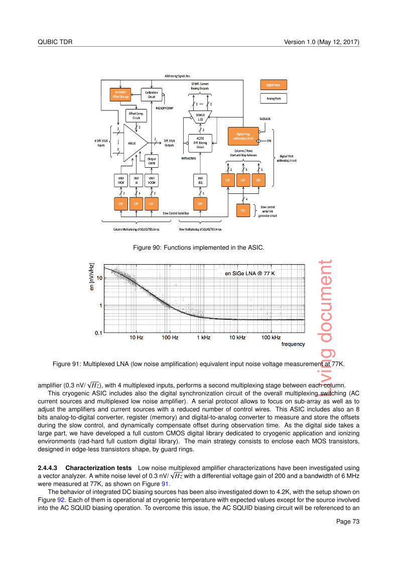
Livi
ngdo
cum
ent
QUBIC TDR Version 1.0 (May 12, 2017)
Figure 90: Functions implemented in the ASIC.
Figure 91: Multiplexed LNA (low noise amplification) equivalent input noise voltage measurement at 77K.
amplifier (0.3 nV/√
Hz), with 4 multiplexed inputs, performs a second multiplexing stage between each column.This cryogenic ASIC includes also the digital synchronization circuit of the overall multiplexing switching (AC
current sources and multiplexed low noise amplifier). A serial protocol allows to focus on sub-array as well as toadjust the amplifiers and current sources with a reduced number of control wires. This ASIC includes also an 8bits analog-to-digital converter, register (memory) and digital-to-analog converter to measure and store the offsetsduring the slow control, and dynamically compensate offset during observation time. As the digital side takes alarge part, we have developed a full custom CMOS digital library dedicated to cryogenic application and ionizingenvironments (rad-hard full custom digital library). The main strategy consists to enclose each MOS transistors,designed in edge-less transistors shape, by guard rings.
2.4.4.3 Characterization tests Low noise multiplexed amplifier characterizations have been investigated usinga vector analyzer. A white noise level of 0.3 nV/
√Hz with a differential voltage gain of 200 and a bandwidth of 6 MHz
were measured at 77K, as shown on Figure 91.The behavior of integrated DC biasing sources has been also investigated down to 4.2K, with the setup shown on
Figure 92. Each of them is operational at cryogenic temperature with expected values except for the source involvedinto the AC SQUID biasing operation. To overcome this issue, the AC SQUID biasing circuit will be referenced to an
Page 73
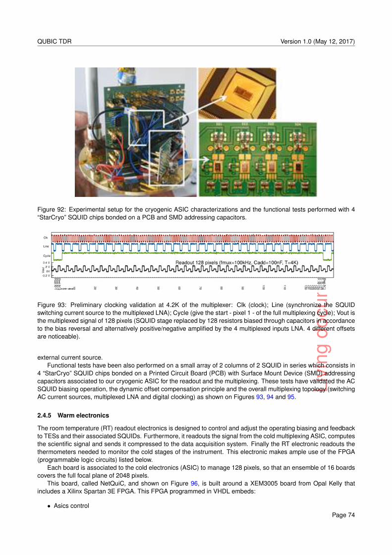
Livi
ngdo
cum
ent
QUBIC TDR Version 1.0 (May 12, 2017)
Figure 92: Experimental setup for the cryogenic ASIC characterizations and the functional tests performed with 4“StarCryo” SQUID chips bonded on a PCB and SMD addressing capacitors.
Figure 93: Preliminary clocking validation at 4.2K of the multiplexer: Clk (clock); Line (synchronize the SQUIDswitching current source to the multiplexed LNA); Cycle (give the start - pixel 1 - of the full multiplexing cycle); Vout isthe multiplexed signal of 128 pixels (SQUID stage replaced by 128 resistors biased through capacitors in accordanceto the bias reversal and alternatively positive/negative amplified by the 4 multiplexed inputs LNA. 4 different offsetsare noticeable).
external current source.Functional tests have been also performed on a small array of 2 columns of 2 SQUID in series which consists in
4 “StarCryo” SQUID chips bonded on a Printed Circuit Board (PCB) with Surface Mount Device (SMD) addressingcapacitors associated to our cryogenic ASIC for the readout and the multiplexing. These tests have validated the ACSQUID biasing operation, the dynamic offset compensation principle and the overall multiplexing topology (switchingAC current sources, multiplexed LNA and digital clocking) as shown on Figures 93, 94 and 95.
2.4.5 Warm electronics
The room temperature (RT) readout electronics is designed to control and adjust the operating biasing and feedbackto TESs and their associated SQUIDs. Furthermore, it readouts the signal from the cold multiplexing ASIC, computesthe scientific signal and sends it compressed to the data acquisition system. Finally the RT electronic readouts thethermometers needed to monitor the cold stages of the instrument. This electronic makes ample use of the FPGA(programmable logic circuits) listed below.
Each board is associated to the cold electronics (ASIC) to manage 128 pixels, so that an ensemble of 16 boardscovers the full focal plane of 2048 pixels.
This board, called NetQuiC, and shown on Figure 96, is built around a XEM3005 board from Opal Kelly thatincludes a Xilinx Spartan 3E FPGA. This FPGA programmed in VHDL embeds:
• Asics controlPage 74
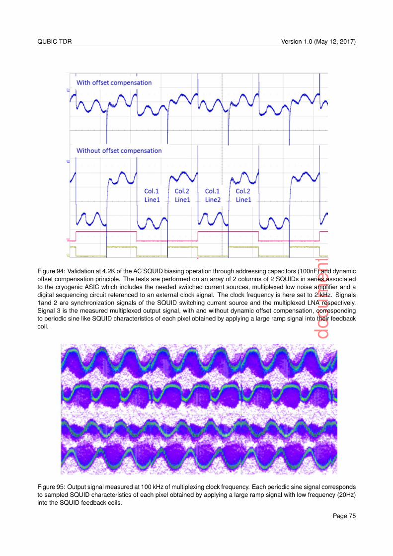
Livi
ngdo
cum
ent
QUBIC TDR Version 1.0 (May 12, 2017)
Figure 94: Validation at 4.2K of the AC SQUID biasing operation through addressing capacitors (100nF) and dynamicoffset compensation principle. The tests are performed on an array of 2 columns of 2 SQUIDs in series associatedto the cryogenic ASIC which includes the needed switched current sources, multiplexed low noise amplifier and adigital sequencing circuit referenced to an external clock signal. The clock frequency is here set to 2 kHz. Signals1and 2 are synchronization signals of the SQUID switching current source and the multiplexed LNA respectively.Signal 3 is the measured multiplexed output signal, with and without dynamic offset compensation, correspondingto periodic sine like SQUID characteristics of each pixel obtained by applying a large ramp signal into their feedbackcoil.
Figure 95: Output signal measured at 100 kHz of multiplexing clock frequency. Each periodic sine signal correspondsto sampled SQUID characteristics of each pixel obtained by applying a large ramp signal with low frequency (20Hz)into the SQUID feedback coils.
Page 75
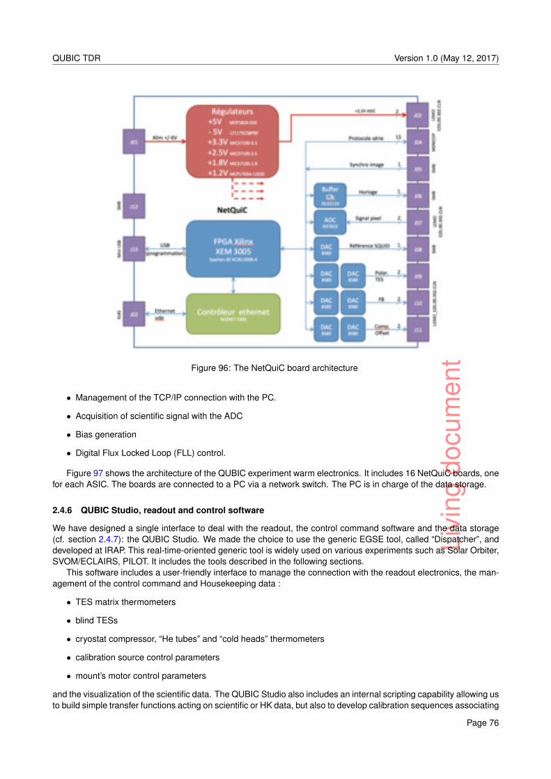
Livi
ngdo
cum
ent
QUBIC TDR Version 1.0 (May 12, 2017)
Figure 96: The NetQuiC board architecture
• Management of the TCP/IP connection with the PC.
• Acquisition of scientific signal with the ADC
• Bias generation
• Digital Flux Locked Loop (FLL) control.
Figure 97 shows the architecture of the QUBIC experiment warm electronics. It includes 16 NetQuiC boards, onefor each ASIC. The boards are connected to a PC via a network switch. The PC is in charge of the data storage.
2.4.6 QUBIC Studio, readout and control software
We have designed a single interface to deal with the readout, the control command software and the data storage(cf. section 2.4.7): the QUBIC Studio. We made the choice to use the generic EGSE tool, called “Dispatcher”, anddeveloped at IRAP. This real-time-oriented generic tool is widely used on various experiments such as Solar Orbiter,SVOM/ECLAIRS, PILOT. It includes the tools described in the following sections.
This software includes a user-friendly interface to manage the connection with the readout electronics, the man-agement of the control command and Housekeeping data :
• TES matrix thermometers
• blind TESs
• cryostat compressor, “He tubes” and “cold heads” thermometers
• calibration source control parameters
• mount’s motor control parameters
and the visualization of the scientific data. The QUBIC Studio also includes an internal scripting capability allowing usto build simple transfer functions acting on scientific or HK data, but also to develop calibration sequences associating
Page 76
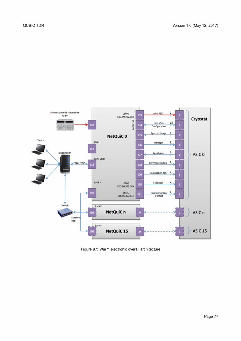
Livi
ngdo
cum
ent
QUBIC TDR Version 1.0 (May 12, 2017)
Figure 97: Warm electronic overall architecture
Page 77
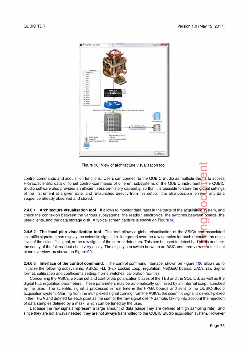
Livi
ngdo
cum
ent
QUBIC TDR Version 1.0 (May 12, 2017)
Figure 98: View of architecture visualization tool
control commands and acquisition functions. Users can connect to the QUBIC Studio as multiple clients to accessHK/raw/scientific data or to set control-commands of different subsystems of the QUBIC instrument. The QUBICStudio software also provides an efficient session-history capability, so that it is possible to store the global settingsof the instrument at a given date, and re-launched directly from this setup. It is also possible to rerun any datasequence already observed and stored.
2.4.6.1 Architecture visualisation tool It allows to monitor data rates in the parts of the acquisition system, andcheck the connexion between the various subsystems: the readout electronics, the switches between boards, theuser-clients, and the data storage disk. A typical screen capture is shown on Figure 98.
2.4.6.2 The focal plan visualization tool This tool allows a global visualisation of the ASICs and associatedscientific signals. It can display the scientific signal, i.e. integrated over the raw samples for each detector, the noiselevel of the scientific signal, or the raw signal of the current detectors. This can be used to detect bad pixels or checkthe sanity of the full readout chain very easily. The display can switch between an ASIC-centered view or a full focalplane overview, as shown on Figure 99.
2.4.6.3 Interface of the control command. The control command interface, shown on Figure 100 allows us toinitialize the following subsystems: ASICs, FLL (Flux Locked Loop) regulation, NetQuiC boards, DACs, raw Signalformat, calibration and coefficients setting, horns switches, calibration facilities
Concerning the ASICs, we can set and control the polarization biases of the TES and the SQUIDS, as well as thedigital FLL regulation parameters. These parameters may be automatically optimized by an internal script launchedby the user. The scientific signal is processed in real time in the FPGA boards and sent to the QUBIC-Studioacquisition system. Starting from the multiplexed signal coming from the ASICs, the scientific signal is de-multiplexedin the FPGA and defined for each pixel as the sum of the raw signal over NSample, taking into account the rejectionof data samples defined by a mask, which can be tuned by the user.
Because the raw signals represent a large amount of data (since they are defined at high sampling rate), andsince they are not always needed, they are not always transmitted to the QUBIC Studio acquisition system. However
Page 78
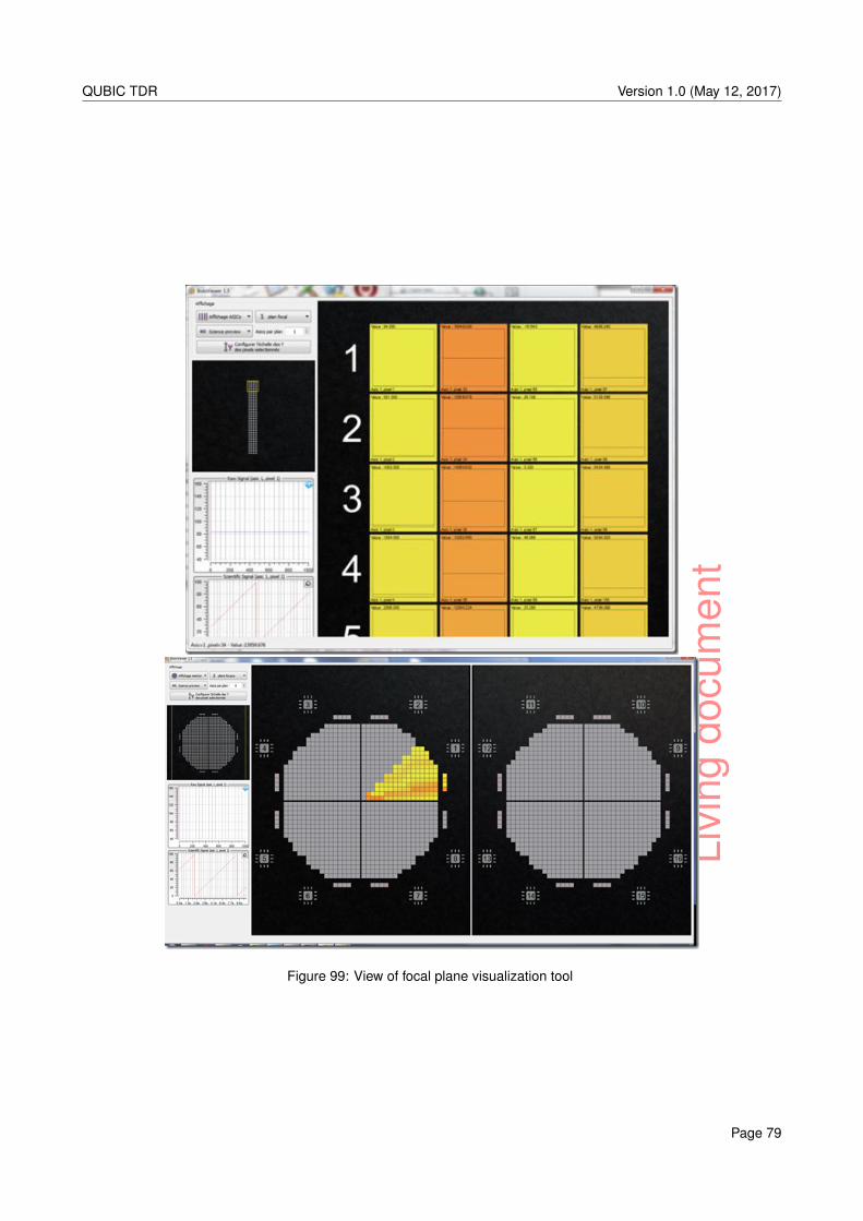
Livi
ngdo
cum
ent
QUBIC TDR Version 1.0 (May 12, 2017)
Figure 99: View of focal plane visualization tool
Page 79
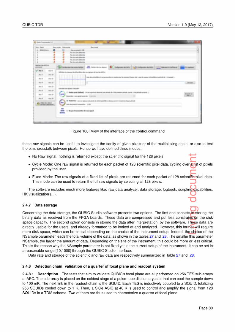
Livi
ngdo
cum
ent
QUBIC TDR Version 1.0 (May 12, 2017)
Figure 100: View of the interface of the control command
these raw signals can be useful to investigate the sanity of given pixels or of the multiplexing chain, or also to testthe e.m. crosstalk between pixels. Hence we have defined three modes:
• No Raw signal: nothing is returned except the scientific signal for the 128 pixels
• Cycle Mode: One raw signal is returned for each packet of 128 scientific pixel data, cycling over a list of pixelsprovided by the user
• Fixed Mode: The raw signals of a fixed list of pixels are returned for each packet of 128 scientific pixel data.This mode can be used to return the full raw signals by selecting all 128 pixels.
The software includes much more features like: raw data analyzer, data storage, logbook, scripting capabilities,HK visualization (...).
2.4.7 Data storage
Concerning the data storage, the QUBIC Studio software presents two options. The first one consists in storing thebinary data as received from the FPGA boards. These data are compressed and put less constrains on the diskspace capacity. The second option consists in storing the data after interpretation by the software. These data aredirectly usable for the users, and already formatted to be looked at and analyzed. However, this format will requiremore disk space, which can be critical depending on the choice of the instrument setup. Indeed, the choice of theNSample parameter leads the total volume of the data, as shown in the tables 27 and 28. The smaller this parameterNSample, the larger the amount of data. Depending on the site of the instrument, this could be more or less critical.This is the reason why the NSample parameter is not fixed yet in the current setup of the instrument. It can be set ina reasonable range [10,1000] through the QUBIC Studio interface.
Data rate and storage of the scientific and raw data are respectively summarized in Table 27 and 28.
2.4.8 Detection chain: validation of a quarter of focal plane and readout system
2.4.8.1 Description The tests that aim to validate QUBIC’s focal plane are all performed on 256 TES sub-arraysat APC. The sub-array is placed on the coldest stage of a pulse-tube dilution cryostat that can cool the sample downto 100 mK. The next link in the readout chain is the SQUID. Each TES is inductively coupled to a SQUID, totalizing256 SQUIDs cooled down to 1 K. Then, a SiGe ASIC at 40 K is used to control and amplify the signal from 128SQUIDs in a TDM scheme. Two of them are thus used to characterize a quarter of focal plane.
Page 80
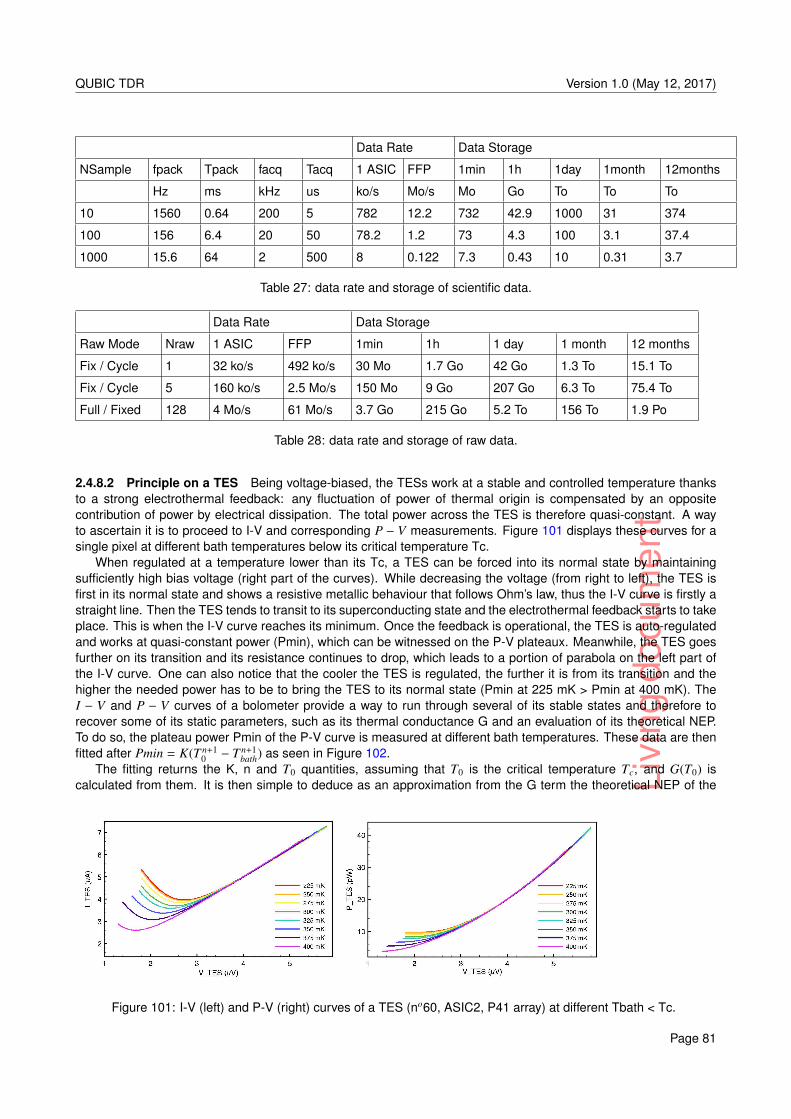
Livi
ngdo
cum
ent
QUBIC TDR Version 1.0 (May 12, 2017)
Data Rate Data Storage
NSample fpack Tpack facq Tacq 1 ASIC FFP 1min 1h 1day 1month 12months
Hz ms kHz us ko/s Mo/s Mo Go To To To
10 1560 0.64 200 5 782 12.2 732 42.9 1000 31 374
100 156 6.4 20 50 78.2 1.2 73 4.3 100 3.1 37.4
1000 15.6 64 2 500 8 0.122 7.3 0.43 10 0.31 3.7
Table 27: data rate and storage of scientific data.
Data Rate Data Storage
Raw Mode Nraw 1 ASIC FFP 1min 1h 1 day 1 month 12 months
Fix / Cycle 1 32 ko/s 492 ko/s 30 Mo 1.7 Go 42 Go 1.3 To 15.1 To
Fix / Cycle 5 160 ko/s 2.5 Mo/s 150 Mo 9 Go 207 Go 6.3 To 75.4 To
Full / Fixed 128 4 Mo/s 61 Mo/s 3.7 Go 215 Go 5.2 To 156 To 1.9 Po
Table 28: data rate and storage of raw data.
2.4.8.2 Principle on a TES Being voltage-biased, the TESs work at a stable and controlled temperature thanksto a strong electrothermal feedback: any fluctuation of power of thermal origin is compensated by an oppositecontribution of power by electrical dissipation. The total power across the TES is therefore quasi-constant. A wayto ascertain it is to proceed to I-V and corresponding P − V measurements. Figure 101 displays these curves for asingle pixel at different bath temperatures below its critical temperature Tc.
When regulated at a temperature lower than its Tc, a TES can be forced into its normal state by maintainingsufficiently high bias voltage (right part of the curves). While decreasing the voltage (from right to left), the TES isfirst in its normal state and shows a resistive metallic behaviour that follows Ohm’s law, thus the I-V curve is firstly astraight line. Then the TES tends to transit to its superconducting state and the electrothermal feedback starts to takeplace. This is when the I-V curve reaches its minimum. Once the feedback is operational, the TES is auto-regulatedand works at quasi-constant power (Pmin), which can be witnessed on the P-V plateaux. Meanwhile, the TES goesfurther on its transition and its resistance continues to drop, which leads to a portion of parabola on the left part ofthe I-V curve. One can also notice that the cooler the TES is regulated, the further it is from its transition and thehigher the needed power has to be to bring the TES to its normal state (Pmin at 225 mK > Pmin at 400 mK). TheI − V and P − V curves of a bolometer provide a way to run through several of its stable states and therefore torecover some of its static parameters, such as its thermal conductance G and an evaluation of its theoretical NEP.To do so, the plateau power Pmin of the P-V curve is measured at different bath temperatures. These data are thenfitted after Pmin = K(T n+1
0 − T n+1bath) as seen in Figure 102.
The fitting returns the K, n and T0 quantities, assuming that T0 is the critical temperature Tc, and G(T0) iscalculated from them. It is then simple to deduce as an approximation from the G term the theoretical NEP of the
Figure 101: I-V (left) and P-V (right) curves of a TES (no60, ASIC2, P41 array) at different Tbath < Tc.
Page 81
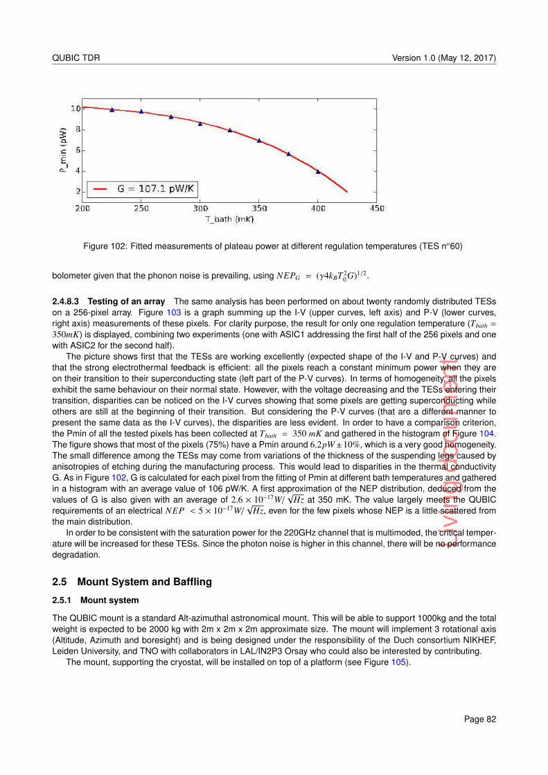
Livi
ngdo
cum
ent
QUBIC TDR Version 1.0 (May 12, 2017)
Figure 102: Fitted measurements of plateau power at different regulation temperatures (TES no60)
bolometer given that the phonon noise is prevailing, using NEPG = (γ4kBT 20G)1/2.
2.4.8.3 Testing of an array The same analysis has been performed on about twenty randomly distributed TESson a 256-pixel array. Figure 103 is a graph summing up the I-V (upper curves, left axis) and P-V (lower curves,right axis) measurements of these pixels. For clarity purpose, the result for only one regulation temperature (Tbath =
350mK) is displayed, combining two experiments (one with ASIC1 addressing the first half of the 256 pixels and onewith ASIC2 for the second half).
The picture shows first that the TESs are working excellently (expected shape of the I-V and P-V curves) andthat the strong electrothermal feedback is efficient: all the pixels reach a constant minimum power when they areon their transition to their superconducting state (left part of the P-V curves). In terms of homogeneity, all the pixelsexhibit the same behaviour on their normal state. However, with the voltage decreasing and the TESs entering theirtransition, disparities can be noticed on the I-V curves showing that some pixels are getting superconducting whileothers are still at the beginning of their transition. But considering the P-V curves (that are a different manner topresent the same data as the I-V curves), the disparities are less evident. In order to have a comparison criterion,the Pmin of all the tested pixels has been collected at Tbath = 350 mK and gathered in the histogram of Figure 104.The figure shows that most of the pixels (75%) have a Pmin around 6.2pW±10%, which is a very good homogeneity.The small difference among the TESs may come from variations of the thickness of the suspending legs caused byanisotropies of etching during the manufacturing process. This would lead to disparities in the thermal conductivityG. As in Figure 102, G is calculated for each pixel from the fitting of Pmin at different bath temperatures and gatheredin a histogram with an average value of 106 pW/K. A first approximation of the NEP distribution, deduced from thevalues of G is also given with an average of 2.6 × 10⁻¹⁷W/
√Hz at 350 mK. The value largely meets the QUBIC
requirements of an electrical NEP < 5 × 10⁻¹⁷W/√
Hz, even for the few pixels whose NEP is a little scattered fromthe main distribution.
In order to be consistent with the saturation power for the 220GHz channel that is multimoded, the critical temper-ature will be increased for these TESs. Since the photon noise is higher in this channel, there will be no performancedegradation.
2.5 Mount System and Baffling
2.5.1 Mount system
The QUBIC mount is a standard Alt-azimuthal astronomical mount. This will be able to support 1000kg and the totalweight is expected to be 2000 kg with 2m x 2m x 2m approximate size. The mount will implement 3 rotational axis(Altitude, Azimuth and boresight) and is being designed under the responsibility of the Duch consortium NIKHEF,Leiden University, and TNO with collaborators in LAL/IN2P3 Orsay who could also be interested by contributing.
The mount, supporting the cryostat, will be installed on top of a platform (see Figure 105).
Page 82
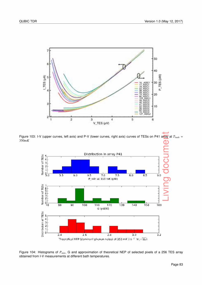
Livi
ngdo
cum
ent
QUBIC TDR Version 1.0 (May 12, 2017)
Figure 103: I-V (upper curves, left axis) and P-V (lower curves, right axis) curves of TESs on P41 array at Tbath =
350mK
Figure 104: Histograms of Pmin, G and approximation of theoretical NEP of selected pixels of a 256 TES arrayobtained from I-V measurements at different bath temperatures.
Page 83
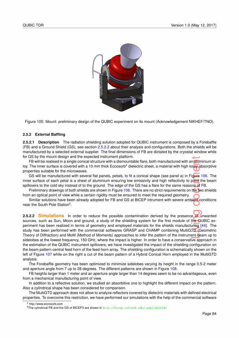
Livi
ngdo
cum
ent
QUBIC TDR Version 1.0 (May 12, 2017)
Figure 105: Mount: preliminary design of the QUBIC experiment on its mount (Acknowledgement NIKHEF/TNO).
2.5.2 External Baffling
2.5.2.1 Description The radiation shielding solution adopted for QUBIC instrument is composed by a Forebaffle(FB) and a Ground Shield (GS), see section 2.5.2.2 about their analysis and configurations. Both the shields will bemanufactured by a selected external supplier. The final dimensions of FB are dictated by the cryostat window whilefor GS by the mount design and the expected instrument platform.
FB will be realised in a single conical structure with a dismountable flare, both manufactured with an aluminium al-loy. The inner surface is covered with a 10 mm thick Eccosorb4 dielectric sheet, a material with high lossy absorptiveproperties suitable for the microwaves.
GS will be manufactured with several flat panels, petals, to fit a conical shape (see panel a) in Figure 106. Theinner surface of each petal is a sheet of aluminium ensuring low emissivity and high reflectivity to point the beamspillovers to the cold sky instead of to the ground. The edge of the GS has a flare for the same reasons of FB.
Preliminary drawings of both shields are shown in Figure 106. There are no strict requirements on the two shieldsfrom an optical point of view while a certain rigidity must be ensured to meet the required geometry.
Similar solutions have been already adopted for FB and GS at BICEP intrument with severe ambient conditionsnear the South Pole Station5.
2.5.2.2 Simulations In order to reduce the possible contamination derived by the presence of unwantedsources, such as Sun, Moon and ground, a study of the shielding system for the first module of the QUBIC ex-periment has been realized in terms of geometry and employed materials for the shields manufacturing [44]. Thestudy has been performed with the commercial softwares GRASP and CHAMP combining MultiGTD (GeometricTheory of Diffraction) and MoM (Method of Moments) approaches to infer the pattern of the instrument beam up tosidelobes at the lowest frequency, 150 GHz, where the impact is higher. In order to have a conservative approach inthe estimation of the QUBIC instrument spillovers, we have investigated the impact of the shielding configuration onthe beam pattern central feed horn of the feed-horn array. The shielding configuration is schematically shown on theleft of Figure 107 while on the right a cut of the beam pattern of a Hybrid Conical Horn employed in the MultiGTDanalysis.
The Forebaffle geometry has been optimized to minimize sidelobes varying its height in the range 0.5-2 meterand aperture angle from 7 up to 28 degrees. The different patterns are shown in Figure 108.
FB heights larger than 1 meter and an aperture angle larger than 14 degrees seem to be no advantageous, evenfrom a mechanical manufacturing point of view.
In addition to a reflective solution, we studied an absorbitive one to highlight the different impact on the pattern.Also a cylindrical shape has been considered for comparison.
The MultiGTD approach does not allow to analyze reflectors covered by dielectric materials with defined electricalproperties. To overcome this restriction, we have performed our simulations with the help of the commercial software
4 http://www.eccosorb.com5The cylindrical FB and the GS of BICEP3 are shown in http://bicep.caltech.edu/~yuki/shield/
Page 84
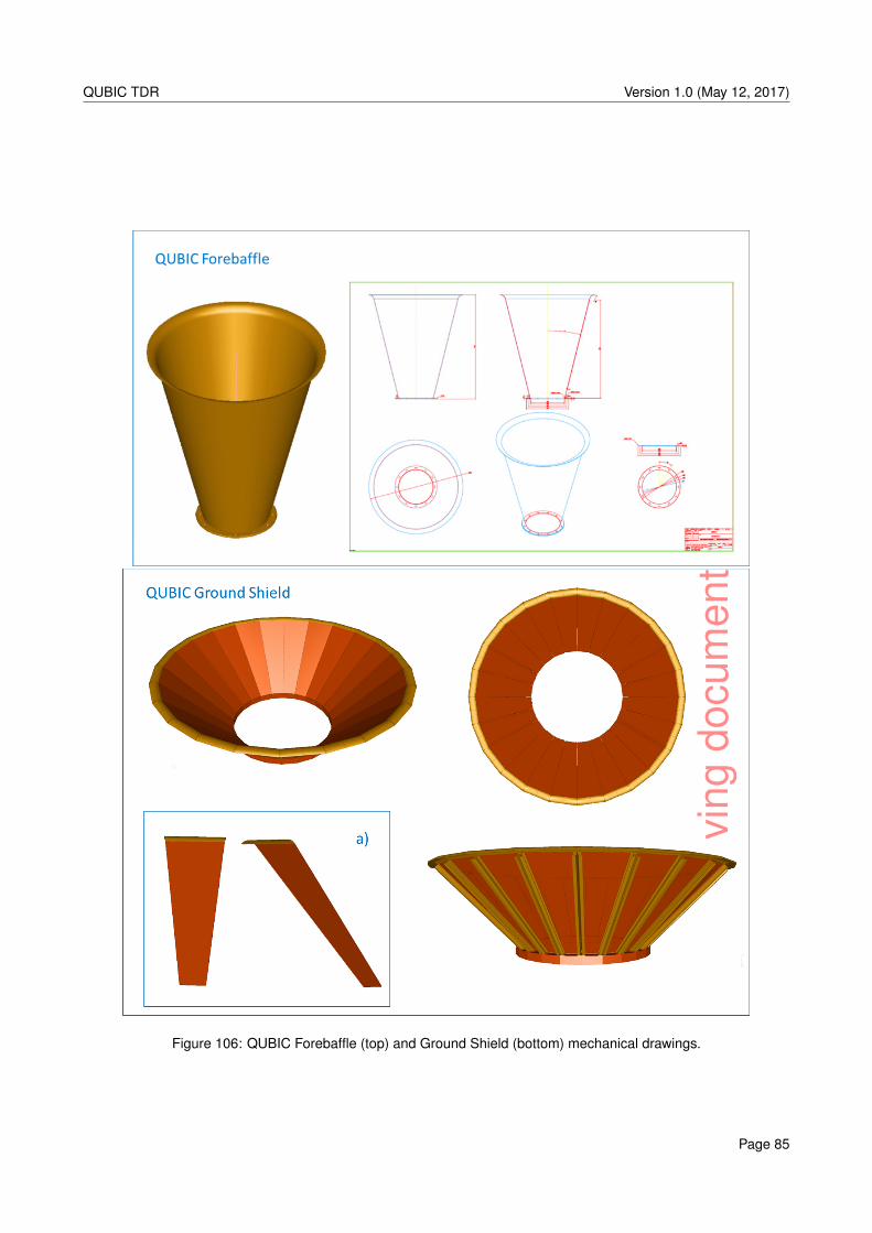
Livi
ngdo
cum
ent
QUBIC TDR Version 1.0 (May 12, 2017)
Figure 106: QUBIC Forebaffle (top) and Ground Shield (bottom) mechanical drawings.
Page 85
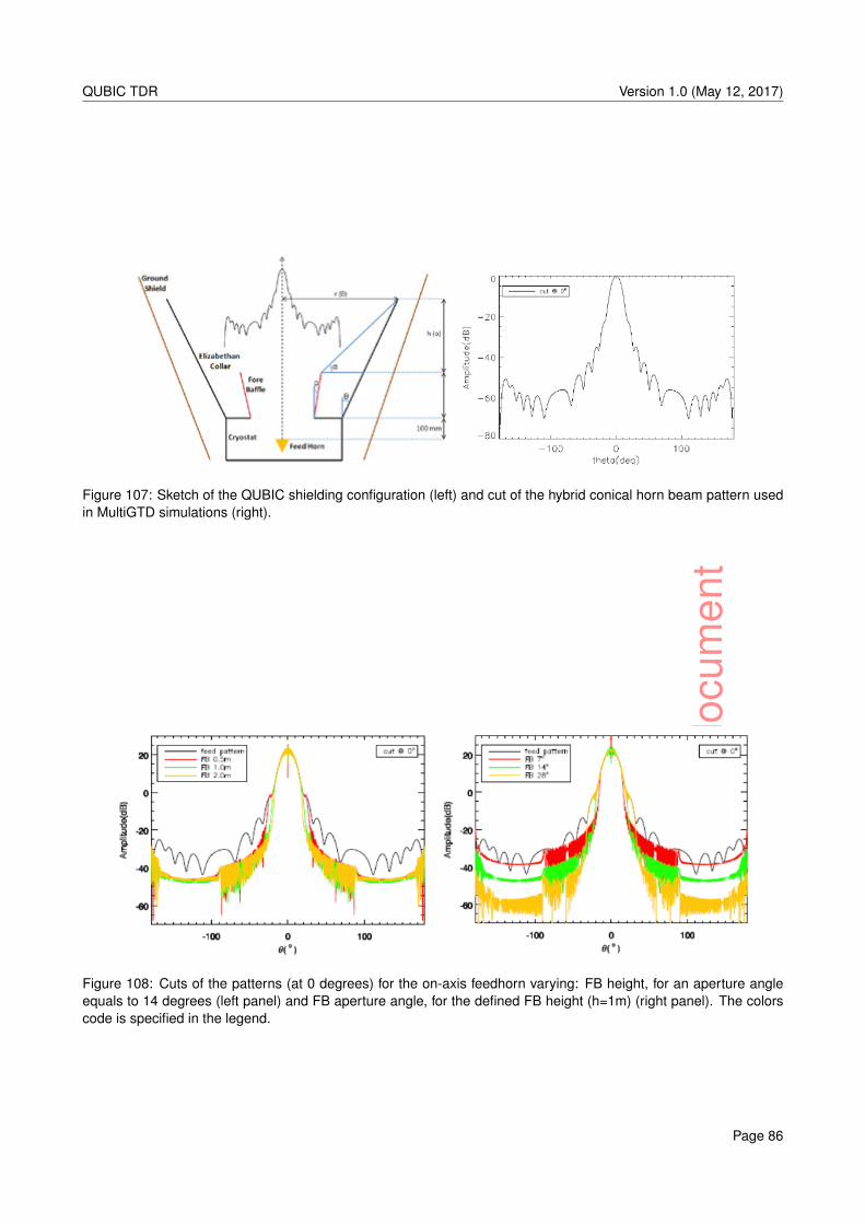
Livi
ngdo
cum
ent
QUBIC TDR Version 1.0 (May 12, 2017)
Figure 107: Sketch of the QUBIC shielding configuration (left) and cut of the hybrid conical horn beam pattern usedin MultiGTD simulations (right).
Figure 108: Cuts of the patterns (at 0 degrees) for the on-axis feedhorn varying: FB height, for an aperture angleequals to 14 degrees (left panel) and FB aperture angle, for the defined FB height (h=1m) (right panel). The colorscode is specified in the legend.
Page 86
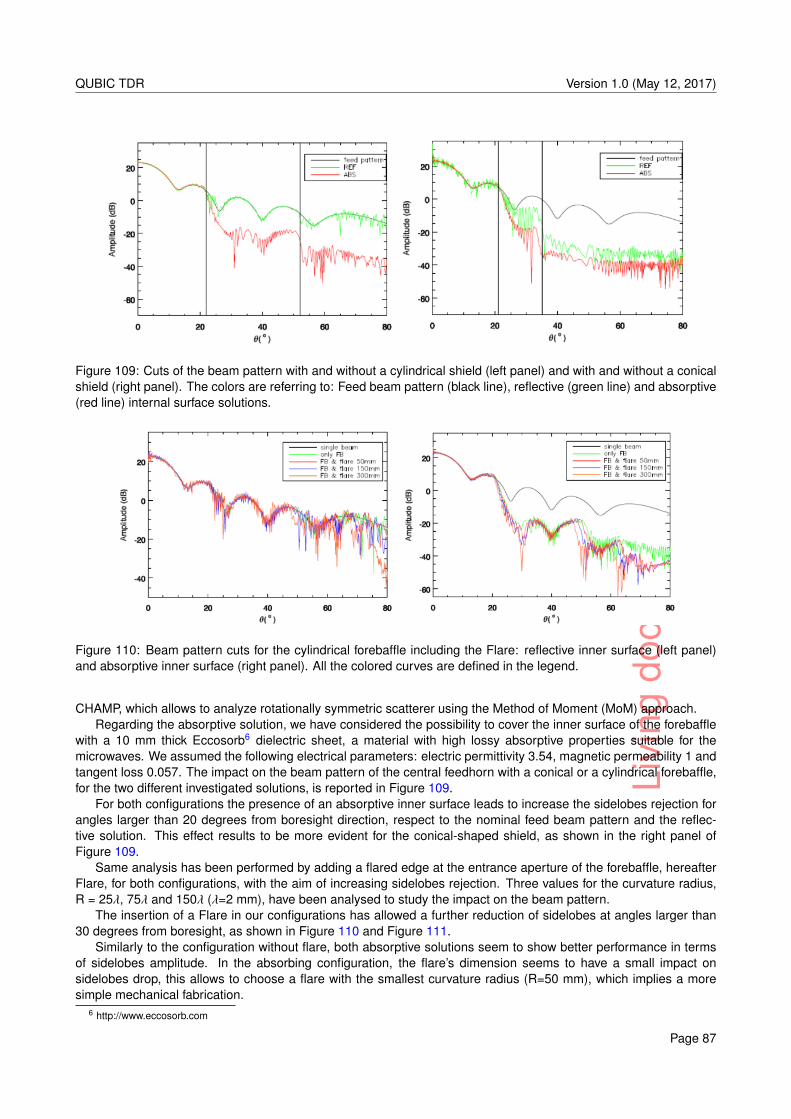
Livi
ngdo
cum
ent
QUBIC TDR Version 1.0 (May 12, 2017)
Figure 109: Cuts of the beam pattern with and without a cylindrical shield (left panel) and with and without a conicalshield (right panel). The colors are referring to: Feed beam pattern (black line), reflective (green line) and absorptive(red line) internal surface solutions.
Figure 110: Beam pattern cuts for the cylindrical forebaffle including the Flare: reflective inner surface (left panel)and absorptive inner surface (right panel). All the colored curves are defined in the legend.
CHAMP, which allows to analyze rotationally symmetric scatterer using the Method of Moment (MoM) approach.Regarding the absorptive solution, we have considered the possibility to cover the inner surface of the forebaffle
with a 10 mm thick Eccosorb6 dielectric sheet, a material with high lossy absorptive properties suitable for themicrowaves. We assumed the following electrical parameters: electric permittivity 3.54, magnetic permeability 1 andtangent loss 0.057. The impact on the beam pattern of the central feedhorn with a conical or a cylindrical forebaffle,for the two different investigated solutions, is reported in Figure 109.
For both configurations the presence of an absorptive inner surface leads to increase the sidelobes rejection forangles larger than 20 degrees from boresight direction, respect to the nominal feed beam pattern and the reflec-tive solution. This effect results to be more evident for the conical-shaped shield, as shown in the right panel ofFigure 109.
Same analysis has been performed by adding a flared edge at the entrance aperture of the forebaffle, hereafterFlare, for both configurations, with the aim of increasing sidelobes rejection. Three values for the curvature radius,R = 25λ, 75λ and 150λ (λ=2 mm), have been analysed to study the impact on the beam pattern.
The insertion of a Flare in our configurations has allowed a further reduction of sidelobes at angles larger than30 degrees from boresight, as shown in Figure 110 and Figure 111.
Similarly to the configuration without flare, both absorptive solutions seem to show better performance in termsof sidelobes amplitude. In the absorbing configuration, the flare’s dimension seems to have a small impact onsidelobes drop, this allows to choose a flare with the smallest curvature radius (R=50 mm), which implies a moresimple mechanical fabrication.
6 http://www.eccosorb.com
Page 87
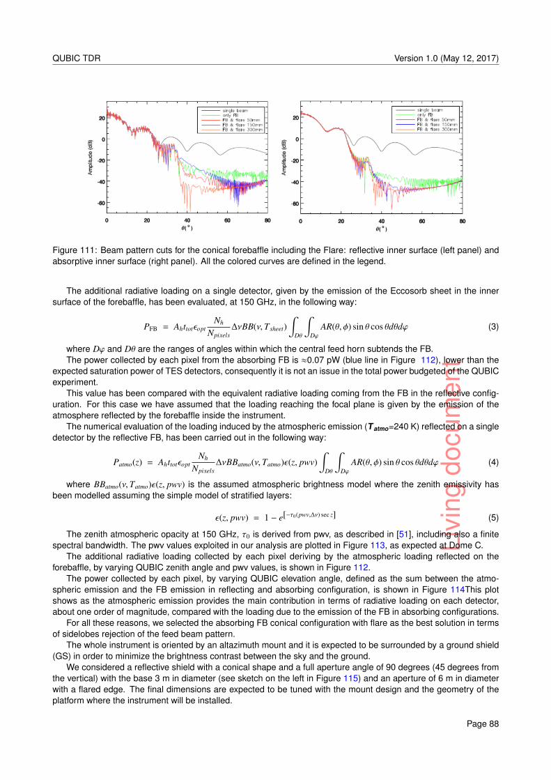
Livi
ngdo
cum
ent
QUBIC TDR Version 1.0 (May 12, 2017)
Figure 111: Beam pattern cuts for the conical forebaffle including the Flare: reflective inner surface (left panel) andabsorptive inner surface (right panel). All the colored curves are defined in the legend.
The additional radiative loading on a single detector, given by the emission of the Eccosorb sheet in the innersurface of the forebaffle, has been evaluated, at 150 GHz, in the following way:
PFB = AhttotεoptNh
Npixels∆νBB(ν,Tsheet)
∫Dθ
∫Dϕ
AR(θ, φ) sin θ cos θdθdϕ (3)
where Dϕ and Dθ are the ranges of angles within which the central feed horn subtends the FB.The power collected by each pixel from the absorbing FB is ≈0.07 pW (blue line in Figure 112), lower than the
expected saturation power of TES detectors, consequently it is not an issue in the total power budgeted of the QUBICexperiment.
This value has been compared with the equivalent radiative loading coming from the FB in the reflective config-uration. For this case we have assumed that the loading reaching the focal plane is given by the emission of theatmosphere reflected by the forebaffle inside the instrument.
The numerical evaluation of the loading induced by the atmospheric emission (Tatmo=240 K) reflected on a singledetector by the reflective FB, has been carried out in the following way:
Patmo(z) = AhttotεoptNh
Npixels∆νBBatmo(ν,Tatmo)ε(z, pwv)
∫Dθ
∫Dϕ
AR(θ, φ) sin θ cos θdθdϕ (4)
where BBatmo(ν,Tatmo)ε(z, pwv) is the assumed atmospheric brightness model where the zenith emissivity hasbeen modelled assuming the simple model of stratified layers:
ε(z, pwv) = 1 − e[−τ0(pwv,∆ν) sec z] (5)
The zenith atmospheric opacity at 150 GHz, τ0 is derived from pwv, as described in [51], including also a finitespectral bandwidth. The pwv values exploited in our analysis are plotted in Figure 113, as expected at Dome C.
The additional radiative loading collected by each pixel deriving by the atmospheric loading reflected on theforebaffle, by varying QUBIC zenith angle and pwv values, is shown in Figure 112.
The power collected by each pixel, by varying QUBIC elevation angle, defined as the sum between the atmo-spheric emission and the FB emission in reflecting and absorbing configuration, is shown in Figure 114This plotshows as the atmospheric emission provides the main contribution in terms of radiative loading on each detector,about one order of magnitude, compared with the loading due to the emission of the FB in absorbing configurations.
For all these reasons, we selected the absorbing FB conical configuration with flare as the best solution in termsof sidelobes rejection of the feed beam pattern.
The whole instrument is oriented by an altazimuth mount and it is expected to be surrounded by a ground shield(GS) in order to minimize the brightness contrast between the sky and the ground.
We considered a reflective shield with a conical shape and a full aperture angle of 90 degrees (45 degrees fromthe vertical) with the base 3 m in diameter (see sketch on the left in Figure 115) and an aperture of 6 m in diameterwith a flared edge. The final dimensions are expected to be tuned with the mount design and the geometry of theplatform where the instrument will be installed.
Page 88
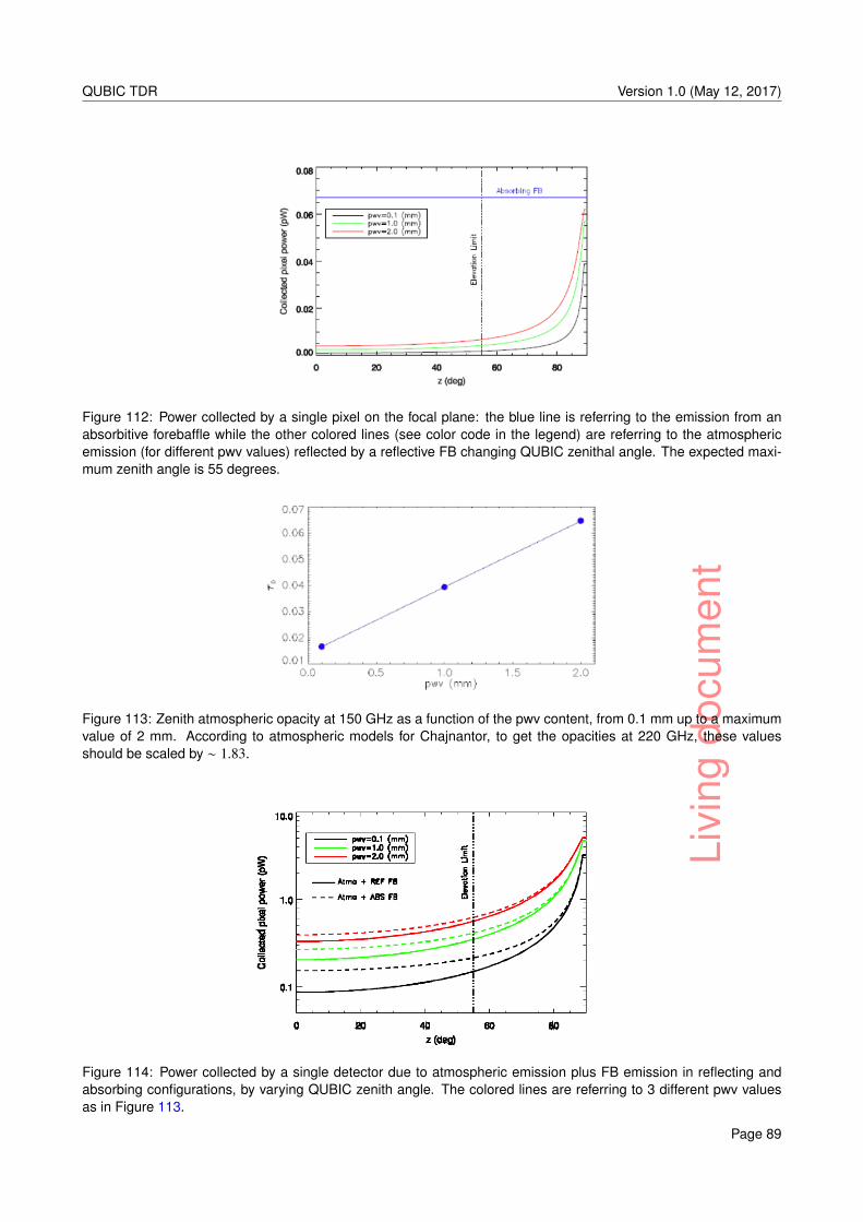
Livi
ngdo
cum
ent
QUBIC TDR Version 1.0 (May 12, 2017)
Figure 112: Power collected by a single pixel on the focal plane: the blue line is referring to the emission from anabsorbitive forebaffle while the other colored lines (see color code in the legend) are referring to the atmosphericemission (for different pwv values) reflected by a reflective FB changing QUBIC zenithal angle. The expected maxi-mum zenith angle is 55 degrees.
Figure 113: Zenith atmospheric opacity at 150 GHz as a function of the pwv content, from 0.1 mm up to a maximumvalue of 2 mm. According to atmospheric models for Chajnantor, to get the opacities at 220 GHz, these valuesshould be scaled by ∼ 1.83.
Figure 114: Power collected by a single detector due to atmospheric emission plus FB emission in reflecting andabsorbing configurations, by varying QUBIC zenith angle. The colored lines are referring to 3 different pwv valuesas in Figure 113.
Page 89
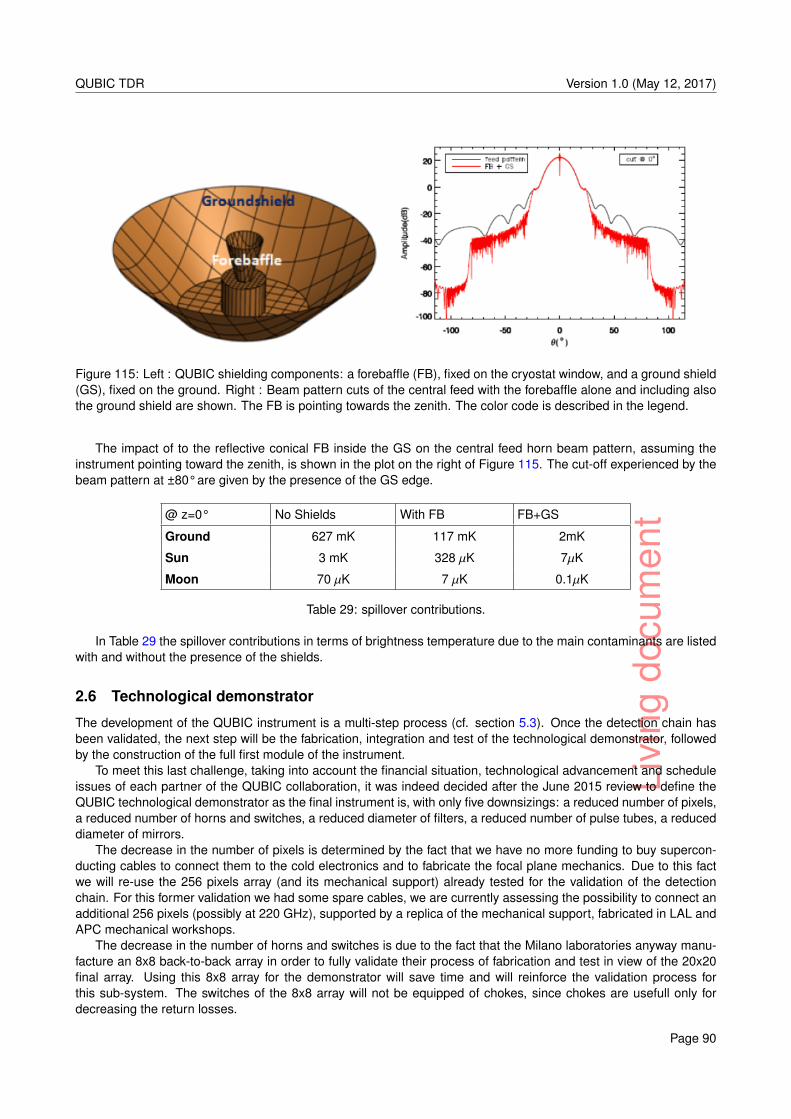
Livi
ngdo
cum
ent
QUBIC TDR Version 1.0 (May 12, 2017)
Figure 115: Left : QUBIC shielding components: a forebaffle (FB), fixed on the cryostat window, and a ground shield(GS), fixed on the ground. Right : Beam pattern cuts of the central feed with the forebaffle alone and including alsothe ground shield are shown. The FB is pointing towards the zenith. The color code is described in the legend.
The impact of to the reflective conical FB inside the GS on the central feed horn beam pattern, assuming theinstrument pointing toward the zenith, is shown in the plot on the right of Figure 115. The cut-off experienced by thebeam pattern at ±80° are given by the presence of the GS edge.
@ z=0° No Shields With FB FB+GS
Ground 627 mK 117 mK 2mK
Sun 3 mK 328 µK 7µK
Moon 70 µK 7 µK 0.1µK
Table 29: spillover contributions.
In Table 29 the spillover contributions in terms of brightness temperature due to the main contaminants are listedwith and without the presence of the shields.
2.6 Technological demonstrator
The development of the QUBIC instrument is a multi-step process (cf. section 5.3). Once the detection chain hasbeen validated, the next step will be the fabrication, integration and test of the technological demonstrator, followedby the construction of the full first module of the instrument.
To meet this last challenge, taking into account the financial situation, technological advancement and scheduleissues of each partner of the QUBIC collaboration, it was indeed decided after the June 2015 review to define theQUBIC technological demonstrator as the final instrument is, with only five downsizings: a reduced number of pixels,a reduced number of horns and switches, a reduced diameter of filters, a reduced number of pulse tubes, a reduceddiameter of mirrors.
The decrease in the number of pixels is determined by the fact that we have no more funding to buy supercon-ducting cables to connect them to the cold electronics and to fabricate the focal plane mechanics. Due to this factwe will re-use the 256 pixels array (and its mechanical support) already tested for the validation of the detectionchain. For this former validation we had some spare cables, we are currently assessing the possibility to connect anadditional 256 pixels (possibly at 220 GHz), supported by a replica of the mechanical support, fabricated in LAL andAPC mechanical workshops.
The decrease in the number of horns and switches is due to the fact that the Milano laboratories anyway manu-facture an 8x8 back-to-back array in order to fully validate their process of fabrication and test in view of the 20x20final array. Using this 8x8 array for the demonstrator will save time and will reinforce the validation process forthis sub-system. The switches of the 8x8 array will not be equipped of chokes, since chokes are usefull only fordecreasing the return losses.
Page 90
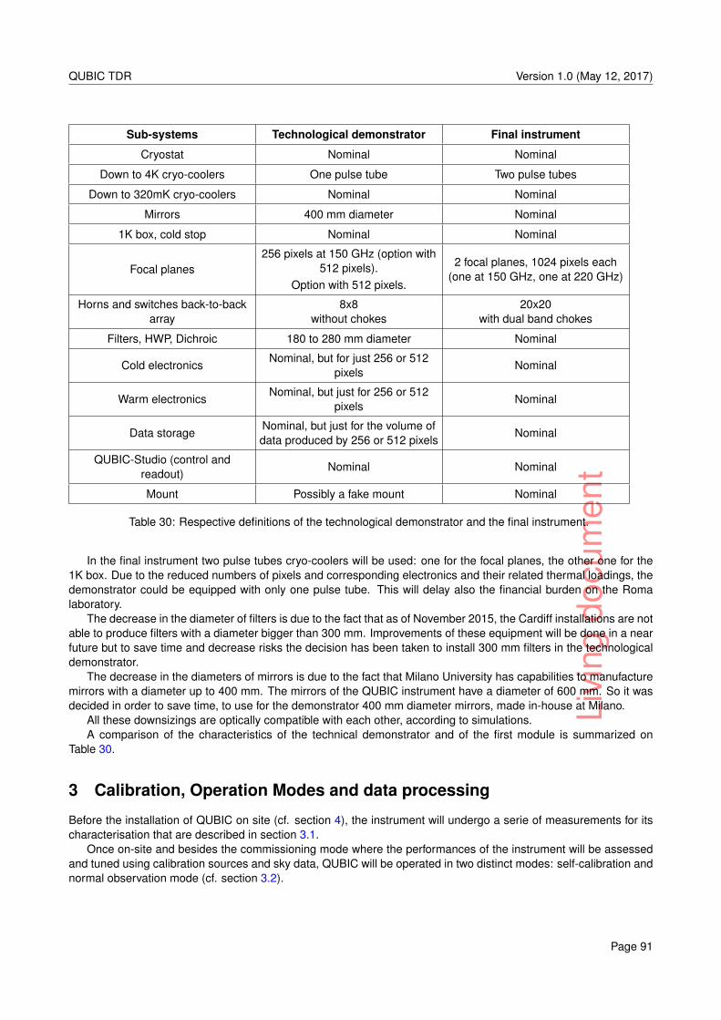
Livi
ngdo
cum
ent
QUBIC TDR Version 1.0 (May 12, 2017)
Sub-systems Technological demonstrator Final instrument
Cryostat Nominal Nominal
Down to 4K cryo-coolers One pulse tube Two pulse tubes
Down to 320mK cryo-coolers Nominal Nominal
Mirrors 400 mm diameter Nominal
1K box, cold stop Nominal Nominal
Focal planes256 pixels at 150 GHz (option with
512 pixels).Option with 512 pixels.
2 focal planes, 1024 pixels each(one at 150 GHz, one at 220 GHz)
Horns and switches back-to-backarray
8x8without chokes
20x20with dual band chokes
Filters, HWP, Dichroic 180 to 280 mm diameter Nominal
Cold electronicsNominal, but for just 256 or 512
pixelsNominal
Warm electronicsNominal, but just for 256 or 512
pixelsNominal
Data storageNominal, but just for the volume ofdata produced by 256 or 512 pixels
Nominal
QUBIC-Studio (control andreadout)
Nominal Nominal
Mount Possibly a fake mount Nominal
Table 30: Respective definitions of the technological demonstrator and the final instrument.
In the final instrument two pulse tubes cryo-coolers will be used: one for the focal planes, the other one for the1K box. Due to the reduced numbers of pixels and corresponding electronics and their related thermal loadings, thedemonstrator could be equipped with only one pulse tube. This will delay also the financial burden on the Romalaboratory.
The decrease in the diameter of filters is due to the fact that as of November 2015, the Cardiff installations are notable to produce filters with a diameter bigger than 300 mm. Improvements of these equipment will be done in a nearfuture but to save time and decrease risks the decision has been taken to install 300 mm filters in the technologicaldemonstrator.
The decrease in the diameters of mirrors is due to the fact that Milano University has capabilities to manufacturemirrors with a diameter up to 400 mm. The mirrors of the QUBIC instrument have a diameter of 600 mm. So it wasdecided in order to save time, to use for the demonstrator 400 mm diameter mirrors, made in-house at Milano.
All these downsizings are optically compatible with each other, according to simulations.A comparison of the characteristics of the technical demonstrator and of the first module is summarized on
Table 30.
3 Calibration, Operation Modes and data processing
Before the installation of QUBIC on site (cf. section 4), the instrument will undergo a serie of measurements for itscharacterisation that are described in section 3.1.
Once on-site and besides the commissioning mode where the performances of the instrument will be assessedand tuned using calibration sources and sky data, QUBIC will be operated in two distinct modes: self-calibration andnormal observation mode (cf. section 3.2).
Page 91
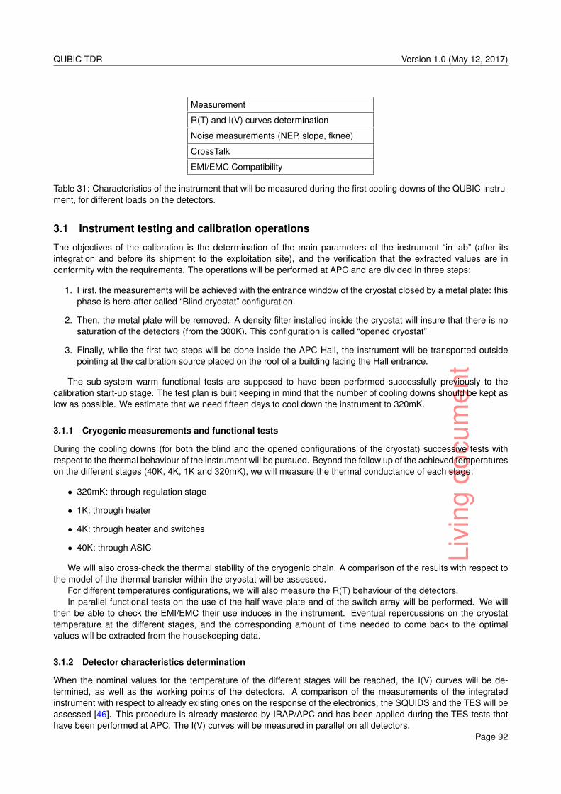
Livi
ngdo
cum
ent
QUBIC TDR Version 1.0 (May 12, 2017)
Measurement
R(T) and I(V) curves determination
Noise measurements (NEP, slope, fknee)
CrossTalk
EMI/EMC Compatibility
Table 31: Characteristics of the instrument that will be measured during the first cooling downs of the QUBIC instru-ment, for different loads on the detectors.
3.1 Instrument testing and calibration operations
The objectives of the calibration is the determination of the main parameters of the instrument “in lab” (after itsintegration and before its shipment to the exploitation site), and the verification that the extracted values are inconformity with the requirements. The operations will be performed at APC and are divided in three steps:
1. First, the measurements will be achieved with the entrance window of the cryostat closed by a metal plate: thisphase is here-after called “Blind cryostat” configuration.
2. Then, the metal plate will be removed. A density filter installed inside the cryostat will insure that there is nosaturation of the detectors (from the 300K). This configuration is called “opened cryostat”
3. Finally, while the first two steps will be done inside the APC Hall, the instrument will be transported outsidepointing at the calibration source placed on the roof of a building facing the Hall entrance.
The sub-system warm functional tests are supposed to have been performed successfully previously to thecalibration start-up stage. The test plan is built keeping in mind that the number of cooling downs should be kept aslow as possible. We estimate that we need fifteen days to cool down the instrument to 320mK.
3.1.1 Cryogenic measurements and functional tests
During the cooling downs (for both the blind and the opened configurations of the cryostat) successive tests withrespect to the thermal behaviour of the instrument will be pursued. Beyond the follow up of the achieved temperatureson the different stages (40K, 4K, 1K and 320mK), we will measure the thermal conductance of each stage:
• 320mK: through regulation stage
• 1K: through heater
• 4K: through heater and switches
• 40K: through ASIC
We will also cross-check the thermal stability of the cryogenic chain. A comparison of the results with respect tothe model of the thermal transfer within the cryostat will be assessed.
For different temperatures configurations, we will also measure the R(T) behaviour of the detectors.In parallel functional tests on the use of the half wave plate and of the switch array will be performed. We will
then be able to check the EMI/EMC their use induces in the instrument. Eventual repercussions on the cryostattemperature at the different stages, and the corresponding amount of time needed to come back to the optimalvalues will be extracted from the housekeeping data.
3.1.2 Detector characteristics determination
When the nominal values for the temperature of the different stages will be reached, the I(V) curves will be de-termined, as well as the working points of the detectors. A comparison of the measurements of the integratedinstrument with respect to already existing ones on the response of the electronics, the SQUIDS and the TES will beassessed [46]. This procedure is already mastered by IRAP/APC and has been applied during the TES tests thathave been performed at APC. The I(V) curves will be measured in parallel on all detectors.
Page 92
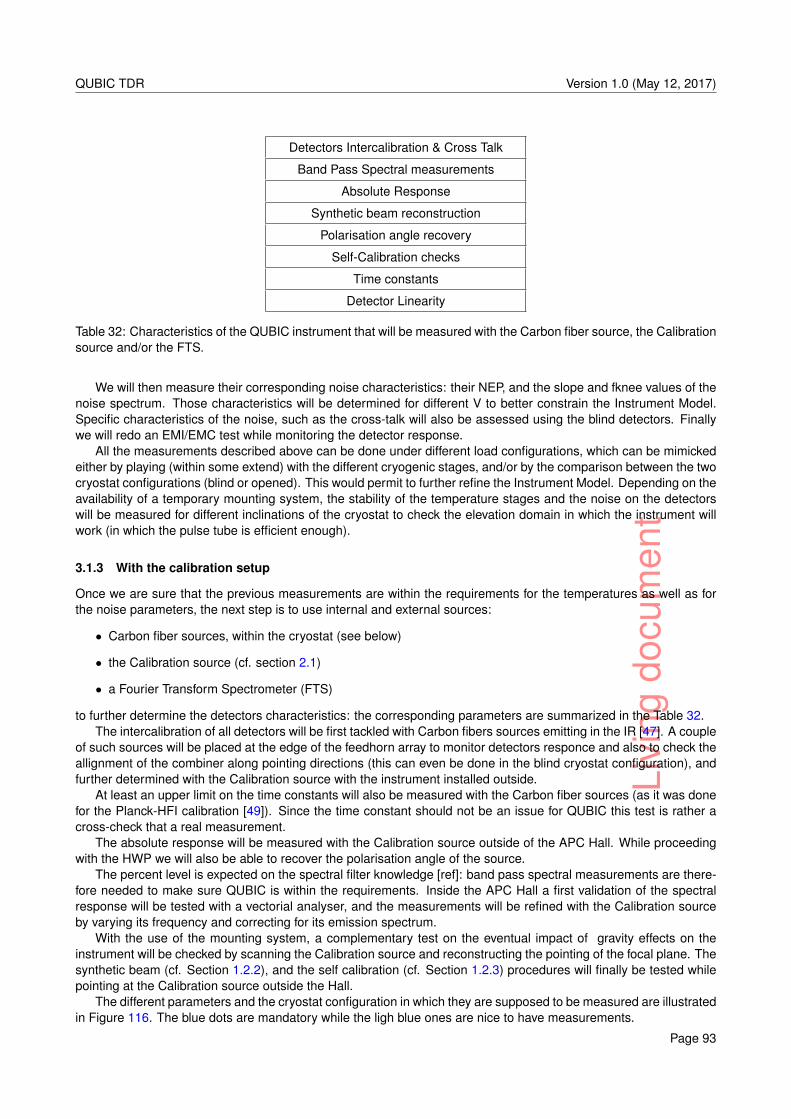
Livi
ngdo
cum
ent
QUBIC TDR Version 1.0 (May 12, 2017)
Detectors Intercalibration & Cross Talk
Band Pass Spectral measurements
Absolute Response
Synthetic beam reconstruction
Polarisation angle recovery
Self-Calibration checks
Time constants
Detector Linearity
Table 32: Characteristics of the QUBIC instrument that will be measured with the Carbon fiber source, the Calibrationsource and/or the FTS.
We will then measure their corresponding noise characteristics: their NEP, and the slope and fknee values of thenoise spectrum. Those characteristics will be determined for different V to better constrain the Instrument Model.Specific characteristics of the noise, such as the cross-talk will also be assessed using the blind detectors. Finallywe will redo an EMI/EMC test while monitoring the detector response.
All the measurements described above can be done under different load configurations, which can be mimickedeither by playing (within some extend) with the different cryogenic stages, and/or by the comparison between the twocryostat configurations (blind or opened). This would permit to further refine the Instrument Model. Depending on theavailability of a temporary mounting system, the stability of the temperature stages and the noise on the detectorswill be measured for different inclinations of the cryostat to check the elevation domain in which the instrument willwork (in which the pulse tube is efficient enough).
3.1.3 With the calibration setup
Once we are sure that the previous measurements are within the requirements for the temperatures as well as forthe noise parameters, the next step is to use internal and external sources:
• Carbon fiber sources, within the cryostat (see below)
• the Calibration source (cf. section 2.1)
• a Fourier Transform Spectrometer (FTS)
to further determine the detectors characteristics: the corresponding parameters are summarized in the Table 32.The intercalibration of all detectors will be first tackled with Carbon fibers sources emitting in the IR [47]. A couple
of such sources will be placed at the edge of the feedhorn array to monitor detectors responce and also to check theallignment of the combiner along pointing directions (this can even be done in the blind cryostat configuration), andfurther determined with the Calibration source with the instrument installed outside.
At least an upper limit on the time constants will also be measured with the Carbon fiber sources (as it was donefor the Planck-HFI calibration [49]). Since the time constant should not be an issue for QUBIC this test is rather across-check that a real measurement.
The absolute response will be measured with the Calibration source outside of the APC Hall. While proceedingwith the HWP we will also be able to recover the polarisation angle of the source.
The percent level is expected on the spectral filter knowledge [ref]: band pass spectral measurements are there-fore needed to make sure QUBIC is within the requirements. Inside the APC Hall a first validation of the spectralresponse will be tested with a vectorial analyser, and the measurements will be refined with the Calibration sourceby varying its frequency and correcting for its emission spectrum.
With the use of the mounting system, a complementary test on the eventual impact of gravity effects on theinstrument will be checked by scanning the Calibration source and reconstructing the pointing of the focal plane. Thesynthetic beam (cf. Section 1.2.2), and the self calibration (cf. Section 1.2.3) procedures will finally be tested whilepointing at the Calibration source outside the Hall.
The different parameters and the cryostat configuration in which they are supposed to be measured are illustratedin Figure 116. The blue dots are mandatory while the ligh blue ones are nice to have measurements.
Page 93
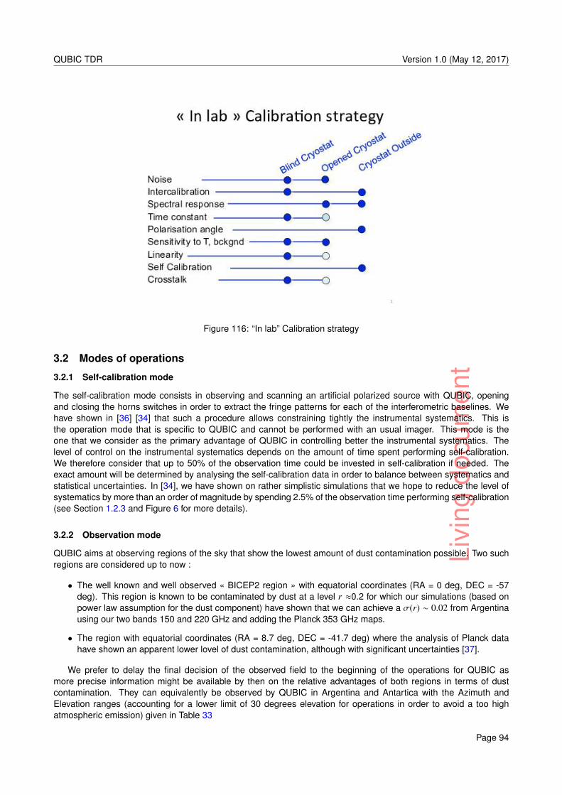
Livi
ngdo
cum
ent
QUBIC TDR Version 1.0 (May 12, 2017)
Figure 116: “In lab” Calibration strategy
3.2 Modes of operations
3.2.1 Self-calibration mode
The self-calibration mode consists in observing and scanning an artificial polarized source with QUBIC, openingand closing the horns switches in order to extract the fringe patterns for each of the interferometric baselines. Wehave shown in [36] [34] that such a procedure allows constraining tightly the instrumental systematics. This isthe operation mode that is specific to QUBIC and cannot be performed with an usual imager. This mode is theone that we consider as the primary advantage of QUBIC in controlling better the instrumental systematics. Thelevel of control on the instrumental systematics depends on the amount of time spent performing self-calibration.We therefore consider that up to 50% of the observation time could be invested in self-calibration if needed. Theexact amount will be determined by analysing the self-calibration data in order to balance between systematics andstatistical uncertainties. In [34], we have shown on rather simplistic simulations that we hope to reduce the level ofsystematics by more than an order of magnitude by spending 2.5% of the observation time performing self-calibration(see Section 1.2.3 and Figure 6 for more details).
3.2.2 Observation mode
QUBIC aims at observing regions of the sky that show the lowest amount of dust contamination possible. Two suchregions are considered up to now :
• The well known and well observed « BICEP2 region » with equatorial coordinates (RA = 0 deg, DEC = -57deg). This region is known to be contaminated by dust at a level r ≈0.2 for which our simulations (based onpower law assumption for the dust component) have shown that we can achieve a σ(r) ∼ 0.02 from Argentinausing our two bands 150 and 220 GHz and adding the Planck 353 GHz maps.
• The region with equatorial coordinates (RA = 8.7 deg, DEC = -41.7 deg) where the analysis of Planck datahave shown an apparent lower lovel of dust contamination, although with significant uncertainties [37].
We prefer to delay the final decision of the observed field to the beginning of the operations for QUBIC asmore precise information might be available by then on the relative advantages of both regions in terms of dustcontamination. They can equivalently be observed by QUBIC in Argentina and Antartica with the Azimuth andElevation ranges (accounting for a lower limit of 30 degrees elevation for operations in order to avoid a too highatmospheric emission) given in Table 33
Page 94
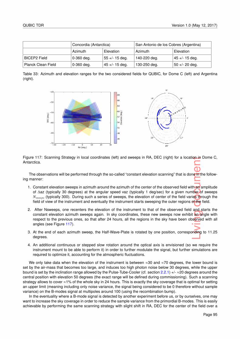
Livi
ngdo
cum
ent
QUBIC TDR Version 1.0 (May 12, 2017)
Concordia (Antarctica) San Antonio de los Cobres (Argentina)
Azimuth Elevation Azimuth Elevation
BICEP2 Field 0-360 deg. 55 +/- 15 deg. 140-220 deg. 45 +/- 15 deg.
Planck Clean Field 0-360 deg. 45 +/- 15 deg. 130-250 deg. 50 +/- 20 deg.
Table 33: Azimuth and elevation ranges for the two considered fields for QUBIC, for Dome C (left) and Argentina(right).
Figure 117: Scanning Strategy in local coordinates (left) and sweeps in RA, DEC (right) for a location in Dome C,Antarctica.
The observations will be performed through the so-called “constant elevation scanning” that is done in the follow-ing manner:
1. Constant elevation sweeps in azimuth around the azimuth of the center of the observed field with an amplitudeof ∆az (typically 30 degrees) at the angular speed vaz (typically 1 deg/sec) for a given number of sweepsNsweeps (typically 300). During such a series of sweeps, the elevation of center of the field varies through thefield of view of the instrument and eventually the instrument starts sweeping the outer regions of the field.
2. After Nsweeps, one recenters the elevation of the instrument to that of the observed field and starts theconstant elevation azimuth sweeps again. In sky coordinates, these new sweeps now exhibit an angle withrespect to the previous ones, so that after 24 hours, all the regions in the sky have been observed with allangles (see Figure 117).
3. At the end of each azimuth sweep, the Half-Wave-Plate is rotated by one position, corresponding to 11.25degrees.
4. An additional continuous or stepped slow rotation around the optical axis is envisioned (so we require theinstrument mount to be able to perform it) in order to further modulate the signal, but further simulations arerequired to optimize it, accounting for the atmospheric fluctuations.
We only take data when the elevation of the instrument is between ≈30 and ≈70 degrees, the lower bound isset by the air-mass that becomes too large, and induces too high photon noise below 30 degrees, while the upperbound is set by the inclination range allowed by the Pulse-Tube-Cooler (cf. section 2.2.1) +/- ≈20 degrees around thecentral position with elevation 50 degrees (the exact range will be defined during commissioning). Such a scanningstrategy allows to cover ≈1% of the whole sky in 24 hours. This is exactly the sky coverage that is optimal for settingan upper limit (meaning including only noise variance, the signal being considered to be 0 therefore without samplevariance) on the B-modes signal at multipoles around 100 (using the recombination bump).
In the eventuality where a B-mode signal is detected by another experiment before us, or by ourselves, one maywant to increase the sky coverage in order to reduce the sample variance from the primordial B-modes. This is easilyachievable by performing the same scanning strategy with slight shift in RA, DEC for the center of the field over a
Page 95
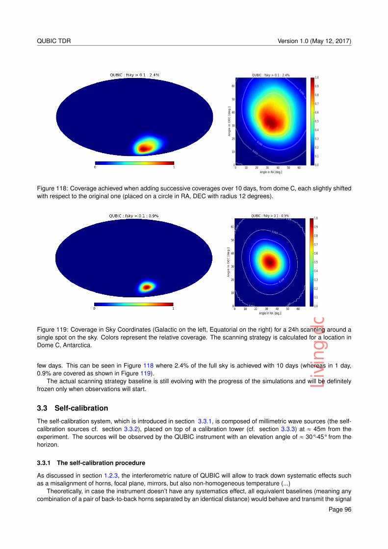
Livi
ngdo
cum
ent
QUBIC TDR Version 1.0 (May 12, 2017)
Figure 118: Coverage achieved when adding successive coverages over 10 days, from dome C, each slightly shiftedwith respect to the original one (placed on a circle in RA, DEC with radius 12 degrees).
Figure 119: Coverage in Sky Coordinates (Galactic on the left, Equatorial on the right) for a 24h scanning around asingle spot on the sky. Colors represent the relative coverage. The scanning strategy is calculated for a location inDome C, Antarctica.
few days. This can be seen in Figure 118 where 2.4% of the full sky is achieved with 10 days (whereas in 1 day,0.9% are covered as shown in Figure 119).
The actual scanning strategy baseline is still evolving with the progress of the simulations and will be definitelyfrozen only when observations will start.
3.3 Self-calibration
The self-calibration system, which is introduced in section 3.3.1, is composed of millimetric wave sources (the self-calibration sources cf. section 3.3.2), placed on top of a calibration tower (cf. section 3.3.3) at ≈ 45m from theexperiment. The sources will be observed by the QUBIC instrument with an elevation angle of ≈ 30°-45° from thehorizon.
3.3.1 The self-calibration procedure
As discussed in section 1.2.3, the interferometric nature of QUBIC will allow to track down systematic effects suchas a misalignment of horns, focal plane, mirrors, but also non-homogeneous temperature (...)
Theoretically, in case the instrument doesn’t have any systematics effect, all equivalent baselines (meaning anycombination of a pair of back-to-back horns separated by an identical distance) would behave and transmit the signal
Page 96
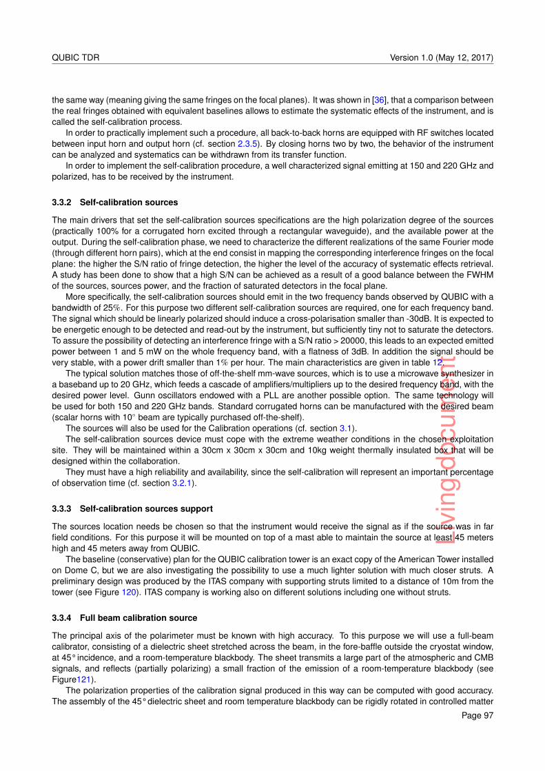
Livi
ngdo
cum
ent
QUBIC TDR Version 1.0 (May 12, 2017)
the same way (meaning giving the same fringes on the focal planes). It was shown in [36], that a comparison betweenthe real fringes obtained with equivalent baselines allows to estimate the systematic effects of the instrument, and iscalled the self-calibration process.
In order to practically implement such a procedure, all back-to-back horns are equipped with RF switches locatedbetween input horn and output horn (cf. section 2.3.5). By closing horns two by two, the behavior of the instrumentcan be analyzed and systematics can be withdrawn from its transfer function.
In order to implement the self-calibration procedure, a well characterized signal emitting at 150 and 220 GHz andpolarized, has to be received by the instrument.
3.3.2 Self-calibration sources
The main drivers that set the self-calibration sources specifications are the high polarization degree of the sources(practically 100% for a corrugated horn excited through a rectangular waveguide), and the available power at theoutput. During the self-calibration phase, we need to characterize the different realizations of the same Fourier mode(through different horn pairs), which at the end consist in mapping the corresponding interference fringes on the focalplane: the higher the S/N ratio of fringe detection, the higher the level of the accuracy of systematic effects retrieval.A study has been done to show that a high S/N can be achieved as a result of a good balance between the FWHMof the sources, sources power, and the fraction of saturated detectors in the focal plane.
More specifically, the self-calibration sources should emit in the two frequency bands observed by QUBIC with abandwidth of 25%. For this purpose two different self-calibration sources are required, one for each frequency band.The signal which should be linearly polarized should induce a cross-polarisation smaller than -30dB. It is expected tobe energetic enough to be detected and read-out by the instrument, but sufficiently tiny not to saturate the detectors.To assure the possibility of detecting an interference fringe with a S/N ratio > 20000, this leads to an expected emittedpower between 1 and 5 mW on the whole frequency band, with a flatness of 3dB. In addition the signal should bevery stable, with a power drift smaller than 1% per hour. The main characteristics are given in table 12.
The typical solution matches those of off-the-shelf mm-wave sources, which is to use a microwave synthesizer ina baseband up to 20 GHz, which feeds a cascade of amplifiers/multipliers up to the desired frequency band, with thedesired power level. Gunn oscillators endowed with a PLL are another possible option. The same technology willbe used for both 150 and 220 GHz bands. Standard corrugated horns can be manufactured with the desired beam(scalar horns with 10 beam are typically purchased off-the-shelf).
The sources will also be used for the Calibration operations (cf. section 3.1).The self-calibration sources device must cope with the extreme weather conditions in the chosen exploitation
site. They will be maintained within a 30cm x 30cm x 30cm and 10kg weight thermally insulated box that will bedesigned within the collaboration.
They must have a high reliability and availability, since the self-calibration will represent an important percentageof observation time (cf. section 3.2.1).
3.3.3 Self-calibration sources support
The sources location needs be chosen so that the instrument would receive the signal as if the source was in farfield conditions. For this purpose it will be mounted on top of a mast able to maintain the source at least 45 metershigh and 45 meters away from QUBIC.
The baseline (conservative) plan for the QUBIC calibration tower is an exact copy of the American Tower installedon Dome C, but we are also investigating the possibility to use a much lighter solution with much closer struts. Apreliminary design was produced by the ITAS company with supporting struts limited to a distance of 10m from thetower (see Figure 120). ITAS company is working also on different solutions including one without struts.
3.3.4 Full beam calibration source
The principal axis of the polarimeter must be known with high accuracy. To this purpose we will use a full-beamcalibrator, consisting of a dielectric sheet stretched across the beam, in the fore-baffle outside the cryostat window,at 45° incidence, and a room-temperature blackbody. The sheet transmits a large part of the atmospheric and CMBsignals, and reflects (partially polarizing) a small fraction of the emission of a room-temperature blackbody (seeFigure121).
The polarization properties of the calibration signal produced in this way can be computed with good accuracy.The assembly of the 45° dielectric sheet and room temperature blackbody can be rigidly rotated in controlled matter
Page 97
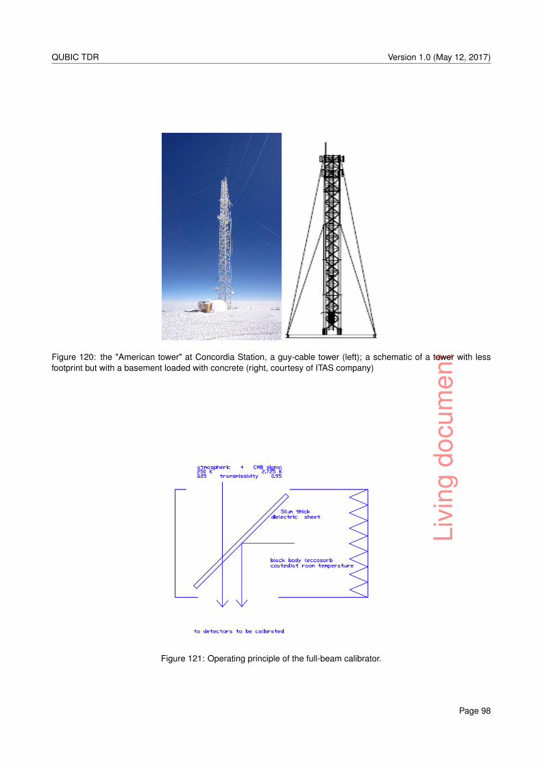
Livi
ngdo
cum
ent
QUBIC TDR Version 1.0 (May 12, 2017)
Figure 120: the "American tower" at Concordia Station, a guy-cable tower (left); a schematic of a tower with lessfootprint but with a basement loaded with concrete (right, courtesy of ITAS company)
Figure 121: Operating principle of the full-beam calibrator.
Page 98
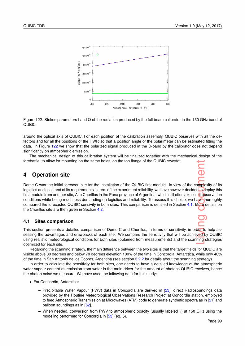
Livi
ngdo
cum
ent
QUBIC TDR Version 1.0 (May 12, 2017)
Figure 122: Stokes parameters I and Q of the radiation produced by the full beam calibrator in the 150 GHz band ofQUBIC.
around the optical axis of QUBIC. For each position of the calibration assembly, QUBIC observes with all the de-tectors and for all the positions of the HWP, so that a position angle of the polarimeter can be estimated fitting thedata. In Figure 122 we show that the polarized signal produced in the D-band by the calibrator does not dependsignificantly on atmospheric emission.
The mechanical design of this calibration system will be finalized together with the mechanical design of theforebaffle, to allow for mounting on the same holes, on the top flange of the QUBIC cryostat.
4 Operation site
Dome C was the initial foreseen site for the installation of the QUBIC first module. In view of the complexity of itslogistics and cost, and of its requirements in term of the experiment reliability, we have however decided to deploy thisfirst module from another site, Alto Chorillos in the Puna province of Argentina, which still offers excellent observationconditions while being much less demanding on logistics and reliability. To assess this choice, we have thoroughlycompared the forecasted QUBIC sensivity in both sites. This comparison is detailed in Section 4.1. More details onthe Chorillos site are then given in Section 4.2.
4.1 Sites comparison
This section presents a detailed comparison of Dome C and Chorillos, in terms of sensitivity, in order to help as-sessing the advantages and drawbacks of each site. We compare the sensitivity that will be achieved by QUBICusing realistic meteorological conditions for both sites (obtained from measurements) and the scanning strategiesoptimized for each site.
Regarding the scanning strategy, the main difference between the two sites is that the target fields for QUBIC arevisible above 30 degrees and below 70 degrees elevation 100% of the time in Concordia, Antarctica, while only 40%of the time in San Antonio de los Cobres, Argentina (see section 3.2.2 for details about the scanning strategy).
In order to calculate the sensitivity for both sites, one needs to have a detailed knowledge of the atmosphericwater vapour content as emission from water is the main driver for the amount of photons QUBIC receives, hencethe photon noise we measure. We have used the following data for this study:
• For Concordia, Antarctica:
– Precipitable Water Vapour (PWV) data in Concordia are derived in [53], direct Radiosoundings dataprovided by the Routine Meteorological Observations Research Project at Concordia station, employedto feed Atmospheric Transmission at Microwaves (ATM) code to generate synthetic spectra as in [51] andballoon soundings as in [62].
– When needed, conversion from PWV to atmospheric opacity (usually labeled τ) at 150 GHz using themodeling performed for Concordia in [53] (eq. 5).
Page 99
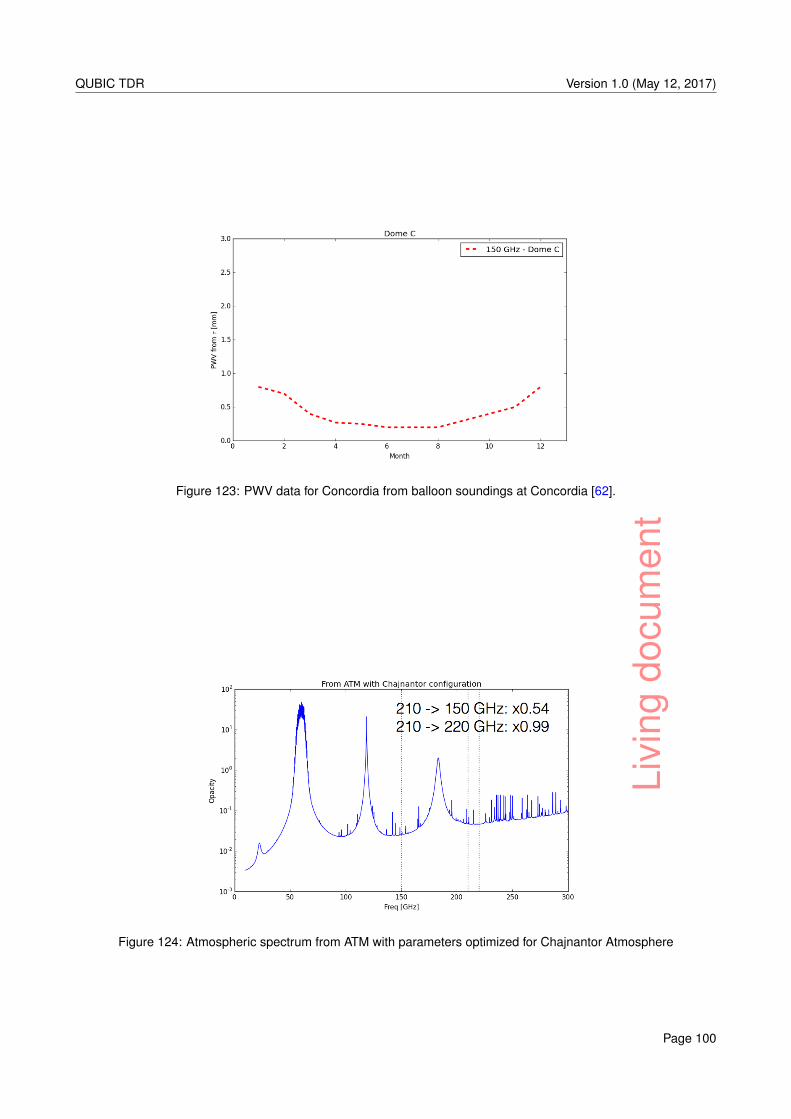
Livi
ngdo
cum
ent
QUBIC TDR Version 1.0 (May 12, 2017)
Figure 123: PWV data for Concordia from balloon soundings at Concordia [62].
Figure 124: Atmospheric spectrum from ATM with parameters optimized for Chajnantor Atmosphere
Page 100
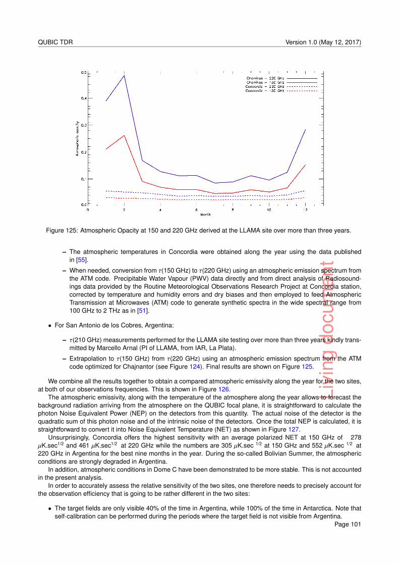
Livi
ngdo
cum
ent
QUBIC TDR Version 1.0 (May 12, 2017)
Figure 125: Atmospheric Opacity at 150 and 220 GHz derived at the LLAMA site over more than three years.
– The atmospheric temperatures in Concordia were obtained along the year using the data publishedin [55].
– When needed, conversion from τ(150 GHz) to τ(220 GHz) using an atmospheric emission spectrum fromthe ATM code. Precipitable Water Vapour (PWV) data directly and from direct analysis of Radiosound-ings data provided by the Routine Meteorological Observations Research Project at Concordia station,corrected by temperature and humidity errors and dry biases and then employed to feed AtmosphericTransmission at Microwaves (ATM) code to generate synthetic spectra in the wide spectral range from100 GHz to 2 THz as in [51].
• For San Antonio de los Cobres, Argentina:
– τ(210 GHz) measurements performed for the LLAMA site testing over more than three years kindly trans-mitted by Marcello Arnal (PI of LLAMA, from IAR, La Plata).
– Extrapolation to τ(150 GHz) from τ(220 GHz) using an atmospheric emission spectrum from the ATMcode optimized for Chajnantor (see Figure 124). Final results are shown on Figure 125.
We combine all the results together to obtain a compared atmospheric emissivity along the year for the two sites,at both of our observations frequencies. This is shown in Figure 126.
The atmospheric emissivity, along with the temperature of the atmosphere along the year allows to forecast thebackground radiation arriving from the atmosphere on the QUBIC focal plane, it is straightforward to calculate thephoton Noise Equivalent Power (NEP) on the detectors from this quantity. The actual noise of the detector is thequadratic sum of this photon noise and of the intrinsic noise of the detectors. Once the total NEP is calculated, it isstraightforward to convert it into Noise Equivalent Temperature (NET) as shown in Figure 127.
Unsurprisingly, Concordia offers the highest sensitivity with an average polarized NET at 150 GHz of 278µK.sec1/2 and 461 µK.sec1/2 at 220 GHz while the numbers are 305 µK.sec 1/2 at 150 GHz and 552 µK.sec 1/2 at220 GHz in Argentina for the best nine months in the year. During the so-called Bolivian Summer, the atmosphericconditions are strongly degraded in Argentina.
In addition, atmospheric conditions in Dome C have been demonstrated to be more stable. This is not accountedin the present analysis.
In order to accurately assess the relative sensitivity of the two sites, one therefore needs to precisely account forthe observation efficiency that is going to be rather different in the two sites:
• The target fields are only visible 40% of the time in Argentina, while 100% of the time in Antarctica. Note thatself-calibration can be performed during the periods where the target field is not visible from Argentina.
Page 101
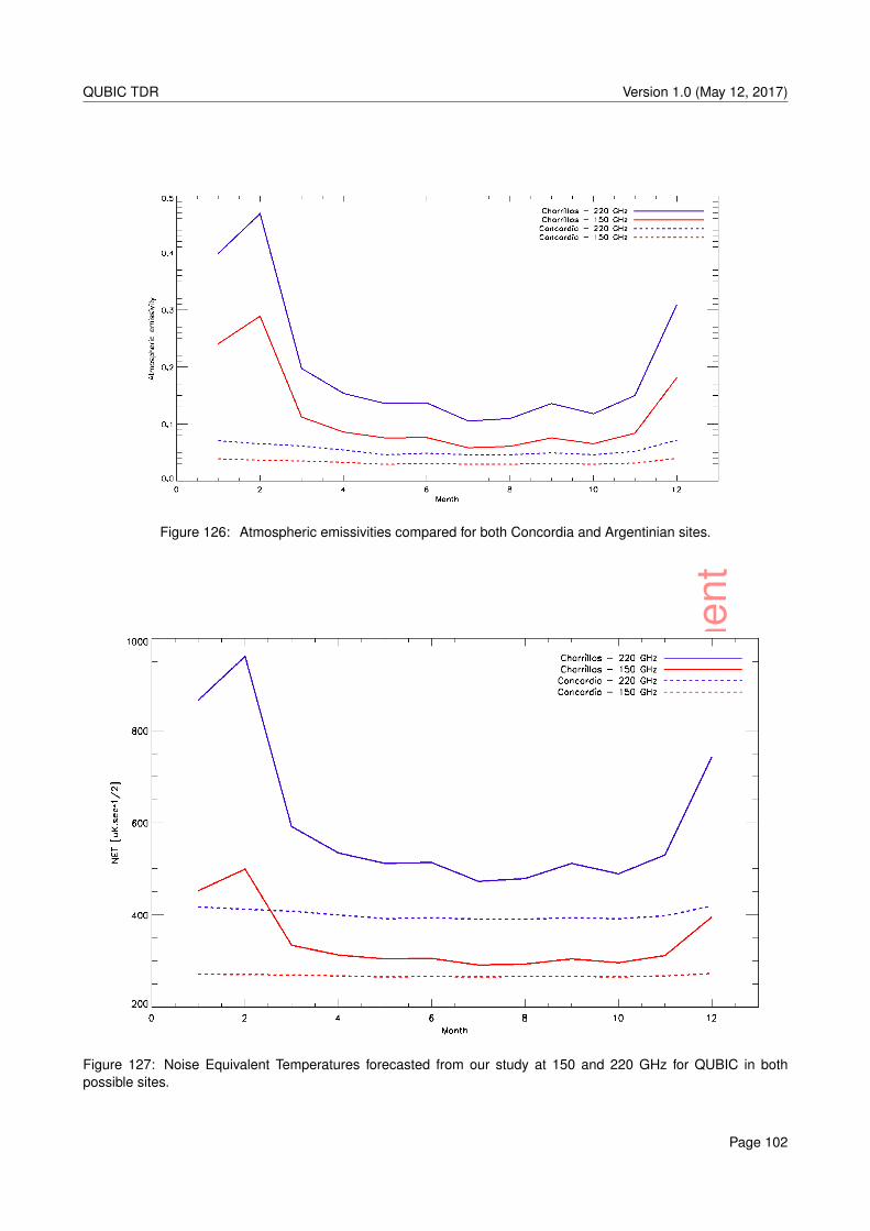
Livi
ngdo
cum
ent
QUBIC TDR Version 1.0 (May 12, 2017)
Figure 126: Atmospheric emissivities compared for both Concordia and Argentinian sites.
Figure 127: Noise Equivalent Temperatures forecasted from our study at 150 and 220 GHz for QUBIC in bothpossible sites.
Page 102
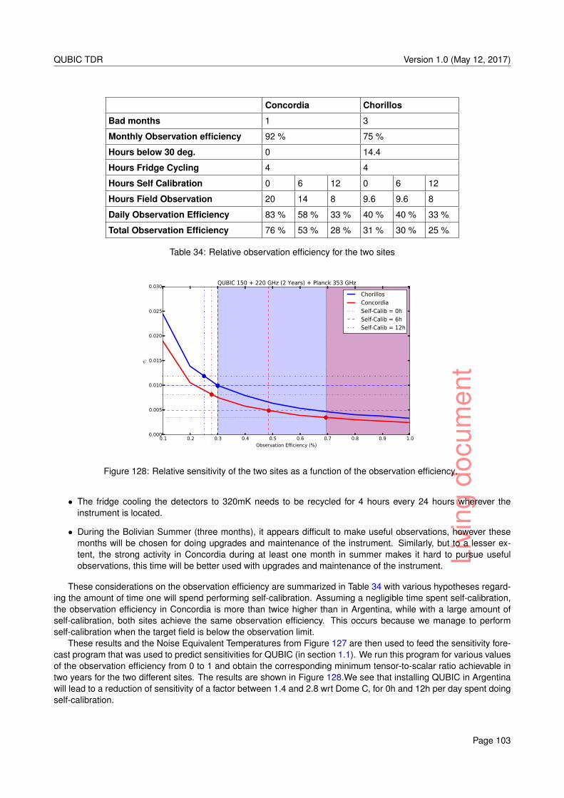
Livi
ngdo
cum
ent
QUBIC TDR Version 1.0 (May 12, 2017)
Concordia Chorillos
Bad months 1 3
Monthly Observation efficiency 92 % 75 %
Hours below 30 deg. 0 14.4
Hours Fridge Cycling 4 4
Hours Self Calibration 0 6 12 0 6 12
Hours Field Observation 20 14 8 9.6 9.6 8
Daily Observation Efficiency 83 % 58 % 33 % 40 % 40 % 33 %
Total Observation Efficiency 76 % 53 % 28 % 31 % 30 % 25 %
Table 34: Relative observation efficiency for the two sites
0.1 0.2 0.3 0.4 0.5 0.6 0.7 0.8 0.9 1.0Observation Efficiency (%)
0.000
0.005
0.010
0.015
0.020
0.025
0.030
σr
QUBIC 150 + 220 GHz (2 Years) + Planck 353 GHz
ChorillosConcordiaSelf-Calib = 0hSelf-Calib = 6hSelf-Calib = 12h
Figure 128: Relative sensitivity of the two sites as a function of the observation efficiency.
• The fridge cooling the detectors to 320mK needs to be recycled for 4 hours every 24 hours wherever theinstrument is located.
• During the Bolivian Summer (three months), it appears difficult to make useful observations, however thesemonths will be chosen for doing upgrades and maintenance of the instrument. Similarly, but to a lesser ex-tent, the strong activity in Concordia during at least one month in summer makes it hard to pursue usefulobservations, this time will be better used with upgrades and maintenance of the instrument.
These considerations on the observation efficiency are summarized in Table 34 with various hypotheses regard-ing the amount of time one will spend performing self-calibration. Assuming a negligible time spent self-calibration,the observation efficiency in Concordia is more than twice higher than in Argentina, while with a large amount ofself-calibration, both sites achieve the same observation efficiency. This occurs because we manage to performself-calibration when the target field is below the observation limit.
These results and the Noise Equivalent Temperatures from Figure 127 are then used to feed the sensitivity fore-cast program that was used to predict sensitivities for QUBIC (in section 1.1). We run this program for various valuesof the observation efficiency from 0 to 1 and obtain the corresponding minimum tensor-to-scalar ratio achievable intwo years for the two different sites. The results are shown in Figure 128.We see that installing QUBIC in Argentinawill lead to a reduction of sensitivity of a factor between 1.4 and 2.8 wrt Dome C, for 0h and 12h per day spent doingself-calibration.
Page 103
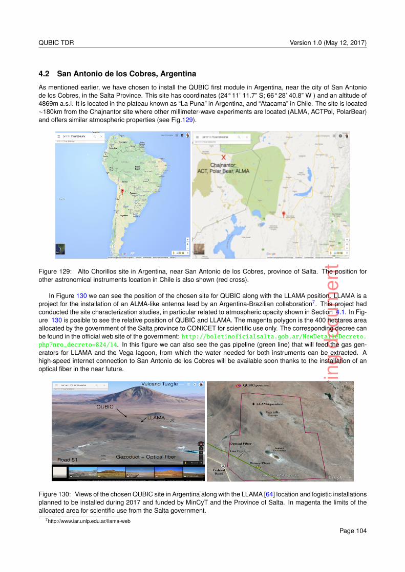
Livi
ngdo
cum
ent
QUBIC TDR Version 1.0 (May 12, 2017)
4.2 San Antonio de los Cobres, Argentina
As mentioned earlier, we have chosen to install the QUBIC first module in Argentina, near the city of San Antoniode los Cobres, in the Salta Province. This site has coordinates (24° 11’ 11.7” S; 66° 28’ 40.8” W ) and an altitude of4869m a.s.l. It is located in the plateau known as “La Puna” in Argentina, and “Atacama” in Chile. The site is located∼180km from the Chajnantor site where other millimeter-wave experiments are located (ALMA, ACTPol, PolarBear)and offers similar atmospheric properties (see Fig.129).
Figure 129: Alto Chorillos site in Argentina, near San Antonio de los Cobres, province of Salta. The position forother astronomical instruments location in Chile is also shown (red cross).
In Figure 130 we can see the position of the chosen site for QUBIC along with the LLAMA position. LLAMA is aproject for the installation of an ALMA-like antenna lead by an Argentina-Brazilian collaboration7. This project hadconducted the site characterization studies, in particular related to atmospheric opacity shown in Section 4.1. In Fig-ure 130 is posible to see the relative position of QUBIC and LLAMA. The magenta polygon is the 400 hectares areaallocated by the government of the Salta province to CONICET for scientific use only. The corresponding decree canbe found in the official web site of the government: http://boletinoficialsalta.gob.ar/NewDetalleDecreto.php?nro_decreto=824/14. In this figure we can also see the gas pipeline (green line) that will feed the gas gen-erators for LLAMA and the Vega lagoon, from which the water needed for both instruments can be extracted. Ahigh-speed internet connection to San Antonio de los Cobres will be available soon thanks to the installation of anoptical fiber in the near future.
Figure 130: Views of the chosen QUBIC site in Argentina along with the LLAMA [64] location and logistic installationsplanned to be installed during 2017 and funded by MinCyT and the Province of Salta. In magenta the limits of theallocated area for scientific use from the Salta government.
7http://www.iar.unlp.edu.ar/llama-web
Page 104
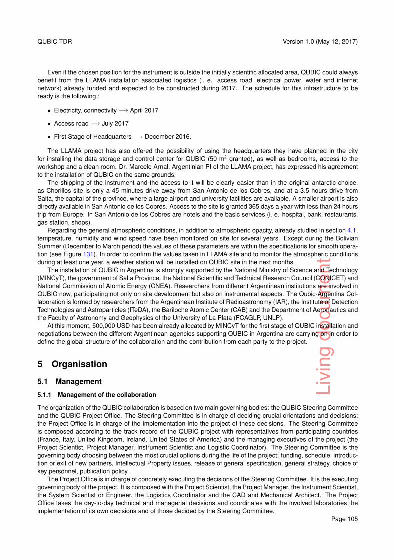
Livi
ngdo
cum
ent
QUBIC TDR Version 1.0 (May 12, 2017)
Even if the chosen position for the instrument is outside the initially scientific allocated area, QUBIC could alwaysbenefit from the LLAMA installation associated logistics (i. e. access road, electrical power, water and internetnetwork) already funded and expected to be constructed during 2017. The schedule for this infrastructure to beready is the following :
• Electricity, connectivity −→ April 2017
• Access road −→ July 2017
• First Stage of Headquarters −→ December 2016.
The LLAMA project has also offered the possibility of using the headquarters they have planned in the cityfor installing the data storage and control center for QUBIC (50 m2 granted), as well as bedrooms, access to theworkshop and a clean room. Dr. Marcelo Arnal, Argentinian PI of the LLAMA project, has expressed his agreementto the installation of QUBIC on the same grounds.
The shipping of the instrument and the access to it will be clearly easier than in the original antarctic choice,as Chorillos site is only a 45 minutes drive away from San Antonio de los Cobres, and at a 3.5 hours drive fromSalta, the capital of the province, where a large airport and university facilities are available. A smaller airport is alsodirectly available in San Antonio de los Cobres. Access to the site is granted 365 days a year with less than 24 hourstrip from Europe. In San Antonio de los Cobres are hotels and the basic services (i. e. hospital, bank, restaurants,gas station, shops).
Regarding the general atmospheric conditions, in addition to atmospheric opacity, already studied in section 4.1,temperature, humidity and wind speed have been monitored on site for several years. Except during the BolivianSummer (December to March period) the values of these parameters are within the specifications for smooth opera-tion (see Figure 131). In order to confirm the values taken in LLAMA site and to monitor the atmospheric conditionsduring at least one year, a weather station will be installed on QUBIC site in the next months.
The installation of QUBIC in Argentina is strongly supported by the National Ministry of Science and Technology(MINCyT), the government of Salta Province, the National Scientific and Technical Research Council (CONICET) andNational Commission of Atomic Energy (CNEA). Researchers from different Argentinean institutions are involved inQUBIC now, participating not only on site development but also on instrumental aspects. The Qubic-Argentina Col-laboration is formed by researchers from the Argentinean Institute of Radioastronomy (IAR), the Institute of DetectionTechnologies and Astroparticles (ITeDA), the Bariloche Atomic Center (CAB) and the Department of Aeronautics andthe Faculty of Astronomy and Geophysics of the University of La Plata (FCAGLP, UNLP).
At this moment, 500,000 USD has been already allocated by MINCyT for the first stage of QUBIC installation andnegotiations between the different Argentinean agencies supporting QUBIC in Argentina are carrying on in order todefine the global structure of the collaboration and the contribution from each party to the project.
5 Organisation
5.1 Management
5.1.1 Management of the collaboration
The organization of the QUBIC collaboration is based on two main governing bodies: the QUBIC Steering Committeeand the QUBIC Project Office. The Steering Committee is in charge of deciding crucial orientations and decisions;the Project Office is in charge of the implementation into the project of these decisions. The Steering Committeeis composed according to the track record of the QUBIC project with representatives from participating countries(France, Italy, United Kingdom, Ireland, United States of America) and the managing executives of the project (theProject Scientist, Project Manager, Instrument Scientist and Logistic Coordinator). The Steering Committee is thegoverning body choosing between the most crucial options during the life of the project: funding, schedule, introduc-tion or exit of new partners, Intellectual Property issues, release of general specification, general strategy, choice ofkey personnel, publication policy.
The Project Office is in charge of concretely executing the decisions of the Steering Committee. It is the executinggoverning body of the project. It is composed with the Project Scientist, the Project Manager, the Instrument Scientist,the System Scientist or Engineer, the Logistics Coordinator and the CAD and Mechanical Architect. The ProjectOffice takes the day-to-day technical and managerial decisions and coordinates with the involved laboratories theimplementation of its own decisions and of those decided by the Steering Committee.
Page 105
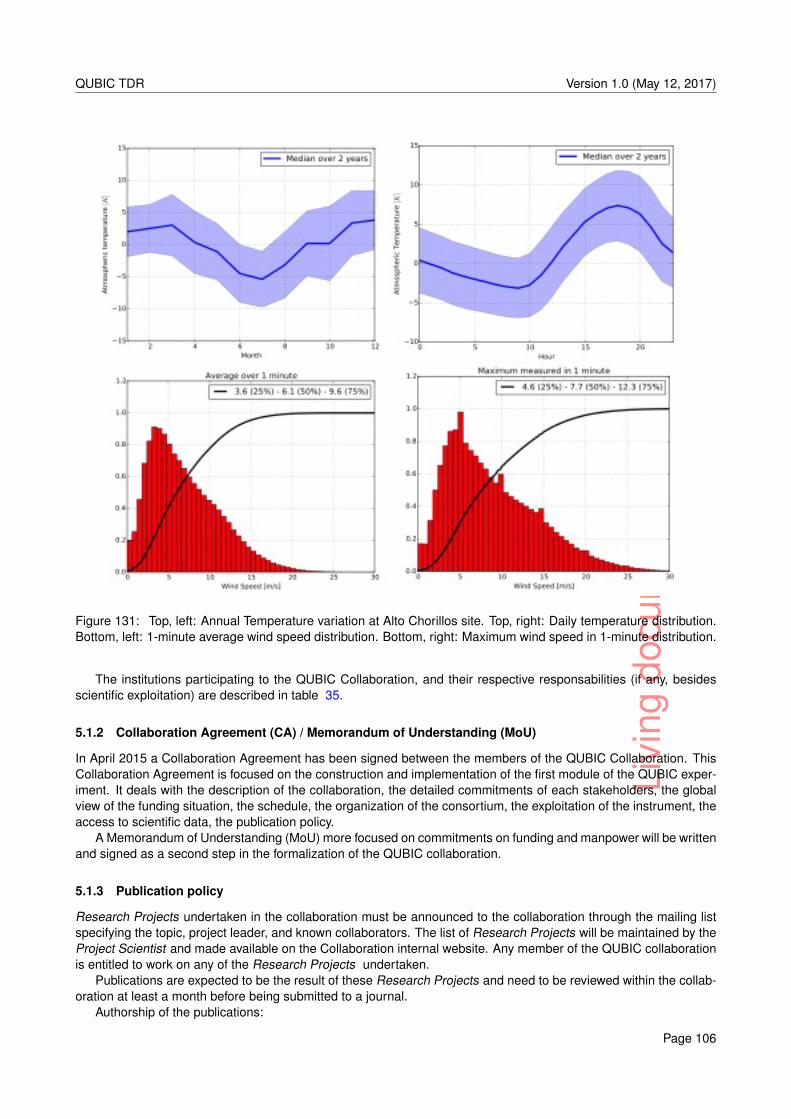
Livi
ngdo
cum
ent
QUBIC TDR Version 1.0 (May 12, 2017)
Figure 131: Top, left: Annual Temperature variation at Alto Chorillos site. Top, right: Daily temperature distribution.Bottom, left: 1-minute average wind speed distribution. Bottom, right: Maximum wind speed in 1-minute distribution.
The institutions participating to the QUBIC Collaboration, and their respective responsabilities (if any, besidesscientific exploitation) are described in table 35.
5.1.2 Collaboration Agreement (CA) / Memorandum of Understanding (MoU)
In April 2015 a Collaboration Agreement has been signed between the members of the QUBIC Collaboration. ThisCollaboration Agreement is focused on the construction and implementation of the first module of the QUBIC exper-iment. It deals with the description of the collaboration, the detailed commitments of each stakeholders, the globalview of the funding situation, the schedule, the organization of the consortium, the exploitation of the instrument, theaccess to scientific data, the publication policy.
A Memorandum of Understanding (MoU) more focused on commitments on funding and manpower will be writtenand signed as a second step in the formalization of the QUBIC collaboration.
5.1.3 Publication policy
Research Projects undertaken in the collaboration must be announced to the collaboration through the mailing listspecifying the topic, project leader, and known collaborators. The list of Research Projects will be maintained by theProject Scientist and made available on the Collaboration internal website. Any member of the QUBIC collaborationis entitled to work on any of the Research Projects undertaken.
Publications are expected to be the result of these Research Projects and need to be reviewed within the collab-oration at least a month before being submitted to a journal.
Authorship of the publications:
Page 106
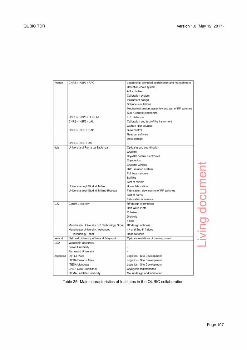
Livi
ngdo
cum
ent
QUBIC TDR Version 1.0 (May 12, 2017)
France CNRS / IN2P3 / APC Leadership, technical coordination and management
Detection chain system
AIT activities
Calibration system
Instrument design
Science simulations
Mechanical design, assembly and test of RF switches
Sub-K control electronics
CNRS / IN2P3 / CSNSM TES detectors
CNRS / IN2P3 / LAL Calibration and test of the instrument
Carbon fiber sources
CNRS / INSU / IRAP Slow control
Readout software
Data storage
CNRS / INSU / IAS -
Italy Università di Roma La Sapienza Optical group coordination
Cryostat
Cryostat control electronics
Cryogenics
Cryostat window
HWP rotation system
Full beam source
Baffling
Test of mirrors
Universita degli Studi di Milano Horns fabrication
Universita degli Studi di Milano-Bicocca Fabrication, slow control of RF switches
Test of horns
Fabrication of mirrors
U.K. Cardiff University RF design of switches
Half Wave Plate
Polarizer
Dichroïc
Filters
Manchester University / JB Technology Group RF design of horns
Manchester University / Advanced 1K and Sub-K fridges
Technology Team Heat-switches
Ireland National University of Ireland, Maynooth Optical simulations of the instrument
USA Wisconsin University -
Brown University -
Richmond University -
Argentina IAR La Plata Logistics - Site Development
ITEDA Buenos Aires Logistics - Site Development
ITEDA Mendoza Logistics - Site Development
CNEA CAB (Bariloche) Cryogenic maintenance
GEMA La Plata University Mount design and fabrication
Table 35: Main characteristics of Institutes in the QUBIC collaboration
Page 107

Livi
ngdo
cum
ent
QUBIC TDR Version 1.0 (May 12, 2017)
• Any member of the QUBIC collaboration can request that his/her name be added to the list of author of anarticle. It is the responsibility of the Research Project leader to accept or not this request depending on hiscontribution to this specific research project. The ordering of the list of authors is left to the choice of thespecific Research Project members.
• QUBIC members having the Architect status have the right to choose to be co-author of any of the publications.The Architect status is granted by the Steering Committee based on significant contributions to any stage ofthe experiment (design, construction, integration, operation or analysis).
• The default policy for signature of papers is: first the main authors, then other involved people in alphabeticorder.
Any disagreement should be resolved through the Steering Committee whose decision would be final.In addition to the Research Projects, The QUBIC Project Scientist, in agreement with the Steering Committee,
may establish Key Projects and Working Groups whose work could also result in a publication. The authorship forsuch projects will be discussed in the Steering Committee and would by default be the whole QUBIC collaborationin alphabetical order.
5.2 Organization
5.2.1 Product Breakdown Structure (PBS)
The QUBIC system is structured as in Table 36.
5.2.2 Works Breakdown Structure / Works packages
The different tasks for design, fabrication, tests for each component of QUBIC are described in the chart shown onFigure 132.
Otherwise explicitly stated, a component is designed, fabricated and tested by the same laboratory.Besides activities for providing the components parts of QUBIC, integration activities, under the responsibility of
APC, have been integrated in the chart. The global management and coordination of the experiment is also underthe responsibility of APC.
Each laboratory is represented by its own color code in the graph.
5.3 Development plan
The development of the QUBIC instrument is a multi-step process. After i) the first R&D works, it was decided in areview held in 2013 to ii) validate the detection chain. Now this validation is almost done. The next steps are iii) thevalidation of a technological demonstrator, and then iv) the construction of the full first module of the instrument. Thefinal step will be v) the fabrication and implementation of the five additional modules.
5.3.1 Heritage and first R&D works
Since 2008, many Research and Development works on the following topics have path the way to the constructionof QUBIC.
• Proof of principle concept of bolometric interferometry:
MBI-4 and BRAIN have been successful demonstrator of the concept of bolometric interferometry.The merge of this two projects and their respective teams gave birth to the QUBIC project.
• Exploitation site:
BRAIN has been successfully installed and exploited in the Concordia Station in Antarctica in 2006. This implantationhas been of great value with respect to the exploitation of such an instrument and its main sub-systems (such as thepulse tube cryo-coolers) in the harsh conditions of Antarctica.
Besides this installation measurements have been made on the quality of the sky at Concordia Station by DrAlessandro Schillaci in 2010 and 2011.
Page 108
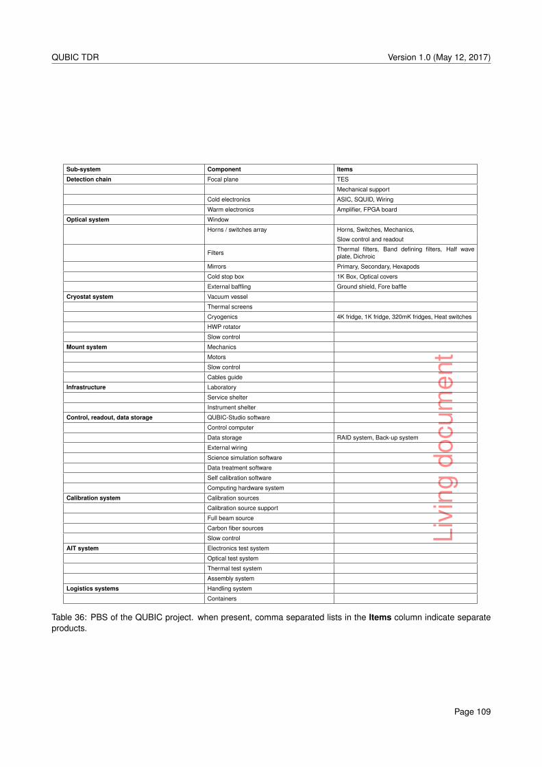
Livi
ngdo
cum
ent
QUBIC TDR Version 1.0 (May 12, 2017)
Sub-system Component Items
Detection chain Focal plane TES
Mechanical support
Cold electronics ASIC, SQUID, Wiring
Warm electronics Amplifier, FPGA board
Optical system Window
Horns / switches array Horns, Switches, Mechanics,
Slow control and readout
Filters Thermal filters, Band defining filters, Half waveplate, Dichroic
Mirrors Primary, Secondary, Hexapods
Cold stop box 1K Box, Optical covers
External baffling Ground shield, Fore baffle
Cryostat system Vacuum vessel
Thermal screens
Cryogenics 4K fridge, 1K fridge, 320mK fridges, Heat switches
HWP rotator
Slow control
Mount system Mechanics
Motors
Slow control
Cables guide
Infrastructure Laboratory
Service shelter
Instrument shelter
Control, readout, data storage QUBIC-Studio software
Control computer
Data storage RAID system, Back-up system
External wiring
Science simulation software
Data treatment software
Self calibration software
Computing hardware system
Calibration system Calibration sources
Calibration source support
Full beam source
Carbon fiber sources
Slow control
AIT system Electronics test system
Optical test system
Thermal test system
Assembly system
Logistics systems Handling system
Containers
Table 36: PBS of the QUBIC project. when present, comma separated lists in the Items column indicate separateproducts.
Page 109
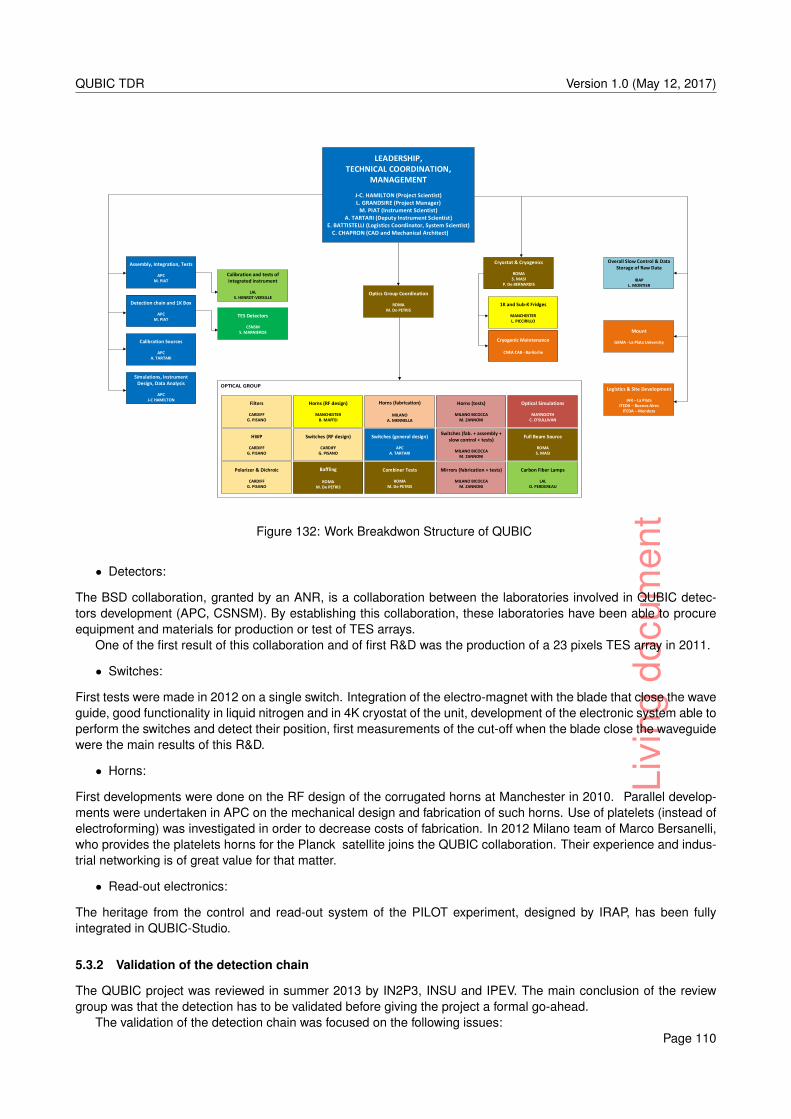
Livi
ngdo
cum
ent
QUBIC TDR Version 1.0 (May 12, 2017)
LEADERSHIP, TECHNICAL COORDINATION,
MANAGEMENT
J-C. HAMILTON (Project Scientist)L. GRANDSIRE (Project Manager)
M. PIAT (Instrument Scientist)A. TARTARI (Deputy Instrument Scientist)
E. BATTISTELLI (Logistics Coordinator, System Scientist)C. CHAPRON (CAD and Mechanical Architect)
Assembly, Integration, Tests
APCM. PIAT
Detection chain and 1K Box
APCM. PIAT
Calibration Sources
APCA. TARTARI
Simulations, Instrument Design, Data Analysis
APCJ-C HAMILTON
Switches (general design)
APCA. TARTARI
Calibration and tests of integrated instrument
LALS. HENROT-VERSILLE
Carbon Fiber Lamps
LALO. PERDEREAU
TES Detectors
CSNSMS. MARNIEROS
Optics Group Coordination
ROMAM. De PETRIS
Cryostat & Cryogenics
ROMAS. MASI
P. De BERNARDIS
Baffling
ROMAM. De PETRIS
Combiner Tests
ROMAM. De PETRIS
Full Beam Source
ROMAS. MASI
Overall Slow Control & Data Storage of Raw Data
IRAPL. MONTIER
1K and Sub-K Fridges
MANCHESTERL. PICCIRILLO
Horns (RF design)
MANCHESTERB. MAFFEI
Mount
GEMA - La Plata University
Logistics & Site Development
IAR – La PlataITEDA – Buenos Aires
ITEDA – Mendoza
Cryogenic Maintenance
CNEA CAB - Bariloche
Filters
CARDIFFG. PISANO
HWP
CARDIFFG. PISANO
Polarizer & Dichroic
CARDIFFG. PISANO
Switches (RF design)
CARDIFFG. PISANO
Horns (fabrication)
MILANOA. MENNELLA
Horns (tests)
MILANO BICOCCAM. ZANNONI
Switches (fab. + assembly + slow control + tests)
MILANO BICOCCAM. ZANNONI
Mirrors (fabrication + tests)
MILANO BICOCCAM. ZANNONI
Optical Simulations
MAYNOOTHC. O SULLIVAN
Figure 132: Work Breakdwon Structure of QUBIC
• Detectors:
The BSD collaboration, granted by an ANR, is a collaboration between the laboratories involved in QUBIC detec-tors development (APC, CSNSM). By establishing this collaboration, these laboratories have been able to procureequipment and materials for production or test of TES arrays.
One of the first result of this collaboration and of first R&D was the production of a 23 pixels TES array in 2011.
• Switches:
First tests were made in 2012 on a single switch. Integration of the electro-magnet with the blade that close the waveguide, good functionality in liquid nitrogen and in 4K cryostat of the unit, development of the electronic system able toperform the switches and detect their position, first measurements of the cut-off when the blade close the waveguidewere the main results of this R&D.
• Horns:
First developments were done on the RF design of the corrugated horns at Manchester in 2010. Parallel develop-ments were undertaken in APC on the mechanical design and fabrication of such horns. Use of platelets (instead ofelectroforming) was investigated in order to decrease costs of fabrication. In 2012 Milano team of Marco Bersanelli,who provides the platelets horns for the Planck satellite joins the QUBIC collaboration. Their experience and indus-trial networking is of great value for that matter.
• Read-out electronics:
The heritage from the control and read-out system of the PILOT experiment, designed by IRAP, has been fullyintegrated in QUBIC-Studio.
5.3.2 Validation of the detection chain
The QUBIC project was reviewed in summer 2013 by IN2P3, INSU and IPEV. The main conclusion of the reviewgroup was that the detection has to be validated before giving the project a formal go-ahead.
The validation of the detection chain was focused on the following issues:Page 110
Livi
ngdo
cum
ent
QUBIC TDR Version 1.0 (May 12, 2017)
• Definition of the numerous steps of fabrication for the production of an array of 256 TES,
• Production and test of this array (checking short-circuit or cut in the routing, control of superconducting transi-tion temperature, decrease of the percentage of damaged pixels),
• Finalization of the cold and warm electronic read-out (definition, purchase, fabrication and tests of SQUIDs,ASICs, PCBs, superconducting and cryogenics cables and connectors, warm amplifier, warm electronic PCBwith embedded FPGA, software system QUBIC-Studio for control and read-out),
• Mechanical, thermal and electrical integration of all these elements into a dilution-cooled test cryostat at APC,
• Functional tests of this detection chain (measurement of Tc, ability of reading transition on the system),
• Characterization of the TES (measurement of V(I) curves)
• Measurement of the noise level of the system.
All of these steps have been successfully performed. The noise level measurement has been done in spring2016 by increasing the sampling rate, integrating a numerical FLL in the FPGA using a updated version of the read-out PCB. However, the noise level measured 10−16W/
√Hz. is a factor two above the 5.10−17W/
√Hz requirement.
This is now understood and is due to noise aliasing. This explanation has been demonstrated by increasing theread-out rate yielding to a reduced noise level. The natural solution is to add superconducting inductances in frontof the SQUIDs which is currently being implemented on a new test TES array. The expected noise reduction is atleast a factor of two (therefore reaching the requirement) or even better. The detection chain of QUBIC is thereforetechnically validated although the ultimate noise will only be reached after the test of the new TES array incorporatingthe inductances to limit the noise aliasing.
We can already say that this validation process allows us to have a far better understanding of the QUBICdetection chain. Procurement of parts, efficiency of potential suppliers, cost issues, technical difficulties and incom-patibilities into the industrial process of fabrication, thermal issues are matters that have been greatly clarified.
5.3.3 Validation of a technological demonstrator
In June 2015, a new review assessed the progress in the QUBIC project and especially the status of the detectionchain validation.
A major conclusion of this review was to encourage the fabrication of a demonstrator of the final QUBIC in-strument with the already available funding, before end of 2016. Details on the configuration of this demonstratorare given in Section 2.6. The QUBIC technological demonstrator, when assembled and tested will validate the fullinstrument design and test it electrically, thermally and optically.
The test plam of the technological demonstrator is similar to that of the first module, which is described inSection 3.1.
5.3.4 Construction and implementation of the first module
The final results of the detection chain will be available in 2016 and the technological demonstrator of the instrumentwill be assembled in early 2017 and will undergo first tests during this same year. This way, it is expected that fundingagencies and authorities of each partners will give the go-ahead and funding and manpower for the fabrication ofthe final first module (i.e instrument, mount and logistics).
With the additional funding for superconducting and cryogenics electrical cables, for mechanics of focal planes,final filters and additional pulse-tube, the assembly and tests of the first module are expected to take place duringthe second half of 2017 in the assembly hall of APC.
When assembled, the instrument will be tested following the plan described in Section 3.1.After all these steps an important milestone will be the acceptance review of the QUBIC first module in order to
get the approval from authorities before shipping it to the exploitation site.Shipping the first module, the mount and all ancillary materials to the exploitation site will take a few months.Once arrived on site the instrument will be visually inspected in order to check that its integrity has been kept
during the shipping. Then the mount will be installed on its platform. Afterwards the instrument is put on the mount.Once done, the commissioning phase begins.
When the instrument is fully checked in its good health and performances, the scientific operations begin. Theyare expected to take two years.
Page 111

Livi
ngdo
cum
ent
QUBIC TDR Version 1.0 (May 12, 2017)
Agency GrantFunded sub-system(hardware, software or temporary manpower)
ANR 640 k€
SQUIDs, ASICs, cold and warm electronics, focalplane mechanics, horns and switches, QUBIC-Studiosoftware, equipment for TES production, temporarymanpower, missions.
PNRA 293 k€ Cryostat and cryogenics, horns, switches, optics.
Labex UnivEarths 231 k€ Manpower, ASIC, misc. material
CNRS (INSU, IN2P3, PNCG, CSAA) 98 k€Missions, superconducting wiring, mechanics, elec-tronics.
Table 37: Fundings for R&D and validation of detection chain
5.4 Schedule
5.4.1 Construction and test of the technological demonstrator
The fabrication, procurement and test of each sub-systems of the technological demonstrator is expected to be donebetween october 2016 and the beginning of 2017. Tests are expected to start soon afterwards.
5.4.2 Construction of and test the first module instrument
The construction of the first module will start as soon as the tests on the technological demonstrator will be finishedand that requested funding to achieve the instrument (cabling, mechanics for focal plane, additional pulse tube) aredelivered in due time by the authorities. The goal is to finish assembly and tests by end 2017.
5.5 Costs and funding
5.5.1 Costs an funding for R&D and validation of the detection chain
Main R&D and cost for construction and test of a prototype detection chain have been funded by the main contribu-tions listed in Table 37.
5.5.2 Costs and funding for construction and test of the technological demonstrator
The construction of the technological demonstrator is expected to be constructed without any additional funding (atleast for the French contribution).
5.5.3 Cost and funding for the construction of the first module
The cost for construction of the first module is likely to be shared between the agencies listed in Table 38.
5.5.4 Cost and funding for the implementation on site of the first module
Regarding implementation on site and logistics (buildings and shelters, manpower for installation of infrastructure,shipping of goods, consumed power, etc.) the agencies in charge of the sites are expected to take these costs astheir participation to the project. A rough estimate of these logistics costs can be read in section 4.2.
Regarding scientific exploitation, an application has been sent to the ANR 2016 call for that purpose.
5.6 QUBIC Evolution to a CMB Stage IV experiment
The technology proposed by QUBIC is innovative and therefore includes a balance of risk (novel technology) andvirtues (high sensitivity, higher immunity to systematic effects, one of the main concerns in deep microwave back-ground polarimetry). Therefore, definitive statements on what we envision beyond the first module can only occurafter a precise assessment of its results after at least few months of observations. We can however depict a roadmap
Page 112
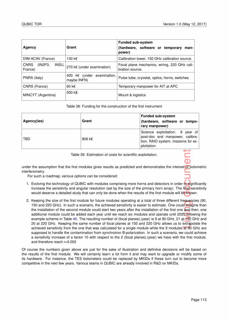
Livi
ngdo
cum
ent
QUBIC TDR Version 1.0 (May 12, 2017)
Agency GrantFunded sub-system(hardware, software or temporary man-power)
DIM-ACAV (France) 130 k€ Calibration tower, 150 GHz calibration source.
CNRS (IN2P3, INSU,France)
270 k€ (under examination)Focal plane mechanics, wiring, 220 GHz cali-bration source.
PNRA (Italy)400 k€ (under examination,maybe INFN)
Pulse tube, cryostat, optics, horns, switches.
CNRS (France) 60 k€ Temporary manpower for AIT at APC
MINCYT (Argentina)500 k$
Mount & logistics
Table 38: Funding for the construction of the first instrument
Agency(ies) GrantFunded sub-system(hardware, software or tempo-rary manpower)
TBD 806 k€
Science exploitation: 8 year ofpost-doc and manpower, calibra-tion, RAID system, missions for ex-ploitation.
Table 39: Estimation of costs for scientific exploitation.
under the assumption that the first modules gives results as predicted and demonstrates the interest of bolometricinterferometry.
For such a roadmap, various options can be considered:
1. Evolving the technology of QUBIC with modules comprising more horns and detectors in order to significantlyincrease the sensitivity and angular resolution (set by the size of the primary horn array). The final sensitivitywould deserve a detailed study that can only be done when the results of the first module will be known.
2. Keeping the size of the first module for future modules operating at a total of three different frequencies (90,150 and 220 GHz). In such a scenario, the achieved sensitivity is easier to estimate. One could imagine thanthe installation of the second module could start two years after the installation of the first one and then, oneadditional module could be added each year until we reach six modules and operate until 2025 following theexample scheme in Table 40. The resulting number of (focal planes).(year) is 9 at 90 GHz, 21 at 150 GHz and20 at 220 GHz. Keeping the same number of focal planes at 150 and 220 GHz allows us to extrapolate theachieved sensitivity from the one that was calculated for a single module while the 9 modules at 90 GHz aresupposed to handle the contamination from synchrotron B-polarization. In such a scenario, we could achievea sensitivity increase of a factor 10 with respect to the 2 (focal planes).(year) we have with the first module,and therefore reach r=0.002
Of course the numbers given above are just for the sake of illustration and definitve decisions will be based onthe results of the first module. We will certainly learn a lot from it and may want to upgrade or modify some ofits hardware. For instance, the TES bolometers could be replaced by MKIDs if these turn out to become morecompetitive in the next few years. Various teams in QUBIC are already involved in R&D on MKIDs.
Page 113
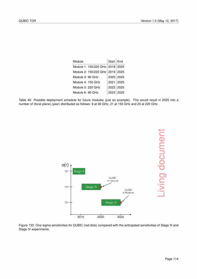
Livi
ngdo
cum
ent
QUBIC TDR Version 1.0 (May 12, 2017)
Module Start End
Module 1: 150/220 GHz 2018 2025
Module 2: 150/220 GHz 2019 2025
Module 3: 90 GHz 2020 2025
Module 4: 150 GHz 2021 2025
Module 5: 220 GHz 2022 2025
Module 6: 90 GHz 2023 2025
Table 40: Possible deployment schedule for future modules (just an example). This would result in 2025 into anumber of (focal plane).(year) distributed as follows: 9 at 90 GHz, 21 at 150 GHz and 20 at 220 GHz.
Figure 133: One sigma sensitivities for QUBIC (red dots) compared with the anticipated sensitivities of Stage III andStage IV experiments.
Page 114
Livi
ngdo
cum
ent
List of Figures
1 Recent B-modes measurements ; Total B-modes expected signal . . . . . . . . . . . . . . . . . . . . 62 Sketch of QUBIC (see text for explanation) . . . . . . . . . . . . . . . . . . . . . . . . . . . . . . . . 103 QUBIC primary horn array and corresponding beam on the sky for the central detector of any of the
two focal planes. . . . . . . . . . . . . . . . . . . . . . . . . . . . . . . . . . . . . . . . . . . . . . . 114 Current results with the QUBIC mapmaking under the Gaussian peaks assumption . . . . . . . . . . 125 Results of the current version of the map-making . . . . . . . . . . . . . . . . . . . . . . . . . . . . . 126 “Self-calibration” simulated result . . . . . . . . . . . . . . . . . . . . . . . . . . . . . . . . . . . . . 137 Full end-to-end Monte-Carlo simulation error-bars (dispersion) at 150 GHz . . . . . . . . . . . . . . . 148 Expected noise-only error bars for QUBIC ; Expected forecasts on dust spectral index and tensor-to-
scalar ratio with QUBIC . . . . . . . . . . . . . . . . . . . . . . . . . . . . . . . . . . . . . . . . . . . 149 schematic "top-view" of the TES bolometers for one focal plane of the QUBIC 1st module. Active
detectors are shown in blue. . . . . . . . . . . . . . . . . . . . . . . . . . . . . . . . . . . . . . . . . 1710 Picture of a TES array covering a quarter of the focal plane. Yellow lines are wires used for the reading
of the TESes signal. The TES in red is not used. . . . . . . . . . . . . . . . . . . . . . . . . . . . . . 1811 (left) Picture on one of the QUBIC focal plane TESes ; (right) Absorbing part of one TES (in blue). . . 1912 Simulated power loss of a detector at 150GHz and 220GHz with respect to backshort distance. An
optimal value for the backshort is 400µm. . . . . . . . . . . . . . . . . . . . . . . . . . . . . . . . . . 1913 Schematics of the cryostat shell, with outer dimensions indicated, including the two Pulse-Tube heads. 2314 Views of the 40K shield (first PT stage) with main dimensions. . . . . . . . . . . . . . . . . . . . . . 2415 Views of the 4K shield (second PT stage) with main dimensions. . . . . . . . . . . . . . . . . . . . . 2516 Left: flexible thermal interfaces between the PTs and the shields. Right: system of copper belts used
to thermalize the shields. . . . . . . . . . . . . . . . . . . . . . . . . . . . . . . . . . . . . . . . . . . 2617 Views of the fiberglass tubes “drum” holding firmly in place the 40K and 4K shields. . . . . . . . . . . 2618 1K box and its inner parts . . . . . . . . . . . . . . . . . . . . . . . . . . . . . . . . . . . . . . . . . 2719 Sketch of the 1K box . . . . . . . . . . . . . . . . . . . . . . . . . . . . . . . . . . . . . . . . . . . . 2820 Main dimensions of the 1K box. . . . . . . . . . . . . . . . . . . . . . . . . . . . . . . . . . . . . . . 2821 Moles of 4He as function of temperature during the cooling phase. . . . . . . . . . . . . . . . . . . . 2922 CAD drawings of the 1K Fridge . . . . . . . . . . . . . . . . . . . . . . . . . . . . . . . . . . . . . . 3023 Photos of the 4He Sorption Cooler alone and mountend on the 4K stage . . . . . . . . . . . . . . . . 3024 Chase Cryogenics fridge picture and load curve . . . . . . . . . . . . . . . . . . . . . . . . . . . . . 3125 The effect on GM cooler 2nd-stage T from operation of the fridge . . . . . . . . . . . . . . . . . . . . 3226 Both switch types . . . . . . . . . . . . . . . . . . . . . . . . . . . . . . . . . . . . . . . . . . . . . . 3327 Heat switch on and off . . . . . . . . . . . . . . . . . . . . . . . . . . . . . . . . . . . . . . . . . . . 3428 The off-axis dual reflector chosen for the QUBIC beam combiner . . . . . . . . . . . . . . . . . . . . 3529 Detail of the window mounting system. . . . . . . . . . . . . . . . . . . . . . . . . . . . . . . . . . . 3530 Embedded mesh-HWP based on metamaterials. . . . . . . . . . . . . . . . . . . . . . . . . . . . . 3631 Large bandwidth (˜93%) mesh-HWP prototype: modeled and measured performance. . . . . . . . . . 3732 Expected performance of the QUBIC broadband mesh-HWP design. . . . . . . . . . . . . . . . . . . 3733 General view of the cryogenic waveplate rotator. . . . . . . . . . . . . . . . . . . . . . . . . . . . . . 3834 Detail of the HWP clamp. . . . . . . . . . . . . . . . . . . . . . . . . . . . . . . . . . . . . . . . . . . 3835 Transmission performance of thermal filters for the QUBIC instrument. . . . . . . . . . . . . . . . . . 4036 Transmission performance of prototyped common LPE blocking filters . . . . . . . . . . . . . . . . . 4037 Transmission performance of possible 12cm−1 blocking filter. . . . . . . . . . . . . . . . . . . . . . . 4038 Transmission performance of possible 12cm−1 blocking filter. . . . . . . . . . . . . . . . . . . . . . . 4139 Transmission performance of a prototype 6.5cm−1 high-pass dichroic . . . . . . . . . . . . . . . . . . 4140 Example previously manufactured large diameter polariser (45cm diameter). . . . . . . . . . . . . . . 4241 Designs of the QUBIC feed horns . . . . . . . . . . . . . . . . . . . . . . . . . . . . . . . . . . . . . 4342 Outer view of the brass QUBIC1 prototype. . . . . . . . . . . . . . . . . . . . . . . . . . . . . . . . . 4443 Inside view of the brass QUBIC1 prototype . . . . . . . . . . . . . . . . . . . . . . . . . . . . . . . . 4444 Brass, anticorodal and silver-plated anticorodal prototypes . . . . . . . . . . . . . . . . . . . . . . . . 4445 QUBIC1 aluminum and QUBIC2 anticorodal prototypes . . . . . . . . . . . . . . . . . . . . . . . . . 4546 Absolute and relative deviations of measured diameters with respect to the nominal ones as a function
of the diameter . . . . . . . . . . . . . . . . . . . . . . . . . . . . . . . . . . . . . . . . . . . . . . . 4547 Deviation of the hole center position with respect to the nominal value . . . . . . . . . . . . . . . . . 46
115
Livi
ngdo
cum
ent
QUBIC TDR Version 1.0 (May 12, 2017)
48 Impact of cusps on the feed-horn return loss . . . . . . . . . . . . . . . . . . . . . . . . . . . . . . . 4749 Effect of cusps on maximum cross-polarization . . . . . . . . . . . . . . . . . . . . . . . . . . . . . . 4750 Simulated beam patterns showing the effect of cusps on the E and H planes . . . . . . . . . . . . . . 4851 Return loss measured on one horn of each of the three prototypes . . . . . . . . . . . . . . . . . . . 4852 Measured main beam patterns . . . . . . . . . . . . . . . . . . . . . . . . . . . . . . . . . . . . . . . 4953 CAD design of prototype #6 (128 horn array) . . . . . . . . . . . . . . . . . . . . . . . . . . . . . . . 5054 First realization of the back flange of the 8x8 prototype. . . . . . . . . . . . . . . . . . . . . . . . . . 5055 Particular of the waveguide shutter for the 8x8 prototype . . . . . . . . . . . . . . . . . . . . . . . . . 5156 Switch Performance forecast when in “ON” (Top Panel) and “OFF” positions . . . . . . . . . . . . . . 5157 instrumental set-up to measure the Single switch S parameters, return loss and insertion loss . . . . 5258 The two sides of the board able to operate and acquire the position of 16 switches . . . . . . . . . . . 5259 The 8x8 switch block prototype . . . . . . . . . . . . . . . . . . . . . . . . . . . . . . . . . . . . . . . 5360 M1, primary mirror. . . . . . . . . . . . . . . . . . . . . . . . . . . . . . . . . . . . . . . . . . . . . . 5461 M2, secondary mirror. . . . . . . . . . . . . . . . . . . . . . . . . . . . . . . . . . . . . . . . . . . . 5462 3D drawings of the 45 degrees dichroic mount and of the radiation shield for the on-axis focal plane. . 5563 3D views of the optical path through the combiner . . . . . . . . . . . . . . . . . . . . . . . . . . . . 5564 Maps of power on the on-axis focal plane array considering a tangential couple and a sagittal couple
of feed horns . . . . . . . . . . . . . . . . . . . . . . . . . . . . . . . . . . . . . . . . . . . . . . . . 5665 Power on the on-axis focal plane collected from the feed horn ID-53 passing through the combiner
and as straylight . . . . . . . . . . . . . . . . . . . . . . . . . . . . . . . . . . . . . . . . . . . . . . . 5766 Equivalent on-axis system for the QUBIC beam combiner. . . . . . . . . . . . . . . . . . . . . . . . 5767 Gaussian beam width (w) as a function of propagation distance through the QUBIC beam combiner . 5868 Footprint of 400 antenna beams on a 600-mm diameter secondary mirror, and the same simulation
for the outer ring of 12.9° horn beams . . . . . . . . . . . . . . . . . . . . . . . . . . . . . . . . . . . 5869 3D rendering of the PO beams in a CAD model of the QUBIC combiner [5]. . . . . . . . . . . . . . . 5970 (adapted from ref. [14]) Dispersion curves for the 12.9° feed horn showing the modes that can propa-
gate (β is the waveguide wave number for a given mode) at various frequencies in the narrowest pointof the feed horn. In this case for for QUBIC’s 12.9° feed horn the narrowest inner (ri) and outer (ro)radii are 0.684 mm and 1.394 mm respectively. . . . . . . . . . . . . . . . . . . . . . . . . . . . . . . 59
71 Plots of hybrid mode (and) aperture fields for the 5 dominant modes of the QUBIC 220-GHz channel(orthogonal modes exist for n > 0): the HE11 and its orthogonal mode, the E02 mode and the HE21and its orthogonal mode. . . . . . . . . . . . . . . . . . . . . . . . . . . . . . . . . . . . . . . . . . . 60
72 (left)Farfield beam patterns calculated across the 150-GHz band (4GHz intervals) where the hornsare single-moded and (right) the beam patterns across the 220-GHz band. . . . . . . . . . . . . . . 61
73 Plots of the beam pattern from each of 400 input horns on the circular focal plane ; total percentageof power from each beam that is integrated on the focal plane . . . . . . . . . . . . . . . . . . . . . . 61
74 Average of the fringe patterns generated by 145 equivalent νλ = 50 baselines . . . . . . . . . . . . . 6275 Diagonal window function of the real beam combiner divided by that of an ideal non-aberrating instru-
ment . . . . . . . . . . . . . . . . . . . . . . . . . . . . . . . . . . . . . . . . . . . . . . . . . . . . . 6376 Simulated QUBIC PSF for the dual band combiner, operated at 150 GHz, for an on-axis source or
central pixel . . . . . . . . . . . . . . . . . . . . . . . . . . . . . . . . . . . . . . . . . . . . . . . . . 6377 Superconducting transition characteristics of four Nb0.15Si0.85 TES distributed far away from each
other on a 256 pixel array. . . . . . . . . . . . . . . . . . . . . . . . . . . . . . . . . . . . . . . . . . 6478 CAO of the 1024 array, of one pixel and of the TES with its interleaved electrodes . . . . . . . . . . . 6579 Picture of the Deep etching of the Si to form the membrane of the pixels, microscope image of the
TES and the comb shaped electrodes . . . . . . . . . . . . . . . . . . . . . . . . . . . . . . . . . . . 6580 Pictures of the 256 TES array being processed (left) and being integrated for the test (right) . . . . . . 6681 Detection Chain including TES, TES biasing (Rsh), SQUID, ASIC (LNA) and Warm Digital Readout
(ADC+FPGA) . . . . . . . . . . . . . . . . . . . . . . . . . . . . . . . . . . . . . . . . . . . . . . . . 6682 Flux to voltage SQUID transfer function for current biasing from 0 to 17.5 µA. And I(V) SQUID output
characteristic. . . . . . . . . . . . . . . . . . . . . . . . . . . . . . . . . . . . . . . . . . . . . . . . . 6783 flux-to-voltage open loop SQUID gain and feedback transfer function ; FLL flux-to-voltage linearized
transfer function . . . . . . . . . . . . . . . . . . . . . . . . . . . . . . . . . . . . . . . . . . . . . . . 6784 Layout and photo of the SQUID and the full wafer . . . . . . . . . . . . . . . . . . . . . . . . . . . . 6985 I(φ) measurement using a vector analyzer allows to obtain the SQUID V(φ) transfer function . . . . . 70
Page 116
Livi
ngdo
cum
ent
QUBIC TDR Version 1.0 (May 12, 2017)
86 Topology of the 128 to 1 multiplexer sub-system (4x32 SQUID + 1 ASIC). Integration of 32 SQUIDs(1 collumn) with bias capacitors and filter devices. . . . . . . . . . . . . . . . . . . . . . . . . . . . . 70
87 SQUID glued and wire bonded with filter devices. Values of the filter devices put close to SQUIDs. . . 7188 Two SQUID boards stacked to finally obtain a SQUID box composed of 4 PCBs, TES thermo-
mechanical structure showing the 2 SQUIDs boxes near the TES array . . . . . . . . . . . . . . . . . 7189 Microphotography of cryogenic ASIC designed to readout 4x32 TES/SQUID pixels . . . . . . . . . . 7290 Functions implemented in the ASIC. . . . . . . . . . . . . . . . . . . . . . . . . . . . . . . . . . . . . 7391 Multiplexed LNA (low noise amplification) equivalent input noise voltage measurement at 77K. . . . . 7392 Experimental setup for the cryogenic ASIC characterizations and the functional tests performed with
4 “StarCryo” SQUID chips bonded on a PCB and SMD addressing capacitors. . . . . . . . . . . . . . 7493 Preliminary clocking validation at 4.2K of the multiplexer . . . . . . . . . . . . . . . . . . . . . . . . . 7494 Validation at 4.2K of the AC SQUID biasing operation through addressing capacitors (100nF) and
dynamic offset compensation principle . . . . . . . . . . . . . . . . . . . . . . . . . . . . . . . . . . 7595 Output signal measured at 100 kHz of multiplexing clock frequency . . . . . . . . . . . . . . . . . . . 7596 The NetQuiC board architecture . . . . . . . . . . . . . . . . . . . . . . . . . . . . . . . . . . . . . . 7697 Warm electronic overall architecture . . . . . . . . . . . . . . . . . . . . . . . . . . . . . . . . . . . . 7798 View of architecture visualization tool . . . . . . . . . . . . . . . . . . . . . . . . . . . . . . . . . . . 7899 View of focal plane visualization tool . . . . . . . . . . . . . . . . . . . . . . . . . . . . . . . . . . . 79100 View of the interface of the control command . . . . . . . . . . . . . . . . . . . . . . . . . . . . . . . 80101 I-V and P-V curves of a TES (no60, ASIC2, P41 array) at different Tbath < Tc . . . . . . . . . . . . . 81102 Fitted measurements of plateau power at different regulation temperatures (TES no60) . . . . . . . . 82103 I-V and P-V curves of TESs on P41 array at Tbath = 350mK . . . . . . . . . . . . . . . . . . . . . . . 83104 Histograms of Pmin, G and approximation of theoretical NEP of selected pixels of a 256 TES array
obtained from I-V measurements at different bath temperatures. . . . . . . . . . . . . . . . . . . . . 83105 Mount . . . . . . . . . . . . . . . . . . . . . . . . . . . . . . . . . . . . . . . . . . . . . . . . . . . . 84106 QUBIC Forebaffle and Ground Shield mechanical drawings . . . . . . . . . . . . . . . . . . . . . . . 85107 Sketch of the QUBIC shielding configuration and cut of the hybrid conical horn beam pattern used in
MultiGTD simulations . . . . . . . . . . . . . . . . . . . . . . . . . . . . . . . . . . . . . . . . . . . . 86108 Cuts of the patterns (at 0 degrees) for the on-axis feedhorn varying FB height and aperture angle . . 86109 Cuts of the beam pattern with and without a cylindrical shield and with and without a conical shield . . 87110 Beam pattern cuts for the cylindrical forebaffle including the Flare . . . . . . . . . . . . . . . . . . . . 87111 Beam pattern cuts for the conical forebaffle including the Flare . . . . . . . . . . . . . . . . . . . . . 88112 Power collected by a single pixel on the focal plane . . . . . . . . . . . . . . . . . . . . . . . . . . . . 89113 Zenith atmospheric opacity at 150 GHz as a function of the pwv content, from 0.1 mm up to a max-
imum value of 2 mm. According to atmospheric models for Chajnantor, to get the opacities at 220GHz, these values should be scaled by ∼ 1.83. . . . . . . . . . . . . . . . . . . . . . . . . . . . . . 89
114 Power collected by a single detector due to atmospheric emission plus FB emission in reflecting andabsorbing configurations . . . . . . . . . . . . . . . . . . . . . . . . . . . . . . . . . . . . . . . . . . 89
115 QUBIC shielding components: a forebaffle (FB) and a ground shield (GS) ; Beam pattern cuts of thecentral feed with the forebaffle alone and including also the ground shield . . . . . . . . . . . . . . . 90
116 “In lab” Calibration strategy . . . . . . . . . . . . . . . . . . . . . . . . . . . . . . . . . . . . . . . . . 94117 Scanning Strategy in local coordinates and sweeps in RA, DEC (right) for a location in Dome C,
Antarctica . . . . . . . . . . . . . . . . . . . . . . . . . . . . . . . . . . . . . . . . . . . . . . . . . . 95118 Coverage achieved when adding successive coverages over 10 days . . . . . . . . . . . . . . . . . . 96119 coverage in Sky Coordinates for a 24h scanning around a single spot on the sky . . . . . . . . . . . . 96120 The "American tower" at Concordia Station and a schematic of a tower with less footprint . . . . . . . 98121 Operating principle of the full-beam calibrator. . . . . . . . . . . . . . . . . . . . . . . . . . . . . . . 98122 Stokes parameters I and Q of the radiation produced by the full beam calibrator in the 150 GHz band
of QUBIC. . . . . . . . . . . . . . . . . . . . . . . . . . . . . . . . . . . . . . . . . . . . . . . . . . . 99123 PWV data for Concordia from balloon soundings at Concordia . . . . . . . . . . . . . . . . . . . . . . 100124 Atmospheric spectrum from ATM with parameters optimized for Chajnantor Atmosphere . . . . . . . 100125 Atmospheric Opacity at 150 and 220 GHz derived at the LLAMA site over more than three years. . . 101126 Atmospheric emissivities compared for both Concordia and Argentinian sites. . . . . . . . . . . . . . 102127 Noise Equivalent Temperatures forecasted from our study at 150 and 220 GHz for QUBIC in both
possible sites. . . . . . . . . . . . . . . . . . . . . . . . . . . . . . . . . . . . . . . . . . . . . . . . . 102128 Relative sensitivity of the two sites as a function of the observation efficiency. . . . . . . . . . . . . . 103
Page 117
Livi
ngdo
cum
ent
QUBIC TDR Version 1.0 (May 12, 2017)
129 Alto Chorillos site in Argentina, near San Antonio de los Cobres, province of Salta. The position forother astronomical instruments location in Chile is also shown (red cross). . . . . . . . . . . . . . . . 104
130 Views of the chosen QUBIC site in Argentina along with the LLAMA [64] location and logistic instal-lations planned to be installed during 2017 and funded by MinCyT and the Province of Salta. Inmagenta the limits of the allocated area for scientific use from the Salta government. . . . . . . . . . 104
131 Top, left: Annual Temperature variation at Alto Chorillos site. Top, right: Daily temperature distribution.Bottom, left: 1-minute average wind speed distribution. Bottom, right: Maximum wind speed in 1-minute distribution. . . . . . . . . . . . . . . . . . . . . . . . . . . . . . . . . . . . . . . . . . . . . . 106
132 Work Breakdwon Structure of QUBIC . . . . . . . . . . . . . . . . . . . . . . . . . . . . . . . . . . . 110133 One sigma sensitivities for QUBIC (red dots) compared with the anticipated sensitivities of Stage III
and Stage IV experiments. . . . . . . . . . . . . . . . . . . . . . . . . . . . . . . . . . . . . . . . . 114134 Location and view of the Concordia Station in Dome C, Antarctica . . . . . . . . . . . . . . . . . . . . 124135 location of a QUBIC module in the case of QUBIC 3 and 3bis option . . . . . . . . . . . . . . . . . . 125136 Materials delivery: typical time schedule for cargo delivery at Concordia. . . . . . . . . . . . . . . . . 126137 Map of the Antarctic base Concordia-Dome C with an inset where the possible locations of a QUBIC
module are highlighted. . . . . . . . . . . . . . . . . . . . . . . . . . . . . . . . . . . . . . . . . . . . 130
Page 118
Livi
ngdo
cum
ent
List of Tables
1 Summary of the main ground and balloon projects aiming at measuring B-modes . . . . . . . . . . . 82 General requirements on the bolometric interferometer design. . . . . . . . . . . . . . . . . . . . . . 153 Requirements on horns . . . . . . . . . . . . . . . . . . . . . . . . . . . . . . . . . . . . . . . . . . . 154 Requirements on cold optics chain . . . . . . . . . . . . . . . . . . . . . . . . . . . . . . . . . . . . 165 Requirements on mirrors and optical properties . . . . . . . . . . . . . . . . . . . . . . . . . . . . . . 166 Requirements on switches . . . . . . . . . . . . . . . . . . . . . . . . . . . . . . . . . . . . . . . . . 167 Requirements on the external shields . . . . . . . . . . . . . . . . . . . . . . . . . . . . . . . . . . . 178 Requirements on the TES detectors . . . . . . . . . . . . . . . . . . . . . . . . . . . . . . . . . . . . 189 Requirements on the sensitivity . . . . . . . . . . . . . . . . . . . . . . . . . . . . . . . . . . . . . . 2010 Requirement on cryostat and cryogenics . . . . . . . . . . . . . . . . . . . . . . . . . . . . . . . . . 2011 Requirements on instrument internal structure . . . . . . . . . . . . . . . . . . . . . . . . . . . . . . 2112 Requirements on calibration sources . . . . . . . . . . . . . . . . . . . . . . . . . . . . . . . . . . . 2113 General requirements on the mount system. . . . . . . . . . . . . . . . . . . . . . . . . . . . . . . . 2214 Summary of simulated heat loads on 4K and 40K stages. . . . . . . . . . . . . . . . . . . . . . . . . 2715 Sub-K fridge electrical interfaces . . . . . . . . . . . . . . . . . . . . . . . . . . . . . . . . . . . . . . 3216 3He hold times for two load values. . . . . . . . . . . . . . . . . . . . . . . . . . . . . . . . . . . . . 3217 4He hold times for one load value. . . . . . . . . . . . . . . . . . . . . . . . . . . . . . . . . . . . . 3218 Heat switch electrical interfaces (per switch) . . . . . . . . . . . . . . . . . . . . . . . . . . . . . . . 3419 Mesh-HWP bandwidth requirements. . . . . . . . . . . . . . . . . . . . . . . . . . . . . . . . . . . . 3620 Metal mesh devices to be supplied by Cardiff University to the QUBIC project. Z coordinates are given
in the Global Reference Frame (GRF). (*) emissivity could be lower. (**) low frequency in reflexion,high frequency in transmission. . . . . . . . . . . . . . . . . . . . . . . . . . . . . . . . . . . . . . . 39
21 List of QUBIC feed horn array prototypes . . . . . . . . . . . . . . . . . . . . . . . . . . . . . . . . . 4322 Measured Insertion Loss (IL) of the three QUBIC1 prototypes . . . . . . . . . . . . . . . . . . . . . . 4923 Combiner parameters (the primary mirror surface was further optimised using the Zemax ray-tracing
package and the final design, specified by a set of quadratic surface parameters differs slightly fromthe conic surface specified here). . . . . . . . . . . . . . . . . . . . . . . . . . . . . . . . . . . . . . 53
24 Weighting of hybrid modes in the 220 GHz band. (No n = 4 power). . . . . . . . . . . . . . . . . . . . 6025 Requirements criteria for selection of SQUIDs . . . . . . . . . . . . . . . . . . . . . . . . . . . . . . 6826 Main characteristics of the cold electronics . . . . . . . . . . . . . . . . . . . . . . . . . . . . . . . . 7227 data rate and storage of scientific data. . . . . . . . . . . . . . . . . . . . . . . . . . . . . . . . . . . 8128 data rate and storage of raw data. . . . . . . . . . . . . . . . . . . . . . . . . . . . . . . . . . . . . . 8129 spillover contributions. . . . . . . . . . . . . . . . . . . . . . . . . . . . . . . . . . . . . . . . . . . . 9030 Respective definitions of the technological demonstrator and the final instrument. . . . . . . . . . . . 9131 Characteristics of the instrument that will be measured during the first cooling downs of the QUBIC
instrument, for different loads on the detectors. . . . . . . . . . . . . . . . . . . . . . . . . . . . . . . 9232 Characteristics of the QUBIC instrument that will be measured with the Carbon fiber source, the
Calibration source and/or the FTS. . . . . . . . . . . . . . . . . . . . . . . . . . . . . . . . . . . . . 9333 Azimuth and elevation ranges for the two considered fields for QUBIC, for Dome C (left) and Argentina
(right). . . . . . . . . . . . . . . . . . . . . . . . . . . . . . . . . . . . . . . . . . . . . . . . . . . . 9534 Relative observation efficiency for the two sites . . . . . . . . . . . . . . . . . . . . . . . . . . . . . . 10335 Main characteristics of Institutes in the QUBIC collaboration . . . . . . . . . . . . . . . . . . . . . . 10736 PBS of the QUBIC project. when present, comma separated lists in the Items column indicate sepa-
rate products. . . . . . . . . . . . . . . . . . . . . . . . . . . . . . . . . . . . . . . . . . . . . . . . . 10937 Fundings for R&D and validation of detection chain . . . . . . . . . . . . . . . . . . . . . . . . . . . 11238 Funding for the construction of the first instrument . . . . . . . . . . . . . . . . . . . . . . . . . . . . 11339 Estimation of costs for scientific exploitation. . . . . . . . . . . . . . . . . . . . . . . . . . . . . . . . 11340 Possible deployment schedule for future modules (just an example). This would result in 2025 into a
number of (focal plane).(year) distributed as follows: 9 at 90 GHz, 21 at 150 GHz and 20 at 220 GHz. 11441 Milestones for the implementation of QUBIC in Concordia Station, YY stands for the year for which
the experiment module would be available for shipping. . . . . . . . . . . . . . . . . . . . . . . . . . 12642 Tentative schedule with a departure date on August, 20th 2016 and estimation of costs for transporta-
tion of materials. . . . . . . . . . . . . . . . . . . . . . . . . . . . . . . . . . . . . . . . . . . . . . . 127
119

Livi
ngdo
cum
ent
QUBIC TDR Version 1.0 (May 12, 2017)
43 Logistic costs: Logistic costs foreseen for the QUBIC experiment. We have divided the costs withinthe years. . . . . . . . . . . . . . . . . . . . . . . . . . . . . . . . . . . . . . . . . . . . . . . . . . . 129
44 Pro and cons of QUBIC 1 option . . . . . . . . . . . . . . . . . . . . . . . . . . . . . . . . . . . . . . 13145 Pro and cons of QUBIC 2 option . . . . . . . . . . . . . . . . . . . . . . . . . . . . . . . . . . . . . . 13146 Pro and cons of QUBIC 3 option . . . . . . . . . . . . . . . . . . . . . . . . . . . . . . . . . . . . . . 13247 Possible locations of a QUBIC module with coordinates. In red we highlight not viable solutions
(unless no other options are possible), in orange we highlight possible solutions with some limitationsand loss on efficiency, in green we highlight our preferred solution which, from our point of view, is thebest trade-off solution with minimal interference. . . . . . . . . . . . . . . . . . . . . . . . . . . . . . 133
Page 120

Livi
ngdo
cum
ent
QUBIC TDR Version 1.0 (May 12, 2017)
6 References
[1] N. Krachmalnicoff, C. Baccigalupi, J. Aumont, M. Bersanelli and A. Mennella, Astron. Astrophys. 588, A65 (2016)doi:10.1051/0004-6361/201527678 [arXiv:1511.00532 [astro-ph.CO]].
[2] P.T. Timbie and G.S. Tucker, Adding inteferometry for CMBpol, Journal of Physics: Conference Series 155,012003 (2009)
[3] D. Baumann, CMBPol Mission Concept Study. AIP Conference Proceedings, Volume 1141, pp. 10-120 (2009)arXiv:0811.3919
[4] Smith, K. M. 2006, Phys. Rev. D, 74, 083002
[Calvo et al.(2016)] Calvo, M., Benoît, A., Catalano, A., et al. 2016, Journal of Low Temperature Physics, 184, 816
[5] D. Gayer et al., Proc. of SPIE Vol. 8452 (2012)
[6] Smith, K. M., & Zaldarriaga, M. 2007, Phys. Rev. D, 76, 043001
[7] Zemax-EE, ZEMAX Development Corporation. Online at http://www.zemax.com/ (as of August 2015).
[8] O’Sullivan, C., et al., (2002). Far Infra-red Optics Design & Verification. International Journal of Infrared andMillimeter Waves 23,(7), 1029-1045.
[9] Goldsmith, P.F., (1998). Quasioptical Systems: Gaussian Beam Quasioptical Propagation and Applications, IEEEPress series on microwave technology and techniques.
[10] C. O’Sullivan et al., 36th ESA Antenna Workshop, Noordwijk, The Netherlands, 2015
[11] Gradziel, M. Ł, et al., (2007). Modelling of the optical performance of millimeter-wave instruments in MODAL, inProc. SPIE 6472, 64720D.
[12] GRASP9, TICRA Engineering Consultants. Online at http://www.ticra.dk/ (as of August 2015).
[13] Murphy, J. A., et al., (2001). Radiation patterns of multi-moded corrugated horns for far-IR space applications.Infrared Phys. and Tech. 42, 515-528.
[14] Scully, S., PhD Thesis, National University of Ireland, Maynooth (submitted October 2015).
[15] Gayer, D., PhD Thesis, National University of Ireland, Maynooth (in preparation).
[16] R. Charlassier, et al., Astron. Astrophys. 497-3, 963:971 (2009), Charlassier, PhD thesis
[17] Hamilton, J.-C., Charlassier, R., Cressiot, C., et al. 2008, A&A, 491, 923
[18] Bicep& Planck , Phys. Rev. Lett. 114, 101301 (2015)
[19] Ade, P. A. R., Akiba, Y., Anthony, A. E., et al. 2014, Physical Review Letters, 113, 021301
[20] S. Naess et al. [ACTPol Collaboration], JCAP 1410, no. 10, 007 (2014) doi:10.1088/1475-7516/2014/10/007[arXiv:1405.5524 [astro-ph.CO]].
[21] Keisler, R., Hoover, S., Harrington, N., et al. 2015, ApJ, 807, 151
[22] http://moriond.in2p3.fr/J16/transparencies/1_sunday/1_morning/7_bischoff.pdf
[23] http://moriond.in2p3.fr/J16/transparencies/3_tuesday/1_morning/1_bender.pdf
[24] http://moriond.in2p3.fr/J16/transparencies/3_tuesday/1_morning/5_niemack.pdf
[25] http://max.ifca.unican.es/EWASS2015/TalksOnTheWeb/Number09_Borrill.pdf
[26] http://moriond.in2p3.fr/J16/transparencies/3_tuesday/1_morning/6_moncelsi.pdf
[27] Lazear, J., Ade, P. A. R., Benford, D., et al. 2014, Proc. SPIE, 9153, 91531L
Page 121
Livi
ngdo
cum
ent
QUBIC TDR Version 1.0 (May 12, 2017)
[28] EBEX 10K proposal to NASA, 2015
[29] Essinger-Hileman, T., Ali, A., Amiri, M., et al. 2014, Proc. SPIE, 9153, 91531I
[30] The LSPE collaboration, Aiola, S., Amico, G., et al. 2012, arXiv:1208.0281
[31] Errard, J., Feeney, S. M., Peiris, H. V., & Jaffe, A. H. 2016, J. Cosmology Astropart. Phys., 3, 052
[32] Chanial et al., in preparation
[33] Salatino, M., & de Bernardis, P. 2010, arXiv:1006.3225 Salatino et al., 2010, http://pilot.irap.omp.eu/PAGE_PILOT/index.html
[34] M.-A. Bigot-Sazy, R. Charlassier, J.-C. Hamilton, J. Kaplan and G. Zahariade, Astron. Astrophys. 550 (2013)A59 doi:10.1051/0004-6361/201220429 [arXiv:1209.4905 [astro-ph.IM]].
[35] Errard, J., Ade, P. A. R., Akiba, Y., et al. 2015, ApJ, 809, 63
[36] Marie-Anne Bigot-Sazy, M.-A., (2013). PhD Thesis, Université Paris Diderot, Paris 7.
[37] R. Adam et al. [Planck Collaboration], arXiv:1409.5738 [astro-ph.CO].
[38] Scott, P. F.; et al. (2003). "First results from the Very Small Array III: The CMB Power Spectrum". MNRAS 341(4): 1076-1083. arXiv:astro-ph/0205380
[39] Kovac, J. M., Leitch, E. M., Pryke, C., et al. 2002, Nature, 420, 772
[40] Readhead, A. C. S., Myers, S. T., Pearson, T. J., et al. 2004, Science, 306, 836
[41] Fuskeland, U., Wehus, I. K., Eriksen, H. K., & Næss, S. K. 2014, ApJ, 790, 104
[42] Bennett, D. G., (2014) PhD Thesis, National University of Ireland, Maynooth
[43] Rusch, W. V. T., et al., (1990). Derivation and application of the equivalent paraboloid for classical offsetCassegrain and Gregorian antennas, IEEE Trans. Antennas and Propagat. 38, (8), 1141.
[44] Buzi, D., PhD Thesis, University La Sapienza, Rome (submitted October 2015).
[45] Franceschet, Cristian, (2013) Analysis of non idealities on the D-band QUBIC feed horn performance.
[46] Martino, J. Characterization of a detection chain using superconducting bolometers for polarization measure-ment of the Cosmic Microwave Background https://tel.archives-ouvertes.fr/tel-00794700 + Perbost C. to come
[47] Henrot−Versillé, S., et al., Pulsed Carbon fiber illuminators for FIR instrument characterization. Infrared Physics&Technology 2009 52 159−165
[48] P. Battaglia, F. Cavaliere, C. Franceschet, E. Pagana, A. Simonetto, M. Zannoni "D Band Antenna TechnologicalDemonstrator Test Report”, QUBIC Internal Report, University of Milano 2014
[49] Planck Collaboration, A&A Volume 520, September-October 2010 “Pre-launch status of the Planck mission HFIground calibration”, A10
[50] P. A. R. Ade et al. [BICEP2 Collaboration], Sumitted to PRL, arXiv:1510.09217
[51] De Gregori et al. (MNRAS, 425, 222-230, 2012.) De Gregori et al.
[52] Polenta et al. NA 51, 3-4, 2007
[53] Battistelli et al. MNRAS 423, 1293, 2012 Battistelli et al. 2012
[54] De Petris et al. in preparation
[55] Aristidi et al. A&A 444, 651-659 (2005)
[56] Tristram, M., Patanchon, G., Macías-Pérez, J. F., et al. 2005, A&A, 436, 785
Page 122
Livi
ngdo
cum
ent
QUBIC TDR Version 1.0 (May 12, 2017)
[57] Ferté, A., Grain, J., Tristram, M., & Stompor, R. 2013, Phys. Rev. D, 88, 023524, Ferté, PhD Thesis 2014
[58] Grain, J., Tristram, M., & Stompor, R. 2009, Phys. Rev. D, 79, 123515
[59] Fraisse et al., JCAP04 (2013) 047 arXiv:1106.3087.
[60] Tomasi, C., Petkov, B., Maria Dinelli, B., et al. 2011, Journal of Atmospheric and Solar-Terrestrial Physics, 73,2237
[61] Salatino M., et al., Astron. & Astrophys. 528, A138 (2011)
[62] R. Puddu, PhD thesis, University of Siena (2016)
[63] Clarricoats, P.J.B., and Olver, A.D., Corrugated Horns for Microwave Antennas, IEE Electromagnetic wavesseries, Vol. 18, Peter Peregrinus Ltd., London, (1984)
[64] http://www.iar.unlp.edu.ar/llama-web/project.htm
[65] “Project QUBIC: Estimation des dépenses pour le 1er module” IPEV Document dated 13/11/2012.
Page 123
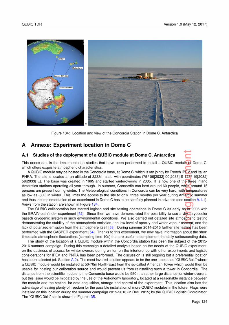
Livi
ngdo
cum
ent
QUBIC TDR Version 1.0 (May 12, 2017)
//
Figure 134: Location and view of the Concordia Station in Dome C, Antarctica
A Annexe: Experiment location in Dome C
A.1 Studies of the deployment of a QUBIC module at Dome C, Antarctica
This annex details the implementation studies that have been performed to install a QUBIC module at Dome C,which offers exquisite atmospheric characteristics.
A QUBIC module may be hosted in the Concordia base, at Dome C, which is ran jointly by French IPEV and ItalianPNRA. The site is located at an altitude of 3233m a.s.l. with coordinates (75° 06[2032] 00[2033] S 123° 19[2032]58[2033] E). The base was created in 1995 and started winterovering in 2005. It is now one of the three inlandAntarctica stations operating all year through. In summer, Concordia can host around 60 people, while around 15persons are present during winter. The Meteorological conditions in Concordia can be very hard, with temperaturesas low as -80C in winter. This limits the access to the site to only ˜three months per year during Antarctic summerand thus the implementation of an experiment in Dome C has to be carefully planned in advance (see section A.1.1).Views from the station are shown in Figure 134.
The QUBIC collaboration has started logistic and site testing operations in Dome C as early as in 2006 withthe BRAIN-pathfinder experiment [52]. Since then we have demonstrated the possibility to use a dry (cryocoolerbased) cryogenic system in such environmental conditions. We also carried out detailed site atmospheric testingdemonstrating the stability of the atmospheric emission, the low level of opacity and water vapour content, and thelack of polarized emission from the atmosphere itself [53]. During summer 2014-2015 further site testing has beenperformed with the CASPER experiment [54]. Thanks to this experiment, we now have information about the shorttimescale atmospheric fluctuations (sampling time 10s) that are useful to complement the daily radiosounding data.
The study of the location of a QUBIC module within the Concordia station has been the subject of the 2015-2016 summer campaign. During this campaign a detailed analysis based on the needs of the QUBIC experiment,on the easiness of access for winter-overers during winter, on the interference with other experiments and logisticconsiderations for IPEV and PNRA has been performed. The discussion is still ongoing but a preferential locationhas been selected (cf. Section A.2). The most favored solution appears to be the one labeled as “QUBIC 3bis” wherea QUBIC module would be installed at 50-70m North-East from the so-called American Tower which would then beusable for hosting our calibration source and would prevent us from reinstalling such a tower in Concordia. Thedistance from the scientific module to the Concordia base would be 950m, a rather large distance for winter-overers,but this issue would be mitigated by the use of the Astronomy laboratory, located at a reasonable distance betweenthe module and the station, for data acquisition, storage and control of the experiment. This location also has theadvantage of leaving plenty of freedom for the possible installation of more QUBIC modules in the future. Flags wereinstalled on this location during the summer campaign 2015-2016 (in Dec. 2015) by the QUBIC Logistic Coordinator.The “QUBIC 3bis” site is shown in Figure 135.
Page 124
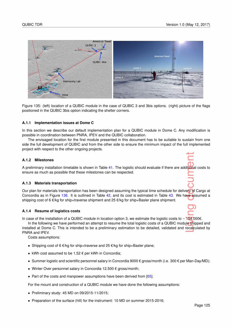
Livi
ngdo
cum
ent
QUBIC TDR Version 1.0 (May 12, 2017)
Figure 135: (left) location of a QUBIC module in the case of QUBIC 3 and 3bis options. (right) picture of the flagspositioned in the QUBIC 3bis option indicating the shelter corners.
A.1.1 Implementation issues at Dome C
In this section we describe our default implementation plan for a QUBIC module in Dome C. Any modification ispossible in coordination between PNRA, IPEV and the QUBIC collaboration.
The envisaged location for the first module presented in this document has to be suitable to sustain from oneside the full development of QUBIC and from the other side to ensure the minimum impact of the full implementedproject with respect to the other ongoing projects.
A.1.2 Milestones
A preliminary installation timetable is shown in Table 41. The logistic should evaluate if there are additional costs toensure as much as possible that these milestones can be respected.
A.1.3 Materials transportation
Our plan for materials transportation has been designed assuming the typical time schedule for delivery of Cargo atConcordia as in Figure 136. It is outlined in Table 42, and its cost is estimated in Table 43. We have assumed ashipping cost of 6 €/kg for ship+traverse shipment and 25 €/kg for ship+Basler plane shipment.
A.1.4 Resume of logistics costs
In case of the installation of a QUBIC module in location option 3, we estimate the logistic costs to ∼ 154.000€.In the following we have performed an attempt to resume the total logistic costs of a QUBIC module shipped and
installed at Dome C. This is intended to be a preliminary estimation to be detailed, validated and recalculated byPNRA and IPEV.
Costs assumptions:
• Shipping cost of 6 €/kg for ship+traverse and 25 €/kg for ship+Basler plane;
• kWh cost assumed to be 1,52 € per kWh in Concordia;
• Summer logistic and scientific personnel salary in Concordia 9000 € gross/month (i.e. 300 € per Man-Day/MD);
• Winter Over personnel salary in Concordia 12.500 € gross/month;
• Part of the costs and manpower assumptions have been derived from [65].
For the mount and construction of a QUBIC module we have done the following assumptions:
• Preliminary study: 45 MD on 09/2015-11/2015;
• Preparation of the surface (hill) for the instrument: 10 MD on summer 2015-2016;Page 125
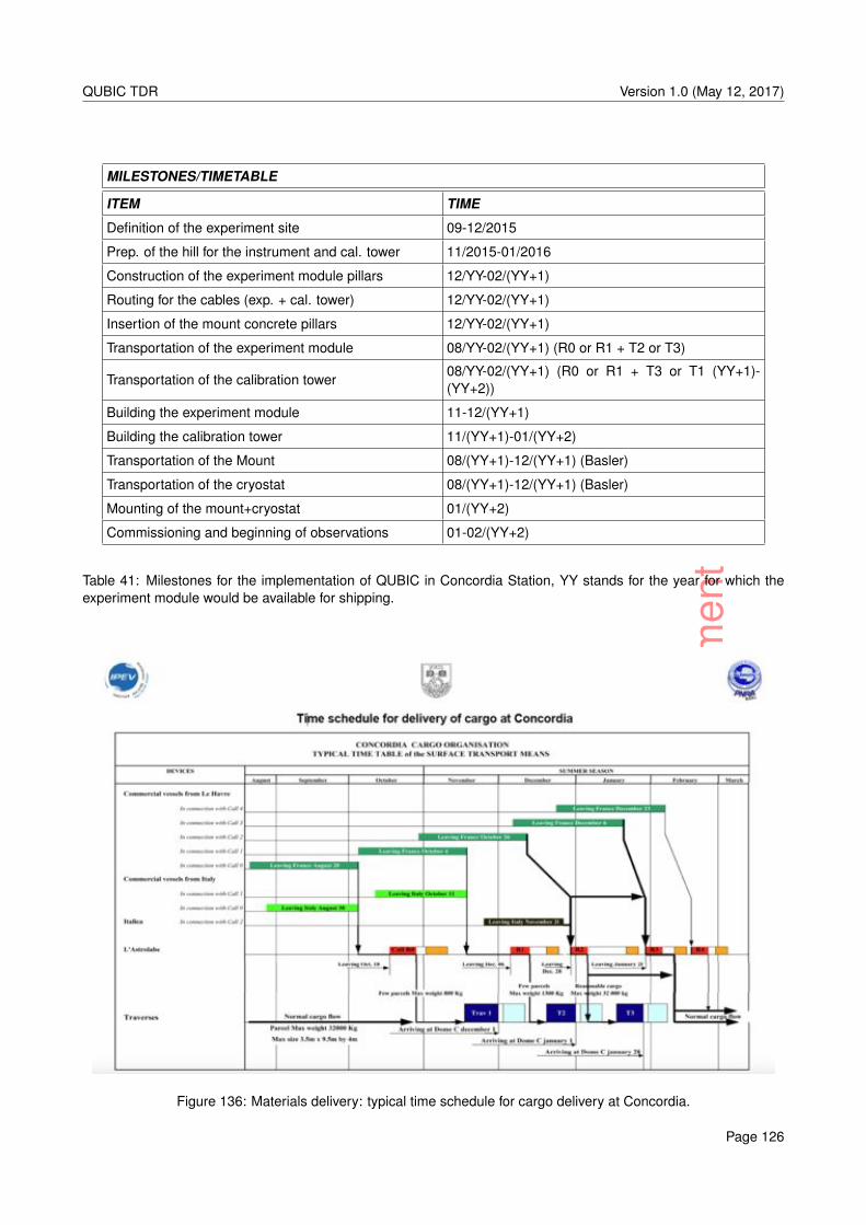
Livi
ngdo
cum
ent
QUBIC TDR Version 1.0 (May 12, 2017)
MILESTONES/TIMETABLE
ITEM TIME
Definition of the experiment site 09-12/2015
Prep. of the hill for the instrument and cal. tower 11/2015-01/2016
Construction of the experiment module pillars 12/YY-02/(YY+1)
Routing for the cables (exp. + cal. tower) 12/YY-02/(YY+1)
Insertion of the mount concrete pillars 12/YY-02/(YY+1)
Transportation of the experiment module 08/YY-02/(YY+1) (R0 or R1 + T2 or T3)
Transportation of the calibration tower08/YY-02/(YY+1) (R0 or R1 + T3 or T1 (YY+1)-(YY+2))
Building the experiment module 11-12/(YY+1)
Building the calibration tower 11/(YY+1)-01/(YY+2)
Transportation of the Mount 08/(YY+1)-12/(YY+1) (Basler)
Transportation of the cryostat 08/(YY+1)-12/(YY+1) (Basler)
Mounting of the mount+cryostat 01/(YY+2)
Commissioning and beginning of observations 01-02/(YY+2)
Table 41: Milestones for the implementation of QUBIC in Concordia Station, YY stands for the year for which theexperiment module would be available for shipping.
Figure 136: Materials delivery: typical time schedule for cargo delivery at Concordia.
Page 126
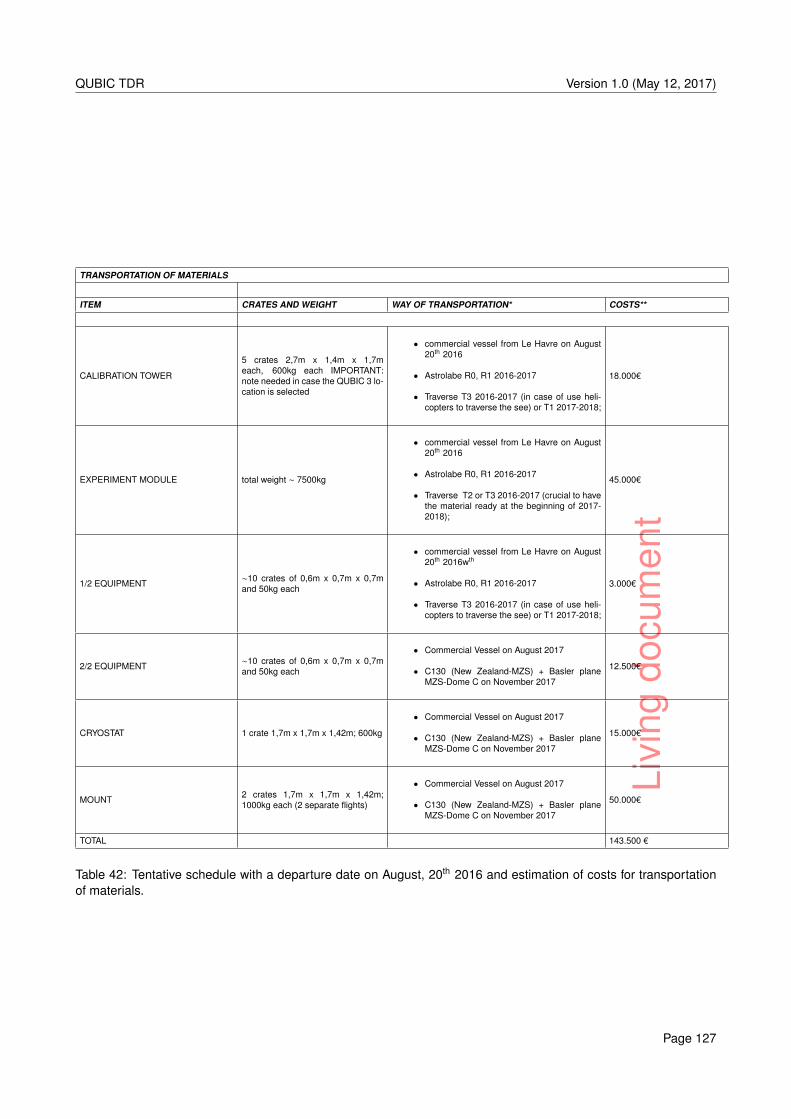
Livi
ngdo
cum
ent
QUBIC TDR Version 1.0 (May 12, 2017)
TRANSPORTATION OF MATERIALS
ITEM CRATES AND WEIGHT WAY OF TRANSPORTATION* COSTS**
CALIBRATION TOWER
5 crates 2,7m x 1,4m x 1,7meach, 600kg each IMPORTANT:note needed in case the QUBIC 3 lo-cation is selected
• commercial vessel from Le Havre on August20th 2016
• Astrolabe R0, R1 2016-2017
• Traverse T3 2016-2017 (in case of use heli-copters to traverse the see) or T1 2017-2018;
18.000€
EXPERIMENT MODULE total weight ∼ 7500kg
• commercial vessel from Le Havre on August20th 2016
• Astrolabe R0, R1 2016-2017
• Traverse T2 or T3 2016-2017 (crucial to havethe material ready at the beginning of 2017-2018);
45.000€
1/2 EQUIPMENT ∼10 crates of 0,6m x 0,7m x 0,7mand 50kg each
• commercial vessel from Le Havre on August20th 2016wth
• Astrolabe R0, R1 2016-2017
• Traverse T3 2016-2017 (in case of use heli-copters to traverse the see) or T1 2017-2018;
3.000€
2/2 EQUIPMENT ∼10 crates of 0,6m x 0,7m x 0,7mand 50kg each
• Commercial Vessel on August 2017
• C130 (New Zealand-MZS) + Basler planeMZS-Dome C on November 2017
12.500€
CRYOSTAT 1 crate 1,7m x 1,7m x 1,42m; 600kg
• Commercial Vessel on August 2017
• C130 (New Zealand-MZS) + Basler planeMZS-Dome C on November 2017
15.000€
MOUNT 2 crates 1,7m x 1,7m x 1,42m;1000kg each (2 separate flights)
• Commercial Vessel on August 2017
• C130 (New Zealand-MZS) + Basler planeMZS-Dome C on November 2017
50.000€
TOTAL 143.500 €
Table 42: Tentative schedule with a departure date on August, 20th 2016 and estimation of costs for transportationof materials.
Page 127
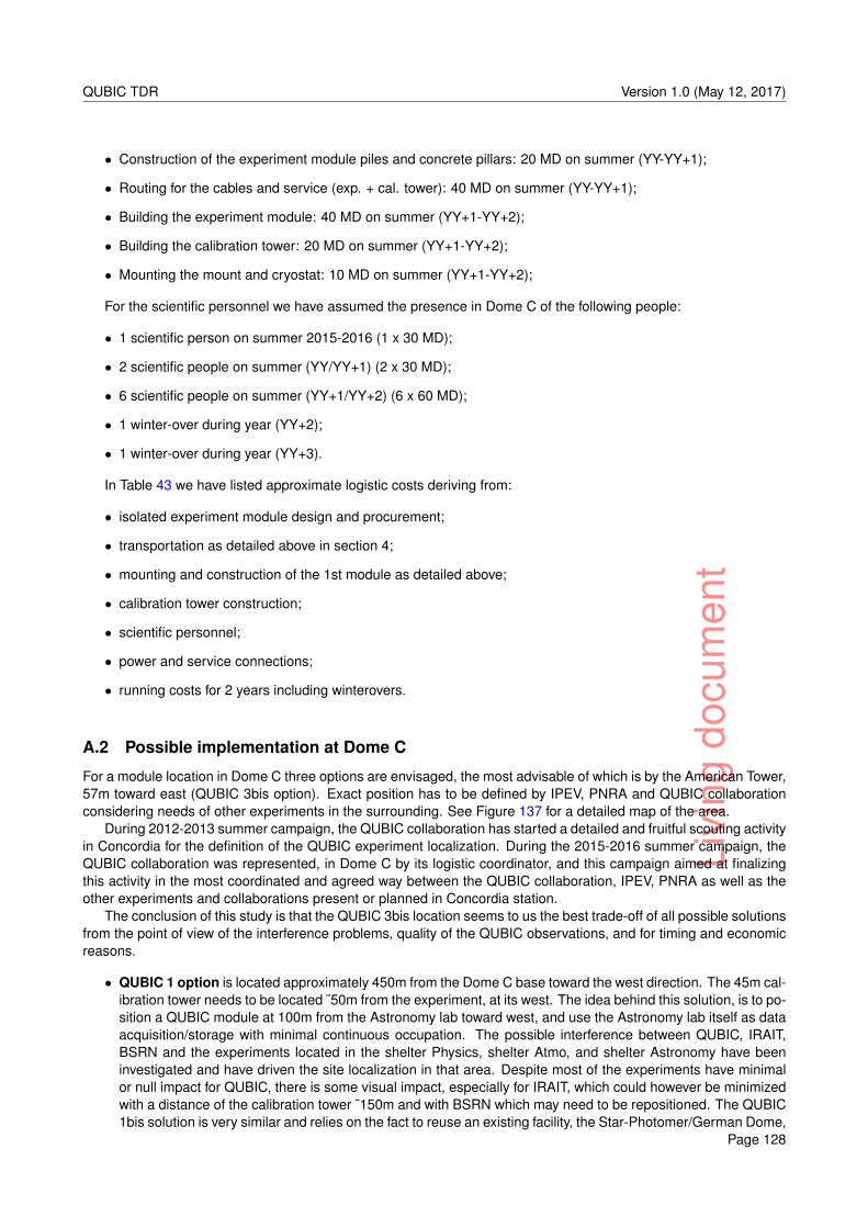
Livi
ngdo
cum
ent
QUBIC TDR Version 1.0 (May 12, 2017)
• Construction of the experiment module piles and concrete pillars: 20 MD on summer (YY-YY+1);
• Routing for the cables and service (exp. + cal. tower): 40 MD on summer (YY-YY+1);
• Building the experiment module: 40 MD on summer (YY+1-YY+2);
• Building the calibration tower: 20 MD on summer (YY+1-YY+2);
• Mounting the mount and cryostat: 10 MD on summer (YY+1-YY+2);
For the scientific personnel we have assumed the presence in Dome C of the following people:
• 1 scientific person on summer 2015-2016 (1 x 30 MD);
• 2 scientific people on summer (YY/YY+1) (2 x 30 MD);
• 6 scientific people on summer (YY+1/YY+2) (6 x 60 MD);
• 1 winter-over during year (YY+2);
• 1 winter-over during year (YY+3).
In Table 43 we have listed approximate logistic costs deriving from:
• isolated experiment module design and procurement;
• transportation as detailed above in section 4;
• mounting and construction of the 1st module as detailed above;
• calibration tower construction;
• scientific personnel;
• power and service connections;
• running costs for 2 years including winterovers.
A.2 Possible implementation at Dome C
For a module location in Dome C three options are envisaged, the most advisable of which is by the American Tower,57m toward east (QUBIC 3bis option). Exact position has to be defined by IPEV, PNRA and QUBIC collaborationconsidering needs of other experiments in the surrounding. See Figure 137 for a detailed map of the area.
During 2012-2013 summer campaign, the QUBIC collaboration has started a detailed and fruitful scouting activityin Concordia for the definition of the QUBIC experiment localization. During the 2015-2016 summer campaign, theQUBIC collaboration was represented, in Dome C by its logistic coordinator, and this campaign aimed at finalizingthis activity in the most coordinated and agreed way between the QUBIC collaboration, IPEV, PNRA as well as theother experiments and collaborations present or planned in Concordia station.
The conclusion of this study is that the QUBIC 3bis location seems to us the best trade-off of all possible solutionsfrom the point of view of the interference problems, quality of the QUBIC observations, and for timing and economicreasons.
• QUBIC 1 option is located approximately 450m from the Dome C base toward the west direction. The 45m cal-ibration tower needs to be located ˜50m from the experiment, at its west. The idea behind this solution, is to po-sition a QUBIC module at 100m from the Astronomy lab toward west, and use the Astronomy lab itself as dataacquisition/storage with minimal continuous occupation. The possible interference between QUBIC, IRAIT,BSRN and the experiments located in the shelter Physics, shelter Atmo, and shelter Astronomy have beeninvestigated and have driven the site localization in that area. Despite most of the experiments have minimalor null impact for QUBIC, there is some visual impact, especially for IRAIT, which could however be minimizedwith a distance of the calibration tower ˜150m and with BSRN which may need to be repositioned. The QUBIC1bis solution is very similar and relies on the fact to reuse an existing facility, the Star-Photomer/German Dome,
Page 128
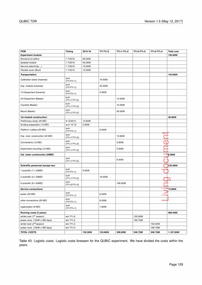
Livi
ngdo
cum
ent
QUBIC TDR Version 1.0 (May 12, 2017)
ITEM Timing 2015-16 YY-YY+2 YY+1-YY+2 YY+2-YY+3 YY+3-YY+4 Total cost
Experiment module: 130.000€
Structure on pillars 1-7/2016 65.000€
Isolated module 1-7/2016 45.000€
Service (electricity,...) 1-7/2016 10.000€
Flexible cover (Boot) 1-7/2016 10.000€
Transportation: 143.500€
Calibration tower (traverse) sum(YY/YY+1) 18.000€
Exp. module (traverse) sum(YY/YY+1) 45.000€
1/2 Equipment (traverse) sum(YY/YY+1) 3.000€
2/2 Equipment (Basler) sum(YY+1/YY+2) 12.500€
Cryostat (Basler) sum(YY+1/YY+2) 15.000€
Mount (Basler) sum(YY+1/YY+2) 50.000€
1st module construction: 39.900€
Preliminary study (45 MD) 9-12/2015 13.500€
Surface preparation (10 MD) sum 15-16 3.000€
Platform n pillars (20 MD) sum(YY/YY+1) 6.000€
Exp. mod. construction (40 MD) sum(YY+1/YY+2) 10.800€
Connections (12 MD) sum(YY+1/YY+2) 3.600€
Experiment mounting (10 MD) sum(YY+1/YY+2) 3.000€
Cal. tower construction (20MD) 6.000€
sum(YY+1/YY+2) 6.000€
Scientific personnel (except wo): 135.000€
1 scientific (1 x 30MD) sum(YY/YY+1) 9.000€
2 scientific (2 x 30MD) sum(YY+1/YY+2) 18.000€
6 scientific (6 x 60MD) sum(YY+2/YY+3) 108.000€
Service connections: 13.800€
power (20 MD) sum(YY/YY+1) 6.000€
other connections (20 MD) sum(YY/YY+1) 6.000€
organization (6 MD) sum(YY/YY+1) 1.800€
Running costs (2 years): 699.456€
winter-over (1st season) win YY+2 150.000€
power cons. (15kW x 365 days) win YY+2 199.728€
winter-over (2ndseason) win YY+3 150.000€
power cons. (15kW x 365 days) win YY+3 199.728€
TOTAL COSTS: 155.500€ 103.800€ 208.900€ 349.728€ 349.728€ 1.167.656€
Table 43: Logistic costs: Logistic costs foreseen for the QUBIC experiment. We have divided the costs within theyears.
Page 129
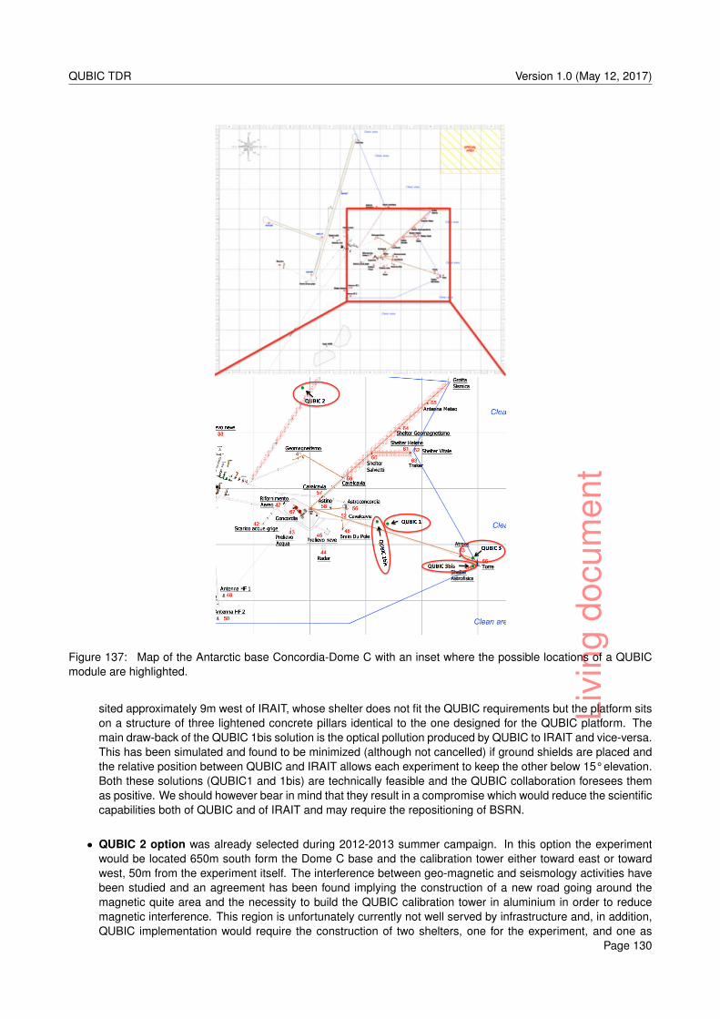
Livi
ngdo
cum
ent
QUBIC TDR Version 1.0 (May 12, 2017)
Figure 137: Map of the Antarctic base Concordia-Dome C with an inset where the possible locations of a QUBICmodule are highlighted.
sited approximately 9m west of IRAIT, whose shelter does not fit the QUBIC requirements but the platform sitson a structure of three lightened concrete pillars identical to the one designed for the QUBIC platform. Themain draw-back of the QUBIC 1bis solution is the optical pollution produced by QUBIC to IRAIT and vice-versa.This has been simulated and found to be minimized (although not cancelled) if ground shields are placed andthe relative position between QUBIC and IRAIT allows each experiment to keep the other below 15° elevation.Both these solutions (QUBIC1 and 1bis) are technically feasible and the QUBIC collaboration foresees themas positive. We should however bear in mind that they result in a compromise which would reduce the scientificcapabilities both of QUBIC and of IRAIT and may require the repositioning of BSRN.
• QUBIC 2 option was already selected during 2012-2013 summer campaign. In this option the experimentwould be located 650m south form the Dome C base and the calibration tower either toward east or towardwest, 50m from the experiment itself. The interference between geo-magnetic and seismology activities havebeen studied and an agreement has been found implying the construction of a new road going around themagnetic quite area and the necessity to build the QUBIC calibration tower in aluminium in order to reducemagnetic interference. This region is unfortunately currently not well served by infrastructure and, in addition,QUBIC implementation would require the construction of two shelters, one for the experiment, and one as
Page 130

Livi
ngdo
cum
ent
QUBIC TDR Version 1.0 (May 12, 2017)
Advantages / Gain Disadvantages / Mitigation
Short distance from the base / Easier operationsfor winter-over
Less immune from Dome C base optical pollutiondue to its vicinity to the Base
Only one shelter to build (i.e. the data acquisitionmodule would be the Astronomy lab.)
Interaction with BSRN: possible need to repositionthe experiment
Large bandwidth connection between experi-ment module and Astronomy lab
Interaction with IRAIT: reduce the sky area directlyaccessible to IRAIT
For QUBIC 1bis: reuse the existing concrete pil-lars structure
For QUBIC 1bis: direct air pollution on and fromIRAIT
Need to build the calibration tower
Not straight-forward to have a plan for the hypothet-ical QUBIC next generation formed by 6 identicalmodules
Table 44: Pro and cons of QUBIC 1 option
Advantages / Gain Disadvantages / Mitigation
quite and free-from-interference observationalsite
need to build a new road going around the Amagneticarea
straight-forward to implement the hypotheticalnext generation 6-modules experiment
expensive and difficult operation due to the constraintscreated by the interference with geomagnetic opera-tions
need to build a calibration tower
need to build 2 brand new shelters
Table 45: Pro and cons of QUBIC 2 option
data acquisition/storage. This service would be expensive and time consuming especially in the light of theconstraints set by other impacted activities. Unless there are no other choices, at the present status weconsider this option not viable because it would be too expensive.
• QUBIC 3 option (see Figure QUBIC 3) foresees a QUBIC module installation at 950m west from the DomeC base, by the existing American Tower. The idea behind this solution, is to position the QUBIC experimentshelter as close as possible to the American tower (˜60m from it) at its east, clearly outside the clean area, inorder to use the American Tower as Calibration Tower and being able to observe the calibration source with ashigh as possible elevation angle. The use of the American Tower as calibration tower would result in no need tobuild an additional tower with clear economic and time advantages. The impact of our calibration source on thetower would be minimal. Also, we foresee the possibility to use the Astronomy lab as data acquisition/storagewith minimal continuous occupation. Within this solution we selected two possible locations: QUBIC 3 locationwould result at 60/70 m from the American Tower, south-east of it, while QUBIC 3bis location would be at50/60m from the Tower, north-east from it. From a recognition performed in order to establish the possibleinterference between QUBIC and other experiments mounted on the American Tower, it seems clear that,despite most of the experiments have no impact to and from QUBIC, the positioning of QUBIC toward south(main wind direction in Dome C, QUBIC 3 option) would have an impact due to the change of the snowaccumulation in the surrounding area (although QUBIC would anyway be outside the clean area). On theother hand, positioning a QUBIC module on the north(-east) side of the tower (QUBIC 3bis option), designingthe experiment module in such a way that the snow accumulation would be kept under control, and keepingthe experiment module as low as possible, would result in negligible effect on the activities on-going from the
Page 131
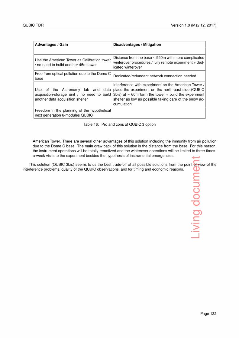
Livi
ngdo
cum
ent
QUBIC TDR Version 1.0 (May 12, 2017)
Advantages / Gain Disadvantages / Mitigation
Use the American Tower as Calibration tower/ no need to build another 45m tower
Distance from the base ∼ 950m with more complicatedwinterover procedures / fully remote experiment + ded-icated winterover
Free from optical pollution due to the Dome Cbase
Dedicated/redundant network connection needed
Use of the Astronomy lab and dataacquisition-storage unit / no need to buildanother data acquisition shelter
Interference with experiment on the American Tower /place the experiment on the north-east side (QUBIC3bis) at ∼ 60m form the tower + build the experimentshelter as low as possible taking care of the snow ac-cumulation
Freedom in the planning of the hypotheticalnext generation 6-modules QUBIC
Table 46: Pro and cons of QUBIC 3 option
American Tower. There are several other advantages of this solution including the immunity from air pollutiondue to the Dome C base. The main draw back of this solution is the distance from the base. For this reason,the instrument operations will be totally remotized and the winterover operations will be limited to three-times-a-week visits to the experiment besides the hypothesis of instrumental emergencies.
This solution (QUBIC 3bis) seems to us the best trade-off of all possible solutions from the point of view of theinterference problems, quality of the QUBIC observations, and for timing and economic reasons.
Page 132

Livi
ngdo
cum
ent
QUBIC TDR Version 1.0 (May 12, 2017)
LOCATION Lat. Lon. Notes
BASE S 75° 06’ 00.1’’ E 123° 19’ 57.4’’
ASTRONOMY LAB S 75° 05’ 59.3’’ E 123° 19’ 13.4’’ ˜350m from the base
AMERICAN TOWER S 75° 05’ 50.7’’ E 123° 17’ 58.4’’ ˜970m from the base
QUBIC 1 S 75° 05’ 58.2’’ E 123° 18’ 59.7’’ at ∼100m from Astronomy Lab
CALIBRATION TOWER 1 S 75° 05’ 57.4’’ E 123° 18’ 53.0’’ ∼50m from the experiment
QUBIC 1bis S 75° 06’ 01.5’’ E 123° 19’ 09.5’’ reuse German-Dome platform
CALIBRATION TOWER 1bis S 75° 06’ 01.5’’ E 123° 19’ 03.3’’ ∼50m from the experiment
QUBIC 2 S 75° 06’ 22.6’’ E 123° 19’ 48.7’’ ∼650m from the base
CALIBRATION TOWER 2 S 75° 06’ 22.6’’ E 123° 19’ 42.5’’ ∼ 50m from the experiment
QUBIC 3 S 75° 05’ 51.9’’ E 123° 18’ 07.1’’ ∼950m form the base
QUBIC 3bis S 75° 05’ 50.3’’ E 123° 18’ 05.5’’ reduce interference
QUBIC 3bis corner 1 S 75° 05’ 50.5’’ E 123° 18’ 05.1’’ SW corner of the shelter
QUBIC 3bis corner 2 S 75° 05’ 50.5’’ E 123° 18’ 06.2’’ SE corner of the shelter
QUBIC 3bis corner 3 S 75° 05’ 50.0’’ E 123° 18’ 06.1’’ NE corner of the shelter
QUBIC 3bis corner 4 S 75° 05’ 50.0’’ E 123° 18’ 05.2’’ NW corner of the shelter
CALIBRATION TOWER 3/ S 75° 05’ 50.7’’ E 123° 17’ 58.4’’ no need to build another 45m tower
AMERICAN TOWER
Table 47: Possible locations of a QUBIC module with coordinates. In red we highlight not viable solutions (unlessno other options are possible), in orange we highlight possible solutions with some limitations and loss on efficiency,in green we highlight our preferred solution which, from our point of view, is the best trade-off solution with minimalinterference.
Page 133

Livi
ngdo
cum
ent
QUBIC TDR Version 1.0 (May 12, 2017)
B ATRIUM-77335
Page 134
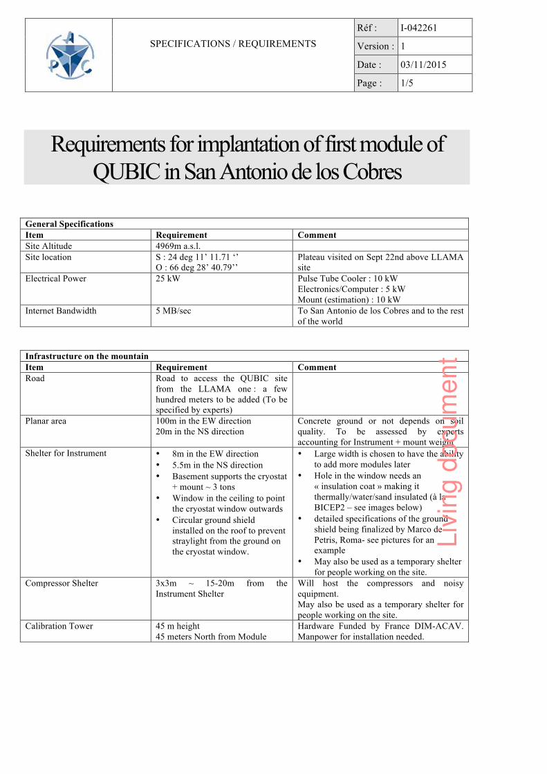
SPECIFICATIONS / REQUIREMENTS
Réf : I-042261
Version : 1
Date : 03/11/2015
Page : 1/5
Requirements for implantation of first module of
QUBIC in San Antonio de los Cobres
General Specifications
Item Requirement Comment
Site Altitude 4969m a.s.l.
Site location S : 24 deg 11’ 11.71 ‘’
O : 66 deg 28’ 40.79’’
Plateau visited on Sept 22nd above LLAMA
site
Electrical Power 25 kW Pulse Tube Cooler : 10 kW
Electronics/Computer : 5 kW
Mount (estimation) : 10 kW
Internet Bandwidth 5 MB/sec To San Antonio de los Cobres and to the rest
of the world
Infrastructure on the mountain
Item Requirement Comment
Road Road to access the QUBIC site
from the LLAMA one : a few
hundred meters to be added (To be
specified by experts)
Planar area 100m in the EW direction
20m in the NS direction
Concrete ground or not depends on soil
quality. To be assessed by experts
accounting for Instrument + mount weight
Shelter for Instrument • 8m in the EW direction
• 5.5m in the NS direction
• Basement supports the cryostat
+ mount ~ 3 tons
• Window in the ceiling to point
the cryostat window outwards
• Circular ground shield
installed on the roof to prevent
straylight from the ground on
the cryostat window.
• Large width is chosen to have the ability
to add more modules later
• Hole in the window needs an
« insulation coat » making it
thermally/water/sand insulated (à la
BICEP2 – see images below)
• detailed specifications of the ground
shield being finalized by Marco de
Petris, Roma- see pictures for an
example
• May also be used as a temporary shelter
for people working on the site.
Compressor Shelter 3x3m ~ 15-20m from the
Instrument Shelter
Will host the compressors and noisy
equipment.
May also be used as a temporary shelter for
people working on the site.
Calibration Tower 45 m height
45 meters North from Module
Hardware Funded by France DIM-ACAV.
Manpower for installation needed.
Livi
ngdo
cum
ent

SPECIFICATIONS / REQUIREMENTS
Réf : I-042261
Version : 1
Date : 03/11/2015
Page : 2/5
Infrastructure in San Antonio de los Cobres (inside LLAMA building)
Item Requirement Comment
Offices and labs 50 sqm permanently allocated to
QUBIC
Clean Room Access when needed for instrument
upgrade
Bedrooms Two bedrooms permanently
Kitchen / Restrooms / common
facilities
Shared access with LLAMA
Integration / Operations
Item Requirement Comment
Integration • Personal from Argentina and
their QUBIC partners to
perform integration
• Cranes, trucks, transportation
in Argentina to be funded by
Argentina
• Integration hangar (around 50
sqm) in Salta (or San Antonio
de los Cobres) to integrate and
test Mount+Instrument prior
installation on site.
Operation Two trained technicians
permanently in San Antonio de los
Cobres with regular visits to the
instrument (frequency and duties to
be detailed later)
Cryogenic Maintenance Under the responsibility of San
Carlos de Bariloche Team
Important questions to be answered :
• Assess cost of the above infrastructure
• Assess date at which it could be available for QUBIC installation
• Precise various aspects of the above table by interaction with experts (especially J. Viramonte).
Illustrations:
Figure 1: BICEP2 Insulating coat, forebaffle (black) and ground shield (metal)
Livi
ngdo
cum
ent
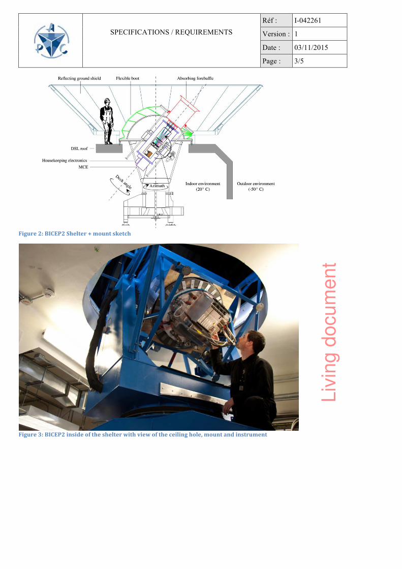
SPECIFICATIONS / REQUIREMENTS
Réf : I-042261
Version : 1
Date : 03/11/2015
Page : 3/5
Figure 2: BICEP2 Shelter + mount sketch
Figure 3: BICEP2 inside of the shelter with view of the ceiling hole, mount and instrument
Livi
ngdo
cum
ent
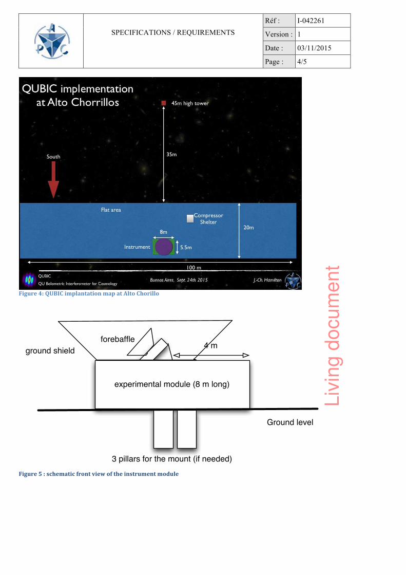
SPECIFICATIONS / REQUIREMENTS
Réf : I-042261
Version : 1
Date : 03/11/2015
Page : 4/5
Figure 4: QUBIC implantation map at Alto Chorillo
experimental module (8 m long)
3 pillars for the mount (if needed)
4 m ground shield
forebaffle
Ground level
Figure 5 : schematic front view of the instrument module
Livi
ngdo
cum
ent
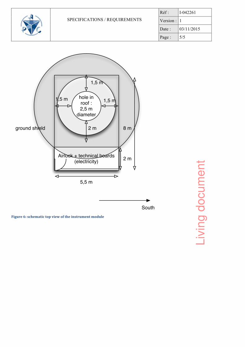
SPECIFICATIONS / REQUIREMENTS
Réf : I-042261
Version : 1
Date : 03/11/2015
Page : 5/5
2 m
5,5 m
ground shield
South
Airlock + technical boards (electricity)
hole in roof : 2,5 m
diameter
2 m
1,5 m
1,5 m 1,5 m
8 m
Figure 6: schematic top view of the instrument module
Livi
ngdo
cum
ent


