Embed Size (px)
Citation preview
School of Chemical and Petroleum Engineering
Department of Chemical Engineering
LNG Plant Modeling and Optimization
Bahareh Salehi
This thesis is presented for the Degree of
Doctor of Philosophy
of
Curtin University
January 2018

DECLARATION
To the best of my knowledge and belief, this thesis contains no material previously
published by any other person except where due acknowledgment has been made.
This thesis contains no material that has been accepted for the award of any other
degree or diploma in any university.
.
Signature: ………………………………………….
Date: ………………………...

List of publications in support of the thesis
1. Salehi, B., Barifcani, A., 2016. Optimization of LPG Extraction from Natural Gas for
99.5% Recovery. Peer reviewed by SPE Journal. Manuscript ID: PFC-1115-0004.
2. Salehi, B., Barifcani, A., Energy and Process Optimization of Coal-Seam Gas LNG
Plant. CHEMECA conference of chemical engineering. 28 September to Wednesday 1
October 2014.

i
Acknowledgements
I would like to acknowledge many individuals. The accomplishment of this work would
not have been possible without their technical and emotional support.
I am particularly thankful to my supervisor, Professor Vishnu Pareek, for all of his support
over the last four years. I am indebted to him for his wholehearted support, which encouraged
me to pursue exploratory research continuously. I have learned a lot from his viewpoint on the
quality of my work. I also appreciate the opportunities I have had under his supervision.
I would like to express my gratitude to my co-supervisor, Dr Ahmed Barifcani. I
appreciated his attention, advice, and support for my research commitments. I have been truly
fortunate to interact with this dedicated supervisory panel.
The financial support of my research from the Department of Innovation, Industry, Science,
and Research in Australia for International Postgraduate Research Scholarship (IPRS), the
Office of Research and Development at Curtin University, Perth, Western Australia for
providing the Australian Postgraduate Award (APA), and the State Government of Western
Australia for providing the top up scholarship through the Western Australian Energy
Research Alliance (WA:ERA) are gratefully acknowledged.
I am grateful to my mother for her unconditional love and support during my studies
overseas. I am indebted to my father, who guided me in the direction of seeking knowledge. I
am forever obliged to my husband, Mehdi, for his authentic love and unlimited patience.
Finally, I am also grateful to my daughters, Arina and Anita, for the joy they bring to my life
with their wonderful sense of humour.
There are still so many who deserve my acknowledgment. My sincere apologies to all
whose names are not mentioned here but who have played a role in my achievements.
i
Table of Contents
1. Introduction ................................................................................................................... 1
1.1. Liquefied natural gas production ............................................................................... 1
1.1.1. An introduction to the cascade refrigeration process ......................................... 6
1.1.2. An Introduction to mixed refrigerant liquefaction process description .............. 7
1.1.3. An introduction to the pre-cooled mixed refrigerant process ........................... 10
1.1.4. Integrated NGL and LNG plants ...................................................................... 11
1.1.5. Thesis overview ................................................................................................ 13
2. Literature review .......................................................................................................... 16
2.2. LNG plant modelling and simulation....................................................................... 16
2.3. LNG plant optimization algorithms ......................................................................... 23
3. Modelling and optimization methodology ......................................................................... 27
3.1. Process modelling .................................................................................................... 27
3.2. Evolutionary optimization algorithms ..................................................................... 28
3.2.1. An introduction to Genetic algorithms .............................................................. 30
3.2.2. Generation of the initial population .................................................................. 30
3.2.3. Fitness function evaluation ............................................................................... 30
3.2.4. Selection of the next generation function ......................................................... 31
3.2.5. Generation selection based on the tournament method .................................... 31
3.2.6. Generation Selection based on the roulette wheel method ............................... 31
3.2.7. Selection of the strongest chromosomes........................................................... 32
3.2.8. Genetic operator transfer .................................................................................. 33
3.3. Termination condition of a GA algorithm ............................................................... 34
3.4. Advantages of GA evolutionary algorithms ............................................................ 34
ii
3.5. Limitations of GA evolutionary algorithms ............................................................. 35
3.6. Particle swarm optimization algorithm .................................................................... 35
3.7. The PSO algorithm procedure for coding ................................................................ 39
3.8. Parameter selection for particle swarm algorithms .................................................. 42
3.8.2. The maximum velocity Vmax .......................................................................... 44
3.8.3. The swarm size ................................................................................................. 45
3.8.4. The acceleration coefficients C1 and C2 .......................................................... 45
3.8.5. The neighbourhood topologies in PSO ............................................................. 46
3.8.6. Particle swarm optimization algorithm advantages .......................................... 47
3.8.7. Particle swarm optimization algorithm limitations........................................... 47
3.9. comparison between GA and PSO ........................................................................... 48
4. Liquefaction unit optimization with particle swarm optimization and genetic algorithms 51
4.1. Optimization of the optimum process scheme ......................................................... 51
4.2. Optimization method................................................................................................ 53
4.2.1. The optimization results of the pre-cooled mixed refrigerant unit using evolutionary algorithms ................................................................................................... 57
4.2.2. The optimization results of the liquefaction unit using the PSO algorithm ..... 60
4.2.3. The graph of optimization results from the first run using evolutionary population algorithms ...................................................................................................... 61
5. Design integrity and optimization of liquefied petroleum gas units ............................ 65
5.1. Process description of natural gas liquid production ............................................... 65
5.2. LPG extraction optimum process selection ............................................................. 71
5.2.1. JT valve without refrigeration .......................................................................... 71
5.2.2. Turbo expander without propane refrigeration ................................................. 71
iii
5.2.3. JT valve with propane refrigeration .................................................................. 72
5.2.4. Turbo expander with propane refrigeration ...................................................... 73
5.2.5. Sensitivity analysis of process variables........................................................... 78
5.2.6. Turbo expander inlet pressure .......................................................................... 80
5.2.7. Turbo expander outlet pressure ........................................................................ 81
5.2.8. De-ethanizer column pressure .......................................................................... 82
5.2.9. Number of ideal stages and feed inlet location ................................................. 83
5.2.10. Optimization algorithm ............................................................................. 84
5.3. Optimization results of the LPG recovery unit ........................................................ 85
5.4. Optimization results of the LPG recovery unit ........................................................ 88
6. Comparison of two evolutionary optimization results for liquefaction and fractionation units 94
6.1. Results ...................................................................................................................... 94
6.2. Comparison between PSO and GA algorithms results ............................................ 96
Appendix A: Evolutionary-Population Optimization Algorithms MATLAB Code ............ 103
HYSYS simulation PFD (pre-cooled mixed refrigerant) ..................................................... 117
lpg fractionation PFD: Joule-Thomson case without refrigeration ...................................... 118
lpg fractionation PFD: Joule-Thomson case with propane refrigeration .............................. 119
LPG fractionation PFD: Turbo-expander case without propane refrigeration ..................... 120
LPG fractionation PFD: Turbo-expander case without refrigeration ................................... 121
References............................................................................................................................. 122
iv
List of figures
Figure 1-1.Block diagram of a typical LNG plant. ................................................................... 1
Figure 1-2. Cascade refrigeration cycle schematic. .................................................................. 7
Figure 1-3. Mixed refrigerant process schematic ..................................................................... 8
Figure 1-4. Propane pre-cooled mixed refrigerant. ................................................................ 11
Figure 1-5. Block diagram showing integrated LNG and NGL units. ................................... 13
Figure 1-6: Map of the research methodology ....................................................................... 15
Figure 3-1: Tournament selection method. ............................................................................. 31
Figure 3-2: The selection of the roulette wheel method ......................................................... 32
Figure 3-3: Crossover operation to generate offspring. .......................................................... 34
Figure 3-4: The PSO Algorithm schematic. ........................................................................... 37
Figure 3-5: Illustrating the dynamic of a particle in PSO. ...................................................... 44
Figure 3-6: Processing time to reach the optimum for the F8 function. ................................. 49
Figure -4-1. Single mixed refrigerant liquefaction unit schematic. ........................................ 52
Figure -4-2. Main cryogenic heat exchanger in SMR unit. .................................................... 53
Figure 4-3. Total compressors power vs LP stage compressor outlet pressure. ..................... 58
Figure -4-4. Total compressors power vs HP stage compressor outlet pressure. ................... 59
Figure 4-5: Total compressors power vs outlet temperature of the main cryogenic heat exchanger. ............................................................................................................................... 59
Figure 4-6: GA optimization result from MATLAB software (first run). .............................. 61
Figure 4-7: GA optimization result from MATLAB software (second run). ....................... 61
Figure 4-8: GA optimization result from MATLAB software (third run).............................. 62
Figure 4-9: PSO optimization result from MATLAB software (first run). ............................ 62
Figure 4-10: PSO optimization result from MATLAB software (second run). ..................... 63
v
Figure 4-11: Hot and cold composite curves in the MCHE. .................................................. 64
Figure -5-1. CO2 freeze point. ................................................................................................ 67
Figure 5-2. Inlet stream phase envelope. ................................................................................ 68
Figure 5-3. Typical LPG extraction. ....................................................................................... 69
Figure 5-4. JT valve without refrigeration. ............................................................................. 71
Figure 5-5. Turbo expander without refrigeration. ................................................................. 72
Figure 5-6. JT valve with refrigeration. .................................................................................. 73
Figure 5-7. Turbo expander with refrigeration ....................................................................... 74
Figure 5-8. Expander inlet pressure impact on PAV. ............................................................. 80
Figure 5-9. Expander outlet pressure impact on PAV. ........................................................... 82
Figure -5-10. Impact of de-ethanizer reboiler duty on PAV. ................................................. 83
Figure 5-11. Impact of de-ethanizer column spec on PAV. ................................................... 84
Figure 5-12. Sensitivity analysis of inlet temperature to the de-C2 column vs. ethane recovery. ................................................................................................................................................ 86
Figure -5-13. Sensitivity analysis of inlet stream pressure to LPG recovery vs. ethane recovery. ................................................................................................................................................ 86
Figure -5-14. Sensitivity analysis of inlet stream pressure to de-C2 column vs. ethane recovery. ................................................................................................................................................ 87
Figure -5-15. Ethane recovery GA optimization with MATLAB (first run). ......................... 89
Figure 5-16. Ethane recovery GA optimization with MATLAB (second run). ..................... 89
Figure 5-17. Ethane recovery GA optimization with MATLAB (third run). ......................... 90
Figure 5-18. Ethane recovery PSO optimization with MATLAB (first run). ........................ 91
Figure 5-19. Ethane recovery PSO optimization with MATLAB (second run). .................... 91
Figure -5-20. Ethane recovery PSO optimization with MATLAB (third run). ...................... 92
Figure -6-1. PSO and GA optimization algorithms comparison of a liquefaction unit (total power). .................................................................................................................................... 97

vi
Figure 6-2. PSO and GA optimization algorithms comparison of NGL fractionation (Ethane recovery). ................................................................................................................................ 97
Figure -6-3. The optimized NGL process schematic ............................................................ 102
vii
List of Tables
Table 3-1: Qualitative comparison of GA and PSO ............................................................... 49
Table 4-1. Inlet gas composition to the LNG plant ................................................................ 52
Table 4-2. Decision variables constraint for the liquefaction system ..................................... 58
Table 4-3. Optimization results in liquefaction unit using the PSO algorithm ...................... 60
Table 5-1. Input simulation parameters for the JT Valve without the refrigeration scheme .. 71
Table 5-2. Input simulation parameters for turbo-expander without refrigeration scheme .... 72
Table 5-3. Input simulation parameters for the JT Valve with refrigeration scheme ............. 73
Table 5-4. Input simulation parameters for the turbo expander with refrigeration scheme ... 74
Table 5-5. Simulation results analysis in the turbo-expander, Joule Thomson + chilling and turbo expander + chilling ........................................................................................................ 75
Table 5-6. Economic evaluation basis .................................................................................... 75
Table 5-7. Economic results summary ................................................................................... 76
Table 5-8. Economic analysis ................................................................................................. 77
Table 5-9. Economic evaluation and PAV calculation ........................................................... 79
Table 5-10. Effect of expander inlet pressure on plant performance ..................................... 80
Table 5-11. Effect of expander outlet pressure on plant performance ................................... 81
Table 5-12. Effect of de-ethanizer column pressure on plant performance ........................... 82
Table 5-13. Effect of ideal stages and feed inlet location ....................................................... 83
Table 5-14. Example of the reboiler duty optimization .......................................................... 84
Table 5-15. Decision variables for LPG unit .......................................................................... 85
Table 5-16. Optimization results for the NGL system using the particle swarm optimization (PSO) algorithm ...................................................................................................................... 88
Table.6-1. Comparison of PSO and GA results in liquefaction unit optimization ................. 95

viii
Table 6-2 Comparison of PSO and GA results in NGL unit optimization ............................. 96
Table 6-3. Performance summary of the optimized plant .................................................... 101

ix
Abbreviation List
LNG Liquefied Natural Gas LPG Liquefied Petroleum Gas NGL Natural Gas Liquid NG Natural Gas FPSO Floating Production Storage Offloading SRU Sulphur Recovery Unit SMR Single Mixed Refrigerant Process PMR Pre-cooled Mixed Refrigerant Process MCR Mixed Cryogenic Refrigerant DMR Dual Mixed Refrigerant MCHE Main Cryogenic Heat Exchanger JT Joule Thomson NPV Net Present Value PAV Project Added Value OPEX Operational Expenditure CAPEX Capital Expenditure GA Genetic Algorithm PSO Particle Swarm Optimization TBX Turbo Expander LP Low Pressure HP High Pressure SQP Sequential Quadratic Programming APCI Air Products and Chemicals Inc. HHV High Heating Value
x
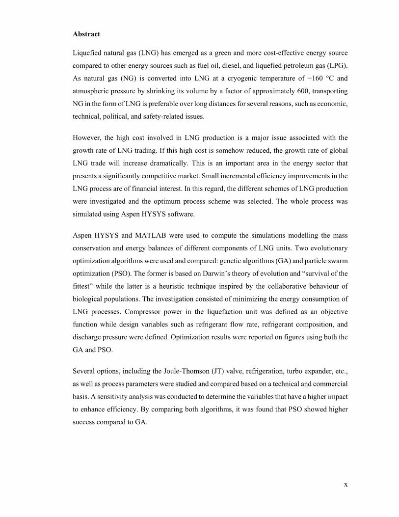
Abstract
Liquefied natural gas (LNG) has emerged as a green and more cost-effective energy source
compared to other energy sources such as fuel oil, diesel, and liquefied petroleum gas (LPG).
As natural gas (NG) is converted into LNG at a cryogenic temperature of −160 °C and
atmospheric pressure by shrinking its volume by a factor of approximately 600, transporting
NG in the form of LNG is preferable over long distances for several reasons, such as economic,
technical, political, and safety-related issues.
However, the high cost involved in LNG production is a major issue associated with the
growth rate of LNG trading. If this high cost is somehow reduced, the growth rate of global
LNG trade will increase dramatically. This is an important area in the energy sector that
presents a significantly competitive market. Small incremental efficiency improvements in the
LNG process are of financial interest. In this regard, the different schemes of LNG production
were investigated and the optimum process scheme was selected. The whole process was
simulated using Aspen HYSYS software.
Aspen HYSYS and MATLAB were used to compute the simulations modelling the mass
conservation and energy balances of different components of LNG units. Two evolutionary
optimization algorithms were used and compared: genetic algorithms (GA) and particle swarm
optimization (PSO). The former is based on Darwin’s theory of evolution and “survival of the
fittest” while the latter is a heuristic technique inspired by the collaborative behaviour of
biological populations. The investigation consisted of minimizing the energy consumption of
LNG processes. Compressor power in the liquefaction unit was defined as an objective
function while design variables such as refrigerant flow rate, refrigerant composition, and
discharge pressure were defined. Optimization results were reported on figures using both the
GA and PSO.
Several options, including the Joule-Thomson (JT) valve, refrigeration, turbo expander, etc.,
as well as process parameters were studied and compared based on a technical and commercial
basis. A sensitivity analysis was conducted to determine the variables that have a higher impact
to enhance efficiency. By comparing both algorithms, it was found that PSO showed higher
success compared to GA.
1
1. Introduction
1.1. Liquefied natural gas production
Ironically, most large gas reserves are often far away from the consumption areas and
liquefaction provides a means of transporting the gas economically over remote distances.
There is nearly a 600-fold reduction in the volume when natural gas is converted to its liquid
state. This reduction in volume offers a significant advantage for both storing and transporting
the gas, especially when gas transportation using pipelines is not feasible and economical
(Barclay, 2005).With this advantage, the prospect for liquefied natural gas (LNG) is positive
and it will likely play a significant role in meeting future natural gas demands, particularly in
industrial nations where natural gas (NG) is fast becoming a favoured fuel for power
generation.
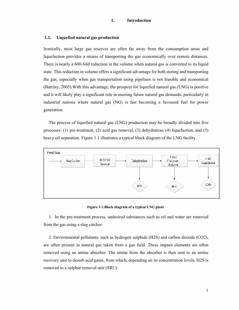
The process of liquefied natural gas (LNG) production may be broadly divided into five
processes: (1) pre-treatment, (2) acid gas removal, (3) dehydration, (4) liquefaction, and (5)
heavy oil separation. Figure 1.1 illustrates a typical block diagram of the LNG facility.
Figure 1-1.Block diagram of a typical LNG plant.
1. In the pre-treatment process, undesired substances such as oil and water are removed
from the gas using a slug catcher.
2. Environmental pollutants, such as hydrogen sulphide (H2S) and carbon dioxide (CO2),
are often present in natural gas taken from a gas field. These impure elements are often
removed using an amine absorber. The amine from the absorber is then sent to an amine
recovery unit to desorb acid gases, from which, depending on its concentration levels, H2S is
removed in a sulphur removal unit (SRU)
Chapter 1: Introduction
2
3. In the dehydration unit, an adsorbent is used to remove water from the treated natural
gas to prevent any ice formation throughout the following liquefaction process.
4. Traces of harmful mercury are also removed in another adsorbent bed before sending the
gas to the liquefaction unit.
5. The process of removing heavy compounds is an essential part LNG plants where natural
gas is cooled and liquefied to –160°C or less using refrigeration. As the gas is cooled and
liquefied to an extremely low temperature throughout the process, a massive amount of energy
is consumed. Hence, minimizing this energy consumption significantly important.
Consequently, a number of commercial processes exist claiming varying degrees of efficiency.
Numerous commercial LNG plants have been designed and constructed during the past
three decades. Depending on the mode of trading, these plants fall into two categories: peak
shave or base load plants.
Peak shave plants are relatively small units (0.1 – 0.25 million tons per year (tpy)) that
liquefy and store excess gas production during times of low demand. The gas is then re-
vaporised during peak demand catering to any requirements above the gas well production
capacity.
Base load plants are typically large and consist of several liquefaction trains, each
producing five million tpy or more. These plants are used to continuously supply liquefied gas
at a relatively constant rate, which is transported over long distances using purpose-built gas
carriers. Base load LNG plants are complicated facilities including liquefaction, storage,
loading and stand-alone utility systems (Shukri, 2004). Owing to potential fire hazards, these
large-scale LNG plants are often subjected to strict regulatory processes. Especially, major
difficulties have been faced by offshore LNG projects because of the lengthy approval process
required. Often, if the LNG production plant is located on offshore platforms, fewer safety
approvals are required.
Offshore plants as large as onshore base load units are technically feasible and may be
constructed in regions such as West Africa on large concrete or steel-hulled floating,
production, storage, and offloading (FPSO) vessels. Some mid-sized plants (1 million tpy
capacity) may also be built, although significant effort would be required to reduce the unit's
capital cost to make it commercially viable. Locating LNG plants on mobile FPSOs is
Chapter 1: Introduction
3
particularly attractive as it could enable a single facility to harness several gas fields across
its lifetime. This would allow many gas fields to be developed cost-effectively and may allow
capital costs to be repaid across numerous development projects.
The cryogenic industry has had its early start since Dr Carl von Linde developed air and
gas separation technologies in the nineteenth century in Munich, Germany. The LNG industry
started its early development by using LNG technology for natural gas peak shaving. Peak
shaving is a strategy used by the power industry to store natural gas for peak demand that
cannot be met by their typical pipeline volume. Utility companies liquefy natural gas during
low demand and re-gasify it during peak demand to augment available supply (Dr Chen-
Hwahiu, 2008).
At first, the cascade cycle was used in LNG plants. Later, A. Klimenko presented the mixed
refrigerant concept (Dr Chen-Hwahiu, 2008) at the LNG-1 Conference. Air Products applied
its mixed refrigerant cycle to the Libya Marsa El Brega LNG plant. Afterwards, Air Products
improved the cycle to create the propane pre-cooled mixed refrigerant (C3-MR) cycle, which
is being used in more than 80% of LNG plants globally.
Phillips Petroleum invented the cascade liquefaction cycle (Dr Chen-Hwahiu, 2008). This
cascade cycle is a closed loop cycle of propane, ethylene, and methane refrigerants.
Interestingly, when the C3-MR cycle was built at the Brunei LNG plant, the cascade cycle
was built for the Kenai LNG plant in Alaska and Prichard’s all MR cycle was built later in
Africa. A newer version of Phillips’ open loop cascade cycle has been built in Trinidad and
several other places such as Egypt, Darwin, and Equatorial Guinea.
Early contributors to the LNG industry include Lee Gaumer and Chuck Newton who
invented the all mixed refrigerant cycle and the C3-MR cycle for Air Products’ LNG process.
The Wilkes Barre cryogenic facility has manufactured the coil wound LNG Main Cryogenic
Heat Exchangers (MCHE) since the late 1960s. Ludwig Kniel of Lummus invented a cascade
cycle and regasification plant synergy for an ethylene plant. Ludwig also introduced a nitrogen
expansion cycle as a subcooling section for the LNG process (Dr.Chen-Hwahiu, 2008). Dr C.
M. “Cheddy” Sliepcevich pioneered and managed the research, development, and
implementation of the first commercial process for liquefaction and LNG ocean transport
during his work with Chicago Stock Yards and Continental Oil Company at the University of
4
Oklahoma. For his pioneering research in LNG technology, Cheddy, also referred to as the
“Father of LNG”, received the
Gas Industry Research Award from the American Gas Association Operating section in
1986 in Seattle. The award, sponsored by Sprague Schlumberger, honoured his scientific
achievement in LNG research and his contribution to LNG safety. Some of his students, Dr
Hardi Hashemi, Dr Harry West, and Dr Jerry Havens (2005), have further developed his work
in LNG safety.
In the beginning, steam turbines were preferred for LNG plant application because of their
prevalence in oil refineries. Steam turbines were implemented at the Bontang LNG plant in
Badak, Brunei and Das Island LNG plants. Later, it was discovered that gas turbines can be
more economically applied in LNG plants and, therefore, new LNG plants started using gas
turbines.
As gas turbine drivers are being improved, the water-cooled exchangers are being changed
to ambient air cooled heat exchangers. This is attributed to two factors: one is the concern over
water temperature changes and to the second is because of the simple and more efficient use
of large ambient air cooled exchangers.
Heat exchangers used in LNG are classified into coil-wound heat exchangers and plate-fin
core exchangers.
Coil-wound heat exchangers have evolved from smaller sizes to reach an approximate 15-
feet diameter and approximately 200 feet in height and weighs up to 300 metric tons, including
thousands of tubing capable of holding internal pressure up to 1,100 psig. Currently, Air
Products and Linde manufacture these cryogenic heat exchangers and it can take up to 25
months to complete one exchanger.
Plate-fin exchangers are manufactured by several vendors and are much cheaper than the
coil-wound heat exchangers. Variations include core-in-kettle exchangers. These exchangers
are manufactured by vacuum brazing the aluminium components into the whole exchanger
and require shop testing for high-pressure performance.
Phillips Petroleum developed the close loop optimized LNG cascade cycle and improved
it in the early 90s to what is known today as the open-loop process cycle. For mixed refrigerant
cycles, there are the Pritchard PRICO cycle and Air Products all MR and C3-MR cycles. There

Chapter 2 Literature review
5
are also other cycles by some French companies. Conoco Phillips’ optimum cascade cycle can
be built in large LNG plants up to 8+ MTPA. This process is being used in LNG plants built
in Darwin, Egypt, and Equatorial Guinea and will be used in the Angola LNG plant.
Chapter 1: Introduction
6
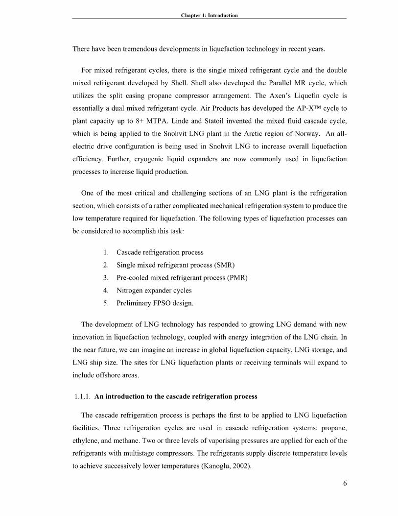
There have been tremendous developments in liquefaction technology in recent years.
For mixed refrigerant cycles, there is the single mixed refrigerant cycle and the double
mixed refrigerant developed by Shell. Shell also developed the Parallel MR cycle, which
utilizes the split casing propane compressor arrangement. The Axen’s Liquefin cycle is
essentially a dual mixed refrigerant cycle. Air Products has developed the AP-X™ cycle to
plant capacity up to 8+ MTPA. Linde and Statoil invented the mixed fluid cascade cycle,
which is being applied to the Snohvit LNG plant in the Arctic region of Norway. An all-
electric drive configuration is being used in Snohvit LNG to increase overall liquefaction
efficiency. Further, cryogenic liquid expanders are now commonly used in liquefaction
processes to increase liquid production.
One of the most critical and challenging sections of an LNG plant is the refrigeration
section, which consists of a rather complicated mechanical refrigeration system to produce the
low temperature required for liquefaction. The following types of liquefaction processes can
be considered to accomplish this task:
1. Cascade refrigeration process
2. Single mixed refrigerant process (SMR)
3. Pre-cooled mixed refrigerant process (PMR)
4. Nitrogen expander cycles
5. Preliminary FPSO design.
The development of LNG technology has responded to growing LNG demand with new
innovation in liquefaction technology, coupled with energy integration of the LNG chain. In
the near future, we can imagine an increase in global liquefaction capacity, LNG storage, and
LNG ship size. The sites for LNG liquefaction plants or receiving terminals will expand to
include offshore areas.
1.1.1. An introduction to the cascade refrigeration process
The cascade refrigeration process is perhaps the first to be applied to LNG liquefaction
facilities. Three refrigeration cycles are used in cascade refrigeration systems: propane,
ethylene, and methane. Two or three levels of vaporising pressures are applied for each of the
refrigerants with multistage compressors. The refrigerants supply discrete temperature levels
to achieve successively lower temperatures (Kanoglu, 2002).
Chapter 1: Introduction
7
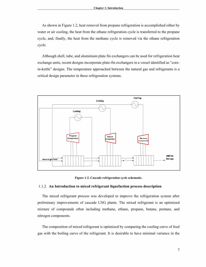
As shown in Figure 1.2, heat removal from propane refrigeration is accomplished either by
water or air cooling, the heat from the ethane refrigeration cycle is transferred to the propane
cycle, and, finally, the heat from the methane cycle is removed via the ethane refrigeration
cycle.
Although shell, tube, and aluminium plate fin exchangers can be used for refrigeration heat
exchange units, recent designs incorporate plate-fin exchangers in a vessel identified as “core-
in-kettle” designs. The temperature approached between the natural gas and refrigerants is a
critical design parameter in these refrigeration systems.
Figure 1-2. Cascade refrigeration cycle schematic.
1.1.2. An Introduction to mixed refrigerant liquefaction process description
The mixed refrigerant process was developed to improve the refrigeration system after
preliminary improvements of cascade LNG plants. The mixed refrigerant is an optimized
mixture of compounds often including methane, ethane, propane, butane, pentane, and
nitrogen components.
The composition of mixed refrigerant is optimized by comparing the cooling curve of feed
gas with the boiling curve of the refrigerant. It is desirable to have minimal variance in the
Chapter 2 Literature review
8
temperature difference between these two curves so an optimum can be achieved between the
power consumption and heat-exchange area.
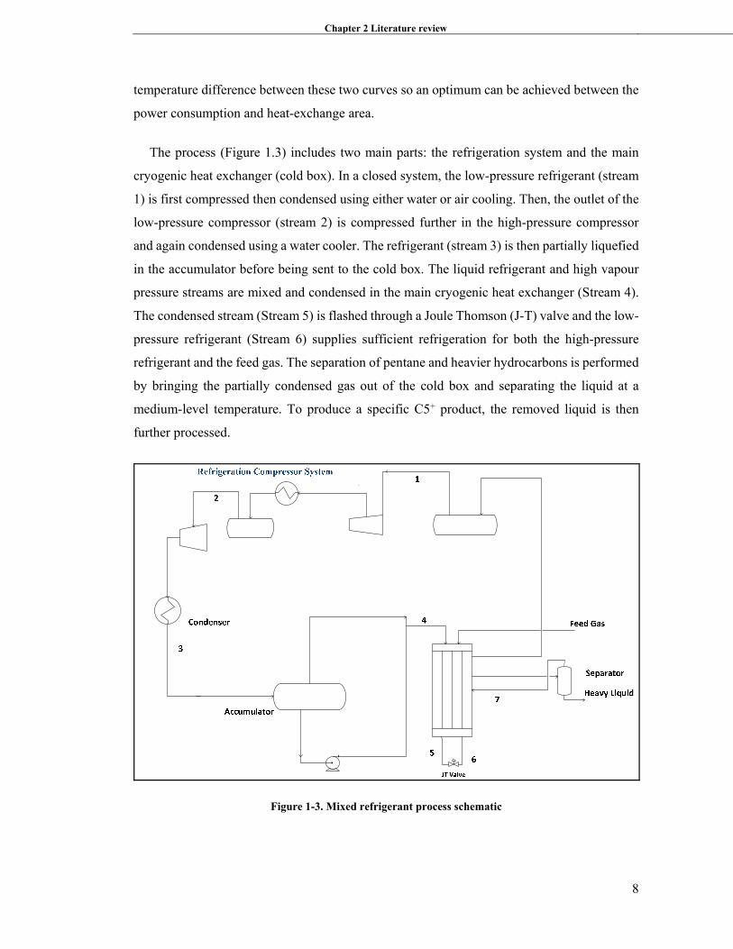
The process (Figure 1.3) includes two main parts: the refrigeration system and the main
cryogenic heat exchanger (cold box). In a closed system, the low-pressure refrigerant (stream
1) is first compressed then condensed using either water or air cooling. Then, the outlet of the
low-pressure compressor (stream 2) is compressed further in the high-pressure compressor
and again condensed using a water cooler. The refrigerant (stream 3) is then partially liquefied
in the accumulator before being sent to the cold box. The liquid refrigerant and high vapour
pressure streams are mixed and condensed in the main cryogenic heat exchanger (Stream 4).
The condensed stream (Stream 5) is flashed through a Joule Thomson (J-T) valve and the low-
pressure refrigerant (Stream 6) supplies sufficient refrigeration for both the high-pressure
refrigerant and the feed gas. The separation of pentane and heavier hydrocarbons is performed
by bringing the partially condensed gas out of the cold box and separating the liquid at a
medium-level temperature. To produce a specific C5+ product, the removed liquid is then
further processed.
Figure 1-3. Mixed refrigerant process schematic
Chapter 1: Introduction
9
.
The single mixed refrigeration system is used in modern plants, where the feed gas from
dehydration and acid removal units is fed to the main heat exchanger where it is initially cooled
to between - 45 °C and - 74 °C. Gas and heavy hydrocarbons, which might freeze at low
temperatures, are separated from the exchanger and directed to a separator drum. The cold gas
(Stream 7) is then returned to the main heat exchanger where it is condensed and subcooled.
The steel cold box assembly, including fin plates, are compactly integrated into the main
cryogenic heat exchanger, which not only serves as the exchange assembly but also provides
convenience in insulating the systems. The box and all welded internal connections are filled
with expanded perlite insulation. The external flanges for process connections to the cold box
minimize the leakage possibilities during the operation.
Both vapour and liquid refrigerant mediums are produced by closed-loop compression and
cooling. The outlet liquid of the accumulator is pumped and the vapour is sent under pressure
to the main exchanger, respectively, where both are mixed at the exchanger’s inlet (Stream 4).
The two-phase stream moves down the exchanger and exits as a liquid at approximately the
same temperature as the LNG. Refrigerant pressure is decreased through a control valve (JT)
and sent back to the exchanger. The low-pressure stream vaporises up-flow in the heat
exchanger and provides all the refrigeration for condensing the natural gas and, hence, in
producing LNG. When the refrigerant returns to compression system, the refrigerant loop is
completed. Multiple refrigeration loops have been used in more complex systems; however,
these plants are more expensive and difficult to operate, especially for small-scale LNG plants,
which must operate with minimum operating costs. LNG is produced in the main cryogenic
heat exchanger (MCHE) at -151 °C to -160 °C and is then sent to storage tanks near
atmospheric pressure.
Separation conditions can be adjusted to remove liquefiable components to required
specifications. To prevent solids from forming in liquefaction systems, pentane and heavy
components should be removed. To control the heating value of the LNG, the propane and
butane portions should be adjusted as well; the mid-point temperature in the exchanger should
be used to set the amount of removal.
Chapter 1: Introduction
10
The removed heavy hydrocarbons are reused as fuel gas or returned to the feed gas pipeline.
Liquids are further processed to provide a stabilized product for market. In most small-scale
LNG plants, there is not enough liquid to produce stabilized products. In some cases, different
sources of feed gases with different compositions are used in LNG plants so the amount of
liquid production becomes variable and uncertain.
The large refrigeration compressor is perhaps the most expensive and complicated
component in the liquefaction process. Small plants may contain reciprocating compressors or
screw compressors, whereas large units have centrifugal compressors either inline or in
integrally geared units. The selection of a driver is an important criterion in the cost of a
project, which can be a turbine or electric motor.
Owing to their low power cost, electric motors were chosen. Electric packages are cheaper
than turbine drives and lower operating and maintenance are required. Further, there are fewer
environmental effects caused by exhaust emissions. In some plants, there are start-up concerns
and electrical utility is required, as well.
While fuel gas cost is much cheaper than power cost, turbine drives are preferred in the
plants. In many installations, the fuel gas of gas turbines is usually supplied from process waste
gases or other facilities. Discrete sizes and single or dual gas turbines can supply a large
capacity range in the plants.
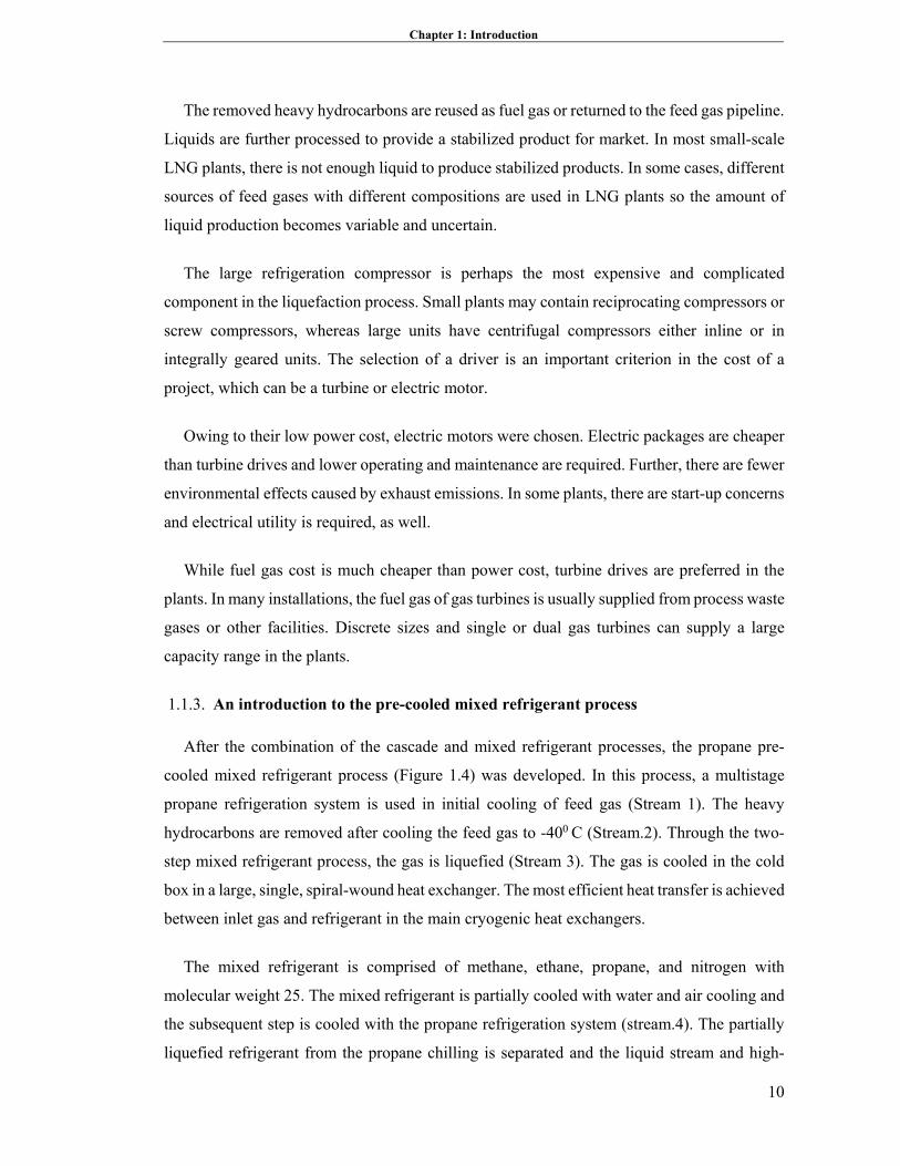
1.1.3. An introduction to the pre-cooled mixed refrigerant process
After the combination of the cascade and mixed refrigerant processes, the propane pre-
cooled mixed refrigerant process (Figure 1.4) was developed. In this process, a multistage
propane refrigeration system is used in initial cooling of feed gas (Stream 1). The heavy
hydrocarbons are removed after cooling the feed gas to -400 C (Stream.2). Through the two-
step mixed refrigerant process, the gas is liquefied (Stream 3). The gas is cooled in the cold
box in a large, single, spiral-wound heat exchanger. The most efficient heat transfer is achieved
between inlet gas and refrigerant in the main cryogenic heat exchangers.
The mixed refrigerant is comprised of methane, ethane, propane, and nitrogen with
molecular weight 25. The mixed refrigerant is partially cooled with water and air cooling and
the subsequent step is cooled with the propane refrigeration system (stream.4). The partially
liquefied refrigerant from the propane chilling is separated and the liquid stream and high-
Chapter 2 Literature review
11
pressure vapour are directed separately to the main cryogenic heat exchanger. After flashing,
the liquid supplies the preliminary cooling of the gas. The high-pressure vapour is liquefied in
the main exchanger (Stream 5) and provides the low level, final liquefaction of the gas (DOE,
2005).
Finally, the LNG exits the exchanger sub-cooled and is flashed for fuel reuse and pumped
to storage (Stream 3).
Figure 1-4. Propane pre-cooled mixed refrigerant.
Either two or three cycles are used in all modern large liquefaction facilities. The workhorse
of the industry is the two-cycle C3MR. The mixed refrigerant and feed gas process are
precooled with propane refrigerant at the first step. The natural gas is subcooled to low
temperatures at the second cycle by a mixed refrigerant. Two separate refrigerants require their
own dedicated compressors, drivers, heat exchanger, inter and after coolers, etc.
1.1.4. Integrated NGL and LNG plants
Historically, heavy hydrocarbons were separated from natural gas as a part of feed
conditioning. Generally, the residue gas (including mainly of methane) from the NGL
Chapter 1: Introduction
12
recovery plant is transported to the LNG plant for liquefaction. It is practical for NGL
recovery to be considered as an isolated plant from LNG liquefaction facilities for many
marketable or geographical conditions. One such economic advantage is that once NGL is
extracted, sales agreements for it can take place well in advance of LNG.
Integrating NGL extraction not only decreases capital cost by using mainly all equipment
in the NGL plant for LNG production but also progresses overall thermodynamic efficiency.
There are substantial advantages in doing so:
• Both capital and operating expenditures are reduced in the overall integrated plant.
• CO2 and NOX emissions are reduced through an integrated process by enhancing the
thermodynamic efficiency of the overall plant.
• Higher recovery of ethane (and propane) is achieved.
• Most LNG liquefaction equipment is already available in NGL units.
The capital cost is reduced while the requirement of a separate NGL recovery column is
replaced in LNG facilities for cryogenically separating ethane, propane, and heavier portions
in the integrated plant. The amount of NGL recovery is optimized based on the desired
specifications and relative market costs of NGL, LPG, and LNG by adjusting the operating
conditions.
As one common utility is considered, the capital expenses will be saved accordingly in the
integrated facilities. The NGL recovery units of the process can be constructed at an early
phase and later incorporated into LNG liquefaction process unit if an accurate strategy is
considered. The economic conditions of the LNG project may be significantly enhanced by
the possibility for early NGL sales in the market. An easy transition between ethane rejection
and recovery is achieved by changeable design of an integrated process, which is applicable
given approximately regular changes in ethane requirements.
Separating liquefied impurities, such as benzene and cyclohexane, is also improved while
better extraction of heavier hydrocarbon components is achieved in the integrated NGL
recovery unit in the natural gas liquefaction plant. As the low concentration of mentioned
impurities can cause freezing concerns in low-temperature sections of the LNG plant,
extracting the impurities is essential.
Chapter 1: Introduction
13
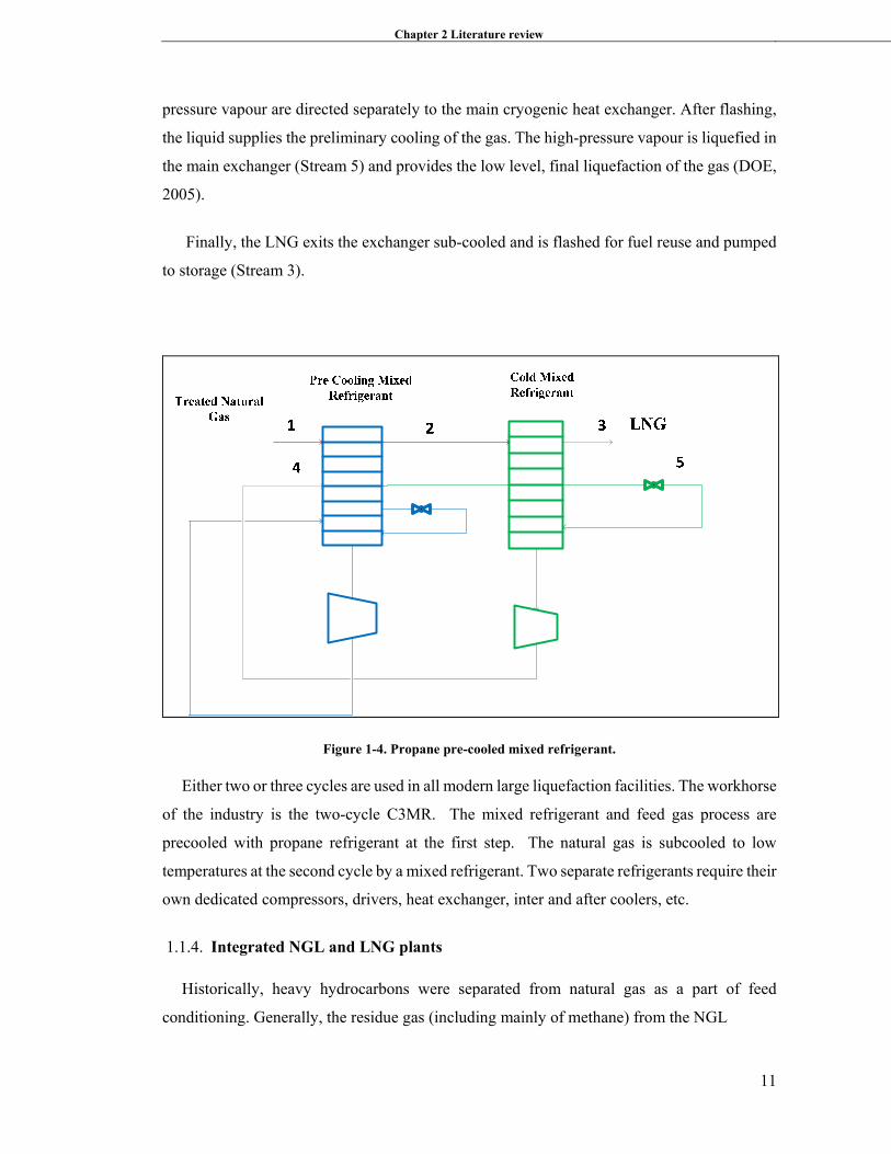
Appropriate integration of natural gas and a liquid recovery schematic within a liquefied
natural gas schematic achieve substantial benefits by decreasing total capital expenditure and
enhancing both LNG and NGL production. By accurately selecting a process scheme and heat
integration, integrated LNG/NGL plants can achieve lower specific consumed power and
higher net present value (NPV) compared to non-integrated installations.
Figure 1-5. Block diagram showing integrated LNG and NGL units.
In this research, the NGL unit has been integrated with the LNG unit as presented in Chapter
4. The optimization has been performed for an LNG liquefaction unit with the objective
function of minimizing the total power consumption in mixed refrigerant compressors and
NGL recovery unit and simultaneously maximizing ethane recovery. The optimization has
been performed using MATLAB software with two algorithms, which are presented in
chapters 4 and 5.
1.1.5. Thesis overview
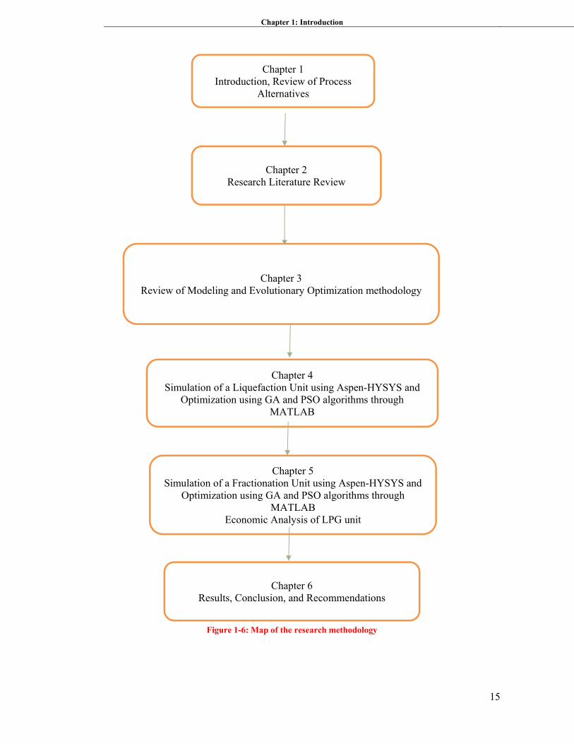
Chapter 1: briefly describes the background information for the research project. The different
methods of LNG production units are discussed and the advantages and disadvantages of each
method are investigated;
Chapter 2: The LNG optimization methods and different algorithms are reviewed. The basic
concept of LNG optimization is elaborated. The techniques in published papers are reviewed,
discussed, and evaluated. As a result, the limitations of existing techniques are identified.
Chapter 1: Introduction
14
Chapter 3: The two evolutionary algorithms (EAs), the GA and PSO, are investigated and the
methodology and correlation and coding methods are presented;
Chapter 4: The HYSYS simulation of liquefaction unit is presented and the modelling
assumption and procedure are discussed. Power consumption as an objective function is
optimized using PSO and GA algorithms and results are presented. The investigation consisted
of minimizing the energy consumption of LNG processes.
Compressor powers are defined as an objective function while design variables, such as
refrigerant flow rate, refrigerant composition, and discharge pressure are defined.
Optimization results are reported on figures using GA and PSO algorithms.
Chapter 5: The LPG fractionation unit is modelled using Aspen HYSYS software. An
economic analysis is performed to compare CAPEX and OPEX of different production
methods. Further, ethane recovery as an objective function is optimized through GA and PSO
algorithms. Several options, such as including a JT valve, refrigeration, turbo expander etc.,
as well as process parameters, are studied and compared based on a technical and commercial
basis. A sensitivity analysis is conducted to determine the variables that have a higher impact
on enhancing efficiency. By comparing both algorithms it is found that PSO showed higher
success compared to GA.
Chapter 6: The performance of optimization algorithms is compared and results are discussed.
Finally, the optimized variables are incorporated in HYSYS simulation to achieve maximum
LPG and propane recovery value as the objective function.
Chapter 1: Introduction
15
Chapter 2 Research Literature Review
Chapter 3 Review of Modeling and Evolutionary Optimization methodology
Chapter 1 Introduction, Review of Process
Alternatives
Chapter 4 Simulation of a Liquefaction Unit using Aspen-HYSYS and
Optimization using GA and PSO algorithms through MATLAB
Chapter 5 Simulation of a Fractionation Unit using Aspen-HYSYS and
Optimization using GA and PSO algorithms through MATLAB
Economic Analysis of LPG unit
Chapter 6 Results, Conclusion, and Recommendations
Figure 1.6: Map of research methodology Figure 1-6: Map of the research methodology
16
2. Literature Review
2.2. LNG plant modelling and simulation
As liquefaction temperatures are quite low (-160 0C), LNG production is an extremely
energy-intensive process. This means LNG liquefaction needs a large amount of refrigeration
energy and massive operating expenditures for liquefaction plants. As a result, refrigeration
system(s) represent a large portion of an LNG facility. Thus, reducing total power
consumption is the main competitive advantage for LNG producers in the liquefaction units
(Shukri, 2004). Hence, this aspect has received the attention of several researchers in the last
decade. Below is a brief review of those studies.
Historically, several schemes have been recommended for optimizing LNG processes by
varying both the equipment designs and refrigerant mediums. Examples include turbo-
expander units (the refrigerant was nitrogen), the cascade process, and dual/single mixed
refrigerant (SMR/DMR) processes. These variations in the approaches depend on the
operational and capital expenditures of each system and on the correlation between the cold
and hot composite curves. In fact, open loop turbo expander systems are the simplest
liquefaction method, where nitrogen is used as a refrigerant in turbo-expanders. Although this
is not the most efficient liquefaction scheme, it has the advantage of being safe and less
hazardous, making it suitable for small production capacities or offshore applications.
In cascade cycles, sequential stages are applied each with progressively colder refrigerants
having their own dedicated compression system. The list of refrigerants includes methane,
ethane, and propane (Shukri, 2004). By using a sequence of pressure drops to decrease the
temperature, an enhanced approach between the cold and hot composite curves is achieved. A
significant benefit of this scheme is the enhanced efficiency. Further, as there are fewer
available variables, the use of the cascade cycle allows for better control of the process.
However, all of this also leads to massively increased operating costs. Accordingly, it is only
suitable for large-scale processes.
Recently, more than seventy-five percent new LNG plants have used the mixed refrigerant
process, which requires relatively less number of heat exchanger elements and compressor
equipment thus making them less investment-demanding. However, the application of mixed
refrigerant processes increases the complexity of process operation
Chapter 2 Literature review
17
and design owing to greater interaction of thermodynamic conditions leading control
systems being extremely challenging (Barclay& Denton, 2005).
Irrespective of the refrigeration process employed, LNG plants are extremely expensive to
operate; hence, there have been a number of studies on optimizing the process. Most of these
studies have focused on optimizing operational expenditure (OPEX) with only a handful
addressing capital expenditure (CAPEX). The main aim of optimizing operating expenditure
has been to minimize the gap between hot and cold composite curves, which is what primarily
affects the process efficiency. Some specific example of such studies include the work of Shah
et al. (Shah, Rangaiah & Hoadley, 2009), who optimized two objective functions
simultaneously, namely, capital expenditure and energy efficiency, and Jensen and Skogestad
(2009), who included capital expenditures as a portion of the optimization investigation of the
single mixed refrigerant (SMR) process.
Jensen and Skogestad (2009) specifically considered the impacts of regulating pressure
and flows on determining the area of heat exchanger ‘expected compressor design’, placing
attention on the highest amount of power consumption of the compressor. The authors also
permitted optimization of the composition of refrigerants and were perhaps the first to improve
the objective function involving operating expenditures. Although their method of
optimization was described clearly, specific information about the initial value and objective
function was unavailable.
Ait-Ali’s (1979) optimization study on mixed refrigerant process operation proved to be a
major contribution to the refrigeration processes. However, it was strictly restricted to the
optimization computational methodology dominant at that time. Importance was placed on
decreasing the compressor’s power and numerous simplifications were considered to attain
that target. Gao, Lin and Gu (2009) performed an optimization study on an LNG process for
coal bed methane (CBM) within the simulation package HYSYS. The optimization was
performed using a consecutive method, related to the method of Lee et al. (2002), which could
not ensure inclusive optimality. The system’s key parameters were optimized in sequential
order: composition of components, discharge pressures, and temperatures of the heat
exchanger. In the research, Gao et al. (2009) did not incorporate butane as a component of the
mixed refrigerant though butane composition had a significant consequence on optimum
performance. In addition, propane was tuned as constant; hence, the residual component flows
were permitted to vary until the minimum value for the objective
Chapter 2 Literature review
18
function was achieved. Regarding the optimization objective, the consumed compressor
power and shared production flow rates were minimized.
Nogal, Kim, Perry, and Smith (2011), using a non-experimental method, established
approaches of applying minimum temperature differences along temperature profiles and used
expenditure approaches. The mentioned study considered a genetic algorithm but did not
clarify what specific objective functions were used.
Gandhiraju (2009) specified the ‘acclaimed’ composition of mixed refrigerants for pre-
cooled systems claiming the ‘optimal’ composition of refrigerant. Gandhiraju (2009) proposed
that using and executing the technology in operational plants is challenging, as the necessary
compositions differ intensely with varying plant conditions and schemes. An essential method
of assessing efficiency is the closeness between the cold and hot composite curves. The
technology cannot demonstrate the temperature profiles for the shown refrigeration
compositions. Though, the points between these cold and hot composite curves differ between
7 0C and 12 0C, which specifies process inefficiencies. The author concluded that it is possible
to achieve even greater efficiencies and/higher amount of refrigeration with suitable variations
to the composition of refrigerant and/or the operating/design condition.
A common approach for the optimum production of a cascade refrigeration system to make
the most of energy efficiency was prepared by Jian Zhang (2011). The exergy–temperature
graph mixed with the exergy investigation was shown to systematically examine the
thermodynamic environment of a refrigeration system, which offered a firm basis for the
conceptual design/retrofit of the complicated refrigeration system. In addition, an exergy fixed
model was established for the optimum synthesis of a typical cascade refrigeration system.
A simple and applicable approach for choosing a suitable refrigerant composition was
prepared, which was motivated by information on the difference in the boiling points of mixed
refrigerant components and the specific refrigeration impacts in getting a mixed refrigerant
system adjacent to a reversible operation by Mohd Shariq Khan (2013). An enthalpy diagram
and composite curves were considered for full implementation of the approaching
temperature. The offered information based on an optimization approach was explained and
used for a single mixed refrigerant and a propane pre-cooled mixed refrigerant system for
natural gas liquefaction. Increasing the exergy efficiency of the heat exchanger was reflected
as the optimization objective to attain an energy efficient design target.
Chapter 2 Literature review
19
The different design and operation objectives were specified for optimizing an LNG mixed
refrigerant process by Prue Hatcher (2012). The author concentrated on establishing and
analysing eight objective functions to specify the most suitable correlations. Four of the
objective functions concentrated on the operational features of the LNG process and the other
four focused on the design phase. It was specified that the most efficient operation
optimization objective function was the minimization of the main operating expenditure,
existing compressor power (Ws). For the design objective functions, the minimization of net
present value (NPV) is preferred. Hence, no limitation occurred in the area presented for LNG
plant construction. However, minimizing the objective function (Ws-UA) was chosen in
cases where a boundary of the processing unit was enforced.
Abdullah Alabdulkarem (2010) optimized the propane pre-cooled mixed refrigerant LNG
plant. To decrease the difficulty of the challenge, optimization was performed in two steps. In
the first step, optimization of the mixed cryogenic refrigerant cycle and formerly propane cycle
optimization were completed with relevant limitations. The optimum composition of the
mixed refrigerant was compared with two optimized compositions of refrigerant mixtures. The
optimization was performed with four pinch temperatures (0.01, 1, 3 and 5K) that showed
different corporate heat exchangers in LNG applications.
The possible energy efficiency improvements of numerous alternatives of applying the
waste heat powered absorption chillers in the propane pre-cooled mixed refrigerant (APCI)
liquefaction cycle was studied by Amir Mortazavi (2008) to improve the efficiency of energy
of LNG unit. After improving the LNG process, absorption chillers and gas turbines, six
selections of gas turbine waste heat consumption were simulated. The simulation reports
showed how considering 210C and 100C evaporators cooling and evaporators, the condenser
of the propane cycle at 120C and inter-cooling the compressor of the mixed refrigerant cycle
with absorption chillers, which are driven by waste heat from the gas turbine, both fuel
consumption and power consumption reductions as much as 20.43% were reported.
Kanoglu et al. (2001) highlighted the advantages of replacing the Joule Thomson valve (JT)
instead of the turbine expander for LNG expansion units. Renaudin et al. (1995) tested the
impact of exchanging mixed refrigerant expansion and LNG valves using liquid turbines.
Mortazavi et al. (2010) observed the impact of substituting expansion valves with liquid
turbines and two-phase expanders on the capacity and efficiency of the propane pre-cooled

Chapter 1: Introduction
20
multi-component refrigerant (MCR) natural gas liquefaction cycle licensed by Air Products
and
Chapter 2 Literature review
21
Chemicals, Inc. (APCI). Kalinowski et al. (2008) measured exchanging the propane cycle
with absorption chillers. Four processes consisting of a two-stage expander nitrogen
refrigerant, two loop expander processes, and a single mixed refrigerant were simulated at a
steady state on an identical basis by Remeljej (2006). Composite curves for the recycle and
feed streams and the cold or refrigerant recycle stream presented the existing degree of
optimization within each process. The study of full exergy presented the comparative
proportions to the overall required shaft work, with the minimum being the single mixed
refrigerant process. The key difference between processes is considered the lower efficiency
of the expander compressors. More common judgement recommended that the new LNG
open-loop process and nitrogen refrigerant process are the greatest options for offshore
compact LNG production.
Napoli (1980) established that steam boiler and gas turbine mixed cycle drivers were more
efficient and economical than steam boiler cycles for LNG plants. Kalinowski et al. (2009)
reviewed the application of gas turbine waste to replace the propane cycle of an LNG plant.
Mortazavi and Rodgers et al. (2008) considered LNG plant gas turbine driver waste heat to
decrease the energy consumption of liquefaction. Del Nogal et al. (2011) established a method
in accordance with mathematical programming to specify the most cost-effective set of drivers
for LNG plants.
Cao et al. (2006) improved power consumption N2-CH4 expander cycle and the mixed
refrigerant cycle using HYSYS software, which was useful in the NG liquefaction process.
There were two steps for pre-cooling, liquefying, and sub-cooling natural gas in both
processes. The authors achieved the idea that in the N2-CH4 expander cycle, a contribution of
demand power for compressors, is improved in the expander. Therefore, the process needed
less power in the compression steps.
In addition, Vaidyaraman et al. (2007) considered non-linear programming (NLP) to reduce
the power consumption of a cascade mixed refrigerant cycle. The optimization parameters
were refrigerant composition (C1, C2, C3 and n-butane), vapour fraction in flash tanks, and
ratios of compressor pressure. However, these simulation correlations only applied a
temperature cross at the outlet of the heat exchangers and could not assure the second law of
thermodynamics has not been disrupted by having a temperature cross in the intermediate heat
exchanger.
Chapter 2 Literature review
22
Paradowski et al. (2004) performed parametric research on a pre-cooled propane mixed
refrigerant cycle. In their study, mixed refrigerant composition, propane cycle pressures, pre-
cooling temperature, and propane cycle compressor speed were investigated. The study
focused on the importance of the propane-mixed refrigerant cycle even for larger plants than
those already constructed, consequently maintaining its position as the first option liquefaction
cycle.
Wang et al. (2011) minimized consumed energy by suggesting a synthesis approach in
accordance with mixed integer nonlinear programming (MINLP) formulation. They
conducted preliminary thermodynamic analysis, simulation, and optimization with the
intention of minimizing the energy consumption.
The liquefaction processes of the propane pre-cooled mixed refrigerant cycle (C3/MRC),
mixed refrigerant cycle (MRC), and nitrogen expander cycle (N2 expander) were examined
methodically by Li (2010). The processes were examined bearing in mind the chief features
including the presentation factors, economic presentation, plot plan, sensitivity to waves,
suitability to dissimilar gas resources, safety and reliability, accounting for the properties of
the floating production, storage, and offloading the unit for liquefied natural gas (LNG-FPSO)
in marine environments.
Saffari (2009) optimized the energy efficiency of an industrial pre-cooled propane mixed
refrigerant LNG base load plant by varying the components of refrigerants and the mole
fractions in liquefaction and sub-cooling cycles. This process was simulated by means of the
HYSYS software. The Peng Robinson equation of state was used for thermodynamic
calculations of properties both for natural gas and the refrigerants. Two approaches for
modelling and optimization were studied and a number of parameters were evaluated.
Computer software and methodology were developed for the optimum design of a
refrigeration system by Boiarskii (2009). The investigation considered mixed refrigerant
properties, properties of a counter-flow heat exchanger, and a given compressor. The model,
united with restricted experimental data, permitted an estimate of the refrigeration
performance of a cooler with good exactness. To evaluate several schemes of counter-flow
heat exchangers, heat exchanger efficiency was considered as a factor. It was specified as a
ratio of a given cooler performance to the performance of an idealized cycle. The approach
was applied in establishing mixed refrigerant- based coolers using a single-stage compressor.
Chapter 1: Introduction
23
Two distinctive small-scale natural gas liquefaction processes in a skid-mounted package
were considered and simulated by Wen-Sheng (2006). The main factors of the two processes
were evaluated and the matching of the cooling and heating curves in heat exchangers was
also examined. The authors found that a big temperature difference and heat exchange capacity
were the principal causes of losing exergy in heat exchangers. The power consumption of the
compressor was significant to the power consumption per unit of LNG. Consequently,
compression with intercooling should be implemented.
2.3. LNG plant optimization algorithms
Shah et al. (2009) investigated the optimization of the multi-objective methodology of a
single mixed refrigerant plant. They conducted coincident optimization of several objectives
in viewing various operating variables, such as pressure ratios in refrigeration compression
units, the minimum temperature difference of heat exchangers, and the number of refrigeration
stages (capital cost factors). The method involved improving some process flow diagrams and
choosing the applicable schematic was determined by analysing a number of refrigeration
stages. In the design variables, the approach was considered discrete. Hence, the distinct
number of levels were analysed according to the value of the final refrigeration temperature
and pressure ratio. The detached environment of design factors might recommend suboptimal
solutions because of the discrete classes. The authors (Shah et al. 2009) handled the
complicated nature of the simulation by including a visual basic, a flowsheet simulator line,
and a non-dominated sorting genetic algorithm (GA) optimizer.
Venkatarathnam (2008) accomplished optimization research on a C3-MR cycle by means
of the sequential quadratic programming (SQP) technique in the Aspen Plus optimization tool.
The author confirmed refrigerant composition and compressor pressure ratios to maximize the
cycle’s exergy efficiency.
Two compression stages in a single-stage mixed refrigerant (SMR) cryogenic cycle were
reviewed for LNG production by Mokrizadeh (2010). The consumed energy of the process as
an objective function was optimized by defining the main parameters of the design. The author
included thermodynamic theories and properties in MATLAB to develop the objective
function and applied a GA as a strong optimization approach.
Chapter 1: Introduction
24
The AP-X process, designed by Heng Sun et al. (2016), is regarded as a promising energy-
efficient process for large-scale LNG plants. To decrease the power consumption further, a
GA was used to globally optimize the process and a suitable refrigerant for use in the sub-
cooling cycle was studied. The optimized unit power consumption was 4.337 kW h/kmol,
which was 15.56% less than that of the base case and 15.62% less than that of the C3MR
process with its multi-throttling pre-cooling cycle. Results show the optimized AP-X process
is the most efficient liquefaction process for large-scale LNG plants to date. Exergy analysis
was conducted to calculate the lost work for main equipment items used in the AP-X process.
The polytropic efficiency of compressors is the most important item for potential
improvements in energy efficiency.
A re-liquefaction LNG plant was studied by Hoseyn Sayyadi (2011) using a multi-objective
method for simultaneously considering exergoeconomic and energetic objectives. The
optimization was conducted to improve the exergetic efficiency of the plant and minimize the
unit expenditure of the production system. The thermodynamic modelling was conducted in
accordance with energy and exergy, whereas an exergoeconomic model in accordance with
the whole income necessity was established. Optimization programming usin MATLAB was
achieved by means of one of the most powerful and strong multi-objective optimization
algorithms, namely NSGA-II. This method is related to the GA and is useful for discovering
a set of Pareto-optimal solutions.
The effect of LNG supplying risk on the combined gas and electricity system’s operation
under the multi gas-source supply background was considered by Gang Chena (2016) and the
optimization planning model of the combined system’s LNG reserve was developed. The
optimization objective of the model was to minimize the annual cost of the combined system,
considering operation simulation of several typical scenarios along 52 weeks in a whole year
and the annualized investment of LNG tanks. The operation objective of each scenario was
determined by the LNG’s arrival and the operation mode of the LNG terminals. The optimal
LNG reserve of the test system was solved and the effect of load level and operation mode on
the reserve planning was also analysed (Gang Chena, 2016).
Heat leakage and mechanical energy input by equipment evaporate LNG in LNG-receiving
terminals into boil-off gas (BOG), which must be compressed and liquefied by sub-cooled
LNG in a recondenser. During ship unloading, there are sharp fluctuations in BOG waste
resources, causing economic loss. Meanwhile, the liquid levels of the recondenser are unstable
Chapter 1: Introduction
25
and the consequent pump cavitation and equipment vibration introduce risks to the operation.
Yajun (2016) focused on the problems above in an actual LNG-receiving terminal. The factors
affecting the BOG generation in the LNG-receiving terminal and the generation rules were
analysed. To find effective improvements for these problems, an optimization model was built
and solved using a dynamic simulation tool, which provided a reference for further dynamic
research. After optimization, 0.19 million m3 of natural gas avoided being flared and the
energy consumption of the BOG compressors was reduced by 4.2%, i.e., 0.19 million kWh.
As a result, 0.14 million USD is saved annually. In addition, pump cavitation and recondenser
vibration were also reduced and the recondensing system was easier to control, which
contributed to the terminal’s safe operation.
Per E. Wahl (2015) has investigated three selections of variables. In all sets, the refrigerant
compressor suction and discharge pressure were used as variables. The additional variables
characterized the refrigerant flow. Using the component molar flow rates performed slightly
better than using the molar fractions and total molar flow while using the heat flow had less
success. Per E. Wahl (2015) investigated the effects of different aspects of the optimization
problem formulation, such as variable selection, formulae for estimating derivatives, initial
values, variable bounds, and formulation of constraints. Especially, formulation of the
constraint for the temperature difference between the hot and cold composite curve is essential.
In conclusion, previously published research has provided a strong foundation for further
optimization of liquefied natural gas plants. However, the literature lacks detailed study on
optimizing LNG units. This is perhaps because of the nonlinearity of LNG process variables.
The present study is aimed at filling this gap. The outline of the thesis is presented in the
diagram on the next page. The EAs are used to optimize the LNG plant efficiently.
Evolutionary algorithms (EAs) are stochastic search methods that mimic the natural
biological evolution and/or the social behaviour of species. Such algorithms have been
developed to arrive at near-optimum solutions to large-scale optimization problems, for which
traditional mathematical techniques may fail. This thesis compares the formulation and results
of two recent evolutionary-based algorithms: genetic algorithms and particle swarm
optimization. Benchmark comparisons among the algorithms are presented for both
continuous and discrete optimization problems, in terms of processing time, convergence
speed, and quality of the results. Based on this comparative analysis, the performance of EAs
is discussed along with some guidelines for determining the best operators for each algorithm.

Chapter 1: Introduction
26
The study presents sophisticated ideas in a simplified form that should be beneficial to
practitioners and researchers involved in optimizing LNG plants.
In this research, the proper and the most efficient EAs for LNG plant optimization as a non-
linear and complex system is investigated and the objective is to compare which (GA or PSO)
is more favourable.
27
3. Modelling and optimization methodology
3.1. Process modelling
This research was performed using computer simulations in Aspen HYSYS and MATLAB
software. The process schematic was simulated using Aspen HYSYS software and Peng-
Robinson equation state was used for thermodynamic properties’ calculations. The whole
LNG plant (reception facility, dehydration, acid gas removal, and fractionation) were
simulated using Aspen-HYSYS software (8.6), which is presented in Appendix B.
The main equation of mass conservation for a steady state and steady flow system is:
. . 0
The energy balance of each component is achieved by considering the first law of
thermodynamics of the system, as follows:
∑ ∑ ∑ ∑ +W=0
The energy balance of each system (each system can be specified as a control volume with
inlet and outlet streams, power and heat interactions) can be achieved by the above equation.
The LNG processes are thermodynamically complicated, extremely interrelating and
nonlinear, presenting difficulties in the optimization. There are additional optimization
obstacles caused by incompatible objectives. For instance, the heat transfer area increases
while flows and pressure differentials increase in the heat exchangers. Conversely, the most
important parameter on total operating expenditures is considered as total power consumptions
by compressors in the liquefaction unit. On the other hand, drops in pressure differentials and
flows increase the area needed for heat transfer, causing greater capital costs (CAPEX). In
traditional methods, the LNG process demonstrates the trade-off between OPEX and CAPEX.
As the liquefaction and fractionation units of LNG plants are critical and cost-sensitive, the
design parameters of the liquefaction unit and fractionation units have been optimised using
PSO and GAs in MATLAB. The results have been compared to generate the best outcomes.
For the liquefaction unit, total refrigerant compressor power was considered as an objective
function and the amount of ethane recovery was considered as an objective function for
fractionation unit
Chapter 3: Modelling and optimization methodology
28
optimization. Particle swarm optimization was used to optimise the liquefaction and
separation fractionation units, which have been previously ignored in the optimization of pre-
cooled mixed refrigerant LNG plants despite their obvious importance. The algorithm was
coded in MATLAB software and linked with Aspen HYSYS software to gain simultaneous
access to objective function and design variables. The written codes in MATLAB have been
presented in Appendix A.
3.2. Evolutionary Optimization algorithms
One traditional optimization method is the gradient-based methods. In these methods, the
function and its differential are identified in the investigated data range. In these calculation
methods, the second differential is identified as well as the first differential in the required
calculation range. Although these methods achieve quick results, they cannot specify the
optimum points in the discrete spaces and unidentified differential points. Further, they often
get terminated at the local minimum points. In this regard, in the nonlinear functions with
several minimum local points or indirect correlation of function with parameters, the
population-based algorithms should be considered for optimization.
The genetic algorithm (GA) and particle swarm optimization (PSO) are population-based
optimization algorithms. In recent times, GAs and PSO have caused significant thought about
several modern heuristic optimization methods. The GA has been favoured in the industry and
academia mostly because of its intuitiveness, the simplicity of its application, and the capacity
to effectively solve highly non-linear, mixed integer optimization challenges that are
distinctive of complex engineering plants. The PSO method is a comparatively modern
heuristic search technique whose procedures are motivated by the swarming or collaborative
behaviour of biological populations. Further, the two methodologies are supposed to discover
an answer to a given objective function but employ different strategies and computational
determinations.
The difficulties associated with using mathematical optimization on large-scale engineering
problems have contributed to the development of alternative solutions. Linear programming
and dynamic programming techniques, for example, often fail (or reach local optimum) in
solving NP-hard problems with a large number of variables and non-linear objective functions
(Emad Elbeltagia, 2005). To overcome these problems, researchers have proposed
evolutionary-based algorithms for discovering near-optimum solutions to problems.
Chapter 3: Modelling and optimization methodology
29
Evolutionary algorithms (EAs) are stochastic search methods that mimic natural biological
evolution and/or the social behaviour of species. Examples include how ants find the shortest
route to a source of food and how birds find their destinations during migration. The behaviour
of such species is guided by learning, adaptation, and evolution (Emad Elbeltagia, 2016). To
mimic the efficient behaviour of these species, various researchers have developed
computational systems that seek fast and robust solutions to complex optimization problems.
The first evolutionary-based technique introduced in the literature was Gas. GAs were
developed based on the Darwinian principle of the ‘survival of the fittest’ and the natural
process of evolution through reproduction.
Based on its demonstrated ability to reach near-optimum solutions to large problems, the
GA technique has been used in many applications in science and engineering. Despite their
benefits, GAs may require long processing time for a near optimum solution to evolve. Further,
not all problems lend themselves well to a solution with GAs.
To reduce processing time and improve the quality of solutions, particularly to avoid being
trapped in local optima, other EAs have been introduced in the past 10 years.
Hamid Saffari (2010) performed thermodynamic simulation and optimization of the C3MR
system using a GA. For this purpose, in the first step, the Peng Robinson equation of state is
simulated with a code in MATLAB and then used for simulating thermodynamic properties
of natural gas and refrigerants are used in the cycle. Afterwards, the cycle is
thermodynamically simulated and composite curves for sub-cooling and liquefaction heat
exchangers are plotted. If composite curves in heat exchangers approach, the total power will
decrease. Then, the total power used by the compressors is calculated. In the next step,
thermodynamic modelling is linked with GAs and the power consumed by compressors is
defined as an objective function. The best value resulting from optimization has 23% less
power than the base design. In addition, the heat exchange curves are close together.
Hence, the GAs are to be used for discrete spaces and PSO is more applicable for
continuous areas. In previous studies on natural gas plant optimization, GAs have been used
extensively. Hence, a brief description and comparison of both EAs are presented below.
Chapter 3: Modelling and optimization methodology
30
3.2.1. An introduction to Genetic algorithms
This method is based on Darwin’s theory of evolution and “survival of fittest”. This method
comprises several steps that have not been described here. Only the application of this
algorithm has been described.
3.2.2. Generation of the initial population
The nature of the problem specifies the size of the population but typically contains
numerous hundreds or thousands of probable answers. Frequently, the initial population is
generated randomly, permitting a whole boundary of probable solutions (the exploration
space). Frequently, the answers can be “seeded” in spaces; hence, optimum solutions are likely
to be achieved (Goldberg DE, 1975).
This algorithm is implemented in binary space. Consequently, the bytes of each variable
must be identified in the first step. The number of bytes to be identified affect the accuracy.
For instance, the number of bytes ith variable will be specified with ei accuracy as follows:
log 1
log 2
The Hi and Li are the upper and lower bound of the required variable, respectively. Then,
each byte is related to number one or zero, respectively, which is performed absolutely
randomly with a uniform distribution. For better convergence, the initialization must be
implemented with the knowledge of the problem.
3.2.3. Fitness function evaluation
Each chromosome must be transferred to the decimal space then the objective function will
be calculated for the required variable. It should be noted that the variables will not be
converted to the continuous space while the space is discrete. Sometimes, these bytes can
adopt only one or zero values and there is no requirement for the description of bytes
(Goldberg DE, 1975).
For instance, if the whole number of neurons to be considered is between 4 and 11, then
the whole space will have eight members. In this regard, the three bytes can be produced with
these eight members. However, these three bytes will generate numbers between zero to seven
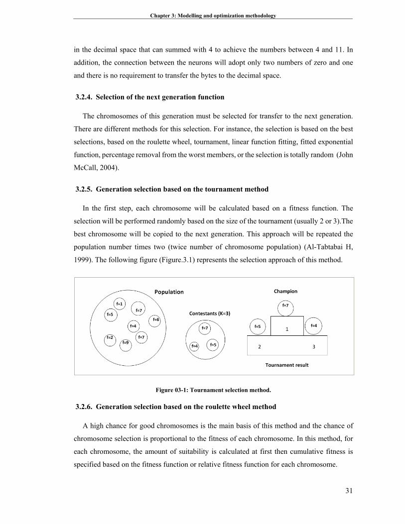
Chapter 3: Modelling and optimization methodology
31
in the decimal space that can summed with 4 to achieve the numbers between 4 and 11. In
addition, the connection between the neurons will adopt only two numbers of zero and one
and there is no requirement to transfer the bytes to the decimal space.
3.2.4. Selection of the next generation function
The chromosomes of this generation must be selected for transfer to the next generation.
There are different methods for this selection. For instance, the selection is based on the best
selections, based on the roulette wheel, tournament, linear function fitting, fitted exponential
function, percentage removal from the worst members, or the selection is totally random (John
McCall, 2004).
3.2.5. Generation selection based on the tournament method
In the first step, each chromosome will be calculated based on a fitness function. The
selection will be performed randomly based on the size of the tournament (usually 2 or 3).The
best chromosome will be copied to the next generation. This approach will be repeated the
population number times two (twice number of chromosome population) (Al-Tabtabai H,
1999). The following figure (Figure.3.1) represents the selection approach of this method.
Figure 03-1: Tournament selection method.
3.2.6. Generation Selection based on the roulette wheel method
A high chance for good chromosomes is the main basis of this method and the chance of
chromosome selection is proportional to the fitness of each chromosome. In this method, for
each chromosome, the amount of suitability is calculated at first then cumulative fitness is
specified based on the fitness function or relative fitness function for each chromosome.
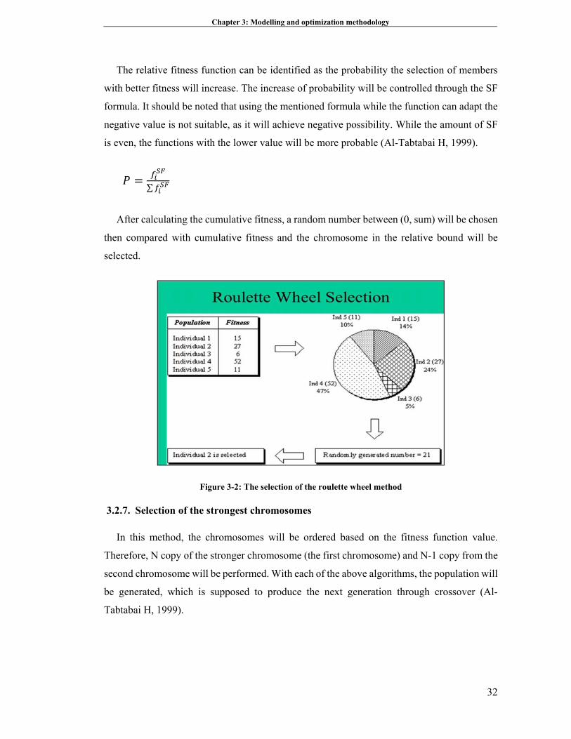
Chapter 3: Modelling and optimization methodology
32
The relative fitness function can be identified as the probability the selection of members
with better fitness will increase. The increase of probability will be controlled through the SF
formula. It should be noted that using the mentioned formula while the function can adapt the
negative value is not suitable, as it will achieve negative possibility. While the amount of SF
is even, the functions with the lower value will be more probable (Al-Tabtabai H, 1999).
∑
After calculating the cumulative fitness, a random number between (0, sum) will be chosen
then compared with cumulative fitness and the chromosome in the relative bound will be
selected.
Figure 3-2: The selection of the roulette wheel method
3.2.7. Selection of the strongest chromosomes
In this method, the chromosomes will be ordered based on the fitness function value.
Therefore, N copy of the stronger chromosome (the first chromosome) and N-1 copy from the
second chromosome will be performed. With each of the above algorithms, the population will
be generated, which is supposed to produce the next generation through crossover (Al-
Tabtabai H, 1999).
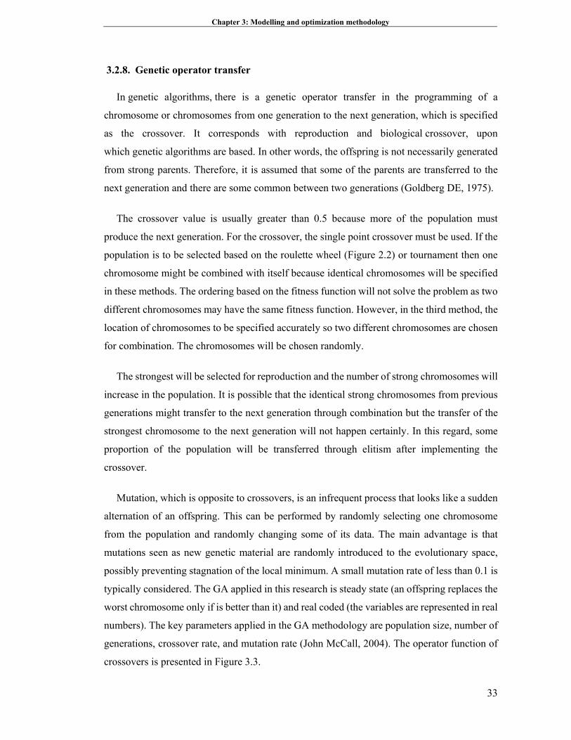
Chapter 3: Modelling and optimization methodology
33
3.2.8. Genetic operator transfer
In genetic algorithms, there is a genetic operator transfer in the programming of a
chromosome or chromosomes from one generation to the next generation, which is specified
as the crossover. It corresponds with reproduction and biological crossover, upon
which genetic algorithms are based. In other words, the offspring is not necessarily generated
from strong parents. Therefore, it is assumed that some of the parents are transferred to the
next generation and there are some common between two generations (Goldberg DE, 1975).
The crossover value is usually greater than 0.5 because more of the population must
produce the next generation. For the crossover, the single point crossover must be used. If the
population is to be selected based on the roulette wheel (Figure 2.2) or tournament then one
chromosome might be combined with itself because identical chromosomes will be specified
in these methods. The ordering based on the fitness function will not solve the problem as two
different chromosomes may have the same fitness function. However, in the third method, the
location of chromosomes to be specified accurately so two different chromosomes are chosen
for combination. The chromosomes will be chosen randomly.
The strongest will be selected for reproduction and the number of strong chromosomes will
increase in the population. It is possible that the identical strong chromosomes from previous
generations might transfer to the next generation through combination but the transfer of the
strongest chromosome to the next generation will not happen certainly. In this regard, some
proportion of the population will be transferred through elitism after implementing the
crossover.
Mutation, which is opposite to crossovers, is an infrequent process that looks like a sudden
alternation of an offspring. This can be performed by randomly selecting one chromosome
from the population and randomly changing some of its data. The main advantage is that
mutations seen as new genetic material are randomly introduced to the evolutionary space,
possibly preventing stagnation of the local minimum. A small mutation rate of less than 0.1 is
typically considered. The GA applied in this research is steady state (an offspring replaces the
worst chromosome only if is better than it) and real coded (the variables are represented in real
numbers). The key parameters applied in the GA methodology are population size, number of
generations, crossover rate, and mutation rate (John McCall, 2004). The operator function of
crossovers is presented in Figure 3.3.
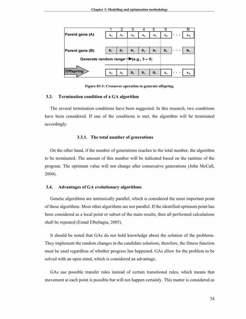
Chapter 3: Modelling and optimization methodology
34
Figure 03-3: Crossover operation to generate offspring.
3.3. Termination condition of a GA algorithm
The several termination conditions have been suggested. In this research, two conditions
have been considered. If one of the conditions is met, the algorithm will be terminated
accordingly.
3.3.1. The total number of generations
On the other hand, if the number of generations reaches to the total number, the algorithm
to be terminated. The amount of this number will be indicated based on the runtime of the
program. The optimum value will not change after consecutive generations (John McCall,
2004).
3.4. Advantages of GA evolutionary algorithms
Genetic algorithms are intrinsically parallel, which is considered the most important point
of these algorithms. Most other algorithms are not parallel. If the identified optimum point has
been considered as a local point or subset of the main results, then all performed calculations
shall be repeated (Emad Elbeltagia, 2005).
It should be noted that GAs do not hold knowledge about the solution of the problems.
They implement the random changes in the candidate solutions; therefore, the fitness function
must be used regardless of whether progress has happened. GAs allow for the problem to be
solved with an open mind, which is considered an advantage.
GAs use possible transfer rules instead of certain transitional rules, which means that
movement at each point is possible but will not happen certainly. This matter is considered as
Chapter 3: Modelling and optimization methodology
35
an advantage of GAs, which prevent achieving the local minimum point. In addition, the
algorithm can converge to several optimum results.
The variables can be coded in these algorithms and optimization will be implemented
through coded variables and supply the ability of optimization in a discrete landscape.
3.5. Limitations of GA evolutionary algorithms
The challenge is defining the evaluator that achieves the best solutions. If the performance
of fitness is not selected well, no solution may be found for the problem or the problem could
be solved wrongly. In addition, other parameters must be considered, such as population size
and combination rate.
The other challenge is known as prematurity if there is a significant distance between one
gene to other sizes of genes in the generation. The results will lead to local optimum points in
a low population. The methods will solve these challenges, such as tournament selection and
rank scaling. The other challenge of these algorithms is the difficulty of implementing
conditional problems (Emad Elbeltagia, 2005).
3.6. Particle swarm optimization algorithm
The PSO method is used to specify the optimum point or area of the whole system. In these
landscapes, the assumptions are considered and the primary location and velocity are indicated
for each individual particle. The particles can fly freely in all directions. Also, there are some
connection channels between particles.
For open-ended challenges to nonlinear optimizations, a new solution was derived based
on a new concept of evolutionary exploration algorithms by Holland (1975). Stimulated by
the natural alterations of the biological species, Holland used Darwin’s theory using his most
common and well-recognized algorithm, presently recognized as genetic algorithms (GAs).
Holland and his colleagues, including Goldberg and Dejong, promoted the theory of GAs and
validated the way natural mutations and crossovers of chromosomes is understood in the
algorithm to progress the feature of answers through consecutive iterations. In 1995, Kennedy
and Eberhart uttered a substitute answer to the nonlinear complicated optimization challenge
by matching the collective performance of particles, bird flocks, and introduced particle swarm
optimization (PSO). Price and Storn (1997) performed an accurate effort to substitute

Chapter 3: Modelling and optimization methodology
36
traditional mutations and crossovers in GAs using other operators and developed a proper
differential operator to manage the challenge. GA and PSO algorithms do not need any
gradient data for the function to be optimised, just basic mathematical operators. The
algorithms can be applied in any computer programming software directly and need minimum
factors tuning. The presentation of the algorithm does not decline strictly with the development
of the examination space dimensions. Therefore, the particles fly in the response space and the
results will be identified based on eligibility criteria for a time range.
Over time, the particles accelerate to the particles with higher eligibility and the same
connection in a group. This method is successful for optimization in continuous spaces like
LNG units. The steps of the algorithm are shown in Figure 3.4.
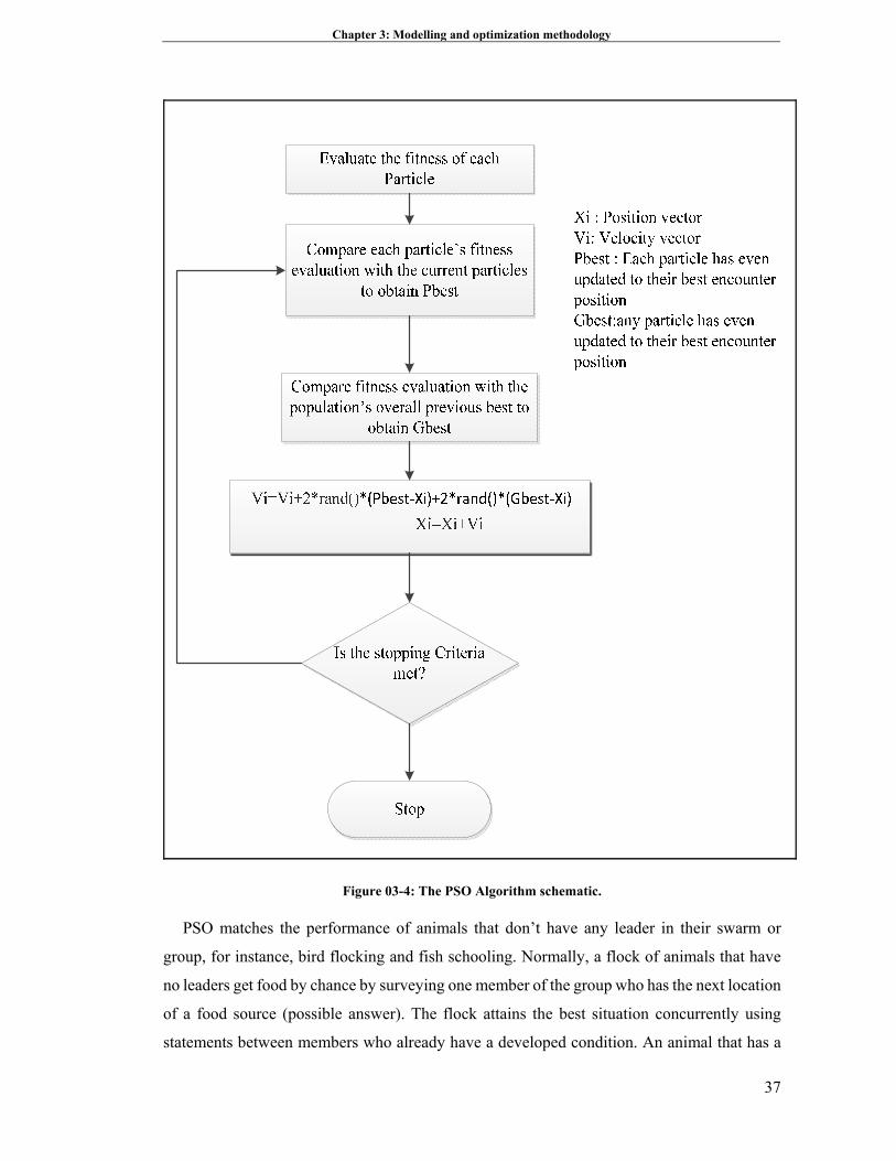
Chapter 3: Modelling and optimization methodology
37
Figure 03-4: The PSO Algorithm schematic.
PSO matches the performance of animals that don’t have any leader in their swarm or
group, for instance, bird flocking and fish schooling. Normally, a flock of animals that have
no leaders get food by chance by surveying one member of the group who has the next location
of a food source (possible answer). The flock attains the best situation concurrently using
statements between members who already have a developed condition. An animal that has a
Chapter 3: Modelling and optimization methodology
38
greater situation will tell its flock and the others will move instantaneously to that place. This
would happen frequently until the best situations or a food sources revealed. The method of
PSO in discovery optimal values surveys the work of this animal society. Particle swarm
optimization comprises of a swarm of particles, where particles suggest a possible answer
(Bai, 2010).
There have been numerous amendments to the original PSO. It has been adjusted to quicken
attaining the greatest circumstances. The improvement will deliver new benefits and the
variety of difficulties to be determined. The investigation on PSO improvement is essential to
determine its improvement, its benefits and limitations and how much use this technique has
to resolve a challenge.
PSO is a multi-agent parallel examination method. Particles are conceptual objects that fly
through the multi-dimensional examination space. In any specific direction, each particle has
a location and a speed. The situation vector of a particle regarding the source of the analysis
space represents a trial solution of the search problem. At the beginning, a population of
particles is modified with random positions obvious by vectors and random velocities
the population of such particles is called a “swarm” S.
Each particle P has two state variables viz., its present position ,and its present velocity
(t). It also has a small memory including its previous best situation (one yielding the highest
value of the fitness function established up to now) , i.e., individual best experience and
the best of all P ∈ N(P): , i.e., the best station established so far in the neighbourhood
of the particle. Once we set N (P) = S, is stated to as the globally best particle in the whole
swarm. The PSO (PSO) pattern has the resulting algorithmic factors:
a. Vmax or maximum velocity, which limits within the interval
, ;
b. An inertial weight factor ω;
c. Two uniformly distributed random numbers 1and 2 that correspondingly
define the effect of and on the velocity updated formula;
d. Two constant multiplier terms C1 and C2 recognized as “self-confidence” and
“swarm confidence”, individually.
Firstly, the sets of and are 0 = 0 = 0 for whole particles. Formerly,
the particles are all modified and an iterative optimization process commences where the
situations and speeds of all the particles are rehabilitated by the following recursive
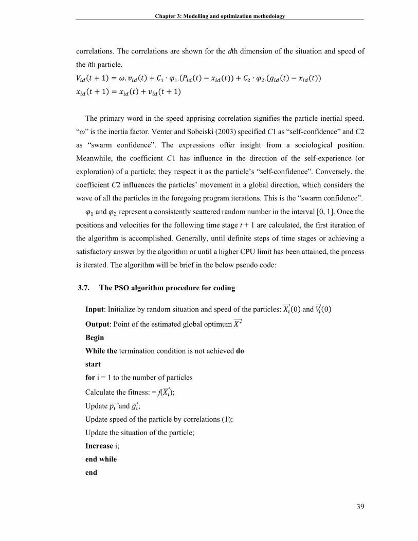
Chapter 3: Modelling and optimization methodology
39
correlations. The correlations are shown for the dth dimension of the situation and speed of
the ith particle.
1 . ∙ ∙ ∙ ∙
1 1
The primary word in the speed apprising correlation signifies the particle inertial speed.
“ω” is the inertia factor. Venter and Sobeiski (2003) specified C1 as “self-confidence” and C2
as “swarm confidence”. The expressions offer insight from a sociological position.
Meanwhile, the coefficient C1 has influence in the direction of the self-experience (or
exploration) of a particle; they respect it as the particle’s “self-confidence”. Conversely, the
coefficient C2 influences the particles’ movement in a global direction, which considers the
wave of all the particles in the foregoing program iterations. This is the “swarm confidence”.
and represent a consistently scattered random number in the interval [0, 1]. Once the
positions and velocities for the following time stage t + 1 are calculated, the first iteration of
the algorithm is accomplished. Generally, until definite steps of time stages or achieving a
satisfactory answer by the algorithm or until a higher CPU limit has been attained, the process
is iterated. The algorithm will be brief in the below pseudo code:
3.7. The PSO algorithm procedure for coding
Input: Initialize by random situation and speed of the particles: 0 and 0
Output: Point of the estimated global optimum ∗
Begin
While the termination condition is not achieved do
start
for i = 1 to the number of particles
Calculate the fitness: = f( );
Update and ;
Update speed of the particle by correlations (1);
Update the situation of the particle;
Increase i;
end while
end
Chapter 3: Modelling and optimization methodology
40
Kennedy and Eberhart presented the perception of optimising a function through a particle
swarm. Assuming the global optimum of an n-dimensional function has been considered, the
function can be signified from a mathematical viewpoint as:
, , , … . ,
Somewhere, is the exploration-variable vector, which essentially signifies the group of
independent factors of the assumed function. This assignment will explore where the value
of function is also a minimum or a maximum signified by f∗. If the constituents of
undertake actual values then the charge is to find a specific opinion in the n-dimensional
hyperspace, which is a continuum of such points.
Surveying is the capability of an exploration algorithm to discover diverse areas of the
search space in order to trace a good optimum. Exploitation, conversely, is the capability to
emphasise the search around a favourable area in order to develop a nominee answer. With
their exploration and exploitation, the particles of the swarm fly through hyperspace and have
two vital cognitive capabilities: their memory of their own best position (local best (lb)) and
information of the global or their neighbourhood’s best (global best (gb)).
The particle’s location is influenced by velocity. Let (t) signify the location of particle i
in the exploration space at time step t; unless otherwise specified, t designates discrete time
stages. The particle’s situation changes by adding velocity to the current position
generated by Kennedy and Eberhart (2001):
1 1 (1)
where
1 1
1 (2)
with 0 ~ , , acceleration coefficient C1 and C2, and random vector and
. For a simple example of PSO, there is the function:
where
Take as a lower boundary and as an upper boundary. Consequently, the PSO
process is defined by the subsequent stages. First, consider that N is the size of the group
particle. It is essential that the size N is not enormous but not negligible, so there are several
probable locations in the direction of the best or optimal solution. Second, generate preliminary
Chapter 3: Modelling and optimization methodology
41
population with range and by random direction to calculate the , ,…, .
It is essential if the total value of the particle is consistently in the exploration space.
Subsequently, the particle j and the velocity at iteration i are signified as and
.Consequently, the preliminary particles will be 0 , 0 ,… . , 0 . Vector 0 ,
(j=1, 2, 3,…, n) is entitled a particle or vector coordinates of the particle (such as
chromosomes in GAs). Evaluation of the objective function value for each particle is presented
by 0 , 0 ,… , 0 formerly calculate the velocity of all particles. All
particles move on the way to the optimal location with velocity. Firstly, all of the particles’
velocity is estimated to be zero. Set iteration i=1.
At the iteration, discover the two important parameters for each particle. That is:
a) The best rate of (the directs of particle j at iteration ) and state as Pbest ( ),
with the lowest value of the objective function (minimization item), , which
initiates particle j at all previous iterations. The best value for all particles ,
which is established up to the ith iteration, Gbest with the value function the smallest
objective/minimum among all particles for all previous iterations, .
b) Analyse the velocity of particle j at iteration by using the following method
(2): Where and, correspondingly, are learning rates for individual capability
(cognitive) and social stimulus (group), and r1 and r2 are consistently random
numbers to be dispersed in the interval 0 and 1. Consequently, the elements C1and
C2 signify weight of memory (position) of a particle towards memory (position) of
the groups (swarm). The significance of C1 and C2 is usually 2, so multiplying C1r1
and C2r2 certifies that the particles will attitude the purpose about half of the
difference.
c) Compute the position or coordinates of particle j at the th iteration by:
1 1
Evaluation of the objective function value for each particle and stated as ,
, … , .
The next stage includes checking whether the present answer has converged. If the
situations of all particles reach the same value, then this is entitled convergence. If it is not
convergent then phase 4 is repeated by updating iterations = +1, after calculating new
values from Pbest (j) and Gbest. The iteration process remains till all particles converge to a
Chapter 3: Modelling and optimization methodology
42
similar solution. This is frequently recognized by the termination criteria (stopping criterion),
for instance, the amount of additional solution with a solution formerly been very minor.
If the present explanation is convergent, then the iteration is to be stopped. It is not clear
whether the final value is the best value. There are some termination criteria conditions for the
iteration: First, terminate when a maximum number of iterations, or FEs, has been surpassed.
Second, terminate once a satisfactory answer has been established, Third, terminate when no
development is detected over a number of iterations. Fourth, terminate while the stabilised
swarm radius is next to zero. Fifth, terminate when the objective function slope is almost zero.
Even though the particle was not moving, we do not know whether the particle will field on
local optima, local minima, global optima, or global optima.
In the novel PSO, there is also an absence of keys, as it is very simple to transfer to local
optima. In definite conditions, a new situation of the particle is equal to the global best and
local best then the particle will not change its location. If that particle is the global best of the
whole swarm, then all the other particles will decide to move in the direction of that particle.
The end of result is the swarm converging in advance to a local optimum. If the particle’s new
position is completely away from the global and local best then the speed to be changed rapidly
evolves into a great value. This will, in a straight line, impact the particle’s location in the next
stage. For now on, the particle will experience an updated situation of capital value.
Consequently, the particle may be out of limits in the hunt region.
Benefits of the straightforward particle swarm optimization algorithm: PSO is in
accordance with memory. It is used in both scientific research and engineering applications.
PSO has no coinciding or mutation calculations. The exploration is performed by the particle’s
velocity. Throughout the improvement of several generations, only the most optimistic particle
can communicate data onto the other particles and the velocity of the exploration is very quick.
Subsequently, the calculation in PSO is very straightforward. Compared with other
calculations, it conquers the superior optimization capability and can be accomplished easily.
3.8. Parameter selection for particle swarm algorithms
The key constraints of the canonical PSO model are ω, C1, C2, Vmax, and the swarm size
S. The contexts of the factors define how it optimises the search. For example, one will use a
universal background that yields fair effects on most difficulties but is rarely is optimal.
Meanwhile, the same parameter settings do not at all guarantee success in different problems;
Chapter 3: Modelling and optimization methodology
43
we must possess information about the impacts of different scenes, such that we choose a
proper setting from problem to problem.
3.8.1. The inertia weight ω
The particle’s momentum is controlled by inertia weight ω. If ω << 1, only a slight
momentum is conserved from the preceding time-stage. Therefore, rapid variations of the path
are probable with the adjustments. The conception rate is entirely lost if ω = 0, and the particle
then transfers in each step without information of the past velocity. Alternatively, if ω is high
(>1), they perceive the same result as when C1 and C2 are low. Particles will scarcely alter
their trend and turn around, which suggests a greater area of exploration, as well as an
unwillingness for convergence towards the optimum. Setting ω > 1 needs to be done with care,
as velocities are further individual for exponential growth (Fig. 2.5). This setting is
infrequently perceived in PSO application along with Vmax. To sum up, high settings near 1
enable global exploration and low settings in the range [0.2, 0.5] simplify quick local
exploration.
Eberhart and Shi (2000) calculated ω in numerous papers and found that “when Vmax is
not small (≥3), an inertia-weight of 0.8 is a good select”.
Even though this declaration is special according to a single test function, this setting really
is a proper selection in several cases. In addition, these writers considered a strengthening
arrangement for the ω-setting of the PSO, where ω decreases linearly from ω = 0.9 to ω = 0.4
over the whole run. They compared their establishment arrangement results to results with ω
= 1 achieved by Angeline and decided on a significant performance improvement for the four
tested functions.
The declining ω-strategy is a near-optimal positioning for many difficulties, as it leaves the
swarm to explore the search-space in the starting time of the run and even manages to shift
towards a local search when fine-tuning is required. This is called the PSO-TVIW method
(PSO with time-varying inertia weight).
In conclusion, Eberhart and Shi (2000) planned an adaptive fuzzy PSO, where a fuzzy
controller was considered to control ω during the time. The overture was very stimulating.
Subsequently, it theoretically permits the PSO to self-adapt ω to the problem and thus
optimises and removes a factor of the algorithm. This keeps time during the research, as fine-
tuning of ω is no longer essential. At each time-stage, the controller takes the normalized
current best performance evaluation (NCBPE) and the present setting of ω as inputs, and it
outputs a probable modification in ω. The dynamic property of a particle in the PSO algorithm
is presented in Figure 3.5.
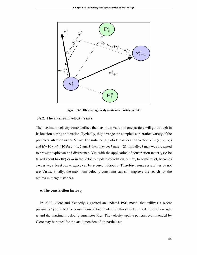
Chapter 3: Modelling and optimization methodology
44
Figure 03-5: Illustrating the dynamic of a particle in PSO.
3.8.2. The maximum velocity Vmax
The maximum velocity Vmax defines the maximum variation one particle will go through in
its location during an iteration. Typically, they arrange the complete exploration variety of the
particle’s situation as the Vmax. For instance, a particle has location vector = (x1, x2, x3)
and if −10 ≤ xi ≤ 10 for i = 1, 2 and 3 then they set Vmax = 20. Initially, Vmax was presented
to prevent explosion and divergence. Yet, with the application of constriction factor χ (to be
talked about briefly) or ω in the velocity update correlation, Vmax, to some level, becomes
excessive; at least convergence can be secured without it. Therefore, some researchers do not
use Vmax. Finally, the maximum velocity constraint can still improve the search for the
optima in many instances.
e. The constriction factor χ
In 2002, Clerc and Kennedy suggested an updated PSO model that utilizes a recent
parameter ‘χ’, entitled the constriction factor. In addition, this model omitted the inertia weight
ω and the maximum velocity parameter Vmax. The velocity update pattern recommended by
Clerc may be stated for the dth dimension of ith particle as:
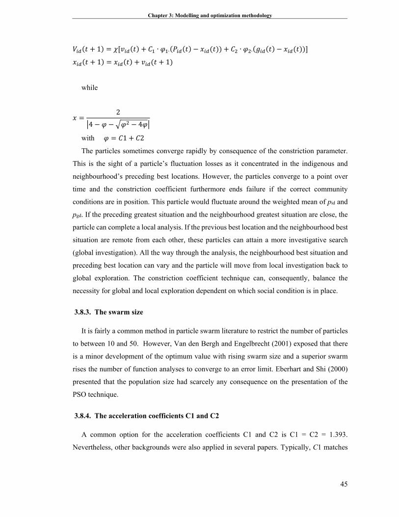
Chapter 3: Modelling and optimization methodology
45
1 ∙ ∙ ∙ ∙
1 1
while
2
4 4
with 1 2
The particles sometimes converge rapidly by consequence of the constriction parameter.
This is the sight of a particle’s fluctuation losses as it concentrated in the indigenous and
neighbourhood’s preceding best locations. However, the particles converge to a point over
time and the constriction coefficient furthermore ends failure if the correct community
conditions are in position. This particle would fluctuate around the weighted mean of pid and
pgd. If the preceding greatest situation and the neighbourhood greatest situation are close, the
particle can complete a local analysis. If the previous best location and the neighbourhood best
situation are remote from each other, these particles can attain a more investigative search
(global investigation). All the way through the analysis, the neighbourhood best situation and
preceding best location can vary and the particle will move from local investigation back to
global exploration. The constriction coefficient technique can, consequently, balance the
necessity for global and local exploration dependent on which social condition is in place.
3.8.3. The swarm size
It is fairly a common method in particle swarm literature to restrict the number of particles
to between 10 and 50. However, Van den Bergh and Engelbrecht (2001) exposed that there
is a minor development of the optimum value with rising swarm size and a superior swarm
rises the number of function analyses to converge to an error limit. Eberhart and Shi (2000)
presented that the population size had scarcely any consequence on the presentation of the
PSO technique.
3.8.4. The acceleration coefficients C1 and C2
A common option for the acceleration coefficients C1 and C2 is C1 = C2 = 1.393.
Nevertheless, other backgrounds were also applied in several papers. Typically, C1 matches
Chapter 3: Modelling and optimization methodology
46
to C2 and ranges from [0, 3]. Ratnaweera et al. (2004) examined the issue of changing the
coefficients over time. They adapted C1 and C2 over time in a subsequent manner:
C1 1 1 1
C2 2 2 2
Wherever, 1 , 1 , 2 and C2f are constants, iter is the current iteration number and
MAXITER is the number of maximum acceptable iterations. The target of the change is to
encourage worldwide exploration over the whole exploration space throughout the former
portion of the optimization and to inspire the particles to converge to the global optimum at
the conclusion of the hunt. The researchers referred to this as the PSO-TVAC (PSO with time
changing acceleration coefficients) technique. In fact, C1 was reduced from 3.5 to 0.4 whereas
C2 was improved from 0.5 to 2.5.
3.8.5. The neighbourhood topologies in PSO
The frequently applied PSOs are either the local or global form of particle swarm
optimization. In the global category of particle swarm, the particles fly amongst the
exploration area with a speed that is dynamically tuned based on the individual best
performance the particles have accomplished and the best performance attained by all
elements. Hence, in the local version of particle swarm, the velocity of each particle can be set
based on its individual best and the best performance reached within its region. The region of
every molecule is commonly well specified as topologically adjacent particles to the particles
at their individual positions. In addition, the global version of particle swarm is seen as a local
version of particle swarm with each particle’s neighbourhood being solid residents. It was
proposed that the global version of particle swarm can converge faster but with the possibility
of converging to the local minimum when the local version of particle swarm may have more
probabilities to get improved answers slowly. Meanwhile, some investigators researched on
developing its operation by planning or applying dissimilar kinds of neighbourhood
arrangements in particle swarm. Kennedy (2001) appealed that PSO with negligible
neighbourhoods may behave well on efficient challenges when particle swarm with a large
neighbourhood could perform seriously for easy challenges.
Chapter 3: Modelling and optimization methodology
47
3.8.6. Particle swarm optimization algorithm advantages
This method is a memory-based approach, it means that the knowledge of suitable solutions
is kept through particles. In other words, each particle profits from historical data in the
practical swarm optimization algorithm. This behaviour and property are not available in other
EAs. For instance, such memory does not exist in GAs and previous knowledge is demolished
with population changes.
In this algorithm, each member of society will change its location based on individual
experiences and the whole society’s experience. The common social data between societal
members will cause some evolutionary advantages and this assumption is considered as the
base of PSO algorithms’ criteria and development. In this regard, there is a beneficial
cooperation between the particles and the particles share their knowledge together.
The group movement of particles is considered as an optimization technique; hence, each
particle tries to move in a direction where the best individual and group experiences have
happened.
3.8.7. Particle swarm optimization algorithm limitations
The biggest concern for particle swarm optimization algorithm is premature convergence.
In this algorithm, the particles are gradually investigated in the space close to the global
optimum point and other parts of the space are not investigated. In the other words, the
particles will converge because the velocity of the particle will decrease by increasing the
iteration numbers. In this regard, the algorithm has to be converged in the best-explored
location and there is no guarantee for the global optimum point of the solution. This concern
of the algorithm is related to the unsuitable balance between global and local exploration in
the mathematical landscape.
In the PSO algorithm, global exploration is preferred in the preliminary iterations, which
helps to improve the performance. Eventually, the global explorations will decrease in the
final iterations and, for exploitation of achieved data, the local exploration is preferred.
In the exploration process, some particles of the population will be stuck at the local
optimum point and will not be included in the next explorations. The stuck particles at the
local optimum point will cause weak and premature convergence.
Chapter 3: Modelling and optimization methodology
48
In the PSO algorithm, after initializing the particles, the particles will be converged to local
or global points after the consecutive exploration process and other particles will be gathered
around the best-explored particle. In other words, they will become compact. Consequently,
the diversity of the population will decrease gradually. In dynamic environments, there is no
possibility to specify the global optimum point while there is no probability of optimum global
change. In this regard, the converged particles cannot explore globally to trace the optimum
points.
3.9. Comparison between GA and PSO
Emad Elbeltagi (2005) compared five evolutionary-based optimization algorithms: GA, MA,
PSO, ACO, and SFL. Visual Basic programs were written to implement each algorithm. Two
benchmark continuous optimization test problems were solved using all but the ACO
algorithm and the comparative results were presented. Also presented were the comparative
results found when a discrete optimization test problem was solved using all five algorithms.
The PSO method was generally found to perform better than other EAs in terms of success
rate and solution quality while being second best in terms of processing time.
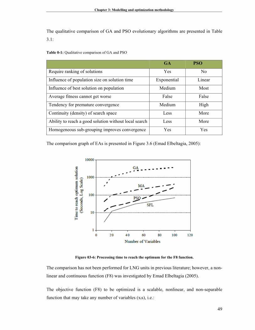
Chapter 3: Modelling and optimization methodology
49
The qualitative comparison of GA and PSO evolutionary algorithms are presented in Table
3.1:
Table 0-1: Qualitative comparison of GA and PSO
GA PSO
Require ranking of solutions Yes No
Influence of population size on solution time Exponential Linear
Influence of best solution on population Medium Most
Average fitness cannot get worse False False
Tendency for premature convergence Medium High
Continuity (density) of search space Less More
Ability to reach a good solution without local search Less More
Homogeneous sub-grouping improves convergence Yes Yes
The comparison graph of EAs is presented in Figure 3.6 (Emad Elbeltagia, 2005):
Figure 03-6: Processing time to reach the optimum for the F8 function.
The comparison has not been performed for LNG units in previous literature; however, a non-
linear and continuous function (F8) was investigated by Emad Elbeltagia (2005).
The objective function (F8) to be optimized is a scalable, nonlinear, and non-separable
function that may take any number of variables (xis), i.e.:

Chapter 3: Modelling and optimization methodology
50
The summation term of the F8 function includes a parabolic shape while the cosine function
in the product term creates waves over the parabolic surface. These waves create local optima
over the solution space. The F8 function can be scaled to any number of variables N.
The above comparison shows the poor performance of GA algorithms compared with PSO
algorithms in nonlinear and continuous functions.
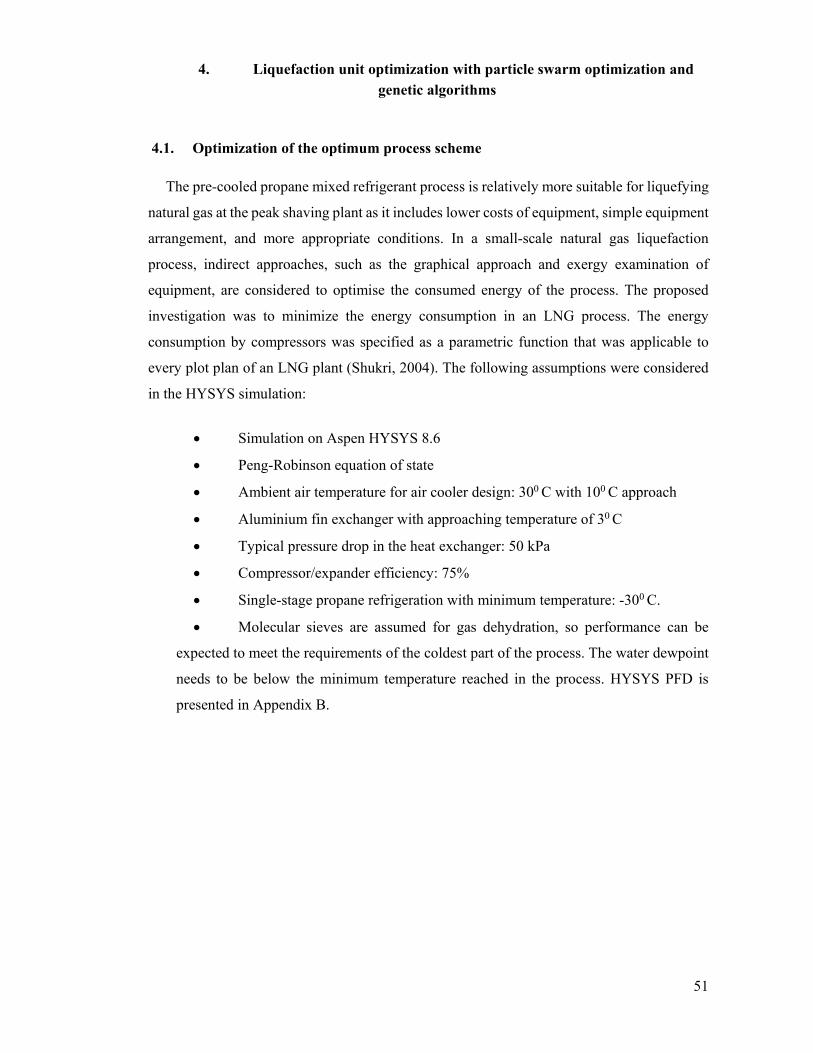
51
4. Liquefaction unit optimization with particle swarm optimization and genetic algorithms
4.1. Optimization of the optimum process scheme
The pre-cooled propane mixed refrigerant process is relatively more suitable for liquefying
natural gas at the peak shaving plant as it includes lower costs of equipment, simple equipment
arrangement, and more appropriate conditions. In a small-scale natural gas liquefaction
process, indirect approaches, such as the graphical approach and exergy examination of
equipment, are considered to optimise the consumed energy of the process. The proposed
investigation was to minimize the energy consumption in an LNG process. The energy
consumption by compressors was specified as a parametric function that was applicable to
every plot plan of an LNG plant (Shukri, 2004). The following assumptions were considered
in the HYSYS simulation:
Simulation on Aspen HYSYS 8.6
Peng-Robinson equation of state
Ambient air temperature for air cooler design: 300 C with 100 C approach
Aluminium fin exchanger with approaching temperature of 30 C
Typical pressure drop in the heat exchanger: 50 kPa
Compressor/expander efficiency: 75%
Single-stage propane refrigeration with minimum temperature: -300 C.
Molecular sieves are assumed for gas dehydration, so performance can be
expected to meet the requirements of the coldest part of the process. The water dewpoint
needs to be below the minimum temperature reached in the process. HYSYS PFD is
presented in Appendix B.
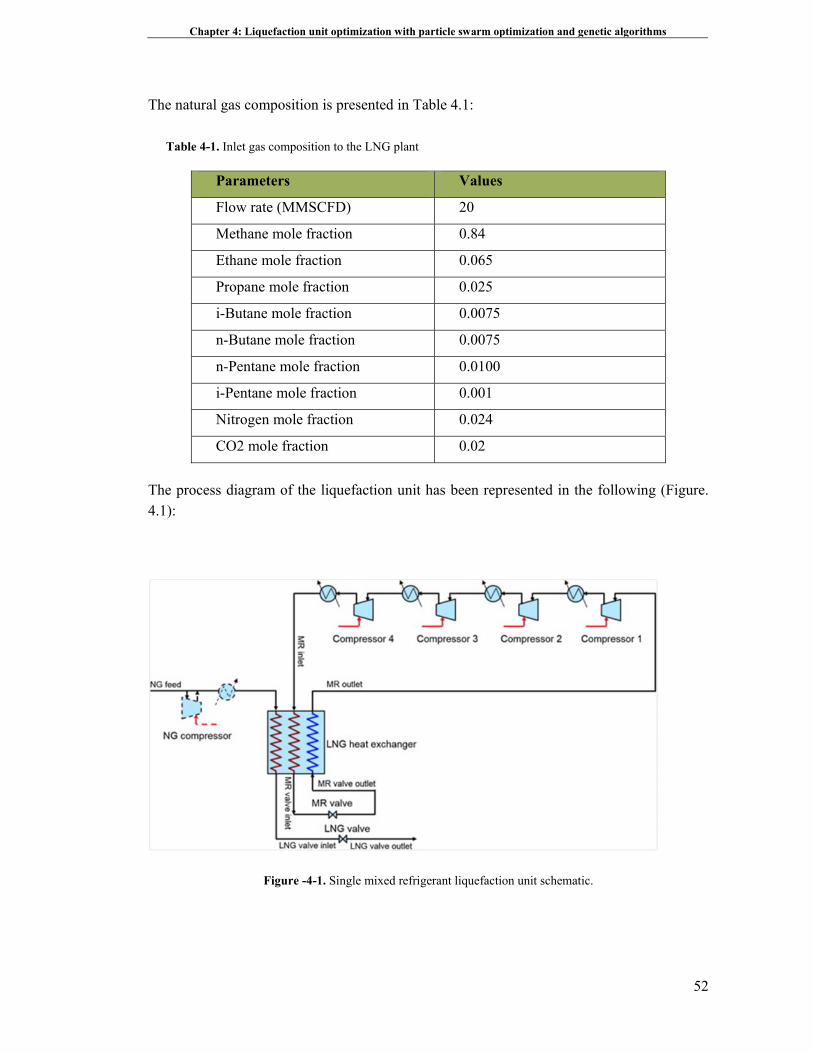
Chapter 4: Liquefaction unit optimization with particle swarm optimization and genetic algorithms
52
The natural gas composition is presented in Table 4.1:
Table 4-1. Inlet gas composition to the LNG plant
Parameters Values
Flow rate (MMSCFD) 20
Methane mole fraction 0.84
Ethane mole fraction 0.065
Propane mole fraction 0.025
i-Butane mole fraction 0.0075
n-Butane mole fraction 0.0075
n-Pentane mole fraction 0.0100
i-Pentane mole fraction 0.001
Nitrogen mole fraction 0.024
CO2 mole fraction 0.02
The process diagram of the liquefaction unit has been represented in the following (Figure. 4.1):
Figure -4-1. Single mixed refrigerant liquefaction unit schematic.
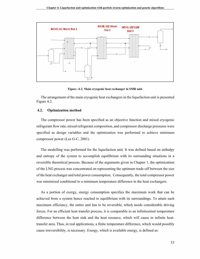
Chapter 4: Liquefaction unit optimization with particle swarm optimization and genetic algorithms
53
Figure -4-2. Main cryogenic heat exchanger in SMR unit.
The arrangement of the main cryogenic heat exchangers in the liquefaction unit is presented Figure 4.2.
4.2. Optimization method
The compressor power has been specified as an objective function and mixed cryogenic
refrigerant flow rate, mixed refrigerant composition, and compressor discharge pressures were
specified as design variables and the optimization was performed to achieve minimum
compressor power (Lee G-C, 2001).
The modelling was performed for the liquefaction unit. It was defined based on enthalpy
and entropy of the system to accomplish equilibrium with its surrounding situations in a
reversible theoretical process. Because of the arguments given in Chapter 1, the optimization
of the LNG process was concentrated on representing the optimum trade-off between the size
of the heat exchanger and total power consumption. Consequently, the total compressor power
was minimized conditional to a minimum temperature difference in the heat exchangers.
As a portion of exergy, energy consumption specifies the maximum work that can be
achieved from a system hence reached to equilibrium with its surroundings. To attain such
maximum efficiency, the entire unit has to be reversible, which needs considerable driving
forces. For an efficient heat transfer process, it is comparable to an infinitesimal temperature
difference between the heat sink and the heat resource, which will cause in infinite heat-
transfer area. Thus, in real applications, a finite temperature difference, which would possibly
cause irreversibility, is necessary. Exergy, which is available energy, is defined as:
Chapter 4: Liquefaction unit optimization with particle swarm optimization and genetic algorithms
54
EX = (H1 – H0) – T0 (S1 – S0)
where S0 and H0 are the enthalpy and entropy at the equilibrium state condition,
respectively, generally existing in accordance with the ambient pressure and ambient
temperature. The variation of this condition designates the maximum amount of efficient work
that will be recoverable (or the minimum work that necessities is provided). Hence, this system
follows a process as follows:
∆EX = (H – T0S) final state – (H – T0S) initial state
In the thesis, the natural gas moves in the multi-stream MCHE to transform the LNG
product. Consequently, the minimum amount of reversible work according to refrigeration
load for the LNG liquefaction process is identified as:
Wrev = (H – T0S) HP – (H – T0S) NG
The actual work necessary to switch from the preliminary condition to the final condition
is more than ideal work because of the irreversibility of the process. More than 1.5 times the
minimum reversible ideal power is required in the large-scale liquefied natural gas plants. The
maximum proportion of irreversibility in an LNG plant lies in the compressor station’s multi-
stream MCHE because of the high temperature difference and pressure reduction in the mixed
cryogenic refrigerant cycle. In the real process, the definite work is accomplished according
to the first law of thermodynamics. The lost work occurs according to the difference between
actual ideal work and reversible work as follows:
W lost = W actual – ∆EX
The lost work in the whole procedure is assessed according to calculating exergy loss in
overall equipment in the whole plant. The pinch analysis is accomplished for cooling fluids
and utility levels and optimum heat exchangers network in the plant. Brazed aluminium heat
exchangers (MCHE), which are the gold standard in liquefaction, facilitate efficient flow
arrangements, which minimize the necessary heat transfer area as capital cost.
The practical values for ∆Tmin are about 20 K for general bulk duties of sensibly free-
flowing liquids and around 10 K for processes with high quantity or continuous operation;
hence, for cryogenic plants, 2-3 K is a practical value.
Chapter 4: Liquefaction unit optimization with particle swarm optimization and genetic algorithms
55
Hence, the minimum temperature difference is considered as small as 3 and 5 K at the cold
ends in the main cryogenic heat exchanger, the amount of heat transfer is enhanced
significantly. By a small temperature difference, the improved thermodynamic efficiency and
reduced entropy generation are achieved. The main involvement of exergy loss in the heat
exchangers of LNG plants refers to temperature difference and heat exchange load
accordingly.
The analysis of the sensitivity of process variables as performed in preceding optimization
studies is not only unsuitable in recognizing the significance of manipulated parameters but
are in identifying the initial values. The preliminary values should also be within the probable
area as definite by formulated limitations. To meet thermodynamic restrictions, some
limitations had to be considered for both design and operation of objective functions. The
details are presented as follows:
1. The MR returning to the compressor should be saturated vapour so that no
liquid droplets are available in the compressor:
1
where and are molar flow-rates of liquid and vapour existing in the stream.
2. Meanwhile, the variance of the MCHE is negligible and its performance is
preserved as constant. Consequently, the conditions of the MCHE would be defined as
the following equations also, where cold and hot composite curves must not cross:
0<THMCHE-101- TC
MCHE-101< δ1
0<THMCHE-102- TC
MCHE-102< δ2
0<THMCHE-103- TC
MCHE-103< δ3
where THMCHE-101 is the temperature of the hot composite stream at any point within MCHE-
101, TCMCHE101 is the temperature of the cold composite stream at any point within MCHE-
101 and δ1 is the temperature difference between the hot and cold composite curves in MCHE-
101.
Chapter 4: Liquefaction unit optimization with particle swarm optimization and genetic algorithms
56
3. The first stage compression (LP) cannot compress the mixed refrigerant to
pressures greater than the second stage compression (HP):
CP2- CP1<0
Meanwhile CP2, CP1 are the outlet pressures of HP and LP compressors correspondingly.
4. All streams emerging from the heat exchanger shall be the same temperature:
Tout1MCHE-101= Tout2
MCHE-101= Tout3MCHE-101
Tout1MCHE-102= Tout2
MCHE-102= Tout3MCHE-102
Tout1MCHE-103= Tout2
MCHE-103
Tout1MCHE-101 is the temperature of the first outlet stream of heat exchanger MCHE-101.
Once the purpose is to specify optimum design operating conditions, the following additional
limitations are needed:
UAmin ≤ UAMCHE-101 ≤ UAmax
UAmin ≤ UAMCHE-102 ≤ UAmax
UAmin ≤ UAMCHE-103 ≤ UAmax
In this research, the sum of the consumed power in the compression unit was an objective
function in the overall form of optimization referring to the main design variables as below:
Minimum subjected to f(X) =W1+W2 =FMRC [(H HP outlet –H HP Inlet)/ηc + (H MP Outlet –H MP
Inlet)/ηc
where H is enthalpy of streams in the isentropic compression. The total compressor power
is to be considered as an objective function specified using PSO and GAs.
The temperature of the mixed refrigerant at the inlet of compressors is higher than its dew
point. This nonlinear inequality constraint is specified as:
T(X) = (Tdew point)R1- TR1 < 0
Chapter 4: Liquefaction unit optimization with particle swarm optimization and genetic algorithms
57
The calculation of dew point temperature is also compared with the actual temperature of
the inlet stream.
In HYSYS simulation, the 100 intervals for each of the streams was used to model the main
cryogenic heat exchanger, distributed in segments of equal enthalpy variation. Because the
intervals do not essentially match, the composite curves are composed of one evaluation point
for each interval endpoint for all fluids for each of these evaluation points, the values of the
two other streams are established by linear interpolation among the intervals of the
corresponding streams.
4.2.1. The optimization results of the pre-cooled mixed refrigerant unit using evolutionary algorithms
For optimization, the objective function and the effective variables on objective function
must be identified in the first step. Therefore, the sensitivity analysis of the variables is
performed to specify their impacts on the objective function. The total compressor power of
the mixed refrigerant unit was considered as an objective function in the liquefaction unit of
the pre-cooled propane mixed refrigerant.
The outlet pressure of HP and LP stage mixed refrigerant compressors, inlet temperature to
the cold box, mixed refrigerant composition, and flow rate are considered as optimization
variables.
The variables must be identified as the objective function to be minimized.
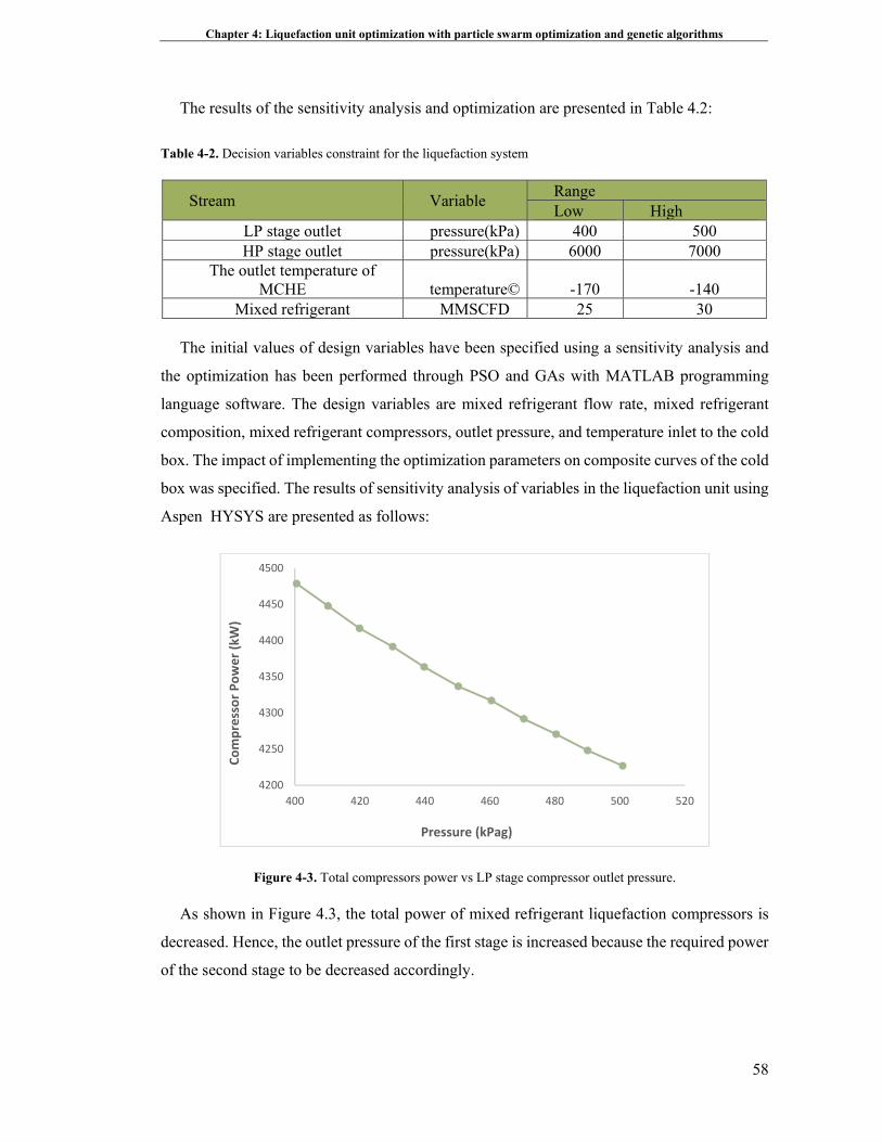
Chapter 4: Liquefaction unit optimization with particle swarm optimization and genetic algorithms
58
The results of the sensitivity analysis and optimization are presented in Table 4.2:
Table 4-2. Decision variables constraint for the liquefaction system
RangeVariable Stream
High Low500400pressure(kPa)LP stage outlet 70006000pressure(kPa)HP stage outlet
-140-170temperature©The outlet temperature of
MCHE 3025MMSCFDMixed refrigerant
The initial values of design variables have been specified using a sensitivity analysis and
the optimization has been performed through PSO and GAs with MATLAB programming
language software. The design variables are mixed refrigerant flow rate, mixed refrigerant
composition, mixed refrigerant compressors, outlet pressure, and temperature inlet to the cold
box. The impact of implementing the optimization parameters on composite curves of the cold
box was specified. The results of sensitivity analysis of variables in the liquefaction unit using
Aspen HYSYS are presented as follows:
Figure 4-3. Total compressors power vs LP stage compressor outlet pressure.
As shown in Figure 4.3, the total power of mixed refrigerant liquefaction compressors is
decreased. Hence, the outlet pressure of the first stage is increased because the required power
of the second stage to be decreased accordingly.
4200
4250
4300
4350
4400
4450
4500
400 420 440 460 480 500 520
Compressor Power (kW)
Pressure (kPag)
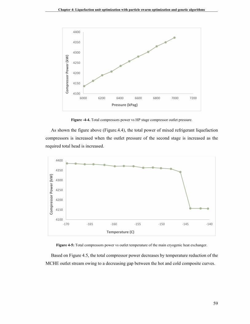
Chapter 4: Liquefaction unit optimization with particle swarm optimization and genetic algorithms
59
Figure -4-4. Total compressors power vs HP stage compressor outlet pressure.
As shown the figure above (Figure.4.4), the total power of mixed refrigerant liquefaction
compressors is increased when the outlet pressure of the second stage is increased as the
required total head is increased.
Figure 4-5: Total compressors power vs outlet temperature of the main cryogenic heat exchanger.
Based on Figure 4.5, the total compressor power decreases by temperature reduction of the
MCHE outlet stream owing to a decreasing gap between the hot and cold composite curves.
4100
4150
4200
4250
4300
4350
4400
6000 6200 6400 6600 6800 7000 7200
Compressor Power (kW)
Pressure (kPag)
4100
4150
4200
4250
4300
4350
4400
‐170 ‐165 ‐160 ‐155 ‐150 ‐145 ‐140
Compressor Power (kW
)
Temperature (C)
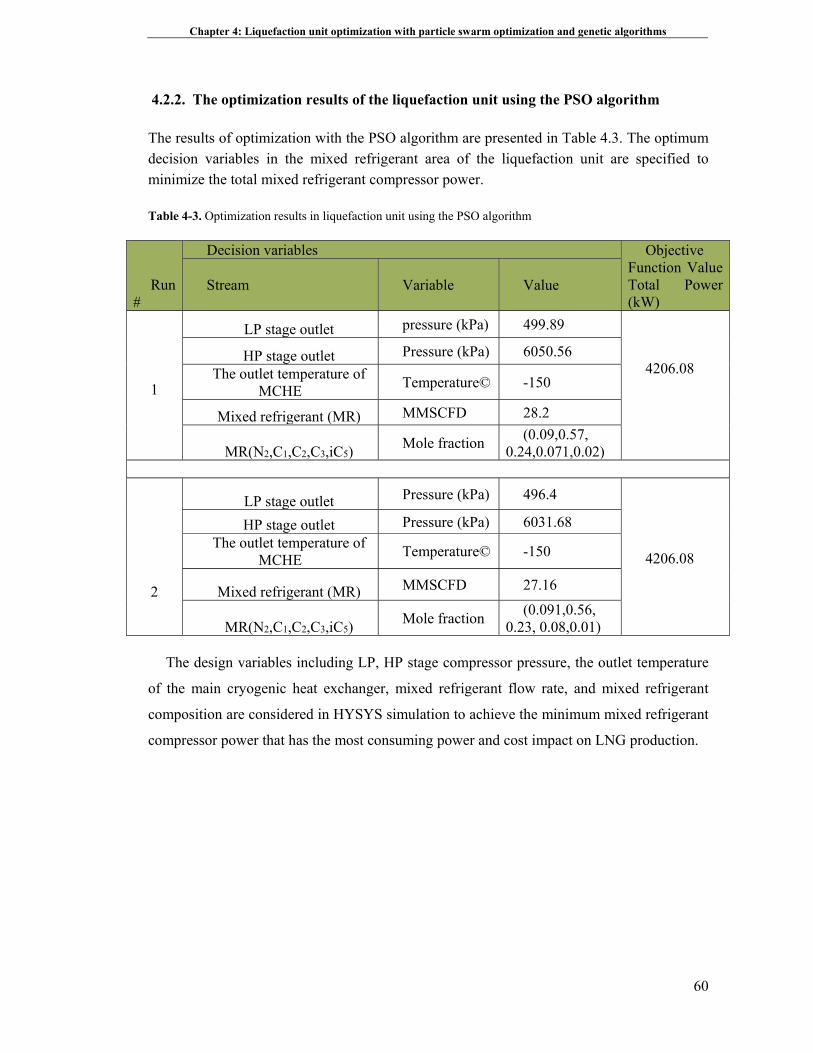
Chapter 4: Liquefaction unit optimization with particle swarm optimization and genetic algorithms
60
4.2.2. The optimization results of the liquefaction unit using the PSO algorithm
The results of optimization with the PSO algorithm are presented in Table 4.3. The optimum decision variables in the mixed refrigerant area of the liquefaction unit are specified to minimize the total mixed refrigerant compressor power.
Table 4-3. Optimization results in liquefaction unit using the PSO algorithm
Objective Function Value Total Power (kW)
Decision variables
Run #
Value Variable Stream
4206.08
499.89 pressure (kPa) LP stage outlet
1
6050.56 Pressure (kPa) HP stage outlet
-150 Temperature© The outlet temperature of
MCHE
28.2 MMSCFD Mixed refrigerant (MR)(0.09,0.57,
0.24,0.071,0.02) Mole fraction
MR(N2,C1,C2,C3,iC5)
4206.08
496.4 Pressure (kPa) LP stage outlet
2
6031.68 Pressure (kPa) HP stage outlet
-150 Temperature© The outlet temperature of
MCHE
27.16 MMSCFD Mixed refrigerant (MR)
(0.091,0.56,
0.23, 0.08,0.01) Mole fraction
MR(N2,C1,C2,C3,iC5)
The design variables including LP, HP stage compressor pressure, the outlet temperature
of the main cryogenic heat exchanger, mixed refrigerant flow rate, and mixed refrigerant
composition are considered in HYSYS simulation to achieve the minimum mixed refrigerant
compressor power that has the most consuming power and cost impact on LNG production.
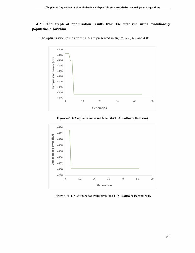
Chapter 4: Liquefaction unit optimization with particle swarm optimization and genetic algorithms
61
4.2.3. The graph of optimization results from the first run using evolutionary population algorithms
The optimization results of the GA are presented in figures 4.6, 4.7 and 4.8:
Figure 4-6: GA optimization result from MATLAB software (first run).
Figure 4-7: GA optimization result from MATLAB software (second run).
4346
4346
4346
4346
4346
4346
4346
4346
4346
4346
0 10 20 30 40 50
Compressor power (kw)
Generation
4298
4300
4302
4304
4306
4308
4310
4312
4314
0 10 20 30 40 50 60
Compressor power (kw
)
Generation
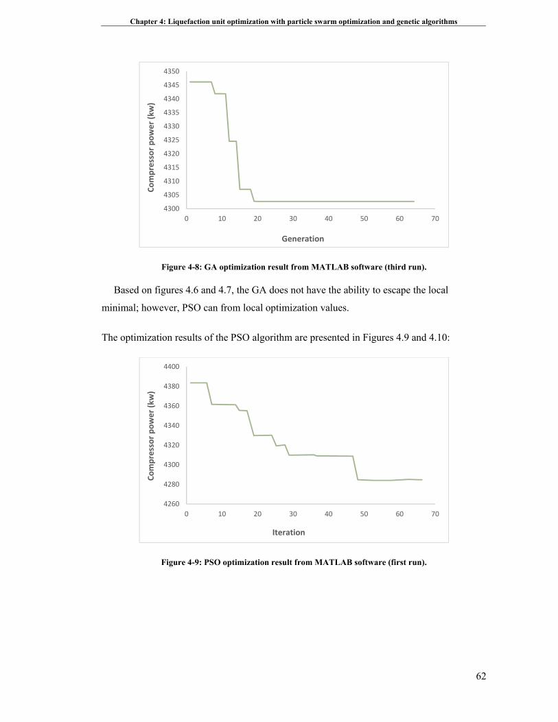
Chapter 4: Liquefaction unit optimization with particle swarm optimization and genetic algorithms
62
Figure 4-8: GA optimization result from MATLAB software (third run).
Based on figures 4.6 and 4.7, the GA does not have the ability to escape the local
minimal; however, PSO can from local optimization values.
The optimization results of the PSO algorithm are presented in Figures 4.9 and 4.10:
Figure 4-9: PSO optimization result from MATLAB software (first run).
4300
4305
4310
4315
4320
4325
4330
4335
4340
4345
4350
0 10 20 30 40 50 60 70
Compressor power (kw
)
Generation
4260
4280
4300
4320
4340
4360
4380
4400
0 10 20 30 40 50 60 70
Compressor power (kw
)
Iteration
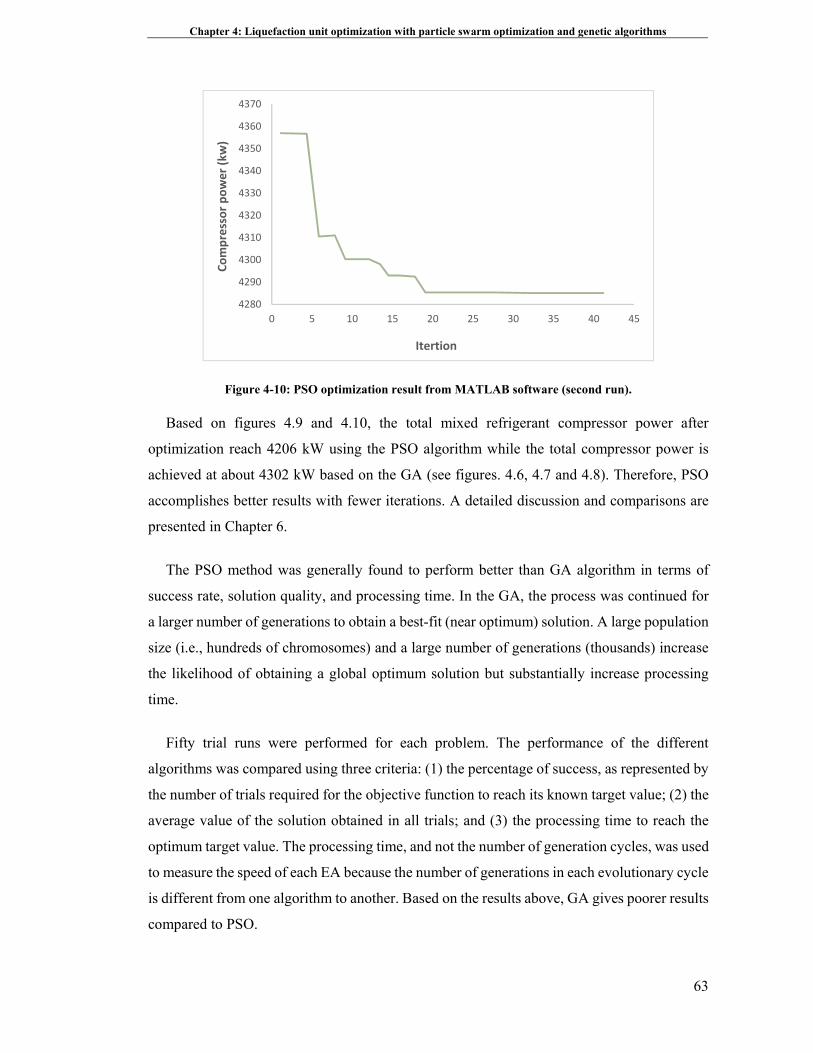
Chapter 4: Liquefaction unit optimization with particle swarm optimization and genetic algorithms
63
Figure 4-10: PSO optimization result from MATLAB software (second run).
Based on figures 4.9 and 4.10, the total mixed refrigerant compressor power after
optimization reach 4206 kW using the PSO algorithm while the total compressor power is
achieved at about 4302 kW based on the GA (see figures. 4.6, 4.7 and 4.8). Therefore, PSO
accomplishes better results with fewer iterations. A detailed discussion and comparisons are
presented in Chapter 6.
The PSO method was generally found to perform better than GA algorithm in terms of
success rate, solution quality, and processing time. In the GA, the process was continued for
a larger number of generations to obtain a best-fit (near optimum) solution. A large population
size (i.e., hundreds of chromosomes) and a large number of generations (thousands) increase
the likelihood of obtaining a global optimum solution but substantially increase processing
time.
Fifty trial runs were performed for each problem. The performance of the different
algorithms was compared using three criteria: (1) the percentage of success, as represented by
the number of trials required for the objective function to reach its known target value; (2) the
average value of the solution obtained in all trials; and (3) the processing time to reach the
optimum target value. The processing time, and not the number of generation cycles, was used
to measure the speed of each EA because the number of generations in each evolutionary cycle
is different from one algorithm to another. Based on the results above, GA gives poorer results
compared to PSO.
4280
4290
4300
4310
4320
4330
4340
4350
4360
4370
0 5 10 15 20 25 30 35 40 45
Compressor power (kw)
Itertion
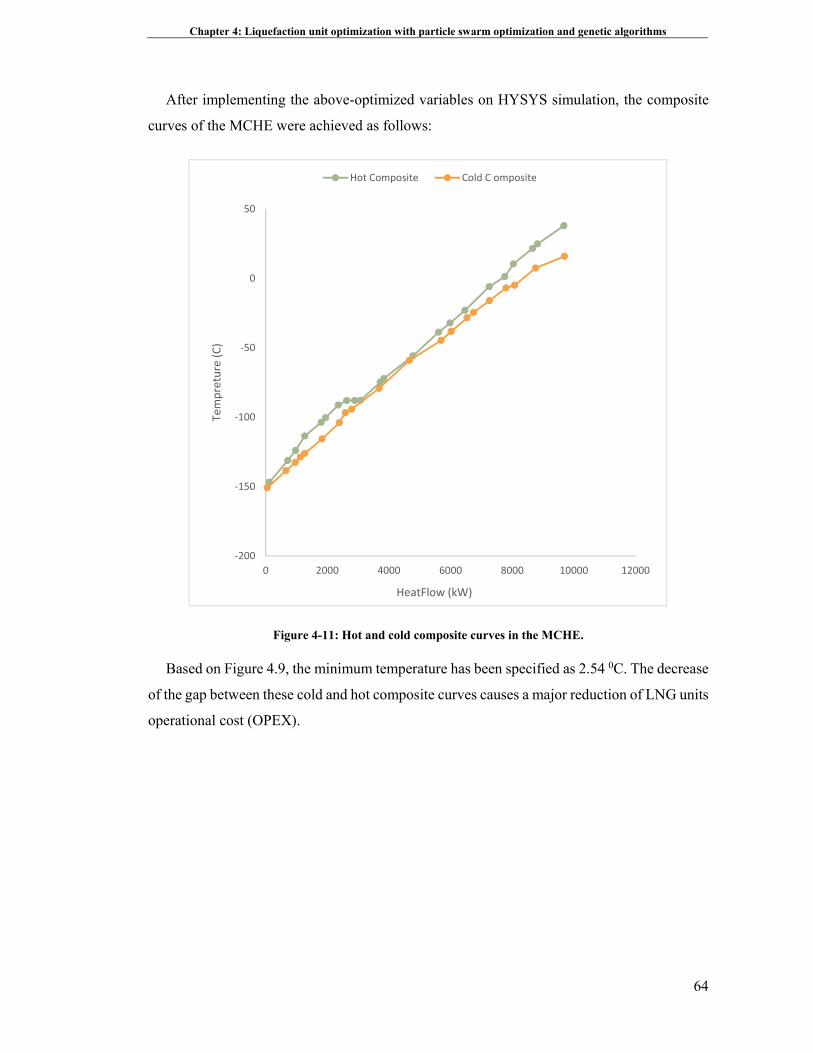
Chapter 4: Liquefaction unit optimization with particle swarm optimization and genetic algorithms
64
After implementing the above-optimized variables on HYSYS simulation, the composite
curves of the MCHE were achieved as follows:
Figure 4-11: Hot and cold composite curves in the MCHE.
Based on Figure 4.9, the minimum temperature has been specified as 2.54 0C. The decrease
of the gap between these cold and hot composite curves causes a major reduction of LNG units
operational cost (OPEX).
‐200
‐150
‐100
‐50
0
50
0 2000 4000 6000 8000 10000 12000
Tempreture (C)
HeatFlow (kW)
Hot Composite Cold C omposite
65
5. Design integrity and optimization of liquefied petroleum gas units
5.1. Process description of natural gas liquid production
The combination of changing global markets for natural gas liquids (NGL) with the
simultaneous increase in global request for liquefied natural gas (LNG) has motivated attention
on the integration of LNG liquefaction technologies with NGL recovery technology.
Liquefied petroleum gas (LPG) recovery from natural gases is important in industrial,
commercial, agricultural, and manufacturing applications. LPG has a high heating or caloric
value, which means that as an energy resource, LPG provides a high level of heat in a short
lifetime. The Australian government encourages the consumption of LPG.
Within the LPG recovery unit of the plant, there are both operating expenditure and operating
flexibility concerns that directly affect the processing cost. Hence, it is easily specified that the
efficiency of the selected liquids’ recovery process is an important parameter in the processing
cost. The flexibility of the process to either recover or reject ethane without sacrificing efficiency
or propane recovery is often a serious factor in specifying the profitability of a gas-processing
plant. Low-temperature fractionation in LPG recovery remains the most important unit for
purifying and separating gas mixtures, particularly where highly efficient recoveries are needed.
An LPG recovery system is an important industry example of such a process that utilizes
interactions between the separation units, refrigeration, and heat recovery integration systems.
This research applied process models to the components of a complicated LPG recovery system,
including addressing the heat recovery with multi-stream exchangers. A base case design of the
flowsheet is simulated using simplified models allowing for their validation against Aspen
HYSYS simulation results. Key degrees of freedom for the system are identified from the
sensitivity analysis. The sensitivity analysis showed the operating conditions that maximise the
project added value (PAV) of the plant. PAV is used to assess financial efficiency.
The alternative options for LPG recovery flow schemes, both in theory and commercially,
are large. In this research, the different process schemes were evaluated and the economic
feasibility measure was used as a basis for preliminary sensitivity analysis; eventually, the
evolutionary population-based optimization algorithms (PSO and GA) were used for design
variables optimization to achieve maximum ethane recovery as an objective function.
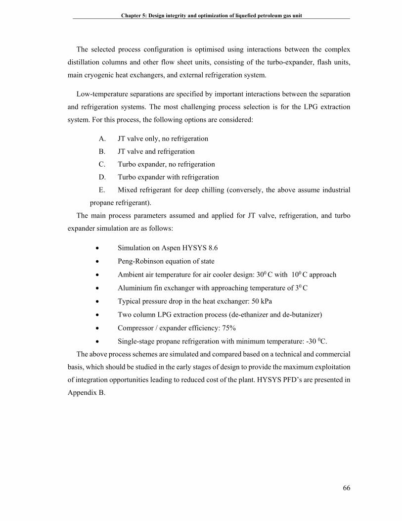
Chapter 5: Design integrity and optimization of liquefied petroleum gas unit
66
The selected process configuration is optimised using interactions between the complex
distillation columns and other flow sheet units, consisting of the turbo-expander, flash units,
main cryogenic heat exchangers, and external refrigeration system.
Low-temperature separations are specified by important interactions between the separation
and refrigeration systems. The most challenging process selection is for the LPG extraction
system. For this process, the following options are considered:
A. JT valve only, no refrigeration
B. JT valve and refrigeration
C. Turbo expander, no refrigeration
D. Turbo expander with refrigeration
E. Mixed refrigerant for deep chilling (conversely, the above assume industrial
propane refrigerant).
The main process parameters assumed and applied for JT valve, refrigeration, and turbo
expander simulation are as follows:
Simulation on Aspen HYSYS 8.6
Peng-Robinson equation of state
Ambient air temperature for air cooler design: 300 C with 100 C approach
Aluminium fin exchanger with approaching temperature of 30 C
Typical pressure drop in the heat exchanger: 50 kPa
Two column LPG extraction process (de-ethanizer and de-butanizer)
Compressor / expander efficiency: 75%
Single-stage propane refrigeration with minimum temperature: -30 0C.
The above process schemes are simulated and compared based on a technical and commercial
basis, which should be studied in the early stages of design to provide the maximum exploitation
of integration opportunities leading to reduced cost of the plant. HYSYS PFD’s are presented in
Appendix B.
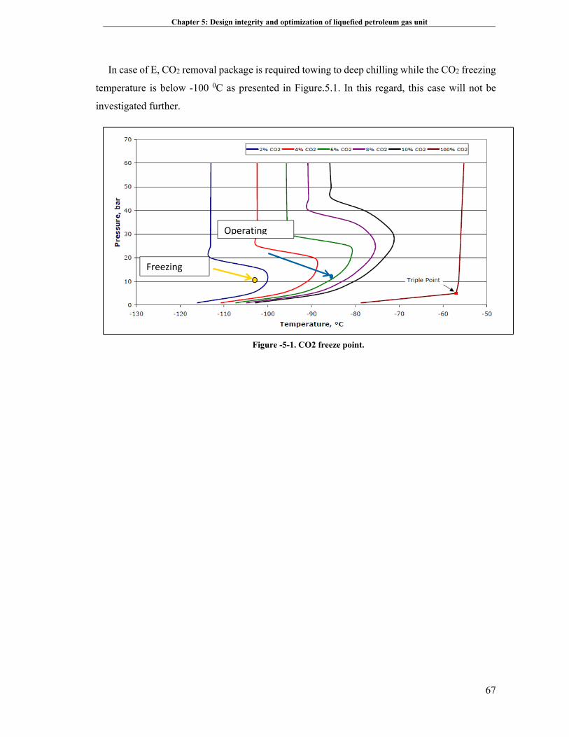
Chapter 5: Design integrity and optimization of liquefied petroleum gas unit
67
In case of E, CO2 removal package is required towing to deep chilling while the CO2 freezing
temperature is below -100 0C as presented in Figure.5.1. In this regard, this case will not be
investigated further.
Freezing
Operating
Figure 16. Figure -5-1. CO2 freeze point.
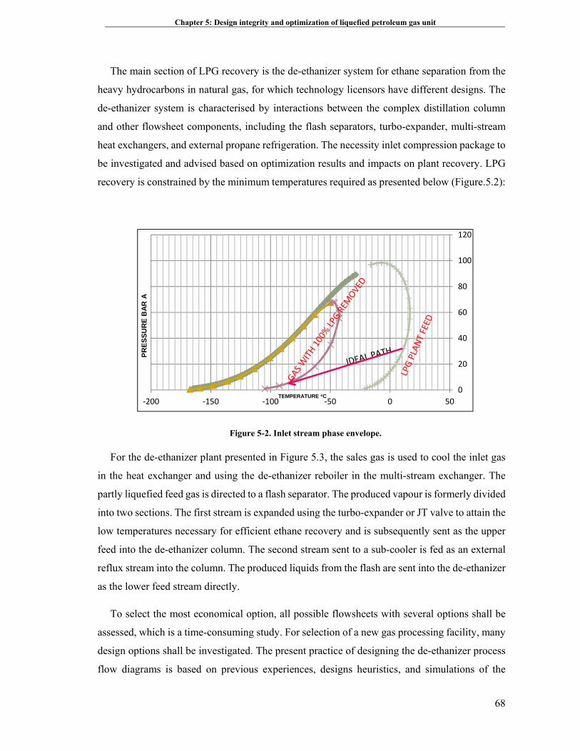
Chapter 5: Design integrity and optimization of liquefied petroleum gas unit
68
The main section of LPG recovery is the de-ethanizer system for ethane separation from the
heavy hydrocarbons in natural gas, for which technology licensors have different designs. The
de-ethanizer system is characterised by interactions between the complex distillation column
and other flowsheet components, including the flash separators, turbo-expander, multi-stream
heat exchangers, and external propane refrigeration. The necessity inlet compression package to
be investigated and advised based on optimization results and impacts on plant recovery. LPG
recovery is constrained by the minimum temperatures required as presented below (Figure.5.2):
Figure 5-2. Inlet stream phase envelope.
For the de-ethanizer plant presented in Figure 5.3, the sales gas is used to cool the inlet gas
in the heat exchanger and using the de-ethanizer reboiler in the multi-stream exchanger. The
partly liquefied feed gas is directed to a flash separator. The produced vapour is formerly divided
into two sections. The first stream is expanded using the turbo-expander or JT valve to attain the
low temperatures necessary for efficient ethane recovery and is subsequently sent as the upper
feed into the de-ethanizer column. The second stream sent to a sub-cooler is fed as an external
reflux stream into the column. The produced liquids from the flash are sent into the de-ethanizer
as the lower feed stream directly.
To select the most economical option, all possible flowsheets with several options shall be
assessed, which is a time-consuming study. For selection of a new gas processing facility, many
design options shall be investigated. The present practice of designing the de-ethanizer process
flow diagrams is based on previous experiences, designs heuristics, and simulations of the
0
20
40
60
80
100
120
‐200 ‐150 ‐100 ‐50 0 50
PR
ES
SU
RE
BA
R A
TEMPERATURE oC
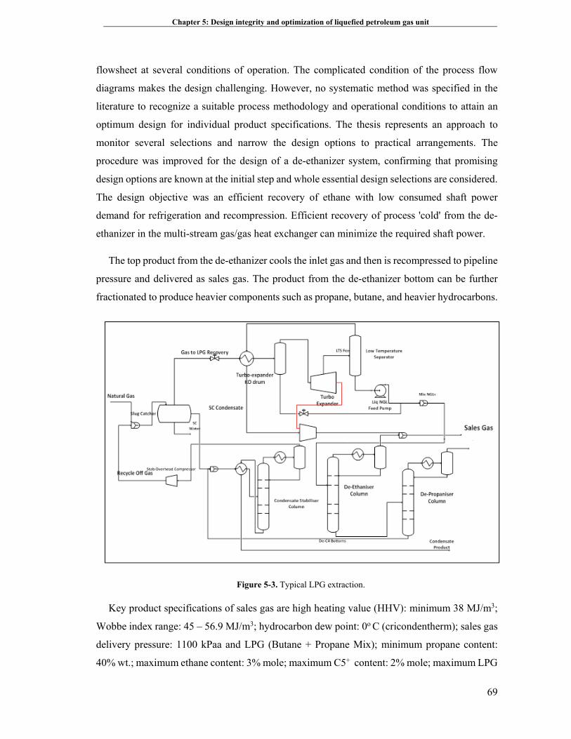
Chapter 5: Design integrity and optimization of liquefied petroleum gas unit
69
flowsheet at several conditions of operation. The complicated condition of the process flow
diagrams makes the design challenging. However, no systematic method was specified in the
literature to recognize a suitable process methodology and operational conditions to attain an
optimum design for individual product specifications. The thesis represents an approach to
monitor several selections and narrow the design options to practical arrangements. The
procedure was improved for the design of a de-ethanizer system, confirming that promising
design options are known at the initial step and whole essential design selections are considered.
The design objective was an efficient recovery of ethane with low consumed shaft power
demand for refrigeration and recompression. Efficient recovery of process 'cold' from the de-
ethanizer in the multi-stream gas/gas heat exchanger can minimize the required shaft power.
The top product from the de-ethanizer cools the inlet gas and then is recompressed to pipeline
pressure and delivered as sales gas. The product from the de-ethanizer bottom can be further
fractionated to produce heavier components such as propane, butane, and heavier hydrocarbons.
Figure 5-3. Typical LPG extraction.
Key product specifications of sales gas are high heating value (HHV): minimum 38 MJ/m3;
Wobbe index range: 45 – 56.9 MJ/m3; hydrocarbon dew point: 0o C (cricondentherm); sales gas
delivery pressure: 1100 kPaa and LPG (Butane + Propane Mix); minimum propane content:
40% wt.; maximum ethane content: 3% mole; maximum C5+ content: 2% mole; maximum LPG
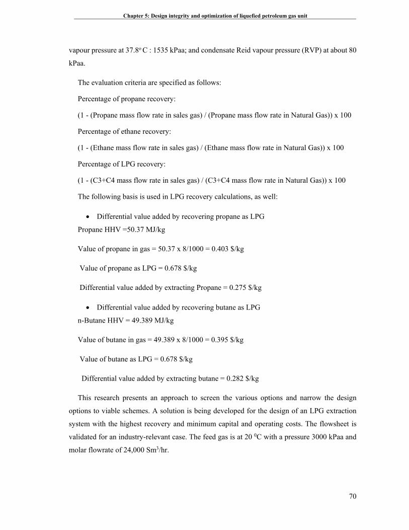
Chapter 5: Design integrity and optimization of liquefied petroleum gas unit
70
vapour pressure at 37.8o C : 1535 kPaa; and condensate Reid vapour pressure (RVP) at about 80
kPaa.
The evaluation criteria are specified as follows:
Percentage of propane recovery:
(1 - (Propane mass flow rate in sales gas) / (Propane mass flow rate in Natural Gas)) x 100
Percentage of ethane recovery:
(1 - (Ethane mass flow rate in sales gas) / (Ethane mass flow rate in Natural Gas)) x 100
Percentage of LPG recovery:
(1 - (C3+C4 mass flow rate in sales gas) / (C3+C4 mass flow rate in Natural Gas)) x 100
The following basis is used in LPG recovery calculations, as well:
Differential value added by recovering propane as LPG
Propane HHV =50.37 MJ/kg
Value of propane in gas = 50.37 x 8/1000 = 0.403 $/kg
Value of propane as LPG = 0.678 $/kg
Differential value added by extracting Propane = 0.275 $/kg
Differential value added by recovering butane as LPG
n-Butane HHV = 49.389 MJ/kg
Value of butane in gas = 49.389 x 8/1000 = 0.395 $/kg
Value of butane as LPG = 0.678 $/kg
Differential value added by extracting butane = 0.282 $/kg
This research presents an approach to screen the various options and narrow the design
options to viable schemes. A solution is being developed for the design of an LPG extraction
system with the highest recovery and minimum capital and operating costs. The flowsheet is
validated for an industry-relevant case. The feed gas is at 20 0C with a pressure 3000 kPaa and
molar flowrate of 24,000 Sm3/hr.

Chapter 5: Design integrity and optimization of liquefied petroleum gas unit
71
5.2. LPG extraction optimum process selection 5.2.1. JT valve without refrigeration
Assuming no refrigeration, the gas is let down to a nominal margin above the battery limit
delivery pressure, so it exits the low temperature (LT) separator at 1200 kPaa. This case was run
with and without a KO pot upstream of the JT valve. The sales gas HHV is 51.95 MJ/Nm3, there
is the Wobbe index of 59.8 MJ/Nm3 and the sales gas cricondentherm is 11.5o C, well above the
spec of 0o C. Although, this case has the lowest capital expenditure cost (CAPEX) it is not
workable because the sales gas fails to meet the specified cricondentherm (or Wobbe index).
Therefore, it is demonstrated that refrigeration or turbo expansion is clearly necessary. The LPG
recovery is achieved at 14%.This case will not be investigated (Figure.5.4). The input
parameters in the simulation are presented in Table 5.1:
Table 5-1. Input simulation parameters for the JT Valve without the refrigeration scheme
Item Units TBX
Inlet temperature oC 20 Pressure kPaa 3000 Outlet pressure of the JT valve kPaa 1200 Propane spec on de-ethanizer overhead mole 0.008 Ethane spec on the de-ethanizer bottom mole 0.025 De-ethanizer column pressure kPaa 2300 De-propanizer column pressure kPaa 1300
Figure 5-4. JT valve without refrigeration.
5.2.2. Turbo expander without propane refrigeration
The sales gas HHV is 45.98 MJ/Nm3 with a Wobbe index of 54.9 MJ/Nm3; this case is
workable (Figure 4.5) because the sales gas meets specifications. The LPG recovery as the
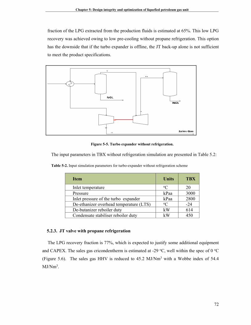
Chapter 5: Design integrity and optimization of liquefied petroleum gas unit
72
fraction of the LPG extracted from the production fluids is estimated at 65%. This low LPG
recovery was achieved owing to low pre-cooling without propane refrigeration. This option
has the downside that if the turbo expander is offline, the JT back-up alone is not sufficient
to meet the product specifications.
Figure 5-5. Turbo expander without refrigeration.
The input parameters in TBX without refrigeration simulation are presented in Table 5.2:
Table 5-2. Input simulation parameters for turbo-expander without refrigeration scheme
Item Units TBX
Inlet temperature oC 20 Pressure kPaa 3000 Inlet pressure of the turbo expander kPaa 2800 De-ethanizer overhead temperature (LTS) oC -24 De-butanizer reboiler duty kW 614 Condensate stabiliser reboiler duty kW 450
5.2.3. JT valve with propane refrigeration
The LPG recovery fraction is 77%, which is expected to justify some additional equipment
and CAPEX. The sales gas cricondentherm is estimated at -29 oC, well within the spec of 0 oC
(Figure 5.6). The sales gas HHV is reduced to 45.2 MJ/Nm3 with a Wobbe index of 54.4
MJ/Nm3.
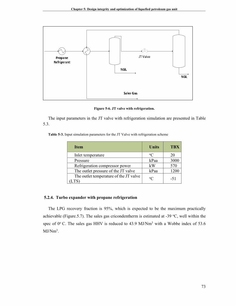
Chapter 5: Design integrity and optimization of liquefied petroleum gas unit
73
Figure 5-6. JT valve with refrigeration.
The input parameters in the JT valve with refrigeration simulation are presented in Table 5.3.
Table 5-3. Input simulation parameters for the JT Valve with refrigeration scheme
Item Units TBX
Inlet temperature oC 20 Pressure kPaa 3000 Refrigeration compressor power kW 570 The outlet pressure of the JT valve kPaa 1200 The outlet temperature of the JT valve
(LTS) oC -51
5.2.4. Turbo expander with propane refrigeration
The LPG recovery fraction is 95%, which is expected to be the maximum practically
achievable (Figure.5.7). The sales gas cricondentherm is estimated at -39 oC, well within the
spec of 0o C. The sales gas HHV is reduced to 43.9 MJ/Nm3 with a Wobbe index of 53.6
MJ/Nm3.
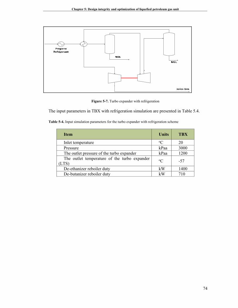
Chapter 5: Design integrity and optimization of liquefied petroleum gas unit
74
Figure 5-7. Turbo expander with refrigeration
The input parameters in TBX with refrigeration simulation are presented in Table 5.4.
Table 5-4. Input simulation parameters for the turbo expander with refrigeration scheme
Item Units TBX
Inlet temperature oC 20 Pressure kPaa 3000 The outlet pressure of the turbo expander kPaa 1200 The outlet temperature of the turbo expander
(LTS) oC -57
De-ethanizer reboiler duty kW 1400 De-butanizer reboiler duty kW 710
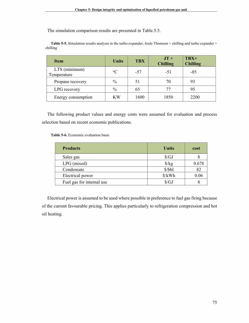
Chapter 5: Design integrity and optimization of liquefied petroleum gas unit
75
The simulation comparison results are presented in Table.5.5.
Table 5-5. Simulation results analysis in the turbo-expander, Joule Thomson + chilling and turbo expander + chilling
Item Units TBX JT +
Chilling TBX+ Chilling
LTS (minimum) Temperature
oC -57 -51 -85
Propane recovery % 51 70 93
LPG recovery % 65 77 95
Energy consumption KW 1600 1850 2200
The following product values and energy costs were assumed for evaluation and process
selection based on recent economic publications.
Table 5-6. Economic evaluation basis
Products Units cost
Sales gas $/GJ 8
LPG (mixed) $/kg 0.678 Condensate $/bbl 82Electrical power $/kWh 0.06
Fuel gas for internal use $/GJ 8
Electrical power is assumed to be used where possible in preference to fuel gas firing because
of the current favourable pricing. This applies particularly to refrigeration compression and hot
oil heating.
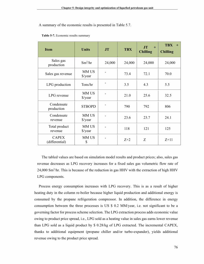
Chapter 5: Design integrity and optimization of liquefied petroleum gas unit
76
A summary of the economic results is presented in Table 5.7.
Table 5-7. Economic results summary
Item Units JT TBX JT +
Chilling
TBX +
Chilling
Sales gas production
Sm3/hr 24,000 24,000 24,000 24,000
Sales gas revenue MM US $/year
- 73.4 72.1 70.0
LPG production Tons/hr - 3.5 4.3 5.5
LPG revenue MM US $/year
- 21.0 25.6 32.5
Condensate production
STBOPD - 790 792 806
Condensate revenue
MM US $/year
- 23.6 23.7 24.1
Total product revenue
MM US $/year
- 118 121 125
CAPEX (differential)
MM US $
- Z+2 Z Z+11
The tabled values are based on simulation model results and product prices; also, sales gas
revenue decreases as LPG recovery increases for a fixed sales gas volumetric flow rate of
24,000 Sm3/hr. This is because of the reduction in gas HHV with the extraction of high HHV
LPG components.
Process energy consumption increases with LPG recovery. This is as a result of higher
heating duty in the column re-boiler because higher liquid production and additional energy is
consumed by the propane refrigeration compressor. In addition, the difference in energy
consumption between the three processes is US $ 0.2 MM/year, i.e. not significant to be a
governing factor for process scheme selection. The LPG extraction process adds economic value
owing to product price spread, i.e., LPG sold as a heating value in sales gas earns lower revenue
than LPG sold as a liquid product by $ 0.28/kg of LPG extracted. The incremental CAPEX,
thanks to additional equipment (propane chiller and/or turbo-expander), yields additional
revenue owing to the product price spread.
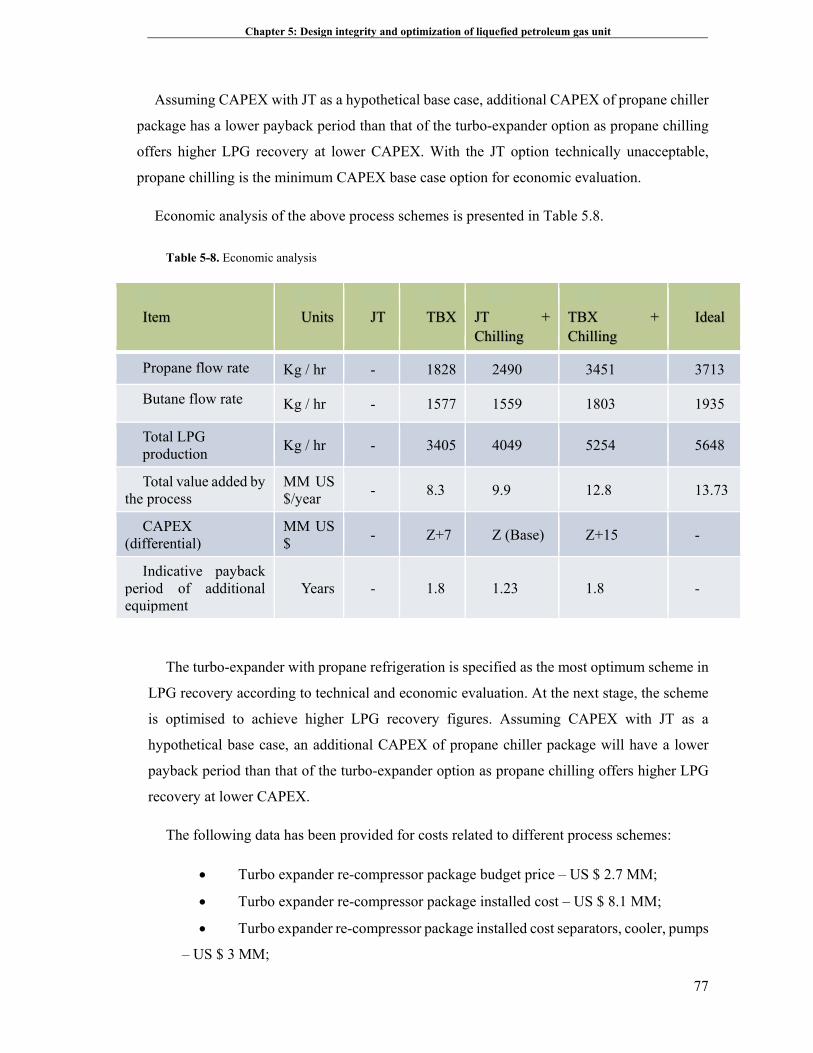
Chapter 5: Design integrity and optimization of liquefied petroleum gas unit
77
Assuming CAPEX with JT as a hypothetical base case, additional CAPEX of propane chiller
package has a lower payback period than that of the turbo-expander option as propane chilling
offers higher LPG recovery at lower CAPEX. With the JT option technically unacceptable,
propane chilling is the minimum CAPEX base case option for economic evaluation.
Economic analysis of the above process schemes is presented in Table 5.8.
Table 5-8. Economic analysis
Item
Units
JT
TBX
JT + Chilling
TBX + Chilling
Ideal
Propane flow rate Kg / hr - 1828 2490 3451 3713
Butane flow rate Kg / hr - 1577 1559 1803 1935
Total LPG production
Kg / hr - 3405 4049 5254 5648
Total value added by the process
MM US $/year
- 8.3 9.9 12.8 13.73
CAPEX (differential)
MM US $
- Z+7 Z (Base) Z+15 -
Indicative payback period of additional equipment
Years - 1.8 1.23 1.8 -
The turbo-expander with propane refrigeration is specified as the most optimum scheme in
LPG recovery according to technical and economic evaluation. At the next stage, the scheme
is optimised to achieve higher LPG recovery figures. Assuming CAPEX with JT as a
hypothetical base case, an additional CAPEX of propane chiller package will have a lower
payback period than that of the turbo-expander option as propane chilling offers higher LPG
recovery at lower CAPEX.
The following data has been provided for costs related to different process schemes:
Turbo expander re-compressor package budget price – US $ 2.7 MM;
Turbo expander re-compressor package installed cost – US $ 8.1 MM;
Turbo expander re-compressor package installed cost separators, cooler, pumps
– US $ 3 MM;
Chapter 5: Design integrity and optimization of liquefied petroleum gas unit
78
Total installed cost of the turbo expander re-compressor package – US $ 11
MM;
Propane refrigeration package budget Price – US $ 3.0 MM ;
Propane refrigeration installed cost – US $ 9.0 MM.
The operation and maintenance concerns have been presented below:
TBX process requires a cryogenic pump to transfer the recovered liquid from
the turbo-expander outlet separator;
Additional CAPEX associated with TBX inlet KO drum, discharge separator,
and re-compressor cooler;
Turbo-expanders are complex high-speed (~ 50,000 RPM) rotating machines
requiring higher CAPEX, auxiliary systems, and maintenance;
Turbo-expander performance is sensitive to feed gas composition and has
turndown limitations (drop in isentropic efficiency at reduced throughput);
The incremental CAPEX towing to additional equipment (propane chiller
and/or turbo-expander) yields additional revenue because of the product price spread;
5.2.5. Sensitivity analysis of process variables
A determination of which variables are the most efficient to enhance the output variable and
investigation on the impact of changing assumptions used in the calculations is considered as
the objective of a sensitivity analysis. The results are usually plotted as percent change in the
input variables versus the percent change in the output result (Baasel 1990; Saltelli et al. 2004).
The procedure considers the interaction of the de-ethanizer column with the upstream units
such as the flash separator, the turbo-expander, and the multi-stream exchanger. In a typical de-
ethanizer process, the power requirement constitutes the highest percentage of the operating
cost. This includes the power requirement in the re-compressor for sales gas and shaft work
requirement in the external refrigeration. The economic analysis is investigated to maximize
PAV for the process, given the feed composition, the inlet pressure, the sales gas pressure, and
maximum methane/ethane ratio in the bottom product. The PAV was calculated using the
discount flow method, which discounted all the investment and cash flow acquired during the
project’s life to present. The results of the discount flow are presented in Table 5.9. Value added
was based on propane @ US $0.275/kg, butane @ US $0.282/kg, condensate US $8/bbl, and
sales gas US $8/GJ. The PAV calculation procedure is presented in the following table and was
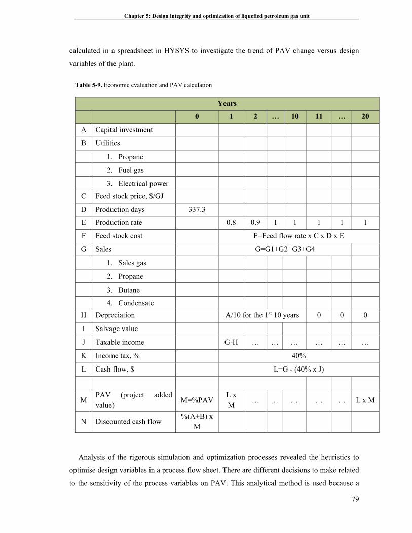
Chapter 5: Design integrity and optimization of liquefied petroleum gas unit
79
calculated in a spreadsheet in HYSYS to investigate the trend of PAV change versus design
variables of the plant.
Table 5-9. Economic evaluation and PAV calculation
Years
0 1 2 … 10 11 … 20
A Capital investment
B Utilities
1. Propane
2. Fuel gas
3. Electrical power
C Feed stock price, $/GJ
D Production days 337.3
E Production rate 0.8 0.9 1 1 1 1 1
F Feed stock cost F=Feed flow rate x C x D x E
G Sales G=G1+G2+G3+G4
1. Sales gas
2. Propane
3. Butane
4. Condensate
H Depreciation A/10 for the 1st 10 years 0 0 0
I Salvage value
J Taxable income G-H … … … … … …
K Income tax, % 40%
L Cash flow, $ L=G - (40% x J)
M PAV (project added value)
M=%PAV L x M
… … … … … L x M
N Discounted cash flow %(A+B) x
M
Analysis of the rigorous simulation and optimization processes revealed the heuristics to
optimise design variables in a process flow sheet. There are different decisions to make related
to the sensitivity of the process variables on PAV. This analytical method is used because a
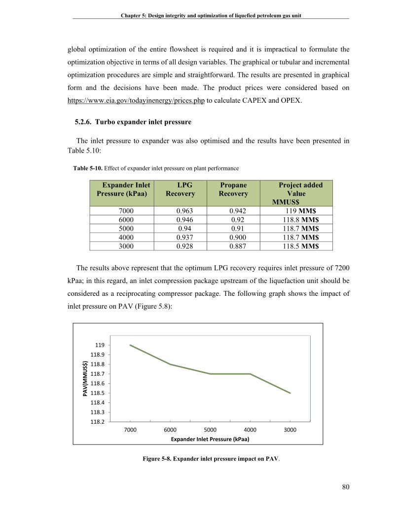
Chapter 5: Design integrity and optimization of liquefied petroleum gas unit
80
global optimization of the entire flowsheet is required and it is impractical to formulate the
optimization objective in terms of all design variables. The graphical or tubular and incremental
optimization procedures are simple and straightforward. The results are presented in graphical
form and the decisions have been made. The product prices were considered based on
https://www.eia.gov/todayinenergy/prices.php to calculate CAPEX and OPEX.
5.2.6. Turbo expander inlet pressure
The inlet pressure to expander was also optimised and the results have been presented in Table 5.10:
Table 5-10. Effect of expander inlet pressure on plant performance
Expander Inlet Pressure (kPaa)
LPG Recovery
Propane Recovery
Project added Value
MMUS$ 7000 0.963 0.942 119 MM$ 6000 0.946 0.92 118.8 MM$ 5000 0.94 0.91 118.7 MM$ 4000 0.937 0.900 118.7 MM$ 3000 0.928 0.887 118.5 MM$
The results above represent that the optimum LPG recovery requires inlet pressure of 7200
kPaa; in this regard, an inlet compression package upstream of the liquefaction unit should be
considered as a reciprocating compressor package. The following graph shows the impact of
inlet pressure on PAV (Figure 5.8):
Figure 5-8. Expander inlet pressure impact on PAV.
118.2
118.3
118.4
118.5
118.6
118.7
118.8
118.9
119
7000 6000 5000 4000 3000
PAV(M
MUS$)
Expander Inlet Pressure (kPaa)
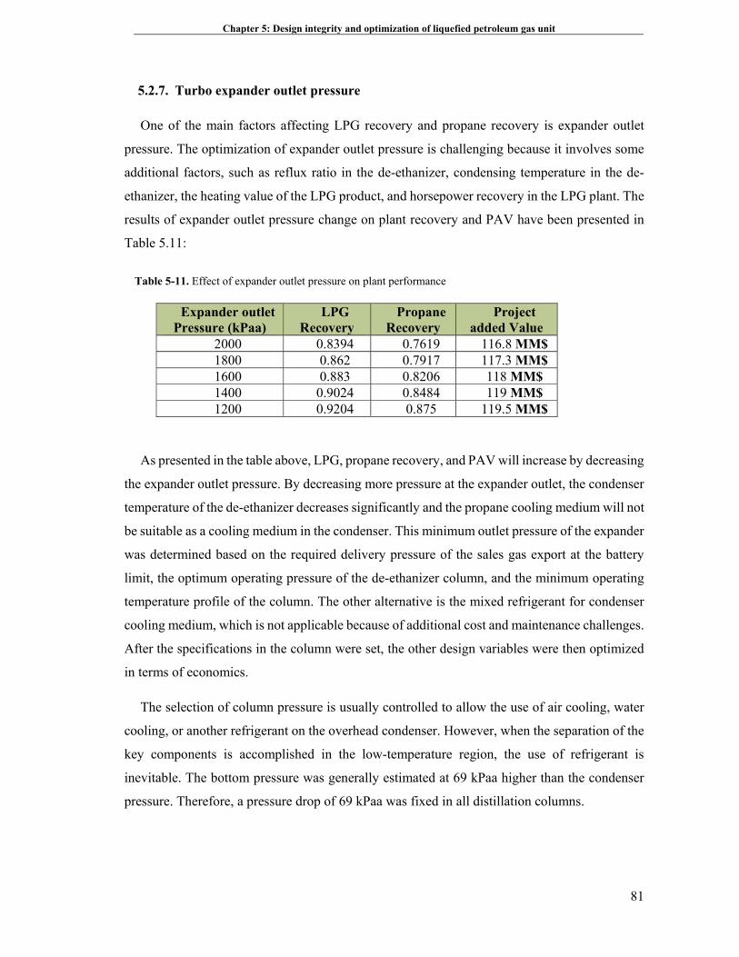
Chapter 5: Design integrity and optimization of liquefied petroleum gas unit
81
5.2.7. Turbo expander outlet pressure
One of the main factors affecting LPG recovery and propane recovery is expander outlet
pressure. The optimization of expander outlet pressure is challenging because it involves some
additional factors, such as reflux ratio in the de-ethanizer, condensing temperature in the de-
ethanizer, the heating value of the LPG product, and horsepower recovery in the LPG plant. The
results of expander outlet pressure change on plant recovery and PAV have been presented in
Table 5.11:
Table 5-11. Effect of expander outlet pressure on plant performance
Expander outlet Pressure (kPaa)
LPG Recovery
Propane Recovery
Project added Value
2000 0.8394 0.7619 116.8 MM$ 1800 0.862 0.7917 117.3 MM$ 1600 0.883 0.8206 118 MM$ 1400 0.9024 0.8484 119 MM$ 1200 0.9204 0.875 119.5 MM$
As presented in the table above, LPG, propane recovery, and PAV will increase by decreasing
the expander outlet pressure. By decreasing more pressure at the expander outlet, the condenser
temperature of the de-ethanizer decreases significantly and the propane cooling medium will not
be suitable as a cooling medium in the condenser. This minimum outlet pressure of the expander
was determined based on the required delivery pressure of the sales gas export at the battery
limit, the optimum operating pressure of the de-ethanizer column, and the minimum operating
temperature profile of the column. The other alternative is the mixed refrigerant for condenser
cooling medium, which is not applicable because of additional cost and maintenance challenges.
After the specifications in the column were set, the other design variables were then optimized
in terms of economics.
The selection of column pressure is usually controlled to allow the use of air cooling, water
cooling, or another refrigerant on the overhead condenser. However, when the separation of the
key components is accomplished in the low-temperature region, the use of refrigerant is
inevitable. The bottom pressure was generally estimated at 69 kPaa higher than the condenser
pressure. Therefore, a pressure drop of 69 kPaa was fixed in all distillation columns.
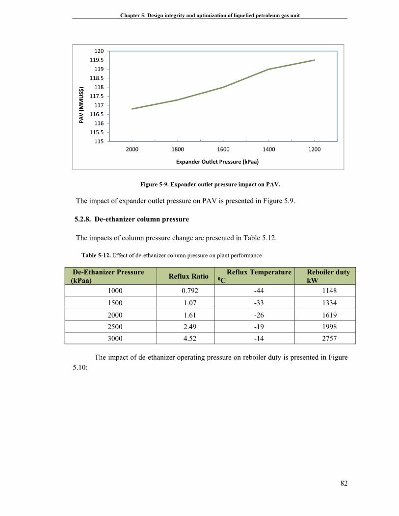
Chapter 5: Design integrity and optimization of liquefied petroleum gas unit
82
Figure 5-9. Expander outlet pressure impact on PAV.
The impact of expander outlet pressure on PAV is presented in Figure 5.9.
5.2.8. De-ethanizer column pressure
The impacts of column pressure change are presented in Table 5.12.
Table 5-12. Effect of de-ethanizer column pressure on plant performance
De-Ethanizer Pressure (kPaa)
Reflux Ratio Reflux Temperature
0CReboiler duty kW
1000 0.792 -44 1148
1500 1.07 -33 1334
2000 1.61 -26 1619
2500 2.49 -19 1998
3000 4.52 -14 2757
The impact of de-ethanizer operating pressure on reboiler duty is presented in Figure 5.10:
115
115.5
116
116.5
117
117.5
118
118.5
119
119.5
120
2000 1800 1600 1400 1200
PAV (MMUS$)
Expander Outlet Pressure (kPaa)
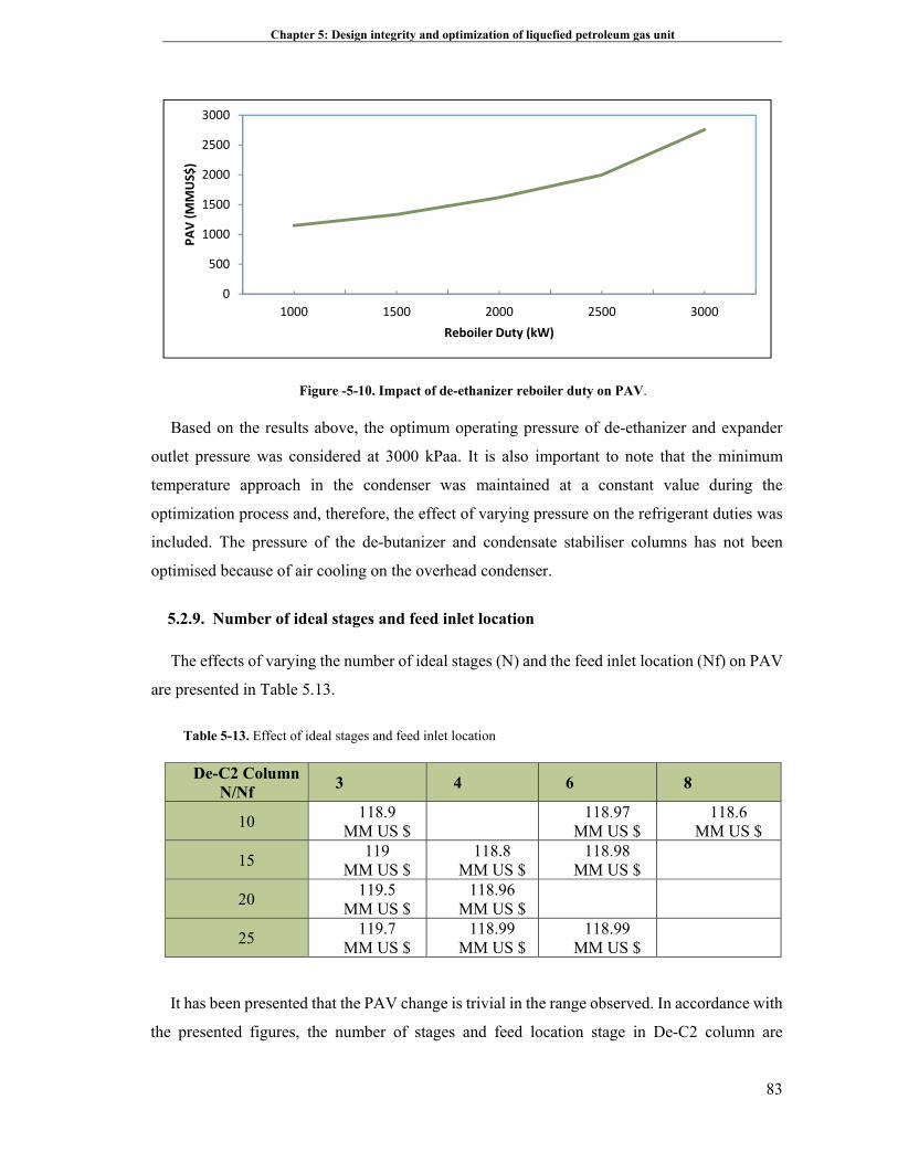
Chapter 5: Design integrity and optimization of liquefied petroleum gas unit
83
Figure -5-10. Impact of de-ethanizer reboiler duty on PAV.
Based on the results above, the optimum operating pressure of de-ethanizer and expander
outlet pressure was considered at 3000 kPaa. It is also important to note that the minimum
temperature approach in the condenser was maintained at a constant value during the
optimization process and, therefore, the effect of varying pressure on the refrigerant duties was
included. The pressure of the de-butanizer and condensate stabiliser columns has not been
optimised because of air cooling on the overhead condenser.
5.2.9. Number of ideal stages and feed inlet location
The effects of varying the number of ideal stages (N) and the feed inlet location (Nf) on PAV
are presented in Table 5.13.
Table 5-13. Effect of ideal stages and feed inlet location
De-C2 Column N/Nf
3 4 6 8
10 118.9
MM US $
118.97 MM US $
118.6 MM US $
15 119
MM US $118.8
MM US $118.98
MM US $
20 119.5
MM US $118.96
MM US $
25 119.7
MM US $118.99
MM US $118.99
MM US $
It has been presented that the PAV change is trivial in the range observed. In accordance with
the presented figures, the number of stages and feed location stage in De-C2 column are
0
500
1000
1500
2000
2500
3000
1000 1500 2000 2500 3000
PAV (MMUS$)
Reboiler Duty (kW)
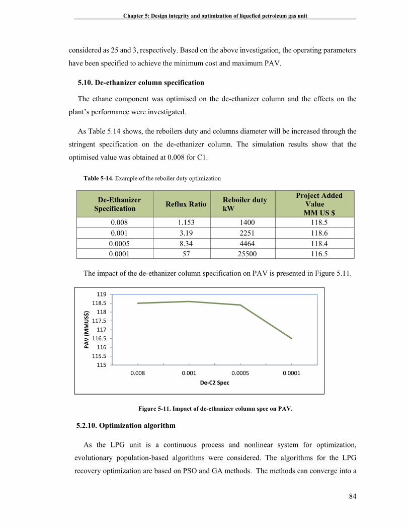
Chapter 5: Design integrity and optimization of liquefied petroleum gas unit
84
considered as 25 and 3, respectively. Based on the above investigation, the operating parameters
have been specified to achieve the minimum cost and maximum PAV.
5.10. De-ethanizer column specification
The ethane component was optimised on the de-ethanizer column and the effects on the
plant’s performance were investigated.
As Table 5.14 shows, the reboilers duty and columns diameter will be increased through the
stringent specification on the de-ethanizer column. The simulation results show that the
optimised value was obtained at 0.008 for C1.
Table 5-14. Example of the reboiler duty optimization
De-Ethanizer Specification
Reflux Ratio Reboiler duty kW
Project Added Value MM US $
0.008 1.153 1400 118.5
0.001 3.19 2251 118.6
0.0005 8.34 4464 118.4 0.0001 57 25500 116.5
The impact of the de-ethanizer column specification on PAV is presented in Figure 5.11.
Figure 5-11. Impact of de-ethanizer column spec on PAV.
5.2.10. Optimization algorithm
As the LPG unit is a continuous process and nonlinear system for optimization,
evolutionary population-based algorithms were considered. The algorithms for the LPG
recovery optimization are based on PSO and GA methods. The methods can converge into a
115
115.5
116
116.5
117
117.5
118
118.5
119
0.008 0.001 0.0005 0.0001
PAV (MMUS$)
De‐C2 Spec
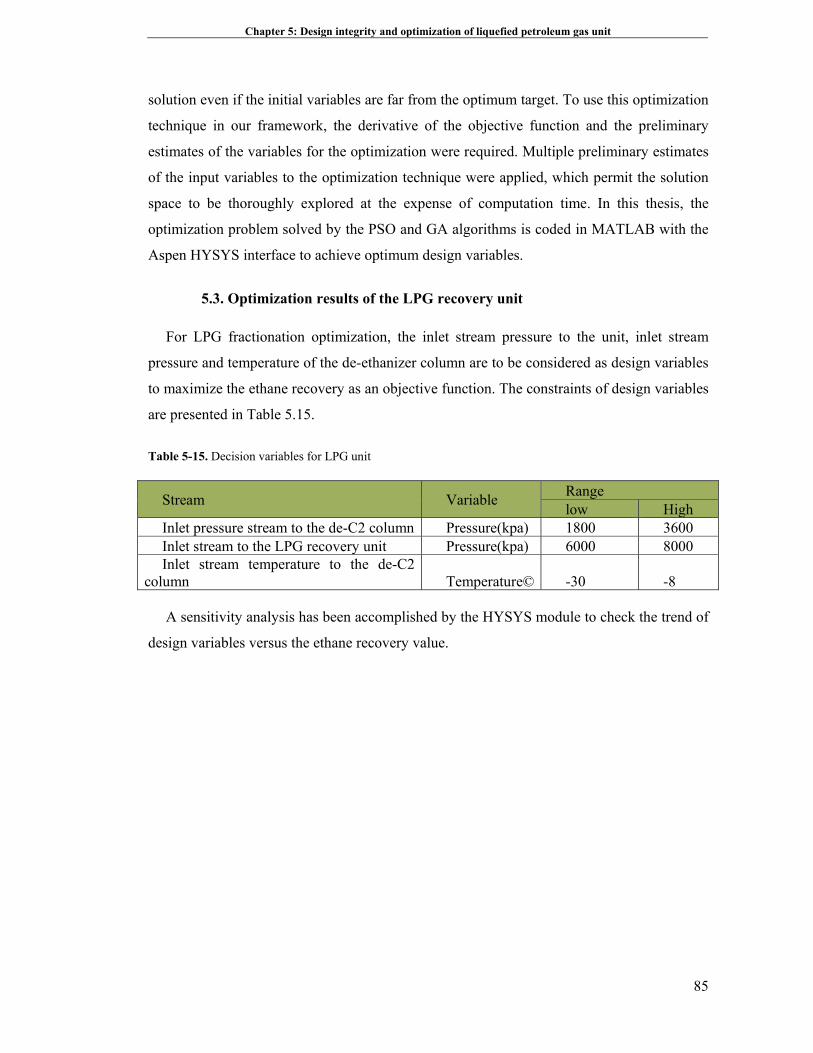
Chapter 5: Design integrity and optimization of liquefied petroleum gas unit
85
solution even if the initial variables are far from the optimum target. To use this optimization
technique in our framework, the derivative of the objective function and the preliminary
estimates of the variables for the optimization were required. Multiple preliminary estimates
of the input variables to the optimization technique were applied, which permit the solution
space to be thoroughly explored at the expense of computation time. In this thesis, the
optimization problem solved by the PSO and GA algorithms is coded in MATLAB with the
Aspen HYSYS interface to achieve optimum design variables.
5.3. Optimization results of the LPG recovery unit
For LPG fractionation optimization, the inlet stream pressure to the unit, inlet stream
pressure and temperature of the de-ethanizer column are to be considered as design variables
to maximize the ethane recovery as an objective function. The constraints of design variables
are presented in Table 5.15.
Table 5-15. Decision variables for LPG unit
Range Variable Stream
Highlow 36001800 Pressure(kpa)Inlet pressure stream to the de-C2 column80006000 Pressure(kpa)Inlet stream to the LPG recovery unit
-8-30 Temperature©Inlet stream temperature to the de-C2
column
A sensitivity analysis has been accomplished by the HYSYS module to check the trend of
design variables versus the ethane recovery value.
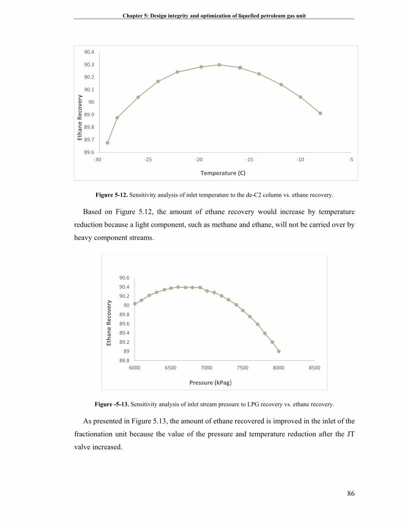
Chapter 5: Design integrity and optimization of liquefied petroleum gas unit
86
Figure 5-12. Sensitivity analysis of inlet temperature to the de-C2 column vs. ethane recovery.
Based on Figure 5.12, the amount of ethane recovery would increase by temperature
reduction because a light component, such as methane and ethane, will not be carried over by
heavy component streams.
Figure -5-13. Sensitivity analysis of inlet stream pressure to LPG recovery vs. ethane recovery.
As presented in Figure 5.13, the amount of ethane recovered is improved in the inlet of the
fractionation unit because the value of the pressure and temperature reduction after the JT
valve increased.
89.6
89.7
89.8
89.9
90
90.1
90.2
90.3
90.4
‐30 ‐25 ‐20 ‐15 ‐10 ‐5
Ethan
e Recovery
Temperature (C)
88.8
89
89.2
89.4
89.6
89.8
90
90.2
90.4
90.6
6000 6500 7000 7500 8000 8500
Ethan
e Recovery
Pressure (kPag)
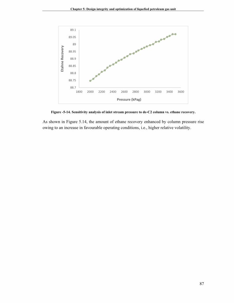
Chapter 5: Design integrity and optimization of liquefied petroleum gas unit
87
Figure -5-14. Sensitivity analysis of inlet stream pressure to de-C2 column vs. ethane recovery.
As shown in Figure 5.14, the amount of ethane recovery enhanced by column pressure rise owing to an increase in favourable operating conditions, i.e., higher relative volatility.
88.7
88.75
88.8
88.85
88.9
88.95
89
89.05
89.1
1800 2000 2200 2400 2600 2800 3000 3200 3400 3600
Etah
ne Recovery
Pressure (kPag)
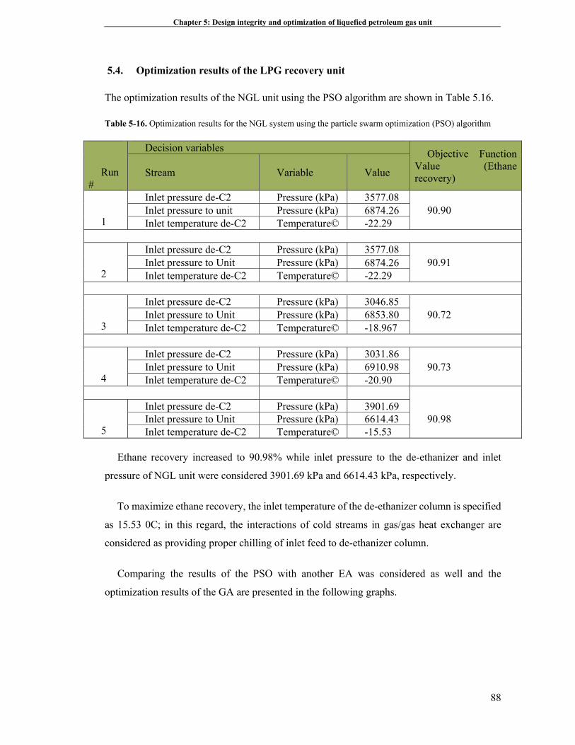
Chapter 5: Design integrity and optimization of liquefied petroleum gas unit
88
5.4. Optimization results of the LPG recovery unit
The optimization results of the NGL unit using the PSO algorithm are shown in Table 5.16.
Table 5-16. Optimization results for the NGL system using the particle swarm optimization (PSO) algorithm
Objective Function Value (Ethane recovery)
Decision variables
Run #
Value Variable Stream
3577.08 Pressure (kPa) Inlet pressure de-C2
1 90.90 6874.26Pressure (kPa) Inlet pressure to unit -22.29 Temperature© Inlet temperature de-C2
3577.08 Pressure (kPa) Inlet pressure de-C2
2 90.91 6874.26Pressure (kPa) Inlet pressure to Unit -22.29 Temperature© Inlet temperature de-C2
90.72 3046.85 Pressure (kPa) Inlet pressure de-C2
3 6853.80 Pressure (kPa) Inlet pressure to Unit -18.967 Temperature© Inlet temperature de-C2
90.73 3031.86 Pressure (kPa) Inlet pressure de-C2
4 6910.98 Pressure (kPa) Inlet pressure to Unit -20.90 Temperature© Inlet temperature de-C2
3901.69Pressure (kPa) Inlet pressure de-C2
5 90.98 6614.43Pressure (kPa)Inlet pressure to Unit -15.53 Temperature© Inlet temperature de-C2
Ethane recovery increased to 90.98% while inlet pressure to the de-ethanizer and inlet
pressure of NGL unit were considered 3901.69 kPa and 6614.43 kPa, respectively.
To maximize ethane recovery, the inlet temperature of the de-ethanizer column is specified
as 15.53 0C; in this regard, the interactions of cold streams in gas/gas heat exchanger are
considered as providing proper chilling of inlet feed to de-ethanizer column.
Comparing the results of the PSO with another EA was considered as well and the
optimization results of the GA are presented in the following graphs.
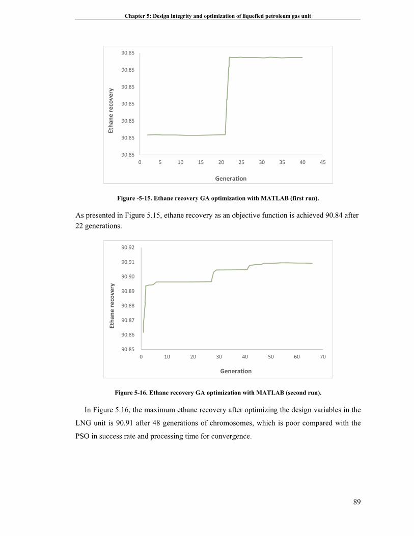
Chapter 5: Design integrity and optimization of liquefied petroleum gas unit
89
Figure -5-15. Ethane recovery GA optimization with MATLAB (first run).
As presented in Figure 5.15, ethane recovery as an objective function is achieved 90.84 after 22 generations.
Figure 5-16. Ethane recovery GA optimization with MATLAB (second run).
In Figure 5.16, the maximum ethane recovery after optimizing the design variables in the
LNG unit is 90.91 after 48 generations of chromosomes, which is poor compared with the
PSO in success rate and processing time for convergence.
90.85
90.85
90.85
90.85
90.85
90.85
90.85
0 5 10 15 20 25 30 35 40 45
Ethan
e recovery
Generation
90.85
90.86
90.87
90.88
90.89
90.90
90.91
90.92
0 10 20 30 40 50 60 70
Ethan
e recovery
Generation
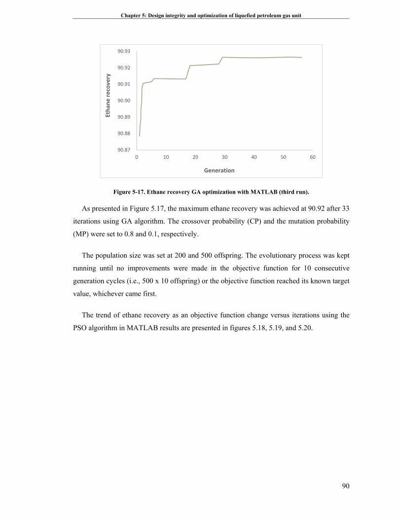
Chapter 5: Design integrity and optimization of liquefied petroleum gas unit
90
Figure 5-17. Ethane recovery GA optimization with MATLAB (third run).
As presented in Figure 5.17, the maximum ethane recovery was achieved at 90.92 after 33
iterations using GA algorithm. The crossover probability (CP) and the mutation probability
(MP) were set to 0.8 and 0.1, respectively.
The population size was set at 200 and 500 offspring. The evolutionary process was kept
running until no improvements were made in the objective function for 10 consecutive
generation cycles (i.e., 500 x 10 offspring) or the objective function reached its known target
value, whichever came first.
The trend of ethane recovery as an objective function change versus iterations using the
PSO algorithm in MATLAB results are presented in figures 5.18, 5.19, and 5.20.
90.87
90.88
90.89
90.90
90.91
90.92
90.93
0 10 20 30 40 50 60
Ethan
e recovery
Generation
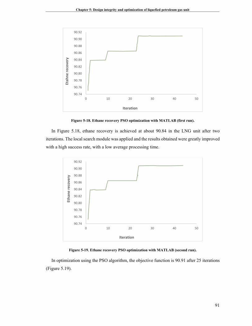
Chapter 5: Design integrity and optimization of liquefied petroleum gas unit
91
Figure 5-18. Ethane recovery PSO optimization with MATLAB (first run).
In Figure 5.18, ethane recovery is achieved at about 90.84 in the LNG unit after two
iterations. The local search module was applied and the results obtained were greatly improved
with a high success rate, with a low average processing time.
Figure 5-19. Ethane recovery PSO optimization with MATLAB (second run).
In optimization using the PSO algorithm, the objective function is 90.91 after 25 iterations
(Figure 5.19).
90.74
90.76
90.78
90.80
90.82
90.84
90.86
90.88
90.90
90.92
0 10 20 30 40 50
Etah
ne recovery
Iteration
90.74
90.76
90.78
90.80
90.82
90.84
90.86
90.88
90.90
90.92
0 10 20 30 40 50
Ethan
e recovery
Iteration
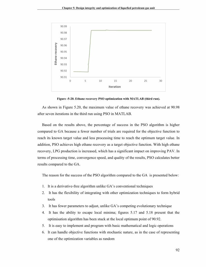
Chapter 5: Design integrity and optimization of liquefied petroleum gas unit
92
Figure -5-20. Ethane recovery PSO optimization with MATLAB (third run).
As shown in Figure 5.20, the maximum value of ethane recovery was achieved at 90.98
after seven iterations in the third run using PSO in MATLAB.
Based on the results above, the percentage of success in the PSO algorithm is higher
compared to GA because a fewer number of trials are required for the objective function to
reach its known target value and less processing time to reach the optimum target value. In
addition, PSO achieves high ethane recovery as a target objective function. With high ethane
recovery, LPG production is increased, which has a significant impact on improving PAV. In
terms of processing time, convergence speed, and quality of the results, PSO calculates better
results compared to the GA.
The reason for the success of the PSO algorithm compared to the GA is presented below:
1. It is a derivative-free algorithm unlike GA’s conventional techniques
2. It has the flexibility of integrating with other optimization techniques to form hybrid
tools
3. It has fewer parameters to adjust, unlike GA’s competing evolutionary technique
4. It has the ability to escape local minima; figures 5.17 and 5.18 present that the
optimisation algorithm has been stuck at the local optimum point of 90.92.
5. It is easy to implement and program with basic mathematical and logic operations
6. It can handle objective functions with stochastic nature, as in the case of representing
one of the optimization variables as random
90.91
90.92
90.93
90.94
90.95
90.96
90.97
90.98
90.99
0 5 10 15 20 25 30
Ethan
e recovery
Iteration

Chapter 5: Design integrity and optimization of liquefied petroleum gas unit
93
7. It does not require a good initial solution to start its iteration process
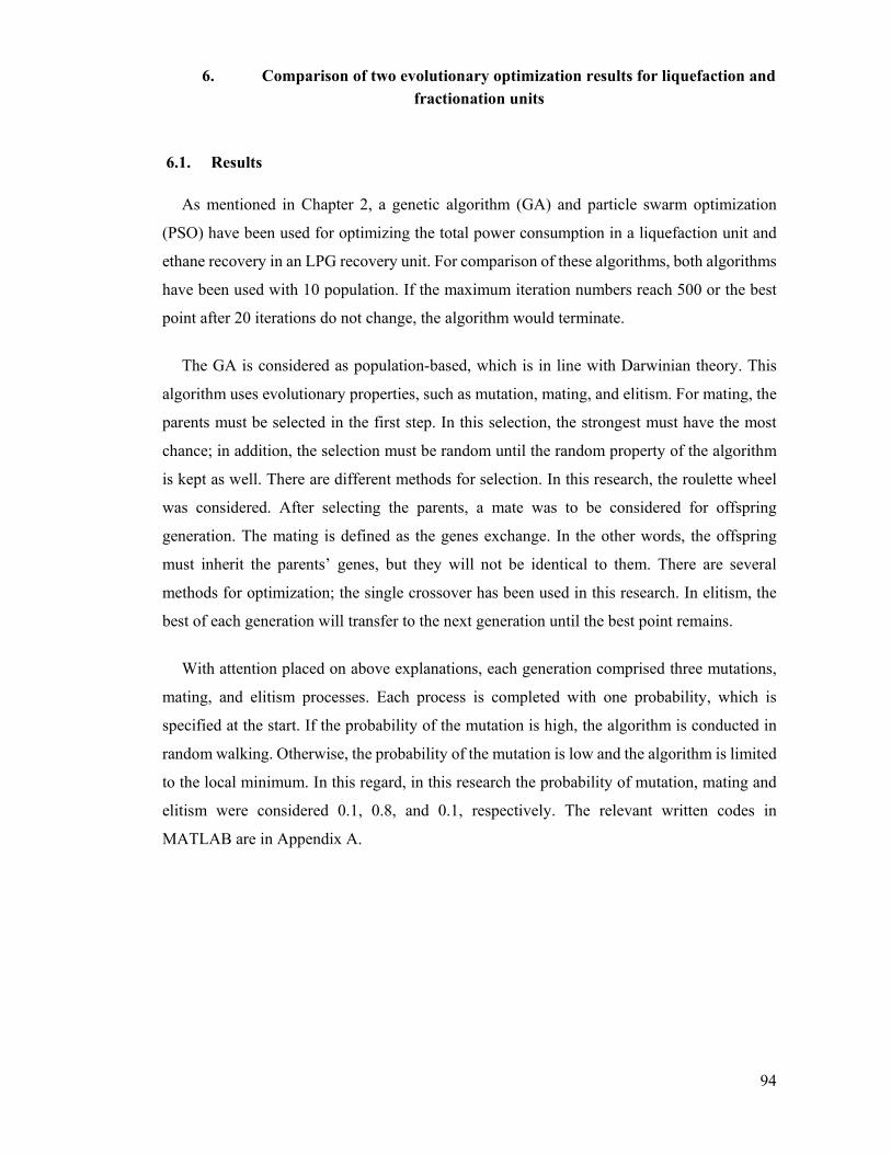
94
6. Comparison of two evolutionary optimization results for liquefaction and fractionation units
6.1. Results
As mentioned in Chapter 2, a genetic algorithm (GA) and particle swarm optimization
(PSO) have been used for optimizing the total power consumption in a liquefaction unit and
ethane recovery in an LPG recovery unit. For comparison of these algorithms, both algorithms
have been used with 10 population. If the maximum iteration numbers reach 500 or the best
point after 20 iterations do not change, the algorithm would terminate.
The GA is considered as population-based, which is in line with Darwinian theory. This
algorithm uses evolutionary properties, such as mutation, mating, and elitism. For mating, the
parents must be selected in the first step. In this selection, the strongest must have the most
chance; in addition, the selection must be random until the random property of the algorithm
is kept as well. There are different methods for selection. In this research, the roulette wheel
was considered. After selecting the parents, a mate was to be considered for offspring
generation. The mating is defined as the genes exchange. In the other words, the offspring
must inherit the parents’ genes, but they will not be identical to them. There are several
methods for optimization; the single crossover has been used in this research. In elitism, the
best of each generation will transfer to the next generation until the best point remains.
With attention placed on above explanations, each generation comprised three mutations,
mating, and elitism processes. Each process is completed with one probability, which is
specified at the start. If the probability of the mutation is high, the algorithm is conducted in
random walking. Otherwise, the probability of the mutation is low and the algorithm is limited
to the local minimum. In this regard, in this research the probability of mutation, mating and
elitism were considered 0.1, 0.8, and 0.1, respectively. The relevant written codes in
MATLAB are in Appendix A.
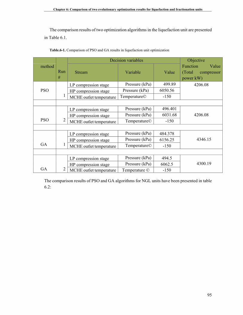
Chapter 6: Comparison of two evolutionary optimization results for liquefaction and fractionation units
95
The comparison results of two optimization algorithms in the liquefaction unit are presented
in Table 6.1.
Table.6-1. Comparison of PSO and GA results in liquefaction unit optimization
Objective Function Value (Total compressor power kW)
Decision variables
Run #
Value Variable Stream method
4206.08
499.89 Pressure (kPa) LP compression stage
1
6050.56 Pressure (kPa) HP compression stagePSO
-150 Temperature© MCHE outlet temperature
4206.08 496.401 Pressure (kPa) LP compression stage
2
PSO 6031.68 Pressure (kPa) HP compression stage
-150 Temperature©MCHE outlet temperature
4346.15 484.378 Pressure (kPa) LP compression stage
1
GA 6156.25 Pressure (kPa) HP compression stage
-150 Temperature©MCHE outlet temperature
4300.19 494.5 Pressure (kPa) LP compression stage
2
GA 6062.5 Pressure (kPa) HP compression stage-150 Temperature © MCHE outlet temperature
The comparison results of PSO and GA algorithms for NGL units have been presented in table 6.2:
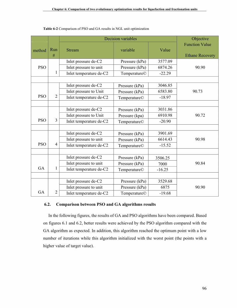
Chapter 6: Comparison of two evolutionary optimization results for liquefaction and fractionation units
96
Table 6-2 Comparison of PSO and GA results in NGL unit optimization
Objective Function Value
Ethane Recovery
Decision variables
Run #
Value variable Stream method
90.90 3577.09 Pressure (kPa)Inlet pressure de-C2
1
6874.26 Pressure (kPa)Inlet pressure to unit PSO -22.29 Temperature©Inlet temperature de-C2
90.73 3046.85 Pressure (kPa) Inlet pressure de-C2
2
PSO 6583.80 Pressure (kPa) Inlet pressure to Unit -18.97 Temperature© Inlet temperature de-C2
90.72 3031.86 Pressure (kPa) Inlet pressure de-C2
3
PSO 6910.98 Pressure (kpa) Inlet pressure to Unit -20.90 Temperature© Inlet temperature de-C2
3901.69 Pressure (kPa) Inlet pressure de-C2
4
PSO 90.98 6614.43 Pressure (kPa) Inlet pressure to unit
-15.52 Temperature© Inlet temperature de-C2
90.84 3506.25 Pressure (kPa) Inlet pressure de-C2
1
GA 7000 Pressure (kPa) Inlet pressure to unit
-16.25 Temperature© Inlet temperature de-C2
90.90 3529.68 Pressure (kPa)Inlet pressure de-C2
2
GA 6875 Pressure (kPa)Inlet pressure to unit
-19.68 Temperature©Inlet temperature de-C2
6.2. Comparison between PSO and GA algorithms results
In the following figures, the results of GA and PSO algorithms have been compared. Based
on figures 6.1 and 6.2, better results were achieved by the PSO algorithm compared with the
GA algorithm as expected. In addition, this algorithm reached the optimum point with a low
number of iterations while this algorithm initialized with the worst point (the points with a
higher value of target value).
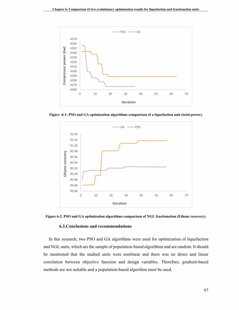
Chapter 6: Comparison of two evolutionary optimization results for liquefaction and fractionation units
97
Figure -6-1. PSO and GA optimization algorithms comparison of a liquefaction unit (total power).
Figure 6-2. PSO and GA optimization algorithms comparison of NGL fractionation (Ethane recovery).
6.3.Conclusions and recommendations
In this research, two PSO and GA algorithms were used for optimization of liquefaction
and NGL units, which are the sample of population-based algorithms and are random. It should
be mentioned that the studied units were nonlinear and there was no direct and linear
correlation between objective function and design variables. Therefore, gradient-based
methods are not suitable and a population-based algorithm must be used.
4260
4270
4280
4290
4300
4310
4320
4330
4340
4350
4360
4370
0 10 20 30 40 50 60 70
Compressor power (kw)
Iteration
PSO GA
90.84
90.86
90.88
90.90
90.92
90.94
90.96
90.98
91.00
91.02
91.04
0 10 20 30 40 50 60 70
Ethan
e recovery
Iteration
GA PSO
Chapter 6: Comparison of two evolutionary optimization results for liquefaction and fractionation units
98
Three criteria were used to compare the performance of the two EAs: (1) the percentage of
success, as signified by the number of trials essential for the objective function to achieve its
known target value; (2) the average value of the solution attained in all trials; and (3) the time
of processing to attain the optimum target value. The processing time, and not the number of
generation cycles, was used to analyse the speed of each optimization algorithm because the
number of generations in each evolutionary cycle is different from one algorithm to another.
With attention on the presented results, the PSO algorithm could achieve better optimum
points; in other words, in the liquefaction unit, PSO presented a point with lower consumed
energy compared with the GA and, in the fractionation unit, the PSO algorithm found a point
with higher ethane recovery compared to the GA. The main reason is related to continuity of
design variables in both systems. While GAs are used for discrete spaces, it does not mean a
GA cannot optimize continuous variables. However, GAs have a week performance compared
to PSO, as PSO was designed for continuous variables. In this thesis, the GA that was
extensively used in previous research in published papers cannot achieve the optimum results
of PSO. In addition, more calculations are required to determine a close result to the optimum
target value.
The main advantage of PSO is in accordance with intelligence. It is used in both scientific
engineering and research applications. PSO has no mutation or overlapping calculations. The
search is performed by the velocity of the particle. Throughout the improvement of several
generations, only the most ideal particle can communicate data to the other particles and the
speed of the research is high. Afterwards, the calculation using PSO is simple. Compared with
other evolutionary calculations, it holds a superior optimization capability and is completed
easily. The last point is PSO adopts the real number code and is decided directly by the
solution. The number of the dimension is equal to the constant of the answer.
Finally, the PSO algorithm is recommended as the best evolutionary optimization algorithm
in terms of success rate and solution quality for optimization of continuous and nonlinear
process units.
Chapter 6: Comparison of two evolutionary optimization results for liquefaction and fractionation units
99
6.4. New efficient, high recovery of liquids from natural gas with propane
recovery 99.5%
The inlet operating pressure, expander pressure, de-ethanizer column pressure and
temperature, the number of stages, and feed inlet stage are design variables that were
optimized based PSO. The optimized design variables were incorporated in HYSYS
simulation instead of previous values to maximize ethane and propane recovery as an objective
function. In Chapter 4, different process schemes including JT with and without propane
refrigeration and a turbo-expander with and without propane refrigeration were evaluated. It
was found that the most efficient in ethane recovery and economic benchmarks is the turbo-
expander with propane refrigeration. The turbo-expander with propane refrigeration is
indicated as the most optimum process scheme in LPG recovery based on technical and
economic evaluations (CAPEX and OPEX). At the next stage, the scheme was optimized to
specify higher LPG recovery values. The key to achieving high LPG recovery levels lies in
the properties of the reflux liquid. Ideally, the reflux should be subcooled with primarily
methane and ethane, with very low concentrations of LPG. While many conventional
processes generate artificial reflux using a portion of the feed gas, as the feed gas also contains
LPG and heavier components, equilibrium losses of these desired components into the sales
gas stream will occur and reduce recovery levels. This process scheme features a two-tower
approach and LPG recovery levels approaching 100% are typical. As presented in Figure 5.3,
the absorber recovers the LPG components from the feed gas and the de-ethanizer removes
the co-absorbed lighter components so the LPG product will meet specifications. The de-
ethanizer overhead has a low LPG content and is, therefore, used to provide the reflux stream
for both towers.
When processing lean feed gases, co-absorption of methane in the absorber bottoms
increases thus requiring colder condenser temperatures in the de-ethanizer overhead. When
propane is used as a refrigerant, the coldest practical condensing temperature is approximately
-37°C. This process scheme incorporates a reboiler on the absorber to reduce the methane
content of the absorber bottoms liquid and, thereby, controls the de-ethanizer reflux
composition and condensing temperature. This allows flexibility in operation over a wide
range of feed gas compositions and avoids the need for more expensive refrigeration systems,
such as mixed refrigerant systems.
Chapter 6: Comparison of two evolutionary optimization results for liquefaction and fractionation units
100
In the recommended scheme, the feed gas passes through the mercury removal bed and
then undergoes precooling in which 50% of the gas enters the gas-gas exchanger and the
remaining gas is routed to the gas-liquid exchanger. Both heat exchangers are brazed
aluminium heat exchangers (BAHX). The gas-gas exchanger cooling is provided by the sales
gas. The gas-liquid exchanger cooling is provided by the absorber bottoms. This heat
integration recovers cold from the absorber and de-ethanizer, which reduces the refrigerant
required and the heat requirements in the de-ethanizer reboiler.
The chilled inlet gas leaves the gas- gas exchanger and the gas-liquid exchanger and is
mixed, forming a two-phase mixture at 6463 kPaa and -29 0C. The two-phase mixture is fed
to the cold separator. The gas phase is transferred to the expander where the pressure is
dropped to 3172 kPaa before being fed to the upper section of the absorber. The liquid phase
from the cold separator is also dropped to 3172 kPaa and fed to the lower section of the
absorber. The gas-liquid exchanger heats liquid from a draw from a lower section of the
absorber and preheats bottoms before they are fed to the de-ethanizer. The absorber uses a slip
stream of reflux from the de-ethanizer to absorb the C3+ material contained in the vapour
phase. The reflux stream is subcooled against the absorber tower’s overhead stream before
entering the top of the absorber. This cold, light reflux stream high in ethane and low in
propane content is the key to achieving extremely high LPG recovery.
The overhead gas stream from the absorber is heated against the reflux stream feeding the
absorber, as described above. The gas then combines with a relatively small overhead stream
from the de-ethanizer reflux drum and further heated to 32 0C against the dry, treated gas from
dehydration in the gas-gas exchanger. This gas is compressed to 3658 kPaa in the booster
compressor, which is an expander driven centrifugal compressor. The compressed gas is
cooled against the feed gas from approximately 470 C to 390 C before being sent to sales gas
compression. The liquids from the absorber are pumped by the absorber bottoms pumps. This
stream then feeds the de-ethanizer. The de-ethanizer is a refluxed fractionator operating
approximately 3241 kPaa. The methane and ethane are taken overhead and essentially all of
the C3+ material is recovered as a liquid in the bottom of the tower. The overhead stream from
the de-ethanizer feeds the de-ethanizer condenser, which is a partial condenser. Propane
refrigeration provides the cooling on the shell side of the exchanger. The liquid is pumped to
the de-ethanizer and absorbers as reflux by the de-ethanizer reflux pumps.
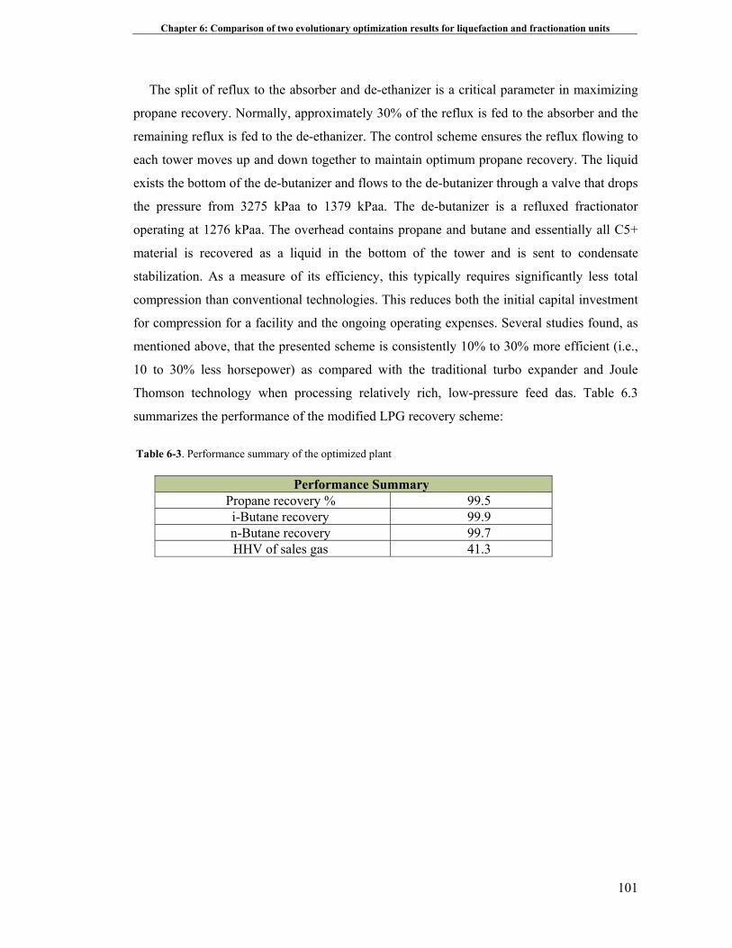
Chapter 6: Comparison of two evolutionary optimization results for liquefaction and fractionation units
101
The split of reflux to the absorber and de-ethanizer is a critical parameter in maximizing
propane recovery. Normally, approximately 30% of the reflux is fed to the absorber and the
remaining reflux is fed to the de-ethanizer. The control scheme ensures the reflux flowing to
each tower moves up and down together to maintain optimum propane recovery. The liquid
exists the bottom of the de-butanizer and flows to the de-butanizer through a valve that drops
the pressure from 3275 kPaa to 1379 kPaa. The de-butanizer is a refluxed fractionator
operating at 1276 kPaa. The overhead contains propane and butane and essentially all C5+
material is recovered as a liquid in the bottom of the tower and is sent to condensate
stabilization. As a measure of its efficiency, this typically requires significantly less total
compression than conventional technologies. This reduces both the initial capital investment
for compression for a facility and the ongoing operating expenses. Several studies found, as
mentioned above, that the presented scheme is consistently 10% to 30% more efficient (i.e.,
10 to 30% less horsepower) as compared with the traditional turbo expander and Joule
Thomson technology when processing relatively rich, low-pressure feed das. Table 6.3
summarizes the performance of the modified LPG recovery scheme:
Table 6-3. Performance summary of the optimized plant
Performance SummaryPropane recovery % 99.5i-Butane recovery 99.9n-Butane recovery 99.7HHV of sales gas 41.3
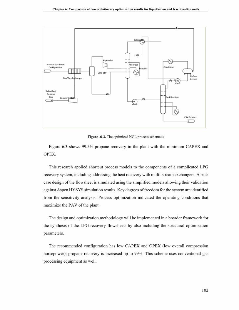
Chapter 6: Comparison of two evolutionary optimization results for liquefaction and fractionation units
102
Figure -6-3. The optimized NGL process schematic
Figure 6.3 shows 99.5% propane recovery in the plant with the minimum CAPEX and
OPEX.
This research applied shortcut process models to the components of a complicated LPG
recovery system, including addressing the heat recovery with multi-stream exchangers. A base
case design of the flowsheet is simulated using the simplified models allowing their validation
against Aspen HYSYS simulation results. Key degrees of freedom for the system are identified
from the sensitivity analysis. Process optimization indicated the operating conditions that
maximize the PAV of the plant.
The design and optimization methodology will be implemented in a broader framework for
the synthesis of the LPG recovery flowsheets by also including the structural optimization
parameters.
The recommended configuration has low CAPEX and OPEX (low overall compression
horsepower); propane recovery is increased up to 99%. This scheme uses conventional gas
processing equipment as well.
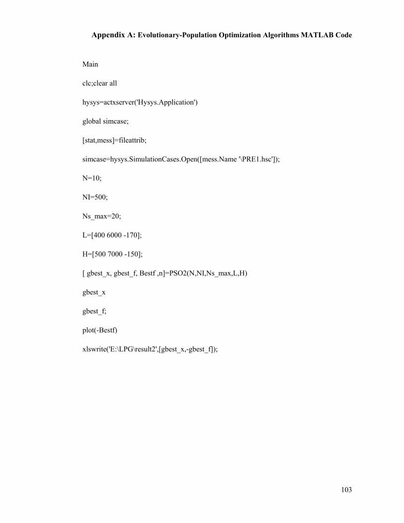
103
Appendix A: Evolutionary-Population Optimization Algorithms MATLAB Code
Main
clc;clear all
hysys=actxserver('Hysys.Application')
global simcase;
[stat,mess]=fileattrib;
simcase=hysys.SimulationCases.Open([mess.Name '\PRE1.hsc']);
N=10;
NI=500;
Ns_max=20;
L=[400 6000 -170];
H=[500 7000 -150];
[ gbest_x, gbest_f, Bestf ,n]=PSO2(N,NI,Ns_max,L,H)
gbest_x
gbest_f;
plot(-Bestf)
xlswrite('E:\LPG\result2',[gbest_x,-gbest_f]);
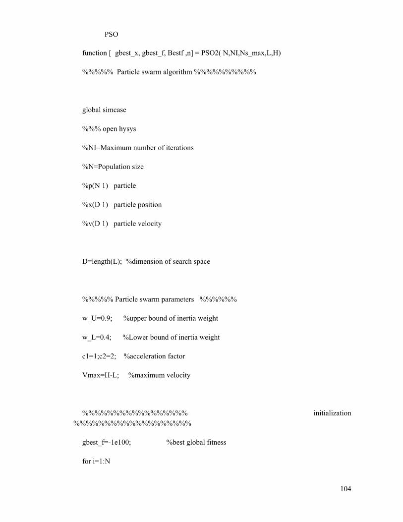
104
PSO
function [ gbest_x, gbest_f, Bestf ,n] = PSO2( N,NI,Ns_max,L,H)
%%%%% Particle swarm algorithm %%%%%%%%%%
global simcase
%%% open hysys
%NI=Maximum number of iterations
%N=Population size
%p(N 1) particle
%x(D 1) particle position
%v(D 1) particle velocity
D=length(L); %dimension of search space
%%%%% Particle swarm parameters %%%%%%
w_U=0.9; %upper bound of inertia weight
w_L=0.4; %Lower bound of inertia weight
c1=1;c2=2; %acceleration factor
Vmax=H-L; %maximum velocity
%%%%%%%%%%%%%%%%% initialization %%%%%%%%%%%%%%%%%%%
gbest_f=-1e100; %best global fitness
for i=1:N
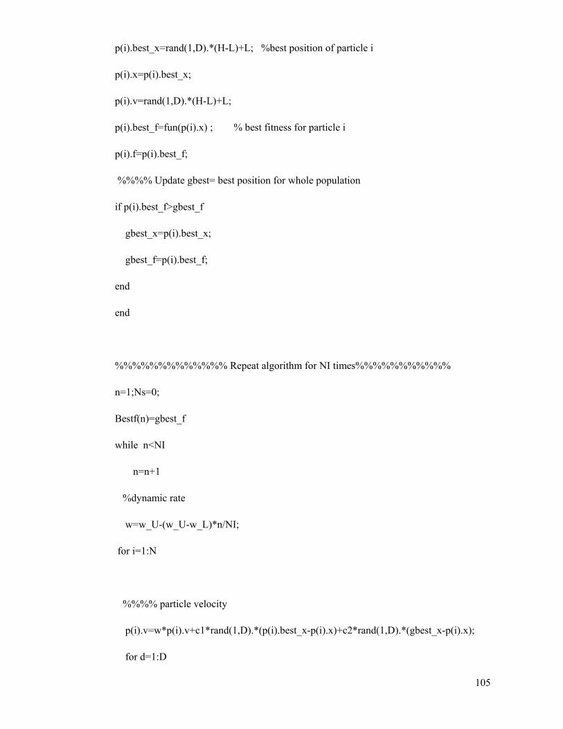
105
p(i).best_x=rand(1,D).*(H-L)+L; %best position of particle i
p(i).x=p(i).best_x;
p(i).v=rand(1,D).*(H-L)+L;
p(i).best_f=fun(p(i).x) ; % best fitness for particle i
p(i).f=p(i).best_f;
%%%% Update gbest= best position for whole population
if p(i).best_f>gbest_f
gbest_x=p(i).best_x;
gbest_f=p(i).best_f;
end
end
%%%%%%%%%%%%% Repeat algorithm for NI times%%%%%%%%%%%
n=1;Ns=0;
Bestf(n)=gbest_f
while n<NI
n=n+1
%dynamic rate
w=w_U-(w_U-w_L)*n/NI;
for i=1:N
%%%% particle velocity
p(i).v=w*p(i).v+c1*rand(1,D).*(p(i).best_x-p(i).x)+c2*rand(1,D).*(gbest_x-p(i).x);
for d=1:D
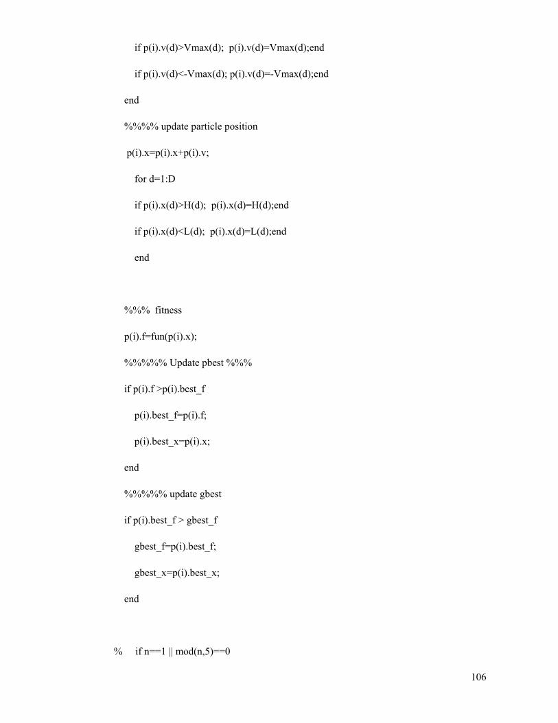
106
if p(i).v(d)>Vmax(d); p(i).v(d)=Vmax(d);end
if p(i).v(d)<-Vmax(d); p(i).v(d)=-Vmax(d);end
end
%%%% update particle position
p(i).x=p(i).x+p(i).v;
for d=1:D
if p(i).x(d)>H(d); p(i).x(d)=H(d);end
if p(i).x(d)<L(d); p(i).x(d)=L(d);end
end
%%% fitness
p(i).f=fun(p(i).x);
%%%%% Update pbest %%%
if p(i).f >p(i).best_f
p(i).best_f=p(i).f;
p(i).best_x=p(i).x;
end
%%%%% update gbest
if p(i).best_f > gbest_f
gbest_f=p(i).best_f;
gbest_x=p(i).best_x;
end
% if n==1 || mod(n,5)==0

107
% for ii=1:N
% X(ii)=p(ii).x(1);Y(ii)=p(ii).x(2);
% end
% figure(n)
% plot(X,Y,'*r')
% axis([L(1) H(1) L(2) H(2)])
% end
end
Bestf(n)=gbest_f;
if n>1 && abs(Bestf(n)-Bestf(n-1))<1e-8
Ns=Ns+1;
else
Ns=0;
end
if Ns>=Ns_max;break;end
end
end

108
Objective Function (second system)
function OF= fun(x)
global simcase
fs=simcase.get('flowsheet');
ms=fs.get('MaterialStreams');
ss=fs.get('Operations');
sheet=ss.Item('power');
ms.Item('41').PressureValue=x(1);
ms.Item('46').PressureValue=x(2);
ms.Item('30').TemperatureValue=x(3);
OF=-(sheet.Cell('A3').CellValue);
end
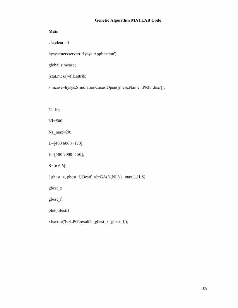
109
Genetic Algorithm MATLAB Code
Main
clc;clear all
hysys=actxserver('Hysys.Application')
global simcase;
[stat,mess]=fileattrib;
simcase=hysys.SimulationCases.Open([mess.Name '\PRE1.hsc']);
N=10;
NI=500;
Ns_max=20;
L=[400 6000 -170];
H=[500 7000 -150];
S=[6 6 6];
[ gbest_x, gbest_f, Bestf ,n]=GA(N,NI,Ns_max,L,H,S)
gbest_x
gbest_f;
plot(-Bestf)
xlswrite('E:\LPG\result2',[gbest_x,-gbest_f]);
110
GA
function [ best_x , best_f,Bestf,g] = GA( N,NG,Ns_max,L,H,S)
%%%%%%%%%%%%%%%%%%%% Genetic Algorithm %%%%%%%%%%%%%%%%%
%selection by roulette wheel
%N Population size
%NG Maximum generation
%L Lower bound of inputs
%H Upper bound of inputs
%S Number of bits for each input
CL=sum(S); %chromosome length
mps=2*N; %mating pool size
SF=1; %selection factor, it must be an odd number if f has a value<0 or when we want to minimise error
Pc=0.9; %crossover rate= it is related to the generation gap
Pm=0.1; %mutation rate
C=zeros(N,CL); % population of chromosome
f=zeros(N,1); %fitness
best_c=zeros(1,CL); %best chromosome;
best_f=-1e100; %best fitness
%%%%%%%%%%%%%%%% initialisation %%%%%%%%%%%%%%%%%
for i=1:N
for j=1:CL
if(rand()<0.5)
C(i,j)=0;
else

111
C(i,j)=1;
end
end
end
g=0;Ns=1;
%%%%%%%%%%%%%%%% Gentic algorithm for NG times %%%%%%%%%%%%%%%%%
while g<NG && Ns<Ns_max
%%%%%% Evaluation
if g==0
ig=1;
else
ig=2;
end
for i=ig:N
x=decode(C(i,:),L,H,S);
f(i)=fun(x);
end
%%% Update best solution%%%%
[best_f , i_max]=max(f);
best_c=C(i_max,:);
%%%%%%%%%%%%%%%%% Selection %%%%%%%%%%%%%%%%%%%%%%%
112
%%% selection probability and scale it between(0,1)
ps=f.^SF;
ps=(ps-min(ps))/(max(ps)-min(ps));
%%%% Mating
mp=zeros(mps,CL);
%%%%% retain best chromosome
mp(1,:)=best_c;
%%%%% roulette wheel selection
for i=2:mps
tw=rand()*sum(ps);
k=1;s=ps(1);
while tw>=s
s=s+ps(k);
k=k+1;
end
%%%%% chromosome k is selected
if k==N+1; k=N;end
mp(i,:)=C(k,:);
end
%%%%%%%%%%% 1-site crossover
for i=1:2:N
Rc=rand();
%%%% select an another chromosome to pair with i
ii=randi([1,mps]);
while ii==i

113
ii=randi([1,mps]);
end
if Rc<Pc
site=round(Rc*CL);
if site==0; site=1; end
%%%% crossover for two selected chromosomes in the mating pool
tc=mp(i,1:site);
mp(i,1:site)=mp(ii,1:site);
mp(ii,1:site)=tc;
%%%%% copy these two new chromosomes from the mating pool to the new population
%%%remaining from the old population
C(i,:)=mp(i,:);
C(i+1,:)=mp(ii,:);
end
% remaining from the mating pool
C(i,:)=mp(i,:);
C(i+1,:)=mp(ii,:);
end
%%%%% elitism
C(1,:)=best_c;
f(1)=best_f;
%%%%%%%%%%%% Mutation %%%%%%%%%%

114
for i=2:N
if rand()< Pm
C(i,:)=1-C(i,:);
end
end
g=g+1;
Bestf(g)=best_f;
best_f
if g>1 && abs(Bestf(g)-Bestf(g-1))<=1e-5
Ns=Ns+1;
else
Ns=1;
end
end
best_x=decode(best_c,L,H,S);
end
%%%%%%%%%%%%%%%% Decode chromosome %%%%%%%%%%%%%%%%%
function [x]= decode(c,L,H,S)
kd=1;
s=0;
for i=1:length(S)
s=s+S(i);
b=c(kd:s);

115
x(i)=sum((2.^[S(i)-1:-1:0]).*b) /2^S(i)*(H(i)-L(i))+L(i);
kd=S(i)+kd;
end
end
116
Objective Function (second system)
function OF= fun(x)
global simcase
fs=simcase.get('flowsheet');
ms=fs.get('MaterialStreams');
ss=fs.get('Operations');
sheet=ss.Item('power');
ms.Item('41').PressureValue=x(1);
ms.Item('46').PressureValue=x(2);
ms.Item('30').TemperatureValue=x(3);
OF=-(sheet.Cell('A3').CellValue);
End
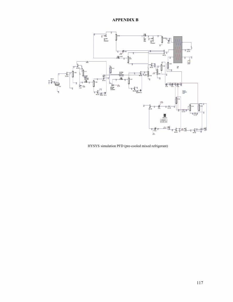
117
APPENDIX B
HYSYS simulation PFD (pre-cooled mixed refrigerant)
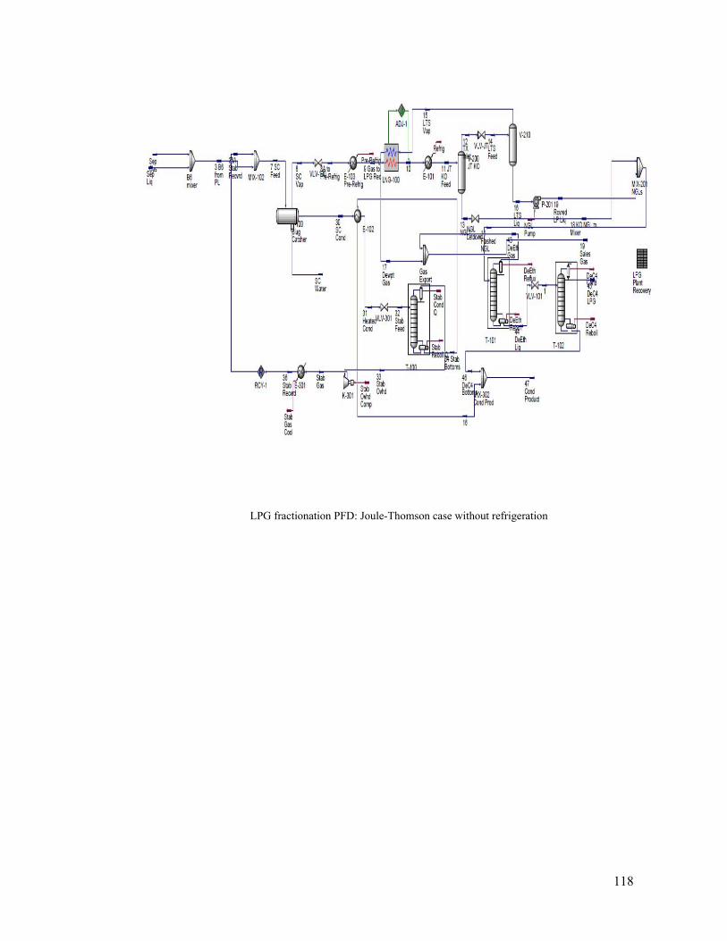
118
LPG fractionation PFD: Joule-Thomson case without refrigeration
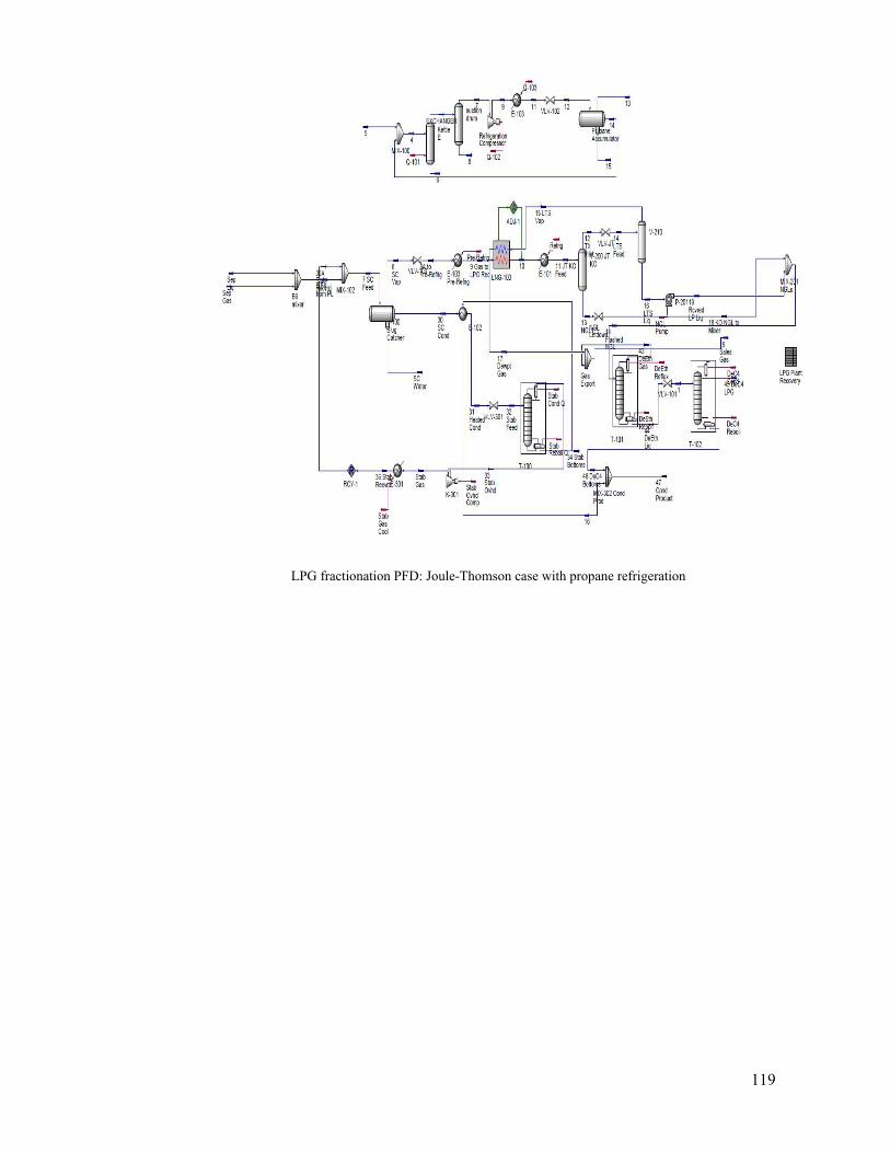
119
LPG fractionation PFD: Joule-Thomson case with propane refrigeration
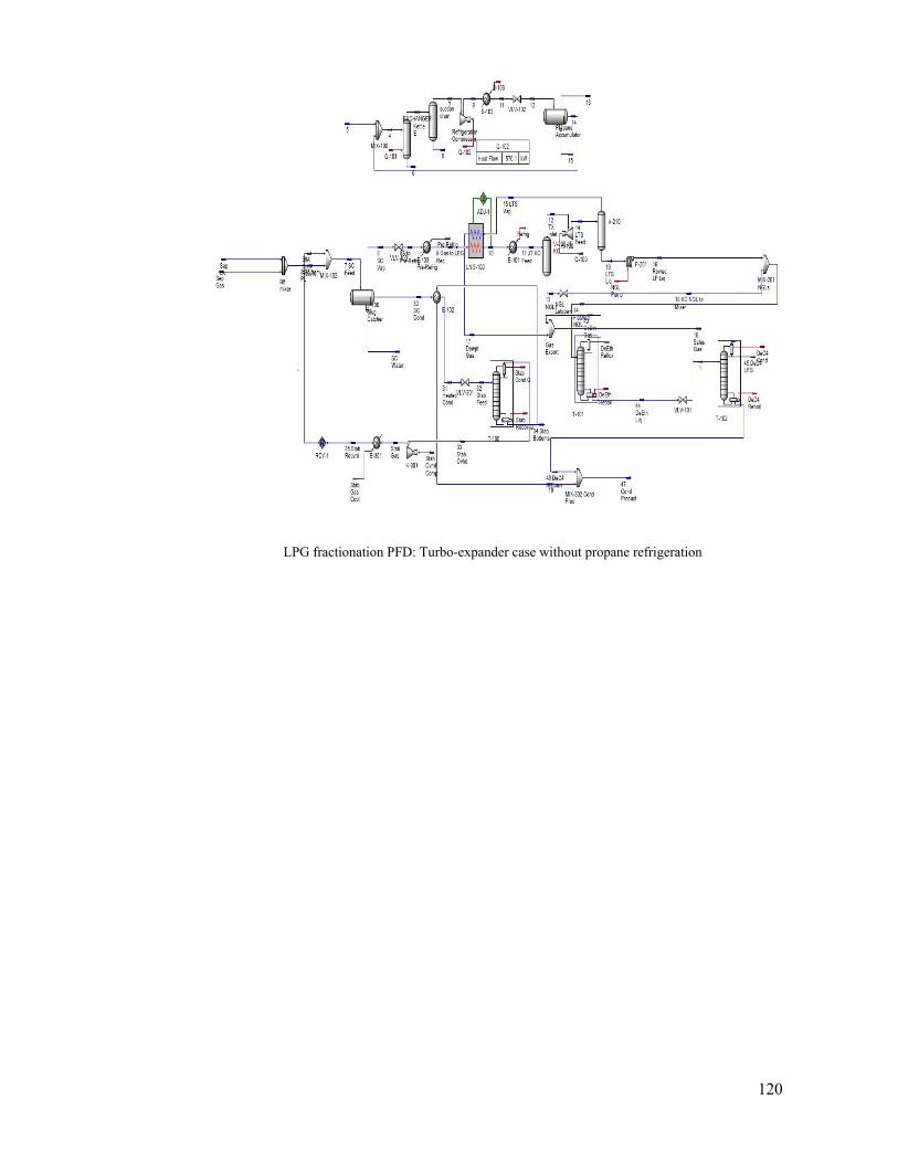
120
LPG fractionation PFD: Turbo-expander case without propane refrigeration
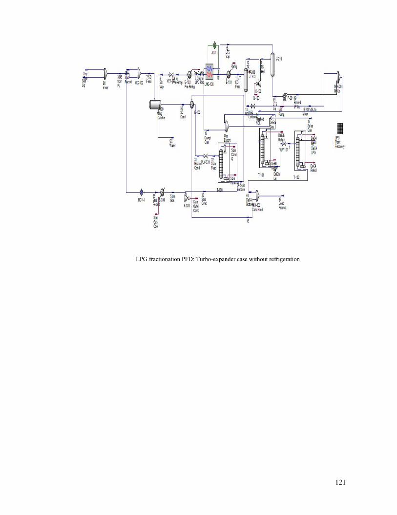
121
LPG fractionation PFD: Turbo-expander case without refrigeration
122
REFERENCES
1. Dr Chen-Hwa Chiu., 18 November 2008. History of the development of LNG
technology, Texas AIChE Annual Conference Hundred Years of Advancements in Fuels and
Petrochemicals Philadelphia, Pennsylvania.
2. Kanoglu, M., 2002. Exergy analysis of multistage cascade refrigeration cycle used for
natural gas liquefaction, International Journal of Energy Research.
3. DOE., 2005. Liquefied natural gas: Understanding the basic acts. Washington: U.S.
Department of Energy.
4. Shukri, T., 2004. LNG Technology Selection. Hydrocarbon Engineering.
5. Barclay, M., & Denton, N., 2005. Selecting offshore LNG processes. LNG Journal,
34-36.
6. Jensen, J.B., & G.V.R.Skogestad, S., 2009a. Single-cycle mixed fluid LNG process-
Part I: Optimal design. In G.V.R. Reklaitis, H.E. Alfadala, &M.M.EI-Halwagi (Eds), 1st Annual
Gas Processing Symposium. Qatar: Elsevier.
7. Shah, N., Rangaiah, G.P.,& Hoadley, A.,2009. Multi-objective optimization of the
dual independent expander gas-phase refrigeration process for LNG. In AIChE Annual Meeting
Salt Lake City, UT, USA, November 4-9.
8. Price, B.C.,& Moortko.R.A.,1996. PRICO-A simple, flexible proven approach to
natural gas liquefaction. In L. Gastech (Ed.) Natural gas, LPG International Conference Vienna.
9. Stebbing, R., & O'Brien, J., 1975. An updated report on the PRICO ™ process for LNG
plants. In L. Gastech (Ed), Natural gas, LPG International Conference, Paris.
10. Ait-ALI, M.A., 1979. Optimal mixed refrigerant liquefaction of natural gas. Stanford
University.
11. Lee, G.C. Smith, R & Zhu, X.X., 2002. Optimal synthesis of mixed refrigerant systems
for low-temperature processes. Industrial & Engineering Chemistry Research, 48, 6652-6659.
12. Jensen, J.B., & G.V.R.Skogestad, S., 2009. Single-cycle mixed fluid LNG process-
Part II: Optimal design. In G.V.R. Reklaitis, H.E. Alfadala, &M.M.EI-Halwagi (Eds), 1st
Annual Gas Processing Symposium. Qatar: Elsevier.
13. Jensen, J.B., & G.V.R.Skogestad, S., 2006. Optimal operation of a simple LNG
process. International Symposium on Advanced Control of Chemical Processes Gramado,
Brazil ADCHEM.
14. Jensen, J.B., & Skogestad, S., 2009. Steady-state operational degrees of freedom with
application to refrigeration cycles. Industrial & Engineering Chemistry Research, 48-6652-
6659.
123
15. Gao, T., Lin, W., GU, A., & GU, M., 2009. Optimization of coalbed methane
liquefaction process adapting mixed refrigerant cycle with propane pre-cooling. Journal of
Chemical Engineering Japan, 42, 893-901.
16. Aspelund, A., Gundersen, T., Myklebust, J., Nowak, M. P., & Tomasgard, A., 2009.
An optimization–simulation model for simple LNG process. Norway: The Norwegian
University of Science and Technology.
17. Nogal, F.L.D., Kim, J-K., Perry, S., & Smith, R., 2008. Optimal design of mixed
refrigerant cycles. Industrial & Engineering Chemistry Research, 47, 8724-8740.
18. Grandhiraju, V., 2009. United States patent application.
19. Xiongwen Xu, Jinping Liu, Le Co., 2013. Optimization and analysis of mixed
refrigerant composition for the PRICO natural gas liquefaction process. Elsevier.
20. Jian Zhang, Qiang Xu., 2011, Cascade refrigeration system synthesis based on exergy
analysis. Elsevier.
21. Mohd Shariq Khan, Sanggyu Lee, Moonyong Lee., 2013. Knowledge-based decision-
making method for the selection of mixed refrigerant systems for energy efficient LNG
processes. Elsevier.
22. Prue Hatcher, Rajab Khalilpour, Ali Abbas., 2012. Optimization of LNG mixed-
refrigerant process considering operation and design objectives. Elsevier.
23. Abdullah Alabdulkarem, Amir Mortazavi., 2010. Optimization of propane pre-cooled
mixed refrigerant LNG plant. Elsevier.
24. Amir Mortazavi, Christopher Somers., 2010. Enhancement of APCI cycle efficiency
with absorption chillers. Elsevier.
25. Kanoglu M., 2001. Cryogenic turbine efficiencies. Exergy International Journal;
1(3):202-8.
26. Renaudin G., 1995. Improvement of natural gas liquefaction processes by using liquid
turbines. In: Proceeding of the eleventh international conference on liquefied natural gas.
Chicago: Institute of Gas Technology.
27. Mortazavi A, Somers C, Hwang Y, Radermacher R, Al-Hashimi S and Rodgers P.,
2008. Performance enhancement of propane precooled mixed refrigerant LNG Plant. Energy
2030 Conference, Abu Dhabi, UAE.
28. Barclay M., 2005. Selecting offshore LNG processes. LNG Journal.
29. Kalinowski P, Hwang Y, Radermacher R, Al-Hashimi S and Rodgers P., 2008.
Performance enhancement of propane precooled mixed refrigerant LNG plant. Energy 2030
Conference, Abu Dhabi, UAE.
124
30. C.W. Remeljej, A.FA. Hoadley., 2006. An exergy analysis of small-scale liquefied
natural gas (LNG) liquefaction process. Elsevier.
31. M. Mokrizadeh Haghighi Shirazi, D. Molaw., 2010. Energy optimization for
liquefaction process of natural gas in peak shaving plant.
32. DiNapoli RN., 1980. Gas turbines prove effective as drivers for LNG plants. Oil and
Gas Journal, 1980.
33. Kalinowski P, Hwang Y, Radermaher R, Al-Hashimi S, Rodgers P., 2009. Application
of waste heat powered absorption refrigeration system to the LNG recovery process. Int J
Refrig; 32(4):687-94.
34. Mortazavi A, Somers C, Alabdulkarem A, Hwang Y, Radermacher R.,
2010.Enhancement of APCI cycle efficiency with absorption chillers.Energy;35(9):3877-82.
35. Rodgers P, Mortazavi A, Eveloy V, Al-Hashimi S, Hwang Y., 2012. Enhancement of
LNG plant propane cycle through waste heat powered absorption cooling. Appl Them Eng;
48:41-53.
36. Del Nogal FL, Kim J-K, Perry S, Smith R., 2011. Synthesis of mechanical driver and
power generation configurations. , Part 1: Optimization framework. AIChe J; 56(9):2356-76.
37. Del Nogal FL, Kim J-K, Perry S, Smith R., 2011. Synthesis of mechanical driver and
power generation configurations, Part 2: LNG applications. AICHE J; 56(9):2377-89.
38. Cao WS, Lu XS, Lin WS., 2006. Parameter comparison of two small scale natural gas
liquefaction processes in skid mounted packages. Applied Thermal Engineering; 26(8-9):898-
904.
39. S.Vaidyaramana, C. Maranas., 2007. Synthesis of mixed refrigerant cascade cycles.
Chemical Engineering Communications 1057-1078.
40. H. Paradowski, M. Bamba, C., 2004. Propane precooling cycles for increased LNG
train capacity, in 14th International Conference and Exhibition on Liquefied Natural Gas,
pp.107-124.
41. G. Venkatarathnam., 2008. Cryogenic Mixed Refrigerant Processes.Springer-Verlag,
New York, LLC.
42. Q. Bai., 2010. Analysis of Particle Swarm Optimization Algorithm, Computer and
Information Science, volume 3 No 1, Pebruari.
43. Wang, M.Q; Zhang, J., Xu, Q.; Li, K. Y., 2001. Thermodynamic analysis–based
energy consumption minimization for natural gas liquefaction. Ind. Eng. Chem. Res.
44. Hoseyn Sayadi, M. Babaelahi., 2011. Multi-objective optimization of a joule cycle for
re-liquefaction of the Liquefied Natural Gas. Applied Energy, Elsevier.
125
45. Q.Y.Li, Y.L. Ju., 2010. Design and analysis of liquefaction process for offshore
associated gas resources. Applied Thermal Engineering Elsevier Journal.
46. Boiarskii M, Kharti A, Kovalenko V., 2009. Design optimization of the throttle cycle
cooler with mixed refrigerant Cryocoolers.
47. Wen-sheng Cao, Xue-sheng Lu, Wen-sheng Lin, An-zhong Gu., 2006. Parameter
comparison of two small-scale natural gas liquefaction processes in skid-mounted packages.
Applied Thermal Engineering.
48. A. P. Engelbrecht., 2005. Fundamental of Computational Swarm Intelligent, First ed.
The atrium, Southern Gate, Chichester, West Sussex PO19 8SQ, England: John Wiley & Sons
Ltd.
49. B. Santosa., 2006."Tutorial Particle Swarm optimization”.
50. F. Shahzad, et al., 2009. Opposition-based particle swarm optimization with velocity
clamping (OVCPSO), Journal Advances in Computational Intelligent, AISC 61, pp, 339-2348.
51. M. Ben Ghalia., 2008. Particle swarm optimization with an improved exploration-
exploitation balance, in Circuits and Systems, 2008. MWSCAS 2008. 51st Midwest Symposium
on, pp. 759-762.
52. Venter G and Sobieszczanski-Sobieski J., 2003. Particle Swarm Optimization, AIAA
Journal, 41(8), 1583–1589.
53. Eberhart RC and Shi Y., 2000. Comparing inertia weights and constriction factors in
particle swarm optimization, in Proceedings of IEEE International Congress on Evolutionary
Computation, vol. 1, pp. 84–88.
54. Kennedy J and Eberhart RC., 1997. A discrete binary version of the particle swarm
algorithm, in Proceedings of the 1997 Conference on Systems, Man, and Cybernetics, IEEE
Service Center, Piscataway, NJ, pp. 4104–4109.
55. Ratnaweera A, Halgamuge SK, and Watson HC., 2004. Self-organizing hierarchical
particle swarm optimiser with time-varying acceleration coefficients, IEEE Transactions on
Evolutionary Computation, 8(3), 240–255.
56. Holland JH., 1975. Adaptation in natural and artificial systems, University of Michigan
Press, Ann Arbor.
57. Kennedy J, Eberhart R and Shi Y., 2001. Swarm Intelligence, Morgan Kaufmann, Los
Altos, CA.
58. Goldberg DE., 1975. Genetic Algorithms in Search, Optimization and Machine
Learning, Addison-Wesley, Reading, MA.
59. Kohl, A., L., and R. B. Nielsen., 1997. Gas Purification, 5th ed., Gulf Publishing Company, Houston, Texas.
126
60. Lee G-C., 2001.Optimal design and analysis of refrigeration systems for low temperature processes, PhD, School of Chemical Engineering and Analytical Science, the University of Manchester, UMIST, Manchester, UK.
61. Garret, D.E., 1989. Chemical Engineering Economics. New York: Van Nostrand
Reinhold.
62. Gerrard, A.M., 2000. Guide to Capital Cost Estimating.4th ed. Rugb, Warwickshire:
McGraw-Hill.
63. Baasel, W.D., 1990. Preliminary Chemical Engineering Plant Design, 2nd ed. New
York: Van Nostrand Reinhold.
64. Kidnay, A., and W. Parrish., 2006. Fundamentals of natural gas processing. USA:
Taylor and Francis Group, LLC.
65. Storn R and Price K., 1997. Differential Evolution – A Simple and Efficient Heuristic
for Global Optimization over Continuous Spaces, Journal of Global Optimization, 11(4), 341–
359.
66. Heng Sun, Ding He Ding, Ming He, Sun Shoujun Sun., 2016. Simulation and
optimization of AP-X process in a large-scale LNG plant, Journal of Natural Gas Science and
Engineering.
67. Gang Chena, Qinzhe Liub., the 8th International Conference on Applied Energy –
ICAE., 2016. Optimization of LNG Terminal Reserve Planning for Combined Gas and
Electricity System, Science Direct.
68. Yajun Li, Yue Li., 2016. Dynamic optimization of the Boil-Off Gas (BOG)
fluctuations at an LNG receiving terminal, Journal of Natural Gas Science and Engineering.
69. Emad Elbeltagia, Tarek Hegazyb, Donald Griersonb ., 2005. Comparison among five
evolutionary-based optimization algorithms, Journal of Computation and Engineering.
70. Al-Tabtabai H, Alex PA., 1999. Using genetic algorithms to solve optimization
problems in construction. Eng Constr Archit Manage; 6(2):121–32.
71. John McCall., 2004, Genetic algorithms for modelling and optimization, Journal of
Computation and Engineering.
72. Hamidreza Taleshbahrami, Hamid Saffari., 2010, Optimization of the C3MR cycle
with genetic algorithm, Journal of Computation and Engineering.
73. H. H. West and C.-H. Chiu., 2005, LNG Safety: An Issue of Increasing Importance,
Process Safety Progress, 24.
74. J. Havens and T. Spicer., 2005, LNG Vapour Cloud Exclusion Zones for Spills into
Impoundments, Process Safety Progress, 24 (3).
75. U.S. Energy Information Administration Natural Gas Priceshttps://www.eia.gov.
127
76. Lee, I., and Moon, I., 2017, Economic Optimization of Dual Mixed Refrigerant
Liquefied Natural Gas Plant Considering Natural Gas Extraction Rate Ind. Eng. Chem. Res., 56
(10), 2804-2814.
77. Price K, Storn R, and Lampinen J., 2005, Differential Evolution – A Practical
Approach to Global Optimization, Springer, Berlin Heidelberg New York.
78. Krink T and Løvbjerg M., 2002. The Lifecycle Model: Combining Particle Swarm
Optimization, Genetic Algorithms and Hill Climbers, In Proceedings of PPSN 2002, pp. 621–
630.
79. Per E. Wahl, Sigurd W., 2015, formulating the optimization problem when using
sequential quadratic programming applied to a simple LNG process Per E. Computers and
Chemical Engineering Journal.
Every reasonable effort has been made to acknowledge the owners of copyrighted material.
I would be pleased to hear from any copyright owner who has been omitted or incorrectly
acknowledged.


