Embed Size (px)
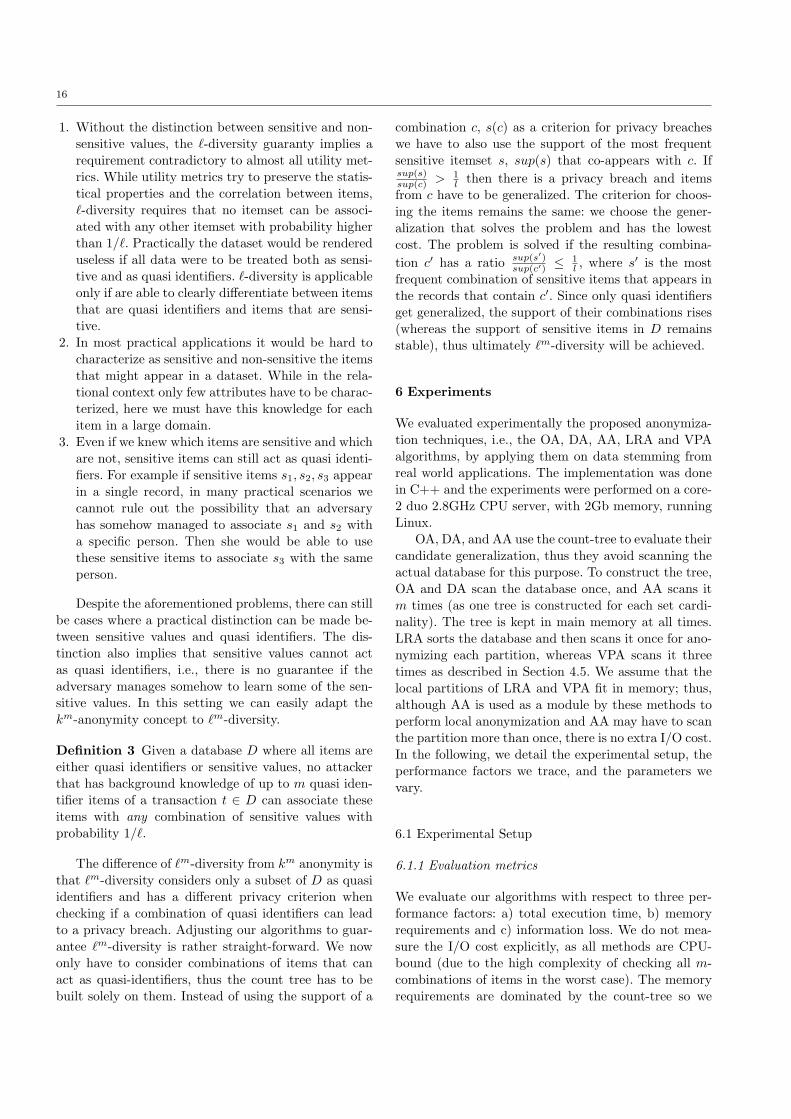
Citation preview
Noname manuscript No.(will be inserted by the editor)
Local and Global Recoding Methods for AnonymizingSet-valued Data
Manolis Terrovitis · Nikos Mamoulis · Panos Kalnis
Received: date / Accepted: date
Abstract In this paper we study the problem of pro-tecting privacy in the publication of set-valued data.
Consider a collection of supermarket transactions that
contains detailed information about items bought to-gether by individuals. Even after removing all personal
characteristics of the buyer, which can serve as links to
his identity, the publication of such data is still subjectto privacy attacks from adversaries who have partial
knowledge about the set. Unlike most previous works,
we do not distinguish data as sensitive and non-sensitive,
but we consider them both as potential quasi-identifiersand potential sensitive data, depending on the knowl-
edge of the adversary. We define a new version of the
k-anonymity guarantee, the km-anonymity, to limit theeffects of the data dimensionality and we propose effi-
cient algorithms to transform the database. Our anony-
mization model relies on generalization instead of sup-pression, which is the most common practice in related
works on such data. We develop an algorithm which
finds the optimal solution, however, at a high cost which
makes it inapplicable for large, realistic problems. Then,we propose a greedy heuristic, which performs general-
Manolis TerrovitisInstitute for the Management of Information Systems (IMIS)Research Center “Athena”E-mail: [email protected]
Nikos MamoulisDept. of Computer ScienceUniversity of Hong KongE-mail: [email protected]
Panos KalnisDiv. of Mathematical and Computer Sciences and EngineeringKing Abdullah University of Science and TechnologyE-mail: [email protected]
izations in an Apriori, level-wise fashion. The heuristicscales much better and in most of the cases finds a so-
lution close to the optimal. Finally, we investigate the
application of techniques that partition the databaseand perform anonymization locally, aiming at the re-
duction of the memory consumption and further scal-
ability. A thorough experimental evaluation with realdatasets shows that a vertical partitioning approach
achieves excellent results in practice.
1 Introduction
We consider the problem of publishing set-valued data,
while preserving the privacy of individuals associatedwith them. Consider a database D, which stores in-
formation about items purchased at a supermarket by
various customers. We observe that the direct publica-tion of D may result in unveiling the identity of the
person associated with a particular transaction, if the
adversary has some partial knowledge about a subset of
items purchased by that person. For example, assumethat Bob went to the supermarket on a particular day
and purchased a set of items including coffee, bread,
brie cheese, diapers, milk, tea, scissors and a light bulb.Assume that some of the items purchased by Bob were
on top of his shopping bag (e.g., brie cheese, scissors,
light bulb) and were spotted by his neighbor Jim, whileboth persons were on the same bus. Bob would not like
Jim to find out other items that he bought. However,
if the supermarket decides to publish its transactions
and there is only one transaction containing brie cheese,scissors, and light bulb, Jim can immediately infer that
this transaction corresponds to Bob and he can find out
his complete shopping bag contents.
2
This motivating example stresses the need to trans-
form the original transactional databaseD to a databaseD′ before publication, in order to avoid the association
of specific transactions to a particular person or event.
In practice, we expect the adversary to have only par-tial knowledge about the transactions (otherwise, there
would be little sensitive information to hide). On the
other hand, since the knowledge of the adversary is notknown to the data publisher, it makes sense to define
a generic model for privacy, which protects against ad-
versaries having knowledge limited to a level, expressed
as a parameter of the model.
In this paper, we propose such a km-anonymizationmodel, for transactional databases. Assuming that the
maximum knowledge of the adversary is at most m
items in a specific transaction, we want to prevent himfrom distinguishing the transaction from a set of k pub-
lished transactions in the database. Equivalently, for
any set of m or less items, there should be at leastk transactions that contain this set, in the published
database D′. In our example, Jim would not be able to
identify Bob’s transaction in a set of 5 transactions of
D′, if D′ is 53-anonymous.
This anonymization problem is quite different com-pared to well-studied privacy preservation problems in
the literature. Unlike the k-anonymity problem in rela-
tional databases [24,25], there is no fixed, well-definedset of quasi-identifier attributes and sensitive data. A
subset of items in a transaction could play the role of
the quasi-identifier for the remaining (sensitive) ones
and vice-versa. Another fundamental difference is thattransactions have variable length and high dimensional-
ity, as opposed to a fixed set of relatively few attributes
in relational tuples. Finally, we can consider that allitems that participate in transactions take values from
the same domain (i.e., complete universe of items), un-
like relational data, where different attributes of a tuplehave different domains.
The m parameter in the km guaranty introduces a
degree of flexibility in the traditional k-anonymity. It
allows considering different scenarios of privacy threats
and adjusting the guaranty depending on the sever-ity of the threat and the sensitivity of the data. km-
anonymity simulates k-anonymity if m is set equal to
the domain size, i.e., the adversary knows all items.Still, this is not a realistic scenario in the transactional
context. Since all items can act as quasi-identifiers, an
attacker who knows them all and can link them to aspecific person has nothing to learn from the original
database; her background knowledge already contains
the original data.
To solve the km-anonymization problem for a trans-
actional database, we follow a generalization approach.
We consider a domain hierarchy for the items that par-
ticipate in transactions. If the original database D doesnot meet the km-anonymity requirement, we gradu-
ally transform D, by replacing precise item descriptions
with more generalized ones. For example, “skimmedmilk” could be generalized to “milk” and then to “dairy
product” if necessary. By carefully browsing into the
lattice of possible item generalizations, we aim at find-ing a set of item generalizations that satisfies the km-
anonymity requirement, while retaining as much detail
as possible to the published data D′.
We propose three classes of algorithms in this di-
rection. Our first algorithmic class is represented bythe optimal anonymization (OA) algorithm, which ex-
plores in a bottom-up fashion the lattice of all possi-
ble combinations of item generalizations, and finds themost detailed such sets of combinations that satisfy
km-anonymity. The best combination is then picked,
according to an information loss metric. Although op-timal, OA has very high computational cost and can-
not be applied to realistic databases with thousands of
items.
Motivated by the scalability problems of the OA, we
propose a second class of heuristic algorithms, whichgreedily identify itemsets that violate the anonymity
requirement and choose generalization rules that fix the
corresponding problems.
The first direct anonymization (DA) heuristic op-erates directly on m-sized itemsets found to violate k-
anonymity. Our second, apriori anonymization (AA) is
a more carefully designed heuristic, which explores the
space of itemsets, in an Apriori, bottom-up fashion. AAfirst identifies and solves anonymity violations by (l−1)-
itemsets, before checking l-itemsets, for l=2 to m. By
operating in such a bottom-up fashion, the combina-tions of itemsets that have to be checked at a higher
level can be greatly reduced, as in the meanwhile de-
tailed items (e.g., “skimmed milk”, “choco-milk”, “full-fat milk”) could have been generalized to more gener-
alized ones (e.g., “milk”), thus reducing the number
of items to be combined. Our experimental evaluation,
using real datasets, shows that AA is a practical algo-rithm, as it scales well with the number of items and
transactions, and finds a solution close to the optimal
in most tested cases.
AA does not operate under limited memory, so thereis still a case where the database will be large enough
to prohibit its execution. We introduce a third class
of algorithms, Local Recoding Anonymization (LRA)
and Vertical Partitioning Anonymization (VPA), whichanonymize the dataset in the presence of limited mem-
ory. The basic idea in both cases is that the database is
partitioned and each part is processed separately from
3
the others. A short version of this paper covering the
first two classes of algorithms appears in [26].The rest of the paper is organized as follows. Sec-
tion 2 describes related work and positions this paper
against it. Section 3 formally describes the problem,provides an analysis for its solution space, and defines
the information loss metric. In Section 4, we describe
the algorithms and the data structures used by them.In Section 5 we discuss the advanced concepts of nega-
tive knowledge and ℓm-diversity. Section 6 includes the
experimental evaluation, and Section 7 concludes the
paper.
2 Related Work
Anonymity for relational data has received consider-able attention due to the need of several organizations
to publish data (often called microdata) without re-
vealing the identity of individual records. Even if the
identifying attributes (e.g., name) are removed, an at-tacker may be able to associate records with specific
persons using combinations of other attributes (e.g.,
〈zip, sex, birthdate〉), called quasi-identifiers (QI ). Atable is k-anonymized if each record is indistinguishable
from at least k− 1 other records with respect to the QI
set [24,25]. Records with identical QI values form ananonymized group. Two techniques to preserve privacy
are generalization and suppression [25]. Generalization
replaces their actual QI values with more general ones
(e.g., replaces the city with the state); typically, there isa generalization hierarchy (e.g., city→state→country).
Suppression excludes some QI attributes or entire records
(known as outliers) from the microdata.The privacy preserving transformation of the mi-
crodata is referred to as recoding. Two models exist:
in global recoding, a particular detailed value must bemapped to the same generalized value in all records. Lo-
cal recoding, on the other hand, allows the same detailed
value to be mapped to different generalized values in
each anonymized group. The recoding process can alsobe classified into single-dimensional, where the map-
ping is performed for each attribute individually, and
multi-dimensional, which maps the Cartesian productof multiple attributes. Our work is based on global re-
coding and can be roughly considered as single-dime-
nsional (although this is not entirely accurate), sincein our problem all items take values from the same do-
main.
[18] proved that optimal k-anonymity for multidi-
mensional QI is NP -hard, under both the generaliza-tion and suppression models. For the latter, they pro-
posed an approximate algorithm that minimizes the
number of suppressed values; the approximation bound
is O(k · logk). [3] improved this bound to O(k), while
[22] further reduced it to O(log k). Several approacheslimit the search space by considering only global re-
coding. [5] proposed an optimal algorithm for single-
dimensional global recoding with respect to the Classi-fication Metric (CM ) and Discernibility Metric (DM ),
which we discuss in Section 3.3. Incognito [14] takes
a dynamic programming approach and finds an opti-mal solution for any metric by considering all possible
generalizations, but only for global, full-domain recod-
ing. Full-domain means that all values in a dimension
must be mapped to the same level of hierarchy. Forexample, in the country→continent→world hierarchy,
if Italy is mapped to Europe, then Thailand must be
mapped to Asia, even if the generalization of Thailandis not necessary to guarantee anonymity. A different
approach is taken in [21], where the authors propose to
use natural domain generalization hierarchies (as op-posed to user-defined ones) to reduce information loss.
Our optimal algorithm is inspired by Incognito; how-
ever, we do not perform full-domain recoding, because,
given that we have only one domain, this would leadto unacceptable information loss due to unnecessary
generalization. As we discuss in the next section, our
solution space is essentially different due to the avoid-ance of full-domain recoding. The computational cost
of Incognito (and that of our optimal algorithm) grows
exponentially, so it cannot be used for more than 20 di-mensions. In our problem, every item can be considered
as a dimension. Typically, we have thousands of items,
therefore we develop fast greedy heuristics (based on
the same generalization model), which are scalable tothe number of items in the set domain.
Several methods employ multidimensional local re-
coding, which achieves lower information loss. Mon-
drian [15] partitions the space recursively across thedimension with the widest normalized range of values
and supports a limited version of local recoding. [2]
model the problem as clustering and propose a con-
stant factor approximation of the optimal solution, butthe bound only holds for the Euclidean distance met-
ric. [29] propose agglomerative and divisive recursive
clustering algorithms, which attempt to minimize theNCP metric (to be described in Section 3.3). Our prob-
lem is not suitable for multidimensional recoding (after
modeling sets as binary vectors), because the dimen-sionality of our data is too high; any multidimensional
grouping is likely to cause high information loss due to
the dimensionality curse. [20,19] studied multirelational
k-anonymity, which can be translated to a problem sim-ilar to the one studied here, but still there is the funda-
mental separation between sensitive values and quasi-
identifiers. Moreover there is the underlying assumption
4
that the dimensionality of the quasi-identifier is limited,
since the authors accept the traditional unconditionaldefinition of k-anonymity.
In general, k-anonymity assumes that the set of QIattributes is known. Our problem is different, since any
combination ofm items (which correspond to attributes)
can be used by the attacker as a quasi-identifier. Re-cently, the concept of ℓ-diversity [17] was introduced
to address the limitations of k-anonymity. The latter
may disclose sensitive information when there are many
identical sensitive attribute (SA) values within an ano-nymized group (e.g., all persons suffer from the same
disease). [28,31,7] present various methods to solve the
ℓ-diversity problem efficiently. [8] extends [28] for trans-actional datasets with a large number of items per trans-
action, however, as opposed to our work, distinguishes
between non-sensitive and sensitive attributes. This dis-tinction allows for a simpler solution that the one re-
quired in out setting, since the QI remains unchanged
for all attackers. [30] also considers transactional data
and distinguishes between sensitive and non-sensitiveitems, but assumes that the attacker has limited knowl-
edge of up to p non-sensitive items in each transaction
(i.e., p similar to our parameter m). Given this, [30]aims at satisfaction of ℓ-diversity, when anonymizing
the dataset and requires that the original support of
any itemset retained in the anonymized database is pre-served. A greedy anonymization technique is proposed,
which is based on suppression of items that cause pri-
vacy leaks. Thus, the main differences of our work to
[30] is that we do not distinguish between sensitive andpublic items and that we consider generalization instead
of suppression, which in general results in lower infor-
mation loss. [16] proposes an extension of ℓ-diversity,called t-closeness. Observe that in ℓ-diversity the QI
values of all tuples in a group must be the same, whereas
the SA values must be different. Therefore, introducingthe ℓ-diversity concept in our problem is a challenging,
if not infeasible, task, since any attribute can be consid-
ered as QI or SA, leading to contradicting requirements.
In Section 5 we discuss this issue in more detail.
Related issues were also studied in the context of
data mining. [27] consider a dataset D of transactions,each of which contains a number of items. Let S be a
set of association rules that can be generated by the
dataset, and S′ ⊂ S be a set of association rules thatshould be hidden. The original transactions are altered
by adding or removing items, in such a way that S′
cannot be generated. This method requires the knowl-
edge of S′ and depends on the mining algorithm, there-fore it is not applicable to our problem. Another ap-
proach is presented in [4], where the data owner gen-
erates a set of anonymized association rules, and pub-
lishes them instead of the original dataset. Assume a
rule a1a2a3 ⇒ a4 (ai’s are items) with support 80 ≫ kand confidence 98.7%. By definition, we can calculate
the support of itemset a1a2a3 as 80/0.987 ≃ 81, there-
fore we infer that a1a2a3¬a4 appears in 81 − 80 = 1transaction. If that itemset can be used as QI, the pri-
vacy of the corresponding individual is compromised.
[4] presents a method to solve the inference problemwhich is based on the apriori principle, similar to our
approach. Observe that inference is possible because of
publishing the rules instead of the transactions. In our
case we publish the anonymized transactions, thereforethe support of a1a2a3¬a4 is by default known to the
attacker and does not constitute a privacy breach.
Concurrently to our work, a new approach for ano-
nymizing transactional data was proposed in [12]. The
authors introduce a top-down local recoding method,named Partition using the same assumptions for data
as we do, but they focus on a stronger privacy guaranty,
the complete k-anonymity. They present a comparisonbetween their method and AA algorithm. Partition is
superior to AA, when large values of m are used by
AA to approximate complete k-anonymity1, However,Partition is inferior to AA for a small m. Since both lo-
cal recoding algorithms we propose in this paper use the
AA algorithm, we are able to provide a qualitative com-
parison with the Partition algorithm. The comparisonappears in Section 6 and it is based on the experimental
results of [12] for the AA and Partition algorithms.
3 Problem Setting
Let D be a database containing |D| transactions. Each
transaction t ∈ D is a set of items 2. Formally, t is a non-
empty subset of I = {o1, o2, . . . , o|I|}. I is the domain
of possible items that can appear in a transaction. We
assume that the database provides answers to subset
queries, i.e., queries of the form {t | (qs ⊆ t)∧ (t ∈ D)},where qs is a set of items from I provided by the user.
The number of query items in qs defines the size of
the query. We define a database as km-anonymous asfollows:
Definition 1 Given a database D, no attacker that
has background knowledge of up to m items of a trans-
1 It should be noted that even if m is equal to the maximumrecord length, km-anonymity is not equivalent to k-anonymity,as explained in [12].
2 We consider only sets and not multisets for reasons of sim-plicity. In a multiset transaction, each item is tagged with a num-
ber of occurrences, adding to the dimensionality of the solution
space. We can transform multisets to sets by considering each
combination of (〈item〉,〈number of appearances〉) as a different
item.
5
action t ∈ D can use these items to identify fewer than
k tuples from D.
In other words, any subset query of size m or less,
issued by the attacker should return either nothing or
more than k answers. Note that queries with zero an-swers are also secure, since they correspond to back-
ground information that cannot be associated to any
transaction.
3.1 Generalization Model
If D is not km-anonymous, we can transform it to a
km-anonymous database D′ by using generalization.
Generalization refers to the mapping of values froman initial domain to another domain, such that sev-
eral different values of the initial domain are mapped
to a single value in the destination domain. In the gen-eral case, we assume the existence of a generalization
hierarchy where each value of the initial domain can
be mapped to a value in the next most general level,
and these values can be mapped to even more gen-eral ones, etc. For example, we could generalize items
“skimmed milk”, “choco-milk”, and “full-fat milk”, to
a single value “milk” that represents all three detailedconcepts. At a higher generalization level, “milk”, “yo-
gurt” and “cheese” could be generalized to “dairy prod-
uct”. The effect of generalization is that sets of itemswhich are different in a detailed level (e.g., {skimmed
milk, bread}, {full-fat milk, bread}) could become iden-
tical (e.g., {milk, bread}).
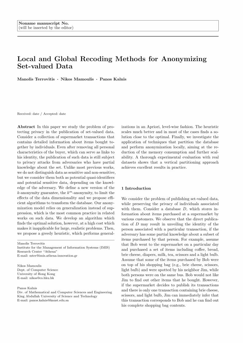
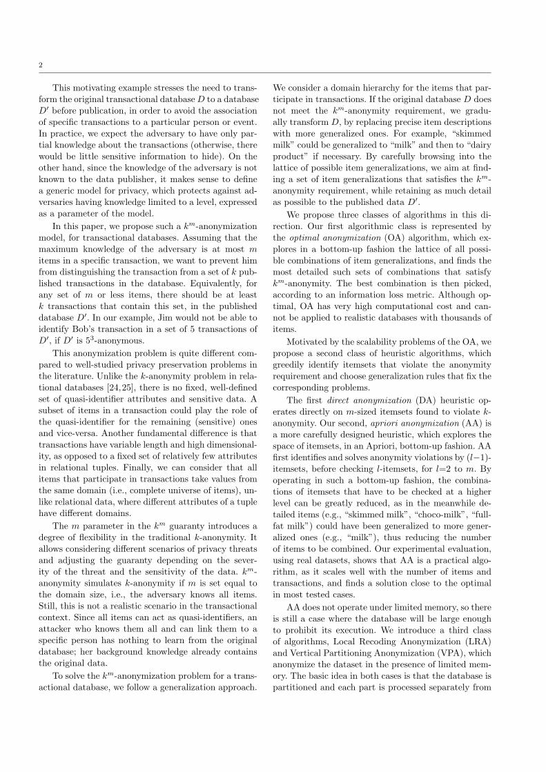
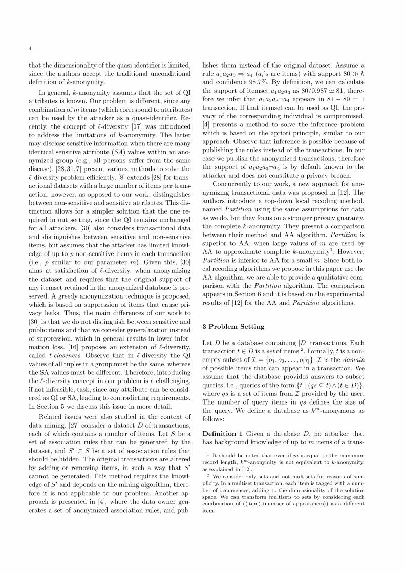
Formally, we use a generalization hierarchy for thecomplete domain I of items that may appear in a trans-
action. Such an exemplary hierarchy is shown in Figure
1. In this example we assume I = {a1, a2, b1, b2}, itemsa1, a2 can be generalized to A, items b1, b2 can be gen-
eralized to B, and the two classes A, B can be further
generalized to ALL.
A B
a1 a2 b1 b2
ALL
Fig. 1 Sample generalization hierarchy
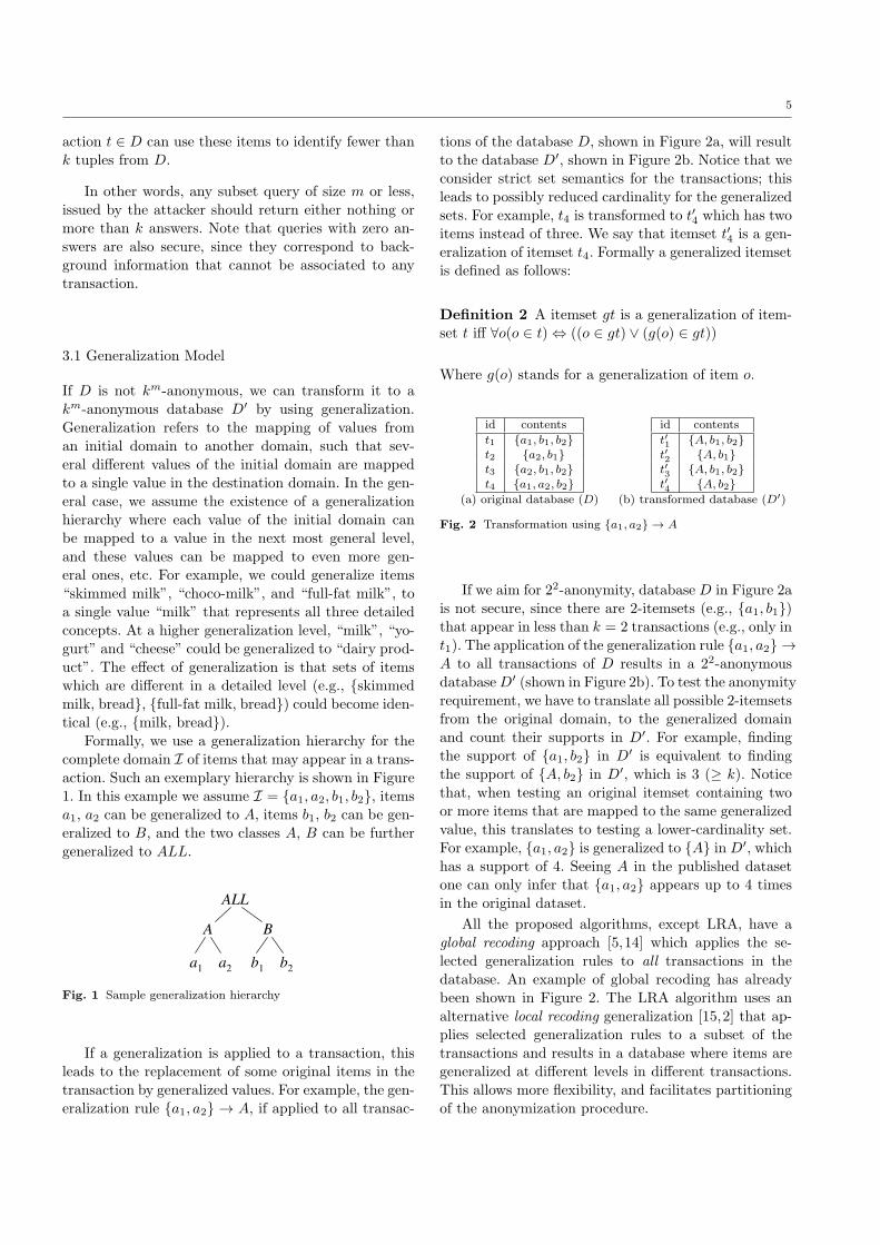
If a generalization is applied to a transaction, thisleads to the replacement of some original items in the
transaction by generalized values. For example, the gen-
eralization rule {a1, a2} → A, if applied to all transac-
tions of the database D, shown in Figure 2a, will result
to the database D′, shown in Figure 2b. Notice that weconsider strict set semantics for the transactions; this
leads to possibly reduced cardinality for the generalized
sets. For example, t4 is transformed to t′4 which has twoitems instead of three. We say that itemset t′4 is a gen-
eralization of itemset t4. Formally a generalized itemset
is defined as follows:
Definition 2 A itemset gt is a generalization of item-set t iff ∀o(o ∈ t) ⇔ ((o ∈ gt) ∨ (g(o) ∈ gt))
Where g(o) stands for a generalization of item o.
id contents
t1 {a1, b1, b2}
t2 {a2, b1}
t3 {a2, b1, b2}t4 {a1, a2, b2}
id contents
t′1
{A, b1, b2}
t′2
{A, b1}
t′3
{A, b1, b2}t′4
{A, b2}
(a) original database (D) (b) transformed database (D′)
Fig. 2 Transformation using {a1, a2} → A
If we aim for 22-anonymity, database D in Figure 2a
is not secure, since there are 2-itemsets (e.g., {a1, b1})that appear in less than k = 2 transactions (e.g., only in
t1). The application of the generalization rule {a1, a2} →
A to all transactions of D results in a 22-anonymousdatabaseD′ (shown in Figure 2b). To test the anonymity
requirement, we have to translate all possible 2-itemsets
from the original domain, to the generalized domainand count their supports in D′. For example, finding
the support of {a1, b2} in D′ is equivalent to finding
the support of {A, b2} in D′, which is 3 (≥ k). Notice
that, when testing an original itemset containing twoor more items that are mapped to the same generalized
value, this translates to testing a lower-cardinality set.
For example, {a1, a2} is generalized to {A} in D′, whichhas a support of 4. Seeing A in the published dataset
one can only infer that {a1, a2} appears up to 4 times
in the original dataset.
All the proposed algorithms, except LRA, have aglobal recoding approach [5,14] which applies the se-
lected generalization rules to all transactions in the
database. An example of global recoding has alreadybeen shown in Figure 2. The LRA algorithm uses an
alternative local recoding generalization [15,2] that ap-
plies selected generalization rules to a subset of the
transactions and results in a database where items aregeneralized at different levels in different transactions.
This allows more flexibility, and facilitates partitioning
of the anonymization procedure.
6
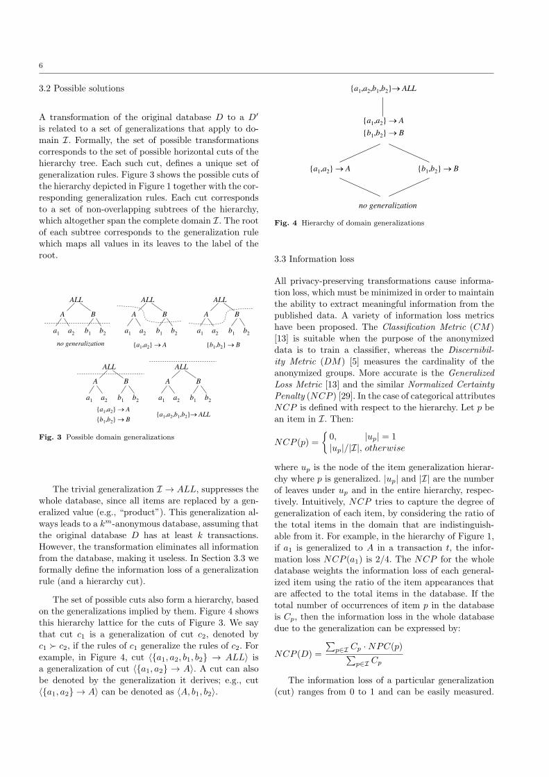
3.2 Possible solutions
A transformation of the original database D to a D′
is related to a set of generalizations that apply to do-
main I. Formally, the set of possible transformations
corresponds to the set of possible horizontal cuts of thehierarchy tree. Each such cut, defines a unique set of
generalization rules. Figure 3 shows the possible cuts of
the hierarchy depicted in Figure 1 together with the cor-responding generalization rules. Each cut corresponds
to a set of non-overlapping subtrees of the hierarchy,
which altogether span the complete domain I. The root
of each subtree corresponds to the generalization rulewhich maps all values in its leaves to the label of the
root.
A B
a1 a2 b1 b2
ALL
no generalization
A B
a1 a2 b1 b2
ALL
{a1,a2} A
A B
a1 a2 b1 b2
ALL
{b1,b2} B
A B
a1 a2 b1 b2
ALL
{a1,a2} A
{b1,b2} B
A B
a1 a2 b1 b2
ALL
{a1,a2,b1,b2} ALL
Fig. 3 Possible domain generalizations
The trivial generalization I → ALL, suppresses the
whole database, since all items are replaced by a gen-
eralized value (e.g., “product”). This generalization al-ways leads to a km-anonymous database, assuming that
the original database D has at least k transactions.
However, the transformation eliminates all information
from the database, making it useless. In Section 3.3 weformally define the information loss of a generalization
rule (and a hierarchy cut).
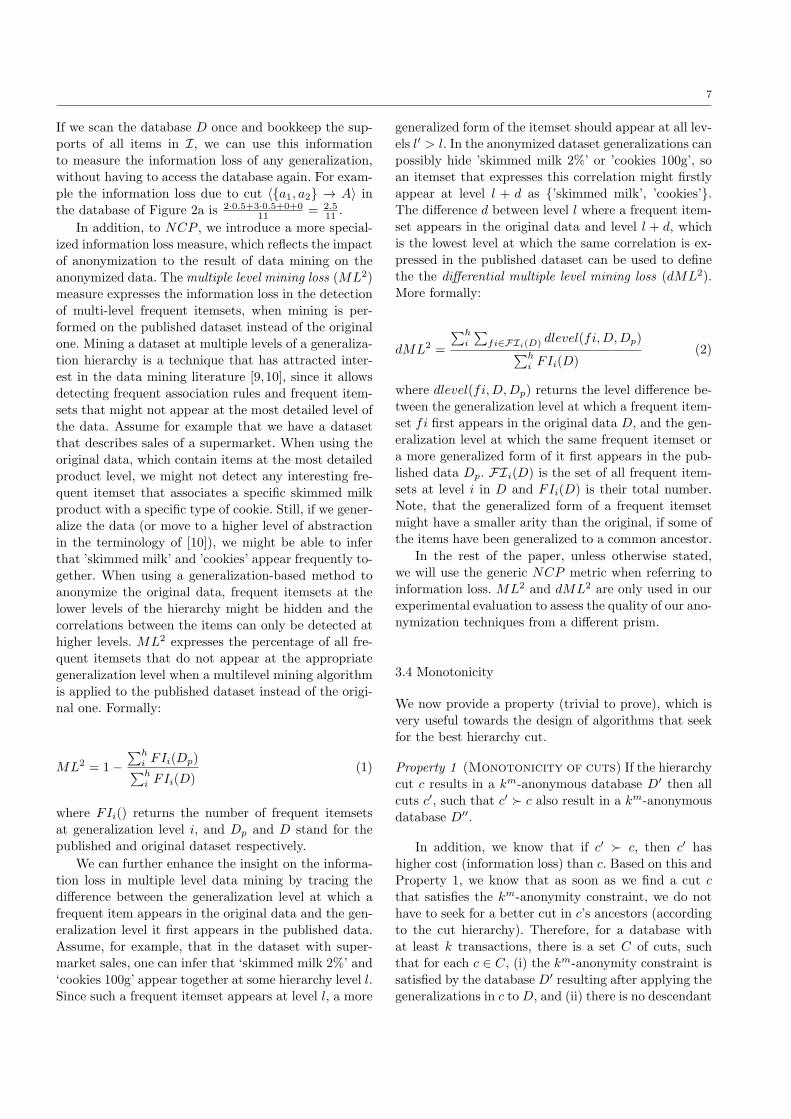
The set of possible cuts also form a hierarchy, based
on the generalizations implied by them. Figure 4 showsthis hierarchy lattice for the cuts of Figure 3. We say
that cut c1 is a generalization of cut c2, denoted by
c1 ≻ c2, if the rules of c1 generalize the rules of c2. For
example, in Figure 4, cut 〈{a1, a2, b1, b2} → ALL〉 isa generalization of cut 〈{a1, a2} → A〉. A cut can also
be denoted by the generalization it derives; e.g., cut
〈{a1, a2} → A〉 can be denoted as 〈A, b1, b2〉.
no generalization
{a1,a2} A {b1,b2} B
{a1,a2} A
{b1,b2} B
{a1,a2,b1,b2} ALL
Fig. 4 Hierarchy of domain generalizations
3.3 Information loss
All privacy-preserving transformations cause informa-
tion loss, which must be minimized in order to maintain
the ability to extract meaningful information from thepublished data. A variety of information loss metrics
have been proposed. The Classification Metric (CM)
[13] is suitable when the purpose of the anonymizeddata is to train a classifier, whereas the Discernibil-
ity Metric (DM) [5] measures the cardinality of the
anonymized groups. More accurate is the Generalized
Loss Metric [13] and the similar Normalized Certainty
Penalty (NCP ) [29]. In the case of categorical attributes
NCP is defined with respect to the hierarchy. Let p be
an item in I. Then:
NCP (p) =
{
0, |up| = 1
|up|/|I|, otherwise
where up is the node of the item generalization hierar-
chy where p is generalized. |up| and |I| are the number
of leaves under up and in the entire hierarchy, respec-
tively. Intuitively, NCP tries to capture the degree ofgeneralization of each item, by considering the ratio of
the total items in the domain that are indistinguish-
able from it. For example, in the hierarchy of Figure 1,if a1 is generalized to A in a transaction t, the infor-
mation loss NCP (a1) is 2/4. The NCP for the whole
database weights the information loss of each general-ized item using the ratio of the item appearances that
are affected to the total items in the database. If the
total number of occurrences of item p in the database
is Cp, then the information loss in the whole databasedue to the generalization can be expressed by:
NCP (D) =
∑
p∈I Cp ·NPC(p)∑
p∈I Cp
The information loss of a particular generalization
(cut) ranges from 0 to 1 and can be easily measured.
7
If we scan the database D once and bookkeep the sup-
ports of all items in I, we can use this informationto measure the information loss of any generalization,
without having to access the database again. For exam-
ple the information loss due to cut 〈{a1, a2} → A〉 inthe database of Figure 2a is 2·0.5+3·0.5+0+0
11 = 2.511 .
In addition, to NCP , we introduce a more special-
ized information loss measure, which reflects the impactof anonymization to the result of data mining on the
anonymized data. Themultiple level mining loss (ML2)
measure expresses the information loss in the detectionof multi-level frequent itemsets, when mining is per-
formed on the published dataset instead of the original
one. Mining a dataset at multiple levels of a generaliza-
tion hierarchy is a technique that has attracted inter-est in the data mining literature [9,10], since it allows
detecting frequent association rules and frequent item-
sets that might not appear at the most detailed level ofthe data. Assume for example that we have a dataset
that describes sales of a supermarket. When using the
original data, which contain items at the most detailedproduct level, we might not detect any interesting fre-
quent itemset that associates a specific skimmed milk
product with a specific type of cookie. Still, if we gener-
alize the data (or move to a higher level of abstractionin the terminology of [10]), we might be able to infer
that ’skimmed milk’ and ’cookies’ appear frequently to-
gether. When using a generalization-based method toanonymize the original data, frequent itemsets at the
lower levels of the hierarchy might be hidden and the
correlations between the items can only be detected athigher levels. ML2 expresses the percentage of all fre-
quent itemsets that do not appear at the appropriate
generalization level when a multilevel mining algorithm
is applied to the published dataset instead of the origi-nal one. Formally:
ML2 = 1−
∑hi FIi(Dp)
∑hi FIi(D)
(1)
where FIi() returns the number of frequent itemsets
at generalization level i, and Dp and D stand for thepublished and original dataset respectively.
We can further enhance the insight on the informa-
tion loss in multiple level data mining by tracing thedifference between the generalization level at which a
frequent item appears in the original data and the gen-
eralization level it first appears in the published data.
Assume, for example, that in the dataset with super-market sales, one can infer that ‘skimmed milk 2%’ and
‘cookies 100g’ appear together at some hierarchy level l.
Since such a frequent itemset appears at level l, a more
generalized form of the itemset should appear at all lev-
els l′ > l. In the anonymized dataset generalizations canpossibly hide ’skimmed milk 2%’ or ’cookies 100g’, so
an itemset that expresses this correlation might firstly
appear at level l + d as {’skimmed milk’, ’cookies’}.The difference d between level l where a frequent item-
set appears in the original data and level l + d, which
is the lowest level at which the same correlation is ex-pressed in the published dataset can be used to define
the the differential multiple level mining loss (dML2).
More formally:
dML2 =
∑hi
∑
fi∈FIi(D) dlevel(fi,D,Dp)∑h
i FIi(D)(2)
where dlevel(fi,D,Dp) returns the level difference be-tween the generalization level at which a frequent item-
set fi first appears in the original data D, and the gen-
eralization level at which the same frequent itemset ora more generalized form of it first appears in the pub-
lished data Dp. FIi(D) is the set of all frequent item-
sets at level i in D and FIi(D) is their total number.
Note, that the generalized form of a frequent itemsetmight have a smaller arity than the original, if some of
the items have been generalized to a common ancestor.
In the rest of the paper, unless otherwise stated,
we will use the generic NCP metric when referring to
information loss. ML2 and dML2 are only used in ourexperimental evaluation to assess the quality of our ano-
nymization techniques from a different prism.
3.4 Monotonicity
We now provide a property (trivial to prove), which is
very useful towards the design of algorithms that seek
for the best hierarchy cut.
Property 1 (Monotonicity of cuts) If the hierarchy
cut c results in a km-anonymous database D′ then all
cuts c′, such that c′ ≻ c also result in a km-anonymousdatabase D′′.
In addition, we know that if c′ ≻ c, then c′ has
higher cost (information loss) than c. Based on this and
Property 1, we know that as soon as we find a cut cthat satisfies the km-anonymity constraint, we do not
have to seek for a better cut in c’s ancestors (according
to the cut hierarchy). Therefore, for a database with
at least k transactions, there is a set C of cuts, suchthat for each c ∈ C, (i) the km-anonymity constraint is
satisfied by the database D′ resulting after applying the
generalizations in c toD, and (ii) there is no descendant
8
of c in the hierarchy of cuts, for which condition (i) is
true.
We call C the set of minimal cuts. The ultimate
objective of an anonymization algorithm is to find oneof the optimal cuts copt in C, which incurs the minimum
information loss by transforming D to D′. In the next
section, we propose a set of algorithms that operate inthis direction.
4 Anonymization techniques
The aim of the anonymization procedure is to detect
the cut in the generalization hierarchy that prevents
any privacy breach and at the same time introduces
the minimum information loss. We first apply a system-atic search algorithm, which seeks for the optimal cut,
operating in a fashion similar to Incognito [14]. This
algorithm suffers from the dimensionality of the gener-alization space and becomes unacceptably slow for large
item domains I and generalization hierarchies. To deal
with this problem we propose heuristics, which insteadof searching the whole generalization space, they detect
the privacy breaches and search for local solutions. The
result of these methods is a cut on the generalization hi-
erarchy that guarantees km-anonymity, while incurringlow information loss. Before presenting these methods
in detail, we present a data structure, which is used by
all algorithms to accelerate the search of itemset sup-ports.
4.1 The count-tree
An important issue in determining whether applying a
generalization to D can provide km-anonymity or not,
is to be able to count efficiently the supports of all thecombinations of m items that appear in the database.
Moreover, if we want to avoid scanning the database
each time we need to check a generalization, we must
keep track of how each possible generalization can affectthe database. To achieve both goals we construct a data
structure that keeps track not only of all combinations
of m items from I, but also all combinations of itemsfrom the generalized databases that could be generated
by applying any of the possible cuts in the hierarchy
tree. The information we trace is the support of eachcombination of m items from I, be detailed or gener-
alized. Note that, if we keep track of the support of all
combinations of size m of items from I, it is enough to
establish whether there is a privacy breach or not byshorter itemsets. This follows from the Apriori princi-
ple that states that the support of an itemset is always
less or equal to the support of its subsets.
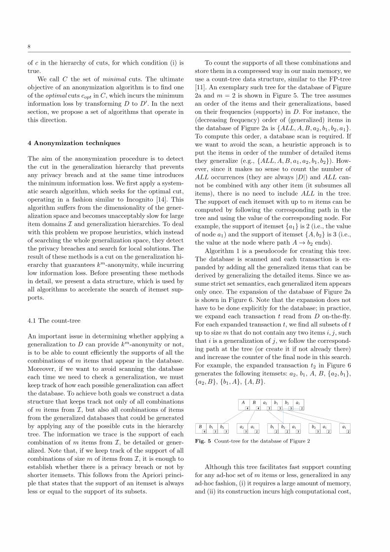
To count the supports of all these combinations and
store them in a compressed way in our main memory, weuse a count-tree data structure, similar to the FP-tree
[11]. An exemplary such tree for the database of Figure
2a and m = 2 is shown in Figure 5. The tree assumesan order of the items and their generalizations, based
on their frequencies (supports) in D. For instance, the
(decreasing frequency) order of (generalized) items inthe database of Figure 2a is {ALL,A,B, a2, b1, b2, a1}.
To compute this order, a database scan is required. If
we want to avoid the scan, a heuristic approach is to
put the items in order of the number of detailed itemsthey generalize (e.g., {ALL,A,B, a1, a2, b1, b2}). How-
ever, since it makes no sense to count the number of
ALL occurrences (they are always |D|) and ALL can-not be combined with any other item (it subsumes all
items), there is no need to include ALL in the tree.
The support of each itemset with up to m items can becomputed by following the corresponding path in the
tree and using the value of the corresponding node. For
example, the support of itemset {a1} is 2 (i.e., the value
of node a1) and the support of itemset {A, b2} is 3 (i.e.,the value at the node where path A → b2 ends).
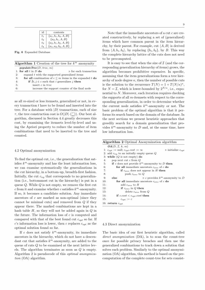
Algorithm 1 is a pseudocode for creating this tree.
The database is scanned and each transaction is ex-
panded by adding all the generalized items that can bederived by generalizing the detailed items. Since we as-
sume strict set semantics, each generalized item appears
only once. The expansion of the database of Figure 2ais shown in Figure 6. Note that the expansion does not
have to be done explicitly for the database; in practice,
we expand each transaction t read from D on-the-fly.For each expanded transaction t, we find all subsets of t
up to size m that do not contain any two items i, j, such
that i is a generalization of j, we follow the correspond-
ing path at the tree (or create it if not already there)and increase the counter of the final node in this search.
For example, the expanded transaction t2 in Figure 6
generates the following itemsets: a2, b1, A, B, {a2, b1},{a2, B}, {b1, A}, {A,B}.
A
b2b12 2
a13
a23
a12
4
B4
a2
3
b1
3
b2
3
a1
2
b1B4 3
b23
b23
a12
a12
Fig. 5 Count-tree for the database of Figure 2
Although this tree facilitates fast support countingfor any ad-hoc set of m items or less, generalized in any
ad-hoc fashion, (i) it requires a large amount of memory,
and (ii) its construction incurs high computational cost,
9
id contents
t1 {a1, b1, b2, A,B}t2 {a2, b1, A,B}
t3 {a2, b1, b2, A,B}
t4 {a1, a2, b2, A,B}
Fig. 6 Expanded Database
Algorithm 1 Creation of the tree for km anonymitypopulateTree(D, tree, m)
1: for all t in D do ⊲ for each transaction2: expand t with the supported generalized items3: for all combination of c ≤ m items in the expanded t do
4: if ∄i, j ∈ c such that i generalizes j then
5: insert c in tree
6: increase the support counter of the final node
as all m-sized or less itemsets, generalized or not, in ev-ery transaction t have to be found and inserted into the
tree. For a database with |D| transactions, each of size
τ , the tree construction cost is O(|D|·(
τm
)
). Our best al-gorithm, discussed in Section 4.4 greatly decreases this
cost, by examining the itemsets level-by-level and us-
ing the Apriori property to reduce the number of item
combinations that need to be inserted to the tree andcounted.
4.2 Optimal anonymization
To find the optimal cut, i.e., the generalization that sat-
isfies km-anonymity and has the least information loss,
we can examine systematically the generalizations inthe cut hierarchy, in a bottom-up, breadth-first fashion.
Initially, the cut cng that corresponds to no generaliza-
tion (i.e., bottommost cut in the hierarchy) is put in aqueue Q. While Q is not empty, we remove the first cut
c from it and examine whether c satisfies km-anonymity.
If so, it becomes a candidate solution. Any immediateancestors of c are marked as non-optimal (since they
cannot be minimal cuts) and removed from Q if they
appear there. The marked combinations are kept in a
hash table H, so they will not be added again in Q inthe future. The information loss of c is computed and
compared with that of the best found cut copt so far. If
c’s information loss is lower, then c replaces copt as theoptimal solution found so far.
If c does not satisfy km-anonymity, its immediate
ancestors in the hierarchy, which do not have a descen-
dant cut that satisfies km-anonymity, are added to the
queue of cuts Q to be examined at the next lattice lev-els. The algorithm terminates as soon as Q is empty.
Algorithm 2 is pseudocode of this optimal anonymiza-
tion (OA) algorithm.
Note that the immediate ancestors of a cut c are cre-
ated constructively, by replacing a set of (generalized)items which have common parent in the item hierar-
chy, by their parent. For example, cut 〈A,B〉 is derived
from 〈A, b1, b2〉, by replacing {b1, b2}, by B. This waythe complete hierarchy lattice of the cuts does not need
to be precomputed.
It is easy to see that when the size of I (and the cor-
responding generalization hierarchy of items) grows, the
algorithm becomes prohibitive expensive. In specific,assuming that the item generalizations form a tree hier-
archy of node degree κ, then the number of possible cuts
is the solution to the recurrence T (N) = 1 + T (N/κ)κ,for N = I, which is lower-bounded by 2N/κ, i.e., expo-
nential to N . Moreover, each iteration requires checking
the supports of all m-itemsets with respect to the corre-
sponding generalization, in order to determine whetherthe current node satisfies km-anonymity or not. The
basic problem of the optimal algorithm is that it per-
forms its search based on the domain of the database. Inthe next sections we present heuristic approaches that
greedily search for a domain generalization that pro-
vides km-anonymity to D and, at the same time, havelow information loss.
Algorithm 2 Optimal Anonymization algorithmOA(D, I, k, m)
1: copt := null; copt.cost := ∞ ⊲ initialize copt2: add cng to an initially empty queue Q
3: while (Q is not empty) do
4: pop next cut c from Q
5: if c does not provide km-anonymity to D then
6: for all immediate ancestors cans of c do
7: if cans does not appear in H then
8: push cans to Q
9: else ⊲ c provides km-anonymity to D
10: for all immediate ancestors cans of c do
11: add cans to H
12: if cans in Q then
13: delete cans from Q
14: if c.cost < copt.cost then
15: copt := c
16: return copt
4.3 Direct anonymization
The basic idea of our first heuristic algorithm, called
direct anonymization (DA), is to scan the count-tree
once for possible privacy breaches and then use the
generalized combinations to track down a solution thatsolves each problem. Similarly to the optimal anonymi-
zation (OA) algorithm, this method is based on the pre-
computation of the complete count-tree for sets consist-
10
ing of up to m (generalized) itemsets. DA scans the tree
to detect m-sized paths that have support less than k.For each such path, it generates all the possible general-
izations, in a level-wise fashion, similar to the optimal
anonymization (OA) algorithm, and finds among theminimal cuts that solve the specific problem, the one
which incurs the lowest information loss.
Specifically, once the count-tree has been created,
DA initializes the output generalization cout, as the
bottommost cut of the lattice (i.e., no generalization).
It then performs a preorder (i.e., depth-first) traversalof the tree. For every node encountered (correspond-
ing to a prefix), if the item corresponding to that node
has already been generalized in cout, DA backtracks,as all complete m-sized paths passing from there cor-
respond to itemsets that will not appear in the gener-
alized database based on cout (and therefore their sup-ports need not be checked). For example, if the algo-
rithm reaches the prefix path B-a2 the algorithm will
examine its descendants only if B and a2 have not al-
ready been further generalized. Note that this path willbe examined even if the items b1 and b2 have not been
generalized to item B. Due to the monotonicity of the
problem, we know that ifB-a2 leads to a privacy breach,then it is certain that b1-a2 and b1-a1 lead to privacy
breach. Addressing the problem for the path B-a2 al-
lows the algorithm to avoid examining the other twopaths. During the traversal, if a leaf node is encoun-
tered, corresponding to an m-itemset J (with or with-
out generalized components), DA checks whether the
corresponding count J.count is less than k. In this case,DA seeks for a cut that (i) includes the current general-
ization rules in cout and (ii) makes the support of J at
least k. This is done in a similar fashion as in OA, butrestricted only to the generalization rules that affect
the items of J . For example, if J = {a1, a2}, only gen-
eralizations {a1, a2} → A and {a1, a2, b1, b2} → ALLwill be tested. In addition, from the possible set of cuts
that solve the anonymity breach with respect to J , the
one with the minimum information loss is selected (e.g.,
{a1, a2} → A). The generalization rules included in thiscut are then committed (i.e., added to cout) and any
path of the count-tree which contains items at a more
detailed level (e.g., a1 and a2) than cout is pruned fromsearch subsequently. Algorithm 3 is a high-level pseu-
docode for DA.
As an example, assume that we want to make the
database of Figure 2a 22-anonymous. First, DA con-
structs the count-tree, shown in Figure 5. cout is ini-
tialized to contain no generalization rules. Then DAperforms a preorder traversal of the tree. The first leaf
node encountered with a support less than 2 is a1 (i.e.,
path a2-a1). The only minimal cut that makes {a2, a1}
Algorithm 3 Direct AnonymizationDA (D, I, k, m)
1: scan D and create count-tree2: initialize cout3: for each node v in preorder count-tree traversal do4: if the item of v has been generalized in cout then
5: backtrack6: if v is a leaf node and v.count < k then
7: J := itemset corresponding to v
8: find generalization of items in J that make J k-anonymous
9: merge generalization rules with cout10: backtrack to longest prefix of path J , wherein no item
has been generalized in cout
11: return cout
k-anonymous is {a1, a2} → A, therefore the correspond-ing rule is added to cout. DA then backtracks to the
next entry of the root (i.e., b1) since any other path
starting from a2 would be invalid based on cout (i.e.,its corresponding itemset could not appear in the gen-
eralized database according to cout). The next path to
check would be b1-b2, which is found non-problematic.DA then examines b1-a1, but backtracks immediately,
since a1 has already been generalized in cout. The same
happens with b2-a1 and the algorithm terminates with
output the cut 〈{a1, a2} → A〉.
The main problem of DA is that it has significant
memory requirements and computational cost, because
it generates and scans the complete count-tree for all
m-sized combinations, whereas it might be evident fromsmaller-sized combinations that several generalizations
are necessary. This observation leads to our next algo-
rithm.
4.4 Apriori-based anonymization
Our second heuristic algorithm is based on the apri-
ori principle; if an itemset J of size i causes a privacy
breach, then each superset of J causes a privacy breach.Thus, it is possible to perform the necessary gener-
alizations progressively. First we examine the privacy
breaches that might be feasible if the adversary knowsonly one item from each transaction, then two and so
forth till we examine privacy threats from an adversary
that knows m items.
The benefit of this algorithm is that we can exploitthe generalizations performed in step i, to reduce the
search space at step i+1. The algorithm practically it-
erates the direct algorithm for combinations of sizes
i = {1, . . . ,m}. At each iteration i the database isscanned and the count-tree is populated with itemsets
of length i. The population of the tree takes into ac-
count the current set of generalization rules cout, thus
11
significantly limiting the combinations of items to be
inserted to the tree. In other words, in the count-treeat level i, i-itemsets which contain items already gen-
eralized in cout are disregarded. Algorithm 4 is a pseu-
docode for this apriori-based anonymization (AA) tech-nique.
Algorithm 4 Apriori-based AnonymizationAA (D, I, k, m)
1: initialize cout2: for i := 1 to m do ⊲ for each itemset length3: initialize a new count-tree4: for all t ∈ D do ⊲ scan D
5: extend t according to cout6: add all i-subsets of extended t to count-tree7: run DA on count-tree for m = i and update cout
Note that in Line 5 of the algorithm, the current
transaction t is first expanded to include all item gen-
eralizations (as discussed in Section 4.1), and then allitems that are generalized in cout are removed from the
extended t. For example, assume that after the first loop
(i.e., after examining 1-itemsets), cout = 〈{a1, a2} →A〉. In the second loop (i=2), t4 = {a1, a2, b2} is first
expanded to t4 = {a1, a2, b2, A,B} and then reduced
to t4 = {b2, A,B}, since items a1 and a2 have alreadybeen generalized in cout. Therefore, the 2-itemsets to
be inserted to the count-tree due to this transaction
are significantly decreased.
The size of the tree itself is accordingly decreasedsince combinations that include detailed items (based
on cout) do not appear in the tree. As the algorithm
progresses to larger values of i, the effect of pruned de-tailed items (due to cout) increases because (i) more
rules are expected to be in cout (ii) the total num-
ber of i-combinations increases exponentially with i.Overall, although D is scanned by AA m times, the
computational cost of the algorithm is expected to be
much lower compared to DA (and OA). The three al-
gorithms are compared in the Section 6 with respect to(i) their computational cost and (ii) the quality of the
km-anonymization they achieve.
4.5 Local recoding
Local recoding has been used in traditional k-anonymityand ℓ-diversity problems. It relies on generalizing ex-
isting values, but unlike global recoding, where all or
none of the occurrences of an item o are replaced with
a more generalized item g, the replacement here can bepartial; only some occurrences of o are replaced with
g. Local recoding can potentially reduce the distortion
in the data, by replacing o only in a neighborhood of
the data. The detection of a suitable neighborhood is
hard to achieve in a multidimensional setting, where itis hard to detect data with similar values. Still, by using
local recoding we can process the database locally, i.e.,
only a part of the dataset is processed at each moment.Even if the information loss is greater compared to the
AA algorithm, there is better potential for scalability,
since the database can be partitioned according to theavailable memory.
As we discussed, the memory requirements for the
count tree that is used by the anonymization heuristicscan be significant. Algorithms like AA algorithm reduce
the count tree’s size, by progressively computing the
required generalizations for publishing a ki-anonymous,i = 1, . . . ,m, database. Nevertheless, even AA does not
provide effective control over the memory requirements
of the anonymization procedure. If the database and the
items domain are large, AA might have requirementsthat exceed the available memory.
The basic idea in the local recoding anonymization(LRA) algorithm is to partition the original dataset,
and anonymize each part independently, using one of
the proposed algorithms (e.g., AA). It is easy to see
that if all parts of the database are km-anonymous,then the database will be km-anonymous, too. If a part
is km anonymous, then each m-sized combination of
items would appear at least k times in this part. Unify-ing this part with other database parts, cannot reduce
the number of appearances of any m-sized combination.
Hence, if all parts are km-anonymous, i.e. all m-sizedcombinations of items appear at least k times in each
part, then the whole anonymized database (which is
their union) every m-sized combination will appear at
least k-times. By splitting the database into the desirednumber of chunks, we can implicitly define the memory
requirements.
Local anonymization can affect the data quality in
two, conflicting, ways. On the one hand, it fixes a prob-
lem locally, thus it does not distort the whole database
in order to tackle a privacy threat. For example, assumethat we split the database in two parts D1 and D2 and
that items o1, o2, which are both specializations of item
g, appear 2 times each in D1 and 0 and 4 times in D2,respectively. With k = 3, local anonymization would
generalize both o1 and o2 to g in D1, and it would leave
o2 intact in D2. On the other hand, the algorithm de-cides whether there is a privacy breach at a local level,
and fails to see whether this problem holds when the
whole database is considered. For example, if we decide
to split database D to two parts D1 and D2, a combina-tion c which appears 2k− 2 times (k > 2) and does not
pose any threat for the user privacy, might only appear
k − 1 times in both D1 and D2, thus causing general-
12
izations that could have been avoided. Intuitively, we
could mitigate this negative effect by mustering all theoccurrences of any item combination in a single chunk of
D. This is far from trivial to achieve, since each record
supports numerous different combinations. Splitting thedatabase in a way that we get both the desired number
of chunks and completely different item combinations
at each chunk is usually impossible. In the following wepropose a heuristic that tries to split the database into
the desired number of chunks, by minimizing the over-
lap of the sets of different combinations of items that
appear in each chunk.
Decimal Gray Binary
0 000 000
1 001 001
2 011 010
3 010 011
4 110 100
5 111 101
6 101 110
7 100 111
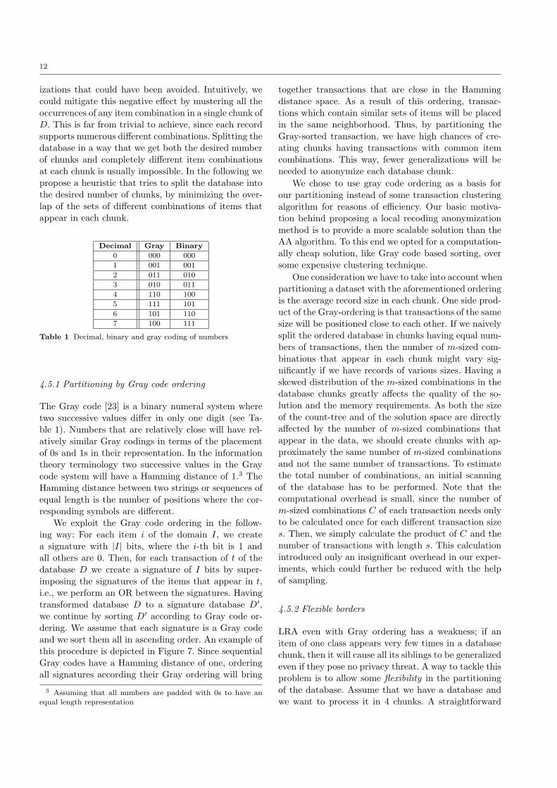
Table 1 Decimal, binary and gray coding of numbers
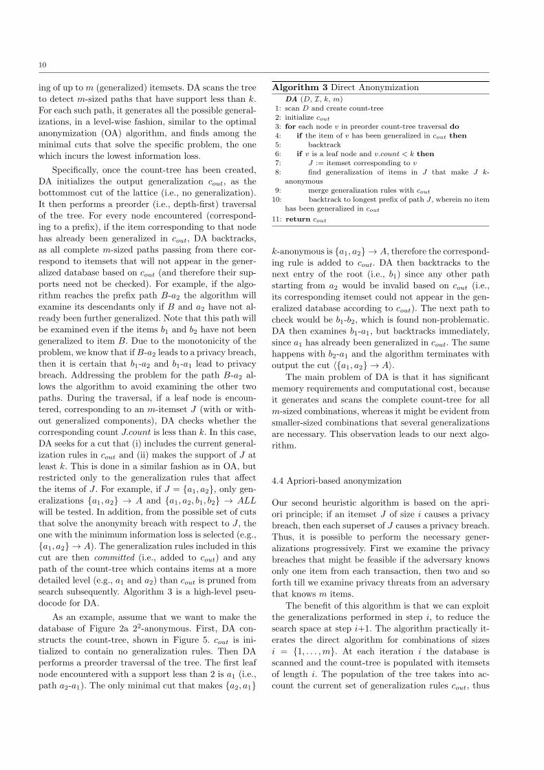
4.5.1 Partitioning by Gray code ordering
The Gray code [23] is a binary numeral system where
two successive values differ in only one digit (see Ta-
ble 1). Numbers that are relatively close will have rel-atively similar Gray codings in terms of the placement
of 0s and 1s in their representation. In the information
theory terminology two successive values in the Graycode system will have a Hamming distance of 1.3 The
Hamming distance between two strings or sequences of
equal length is the number of positions where the cor-
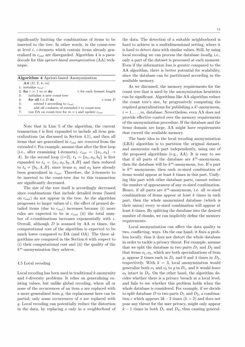
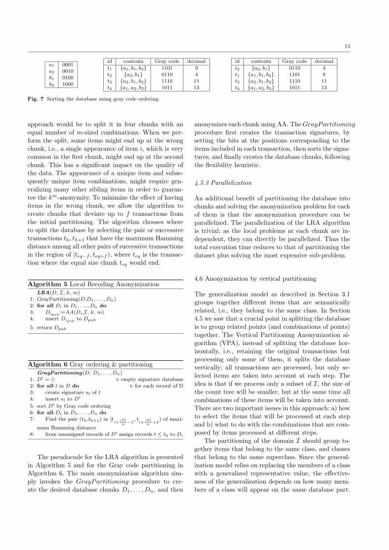
responding symbols are different.We exploit the Gray code ordering in the follow-
ing way: For each item i of the domain I, we create
a signature with |I| bits, where the i-th bit is 1 andall others are 0. Then, for each transaction of t of the
database D we create a signature of I bits by super-
imposing the signatures of the items that appear in t,i.e., we perform an OR between the signatures. Having
transformed database D to a signature database D′,
we continue by sorting D′ according to Gray code or-
dering. We assume that each signature is a Gray codeand we sort them all in ascending order. An example of
this procedure is depicted in Figure 7. Since sequential
Gray codes have a Hamming distance of one, orderingall signatures according their Gray ordering will bring
3 Assuming that all numbers are padded with 0s to have an
equal length representation
together transactions that are close in the Hamming
distance space. As a result of this ordering, transac-tions which contain similar sets of items will be placed
in the same neighborhood. Thus, by partitioning the
Gray-sorted transaction, we have high chances of cre-ating chunks having transactions with common item
combinations. This way, fewer generalizations will be
needed to anonymize each database chunk.
We chose to use gray code ordering as a basis forour partitioning instead of some transaction clustering
algorithm for reasons of efficiency. Our basic motiva-
tion behind proposing a local recoding anonymizationmethod is to provide a more scalable solution than the
AA algorithm. To this end we opted for a computation-
ally cheap solution, like Gray code based sorting, oversome expensive clustering technique.
One consideration we have to take into account when
partitioning a dataset with the aforementioned ordering
is the average record size in each chunk. One side prod-uct of the Gray-ordering is that transactions of the same
size will be positioned close to each other. If we naively
split the ordered database in chunks having equal num-bers of transactions, then the number of m-sized com-
binations that appear in each chunk might vary sig-
nificantly if we have records of various sizes. Having a
skewed distribution of the m-sized combinations in thedatabase chunks greatly affects the quality of the so-
lution and the memory requirements. As both the size
of the count-tree and of the solution space are directlyaffected by the number of m-sized combinations that
appear in the data, we should create chunks with ap-
proximately the same number of m-sized combinationsand not the same number of transactions. To estimate
the total number of combinations, an initial scanning
of the database has to be performed. Note that the
computational overhead is small, since the number ofm-sized combinations C of each transaction needs only
to be calculated once for each different transaction size
s. Then, we simply calculate the product of C and thenumber of transactions with length s. This calculation
introduced only an insignificant overhead in our exper-
iments, which could further be reduced with the helpof sampling.
4.5.2 Flexible borders
LRA even with Gray ordering has a weakness; if an
item of one class appears very few times in a database
chunk, then it will cause all its siblings to be generalized
even if they pose no privacy threat. A way to tackle thisproblem is to allow some flexibility in the partitioning
of the database. Assume that we have a database and
we want to process it in 4 chunks. A straightforward
13
a1 0001
a2 0010
b1 0100b2 1000
id contents Gray code decimal
t1 {a1, b1, b2} 1101 9t2 {a2, b1} 0110 4
t3 {a2, b1, b2} 1110 11
t4 {a1, a2, b2} 1011 13
id contents Gray code decimal
t2 {a2, b1} 0110 4t1 {a1, b1, b2} 1101 9
t3 {a2, b1, b2} 1110 11
t4 {a1, a2, b2} 1011 13
Fig. 7 Sorting the database using gray code ordering
approach would be to split it in four chunks with an
equal number of m-sized combinations. When we per-form the split, some items might end up at the wrong
chunk, i.e., a single appearance of item i, which is very
common in the first chunk, might end up at the secondchunk. This has a significant impact on the quality of
the data. The appearance of a unique item and subse-
quently unique item combinations, might require gen-eralizing many other sibling items in order to guaran-
tee the km-anonymity. To minimize the effect of having
items in the wrong chunk, we allow the algorithm to
create chunks that deviate up to f transactions fromthe initial partitioning. The algorithm chooses where
to split the database by selecting the pair or successive
transactions th, th+1 that have the maximum Hammingdistance among all other pairs of successive transactions
in the region of [teq−f , teq+f ), where teq is the transac-
tion where the equal size chunk teq would end.
Algorithm 5 Local Recoding AnonymizationLRA(D, I, k, m)
1: GrayPartitioning(D,D1, . . . , Dn)
2: for all Di in D1, . . . , Dn do
3: Dipub:=AA(Di,I, k, m)
4: insert Dipubto Dpub
5: return Dpub
Algorithm 6 Gray ordering & partitioningGrayPartitioning(D, D1, . . . , Dn)
1: D′ = ⊘ ⊲ empty signature database2: for all t in D do ⊲ for each record of D3: create signature st of t
4: insert st to D′
5: sort D′ by Gray code ordering
6: for all Di in D1, . . . , Dn do
7: Find the pair (th,th+1) in [ti×
|D|n
−f, t
i×|D|n
+f) of maxi-
mum Hamming distance8: from unassigned records of D′ assign records t ≤ th to Di
The pseudocode for the LRA algorithm is presented
in Algorithm 5 and for the Gray code partitioning inAlgorithm 6. The main anonymization algorithm sim-
ply invokes the GrayPartitioning procedure to cre-
ate the desired database chunks D1, . . . , Dn, and then
anonymizes each chunk using AA. TheGrayPartitioning
procedure first creates the transaction signatures, bysetting the bits at the positions corresponding to the
items included in each transaction, then sorts the signa-
tures, and finally creates the database chunks, followingthe flexibility heuristic.
4.5.3 Parallelization
An additional benefit of partitioning the database intochunks and solving the anonymization problem for each
of them is that the anonymization procedure can be
parallelized. The parallelization of the LRA algorithmis trivial; as the local problems at each chunk are in-
dependent, they can directly be parallelized. Thus the
total execution time reduces to that of partitioning the
dataset plus solving the most expensive sub-problem.
4.6 Anonymization by vertical partitioning
The generalization model as described in Section 3.1
groups together different items that are semantically
related, i.e., they belong to the same class. In Section4.5 we saw that a crucial point in splitting the database
is to group related points (and combinations of points)
together. The Vertical Partitioning Anonymization al-
gorithm (VPA), instead of splitting the database hor-izontally, i.e., retaining the original transactions but
processing only some of them, it splits the database
vertically; all transactions are processed, but only se-lected items are taken into account at each step. The
idea is that if we process only a subset of I, the size of
the count tree will be smaller, but at the same time allcombinations of these items will be taken into account.
There are two important issues in this approach: a) how
to select the items that will be processed at each step
and b) what to do with the combinations that are com-posed by items processed at different steps.
The partitioning of the domain I should group to-
gether items that belong to the same class, and classes
that belong to the same superclass. Since the general-
ization model relies on replacing the members of a classwith a generalized representative value, the effective-
ness of the generalization depends on how many mem-
bers of a class will appear on the same database part.
14
Independently of the original item and class identifiers,
it is possible to sort I in such a way that each classwill contain a contiguous region of items in the order of
I as depicted in Figure 8. For reasons of simplicity we
assume that I is sorted this way, so that we can eas-ily split the domain in the desired number of regions.
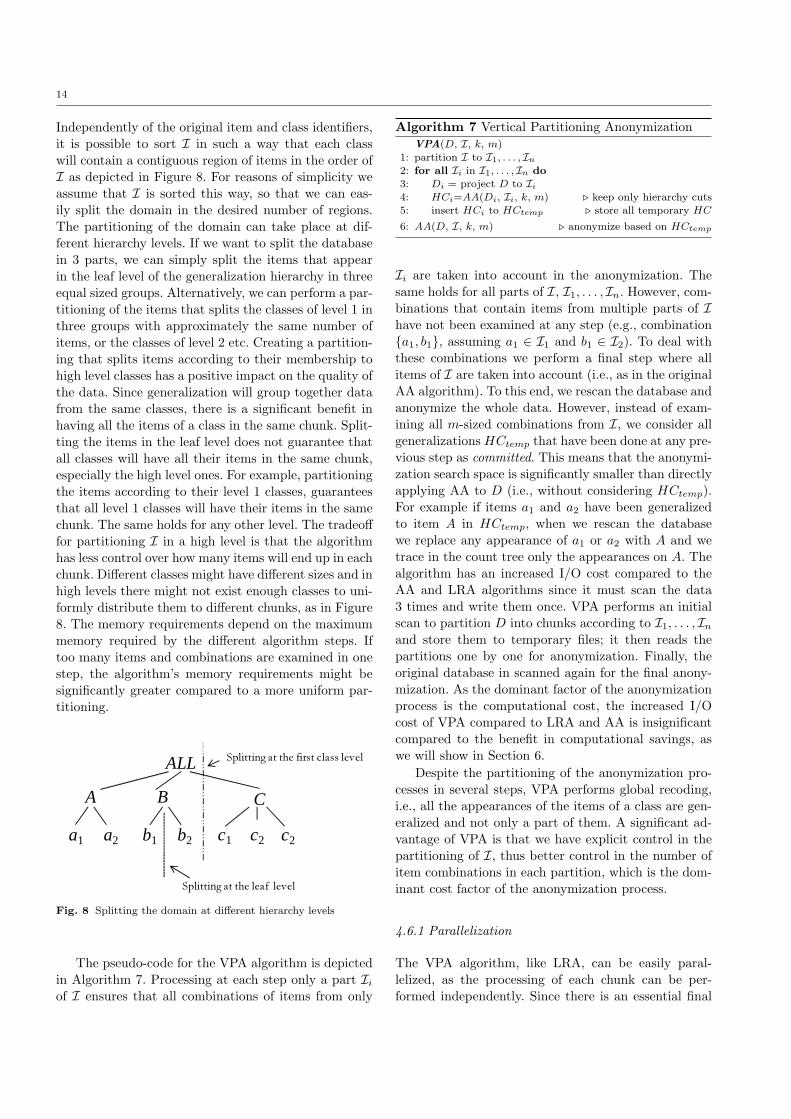
The partitioning of the domain can take place at dif-
ferent hierarchy levels. If we want to split the databasein 3 parts, we can simply split the items that appear
in the leaf level of the generalization hierarchy in three
equal sized groups. Alternatively, we can perform a par-
titioning of the items that splits the classes of level 1 inthree groups with approximately the same number of
items, or the classes of level 2 etc. Creating a partition-
ing that splits items according to their membership tohigh level classes has a positive impact on the quality of
the data. Since generalization will group together data
from the same classes, there is a significant benefit inhaving all the items of a class in the same chunk. Split-
ting the items in the leaf level does not guarantee that
all classes will have all their items in the same chunk,
especially the high level ones. For example, partitioningthe items according to their level 1 classes, guarantees
that all level 1 classes will have their items in the same
chunk. The same holds for any other level. The tradeofffor partitioning I in a high level is that the algorithm
has less control over how many items will end up in each
chunk. Different classes might have different sizes and inhigh levels there might not exist enough classes to uni-
formly distribute them to different chunks, as in Figure
8. The memory requirements depend on the maximum
memory required by the different algorithm steps. Iftoo many items and combinations are examined in one
step, the algorithm’s memory requirements might be
significantly greater compared to a more uniform par-titioning.
A B
a1 a2 b1 b2
ALL
C
c1 c2 c2
Splitting at the first class level
Splitting at the leaf levelFig. 8 Splitting the domain at different hierarchy levels
The pseudo-code for the VPA algorithm is depicted
in Algorithm 7. Processing at each step only a part Iiof I ensures that all combinations of items from only
Algorithm 7 Vertical Partitioning AnonymizationVPA(D, I, k, m)
1: partition I to I1, . . . , In2: for all Ii in I1, . . . , In do
3: Di = project D to Ii4: HCi=AA(Di, Ii, k, m) ⊲ keep only hierarchy cuts
5: insert HCi to HCtemp ⊲ store all temporary HC
6: AA(D, I, k, m) ⊲ anonymize based on HCtemp
Ii are taken into account in the anonymization. The
same holds for all parts of I, I1, . . . , In. However, com-binations that contain items from multiple parts of I
have not been examined at any step (e.g., combination
{a1, b1}, assuming a1 ∈ I1 and b1 ∈ I2). To deal with
these combinations we perform a final step where allitems of I are taken into account (i.e., as in the original
AA algorithm). To this end, we rescan the database and
anonymize the whole data. However, instead of exam-ining all m-sized combinations from I, we consider all
generalizationsHCtemp that have been done at any pre-
vious step as committed. This means that the anonymi-zation search space is significantly smaller than directly
applying AA to D (i.e., without considering HCtemp).
For example if items a1 and a2 have been generalized
to item A in HCtemp, when we rescan the databasewe replace any appearance of a1 or a2 with A and we
trace in the count tree only the appearances on A. The
algorithm has an increased I/O cost compared to theAA and LRA algorithms since it must scan the data
3 times and write them once. VPA performs an initial
scan to partition D into chunks according to I1, . . . , Inand store them to temporary files; it then reads the
partitions one by one for anonymization. Finally, the
original database in scanned again for the final anony-
mization. As the dominant factor of the anonymizationprocess is the computational cost, the increased I/O
cost of VPA compared to LRA and AA is insignificant
compared to the benefit in computational savings, aswe will show in Section 6.
Despite the partitioning of the anonymization pro-
cesses in several steps, VPA performs global recoding,i.e., all the appearances of the items of a class are gen-
eralized and not only a part of them. A significant ad-
vantage of VPA is that we have explicit control in the
partitioning of I, thus better control in the number ofitem combinations in each partition, which is the dom-
inant cost factor of the anonymization process.
4.6.1 Parallelization
The VPA algorithm, like LRA, can be easily paral-
lelized, as the processing of each chunk can be per-
formed independently. Since there is an essential final
15
pass over the whole database, the cost is determined
by the two database scans (one in the beginning for thedata partitioning and the final pass in the end) plus the
cost of anonymizing the most expensive partition.
5 Negative knowledge and ℓ-diversity
In this section, we discuss the impact of negative knowl-edge in k-anonymity. In addition, we outline the reasons
that make the concept of ℓ-diversity hard to apply in
our privacy problem and provide an ℓ-diversity defini-tion for cases where such a concept can be applied.
5.1 Negative knowledge
An important issue in privacy preservation is the treat-
ment of negative knowledge: the fact that an attacker
knows that a record does not contain a certain item.This problem is more evident in multidimensional data,
since in relational data nulls in quasi identifiers are usu-
ally treated as all other values. Negative knowledge act-ing as an inference channel for guessing sensitive values
is studied in [4]: knowing that a value does not exist in
a record can be exploited to breach privacy in several
cases. Negative knowledge can be used in the contextof this paper to isolate fewer than k-tuples for a given
combination ofm or fewer items; still, we opted to focus
on positive knowledge for three reasons:
1. Taking into account negative knowledge in a tradi-
tional privacy guaranty, like k-anonymity, will lead
to extensive information loss due to the curse of di-mensionality [1]. Forfeiting negative knowledge was
one of the mechanisms we used to reduce this cost.
We believe it offers a good trade-off since nega-tive knowledge is fairly weak. Transactional data
are usually sparse, containing only a small subset
of the itemset domain. This means that positively
knowing an item that appears in a transaction is alot more identifying than knowing an item that does
not.
2. Apart from being weaker, negative knowledge is usu-ally a lot harder to obtain in most practical sce-
narios. E.g., in a supermarket a customer usually
buys tenths of different products and never buysthousands of them. Not only is the knowledge of
those she does not buy unimportant compared to
the knowledge of those that she buys, but also is it a
lot harder to obtain this knowlegde. For a casual ob-server she has to follow all visits of the customer to
the supermarket in order to make sure that a prod-
uct is not bought, but she only has to observe the
customer for a limited time to know the buying of
certain products. The same goes for more powerfulattackers who might be able to trace the consump-
tion of whole product series (for example through
promotional campaigns for certain products, thatrequire users to register); it is easier to acknowledge
that someone exploited the promotion and bought
a product than to rule out that someone has notbought it.
3. Finally, we have left negative knowledge out of the
scope of our discussion for reasons of simplicity. The
km-anonymity guaranty can easily be extended totake into account negative knowledge. Instead of
considering m-sized combinations of items that ap-
pear in a record, we have to consider any m-sizedcombination of items whether they appear in a record
or not. To make this more clear, assume that we
populate each record with the negation of each prod-uct that does not appear in it; e.g., for a user that
has bought only products a and b, we should mark
{a, b,¬c,¬d} (assuming that our domain contains
only items a, b, c, d). Using such a representationwe can generalize our privacy guarantee so that the
anonymized dataset will consider allm-combinations
of any positively or negatively traced product in therecords. In other words, any combination of m items
that are associated or not associated with a per-
son, will appear at least k times in the anonymizeddatabase. For instance, for m = 3 {a, b,¬c} can act
as quasi identifier. For a dataset to be k3 anony-
mous, this quasi identifier has to appear at least k
times.
5.2 ℓm-diversity
An important weakness of the k-anonymity guaranty isthat it does not prohibit an adversary from uncovering
certain values that are associated to a person. For ex-
ample assume that a database D contains three records
that are all identical: a, b, s1, where a and b are quasiidentifiers and s1 a sensitive value. The database might
be 3-anonymous, but an adversary that knows a per-
son which is associated to values a and b can be certainthat the same person is associated with value s1 too.
To tackle this problem the authors of [17], proposed
the ℓ-diversity guaranty where any person cannot beassociated with less than ℓ sensitive values. ℓ-diversity
practically leads to the creation of equivalence classes,
where each set of quasi identifiers is associated with at
least ℓ different sensitive values. This way linking pub-lic knowledge (quasi identifiers) to sensitive knowledge
cannot be done with certainty. There are basically three
problems with applying ℓ-diversity in our context:
16
1. Without the distinction between sensitive and non-
sensitive values, the ℓ-diversity guaranty implies arequirement contradictory to almost all utility met-
rics. While utility metrics try to preserve the statis-
tical properties and the correlation between items,ℓ-diversity requires that no itemset can be associ-
ated with any other itemset with probability higher
than 1/ℓ. Practically the dataset would be rendereduseless if all data were to be treated both as sensi-
tive and as quasi identifiers. ℓ-diversity is applicable
only if are able to clearly differentiate between items
that are quasi identifiers and items that are sensi-tive.
2. In most practical applications it would be hard to
characterize as sensitive and non-sensitive the itemsthat might appear in a dataset. While in the rela-
tional context only few attributes have to be charac-
terized, here we must have this knowledge for eachitem in a large domain.
3. Even if we knew which items are sensitive and which
are not, sensitive items can still act as quasi identi-
fiers. For example if sensitive items s1, s2, s3 appearin a single record, in many practical scenarios we
cannot rule out the possibility that an adversary
has somehow managed to associate s1 and s2 witha specific person. Then she would be able to use
these sensitive items to associate s3 with the same
person.
Despite the aforementioned problems, there can still
be cases where a practical distinction can be made be-
tween sensitive values and quasi identifiers. The dis-tinction also implies that sensitive values cannot act
as quasi identifiers, i.e., there is no guarantee if the
adversary manages somehow to learn some of the sen-sitive values. In this setting we can easily adapt the
km-anonymity concept to ℓm-diversity.
Definition 3 Given a database D where all items are
either quasi identifiers or sensitive values, no attacker
that has background knowledge of up to m quasi iden-tifier items of a transaction t ∈ D can associate these
items with any combination of sensitive values with
probability 1/ℓ.
The difference of ℓm-diversity from km anonymity is
that ℓm-diversity considers only a subset of D as quasiidentifiers and has a different privacy criterion when
checking if a combination of quasi identifiers can lead
to a privacy breach. Adjusting our algorithms to guar-
antee ℓm-diversity is rather straight-forward. We nowonly have to consider combinations of items that can
act as quasi-identifiers, thus the count tree has to be
built solely on them. Instead of using the support of a
combination c, s(c) as a criterion for privacy breaches
we have to also use the support of the most frequentsensitive itemset s, sup(s) that co-appears with c. Ifsup(s)sup(c) > 1
l then there is a privacy breach and itemsfrom c have to be generalized. The criterion for choos-
ing the items remains the same: we choose the gener-
alization that solves the problem and has the lowestcost. The problem is solved if the resulting combina-
tion c′ has a ratio sup(s′)sup(c′) ≤ 1
l , where s′ is the most
frequent combination of sensitive items that appears inthe records that contain c′. Since only quasi identifiers
get generalized, the support of their combinations rises
(whereas the support of sensitive items in D remainsstable), thus ultimately ℓm-diversity will be achieved.
6 Experiments
We evaluated experimentally the proposed anonymiza-
tion techniques, i.e., the OA, DA, AA, LRA and VPA
algorithms, by applying them on data stemming from
real world applications. The implementation was donein C++ and the experiments were performed on a core-
2 duo 2.8GHz CPU server, with 2Gb memory, running
Linux.OA, DA, and AA use the count-tree to evaluate their
candidate generalization, thus they avoid scanning the
actual database for this purpose. To construct the tree,OA and DA scan the database once, and AA scans it
m times (as one tree is constructed for each set cardi-
nality). The tree is kept in main memory at all times.
LRA sorts the database and then scans it once for ano-nymizing each partition, whereas VPA scans it three
times as described in Section 4.5. We assume that the
local partitions of LRA and VPA fit in memory; thus,although AA is used as a module by these methods to
perform local anonymization and AA may have to scan
the partition more than once, there is no extra I/O cost.In the following, we detail the experimental setup, the
performance factors we trace, and the parameters we
vary.
6.1 Experimental Setup
6.1.1 Evaluation metrics
We evaluate our algorithms with respect to three per-
formance factors: a) total execution time, b) memory
requirements and c) information loss. We do not mea-
sure the I/O cost explicitly, as all methods are CPU-bound (due to the high complexity of checking all m-
combinations of items in the worst case). The memory
requirements are dominated by the count-tree so we
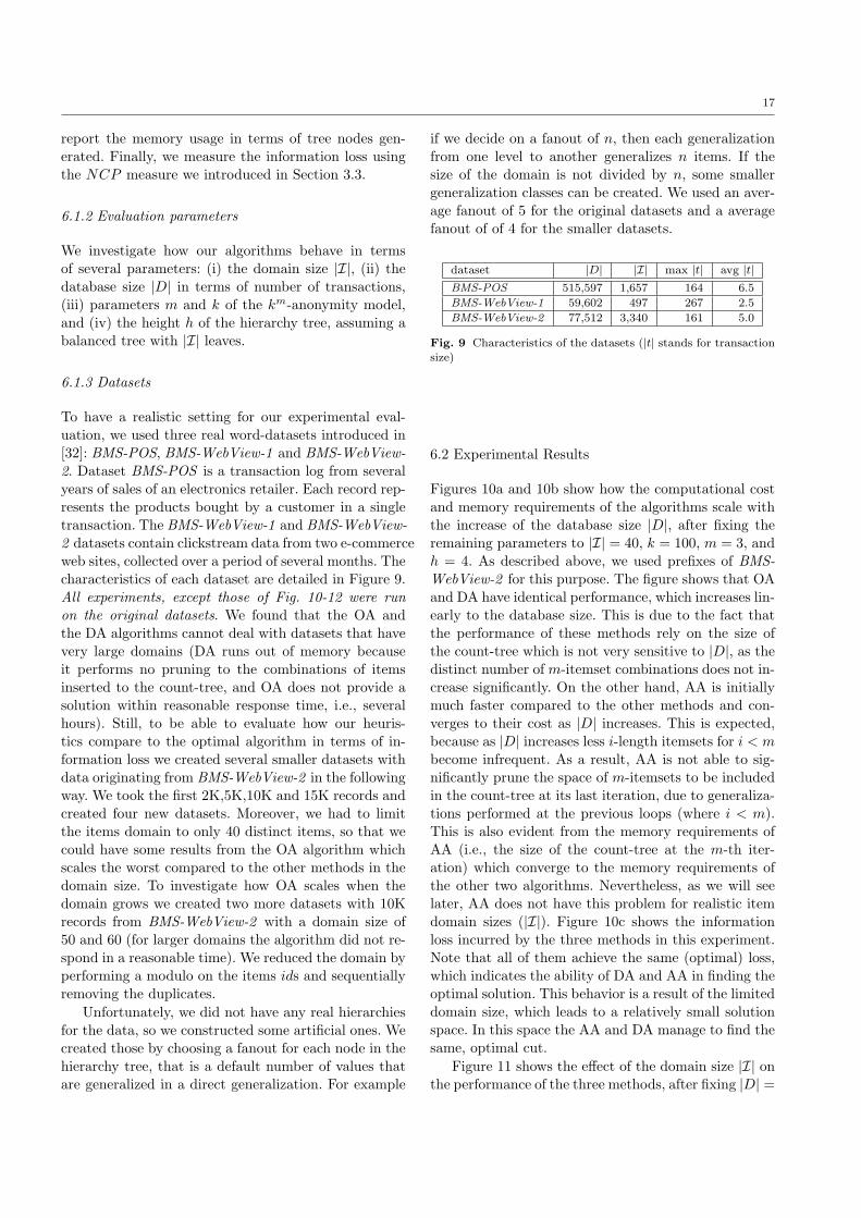
17
report the memory usage in terms of tree nodes gen-
erated. Finally, we measure the information loss usingthe NCP measure we introduced in Section 3.3.
6.1.2 Evaluation parameters
We investigate how our algorithms behave in terms
of several parameters: (i) the domain size |I|, (ii) the
database size |D| in terms of number of transactions,(iii) parameters m and k of the km-anonymity model,
and (iv) the height h of the hierarchy tree, assuming a
balanced tree with |I| leaves.
6.1.3 Datasets
To have a realistic setting for our experimental eval-uation, we used three real word-datasets introduced in
[32]: BMS-POS, BMS-WebView-1 and BMS-WebView-
2. Dataset BMS-POS is a transaction log from several
years of sales of an electronics retailer. Each record rep-resents the products bought by a customer in a single
transaction. The BMS-WebView-1 and BMS-WebView-
2 datasets contain clickstream data from two e-commerceweb sites, collected over a period of several months. The
characteristics of each dataset are detailed in Figure 9.
All experiments, except those of Fig. 10-12 were run
on the original datasets. We found that the OA and
the DA algorithms cannot deal with datasets that have
very large domains (DA runs out of memory because
it performs no pruning to the combinations of itemsinserted to the count-tree, and OA does not provide a
solution within reasonable response time, i.e., several
hours). Still, to be able to evaluate how our heuris-tics compare to the optimal algorithm in terms of in-
formation loss we created several smaller datasets with
data originating from BMS-WebView-2 in the followingway. We took the first 2K,5K,10K and 15K records and
created four new datasets. Moreover, we had to limit
the items domain to only 40 distinct items, so that we
could have some results from the OA algorithm whichscales the worst compared to the other methods in the
domain size. To investigate how OA scales when the
domain grows we created two more datasets with 10Krecords from BMS-WebView-2 with a domain size of
50 and 60 (for larger domains the algorithm did not re-
spond in a reasonable time). We reduced the domain byperforming a modulo on the items ids and sequentially
removing the duplicates.
Unfortunately, we did not have any real hierarchies
for the data, so we constructed some artificial ones. Wecreated those by choosing a fanout for each node in the
hierarchy tree, that is a default number of values that
are generalized in a direct generalization. For example
if we decide on a fanout of n, then each generalization
from one level to another generalizes n items. If thesize of the domain is not divided by n, some smaller
generalization classes can be created. We used an aver-
age fanout of 5 for the original datasets and a averagefanout of of 4 for the smaller datasets.
dataset |D| |I| max |t| avg |t|
BMS-POS 515,597 1,657 164 6.5
BMS-WebView-1 59,602 497 267 2.5
BMS-WebView-2 77,512 3,340 161 5.0
Fig. 9 Characteristics of the datasets (|t| stands for transactionsize)
6.2 Experimental Results
Figures 10a and 10b show how the computational cost
and memory requirements of the algorithms scale with
the increase of the database size |D|, after fixing theremaining parameters to |I| = 40, k = 100, m = 3, and
h = 4. As described above, we used prefixes of BMS-
WebView-2 for this purpose. The figure shows that OAand DA have identical performance, which increases lin-
early to the database size. This is due to the fact that
the performance of these methods rely on the size of
the count-tree which is not very sensitive to |D|, as thedistinct number of m-itemset combinations does not in-
crease significantly. On the other hand, AA is initially
much faster compared to the other methods and con-verges to their cost as |D| increases. This is expected,
because as |D| increases less i-length itemsets for i < m
become infrequent. As a result, AA is not able to sig-nificantly prune the space of m-itemsets to be included
in the count-tree at its last iteration, due to generaliza-
tions performed at the previous loops (where i < m).
This is also evident from the memory requirements ofAA (i.e., the size of the count-tree at the m-th iter-
ation) which converge to the memory requirements of
the other two algorithms. Nevertheless, as we will seelater, AA does not have this problem for realistic item
domain sizes (|I|). Figure 10c shows the information
loss incurred by the three methods in this experiment.Note that all of them achieve the same (optimal) loss,
which indicates the ability of DA and AA in finding the
optimal solution. This behavior is a result of the limited
domain size, which leads to a relatively small solutionspace. In this space the AA and DA manage to find the
same, optimal cut.
Figure 11 shows the effect of the domain size |I| on
the performance of the three methods, after fixing |D| =
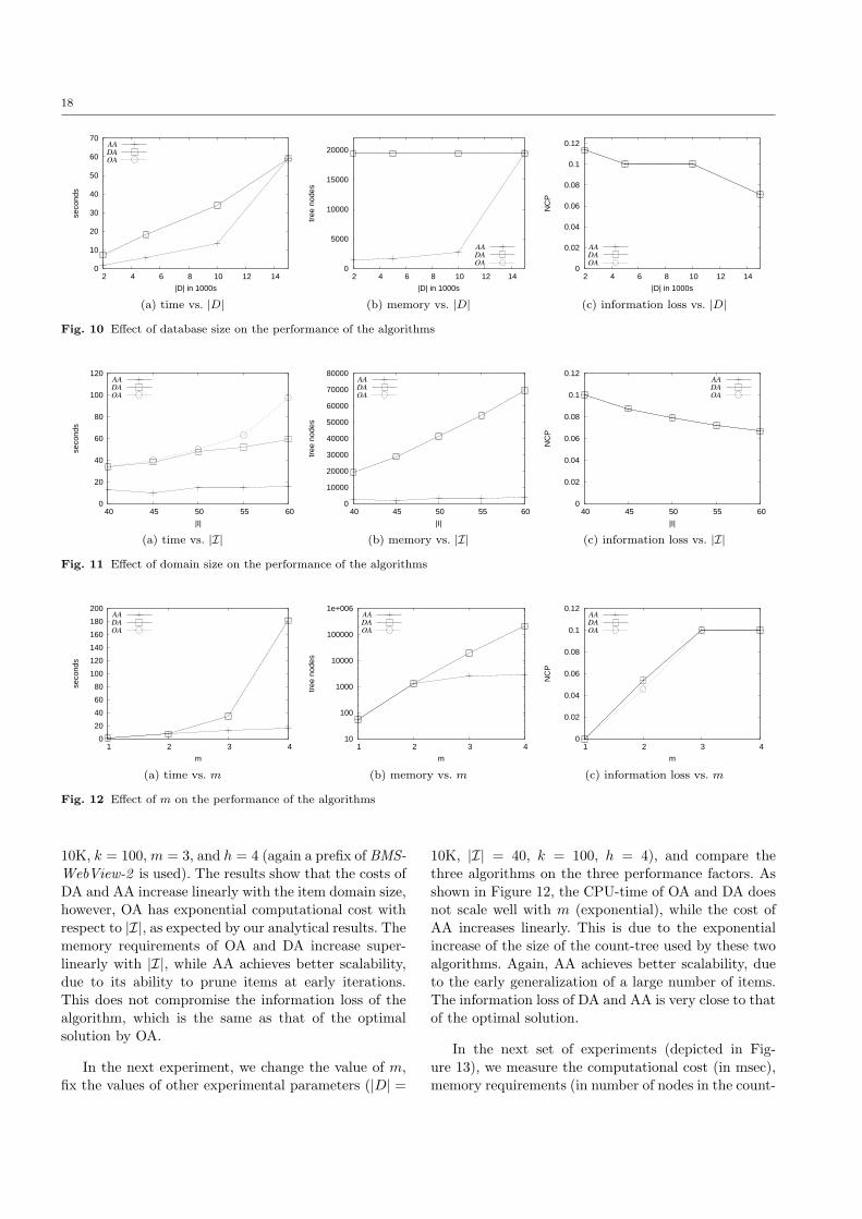
18
0
10
20
30
40
50
60
70
2 4 6 8 10 12 14
seco
nds
|D| in 1000s
AA
DA
OA
0
5000
10000
15000
20000
2 4 6 8 10 12 14
tree
nod
es
|D| in 1000s
AA
DA
OA 0
0.02
0.04
0.06
0.08
0.1
0.12
2 4 6 8 10 12 14
NC
P
|D| in 1000s
AA
DA
OA
(a) time vs. |D| (b) memory vs. |D| (c) information loss vs. |D|
Fig. 10 Effect of database size on the performance of the algorithms
0
20
40
60
80
100
120
40 45 50 55 60
seco
nds
|I|
AA
DA
OA
0
10000
20000
30000
40000
50000
60000
70000
80000
40 45 50 55 60
tree
nod
es
|I|
AA
DA
OA
0
0.02
0.04
0.06
0.08
0.1
0.12
40 45 50 55 60
NC
P
|I|
AA
DA
OA
(a) time vs. |I| (b) memory vs. |I| (c) information loss vs. |I|
Fig. 11 Effect of domain size on the performance of the algorithms
0
20
40
60
80
100
120
140
160
180
200
1 2 3 4
seco
nds
m
AA
DA
OA
10
100
1000
10000
100000
1e+006
1 2 3 4
tree
nod
es
m
AA
DA
OA
0
0.02
0.04
0.06
0.08
0.1
0.12
1 2 3 4
NC
P
m
AA
DA
OA
(a) time vs. m (b) memory vs. m (c) information loss vs. m
Fig. 12 Effect of m on the performance of the algorithms
10K, k = 100,m = 3, and h = 4 (again a prefix of BMS-
WebView-2 is used). The results show that the costs ofDA and AA increase linearly with the item domain size,
however, OA has exponential computational cost with
respect to |I|, as expected by our analytical results. Thememory requirements of OA and DA increase super-
linearly with |I|, while AA achieves better scalability,
due to its ability to prune items at early iterations.This does not compromise the information loss of the
algorithm, which is the same as that of the optimal
solution by OA.
In the next experiment, we change the value of m,
fix the values of other experimental parameters (|D| =
10K, |I| = 40, k = 100, h = 4), and compare the
three algorithms on the three performance factors. Asshown in Figure 12, the CPU-time of OA and DA does
not scale well with m (exponential), while the cost of
AA increases linearly. This is due to the exponentialincrease of the size of the count-tree used by these two
algorithms. Again, AA achieves better scalability, due
to the early generalization of a large number of items.The information loss of DA and AA is very close to that
of the optimal solution.
In the next set of experiments (depicted in Fig-
ure 13), we measure the computational cost (in msec),
memory requirements (in number of nodes in the count-
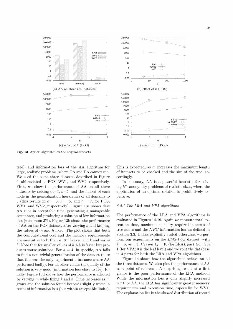
19
0.01
0.1
1
10
100
1000
10000
100000
1e+006
1e+007
time memory NCP
POSWV1WV2
0.01
0.1
1
10
100
1000
10000
100000
1e+006
1 10 100 1000
k
timenodes
loss
(a) AA on three real datasets (b) effect of k (POS)
0.01
0.1
1
10
100
1000
10000
100000
1e+006
4 5 6 7
h
timenodes
loss
0.001
0.01
0.1
1
10
100
1000
10000
100000
1e+006
1e+007
1 2 3 4
m
a-timea-nodes
a-loss
(c) effect of h (POS) (d) effect of m (POS)
Fig. 13 Apriori algorithm on the original datasets
tree), and information loss of the AA algorithm for
large, realistic problems, where OA and DA cannot run.
We used the same three datasets described in Figure
9, abbreviated as POS, WV1, and WV2, respectively.First, we show the performance of AA on all three
datasets by setting m=3, k=5, and the fanout of each
node in the generalization hierarchies of all domains to5 (this results in h = 6, h = 5, and h = 7, for POS,
WV1, and WV2, respectively). Figure 13a shows that
AA runs in acceptable time, generating a manageablecount-tree, and producing a solution of low information
loss (maximum 3%). Figure 13b shows the performance
of AA on the POS dataset, after varying k and keeping
the values of m and h fixed. The plot shows that boththe computational cost and the memory requirements
are insensitive to k. Figure 13c, fixesm and k and varies
h. Note that for smaller values of h AA is faster but pro-duces worse solutions. For h = 4, in specific, AA fails
to find a non-trivial generalization of the dataset (note
that this was the only experimental instance where AAperformed badly). For all other values the quality of the
solution is very good (information loss close to 1%). Fi-
nally, Figure 13d shows how the performance is affected
by varying m while fixing k and h. Time increases as mgrows and the solution found becomes slightly worse in
terms of information loss (but within acceptable limits).
This is expected, as m increases the maximum length
of itemsets to be checked and the size of the tree, ac-
cordingly.
In summary, AA is a powerful heuristic for solv-ing km-anonymity problems of realistic sizes, where the
application of an optimal solution is prohibitively ex-
pensive.
6.2.1 The LRA and VPA algorithms
The performance of the LRA and VPA algorithms is
evaluated in Figures 14-19. Again we measure total ex-
ecution time, maximum memory required in terms of
tree nodes and the NPC information loss as defined inSection 3.3. Unless explicitly stated otherwise, we per-
form our experiments on the BMS-POS dataset, with
k = 5,m = 3, flexibility = 10 (for LRA), partition level =1 (for VPA; 0 is the leaf level) and we split the database
in 3 parts for both the LRA and VPA algorithms.
Figure 14 shows how the algorithms behave on allthe three datasets. We also plot the performance of AA
as a point of reference. A surprising result at a first
glance is the poor performance of the LRA method.
While the information loss is only slightly increasedw.r.t. to AA, the LRA has significantly greater memory
requirements and execution time, especially for WV1.
The explanation lies in the skewed distribution of record
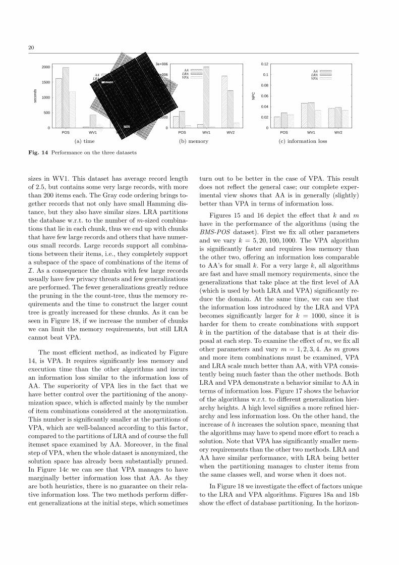
20
0
500
1000
1500
2000
POS WV1 WV2
seco
nds
AA
LRA
VPA
0
500000
1e+006
1.5e+006
2e+006
2.5e+006
3e+006
POS WV1 WV2
tree
nod
es
AA
LRA
VPA
0
0.02
0.04
0.06
0.08
0.1
0.12
POS WV1 WV2
NP
C
AA
LRA
VPA
(a) time (b) memory (c) information loss
Fig. 14 Performance on the three datasets
sizes in WV1. This dataset has average record length
of 2.5, but contains some very large records, with morethan 200 items each. The Gray code ordering brings to-
gether records that not only have small Hamming dis-
tance, but they also have similar sizes. LRA partitionsthe database w.r.t. to the number of m-sized combina-
tions that lie in each chunk, thus we end up with chunks
that have few large records and others that have numer-ous small records. Large records support all combina-
tions between their items, i.e., they completely support
a subspace of the space of combinations of the items of
I. As a consequence the chunks with few large recordsusually have few privacy threats and few generalizations
are performed. The fewer generalizations greatly reduce
the pruning in the the count-tree, thus the memory re-quirements and the time to construct the larger count
tree is greatly increased for these chunks. As it can be
seen in Figure 18, if we increase the number of chunkswe can limit the memory requirements, but still LRA
cannot beat VPA.
The most efficient method, as indicated by Figure
14, is VPA. It requires significantly less memory andexecution time than the other algorithms and incurs
an information loss similar to the information loss of
AA. The superiority of VPA lies in the fact that we
have better control over the partitioning of the anony-mization space, which is affected mainly by the number
of item combinations considered at the anonymization.
This number is significantly smaller at the partitions ofVPA, which are well-balanced according to this factor,
compared to the partitions of LRA and of course the full
itemset space examined by AA. Moreover, in the finalstep of VPA, when the whole dataset is anonymized, the
solution space has already been substantially pruned.
In Figure 14c we can see that VPA manages to have
marginally better information loss that AA. As theyare both heuristics, there is no guarantee on their rela-
tive information loss. The two methods perform differ-
ent generalizations at the initial steps, which sometimes
turn out to be better in the case of VPA. This result
does not reflect the general case; our complete exper-imental view shows that AA is in generally (slightly)
better than VPA in terms of information loss.
Figures 15 and 16 depict the effect that k and m
have in the performance of the algorithms (using the
BMS-POS dataset). First we fix all other parametersand we vary k = 5, 20, 100, 1000. The VPA algorithm
is significantly faster and requires less memory than
the other two, offering an information loss comparableto AA’s for small k. For a very large k, all algorithms
are fast and have small memory requirements, since the
generalizations that take place at the first level of AA
(which is used by both LRA and VPA) significantly re-duce the domain. At the same time, we can see that
the information loss introduced by the LRA and VPA
becomes significantly larger for k = 1000, since it isharder for them to create combinations with support
k in the partition of the database that is at their dis-
posal at each step. To examine the effect of m, we fix allother parameters and vary m = 1, 2, 3, 4. As m grows
and more item combinations must be examined, VPA
and LRA scale much better than AA, with VPA consis-
tently being much faster than the other methods. BothLRA and VPA demonstrate a behavior similar to AA in
terms of information loss. Figure 17 shows the behavior
of the algorithms w.r.t. to different generalization hier-archy heights. A high level signifies a more refined hier-
archy and less information loss. On the other hand, the
increase of h increases the solution space, meaning thatthe algorithms may have to spend more effort to reach a
solution. Note that VPA has significantly smaller mem-
ory requirements than the other two methods. LRA and
AA have similar performance, with LRA being betterwhen the partitioning manages to cluster items from
the same classes well, and worse when it does not.
In Figure 18 we investigate the effect of factors unique
to the LRA and VPA algorithms. Figures 18a and 18b
show the effect of database partitioning. In the horizon-
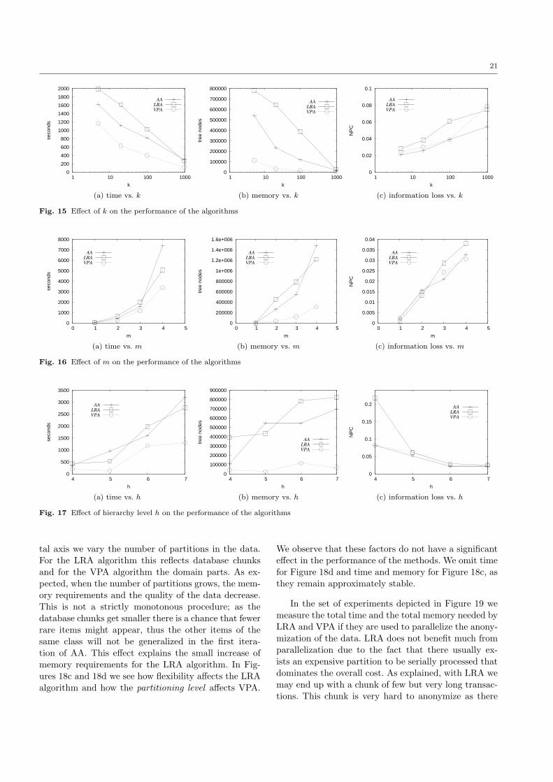
21
0
200
400
600
800
1000
1200
1400
1600
1800
2000
1 10 100 1000
seco
nds
k
AA
LRA
VPA
0
100000
200000
300000
400000
500000
600000
700000
800000
1 10 100 1000
tree
nod
es
k
AA
LRA
VPA
0
0.02
0.04
0.06
0.08
0.1
1 10 100 1000
NP
C
k
AA
LRA
VPA
(a) time vs. k (b) memory vs. k (c) information loss vs. k
Fig. 15 Effect of k on the performance of the algorithms
0
1000
2000
3000
4000
5000
6000
7000
8000
0 1 2 3 4 5
seco
nds
m
AA
LRA
VPA
0
200000
400000
600000
800000
1e+006
1.2e+006
1.4e+006
1.6e+006
0 1 2 3 4 5
tree
nod
es
m
AA
LRA
VPA
0
0.005
0.01
0.015
0.02
0.025
0.03
0.035
0.04
0 1 2 3 4 5
NP
C
m
AA
LRA
VPA
(a) time vs. m (b) memory vs. m (c) information loss vs. m
Fig. 16 Effect of m on the performance of the algorithms
0
500
1000
1500
2000
2500
3000
3500
4 5 6 7
seco
nds
h
AA
LRA
VPA
0
100000
200000
300000
400000
500000
600000
700000
800000
900000
4 5 6 7
tree
nod
es
h
AA
LRA
VPA
0
0.05
0.1
0.15
0.2
4 5 6 7
NP
C
h
AA
LRA
VPA
(a) time vs. h (b) memory vs. h (c) information loss vs. h
Fig. 17 Effect of hierarchy level h on the performance of the algorithms
tal axis we vary the number of partitions in the data.
For the LRA algorithm this reflects database chunksand for the VPA algorithm the domain parts. As ex-
pected, when the number of partitions grows, the mem-
ory requirements and the quality of the data decrease.This is not a strictly monotonous procedure; as the
database chunks get smaller there is a chance that fewer
rare items might appear, thus the other items of thesame class will not be generalized in the first itera-
tion of AA. This effect explains the small increase of
memory requirements for the LRA algorithm. In Fig-
ures 18c and 18d we see how flexibility affects the LRAalgorithm and how the partitioning level affects VPA.
We observe that these factors do not have a significant
effect in the performance of the methods. We omit timefor Figure 18d and time and memory for Figure 18c, as
they remain approximately stable.
In the set of experiments depicted in Figure 19 we
measure the total time and the total memory needed byLRA and VPA if they are used to parallelize the anony-
mization of the data. LRA does not benefit much from
parallelization due to the fact that there usually ex-
ists an expensive partition to be serially processed thatdominates the overall cost. As explained, with LRA we
may end up with a chunk of few but very long transac-
tions. This chunk is very hard to anonymize as there
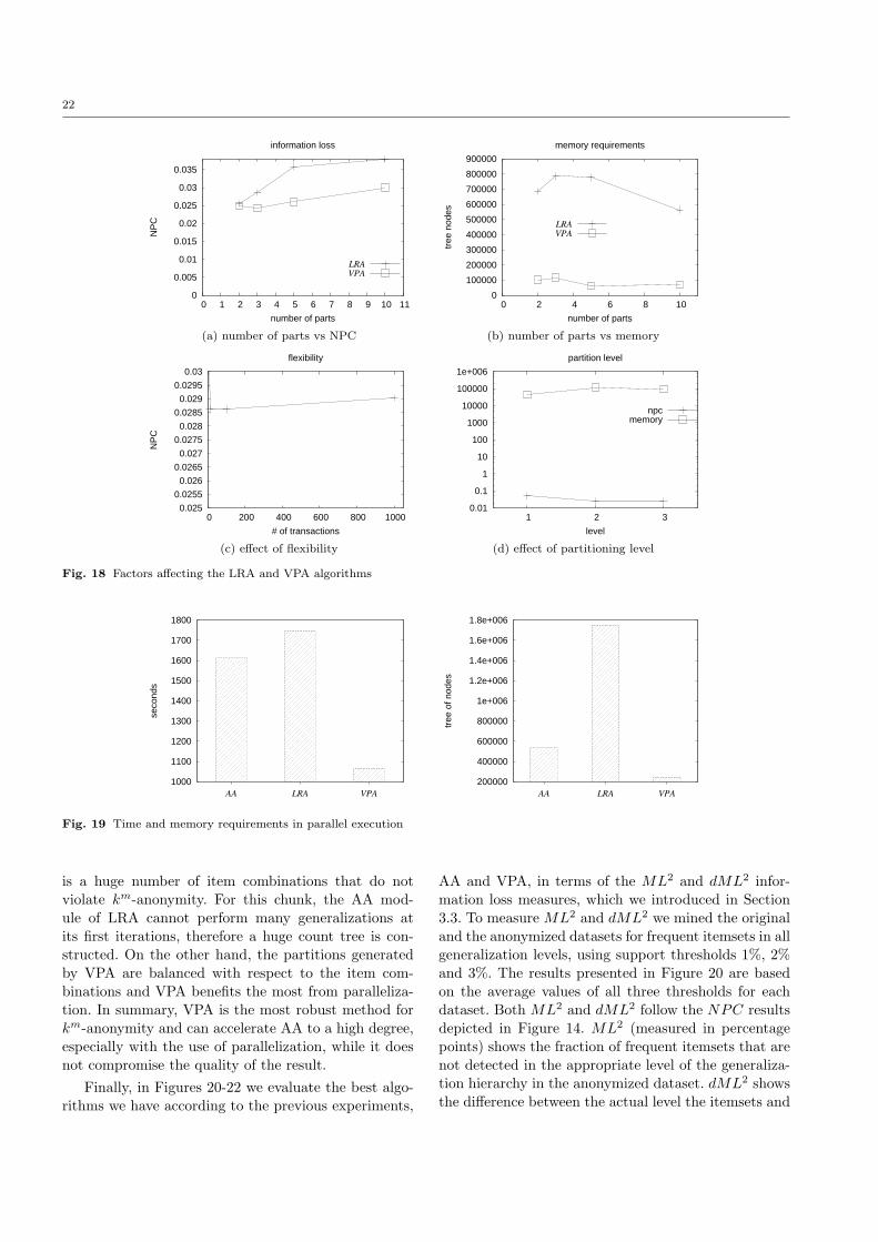
22
0
0.005
0.01
0.015
0.02
0.025
0.03
0.035
0 1 2 3 4 5 6 7 8 9 10 11
NP
C
number of parts
information loss
LRA
VPA
0
100000
200000
300000
400000
500000
600000
700000
800000
900000
0 2 4 6 8 10
tree
nod
es
number of parts
memory requirements
LRA
VPA
(a) number of parts vs NPC (b) number of parts vs memory
0.025
0.0255
0.026
0.0265
0.027
0.0275
0.028
0.0285
0.029
0.0295
0.03
0 200 400 600 800 1000
NP
C
# of transactions
flexibility
0.01
0.1
1
10
100
1000
10000
100000
1e+006
1 2 3
level
partition level
npcmemory
(c) effect of flexibility (d) effect of partitioning level
Fig. 18 Factors affecting the LRA and VPA algorithms
1000
1100
1200
1300
1400
1500
1600
1700
1800
AA LRA VPA
seco
nds
200000
400000
600000
800000
1e+006
1.2e+006
1.4e+006
1.6e+006
1.8e+006
AA LRA VPA
tree
of n
odes
Fig. 19 Time and memory requirements in parallel execution
is a huge number of item combinations that do notviolate km-anonymity. For this chunk, the AA mod-
ule of LRA cannot perform many generalizations at
its first iterations, therefore a huge count tree is con-structed. On the other hand, the partitions generated
by VPA are balanced with respect to the item com-
binations and VPA benefits the most from paralleliza-tion. In summary, VPA is the most robust method for
km-anonymity and can accelerate AA to a high degree,
especially with the use of parallelization, while it does
not compromise the quality of the result.
Finally, in Figures 20-22 we evaluate the best algo-
rithms we have according to the previous experiments,
AA and VPA, in terms of the ML2 and dML2 infor-mation loss measures, which we introduced in Section
3.3. To measure ML2 and dML2 we mined the original
and the anonymized datasets for frequent itemsets in allgeneralization levels, using support thresholds 1%, 2%
and 3%. The results presented in Figure 20 are based
on the average values of all three thresholds for eachdataset. Both ML2 and dML2 follow the NPC results
depicted in Figure 14. ML2 (measured in percentage
points) shows the fraction of frequent itemsets that are
not detected in the appropriate level of the generaliza-tion hierarchy in the anonymized dataset. dML2 shows
the difference between the actual level the itemsets and
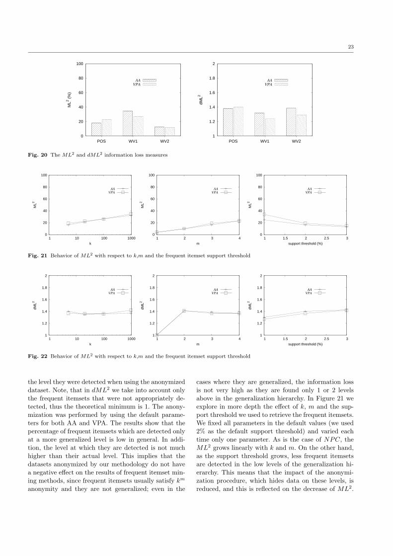
23
0
20
40
60
80
100
POS WV1 WV2
ML2 (
%)
AA
VPA
1
1.2
1.4
1.6
1.8
2
POS WV1 WV2
dML2
AA
VPA
Fig. 20 The ML2 and dML2 information loss measures
0
20
40
60
80
100
1 10 100 1000
ML2
k
AA
VPA
0
20
40
60
80
100
1 2 3 4
ML2
m
AA
VPA
0
20
40
60
80
100
1 1.5 2 2.5 3
ML2
support threshold (%)
AA
VPA
Fig. 21 Behavior of ML2 with respect to k,m and the frequent itemset support threshold
1
1.2
1.4
1.6
1.8
2
1 10 100 1000
dML2
k
AA
VPA
1
1.2
1.4
1.6
1.8
2
1 2 3 4
dML2
m
AA
VPA
1
1.2
1.4
1.6
1.8
2
1 1.5 2 2.5 3
dML2
support threshold (%)
AA
VPA
Fig. 22 Behavior of ML2 with respect to k,m and the frequent itemset support threshold
the level they were detected when using the anonymized
dataset. Note, that in dML2 we take into account only
the frequent itemsets that were not appropriately de-
tected, thus the theoretical minimum is 1. The anony-mization was performed by using the default parame-
ters for both AA and VPA. The results show that the
percentage of frequent itemsets which are detected onlyat a more generalized level is low in general. In addi-
tion, the level at which they are detected is not much
higher than their actual level. This implies that thedatasets anonymized by our methodology do not have
a negative effect on the results of frequent itemset min-
ing methods, since frequent itemsets usually satisfy km
anonymity and they are not generalized; even in the
cases where they are generalized, the information loss
is not very high as they are found only 1 or 2 levels
above in the generalization hierarchy. In Figure 21 we
explore in more depth the effect of k, m and the sup-port threshold we used to retrieve the frequent itemsets.
We fixed all parameters in the default values (we used
2% as the default support threshold) and varied eachtime only one parameter. As is the case of NPC, the
ML2 grows linearly with k and m. On the other hand,
as the support threshold grows, less frequent itemsetsare detected in the low levels of the generalization hi-
erarchy. This means that the impact of the anonymi-
zation procedure, which hides data on these levels, is
reduced, and this is reflected on the decrease of ML2.
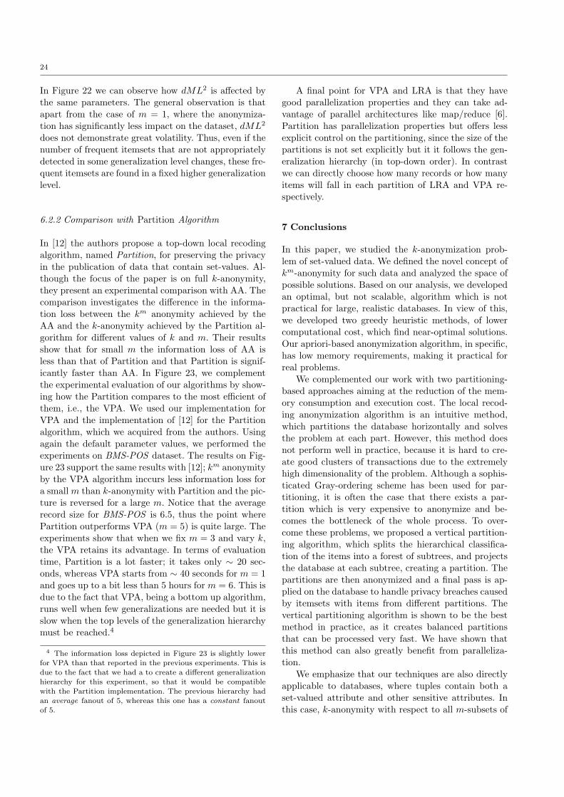
24
In Figure 22 we can observe how dML2 is affected by
the same parameters. The general observation is thatapart from the case of m = 1, where the anonymiza-
tion has significantly less impact on the dataset, dML2
does not demonstrate great volatility. Thus, even if thenumber of frequent itemsets that are not appropriately
detected in some generalization level changes, these fre-
quent itemsets are found in a fixed higher generalizationlevel.
6.2.2 Comparison with Partition Algorithm
In [12] the authors propose a top-down local recoding
algorithm, named Partition, for preserving the privacy
in the publication of data that contain set-values. Al-though the focus of the paper is on full k-anonymity,
they present an experimental comparison with AA. The
comparison investigates the difference in the informa-tion loss between the km anonymity achieved by the
AA and the k-anonymity achieved by the Partition al-
gorithm for different values of k and m. Their resultsshow that for small m the information loss of AA is
less than that of Partition and that Partition is signif-
icantly faster than AA. In Figure 23, we complement
the experimental evaluation of our algorithms by show-ing how the Partition compares to the most efficient of
them, i.e., the VPA. We used our implementation for
VPA and the implementation of [12] for the Partitionalgorithm, which we acquired from the authors. Using
again the default parameter values, we performed the
experiments on BMS-POS dataset. The results on Fig-ure 23 support the same results with [12]; km anonymity
by the VPA algorithm inccurs less information loss for
a small m than k-anonymity with Partition and the pic-
ture is reversed for a large m. Notice that the averagerecord size for BMS-POS is 6.5, thus the point where
Partition outperforms VPA (m = 5) is quite large. The
experiments show that when we fix m = 3 and vary k,the VPA retains its advantage. In terms of evaluation
time, Partition is a lot faster; it takes only ∼ 20 sec-
onds, whereas VPA starts from ∼ 40 seconds for m = 1and goes up to a bit less than 5 hours for m = 6. This is
due to the fact that VPA, being a bottom up algorithm,
runs well when few generalizations are needed but it is
slow when the top levels of the generalization hierarchymust be reached.4
4 The information loss depicted in Figure 23 is slightly lowerfor VPA than that reported in the previous experiments. This isdue to the fact that we had a to create a different generalizationhierarchy for this experiment, so that it would be compatiblewith the Partition implementation. The previous hierarchy hadan average fanout of 5, whereas this one has a constant fanout
of 5.
A final point for VPA and LRA is that they have
good parallelization properties and they can take ad-vantage of parallel architectures like map/reduce [6].
Partition has parallelization properties but offers less
explicit control on the partitioning, since the size of thepartitions is not set explicitly but it it follows the gen-
eralization hierarchy (in top-down order). In contrast
we can directly choose how many records or how manyitems will fall in each partition of LRA and VPA re-
spectively.
7 Conclusions
In this paper, we studied the k-anonymization prob-
lem of set-valued data. We defined the novel concept of
km-anonymity for such data and analyzed the space ofpossible solutions. Based on our analysis, we developed
an optimal, but not scalable, algorithm which is not
practical for large, realistic databases. In view of this,
we developed two greedy heuristic methods, of lowercomputational cost, which find near-optimal solutions.
Our apriori-based anonymization algorithm, in specific,
has low memory requirements, making it practical forreal problems.
We complemented our work with two partitioning-
based approaches aiming at the reduction of the mem-ory consumption and execution cost. The local recod-
ing anonymization algorithm is an intuitive method,
which partitions the database horizontally and solves
the problem at each part. However, this method doesnot perform well in practice, because it is hard to cre-
ate good clusters of transactions due to the extremely
high dimensionality of the problem. Although a sophis-ticated Gray-ordering scheme has been used for par-
titioning, it is often the case that there exists a par-
tition which is very expensive to anonymize and be-comes the bottleneck of the whole process. To over-
come these problems, we proposed a vertical partition-
ing algorithm, which splits the hierarchical classifica-
tion of the items into a forest of subtrees, and projectsthe database at each subtree, creating a partition. The
partitions are then anonymized and a final pass is ap-
plied on the database to handle privacy breaches causedby itemsets with items from different partitions. The
vertical partitioning algorithm is shown to be the best
method in practice, as it creates balanced partitionsthat can be processed very fast. We have shown that
this method can also greatly benefit from paralleliza-
tion.
We emphasize that our techniques are also directlyapplicable to databases, where tuples contain both a
set-valued attribute and other sensitive attributes. In
this case, k-anonymity with respect to all m-subsets of
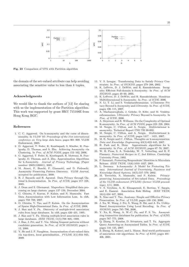
25
0
0.05
0.1
0.15
0.2
1 10 100 1000
NP
C
k
PartitionVPA
0
0.02
0.04
0.06
0.08
0.1
0 1 2 3 4 5 6
NP
C
m
PartitionVPA
Fig. 23 Comparison of VPA with Partition algorithm
the domain of the set-valued attribute can help avoiding
associating the sensitive value to less than k tuples.
Acknowledgments
We would like to thank the authors of [12] for sharingwith us the implementation of the Partition algorithm.
This work was supported by grant HKU 715108E from
Hong Kong RGC.
References
1. C. C. Aggarwal. On k-anonymity and the curse of dimen-
sionality. In VLDB ’05: Proceedings of the 31st internationalconference on Very large data bases, pages 901–909. VLDBEndowment, 2005.
2. G. Aggarwal, T. Feder, K. Kenthapadi, S. Khuller, R. Pan-igrahy, D. Thomas, and A. Zhu. Achieving Anonymity viaClustering. In Proc. of ACM PODS, pages 153–162, 2006.
3. G. Aggarwal, T. Feder, K. Kenthapadi, R. Motwani, R. Pan-igrahy, D. Thomas, and A. Zhu. Approximation Algorithmsfor k-Anonymity. Journal of Privacy Technology, (Papernumber: 20051120001), 2005.
4. M. Atzori, F. Bonchi, F. Giannotti, and D. Pedreschi.
Anonymity Preserving Pattern Discovery. VLDB Journal,accepted for publication, 2008.
5. R. J. Bayardo and R. Agrawal. Data Privacy through Op-
timal k-Anonymization. In Proc. of ICDE, pages 217–228,2005.
6. J. Dean and S. Ghemawat. Mapreduce: Simplified data pro-cessing on large clusters. pages 137–150, December 2004.
7. G. Ghinita, P. Karras, P. Kalnis, and N. Mamoulis. FastData Anonymization with Low Information Loss. In vldb,pages 758–769, 2007.
8. G. Ghinita, Y. Tao, and P. Kalnis. On the Anonymization
of Sparse High-Dimensional Data. In Proc. of ICDE, 2008.9. J. Han and Y. Fu. Discovery of multiple-level association
rules from large databases. In vldb, pages 420–431, 1995.
10. J. Han and Y. Fu. Mining multiple-level association rules inlarge databases. IEEE TKDE, 11(5):798–805, 1999.
11. J. Han, J. Pei, and Y. Yin. Mining frequent patterns withoutcandidate generation. In Proc. of ACM SIGMOD, pages 1–
12, 2000.12. Y. He and J. F. Naughton. Anonymization of set-valued data
via top-down, local generalization. PVLDB, 2(1):934–945,
2009.
13. V. S. Iyengar. Transforming Data to Satisfy Privacy Con-
straints. In Proc. of SIGKDD, pages 279–288, 2002.14. K. LeFevre, D. J. DeWitt, and R. Ramakrishnan. Incog-
nito: Efficient Full-domain k-Anonymity. In Proc. of ACMSIGMOD, pages 49–60, 2005.
15. K. LeFevre, D. J. DeWitt, and R. Ramakrishnan. Mondrian
Multidimensional k-Anonymity. In Proc. of ICDE, 2006.16. N. Li, T. Li, and S. Venkatasubramanian. t-Closeness: Pri-
vacy Beyond k-Anonymity and l-Diversity. In Proc. of ICDE,pages 106–115, 2007.
17. A. Machanavajjhala, J. Gehrke, D. Kifer, and M. Venkita-
subramaniam. l-Diversity: Privacy Beyond k-Anonymity. InProc. of ICDE, 2006.
18. A. Meyerson and R. Williams. On the Complexity of OptimalK-anonymity. In Proc. of ACM PODS, pages 223–228, 2004.
19. M. Nergiz, C. Clifton, and A. Nergiz. Multirelational k-
anonymity. Technical Report CSD TR 08-002.20. M. Nergiz, C. Clifton, and A. Nergiz. Multirelational k-
anonymity. In Proc. of ICDE, pages 1417 – 1421, 2007.21. M. E. Nergiz and C. Clifton. Thoughts on k-anonymization.
Data and Knowledge Engineering, 63(3):622–645, 2007.22. H. Park and K. Shim. Approximate algorithms for k-
anonymity. In Proc. of ACM SIGMOD, pages 67–78, 2007.23. W. H. Press, S. A. Teukolsky, W. T. Vetterling, and B. P.
Flannery. Numerical Recipes in C, 2nd Edition. CambridgeUniversity Press, 1992.
24. P. Samarati. Protecting Respondents’ Identities in Microdata
Release. IEEE TKDE, 13(6):1010–1027, 2001.25. L. Sweeney. k-Anonymity: A Model for Protecting Pri-
vacy. International Journal of Uncertainty, Fuzziness andKnowledge-Based Systems, 10(5):557–570, 2002.
26. M. Terrovitis, N. Mamoulis, and P. Kalnis. Privacy-preserving Anonymization of Set-valued Data. Proceedingsof the VLDB endowment (PVLDB) (former VLDB proceed-ings), 1(1), 2008.
27. V. S. Verykios, A. K. Elmagarmid, E. Bertino, Y. Saygin,
and E. Dasseni. Association Rule Hiding. IEEE TKDE,16(4):434–447, 2004.
28. X. Xiao and Y. Tao. Anatomy: Simple and Effective PrivacyPreservation. In Proc. of VLDB, pages 139–150, 2006.
29. J. Xu, W. Wang, J. Pei, X. Wang, B. Shi, and A. Fu. Utility-
Based Anonymization Using Local Recoding. In Proc. ofSIGKDD, pages 785–790, 2006.
30. Y. Xu, K. Wang, A. W.-C. Fu, and P. S. Yu. Anonymi-zing transaction databases for publication. In Proc. of KDD,
pages 767–775, 2008.31. Q. Zhang, N. Koudas, D. Srivastava, and T. Yu. Aggregate
Query Answering on Anonymized Tables. In Proc. of ICDE,pages 116–125, 2007.
32. Z. Zheng, R. Kohavi, and L. Mason. Real world performance
of association rule algorithms. In Proc. of KDD, pages 401–406, 2001.