Local perfection

JOURNAL OF ECONOMIC THEORY 43, 134-156 (1987)

Local Perfection *

LEO K. SIMON

Department of Economics, University of California, Berkeley, California 94720

Received December 5, 1985; revised August 3, 1986

We investigate solution concepts for normal-form games with large strategy spaces. “Trembling hand” perfection (THP) is extended to games with compact metric strategy sets. A Nash equilibrium is THP if it is the limit of.equilibria in which agents face vanishingly small uncertainty. We refine THP by imposing some structure on the kind of uncertainty that agents face: a THP equilibrium is locally perfect if the uncertainty is “predominantly local” in nature, i.e., if agents’ probability assessments assign, in the limit, an overwhelmingly lage proportion of the total probability mass to events “in the vicinity of the truth.” Journal of Economic Literature Classification Numbers: 021, 022, 611. b 1987 Academic Press, Inc.

This paper investigates solution concepts for games with large strategy spaces. Selten’s [S] notion of “trembling hand” perfection (THP) is extended to games with compact metric strategy sets. Loosely, a Nash equilibrium is THP if it is the limit of equilibria in which agents face vanishingly small uncertainty. We introduce a refinement of THP, called local perfection: some structure is imposed on the kind of uncertainty that agents face.’ Informally, a THP equilibrium is locally perfect (LP) if the uncertainty agents face is “predominantly local” in nature, i.e., if agents’ probability assessments assign, in the limit, an overwhelmingly large proportion of the total probability mass to events “in the vicinity of the truth.”

To fix ideas, let S= (S,, S2) be a pure-strategy Nash equilibrium for some two-person game. Let Pi denote player ?s payoff function. Suppose that there exists an alternative strategy for player 1, s;, and a neighborhood,

* I am indebted to Robert Anderson, Andreu Mas-Colell, Roger Myerson, John Nachbar, Hugo Sonnenschein and Max Stinchcombe for their help at various stages. I am particularly grateful to an associate editor of JET for extremely helpful suggestions. Many of these are incorporated into the paper without further acknowledgment. Research was supported by grants from the National Science Foundation, and from the Institute for Business and Economic Research, U. C. Berkeley. Figure 1 courtesy of Goldman Graphics.

’ Myerson’s criterion, “properness,” [‘I] also imposes structure on the kind of uncertainty faced by agents. The relationship between the two ideas is discussed in Section III.

134 0022-0531/87 $3.00 Copyright 0 1987 by Academic Press, Inc. All rights of reproduction in any lam reserved.

LOCAL PERFECTION 135

U,, of S,, such that P,(s;, .) $ Pi@,, .) on U2.2 Also assume that for some t, “far away from” S2, P,(S,, t2)> Pi(s;, t2). (Thus, S1 is not weakly dominated by s;, but, one might say, it is “locally weakly dominated.“) Agent # 1 will be indifferent between S1 and s; if he is absolutely certain that player # 2 will choose precisely S2. He will choose s; over S, if he is “virtually sure” that # 2 will choose an action “in the vicinity of’ S;, but cannot predict his decision with aboslute precision. If, on the other hand, he is almost sure that if S, is not played, then t, wiZ1 be played, then he will choose S, over s;. For this game, S will be a THP equilibrium but not a LP equilibrium.

The paper is organized as follows. Section I begins with an example. We then introduce the formal definitions. Section II contains the formal model. In Section III we focus on finite games, and compare local perfection to established solution concepts. Existence results are presented in Section IV.

I. INTR~OUCTION

In this introductory section, we restrict attention to two-person games with no mixed strategies. We extend Selten’s definition of trembling hand perfection to games with infinite strategy sets and illustrate the relationship between this concept and our refinement. The reader should be aware that once there are more than two players, the relationship between local and trembling hand perfection will not be quite so straightforward.

The game defined below has a continuum of (pure-strategy) Nash equilibria. All of these are trembling hand perfect, but only one is locally perfect. The set of strategy profiles is S= S, x S2 = [0,2] x [0, 11, The payoff function, P: S + R2 is defined below. The strategy s, = 0 is a dominant strategy for player # 1. Player #2’s payoffs are illustrated in Fig. 1. For s=(s,,s,)ES:

P,(s) = 2 - s1

~2CW~/s2)~ - bI/s213 - 2(s1/s2)1 if s2 >+~r (Example 1)

if s,<$s,

The set of pure strategy equilibria for this game is: { (0, s2): s2 E [0, I]}. This plethora of equilibria is a consequence of the perfect information assumption underlying the Nash solution concept: player #2 has no basis for preferring any particular one of his strategies, only because he is presumed to be absolutely certain that player # 1 will select precisely “0.”

* For two functions f and g on A’, we will write f $ g if f(x) 2 g(x), for all XE A’, with strict inequality holding for some x.

136 LEO K. SIMON

FIGURE 1

This leads to the question: What if players’ perceptions are less finely honed than the Nash hypothesis presumes? To answer this question, we develop a model of “slightly fuzzy” or “blurry” perceptions and explore the consequences of viewing perfect information games as the limits of games played by agents whose perceptions are not absolutely precise. Viewed from this perspective, the game described above has only one “valid” equilibrium, the profile (0,O).

What strategy will player #2 choose if he is almost but not absolutely certain that # 1 will choose s1 = O? Unless some restrictions are imposed on the structure of admissible beliefs, virtually any answer is possible. For example, s2 z 1 will be a best response for player #2 if, conditional on the event s, # 0, he assigns a sufficiently high probability to the event s, z 3/2. Such beliefs might seem implausible on a priori grounds; they are certainly antithetical to the spirit of “fuzzy perceptions.” The example suggests a natural restriction on beliefs: agents must assign relatively high probability to “events in the vicinity of the truth.”

Given any 6 > 0, if player # 2 is not completely certain that player # 1 will play s1 = 0, but is almost completely certain he will choose some strategy in [0, S], he will reject any s2 > 6, since such a strategy would yield a negative expected payoff (see Fig. 1). Without a further specification of #2’s precise beliefs, however, we cannot pin down his best action more precisely than this. Now consider a sequence of probability assessments for player #2, with the property that uncertainty becomes increasingly more heavily concentrated in the vicinity of 0. Specifically, suppose that:

V6 > 0, for any open set 0, c [0,6)

the probability assigned by #2 to the event s1 6 [0,6)

tends to zero relative to the probability that s1 E 0 r.

(*)


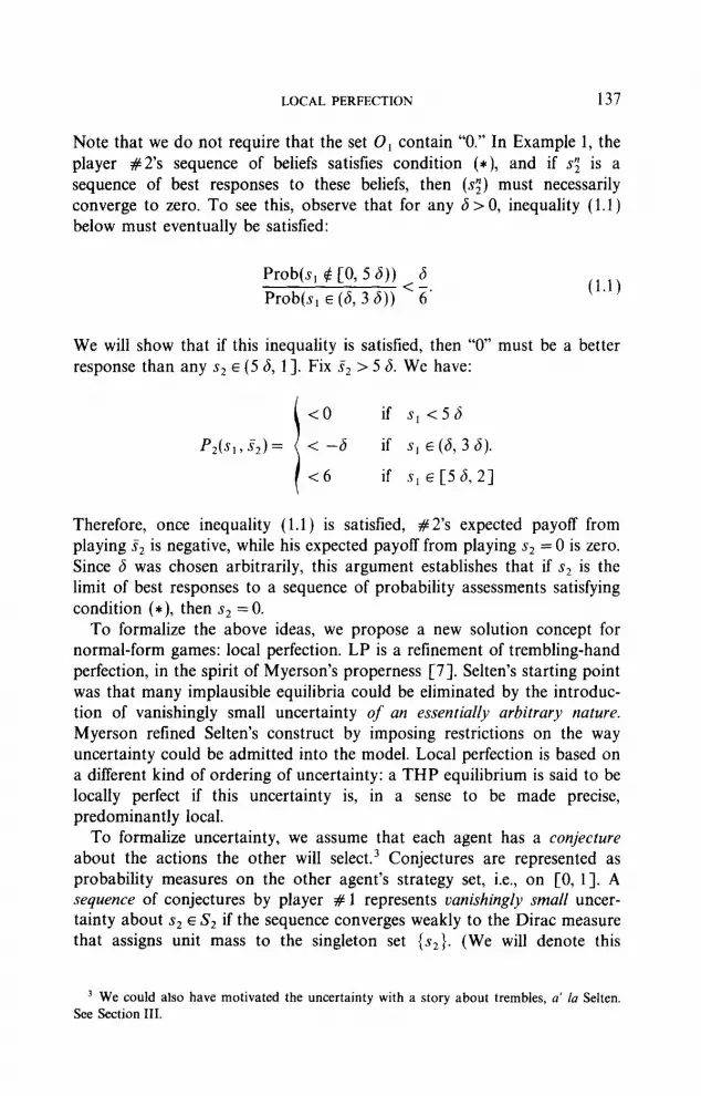
Note that we do not require that the set 0, contain “0.” In Example 1, the player #2’s sequence of beliefs satisfies condition (*), and if s; is a sequence of best responses to these beliefs, then (3;) must necessarily converge to zero. To see this, observe that for any 6 > 0, inequality (1.1) below must eventually be satisfied:

Prob(s, +! [0, 5 6)) 6 Prob(s, E (6, 3 6)) < 6’ (1.1)

We will show that if this inequality is satisfied, then “0” must be a better response than any s2 E (5 6, 11. Fix S, > 5 6. We have:

i

<o if s,<56

PAS, > S,) = < -6 if s, E (6, 3 6).

<6 if s, E [5 6, 21

Therefore, once inequality (1.1) is satisfied, # 2’s expected payoff from playing S2 is negative, while his expected payoff from playing s2 = 0 is zero. Since 6 was chosen arbitrarily, this argument establishes that if s2 is the limit of best responses to a sequence of probability assessments satisfying condition (*), then s2 = 0.

To formalize the above ideas, we propose a new solution concept for normal-form games: local perfection. LP is a refinement of trembling-hand perfection, in the spirit of Myerson’s properness [7]. Selten’s starting point was that many implausible equilibria could be eliminated by the introduc- tion of vanishingly small uncertainty of an essentially arbitrary nature. Myerson refined Selten’s construct by imposing restrictions on the way uncertainty could be admitted into the model. Local perfection is based on a different kind of ordering of uncertainty: a THP equilibrium is said to be locally perfect if this uncertainty is, in a sense to be made precise, predominantly local.

To formalize uncertainty, we assume that each agent has a conjecture about the actions the other will select.3 Conjectures are represented as probability measures on the other agent’s strategy set, i.e., on [0, 11. A sequence of conjectures by player # 1 represents vanishingly small uncertainty about sa E S2 if the sequence converges weakly to the Dirac measure that assigns unit mass to the singleton set (szj. (We will denote this

3 We could also have motivated the uncertainty with a story about trembles, a’ la Selten. See Section III.

138 LEO K. SIMON

measure by S,,.) A pure-strategy Nash equilibrium, S= (Sr, S,), will be called trembling hand perfect (THP) if for each i, there exists a sequence of conjectures, (pi,“), ~‘9’ +n 6,, and a sequence of strategies, (s;), S; -+, Si, such that, for each n if i conditions on the conjecture ~‘7”~ then s; maximizes his expected payoff function.

The set of THP equilibria may be very large. In example 1 above, any profile (0, sZ), s2 E [0, l] can be supported as a THP equilibrium. To illustrate this, choose 6 E (0, 11. We will construct conjectures that support the profile s(6) = (0,2 6). We need be concerned only with player #2 since, clearly, s1 = 0 will be a best response for player # 1, regardless of his conjecture. Let (/.?“) be the sequence of conjectures on [0,2] defined by, for all n: p2.“({O})=(l-n-1-n-2); p*‘“({36))=n-’ and the remaining mass, (np2), is distributed uniformly over the remainder of [0,2]. Clearly, (p’.“) converges weakly to 6,. Moreover, P,(3 6, .) attains a strict global maximum at s2 = 2 6.4 Therefore, if for each n, S; maximizes

s co,ll P2(t,, .I dp2?tl), then s; +n 2 6. This establishes that s(6) is a THP equilibrium.

The above construction illustrates that the conjectures needed to support a particular THP equilibria may have to be very artificial. For example, to support any profile other than (0, 0), we had to assign a significant “lump” of probability mass to some event that was isoZated from “the truth,” i.e., from the event s1 = 0. This motivates the following refinement: a strategy profile will be called locally perfect if it can be supported by conjectures representing predominantly local uncertainty. We mean by this that agents’ conjectures must, in the limit, assign an overwhelmingly high proportion of the total probability mass to events “in the vicinity of the truth.” In the following section, we formalize this restriction by generalizing condition (*) above. From our earlier argument, we have established that Example 1 has a unique LP equilibrium, the profile (0,O).

In the following section, we establish that condition (*) can be satisfied for a large and reasonable class of conjecture sequences. The simplest example is a sequence of truncated-normally distributed conjectures, cen- tered about zero and with variance converging to zero. For example, let player # 2’s nth conjecture, p2,n, be the truncated normal distribution on [0, 23, with mean 0 and variance l/n. Let f ‘; denote the density of p2+. Fix 6 > 0. Inequality ( 1.1) is satisfied if we pick n sufficiently large that f ;(5 8)/f ‘;(3 6) < a2/6. In this case, we have

Prob(s, 4 [O, 5 6)) < a2(2 - 5 6) 6 Prob(s, E (6, 3 6)) 6(26) (6’

4 (s/as,)P,(3S,.)=(s,/s,)2 [2(s,/sz)-31 and (8'/(as,)')P,(36, 26)<0.


II. LOCAL PERFECTION

We begin by defining local perfection for games in which mixed strategies are inadmissible. We then extend the concept to general games. The special and general concepts are treated separately for two reasons. First, the former is more intuitive, and motivates the general definition. Second, the two notions are conceptually distinct: there are degenerate (i.e., singleton support) mixed-strategy LP equilibria that are not locally perfect in the pure-strategy sense. (This is less surprising than at first sight: as we shall see, the meaning of “predominantly local uncertainty” is quite different, depending on whether or not mixed strategies are admitted. Since in many economic contexts, mixed strategies have no sensible interpretation, it is useful to have a separate concept for pure strategy games.)

Pure Strategies

Let I denote a finite set of players, with generic element i. Player i’s pure strategies will be represented by S;, with generic element s;. We assume that Si is a compact metric space. Let d;F be a metric for S;. Let S = ni,, Sj and let dS = maxit I d,S. The set S will frequently be written as Si x Sj, where ,S_; = nj,i S,. (We will use the notation ( ‘i, -‘) frequently below, without further comment.) An element s = (si, spi) E S will be called a pure strategy profile.

A payoff function P: S + R#‘, assigns to each strategy profile a vector of payoffs, one for each agent. We assume P is continuous w.r.t. dS. A game is a pair (S, P). A pure strategy Nash equilibrium for (S, P) is a profile s E S such that for all iEI and all s:cSi, P,(s)> Pi(s,!, sei).

Let M(S,) denote the set of Bore1 probability measures on playerj’s pure strategies. Let M(S,) denote the Bore1 product probability measures on S-i.5 A point pin M(Si) will be called a conjecture by i. The conjecture pLi represents i’s beliefs about the strategies other agents will choose. That is, for the Bore1 subset Tei of S,, $(TAi) is the probability assigned by i to the event that other agents will choose pure strategies in Tei. Let dp denote the Prohorov metric on M(S,) and let dP, = maxIf, d,’ denote the product Prohorov metric on M(S-i).6 A conjecture profile, p = (P~)~~,, is a list of conjectures, one for each agent, i.e., an element of nis, M(S,). We

5 A probability measure m’ defined on the Bore1 rectangles of S-, is a product measure if there exists a family of measures, (m,),,,, where m, EM(S,), such that for every Bore1 rectangle T-(ES_,, m’(T-,)=n,,, M,( r,). See Hildenbrand [S, p. 41, 471 for precise definitions.

6 The Prohorov metric is a metric for the topology of weak convergence. See Hildenbrand

IS, P. 491.

140 LEO K. SIMON

will say that a sequence of conjectures by i, (pi*“), is rich if every open subset of Si is eventually assigned positive measure by (pi,“), i.e., if7

for any open set 0 -i c Si, 317 s.t. Vn > ti, #“(Obi) > 0. (2.1)

For sj ES,, let 6, E M(S,) denote the Dirac measure at sj, that is, the measure defined by: ds,( {s,}) = 1. Define 6,-, and 6, analogously. The conjecture pi = 6,-, represents certainty by i that other players will choose SLY.

A sequence of (conjecture profile)-(pure strategy profile) pairs, (p”, s”), will be said to “validate” a strategy profile S if for each i: (a) for each n, s: is a best reply against ~‘2’; (b) the sequence (#“) converges weakly to 6,-,; (c) the sequence (3;) converges to Si. Formally, a sequence (pLn, s”) in JJis,M(S-,)x S validates SES if for all i,

Qs; E Si, s

(Pi(s:, tui)-Pi@;, t-i))d$,n(tpi)>O; (2.2a) s-t

dPi(pi’“, ‘Fe,) 7 0; (2.2b)

d;(s;, Si) 7 0. (2.2c)

We will be concerned with conjectures that assign, in the limit, an overwhelmingly large proportion of the total probability mass to events “in the vicinity of’ the event (S}. To formalize this idea, we introduce the idea of an “order restriction” on Smi. We will say that a sequence of conjectures, (pi,“) is S-ordered about S_; if there exists a sequence of open subsets of Si, ( Pi)k”, 1, satisfying

(2.3a)

Vk, for any open set 0-i C uki, “:(“,~~~-~i) 7 O. (2.3b) I 1

See Fig. 2. A profile, SE S is a pure strategy locally perfect (LP) equilibrium if there

exists some sequence ($, sn) in ni,, M(S-,) x S such that

Vi E I, (pi-n) is rich; (2.4a)

(p”, 8”) validates S; (1.4b)

Vi, ($3”) is S-ordered about dei. (2.4)

’ It would be more conventional to require that for all n, supp(~‘~“)= S-,. Our weaker requirement is easier to work with when S-, is an infinite dimensional space.


0-i

FIGURE 2

S-Ordering with Pure Strategies

Condition (2.3) is a strictly stronger requirement than weak convergence. For example, consider again Example 1 above, and the sequence of conjectures, (p2*“), on [0,2], defined in Section I: g*“( (0)) = (1 -n ~’ -n-‘); $‘“({3fs})=n+ with the remaining mass, (K*), being distributed uniformly over the remainder of [O, 21. This sequence converges weakly to 6, but is not S-ordered about Si, since ,B*‘“(S, N (0, 3 S))/p**“((O, 3 6)) +n co. The general point is that weak convergence to b0 does not guarantee that the probability assigned to strategies far away from zero will become small relative 20 the probability assigned to any set close to, but not containing the point zero itself.

What conditions do guarantee that a sequence, (,uiv”), will be S-ordered about Sei? It is not sufficient, obviously, that the supports of the Z?? collapse to (Sei>. Indeed, if condition (2.3) is satisfied, then the supports of the Z.P’s cannot converge to (SW;>. (If O-i c UL, for some k, then ,P(OPi) must eventually be positive.) However, condition (2.3) will be satisfied if (@“) is a convex combination of two measures, (pi”) and (,uy), where the supports of the ,Q’s collapse to {s-~> and the py’s are distributed normally, with means converging to sBi and variances converging to zero.

For example, let Sj = [0, 11, for all i. For i E Z, let Xi be an arbitrary, positive definite ( # Z - 1 x #I- 1 )-dimensional matrix. Define the function fi,n: SPi xSei + R, by:f’*“(., sei): Ki + R, is the density of the trun-

142 LEO K.SIMON

cated normal distribution with mean s-i and variance-covariance matrix n-‘Cwi, i.e.,

(2.5)

(Here and elsewhere, we denote Lebesgue measure on R“ by I”.) Now fix SEi E Si and let sTi be a sequence in Sei such that sYi +,, SVi. For n E N, let ~Lij” denote the distribution of f’,“( ., sTi), (that is, for any Bore1 set TeicSi, ~~(T_j)=~,_,~(r_,,s”j)d~#‘~‘(r_i)). Alsopickasequence (pi”) in M(S,) such that supp(&“)-+, ~3~~. Finally, let (~1”) be an arbitrary sequence in (0, l] and set $.n = cP~Y + (1 - a”) pp. We have:

PROFQSITION la. The sequence (p’s”) is S-ordered about SKi.

Proof of Proposition Ia. For kE N, let vi= {Spi ESpi: (s-~-s-~)‘GI:(s-, -S-i)< l/k}. N ow fix k and an open set 0-i C Uki Also pick 6>0 such that (s_i--S_i)‘Cl,‘(s_i--si)<l/k-26, for all s _ i E 0 _ i. Finally pick fi sufficiently large that for all n > fi &?( Uki) = 1 and (s-~ -s:,)’ ,Z’:;(S-~ -Pi) > l/k - 6, for all sei E Si - Uki. For n>ii. we have

/.Lys-i - U’l”;.) ct”p’;“(s-i - l/y)+ (1 -cc”) Pf”(SMi N us:., /P(Opi) = a”/Jy(O-i) + (1 -Cln) /Jy(O-i)

d p’;“(S_, - uy,

/l:“(O-j)

= jSm,-de,Y(r-i, s’Li)dA#I-‘(r-i)

So-, p(rei, syi) dAX’-‘(r-J

exp{ -(n/2)(1/k-@) ‘exp{-(n/2)(l/k-28)j”00. ’

Mixed Strategies

A mixed strategy for i is a Bore1 probability measure on Si, i.e., an element of M(S,). Let vi denote the generic mixed strategy for i. A mixed strategy profile is a Bore1 product probability measure, i.e., a point in M(S). A Nash equilibrium for (S, P) is a profile v E M(S) such that for all ieZ and all s: E Si, Is P,(t) du>J,_, P,(s:, tei) du_i.

As before, a conjecture by i is a point in M(S,). A sequence (pL”, vn), will be said to validate a mixed-strategy profile 17 if for each i: (a) for each n, v; is a best reply against P’*~; (b) (pi*” converges weakly to VPi; (c) (~7) con-


verges weakly to Vi. Formally, a sequence (p”“, u”) in ni, I M(S-,) x M(S) validates 17 E M(S) if for all i,

VS:ES~,J‘ [I Pi(t;, tPi)dul(ti)-Pi(s:, t-;)I dp’+(tLi)>O; (2.2a’) s-t s

dPi(pi*n, v-;) n. o; (2.2b’)

df’(u;, V;) n’ 0; (2.2c’)

We now extend our notion of S-ordering to incorporate mixed strategies. It turns out that the general notion is necessarily more intricate than the special case. In the pure strategy case, our S-ordering concept was defined relative to a point in pure-strategy space. When we generalize this notion to mixed strategies, we need to define S-ordering about a conuergent sequence of mixed strategies. The following argument indicates why this change is necessary. Fix a Nash equilibrium, 6, and a convergent sequence of strategy-conjecture profile pairs, (un, pn), such that the u”‘s are the best replies to the ~“‘s. Now, our intuitive notion is that V will be locally perfect if the ~‘5 represent predominantly local uncertainty about the u”‘s, that is, if a relatively high proportion of the “residual” probability mass is assigned to strategies close the supports of the 0”‘s. However, weak convergence of (0”) to V does not guarantee that the supports of the S’S converge to the support of U. Therefore, the ,P’s may assign “lumps” of probability mass to strategies isolated from the support of the limit profile. For example, let I= (1,2) and S, = [0, 11. For each n, define v; and ,u~*” by

n-l u;=-6,+~c3,; n

for any Bore1

T, c LP2v-l) = .c,, [G f2.“(rl,0)+~f2.n(rl, l)]di.‘(r,),

where f*,“( ., sl) is defined by (2.5) above. Clearly, the sequence (~~3”) is not S-ordered about zero. The conjectures do, however, represent predominantly local uncertainty about the u;‘s, and so should be admissible, according to our intuitive criterion. It is inappropriate, therefore, to define S-ordering in terms of the limit profile alone: the sequence of validating best responses must enter explicitly into the

642143’1.IO

144 LEO K. SIMON

definition of our concept. Accordingly, our mixed-strategy analog of (2.3) requires that any open set of pure-strategies close to the support of lim, vTi be assigned high probability relative to the probability assigned to strategies isolated from the supports of the v”~‘s.

Formally, we will say that a convergent sequence of conjectures, (#“) is S-ordered about (vTi) if there exists a sequence of pairs of open sets, (U?$ U?:)p= 1, satisfying’

(2.3a’)

tlk, for any open set 0 -; c U’,k. ” 0 “(S-i N U?:) _) 0

gyo-j) ” . (2.3b’)

For example, consider the sequence, (v;, p’s”), defined above (expression (2.6)). Since Ls(supp(vq)) = (0, 1 }, the conjecture sequence (~~3”) satisfies condition (2.3’): take Ukk = [0, l/k) and U$” = [0, l/k) u ((k - 1)/k, 11. More generally, we establish below (Proposition Ib) that a sequence of v:,- weighted combinations of truncated normals will be S-ordered about (vyi).

A mixed strategy profile, 17, is a locally perfect (LP) equilibrium if there exists a sequence (p”, u”) satisfying:

Vi, (pi,“) is rich; (2.4a’)

($‘, u”) validates V; (2.4b’)

Vi, ($9”) is S-ordered about (UT,). (2.4~‘)

Since condition (2.3’) is clearly weaker than (2.3), there exist singleton support LP equilibria which are not pure-strategy LP equilibria. For example, consider the two-person game, (S, P), where S, = [0, 11, S, = (f, r} and P is defined by

P,(s,,1)=P,(s,,r)=s:-s,.

P,(S,? s2) = i s1 -s: if s2=1

$3, if s2 = r.

(Example 2)

8 “Ls” denotes the “topological limes superior” (see Hildenbrand [S, p. 151; SC, ~Ls(supp(v”-,)) if there exists a subsequence (v”‘<) and for every q an element t<,osupp(o<,) such that t”!,-+s_,. For example, if ~“~=((n-l)/n)6,+(l/n)6,, then Ls(supp(v”_,))= (0, 1). The reader is cautioned not to confuse Ls(supp(v”,)) with L.r(supp(p’.“)): since the ~““‘s are rich, Ls(supp(#,“)) = S-;! Note that condition (2.3b’) does not imply weak convergence of the @“‘s to lim, vyi (cf. the corresponding condition (2.3b), which did imply that @@s converged weakly to S-,.)


The pure-strategy Nash equilibrium (0, r) is not a pure-strategy LP equilibrium. Against any sequence of conjectures that is S-ordered about 0, player #2 clearly does better by playing “left.” On the other hand, 6,,, is a locally perfect equilibrium in the mixed-strategy sense: 6,,[ is validated by (u”, p”), where u’; and ,u(; are defined above (expression (2.6)). The reason for the difference is, simply that if mixed strategies are admitted, there are more convergent sequences of strategies, and, consequently, more conjecture sequences representing local uncertainty about such strategies.

Stronger Variants

An LP equilibrium may be validated by idiosyncratic beliefs. That is, two agents’ conjectures about a third agent’s actions may differ. In some contexts, it may be appropriate to impose the stronger requirement that conjectures are consistent, i.e., that any two agents must have the same beliefs about what any third agent is likely to do. (Discussion of the consistency issue is deferred until Section III.) Accordingly, we define a sequence of conjecture profiles, ($‘) = (P’,~);~ ,, to be consistent if

Vn, 3~” E M(S) s.t. Vi E Z, pi,n = x? i (2.7)

We will say that a pure strategy LP equilibrium, J;, is a consistent locally perfect (CM) equilibrium if it can be validated by some sequence of pairs, ($, sn), such that (flu”) is consistent. (The mixed strategy notion is defined analogously.) Note that in a two player game, condition (2.7) is satisfied trivially.

Our second variant is introduced so that LP can be applied to games with finite strategy sets. Since finite sets have a trivial topological structure, local perfection has no bite in finite games: a Nash equilibrium for a finite game is CLP iff it is trembling hand perfect. On the other hand, local perfection without consistency is strictly weaker than THP for finite games: a Nash equilibrium for a finite game is LP iff no agent’s strategy is weakly dominated by some other mixed strategy.’

In many games of economic interest, however, there is a natural metric structure, and it may be quite reasonable to require that uncertainty be locally concentrated. For example, strategies may be a finite subset of some “natural continuum”: prices may be denominated in dollars and cents, time units in days, etc, output in integers, etc. In such games, we can eliminate certain implausible equilibria if we replace our original S-ordering condition with a more stringent, metric condition.

To capture the intuition of local perfection in finite games, we substitute

9 This fact can be proved by manipulating Rockafellar [ll, Theorem 22.1. p. 1981,

146 LEO K. SIMON

a net of balls for the sequence of neighborhoods in condition (2.3). We say that a sequence of conjectures, (pi,‘), is metrically S-ordered about Sei if

ViEI, VEER, k>O and any open set O-icB(S-i, l/k), (2.3b”)

/li'"(Sp; - B(Ci, ilk)) _) 0 /i.i'n(O-i) n '

The mixed strategy analog of metric S-ordering is defined in the obvious way: a convergent sequence of conjectures, (pi,“) is metrically S-ordered about (I?~) if

Vi E Z, V’k E R, and any open set 0 pi c BH(supp(lim o”~), l/k), (2.3b”‘) n

~Li’n(S-iNBH(LS(SUpp(u”j)), ilk))- o /P(O-j) n .

(BH( Tpi, 6) is the Hausdorff ball about the set T_ ;, i.e., BH( T-i, 6) = (SLi E sei 3 tci E spi s.t. d:,(t-,, sxi) < S}.,

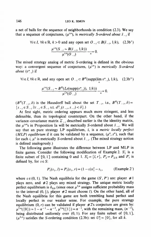
At first sight, metric ordering appears much more stringent, and less defensible, than its topological counterpart. On the other hand, if the variance-covariance matrix Cei described earlier is the the identity matrix, the ~~3”‘s in Proposition Ia will be metrically S-ordered about SKi. We will say that an pure strategy LP equilibrium, S, is a metric locally perfect (MLP) equilibrium if it can be validated by a sequence, (p”, s”), such that for each i, pLn is metrically S-ordered about S- ;. (The mixed strategy notion is defined analogously.)

The following game illustrates the difference between LP and MLP in finite games. Consider the following modification of Example 2. S; is a finite subset of [0, l] containing 0 and 1. S; = (I, r}, Pi = P2,s and Pi is defined by, for s E S:

P;(s,,I)=P;(s,,r)=(l-&)S:--SI, (Example 2’)

where E E (0, 1). The Nash equilibria for the game (S’, P’) are: player # 1 plays zero, and #2 plays any mixed strategy. The unique metric locally perfect equilibrium is a,,, (since once p2*” assigns sufficient probability mass to the interval (0, t), player #2 must choose I). On the other hand, all of the Nash equilibria for this game are both trembling hand perfect and locally perfect in our weaker sense. For example, the pure strategy equilibrium (0, r) can be validated if player #2’s conjecture are given by: ~2~n({0})=1-~~1-~-2,~2~n((1})=~~1,withtheremainingmass,(n~2), being distributed uniformly over (0, 1). For any finite subset of [O, l], (~~3”) satisfies the S-ordering condition (2.3b): set Ut = {0), for all k.


Large Strateg-v Spaces

Local perfection has proved to be a powerful concept when strategy sets are very large (e.g., function spaces). For example, in a game described in Simon 193, strategies are indifference surfaces. The set of THP equilibria for this game is extremely large, but the locally perfect equilibria are all outcome equivalent. Indeed, in the the locally perfect equilibria, agents’ announced indifference surfaces coincide (locally) with their true preferences.

Once strategy sets are infinite-dimensional, however, the construction of S-ordered conjectures is somewhat delicate. A natural way to proceed is to approximate the S,‘s with finite-dimensional sets, and define a sequence of normal distributions on the corresponding Euclidean spaces, This section illustrates such a construction. Proposition Ib below is an infinite-dimensional, mixed-strategy version of Proposition la. It plays a key role in our existence proof in Section IV.

Let S, be a convex, compact subset of metrizable topological vector space, and let d,’ be a metric for S,. Let S; be an nondecreasing (by inclusion) sequence of convex, finite dimensional subsets of S, such that cl(lJ, S;‘) = S,. Let p,(n) = dim(Sy).‘” Without loss of generality, assume that p,(n) <n.

For each n, choose a homeomorphism g;: SY, + R’+(n). Define the function gr: a;(S;) x S, + R + by, for (xi3 s,) E a;(y) x S,,

gl’(x,, s;) = exp( -(n’/2) d,S((a;)-‘(x,), s,)}

s +5;, exp{ -(n’/2) dT((cr;)-‘(y,), s,)} dlQ(“‘(y,) (2’5’)

With the obvious caveat when pj(lz) =O, g; is a well-defined density on c;(S;). Note that the variances of the g;‘s are shrinking at a faster rate than those of thef’,“‘s defined by (2.5). Define gin: n[+; o;!(S;) x Si + R, by

g’q.xL;, t mi) = n g;(xj, f,). (2.8) /#i

Let (0” i) be a convergent sequence in M( S i). For n E N, define pi.” on S, by, for any Bore1 set Tmj cKi,

I”.“(T~,)=js~~jbl.rr,~~ ) gi.“(y-,, tci) dP’“‘(.v~,) du”_;(tp;). (2.9) -,

Clearly, p i.n is a well-defined probability measure on S,. We have:

PROPOSITION Ib. The sequence (pi*“) is rich and metrically S-ordered about ( VF i).

lo Given a vector space, V, dim(V) denotes the dimension of V.

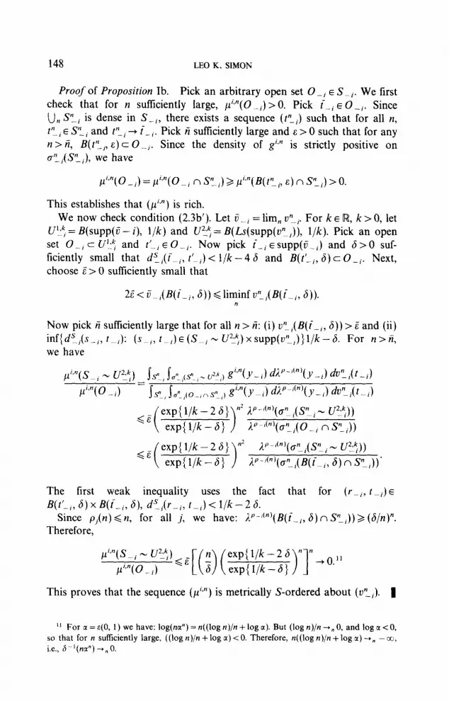
148 LEO K. SIMON

Proof of Proposition Ib. Pick an arbitrary open set Oei E Sei. We first check that for n sufficiently large, ~“~(0~~) > 0. Pick Ci E O-j. Since Un S”i is dense in Spi, there exists a sequence (t: J such that for all n, t”, E Sri and Pi -+ iCi. Pick ii sufficiently large and E > 0 such that for any n > ii, B(P, E) c O-,. Since the density of g’,” is strictly positive on cYi(s” ;), we have

This establishes that (p”“) is rich. We now check condition (2.3b’). Let V pi = lim, v” i’ For k E R, k > 0, let

U’l”, = B( supp( V - i), l/k) and U?: = B( Ls( supp( VT i)), l/k). Pick an open set 0 _; c 175: and t’-, E 0 --i. Now pick Ci E supp(Ei) and 6 > 0 sufficiently small that dSi(f_,, t/L;)< l/k-4 6 and B(t’L,, 6)cO-,. Next, choose E > 0 sufficiently small that

2F< K,(B(i-,, 6)) <liminf u:,(B(t-,, 6)). n

Now pick C sufficiently large that for all n > t? (i) v:,(B(iCi, 6)) > E and (ii) inf{dsi(s-;, t-,): (s-,, tLi)E(Spi- CT?:) x supp(v:,)} l/k - 6. For n > ti, we have

> nz p’(“)(&(s”;- uy))

P~‘“‘(a”i(B(i_;, 6) n s”,))’

The first weak inequality uses the fact that for (rei, t pi) E B(t’l,,6)~B(i-~,6), dTi(rdi, tpi)<l/k-26.

Since pi(n) <n, for all j, we have: AP-““‘(B(i_i, 6) n Fe,)) 2 (d/n)“. Therefore,

This proves that the sequence (cl”“) is metrically S-ordered about (v”~). 1

” For a = ~(0, 1) we have: log(na”) = n((log n)/n + log a). But (log n)/n -t” 0, and log G( < 0, so that for n suffkiently large, ((log n)/n + log 61) -C 0. Therefore, n((log n)/n + log c() --+” - co, i.e., @‘(~a”) -+n 0.


III. LOCAL PERFECTION AND RELATED SOLUTION CONCEPTS

III. 1. “Trembling- Hand’ Perfection (Selten [S] )

Selten defined “trembling hand” perfection only for games with finite strategy sets. The definition below coincides with Selten’s for finite games and appears to be a natural extension to larger spaces. A strategy profile, v E M(S), is a trembling hand perfect equilibrium if there exists some sequence ($I, u”) satisfying

Vi, (p”“) is rich; (2.4a)

($‘, 3”) validates V; (2.4b’)

(pL”) is consistent. (2.4d)

As we have noted, consistent local perfection and trembling hand perfection are equivalent for finite games, but LP is strictly weaker. Consistency is omitted from our basic definition of local perfection for three reasons. The first is pragmatic: to verify that a given equilibrium is locally perfect, it is sometimes easier to construct an individual sequence of conjectures for each agent. Second, LP is a more parsimonious concept than CLP. In the economic applications that we have considered, we have been able to exclude all the Nash equilibria we wished to exclude with the weaker concept. Finally, we argue below that whether or not one imposes consistency affects the heuristic intepretation that one can attach to the solution concept.

Selten motivates trembling hand perfection as “a model of slight mistakes.“12 He imagines sequences of games in which agents occasionally fail to act rationally. With vanishingly small probabilities, their “hands tremble,” causing them to select nonoptimal strategies. These trembles generate probability distributions on the space of strategy profiles. An equilibrium is THP if it is a limit of best responses to some such sequence of distributions. Consistency is a natural restriction to apply in this context; indeed, it is implied by the minimal presumption that agents “know the model.”

We have proposed a rather different heuristic fiction. Rationally is absolute but perceptions are slightly “fuzzy.” There is uncertainty in our model, not because agents are actually trembling but because other agents do not know precisely which strategies they are playing. Consistency is surely as unnatural in this context as it is natural in Selten’s: why should two agents’ purely subjective assessments about what a third agent will do coincide?

I2 This “model” is, of course, only a heuristic fiction, invented to justify his formalism. He observes: “there cannot be any mistakes if agents are rational.”

150 LEO K. SIMON

111.2. Proper Equilibria (Myerson [ 71)

Many trembling-hand perfect equilibria are quite implausible. Myerson proposed an “order restriction” rather similar to ours, as a way of excluding some of these equilibria. Suppose that S is a finite set. Let (x”) be a sequence of full support measures in M(S). We will say that (x”) is P-ordered if, for all i and all si, s: E Si, x; satisfies:

if 3ii s.t. Vn > ti, I (PitSit t-i)-P,(s:, tLi))d~Y;(tLi)>O (3.1)

S-.

then

A THP strategy profile, 6, is a proper equilibrium if it can be validated by some ($‘, v”) such that

Vn, ~x”EM(S)~.~.V~EZ,I*~“=X”~ (2.7)

(x:) is P-ordered; (2.4e)

Myerson’s rationale for imposing this condition is that agents are presumably much more likely to “tremble toward” strategies yielding them higher rather than lower payoffs.

Local perfection and properness are similar in that they involve “order restrictions” on the probabilities assigned to different low-probability events: i.e., under certain conditions, the ratio of these probabilities must converge to zero. The difference between Myerson’s construction and ours is: in Myerson’s, events are ordered according to the relative magnitudes of their associated payoffs; in ours, the relevant consideration is the location of events in the strategy space. (This explains why we chose the terms P- ordering and S-ordering). To see the difference, consider again Example 2’, defined above. Choose E E (0, 4) and set Sl, = (0, 2s,4s, ,.., 1 }. Note that &=P;(1,.)>P1(2&,.) = (l-s)s2-2s, so that player #l’s second best strategy is 1. Any tremble by 1 that supports a proper equilibrium must therefore assign most of the residual probability mass to the event s1 = 1. Since r is a better response than 1 for player #2 against si = 1, the unique proper equilibrium is (0, r). On the other hand, as we have seen, the unique metric locally perfect equilibrium is (0,Z). Whether one prefers the locally perfect equlibrium to the proper equilibrium depends on how one inter- prets the trembles and how seriously one takes the metric structure of the game. The smaller is E, obviously, the more compelling is the argument for


local perfection. On the other hand, one might argue that if the differences between the payoffs to different strategies is very large, agents might be very careful to err in the direction of least payoff loss. Obviously, there is no categorical answer.

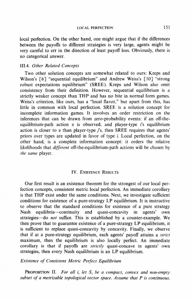
111.4. Other Related Concepts

Two other solution concepts are somewhat related to ours: Kreps and Wilson’s [6] “sequential equilibrium” and Andrew Weiss’s [lo] “strong robust expectations equilibrium” (SREE). Kreps and Wilson also omit consistency from their definition. However, sequential equilibrium is a strictly weaker concept than THP and has no bite in normal form games. Weiss’s criterion, like ours, has a “local flavor,” but apart from this, has little in common with local perfection. SREE is a solution concept for incomplete information games. It involves an order restriction on the inferences that can be drawn from zero-probability events: if an off-the- equilibrium-path action c( is observed, and player-type is equilibrium action is closer to a than player-type Js, then SREE requires that agents’ priors over types are updated in favor of type i. Local perfection, on the other hand, is a complete information concept: it orders the relative likelihoods that different off-the-equilibrium-path actions will be chosen by the same player.

IV. EXISTENCE RESULTS

Our first result is an existence theorem for the strongest of our local perfection concepts, consistent metric local perfection. An immediate corollary is that THP exist under the same conditions. Next, we investigate sufficient conditions for existence of a pure-strategy LP equilibrium. It is instructive to observe that the standard conditions for existence of a pure strategy Nash equilibria-continuity and quasi-concavity in agents’ own strategies-do not suffice. This is established by a counter-example. We then prove that to guarantee existence of a pure-strategy LP equilibrium, it is sufficient to replace quasi-concavity by concavity. Finally, we observe that if at a pure-strategy equilibrium, each agents’ payoff attains a strict maximum, then the equilibrium is also locally perfect. An immediate corollary is that if payoffs are strictly quasi-concave in agents’ own strategies, then every Nash equilibrium is an LP equilibrium.

Existence of Consistent Metric Perfect Equilibrium

PROPOSITION II. For all i, let Si be a compact, convex and non-empty subset of a metrizable topological vector space. Assume that P is continuous.

152 LEO K. SIMON

Then a consistent metric LP equilibrium (and hence a THP equilibrium) exists for the game (S, P).

Proof of Proposition II. The proof will make frequent use of the definitions and construction introduced earlier. For each j, construct a sequence of approximating sets, (Sin), and the family of functions g’,” defined by (2.8). Define the payoff function, P”, by, for each i and s E S,

p:(s) = jgL,(9w ) Pi(Si, ~li(~-i)) gi”‘(y_l, s-i) dAp-8’“‘(y-i). (4-I)

Clearly, P” is continuous, so that (S, P”) satisfies the standard conditions for existence of a Nash equilibrium (Debreu [ 11, Glicksberg [4], Fan [3]). Let un be an equilibrium for (S, P”). Pick a convergent subsequence of (u”), again indexed by n, and let V be the limit of this sequence. We will show that V is a CMLP equilibrium for (S, P).

For each n, let $ = (#n),E,r where $,n is defined by (2.9). By Proposition Ib, (pi,“) is rich and metrically S-ordered about (0: ;). Also, ~‘3~ clearly converges weakly to Ki. Moreover, for all n, i, and si E S,,

IS P;(t;, tpi) dpis”(t~i) dv;(tJ s, s-t

= ss 5 Pi(tit (oYl)-’ (y-i)) g”“(Y-i, t-i)

s, s-, o”,(f-,I

x dilp-z’“‘(y-,) dv”;(tpi) dv;(tJ

= i p:(t) dv”( t) s,

= I s pi(Sj, (aYi)p’ (Y-i)) g”“(Y-iv t-i)

s-, u”,Cs”-,,

x dA’m’(y-i) dv’Ii(t-i)

= s Pi(~j, t-;)dpisn(t-i). s-s

This establishes that ($‘, v”) validates V and completes the proof. 1


FIGURE 3

A Quasi-concave Game with No Pure Strategy Locally Perfect Equilibrium

Consider the following game. There are two players. The set of strategy profiles is S = S’ x S2 = [0, I] x [0,2]. The payoff function, P: S + R2, is illustrated in Fig. 3. It is defined by, for s = (s,, s2) E S:

I s2,

PI(s)= 4(s, -+1-s,, s -4s

2 1,

[ Z-32,

(2-s2)(1+2s, -szh

(2 - s2)(1 - 2s, + S?),

Note that Pi is quasi-concave in si.

SE L-0, ; (1 +sz)l x [O, 11

SE(5(1 +s,), 11 x co, 11 SE [o,; (s2 - 111 x Cl,21 sE(t(Jz-l), 11x(1,21

5-E co, 44 x co, 11

3-E ($32, t @I! + 1)l x co, 11 s E C&S2 - 1 ), 4 $1 x (L23

3E(4-72, 11 x (421 otherwise.

(Example 3 )

154 LEO K. SIMON

The profile (f, 1) is the unique pure-strategy Nash equilibrium for this game. There is also a mixed strategy equilibrium, V, where Vi = 4 6, + 4 6, and V, = 16, + 4 6,. The payoffs are the same in each of the two equilibria: each player’s payoff, or expected payoff, is 1.

The profile (4, 1) is clearly not an THP equilibrium and hence cannot be an LP equilibrium. Player #l’s strategy “$” is weakly dominated both by “0” and by “1.” Indeed, given any conjecture, pl, by player # 1, si will be a best response to this conjecture only if si E (0, l}. Therefore, there exists no sequence of conjecture profiles that validates (&, 1). On the other hand, V is locally perfect. It is validated by the sequence ($, vn), where v” = V and p’,” and p2.” are, respectively, the distributions of [f f’.“( ., 0) + + f’,“( ., I)] and l-4 f2,“( ., 0) + t f2.“( ., 2)]. (As usual, the f”‘s are defined by (2.5).)

There is a modification of the above game that has a unique pure- strategy THP equilibrium that is not locally perfect. The modification involves replacing P, by Pi, defined as follows: let E E (0, 4) be arbitrarily small and let P’, be continuous, quasi-concave in s,, agree with P, except on {.YES:S~ E(;-s, f+e)} and satisfy, for all si #$, P’,(s,, 5) < P’,(i, f) = $. We can support (4, 1) as a THP equilibrium for the game (S, (P’, , P2)), by choosing conjectures for player # 1 that assign an overwhelming proportion of the residual probability mass to some appropriately small neighborhood of s2 = t.

What outcome would we expect to observe if Example 3, or the above modification of it, were played in practice? In either case, we find it implausible that agents would arrive at the pure-strategy equilibrium. The locally perfect mixed-strategy equilibrium yields the same payoffs and is clearly much more “robust.” We conclude from this that Local Perfection may provide a useful criterion by which to eliminate even a unique pure- strategy equilibrium.

Existence of LP Equilibria when Payoffs are Concave

The fragility of the equilibrium (4, 1) in Example 3 can be traced to the fact that PI( ., s2) is only quasi-concave, rather than concave. To see why quasi-concavity causes existence problems, let P, be the concave function defined by, for all s2 E S,:

When P, is replaced by P, in Example 3, player # l’s choice of 4 in response to sZ = 1 rather than “0” or “1” can be defended. Indeed, it can be verified that the profile (4, 1) is a Locally Perfect equilibrium for the game (S, (pi, P2)). The intuition suggested by this example generalizes to the following result:


PROPOSITION III. Let (S, P) satisfy the conditions of Proposition II above. Assume in addition that Vi, Pi is concave in s;. Then a pure-strategy CMLP equilibrium exists for the game (S, P).

Proof of PropositionIIJ. The proof is virtually identical to the proof of Proposition II. Since Pi is concave in si, the Pps defined by (4.1) are also concave in si. Therefore, a pure-strategy equilibrium exists for (S, P”). Let s” be such an equilibrium and let S be the limit of a subsequence of (s”). The argument used above establishes that S is a pure-strategy CMLP for (X P). I

We conclude the paper with two elementary results. If each agent’s payoffs attain a strict maximum at a Nash equilibrium, then the equilibrium is LP. An immediate corollary is that in games with strictly quasi-concave payoff functions, every Nash equilibrium is Locally Perfect (and hence THP). We now state these results precisely.

PROPOSITION IV. Let S be compact and non-empty, let Pi be continuous, for all i, and let S be a Nash equilibrium ,for (S, P). If Vi and all sj E si - (S,), Pj(Si, S.. ;) > Pj(sj, Spi), then S is an LP equilibrium.

Proof of Proposition IV. For all i, n and SK, E Spi, define f’:, and P; as in the preceding proofs. For all n, let s’ be a maximizer of P:( ., SE,). Pick a convergent subsequence of (SC), again indexed by n, and let S, be the limit of this sequence. By Berge’s theorem (see Debreu [2, p. 191) Sj is a maximizer of lim, P;( ., S- ;) = Pi( ., SK,). But by assumption, this maximizer is unique. Therefore, Sj = Si. 1

PROPOSITION V. Let S be compact and non-empty. If Vi, P, is continuous in s and strictly quasi-concave in si, then every Nash equilibrium for (S, P) is an LP equilibrium.

Proof of Proposition V. A local maximum of a strictly quasi-concave function is a strict global maximum. 1

REFERENCES

1. G. DEBRELJ, A social existence theorem, Proc. Nut. Acad. Sci. 38 (1952), 886-893. 2. G. DEBRELJ, “Theory of Value,” Wiley, New York, 1959. 3. K. FAN, Fixed point and minimax theorems in locally convex topological linear spaces,

Proc. Nut. Acad. Sci. 38 (1952), 121-126. 4. I. L. GLICKSBERG, A further generalization of the Kakutani fixed point theorem with

applications to Nash equilibrium points, Proc. Nat. Acad. Sci. 38 (1952), 17&174. 5. W. HILDENBRAND, “Core and Equilibrium of a Large Economy,” Princeton Univ. Press.

Princeton, NJ, 1974.

156 LEO K. SIMON

6. D. KREPS AND R. W. WILSON, Sequential equilibria, Econometrica 50 (1982), 863-894. 7. R. MYERSON, Refinements of the Nash equilibrium concept, Inf. J. Game Theory 7 (1975)

73-80. 8. R. SELTEN, Reexamitation of the perfectness concept for equilibrium points in extensive

games, Int. J. Game Theory 4 (1975), 448460. 9. L. SIMON, A Bertrand model with differentiated commodities, J. Econ. Theory 41 (1987),

304-332. 10. A. WEISS, A sorting-cum-learning model of education, J. Polit. Econ. 91 (1983). 42CM42. 11. R. T. ROCKAFELLAR, “Convex Analysis,” Princeton Univ. Press, Princeton, NJ, 1970.

Documents

Local perfection