Local subdivision of

Powell-Sabin splines

Hendrik Speleers

Paul Dierckx

Stefan Vandewalle

Report TW424, March 2005

Katholieke Universiteit LeuvenDepartment of Computer Science

Celestijnenlaan 200A – B-3001 Heverlee (Belgium)

Local subdivision of

Powell-Sabin splines

Hendrik Speleers

Paul Dierckx

Stefan Vandewalle

Report TW424, March 2005

Department of Computer Science, K.U.Leuven

Abstract

We present an algorithm for local subdivision of Powell-Sabin splinesurfaces. The construction of such a spline is based on a particularPS-refinement of a given triangulation. We build the new triangu-lation on top of this PS-refinement by applying a

√3-subdivision

scheme on a local part of the domain. To avoid degeneration weintroduce a simple heuristic for refinement propagation, driven by aparameter. This parameter manages the trade-off between the meshquality and the refinement localization.

Keywords : Powell-Sabin splines, subdivision, adaptive refinement, CAGDAMS(MOS) Classification : Primary : 65D17, Secondary : 65D07

Local subdivision of Powell-Sabin splines

Hendrik Speleers, Paul Dierckx and Stefan Vandewalle

Department of Computer Science, Katholieke Universiteit Leuven

Celestijnenlaan 200A, B-3001 Leuven, Belgium

Abstract

We present an algorithm for local subdivision of Powell-Sabin spline surfaces. The construction

of such a spline is based on a particular PS-refinement of a given triangulation. We build the

new triangulation on top of this PS-refinement by applying a√

3-subdivision scheme on a

local part of the domain. To avoid degeneration we introduce a simple heuristic for refinement

propagation, driven by a parameter. This parameter manages the trade-off between the mesh

quality and the refinement localization.

Keywords: Powell-Sabin splines, subdivision, adaptive refinement, CAGD

AMS classification: 65D07, 65D17, 68U07

1 Introduction

The tensor product B-spline representation [9, 3] is nowadays commonly used in many computeraided geometric design packages, because of its compactness, ease of implementation, and compu-tational efficiency. With the aid of the tensor product B-spline control net surfaces can be locallyadapted in a geometrically intuitive and flexible way. Tensor product splines have, however, adefinite drawback: they are restricted to regular rectangular meshes. These limit the shape of thedomain and often preclude an adequate adaptive mesh refinement.

An alternative is to consider piecewise polynomials on triangulations. Bernstein-Bezier polynomialpatches [8] can be used to this purpose. Unfortunately, imposing smoothness conditions betweenthe triangular patches usually results in a large number of non-trivial relations between the coef-ficients. Other candidates are Powell-Sabin (PS-)splines [15]. These C1-continuous quadraticsplines can be represented in a compact normalized B-spline basis with an intuitive geometricalinterpretation involving tangent control triangles [4]. These properties ensure their effectivenessin a wide range of application domains. Willemans [20] used Powell-Sabin splines for smoothingscattered data. Their application in surface modelling was analysed by Windmolders [21]. Powell-Sabin spline wavelets are developed in [23, 18]. Recently, Powell-Sabin splines were also applied asquasi-interpolants [14], and as finite elements [16] for solving partial differential equations.

A natural question that comes up in many such applications is how to represent a given functiondefined on a particular mesh on a refinement of that mesh. The procedures to do so are calledsubdivision schemes and allow, e.g., an increased local control for surface manipulation. Theschemes introduced by Catmull and Clark [1], and by Doo and Sabin [6] marked the beginningof subdivision for surface modelling. Many more schemes like the ones by Loop [13] and byKobbelt [10], the Butterfly [7] and the

√3-subdivision [11] scheme, and further variants have since

become popular. Windmolders and Dierckx [22] solved the subdivision problem for uniform Powell-Sabin splines with a dyadic scheme, and Vanraes et al. presented a triadic subdivision scheme forgeneral Powell-Sabin splines in [19]. Both schemes perform a global refinement at every level of

1

2 POWELL-SABIN SPLINES 2

subdivision. When an increased surface resolution is only required in a small part of the surface,global subdivision may lead to excessive computational and storage costs. In such case, a locallyadaptive subdivision strategy is called for. The development of such a strategy for Powell-Sabinsplines has remained an open problem in the CAGD literature. In this paper, we address thatproblem and we derive a local subdivision scheme for general Powell-Sabin splines. It is basedon a

√3-subdivision scheme to refine a local neighbourhood, and is combined with a refinement

propagation heuristic in order to improve the quality of the refined triangulation.

The paper is organized as follows. Section 2 reviews some general concepts of polynomials ontriangulations, and recalls the definition of the Powell-Sabin spline space. The section also coversthe relevant aspects of the construction of a normalized B-spline basis and its Bernstein-Bezierrepresentation. In the remaining sections we treat the local subdivision scheme. Section 3 showshow the triangulation is locally refined, and in section 4 we develop the corresponding subdivisionrules. Finally, section 5 concludes with some remarks and points out possible application domains.

2 Powell-Sabin splines

2.1 Bivariate polynomials in the Bernstein-Bezier representation

Consider a non-degenerate triangle ρ(V1, V2, V3), defined by vertices Vi with Cartesian coordinates(xi, yi) ∈ R

2, i = 1, 2, 3. Any point (x, y) ∈ R2 can be expressed in terms of its barycentric co-

ordinates τ = (τ1, τ2, τ3) with respect to ρ. Let Πm denote the linear space of bivariate polynomialsof total degree less than or equal to m. Any polynomial pm(x, y) ∈ Πm on the triangle ρ has aunique representation of the form

pm(x, y) = bmρ (τ) =

∑

|λ|=m

bλBmλ (τ). (2.1)

Here, λ = (λ1, λ2, λ3) is a multi-index of length |λ| = λ1 + λ2 + λ3, and

Bmλ (τ) =

m!

λ1!λ2!λ3!τλ1

1 τλ2

2 τλ3

3 (2.2)

is a Bernstein-Bezier polynomial defined on the triangle [8]. The coefficients bλ are called the Bezierordinates of pm(x, y). By associating each ordinate bλ with the point (λ1

m, λ2

m, λ3

m) in the triangle, we

can display this Bernstein-Bezier representation schematically as in Figure 1 for the case m = 2.The points ( λ

m, bλ) are called control points for the surface z = bm

ρ (τ) and the piecewise linearinterpolant at these points is the Bezier control net. This control net is tangent to the polynomialsurface at the three vertices of the triangle.

Polynomials in their Bernstein-Bezier representation can be evaluated efficiently using the deCasteljau algorithm, i.e.,

b(τ) = bm0,0,0(τ) (2.3a)

with

b0λ1,λ2,λ3

(τ) = bλ1,λ2,λ3, |λ| = m (2.3b)

brλ1,λ2,λ3

(τ) = τ1br−1

λ1+1,λ2,λ3(τ) + τ2b

r−1

λ1,λ2+1,λ3(τ) + τ3b

r−1

λ1,λ2,λ3+1(τ),

|λ| = m − r and r = 1, . . . ,m. (2.3c)

The algorithm is numerically stable and has many interesting properties [8]. For example, thederivation of the continuity conditions on neighbouring triangles is straightforward.

2 POWELL-SABIN SPLINES 3

V1

V2

V3

b2,0,0

b1,0,1

b0,0,2

b1,1,0

b0,1,1

b0,2,0

Figure 1: Schematic representation of a quadratic bivariate polynomial by means of its Bezierordinates bλ with λ = (λ1, λ2, λ3) and |λ| = 2.

2.2 The Powell-Sabin spline space

Consider a simply connected subset Ω ∈ R2 with polygonal boundary ∂Ω. Assume a conforming

triangulation ∆ of Ω is given, consisting of t triangles ρj , j = 1, . . . , t, and having vertices Vk

with Cartesian coordinates (xk, yk), k = 1, . . . , n. The Powell-Sabin refinement ∆∗ of ∆ partitionseach triangle ρj into six smaller triangles with a common vertex Zj . This partition is definedalgorithmically as follows:

1. Choose an interior point Zj in each triangle ρj , so that if two triangles ρi and ρj have acommon edge, then the line joining Zi and Zj intersects the common edge at a point Rij

between its vertices.

2. Join each point Zj to the vertices of ρj .

3. For each edge of the triangle ρj

(a) which belongs to the boundary ∂Ω: join Zj to an arbitrary point on that edge;

(b) which is common to a triangle ρi: join Zj to Rij .

Figure 2(a) displays a triangulation with 8 elements, and a corresponding PS-refinement containing48 triangles. The space of piecewise quadratic polynomials on ∆∗ with global C1-continuity is calledthe Powell-Sabin spline space:

S12(∆∗) :=

s ∈ C1(Ω) : s|ρ∗j∈ Π2, ρ∗j ∈ ∆∗

. (2.4)

Each of the 6t triangles resulting from the PS-refinement is the domain triangle of a quadraticBernstein-Bezier polynomial, i.e., with m = 2 in equations (2.1) and (2.2). Powell and Sabin [15]proved that the following interpolation problem

s(Vl) = fl,∂s

∂x(Vl) = fx,l,

∂s

∂y(Vl) = fy,l, l = 1, . . . , n. (2.5)

has a unique solution s(x, y) ∈ S12(∆∗) for any given set of n (fl, fx,l, fy,l)-values. It follows that

the dimension of the Powell-Sabin spline space S12(∆∗) equals 3n.

2 POWELL-SABIN SPLINES 4

(a) (b)

Figure 2: (a) A PS-refinement ∆∗ (dashed lines) of a given triangulation ∆ (solid lines); (b) thePS-points (bullets) and a set of suitable PS-triangles (shaded).

2.3 A normalized B-spline representation

A procedure for the construction of a locally supported basis for S12(∆∗) was developed in [4]. With

each vertex Vi three linearly independent triplets (αi,j , βi,j , γi,j), j = 1, 2, 3 are associated. The

basis function Bji (x, y) can be found as the unique solution of the interpolation problem (2.5) with

all (fl, fx,l, fy,l) = (0, 0, 0) except for l = i, where (fi, fx,i, fy,i) = (αi,j , βi,j , γi,j) 6= (0, 0, 0). It is

easy to see that this B-spline has a local support, because Bji (x, y) vanishes outside the so-called

molecule Mi of Vi, meaning the union of all triangles containing Vi. Every Powell-Sabin spline canthen be represented as

s(x, y) =n

∑

i=1

3∑

j=1

ci,jBji (x, y). (2.6)

The basis forms a convex partition of unity on Ω if

Bji (x, y) ≥ 0, and

n∑

i=1

3∑

j=1

Bji (x, y) = 1, (2.7)

for all (x, y) ∈ Ω. This property, together with the local support of the Powell-Sabin B-splines, liesat the basis of their computational effectiveness for CAGD applications [21].

Dierckx [4] has presented a geometrical way to derive and construct such a normalized basis:

1. For each vertex Vi ∈ ∆, identify the corresponding PS-points. Those are defined as themidpoints of all edges in the PS-refinement ∆∗ containing Vi. The vertex Vi itself is also aPS-point. In Figure 2(b) the PS-points are indicated as bullets.

2. For each vertex Vi, find a triangle ti(Qi,1, Qi,2, Qi,3) that contains all the PS-points of Vi.Denote its vertices as Qi,j(Xi,j , Yi,j). The triangles ti, i = 1, . . . , n are called PS-triangles.We remark that the PS-triangles are not uniquely defined. Figure 2(b) shows some valid PS-triangles. One possibility for their construction [4] is to calculate a triangle of minimal area.

2 POWELL-SABIN SPLINES 5

Vi

Vj

Vk

Rjk

Rij

Rki

Z

Si

S′i

Si

Qi,1

Qi,2

Qi,3

(a)

si ui

vi

wi

sj

uj

vj

wj

sk

uk

vk

wk

riθi

rj

θj

rk

θk

ω

(b)

Figure 3: (a) PS-refinement of triangle ρ(Vi, Vj , Vk) together with PS-triangle ti(Qi,1, Qi,2, Qi,3) ofvertex Vi; (b) schematic representation of the Bezier ordinates of a Powell-Sabin spline.

Computationally, this problem leads to a quadratic programming problem. An alternativesolution is given in [17], where the sides of the PS-triangle are found by connecting two PS-points. From a practical point of view, other choices may be more appropriate. A particularchoice of the PS-triangles can, e.g., simplify the treatment of boundary conditions [16] whenPS B-splines are used in a finite element PDE solution procedure. For quasi-interpolation[14] the corners of the PS-triangle must be chosen on the edges of the triangulation.

3. The three linearly independent triplets (αi,j , βi,j , γi,j), j = 1, 2, 3 are derived from the PS-triangle ti of a vertex Vi as follows:

αi = (αi,1, αi,2, αi,3) are the barycentric coordinates of Vi with respect to ti, (2.8a)

βi = (βi,1, βi,2, βi,3) = (Yi,2 − Yi,3, Yi,3 − Yi,1, Yi,1 − Yi,2)/E, (2.8b)

γi = (γi,1, γi,2, γi,3) = (Xi,3 − Xi,2, Xi,1 − Xi,3, Xi,2 − Xi,1)/E, (2.8c)

where E =

∣

∣

∣

∣

∣

∣

Xi,1 Yi,1 1Xi,2 Yi,2 1Xi,3 Yi,3 1

∣

∣

∣

∣

∣

∣

.

Note that |αi| = 1 and |βi| = |γi| = 0. The fact that the PS-triangle ti contains the PS-pointsof the vertex Vi guarantees the positivity property of (2.7). We define the control points asCi,j = (Qi,j , ci,j) and the control triangles as Ti(Ci,1, Ci,2, Ci,3). One can easily prove that thecontrol triangle Ti is tangent to the surface z = s(x, y) at the vertex Vi.

2.4 The Bernstein-Bezier representation of a Powell-Sabin spline

Consider a domain triangle ρ(Vi, Vj , Vk) ∈ ∆ with its PS-refinement ∆∗, and consider the points in-dicated in Figure 3(a), with the following barycentric coordinates: Vi(1, 0, 0), Vj(0, 1, 0), Vk(0, 0, 1),Z(ai, aj , ak), Rij(λij , λji, 0), Rjk(0, λjk, λkj), and Rki(λik, 0, λki). On each of the six triangles in∆∗ the Powell-Sabin spline (2.6) is a quadratic polynomial, that can be represented in its Bernstein-Bezier formulation by means of Bezier ordinates. In [5] the values of these Bezier ordinates are

3 LOCAL REFINEMENT OF POWELL-SABIN TRIANGULATIONS 6

derived. The outcome is schematically represented in Figure 3(b), with

si = αi,1ci,1 + αi,2ci,2 + αi,3ci,3 (2.9a)

ui = Li,1ci,1 + Li,2ci,2 + Li,3ci,3 (2.9b)

vi = L′i,1ci,1 + L′

i,2ci,2 + L′i,3ci,3 (2.9c)

wi = Li,1ci,1 + Li,2ci,2 + Li,3ci,3 (2.9d)

As was shown in [4], the values (αi,1, αi,2, αi,3), (Li,1, Li,2, Li,3), (L′i,1, L

′i,2, L

′i,3) and (Li,1, Li,2, Li,3)

are the barycentric coordinates of the PS-points Vi, Si, S′i, and S with respect to the PS-triangle

ti(Qi,1, Qi,2, Qi,3). The other Bezier ordinates can be found from the continuity conditions of thePowell-Sabin spline, e.g.,

rk = λijui + λjivj (2.9e)

θk = λijwi + λjiwj (2.9f)

ω = aiwi + ajwj + akwk (2.9g)

In this Bernstein-Bezier representation Powell-Sabin splines can easily be manipulated using thede Casteljau algorithm (2.3).

3 Local refinement of Powell-Sabin triangulations

Subdivision produces the new B-spline representation (2.6) of a Powell-Sabin surface on a refine-ment of the given triangulation. In this section we propose a local refinement strategy using the√

3-refinement scheme. Afterwards, in section 4, we determine the corresponding control trianglesso as to preserve the original surface.

3.1 Local refinement scheme

A central difficulty in any adaptive refinement is the joining of triangles from different refinementlevels such that the resulting triangulation is conforming. The

√3-subdivision scheme [11, 12]

handles this requirement in a natural way. The scheme proceeds as follows:

1. Split every triangle into three subtriangles by inserting a new vertex Vijk inside the oldtriangle ρ(Vi, Vj , Vk), and connect it to the surrounding old vertices. For example, in thePS-case the new vertex could be located at the interior point Zijk.

2. Flip each edge adjacent to two refined triangles of the original mesh in order to rebalancethe new triangulation. These edges connect now two new vertices instead of two originalvertices.

These two steps are illustrated in Figure 4. From the construction it follows that the refinedtriangulation does not preserve the original edges except at the boundary. Yet, if the new vertexVijk is chosen as the interior point Zijk of the PS-refinement, the new edges still belong to the oldPS-refinement. When we apply the

√3-refinement scheme twice, we obtain a triadic split, as shown

in Figure 5. Every original edge is trisected and each original triangle is split into nine subtriangles.Vanraes et al. [19] developed a global triadic subdivision scheme for a Powell-Sabin surface basedon the

√3-refinement. Here, we will use the

√3-refinement to obtain a local subdivision scheme.

In order to make subdivision possible, the interior points of the√

3-refined triangulation must bechosen such that the new PS-refinement contains the edges of the original PS-refinement.

3 LOCAL REFINEMENT OF POWELL-SABIN TRIANGULATIONS 7

(a) (b) (c)

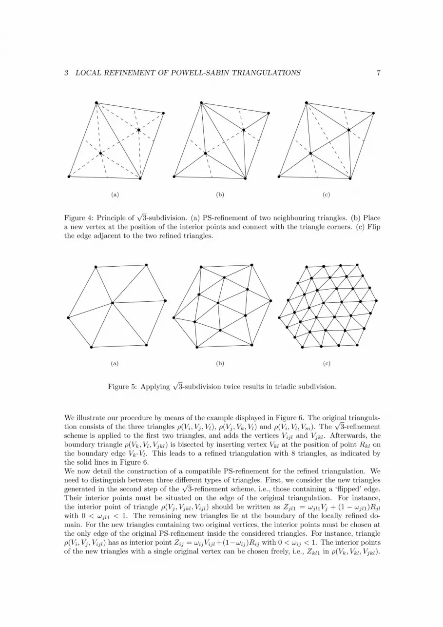
Figure 4: Principle of√

3-subdivision. (a) PS-refinement of two neighbouring triangles. (b) Placea new vertex at the position of the interior points and connect with the triangle corners. (c) Flipthe edge adjacent to the two refined triangles.

(a) (b) (c)

Figure 5: Applying√

3-subdivision twice results in triadic subdivision.

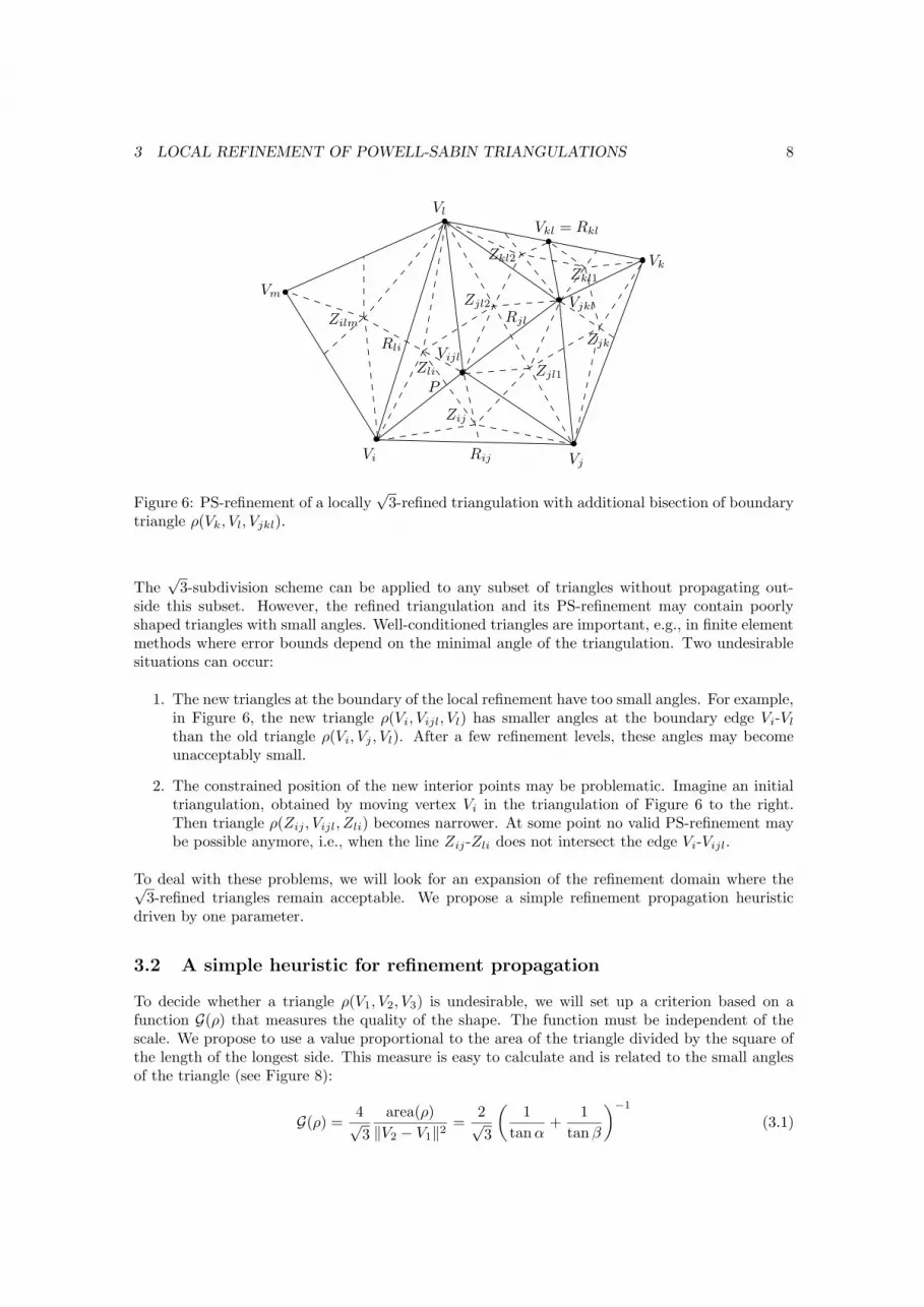
We illustrate our procedure by means of the example displayed in Figure 6. The original triangula-tion consists of the three triangles ρ(Vi, Vj , Vl), ρ(Vj , Vk, Vl) and ρ(Vi, Vl, Vm). The

√3-refinement

scheme is applied to the first two triangles, and adds the vertices Vijl and Vjkl. Afterwards, theboundary triangle ρ(Vk, Vl, Vjkl) is bisected by inserting vertex Vkl at the position of point Rkl onthe boundary edge Vk-Vl. This leads to a refined triangulation with 8 triangles, as indicated bythe solid lines in Figure 6.We now detail the construction of a compatible PS-refinement for the refined triangulation. Weneed to distinguish between three different types of triangles. First, we consider the new trianglesgenerated in the second step of the

√3-refinement scheme, i.e., those containing a ‘flipped’ edge.

Their interior points must be situated on the edge of the original triangulation. For instance,the interior point of triangle ρ(Vj , Vjkl, Vijl) should be written as Zjl1 = ωjl1Vj + (1 − ωjl1)Rjl

with 0 < ωjl1 < 1. The remaining new triangles lie at the boundary of the locally refined do-main. For the new triangles containing two original vertices, the interior points must be chosen atthe only edge of the original PS-refinement inside the considered triangles. For instance, triangleρ(Vi, Vj , Vijl) has as interior point Zij = ωijVijl +(1−ωij)Rij with 0 < ωij < 1. The interior pointsof the new triangles with a single original vertex can be chosen freely, i.e., Zkl1 in ρ(Vk, Vkl, Vjkl).

3 LOCAL REFINEMENT OF POWELL-SABIN TRIANGULATIONS 8

Vi Vj

Vk

Vl

Vm

Vijl

Vjkl

Vkl = Rkl

Rij

Rjl

Zij

Zjk

Zli Zjl1

Zjl2

Zilm

Rli

Zkl1

Zkl2

P

Figure 6: PS-refinement of a locally√

3-refined triangulation with additional bisection of boundarytriangle ρ(Vk, Vl, Vjkl).

The√

3-subdivision scheme can be applied to any subset of triangles without propagating out-side this subset. However, the refined triangulation and its PS-refinement may contain poorlyshaped triangles with small angles. Well-conditioned triangles are important, e.g., in finite elementmethods where error bounds depend on the minimal angle of the triangulation. Two undesirablesituations can occur:

1. The new triangles at the boundary of the local refinement have too small angles. For example,in Figure 6, the new triangle ρ(Vi, Vijl, Vl) has smaller angles at the boundary edge Vi-Vl

than the old triangle ρ(Vi, Vj , Vl). After a few refinement levels, these angles may becomeunacceptably small.

2. The constrained position of the new interior points may be problematic. Imagine an initialtriangulation, obtained by moving vertex Vi in the triangulation of Figure 6 to the right.Then triangle ρ(Zij , Vijl, Zli) becomes narrower. At some point no valid PS-refinement maybe possible anymore, i.e., when the line Zij-Zli does not intersect the edge Vi-Vijl.

To deal with these problems, we will look for an expansion of the refinement domain where the√3-refined triangles remain acceptable. We propose a simple refinement propagation heuristic

driven by one parameter.

3.2 A simple heuristic for refinement propagation

To decide whether a triangle ρ(V1, V2, V3) is undesirable, we will set up a criterion based on afunction G(ρ) that measures the quality of the shape. The function must be independent of thescale. We propose to use a value proportional to the area of the triangle divided by the square ofthe length of the longest side. This measure is easy to calculate and is related to the small anglesof the triangle (see Figure 8):

G(ρ) =4√3

area(ρ)

‖V2 − V1‖2=

2√3

(

1

tan α+

1

tan β

)−1

(3.1)

3 LOCAL REFINEMENT OF POWELL-SABIN TRIANGULATIONS 9

Vi Vj

Vk

Vl

Vm

Vijl

Vjkl

Vkl

Zij

Zli1

Zli2 Zjl1

Zjl2

Vilm

Figure 7: PS-refinement of a locally√

3-refined triangulation (continued).

V1

V2

V3

αβ

Figure 8: The function G(ρ) measures the quality of triangle ρ(V1, V2, V3).

with α and β the angles adjacent to the longest edge V1-V2 of triangle ρ. A low value of G indicatesthe presence of small angles, as depicted in Figure 9. We can easily verify that 0 < G ≤ 1. Theupper bound is attained in the case of equilateral triangles.

We propose now a heuristic for refinement propagation based on G, to deal with both undesirablesituations mentioned in section 3.1. Referring to Figure 6, we will split the neighbour of triangleρ(Vi, Vj , Vl) adjacent to the side Vi-Vl if

min

G(ρ(Vi, Vl, Vijl)),G(ρ(Zli, Zij , Vijl)),G(ρ(Zli, Zjl2, Vijl))

< δ, (3.2)

with 0 < δ < 1 a user-defined threshold parameter. A high value of δ will generate well-conditionedtriangles, but will spread out the refinement. A low value will keep the locality at the cost of leavingpoorly shaped triangles.

Referring to Figures 6 and 7, we explain how the propagation heuristic copes with the mentionedundesirable situations. The inequality (3.2) tests whether triangles ρ(Vi, Vl, Vijl), ρ(Zli, Zij , Vijl),and ρ(Zli, Zjl2, Vijl) are poorly shaped. By splitting the neighbouring triangle ρ(Vi, Vl, Vm) inFigure 6, we can improve the quality of the three triangles. The edge Vi-Vl is flipped, and two newtriangles ρ(Vi, Vijl, Vilm) and ρ(Vl, Vilm, Vijl) are created, as shown in Figure 7. Both triangles havea more favorable shape than ρ(Vi, Vl, Vijl). The triangles in the PS-refinement are also improved,e.g., triangle ρ(Zli, Zij , Vijl) is replaced by ρ(Zij , Zli2, Vijl). When this triangle is not yet goodenough, one may also decide to split the triangle adjacent to the side Vi-Vj .

We can characterize the latter improvement by the barycentric coordinates of P (η, 0, 1 − η) withrespect to triangle ρ(Vi, Vj , Vijl), where P is the intersection point of the lines Vi-Vijl and Zij-Zli (see Figure 6). Assume that the interior points of ρ(Vi, Vj , Vijl) and ρ(Vl, Vi, Vijl) are chosen

3 LOCAL REFINEMENT OF POWELL-SABIN TRIANGULATIONS 10

a

b

0 20 40 60 80 100 120 140 160 1800

20

40

60

80

100

120

140

160

180

Figure 9: Contour plot of G(ρ) in function of two angles of triangle ρ.

with the same ωi, i.e., Zij = ωiVijl + (1 − ωi)Rij and Zli = ωiVijl + (1 − ωi)Rli. If we includethe two neighbouring triangles into the refinement domain, the considered interior points becomeZij1 = ωiVi +(1−ωi)Rij and Zli2 = ωiVi +(1−ωi)Rli. Calculating the barycentric coordinates ofthe new intersection point P ∗(η∗, 0, 1− η∗) results in the relation η∗ = η +ωi. The increased valueof η∗ will guarantee that the resulting triangle is less narrow. It follows that by means of a goodchoice of ωi and the split of the adjacent triangles, we can cope with the undesirable situation.

Finally, we state the refinement propagation strategy algorithmically. Suppose we want to refinea triangulation ∆ by splitting all triangles in subset ⊂ ∆. The strategy iteratively enlargesthe subset in order to try to satisfy the imposed quality constraints. We calculate the qualityfunction G for two types of triangles: type1 stands for triangles in the original PS-refinement,e.g., triangle ρ(Vi, Vl, Vijl) in Figure 6, and type2 for triangles in the new PS-refinement, e.g.,triangle ρ(Zli, Zij , Vijl). The refinement propagation algorithm works as follows:

1. For each boundary edge of a triangle in subset: prepare the decision on whether to includethe neighbouring triangle into the refinement region by calculating the G-values of threetriangles. These triangles can be identified in analogy to the ones in (3.2) for triangleρ(Vi, Vj , Vl). One of these triangles is of type1; two are of type2. Add the values tothe list G.

2. (Propagation) While G contains G-values smaller than δ:

(a) Determine the element with the minimal G-value in G.

(b) If the element is of type1 then:

When the neighbouring triangle exists and is not yet in subset:

• Add the neighbouring triangle to subset

• Choose ωi

• Update G, by adding the G-values associated with the new boundary edges.

(c) Else:

When at least one of the two adjacent triangles exists and is not yet in subset:

• Add the valid adjacent triangles to subset

• Choose ωi

• Update G, by adding the G-values associated with the new boundary edges.

(d) Remove the element from G.

3. Apply the√

3-refinement scheme to the triangles of subset.

3 LOCAL REFINEMENT OF POWELL-SABIN TRIANGULATIONS 11

Vi Vj

Vk

Vl

Zki2

Rki

Figure 10: The choice of ωi for the interior point Zki2 = ωiVk + (1 − ωi)Rki influences the qualityof the shaded triangles in the PS-refinement.

Some remarks are in order here:

1. Although the algorithm strives to generate triangles that are as equilateral as possible, itcannot guarantee that the imposed quality requirement is satisfied everywhere. In particular,the quality of the locally refined mesh is bounded by that of the original triangulation andits PS-refinement.

2. The refinement strategy is guaranteed to terminate in a finite number of steps. The propaga-tion definitively stops when subset contains all triangles of the given triangulation.

3. Further fine tuning of the algorithm is possible, for example in step (2c): split only oneadjacent triangle if that already leads to acceptable boundary triangles.

4. The quality of the result is influenced by the value of ωi. Finding the best value is a hardglobal optimization problem which is not attractive to solve. Figure 10 shows the triangles inthe PS-refinement that are directly influenced by the choice of a single ωi. For simplicity, wecan take the fixed value ωi = 1/3, as proposed in [19], which is inspired by the case of equi-lateral triangles. Otherwise, we could think of simplifying the general optimization problemby varying only one interior point at a time, while fixing the positions of the surroundinginterior points, e.g. with ωi = 1/3.

3.3 Refinement near the boundary

When the refinement propagation reaches a domain boundary triangle, we cannot flip the boundaryedge because the triangle has no neighbour. One possibility is to bisect the triangle by adding anew vertex at the boundary side, e.g., vertex Vkl in Figure 6, which must be coincide with thePS-refinement point Rkl. With this approach, the boundary angle remains as small as it was, butthe new triangle is not so wide anymore.

An alternative solution is the creation of an artificial vertex outside the domain. That allows toflip the boundary edge and to form two well-conditioned triangles. On a further refinement levelit is possible to remove this artificial vertex. In Figure 11 the artificial vertex V a

ij is added to themesh of Figure 6. To enable a flip of edge Vi-Vj , vertex V a

ij must be chosen on the line Vijl-Rij .The new triangles ρ(Vi, V

aij , Vijl) and ρ(Vj , Vijl, V

aij) lie partly outside of the domain. When we

3 LOCAL REFINEMENT OF POWELL-SABIN TRIANGULATIONS 12

Vi Vj

Vk

Vl

Vm

Vijl

Vjkl

Vkl

V aij

Zij1 Zij2

Rij

Figure 11: Splitting at the boundary side Vi-Vj introduces an artificial vertex V aij outside the

boundary, chosen at the line Vijl-Rij . The PS-refinement is indicated with dashed lines.

Vi Vj

Vk

Vl

Vm

Vijl

Vjkl

Vkl

Vilm

Vij1 Vij2

Figure 12: A new refinement at the boundary removes the artificial vertex V aij from Figure 11.

3 LOCAL REFINEMENT OF POWELL-SABIN TRIANGULATIONS 13

number of vertices

global local refinementlevel (triadic) δ = 0.6 δ = 0.3 δ = 0.2 δ = 0.1

0 21 21 21 21 211 61 34 29 272 154 154 65 44 333 460 91 56 394 1297 1297 150 69 455 3889 206 84 516 11422 11422 285 95 577 34264 461 107 638 102061 102061 903 121 69

Table 1: Number of vertices for the triangulations successively refined by the global triadic subdi-vision scheme, and by the vertex-centered local subdivision scheme with different δ-values.

overall minimal angle/mean minimal angle

global local refinementlevel (triadic) δ = 0.6 δ = 0.3 δ = 0.2 δ = 0.1

0 26.6/37.4 26.6/37.4 26.6/37.4 26.6/37.4 26.6/37.41 18.9/39.4 17.1/37.6 17.1/36.3 12.5/35.82 20.6/39.4 20.6/39.4 17.1/35.5 16.7/34.0 8.7/34.53 18.9/39.5 17.1/36.1 16.7/34.3 8.7/34.24 15.7/39.3 15.7/39.3 17.1/35.6 15.2/33.5 8.7/33.45 15.8/39.5 17.1/36.2 14.8/33.9 8.7/33.16 12.8/39.2 12.8/39.2 17.1/36.2 14.8/33.5 8.7/32.67 13.0/39.2 17.1/36.3 14.2/33.4 8.7/32.18 11.0/39.1 11.0/39.1 17.1/36.2 14.2/33.2 8.7/31.7

Table 2: Overall minimal angle and the mean of the minimal angle of the triangles, for successivelyrefined triangulations by the global triadic subdivision scheme and by the vertex-centered localsubdivision scheme with different δ-values.

refine these triangles again, as in Figure 12, the artificial vertex V aij is not needed anymore. Note

that this strategy is reminiscent of a classical construction of one-dimensional B-splines near aninterval boundary. Also there, knots may be defined outside the domain [2].

3.4 A numerical example

For the numerical example, we will assume that an initial subset of triangles has been markedfor refinement. In data fitting and finite element applications, this subset is typically determinedby an error analysis. For CAGD it is more common to use a vertex-centered approach, i.e., alltriangles in the molecule of a selected vertex are put in the refinement set. The choice of a properδ-value in (3.2) may be inspired by the application. In CAGD a small δ-value may be sufficient ifa PS-spline has to be locally refined. When solving a PDE with finite elements, the error is oftenspread out over a large part of the domain. Then, a larger value for δ is advisable.

The vertex-centered refinement scheme is illustrated in Figures 14 and 15. The initial mesh istaken from [5] and is shown in Figure 13. We applied the scheme to the central vertex V (0.5, 0.5).When the refinement propagation reaches the boundary, we used artificial vertices. In Figure 14,

3 LOCAL REFINEMENT OF POWELL-SABIN TRIANGULATIONS 14

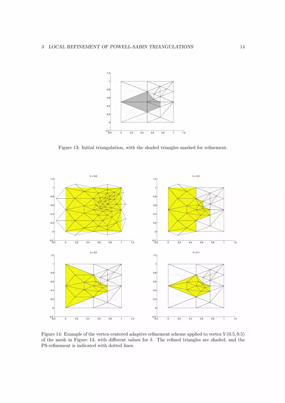
Figure 13: Initial triangulation, with the shaded triangles marked for refinement.

Figure 14: Example of the vertex-centered adaptive refinement scheme applied to vertex V (0.5, 0.5)of the mesh in Figure 13, with different values for δ. The refined triangles are shaded, and thePS-refinement is indicated with dotted lines.

3 LOCAL REFINEMENT OF POWELL-SABIN TRIANGULATIONS 15

Figure 15: Example of the vertex-centered adaptive refinement scheme applied four times to vertexV (0.5, 0.5) of the mesh in Figure 13 with δ = 0.3.

δ is varied to show its influence. The small value δ = 0.1 only refines the molecule of the vertex atthe centre of the mesh; larger values of δ lead to the refinement of more triangles. With δ = 0.6the whole triangulation is refined. In Figure 15 we apply the vertex-centered scheme successivelyto the same vertex with the value δ = 0.3. The dimensions of the successively refined Powell-Sabinspline spaces are 63, 102, 195, 273 and 450. In Table 1 we compare the growth of the number ofvertices for the global triadic scheme from [19] with our local scheme. Table 2 gives the minimalangle of the corresponding meshes, and the mean value of the minimal angle in the triangulations.

We observe that two refinement levels with δ = 0.6 are similar to one global triadic refinementlevel. This explains the appearance of the identical value sets in the second and third columnsof Table 2. A small value of δ strongly limits the propagation of the refinement, at the cost of asmall minimal angle of the triangulation. Larger values of δ enlarge the minimal angle of the mesh,up to a certain value, but generates more vertices. The minimal angle of a globally

√3-refined

triangulation is an indication of the attainable improvement. However, some choices of δ can dobetter, e.g., in the eighth refinement level δ = 0.3 leads to a much better minimal angle thanδ = 0.6 (see Table 2).

4 CONSTRUCTION OF THE LOCALLY REFINED B-SPLINE REPRESENTATION 16

Vi

Vj

Vk

Vijk

Rij

Rjk

Zij

Qj,1

Qj,2

Qj,3

tj

t∗j

Figure 16: Rescaling the original PS-triangle tj gives a new PS-triangle t∗j . The PS-points of Vj inthe original triangulation are indicated with squares, the ones in the refined mesh with bullets.

4 Construction of the locally refined B-spline representation

In this section we will explain how to derive the B-spline coefficients corresponding to the locallyrefined triangulation, of a Powell-Sabin surface when the B-spline coefficients were given on theoriginal triangulation. Our refinement algorithm applies global

√3-subdivision on a subset of the

triangulation. Hence, we can take over the subdivision rules developed by Vanraes et al. in [19].Only at the boundary of the refinement domain a reformulation of some rules is needed.

4.1 The new control triangles of the vertices in the original triangulation

For the original vertices one can reuse the old PS-triangles and control triangles. This is a validchoice because any new PS-point in the refined triangulation lies closer to the considered originalvertex. However, often an optimization is possible. When all triangles in the molecule of the vertexare refined, it is possible to determine a smaller PS-triangle by rescaling the original one. Denotethe new PS-triangle of vertex Vj as t∗j (Q

∗j,1, Q

∗j,2, Q

∗j,3). To find the appropriate scaling factor, we

compare the positions of the old and new PS-points. Figure 16 shows a part of the original andrefined molecule of Vj together with the corresponding PS-points. Suppose each interior pointinside the refined molecule is written as Zij = ωijVj + (1 − ωij)Rij . The scaling factor ω is thenfound as the minimal value of the ωij . The new corners are given by

Q∗j,m = ωVj + (1 − ω)Qj,m, m = 1, 2, 3, (4.1)

and the corresponding control points are calculated as [19]:

C∗j,1 = (ωαj,1 + 1 − ω)Cj,1 + ωαj,2Cj,2 + ωαj,3Cj,3 (4.2a)

C∗j,2 = ωαj,1Cj,1 + (ωαj,2 + 1 − ω)Cj,2 + ωαj,3Cj,3 (4.2b)

C∗j,3 = ωαj,1Cj,1 + ωαj,2Cj,2 + (ωαj,3 + 1 − ω)Cj,3. (4.2c)

4 CONSTRUCTION OF THE LOCALLY REFINED B-SPLINE REPRESENTATION 17

Vi

Vj

Vk

Vijk

Q∗ijk,1

Q∗ijk,2

Q∗ijk,3

A

B

C

Z

Figure 17: The PS-triangle t∗ijk for vertex Vijk(= Zijk) is found by rescaling the original triangleρ(Vi, Vj , Vk). The corresponding PS-points are marked as bullets.

4.2 The new control triangles of vertices at the original interior points

For each refined triangle ρ(Vi, Vj , Vk) a new vertex Vijk at the position of the interior point Zijk isadded to the triangulation. Its PS-triangle t∗ijk(Q∗

ijk,1, Q∗ijk,2, Q

∗ijk,3) can be chosen as

Q∗ijk,1 = (Vijk + Vi)/2, Q∗

ijk,2 = (Vijk + Vj)/2, and, Q∗ijk,3 = (Vijk + Vk)/2. (4.3)

In [19] is proven that t∗ijk is a valid PS-triangle in the case where the three neighbouring trianglesare refined. The PS-triangle is also valid when one or more adjacent triangles are not refined.Figure 17 illustrates the case where the triangle adjacent to side Vi-Vj is not refined. Let theinterior point Z have the barycentric coordinates (a, b, c) with respect to triangle ρ(Vi, Vj , Vijk).PS-point A can then be written as A = aQ∗

ijk,1 + bQ∗ijk,2 + cVijk, which proves that the point lies

inside the PS-triangle.

Note that the corners of PS-triangle t∗ijk coincide with the PS-points Si, Sj and Sk of the originaltriangulation, as indicated in Figure 3(a). In [19] it is shown that the corresponding Bezier ordinateswi, wj and wk are valid control points. From equation (2.9d) we may then conclude that

C∗ijk,1 = Li,1Ci,1 + Li,2Ci,2 + Li,3Ci,3 (4.4a)

C∗ijk,2 = Lj,1Cj,1 + Lj,2Cj,2 + Lj,3Cj,3 (4.4b)

C∗ijk,3 = Lk,1Ck,1 + Lk,2Ck,2 + Lk,3Ck,3. (4.4c)

4.3 The new control triangles for boundary refinement

For the refinement of a boundary triangle ρ(Vi, Vj , Vk) two strategies were proposed in section 3.3.They introduce either a new vertex at the boundary side, or an artificial vertex outside of thedomain. The subdivision rules for both situations are now developed.

The first case is shown in Figure 18. The new vertex Vij coincides with the PS-refinement pointRij at the boundary edge Vi-Vj . Choosing the new interior point Zij1 at the line Rij1-Vijk and

4 CONSTRUCTION OF THE LOCALLY REFINED B-SPLINE REPRESENTATION 18

Vi

Vj

Vk

Vij

Vijk

Q∗ijk,1

Q∗ijk,2

Q∗ijk,3

Q∗ij,1 Q∗

ij,2

Q∗ij,3

Rij1

Rij2

Zij1 Zij2

Figure 18: The PS-triangle t∗ij for the boundary vertex Vij(= Rij). The corresponding PS-pointsare marked as bullets.

Zij2 at Rij2-Vijk, the new PS-triangle t∗ij(Q∗ij,1, Q

∗ij,2, Q

∗ij,3) can be determined as

Q∗ij,1 = (Vij + Rij1)/2, Q∗

ij,2 = (Vij + Rij2)/2, and Q∗ij,3 = (Vij + Vijk)/2. (4.5)

Obviously this PS-triangle is valid. To find an expression for the new control points with respectto the old ones, we first reformulate (4.5). Corner Q∗

ij,3 can be calculated as

Q∗ij,3 = λijQ

∗ijk,1 + λjiQ

∗ijk,2, (4.6)

with λij and λji defined as in (2.9e). Since point Rij1 can be chosen freely at the edge Vi-Vij , wemay write Rij1 = νiVi + (1 − νi)Vij . Let Si = (Vi + Vij)/2 and Sj = (Vj + Vij)/2, then we find

Q∗ij,1 = νiSi + (1 − νi)Vij = (νi + λij − νiλij)Si + λji(1 − νi)Sj . (4.7)

For Q∗ij,2 we obtain an analogous expression. We refer to Figure 3 to recall that the points Si, Sj

and Q∗ij,3 are Bezier points. Because of the tangent property of the Bezier control net for each of

the triangles in the PS-refinement, the corresponding Bezier ordinates ui, vj and θk form a planetangent to the surface at Rij = Vij . Using equations (2.9b)-(2.9c) and (4.6)-(4.7), we find thefollowing values for the control points

C∗ij,1 = (νi + λij − νiλij)(Li,1Ci,1 + Li,2Ci,2 + Li,3Ci,3)

+ λji(1 − νi)(L′j,1Cj,1 + L′

j,2Cj,2 + L′j,3Cj,3) (4.8a)

C∗ij,2 = λij(1 − νj)(Li,1Ci,1 + Li,2Ci,2 + Li,3Ci,3)

+ (νj + λji − νjλji)(L′j,1Cj,1 + L′

j,2Cj,2 + L′j,3Cj,3) (4.8b)

C∗ij,3 = λijC

∗ijk,1 + λjiC

∗ijk,2. (4.8c)

In the second situation, a triangulation with an artificial vertex V aij is used, as shown in Figure 19.

The artificial vertex is put at the line Vijk-Rij such that Rij = νV aij +(1− ν)Vijk for some value ν,

e.g., ν = 1/2. The corresponding PS-triangle ta∗ij (Qa∗

ij,1, Qa∗ij,2, Q

a∗ij,3) can be chosen as

Qa∗ij,1 = (V a

ij + Vi)/2, Qa∗ij,2 = (V a

ij + Vj)/2, and Qa∗ij,3 = V a

ij . (4.9)

4 CONSTRUCTION OF THE LOCALLY REFINED B-SPLINE REPRESENTATION 19

Vi

Vj

Vk

V aij

Vijk

Q∗ijk,1

Q∗ijk,2

Q∗ijk,3

Qa∗ij,1

Qa∗ij,2

Qa∗ij,3

Rij

Zij1 Zij2

Figure 19: The PS-triangle ta∗ij for the artificial vertex V aij . Its PS-points are marked as bullets.

The first two control points are calculated as in (4.4a)-(4.4b). The third control point is of theform (xa

ij , yaij , c

a∗ij,3) with (xa

ij , yaij) the Cartesian coordinates of vertex V a

ij . We will show that thecoefficient ca∗

ij,3 can be chosen freely.

The proof follows by considering the Bernstein-Bezier representation of the basis function Ba∗,3ij .

Let Rij = λijVi + λjiVj , Ri = µiVi + (1 − µi)Vaij and Zij1 = ωiVi + (1 − ωi)Rij , see Figure 20(a).

The barycentric coordinates of the PS-points V aij , S, S′ and S with respect to PS-triangle ta∗ij are

V aij = (α1, α2, α3) = (0, 0, 1)

S = (L1, L2, L3) = (λij , λji, 0),

S′ = (L′1, L

′2, L

′3) = (µi, 0, 1 − µi),

S = (L1, L2, L3) = (λij + ωiλji, λji − ωiλji, 0).

Using formula (2.9) we immediately obtain the Bezier ordinates of the three basis functions Ba∗,mij

with m = 1, 2, 3. Figure 20(b) shows the Bezier ordinates of Ba∗,3ij . All Bezier ordinates inside the

original domain are zero. Hence, the coefficient ca∗ij,3 will not influence the PS-spline surface there,

and may be chosen arbitrarily. For simplicity we take ca∗ij,3 = 0.

The control points of the artificial vertex V aij can then be computed as

Ca∗ij,1 = Li,1Ci,1 + Li,2Ci,2 + Li,3Ci,3 (4.10a)

Ca∗ij,2 = Lj,1Cj,1 + Lj,2Cj,2 + Lj,3Cj,3 (4.10b)

Ca∗ij,3 = (xa

ij , yaij , 0). (4.10c)

4 CONSTRUCTION OF THE LOCALLY REFINED B-SPLINE REPRESENTATION 20

Vi

Vijk

V aij

Rij

Ri

Zij1

S S

S′

Qa∗ij,1

Qa∗ij,2

Qa∗ij,3

(a)

Vi

Vijk

V aij

0

0

0

0

0

00

0

0

0

00

0

0

(1 − µi)2 0 0

1 − µi1

(b)

Figure 20: (a) PS-refinement of triangle ρ(Vi, Vaij , Vijk) together with PS-triangle ta∗ij ; (b) Bezier

ordinates of basis spline Ba∗,3ij .

Vi

Vj

Vk

V aij

Vijk

Q∗ijk,1

Q∗ijk,2

Q∗ijk,3

Q∗ij1,1

Q∗ij1,2

Q∗ij1,3

Q∗∗ij1,3

Qa∗ij,1

Qa∗ij,2

Qa∗ij,3

RijVij1

Vij2

Figure 21: The PS-triangle t∗ij1 for the boundary vertex Vij1, using the artificial PS-triangle ta∗ij .

5 CONCLUDING REMARKS 21

In a subsequent refinement level we can remove the artificial vertex V aij . This is illustrated

in Figure 21. Valid control triangles at boundary vertices such as Vij1 can be determined bysimply applying (4.3) and (4.4). Note that a further optimization is possible for the PS-trianglet∗ij1(Q

∗ij1,1, Q

∗ij1,2, Q

∗ij1,3). The triangle can be replaced by the smaller PS-triangle t∗∗ij1(Q

∗ij1,1,

Q∗ij1,2, Q

∗∗ij1,3). Using the relation Rij = νV a

ij + (1 − ν)Vijk, we can immediately derive the valuefor C∗∗

ij1,3, i.e., C∗∗ij1,3 = νC∗

ij1,3 + (1 − ν)C∗ij1,2.

5 Concluding remarks

In this paper, we have proposed a subdivision algorithm for calculating the B-spline representationof a Powell-Sabin spline on a local refinement of a given triangulation. The subdivision strategyis based on the

√3-subdivision scheme. This scheme could be used to refine a local part of the

domain without disturbing the neighbouring triangles. However, as has been shown, this proceduremay introduce poorly shaped triangles. This problem has been dealt with by adding a refinementpropagation heuristic. When a triangle fails to satisfy a certain quality requirement, an adjacenttriangle is also refined. This results in an expansion of the refinement domain. If this refinementpropagation reaches the boundary, an artificial vertex outside the domain is inserted into thetriangulation. In the next refinement level the artificial vertex can be removed again. For thislocal refinement scheme, the corresponding subdivision rules have been developed. One of theadvantages of our algorithm is that both global and local subdivision are possible. When theglobal subdivision scheme is applied twice, the triadic subdivision of [19] is exactly recovered.

The subdivision algorithm provides the user some further freedom. The splitting conditions aredriven by the parameter δ, which steers the trade-off between balancing the mesh quality andlocalizing the refinement. A good value for this parameter is application-dependent. For CAGDone can take a low value for δ; in finite element applications, larger values may be more appro-priate. The generated new PS-triangles are not optimal in the sense of minimal area [4]. Controlpoints associated with a minimal area PS-triangle are as close as possible to the surface, which isadvantageous for local editing. Still, our control triangles are not too large and can be calculatedwith a minimal cost.

In many application domains local subdivision is of interest. It is, of course, an important in-gredient of surface modelling. Local subdivision results in an efficient time and memory usage forrepresenting complex surfaces. The new basis functions after subdivision have a smaller supportand give the designer more local control for manipulating surfaces. The locality of the schemeensures that the dimension of the subdivided space stays reasonable. The scheme is also useful fordata fitting and finite element applications. The original spline space is a subspace of the refinedone. Hence, we are guaranteed of a better approximation with an increased local resolution whena least squares data fitting approach is applied. When using an iterative solver in a finite elementcontext, subdivision allows a trivial nested iteration strategy, where an initial fine mesh approxim-ation is produced from a coarse mesh solution. Multiresolution techniques need subdivision too.Wavelets can be developed by means of the lifting scheme with subdivision as the prediction stepand an extra update step. Geometric multigrid uses subdivision to make a prediction at the finerlevel. A number of applications for local subdivision scheme proposed in this paper are currentlysubject of further investigation.

Acknowledgement

Hendrik Speleers is funded as a Research Assistant of the Fund for Scientific Research Flanders(Belgium).

REFERENCES 22

References

[1] E. Catmull and J. Clark. Recursively generated B-spline surfaces on arbitrary topologicalmeshes. Comput. Aided Design, 10(6):350–355, 1978.

[2] C. de Boor. On calculating with B-splines. J. Approx. Theory, 6:50–62, 1972.

[3] P. Dierckx. Curve and Surface Fitting with Splines. Oxford University Press, Oxford, 1993.

[4] P. Dierckx. On calculating normalized Powell-Sabin B-splines. Comput. Aided Geom. Design,15(3):61–78, 1997.

[5] P. Dierckx, S. Van Leemput, and T. Vermeire. Algorithms for surface fitting using Powell-Sabin splines. IMA J. Numer. Anal., 12:271–299, 1992.

[6] D. Doo and M.A. Sabin. Behaviour of recursive division surfaces near extraordinary points.Comput. Aided Design, 10:356–360, 1978.

[7] N. Dyn, J. Gregory, and D. Levin. A butterfly subdivision scheme for surface interpolationwith tension control. ACM Trans. Graphics, 9(2):160–169, 1990.

[8] G. Farin. Triangular Bernstein-Bezier patches. Comput. Aided Geom. Design, 3(2):83–127,1986.

[9] G. Farin. Curves and Surfaces for Computer-Aided Geometric Design: A Practical Guide.Academic Press, Boston, 1990.

[10] L. Kobbelt. Interpolatory subdivision on open quadrilateral nets with arbitrary topology. InProceedings of Eurographics, pages 409–420, 1996.

[11] L. Kobbelt.√

3-Subdivision. In Computer Graphics Proceedings, Annual Conference Series,pages 103–112. ACM SIGGRAPH, 2000.

[12] U. Labsik and G. Greiner. Interpolatory√

3-subdivision. In Proceedings of the 21th EuropeanConference on Computer Graphics, volume 19 of Computer Graphics Forum, pages 131–138,Cambridge, 2000.

[13] C.T. Loop. Smooth subdivision surfaces based on triangles. Master’s thesis, Dep. Comp.Science, University of Utah, 1987.

[14] C. Manni and P. Sablonniere. Quadratic spline quasi-interpolants on Powell-Sabin partitions.Technical Report IRMAR 04-16, 2004.

[15] M.J.D. Powell and M.A. Sabin. Piecewise quadratic approximations on triangles. ACM Trans.Math. Softw., 3:316–325, 1977.

[16] H. Speleers, P. Dierckx, and S. Vandewalle. Numerical solution of partial differential equationswith Powell-Sabin splines. J. Comp. Appl. Math., in press, 2005.

[17] E. Vanraes, P. Dierckx, and A. Bultheel. On the choice of the PS-triangles. Technical Report353, Dep. Comp. Science, K.U. Leuven, 2003.

[18] E. Vanraes, J. Maes, and A. Bultheel. Powell-Sabin spline wavelets. Int. J. Wav. Multires.Inf. Proc., 2(1):23–42, 2004.

[19] E. Vanraes, J. Windmolders, A. Bultheel, and P. Dierckx. Automatic construction of controltriangles for subdivided Powel-Sabin splines. Comput. Aided Geom. Design, 21(7):671–682,2004.

REFERENCES 23

[20] K. Willemans and P. Dierckx. Surface fitting using convex Powell-Sabin splines. J. Comput.Appl. Math., 56:263–282, 1994.

[21] J. Windmolders. Powell-Sabin splines for computer aided geometric design. PhD thesis, Dep.Comp. Science, K.U. Leuven, 2003.

[22] J. Windmolders and P. Dierckx. Subdivision of uniform Powell-Sabin splines. Comput. AidedGeom. Design, 16:301–315, 1999.

[23] J. Windmolders, E. Vanraes, P. Dierckx, and A. Bultheel. Uniform Powell-Sabin spline wave-lets. J. Comp. Appl. Math., 154(1):125–142, 2003.