Embed Size (px)
Citation preview
Low-Concentrating, Stationary
Solar Thermal Collectors for
Process Heat Generation
Ph.D. Thesis
Stefan Hess
2014
De Montfort University Leicester
Institute of Energy and Sustainable Development IESD
Fraunhofer Institute for Solar Energy Systems ISE
Division Solar Thermal and Optics
Low-Concentrating, Stationary
Solar Thermal Collectors for
Process Heat Generation
Stefan Hess
A thesis submitted in partial fulfillment of the
requirements of De Montfort University for the
degree Doctor of Philosophy (Ph.D.)
Freiburg, December 2014
Shaker VerlagAachen 2015
Schriftenreihe der Reiner Lemoine-Stiftung
Stefan Hess
Low-Concentrating, Stationary Solar ThermalCollectors for Process Heat Generation

Bibliographic information published by the Deutsche NationalbibliothekThe Deutsche Nationalbibliothek lists this publication in the DeutscheNationalbibliografie; detailed bibliographic data are available in the Internet athttp://dnb.d-nb.de.
Zugl.: De Montfort University Leicester, Diss., 2014
Copyright Shaker Verlag 2015All rights reserved. No part of this publication may be reproduced, stored in aretrieval system, or transmitted, in any form or by any means, electronic,mechanical, photocopying, recording or otherwise, without the prior permissionof the publishers.
Printed in Germany.
ISBN 978-3-8440-3402-8ISSN 2193-7575
Shaker Verlag GmbH • P.O. BOX 101818 • D-52018 AachenPhone: 0049/2407/9596-0 • Telefax: 0049/2407/9596-9Internet: www.shaker.de • e-mail: [email protected]

Abstract
I
Abstract
The annual gain of stationary solar thermal collectors can be increased by non-focusing
reflectors. Such concentrators make use of diffuse irradiance. A collector’s incidence
angle modifier for diffuse (diffuse-IAM) accounts for this utilization. The diffuse irradi-
ance varies over the collector hemisphere, which dynamically influences the diffuse-
IAM. This is not considered by state-of-the-art collector models. They simply calculate
with one constant IAM value for isotropic diffuse irradiance from sky and ground.
This work is based on the development of a stationary, double-covered process heat
flat-plate collector with a one-sided, segmented booster reflector (RefleC). This reflec-
tor approximates one branch of a compound parabolic concentrator (CPC). Optical
measurement results of the collector components as well as raytracing results of differ-
ent variants are given. The thermal and optical characterization of test samples up to
190 °C in an outdoor laboratory as well as the validation of the raytracing are discussed.
A collector simulation model with varying diffuse-IAM is described. Therein, ground
reflected and sky diffuse irradiance are treated separately. Sky diffuse is weighted with
an anisotropic IAM, which is re-calculated in every time step. This is realized by gener-
ating an anisotropic sky radiance distribution with the model of Brunger and Hooper,
and by weighting the irradiance from distinct sky elements with their raytraced beam-
IAM values. According to the simulations, the RefleC booster increases the annual out-
put of the double-covered flat-plate in Würzburg, Germany, by 87 % at a constant inlet
temperature of 120 °C and by 20 % at 40 °C. Variations of the sky diffuse-IAM of up to
25 % during one day are found. A constant, isotropic diffuse-IAM would have under-
valued the gains from the booster by 40 % at 40 °C and by 20 % at 120 °C. The results
indicate that the gain of all non-focusing solar collectors is undervalued when constant,
isotropic diffuse-IAMs calculated from raytracing or steady-state test data are used.
Process heat generation with RefleC is demonstrated in a monitored pilot plant at work-
ing temperatures of up to 130 °C. The measured annual system utilization ratio is 35 %.
Comparing the gains at all inlet temperatures above 80 °C, the booster increases the
annual output of the double-covered flat-plates by 78 %. Taking all inlet temperatures,
the total annual gains of RefleC are 39 % above that of the flat-plates without reflectors.
A qualitative comparison of the new simulation model results to the laboratory results
and monitoring data shows good agreement. It is shown that the accuracy of existing
collector models can be increased with low effort by calculating separate isotropic
IAMs for diffuse sky and ground reflected irradiance. The highest relevance of this
work is seen for stationary collectors with very distinctive radiation acceptance.

Declaration
II
Declaration
I declare that the content of this submission is my own work. The contents of the work
have not been submitted for any other academic or professional award. This thesis is
submitted according to the conditions laid down in the regulations.
Furthermore, I declare that the work was carried out as part of the course for which I
was registered at De Montfort University, United Kingdom from October 2008 until
September 2014.
I draw attention to any relevant considerations of rights of third parties.
Acknowledgements
III
Acknowledgements
I thank my supervisor Prof. Victor Ian Hanby for his wise and motivating guidance of
this work. His knowledge and great sense of humor highly contributed to make my ex-
ternal doctorate at DMU with the annual stays in Leicester a positive and enriching ex-
perience. Prof. Ursula Eicker and Dr. Michael Hermann supported me during the initial
phase of this dissertation project.
The research reported here is based upon the collector development project RefleC,
which I carried out at Fraunhofer ISE together with students and the industry partner
Wagner & Co. Solartechnik GmbH. I am very thankful to Prof. Matthias Rommel for
his trust and encouragement to start working on a doctorate.
The committed support of students and colleagues to the RefleC project highly contrib-
uted to the quality of this thesis. Paolo Di Lauro did many of the raytracing-simulations,
using the OptiCad collector model I had set up before. He helped to measure the collec-
tor test samples, set up the sun position calculation tool used in this work and was al-
ways open for discussions on the IAM. Stefanie Rose carried out most optical meas-
urements of the material samples. Christoph Raucher did a great job implementing the
first version of the anisotropic collector simulation model in Fortran. Axel Oliva per-
formed system simulations for the dimensioning of the pilot plant and Michael Klemke
carefully calibrated and installed the monitoring equipment. Christoph Thoma instruct-
ed me to work with the medium temperature collector test stand and was always helpful
in case of questions. I also would like to thank all the other great people at ISE and
Wagner who contributed to this work.
I had the honor to briefly discuss some of my ideas with Prof. Roland Winston, Dr.
Bengt Perers, Prof. Björn Karlsson, Prof. Manuel Collares-Pereira and Dr. Alfred
Brunger. I am very thankful for their feedback and for helpful literature.
RefleC was funded by the German Federal Ministry for the Environment, Nature Con-
servation and Nuclear Safety (BMU). The work in hand was funded by a Ph.D. scholar-
ship of the Reiner-Lemoine-Stiftung. This important support gave me the freedom for
independent research and to continue monitoring the RefleC pilot plant after the fi-
nanced RefleC project had ended.
This work would not have been finalized without the love, support and understanding of
my friends and family. In hard times, you listened and kept me going. In good times,
you were happy with me. I am very grateful for having you in my life.

Content
IV
Content
Abstract .............................................................................................................. I
Declaration ........................................................................................................ II
Acknowledgements ......................................................................................... III
Content ............................................................................................................. IV
Nomenclature .................................................................................................. VII
1 Introduction.................................................................................................. 1
1.1 This Work .............................................................................................. 2
1.1.1 RefleC Project ........................................................................... 2
1.1.2 Structure, Approach and Contribution to Knowledge ................ 3
1.2 Solar Thermal Process Heating ............................................................. 4
1.2.1 Process Heat Demand .............................................................. 4
1.2.2 Potential Contribution of Solar Thermal Systems ...................... 6
1.2.3 State of the Art, Perspectives and Further Readings ................ 7
1.3 Stationary Process Heat Collectors ..................................................... 11
1.3.1 Collector Categories ................................................................ 11
1.3.2 Standard Flat-plates and Evacuated Tube Collectors ............. 12
1.3.3 Low-Concentrating, Stationary Collectors ............................... 14
2 Optical Investigations ............................................................................... 19
2.1 Solar Irradiance ................................................................................... 19
2.1.1 Components and Characteristics ............................................ 19
2.1.2 Radiation Data Measurement .................................................. 22
2.1.3 Irradiance on Tilted Planes ...................................................... 24
2.1.4 Conventions for Sun Position and Reference Planes .............. 26
2.2 Raytracing ........................................................................................... 29
2.2.1 Optical Loss Mechanisms ....................................................... 30
2.2.2 Incidence Angle Modifier for Beam Irradiance ......................... 31
2.2.3 Raytracing Procedure and Parameters ................................... 34
2.3 Material Properties .............................................................................. 36
2.3.1 Reflectors ................................................................................ 37
2.3.2 Transparent Covers................................................................. 42
2.3.3 Absorber .................................................................................. 47
Content
V
2.4 Concentrator Design ........................................................................... 49
2.4.1 Concentration of Solar Radiation ............................................ 49
2.4.2 Compound Parabolic Concentrator ......................................... 51
2.4.3 Annual Acceptance of Irradiance ............................................ 54
2.4.4 Flat Reflectors (V-Trough) Compared to a CPC ..................... 56
2.5 Raytracing Results .............................................................................. 59
3 RefleC Collector Testing .......................................................................... 61
3.1 Stages of Development ....................................................................... 61
3.2 Fundamentals of Collector Performance ............................................. 66
3.2.1 Efficiency, IAM and Power ...................................................... 66
3.2.2 IAM Values for Beam Irradiance ............................................. 70
3.2.3 IAM Values for Isotropic Diffuse Irradiance ............................. 71
3.3 Collector Efficiency Testing ................................................................. 74
3.3.1 Efficiency Curve Determination ............................................... 74
3.3.2 Importance of High Temperature Testing ............................... 78
3.4 Test Results ........................................................................................ 79
3.4.1 Mass Flow Influence on Efficiency .......................................... 79
3.4.2 Absorber Temperatures and Local Concentration .................. 80
3.4.3 Validation of Raytracing .......................................................... 82
3.4.4 IAM Effect on Thermal Efficiency Curve ................................. 89
3.4.5 Test Sample Performance with two CPC Reflectors ............... 90
3.4.6 Test Sample Performance with One Reflector ........................ 94
3.4.7 Efficiency Curve Calculation for RefleC .................................. 95
4 Energy Gain Simulations .......................................................................... 97
4.1 Modeling Anisotropic Diffuse Irradiance .............................................. 98
4.1.1 Review of Available Models .................................................... 98
4.1.2 Brunger Model ...................................................................... 100
4.2 Collector Simulation Model ............................................................... 106
4.2.1 State of the Art ...................................................................... 106
4.2.2 Model Description ................................................................. 108
4.3 Simulation Results ............................................................................ 111
4.3.1 Irradiation Distribution Diagrams ........................................... 111
4.3.2 Anisotropy-Effect on the IAM ................................................ 113
4.3.3 Anisotropy-Effect on Collector Output ................................... 115
Content
VI
5 Pilot Plant ................................................................................................. 123
5.1 Pilot Plant Description ....................................................................... 123
5.1.1 Laundry Laguna .................................................................... 123
5.1.2 Solar Thermal Installation ...................................................... 125
5.1.3 Monitoring System................................................................. 130
5.2 Monitoring Results ............................................................................. 133
5.2.1 System Performance ............................................................. 133
5.2.2 Collector Performance ........................................................... 135
5.3 Economic Assessment of RefleC Boosters ....................................... 143
6 Conclusions and Perspectives............................................................... 145
6.1 Low-Concentrating, Stationary Collectors ......................................... 145
6.2 IAM for Beam and Diffuse Irradiance................................................. 146
6.3 Simulation Model ............................................................................... 147
6.4 Pilot Plant .......................................................................................... 149
Appendix ....................................................................................................... 151
A Collector Variants .............................................................................. 152
B Collector Test Results ....................................................................... 155
C Raytracing Results ............................................................................ 164
D Collector Simulation Model Type 154 ................................................ 166
E Monitoring Scheme and Results ........................................................ 179
Figures........................................................................................................... 182
Tables ............................................................................................................ 187
Publications .................................................................................................. 188
Bibliography .................................................................................................. 190
Nomenclature
VII
Nomenclature
Latin Symbols
Symbol Unit Meaning
𝑎 − Aperture half-width of concentrator entrance
𝑎´ − Aperture half-width of concentrator exit
𝑎0 − Coefficient of the Brunger distribution
𝑎1 − Coefficient of the Brunger distribution
𝑎2 − Coefficient of the Brunger distribution
𝑎3 − Coefficient of the Brunger distribution
𝐴1 m2 Area normal to direction of irradiance
𝐴2 m2 Area turned away by 𝜃 from normal of irradiance
𝐴𝑎𝑝 m2 Aperture area (index R = reflector, fp = flat plate,
u = upper reflector, l = lower reflector)
𝐴𝑔𝑟 m2 Gross area
𝐴𝑟 m2 Receiver area
𝑏0 − Parameter of Souka/Safwat IAM function
𝑐1 W/( m2K) Heat loss coefficient of the first order
𝑐2 W/( m2K2) Heat loss coefficient of the second order
𝑐𝑒𝑓𝑓 J/(m2K) Effective heat capacity of the collector (material and
fluid)
𝑐𝑝, 𝑓𝑙 J/(kg K) Specific heat capacity of the collector fluid
𝑐�̅�,𝑓𝑙 J/(kg K) Mean specific heat capacity of the collector fluid
𝐶𝑔𝑒𝑜 − Geometric concentration ratio
𝐶𝑟𝑎𝑑 − Concentration ratio for radiation
𝑓 m Focal length
𝑓𝑎 1/𝑎 Annuity factor
𝑓𝑎𝑐𝑐,𝑖𝑠𝑜 − Concentrator acceptance factor for isotropic irradiance
𝑓𝑏 − Fraction of beam irradiance
𝑓𝑑 − Fraction of diffuse irradiance (1 − 𝑓𝑏)
𝐹´ − Collector efficiency factor
𝐺 W/m2 Global (hemispherical) irradiance on horizontal (GHI)
𝐺0 W/m2 Extraterrestrial irradiance on horizontal
𝐺𝑏 W/m2 Beam irradiance (horizontal)
Nomenclature
VIII
Symbol Unit Meaning
𝐺𝑏𝑛 W/m2 Beam irradiance perpendicular to sun direction (DNI)
𝐺𝑏𝑡 W/m2 Beam irradiance (tilted plane)
𝐺𝑑 W/m2 Diffuse irradiance on horizontal (DHI)
𝐺𝑑𝑡 W/m2 Diffuse irradiance on tilted plane (𝐺𝑠𝑡 + 𝐺𝑟𝑡)
𝐺𝑟𝑡 W/m2 Diffuse ground irradiance (tilted plane)
𝐺𝑠𝑐 W/m2 Solar Constant (1367 ± 23 W/m2)
𝐺𝑠𝑡 W/m2 Diffuse sky irradiance (tilted plane)
𝐺𝑠𝑡,𝐵𝑟 W/m2 Diffuse sky irradiance from Brunger distribution
𝐺𝑡 W/m2 Global (hemispherical) irradiance (tilted plane)
𝑖 − Day of the year
𝐼(𝜃𝑠, 𝑎3) − Function within Brunger model
𝐼𝑎𝑝 W Integral intensity at concentrator aperture area
𝐼𝑟 W Integral intensity at concentrator receiver area
𝑘 − Fraction of diffuse irradiance on horizontal
𝑘𝑡 − Atmospheric clearness Index
𝐾 − Extinction coefficient of solid, transparent material
𝐾𝑏 − IAM for beam irradiance 𝐺𝑏𝑡
𝐾𝑑 − IAM for isotropic diffuse irradiance from collector
hemisphere (𝐺𝑠𝑡 + 𝐺𝑟𝑡)
𝐾ℎ − IAM for global hemispherical irrad. (𝐺𝑏𝑡 + 𝐺𝑠𝑡 + 𝐺𝑟𝑡)
𝐾𝑖𝑛𝑣 EUR/(m2) Investment costs per unit area
𝐾𝑚𝑎𝑖𝑛 EUR/(m2a) Maintenance costs per year and unit area
𝐾𝑜𝑝 EUR/(kWh) Operational costs per kWh useful solar gain
𝐾𝑟 − IAM for diffuse irradiance from the ground 𝐺𝑟𝑡
𝐾𝑠 − IAM for diffuse irradiance from the sky 𝐺𝑠𝑡
𝐾𝑠𝑜𝑙 EUR/(kWh) Solar heat generation costs
𝐿(𝜃ℎ, 𝜙ℎ) W/(m2sr) Sky radiance in direction (𝜃, 𝜙)
�̇� kg/(m2h) Specific mass flow rate per 𝑚² of aperture area
𝑚𝑐𝑜𝑙𝑙 − Number of collectors (parallel)
�̇� kg/h Absolute mass flow rate
𝑛 − Refractive index
𝑛 − Number of measured values for error calculation
𝑛𝜙,ℎ − Number of steps in direction 𝜙ℎ
𝑛𝜃,ℎ − Number of steps in direction 𝜃ℎ
𝑛𝑎𝑖𝑟 − Refractive index air (optically thinner medium)
Nomenclature
IX
Symbol Unit Meaning
𝑛𝑐𝑜𝑣 − Refractive index cover (optically denser medium)
𝑛𝑐𝑜𝑙𝑙 − Number of collectors (serial)
𝑛𝑐𝑜𝑙𝑙, 𝑆 − Projection of collector normal vector onto south axis
𝑛𝑐𝑜𝑙𝑙, 𝑊 − Projection of collector normal vector onto west axis
𝑛𝑐𝑜𝑙𝑙, 𝑍 − Projection of collector normal vector onto zenith axis
�⃗� 0, 𝑐𝑜𝑙𝑙 − Normal unit vector of the collector plane
𝑛𝑙𝑜𝑛𝑔 − Number of longitudinal IAM values in external file
𝑛𝑡𝑟𝑎𝑛𝑠 − Number of transversal IAM values in external file
𝑝 − Capital interest rate
�̇�𝑔𝑎𝑖𝑛 W/m2 Collector gain per aperture area (stationary)
�̇�𝑙𝑜𝑠𝑠 W/m2 Thermal losses heat flow
�̇�𝑟𝑎𝑑 W/m2 Radiative solar gains heat flow
𝑄𝑠𝑜𝑙 kWh/(m2a) Usable solar heat per year and unit area
�̇�𝑢𝑠𝑒 W/m2 Thermal collector output (dynamic, with capacity)
�̇�𝑢𝑠𝑒 W Thermal collector (field) output (with capacity)
𝑟 − Parameter of Ambrosetti IAM function
𝑟𝑆 m Sun radius (6.95 108)
𝑟𝑆𝐸 m Median orbital radius of earth around sun (1.50 1011
)
𝑠𝑆 − Projection of solar unit vector onto south axis
𝑠𝑊 − Projection of solar unit vector onto west axis
𝑠𝑍 − Projection of solar unit vector onto zenith axis
𝑠 0 − Solar unit vector
𝑠 0, 𝑙 − Projection of solar unit vector into longitudinal plane
𝑠 0, 𝑡 − Projection of solar unit vector into transversal plane
𝑇 a Technical service life of booster reflectors in years
𝑇𝑎 K Ambient temperature
𝑇𝑓 K Mean collector (field) fluid temperature
𝑇𝑖𝑛 K Fluid inlet temperature
𝑇𝑜𝑛,𝑅𝐾 °C Activation temperature of stagnation cooler
𝑇𝑜𝑢𝑡 K Fluid outlet temperature
𝑇𝑝 K Mean absorber plate temperature
𝑇𝑠𝑡𝑎𝑔 K Stagnation temperature
𝑇𝑡𝑟𝑒 °C Temperature threshold to switch storage charging
Δ𝑡 s Width of timestep in TRNSYS
Nomenclature
X
Symbol Unit Meaning
Δ𝑇/𝐺 (m2K)/W Reduced temperature difference
𝑈𝑙𝑜𝑠𝑠 W/(m2K) Heat loss coefficient of the collector
�̇� l/h Volume flow
𝑦𝑐𝑖 [yci] Calculated value for error calculation
𝑦𝑚𝑖 [ymi] Measured value for error calculation
Greek Symbols
Symbol Unit Meaning
𝛼 − Absorptance
𝛼𝐷 rad Divergence of sunlight (0.54° or 0.0094 rad)
𝛽 rad Collector tilt or slope from horizontal
𝛾 rad Collector azimuth angle from south (west positive)
𝛿 rad Concentrator shading angle for beam irradiance
휀 − Emittance
𝜂 − Collector efficiency
𝜂0 − Conversion factor at perpendicular beam irradiance
𝜂0,𝑏 − Conversion factor for pure beam irradiance
𝜂0,ℎ − Conversion factor for hemispherical irradiance
𝜃 rad Incidence angle
𝜃(𝜃𝑠, 𝜙𝑠) rad Incidence angle of sun on aperture
𝜃(𝜃ℎ, 𝜙ℎ) rad Incidence angle of sky element on aperture
𝜃𝑎 rad Acceptance half-angle of concentrator
𝜃𝑎,𝑉 rad Acceptance half-angle of V-trough
𝛥𝜃𝑑𝑖𝑓𝑓 rad Angular step width of diffuse integration in Type 154
𝜃ℎ rad Zenith angle of sky element
∆𝜃ℎ rad Angular width of sky element at 𝜃ℎ
𝜃ℎ∗ rad Zenith angle of ground element
∆𝜃ℎ∗ rad Angular width of ground elem. at 𝜃ℎ
∗
𝜃𝑙 rad Projection of 𝜃 into longitudinal plane
𝜃𝑝,𝑁𝑆 rad South projection angle
𝜃𝑟 rad Angle of reflection
𝜃𝑠 rad Zenith angle of the sun
𝜃𝑡 rad Projection of 𝜃 into transversal plane
𝜃𝑡𝑟𝑢𝑛𝑐 rad Truncation angle of a CPC
Nomenclature
XI
Symbol Unit Meaning
𝜆 m Wavelength
𝜌 − Reflectance (total, hemispherical)
𝜌𝑑𝑖𝑓𝑓 − Diffuse reflectance (share reflected diffuse)
𝜌𝑓𝑙 kg/m³ Density of collector fluid
𝜌𝑔𝑟𝑑 − Reflectance of the ground
𝜌𝑠𝑝𝑒𝑐 − Specular reflectance (share reflected specular)
(𝜌𝜏𝛼)𝑒 − Effective reflectance-transmittance-absorptance prod-
uct (effective optical loss factor)
𝜎 rad Standard deviation (of scattered rays after reflection)
𝜎𝑜𝑟𝑖 rad Standard deviation from macroscopic (shape) errors
𝜎𝑟𝑒𝑓𝑙 rad Standard deviation from microscopic surface errors
𝜎𝑠𝑢𝑛 rad Standard deviation from solar irradiation direction
𝜏 − Transmittance
(𝜏𝛼) 𝑒 − Effective transmittance-absorptance product
𝜙 rad Sun azimuth angle from collector (west positive)
𝜙𝑠 rad Sun azimuth angle from south direction (west positive)
𝜙ℎ rad Azimuth of sky element (west positive)
∆𝜙ℎ rad Angular width of sky element at 𝜙ℎ
𝜙ℎ∗ rad Azimuth of ground element (west pos.)
∆𝜙ℎ∗ rad Angular width of ground element at 𝜙ℎ
∗
𝜑𝑠/2 rad Opening half angle of the sun (0.27°)
𝜓 rad Opening half angle of a V-trough
Ψ rad Angular distance from sun to sky element
Ω sr Angular width of sky element
Abbreviations
a annum (year)
a.m. ante meridiem
AM Air mass
AR Anti-reflective, i.e. with reduced reflectivity
ASA Advanced security appliance (hardware-firewall)
ASTM American Society for Testing and Materials
approx. approximately
App. Appendix
BMWi German Federal Ministry for Economic Affairs and Energy
BSW German Solar Industry Association
Nomenclature
XII
CPC Compound Parabolic Concentrator
CSR Circumsolar ratio
d day
DGS German Solar Energy Society
DNI Direct normal irradiance
EU European Union
Eq. Equation
ETC Evacuated tube collector
ETFE Ethylene tetrafluoroethylene
FEP Fluorinated ethylene propylene
Fortran Formula translation (programming language)
GHI Global hemispherical irradiance on horizontal plane
h hour
IAM Incidence angle modifier
IEA International Energy Agency
IR Infrared wavelengths of solar spectrum
ISE Fraunhofer Institute for Solar Energy Systems
LED Light emitting diode
L/H Ratio of booster reflector length to receiver flat-plate height
MBE Mean bias error
min minute
MID Magneto-inductive flow meter
MTTS Medium temperature collector test stand
NREL National Renewable Energy Laboratory
p.m. post meridiem
prim. Data plotted to the primary (left) axis
PE Polyethylene
PFA Perfluoroalkoxy alkanes
PHC Process heat collector
PTFE Polytetrafluoroethylene
RMSE Root mean square error
s second
sec. Data plotted to the secondary (right) axis
SHC Solar Heating and Cooling (Program)
SPH Solar thermal process heat(ing)
ST Solar thermal
TMY Typical meteorological year
TRNSYS Transient system simulation software
US United States of America
UTC Coordinated Universal Time
UV Ultraviolet wavelengths of solar spectrum
Vis Visible wavelengths of solar spectrum
Chapter 1: Introduction
1
1 Introduction
The field of solar thermal heat generation is briefly introduced. The con-
text of this work, its approach, structure and intended contribution to
knowledge are described. An overview on solar thermal process heating
is given and the state of the art in the development of low-concentrating,
stationary solar thermal process heat collectors is discussed.
The transition towards a sustainable energy supply is a global challenge. Not only
against the background of scarce fossil and nuclear resources, but also due to the rapidly
progressing climate change it is imperative to develop and improve technologies for
renewable energy utilization. Apart from gravity forces, the sun’s photons are the only
external energy source available to our planet, so direct use of solar energy is obvious.
Solar thermal (ST) systems are often applied in combination with other heating technol-
ogies, which compensate for the fluctuating solar resource. They generate heat on-site
and can significantly reduce the dependence on conventional energy carriers.
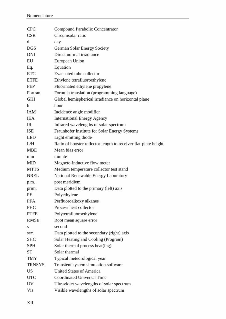
Solar Heat Worldwide: Weiss and Mauthner (2014) annually provide an overview on
the worldwide ST market. According to them, by the end of 2012 a ST collector area of
384.7 million m2 was in operation, corresponding to 269.3 GWth total power (conver-
sion factor 0.7 kWth/m2). Compared to 2011, the newly installed capacity grew by 9.4 %
in 2012. China (44.7 GWth) and Europe
(3.7 GWth) were the main markets; they
together account for 92 % of all newly
installed collector area. For 2013, Weiss
and Mauthner estimate that ST systems
of overall 471 million m2 collector area
produced a total energy of 281 TWhth. So
in 2013 ST systems produced about 80 %
more energy than photovoltaic systems
(about 160 TWhel). ST electric power
generation accounted for 5 TWhel.
Only a very small share of the installed
area (about 1 % or 4 million m2) provid-
ed heat for district heating, thermally
driven solar cooling or process heat.
Figure 1.1: The most widespread ST tech-
nology is thermo-siphon systems
with evacuated tubes for domestic hot wa-
ter preparation. Picture: SUNNY (2014)
Chapter 1: Introduction
2
1.1 This Work
1.1.1 RefleC Project
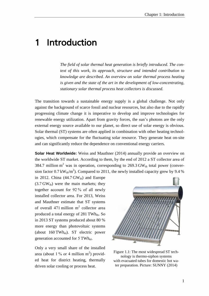
The company Wagner & Co. Solartechnik GmbH developed together with the Fraunho-
fer Institute for Solar Energy Systems ISE a stationary, double-covered ST flat-plate
collector with external reflectors for process heat generation. From August 2007 to De-
cember 2010, this project was funded by the German Federal Ministry for the Environ-
ment, Nature Conservation and Nuclear Safety (funding reference FK 0329 280 C).
Figure 1.2 shows the initial collector concept.
Figure 1.2: Computer graphic of the initial RefleC collector concept. Sloped collector
rows with CPC-reflectors are installed on the flat roof of an industrial building.
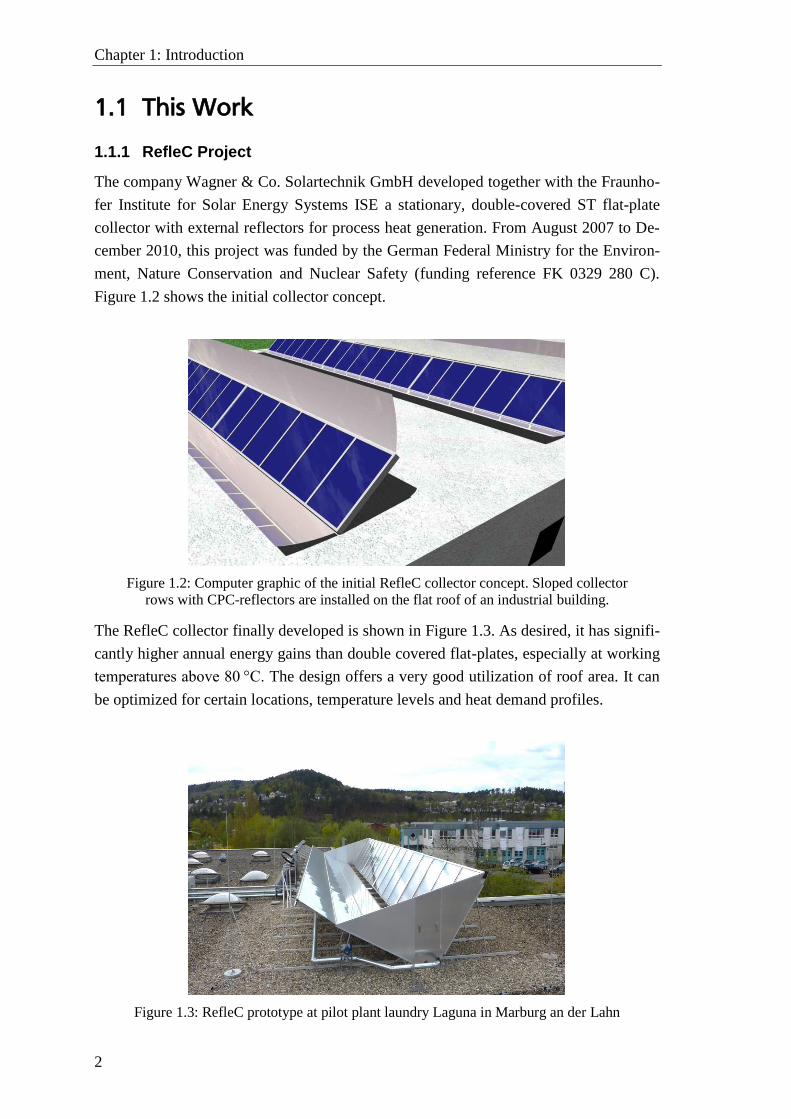
The RefleC collector finally developed is shown in Figure 1.3. As desired, it has signifi-
cantly higher annual energy gains than double covered flat-plates, especially at working
temperatures above 80 °C. The design offers a very good utilization of roof area. It can
be optimized for certain locations, temperature levels and heat demand profiles.
Figure 1.3: RefleC prototype at pilot plant laundry Laguna in Marburg an der Lahn
Chapter 1.1 This Work
3
The work in hand addresses questions that arose from development and optimization of
the RefleC collector. Research from within and after the funded project duration is re-
ported and general conclusions for assessment and optimization of stationary solar
thermal process heat collectors with reflectors are drawn.
1.1.2 Structure, Approach and Contribution to Knowledge
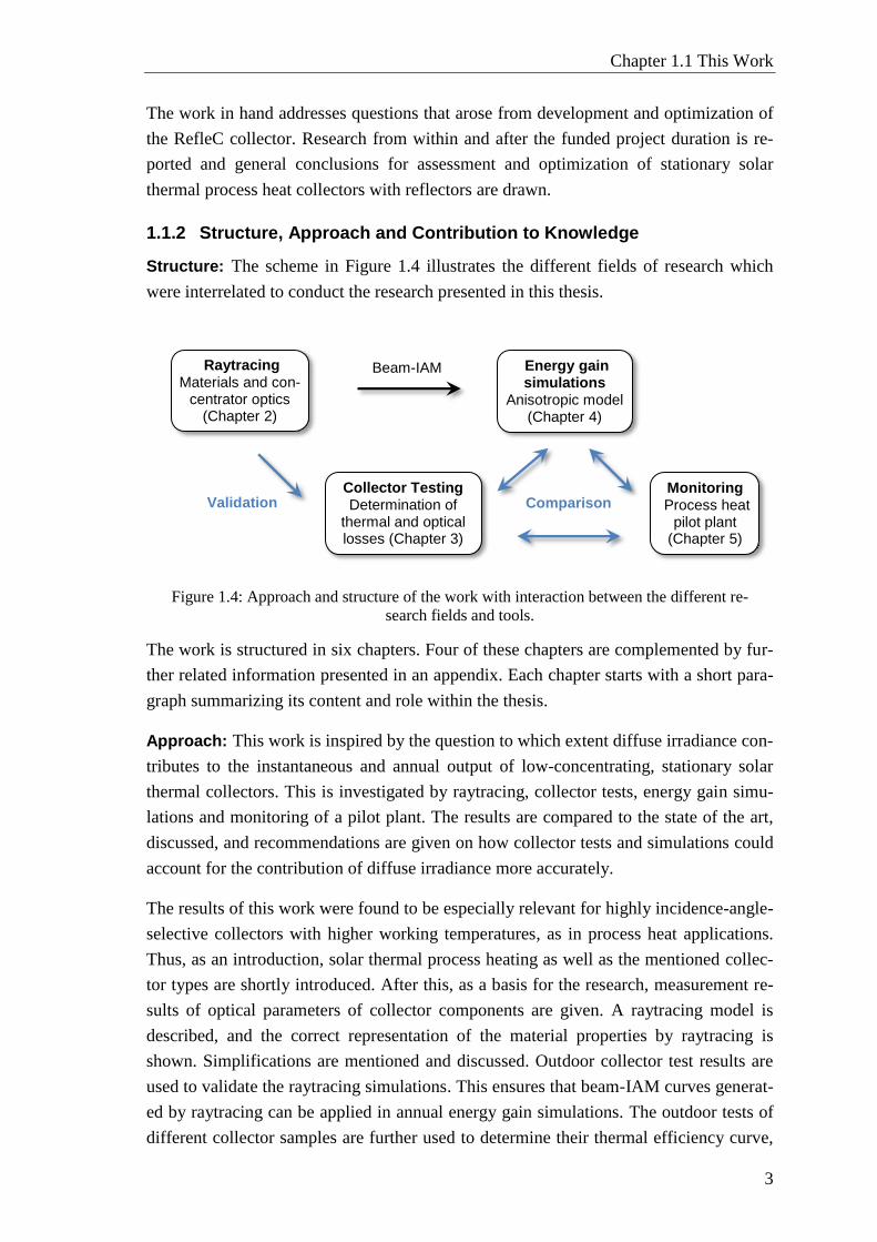
Structure: The scheme in Figure 1.4 illustrates the different fields of research which
were interrelated to conduct the research presented in this thesis.
Figure 1.4: Approach and structure of the work with interaction between the different re-
search fields and tools.
The work is structured in six chapters. Four of these chapters are complemented by fur-
ther related information presented in an appendix. Each chapter starts with a short para-
graph summarizing its content and role within the thesis.
Approach: This work is inspired by the question to which extent diffuse irradiance con-
tributes to the instantaneous and annual output of low-concentrating, stationary solar
thermal collectors. This is investigated by raytracing, collector tests, energy gain simu-
lations and monitoring of a pilot plant. The results are compared to the state of the art,
discussed, and recommendations are given on how collector tests and simulations could
account for the contribution of diffuse irradiance more accurately.
The results of this work were found to be especially relevant for highly incidence-angle-
selective collectors with higher working temperatures, as in process heat applications.
Thus, as an introduction, solar thermal process heating as well as the mentioned collec-
tor types are shortly introduced. After this, as a basis for the research, measurement re-
sults of optical parameters of collector components are given. A raytracing model is
described, and the correct representation of the material properties by raytracing is
shown. Simplifications are mentioned and discussed. Outdoor collector test results are
used to validate the raytracing simulations. This ensures that beam-IAM curves generat-
ed by raytracing can be applied in annual energy gain simulations. The outdoor tests of
different collector samples are further used to determine their thermal efficiency curve,
Raytracing Materials and con-
centrator optics (Chapter 2)
Energy gain simulations
Anisotropic model (Chapter 4)
Collector Testing Determination of
thermal and optical losses (Chapter 3)
Monitoring Process heat
pilot plant (Chapter 5)
Validation Comparison
Beam-IAM

Chapter 1: Introduction
4
to assess certain theoretically expected effects of the booster reflectors, and to optimize
the RefleC collector. A collector simulation model for the calculation of annual and
instantaneous collector gains in TRNSYS is developed. This model has three optical
modes: Diffuse irradiance can be treated as isotropic, separately isotropic for sky and
ground, or separately with an anisotropic sky. The model is applied to both the final
RefleC collector and its double-covered receiver flat-plate without reflectors. The dif-
ferences resulting from the three optical modes are analyzed. Finally, RefleC and its
flat-plate receiver are monitored in a solar process heat pilot plant. The results from the
collector tests, the TRNSYS simulations, and the pilot plant are compared in order to
draw general conclusions with respect to the research questions stated above.
Contribution to knowledge: In practice, the research presented in this work contribut-
ed to the development of the new RefleC collector. This collector has significant ad-
vantages compared to the state of the art.
A significant theoretical contribution to solar thermal research is the assessment of the
impact of anisotropic sky irradiance on instantaneous diffuse-IAM values and on simu-
lated collector output. Two extremes, the RefleC collector with very selective radiation
acceptance, and the double covered flat plate with very broad acceptance, have been
tested and simulated. For both collectors an undervaluation of the annual gains by state-
of-the-art isotropically calculated diffuse-IAMs was found. It is concluded that the re-
sults of this work are relevant for all non-focusing ST collector types.
1.2 Solar Thermal Process Heating
Though the focus of this work is on low-concentrating ST collectors, in this section a
short introduction to solar thermal process heating (SPH) is given. Its potential, current
state and future perspectives are discussed. Further readings are recommended as well.
As implied above, the vast majority of ST systems are currently used for domestic hot
water preparation in the residential sector. According to Weiss and Mauthner (2014, p.
6), about 87 % of the worldwide collector area serves for this purpose. In comparison to
these systems, SPH is usually more complex. There is a high discrepancy between the
SPH potential and the number of systems installed for industry and service applications.
1.2.1 Process Heat Demand
To give an insight into the relevance of process heat in a highly industrialized country,
the final energy demand of Germany is analyzed in more detail in Figure 1.5. Therein,
the transport sector has no process heat demand at all. In private households, a share of
6 % of the energy demand is process heat (used e.g. for cooking or washing).
Chapter 1.2 Solar Thermal Process Heating
5
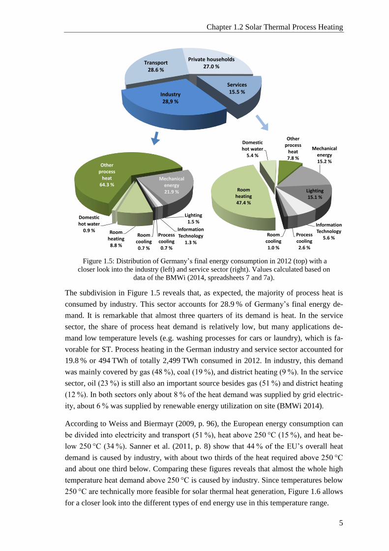
Figure 1.5: Distribution of Germany’s final energy consumption in 2012 (top) with a
closer look into the industry (left) and service sector (right). Values calculated based on
data of the BMWi (2014, spreadsheets 7 and 7a).
The subdivision in Figure 1.5 reveals that, as expected, the majority of process heat is
consumed by industry. This sector accounts for 28.9 % of Germany’s final energy de-
mand. It is remarkable that almost three quarters of its demand is heat. In the service
sector, the share of process heat demand is relatively low, but many applications de-
mand low temperature levels (e.g. washing processes for cars or laundry), which is fa-
vorable for ST. Process heating in the German industry and service sector accounted for
19.8 % or 494 TWh of totally 2,499 TWh consumed in 2012. In industry, this demand
was mainly covered by gas (48 %), coal (19 %), and district heating (9 %). In the service
sector, oil (23 %) is still also an important source besides gas (51 %) and district heating
(12 %). In both sectors only about 8 % of the heat demand was supplied by grid electric-
ity, about 6 % was supplied by renewable energy utilization on site (BMWi 2014).
According to Weiss and Biermayr (2009, p. 96), the European energy consumption can
be divided into electricity and transport (51 %), heat above 250 °C (15 %), and heat be-
low 250 °C (34 %). Sanner et al. (2011, p. 8) show that 44 % of the EU’s overall heat
demand is caused by industry, with about two thirds of the heat required above 250 °C
and about one third below. Comparing these figures reveals that almost the whole high
temperature heat demand above 250 °C is caused by industry. Since temperatures below
250 °C are technically more feasible for solar thermal heat generation, Figure 1.6 allows
for a closer look into the different types of end energy use in this temperature range.
Other process
heat64.3 %
Mechanical energy 21.9 %
Lighting1.5 %
Information Technology
1.3 %
Process cooling0.7 %
Room cooling0.7 %
Room heating8.8 %
Domestic hot water
0.9 %
Private households27.0 %
Transport28.6 %
Industry28,9 %
Services15.5 %
Other process
heat7.8 %
Mechanical energy 15.2 %
Lighting 15.1 %
Information Technology
5.6 %Process cooling2.6 %
Room cooling1.0 %
Room heating 47.4 %
Domestic hot water
5.4 %
Chapter 1: Introduction
6
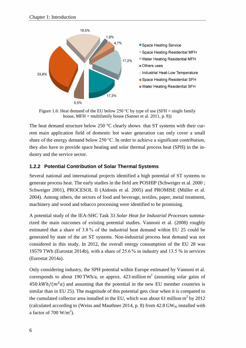
Figure 1.6: Heat demand of the EU below 250 °C by type of use (SFH = single family
house, MFH = multifamily house (Sanner et al. 2011, p. 8))
The heat demand structure below 250 °C clearly shows that ST systems with their cur-
rent main application field of domestic hot water generation can only cover a small
share of the energy demand below 250 °C. In order to achieve a significant contribution,
they also have to provide space heating and solar thermal process heat (SPH) in the in-
dustry and the service sector.
1.2.2 Potential Contribution of Solar Thermal Systems
Several national and international projects identified a high potential of ST systems to
generate process heat. The early studies in the field are POSHIP (Schweiger et al. 2000 ;
Schweiger 2001), PROCESOL II (Aidonis et al. 2005) and PROMISE (Müller et al.
2004). Among others, the sectors of food and beverage, textiles, paper, metal treatment,
machinery and wood and tobacco processing were identified to be promising.
A potential study of the IEA-SHC Task 33 Solar Heat for Industrial Processes summa-
rized the main outcomes of existing potential studies. Vannoni et al. (2008) roughly
estimated that a share of 3.8 % of the industrial heat demand within EU 25 could be
generated by state of the art ST systems. Non-industrial process heat demand was not
considered in this study. In 2012, the overall energy consumption of the EU 28 was
19579 TWh (Eurostat 2014b), with a share of 25.6 % in industry and 13.5 % in services
(Eurostat 2014a).
Only considering industry, the SPH potential within Europe estimated by Vannoni et al.
corresponds to about 190 TWh/a, or approx. 423 million m2 (assuming solar gains of
450 𝑘𝑊ℎ/(𝑚2𝑎) and assuming that the potential in the new EU member countries is
similar than in EU 25). The magnitude of this potential gets clear when it is compared to
the cumulated collector area installed in the EU, which was about 61 million m2 by 2012
(calculated according to (Weiss and Mauthner 2014, p. 8) from 42.8 GWth installed with
a factor of 700 W/m2).
Chapter 1.2 Solar Thermal Process Heating
7
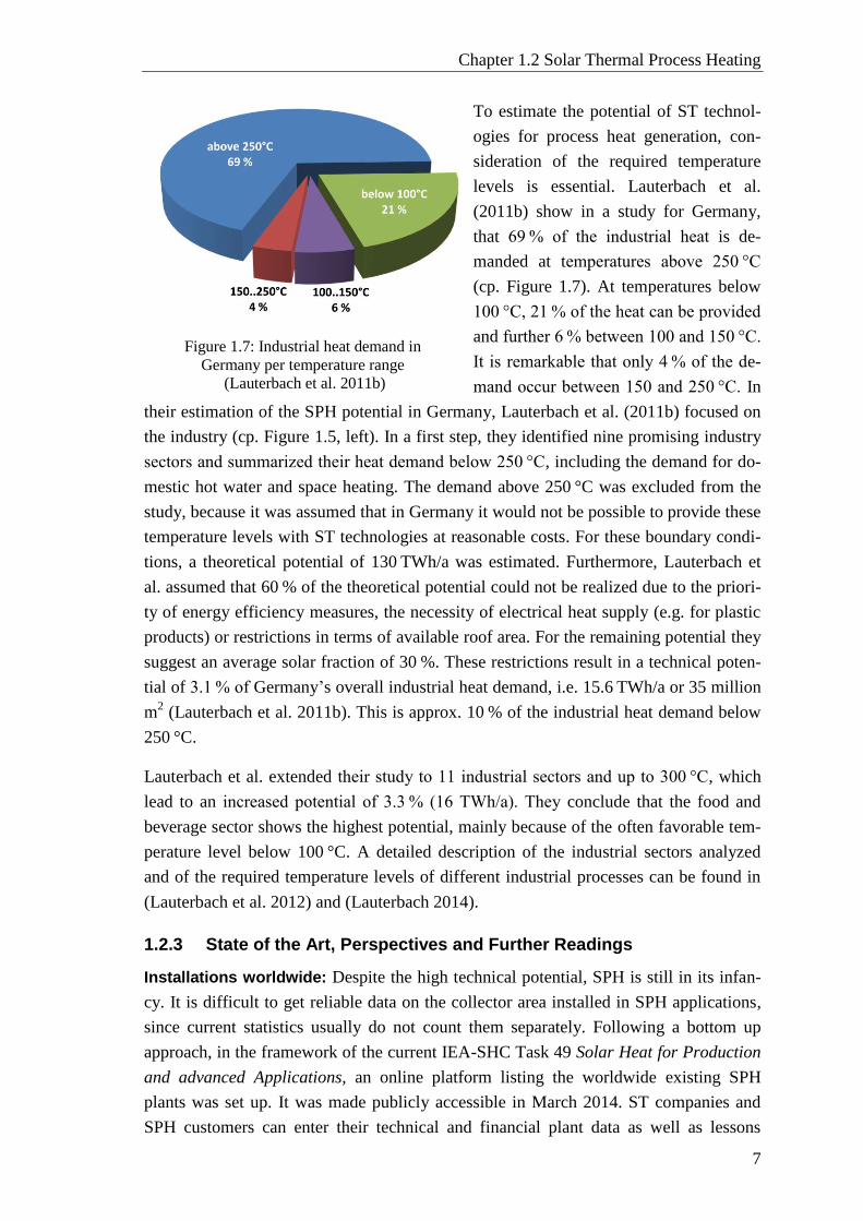
To estimate the potential of ST technol-
ogies for process heat generation, con-
sideration of the required temperature
levels is essential. Lauterbach et al.
(2011b) show in a study for Germany,
that 69 % of the industrial heat is de-
manded at temperatures above 250 °C
(cp. Figure 1.7). At temperatures below
100 °C, 21 % of the heat can be provided
and further 6 % between 100 and 150 °C.
It is remarkable that only 4 % of the de-
mand occur between 150 and 250 °C. In
their estimation of the SPH potential in Germany, Lauterbach et al. (2011b) focused on
the industry (cp. Figure 1.5, left). In a first step, they identified nine promising industry
sectors and summarized their heat demand below 250 °C, including the demand for do-
mestic hot water and space heating. The demand above 250 °C was excluded from the
study, because it was assumed that in Germany it would not be possible to provide these
temperature levels with ST technologies at reasonable costs. For these boundary condi-
tions, a theoretical potential of 130 TWh/a was estimated. Furthermore, Lauterbach et
al. assumed that 60 % of the theoretical potential could not be realized due to the priori-
ty of energy efficiency measures, the necessity of electrical heat supply (e.g. for plastic
products) or restrictions in terms of available roof area. For the remaining potential they
suggest an average solar fraction of 30 %. These restrictions result in a technical poten-
tial of 3.1 % of Germany’s overall industrial heat demand, i.e. 15.6 TWh/a or 35 million
m2 (Lauterbach et al. 2011b). This is approx. 10 % of the industrial heat demand below
250 °C.
Lauterbach et al. extended their study to 11 industrial sectors and up to 300 °C, which
lead to an increased potential of 3.3 % (16 TWh/a). They conclude that the food and
beverage sector shows the highest potential, mainly because of the often favorable tem-
perature level below 100 °C. A detailed description of the industrial sectors analyzed
and of the required temperature levels of different industrial processes can be found in
(Lauterbach et al. 2012) and (Lauterbach 2014).
1.2.3 State of the Art, Perspectives and Further Readings
Installations worldwide: Despite the high technical potential, SPH is still in its infan-
cy. It is difficult to get reliable data on the collector area installed in SPH applications,
since current statistics usually do not count them separately. Following a bottom up
approach, in the framework of the current IEA-SHC Task 49 Solar Heat for Production
and advanced Applications, an online platform listing the worldwide existing SPH
plants was set up. It was made publicly accessible in March 2014. ST companies and
SPH customers can enter their technical and financial plant data as well as lessons
Figure 1.7: Industrial heat demand in
Germany per temperature range
(Lauterbach et al. 2011b)
Chapter 1: Introduction
8
learned. At the beginning of September 2014, 134 SPH plants from all over the world
with an overall collector area of 126,421 m² (corresponding to 88.5 MWth) were listed.
Among them, 19 plants were above 1000 m² and 29 between 500 and 1000 m² (AEE
INTEC 2014). Since the database was set up recently, it can be expected to grow further
when more actors in the field of SPH know about it.
Challenges: Currently, there are still high technical and economic barriers for an in-
creased marked deployment of SPH systems. Technically, a very high variety of system
designs is possible, because a high variety of processes can be supported. Thus, SPH
systems usually need a high effort for planning and installation, especially in countries
where the processes are on a high technological level. In this case, SPH systems are
usually much more complex than ST systems for domestic purposes, since they have to
be planned sector specific and individually. Due to the higher complexity of the sys-
tems, there is also often a lack of knowledge about technical concepts for solar heat in-
tegration and about SPH system hydraulics and control. No easy to handle software
tools for SPH system design and optimization are available. This leads to considerable
uncertainties about the solar gains to be expected from a certain design variant.
Economically, SPH generation is also a challenge. In larger industries, usually the most
important decision criterion for an investment is its amortization period. Very often time
frames of below five years are expected, which is hard to achieve for SPH systems.
Thus, for the successful realization of a SPH project, also energy efficiency measures,
often offering significantly lower amortization times than SPH systems, should be con-
sidered. To be attractive against this background, the planning, installation and compo-
nent selection of SPH systems must be very cost-effective. Furthermore, interactions
between the SPH system and the existing heat supply have to be considered. The instan-
taneous solar gains and also the service lifetime of a SPH plant can vary significantly
when heat demand, mass flow or temperature level at the solar heat integration point are
changing. Thus, the assessment of possible long-term effects on the thermal load at an
integration point is another crucial aspect for ST process heating.
Selected further readings: SPH had been of interest in ST research for decades. Dedi-
cated book chapters addressing this application field can be found e.g. in (Goswami et
al. 1999), (Tiwari 2002), (Kalogirou 2004) and (Duffie and Beckman 2013). The poten-
tial study of Schweiger et al. (2000) mentioned above also contains a state of the art
review for Spain and Portugal. Karagiorgas et al. (2001) analyzed 10 SPH systems,
which have been installed during the 1990s in Greece. A list of suitable processes can
be found in (Kalogirou 2003), who also comments on difficulties and framework condi-
tions for SPH. Smyth and Russell (2009) analyzed the potential of ST and photovoltaic
systems for the global wine production. Solar cooling of industrial processes has been
successfully demonstrated by Motta (2010). For Australia, the state of the art in SPH
has been analyzed by Fuller (2011). A contracting-financed project integrating SPH in a
Chapter 1.2 Solar Thermal Process Heating
9
gas pressure regulating station was realized by Heinzen et al. (2011). Economic assess-
ments of SPH in Central Europe can be found in (Lauterbach et al. 2011a) and (Faber et
al. 2011). Norton (2012) published a comprehensive literature survey on the field of
SPH. Recently, SPH was also included in the handbook for planners and installers of
the German Solar Energy Society DGS (Kasper et al. 2012). Feasibility analyses for
Tunisia are presented by Calderoni et al. (2012) and Frein et al. (2014). Silva et al.
(2014) did a study on SPH for vegetable preservation in Spain.
The EU-funded project Solar Process Heat (SoPro) was one of the first publicly funded
projects addressing barriers for SPH on an international level. It supported the market
deployment in six European regions. In sum, 90 energy screenings of industrial compa-
nies were carried out. Checklists were developed, training seminars were held and the
chances and barriers for SPH contracting have been analyzed. Based on a process-
specific approach, simplified design guidelines for SPH systems for four common ap-
plications were developed (Hess and Oliva 2010). These applications are heating of
water for washing or cleaning, heating of make-up water, heating of baths or vessels
and drying with air collectors. It was shown that SPH systems supporting open loop
processes at low temperature levels can have significantly higher annual gains than
standard ST systems in the domestic sector. The work within SoPro triggered 10 new
SPH installations within the regions (Egger 2011). The summarized project results to-
gether with practical examples for application of the simple system dimensioning meth-
odology are presented in (Hess et al. 2011).
Following a sector-specific approach, Schmitt et al. (2012a) presented a branch-concept
for SPH integration in breweries. A guideline for planners for this sector was published
as well (Schmitt et al. 2012b). Based on this work, generalized technical solar heat inte-
gration concepts were developed (Schmitt 2014). Lauterbach (2014) developed a pre-
liminary design methodology for SPH systems.
Selected recent examples for scientifically monitored commercial solar process heat
plants are the Hofmuehl brewery with a system utilization ratio of about 20 % (Wutzler
et al. 2011), the Alanod demonstration plant for direct steam generation (Krueger et al.
2011) as well as the electroplating company Steinbach & Vollmann, where in the course
of system optimization an innovative storage charging concept was implemented
(Schramm and Adam 2014).
Lauterbach et al. (2014) monitored the Hütt brewery. By incorporating the measured
ambient temperature, irradiance, process load profiles and system operation data in a
TRNSYS simulation, the authors found a very good correlation between the measured
and simulated performance of the flat-plate SPH system applied. Recently, SPH systems
for brick manufacturing (Vittoriosi et al. 2014) and meat production (Cotrado et al.
2014) were installed and are monitored.
Chapter 1: Introduction
10
Visions and research priorities: In spite of the barriers described above, stakeholders
have very high expectations for SPH. The German solar industry association BSW sees
SPH below 100 °C in its Fahrplan Solarwärme as a strategic focus issue with decisive
importance for market deployment of ST. With a joint effort of the whole ST sector, the
BSW has set the ambitious target of 1.500 SPH plants installed in Germany by the year
2020 and perspectively more than 28.000 by 2030 (Ebert et al. 2012, p. 11).
The International Energy Agency IEA states in its Technology Roadmap for Solar Heat-
ing and Cooling, that ST systems globally could supply 20 % of the industrial heat de-
mand below 120 °C until 2050 (IEA 2012, p. 22).
Based upon a Common Vision for the Renewable Heating and Cooling Sector in Europe
(Sanner et al. 2011), the European Technology Platform on Renewable Heating and
Cooling published Strategic Research Priorities for ST collectors until 2020 and be-
yond (Stryi-Hipp et al. 2012, p. 45). In their Strategic Research and Innovation Agenda
for the renewable heating and cooling sector, the platform members defined research
and innovation priorities for SPH collectors and systems (Sanner et al. 2013, p. 53).
They further detailed their suggestions in a Solar Heating & Cooling Technology
Roadmap, containing technological and non-technological measures for SPH until 2020
with objectives and milestones. Among else, they recommend the development of mid
temperature collectors with improved efficiency, self-carrying and modular collector
structures for large-scale collector arrays on industrial roofs, as well as improved reflec-
tor materials for concentrating collectors (Ivancic et al. 2014, pp. 26-28).
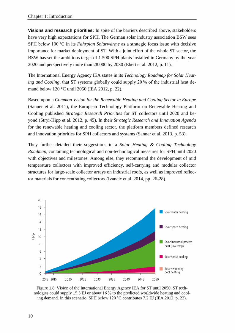
Figure 1.8: Vision of the International Energy Agency IEA for ST until 2050. ST tech-
nologies could supply 15.5 EJ or about 16 % to the predicted worldwide heating and cool-
ing demand. In this scenario, SPH below 120 °C contributes 7.2 EJ (IEA 2012, p. 22).
Chapter 1.3 Stationary Process Heat Collectors
11
1.3 Stationary Process Heat Collectors
1.3.1 Collector Categories
The purpose of a solar thermal collector is to convert solar irradiance incident on its
aperture area1 into useful heat. To efficiently generate temperatures above 100 °C a high
variety of collector designs and materials is applied. The existing concepts can be cate-
gorized according to different criteria: Stationary (i.e. non-tracking), seasonally-tilted,
one-axis tracked and two-axis tracked collectors are built. When the flux density of ir-
radiance onto an absorber is enhanced by concentrators, high concentrating focusing
collectors differ from the low-concentrating and are usually non-focusing. Thermally,
non-evacuated collectors have to be distinguished from evacuated ones. Different heat
transfer fluids such as water, water-glycol mixture, air, thermal oil or molten salt are
used.
The term process heat collector (PHC) is not a clear definition, since process heat as
defined above can be generated by all ST collector types. But since this term is mainly
used in collector development, within this work it describes collectors, which are de-
signed and optimized for output temperatures in the mid-temperature range (100 to
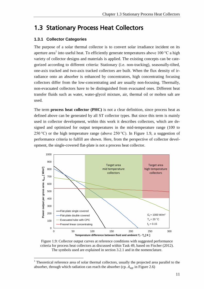
250 °C) or the high temperature range (above 250 °C). In Figure 1.9, a suggestion of
performance criteria to fulfill are shown. Here, from the perspective of collector devel-
opment, the single-covered flat-plate is not a process heat collector.
Figure 1.9: Collector output curves at reference conditions with suggested performance
criteria for process heat collectors as discussed within Task 49, based on Fischer (2012).
The symbols used are explained in section 3.2.1 and in the nomenclature.
1 Theoretical reference area of solar thermal collectors, usually the projected area parallel to the
absorber, through which radiation can reach the absorber (cp. 𝐴𝑎𝑝 in Figure 2.6)
0
100
200
300
400
500
600
700
800
900
1000
0 50 100 150 200 250 300
Po
wer
ou
tpu
t p
er
gro
ss a
rea q
use
[ W
/m2]
Temperature difference between fluid and ambient Tf - Ta [ K ]
Flat-plate single covered
Flat-plate double covered
Evacuated tube with CPC
Fresnel linear concentrating
Target areamid temperature
collectors
Target areahigh temperature
collectors
Gt = 1000 W/m2
Ta = 20 C
fd = 0.15
Chapter 1: Introduction
12
1.3.2 Standard Flat-plates and Evacuated Tube Collectors
Flat-plate collectors: Standard-flat-plate collectors are the most common collector
type in Europe (Weiss and Mauthner 2014, p. 11). Due to the low difference between
gross and aperture area they collect much beam irradiance per gross area and make good
use of diffuse irradiance. They are stationary mounted, simply constructed and need low
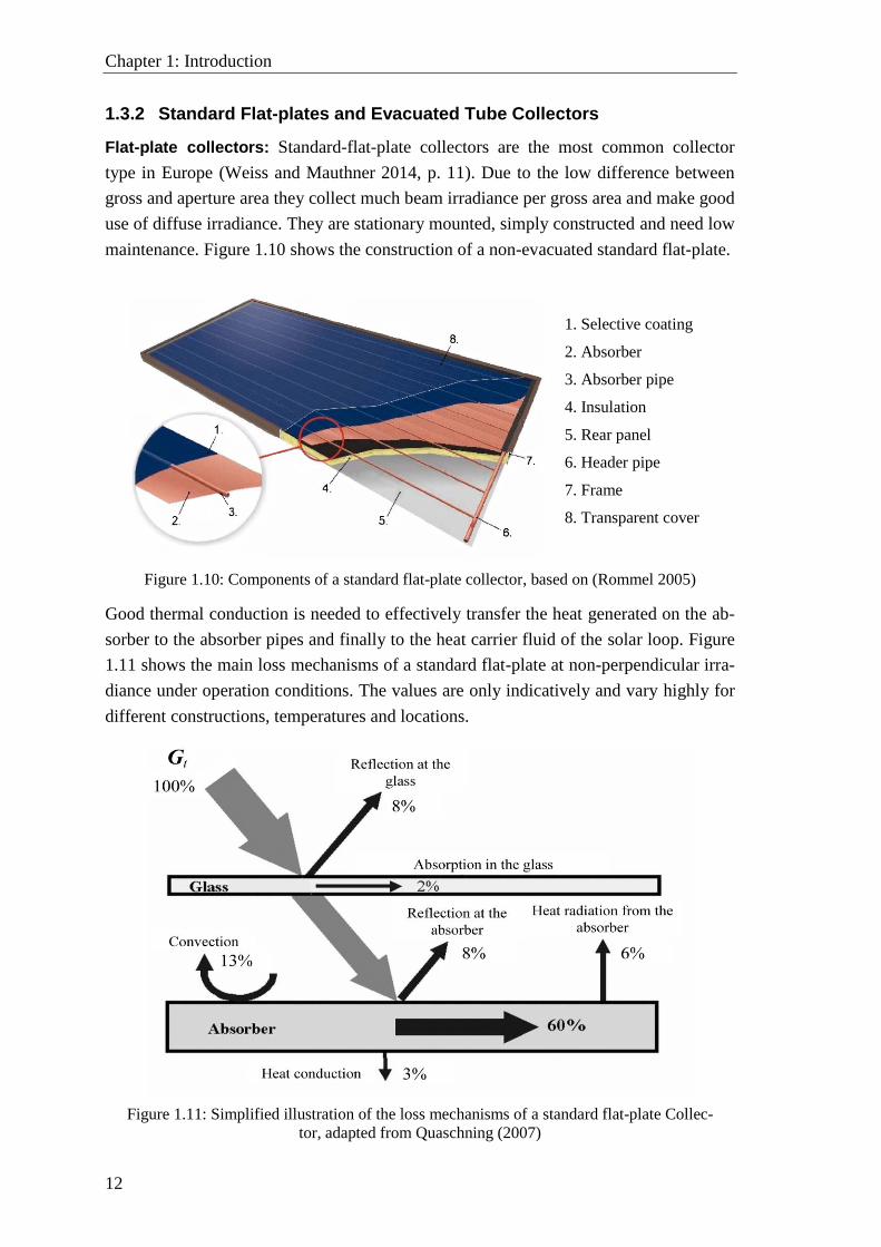
maintenance. Figure 1.10 shows the construction of a non-evacuated standard flat-plate.
1. Selective coating
2. Absorber
3. Absorber pipe
4. Insulation
5. Rear panel
6. Header pipe
7. Frame
8. Transparent cover
Figure 1.10: Components of a standard flat-plate collector, based on (Rommel 2005)
Good thermal conduction is needed to effectively transfer the heat generated on the ab-
sorber to the absorber pipes and finally to the heat carrier fluid of the solar loop. Figure
1.11 shows the main loss mechanisms of a standard flat-plate at non-perpendicular irra-
diance under operation conditions. The values are only indicatively and vary highly for
different constructions, temperatures and locations.
Figure 1.11: Simplified illustration of the loss mechanisms of a standard flat-plate Collec-
tor, adapted from Quaschning (2007)
Chapter 1.3 Stationary Process Heat Collectors
13
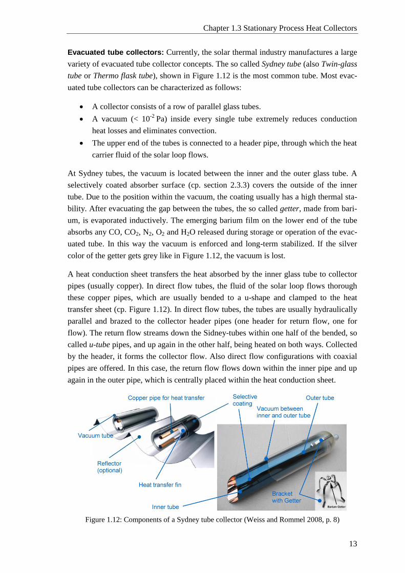
Evacuated tube collectors: Currently, the solar thermal industry manufactures a large
variety of evacuated tube collector concepts. The so called Sydney tube (also Twin-glass
tube or Thermo flask tube), shown in Figure 1.12 is the most common tube. Most evac-
uated tube collectors can be characterized as follows:
A collector consists of a row of parallel glass tubes.
A vacuum (< 10-2
Pa) inside every single tube extremely reduces conduction
heat losses and eliminates convection.
The upper end of the tubes is connected to a header pipe, through which the heat
carrier fluid of the solar loop flows.
At Sydney tubes, the vacuum is located between the inner and the outer glass tube. A
selectively coated absorber surface (cp. section 2.3.3) covers the outside of the inner
tube. Due to the position within the vacuum, the coating usually has a high thermal sta-
bility. After evacuating the gap between the tubes, the so called getter, made from bari-
um, is evaporated inductively. The emerging barium film on the lower end of the tube
absorbs any CO, CO2, N2, O2 and H2O released during storage or operation of the evac-
uated tube. In this way the vacuum is enforced and long-term stabilized. If the silver
color of the getter gets grey like in Figure 1.12, the vacuum is lost.
A heat conduction sheet transfers the heat absorbed by the inner glass tube to collector
pipes (usually copper). In direct flow tubes, the fluid of the solar loop flows thorough
these copper pipes, which are usually bended to a u-shape and clamped to the heat
transfer sheet (cp. Figure 1.12). In direct flow tubes, the tubes are usually hydraulically
parallel and brazed to the collector header pipes (one header for return flow, one for
flow). The return flow streams down the Sidney-tubes within one half of the bended, so
called u-tube pipes, and up again in the other half, being heated on both ways. Collected
by the header, it forms the collector flow. Also direct flow configurations with coaxial
pipes are offered. In this case, the return flow flows down within the inner pipe and up
again in the outer pipe, which is centrally placed within the heat conduction sheet.
Figure 1.12: Components of a Sydney tube collector (Weiss and Rommel 2008, p. 8)
Chapter 1: Introduction
14
In heat-pipe collectors, collector pipes and solar loop are hydraulically disconnected. A
working fluid evaporates within the collector pipes at low temperatures and condenses
at the top of the pipe. The condensers are thermally connected to the header pipe, either
dipping into the solar fluid (referred to as wet connection) or clamped to the header pipe
and using heat conduction paste (dry connection).
1.3.3 Low-Concentrating, Stationary Collectors
Reflectors are applied to increase the energy gain of ST collectors by re-directing or
concentrating solar irradiance onto an absorber. Focusing reflectors concentrate irradi-
ance onto a focal point or line. Such collector types have to track the sun to keep the
focus on the absorber. To avoid tracking, reflectors must be shaped in a way that the
radiant flux density onto the absorber is increased for a certain range of incidence an-
gles. Such reflectors are called non-focusing or non-imaging concentrators. With these
concepts, only small concentration ratios are reasonable. Thermally, it is important to
distinguish between reflector concepts, which are placed outside the thermal sealing of a
collector (cp. Figure 1.13) or within (cp. Figure 1.14). Placing the reflectors inside pro-
tects them from hail, dust and water. But at such concepts conduction and convection
occur within the whole casing, so the loss reduction related to the aperture area is usual-
ly smaller.
This section intends to reflect the state of the art of low-concentrating, stationary collec-
tors, focusing on flat-plate based concepts that were theoretically optimized, character-
ized in laboratories, annually simulated or annually measured. The technical terms used
are explained in the following chapters, mainly in section 2.4.1. Further literature with
relevance for this work is referenced within the respective chapters.
The use of external so called booster reflectors for ST collector arrays (cp. Figure 1.13)
has been investigated since the 1950s, when Tabor (1958) projected the incidence angle
of beam irradiance into a vertical north-south plane and determined necessary ac-
ceptance angles of stationary concentrators.
Perers and Karlsson (1993) presented a simplified model to calculate the additional
energy gain of flat-plate collectors equipped with flat or CPC booster reflectors. In
Studsvik, Sweden, they measured the annual gain of a flat-plate equipped with
optimized flat booster reflector and of an identical reference flat-plate without reflector.
The flat-plates were double-covered with white glazing (i.e. low iron content) and a
Teflon foil, and the length of the flat reflector in front of the flat-plates was 1.25 the
height of the flat-plates (ratio L/H = 1.25). The reflectors extended the length of the flat-
plates by one meter in the east-west direction to minimize end losses. After four
operating seasons they measured an annual output increase due to the reflector of 30 %.
In a simulation study, they applied reflectors of 𝜌 = 0.8 ( 𝜌𝑠𝑝𝑒𝑐 = 0.6) to the described
flat-plate collectors and calculated the annual gain for 𝑇𝑓 = 70 °C in Stockholm, Swe-
Chapter 1.3 Stationary Process Heat Collectors
15
den. For L/H = 1.25, a collector with CPC-booster achieved 15 % higher output than
with a flat booster. For L/H = 2, the authors expect additional gains of 50 % by a CPC
booster. Perers (1995) further optimized different flat and CPC booster geometries for
the flat-plate mentioned above. Assuming costs of ground area and a cost-range for the
reflectors, he calculated an investment cost reduction of up to 25 % per delivered kWh
for the Stockholm climate, when flat booster reflectors with optimal ratio of L/H = 1.5
are applied. In the study, the maximum yield per ground area was achieved by flat
boosters; the maximum yield per receiver flat-plate area was achieved by a CPC.
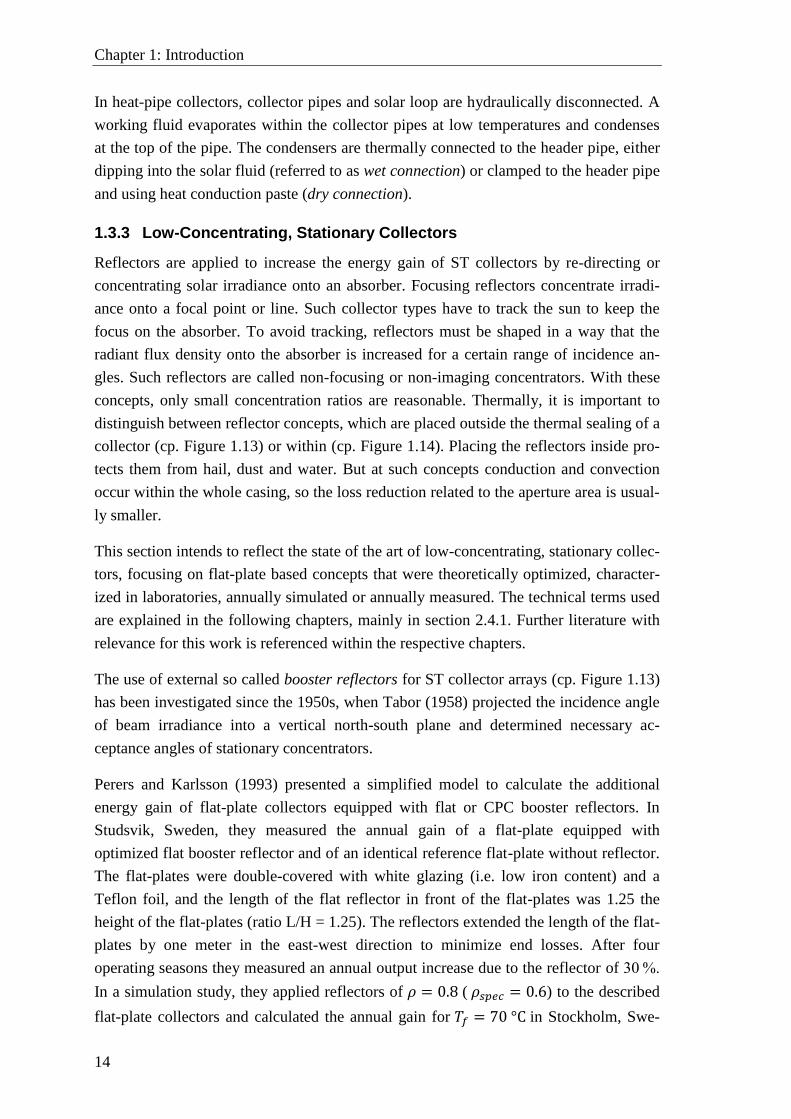
Figure 1.13: Flat-plate collector field with trapezoidal corrugated aluminum sheet booster
reflectors supplying a hospital in Östhammer, Sweden.
Picture: Björn Karlsson, cp. (Rönnelid and Karlsson 1999, p. 347).
Hellstrom et al. (2003) investigated the impact of different flat booster reflector
materials on the additional annual energy gain of a standard flat-plate with solar
transmittance of 0.90 in Stockholm. For L/H = 2.06, the optimized concepts were
assessed at mean temperatures of 70 °C. A PVF2-coated aluminium sheet increased the
annual gain by 25.7 %, anodized aluminium by 32.7 %, and silver coated glass by
36.4 %. The relative improvement increased with increasing operation temperatures.
Rönnelid and Karlsson (1999) showed that v-corrugation of flat booster reflectors can
further increase the annual beam irradiance onto the flat-plate by approx. 10 % and the
annual output by approx. additional 3 % compared to a flat booster (for L/H = 2).
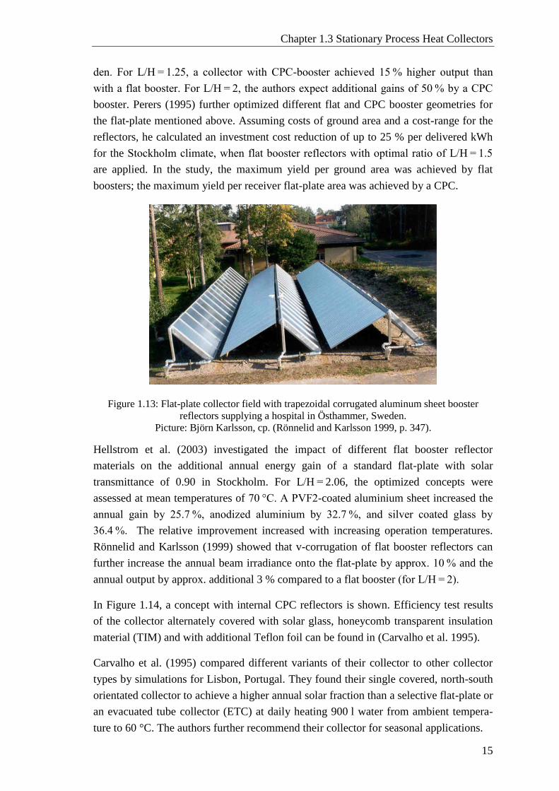
In Figure 1.14, a concept with internal CPC reflectors is shown. Efficiency test results
of the collector alternately covered with solar glass, honeycomb transparent insulation
material (TIM) and with additional Teflon foil can be found in (Carvalho et al. 1995).
Carvalho et al. (1995) compared different variants of their collector to other collector
types by simulations for Lisbon, Portugal. They found their single covered, north-south
orientated collector to achieve a higher annual solar fraction than a selective flat-plate or
an evacuated tube collector (ETC) at daily heating 900 l water from ambient tempera-
ture to 60 °C. The authors further recommend their collector for seasonal applications.
Chapter 1: Introduction
16
Supporting a single-stage adsorption chiller at 90 °C in Lisbon, the single-covered vari-
ant achieved higher gains than a selective flat-plate. Carvalho et al. (1995) further state,
that the double covered variant would have a better cost/performance ratio than an ETC
in this application. Detailed analytical solutions for the optical parameters of “inverted
v”-absorbers can be found in (Fraidenraich et al. 2008).
Rönnelid et al. (1996) constructed a flat-plate with internal, symmetric v-trough concen-
trator with a flat absorber. Laboratory heat loss tests revealed that a low-emitting reflec-
tor and an additional 25 μm FEP Teflon film reduced the heat losses by about 20 %. But
the optimized CPC concept with 𝐶𝑔𝑒𝑜 = 1.56, 𝜃𝑎 = 35° and a truncation ratio of 0.4,
had only approx. 5 % higher annual gains than a standard flat-plate, when it was orien-
tated east-west and simulated in Stockholm at 𝑇𝑓 = 70 °C (read from graph in (Rönnelid
and Karlsson 1996, p. 178)). So for an annual load the additional costs for manufactur-
ing internal reflectors of this kind might not be justified. A very similar collector had
been investigated by Fasulo et al. (1987), who could significantly reduce convection
losses by covering the flat absorbers with transparent foil, but the overall efficiencies of
the concept were rather low and no annual energy gain simulations have been reported.
Buttinger et al. (2010) investigated a flat-plate collector with internal CPC and tubular
absorber. A prototype with krypton gas filling and very low pressure of 0.01 bar showed
efficiencies of about 50 % at 𝐺 = 1000 W/m² with 𝑓𝑑 = 0.1.
In order to replace collector components by cheaper reflector area, the collector concept
shown in Figure 1.15 was developed for high latitudes.
1. Aluminum frame
2. EPDM gasket
3. Polyurethane insulation
4. Absorber fin with
selective coating
on both sides
5. Back sheet
6. Transparent cover
7. Header tube
8. CPC reflector
Figure 1.14: AoSol CPC collector with “inverted v”-absorber.
For highest gains the collector is orientated east-west. 𝐶𝑔𝑒𝑜 = 1.12, 𝜃𝑎 = 56,4°,
𝐴𝑎𝑝 = 1.98 m2. Parameters from Pereira et al. (2003). Pictures: Manuel Collares Pereira
Chapter 1.3 Stationary Process Heat Collectors
17
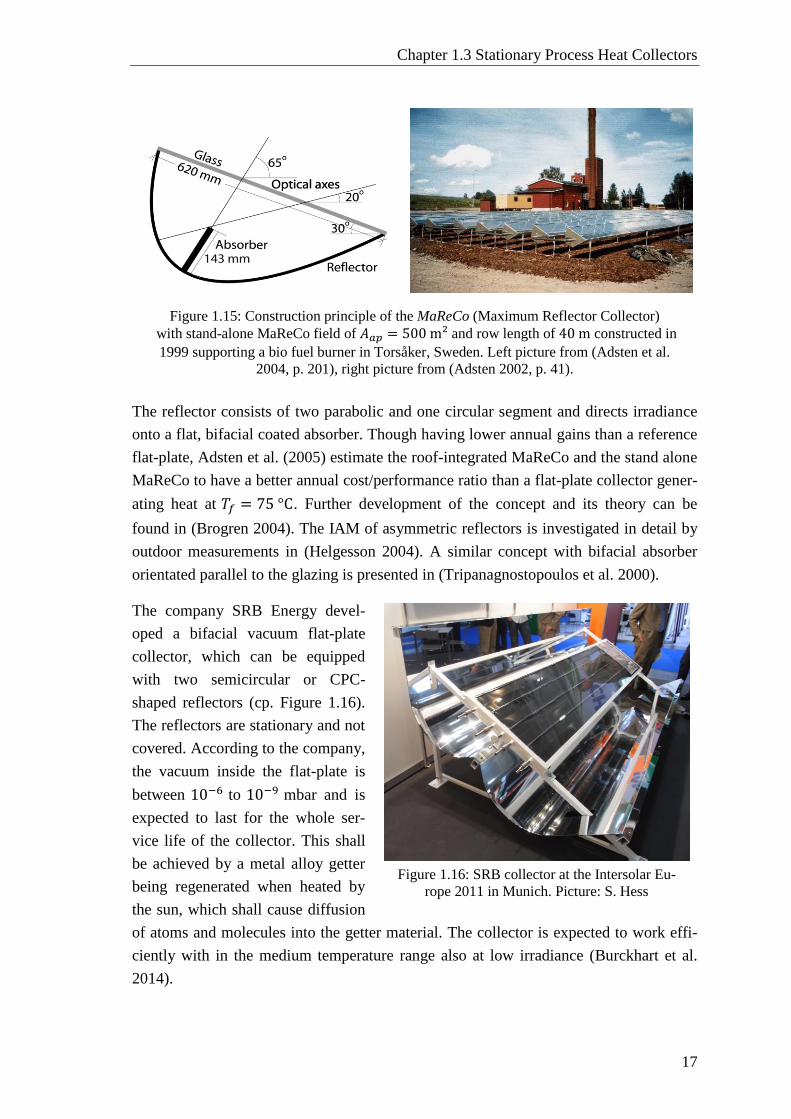
The reflector consists of two parabolic and one circular segment and directs irradiance
onto a flat, bifacial coated absorber. Though having lower annual gains than a reference
flat-plate, Adsten et al. (2005) estimate the roof-integrated MaReCo and the stand alone
MaReCo to have a better annual cost/performance ratio than a flat-plate collector gener-
ating heat at 𝑇𝑓 = 75 °C. Further development of the concept and its theory can be
found in (Brogren 2004). The IAM of asymmetric reflectors is investigated in detail by
outdoor measurements in (Helgesson 2004). A similar concept with bifacial absorber
orientated parallel to the glazing is presented in (Tripanagnostopoulos et al. 2000).
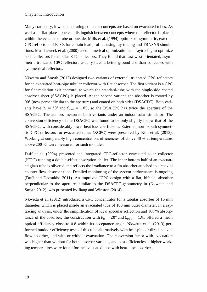
The company SRB Energy devel-
oped a bifacial vacuum flat-plate
collector, which can be equipped
with two semicircular or CPC-
shaped reflectors (cp. Figure 1.16).
The reflectors are stationary and not
covered. According to the company,
the vacuum inside the flat-plate is
between 10−6 to 10−9 mbar and is
expected to last for the whole ser-
vice life of the collector. This shall
be achieved by a metal alloy getter
being regenerated when heated by
the sun, which shall cause diffusion
of atoms and molecules into the getter material. The collector is expected to work effi-
ciently with in the medium temperature range also at low irradiance (Burckhart et al.
2014).
Figure 1.15: Construction principle of the MaReCo (Maximum Reflector Collector)
with stand-alone MaReCo field of 𝐴𝑎𝑝 = 500 m² and row length of 40 m constructed in
1999 supporting a bio fuel burner in Torsåker, Sweden. Left picture from (Adsten et al.
2004, p. 201), right picture from (Adsten 2002, p. 41).
Figure 1.16: SRB collector at the Intersolar Eu-
rope 2011 in Munich. Picture: S. Hess
Chapter 1: Introduction
18
Many stationary, low concentrating collector concepts are based on evacuated tubes. As
well as at flat-plates, one can distinguish between concepts where the reflector is placed
within the evacuated tube or outside. Mills et al. (1994) optimized asymmetric, external
CPC reflectors of ETCs for certain load profiles using ray-tracing and TRNSYS simula-
tions. Muschaweck et al. (2000) used numerical optimization and raytracing to optimize
such collectors for tubular ETC collectors. They found that east-west-orientated, asym-
metric truncated CPC reflectors usually have a better ground use than collectors with
symmetrical reflectors.
Nkwetta and Smyth (2012) designed two variants of external, truncated CPC reflectors
for an evacuated heat-pipe tubular collector with flat absorber. The first variant is a CPC
for flat radiation exit aperture, at which the standard-tube with the single-side coated
absorber sheet (SSACPC) is placed. At the second variant, the absorber is rotated by
90° (now perpendicular to the aperture) and coated on both sides (DSACPC). Both vari-
ants have 𝜃𝑎 = 30° and 𝐶𝑔𝑒𝑜 = 1.85, so the DSACPC has twice the aperture of the
SSACPC. The authors measured both variants under an indoor solar simulator. The
conversion efficiency of the DSACPC was found to be only slightly below that of the
SSACPC, with considerably lower heat loss coefficients. External, north-south symmet-
ric CPC reflectors for evacuated tubes (XCPC) were presented by Kim et al. (2013).
Working at comparably high concentration, efficiencies of above 40 % at temperatures
above 200 °C were measured for such modules.
Duff et al. (2004) presented the integrated CPC-reflector evacuated solar collector
(ICPC) running a double-effect absorption chiller. The inner bottom half of an evacuat-
ed glass tube is silvered and reflects the irradiance to a fin absorber attached to a coaxial
counter flow absorber tube. Detailed monitoring of the system performance is ongoing
(Duff and Daosukho 2011). An improved ICPC design with a flat, bifacial absorber
perpendicular to the aperture, similar to the DSACPC-geommetry in (Nkwetta and
Smyth 2012), was presented by Jiang and Winston (2014).
Nkwetta et al. (2012) introduced a CPC concentrator for a tubular absorber of 15 mm
diameter, which is placed inside an evacuated tube of 100 mm outer diameter. In a ray-
tracing analysis, under the simplification of ideal specular reflection and 100 % absorp-
tance of the absorber, the construction with 𝜃𝑎 = 20° and 𝐶𝑔𝑒𝑜 = 1.95 offered a mean
optical efficiency close to 0.8 within its acceptance angle. Nkwetta et al. (2013) per-
formed outdoor-efficiency tests of this tube alternatively with heat-pipe or direct coaxial
flow absorber, and with or without evacuation. The conversion factor with evacuation
was higher than without for both absorber variants, and best efficiencies at higher work-
ing temperatures were found for the evacuated tube with heat-pipe absorber.
Chapter 2: Optical Investigations
19
2 Optical Investigations
The main subject of this work is the utilization of anisotropic diffuse sky
radiance by low-concentrating solar thermal collectors. Thus, this chap-
ter starts with a background on solar irradiance. The concept of the in-
cidence angle modifier and its determination for certain design variants
of the RefleC collector by raytracing is explained. The parameterization
of RefleC in the raytracing-model is discussed based on measured mate-
rial properties. Finally, the reflector design is explained and raytracing
results relevant for the following investigations are given.
2.1 Solar Irradiance
2.1.1 Components and Characteristics
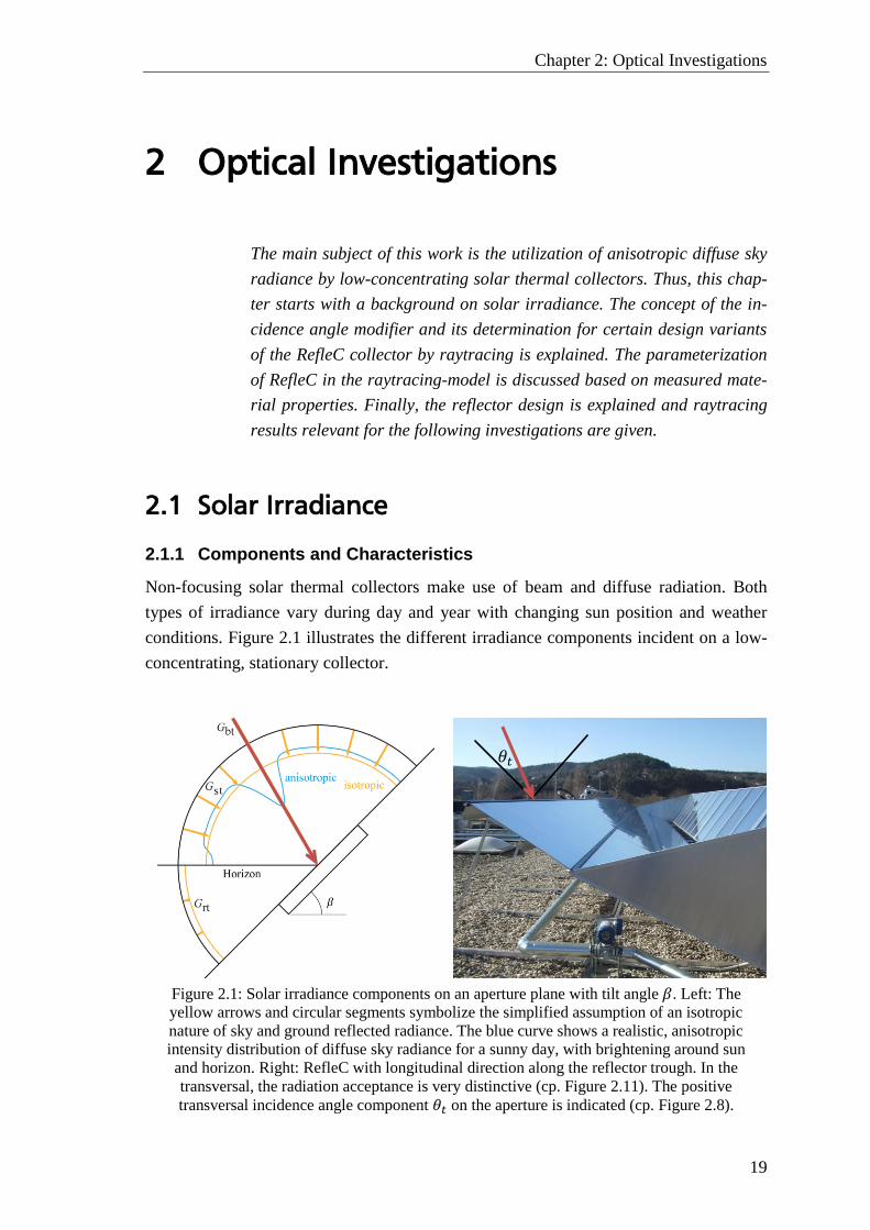
Non-focusing solar thermal collectors make use of beam and diffuse radiation. Both
types of irradiance vary during day and year with changing sun position and weather
conditions. Figure 2.1 illustrates the different irradiance components incident on a low-
concentrating, stationary collector.
Figure 2.1: Solar irradiance components on an aperture plane with tilt angle 𝛽. Left: The
yellow arrows and circular segments symbolize the simplified assumption of an isotropic
nature of sky and ground reflected radiance. The blue curve shows a realistic, anisotropic
intensity distribution of diffuse sky radiance for a sunny day, with brightening around sun
and horizon. Right: RefleC with longitudinal direction along the reflector trough. In the
transversal, the radiation acceptance is very distinctive (cp. Figure 2.11). The positive
transversal incidence angle component 𝜃𝑡 on the aperture is indicated (cp. Figure 2.8).
𝜃𝑡
Chapter 2: Optical Investigations
20
Beam irradiance 𝐺𝑏𝑡 on the tilted aperture plane reaches the collector from a solid angle
of approx. 6° diameter (cp. section 2.1.2) with the sun at its centre. Diffuse irradiance
from the sky 𝐺𝑠𝑡 originates from the whole sky dome visible from the aperture (exclud-
ing the disk of approx. 6°). Ground reflected irradiance 𝐺𝑟𝑡 reaches the aperture from
directions below the horizon with transversal incidence angles 𝜃𝑡 = [−90;−90 + 𝛽].
Table 2.1 gives an overview on the terms used within this work to distinguish between
radiation sent out and received as well as between instantaneous power and energy.
Table 2.1: Terms for solar radiation as suggested by Iqbal (1983, p. 41). All terms refer to the
integrated power of the whole solar radiation spectrum.
Term Unit Meaning
Radiation - Used qualitatively to distinguish irradiance components
Radiance W/(m2sr) Emitted solar radiant flux within a unit solid angle
Irradiance W/m2 Incident solar radiance per unit aperture area
Irradiation kWh/m2 Integrated irradiance within time interval per aperture area
In the following, details on characteristics and calculation of the solar irradiance com-
ponents as well as their use in simulation programmes will be given. An obvious start-
ing point for this is the sun itself.
Extraterrestrial solar radiation: The sun is the center of our planetary system and con-
tains 99.85 % of its total mass. Within the sun, hydrogen is fused to helium, which re-
sults in a mass loss of approx. 4.3 106 t/s in the form of radiative energy. Using Ein-
stein’s law it can easily be shown that the sun emits an enormous radiant flux of approx.
3.86465 1026 W to outer space. The temperature of the sun’s center is approx. 107 K.
It decreases towards the photosphere, the approx. 200 km thick “surface” of the sun, to
finally approx. 5,790 K. There, the major part of radiance is emitted. Simplified, the sun
can be seen as a black body emitter. Under this assumption, its radiance can be calculat-
ed according to the Stefan-Boltzmann law with an approximated effective black body
temperature of 5,777 K (Duffie and Beckman 2006, p. 3).
When viewed from earth, the opening half angle of the solar disk itself is as small as
approx. 0.27° , which results in a divergence of direct sunlight of approx. 0.54°
or 9.4 mrad. From satellite measurements the exact value for the intensity at the outer
earth atmosphere normal to the sun direction was defined to
𝐺𝑠𝑐 = 1,367 ± 23 W
m2 ( 2.1 )
This value 𝐺𝑠𝑐 is called solar constant (Duffie and Beckman 2006, p. 5). The fluctuation
range of this value results from the eccentricity of the earth’s elliptical orbit around the
sun, which causes annual variations of approx. 1.7 %. 𝐺𝑠𝑐 can be determined by Eq. 2.2.
2.1 Solar Irradiance
21
𝐺𝑠𝑐 = 1,367 ⋅ [1 + 0.0033 cos (2𝜋 𝑖
365)] ( 2.2 )
Herein, i is the day of the year (Duffie and Beckman 2006, p. 37). The equation for the
instantaneous extraterrestrial irradiation on a horizontal plane 𝐺0 (parallel to the earth’s
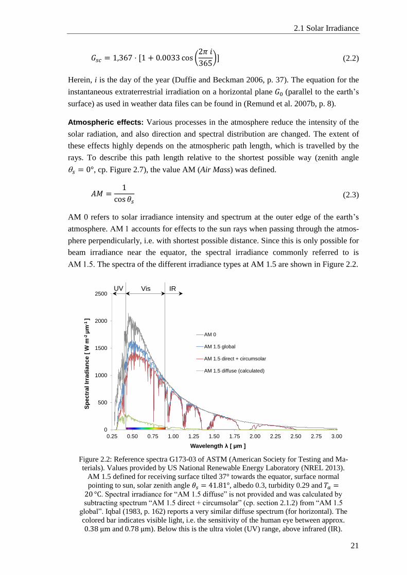
surface) as used in weather data files can be found in (Remund et al. 2007b, p. 8).
Atmospheric effects: Various processes in the atmosphere reduce the intensity of the
solar radiation, and also direction and spectral distribution are changed. The extent of
these effects highly depends on the atmospheric path length, which is travelled by the
rays. To describe this path length relative to the shortest possible way (zenith angle
𝑠 = 0°, cp. Figure 2.7), the value AM (Air Mass) was defined.
𝐴𝑀 =1
cos 𝜃𝑠 ( 2.3 )
AM 0 refers to solar irradiance intensity and spectrum at the outer edge of the earth’s
atmosphere. AM 1 accounts for effects to the sun rays when passing through the atmos-
phere perpendicularly, i.e. with shortest possible distance. Since this is only possible for
beam irradiance near the equator, the spectral irradiance commonly referred to is
AM 1.5. The spectra of the different irradiance types at AM 1.5 are shown in Figure 2.2.
Figure 2.2: Reference spectra G173-03 of ASTM (American Society for Testing and Ma-
terials). Values provided by US National Renewable Energy Laboratory (NREL 2013).
AM 1.5 defined for receiving surface tilted 37° towards the equator, surface normal
pointing to sun, solar zenith angle 𝜃𝑠 = 41.81°, albedo 0.3, turbidity 0.29 and 𝑇𝑎 =20 °C. Spectral irradiance for “AM 1.5 diffuse” is not provided and was calculated by
subtracting spectrum “AM 1.5 direct + circumsolar” (cp. section 2.1.2) from “AM 1.5
global”. Iqbal (1983, p. 162) reports a very similar diffuse spectrum (for horizontal). The
colored bar indicates visible light, i.e. the sensitivity of the human eye between approx.
0.38 μm and 0.78 μm). Below this is the ultra violet (UV) range, above infrared (IR).
0
500
1000
1500
2000
2500
0.25 0.50 0.75 1.00 1.25 1.50 1.75 2.00 2.25 2.50 2.75 3.00
Sp
ec
tra
l Ir
rad
ian
ce
[ W
m-2μm
-1 ]
Wavelength λ [ µm ]
AM 0
AM 1.5 global
AM 1.5 direct + circumsolar
AM 1.5 diffuse (calculated)
UV Vis IR
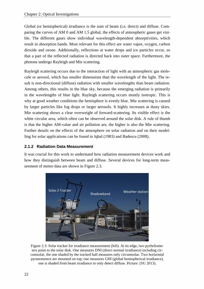
Chapter 2: Optical Investigations
22
Global (or hemispherical) irradiance is the sum of beam (i.e. direct) and diffuse. Com-
paring the curves of AM 0 and AM 1.5 global, the effects of atmospheric gases get visi-
ble. The different gases show individual wavelength-dependent absorptivities, which
result in absorption bands. Most relevant for this effect are water vapor, oxygen, carbon
dioxide and ozone. Additionally, reflections at water drops and ice particles occur, so
that a part of the reflected radiation is directed back into outer space. Furthermore, the
photons undergo Rayleigh and Mie scattering.
Rayleigh scattering occurs due to the interaction of light with an atmospheric gas mole-
cule or aerosol, which has smaller dimensions than the wavelength of the light. The re-
sult is non-directional (diffuse) radiation with smaller wavelengths than beam radiation.
Among others, this results in the blue sky, because the emerging radiation is primarily
in the wavelengths of blue light. Rayleigh scattering occurs mostly isotropic. This is
why at good weather conditions the hemisphere is evenly blue. Mie scattering is caused
by larger particles like fog drops or larger aerosols. It highly increases at dusty skies.
Mie scattering shows a clear overweight of forward-scattering. Its visible effect is the
white circular area, which often can be observed around the solar disk. A rule of thumb
is that the higher AM-value and air pollution are, the higher is also the Mie scattering.
Further details on the effects of the atmosphere on solar radiation and on their model-
ling for solar applications can be found in Iqbal (1983) and Badescu (2008).
2.1.2 Radiation Data Measurement
It was crucial for this work to understand how radiation measurement devices work and
how they distinguish between beam and diffuse. Several devices for long-term meas-
urement of meteo data are shown in Figure 2.3.
Figure 2.3: Solar tracker for irradiance measurement (left). At its edge, two pyrheliome-
ters point to the solar disk. One measures DNI (direct normal irradiance) including cir-
cumsolar, the one shaded by the tracked ball measures only circumsolar. Two horizontal
pyranometers are mounted on top; one measures GHI (global hemispherical irradiance),
one is shaded from beam irradiance to only detect diffuse. Picture: (SU 2013).
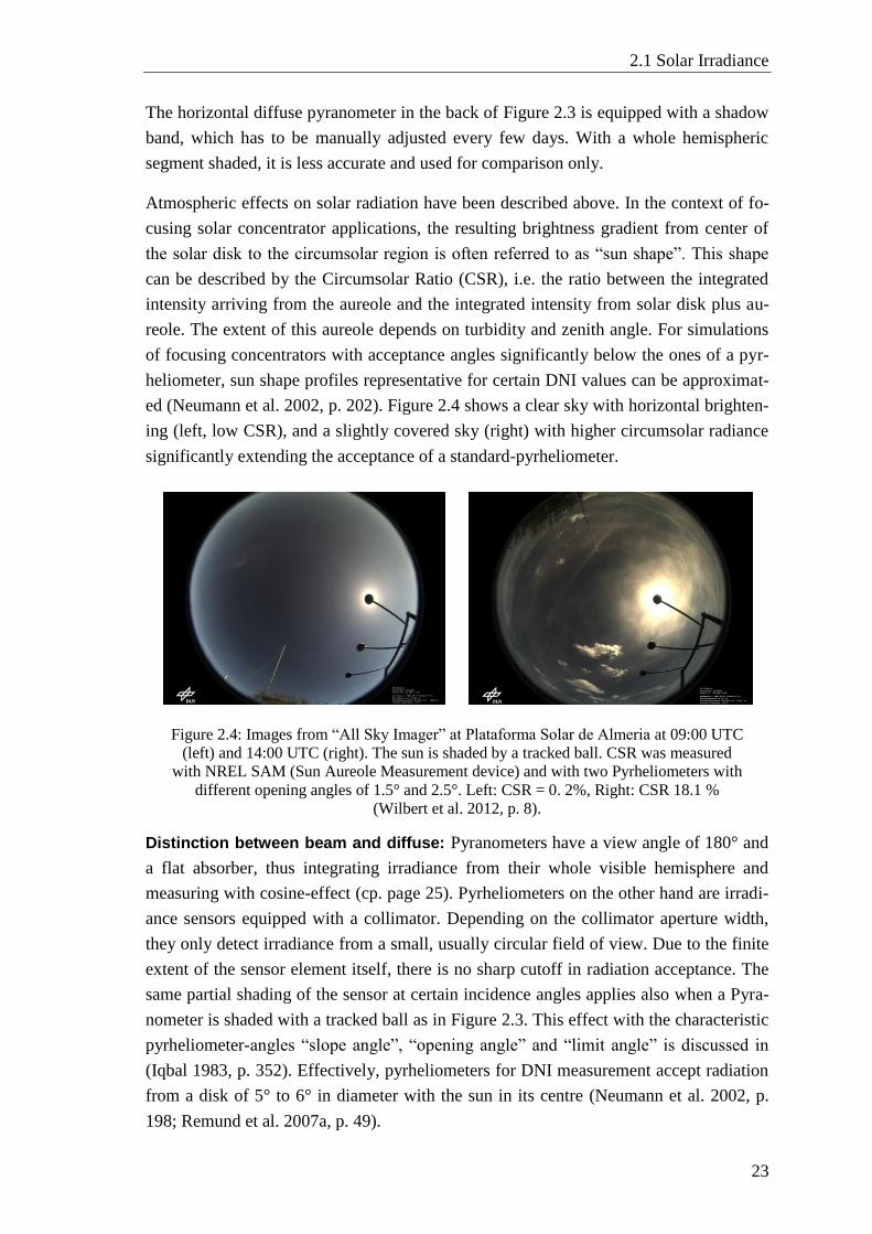
2.1 Solar Irradiance
23
The horizontal diffuse pyranometer in the back of Figure 2.3 is equipped with a shadow
band, which has to be manually adjusted every few days. With a whole hemispheric
segment shaded, it is less accurate and used for comparison only.
Atmospheric effects on solar radiation have been described above. In the context of fo-
cusing solar concentrator applications, the resulting brightness gradient from center of
the solar disk to the circumsolar region is often referred to as “sun shape”. This shape
can be described by the Circumsolar Ratio (CSR), i.e. the ratio between the integrated
intensity arriving from the aureole and the integrated intensity from solar disk plus au-
reole. The extent of this aureole depends on turbidity and zenith angle. For simulations
of focusing concentrators with acceptance angles significantly below the ones of a pyr-
heliometer, sun shape profiles representative for certain DNI values can be approximat-
ed (Neumann et al. 2002, p. 202). Figure 2.4 shows a clear sky with horizontal brighten-
ing (left, low CSR), and a slightly covered sky (right) with higher circumsolar radiance
significantly extending the acceptance of a standard-pyrheliometer.
Figure 2.4: Images from “All Sky Imager” at Plataforma Solar de Almeria at 09:00 UTC
(left) and 14:00 UTC (right). The sun is shaded by a tracked ball. CSR was measured
with NREL SAM (Sun Aureole Measurement device) and with two Pyrheliometers with
different opening angles of 1.5° and 2.5°. Left: CSR = 0. 2%, Right: CSR 18.1 %
(Wilbert et al. 2012, p. 8).
Distinction between beam and diffuse: Pyranometers have a view angle of 180° and
a flat absorber, thus integrating irradiance from their whole visible hemisphere and
measuring with cosine-effect (cp. page 25). Pyrheliometers on the other hand are irradi-
ance sensors equipped with a collimator. Depending on the collimator aperture width,
they only detect irradiance from a small, usually circular field of view. Due to the finite
extent of the sensor element itself, there is no sharp cutoff in radiation acceptance. The
same partial shading of the sensor at certain incidence angles applies also when a Pyra-
nometer is shaded with a tracked ball as in Figure 2.3. This effect with the characteristic
pyrheliometer-angles “slope angle”, “opening angle” and “limit angle” is discussed in
(Iqbal 1983, p. 352). Effectively, pyrheliometers for DNI measurement accept radiation
from a disk of 5° to 6° in diameter with the sun in its centre (Neumann et al. 2002, p.
198; Remund et al. 2007a, p. 49).
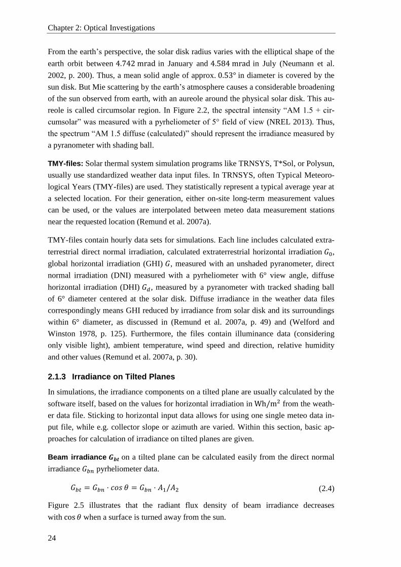
Chapter 2: Optical Investigations
24
From the earth’s perspective, the solar disk radius varies with the elliptical shape of the
earth orbit between 4.742 mrad in January and 4.584 mrad in July (Neumann et al.
2002, p. 200). Thus, a mean solid angle of approx. 0.53° in diameter is covered by the
sun disk. But Mie scattering by the earth’s atmosphere causes a considerable broadening
of the sun observed from earth, with an aureole around the physical solar disk. This au-
reole is called circumsolar region. In Figure 2.2, the spectral intensity “AM 1.5 + cir-
cumsolar” was measured with a pyrheliometer of 5° field of view (NREL 2013). Thus,
the spectrum “AM 1.5 diffuse (calculated)” should represent the irradiance measured by
a pyranometer with shading ball.
TMY-files: Solar thermal system simulation programs like TRNSYS, T*Sol, or Polysun,
usually use standardized weather data input files. In TRNSYS, often Typical Meteoro-
logical Years (TMY-files) are used. They statistically represent a typical average year at
a selected location. For their generation, either on-site long-term measurement values
can be used, or the values are interpolated between meteo data measurement stations
near the requested location (Remund et al. 2007a).
TMY-files contain hourly data sets for simulations. Each line includes calculated extra-
terrestrial direct normal irradiation, calculated extraterrestrial horizontal irradiation 𝐺0,
global horizontal irradiation (GHI) 𝐺, measured with an unshaded pyranometer, direct
normal irradiation (DNI) measured with a pyrheliometer with 6° view angle, diffuse
horizontal irradiation (DHI) 𝐺𝑑, measured by a pyranometer with tracked shading ball
of 6° diameter centered at the solar disk. Diffuse irradiance in the weather data files
correspondingly means GHI reduced by irradiance from solar disk and its surroundings
within 6° diameter, as discussed in (Remund et al. 2007a, p. 49) and (Welford and
Winston 1978, p. 125). Furthermore, the files contain illuminance data (considering
only visible light), ambient temperature, wind speed and direction, relative humidity
and other values (Remund et al. 2007a, p. 30).
2.1.3 Irradiance on Tilted Planes
In simulations, the irradiance components on a tilted plane are usually calculated by the
software itself, based on the values for horizontal irradiation in Wh/m2 from the weath-
er data file. Sticking to horizontal input data allows for using one single meteo data in-
put file, while e.g. collector slope or azimuth are varied. Within this section, basic ap-
proaches for calculation of irradiance on tilted planes are given.
Beam irradiance 𝑮𝒃𝒕 on a tilted plane can be calculated easily from the direct normal
irradiance 𝐺𝑏𝑛 pyrheliometer data.
𝐺𝑏𝑡 = 𝐺𝑏𝑛 ⋅ 𝑐𝑜𝑠 𝜃 = 𝐺𝑏𝑛 ⋅ 𝐴1/𝐴2 ( 2.4 )
Figure 2.5 illustrates that the radiant flux density of beam irradiance decreases
with cos 𝜃 when a surface is turned away from the sun.
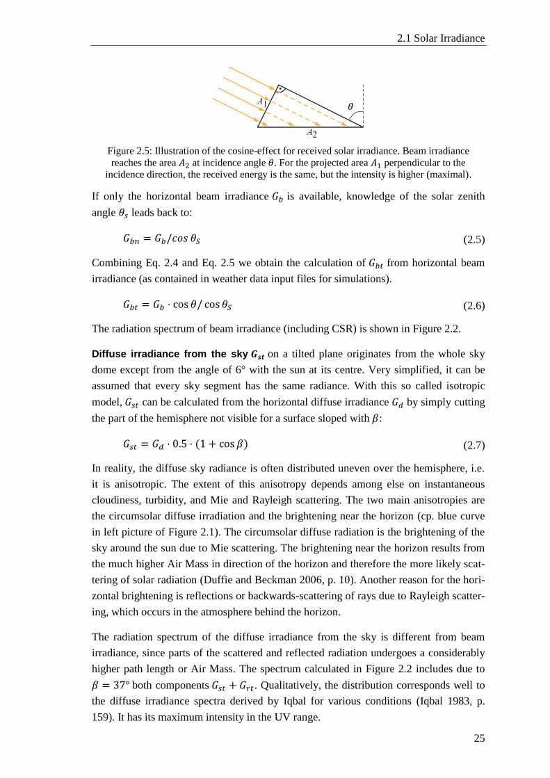
2.1 Solar Irradiance
25
Figure 2.5: Illustration of the cosine-effect for received solar irradiance. Beam irradiance
reaches the area 𝐴2 at incidence angle 𝜃. For the projected area 𝐴1 perpendicular to the
incidence direction, the received energy is the same, but the intensity is higher (maximal).
If only the horizontal beam irradiance 𝐺𝑏 is available, knowledge of the solar zenith
angle 𝜃𝑠 leads back to:
𝐺𝑏𝑛 = 𝐺𝑏/𝑐𝑜𝑠 𝜃𝑆 ( 2.5 )
Combining Eq. 2.4 and Eq. 2.5 we obtain the calculation of 𝐺𝑏𝑡 from horizontal beam
irradiance (as contained in weather data input files for simulations).
𝐺𝑏𝑡 = 𝐺𝑏 ⋅ cos 𝜃/ cos 𝜃𝑆 ( 2.6 )
The radiation spectrum of beam irradiance (including CSR) is shown in Figure 2.2.
Diffuse irradiance from the sky 𝑮𝒔𝒕 on a tilted plane originates from the whole sky
dome except from the angle of 6° with the sun at its centre. Very simplified, it can be
assumed that every sky segment has the same radiance. With this so called isotropic
model, 𝐺𝑠𝑡 can be calculated from the horizontal diffuse irradiance 𝐺𝑑 by simply cutting
the part of the hemisphere not visible for a surface sloped with 𝛽:
𝐺𝑠𝑡 = 𝐺𝑑 ⋅ 0.5 ⋅ (1 + cos 𝛽) ( 2.7 )
In reality, the diffuse sky radiance is often distributed uneven over the hemisphere, i.e.
it is anisotropic. The extent of this anisotropy depends among else on instantaneous
cloudiness, turbidity, and Mie and Rayleigh scattering. The two main anisotropies are
the circumsolar diffuse irradiation and the brightening near the horizon (cp. blue curve
in left picture of Figure 2.1). The circumsolar diffuse radiation is the brightening of the
sky around the sun due to Mie scattering. The brightening near the horizon results from
the much higher Air Mass in direction of the horizon and therefore the more likely scat-
tering of solar radiation (Duffie and Beckman 2006, p. 10). Another reason for the hori-
zontal brightening is reflections or backwards-scattering of rays due to Rayleigh scatter-
ing, which occurs in the atmosphere behind the horizon.
The radiation spectrum of the diffuse irradiance from the sky is different from beam
irradiance, since parts of the scattered and reflected radiation undergoes a considerably
higher path length or Air Mass. The spectrum calculated in Figure 2.2 includes due to
𝛽 = 37° both components 𝐺𝑠𝑡 + 𝐺𝑟𝑡. Qualitatively, the distribution corresponds well to
the diffuse irradiance spectra derived by Iqbal for various conditions (Iqbal 1983, p.
159). It has its maximum intensity in the UV range.
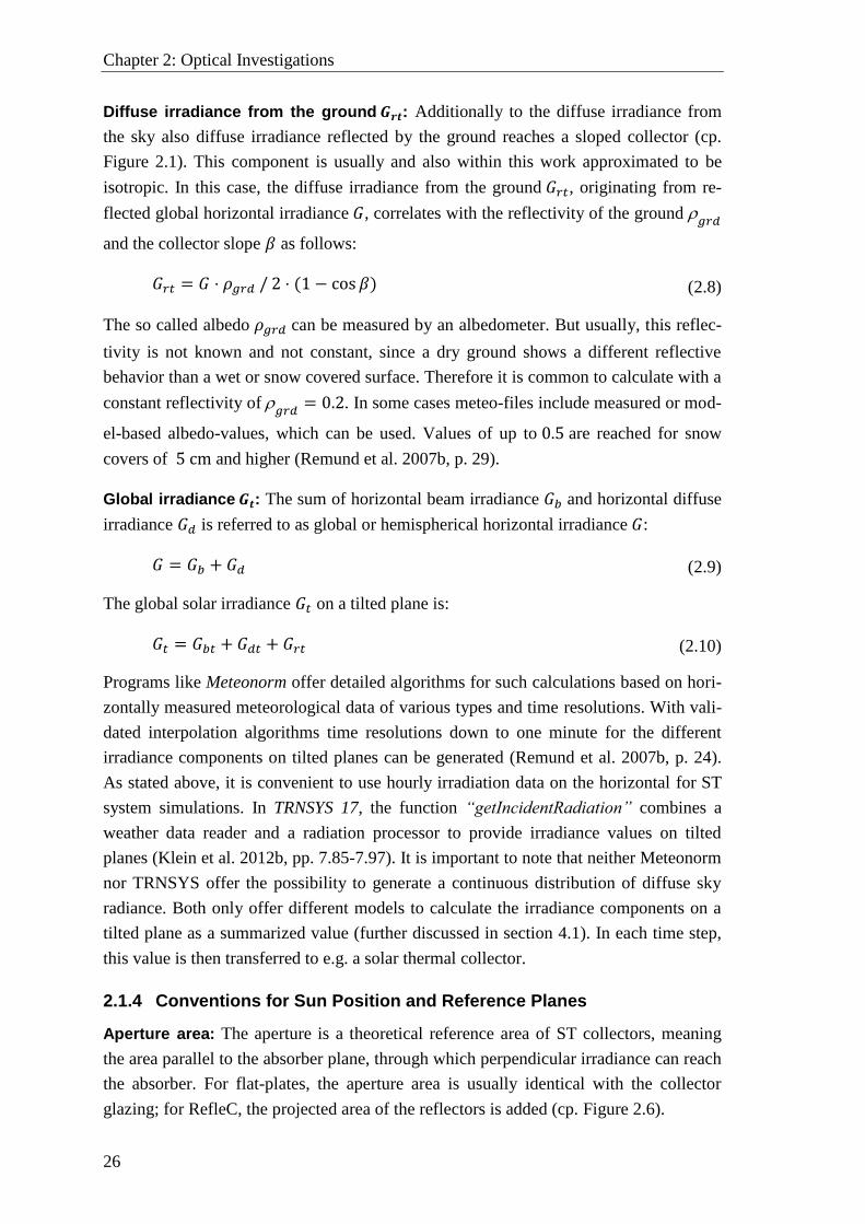
Chapter 2: Optical Investigations
26
Diffuse irradiance from the ground 𝑮𝒓𝒕: Additionally to the diffuse irradiance from
the sky also diffuse irradiance reflected by the ground reaches a sloped collector (cp.
Figure 2.1). This component is usually and also within this work approximated to be
isotropic. In this case, the diffuse irradiance from the ground 𝐺𝑟𝑡, originating from re-
flected global horizontal irradiance 𝐺, correlates with the reflectivity of the ground 𝑔𝑟𝑑
and the collector slope 𝛽 as follows:
𝐺𝑟𝑡 = 𝐺 ⋅ 𝜌𝑔𝑟𝑑 / 2 ⋅ (1 − cos 𝛽) ( 2.8 )
The so called albedo 𝜌𝑔𝑟𝑑 can be measured by an albedometer. But usually, this reflec-
tivity is not known and not constant, since a dry ground shows a different reflective
behavior than a wet or snow covered surface. Therefore it is common to calculate with a
constant reflectivity of 𝑔𝑟𝑑
= 0.2. In some cases meteo-files include measured or mod-
el-based albedo-values, which can be used. Values of up to 0.5 are reached for snow
covers of 5 cm and higher (Remund et al. 2007b, p. 29).
Global irradiance 𝑮𝒕: The sum of horizontal beam irradiance 𝐺𝑏 and horizontal diffuse
irradiance 𝐺𝑑 is referred to as global or hemispherical horizontal irradiance 𝐺:
𝐺 = 𝐺𝑏 + 𝐺𝑑 ( 2.9 )
The global solar irradiance 𝐺𝑡 on a tilted plane is:
𝐺𝑡 = 𝐺𝑏𝑡 + 𝐺𝑑𝑡 + 𝐺𝑟𝑡 ( 2.10 )
Programs like Meteonorm offer detailed algorithms for such calculations based on hori-
zontally measured meteorological data of various types and time resolutions. With vali-
dated interpolation algorithms time resolutions down to one minute for the different
irradiance components on tilted planes can be generated (Remund et al. 2007b, p. 24).
As stated above, it is convenient to use hourly irradiation data on the horizontal for ST
system simulations. In TRNSYS 17, the function “getIncidentRadiation” combines a
weather data reader and a radiation processor to provide irradiance values on tilted
planes (Klein et al. 2012b, pp. 7.85-7.97). It is important to note that neither Meteonorm
nor TRNSYS offer the possibility to generate a continuous distribution of diffuse sky
radiance. Both only offer different models to calculate the irradiance components on a
tilted plane as a summarized value (further discussed in section 4.1). In each time step,
this value is then transferred to e.g. a solar thermal collector.
2.1.4 Conventions for Sun Position and Reference Planes
Aperture area: The aperture is a theoretical reference area of ST collectors, meaning
the area parallel to the absorber plane, through which perpendicular irradiance can reach
the absorber. For flat-plates, the aperture area is usually identical with the collector
glazing; for RefleC, the projected area of the reflectors is added (cp. Figure 2.6).
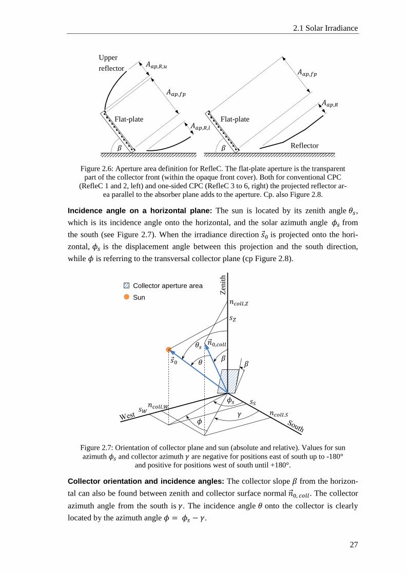
2.1 Solar Irradiance
27
Figure 2.6: Aperture area definition for RefleC. The flat-plate aperture is the transparent
part of the collector front (within the opaque front cover). Both for conventional CPC
(RefleC 1 and 2, left) and one-sided CPC (RefleC 3 to 6, right) the projected reflector ar-
ea parallel to the absorber plane adds to the aperture. Cp. also Figure 2.8.
Incidence angle on a horizontal plane: The sun is located by its zenith angle 𝜃𝑠 ,
which is its incidence angle onto the horizontal, and the solar azimuth angle 𝜙𝑠 from
the south (see Figure 2.7). When the irradiance direction 𝑠 0 is projected onto the hori-
zontal, 𝜙𝑠 is the displacement angle between this projection and the south direction,
while 𝜙 is referring to the transversal collector plane (cp Figure 2.8).
Figure 2.7: Orientation of collector plane and sun (absolute and relative). Values for sun
azimuth 𝜙𝑠 and collector azimuth 𝛾 are negative for positions east of south up to -180°
and positive for positions west of south until +180°.
Collector orientation and incidence angles: The collector slope 𝛽 from the horizon-
tal can also be found between zenith and collector surface normal �⃗� 0, 𝑐𝑜𝑙𝑙. The collector
azimuth angle from the south is 𝛾. The incidence angle 𝜃 onto the collector is clearly
located by the azimuth angle 𝜙 = 𝜙𝑠 − 𝛾.
𝜃
𝜃𝑠
Zen
ith
𝛽
𝑠𝑍
𝑛𝑐𝑜𝑙𝑙,𝑍
𝑛𝑐𝑜𝑙𝑙,𝑆 𝑛𝑐𝑜𝑙𝑙,𝑊
𝑠𝑊 𝑠𝑆
�⃗� 0,𝑐𝑜𝑙𝑙
𝑠 0
𝛾 𝜙
𝜙𝑠
Collector aperture area
Sun
𝛽
𝛽 𝛽
Flat-plate Flat-plate
Upper
reflector
Reflector
𝐴𝑎𝑝,𝑅,𝑢
𝐴𝑎𝑝,𝑅,𝑙
𝐴𝑎𝑝,𝑓𝑝
𝐴𝑎𝑝,𝑓𝑝
𝐴𝑎𝑝,𝑅
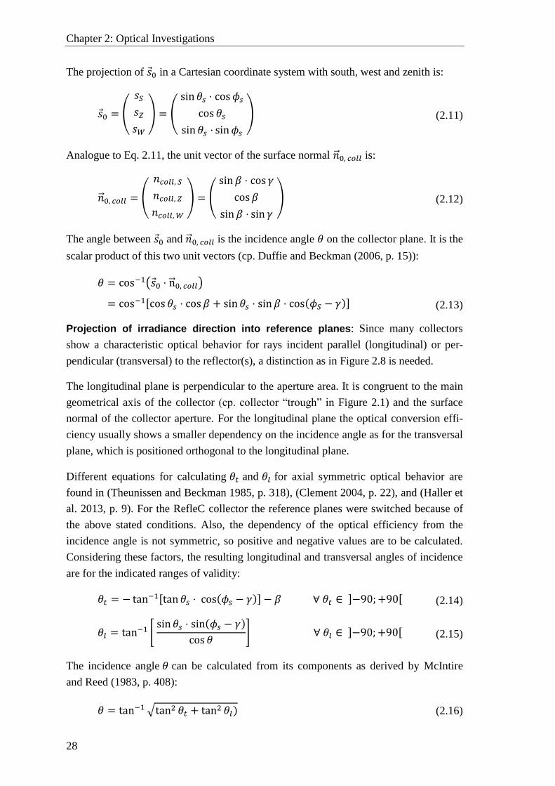
Chapter 2: Optical Investigations
28
The projection of 𝑠 0 in a Cartesian coordinate system with south, west and zenith is:
𝑠 0 = (
𝑠𝑆
𝑠𝑍
𝑠𝑊
) = (
sin 𝜃𝑠 ⋅ cos 𝜙𝑠
cos 𝜃𝑠
sin 𝜃𝑠 ⋅ sin𝜙𝑠
) ( 2.11 )
Analogue to Eq. 2.11, the unit vector of the surface normal �⃗� 0, 𝑐𝑜𝑙𝑙 is:
�⃗� 0, 𝑐𝑜𝑙𝑙 = (
𝑛𝑐𝑜𝑙𝑙, 𝑆
𝑛𝑐𝑜𝑙𝑙, 𝑍
𝑛𝑐𝑜𝑙𝑙, 𝑊
) = (
sin 𝛽 ⋅ cos 𝛾
cos𝛽
sin 𝛽 ⋅ sin 𝛾
) ( 2.12 )
The angle between 𝑠 0 and �⃗� 0, 𝑐𝑜𝑙𝑙 is the incidence angle 𝜃 on the collector plane. It is the
scalar product of this two unit vectors (cp. Duffie and Beckman (2006, p. 15)):
𝜃 = cos−1(𝑠 0 ⋅ n⃗ 0, 𝑐𝑜𝑙𝑙)
= cos−1[cos 𝜃𝑠 ⋅ cos 𝛽 + sin 𝜃𝑠 ⋅ sin 𝛽 ⋅ cos(𝜙𝑆 − 𝛾)]
(
2.13
)
Projection of irradiance direction into reference planes: Since many collectors
show a characteristic optical behavior for rays incident parallel (longitudinal) or per-
pendicular (transversal) to the reflector(s), a distinction as in Figure 2.8 is needed.
The longitudinal plane is perpendicular to the aperture area. It is congruent to the main
geometrical axis of the collector (cp. collector “trough” in Figure 2.1) and the surface
normal of the collector aperture. For the longitudinal plane the optical conversion effi-
ciency usually shows a smaller dependency on the incidence angle as for the transversal
plane, which is positioned orthogonal to the longitudinal plane.
Different equations for calculating 𝜃𝑡 and 𝜃𝑙 for axial symmetric optical behavior are
found in (Theunissen and Beckman 1985, p. 318), (Clement 2004, p. 22), and (Haller et
al. 2013, p. 9). For the RefleC collector the reference planes were switched because of
the above stated conditions. Also, the dependency of the optical efficiency from the
incidence angle is not symmetric, so positive and negative values are to be calculated.
Considering these factors, the resulting longitudinal and transversal angles of incidence
are for the indicated ranges of validity:
𝜃𝑡 = − tan−1[tan 𝜃𝑠 ⋅ cos(𝜙𝑠 − 𝛾)] − 𝛽 ∀ 𝜃𝑡 ∈ ]−90;+90[ ( 2.14 )
𝜃𝑙 = tan−1 [ sin 𝜃𝑠 ⋅ sin(𝜙𝑠 − 𝛾)
cos 𝜃] ∀ 𝜃𝑙 ∈ ]−90;+90[ ( 2.15 )
The incidence angle 𝜃 can be calculated from its components as derived by McIntire
and Reed (1983, p. 408):
𝜃 = tan−1 √tan2 𝜃𝑡 + tan2 𝜃𝑙) ( 2.16 )
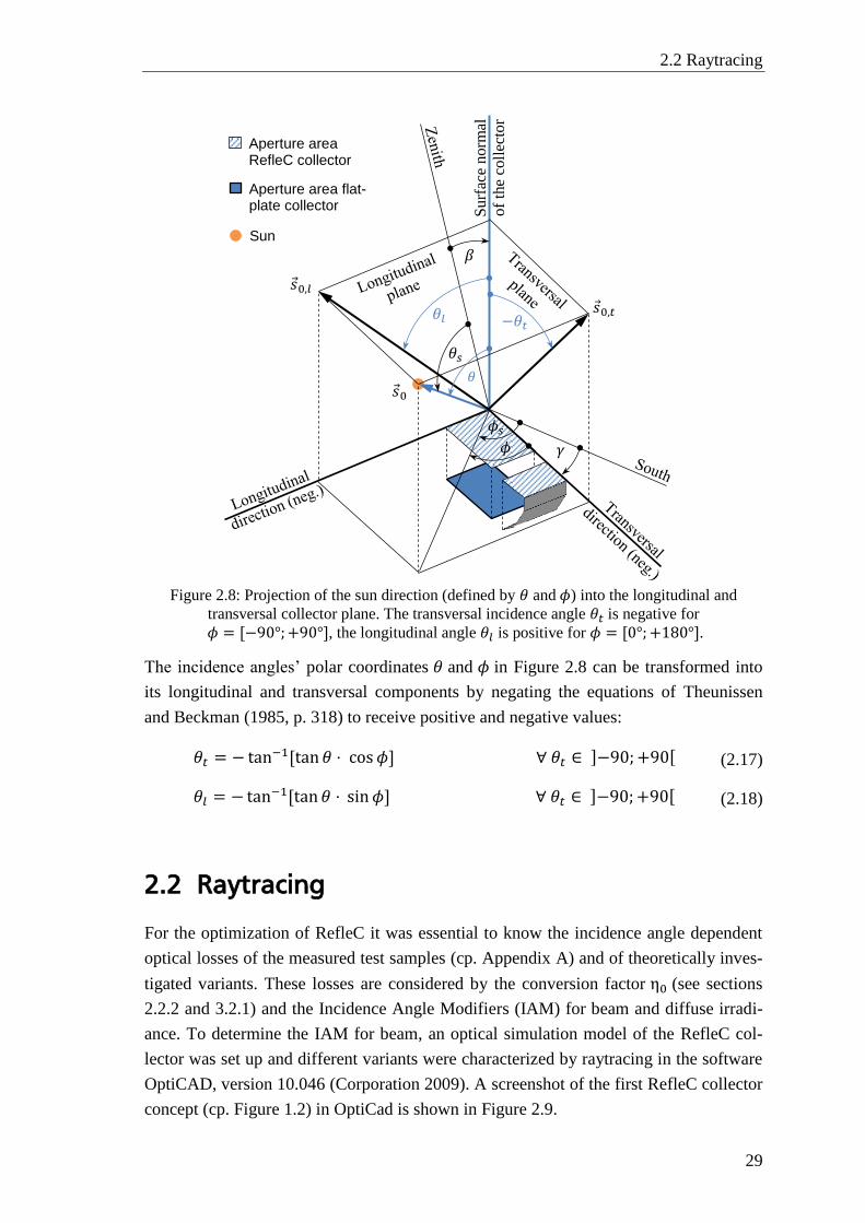
2.2 Raytracing
29
Figure 2.8: Projection of the sun direction (defined by 𝜃 and 𝜙) into the longitudinal and
transversal collector plane. The transversal incidence angle 𝜃𝑡 is negative for
𝜙 = [−90°;+90°], the longitudinal angle 𝜃𝑙 is positive for 𝜙 = [0°;+180°].
The incidence angles’ polar coordinates 𝜃 and 𝜙 in Figure 2.8 can be transformed into
its longitudinal and transversal components by negating the equations of Theunissen
and Beckman (1985, p. 318) to receive positive and negative values:
𝜃𝑡 = − tan−1[tan 𝜃 ⋅ cos 𝜙] ∀ 𝜃𝑡 ∈ ]−90;+90[ ( 2.17 )
𝜃𝑙 = − tan−1[tan 𝜃 ⋅ sin𝜙] ∀ 𝜃𝑡 ∈ ]−90;+90[ ( 2.18 )
2.2 Raytracing
For the optimization of RefleC it was essential to know the incidence angle dependent
optical losses of the measured test samples (cp. Appendix A) and of theoretically inves-
tigated variants. These losses are considered by the conversion factor η0 (see sections
2.2.2 and 3.2.1) and the Incidence Angle Modifiers (IAM) for beam and diffuse irradi-
ance. To determine the IAM for beam, an optical simulation model of the RefleC col-
lector was set up and different variants were characterized by raytracing in the software
OptiCAD, version 10.046 (Corporation 2009). A screenshot of the first RefleC collector
concept (cp. Figure 1.2) in OptiCad is shown in Figure 2.9.
Su
rfac
e n
orm
al
of
the
coll
ecto
r
𝛽
𝑠 0,𝑙
𝑠 0,𝑡
𝑠 0
𝜃𝑙
𝜃
−𝜃𝑡
𝛾
𝜙𝑠
Aperture area flat-plate collector
Aperture area RefleC collector
Sun
𝜃𝑠
𝜙
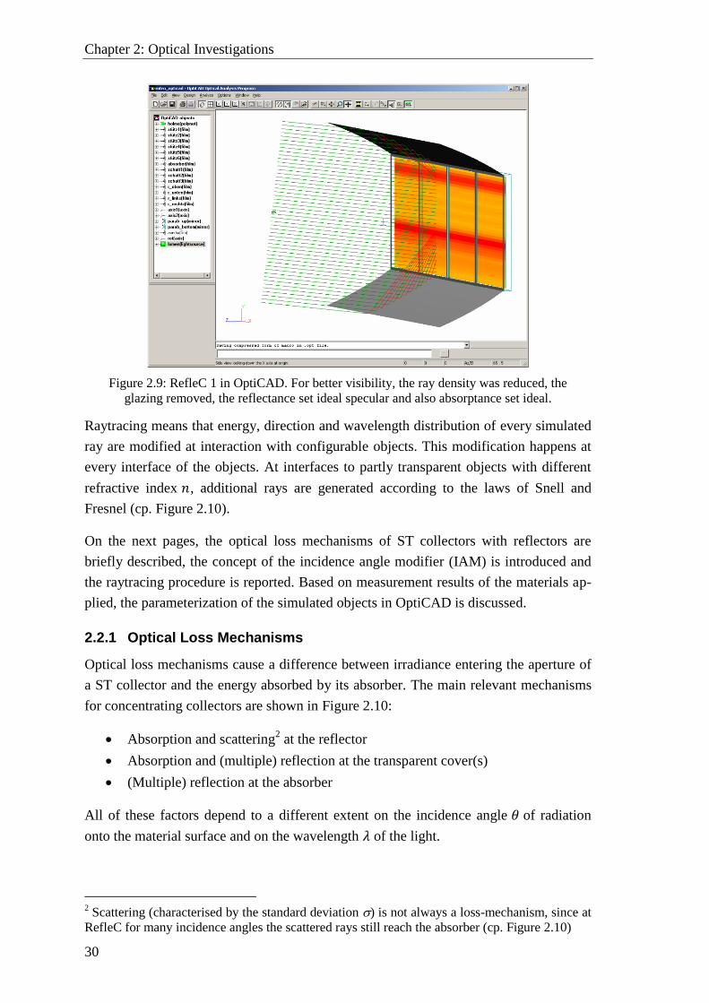
Chapter 2: Optical Investigations
30
Figure 2.9: RefleC 1 in OptiCAD. For better visibility, the ray density was reduced, the
glazing removed, the reflectance set ideal specular and also absorptance set ideal.
Raytracing means that energy, direction and wavelength distribution of every simulated
ray are modified at interaction with configurable objects. This modification happens at
every interface of the objects. At interfaces to partly transparent objects with different
refractive index 𝑛, additional rays are generated according to the laws of Snell and
Fresnel (cp. Figure 2.10).
On the next pages, the optical loss mechanisms of ST collectors with reflectors are
briefly described, the concept of the incidence angle modifier (IAM) is introduced and
the raytracing procedure is reported. Based on measurement results of the materials ap-
plied, the parameterization of the simulated objects in OptiCAD is discussed.
2.2.1 Optical Loss Mechanisms
Optical loss mechanisms cause a difference between irradiance entering the aperture of
a ST collector and the energy absorbed by its absorber. The main relevant mechanisms
for concentrating collectors are shown in Figure 2.10:
Absorption and scattering2 at the reflector
Absorption and (multiple) reflection at the transparent cover(s)
(Multiple) reflection at the absorber
All of these factors depend to a different extent on the incidence angle 𝜃 of radiation
onto the material surface and on the wavelength 𝜆 of the light.
2 Scattering (characterised by the standard deviation ) is not always a loss-mechanism, since at
RefleC for many incidence angles the scattered rays still reach the absorber (cp. Figure 2.10)
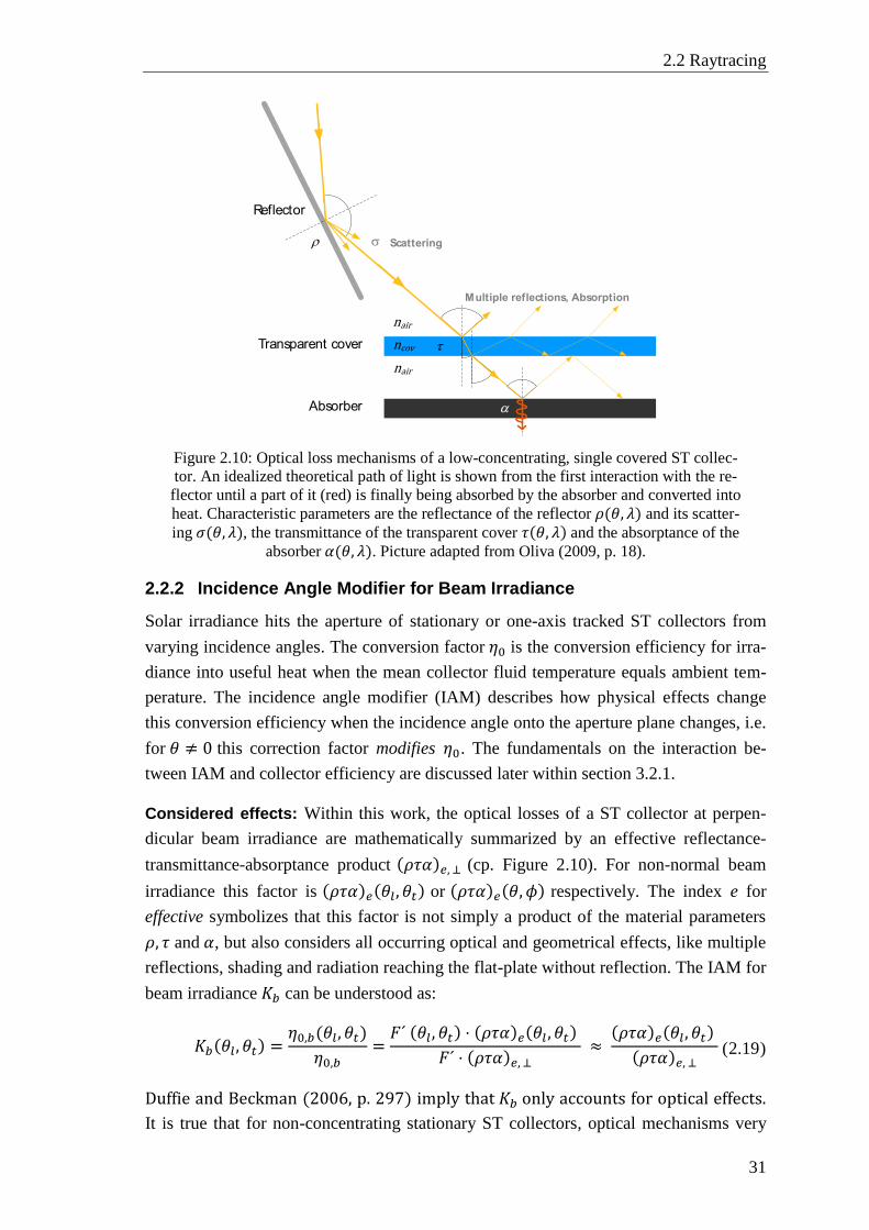
2.2 Raytracing
31
Figure 2.10: Optical loss mechanisms of a low-concentrating, single covered ST collec-
tor. An idealized theoretical path of light is shown from the first interaction with the re-
flector until a part of it (red) is finally being absorbed by the absorber and converted into
heat. Characteristic parameters are the reflectance of the reflector 𝜌(𝜃, 𝜆) and its scatter-
ing 𝜎(𝜃, 𝜆), the transmittance of the transparent cover 𝜏(𝜃, 𝜆) and the absorptance of the
absorber 𝛼(𝜃, 𝜆). Picture adapted from Oliva (2009, p. 18).
2.2.2 Incidence Angle Modifier for Beam Irradiance
Solar irradiance hits the aperture of stationary or one-axis tracked ST collectors from
varying incidence angles. The conversion factor 𝜂0 is the conversion efficiency for irra-
diance into useful heat when the mean collector fluid temperature equals ambient tem-
perature. The incidence angle modifier (IAM) describes how physical effects change
this conversion efficiency when the incidence angle onto the aperture plane changes, i.e.
for 𝜃 ≠ 0 this correction factor modifies 𝜂0. The fundamentals on the interaction be-
tween IAM and collector efficiency are discussed later within section 3.2.1.
Considered effects: Within this work, the optical losses of a ST collector at perpen-
dicular beam irradiance are mathematically summarized by an effective reflectance-
transmittance-absorptance product (𝜌𝜏𝛼)𝑒, ⊥ (cp. Figure 2.10). For non-normal beam
irradiance this factor is (𝜌𝜏𝛼)𝑒(𝜃𝑙, 𝜃𝑡) or (𝜌𝜏𝛼)𝑒(𝜃, 𝜙) respectively. The index e for
effective symbolizes that this factor is not simply a product of the material parameters
𝜌, 𝜏 and 𝛼, but also considers all occurring optical and geometrical effects, like multiple
reflections, shading and radiation reaching the flat-plate without reflection. The IAM for
beam irradiance 𝐾𝑏 can be understood as:
𝐾𝑏(𝜃𝑙, 𝜃𝑡) =𝜂0,𝑏(𝜃𝑙, 𝜃𝑡)
𝜂0,𝑏=
𝐹´ (𝜃𝑙, 𝜃𝑡) ⋅ (𝜌𝜏𝛼)𝑒(𝜃𝑙 , 𝜃𝑡)
𝐹´ ⋅ (𝜌𝜏𝛼)𝑒, ⊥ ≈
(𝜌𝜏𝛼)𝑒(𝜃𝑙, 𝜃𝑡)
(𝜌𝜏𝛼)𝑒, ⊥ ( 2.19 )
Duffie and Beckman (2006, p. 297) imply that 𝐾𝑏 only accounts for optical effects.
It is true that for non-concentrating stationary ST collectors, optical mechanisms very
nair
nair
ncov
Reflector
Transparent cover
Absorber
Multiple reflections, Absorption
Scattering
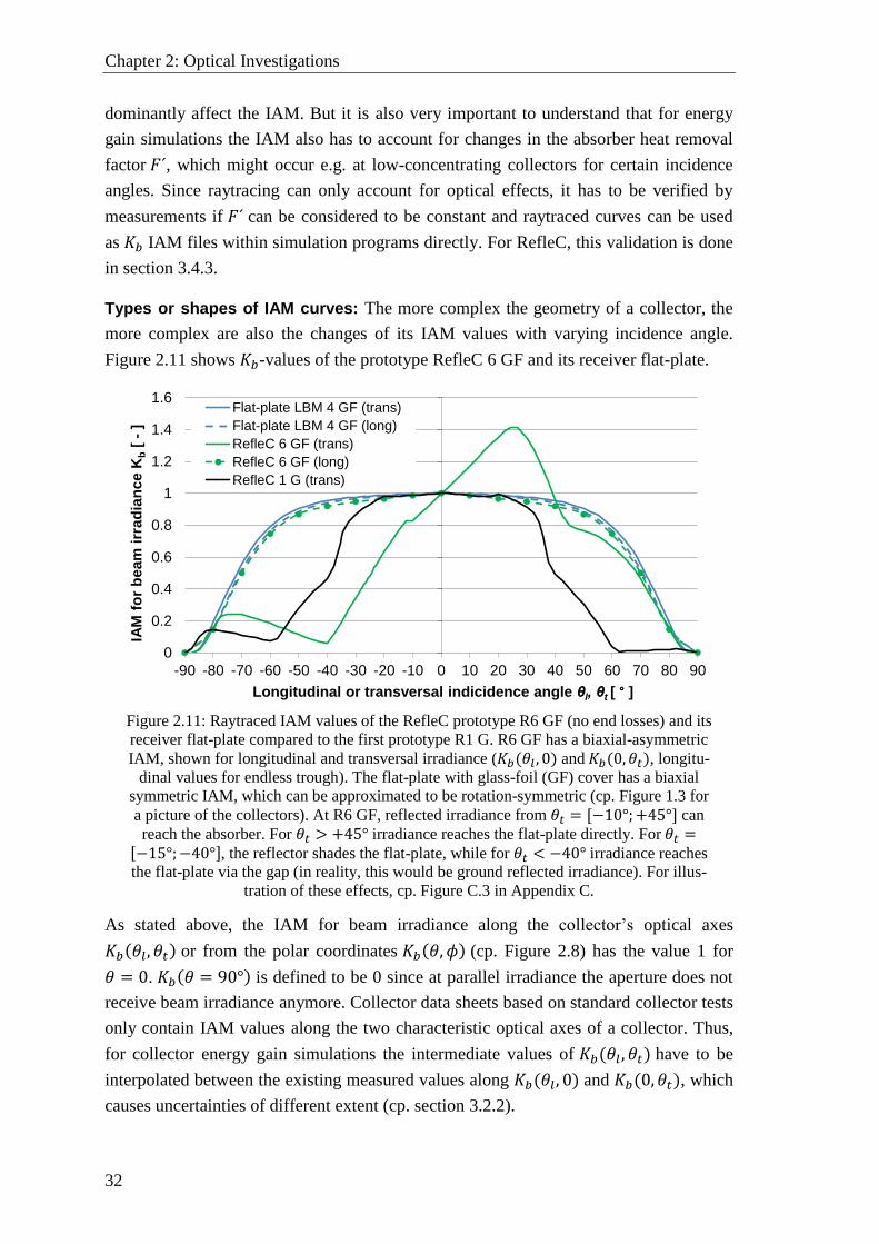
Chapter 2: Optical Investigations
32
dominantly affect the IAM. But it is also very important to understand that for energy
gain simulations the IAM also has to account for changes in the absorber heat removal
factor 𝐹´, which might occur e.g. at low-concentrating collectors for certain incidence
angles. Since raytracing can only account for optical effects, it has to be verified by
measurements if 𝐹´ can be considered to be constant and raytraced curves can be used
as 𝐾𝑏 IAM files within simulation programs directly. For RefleC, this validation is done
in section 3.4.3.
Types or shapes of IAM curves: The more complex the geometry of a collector, the
more complex are also the changes of its IAM values with varying incidence angle.
Figure 2.11 shows 𝐾𝑏-values of the prototype RefleC 6 GF and its receiver flat-plate.
Figure 2.11: Raytraced IAM values of the RefleC prototype R6 GF (no end losses) and its
receiver flat-plate compared to the first prototype R1 G. R6 GF has a biaxial-asymmetric
IAM, shown for longitudinal and transversal irradiance (𝐾𝑏(𝜃𝑙 , 0) and 𝐾𝑏(0, 𝜃𝑡), longitu-
dinal values for endless trough). The flat-plate with glass-foil (GF) cover has a biaxial
symmetric IAM, which can be approximated to be rotation-symmetric (cp. Figure 1.3 for
a picture of the collectors). At R6 GF, reflected irradiance from 𝜃𝑡 = [−10°;+45°] can
reach the absorber. For 𝜃𝑡 > +45° irradiance reaches the flat-plate directly. For 𝜃𝑡 =[−15°;−40°], the reflector shades the flat-plate, while for 𝜃𝑡 < −40° irradiance reaches
the flat-plate via the gap (in reality, this would be ground reflected irradiance). For illus-
tration of these effects, cp. Figure C.3 in Appendix C.
As stated above, the IAM for beam irradiance along the collector’s optical axes
𝐾𝑏(𝜃𝑙, 𝜃𝑡) or from the polar coordinates 𝐾𝑏(𝜃, 𝜙) (cp. Figure 2.8) has the value 1 for
𝜃 = 0. 𝐾𝑏(𝜃 = 90°) is defined to be 0 since at parallel irradiance the aperture does not
receive beam irradiance anymore. Collector data sheets based on standard collector tests
only contain IAM values along the two characteristic optical axes of a collector. Thus,
for collector energy gain simulations the intermediate values of 𝐾𝑏(𝜃𝑙 , 𝜃𝑡) have to be
interpolated between the existing measured values along 𝐾𝑏(𝜃𝑙, 0) and 𝐾𝑏(0, 𝜃𝑡), which
causes uncertainties of different extent (cp. section 3.2.2).
0
0.2
0.4
0.6
0.8
1
1.2
1.4
1.6
-90 -80 -70 -60 -50 -40 -30 -20 -10 0 10 20 30 40 50 60 70 80 90
IAM
fo
r b
eam
irr
ad
ian
ce K
b[
-]
Longitudinal or transversal indicidence angle θl, θt [ ° ]
Flat-plate LBM 4 GF (trans)
Flat-plate LBM 4 GF (long)
RefleC 6 GF (trans)
RefleC 6 GF (long)
RefleC 1 G (trans)
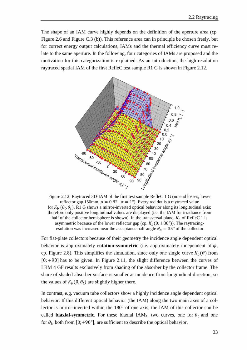
2.2 Raytracing
33
The shape of an IAM curve highly depends on the definition of the aperture area (cp.
Figure 2.6 and Figure C.3 (b)). This reference area can in principle be chosen freely, but
for correct energy output calculations, IAMs and the thermal efficiency curve must re-
late to the same aperture. In the following, four categories of IAMs are proposed and the
motivation for this categorization is explained. As an introduction, the high-resolution
raytraced spatial IAM of the first RefleC test sample R1 G is shown in Figure 2.12.
Figure 2.12: Raytraced 3D-IAM of the first test sample RefleC 1 G (no end losses, lower
reflector gap 150mm, 𝜌 = 0.82, 𝜎 = 1°). Every red dot is a raytraced value
for 𝐾𝑏 (𝜃𝑙 , 𝜃𝑡). R1 G shows a mirror-inverted optical behavior along its longitudinal axis;
therefore only positive longitudinal values are displayed (i.e. the IAM for irradiance from
half of the collector hemisphere is shown). In the transversal plane, 𝐾𝑏 of RefleC 1 is
asymmetric because of the lower reflector gap (cp. 𝐾𝑏(0;±80°)). The raytracing-
resolution was increased near the acceptance half-angle 𝜃𝑎 = 35° of the collector.
For flat-plate collectors because of their geometry the incidence angle dependent optical
behavior is approximately rotation-symmetric (i.e. approximately independent of 𝜙,
cp. Figure 2.8). This simplifies the simulation, since only one single curve 𝐾𝑏(𝜃) from
[0; +90] has to be given. In Figure 2.11, the slight difference between the curves of
LBM 4 GF results exclusively from shading of the absorber by the collector frame. The
share of shaded absorber surface is smaller at incidence from longitudinal direction, so
the values of 𝐾𝑏(0, 𝜃𝑙) are slightly higher there.
In contrast, e.g. vacuum tube collectors show a highly incidence angle dependent optical
behavior. If this different optical behavior (the IAM) along the two main axes of a col-
lector is mirror-inverted within the 180° of one axis, the IAM of this collector can be
called biaxial-symmetric. For these biaxial IAMs, two curves, one for 𝜃𝑡 and one
for 𝜃𝑙, both from [0;+90°], are sufficient to describe the optical behavior.
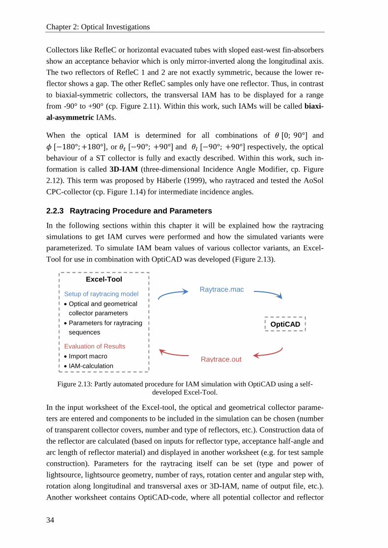
Chapter 2: Optical Investigations
34
Collectors like RefleC or horizontal evacuated tubes with sloped east-west fin-absorbers
show an acceptance behavior which is only mirror-inverted along the longitudinal axis.
The two reflectors of RefleC 1 and 2 are not exactly symmetric, because the lower re-
flector shows a gap. The other RefleC samples only have one reflector. Thus, in contrast
to biaxial-symmetric collectors, the transversal IAM has to be displayed for a range
from -90° to +90° (cp. Figure 2.11). Within this work, such IAMs will be called biaxi-
al-asymmetric IAMs.
When the optical IAM is determined for all combinations of 𝜃 [0; 90°] and
𝜙 [−180°;+180°], or 𝜃𝑡 [−90°; +90°] and 𝜃𝑙 [−90°; +90°] respectively, the optical
behaviour of a ST collector is fully and exactly described. Within this work, such in-
formation is called 3D-IAM (three-dimensional Incidence Angle Modifier, cp. Figure
2.12). This term was proposed by Häberle (1999), who raytraced and tested the AoSol
CPC-collector (cp. Figure 1.14) for intermediate incidence angles.
2.2.3 Raytracing Procedure and Parameters
In the following sections within this chapter it will be explained how the raytracing
simulations to get IAM curves were performed and how the simulated variants were
parameterized. To simulate IAM beam values of various collector variants, an Excel-
Tool for use in combination with OptiCAD was developed (Figure 2.13).
Figure 2.13: Partly automated procedure for IAM simulation with OptiCAD using a self-
developed Excel-Tool.
In the input worksheet of the Excel-tool, the optical and geometrical collector parame-
ters are entered and components to be included in the simulation can be chosen (number
of transparent collector covers, number and type of reflectors, etc.). Construction data of
the reflector are calculated (based on inputs for reflector type, acceptance half-angle and
arc length of reflector material) and displayed in another worksheet (e.g. for test sample
construction). Parameters for the raytracing itself can be set (type and power of
lightsource, lightsource geometry, number of rays, rotation center and angular step with,
rotation along longitudinal and transversal axes or 3D-IAM, name of output file, etc.).
Another worksheet contains OptiCAD-code, where all potential collector and reflector
Raytrace.out
Raytrace.mac
Excel-Tool
Setup of raytracing model
Optical and geometrical
collector parameters
Parameters for raytracing
sequences
Evaluation of Results
Import macro
IAM-calculation
OptiCAD
2.2 Raytracing
35
types with their parameters and also the specifications on the raytracing itself are in-
cluded. This worksheet is modified according to the information from the input-sheet,
where also the reflector geommetry is calculated. If for example no second transparent
cover and no upper reflector are to be simulated, the respective passages of the code are
commented out. The modified code is then manually exported as a macro, named e.g.
Raytrace.mac. This macro then runs in OptiCAD. Results for absorbed energy are
stored in one single output text file, e.g. Raytrace.out. This file can be imported into the
Excel-tool again, where IAM values for the simulated setup are calculated by compar-
ing the energy onto the aperture and that absorbed at all investigated incidence angles.
Due to this procedure it was ensured that RefleC parameters, construction data, raytrac-
ing-macro, simulation results and calculated IAM values were always consistent and
documented in one folder.
The geometrical dimensions of the collector variants were simulated 1:1 in OptiCAD.
The lightsource used in the simulation consisted of ideal parallel rays. The ray density
of the lightsource was usually 1/mm at perpendicular irradiance onto the aperture area.
The lightsource was then rotated to simulate different incidence angles on the aperture.
The IAM of stationary collectors must not account for cosine-losses3, so the ray density
was increased by cos 𝜃 already in the input macro. Its absolute power and number of
rays was not changed. This way, the IAM for beam irradiance can be calculated directly
from the raytracing results by dividing the absorbed power at a certain incidence angle
by the absorbed power at perpendicular irradiance. To determine the transversal IAMs
of an investigated variant, it was enough to simulate one row of ideal parallel rays as
shown in Figure 2.9. For IAM simulations with a longitudinal component (and thus for
all 3D-IAM) a rectangular lightsource was used to accurately account for end losses and
optical effects that only a part of the rays undergo.
The main reasons for the application of raytracing in this work are:
Complexity of optical effects
Scattering by reflectors, various incidence angles onto a receiver after reflec-
tion, transmission of scattered rays through multiple covers and the polarization
of light are very difficult to determine analytically.
IAM for pure beam irradiance
The IAM for pure beam irradiance can be determined, which is not possible by
measurements, since in reality always a part of irradiance is diffuse.
High resolution
IAM values for a higher number of incidence angles than via measurements can
be generated, which improves the accuracy (cp. high resolution 3D-IAM).
3 This effect is a decrease of ray density incident on a receiver surface by cos 𝜃, cp. Figure 2.5.
It must not be included in the IAM, because the measured irradiance 𝐺𝑡 already accounts for it.
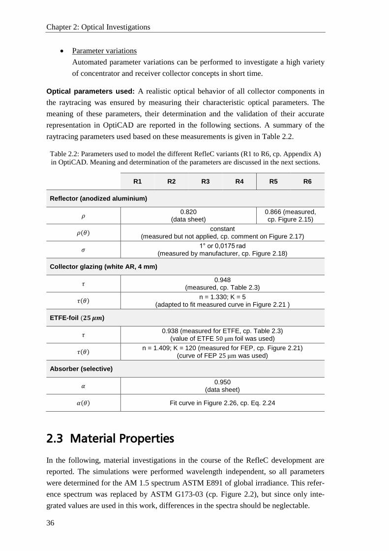
Chapter 2: Optical Investigations
36
Parameter variations
Automated parameter variations can be performed to investigate a high variety
of concentrator and receiver collector concepts in short time.
Optical parameters used: A realistic optical behavior of all collector components in
the raytracing was ensured by measuring their characteristic optical parameters. The
meaning of these parameters, their determination and the validation of their accurate
representation in OptiCAD are reported in the following sections. A summary of the
raytracing parameters used based on these measurements is given in Table 2.2.
Table 2.2: Parameters used to model the different RefleC variants (R1 to R6, cp. Appendix A)
in OptiCAD. Meaning and determination of the parameters are discussed in the next sections.
R1 R2 R3 R4 R5 R6
Reflector (anodized aluminium)
𝜌 0.820
(data sheet) 0.866 (measured, cp. Figure 2.15)
𝜌(𝜃) constant
(measured but not applied, cp. comment on Figure 2.17)
𝜎 1 or 0,0175 rad
(measured by manufacturer, cp. Figure 2.18)
Collector glazing (white AR, 4 mm)
𝜏 0.948
(measured, cp. Table 2.3)
𝜏(𝜃) n = 1.330; K = 5
(adapted to fit measured curve in Figure 2.21 )
ETFE-foil (𝟐𝟓 𝝁𝒎)
𝜏 0.938 (measured for ETFE, cp. Table 2.3)
(value of ETFE 50 μm foil was used)
𝜏(𝜃) n = 1.409; K = 120 (measured for FEP, cp. Figure 2.21)
(curve of FEP 25 μm was used)
Absorber (selective)
𝛼 0.950
(data sheet)
𝛼(𝜃) Fit curve in Figure 2.26, cp. Eq. 2.24
2.3 Material Properties
In the following, material investigations in the course of the RefleC development are
reported. The simulations were performed wavelength independent, so all parameters
were determined for the AM 1.5 spectrum ASTM E891 of global irradiance. This refer-
ence spectrum was replaced by ASTM G173-03 (cp. Figure 2.2), but since only inte-
grated values are used in this work, differences in the spectra should be neglectable.
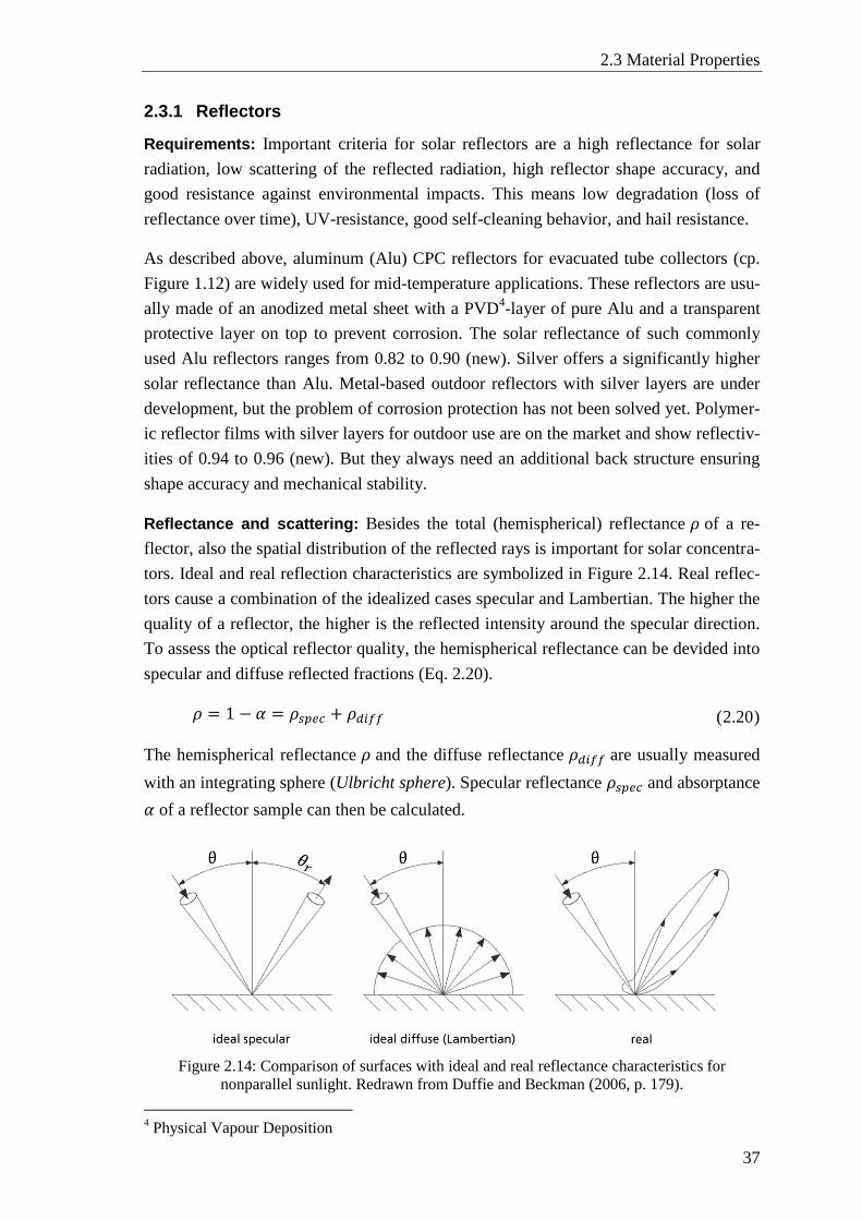
2.3 Material Properties
37
2.3.1 Reflectors
Requirements: Important criteria for solar reflectors are a high reflectance for solar
radiation, low scattering of the reflected radiation, high reflector shape accuracy, and
good resistance against environmental impacts. This means low degradation (loss of
reflectance over time), UV-resistance, good self-cleaning behavior, and hail resistance.
As described above, aluminum (Alu) CPC reflectors for evacuated tube collectors (cp.
Figure 1.12) are widely used for mid-temperature applications. These reflectors are usu-
ally made of an anodized metal sheet with a PVD4-layer of pure Alu and a transparent
protective layer on top to prevent corrosion. The solar reflectance of such commonly
used Alu reflectors ranges from 0.82 to 0.90 (new). Silver offers a significantly higher
solar reflectance than Alu. Metal-based outdoor reflectors with silver layers are under
development, but the problem of corrosion protection has not been solved yet. Polymer-
ic reflector films with silver layers for outdoor use are on the market and show reflectiv-
ities of 0.94 to 0.96 (new). But they always need an additional back structure ensuring
shape accuracy and mechanical stability.
Reflectance and scattering: Besides the total (hemispherical) reflectance 𝜌 of a re-
flector, also the spatial distribution of the reflected rays is important for solar concentra-
tors. Ideal and real reflection characteristics are symbolized in Figure 2.14. Real reflec-
tors cause a combination of the idealized cases specular and Lambertian. The higher the
quality of a reflector, the higher is the reflected intensity around the specular direction.
To assess the optical reflector quality, the hemispherical reflectance can be devided into
specular and diffuse reflected fractions (Eq. 2.20).
𝜌 = 1 − 𝛼 = 𝜌𝑠𝑝𝑒𝑐 + 𝜌𝑑𝑖𝑓𝑓 ( 2.20 )
The hemispherical reflectance 𝜌 and the diffuse reflectance 𝜌𝑑𝑖𝑓𝑓 are usually measured
with an integrating sphere (Ulbricht sphere). Specular reflectance 𝜌𝑠𝑝𝑒𝑐 and absorptance
𝛼 of a reflector sample can then be calculated.
Figure 2.14: Comparison of surfaces with ideal and real reflectance characteristics for
nonparallel sunlight. Redrawn from Duffie and Beckman (2006, p. 179).
4 Physical Vapour Deposition
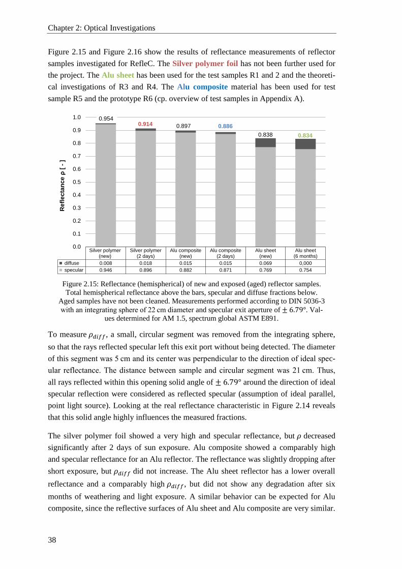
Chapter 2: Optical Investigations
38
Figure 2.15 and Figure 2.16 show the results of reflectance measurements of reflector
samples investigated for RefleC. The Silver polymer foil has not been further used for
the project. The Alu sheet has been used for the test samples R1 and 2 and the theoreti-
cal investigations of R3 and R4. The Alu composite material has been used for test
sample R5 and the prototype R6 (cp. overview of test samples in Appendix A).
Figure 2.15: Reflectance (hemispherical) of new and exposed (aged) reflector samples.
Total hemispherical reflectance above the bars, specular and diffuse fractions below.
Aged samples have not been cleaned. Measurements performed according to DIN 5036-3
with an integrating sphere of 22 cm diameter and specular exit aperture of ± 6.79°. Val-
ues determined for AM 1.5, spectrum global ASTM E891.
To measure 𝜌𝑑𝑖𝑓𝑓, a small, circular segment was removed from the integrating sphere,
so that the rays reflected specular left this exit port without being detected. The diameter
of this segment was 5 cm and its center was perpendicular to the direction of ideal spec-
ular reflectance. The distance between sample and circular segment was 21 cm. Thus,
all rays reflected within this opening solid angle of ± 6.79° around the direction of ideal
specular reflection were considered as reflected specular (assumption of ideal parallel,
point light source). Looking at the real reflectance characteristic in Figure 2.14 reveals
that this solid angle highly influences the measured fractions.
The silver polymer foil showed a very high and specular reflectance, but 𝜌 decreased
significantly after 2 days of sun exposure. Alu composite showed a comparably high
and specular reflectance for an Alu reflector. The reflectance was slightly dropping after
short exposure, but 𝜌𝑑𝑖𝑓𝑓 did not increase. The Alu sheet reflector has a lower overall
reflectance and a comparably high 𝜌𝑑𝑖𝑓𝑓, but did not show any degradation after six
months of weathering and light exposure. A similar behavior can be expected for Alu
composite, since the reflective surfaces of Alu sheet and Alu composite are very similar.
Silver polymer(new)
Silver polymer(2 days)
Alu composite(new)
Alu composite(2 days)
Alu sheet(new)
Alu sheet(6 months)
diffuse 0.008 0.018 0.015 0.015 0.069 0,000
specular 0.946 0.896 0.882 0.871 0.769 0.754
0.0
0.1
0.2
0.3
0.4
0.5
0.6
0.7
0.8
0.9
1.0
Re
fle
cta
nc
e ρ
[ -
]
0.9540.954 0.954
0.9540.914 0.897 0.886
0.838 0.834
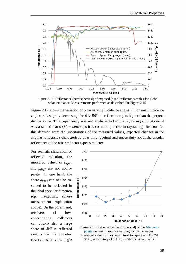
2.3 Material Properties
39
Figure 2.16: Reflectance (hemispherical) of exposed (aged) reflector samples for global
solar irradiance. Measurements performed as described for Figure 2.15.
Figure 2.17 shows the variation of 𝜌 for varying incidence angles 𝜃. For small incidence
angles, 𝜌 is slightly decreasing; for 𝜃 > 50° the reflectance gets higher than the perpen-
dicular value. This dependency was not implemented in the raytracing simulations; it
was assumed that 𝜌 (𝜃) = 𝑐𝑜𝑛𝑠𝑡 (as it is common practice in raytracing). Reasons for
this decision were the uncertainties of the measured values, expected changes in the
angular reflectance characteristic over time (ageing) and uncertainty about the angular
reflectance of the other reflector types simulated.
For realistic simulation of
reflected radiation, the
measured values of 𝜌𝑠𝑝𝑒𝑐
and 𝜌𝑑𝑖𝑓𝑓 are not appro-
priate. On one hand, the
share 𝜌𝑠𝑝𝑒𝑐 can not be as-
sumed to be reflected in
the ideal specular direction
(cp. integrating sphere
measurement explanation
above). On the other hand,
receivers of low-
concentrating collectors
can absorb also a large
share of diffuse reflected
rays, since the absorber
covers a wide view angle
0
160
320
480
640
800
960
1120
1280
1440
1600
0.0
0.1
0.2
0.3
0.4
0.5
0.6
0.7
0.8
0.9
1.0
0.25 0.50 0.75 1.00 1.25 1.50 1.75 2.00 2.25 2.50
Inte
nsit
y [
(W
/(m
2*μ
m)]
Refl
ecta
nce
ρ[
-]
Wavelength λ [ µm ]
Alu composite, 2 days aged (prim.)
Alu sheet, 6 months aged (prim.)
Silver polymer, 2 days aged (prim.)
Solar spectrum AM1.5 global ASTM E891 (sec.)
Figure 2.17: Reflectance (hemispherical) of the Alu com-
posite material (new) for varying incidence angles.
Measured values (blue) determined for spectrum ASTM
G173, uncertainty of ± 1.5 % of the measured value
0.86
0.88
0.90
0.92
0.94
0.96
0.98
1.00
0 10 20 30 40 50 60 70 80 90
Refl
ecta
nce ρ
[ -
]
Incidence angle θ [ ° ]
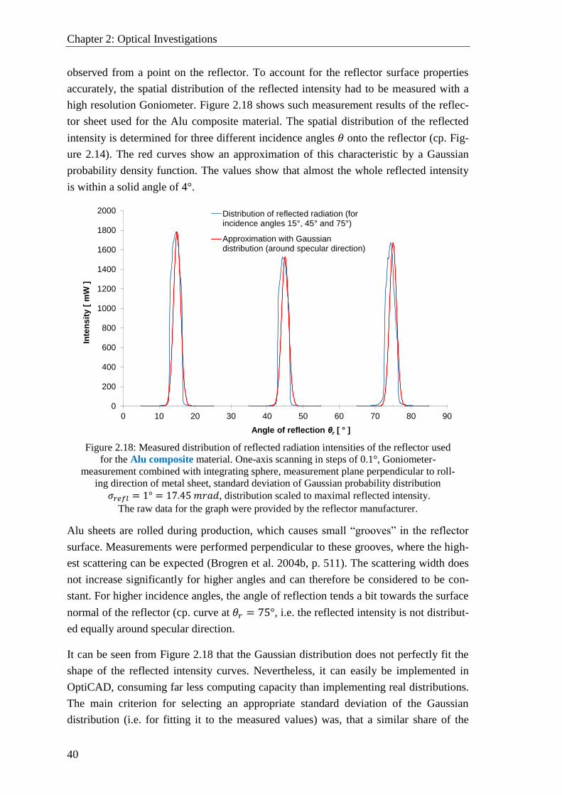
Chapter 2: Optical Investigations
40
observed from a point on the reflector. To account for the reflector surface properties
accurately, the spatial distribution of the reflected intensity had to be measured with a
high resolution Goniometer. Figure 2.18 shows such measurement results of the reflec-
tor sheet used for the Alu composite material. The spatial distribution of the reflected
intensity is determined for three different incidence angles 𝜃 onto the reflector (cp. Fig-
ure 2.14). The red curves show an approximation of this characteristic by a Gaussian
probability density function. The values show that almost the whole reflected intensity
is within a solid angle of 4°.
Figure 2.18: Measured distribution of reflected radiation intensities of the reflector used
for the Alu composite material. One-axis scanning in steps of 0.1°, Goniometer-
measurement combined with integrating sphere, measurement plane perpendicular to roll-
ing direction of metal sheet, standard deviation of Gaussian probability distribution
𝜎𝑟𝑒𝑓𝑙 = 1° = 17.45 𝑚𝑟𝑎𝑑, distribution scaled to maximal reflected intensity.
The raw data for the graph were provided by the reflector manufacturer.
Alu sheets are rolled during production, which causes small “grooves” in the reflector
surface. Measurements were performed perpendicular to these grooves, where the high-
est scattering can be expected (Brogren et al. 2004b, p. 511). The scattering width does
not increase significantly for higher angles and can therefore be considered to be con-
stant. For higher incidence angles, the angle of reflection tends a bit towards the surface
normal of the reflector (cp. curve at 𝜃𝑟 = 75°, i.e. the reflected intensity is not distribut-
ed equally around specular direction.
It can be seen from Figure 2.18 that the Gaussian distribution does not perfectly fit the
shape of the reflected intensity curves. Nevertheless, it can easily be implemented in
OptiCAD, consuming far less computing capacity than implementing real distributions.
The main criterion for selecting an appropriate standard deviation of the Gaussian
distribution (i.e. for fitting it to the measured values) was, that a similar share of the
0
200
400
600
800
1000
1200
1400
1600
1800
2000
0 10 20 30 40 50 60 70 80 90
Inte
nsit
y [
mW
]
Angle of reflection θr [ ° ]
Distribution of reflected radiation (forincidence angles 15°, 45° and 75°)
Approximation with Gaussiandistribution (around specular direction)
2.3 Material Properties
41
reflected radiation is within the solid angle of 4° than for the real reflector. Integrating
the measured intensities within 4° (2° radius from maximum) shows, that at 𝜃𝑟 = 15°,
about 97,29 % of the reflected energy is within this range. The Gauss curve shows for
the selected standard deviation of 𝜎𝑟𝑒𝑓𝑙 = 1° per definition 95.45 % of the reflected
intensity is within 2 𝜎𝑟𝑒𝑓𝑙 = 4°. The drawback of the good representation in this respect
is that the intensity distribution within the 4° is more dense than in reality, slightly
distorting the shape of the IAM curve around the acceptance half angle. Furthermore,
𝜎𝑟𝑒𝑓𝑙 is expected to increase due to ageing and/or soiling (Brogren et al. 2004b).
Scattering of the reflected rays does not only occur due to microscopic reflector surface
errors, which are accounted by 𝜎𝑟𝑒𝑓𝑙, but additionally due to surface displacement or
shape errors 𝜎𝑜𝑟𝑖 , and due to the non-parallel light reflected (sunshape-distribution
𝜎𝑠𝑢𝑛). Assuming a Gaussian distribution of these errors, they can be superpositioned to
get the standard deviation for overall ray scattering 𝜎:
𝜎 = √𝜎𝑟𝑒𝑓𝑙2 + 𝜎𝑜𝑟𝑖
2 + 𝜎𝑠𝑢𝑛2 ( 2.21 )
The overall scattering parameter 𝜎 is highly influenced by the highest of the
contributing scattering errors. For the raytracing simulations, surface orientation errors
were neglected, because the raytracing values should represent an ideal shaped reflector.
The sunshape distribution can only poorly be approximated by a gaussian distribution,
but the vast majority of beam irradiance originates from a solid angle within 4.65 mrad
(Badescu 2008). A representative standard deviation would then be about a factor 6
smaller than 𝜎𝑟𝑒𝑓𝑙, almost not influencing 𝜎. Thus, only the microscopic scattering of
the reflector was considered and it was simulated with 𝜎 = 𝜎𝑟𝑒𝑓𝑙 = 1° . Detailed
measurements on optical properties and durability of reflectors for low-concentrating
collectors have been reported by Nostell et al. (1998), Brogren et al. (2004b) and
Brogren et al. (2004a). Lindseth et al. (1999) and Nilsson et al. (2007) evaluated
uncertainties of Al-reflector characterization with integrating spheres.
Hail impact tests: The reflectors of RefleC are quite large. They fulfill a static function
and are the most eye catching part of the collector. Thus, ensuring the mechanical sta-
bility and resistance against environmental impacts at affordable costs was crucial for
the concept. Pre-fabricated and self-fabricated sandwich reflector constructions were
tested. Figure 2.19 shows hail resistance test results. All in all, twelve reflector con-
structions were tested systematically according to the standard (EN 12975-2:2006),
method two, with ice balls. The main boundary conditions for the ice ball are a diameter
of 25 mm (− 5 %), a mass of 7.53 𝑔 (− 5 %), and a velocity of 23 𝑚/𝑠 (± 5 %).
After a reflector was tested under standard-conditions, the impulse energies of the ice
balls were either increased or decreased to assess a constructions potential for further
development. Sample 1 showed deep indentations even at low impulses and was there-
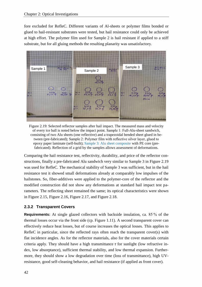
Chapter 2: Optical Investigations
42
fore excluded for RefleC. Different variants of Al-sheets or polymer films bonded or
glued to hail-resistant substrates were tested, but hail resistance could only be achieved
at high effort. The polymer film used for Sample 2 is hail resistant if applied to a stiff
substrate, but for all gluing methods the resulting planarity was unsatisfactory.
Figure 2.19: Selected reflector samples after hail impact. The measured mass and velocity
of every ice ball is noted below the impact point. Sample 1: Full-Alu-sheet sandwich,
consisting of two Alu sheets (one reflective) and a trapezoidal bended sheet glued in be-
tween (pre-fabricated); Sample 2: Polymer film with reflective silver layer, glued to
epoxy paper laminate (self-built); Sample 3: Alu sheet composite with PE core (pre-
fabricated). Reflection of a grid by the samples allows assessment of deformations.
Comparing the hail resistance test, reflectivity, durability, and price of the reflector con-
structions, finally a pre-fabricated Alu sandwich very similar to Sample 3 in Figure 2.19
was used for RefleC. The mechanical stability of Sample 3 was sufficient, but in the hail
resistance test it showed small deformations already at comparably low impulses of the
hailstones. So, fiber-additives were applied to the polymer-core of the reflector and the
modified construction did not show any deformations at standard hail impact test pa-
rameters. The reflecting sheet remained the same; its optical characteristics were shown
in Figure 2.15, Figure 2.16, Figure 2.17, and Figure 2.18.
2.3.2 Transparent Covers
Requirements: At single glazed collectors with backside insulation, ca. 85 % of the
thermal losses occur via the front side (cp. Figure 1.11). A second transparent cover can
effectively reduce heat losses, but of course increases the optical losses. This applies to
RefleC in particular, since the reflected rays often reach the transparent cover(s) with
flat incidence angles. As for the reflector materials, also for the cover materials certain
criteria apply. They should have a high transmittance 𝜏 for sunlight (low refractive in-
dex, low absorptance), sufficient thermal stability, and low thermal expansion. Further-
more, they should show a low degradation over time (loss of transmittance), high UV-
resistance, good self-cleaning behavior, and hail resistance (if applied as front cover).
Sample 1 Sample 2
Sample 3
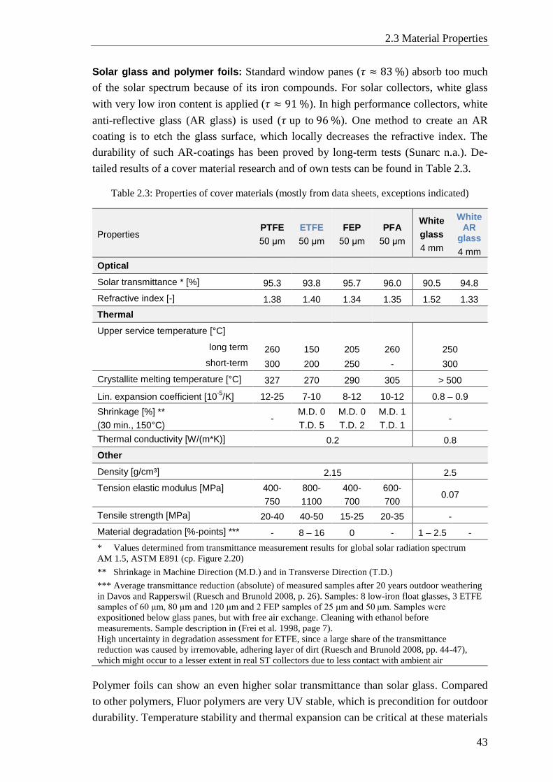
2.3 Material Properties
43
Solar glass and polymer foils: Standard window panes (𝜏 ≈ 83 %) absorb too much
of the solar spectrum because of its iron compounds. For solar collectors, white glass
with very low iron content is applied (𝜏 ≈ 91 %). In high performance collectors, white
anti-reflective glass (AR glass) is used (𝜏 up to 96 %). One method to create an AR
coating is to etch the glass surface, which locally decreases the refractive index. The
durability of such AR-coatings has been proved by long-term tests (Sunarc n.a.). De-
tailed results of a cover material research and of own tests can be found in Table 2.3.
Table 2.3: Properties of cover materials (mostly from data sheets, exceptions indicated)
Properties PTFE
50 μm
ETFE
50 μm
FEP
50 μm
PFA
50 μm
White
glass
4 mm
WhiteAR
glass
4 mm
Optical
Solar transmittance * [%] 95.3 93.8 95.7 96.0 90.5 94.8
Refractive index [-] 1.38 1.40 1.34 1.35 1.52 1.33
Thermal
Upper service temperature [°C]
260 150 205 260 250 long term
short-term 300 200 250 - 300
Crystallite melting temperature [°C] 327 270 290 305 > 500
Lin. expansion coefficient [10-5
/K] 12-25 7-10 8-12 10-12 0.8 – 0.9
Shrinkage [%] **
(30 min., 150°C) -
M.D. 0
T.D. 5
M.D. 0
T.D. 2
M.D. 1
T.D. 1 -
Thermal conductivity [W/(m*K)] 0.2 0.8
Other
Density [g/cm³] 2.15 2.5
Tension elastic modulus [MPa] 400-
750
800-
1100
400-
700
600-
700 0.07
Tensile strength [MPa] 20-40 40-50 15-25 20-35 -
Material degradation [%-points] *** - 8 – 16 0 - 1 – 2.5 -
* Values determined from transmittance measurement results for global solar radiation spectrum
AM 1.5, ASTM E891 (cp. Figure 2.20)
** Shrinkage in Machine Direction (M.D.) and in Transverse Direction (T.D.)
*** Average transmittance reduction (absolute) of measured samples after 20 years outdoor weathering
in Davos and Rapperswil (Ruesch and Brunold 2008, p. 26). Samples: 8 low-iron float glasses, 3 ETFE
samples of 60 μm, 80 μm and 120 μm and 2 FEP samples of 25 μm and 50 μm. Samples were
expositioned below glass panes, but with free air exchange. Cleaning with ethanol before
measurements. Sample description in (Frei et al. 1998, page 7).
High uncertainty in degradation assessment for ETFE, since a large share of the transmittance
reduction was caused by irremovable, adhering layer of dirt (Ruesch and Brunold 2008, pp. 44-47),
which might occur to a lesser extent in real ST collectors due to less contact with ambient air
Polymer foils can show an even higher solar transmittance than solar glass. Compared
to other polymers, Fluor polymers are very UV stable, which is precondition for outdoor
durability. Temperature stability and thermal expansion can be critical at these materials
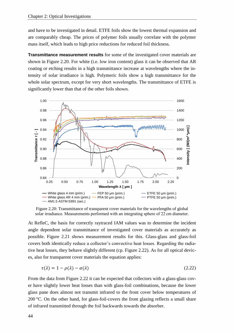
Chapter 2: Optical Investigations
44
and have to be investigated in detail. ETFE foils show the lowest thermal expansion and
are comparably cheap. The prices of polymer foils usually correlate with the polymer
mass itself, which leads to high price reductions for reduced foil thickness.
Transmittance measurement results for some of the investigated cover materials are
shown in Figure 2.20. For white (i.e. low iron content) glass it can be observed that AR
coating or etching results in a high transmittance increase at wavelengths where the in-
tensity of solar irradiance is high. Polymeric foils show a high transmittance for the
whole solar spectrum, except for very short wavelengths. The transmittance of ETFE is
significantly lower than that of the other foils shown.
Figure 2.20: Transmittance of transparent cover materials for the wavelengths of global
solar irradiance. Measurements performed with an integrating sphere of 22 cm diameter.
At RefleC, the basis for correctly raytraced IAM values was to determine the incident
angle dependent solar transmittance of investigated cover materials as accurately as
possible. Figure 2.21 shows measurement results for this. Glass-glass and glass-foil
covers both identically reduce a collector’s convective heat losses. Regarding the radia-
tive heat losses, they behave slightly different (cp. Figure 2.22). As for all optical devic-
es, also for transparent cover materials the equation applies:
𝜏(𝜆) = 1 − 𝜌(𝜆) − 𝛼(𝜆) ( 2.22 )
From the data from Figure 2.22 it can be expected that collectors with a glass-glass cov-
er have slightly lower heat losses than with glass-foil combinations, because the lower
glass pane does almost not transmit infrared to the front cover below temperatures of
200 °C. On the other hand, for glass-foil-covers the front glazing reflects a small share
of infrared transmitted through the foil backwards towards the absorber.
0
200
400
600
800
1000
1200
1400
1600
0.84
0.86
0.88
0.90
0.92
0.94
0.96
0.98
1.00
0.25 0.50 0.75 1.00 1.25 1.50 1.75 2.00 2.25
Inte
nsit
y [
(W
/(m
2*μ
m)]
Tra
nsm
itta
nce τ
[ -
]
Wavelength λ [ µm ]
White glass 4 mm (prim.) FEP 50 μm (prim.) ETFE 50 μm (prim.)
White glass AR 4 mm (prim.) PFA 50 μm (prim.) PTFE 50 μm (prim.)
AM1.5 ASTM E891 (sec.)
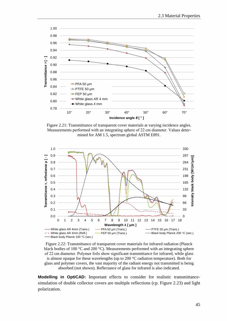
2.3 Material Properties
45
Figure 2.21: Transmittance of transparent cover materials at varying incidence angles.
Measurements performed with an integrating sphere of 22 cm diameter. Values deter-
mined for AM 1.5, spectrum global ASTM E891.
Figure 2.22: Transmittance of transparent cover materials for infrared radiation (Planck
black bodies of 100 °C and 200 °C). Measurements performed with an integrating sphere
of 22 cm diameter. Polymer foils show significant transmittance for infrared, while glass
is almost opaque for these wavelengths (up to 200 °C radiation temperature). Both for
glass and polymer covers, the vast majority of the radiant energy not transmitted is being
absorbed (not shown). Reflectance of glass for infrared is also indicated.
Modelling in OptiCAD: Important effects to consider for realistic transmittance-
simulation of double collector covers are multiple reflections (cp. Figure 2.23) and light
polarization.
0.78
0.80
0.82
0.84
0.86
0.88
0.90
0.92
0.94
0.96
0.98
1.00
10° 20° 30° 40° 50° 60° 70°
Tra
nsm
itta
nce τ
[ -
]
Incidence angle θ [ ° ]
PFA 50 μm
PTFE 50 μm
FEP 50 μm
White glass AR 4 mm
White glass 4 mm
0
33
66
99
132
165
198
231
264
297
330
0.0
0.1
0.2
0.3
0.4
0.5
0.6
0.7
0.8
0.9
1.0
0 1 2 3 4 5 6 7 8 9 10 11 12 13 14 15 16 17 18
Inte
nsi
ty b
lack
bo
dy
[W
/(m
²µm
)]
Tra
nsm
itta
nce
τ,
refl
ect
an
ce ρ
[ -
]
Wavelength λ [ µm ]
White glass AR 4mm (Trans.) PFA 50 μm (Trans.) PTFE 50 μm (Trans.)
White glass AR 4mm (Refl.) FEP 50 μm (Trans.) Black body Planck 200 °C (sec.)
Black body Planck 100 °C (sec.)
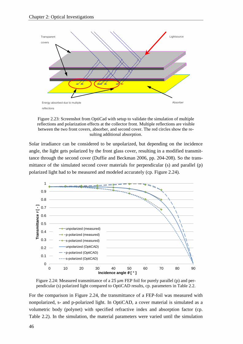
Chapter 2: Optical Investigations
46
Figure 2.23: Screenshot from OptiCad with setup to validate the simulation of multiple
reflections and polarization effects at the collector front. Multiple reflections are visible
between the two front covers, absorber, and second cover. The red circles show the re-
sulting additional absorption.
Solar irradiance can be considered to be unpolarized, but depending on the incidence
angle, the light gets polarized by the front glass cover, resulting in a modified transmit-
tance through the second cover (Duffie and Beckman 2006, pp. 204-208). So the trans-
mittance of the simulated second cover materials for perpendicular (s) and parallel (p)
polarized light had to be measured and modeled accurately (cp. Figure 2.24).
Figure 2.24: Measured transmittance of a 25 μ𝑚 FEP foil for purely parallel (p) and per-
pendicular (s) polarized light compared to OptiCAD results, cp. parameters in Table 2.2.
For the comparison in Figure 2.24, the transmittance of a FEP-foil was measured with
nonpolarized, s- and p-polarized light. In OptiCAD, a cover material is simulated as a
volumetric body (polynet) with specified refractive index and absorption factor (cp.
Table 2.2). In the simulation, the material parameters were varied until the simulation
0
0.1
0.2
0.3
0.4
0.5
0.6
0.7
0.8
0.9
1
0 10 20 30 40 50 60 70 80 90
Tra
nsm
itta
nce τ
[ -
]
Incidence angle θ [ ° ]
unpolarized (measured)
p-polarized (measured)
s-polarized (measured)
unpolarized (OptiCAD)
p-polarized (OptiCAD)
s-polarized (OptiCAD)
Transparent covers
Energy absorbed due to multiple reflections
Absorber
Lightsource
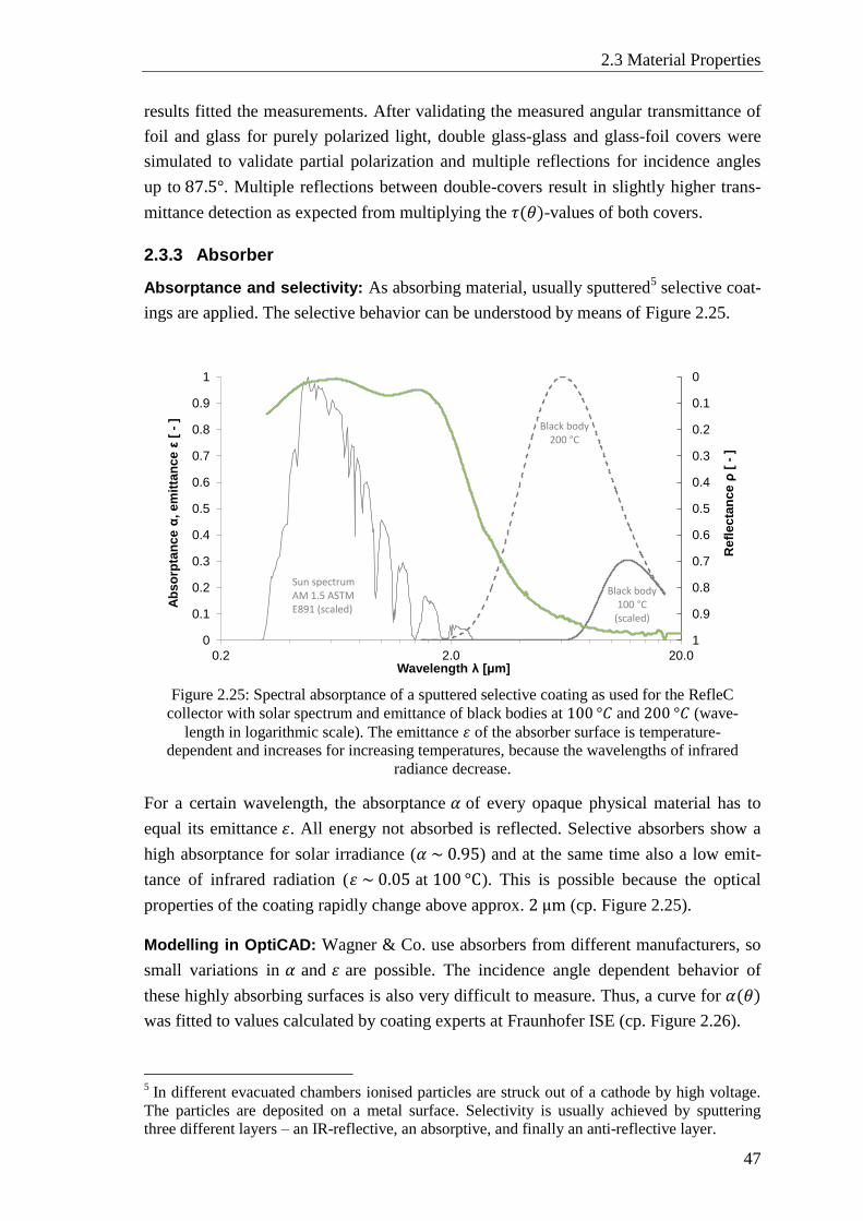
2.3 Material Properties
47
results fitted the measurements. After validating the measured angular transmittance of
foil and glass for purely polarized light, double glass-glass and glass-foil covers were
simulated to validate partial polarization and multiple reflections for incidence angles
up to 87.5°. Multiple reflections between double-covers result in slightly higher trans-
mittance detection as expected from multiplying the 𝜏(𝜃)-values of both covers.
2.3.3 Absorber
Absorptance and selectivity: As absorbing material, usually sputtered5 selective coat-
ings are applied. The selective behavior can be understood by means of Figure 2.25.
Figure 2.25: Spectral absorptance of a sputtered selective coating as used for the RefleC
collector with solar spectrum and emittance of black bodies at 100 °𝐶 and 200 °𝐶 (wave-
length in logarithmic scale). The emittance 휀 of the absorber surface is temperature-
dependent and increases for increasing temperatures, because the wavelengths of infrared
radiance decrease.
For a certain wavelength, the absorptance 𝛼 of every opaque physical material has to
equal its emittance 휀. All energy not absorbed is reflected. Selective absorbers show a
high absorptance for solar irradiance (𝛼 ~ 0.95) and at the same time also a low emit-
tance of infrared radiation (휀 ~ 0.05 at 100 °C). This is possible because the optical
properties of the coating rapidly change above approx. 2 μm (cp. Figure 2.25).
Modelling in OptiCAD: Wagner & Co. use absorbers from different manufacturers, so
small variations in 𝛼 and 휀 are possible. The incidence angle dependent behavior of
these highly absorbing surfaces is also very difficult to measure. Thus, a curve for 𝛼(𝜃)
was fitted to values calculated by coating experts at Fraunhofer ISE (cp. Figure 2.26).
5 In different evacuated chambers ionised particles are struck out of a cathode by high voltage.
The particles are deposited on a metal surface. Selectivity is usually achieved by sputtering
three different layers – an IR-reflective, an absorptive, and finally an anti-reflective layer.
0
0.1
0.2
0.3
0.4
0.5
0.6
0.7
0.8
0.9
10
0.1
0.2
0.3
0.4
0.5
0.6
0.7
0.8
0.9
1
0.2 2.0 20.0
Refl
ecta
nce ρ
[ -
]
Ab
so
rpta
nce α
, em
itta
nce ε
[ -
]
Wavelength λ [μm]
Sun spectrum AM 1.5 ASTM E891 (scaled)
Black body 200 °C
Black body 100 °C
(scaled)
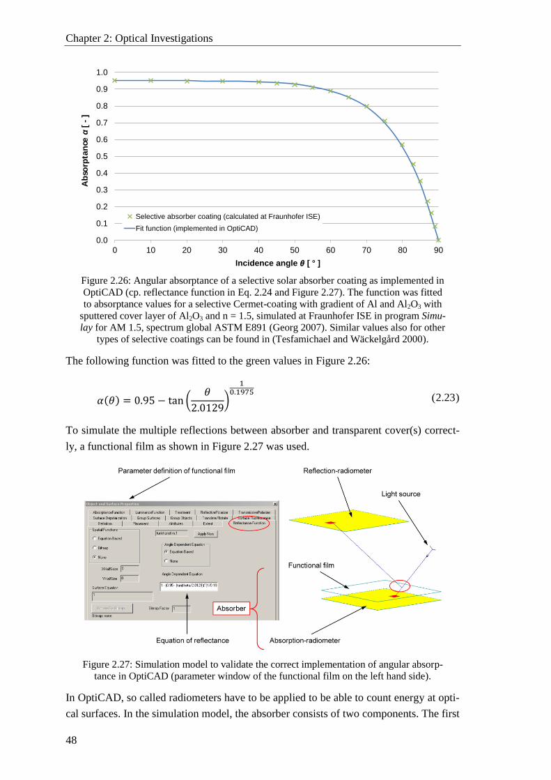
Chapter 2: Optical Investigations
48
Figure 2.26: Angular absorptance of a selective solar absorber coating as implemented in
OptiCAD (cp. reflectance function in Eq. 2.24 and Figure 2.27). The function was fitted
to absorptance values for a selective Cermet-coating with gradient of Al and Al2O3 with
sputtered cover layer of Al2O3 and n = 1.5, simulated at Fraunhofer ISE in program Simu-
lay for AM 1.5, spectrum global ASTM E891 (Georg 2007). Similar values also for other
types of selective coatings can be found in (Tesfamichael and Wäckelgård 2000).
The following function was fitted to the green values in Figure 2.26:
𝛼(𝜃) = 0.95 − tan (𝜃
2.0129)
10.1975
( 2.23 )
To simulate the multiple reflections between absorber and transparent cover(s) correct-
ly, a functional film as shown in Figure 2.27 was used.
Figure 2.27: Simulation model to validate the correct implementation of angular absorp-
tance in OptiCAD (parameter window of the functional film on the left hand side).
In OptiCAD, so called radiometers have to be applied to be able to count energy at opti-
cal surfaces. In the simulation model, the absorber consists of two components. The first
0.0
0.1
0.2
0.3
0.4
0.5
0.6
0.7
0.8
0.9
1.0
0 10 20 30 40 50 60 70 80 90
Ab
sorp
tan
ce α
[ -
]
Incidence angle 𝜃 [ ° ]
Selective absorber coating (calculated at Fraunhofer ISE)
Fit function (implemented in OptiCAD)
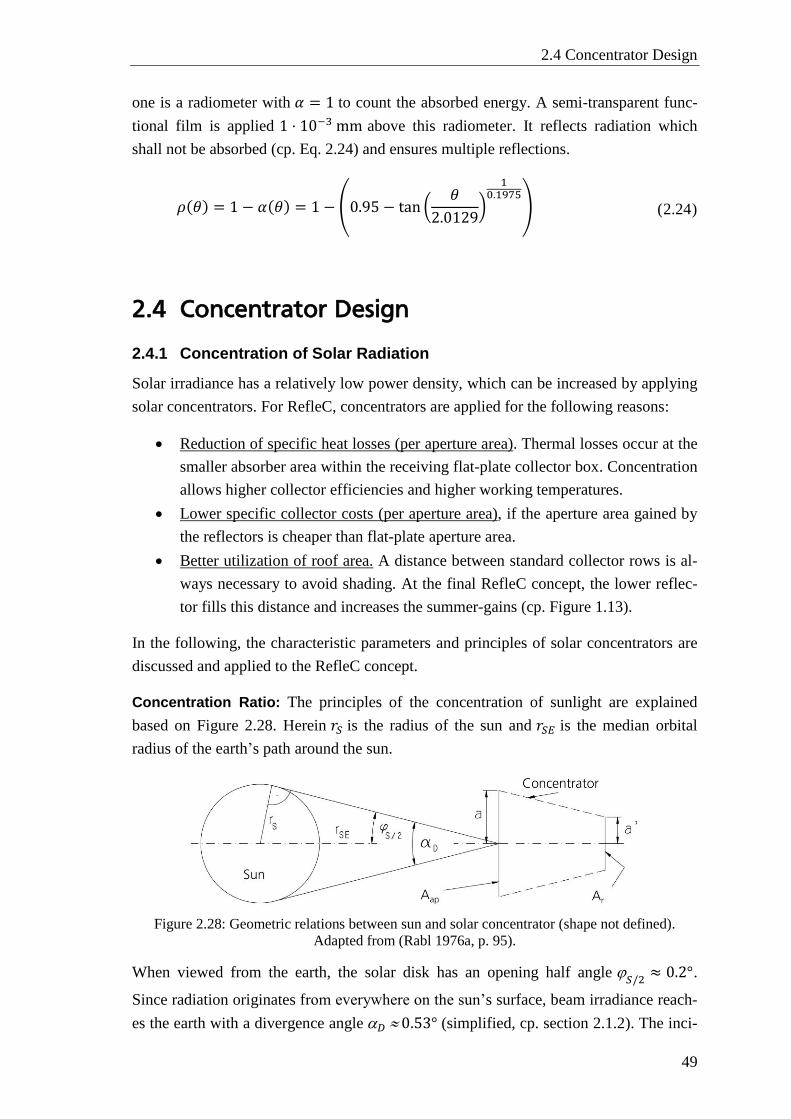
2.4 Concentrator Design
49
one is a radiometer with 𝛼 = 1 to count the absorbed energy. A semi-transparent func-
tional film is applied 1 ⋅ 10−3 mm above this radiometer. It reflects radiation which
shall not be absorbed (cp. Eq. 2.24) and ensures multiple reflections.
𝜌(𝜃) = 1 − 𝛼(𝜃) = 1 − (0.95 − tan (𝜃
2.0129)
10.1975
) ( 2.24 )
2.4 Concentrator Design
2.4.1 Concentration of Solar Radiation
Solar irradiance has a relatively low power density, which can be increased by applying
solar concentrators. For RefleC, concentrators are applied for the following reasons:
Reduction of specific heat losses (per aperture area). Thermal losses occur at the
smaller absorber area within the receiving flat-plate collector box. Concentration
allows higher collector efficiencies and higher working temperatures.
Lower specific collector costs (per aperture area), if the aperture area gained by
the reflectors is cheaper than flat-plate aperture area.
Better utilization of roof area. A distance between standard collector rows is al-
ways necessary to avoid shading. At the final RefleC concept, the lower reflec-
tor fills this distance and increases the summer-gains (cp. Figure 1.13).
In the following, the characteristic parameters and principles of solar concentrators are
discussed and applied to the RefleC concept.
Concentration Ratio: The principles of the concentration of sunlight are explained
based on Figure 2.28. Herein 𝑟𝑆 is the radius of the sun and 𝑟𝑆𝐸 is the median orbital
radius of the earth’s path around the sun.
Figure 2.28: Geometric relations between sun and solar concentrator (shape not defined).
Adapted from (Rabl 1976a, p. 95).
When viewed from the earth, the solar disk has an opening half angle 𝑆/2
≈ 0.2°.
Since radiation originates from everywhere on the sun’s surface, beam irradiance reach-
es the earth with a divergence angle 𝐷 0.53° (simplified, cp. section 2.1.2). The inci-
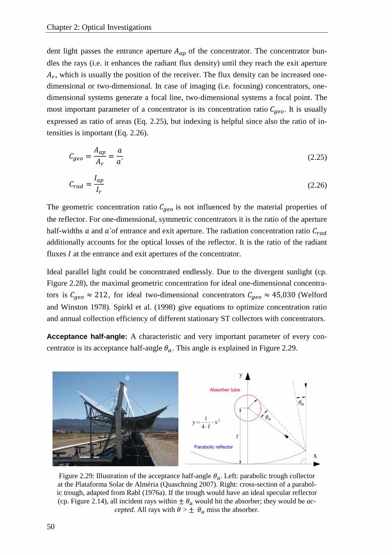
Chapter 2: Optical Investigations
50
dent light passes the entrance aperture 𝐴𝑎𝑝 of the concentrator. The concentrator bun-
dles the rays (i.e. it enhances the radiant flux density) until they reach the exit aperture
𝐴𝑟, which is usually the position of the receiver. The flux density can be increased one-
dimensional or two-dimensional. In case of imaging (i.e. focusing) concentrators, one-
dimensional systems generate a focal line, two-dimensional systems a focal point. The
most important parameter of a concentrator is its concentration ratio 𝐶𝑔𝑒𝑜. It is usually
expressed as ratio of areas (Eq. 2.25), but indexing is helpful since also the ratio of in-
tensities is important (Eq. 2.26).
𝐶𝑔𝑒𝑜 =𝐴𝑎𝑝
𝐴𝑟=
𝑎
𝑎´ ( 2.25 )
𝐶𝑟𝑎𝑑 =𝐼𝑎𝑝
𝐼𝑟 ( 2.26 )
The geometric concentration ratio 𝐶𝑔𝑒𝑜 is not influenced by the material properties of
the reflector. For one-dimensional, symmetric concentrators it is the ratio of the aperture
half-widths 𝑎 and 𝑎´of entrance and exit aperture. The radiation concentration ratio 𝐶𝑟𝑎𝑑
additionally accounts for the optical losses of the reflector. It is the ratio of the radiant
fluxes 𝐼 at the entrance and exit apertures of the concentrator.
Ideal parallel light could be concentrated endlessly. Due to the divergent sunlight (cp.
Figure 2.28), the maximal geometric concentration for ideal one-dimensional concentra-
tors is 𝐶𝑔𝑒𝑜 ≈ 212, for ideal two-dimensional concentrators 𝐶𝑔𝑒𝑜 ≈ 45,030 (Welford
and Winston 1978). Spirkl et al. (1998) give equations to optimize concentration ratio
and annual collection efficiency of different stationary ST collectors with concentrators.
Acceptance half-angle: A characteristic and very important parameter of every con-
centrator is its acceptance half-angle 𝜃𝑎. This angle is explained in Figure 2.29.
Figure 2.29: Illustration of the acceptance half-angle 𝜃𝑎. Left: parabolic trough collector
at the Plataforma Solar de Alméria (Quaschning 2007). Right: cross-section of a parabol-
ic trough, adapted from Rabl (1976a). If the trough would have an ideal specular reflector
(cp. Figure 2.14), all incident rays within ± 𝜃𝑎 would hit the absorber; they would be ac-
cepted. All rays with 𝜃 > ± 𝜃𝑎 miss the absorber.
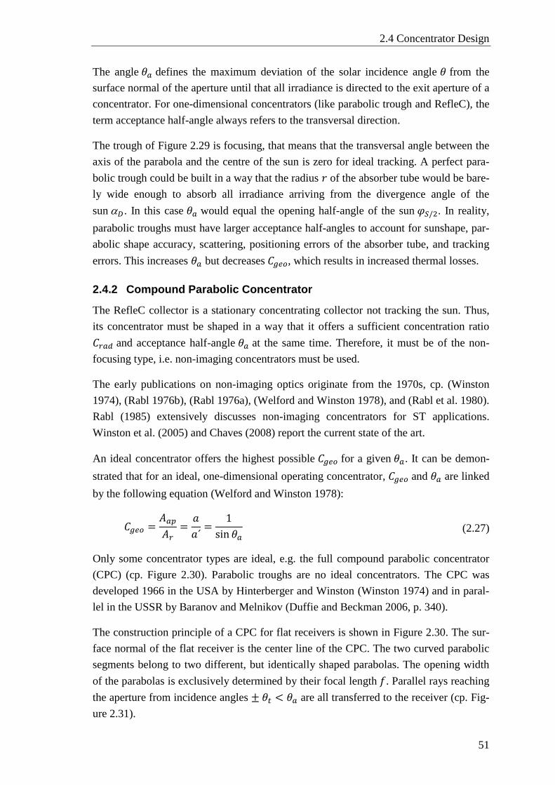
2.4 Concentrator Design
51
The angle 𝜃𝑎 defines the maximum deviation of the solar incidence angle 𝜃 from the
surface normal of the aperture until that all irradiance is directed to the exit aperture of a
concentrator. For one-dimensional concentrators (like parabolic trough and RefleC), the
term acceptance half-angle always refers to the transversal direction.
The trough of Figure 2.29 is focusing, that means that the transversal angle between the
axis of the parabola and the centre of the sun is zero for ideal tracking. A perfect para-
bolic trough could be built in a way that the radius 𝑟 of the absorber tube would be bare-
ly wide enough to absorb all irradiance arriving from the divergence angle of the
sun 𝐷. In this case 𝜃𝑎 would equal the opening half-angle of the sun 𝜑𝑆/2. In reality,
parabolic troughs must have larger acceptance half-angles to account for sunshape, par-
abolic shape accuracy, scattering, positioning errors of the absorber tube, and tracking
errors. This increases 𝜃𝑎 but decreases 𝐶𝑔𝑒𝑜, which results in increased thermal losses.
2.4.2 Compound Parabolic Concentrator
The RefleC collector is a stationary concentrating collector not tracking the sun. Thus,
its concentrator must be shaped in a way that it offers a sufficient concentration ratio
𝐶𝑟𝑎𝑑 and acceptance half-angle 𝜃𝑎 at the same time. Therefore, it must be of the non-
focusing type, i.e. non-imaging concentrators must be used.
The early publications on non-imaging optics originate from the 1970s, cp. (Winston
1974), (Rabl 1976b), (Rabl 1976a), (Welford and Winston 1978), and (Rabl et al. 1980).
Rabl (1985) extensively discusses non-imaging concentrators for ST applications.
Winston et al. (2005) and Chaves (2008) report the current state of the art.
An ideal concentrator offers the highest possible 𝐶𝑔𝑒𝑜 for a given 𝜃𝑎. It can be demon-
strated that for an ideal, one-dimensional operating concentrator, 𝐶𝑔𝑒𝑜 and 𝜃𝑎 are linked
by the following equation (Welford and Winston 1978):
𝐶𝑔𝑒𝑜 =𝐴𝑎𝑝
𝐴𝑟=
𝑎
𝑎´=
1
sin 𝜃𝑎 ( 2.27 )
Only some concentrator types are ideal, e.g. the full compound parabolic concentrator
(CPC) (cp. Figure 2.30). Parabolic troughs are no ideal concentrators. The CPC was
developed 1966 in the USA by Hinterberger and Winston (Winston 1974) and in paral-
lel in the USSR by Baranov and Melnikov (Duffie and Beckman 2006, p. 340).
The construction principle of a CPC for flat receivers is shown in Figure 2.30. The sur-
face normal of the flat receiver is the center line of the CPC. The two curved parabolic
segments belong to two different, but identically shaped parabolas. The opening width
of the parabolas is exclusively determined by their focal length 𝑓. Parallel rays reaching
the aperture from incidence angles ± 𝜃𝑡 < 𝜃𝑎 are all transferred to the receiver (cp. Fig-
ure 2.31).
Chapter 2: Optical Investigations
52
Figure 2.30: Schematic drawing of a symmetric CPC with 𝜃𝑎 = 35°. The continuous blue
line is the reflector after truncation. The reflector of a full CPC would extend to the upper
end of the dashed blue line. Adapted from (Duffie and Beckman 2006 p. 341).
The relation between 𝑓, 𝜃𝑎 and 𝑎´ is (Duffie and Beckman 2006, p. 344):
𝑓 = 𝑎´ ⋅ (1 + sin 𝜃𝑎) ( 2.28 )
The placement of the parabolas is defined by meeting three conditions:
Their focal points are the endpoints of the receiver.
Their centre lines are sloped by 𝜃𝑎 (in this case 35°) towards the receiver.
The parabolas intersect the endpoints of the receiver.
The left parabola is a mirror image of the right one. The reflector height of an ideal
(full) CPC is reached when the tangents of the parabolic branches are parallel to the
center axis of the CPC, so that the aperture width cannot increase further. In practice a
CPC is usually truncated (cp. truncation angle 𝜃𝑡𝑟𝑢𝑛𝑐 in Figure 2.30), so that the reflec-
tor height is usually not as large as for a full-CPC. Drawback of a truncation is a re-
duced 𝐶𝑔𝑒𝑜 for the same 𝜃𝑎, so the conditions of an ideal concentrator are not met any-
more. On the other hand the upper part of the full-CPC reflector contributes much less
to 𝐶𝑔𝑒𝑜 than the lower part and an application of a full-CPC would result in extreme
reflector-heights and costs.
To illustrate the radiation acceptance behavior of the CPC in Figure 2.30, Figure 2.31
shows simplified raytracing. A schematic acceptance curve is given in Figure 2.32.
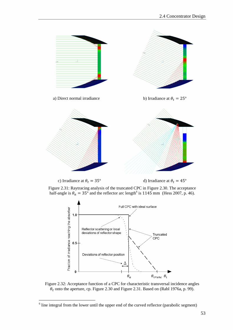
2.4 Concentrator Design
53
a) Direct normal irradiance b) Irradiance at 𝜃𝑡 = 25°
c) Irradiance at 𝜃𝑡 = 35° d) Irradiance at 𝜃𝑡 = 45°
Figure 2.31: Raytracing analysis of the truncated CPC in Figure 2.30. The acceptance
half-angle is 𝜃𝑎 = 35° and the reflector arc length6 is 1145 mm (Hess 2007, p. 46).
Figure 2.32: Acceptance function of a CPC for characteristic transversal incidence angles
𝜃𝑡 onto the aperture, cp. Figure 2.30 and Figure 2.31. Based on (Rabl 1976a, p. 99).
6 line integral from the lower until the upper end of the curved reflector (parabolic segment)
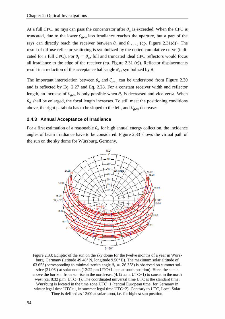
Chapter 2: Optical Investigations
54
At a full CPC, no rays can pass the concentrator after 𝜃𝑎 is exceeded. When the CPC is
truncated, due to the lower 𝐶𝑔𝑒𝑜 less irradiance reaches the aperture, but a part of the
rays can directly reach the receiver between 𝜃𝑎 and 𝜃𝑡𝑟𝑢𝑛𝑐 (cp. Figure 2.31(d)). The
result of diffuse reflector scattering is symbolized by the dotted cumulative curve (indi-
cated for a full CPC). For 𝜃𝑡 = 𝜃𝑎, full and truncated ideal CPC reflectors would focus
all irradiance to the edge of the receiver (cp. Figure 2.31 (c)). Reflector displacements
result in a reduction of the acceptance half-angle 𝜃𝑎, symbolized by ∆.
The important interrelation between 𝜃𝑎 and 𝐶𝑔𝑒𝑜 can be understood from Figure 2.30
and is reflected by Eq. 2.27 and Eq. 2.28. For a constant receiver width and reflector
length, an increase of 𝐶𝑔𝑒𝑜 is only possible when 𝜃𝑎 is decreased and vice versa. When
𝜃𝑎 shall be enlarged, the focal length increases. To still meet the positioning conditions
above, the right parabola has to be sloped to the left, and 𝐶𝑔𝑒𝑜 decreases.
2.4.3 Annual Acceptance of Irradiance
For a first estimation of a reasonable 𝜃𝑎 for high annual energy collection, the incidence
angles of beam irradiance have to be considered. Figure 2.33 shows the virtual path of
the sun on the sky dome for Würzburg, Germany.
Figure 2.33: Ecliptic of the sun on the sky dome for the twelve months of a year in Würz-
burg, Germany (latitude 49.48° N, longitude 9.56° E). The maximum solar altitude of
63.65° (corresponding to minimal zenith angle 𝜃𝑠 = 26.35°) is observed on summer sol-
stice (21.06.) at solar noon (12:22 pm UTC+1, sun at south position). Here, the sun is
above the horizon from sunrise in the north-east (4:12 a.m. UTC+1) to sunset in the north
west (ca. 8:32 p.m. UTC+1). The coordinated universal time UTC is the standard time,
Würzburg is located in the time zone UTC+1 (central European time; for Germany in
winter legal time UTC+1, in summer legal time UTC+2). Contrary to UTC, Local Solar
Time is defined as 12:00 at solar noon, i.e. for highest sun position.
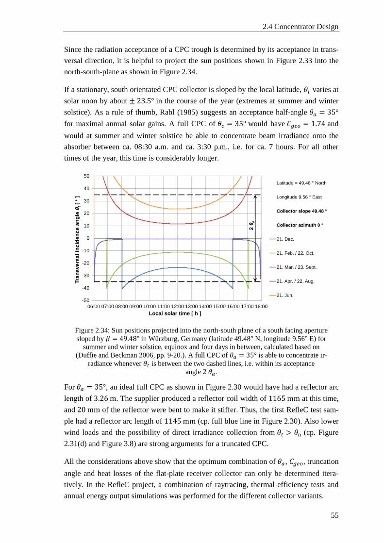
2.4 Concentrator Design
55
Since the radiation acceptance of a CPC trough is determined by its acceptance in trans-
versal direction, it is helpful to project the sun positions shown in Figure 2.33 into the
north-south-plane as shown in Figure 2.34.
If a stationary, south orientated CPC collector is sloped by the local latitude, 𝜃𝑡 varies at
solar noon by about ± 23.5° in the course of the year (extremes at summer and winter
solstice). As a rule of thumb, Rabl (1985) suggests an acceptance half-angle 𝜃𝑎 = 35°
for maximal annual solar gains. A full CPC of 𝜃𝑐 = 35° would have 𝐶𝑔𝑒𝑜 = 1.74 and
would at summer and winter solstice be able to concentrate beam irradiance onto the
absorber between ca. 08:30 a.m. and ca. 3:30 p.m., i.e. for ca. 7 hours. For all other
times of the year, this time is considerably longer.
Figure 2.34: Sun positions projected into the north-south plane of a south facing aperture
sloped by 𝛽 = 49.48° in Würzburg, Germany (latitude 49.48° N, longitude 9.56° E) for
summer and winter solstice, equinox and four days in between, calculated based on
(Duffie and Beckman 2006, pp. 9-20.). A full CPC of 𝜃𝑎 = 35° is able to concentrate ir-
radiance whenever 𝜃𝑡 is between the two dashed lines, i.e. within its acceptance
angle 2 𝜃𝑎.
For 𝜃𝑎 = 35°, an ideal full CPC as shown in Figure 2.30 would have had a reflector arc
length of 3.26 m. The supplier produced a reflector coil width of 1165 mm at this time,
and 20 mm of the reflector were bent to make it stiffer. Thus, the first RefleC test sam-
ple had a reflector arc length of 1145 mm (cp. full blue line in Figure 2.30). Also lower
wind loads and the possibility of direct irradiance collection from 𝜃𝑡 > 𝜃𝑎 (cp. Figure
2.31(d) and Figure 3.8) are strong arguments for a truncated CPC.
All the considerations above show that the optimum combination of 𝜃𝑎, 𝐶𝑔𝑒𝑜, truncation
angle and heat losses of the flat-plate receiver collector can only be determined itera-
tively. In the RefleC project, a combination of raytracing, thermal efficiency tests and
annual energy output simulations was performed for the different collector variants.
-50
-40
-30
-20
-10
0
10
20
30
40
50
06:00 07:00 08:00 09:00 10:00 11:00 12:00 13:00 14:00 15:00 16:00 17:00 18:00
Tra
nsvers
al
incid
en
ce a
ng
le θ
t[
°]
Local solar time [ h ]
Latitude = 49.48 ° North
Longitude 9.56 ° East
Collector slope 49.48 °
Collector azimuth 0 °
21. Dec.
21. Feb. / 22. Oct.
21. Mar. / 23. Sept.
21. Apr. / 22. Aug.
21. Jun.
2 θ
a
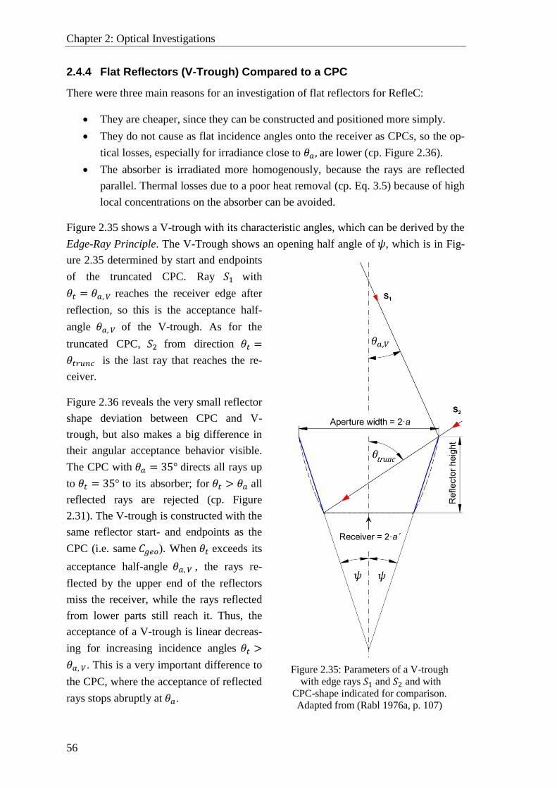
Chapter 2: Optical Investigations
56
2.4.4 Flat Reflectors (V-Trough) Compared to a CPC
There were three main reasons for an investigation of flat reflectors for RefleC:
They are cheaper, since they can be constructed and positioned more simply.
They do not cause as flat incidence angles onto the receiver as CPCs, so the op-
tical losses, especially for irradiance close to 𝜃𝑎 , are lower (cp. Figure 2.36).
The absorber is irradiated more homogenously, because the rays are reflected
parallel. Thermal losses due to a poor heat removal (cp. Eq. 3.5) because of high
local concentrations on the absorber can be avoided.
Figure 2.35 shows a V-trough with its characteristic angles, which can be derived by the
Edge-Ray Principle. The V-Trough shows an opening half angle of 𝜓, which is in Fig-
ure 2.35 determined by start and endpoints
of the truncated CPC. Ray 𝑆1 with
𝜃𝑡 = 𝜃𝑎, 𝑉 reaches the receiver edge after
reflection, so this is the acceptance half-
angle 𝜃𝑎, 𝑉 of the V-trough. As for the
truncated CPC, 𝑆2 from direction 𝜃𝑡 =
𝜃𝑡𝑟𝑢𝑛𝑐 is the last ray that reaches the re-
ceiver.
Figure 2.36 reveals the very small reflector
shape deviation between CPC and V-
trough, but also makes a big difference in
their angular acceptance behavior visible.
The CPC with 𝜃𝑎 = 35° directs all rays up
to 𝜃𝑡 = 35° to its absorber; for 𝜃𝑡 > 𝜃𝑎 all
reflected rays are rejected (cp. Figure
2.31). The V-trough is constructed with the
same reflector start- and endpoints as the
CPC (i.e. same 𝐶𝑔𝑒𝑜). When 𝜃𝑡 exceeds its
acceptance half-angle 𝜃𝑎, 𝑉 , the rays re-
flected by the upper end of the reflectors
miss the receiver, while the rays reflected
from lower parts still reach it. Thus, the
acceptance of a V-trough is linear decreas-
ing for increasing incidence angles 𝜃𝑡 >
𝜃𝑎, 𝑉. This is a very important difference to
the CPC, where the acceptance of reflected
rays stops abruptly at 𝜃𝑎.
Figure 2.35: Parameters of a V-trough
with edge rays 𝑆1 and 𝑆2 and with
CPC-shape indicated for comparison.
Adapted from (Rabl 1976a, p. 107)
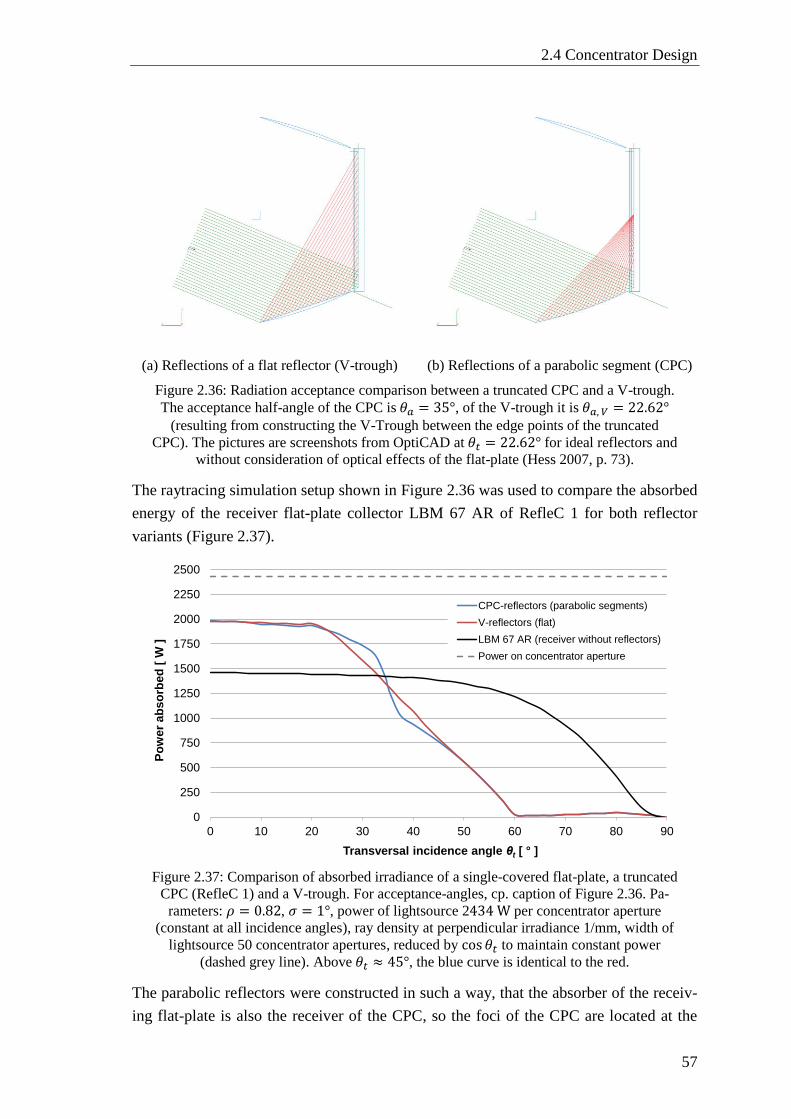
2.4 Concentrator Design
57
(a) Reflections of a flat reflector (V-trough) (b) Reflections of a parabolic segment (CPC)
Figure 2.36: Radiation acceptance comparison between a truncated CPC and a V-trough.
The acceptance half-angle of the CPC is 𝜃𝑎 = 35°, of the V-trough it is 𝜃𝑎, 𝑉 = 22.62° (resulting from constructing the V-Trough between the edge points of the truncated
CPC). The pictures are screenshots from OptiCAD at 𝜃𝑡 = 22.62° for ideal reflectors and
without consideration of optical effects of the flat-plate (Hess 2007, p. 73).
The raytracing simulation setup shown in Figure 2.36 was used to compare the absorbed
energy of the receiver flat-plate collector LBM 67 AR of RefleC 1 for both reflector
variants (Figure 2.37).
Figure 2.37: Comparison of absorbed irradiance of a single-covered flat-plate, a truncated
CPC (RefleC 1) and a V-trough. For acceptance-angles, cp. caption of Figure 2.36. Pa-
rameters: 𝜌 = 0.82, 𝜎 = 1°, power of lightsource 2434 W per concentrator aperture
(constant at all incidence angles), ray density at perpendicular irradiance 1/mm, width of
lightsource 50 concentrator apertures, reduced by cos 𝜃𝑡 to maintain constant power
(dashed grey line). Above 𝜃𝑡 ≈ 45°, the blue curve is identical to the red.
The parabolic reflectors were constructed in such a way, that the absorber of the receiv-
ing flat-plate is also the receiver of the CPC, so the foci of the CPC are located at the
0
250
500
750
1000
1250
1500
1750
2000
2250
2500
0 10 20 30 40 50 60 70 80 90
Po
wer
ab
so
rbed
[ W
]
Transversal incidence angle θt [ ° ]
CPC-reflectors (parabolic segments)
V-reflectors (flat)
LBM 67 AR (receiver without reflectors)
Power on concentrator aperture
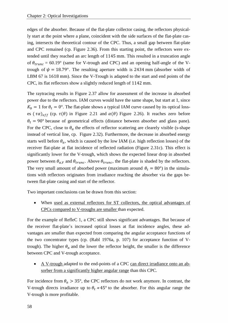
Chapter 2: Optical Investigations
58
edges of the absorber. Because of the flat-plate collector casing, the reflectors physical-
ly start at the point where a plane, coincident with the side surfaces of the flat-plate cas-
ing, intersects the theoretical contour of the CPC. Thus, a small gap between flat-plate
and CPC remained (cp. Figure 2.36). From this starting point, the reflectors were ex-
tended until they reached an arc length of 1145 mm. This resulted in a truncation angle
of 𝜃𝑡𝑟𝑢𝑛𝑐 = 60.19° (same for V-trough and CPC) and an opening half-angle of the V-
trough of 𝜓 = 18.79°. The resulting aperture width is 2434 mm (absorber width of
LBM 67 is 1618 mm). Since the V-Trough is adapted to the start and end points of the
CPC, its flat reflectors show a slightly reduced length of 1142 mm.
The raytracing results in Figure 2.37 allow for assessment of the increase in absorbed
power due to the reflectors. IAM curves would have the same shape, but start at 1, since
𝐾𝑏 = 1 for 𝜃𝑡 = 0°. The flat-plate shows a typical IAM curve caused by its optical loss-
es ( 𝜏𝛼)𝑒𝑓𝑓 (cp. 𝜏(𝜃) in Figure 2.21 and 𝛼(𝜃) Figure 2.26). It reaches zero before
𝜃𝑡 = 90° because of geometrical effects (distance between absorber and glass pane).
For the CPC, close to 𝜃𝑎 the effects of reflector scattering are clearely visible (s-shape
instead of vertical line, cp. Figure 2.32). Furthermore, the decrease in absorbed energy
starts well before 𝜃𝑎, which is caused by the low IAM (i.e. high reflection losses) of the
receiver flat-plate at flat incidence of reflected radiation (Figure 2.31c). This effect is
significantly lower for the V-trough, which shows the expected linear drop in absorbed
power between 𝜃𝑎,𝑉 and 𝜃𝑡𝑟𝑢𝑛𝑐. Above 𝜃𝑡𝑟𝑢𝑛𝑐, the flat-plate is shaded by the reflectors.
The very small amount of absorbed power (maximum around 𝜃𝑡 = 80°) in the simula-
tions with reflectors originates from irradiance reaching the absorber via the gaps be-
tween flat-plate casing and start of the reflector.
Two important conclusions can be drawn from this section:
When used as external reflectors for ST collectors, the optical advantages of
CPCs compared to V-troughs are smaller than expected.
For the example of RefleC 1, a CPC still shows significant advantages. But because of
the receiver flat-plate’s increased optical losses at flat incidence angles, these ad-
vantages are smaller than expected from comparing the angular acceptance functions of
the two concentrator types (cp. (Rabl 1976a, p. 107) for acceptance function of V-
trough). The higher 𝜃𝑎 and the lower the reflector height, the smaller is the difference
between CPC and V-trough acceptance.
A V-trough adapted to the end-points of a CPC can direct irradiance onto an ab-
sorber from a significantly higher angular range than this CPC.
For incidence from 𝜃𝑎 > 35°, the CPC reflectors do not work anymore. In contrast, the
V-trough directs irradiance up to 𝜃𝑡 45° to the absorber. For this angular range the
V-trough is more profitable.
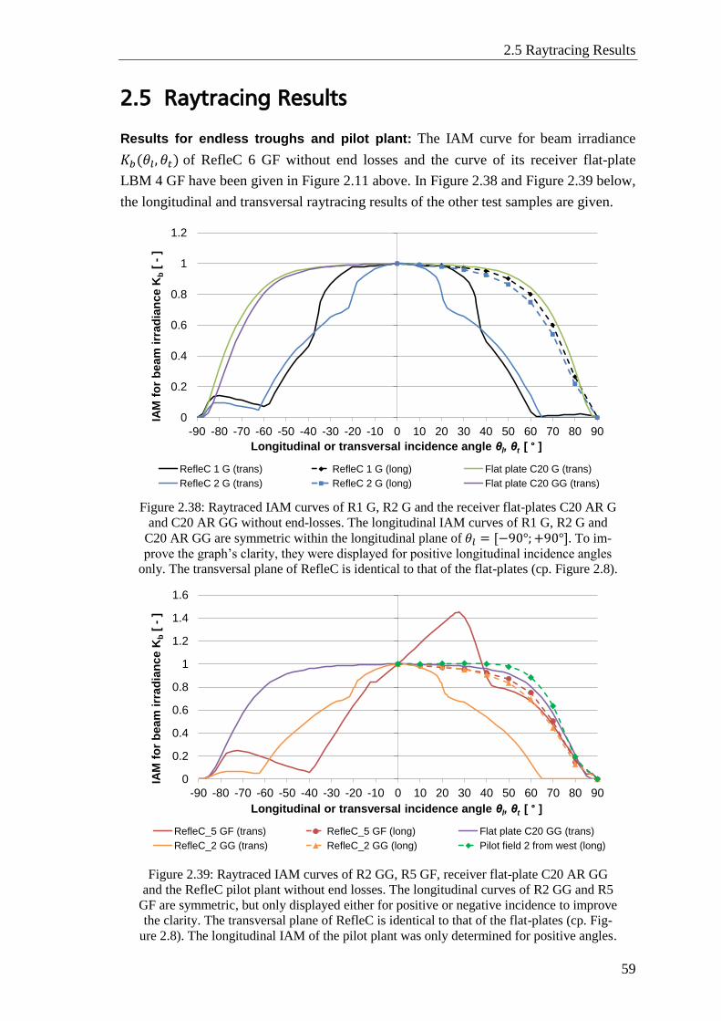
2.5 Raytracing Results
59
2.5 Raytracing Results
Results for endless troughs and pilot plant: The IAM curve for beam irradiance
𝐾𝑏(𝜃𝑙, 𝜃𝑡) of RefleC 6 GF without end losses and the curve of its receiver flat-plate
LBM 4 GF have been given in Figure 2.11 above. In Figure 2.38 and Figure 2.39 below,
the longitudinal and transversal raytracing results of the other test samples are given.
Figure 2.38: Raytraced IAM curves of R1 G, R2 G and the receiver flat-plates C20 AR G
and C20 AR GG without end-losses. The longitudinal IAM curves of R1 G, R2 G and
C20 AR GG are symmetric within the longitudinal plane of 𝜃𝑙 = [−90°;+90°]. To im-
prove the graph’s clarity, they were displayed for positive longitudinal incidence angles
only. The transversal plane of RefleC is identical to that of the flat-plates (cp. Figure 2.8).
Figure 2.39: Raytraced IAM curves of R2 GG, R5 GF, receiver flat-plate C20 AR GG
and the RefleC pilot plant without end losses. The longitudinal curves of R2 GG and R5
GF are symmetric, but only displayed either for positive or negative incidence to improve
the clarity. The transversal plane of RefleC is identical to that of the flat-plates (cp. Fig-
ure 2.8). The longitudinal IAM of the pilot plant was only determined for positive angles.
0
0.2
0.4
0.6
0.8
1
1.2
-90 -80 -70 -60 -50 -40 -30 -20 -10 0 10 20 30 40 50 60 70 80 90
IAM
fo
r b
eam
irr
ad
ian
ce K
b[
-]
Longitudinal or transversal incidence angle θl, θt [ ° ]
RefleC 1 G (trans) RefleC 1 G (long) Flat plate C20 G (trans)
RefleC 2 G (trans) RefleC 2 G (long) Flat plate C20 GG (trans)
0
0.2
0.4
0.6
0.8
1
1.2
1.4
1.6
-90 -80 -70 -60 -50 -40 -30 -20 -10 0 10 20 30 40 50 60 70 80 90
IAM
fo
r b
eam
irr
ad
ian
ce K
b[
-]
Longitudinal or transversal incidence angle θl, θt [ ° ]
RefleC_5 GF (trans) RefleC_5 GF (long) Flat plate C20 GG (trans)
RefleC_2 GG (trans) RefleC_2 GG (long) Pilot field 2 from west (long)
Chapter 2: Optical Investigations
60
In Figure 2.38, the effect of a second glass cover on the IAM can be observed when
comparing C20 G (trans) to C20 GG (trans). This effect is very similar for a glass-foil
covered collector. At RefleC 1 G and RefleC 2 G the drops of the IAM at their ac-
ceptance half-angle 𝜃𝑎 are clearly visible. It is also shown that their radiation ac-
ceptance is significantly reduced compared to a flat-plate.
In Figure 2.39, the longitudinal IAM of the RefleC subfield 2 of the pilot plant remains
close to 1 until 𝜃𝑙 = 50°. This is due to the trough closure reflectors (cp. Figure 5.4 and
Figure 5.5).
Results for test samples: The results for the test sample modules accounting for their
end-losses are given in Appendix C. The transversal IAMs of the test-samples are not
influenced by the trough length. But for the longitudinal IAMs, the exact assessment of
the influence of reflected longitudinal irradiance missing the flat-plates laterally was
important, e.g. for the calculation of the test sample’s IAM for isotropic diffuse irradi-
ance.
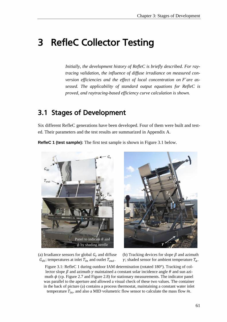
Chapter 3: Stages of Development
61
3 RefleC Collector Testing
Initially, the development history of RefleC is briefly described. For ray-
tracing validation, the influence of diffuse irradiance on measured con-
version efficiencies and the effect of local concentration on 𝐹´are as-
sessed. The applicability of standard output equations for RefleC is
proved, and raytracing-based efficiency curve calculation is shown.
3.1 Stages of Development
Six different RefleC generations have been developed. Four of them were built and test-
ed. Their parameters and the test results are summarized in Appendix A.
RefleC 1 (test sample): The first test sample is shown in Figure 3.1 below.
(a) Irradiance sensors for global 𝐺𝑡 and diffuse
𝐺𝑑𝑡; temperatures at inlet 𝑇𝑖𝑛 and outlet 𝑇𝑜𝑢𝑡.
(b) Tracking devices for slope 𝛽 and azimuth
𝛾; shaded sensor for ambient temperature 𝑇𝑎.
Figure 3.1: RefleC 1 during outdoor IAM determination (rotated 180°). Tracking of col-
lector slope 𝛽 and azimuth 𝛾 maintained a constant solar incidence angle 𝜃 and sun azi-
muth 𝜙 (cp. Figure 2.7 and Figure 2.8) for stationary measurements. The indicator panel
was parallel to the aperture and allowed a visual check of these two values. The container
in the back of picture (a) contains a process thermostat, maintaining a constant water inlet
temperature 𝑇𝑖𝑛, and also a MID volumetric flow sensor to calculate the mass flow �̇�.
𝜸
𝜷
𝑻𝒂
Panel to indicate 𝜃 and
𝜙 by shading needle
𝐺𝑑𝑡
𝐺𝑡
𝑇𝑜𝑢𝑡
𝑇𝑖𝑛
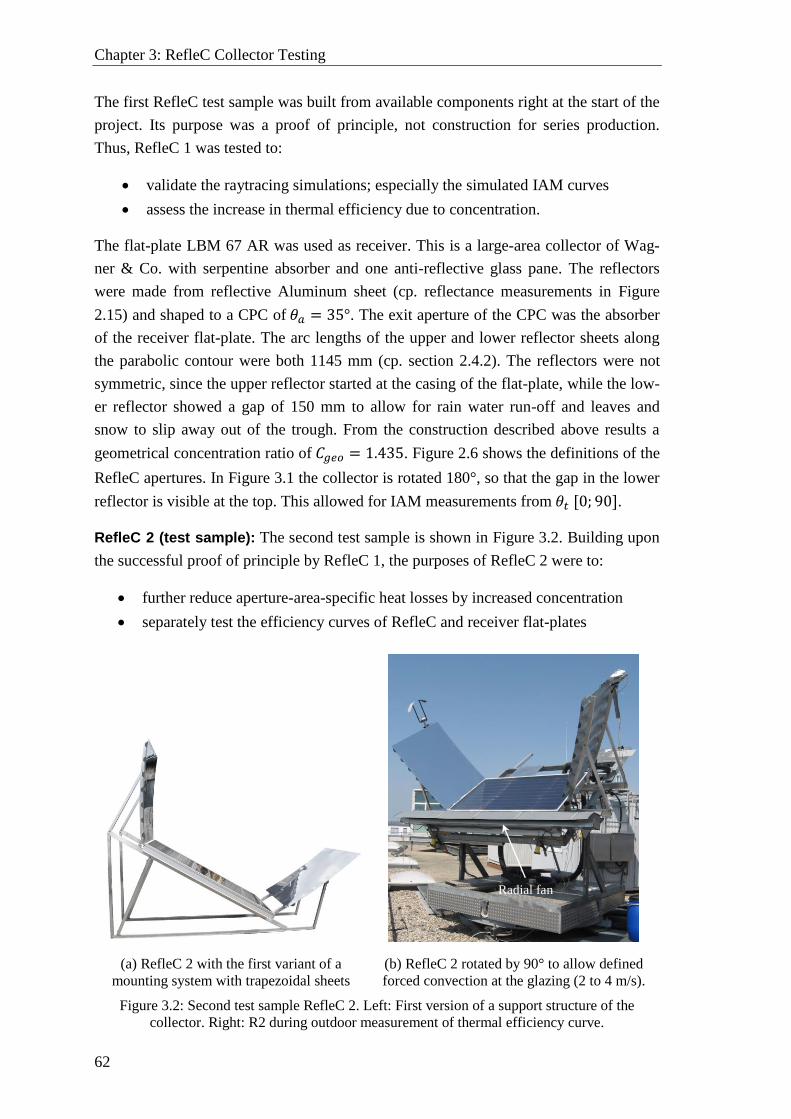
Chapter 3: RefleC Collector Testing
62
The first RefleC test sample was built from available components right at the start of the
project. Its purpose was a proof of principle, not construction for series production.
Thus, RefleC 1 was tested to:
validate the raytracing simulations; especially the simulated IAM curves
assess the increase in thermal efficiency due to concentration.
The flat-plate LBM 67 AR was used as receiver. This is a large-area collector of Wag-
ner & Co. with serpentine absorber and one anti-reflective glass pane. The reflectors
were made from reflective Aluminum sheet (cp. reflectance measurements in Figure
2.15) and shaped to a CPC of 𝜃𝑎 = 35°. The exit aperture of the CPC was the absorber
of the receiver flat-plate. The arc lengths of the upper and lower reflector sheets along
the parabolic contour were both 1145 mm (cp. section 2.4.2). The reflectors were not
symmetric, since the upper reflector started at the casing of the flat-plate, while the low-
er reflector showed a gap of 150 mm to allow for rain water run-off and leaves and
snow to slip away out of the trough. From the construction described above results a
geometrical concentration ratio of 𝐶𝑔𝑒𝑜 = 1.435. Figure 2.6 shows the definitions of the
RefleC apertures. In Figure 3.1 the collector is rotated 180°, so that the gap in the lower
reflector is visible at the top. This allowed for IAM measurements from 𝜃𝑡 [0; 90].
RefleC 2 (test sample): The second test sample is shown in Figure 3.2. Building upon
the successful proof of principle by RefleC 1, the purposes of RefleC 2 were to:
further reduce aperture-area-specific heat losses by increased concentration
separately test the efficiency curves of RefleC and receiver flat-plates
(a) RefleC 2 with the first variant of a
mounting system with trapezoidal sheets
(b) RefleC 2 rotated by 90° to allow defined
forced convection at the glazing (2 to 4 m/s).
Figure 3.2: Second test sample RefleC 2. Left: First version of a support structure of the
collector. Right: R2 during outdoor measurement of thermal efficiency curve.
Radial fan
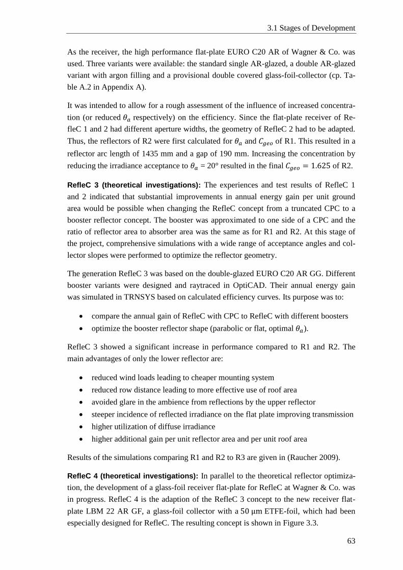
3.1 Stages of Development
63
As the receiver, the high performance flat-plate EURO C20 AR of Wagner & Co. was
used. Three variants were available: the standard single AR-glazed, a double AR-glazed
variant with argon filling and a provisional double covered glass-foil-collector (cp. Ta-
ble A.2 in Appendix A).
It was intended to allow for a rough assessment of the influence of increased concentra-
tion (or reduced 𝜃𝑎 respectively) on the efficiency. Since the flat-plate receiver of Re-
fleC 1 and 2 had different aperture widths, the geometry of RefleC 2 had to be adapted.
Thus, the reflectors of R2 were first calculated for 𝜃𝑎 and 𝐶𝑔𝑒𝑜 of R1. This resulted in a
reflector arc length of 1435 mm and a gap of 190 mm. Increasing the concentration by
reducing the irradiance acceptance to 𝜃𝑎 = 20° resulted in the final 𝐶𝑔𝑒𝑜 = 1.625 of R2.
RefleC 3 (theoretical investigations): The experiences and test results of RefleC 1
and 2 indicated that substantial improvements in annual energy gain per unit ground
area would be possible when changing the RefleC concept from a truncated CPC to a
booster reflector concept. The booster was approximated to one side of a CPC and the
ratio of reflector area to absorber area was the same as for R1 and R2. At this stage of
the project, comprehensive simulations with a wide range of acceptance angles and col-
lector slopes were performed to optimize the reflector geometry.
The generation RefleC 3 was based on the double-glazed EURO C20 AR GG. Different
booster variants were designed and raytraced in OptiCAD. Their annual energy gain
was simulated in TRNSYS based on calculated efficiency curves. Its purpose was to:
compare the annual gain of RefleC with CPC to RefleC with different boosters
optimize the booster reflector shape (parabolic or flat, optimal 𝜃𝑎).
RefleC 3 showed a significant increase in performance compared to R1 and R2. The
main advantages of only the lower reflector are:
reduced wind loads leading to cheaper mounting system
reduced row distance leading to more effective use of roof area
avoided glare in the ambience from reflections by the upper reflector
steeper incidence of reflected irradiance on the flat plate improving transmission
higher utilization of diffuse irradiance
higher additional gain per unit reflector area and per unit roof area
Results of the simulations comparing R1 and R2 to R3 are given in (Raucher 2009).
RefleC 4 (theoretical investigations): In parallel to the theoretical reflector optimiza-
tion, the development of a glass-foil receiver flat-plate for RefleC at Wagner & Co. was
in progress. RefleC 4 is the adaption of the RefleC 3 concept to the new receiver flat-
plate LBM 22 AR GF, a glass-foil collector with a 50 μm ETFE-foil, which had been
especially designed for RefleC. The resulting concept is shown in Figure 3.3.
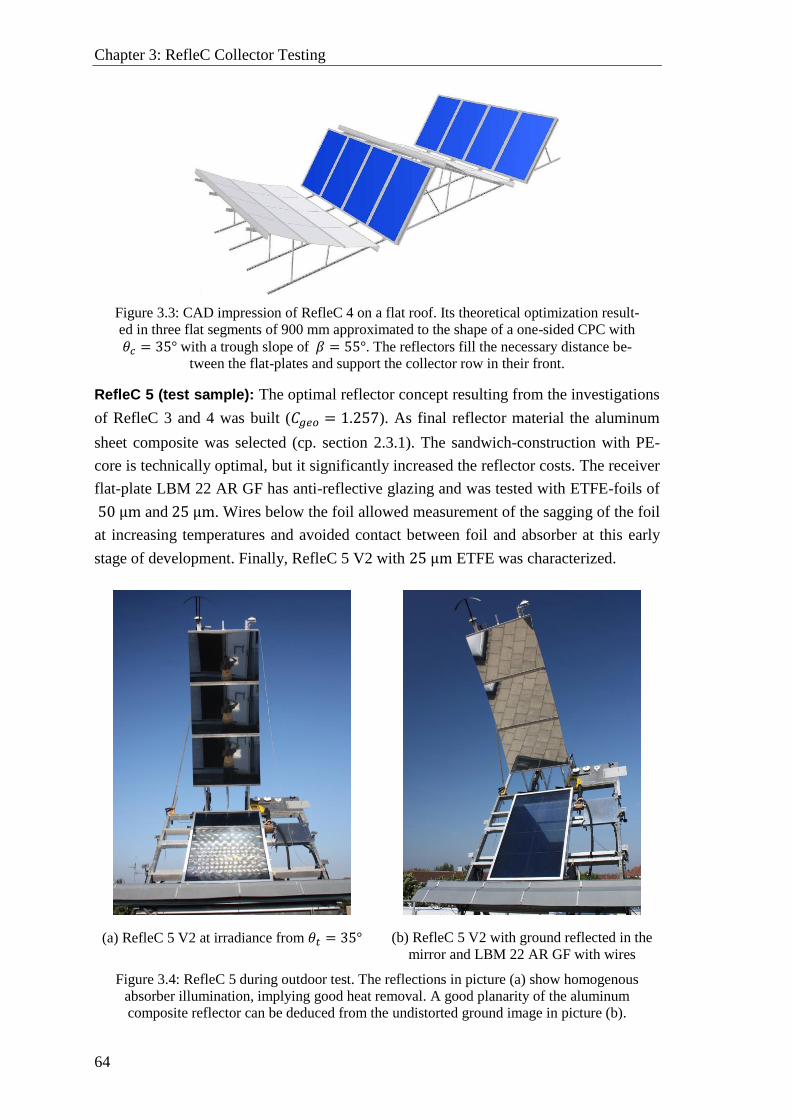
Chapter 3: RefleC Collector Testing
64
Figure 3.3: CAD impression of RefleC 4 on a flat roof. Its theoretical optimization result-
ed in three flat segments of 900 mm approximated to the shape of a one-sided CPC with
𝜃𝑐 = 35° with a trough slope of 𝛽 = 55°. The reflectors fill the necessary distance be-
tween the flat-plates and support the collector row in their front.
RefleC 5 (test sample): The optimal reflector concept resulting from the investigations
of RefleC 3 and 4 was built (𝐶𝑔𝑒𝑜 = 1.257). As final reflector material the aluminum
sheet composite was selected (cp. section 2.3.1). The sandwich-construction with PE-
core is technically optimal, but it significantly increased the reflector costs. The receiver
flat-plate LBM 22 AR GF has anti-reflective glazing and was tested with ETFE-foils of
50 μm and 25 μm. Wires below the foil allowed measurement of the sagging of the foil
at increasing temperatures and avoided contact between foil and absorber at this early
stage of development. Finally, RefleC 5 V2 with 25 μm ETFE was characterized.
(a) RefleC 5 V2 at irradiance from 𝜃𝑡 = 35° (b) RefleC 5 V2 with ground reflected in the
mirror and LBM 22 AR GF with wires
Figure 3.4: RefleC 5 during outdoor test. The reflections in picture (a) show homogenous
absorber illumination, implying good heat removal. A good planarity of the aluminum
composite reflector can be deduced from the undistorted ground image in picture (b).
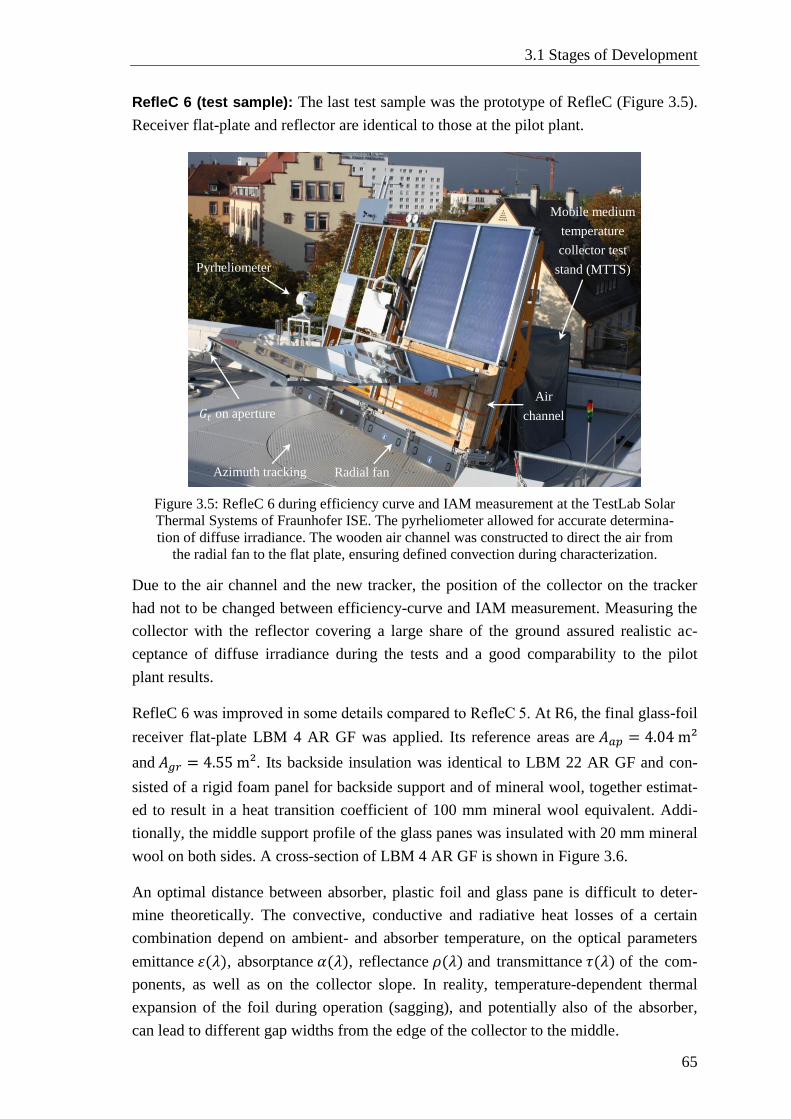
3.1 Stages of Development
65
RefleC 6 (test sample): The last test sample was the prototype of RefleC (Figure 3.5).
Receiver flat-plate and reflector are identical to those at the pilot plant.
Figure 3.5: RefleC 6 during efficiency curve and IAM measurement at the TestLab Solar
Thermal Systems of Fraunhofer ISE. The pyrheliometer allowed for accurate determina-
tion of diffuse irradiance. The wooden air channel was constructed to direct the air from
the radial fan to the flat plate, ensuring defined convection during characterization.
Due to the air channel and the new tracker, the position of the collector on the tracker
had not to be changed between efficiency-curve and IAM measurement. Measuring the
collector with the reflector covering a large share of the ground assured realistic ac-
ceptance of diffuse irradiance during the tests and a good comparability to the pilot
plant results.
RefleC 6 was improved in some details compared to RefleC 5. At R6, the final glass-foil
receiver flat-plate LBM 4 AR GF was applied. Its reference areas are 𝐴𝑎𝑝 = 4.04 m²
and 𝐴𝑔𝑟 = 4.55 m². Its backside insulation was identical to LBM 22 AR GF and con-
sisted of a rigid foam panel for backside support and of mineral wool, together estimat-
ed to result in a heat transition coefficient of 100 mm mineral wool equivalent. Addi-
tionally, the middle support profile of the glass panes was insulated with 20 mm mineral
wool on both sides. A cross-section of LBM 4 AR GF is shown in Figure 3.6.
An optimal distance between absorber, plastic foil and glass pane is difficult to deter-
mine theoretically. The convective, conductive and radiative heat losses of a certain
combination depend on ambient- and absorber temperature, on the optical parameters
emittance 휀(𝜆), absorptance 𝛼(𝜆), reflectance 𝜌(𝜆) and transmittance 𝜏(𝜆) of the com-
ponents, as well as on the collector slope. In reality, temperature-dependent thermal
expansion of the foil during operation (sagging), and potentially also of the absorber,
can lead to different gap widths from the edge of the collector to the middle.
Pyrheliometer
Mobile medium
temperature
collector test
stand (MTTS)
Air
channel 𝐺𝑡 on aperture
Radial fan Azimuth tracking
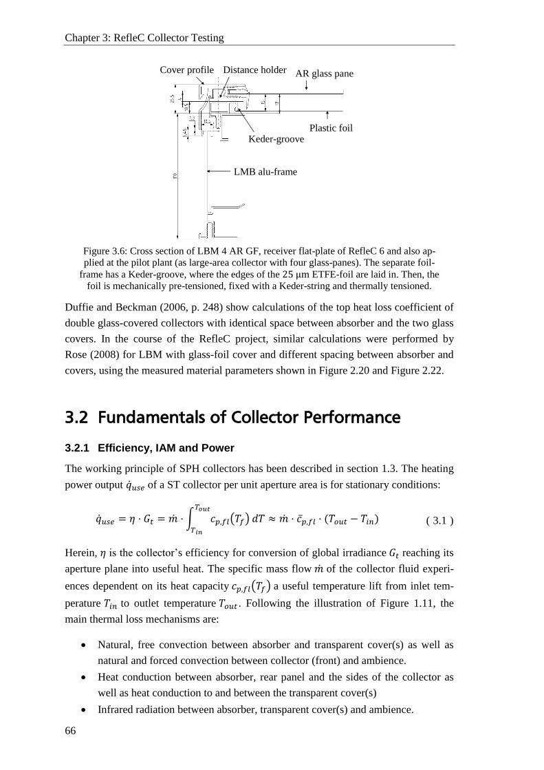
Chapter 3: RefleC Collector Testing
66
Figure 3.6: Cross section of LBM 4 AR GF, receiver flat-plate of RefleC 6 and also ap-
plied at the pilot plant (as large-area collector with four glass-panes). The separate foil-
frame has a Keder-groove, where the edges of the 25 μm ETFE-foil are laid in. Then, the
foil is mechanically pre-tensioned, fixed with a Keder-string and thermally tensioned.
Duffie and Beckman (2006, p. 248) show calculations of the top heat loss coefficient of
double glass-covered collectors with identical space between absorber and the two glass
covers. In the course of the RefleC project, similar calculations were performed by
Rose (2008) for LBM with glass-foil cover and different spacing between absorber and
covers, using the measured material parameters shown in Figure 2.20 and Figure 2.22.
3.2 Fundamentals of Collector Performance
3.2.1 Efficiency, IAM and Power
The working principle of SPH collectors has been described in section 1.3. The heating
power output �̇�𝑢𝑠𝑒 of a ST collector per unit aperture area is for stationary conditions:
�̇�𝑢𝑠𝑒 = 𝜂 ⋅ 𝐺𝑡 = �̇� ⋅ ∫ 𝑐𝑝,𝑓𝑙(𝑇𝑓) 𝑑𝑇𝑇𝑜𝑢𝑡
𝑇𝑖𝑛
≈ �̇� ⋅ 𝑐�̅�,𝑓𝑙 ⋅ (𝑇𝑜𝑢𝑡 − 𝑇𝑖𝑛) ( 3.1 )
Herein, 𝜂 is the collector’s efficiency for conversion of global irradiance 𝐺𝑡 reaching its
aperture plane into useful heat. The specific mass flow �̇� of the collector fluid experi-
ences dependent on its heat capacity 𝑐𝑝,𝑓𝑙(𝑇𝑓) a useful temperature lift from inlet tem-
perature 𝑇𝑖𝑛 to outlet temperature 𝑇𝑜𝑢𝑡 . Following the illustration of Figure 1.11, the
main thermal loss mechanisms are:
Natural, free convection between absorber and transparent cover(s) as well as
natural and forced convection between collector (front) and ambience.
Heat conduction between absorber, rear panel and the sides of the collector as
well as heat conduction to and between the transparent cover(s)
Infrared radiation between absorber, transparent cover(s) and ambience.
LBM Alu-Rahmen
SKS Kederprofil
Folie
AbstandsleisteDeckleiste
Glas
LBM Alu-Rahmen
SKS Kederprofil
Folie
AbstandsleisteDeckleiste
Glas
LMB alu-frame
Cover profile Distance holder AR glass pane
Keder-groove Plastic foil
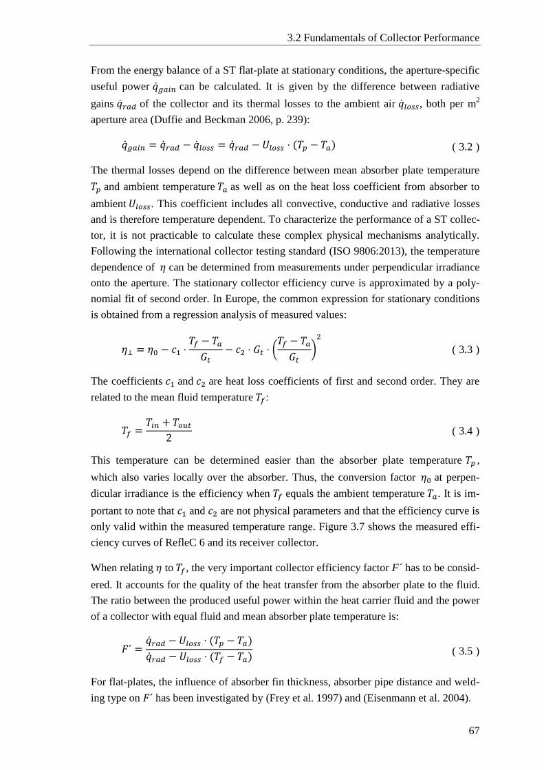
3.2 Fundamentals of Collector Performance
67
From the energy balance of a ST flat-plate at stationary conditions, the aperture-specific
useful power �̇�𝑔𝑎𝑖𝑛 can be calculated. It is given by the difference between radiative
gains �̇�𝑟𝑎𝑑 of the collector and its thermal losses to the ambient air �̇�𝑙𝑜𝑠𝑠, both per m2
aperture area (Duffie and Beckman 2006, p. 239):
�̇�𝑔𝑎𝑖𝑛 = �̇�𝑟𝑎𝑑 − �̇�𝑙𝑜𝑠𝑠 = �̇�𝑟𝑎𝑑 − 𝑈𝑙𝑜𝑠𝑠 ⋅ (𝑇𝑝 − 𝑇𝑎) ( 3.2 )
The thermal losses depend on the difference between mean absorber plate temperature
𝑇𝑝 and ambient temperature 𝑇𝑎 as well as on the heat loss coefficient from absorber to
ambient 𝑈𝑙𝑜𝑠𝑠. This coefficient includes all convective, conductive and radiative losses
and is therefore temperature dependent. To characterize the performance of a ST collec-
tor, it is not practicable to calculate these complex physical mechanisms analytically.
Following the international collector testing standard (ISO 9806:2013), the temperature
dependence of 𝜂 can be determined from measurements under perpendicular irradiance
onto the aperture. The stationary collector efficiency curve is approximated by a poly-
nomial fit of second order. In Europe, the common expression for stationary conditions
is obtained from a regression analysis of measured values:
𝜂⊥ = 𝜂0 − 𝑐1 ⋅𝑇𝑓 − 𝑇𝑎
𝐺𝑡− 𝑐2 ⋅ 𝐺𝑡 ⋅ (
𝑇𝑓 − 𝑇𝑎
𝐺𝑡)2
( 3.3 )
The coefficients 𝑐1 and 𝑐2 are heat loss coefficients of first and second order. They are
related to the mean fluid temperature 𝑇𝑓:
𝑇𝑓 =𝑇𝑖𝑛 + 𝑇𝑜𝑢𝑡
2 ( 3.4 )
This temperature can be determined easier than the absorber plate temperature 𝑇𝑝 ,
which also varies locally over the absorber. Thus, the conversion factor 𝜂0 at perpen-
dicular irradiance is the efficiency when 𝑇𝑓 equals the ambient temperature 𝑇𝑎. It is im-
portant to note that 𝑐1 and 𝑐2 are not physical parameters and that the efficiency curve is
only valid within the measured temperature range. Figure 3.7 shows the measured effi-
ciency curves of RefleC 6 and its receiver collector.
When relating 𝜂 to 𝑇𝑓, the very important collector efficiency factor F´ has to be consid-
ered. It accounts for the quality of the heat transfer from the absorber plate to the fluid.
The ratio between the produced useful power within the heat carrier fluid and the power
of a collector with equal fluid and mean absorber plate temperature is:
𝐹´ =�̇�𝑟𝑎𝑑 − 𝑈𝑙𝑜𝑠𝑠 ⋅ (𝑇𝑝 − 𝑇𝑎)
�̇�𝑟𝑎𝑑 − 𝑈𝑙𝑜𝑠𝑠 ⋅ (𝑇𝑓 − 𝑇𝑎) ( 3.5 )
For flat-plates, the influence of absorber fin thickness, absorber pipe distance and weld-
ing type on 𝐹´ has been investigated by (Frey et al. 1997) and (Eisenmann et al. 2004).
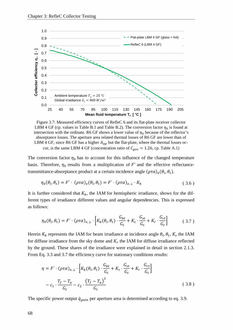
Chapter 3: RefleC Collector Testing
68
Figure 3.7: Measured efficiency curves of RefleC 6 and its flat-plate receiver collector
LBM 4 GF (cp. values in Table B.1 and Table B.2). The conversion factor 𝜂0 is found at
intersection with the ordinate. R6 GF shows a lower value of 𝜂0 because of the reflector’s
absorptance losses. The aperture area related thermal losses of R6 GF are lower than of
LBM 4 GF, since R6 GF has a higher 𝐴𝑎𝑝 but the flat-plate, where the thermal losses oc-
cur, is the same LBM 4 GF (concentration ratio of 𝐶𝑔𝑒𝑜 = 1.26, cp. Table A.1)
The conversion factor 𝜂0 has to account for this influence of the changed temperature
basis. Therefore, 𝜂0 results from a multiplication of 𝐹´ and the effective reflectance-
transmittance-absorptance product at a certain incidence angle (ρτα)e(𝜃𝑙 , 𝜃𝑡).
𝜂0(𝜃𝑙, 𝜃𝑡) = 𝐹´ ⋅ (𝜌𝜏𝛼)𝑒(𝜃𝑙, 𝜃𝑡) = 𝐹´ ⋅ (𝜌𝜏𝛼)𝑒, ⊥ ⋅ 𝐾ℎ ( 3.6 )
It is further considered that 𝐾ℎ, the IAM for hemispheric irradiance, shows for the dif-
ferent types of irradiance different values and angular dependencies. This is expressed
as follows:
𝜂0(𝜃𝑙, 𝜃𝑡) = 𝐹´ ⋅ (𝜌𝜏𝛼)𝑒, ⊥ ⋅ [𝐾𝑏(𝜃𝑙 , 𝜃𝑡) ⋅𝐺𝑏𝑡
𝐺𝑡+ 𝐾𝑠 ⋅
𝐺𝑠𝑡
𝐺𝑡+ 𝐾𝑟 ⋅
𝐺𝑟𝑡
𝐺𝑡] ( 3.7 )
Herein 𝐾𝑏 represents the IAM for beam irradiance at incidence angle 𝜃𝑙 , 𝜃𝑡, 𝐾𝑠 the IAM
for diffuse irradiance from the sky dome and 𝐾𝑟 the IAM for diffuse irradiance reflected
by the ground. These shares of the irradiance were explained in detail in section 2.1.3.
From Eq. 3.3 and 3.7 the efficiency curve for stationary conditions results:
𝜂 = 𝐹´ ⋅ (𝜌𝜏𝛼)𝑒, ⊥ ⋅ [𝐾𝑏(𝜃𝑙, 𝜃𝑡) ⋅𝐺𝑏𝑡
𝐺𝑡+ 𝐾𝑠 ⋅
𝐺𝑠𝑡
𝐺𝑡+ 𝐾𝑟 ⋅
𝐺𝑟𝑡
𝐺𝑡]
− 𝑐1 ⋅𝑇𝑓 − 𝑇𝑎
𝐺𝑡− 𝑐2 ⋅
(𝑇𝑓 − 𝑇𝑎)2
𝐺𝑡
(
3.8
)
The specific power output �̇�𝑔𝑎𝑖𝑛 per aperture area is determined according to eq. 3.9.
0.0
0.1
0.2
0.3
0.4
0.5
0.6
0.7
0.8
0.9
1.0
25 40 55 70 85 100 115 130 145 160 175 190 205
Collecto
r effic
iency η
┴[
-]
Mean fluid temperature Tf [ °C ]
Flat-plate LBM 4 GF (glass + foil)
RefleC 6 (LBM 4 GF)
Ambient temperature
Global irradiance
3.2 Fundamentals of Collector Performance
69
�̇�𝑔𝑎𝑖𝑛 = 𝜂0 ⋅ [𝐾𝑏(𝜃𝑙 , 𝜃𝑡) ⋅ 𝐺𝑏𝑡 + 𝐾𝑠 ⋅ 𝐺𝑠𝑡 + 𝐾𝑟 ⋅ 𝐺𝑟𝑡]
− 𝑐1 ⋅ (𝑇𝑓 − 𝑇𝑎) − 𝑐2 ⋅ (𝑇𝑓 − 𝑇𝑎)2
(
3.9
)
The output results from specific radiative gains �̇�𝑟𝑎𝑑 and thermal losses �̇�𝑙𝑜𝑠𝑠:
�̇�𝑟𝑎𝑑 = 𝜂0 ⋅ [𝐾𝑏(𝜃𝑙, 𝜃𝑡) ⋅ 𝐺𝑏𝑡 + 𝐾𝑠 ⋅ 𝐺𝑠𝑡 + 𝐾𝑟 ⋅ 𝐺𝑟𝑡] ( 3.10 )
�̇�𝑙𝑜𝑠𝑠 = 𝑐1 ⋅ (𝑇𝑓 − 𝑇𝑎) + 𝑐2 ⋅ (𝑇𝑓 − 𝑇𝑎)2 ( 3.11 )
Besides the very detailed modeled optical behavior, the following dynamic simulations
take also the effective thermal capacity 𝑐𝑒𝑓𝑓 of the collector into account (i.e. the capac-
ity of all components and fluid content of the collector). This is especially necessary
because of the high working temperatures of more than 100 °C and due to rapidly
changing irradiance conditions at locations in Central Europe. For the dynamic, aperture
area related specific useful power �̇�𝑢𝑠𝑒 then it can be written:
�̇�𝑢𝑠𝑒 = �̇�𝑔𝑎𝑖𝑛 − 𝑐𝑒𝑓𝑓 ⋅𝑑𝑇𝑓
𝑑𝑡= �̇�𝑟𝑎𝑑 − �̇�𝑙𝑜𝑠𝑠 − 𝑐𝑒𝑓𝑓 ⋅
𝑑𝑇𝑓
𝑑𝑡 ( 3.12 )
Thermally, Eq. 3.12 with input from Eq. 3.10 and 3.11 follows the standard expression
of full instantaneous steady-state efficiency test results as described in the current
standard (ISO 9806:2013, p. 105).
When testing according to the steady-state method, the IAM 𝐾𝑑 is not identified from
the measurements, but determined from the 𝐾𝑏 test results afterwards. This is done un-
der the simplifying assumption of isotropic irradiance from the overall collector hemi-
sphere (180°, cp. Figure 2.1, left). The dynamic test method also assumes isotropic irra-
diance from the collector hemisphere, but the important difference is that 𝐾𝑑 is deter-
mined from the test results directly. This way, the real sky anisotropy during the test
affects 𝐾𝑑, so that for the same collector often higher 𝐾𝑑 values are determined. But in
both methods as well as in state-of-the-art collector simulation models, 𝐺𝑠𝑡 and 𝐺𝑟𝑡 are
summarized and one single IAM 𝐾𝑑 for diffuse irradiance accounts for their utilization
(cp. e.g. (Haller et al. 2013, p. 6)). 𝐾𝑑 is always constant and independent of 𝛽. It is
provided in collector test reports and not varied within a simulation. In Eq. 3.10 and in
the model developed within this work, 𝐺𝑠𝑡 and 𝐺𝑟𝑡 are treated separately to allow for
separate 𝐾𝑠 and 𝐾𝑟.
The three IAMs of the irradiance components introduced above account for all optical,
geometrical and thermal effects occurring when incidence of irradiance is not perpen-
dicular to the aperture. The IAM leads to a decrease or increase of η0, resulting in a par-
allel translation of the collector efficiency curve. It is therefore notable that the relative
influence of the IAM on the collector output increases with increasing thermal losses
(i.e. at low-efficiency operation as in some process heat applications, for further expla-
nation cp. section 3.4.4).
Chapter 3: RefleC Collector Testing
70
This work primarily assesses the effect of anisotropic irradiance modeling on the collec-
tor output. Therefore, the expression in Eq. 3.12 was considered to be sufficient. State-
of-the-art dynamic collector characterization determines four other factors: zero heat
loss coefficient dependency on wind speed, the thermal loss coefficients dependency on
wind speed, radiative gains dependency on infrared (“sky-temperature”), and a coeffi-
cient for condensation gains (when the collector is below 𝑇𝑎). These factors are included
in dynamic collector models (ISO 9806:2013), (Haller et al. 2013), (Fischer et al. 2004),
but are mainly relevant for uncovered collectors. For steady-state tested, covered ST
collectors these parameters are not determined separately and therefore they are not in-
cluded in the model developed.
Test reports with performance parameters (efficiency curve and IAM) of certified ST
collectors can be obtained from the online databases of the CEN (Comité Européen de
Normalisation), Solar Keymark Scheme (Solarkeymark 2014), and the US SRCC (Solar
Rating and Certification Corporation) (SRCC 2014). Solar Keymark reports also in-
clude calculated values of monthly collector output at constant mean collector fluid
temperatures 𝑇𝑓 of 25 °𝐶, 50 °𝐶 and 75 °𝐶 for Stockholm, Athens, Davos and Würz-
burg. They are calculated with the publicly available Excel-based tool SCEnOCalc (So-
lar Collector Energy Output Calculator) (SCEnOCalc 2014).
3.2.2 IAM Values for Beam Irradiance
In section 2.2.2, the IAM for beam irradiance has been introduced and different catego-
ries have been proposed.
Interpolations for rotation symmetric IAMs: When testing flat-plate collectors with
rotation symmetric IAM, often only one single value 𝐾𝑏(𝜃 = 50°) is determined. Since
the shape of the IAM curve mainly depends on the optical losses caused by collector
cover and absorber, Souka and Safwat suggest the use of a cosine-function with the col-
lector-specific parameter 𝑏0 to describe the shape of such an IAM curve (Souka and
Safwat 1966, p. 171). Such IAM reach the value of zero well before 𝜃 = 90°, which
accounts for shading effects at high incidence angles. The function of the often so called
“𝑏0-method” is usually written as:
𝐾𝑏(𝜃) = 1 − 𝑏0(1
cos𝜃− 1) solved for 𝑏0 =
1−𝐾𝑏(𝜃)1
cos𝜃−1
( 3.13 )
Solving the equation for 𝑏0 allows for approximating all 𝐾𝑏(𝜃) from one known value.
Ambrosetti and Keller (1985, p. 19) suggest to use a tangent function instead, which
results in the effect that for all parameters 𝑟 the IAM reaches a value of zero at 𝜃 = 90°.
This can be more accurate for small distances between absorber and glazing.
𝐾𝑏(𝜃) = 1 − (tan𝜃
2)
1
𝑟 solved for 𝑟 =
ln(tan𝜃
2)
ln(1−𝐾𝑏(𝜃)) ( 3.14 )
3.2 Fundamentals of Collector Performance
71
A good overview on these and other interpolation methods is given by (Fischer 2011,
pp. 45-50). If, as in case of evacuated tube collectors, IAM values at 𝜃 = 20°, 40° and
60° have been determined, Fischer recommends a linear interpolation ending at
𝐾𝑏(𝜃 = 90°) = 0 (Fischer 2011, p. 49).
Interpolations for biaxial IAMs: When the shapes of the longitudinal and transversal
IAM curve differ significantly (as for evacuated tubes and RefleC), values of 𝐾𝑏(𝜃𝑙, 𝜃𝑡)
have to be calculated for intermediate angles (usually no 3D-IAM is available). The
state-of-the-art approach is the approximation of McIntire (1982, p. 315):
𝐾𝑏(𝜃𝑙, 𝜃𝑡) 𝐾𝑏(𝜃𝑙 , 0) ⋅ 𝐾𝑏(0, 𝜃𝑡) ( 3.15 )
This so called multiplication approach shows the highest relative errors in 𝐾𝑏 for high
incidence angles θ and from directions, where 𝐾𝑏(𝜃𝑙 , 0)and 𝐾𝑏(0, 𝜃𝑡) differ much from
each other (cp. 3D-IAM of RefleC in Figure 2.12).
Rönnelid et al. classified beam irradiance data of Stockholm (only above 200 W/m2
and from March to October) into 10°-intervals of 𝜃𝑡 and 𝜃𝑙. Accurate raytracing-values
of 𝐾𝑏(𝜃𝑙, 𝜃𝑡) of a symmetric CPC-collector were available (flat absorber, 𝐶𝑔𝑒𝑜 = 1.56,
𝜃𝑎 = 35°, truncation 0.4). The absorbed energy using the exact raytraced values was
lower than for the approximated values determined by eq. 3.15. In comparison to the
measured output of the collector (𝛽 = 40°, 𝑇𝑚 ≈ 70 °C) the authors conclude that a
simulation with the approximation of Eq. 3.15 would have overestimated the annual
collector output by approx. 4 to 5 % in this specific case (Rönnelid et al. 1997, p. 285).
The factorized calculation method of McIntire is used in nearly all established computer
programs for solar thermal simulations and is therefore a factor of uncertainty for calcu-
lations of annual energy gains. For specific collector designs, specific modifications of
the approach of McIntire have been proposed, e.g. by Helgesson (2004, p. 114), who
introduced a multiplication approach where the influence of the glazing and the reflec-
tor were accounted separately for a flat-plate variant of the MaReCo (cp. Figure 1.15).
3.2.3 IAM Values for Isotropic Diffuse Irradiance
The nature of diffuse irradiance from sky and ground has been discussed in detail within
section 2.1. Particularly in central Europe with latitudes between 40° and 60° N the con-
tribution of diffuse to the overall annual irradiation is in the range of 40 % to 60 %
(Badescu 2008, page 427).
Concentrator acceptance: Before the IAM for diffuse irradiance is discussed, the ra-
diation acceptance of R1 is used to illustrate some basic considerations. In Figure 3.8,
the collector is exposed to an ideal isotropic sky. The dashed parabolic segments show a
full CPC. It accepts all diffuse irradiance from 𝜃𝑡 < 𝜃𝑎, because it directs all irradiance
from within its acceptance angle towards the absorber (green arrows).
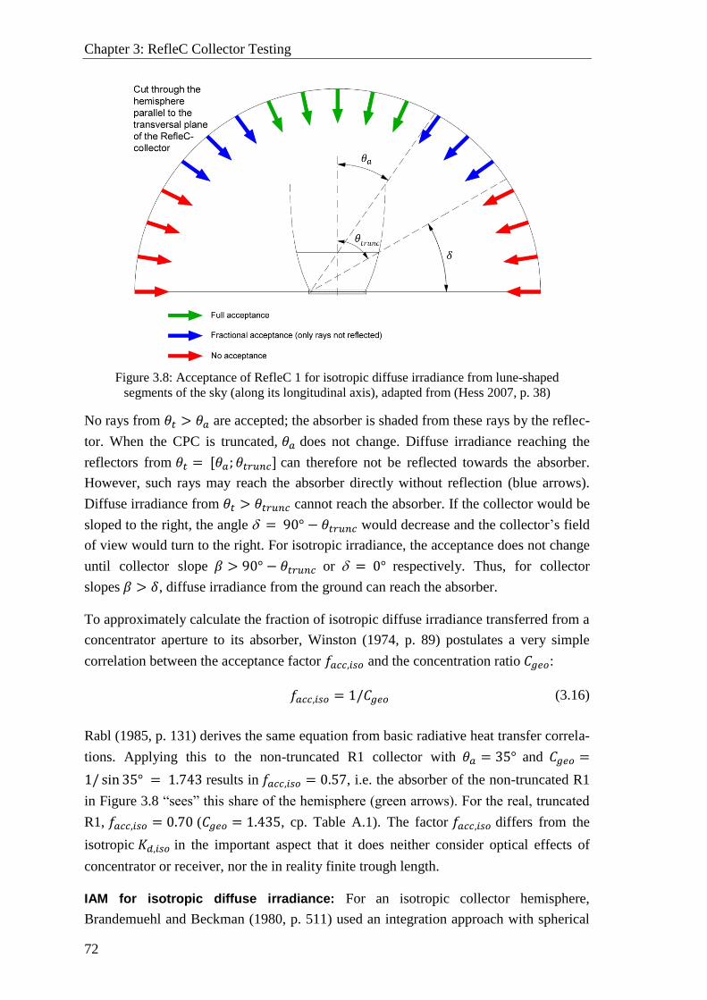
Chapter 3: RefleC Collector Testing
72
Figure 3.8: Acceptance of RefleC 1 for isotropic diffuse irradiance from lune-shaped
segments of the sky (along its longitudinal axis), adapted from (Hess 2007, p. 38)
No rays from 𝜃𝑡 > 𝜃𝑎 are accepted; the absorber is shaded from these rays by the reflec-
tor. When the CPC is truncated, 𝜃𝑎 does not change. Diffuse irradiance reaching the
reflectors from 𝜃𝑡 = [𝜃𝑎; 𝜃𝑡𝑟𝑢𝑛𝑐] can therefore not be reflected towards the absorber.
However, such rays may reach the absorber directly without reflection (blue arrows).
Diffuse irradiance from 𝜃𝑡 > 𝜃𝑡𝑟𝑢𝑛𝑐 cannot reach the absorber. If the collector would be
sloped to the right, the angle = 90° − 𝜃𝑡𝑟𝑢𝑛𝑐 would decrease and the collector’s field
of view would turn to the right. For isotropic irradiance, the acceptance does not change
until collector slope 𝛽 > 90° − 𝜃𝑡𝑟𝑢𝑛𝑐 or = 0° respectively. Thus, for collector
slopes 𝛽 > 𝛿, diffuse irradiance from the ground can reach the absorber.
To approximately calculate the fraction of isotropic diffuse irradiance transferred from a
concentrator aperture to its absorber, Winston (1974, p. 89) postulates a very simple
correlation between the acceptance factor 𝑓𝑎𝑐𝑐,𝑖𝑠𝑜 and the concentration ratio 𝐶𝑔𝑒𝑜:
𝑓𝑎𝑐𝑐,𝑖𝑠𝑜 = 1/𝐶𝑔𝑒𝑜 ( 3.16 )
Rabl (1985, p. 131) derives the same equation from basic radiative heat transfer correla-
tions. Applying this to the non-truncated R1 collector with 𝜃𝑎 = 35° and 𝐶𝑔𝑒𝑜 =
1/ sin 35° = 1.743 results in 𝑓𝑎𝑐𝑐,𝑖𝑠𝑜 = 0.57, i.e. the absorber of the non-truncated R1
in Figure 3.8 “sees” this share of the hemisphere (green arrows). For the real, truncated
R1, 𝑓𝑎𝑐𝑐,𝑖𝑠𝑜 = 0.70 (𝐶𝑔𝑒𝑜 = 1.435, cp. Table A.1). The factor 𝑓𝑎𝑐𝑐,𝑖𝑠𝑜 differs from the
isotropic 𝐾𝑑,𝑖𝑠𝑜 in the important aspect that it does neither consider optical effects of
concentrator or receiver, nor the in reality finite trough length.
IAM for isotropic diffuse irradiance: For an isotropic collector hemisphere,
Brandemuehl and Beckman (1980, p. 511) used an integration approach with spherical
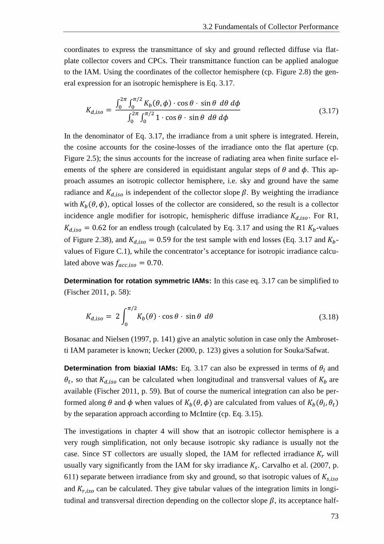
3.2 Fundamentals of Collector Performance
73
coordinates to express the transmittance of sky and ground reflected diffuse via flat-
plate collector covers and CPCs. Their transmittance function can be applied analogue
to the IAM. Using the coordinates of the collector hemisphere (cp. Figure 2.8) the gen-
eral expression for an isotropic hemisphere is Eq. 3.17.
𝐾𝑑,𝑖𝑠𝑜 = ∫ ∫ 𝐾𝑏(𝜃, 𝜙) ⋅ cos 𝜃 ⋅
𝜋/2
0
2𝜋
0sin 𝜃 𝑑𝜃 𝑑𝜙
∫ ∫ 1 ⋅ cos 𝜃 ⋅ 𝜋/2
0
2𝜋
0sin 𝜃 𝑑𝜃 𝑑𝜙
( 3.17 )
In the denominator of Eq. 3.17, the irradiance from a unit sphere is integrated. Herein,
the cosine accounts for the cosine-losses of the irradiance onto the flat aperture (cp.
Figure 2.5); the sinus accounts for the increase of radiating area when finite surface el-
ements of the sphere are considered in equidistant angular steps of 𝜃 and 𝜙. This ap-
proach assumes an isotropic collector hemisphere, i.e. sky and ground have the same
radiance and 𝐾𝑑,𝑖𝑠𝑜 is independent of the collector slope 𝛽. By weighting the irradiance
with 𝐾𝑏(𝜃, 𝜙), optical losses of the collector are considered, so the result is a collector
incidence angle modifier for isotropic, hemispheric diffuse irradiance 𝐾𝑑,𝑖𝑠𝑜. For R1,
𝐾𝑑,𝑖𝑠𝑜 = 0.62 for an endless trough (calculated by Eq. 3.17 and using the R1 𝐾𝑏-values
of Figure 2.38), and 𝐾𝑑,𝑖𝑠𝑜 = 0.59 for the test sample with end losses (Eq. 3.17 and 𝐾𝑏-
values of Figure C.1), while the concentrator’s acceptance for isotropic irradiance calcu-
lated above was 𝑓𝑎𝑐𝑐,𝑖𝑠𝑜 = 0.70.
Determination for rotation symmetric IAMs: In this case eq. 3.17 can be simplified to
(Fischer 2011, p. 58):
𝐾𝑑,𝑖𝑠𝑜 = 2∫ 𝐾𝑏(𝜃) ⋅ cos 𝜃 ⋅𝜋/2
0
sin 𝜃 𝑑𝜃 ( 3.18 )
Bosanac and Nielsen (1997, p. 141) give an analytic solution in case only the Ambroset-
ti IAM parameter is known; Uecker (2000, p. 123) gives a solution for Souka/Safwat.
Determination from biaxial IAMs: Eq. 3.17 can also be expressed in terms of 𝜃𝑙 and
𝜃𝑡, so that 𝐾𝑑,𝑖𝑠𝑜 can be calculated when longitudinal and transversal values of 𝐾𝑏 are
available (Fischer 2011, p. 59). But of course the numerical integration can also be per-
formed along 𝜃 and 𝜙 when values of 𝐾𝑏(𝜃, 𝜙) are calculated from values of 𝐾𝑏(𝜃𝑙, 𝜃𝑡)
by the separation approach according to McIntire (cp. Eq. 3.15).
The investigations in chapter 4 will show that an isotropic collector hemisphere is a
very rough simplification, not only because isotropic sky radiance is usually not the
case. Since ST collectors are usually sloped, the IAM for reflected irradiance 𝐾𝑟 will
usually vary significantly from the IAM for sky irradiance 𝐾𝑠. Carvalho et al. (2007, p.
611) separate between irradiance from sky and ground, so that isotropic values of 𝐾𝑠,𝑖𝑠𝑜
and 𝐾𝑟,𝑖𝑠𝑜 can be calculated. They give tabular values of the integration limits in longi-
tudinal and transversal direction depending on the collector slope 𝛽, its acceptance half-
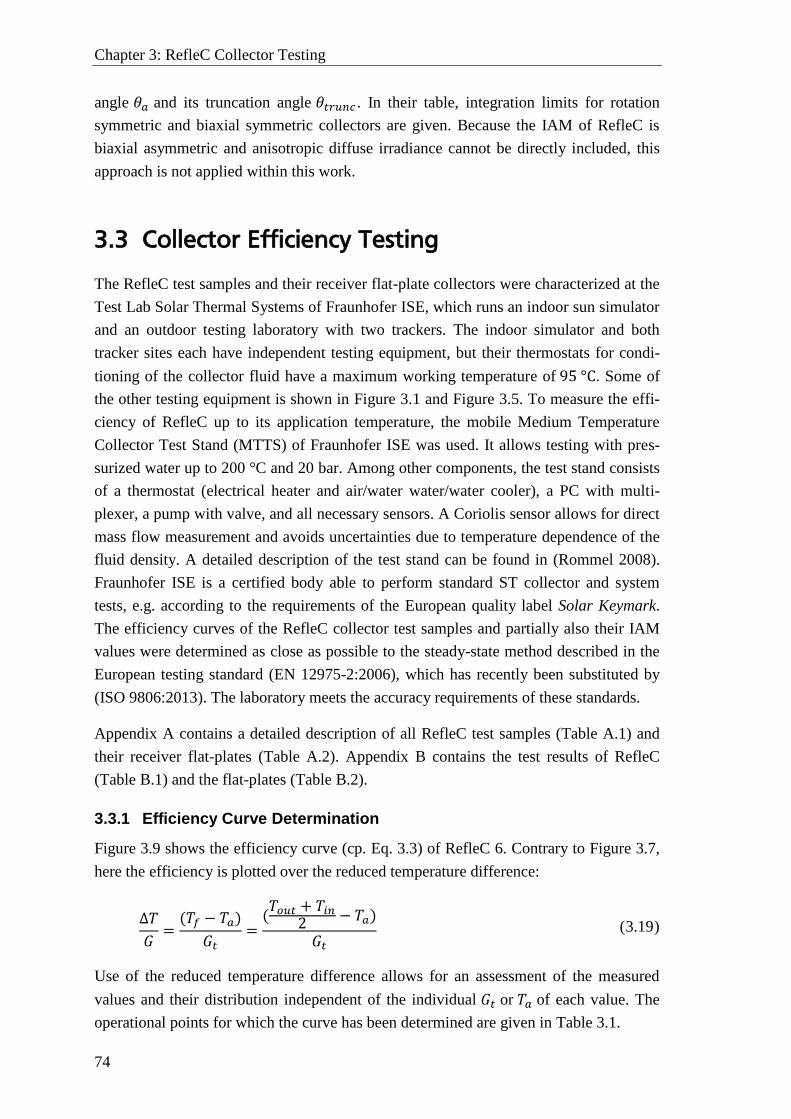
Chapter 3: RefleC Collector Testing
74
angle 𝜃𝑎 and its truncation angle 𝜃𝑡𝑟𝑢𝑛𝑐 . In their table, integration limits for rotation
symmetric and biaxial symmetric collectors are given. Because the IAM of RefleC is
biaxial asymmetric and anisotropic diffuse irradiance cannot be directly included, this
approach is not applied within this work.
3.3 Collector Efficiency Testing
The RefleC test samples and their receiver flat-plate collectors were characterized at the
Test Lab Solar Thermal Systems of Fraunhofer ISE, which runs an indoor sun simulator
and an outdoor testing laboratory with two trackers. The indoor simulator and both
tracker sites each have independent testing equipment, but their thermostats for condi-
tioning of the collector fluid have a maximum working temperature of 95 °C. Some of
the other testing equipment is shown in Figure 3.1 and Figure 3.5. To measure the effi-
ciency of RefleC up to its application temperature, the mobile Medium Temperature
Collector Test Stand (MTTS) of Fraunhofer ISE was used. It allows testing with pres-
surized water up to 200 °C and 20 bar. Among other components, the test stand consists
of a thermostat (electrical heater and air/water water/water cooler), a PC with multi-
plexer, a pump with valve, and all necessary sensors. A Coriolis sensor allows for direct
mass flow measurement and avoids uncertainties due to temperature dependence of the
fluid density. A detailed description of the test stand can be found in (Rommel 2008).
Fraunhofer ISE is a certified body able to perform standard ST collector and system
tests, e.g. according to the requirements of the European quality label Solar Keymark.
The efficiency curves of the RefleC collector test samples and partially also their IAM
values were determined as close as possible to the steady-state method described in the
European testing standard (EN 12975-2:2006), which has recently been substituted by
(ISO 9806:2013). The laboratory meets the accuracy requirements of these standards.
Appendix A contains a detailed description of all RefleC test samples (Table A.1) and
their receiver flat-plates (Table A.2). Appendix B contains the test results of RefleC
(Table B.1) and the flat-plates (Table B.2).
3.3.1 Efficiency Curve Determination
Figure 3.9 shows the efficiency curve (cp. Eq. 3.3) of RefleC 6. Contrary to Figure 3.7,
here the efficiency is plotted over the reduced temperature difference:
∆𝑇
𝐺=
(𝑇𝑓 − 𝑇𝑎)
𝐺𝑡=
(𝑇𝑜𝑢𝑡 + 𝑇𝑖𝑛
2 − 𝑇𝑎)
𝐺𝑡 ( 3.19 )
Use of the reduced temperature difference allows for an assessment of the measured
values and their distribution independent of the individual 𝐺𝑡 or 𝑇𝑎 of each value. The
operational points for which the curve has been determined are given in Table 3.1.
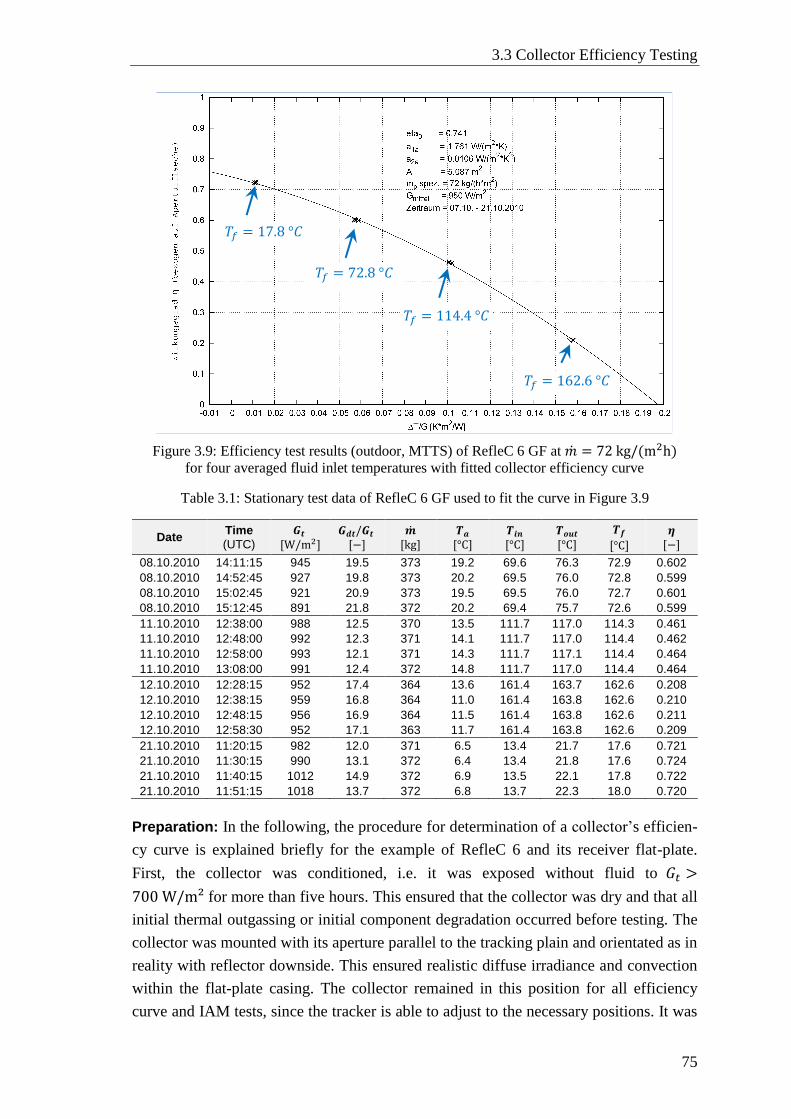
3.3 Collector Efficiency Testing
75
Figure 3.9: Efficiency test results (outdoor, MTTS) of RefleC 6 GF at �̇� = 72 kg/(m2h) for four averaged fluid inlet temperatures with fitted collector efficiency curve
Table 3.1: Stationary test data of RefleC 6 GF used to fit the curve in Figure 3.9
Date Time
(UTC)
𝑮𝒕 [W/m2]
𝑮𝒅𝒕/𝑮𝒕 [−]
�̇�
[kg] 𝑻𝒂
[°C] 𝑻𝒊𝒏
[°C] 𝑻𝒐𝒖𝒕
[°C]
𝑻𝒇
[°C]
𝜼
[−]
08.10.2010 14:11:15 945 19.5 373 19.2 69.6 76.3 72.9 0.602
08.10.2010 14:52:45 927 19.8 373 20.2 69.5 76.0 72.8 0.599
08.10.2010 15:02:45 921 20.9 373 19.5 69.5 76.0 72.7 0.601
08.10.2010 15:12:45 891 21.8 372 20.2 69.4 75.7 72.6 0.599
11.10.2010 12:38:00 988 12.5 370 13.5 111.7 117.0 114.3 0.461
11.10.2010 12:48:00 992 12.3 371 14.1 111.7 117.0 114.4 0.462
11.10.2010 12:58:00 993 12.1 371 14.3 111.7 117.1 114.4 0.464
11.10.2010 13:08:00 991 12.4 372 14.8 111.7 117.0 114.4 0.464
12.10.2010 12:28:15 952 17.4 364 13.6 161.4 163.7 162.6 0.208
12.10.2010 12:38:15 959 16.8 364 11.0 161.4 163.8 162.6 0.210
12.10.2010 12:48:15 956 16.9 364 11.5 161.4 163.8 162.6 0.211
12.10.2010 12:58:30 952 17.1 363 11.7 161.4 163.8 162.6 0.209
21.10.2010 11:20:15 982 12.0 371 6.5 13.4 21.7 17.6 0.721
21.10.2010 11:30:15 990 13.1 372 6.4 13.4 21.8 17.6 0.724
21.10.2010 11:40:15 1012 14.9 372 6.9 13.5 22.1 17.8 0.722
21.10.2010 11:51:15 1018 13.7 372 6.8 13.7 22.3 18.0 0.720
Preparation: In the following, the procedure for determination of a collector’s efficien-
cy curve is explained briefly for the example of RefleC 6 and its receiver flat-plate.
First, the collector was conditioned, i.e. it was exposed without fluid to 𝐺𝑡 >
700 W/m² for more than five hours. This ensured that the collector was dry and that all
initial thermal outgassing or initial component degradation occurred before testing. The
collector was mounted with its aperture parallel to the tracking plain and orientated as in
reality with reflector downside. This ensured realistic diffuse irradiance and convection
within the flat-plate casing. The collector remained in this position for all efficiency
curve and IAM tests, since the tracker is able to adjust to the necessary positions. It was
𝑇𝑓 = 17.8 °𝐶
𝑇𝑓 = 72.8 °𝐶
𝑇𝑓 = 114.4 °𝐶
𝑇𝑓 = 162.6 °𝐶
Chapter 3: RefleC Collector Testing
76
ensured that the global tilted irradiance pyranometer was within the aperture plane be-
side the collector and that the pyrheliometer was placed nearby. A wind channel en-
sured an even distribution of the forced convection over the cover of the receiver (cp.
Figure 3.5). The hydraulic circuit consisted of thermostat, pump, mass flow sensor and
adjustment valve, expansion vessel, deaerator, and the collector with the Pt 100 sensors
𝑇𝑖𝑛 and 𝑇𝑜𝑢𝑡. The circuit was fully insulated and free of leakage or air. Inlet and outlet
temperature sensors were positioned directly beside the collector and had been calibrat-
ed absolutely and then relative to each other. They were mounted in such a way that the
fluid flow was parallel towards the tips of the centred temperature lance of the sensors.
Testing: To account for the particular characteristics of RefleC, special attention was
paid to the accurate determination of incidence angle (visual verification) and fraction
of diffuse irradiance. The collector efficiency tests were performed under clear sky con-
ditions. The collector efficiency was determined for at least four different temperature
levels 𝑇𝑓. These temperature levels were evenly distributed over the operation range of
the collector. For each of the four temperature levels, at least four independent station-
ary test data points (mean value of 10 min interval) were determined (cp. Table 3.1), i.e.
a minimum of 16 valid data points was determined to generate one efficiency curve.
The (stability) criteria for these data points are given in Table 3.2. Before a valid sta-
tionary phase of 10 min can start, a pre-conditioning phase of 15 min with a stable inlet
temperature (i.e. with deviation according to Table 3.2) is mandatory. The values of all
sensors were logged by the multiplexer in a 15 s interval and stored in daily files.
Table 3.2: Criteria for valid outdoor steady-state efficiency test points according to (EN 12975-
2:2006) with own comment on test of RefleC 6 and LBM 4 GF (n. s. = not specified). The crite-
ria are identical to these in the current standard (ISO 9806:2013).
Parameter Requirement Permitted deviation* Comment
𝐺𝑡 > 700 W/m² ±50 W/m² Pyranometer in 𝐴𝑎𝑝
𝐺𝑑𝑡/𝐺𝑏𝑡 < 0.3 n. s. 𝐺𝑑𝑡 calculated from pyrheliometer-DNI
𝑇𝑎 n.s. ±1.5 K Shaded and vented
𝑇𝑖𝑛 One temperature level
𝑇𝑓 > 80 °C ±0.1 K
Recommended: One level at ∆𝑇/𝐺 > 0.09,
one at 𝑇𝑓 = 𝑇𝑎 ± 3 K
𝑇𝑜𝑢𝑡 𝑇𝑜𝑢𝑡 > 𝑇𝑖𝑛 + 1 K n.s Avoiding high errors
�̇� 0.02 kg/(m2s) ** if not specified
±0.1 % i.e. 72 kg/(m2h)
Air speed 3 m/s ±1 m/s at flat-plate aperture
* of 30s average value from mean value within one 10 min data point test interval ** the selected �̇� must not vary above 10 % for all data points of an efficiency curve
Efficiency curve determination: The test data were filtered for valid test data points
by a script with adjustable conditioning phase and deviation ranges. The final selection
of valid data points for one temperature level was done manually, taking high resolution
curve-plots of all sensor values into account. The collector efficiency of one test interval
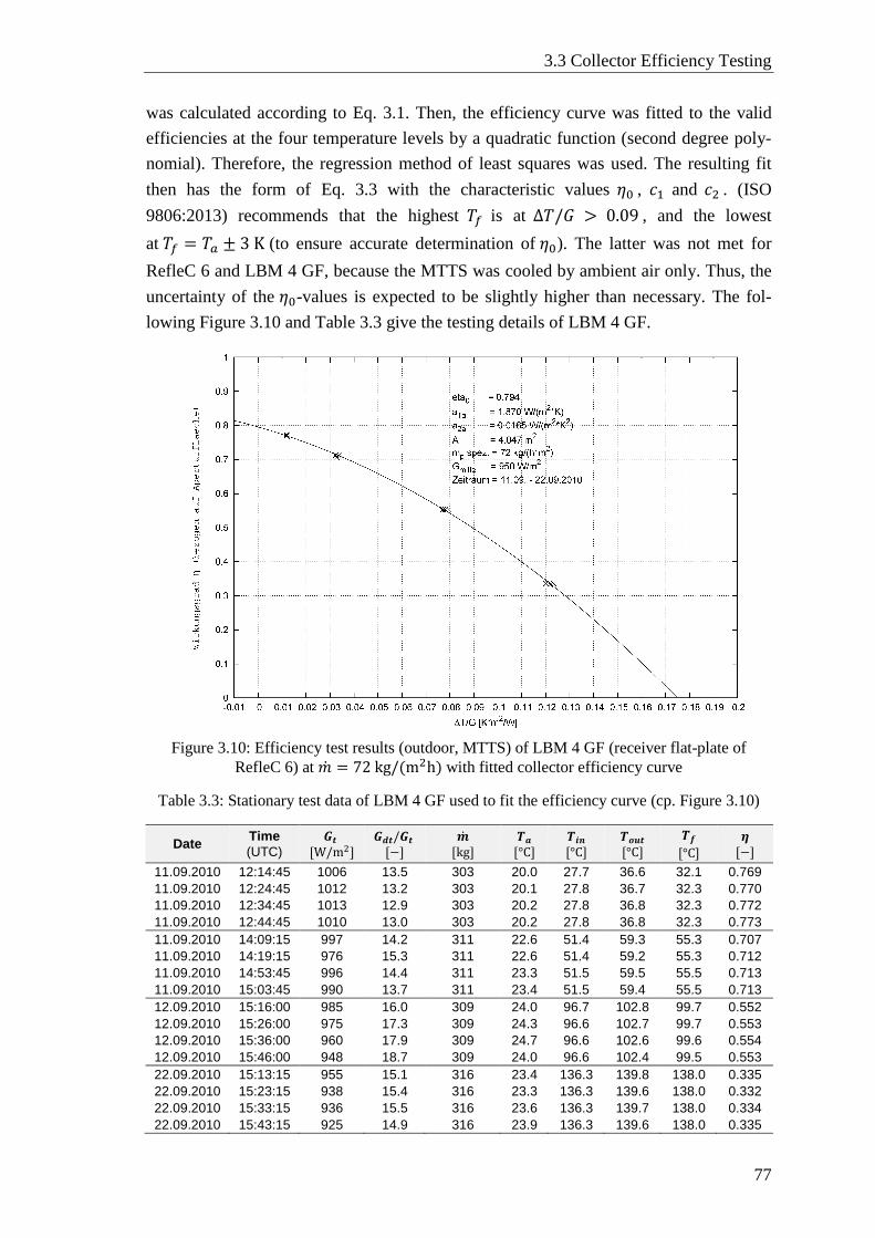
3.3 Collector Efficiency Testing
77
was calculated according to Eq. 3.1. Then, the efficiency curve was fitted to the valid
efficiencies at the four temperature levels by a quadratic function (second degree poly-
nomial). Therefore, the regression method of least squares was used. The resulting fit
then has the form of Eq. 3.3 with the characteristic values 𝜂0 , 𝑐1 and 𝑐2 . (ISO
9806:2013) recommends that the highest 𝑇𝑓 is at ∆𝑇/𝐺 > 0.09 , and the lowest
at 𝑇𝑓 = 𝑇𝑎 ± 3 K (to ensure accurate determination of 𝜂0). The latter was not met for
RefleC 6 and LBM 4 GF, because the MTTS was cooled by ambient air only. Thus, the
uncertainty of the 𝜂0-values is expected to be slightly higher than necessary. The fol-
lowing Figure 3.10 and Table 3.3 give the testing details of LBM 4 GF.
Figure 3.10: Efficiency test results (outdoor, MTTS) of LBM 4 GF (receiver flat-plate of
RefleC 6) at �̇� = 72 kg/(m2h) with fitted collector efficiency curve
Table 3.3: Stationary test data of LBM 4 GF used to fit the efficiency curve (cp. Figure 3.10)
Date Time
(UTC)
𝑮𝒕 [W/m2]
𝑮𝒅𝒕/𝑮𝒕 [−]
�̇�
[kg] 𝑻𝒂
[°C] 𝑻𝒊𝒏
[°C] 𝑻𝒐𝒖𝒕
[°C]
𝑻𝒇
[°C]
𝜼
[−]
11.09.2010 12:14:45 1006 13.5 303 20.0 27.7 36.6 32.1 0.769
11.09.2010 12:24:45 1012 13.2 303 20.1 27.8 36.7 32.3 0.770
11.09.2010 12:34:45 1013 12.9 303 20.2 27.8 36.8 32.3 0.772
11.09.2010 12:44:45 1010 13.0 303 20.2 27.8 36.8 32.3 0.773
11.09.2010 14:09:15 997 14.2 311 22.6 51.4 59.3 55.3 0.707
11.09.2010 14:19:15 976 15.3 311 22.6 51.4 59.2 55.3 0.712
11.09.2010 14:53:45 996 14.4 311 23.3 51.5 59.5 55.5 0.713
11.09.2010 15:03:45 990 13.7 311 23.4 51.5 59.4 55.5 0.713
12.09.2010 15:16:00 985 16.0 309 24.0 96.7 102.8 99.7 0.552
12.09.2010 15:26:00 975 17.3 309 24.3 96.6 102.7 99.7 0.553
12.09.2010 15:36:00 960 17.9 309 24.7 96.6 102.6 99.6 0.554
12.09.2010 15:46:00 948 18.7 309 24.0 96.6 102.4 99.5 0.553
22.09.2010 15:13:15 955 15.1 316 23.4 136.3 139.8 138.0 0.335
22.09.2010 15:23:15 938 15.4 316 23.3 136.3 139.6 138.0 0.332
22.09.2010 15:33:15 936 15.5 316 23.6 136.3 139.7 138.0 0.334
22.09.2010 15:43:15 925 14.9 316 23.9 136.3 139.6 138.0 0.335
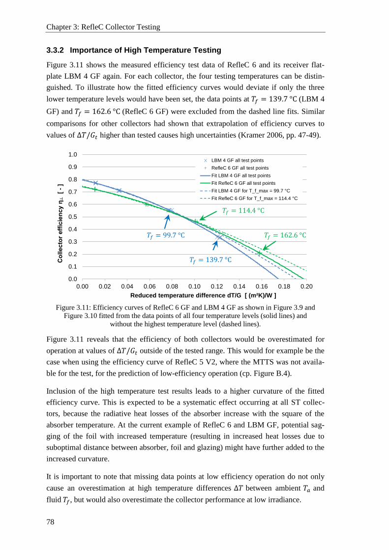
Chapter 3: RefleC Collector Testing
78
3.3.2 Importance of High Temperature Testing
Figure 3.11 shows the measured efficiency test data of RefleC 6 and its receiver flat-
plate LBM 4 GF again. For each collector, the four testing temperatures can be distin-
guished. To illustrate how the fitted efficiency curves would deviate if only the three
lower temperature levels would have been set, the data points at 𝑇𝑓 = 139.7 °C (LBM 4
GF) and 𝑇𝑓 = 162.6 °C (RefleC 6 GF) were excluded from the dashed line fits. Similar
comparisons for other collectors had shown that extrapolation of efficiency curves to
values of ∆𝑇/𝐺𝑡 higher than tested causes high uncertainties (Kramer 2006, pp. 47-49).
Figure 3.11: Efficiency curves of RefleC 6 GF and LBM 4 GF as shown in Figure 3.9 and
Figure 3.10 fitted from the data points of all four temperature levels (solid lines) and
without the highest temperature level (dashed lines).
Figure 3.11 reveals that the efficiency of both collectors would be overestimated for
operation at values of ∆𝑇/𝐺𝑡 outside of the tested range. This would for example be the
case when using the efficiency curve of RefleC 5 V2, where the MTTS was not availa-
ble for the test, for the prediction of low-efficiency operation (cp. Figure B.4).
Inclusion of the high temperature test results leads to a higher curvature of the fitted
efficiency curve. This is expected to be a systematic effect occurring at all ST collec-
tors, because the radiative heat losses of the absorber increase with the square of the
absorber temperature. At the current example of RefleC 6 and LBM GF, potential sag-
ging of the foil with increased temperature (resulting in increased heat losses due to
suboptimal distance between absorber, foil and glazing) might have further added to the
increased curvature.
It is important to note that missing data points at low efficiency operation do not only
cause an overestimation at high temperature differences ∆𝑇 between ambient 𝑇𝑎 and
fluid 𝑇𝑓, but would also overestimate the collector performance at low irradiance.
0.0
0.1
0.2
0.3
0.4
0.5
0.6
0.7
0.8
0.9
1.0
0.00 0.02 0.04 0.06 0.08 0.10 0.12 0.14 0.16 0.18 0.20
Collecto
r effic
iency η
┴[
-]
Reduced temperature difference dT/G [ (m²K)/W ]
LBM 4 GF all test points
RefleC 6 GF all test points
Fit LBM 4 GF all test points
Fit RefleC 6 GF all test points
Fit LBM 4 GF for T_f_max = 99.7 °C
Fit RefleC 6 GF for T_f_max = 114.4 °C
𝑇𝑓 = 99.7 °C
𝑇𝑓 = 114.4 °C
𝑇𝑓 = 139.7 °C
𝑇𝑓 = 162.6 °C
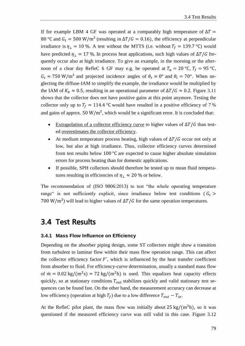
3.4 Test Results
79
If for example LBM 4 GF was operated at a comparably high temperature of ∆𝑇 =
80 °C and 𝐺𝑡 = 500 W/m² (resulting in ∆𝑇/𝐺 = 0.16), the efficiency at perpendicular
irradiance is 𝜂⊥ = 10 %. A test without the MTTS (i.e. without 𝑇𝑓 = 139.7 °C) would
have predicted 𝜂⊥ = 17 %. In process heat applications, such high values of ∆𝑇/𝐺 fre-
quently occur also at high irradiance. To give an example, in the morning or the after-
noon of a clear day RefleC 6 GF may e.g. be operated at 𝑇𝑎 = 20 °C, 𝑇𝑓 = 95 °C,
𝐺𝑡 ≈ 750 W/m² and projected incidence angles of 𝜃𝑡 ≈ 0° and 𝜃𝑙 = 70°. When ne-
glecting the diffuse-IAM to simplify the example, the irradiance would be multiplied by
the IAM of 𝐾𝑏 ≈ 0.5, resulting in an operational parameter of ∆𝑇/𝐺 ≈ 0.2. Figure 3.11
shows that the collector does not have positive gains at this point anymore. Testing the
collector only up to 𝑇𝑓 = 114.4 °C would have resulted in a positive efficiency of 7 %
and gains of approx. 50 W/m², which would be a significant error. It is concluded that:
Extrapolation of a collector efficiency curve to higher values of ∆𝑇/𝐺 than test-
ed overestimates the collector efficiency.
At medium temperature process heating, high values of ∆𝑇/𝐺 occur not only at
low, but also at high irradiance. Thus, collector efficiency curves determined
from test results below 100 °C are expected to cause higher absolute simulation
errors for process heating than for domestic applications.
If possible, SPH collectors should therefore be tested up to mean fluid tempera-
tures resulting in efficiencies of 𝜂⊥ ≈ 20 % or below.
The recommendation of (ISO 9806:2013) to test “the whole operating temperature
range“ is not sufficiently explicit, since irradiance below test conditions ( 𝐺𝑡 >
700 W/m²) will lead to higher values of ∆𝑇/𝐺 for the same operation temperatures.
3.4 Test Results
3.4.1 Mass Flow Influence on Efficiency
Depending on the absorber piping design, some ST collectors might show a transition
from turbulent to laminar flow within their mass flow operation range. This can affect
the collector efficiency factor 𝐹´, which is influenced by the heat transfer coefficient
from absorber to fluid. For efficiency-curve determination, usually a standard mass flow
of �̇� = 0.02 kg/(m2s) = 72 kg/(m2h) is used. This equalizes heat capacity effects
quickly, so at stationary conditions 𝑇𝑜𝑢𝑡 stabilizes quickly and valid stationary test se-
quences can be found fast. On the other hand, the measurement accuracy can decrease at
low efficiency (operation at high 𝑇𝑓) due to a low difference 𝑇𝑜𝑢𝑡 − 𝑇𝑖𝑛.
At the RefleC pilot plant, the mass flow was initially about 25 kg/(m2h), so it was
questioned if the measured efficiency curve was still valid in this case. Figure 3.12
Chapter 3: RefleC Collector Testing
80
shows test results at standard and reduced mass flow. For the receiver flat-plate it indi-
cates a slight decrease in 𝐹´, which results in a parallel, slightly lower efficiency curve.
RefleC 6 GF shows no decrease, but �̇� through the LBM is a factor of 𝐶𝑔𝑒𝑜 higher,
since it is related to aperture. The high temperature results of RefleC 6 at �̇� =
35 kg/(m2h) have a high uncertainty, since 𝑇𝑜𝑢𝑡 − 𝑇𝑖𝑛 is very low in this case.
Figure 3.12: Comparison of MTTS-measured collector efficiencies of RefleC 6 GF and
LBM 4 GF at mass flow rates 72 kg/(m2h) and 35 kg/(m2h), cp. Figure 3.10 to Figure
B.10 and Figure 3.9 to Figure B.6 for original test results. No fit curve is provided for Re-
fleC 6 GF at 35 kg/(m2h) because only two temperatures could be tested.
The receiver of RefleC 5 V2 has the same LBM absorber as RefleC 6. It was tested at
�̇� = 72 kg/(m2h) and �̇� = 26 kg/(m2h) (not shown in Figure 3.12, cp. Figure B.4
and Figure B.5). Since standard equipment was used (limitation to 𝑇𝑜𝑢𝑡 = 95 °C), a
comparison of the efficiency curves does not make much sense in this case; no efficien-
cies below 55 % were determined. But due to the process thermostat, 𝜂0 was measured
very accurately and is as at RefleC 6 GF not affected by the smaller mass flow.
3.4.2 Absorber Temperatures and Local Concentration
On their receivers, CPC concentrators cause regions with higher intensity. Raytracing
shows that this is maximal at transversal irradiance from 𝜃𝑡 = 𝜃𝑎, where all irradiance
reaching a reflector is focused onto the edge of the absorber. In this case, a concentra-
tion line is created (cp. Figure 2.31 c and Figure 3.13). The highest local concentrations
are to be expected for RefleC 2, since it has the highest 𝐶𝑔𝑒𝑜. To investigate effects of
this, a combination of thermographic imaging and absorber temperature measurement
with direct contact sensors was used. The tests were carried out with a single glass cov-
er because the transmittance of the glazing for infrared radiance from the absorber is
poor (cp. Figure 2.22). Figure 3.14 and Figure 3.15 show the results.
0.0
0.1
0.2
0.3
0.4
0.5
0.6
0.7
0.8
0.9
1.0
0.00 0.02 0.04 0.06 0.08 0.10 0.12 0.14 0.16 0.18 0.20
Collecto
r effic
iency η
┴[
-]
Reduced temperature difference dT/G [ (m²K)/W ]
LBM 4 GF all test points (m_p = 72)
RefleC 6 GF all test points (m_p = 72)
LBM 4 GF all test points (m_p = 35)
RefleC 6 GF all test points (m_p = 35)
Fit LBM 4 GF all test points (m_p = 72)
Fit RefleC 6 GF all test points (m_p = 72)
Fit LBM 4 GF all test points (m_p = 35)
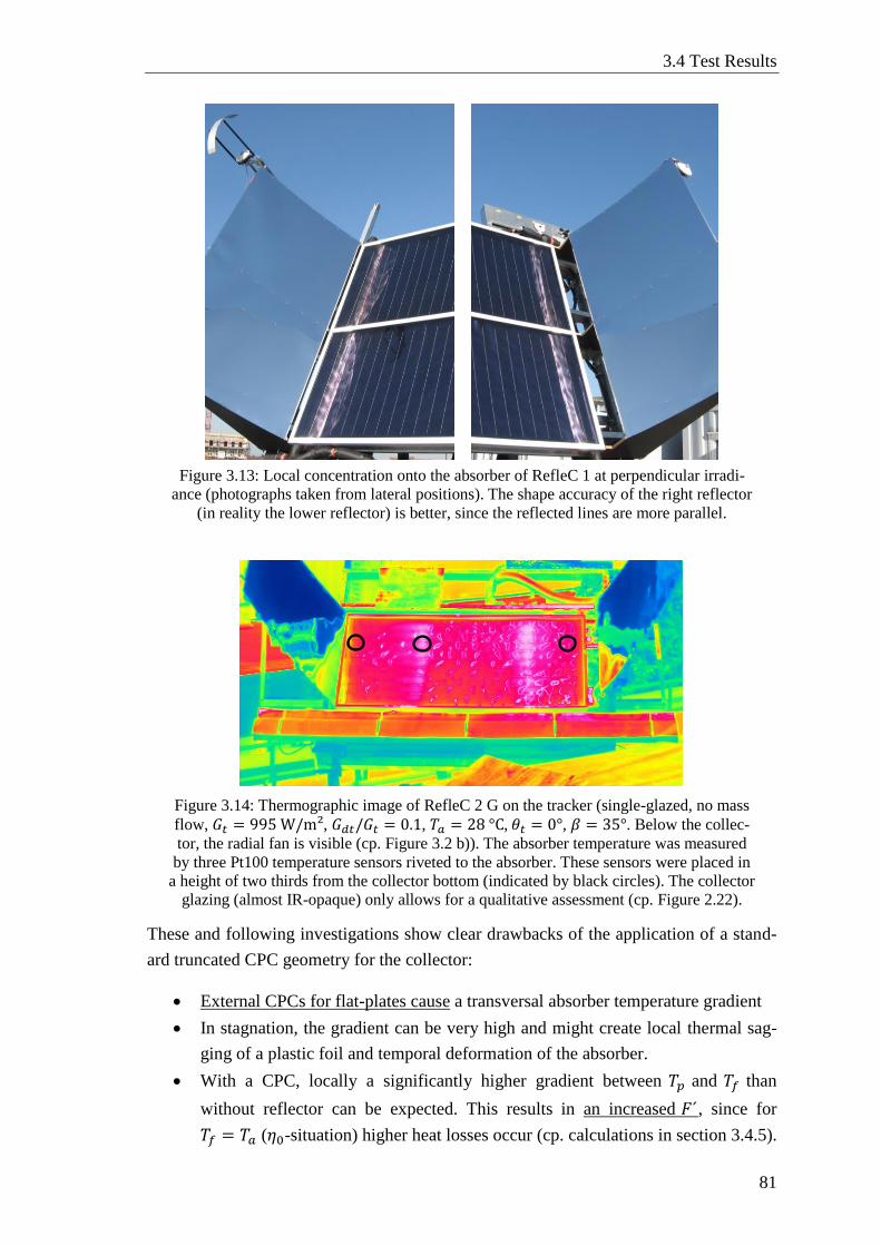
3.4 Test Results
81
Figure 3.13: Local concentration onto the absorber of RefleC 1 at perpendicular irradi-
ance (photographs taken from lateral positions). The shape accuracy of the right reflector
(in reality the lower reflector) is better, since the reflected lines are more parallel.
Figure 3.14: Thermographic image of RefleC 2 G on the tracker (single-glazed, no mass
flow, 𝐺𝑡 = 995 W/m², 𝐺𝑑𝑡/𝐺𝑡 = 0.1, 𝑇𝑎 = 28 °C, 𝜃𝑡 = 0°, 𝛽 = 35°. Below the collec-
tor, the radial fan is visible (cp. Figure 3.2 b)). The absorber temperature was measured
by three Pt100 temperature sensors riveted to the absorber. These sensors were placed in
a height of two thirds from the collector bottom (indicated by black circles). The collector
glazing (almost IR-opaque) only allows for a qualitative assessment (cp. Figure 2.22).
These and following investigations show clear drawbacks of the application of a stand-
ard truncated CPC geometry for the collector:
External CPCs for flat-plates cause a transversal absorber temperature gradient
In stagnation, the gradient can be very high and might create local thermal sag-
ging of a plastic foil and temporal deformation of the absorber.
With a CPC, locally a significantly higher gradient between 𝑇𝑝 and 𝑇𝑓 than
without reflector can be expected. This results in an increased 𝐹´, since for
𝑇𝑓 = 𝑇𝑎 (𝜂0-situation) higher heat losses occur (cp. calculations in section 3.4.5).
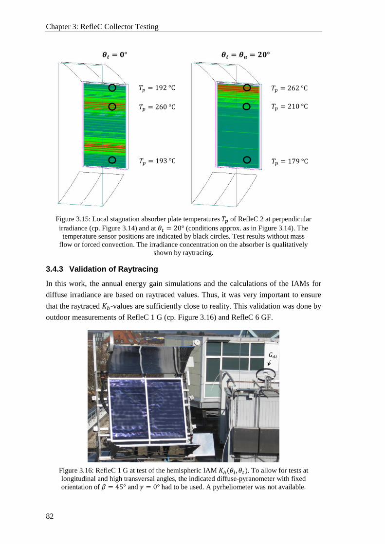
Chapter 3: RefleC Collector Testing
82
𝜽𝒕 = 𝟎°
𝜽𝒕 = 𝜽𝒂 = 𝟐𝟎°
Figure 3.15: Local stagnation absorber plate temperatures 𝑇𝑝 of RefleC 2 at perpendicular
irradiance (cp. Figure 3.14) and at 𝜃𝑡 = 20° (conditions approx. as in Figure 3.14). The
temperature sensor positions are indicated by black circles. Test results without mass
flow or forced convection. The irradiance concentration on the absorber is qualitatively
shown by raytracing.
3.4.3 Validation of Raytracing
In this work, the annual energy gain simulations and the calculations of the IAMs for
diffuse irradiance are based on raytraced values. Thus, it was very important to ensure
that the raytraced 𝐾𝑏-values are sufficiently close to reality. This validation was done by
outdoor measurements of RefleC 1 G (cp. Figure 3.16) and RefleC 6 GF.
Figure 3.16: RefleC 1 G at test of the hemispheric IAM 𝐾ℎ(𝜃𝑙, 𝜃𝑡). To allow for tests at
longitudinal and high transversal angles, the indicated diffuse-pyranometer with fixed
orientation of 𝛽 = 45° and 𝛾 = 0° had to be used. A pyrheliometer was not available.
𝑇𝑝 = 192 °C
𝑇𝑝 = 260 °C
𝑇𝑝 = 193 °C 𝑇𝑝 = 179 °C
𝑇𝑝 = 210 °C
𝑇𝑝 = 262 °C
𝐺𝑑𝑡
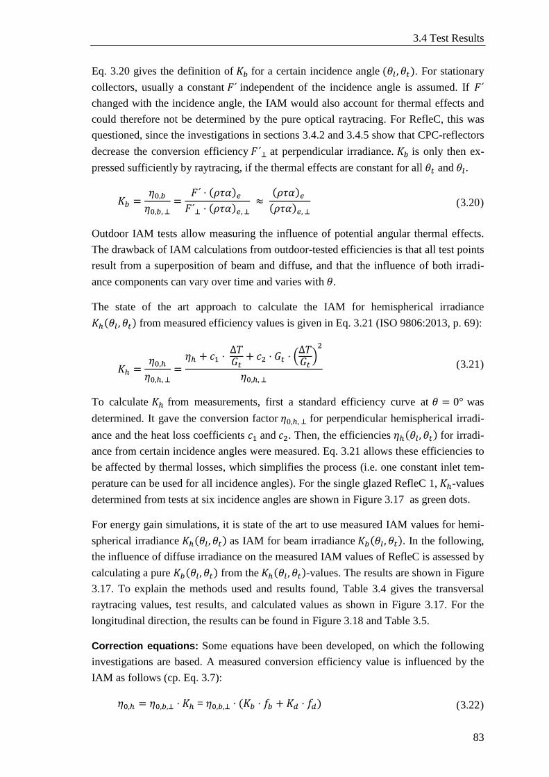
3.4 Test Results
83
Eq. 3.20 gives the definition of 𝐾𝑏 for a certain incidence angle (𝜃𝑙 , 𝜃𝑡). For stationary
collectors, usually a constant 𝐹´ independent of the incidence angle is assumed. If 𝐹´
changed with the incidence angle, the IAM would also account for thermal effects and
could therefore not be determined by the pure optical raytracing. For RefleC, this was
questioned, since the investigations in sections 3.4.2 and 3.4.5 show that CPC-reflectors
decrease the conversion efficiency 𝐹´⊥ at perpendicular irradiance. 𝐾𝑏 is only then ex-
pressed sufficiently by raytracing, if the thermal effects are constant for all 𝜃𝑡 and 𝜃𝑙.
𝐾𝑏 =𝜂0,𝑏
𝜂0,𝑏, ⊥=
𝐹´ ⋅ (𝜌𝜏𝛼)𝑒
𝐹´⊥ ⋅ (𝜌𝜏𝛼)𝑒, ⊥ ≈
(𝜌𝜏𝛼)𝑒
(𝜌𝜏𝛼)𝑒, ⊥ ( 3.20 )
Outdoor IAM tests allow measuring the influence of potential angular thermal effects.
The drawback of IAM calculations from outdoor-tested efficiencies is that all test points
result from a superposition of beam and diffuse, and that the influence of both irradi-
ance components can vary over time and varies with 𝜃.
The state of the art approach to calculate the IAM for hemispherical irradiance
𝐾ℎ(𝜃𝑙 , 𝜃𝑡) from measured efficiency values is given in Eq. 3.21 (ISO 9806:2013, p. 69):
𝐾ℎ =𝜂0,ℎ
𝜂0,ℎ, ⊥=
𝜂ℎ + 𝑐1 ⋅ ∆𝑇𝐺𝑡
+ 𝑐2 ⋅ 𝐺𝑡 ⋅ (∆𝑇𝐺𝑡
)2
𝜂0,ℎ, ⊥ ( 3.21 )
To calculate 𝐾ℎ from measurements, first a standard efficiency curve at 𝜃 = 0° was
determined. It gave the conversion factor 𝜂0,ℎ, ⊥ for perpendicular hemispherical irradi-
ance and the heat loss coefficients 𝑐1 and 𝑐2. Then, the efficiencies 𝜂ℎ(𝜃𝑙, 𝜃𝑡) for irradi-
ance from certain incidence angles were measured. Eq. 3.21 allows these efficiencies to
be affected by thermal losses, which simplifies the process (i.e. one constant inlet tem-
perature can be used for all incidence angles). For the single glazed RefleC 1, 𝐾ℎ-values
determined from tests at six incidence angles are shown in Figure 3.17 as green dots.
For energy gain simulations, it is state of the art to use measured IAM values for hemi-
spherical irradiance 𝐾ℎ(𝜃𝑙, 𝜃𝑡) as IAM for beam irradiance 𝐾𝑏(𝜃𝑙 , 𝜃𝑡). In the following,
the influence of diffuse irradiance on the measured IAM values of RefleC is assessed by
calculating a pure 𝐾𝑏(𝜃𝑙, 𝜃𝑡) from the 𝐾ℎ(𝜃𝑙 , 𝜃𝑡)-values. The results are shown in Figure
3.17. To explain the methods used and results found, Table 3.4 gives the transversal
raytracing values, test results, and calculated values as shown in Figure 3.17. For the
longitudinal direction, the results can be found in Figure 3.18 and Table 3.5.
Correction equations: Some equations have been developed, on which the following
investigations are based. A measured conversion efficiency value is influenced by the
IAM as follows (cp. Eq. 3.7):
𝜂0,ℎ = 𝜂0,𝑏,⊥ ⋅ 𝐾ℎ = 𝜂0,𝑏,⊥ ⋅ (𝐾𝑏 ⋅ 𝑓𝑏 + 𝐾𝑑 ⋅ 𝑓𝑑) ( 3.22 )
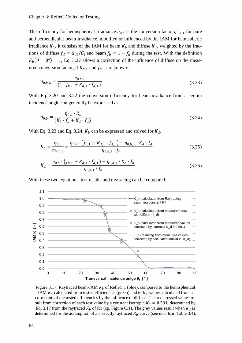
Chapter 3: RefleC Collector Testing
84
This efficiency for hemispherical irradiance 𝜂0,ℎ is the conversion factor 𝜂0,𝑏,⊥ for pure
and perpendicular beam irradiance, modified or influenced by the IAM for hemispheric
irradiance 𝐾ℎ. It consists of the IAM for beam 𝐾𝑏 and diffuse 𝐾𝑑, weighted by the frac-
tions of diffuse 𝑓𝑑 = 𝐺𝑑𝑡/𝐺𝑡 and beam 𝑓𝑏 = 1 − 𝑓𝑑 during the test. With the definition
𝐾𝑏(𝜃 = 0°) = 1, Eq. 3.22 allows a correction of the influence of diffuse on the meas-
ured conversion factor, if 𝐾𝑑,⊥ and 𝑓𝑑,⊥ are known:
𝜂0,𝑏,⊥ =𝜂0,ℎ,⊥
(1 ⋅ 𝑓𝑏,⊥ + 𝐾𝑑,⊥ ⋅ 𝑓𝑑,⊥) ( 3.23 )
With Eq. 3.20 and 3.22 the conversion efficiency for beam irradiance from a certain
incidence angle can generally be expressed as:
𝜂0,𝑏 =𝜂0,ℎ ⋅ 𝐾𝑏
(𝐾𝑏 ⋅ 𝑓𝑏 + 𝐾𝑑 ⋅ 𝑓𝑑) ( 3.24 )
With Eq. 3.23 and Eq. 3.24, 𝐾𝑏 can be expressed and solved for 𝐾𝑑 .
𝐾𝑏 =𝜂0,𝑏
𝜂0,𝑏, ⊥=
𝜂0,ℎ ⋅ (𝑓𝑏,⊥ + 𝐾𝑑,⊥ ⋅ 𝑓𝑑,⊥) − 𝜂0,ℎ,⊥ ⋅ 𝐾𝑑 ⋅ 𝑓𝑑𝜂0,ℎ,⊥ ⋅ 𝑓𝑏
( 3.25 )
𝐾𝑑 =𝜂0,ℎ ⋅ (𝑓𝑏,⊥ + 𝐾𝑑,⊥ ⋅ 𝑓𝑑,⊥) − 𝜂0,ℎ,⊥ ⋅ 𝐾𝑏 ⋅ 𝑓𝑏
𝜂0,ℎ,⊥ ⋅ 𝑓𝑑 ( 3.26 )
With these two equations, test results and raytracing can be compared.
Figure 3.17: Raytraced beam-IAM 𝐾𝑏 of RefleC 1 (blue), compared to the hemispherical
IAM 𝐾ℎ calculated from tested efficiencies (green) and to 𝐾𝑏-values calculated from a
correction of the tested efficiencies by the influence of diffuse. The red crossed values re-
sult from correction of each test value by a constant isotropic 𝐾𝑑 = 0.591, determined by
Eq. 3.17 from the raytraced 𝐾𝑏 of R1 (cp. Figure C.1). The grey values result when 𝐾𝑑 is
determined for the assumption of a correctly raytraced 𝐾𝑏-curve (see details in Table 3.4).
0.0
0.1
0.2
0.3
0.4
0.5
0.6
0.7
0.8
0.9
1.0
1.1
0 10 20 30 40 50 60 70 80 90
IAM
K
[ -
]
Transversal incidence anlge θt [ ° ]
K_b (calculated from Raytracingassuming constant F´)
K_h (calculated from measurementswith different f_d)
K_b (calculated from measured valuescorrected by isotropic K_d = 0.591)
K_b (resulting from measured valuescorrected by calculated individual K_d)
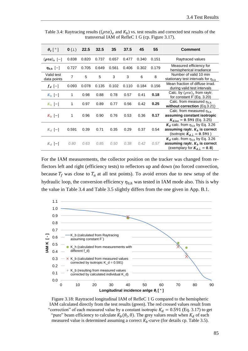
3.4 Test Results
85
Table 3.4: Raytracing results ((𝜌𝜏𝛼)𝑒 and 𝐾𝑏) vs. test results and corrected test results of the
transversal IAM of RefleC 1 G (cp. Figure 3.17).
𝜽𝒕 [ ° ] 0 (⊥) 22.5 32.5 35 37.5 45 55 Comment
(𝝆𝝉𝜶)𝒆 [−] 0.838 0.820 0.737 0.657 0.477 0.340 0.151 Raytraced values
𝜼𝟎,𝒉 [−] 0.727 0.705 0.649 0.561 0.406 0.302 0.179 Measured efficiency for hemispherical irradiance
Valid test data points
7 5 5 3 3 6 8 Number of valid 10 min
stationary test intervals for 𝜂0,ℎ
𝒇𝒅 [−] 0.093 0.078 0.135 0.102 0.110 0.184 0.156 Mean fraction of diffuse irrad.
during valid test intervals
𝑲𝒃 [−] 1 0.98 0.88 0.78 0.57 0.41 0.18 Calc. by (𝜌𝜏𝛼)𝑒 from raytr.
for constant F´(Eq. 3.20)
𝑲𝒉 [−] 1 0.97 0.89 0.77 0.56 0.42 0.25 Calc. from measured 𝜂0,ℎ
without correction (Eq.3.21)
𝑲𝒃 [−] 1 0.96 0.90 0.76 0.53 0.36 0.17
Calc. from measured 𝜂0,ℎ
assuming constant isotropic
𝑲𝒅,𝒊𝒔𝒐 = 𝟎. 𝟓𝟗𝟏 (Eq. 3.25)
𝑲𝒅 [−] 0.591 0.39 0.71 0.35 0.29 0.37 0.54
𝑲𝒅 calc. from 𝜂0,ℎ by Eq. 3.26
assuming raytr. 𝑲𝒃 is correct
(isotropic 𝑲𝒅,⊥ = 𝟎. 𝟓𝟗𝟏 )
𝑲𝒅 [−] 0.80 0.63 0.85 0.50 0.38 0.42 0.57
𝑲𝒅 calc. from 𝜂0,ℎ by Eq. 3.26
assuming raytr. 𝑲𝒃 is correct
(exemplary for 𝑲𝒅,⊥ = 𝟎. 𝟖)
For the IAM measurements, the collector position on the tracker was changed from re-
flectors left and right (efficiency tests) to reflectors up and down (no forced convection,
because 𝑇𝑓 was close to 𝑇𝑎 at all test points). To avoid errors due to new setup of the
hydraulic loop, the conversion efficiency 𝜂0,ℎ was tested in IAM mode also. This is why
the value in Table 3.4 and Table 3.5 slightly differs from the one given in App. B.1.
Figure 3.18: Raytraced longitudinal IAM of RefleC 1 G compared to the hemispheric
IAM calculated directly from the test results (green). The red crossed values result from
“correction” of each measured value by a constant isotropic 𝐾𝑑 = 0.591 (Eq. 3.17) to get
“pure” beam efficiency to calculate 𝐾𝑏(𝜃𝑙, 0). The grey values result when 𝐾𝑑 of each
measured value is determined assuming a correct 𝐾𝑏-curve (for details cp. Table 3.5).
0.0
0.1
0.2
0.3
0.4
0.5
0.6
0.7
0.8
0.9
1.0
1.1
0 10 20 30 40 50 60 70 80 90
IAM
K
[ -
]
Longitudinal incidence anlge θl [ ° ]
K_b (calculated from Raytracingassuming constant F´)
K_h (calculated from measurements withdifferent f_d)
K_b (calculated from measured valuescorrected by isotropic K_d = 0.591)
K_b (resulting from measured valuescorrected by calculated individual K_d)
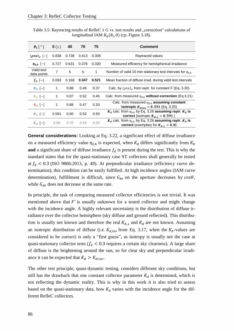
Chapter 3: RefleC Collector Testing
86
Table 3.5: Raytracing results of RefleC 1 G vs. test results and „correction“ calculations of
longitudinal IAM 𝐾𝑏(𝜃𝑙, 0) (cp. Figure 3.18).
𝜽𝒍 [ ° ] 0 (⊥) 40 70 75 Comment
(𝝆𝝉𝜶)𝒆 [−] 0.838 0.738 0.413 0.308 Raytraced values
𝜼𝟎,𝒉 [−] 0.727 0.631 0.378 0.330 Measured efficiency for hemispherical irradiance
Valid test data points
7 5 5 1 Number of valid 10 min stationary test intervals for 𝜂0,ℎ
𝒇𝒅 [−] 0.093 0.168 0.347 0.521 Mean fraction of diffuse irrad. during valid test intervals
𝑲𝒃 [−] 1 0.88 0.49 0.37 Calc. by (𝜌𝜏𝛼)𝑒 from raytr. for constant F´(Eq. 3.20)
𝑲𝒉 [−] 1 0.87 0.52 0.45 Calc. from measured 𝜂0,ℎ without correction (Eq.3.21)
𝑲𝒃 [−] 1 0.88 0.47 0.33 Calc. from measured 𝜂0,ℎ assuming constant
isotropic 𝑲𝒅,𝒊𝒔𝒐 = 𝟎. 𝟓𝟗𝟏 (Eq. 3.25)
𝑲𝒅 [−] 0.591 0.60 0.52 0.50 𝑲𝒅 calc. from 𝜂0,ℎ by Eq. 3.26 assuming raytr. 𝑲𝒃 is
correct (isotropic 𝑲𝒅,⊥ = 𝟎. 𝟓𝟗𝟏 )
𝑲𝒅 [−] 0.80 0.70 0.54 0.52 𝑲𝒅 calc. from 𝜂0,ℎ by Eq. 3.26 assuming raytr. 𝑲𝒃 is
correct (exemplary for 𝑲𝒅,⊥ = 𝟎.𝟖)
General considerations: Looking at Eq. 3.22, a significant effect of diffuse irradiance
on a measured efficiency value 𝜂0,ℎ is expected, when 𝐾𝑑 differs significantly from 𝐾𝑏
and a significant share of diffuse irradiance 𝑓𝑑 is present during the test. This is why the
standard states that for the quasi-stationary case ST collectors shall generally be tested
at 𝑓𝑑 < 0.3 (ISO 9806:2013, p. 49). At perpendicular irradiance (efficiency curve de-
termination), this condition can be easily fulfilled. At high incidence angles (IAM curve
determination), fulfillment is difficult, since 𝐺𝑏𝑡 on the aperture decreases by 𝑐𝑜𝑠𝜃 ,
while 𝐺𝑑𝑡 does not decrease at the same rate.
In principle, the task of comparing measured collector efficiencies is not trivial. It was
mentioned above that 𝐹´ is usually unknown for a tested collector and might change
with the incidence angle. A highly relevant uncertainty is the distribution of diffuse ir-
radiance over the collector hemisphere (sky diffuse and ground reflected). This distribu-
tion is usually not known and therefore the real 𝐾𝑑,⊥ and 𝐾𝑑 are not known. Assuming
an isotropic distribution of diffuse (i.e. 𝐾𝑑,𝑖𝑠𝑜 from Eq. 3.17, when the 𝐾𝑏-values are
considered to be correct) is only a “first guess”, as isotropy is usually not the case at
quasi-stationary collector tests (𝑓𝑑 < 0.3 requires a certain sky clearness). A large share
of diffuse is the brightening around the sun, so for clear sky and perpendicular irradi-
ance it can be expected that 𝐾𝑑 > 𝐾𝑑,𝑖𝑠𝑜.
The other test principle, quasi-dynamic testing, considers different sky conditions, but
still has the drawback that one constant collector parameter 𝐾𝑑 is determined, which is
not reflecting the dynamic reality. This is why in this work it is also tried to assess
based on the quasi-stationary data, how 𝐾𝑑 varies with the incidence angle for the dif-
ferent RefleC collectors.
3.4 Test Results
87
Influence of diffuse irradiance on the conversion factor: When the isotropic
𝐾𝑑,⊥ = 0.591 of the RefleC 1 test sample is used, 𝜂0,𝑏,⊥ ≈ 0.756 results (calculated
by Eq. 3.23 with values of Table 3.4). When a freely chosen but tendentially more re-
alistic value of 𝐾𝑑,⊥ = 0.8 is assumed (last line of Table 3.4), then 𝜂0,𝑏,⊥ ≈ 0.741. If
𝐾𝑑,⊥ should indeed have been in the range between 0.6 and 0.8 during measure-
ment of the conversion efficiency, then the underestimation of 𝜂0,𝑏,⊥ by using the
measured value of 𝜂0,ℎ,⊥ would be in the range of 2 to 4 % for the 𝑓𝑑 present at the
test. For a higher 𝑓𝑑 , of course the influence of diffuse would be higher.
Influence of diffuse irradiance, 𝐾𝑑 and 𝐹´ on 𝐾ℎ: First, we have to consider that the
IAM is determined from a division of measured conversion factors. This means, that if
two conversion factors with identical 𝑓𝑑 , 𝐾𝑑 and 𝐹´would be divided to calculate an
IAM, we would receive a “pure” 𝐾𝑏-value and the influence of diffuse and 𝐹´ on the
IAM would be zero. So their influence is only significant when one or several of the
factors 𝑓𝑑, 𝐾𝑑 and 𝐹´ vary between the tests at perpendicular and angular irradiance.
Looking at Figure 3.17, simply dividing the hemispheric conversion factors to receive a
hemispheric IAM 𝐾ℎ (green dots) shows a good correlation with the raytraced curve
of 𝐾𝑏, except for 𝜃𝑡 = 55°. This is also observed at 𝜃𝑙 = 75° in Figure 3.18. At such
high incidence angles, contrary to 𝜃𝑡 = 0°, 𝐾𝑑 is higher than 𝐾𝑏, and thus diffuse is af-
fecting the collector output significantly more. This is proven by the red crossed values
of 𝐾𝑏, resulting from the “isotropically corrected” measured efficiency values. Finally,
the grey values of 𝐾𝑑 in Table 3.4 and Table 3.5 show how the IAM for diffuse irradi-
ance 𝐾𝑑 would have been during test of 𝜂0,ℎ, when 𝐾𝑑,⊥of 0.591 or 0.8 and correct ray-
tracing values of 𝐾𝑏 (with constant 𝐹´) are assumed. For the longitudinal results, very
realistic values are found for 𝐾𝑑,⊥ = 0.8. In the transversal direction, a variation of 𝐹´
cannot be excluded but is also not clearly indicated by the results. Such variations might
be caused by varying distances between concentration lines and absorber tube weldings
(cp. Figure 3.13) or by the fact that at 𝜃𝑡 = 55° a large share of the absorber is shaded
from beam due to the opposite reflector. Finally, it has to be stressed that there is a high
uncertainty in the values of 𝐺𝑑,𝑡 (and thus 𝑓𝑑), since they were not measured in the col-
lector aperture plane and the shading of a large part of the hemisphere by the shadow
band leads to high errors.
All in all, having the above considerations and measurement uncertainties in mind, the
IAM test results show a good correlation with the raytracing results; the calculated val-
ues of 𝐾𝑑 are in a comparably reasonable range. From the investigations above for Re-
fleC 1 it cannot clearly be answered if 𝐹´(𝜃𝑡) = 𝑐𝑜𝑛𝑠𝑡.
To conclude, the raytracing simulations of the single-covered RefleC 1 collector with
CPC are considered to represent the collector’s IAM for beam irradiance sufficiently.
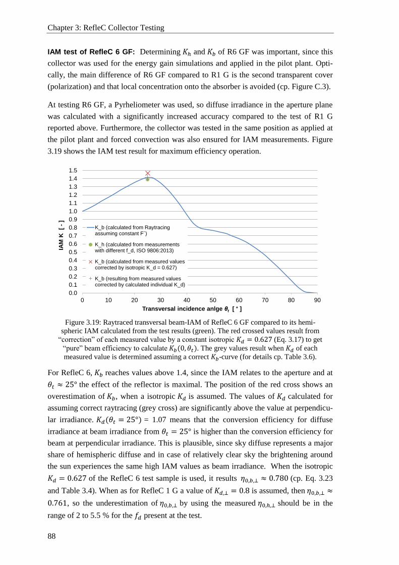
Chapter 3: RefleC Collector Testing
88
IAM test of RefleC 6 GF: Determining 𝐾ℎ and 𝐾𝑏 of R6 GF was important, since this
collector was used for the energy gain simulations and applied in the pilot plant. Opti-
cally, the main difference of R6 GF compared to R1 G is the second transparent cover
(polarization) and that local concentration onto the absorber is avoided (cp. Figure C.3).
At testing R6 GF, a Pyrheliometer was used, so diffuse irradiance in the aperture plane
was calculated with a significantly increased accuracy compared to the test of R1 G
reported above. Furthermore, the collector was tested in the same position as applied at
the pilot plant and forced convection was also ensured for IAM measurements. Figure
3.19 shows the IAM test result for maximum efficiency operation.
Figure 3.19: Raytraced transversal beam-IAM of RefleC 6 GF compared to its hemi-
spheric IAM calculated from the test results (green). The red crossed values result from
“correction” of each measured value by a constant isotropic 𝐾𝑑 = 0.627 (Eq. 3.17) to get
“pure” beam efficiency to calculate 𝐾𝑏(0, 𝜃𝑡). The grey values result when 𝐾𝑑 of each
measured value is determined assuming a correct 𝐾𝑏-curve (for details cp. Table 3.6).
For RefleC 6, 𝐾𝑏 reaches values above 1.4, since the IAM relates to the aperture and at
𝜃𝑡 ≈ 25° the effect of the reflector is maximal. The position of the red cross shows an
overestimation of 𝐾𝑏, when a isotropic 𝐾𝑑 is assumed. The values of 𝐾𝑑 calculated for
assuming correct raytracing (grey cross) are significantly above the value at perpendicu-
lar irradiance. 𝐾𝑑(𝜃𝑡 = 25°) = 1.07 means that the conversion efficiency for diffuse
irradiance at beam irradiance from 𝜃𝑡 = 25° is higher than the conversion efficiency for
beam at perpendicular irradiance. This is plausible, since sky diffuse represents a major
share of hemispheric diffuse and in case of relatively clear sky the brightening around
the sun experiences the same high IAM values as beam irradiance. When the isotropic
𝐾𝑑 = 0.627 of the RefleC 6 test sample is used, it results 𝜂0,𝑏,⊥ ≈ 0.780 (cp. Eq. 3.23
and Table 3.4). When as for RefleC 1 G a value of 𝐾𝑑,⊥ = 0.8 is assumed, then 𝜂0,𝑏,⊥ ≈
0.761, so the underestimation of 𝜂0,𝑏,⊥ by using the measured 𝜂0,ℎ,⊥ should be in the
range of 2 to 5.5 % for the 𝑓𝑑 present at the test.
0.0
0.1
0.2
0.3
0.4
0.5
0.6
0.7
0.8
0.9
1.0
1.1
1.2
1.3
1.4
1.5
0 10 20 30 40 50 60 70 80 90
IAM
K
[ -
]
Transversal incidence anlge θt [ ° ]
K_b (calculated from Raytracingassuming constant F´)
K_h (calculated from measurementswith different f_d, ISO 9806:2013)
K_b (calculated from measured valuescorrected by isotropic K_d = 0.627)
K_b (resulting from measured valuescorrected by calculated individual K_d)
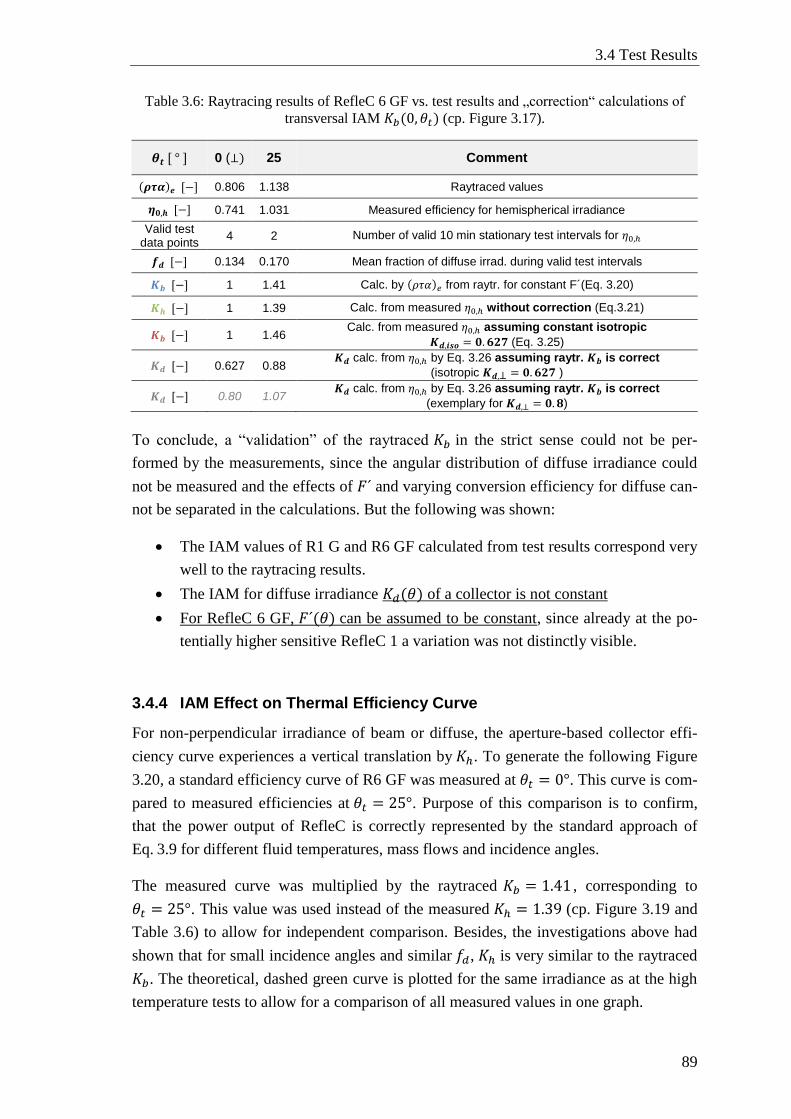
3.4 Test Results
89
Table 3.6: Raytracing results of RefleC 6 GF vs. test results and „correction“ calculations of
transversal IAM 𝐾𝑏(0, 𝜃𝑡) (cp. Figure 3.17).
𝜽𝒕 [ ° ] 0 (⊥) 25 Comment
(𝝆𝝉𝜶)𝒆 [−] 0.806 1.138 Raytraced values
𝜼𝟎,𝒉 [−] 0.741 1.031 Measured efficiency for hemispherical irradiance
Valid test data points
4 2 Number of valid 10 min stationary test intervals for 𝜂0,ℎ
𝒇𝒅 [−] 0.134 0.170 Mean fraction of diffuse irrad. during valid test intervals
𝑲𝒃 [−] 1 1.41 Calc. by (𝜌𝜏𝛼)𝑒 from raytr. for constant F´(Eq. 3.20)
𝑲𝒉 [−] 1 1.39 Calc. from measured 𝜂0,ℎ without correction (Eq.3.21)
𝑲𝒃 [−] 1 1.46 Calc. from measured 𝜂0,ℎ assuming constant isotropic
𝑲𝒅,𝒊𝒔𝒐 = 𝟎. 𝟔𝟐𝟕 (Eq. 3.25)
𝑲𝒅 [−] 0.627 0.88 𝑲𝒅 calc. from 𝜂0,ℎ by Eq. 3.26 assuming raytr. 𝑲𝒃 is correct
(isotropic 𝑲𝒅,⊥ = 𝟎. 𝟔𝟐𝟕 )
𝑲𝒅 [−] 0.80 1.07 𝑲𝒅 calc. from 𝜂0,ℎ by Eq. 3.26 assuming raytr. 𝑲𝒃 is correct
(exemplary for 𝑲𝒅,⊥ = 𝟎.𝟖)
To conclude, a “validation” of the raytraced 𝐾𝑏 in the strict sense could not be per-
formed by the measurements, since the angular distribution of diffuse irradiance could
not be measured and the effects of 𝐹´ and varying conversion efficiency for diffuse can-
not be separated in the calculations. But the following was shown:
The IAM values of R1 G and R6 GF calculated from test results correspond very
well to the raytracing results.
The IAM for diffuse irradiance 𝐾𝑑(𝜃) of a collector is not constant
For RefleC 6 GF, 𝐹´(𝜃) can be assumed to be constant, since already at the po-
tentially higher sensitive RefleC 1 a variation was not distinctly visible.
3.4.4 IAM Effect on Thermal Efficiency Curve
For non-perpendicular irradiance of beam or diffuse, the aperture-based collector effi-
ciency curve experiences a vertical translation by 𝐾ℎ. To generate the following Figure
3.20, a standard efficiency curve of R6 GF was measured at 𝜃𝑡 = 0°. This curve is com-
pared to measured efficiencies at 𝜃𝑡 = 25°. Purpose of this comparison is to confirm,
that the power output of RefleC is correctly represented by the standard approach of
Eq. 3.9 for different fluid temperatures, mass flows and incidence angles.
The measured curve was multiplied by the raytraced 𝐾𝑏 = 1.41 , corresponding to
𝜃𝑡 = 25°. This value was used instead of the measured 𝐾ℎ = 1.39 (cp. Figure 3.19 and
Table 3.6) to allow for independent comparison. Besides, the investigations above had
shown that for small incidence angles and similar 𝑓𝑑, 𝐾ℎ is very similar to the raytraced
𝐾𝑏. The theoretical, dashed green curve is plotted for the same irradiance as at the high
temperature tests to allow for a comparison of all measured values in one graph.
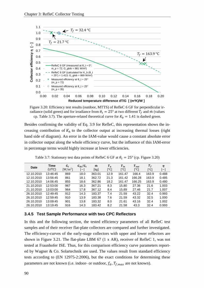
Chapter 3: RefleC Collector Testing
90
Figure 3.20: Efficiency test results (outdoor, MTTS) of RefleC 6 GF for perpendicular ir-
radiance (solid green) and for irradiance from 𝜃𝑡 = 25° at two different 𝑇𝑓 and �̇� (values
cp. Table 3.7). The aperture-related theoretical curve for 𝐾𝑏 = 1.41 is dashed green.
Besides confirming the validity of Eq. 3.9 for RefleC, this representation shows the in-
creasing contribution of 𝐾ℎ to the collector output at increasing thermal losses (right
hand side of diagram). An error in the IAM-value would cause a constant absolute error
in collector output along the whole efficiency curve, but the influence of this IAM-error
in percentage terms would highly increase at lower efficiencies.
Table 3.7: Stationary test data points of RefleC 6 GF at 𝜃𝑡 = 25° (cp. Figure 3.20)
Date Time
(UTC)
𝑮𝒕 [W/m2]
𝑮𝒅𝒕/𝑮𝒕 [−]
�̇�
[kg] 𝑻𝒂
[°C] 𝑻𝒊𝒏
[°C] 𝑻𝒐𝒖𝒕
[°C]
𝑻𝒇
[°C]
𝜼
[−]
12.10.2010 13:46:45 869 18.0 363.01 12.9 161.47 166.4 163.9 0.488
12.10.2010 13:56:45 861 18.1 362.72 21.3 161.42 166.28 163.9 0.485
12.10.2010 14:06:45 855 18.6 362.86 18.2 161.47 166.25 163.9 0.480
21.10.2010 12:53:00 967 16.3 367.21 8.3 15.80 27.36 21.6 1.003
21.10.2010 13:03:00 964 17.8 367.12 8.4 15.89 27.46 21.7 1.007
26.10.2010 12:49:45 912 14.3 183.37 7.4 21.59 43.22 32.4 0.993
26.10.2010 12:59:45 910 13.9 183.38 7.6 21.59 43.32 32.5 1.000
26.10.2010 13:09:45 901 13.8 183.32 8.0 21.61 43.16 32.4 1.002
26.10.2010 13:19:45 916 14.3 183.42 8.2 21.58 43.3 32.4 0.993
3.4.5 Test Sample Performance with two CPC Reflectors
In this and the following section, the tested efficiency parameters of all RefleC test
samples and of their receiver flat-plate collectors are compared and further investigated.
The efficiency-curves of the early-stage collectors with upper and lower reflectors are
shown in Figure 3.21. The flat-plate LBM 67 (1 x AR), receiver of RefleC 1, was not
tested at Fraunhofer ISE. Thus, for this comparison efficiency curve parameters report-
ed by Wagner & Co. Solartechnik are used. The values result from standard efficiency
tests according to (EN 12975-2:2006), but the exact conditions for determining these
parameters are not known (i.e. indoor- or outdoor, 𝑓𝑑, 𝑇𝑓,𝑚𝑎𝑥 are not known).
0.0
0.1
0.2
0.3
0.4
0.5
0.6
0.7
0.8
0.9
1.0
1.1
0.00 0.02 0.04 0.06 0.08 0.10 0.12 0.14 0.16 0.18 0.20
Co
lle
cto
r e
ffic
ien
cy η
[
-]
Reduced temperature difference dT/G [ (m²K)/W ]
RefleC 6 GF (measured at θ_t = 0°; m_p = 72; G_glob = 981 W/m²)
RefleC 6 GF (calculated for K_b (θ_t = 25°) = 1.413; G_glob = 869 W/m²)
Measured efficiency at θ_t = 25°(m_p = 72)
Measured efficiency at θ_t = 25°(m_p = 35)
𝑇𝑓 = 21.7 °C
𝑇𝑓 = 32.4 °C
𝑇𝑓 = 163.9 °C
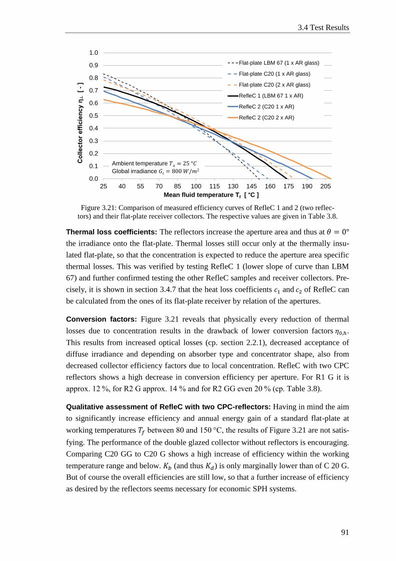
3.4 Test Results
91
Figure 3.21: Comparison of measured efficiency curves of RefleC 1 and 2 (two reflec-
tors) and their flat-plate receiver collectors. The respective values are given in Table 3.8.
Thermal loss coefficients: The reflectors increase the aperture area and thus at 𝜃 = 0°
the irradiance onto the flat-plate. Thermal losses still occur only at the thermally insu-
lated flat-plate, so that the concentration is expected to reduce the aperture area specific
thermal losses. This was verified by testing RefleC 1 (lower slope of curve than LBM
67) and further confirmed testing the other RefleC samples and receiver collectors. Pre-
cisely, it is shown in section 3.4.7 that the heat loss coefficients 𝑐1 and 𝑐2 of RefleC can
be calculated from the ones of its flat-plate receiver by relation of the apertures.
Conversion factors: Figure 3.21 reveals that physically every reduction of thermal
losses due to concentration results in the drawback of lower conversion factors 𝜂0,ℎ.
This results from increased optical losses (cp. section 2.2.1), decreased acceptance of
diffuse irradiance and depending on absorber type and concentrator shape, also from
decreased collector efficiency factors due to local concentration. RefleC with two CPC
reflectors shows a high decrease in conversion efficiency per aperture. For R1 G it is
approx. 12 %, for R2 G approx. 14 % and for R2 GG even 20 % (cp. Table 3.8).
Qualitative assessment of RefleC with two CPC-reflectors: Having in mind the aim
to significantly increase efficiency and annual energy gain of a standard flat-plate at
working temperatures 𝑇𝑓 between 80 and 150 °C, the results of Figure 3.21 are not satis-
fying. The performance of the double glazed collector without reflectors is encouraging.
Comparing C20 GG to C20 G shows a high increase of efficiency within the working
temperature range and below. 𝐾𝑏 (and thus 𝐾𝑑) is only marginally lower than of C 20 G.
But of course the overall efficiencies are still low, so that a further increase of efficiency
as desired by the reflectors seems necessary for economic SPH systems.
0.0
0.1
0.2
0.3
0.4
0.5
0.6
0.7
0.8
0.9
1.0
25 40 55 70 85 100 115 130 145 160 175 190 205
Collecto
r effic
iency η
┴[
-]
Mean fluid temperature Tf [ °C ]
Flat-plate LBM 67 (1 x AR glass)
Flat-plate C20 (1 x AR glass)
Flat-plate C20 (2 x AR glass)
RefleC 1 (LBM 67 1 x AR)
RefleC 2 (C20 1 x AR)
RefleC 2 (C20 2 x AR)
Ambient temperature
Global irradiance
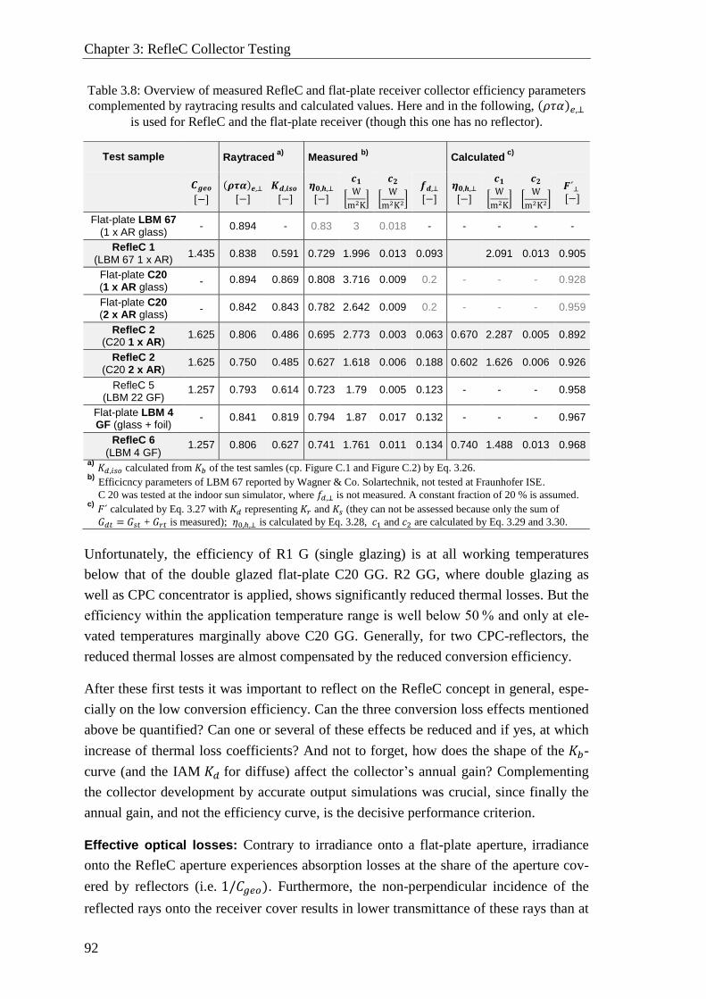
Chapter 3: RefleC Collector Testing
92
Table 3.8: Overview of measured RefleC and flat-plate receiver collector efficiency parameters
complemented by raytracing results and calculated values. Here and in the following, (𝜌𝜏𝛼)𝑒,⊥
is used for RefleC and the flat-plate receiver (though this one has no reflector).
Unfortunately, the efficiency of R1 G (single glazing) is at all working temperatures
below that of the double glazed flat-plate C20 GG. R2 GG, where double glazing as
well as CPC concentrator is applied, shows significantly reduced thermal losses. But the
efficiency within the application temperature range is well below 50 % and only at ele-
vated temperatures marginally above C20 GG. Generally, for two CPC-reflectors, the
reduced thermal losses are almost compensated by the reduced conversion efficiency.
After these first tests it was important to reflect on the RefleC concept in general, espe-
cially on the low conversion efficiency. Can the three conversion loss effects mentioned
above be quantified? Can one or several of these effects be reduced and if yes, at which
increase of thermal loss coefficients? And not to forget, how does the shape of the 𝐾𝑏-
curve (and the IAM 𝐾𝑑 for diffuse) affect the collector’s annual gain? Complementing
the collector development by accurate output simulations was crucial, since finally the
annual gain, and not the efficiency curve, is the decisive performance criterion.
Effective optical losses: Contrary to irradiance onto a flat-plate aperture, irradiance
onto the RefleC aperture experiences absorption losses at the share of the aperture cov-
ered by reflectors (i.e. 1/𝐶𝑔𝑒𝑜). Furthermore, the non-perpendicular incidence of the
reflected rays onto the receiver cover results in lower transmittance of these rays than at
Test sample Raytraced a)
Measured b)
Calculated c)
𝑪𝒈𝒆𝒐
[−]
(𝝆𝝉𝜶)𝒆,⊥
[−]
𝑲𝒅,𝒊𝒔𝒐
[−]
𝜼𝟎,𝒉,⊥
[−]
𝒄𝟏
[W
m2K]
𝒄𝟐
[W
m2K2]
𝒇𝒅,⊥
[−]
𝜼𝟎,𝒉,⊥
[−]
𝒄𝟏
[W
m2K]
𝒄𝟐
[W
m2K2]
𝑭´⊥ [−]
Flat-plate LBM 67
(1 x AR glass) - 0.894 - 0.83 3 0.018 - - - - -
RefleC 1
(LBM 67 1 x AR) 1.435 0.838 0.591 0.729 1.996 0.013 0.093 2.091 0.013 0.905
Flat-plate C20 (1 x AR glass)
- 0.894 0.869 0.808 3.716 0.009 0.2 - - - 0.928
Flat-plate C20 (2 x AR glass)
- 0.842 0.843 0.782 2.642 0.009 0.2 - - - 0.959
RefleC 2 (C20 1 x AR)
1.625 0.806 0.486 0.695 2.773 0.003 0.063 0.670 2.287 0.005 0.892
RefleC 2 (C20 2 x AR)
1.625 0.750 0.485 0.627 1.618 0.006 0.188 0.602 1.626 0.006 0.926
RefleC 5 (LBM 22 GF)
1.257 0.793 0.614 0.723 1.79 0.005 0.123 - - - 0.958
Flat-plate LBM 4 GF (glass + foil)
- 0.841 0.819 0.794 1.87 0.017 0.132 - - - 0.967
RefleC 6
(LBM 4 GF) 1.257 0.806 0.627 0.741 1.761 0.011 0.134 0.740 1.488 0.013 0.968
a) 𝐾𝑑,𝑖𝑠𝑜 calculated from 𝐾𝑏 of the test samles (cp. Figure C.1 and Figure C.2) by Eq. 3.26. b) Efficicncy parameters of LBM 67 reported by Wagner & Co. Solartechnik, not tested at Fraunhofer ISE.
C 20 was tested at the indoor sun simulator, where 𝑓𝑑,⊥ is not measured. A constant fraction of 20 % is assumed. c) 𝐹´ calculated by Eq. 3.27 with 𝐾𝑑 representing 𝐾𝑟 and 𝐾𝑠 (they can not be assessed because only the sum of
𝐺𝑑𝑡 = 𝐺𝑠𝑡 + 𝐺𝑟𝑡 is measured); 𝜂0,ℎ,⊥ is calculated by Eq. 3.28, 𝑐1 and 𝑐2 are calculated by Eq. 3.29 and 3.30.
3.4 Test Results
93
perpendicular incidence. Both factors reduce (𝜌𝜏𝛼)𝑒,⊥. Comparing RefleC 2 to its re-
ceiver collectors C20 G and C 20 GG in Table 3.8 reveals that for both the decrease in
optical efficiency is very high. The raytracing values show for R1 G a reduction in optical
efficiency of ca. 6 % compared to LBM 67 G. This further decreases for R2 G (ca. 10 %
compared to C20 G) and R2 GG (ca. 11 % compared to C20 GG).
IAM for diffuse: The diffuse-IAM 𝐾𝑑,𝑖𝑠𝑜 of the single-covered flat-plates is maximal
and slightly decreasing for a double cover. The 𝐾𝑏-shape of each RefleC test sample
determines 𝐾𝑑,𝑖𝑠𝑜. Due to the reduced acceptance angle, R1 G shows a decrease of ca.
30 % in diffuse utilization, while R2 G and GG show an even higher decrease of above
40 % compared to their receiver flat plates.
Calculated collector efficiency factors: From the investigations in section 3.4.3 it is
expected that setting 𝐾𝑑,⊥ = 𝐾𝑑,𝑖𝑠𝑜 does not reflect reality. But possible errors of this
approach can be expected to be similar for one RefleC geommetry. For the purpose to
finally separate the effects of optical losses, reduced diffuse acceptance and reduced 𝐹´,
it can be calculated following Eq. 3.7:
𝐹´⊥ =𝜂0,ℎ,⊥
(𝜌𝜏𝛼)𝑒, ⊥⋅[(1−𝑓𝑑)+𝑓𝑑⋅𝐾𝑑,⊥] with 𝑓𝑑 =
𝐺𝑑𝑡
𝐺𝑡= 1 − 𝑓𝑏 ( 3.27 )
The results of this calculation are remarkable already for the flat-plate. The optical effi-
ciency (𝜌𝜏𝛼)𝑒,⊥ of C20 GG is approx. 6 % below that of C20 G, while the difference in
𝜂0,ℎ is only approx. 3 %. Application of Eq. 3.27 reveals that this is due to an approx.
3 % increase of 𝐹´, when the second cover is applied (cp. right column of Table 3.8).
This is plausible, since 𝐹´ depends on the front heat losses, which are reduced by the
second cover. Both collector variants were tested at a solar simulator, for which a dif-
fuse fraction of 𝑓𝑑,⊥ = 0.2 is assumed (not measured). For RefleC, the 𝐹´-calculation is
also very enlightening. A comparison of R2 with its respective receivers indeed shows
an decrease of 𝐹´ due to the CPC-concentration of about 4 %, both in the case of single
and double glazing. Since the flat-plate LBM 67 was not tested at ISE, 𝐹´ cannot be
calculated here due to missing information. But R2 G and R1 G show a very similar
calculated 𝐹´, so that the effect can be assumed for all flat-plates with CPC reflectors.
Sensitivity of the decreased hemispheric conversion efficiency: The high absolute
reduction of (𝜌𝜏𝛼)𝑒,⊥ by the reflectors and its direct effect on 𝜂0,ℎ due to multiplication (cp.
Eq. 3.7) reveal that the major share of the observed reduction of the conversion efficiencies
is caused by the increased optical losses. The efficiency factor 𝐹´ is also directly multiplied,
so a decrease here causes the same decrease of 𝜂0,ℎ
. The effect of 𝐾𝑑,𝑖𝑠𝑜 on 𝜂0,ℎ depends on
𝑓𝑑 during the test. In case of R2 G the effect of reduced 𝐾𝑑,𝑖𝑠𝑜 is smaller than of the
reduced 𝐹´; in case of R2 GG the reduced 𝐾𝑑,𝑖𝑠𝑜 overweighs because of the relatively
high 𝑓𝑑 = 0.188 during this test.
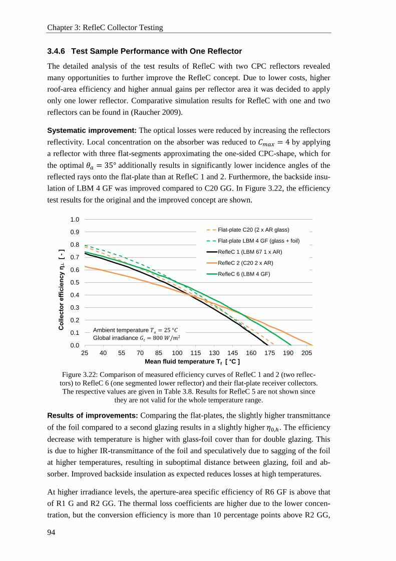
Chapter 3: RefleC Collector Testing
94
3.4.6 Test Sample Performance with One Reflector
The detailed analysis of the test results of RefleC with two CPC reflectors revealed
many opportunities to further improve the RefleC concept. Due to lower costs, higher
roof-area efficiency and higher annual gains per reflector area it was decided to apply
only one lower reflector. Comparative simulation results for RefleC with one and two
reflectors can be found in (Raucher 2009).
Systematic improvement: The optical losses were reduced by increasing the reflectors
reflectivity. Local concentration on the absorber was reduced to 𝐶𝑚𝑎𝑥 = 4 by applying
a reflector with three flat-segments approximating the one-sided CPC-shape, which for
the optimal 𝜃𝑎 = 35° additionally results in significantly lower incidence angles of the
reflected rays onto the flat-plate than at RefleC 1 and 2. Furthermore, the backside insu-
lation of LBM 4 GF was improved compared to C20 GG. In Figure 3.22, the efficiency
test results for the original and the improved concept are shown.
Figure 3.22: Comparison of measured efficiency curves of RefleC 1 and 2 (two reflec-
tors) to RefleC 6 (one segmented lower reflector) and their flat-plate receiver collectors.
The respective values are given in Table 3.8. Results for RefleC 5 are not shown since
they are not valid for the whole temperature range.
Results of improvements: Comparing the flat-plates, the slightly higher transmittance
of the foil compared to a second glazing results in a slightly higher 𝜂0,ℎ. The efficiency
decrease with temperature is higher with glass-foil cover than for double glazing. This
is due to higher IR-transmittance of the foil and speculatively due to sagging of the foil
at higher temperatures, resulting in suboptimal distance between glazing, foil and ab-
sorber. Improved backside insulation as expected reduces losses at high temperatures.
At higher irradiance levels, the aperture-area specific efficiency of R6 GF is above that
of R1 G and R2 GG. The thermal loss coefficients are higher due to the lower concen-
tration, but the conversion efficiency is more than 10 percentage points above R2 GG,
0.0
0.1
0.2
0.3
0.4
0.5
0.6
0.7
0.8
0.9
1.0
25 40 55 70 85 100 115 130 145 160 175 190 205
Collecto
r effic
iency η
┴[
-]
Mean fluid temperature Tf [ °C ]
Flat-plate C20 (2 x AR glass)
Flat-plate LBM 4 GF (glass + foil)
RefleC 1 (LBM 67 1 x AR)
RefleC 2 (C20 2 x AR)
RefleC 6 (LBM 4 GF)
Ambient temperature
Global irradiance
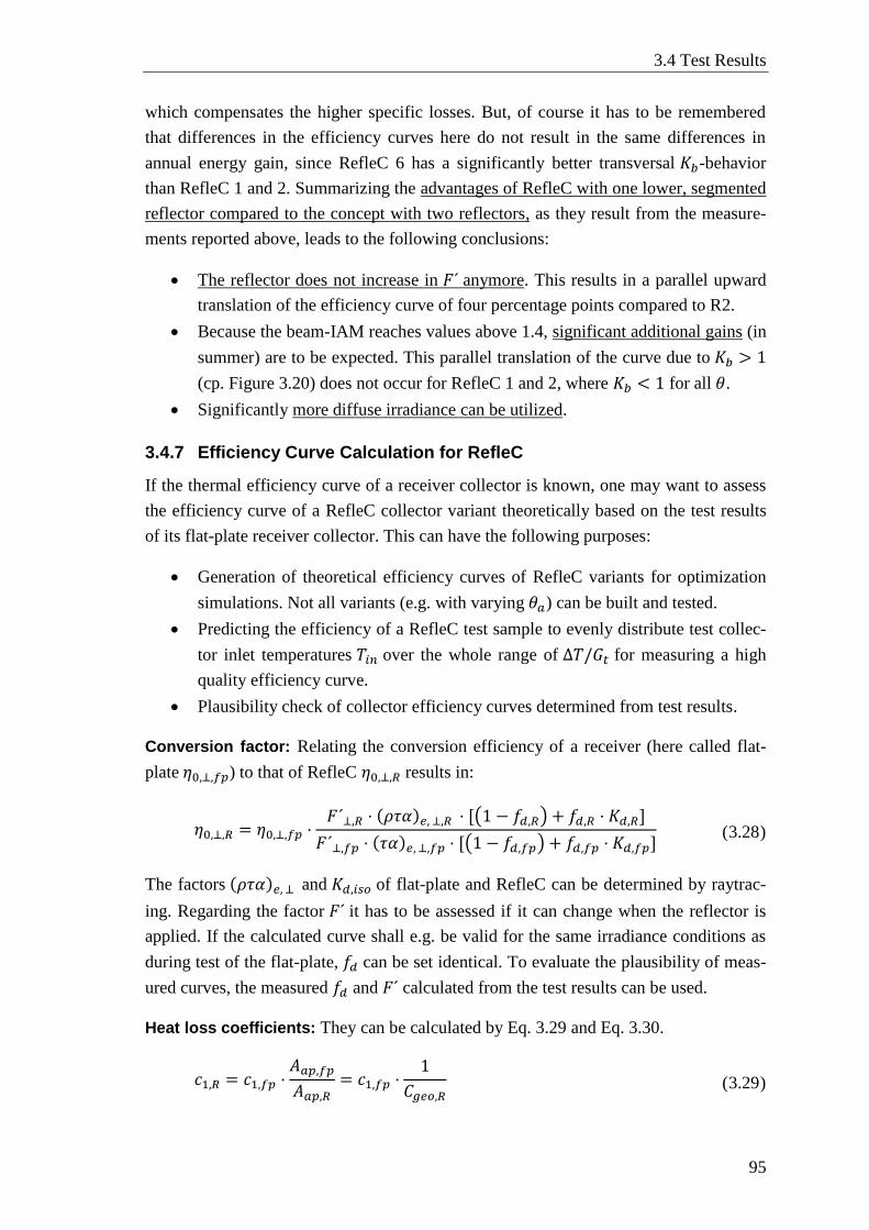
3.4 Test Results
95
which compensates the higher specific losses. But, of course it has to be remembered
that differences in the efficiency curves here do not result in the same differences in
annual energy gain, since RefleC 6 has a significantly better transversal 𝐾𝑏-behavior
than RefleC 1 and 2. Summarizing the advantages of RefleC with one lower, segmented
reflector compared to the concept with two reflectors, as they result from the measure-
ments reported above, leads to the following conclusions:
The reflector does not increase in 𝐹´ anymore. This results in a parallel upward
translation of the efficiency curve of four percentage points compared to R2.
Because the beam-IAM reaches values above 1.4, significant additional gains (in
summer) are to be expected. This parallel translation of the curve due to 𝐾𝑏 > 1
(cp. Figure 3.20) does not occur for RefleC 1 and 2, where 𝐾𝑏 < 1 for all 𝜃.
Significantly more diffuse irradiance can be utilized.
3.4.7 Efficiency Curve Calculation for RefleC
If the thermal efficiency curve of a receiver collector is known, one may want to assess
the efficiency curve of a RefleC collector variant theoretically based on the test results
of its flat-plate receiver collector. This can have the following purposes:
Generation of theoretical efficiency curves of RefleC variants for optimization
simulations. Not all variants (e.g. with varying 𝜃𝑎) can be built and tested.
Predicting the efficiency of a RefleC test sample to evenly distribute test collec-
tor inlet temperatures 𝑇𝑖𝑛 over the whole range of Δ𝑇/𝐺𝑡 for measuring a high
quality efficiency curve.
Plausibility check of collector efficiency curves determined from test results.
Conversion factor: Relating the conversion efficiency of a receiver (here called flat-
plate 𝜂0,⊥,𝑓𝑝) to that of RefleC 𝜂0,⊥,𝑅 results in:
𝜂0,⊥,𝑅 = 𝜂0,⊥,𝑓𝑝 ⋅𝐹´⊥,𝑅 ⋅ (𝜌𝜏𝛼)𝑒, ⊥,𝑅 ⋅ [(1 − 𝑓𝑑,𝑅) + 𝑓𝑑,𝑅 ⋅ 𝐾𝑑,𝑅]
𝐹´⊥,𝑓𝑝 ⋅ (𝜏𝛼)𝑒, ⊥,𝑓𝑝 ⋅ [(1 − 𝑓𝑑,𝑓𝑝) + 𝑓𝑑,𝑓𝑝 ⋅ 𝐾𝑑,𝑓𝑝] ( 3.28 )
The factors (𝜌𝜏𝛼)𝑒, ⊥ and 𝐾𝑑,𝑖𝑠𝑜 of flat-plate and RefleC can be determined by raytrac-
ing. Regarding the factor 𝐹´ it has to be assessed if it can change when the reflector is
applied. If the calculated curve shall e.g. be valid for the same irradiance conditions as
during test of the flat-plate, 𝑓𝑑 can be set identical. To evaluate the plausibility of meas-
ured curves, the measured 𝑓𝑑 and 𝐹´ calculated from the test results can be used.
Heat loss coefficients: They can be calculated by Eq. 3.29 and Eq. 3.30.
𝑐1,𝑅 = 𝑐1,𝑓𝑝 ⋅𝐴𝑎𝑝,𝑓𝑝
𝐴𝑎𝑝,𝑅= 𝑐1,𝑓𝑝 ⋅
1
𝐶𝑔𝑒𝑜,𝑅 ( 3.29 )
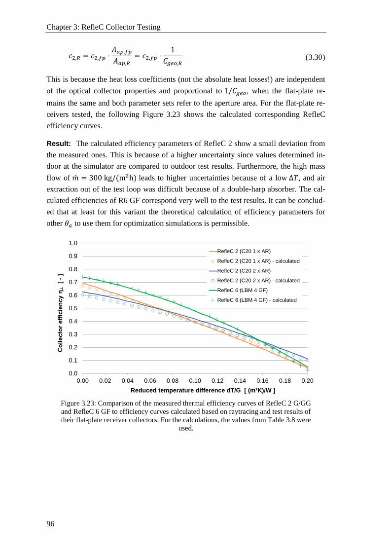
Chapter 3: RefleC Collector Testing
96
𝑐2,𝑅 = 𝑐2,𝑓𝑝 ⋅𝐴𝑎𝑝,𝑓𝑝
𝐴𝑎𝑝,𝑅= 𝑐2,𝑓𝑝 ⋅
1
𝐶𝑔𝑒𝑜,𝑅 ( 3.30 )
This is because the heat loss coefficients (not the absolute heat losses!) are independent
of the optical collector properties and proportional to 1/𝐶𝑔𝑒𝑜, when the flat-plate re-
mains the same and both parameter sets refer to the aperture area. For the flat-plate re-
ceivers tested, the following Figure 3.23 shows the calculated corresponding RefleC
efficiency curves.
Result: The calculated efficiency parameters of RefleC 2 show a small deviation from
the measured ones. This is because of a higher uncertainty since values determined in-
door at the simulator are compared to outdoor test results. Furthermore, the high mass
flow of �̇� = 300 kg/(m2h) leads to higher uncertainties because of a low Δ𝑇, and air
extraction out of the test loop was difficult because of a double-harp absorber. The cal-
culated efficiencies of R6 GF correspond very well to the test results. It can be conclud-
ed that at least for this variant the theoretical calculation of efficiency parameters for
other 𝜃𝑎 to use them for optimization simulations is permissible.
Figure 3.23: Comparison of the measured thermal efficiency curves of RefleC 2 G/GG
and RefleC 6 GF to efficiency curves calculated based on raytracing and test results of
their flat-plate receiver collectors. For the calculations, the values from Table 3.8 were
used.
0.0
0.1
0.2
0.3
0.4
0.5
0.6
0.7
0.8
0.9
1.0
0.00 0.02 0.04 0.06 0.08 0.10 0.12 0.14 0.16 0.18 0.20
Collecto
r effic
iency η
┴[
-]
Reduced temperature difference dT/G [ (m²K)/W ]
RefleC 2 (C20 1 x AR)
RefleC 2 (C20 1 x AR) - calculated
RefleC 2 (C20 2 x AR)
RefleC 2 (C20 2 x AR) - calculated
RefleC 6 (LBM 4 GF)
RefleC 6 (LBM 4 GF) - calculated
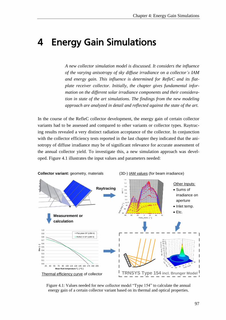
Chapter 4: Energy Gain Simulations
97
4 Energy Gain Simulations
A new collector simulation model is discussed. It considers the influence
of the varying anisotropy of sky diffuse irradiance on a collector’s IAM
and energy gain. This influence is determined for RefleC and its flat-
plate receiver collector. Initially, the chapter gives fundamental infor-
mation on the different solar irradiance components and their considera-
tion in state of the art simulations. The findings from the new modeling
approach are analyzed in detail and reflected against the state of the art.
In the course of the RefleC collector development, the energy gain of certain collector
variants had to be assessed and compared to other variants or collector types. Raytrac-
ing results revealed a very distinct radiation acceptance of the collector. In conjunction
with the collector efficiency tests reported in the last chapter they indicated that the ani-
sotropy of diffuse irradiance may be of significant relevance for accurate assessment of
the annual collector yield. To investigate this, a new simulation approach was devel-
oped. Figure 4.1 illustrates the input values and parameters needed:
Figure 4.1: Values needed for new collector model “Type 154” to calculate the annual
energy gain of a certain collector variant based on its thermal and optical properties.
Collector variant: geometry, materials
Raytracing
0.0
0.1
0.2
0.3
0.4
0.5
0.6
0.7
0.8
0.9
1.0
25 40 55 70 85 100 115 130 145 160 175 190 205
Eta
[
-]
Mean fluid temperature Tf [ °C ]
Flat plate GF (LBM 4)
RefleC 6 GF (LBM 4)
(3D-) IAM values (for beam irradiance)
Measurement or
calculation
TRNSYS Type 154 incl. Brunger Model Thermal efficiency curve of collector
Other Inputs:
Sums of
irradiance on
aperture
Inlet temp.
Etc.
Chapter 4: Energy Gain Simulations
98
4.1 Modeling Anisotropic Diffuse Irradiance
Low-concentrating ST collectors show a high but very incidence-angle selective ac-
ceptance of diffuse irradiance. In reality this irradiance is to different extents anisotropic
(cp. section 2.1.3) and the varying circumsolar radiance is at times with high collector
gains often within 𝜃𝑎 of the collector. Therefore, the angular distribution of incident
diffuse irradiance is expected to have significant influence on the collector energy gain.
From the discussions in section 3.2.3, we realize that diffuse irradiance can be under-
stood as beam irradiance originating from the whole collector hemisphere (sky dome
and ground). This leads to the fundamental approach of this work, which is that accurate
instantaneous diffuse-IAM values for sky and ground irradiance (𝐾𝑠 and 𝐾𝑟) can be cal-
culated by weighting the irradiance from hemispheric sky and ground segments visible
for the collector aperture by the individual beam-IAM values of these segments. Eq.
3.17 already follows this thought, but assumes isotropic radiance.
To evaluate the different RefleC concepts and to accurately calculate the additional
gains by the reflectors, a time-dependent anisotropic modelling of diffuse irradiance and
the corresponding 𝐾𝑠 was realized. In this case, 𝐾𝑠 is not a constant collector parameter
anymore, but changes with varying diffuse irradiance distribution.
This distribution is not available from weather data files or the radiation processors used
in state-of-the-art solar thermal simulation programs (cp. sections 2.1.2 and 4.2.1).
Thus, it had to be modelled within the developed collector Type 154 to allow for con-
sidering it when determining 𝐾𝑠. As a first step, an appropriate model for the anisotropic
distribution of diffuse radiance across the sky dome had to be selected.
4.1.1 Review of Available Models
To account for anisotropic sky radiance incident on sloped surfaces, different models
have been developed. The most common are the Hay-Davies-Model (Hay 1979), the
Reindl-Model (Reindl et al. 1990) and the Perez-Models (Perez et al. 1986 ; Perez et al.
1987 ; Perez et al. 1990). A comparison between these and some other models can be
found e.g. in (Reindl et al. 1990), (Evseev and Kudish 2009), or (Gueymard 2009). All
of the named models have in common that they provide the sum of incident diffuse irra-
diance from a non-uniform sky on a tilted plane, but they do not give a continuous ani-
sotropic distribution of diffuse sky radiance.
To achieve a high accuracy at calculating 𝐾𝑠, only more detailed models, providing a
continuous sky radiance distribution over the hemisphere, were considered. The models
of Igawa et al. (2004), the Perez All-Weather-Model (Perez et al. 1993), the Brunger
Model (Brunger and Hooper 1993), and the models of Harrison (1991) and Kittler
(1985) fall into this category.
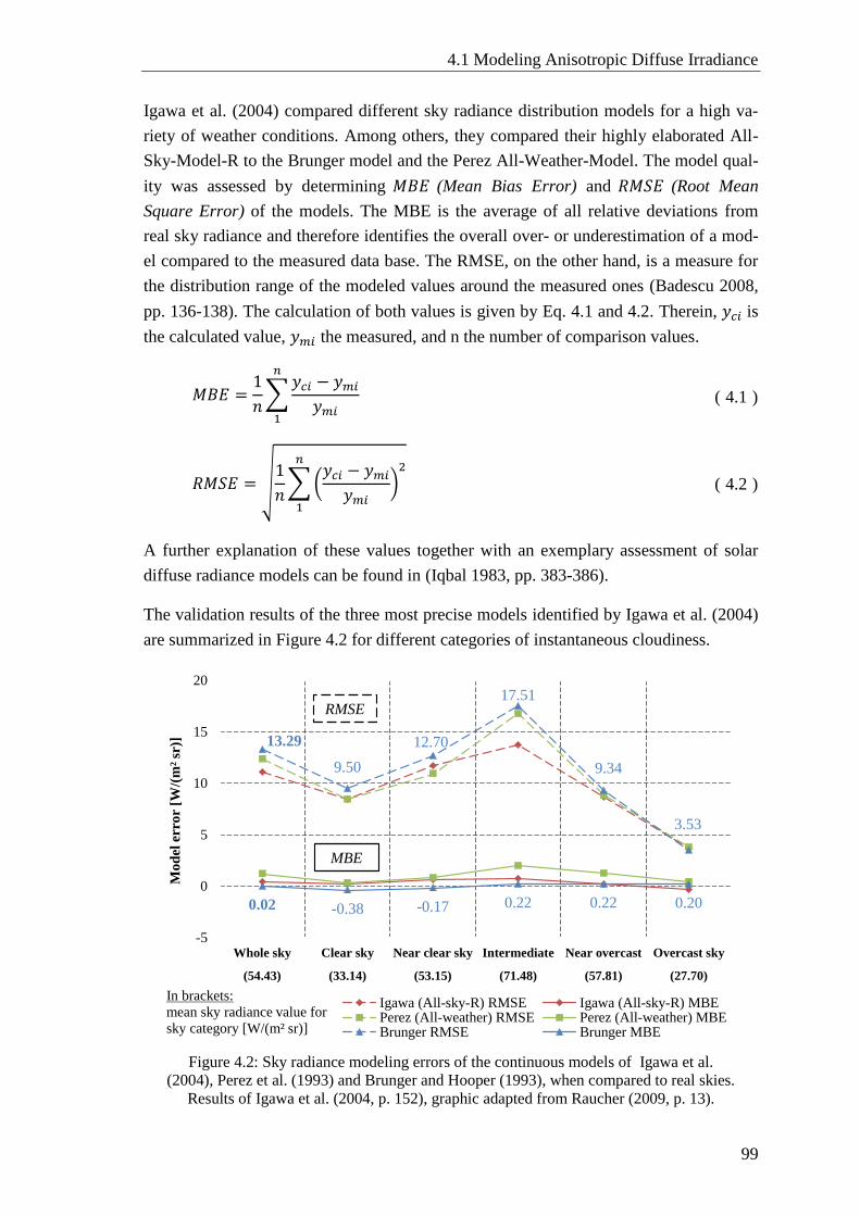
4.1 Modeling Anisotropic Diffuse Irradiance
99
Igawa et al. (2004) compared different sky radiance distribution models for a high va-
riety of weather conditions. Among others, they compared their highly elaborated All-
Sky-Model-R to the Brunger model and the Perez All-Weather-Model. The model qual-
ity was assessed by determining 𝑀𝐵𝐸 (Mean Bias Error) and 𝑅𝑀𝑆𝐸 (Root Mean
Square Error) of the models. The MBE is the average of all relative deviations from
real sky radiance and therefore identifies the overall over- or underestimation of a mod-
el compared to the measured data base. The RMSE, on the other hand, is a measure for
the distribution range of the modeled values around the measured ones (Badescu 2008,
pp. 136-138). The calculation of both values is given by Eq. 4.1 and 4.2. Therein, 𝑦𝑐𝑖 is
the calculated value, 𝑦𝑚𝑖 the measured, and n the number of comparison values.
𝑀𝐵𝐸 =1
𝑛∑
𝑦𝑐𝑖 − 𝑦𝑚𝑖
𝑦𝑚𝑖
𝑛
1
( 4.1 )
𝑅𝑀𝑆𝐸 = √1
𝑛∑(
𝑦𝑐𝑖 − 𝑦𝑚𝑖
𝑦𝑚𝑖)2
𝑛
1
( 4.2 )
A further explanation of these values together with an exemplary assessment of solar
diffuse radiance models can be found in (Iqbal 1983, pp. 383-386).
The validation results of the three most precise models identified by Igawa et al. (2004)
are summarized in Figure 4.2 for different categories of instantaneous cloudiness.
Figure 4.2: Sky radiance modeling errors of the continuous models of Igawa et al.
(2004), Perez et al. (1993) and Brunger and Hooper (1993), when compared to real skies.
Results of Igawa et al. (2004, p. 152), graphic adapted from Raucher (2009, p. 13).
13.29
9.50
12.70
17.51
9.34
3.53
0.02 -0.38 -0.17 0.22 0.22 0.20
-5
0
5
10
15
20
Whole sky Clear sky Near clear sky Intermediate Near overcast Overcast sky
(54.43) (33.14) (53.15) (71.48) (57.81) (27.70)
Mo
del
erro
r [
W/(
m²
sr)]
Igawa (All-sky-R) RMSE Igawa (All-sky-R) MBEPerez (All-weather) RMSE Perez (All-weather) MBEBrunger RMSE Brunger MBE
In brackets:
mean sky radiance value for
sky category [W/(m² sr)]
RMSE
MBE
Chapter 4: Energy Gain Simulations
100
The irradiance data used for this validation were measured with a sky-scanner of ac-
ceptance half-angle 11°. The data were collected from March 1992 to September 1993
in Tokyo and from January to December 1994 in Fukuoka, Japan. These values at the
same time also provide the database for the development of the Igawa-Model. There-
fore, it is important to note that the validation of this model was not done independently.
The Brunger model shows the lowest MBE of the three models when all sky conditions
are considered (cp. 0.02 W/(m2sr) for whole sky), so for annual simulations the gener-
ated distributions should be a good representation of the distributions occurring in reali-
ty. In comparison to the model of Igawa, the models of Perez (All-Weather) and
Brunger show significantly higher RMSE values for intermediate skies. The RSME of
Brunger is the highest of all three models but still only approx. 2 W/(m2sr) higher than
Igawa, when all sky conditions are considered. Brunger and Hooper state that their
model covers 83 % of the deterministic variation in instantaneous sky radiance and they
recommend their model to calculate irradiance incident on CPC collectors with complex
or biangular incidence angle modifiers (Brunger and Hooper 1993, p. 53). Only the All
Sky Model-R of Igawa and the Brunger Model were explicitly designed for solar sky
radiance distribution. The All Sky Model-L of Igawa, the Perez All-weather-, Harrison-
and Kittler-Model were originally developed for sky brightness distribution. Badescu
(2008, p. 428) states that brightness is in direct correlation with radiance since it is only
weighted with the sensitivity of the human eye, so the relative distribution of brightness
and radiance should be approximately identical. Figure 4.2 indeed does not show an
apparent systematic error of the brightness models in predicting sky radiance. But Fig-
ure 2.16, Figure 2.20 and Figure 2.25 clearly show the wavelength-dependence of the
optical ST collector properties, also outside the spectrum of visible light. A significant
share of diffuse spectral irradiance is in the UV range (cp. Figure 2.2). Thus, selecting a
brightness distribution model for the current task might have involved additional uncer-
tainties for ST collector output calculation.
Finally, the selection of a model to apply in collector energy gain simulations could not
only be based on the maximal accurate representation of irradiance from real skies. The
formulation of the model also had to be not too complex, because programming errors
and long simulation times had to be avoided. The Igawa model has a significantly high-
er complexity than the Brunger model. Considering and weighing all the factors above,
it was decided to use the Brunger model for inclusion in Type 154.
4.1.2 Brunger Model
Within collector Type 154 described in the next section, the model of Brunger and
Hooper (1993) is applied to generate a realistic distribution of sky diffuse radiance over
the sky dome in every simulation time step. This is used to calculate the irradiance from
finite sky elements onto the sloped collector. This irradiance is weighted with the re-
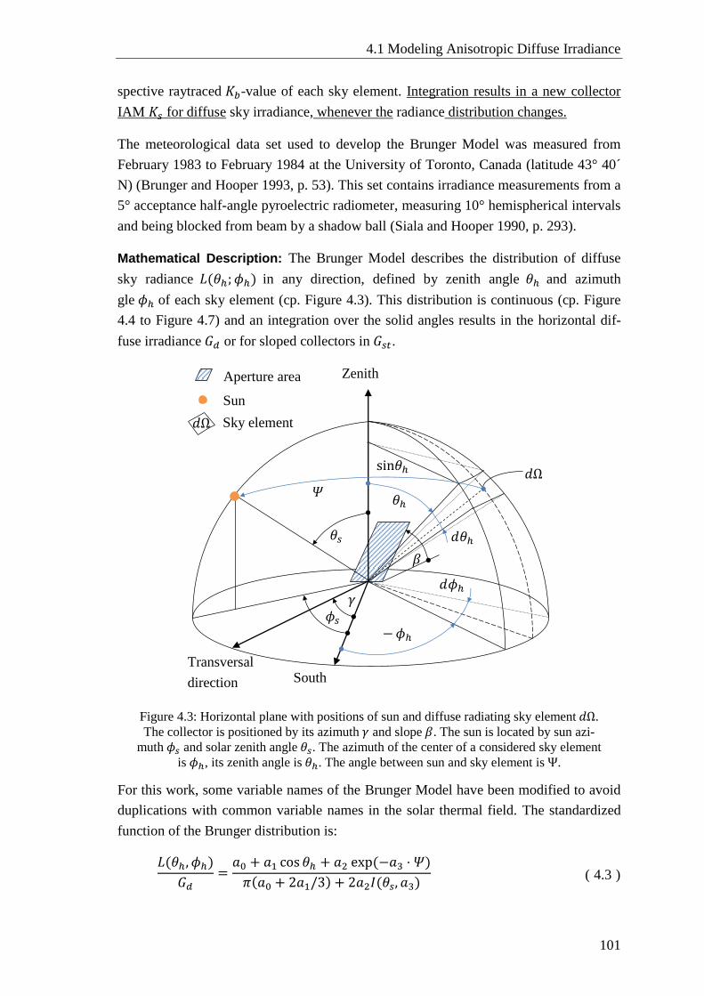
4.1 Modeling Anisotropic Diffuse Irradiance
101
spective raytraced 𝐾𝑏-value of each sky element. Integration results in a new collector
IAM 𝐾𝑠 for diffuse sky irradiance, whenever the radiance distribution changes.
The meteorological data set used to develop the Brunger Model was measured from
February 1983 to February 1984 at the University of Toronto, Canada (latitude 43° 40´
N) (Brunger and Hooper 1993, p. 53). This set contains irradiance measurements from a
5° acceptance half-angle pyroelectric radiometer, measuring 10° hemispherical intervals
and being blocked from beam by a shadow ball (Siala and Hooper 1990, p. 293).
Mathematical Description: The Brunger Model describes the distribution of diffuse
sky radiance 𝐿(𝜃ℎ; 𝜙ℎ) in any direction, defined by zenith angle 𝜃ℎ and azimuth
gle 𝜙ℎ of each sky element (cp. Figure 4.3). This distribution is continuous (cp. Figure
4.4 to Figure 4.7) and an integration over the solid angles results in the horizontal dif-
fuse irradiance 𝐺𝑑 or for sloped collectors in 𝐺𝑠𝑡.
Figure 4.3: Horizontal plane with positions of sun and diffuse radiating sky element 𝑑Ω.
The collector is positioned by its azimuth 𝛾 and slope 𝛽. The sun is located by sun azi-
muth 𝜙𝑠 and solar zenith angle 𝜃𝑠. The azimuth of the center of a considered sky element
is 𝜙ℎ, its zenith angle is 𝜃ℎ. The angle between sun and sky element is Ψ.
For this work, some variable names of the Brunger Model have been modified to avoid
duplications with common variable names in the solar thermal field. The standardized
function of the Brunger distribution is:
𝐿(𝜃ℎ, 𝜙ℎ)
𝐺𝑑=
𝑎0 + 𝑎1 cos 𝜃ℎ + 𝑎2 exp (−𝑎3 ⋅ 𝛹)
𝜋(𝑎0 + 2𝑎1/3) + 2𝑎2𝐼(𝜃𝑠, 𝑎3) ( 4.3 )
Transversal
direction
𝑑Ω
Sun
Zenith
𝜙𝑠 𝛾
𝑑Ω Sky element
𝜃𝑠
𝛹
𝛽
Aperture area
−𝜙ℎ
𝑑𝜙ℎ
𝑑𝜃ℎ
sin𝜃ℎ
𝜃ℎ
South
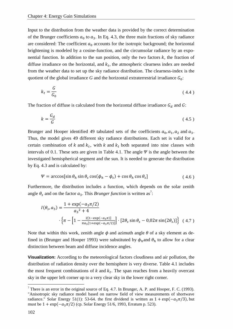
Chapter 4: Energy Gain Simulations
102
Input to the distribution from the weather data is provided by the correct determination
of the Brunger coefficients 𝑎0 to 𝑎3. In Eq. 4.3, the three main fractions of sky radiance
are considered: The coefficient 𝑎0 accounts for the isotropic background; the horizontal
brightening is modeled by a cosine-function, and the circumsolar radiance by an expo-
nential function. In addition to the sun position, only the two factors 𝑘, the fraction of
diffuse irradiance on the horizontal, and 𝑘𝑡, the atmospheric clearness index are needed
from the weather data to set up the sky radiance distribution. The clearness-index is the
quotient of the global irradiance G and the horizontal extraterrestrial irradiance 𝐺0:
𝑘𝑡 =𝐺
𝐺0 ( 4.4 )
The fraction of diffuse is calculated from the horizontal diffuse irradiance 𝐺𝑑 and 𝐺:
𝑘 =𝐺𝑑
𝐺 ( 4.5 )
Brunger and Hooper identified 49 tabulated sets of the coefficients 𝑎0, 𝑎1, 𝑎2 and 𝑎3.
Thus, the model gives 49 different sky radiance distributions. Each set is valid for a
certain combination of 𝑘 and 𝑘𝑡 , with 𝑘 and 𝑘𝑡 both separated into nine classes with
intervals of 0.1. These sets are given in Table 4.1. The angle 𝛹 is the angle between the
investigated hemispherical segment and the sun. It is needed to generate the distribution
by Eq. 4.3 and is calculated by:
𝛹 = arccos[sin 𝜃ℎ sin 𝜃𝑠 cos(𝜙ℎ − 𝜙𝑠) + cos 𝜃ℎ cos 𝜃𝑠] ( 4.6 )
Furthermore, the distribution includes a function, which depends on the solar zenith
angle 𝜃𝑠 and on the factor 𝑎3. This Brunger function is written as7:
𝐼(𝜃𝑠, 𝑎3) =1 + exp(−𝑎3𝜋/2)
𝑎32 + 4
⋅ {𝜋 − [1 −2[1−exp(−𝑎3𝜋)]
𝜋𝑎3[1+exp(−𝑎3𝜋/2)]] ⋅ [2𝜃𝑠 sin 𝜃𝑠 − 0,02𝜋 sin(2𝜃𝑠)]}
(
4.7
)
Note that within this work, zenith angle 𝜙 and azimuth angle 𝜃 of a sky element as de-
fined in (Brunger and Hooper 1993) were substituted by 𝜙ℎand 𝜃ℎ to allow for a clear
distinction between beam and diffuse incidence angles.
Visualization: According to the meteorological factors cloudiness and air pollution, the
distribution of radiation density over the hemisphere is very diverse. Table 4.1 includes
the most frequent combinations of 𝑘 and 𝑘𝑡. The span reaches from a heavily overcast
sky in the upper left corner up to a very clear sky in the lower right corner.
7 There is an error in the original source of Eq. 4.7. In Brunger, A. P. and Hooper, F. C. (1993).
"Anisotropic sky radiance model based on narrow field of view measurements of shortwave
radiance." Solar Energy 51(1): 53-64. the first dividend is written as 1 + exp(−𝑎3𝜋/3), but
must be 1 + exp(−𝑎3𝜋/2) (cp. Solar Energy 51/6, 1993, Erratum p. 523).
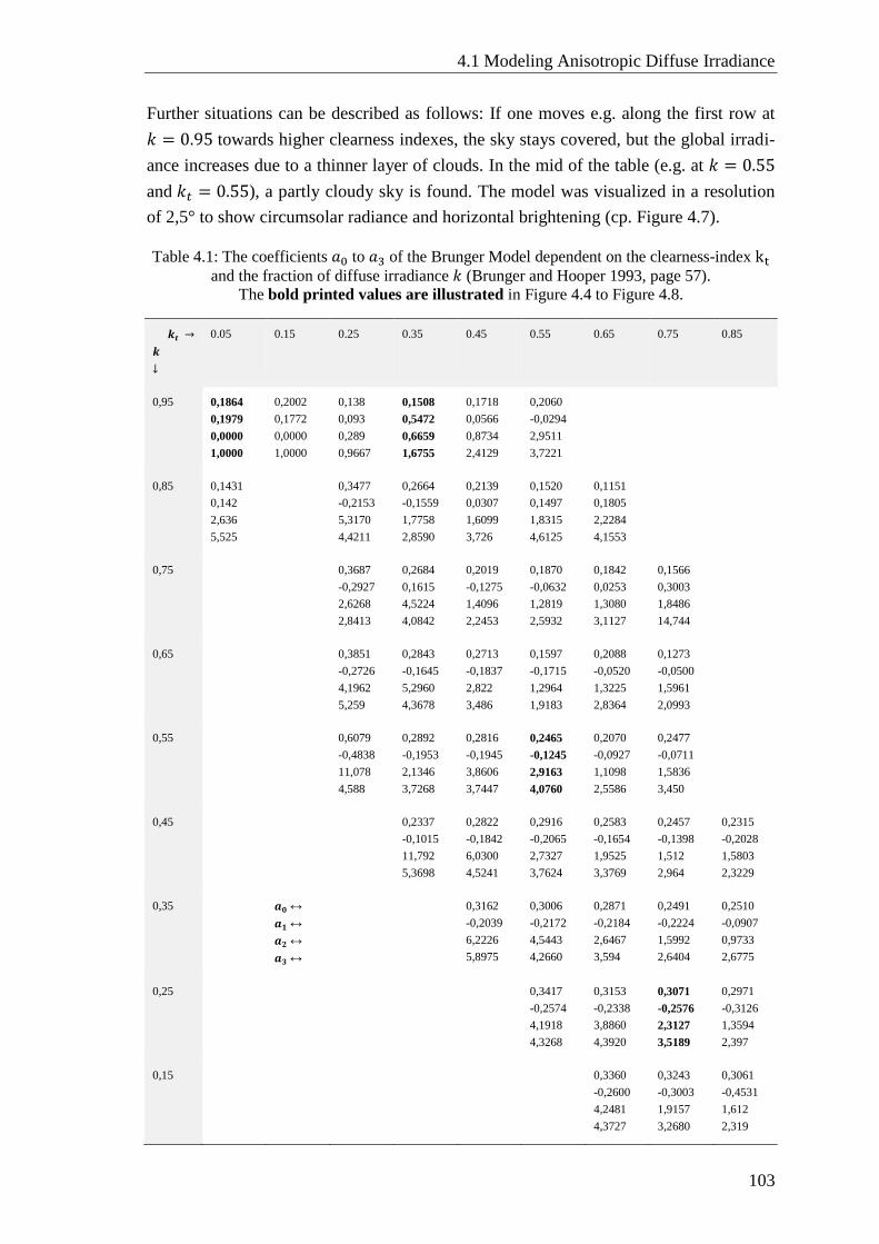
4.1 Modeling Anisotropic Diffuse Irradiance
103
Further situations can be described as follows: If one moves e.g. along the first row at
𝑘 = 0.95 towards higher clearness indexes, the sky stays covered, but the global irradi-
ance increases due to a thinner layer of clouds. In the mid of the table (e.g. at 𝑘 = 0.55
and 𝑘𝑡 = 0.55), a partly cloudy sky is found. The model was visualized in a resolution
of 2,5° to show circumsolar radiance and horizontal brightening (cp. Figure 4.7).
Table 4.1: The coefficients 𝑎0 to 𝑎3 of the Brunger Model dependent on the clearness-index kt
and the fraction of diffuse irradiance 𝑘 (Brunger and Hooper 1993, page 57).
The bold printed values are illustrated in Figure 4.4 to Figure 4.8.
𝒌𝒕 →
𝒌
↓
0.05 0.15 0.25 0.35 0.45 0.55 0.65 0.75 0.85
0,95
0,1864
0,1979
0,0000
1,0000
0,2002
0,1772
0,0000
1,0000
0,138
0,093
0,289
0,9667
0,1508
0,5472
0,6659
1,6755
0,1718
0,0566
0,8734
2,4129
0,2060
-0,0294
2,9511
3,7221
0,85
0,1431
0,142
2,636
5,525
0,3477
-0,2153
5,3170
4,4211
0,2664
-0,1559
1,7758
2,8590
0,2139
0,0307
1,6099
3,726
0,1520
0,1497
1,8315
4,6125
0,1151
0,1805
2,2284
4,1553
0,75 0,3687
-0,2927
2,6268
2,8413
0,2684
0,1615
4,5224
4,0842
0,2019
-0,1275
1,4096
2,2453
0,1870
-0,0632
1,2819
2,5932
0,1842
0,0253
1,3080
3,1127
0,1566
0,3003
1,8486
14,744
0,65 0,3851
-0,2726
4,1962
5,259
0,2843
-0,1645
5,2960
4,3678
0,2713
-0,1837
2,822
3,486
0,1597
-0,1715
1,2964
1,9183
0,2088
-0,0520
1,3225
2,8364
0,1273
-0,0500
1,5961
2,0993
0,55 0,6079
-0,4838
11,078
4,588
0,2892
-0,1953
2,1346
3,7268
0,2816
-0,1945
3,8606
3,7447
0,2465
-0,1245
2,9163
4,0760
0,2070
-0,0927
1,1098
2,5586
0,2477
-0,0711
1,5836
3,450
0,45 0,2337
-0,1015
11,792
5,3698
0,2822
-0,1842
6,0300
4,5241
0,2916
-0,2065
2,7327
3,7624
0,2583
-0,1654
1,9525
3,3769
0,2457
-0,1398
1,512
2,964
0,2315
-0,2028
1,5803
2,3229
0,35 𝒂𝟎 ↔
𝒂𝟏 ↔
𝒂𝟐 ↔
𝒂𝟑 ↔
0,3162
-0,2039
6,2226
5,8975
0,3006
-0,2172
4,5443
4,2660
0,2871
-0,2184
2,6467
3,594
0,2491
-0,2224
1,5992
2,6404
0,2510
-0,0907
0,9733
2,6775
0,25 0,3417
-0,2574
4,1918
4,3268
0,3153
-0,2338
3,8860
4,3920
0,3071
-0,2576
2,3127
3,5189
0,2971
-0,3126
1,3594
2,397
0,15 0,3360
-0,2600
4,2481
4,3727
0,3243
-0,3003
1,9157
3,2680
0,3061
-0,4531
1,612
2,319
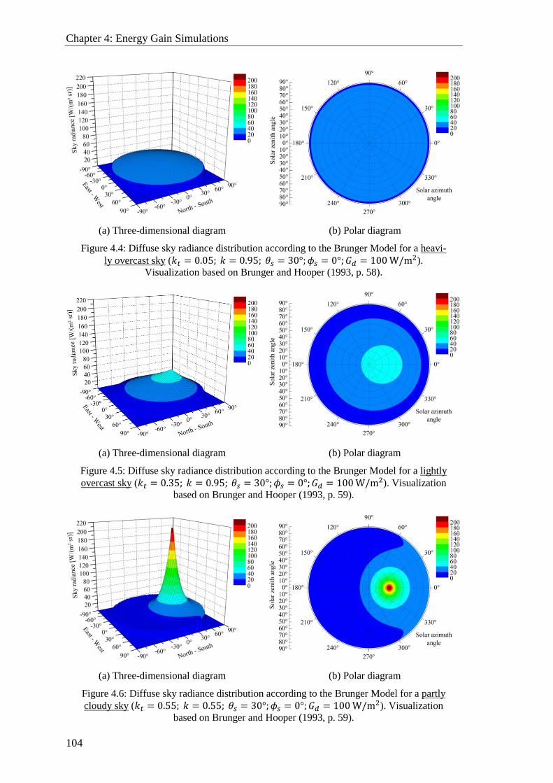
Chapter 4: Energy Gain Simulations
104
(a) Three-dimensional diagram (b) Polar diagram
Figure 4.4: Diffuse sky radiance distribution according to the Brunger Model for a heavi-
ly overcast sky (𝑘𝑡 = 0.05; 𝑘 = 0.95; 𝜃𝑠 = 30°;𝜙𝑠 = 0°; 𝐺𝑑 = 100 W/m2).
Visualization based on Brunger and Hooper (1993, p. 58).
(a) Three-dimensional diagram (b) Polar diagram
Figure 4.5: Diffuse sky radiance distribution according to the Brunger Model for a lightly
overcast sky (𝑘𝑡 = 0.35; 𝑘 = 0.95; 𝜃𝑠 = 30°; 𝜙𝑠 = 0°;𝐺𝑑 = 100 W/m2). Visualization
based on Brunger and Hooper (1993, p. 59).
(a) Three-dimensional diagram (b) Polar diagram
Figure 4.6: Diffuse sky radiance distribution according to the Brunger Model for a partly
cloudy sky (𝑘𝑡 = 0.55; 𝑘 = 0.55; 𝜃𝑠 = 30°;𝜙𝑠 = 0°;𝐺𝑑 = 100 W/m2). Visualization
based on Brunger and Hooper (1993, p. 59).
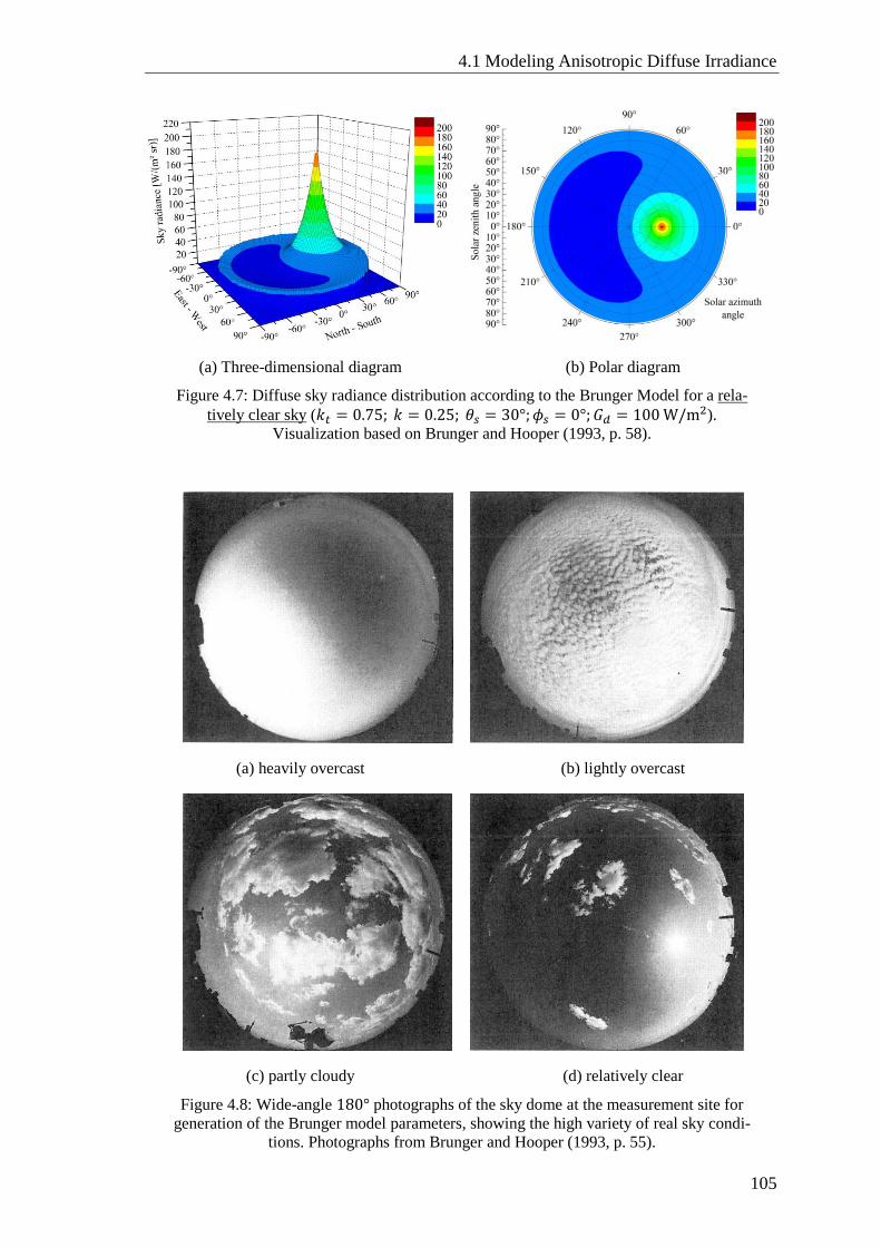
4.1 Modeling Anisotropic Diffuse Irradiance
105
(a) Three-dimensional diagram (b) Polar diagram
Figure 4.7: Diffuse sky radiance distribution according to the Brunger Model for a rela-
tively clear sky (𝑘𝑡 = 0.75; 𝑘 = 0.25; 𝜃𝑠 = 30°;𝜙𝑠 = 0°; 𝐺𝑑 = 100 W/m2).
Visualization based on Brunger and Hooper (1993, p. 58).
(a) heavily overcast (b) lightly overcast
(c) partly cloudy (d) relatively clear
Figure 4.8: Wide-angle 180° photographs of the sky dome at the measurement site for
generation of the Brunger model parameters, showing the high variety of real sky condi-
tions. Photographs from Brunger and Hooper (1993, p. 55).
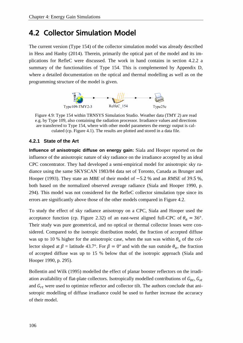
Chapter 4: Energy Gain Simulations
106
4.2 Collector Simulation Model
The current version (Type 154) of the collector simulation model was already described
in Hess and Hanby (2014). Therein, primarily the optical part of the model and its im-
plications for RefleC were discussed. The work in hand contains in section 4.2.2 a
summary of the functionalities of Type 154. This is complemented by Appendix D,
where a detailed documentation on the optical and thermal modelling as well as on the
programming structure of the model is given.
Figure 4.9: Type 154 within TRNSYS Simulation Studio. Weather data (TMY 2) are read
e.g. by Type 109, also containing the radiation processor. Irradiance values and directions
are transferred to Type 154, where with other model parameters the energy output is cal-
culated (cp. Figure 4.1). The results are plotted and stored in a data file.
4.2.1 State of the Art
Influence of anisotropic diffuse on energy gain: Siala and Hooper reported on the
influence of the anisotropic nature of sky radiance on the irradiance accepted by an ideal
CPC concentrator. They had developed a semi-empirical model for anisotropic sky ra-
diance using the same SKYSCAN 1983/84 data set of Toronto, Canada as Brunger and
Hooper (1993). They state an MBE of their model of −5.2 % and an RMSE of 39.5 %,
both based on the normalized observed average radiance (Siala and Hooper 1990, p.
294). This model was not considered for the RefleC collector simulation type since its
errors are significantly above those of the other models compared in Figure 4.2.
To study the effect of sky radiance anisotropy on a CPC, Siala and Hooper used the
acceptance function (cp. Figure 2.32) of an east-west aligned full-CPC of 𝜃𝑎 = 36°.
Their study was pure geometrical, and no optical or thermal collector losses were con-
sidered. Compared to the isotropic distribution model, the fraction of accepted diffuse
was up to 10 % higher for the anisotropic case, when the sun was within 𝜃𝑎 of the col-
lector sloped at 𝛽 = latitude 43.7°. For 𝛽 = 0° and with the sun outside 𝜃𝑎, the fraction
of accepted diffuse was up to 15 % below that of the isotropic approach (Siala and
Hooper 1990, p. 295).
Bollentin and Wilk (1995) modelled the effect of planar booster reflectors on the irradi-
ation availability of flat-plate collectors. Isotropically modelled contributions of 𝐺𝑏𝑡, 𝐺𝑠𝑡
and 𝐺𝑟𝑡 were used to optimize reflector and collector tilt. The authors conclude that ani-
sotropic modelling of diffuse irradiance could be used to further increase the accuracy
of their model.
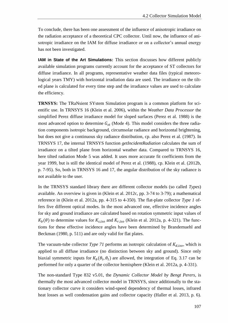
4.2 Collector Simulation Model
107
To conclude, there has been one assessment of the influence of anisotropic irradiance on
the radiation acceptance of a theoretical CPC collector. Until now, the influence of ani-
sotropic irradiance on the IAM for diffuse irradiance or on a collector’s annual energy
has not been investigated.
IAM in State of the Art Simulations: This section discusses how different publicly
available simulation programs currently account for the acceptance of ST collectors for
diffuse irradiance. In all programs, representative weather data files (typical meteoro-
logical years TMY) with horizontal irradiation data are used. The irradiance on the tilt-
ed plane is calculated for every time step and the irradiance values are used to calculate
the efficiency.
TRNSYS: The TRaNsient SYstem Simulation program is a common platform for sci-
entific use. In TRNSYS 16 (Klein et al. 2006), within the Weather Data Processor the
simplified Perez diffuse irradiance model for sloped surfaces (Perez et al. 1988) is the
most advanced option to determine 𝐺𝑠𝑡 (Mode 4). This model considers the three radia-
tion components isotropic background, circumsolar radiance and horizontal brightening,
but does not give a continuous sky radiance distribution, cp. also Perez et al. (1987). In
TRNSYS 17, the internal TRNSYS function getIncidentRadiation calculates the sum of
irradiance on a tilted plane from horizontal weather data. Compared to TRNSYS 16,
here tilted radiation Mode 5 was added. It uses more accurate fit coefficients from the
year 1999, but is still the identical model of Perez et al. (1988), cp. Klein et al. (2012b,
p. 7-95). So, both in TRNSYS 16 and 17, the angular distribution of the sky radiance is
not available to the user.
In the TRNSYS standard library there are different collector models (so called Types)
available. An overview is given in (Klein et al. 2012c, pp. 3-74 to 3-79); a mathematical
reference in (Klein et al. 2012a, pp. 4-315 to 4-350). The flat-plate collector Type 1 of-
fers five different optical modes. In the most advanced one, effective incidence angles
for sky and ground irradiance are calculated based on rotation symmetric input values of
𝐾𝑏(𝜃) to determine values for 𝐾𝑠,𝑖𝑠𝑜 and 𝐾𝑟,𝑖𝑠𝑜 (Klein et al. 2012a, p. 4-321). The func-
tions for these effective incidence angles have been determined by Brandemuehl and
Beckman (1980, p. 511) and are only valid for flat plates.
The vacuum-tube collector Type 71 performs an isotropic calculation of 𝐾𝑑,𝑖𝑠𝑜, which is
applied to all diffuse irradiance (no distinction between sky and ground). Since only
biaxial symmetric inputs for 𝐾𝑏(𝜃𝑙, 𝜃𝑡) are allowed, the integration of Eq. 3.17 can be
performed for only a quarter of the collector hemisphere (Klein et al. 2012a, p. 4-331).
The non-standard Type 832 v5.01, the Dynamic Collector Model by Bengt Perers, is
thermally the most advanced collector model in TRNSYS, since additionally to the sta-
tionary collector curve it considers wind-speed dependency of thermal losses, infrared
heat losses as well condensation gains and collector capacity (Haller et al. 2013, p. 6).
Chapter 4: Energy Gain Simulations
108
As in Type 71, no distinction between sky and ground diffuse is made. Different from
Type 71, 𝐾𝑑,𝑖𝑠𝑜 here is an input parameter which the user has to take from test lab re-
ports or calculate with Eq. 3.17.
T*SOL, Polysun: T*Sol Pro v5.5 (Valentin 2014) and Polysun v5.10 (Velasolaris
2013) are common commercial solar thermal system simulation programs used by plan-
ners. Extensive collector bibliotheca are available containing biaxial symmetric
𝐾𝑏(𝜃𝑙, 𝜃𝑡)-values and 𝐾𝑑,𝑖𝑠𝑜 as input parameter from test lab measurements. These val-
ues can also be entered for a self-defined collector.
SCEnOCalc: The Solar Collector ENergy Output CALCulator v4.06 is a MS Excel-
based tool to calculate the thermal output of Solar Keymark tested collectors for the four
locations Athens, Davos, Stockholm and Würzburg for the three constant collector
mean temperatures 25 °C, 50 °C and 75 °C (SCEnOCalc 2014). When quasi-dynamic
test results are used, also biaxial asymmetric 𝐾𝑏(𝜃𝑙, 𝜃𝑡)-values can be entered. As in
TRNSYS Type 71, 𝐾𝑑,𝑖𝑠𝑜 is an input parameter and no distinction between diffuse from
sky and ground is made.
To conclude, state of the art simulation programs / collector models:
do not have the angular distribution of diffuse sky radiance available
consider IAM values 𝐾𝑑 (or 𝐾𝑠 and 𝐾𝑟) as constant collector parameters only.
Only RefleC_154 and TRNSYS Type 71 do work with 3D 𝐾𝑏-values from an external
file. The other types use two-dimensional IAM curves (e.g. flat-plate IAM approach of
Souka/Safwat for longitudinal direction and measured transversal IAM values). The
beam-IAMs for intermediate angles are calculated within the collector types itself by
the separation approach of McIntire.
4.2.2 Model Description
Modelling the IAM for anisotropic diffuse irradiance: The collector simulation mod-
el introduced here was programed in Fortran and is applied in TRNSYS 16 as user-
defined Type 154. Its unique difference compared to existing models is that the IAM for
diffuse irradiance from the sky 𝐾𝑠 is re-calculated in every time step based on realisti-
cally distributed anisotropic diffuse sky radiance. The change of the optical efficiency
with varying skies allows for investigating to which extent the sky radiance anisotropy
influences the collector output. For this purpose, Type 154 distributes the sum of hori-
zontal sky diffuse irradiance (input from weather data reader) over the hemisphere ac-
cording to the model of Brunger and Hooper (1993), cp. section 4.1.2 for a description.
Ground reflected diffuse is treated isotropic. The model calculates the collector’s
IAMs 𝐾𝑏, 𝐾𝑠 and 𝐾𝑟 separately and for arbitrarily shaped 𝐾𝑏-curves provided in an in-
put text file. Figure 4.10 illustrates schematically the functions of Type 154.
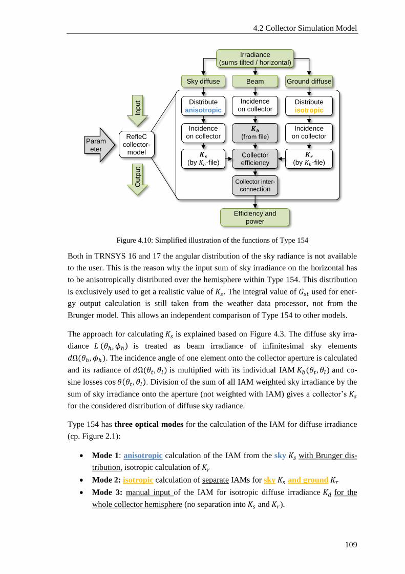
4.2 Collector Simulation Model
109
Figure 4.10: Simplified illustration of the functions of Type 154
Both in TRNSYS 16 and 17 the angular distribution of the sky radiance is not available
to the user. This is the reason why the input sum of sky irradiance on the horizontal has
to be anisotropically distributed over the hemisphere within Type 154. This distribution
is exclusively used to get a realistic value of 𝐾𝑠. The integral value of 𝐺𝑠𝑡 used for ener-
gy output calculation is still taken from the weather data processor, not from the
Brunger model. This allows an independent comparison of Type 154 to other models.
The approach for calculating 𝐾𝑠 is explained based on Figure 4.3. The diffuse sky irra-
diance 𝐿 (𝜃ℎ, 𝜙ℎ) is treated as beam irradiance of infinitesimal sky elements
𝑑Ω(𝜃ℎ, 𝜙ℎ). The incidence angle of one element onto the collector aperture is calculated
and its radiance of 𝑑Ω(𝜃𝑡, 𝜃𝑙) is multiplied with its individual IAM 𝐾𝑏(𝜃𝑡, 𝜃𝑙) and co-
sine losses cos 𝜃(𝜃𝑡, 𝜃𝑙). Division of the sum of all IAM weighted sky irradiance by the
sum of sky irradiance onto the aperture (not weighted with IAM) gives a collector’s 𝐾𝑠
for the considered distribution of diffuse sky radiance.
Type 154 has three optical modes for the calculation of the IAM for diffuse irradiance
(cp. Figure 2.1):
Mode 1: anisotropic calculation of the IAM from the sky 𝐾𝑠 with Brunger dis-
tribution, isotropic calculation of 𝐾𝑟
Mode 2: isotropic calculation of separate IAMs for sky 𝐾𝑠 and ground 𝐾𝑟
Mode 3: manual input of the IAM for isotropic diffuse irradiance 𝐾𝑑 for the
whole collector hemisphere (no separation into 𝐾𝑠 and 𝐾𝑟).
RefleC
collector- model
Input
Outp
ut
Param
eter
Irradiance (sums tilted / horizontal)
Sky diffuse Beam Ground diffuse
Distribute
anisotropic
𝑲𝒃 (from file)
Distribute
isotropic
Incidence on collector
Incidence on collector
𝑲𝒔
(by 𝐾𝑏-file)
𝑲𝒓
(by 𝐾𝑏-file)
Collector efficiency
Collector inter-
connection
Incidence on collector
Efficiency and power
Chapter 4: Energy Gain Simulations
110
In Mode 1, 𝐾𝑠 is calculated new for every time step, since 𝐾𝑠 depends on the current
sky radiance distribution. 𝐾𝑟 is calculated once per simulation for isotropic ground radi-
ance. Both 𝐾𝑠 and 𝐾𝑟 depend on the collector’s IAM for beam irradiance 𝐾𝑏 and there-
fore also on the collector slope 𝛽.
In Mode 2, 𝐾𝑠 and 𝐾𝑟 are calculated once per simulation for isotropic sky and ground.
They depend on the collector´s IAM for beam irradiance 𝐾𝑏 and therefore also on the
collector slope 𝛽.
Mode 3 does not distinguish between sky and ground diffuse irradiance. In this most
simple case, the sum of diffuse irradiance is considered to originate from a 180° collec-
tor hemisphere of isotropic radiance. Only for this simplification, the IAM for diffuse
irradiance (sky and ground) 𝐾𝑑 is a constant collector parameter, which only depends
on the IAM for beam irradiance 𝐾𝑏. It is independent of 𝛽 and of the current values of
𝐺𝑠𝑡 and 𝐺𝑏𝑡 . For 𝛽 = 0, 𝐾𝑑 equals 𝐾𝑠 from Mode 2. All collector simulation models
described in section 4.2.1 calculate according to this approach, which is a very rough
simplification and source of uncertainty for most collector types, as will be shown in the
next sections.
The values of 𝐾𝑏(𝜃𝑡, 𝜃𝑙) are provided by the user in an external text file and can origi-
nate from measurements or raytracing. Thus, the errors by applying the separation ap-
proach of (McIntire 1982) are not made within Type 154 and it depends on the external
IAM file how exactly 𝐾𝑏(𝜃𝑡, 𝜃𝑙) is accounted for. Type 154 is the only collector model
allowing for biaxial, asymmetric 3D-IAM input.
Type 154 offers the following functions:
Three optical modes to calculate the IAM for diffuse irradiance are provided.
Input of biaxial, asymmetric 3D-IAM values is possible.
The effective thermal collector capacity 𝑐𝑒𝑓𝑓 is considered.
Up to ten collectors can be connected serially, an unlimited number in parallel.
The outlet temperatures of all serially connected collectors 𝑇𝑜𝑢𝑡,𝑖 are provided
When there is no mass flow, the stagnation temperature is calculated.
The modelling of Type 154 is described in detail in Appendix D. In Appendix D.1, an
overview on the modelling structure is given. Appendix D.2 contains all Inputs, Pa-
rameters and Outputs of the model. Therein, “inputs” are variables provided from links
to other TRNSYS types, “parameters” are constant user-input values and “outputs” are
variables calculated by Type 154 based on the inputs and parameters. The appendices
D.3 to D.7 give detailed information on the optical and thermal modelling.
In the following, simulation results of Type 154 for RefleC and the flat-plate are given.
Their implications on the simulation of stationary solar thermal collectors are discussed.
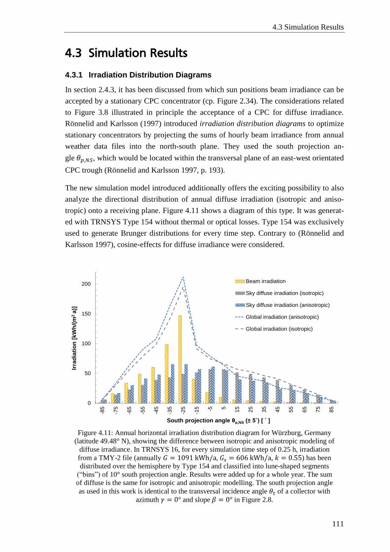
4.3 Simulation Results
111
4.3 Simulation Results
4.3.1 Irradiation Distribution Diagrams
In section 2.4.3, it has been discussed from which sun positions beam irradiance can be
accepted by a stationary CPC concentrator (cp. Figure 2.34). The considerations related
to Figure 3.8 illustrated in principle the acceptance of a CPC for diffuse irradiance.
Rönnelid and Karlsson (1997) introduced irradiation distribution diagrams to optimize
stationary concentrators by projecting the sums of hourly beam irradiance from annual
weather data files into the north-south plane. They used the south projection an-
gle 𝜃𝑝,𝑁𝑆, which would be located within the transversal plane of an east-west orientated
CPC trough (Rönnelid and Karlsson 1997, p. 193).
The new simulation model introduced additionally offers the exciting possibility to also
analyze the directional distribution of annual diffuse irradiation (isotropic and aniso-
tropic) onto a receiving plane. Figure 4.11 shows a diagram of this type. It was generat-
ed with TRNSYS Type 154 without thermal or optical losses. Type 154 was exclusively
used to generate Brunger distributions for every time step. Contrary to (Rönnelid and
Karlsson 1997), cosine-effects for diffuse irradiance were considered.
Figure 4.11: Annual horizontal irradiation distribution diagram for Würzburg, Germany
(latitude 49.48° N), showing the difference between isotropic and anisotropic modeling of
diffuse irradiance. In TRNSYS 16, for every simulation time step of 0.25 h, irradiation
from a TMY-2 file (annually 𝐺 = 1091 kWh/a, 𝐺𝑠 = 606 kWh/a, 𝑘 = 0.55) has been
distributed over the hemisphere by Type 154 and classified into lune-shaped segments
(“bins”) of 10° south projection angle. Results were added up for a whole year. The sum
of diffuse is the same for isotropic and anisotropic modelling. The south projection angle
as used in this work is identical to the transversal incidence angle 𝜃𝑡 of a collector with
azimuth 𝛾 = 0° and slope 𝛽 = 0° in Figure 2.8.
0
50
100
150
200
-85
-75
-65
-55
-45
-35
-25
-15 -5 5
15
25
35
45
55
65
75
85
Irra
dia
tio
n [
kW
h/(
m2 a
)]
South projection angle θp,NS (± 5˚) [ ˚ ]
Beam irradiation
Sky diffuse irradiation (isotropic)
Sky diffuse irradiation (anisotropic)
Global irradiation (anisotropic)
Global irradiation (isotropic)
Chapter 4: Energy Gain Simulations
112
The distribution of beam can be understood from Figure 2.33 and Figure 2.34 and cor-
responds very well to the results of Rönnelid and Karlsson (1997). It is not affected by
the diffuse irradiance model used. When looking at the distribution of diffuse, in case of
isotropic distribution only the cosine effect is visible, since in Mode 2, Type 154 dis-
tributes the sky radiance evenly over the hemisphere. The sums of isotropic irradiation
are mirror-symmetric between the northern and southern hemisphere. When distributing
it according to Brunger by Mode 1, the result is considerably different. Particularly from
directions with regular beam irradiance, a significant increase of diffuse irradiance can
be observed. This is expected to be caused by broad circumsolar diffuse irradiance. For
the simplified assumption of an isotropic sky, 70 % of the annual global irradiance orig-
inates from the southern hemisphere. This value increases to 77 % for more realistic
anisotropic modelling. It is found that for Würzburg, isotropic modelling underestimates
the diffuse irradiance from the southern hemisphere by 20 %.
But how does this affect the irradiance onto the sloped RefleC collector? Figure 4.12
shows the same investigation as in Figure 4.11, but for the aperture plane of RefleC 6
GF sloped by 𝛽 = 55°, and with a simplified transversal 𝐾𝑏-curve indicated. To under-
stand Figure 4.12, it is again important that the annual sum 𝐺𝑠𝑡 is the same in the iso-
tropic and the anisotropic case, since Type 154 was only used to classify the directions
of irradiance into transversal intervals, not to calculate the irradiation itself. As in Figure
4.11, the anisotropic distribution causes significantly higher sky diffuse irradiation from
the segments with high beam irradiation. Correspondingly, less irradiance originates
from the north. Comparing Figure 4.12 to Figure 4.11 shows that for the isotropic case
the incident sky diffuse irradiance is as expected still mirror-symmetric to the surface
normal, when we consider that 𝜃𝑡 = −35° represents a sky segment of only half the
width than its opposite segment 𝜃𝑡 = +35°. This is because of the fact that for 𝛽 = 55°
the horizon is within the interval 𝜃𝑡 = −35° = [−40°;−30°], dividing it into two equal
lune shaped segments, of which the lower one already belongs to the ground.
The ground reflected diffuse irradiation is one order of magnitude smaller than diffuse
from the sky. There is also some ground reflected diffuse from 𝜃𝑡 < −35°, since ground
irradiance from east or west has smaller projected transversal incidence angles (cp. Fig-
ure 2.8). Comparing the distributions of ground and sky diffuse irradiance gives clear
indication that the isotropic distribution of 𝐺𝑑𝑡 = 𝐺𝑠𝑡 + 𝐺𝑟𝑡 over the collector hemi-
sphere, as it is practice in standard simulation programs and possible with Mode 3 of
Type 154, is a very rough simplification expected to cause significant errors in simulat-
ed annual energy gain. This is relevant for all stationary collectors, we considered only
the irradiance on the tilted plane, and not yet the irradiation utilization by RefleC.
Figure 4.12 shows a clear maximum of beam irradiance from 𝜃𝑡 = [20; 30]. For RefleC
sloped 𝛽 = 55°, this is also the maximum of 𝐾𝑏. So Figure 4.12 indicates that this slope
can be expected to be around the optimum for maximal annual gains.
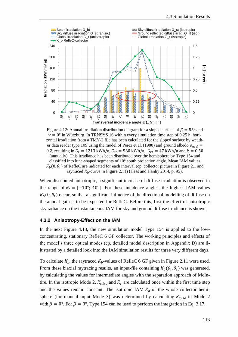
4.3 Simulation Results
113
Figure 4.12: Annual irradiation distribution diagram for a sloped surface of 𝛽 = 55° and
𝛾 = 0° in Würzburg. In TRNSYS 16 within every simulation time step of 0.25 h, hori-
zontal irradiation from a TMY-2 file has been calculated for the sloped surface by weath-
er data reader type 109 using the model of Perez et al. (1988) and ground albedo 𝜌𝑔𝑟𝑑 =
0.2, resulting in 𝐺𝑡 = 1213 kWh/a, 𝐺𝑠𝑡 = 560 kWh/a, 𝐺𝑟𝑡 = 47 kWh/a and 𝑘 = 0.50
(annually). This irradiance has been distributed over the hemisphere by Type 154 and
classified into lune-shaped segments of 10° south projection angle. Mean IAM values
𝐾𝑏(0, 𝜃𝑡) of RefleC are indicated for each interval (cp. collector picture in Figure 2.1 and
raytraced 𝐾𝑏-curve in Figure 2.11) (Hess and Hanby 2014, p. 95).
When distributed anisotropic, a significant increase of diffuse irradiation is observed in
the range of 𝜃𝑡 = [−10°; 40°]. For these incidence angles, the highest IAM values
𝐾𝑏(0, 𝜃𝑡) occur, so that a significant influence of the directional modelling of diffuse on
the annual gain is to be expected for RefleC. Before this, first the effect of anisotropic
sky radiance on the instantaneous IAM for sky and ground diffuse irradiance is shown.
4.3.2 Anisotropy-Effect on the IAM
In the next Figure 4.13, the new simulation model Type 154 is applied to the low-
concentrating, stationary RefleC 6 GF collector. The working principles and effects of
the model’s three optical modes (cp. detailed model description in Appendix D) are il-
lustrated by a detailed look into the IAM simulation results for three very different days.
To calculate 𝐾𝑠, the raytraced 𝐾𝑏-values of RefleC 6 GF given in Figure 2.11 were used.
From these biaxial raytracing results, an input-file containing 𝐾𝑏(𝜃𝑙, 𝜃𝑡) was generated,
by calculating the values for intermediate angles with the separation approach of McIn-
tire. In the isotropic Mode 2, 𝐾𝑠,𝑖𝑠𝑜 and 𝐾𝑟 are calculated once within the first time step
and the values remain constant. The isotropic IAM 𝐾𝑑 of the whole collector hemi-
sphere (for manual input Mode 3) was determined by calculating 𝐾𝑠,𝑖𝑠𝑜 in Mode 2
with 𝛽 = 0°. For 𝛽 = 0°, Type 154 can be used to perform the integration in Eq. 3.17.
0
0.25
0.5
0.75
1
1.25
1.5
0
40
80
120
160
200
240
-85
-75
-65
-55
-45
-35
-25
-15 -5 5
15
25
35
45
55
65
75
85
IAM
Kb
[ -
]
Irra
dia
tio
n [
kW
h/(
m2
a)]
Transversal incidence angle θt (± 5˚) [ ˚ ]
Beam irradiation G_bt Sky diffuse irradiation G_st (isotropic)Sky diffuse irradiation G_st (aniso.) Ground reflected diffuse irrad. G_rt (iso.)Global irradiation G_t (anisotropic) Global irradiation G_t (isotropic)K_b RefleC-collector
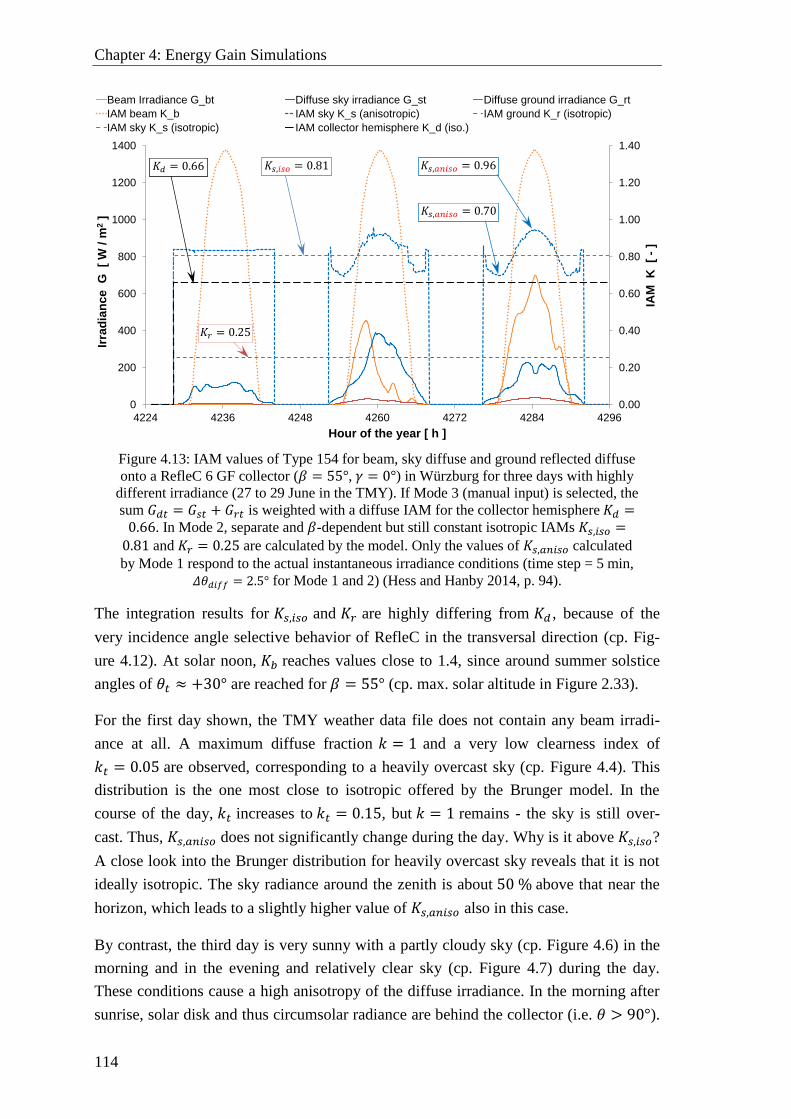
Chapter 4: Energy Gain Simulations
114
Figure 4.13: IAM values of Type 154 for beam, sky diffuse and ground reflected diffuse
onto a RefleC 6 GF collector (𝛽 = 55°, 𝛾 = 0°) in Würzburg for three days with highly
different irradiance (27 to 29 June in the TMY). If Mode 3 (manual input) is selected, the
sum 𝐺𝑑𝑡 = 𝐺𝑠𝑡 + 𝐺𝑟𝑡 is weighted with a diffuse IAM for the collector hemisphere 𝐾𝑑 =0.66. In Mode 2, separate and 𝛽-dependent but still constant isotropic IAMs 𝐾𝑠,𝑖𝑠𝑜 =
0.81 and 𝐾𝑟 = 0.25 are calculated by the model. Only the values of 𝐾𝑠,𝑎𝑛𝑖𝑠𝑜 calculated
by Mode 1 respond to the actual instantaneous irradiance conditions (time step = 5 min,
𝛥𝜃𝑑𝑖𝑓𝑓 = 2.5° for Mode 1 and 2) (Hess and Hanby 2014, p. 94).
The integration results for 𝐾𝑠,𝑖𝑠𝑜 and 𝐾𝑟 are highly differing from 𝐾𝑑 , because of the
very incidence angle selective behavior of RefleC in the transversal direction (cp. Fig-
ure 4.12). At solar noon, 𝐾𝑏 reaches values close to 1.4, since around summer solstice
angles of 𝜃𝑡 ≈ +30° are reached for 𝛽 = 55° (cp. max. solar altitude in Figure 2.33).
For the first day shown, the TMY weather data file does not contain any beam irradi-
ance at all. A maximum diffuse fraction 𝑘 = 1 and a very low clearness index of
𝑘𝑡 = 0.05 are observed, corresponding to a heavily overcast sky (cp. Figure 4.4). This
distribution is the one most close to isotropic offered by the Brunger model. In the
course of the day, 𝑘𝑡 increases to 𝑘𝑡 = 0.15, but 𝑘 = 1 remains - the sky is still over-
cast. Thus, 𝐾𝑠,𝑎𝑛𝑖𝑠𝑜 does not significantly change during the day. Why is it above 𝐾𝑠,𝑖𝑠𝑜?
A close look into the Brunger distribution for heavily overcast sky reveals that it is not
ideally isotropic. The sky radiance around the zenith is about 50 % above that near the
horizon, which leads to a slightly higher value of 𝐾𝑠,𝑎𝑛𝑖𝑠𝑜 also in this case.
By contrast, the third day is very sunny with a partly cloudy sky (cp. Figure 4.6) in the
morning and in the evening and relatively clear sky (cp. Figure 4.7) during the day.
These conditions cause a high anisotropy of the diffuse irradiance. In the morning after
sunrise, solar disk and thus circumsolar radiance are behind the collector (i.e. 𝜃 > 90°).
0.00
0.20
0.40
0.60
0.80
1.00
1.20
1.40
0
200
400
600
800
1000
1200
1400
4224 4236 4248 4260 4272 4284 4296
IAM
K
[
-]
Irra
dia
nce
G [
W / m
2]
Hour of the year [ h ]
Beam Irradiance G_bt Diffuse sky irradiance G_st Diffuse ground irradiance G_rt
IAM beam K_b IAM sky K_s (anisotropic) IAM ground K_r (isotropic)
IAM sky K_s (isotropic) IAM collector hemisphere K_d (iso.)
𝐾𝑟 = 0.25
𝐾𝑠,𝑖𝑠𝑜 = 0.81 𝐾𝑠,𝑎𝑛𝑖𝑠𝑜 = 0.96 𝐾𝑑 = 0.66
𝐾𝑠,𝑎𝑛𝑖𝑠𝑜 = 0.70
4.3 Simulation Results
115
Since a share of the brightening around the sun is diffuse, in the morning of a clear day
the majority of sky radiance is in the northern hemisphere. At this time, for the RefleC
aperture, 𝐾𝑠,𝑎𝑛𝑖𝑠𝑜 is smaller than for the isotropic assumption. With progressing sun
movement in the course of the day this changes, and around noon the solar brightening
is incident from 𝜃𝑡 ≈ +30°, where 𝐾𝑏 of RefleC is maximal. Due to these effects, varia-
tions of 𝐾𝑠,𝑎𝑛𝑖𝑠𝑜 by up to ca. 25 %-points during one day are possible. Analyzing Figure
4.13, we can conclude for RefleC that constant, isotropic treatment of diffuse irradiance
from the collector hemisphere (i.e. 𝐾𝑑 in Mode 3):
significantly overestimates the contribution of ground reflected diffuse, and
highly underestimates the contribution of sky diffuse irradiance.
For RefleC, the impact of these errors is very high. 𝐾𝑏 reflects the character of the re-
flector: It shades the absorber for ground irradiance and increases the absorbed irradi-
ance from the sky. So another conclusion, proved by Figure 4.13, is:
For RefleC, the calculation of a separate, but isotropic diffuse IAM for the sky
(Mode 2) still underestimates the contribution of sky diffuse irradiance.
This is because relevant collector gains occur when sun and diffuse circumsolar have
small incidence angles onto the collector at high 𝐾𝑏-values. During these times, usually
𝐾𝑠,𝑎𝑛𝑖𝑠𝑜 > 𝐾𝑠,𝑖𝑠𝑜 is observed (cp. Figure 4.13, days two and three). Qualitatively very
similar daily variations of 𝐾𝑠,𝑎𝑛𝑖𝑠𝑜 are predicted by Siala and Hooper (1990, p. 295).
4.3.3 Anisotropy-Effect on Collector Output
The results of annual energy output simulations of RefleC and its flat-plate receiver are
given in Table 4.2. Differences between the three optical modes of Type 154 are shown.
In terms of radiation acceptance, RefleC 6 GF and LBM 4 GF form two extremes: The
concentrating RefleC has a very incidence angle selective acceptance, while its non-
concentrating flat-plate shows a very good acceptance also for high incidence angles.
The main market of Wagner & Co. Solartechnik is in Europe. To determine the effect of
different annual fractions of beam and diffuse irradiance on the gain of RefleC, the loca-
tions Würzburg and Seville were selected for comparison. Würzburg has moderate irra-
diance and a high diffuse fraction, while Seville has high irradiance and a small fraction
of diffuse. For Table 4.2, the irradiance was calculated by Type 109 from a TMY-2 Me-
teonorm file with the model of Perez et al. (1988). In Würzburg (49.48° N) at 𝛽 = 55° it
is 1213 kWh/(m2 a) with diffuse fraction 𝑘 = 50 % (sky: 46 %, ground 4 %), in Seville
(37.25 N) at 𝛽 = 45° it is 1955 kWh/(m2 a) with 𝑘 = 36 % (sky: 33 %, ground 3 %).
Annual collector output: Assessing the relevance of anisotropic sky modelling for
RefleC, the most important result of Table 4.2 is that the use of an isotropic 𝐾𝑑 (Mode
3), as it is state of the art, would underestimate the annual output of RefleC in Würzburg
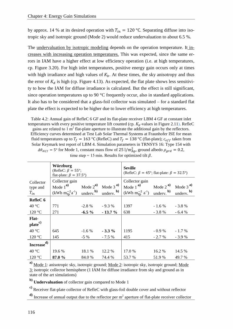
Chapter 4: Energy Gain Simulations
116
by approx. 14 % at its desired operation with 𝑇𝑖𝑛 = 120 °C. Separating diffuse into iso-
tropic sky and isotropic ground (Mode 2) would reduce undervaluation to about 6.5 %.
The undervaluation by isotropic modeling depends on the operation temperature. It in-
creases with increasing operation temperatures. This was expected, since the same er-
rors in IAM have a higher effect at low efficiency operation (i.e. at high temperatures,
cp. Figure 3.20). For high inlet temperatures, positive energy gain occurs only at times
with high irradiance and high values of 𝐾𝑏. At these times, the sky anisotropy and thus
the error of 𝐾𝑑 is high (cp. Figure 4.13). As expected, the flat plate shows less sensitivi-
ty to how the IAM for diffuse irradiance is calculated. But the effect is still significant,
since operation temperatures up to 90 °C frequently occur, also in standard applications.
It also has to be considered that a glass-foil collector was simulated – for a standard flat
plate the effect is expected to be higher due to lower efficiency at high temperatures.
Table 4.2: Annual gain of RefleC 6 GF and its flat-plate receiver LBM 4 GF at constant inlet
temperatures with every positive temperature lift counted (cp. 𝐾𝑏-values in Figure 2.11). RefleC
gains are related to 1 m2 flat-plate aperture to illustrate the additional gain by the reflectors.
Efficiency curves determined at Test Lab Solar Thermal Systems at Fraunhofer ISE for mean
fluid temperatures up to 𝑇𝑓 = 163 °C (RefleC) and 𝑇𝑓 = 138 °C (flat-plate); 𝑐𝑒𝑓𝑓 taken from
Solar Keymark test report of LBM 4. Simulation parameters in TRNSYS 16: Type 154 with
𝛥𝜃𝑑𝑖𝑓𝑓 = 5° for Mode 1, constant mass flow of 25 l/mAp2 , ground albedo 𝜌𝑔𝑟𝑑 = 0.2,
time step = 15 min. Results for optimized tilt 𝛽.
Würzburg (RefleC: 𝛽 = 55°; flat-plate: 𝛽 = 37.5°)
Seville (RefleC: 𝛽 = 45°; flat-plate: 𝛽 = 32.5°)
Collector
type and
𝑇𝑖𝑛
Collector gain
Mode 1a)
(kWh mfp−2a
-1)
Mode 2a)
underv.b)
Mode 3 a)
underv. b)
Collector gain
Mode 1 a)
(kWh mfp−2 a
-1)
Mode 2 a)
underv. b)
Mode 3 a)
underv. b)
RefleC 6
40 °C 771 -2.8 % - 9.3 % 1397 - 1.6 % - 3.8 %
120 °C 271 -6.5 % - 13.7 % 638 - 3.8 % - 6.4 %
Flat-
platec)
40 °C 645 -1.6 % - 3.3 % 1195 - 0.9 % - 1.7 %
120 °C 145 -5 % - 7.5 % 415 - 2.7 % - 3.9 %
Increased)
40 °C 19.6 % 18.1 % 12.2 % 17.0 % 16.2 % 14.5 %
120 °C 87.0 % 84.0 % 74.4 % 53.7 % 51.9 % 49.7 %
a) Mode 1: anisotropic sky, isotropic ground; Mode 2: isotropic sky, isotropic ground; Mode
3: isotropic collector hemisphere (1 IAM for diffuse irradiance from sky and ground as in
state of the art simulations) b)
Undervaluation of collector gain compared to Mode 1
c) Receiver flat-plate collector of RefleC with glass-foil double cover and without reflector
d) Increase of annual output due to the reflector per m
2 aperture of flat-plate receiver collector
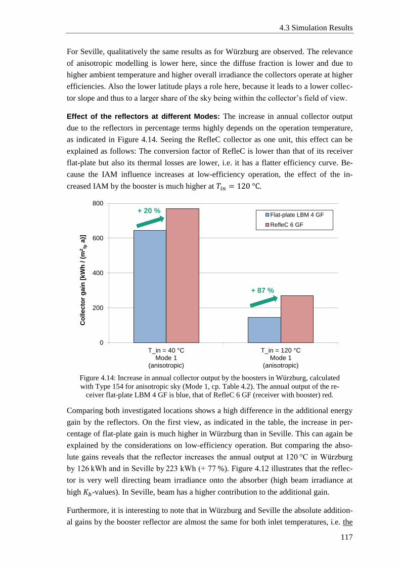
4.3 Simulation Results
117
For Seville, qualitatively the same results as for Würzburg are observed. The relevance
of anisotropic modelling is lower here, since the diffuse fraction is lower and due to
higher ambient temperature and higher overall irradiance the collectors operate at higher
efficiencies. Also the lower latitude plays a role here, because it leads to a lower collec-
tor slope and thus to a larger share of the sky being within the collector’s field of view.
Effect of the reflectors at different Modes: The increase in annual collector output
due to the reflectors in percentage terms highly depends on the operation temperature,
as indicated in Figure 4.14. Seeing the RefleC collector as one unit, this effect can be
explained as follows: The conversion factor of RefleC is lower than that of its receiver
flat-plate but also its thermal losses are lower, i.e. it has a flatter efficiency curve. Be-
cause the IAM influence increases at low-efficiency operation, the effect of the in-
creased IAM by the booster is much higher at 𝑇𝑖𝑛 = 120 °C.
Figure 4.14: Increase in annual collector output by the boosters in Würzburg, calculated
with Type 154 for anisotropic sky (Mode 1, cp. Table 4.2). The annual output of the re-
ceiver flat-plate LBM 4 GF is blue, that of RefleC 6 GF (receiver with booster) red.
Comparing both investigated locations shows a high difference in the additional energy
gain by the reflectors. On the first view, as indicated in the table, the increase in per-
centage of flat-plate gain is much higher in Würzburg than in Seville. This can again be
explained by the considerations on low-efficiency operation. But comparing the abso-
lute gains reveals that the reflector increases the annual output at 120 °C in Würzburg
by 126 kWh and in Seville by 223 kWh (+ 77 %). Figure 4.12 illustrates that the reflec-
tor is very well directing beam irradiance onto the absorber (high beam irradiance at
high 𝐾𝑏-values). In Seville, beam has a higher contribution to the additional gain.
Furthermore, it is interesting to note that in Würzburg and Seville the absolute addition-
al gains by the booster reflector are almost the same for both inlet temperatures, i.e. the
0
200
400
600
800
T_in = 40 °CMode 1
(anisotropic)
T_in = 120 °CMode 1
(anisotropic)
Co
llecto
r g
ain
[kW
h /
(m
2fp
a)]
Flat-plate LBM 4 GF
RefleC 6 GF
+ 20 %
+ 87 %

Chapter 4: Energy Gain Simulations
118
absolute additional gains by the reflectors are largely independent of the fluid-
temperature. This confirms the observation of Perers and Karlsson (1993, p. 336).
Comparison of the results from the different Modes shows, that consideration of the sky
anisotropy is essential to predict the reflector-gains accurately (cp. Figure 4.15). At
𝑇𝑖𝑛 = 40 °𝐶 the simulated additional gain caused by the reflector increases by 66 %,
when instead of an isotropic collector hemisphere (Mode 3) an anisotropic sky IAM 𝐾𝑠
is simulated. At 120 °C the difference is reduced but still significant. For Seville, the
deviations are again smaller since the contribution of diffuse is smaller here.
Figure 4.15: Annual output of RefleC 6 GF (blue plus red) and its receiver LBM 4 GF
(blue) in Würzburg. The arrows separately indicate the increase in collector output by
both RefleC components (flat-plate and reflector) when simulated with anisotropic Mode
1 (new model) instead of isotropic Mode 3 (state of the art). Overall RefleC increase us-
ing Mode 1 instead of 3 is 10 % at 𝑇𝑖𝑛 = 40 °C and 16 % at 𝑇𝑖𝑛 = 120 °C, cp. Table 4.2.
Seasonal analysis: Figure 4.16 and Figure 4.17 show the monthly RefleC collector
gains, on which the annual values of Table 4.2 are based, for 𝑇𝑖𝑛 = 120 °C. In Würz-
burg, from November to January there is almost no collector gain – neither from the
double covered flat-plate (𝛽 = 37.5°) nor from RefleC (𝛽 = 55°). At the low overall
irradiation level and the low ambient temperatures, almost no positive collector effi-
ciencies are reached for this constantly high inlet temperature. A closer look into Figure
2.11 reveals that the reflectors are not active during these months of the year, since most
of the day it is 𝜃𝑡 < −10°, so in the morning and in the afternoon the flat-plate is also
shaded by the reflectors8. In February and October, the sun takes a glimpse above the
reflector, so at noon there is relevant contribution by the reflectors.
8 For ground or flat roof installations with several rows, the „shading“ of the flat-plate by the
reflector is no drawback, because in a collector field the flat-plates would shade each other.
0
200
400
600
800
T_in = 40 °CMode 3
(isotropic)
T_in = 40 °CMode 1
(anisotropic)
T_in = 120 °CMode 3
(isotropic)
T_in = 120 °CMode 1
(anisotropic)
Co
lle
cto
r g
ain
[k
Wh
/ (
m2fp
a)]
Additional gain reflector
Flat-plate LBM 4 GF
+ 8 %
+ 3 %
+ 26 %
+ 66 %
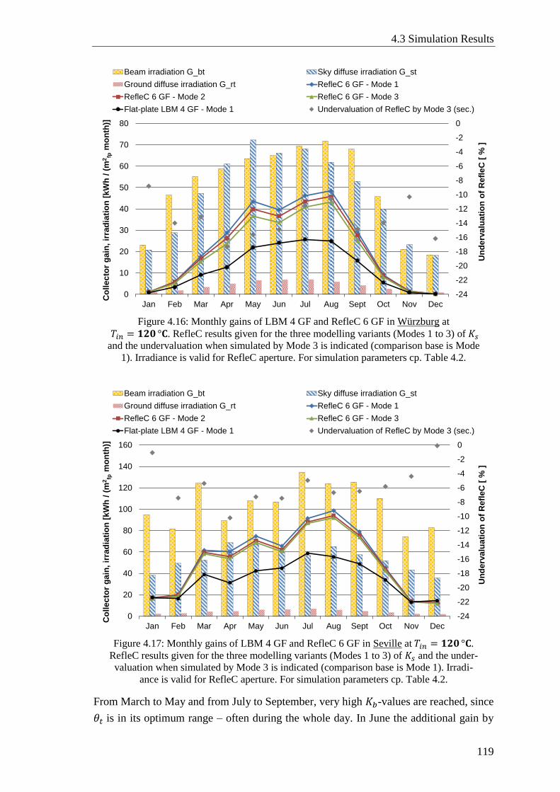
4.3 Simulation Results
119
Figure 4.16: Monthly gains of LBM 4 GF and RefleC 6 GF in Würzburg at
𝑇𝑖𝑛 = 𝟏𝟐𝟎 °𝐂. RefleC results given for the three modelling variants (Modes 1 to 3) of 𝐾𝑠
and the undervaluation when simulated by Mode 3 is indicated (comparison base is Mode
1). Irradiance is valid for RefleC aperture. For simulation parameters cp. Table 4.2.
Figure 4.17: Monthly gains of LBM 4 GF and RefleC 6 GF in Seville at 𝑇𝑖𝑛 = 𝟏𝟐𝟎 °𝐂.
RefleC results given for the three modelling variants (Modes 1 to 3) of 𝐾𝑠 and the under-
valuation when simulated by Mode 3 is indicated (comparison base is Mode 1). Irradi-
ance is valid for RefleC aperture. For simulation parameters cp. Table 4.2.
From March to May and from July to September, very high 𝐾𝑏-values are reached, since
𝜃𝑡 is in its optimum range – often during the whole day. In June the additional gain by
-24
-22
-20
-18
-16
-14
-12
-10
-8
-6
-4
-2
0
0
10
20
30
40
50
60
70
80
Jan Feb Mar Apr May Jun Jul Aug Sept Oct Nov Dec
Un
de
rva
lua
tio
n o
f R
efl
eC
[ %
]
Co
lle
cto
r g
ain
, ir
rad
iati
on
[k
Wh
/ (
m2fp
mo
nth
)]
Beam irradiation G_bt Sky diffuse irradiation G_st
Ground diffuse irradiation G_rt RefleC 6 GF - Mode 1
RefleC 6 GF - Mode 2 RefleC 6 GF - Mode 3
Flat-plate LBM 4 GF - Mode 1 Undervaluation of RefleC by Mode 3 (sec.)
-24
-22
-20
-18
-16
-14
-12
-10
-8
-6
-4
-2
0
0
20
40
60
80
100
120
140
160
Jan Feb Mar Apr May Jun Jul Aug Sept Oct Nov Dec
Un
de
rva
lua
tio
n o
f R
efl
eC
[ %
]
Co
lle
cto
r g
ain
, ir
rad
iati
on
[k
Wh
/ (
m2fp
mo
nth
)]
Beam irradiation G_bt Sky diffuse irradiation G_st
Ground diffuse irradiation G_rt RefleC 6 GF - Mode 1
RefleC 6 GF - Mode 2 RefleC 6 GF - Mode 3
Flat-plate LBM 4 GF - Mode 1 Undervaluation of RefleC by Mode 3 (sec.)
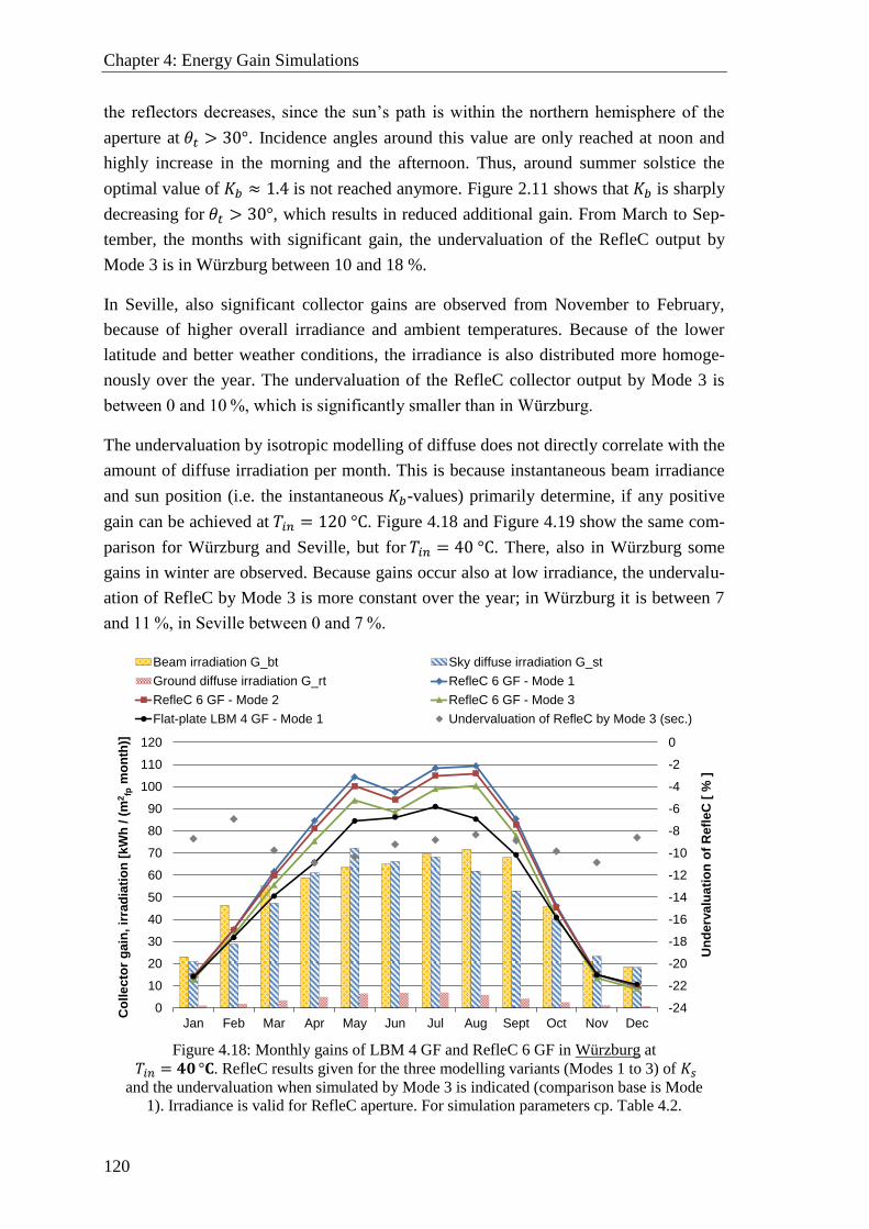
Chapter 4: Energy Gain Simulations
120
the reflectors decreases, since the sun’s path is within the northern hemisphere of the
aperture at 𝜃𝑡 > 30°. Incidence angles around this value are only reached at noon and
highly increase in the morning and the afternoon. Thus, around summer solstice the
optimal value of 𝐾𝑏 ≈ 1.4 is not reached anymore. Figure 2.11 shows that 𝐾𝑏 is sharply
decreasing for 𝜃𝑡 > 30°, which results in reduced additional gain. From March to Sep-
tember, the months with significant gain, the undervaluation of the RefleC output by
Mode 3 is in Würzburg between 10 and 18 %.
In Seville, also significant collector gains are observed from November to February,
because of higher overall irradiance and ambient temperatures. Because of the lower
latitude and better weather conditions, the irradiance is also distributed more homoge-
nously over the year. The undervaluation of the RefleC collector output by Mode 3 is
between 0 and 10 %, which is significantly smaller than in Würzburg.
The undervaluation by isotropic modelling of diffuse does not directly correlate with the
amount of diffuse irradiation per month. This is because instantaneous beam irradiance
and sun position (i.e. the instantaneous 𝐾𝑏-values) primarily determine, if any positive
gain can be achieved at 𝑇𝑖𝑛 = 120 °C. Figure 4.18 and Figure 4.19 show the same com-
parison for Würzburg and Seville, but for 𝑇𝑖𝑛 = 40 °C. There, also in Würzburg some
gains in winter are observed. Because gains occur also at low irradiance, the undervalu-
ation of RefleC by Mode 3 is more constant over the year; in Würzburg it is between 7
and 11 %, in Seville between 0 and 7 %.
Figure 4.18: Monthly gains of LBM 4 GF and RefleC 6 GF in Würzburg at
𝑇𝑖𝑛 = 𝟒𝟎 °𝐂. RefleC results given for the three modelling variants (Modes 1 to 3) of 𝐾𝑠
and the undervaluation when simulated by Mode 3 is indicated (comparison base is Mode
1). Irradiance is valid for RefleC aperture. For simulation parameters cp. Table 4.2.
-24
-22
-20
-18
-16
-14
-12
-10
-8
-6
-4
-2
0
0
10
20
30
40
50
60
70
80
90
100
110
120
Jan Feb Mar Apr May Jun Jul Aug Sept Oct Nov Dec
Un
de
rva
lua
tio
n o
f R
efl
eC
[ %
]
Co
lle
cto
r g
ain
, ir
rad
iati
on
[k
Wh
/ (
m2fp
mo
nth
)]
Beam irradiation G_bt Sky diffuse irradiation G_st
Ground diffuse irradiation G_rt RefleC 6 GF - Mode 1
RefleC 6 GF - Mode 2 RefleC 6 GF - Mode 3
Flat-plate LBM 4 GF - Mode 1 Undervaluation of RefleC by Mode 3 (sec.)
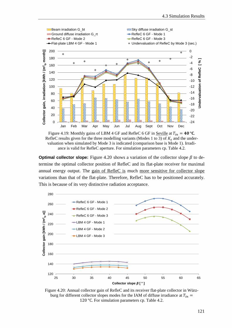
4.3 Simulation Results
121
Figure 4.19: Monthly gains of LBM 4 GF and RefleC 6 GF in Seville at 𝑇𝑖𝑛 = 𝟒𝟎 °𝐂.
RefleC results given for the three modelling variants (Modes 1 to 3) of 𝐾𝑠 and the under-
valuation when simulated by Mode 3 is indicated (comparison base is Mode 1). Irradi-
ance is valid for RefleC aperture. For simulation parameters cp. Table 4.2.
Optimal collector slope: Figure 4.20 shows a variation of the collector slope 𝛽 to de-
termine the optimal collector position of RefleC and its flat-plate receiver for maximal
annual energy output. The gain of RefleC is much more sensitive for collector slope
variations than that of the flat-plate. Therefore, RefleC has to be positioned accurately.
This is because of its very distinctive radiation acceptance.
Figure 4.20: Annual collector gain of RefleC and its receiver flat-plate collector in Würz-
burg for different collector slopes modes for the IAM of diffuse irradiance at 𝑇𝑖𝑛 =120 °C. For simulation parameters cp. Table 4.2.
-24
-22
-20
-18
-16
-14
-12
-10
-8
-6
-4
-2
0
0
20
40
60
80
100
120
140
160
180
200
Jan Feb Mar Apr May Jun Jul Aug Sept Oct Nov Dec
Un
de
rva
lua
tio
n o
f R
efl
eC
[
% ]
Co
lle
cto
r g
ain
, ir
rad
iati
on
[k
Wh
/ (
m2fp
mo
nth
)]
Beam irradiation G_bt Sky diffuse irradiation G_st
Ground diffuse irradiation G_rt RefleC 6 GF - Mode 1
RefleC 6 GF - Mode 2 RefleC 6 GF - Mode 3
Flat-plate LBM 4 GF - Mode 1 Undervaluation of RefleC by Mode 3 (sec.)
120
140
160
180
200
220
240
260
280
25 30 35 40 45 50 55 60 65
Co
llecto
r g
ain
[kW
h /
(m
2fp
a)]
Collector slope β [ ]
RefleC 6 GF - Mode 1
RefleC 6 GF - Mode 2
RefleC 6 GF - Mode 3
LBM 4 GF - Mode 1
LBM 4 GF - Mode 2
LBM 4 GF - Mode 3
Chapter 4: Energy Gain Simulations
122
From comparing the curves generated by the three different simulation modes it can be
concluded that for both collectors the correct determination of the optimal 𝛽 is almost
not affected by the method of determining the IAM for diffuse irradiance. This is be-
cause the incidence angles of beam irradiance during the year are the dominating effect
that changes the annual energy gain with varying collector slope 𝛽. Qualitatively the
same curves are observed for Seville. They are flatter, since beam irradiance is distrib-
uted more homogenous over the year. For 𝑇𝑖𝑛 = 40 °C, the identical optimal collector
slopes as for 120 °C were found. They were as well not affected by the diffuse IAM
Mode.
It can be concluded that simplified, isotropic hemispherical modelling of a collector’s
diffuse-IAM (Mode 3) does not lead to a wrong optimal collector slope. Furthermore,
the optimal slope is independent of the operation temperature.
The other important results of this chapter can be summarized as follows:
It is expected that isotropic hemispherical modelling of a collector’s diffuse-
IAM significantly undervalues the diffuse utilization of all non-focusing collec-
tors, when this diffuse-IAM is determined from 𝐾𝑏-values out of raytracing sim-
ulations or steady-state collector tests.
This undervaluation can be significantly reduced by simply generating separate
isotropic diffuse-IAMs for sky and ground irradiance. These IAMs only depend
on the collector slope 𝛽 and are constant during the simulation. Their determina-
tion at the start of the simulation would not notably increase the simulation time.
Simulation with a dynamic diffuse-IAM for anisotropic sky radiance (Mode 1)
especially increases the accuracy in instantaneous power output prediction of ST
collectors.
Furthermore, it is expected to be essential for accurate prediction of the addi-
tional gains by booster reflectors.
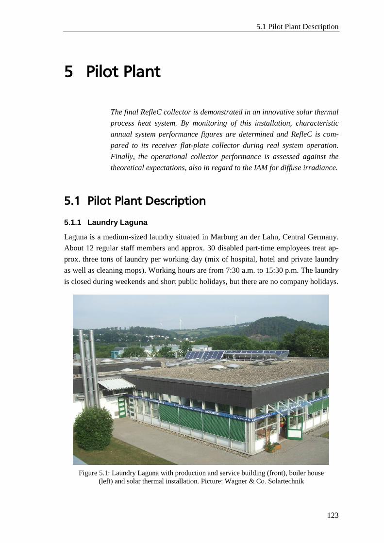
5.1 Pilot Plant Description
123
5 Pilot Plant
The final RefleC collector is demonstrated in an innovative solar thermal
process heat system. By monitoring of this installation, characteristic
annual system performance figures are determined and RefleC is com-
pared to its receiver flat-plate collector during real system operation.
Finally, the operational collector performance is assessed against the
theoretical expectations, also in regard to the IAM for diffuse irradiance.
5.1 Pilot Plant Description
5.1.1 Laundry Laguna
Laguna is a medium-sized laundry situated in Marburg an der Lahn, Central Germany.
About 12 regular staff members and approx. 30 disabled part-time employees treat ap-
prox. three tons of laundry per working day (mix of hospital, hotel and private laundry
as well as cleaning mops). Working hours are from 7:30 a.m. to 15:30 p.m. The laundry
is closed during weekends and short public holidays, but there are no company holidays.
Figure 5.1: Laundry Laguna with production and service building (front), boiler house
(left) and solar thermal installation. Picture: Wagner & Co. Solartechnik
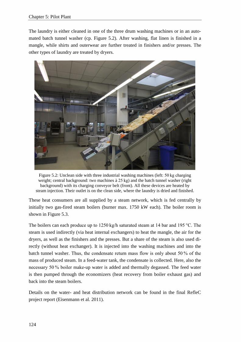
Chapter 5: Pilot Plant
124
The laundry is either cleaned in one of the three drum washing machines or in an auto-
mated batch tunnel washer (cp. Figure 5.2). After washing, flat linen is finished in a
mangle, while shirts and outerwear are further treated in finishers and/or presses. The
other types of laundry are treated by dryers.
Figure 5.2: Unclean side with three industrial washing machines (left: 50 kg charging
weight; central background: two machines à 25 kg) and the batch tunnel washer (right
background) with its charging conveyor belt (front). All these devices are heated by
steam injection. Their outlet is on the clean side, where the laundry is dried and finished.
These heat consumers are all supplied by a steam network, which is fed centrally by
initially two gas-fired steam boilers (burner max. 1750 kW each). The boiler room is
shown in Figure 5.3.
The boilers can each produce up to 1250 kg/h saturated steam at 14 bar and 195 °C. The
steam is used indirectly (via heat internal exchangers) to heat the mangle, the air for the
dryers, as well as the finishers and the presses. But a share of the steam is also used di-
rectly (without heat exchanger). It is injected into the washing machines and into the
batch tunnel washer. Thus, the condensate return mass flow is only about 50 % of the
mass of produced steam. In a feed-water tank, the condensate is collected. Here, also the
necessary 50 % boiler make-up water is added and thermally degassed. The feed water
is then pumped through the economizers (heat recovery from boiler exhaust gas) and
back into the steam boilers.
Details on the water- and heat distribution network can be found in the final RefleC
project report (Eisenmann et al. 2011).
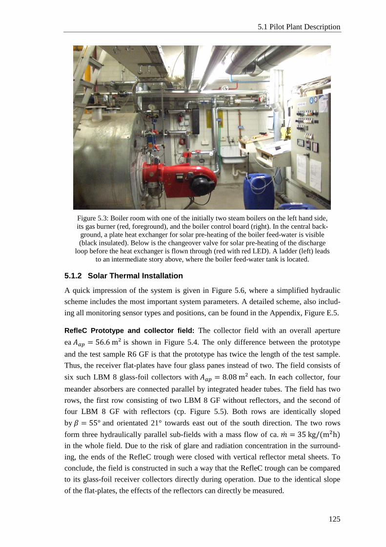
5.1 Pilot Plant Description
125
Figure 5.3: Boiler room with one of the initially two steam boilers on the left hand side,
its gas burner (red, foreground), and the boiler control board (right). In the central back-
ground, a plate heat exchanger for solar pre-heating of the boiler feed-water is visible
(black insulated). Below is the changeover valve for solar pre-heating of the discharge
loop before the heat exchanger is flown through (red with red LED). A ladder (left) leads
to an intermediate story above, where the boiler feed-water tank is located.
5.1.2 Solar Thermal Installation
A quick impression of the system is given in Figure 5.6, where a simplified hydraulic
scheme includes the most important system parameters. A detailed scheme, also includ-
ing all monitoring sensor types and positions, can be found in the Appendix, Figure E.5.
RefleC Prototype and collector field: The collector field with an overall aperture
ea 𝐴𝑎𝑝 = 56.6 m² is shown in Figure 5.4. The only difference between the prototype
and the test sample R6 GF is that the prototype has twice the length of the test sample.
Thus, the receiver flat-plates have four glass panes instead of two. The field consists of
six such LBM 8 glass-foil collectors with 𝐴𝑎𝑝 = 8.08 m² each. In each collector, four
meander absorbers are connected parallel by integrated header tubes. The field has two
rows, the first row consisting of two LBM 8 GF without reflectors, and the second of
four LBM 8 GF with reflectors (cp. Figure 5.5). Both rows are identically sloped
by 𝛽 = 55° and orientated 21° towards east out of the south direction. The two rows
form three hydraulically parallel sub-fields with a mass flow of ca. �̇� = 35 kg/(m2h)
in the whole field. Due to the risk of glare and radiation concentration in the surround-
ing, the ends of the RefleC trough were closed with vertical reflector metal sheets. To
conclude, the field is constructed in such a way that the RefleC trough can be compared
to its glass-foil receiver collectors directly during operation. Due to the identical slope
of the flat-plates, the effects of the reflectors can directly be measured.
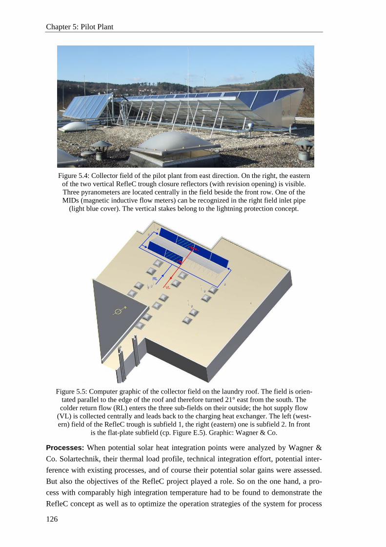
Chapter 5: Pilot Plant
126
Figure 5.4: Collector field of the pilot plant from east direction. On the right, the eastern
of the two vertical RefleC trough closure reflectors (with revision opening) is visible.
Three pyranometers are located centrally in the field beside the front row. One of the
MIDs (magnetic inductive flow meters) can be recognized in the right field inlet pipe
(light blue cover). The vertical stakes belong to the lightning protection concept.
Figure 5.5: Computer graphic of the collector field on the laundry roof. The field is orien-
tated parallel to the edge of the roof and therefore turned 21° east from the south. The
colder return flow (RL) enters the three sub-fields on their outside; the hot supply flow
(VL) is collected centrally and leads back to the charging heat exchanger. The left (west-
ern) field of the RefleC trough is subfield 1, the right (eastern) one is subfield 2. In front
is the flat-plate subfield (cp. Figure E.5). Graphic: Wagner & Co.
Processes: When potential solar heat integration points were analyzed by Wagner &
Co. Solartechnik, their thermal load profile, technical integration effort, potential inter-
ference with existing processes, and of course their potential solar gains were assessed.
But also the objectives of the RefleC project played a role. So on the one hand, a pro-
cess with comparably high integration temperature had to be found to demonstrate the
RefleC concept as well as to optimize the operation strategies of the system for process
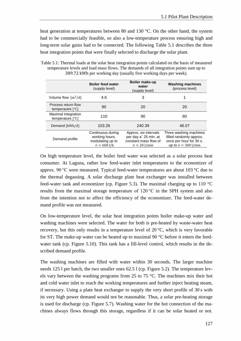
5.1 Pilot Plant Description
127
heat generation at temperatures between 80 and 130 °C. On the other hand, the system
had to be commercially feasible, so also a low-temperature process ensuring high and
long-term solar gains had to be connected. The following Table 5.1 describes the three
heat integration points that were finally selected to discharge the solar plant.
Table 5.1: Thermal loads at the solar heat integration points calculated on the basis of measured
temperature levels and load mass flows. The demands of all integration points sum up to
389.72 kWh per working day (usually five working days per week).
On high temperature level, the boiler feed water was selected as a solar process heat
consumer. At Laguna, rather low feed-water inlet temperatures to the economizer of
approx. 90 °C were measured. Typical feed-water temperatures are about 103 °C due to
the thermal degassing. A solar discharge plate heat exchanger was installed between
feed-water tank and economizer (cp. Figure 5.3). The maximal charging up to 110 °C
results from the maximal storage temperature of 120 °C in the SPH system and also
from the intention not to affect the efficiency of the economizer. The feed-water de-
mand profile was not measured.
On low-temperature level, the solar heat integration points boiler make-up water and
washing machines were selected. The water for both is pre-heated by waste-water heat
recovery, but this only results in a temperature level of 20 °C, which is very favorable
for ST. The make-up water can be heated up to maximal 90 °C before it enters the feed-
water tank (cp. Figure 5.10). This tank has a fill-level control, which results in the de-
scribed demand profile.
The washing machines are filled with water within 30 seconds. The larger machine
needs 125 l per batch, the two smaller ones 62.5 l (cp. Figure 5.2). The temperature lev-
els vary between the washing programs from 25 to 75 °C. The machines mix their hot
and cold water inlet to reach the working temperatures and further inject heating steam,
if necessary. Using a plate heat exchanger to supply the very short profile of 30 s with
its very high power demand would not be reasonable. Thus, a solar pre-heating storage
is used for discharge (cp. Figure 5.7). Washing water for the hot connection of the ma-
chines always flows through this storage, regardless if it can be solar heated or not.
Boiler feed water
(supply level)
Boiler make-up water
(supply level)
Washing machines
(process level)
Volume flow [m3/d]
4.6 3 1
Process return flow temperautre [°C]
90 20 20
Maximal integration
temperature [°C] 110 90 60
Demand [kWh/d] 103.26 240.39 46.07
Demand profile
Continuous during working hours,
modulating up to �̇� = 600 l/h
Approx. six intervals per day a´ 25 min. at constant mass flow of
�̇� = 20 l/min
Three washing machines filled randomly approx. once per hour for 30 s.
up to �̇� = 300 l/min
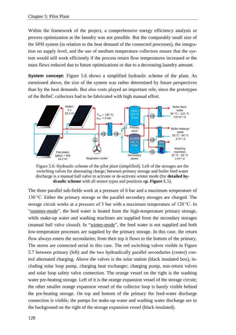
Chapter 5: Pilot Plant
128
Within the framework of the project, a comprehensive energy efficiency analysis or
process optimization at the laundry was not possible. But the comparably small size of
the SPH system (in relation to the heat demand of the connected processes), the integra-
tion on supply level, and the use of medium temperature collectors ensure that the sys-
tem would still work efficiently if the process return flow temperatures increased or the
mass flows reduced due to future optimizations or due to a decreasing laundry amount.
System concept: Figure 5.6 shows a simplified hydraulic scheme of the plant. As
mentioned above, the size of the system was rather determined by future perspectives
than by the heat demands. But also costs played an important role, since the prototypes
of the RefleC collectors had to be fabricated with high manual effort.
Figure 5.6: Hydraulic scheme of the pilot plant (simplified). Left of the storages are the
switching valves for alternating charge; between primary storage and boiler feed water
discharge is a manual ball valve to activate or de-activate winter mode (for detailed hy-
draulic scheme with all sensor types and positions cp. Figure E.5).
The three parallel sub-fields work at a pressure of 6 bar and a maximum temperature of
130 °C. Either the primary storage or the parallel secondary storages are charged. The
storage circuit works at a pressure of 3 bar with a maximum temperature of 120 °C. In
“summer-mode”, the feed water is heated from the high-temperature primary storage,
while make-up water and washing machines are supplied from the secondary storages
(manual ball valve closed). In “winter-mode”, the feed water is not supplied and both
low-temperature processes are supplied by the primary storage. In this case, the return
flow always enters the secondaries; from their top it flows to the bottom of the primary.
The stores are connected serial in this case. The red switching valves visible in Figure
5.7 between primary (left) and the two hydraulically parallel secondaries (center) con-
trol alternated charging. Above the valves is the solar station (black insulated box), in-
cluding solar loop pump, charging heat exchanger, charging pump, non-return valves
and solar loop safety valve connection. The orange vessel on the right is the washing
water pre-heating storage. Left of it is the orange expansion vessel of the storage circuit;
the other smaller orange expansion vessel of the collector loop is barely visible behind
the pre-heating storage. On top and bottom of the primary the feed-water discharge
connection is visible; the pumps for make-up water and washing water discharge are in
the background on the right of the storage expansion vessel (black insulated).
storage1000 l
120 °C
3 bar
stora
ge
2x1000l
110 °C
3 bar
Boiler feed-
water
90 °C – 110 °C
4,6 m³ / d
Boiler makeup-
water
20 °C - 90 °C
3 m³ / d
Washing
machines
20 °C - 60 °C
1 m³ / d
RefleC
2 x
20,2 m²
Flat-plates
(glass + foil)
16,2 m²
Tmax = 130 °C
psys = 6 bar
Stagnation cooler
Primary
store
Secondary
stores
300l
60°C
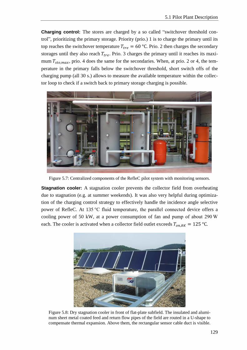
5.1 Pilot Plant Description
129
Charging control: The stores are charged by a so called “switchover threshold con-
trol”, prioritizing the primary storage. Priority (prio.) 1 is to charge the primary until its
top reaches the switchover temperature 𝑇𝑡𝑟𝑒 = 60 °C. Prio. 2 then charges the secondary
storages until they also reach 𝑇𝑡𝑟𝑒. Prio. 3 charges the primary until it reaches its maxi-
mum 𝑇𝑠𝑡𝑜,𝑚𝑎𝑥, prio. 4 does the same for the secondaries. When, at prio. 2 or 4, the tem-
perature in the primary falls below the switchover threshold, short switch offs of the
charging pump (all 30 s.) allows to measure the available temperature within the collec-
tor loop to check if a switch back to primary storage charging is possible.
Figure 5.7: Centralized components of the RefleC pilot system with monitoring sensors.
Stagnation cooler: A stagnation cooler prevents the collector field from overheating
due to stagnation (e.g. at summer weekends). It was also very helpful during optimiza-
tion of the charging control strategy to effectively handle the incidence angle selective
power of RefleC. At 135 °C fluid temperature, the parallel connected device offers a
cooling power of 50 kW, at a power consumption of fan and pump of about 290 W
each. The cooler is activated when a collector field outlet exceeds 𝑇𝑜𝑛,𝑅𝐾 = 125 °C.
Figure 5.8: Dry stagnation cooler in front of flat-plate subfield. The insulated and alumi-
num sheet metal coated feed and return flow pipes of the field are routed in a U-shape to
compensate thermal expansion. Above them, the rectangular sensor cable duct is visible.
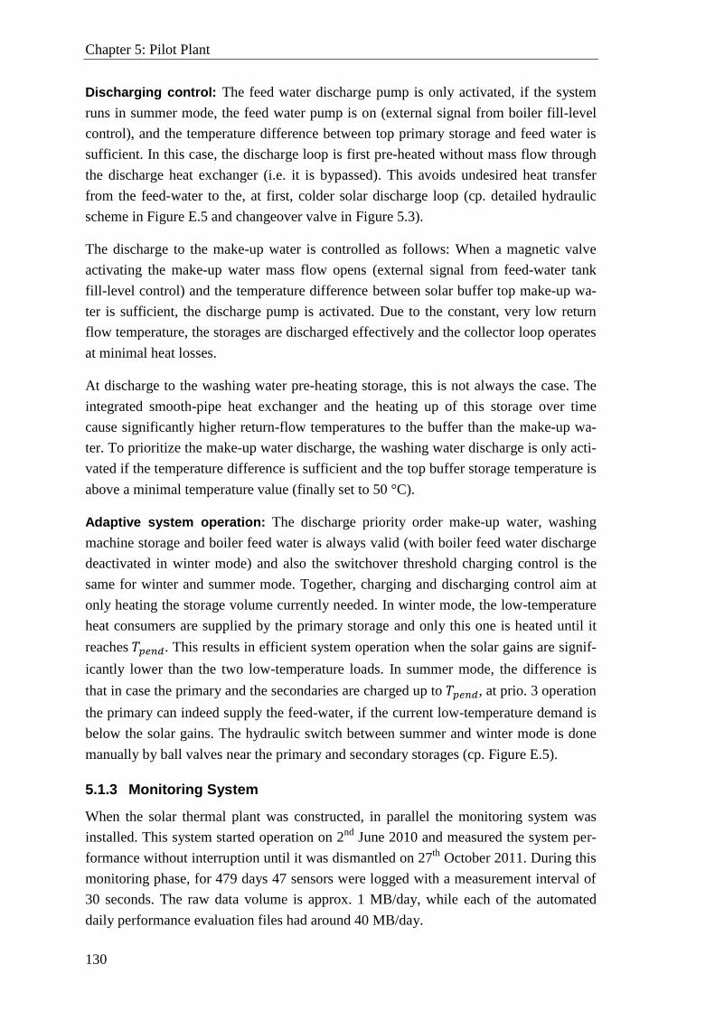
Chapter 5: Pilot Plant
130
Discharging control: The feed water discharge pump is only activated, if the system
runs in summer mode, the feed water pump is on (external signal from boiler fill-level
control), and the temperature difference between top primary storage and feed water is
sufficient. In this case, the discharge loop is first pre-heated without mass flow through
the discharge heat exchanger (i.e. it is bypassed). This avoids undesired heat transfer
from the feed-water to the, at first, colder solar discharge loop (cp. detailed hydraulic
scheme in Figure E.5 and changeover valve in Figure 5.3).
The discharge to the make-up water is controlled as follows: When a magnetic valve
activating the make-up water mass flow opens (external signal from feed-water tank
fill-level control) and the temperature difference between solar buffer top make-up wa-
ter is sufficient, the discharge pump is activated. Due to the constant, very low return
flow temperature, the storages are discharged effectively and the collector loop operates
at minimal heat losses.
At discharge to the washing water pre-heating storage, this is not always the case. The
integrated smooth-pipe heat exchanger and the heating up of this storage over time
cause significantly higher return-flow temperatures to the buffer than the make-up wa-
ter. To prioritize the make-up water discharge, the washing water discharge is only acti-
vated if the temperature difference is sufficient and the top buffer storage temperature is
above a minimal temperature value (finally set to 50 °C).
Adaptive system operation: The discharge priority order make-up water, washing
machine storage and boiler feed water is always valid (with boiler feed water discharge
deactivated in winter mode) and also the switchover threshold charging control is the
same for winter and summer mode. Together, charging and discharging control aim at
only heating the storage volume currently needed. In winter mode, the low-temperature
heat consumers are supplied by the primary storage and only this one is heated until it
reaches 𝑇𝑝𝑒𝑛𝑑. This results in efficient system operation when the solar gains are signif-
icantly lower than the two low-temperature loads. In summer mode, the difference is
that in case the primary and the secondaries are charged up to 𝑇𝑝𝑒𝑛𝑑, at prio. 3 operation
the primary can indeed supply the feed-water, if the current low-temperature demand is
below the solar gains. The hydraulic switch between summer and winter mode is done
manually by ball valves near the primary and secondary storages (cp. Figure E.5).
5.1.3 Monitoring System
When the solar thermal plant was constructed, in parallel the monitoring system was
installed. This system started operation on 2nd
June 2010 and measured the system per-
formance without interruption until it was dismantled on 27th
October 2011. During this
monitoring phase, for 479 days 47 sensors were logged with a measurement interval of
30 seconds. The raw data volume is approx. 1 MB/day, while each of the automated
daily performance evaluation files had around 40 MB/day.
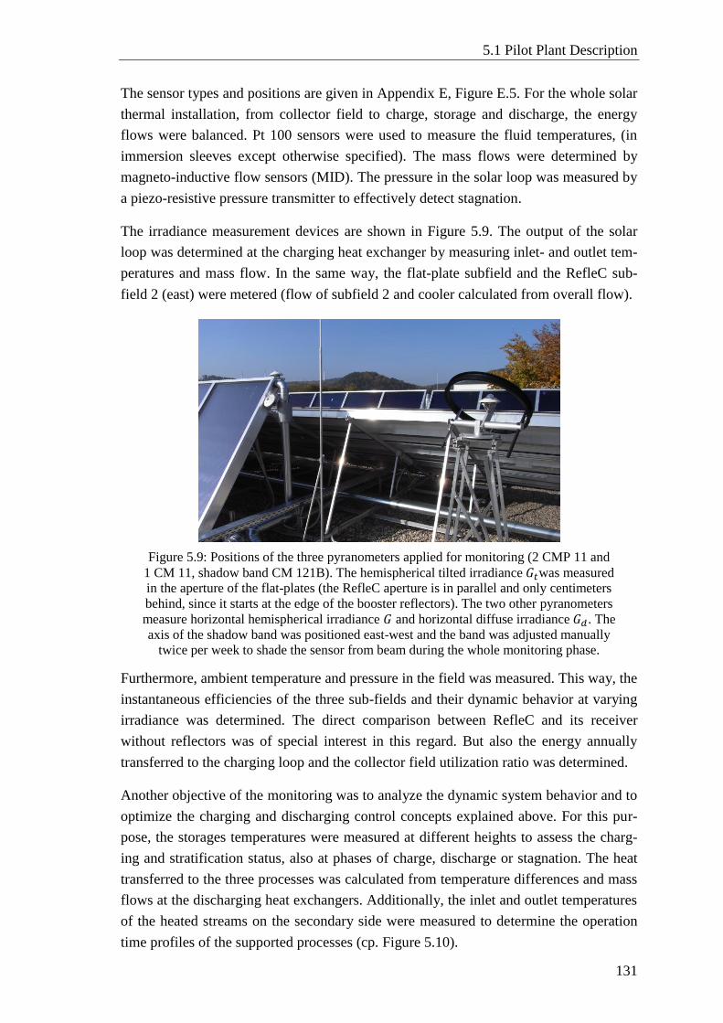
5.1 Pilot Plant Description
131
The sensor types and positions are given in Appendix E, Figure E.5. For the whole solar
thermal installation, from collector field to charge, storage and discharge, the energy
flows were balanced. Pt 100 sensors were used to measure the fluid temperatures, (in
immersion sleeves except otherwise specified). The mass flows were determined by
magneto-inductive flow sensors (MID). The pressure in the solar loop was measured by
a piezo-resistive pressure transmitter to effectively detect stagnation.
The irradiance measurement devices are shown in Figure 5.9. The output of the solar
loop was determined at the charging heat exchanger by measuring inlet- and outlet tem-
peratures and mass flow. In the same way, the flat-plate subfield and the RefleC sub-
field 2 (east) were metered (flow of subfield 2 and cooler calculated from overall flow).
Figure 5.9: Positions of the three pyranometers applied for monitoring (2 CMP 11 and
1 CM 11, shadow band CM 121B). The hemispherical tilted irradiance 𝐺𝑡was measured
in the aperture of the flat-plates (the RefleC aperture is in parallel and only centimeters
behind, since it starts at the edge of the booster reflectors). The two other pyranometers
measure horizontal hemispherical irradiance 𝐺 and horizontal diffuse irradiance 𝐺𝑑. The
axis of the shadow band was positioned east-west and the band was adjusted manually
twice per week to shade the sensor from beam during the whole monitoring phase.
Furthermore, ambient temperature and pressure in the field was measured. This way, the
instantaneous efficiencies of the three sub-fields and their dynamic behavior at varying
irradiance was determined. The direct comparison between RefleC and its receiver
without reflectors was of special interest in this regard. But also the energy annually
transferred to the charging loop and the collector field utilization ratio was determined.
Another objective of the monitoring was to analyze the dynamic system behavior and to
optimize the charging and discharging control concepts explained above. For this pur-
pose, the storages temperatures were measured at different heights to assess the charg-
ing and stratification status, also at phases of charge, discharge or stagnation. The heat
transferred to the three processes was calculated from temperature differences and mass
flows at the discharging heat exchangers. Additionally, the inlet and outlet temperatures
of the heated streams on the secondary side were measured to determine the operation
time profiles of the supported processes (cp. Figure 5.10).
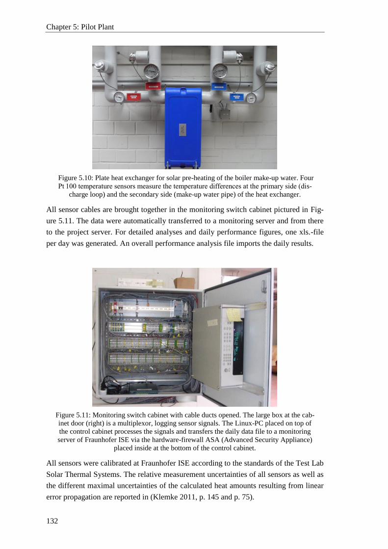
Chapter 5: Pilot Plant
132
Figure 5.10: Plate heat exchanger for solar pre-heating of the boiler make-up water. Four
Pt 100 temperature sensors measure the temperature differences at the primary side (dis-
charge loop) and the secondary side (make-up water pipe) of the heat exchanger.
All sensor cables are brought together in the monitoring switch cabinet pictured in Fig-
ure 5.11. The data were automatically transferred to a monitoring server and from there
to the project server. For detailed analyses and daily performance figures, one xls.-file
per day was generated. An overall performance analysis file imports the daily results.
Figure 5.11: Monitoring switch cabinet with cable ducts opened. The large box at the cab-
inet door (right) is a multiplexor, logging sensor signals. The Linux-PC placed on top of
the control cabinet processes the signals and transfers the daily data file to a monitoring
server of Fraunhofer ISE via the hardware-firewall ASA (Advanced Security Appliance)
placed inside at the bottom of the control cabinet.
All sensors were calibrated at Fraunhofer ISE according to the standards of the Test Lab
Solar Thermal Systems. The relative measurement uncertainties of all sensors as well as
the different maximal uncertainties of the calculated heat amounts resulting from linear
error propagation are reported in (Klemke 2011, p. 145 and p. 75).
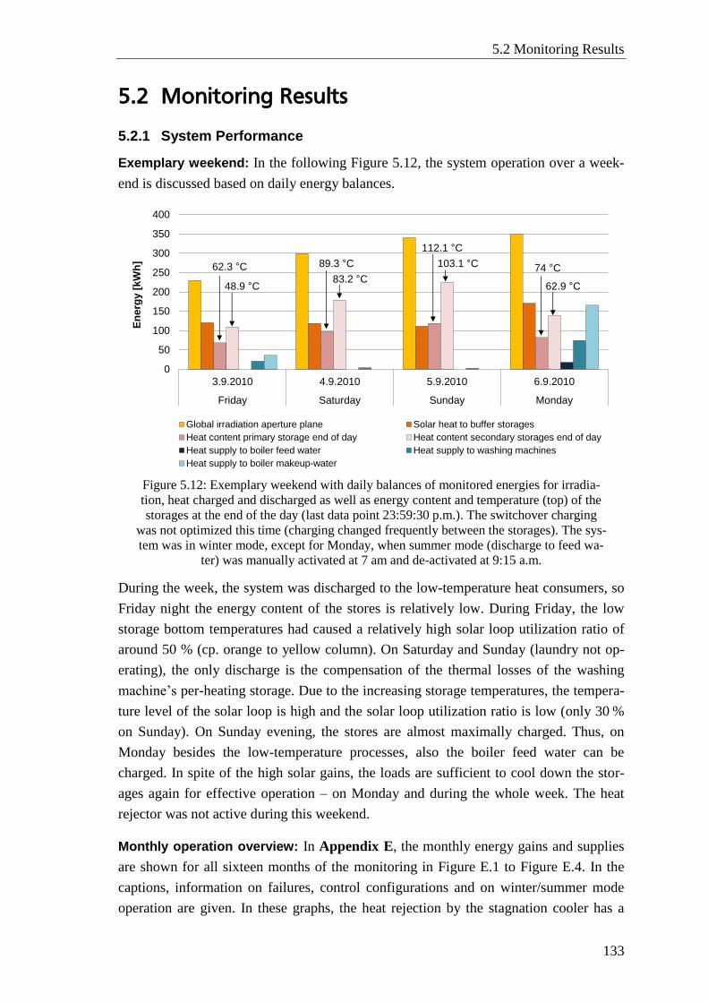
5.2 Monitoring Results
133
5.2 Monitoring Results
5.2.1 System Performance
Exemplary weekend: In the following Figure 5.12, the system operation over a week-
end is discussed based on daily energy balances.
Figure 5.12: Exemplary weekend with daily balances of monitored energies for irradia-
tion, heat charged and discharged as well as energy content and temperature (top) of the
storages at the end of the day (last data point 23:59:30 p.m.). The switchover charging
was not optimized this time (charging changed frequently between the storages). The sys-
tem was in winter mode, except for Monday, when summer mode (discharge to feed wa-
ter) was manually activated at 7 am and de-activated at 9:15 a.m.
During the week, the system was discharged to the low-temperature heat consumers, so
Friday night the energy content of the stores is relatively low. During Friday, the low
storage bottom temperatures had caused a relatively high solar loop utilization ratio of
around 50 % (cp. orange to yellow column). On Saturday and Sunday (laundry not op-
erating), the only discharge is the compensation of the thermal losses of the washing
machine’s per-heating storage. Due to the increasing storage temperatures, the tempera-
ture level of the solar loop is high and the solar loop utilization ratio is low (only 30 %
on Sunday). On Sunday evening, the stores are almost maximally charged. Thus, on
Monday besides the low-temperature processes, also the boiler feed water can be
charged. In spite of the high solar gains, the loads are sufficient to cool down the stor-
ages again for effective operation – on Monday and during the whole week. The heat
rejector was not active during this weekend.
Monthly operation overview: In Appendix E, the monthly energy gains and supplies
are shown for all sixteen months of the monitoring in Figure E.1 to Figure E.4. In the
captions, information on failures, control configurations and on winter/summer mode
operation are given. In these graphs, the heat rejection by the stagnation cooler has a
0
50
100
150
200
250
300
350
400
3.9.2010 4.9.2010 5.9.2010 6.9.2010
Friday Saturday Sunday Monday
En
erg
y [
kW
h]
Global irradiation aperture plane Solar heat to buffer storages
Heat content primary storage end of day Heat content secondary storages end of day
Heat supply to boiler feed water Heat supply to washing machines
Heat supply to boiler makeup-water
62.3 C 89.3 C
112.1 C
74 C
48.9 C83.2 C
103.1 C
62.9 C
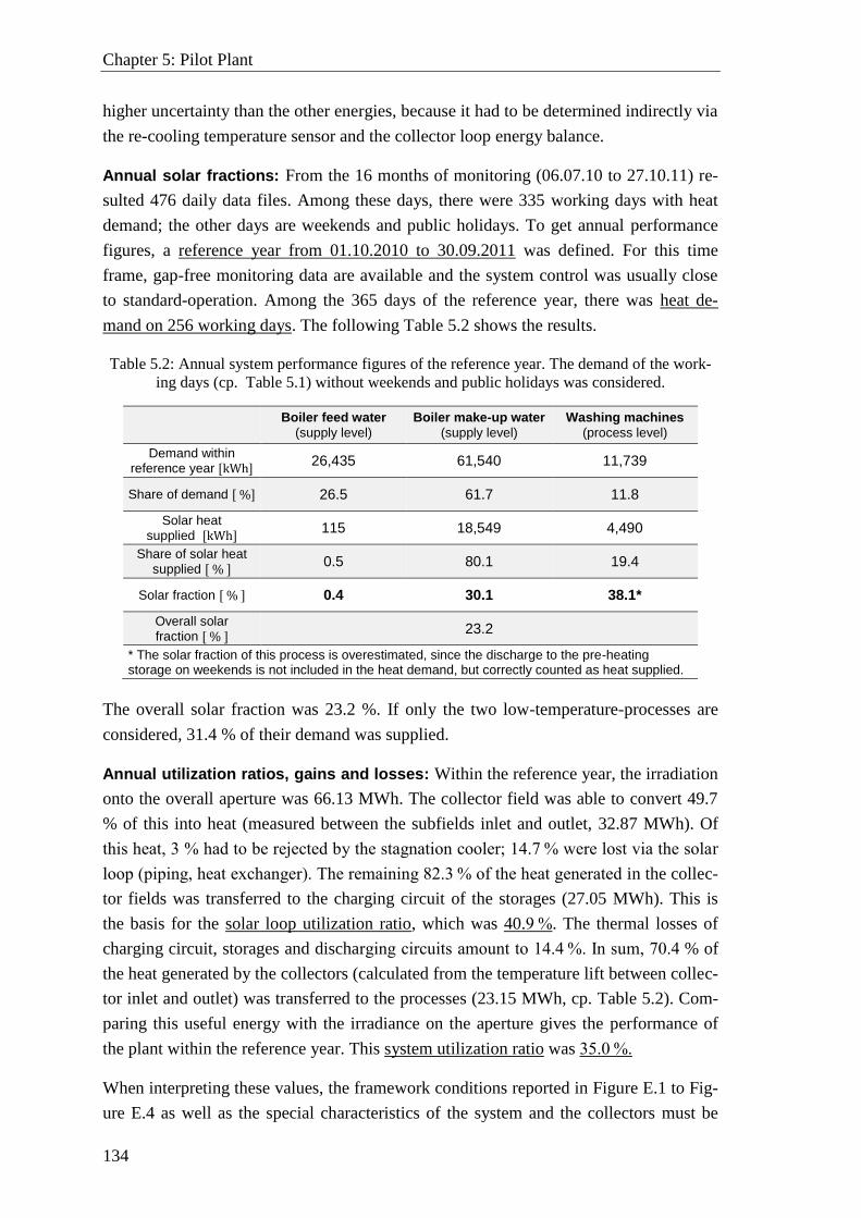
Chapter 5: Pilot Plant
134
higher uncertainty than the other energies, because it had to be determined indirectly via
the re-cooling temperature sensor and the collector loop energy balance.
Annual solar fractions: From the 16 months of monitoring (06.07.10 to 27.10.11) re-
sulted 476 daily data files. Among these days, there were 335 working days with heat
demand; the other days are weekends and public holidays. To get annual performance
figures, a reference year from 01.10.2010 to 30.09.2011 was defined. For this time
frame, gap-free monitoring data are available and the system control was usually close
to standard-operation. Among the 365 days of the reference year, there was heat de-
mand on 256 working days. The following Table 5.2 shows the results.
Table 5.2: Annual system performance figures of the reference year. The demand of the work-
ing days (cp. Table 5.1) without weekends and public holidays was considered.
The overall solar fraction was 23.2 %. If only the two low-temperature-processes are
considered, 31.4 % of their demand was supplied.
Annual utilization ratios, gains and losses: Within the reference year, the irradiation
onto the overall aperture was 66.13 MWh. The collector field was able to convert 49.7
% of this into heat (measured between the subfields inlet and outlet, 32.87 MWh). Of
this heat, 3 % had to be rejected by the stagnation cooler; 14.7 % were lost via the solar
loop (piping, heat exchanger). The remaining 82.3 % of the heat generated in the collec-
tor fields was transferred to the charging circuit of the storages (27.05 MWh). This is
the basis for the solar loop utilization ratio, which was 40.9 %. The thermal losses of
charging circuit, storages and discharging circuits amount to 14.4 %. In sum, 70.4 % of
the heat generated by the collectors (calculated from the temperature lift between collec-
tor inlet and outlet) was transferred to the processes (23.15 MWh, cp. Table 5.2). Com-
paring this useful energy with the irradiance on the aperture gives the performance of
the plant within the reference year. This system utilization ratio was 35.0 %.
When interpreting these values, the framework conditions reported in Figure E.1 to Fig-
ure E.4 as well as the special characteristics of the system and the collectors must be
Boiler feed water
(supply level)
Boiler make-up water
(supply level)
Washing machines
(process level)
Demand within reference year [kWh]
26,435 61,540 11,739
Share of demand [ %]
26.5 61.7 11.8
Solar heat supplied [kWh]
115 18,549 4,490
Share of solar heat supplied [ % ]
0.5 80.1 19.4
Solar fraction [ % ] 0.4 30.1 38.1*
Overall solar fraction [ % ]
23.2
* The solar fraction of this process is overestimated, since the discharge to the pre-heating storage on weekends is not included in the heat demand, but correctly counted as heat supplied.
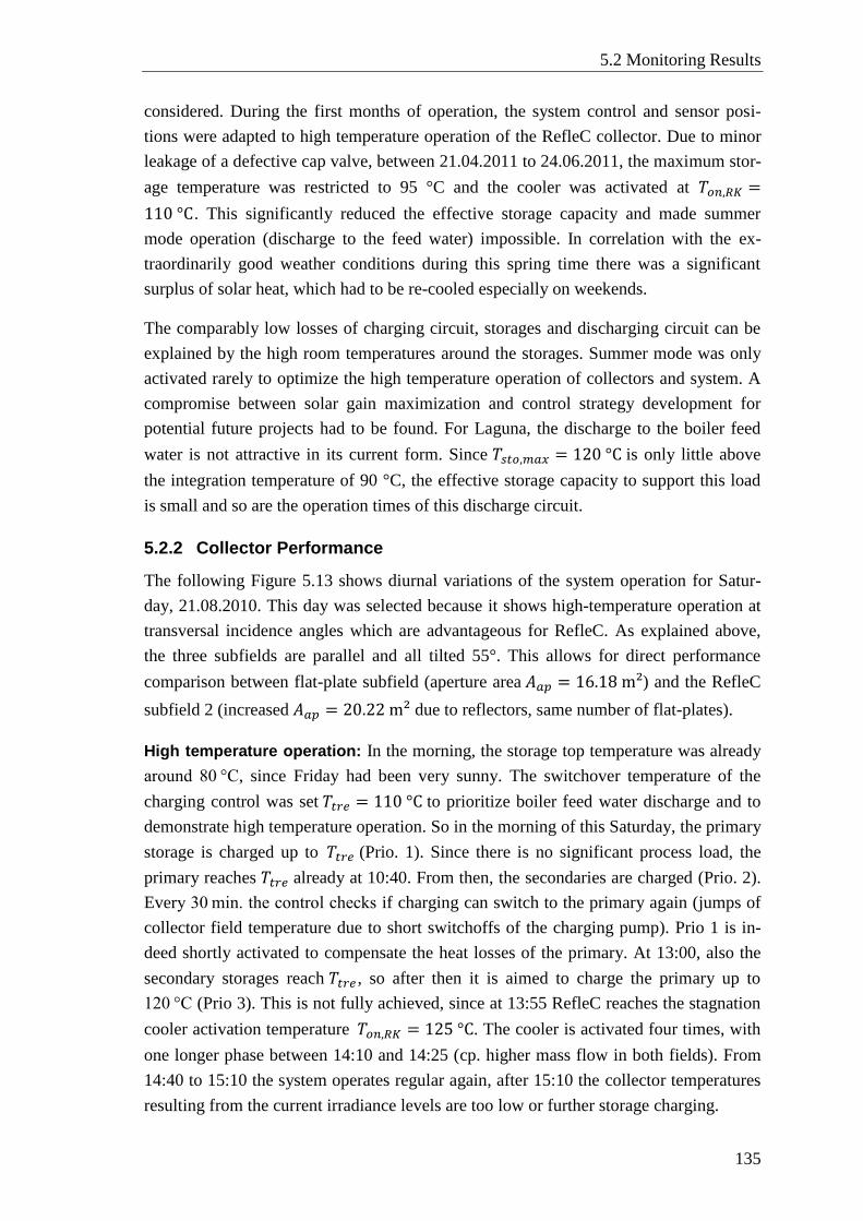
5.2 Monitoring Results
135
considered. During the first months of operation, the system control and sensor posi-
tions were adapted to high temperature operation of the RefleC collector. Due to minor
leakage of a defective cap valve, between 21.04.2011 to 24.06.2011, the maximum stor-
age temperature was restricted to 95 °C and the cooler was activated at 𝑇𝑜𝑛,𝑅𝐾 =
110 °C. This significantly reduced the effective storage capacity and made summer
mode operation (discharge to the feed water) impossible. In correlation with the ex-
traordinarily good weather conditions during this spring time there was a significant
surplus of solar heat, which had to be re-cooled especially on weekends.
The comparably low losses of charging circuit, storages and discharging circuit can be
explained by the high room temperatures around the storages. Summer mode was only
activated rarely to optimize the high temperature operation of collectors and system. A
compromise between solar gain maximization and control strategy development for
potential future projects had to be found. For Laguna, the discharge to the boiler feed
water is not attractive in its current form. Since 𝑇𝑠𝑡𝑜,𝑚𝑎𝑥 = 120 °C is only little above
the integration temperature of 90 °C, the effective storage capacity to support this load
is small and so are the operation times of this discharge circuit.
5.2.2 Collector Performance
The following Figure 5.13 shows diurnal variations of the system operation for Satur-
day, 21.08.2010. This day was selected because it shows high-temperature operation at
transversal incidence angles which are advantageous for RefleC. As explained above,
the three subfields are parallel and all tilted 55°. This allows for direct performance
comparison between flat-plate subfield (aperture area 𝐴𝑎𝑝 = 16.18 m²) and the RefleC
subfield 2 (increased 𝐴𝑎𝑝 = 20.22 m² due to reflectors, same number of flat-plates).
High temperature operation: In the morning, the storage top temperature was already
around 80 °C, since Friday had been very sunny. The switchover temperature of the
charging control was set 𝑇𝑡𝑟𝑒 = 110 °C to prioritize boiler feed water discharge and to
demonstrate high temperature operation. So in the morning of this Saturday, the primary
storage is charged up to 𝑇𝑡𝑟𝑒 (Prio. 1). Since there is no significant process load, the
primary reaches 𝑇𝑡𝑟𝑒 already at 10:40. From then, the secondaries are charged (Prio. 2).
Every 30 min. the control checks if charging can switch to the primary again (jumps of
collector field temperature due to short switchoffs of the charging pump). Prio 1 is in-
deed shortly activated to compensate the heat losses of the primary. At 13:00, also the
secondary storages reach 𝑇𝑡𝑟𝑒 , so after then it is aimed to charge the primary up to
120 °C (Prio 3). This is not fully achieved, since at 13:55 RefleC reaches the stagnation
cooler activation temperature 𝑇𝑜𝑛,𝑅𝐾 = 125 °C. The cooler is activated four times, with
one longer phase between 14:10 and 14:25 (cp. higher mass flow in both fields). From
14:40 to 15:10 the system operates regular again, after 15:10 the collector temperatures
resulting from the current irradiance levels are too low or further storage charging.
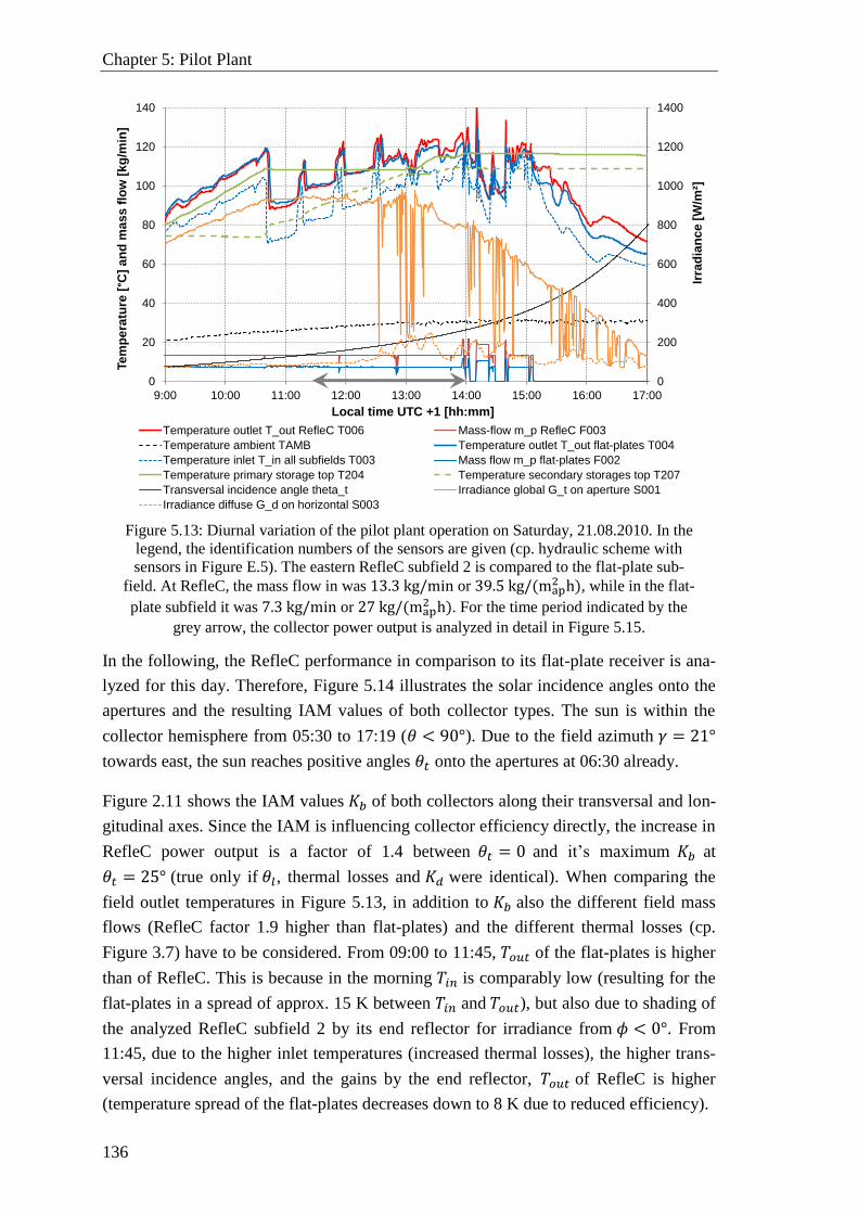
Chapter 5: Pilot Plant
136
Figure 5.13: Diurnal variation of the pilot plant operation on Saturday, 21.08.2010. In the
legend, the identification numbers of the sensors are given (cp. hydraulic scheme with
sensors in Figure E.5). The eastern RefleC subfield 2 is compared to the flat-plate sub-
field. At RefleC, the mass flow in was 13.3 kg/min or 39.5 kg/(map2 h), while in the flat-
plate subfield it was 7.3 kg/min or 27 kg/(map2 h). For the time period indicated by the
grey arrow, the collector power output is analyzed in detail in Figure 5.15.
In the following, the RefleC performance in comparison to its flat-plate receiver is ana-
lyzed for this day. Therefore, Figure 5.14 illustrates the solar incidence angles onto the
apertures and the resulting IAM values of both collector types. The sun is within the
collector hemisphere from 05:30 to 17:19 (𝜃 < 90°). Due to the field azimuth 𝛾 = 21°
towards east, the sun reaches positive angles 𝜃𝑡 onto the apertures at 06:30 already.
Figure 2.11 shows the IAM values 𝐾𝑏 of both collectors along their transversal and lon-
gitudinal axes. Since the IAM is influencing collector efficiency directly, the increase in
RefleC power output is a factor of 1.4 between 𝜃𝑡 = 0 and it’s maximum 𝐾𝑏 at
𝜃𝑡 = 25° (true only if 𝜃𝑙, thermal losses and 𝐾𝑑 were identical). When comparing the
field outlet temperatures in Figure 5.13, in addition to 𝐾𝑏 also the different field mass
flows (RefleC factor 1.9 higher than flat-plates) and the different thermal losses (cp.
Figure 3.7) have to be considered. From 09:00 to 11:45, 𝑇𝑜𝑢𝑡 of the flat-plates is higher
than of RefleC. This is because in the morning 𝑇𝑖𝑛 is comparably low (resulting for the
flat-plates in a spread of approx. 15 K between 𝑇𝑖𝑛 and 𝑇𝑜𝑢𝑡), but also due to shading of
the analyzed RefleC subfield 2 by its end reflector for irradiance from 𝜙 < 0°. From
11:45, due to the higher inlet temperatures (increased thermal losses), the higher trans-
versal incidence angles, and the gains by the end reflector, 𝑇𝑜𝑢𝑡 of RefleC is higher
(temperature spread of the flat-plates decreases down to 8 K due to reduced efficiency).
0
200
400
600
800
1000
1200
1400
0
20
40
60
80
100
120
140
9:00 10:00 11:00 12:00 13:00 14:00 15:00 16:00 17:00
Irra
dia
nc
e [
W/m
²]
Te
mp
era
ture
[°C
] a
nd
ma
ss
flo
w [
kg
/min
]
Local time UTC +1 [hh:mm]
Temperature outlet T_out RefleC T006 Mass-flow m_p RefleC F003
Temperature ambient TAMB Temperature outlet T_out flat-plates T004
Temperature inlet T_in all subfields T003 Mass flow m_p flat-plates F002
Temperature primary storage top T204 Temperature secondary storages top T207
Transversal incidence angle theta_t Irradiance global G_t on aperture S001
Irradiance diffuse G_d on horizontal S003
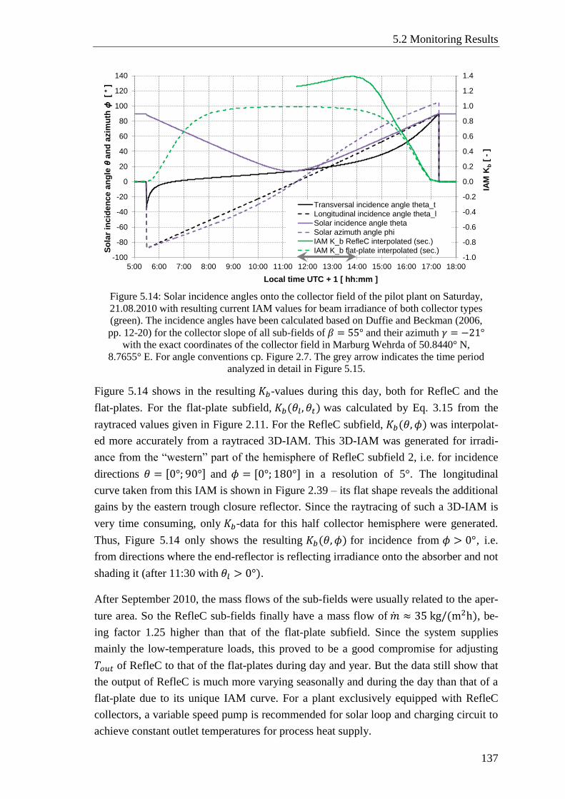
5.2 Monitoring Results
137
Figure 5.14: Solar incidence angles onto the collector field of the pilot plant on Saturday,
21.08.2010 with resulting current IAM values for beam irradiance of both collector types
(green). The incidence angles have been calculated based on Duffie and Beckman (2006,
pp. 12-20) for the collector slope of all sub-fields of 𝛽 = 55° and their azimuth 𝛾 = −21° with the exact coordinates of the collector field in Marburg Wehrda of 50.8440° N,
8.7655° E. For angle conventions cp. Figure 2.7. The grey arrow indicates the time period
analyzed in detail in Figure 5.15.
Figure 5.14 shows in the resulting 𝐾𝑏-values during this day, both for RefleC and the
flat-plates. For the flat-plate subfield, 𝐾𝑏(𝜃𝑙, 𝜃𝑡) was calculated by Eq. 3.15 from the
raytraced values given in Figure 2.11. For the RefleC subfield, 𝐾𝑏(𝜃, 𝜙) was interpolat-
ed more accurately from a raytraced 3D-IAM. This 3D-IAM was generated for irradi-
ance from the “western” part of the hemisphere of RefleC subfield 2, i.e. for incidence
directions 𝜃 = [0°; 90°] and 𝜙 = [0°; 180°] in a resolution of 5°. The longitudinal
curve taken from this IAM is shown in Figure 2.39 – its flat shape reveals the additional
gains by the eastern trough closure reflector. Since the raytracing of such a 3D-IAM is
very time consuming, only 𝐾𝑏-data for this half collector hemisphere were generated.
Thus, Figure 5.14 only shows the resulting 𝐾𝑏(𝜃, 𝜙) for incidence from 𝜙 > 0°, i.e.
from directions where the end-reflector is reflecting irradiance onto the absorber and not
shading it (after 11:30 with 𝜃𝑙 > 0°).
After September 2010, the mass flows of the sub-fields were usually related to the aper-
ture area. So the RefleC sub-fields finally have a mass flow of �̇� ≈ 35 kg/(m2h), be-
ing factor 1.25 higher than that of the flat-plate subfield. Since the system supplies
mainly the low-temperature loads, this proved to be a good compromise for adjusting
𝑇𝑜𝑢𝑡 of RefleC to that of the flat-plates during day and year. But the data still show that
the output of RefleC is much more varying seasonally and during the day than that of a
flat-plate due to its unique IAM curve. For a plant exclusively equipped with RefleC
collectors, a variable speed pump is recommended for solar loop and charging circuit to
achieve constant outlet temperatures for process heat supply.
-1.0
-0.8
-0.6
-0.4
-0.2
0.0
0.2
0.4
0.6
0.8
1.0
1.2
1.4
-100
-80
-60
-40
-20
0
20
40
60
80
100
120
140
5:00 6:00 7:00 8:00 9:00 10:00 11:00 12:00 13:00 14:00 15:00 16:00 17:00 18:00
IAM
Kb
[ -
]
So
lar
inc
ide
nc
e a
ng
le θ
an
d a
zim
uth
ϕ[
°]
Local time UTC + 1 [ hh:mm ]
Transversal incidence angle theta_t
Longitudinal incidence angle theta_l
Solar incidence angle theta
Solar azimuth angle phi
IAM K_b RefleC interpolated (sec.)
IAM K_b flat-plate interpolated (sec.)
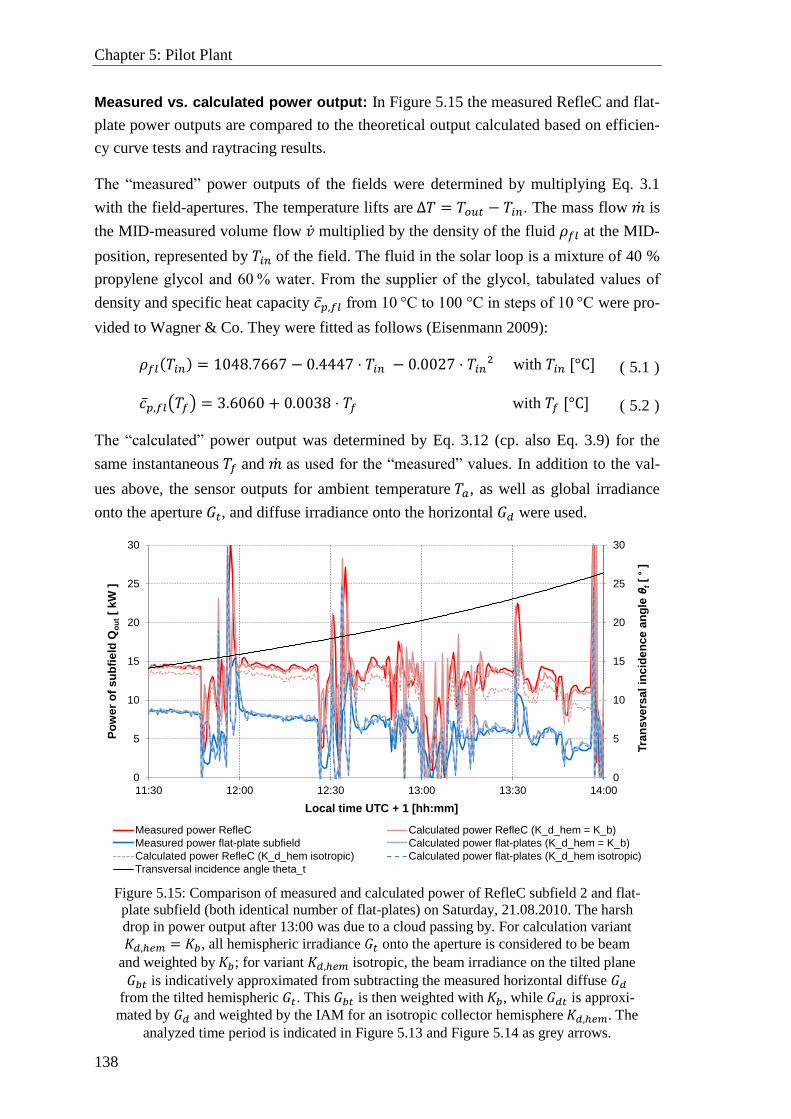
Chapter 5: Pilot Plant
138
Measured vs. calculated power output: In Figure 5.15 the measured RefleC and flat-
plate power outputs are compared to the theoretical output calculated based on efficien-
cy curve tests and raytracing results.
The “measured” power outputs of the fields were determined by multiplying Eq. 3.1
with the field-apertures. The temperature lifts are Δ𝑇 = 𝑇𝑜𝑢𝑡 − 𝑇𝑖𝑛. The mass flow �̇� is
the MID-measured volume flow �̇� multiplied by the density of the fluid 𝜌𝑓𝑙 at the MID-
position, represented by 𝑇𝑖𝑛 of the field. The fluid in the solar loop is a mixture of 40 %
propylene glycol and 60 % water. From the supplier of the glycol, tabulated values of
density and specific heat capacity 𝑐�̅�,𝑓𝑙 from 10 °C to 100 °C in steps of 10 °C were pro-
vided to Wagner & Co. They were fitted as follows (Eisenmann 2009):
𝜌𝑓𝑙(𝑇𝑖𝑛) = 1048.7667 − 0.4447 ⋅ 𝑇𝑖𝑛 − 0.0027 ⋅ 𝑇𝑖𝑛² with 𝑇𝑖𝑛 [°C] ( 5.1 )
𝑐�̅�,𝑓𝑙(𝑇𝑓) = 3.6060 + 0.0038 ⋅ 𝑇𝑓 with 𝑇𝑓 [°C] ( 5.2 )
The “calculated” power output was determined by Eq. 3.12 (cp. also Eq. 3.9) for the
same instantaneous 𝑇𝑓 and �̇� as used for the “measured” values. In addition to the val-
ues above, the sensor outputs for ambient temperature 𝑇𝑎, as well as global irradiance
onto the aperture 𝐺𝑡, and diffuse irradiance onto the horizontal 𝐺𝑑 were used.
Figure 5.15: Comparison of measured and calculated power of RefleC subfield 2 and flat-
plate subfield (both identical number of flat-plates) on Saturday, 21.08.2010. The harsh
drop in power output after 13:00 was due to a cloud passing by. For calculation variant
𝐾𝑑,ℎ𝑒𝑚 = 𝐾𝑏, all hemispheric irradiance 𝐺𝑡 onto the aperture is considered to be beam
and weighted by 𝐾𝑏; for variant 𝐾𝑑,ℎ𝑒𝑚 isotropic, the beam irradiance on the tilted plane
𝐺𝑏𝑡 is indicatively approximated from subtracting the measured horizontal diffuse 𝐺𝑑
from the tilted hemispheric 𝐺𝑡. This 𝐺𝑏𝑡 is then weighted with 𝐾𝑏, while 𝐺𝑑𝑡 is approxi-
mated by 𝐺𝑑 and weighted by the IAM for an isotropic collector hemisphere 𝐾𝑑,ℎ𝑒𝑚. The
analyzed time period is indicated in Figure 5.13 and Figure 5.14 as grey arrows.
0
5
10
15
20
25
30
0
5
10
15
20
25
30
11:30 12:00 12:30 13:00 13:30 14:00
Tra
ns
ve
rsa
l in
cid
en
ce
an
gle
θt[
°]
Po
we
r o
f s
ub
fie
ld Q
ou
t[
kW
]
Local time UTC + 1 [hh:mm]
Measured power RefleC Calculated power RefleC (K_d_hem = K_b)
Measured power flat-plate subfield Calculated power flat-plates (K_d_hem = K_b)
Calculated power RefleC (K_d_hem isotropic) Calculated power flat-plates (K_d_hem isotropic)
Transversal incidence angle theta_t
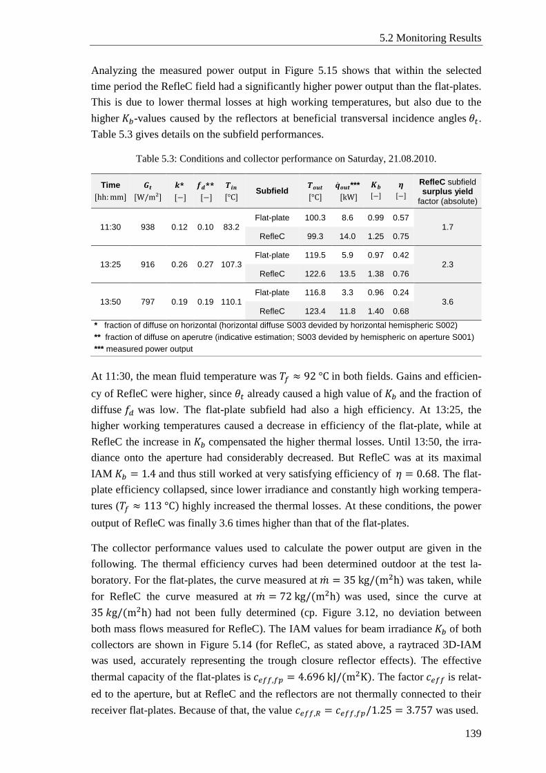
5.2 Monitoring Results
139
Analyzing the measured power output in Figure 5.15 shows that within the selected
time period the RefleC field had a significantly higher power output than the flat-plates.
This is due to lower thermal losses at high working temperatures, but also due to the
higher 𝐾𝑏-values caused by the reflectors at beneficial transversal incidence angles 𝜃𝑡.
Table 5.3 gives details on the subfield performances.
Table 5.3: Conditions and collector performance on Saturday, 21.08.2010.
At 11:30, the mean fluid temperature was 𝑇𝑓 ≈ 92 °C in both fields. Gains and efficien-
cy of RefleC were higher, since 𝜃𝑡 already caused a high value of 𝐾𝑏 and the fraction of
diffuse 𝑓𝑑 was low. The flat-plate subfield had also a high efficiency. At 13:25, the
higher working temperatures caused a decrease in efficiency of the flat-plate, while at
RefleC the increase in 𝐾𝑏 compensated the higher thermal losses. Until 13:50, the irra-
diance onto the aperture had considerably decreased. But RefleC was at its maximal
IAM 𝐾𝑏 = 1.4 and thus still worked at very satisfying efficiency of 𝜂 = 0.68. The flat-
plate efficiency collapsed, since lower irradiance and constantly high working tempera-
tures (𝑇𝑓 ≈ 113 °C) highly increased the thermal losses. At these conditions, the power
output of RefleC was finally 3.6 times higher than that of the flat-plates.
The collector performance values used to calculate the power output are given in the
following. The thermal efficiency curves had been determined outdoor at the test la-
boratory. For the flat-plates, the curve measured at �̇� = 35 kg/(m2h) was taken, while
for RefleC the curve measured at �̇� = 72 kg/(m2h) was used, since the curve at
35 𝑘g/(m2h) had not been fully determined (cp. Figure 3.12, no deviation between
both mass flows measured for RefleC). The IAM values for beam irradiance 𝐾𝑏 of both
collectors are shown in Figure 5.14 (for RefleC, as stated above, a raytraced 3D-IAM
was used, accurately representing the trough closure reflector effects). The effective
thermal capacity of the flat-plates is 𝑐𝑒𝑓𝑓,𝑓𝑝 = 4.696 kJ/(m2K). The factor 𝑐𝑒𝑓𝑓 is relat-
ed to the aperture, but at RefleC and the reflectors are not thermally connected to their
receiver flat-plates. Because of that, the value 𝑐𝑒𝑓𝑓,𝑅 = 𝑐𝑒𝑓𝑓,𝑓𝑝/1.25 = 3.757 was used.
[hh:mm]
Time
𝑮𝒕
[W/m²]
𝒌*
[−]
𝒇𝒅**
[−]
𝑻𝒊𝒏
[°C] Subfield
𝑻𝒐𝒖𝒕
[°C]
�̇�𝒐𝒖𝒕***
[kW]
𝑲𝒃
[−]
𝜼
[−]
RefleC subfield surplus yield
factor (absolute)
11:30
938 0.12 0.10 83.2 Flat-plate 100.3 8.6 0.99 0.57
1.7 RefleC 99.3 14.0 1.25 0.75
13:25
916 0.26 0.27 107.3 Flat-plate 119.5 5.9 0.97 0.42
2.3 RefleC 122.6 13.5 1.38 0.76
13:50
797 0.19 0.19 110.1 Flat-plate 116.8 3.3 0.96 0.24
3.6 RefleC 123.4 11.8 1.40 0.68
* fraction of diffuse on horizontal (horizontal diffuse S003 devided by horizontal hemispheric S002)
** fraction of diffuse on aperutre (indicative estimation; S003 devided by hemispheric on aperture S001)
*** measured power output
Chapter 5: Pilot Plant
140
The day selected for the exemplary comparison between measured and calculated col-
lector field output in Figure 5.16 is one with high hemispherical irradiance and highly
anisotropic diffuse irradiance. The unshaded pyranometers shown in Figure 5.9 deter-
mine the hemispherical irradiance onto horizontal 𝐺 and aperture 𝐺𝑡. Measurement of
diffuse irradiance on the horizontal 𝐺𝑑 is done by the shadow band pyranometer and
thus less accurate. Neither a pyrheliometer, to determine the exact diffuse irradiance
onto horizontal and aperture (by subtracting 𝐺𝑏 from DNI-measurement from the re-
spective hemispherical values), nor an albedometer to distinguish between sky and
ground reflected diffuse irradiance onto the aperture was available.
Having in mind these limitations, two variants to calculate the power output for a com-
parison to the measured performance were applied. The variant “𝑲𝒅,𝒉𝒆𝒎 = 𝑲𝒃” treats
all irradiance onto the aperture as if originating from sun direction. At the very high 𝐾𝑏-
values occurring within the investigated time period, this overestimates the influence of
diffuse. On the other hand, the measured 𝐺𝑡 accurately accounts for the diffuse irradi-
ance from sky and ground received by the collector. Furthermore, due to the high sky
anisotropy (cp. horizontal diffuse fraction 𝑘 in Table 5.3) the major share of diffuse is
expected to be brightening around the sun. The variant “𝑲𝒅,𝒉𝒆𝒎 isotropic” aims at
distinguishing between beam and diffuse. At the pilot plant, this in principle right inten-
tion has the drawback that the diffuse irradiance onto the aperture is not measured. The
simplification of using the inaccurately measured horizontal diffuse instead induces
very high uncertainties both for 𝐺𝑑𝑡 and the 𝐺𝑏𝑡 calculated with it. Since furthermore
the distribution of diffuse over the sky dome is not known, the common isotropic ap-
proach was taken for comparison to variant “𝐾𝑑,ℎ𝑒𝑚 = 𝐾𝑏”. Therefore, for both collec-
tors the IAM for isotropic diffuse irradiance 𝐾𝑑,ℎ𝑒𝑚 from the whole collector hemi-
sphere was needed. For both, the identical values as from the energy gain simulations
were used. For the flat-plate, this is 𝐾𝑑,ℎ𝑒𝑚 = 0.82; for RefleC it is 𝐾𝑑,ℎ𝑒𝑚 = 0.66. As-
suming an endless RefleC trough slightly overestimates 𝐾𝑑,ℎ𝑒𝑚 of the pilot plant, but the
raytraced 3D-IAM of the RefleC subfield 2 was only valid for the half collector hemi-
sphere with 𝜙 > 0° and could therefore not be used.
The first 15 min in Figure 5.15 are most suitable for the comparison because of the qua-
si-stationary conditions (almost constant irradiance and 𝑇𝑓 , cp. Figure 5.13). For the
conditions of this time period, variant “𝑲𝒅,𝒉𝒆𝒎 = 𝑲𝒃” predicts the measured power
very accurately. At the flat-plates, the measured energy gain of this period is about
0.5 % below the calculated, while for RefleC the measured gain is 0.2 % above. When
the time frame is extended to unstationary operation, the deviations are slightly higher.
For the flat-plate, IAM values for the whole day are available, so a time period symmet-
ric around 𝜙 = 0° from 09:15 to 13:45 can be used. Here, the measured output is 2 %
below the calculated. For the RefleC subfield 2, where no full-day IAM values are
available, from 11:30 to 13:45 the measured output is even 2 % above the calculated.
5.2 Monitoring Results
141
When applying variant “𝐾𝑑,ℎ𝑒𝑚 isotropic”, at the flat-plates almost no difference in cal-
culated output compared to the other variant is observed. This is because at the flat-
plates the IAM values for beam and isotropic diffuse are not highly differing and the
fraction of diffuse is small (see 𝑓𝑑 and cp. 𝐾𝑑,ℎ𝑒𝑚 = 0.82 to 𝐾𝑏 in Table 5.3). Only at
13:25, because of the higher 𝑓𝑑, the power calculated by variant “𝐾𝑑,ℎ𝑒𝑚 isotropic” is
slightly below that calculated by “𝐾𝑑,ℎ𝑒𝑚 = 𝐾𝑏”. For RefleC, there is a high deviation
between the variants. The undervaluation by “𝐾𝑑,ℎ𝑒𝑚 isotropic” increases with increas-
ing 𝑓𝑑 and 𝐾𝑏 . This is because 𝐾𝑑,ℎ𝑒𝑚 = 0.66 is highly differing from 𝐾𝑏 , so the ac-
ceptance of diffuse is indeed highly influencing the calculated value.
The comparison of the raytracing simulations with measured IAM values at the test la-
boratory under a very similar incidence angle had already indicated that the isotropic
approach significantly underestimates the contribution of diffuse to the output of RefleC
(cp. Figure 3.19). Having in mind the measurement uncertainties of the sensors at pilot
plant and test laboratory, but also the uncertainties of the raytracing simulations, the
calculated power correlates very well with the measured. Further considering that at the
pilot plant the uncertainties of the irradiance determination for calculation variant
“𝐾𝑑,ℎ𝑒𝑚 isotropic” are identical for RefleC and the flat-plates, the presented comparison
between measured and calculated power confirms that the isotropic approach underes-
timates the power output of RefleC. Furthermore, the comparison shows that RefleC
and flat-plates work as theoretically expected also at a real installation.
Annual additional gains by the reflectors: Figure 5.16 gives a monthly overview on
the mean daily irradiance as well as specific flat-plate and RefleC gains of the whole
monitoring period. To calculate the additional gain by the reflectors as shown, the
measured monthly gross-energy gain of the RefleC subfield 2 was directly compared to
that of the flat-plate subfield. In summer 2011, the solar irradiance was low compared to
2010 due to bad weather periods (cp. e.g. variation for July). The additional gains show
a sinus-like characteristic – high and stable additional output is observed from April to
September. The additional gains in percentage terms mainly depend on the annual sun
path; they are fairly independent of the absolute irradiance. This is proved when com-
paring the additional gains in August, September and October 2010 to the almost identi-
cal values in 2011. The reflectors were installed on 9 July 2010, so the values given for
this month should not be compared to July 2011. In June and July 2011 the sinus-like
shape of the additional gains flattens a bit, since around noon 𝜃𝑡 is often above 35°,
which leads to a decrease in 𝐾𝑏 (i.e. the mirrors do not direct beam to the receiver but
reflect it back into the sky above the flat-plates).
To allow an indicative comparison between the annual performance of RefleC and its
flat-plate at the pilot plant, the reference year from 1 October 2010 to 30 September
2011 as defined above is used. At this comparison, for RefleC again only the measured
gains of subfield 2 are used since this subfield had its own mass flow sensor.
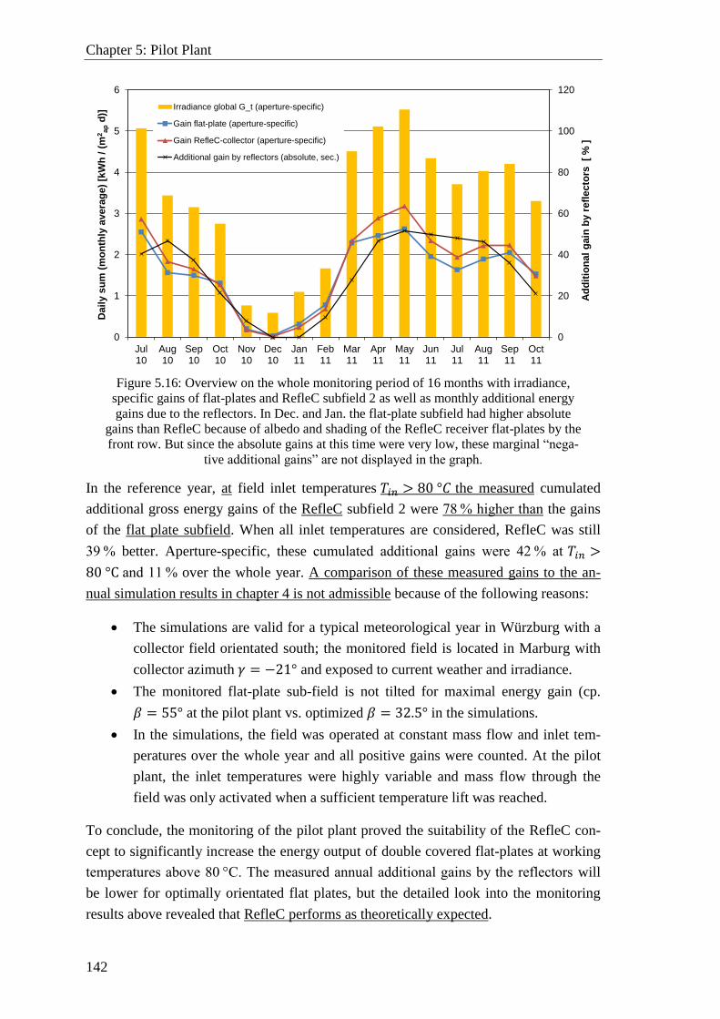
Chapter 5: Pilot Plant
142
Figure 5.16: Overview on the whole monitoring period of 16 months with irradiance,
specific gains of flat-plates and RefleC subfield 2 as well as monthly additional energy
gains due to the reflectors. In Dec. and Jan. the flat-plate subfield had higher absolute
gains than RefleC because of albedo and shading of the RefleC receiver flat-plates by the
front row. But since the absolute gains at this time were very low, these marginal “nega-
tive additional gains” are not displayed in the graph.
In the reference year, at field inlet temperatures 𝑇𝑖𝑛 > 80 °𝐶 the measured cumulated
additional gross energy gains of the RefleC subfield 2 were 78 % higher than the gains
of the flat plate subfield. When all inlet temperatures are considered, RefleC was still
39 % better. Aperture-specific, these cumulated additional gains were 42 % at 𝑇𝑖𝑛 >
80 °C and 11 % over the whole year. A comparison of these measured gains to the an-
nual simulation results in chapter 4 is not admissible because of the following reasons:
The simulations are valid for a typical meteorological year in Würzburg with a
collector field orientated south; the monitored field is located in Marburg with
collector azimuth 𝛾 = −21° and exposed to current weather and irradiance.
The monitored flat-plate sub-field is not tilted for maximal energy gain (cp.
𝛽 = 55° at the pilot plant vs. optimized 𝛽 = 32.5° in the simulations.
In the simulations, the field was operated at constant mass flow and inlet tem-
peratures over the whole year and all positive gains were counted. At the pilot
plant, the inlet temperatures were highly variable and mass flow through the
field was only activated when a sufficient temperature lift was reached.
To conclude, the monitoring of the pilot plant proved the suitability of the RefleC con-
cept to significantly increase the energy output of double covered flat-plates at working
temperatures above 80 °C. The measured annual additional gains by the reflectors will
be lower for optimally orientated flat plates, but the detailed look into the monitoring
results above revealed that RefleC performs as theoretically expected.
0
20
40
60
80
100
120
0
1
2
3
4
5
6
Jul10
Aug10
Sep10
Oct10
Nov10
Dec10
Jan11
Feb11
Mar11
Apr11
May11
Jun11
Jul11
Aug11
Sep11
Oct11
Ad
dit
ion
al
ga
in b
y r
efl
ec
tors
[
% ]
Dail
y s
um
(m
on
thly
ave
rag
e)
[kW
h / (
m2ap
d)]
Irradiance global G_t (aperture-specific)
Gain flat-plate (aperture-specific)
Gain RefleC-collector (aperture-specific)
Additional gain by reflectors (absolute, sec.)
5.3 Economic Assessment of RefleC Boosters
143
5.3 Economic Assessment of RefleC Boosters
The anisotropic simulations discussed above showed that the additional gain caused by
the RefleC booster reflectors is much higher than predicted by isotropic, state of the art
modelling (cp. Figure 4.15). This can be of high practical relevance for the ST industry,
because it positively influences the cost/performance ratio of the boosters.
Taking the anisotropically calculated booster gains into account, this section aims to
estimate up to which investment costs per unit reflector area boosters may be economi-
cally attractive for applications similar to the RefleC pilot plant. This estimation starts
from the expression of solar heat generation costs 𝐾𝑠𝑜𝑙 (VDI 2004, p. 66):
𝐾𝑠𝑜𝑙 = 𝐾𝑖𝑛𝑣 ⋅ 𝑓𝑎 + 𝐾𝑚𝑎𝑖𝑛
𝑄𝑠𝑜𝑙+ 𝐾𝑜𝑝 ( 5.3 )
Therein, 𝐾𝑖𝑛𝑣 is the overall investment costs, 𝑓𝑎 is the annuity factor accounting for the
annual capital costs, 𝐾𝑚𝑎𝑖𝑛 and 𝐾𝑜𝑝 are the annual maintenance and operational costs,
and 𝑄𝑠𝑜𝑙 is the annual solar gains. The annuity factor 𝑓𝑎 is calculated from the capital
interest rate 𝑝 and the service life 𝑇 of the boosters (VDI 2004, p. 66):
𝑓𝑎 = (1 + 𝑝)𝑇 ⋅ 𝑝
(1 + 𝑝)𝑇 − 1 ( 5.4 )
At the RefleC pilot plant, the reflectors are not cleaned and therefore do not cause addi-
tional operational or maintenance costs compared to a system of flat plate collectors
without reflectors. Thus, because only costs and gains related to the reflector shall be
analyzed, 𝐾𝑜𝑝 and 𝐾𝑚𝑎𝑖𝑛 do not have to be considered and eq. 5.3 can be written as:
𝐾𝑖𝑛𝑣 = 𝐾𝑠𝑜𝑙 ⋅ 𝑄𝑠𝑜𝑙
𝑓𝑎 ( 5.5 )
First, the additional annual gains by the booster reflectors 𝑄𝑠𝑜𝑙 have to be quantified.
This must be the difference between an optimized system with double-covered flat-
plates and a system with RefleC collectors. It was discussed at the end of the last section
5.2.2 that the additional gains measured at the pilot plant do not represent this differ-
ence. But because the monitored system worked as theoretically expected, the simula-
tion results for RefleC 6 and LBM 4 GF can be used. These simulations revealed that
the absolute additional collector gain caused by the boosters depends on the location,
but is similar for both simulated inlet temperatures of 40 °C and 120 °C (cp. Figure 4.14
and Table 4.2). For the following assessment, it is assumed that these temperatures
mark the expected working temperature range of stationary collectors with boosters. It
is further assumed that the additional gains by the boosters are temperature-
independent, so that a mean value of the simulated additional gain can be used. This is
in Würzburg 126.0 kWh mfp−2 a−1 and in Seville 212.5 kWh mfp
−2 a−1 (cp. Table 4.2).
Chapter 5: Pilot Plant
144
These values do not yet represent the useable heat 𝑄𝑠𝑜𝑙, because the simulation results
in section 4.3.3 give only the collector gain and do not consider losses within a SPH
system. At the RefleC pilot plant, 70.4 % of the heat produced by the collector field was
transferred to the processes (cp. p. 134). This measured system efficiency accounts for
the whole spectrum of operation temperatures (30 °C up to 130 °C), for the losses
caused by the stagnation cooler, and for the non-optimized system control during the
first months. Although the system efficiency might be higher at larger SPH systems
with boosters, the value of the RefleC pilot plant is used here. Based on this conserva-
tive system efficiency and the simulation results, the calculated additional energy sup-
ply to the processes caused by the reflectors is in Würzburg 𝑄𝑠𝑜𝑙 = 88.7 kWh mfp−2 a−1
and in Seville 𝑄𝑠𝑜𝑙 = 149.6 kWh mfp−2 a−1.
To calculate a minimal selling price for the reflectors by eq. 5.5, acceptable solar heat
generation costs 𝐾𝑠𝑜𝑙 for the useful energy from the reflectors have to be estimated. Be-
cause the RefleC pilot plant is a laundry, conventional heating costs from the laundry
sector are used as a basis for comparison. Beeh and Hess (2014) collected data of 20
laundries, most of them located in Germany and having a gas-fired steam network.
When losses of 20 % for heat generation and distribution are taken into account, the
typical conventional heating costs at these laundries are about 0.06 EUR/kWh (Beeh
and Hess 2014, p. 13). As an example, the following assessment assumes that the appli-
cation of booster reflectors might be attractive if they generate useful solar heat at two
thirds of this price, i.e. 𝐾𝑠𝑜𝑙 = 0.04 EUR/kWh. To estimate the capital costs, an interest
rate 𝑝 = 4 % and a lifetime of the system of 𝑇 = 20 years are assumed. With eq. 5.4
this results in an annuity factor of 𝑓 = 0.0736.
From the estimations and framework conditions discussed above, the resulting invest-
ment costs 𝐾𝑖𝑛𝑣, i.e. the minimal selling price of the reflector for one m2 of flat-plate
receiver aperture can be calculated by eq. 5.5. If the same framework conditions are
assumed for both locations, the result is for Würzburg 𝐾𝑖𝑛𝑣 = 48 EUR/mfp2 and for Se-
ville 𝐾𝑖𝑛𝑣 = 81 EUR/mfp2 . The RefleC collector as applied at the pilot plant uses the
flat-plate collector LBM 8 of Wagner & Co. Solartechnik with four glass panes as re-
ceiver. This flat-plate has an overall aperture area 𝐴𝑎𝑝 = 8,15 m2 and is equipped with
an overall reflector area of 12,57 m2 (Kramp 2010).
The exemplary calculation above gives a minimal reflector price for Würzburg of
𝐾𝑖𝑛𝑣 = 31 EUR/m2 (or 393 EUR per LBM 8 equipped) and for Seville of 𝐾𝑖𝑛𝑣 =
53 EUR/m2 (or 663 EUR per LBM 8). For the customer this would mean a static pay-
back period of approx. nine years (calculated from dividing the investment for the
boosters by the annually saved gas costs). It has to be stressed that other framework
conditions can result in highly different values. Especially the interest rate has a very
high impact on reflector price and amortization period.
Chapter 6: Conclusions and Perspectives
145
6 Conclusions and Perspectives
The findings of this work are summarized and discussed against the state
of the art. Suggestions for further research are made.
6.1 Low-Concentrating, Stationary Collectors
External reflectors can highly increase the gain of stationary ST collectors. Boosters
between collector rows offer better roof area utilization and acceptance for diffuse irra-
diance than reflectors on both the upper and lower sides of a collector. CPC reflectors
have a higher acceptance angle than flat reflectors. But when reflecting on flat-plates,
this advantage is partly compensated by lower transmittance of the reflected rays
through the cover(s). CPC reflectors also cause local concentration on the absorber.
This reduced the collector efficiency factor 𝐹´ of the flat-plates tested. The booster of
RefleC approximates a half CPC by flat segments, which avoided this decrease.
Simulation results revealed that the RefleC booster increases the annual output of the
double-covered flat-plate in Würzburg by 20 % at a constant inlet temperature of 40 °C
and by 87 % at an inlet of 120 °C. The absolute increase is largely temperature inde-
pendent. Simulating with a varying, anisotropic diffuse-IAM is considered to be essen-
tial for realistic modelling of instantaneous collector gains and for accurate assessment
of the cost-benefit ratio of stationary reflectors. Isotropic modelling undervalued the
additional gains from the RefleC booster by 40 % at 40 °C and by 20 % at 120 °C.
Accurate efficiency curve and IAM determination is of special importance for medium
temperature collectors. Extrapolation of an efficiency curve to values of ∆𝑇/𝐺 higher
than tested overestimates the collector efficiency. Therefore, one operation point with
efficiency below 20 % is recommended for collector efficiency tests. The influence of
the IAM on efficiency and annual gains increases with increasing thermal losses.
It was shown that the efficiency curve of a stationary collector with external reflector
can be estimated without measurements, when the efficiency curve of the collector and
raytracing of the receiver-booster combination are available, and when 𝐹´ does not
change. This can be used to assess the effect of optimized external reflectors for existing
collectors by annual energy gain simulations. Thus, future work in this field could in-
clude theoretical assessments of the performance increase of e.g. standard evacuated
tube collectors or evacuated flat-plates due to optimized external booster reflectors.
Appendix A: Collector Variants
146
6.2 IAM for Beam and Diffuse Irradiance
Diffuse irradiance originates from the whole 180° hemisphere of a sloped ST collector,
except of a solid angle of approx. 6° diameter around the sun, from where pyrheliome-
ters detect beam. The diffuse radiance is not isotropic, and its anisotropy changes with
varying meteorological conditions. The influence of both the IAM for beam and diffuse
on efficiency and annual gain increases with increasing thermal losses, so accurate IAM
values are of increased relevance for medium temperature collectors.
Beam-IAM curves determined from steady-state outdoor-tests at hemispherical irradi-
ance are considered to describe the IAM of low-concentrating collectors sufficiently
within their concentrator acceptance angle, if the diffuse fractions during the test inter-
vals are similar. For irradiance from outside the acceptance angle or for highly different
diffuse fractions, “correction” of the diffuse influence as applied in this work is recom-
mended. Such a correction was shown under the simplifying assumption of isotropic
diffuse irradiance. A comparative correction calculation with diffuse-IAM values that
may reflect the hemispheric anisotropy during the test led to the conclusion that the ac-
curacy of the correction could in the future be improved by considering this anisotropy.
A hemispheric, isotropic diffuse-IAM determined from steady-state outdoor-tests is
underestimating the annual diffuse utilization of all ST collectors. Quasi-dynamic tests
have not been performed in this work. Such tests identify the diffuse-IAM from meas-
ured collector output. Although this is also done assuming an isotropic hemisphere, the
identified diffuse-IAM value is expected to better represent the annual diffuse utiliza-
tion of a collector, since its value also reflects the anisotropic irradiance during the test.
Considering the varying anisotropy of diffuse sky radiance in collector simulation mod-
els by a varying, anisotropically calculated diffuse-IAM is considered to be essential for
realistic modelling of instantaneous collector gains and for accurate assessment of the
cost-benefit ratio of stationary reflectors.
In future research, to determine beam and diffuse IAM data from outdoor measure-
ments, a pyrheliometer and an albedometer should be applied. These two sensors allow
for accurately distinguishing between beam, sky diffuse, and ground reflected diffuse
irradiance onto the aperture. This makes instantaneous clearness index calculation pos-
sible, so that the sky radiance could be anisotropically distributed according to the
Brunger model. With this, the instantaneous IAM of a collector for anisotropic diffuse
irradiance can be calculated as introduced in this work. Following the test value “cor-
rection” approach given, the contributions of the three irradiance components to the
measured output and thus the three IAMs of the separated irradiance components could
be determined iteratively from a set of incidence angles tested. Highest relevance is ex-
pected for stationary, incidence-angle selective collectors like RefleC.
6.3 Simulation Model
147
6.3 Simulation Model
Existing collector simulation models do not consider the effect of the varying anisotro-
py of diffuse irradiance on the diffuse-IAM. They calculate with a constant IAM for
isotropic diffuse irradiance. Furthermore, they all use one IAM for diffuse irradiance
from the 180° collector hemisphere, not distinguishing between sky and ground.
In the TRNSYS simulation software, the radiation processor considers the sky anisotro-
py e.g. by applying the Perez-Model to calculate irradiance on a tilted plane from
weather data files. But the radiation processor only gives the correct sum of the irradi-
ance, not its distribution. That is why existing collector models can not consider the
anisotropy of sky irradiance. The collector simulation model presented in this work cal-
culates separate IAMs for sky diffuse irradiance and ground reflected diffuse irradiance.
It uses the model of Brunger and Hooper to generate an anisotropic sky based on the
current fraction of diffuse and the clearness index. To calculate an anisotropic diffuse-
IAM for sky radiance, the model divides the sky into segments and weights their irradi-
ance with raytraced beam-IAM values for the individual incidence angles of these seg-
ments. This is done once per time step. The Brunger distribution is exclusively used to
calculate the diffuse-IAM for anisotropic sky irradiance. The IAM for diffuse ground
irradiance is calculated with an isotropic approach and is constant during the simulation.
The model is also capable of calculating a diffuse-IAM for an isotropic collector hemi-
sphere (state of the art) or separate isotropic diffuse IAMs for sky and ground irradi-
ance. The sums of sky and ground reflected diffuse irradiance onto the aperture are in-
put to the model and taken from the radiation processor as usual.
The model was applied to RefleC and its flat-plate receiver for constant inlet tempera-
tures of 40 °C and 120 °C in Würzburg and Seville. At the anisotropic calculation, in
Würzburg for RefleC a daily variation of the diffuse IAM of up to 25 % was observed.
Separate IAM calculation for anisotropic sky and isotropic ground instead of the hemi-
spherical isotropic calculation resulted for RefleC at 40 °C inlet in 10 % increased annu-
al gains; at 120 °C the gains were 16 % higher. The flat-plate without reflectors showed
an increase of 3 % at 40 °C and 8 % at 120 °C. The undervaluation by isotropic model-
ling was reduced to about 6.5 % (for RefleC at 120 °C), when separate diffuse-IAMs for
sky and ground were calculated. In Seville, due to a lower diffuse fraction, the under-
valuation in percent was lower than in Würzburg.
The results indicate that the diffuse-utilization of all non-focusing collectors is under-
valued by existing simulation models, when isotropic diffuse-IAMs calculated from
raytracing or steady-state tests are used. This is concluded from the irradiation diagram
shown and because underestimation was also found for the flat-plate, which is the least
incidence angle sensitive collector type. The optimal collector slope was not affected by
the anisotropic diffuse-IAM modelling, so current models are sufficient in this respect.
Appendix A: Collector Variants
148
In the future, the simulation comparison between annual output with constant isotropic
and varying anisotropic diffuse-IAMs should also be performed using isotropic diffuse-
IAM values from quasi-dynamic collector tests. In this case, the error of isotropic mod-
elling is expected to be smaller. Such comparisons for different common collector types
would allow assessing the individual relevance of anisotropic diffuse-IAM modelling.
The developed simulation model itself should be further improved. Currently, the spe-
cific fluid heat capacity is a constant parameter. Its temperature-dependency must be
included to compare simulated output temperatures to measured values accurately. The
annual output should be much less sensitive for this. Furthermore, the missing parame-
ters of the dynamic collector model of Perers could be implemented. The model has not
been validated yet, and also the reported differences between isotropic and anisotropic
modelling results were not determined independently, since the same model was used
for both. Future work should therefore first compare the different diffuse-IAM modes of
the new model to existing collector simulation models.
The simulations given in this work were only determined for constant collector inlet
temperatures and constant mass flow, and every positive gain was counted. Future
works should compare this simplified collector gain simulation to more realistic cases
by applying the new model for in simulations of complete ST systems.
For a real validation of the model, a setup as described at the end of the last section 6.2
is recommended. The measured irradiance and collector test data could be used as mod-
el-input, so that the modeled collector output temperatures could be compared to the
measured ones for the variety of sky radiance conditions covered by the Brunger model.
At RefleC and similar collectors, the undervaluation of the annual sky-diffuse utiliza-
tion by the isotropic IAM might be partly compensated by an overvaluation due to the
application of the simplified beam-IAM separation approach of McIntire. This means
that it is possible that the undervaluation of real annual gains by the existing simulation
models might in reality be smaller than resulting from this work. So, future work should
determine the error of this separation approach for RefleC and other stationary collector
types by 3D-raytracing and annual simulations. The collector model presented is very
suitable for this purpose, since it can directly use a 3D-IAM.
The use of raytraced beam-IAM curves in energy gain simulations has a general limita-
tion. They only represent a collector’s IAM correctly, when the thermal loss mecha-
nisms do not change with the incidence angle. Such changes can e.g. be caused by a
varying 𝐹´ resulting from local concentrations varying with the incidence angle.
In the short term, the accuracy of standard simulation tools could be significantly in-
creased by implementing a separate calculation of constant isotropic diffuse-IAMs for
sky and ground, as documented in this work. Since such a calculation has to be done
only once per simulation, no effect on the simulation time of standard tools is expected.
6.4 Pilot Plant
149
6.4 Pilot Plant
Process heat generation with the RefleC collector is demonstrated at a laundry in Ger-
many with an innovative, monitored ST system. The system supplies hot water for the
washing machines, boiler makeup-water, and boiler feed water. A trough of RefleC col-
lectors was directly compared to a row of double-covered flat-plates without reflectors.
For a reference year, the annual solar fraction of the system was determined to be
23.2 %, the solar loop utilization ratio was 40.9 %, and the system utilization ratio was
35 %. The system utilization ratio is particularly satisfying compared to other monitored
process heat systems. For future collector fields with booster reflectors, adaptive varia-
ble speed pumps are recommended to account for the very incidence angle dependent
power output and to avoid too high outlet temperatures.
Comparing all gains within the reference year at inlet temperatures above 80 °C, the
RefleC boosters increased the gain of the double-covered reference flat-plates by 78 %.
During the whole year, the gain of RefleC was 39 % above that of the double-covered
flat-plates. The basis of this comparison is a unit area of flat-plate receiver.
A comparison between measured and calculated collector output showed that the flat-
plate as well as the RefleC collector work as theoretically expected. For a representative
day with a clear sky, the calculated collector output of RefleC was significantly beyond
the measured, when a diffuse-IAM for an isotropic sky was used. Calculation with a
diffuse-IAM value increased to the beam-IAM (which is expected to be more realistic at
clear sky conditions) reproduced the measured collector output correctly.
During the monitoring sequence analyzed, the influence of the diffuse-IAM on the cal-
culated output of the flat-plate was low, because the values of beam- and diffuse-IAM
did not differ much. Thus, anisotropy effects on the flat-plate output could not be clear-
ly reproduced yet and might be within the measurement uncertainty range. But for Re-
fleC the comparison clearly indicates an undervaluation by the isotropic approach. For
the calculation of the RefleC output, a raytraced 3D-IAM was used, so that errors of the
McIntire interpolation approach can be excluded.
For future monitoring projects with similar collectors, a dedicated analysis tool coupled
with a monitoring database is recommended. To effectively analyze the utilization of
diffuse irradiance by a collector from monitored data, a pyrheliometer and an albedome-
ter, as discussed in section 6.2 above, should be applied. While test stand measurements
only allow for a validation at certain irradiance situations and fluid temperatures, a clas-
sification of annually monitored data into intervals of operation temperatures and
Brunger distributions would allow for a comprehensive validation of the simulation
model discussed within this work.


Appendix
151
Appendix
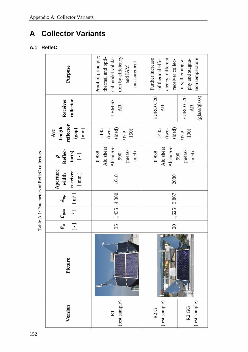
Appendix A: Collector Variants
152
A Collector Variants
A.1 RefleC
Tab
le A
.1:
Par
amet
ers
of
Ref
leC
coll
ecto
rs
Pu
rpose
Pro
of
of
pri
nci
ple
;
ther
mal
and o
pti
-
cal
model
val
ida-
tion b
y e
ffic
iency
and I
AM
mea
sure
men
t
Furt
her
incr
ease
of
ther
mal
eff
i-
cien
cy;
dif
fere
nt
rece
iver
coll
ec-
tors
; th
erm
ogra
-
phy a
nd s
tagn
a-
tion t
emper
ature
Rec
eiv
er
coll
ecto
r
LB
M 6
7
AR
EU
RO
C20
AR
EU
RO
C20
AR
(gla
ss/g
lass
)
Arc
len
gth
refl
ect
or
(gap
)
[mm
]
1145
(tw
o-
sided
)
(gap
=
150)
1435
(tw
o-
sided
)
(gap
=
190)
𝝆
Ref
lec-
tor(
s)
[ -
]
0.8
38
Alu
shee
t
Alc
an S
S-
990
(mea
s-
ure
d)
0.8
38
Alu
shee
t
Alc
an S
S-
990
(mea
s-
ure
d)
Ap
ertu
re
wid
th
recei
ver
[ m
m ]
1618
2080
𝑨𝒂𝒑
[ m
² ]
4.3
80
3.8
67
𝑪𝒈𝒆𝒐
[ °
]
1,4
35
1,6
25
𝜽𝒂
[ -
]
35
20
Pic
ture
Ver
sion
R1
(tes
t sa
mple
)
R2 G
(tes
t sa
mple
)
R2 G
G
(tes
t sa
mple
)
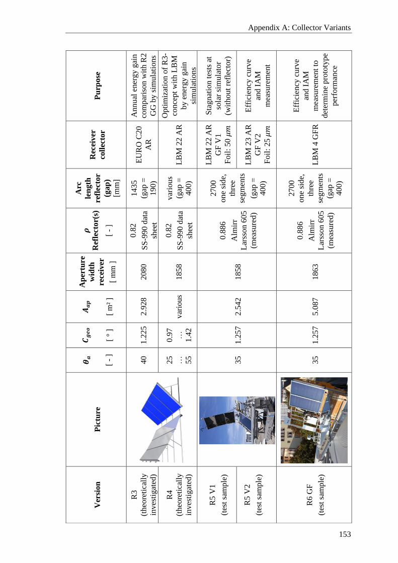
Appendix A: Collector Variants
153
Pu
rpose
Annual
ener
gy g
ain
com
par
ison w
ith R
2
GG
by s
imula
tions
Opti
miz
atio
n o
f R
3-
conce
pt
wit
h L
BM
by e
ner
gy g
ain
sim
ula
tions
Sta
gnat
ion t
ests
at
sola
r si
mula
tor
(wit
hout
refl
ecto
r)
Eff
icie
ncy
curv
e
and I
AM
mea
sure
men
t
Eff
icie
ncy
curv
e
and I
AM
mea
sure
men
t to
det
erm
ine
pro
toty
pe
per
form
ance
Rec
eiv
er
coll
ecto
r
EU
RO
C20
AR
LB
M 2
2 A
R
LB
M 2
2 A
R
GF
V1
Foil
: 50 𝜇
𝑚
LB
M 2
3 A
R
GF
V2
Foil
: 25 𝜇
𝑚
LB
M 4
GF
R
Arc
len
gth
refl
ect
or
(gap
)
[mm
]
1435
(gap
=
190)
var
ious
(gap
=
400)
2700
one
side,
thre
e
segm
ents
(gap
=
400)
2700
one
side,
thre
e
segm
ents
(gap
=
400)
𝝆
Ref
lecto
r(s)
[ -
]
0.8
2
SS
-990 d
ata
shee
t
0.8
2
SS
-990 d
ata
shee
t
0.8
86
Alm
irr
Lar
sson 6
05
(mea
sure
d)
0.8
86
Alm
irr
Lar
sson 6
05
(mea
sure
d)
Ap
ertu
re
wid
th
recei
ver
[ m
m ]
2080
1858
1858
1863
𝑨𝒂𝒑
[ m
² ]
2.9
28
var
ious
2.5
42
5.0
87
𝑪𝒈𝒆𝒐
[ °
]
1.2
25
0.9
7
…
1.4
2
1.2
57
1.2
57
𝜽𝒂
[ -
]
40
25
…
55
35
35
Pic
ture
Ver
sion
R3
(theo
reti
call
y
inves
tigat
ed)
R4
(theo
reti
call
y
inves
tigat
ed)
R5 V
1
(tes
t sa
mple
)
R5 V
2
(tes
t sa
mple
)
R6 G
F
(tes
t sa
mple
)
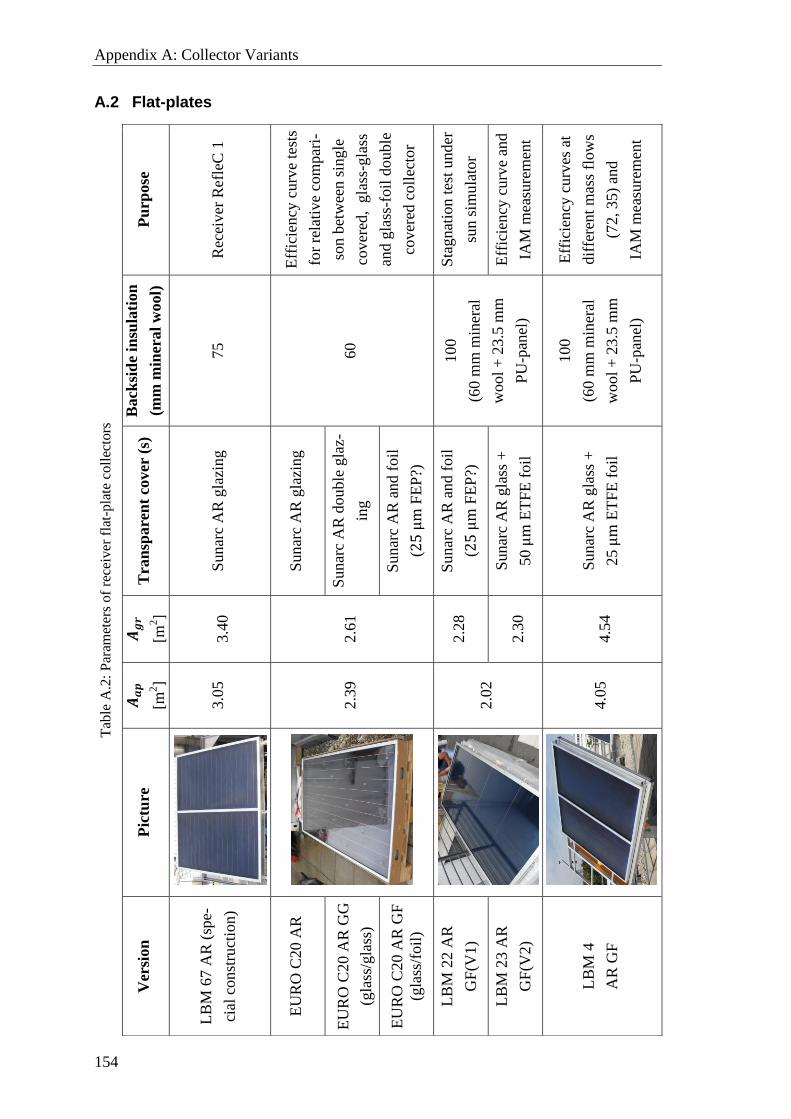
Appendix A: Collector Variants
154
A.2 Flat-plates T
able
A.2
: P
aram
eter
s of
rece
iver
fla
t-pla
te c
oll
ecto
rs
Pu
rpose
Rec
eiver
Ref
leC
1
Eff
icie
ncy
curv
e te
sts
for
rela
tive
com
par
i-
son b
etw
een s
ingle
cover
ed, g
lass
-gla
ss
and g
lass
-foil
double
cover
ed c
oll
ecto
r
Sta
gnat
ion t
est
under
sun s
imula
tor
Eff
icie
ncy
curv
e an
d
IAM
mea
sure
men
t
Eff
icie
ncy
curv
es a
t
dif
fere
nt
mas
s fl
ow
s
(72, 35)
and
IAM
mea
sure
men
t
Back
sid
e in
sula
tion
(mm
min
eral
wool)
75
60
100
(60 m
m m
iner
al
wool
+ 2
3.5
mm
PU
-pan
el)
100
(60 m
m m
iner
al
wool
+ 2
3.5
mm
PU
-pan
el)
Tra
nsp
are
nt
cover
(s)
Sunar
c A
R g
lazi
ng
Sunar
c A
R g
lazi
ng
Sunar
c A
R d
ouble
gla
z-
ing
Sunar
c A
R a
nd f
oil
(25 μ
m F
EP
?)
Sunar
c A
R a
nd f
oil
(25 μ
m F
EP
?)
Sunar
c A
R g
lass
+
50 μ
m E
TF
E f
oil
Sunar
c A
R g
lass
+
25 μ
m E
TF
E f
oil
𝑨𝒈𝒓
[m2]
3.4
0
2.6
1
2.2
8
2.3
0
4.5
4
𝑨𝒂𝒑
[m2]
3.0
5
2.3
9
2.0
2
4.0
5
Pic
ture
Ver
sion
LB
M 6
7 A
R (
spe-
cial
const
ruct
ion
)
EU
RO
C20
AR
EU
RO
C20 A
R G
G
(gla
ss/g
lass
)
EU
RO
C20 A
R G
F
(gla
ss/f
oil
)
LB
M 2
2 A
R
GF
(V1)
LB
M 2
3 A
R
GF
(V2)
LB
M 4
AR
GF
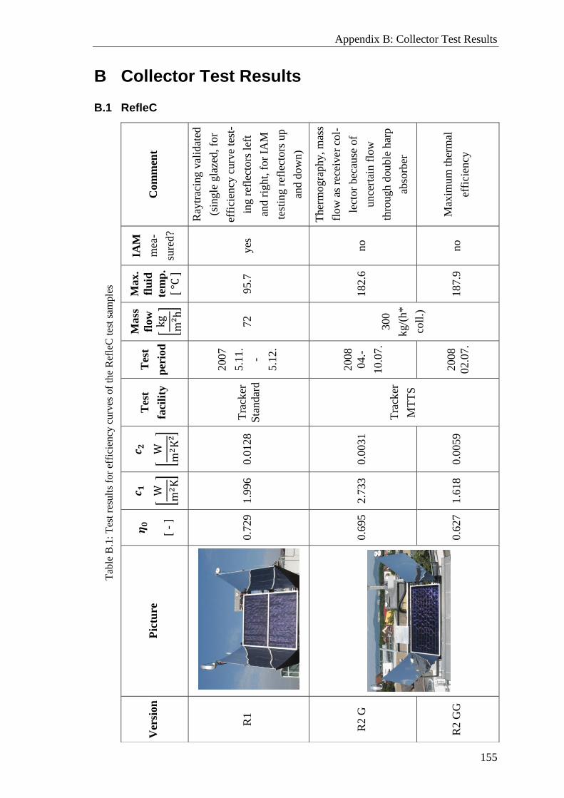
Appendix B: Collector Test Results
155
B Collector Test Results
B.1 RefleC T
able
B.1
: T
est
resu
lts
for
effi
cien
cy c
urv
es o
f th
e R
efle
C t
est
sam
ple
s
Com
men
t
Ray
trac
ing v
alid
ated
(sin
gle
gla
zed, fo
r
effi
cien
cy c
urv
e te
st-
ing
ref
lect
ors
lef
t
and r
ight,
for
IAM
test
ing r
efle
ctors
up
and d
ow
n)
Ther
mogra
phy
, m
ass
flow
as
rece
iver
col-
lect
or
bec
ause
of
unce
rtai
n f
low
thro
ugh d
ouble
har
p
abso
rber
Max
imum
ther
mal
effi
cien
cy
IAM
mea
-
sure
d?
yes
no
no
[ °C
]
Max.
flu
id
tem
p.
95.7
182.6
187.9
[kg
m²h
]
Mass
flow
72
300
kg/(
h*
coll
.)
Tes
t
per
iod
2007
5.1
1.
-
5.1
2.
2008
04.-
10.0
7.
2008
02.0
7.
Tes
t
faci
lity
Tra
cker
Sta
ndar
d
Tra
cker
MT
TS
𝒄𝟐
[W
m2K²]
0.0
128
0.0
031
0.0
059
𝒄𝟏
[W m2K]
1.9
96
2.7
33
1.6
18
𝜼𝟎
[ -
]
0.7
29
0.6
95
0.6
27
Pic
ture
Ver
sion
R1
R2 G
R2 G
G
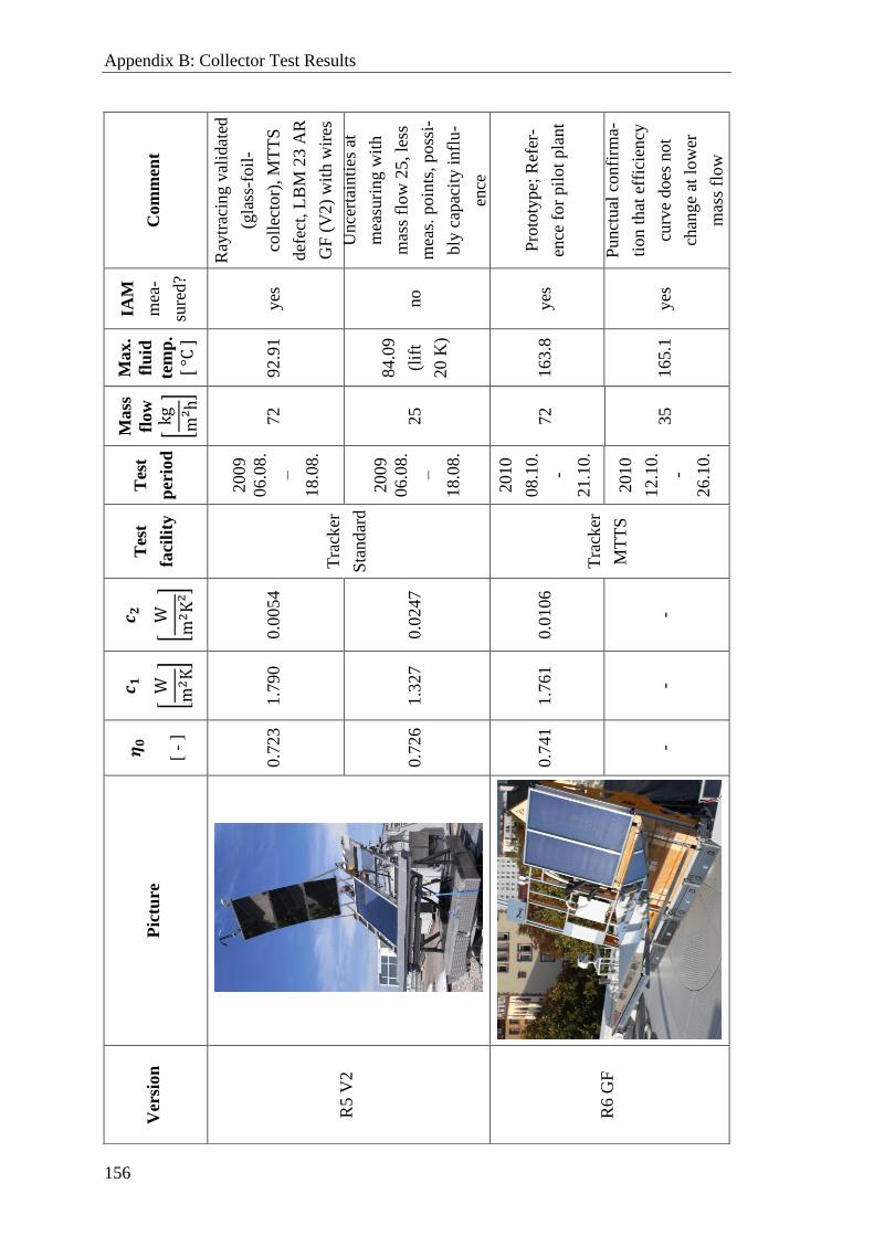
Appendix B: Collector Test Results
156
Com
men
t
Ray
trac
ing v
alid
ated
(gla
ss-f
oil
-
coll
ecto
r), M
TT
S
def
ect,
LB
M 2
3 A
R
GF
(V
2)
wit
h w
ires
Unce
rtai
nti
es a
t
mea
suri
ng w
ith
mas
s fl
ow
25, le
ss
mea
s. p
oin
ts,
poss
i-
bly
cap
acit
y i
nfl
u-
ence
Pro
toty
pe;
Ref
er-
ence
fo
r pil
ot
pla
nt
Punct
ual
confi
rma-
tion t
hat
eff
icie
ncy
curv
e does
not
chan
ge
at l
ow
er
mas
s fl
ow
IAM
mea
-
sure
d?
yes
no
yes
yes
[ °C
]
Max.
flu
id
tem
p.
92.9
1
84.0
9
(lif
t
20 K
)
163
.8
165.1
[kg
m²h
]
Mass
flow
72
25
72
35
Tes
t
per
iod
20
09
06
.08.
–
18
.08.
20
09
06
.08.
–
18
.08.
20
10
08
.10.
-
21
.10.
20
10
12
.10.
-
26
.10.
Tes
t
faci
lity
Tra
cker
Sta
ndar
d
Tra
cker
MT
TS
𝒄𝟐
[W
m2K²]
0.0
054
0.0
247
0.0
106
-
𝒄𝟏
[W m2K]
1.7
90
1.3
27
1.7
61
-
𝜼𝟎
[ -
]
0.7
23
0.7
26
0.7
41
-
Pic
ture
Ver
sion
R5 V
2
R6 G
F
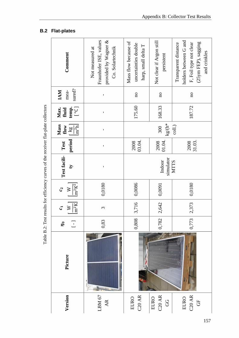
Appendix B: Collector Test Results
157
B.2 Flat-plates
Tab
le B
.2:
Tes
t re
sult
s fo
r ef
fici
ency
curv
es o
f th
e re
ceiv
er f
lat-
pla
te c
oll
ecto
rs
Com
men
t
Not
mea
sure
d a
t
Fra
unhofe
r IS
E, val
ues
pro
vid
ed b
y W
agn
er &
Co. S
ola
rtec
hnik
Mas
s fl
ow
bec
ause
of
unce
rtai
nti
es d
ouble
har
p, sm
all
del
ta T
Not
clea
r if
Arg
on s
till
per
sist
ent
Tra
nsp
aren
t dis
tance
hold
ers
bet
wee
n G
and
F, F
oil
type
not
clea
r
(25ym
FE
P),
sag
gin
g
and c
rinkle
s
IAM
mea
-
sure
d?
- no
no
no
[ °C ]
Max.
flu
id
tem
p.
-
175.6
0
168.3
3
187.7
2
[kg
m²h
]
Mass
flow
-
300
kg
/(h*
coll
.)
Tes
t
per
iod
-
2008
03.0
4.
2008
01.0
4.
2008
31.0
3.
Tes
t fa
cili
-
ty
-
Indoor
sim
ula
tor
MT
TS
𝒄𝟐
[W
m2K²]
0,0
180
0,0
086
0,0
091
0,0
180
𝒄𝟏
[W m2K]
3
3,7
16
2,6
42
2,3
73
𝜼𝟎
[ -
]
0,8
3
0,8
08
0,7
82
0,7
73
Pic
ture
Ver
sion
LB
M 6
7
AR
EU
RO
C20 A
R
EU
RO
C20 A
R
GG
EU
RO
C20 A
R
GF
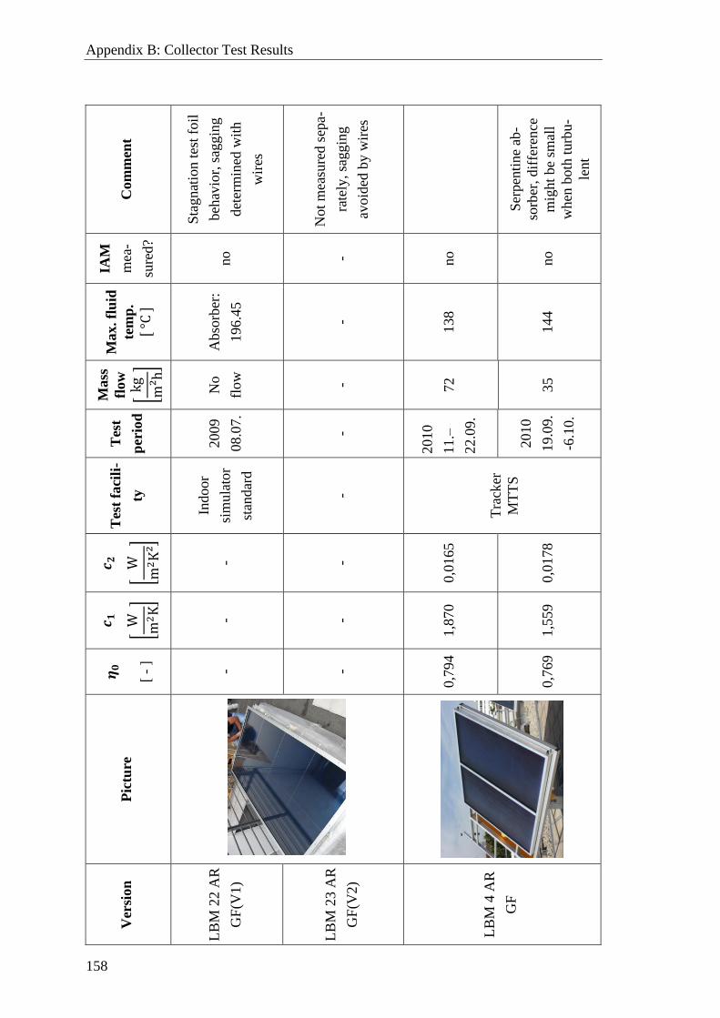
Appendix B: Collector Test Results
158
Com
men
t
Sta
gnat
ion t
est
foil
beh
avio
r, s
aggin
g
det
erm
ined
wit
h
wir
es
Not
mea
sure
d s
epa-
rate
ly, sa
ggin
g
avoid
ed b
y w
ires
Ser
pen
tine
ab-
sorb
er, dif
fere
nce
mig
ht
be
smal
l
when
both
turb
u-
lent
IAM
mea
-
sure
d?
no
- no
no
[ °C
]
Max. fl
uid
tem
p.
Abso
rber
:
196.4
5
-
138
144
[kg
m²h
]
Mass
flow
No
flow
- 72
35
Tes
t
per
iod
2009
08.0
7.
-
2010
11.–
22.0
9.
2010
19.0
9.
-6.1
0.
Tes
t fa
cili
-
ty
Indoor
sim
ula
tor
stan
dar
d
-
Tra
cker
MT
TS
𝒄𝟐
[W
m2K²]
- -
0,0
165
0,0
178
𝒄𝟏
[W m2K]
- -
1,8
70
1,5
59
𝜼𝟎
[ -
]
- -
0,7
94
0,7
69
Pic
ture
Ver
sion
LB
M 2
2 A
R
GF
(V1)
LB
M 2
3 A
R
GF
(V2)
LB
M 4
AR
GF
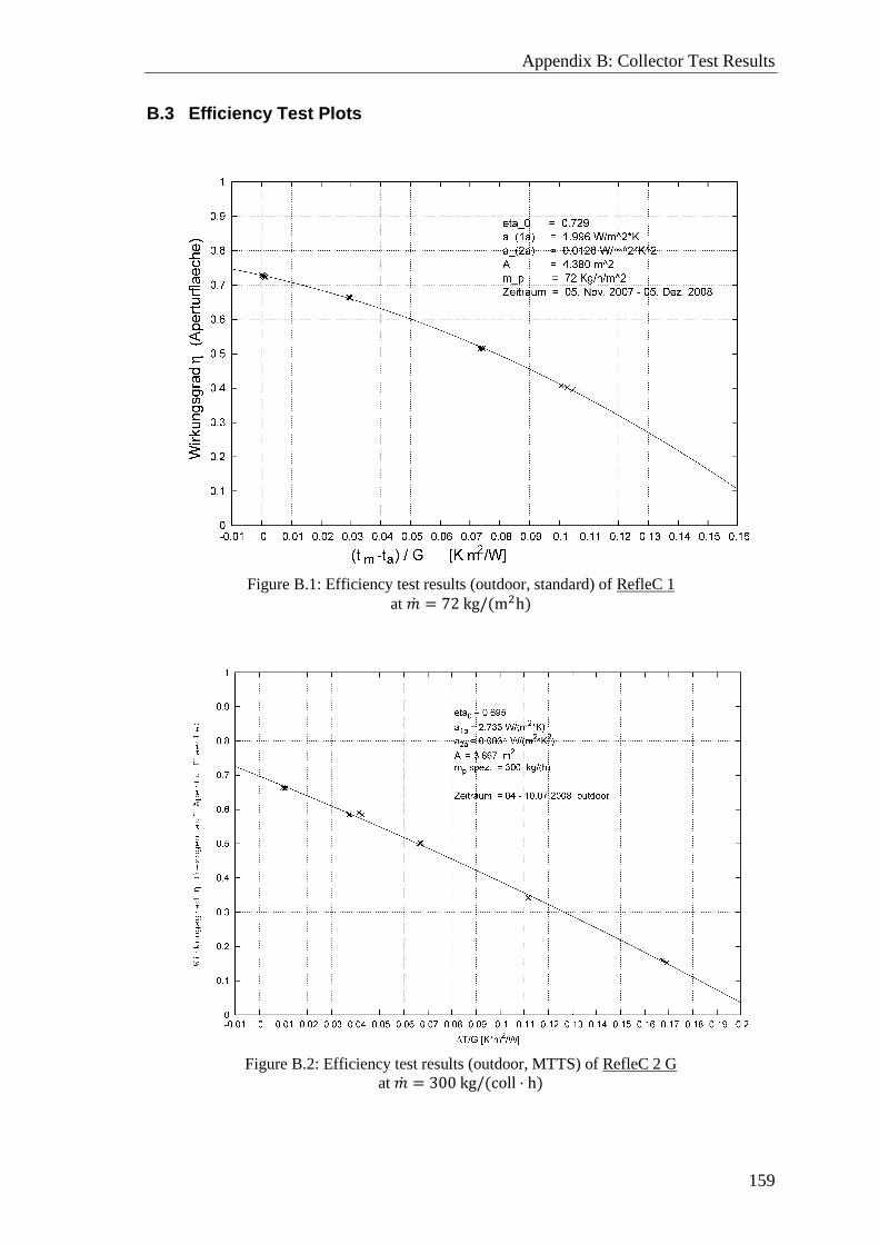
Appendix B: Collector Test Results
159
B.3 Efficiency Test Plots
Figure B.1: Efficiency test results (outdoor, standard) of RefleC 1
at �̇� = 72 kg/(m2h)
Figure B.2: Efficiency test results (outdoor, MTTS) of RefleC 2 G
at �̇� = 300 kg/(coll ⋅ h)
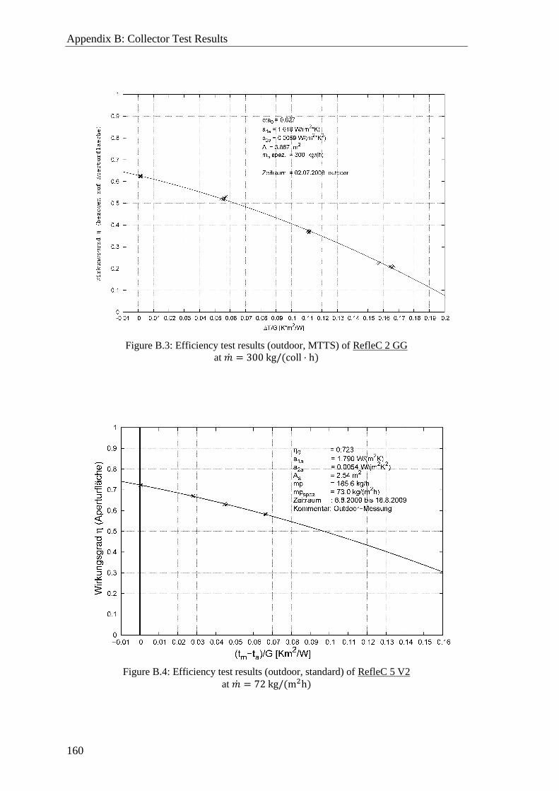
Appendix B: Collector Test Results
160
Figure B.3: Efficiency test results (outdoor, MTTS) of RefleC 2 GG
at �̇� = 300 kg/(coll ⋅ h)
Figure B.4: Efficiency test results (outdoor, standard) of RefleC 5 V2
at �̇� = 72 kg/(m2h)
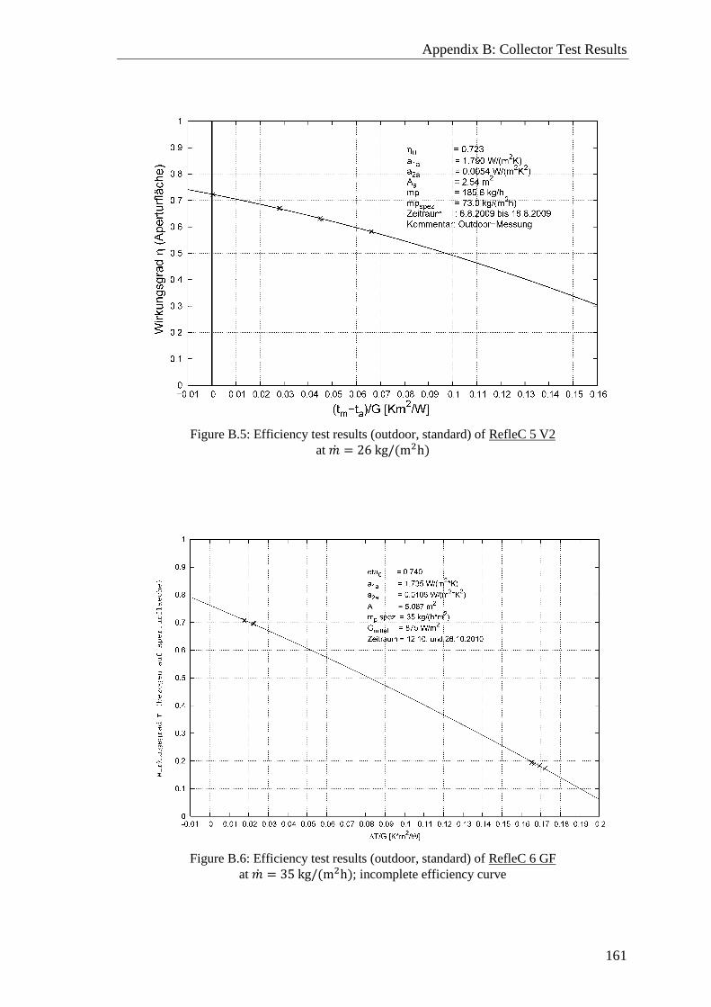
Appendix B: Collector Test Results
161
Figure B.5: Efficiency test results (outdoor, standard) of RefleC 5 V2
at �̇� = 26 kg/(m2h)
Figure B.6: Efficiency test results (outdoor, standard) of RefleC 6 GF
at �̇� = 35 kg/(m2h); incomplete efficiency curve
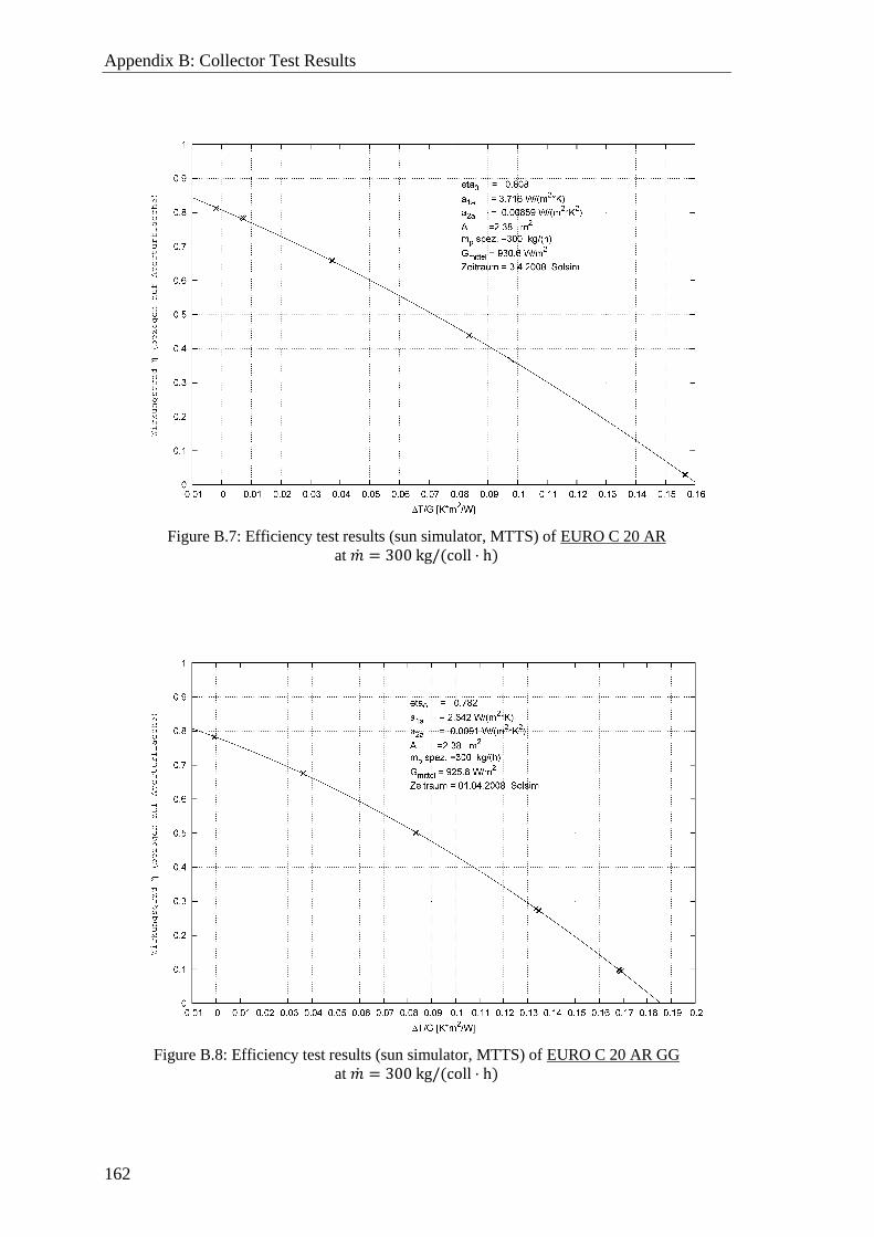
Appendix B: Collector Test Results
162
Figure B.7: Efficiency test results (sun simulator, MTTS) of EURO C 20 AR
at �̇� = 300 kg/(coll ⋅ h)
Figure B.8: Efficiency test results (sun simulator, MTTS) of EURO C 20 AR GG
at �̇� = 300 kg/(coll ⋅ h)
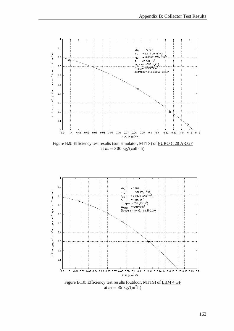
Appendix B: Collector Test Results
163
Figure B.9: Efficiency test results (sun simulator, MTTS) of EURO C 20 AR GF
at �̇� = 300 kg/(coll ⋅ h)
Figure B.10: Efficiency test results (outdoor, MTTS) of LBM 4 GF
at �̇� = 35 kg/(m2h)
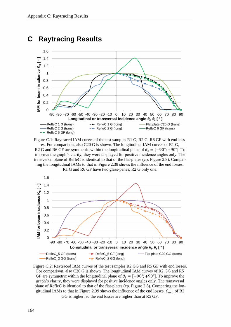
Appendix C: Raytracing Results
164
C Raytracing Results
Figure C.1: Raytraced IAM curves of the test samples R1 G, R2 G, R6 GF with end loss-
es. For comparison, also C20 G is shown. The longitudinal IAM curves of R1 G,
R2 G and R6 GF are symmetric within the longitudinal plane of 𝜃𝑡 = [−90°;+90°]. To
improve the graph’s clarity, they were displayed for positive incidence angles only. The
transversal plane of RefleC is identical to that of the flat-plates (cp. Figure 2.8). Compar-
ing the longitudinal IAMs to that in Figure 2.38 shows the influence of the end losses.
R1 G and R6 GF have two glass-panes, R2 G only one.
Figure C.2: Raytraced IAM curves of the test samples R2 GG and R5 GF with end losses.
For comparison, also C20 G is shown. The longitudinal IAM curves of R2 GG and R5
GF are symmetric within the longitudinal plane of 𝜃𝑡 = [−90°;+90°]. To improve the
graph’s clarity, they were displayed for positive incidence angles only. The transversal
plane of RefleC is identical to that of the flat-plates (cp. Figure 2.8). Comparing the lon-
gitudinal IAMs to that in Figure 2.39 shows the influence of the end losses. 𝐶𝑔𝑒𝑜 of R2
GG is higher, so the end losses are higher than at R5 GF.
0
0.2
0.4
0.6
0.8
1
1.2
1.4
1.6
-90 -80 -70 -60 -50 -40 -30 -20 -10 0 10 20 30 40 50 60 70 80 90
IAM
fo
r b
ea
m i
rra
dia
nc
e K
b[
-]
Longitudinal or transversal incidence angle θl, θt [ ° ]
RefleC 1 G (trans) RefleC 1 G (long) Flat plate C20 G (trans)
RefleC 2 G (trans) RefleC 2 G (long) RefleC 6 GF (trans)
RefleC 6 GF (long)
0
0.2
0.4
0.6
0.8
1
1.2
1.4
1.6
-90 -80 -70 -60 -50 -40 -30 -20 -10 0 10 20 30 40 50 60 70 80 90
IAM
fo
r b
ea
m i
rra
dia
nc
e K
b[
-]
Longitudinal or transversal incidence angle θl, θt [ ° ]
RefleC_5 GF (trans) RefleC_5 GF (long) Flat plate C20 GG (trans)
RefleC_2 GG (trans) RefleC_2 GG (long)
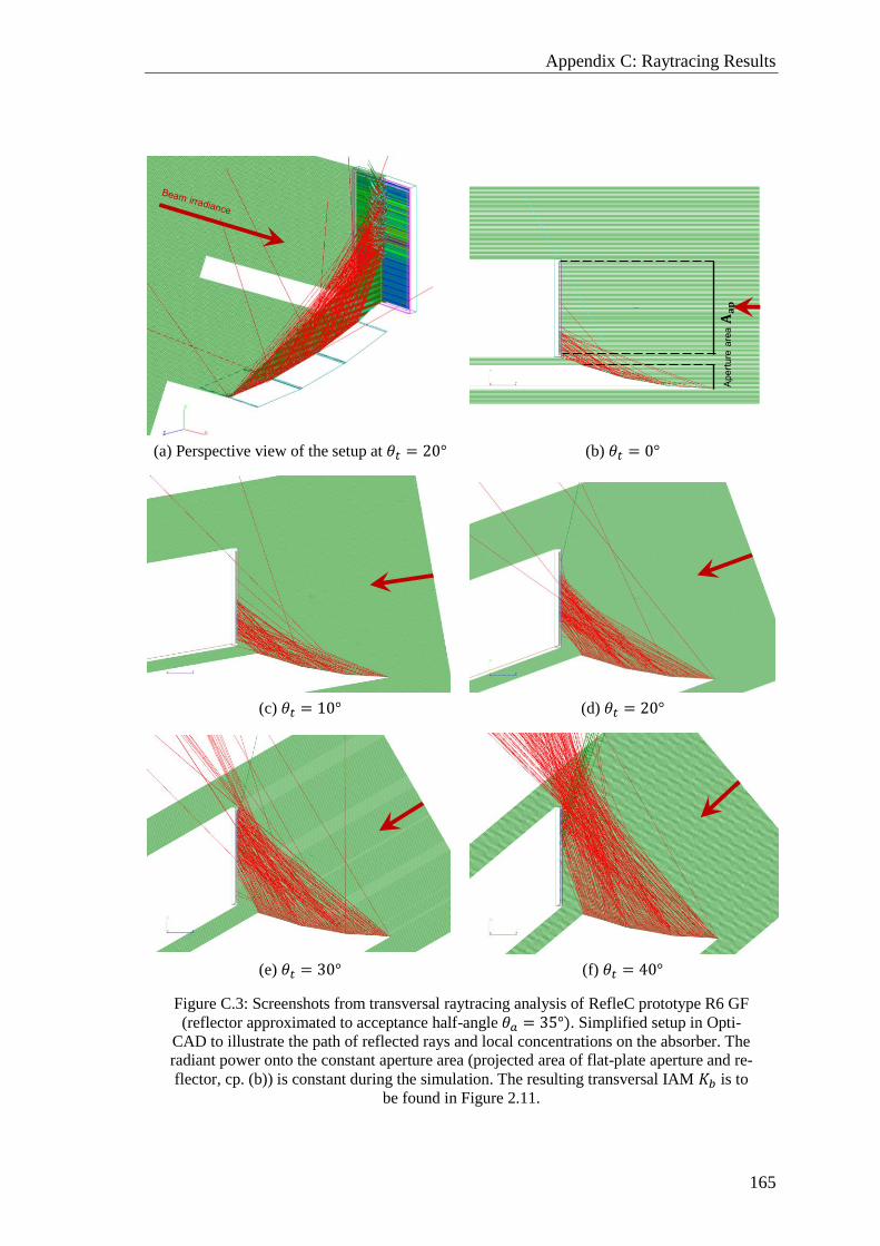
Appendix C: Raytracing Results
165
(a) Perspective view of the setup at 𝜃𝑡 = 20° (b) 𝜃𝑡 = 0°
(c) 𝜃𝑡 = 10° (d) 𝜃𝑡 = 20°
(e) 𝜃𝑡 = 30° (f) 𝜃𝑡 = 40°
Figure C.3: Screenshots from transversal raytracing analysis of RefleC prototype R6 GF
(reflector approximated to acceptance half-angle 𝜃𝑎 = 35°). Simplified setup in Opti-
CAD to illustrate the path of reflected rays and local concentrations on the absorber. The
radiant power onto the constant aperture area (projected area of flat-plate aperture and re-
flector, cp. (b)) is constant during the simulation. The resulting transversal IAM 𝐾𝑏 is to
be found in Figure 2.11.
Aper
ture
area
𝐀𝐚𝐩
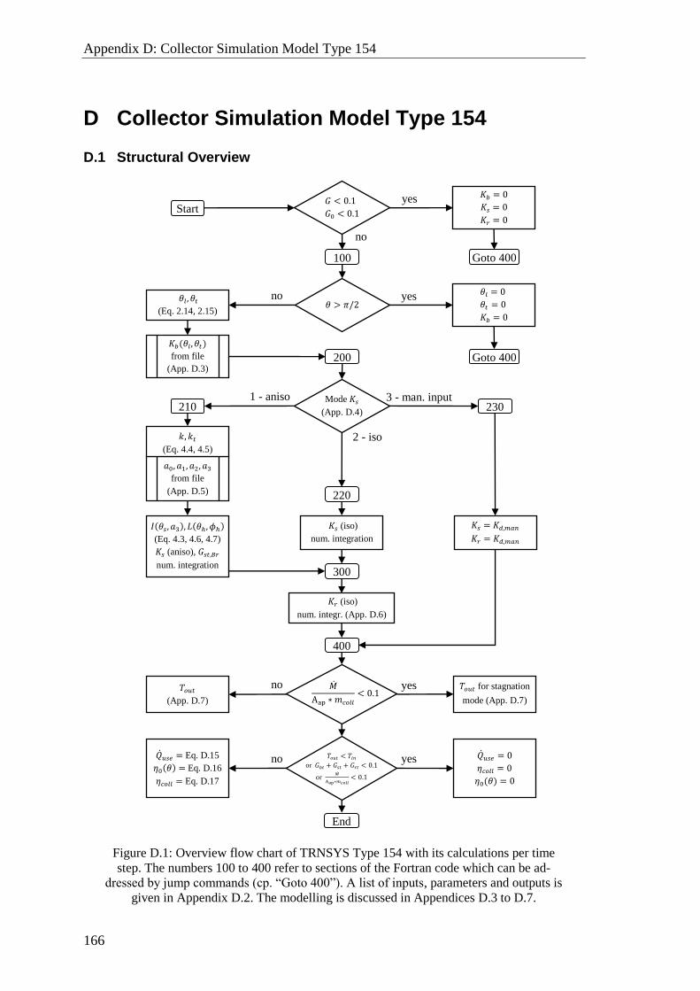
Appendix D: Collector Simulation Model Type 154
166
D Collector Simulation Model Type 154
D.1 Structural Overview
Figure D.1: Overview flow chart of TRNSYS Type 154 with its calculations per time
step. The numbers 100 to 400 refer to sections of the Fortran code which can be ad-
dressed by jump commands (cp. “Goto 400”). A list of inputs, parameters and outputs is
given in Appendix D.2. The modelling is discussed in Appendices D.3 to D.7.
yes 𝐾𝑏 = 0
𝐾𝑠 = 0
𝐾𝑟 = 0 Start
𝐺 < 0.1
𝐺0 < 0.1
Goto 400
𝜃 > 𝜋/2 yes 𝜃𝑙 = 0
𝜃𝑡 = 0
𝐾𝑏 = 0
100
no
no
𝐾𝑏(𝜃𝑙,𝜃𝑡)
from file
(App. D.3)
𝜃𝑙,𝜃𝑡
(Eq. 2.14, 2.15)
Mode 𝐾𝑠 (App. D.4)
3 - man. input
200
1 - aniso
220
210 230
2 - iso
𝑎0,𝑎1,𝑎2,𝑎3
from file
(App. D.5)
𝐼(𝜃𝑠,𝑎3),𝐿(𝜃ℎ,𝜙ℎ)
(Eq. 4.3, 4.6, 4.7)
𝐾𝑠 (aniso), 𝐺𝑠𝑡,𝐵𝑟
num. integration
𝐾𝑠 (iso)
num. integration
𝐾𝑠 = 𝐾𝑑,𝑚𝑎𝑛
𝐾𝑟 = 𝐾𝑑,𝑚𝑎𝑛
300
𝐾𝑟 (iso)
num. integr. (App. D.6)
400
𝑇𝑜𝑢𝑡
(App. D.7)
yes no 𝑇𝑜𝑢𝑡 for stagnation
mode (App. D.7)
�̇�
Aap ∗𝑚𝑐𝑜𝑙𝑙
< 0.1
𝑇𝑜𝑢𝑡 < 𝑇𝑖𝑛
or 𝐺𝑏𝑡 + 𝐺𝑠𝑡 + 𝐺𝑟𝑡 < 0.1
or �̇�
Aap∗𝑚𝑐𝑜𝑙𝑙< 0.1
�̇�𝑢𝑠𝑒 = Eq. D.15
𝜂0(𝜃) = Eq. D.16
𝜂𝑐𝑜𝑙𝑙 = Eq. D.17
no �̇�𝑢𝑠𝑒 = 0
𝜂𝑐𝑜𝑙𝑙 = 0
𝜂0(𝜃) = 0
End
yes
Goto 400
𝑘, 𝑘𝑡
(Eq. 4.4, 4.5)
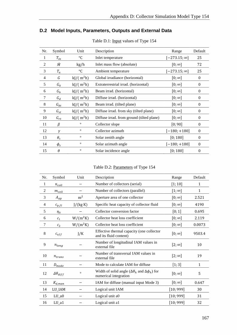
Appendix D: Collector Simulation Model Type 154
167
D.2 Model Inputs, Parameters, Outputs and External Data
Table D.1: Input values of Type 154
Nr. Symbol Unit Description Range Default
1 𝑇𝑖𝑛 °C Inlet temperature [−273.15;∞] 25
2 �̇� kg/h Inlet mass flow (absolute) [0;∞] 72
3 𝑇𝑎 °C Ambient temperature [−273.15;∞] 25
4 𝐺 kJ/( m2h) Global irradiance (horizontal) [0;∞] 0
5 𝐺0 kJ/( m2h) Extraterrestrial irrad. (horizontal) [0;∞] 0
6 𝐺𝑏 kJ/( m2h) Beam irrad. (horizontal) [0;∞] 0
7 𝐺𝑑 kJ/( m2h) Diffuse irrad. (horizontal) [0;∞] 0
8 𝐺𝑏𝑡 kJ/( m2h) Beam irrad. (tilted plane) [0;∞] 0
9 𝐺𝑠𝑡 kJ/( m2h) Diffuse irrad. from sky (tilted plane) [0;∞] 0
10 𝐺𝑟𝑡 kJ/( m2h) Diffuse irrad. from ground (tilted plane) [0;∞] 0
11 𝛽 ° Collector slope [0; 90] 0
12 𝛾 ° Collector azimuth [−180;+180] 0
13 𝜃𝑠 ° Solar zenith angle [0; 180] 0
14 𝜙𝑠 ° Solar azimuth angle [−180;+180] 0
15 𝜃 ° Solar incidence angle [0; 180] 0
Table D.2: Parameters of Type 154
Nr. Symbol Unit Description Range Default
1 𝑛𝑐𝑜𝑙𝑙 − Number of collectors (serial) [1; 10] 1
2 𝑚𝑐𝑜𝑙𝑙 − Number of collectors (parallel) [1;∞] 1
3 𝐴𝑎𝑝 m2 Aperture area of one collector [0;∞] 2.521
4 𝑐𝑝,𝑓𝑙 J/(kg K) Specific heat capacity of collector fluid [0;∞] 4190
5 𝜂0 − Collector conversion factor [0; 1] 0.695
6 𝑐1 W/(m2K) Collector heat loss coefficient [0;∞] 2.119
7 𝑐2 W/(m2K) Collector heat loss coefficient [0;∞] 0.0073
8 𝑐𝑒𝑓𝑓 J/K Effective thermal capacity (one collector
and its fluid content) [0;∞] 9503.4
9 𝑛𝑙𝑜𝑛𝑔 − Number of longitudinal IAM values in
external file [2;∞] 10
10 𝑛𝑡𝑟𝑎𝑛𝑠 − Number of transversal IAM values in
external file [2;∞] 19
11 𝐷𝑚𝑜𝑑𝑒 − Mode to calculate IAM for diffuse [1; 3] 1
12 𝛥𝜃𝑑𝑖𝑓𝑓 ° Width of solid angle (Δ𝜃ℎ and Δ𝜙ℎ) for
numerical integration [0;∞] 5
13 𝐾𝑑,𝑚𝑎𝑛 − IAM for diffuse (manual input Mode 3) [0;∞] 0.647
14 LU_IAM − Logical unit IAM [10; 999] 30
15 LU_a0 − Logical unit a0 [10; 999] 31
16 LU_a1 − Logical unit a1 [10; 999] 32
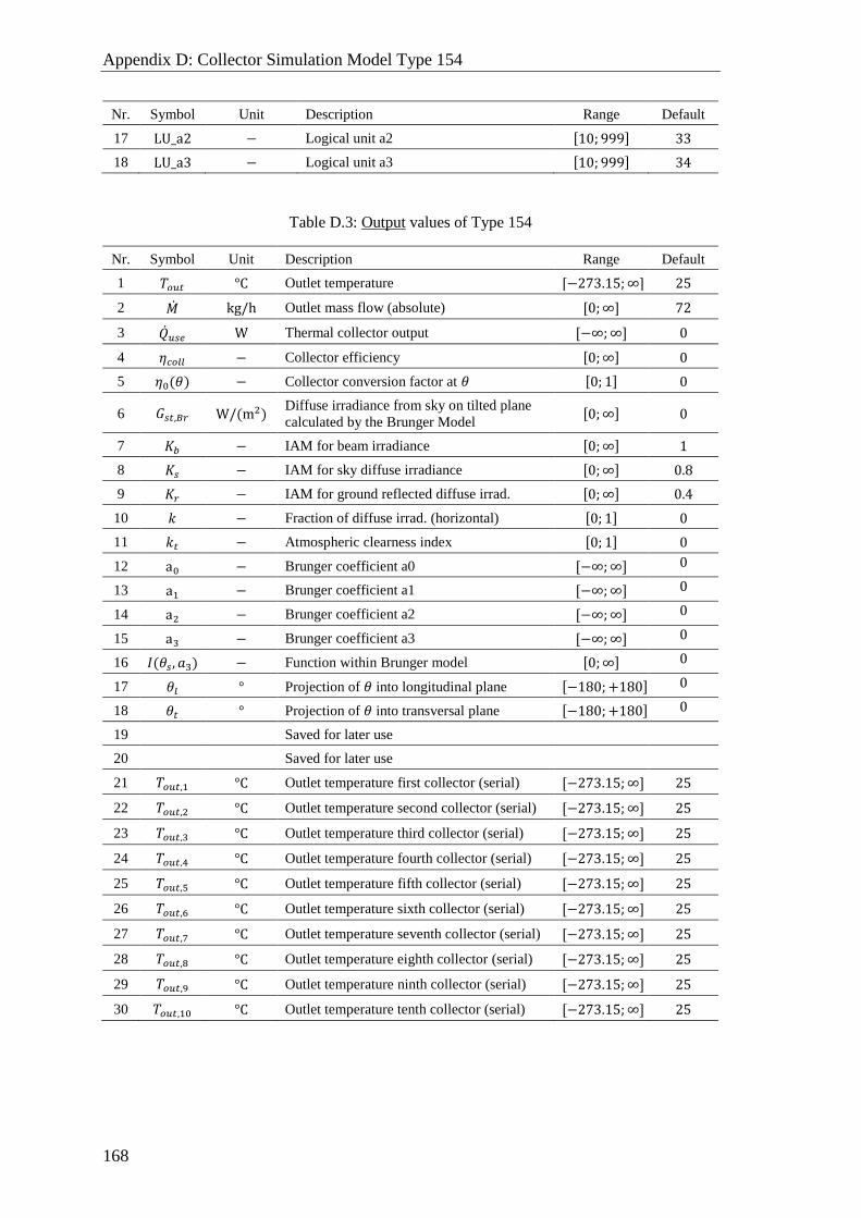
Appendix D: Collector Simulation Model Type 154
168
Nr. Symbol Unit Description Range Default
17 LU_a2 − Logical unit a2 [10; 999] 33
18 LU_a3 − Logical unit a3 [10; 999] 34
Table D.3: Output values of Type 154
Nr. Symbol Unit Description Range Default
1 𝑇𝑜𝑢𝑡 °C Outlet temperature [−273.15;∞] 25
2 �̇� kg/h Outlet mass flow (absolute) [0;∞] 72
3 �̇�𝑢𝑠𝑒 W Thermal collector output [−∞;∞] 0
4 𝜂𝑐𝑜𝑙𝑙 − Collector efficiency [0;∞] 0
5 𝜂0(𝜃) − Collector conversion factor at 𝜃 [0; 1] 0
6 𝐺𝑠𝑡,𝐵𝑟 W/(m2) Diffuse irradiance from sky on tilted plane
calculated by the Brunger Model [0;∞] 0
7 𝐾𝑏 − IAM for beam irradiance [0;∞] 1
8 𝐾𝑠 − IAM for sky diffuse irradiance [0;∞] 0.8
9 𝐾𝑟 − IAM for ground reflected diffuse irrad. [0;∞] 0.4
10 𝑘 − Fraction of diffuse irrad. (horizontal) [0; 1] 0
11 𝑘𝑡 − Atmospheric clearness index [0; 1] 0
12 a0 − Brunger coefficient a0 [−∞;∞] 0
13 a1 − Brunger coefficient a1 [−∞;∞] 0
14 a2 − Brunger coefficient a2 [−∞;∞] 0
15 a3 − Brunger coefficient a3 [−∞;∞] 0
16 𝐼(𝜃𝑠, 𝑎3) − Function within Brunger model [0;∞] 0
17 𝜃𝑙 ° Projection of 𝜃 into longitudinal plane [−180;+180] 0
18 𝜃𝑡 ° Projection of 𝜃 into transversal plane [−180;+180] 0
19 Saved for later use
20 Saved for later use
21 𝑇𝑜𝑢𝑡,1 °C Outlet temperature first collector (serial) [−273.15;∞] 25
22 𝑇𝑜𝑢𝑡,2 °C Outlet temperature second collector (serial) [−273.15;∞] 25
23 𝑇𝑜𝑢𝑡,3 °C Outlet temperature third collector (serial) [−273.15;∞] 25
24 𝑇𝑜𝑢𝑡,4 °C Outlet temperature fourth collector (serial) [−273.15;∞] 25
25 𝑇𝑜𝑢𝑡,5 °C Outlet temperature fifth collector (serial) [−273.15;∞] 25
26 𝑇𝑜𝑢𝑡,6 °C Outlet temperature sixth collector (serial) [−273.15;∞] 25
27 𝑇𝑜𝑢𝑡,7 °C Outlet temperature seventh collector (serial) [−273.15;∞] 25
28 𝑇𝑜𝑢𝑡,8 °C Outlet temperature eighth collector (serial) [−273.15;∞] 25
29 𝑇𝑜𝑢𝑡,9 °C Outlet temperature ninth collector (serial) [−273.15;∞] 25
30 𝑇𝑜𝑢𝑡,10 °C Outlet temperature tenth collector (serial) [−273.15;∞] 25

Appendix D: Collector Simulation Model Type 154
169
Table D.4: External links of Type 154
Nr. Description Default
1 Which file contains the values of IAM 𝐾𝑏? −
2 Which file contains a0? 𝑎0. 𝑑𝑎𝑡
3 Which file contains a1? 𝑎1. 𝑑𝑎𝑡
4 Which file contains a2? 𝑎2. 𝑑𝑎𝑡
5 Which file contains a3? 𝑎3. 𝑑𝑎𝑡

Appendix D: Collector Simulation Model Type 154
170
D.3 100 – IAM for beam irradiance 𝑲𝒃
Input file: The IAM values of an investigated collector are provided to Type 154 for
TRNSYS in a tab-spaced text file. This file must be named “filename.dat” and must
have the following structure:
-90 -80 -72.5 ... 90 !n_long longitudinal angle component of nodes
-90 -85 -80 ... 90 !n_trans transversal angle component of nodes
Value 1 !i_long = 1 (-90); i_trans = 1 (-90)
Value 2 !i_long = 1 (-90); i_trans = 2 (-85)
Value 3 !i_long = 1 (-90); i_trans = 2 (-72.5)
...
Value n_trans !i_long = 1 (-90); i_trans = n_trans (90)
Value n_trans+1 !i_long = 2 (-80); i_trans = 1 (-90)
...
Value n_trans*n_long !i_long = n_long (90); i_trans = n_trans (90)
The first two rows contain the incidence angles 𝜃𝑙 and 𝜃𝑡 for which nodes with IAM
values are contained in the file. Along both collector planes, values from [−90°;+90°]
have to be provided (regardless of the IAM type or shape, cp. section 3.2.2). They do
not have to be equidistant. The incidence angle conventions are shown in Figure 2.8 on
page 29. From the third row on, each row contains one node 𝐾𝑏(𝑖𝑙𝑜𝑛𝑔, 𝑖𝑡𝑟𝑎𝑛𝑠) for each
combination of the incidence angles listed in row one and two. Thus, the file allows for:
biaxial, asymmetric shapes of 𝐾𝑏
a three-dimensional grid of node values 𝐾𝑏(𝜃𝑙 , 𝜃𝑡) (3D-IAM)
For convenience, the IAM files should be generated within a spreadsheet and then saved
as .dat-file. Within the spreadsheet, the values of 𝐾𝑏(𝑖𝑙𝑜𝑛𝑔, 𝑖𝑡𝑟𝑎𝑛𝑠) can be determined in
two ways:
approximation by separation approach of McIntire (Eq. 3.15)
(if only values 𝐾𝑏(𝑖𝑙𝑜𝑛𝑔, 0) and 𝐾𝑏(0, 𝑖𝑡𝑟𝑎𝑛𝑠) are available)
use of exact 3D-IAM from raytracing
Realization in Type 154: In case there is solar irradiance onto the aperture
(𝐺0 > 0.1 W/m2 ⋀ 𝐺 > 0.1 W/m2) and the sun is visible for the collector at the same
time (𝜃 < 𝜋/2), 𝐾𝑏 is determined for the solar incidence angle components 𝜃𝑙 and 𝜃𝑡.
In TRNSYS, the programme DynamicData calls the file “filename.dat” and imports all
provided values 𝐾𝑏(𝑖𝑙𝑜𝑛𝑔, 𝑖𝑡𝑟𝑎𝑛𝑠) into an array. The searched value 𝐾𝑏(𝜃𝑙, 𝜃𝑡) is then
linearly interpolated between the four nearest available nodes 𝐾𝑏(𝑖𝑙𝑜𝑛𝑔, 𝑖𝑡𝑟𝑎𝑛𝑠). Dynam-
icData is explained in (Klein et al. 2012b, pp. 7-98 to 7-100).
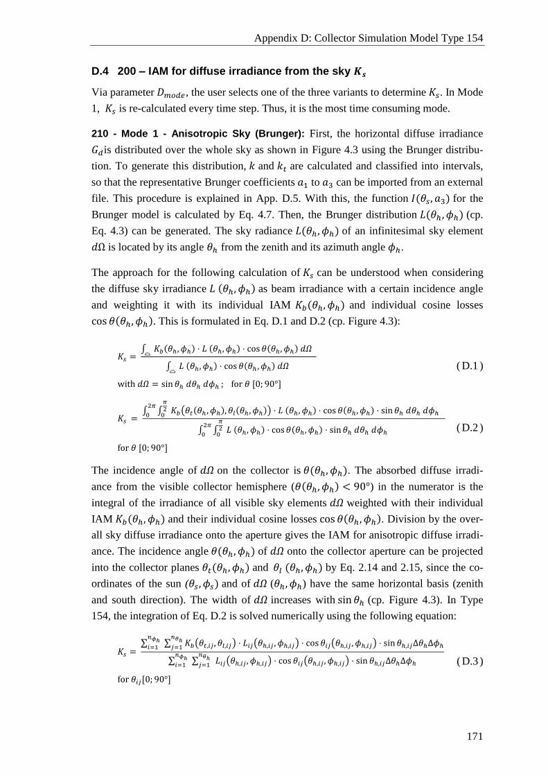
Appendix D: Collector Simulation Model Type 154
171
D.4 200 – IAM for diffuse irradiance from the sky 𝑲𝒔
Via parameter 𝐷𝑚𝑜𝑑𝑒, the user selects one of the three variants to determine 𝐾𝑠. In Mode
1, 𝐾𝑠 is re-calculated every time step. Thus, it is the most time consuming mode.
210 - Mode 1 - Anisotropic Sky (Brunger): First, the horizontal diffuse irradiance
𝐺𝑑is distributed over the whole sky as shown in Figure 4.3 using the Brunger distribu-
tion. To generate this distribution, 𝑘 and 𝑘𝑡 are calculated and classified into intervals,
so that the representative Brunger coefficients 𝑎1 to 𝑎3 can be imported from an external
file. This procedure is explained in App. D.5. With this, the function 𝐼(𝜃𝑠, 𝑎3) for the
Brunger model is calculated by Eq. 4.7. Then, the Brunger distribution 𝐿(𝜃ℎ , 𝜙ℎ) (cp.
Eq. 4.3) can be generated. The sky radiance 𝐿(𝜃ℎ , 𝜙ℎ) of an infinitesimal sky element
𝑑Ω is located by its angle 𝜃ℎ from the zenith and its azimuth angle 𝜙ℎ.
The approach for the following calculation of 𝐾𝑠 can be understood when considering
the diffuse sky irradiance 𝐿 (𝜃ℎ, 𝜙ℎ) as beam irradiance with a certain incidence angle
and weighting it with its individual IAM 𝐾𝑏(𝜃ℎ, 𝜙ℎ) and individual cosine losses
cos 𝜃(𝜃ℎ, 𝜙ℎ). This is formulated in Eq. D.1 and D.2 (cp. Figure 4.3):
𝐾𝑠 = ∫ 𝐾𝑏(𝜃ℎ , 𝜙ℎ) ⋅ 𝐿 (𝜃ℎ, 𝜙ℎ) ⋅ cos 𝜃(𝜃ℎ, 𝜙ℎ) 𝑑𝛺 ⌓
∫ 𝐿 (𝜃ℎ, 𝜙ℎ) ⋅ cos 𝜃(𝜃ℎ , 𝜙ℎ) 𝑑𝛺 ⌓
with 𝑑𝛺 = sin 𝜃ℎ 𝑑𝜃ℎ 𝑑𝜙ℎ ; for 𝜃 [0; 90°]
( D.1 )
𝐾𝑠 = ∫ ∫ 𝐾𝑏(𝜃𝑡(𝜃ℎ , 𝜙ℎ), 𝜃𝑙(𝜃ℎ, 𝜙ℎ)) ⋅ 𝐿 (𝜃ℎ, 𝜙ℎ) ⋅ cos 𝜃(𝜃ℎ, 𝜙ℎ) ⋅ sin 𝜃ℎ 𝑑𝜃ℎ 𝑑𝜙ℎ
𝜋20
2𝜋
0
∫ ∫ 𝐿 (𝜃ℎ, 𝜙ℎ) ⋅ cos 𝜃(𝜃ℎ, 𝜙ℎ) ⋅ sin 𝜃ℎ 𝑑𝜃ℎ 𝑑𝜙ℎ
𝜋20
2𝜋
0
for 𝜃 [0; 90°]
( D.2 )
The incidence angle of 𝑑𝛺 on the collector is 𝜃(𝜃ℎ, 𝜙ℎ). The absorbed diffuse irradi-
ance from the visible collector hemisphere (𝜃(𝜃ℎ, 𝜙ℎ) < 90°) in the numerator is the
integral of the irradiance of all visible sky elements 𝑑𝛺 weighted with their individual
IAM 𝐾𝑏(𝜃ℎ, 𝜙ℎ) and their individual cosine losses cos 𝜃(𝜃ℎ , 𝜙ℎ). Division by the over-
all sky diffuse irradiance onto the aperture gives the IAM for anisotropic diffuse irradi-
ance. The incidence angle 𝜃(𝜃ℎ , 𝜙ℎ) of 𝑑𝛺 onto the collector aperture can be projected
into the collector planes 𝜃𝑡(𝜃ℎ, 𝜙ℎ) and 𝜃𝑙 (𝜃ℎ, 𝜙ℎ) by Eq. 2.14 and 2.15, since the co-
ordinates of the sun (𝜃𝑠 , 𝜙𝑠) and of 𝑑𝛺 (𝜃ℎ , 𝜙ℎ) have the same horizontal basis (zenith
and south direction). The width of 𝑑𝛺 increases with sin 𝜃ℎ (cp. Figure 4.3). In Type
154, the integration of Eq. D.2 is solved numerically using the following equation:
𝐾𝑠 = ∑ ∑ 𝐾𝑏(𝜃𝑡,𝑖𝑗 , 𝜃𝑙,𝑖𝑗) ⋅ 𝐿𝑖𝑗(𝜃ℎ,𝑖𝑗 , 𝜙ℎ,𝑖𝑗) ⋅ cos 𝜃𝑖𝑗(𝜃ℎ,𝑖𝑗 , 𝜙ℎ,𝑖𝑗) ⋅ sin 𝜃ℎ,𝑖𝑗∆𝜃ℎ∆𝜙ℎ
𝑛𝜃ℎ
𝑗=1
𝑛𝜙ℎ
𝑖=1
∑ ∑ 𝐿𝑖𝑗(𝜃ℎ,𝑖𝑗 , 𝜙ℎ,𝑖𝑗) ⋅ cos 𝜃𝑖𝑗(𝜃ℎ,𝑖𝑗 , 𝜙ℎ,𝑖𝑗) ⋅ sin 𝜃ℎ,𝑖𝑗∆𝜃ℎ∆𝜙ℎ
𝑛𝜃ℎ
𝑗=1
𝑛𝜙ℎ
𝑖=1
for 𝜃𝑖𝑗[0; 90°]
( D.3 )
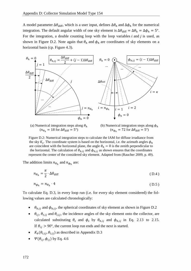
Appendix D: Collector Simulation Model Type 154
172
A model parameter ∆𝜃diff, which is a user input, defines ∆𝜃ℎ and ∆𝜙ℎ for the numerical
integration. The default angular width of one sky element is ∆𝜃diff = ∆𝜃ℎ = ∆𝜙ℎ = 5°.
For the integration, a double counting loop with the loop variables 𝑖 and 𝑗 is used, as
shown in Figure D.2. Note again that 𝜃ℎ and 𝜙ℎ are coordinates of sky elements on a
horizontal basis (cp. Figure 4.3).
(a) Numerical integration steps along 𝜃ℎ
(𝑛𝜃ℎ= 18 for ∆𝜃diff = 5°)
(b) Numerical integration steps along 𝜙ℎ
(𝑛𝜙ℎ= 72 for ∆𝜃diff = 5°)
Figure D.2: Numerical integration steps to calculate the IAM for diffuse irradiance from
the sky 𝐾𝑠. The coordinate system is based on the horizontal, i.e. the azimuth angles 𝜙ℎ
are coincident with the horizontal plane, the angle 𝜃ℎ = 0 is the zenith perpendicular to
the horizontal. The calculation of 𝜃ℎ,𝑖𝑗 and 𝜙ℎ,𝑖𝑗 as shown ensures that the coordinates
represent the center of the considered sky element. Adapted from (Raucher 2009, p. 49).
The addition limits 𝑛𝜃ℎ and 𝑛𝜙ℎ
are:
𝑛𝜃ℎ=
𝜋
2⋅ ∆𝜃diff ( D.4 )
𝑛𝜙ℎ= 𝑛𝜃ℎ
⋅ 4 ( D.5 )
To calculate Eq. D.3, in every loop run (i.e. for every sky element considered) the fol-
lowing values are calculated chronologically:
𝜃ℎ,𝑖𝑗 and 𝜙ℎ,𝑖𝑗, the spherical coordinates of sky element as shown in Figure D.2
𝜃𝑖𝑗, 𝜃𝑡,𝑖𝑗 and 𝜃𝑙,𝑖𝑗, the incidence angles of the sky element onto the collector, are
calculated substituting 𝜃𝑠 and 𝜙𝑠 by 𝜃ℎ,𝑖𝑗 and 𝜙ℎ,𝑖𝑗 in Eq. 2.13 to 2.15.
If 𝜃𝑖𝑗 > 90°, the current loop run ends and the next is started.
𝐾𝑏(𝜃𝑡,𝑖𝑗, 𝜃𝑙,𝑖𝑗) as described in Appendix D.3
𝛹(𝜃𝑖𝑗 , 𝜙𝑖𝑗) by Eq. 4.6
∆𝜃diff
2
∆𝜃diff
𝑗 = 1
𝜃ℎ = 0
𝑗
𝑗 = 𝑛𝜃ℎ
𝜃ℎ,𝑖𝑗 =∆𝜃diff
2+ (𝑗 − 1)∆𝜃diff
…
…
𝜙ℎ = 0
∆𝜃diff
𝑖 = 1
𝜃ℎ = 0
𝑖 = 𝜅
𝑖 = 𝑛𝜙ℎ
𝜙ℎ,𝑖𝑗 = (𝑖 − 1)∆𝜃diff
… …
𝜙ℎ = 0
…
𝑖 = 2
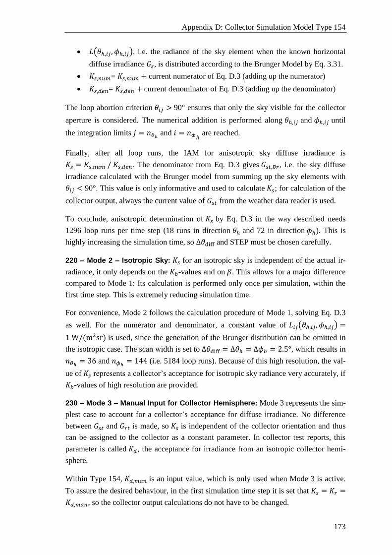
Appendix D: Collector Simulation Model Type 154
173
𝐿(𝜃ℎ,𝑖𝑗, 𝜙ℎ,𝑖𝑗), i.e. the radiance of the sky element when the known horizontal
diffuse irradiance 𝐺𝑠, is distributed according to the Brunger Model by Eq. 3.31.
𝐾𝑠,𝑛𝑢𝑚= 𝐾𝑠,𝑛𝑢𝑚 + current numerator of Eq. D.3 (adding up the numerator)
𝐾𝑠,𝑑𝑒𝑛= 𝐾𝑠,𝑑𝑒𝑛 + current denominator of Eq. D.3 (adding up the denominator)
The loop abortion criterion 𝜃𝑖𝑗 > 90° ensures that only the sky visible for the collector
aperture is considered. The numerical addition is performed along 𝜃ℎ,𝑖𝑗 and 𝜙ℎ,𝑖𝑗 until
the integration limits 𝑗 = 𝑛𝜃ℎ and 𝑖 = 𝑛𝜙ℎ
are reached.
Finally, after all loop runs, the IAM for anisotropic sky diffuse irradiance is
𝐾𝑠 = 𝐾𝑠,𝑛𝑢𝑚 / 𝐾𝑠,𝑑𝑒𝑛. The denominator from Eq. D.3 gives 𝐺𝑠𝑡,𝐵𝑟, i.e. the sky diffuse
irradiance calculated with the Brunger model from summing up the sky elements with
𝜃𝑖𝑗 < 90°. This value is only informative and used to calculate 𝐾𝑠; for calculation of the
collector output, always the current value of 𝐺𝑠𝑡 from the weather data reader is used.
To conclude, anisotropic determination of 𝐾𝑠 by Eq. D.3 in the way described needs
1296 loop runs per time step (18 runs in direction 𝜃ℎ and 72 in direction 𝜙ℎ). This is
highly increasing the simulation time, so ∆𝜃diff and STEP must be chosen carefully.
220 – Mode 2 – Isotropic Sky: 𝐾𝑠 for an isotropic sky is independent of the actual ir-
radiance, it only depends on the 𝐾𝑏-values and on 𝛽. This allows for a major difference
compared to Mode 1: Its calculation is performed only once per simulation, within the
first time step. This is extremely reducing simulation time.
For convenience, Mode 2 follows the calculation procedure of Mode 1, solving Eq. D.3
as well. For the numerator and denominator, a constant value of 𝐿𝑖𝑗(𝜃ℎ,𝑖𝑗, 𝜙ℎ,𝑖𝑗) =
1 W/(m2sr) is used, since the generation of the Brunger distribution can be omitted in
the isotropic case. The scan width is set to ∆𝜃diff = ∆𝜃ℎ = ∆𝜙ℎ = 2.5°, which results in
𝑛𝜃ℎ= 36 and 𝑛𝜙ℎ
= 144 (i.e. 5184 loop runs). Because of this high resolution, the val-
ue of 𝐾𝑠 represents a collector’s acceptance for isotropic sky radiance very accurately, if
𝐾𝑏-values of high resolution are provided.
230 – Mode 3 – Manual Input for Collector Hemisphere: Mode 3 represents the sim-
plest case to account for a collector’s acceptance for diffuse irradiance. No difference
between 𝐺𝑠𝑡 and 𝐺𝑟𝑡 is made, so 𝐾𝑠 is independent of the collector orientation and thus
can be assigned to the collector as a constant parameter. In collector test reports, this
parameter is called 𝐾𝑑, the acceptance for irradiance from an isotropic collector hemi-
sphere.
Within Type 154, 𝐾𝑑,𝑚𝑎𝑛 is an input value, which is only used when Mode 3 is active.
To assure the desired behaviour, in the first simulation time step it is set that 𝐾𝑠 = 𝐾𝑟 =
𝐾𝑑,𝑚𝑎𝑛, so the collector output calculations do not have to be changed.

Appendix D: Collector Simulation Model Type 154
174
D.5 Brunger Coefficients
Input files: For each of the Brunger coefficients 𝑎0, 𝑎1, 𝑎2 and 𝑎3, an individual input
file “a0.dat”, “a1.dat”, “a2.dat” and “a3.dat” must be placed in the same folder as the
simulated TRNSYS deck. These files contain the values of the Brunger coefficients
shown in Table 4.1 on page 103. The structure of the four files is identical to the exter-
nal IAM file. To give an example, “a1.dat” looks like this:
0.05 0.15 0.25 0.35 0.45 0.55 0.65 0.75 0.85 !k_t
0.15 0.25 0.35 0.45 0.55 0.65 0.75 0.85 0.95 !k
0.3360 !k_t = 0,05 k = 0,15
0.3417 !k_t = 0,05 k = 0,25
0.3162 !k_t = 0,05 k = 0,35
...
0.3162 !k_t = 0,45 k = 0,35
0.2822 !k_t = 0,45 k = 0,45
0.2816 !k_t = 0,45 k = 0,55
0.2713 !k_t = 0,45 k = 0,65
0.2019 !k_t = 0,45 k = 0,75
...
0.2060 !k_t = 0,85 k = 0,95
Brunger and Hooper provide 49 sets of coefficients. They are valid for all combinations
of 𝑘 and 𝑘𝑡 which occurred during model calibration (Brunger and Hooper 1993, p. 56).
It is ensured that the simulation does not stop in the potentially rare case a combination
should occur, for which no coefficients are provided. Therefore, to generate the coeffi-
cient input files, the Brunger table was completely filled (81 sets). This was done by
inserting the nearest available coefficient set in 𝑘𝑡-direction, when none was given (e.g.
the value 0.3360 in the third line above is originally given for 𝑘 = 0.15 and 𝑘𝑡 =0.65).
Realization in Type 154: To read the coefficients out of these files, the same proce-
dure as for reading the 𝐾𝑏-file (cp. section D.3) is used. Prior to that, the appropriate set
out of the 49 sets of coefficients is identified, i.e. the current 𝑘 and 𝑘𝑡 are classified into
the Brunger categories by Eq. D.6 and D.7. The result is e.g. 𝑘 = 0.45 ∶= [0.4; 0.5[. To
achieve this, a rounding down-function resulting in the next smaller integer-value is
used in the following classification functions:
𝑘 =⌊ 10 ⋅ 𝑘⌋ + 0.5
10 ( D.6 )
𝑘𝑡 =⌊ 10 ⋅ 𝑘𝑡⌋ + 0.5
10 ( D.7 )
This classification before reading avoids that DynamicData interpolates the values to be
selected.
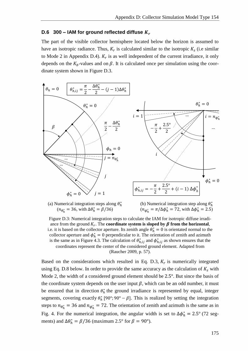
Appendix D: Collector Simulation Model Type 154
175
D.6 300 – IAM for ground reflected diffuse 𝑲𝒓
The part of the visible collector hemisphere located below the horizon is assumed to
have an isotropic radiance. Thus, 𝐾𝑟 is calculated similar to the isotropic 𝐾𝑠 (i.e similar
to Mode 2 in Appendix D.4). 𝐾𝑟 is as well independent of the current irradiance, it only
depends on the 𝐾𝑏-values and on 𝛽. It is calculated once per simulation using the coor-
dinate system shown in Figure D.3.
Figure D.3: Numerical integration steps to calculate the IAM for isotropic diffuse irradi-
ance from the ground 𝐾𝑟. The coordinate system is sloped by 𝜷 from the horizontal,
i.e. it is based on the collector aperture. Its zenith angle 𝜃ℎ∗ = 0 is orientated normal to the
collector aperture and 𝜙ℎ∗ = 0 perpendicular to it. The orientation of zenith and azimuth
is the same as in Figure 4.3. The calculation of 𝜃ℎ,𝑖𝑗∗ and 𝜙ℎ,𝑖𝑗
∗ as shown ensures that the
coordinates represent the center of the considered ground element. Adapted from
(Raucher 2009, p. 57).
Based on the considerations which resulted in Eq. D.3, 𝐾𝑟 is numerically integrated
using Eq. D.8 below. In order to provide the same accuracy as the calculation of 𝐾𝑠 with
Mode 2, the width of a considered ground element should be 2.5°. But since the basis of
the coordinate system depends on the user input 𝛽, which can be an odd number, it must
be ensured that in direction 𝜃ℎ∗ the ground irradiance is represented by equal, integer
segments, covering exactly 𝜃ℎ∗ [90°; 90° − 𝛽]. This is realized by setting the integration
steps to 𝑛𝜃ℎ∗ = 36 and 𝑛𝜙ℎ
∗ = 72. The orientation of zenith and azimuth is the same as in
Fig. 4. For the numerical integration, the angular width is set to ∆𝜙ℎ∗ = 2.5° (72 seg-
ments) and ∆𝜃ℎ∗ = 𝛽/36 (maximum 2.5° for 𝛽 = 90°).
(a) Numerical integration steps along 𝜃ℎ∗
(𝑛𝜃ℎ∗ = 36, with ∆𝜃ℎ
∗ = 𝛽/36)
(b) Numerical integration step along 𝜃ℎ∗
(𝑛𝜙ℎ∗ = 𝜋/∆𝜙ℎ
∗ = 72, with ∆𝜙ℎ∗ = 2.5)
𝛽
𝑗 = 1
𝜃ℎ∗ = 0
𝑗
𝑗 = 𝑛𝜃ℎ∗
𝜃ℎ,𝑖𝑗∗ =
𝜋
2−
∆𝜃ℎ∗
2− (𝑗 − 1)∆𝜃ℎ
∗
…
…
𝜙ℎ∗ = 0
𝜋
2−
∆𝜃ℎ∗
2
𝜃ℎ = 0
𝜙ℎ = 0
𝑖 = 1
𝜃ℎ∗ = 0
𝑖
𝑖 = 𝑛𝜙ℎ∗
−𝜋
2+
2.5°
2
…
𝜙ℎ∗ = 0
…
𝜙ℎ,𝑖𝑗∗ = −
𝜋
2+
2.5°
2+ (𝑖 − 1) ∆𝜙ℎ
∗
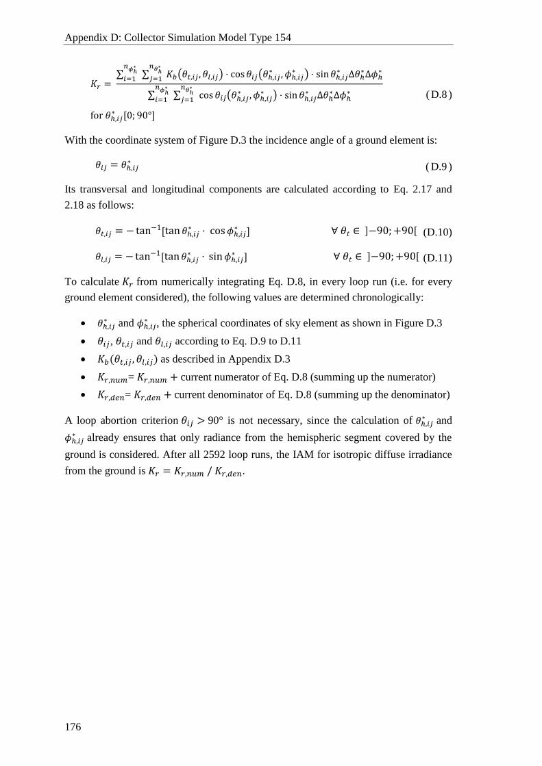
Appendix D: Collector Simulation Model Type 154
176
𝐾𝑟 = ∑ ∑ 𝐾𝑏(𝜃𝑡,𝑖𝑗, 𝜃𝑙,𝑖𝑗) ⋅ cos𝜃𝑖𝑗(𝜃ℎ,𝑖𝑗
∗ , 𝜙ℎ,𝑖𝑗∗ ) ⋅ sin𝜃ℎ,𝑖𝑗
∗ ∆𝜃ℎ∗∆𝜙ℎ
∗𝑛𝜃ℎ
∗
𝑗=1
𝑛𝜙ℎ∗
𝑖=1
∑ ∑ cos 𝜃𝑖𝑗(𝜃ℎ,𝑖𝑗∗ , 𝜙ℎ,𝑖𝑗
∗ ) ⋅ sin𝜃ℎ,𝑖𝑗∗ ∆𝜃ℎ
∗∆𝜙ℎ∗
𝑛𝜃ℎ∗
𝑗=1
𝑛𝜙ℎ∗
𝑖=1
for 𝜃ℎ,𝑖𝑗∗ [0; 90°]
( D.8 )
With the coordinate system of Figure D.3 the incidence angle of a ground element is:
𝜃𝑖𝑗 = 𝜃ℎ,𝑖𝑗∗ ( D.9 )
Its transversal and longitudinal components are calculated according to Eq. 2.17 and
2.18 as follows:
𝜃𝑡,𝑖𝑗 = −tan−1[tan𝜃ℎ,𝑖𝑗∗ ⋅ cos𝜙ℎ,𝑖𝑗
∗ ] ∀ 𝜃𝑡 ∈ ]−90;+90[ ( D.10 )
𝜃𝑙,𝑖𝑗 = −tan−1[tan𝜃ℎ,𝑖𝑗∗ ⋅ sin𝜙ℎ,𝑖𝑗
∗ ] ∀ 𝜃𝑡 ∈ ]−90;+90[ ( D.11 )
To calculate 𝐾𝑟 from numerically integrating Eq. D.8, in every loop run (i.e. for every
ground element considered), the following values are determined chronologically:
𝜃ℎ,𝑖𝑗∗ and 𝜙ℎ,𝑖𝑗
∗ , the spherical coordinates of sky element as shown in Figure D.3
𝜃𝑖𝑗, 𝜃𝑡,𝑖𝑗 and 𝜃𝑙,𝑖𝑗 according to Eq. D.9 to D.11
𝐾𝑏(𝜃𝑡,𝑖𝑗, 𝜃𝑙,𝑖𝑗) as described in Appendix D.3
𝐾𝑟,𝑛𝑢𝑚= 𝐾𝑟,𝑛𝑢𝑚 + current numerator of Eq. D.8 (summing up the numerator)
𝐾𝑟,𝑑𝑒𝑛= 𝐾𝑟,𝑑𝑒𝑛 + current denominator of Eq. D.8 (summing up the denominator)
A loop abortion criterion 𝜃𝑖𝑗 > 90° is not necessary, since the calculation of 𝜃ℎ,𝑖𝑗∗ and
𝜙ℎ,𝑖𝑗∗ already ensures that only radiance from the hemispheric segment covered by the
ground is considered. After all 2592 loop runs, the IAM for isotropic diffuse irradiance
from the ground is 𝐾𝑟 = 𝐾𝑟,𝑛𝑢𝑚 / 𝐾𝑟,𝑑𝑒𝑛.
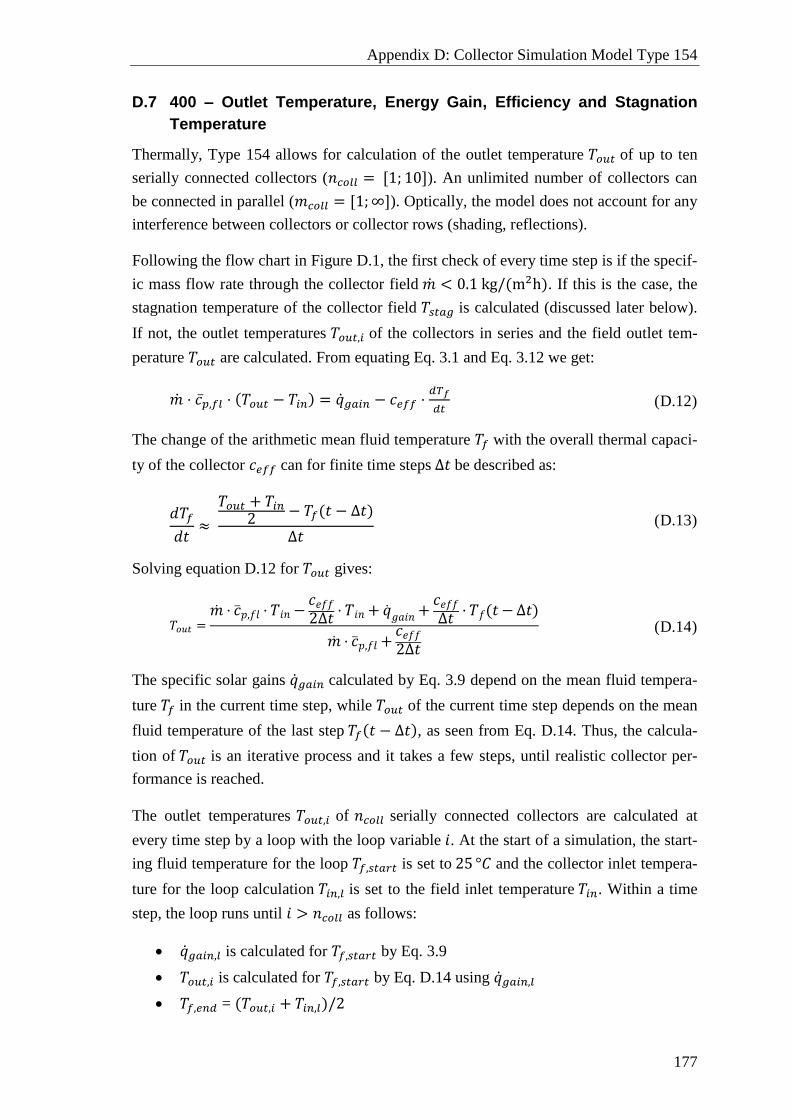
Appendix D: Collector Simulation Model Type 154
177
D.7 400 – Outlet Temperature, Energy Gain, Efficiency and Stagnation
Temperature
Thermally, Type 154 allows for calculation of the outlet temperature 𝑇𝑜𝑢𝑡 of up to ten
serially connected collectors (𝑛𝑐𝑜𝑙𝑙 = [1; 10]). An unlimited number of collectors can
be connected in parallel (𝑚𝑐𝑜𝑙𝑙 = [1;∞]). Optically, the model does not account for any
interference between collectors or collector rows (shading, reflections).
Following the flow chart in Figure D.1, the first check of every time step is if the specif-
ic mass flow rate through the collector field �̇� < 0.1 kg/(m2h). If this is the case, the
stagnation temperature of the collector field 𝑇𝑠𝑡𝑎𝑔 is calculated (discussed later below).
If not, the outlet temperatures 𝑇𝑜𝑢𝑡,𝑖 of the collectors in series and the field outlet tem-
perature 𝑇𝑜𝑢𝑡 are calculated. From equating Eq. 3.1 and Eq. 3.12 we get:
�̇� ⋅ 𝑐�̅�,𝑓𝑙 ⋅ (𝑇𝑜𝑢𝑡 − 𝑇𝑖𝑛) = �̇�𝑔𝑎𝑖𝑛 − 𝑐𝑒𝑓𝑓 ⋅𝑑𝑇𝑓
𝑑𝑡 ( D.12 )
The change of the arithmetic mean fluid temperature 𝑇𝑓 with the overall thermal capaci-
ty of the collector 𝑐𝑒𝑓𝑓 can for finite time steps ∆𝑡 be described as:
𝑑𝑇𝑓
𝑑𝑡≈
𝑇𝑜𝑢𝑡 + 𝑇𝑖𝑛
2 − 𝑇𝑓(𝑡 − ∆𝑡)
∆𝑡 ( D.13 )
Solving equation D.12 for 𝑇𝑜𝑢𝑡 gives:
𝑇𝑜𝑢𝑡 =�̇� ⋅ �̅�𝑝,𝑓𝑙 ⋅ 𝑇𝑖𝑛 −
𝑐𝑒𝑓𝑓
2∆𝑡⋅ 𝑇𝑖𝑛 + �̇�𝑔𝑎𝑖𝑛 +
𝑐𝑒𝑓𝑓
∆𝑡⋅ 𝑇𝑓(𝑡 − ∆𝑡)
�̇� ⋅ �̅�𝑝,𝑓𝑙 +𝑐𝑒𝑓𝑓
2∆𝑡
( D.14 )
The specific solar gains �̇�𝑔𝑎𝑖𝑛 calculated by Eq. 3.9 depend on the mean fluid tempera-
ture 𝑇𝑓 in the current time step, while 𝑇𝑜𝑢𝑡 of the current time step depends on the mean
fluid temperature of the last step 𝑇𝑓(𝑡 − ∆𝑡), as seen from Eq. D.14. Thus, the calcula-
tion of 𝑇𝑜𝑢𝑡 is an iterative process and it takes a few steps, until realistic collector per-
formance is reached.
The outlet temperatures 𝑇𝑜𝑢𝑡,𝑖 of 𝑛𝑐𝑜𝑙𝑙 serially connected collectors are calculated at
every time step by a loop with the loop variable 𝑖. At the start of a simulation, the start-
ing fluid temperature for the loop 𝑇𝑓,𝑠𝑡𝑎𝑟𝑡 is set to 25 °𝐶 and the collector inlet tempera-
ture for the loop calculation 𝑇𝑖𝑛,𝑙 is set to the field inlet temperature 𝑇𝑖𝑛. Within a time
step, the loop runs until 𝑖 > 𝑛𝑐𝑜𝑙𝑙 as follows:
�̇�𝑔𝑎𝑖𝑛,𝑙 is calculated for 𝑇𝑓,𝑠𝑡𝑎𝑟𝑡 by Eq. 3.9
𝑇𝑜𝑢𝑡,𝑖 is calculated for 𝑇𝑓,𝑠𝑡𝑎𝑟𝑡 by Eq. D.14 using �̇�𝑔𝑎𝑖𝑛,𝑙
𝑇𝑓,𝑒𝑛𝑑 = (𝑇𝑜𝑢𝑡,𝑖 + 𝑇𝑖𝑛,𝑙)/2
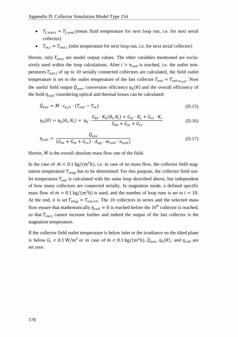
Appendix D: Collector Simulation Model Type 154
178
𝑇𝑓,𝑠𝑡𝑎𝑟𝑡 = 𝑇𝑓,𝑒𝑛𝑑 (mean fluid temperature for next loop run, i.e. for next serial
collector)
𝑇𝑖𝑛,𝑙 = 𝑇𝑜𝑢𝑡,𝑖 (inlet temperature for next loop run, i.e. for next serial collector)
Herein, only 𝑇𝑜𝑢𝑡,𝑖 are model output values. The other variables mentioned are exclu-
sively used within the loop calculations. After 𝑖 > 𝑛𝑐𝑜𝑙𝑙 is reached, i.e. the outlet tem-
peratures 𝑇𝑜𝑢𝑡,𝑖 of up to 10 serially connected collectors are calculated, the field outlet
temperature is set to the outlet temperature of the last collector 𝑇𝑜𝑢𝑡 = 𝑇𝑜𝑢𝑡,𝑛𝑐𝑜𝑙𝑙. Now
the useful field output �̇�𝑢𝑠𝑒, conversion efficiency 𝜂0(𝜃) and the overall efficiency of
the field 𝜂𝑐𝑜𝑙𝑙 considering optical and thermal losses can be calculated:
�̇�𝑢𝑠𝑒 = �̇� ⋅ 𝑐𝑝,𝑓𝑙 ⋅ (𝑇𝑜𝑢𝑡 − 𝑇𝑖𝑛) ( D.15 )
𝜂0(𝜃) = 𝜂0(𝜃𝑙, 𝜃𝑡) = 𝜂0 ⋅𝐺𝑏𝑡 ⋅ 𝐾𝑏(𝜃𝑙, 𝜃𝑡) + 𝐺𝑠𝑡 ⋅ 𝐾𝑠 + 𝐺𝑟𝑡 ⋅ 𝐾𝑟
𝐺𝑏𝑡 + 𝐺𝑠𝑡 + 𝐺𝑟𝑡 ( D.16 )
𝜂𝑐𝑜𝑙𝑙 = �̇�𝑢𝑠𝑒
(𝐺𝑏𝑡 + 𝐺𝑠𝑡 + 𝐺𝑟𝑡) ⋅ 𝐴𝑎𝑝 ⋅ 𝑚𝑐𝑜𝑙𝑙 ⋅ 𝑛𝑐𝑜𝑙𝑙) ( D.17 )
Herein, �̇� is the overall absolute mass flow rate of the field.
In the case of �̇� < 0.1 kg/(m2h), i.e. in case of no mass flow, the collector field stag-
nation temperature 𝑇𝑠𝑡𝑎𝑔 has to be determined. For this purpose, the collector field out-
let temperature 𝑇𝑜𝑢𝑡 is calculated with the same loop described above, but independent
of how many collectors are connected serially. In stagnation mode, a defined specific
mass flow of �̇� = 0.1 kg/(m2h) is used, and the number of loop runs is set to 𝑖 = 10.
At the end, it is set 𝑇𝑠𝑡𝑎𝑔 = 𝑇𝑜𝑢𝑡,10. The 10 collectors in series and the selected mass
flow ensure that mathematically 𝜂𝑐𝑜𝑙𝑙 = 0 is reached before the 10th
collector is reached,
so that 𝑇𝑜𝑢𝑡,𝑖 cannot increase further and indeed the output of the last collector is the
stagnation temperature.
If the collector field outlet temperature is below inlet or the irradiance on the tilted plane
is below 𝐺𝑡 < 0.1 W/m² or in case of �̇� < 0.1 kg/(m2h), �̇�𝑢𝑠𝑒 , 𝜂0(𝜃), and 𝜂𝑐𝑜𝑙𝑙 are
set zero.
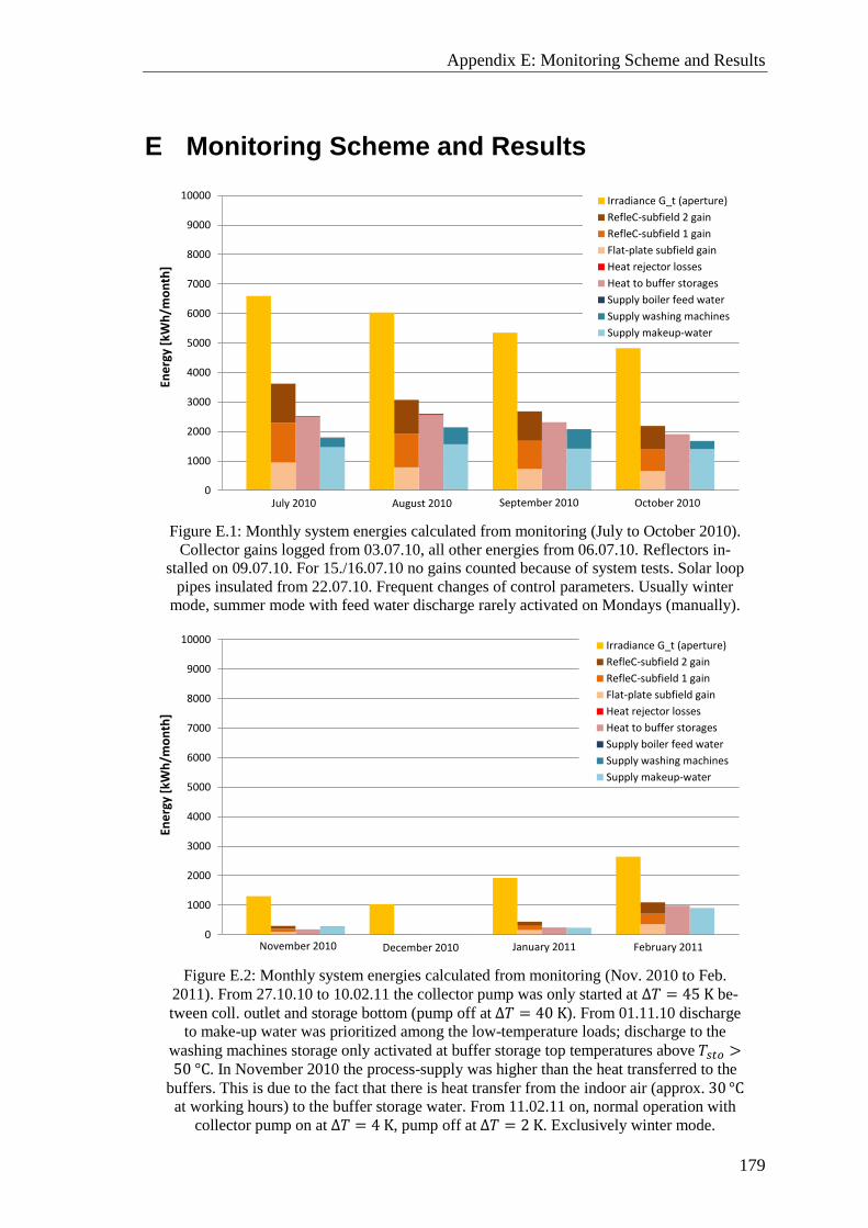
Appendix E: Monitoring Scheme and Results
179
E Monitoring Scheme and Results
Figure E.1: Monthly system energies calculated from monitoring (July to October 2010).
Collector gains logged from 03.07.10, all other energies from 06.07.10. Reflectors in-
stalled on 09.07.10. For 15./16.07.10 no gains counted because of system tests. Solar loop
pipes insulated from 22.07.10. Frequent changes of control parameters. Usually winter
mode, summer mode with feed water discharge rarely activated on Mondays (manually).
Figure E.2: Monthly system energies calculated from monitoring (Nov. 2010 to Feb.
2011). From 27.10.10 to 10.02.11 the collector pump was only started at Δ𝑇 = 45 K be-
tween coll. outlet and storage bottom (pump off at Δ𝑇 = 40 K). From 01.11.10 discharge
to make-up water was prioritized among the low-temperature loads; discharge to the
washing machines storage only activated at buffer storage top temperatures above 𝑇𝑠𝑡𝑜 >50 °C. In November 2010 the process-supply was higher than the heat transferred to the
buffers. This is due to the fact that there is heat transfer from the indoor air (approx. 30 °C
at working hours) to the buffer storage water. From 11.02.11 on, normal operation with
collector pump on at Δ𝑇 = 4 K, pump off at Δ𝑇 = 2 K. Exclusively winter mode.
0
1000
2000
3000
4000
5000
6000
7000
8000
9000
10000
Ene
rgy
[kW
h/m
on
th]
Irradiance G_t (aperture)
RefleC-subfield 2 gain
RefleC-subfield 1 gain
Flat-plate subfield gain
Heat rejector losses
Heat to buffer storages
Supply boiler feed water
Supply washing machines
Supply makeup-water
July 2010 August 2010 September 2010 October 2010
0
1000
2000
3000
4000
5000
6000
7000
8000
9000
10000
Ene
rgy
[kW
h/m
on
th]
Irradiance G_t (aperture)
RefleC-subfield 2 gain
RefleC-subfield 1 gain
Flat-plate subfield gain
Heat rejector losses
Heat to buffer storages
Supply boiler feed water
Supply washing machines
Supply makeup-water
November 2010 December 2010 January 2011 February 2011
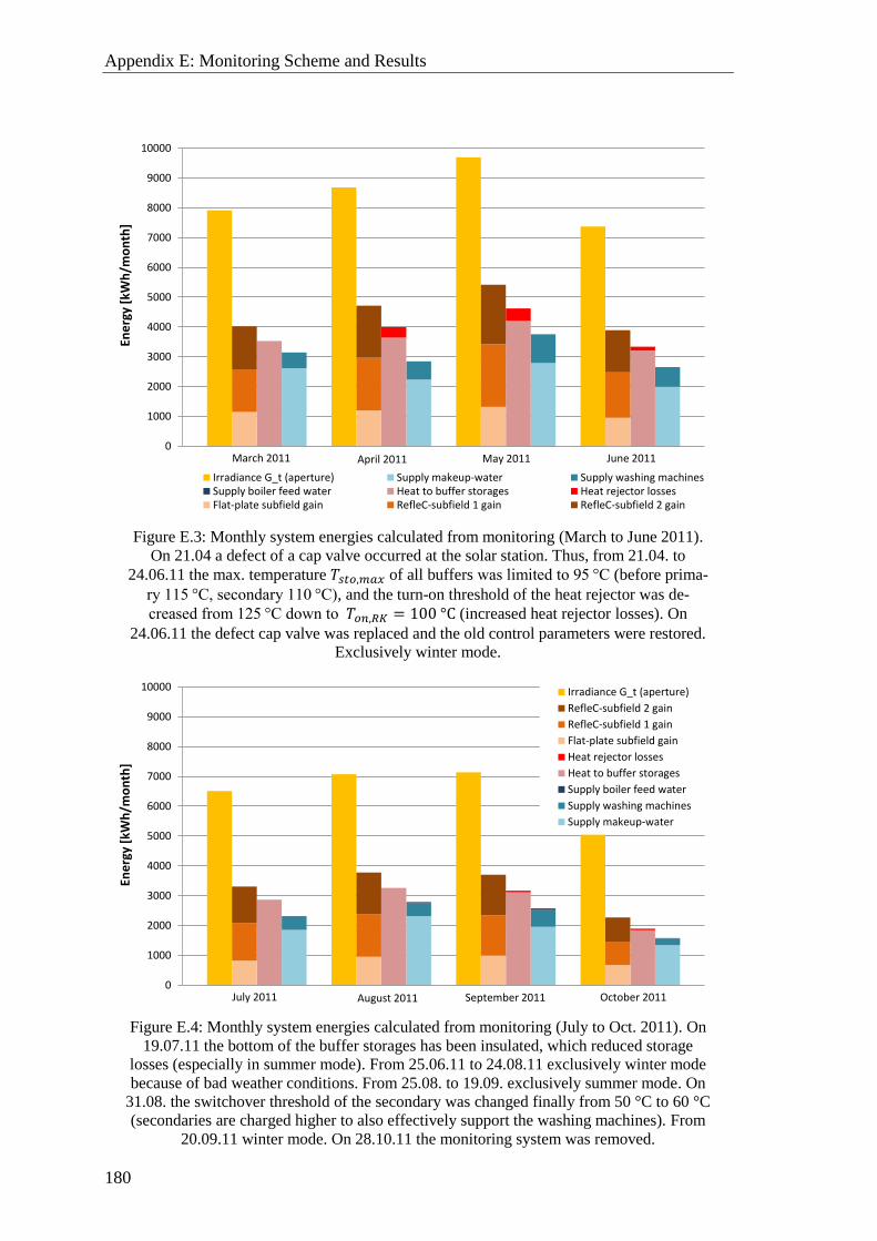
Appendix E: Monitoring Scheme and Results
180
Figure E.3: Monthly system energies calculated from monitoring (March to June 2011).
On 21.04 a defect of a cap valve occurred at the solar station. Thus, from 21.04. to
24.06.11 the max. temperature 𝑇𝑠𝑡𝑜,𝑚𝑎𝑥 of all buffers was limited to 95 °C (before prima-
ry 115 °C, secondary 110 °C), and the turn-on threshold of the heat rejector was de-
creased from 125 °C down to 𝑇𝑜𝑛,𝑅𝐾 = 100 °C (increased heat rejector losses). On
24.06.11 the defect cap valve was replaced and the old control parameters were restored.
Exclusively winter mode.
Figure E.4: Monthly system energies calculated from monitoring (July to Oct. 2011). On
19.07.11 the bottom of the buffer storages has been insulated, which reduced storage
losses (especially in summer mode). From 25.06.11 to 24.08.11 exclusively winter mode
because of bad weather conditions. From 25.08. to 19.09. exclusively summer mode. On
31.08. the switchover threshold of the secondary was changed finally from 50 °C to 60 °C
(secondaries are charged higher to also effectively support the washing machines). From
20.09.11 winter mode. On 28.10.11 the monitoring system was removed.
0
1000
2000
3000
4000
5000
6000
7000
8000
9000
10000
Ene
rgy
[kW
h/m
on
th]
Irradiance G_t (aperture) Supply makeup-water Supply washing machinesSupply boiler feed water Heat to buffer storages Heat rejector lossesFlat-plate subfield gain RefleC-subfield 1 gain RefleC-subfield 2 gain
March 2011 April 2011 May 2011 June 2011
0
1000
2000
3000
4000
5000
6000
7000
8000
9000
10000
Ene
rgy
[kW
h/m
on
th]
Irradiance G_t (aperture)
RefleC-subfield 2 gain
RefleC-subfield 1 gain
Flat-plate subfield gain
Heat rejector losses
Heat to buffer storages
Supply boiler feed water
Supply washing machines
Supply makeup-water
July 2011 August 2011 September 2011 October 2011
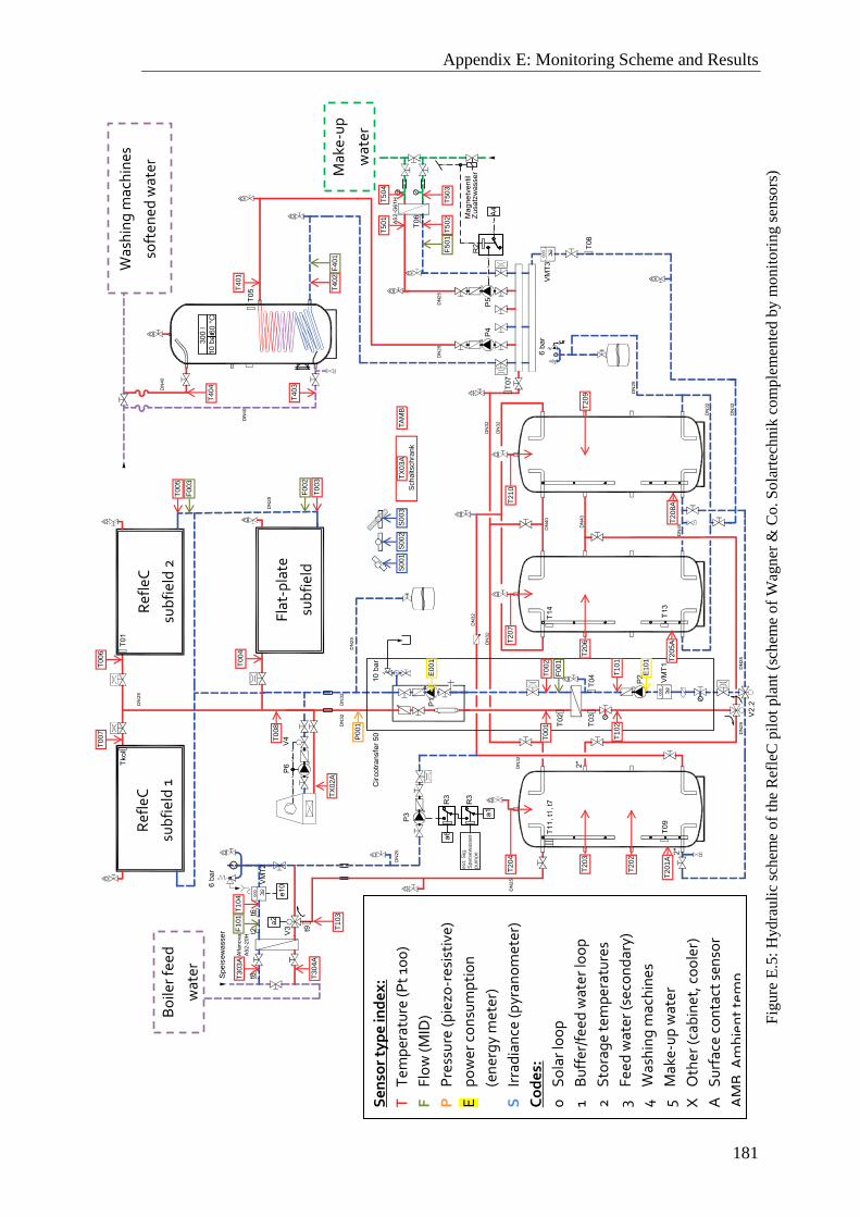
Appendix E: Monitoring Scheme and Results
181
∑
∑
∑
Fe
ld 3
Refle
C R
1
Fe
ld 2
Re
fleC
R2
Fe
ld 1
Fla
chko
llekto
r
T0
01
T0
02
TX
02
A
T0
03
T0
04
T00
6
T005
T00
7
T008
T10
2T
10
1
E101
E00
1
P001
F001
F00
2
F00
3
T2
04
T20
3
T2
02
T20
1A
T2
07
T20
6
T2
05A
T21
0
T20
9
T2
08
A
T1
03
T10
4F
101
T3
03
A
T304A
F501
T5
02
T50
3
T5
01
T5
04
T40
4
T4
03
T40
2F
401
T4
01
Sch
altsch
rank
TX
03A
TA
MB
S00
1S
002
S003
ext.
Sig
.S
peis
ew
asser-
pum
pe
Le
ge
nde
Messste
llen:
TTe
mp
era
turm
essu
ng
FD
urc
hflu
ssm
essu
ng
PD
ruckm
essun
g (
absolu
t)E
Me
ssu
ng
de
r ele
ktr
ische
n
Leis
tun
gS
Me
ssu
ng
de
rE
instr
ahlu
ng
sle
istu
ng
0S
ola
rkre
is1
Pu
ffers
pe
ich
er-
/S
pe
ise
wa
sse
rkre
is2
Me
ssu
ng
an
/in
de
n S
peic
her
3S
pe
ise
wa
sse
r ve
rbra
uche
rse
itig
4W
eic
hw
asse
rvo
rwä
rmu
ng
5K
esse
lzu
sa
tzw
asse
r-vo
rwä
rmu
ng
XA
nd
ere
Zu
ord
nun
gA
An
leg
ete
mpe
ratu
rfüh
ler
Se
nso
r ty
pe
ind
ex
:
T
Tem
per
atu
re (
Pt
100
)
F
Flo
w (M
ID)
P
Pre
ssu
re (
pie
zo-r
esis
tive
)
E
po
wer
co
nsu
mp
tio
n
(e
ner
gy
met
er)
S
Irra
dia
nce
(pyr
ano
met
er)
Co
de
s:
0
So
lar
loo
p
1
Bu
ffer
/fee
d w
ater
loo
p
2
Sto
rag
e t
emp
erat
ure
s
3 Fe
ed
wat
er (s
eco
nd
ary)
4
Was
hin
g m
ach
ines
5
Mak
e-u
p w
ater
X
Oth
er (c
abin
et, c
oo
ler)
A
Su
rfac
e co
nta
ct s
enso
r
AM
B A
mb
ien
t te
mp
.
Bo
iler
feed
wat
er
Was
hin
g m
ach
ines
soft
ened
wat
er
Mak
e-u
p
wat
er
Ref
leC
sub
fiel
d 1
Ref
leC
sub
fiel
d 2
Flat
-pla
te
sub
fiel
d
Fig
ure
E.5
: H
yd
rau
lic
sch
eme
of
the
Ref
leC
pil
ot
pla
nt
(sch
eme
of
Wag
ner
& C
o. S
ola
rtec
hnik
co
mp
lem
ente
d b
y m
on
ito
rin
g s
enso
rs)
Figures
182
Figures
Figure 1.1: The most widespread ST technology is thermo-siphon systems .................... 1
Figure 1.2: Computer graphic of the initial RefleC collector concept. ............................. 2
Figure 1.3: RefleC prototype at pilot plant laundry Laguna in Marburg an der Lahn ...... 2
Figure 1.4: Approach and structure of the work ............................................................... 3
Figure 1.5: Distribution of Germany’s final energy consumption in 2012 ....................... 5
Figure 1.6: Heat demand of the EU below 250 °C ............................................................ 6
Figure 1.7: Industrial heat demand in Germany per temperature range ............................ 7
Figure 1.8: Vision of the International Energy Agency IEA for ST until 2050. ............. 10
Figure 1.9: Collector output curves at reference conditions ........................................... 11
Figure 1.10: Components of a standard flat-plate collector ............................................ 12
Figure 1.11: Simplified illustration of the loss mechanisms of a standard flat-plate ...... 12
Figure 1.12: Components of a Sydney tube collector ..................................................... 13
Figure 1.13: Flat-plate collector field with trapezoidal corrugated aluminum sheet
booster reflectors .......................................................................................... 15
Figure 1.14: AoSol CPC collector with “inverted v”-absorber. ...................................... 16
Figure 1.15: Construction principle of the MaReCo (Maximum Reflector Collector) ... 17
Figure 1.16: SRB collector at the Intersolar Europe 2011 in Munich. Picture: S. Hess . 17
Figure 2.1: Solar irradiance components on an aperture plane with tilt angle 𝛽. ........... 19
Figure 2.2: Reference spectra G173-03 of ASTM .......................................................... 21
Figure 2.3: Solar tracker for irradiance measurement ..................................................... 22
Figure 2.4: Images from “All Sky Imager” at Plataforma Solar de Almeria .................. 23
Figure 2.5: Illustration of the cosine-effect for received solar irradiance. ...................... 25
Figure 2.6: Aperture area definition for RefleC. ............................................................. 27
Figure 2.7: Orientation of collector plane and sun .......................................................... 27
Figure 2.8: Projection of the sun direction (defined by 𝜃 and 𝜙) into the longitudinal
and transversal collector plane. .................................................................... 29
Figure 2.9: RefleC 1 in OptiCAD. .................................................................................. 30
Figure 2.10: Optical loss mechanisms of a low-concentrating, single covered ST
collector. ....................................................................................................... 31
Figure 2.11: Raytraced IAM values of the RefleC prototype R6 GF (no end losses)
and its receiver flat-plate compared to the first prototype R1 G. ................. 32
Figure 2.12: Raytraced 3D-IAM of the first test sample RefleC 1 G ............................. 33
Figure 2.13: Partly automated procedure for IAM simulation ........................................ 34
Figure 2.14: Comparison of surfaces with ideal and real reflectance characteristics ..... 37
Figure 2.15: Reflectance (hemispherical) of new and exposed (aged) reflector
samples. ........................................................................................................ 38
Figure 2.16: Reflectance (hemispherical) of exposed (aged) reflector samples ............. 39
Figures
183
Figure 2.17: Reflectance (hemispherical) of the Alu composite material (new) for
varying incidence angles. ............................................................................. 39
Figure 2.18: Measured distribution of reflected radiation intensities of the reflector .... 40
Figure 2.19: Selected reflector samples after hail impact. .............................................. 42
Figure 2.20: Transmittance of transparent cover materials ............................................ 44
Figure 2.21: Transmittance of transparent cover materials at varying incidence angles.45
Figure 2.22: Transmittance of transparent cover materials for infrared radiation .......... 45
Figure 2.23: Screenshot from OptiCad with setup to validate the simulation of
multiple reflections and polarization effects at the collector front. ............. 46
Figure 2.24: Measured transmittance of a 25 μ𝑚 FEP foil ............................................ 46
Figure 2.25: Spectral absorptance of a sputtered selective coating as used for the
RefleC collector with solar spectrum and emittance of black bodies at
100 °𝐶 and 200 °𝐶 ....................................................................................... 47
Figure 2.26: Angular absorptance of a selective solar absorber coating as implemented
in OptiCAD .................................................................................................. 48
Figure 2.27: Simulation model to validate the correct implementation of angular
absorptance in OptiCAD .............................................................................. 48
Figure 2.28: Geometric relations between sun and solar concentrator (shape not
defined). Adapted from (Rabl 1976a, p. 95). ............................................... 49
Figure 2.29: Illustration of the acceptance half-angle .................................................... 50
Figure 2.30: Schematic drawing of a symmetric CPC .................................................... 52
Figure 2.31: Raytracing analysis of the truncated CPC in Figure 2.30. ......................... 53
Figure 2.32: Acceptance function of a CPC ................................................................... 53
Figure 2.33: Ecliptic of the sun on the sky dome for the twelve months of a year in
Würzburg ..................................................................................................... 54
Figure 2.34: Sun positions projected into the north-south plane of a south facing
aperture sloped by 𝛽 = 49.48° in Würzburg ............................................... 55
Figure 2.35: Parameters of a V-trough ........................................................................... 56
Figure 2.36: Radiation acceptance comparison between a truncated CPC and a V-
trough. .......................................................................................................... 57
Figure 2.37: Comparison of absorbed irradiance of a single-covered flat-plate, a
truncated CPC (RefleC 1) and a V-trough. .................................................. 57
Figure 2.38: Raytraced IAM curves of R1 G, R2 G and the receiver flat-plates C20
AR G and C20 AR GG without end-losses. ................................................ 59
Figure 2.39: Raytraced IAM curves of R2 GG, R5 GF, receiver flat-plate C20 AR GG
and the RefleC pilot plant without end losses. ............................................. 59
Figure 3.1: RefleC 1 during outdoor IAM determination ............................................... 61
Figure 3.2: Second test sample RefleC 2. ....................................................................... 62
Figure 3.3: CAD impression of RefleC 4 on a flat roof. ................................................ 64
Figure 3.4: RefleC 5 during outdoor test. ....................................................................... 64
Figure 3.5: RefleC 6 during efficiency curve and IAM measurement ........................... 65

Figures
184
Figure 3.6: Cross section of LBM 4 AR GF, receiver flat-plate of RefleC 6 ................. 66
Figure 3.7: Measured efficiency curves of RefleC 6 and its flat-plate ........................... 68
Figure 3.8: Acceptance of RefleC 1 for isotropic diffuse irradiance .............................. 72
Figure 3.9: Efficiency test results (outdoor, MTTS) of RefleC 6 ................................... 75
Figure 3.10: Efficiency test results (outdoor, MTTS) of LBM 4 GF .............................. 77
Figure 3.11: Efficiency curves of RefleC 6 GF and LBM 4 GF as shown in Figure 3.9
and Figure 3.10 fitted from the data points of all four temperature levels
(solid lines) and without the highest temperature level (dashed lines). ....... 78
Figure 3.12: Comparison of MTTS-measured collector efficiencies of RefleC 6 GF
and LBM 4 GF at mass flow rates 72 kg/(m2h) and 35 kg/(m2h) .......... 80
Figure 3.13: Local concentration onto the absorber of RefleC 1 .................................... 81
Figure 3.14: Thermographic image of RefleC 2 G ......................................................... 81
Figure 3.15: Local stagnation absorber plate temperatures 𝑇𝑝 of RefleC 2 ................... 82
Figure 3.16: RefleC 1 G at test of the hemispheric IAM ................................................ 82
Figure 3.17: Raytraced beam-IAM 𝐾𝑏 of RefleC 1 (blue), compared to the
hemispherical IAM 𝐾ℎ calculated from tested efficiencies (green) and to
𝐾𝑏-values calculated from a correction of the tested efficiencies by the
influence of diffuse. ...................................................................................... 84
Figure 3.18: Raytraced longitudinal IAM of RefleC 1 G compared to the hemispheric
IAM calculated directly from the test results ............................................... 85
Figure 3.19: Raytraced transversal beam-IAM of RefleC 6 GF compared to its
hemispheric IAM calculated from the test results (green). .......................... 88
Figure 3.20: Efficiency test results (outdoor, MTTS) of RefleC 6 GF ........................... 90
Figure 3.21: Comparison of measured efficiency curves of RefleC 1 and 2 (two
reflectors) and their flat-plate receiver collectors. ........................................ 91
Figure 3.22: Comparison of measured efficiency curves of RefleC 1 and 2 (two
reflectors) to RefleC 6 (one segmented lower reflector) and their flat-plate
receiver collectors. ........................................................................................ 94
Figure 3.23: Comparison of the measured thermal efficiency curves of RefleC 2 G/GG
and RefleC 6 GF to efficiency curves calculated ......................................... 96
Figure 4.1: Values needed for new collector model “Type 154” .................................... 97
Figure 4.2: Sky radiance modeling errors of the continuous models of Igawa et al.
(2004), Perez et al. (1993) and Brunger and Hooper (1993), ....................... 99
Figure 4.3: Horizontal plane with positions of sun and diffuse radiating sky
element 𝑑Ω. ................................................................................................ 101
Figure 4.4: Diffuse sky radiance distribution according to the Brunger Model for a
heavily overcast sky ................................................................................... 104
Figure 4.5: Diffuse sky radiance distribution according to the Brunger Model for a
lightly overcast sky ..................................................................................... 104
Figure 4.6: Diffuse sky radiance distribution according to the Brunger Model for a
partly cloudy sky ........................................................................................ 104
Figures
185
Figure 4.7: Diffuse sky radiance distribution according to the Brunger Model for a
relatively clear sky ..................................................................................... 105
Figure 4.8: Wide-angle 180° photographs of the sky dome at the measurement site for
generation of the Brunger model parameters ............................................. 105
Figure 4.9: Type 154 within TRNSYS Simulation Studio. .......................................... 106
Figure 4.10: Simplified illustration of the functions of Type 154 ................................ 109
Figure 4.11: Annual horizontal irradiation distribution diagram for Würzburg ........... 111
Figure 4.12: Annual irradiation distribution diagram for a sloped surface of 𝛽 = 55°
and 𝛾 = 0° in Würzburg. ........................................................................... 113
Figure 4.13: IAM values of Type 154 for beam, sky diffuse and ground reflected
diffuse onto a RefleC 6 GF collector ......................................................... 114
Figure 4.14: Increase in annual collector output by the boosters in Würzburg ............ 117
Figure 4.15: Annual output of RefleC 6 GF ................................................................. 118
Figure 4.16: Monthly gains of LBM 4 GF and RefleC 6 GF in Würzburg .................. 119
Figure 4.17: Monthly gains of LBM 4 GF and RefleC 6 GF in Seville ....................... 119
Figure 4.18: Monthly gains of LBM 4 GF and RefleC 6 GF in Würzburg .................. 120
Figure 4.19: Monthly gains of LBM 4 GF and RefleC 6 GF in Seville ....................... 121
Figure 4.20: Annual collector gain of RefleC and its receiver flat-plate collector in
Würzburg for different collector slopes ..................................................... 121
Figure 5.1: Laundry Laguna ......................................................................................... 123
Figure 5.2: Unclean side with three industrial washing machines ............................... 124
Figure 5.3: Boiler room with one of the initially two steam boilers ............................. 125
Figure 5.4: Collector field of the pilot plant from east direction. ................................. 126
Figure 5.5: Computer graphic of the collector field on the laundry roof. ..................... 126
Figure 5.6: Hydraulic scheme of the pilot plant (simplified). ...................................... 128
Figure 5.7: Centralized components of the RefleC pilot system .................................. 129
Figure 5.8: Dry stagnation cooler in front of flat-plate subfield. The insulated and
aluminum sheet metal coated feed and return flow pipes of the field are
routed in a U-shape to compensate thermal expansion. Above them, the
rectangular sensor cable duct is visible. ..................................................... 129
Figure 5.9: Positions of the three pyranometers applied for monitoring ...................... 131
Figure 5.10: Plate heat exchanger for solar pre-heating of the boiler make-up water. . 132
Figure 5.11: Monitoring switch cabinet with cable ducts opened. ............................... 132
Figure 5.12: Exemplary weekend with daily balances of monitored energies ............. 133
Figure 5.13: Diurnal variation of the pilot plant operation on Saturday, 21.08.2010. .. 136
Figure 5.14: Solar incidence angles onto the collector field of the pilot plant ............. 137
Figure 5.15: Comparison of measured and calculated power of RefleC subfield 2 and
flat-plate subfield ....................................................................................... 138
Figure 5.16: Overview on the whole monitoring period of 16 months ........................ 142
Figure B.1: Efficiency test results (outdoor, standard) of RefleC 1 ............................. 159
Figure B.2: Efficiency test results (outdoor, MTTS) of RefleC 2 G ............................ 159
Figures
186
Figure B.3: Efficiency test results (outdoor, MTTS) of RefleC 2 GG .......................... 160
Figure B.4: Efficiency test results (outdoor, standard) of RefleC 5 V2 ........................ 160
Figure B.5: Efficiency test results (outdoor, standard) of RefleC 5 V2 ........................ 161
Figure B.6: Efficiency test results (outdoor, standard) of RefleC 6 GF ........................ 161
Figure B.7: Efficiency test results (sun simulator, MTTS) of EURO C 20 AR............ 162
Figure B.8: Efficiency test results (sun simulator, MTTS) of EURO C 20 AR GG ..... 162
Figure B.9: Efficiency test results (sun simulator, MTTS) of EURO C 20 AR GF ..... 163
Figure B.10: Efficiency test results (outdoor, MTTS) of LBM 4 GF ........................... 163
Figure C.1: Raytraced IAM curves of the test samples R1 G, R2 G, R6 GF with end
losses. ......................................................................................................... 164
Figure C.2: Raytraced IAM curves of the test samples R2 GG and R5 GF with end
losses. ......................................................................................................... 164
Figure C.3: Screenshots from transversal raytracing analysis of RefleC ...................... 165
Figure D.1: Overview flow chart of TRNSYS Type 154 ............................................. 166
Figure D.2: Numerical integration steps to calculate the IAM for diffuse irradiance
from the sky ................................................................................................ 172
Figure D.3: Numerical integration steps to calculate the IAM for isotropic diffuse
irradiance from the ground ......................................................................... 175
Figure E.1: Monthly system energies calculated from monitoring (July to October
2010). .......................................................................................................... 179
Figure E.2: Monthly system energies calculated from monitoring (Nov. 2010 to Feb.
2011). .......................................................................................................... 179
Figure E.3: Monthly system energies calculated from monitoring (March to June
2011). .......................................................................................................... 180
Figure E.4: Monthly system energies calculated from monitoring (July to Oct. 2011).180
Figure E.5: Hydraulic scheme of the RefleC pilot plant ............................................... 181
Tables
187
Tables
Table 2.1: Terms for solar radiation as suggested by Iqbal (1983, p. 41). ..................... 20
Table 2.2: Parameters used to model the different RefleC variants (R1 to R6, cp.
Appendix A) in OptiCAD. ........................................................................... 36
Table 2.3: Properties of cover materials ......................................................................... 43
Table 3.1: Stationary test data of RefleC 6 GF used to fit the curve in Figure 3.9......... 75
Table 3.2: Criteria for valid outdoor steady-state efficiency test points according to
(EN 12975-2:2006) ...................................................................................... 76
Table 3.3: Stationary test data of LBM 4 GF used to fit the efficiency curve (cp.
Figure 3.10) .................................................................................................. 77
Table 3.4: Raytracing results (𝜌𝜏𝛼𝑒 and 𝐾𝑏) vs. test results and corrected test results
of the transversal IAM ................................................................................. 85
Table 3.5: Raytracing results of RefleC 1 G vs. test results and „correction“
calculations of longitudinal IAM ................................................................. 86
Table 3.6: Raytracing results of RefleC 6 GF vs. test results and „correction“
calculations of transversal IAM ................................................................... 89
Table 3.7: Stationary test data points of RefleC 6 GF at 𝜃𝑡 = 25° (cp. Figure 3.20) .... 90
Table 3.8: Overview of measured RefleC and flat-plate receiver collector efficiency
parameters complemented by raytracing results and calculated values. ...... 92
Table 4.1: The coefficients 𝑎0 to 𝑎3 of the Brunger Model ......................................... 103
Table 4.2: Annual gain of RefleC 6 GF and its flat-plate receiver LBM 4 GF ............ 116
Table 5.1: Thermal loads at the solar heat integration points ....................................... 127
Table 5.2: Annual system performance figures of the reference year. ......................... 134
Table 5.3: Conditions and collector performance on Saturday, 21.08.2010. ............... 139
Table A.1: Parameters of RefleC collectors ................................................................. 152
Table A.2: Parameters of receiver flat-plate collectors ................................................ 154
Table B.1: Test results for efficiency curves of the RefleC test samples ..................... 155
Table B.2: Test results for efficiency curves of the receiver flat-plate collectors ........ 157
Table D.1: Input values of Type 154 ............................................................................ 167
Table D.2: Parameters of Type 154 .............................................................................. 167
Table D.3: Output values of Type 154 ......................................................................... 168
Table D.4: External links of Type 154 ......................................................................... 169

Publications
188
Publications
Selected Publications with Relation to this Work
Hess, S. and Hanby, V. I. (2014). "Collector Simulation Model with Dynamic Incidence Angle
Modifier for Anisotropic Diffuse Irradiance." Energy Procedia 48(0): 87-96.
Hess, S., Oliva, A., et al. (2012). Ergebnisse des IEE-Projekts SO-PRO: Auslegung von
Solaranlagen für vier ausgewählte industrielle Prozesse. 22. OTTI-Symposium Thermische
Solarenergie. Bad Staffelstein.
Hess, S., Klemke, M., Oliva, A., Di Lauro, P., Hermann, M., Stryi-Hipp, G., Kramp, G., von
Bodungen, O., Eisenmann, W. and Hanby, V. (2011). Pilotanlage mit RefleC Kollektoren:
Anlagenkonzept und Monitoring-Ergebnisse. 21. OTTI-Symposium Thermische
Solarenergie. Bad Staffelstein: 124-129.
Hess, S., Oliva, A., Hermann, M., Stryi-Hipp, G. and Hanby, V. (2011). Solar Process Heat –
System Design for Selected Low-temperature Applications in the Industry. Solar World
Congress 2011. Kassel.
Hess, S. and Oliva, A. (2010). Guide to Solar Thermal System Design for Selected Industrial
Processes. URL: www.solar-process-heat.eu/guide.
Hess, S., Oliva, A., Di Lauro, P., Klemke, M., Hermann, M., Kramp, G., Eisenmann, W. and
Hanby, V. (2010). Solar Heat for Industrial Processes: RefleC Collector Development and
System Design. EuroSun 2010. Graz.
Hess, S., Oliva, A., Di Lauro, P., Klemke, M., Hermann, M., Stryi-Hipp, G., Kallwellis, V.,
Kramp, G., Eisenmann, W. and Hanby, V. (2010). Flachkollektor mit externen Reflektoren
(RefleC): Entwicklungserfahrungen. 20. OTTI-Symposium Thermische Solarenergie. Bad
Staffelstein: 150-155.
Hess, S., Di Lauro, P., Oliva, A. and Hanby, V. (2009). RefleC – A new Collector for Solar
Cooling Applications with Operating Temperatures up to 150 °C. 3rd International OTTI-
Conference on Solar Air-Conditioning. Palermo: 393-398.
Hess, S., Di Lauro, P., Oliva, A. and Hanby, V. (2009). RefleC – Ein verbesserter
Flachkollektor mit externen Reflektoren zur Erzeugung von Prozesswärme bis 150 °C. 19.
OTTI-Symposium Thermische Solarenergie. Bad Staffelstein: 116-117.
Hess, S., Di Lauro, P., Rose, S. and Rommel, M. (2008). Comparison of Medium Temperature
Collectors for the Generation of Process Heat. EuroSun 2008. Lisbon: paper 513.
Hess, S., Rommel, M., Di Lauro, P. and Rose, S. (2008). Raytracing-Untersuchungen für die
Entwicklung von Prozesswärmekollektoren. 18. OTTI-Symposium Thermische Solarener-
gie. Bad Staffelstein: 416-421.
Hess, S. (2007). Application of Medium Temperature Collectors for Solar Air-Conditioning.
2nd International Conference on Solar Air-Conditioning. Tarragona: 118-123.

Publications
189
Theses of Students Supervised during this Work
Schmid, M. (2014). Identifikation und Bewertung von Systemkonzepten zur Integration solarer
Prozesswärme in Wäschereien. Diploma Thesis. Universität Kassel.
Klemke, M. (2011). Monitoring einer solarthermischen Demonstrationsanlage zur
Bereitstellung von Wärme für industrielle Prozesse. Diploma Thesis. Fachhochschule
Gießen-Friedberg.
Oliva, A. (2009). Einbindung der Energie eines konzentrierenden solarthermischen
Flachkollektors in industrielle Prozesse. Diploma Thesis. Technische Universität
Hamburg-Harburg.
Raucher, C. (2009). Untersuchungen zur Einbindung der Energie eines konzentrierenden
solarthermischen Flachkollektors in industrielle Prozesse. Master Thesis. Universität
Kassel.
Rose, S. (2008). Untersuchungen zur Entwicklung einer Zweifachabdeckung für einen
Prozesswärme-Flachkollektor mit externen Reflektoren. Diploma Thesis. Hochschule Ulm.
Di Lauro, P. (2008). Untersuchungen zum einstrahlwinkelabhängigen Wirkungsgrad eines
Prozesswärme-Flachkollektors mit externen Reflektoren. Diploma Thesis. Hochschule
Ulm.

Bibliography
190
Bibliography
Adsten, M. (2002). Solar Thermal Collectors at High Latitudes-Design and performance of
nontracking concentrators. Uppsala University.
Adsten, M., Helgesson, A., et al. (2005). "Evaluation of CPC-collector designs for stand-alone,
roof- or wall installation." Solar Energy 79(6): 638-647.
Adsten, M., Hellström, B., et al. (2004). "Measurement of radiation distribution on the absorber
in an asymmetric CPC collector." Solar Energy 76(1–3): 199-206.
AEE INTEC (2014). "Database for applications of solar heat integration in industrial
processes." Retrieved 05.09.2014. URL: http://www.ship-plants.info/.
Aidonis, A., Drosou, V., et al. (2005). PROCESOL II - Solar thermal plants in industrial
processes. Design and Maintenance Guidelines. Centre for Renewable Energy Sources.
Pikermi. URL: http://www.aee-intec.at/0uploads/dateienEnglisch124.pdf.
Ambrosetti, P. and Keller, J. (1985). Das neue Bruttowärmeertragsmodell für verglaste
Solarkollektoren. Eidgenössisches Institut für Reaktorforschung. Würlingen (CH).
Badescu, V. (2008). Modeling Solar Radiation at the Earth's Surface: Recent Advances. Berlin,
Springer Verlag.
Beeh, M. and Hess, S. (2014). Bericht zu Screenings und Fallstudien in SoProW. Bönnigheim.
BMWi (2014). Energiedaten: Gesamtausgabe. Stand: April 2014. URL:
http://www.bmwi.de/DE/Themen/Energie/Energiedaten-und-
analysen/Energiedaten/gesamtausgabe,did=476134.html.
Bollentin, J. W. and Wilk, R. D. (1995). "Modeling the solar irradiation on flat plate collectors
augmented with planar reflectors." Solar Energy 55(5): 343-354.
Bosanac, M. and Nielsen, J. E. (1997). "In situ check of collector array performance." Solar
Energy 59(4–6): 135-142.
Brandemuehl, M. J. and Beckman, W. A. (1980). "Transmission of diffuse radiation through
CPC and flat plate collector glazings." Solar Energy 24(5): 511-513.
Brogren, M. (2004). Optical Efficiency of Low-Concentrating Solar Energy Systems with
Parabolic Reflectors. Dissertation. Uppsala University.
Brogren, M., Helgesson, A., et al. (2004a). "Optical properties, durability, and system aspects of
a new aluminium-polymer-laminated steel reflector for solar concentrators." Solar
Energy Materials and Solar Cells 82(3): 387-412.
Brogren, M., Karlsson, B., et al. (2004b). "Analysis of the effects of outdoor and accelerated
ageing on the optical properties of reflector materials for solar energy applications."
Solar Energy Materials and Solar Cells 82(4): 491-515.
Brunger, A. P. and Hooper, F. C. (1993). "Anisotropic sky radiance model based on narrow
field of view measurements of shortwave radiance." Solar Energy 51(1): 53-64.
Burckhart, H. J., Audinet, F., et al. (2014). "Application of a Novel, Vacuum-insulated Solar
Collector for Heating and Cooling." Energy Procedia 48(0): 790-795.
Buttinger, F., Beikircher, T., et al. (2010). "Development of a new flat stationary evacuated
CPC-collector for process heat applications." Solar Energy 84(7): 1166-1174.
Calderoni, M., Aprile, M., et al. (2012). "Solar Thermal Plants for Industrial Process Heat in
Tunisia: Economic Feasibility Analysis and Ideas for a New Policy." Energy Procedia
30(0): 1390-1400.
Carvalho, M. J., Collares-Pereira, M., et al. (1995). "Optical and thermal testing of a new 1.12X
CPC solar collector." Solar Energy Materials and Solar Cells 37(2): 175-190.
Bibliography
191
Carvalho, M. J., Horta, P., et al. (2007). Incidence angle modifiers: A general approach for
energy calculations. ISES Solar World Congress, September 18-21. D. Y. Goswami and
Y. Zhao. Beijing, China, Springer 608-612.
Chaves, J. (2008). Introduction to Nonimaging Optics (Optical Science and Engineering). Boca
Raton, CRC Press Inc.
Clement, C. (2004). Verfahren zur optischen und thermischen Auslegung von konzentrierenden
Solarkollektoren für Prozesswärmeanlagen. Dissertation. Technische Universität
München.
Corporation, O. (2009). OptiCAD - Optical Analysis Program - User´s Guide version 10.046.
Santa Fe. URL: www.opticad.com.
Cotrado, M., Dalibard, A., et al. (2014). "Design, Control and First Monitoring Data of a Large
Scale Solar Plant at the Meat Factory Berger, Austria." Energy Procedia 48(0): 1144-
1151.
Duff, W. S. and Daosukho, J. (2011). Evaluation of the Reliability of a Novel ICPC Solar
Collector Installation: Incorporating the Diffuse Radiation Component into the Analysis
and Its Impact on the Comparison between Measured and Predicted Performance. ISES
Solar World Congress. Kassel.
Duff, W. S., Winston, R., et al. (2004). "Performance of the Sacramento demonstration ICPC
collector and double effect chiller." Solar Energy 76(1–3): 175-180.
Duffie, J. A. and Beckman, W. A. (2006). Solar Engineering of Thermal Processes. 3rd Edition.
New Jersey, John Wiley & Sons, inc.
Duffie, J. A. and Beckman, W. A. (2013). Solar Engineering of Thermal Processes. 4th Edition.
New Jersey, John Wiley & Sons, Inc.
Ebert, V., Günther, R., et al. (2012). Fahrplan Solarwärme. Strategie und Maßnahmen der
Solarwärme-Branche für ein beschleunigtes Marktwachstum bis 2030. Berlin. URL:
http://www.solarwirtschaft.de/fileadmin/media/pdf/120854_bsw_studie_st.pdf.
Egger, C. (2011). Solar Process Heat So-Pro. Publishable, result-orientated report. Final project
report. Linz. URL: www.solar-process-heat.eu/report.
Eisenmann, W. (2009). Physical properties of solar fluid DC20 in a mixture with 60 % water.
Fit functions determined from tabulated values between 10 °C and 100 °C in steps of 10
°C sent by Mr. Krakat, Fragol GmbH to Mr. Eisenmann, Wagner & Co. on 30.10.2009.
Eisenmann, W., Hess, S., et al. (2011). Entwicklung eines leistungsgesteigerten Flachkollektors
mit Reflektoren für die Gewinnung von Prozesswärme bis 150 °C. Final project report.
TIB Hannover. URL: http://edok01.tib.uni-hannover.de/edoks/e01fb11/668455144.pdf.
Eisenmann, W., Vajen, K., et al. (2004). "On the correlations between collector efficiency factor
and material content of parallel flow flat-plate solar collectors." Solar Energy 76(4):
381-387.
EN 12975-2:2006 Thermal solar systems and components - Solar collectors - Part 2: Test
methods. Brussels, European Committee for Standardization.
Eurostat (2014a). "Energy statistics - final energy consumption by sector - annual data
(tsdpc320)." URL: http://epp.eurostat.ec.europa.eu/tgm/table.do?tab=table&init=1&
plugin=1&language=en&pcode=tsdpc320.
Eurostat (2014b). "Energy statistics - supply, transformation, consumption - all products -
annual data (nrg_100a)." URL: http://appsso.eurostat.ec.europa.eu/nui/show.do?
dataset=nrg_100a&lang=en.
Evseev, E. G. and Kudish, A. I. (2009). "The assessment of different models to predict the
global solar radiation on a surface tilted to the south." Solar Energy 83(3): 377-388.
Faber, C., Anthrakidis, A., et al. (2011). Barriers to Solar Process Heat Applications. ISES Solar
World Congress 2011. Kassel.
Bibliography
192
Fasulo, A., Odicino, L., et al. (1987). "Development of a CPC with low thermal losses." Solar &
Wind Technology 4(2): 157-162.
Fischer, S. (2011). Dynamische Prüfung von Sonnenkollektoren unter besonderer
Berücksichtigung der Einfallswinkelkorrektur und der Reduzierung der Prüfdauer.
Dissertation. Universität Stuttgart.
Fischer, S. (2012). Proposal for Definition of Temperature Ranges and Terminology. IEA-Task
49, 2nd
Expert Meeting, 6.09.-7.09.12, Graz.
Fischer, S., Heidemann, W., et al. (2004). "Collector test method under quasi-dynamic
conditions according to the European Standard EN 12975-2." Solar Energy 76(1–3):
117-123.
Fraidenraich, N., Tiba, C., et al. (2008). "Analytic solutions for the geometric and optical
properties of stationary compound parabolic concentrators with fully illuminated
inverted V receiver." Solar Energy 82(2): 132-143.
Frei, U., Brunold, S., et al. (1998). Langzeit-Alterungsuntersuchungen an
Abdeckungsmaterialien für thermische Sonnenkollektoren. Institut für Solartechnik
Prüfung Forschung SPF. Rapperswil. URL: http://www.solarenergy.ch/fileadmin/daten/
publ/abde.pdf.
Frein, A., Calderoni, M., et al. (2014). "Solar Thermal Plant Integration into an Industrial
Process." Energy Procedia 48(0): 1152-1163.
Frey, R., Frei, U., et al. (1997). Bestimmung des Kollektorwirkungsgradfaktors F’ an
flüssigkeitsführenden Solarabsorbern. Rapperswil. URL: http://www.spf.ch/fileadmin/
daten/publ/fstrich.pdf.
Fuller, R. J. (2011). "Solar industrial process heating in Australia - Past and current status."
Renewable Energy 36: 216-221.
Georg, A. (2007). Simulated absorpance values for Cermet selective coating. Fraunhofer ISE,
unpublished values.
Goswami, D. Y., Kreith, F., et al. (1999). Principles of Solar Engineering. 2nd. Philadelphia,
Taylor & Francis.
Gueymard, C. A. (2009). "Direct and indirect uncertainties in the prediction of tilted irradiance
for solar engineering applications." Solar Energy 83(3): 432-444.
Häberle, A. (1999). Vermessung und Modellierung von stationären, konzentrierenden
Kollektoren. Dissertation. Universität Freiburg.
Haller, M., Perers, B., et al. (2013). TRNSYS Type 832 v5.01 - Dynamic Collector Model by
Bengt Perers - Updated Input-Output Reference. URL: http://www.solarenergy.ch/
Type-832-Kollektormodell.223.0.html?&no_cache=1&L=0&no_cache=1.
Harrison, A. W. (1991). "Directional sky luminance versus cloud cover and solar position."
Solar Energy 46(1): 13-19.
Hay, J. E. (1979). "Calculation of monthly mean solar radiation for horizontal and inclined
surfaces." Solar Energy 23(4): 301-307.
Heinzen, R., Zaß, K., et al. (2011). Integration of Solar Thermal Systems into Gas Pressure
Regulating Stations. ISES Solar World Congress. Kassel.
Helgesson, A. (2004). Optical Characterization of Solar Collectors from Outdoor
Measurements. Dissertation. Lund University.
Hellstrom, B., Adsten, M., et al. (2003). "The impact of optical and thermal properties on the
performance of flat plate solar collectors." Renewable Energy 28(3): 331-344.
Hess, S. (2007). Untersuchungen zur Entwicklung eines Prozesswärme-Flachkollektors mit
externen Reflektoren. Diploma Thesis. Fachhochschule Augsburg.
Hess, S. and Hanby, V. I. (2014). "Collector Simulation Model with Dynamic Incidence Angle
Modifier for Anisotropic Diffuse Irradiance." Energy Procedia 48(0): 87-96.
Bibliography
193
Hess, S. and Oliva, A. (2010). Guide to Solar Thermal System Design for Selected Industrial
Processes. Linz. URL: www.solar-process-heat.eu/guide.
Hess, S., Oliva, A., et al. (2011). Solar Process Heat – System Design for Selected Low-
temperature Applications in the Industry. Solar World Congress 2011. Kassel.
IEA (2012). IEA Technology Roadmap Solar Heating and Cooling. International Energy
Agency. Paris. URL: http://www.iea.org/publications/freepublications/publication/
Solar_Heating_Cooling_Roadmap_2012_WEB.pdf.
Igawa, N., Koga, Y., et al. (2004). "Models of sky radiance distribution and sky luminance
distribution." Solar Energy 77(2): 137-157.
Iqbal, M. (1983). An Introduction to solar Radiation. New York, Academic Press, Inc.
ISO 9806:2013 Solar energy — solar thermal collectors — test methods, edition 2013-11.
Ivancic, A., Mugnier, D., et al. (2014). RHC Solar Heating and Cooling Technology Roadmap.
Renewable Heating and Cooling Platform. Brussels. URL: http://www.rhc-
platform.org/publications/.
Jiang, L. and Winston, R. (2014). "Progress on Integrated Compound Concentrator Design."
Energy Procedia 48(0): 114-122.
Kalogirou, S. (2003). "The potential of solar industrial process heat applications." Applied
Energy 76(4): 337-361.
Kalogirou, S. A. (2004). "Solar thermal collectors and applications." Progress in Energy and
Combustion Science 30(3): 231-295.
Karagiorgas, M., Botzios, A., et al. (2001). "Industrial solar thermal applications in Greece
Economic evaluation, quality requirements and case studies." Renewable and
Sustainable Energy Reviews 5: 157–173.
Kasper, B.-R., Weyers-Borchert, B., et al. (2012). Solarthermische Anlagen: Leitfaden für das
SHK-, Elektro- und Dachdeckerhandwerk, Fachplaner, Architekten, Bauherrn und
Weiterbildungsinstitutionen. 9th Edition. Berlin, DGS, Deutsche Gesellschaft für
Sonnenenergie.
Kim, Y. S., Balkoski, K., et al. (2013). "Efficient stationary solar thermal collector systems
operating at a medium-temperature range." Applied Energy 111(0): 1071-1079.
Kittler, R. (1985). "Luminance distribution characteristics of homogeneous skies: a
measurement and prediction strategy." Lighting Research and Technology 17(4): 183-
188.
Klein, S. A., Beckman, W. A., et al. (2006). Trnsys 16 - a transient system simulation program,
Solar Energy Laboratory, University of Wisconsin-Madison.
Klein, S. A., Beckman, W. A., et al. (2012a). Trnsys 17 - a TRaNsient SYstem Simulation
program. Mathematical Reference, Solar Energy Laboratory, University of Wisconsin-
Madison.
Klein, S. A., Beckman, W. A., et al. (2012b). Trnsys 17 - a TRaNsient SYstem Simulation
program. Programmer´s Guide, Solar Energy Laboratory, University of Wisconsin-
Madison.
Klein, S. A., Beckman, W. A., et al. (2012c). Trnsys 17 - a TRaNsient SYstem Simulation
program. Standard Component Library Overview, Solar Energy Laboratory, University
of Wisconsin-Madison.
Klemke, M. (2011). Monitoring einer solarthermischen Demonstrationsanlage zur
Bereitstellung von Wärme für industrielle Prozesse. Diploma Thesis. Fachhochschule
Gießen-Friedberg.
Kramer, K. (2006). Aufbau und Einsatz eines Teststandes zur Messung der
Wirkungsgradkennlinien von Prozesswärme-Solarkollektoren. Diploma Thesis.
Fachhochschule Augsburg.
Bibliography
194
Kramp, G. (2010). Technical drawing of final RefleC collector as used for the pilot plant. STEP
construction data of Wagner & Co. Solartechnik GmbH, received per email on
19.02.2010.
Krueger, D., Lichtenhaeler, N., et al. (2011). Solar Steam Supply: Initial Operation of a Plant.
ISES Solar World Congress. Kassel.
Lauterbach, C. (2014). Potential, system analysis and preliminary design of low-temperature
solar process heat systems. Dissertation. Kassel University.
Lauterbach, C., Rad, J. S., et al. (2011a). Feasibility Assessment of Solar Process Heat
Applications. Solar World Congress. Kassel.
Lauterbach, C., Schmitt, B., et al. (2012). "The potential of solar heat for industrial processes in
Germany." Renewable and Sustainable Energy Reviews 16(7): 5121-5130.
Lauterbach, C., Schmitt, B., et al. (2011b). Das Potential solarer Prozesswärme in Deutschland.
Teil 1 des Abschlussberichts zum Forschungsvorhaben SOPREN, Solare Prozesswärme
und Energieeffizienz Kassel. URL: http://solar.umwelt-uni-kassel.de/
downloads.de.html.
Lauterbach, C., Schmitt, B., et al. (2014). "System analysis of a low-temperature solar process
heat system." Solar Energy 101(0): 117-130.
Lindseth, I., Bardal, A., et al. (1999). "Reflectance measurements of aluminium surfaces using
integrating spheres." Optics and Lasers in Engineering 32(5): 419-435.
McIntire, W. R. (1982). "Factored approximations for biaxial incident angle modifiers." Solar
Energy 29(4): 315-322.
McIntire, W. R. and Reed, K. A. (1983). "Orientational relationships for optically non-
symmetric solar collectors." Solar Energy 31(4): 405-410.
Mills, D. R., Monger, A., et al. (1994). "Comparison of fixed asymmetrical and symmetrical
reflectors for evacuated tube solar receivers." Solar Energy 53(1): 91-104.
Motta, M. (2010). MEDiterranean food and agro Industry applications of Solar COoling
technologies. Milano. URL: http://cordis.europa.eu/documents/documentlibrary/
124585001EN6.pdf.
Müller, T., Weiss, W., et al. (2004). Produzieren mit Sonnenenergie: Potenzialstudie zur
thermischen Solarenergienutzung in österreichischen Gewerbe- und Industriebetrieben.
Wien.
Muschaweck, J., Spirkl, W., et al. (2000). "Optimized reflectors for non-tracking solar
collectors with tubular absorbers." Solar Energy 68(2): 151-159.
Neumann, A., Witzke, A., et al. (2002). "Representative Terrestrial Solar Brightness Profiles."
ASME Journal of Solar Energy Engineering Vol. 124: 198-204.
Nilsson, J., Leutz, R., et al. (2007). "Micro-structured reflector surfaces for a stationary
asymmetric parabolic solar concentrator." Solar Energy Materials and Solar Cells 91(6):
525-533.
Nkwetta, D. N. and Smyth, M. (2012). "Performance analysis and comparison of concentrated
evacuated tube heat pipe solar collectors." Applied Energy 98(0): 22-32.
Nkwetta, D. N., Smyth, M., et al. (2013). "Experimental performance evaluation and
comparative analyses of heat pipe and direct flow augmented solar collectors." Applied
Thermal Engineering 60(1–2): 225-233.
Nkwetta, D. N., Smyth, M., et al. (2012). "Optical evaluation and analysis of an internal low-
concentrated evacuated tube heat pipe solar collector for powering solar air-
conditioning systems." Renewable Energy 39(1): 65-70.
Norton, B., Ed. (2012). Industrial and Agricultural Applications of Solar Heat. Comprehensive
Renewable Energy. Oxford, Elsevier.
Nostell, P., Roos, A., et al. (1998). "Ageing of solar booster reflector materials." Solar Energy
Materials and Solar Cells 54(1–4): 235-246.
Bibliography
195
NREL (2013, 07.11.2013). "ASTM G173-03 Reference Spectra - derived from SMARTS v.
2.9.2." URL: http://rredc.nrel.gov/solar/spectra/am1.5/.
Oliva, A. (2009). Einbindung der Energie eines konzentrierenden solarthermischen
Flachkollektors in industrielle Prozesse. Diploma Thesis. Technische Universität
Hamburg-Harburg.
Pereira, M. C., Carvalho, M. J., et al. (2003). New Low Concentration CPC Type Collector with
Convection Controlled by a Honeycomb TIM Material. ISES Solar World Congress
2003. Göteborg. URL: http://www.psa.es/webeng/aquasol/files/Congresos/
ISES2003_O3_13_Aquasol.pdf.
Perers, B. (1995). Optical Modelling of Solar Collectors and Booster Reflectors under Non
Stationary Conditions. Dissertation. Uppsala University.
Perers, B. and Karlsson, B. (1993). "External reflectors for large solar collector arrays,
simulation model and experimental results." Solar Energy 51(5): 327-337.
Perez, R., Ineichen, P., et al. (1990). "Modeling daylight availability and irradiance components
from direct and global irradiance." Solar Energy 44(5): 271-289.
Perez, R., Seals, R., et al. (1987). "A new simplified version of the perez diffuse irradiance
model for tilted surfaces." Solar Energy 39(3): 221-231.
Perez, R., Seals, R., et al. (1993). "All-weather model for sky luminance distribution—
Preliminary configuration and validation." Solar Energy 50(3): 235-245.
Perez, R., Stewart, R., et al. (1986). "An anisotropic hourly diffuse radiation model for sloping
surfaces: Description, performance validation, site dependency evaluation." Solar
Energy 36(6): 481-497.
Perez, R., Stewart, R., et al. (1988). The Development and Verification of the Perez Diffuse
Radiation Model.
Quaschning, V. (2007). Regenerative Energiesysteme. 5th Edition. München, Hanser Verlag.
Rabl, A. (1976a). "Comparison of Solar Concentrators." Solar Energy Vol. 18: 93-111.
Rabl, A. (1976b). "Optical and thermal properties of compound parabolic concentrators." Solar
Energy 18(6): 497-511.
Rabl, A. (1985). Active Solar Collectors and Their Applications. New Jork, Oxford University
Press.
Rabl, A., O'Gallagher, J., et al. (1980). "Design and test of non-evacuated solar collectors with
compound parabolic concentrators." Solar Energy 25(4): 335-351.
Raucher, C. (2009). Untersuchungen zur Einbindung der Energie eines konzentrierenden
solarthermischen Flachkollektors in industrielle Prozesse. Master Thesis. Universität
Kassel.
Reindl, D. T., Beckman, W. A., et al. (1990). "Evaluation of hourly tilted surface radiation
models." Solar Energy 45(1): 9-17.
Remund, J., Müller, S., et al. (2007a). Meteonorm: Global Meteorological Database, Part 1:
Software, Version 7. Bern, Meteotest.
Remund, J., Müller, S., et al. (2007b). Meteonorm: Global Meteorological Database, Part 2:
Theory, Version 7. Bern, Meteotest.
Rommel, M. (2005). Medium Temperature Collectors for Solar Process Heat up to 250°C.
Second European Solar Thermal Energy Conference. Freiburg.
Rommel, M. (2008). Solarthermie 2000plus: Kollektorentwicklung und –testung für Solare
Prozesswärme im Bereich von 80 bis 250 °C. TIB Hannover. Freiburg. URL:
https://getinfo.de/app.
Rönnelid, M. and Karlsson, B. (1996). "Experimental investigation of heat losses from low-
concentrating non-imaging concentrators." Solar Energy 57(2): 93-109.

Bibliography
196
Rönnelid, M. and Karlsson, B. (1997). "Irradiation distribution diagrams and their use for
estimating collectable energy." Solar Energy 61(3): 191-201.
Rönnelid, M. and Karlsson, B. (1999). "The Use of Corrugated Booster Reflectors for Solar
Collector Fields." Solar Energy 65(6): 343-351.
Rönnelid, M., Perers, B., et al. (1996). "Construction and testing of a large-area CPC-collector
and comparison with a flat plate collector." Solar Energy 57(3): 177-184.
Rönnelid, M., Perers, B., et al. (1997). "On the factorisation of incidence angle modifiers for
CPC collectors." Solar Energy 59(4–6): 281-286.
Rose, S. (2008). Untersuchungen zur Entwicklung einer Zweifachabdeckung für einen
Prozesswärme-Flachkollektor mit externen Reflektoren. Diploma Thesis. Hochschule
Ulm.
Ruesch, F. and Brunold, S. (2008). Langzeitalterungsuntersuchung an Abdeckungsmaterialien
für thermische Sonnenkollektoren. Ergebnisse einer 20jährigen Freibewitterungsstudie.
Schlussbericht für Bundesamt für Energie. Rapperswil. URL: http://
www.solarenergy.ch/fileadmin/daten/publ/Freibewitterung_Bericht_16-07-2008.pdf.
Sanner, B., Angelino, L., et al. (2013). RHC Strategic Research and Innovation Agenda for
Renewable Heating & Cooling. Renewable Heating and Cooling Platform. Brussels.
URL: http://www.rhc-platform.org/publications/.
Sanner, B., Kalf, R., et al. (2011). RHC Common Vision for the Renewable Heating & Cooling
sector in Europe. European Union. Brussels. URL: http://www.rhc-
platform.org/publications/.
SCEnOCalc (2014). SCEnOCalc v4.06 (Solar Collector Energy Output Calculator), a program
for calculation of annual solar collector energy output, SP Technical Research Institute
of Sweden. URL: http://www.sp.se/en/index/services/solar/ScenoCalc/
Sidor/default.aspx.
Schmitt, B. (2014). Integration thermischer Solaranlagen zur Bereitstellung von Prozesswärme
in Industriebetrieben. Dissertation. Universität Kassel.
Schmitt, B., Lauterbach, C., et al. (2012a). Branchenkonzept Solare Prozesswärme für
Brauereien. Teil 2 des Abschlussberichts zum Forschungsvorhaben "SOPREN - Solare
Prozesswärme und Energieeffizienz". Universität Kassel. Kassel. URL:
http://solar.umwelt-uni-kassel.de/downloads.de.html.
Schmitt, B., Lauterbach, C., et al. (2012b). Leitfaden zur Nutzung solarer Prozesswärme in
Brauereien. Universität Kassel. Kassel. URL: http://solar.umwelt-uni-
kassel.de/downloads.de.html.
Schramm, S. and Adam, M. (2014). "Storage in Solar Process Heat Applications." Energy
Procedia 48(0): 1202-1209.
Schweiger, H. (2001). POSHIP: The Potential of Solar Heat in Industrial Processes. Final
Project Report. Barcelona.
Schweiger, H., Mendes, J. F., et al. (2000). The Potential of Solar Heat in Industrial Processes.
A State of the Art Review for Spain and Portugal. EuroSun Copenhagen, Denmark.
Siala, F. M. F. and Hooper, F. C. (1990). "A model for the directional distribution of the diffuse
sky radiance with an application to a CPC collector." Solar Energy 44(5): 291-296.
Silva, R., Cabrera, F. J., et al. (2014). "Process Heat Generation with Parabolic Trough
Collectors for a Vegetables Preservation Industry in Southern Spain." Energy Procedia
48(0): 1210-1216.
Smyth, M. and Russell, J. (2009). "‘From graft to bottle’—Analysis of energy use in viticulture
and wine production and the potential for solar renewable technologies." Renewable
and Sustainable Energy Reviews 13(8): 1985-1993.

Bibliography
197
Solarkeymark (2014). "The Solar Keymark Database." Retrieved Jan. 4th, 2014. URL:
http://solarkey.dk/solarkeymarkdata/qCollectorCertificates/ShowQCollectorCertificates
Table.aspx.
Souka, A. F. and Safwat, H. H. (1966). "Determination of the optimum orientations for the
double-exposure, flat-plate collector and its reflectors." Solar Energy 10(4): 170-174.
Spirkl, W., Ries, H., et al. (1998). "Nontracking solar concentrators." Solar Energy 62(2): 113-
120.
SRCC (2014). "Ratings Summary Page." Retrieved Jan. 4th, 2014. URL: https://secure.solar-
rating.org/Certification/Ratings/RatingsSummaryPage.aspx.
Stryi-Hipp, G., Weiss, W., et al. (2012). RHC Strategic Research Priorities for Solar Thermal
Technology. Brussels. URL: http://www.rhc-platform.org/publications/.
SU (2013). "Stellenbosch University Solar Resource and Weather Stations." URL:
http://blogs.sun.ac.za/sterg/files/2013/04/Brochure-Sonbesie1.pdf.
Sunarc (n.a.). Test Report Anti Reflection Coating of Uppsala University, Sweden. URL:
http://www.sunarc.net/images/billeder/pdf/report%20sarc.pdf.
SUNNY (2014). "Changzhou SUNNY Solar Technology Co., Ltd." Retrieved 16 July 2013.
URL: http://www.solarpower-waterheater.com/.
Tabor, H. (1958). "Stationary mirror systems for solar collectors." Solar Energy 2(3–4): 27-33.
Tesfamichael, T. and Wäckelgård, E. (2000). "Angular solar absorptance and incident angle
modifier of selective absorbers for solar thermal collectors." Solar Energy 68(4): 335-
341.
Theunissen, P. H. and Beckman, W. A. (1985). "Solar transmittance characteristics of evacuated
tubular collectors with diffuse back reflectors." Solar Energy 35(4): 311-320.
Tiwari, G. N. (2002). Solar Energy - Fundamentals, Design, Modelling and Applications.
Narosa Publishing House.
Tripanagnostopoulos, Y., Yianoulis, P., et al. (2000). "CPC Solar Collectors With Flat Bifacial
Absorbers." Solar Energy 69(3): 191-203.
Uecker, M. (2000). Zur Vermessung, Simulation und Langzeituberwachung großer
solarintegrierter Warmeversorgungsanlagen. Philipps-Universität Marburg
Valentin (2014). T*SOL Pro Version 5.5 User Manual. URL: www.valentin-
software.com/en/downloads.
Vannoni, C., Battisti, R., et al. (2008). Potential for Solar Heat in Industrial Processes.
CIEMAT. Madrid. URL: http://task33.iea-shc.org/publications.
VDI (2004). VDI 6002 Part 1: Solar heating for domestic water: General principles, system
technology and use in residential building. Berlin, Beuth Verlag.
Velasolaris (2013). "Polysun Version 5.10 User Manual."
Vittoriosi, A., Fedrizzi, R., et al. (2014). "Monitoring of a MW Class Solar Field Set up in a
Brick Manufacturing Process." Energy Procedia 48(0): 1217-1225.
Weiss, W. and Biermayr, P. (2009). Potential of Solar Thermal in Europe. European Solar
Thermal Industry Federation (ESTIF). Brussels. URL: http://www.aee-
intec.at/0uploads/dateien758.pdf.
Weiss, W. and Mauthner, F. (2014). Solar Heat Worldwide: Markets and Contribution to the
Energy Supply 2012. Gleisdorf. URL: http://www.iea-shc.org/solar-heat-worldwide.
Weiss, W. and Rommel, M. (2008). Process Heat Collectors: State of the Art. AEE Intec,
Gleisdorf. URL: http://task33.iea-shc.org/publications.
Welford, W. T. and Winston, R. (1978). The Optics of Nonimaging Concentrators: Light and
Solar Energy. San Diego, London: Academic Press, Inc.
Wilbert, S., Pitz-Paal, R., et al. (2012). Circumsolar Radiation and Beam Irradiance
Measurements for Focusing Collectors. ES1002: Workshop May 22nd - 23rd 2012.

Bibliography
198
Winston, R. (1974). "Principles of solar concentrators of a novel design." Solar Energy 16(2):
89-95.
Winston, R., Minano, J. C., et al. (2005). Nonimaging Optics. Oxford, Elsevier.
Wutzler, M., Schirmer, U., et al. (2011). Solar Process Heat Application at the Hofmuehl
Brewery at Eichstätt / Germany. ISES Solar World Congress. Kassel.


