LPJ-GUESS/LSMv1.0: A next generation Land Surface Model

LPJ-GUESS/LSMv1.0: A next generation Land Surface Model withhigh ecological realismDavid Martín Belda1, Peter Anthoni1, David Wårlind2, Stefan Olin2, Guy Schurgers3,5, Jing Tang2,3,4,Benjamin Smith2,6, and Almut Arneth1

1Karlsruhe Institute of Technology KIT, Institute of Meteorology and Climate Research - Atmospheric EnvironmentalResearch (IMK-IFU), 82467 Garmisch-Partenkirchen, Germany2University of Lund, Department of Physical Geography and Ecosystem Science, 223 62, Lund, Sweden3Terrestrial Ecology Section, Department of Biology, Universitetsparken 15, DK-2100, Copenhagen Ø, Denmark4Center for Permafrost (CENPERM), University of Copenhagen, Øster Voldgade 10, DK-1350, Copenhagen K, Denmark5Department of Geosciences and Natural Resource Management, University of Copenhagen, Copenhagen, Denmark6Hawkesbury Institute for the Environment, Western Sydney University, Richmond, NSW, Australia.

Correspondence: David Martín Belda ([email protected])

Abstract. Land biosphere processes are of central importance to the climate system. Specifically, biological processes interact

with the atmosphere through a variety of feedback loops that modulate energy, water and CO2 fluxes between the land surface

and the atmosphere across a wide range of temporal and spatial scales. Human land use and land cover modification add a

further level of complexity to land-atmosphere interactions. Dynamic Global Vegetation Models (DGVMs) attempt to capture

these land surface processes, and are increasingly incorporated into Earth System Models (ESMs), which makes it possible to5

study the coupled dynamics of the land-biosphere and the climate. In this work we describe a number of modifications to the

LPJ-GUESS DGVM, aimed at enabling direct integration into an ESM. These include energy balance closure, the introduction

of a sub-daily time step, a new radiative transfer scheme, and improved soil physics. The implemented modifications allow

the model (LPJ-GUESS/LSM) to simulate the diurnal exchange of energy, water and CO2 between the land-ecosystem and

the atmosphere. A site-based evaluation against FLUXNET2015 data shows reasonable agreement between observed and10

modeled sensible and latent heat fluxes. Differences in predicted ecosystem function between standard LPJ-GUESS and LPJ-

GUESS/LSM vary across land cover types, but the emergent ecosystem composition and structure are consistent between the

two versions. We find that the choice of stomatal conductance model has a major impact on the model’s predictions. The

new LSM implementation described in this work lays the foundation for using the well established LPJ-GUESS DGVM as

an alternative LSM in coupled land-biosphere-climate studies, where an accurate representation of ecosystem processes is15

essential.

1 Introduction

The land surface is of central importance in the climate system, as feedbacks between the land-biosphere and the atmosphere

impact climate across a wide range of temporal and spatial scales (Pitman, 2003). Biological processes affected by climate

variations can feed back into the climate by modulating the fluxes of energy and water between vegetation and the atmosphere20

1

https://doi.org/10.5194/gmd-2022-1Preprint. Discussion started: 17 March 2022c© Author(s) 2022. CC BY 4.0 License.

(Guo et al., 2006; Green et al., 2017). For example, the early, strong greening caused by the warming climate can enhance

evapotranspiration, which may result in a seasonal cooling effect or in an amplification of heat waves, depending on regional

characteristics and water availability (Peñuelas et al., 2009; Lorenz et al., 2013). On decadal time scales, decreased vegetation

cover caused by reduced rainfall can further decrease local precipitation (Zeng et al., 1999). Large scale shifts in vegetation

cover in response to climate change can affect global and regional climate by altering the radiation and water budgets (O’ishi25

and Abe-Ouchi, 2009; Levis et al., 2000; Wramneby et al., 2010; Wu et al., 2021).

The climate and the biosphere are also coupled biogeochemically through the carbon cycle (Luo, 2007). Increased atmo-

spheric carbon dioxide (CO2) concentration promotes vegetation growth through CO2 fertilization, which increases plant CO2

absorption from the atmosphere. However, higher temperatures caused by a higher atmospheric CO2 concentration enhance

the release of CO2 from respiration (Cramer et al., 2001; Piao et al., 2013). Other important effects relate to extreme events30

(Zscheischler et al., 2014), disturbances (Kurz et al., 2008; Metsaranta et al., 2010) or interaction with the nitrogen cycle

(Arneth et al., 2010; Lamarque et al., 2013; Ciais et al., 2014).

Of particular importance is the added complexity arising from land use and land-cover change. Conversion of forests

into cropland or grassland increases surface albedo, which may promote surface cooling in temperate latitudes (e.g. Noblet-

Ducoudré et al., 2012), but is also a significant contributor to anthropogenic CO2 emissions (Arneth et al., 2017; Le Quéré35

et al., 2018). Observations and model studies suggest that historical land cover changes over the industrial era have had a

minor net impact on the climate system at the global scale, but regional effects are large (Brovkin et al., 2004; Pongratz et al.,

2010; Christidis et al., 2013). Further complexity arises from the interaction between land use change and the water cycle (e.g.

Narisma and Pitman, 2003; Kumar et al., 2013; Lawrence and Vandecar, 2015), atmospheric circulation (Swann et al., 2012;

Wu et al., 2017) and from atmospheric teleconnections (Werth and Avissar, 2002; Medvigy et al., 2013).40

Incorporating DGVMs into ESMs allows the interactions between the biosphere and the rest of the climate system to be

studied on the long time scales of vegetation dynamics and biogeochemical and biogeographical responses (Quillet et al., 2010;

Fisher et al., 2018). There is considerable uncertainty regarding the carbon cycle response to future climate warming scenarios

(Friedlingstein et al., 2006, 2014; Jones et al., 2013), much of which has been attributed to uncertainty in the representation

of land surface processes (Huntingford et al., 2009; Booth et al., 2012; Friend et al., 2014) and differences between the global45

circulation models (GCMs) used to make such projections (Ahlström et al., 2013, 2017; Schurgers et al., 2018). Improved

representations of land-biosphere processes and land use change in ESMs are therefore essential to constrain climate change

projections (Friend et al., 2014) and thus to support the assessment of mitigation and adaptation strategies.

DGVMs are frequently coupled to ESMs through an intermediary Land Surface Model (LSM), which facilitates the sub-

daily energy, water and gas exchange calculations (e.g. Bonan et al., 2003; Krinner et al., 2005; Smith et al., 2011; Döscher50

et al., 2021). This approach can, however, entail inconsistencies between the DGVM and the LSM, such as the use of different

time steps and temperatures in photosynthetic calculations, duplicated or inconsistent soil water tracking, or different character-

ization of vegetation types. In this work we modify the LPJ-GUESS DGVM (Smith et al., 2001, 2014) to enable coupling with

an atmospheric model without the need for a mediating LSM. LPJ-GUESS simulates a wide range of land-biosphere processes,

including vegetation growth, establishment and mortality, plant functional type (PFT) competition, disturbances, wildfires, and55

2


land use change. This model has been used in a broad range of applications, including coupled biosphere-atmosphere regional

(Wramneby et al., 2010; Smith et al., 2011; Zhang et al., 2014, 2018; Wu et al., 2016, 2021) and global (Weiss et al., 2014;

Alessandri et al., 2017; Forrest et al., 2020; Döscher et al., 2021) studies, and undergoes active development and evaluation,

which makes it a suitable choice to study climate-biosphere interactions.

Coupling LPJ-GUESS with an atmospheric model requires it to be able to calculate diurnal energy and water exchange rates60

between plant canopies and the atmosphere. To achieve this, we introduced several major modifications to LPJ-GUESS v4.0,

namely: (a) a new radiative transfer scheme, capable of representing direct and diffuse light, as well as treating sunlit and

shaded leaves separately; (b) representation of the energy balance on a sub-daily time step; and (c) an improved representation

of heat and water transport in the soil. Section 2 describes these modifications in detail. A site-based evaluation of the modeled

fluxes against eddy covariance data is presented in Section 3. Finally, the work is discussed and summarized in Section 4.65

2 Model description

2.1 LPJ-GUESS

LPJ-GUESS (Smith et al., 2001, 2014) is a process-based model of vegetation dynamics and ecosystem biogeochemistry

and water cycling that incorporates tree demographic processes and competition for light, space and soil resources among co-

occurring PFTs. Capturing establishment, growth and death of individuals allows to better represent the mechanisms underlying70

competition, population and community structural dynamics, carbon assimilation and ecosystem carbon turnover (Smith et al.,

2001; Wolf et al., 2011a). In LPJ-GUESS, natural vegetation is represented as a co-occurring mixture of different PFTs, divided

into age classes or cohorts, in a modeled area or patch. New cohorts can establish in the patch when climatic conditions

are within PFT-prescribed bioclimatic limits, and compete with other cohorts for light, water and soil nitrogen. Each cohort

assimilates atmospheric CO2 at a rate, updated daily in the standard model, that depends on the amount of photosynthetically75

active radiation (PAR) it absorbs, water availability, temperature, and the maximum rate of carboxylation, Vmax. The maximum

rate of carboxylation is estimated under the assumption that plants redistribute leaf nitrogen content across the canopy so as

to maximize net assimilation at the canopy level (Haxeltine and Prentice, 1996), and is limited by nitrogen availability (Smith

et al., 2014). The yearly assimilated carbon is distributed between roots, leaves and, in the case of woody PFTs, sapwood,

according to a set of PFT-specific allometric constraints. The phenological status of the cohorts (for summergreen and raingreen80

PFTs) is updated daily. Population dynamics (establishment and mortality) and non-fire related disturbances are modeled as

stochastic processes, influenced by environmental factors, vegetation structure, growth and competition. Disturbances occur

recurrently and destroy all vegetation in a patch, restarting the successional cycle. Wildfires are modeled explicitly (Thonicke

et al., 2001). At any given geographical location (gridcell), a number of replicate patches with independent successional

histories are simulated.85

LPJ-GUESS can represent managed land (croplands, pastures/rangelands and managed forest) and land use change (Lin-

deskog et al., 2013, 2021; Olin et al., 2015). Each gridcell contains different land cover types or stands, which are updated

every simulation year (for example, to simulate conversion of forest to cropland). Croplands are represented as single PFT

3


stands, distinguishing various rainfed and irrigated crop functional types. In pasture stands only grassy PFTs are allowed to es-

tablish. Simulated land management practices include crop sowing, irrigation, fertilization, harvest, rotation and abandonment,90

and pasture grazing.

2.2 Model modifications

Figure 1 shows a comparison of the daily loop in standard LPJ-GUESS and in the new LSM implementation. In both versions,

phenology and soil organic matter dynamics are calculated daily, and carbon allocation (growth) and vegetation dynamics

(establishment, mortality and disturbance) are computed at the end of every simulation year.95

Radiative transfer in standard LPJ-GUESS is based on Beer’s law (Monsi and Saeki, 1953, 2005). The canopy is divided in

vertical layers, each absorbing a fraction of the PAR let through by the layer above. The PAR absorbed by each layer is then

split among cohorts according to their share of leaf area index (LAI) in that layer. In this way, taller cohorts have access to

more PAR and shade the lower layers of the canopy. Daily unstressed values of Vmax and canopy conductance gpot are first

computed for each cohort assuming well watered conditions. The actual evapotranspiration rate in the patch is then calculated100

as the minimum of a potential rate, determined by atmospheric conditions and gpot, and a supply rate, which depends on the

amount of soil water available for uptake and the vegetation rooting profiles. For each cohort, the model calculates a daily

assimilation rate that is consistent with its contribution to the total patch evapotranspiration. The soil column consists of a top

layer of 0.5m and a bottom layer of 1m thickness. The fraction of root matter in each soil layer is PFT-specific. Soil water

content is updated taking into account daily precipitation, interception, percolation between the two layers, evapotranspiration105

and runoff. Daily soil temperature is calculated as a dampened, lagged oscillation around the annual mean of the forcing

air temperature, as described in Sitch et al. (2003). More detailed descriptions of the radiative transfer, evapotranspiration,

assimilation and soil organic matter calculations can be found in the supplement to Smith et al. (2001), Smith et al. (2014), and

references therein. The hydrology scheme is described in Gerten et al. (2004).

In the LSM implementation, radiative transfer, energy balance, assimilation and soil heat and water transport are all solved on110

a subdaily basis. Based on Dai et al. (2004), each cohort is conceptualized as two big leaves, representing its sunlit and shaded

parts. Sunlit leaves receive direct solar radiation and diffuse radiation, while shaded leaves receive only diffuse radiation. The

total LAI for each cohort is calculated dynamically by LPJ-GUESS. A stem area index (SAI) was added to account for the

impact of stems and branches in the energy balance and radiative transfer calculations. Whole canopy leaf area and plant area

(PAI) indices are obtained by aggregating over cohorts i:115

LAIc =∑

i

LAI(i); (1)

PAIc =∑

i

[LAI(i) + SAI(i)

]. (2)

Based on Kucharik et al. (1998), we set the stem area index of woody PFTs to 10% of their leaf area index at full leaf coverage.

Grasses do not have stem area index. The sunlit and shaded fractions of leaf and plant area indices are updated in the radiative

transfer routine on a subdaily basis (Sec. 2.2.2).120

4


We replaced the original two-layer soil column with a new profile consisting of 9 layers. The top 4 layers have thicknesses

of 7, 10, 13 and 20cm, in order of increasing depth, and correspond to the top soil layer in the original soil column. The next

three layers have thicknesses of 30, 30 and 40cm, and correspond to the original bottom layer. These 7 layers constitute the

rooting zone. The new water transport scheme assumes, for simplicity, free gravitational drainage at the bottom of the soil

column, which can lead to excessive soil dryness during dry periods. Additionally, no heat flux is allowed through the bottom125

boundary, an approximation better met at higher soil depths. In order to mitigate spurious effects derived from this choice of

boundary conditions, we extended the soil column with two additional layers of 50 and 100cm, reaching a total depth of 3m.

The sunlit and shaded leaves of each cohort have different assimilation rates and stomatal conductances. The temperatures

of sunlit and shaded leaves are different, but common to all the cohorts in the patch. The vertical layering of the canopy is kept

in the radiation calculations, but the new scheme distinguishes direct and diffuse radiation and two separate wavebands (visible130

and near infrared). Infrared radiation does not contribute to photosynthetic assimilation, but needs to be accounted for in the

energy balance calculations. A separate treatment of diffuse and direct radiation allows to resolve sunlit and shaded leaves.

This approach has been shown to lead to predictions of fluxes of energy, water and CO2 that are comparable in accuracy to

those made by more complex, and considerably more computationally expensive, multi-layered canopy models (Wang and

Leuning, 1998).135

Each cohort exchanges sensible and latent heat with a common canopy air space, which in turn exchanges sensible and

latent heat with the atmosphere (Fig. 2). Assimilation and evapotranspiration are calculated consistently in the energy balance

routine. Daily averages of absorbed PAR are used to update Vmax for each cohort. The new energy balance, radiative transfer

and soil physics calculations are detailed in sections 2.2.1 through 2.2.5.

2.2.1 Energy balance140

The energy balance of the patch canopy is described by the following equations (e.g., Bonan, 2008):

Ssun = Lsun +Hsun +λEsun; (3)

Ssha = Lsha +Hsha +λEsha, (4)

where the S terms are absorbed shortwave radiation, L is net emitted longwave radiation, H is sensible heat flux towards the

canopy air space, E is water vapor flux towards the canopy air space, and λ is latent heat of vaporization (here taken constant;145

λ= 2.44 · 106Jkg−1 ◦C−1). The subindices ‘sun’ and ‘sha’ refer to the sunlit and shaded parts of the canopy. The calculation

of the shortwave and longwave radiation terms is detailed in Secs. 2.2.2 and 2.2.3.

The sensible heat flux from the sunlit part of the canopy to the canopy airspace is formulated as:

Hsun =−2PAIc,sunρcP gb(Tca−Tsun), (5)

where PAIc,sun is the plant area index of the sunlit canopy, ρ is air density, cP is the specific heat of air at constant pressure,150

gb is average leaf boundary layer conductance (e.g., Bonan, 2008), Tca is the temperature of the canopy air, and Tsun is the

temperature of the sunlit canopy. The factor 2 expresses heat loss from both sides of the leaf and stem elements.

5


The latent heat flux from the sunlit part of the canopy to the canopy air is:

λEsun =−ρλgw,sun[qca− q∗(Tsun)], (6)

where qca is the specific humidity of the canopy air, q∗(Tsun) is the specific humidity inside the stomatal cavity, taken to be the155

saturated humidity at the leaf temperature, and gw,sun is the conductance for water vapor flux from the sunlit part of the canopy

to the canopy air space. The latter is calculated as a weighted average of the contributions from evaporation of intercepted

water and transpiration through the stomata (Appendix A):

gw,sun = fwetηsunPAIc,sungb

+ (1− fwetηsun)∑

i

LAI(i)sun

g(i)s,sungb

g(i)s,sun + gb

. (7)160

In this equation fwet is the wet fraction of the canopy, the factor ηsun limits evaporation to the amount of intercepted water

present in the canopy, and LAI(i)sun is the leaf area index of the sunlit part of cohort i. The stomatal conductance of cohort

i, g(i)s,sun, is related to its net photosynthetic rate through a semiempirical model. We implemented two selectable stomatal

conductance models: the Ball-Berry model (Ball et al., 1987) and the Medlyn model (Medlyn et al., 2011).

Equations analogous to Eqs. (5) through (7) apply to the shaded part of the canopy.165

The energy balance equation for the ground surface is:

Sg = Lg +Hg +λEg +G, (8)

where G is heat conducted into the ground. The sensible heat from the ground surface to the canopy air space is:

Hg =−ρcP gab(Tca−Tg), (9)

where gab is the aerodynamic conductance from the ground surface to the canopy air space, which is calculated following170

Sakaguchi and Zeng (2009). The latent heat from the ground surface to the canopy air is given by:

λEg =−ρλ gsurfgab

gsurf + gab[qca−αq∗(Tg)], (10)

where we used the model of Sakaguchi and Zeng (2009) for the surface conductance gsurf , and αq∗(Tg) is the air specific

humidity at the ground surface (Philip, 1957).

The heat conducted into the ground is calculated as:175

G=−κ(1)s

T(1)s −Tg

∆z(1)/2, (11)

where κ(1)s , T (1)

s , and ∆z(1) are, respectively, the thermal conductivity, the temperature, and the thickness of the top soil layer.

The following two equations express conservation of latent and sensible heat:

H↑ =Hsun +Hsha +Hg; (12)

λE↑ = λEsun +λEsha +λEg, (13)180

6


where H↑ and λE↑ are respectively the sensible and latent heat fluxes into the atmosphere, given by

H↑ =−ρcP gaa(Tatm−Tca); (14)

λE↑ =−ρλgaa(qatm− qca). (15)

Here, Tatm and qatm are the temperature and specific humidity of the air at the atmospheric reference level, and gaa is the

aerodynamic conductance above the canopy. The latter is calculated by applying Monin-Obukov similarity theory, which185

requires knowledge of the surface roughness length, z0, and the zero plane displacement, zd. These are calculated as a function

of the canopy plant area index, PAIc, and the canopy height, hc, according to the model of Raupach (1994, 1995):

zd

hc= 1− 1− exp(−√7.5PAIc)√

7.5PAIc

; (16)

z0

hc=(

1− zd

hc

)exp

(−kβ

+ 0.193), (17)

where k = 0.4 is the von Karman constant, and β = min(√

0.003 + 0.15PAIc,0.3). Canopy height is calculated, following190

Forrest et al. (2020), as an average of cohort heights weighted by their foliar projective cover (FPC).

Equations (3), (4) and (8), subject to constraints (12) and (13), are solved simultaneously every time step with a multidimen-

sional Newton-Rhapson method (e.g. Press, 2003).

2.2.2 Shortwave radiative transfer

We adapted the two big leaf model of Dai et al. (2004), based on the two-stream model of Dickinson (1983); Sellers (1985),195

to LPJ-GUESS’s multiple cohort, vertically layered canopy. This approach considers direct solar radiation and diffuse at-

mospheric radiation separately. The intensity of the direct solar radiation beam in the canopy decreases exponentially with

cumulative plant area index P (measured from the top of the canopy, increasing downwards) (Monsi and Saeki, 1953, 2005):

I↓D(P ) = I↓D0e−kP , (18)

where I↓D0 is incoming direct solar radiation and k is the direct beam extinction coefficient. The profile of diffuse radiation200

in the canopy results from the multiple scattering and backscattering of incoming radiation by leaves and stems. Corrected

profiles (normalized by incoming radiation) of scattered direct beam (I↑b and I↓b) and scattered atmospheric diffuse radiation

(I↑a and I↓a ) are given in analytic form in Dai et al. (2004) (the arrows indicate the direction of propagation).

The direct beam radiation absorbed in a canopy layer l between P and P + ∆lP is calculated as the fraction of the decrease

in direct beam intensity in that layer that is not scattered:205

S(l)D =−(1−ω)∆lI

↓D, (19)

where ω is the direct beam scattering coefficient, and ∆l denotes change across layer l. The diffuse radiation absorbed in the

layer is the sum of the radiation from the direct beam that is scattered and reabsorbed in the layer and the contribution from the

7


diffuse beams:

S(l)d =−ω∆lI

↓D210

+ I↓D0(∆lI↑b −∆lI

↓b) + I↓d0(∆lI

↑a −∆lI

↓a ), (20)

where I↓d0 is incoming atmospheric diffuse radiation. The radiation absorbed by the sunlit and shaded parts of this layer is

S(l)sun = S

(l)D + f (l)

sunS(l)d ; (21)

S(l)sha = f

(l)shaS

(l)d , (22)

where the sunlit and shaded fractions of the layer are given by215

f (l)sun =−e

−k(P+∆lP )− e−kPk∆lP

; (23)

f(l)sha = 1− f (l)

sun. (24)

The total amount of shortwave radiation absorbed by the sunlit and shaded parts of the canopy is obtained by summing over

layers:

Ssun =∑

l

S(l)sun; (25)220

Ssha =∑

l

S(l)sha. (26)

The shortwave radiation absorbed by the ground surface is calculated as the difference between the downward and upward

beams at P = PAIc,

Sg = I↓D(PAIc) + I↓D0[I↓b(PAIc)− I↑b(PAIc)]

+ I↓d0[I↓a (PAIc)− I↑a (PAIc)]. (27)225

The shortwave radiation reflected back at the atmosphere is obtained by evaluating the upward beams at P = 0:

I↑ = I↑b(0) + I↑a (0). (28)

The optical elements in the canopy have different properties in the visible and near-infrared wave bands, so the equations

above are applied separately to these two parts of the spectrum, and the contributions are summed to calculate total absorption.

In this study, we set the optical properties of the canopy to the following values, regardless of PFT:230

αleaf,vis = 0.1; αstem,vis = 0.16; (29)

τleaf,vis = 0.05; τstem,vis = 0.001; (30)

αleaf,nir = 0.45; αstem,nir = 0.39; (31)

τleaf,nir = 0.25; τstem,nir = 0.001, (32)

8


where α is absorptivity, τ is transmissivity, ’vis’ refers to visible radiation and ’nir’ refers to near-infrared. These values were235

taken from the ones assigned to tropical trees by Oleson et al. (2004). Soil optical properties are from the dataset prepared by

Lawrence and Chase (2007).

The PAR absorbed by the sunlit leaves of a cohort i is obtained as the sum over layers of the absorbed visible radiation

weighted by the cohort’s fractional leaf area index:

PAR(i)sun =

∑

l

S(l)sun,vis

LAI(i,l)

PAI(l). (33)240

The sunlit leaf and plant area indices of cohort i are obtained by aggregating over layers:

LAI(i)sun =

∑

l

f (l)sunLAI(i,l); (34)

PAI(i)sun =

∑

l

f (l)sun

[LAI(i,l) + SAI(i,l)

]. (35)

The sunlit plant area index for the whole canopy is calculated by summing over cohorts:

PAIsun,c =∑

i

PAI(i)sun. (36)245

Equations analogous to Eqs. (33) through (36) apply to the shaded parts of the canopy.

2.2.3 Longwave radiative transfer

The longwave radiation emitted by the sunlit part of the canopy is (Dai et al., 2004):

Lsun = γsun(2σT 4sun−L↓−σT 4

g ); (37)

where σ is the Stefan-Boltzmann constant, L↓ is the incoming atmospheric longwave radiation, Tsun, and Tg are expressed in250

Kelvin, and

γsun =(1− e−PAIc

) PAIsun,c

PAIc. (38)

The thermal emissivity of plants and soil is assumed to be 1. The net emission of longwave radiation by the shaded part of the

canopy is described by analogous equations.

The longwave radiation emitted by the ground surface is255

Lg = σT 4g − γsunσT

4sun− γshaσT

4sha

+ (1− γsun− γsha)L↓. (39)

The bulk longwave radiation emitted by the land surface toward the atmosphere is:

L↑ = γsunσT4sun + γshaσT

4sha

+ (1− γsun− γsha)σT 4g . (40)260

9


2.2.4 Assimilation and stomatal conductance

Photosynthetic assimilation is now calculated within the subdaily energy balance routine. A net photosynthetic rate is computed

for the sunlit and shaded leaves of each cohort separately. These rates are related to stomatal conductance through a semi-

empirical model. As noted above, we implemented two selectable models. In the Ball-Berry model (Ball et al., 1987), stomatal

conductance depends linearly on net assimilation and the fractional humidity at the leaf surface hs, and inversely on CO2265

concentration at the leaf surface, cs. The stomatal conductance for sunlit leaves of cohort i is:

g(i)s,sun = gmin + g1,BB

A(i)n,sunhs,sun

cs,sun, (41)

whereA(i)n,sun is the net photosynthetic rate per unit leaf area, gmin is a minimum stomatal conductance, and g1 is a PFT-specific

parameter. The Medlyn model (Medlyn et al., 2011) is derived from the assumption that stomata optimize CO2 uptake while

minimizing water loss. In this model, stomatal conductance depends inversely on the square root of the vapor pressure deficit270

at the leaf surface, Ds. The stomatal conductance for sunlit leaves of cohort i is:

g(i)s,sun = gmin + 1.6

(1 +

g1,Med√Ds,sun

)A

(i)n,sun

cs,sun. (42)

Values of the parameters g1,BB and g1,Med for specific PFTs were obtained following Sellers et al. (1996) for the Ball-Berry

model and De Kauwe et al. (2015) for the Medlyn model. Figure 3 shows the different behaviour of the stomatal conductance

models as a function of Ds.275

For a given cohort i, the total photosynthetic rate is limited by the maximum rate of carboxylation, V (i)max, which depends

linearly on the total amount of daily absorbed photosynthetic active radiation, PAR(i)day (Haxeltine and Prentice, 1996):

V(i)max,day = fv(T (i)

leaf,dt, · · ·)×PAR(i)day. (43)

In this equation, V (i)max,day is expressed per unit patch area. This potential rate is calculated by LPJ-GUESS for every cohort

daily (Fig 1). The slope of the relationship, fv, depends on environmental factors, including temperature and leaf nitrogen280

content. The daytime-averaged leaf temperature, T (i)leaf,dt, is weighted by the daily averaged fractions of sunlit and shaded

leaves for cohort i:

T(i)leaf,dt =

1ndt

∑

dt

PAI(i)sunTsun + PAI(i)

shaTsha

PAI(i), (44)

where ndt is the number of daytime subdaily periods.

Separating the contributions to daily absorbed PAR from sunlit and shaded leaves, maximum carboxylation rates for the285

sunlit and shaded parts of the cohort are estimated as:

V(i)max,sun,day = fv(T (i)

leaf,dt, · · ·)×PAR(i)sun,day

V(i)max,sha,day = fv(T (i)

leaf,dt, · · ·)×PAR(i)sha,day (45)

10


where PAR(i)sun,day and PAR(i)

sha,day are the total daily PAR absorbed by the sunlit and shaded leaves of cohort i, respectively.

Combining Eqs. (43) and (45) yields, for sunlit leaves:290

V(i)max,sun,day = V

(i)max,day

PAR(i)sun,day

PAR(i)day

. (46)

The maximum carboxylation rate per unit leaf area is then calculated as:

V(i)max,sun,leaf = 86400−1β

V(i)sun,day

LAI(i)sun,dt

, (47)

where LAI(i)sun,dt is the daily-averaged sunlit LAI of cohort i, and we have introduced a factor β to limit the photosynthetic rate

under conditions of water stress. The prefactor 86400−1 converts the rate from day−1 to s−1. Analogous equations apply to295

shaded leaves.

The water stress factor β is formulated as a sum over soil layers of a water uptake function weighed by a PFT-specific

vertical rooting profile:

β =∑

j

r(j)W (j)av , (48)

where r(j) is the fraction of roots in soil layer j. In order to study the impact of the β factor on the model predictions, we300

implemented four different options for the water uptake function W (j)av . In the Noah type (Niu et al., 2011), W (j)

av decreases

linearly in each soil layer with volumetric water content θ(j) down to the wilting point:

W (j)av =

θ(j)− θwilt

θfc− θwilt, (49)

where θwilt and θfc are volumetric water content at wilting point and field capacity respectively. In LPJ-GUESS, the wilting

point is assumed to be at a matric potential of ψwilt =−45m, and the corresponding soil water content is calculated following305

Prentice et al. (1992).

The CLM type water uptake function is formulated in terms of matric potential (Oleson et al., 2004):

W (j)av =

ψwilt,CLM−ψ(j)

ψwilt,CLM−ψsat, (50)

where ψ(j) is the matric potential of layer j, ψsat is the matric potential at saturation, and ψwilt,CLM is the matric potential

at wilting point, set to −150m. In this case, the water uptake response is flatter than in the Noah-type case when the soil is310

wet, and decreases more steeply when the soil gets drier. We also implemented a modified version of the CLM-type uptake

function, with the same functional form but using LPJ-GUESS’s −45m wilting matric potential instead of CLM’s −150m.

The SSiB type water uptake function is:

W (j)av = 1− e−c2 ln[ψwilt/ψ

(j)], (51)

11


where the parameter c2 depends on PFT, and takes values between 4.36 and 6.37 (Xue et al., 1991). In this study, we set c2 to315

a fixed value of 5.8 for all PFTs, which results in high β values in most of the water availability range, and a steep decrease

when approaching the wilting point.

Figure 4 shows the behavior of the different formulations of W (j)av as a function of volumetric water content.

2.2.5 Soil physics

In standard LPJ-GUESS, soil temperature is used in calculations related to ecosystem respiration and nitrogen cycling, while320

soil water content influences plant water uptake and evapotranspiration. Both quantities affect soil organic matter decomposi-

tion rates.

Soil temperature Ts is now calculated by solving the heat transport equation:

∂Ts

∂t=− 1

ch

∂

∂z

(κs∂Ts

∂z

), (52)

where ch(z) and κs(z) are soil heat capacity and thermal conductivity respectively. The top boundary condition is given by325

the heat flux into the ground, G, calculated in the energy balance routine (Eq. 11). Heat flow through the bottom boundary is

neglected. Thermal conductivity is calculated following the method of Johansen (1975, 1977). Soil heat capacity is computed

as a weighted sum of the heat capacities of the dry soil, which depends on texture, and water (de Vries, 1963).

Vertical water transport in the soil column is described by the Richards equation (Richards, 1931), which can be expressed

in the following form:330

∂θ

∂t=

∂

∂z

[λw

∂θ

∂z− γw

]+Sθ(z). (53)

Here, θ is volumetric water content, λw(θ) is hydraulic diffusivity, γw(θ) is hydraulic conductivity, and Sθ(z) is a volumetric

sink term that accounts for plant water uptake (Sθ ≤ 0). Hydraulic diffusivity and conductivity are calculated as a function of

soil texture and soil water content by using the expressions derived by Clapp and Hornberger (1978) and Cosby et al. (1984).

Rain water that is not intercepted by the canopy infiltrates into the soil at a rate limited by the soil’s infiltration capacity as335

given by the Green-Ampt equation (Green and Ampt, 1911). Free gravitational drainage is assumed at the bottom of the soil

column.

Soil temperature, water content, ecosystem respiration, plant water uptake and evapotranspiration are calculated in the sub-

daily loop. Equations (52) and (53) are solved with a Crank-Nicolson scheme (e.g. Press, 2003). Daily averages of water

content and temperature over the layers corresponding to the standard LPJ-GUESS top and bottom layers are then used as340

inputs to the original soil organic matter and nitrogen cycling routines.

12


3 Model verification and evaluation

3.1 Model verification

The revised model was verified by performing energy and water conservation tests. At any given time step, the energy conser-

vation error per unit time and per unit patch area, ∆uerr, is calculated as:345

∆uerr = S↓+L↓−〈L↑+H↑+λE↑+ ∆usoil〉, (54)

where 〈·〉 indicates an average over patches, and ∆usoil is the rate of change of energy stored in the soil column per unit patch

area (Jm−2 s−1). The latter is calculated as:

∆usoil =1

∆t

∑

j

c(j)h ∆z(j)T (j)

s , (55)

where ∆t is the time step in seconds, and c(j)h , ∆z(j) and T (j)s are, respectively, the heat capacity, thickness and temperature350

of soil layer j. Figure 5 (upper panel) shows the frequency of the energy conservation error relative to the energy input to the

system (i.e., the total incoming irradiance, S↓+L↓). The vast majority of the time steps (∼ 98.4%) the error is smaller than is

0.25% of the incoming radiation. Errors larger than 1% of the incoming radiation occur ∼ 0.014% of time steps, and the error

is never larger than 1.75% of the energy input.

The water conservation error is computed as:355

∆werr = P −〈R+E↑+ ∆wsoil + ∆wc〉, (56)

where P is precipitation, R is runoff (including surface runoff and base flow), E↑ is evapotranspiration, ∆wsoil is the change

in soil water content per unit patch area, per unit time, and ∆wc is the change in canopy water content. We found that the bulk

of the water conservation error is due to a generally small overestimation of canopy evaporation when the potential evaporation

at a given time step is substantially larger than the available canopy water. To assess the importance of this error in terms of360

energy fluxes, we plotted it as a percentage of the energy input to the system (Fig. 5, lower panel). Water conservation errors

larger than 1% of the total energy input occur ∼ 0.35% of the time steps, and errors larger than 5% of the energy input occur

∼ 0.006% of the time steps.

We therefore conclude that the magnitude of the errors in energy balance closure and water conservation is negligible the

vast majority of time steps. Relatively larger errors in water conservation due to overestimation of canopy evaporation are small365

in terms of total energy input.

3.2 Evaluation setup

We evaluated the revised model by comparing hourly and monthly simulated fluxes of sensible and latent heat, and annual CO2

fluxes, with flux tower measurements from 21 FLUXNET2015 (Pastorello et al., 2020) sites. The current version of the model

does not simulate snow or frozen soil water, so we restricted our study to sites where the air temperature remained above 0◦C370

13


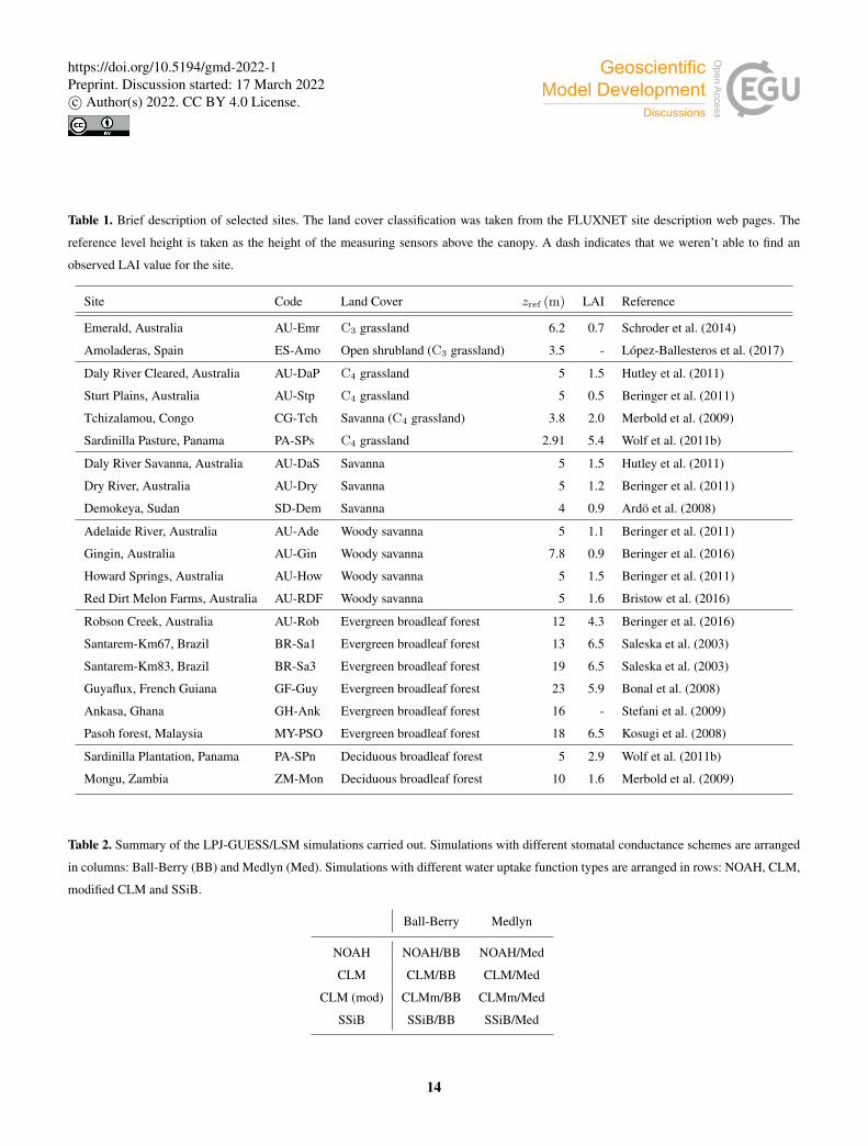
Table 1. Brief description of selected sites. The land cover classification was taken from the FLUXNET site description web pages. The

reference level height is taken as the height of the measuring sensors above the canopy. A dash indicates that we weren’t able to find an

observed LAI value for the site.

Site Code Land Cover zref (m) LAI Reference

Emerald, Australia AU-Emr C3 grassland 6.2 0.7 Schroder et al. (2014)

Amoladeras, Spain ES-Amo Open shrubland (C3 grassland) 3.5 - López-Ballesteros et al. (2017)

Daly River Cleared, Australia AU-DaP C4 grassland 5 1.5 Hutley et al. (2011)

Sturt Plains, Australia AU-Stp C4 grassland 5 0.5 Beringer et al. (2011)

Tchizalamou, Congo CG-Tch Savanna (C4 grassland) 3.8 2.0 Merbold et al. (2009)

Sardinilla Pasture, Panama PA-SPs C4 grassland 2.91 5.4 Wolf et al. (2011b)

Daly River Savanna, Australia AU-DaS Savanna 5 1.5 Hutley et al. (2011)

Dry River, Australia AU-Dry Savanna 5 1.2 Beringer et al. (2011)

Demokeya, Sudan SD-Dem Savanna 4 0.9 Ardö et al. (2008)

Adelaide River, Australia AU-Ade Woody savanna 5 1.1 Beringer et al. (2011)

Gingin, Australia AU-Gin Woody savanna 7.8 0.9 Beringer et al. (2016)

Howard Springs, Australia AU-How Woody savanna 5 1.5 Beringer et al. (2011)

Red Dirt Melon Farms, Australia AU-RDF Woody savanna 5 1.6 Bristow et al. (2016)

Robson Creek, Australia AU-Rob Evergreen broadleaf forest 12 4.3 Beringer et al. (2016)

Santarem-Km67, Brazil BR-Sa1 Evergreen broadleaf forest 13 6.5 Saleska et al. (2003)

Santarem-Km83, Brazil BR-Sa3 Evergreen broadleaf forest 19 6.5 Saleska et al. (2003)

Guyaflux, French Guiana GF-Guy Evergreen broadleaf forest 23 5.9 Bonal et al. (2008)

Ankasa, Ghana GH-Ank Evergreen broadleaf forest 16 - Stefani et al. (2009)

Pasoh forest, Malaysia MY-PSO Evergreen broadleaf forest 18 6.5 Kosugi et al. (2008)

Sardinilla Plantation, Panama PA-SPn Deciduous broadleaf forest 5 2.9 Wolf et al. (2011b)

Mongu, Zambia ZM-Mon Deciduous broadleaf forest 10 1.6 Merbold et al. (2009)

Table 2. Summary of the LPJ-GUESS/LSM simulations carried out. Simulations with different stomatal conductance schemes are arranged

in columns: Ball-Berry (BB) and Medlyn (Med). Simulations with different water uptake function types are arranged in rows: NOAH, CLM,

modified CLM and SSiB.

Ball-Berry Medlyn

NOAH NOAH/BB NOAH/Med

CLM CLM/BB CLM/Med

CLM (mod) CLMm/BB CLMm/Med

SSiB SSiB/BB SSiB/Med

14


throughout the measuring period. We additionally discarded wetland sites, which require a more detailed representation of soil

and ground water hydrology (Wania et al., 2009). A list of the selected sites is presented in Table 1. The location of the sites is

represented on the world map in Fig. 6.

For each site, we ran 8 simulations, covering all possible configurations of the water uptake functions and stomatal con-

ductance schemes described in Sec. 2.2.4 (Table 2). We used the climate data collected at the tower sites to force the model.375

Half-hourly forcing data was converted to hourly averages, and we set a lower boundary of 10% of the dataset median on

the air humidity to correct for physically invalid negative values. Nitrogen deposition data is from Lamarque et al. (2013).

Atmospheric CO2 concentration data is from McGuire et al. (2001). Additionally, we ran a standard (non-LSM) LPJ-GUESS

simulation to compare both model versions’ predictions of monthly evapotranspiration and a number of ecosystem structure

and function variables. The number of replicate patches was set to 100 in all the simulations to avoid spurious effects of the380

stochastic ecosystem processes on the modeled fluxes.

All natural PFTs were allowed to establish in forest and savanna sites. Since the focus of the model evaluation was placed

on the predicted turbulent fluxes, we restricted the simulated PFTs to grassy types at sites classified as grasslands, which limits

modeled surface roughness. This was also done for Spain-Amoladeras and Congo-Tchizalamou. Amoladeras is classified as

an open shrubland on the FLUXNET reference, but the vegetation is short and the most abundant species is Machrocloa385

Tenacissima, a type of grass (López-Ballesteros et al., 2017). Tchizalamou, which is classified as savanna, is actually a C4

grassland (Merbold et al., 2009).

The simulations were spun up for a standard period of 500 years from a bare ground state to bring C and N soil and vegetation

pools to near-equilibrium with the climate (see, e.g., Smith et al., 2014). During the spin-up phase, the site climate spanning the

whole measurement period was repeated cyclically, with interannual trends in air temperature removed, and the atmospheric390

CO2 concentration was kept at the level of the first year of observations at each site.

3.3 Analysis

Half-hourly measured fluxes were converted to hourly averages for direct comparison with model outputs. Subdaily FLUXNET

data are classified into four quality categories: 0 (measured), 1 (good quality gap fill), 2 (poor quality gap fill) and 3 (downscale

from ERA reanalysis data). In our analysis, we only used subdaily fluxes with a quality flag of 0 or 1. For monthly and annual395

fluxes, the quality flag varies between 0 and 1, and indicates the fraction of the subdaily values in that month/year whose

quality is either 0 or 1. We only used monthly and annual fluxes with a quality flag equal to or greater than 0.75. Following

Stöckli et al. (2008), we further discarded fluxes with friction velocity u∗ < 0.2ms−1 in order to avoid possibly biased eddy

covariance measurements during periods of weak turbulence (Schroder et al., 2014).

To evaluate the agreement between measured and simulated turbulent heat fluxes at each site for all different model configu-400

rations we used standard statistical metrics: correlation coefficient (r), mean bias, and root mean square error (RMSE). We also

considered the standard deviation of the modeled fluxes normalized by the standard deviation of the observed fluxes (σm/σo),

which provides a measure of the agreement between observed and simulated variability.

15


3.4 Results

3.4.1 Annual and diurnal cycles of turbulent heat fluxes405

Figure 7 shows examples of simulated and observed monthly averages of turbulent and latent heat fluxes over the course of

a year at four sites: Gingin (AU-Gin), Daly River Savanna (AU-DaS), Santarem Km67 (BR-Sa1) and Guyaflux (GF-Guy).

Examples of the monthly-averaged diurnal cycle for the same sites are shown in Figs. 8 and 9. We chose these sites and years

to illustrate situations with varying degrees of agreement between simulations and measurements. The simulated fluxes are

from the run using the CLM-type water uptake function and the Medlyn model of stomatal conductance.410

At the AU-Gin site, the shape of the annual cycles of latent and sensible heat is similar to the observed (Fig. 7, upper left).

Sensible heat is largest at the beginning of the year, decreases steeply to its minimum around June-July, and starts increasing

again around August. The simulation agrees very well with measurements most of the year, but overestimates sensible heat

by ∼ 40Wm−2 in the first two months. Observed latent heat dominates the turbulent exchange in the wet season (from May

to September). Simulated latent heat is overestimated by up to ∼ 25Wm−2 during the wet season. The shift from larger415

sensible heat to larger latent heat in May is well captured in the simulation, but, due to the overestimation of latent heat,

the shift back to larger sensible heat flux at the beginning of the dry season is delayed by about a month with respect to

the observations. The average simulated diurnal cycle of sensible heat is overestimated in January, peaking at ∼ 700Wm−2

(observed: ∼ 500Wm−2), while it agrees very well with observations in May and September, both in terms of magnitude and

day-to-day variability.420

At the AU-DaS site (Fig. 7, upper right panel), the shapes of measured and simulated annual cycles match relatively well at

the beginning and the end of the year, but diverge substantially during the dry season. Simulated monthly averages of latent heat

are ∼ 20Wm−2 above measured values from March to May, and ∼ 30Wm−2 below the measurements between August and

October. The average simulated diurnal cycle peaks at ∼ 300Wm−2 in May (observed: ∼ 175Wm−2), and at ∼ 30Wm−2

in September (observed: ∼ 150Wm−2; Fig. 8, lower half). This marked divergence from measured values happens in very425

dry periods, when the simulated soil moisture in the rooting zone drops close to the wilting point and there is not enough

precipitation to replenish it until the start of the wet season. As a consequence, sensible heat is greatly overestimated. Simulated

monthly averages rise sharply and peak at ∼ 120–140Wm−2 from September to October, while measured values stay at

∼ 60Wm−2 throughout the dry season. The average sensible heat diurnal cycle peaks at ∼ 530Wm−2 in September, while

the observed average diurnal peak is slightly under ∼ 300Wm−2 (Fig. 8).430

Monthly averages of sensible and latent heat at the BR-Sa1 tropical rainforest site show little variability throughout the year

(Fig. 7, lower left). Measured sensible heat flux stays at∼ 20Wm−2 for most of the year, and increases to∼ 30Wm−2 around

August and September, when measured precipitation reaches its minimum. During this period, the soil retains enough moisture

in the rooting zone to maintain average latent heat levels at ∼ 80–90Wm−2. Sensible and latent heat fluxes are systematically

overestimated by the model by∼ 10–20Wm−2. Average sensible heat flux peaks daily between∼ 170–230Wm−2 (measured:435

∼ 100Wm−2). Latent heat flux peaks daily between ∼ 300–370Wm−2 (measured: ∼ 280–320Wm−2, Fig. 9).

16


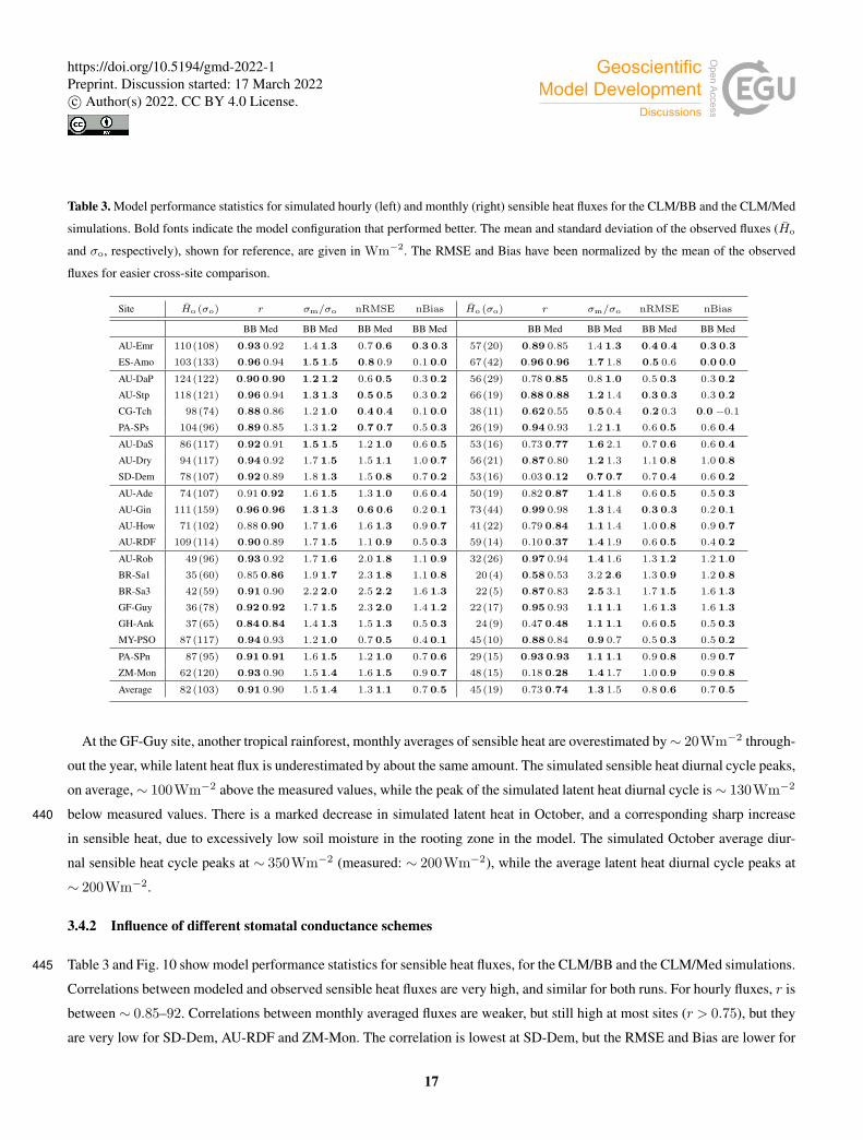
Table 3. Model performance statistics for simulated hourly (left) and monthly (right) sensible heat fluxes for the CLM/BB and the CLM/Med

simulations. Bold fonts indicate the model configuration that performed better. The mean and standard deviation of the observed fluxes (Ho

and σo, respectively), shown for reference, are given in Wm−2. The RMSE and Bias have been normalized by the mean of the observed

fluxes for easier cross-site comparison.

Site Ho (σo) r σm/σo nRMSE nBias Ho (σo) r σm/σo nRMSE nBias

BB Med BB Med BB Med BB Med BB Med BB Med BB Med BB Med

AU-Emr 110(108) 0.93 0.92 1.4 1.3 0.7 0.6 0.3 0.3 57(20) 0.89 0.85 1.4 1.3 0.4 0.4 0.3 0.3

ES-Amo 103(133) 0.96 0.94 1.5 1.5 0.8 0.9 0.1 0.0 67(42) 0.96 0.96 1.7 1.8 0.5 0.6 0.0 0.0

AU-DaP 124(122) 0.90 0.90 1.2 1.2 0.6 0.5 0.3 0.2 56(29) 0.78 0.85 0.8 1.0 0.5 0.3 0.3 0.2

AU-Stp 118(121) 0.96 0.94 1.3 1.3 0.5 0.5 0.3 0.2 66(19) 0.88 0.88 1.2 1.4 0.3 0.3 0.3 0.2

CG-Tch 98(74) 0.88 0.86 1.2 1.0 0.4 0.4 0.1 0.0 38(11) 0.62 0.55 0.5 0.4 0.2 0.3 0.0−0.1

PA-SPs 104(96) 0.89 0.85 1.3 1.2 0.7 0.7 0.5 0.3 26(19) 0.94 0.93 1.2 1.1 0.6 0.5 0.6 0.4

AU-DaS 86(117) 0.92 0.91 1.5 1.5 1.2 1.0 0.6 0.5 53(16) 0.73 0.77 1.6 2.1 0.7 0.6 0.6 0.4

AU-Dry 94(117) 0.94 0.92 1.7 1.5 1.5 1.1 1.0 0.7 56(21) 0.87 0.80 1.2 1.3 1.1 0.8 1.0 0.8

SD-Dem 78(107) 0.92 0.89 1.8 1.3 1.5 0.8 0.7 0.2 53(16) 0.03 0.12 0.7 0.7 0.7 0.4 0.6 0.2

AU-Ade 74(107) 0.91 0.92 1.6 1.5 1.3 1.0 0.6 0.4 50(19) 0.82 0.87 1.4 1.8 0.6 0.5 0.5 0.3

AU-Gin 111(159) 0.96 0.96 1.3 1.3 0.6 0.6 0.2 0.1 73(44) 0.99 0.98 1.3 1.4 0.3 0.3 0.2 0.1

AU-How 71(102) 0.88 0.90 1.7 1.6 1.6 1.3 0.9 0.7 41(22) 0.79 0.84 1.1 1.4 1.0 0.8 0.9 0.7

AU-RDF 109(114) 0.90 0.89 1.7 1.5 1.1 0.9 0.5 0.3 59(14) 0.10 0.37 1.4 1.9 0.6 0.5 0.4 0.2

AU-Rob 49(96) 0.93 0.92 1.7 1.6 2.0 1.8 1.1 0.9 32(26) 0.97 0.94 1.4 1.6 1.3 1.2 1.2 1.0

BR-Sa1 35(60) 0.85 0.86 1.9 1.7 2.3 1.8 1.1 0.8 20(4) 0.58 0.53 3.2 2.6 1.3 0.9 1.2 0.8

BR-Sa3 42(59) 0.91 0.90 2.2 2.0 2.5 2.2 1.6 1.3 22(5) 0.87 0.83 2.5 3.1 1.7 1.5 1.6 1.3

GF-Guy 36(78) 0.92 0.92 1.7 1.5 2.3 2.0 1.4 1.2 22(17) 0.95 0.93 1.1 1.1 1.6 1.3 1.6 1.3

GH-Ank 37(65) 0.84 0.84 1.4 1.3 1.5 1.3 0.5 0.3 24(9) 0.47 0.48 1.1 1.1 0.6 0.5 0.5 0.3

MY-PSO 87(117) 0.94 0.93 1.2 1.0 0.7 0.5 0.4 0.1 45(10) 0.88 0.84 0.9 0.7 0.5 0.3 0.5 0.2

PA-SPn 87(95) 0.91 0.91 1.6 1.5 1.2 1.0 0.7 0.6 29(15) 0.93 0.93 1.1 1.1 0.9 0.8 0.9 0.7

ZM-Mon 62(120) 0.93 0.90 1.5 1.4 1.6 1.5 0.9 0.7 48(15) 0.18 0.28 1.4 1.7 1.0 0.9 0.9 0.8

Average 82(103) 0.91 0.90 1.5 1.4 1.3 1.1 0.7 0.5 45(19) 0.73 0.74 1.3 1.5 0.8 0.6 0.7 0.5

At the GF-Guy site, another tropical rainforest, monthly averages of sensible heat are overestimated by∼ 20Wm−2 through-

out the year, while latent heat flux is underestimated by about the same amount. The simulated sensible heat diurnal cycle peaks,

on average,∼ 100Wm−2 above the measured values, while the peak of the simulated latent heat diurnal cycle is∼ 130Wm−2

below measured values. There is a marked decrease in simulated latent heat in October, and a corresponding sharp increase440

in sensible heat, due to excessively low soil moisture in the rooting zone in the model. The simulated October average diur-

nal sensible heat cycle peaks at ∼ 350Wm−2 (measured: ∼ 200Wm−2), while the average latent heat diurnal cycle peaks at

∼ 200Wm−2.

3.4.2 Influence of different stomatal conductance schemes

Table 3 and Fig. 10 show model performance statistics for sensible heat fluxes, for the CLM/BB and the CLM/Med simulations.445

Correlations between modeled and observed sensible heat fluxes are very high, and similar for both runs. For hourly fluxes, r is

between ∼ 0.85–92. Correlations between monthly averaged fluxes are weaker, but still high at most sites (r > 0.75), but they

are very low for SD-Dem, AU-RDF and ZM-Mon. The correlation is lowest at SD-Dem, but the RMSE and Bias are lower for

17


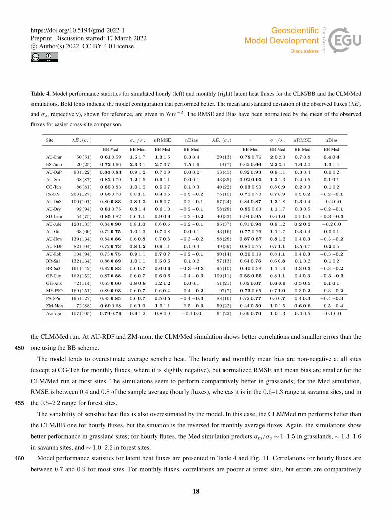
Table 4. Model performance statistics for simulated hourly (left) and monthly (right) latent heat fluxes for the CLM/BB and the CLM/Med

simulations. Bold fonts indicate the model configuration that performed better. The mean and standard deviation of the observed fluxes (λEo

and σo, respectively), shown for reference, are given in Wm−2. The RMSE and Bias have been normalized by the mean of the observed

fluxes for easier cross-site comparison.

Site λEo (σo) r σm/σo nRMSE nBias λEo (σo) r σm/σo nRMSE nBias

BB Med BB Med BB Med BB Med BB Med BB Med BB Med BB Med

AU-Emr 50(51) 0.61 0.59 1.5 1.7 1.3 1.5 0.3 0.4 29(13) 0.78 0.76 2.0 2.3 0.7 0.8 0.4 0.4

ES-Amo 20(25) 0.72 0.66 2.3 3.1 2.7 3.7 1.5 1.6 14(7) 0.62 0.66 2.2 3.4 1.6 2.0 1.3 1.4

AU-DaP 93(122) 0.84 0.84 0.9 1.2 0.7 0.9 0.0 0.2 53(45) 0.92 0.93 0.9 1.1 0.3 0.4 0.0 0.2

AU-Stp 68(87) 0.82 0.79 1.2 1.5 0.9 1.1 0.0 0.1 43(35) 0.92 0.92 1.2 1.3 0.4 0.5 0.1 0.1

CG-Tch 86(81) 0.85 0.83 1.0 1.2 0.5 0.7 0.1 0.3 40(22) 0.93 0.90 0.8 0.9 0.2 0.3 0.1 0.2

PA-SPs 208(127) 0.85 0.78 0.8 1.1 0.4 0.5 −0.3−0.2 75(18) 0.71 0.70 0.7 0.9 0.3 0.2 −0.2−0.1

AU-DaS 100(101) 0.80 0.83 0.8 1.2 0.6 0.7 −0.2−0.1 67(24) 0.84 0.87 1.3 1.8 0.3 0.4 −0.2 0.0

AU-Dry 92(94) 0.81 0.75 0.8 1.4 0.6 1.0 −0.2−0.1 58(28) 0.85 0.83 1.1 1.7 0.3 0.5 −0.2−0.1

SD-Dem 54(75) 0.85 0.82 0.6 1.1 0.9 0.9 −0.3−0.2 40(33) 0.94 0.95 0.6 1.0 0.5 0.4 −0.3−0.3

AU-Ade 120(133) 0.84 0.90 0.8 1.0 0.6 0.5 −0.2−0.1 85(37) 0.91 0.94 0.9 1.2 0.2 0.2 −0.2 0.0

AU-Gin 63(60) 0.72 0.75 1.0 1.3 0.7 0.8 0.0 0.1 43(16) 0.77 0.76 1.1 1.7 0.3 0.4 0.0 0.1

AU-How 139(134) 0.84 0.86 0.6 0.8 0.7 0.6 −0.3−0.2 88(28) 0.87 0.87 0.8 1.2 0.4 0.3 −0.3−0.2

AU-RDF 82(104) 0.72 0.73 0.8 1.2 0.9 1.1 0.1 0.4 49(39) 0.81 0.75 0.7 1.1 0.5 0.7 0.2 0.5

AU-Rob 104(94) 0.73 0.75 0.9 1.1 0.7 0.7 −0.2−0.1 80(14) 0.20 0.19 0.8 1.1 0.4 0.3 −0.3−0.2

BR-Sa1 132(134) 0.86 0.89 1.0 1.1 0.5 0.5 0.1 0.2 87(13) 0.64 0.76 0.6 0.8 0.1 0.2 0.1 0.2

BR-Sa3 161(142) 0.82 0.83 0.6 0.7 0.6 0.6 −0.3−0.3 95(10) 0.40 0.38 1.1 1.6 0.3 0.3 −0.3−0.2

GF-Guy 162(152) 0.87 0.88 0.6 0.7 0.6 0.6 −0.4−0.3 109(11) 0.55 0.55 0.8 1.1 0.4 0.3 −0.3−0.3

GH-Ank 72(114) 0.65 0.66 0.8 0.8 1.2 1.2 0.0 0.1 51(21) 0.02 0.07 0.6 0.6 0.5 0.5 0.1 0.1

MY-PSO 169(151) 0.89 0.93 0.6 0.7 0.6 0.4 −0.4−0.2 97(7) 0.73 0.65 0.7 1.0 0.3 0.2 −0.3−0.2

PA-SPn 195(127) 0.83 0.85 0.6 0.7 0.5 0.5 −0.4−0.3 88(16) 0.72 0.77 0.6 0.7 0.4 0.3 −0.4−0.3

ZM-Mon 72(88) 0.69 0.68 0.6 1.0 1.0 1.1 −0.5−0.3 59(22) 0.44 0.59 1.0 1.5 0.6 0.6 −0.5−0.4

Average 107(105) 0.79 0.79 0.9 1.2 0.8 0.9 −0.1 0.0 64(22) 0.69 0.70 1.0 1.3 0.4 0.5 −0.1 0.0

the CLM/Med run. At AU-RDF and ZM-mon, the CLM/Med simulation shows better correlations and smaller errors than the

one using the BB scheme.450

The model tends to overestimate average sensible heat. The hourly and monthly mean bias are non-negative at all sites

(except at CG-Tch for monthly fluxes, where it is slightly negative), but normalized RMSE and mean bias are smaller for the

CLM/Med run at most sites. The simulations seem to perform comparatively better in grasslands; for the Med simulation,

RMSE is between 0.4 and 0.8 of the sample average (hourly fluxes), whereas it is in the 0.6–1.3 range at savanna sites, and in

the 0.5–2.2 range for forest sites.455

The variability of sensible heat flux is also overestimated by the model. In this case, the CLM/Med run performs better than

the CLM/BB one for hourly fluxes, but the situation is the reversed for monthly average fluxes. Again, the simulations show

better performance in grassland sites; for hourly fluxes, the Med simulation predicts σm/σo ∼ 1–1.5 in grasslands, ∼ 1.3–1.6

in savanna sites, and ∼ 1.0–2.2 in forest sites.

Model performance statistics for latent heat fluxes are presented in Table 4 and Fig. 11. Correlations for hourly fluxes are460

between 0.7 and 0.9 for most sites. For monthly fluxes, correlations are poorer at forest sites, but errors are comparatively

18


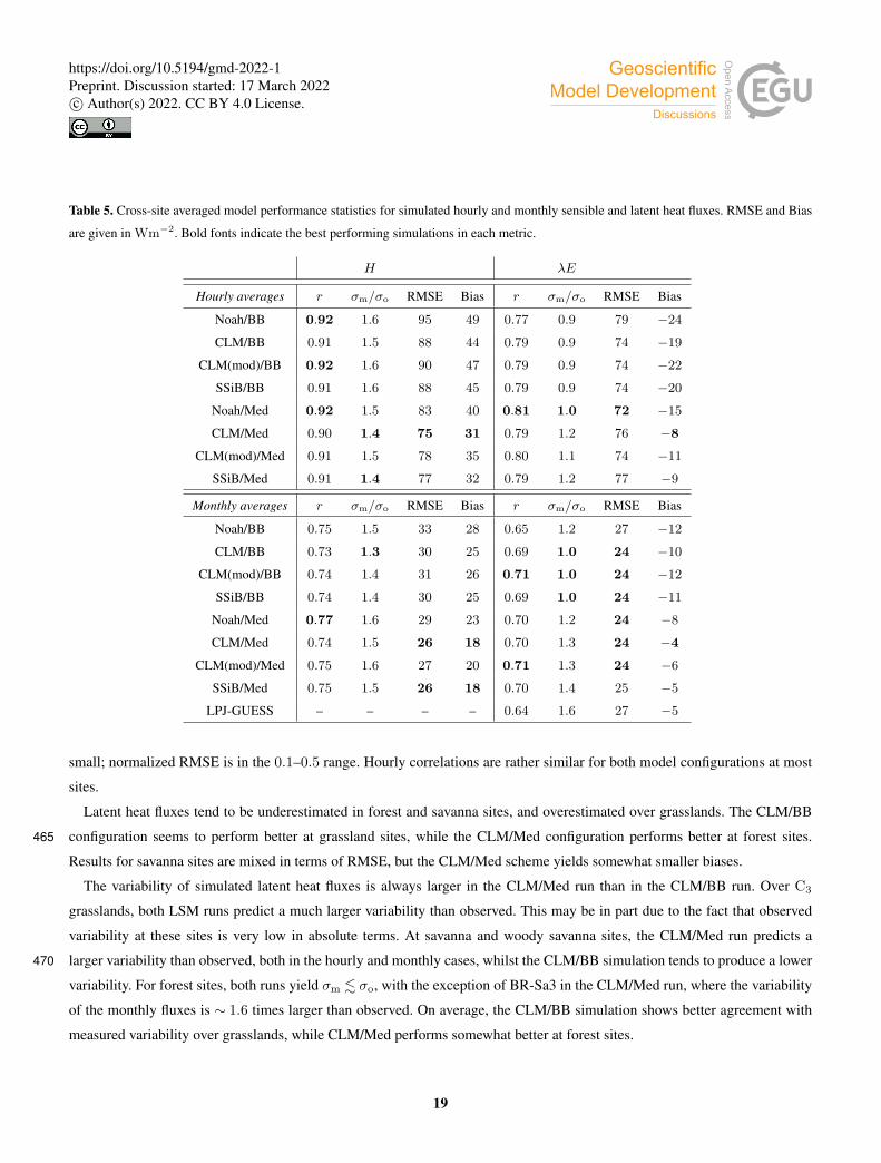
Table 5. Cross-site averaged model performance statistics for simulated hourly and monthly sensible and latent heat fluxes. RMSE and Bias

are given in Wm−2. Bold fonts indicate the best performing simulations in each metric.

H λE

Hourly averages r σm/σo RMSE Bias r σm/σo RMSE Bias

Noah/BB 0.92 1.6 95 49 0.77 0.9 79 −24

CLM/BB 0.91 1.5 88 44 0.79 0.9 74 −19

CLM(mod)/BB 0.92 1.6 90 47 0.79 0.9 74 −22

SSiB/BB 0.91 1.6 88 45 0.79 0.9 74 −20

Noah/Med 0.92 1.5 83 40 0.81 1.0 72 −15

CLM/Med 0.90 1.4 75 31 0.79 1.2 76 −8

CLM(mod)/Med 0.91 1.5 78 35 0.80 1.1 74 −11

SSiB/Med 0.91 1.4 77 32 0.79 1.2 77 −9

Monthly averages r σm/σo RMSE Bias r σm/σo RMSE Bias

Noah/BB 0.75 1.5 33 28 0.65 1.2 27 −12

CLM/BB 0.73 1.3 30 25 0.69 1.0 24 −10

CLM(mod)/BB 0.74 1.4 31 26 0.71 1.0 24 −12

SSiB/BB 0.74 1.4 30 25 0.69 1.0 24 −11

Noah/Med 0.77 1.6 29 23 0.70 1.2 24 −8

CLM/Med 0.74 1.5 26 18 0.70 1.3 24 −4

CLM(mod)/Med 0.75 1.6 27 20 0.71 1.3 24 −6

SSiB/Med 0.75 1.5 26 18 0.70 1.4 25 −5

LPJ-GUESS – – – – 0.64 1.6 27 −5

small; normalized RMSE is in the 0.1–0.5 range. Hourly correlations are rather similar for both model configurations at most

sites.

Latent heat fluxes tend to be underestimated in forest and savanna sites, and overestimated over grasslands. The CLM/BB

configuration seems to perform better at grassland sites, while the CLM/Med configuration performs better at forest sites.465

Results for savanna sites are mixed in terms of RMSE, but the CLM/Med scheme yields somewhat smaller biases.

The variability of simulated latent heat fluxes is always larger in the CLM/Med run than in the CLM/BB run. Over C3

grasslands, both LSM runs predict a much larger variability than observed. This may be in part due to the fact that observed

variability at these sites is very low in absolute terms. At savanna and woody savanna sites, the CLM/Med run predicts a

larger variability than observed, both in the hourly and monthly cases, whilst the CLM/BB simulation tends to produce a lower470

variability. For forest sites, both runs yield σm . σo, with the exception of BR-Sa3 in the CLM/Med run, where the variability

of the monthly fluxes is ∼ 1.6 times larger than observed. On average, the CLM/BB simulation shows better agreement with

measured variability over grasslands, while CLM/Med performs somewhat better at forest sites.

19


3.4.3 Alternative model configurations

To evaluate the overall performance of the different model configurations, we considered the cross-site averaged statistics of475

each simulation (Table 5). Since the covered period differs across sites, this method ensures all sites contribute equally to the

result.

Figure 12 shows the cross-site averaged metrics on a Taylor diagram. The clumping and clear separation of simulations using

different stomatal conductance schemes suggests that this component of the model has a significantly greater influence than the

soil water uptake function on the behaviour of the model, with the exception of the linear (Noah-type) parametrization, which480

is much more restrictive than the other three in terms of water uptake. In this case, both the BB and Med simulations seem to

perform similarly regarding monthly latent heat fluxes, with the variability of the modeled fluxes somewhere in between the

BB and Med clumps.

Simulated sensible heat fluxes display similar correlation with observations in all runs. The correlation coefficient is very

high (r ∼ 0.9) for hourly fluxes, and moderately high (r ∼ 0.75) for monthly averages.485

Sensible heat is overestimated in all model configurations; the average bias is always positive, but the Med simulations

perform better in this respect. In the case of hourly averages, BB runs show an average bias of ∼ 46Wm−2, while the average

value for Med runs is ∼ 35Wm−2. Average errors are also smaller in Med simulations. For hourly fluxes, the average RMSE

is ∼ 90Wm−2 for BB runs, and ∼ 70Wm−2 for Med runs. For monthly fluxes, RMSE averages are ∼ 31Wm−2 and ∼27Wm−2 respectively.490

The model also generally overestimates the variability of sensible heat. For hourly fluxes, the standard deviation of the

sample is, on average, ∼ 1.6 times greater than the measurements for the BB runs, and ∼ 1.5 for the Med runs. In the case of

monthly variability, BB runs perform better; the average standard deviations of modeled fluxes are∼ 1.4 and∼ 1.6 for BB and

Med runs respectively.

Correlations between modeled and measured latent heat fluxes are lower than for sensible heat; r ∼ 0.8 for hourly fluxes495

and ∼ 0.7 for monthly fluxes. All runs show similar RMSE; ∼ 75Wm−2 and ∼ 24Wm−2 for hourly and monthly fluxes

respectively. Latent heat is underestimated on average in all configurations. However, the Med runs perform significantly better

than the BB runs on this metric. The average bias is ∼−11Wm−2 (BB: ∼−21Wm−2) for hourly fluxes, and ∼−6Wm−2

(BB: ∼−11Wm−2) for hourly fluxes. The variability of hourly latent heat fluxes is underestimated in the BB runs by about

the same amount that it is overestimated in the Med runs, but in the case of monthly fluxes, BB simulations seem to reproduce500

the measured variability better (σm ∼ σo, while σm ∼ 1.3σo for Med runs).

Monthly averages of latent heat simulated by the non-LSM version of LPJ-GUESS show a slightly worse correlation with

measurements than the LSM version of the model. The average bias is ∼−5Wm−2, in line with Med simulations and lower

than BB simulations, and the RMSE is slightly higher, but close to the LSM runs. However, the predicted variability is signifi-

cantly exaggerated; the standard deviation of the sample of modeled fluxes is, on average, ∼ 1.6 times larger than observed.505

20


Tabl

e6.

Folia

rpr

ojec

tive

cove

r,av

erag

edov

erth

ew

hole

sim

ulat

edpe

riod

,of

the

plan

tfun

ctio

nalt

ypes

pred

icte

dfo

rea

chsi

te,g

iven

asa

perc

enta

ge.T

heL

SM

sim

ulat

ions

use

the

CL

Mty

pew

ater

upta

kefa

ctor

.The

dom

inan

tPFT

fore

ach

site

ishi

ghlig

hted

inbo

ldfo

nt.

Site

TeB

ETr

BR

TrIB

ETr

BE

C3G

C4G

LPJ

-GB

BM

edL

PJ-G

BB

Med

LPJ

-GB

BM

edL

PJ-G

BB

Med

LPJ

-GB

BM

edL

PJ-G

BB

Med

AU

-Em

r–

––

––

––

––

––

–61

23

24

––

–

ES-

Am

o–

––

––

––

––

––

–61

67

63

––

–

AU

-DaP

––

––

––

––

––

––

1–

–82

94

95

AU

-Stp

––

––

––

––

––

––

1–

–71

56

57

CG

-Tch

––

––

––

––

––

––

1–

–88

98

98

PA-S

Ps–

––

––

––

––

––

––

––

95

98

98

AU

-DaS

––

–11

33

21

414

410

35

––

–61

30

54

AU

-Dry

––

–7

28

–2

61

23

21

––

64

36

85

SD-D

em–

––

19

–1

2–

86

5–

––

38

21

45

AU

-Ade

––

–7

28

22

312

35

36

1–

–63

37

52

AU

-Gin

43

41

31

––

––

––

––

–9

77

––

–

AU

-How

––

–21

40

31

716

12

20

35

––

–41

23

40

AU

-RD

F–

––

10

37

21

415

94

48

1–

–68

20

45

AU

-Rob

––

–57

54

45

29

23

22

21

3–

––

49

10

BR

-Sa1

––

–66

65

63

28

12

23

23

6–

––

86

6

BR

-Sa3

––

–51

50

44

23

21

21

45

3–

––

714

11

GF-

Guy

––

–57

54

50

35

22

23

32

3–

––

712

12

GH

-Ank

––

–61

63

59

24

26

20

26

71

––

83

8

MY

-PSO

––

–53

64

56

26

15

24

44

14

––

–7

65

PA-S

Pn–

––

60

57

51

27

20

20

21

4–

––

68

12

ZM

-Mon

2–

–3

23

43

43

34

52

11

54

44

75

21


Table 7. List of Plant Functional Types in the standard configuration of LPJ-GUESS (only PFTs predicted by the simulations in this study

are listed)

Plant functional type Abbreviation

Temperate Broadleaf Evergreen TeBE

Tropical Broadleaf Raingreen TrBR

Tropical shade-Intolerant Broadleaf Evergreen TrIBE

Tropical Broadleaf Evergreen TrBE

C3 Grass C3G

C4 Grass C4G

3.4.4 Ecosystem structure and function

We compared the predictions of the CLM/BB and the CLM/Med simulations to standard LPJ-GUESS for species composition

and a number of ecosystem structure and function variables.

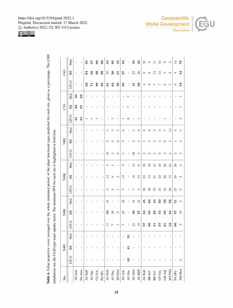
Table 6 shows the FPC of the simulated PFTs (Table 7) at each site. All three simulations predict the same type of grass at

grassland sites. At AU-Emr, the grass coverage predicted by the LSM runs is substantially lower than in standard LPJ-GUESS.510

Land surface model simulations predict a larger FPC at most C4 grassland sites, except at AU-Stp, where FPC is∼ 20% smaller

than in the LPJ-GUESS simulation.

All three simulations predict a temperate forest with a C3 grassy understory at AU-Gin. At the rest of the savanna and woody

savanna sites, the three runs predict a mixture of tropical trees and C4 grasses with a relatively high proportion of the latter. C4

grass is the dominant PFT in the standard LPJ-GUESS and Med simulations, while in the BB simulations the tree coverage is515

close to or larger than that of grasses. In the standard LPJ-GUESS run, the simulated landscape is closer to the savanna IGBP

classification at most sites (tree coverage lower than 30%). The BB simulation predicts a woody savanna (tree coverage higher

than 30%) at all sites except for SD-Dem, while the Med simulation predicts the expected landscape at all sites (Table 1) except

for AU-DaS, where it produces a woody savanna.

At the forest sites, all three simulations predict a mixture of tropical trees and C4 grass, where the coverage of the latter is520

relatively small. The dominant PFT is TrBR, taking between 50 and 65% of the coverage area. A similar prediction is made for

the PA-SPn site, which is classified as a deciduous broadleaf forest. However, for the ZM-Mon site, also a deciduous forest, all

three models yield a PFT composition that is closer to that of savanna sites.

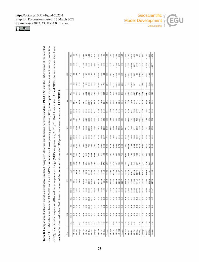
Model predictions for the rest of the selected variables are shown in Table 8. The two C3 grassland sites show different

behaviour with respect to ecosystem productivity and respiration. At AU-Emr, LSM simulations predict substantially lower525

gross primary production (GPP) and autotrophic respiration (Ra) than standard LPJ-GUESS, which results in lower estimates of

net primary production (NPP). This site is a net carbon source (positive net ecosystem exchange, NEE) in all three simulations,

which agrees with observations. Modelled LAI is lower in the LSM simulations, and much closer to the observed value. At ES-

22


Tabl

e8.

Com

pari

son

ofse

lect

edva

riab

les

rela

ted

tosi

mul

ated

ecos

yste

mst

ruct

ure

and

func

tion

betw

een

stan

dard

LPJ

-GU

ESS

and

the

LSM

vers

ion

atth

ese

lect

ed

site

s.T

heL

SMva

lues

are

from

the

CL

M/B

Ban

dth

eC

LM

/Med

sim

ulat

ions

.Gro

sspr

imar

ypr

oduc

tion

(GPP

),au

totr

ophi

cre

spir

atio

n(R

a),n

etpr

imar

ypr

oduc

tion

(NPP

),he

tero

trop

hic

resp

irat

ion

(Rh)

and

nete

cosy

stem

exch

ange

(NE

E)

are

give

nin

gC

m−

2y−

1.B

old

font

sin

the

LA

Ian

dN

EE

colu

mns

indi

cate

the

clos

est

mat

chto

the

obse

rved

valu

e.B

old

font

sin

the

rest

ofth

eco

lum

nsin

dica

teth

eL

SMpr

edic

tion

clos

estt

ost

anda

rdL

PJ-G

UE

SS.

Site

LA

IG

PPR

aN

PPR

hN

EE

Obs

LPJ

-GB

BM

edL

PJ-G

BB

Med

LPJ

-GB

BM

edL

PJ-G

BB

Med

LPJ

-GB

BM

edO

bsL

PJ-G

BB

Med

AU

-Em

r0

.72

.00

.60

.61184

431

414

922

360

330

262

70

84

303

104

93

53

41

33

10

ES-

Am

o–

2.0

2.3

2.1

767

976

850

479

666

540

288

310

310

262

254

233

182

−27

−55

−76

Ave

rage

0.7

2.0

1.4

1.3

976

704

632

700

513

435

275

190

197

283

179

163

118

7−

11

−33

AU

-DaP

1.5

4.0

6.9

7.8

976

1544

1888

296

611

693

681

933

1194

544

807

973

−210

−137

−126

−221

AU

-Stp

0.5

3.0

1.8

2.0

896

548

692

294

215

246

602

333

446

559

299

397

−52

−43

−34

−49

CG

-Tch

2.0

4.5

11

.311

.51020

1965

2019

336

757

780

682

1208

1238

596

1089

1116

−148

−86

−118

−122

PA-S

Ps5

.46

.510

.710

.91447

2026

2099

536

794

823

912

1232

1276

836

1133

1169

277

−76

−98

−107

Ave

rage

2.4

4.5

7.7

8.1

1084

1521

1674

365

594

636

719

926

1039

634

832

914

−33

−86

−94

−125

AU

-DaS

1.5

3.4

3.7

4.2

966

1123

1242

332

541

518

633

582

724

470

425

521

−284

−164

−157

−202

AU

-Dry

1.2

2.8

3.3

4.7

826

1015

1286

263

476

436

563

538

850

428

388

689

−307

−137

−150

−161

SD-D

em0

.91

.31

.21

.3460

421

543

173

195

190

287

225

351

246

189

315

−73

−42

−36

−36

Ave

rage

1.2

2.5

2.7

3.4

751

853

1024

256

404

381

495

449

642

381

334

508

−221

−114

−115

−133

AU

-Ade

1.1

2.8

3.9

4.2

764

1126

1206

235

530

518

529

595

688

400

448

528

−272

−130

−148

−160

AU

-Gin

0.9

1.8

1.9

1.5

1178

1346

1216

914

1109

996

264

236

220

233

234

196

−317

−30

−1

−24

AU

-How

1.5

3.6

4.0

4.4

1073

1223

1298

427

603

588

647

620

710

476

487

529

−692

−171

−133

−181

AU

-RD

F1

.63

.43

.84

.2915

1212

1267

300

633

574

614

579

692

515

492

589

329

−99

−87

−102

Ave

rage

1.3

2.9

3.4

3.6

983

1227

1247

469

719

669

514

507

578

406

415

460

−238

−107

−92

−117

AU

-Rob

4.3

4.7

4.9

4.7

1650

1663

1668

775

800

809

873

861

859

613

626

642

−744

−260

−236

−217

BR

-Sa1

6.5

6.4

5.2

5.7

2266

1910

2022

1137

1038

1058

1130

873

963

939

740

853

−4

−190

−134

−110

BR

-Sa3

6.5

4.5

4.8

4.5

1599

1505

1567

794

739

798

805

766

770

647

646

601

−105

−159

−120

−168

GF-

Guy

5.9

5.5

5.2

5.1

1926

1753

1815

942

882

924

983

871

891

760

683

695

−157

−223

−187

−195

GH

-Ank

–5

.45

.25

.11779

1648

1665

860

844

869

920

803

796

876

701

776

–−

44

−103

−20

MY

-PSO

6.5

5.5

4.6

5.2

2039

1619

1805

993

859

913

1046

759

892

841

616

739

−971

−205

−144

−154

Ave

rage

5.9

5.3

5.0

5.1

1876

1683

1757

917

860

895

959

822

862

779

669

718

−396

−180

−154

−144

PA-S

Pn2

.95

.04

.74

.81654

1550

1605

816

803

810

839

747

794

764

606

640

−458

−75

−143

−155

ZM

-Mon

1.6

2.2

3.5

4.2

621

1002

1101

202

399

370

418

603

731

312

433

581

143

−107

−171

−149

Ave

rage

2.3

3.6

4.1

4.5

1137

1276

1353

509

601

590

629

675

762

538

519

611

−157

−91

−157

−152

23


Amo, GPP is enhanced in the LSM versions, while heterotrophic respiration (Rh) is low compared to standard LPJ-GUESS,

resulting in a slightly enhanced carbon sink in the LSM simulations.530

At three out of four C4 grassland sites, the LSM simulations generate ∼ 50 to 100% higher GPP than LPJ-GUESS. LAI

is extremely high (between ∼ 7 and ∼ 11), and much higher than the observed values. Ra increases too, but not as much,

in absolute terms, as GPP. This results in an increased NPP in the LSM simulations (∼ 30% in the BB run and ∼ 45% in

the Med run, Fig. 13, upper panels). Rh is also enhanced with respect to standard LPJ-GUESS, but again not as much as

NPP, so the CO2 sink is strengthened in both LSM runs (Fig. 13, lower panels). Simulations at the AU-Stp site again show a535

pattern different to the other C4 grassland sites; GPP and NPP simulated in the LSM runs are both lower than in the non-LSM

simulation. However, NPP is substantially higher in the Med simulation than in the BB simulation. This results in NEE being

less negative than in LPJ-GUESS for the BB simulation and more negative than LPJ-GUESS for Med. NEE values predicted

by the Med simulation are closest to the observed fluxes, except at PA-SPs, where all simulations fail to predict a net CO2

source.540

The BB and Med simulations also behave differently at savanna and woody savanna sites. At most sites, BB predicts LAI

values similar to LPJ-GUESS, while Med produces higher LAIs. Both GPP and Ra increase in the LSM runs, but in the BB

simulation the comparatively larger increase in Ra results in an NPP decrease ∼ 8% for savanna and ∼ 2% for woody savanna

with respect to LPJ-GUESS. In the Med simulation, the absolute GPP increase is larger than that ofRa, which results in an NPP

increase of∼ 30% for savanna and∼ 12% for woody savanna relative to the LPJ-GUESS simulation (Fig. 13, upper panels). In545

the BB simulation, Rh is ∼ 12% smaller than the LPJ-GUESS prediction in savanna sites, and close to LPJ-GUESS in woody

savanna sites, which yields similar NEE averages for savanna sites, but a ∼ 15% reduced carbon sink for woody savanna (Fig.

13, lower left). In the Med simulation, savanna and woody savanna show similar tendencies; Rh increases relative to the LPJ-

GUESS run, but not enough to overtake the increase in NPP. As a result, the average net carbon sink is enhanced by ∼ 17% at

savanna sites and by ∼ 9% at woody savanna sites. Observed NEE is generally more negative than the values predicted by the550

simulations, with the exception of AU-RDF, where observations indicate a large net carbon source.

The three simulations slightly underestimate LAI at most evergreen broadleaf forest sites, but the non-LSM version produces

values that are somewhat closer to the observations. Both GPP and Ra are somewhat lower in the LSM simulations, but similar

to the LPJ-GUESS run. The net result is somewhat lower NPP estimates at these sites; a ∼ 14% decrease, relative to LPJ-

GUESS, in the BB simulation and a ∼ 10% decrease in the Med simulation (Fig. 13, upper panels). Rh is also reduced in555

LSM simulations, but the balance with NPP still yields an NEE value above LPJ-GUESS’s diagnostic (increases of ∼ 15%

and ∼ 20% in the BB and the Med simulations, respectively; Fig. 13, lower panels). Observed NEE shows great cross-site

variability. Simulations overestimate the strength of the CO2 sink at the two Brazil sites and the Guiana sites, and greatly

underestimate it at Robson Creek and Pasoh Forest.

The two deciduous broadleaf forest sites show different patterns. At PA-SPn, GPP is somewhat lower in the LSM simulations560

than in LPJ-GUESS, while autotrophic respiration is similar for all three simulations, which results in slightly decreased NPP

values in the LSM runs. However, standard LPJ-GUESS predicts substantially higher heterotrophic respiration, so NEE is

decreased in the LSM runs, but still much higher than the observed value of ∼−458gCm−2y−1. At the ZM-Mon site, GPP,

24


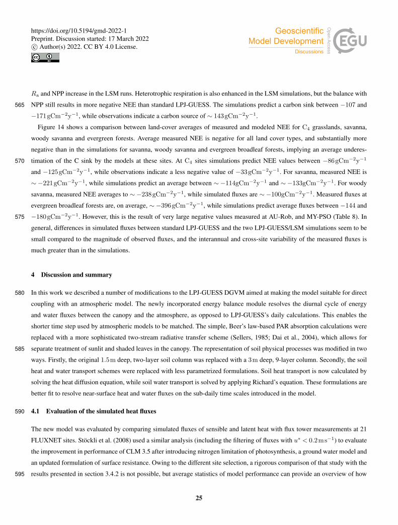
Ra and NPP increase in the LSM runs. Heterotrophic respiration is also enhanced in the LSM simulations, but the balance with

NPP still results in more negative NEE than standard LPJ-GUESS. The simulations predict a carbon sink between −107 and565

−171gCm−2y−1, while observations indicate a carbon source of ∼ 143gCm−2y−1.

Figure 14 shows a comparison between land-cover averages of measured and modeled NEE for C4 grasslands, savanna,

woody savanna and evergreen forests. Average measured NEE is negative for all land cover types, and substantially more

negative than in the simulations for savanna, woody savanna and evergreen broadleaf forests, implying an average underes-

timation of the C sink by the models at these sites. At C4 sites simulations predict NEE values between −86gCm−2y−1570

and −125gCm−2y−1, while observations indicate a less negative value of −33gCm−2y−1. For savanna, measured NEE is

∼−221gCm−2y−1, while simulations predict an average between ∼−114gCm−2y−1 and ∼−133gCm−2y−1. For woody

savanna, measured NEE averages to ∼−238gCm−2y−1, while simulated fluxes are ∼−100gCm−2y−1. Measured fluxes at

evergreen broadleaf forests are, on average, ∼−396gCm−2y−1, while simulations predict average fluxes between −144 and

−180gCm−2y−1. However, this is the result of very large negative values measured at AU-Rob, and MY-PSO (Table 8). In575

general, differences in simulated fluxes between standard LPJ-GUESS and the two LPJ-GUESS/LSM simulations seem to be

small compared to the magnitude of observed fluxes, and the interannual and cross-site variability of the measured fluxes is

much greater than in the simulations.

4 Discussion and summary

In this work we described a number of modifications to the LPJ-GUESS DGVM aimed at making the model suitable for direct580

coupling with an atmospheric model. The newly incorporated energy balance module resolves the diurnal cycle of energy

and water fluxes between the canopy and the atmosphere, as opposed to LPJ-GUESS’s daily calculations. This enables the

shorter time step used by atmospheric models to be matched. The simple, Beer’s law-based PAR absorption calculations were

replaced with a more sophisticated two-stream radiative transfer scheme (Sellers, 1985; Dai et al., 2004), which allows for

separate treatment of sunlit and shaded leaves in the canopy. The representation of soil physical processes was modified in two585

ways. Firstly, the original 1.5m deep, two-layer soil column was replaced with a 3m deep, 9-layer column. Secondly, the soil

heat and water transport schemes were replaced with less parametrized formulations. Soil heat transport is now calculated by

solving the heat diffusion equation, while soil water transport is solved by applying Richard’s equation. These formulations are

better fit to resolve near-surface heat and water fluxes on the sub-daily time scales introduced in the model.

4.1 Evaluation of the simulated heat fluxes590

The new model was evaluated by comparing simulated fluxes of sensible and latent heat with flux tower measurements at 21

FLUXNET sites. Stöckli et al. (2008) used a similar analysis (including the filtering of fluxes with u∗ < 0.2ms−1) to evaluate

the improvement in performance of CLM 3.5 after introducing nitrogen limitation of photosynthesis, a ground water model and

an updated formulation of surface resistance. Owing to the different site selection, a rigorous comparison of that study with the

results presented in section 3.4.2 is not possible, but average statistics of model performance can provide an overview of how595

25


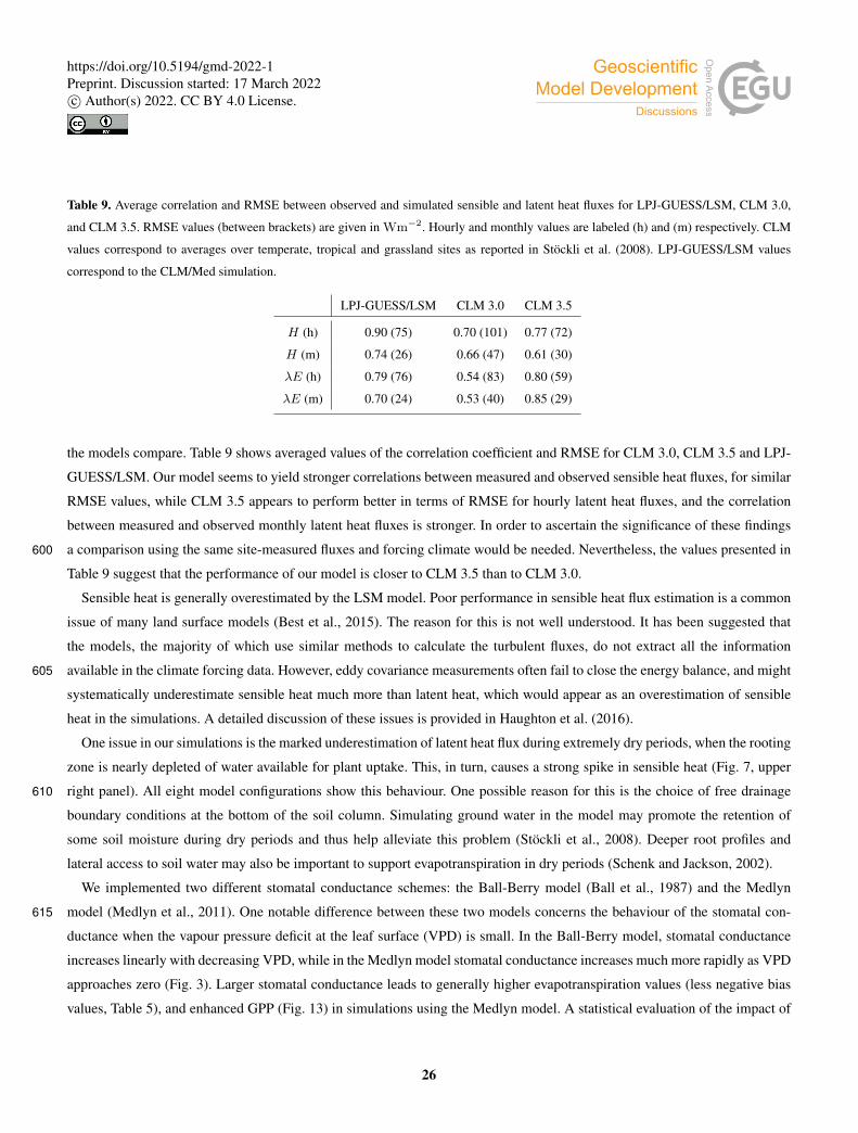
Table 9. Average correlation and RMSE between observed and simulated sensible and latent heat fluxes for LPJ-GUESS/LSM, CLM 3.0,

and CLM 3.5. RMSE values (between brackets) are given in Wm−2. Hourly and monthly values are labeled (h) and (m) respectively. CLM

values correspond to averages over temperate, tropical and grassland sites as reported in Stöckli et al. (2008). LPJ-GUESS/LSM values

correspond to the CLM/Med simulation.

LPJ-GUESS/LSM CLM 3.0 CLM 3.5

H (h) 0.90 (75) 0.70 (101) 0.77 (72)

H (m) 0.74 (26) 0.66 (47) 0.61 (30)

λE (h) 0.79 (76) 0.54 (83) 0.80 (59)

λE (m) 0.70 (24) 0.53 (40) 0.85 (29)

the models compare. Table 9 shows averaged values of the correlation coefficient and RMSE for CLM 3.0, CLM 3.5 and LPJ-

GUESS/LSM. Our model seems to yield stronger correlations between measured and observed sensible heat fluxes, for similar

RMSE values, while CLM 3.5 appears to perform better in terms of RMSE for hourly latent heat fluxes, and the correlation

between measured and observed monthly latent heat fluxes is stronger. In order to ascertain the significance of these findings

a comparison using the same site-measured fluxes and forcing climate would be needed. Nevertheless, the values presented in600

Table 9 suggest that the performance of our model is closer to CLM 3.5 than to CLM 3.0.

Sensible heat is generally overestimated by the LSM model. Poor performance in sensible heat flux estimation is a common

issue of many land surface models (Best et al., 2015). The reason for this is not well understood. It has been suggested that

the models, the majority of which use similar methods to calculate the turbulent fluxes, do not extract all the information

available in the climate forcing data. However, eddy covariance measurements often fail to close the energy balance, and might605

systematically underestimate sensible heat much more than latent heat, which would appear as an overestimation of sensible

heat in the simulations. A detailed discussion of these issues is provided in Haughton et al. (2016).

One issue in our simulations is the marked underestimation of latent heat flux during extremely dry periods, when the rooting

zone is nearly depleted of water available for plant uptake. This, in turn, causes a strong spike in sensible heat (Fig. 7, upper

right panel). All eight model configurations show this behaviour. One possible reason for this is the choice of free drainage610

boundary conditions at the bottom of the soil column. Simulating ground water in the model may promote the retention of

some soil moisture during dry periods and thus help alleviate this problem (Stöckli et al., 2008). Deeper root profiles and

lateral access to soil water may also be important to support evapotranspiration in dry periods (Schenk and Jackson, 2002).

We implemented two different stomatal conductance schemes: the Ball-Berry model (Ball et al., 1987) and the Medlyn

model (Medlyn et al., 2011). One notable difference between these two models concerns the behaviour of the stomatal con-615

ductance when the vapour pressure deficit at the leaf surface (VPD) is small. In the Ball-Berry model, stomatal conductance

increases linearly with decreasing VPD, while in the Medlyn model stomatal conductance increases much more rapidly as VPD

approaches zero (Fig. 3). Larger stomatal conductance leads to generally higher evapotranspiration values (less negative bias

values, Table 5), and enhanced GPP (Fig. 13) in simulations using the Medlyn model. A statistical evaluation of the impact of

26


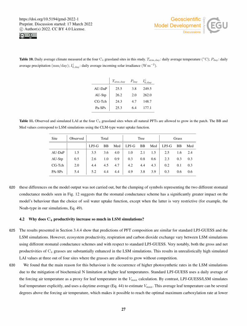
Table 10. Daily average climate measured at the four C4 grassland sites in this study. Tatm,day: daily average temperature (◦C); Pday: daily

average precipitation (mm/day); I↓0,day: daily average incoming solar irradiance (Wm−2).

Tatm,day Pday I↓0,day

AU-DaP 25.5 3.8 249.5

AU-Stp 26.2 2.0 262.0

CG-Tch 24.3 4.7 148.7

Pa-SPs 25.3 6.4 177.1

Table 11. Observed and simulated LAI at the four C4 grassland sites when all natural PFTs are allowed to grow in the patch. The BB and

Med values correspond to LSM simulations using the CLM-type water uptake function.

Site Observed Total Tree Grass

LPJ-G BB Med LPJ-G BB Med LPJ-G BB Med

AU-DaP 1.5 3.5 3.6 4.0 1.0 2.1 1.5 2.5 1.6 2.4

AU-Stp 0.5 2.6 1.0 0.9 0.3 0.8 0.6 2.3 0.3 0.3

CG-Tch 2.0 4.4 4.5 4.7 4.2 4.4 4.3 0.2 0.1 0.3

PA-SPs 5.4 5.2 4.4 4.4 4.9 3.8 3.9 0.3 0.6 0.6

these differences on the model output was not carried out, but the clumping of symbols representing the two different stomatal620

conductance models seen in Fig. 12 suggests that the stomatal conductance scheme has a significantly greater impact on the

model’s behaviour than the choice of soil water uptake function, except when the latter is very restrictive (for example, the

Noah-type in our simulations, Eq. 49).

4.2 Why does C4 productivity increase so much in LSM simulations?

The results presented in Section 3.4.4 show that predictions of PFT composition are similar for standard LPJ-GUESS and the625

LSM simulations. However, ecosystem productivity, respiration and carbon dioxide exchange vary between LSM simulations

using different stomatal conductance schemes and with respect to standard LPJ-GUESS. Very notably, both the gross and net

productivities of C4 grasses are substantially enhanced in the LSM simulations. This results in unrealistically high simulated

LAI values at three out of four sites where the grasses are allowed to grow without competition.

We found that the main reason for this behaviour is the occurrence of higher photosynthetic rates in the LSM simulations630

due to the mitigation of biochemical N limitation at higher leaf temperatures. Standard LPJ-GUESS uses a daily average of

the forcing air temperature as a proxy for leaf temperature in the Vmax calculation. By contrast, LPJ-GUESS/LSM simulates

leaf temperature explicitly, and uses a daytime average (Eq. 44) to estimate Vmax. This average leaf temperature can be several

degrees above the forcing air temperature, which makes it possible to reach the optimal maximum carboxylation rate at lower

27


leaf nitrogen concentrations (see Haxeltine and Prentice, 1996). This makes it easier for the plants to attain the optimal Vmax635

with the available nitrogen, which enhances productivity. Exceedingly high leaf temperatures can have a negative impact on

Vmax due to the thermal breakdown of the biochemical reactions. However, the simulated leaf temperatures are still within the

optimal temperature range for C4 grasses (20 to 45◦C in LPJ-GUESS). The temperature dependence of Vmax, including the

effect on nitrogen limitation, is illustrated in Fig. 15.

At AU-Stp, all three simulations predict much lower productivities. In this case, water availability is the limiting factor. This640

site receives, on average, considerably less rain water than the other three C4 grasslands (Table 10), which leads to lower values

of the β factor (Eq. 48), and brings photosynthetic rates down.

As pointed out in Section 3.2, the simulated PFTs were restricted to grassy types at these sites. Table 11 shows a summary

of LAI values predicted by standard LPJ-GUESS and two representative LSM simulations when establishment is not restricted

to grassy PFTs. All three experiments predict a mixture of trees and grasses, but total LAI in the LSM runs is much lower645

than in the simulations where only grasses were allowed to establish. In these runs, competition with trees limits the resources

available to grasses, and shading from the taller trees helps lowering the average leaf temperature of the grassy understory, all

of which helps counteract the effect described above.

4.3 Conclusion and outlook

The developments presented in this paper will enable to study feedbacks between the climate and the biosphere using the state-650

of-the-art DGVM LPJ-GUESS coupled to an atmospheric model directly. Work is in progress regarding the development of a

flexible interface to enable such coupling, as well as extending the model’s ability to simulate cold-climate ecosystems. More

work is also needed to characterize and fully understand the model’s response to the switch from using air temperature as a

proxy for leaf temperature to simulating leaf temperature explicitly, particularly as these concern the productivity of C4 plants

in well watered, no-competition situations (e.g., monoculture crops or managed pastures). These developments will allow to655

use LPJ-GUESS/LSM in regional as well as global studies. Given the capacity of LPJ-GUESS to represent land use change

and management (Lindeskog et al., 2013, 2021; Olin et al., 2015), the range of applications includes exploring impacts of

management on regional climate, which can be an important tool to help devise and assess climate change mitigation policies.

Code and data availability. LPJ-GUESS is a worldwide developed and refined DGVM. The model code is managed and maintained by

the Department of Physical Geography and Ecosystem Science, Lund University, Sweden. The source code can be made available with a660

collaboration agreement under the acceptance of certain conditions. For this reason, a DOI for the model code cannot be provided. The code

with the augmentations developed for this paper is available to the editor and reviewers via a restricted link, on the condition that the code is

used only for review purposes, and is deleted after the review process. Additional details and information can be found at the LPJ-GUESS

website (http://web.nateko.lu.se/lpj-guess, last access: 17 December 2021). The forcing data, evaluation data, model output and analysis

scripts used in this study have been uploaded to a public repository with DOI 10.5281/zenodo.5813886.665

28


Appendix A: Derivation of the canopy conductance for water vapor flux

During a given time step ∆t, the total amount of water evapotranspirated from the sunlit part of the canopy can be expressed

as the sum of the contributions from the dry and wet parts:

Esun∆t= (1− fwet)Esun,tr∆t

+ fwet[Esun,ev∆twet,sun +Esun,tr(∆t−∆twet,sun)] (A1)670

where Esun is the actual evapotranspiration rate, Esun,tr is the potential rate of transpiration, Esun,ev is the potential rate of

evaporation, and ∆twet,sun is the time that the wet part of the sunlit canopy remains wet at the potential evaporation rate. The

latter is calculated as:

∆twet,sun = min(wcPAIc,sun/PAIc

fwetEsun,ev,∆t), (A2)

where wc is the current canopy water content (kgm−2).675

The evaporation rates in the above equations can be expressed as follows:

Esun =−ρgw,sun[qca− q∗(Tsun)]; (A3)

Etr,sun =−ρ∑

i

LAI(i)sun

g(i)s,sungb

g(i)s,sun + gb

[qca− q∗(Tsun)]; (A4)

Eev,sun =−ρPAIc,sungb[qca− q∗(Tsun)]. (A5)

where the index i runs over cohorts. Inserting these expressions into Eq. (A1), dividing both sides by ∆t, simplifying, and680

rearranging terms yields

gw,sun = fwetηsunPAIc,sungb

+ (1− fwetηsun)∑

i

LAI(i)sun

g(i)s,sungb

g(i)s,sun + gb

, (A6)

where ηsun = ∆twet,sun / ∆t. Identical equations apply to the shaded part of the canopy.

Appendix B: List of symbols, parameters and variables used in the model description685

29


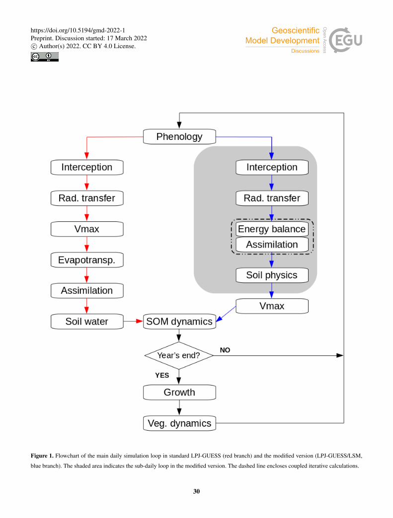
Figure 1. Flowchart of the main daily simulation loop in standard LPJ-GUESS (red branch) and the modified version (LPJ-GUESS/LSM,

blue branch). The shaded area indicates the sub-daily loop in the modified version. The dashed line encloses coupled iterative calculations.

30


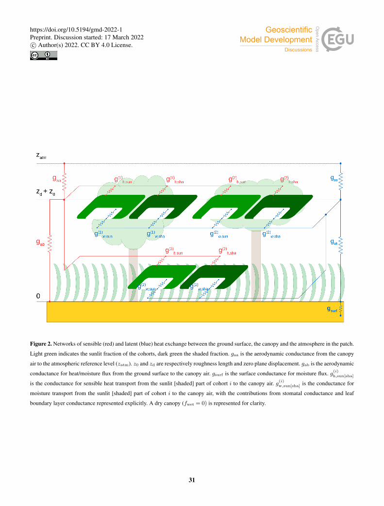
Figure 2. Networks of sensible (red) and latent (blue) heat exchange between the ground surface, the canopy and the atmosphere in the patch.

Light green indicates the sunlit fraction of the cohorts, dark green the shaded fraction. gaa is the aerodynamic conductance from the canopy

air to the atmospheric reference level (zatm). z0 and zd are respectively roughness length and zero plane displacement. gab is the aerodynamic

conductance for heat/moisture flux from the ground surface to the canopy air. gsurf is the surface conductance for moisture flux. g(i)

h,sun[sha]

is the conductance for sensible heat transport from the sunlit [shaded] part of cohort i to the canopy air. g(i)

w,sun[sha] is the conductance for

moisture transport from the sunlit [shaded] part of cohort i to the canopy air, with the contributions from stomatal conductance and leaf

boundary layer conductance represented explicitly. A dry canopy (fwet = 0) is represented for clarity.

31


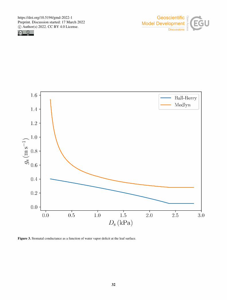
Figure 3. Stomatal conductance as a function of water vapor deficit at the leaf surface.

32


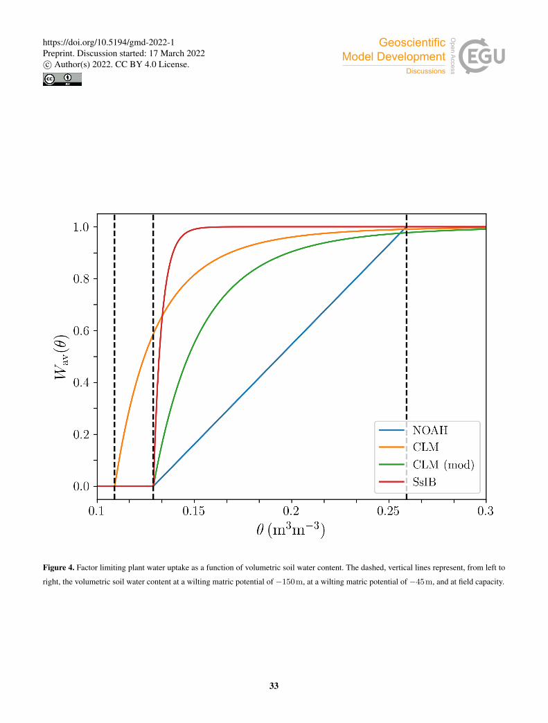
Figure 4. Factor limiting plant water uptake as a function of volumetric soil water content. The dashed, vertical lines represent, from left to

right, the volumetric soil water content at a wilting matric potential of −150m, at a wilting matric potential of −45m, and at field capacity.

33


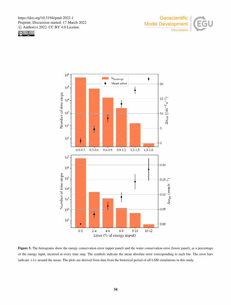
Figure 5. The histograms show the energy conservation error (upper panel) and the water conservation error (lower panel), as a percentage

of the energy input, incurred at every time step. The symbols indicate the mean absolute error corresponding to each bin. The error bars

indicate ±1σ around the mean. The plots are derived from data from the historical period of all LSM simulations in this study.

34


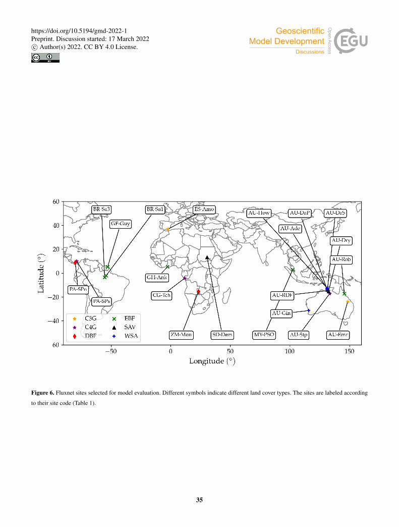
Figure 6. Fluxnet sites selected for model evaluation. Different symbols indicate different land cover types. The sites are labeled according

to their site code (Table 1).

35


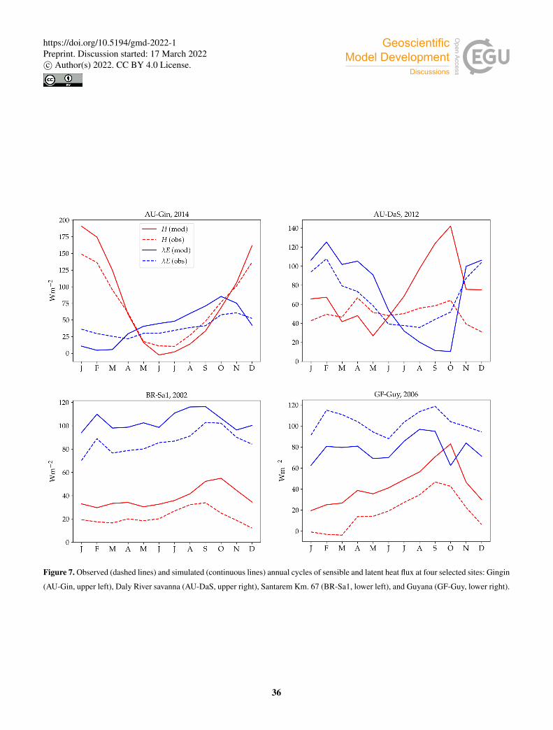
Figure 7. Observed (dashed lines) and simulated (continuous lines) annual cycles of sensible and latent heat flux at four selected sites: Gingin

(AU-Gin, upper left), Daly River savanna (AU-DaS, upper right), Santarem Km. 67 (BR-Sa1, lower left), and Guyana (GF-Guy, lower right).

36


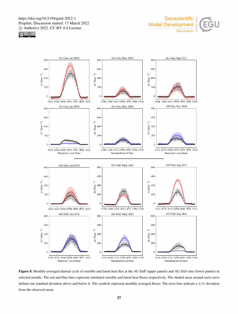
Figure 8. Monthly-averaged diurnal cycle of sensible and latent heat flux at the AU-DaP (upper panels) and AU-DaS sites (lower panels) in

selected months. The red and blue lines represent simulated sensible and latent heat fluxes respectively. The shaded areas around each curve

delimit one standard deviation above and below it. The symbols represent monthly averaged fluxes. The error bars indicate a ±1σ deviation

from the observed mean.

37


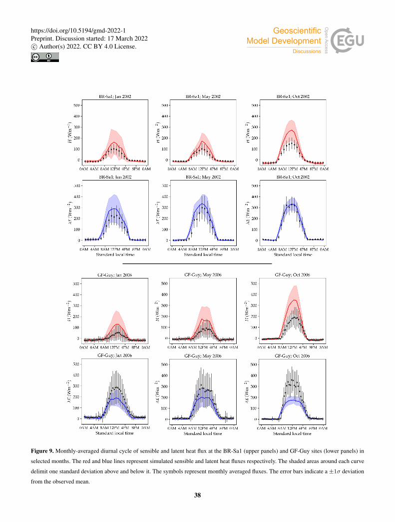
Figure 9. Monthly-averaged diurnal cycle of sensible and latent heat flux at the BR-Sa1 (upper panels) and GF-Guy sites (lower panels) in

selected months. The red and blue lines represent simulated sensible and latent heat fluxes respectively. The shaded areas around each curve

delimit one standard deviation above and below it. The symbols represent monthly averaged fluxes. The error bars indicate a ±1σ deviation

from the observed mean.

38


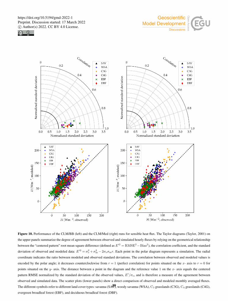
Figure 10. Performance of the CLM/BB (left) and the CLM/Med (right) runs for sensible heat flux. The Taylor diagrams (Taylor, 2001) on

the upper panels summarize the degree of agreement between observed and simulated hourly fluxes by relying on the geometrical relationship

between the “centered pattern” root mean square difference (defined asE′2 = RMSE2−Bias2), the correlation coefficient, and the standard

deviation of observed and modeled data: E′2 = σ2o +σ2

m− 2σoσmr. Each point in the polar diagram represents a simulation. The radial

coordinate indicates the ratio between modeled and observed standard deviations. The correlation between observed and modeled values is

encoded by the polar angle; it decreases counterclockwise from r = 1 (perfect correlation) for points situated on the x- axis to r = 0 for

points situated on the y- axis. The distance between a point in the diagram and the reference value 1 on the x- axis equals the centered

pattern RMSE normalized by the standard deviation of the observed values, E′/σo, and is therefore a measure of the agreement between

observed and simulated data. The scatter plots (lower panels) show a direct comparison of observed and modeled monthly averaged fluxes.

The different symbols refer to different land cover types: savanna (SAV), woody savanna (WSA), C3 grasslands (C3G), C4 grasslands (C4G),

evergreen broadleaf forest (EBF), and deciduous broadleaf forest (DBF).

39


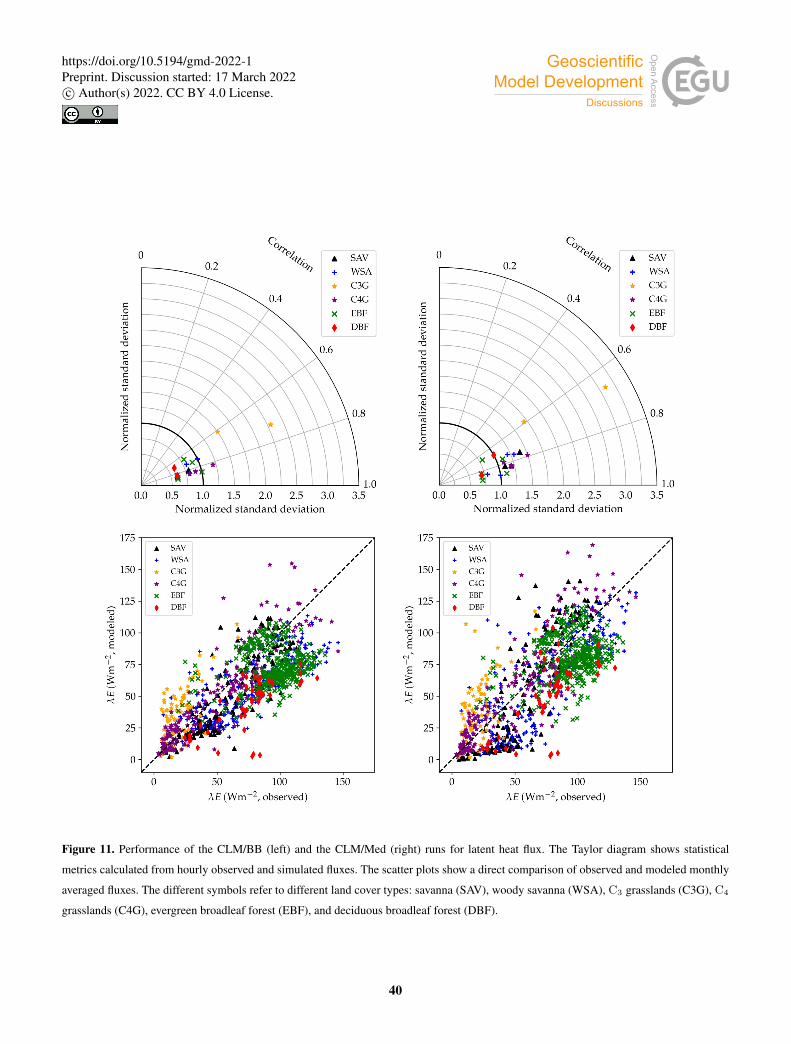
Figure 11. Performance of the CLM/BB (left) and the CLM/Med (right) runs for latent heat flux. The Taylor diagram shows statistical

metrics calculated from hourly observed and simulated fluxes. The scatter plots show a direct comparison of observed and modeled monthly

averaged fluxes. The different symbols refer to different land cover types: savanna (SAV), woody savanna (WSA), C3 grasslands (C3G), C4

grasslands (C4G), evergreen broadleaf forest (EBF), and deciduous broadleaf forest (DBF).

40


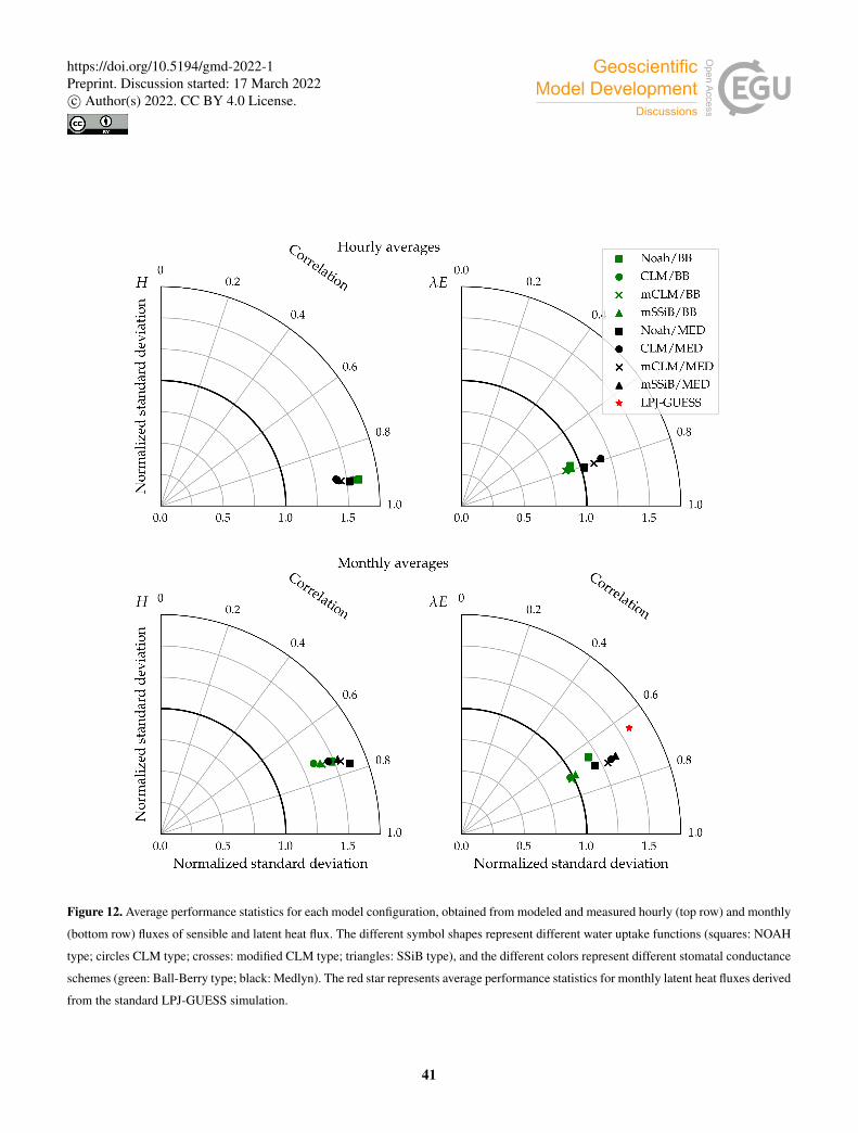
Figure 12. Average performance statistics for each model configuration, obtained from modeled and measured hourly (top row) and monthly

(bottom row) fluxes of sensible and latent heat flux. The different symbol shapes represent different water uptake functions (squares: NOAH

type; circles CLM type; crosses: modified CLM type; triangles: SSiB type), and the different colors represent different stomatal conductance

schemes (green: Ball-Berry type; black: Medlyn). The red star represents average performance statistics for monthly latent heat fluxes derived

from the standard LPJ-GUESS simulation.

41


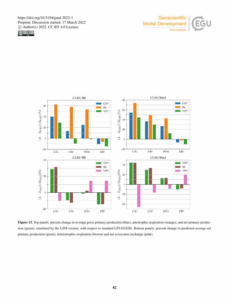
Figure 13. Top panels: percent change in average gross primary production (blue), autotrophic respiration (orange), and net primary produc-

tion (green), simulated by the LSM version, with respect to standard LPJ-GUESS. Bottom panels: percent change in predicted average net

primary production (green), heterotrophic respiration (brown) and net ecosystem exchange (pink).

42


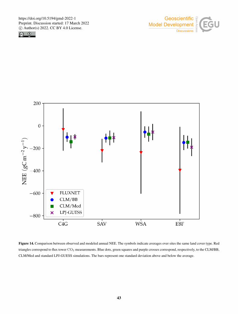
Figure 14. Comparison between observed and modeled annual NEE. The symbols indicate averages over sites the same land cover type. Red

triangles correspond to flux tower CO2 measurements. Blue dots, green squares and purple crosses correspond, respectively, to the CLM/BB,

CLM/Med and standard LPJ-GUESS simulations. The bars represent one standard deviation above and below the average.

43


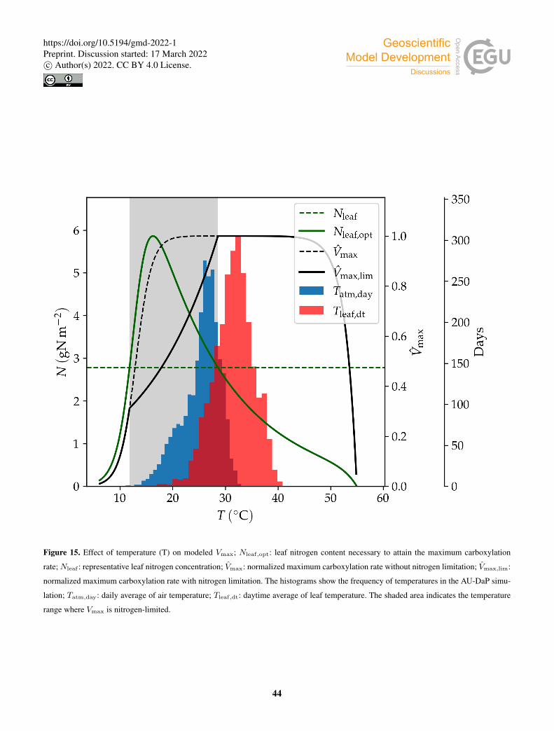
Figure 15. Effect of temperature (T) on modeled Vmax; Nleaf,opt: leaf nitrogen content necessary to attain the maximum carboxylation

rate;Nleaf : representative leaf nitrogen concentration; Vmax: normalized maximum carboxylation rate without nitrogen limitation; Vmax,lim:

normalized maximum carboxylation rate with nitrogen limitation. The histograms show the frequency of temperatures in the AU-DaP simu-

lation; Tatm,day: daily average of air temperature; Tleaf,dt: daytime average of leaf temperature. The shaded area indicates the temperature

range where Vmax is nitrogen-limited.

44


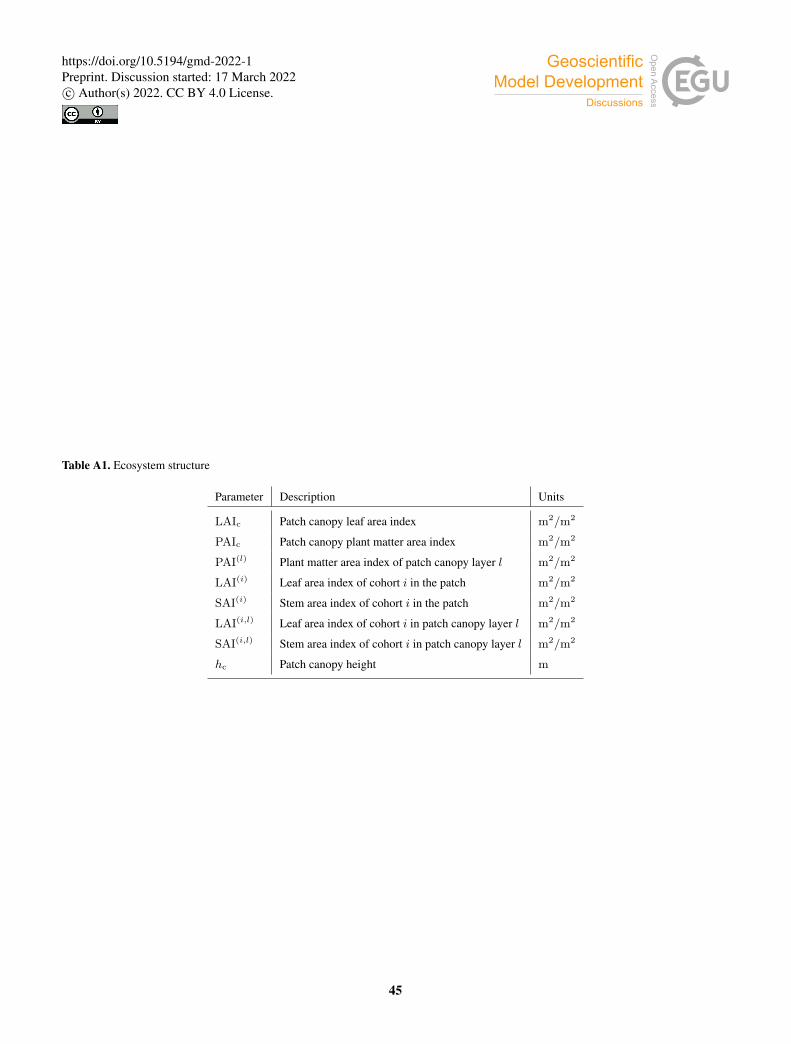
Table A1. Ecosystem structure

Parameter Description Units

LAIc Patch canopy leaf area index m2/m2

PAIc Patch canopy plant matter area index m2/m2

PAI(l) Plant matter area index of patch canopy layer l m2/m2

LAI(i) Leaf area index of cohort i in the patch m2/m2

SAI(i) Stem area index of cohort i in the patch m2/m2

LAI(i,l) Leaf area index of cohort i in patch canopy layer l m2/m2

SAI(i,l) Stem area index of cohort i in patch canopy layer l m2/m2

hc Patch canopy height m

45


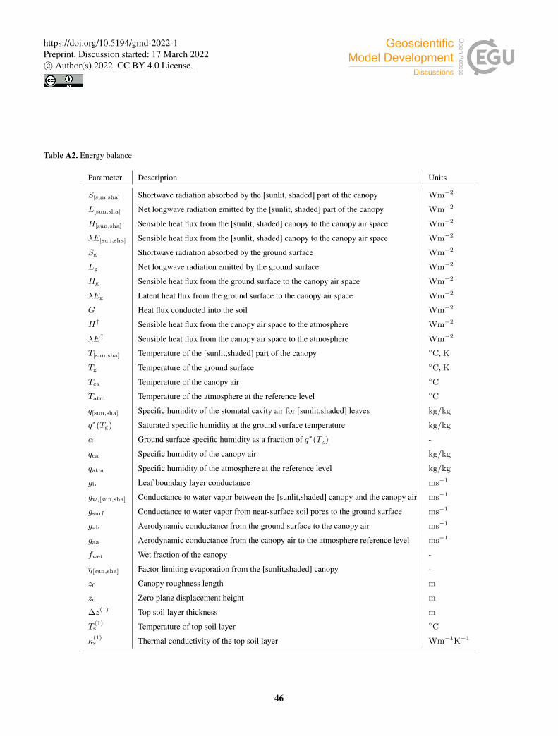
Table A2. Energy balance


S[sun,sha] Shortwave radiation absorbed by the [sunlit, shaded] part of the canopy Wm−2

L[sun,sha] Net longwave radiation emitted by the [sunlit, shaded] part of the canopy Wm−2

H[sun,sha] Sensible heat flux from the [sunlit, shaded] canopy to the canopy air space Wm−2

λE[sun,sha] Sensible heat flux from the [sunlit, shaded] canopy to the canopy air space Wm−2

Sg Shortwave radiation absorbed by the ground surface Wm−2

Lg Net longwave radiation emitted by the ground surface Wm−2

Hg Sensible heat flux from the ground surface to the canopy air space Wm−2

λEg Latent heat flux from the ground surface to the canopy air space Wm−2

G Heat flux conducted into the soil Wm−2

H↑ Sensible heat flux from the canopy air space to the atmosphere Wm−2

λE↑ Sensible heat flux from the canopy air space to the atmosphere Wm−2

T[sun,sha] Temperature of the [sunlit,shaded] part of the canopy ◦C, K

Tg Temperature of the ground surface ◦C, K

Tca Temperature of the canopy air ◦C

Tatm Temperature of the atmosphere at the reference level ◦C

q[sun,sha] Specific humidity of the stomatal cavity air for [sunlit,shaded] leaves kg/kg

q∗(Tg) Saturated specific humidity at the ground surface temperature kg/kg

α Ground surface specific humidity as a fraction of q∗(Tg) -

qca Specific humidity of the canopy air kg/kg

qatm Specific humidity of the atmosphere at the reference level kg/kg

gb Leaf boundary layer conductance ms−1

gw,[sun,sha] Conductance to water vapor between the [sunlit,shaded] canopy and the canopy air ms−1

gsurf Conductance to water vapor from near-surface soil pores to the ground surface ms−1

gab Aerodynamic conductance from the ground surface to the canopy air ms−1

gaa Aerodynamic conductance from the canopy air to the atmosphere reference level ms−1

fwet Wet fraction of the canopy -

η[sun,sha] Factor limiting evaporation from the [sunlit,shaded] canopy -

z0 Canopy roughness length m

zd Zero plane displacement height m

∆z(1) Top soil layer thickness m

T(1)s Temperature of top soil layer ◦C

κ(1)s Thermal conductivity of the top soil layer Wm−1K−1

46


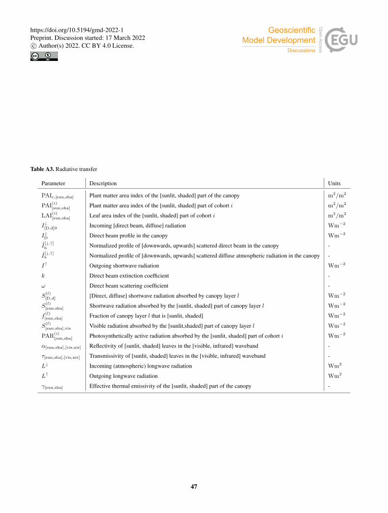
Table A3. Radiative transfer


PAIc,[sun,sha] Plant matter area index of the [sunlit, shaded] part of the canopy m2/m2

PAI(i)

[sun,sha] Plant matter area index of the [sunlit, shaded] part of cohort i m2/m2

LAI(i)

[sun,sha] Leaf area index of the [sunlit, shaded] part of cohort i m2/m2

I↓[D,d]0 Incoming [direct beam, diffuse] radiation Wm−2

I↓D Direct beam profile in the canopy Wm−2

I[↓,↑]b Normalized profile of [downwards, upwards] scattered direct beam in the canopy -

I[↓,↑]a Normalized profile of [downwards, upwards] scattered diffuse atmospheric radiation in the canopy -

I↑ Outgoing shortwave radiation Wm−2

k Direct beam extinction coefficient -

ω Direct beam scattering coefficient -

S(l)

[D,d] [Direct, diffuse] shortwave radiation absorbed by canopy layer l Wm−2

S(l)

[sun,sha] Shortwave radiation absorbed by the [sunlit, shaded] part of canopy layer l Wm−2

f(l)

[sun,sha] Fraction of canopy layer l that is [sunlit, shaded] Wm−2

S(l)

[sun,sha],vis Visible radiation absorbed by the [sunlit,shaded] part of canopy layer l Wm−2

PAR(i)

[sun,sha] Photosynthetically active radiation absorbed by the [sunlit, shaded] part of cohort i Wm−2

α[sun,sha],[vis,nir] Reflectivity of [sunlit, shaded] leaves in the [visible, infrared] waveband -

τ[sun,sha],[vis,nir] Transmissivity of [sunlit, shaded] leaves in the [visible, infrared] waveband -

L↓ Incoming (atmospheric) longwave radiation Wm2

L↑ Outgoing longwave radiation Wm2

γ[sun,sha] Effective thermal emissivity of the [sunlit, shaded] part of the canopy -

47


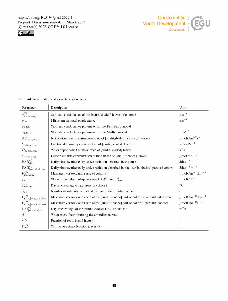
Table A4. Assimilation and stomatal conductance


g(i)

s,[sun,sha] Stomatal conductance of the [sunlit,shaded] leaves of cohort i ms−1

gmin Minimum stomatal conductance ms−1

g1,BB Stomatal conductance parameter for the Ball-Berry model -

g1,Med Stomatal conductance parameter for the Medlyn model kPa0.5

A(i)

n,[sun,sha] Net photosynthetic assimilation rate of [sunlit,shaded] leaves of cohort i µmolCm−2s−1

hs,[sun,sha] Fractional humidity at the surface of [sunlit, shaded] leaves kPakPa−1

Ds,[sun,sha] Water vapor deficit at the surface of [sunlit, shaded] leaves kPa

cs,[sun,sha] Carbon dioxide concentration at the surface of [sunlit, shaded] leaves µmolmol−1

PAR(i)day Daily photosynthetically active radiation absorbed by cohort i Jday−1m−2

PAR(i)

[sun,sha],day Daily photosynthetically active radiation absorbed by the [sunlit, shaded] parts of cohort i Jday−1m−2

V(i)max,day Maximum carboxylation rate of cohort i µmolCm−2day−1

fv Slope of the relationship between PAR(i) and V (i)max µmolCJ−1

T(i)leaf,dt Daytime average temperature of cohort i ◦C

ndt Number of subdaily periods at the end of the simulation day -

V(i)

max,[sun,sha],day Maximum carboxylation rate of the [sunlit, shaded] part of cohort i, per unit patch area µmolCm−2day−1

V(i)

max,[sun,sha],leaf Maximum carboxylation rate of the [sunlit, shaded] part of cohort i, per unit leaf area µmolCm−2s−1

LAI(i)

[sun,sha],dt Daytime average of the [sunlit,shaded] LAI for cohort i. m2m−2

β Water stress factor limiting the assimilation rate -

r(j) Fraction of roots in soil layer j -

W(j)av Soil water uptake function (layer j) -

48


Table A5. Soil physics


Ts Soil temperature ◦C

ch Volumetric heat capacity Jm−3◦C−1

κs Thermal conductivity Wm−1◦C−1

θ(l) Volumetric water content of soil layer l m3m−3

θwilt Volumetric soil water content at wilting point m3m−3

θfc Volumetric soil water content at field capacity m3m−3

ψ(l) Matric potential of soil layer l m

ψwilt Matric potential of soil water at wilting point m

ψfc Matric potential of soil water at saturation point m

γw Hydraulic conductivity ms−1

λw Hydraulic diffusivity m2s−1

Sθ Volumetric soil water uptake sink term m3m−3

49


Author contributions. AA had the original idea and motivated the development. DMB designed the model augmentations described in this

work with input from all the coauthors. DMB implemented the code, ran the experiments and performed the model evaluation analysis. All

coauthors provided input regarding the analysis of the results and the discussion, and helped shape the final form of the manuscript.

Competing interests. The author declare no competing interests.

50


References690

Ahlström, A., Smith, B., Lindström, J., Rummukainen, M., and Uvo, C. B.: GCM characteristics explain the majority of uncertainty in

projected 21st century terrestrial ecosystem carbon balance, Biogeosciences, 10, 1517–1528, https://doi.org/10.5194/bg-10-1517-2013,

publisher: Copernicus GmbH, 2013.

Ahlström, A., Schurgers, G., and Smith, B.: The large influence of climate model bias on terrestrial carbon cycle simulations, Environmental

Research Letters, 12, 014 004, https://doi.org/10.1088/1748-9326/12/1/014004, publisher: IOP Publishing, 2017.695

Alessandri, A., Catalano, F., De Felice, M., Van Den Hurk, B., Doblas Reyes, F., Boussetta, S., Balsamo, G., and Miller, P. A.: Multi-scale

enhancement of climate prediction over land by increasing the model sensitivity to vegetation variability in EC-Earth, Climate Dynamics,

49, 1215–1237, https://doi.org/10.1007/s00382-016-3372-4, 2017.

Ardö, J., Mölder, M., El-Tahir, B. A., and Elkhidir, H. A. M.: Seasonal variation of carbon fluxes in a sparse savanna in semi arid Sudan,

Carbon Balance and Management, 3, 7, https://doi.org/10.1186/1750-0680-3-7, 2008.700

Arneth, A., Harrison, S. P., Zaehle, S., Tsigaridis, K., Menon, S., Bartlein, P. J., Feichter, J., Korhola, A., Kulmala, M., O’Donnell, D.,

Schurgers, G., Sorvari, S., and Vesala, T.: Terrestrial biogeochemical feedbacks in the climate system, Nature Geoscience, 3, 525–532,

https://doi.org/10.1038/ngeo905, bandiera_abtest: a Cg_type: Nature Research Journals Number: 8 Primary_atype: Reviews Publisher:

Nature Publishing Group Subject_term: Biogeochemistry;Climate sciences Subject_term_id: biogeochemistry;climate-sciences, 2010.

Arneth, A., Sitch, S., Pongratz, J., Stocker, B. D., Ciais, P., Poulter, B., Bayer, A. D., Bondeau, A., Calle, L., Chini, L. P., Gasser, T., Fader,705

M., Friedlingstein, P., Kato, E., Li, W., Lindeskog, M., Nabel, J. E. M. S., Pugh, T. a. M., Robertson, E., Viovy, N., Yue, C., and Zaehle,

S.: Historical carbon dioxide emissions caused by land-use changes are possibly larger than assumed, Nature Geoscience, 10, 79–84,

https://doi.org/10.1038/ngeo2882, number: 2 Publisher: Nature Publishing Group, 2017.

Ball, J. T., Woodrow, I. E., and Berry, J. A.: A Model Predicting Stomatal Conductance and its Contribution to the Control of Photosynthesis

under Different Environmental Conditions, in: Progress in Photosynthesis Research: Volume 4 Proceedings of the VIIth International710

Congress on Photosynthesis Providence, Rhode Island, USA, August 10–15, 1986, edited by Biggins, J., pp. 221–224, Springer Nether-

lands, Dordrecht, https://doi.org/10.1007/978-94-017-0519-6_48, 1987.

Beringer, J., Hacker, J., Hutley, L. B., Leuning, R., Arndt, S. K., Amiri, R., Bannehr, L., Cernusak, L. A., Grover, S., Hensley, C., Hocking,

D., Isaac, P., Jamali, H., Kanniah, K., Livesley, S., Neininger, B., U, K. T. P., Sea, W., Straten, D., Tapper, N., Weinmann, R., Wood, S., and

Zegelin, S.: SPECIAL—Savanna Patterns of Energy and Carbon Integrated across the Landscape, Bulletin of the American Meteorological715

Society, 92, 1467–1485, https://doi.org/10.1175/2011BAMS2948.1, publisher: American Meteorological Society Section: Bulletin of the

American Meteorological Society, 2011.

Beringer, J., Hutley, L. B., McHugh, I., Arndt, S. K., Campbell, D., Cleugh, H. A., Cleverly, J., Resco de Dios, V., Eamus, D., Evans, B.,

Ewenz, C., Grace, P., Griebel, A., Haverd, V., Hinko-Najera, N., Huete, A., Isaac, P., Kanniah, K., Leuning, R., Liddell, M. J., Macfarlane,

C., Meyer, W., Moore, C., Pendall, E., Phillips, A., Phillips, R. L., Prober, S. M., Restrepo-Coupe, N., Rutledge, S., Schroder, I., Silberstein,720

R., Southall, P., Yee, M. S., Tapper, N. J., van Gorsel, E., Vote, C., Walker, J., and Wardlaw, T.: An introduction to the Australian and New

Zealand flux tower network – OzFlux, Biogeosciences, 13, 5895–5916, https://doi.org/10.5194/bg-13-5895-2016, publisher: Copernicus

GmbH, 2016.

Best, M. J., Abramowitz, G., Johnson, H. R., Pitman, A. J., Balsamo, G., Boone, A., Cuntz, M., Decharme, B., Dirmeyer, P. A., Dong,

J., Ek, M., Guo, Z., Haverd, V., Hurk, B. J. J. v. d., Nearing, G. S., Pak, B., Peters-Lidard, C., Santanello, J. A., Stevens, L., and725

51


Vuichard, N.: The Plumbing of Land Surface Models: Benchmarking Model Performance, Journal of Hydrometeorology, 16, 1425–1442,

https://doi.org/10.1175/JHM-D-14-0158.1, publisher: American Meteorological Society Section: Journal of Hydrometeorology, 2015.

Bonal, D., Bosc, A., Ponton, S., Goret, J.-Y., Burban, B., Gross, P., Bonnefond, J.-M., Elbers, J., Longdoz, B., Epron, D.,

Guehl, J.-M., and Granier, A.: Impact of severe dry season on net ecosystem exchange in the Neotropical rainforest of

French Guiana, Global Change Biology, 14, 1917–1933, https://doi.org/https://doi.org/10.1111/j.1365-2486.2008.01610.x, _eprint:730

https://onlinelibrary.wiley.com/doi/pdf/10.1111/j.1365-2486.2008.01610.x, 2008.

Bonan, G. B.: Ecological Climatology: Concepts and Applications, https://doi.org/10.1017/CBO9780511805530, 2008.

Bonan, G. B., Levis, S., Sitch, S., Vertenstein, M., and Oleson, K. W.: A dynamic global vegetation model for use with climate mod-

els: concepts and description of simulated vegetation dynamics, Global Change Biology, 9, 1543–1566, https://doi.org/10.1046/j.1365-

2486.2003.00681.x, 2003.735

Booth, B. B. B., Jones, C. D., Collins, M., Totterdell, I. J., Cox, P. M., Sitch, S., Huntingford, C., Betts, R. A., Harris, G. R., and

Lloyd, J.: High sensitivity of future global warming to land carbon cycle processes, Environmental Research Letters, 7, 024 002,

https://doi.org/10.1088/1748-9326/7/2/024002, publisher: IOP Publishing, 2012.

Bristow, M., Hutley, L. B., Beringer, J., Livesley, S. J., Edwards, A. C., and Arndt, S. K.: Quantifying the relative importance of green-

house gas emissions from current and future savanna land use change across northern Australia, Biogeosciences, 13, 6285–6303,740

https://doi.org/10.5194/bg-13-6285-2016, publisher: Copernicus GmbH, 2016.

Brovkin, V., Sitch, S., Bloh, W. V., Claussen, M., Bauer, E., and Cramer, W.: Role of land cover changes for atmospheric CO2 increase

and climate change during the last 150 years, Global Change Biology, 10, 1253–1266, https://doi.org/10.1111/j.1365-2486.2004.00812.x,

_eprint: https://onlinelibrary.wiley.com/doi/pdf/10.1111/j.1365-2486.2004.00812.x, 2004.

Christidis, N., Stott, P. A., Hegerl, G. C., and Betts, R. A.: The role of land use change in the recent warm-745

ing of daily extreme temperatures, Geophysical Research Letters, 40, 589–594, https://doi.org/10.1002/grl.50159, _eprint:

https://agupubs.onlinelibrary.wiley.com/doi/pdf/10.1002/grl.50159, 2013.

Ciais, P., Sabine, C., Bala, G., Bopp, L., Brovkin, V., Al, E., and House, J. I.: Carbon and Other Biogeochemical Cycles, Climate Change

2013: The Physical Science Basis. Contribution of Working Group I to the Fifth Assessment Report of the Intergovernmental Panel on

Climate Change Change, pp. 465–570, https://research-information.bris.ac.uk/en/publications/carbon-and-other-biogeochemical-cycles,750

publisher: Cambridge University Press, 2014.

Clapp, R. B. and Hornberger, G. M.: Empirical equations for some soil hydraulic properties, Wa-

ter Resources Research, 14, 601–604, https://doi.org/https://doi.org/10.1029/WR014i004p00601, _eprint:

https://agupubs.onlinelibrary.wiley.com/doi/pdf/10.1029/WR014i004p00601, 1978.

Cosby, B. J., Hornberger, G. M., Clapp, R. B., and Ginn, T. R.: A Statistical Exploration of the Relationships of Soil Moisture Characteristics755

to the Physical Properties of Soils, Water Resources Research, 20, 682–690, https://doi.org/https://doi.org/10.1029/WR020i006p00682,

_eprint: https://agupubs.onlinelibrary.wiley.com/doi/pdf/10.1029/WR020i006p00682, 1984.

Cramer, W., Bondeau, A., Woodward, F. I., Prentice, I. C., Betts, R. A., Brovkin, V., Cox, P. M., Fisher, V., Foley, J. A., Friend, A. D.,

Kucharik, C., Lomas, M. R., Ramankutty, N., Sitch, S., Smith, B., White, A., and Young-Molling, C.: Global response of terrestrial ecosys-

tem structure and function to CO2 and climate change: results from six dynamic global vegetation models, Global Change Biology, 7, 357–760

373, https://doi.org/https://doi.org/10.1046/j.1365-2486.2001.00383.x, _eprint: https://onlinelibrary.wiley.com/doi/pdf/10.1046/j.1365-

2486.2001.00383.x, 2001.

52


Dai, Y., Dickinson, R. E., and Wang, Y.-P.: A Two-Big-Leaf Model for Canopy Temperature, Photosynthesis, and Stomatal Conductance,

Journal of Climate, 17, 2281–2299, https://doi.org/10.1175/1520-0442(2004)017<2281:ATMFCT>2.0.CO;2, 2004.

De Kauwe, M. G., Kala, J., Lin, Y.-S., Pitman, A. J., Medlyn, B. E., Duursma, R. A., Abramowitz, G., Wang, Y.-P., and Miralles, D. G.: A765

test of an optimal stomatal conductance scheme within the CABLE land surface model, Geoscientific Model Development, 8, 431–452,

https://doi.org/10.5194/gmd-8-431-2015, publisher: Copernicus GmbH, 2015.

de Vries, D.: Thermal properties of soils, Physics of Plant Environment, https://ci.nii.ac.jp/naid/10016146353/, publisher: North-Holland

Publishing Co., 1963.

Dickinson, R. E.: Land Surface Processes and Climate—Surface Albedos and Energy Balance, in: Advances in Geophysics, edited by770

Saltzman, B., vol. 25 of Theory of Climate, pp. 305–353, Elsevier, https://doi.org/10.1016/S0065-2687(08)60176-4, 1983.

Döscher, R., Acosta, M., Alessandri, A., Anthoni, P., Arneth, A., Arsouze, T., Bergmann, T., Bernadello, R., Bousetta, S., Caron, L.-P.,

Carver, G., Castrillo, M., Catalano, F., Cvijanovic, I., Davini, P., Dekker, E., Doblas-Reyes, F. J., Docquier, D., Echevarria, P., Fladrich, U.,

Fuentes-Franco, R., Gröger, M., v. Hardenberg, J., Hieronymus, J., Karami, M. P., Keskinen, J.-P., Koenigk, T., Makkonen, R., Massonnet,

F., Ménégoz, M., Miller, P. A., Moreno-Chamarro, E., Nieradzik, L., van Noije, T., Nolan, P., O’Donnell, D., Ollinaho, P., van den Oord,775

G., Ortega, P., Prims, O. T., Ramos, A., Reerink, T., Rousset, C., Ruprich-Robert, Y., Le Sager, P., Schmith, T., Schrödner, R., Serva, F.,

Sicardi, V., Sloth Madsen, M., Smith, B., Tian, T., Tourigny, E., Uotila, P., Vancoppenolle, M., Wang, S., Wårlind, D., Willén, U., Wyser,

K., Yang, S., Yepes-Arbós, X., and Zhang, Q.: The EC-Earth3 Earth System Model for the Climate Model Intercomparison Project 6,

Geoscientific Model Development Discussions, pp. 1–90, https://doi.org/10.5194/gmd-2020-446, publisher: Copernicus GmbH, 2021.

Fisher, R. A., Koven, C. D., Anderegg, W. R. L., Christoffersen, B. O., Dietze, M. C., Farrior, C. E., Holm, J. A., Hurtt, G. C., Knox,780

R. G., Lawrence, P. J., Lichstein, J. W., Longo, M., Matheny, A. M., Medvigy, D., Muller-Landau, H. C., Powell, T. L., Serbin, S. P.,

Sato, H., Shuman, J. K., Smith, B., Trugman, A. T., Viskari, T., Verbeeck, H., Weng, E., Xu, C., Xu, X., Zhang, T., and Moorcroft,

P. R.: Vegetation demographics in Earth System Models: A review of progress and priorities, Global Change Biology, 24, 35–54,

https://doi.org/10.1111/gcb.13910, _eprint: https://onlinelibrary.wiley.com/doi/pdf/10.1111/gcb.13910, 2018.

Forrest, M., Tost, H., Lelieveld, J., and Hickler, T.: Including vegetation dynamics in an atmospheric chemistry-enabled general circula-785

tion model: linking LPJ-GUESS (v4.0) with the EMAC modelling system (v2.53), Geoscientific Model Development, 13, 1285–1309,

https://doi.org/https://doi.org/10.5194/gmd-13-1285-2020, publisher: Copernicus GmbH, 2020.

Friedlingstein, P., Cox, P., Betts, R., Bopp, L., von Bloh, W., Brovkin, V., Cadule, P., Doney, S., Eby, M., Fung, I., Bala, G., John, J., Jones,

C., Joos, F., Kato, T., Kawamiya, M., Knorr, W., Lindsay, K., Matthews, H. D., Raddatz, T., Rayner, P., Reick, C., Roeckner, E., Schnitzler,

K.-G., Schnur, R., Strassmann, K., Weaver, A. J., Yoshikawa, C., and Zeng, N.: Climate–Carbon Cycle Feedback Analysis: Results from790

the C4MIP Model Intercomparison, Journal of Climate, 19, 3337–3353, https://doi.org/10.1175/JCLI3800.1, 2006.

Friedlingstein, P., Meinshausen, M., Arora, V. K., Jones, C. D., Anav, A., Liddicoat, S. K., and Knutti, R.: Uncertainties in CMIP5 Climate

Projections due to Carbon Cycle Feedbacks, Journal of Climate, 27, 511–526, https://doi.org/10.1175/JCLI-D-12-00579.1, publisher:

American Meteorological Society Section: Journal of Climate, 2014.

Friend, A. D., Lucht, W., Rademacher, T. T., Keribin, R., Betts, R., Cadule, P., Ciais, P., Clark, D. B., Dankers, R., Falloon, P. D., Ito, A.,795

Kahana, R., Kleidon, A., Lomas, M. R., Nishina, K., Ostberg, S., Pavlick, R., Peylin, P., Schaphoff, S., Vuichard, N., Warszawski, L.,

Wiltshire, A., and Woodward, F. I.: Carbon residence time dominates uncertainty in terrestrial vegetation responses to future climate

and atmospheric CO2, Proceedings of the National Academy of Sciences, 111, 3280–3285, https://doi.org/10.1073/pnas.1222477110,

publisher: National Academy of Sciences Section: Biological Sciences, 2014.

53


Gerten, D., Schaphoff, S., Haberlandt, U., Lucht, W., and Sitch, S.: Terrestrial vegetation and water balance—hydrological evaluation of a800

dynamic global vegetation model, Journal of Hydrology, 286, 249–270, https://doi.org/10.1016/j.jhydrol.2003.09.029, 2004.

Green, J. K., Konings, A. G., Alemohammad, S. H., Berry, J., Entekhabi, D., Kolassa, J., Lee, J.-E., and Gentine, P.: Regionally strong

feedbacks between the atmosphere and terrestrial biosphere, Nature Geoscience, 10, 410–414, https://doi.org/10.1038/ngeo2957, number:

6 Publisher: Nature Publishing Group, 2017.

Green, W. H. and Ampt, G. A.: Studies on Soil Phyics., The Journal of Agricultural Science, 4, 1–24,805

https://doi.org/10.1017/S0021859600001441, publisher: Cambridge University Press, 1911.

Guo, Z., Dirmeyer, P. A., Koster, R. D., Sud, Y. C., Bonan, G., Oleson, K. W., Chan, E., Verseghy, D., Cox, P., Gordon, C. T., McGregor, J. L.,

Kanae, S., Kowalczyk, E., Lawrence, D., Liu, P., Mocko, D., Lu, C.-H., Mitchell, K., Malyshev, S., McAvaney, B., Oki, T., Yamada, T.,

Pitman, A., Taylor, C. M., Vasic, R., and Xue, Y.: GLACE: The Global Land–Atmosphere Coupling Experiment. Part II: Analysis, Journal

of Hydrometeorology, 7, 611–625, https://doi.org/10.1175/JHM511.1, publisher: American Meteorological Society Section: Journal of810

Hydrometeorology, 2006.

Haughton, N., Abramowitz, G., Pitman, A. J., Or, D., Best, M. J., Johnson, H. R., Balsamo, G., Boone, A., Cuntz, M., Decharme, B.,

Dirmeyer, P. A., Dong, J., Ek, M., Guo, Z., Haverd, V., Hurk, B. J. J. v. d., Nearing, G. S., Pak, B., Santanello, J. A., Stevens, L. E.,

and Vuichard, N.: The Plumbing of Land Surface Models: Is Poor Performance a Result of Methodology or Data Quality?, Journal

of Hydrometeorology, 17, 1705–1723, https://doi.org/10.1175/JHM-D-15-0171.1, publisher: American Meteorological Society Section:815

Journal of Hydrometeorology, 2016.

Haxeltine, A. and Prentice, I. C.: A General Model for the Light-Use Efficiency of Primary Production, Functional Ecology, 10, 551–561,

https://doi.org/10.2307/2390165, 1996.

Huntingford, C., Lowe, J. A., Booth, B. B. B., Jones, C. D., Harris, G. R., Gohar, L. K., and Meir, P.: Contributions of carbon cycle un-

certainty to future climate projection spread, Tellus B: Chemical and Physical Meteorology, 61, 355–360, https://doi.org/10.1111/j.1600-820

0889.2008.00414.x, publisher: Taylor & Francis _eprint: https://www.tandfonline.com/doi/pdf/10.1111/j.1600-0889.2008.00414.x, 2009.

Hutley, L. B., Beringer, J., Isaac, P. R., Hacker, J. M., and Cernusak, L. A.: A sub-continental scale living laboratory: Spatial pat-

terns of savanna vegetation over a rainfall gradient in northern Australia, Agricultural and Forest Meteorology, 151, 1417–1428,

https://doi.org/10.1016/j.agrformet.2011.03.002, 2011.

Johansen, O.: Thermal Conductivity of Soils, PhD thesis, Trondheim University, Norway, https://ci.nii.ac.jp/naid/10003620379/, 1975.825

Johansen, O.: Thermal Conductivity of Soils, Tech. rep., COLD REGIONS RESEARCH AND ENGINEERING LAB HANOVER NH,

https://apps.dtic.mil/sti/citations/ADA044002, section: Technical Reports, 1977.

Jones, C., Robertson, E., Arora, V., Friedlingstein, P., Shevliakova, E., Bopp, L., Brovkin, V., Hajima, T., Kato, E., Kawamiya, M., Liddicoat,

S., Lindsay, K., Reick, C. H., Roelandt, C., Segschneider, J., and Tjiputra, J.: Twenty-First-Century Compatible CO2 Emissions and

Airborne Fraction Simulated by CMIP5 Earth System Models under Four Representative Concentration Pathways, Journal of Climate, 26,830

4398–4413, https://doi.org/10.1175/JCLI-D-12-00554.1, publisher: American Meteorological Society Section: Journal of Climate, 2013.

Kosugi, Y., Takanashi, S., Ohkubo, S., Matsuo, N., Tani, M., Mitani, T., Tsutsumi, D., and Nik, A. R.: CO2 exchange of a tropical rainforest

at Pasoh in Peninsular Malaysia, Agricultural and Forest Meteorology, 148, 439–452, https://doi.org/10.1016/j.agrformet.2007.10.007,

2008.

Krinner, G., Viovy, N., Noblet-Ducoudré, N. d., Ogée, J., Polcher, J., Friedlingstein, P., Ciais, P., Sitch, S., and Prentice, I. C.:835

A dynamic global vegetation model for studies of the coupled atmosphere-biosphere system, Global Biogeochemical Cycles, 19,

https://doi.org/10.1029/2003GB002199, _eprint: https://agupubs.onlinelibrary.wiley.com/doi/pdf/10.1029/2003GB002199, 2005.

54


Kucharik, C. J., Norman, J. M., and Gower, S. T.: Measurements of branch area and adjusting leaf area index indirect measurements,

Agricultural and Forest Meteorology, 91, 69–88, https://doi.org/10.1016/S0168-1923(98)00064-1, 1998.

Kumar, S., Dirmeyer, P. A., Merwade, V., DelSole, T., Adams, J. M., and Niyogi, D.: Land use/cover change impacts in CMIP5 cli-840

mate simulations: A new methodology and 21st century challenges, Journal of Geophysical Research: Atmospheres, 118, 6337–6353,

https://doi.org/10.1002/jgrd.50463, _eprint: https://agupubs.onlinelibrary.wiley.com/doi/pdf/10.1002/jgrd.50463, 2013.

Kurz, W. A., Dymond, C. C., Stinson, G., Rampley, G. J., Neilson, E. T., Carroll, A. L., Ebata, T., and Safranyik, L.: Mountain pine beetle

and forest carbon feedback to climate change, Nature, 452, 987–990, https://doi.org/10.1038/nature06777, bandiera_abtest: a Cg_type:

Nature Research Journals Number: 7190 Primary_atype: Research Publisher: Nature Publishing Group, 2008.845

Lamarque, J.-F., Dentener, F., McConnell, J., Ro, C.-U., Shaw, M., Vet, R., Bergmann, D., Cameron-Smith, P., Dalsoren, S., Doherty, R.,

Faluvegi, G., Ghan, S. J., Josse, B., Lee, Y. H., MacKenzie, I. A., Plummer, D., Shindell, D. T., Skeie, R. B., Stevenson, D. S., Strode, S.,

Zeng, G., Curran, M., Dahl-Jensen, D., Das, S., Fritzsche, D., and Nolan, M.: Multi-model mean nitrogen and sulfur deposition from the

Atmospheric Chemistry and Climate Model Intercomparison Project (ACCMIP): evaluation of historical and projected future changes,

Atmospheric Chemistry and Physics, 13, 7997–8018, https://doi.org/10.5194/acp-13-7997-2013, publisher: Copernicus GmbH, 2013.850

Lawrence, D. and Vandecar, K.: Effects of tropical deforestation on climate and agriculture, Nature Climate Change, 5, 27–36,

https://doi.org/10.1038/nclimate2430, bandiera_abtest: a Cg_type: Nature Research Journals Number: 1 Primary_atype: Reviews Pub-

lisher: Nature Publishing Group Subject_term: Agroecology;Climate and Earth system modelling;Climate-change impacts;Hydrology

Subject_term_id: agri-ecology;climate-and-earth-system-modelling;climate-change-impacts;hydrology, 2015.

Lawrence, P. J. and Chase, T. N.: Representing a new MODIS consistent land surface in the Community Land Model (CLM 3.0), Journal of855

Geophysical Research: Biogeosciences, 112, https://doi.org/10.1029/2006JG000168, 2007.

Le Quéré, C., Andrew, R. M., Friedlingstein, P., Sitch, S., Hauck, J., Pongratz, J., Pickers, P. A., Korsbakken, J. I., Peters, G. P., Canadell,

J. G., Arneth, A., Arora, V. K., Barbero, L., Bastos, A., Bopp, L., Chevallier, F., Chini, L. P., Ciais, P., Doney, S. C., Gkritzalis, T., Goll,

D. S., Harris, I., Haverd, V., Hoffman, F. M., Hoppema, M., Houghton, R. A., Hurtt, G., Ilyina, T., Jain, A. K., Johannessen, T., Jones,

C. D., Kato, E., Keeling, R. F., Goldewijk, K. K., Landschützer, P., Lefèvre, N., Lienert, S., Liu, Z., Lombardozzi, D., Metzl, N., Munro,860

D. R., Nabel, J. E. M. S., Nakaoka, S.-i., Neill, C., Olsen, A., Ono, T., Patra, P., Peregon, A., Peters, W., Peylin, P., Pfeil, B., Pierrot,

D., Poulter, B., Rehder, G., Resplandy, L., Robertson, E., Rocher, M., Rödenbeck, C., Schuster, U., Schwinger, J., Séférian, R., Skjelvan,

I., Steinhoff, T., Sutton, A., Tans, P. P., Tian, H., Tilbrook, B., Tubiello, F. N., van der Laan-Luijkx, I. T., van der Werf, G. R., Viovy,

N., Walker, A. P., Wiltshire, A. J., Wright, R., Zaehle, S., and Zheng, B.: Global Carbon Budget 2018, Earth System Science Data, 10,

2141–2194, https://doi.org/10.5194/essd-10-2141-2018, publisher: Copernicus GmbH, 2018.865

Levis, S., Foley, J. A., and Pollard, D.: Large-Scale Vegetation Feedbacks on a Doubled CO2 Climate, Journal of Climate, 13, 1313–1325,

https://doi.org/10.1175/1520-0442(2000)013<1313:LSVFOA>2.0.CO;2, publisher: American Meteorological Society Section: Journal of

Climate, 2000.

Lindeskog, M., Arneth, A., Bondeau, A., Waha, K., Seaquist, J., Olin, S., and Smith, B.: Implications of accounting for land use in simulations

of ecosystem carbon cycling in Africa, Earth System Dynamics, 4, 385–407, https://doi.org/10.5194/esd-4-385-2013, 2013.870

Lindeskog, M., Smith, B., Lagergren, F., Sycheva, E., Ficko, A., Pretzsch, H., and Rammig, A.: Accounting for forest management in the

estimation of forest carbon balance using the dynamic vegetation model LPJ-GUESS (v4.0, r9710): implementation and evaluation of

simulations for Europe, Geoscientific Model Development, 14, 6071–6112, https://doi.org/10.5194/gmd-14-6071-2021, publisher: Coper-

nicus GmbH, 2021.

55


Lorenz, R., Davin, E. L., Lawrence, D. M., Stöckli, R., and Seneviratne, S. I.: How Important is Vegetation Phenology for European Climate875

and Heat Waves?, Journal of Climate, 26, 10 077–10 100, https://doi.org/10.1175/JCLI-D-13-00040.1, publisher: American Meteorologi-

cal Society Section: Journal of Climate, 2013.

Luo, Y.: Terrestrial Carbon–Cycle Feedback to Climate Warming, Annual Review of Ecology, Evolution, and Systematics, 38, 683–712,

https://doi.org/10.1146/annurev.ecolsys.38.091206.095808, _eprint: https://doi.org/10.1146/annurev.ecolsys.38.091206.095808, 2007.

López-Ballesteros, A., Serrano-Ortiz, P., Kowalski, A. S., Sánchez-Cañete, E. P., Scott, R. L., and Domingo, F.: Subterranean ventilation880

of allochthonous CO2 governs net CO2 exchange in a semiarid Mediterranean grassland, Agricultural and Forest Meteorology, 234-235,

115–126, https://doi.org/10.1016/j.agrformet.2016.12.021, 2017.

McGuire, A. D., Sitch, S., Clein, J. S., Dargaville, R., Esser, G., Foley, J., Heimann, M., Joos, F., Kaplan, J., Kicklighter, D. W., Meier,

R. A., Melillo, J. M., Moore III, B., Prentice, I. C., Ramankutty, N., Reichenau, T., Schloss, A., Tian, H., Williams, L. J., and Wit-

tenberg, U.: Carbon balance of the terrestrial biosphere in the Twentieth Century: Analyses of CO2, climate and land use effects with885

four process-based ecosystem models, Global Biogeochemical Cycles, 15, 183–206, https://doi.org/10.1029/2000GB001298, _eprint:

https://onlinelibrary.wiley.com/doi/pdf/10.1029/2000GB001298, 2001.

Medlyn, B. E., Duursma, R. A., Eamus, D., Ellsworth, D. S., Prentice, I. C., Barton, C. V. M., Crous, K. Y., Angelis, P. D., Freeman, M.,

and Wingate, L.: Reconciling the optimal and empirical approaches to modelling stomatal conductance, Global Change Biology, 17,

2134–2144, https://doi.org/10.1111/j.1365-2486.2010.02375.x, 2011.890

Medvigy, D., Walko, R. L., Otte, M. J., and Avissar, R.: Simulated Changes in Northwest U.S. Climate in Response to Amazon Deforestation,

Journal of Climate, 26, 9115–9136, https://doi.org/10.1175/JCLI-D-12-00775.1, publisher: American Meteorological Society Section:

Journal of Climate, 2013.

Merbold, L., Ardö, J., Arneth, A., Scholes, R. J., Nouvellon, Y., de Grandcourt, A., Archibald, S., Bonnefond, J. M., Boulain, N., Bruegge-

mann, N., Bruemmer, C., Cappelaere, B., Ceschia, E., El-Khidir, H. a. M., El-Tahir, B. A., Falk, U., Lloyd, J., Kergoat, L., Le Dantec, V.,895

Mougin, E., Muchinda, M., Mukelabai, M. M., Ramier, D., Roupsard, O., Timouk, F., Veenendaal, E. M., and Kutsch, W. L.: Precipitation

as driver of carbon fluxes in 11 African ecosystems, Biogeosciences, 6, 1027–1041, https://doi.org/10.5194/bg-6-1027-2009, publisher:

Copernicus GmbH, 2009.

Metsaranta, J. M., Kurz, W. A., Neilson, E. T., and Stinson, G.: Implications of future disturbance regimes on the carbon balance of

Canada’s managed forest (2010–2100), Tellus B: Chemical and Physical Meteorology, 62, 719–728, https://doi.org/10.1111/j.1600-900

0889.2010.00487.x, publisher: Taylor & Francis _eprint: https://doi.org/10.1111/j.1600-0889.2010.00487.x, 2010.

Monsi, M. and Saeki, T.: On the Factor Light in Plant Communities and its Importance for Matter Production, Japanese Journal of Botany,

14, 22–52, 1953.

Monsi, M. and Saeki, T.: On the Factor Light in Plant Communities and its Importance for Matter Production, Annals of Botany, 95, 549–567,

https://doi.org/10.1093/aob/mci052, 2005.905

Narisma, G. T. and Pitman, A. J.: The Impact of 200 Years of Land Cover Change on the Australian Near-Surface Climate, Journal of Hy-

drometeorology, 4, 424–436, https://doi.org/10.1175/1525-7541(2003)4<424:TIOYOL>2.0.CO;2, publisher: American Meteorological

Society Section: Journal of Hydrometeorology, 2003.

Niu, G.-Y., Yang, Z.-L., Mitchell, K. E., Chen, F., Ek, M. B., Barlage, M., Kumar, A., Manning, K., Niyogi, D., Rosero, E., Tewari, M., and

Xia, Y.: The community Noah land surface model with multiparameterization options (Noah-MP): 1. Model description and evaluation910

with local-scale measurements, Journal of Geophysical Research, 116, https://doi.org/10.1029/2010JD015139, 2011.

56


Noblet-Ducoudré, N. d., Boisier, J.-P., Pitman, A., Bonan, G. B., Brovkin, V., Cruz, F., Delire, C., Gayler, V., Hurk, B. J. J. M. v. d., Lawrence,

P. J., Molen, M. K. v. d., Müller, C., Reick, C. H., Strengers, B. J., and Voldoire, A.: Determining Robust Impacts of Land-Use-Induced

Land Cover Changes on Surface Climate over North America and Eurasia: Results from the First Set of LUCID Experiments, Journal

of Climate, 25, 3261–3281, https://doi.org/10.1175/JCLI-D-11-00338.1, publisher: American Meteorological Society Section: Journal of915

Climate, 2012.

Oleson, K., Dai, Y., Bonan, B., Bosilovichm, M., Dickinson, R., Dirmeyer, P., Hoffman, F., Houser, P., Levis, S., Niu, G.-

Y., Thornton, P., Vertenstein, M., Yang, Z.-L., and Zeng, X.: Technical Description of the Community Land Model (CLM),

https://doi.org/10.5065/D6N877R0, 2004.

Olin, S., Lindeskog, M., Pugh, T. A. M., Schurgers, G., Wårlind, D., Mishurov, M., Zaehle, S., Stocker, B. D., Smith, B., and Arneth, A.: Soil920

carbon management in large-scale Earth system modelling: implications for crop yields and nitrogen leaching, Earth System Dynamics,

6, 745–768, https://doi.org/10.5194/esd-6-745-2015, 2015.

O’ishi, R. and Abe-Ouchi, A.: Influence of dynamic vegetation on climate change arising from increasing CO2, Climate Dynamics, 33,

645–663, https://doi.org/10.1007/s00382-009-0611-y, 2009.

Pastorello, G., Trotta, C., Canfora, E., Chu, H., Christianson, D., Cheah, Y.-W., Poindexter, C., Chen, J., Elbashandy, A., Humphrey, M.,925

Isaac, P., Polidori, D., Reichstein, M., Ribeca, A., van Ingen, C., Vuichard, N., Zhang, L., Amiro, B., Ammann, C., Arain, M. A., Ardö, J.,

Arkebauer, T., Arndt, S. K., Arriga, N., Aubinet, M., Aurela, M., Baldocchi, D., Barr, A., Beamesderfer, E., Marchesini, L. B., Bergeron,

O., Beringer, J., Bernhofer, C., Berveiller, D., Billesbach, D., Black, T. A., Blanken, P. D., Bohrer, G., Boike, J., Bolstad, P. V., Bonal, D.,

Bonnefond, J.-M., Bowling, D. R., Bracho, R., Brodeur, J., Brümmer, C., Buchmann, N., Burban, B., Burns, S. P., Buysse, P., Cale, P.,

Cavagna, M., Cellier, P., Chen, S., Chini, I., Christensen, T. R., Cleverly, J., Collalti, A., Consalvo, C., Cook, B. D., Cook, D., Coursolle, C.,930

Cremonese, E., Curtis, P. S., D’Andrea, E., da Rocha, H., Dai, X., Davis, K. J., Cinti, B. D., Grandcourt, A. d., Ligne, A. D., De Oliveira,

R. C., Delpierre, N., Desai, A. R., Di Bella, C. M., Tommasi, P. d., Dolman, H., Domingo, F., Dong, G., Dore, S., Duce, P., Dufrêne,

E., Dunn, A., Dušek, J., Eamus, D., Eichelmann, U., ElKhidir, H. A. M., Eugster, W., Ewenz, C. M., Ewers, B., Famulari, D., Fares, S.,

Feigenwinter, I., Feitz, A., Fensholt, R., Filippa, G., Fischer, M., Frank, J., Galvagno, M., Gharun, M., Gianelle, D., Gielen, B., Gioli, B.,

Gitelson, A., Goded, I., Goeckede, M., Goldstein, A. H., Gough, C. M., Goulden, M. L., Graf, A., Griebel, A., Gruening, C., Grünwald,935

T., Hammerle, A., Han, S., Han, X., Hansen, B. U., Hanson, C., Hatakka, J., He, Y., Hehn, M., Heinesch, B., Hinko-Najera, N., Hörtnagl,

L., Hutley, L., Ibrom, A., Ikawa, H., Jackowicz-Korczynski, M., Janouš, D., Jans, W., Jassal, R., Jiang, S., Kato, T., Khomik, M., Klatt,

J., Knohl, A., Knox, S., Kobayashi, H., Koerber, G., Kolle, O., Kosugi, Y., Kotani, A., Kowalski, A., Kruijt, B., Kurbatova, J., Kutsch,

W. L., Kwon, H., Launiainen, S., Laurila, T., Law, B., Leuning, R., Li, Y., Liddell, M., Limousin, J.-M., Lion, M., Liska, A. J., Lohila,

A., López-Ballesteros, A., López-Blanco, E., Loubet, B., Loustau, D., Lucas-Moffat, A., Lüers, J., Ma, S., Macfarlane, C., Magliulo, V.,940

Maier, R., Mammarella, I., Manca, G., Marcolla, B., Margolis, H. A., Marras, S., Massman, W., Mastepanov, M., Matamala, R., Matthes,

J. H., Mazzenga, F., McCaughey, H., McHugh, I., McMillan, A. M. S., Merbold, L., Meyer, W., Meyers, T., Miller, S. D., Minerbi, S.,

Moderow, U., Monson, R. K., Montagnani, L., Moore, C. E., Moors, E., Moreaux, V., Moureaux, C., Munger, J. W., Nakai, T., Neirynck,

J., Nesic, Z., Nicolini, G., Noormets, A., Northwood, M., Nosetto, M., Nouvellon, Y., Novick, K., Oechel, W., Olesen, J. E., Ourcival,

J.-M., Papuga, S. A., Parmentier, F.-J., Paul-Limoges, E., Pavelka, M., Peichl, M., Pendall, E., Phillips, R. P., Pilegaard, K., Pirk, N., Posse,945

G., Powell, T., Prasse, H., Prober, S. M., Rambal, S., Rannik, U., Raz-Yaseef, N., Rebmann, C., Reed, D., Dios, V. R. d., Restrepo-Coupe,

N., Reverter, B. R., Roland, M., Sabbatini, S., Sachs, T., Saleska, S. R., Sánchez-Cañete, E. P., Sanchez-Mejia, Z. M., Schmid, H. P.,

Schmidt, M., Schneider, K., Schrader, F., Schroder, I., Scott, R. L., Sedlák, P., Serrano-Ortíz, P., Shao, C., Shi, P., Shironya, I., Siebicke,

L., Šigut, L., Silberstein, R., Sirca, C., Spano, D., Steinbrecher, R., Stevens, R. M., Sturtevant, C., Suyker, A., Tagesson, T., Takanashi,

57


S., Tang, Y., Tapper, N., Thom, J., Tomassucci, M., Tuovinen, J.-P., Urbanski, S., Valentini, R., van der Molen, M., van Gorsel, E., van950

Huissteden, K., Varlagin, A., Verfaillie, J., Vesala, T., Vincke, C., Vitale, D., Vygodskaya, N., Walker, J. P., Walter-Shea, E., Wang, H.,

Weber, R., Westermann, S., Wille, C., Wofsy, S., Wohlfahrt, G., Wolf, S., Woodgate, W., Li, Y., Zampedri, R., Zhang, J., Zhou, G., Zona, D.,

Agarwal, D., Biraud, S., Torn, M., and Papale, D.: The FLUXNET2015 dataset and the ONEFlux processing pipeline for eddy covariance

data, Scientific Data, 7, 225, https://doi.org/10.1038/s41597-020-0534-3, bandiera_abtest: a Cc_license_type: cc_publicdomain Cg_type:

Nature Research Journals Number: 1 Primary_atype: Research Publisher: Nature Publishing Group Subject_term: Carbon cycle;Climate955

sciences;Environmental sciences Subject_term_id: carbon-cycle;climate-sciences;environmental-sciences, 2020.

Peñuelas, J., Rutishauser, T., and Filella, I.: Phenology Feedbacks on Climate Change, Science, 324, 887–888,

https://doi.org/10.1126/science.1173004, publisher: American Association for the Advancement of Science, 2009.

Philip, J. R.: Evaporation, and moisture and heat fields in the soil, Journal of Meteorology, 14, 354–366, https://doi.org/10.1175/1520-

0469(1957)014<0354:EAMAHF>2.0.CO;2, publisher: American Meteorological Society, 1957.960

Piao, S., Sitch, S., Ciais, P., Friedlingstein, P., Peylin, P., Wang, X., Ahlström, A., Anav, A., Canadell, J. G., Cong, N., Hunting-

ford, C., Jung, M., Levis, S., Levy, P. E., Li, J., Lin, X., Lomas, M. R., Lu, M., Luo, Y., Ma, Y., Myneni, R. B., Poulter, B.,

Sun, Z., Wang, T., Viovy, N., Zaehle, S., and Zeng, N.: Evaluation of terrestrial carbon cycle models for their response to cli-

mate variability and to CO2 trends, Global Change Biology, 19, 2117–2132, https://doi.org/https://doi.org/10.1111/gcb.12187, _eprint:

https://onlinelibrary.wiley.com/doi/pdf/10.1111/gcb.12187, 2013.965

Pitman, A. J.: The evolution of, and revolution in, land surface schemes designed for climate models, International Journal of Climatology,

23, 479–510, https://doi.org/10.1002/joc.893, 2003.

Pongratz, J., Reick, C. H., Raddatz, T., and Claussen, M.: Biogeophysical versus biogeochemical climate response to his-

torical anthropogenic land cover change, Geophysical Research Letters, 37, https://doi.org/10.1029/2010GL043010, _eprint:

https://agupubs.onlinelibrary.wiley.com/doi/pdf/10.1029/2010GL043010, 2010.970

Prentice, I. C., Cramer, W., Harrison, S. P., Leemans, R., Monserud, R. A., and Solomon, A. M.: Special Paper: A Global Biome Model Based

on Plant Physiology and Dominance, Soil Properties and Climate, Journal of Biogeography, 19, 117–134, https://doi.org/10.2307/2845499,

publisher: Wiley, 1992.

Press, W. H., ed.: Numerical recipes in Fortran 77: the art of scientific computing, no. the art of scientific computing / William H. Press ...

; Vol. [1,1] in Numerical recipes in FORTRAN, Cambridge Univ. Press, Cambridge, 2. ed., reprinted with corr edn., oCLC: 249641445,975

2003.

Quillet, A., Peng, C., and Garneau, M.: Toward dynamic global vegetation models for simulating vegetation–climate interactions and feed-

backs: recent developments, limitations, and future challenges, Environmental Reviews, 18, 333–353, https://doi.org/10.1139/A10-016,

publisher: NRC Research Press, 2010.

Raupach, M. R.: Simplified expressions for vegetation roughness length and zero-plane displacement as functions of canopy height and area980

index, Boundary-Layer Meteorology, 71, 211–216, https://doi.org/10.1007/BF00709229, 1994.

Raupach, M. R.: Corrigenda, Boundary-Layer Meteorology, 76, 303–304, https://doi.org/10.1007/BF00709356, 1995.

Richards, L. A.: Capillary conduction of liquids through porous mediums, Physics, 1, 318–333, https://doi.org/10.1063/1.1745010, publisher:

American Institute of Physics, 1931.

Sakaguchi, K. and Zeng, X.: Effects of soil wetness, plant litter, and under-canopy atmospheric stability on ground evaporation in the985

Community Land Model (CLM3.5), Journal of Geophysical Research: Atmospheres, 114, https://doi.org/10.1029/2008JD010834, 2009.

58


Saleska, S. R., Miller, S. D., Matross, D. M., Goulden, M. L., Wofsy, S. C., Rocha, H. R. d., Camargo, P. B. d., Crill, P., Daube,

B. C., Freitas, H. C. d., Hutyra, L., Keller, M., Kirchhoff, V., Menton, M., Munger, J. W., Pyle, E. H., Rice, A. H., and

Silva, H.: Carbon in Amazon Forests: Unexpected Seasonal Fluxes and Disturbance-Induced Losses, Science, 302, 1554–1557,

https://doi.org/10.1126/science.1091165, publisher: American Association for the Advancement of Science Section: Report, 2003.990

Schenk, H. J. and Jackson, R. B.: Rooting depths, lateral root spreads and below-ground/above-ground allometries of

plants in water-limited ecosystems, Journal of Ecology, 90, 480–494, https://doi.org/10.1046/j.1365-2745.2002.00682.x, _eprint:

https://onlinelibrary.wiley.com/doi/pdf/10.1046/j.1365-2745.2002.00682.x, 2002.

Schroder, I., Kuske, T., and Zegelin, S.: Eddy Covariance Dataset for Arcturus (2011–2013), Geoscience Australia, Tech. rep., Canberra,

Tech. rep., https://doi. org/102.100. 100/14249, 2014.995

Schurgers, G., Ahlström, A., Arneth, A., Pugh, T. A. M., and Smith, B.: Climate Sensitivity Controls Uncertainty in Fu-

ture Terrestrial Carbon Sink, Geophysical Research Letters, 45, 4329–4336, https://doi.org/10.1029/2018GL077528, _eprint:

https://onlinelibrary.wiley.com/doi/pdf/10.1029/2018GL077528, 2018.

Sellers, P., Randall, D., Collatz, G., Berry, J., Field, C., Dazlich, D., Zhang, C., Collelo, G., and Bounoua, L.: A Revised Land Surface Pa-

rameterization (SiB2) for Atmospheric GCMS. Part I: Model Formulation, Journal of Climate, 9, 676–705, https://doi.org/10.1175/1520-1000

0442(1996)009<0676:ARLSPF>2.0.CO;2, 1996.

Sellers, P. J.: Canopy reflectance, photosynthesis and transpiration, International Journal of Remote Sensing, 6, 1335–1372,

https://doi.org/10.1080/01431168508948283, 1985.

Sitch, S., Smith, B., Prentice, I. C., Arneth, A., Bondeau, A., Cramer, W., Kaplan, J. O., Levis, S., Lucht, W., Sykes, M. T., Thonicke, K.,

and Venevsky, S.: Evaluation of ecosystem dynamics, plant geography and terrestrial carbon cycling in the LPJ dynamic global vegetation1005

model, Global Change Biology, 9, 161–185, https://doi.org/10.1046/j.1365-2486.2003.00569.x, 2003.

Smith, B., Prentice, I. C., and Sykes, M. T.: Representation of vegetation dynamics in the modelling of terrestrial ecosystems: comparing two

contrasting approaches within European climate space, Global Ecology, p. 25, 2001.

Smith, B., Samuelsson, P., Wramneby, A., and Rummukainen, M.: A model of the coupled dynamics of climate, vegetation and

terrestrial ecosystem biogeochemistry for regional applications, Tellus A: Dynamic Meteorology and Oceanography, 63, 87–106,1010

https://doi.org/10.1111/j.1600-0870.2010.00477.x, 2011.

Smith, B., Wårlind, D., Arneth, A., Hickler, T., Leadley, P., Siltberg, J., and Zaehle, S.: Implications of incorporating N cy-

cling and N limitations on primary production in an individual-based dynamic vegetation model, Biogeosciences, 11, 2027–2054,

https://doi.org/https://doi.org/10.5194/bg-11-2027-2014, 2014.

Stefani, P., Belelli Marchesini, L., Consalvo, C., Forgione, A., Bombelli, A., Grieco, E., Mazzenga, F., Vittorini, E., Papale, D., and Valentini,1015

R.: Eddy Flux Tower in Ankasa Park : a new facility for the study of the carbon cycle of primary tropical forests in Africa, 11, 9538,

http://adsabs.harvard.edu/abs/2009EGUGA..11.9538S, conference Name: EGU General Assembly Conference Abstracts, 2009.

Stöckli, R., Lawrence, D. M., Niu, G.-Y., Oleson, K. W., Thornton, P. E., Yang, Z.-L., Bonan, G. B., Denning, A. S., and Run-

ning, S. W.: Use of FLUXNET in the Community Land Model development, Journal of Geophysical Research: Biogeosciences, 113,

https://doi.org/https://doi.org/10.1029/2007JG000562, _eprint: https://agupubs.onlinelibrary.wiley.com/doi/pdf/10.1029/2007JG000562,1020

2008.

Swann, A. L. S., Fung, I. Y., and Chiang, J. C. H.: Mid-latitude afforestation shifts general circulation and tropical precipitation, Proceedings

of the National Academy of Sciences, 109, 712–716, https://doi.org/10.1073/pnas.1116706108, publisher: National Academy of Sciences

Section: Physical Sciences, 2012.

59


Taylor, K. E.: Summarizing multiple aspects of model performance in a single diagram, Journal of Geo-1025

physical Research: Atmospheres, 106, 7183–7192, https://doi.org/https://doi.org/10.1029/2000JD900719, _eprint:

https://agupubs.onlinelibrary.wiley.com/doi/pdf/10.1029/2000JD900719, 2001.

Thonicke, K., Venevsky, S., Sitch, S., and Cramer, W.: The role of fire disturbance for global vegetation dynamics: coupling fire into a

Dynamic Global Vegetation Model, Global Ecology and Biogeography, 10, 661–677, https://doi.org/10.1046/j.1466-822X.2001.00175.x,

_eprint: https://onlinelibrary.wiley.com/doi/pdf/10.1046/j.1466-822X.2001.00175.x, 2001.1030

Wang, Y. P. and Leuning, R.: A two-leaf model for canopy conductance, photosynthesis and partitioning of available energy I:: Model

description and comparison with a multi-layered model, Agricultural and Forest Meteorology, 91, 89–111, https://doi.org/10.1016/S0168-

1923(98)00061-6, 1998.

Wania, R., Ross, I., and Prentice, I. C.: Integrating peatlands and permafrost into a dynamic global vegetation model: 1. Evaluation and

sensitivity of physical land surface processes: PEATLANDS AND PERMAFROST IN LPJ, 1, Global Biogeochemical Cycles, 23, n/a–1035

n/a, https://doi.org/10.1029/2008GB003412, 2009.

Weiss, M., Miller, P. A., Hurk, B. J. J. M. v. d., Noije, T. v., Stefanescu, S., Haarsma, R., Ulft, L. H. v., Hazeleger, W., Sager, P. L., Smith, B.,

and Schurgers, G.: Contribution of Dynamic Vegetation Phenology to Decadal Climate Predictability, Journal of Climate, 27, 8563–8577,

https://doi.org/10.1175/JCLI-D-13-00684.1, publisher: American Meteorological Society Section: Journal of Climate, 2014.

Werth, D. and Avissar, R.: The local and global effects of Amazon deforestation, Journal of Geophys-1040

ical Research: Atmospheres, 107, LBA 55–1–LBA 55–8, https://doi.org/10.1029/2001JD000717, _eprint:


Wolf, A., Ciais, P., Bellassen, V., Delbart, N., Field, C. B., and Berry, J. A.: Forest biomass allometry in

global land surface models, Global Biogeochemical Cycles, 25, https://doi.org/10.1029/2010GB003917, _eprint:

https://onlinelibrary.wiley.com/doi/pdf/10.1029/2010GB003917, 2011a.1045

Wolf, S., Eugster, W., Potvin, C., Turner, B. L., and Buchmann, N.: Carbon sequestration potential of tropical pasture compared with af-

forestation in Panama, Global Change Biology, 17, 2763–2780, https://doi.org/https://doi.org/10.1111/j.1365-2486.2011.02460.x, _eprint:

https://onlinelibrary.wiley.com/doi/pdf/10.1111/j.1365-2486.2011.02460.x, 2011b.

Wramneby, A., Smith, B., and Samuelsson, P.: Hot spots of vegetation-climate feedbacks under future greenhouse forc-

ing in Europe, Journal of Geophysical Research: Atmospheres, 115, https://doi.org/10.1029/2010JD014307, _eprint:1050


Wu, M., Schurgers, G., Rummukainen, M., Smith, B., Samuelsson, P., Jansson, C., Siltberg, J., and May, W.: Vegetation–climate feedbacks

modulate rainfall patterns in Africa under future climate change, Earth System Dynamics, 7, 627–647, https://doi.org/10.5194/esd-7-627-

2016, publisher: Copernicus GmbH, 2016.

Wu, M., Schurgers, G., Ahlström, A., Rummukainen, M., Miller, P. A., Smith, B., and May, W.: Impacts of land use on climate1055

and ecosystem productivity over the Amazon and the South American continent, Environmental Research Letters, 12, 054 016,

https://doi.org/10.1088/1748-9326/aa6fd6, publisher: IOP Publishing, 2017.

Wu, M., Smith, B., Schurgers, G., Ahlström, A., and Rummukainen, M.: Vegetation-Climate Feedbacks Enhance Spatial Het-

erogeneity of Pan-Amazonian Ecosystem States Under Climate Change, Geophysical Research Letters, 48, e2020GL092 001,

https://doi.org/10.1029/2020GL092001, _eprint: https://onlinelibrary.wiley.com/doi/pdf/10.1029/2020GL092001, 2021.1060

60


Xue, Y., Sellers, P. J., Kinter, J. L., and Shukla, J.: A Simplified Biosphere Model for Global Climate Studies, Journal of Climate, 4, 345–364,

https://doi.org/10.1175/1520-0442(1991)004<0345:ASBMFG>2.0.CO;2, publisher: American Meteorological Society Section: Journal of

Climate, 1991.

Zeng, N., Neelin, J. D., Lau, K.-M., and Tucker, C. J.: Enhancement of Interdecadal Climate Variability in the Sahel by Vegetation Interac-

tion, Science, 286, 1537–1540, https://doi.org/10.1126/science.286.5444.1537, publisher: American Association for the Advancement of1065

Science Section: Report, 1999.

Zhang, W., Jansson, C., Miller, P. A., Smith, B., and Samuelsson, P.: Biogeophysical feedbacks enhance the Arctic terrestrial carbon sink in re-

gional Earth system dynamics, Biogeosciences, 11, 5503–5519, https://doi.org/10.5194/bg-11-5503-2014, publisher: Copernicus GmbH,

2014.

Zhang, W., Miller, P. A., Jansson, C., Samuelsson, P., Mao, J., and Smith, B.: Self-Amplifying Feedbacks Accelerate Green-1070

ing and Warming of the Arctic, Geophysical Research Letters, 45, 7102–7111, https://doi.org/10.1029/2018GL077830, _eprint:

https://onlinelibrary.wiley.com/doi/pdf/10.1029/2018GL077830, 2018.

Zscheischler, J., Mahecha, M. D., Buttlar, J. v., Harmeling, S., Jung, M., Rammig, A., Randerson, J. T., Schölkopf, B., Seneviratne, S. I.,

Tomelleri, E., Zaehle, S., and Reichstein, M.: A few extreme events dominate global interannual variability in gross primary production,

Environmental Research Letters, 9, 035 001, https://doi.org/10.1088/1748-9326/9/3/035001, publisher: IOP Publishing, 2014.1075

61


Documents

LPJ-GUESS/LSMv1.0: A next generation Land Surface Model