LSHTM Research Online

Morris, SS; (1994) The analysis of longitudinal studies of common diseases of childhood. PhD thesis,London School of Hygiene & Tropical Medicine. DOI: https://doi.org/10.17037/PUBS.04656147

Downloaded from: https://researchonline.lshtm.ac.uk/id/eprint/4656147/

DOI: https://doi.org/10.17037/PUBS.04656147

Usage Guidelines:

Please refer to usage guidelines at https://researchonline.lshtm.ac.uk/policies.html or alternativelycontact researchonline@lshtm.ac.uk.

Available under license: http://creativecommons.org/licenses/by-nc-nd/3.0/

https://researchonline.lshtm.ac.uk

The analysis of longitudinal studies of common diseases of childhood

Saul Sutkover MORRIS

Thesis submitted for the degree of Doctor of Philosophy, Faculty of Medicine, University of London

London School of Hygiene and Tropical Medicine, November 1994

1

Abstract

Intensive, community-based, prospective studies have become increasingly popular for the study of the common diseases of childhood (diarrhoea, respiratory infections and malaria). The wealth of data collected in these studies permits the estimation of a range of outcome measures describing the incidence, prevalence and duration of disease. However, standard epidemiological and statistical techniques for the analysis of prospective studies were conceived with rare and non-recurrent diseases in mind, and their application to the case of common diseases is not always valid.

This thesis provides a comprehensive approach to the analysis of longitudinal studies of common diseases of childhood. Starting w ith recommendations for successful data handling, it describes the definition, evaluation and calculation of a number of different epidemiological outcome measures, and then proceeds to investigate appropriate strategies for statistical modelling. At all stages, differences between studies of common diseases and the more familiar rare-disease studies are highlighted. The implications of these features of common disease studies for the validity of results obtained by using ‘standard’ analytic techniques are evaluated. A number of more ‘sophisticated’ analytic techniques are compared and contrasted, using criteria specifically proposed for the evaluation of statistical models in epidemiology. This evaluation is based to a large degree on illustrative analyses, using data used collected in a trial of the impact of vitamin A supplementation on the health of young children in Ghana, together with data from a rotavirus vaccine trial in Peru.

2

Wide-ranging reviews are undertaken of the epidemiological literature on common diseases of childhood, permitting the characterisation of the range of analytic practices currently encountered. Recent advances in statistical theory are also critically described. These insights are combined to produce a series of pragmatic recommendations intended as guidance for those working on longitudinal studies of common diseases of childhood in the field.

3

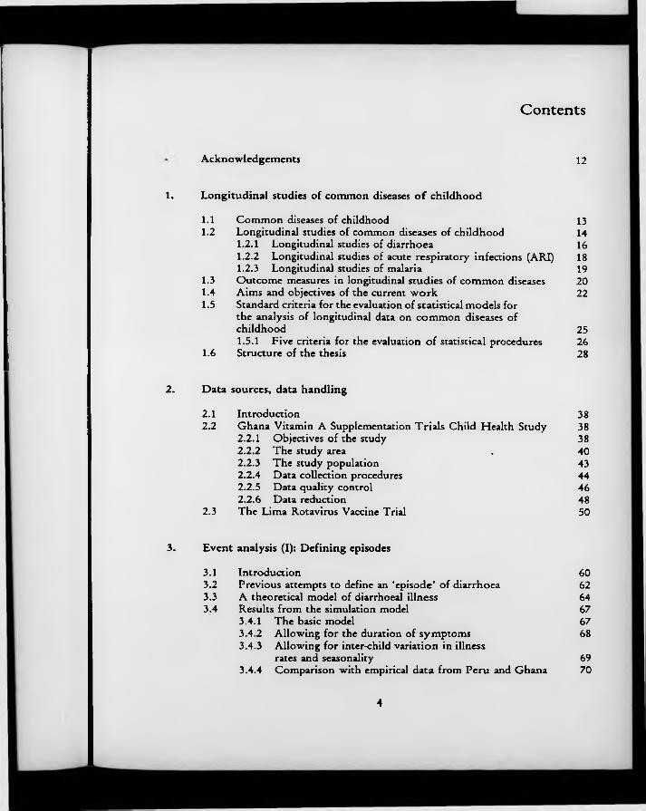
Contents

Acknowledgements 12

1. Longitudinal studies of common diseases of childhood

1.1 Common diseases of childhood 131.2 Longitudinal studies of common diseases of childhood 14

1.2.1 Longitudinal studies of diarrhoea 161.2.2 Longitudinal studies of acute respiratory infections (ARI) 181.2.3 Longitudinal studies of malaria 19

1.3 Outcome measures in longitudinal studies of common diseases 201.4 Aims and objectives of the current work 221.5 Standard criteria for the evaluation of statistical models for

the analysis of longitudinal data on common diseases of childhood 251.5.1 Five criteria for the evaluation of statistical procedures 26

1.6 Structure of the thesis 28

2. Data sources, data handling

2.1 Introduction 382.2 Ghana Vitamin A Supplementation Trials Child Health Study 38

2.2.1 Objectives of the study 382.2.2 The study area . 402.2.3 The study population 432.2.4 Data collection procedures 442.2.5 Data quality control 462.2.6 Data reduction 48

2.3 The Lima Rotavirus Vaccine Trial 50

3. Event analysis (I): Defining episodes

3.1 Introduction 603.2 Previous attempts to define an ‘episode’ of diarrhoea 623.3 A theoretical model of diarrhoeal illness 643.4 Results from the simulation model 67

3.4.1 The basic model 673.4.2 Allowing for the duration of symptoms 683.4.3 Allowing for inter-child variation in illness

rates and seasonality 693.4.4 Comparison with empirical data from Peru and Ghana 70

4

3.5 Conclusions from the simulation model 713.6 Biological plausibility of the model assumptions 733.7 Extensions to other common illnesses 74

4. Event analysis (II): Rates, risks, and measures of association

4.1 Measures of disease frequency 874.2 Measures of association 904.3 A review of current practice in the epidemiological literature 93

4.3.1 Methods 934.3.2 Results 94

4.3.2.1 Aetiology-specific vaccine efficacy 954.3.2.2 Non-specific vaccine efficacy 97

4.4 Discussion 98

5. Event analysis (III): Statistical issues and methods

5.1 Introduction 1075.2 Statistical features of longitudinal data on common diseases 108

5.2.1 Notation 1085.2.2 Within-subject variability 1105.2.3 Between-subject variability 112

5.3 Statistical models for correlated, categorical data 1145.3.1 Conditional models 1155.3.2 ‘Multi-level’ models 1175.3.3 Marginal models 119

5.4 Statistical methods adopted in rotavirus vaccine efficacy trials 1225.5 Conclusions 124Apx Glossary 127

6. Event analysis (IV): Illustrative analysis

6.1 Using the Generalised Estimating Equations algorithms 1366.2 Specifying the form of the within-subject correlation 1386.3 Determining the appropriate width for the time bands 141

6.3.1 Effects on estimates 1426.3.2 Effects on precision 1446.3.3 Conceptual framework and analytic

approach for occasion-specific covariates 1466.4 Differing lengths of follow-up 1476.5 Conclusions 149

5

7. The analysis of prevalence data

7.1 Measures of prevalence in longitudinal studies 1667.2 Episodic prevalence and concept of ‘frailty’ 1697.3 Comparing distributions of episodic prevalences between

different groups of individuals 1717.3.1 Uneven lengths of follow-up, and multiple

measures of episodic prevalence 1737.4 Within-child variability in disease status, and acquired frailty 175

7.4.1 Logistic regression for dependent binary outcomes 1767.5 Discussion and conclusions 179

8. The analysis of data on episode duration

8.1 Introduction 1908.2 Duration data from the Lima Rotavirus Vaccine Trial 1938.3 Modelling duration data 1958.4 Accounting for within-child correlation 1998.5 Discussion and conclusions 200

9. Summary, conclusions and recommendations

9.1 Outcome measures in longitudinal studies of commondiseases of childhood 211

9.2 Statistical features of longitudinal data on common diseasesof childhood 215

9.3 Recent advances in statistical theory relevant to theanalysis of correlated, categorical outcomes 216

9.4 Current practice in the analysis of longitudinal studies ofcommon diseases of childhood 219

9.5 To what degree does the application of traditional methods lead to inappropriate conclusions being drawnfrom the data? 220

9.6 Appropriate data handling strategies 2219.7 Appropriate analytic strategy 222

9.7.1 The analysis of disease incidence 2229.7.2 The analysis of disease prevalence 2259.7.3 The analysis of disease duration 226

9.8 Further research needs for the second half of the 1990s 227

6

Tables

(Tables and Figures are arranged in blocks at the end of the relevant Chapter)

Table 1.1. Selected longitudinal studies of childhood diarrhoea in developing countries.

Table 1.2. Longitudinal studies of acute respiratory infections in children in developing countries.

Table 1.3. Longitudinal studies of childhood malaria in developing countries.

Table 2.1. Ghana VAST Child Survival Study: causes of death in all study children.

Table 2.2. Ghana VAST Child Health Study: total child-weeks of follow-up by age and sex.

Table 3.1. Pathogens demonstrably associated with diarrhoea in children in developing countries.

Table 3.2. Distribution of durations of intervals between days of diarrhoea - simulated data.

Table 3.3. Sensitivities of different definitions of an ‘episode’ under a variety of assumptions on incidence and within-child clustering of trigger events.

Table 4.1. Trigger events, observed bouts of illness, and illness incidence rates calculated by three different methods in a simulated data set.

Table 4.2. Rotavirus vaccine trials: basic details and design features.

Table 4.3. Rotavirus vaccine trials: RV-specific outcomes.

Table 4.4. Rotavirus vaccine trials: all diarrhoeal illness.

Table 5.1. Unadjusted within-child correlations of diarrhoea incidence between consecutive 4-week periods.

Table 5.2. Features and advantages/disadvantages of three different approaches to the analysis of longitudinal count data.

7

Table 6.1. Within-subject correlations, adjusted for main covariate effects.

Table 6.2. Regression coefficients and standard errors from Poisson and GEE (with independence working correlation matrix) models.

Table 6.3. Standard errors from the GEE model using exchangeable and stationary-5 working correlation matrices.

Table 6.4. Regression coefficients from the GEE model with three alternative specifications of the working correlation matrix.

Table 6.5. Regression coefficients from the GEE model with time bands of varying lengths.

Table 6.6. Residual confounding b y age in children classified as aged 0-5 months at the beginning of the one-year follow-up period.

Table 6.7. Associations with age of the child among the full set of covariates examined in the Ghana study.

Table 6.8. Robust SEs from the GEE model with time bands of varying lengths.

Table 6.9. Numbers (and percentages) of time-bands in which the exposure variable is partially misclassified when the value observed at the beginning of the time band is assumed to be correct for the entire duration of that time band.

Table 6.10. Regression coefficients from the GEE model: separate models fitted for 4 sub-groups of children according to their length of follow-up.

Table 6.11. Regression coefficients from the GEE model with and without adjustment for seasonality.

Table 6.12. Summary of recommended analytic strategies for correlated response data.

Table 7.1. Distribution of cough prevalences in children living in compounds with/without an adult with a chronic cough (Ghana VAST CHS).

Table 7.2. Regression analysis of cough prevalence over 3 dosing rounds in the Ghana VAST CHS.

Table 7.3. Comparison of models to predict current illness status (presence of cough) in 100 young children in Northern Ghana observed over 364 consecutive days.

8

Table 8.1. Effect of age and sex on diarrhoea duration (exponential regression).

Table 8.2. The effect of age and sex on diarrhoea duration (exponential, Weibull and Cox regression)

Table 8.3. The effect of age and sex on diarrhoea duration (linear regression using log-transformed duration data).

Table 8.4. The effect of age and sex on diarrhoea duration (exponential regression with/without a correction for within-child correlation).

9

Figures

Figure 2.1. Map of Ghana, showing the Upper East Region.

F igure 2.2. Map of Kassena-Nankana District, showing the Ghana VAST study areas.

F igure 2.3. Ghana VAST Child Health Study: timetable of Events.

F igure 2.4. Morbidity questionnaire used in Ghana VAST Child Health Study.

F igure 3.1. Stool volume in adult volunteers following a pathogenic dose of E. coli (Satterwhite et al., 1987).

F igure 3.2. Four months’ diarrhoea morbidity, child 39, Lima, Peru.

F igure 3.3. Frequency distribution of intervals between trigger events (simulation data).

F igure 3.4. Frequency distribution of diarrhoea in children - Ghana, Peru and simulation data.

F igure 3.5. Frequency distribution of symptom-free intervals between periods of diarrhoea.

F igure 3.6. Presence of cough over 54 consecutive weeks in children in northern Ghana.

F igure 5.1. Within-child variability in diarrhoea incidence.

F igure 5.2. Within-child variability in diarrhoea incidence: relationship between mean 4-weekly episode count and its variance over 13 time periods.

F igure 5.3. Between-child variability in diarrhoea incidence, northern Ghana.

F igure 6.1. Percentage of occasions on which children reportedly slept inside (in children with 12 or more observations of this variable).

F igure 7.1. Point prevalence of ‘intolegere’ over 65 consecutive weeks of data collection, northern Ghana.

10

Figure 7.2. Distribution of episodic prevalences of cough in 1103 children in northern Ghana.

F igure 7.3. Binomial distribution, it — .14, n — 364

Figure 7.4. Distribution of episodic prevalences of cough in children living in compounds with and without an adult with chronic cough, northern Ghana.

F igure 7.5. Within-subject correlations between cough on Day 1 and on subsequent days up to Day 50, Ghana VAST Child Health Study.

F igure 8.1. Lima Rotavirus Vaccine Trial: frequency distribution of duration of diarrhoea episodes.

F igure 8.2. Actual and expected values (Savage scores, based on exponential distribution) of duration data in the Lima data set.

11

Acknowledgements

There are many people to whom I am enormously indebted for their assistance in completing this thesis: foremost among them, my supervisor Betty Kirkwood, who read this thesis more times than any mortal should have to, said many nice things along the way, and has been a source of professional and personal discovery and delight for over four years now.

I would also like to thank the people of Kassena-Nankana district, Ghana, for so patiently answering questions about their children’s health, and the staff of Ghana VAST, for asking them. Many thanks also to Simon Cousens, David Ross, Paul Arthur, Jonathan Sterne, Tom Marshall, Steve Bennett, Dave Leon and Sharon Huttly, for epidemiological and statistical inspiration; the other staff and students of the Maternal and Child Epidemiology Unit, for allowing me time and space in which to work on this project; Therese Stukel of Dartmouth Medical College, for showing me how to use the GEE Macros; Ann Ashworth Hill, for being a nice person to work with, and Helio Herbst, for being a nice person not to work with.

There are of course many more. I hope they w ill forgive me for not mentioning them by name, but it has been a pleasure.

12

Chapter 1 Longitudinal studies o f common diseases of childhood

1.1 Com m on diseases o f childhood

The 1993 World Development Report (World Bank, 1993) has delivered a strong reminder of the dramatic scale of suffering and death attributable to the common childhood diseases - pneumonia, diarrhoea, and, to a lesser extent, malaria. In 1990 alone, lower respiratory infections (essentially pneumonia) resulted in 2.7 million deaths of children under 5 in resource-starved countries, whilst diarrhoea accounted for a further 2.5 million deaths. Another 630,000 children died as a result of malaria. Of the other causes of death, only the group of perinatal causes approached pneumonia or diarrhoea in the number of deaths for which it was responsible.

The degree of suffering caused by these illnesses cannot be measured in terms of mortality alone; children living in poor communities are likely to experience multiple episodes of diarrhoea and respiratory illness each year, to the extent that some of them may spend as much as half the year in a state of ill health. Whilst the geographic bounds of malaria are more restricted, those children who do live in endemic areas can expea to experience one or more episodes of this illness also, either separately or at the same time as an episode of diarrhoea or respiratory illness. In order to capture the degree of disability resulting from illness as well as mortality, the World Development Report has attempted to quantify the total number of ‘Disability Adjusted Life Years’ (DALYs) lost due to each cause of morbidity and mortality. They found that in the 0-4 year age group, respiratory infeaions accounted for 18.5% and 17.6% (in girls and boys, respeaively) of all DALYs lost, and diarrhoea accounted for 16.2% and 15.7%

13

respectively. M alaria accounted for a smaller, but still significant, percentage of all DALYs lost in this age group (4.7% in both sexes).

If these illnesses could somehow be eliminated, and assuming unchanging mortality from other causes, under-5 mortality rates in resource-starved countries would fall by nearly 50%. Furthermore, it is likely that reducing the levels of morbidity from these common illnesses would relieve the strain on children’s nutritional reserves and immune system, and thus reduce their vulnerability to other infections also (Mosley and Becker, 1991). With such enormous gains in welfare potentially achievable, the development of effective interventions to reduce morbidity and mortality from these illnesses is a humanitarian, economic and political imperative.

1.2 L o n g itu d in a l studies o f com m on diseases o f childhood

In order to develop means of reducing the burden of morbidity and mortality from the common childhood diseases, it is first necessary to understand their magnitude, distribution and pre-disposing factors. As recently as the 1950s, however, methods for the study of these illnesses were still poorly developed. It was at this tim e that researchers at the Institute of Nutrition of Central America and Panama (INCAP) started to plan a 5-year study of the interactions between malnutrition and infectious disease. They envisaged an innovative study, in which the health status of a group of young children would be repeatedly assessed at regular intervals, explaining that:

"The traditional methods of the cross-sectional nutritional survey and the prevalence study of infectious disease do not suffice. ...the significance of infectious disease often rests not so much in the immediate event as in the number and progression of preceding episodes and in their relation one to another. Measurement of the postulated synergistic action between infectious disease and malnutrition requires their concurrent study by the epidemiological

14

method of long-term observation of repeated illnesses as they occur under natural conditions." (Scrimshaw et al., 1967).

This type of study, in which repeated observations of the same study subjects are prospectively recorded, is referred to as longitudinal. Longitudinal studies have proved to be of tremendous value in studying the common childhood diseases because these diseases are commonly mild and of short duration, and are thus rapidly forgotten by those taking care of the child, with the result that they are difficult to study retrospectively (Alam et al., 1989; Martorell et al., 1976). They can, of course, be studied cross-sectionally, but this design provides no information about the time sequence of risk factors and health outcomes, and does not allow the researcher to distinguish between children who spend large proportions of their time sick, and others who are normally relatively healthy, but just happen to be ill at the time of the survey.

Of course, a prospective study design does not necessarily imply regular contact with all study subjects: one alternative is simply to wait for cases to present at health facilities. This generally proves to be unsatisfactory in the case of diarrhoea, respiratory infections and malaria, because a large proportion of episodes remain untreated or are treated in the home. In these circumstances, routine home visits by trained interviewers, preferably not less frequently than once a week, is the only approach which can be expected to yield sensitive estimates of disease incidence. The richness and accuracy of the data which these intensive, community-based studies generate has been sufficient to earn them a special place in the epidemiologist’s toolbox. It is these studies which form the subject of this thesis.

Since the completion of the Guatemalan study described above, the community- based longitudinal study has become increasingly popular. Tables 1.1 to 1.3 list some of the many community-based, longitudinal studies of childhood diarrhoea,

15

acute respiratory infections and malaria that have been carried out in a variety of resource-poor countries. The data derived from such studies are of immense importance to health policy makers and planners, who need to know the true burden of morbidity in the communities for which they are responsible. Longitudinal studies can be used to describe this burden in terms of all the usual epidemiological measures of illness frequency: incidence, prevalence and duration. Because these studies generally involve the continuous collection of data over prolonged periods of time, time sequences between risk factors and disease outcomes can be unambiguously established, and important seasonal changes in disease patterns can be studied. Moreover, they are an ideal study design for determining the impact of health interventions delivered at the beginning or in the middle of the period of surveillance. In the following sections, a number of the most important longitudinal studies of diarrhoea, respiratory infections and malaria are discussed in greater detail.

1.2.1 L o n g itu d in a l studies o f diarrhoea

In 1982, Snyder and Merson reviewed the literature on diarrhoea incidence rates derived from community-based studies in developing countries in which household visits were conducted at least once every two weeks and surveillance was maintained for a minimum of one year. Eighteen such studies were identified. In 1992, Bern and co-workers updated this review and were able to identify a further twenty-two studies. Many other studies have been conducted with less frequent visits (or passive surveillance) and shorter lengths of follow-up.

Table 1.1 presents a selection of eighteen studies which have been central to the development of our understanding of the epidemiology of childhood diarrhoea, chosen to illustrate the five different types of objectives which have motivated the setting-up of longitudinal studies. The community intervention model of the early Guatemala study (D8), set up to examine the interactions between nutrition

16

and infection, was soon replicated in Narangwal in the Indian Punjab (D9). Similar study designs have been used to examine the health impacts of water and sanitation improvement projects (D13,D14) and the effects of oral rehydration therapy on diarrhoea case-fatality ratios (D15.D16). An early interest in establishing the frequency of diarrhoeal disease by age and major population sub­groups (Dl,D2) soon gave way to a more specific focus on identifying the precise aetiological agents associated with disease in the community (D3-D7). Prospective observational studies were also used to determine the degree of risk associated with various environmental factors, the consumption of poor quality water, and poor nutritional status at the beginning of the period of observation (D4,D5; D12; DlO.Dll).

More recently, longitudinal study designs have been exploited in individually randomised controlled trials. A large number of trials of rotavirus vaccines have been conducted in both developed and developing countries, w ith the best examples carried out in Peru and Venezuela (D17,D18). Trials of vaccines against other diarrhoeal pathogens, such as cholera and typhoid, have also been conducted, but due to the rarity and severity of these illnesses, intensive home- based surveillance has not been used. A series of studies of the morbidity impacts of periodic, massive dosing with vitamin A have been carried out in Ghana, Brazil, India and Indonesia; they have yet to be reported in detail in the medical press. It is expected that in the near future, the effects of other micronutrient supplements, such as zinc, will also be evaluated, as well as interventions to modify hygiene behaviours.

17

1.2 .2 Longitudinal studies o f acute respiratory infections (ARI)

Community-based, prospective studies of acute respiratory infections (ARI) in young children have been reviewed by Pio et al. (1985) and Rogers (1991). All of th e ARI-specific studies, as well as the more important general studies of childhood morbidity which collected information on respiratory infections, are shown in Table 1.2. Prior to the beginning of the 1980s, data on the epidemiology of acute respiratory infections in childhood came almost exclusively from these general studies, which collected information on a range of different morbidities. Some of these studies, such as that carried out in Matlab in Bangladesh (listed in Table 1.1: D3), contain only minimal information on respiratory infections. Other studies, such as that carried out in San José, Costa Rica (R3), are more informative, reporting incidence rates by age and nutritional status, separately for acute lower respiratory (ALRI) and all acute respiratory infections combined.

D uring the course of the 1980s, a large number of descriptive studies of the epidemiology of acute respiratory infections in children were published. Most of these (R8-R14) came under the umbrella of the Board on Science and Technology for International Development (‘BOSTID’), a series of studies coordinated from the US National Academy of Sciences and using similar case definitions and methods of ascertainment (Selwyn, 1990). Two of these studies (R ll,R 14 ) were birth cohorts, whilst the others included children of mixed ages up to 5 years. The studies focused on age- and seasonal patterns in disease incidence, and - in contrast to many of the longitudinal studies of diarrhoea - contained only limited information on risk factors for disease. One slightly different observational study was that conducted in Basse, in the Gambia (R16). In th is study, detailed information on clinical characteristics of respiratory disease episodes was collected, with a view to identifying clinical predictors of pneumonia.

18

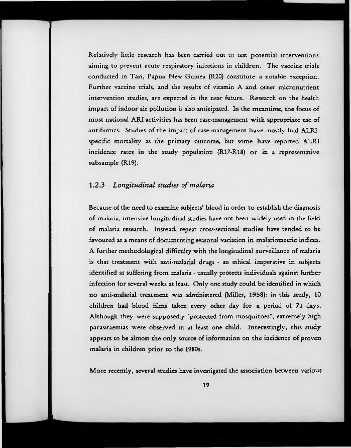
Relatively little research has been carried out to test potential interventions aiming to prevent acute respiratory infections in children. The vaccine trials conducted in Tari, Papua New Guinea (R20) constitute a notable exception. Further vaccine trials, and the results of vitamin A and other micronutrient intervention studies, are expected in the near future. Research on the health impact of indoor air pollution is also anticipated. In the meantime, the focus of most national ARI activities has been case-management w ith appropriate use of antibiotics. Studies of the impact of case-management have mostly had ALRI- specific mortality as the primary outcome, but some have reported ALRI incidence rates in the study population (R17-R18) o r in a representative subsample (R19).

1.2.3 Longitudinal studies o f malaria

Because of the need to examine subjects’ blood in order to establish the diagnosis of malaria, intensive longitudinal studies have not been w idely used in the field of malaria research. Instead, repeat cross-sectional studies have tended to be favoured as a means of documenting seasonal variation in malariometric indices. A further methodological difficulty with the longitudinal surveillance of malaria is that treatment with anti-malarial drugs - an ethical imperative in subjects identified as suffering from malaria - usually protects individuals against further infection for several weeks at least. Only one study could be identified in which no anti-malarial treatment was administered (Miller, 1958): in this study, 10 children had blood films taken every other day for a period of 71 days. Although they were supposedly "protected from mosquitoes", extremely high parasitaemias were observed in at least one child. Interestingly, this study appears to be almost the only source of information on the incidence of proven malaria in children prior to the 1980s.

More recently, several studies have investigated the association between various

19

genetic markers and immunological parameters with clinical malaria, and the impact on malaria of insecticide-impregnated bed nets. Two alternativeapproaches can be identified: in one set of studies (Ml-M2,M5-M6,M9) regular home visits were conducted, and blood slides were taken on children presenting with a history of fever or measured raised temperature. In four other studies (M3-4,M7-8) blood slides were prepared for all study subjects at intervals of between twice a week and once a fortnight. Two studies of the efficacy of new vaccines against Plasmodium falciparum malaria, included for the sake of completeness (M10-11), employed less frequent active case detection (once a month) combined with facilitated passive case detection.

More studies of the impact on morbidity of insecticide-impregnated bed nets, and of new malaria vaccines are expected in the near future. Together, these studies w ill add greatly to our knowledge of the epidemiology of childhood malaria. It is likely, however, that repeated cross-sectional surveys w ill remain the research tool of choice in the area of malaria epidemiology, and for this reason malaria w ill not be a major focus of this thesis.

1.3 O utcom e measures in longitudinal studies o f com m on diseases

Unlike cross-sectional studies, longitudinal studies of common diseases provide estimates of disease incidence as well as prevalence. Furthermore, this type of study facilitates the direct estimation of illness duration, in contrast to the indirect techniques that must be used in cross-sectional studies if information from episodes censored by the survey is to be incorporated. When information has been collected by means of intensive, home-based surveillance, it is possible to estimate all the measures of disease frequency with great reliability in longitudinal studies, a situation which contrasts dramatically w ith the rather poor recall that can be expected in retrospective studies (see above, Section 1.2).

20

Incidence is a measure of disease occurrence. The incidence rate is defined as "the number of disease onsets in the population divided by the sum of the time periods of observation for all individuals in the population" (Rothman, 1986). In the case of common diseases, an individual m ay experience more than one disease onset during the course of the period of observation. This is, of course, quite different from the situation which applies to rare diseases such as cancer, where incidence has generally been taken to refer to the first appearance of the disease in an individual.

Prevalence is a measure of disease status. It may be defined as "the proportion of a population that is affected by disease at any given point in time" (Rothman, 1986). In the case of longitudinal studies of common diseases, measurements of disease status are made repeatedly over the surveillance period, and there are thus many possible points in time to choose from when estimating prevalence. Alternatively, one has the option of focusing on the individual rather than on the time point, and calculating the proportion of time that a given individual experiences illness. Whilst conceptually similar, this measure is no longer prevalence as classically defined.

Duration is related to prevalence, in that the longer the duration of illness episodes, the greater the proportion of the population affected by that illness at any given point in tim e (assuming incidence remains constant). Once again, longitudinal studies of common diseases allow the possibility of examining the distribution of episode durations within individuals, as well as between individuals, provided that individuals experience more than one episode over the period of observation.

The data collected in longitudinal studies of common diseases of childhood are rich and complex, and it is perhaps inevitable that a number of difficulties are encountered when it comes to choosing between and analysing these various

21

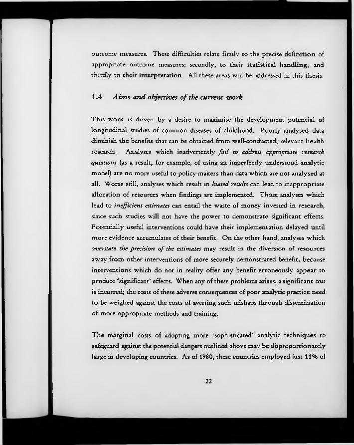
outcome measures. These difficulties relate firstly to the precise defin ition of appropriate outcome measures; secondly, to their statistical handling, and thirdly to their interpretation. All these areas will be addressed in this thesis.

1.4 A im s an d objectives o f the current w ork

This work is driven by a desire to maximise the development potential of longitudinal studies of common diseases of childhood. Poorly analysed data diminish the benefits that can be obtained from well-conducted, relevant health research. Analyses which inadvertently fail to address appropriate research questions (as a result, for example, of using an imperfectly understood analytic model) are no more useful to policy-makers than data which are not analysed at all. Worse still, analyses which result in biased results can lead to inappropriate allocation of resources when findings are implemented. Those analyses which lead to inefficient estimates can entail the waste of money invested in research, since such studies w ill not have the power to demonstrate significant effects. Potentially useful interventions could have their implementation delayed until more evidence accumulates of their benefit. On the other hand, analyses which overstate the precision of the estimates may result in the diversion of resources away from other interventions of more securely demonstrated benefit, because interventions which do not in reality offer any benefit erroneously appear to produce ‘significant’ effects. When any of these problems arises, a significant cost is incurred; the costs of these adverse consequences of poor analytic practice need to be weighed against the costs of averting such mishaps through dissemination of more appropriate methods and training.

The marginal costs of adopting more ‘sophisticated’ analytic techniques to safeguard against the potential dangers outlined above may be disproportionately large in developing countries. As of 1980, these countries employed just 11% of

22

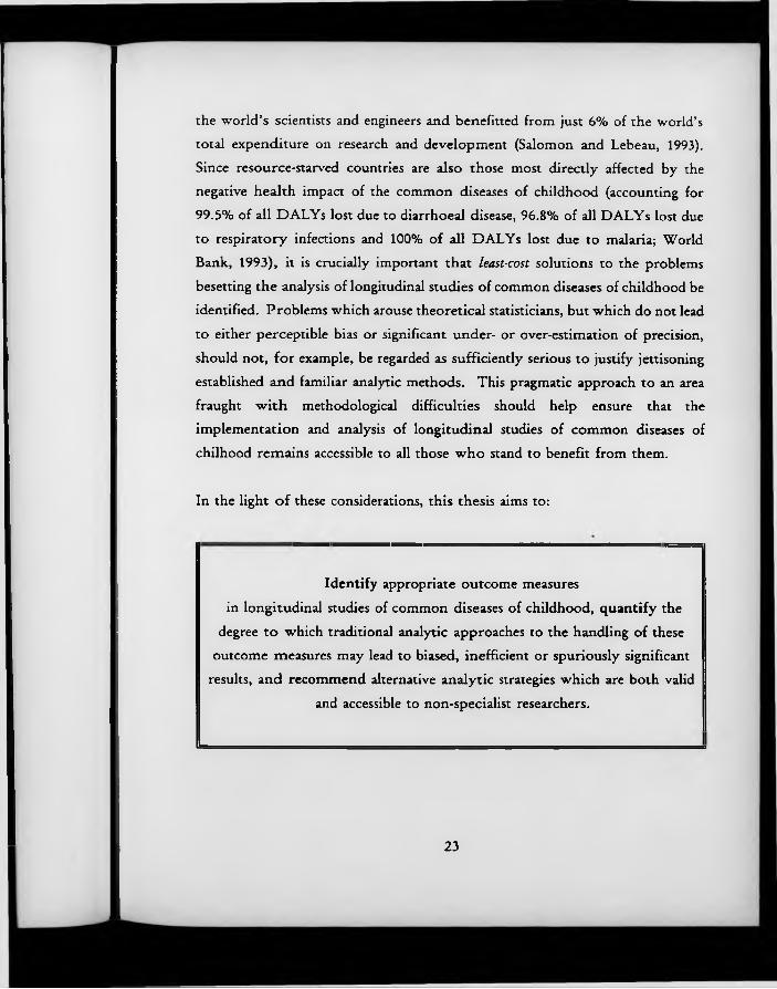
the world’s scientists and engineers and benefitted from just 6% of the world’s total expenditure on research and development (Salomon and Lebeau, 1993). Since resource-starved countries are also those most directly affected by the negative health impact of the common diseases of childhood (accounting for 99.5% of all DALYs lost due to diarrhoeal disease, 96.8% of all DALYs lost due to respiratory infections and 100% of all DALYs lost due to malaria; World Bank, 1993), it is crucially important that least-cost solutions to the problems besetting the analysis of longitudinal studies of common diseases of childhood be identified. Problems which arouse theoretical statisticians, but which do not lead to either perceptible bias or significant under- or over-estimation of precision, should not, for example, be regarded as sufficiently serious to justify jettisoning established and familiar analytic methods. This pragmatic approach to an area fraught w ith methodological difficulties should help ensure that the implementation and analysis of longitudinal studies of common diseases of chilhood remains accessible to all those who stand to benefit from them.

In the light of these considerations, this thesis aims to:

Identify appropriate outcome measures in longitudinal studies of common diseases of childhood, quantify the

degree to which traditional analytic approaches to the handling of these outcome measures may lead to biased, inefficient or spuriously significant

results, and recommend alternative analytic strategies which are both valid and accessible to non-specialist researchers.

23

The following specific objectives are addressed:

1. To describe the range of outcome measures for longitudinal studies of common diseases of childhood, evaluate alternative possible definitions of these measures, and make recommendations for choosing outcome measures appropriate to the specific objectives of each study.

2. To identify the statistical features of longitudinal data on common diseases of childhood which may set them apart from other, less complex, approaches to the study of common morbidities.

3. To describe recent advances in statistical theory which address the specific problems encountered in the analysis of data from longitudinal studies of common diseases of childhood.

4. To describe current practice in the statistical analysis of longitudinal studies of common diseases of childhood.

5. To quantify the degree to which the application of traditional methods of analysis developed for the study of rare diseases to the analysis of data from longitudinal studies of common diseases of childhood may lead to inappropriate conclusions being drawn from the data.

6. To describe appropriate data-handling strategies for large and complex longitudinal data sets.

7. To recommend appropriate strategies for the analysis of longitudinal data on common childhood diseases, on the basis of a set of standardised criteria (see below).

24

1.5 Standard criteria f o r the evaluation o f statistical models fo r the

analysis o f longitudinal data on common diseases o f childhood

New statistical techniques for the analysis of complex data structures are constantly evolving. The descriptions of these models are, for the most part, limited to specialist statistical journals, and little effort is devoted to popularising novel methods within the ‘main-stream’ of epidemiological research. In the case of methodologies for the analysis of longitudinal data on the incidence, prevalence and duration of common diseases, few comparative analyses of available methods have been published, and even when these are undertaken it is often unclear which set of apparently discrepant results is to be preferred, since no standard set of [non-technical] criteria by which to judge such methods has been proposed. This is problematic, because the criteria used by statisticians to judge the technical properties of newly proposed estimators may fail to address a variety of questions which may be equally or more important to those who are destined to use the methods on the ground, such as the relevance to applied research of the underlying conceptual framework. A new set of criteria is therefore required.

I propose a list of five criteria by which to judge the appropriateness of statistical techniques. These criteria include justification of the technical adequacy of the estimators, but also emphasise their flexibility and relevance to applied research. Application of these criteria should permit more rational decision-making about the benefits of investing in sophisticated statistical methodologies. These potential benefits can then be weighed against the costs that such investment would incur. Clearly, the various methodologies would need to be regularly reassessed as new developments became available. No method of scoring on each criterion is proposed at this stage; an element of subjectivity is inevitable in this area.

25

1.5.1 Five criteria fo r the evaluation o f statistical procedures

The following five criteria are proposed:

applicability Do these methods address the kinds of research questions

which epidemiologists actually need to know the answers to?

viability Is the data which is required as inputs for these models

actually available? If not, does this matter?

utility Do the models permit the usual range of statistical activities:

viz. estimation, hypothesis testing, model selection and identification of outliers?

validity Are the estimators asymptotically correct (‘consistent’) and

with minimum variance (‘efficient’)? Is this still the case when model assumptions are broken (i.e. are they ‘robust’)?

potential for wider use

Are the underlying concepts of the model (if not the

technical details) broadly appealing? Can it be adopted

without an massive investment of learning time? Are user- friendly computer applications available/likely to become available?

The first four of these criteria are ordered hierarchically. Clearly, if an analytic approach is not able to test the hypothesis which motivated the setting up of the research project, it should not be given any further consideration. Some models, for example, are unable to handle explanatory variables which vary over time,

26

which might be problematic in a study of the association between water source and diarrhoea morbidity. On the other hand, some analytic procedures will not only provide an answer to the research question at hand, but w ill also estimate any number of additional - extraneous - parameters as well. This may create unnecessary complexity where a simpler procedure would have been adequate, and may be highly undesirable. As for the second criterion, this also needs to be evaluated at the very beginning of the analysis phase, for if the necessary inputs cannot be provided, the analysis cannot proceed. It will sometimes be the case that initial estimates of technical parameters are required as inputs; often, the most appropriate values of these parameters will not be known. However, on occasions, the choice of these input values has only a minor impact on the final results, and this requirement will not therefore be an important constraint.

The third and fourth criteria are technical requirements familiar to statisticians. Estimation, hypothesis testing, model selection and identification of outliers are all indispensable activities in quantitative research, and a model in which one of these options cannot be implemented must be considered seriously handicapped. Possible problems with the technical properties of the estimators (which jointly determine their valid ity , in the broadest sense) w ill be outlined in Chapter 5. These properties are commonly discussed at length in statistical journals, but it is important to recognise that for many applications, a small sacrifice in efficiency, for example, may be acceptable (especially as it can be compensated by increasing the sample size in the field) if it means that a full analysis can be conducted by the original research team, without reference to an external ‘centre of excellence’. Clearly, no universal rules can be developed for deciding how much bias, or loss of precision, may be acceptable in different circumstances. Once the implications of using different analytic approaches are known, however, investigators can decide for themselves whether the likely gains of opting to use a particular technique w ill offset the costs in terms of computing facilities and learning time.

27

The fifth criterion attempts to capture some of these costs. Some of them, such as the profound sense of distrust that new and apparently complex analytic techniques tend to give rise to in those confronting them for the first time, are extremely difficult to measure. Others, such as the cost and user-friendliness of appropriate computer software, can be directly assessed.

1.6 Structure o f the thesis

This thesis consists of nine chapters. This chapter provides an outline of the study context and objectives. Chapter 2 consists of a description of the main data sources used. It contains a detailed account of the approach to data quality control and data reduction adopted in one of the two large-scale field trials which contribute data for this thesis.

The next four chapters focus on event-based analyses. Considerable emphasis is given to this area, as it is felt that longitudinal studies are able to make a unique contribution to epidemiological understanding through the estimation of incidence rates. Chapter 3 examines a number of issues that arise in the definition of illness ‘episodes’. These include conceptual difficulties about exactly what we understand - from a physiological viewpoint - by an ‘episode’ of cough, malaria, or diarrhoea, and also a more technical discussion aiming to provide pragmatic guidelines for the delineation of discrete illness episodes in longitudinal data sets. Chapter 4 moves on to describe how these episodes may be used to define epidemiological measures of disease frequency - risks and rates -and also measures of association - risk and rate ratios. Peculiarities of these measures when used to describe longitudinal data on common diseases are highlighted, and a defined area of the epidemiological literature on common diseases of childhood is examined with a view to identifying which outcome measures are currently being used by investigators in the field.

28

Chapter 5 sets out in some detail the precise nature of the statistical problems that are encountered when attempting to analyse the incidence of common diseases of childhood, and reviews three classes of statistical model which have been proposed to deal with these problems. These modelling strategies are compared and contrasted using the set of standard criteria presented above in Section 1.5. A brief review is also undertaken of the range of analytic methods currently encountered in the epidemiological literature on common diseases of childhood (using as a case-study the same studies as were examined in Chapter 4). Following this, Chapter 6 consists entirely of an illustrative analysis of data on the incidence of diarrhoea from a large-scale field trial with intensive morbidity surveillance. The extent to which ‘standard’ analyses lead to invalid conclusions being drawn about epidemiological parameters is evaluated, and simple, robust methodologies are proposed and illustrated.

A similar approach is then taken to illness prevalence (in Chapter 7) and episode duration (Chapter 8). In these sections, however, greater attention is paid to conceptual issues surrounding the interpretation and applicability of the different outcome measures. In particular, concept of ‘frailty’ is discussed in Chapter 7. Finally, in Chapter 9, the diverse themes of the preceding chapters are drawn together, and summary guidelines for the analysis of longitudinal studies of common diseases of childhood are presented.

29

R e fe re n c e s

General

Alam N, Fitzroy JH, Rahaman MM. Reporting errors in one-week diarrhoea recall surveys: Experience from a prospective study in rural Bangladesh. Int J Epid, 1989; 18:697-99.Cousens SN, Kirkwood BR. Outcome measures in prospective studies of childhood diarrhoea and respiratory infections: choosing and using them. Geneva: World Health Organization, 1990: pp.27.Martorell R, Habicht JP, Yarbrough C et al. Under-reporting in fortnightly morbidity surveys. Environ Child Health, 1976; 129-33.Mosley WH, Becker S. Demographic models for child survival and implications for health intervention programmes. Health Policy Planning 1991; 6(3):218-33.Rothman KJ. Modern epidemiology. Boston/Toronto: Little, Brown & Co., 1986: pp.358.Salomon J, Lebeau A. Mirages of development: science and technology for the Third Worlds. Boulder, Colorada: Lynne Rienner Publishers, 1993. pp. 221.Scrimshaw NS, GuzmSn MA, Gordon JE. Nutrition and infection field study in Guatemalan villages, 1959-64. I. Study plan and experimental design. Arch Environ Health, 1967; 14:657-62.World Bank. World development report 1993: Investing in health. New York: OUP, 1993.

Diarrhoea

Snyder JD, Merson MH. The magnitude of the global problem of acute diarrhoeal disease: a review of active surveillance data. Bull World Health Org, 1982; 60 (4) :605-13 .Bern C, Martines J, de Zoysa I, Glass RI. The magnitude of the global problem of diarhoeal disease: a ten-year update. Bull World Health Org, 1992; 70 (6) :705-14 .D1. Freij L, Wall S. Exploring child health and its ecology. The Kirkos study in Addis Ababa: an evaluation of procedures in the measurement of acute morbidity and a search for causal structure. Acta Paed Scand, 1977; 267(Supp) : 1-120.D2. Leeuwenburg J, Gemert W, Muller AS, Patel SC. Agents affecting health of mother and child in a rural area of Kenya. VII. The incidence of diarrheal disease in the under-five population. Trop Geog Med, 1978; 30:383-91.

30

D3. Black RE, Brown KH, Becker S, Alim ARMA, Hug I. Longitudinal studies of infectious diseases and physical growth of children in rural Bangladesh. II. Incidence of diarrhoea and association with known pathogens. Am J Epid, 1982; 115:315-24.D4. Guerrant RL, Kirchhof LV, Shields DS et al. Prospective study of diarrhoeal illnesses in Northeastern Brazil: Patterns of disease, nutritional impact, etiologies and risk factors. J Infect Dis, 1983; 148:986-97.D5. El Alamy MA, Thacker SB, Arafat RR, Wright CE, Zaki AM. The incidence of diarrhoeal disease in a defined population of rural Egypt. Am J Trop Med Hyg, 1986; 35(5) :1006-12.D6. Goh Rowland SGJ, Lloyd Evans N, Williams K, Rowland MGM. The etiology of diarrhoea studied in the community in young urban Gambian children. J Diar Dis Res, 1985; 3:7-13.D7. Black RE, López de Romaña G, Brown KH, Bravo N, Grados Bazalar O, Creed Kanashiro H. Incidence and etiology of infantile diarrhea and major routes of transmission in Huascar, Peru. Am J Epid, 1989; 129:785-99.D8. Gordon JE, Ascoli W, Mata LJ, Guzmán MA, Scrimshaw NS. Nutrition and infection field study in Guatemalan villages, 1959-1964. VI. Acute diarrhoeal disease and nutritional disorders in general disease incidence. Arch Environ Health, 1968; 16:424-37.D9. Kielmann AA, Taylor CE, DeSweeme C et al. The Narangwal experiment on interactions of nutrition and infections. II. Morbidity and mortality effects. Ind J Med Res, 1978; 68(Supp) :21- 41 .DIO. Sepúlveda J, Willett W, Múñoz A. Malnutrition and diarrhoea: A longitudinal study among urban Mexican children. Am J Epid, 1988; 127 (2) : 365-76 .Dll. Baqui AH, Black RE, Sack RB, Chowdhury HR, Yunus M, Siddique AK. Malnutrition, cell-mediated immune deficiency and diarrhea: community-based longitudinal study in rural Bangladeshi children. Am J Epid, 1993; 137(3):355-65.D12. Curlin GT, Aziz KMA, Khan MR. The influence of drinking tubewell water on diarrhea rates in Matlab Thana, Bangladesh. Dacca, Bangladesh 1977: ICDDR-B Working Paper No. 1.D13. Huttly SRA, Blum D, Kirkwood BR et al. The Imo State (Nigeria) drinking water supply and sanitation project, 2. Impact on dracunculiasis, diarrhoea and nutritional status. Trans Royal Soc Trop Med Hyg, 1990; 84:316-21.D14. Huttly SRA, Hoque BA, Aziz KMA et al. Persistent diarrhea in a rural area of Bangladesh: a community based longitudinal study. Int J Epid, 1989;18:964-9.D15. Rahaman MM, Aziz KMS, Patwari Y, Munshi MH. Diarrhoeal mortality in two Bangladeshi villages with and without community- based oral rehydration therapy. Lancet, 1979; 2 (ii) :809-12.

31

D16. Kumar V, Kumar R, Datta N. Oral rehydration therapy in reducing diarrhoea-related mortality in rural India. J Diar Dis Res, 1987; 5:159-64.D17. Lanata CF, Black RE, del Aguila R et al. Protection of Peruvian children against rotavirus diarrhea of specific serotypes by one, two or three doses of the RIT 4237 attenuated bovine rotavirus vaccine. J Inf Dis, 1989; 159 (3) :452-459.DIS. Perez-Schael I, Garcia D, González M. Prospective study of diarrheal diseases in Venezuelan children to evaluate the efficacy of rhesus rotavirus vaccine. J Med Vir, 1990; 30:219-29.

Acute Respiratory Infections

Pio A, Leowski J, ten Dam HG. The magnitude of the problem of acute respiratory infections. In: Douglas RM, Kerby-Eaton E (Eds). Acute respiratory infections in childhood: proceedings of an international workshop, Sydney, August 1984. Adelaide 1985: University of Adelaide.Rogers S. Pneumonia is a killer disease. ARI News, 1991; 21:2,6.Selwyn BJ on behalf of the coordinated data group of BOSTID researchers. The epidemiology of acute respiratory tract infection in young children: comparison of findings from several developing countries. Rev Inf Dis 1990; 12(supp 8):S870-S888.R1. Datta Banik ND, Krishna R, Mane SIS, Raj L. A longitudinal study of morbidity and mortality pattern of children under the age of five years in an urban community. Ind J Med Res, 1969; 57(5):948-57.R2. Kamath KR, Feldman RA, Sundar Rao PSS, Webb JKG. Infection and disease in a group of South Indian families. II. General morbidity patterns in families and family members . Am J Epid, 1969; 89 (4) :375- 83 .R3. James JW. Longitudinal study of the morbidity of diarrheal and respiratory infections in malnourished children. Am J Clin Nutr, 1972; 25:690-4.R4. Dodge RE Jr, Demeke T. The epidemiology of infant malnutrition in Dabat. Ethiop Med J, 1970; 8:53-72.R5. Freij L, Wall S. Exploring child health and its ecology. The Kirkos study in Addis Ababa: an evaluation of procedures in the measurement of acute morbidity and a search for causal structure. Acta Paed Scand, 1977; 267(Supp):1-120.R6. Lang T, Lafaix C, Fassin D et al. Acute respiratory infections: a longitudinal study of 151 children in Burkina-Faso. Int J Epid, 1986; 15(4):553-9.R7. Martinez-Garcia MAC, Mufioz O, Peniche A, Ramirez-Grande MAE, Gutierrez G. Acute respiratory infections in Mexican rural communities. Achiv Invest Med (Mex), 1989; 20(3): 255-62.

32

R 8 . Oyejide CO, Osinusi K. Acute respiratory tract infection in children in Idikan Community, Ibadan, Nigeria: severity, risk factors, and frequency of occurrence. Rev Inf Dis, 1990; 12(supp 8) : S1042-6 .R 9 . Wafula EM, Onyango FE, Mirza WM. Epidemiology of acute respiratory tract infections among young children in Kenya. Rev Inf Dis, 1990; 12 (supp 8):S1035-8.RIO. Cruz JR, Pareja G, de Fernández A, Peralta F, Cáceres P, Cano F. Epidemiology of acute respiratory tract infections among Guatemalan ambulatory preschool children. Rev Inf Dis, 1990; 12 (supp 8) :S1029-34.R11 . Hortal M, Benitez A, Contera M, Etorena P, Montano A, Meny M. A community-based study of acute respiratory tract infections in children in Uruguay. Rev Inf Dis, 1990; 12(supp 8):S966-73.R12. Tupasi TE, de Leon LE, Lupisan S et al. Patterns of acute respiratory tract infection in children: a longitudinal study in a depressed community in Metro Manila. Rev Inf Dis, 1990; 12 (S 8) : S940-9.R13. Vathanophas K, Sangchai R, Raktham S et al. A community-based study of acute respiratory tract infections in Thai children. Rev Inf Dis, 1990; 12(supp 8):S957-65.R14. Borrero I, Fajardo L, Bedoya A, Zea A, Carmona F, de Borrero M F . Acute respiratory tract infections in a birth cohort of children from Cali, Colombia, who were studied through 17 months of age. Rev Inf Dis, 1990; 12(supp 8):S950-6.R15. Lindtjorn B, Alemu T, Bjorvatn B. Child health in arid areas of Ethiopia: longitudinal study of the morbidity in infectious diseases. Scand J Infect Dis, 1992; 24: 369-77R16. Campbell H, Byass P, Lamont AC et al. Assessment of clinical criteria for identification of severe acute lower respiratory tract infections in children. Lancet, 1989; l(i):297-9.R 17. Pandey MR, Sharma PR, Gubhaju BB et al. Impact of a pilot acute respiratory infection (ARI) control programme in a rural community of the hill region of Nepal. Ann Trop Paed 1989; 9(4) : 212-20.R18. Khan AJ, Khan JA, Akbar M, Addiss DG. Acute respiratory infections in children: A case management intervention in Abottabad District, Pakistan. Bull World Health Org, 1990; 68(5) :577-85.R19. Bang AT, Bang AR, Tale O et al. Reduction in pneumonia mortality and total childhood mortality by means of community-based intervention trial in Gadchiroli, India. Lancet, 1990; 336 (8709) : 201 -6 .R20. Lehmann D, Marshall TF de C, Riley ID, Alpers MP. Immunisation with a polyvalent pneumococcal vaccine: effect on respiratory mortality on children living in the New Guinea highlands. Arch Dis Child, 1981; 56:354-7.

33

Malaria

Ml. Trape JF, Zoulani A, Quinet MC. Assessment of the incidence and prevalence of clinical malaria in semi-immune children exposed to intense and perennial transmission. Am JEpid, 1987 ; 126 (2) -.193-201.M2. Allen BJ, Rowe P, Allsopp CE et al. A prospective study of the influence of a-thalassaemia on morbidity from malaria and immune responses to defined Plasmodium falciparum antigens in Gambian children. Trans Royal Soc Trop Med Hyg, 1993; 87(3) :282-9 (and other references).

M3. Toile R, Fruh K, Doumbo O et al. A prospective study of the association between the human humoral immune response to Plasmodium falciparum blood stage antigen gpl90 and control of malarial infections. Infect Immun, 1993; 61(l):40-7.M4. Rogier C, Trape JF. Malaria attacks in children exposed to high transmission: who is protected? Trans Royal Soc Trop Med Hyg, 1993; 87 (3) : 245-6 .MS. Snow RW, Rowan KM, Greenwood BM. A trial of permethrin-treated bed nets in the prevention of malaria in Gambian children. Trans Royal Soc Trop Med Hyg, 1987; 81:563-7.M6. Snow RW, Lindsay SW, Hayes RJ, Greenwood BM. Permethrin-treated bed nets (mosquito nets) prevent malaria in Gambian children. Trans Royal Soc Trop Med Hyg, 1987; 81:563-7.M7. Sexton JD, Ruebush TK II, Brandling-Bennett AD et al. Permethrin-impregnated curtains and bed-nets prevent malaria in Western Kenya. Am J Trop Med Hyg, 1990; 43:11-18.MS. Msuya FHM, Curtis CF. Trial of pyrethroid-impregnated bed nets in an area of Tanzania holoendemic for malaria. Part 4. Effects on incidence of malaria infection. Acta Trop, 1991; 4*9:165-71.M9. Alonso PL, Lindsay SW, Armstrong Schellenberg JRM et al. A malaria control trial using insecticide-treated bed nets and targeted chemoprophylaxis in a rural area of The Gambia, West Africa. Trans Royal Soc Trop Med Hyg, 1993 ; 87(svipp2) :37-44.M10. Guiguemde TR, Sturchler D, Ouedraogo JB et al. Vaccination against malaria: initial trial with an anti-sporozoite vaccine, (NANP)3-TT (RO 40-2361) in Africa (Bobo Dioulasso, Burkina Faso). Bull Soc Pathol Exot, 1990; 83(2):217-27.Mil. Valero MV, Amador LR, Galindo C et al. Vaccination with SPf66, a chemically synthesised vaccine, against Plasmodium falciparum malaria in Colombia. Lancet, 1993; 341 (8847) :705-10.

34

Table 1.1 Selected longitudinal studies of childhooddiarrhoea in developing countries

Study Location Year Objectives of study Ref

Descriptive epidemiology of diarrhoea; aetiological studies:

Kirkos, Ethiopia Machakos, Kenya Matlab, Bangladesh Pacatuba, NE Brazil Bilbeis, Egypt Bakau, Gambia Huascar, Peru

1972-731974-771978-791978-801980- 811981- 841982- 84

Epidemiology of childhood disease Demogra'ic & disease surveillance Aetiologies; disease & growth Environmental conditions, aetiol. Home environment; aetiologies Basic epidem' logy and aetiologies Aet. and environ'al contamination

D1D2D3D4D5D6D7

Studies of the interaction between diarrhoea and nutrition:

Santa María Cauqué, Guatemala

Narangwal, India Mexico City, Mexico Matlab, Bangladesh

1959-641970-7319841988-89

Int'vn: improved medical care vs. nutrition supplement vs. control Int'vn: medical care vs nutrition Assoc: nutritional status & diarr Assoc: nutr. status, CMI & diarr

D8D9DIODll

Wa t e r and sanitation:

Matlab, Bangladesh Imo State, Nigeria Mirzapur, Bangladesh

19761982-861984-87

Assoc: Consumption tubewell water Int'vn: Boreholes & VIP latrines Int'vn: Pumps,latrines & hyg educD12D13D14

Impact of Oral Rehydration Therapy on the course of illness:

Teknaf, Bangladesh Haryana, India 1977-79early1980s

Efficacy of ORSEfficacy of alternative delivery strategies for ORS

D15D16

Vaccine efficacy studies:

Canto Grande, Peru Caracas, Venezuela 1985-61985-87 Efficacy of attenuated RV vaccine Efficacy of rhesus RV vaccineD17D18

Notes: Int'vn-intervention study; Assoc>observational study; CMI«cell-mediated immunity; RV-rotavirus

35

Table 1.2 Longitudinal studies of acute respiratory-infections in children in developing countries

Study Location year Objectives of study Ref

Non-specific studies of childhood morbidity:

Delhi, India Vellore, India San José, Costa Rica Dabat, Ethiopia Kirkos, Ethiopia

1962-671965- 671966- 67 1968 1972-73

morbidity and SES in children general morbidity of 110 families morbidity and nutritional status morbidity and nutritional status epidemiology of childhood disease

R1R2R3R4R5

Basic epidemiology of ARI:

Rural c'ties, Mexico Bana, Burkina Faso Ibadan, Nigeria Maragua, Kenya Guatemala City, Gu. Montevideo, Uruguay Manila, Philippines Bangkok, Thailand Cali, Colombia Dubluk/Elka,Ethiopia Basse, Gambia

1982- 831983- 841984- 871985- 87 1985-86 1985-871985- 871986- 87 1986-88 1989-91 ?

nationally representative samplesmall rural communitypoor urban communityrural communitymarginal urban areapoor urban area - birth cohortpoor urban communitypoor urban communitypoor urban area - birth cohortrural arid lowland communitiesclinical predictors of pneumonia

R6R7R8R9RIORIIR12R13R14R15R16

Case-management :

Kathmandu Vly, Nepal Abottabad, Pakistan Gadchiroli, India

71985-87 1989-?

Health educ, immun. & antibiotics Active case-detection Morbidity sub-study

R17 Ri 8 RI 9 II

Vaccine efficacy studies:

Tari, P New Guinea 1981-83 Efficacy of pneumococcal vaccine R20

36

Table 1.3 Longitudinal studies of childhood malaria indeveloping countries

Study Location Year Objectives of study Ref

Epidemiology and immunology of childhood malaria:

Dinzolo, Congo Farafenni, Gambia Safo. Mali Dielmo, Senegal

1983-841988-8919891990

1/week; t temp. -. thick film 1/week; t temp -» film; immunology blood films 1/fortnight; immun'y thick films 2/week; temp 1/2 days

MlM2M3M4

Studies of the impact of impregnated bed nets:

Katchang, Gambia Farafenni, Gambia Uriri, KenyaMuheza, Tanzania Soma, Gambia

1985198719881988-891988-90

ACD 1/week; temp., 'fever' -* film ACD 1/week; t temp. -• blood film ACD 2 /week; 'fever' -» temp.;

weekly thick & thin blood film blood slides l/fortnight ACD 1/week; t temp. -► blood film

M5M6M7M8M9

Vaccine efficacy studies:

Vallée du Kou, Burkina Faso

Da Tola, Colombia19881991-92

blood films 1/month + PCDACD 1/month + PCD; temp., symp -« blood film

M10Mil

Notes: ACD=active case detection; 'fever'»reported fever; PCD=passive case detection; sytnp=symptom; temp=temperature.

37

Chapter 2 Data Sources, Data H a n d lin g

2 .1 Introduction

The larger part of the arguments in this thesis will be developed with reference to an empirical data set describing the morbidity experience of young children in northern Ghana over the period 1990-91. These data were collected as part of the Ghana Vitamin A Supplementation Trials, two companion, randomised, placebo-controlled field trials of the effects of large-dose, periodic supplementation with vitamin A on the health and survival of young children. From September 1990, three months after the commencement of morbidity surveillance in the area, I was resident at the field station in Navrongo, where I was employed as statistician for the morbidity study. In the first section of this chapter I w ill describe this data set in some detail, w ith particular reference to the data quality control and data handling procedures developed by me during my time in Navrongo. At the end of this chapter, I w ill describe the other main data source from Peru, used for the comparative analysis of episode definitions in Chapter 3 and an examination of the duration of diarrhoea episodes in Chapter 8.

2 .2 G hana V itam in A Supplementation Trials C h ild H ealth Study

2 .2 .1 O bjectives o f the study

The Ghana Vitamin A Supplementation Trials Child Health Study, henceforth known as Ghana VAST - CHS, was one of four large-scale field trials of the effect of periodic, massive-dose vitamin A supplementation on the health, as

38

distinct from mortality, of young children to be carried out in developing countries in the late 1980s/early 1990s. Vitamin A is a naturally occurring compound which it has long been known is crucially important for the maintenance of epithelial integrity and function in humans (Wolbach and Howe, 1925; Zile et al., 1981). More recently, it has become clear that vitamin A exerts a number of other effects on the immune system (Ross, 1992). A severe form of vitamin A deficiency, known as xerophthalmia, leads to poor vision in dim light (‘night blindness’), reversible opacities on the surface of the eye (‘Bitot’s spots’), and finally, irreversible damage to the cornea, and blindness (Sommer, 1982).

Although the value of vitamin A treatment in measles was demonstrated as early as 1932 (Ellison), it was a series of findings in Indonesia in the early 1980s which aroused new interest in the vitamin in the broader scientific community: Alfred Sommer and co-workers (Sommer et al., 1983) showed that children with night blindness or Bitot’s spots suffered mortality rates over the following 3 month period that were around 4 times higher than those of children without signs of vitamin A deficiency. This finding was rapidly followed by an intervention study in the same area, which showed that massive-dose vitamin A supplementation was able to reduce the mortality rate in children aged 12-71 months by 34% (Sommer et al., 1986). These results, which were confirmed in 1988 by a food fortification study also conducted in Indonesia (Muhilal et al., 1988), and later by other supplementation studies carried out in the south of India (Rahmathullah et al., 1990) and Nepal (West et al., 1991; Daulaire et al., 1992), suggested that the detrimental effects of vitamin A deficiency must be affecting many organs other than the eye, and must be occurring at levels of deficiency not previously recognised as posing a significant threat to health. Two further supplementation studies conducted in the north of India (Vijayaraghavan et al., 1990) and Sudan (Herrera et al., 1992) failed to identify any beneficial impact of vitamin A supplementation on mortality.

39

In an attempt to determine whether the same reductions in childhood mortality could be delivered in an African context, a trial of the effects of massive-dose, periodic supplementation with synthetic vitamin A on childhood mortality (Ghana Vitamin A Supplementation Trials Child Survival Study) was set up in Navrongo, northern Ghana, in early 1989. The companion Child Health Study was established the following year in an adjacent area. The aim of this study was to determine the mechanism by which vitamin A was achieving such impressive impacts on child survival, by documenting in great detail any effects on the incidence, duration and severity of a range of childhood illnesses, principally diarrhoea and respiratory disease. In addition to elucidating the mechanisms by which vitamin A supplementation was able to achieve its mortality-saving effects, it was hoped that this study would provide information about additional gains of vitamin A supplementation arising from the reduction of the morbidity burden in young children. The most important results from the two Ghana VAST trials have been published in the Lancet (Ghana VAST Study Team, 1993).

2 .2 .2 The study area

The Child Health Study was carried out in Kassena-Nankana District, an administrative sub-division of the Upper East Region of Ghana (see map, Figure 2.1). The Upper East Region of Ghana shares a common border with Burkina Faso to the north, and has many ecological and cultural features in common with that country. The climate is sub-Sahelian, w ith an annual average of 852 mm of rain (1981-90, Irrigation Company of the Upper Regions) falling in a single rainy season, which lasts approximately from M ay until September. The bulk of the agricultural activity in the region is concentrated in this period, when sorghum, millet, groundnuts and beans are grown for household consumption. During the remainder of the year, the climate is extremely arid, with relative humidity falling to 20% in March/April. Agriculture is not possible during this period, except for those with access to a dry-season vegetable garden. These are usually

40

irrigated from hand-dug wells, although a small area of the district is irrigated commercially, using water channelled from a large man-made reservoir.

Three different ethnic groups live in the district: the Kassena, the Nankana and the Bulli. All of these are Voltaic peoples, closer to the Moré of Burkina Faso than to the Akan peoples of southern and central Ghana. All three groups live in dispersed settlements, or ‘compounds’, of between 1 and 50 or more inhabitants (median = 8). Although families living in the same compound share bonds of kinship, each ‘nuclear’ household is to a large degree economically independent, leading to large discrepancies in living standards within compounds. The only substantial sized town in the district is the capital Navrongo (20,000 inhabitants), which has two secondary schools and a teacher training college, as well as a medium-sized district hospital. Four other health centres are scattered throughout the district, none of them in the area where the Child Health Study was carried out (see below, Section 2.2.3).

In general, the health situation in the district is extremely poor. Indirect estimates of child mortality derived using the Preceding Birth Technique (Brass, 1985) to analyse data collected in the baseline survey of the study suggest that in the year 1987, the (period) risk of dying by age five (5q0) was around 173/1000. The major causes of death in young children, as identified by the Ghana VAST Child Survival Study, 1989-91, are shown in Table 2.1. Acute gastroenteritis and chronic diarrhoea/malnutrition together account for nearly one third of all deaths of infants and children in the area. Episodes of diarrhoea are frequent, with the average child experiencing 5 episodes each year. Although access to potable water is high, with 72% of families getting their drinking water from a closed system borehole in the dry season, it is likely that much of this water becomes contaminated during storage, and the animal pounds which surround 83% of compounds undoubtedly provide a rich reservoir of enteric pathogens. Hygiene practices are poor, and 78% of mothers in the study area have never

41

attended school.

The burden of parasitic diseases is very heavy, with malaria highly prevalent in young children at all times of year (prevalence ranging from 53% in the dry season to 85% in the rainy season), and responsible for one quarter of all deaths in childhood and infancy. Schistosomiasis and filariasis are common in older children. Respiratory infections appear to account for a somewhat lower percentage of all infant and child deaths than is commonly observed in developing countries (WHO, 1993). It is possible that transmission of respiratory pathogens is reduced by the custom of sleeping on the roofs of the dwellings rather than inside rooms, except during the rainy season, when the prevalence of respiratory symptoms goes up.

Immunisation coverage was poor at the outset of the study, with only 25% of children aged 12-23 months having received the full schedule of vaccines (children without a health card available for inspection assumed not fully vaccinated). Measles occurs in approximately biennial epidemics, w ith a cumulative incidence of 13% in 4-year olds (this of course excludes those children who have died, and is therefore undoubtedly a gross underestimate of the true incidence). In general, nutritional status is very poor, w ith 38% of children under five more than 2 standard deviations below the median weight-for-age of the United States National Centre for Health Statistics reference population (US Public Health Service, 1976). Vitamin A deficiency is widespread; 74% of children were severely or moderately deficient at baseline, with serum retinol levels below 0.7 /xmol/L.

42

2.2 .3 The study population

The Child Health Study was carried out in an area of 198 km2, to the south of Navrongo town (see map, Figure 2.2). This area was divided into four sub­zones. In three of these sub-zones, all children born on or after the 1st January, 1986 were recruited into the study. On completion of the population census in these areas, it became clear that the sample size obtained would not be adequate to evaluate all of the study hypotheses, and the fourth sub-zone was added. In this fourth sub-zone, all children born on or after 1st January, 1988 were recruited into the study. This was to provide relatively greater amounts of follow-up time in the age group 0-23 months, where the bulk of morbid events were expected to occur. In all, 1206 children had been registered into the study by the first day of the baseline clinical examinations, which took place in April (subzones 1 and 2) and June (subzones 3 and 4) of 1990.

Dosing with vitamin A/placebo, along with the initiation of regular weekly morbidity surveillance, took place two months after the baseline clinical examination. A full timetable of the study is shown in Figure 2.3, and it can be seen that activities in subzones 3 and 4 were staggered two months behind those in sub-zones 1 and 2. Once regular home visits had begun it was possible to identify all new births and new arrivals into the study area, and these children continued to be enrolled into the study until the last dosing points in June (subzones 1 and 2) and August (subzones 3 and 4) of 1991. A total of 740 children were enrolled into the study from the first day of the baseline clinical examinations until the end of the study. The total number of child-weeks of follow-up in each age group is shown in Table 2.2.

It should be noted that children did not enter the vitamin A supplementation trial until they were first eligible for dosing, and that no children were eligible for dosing until they reached the age of 6 months or over. The number of

43

children in the vitamin A supplementation trial is therefore less than the number of children in the morbidity study as a whole, and the age structure of the child- weeks of follow-up is different. Analyses in this thesis are based on all children enrolled into the study, rather than the subset who participated in the vitamin A trial.

2 .2 .4 Data collection procedures

Three different types of data were collected during the course of the Child Health Study: baseline demographic, socio-economic, nutritional and previous medical histories; prospective surveillance of morbidity; and repeated measures of time-dependent covariates (risk factors).

The baseline data were collected by means of questionnaires administered in the home prior to the beginning of the study. Some of the data, such as sex, birth order, and exposure to measles, can be viewed as fixed covariates relating specifically to the index child. Another set of data, including the educational level of the child’s mother and her knowledge of oral rehydration therapy are household- rather than individual-level covariates. 24% of study mothers had more than one child in the study. A third set of data, collected on a separate form, relates to characteristics of the residential compound, such as possession of animals or ‘luxury’ items, or presence of animal faeces in the living area.

Current morbidity was assessed in a number of different ways. Between the first and the last dosing points in each sub-zone, all children were visited weekly in their homes, and a detailed morbidity questionnaire was administered (Figure 2.4). The presence of 21 signs or symptoms was enquired about over each day of the preceding week, using a locally understood terminology that was identified prior to the start of the study with the help of a consultant anthropologist. For example, seven distinct diarrhoeal illnesses were enquired about, and four

44

different respiratory complexes. In order to help the respondent (usually the child’s mother) remember the child’s health status on each of the preceding 7 days, a pictorial illness diary was left with the child’s caretaker each week. She was then asked to mark on the diary each day whether the child had some form of diarrhoeal illness, a respiratory illness, another illness, or had been in good health. The diary was then used as an aide-memoire during the course of the morbidity interview.

In addition to the daily presence or absence of the listed signs and symptoms, a number of simple observations of the child’s health status were made by the fieldworker each week. These included measuring the child’s temperature and breathing rate, and listening for signs of respiratory distress. A history of consultations with health service providers (both allopathic and traditional) was taken, and on occasions when diarrhoeal illness was reported during the week, a detailed assessment of illness severity was undertaken.

In the advent of severe illness of any kind, or the presence of warning signs such as raised breathing rate, fieldworkers were instructed to refer children to one of the mobile clinics provided by the project in the study area. Since the clinics visited two different sections of the study area on alternate weeks, referrals were only possible on 2/10 visit days (the day of the clinic, and the day before). For those study subjects living nearer to Navrongo town, another clinic was provided once a week in the district hospital. In addition to those children referred to the clinics by fieldworkers, a larger number of children presented spontaneously to the clinics. Severely sick children were admitted to Navrongo hospital and kept under daily surveillance by the study paediatrician.

45

Once every four weeks, a different set of fieldworkers would visit all the children in their homes to update information on the most important time-dependent covariates. These included feeding mode, sleeping patterns and potential sources of air pollution, source of drinking water, weight and mid-upper arm circumference (these latter intended as additional outcomes for the vitamin A trial). A small number of variables, such as length and vitamin A/placebo dosing status, were only updated at the 4-monthly dosing rounds, and one variable, vaccination status, was only updated a single time at the end of the study. These data can be combined with the morbidity data in risk factor analyses.

2 .2 .5 D ata qu ality control

Data quality control measures were instigated both in the field and in the computer centre. Field measures included scheduled and unscheduled supervisory visits to fieldworkers in the field, blind re-interviews with the children’s carers and random checks on study households, and weekly meetings of all field staff. Due to the high ratio of supervisory to lower-grade staff (one deputy supervisor for every four fieldworkers) an intensive surveillance of field operations could be maintained at all stages of the study.

In the computer centre, all data were entered twice in order to minimise typographic errors. Following the completion of data entry, a series of computerised checks was run to ensure that only permitted values of each variable had been recorded (‘range checks’) and that no inconsistent responses had been recorded within each questionnaire (‘consistency checks’). Consistency of response from one period to the next was verified on a number of key variables - such as breastfeeding and anthropometric status - by scrutiny of the full sequence of records for any unexpected transitions, such as the resumption of breastfeeding after a child had been fully weaned, or weight gain of more than one kilogram in the course of a single month. Such inconsistencies resulted in

46

the retrieval of the original records, discussion with the fieldworker concerned, and, in the case of breastfeeding queries, a detailed interview with the child’s mother in an attempt to establish the true course of events.

Probably the most innovative element of the data quality control measures developed in the computer centre was the elaboration of simple performance indicators based on elements recorded each week on the morbidity questionnaire. By tabulation of these indicators, comparisons could be made between fieldworkers, and those whose performance was poor relative to the average (or suspiciously good) could be singled out for re-training and surveillance by supervisory staff. Indicators which proved particularly useful included the proportion of visits on which the study child was recorded absent and the prevalence of a number of common complaints such as cough or fever. Disaggregation of fieldworker-specific prevalence rates by day since previous interview revealed that whilst some fieldworkers were recording similar prevalences over each day of the week (as should be the case), others appeared not to be probing adequately about events occurring earlier in the week, and were thus recording substantial increases in disease prevalence towards the end of the week. There were also important differences between fieldworkers in the frequency with which whole weeks of illness (suggestive of a failure to establish day of onset and day of recovery) were recorded.

Continuous variables, such as measured breathing rate or axillary temperature also provided rich grounds for the examination of between-fieldworker differences. The proportion of ‘failed readings’ was especially useful in identifying technical problems with use of the instruments (or simply inadequate performance), and proportions above or below critical cut-offs were also useful in establishing systematic observer bias. Measures of variability for these variables proved to be as informative as measures of location, with substantially below-average spread, and uniform rather than Normal-shaped distributions

47

suggestive of falsification of data. Use of these measures of fieldworker performance ensured high quality data and established good communication between the field operations and the computer centre: supervisory staff participated in the interpretation of these data and frequently suggested alternative measures of performance. In this way, analysis was integrated with data collection from an early stage, and was rapidly established as an interactive process.

2 .2 .6 D ata reduction

Due to the complex nature of the data set, considerable difficulty was encountered in reducing the data to a format appropriate for calculating measures of incidence and prevalence. Essentially, two very different approaches may be adopted to the organisation of data sets of this type, with each of them characterised by a number of distinct advantages and disadvantages. The first option is to create files in which each day of observation, for each individual participating in the study, has a separate record, with the various signs and symptoms being recorded as a set of discrete variables. This format is particularly advantageous when it comes to prevalence-type analyses, since the denominator is simply the total number of records (usually excluding missing values), and the numerator can be obtained very straightforwardly by running frequencies on the relevant variables. Obtaining summary statistics on each study individual, such as the number of days with a particular symptom, is also relatively straightforward using analytic packages which permit ‘aggregate’ functions (summarising over common values of an identifier variable). Obtaining episode-type data is, however, awkward with this arrangement of data, since many w idely used analysis packages are not good at scanning multiple records simultaneously (this is necessary to determine whether an episode has really ended, o r is just interrupted by, say, one day without symptoms). Furthermore, this arrangement of the data results in enormous data sets (half a million records,

48

in the case of the Ghana VAST Child Health Study), which are extremely cumbersome to manipulate, especially if they need to be sorted.

A second option is to concatenate all the data for one individual over the whole observation period, creating a single long string variable. C learly this can only be done for one sign/symptom at a time. If, therefore, it is desired to create complex variables representing combinations of signs or symptoms, these must be created before concatenation. The resulting files are much more manageable, since they only have as many records as there are individuals in the study, but multiple files are generated (one for each sign/symptom). This is the approach that was adopted in the Ghana VAST Child Health Study. It has the disadvantage that a further set of programs must then be written (in a programming language, as opposed to using a standard analytic package) to read the morbidity strings and generate summary measures of prevalence and incidence. However, the generation of illness episodes is relatively simple, since looking backwards and ahead to other days in the string presents no problem. Moreover, visual inspection of individuals’ morbidity patterns over time becomes possible, a procedure the usefulness of which should not be underestimated. In spite of this, the disassociation of information on different signs/symptoms is undesirable from many points of view, and this approach should probably only be considered when the amount of information collected is so large that other approaches are not feasible.

Whatever approach is adopted to the organisation of the morbidity data, there are bound to be specific problems which arise during the course of the data processing as a result of the particular design features of each study. It is important to think carefully about the implications of each possible resolution of these problems, and to take pragmatic decisions to facilitate the analysis. An example of such a problem arose in the Ghana VAST study when children moved from one ‘sub-zone’ to another within the same ‘zone’ (see map, Figure

49

2.2). Since within each zone, fieldwork in one sub-zone was staggered one week behind fieldwork in the other sub-zone, this could result in children having more or less than the full year of follow-up. This was undesirable both from the point of view of assessing the impact of vitamin A supplementation, which had to be over the same period of time since dosing for all children, and from a programming perspective. The final week of follow-up was therefore eliminated from those children with 53 rather than 52 weeks of follow-up, and four children who moved zones (and were therefore dosed at 2- or 6- month intervals, rather than the normal four months) were excluded from the analysis altogether.

2 .3 The L im a R otaviru s Vaccine T rial

A second data set is used in Chapter 3 to explore issues in the definition of episodes of illness, and again in Chapter 9 to examine the duration of episodes of diarrhoea. These data were kindly contributed by Dr Claudio Lanata of the Instituto de Investigación Nutricional, Lima, Peru in order to permit comparative analyses with the Ghana VAST Child Health Study data described above.

The Peru study was a randomised, placebo-controlled trial of a single dose of the Rhesus or Rhesus-Human reassortant rotavirus vaccines conducted between August 1987 and October 1990 in a shanty town on the outskirts of the capital, Lima. The primary objective of the study was to determine whether either of the two vaccines, administered to 800 children at two months of age, could bring about a reduction in the number of diarrhoea episodes associated with rotavirus over the following two-year period. A secondary objective was to determine whether the vaccines could bring about a reduction in all-cause diarrhoea over the same period.

Field methods were broadly similar to those described for the Ghana study, although home surveillance was more frequent. Field workers interviewed the

50

mothers/carers of study children in their homes twice every week and recorded data on the total number of stools each day and the number of liquid/semi-liquid stools, as well as on a number of other clinical features of the illness, including the hydration status of the child. Stool samples were taken for laboratory analysis when diarrhoea (defined as 3 or more liquid/semi-liquid stools in a 24- hour period) was reported. Severely sick children were referred to a clinic for attention and specific antibiotics were provided for culture-proven, treatable diarrhoeal illness. However, clinic attendances do not form a major outcome for this study. Also, given the more specific focus of th is study on diarrhoeal disease compared to the Ghana study, there is a more limited array of risk-factor data: only breastfeeding data were regularly updated, in this case on a daily basis. Baseline socio-economic and demographic data were collected at the time each child was enrolled into the study.

Quality control measures were similar to those used in Ghana. A system of incentives and penalties for fieldworker performance was developed to encourage high quality returns. Specially designed data entry systems (using Turbo-Pascal) were developed, giving rise to individual child-day records. The derivation of episode counts forms the basis of the discussion in Chapter 3.

51

R e fe re n c e s

Brass W. Advances in methods for estimating fertility and mortality from limited and defective data. Centre for Population Studies Occasional Publication. London: London School of Hygiene and Tropical Medicine, 1985.Daulaire NMP, Starbuck ES, Houston RM, Church MS, Stukel TA, Pandey MR. Childhood mortality after a high dose of vitamin A in a high risk population. BMJ, 1992; 304:207-10.Ellison JB. Intensive vitamin therapy in measles. BMJ, 1932; 2:708-1 1 .

Ghana VAST Study Team. Vitamin A supplementation in northern Ghana: effects on clinic attendances, hospital admissions, and child mortality. Lancet, 1993; 342 (8862) :7-12.Herrera MG, Nestel P, El Amin A, Fawzi WW, Mohamed KA, Weld L. Vitamin A supplementation and child survival. Lancet 1992; 340:71.267-71.Muhilal, Permeisih D, Idjradinata YR, Muherdiyantiningsih, Karyadi D. Vitamin A-fortified monosodium glutamate and health, growth, and survival of children: a controlled field trial. Am J Clin Nutr, 1988; 48 (1271-6) .Rahmathullah L, Underwood BA, Thulasiraj RD et al. Reduced mortality among children in southern India receiving a small weekly dose of vitamin A. NEJM, 1990; 323 (14) :929-35.Ross AC. Vitamin A status: Relationship to immunity and the antibody response. Proc Soc Exper Biol Med, 1992; 200:303-20.Sommer A. Nutritional blindness: xerophthalmia and keratomalacia. New York: Oxford University Press, 1982.Sommer A, Tarjwoto I, Djunaedi E et al. Impact of vitamin A supplementation on childhood mortality. Lancet, 1986; i: 1169-73.Sommer A, Tarwotjo I, Hussaini G, Susanto D. Increased mortality in children with mild vitamin A deficiency. Lancet, 1983; 8350:585-8.United States Public Health Service, Health Resources Administration. NCHS growth charts. Rockville, MD: Health Resources Administration, 1976.Vijayaraghavan K, Radhaiah G, Surya Prakasam B, Rameshwar Sarma KV, Reddy V. Effect of massive dose vitamin A on morbidity and mortality in Indian children. Lancet 1990; 336:1342-1345.West KP Jr, Pokhrel RP, Katz J. Efficacy of vitamin A in reducing preschool child mortality in Nepal. Lancet 1991; 338(8759):67-71.Wolbach SB, Howe PR. Tissue changes following deprivation of fat- soluble A vitamin. J Exper Med, 1925; 42:753-77.

52

World Health Organization programme for control of acute respiratory- infections. Interim programme report 1992. Geneva: World Health Organization, 1993.Zile MH, Bunge EC, Deluca HF. DNA labelling of rat epithelial tissues in vitamin A deficiency. J Nutr, 1981; 111:777-88.

53

Table 2.1 Ghana VAST Child Survival Study:Causes of death in all study children

Number of deaths %

of total

Deaths with established cause:Malaria 276 25 3%Acute Gastroenteritis 274 25 1% i

I Chronic Diarrhoea or Malnutrition 75 6 9%I Acute Lower Respiratory Infection 203 18 6%Measles 151 13 8%Injury 25 2 3%Meningitis 14 1 3%Other 73 6 7%

Cause not known 326

Total 1417

54

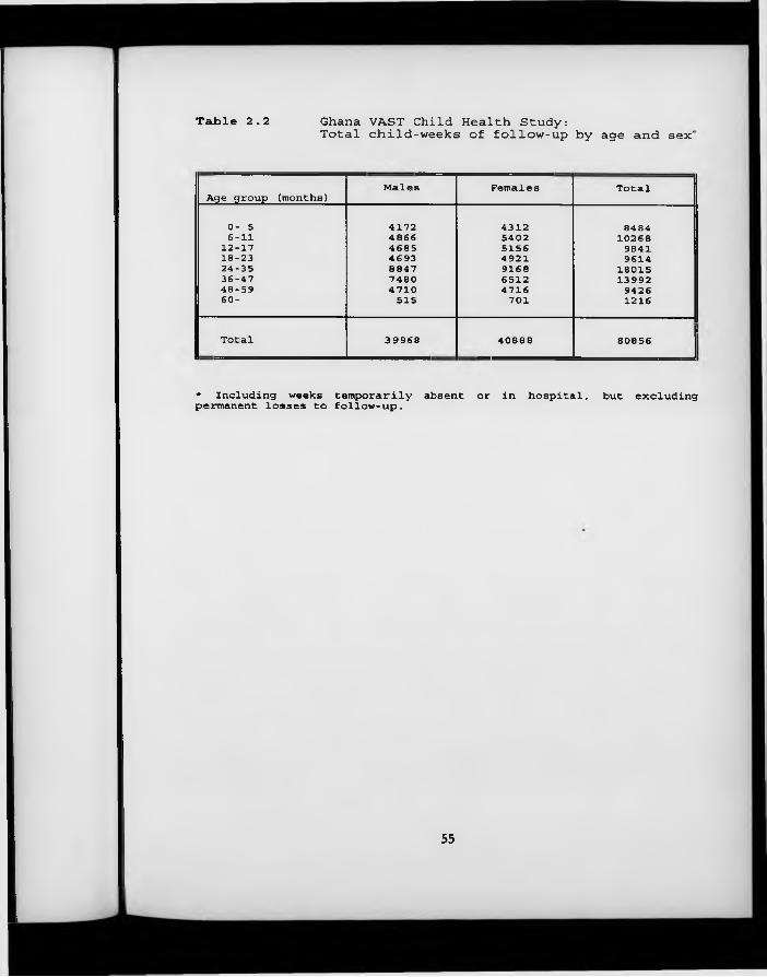
Table 2.2 Ghana VAST Child Health Study:Total child-weeks of follow-up by age and sex'

Age group (months)Males Females Total

0- 5 4172 4312 84846-11 4866 5402 1026812-17 4685 5156 984118-23 4693 4921 961424-35 8847 9168 1801536-47 7480 6512 1399248-59 4710 4716 942660- 515 701 1216

Total 39968 40888 80856

* Including weeks temporarily absent or in hospital, permanent losses to follow-up. but excluding

55

Figure 2.1 Map of Ghana, showing the Upper East Region

56

Figure 2.2 Map of Kassena-Nankana District, showing the Ghana VAST study areas

BURKINA FASO

K /</) .ÿ? ' *2 / * 0 /•vu r '

<I,1"

T o W a « / - * '"

»

v------ -

' Nakong

Osina Boundary

VAST Survival Study Area (by zone)

VAST Health Sludy Area (by subzone)

VAST Ollioes

Roads

Scale 1 850,000

0 5 to km

57

Figure 2.3 Ghana VAST Child Health Study: Timetable of Events

Figure 2.4 Morbidity questionnaire used inVAST Child Health Study

3 . 1T.TMFCS HT3TO9V 2 o f 4

Look. « t th e DIARY; Aek about i l l n e a e e a voday and In th e a w h ."Tor M e n day of th e w eek in te r I= 'ie c . O*0c . - -NK; W;5=T«.«t:<y, S t f l s L a r '. w*ex. For WEEK; ^ C o n d it io n rep c-r ;ea as o c c u rn n .: d u r in g week, «even i f daya HK);O Condition did net orvur; 0s&K/Uir?ert%La oecauae laic ieccepiete.

MAR

POMOSGO

FNOREGO

SAAPELEC

KOTOH

BiSITON

LOGFRE

D a y t im e cough

N ight. L a e cough

B lo cked i/ ru n n y nose

“ I “ ’i• -1 m [COUGH

NCOUGH

DOSE

SAPID

TRIBS

i 1 ; i!i

ii 1

Voae kafcla/V oae aw u ie taule.-'L e l a l e l a a lu n

C h a p r i.s e bobga/N yapigsa borya/ S o n n o vc cw

!:

.Ì l! r

{I ’]

; Ii

;i1 1

K a ta n a v o ae ra aonga sor.ça/Voaei p ag e r e a / 0 Hare o a i lm v e r a n e «

... !i

1 itL J L _

DIFFER

E ar p a i r . 1; T i . I... ]_Jl___ KARPAIN

SARDIS

MEASLES

SKIM

VOMIT

FUA

IMTOL

RKFFOOD

E ar d is c h a r g e __!__ i__!__i__ ____M e a d e «

: ! \S k in r a s h ( exc lude h e a t rash*. ] ! ; __1_____i____ ! \V a n i t in e : 1

Is

P ua/ F o go Paa ?L _____

i:

s*I n to l e g e r e 'Sy in g tu la / Y e e Lorna: 1 j ■ ■: ! Ü

R e f u s in g food/Breaet ;• - i — L j ________

O t h e r : " " " " " " ; ÿ ? 0T^IK

--------1--------i--------O M M junsji»Y sjaM r)| lAYc.t VttEC 1

D ia r r h o e a ; Saa/Chari fcc/Ch. r r ;

Pom osco/Foyr gaer» 'Wuxuru

W a te ry e t c o l due to F ia in e r e g c / P ith a g iin ^ rc 'ç :- K'trigwaa.

* : i } i

! i . i !

! 1 ; I •____________ . J ____ ! _____!_____

\

S aa p e le g o / C h a r i* * lego/C bero - pongo

K otoh/V y a cogo/Kacb 1 c

B ie i to u ,- B is itcR go .'T i i i c h i*

L ogere/L ugya/Sanpca

■ 1 ! : «Îi!

!! . 1 ..

1 :! 1

•! 1

j i ■ 1 1

! !--------!--------_____ 1____

Ghana

59

Chapter 3 E v e n t A n a ly s is (I): D e f in in g E p iso d es

3 .1 Introduction

Despite the fact that all researchers analysing longitudinal studies of common diseases must confront this problem at some point, the question of how to define an episode of a frequently occurring illness such as diarrhoea has attracted surprisingly little attention in the epidemiological literature. In experimentally induced infections, episodes of illness can generally be clearly identified: symptoms begin shortly after administration of the pathogenic challenge, increase in severity as the infection becomes established, and then - in most cases - decline as an effective immune response is mounted. This is illustrated in Figure 3.1, which shows results from a volunteer study (Satterwhite et al., 1978) in which mean stool volume was measured each day following administration of a pathogenic dose of Escherichia coli. In this study, group C was challenged with a large dose of a highly virulent strain of the pathogen, and experienced markedly increased stool volume on days 2, 3 and 4 of the experiment, compared to the other three groups who received smaller inocula or a less virulent strain. Similar patterns are described for other diarrhoeal pathogens (see, for example, Music et al., 1970).

Such clearly defined patterns of sickness and recovery cannot be expected in community-based studies. Exposure to pathogens in the community is not a discrete, time-limited event; instead, children in developing countries grow up in the midst of a reservoir of multiple pathogens. Diarrhoeal pathogens are commonly present in the water these children drink, the food they eat and in animal faeces which they come into contact with around the home (Black et al., 1989). Table 3.1 presents a list of organisms known to cause diarrhoea in

60

children in developing countries. Other infections and non-infectious events are also suspected to be associated with diarrhoea in young children: Plasmodium falciparum malaria (Harinasuta & Bunnag, 1988); food allergy, especially to cow’s m ilk , eggs, fish, peanuts or soya (Helbling, 1994), and - more controversially - personal or familial stress (Dutton et al., 1985). It should not therefore surprise us if children living in contaminated environments are exposed to several distinct challenges in the course of only a few days or weeks. This would naturally produce a more complicated symptomatology than that described in volunteers exposed to a single, controlled dose.

It is also important to note that, contrary to what may be achieved in volunteer studies, other variables are not generally ‘held constant’ when a child becomes sick with diarrhoea. Indeed, active steps are usually taken to manage the child’s illness. Some of these actions may have a palliative effect though they fail to achieve a complete cure. However, even in the absence of deliberate manipulations of the child’s environment, day-to-day fluctuations in the severity of symptoms are to be expected in the course of any illness. Thus the child may experience a few days with milder symptoms before returning to frank illness. In diseases such as shigellosis, relapses are known to occur, even after an apparently radical cure has been affected (see, for example, Gilman et al., 1981). When patients with shigellosis are not treated with antibiotics, carriage of the pathogen may persist for periods approaching three months (DuPont et al.,1969), and changes in the child’s nutritional/immune status may be sufficient to induce relapse.

The net effect of these complexities of community infection is that individual children’s symptom histories may be difficult to interpret confidently in terms of discrete episodes of illness. Figure 3.2 depicts the diarrhoea morbidity experience of a single child in the Lima rotavirus vaccine study described in Section 2.3. It is far from clear how many ‘episodes’ of diarrhoea this child

61

experienced in April 1989 - it may be that the whole month made up a single aetiological episode of illness, with only low-grade symptoms on most days. On the other hand, it is possible even that the peak occurring on the 7th and 8th days of the month could have been aetiologically distinct from the symptoms recorded a few days earlier. Only DNA serotyping of pathogens can provide definitive answers to these questions. Since such a solution is wholly impractical in the majority of community-based studies, I attempt in this chapter to provide pragmatic guidance on appropriate algorithms for defining the beginning and end of diarrhoea episodes. In the final section of the chapter, I discuss the biological plausibility of the conclusions that emerge, and extensions to other common diseases of childhood.

3 .2 Previous attem pts to define an ‘episode’ o f diarrhoea

The standard approach in defining episodes of diarrhoea has been to specify a minimum number of diarrhoea-free days which must intervene between days with symptoms before it can be considered that these periods of diarrhoea represent genuinely distinct episodes. It has been shown, however, that there is little consensus on what should be the minimum number of symptom-free days between distinct ‘episodes’ of diarrhoea (Baqui et a l., 1991). Some studies have required only two symptom-free days between episodes, whilst others have required as many as 14 symptom-free days.

The urgent need for some standardisation of the definition of an episode of diarrhoea was clearly demonstrated in the article by Baqui and co-workers, which showed that altering the number of symptom-free days required to signal the break between one episode and the next from 1 day to 7 days can reduce the apparent total number of episodes by as much as one third, and that estimates of the incidence of ‘persistent’ diarrhoea (episodes of more than 14 days’ duration) are also dramatically affected. Similar conclusions were reached some

62

years earlier in an analysis of diarrhoea data from the Gambia by Pickering et al. (1987). Baqui and colleagues note that the greatest change is seen when varying the number of diarrhoea-free days between episodes from one to three, and that "increasing the requirement for a new episode from three to seven diarrhoea-free days provided very similar measures of diarrhoeal incidence". They therefore conclude that "using fewer than three diarrhoea-free days could possibly over­estimate the overall diarrhoeal incidence".

This conclusion appears to be based on the assumption that it would be unlikely for a child to experience a new episode of diarrhoea within a day or two of recovering from a previous episode. No biological or mathematical justification for this assumption is presented. In order to determine whether such an assumption might be justified, we decided to model the occurrence in time of diarrhoea-provoking ‘trigger’ events, as described in Section 3.3. When this is done, it becomes possible to compare observed distributions of illness in time (or more precisely, the distribution of intervals between days of illness) with the distribution expected under the assumptions of the model. If, in any particular study, the observed distribution of intervals follows the expected distribution closely, it can be concluded that it would not be appropriate to combine in the analysis periods of illness following each other in rapid succession. On the other hand, if there is a large excess of observed over expected symptom-free intervals of - for example - one or two days’ duration, such short intervals as these should probably not be considered sufficient to define a new episode of diarrhoea.

63

3 .3 A theoretical m odel o f diarrhoeal illness

Because of the large number of different possible causes of diarrhoeal illness in young children, the concept of a ‘trigger event’ is central to the development of a theoretical model. A trigger event is defined as any event provoking the appearance of diarrhoea symptoms in the child. In many cases, the trigger event w ill consist of an incident infection w ith a diarrhoeal pathogen, but other possibilities, such as a change in the ch ild ’s ability to contain a pre-existing infection, or a non-specific trigger event such as malaria, are not excluded provided that they are causally associated with symptoms of diarrhoea in the immediately ensuing period of time.

The central assumption of the model is that, in the experience of each child, trigger events are randomly distributed in time. This assumption is reasonable if it is accepted that the trigger events result from encounters between the child and other persons, objects or externally conditioned events, each one of which may be defined in probabilistic terms (see Section 3.6). It implies that by chance alone, a susceptible individual may encounter several trigger events in rapid succession. When this happens, a new period of symptoms may start before the previous illness has resolved. Etiologically distinct periods of symptoms will overlap in time and only one ‘episode’ of illness will be observed.

The model is developed in a number of stages. In the simplest version, it is assumed that all individuals will encounter trigger events at the same constant rate over time (X). This results in a Poisson process (Whittle, 1976), in which time intervals between successive trigger events are distributed with an exponential probability density function,

f(x) - X .e^

64

where x represents the length of the interval between trigger events. Based on this simplistic assumption, a data set is generated representing the morbidity experience of 10,000 children monitored over a period of 365 days.

In subsequent stages of the model development, three potentially important determinants of the distribution in time of periods of diarrhoeal illness and the intervals between them are added sequentially:

(1) The distribution of the duration of symptoms of diarrhoea following a trigger event. This might be expected to influence the proportion of trigger events occurring in the course of a pre-existing period of illness.

(2) Inter-individual variation in the rate at which trigger events are encountered. Since important characteristics of the child such as his/her age, housing conditions, nutrition etc. are known to influence the rate of diarrhoeal illness, the initial assumption of homogeneity of incidence rates is clearly unrealistic.

(3) Seasonal variation in the rate at which trigger events are encountered. This may be considerable in some environments.

Parameters for development of the model are derived from the two empirical data sets from Ghana and Peru described in the previous chapter. Many alternative parametrisations of the model are of course possible; some of these are discussed in Section 3.4.3 following the development of the primary model.

In the simplest version of the model, individuals experience trigger events at a rate of 9 events per child per year. Because some trigger events can be expected to occur during the course of a pre-existing period of diarrhoea symptoms, this would normally be equivalent to a somewhat lower episode incidence rate,

65

probably close to 8.5 episodes per child per year. This episode rate, whilst corresponding fairly well to those found in both the Peru and the Ghana studies, is clearly at the upper end of the range of diarrhoea incidence rates reported in empirical studies from developing countries (Bern et al., 1992). The implication of the use of lower rates is also considered in Section 3.4.3.

As the second stage in the development of the model, allowance was made for the duration of symptoms following a trigger event. Examination of the two empirical data sets reveals that the numbers of consecutive days of diarrhoea had an approximately negative exponential distribution, a curve with a negative slope which is initially steep but asymptotically approaches zero. This curve is fully defined by a single parameter, X ^; the larger the value of Xdu,, the steeper the initial slope. In the Peru study, the mean number of consecutive days of three or more liquid/semi-liquid stools was 2.6, and the distribution was well approximated by a negative exponential distribution with Xdur=0.67 (grouping all durations of 15 days or more and comparing observed versus expected distributions resulted in a x2 statistic of 0.53 on 14 d.f.). In the Ghana study, the distribution of durations was heavily influenced by heaping, on 7 and 14 days, but a similar pattern was apparent. It is therefore assumed that the duration of symptoms may be represented by a negative exponential distribution, with a parameter of Xdur«0.67, as estimated from the Peruvian data.

The third stage in the development of the model involved relaxing the assumption that the underlying rates of diarrhoeal illness would be the same for all children. In order to permit different ‘children’ in the simulated population to have different trigger event rates, the distribution of rates in the population is assumed to follow a Gamma distribution, a flexible family of curves commonly used to model skewed, continuous variables restricted to the positive range (Rothschild & Logothetis, 1986). A scaled-up Gamma distribution with parameters 1.5 (shape), 0.5 (scale) and a multiplying factor of 3 is used to model

66

the between-child variation. This provides a degree of skew in the underlying rates intermediate between those observed in the two empirical data sets, with a mean rate of 9.0, as before.

Finally, the effect of seasonal variation in diarrhoea incidence is allowed for. This might be expected to increase the proportion of trigger events separated from the preceding event by relatively short intervals. Although many alternative seasonal patterns could be considered, the final version of the model incorporates a two-season split, with a mean rate of 5.4 trigger events/year in the first half of the year and 12.6 in the second half of the year. This 2.3-fold increase slightly exceeds the contrast observed in the Ghana data, in an area with a marked climatic change from dry to wet season. The data from Peru showed very little seasonality. Whilst the choice of contrast is arbitrary, it is felt unlikely that seasonal variation would exceed this level in many environments.

3 .4 Results fro m the sim ulation m odel

3 .4 .1 The Basic M odel

The simplest version of the model, in which trigger events are determined by a simple Poisson process, is illustrated in Figure 3.3. In this figure, the distribution of intervals between consecutive trigger events is shown by a continuous line (the duration of symptoms following each trigger event is not considered at this stage). It is apparent from this figure, though perhaps not so intuitively, that the shorter the interval between trigger events, the more frequently it may be expected to occur. The most frequently encountered interval between one trigger event and the next is, therefore, an interval of one day or less.

67

It should be noted at this point that the length of the period of observation may be expected to have a substantial effect on the proportion of all intervals observed between one trigger event and the next that are of short duration. This artefact arises because long intervals are more likely than short intervals to be censored by the end of the observation period. Thus, while 7.9% of all closed intervals are of 3 days duration or less (under the Poisson model) when the period of observation is 365 days long, 11.5% of all such intervals would have been of this length had the period of observation been limited to only 90 days.

3 .4 .2 A llo w in g fo r the duration o f sym ptom s

When each trigger event is assigned a duration (randomly generated from a negative exponential distribution, as described above), it can be shown that 6.3% of all non-initial trigger events occur during the course of a pre-existing period of illness, and so would not be detected in a community study. Similarly, in the model, only a single period of symptoms is observed, starting with the first trigger event and ending when the child is no longer experiencing symptoms resulting from either of the tw o events.

The distribution of intervals between periods of diarrhoea symptoms (trigger events plus their associated durations) is shown by the bars in Figure 3.3. It can be seen that the distribution of intervals is not appreciably altered by the additional assumption that each trigger event is associated with a number of subsequent days of symptoms during which time the impact of new trigger events cannot be detected. Even lengthening the durations considerably does not alter the relative distribution of intervals between periods of symptoms. This is a property of the Poisson distribution.

68

3.4 .3 A llo w in g fo r inter-child varia tio n in illness rates a n d seasonality

Figure 3.4 shows the distribution of the number of periods of diarrhoea experienced by each child in the two empirical data sets (Peru: one year of follow-up only; two alternative definitions of diarrhoea [see below, Section 3.4.4]) and in the simulation model when allowing for clustering of diarrhoeal illness within children. The distribution obtained from the model lies between the three observed distributions.

Table 3.2 shows the model distribution of intervals between periods of diarrhoea when clustering, and clustering plus seasonality, are added to the basic model. The distribution of intervals when neither clustering nor seasonality are present is also shown for comparison. With both clustering and seasonality incorporated into the model, 11.3% of all non-initial trigger events occur during the course of a pre-existing period of diarrhoea. Allowing for clustering of diarrhoea illness appears to substantially increase the proportion of short intervals expected, such that 12.6% of periods of diarrhoea are preceded by three or less symptom-free days, as opposed to only 8.0% without clustering. Allowing for seasonality produces a smaller increase in the expected proportion of short symptom-free intervals (9.3% of periods of diarrhoea are preceded by three or less symptom- free days with seasonality but no clustering, and 14.1% when both seasonality and clustering are present).

This approach allows us to calculate the sensitivities of alternative definitions of an episode, relative to the situation in which a single symptom-free day defines a new episode. The sensitivity of a particular definition is estimated as the proportion of all non-initial ‘episodes’ (separated by at least one day from previous periods of illness) that remain distinct (i.e. are not merged with previous ‘episodes’) under the new definition. Table 3.3 shows the sensitivities of three alternative definitions of an episode - break periods of two, three and seven days

69

without symptoms - assuming a range of different incidence rates and within- child clustering. The results demonstrate that under the assumptions of the model, requiring 7 days o r more free of symptoms between episodes would lead to up to one fifth or even a quarter of genuinely distinct periods of illness being combined in the analysis in situations of high incidence or high within-child clustering. The alternative definitions considered are associated with sensitivities above 90%, regardless of the incidence rate or degree of clustering.

3 .4 .4 Com parison w ith em pirical data fro m Peru an d Ghana

The distribution of intervals between periods of one or more consecutive days of diarrhoea in the two empirical data sets is shown in Figure 3.5. The data from Peru are presented for each of two alternative definitions of diarrhoea: under definition A, diarrhoea is defined as three or more liquid/semi-liquid stools in a 24-hour period. Under definition B, however, two liquid/semi-liquid stools in a 24-hour period also constitute diarrhoea providing that three or more stools were reported on both the previous and following days. It can be seen that there is pronounced heaping on intervals of one day duration in the Peru data set (definition A) and on intervals of seven and fourteen days in the Ghana data set. In the Ghana data set, the observed heaping seems to be an artefact of the data collection system, which was based on once-a-week home visits. It was noted for several of the most common conditions enquired about, and does not appear to be linked to the definition of diarrhoea.

Heaping in the Peru data set, on the other hand, virtually disappears with the use of the more flexible definition of diarrhoea (definition B). This suggests that many of the apparent single-day intervals should in fact be viewed as days of milder symptoms occurring during the course of a longer illness episode. If definition B is in fact the appropriate one, then these results may be used to derive a measure of the specificity of the single day cut-off to define a new

70

episode of diarrhoea when diarrhoea is defined according to the standard algorithm (definition A). In this case, the specificity is lower than desired, at around 90%. The specificity of a two-day cut-off is, however, likely to be acceptably high.

3 .5 Conclusions fro m the sim ulation m odel

Using a simple conceptual framework to develop a model of the distribution over time of diarrhoea symptoms in young children, the following principal findings emerge:

a) The true incidence of trigger events cannot, in practice, be observed, since many such events may occur when the child is already experiencing a period of diarrhoea occasioned by a previous trigger event. Where within child clustering of diarrhoea and seasonality are important, our model suggests that over 10% of all trigger events could be missed in this way.

b) With a high incidence of trigger events and clustering of çUarrhoeal illness in a subset of high-risk children, many periods of diarrhoea resulting from genuinely distinct trigger events are separated from each other by intervals of only a few days. In such circumstances, as many as 10-15% of all periods of diarrhoea may be preceded by just three diarrhoea-free days or less. The choice of the minimum number of days required to define a new episode may, therefore, have a considerable impact on the reported incidence of diarrhoea.

c) In a contrasting situation, with no clustering, and a lower incidence of trigger events - say, five trigger events per child per year - only around 5% of all periods of diarrhoea would be preceded by three or less symptom-free days. In these circumstances, the choice of the minimum number of days required to define a new episode w ill have much less impact on the reported incidence of diarrhoea.

71

d) The model may be used to highlight irregular patterns in the distribution of interval durations in empirical data. If the assumptions of our model are approximately correct, then these irregularities must be due either to deficiencies in the data collection instruments or to the occurrence of occasional symptom- free days in the course of ongoing episodes.

Examination of the tw o data sets from Peru and Ghana confirms the usefulness of the simulation model as an analytic tool. In broad terms, the hypothesised exponential distribution of interval durations is observed, but major disturbances are apparent. In the Peru data, a very large excess of single-day intervals between periods of illness is observed. It is possible to show that this is the consequence of single days of m ilder symptoms intervening in the midst of ongoing episodes. In addition to a slight excess of single-day intervals, there is a marked excess of seven- and fourteen-day intervals in the data from Ghana. It appears that in this study, the method of weekly recall employed led to an overestimate of the number of whole weeks that were completely free of diarrhoea. In this instance, examination of the observed distribution of intervals between periods of illness has highlighted important areas for further investigation.

e) In general, the model endorses the recommendations of previous studies, which have found that two or three days without symptoms w ill - in most circumstances - m ark the beginning of a new episode of diarrhoea. However, a definition in which an interval of just two symptom-free days is sufficient to mark a break between distinct episodes may be more appropriate in areas of high incidence rates and clustering. The development of a simple theoretical model may also help to suggest more appropriate definitions of diarrhoea itself than those currently in use. This is seen in the data from Peru, where a minor adjustment to an accepted definition of diarrhoea eliminates a substantial anomaly in the observed pattern of intervals between days of illness.

72

3 .6 Biological plausibility o f the m odel assumptions

The primary assumption of this model is that trigger events are randomly distributed in time. This would clearly not be the case in a classic single-source epidemic; the model is thus only appropriate for endemic diseases, or for situations in which there are so many different pathogens producing sim ilar symptoms that even if each one of them occurred in epidemics, the overall effect would be of endemic illness. In the case of diarrhoeal disease in young children in developing countries, we have shown that large numbers of different pathogens (and non-pathogens) are capable of triggering symptoms of illness, and that these pathogens (and non-pathogens) are widely distributed in the child’s immediate environment. The random model is therefore probably justified. Indeed, it will be shown in Section 5.2.2 that for individual children (but not for populations), a Poisson model of disease occurrence over time appears adequate. In fact, there is some empirical evidence to suggest that the within-child variability of disease occurrence over time is slightly less than would be expected under the Poisson model. This ‘under-dispersion’ could be partially accounted for by the fact that new trigger events occurring during the course of an existing episode are not directly observed (the so-called ‘dead-time’ effect; see McCullagh & Nelder, 1989, p.193).

One important factor which could potentially invalidate the assumption of randomly distributed trigger events is the occurrence of altered susceptibility to infection as a result of a prior infection. It is indisputably the case that experience of a particular diarrhoeal pathogen confers at least partial protection against infection by that pathogen for a period of many months, if not years (see, for example, Levine et al., 1979). However, it is also clear that immunity is to a large degree serotype-specific. Given the large number of different diarrhoeal pathogens present in the environment, it appears unlikely that acquired immunity to a specific serotype would appreciably alter a child’s morbidity

73

experience over a defined period of time. This supposition is borne out by the observation that rotavirus vaccine trials which have significantly reduced the incidence of rotavirus, the leading cause of childhood diarrhoea in many communities, have nonetheless failed to impact on all-cause diarrhoea (e.g. Lanata et al., 1989).

Recent advances in the epidemiology of persistent diarrhoea further support the conclusions of the simulation study. Baqui and co-workers (1992) in Bangladesh, and Lanata and co-workers (1992) in Peru have analysed sequences of stools from children with persistent diarrhoea identified in the community. Both groups found that few children had the same class of pathogen identified at different time points w ithin a single episode of ‘persistent’ diarrhoea. This unexpected finding suggests that rapid reinfection with pathogens common in the population is a reality in these highly contaminated environments, at least for a vulnerable sub-group of children.

3 .7 Extensions to other com m on illnesses

Figure 3.6 shows the respiratory morbidity of a group of children from the Ghana vitamin A study. Each child’s morbidity experience is shown by a single line, with Is o r Os representing the presence or absence of cough during each of 54 consecutive weeks. Theoretically, similar methods to those described for diarrhoea could be used to determine appropriate definitions of an episode of cough, especially since there are many potential triggers of respiratory illness in young children. However, it can be seen that some children suffer from almost continuous respiratory illness over the entire period of follow-up. Even in less extreme cases, it is difficult to know whether one should reasonably talk of ‘episodes’ of ARI lasting 3-6 months. In this case, measures of disease prevalence or burden are probably more informative. These will be discussed in Chapter 7. As for low er respiratory infections such as pneumonia, these are so rare as to

74

ensure that rapid re-infection will always be an extremely unlikely event.

Malaria infections also present specific problems for the analyst wishing to define discrete episodes. Due to the cycling of the fever and parasitaemia, it is expected that the child will be without symptoms at many points during the biological episode (see, for example, James et al., 1932). Because of this cycling, a computing algorithm incorporating a long break period between episodes is clearly demanded on clinical grounds alone, even if this entails combining some genuinely distinct episodes in the analysis. Because of continuous exposure to mosquitoes and the existence of a number of different strains of malaria, the random distribution assumption is probably justified, although th is assertion requires verification.

75

R e fe r e n c e s

Baqui AH, Black RE, Yunus Md, Hogue ARA, Chowdhury HR and Sack RB. Methodological issues in diarrhoeal diseases epidemiology: definition of diarrhoeal episodes. Int J Epidemiol, 1991; 20: 1057- 1063 .Baqui AH, Sack RB, Black RE et al. Enteropathogens associated with acute and persistent diarrhoea in Bangladeshi children <5 years of age. J Infect Dis, 1992; 166:792-6.Bern C, Martines J, de Zoysa I, Glass RI. The magnitude of the global problem of diarrhoeal disease: a ten-year update. Bull World Health Org, 1992; 70(6):705-14.Black RE, Lopez de Romafia G, Brown KH, Bravo N, Grados Bazalar O, Creed Kanashiro H. Incidence and etiology of infantile diarrhea and major routes of transmission in Huascar, Peru. Am J Epid, 198 9;129(4) :785-99 .DuPont HL, Hornick RB, Dawkins AT, Snyder MJ, Formal SB. The response of man to virulent shigella, flexneri 2a. J Infect Dis, 196 9 ; 119:296-9.Dutton PV, Furnell JRG, Speirs AL. Environmental stress factors associated with toddler's diarrhoea. J Psychosomatic Res, 1985; 29 (1) : 85-8.Gilman RH, Spira W, Rabbani H et al. Single dose ampicillin for severe shigellosis in Bangladesh. J Infect Dis, 1981; 143 (2) :164-9.Harinasuta T, Bunnag D. Clinical features of malaria. In: Wernsdorfer WH, McGregor I (Eds). Malaria: Principles and practice of malariology. Edinburgh: Churchill Livingstone, 1988.Helbling A. Food allery. Therapeutische Umschau, 1994; 51(l):31-7.James SP, Nicol WD, Shute PG. A study of induced malignant tertian malaria. Proc Roy Soc Med, 1932; 25:1153-86.Lanata CF, Black RE, del Aguila R et al. Protection of Peruvian children against rotavirus diarrhea of specific serotypes by one, two or three doses of the RIT 4237 attenuated bovine rotavirus vaccine. J Infect Dis, 1989; 159(3):452-9.Lanata CF, Black RE, Maurtua D et al. Etiologic agents in acute vs persistent diarrhea in children under three years of age in peri­urban Lima, Peru. Acta Paed, 1992 (Supp); 81 (381) :32 - 8.Levine MM, Nalin DR, Hoover DL et al. Immunity to enterotoxigenic Escherichia coli. Infect Immunity, 1979; 23:729-36.McCullagh P, Nelder JA. Generalized linear models (2nd edition). London: Chapman and Hall, 198 9.Molbak K, Wested N, Hojlyng N et al. The etiology of early childhood diarrhoea: a community study from Guinea-Bissau. J Infect Dis, 1994; 169(3) 581-7.

76

Music SI, Libonati JP, Wenzel RP et al. Induced human cholera. Antimicrob Ag Chemother, 1970; 462-6.Ogusanya TI, Rotimi VO, Adenuga A. A study of the aetiological agents of childhood diarrhoea in Lagos, Nigeria. J Med Microbiol, 1994; 40(1):10-14.Pickering H, Hayes RJ, Tomkins AM, Carson D, Dunn DT. Alternative measures of diarrhoeal morbidity and their association with social and environmental factors in urban children in The Gambia. Trans Roy Soc Trop Med Hyg, 1987; 81:853-59.Rothschild V & Logothetis N. Probability distributions. New York: John Wiley and Sons, 1986:43.Satterwhite TK, Evans DG, DuPont HL, Evans DJ Jr. Role of Escherichia coli colonisation factor antigen in acute diarrhoea. Lancet, 1978; 2(i):181-4.Whittle P. Probability. London: John Wiley and Sons, 1976:76.

77

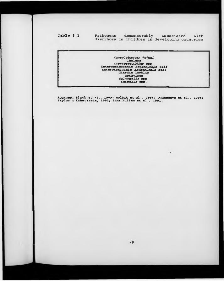
Table 3.1 Pathogens demonstrably associated withdiarrhoea in children in developing countries

Campylobacter jejuni Cholera

Cryptosporidium spp. Enteropathogenic Escherichia coli Enterotoxigenic Escherichia coli

Giardia lamblia Rotavirus

Salmonella spp.Shigella spp.

Sources: Black et a l . , 1989; Molbak et a l . , 1994; Ogunsanya et al ., 1994; Taylor & Echeverria, 1993; Sima Huilan et a l . , 1991.

78

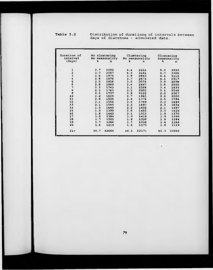
Table 3.2 Distribution of durations of intervals betweendays of diarrhoea - simulated data.

Duration of No clustering Clustering Clusteringinterval No seasonality No seasonality Seasonality(days) % n % n V n

1 2.7 2052 4.4 3231 5.0 35922 2.7 2057 4.3 3141 4.7 33663 2.6 1975 3.9 2843 4.4 31154 2.5 1876 3.7 2673 4.1 29175 2.5 1856 3.5 2574 3.8 26986 2.5 1889 3.4 2497 3.6 25507 2.3 1743 3.1 2288 3.4 24398 2.3 1743 3.1 2252 3.1 22469 2.3 1737 2.9 2122 2.9 206710 2.2 1629 2.7 1941 2.8 200011 2.0 1535 2.4 1776 2.5 179412 2.1 1554 2.5 1789 2.3 164813 2.1 1545 2.3 1697 2.3 163414 1.9 1440 2.2 1602 2.1 149715 1.9 1399 2.0 1462 2.0 142916 1.9 1443 2.1 1513 1.9 137017 1.8 1384 1.9 1412 1.8 129518 1.7 1301 1.8 1326 1.8 128419 1.7 1266 1.7 1232 1.6 116620 1.6 1219 1.6 1173 1.6 111921 + 56.7 42666 44.2 32171 42.3 30266

79

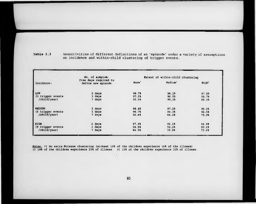
Table 3.3 Sensitivities of different definitions of an 'episode' under a variety of assumptionson incidence and within-child clustering of trigger events.

Incidence :No. of symptom-

free days required to define new episode None*

Extent of within-child clustering Medium1 High1

LOW 2 days 98.7% 98.2% 97.8%(3 trigger events 3 days 97.5% 96.5% 95.7%/child/year) 7 days 93.0% 90.3% 88.2%

MEDIUM 2 days 98.4% 97.2% 96.2%(6 trigger events 3 days 96.7% 94.3% 92.5%/child/year) 7 days 90.6% 84.2% 79.9%

HIGH 2 days 97.3% 96.1% 94.9%(9 trigger events 3 days 94.5% 92.2% 90.1%/child/year) 7 days 84.5% 78.8% 73.6%

Notes : *) No extra-Poisson clustering (sickest 10% of the children experience 16% of the illness) t) 10% of the children experience 25% of illness. ♦) 10% of the children experience 33% of illness.

80

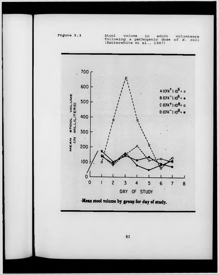
Figure 3.1 Stool volume in adult volunteersfollowing a pathogenic dose of E . coli (Satterwhite et a l ., 1987)

Mean itool volume by group for day of study.

81

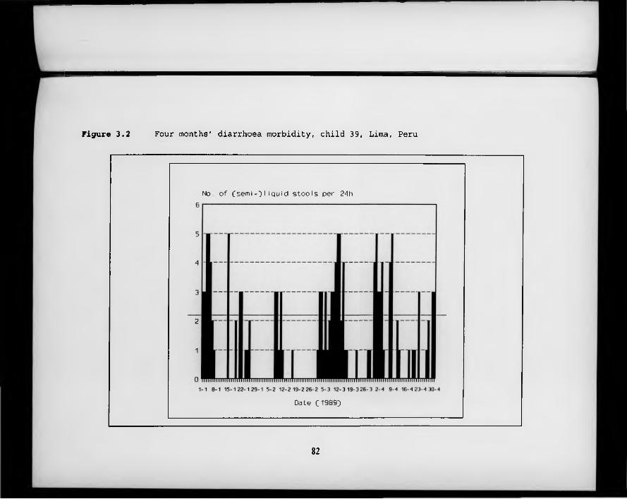
Figure 3.2 Four months' diarrhoea morbidity, child 39, Lima, Peru

No o f Csemi-3 I i q u i d s t o o l s per 24h

Date 0 9 8 9 }

82

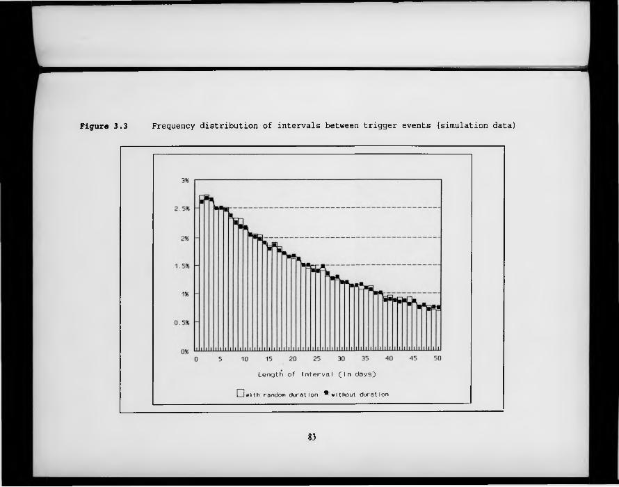
Figure 3.3 Frequency distribution of intervals between trigger events (simulation data)

L e n g t h o f I n t e r v a l f i n d a y s }

E D w ith random d u ra t io n * w ith o u t d u ra tio n

83

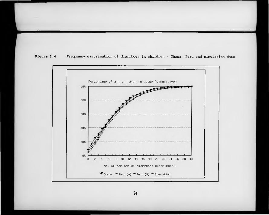
Figure 3.4 Frequency distribution of diarrhoea in children - Ghana, Peru and simulation data

Percentage o f a l l c h i l d r e n in s tu d y (cumu la t i ve])

No. o f p e r io d s o f d ia r r h o e a e x p e r ie n c e d

'^ 'G h a n a “""P eru (A J " ' 'P e ru f B ) "*"Slmu la t ion

84

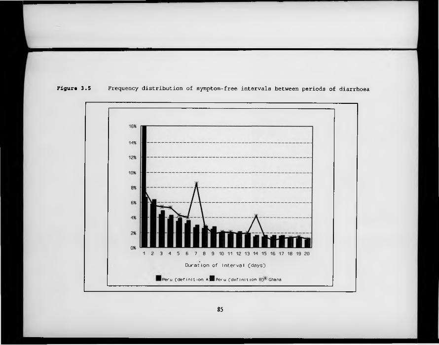
Figure 3.5 Frequency distribution of symptom-free intervals between periods of diarrhoea

D u r a t io n o f i n t e r v a l ( d a y s }

P e r u ( d e f i n i t i o n A j l p e r u ( d e f i n i t i o n Ghana

85

Figure 3.6 Presence of cough over 54 consecutive weeks in children in northern Ghana

Weeks with *5 3 6 5 2 5 2 1 8 2 7 5 0 1 8 0 2 4 7 1 4 1 9 4 6 1 8 3 4 4 6 1 5 2 5 4 5 1 7 1 9 4 5 1 3 8 5 4 3 6 6 1 4 2 6 4 0 4 1 1 6 9 1 4 1 1 8 1 6

coughlllllllllllllllOllllllllllllllllllllllllllllliiiiiiim1 1 1 1 1 1 1 1 1 1 1 1 1 1 1 1 1 1 1 1 1 1 1 1 1 0 1 1 1 1 1 1 1 1 1 1 1 0 1 1 1 1 1 1 1 1 1 o m i n i 1 1 1 0 1 1 1 1 . 1 1 1 0 1 1 1 1 1 1 1 1 1 1 0 1 1 1 1 1 1 1 1 1 1 1 1 1 1 1 1 1 1 1 1 1 1 1 1 1 1 1 1 1 1 1 0 0 1 1 1 1 1 1 1 . 1 1 1 1 . 1 1 1 . 1 1 1 1 1 1 0 1 1 1 0 1 1 1 1 1 1 1 1 1 1 1 1 1 1 1 1 1 1 1 1 . 1 1 0 1 0 1 1 1 1 1 1 1 1 0 . 1 . 1 1 1 1 1 1 1 1 1 1 1 1 1 1 1 1 1 1 1 1 1 1 1 0 1 1 1 1 1 1 1 1 1 1 0 0 1 0 0 1 1 1 0 1 1 1 1 1 1 1 1 1 1 1 1 1 1 1 1 0 1 1 1 1 1 1 1 . 1 1 1 1 1 1 1 1 1 1 1 . 1 1 1 1 1 1 1 1 . 0 1 1 . 1 0 0 1 0 0 1 1 1 1 1 1 1 1 0 1 0 1 . 1 1 1 1 1 1 1 1 1 1 1 1 1 1 1 1 1 1 0 1 1 1 1 0 0 0 0 1 1 1 1 1 1 1 1 1 1 1 1 1 1 1 1 1 1 1 1 1 1 . 0 1 1 1 1 1 0 1 0 0 1 1 1 1 1 1 0 1 1 0 1 1 1 1 1 1 1 1 1 1 1 1 1 1 0 1 1 1 1 1 . 1 1 1 1 1 1 0 1 1 1 1 1 1 . 1 1 . 1 1 1 1 1 1 0 1 1 0 1 0 1 0 1 1 0 1 0 1 1 0 1 1 1 1 1 1 1 1 0 1 1 0 1 1 1 1 1 1 1 1 1 1 0 1 0 1 . 0 1 1 0 1 1 0 1 1 1 1 1 0 1 1 1 0 1 0 0 1 0 1 1 1 1 1 1 1 1 1 1 1 0 1 0 1 1 1 1 1 1 1 1 1 1 1 1 1 0 1 1 1 1 1 1 1 1 1 . 1 1 1 1 1 1 1 1 1 1 1 1 1 1 1 1 1 1 1 1 1 1 0 0 1 0 1 1 1 1 1 1 0 0 1 0 0 1 0 0 1 0 0 0 1 1 1 1 1 1 0 0 0 0 1 0 0 0 0 1 1 1 1 1 0 1 1 1 1 0 1 1 1 1 0 1 1 1 1 0 1 1 1 1 1 1 1 1 0 1 1 1 1 1 1 1 1 1

2 8 1 6 2 7 2 8 1 7 5 2 2 8 1 8 0 1 2 8 1 3 4 2 2 8 1 0 7 4 2 8 1 1 3 3 2 7 1 8 6 1 2 7 1 7 0 6 2 7 1 5 8 5 2 7 1 8 0 5 2 7 1 5 8 9 2 7 8 3 6

01011111.11010. . .10110011111111111111100000000000000001 1111110111100001011001.1111110010011000000001101111 01101111000001111111.11.11111010011101. . 110. . 00 00000.00 00111111111011110111111111111101000010000000000 oooooooo 10 . . 111111010100001011011001111000001000010010011111111 10. . .11010000111111100001011111001101100110.01110011000 0111. .11111. .111111.11111.1111001.0000001000000000000110 0 0 1 1 0 0 1 1 1 1 1 1 1 1 1 1 1 1 1 1 1 1 1 0 1 1 1 1 1 1 1 0 1 0 0 0 0 0 0 0 ............................... 00ooiiiiiiiooooo. o m i n i . l i n o n i , o i i o o o o o o o o o o o o o o o i m 1 1 0 0 0 1 1 1 1 1 1 . 1 0 1 1 0 1 . 1 1 1 1 1 1 1 1 1 . 1 1 0 . 1 1 0 0 0 . 1 0 0 0 0 0 0 0 0 0 0 0 0 0 1 1 0 1 1 1 0 0 . . 1 1 1 . 1 1 1 . 1 1 1 1 1 . . 1 . 1 . 1 1 1 1 1 1 1 1 1 1 1 0 0 0 0 0 0 0 0 0 0 0 0 0 0 0 0 0 liiiioiiiiiiiiooiio i o i i i n n o o o o o i i i n o o o o o o o o o o o o o o o

10 1489 0.011100. .0. .1. .00100000000000010000000101001100000000010 1855 OOOOOOOOllOOOOlOOOOOlOOOOOOOOOOOOOOOOOOOmilOOOOOOOOOli o 1 8 4 3 o o o o o o o o o o o o o o i o o m o o o o o n o o n o o o o o o o o o o o o o o o o o o o o o o o i1 0 1 2 8 2 1 1 0 1 0 0 1 1 0 0 1 . 1 0 0 0 0 0 0 0 0 0 0 1 0 0 0 0 0 0 0 0 0 0 1 0 0 0 0 0 0 0 0 0 0 0 0 0 0 0 0 0 1 1 01 0 1 0 1 5 o i n n o n o o o o o o o i o i o o i o o o o o o o o o o o o o o o o o o o o o o o o o o o o o o o o o10 663 111001000.00.001000100000100000000001000111000000000000i o 6 8 4 . o o o o m n o i o o o o o o o o o o o o i o o o o o o o i i o o o o o o o b o o i o o o o o o o o o o10 1197 00111.1000.000000.0.00.01110.00000000000000011.000000110 1061 00000001100001.001010000000000100100000000011100000000010 1289 0000001100000.0011101111000000000000000000000000000000010 1265 0010. .1.0.1. . .11.0.11100000001010000000000000000000000000 1370 ooooooooooooooooooooooooooooooooooooooooooooooooooooooo00 1445 OOOOOOOO.000000000000000000000..000000000 1499 000000000000.00000000000000000000000000000000000000000000 1344 000000000000000.00000 .. oooooooooooooooooooooooooooooooo00 1345 ooooooooooooooooooooooooooooooooooooooooooooooooooooooo00 686 ooooooooooooooooooooooooooooooooooooooooooooooooooooooo00 658 000000000000000000000000000000.00000000000000000000000000 675 ooooooooooooooooooooooooooooooooooooooooooooooooooooooo00 708 ooooooooooooooooooooooooooooooooooooooooooooooooooooooo00 1239 00000.00.00. .000.00000000000000. .000000000000000000000000 826 ...00..... 000.0000000.0000000000000000000000000000000000 833 .0000..... 000000.0000000000000000000.00000000000000000000 960 000000000000000000000000000000000000.000000.0000000

tID number

86

Chapter 4 Event Analysis (II): Rates, risks, and measures of association

4 .1 Measures o f disease frequency

In the previous chapter, methods were proposed for defining an ‘episode’ of diarrhoea, respiratory illness or malaria. Once such episodes have been identified, it then becomes possible to compare individuals, or groups of individuals, by counting the total numbers of episodes observed over a defined period of time. Specifying the time period concerned is important since - in most circumstances - the number of illness episodes observed will be proportional to the length of the observation period.

Classically, two alternative measures of disease frequency (or incidence) are recognised for non-recurrent illnesses. Both include - structurally or by reference - a tim e element. The first, known as incidence density, or, more loosely, as the (average) incidence rate, is calculated by dividing the total number of new cases over a defined period of time by the amount of observation time accrued by the population at risk over the same period. Individuals may cease to contribute observation time by getting the disease or dying; moving out of the study area or refusing to participate; undergoing medical procedures which make them incapable of experiencing the outcome, or reaching the end of the study (Kleinbaum et al., 1982). Incidence rates are expressed per unit of person-time.

The second measure is referred to as cumulative incidence, and is defined as the proportion of all individuals entering the study who experience the disease outcome within a defined period of time. The public health relevance of this measure stems from the fact that it may sometimes be interpreted as the probability of a disease-free individual developing a given disease over a specified

87

period of time, conditional on their not dying of something else first (referred to as the conditional risk of disease). This interpretation is strictly speaking only valid when all individuals are followed up for the same length of time (Kleinbaum et al., 1982). However, if the cohort is fixed and there is little attrition during the follow-up period, cumulative incidence provides a good estimate of average risk. If there is significant attrition of the initial cohort, the morbidity experience of those lost to follow-up cannot be known, and cumulative incidence may provide a biased estimate of average risk. The same applies when individuals are entering the study cohort at different times, a situation referred to as a ‘dynamic’ population. Actuarial (life-table) methods are available to estimate risk in these circumstances (see Lee, 1992).

For longitudinal studies of common diseases, rates are again an important measure of disease frequency. Since these diseases are recurrent, it is no longer appropriate, however, to define the incidence rate as the number of new cases of disease in those previously unaffected. Rather, the numerator of the rate may be estimated - as for non-recurrent diseases - as the total number of new cases over a specified period of time. The correct way to calculate the denominator (total observation time) has become a matter of some controversy: some researchers prefer to use the total follow-up time for the study population, whilst others prefer to subtract the duration of the disease, and others still subtract the duration of the disease and a further period beyond the end of the episode when the subject is considered not at risk of a further episode. These different approaches can be related to the discussion of trigger events presented in Section 3.3: by dividing the total number of new cases by the total observation time, the average incidence of observed episodes is derived. Using this approach, an individual who is observed to suffer from 7 episodes of diarrhoea during a year of observation w ill be classified as experiencing an incidence rate of 7 per year. On the other hand, by dividing the total number of new cases by the total observation time minus the 'dead time’ when no new episodes can be observed

88

(duration of illness plus duration of symptom-free interval required to define to new episode, see Chapter 3), an estimate of the true incidence of trigger events is obtained, based on the assumption that trigger events will continue to accumulate at the same rate whilst individuals are sick as they do when they are healthy. Thus, an individual who experiences 7 episodes, each of 3 days’ duration, will be classified as experiencing an incidence rate of 7.74 (—7/330 x 365) per year, w ith the excess of 0.74 episodes per year representing the number of trigger events that are likely to have remained unobserved because they occurred during the time the child was already ill. Subtracting just the summed duration of illness from the total observation time is an unhappy compromise between these two approaches, because by not including the disease-free days required to define a new episode, the proportion of the total observation time during which new trigger events could have in reality occurred but could not be discerned in the study is underestimated.

The fundamental difference between these two measures of incidence needs to be carefully considered before any analyses are conducted: for the purposes of descriptive epidemiology, the incidence of observed episodes may be of greater interest, since this shows how often children experience bouts of illness from a given disease, with all the physiological consequences that may entail. When, however, the protective efficacy of a new intervention designed to interrupt transmission is being evaluated, the estimated incidence of trigger events may be a more appropriate measure. There is no guarantee, of course, that the true incidence of trigger events is adequately estimated by this method. In particular, if the duration of symptoms associated with consecutive trigger events ‘overlap’ (see Section 3.3), then this method will underestimate the true incidence of trigger events, since the true incidence of trigger events during the observed periods of illness w ill be higher than predicted.

The risk of being affected by disease over the follow-up period can also be

89

estimated in longitudinal studies. In this case, only the first occurrence of disease in each subject is considered. With common diseases, most subjects will experience the disease outcome within a fairly short period of time. This is shown in Figure 4.1, which depicts the relative cumulative incidence of at least one episode of diarrhoea in 493 children with at least 51 weeks of follow-up in the study of childhood morbidity in northern Ghana described in Chapter 2. One half of these children had experienced an episode of diarrhoea within three weeks of the beginning of the study, and two-thirds had experienced an episode within 45 days. In such situations, risk becomes a rather uninformative measure if the time referent is longer than a few months. In addition, all the information on non-initial episodes is wasted. As in studies of non-recurrent illnesses, cumulative incidence may give a biased estimate of average risk when a dynamic cohort design is used, or rates of attrition from the initial cohort are high.

4 .2 Measures o f association

Epidemiological measures of association can be derived from both rates and risks. Both absolute measures (such as the difference between two-rates) and relative measures (such as the ratio of two rates) may be derived, but two distinct factors favour the use of relative measures: firstly, they ‘fall out’ naturally from several commonly used statistical models for rates, such as Poisson regression (see Section 5.2.1); secondly, it has been shown that relative measures often provide clearer indications of the strength of epidemiological associations, and - when appropriate - causality (Cornfield & Haenszel, 1960).

The incidence density ratio (or simply, relative rate) is derived by dividing the incidence density in a group exposed to some variable of interest by the incidence density in the unexposed group. The time dimension of a single measure of incidence density drops out when the relative measure is used, so that

90

the density ratio is dimensionless; furthermore, the total observation time is assumed to be prior-determined by the design of the study, so that all statistical variability is ascribed to the variation in the episode counts (see Section 5.2.1). The cumulative incidence ratio (or simply, relative risk) is derived by dividing the cumulative incidence in a group exposed to some variable of interest by the cumulative incidence in the unexposed group. The measure is also dimensionless, but refers to a specific time interval. Both the number of individuals experiencing disease, and the number of subjects observed are relevant in determining the statistical variability of this measure.

In longitudinal studies of common diseases of childhood, the interpretation of the relative rate w ill again depend on the w ay that the denominators of the rate have been calculated. Table 4.1 shows the results of a simulation in which both the incidence of trigger events and the duration of symptoms were assumed to vary with the age of the child. Mean incidence rates were assumed to fall linearly with age from 8 trigger events per child-year at 12 months to 4 trigger events per child-year at age 60 months. Between-child heterogeneity was allowed for as described in Section 3.2 (a chi-squared distribution with 3 degrees of freedom was used to generate individual-level trigger event incidence rates). Episode durations were randomly generated from a negative exponential distribution. Geometric mean durations were assumed to fall linearly from 2.36 days at age 12 months to 1.42 days at age 60 months. A uniform distribution of starting ages was assumed, with 10,000 individuals and 365 days of observation.

This simulation analysis shows that incidence rates calculated on the basis of observed episodes of illness are substantially affected by the choice of denominator. In the youngest age group, for example, the reported incidence rate is 12% larger (7.65 per child-year vs. 6.84 per child-year) when days of illness (plus the two-day symptom-free margin) are excluded from the denominator. Estimated rate ratios, comparing each group to the ‘corner’ group, are also

91

slightly affected by the choice of denominator. This is because duration of illness acts as a confounder of the relationship between age and incidence, because duration is associated with age and is also taken into account in the calculation of incidence when the ‘dead-time’ approach is adopted. The confounding effect of duration is not large, perhaps because there was not a very large differential in average durations between the youngest and oldest age groups in this example.

It is important to note that although the estimates derived using observed episodes and denominators that exclude time ill and the 2-day symptom-free margin are closer to the actual incidence of trigger events than those derived when total observation time is used in the denominator, they are not the same as the ‘real’ incidence of trigger events. In order for them to be the same, it would be necessary to subtract from the total observation time the sum of the durations associated with each trigger event; since periods of symptoms overlap, it is not possible to determine the duration associated with each trigger event separately, and the total time ill is not equal to the sum of these durations.

The relative risk is not a suitable outcome measure for longitudinal studies of common diseases of childhood. Because the risk of disease rapidly approaches unity in all groups, the relative risk measure also varies over time, approaching unity as the time referent increases. The relative rate, on the other hand, is constant over time (see Rodrigues and Kirkwood, 1990). The relative risk is also wasteful of information when the follow-up period is long enough to allow a substantial proportion of the study population to experience more than one episode, since non-initial episodes are ignored. Where there is substantial attrition of the initial cohort, relative cumulative incidence is liable to be biased as an estimator of relative risk, since the disease outcome of those lost to follow­up is unknown. This poses a problem when a) rates of attrition are not the same between different exposure groups, or b) rates of attrition are balanced, but the prognosis of those lost to follow is differentially affected by exposure group.

92

4 .3 A review o f current practice in the epidem iological literature

In order to identify the range and quality of current practice regarding the choice and calculation of outcome measures in longitudinal studies of common diseases of childhood, I undertook a comprehensive review of a defined area of the epidemiological literature: trials of potential vaccines against enteric diseases, carried out (and reported) since 1980. This area was chosen because vaccine trials are necessarily characterised by prospective designs, and - since the intervention is intended to protect the individual from infection with the disease - the outcome is invariably reported as some form of incidence rate. Vaccine trials also have the advantage of being characterised by a clearly defined entry point, making calculation of time-at-risk a relatively simple procedure. A considerable number of such trials have been conducted to date, with a focus on three different gastro-intestinal pathogens: rotavirus, cholera and typhoid (see reviews by Black [1993] and Holmgren & Svennerholm [1990]). This chapter will concentrate on rotavirus (RV) vaccine trials, since cholera and typhoid are not common events even in areas where these diseases are endemic.

4 .3 .1 Methods

All references to rotavirus vaccine trials were sought by a search of Medline® 1988-93, using the terms VACCINE plus either DIARRH* or ROTAVIRUS. Only reports of vaccine efficacy (as opposed to immunogenicity or reactogenicity) were retrieved. The bibliographies of all articles retrieved were then reviewed to identify any further vaccine trials carried out since 1980 and not previously indicated in the Medline® search. A total of 19 distinct RV vaccine trials were identified (of which four from bibliographies and review articles only). The studies are listed by alphabetic order of the first author in Table 4.2. All the papers were successfully located.

93

4.3 .2 Results

Rotavirus vaccine trials have now been carried out in a wide variety of different settings, by 12 different groups of investigators and using substantially different study designs (Table 4.2). The studies differed markedly with respect to the number of children enrolled - some were clearly inadequate in this respect, since it is unlikely that any clinical trial could demonstrate a significant difference between treatment groups with only 13 children per group (#11). Recruitment procedures also differed considerably from trial to trial, with seven trials enroling at a single point in time, so that all children were in the trial and ‘exposed’ to the risk of diarrhoea (RV or other) for exactly the same period of time. At the other end of the spectrum, one trial (#12) employed rolling recruitment, so that the length of time ‘exposed’ would have varied from 0 to 17 months depending on each child’s sequential order of enrolment. In the eight trials where recruitment was rolling prior to the onset of the season of RV infections (‘RPOS’), time exposed to the risk of RV infection would be the same for all children, but time exposed to the risk of any diarrhoea would not (unless episodes of diarrhoea were recorded only during the RV season). Conversely, in those trials where rolling recruitment led into a fixed length period of follow­up (‘R/FPFU’), all children are similarly exposed to the risk of all-cause diarrhoea unless there is very marked seasonal variation in diarrhoea incidence, but length of exposure to the risk of RV diarrhoea depends on the timing of the follow-up period with respect to the RV season. All but one of the RV vaccine trials recorded the impact on all-cause diarrhoea as well as on RV-specific diarrhoea, but due to the important interactions between study design and between-subject variations in time-at-risk, the two outcomes will be considered separately.

94

4.3.2.1 Aetiology-specific vaccine efficacy

Table 4.3 shows some important features of the 19 trials with respect to RV- specific outcomes. The trials have been re-ordered so that trials with similar design features appear together. This is to highlight the close dependence that exists between study design and choice of outcome measure.

The most homogenous group of studies in terms of presentation of results are those in which enrolment was staggered over the period of time immediately preceding the onset of the RV season (the ‘RPOS’ group). In 7 of these studies, surveillance was maintained over a single RV season (5-7 months). In the remaining study (#19), two consecutive seasons were considered, but findings were presented for each of the two seasons separately. Only three of the eight studies present data on losses to follow-up (due to death or out-migration) during the study period. In two of these three studies, however, the losses reported are substantial, amounting to nearly one-quarter of those initially recruited. At least five studies in this group have restricted their analysis of vaccine efficacy to those children who completed the study. This introduces a potential for serious bias - known as attrition bias (Dwyer & Feinleib, 1991) - if (a) rates of loss were

different in the two groups, or (b) rates of loss were the same in the two groups, but the treatment group-specific prognoses of those children lost to follow-up were different from children remaining in the trial. Since no information is presented on the characteristics of those children lost to follow-up in these studies, the possibility of serious bias cannot be dismissed.

In all the studies in this group, the primary outcome was the cumulative incidence of RV diarrhoea over the duration of the season, a measure which has been denoted Cl (cumulative incidence). With significant attrition of the initial cohort, this measure may not provide an accurate estimate of an individual’s risk

95

of RV illness over the follow-up period (see above, Section 4.1). If, however, it can be assumed that the losses to follow-up are balanced between the two treatment groups, then the ratio of these measures in each of the two treatment groups should provide an unbiased measure of effect equivalent to the risk ratio. Smith, Rodrigues and Fine (1984) have shown, however, that this is not the appropriate measure of vaccine efficacy when the risk of disease is not small and the model of action of the vaccine is that it reduces the probability of illness in all vaccinees by a constant proportion. This is because all study subjects may be expected to get the disease if surveillance is maintained for long enough, so that C l approaches un ity in both groups over time, and the apparent vaccine efficacy diminishes. In th is situation, the rate ratio, rather than the risk ratio, provides the appropriate estimate of vaccine efficacy. This model of action (all vaccinees experience a reduced probability of illness) appears to be appropriate for RV vaccines, which, it has been suggested, prevent severe but not mild illness (Vesikari, 1993). The alternative model of action is that the vaccine prevents disease completely in some subjects, but is ineffective in others. In these cases, the risk ratio provides the appropriate measure of vaccine efficacy.

In the studies w ith simultaneous enrolment, or rolling recruitment but a fixed period of follow-up (the ‘R/FPFU’ group), cumulative incidence-based analysis has tended to be adopted in the studies with relatively short periods of follow-up, and person-time based analysis in studies with longer follow-up periods (and, in general, a greater proportion of study subjects lost to follow-up). In study #6, it is not clear whether the analysis is based on all children vaccinated or only on those completing follow-up, and no rates or statistics are presented. In study #10, the outcome analysed is the proportion of all diarrhoea episodes with RV present in the two groups, which appears to be a statistically valid approach since the incidence of diarrhoea did not differ between treatment groups. In public health terms, however, the proportion of diarrhoea episodes attributable to rotavirus is of no interest if the overall incidence remains unchanged.

96

In the one study where a rolling recruitment procedure was adopted (#12), two different analyses were performed. Firstly, the proportion of cases in the placebo and treatment groups was compared. This risk-type measure is conceptually rather unsatisfactory in a population where some individuals were under surveillance for a matter of days and others for 17 months, since children with very short follow-up times will appear in the denominator but in reality have little chance of inclusion in the numerator. The ratio of these proportions in the two treatment groups will be sensitive to the number of subjects w ith short follow-up periods, and will be biased if the average follow-up time per individual is not the same in each treatment group, or the rate of disease is related to the period of follow-up. Furthermore, the inflated denominators will very slightly inflate the precision of the effect estimate (if analysed as a risk ratio), though this effect is likely to be negligible.

The second analysis performed in this study focused on the average duration of time elapsing between vaccination and disease in the different treatment groups. This analysis is highly efficient in that it utilises all the information available about the relationship between exposure and outcome, and individuals whose follow-up is censored still contribute information for the length of tim e they were under surveillance.

4 .3 .3 .2 Non-specific vaccine efficacy

Data from 18 of the 19 trials relating to the analysis of the impact on all-cause diarrhoeal illness are presented in Table 4.4. It should be noted that for all but one of the ‘RPOS’ group, diarrhoea surveillance commenced immediately post­vaccination for each study subject, with the result that time at risk varied considerably for individuals within each study. Numbers of episodes recorded are substantially larger than for the cause-specific outcome, and in this table the

97

number of diarrhoea episodes is shown for both treatment groups. Four studies had more than one treatment arm (#19, #9, #10 and #12).

Only six studies quoted any measure of disease frequency in their results. In three instances (#9, #10, #12), the outcome measure chosen was the average incidence rate, IDR. Two authors chose to use the formula in which the total number of episodes is divided by the total time under observation (#9, #10), whilst the other author seems to have used the ‘time at risk’ formulation (denominator = observation time - duration of illness - symptom-free margin). In study #11, the cumulative incidence of diarrhoea over the duration of the study period was the outcome measure reported, and the risk of non-RV diarrhoea was presented in study #4. In all the other studies the outcome measure used, either explicitly or otherwise, was the total number of diarrhoea episodes divided by the number of children entering the trial. This measure has no commonly accepted epidemiological interpretation, and is a poor proxy for the incidence density rate, IDR. However, provided that the average length of follow-up is similar between treatment groups, the ratio of these rate-like measures in the two treatment groups will be equivalent to the true rate ratio, and the precision of the effect measure will also not be affected.

4 .4 Discussion

Both risk (as estimated by cumulative incidence) and rate (as estimated by the incidence density rate) are important outcome measures in studies of non­recurrent or rare diseases. It is clear, however, that cumulative incidence has severe limitations as a measure of the frequency of common diseases of childhood, because it rapidly approaches unity with time referents longer than - say - one month, in the case of diarrhoea in areas with incidence rates of the order o f 7 episodes per child per year. This has the highly undesirable effect that

98

the epidemiological measure of association derived by dividing the cumulative incidence in a group exposed to a particular risk factor b y the cumulative incidence in the unexposed group also approaches unity as the length of the time referent increases, regardless of the magnitude of the true effect. Relative rates, on the other hand, are time invariate, and are also not prone to bias as a result of attrition of the initial cohort.

There is little evidence to suggest, however, that the limitations of cumulative incidence, especially when applied to a dynamic population, are appreciated by those actually carrying out applied research in the area of common diseases of childhood. Inspection of the 19 rotavirus vaccine trials carried out since 1980 reveals that the use of cumulative incidence is widely favoured. The problem of unequal lengths of follow-up is overcome by restricting analysis to those study subjects who completed the follow-up period. Post hoc exclusion of study subjects from the analysis may not, however, be a desirable solution to this problem, since it introduces an important risk of bias. Where it is done, it is essential that the reader be informed of the number of subjects involved, and whether or not they are equally divided between treatment groups. Furthermore, depending on the mode of action of the vaccine,-risk estimates may lead to inappropriate measures of vaccine efficacy, as discussed above.

Estimation of incidence density rates in studies of common diseases is sensitive to the choice of denominators: whether or not the duration of illness and symptom-free margin are subtracted from the total observation time. Relative rate measures are also somewhat sensitive to the choice of denominator. Whilst there is no clearly ‘correct’ approach in this case, it appears that subtracting the illness duration and symptom-free margin produces a measure with no straightforward intuitive interpretation, since it represents neither the frequency of observed bouts of illness, nor the ‘true’ frequency of trigger events. Since analysis of disease duration must focus on observed bout lengths rather than the

99

duration of symptoms associated with each trigger event (the latter being unobservable), the principle of internal consistency would suggest that analyses of disease frequency should also focus on observed bouts, unless there are strong a priori reasons for not doing so. It may be noted that the calculation of stratum-specific follow-up time is far more complex when the duration of illness and symptom-free margin needs to be subtracted. These considerations suggest that total observation time should generally be used in the denominators of incidence rates.

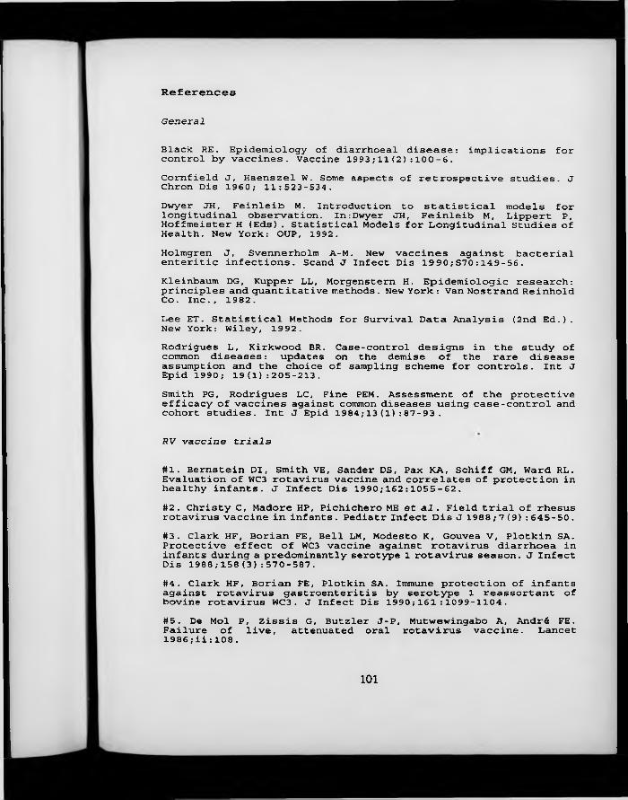
R eferences

General

Black RE. Epidemiology of diarrhoeal disease: implications for control by vaccines. Vaccine 1993;11(2):100-6.Cornfield J, Haenszel W. Some aspects of retrospective studies. J Chron Dis 1960; 11:523-534.Dwyer JH, Feinleib M. Introduction to statistical models for longitudinal observation. In:Dwyer JH, Feinleib M, Lippert P, Hoffmeister H (Eds). Statistical Models for Longitudinal Studies of Health. New York: OUP, 1992.Holmgren J, Svennerholm A-M. New vaccines against bacterial enteritic infections. Scand J Infect Dis 1990;S70:149-56.Kleinbaum DG, Kupper LL, Morgenstern H. Epidemiologic research: principles and quantitative methods. New York : Van Nostrand Reinhold Co. Inc. , 1982.Lee ET. Statistical Methods for Survival Data Analysis (2nd Ed.). New York: Wiley, 1992.Rodrigues L, Kirkwood BR. Case-control designs in the study of common diseases: updates on the demise of the rare disease assumption and the choice of sampling scheme for controls. Int J Epid 1990; 19 (1) :205-213.Smith PG, Rodrigues LC, Fine PEM. Assessment of the protective efficacy of vaccines against common diseases using case-control and cohort studies. Int J Epid 1984;13 (1) :87-93 .

RV vaccine trials

#1. Bernstein DI, Smith VE, Sander DS, Pax KA, Schiff GM, Ward RL. Evaluation of WC3 rotavirus vaccine and correlates of protection in healthy infants. J Infect Dis 1990;162:1055-62.#2. Christy C, Madore HP, Pichichero ME et al. Field trial of rhesus rotavirus vaccine in infants. Pediatr Infect Dis J 1988 ; 7 (9) : 645-50.#3. Clark HF, Borian FE, Bell LM, Modesto K, Gouvea V, Plotkin SA. Protective effect of WC3 vaccine against rotavirus diarrhoea in infants during a predominantly serotype 1 rotavirus season. J Infect Dis 1988;158 (3) :570-587.#4. Clark HF, Borian FE, Plotkin SA. Immune protection of infants against rotavirus gastroenteritis by serotype 1 reassortant of bovine rotavirus WC3 . J Infect Dis 1990;161:1099-1104.#5. De Mol P, Zissis G, Butzler J-P, Mutwewingabo A, André FE. Failure of live, attenuated oral rotavirus vaccine. Lancet 1986 ; ii: 108 .

101

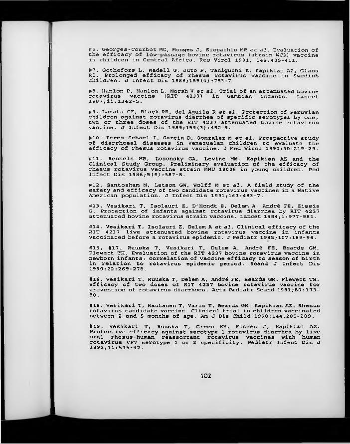
#6. Georges-Courbot MC, Monges J, Siopathis MR et al. Evaluation of the efficacy of low-passage bovine rotavirus (strain WC3) vaccine in children in Central Africa. Res Virol 1991; 142:405-411.#7. Gothefors L, Wadell G, Juto P, Taniguchi K, Kapikian AZ, Glass RI. Prolonged efficacy of rhesus rotavirus vaccine in Swedish children. J Infect Dis 1989 ; 159 (4):753-7 .#8. Hanlon P, Hanlon L, Marsh V et al. Trial of an attenuated bovine rotavirus vaccine (RIT 4237) in Gambian infants. Lancet 1987 ;ii: 1342-5.#9. Lanata CF, Black RE, del Aguila R et al. Protection of Peruvian children against rotavirus diarrhea of specific serotypes by one, two or three doses of the RIT 4237 attenuated bovine rotavirus vaccine. J Infect Dis 1989 ; 159 (3):452-9.#10. Perez-Schael I, Garcia D, Gonzalez M et al. Prospective study of diarrhoeal diseases in Venezuelan children to evaluate the efficacy of rhesus rotavirus vaccine. J Med Virol 1990;30:219-29.#11. Rennels MB, Losonsky GA, Levine MM, Kapikian AZ and the Clinical Study Group. Preliminary evaluation of the efficacy of rhesus rotavirus vaccine strain MMU 18006 in young children. Ped Infect Dis 1986 ; 5 (5) : 587-8.#12. Santosham M, Letson GW, Wolff M et al. A field study of the safety and efficacy of two candidate rotavirus vaccines in a Native American population. J Infect Dis 1991;163:483-7.#13. Vesikari T, Isolauri E, D'Hondt E, Delem A, André FE, Zissis G. Protection of infants against rotavirus diarrhea by RIT 4237 attenuated bovine rotavirus strain vaccine. Lancet 1984 ;i: 977-981.#14. Vesikari T, Isolauri E, Delem A et al. Clinical efficacy of the RIT 4237 live attenuated bovine rotavirus vaccine in infants vaccinated before a rotavirus epidemic. J Pediatr 1985,-107:189-94.#15, #17. Ruuska T, Vesikari T, Delem A, André FE, Beards GM, Flewett T H . Evaluation of the RIT 4237 bovine rotavirus vaccine in newborn infants: correlation of vaccine efficacy to season of birth in relation to rotavirus epidemic period. Scand J Infect Dis 19 9 0 ; 2 2 :269-278.#16. Vesikari T, Ruuska T, Delem A, André FE, Beards GM, Flewett TH. Efficacy of two doses of RIT 4237 bovine rotavirus vaccine for prevention of rotavirus diarrhoea. Acta Pædiatr Scand 1991; 80 :173- 80 .#18. Vesikari T, Rautanen T, Varis T, Beards GM, Kapikian AZ. Rhesus rotavirus candidate vaccine. Clinical trial in children vaccinated between 2 and 5 months of age. Am J Dis Child 1990;144:285-289.#19. Vesikari T, Ruuska T, Green KY, Flores J , Kapikian AZ. Protective efficacy against serotype 1 rotavirus diarrhea by live oral rhesus-human reassortant rotavirus vaccines with human rotavirus VP7 serotype 1 or 2 specificity. Pediatr Infect Dis J 1992;11:535-42.

102

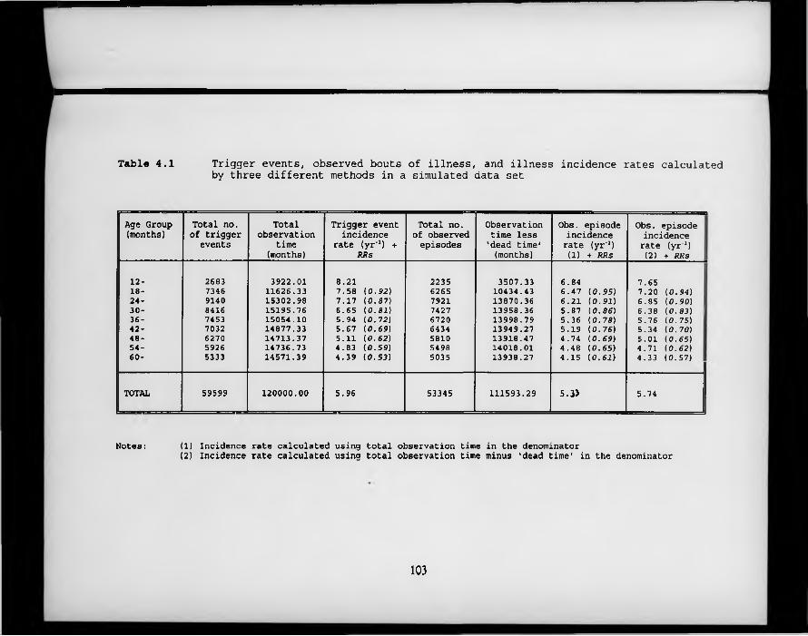
Table 4.1 Trigger events, observed bouts of illness, and illness incidence rates calculatedby three different methods in a simulated data set

Age Group (months)

Total no. of trigger

eventsTotal

observationtime

(months)

Trigger event incidence

rate (yr'1) + R R s

Total no. of observed episodes

Observation time less 'dead time* (months)

Obs. episode incidence rate (yr'1) (1) + R R s

Obs. episode incidence rate (yr'1) (2) + R R s

12- 2683 3922.01 8.21 2235 3507.33 6.84 7.6518- 7346 11626.33 7.58 ( 0 . 9 2 ) 6265 10434.43 6.47 ( 0 . 9 5 ) 7.20 ( 0 . 9 4 )24- 9140 15302.98 7.17 ( 0 . 8 7 ) 7921 13870.36 6.21 ( 0 . 9 1 ) 6.85 ( 0 . 9 0 )30- 8416 15195.76 6.65 ( 0 . 8 1 ) 7427 13958.36 5.87 ( 0 . 8 6 ) 6.38 ( 0 . 8 3 ) 136- 7453 15054.10 5.94 ( 0 . 7 2 ) 6720 13998.79 5.36 ( 0 . 7 8 ) 5.76 (0.75)42- 7032 14877.33 5.67 ( 0 . 6 9 ) 6434 13949.27 5.19 ( 0 . 7 6 ) 5.34 ( 0 . 7 0 )48- 6270 14713.37 5.11 ( 0 . 6 2 ) 5810 13918.47 4.74 ( 0 . 6 9 ) 5.01 (0.65)54- 5926 14736.73 4.83 ( 0 . 5 9 ) 5498 14018.01 4.48 ( 0 . 6 5 ) 4.71 ( 0 . 6 2 )60- 5333 14571.39 4.39 ( 0 . 5 3 ) 5035 13938.27 4.15 ( 0 . 6 1 ) 4.33 (0.57)

TOTAL 59599 120000.00 5.96 53345 111593.29 5.ÎÎ 5.74

Notes: (1) Incidence rate calculated using total observation time in the denominator(2) Incidence rate calculated using total observation time minus 'dead time' in the denominator

103

Table 4.2 Rotavirus vaccine trials -Basic details and design features

F P. Investigator Country Vaccine n1 Recruitment’

l. Bernstein (1990) USA WC3 103 RPOS (3 months)

2 . Christy (1988) USA MMU18006

88 RPOS (4 months)

Clark USA3. (1988) WC3 55 RPOS (4 months)4 . (1990) WI79-9 39 RPOS (? months)

5. De Mol (1986) Rwanda RIT 4237 123 Simultaneous

6 . Georges-Courbot C. Afric. WC3 235 R/FPFU(1987) Republic

7. Gothefors (1989) Sweden MMU18006

51 ± Simultaneous

8 . Hanlon (1987) Gambia RXT 4237 83 RPOS (11 I months)

9. Lanata (1989) Peru RIT 4237 100 R/FPFU

10. Perez-Schael Venezuela MMU 151 R/FPFU(1990) 18006

11. Rennels (1986) USA MMU18006

13» RPOS (2 months)

12. Santosham (1991) USA RIT 4237 107 Rolling

Vesikari Finland13. - a (1984) RIT 4237 92 Simultaneous14 . - b (1985) RIT 4237 160 RPOS15. - c (1990) RIT 4237 121 * Simultaneous16 . - d (1991) RIT 4237 128 ± Simultaneous17. - e (1990) RIT 4237 122 ± Simultaneous18 . - f (1990) RRV-1 100 ± Simultaneous19. - g (1992) DxRRV

a n dDSlxRRV

120 RPOS

N o t e s ■1. Number of children in placebo group.2. Recruitment procedure. Codes«

RPOS - rolling recruitment prior to onset of rotavirus season(in parentheses, period over which recruitment is staggered)

R/FPFU - rolling recruitment with fixed period of follow-up3. Only 10 children were actually followed up for diarrhoea incidence.

104

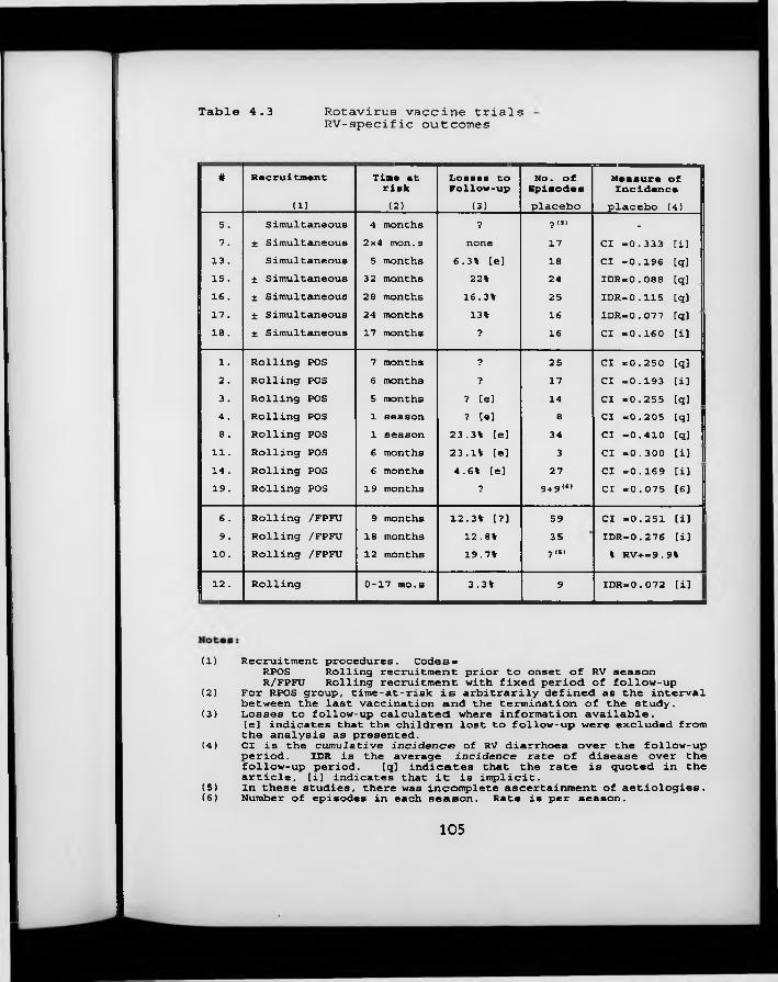
Table 4.3 Rotavirus vaccine trialsRV-specific outcomes

# Recruitment Time at Losses to No. of Measure ofrisk Follow-up Episodes Incidence ;(1) (2) (3) placebo placebo (4)

5 . Simultaneous 4 months ? ■p (5) -7 . ± Simultaneous 2x4 mon.s none 17 Cl =0.333 [i]13 . Simultaneous 5 months 6.3% [e] 18 Cl =0.196 [q]15. ± Simultaneous 32 months 22% 24 IDR=0.088 [q]16 . ± Simultaneous 28 months 16.3% 25 IDR=0.115 [q]17. ± Simultaneous 24 months 13% 16 IDR=0.077 [q]18. ± Simultaneous 17 months ? 16 Cl =0.160 [i]1. Rolling POS 7 months ? 25 Cl =0.250 [q]2. Rolling POS 6 months ? 17 Cl =0.193 [i]3 . Rolling POS 5 months ? [e] 14 Cl =0.255 [q]4 . Rolling POS 1 season ? [e] e Cl =0.205 [q]8 . Rolling POS 1 season 23.3% [e] 34 Cl =0.410 [q]

11 . Rolling POS 6 months 23.1% [e] 3 Cl =0.300 [i]14 . Rolling POS 6 months 4.6% [e] 27 Cl =0.169 [i]19. Rolling POS 19 months ? 9 + 9“’ Cl =0.075 [6]6 . Rolling /FPFU 9 months 12.3% [?] 59 Cl =0.251 [i] I9. Rolling /FPFU 18 months 12.8% 35 IDR=0.276 [i]

10. Rolling /FPFU 12 months 19.7% 7 (5) % RV+—9.9%12 . Rolling 0-17 mo.s 3.3% 9 IDR=0.072 [i]

(1) Recruitment procedures. Codes«RPOS Rolling recruitment prior to onset of RV seasonR/FPFU Rolling recruitment with fixed period of follow-up(2) For RPOS group, time-at-risk is arbitrarily defined as the interval between the last vaccination and the termination of the study.(3) Losses to follow-up calculated where information available.[e] indicates that the children lost to follow-up were excluded from the analysis as presented.(4) Cl is the cumulative incidence of RV diarrhoea over the follow-up period. IDR is the average incidence rate of disease over the follow-up period. [q] indicates that the rate is quoted in the article, [i] indicates that it is implicit.(5) In these studies, there was incomplete ascertainment of aetiologies.(6) Number of episodes in each season. Rate is per season.

105

Table 4.4 Rotavirus vaccine trials All diarrhoeal illness

# Recruitment Time at No. of No. of Measure ofrisk Episodes Episodes Incidence(1) vaccine placebo placebo (2)

5 . Simultaneous 4 months ? ? c/N-0.98 tq]7 . ± Simultaneous 2x4 mon.s 75 79 c/N-1.55 [i]13 . Simultaneous 5 months 15 28 c/N-0.30 [q]15 . ± Simultaneous 32 months

' 181 171 c/N=0.70 [i]17. ± Simultaneous 24 months .

16. ± Simultaneous 28 months 72 76 c/N-0.59 [i]18. ± Simultaneous 17 months 37 52 c/N=0.52 [i]1. Rolling POS 7-9 mon.s 153 179 c/N-1.74 [i]

K) Rolling POS 6-10 mon.s 59 58 c/N-0.66 ti)3 . Rolling POS 5-9 mon.s 12 35 c/N=0.64 [i]4‘ Rolling POS ?-10 mon.s 18 20 c/N=0.51 [3]11. Rolling POS 6-7 mon.s 4 14 c/N-1.40 [i]Cl =0.80 [i]14 . Rolling POS 6 months 27 42 c/N=0.26 [i]19. Rolling POS 9-22 m.s 48,37 70 c/N-0.58 [i]6 . Rolling /FPFU 9 months 514 479 c/N=2.56 [4]9. Rolling /FPFU 18 months 1051,11921 189 1343 . IDR=10.6 [q]10. Rolling /FPFU 12 months 294,48 290 IDR=2.24 [q]12 . Rolling 0-17 mo.s 397,404 383 IDR.3.9 tq]

Notas :

(1) Recruitment procedures. Codes-RPOS Rolling recruitment prior to onset of RV seasonR/FPFU Rolling recruitment with fixed period of follow-up(2) c/N is the number of diarrhoea episodes per child enrolled in the study Cl is the cumulative incidence of diarrhoea over the follow-up period IDR is the average incidence rate of disease over the follow-up period [q] indicates that the rate is quoted in the article, [i] indicatesthat it is implicit in the data quoted in the article.(3) The cumulative incidence of non-RV diarrhoea is quoted in the text.(4) A tabulation of number of episodes per child (grouped data) ispresented.

106

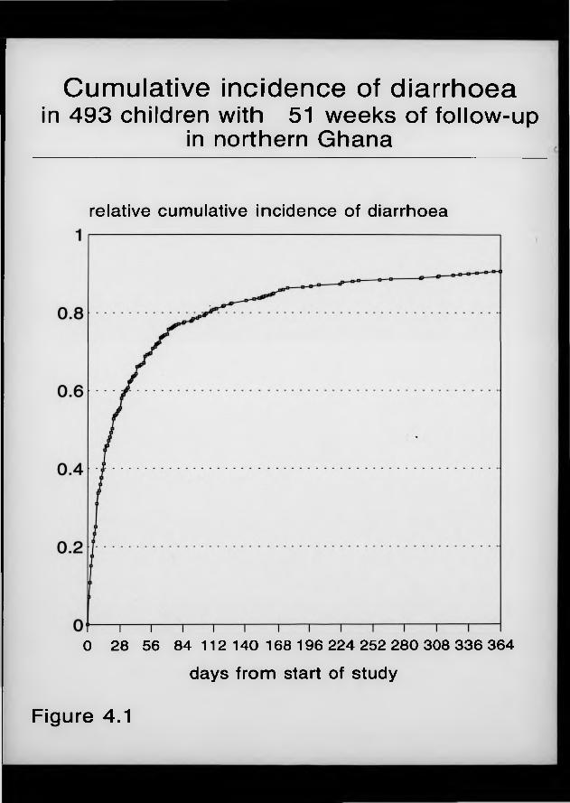
Cumulative incidence of diarrhoeain 493 children with 51 weeks of follow-up

in northern Ghana

relative cumulative incidence of diarrhoea

0 28 56 84 112 140 168 196 224 252 280 308 336 364days from start of study

Figure 4.1

Chapter 5 Event Analysis (III): Statistical issues and methods

5 .1 Introduction

In the previous chapter, different options for the choice of outcome measures in longitudinal studies of common diseases of childhood were discussed, and the advantages of the incidence rate were highlighted. As stated in that chapter, estimation of the incidence rate involves counting the total number of new episodes over a specified period of time, and dividing that number by the total observation time accruing to the study population over the same period. This measure is referred to by Kleinbaum et al. (1982) as the incidence density rate-, it can be viewed as the average value, over the duration of the time band, of a more fundamental measure of disease frequency, termed the instantaneous rate of illness, X, which cannot itself be measured because it is constantly changing. The instantaneous rate (also sometimes called the ‘force of morbidity’) is considered to be the ideal outcome measure for studies "attempting to relate disease occurrence to genetic and environmental factors in a framework of causation" (Breslow and Day, 1980). It may be defined for a particular individual (X,; i varies from 1 to n), a particular time period (Xf; t varies from 1 to m), a group of individuals, or the whole study population.

Methods for analysing illness rates are well developed for outcomes which can occur only once (Breslow and Day, 1987). In this situation, when an individual has once experienced the relevant outcome, they cease to be considered at risk and contribute no further observation time. With recurrent diseases, on the other hand, individuals are not eliminated from the ‘at risk’ group after experiencing the disease outcome (except when a restrictive ‘first-occurrence’ analysis is undertaken, which involves discarding information on all non-initial

107

episodes). The possibility that certain individuals may contribute more than one outcome over the period of observation give.* this type of data a dimension that is missing in non-recurrent disease data.

In this chapter, I investigate more closely the features of longitudinal count data on the incidence of common diseases, using as an example data on diarrhoea morbidity drawn from the Ghana VAST Child Health Study described in Chapter 2. Episodes are defined as proposed in Chapter 3. Having outlined some of the salient statistical features of such data, and the problems that these features give rise to, I then review three alternative methodologies that have been developed by statisticians over recent years to overcome some of the difficulties encountered. This involves the application of the criteria for the evaluation of statistical models proposed in Section 1.5. I then identify the analysis strategies actually pursued by the researchers conducting the trials of rotavirus vaccine efficacy described in Section 4.3, highlighting areas where these fail to address issues outlined earlier in the chapter. To aid the reader, a G L O S S A R Y of the technical terms and symbols used in this chapter is provided as Appendix A.

5 .2 Statistical featu res o f longitudinal data on com m on diseases

5 .2 .1 Notation

Longitudinal data on common diseases of childhood may be conceptualised in terms of a two-dimensional matrix: the columns of this matrix represent calendar time, with the total period of observation divided into m equal-length segments (or bands). The rows of the matrix represent each of n study subjects. The values in each cell correspond to the number of illness episodes observed for individual i and time band t, conventionally shown as y„ (mxn realisations of a

random variable KJ. Dividing yu by the length (in units of time) of time band

108

t gives an estimate of X,„ the time- and subject-specific rate of illness per unit time:

Time periods (f)

1 2 3 4 ... m-4 m-3 m-2 m-1 m

1 V i i y t2 y 2j y l.ml y ,m

su

2 y 22 y 22 y 2m

b 3 y3i y 3m

j 4ec

... y,<

t n-3

s n-2

(0n-1 y n -l,m

n y nl y n2 yn j % yn,m-l y nm

In all of the following discussions, the unit of time is taken to be one time band; the estimated rate per unit of time, X,„ is therefore the same as the observed number of episodes, yir

If the length of follow-up is assumed to be invariate, the analysis of rates focuses on the sampling variability of the observed number of episodes, y„ (Breslow & Day, 1987). Following the usual notation for Generalised Linear Models (McCullagh & Nelder, 1989), the expected value of Yit is denoted E(YJ, and its variance is given by:

109

Var(yi[) = <t>.v,

where vit is a specified variance function and <t> is a dispersion parameter that may or may not be known.

The mean, E(YJ, is related to a linear transformation of a series of p explanatory variables (given the vector notation x j , multiplied by their respective regression coefficients 0. The linearising transformation is referred to as the link function. Thus, we can say that the mean, E(YJ, is related to the linear predictor yit = 0 xit by the link function g{E(YJ} = rjlt, with inverse h = g Denoting the response vector by Y, the mean therefore satisfies

£(Y) - ¿(X 0)

As is apparent from the matrix shown above, the variability of Yit can be divided into two components: that which is accounted for by differences between study subjects (between-subject variability) and that which is accounted for by within- subject differences from one time period to the next (within-subject variability). In the following two sections, each of these sources of variation is described in greater detail.

5.2.2 W ithin-subject variability

Figure 5.1 illustrates the morbidity experience of sixteen children followed for the entire length of the study. In this figure, each 3 mm-high solid block represents a new episode of diarrhoea: child A019, for example, experienced one episode in the first time period, three in the second, two in the third and so on. For each child, the average number of incident episodes of diarrhoea per four

A

weeks of follow-up, \ , is shown in the penultimate column, and the variance of

110

this episode count over the 13 4-week periods is shown in the final column. Casual inspection suggests that the variance tends to be close to the mean rate. This is what would be expected if, at the level of the individual, episodes were distributed randomly in time and thus conformed to a Poisson model (Whittle,1970).

In Figure 5.2, the mean 4-weekly episode count for each child for whom a full 52-weeks of morbidity data were collected is plotted against the variance of the 13 observations for that child (n = 271). Also shown is the straight line representing the relationship variance = mean episode count. Although there is some scatter about this line, and although this variation increases as the mean episode count increases, there does appear to be an approximately linear relationship between these two parameters. There is some indication that the variance may not increase quite as rapidly as the mean episode count: using the method of Ordinary Least Squares to calculate the regression coefficients for the line best describing the relationship between these two parameters, and constraining the intercept to take the value 0, since this is fixed a priori, the relationship can be described by the equation:

Va — 0.84 x \

A

Where A, represents the average number of episodes per 4 weeks of observation for child *'. The calculated standard error of the slope estimate (0.022) cannot be relied upon because of the increasing scatter around the regression line (‘heteroscedasticity’), but there is at least a suggestion that the true slope is less than one. This situation, known as under-dispersion, implies that at the level of each individual, disease rates are slightly less variable from month to month than would be expected under the random occurrence model. One plausible explanation for this slight departure from the Poisson model is that trigger events are randomly distributed in time, but that those occurring during the course of

111

an existing episode fail to be recorded, most frequently when the true incidence is high (see Chapter 3). This situation is equivalent to the ‘dead-time’ experienced by Geiger counters following the arrival of a radioactive particle, as described by McCullagh & Nelder (1989) in their discussion of commonly encountered departures from the Poisson model.

5 .2 .3 Between-subject variability

N ot only do the number of episodes vary at the individual level from month toA

month, but the average rate, also varies from individual to individual. Figure5.3 shows the total number of episodes of diarrhoea experienced by each of the 271 children over the 52-week study period (solid bars). The distribution is h ighly skewed to the right, so that whilst many children experienced only a few episodes over the year, a few experienced over 20. The mean number of episodes per child was 6.23, with a variance of 33.8.

Even if the underlying propensity of each child to diarrhoea had been the same, there would still have been some random between-child variability in the number of episodes observed over the study period. The resulting distribution would, under these circumstances, follow the Poisson distribution, which, with a mean of 6.23 is almost symmetrical and has a variance of 6.23. The distribution expected under the null hypothesis of no heterogeneity in underlying disease rates is shown by the hatched bars in Figure 5.3. There is far more variability in the observed total episode counts than would be expected under this unrealistic null hypothesis. This situation is referred to as over-dispersion (McCullagh & Nelder, 1989). Some of this variability w ill be explained by measured individual-level covariates such as age and socio-economic status. Other important covariates will either have been measured imprecisely, or not measured at a ll. The impossibility of including all predictors in the systematic component

112

of the model will thus leave a portion of the between-child variability unexplained.

Because of this heterogeneity in individuals’ underlying propensity to illness, disease rates measured at different points in time on the same individual will tend to be more similar than disease rates measured at different points in time on different individuals. That is to say, there is within-subject correlation between disease incidence rates in different time periods. Table 5.1 shows - for the 271 children with complete morbidity records - unadjusted correlations between diarrhoea episode counts in each combination of the thirteen different time periods. In this case, there is some suggestion that the correlations may decrease somewhat as the time interval between the two observations increases, a situation which may be modelled as as stationary correlation.

This correlation cannot be ignored in the analysis. To do so would result in the overestimation of the precision of all effect estimates. The reason for this is as follows: when determining the precision of either stand-alone or effect estimates, assumptions are made about the relationship between the sample variance, s2, and the population variance, o2. It can be shown that, provided that each member of the sample is equally likely to be selected,

where otJ represents the covariance between any two observations of the outcome variable (Dwyer & Feinleib, 1991). ‘Standard’ analyses then proceed on the assumption that a,;=0 whenever i^ j (i.e. zero covariance between different elements). This allows the second half of the right-hand side of the equation to be ignored, greatly simplifying the analysis. The existence of within-subject correlation, however, invalidates this simplifying assumption, leading to the

113

underestimation of all standard errors which include the element a2 (that is, the standard errors of all effect estimates) if the correlation is not explicitly modelled.

Although the principal effect of within-subject correlation is to produce bias in the estimated precisions, it is important to note that with categorical outcomes effect estimates themselves are biased when correlations are ignored (Dwyer & Feinleib, 1991). This is a result of the relative down-weighting of multiple episodes occurring to the same individual that occurs when correlation is taken into account. The extent of this bias is investigated in the following chapter.

5 .3 Statistical m odels fo r correlated, categorical data

Considerable efforts have been devoted to tackling the problems of correlated response data when the response variable is continuous, and can be assumed to come from an underlying Normal distribution. Both Analysis of Variance (ANOVA)-type methods and regression models have been developed for such situations. However, the assumption of Normality, common to both these procedures, is wholly inappropriate for the distribution of numbers of disease episodes recorded over a specified period of time. This is because episode counts can only take whole integer, positive values; tend to show a highly skewed distribution, and are characterised by greater variability at higher average levels.

Unfortunately, models for correlated, categorical data are as yet less developed. In this section, I discuss three regression-type approaches to the analysis of such data that have been proposed over recent years. These approaches are the conditional or transition models widely favoured in econometric modelling (Gujarati, 1988), and established for at least the last fifteen years in the area of respiratory health; ‘multi-level' models, developed much more recently in the field of education (Goldstein, 1987); and a family of marginal models, especially

114

the semi-parametric Generalised Estimating Equations which have recently been developed in the Johns Hopkins University School of Public Health, Baltimore (Liang & Zeger, 1986). All of these models are described, and then, in Section 5.5, critically assessed using the criteria developed in Section 1.5.1.

5 .3 .1 C onditional models

One of the most intuitively appealing approaches to the problem of serial (between one time period and the next) correlations in longitudinal data has been the explicit inclusion of variables describing a subject’s previous state as predictors in models seeking to explain his/her subsequent state. Such models are termed conditional models because the response variable is not the vector of outcomes y as it stands, but rather the probability of observing a particular value yit given that the same individual had a known set of outcome(s) in previous time period(s). This may be expressed as:

Because the response variable is not simply the vector of outcomes Y, these models have a quite different interpretation to other models more widely used in health research: the focus is on individual-level change over time rather than on net population-level differences between sub-groups. As indicated by Ware et al. (1988), such models do not address questions such as ‘How does the prevalence of asthma change with age?’; instead, they answer questions such as ‘Does the frequency of reported wheezing in children free of wheezing a year earlier vary according to the age of the child?’. Because of this subject-specific focus, these models are sometimes termed ‘transition models’. It has been suggested that this focus might be appropriate for estimating from observational data the likely health impact of proposed interventions (Dwyer & Feinleib, 1991).

115

Two crucial issues arise when fitting models of this type. The first relates to the number of previous states that need to be included in the model in order to fully capture the autoregressive structure. For example, an early paper on the relationship between asthma and air pollution (Korn and Whittemore 1979) included a variable relating to subjects’ asthma status on the preceding day as a predictor of asthma attacks on the index day. This is known as a first-order autoregressive model. The effects of health status on days further removed from the index day (known as ‘higher order dependencies’) are not explicitly included in the model. Ware et al., on the other hand, show that their model of changes in children’s wheezing status from one year to the next is significantly improved by including the response at t - 2, a second-order autoregressive model. Obviously, if the individual’s history over two previous time periods has to be included in the model, then the first two observations cannot be used in the outcome matrix, as the relevant previous information does not exist. Such a limitation is wasteful and has serious implications for studies in which data is only collected on a limited number of occasions.

Secondly, there is an assumption in this kind of modelling that transition probabilities are independent of time. This means that changes in state from time t • 2 to time t - 1 are assumed to occur with the same probability as between times t - 1 and t. Since violations of this assumption (and the existence of high-order dependencies) make these models difficult to fit (Markus, 1979, quoted in Ware et al., 1988), less restrictive variants of the basic procedures have been sought. One example is a quasi-likelihood approach recently developed by Zeger and Qaqish (1988). Estimation techniques can be complex for autoregressive models, since there is a danger that correlations between explanatory variables and the random error can induce bias and inconsistency in the estimators. Missing data can be particularly troublesome, and observations must be evenly spaced in time.

116

W ith the notable exception of the area of wheezing and air pollution, conditional models have not been widely used in research on common diseases of childhood. Generally, epidemiological research has focused on identifying disease differentials between distinct population sub-groups, and conditional models are ill-suited to address these questions. Furthermore, autoregressive models may fail if exposures affect subjects’ initial state as well as their transitions between states (Stram et al., 1988), a scenario that frequently arises in epidemiological studies.

5 .3 .2 ‘M ulti-level* models

Another area which offers exciting prospects for the analysis of longitudinal data in the future is what has been termed ‘multi-level’ modelling. This approach is being pioneered by Goldstein and colleagues at the Institute of Education in London (see Goldstein, 1987). This type of model explicitly recognises that units of observation at one level are grouped within units at the next higher level; in theory, at least, any number of hierarchical levels can be defined, so that one can envisage analyses in which multiple observations on each subject constitute the basic unit of analysis, with subjects themselves as the second level, families as the third, communities as the fourth and so on. Covariates can be included at each level of the analysis, and can be fixed or random. A major goal of this type of analysis as it is currently being developed consists of estimating how much of the variability in the outcome corresponds to each of the various levels in the hierarchy.

The underlying ideas of multi-level modelling are illustrated with an example relating a continuous outcome (such as weights of young children) measured on multiple occasions to two sets of occasion-specific and child-level covariates. The example is adapted from Goldstein (1987). Let the subscript i refer to the child and the subscript t to one of n, multiple observations on each child. There are

117

thus a total of n observations. In an extension of the previously used notation for Generalised Linear Models, xlt is a vector of occasion-specific covariates, and z, is a vector of child-level covariates. The basic model is thus:

yit = a0 + a, + /3xIt + yz, + e„

where ag is the grand mean (the intercept term for the reference, or comer, individual), and a, is an individual-specific intercept term for child i. The random term elt is independently distributed within each child i with an expected value of zero and constant variance, o2.

In multi-level modelling, the individual-specific intercept, a„ is treated as a random variable with expectation of zero and constant variance, a 2, and the model is rewritten as:

y,, = a + /3xit + yz, + (a, + e j

This model includes elements from both levels in both its fixed and random parts. Goldstein (1986) has developed methods for estimating the parameters a, 0, y , o2 and o 2 by Iterative Generalised Least Squares (IGLS). The approach is extremely flexible, and permits modelling of random coefficients as well as random intercepts; this in turn allows for variance heterogeneity to be introduced into the model by means of random coefficients with zero expected values. In the case of discrete data, the squares of the random variables can be introduced into the model as additional random terms if this is desirable to improve the fit of the linearising transformation (Goldstein, 1991).

With these models, epidemiologists may be able to address issues that they had no means of addressing previously - particularly exciting is the prospect of being able to determine where ‘unexplained variance’ in disease rates actually arises,

118

whether at the individual, household or community level. However, this very flexibility may constitute an important barrier to the widespread adoption of these techniques: highly sophisticated decision-making is necessary to decide which random terms should be included in the model and at which levels; whether coefficients should be treated as fixed or random; whether linear constraints among parameters need to be incorporated, and how parameter estimates should be interpreted. Multi-level models may open the door to a new realm of epidemiology, but admittance, it appears, will be highly restricted!

Multi-level models have been developed most extensively for normally distributed outcomes. Although procedures have been outlined for other types of outcomes - log linear models in particular (Goldstein, 1991) - there is relatively little experience with their use and computer applications are still being refined. Other computational procedures, such as the Penalised Quasi-Likelihood of Breslow and Clayton (1993), are also being developed, but they appear to offer little advantage over the multi-level IGLS procedure currently implemented in the software package ML3.

5.3 .3 M arginal m odels

Whereas in multi-level modelling the amount of variance attributable to the higher-level clusters is of direct interest, in marginal models the focus is on population-averaged associations between covariates and outcome, with response correlation treated either as known or as a nuisance parameter. It is often said that marginal models fail to take advantage of repeated measurements on each study subject, or the fact that the effects of covariate changes within subjects on the response are directly observable (Ware et al., 1988; Neuhaus, 1992). Very often, however, it is precisely questions relating to the population-averaged associations between covariates and outcomes that epidemiologists wish to

119

address. Correlations in response variable are not a focus of interest in themselves, but rather they arise unavoidably as a result of the longitudinal methodology required for the accurate estimation of disease incidence.

Several different forms of marginal models have been developed. These range from fully parametric models in which both the within-individual variation in the outcome and the between-individual variation in mean incidence rates are fully described, to semi-parametric methods in which specification of the form of the association between the mean outcome and the covariates as well as of the mean-variance relationship is combined with ‘working assumptions’ about response correlation. Surprisingly perhaps, fu lly parametric models are poorly developed for count data; the wealth of different models for binary data (many of which, such as the beta-binomial and Normal-binomial models, have been implemented in highly accessible computer software) stands in contrast to the rather limited experience with mixtures such as the negative binomial distribution (see, for example, Lehmann et al., 1991). Two major disadvantages, however, weigh heavily against further investment in these models: firstly, only individual-level (as opposed to occasion-specific) covariates can be modelled, and secondly, the models are only appropriate when all pairs of responses measured on the same individual at two different times are equally correlated.

A much more promising advance has been the development of a semi-parametric approach by Liang and Zeger (1986). This approach incorporates ‘working assumptions’ about the correlations between pairs of outcomes for the same subject into estimating equations for the regression parameters (the so-called Generalised Estimating Equations [GEE], from which the method has taken its name) and into another set of equations for estimating the variances of the estimators. These formulae exploit the independence across subjects when estimating the variance of the regression estimators, and have the remarkable advantage of yielding consistent estimates of /3 and var(/3) even when the

120

arecorrelation structure has been mis-specified! These ‘robust’ estimates maximally efficient only when the correlation structure is right,but the cost of totally mis-specifying the correlation structure is unlikely to exceed 5-10% in many circumstances (Liang and Zeger, 1986). Unequal numbers of observations on different individuals, and very high correlations among repeated observations would be expected to cause a drop in efficiency when the correlation structure was incorrectly specified. It is important to note that the semi-parametric method will always be somewhat less efficient than corresponding parametric methods (Stukel, 1993). This is an example of the ‘price of ignorance’ of the true variance structure.

The Generalised Estimating Equation approach is still relatively new, and is not without difficulties. One of these is that in order for the underlying assumptions to hold, missing data must be totally independent of previous outcomes. It should be added that, whatever the structure of the missing data, its very existence poses substantial problems for the analyst trying to use current computer applications of the GEEs. Secondly, although Wald tests (a form of significance testing involving only the parameter estimate and its standard error) may easily be performed for all variables included in the regression, there is as yet no robust device for hypothesis testing (a naive likelihood ratio test has been derived by Rotnitzky and Jewell, 1990). Such a development will be crucial if full benefit is to be gained from this methodology. On the other hand, the methodology remains highly attractive because of the ready interpretability of the parameters derived, and its apparent ability to ‘absorb’ extra-Poisson variability (over-dispersion) without requiring accurate estimates of the covariance structure, or sacrificing the consistency of the estimates.

121

5 .4 Statistical methods adopted in rotavirus vaccine efficacy trials

In an attempt to verify to what degree an understanding of the statistical peculiarities of longitudinal data on common diseases has permeated the epidemiological literature, the 19 rotavirus vaccine trials described in Section 4.3 were reviewed with respect to the analytic approaches adopted. Since all-cause (as well as RV-specific) diarrhoea is a recurrent illness, failure to control for correlation in the outcome might be expected to lead to exaggerated estimates of the significance of treatment group differences (see above, Section 5.2.3). As discussed in Section 4.3.2.1, 13 studies focused on the cumulative incidence of one or more episodes of RV diarrhoea over the study period, thus bypassing the issue of multiple episodes occurring to the same individual altogether. Of the remaining six studies, one (#5) presented no data on the frequency of RV illness at all, and two (#9, #16) used unspecified chi-squared type tests, which do not account for within-subject correlation, and thus overstate levels of significance in treatment-group comparisons when used in this context.

Two further studies (#15, #17) analysed their data using repeated measures analysis of variance. No details are given in the paper as to how this procedure was carried out, but it may be assumed that the total variation in RV diarrhoea incidence was partitioned as follows:

Between subjects variation Treatment groupSubjects within groups (individual differences)

Within subjects variation Time periodTreatment x time period interaction Individual differences x time period interaction

122

This scheme differs from that which would apply in a no repeated measures two- w ay analysis of variance in just one important respect: instead of a single ‘ residual’ variance category, the within-cell variation is divided into two distinct parts, one relating to the subjects-within-groups effect, and the other to the interaction between individual differences and the time period effect. The appropriate denominator for the F-test for the treatment group effect is the subjects-within-groups variance (M S^ w grou(J , whereas under a no repeated measures factorial design it would be the residual variance (MSrcsidull) (Winer,1971). These features of repeated measures ANOVA lead to a relatively conservative estimate of the F-statistic associated with the between-subjects main effect (treatment group). In order for repeated measures ANOVA to give valid results, however, a number of conditions must be met. The first of these is that the variation due to subjects-within-groups should be homogenous over each level of the main between-subjects effect (i.e. in the vaccine and placebo groups). As mentioned above in Section 5.3, where the response variable consists of count- type data (such as the number of illness episodes), the variance within each group is likely to be proportional to the mean (McCullagh & Nelder, 1989). Homogeneity of variance could not therefore be expected where vaccines are effective in reducing illness episodes.

The last study (#12) used a log rank test to examine treatment-group differences in the average duration of time elapsing between vaccination and disease. This test is highly efficient in that it utilises all the information available about the relationship between exposure and outcome, and individuals whose follow-up is censored still contribute information for the length of time they were under surveillance. Standard techniques do not, however, permit the analysis of non­initial events.

In the analysis of all-cause diarrhoea, chi-squared (or exact binomial) tests were again preferred by most authors. Two studies made some attempt to incorporate

123

information on clustering of disease: in study #11, the Mann-Whitney U test (Mann & Whitney, 1947) was used to evaluate whether the numbers of children with 0,1,2,3... episodes of diarrhoea were similarly distributed in the two groups. This test is perhaps better suited to circumstances in which the response variable takes a broad range of different values, since the study subjects cannot easily be ranked if the response variable (here, number of illness episodes) takes the same value in a substantial proportion of cases. In study #6, a tabulation of number of episodes per child was presented but no test was carried out to evaluate the difference between vaccine and placebo recipients. Although neither approach incorporates information on follow-up time, they m ay offer important insights supplementing the standard techniques which focus on differences in mean rates.

5 .5 Conclusions

There are important differences between the conceptual framework for the analysis of incidence rates in longitudinal studies of common diseases, and that which applies in the case of rare diseases. This is because, in the case of common diseases, the outcome measure varies across two dimensions: person-to-person, and within subjects from one time period to the next. The degree of within- subject correlation is clearly substantial, and there are strong theoretical reasons for believing that it should not be ignored.

These considerations have not gone unnoticed in the statistical literature. Indeed, considerable advances have been made over the last decade in statistical methods for the analysis of longitudinal count data. Three possible approaches have been reviewed, and some of their major features are summarised in Table 5.2. The last section of this table shows how these three approaches compare on the criteria for evaluating statistical models proposed in Section 1.5.1. Conditional models score highly on user-friendliness, validity and ability to offer all the usual

124

statistical options, but they are unlikely to be widely used by epidemiologists studying common diseases of childhood primarily because the focus of the questions they address is different from the classic ‘risk factor’ approach in epidemiology, but also because they are difficult to fit and require uncomfortable assumptions about stationarity of transition probabilities over time. Multi-level modelling is an exciting development which is likely to add considerably to our understanding of the common diseases of childhood if applied intelligently. Furthermore, these models make no special demands in terms of input data, and again offer all the usual statistical options. The level of sophistication required to use these models is, however, very great, and there is no prospect of their routine use to overcome problems of response correlation in longitudinal studies. The GEE approach, on the other hand, appears much better suited to this purpose. It is highly applicable, requires only a limited selection between different options in terms of specific inputs, and is generally simple to use. Further empirical validation of the robustness of the variance estimates is, however, required.

A review of rotavirus vaccine trials carried out since 1980 suggests that, in this area at least, most epidemiologists carrying out longitudinal studies of common diseases in the field are unaware of the statistical peculiarities of the data they are working with. Chi-squared tests remain the analytic technique favoured by most authors, even though they take no account of correlation in the outcome, and are thus liable to overstate the precision of treatment group comparisons. Where an attempt is made to incorporate information on clustering of disease, the methods adopted are often unsuitable - either because they are premised on assumptions which are unquestionably violated, or because they are essentially techniques for significance testing which do not permit the estimation of epidemiological measures of effect. Over half of these studies did not even attempt to assess the impact of rotavirus vaccine on all-cause diarrhoea (or else did not specify the analytic technique used), perhaps in part because of the lack

125

of a generally accepted, valid and accessible methodology for the analysis of this kind of data. Given these difficulties, it is clearly important to establish just how far the nature of the data being analysed is likely to render the established, ‘traditional’ forms of analysis invalid. This task is undertaken in the following chapter.

126

A p p e n d i x A: Gloss a r y

{} refers to usage specific to this Chapter.

• autoregressive. A series of observations wherein the value of each distribution is partly dependent on the values of those which have immediately preceded it.

• bias. A systematic (i.e. non-random) distortion of a statistical result.

• conditional. Refers to the sub-distribution obtained in a set of variables A when the values of another set of variables B are held constant, given that sets A and B have a joint frequency distribution.

• consistent estimator. An estimator which converges in probability, as the sample size increases, to the parameter of which it is an estimator.

• correlation. Interdependence between quantitative data. Commonly measured by the Pearson product-moment correlation coefficient, r, which at the population level is denoted p.

• covariate (=explanatory variable, predictor variable; x) . Variable whose differing values are reflected in changes in the outcome variable (see below).

• efficient estimator. An estimator with a small variance relative to other possible estimators.

• marginal distribution. The unconditional distribution of single variables, or groups of variables, in a multivariate distribution.

• mean rate (=average rate) . The mean number of events per unit time period, averaged over several time periods. {Since in this Chapter a unit of time has been defined as one time band (see below) , the mean rate is equivalent to the mean number of events per time band.

127

• outcome (=response; y) . Variable of interest which varies in accordance with the values of other 'explanatory' variables (x) . {in this case, the number of incident episodes of illness over a defined period of time}.

• over-dispersion. Data are said to be over-dispersed if the variance is greater than the theoretical value assuming independence. Since, for the Poisson distribution, var(Y)=E(Y), data are said to be over-dispersed if var (Y) =<t>E (Y) , where <j>, the dispersion parameter, is greater than one.

• parametric model. Regression model in which the shape ('moments' ) of the underlying theoretical distribution is fully described.

• rate, instantaneous (=force of morbidity; X). Number of new events {in this case, incident episodes of illness; y) per unit of time. At, where the unit of time is infinitesimally small. Usually approximated by the incidence density rate (IDR), the number of events divided by the person-time-at-risk.

• subject (i). Individual {child}.

• systematic. The part of a linear model which is not captured by the 'random' error term(s) . Generally refers to the covariates which have 'fixed' effects on the outcome.

• time band (t). Period of time of defined length, over which the illness rate is presumed invariate.

• under-dispersion. Data are said to be under-dispersed if the variance is less than the theoretical value assuming independence. Since, for the Poisson distribution, var(Y)=E(Y), data are said to be under-dispersed if var (Y) =<t>E (Y) , where <t>, the dispersion parameter, is less than one.

• £ . Summation symbol.

Some of these definitions are adapted from:Marriott, FHC. A dictionary of statistical terms (5th edition). Harlow, UK: Longman Scientific and Technical, 1990.

128

R e fe re n c e s

Breslow NE, Clayton DG. Approximate inference in generalized linear mixed models. J Am Stat Ass, 1993 ;88 (421) :9-25.Breslow NE, Day NE. Statistical Methods in Cancer Research. I. The design and analysis of case-control studies. Lyon: International Agency for Research on Cancer, 1980.Breslow NE, Day NE. Statistical Methods in Cancer Research. II. The design and analysis of cohort studies. Lyon: International Agency for Research on Cancer, 1987.Dwyer JH, Feinleib M. Introduction to statistical models for longitudinal observation. In:Dwyer JH, Feinleib M, Lippert P, Hoffmeister H (Eds). Statistical Models for Longitudinal Studies of Health. New York: OUP, 1992.Goldstein H (1986) . Multilevel mixed linear model analysis using iterative generalized least squares. Biometrika, 1986,-73 (1) :43-56.Goldstein H (1987). Multilevel models in educational and social research. New York: OUP, 1987.Goldstein H (1991). Nonlinear multilevel models , with an application to discrete response data. Biometrika, 1991;78 (1) :45-51.Gujarati DN. Basic Econometrics (2nd Ed.). New York: McGraw-Hill, Inc., 1988.Korn EL, Whittemore AS. Methods for analyzing panel studies of acute health effects of air pollution. Biometrics, 1979;35:795-802.Lehmann D, Marshall TF de C, Riley ID, Alpers MP. Effect of pneumococcal vaccine on morbidity from lower respiratory tract infections in Papua New Guinean children. Ann Trop Paed, 1991;11:247-257.Liang K-Y, Zeger SL. Longitudinal data analysis using generalized linear models. Biometrika, 1986:73(1):13-22.Mann HB, Whitney DR. On a test of whether one of two random variables is stochastically larger than the other. Annals Math Stats, 1947: 18:50-60.Markus GB. Analyzing panel data. Sage University Press, Beverly Hills, CA, 1979.McCullagh P, Nelder JA. Generalized Linear Models (2nd Edition). London: Chapman and Hall, 1989.Neuhaus JM. Statistical methods for longitudinal and clustered designs with binary responses. Statistical Methods in Medical Research, 1992;1:249-273.Rothman K J . Modern Epidemiology. Boston: Little, Brown & Co., 1986.

129

Rotnitzky A, Jewell NP. Hypothesis testing of regression parameters in semiparametric generalized linear models for cluster correlated data. Biometrika, 1990;77 (3) :485-97.Stram DO, Wei LJ, Ware JH. Analysis of repeated ordered categorical outcomes with possibly missing observations and time-dependent covariates. J Am Stat Ass, 1988;83 (4 03) :631-63 7.Stukel TA. Comparison of methods for the analysis of longitudinal interval count data. Statistics in Medicine 1993;12:1339-1351.Ware JH, Lipsitz S, Speizer FE. Issues in the analysis of repeated categorical outcomes. Stats in Med 1988;7:95-107.Whittle, P. Probability. London: John Wiley and Sons, 1980.Zeger SL, Liang K-Y. Longitudinal data analysis for discrete and continuous outcomes. Biometrics 1986; 42:121-30.Zeger SL, Qaqish B. Markov regression models for time series: a quasi-likelihood approach. Biometrics 1988;44:1019-1031.

130

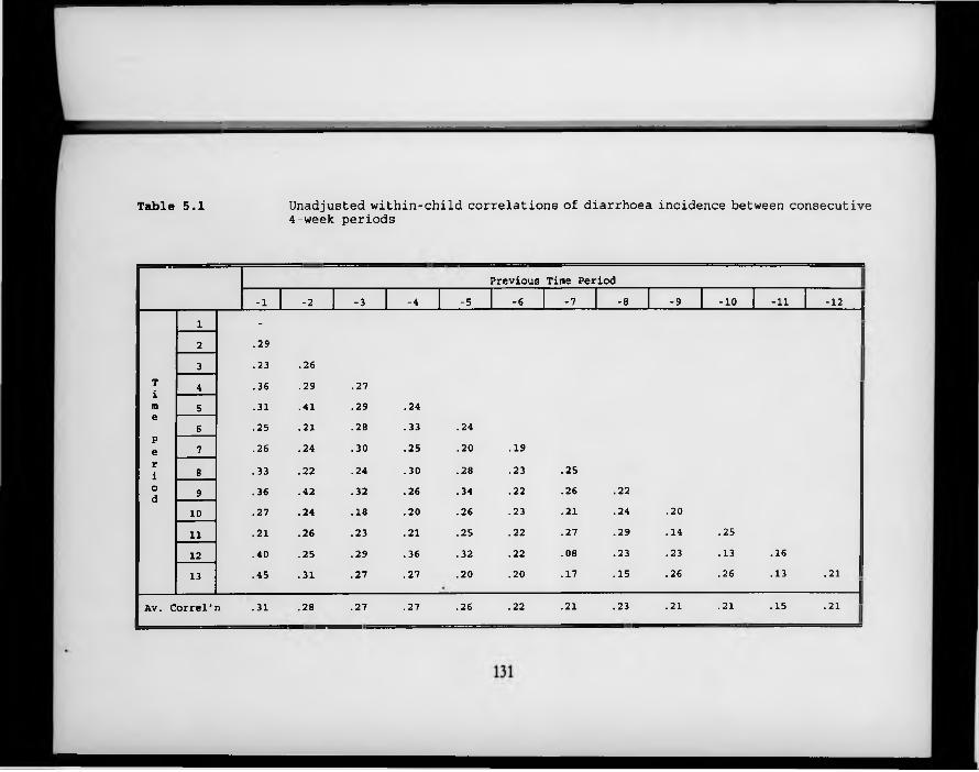
Table 5.1 Unadjusted within-child correlations of diarrhoea incidence between consecutive 4-week periods

Previous Time Period-1 -2 -3 -4 -5 -6 -7 -8 -9 -10 -11 -12

1 -

2 .293 .23 .26

T 4 .36 .29 .27im 5 .31 .41 .29 .24e6 .25 .21 .28 .33 .24

pe 7 .26 .24 .30 .25 .20 .19ri 8 .33 .22 .24 .30 .28 .23 .25od 9 .36 .42 .32 .26 .34 .22 .26 .22

10 .27 .24 .18 .20 .26 .23 .21 .24 .2011 .21 .26 .23 .21 .25 .22 .27 .29 .14 .2512 .40 .25 .29 .36 .32 .22 .08 .23 .23 .13 .1613 .45 .31 .27 .27 .20 .20 .17 .15 .26 .26 .13 .21

Av. Correl'n .31 .28 .27 .27 .26 .22 .21 .23 .21 .21 .15• 2 1

Table 5.2 Features and advantages/disadvantages of three different approaches to the analysis of longitudinal count data

ConditionalModels

Multi-LevelModels

Marginal Models (GEEs)

Application to categor'al data Various Goldstein(1991) Zeger S, Liang (1986)Model output Probability of outcome Y at time

t, conditional on value of Y at time t - 1 and covariates

Fixed and random covariate effects; variance components

Fixed effects;estimated correlations ; overdispersion parameter

Type of correlation that can be modelled

Autoregression Equi-correlation; autoregression (by invoking macro)

Equi-correlation; (non-)stationary correlation; autoregression; user-specified

Fittingtechnique Maximumlikelihood ML; REML; general quasi- likelihoodQuasi- likelihood

Computerapplication Standard stat. software ML3 SAS/IML; S+; SPIDACrucialassumptions

Transition probabilities are independent of time; no higher order dependencies

Strict hierarchy in data structure; independence among level-1 units once higher level effects accounted

for; Normality of higher-level residuals

Missing data independent of previous outcomes; weighted average of est'ed correlation matrices converges to a fixed matrix

APPLICABILITY ** ***** *****

VIABILITY ** ***** * * * *

VALIDITY **** ? i **★

UTILITY ***** **** **

POTENTIAL **** ** ★ **★

Notes :1. Some problems with estimators for non-linear regression in existing software application (ML3); expected to be resolved in next release.

132

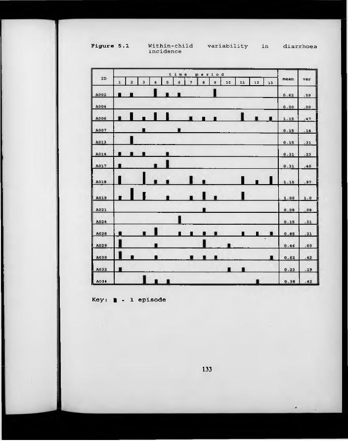
Figure 5.1 Within-child variability in diarrhoeaincidence

A 0 3 4

J __ L

e r i o d1 0 1 1 1 2 1 3

i ■ i i J __L

j ____LJ J L

I ■ I

J __ L J ___L

Key: | . l episode

133

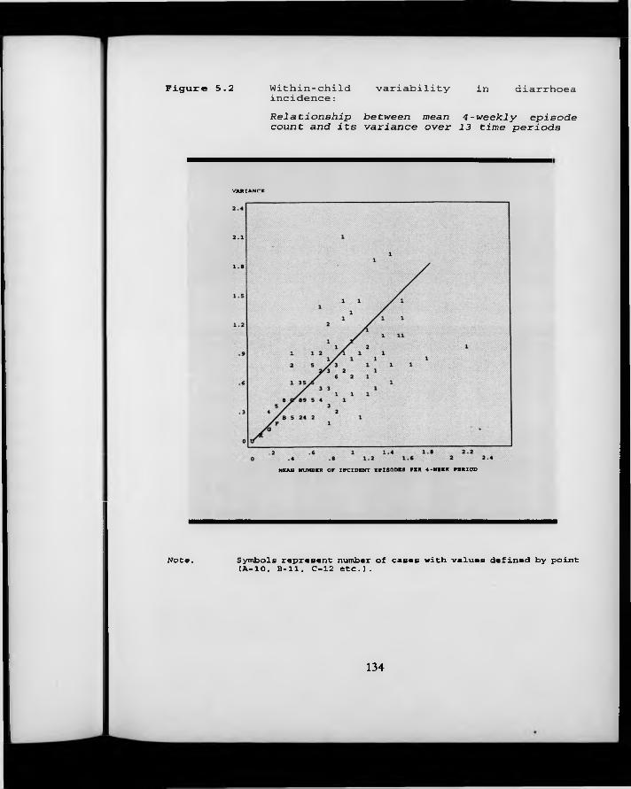
Figure 5.2 Within-childincidence: variability in diarrhoea

Note.

Relationship between mean 4 -weekly episode count and its variance over 13 time periods

VARIANCE

MEAN NUMBER OP INCIDENT EPISODES PER 4-WEEK PERIOD

Symbols represent number of cases with values defined by point (A*10, B=ll, C-12 etc.).

134

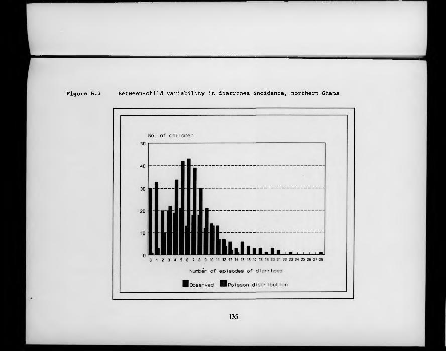
Figure 5.3 Between-child variability in diarrhoea incidence, northern Ghana

135

Chapter 6 Event Analysis (IV) Illustrative Analysis

6 .1 Using the Generalised Estim ating Equations algorithm s

In Chapter 5 it was shown that a number of relatively new statistical techniques are available to tackle the problems inherent in correlated response data. One of the most promising of these is the Generalised Estimating Equation (GEE) approach of Liang and Zeger (1986). The overview of analytic approaches adopted in rotavirus vaccine efficacy trials, presented in Section 5.4, indicates, however, that these ideas are still a long way from achieving widespread acceptance in the world of applied epidemiology. In this chapter, an illustrative analysis is conducted using the GEE approach. The specific issues that are likely to arise during the course of such an analysis are dealt with in some detail, as are the practical implications of relying on more familiar analytic techniques which do not take account of within-child clustering of disease.

A computer algorithm for the iterative derivation of the GEE estimators has been developed by Karim (1988). It is implemented in SAS Macro language, and is invoked from SAS/IML (the matrix algebra module of SAS). The use of this macro should present little difficulty to anyone familiar with SAS, although the module is sensitive to inadequacies in the raw data file, and the error messages generated are generally unhelpful. A similar implementation is available in SPIDA (Statistical Package for Interactive Data Analysis; Statistical Computing Laboratory, NSW, Australia). Although this package is distinctly more user- friendly than SAS, and possibly also faster, only rather small data sets can be analysed due to limited file-size specifications.

Whichever implementation is used, the data file is organised as a series of

136

multiple records for each individual, with each record corresponding to one time band. The number of new illness episodes recorded during the course of each time band is designated as the y-variable, and the various fixed and time- dependent covariates are noted as x-variables. If any of the covariates need to be modelled as factors, then dummy variables must be created by the user. The l in k function is specified as an option by the user: in the case of event analysis, the link w ill normally be logarithmic (as in Poisson regression). The relationship between the mean response and its variance is also specified from a number of options. Again, for event analysis the analogy w ith classic Poisson regression is maintained, and the variance is specified as equal to the mean response. It should be noted, however, that one of the features of the GEE approach is that an extra ‘over-dispersion’ or ‘scale’ parameter is estimated as part of the variance function, so that in reality this assumption only indicates that the variance of the y- variable is proportional to, rather than equal to, its mean.

The cluster of records corresponding to a single study subject is identified by an ID variable indicated by the user. Within each cluster, the form of the correlation expected between different time bands must also be specified. This is referred to as the ‘working’ correlation matrix. The appropriate specification of the form of this within-subject correlation is discussed at length in Section 6.2, since little practical guidance has been given on this issue in previous discussions of the method. The following section (6.3) discusses the appropriate width of the time bands for this type of analysis, since it m ight be believed that that the choice of time banding could affect both the magnitude of the effect estimates themselves and their precision. Section 6.4 deals with the issue of differing lengths of follow-up, and the final section (6.5) brings together the findings of the previous sections to present a unified schema for the analysis of correlated episode data.

The example used in this chapter is drawn from the Ghana Vitamin A

137

Supplementation Trials Child Health Study described in Chapter 2. The incidence of diarrhoea (as defined by the child’s carers) is related to the child’s age and source of drinking water (time-dependent covariates), and the place where the adults of the compound go to defecate, as well as the presence of animal (other than poultry) faeces in the compound (treated as fixed covariates). It should be noted that the output obtained when running the GEE analysis includes two different sets of estimates of the precision of the covariate effects: the first of these, referred to as ‘naive’ standard errors, are calculated on the assumption that the working correlation matrix is a true representation of the underlying process. The second set, referred to as ‘robust’ standard errors, include an allowance for the possibility that the working correlation matrix has in fact been mis-specified.

6 .2 Specifying the fo rm o f the within-subject correlation

In order to analyse longitudinal data on common diseases using the GEE procedures, it is necessary to make assumptions about the form of the correlation in the outcome variable. Although a number of different options are available, essentially the choice is between exchangeable/equi-correlation', which implies that all observations on a given individual are correlated with all other observations on that individual to the same degree, and stationary correlation, which implies that the degree of correlation is determined by the length of the time interval separating the two observations (so that a pair of observations separated by only a short time interval w ill be more highly correlated than a pair of observations separated by a long time interval). Sometimes it is additionally assumed that when the time interval separating two observations is longer than a specified number of time bands, the correlation between them will be effectively zero. This is referred to as - for example - stationary-5 correlation, when the limiting number of time bands is five.

138

Unfortunately, the choice of appropriate correlation structure is not wholly straightforward. Although the presence of within-subject correlation can be detected by examining the crude correlations between the number of illness episodes experienced by the same individual in different time bands, thic procedure w ill exaggerate the degree of the correlation since it fails to take into account important, measurable, individual-level determinants of disease (such as socio-economic status) which remain fixed throughout the period of observation. A preferable method of determining the degree of within-subject correlation between one time band and another is to examine the correlations in the regression errors after fitting a suitable model which includes the most important covariates. This can in fact be done using the GEE procedures, and the results for the diarrhoea data, adjusting for AGE, DRINKING WATER SOURCE, ADULT DEFECATION and PRESENCE OF ANIMAL FAECES in the compound are shown in Table 6.1. It appears that all pairs of observations are correlated, but that the correlations gradually become weaker as the time intervening between the two observations increases. Average correlations above 0.2 are seen for pairs of observations separated by no more than four time bands. It should not be assumed that the observed correlation matrix is a ‘true’ representation of the underlying process, since it is of course influenced by sampling variability.

The implications of ignoring the within-subject correlation are illustrated in Table 6.2. In this table, the results of analysing the data using the GEE algorithms are compared to results obtained using Poisson regression, with each time band treated as an independent observation. In setting up the GEE analysis, zero correlation (iindependence) was specified as the working correlation matrix - this means that the ‘naive’ standard errors should be approximately the same as

those obtained from standard Poisson regression, and the difference between the naive and robust standard errors may be interpreted as a measure of how much the precision of the estimates is exaggerated when the correlation is ignored.

139

It may be seen from the table that the effect estimates (the beta coefficients) are, as expected, unaffected by the choice of Poisson regression versus GEE modelling using an independence working correlation matrix. The naive standard errors derived from the GEE procedures are all 7.6% larger than those derived by means of Poisson regression: this is because the GEE model assumes only that the variance of the dependent variable is proportional to its mean (as opposed to the Poisson model, which stipulates that the variance is equal to the mean). Under the GEE procedure, all calculated standard errors are then inflated by (the square root of) a ‘scale parameter’ which is estimated iteratively. This is a minor difference, however, compared to the discrepancy between the naive standard errors, which are calculated on the assumption that the specified working correlation matrix is correctly specified, and the robust standard errors, which make no such assumption. In this example, the robust standard errors are between 1% and 73% larger than the naive standard errors (median, 34% larger). There is no clear pattern as to which variables show the largest (or smallest) discrepancies between the naive and robust standard errors.

Table 6.3 shows naive and robust estimates of the coefficient standards errors using GEE methods with a) exchangeable, and b) stationary-5 working correlation matrices. In both cases, the discrepancies between the robust and naive estimates are much less than those seen when an independence working correlation matrix was used: with exchangeable correlation, the robust standard errors are between 13% smaller and 15% larger than the naive standard errors (median, 3% larger), whilst with stationary-5 correlation, the robust standard errors are between 4% smaller and 10% larger than the naive standard errors (median, 5% larger). The robust standard errors are to all intents and purposes the same, regardless of whether the working correlation matrix is specified as exchangeable or stationary-5. They are, however, considerably smaller than those estimated when the working correlation matrix is specified as zero- correlation (independence). This is because the zero-correlation matrix is such

140

a poor representation of the true situation that the robust standard errors are estimated very inefficiently.

Table 6.4 compares the effect estimates derived under the three alternative specifications of the working correlation matrix. Significant effects are highlighted in bold. It may be seen that the effect estimates are only minimally affected by the choice of working correlation matrix. In this example, the conclusions that would be drawn from the analysis are identical for all three specifications of the correlation matrix.

6 .3 D eterm ining the appropriate width fo r the tim e bands

A fundamental practical issue that must be resolved in the analysis of longitudinal studies is the appropriate length of each period of observation, or time band. To some degree this is determined by the design of the data collection procedures, since the time bands cannot be shorter than the shortest interval for which disease outcome data are recorded, or longer than the total observation period. Within these limits, however, the length of the time bands which form the units of analysis m ay be freely determined at the outset of the analysis phase.

At one extreme, each child’s total experience can be summarised in a single record; this procedure makes no attempt to model the within-subject element of the variability in the outcome, and extra-Poisson variability is manifest as overdispersion (see Section 5.2.3). At the other extreme, each day’s experience can be dealt with separately, and day-to-day correlations can be modelled; this has the disadvantage of generating enormous data files, and in the case of a study with one year’s follow-up involves the inversion of a 365x365 matrix in order to solve the Liang-Zeger Generalised Estimating Equations, a task beyond the

141

scope of most desk-top computers. A reasonable compromise would seem to be to divide the total observation period into something between 3 and 30 shorter bands, but the implications of the exact choice have not been clearly spelled out.

6 .3 .1 Effects on estimates

Table 6.5 shows the (exponentiated) regression coefficients from the same analysis described previously, using 5 different options for the length of the time bands. These vary from 26 bands of 2 weeks’ duration, to a single band of 52 weeks’ duration. Since information on the time-dependent covariates was collected once every 4 weeks in this study, individuals are classified according to the value observed in the first 4-week period of a time band whenever the time band is longer than 4 weeks. This mimics the situation which would arise if the data on the time-dependent covariates had only been collected once per time period (that is, once every 13 weeks for the 13-week banding, once every 26 weeks for the 26-week banding, etc.). When data on time-dependent covariates are collected more frequently than once per time period, various other strategies are possible. These are discussed in Section 6.3.3. For the two-week time bands, the same covariate value was matched to two consecutive morbidity records.

Obviously, the intercept term is highly sensitive to the length of the time band. Also unsurprisingly, it is seen that effects of the time-invariate variables (WHERE THE ADULTS DEFECATE, and the presence of ANIMAL EXCRETA in the compound) are unaffected by the choice of time banding. The effects of the time-dependent variables, on the other hand, are altered by the choice of banding: the estimated AGE pattern of infection is moderately distorted even when the observation period is divided into 4 13-week periods, such that an accelerated fall-off in risk appears after 18 months. The pattern is radically different when a single band of 52 weeks’ duration is used. This is because age

142

is strongly related to the outcome, and children move rapidly from one age group to the next; therefore, if the child’s age is defined only once every 3 months, or even less frequently, a significant amount of misclassification of exposure group will occur. Misclassification will also occur with other time- dependent variables, such as WATER SOURCE, which may explain some of the fluctuations in the observed effect of this covariate.

Although it is not apparent in Table 6.5, it can be shown that the failure to reset the AGE GROUP variable at frequent intervals can lead to important residual confounding by age. This is demonstrated in Table 6.6, which shows the relationship between sleeping patterns and ALRI in children aged 0-5 months at the beginning of the one year follow-up (the example is again drawn from the Ghana vitamin A data set). In these children, sleeping inside appeared to be protective against ALRI (RR—0.58; P<0.05). However, when they were reclassified according to the age at which they actually experienced the episode of illness and the effect of sleeping pattern was adjusted for age, the protective effect of sleeping inside was no longer significant (Mantel-Haenszel RR = 0.74; P > 0.05).

The implication of this finding is that variables which are not related to the age of the child and which are not subject to seasonal variation - such as WHERE THE ADULTS DEFECATE - m ay be analysed using methods which do not require the division of the observation period into multiple time bands. Parametric negative binomial regression, described briefly in Section 5.3.3, is one such approach. Another even simpler approach involves using ordinary Poisson regression, and allowing for the over-dispersion by inflating the calculated standard errors by a scale factor equal to the square root of the residual deviance divided by the residual degrees of freedom (Aitkin et al., 1989). On the other hand, those variables which are related to the age of the child must be analysed by methods which permit the frequent resetting of the AGE variable, if residual confounding

143

by age is to be avoided. Table 6.7 shows which of the variables collected during the baseline phase of the Ghana Vitamin A study were associated with the age of the child: it can be seen that the majority of the individual-level variables were in fact related to the age of the child. Thus, parametric methods which do not permit the modelling of time-dependent covariates are likely to be of only limited use in the field of the epidemiology of common diseases of childhood.

6 .3 .2 Effects on precision

Table 6.8 shows the estimated precision of the regression coefficients with time bands of 2, 4, 13, 26 and 52 weeks’ duration. The estimates for the first four situations are derived using the GEE approach, whilst the single time band estimate is derived using ordinary Poisson regression with the standard errors inflated as described above (Section 6.3.1). The estimated degree of within-subject correlation (under the assumption of equi-correlation) is shown in the lower section of the Table, together with the scale parameter for the variance function. These latter parameters are of interest because they show that sparse data (which is the result of dividing the observation period into very short time bands) can make it difficult to detect within subject correlation, a finding which I have verified using simulated data.

This table shows that the precision of the time-invariate effects is unaltered w ith increasingly long time bands, but the precision of the time-dependent variable (WATER SOURCE) is decreased, presumably due to increasing misclassification of exposure with longer time bands. Somewhat surprisingly, the precision w ith which the AGE effects are estimated is increased w ith longer time bands. One possible explanation for this phenomenon is that it reflects a problem with using discrete age ‘groups’ to model what is essentially a continuous evolution of risk at different ages. Under the discrete age-group model, a child passing from one

144

age group to another is assumed to experience an immediate transition to a different level of risk; in reality, however, that child will continue to experience much the same level of risk that they experienced a few days earlier. With very short age bands, it will frequently occur that the same child w ill contribute to more than one risk-set during the course of the period of observation, and the variability of disease experience within each age-group will thus be increased (leading, of course, to less precise estimates of the effects of each age group). The same problem would not be expected to arise if a polynomial function of age were used rather than discrete age-groups; ease of interpretability would, however, be sacrificed.

Where discrete age-groups are used, the results of Table 6.8 suggest that it may be preferable to avoid extremely fine time-bandings. In this case, the criterion for the choice of the width of the time bands should be to ensure that they are as wide as possible without incurring significant misclassification of exposure status. Table 6.9 illustrates the degree of misclassification that might be expected in a selection of time-dependent variables studied in the Ghana vitamin A trial if consecutive months of observation were combined into longer time bands. It is assumed that exposure status was correctly ascertained when the data was collected on a 4-weekly basis, and that if longer time bands were to be created, the value observed at the beginning of each time band would be assumed to apply for the entire duration of that time band. It can be seen that when two months of observation are combined, most variables are mis-classified in the second half of the time band in around 10% of all cases. The exceptions to this are the variable describing where the CHILD SLEEPS each night, which is highly occasion-specific, and that describing whether or not any COOKING was done in the compound, which may be considered a fixed characteristic of the compound. When longer time bands are created, the degree of misclassification becomes even more marked, to the extent that serious bias is likely to occur in the analysis.

145

6.3.3 Conceptual fram ework and analytic approach fo r occasion-specific

covariates

The fact that variables such as where the CHILD SLEEPS are highly occasion- specific raises certain problems in the analysis. Two quite different conceptual models can be distinguished: under the first model, as soon as the child is exposed to sleeping indoors (or outdoors, depending on which is considered to be the high-risk category), his/her risk of a negative outcome would increase. In this case, the variable would need to be measured very frequently, and transitional models, described in Section 5.3.1, would probably be the most appropriate analytic approach. These models are examined further in Section 7.4.1, where they are applied to the analysis of illness prevalence. On the other hand, if the conceptual model is that those children who most frequently sleep indoors (or outdoors) will also experience more than average morbidity, then it may be appropriate to summarise the various measurements of the covariate over a time band of at least several months. F igure 6.1 shows the distribution of the percentage of occasions on which each child was reported to be sleeping in a room, as opposed to outside, for children with at least 12 assessments of this variable during the year’s follow-up in the Ghana VAST Child Health Study. Considerable variation was noted in the proportion of occasions on which children slept inside. This variable did not, however, appear to be correlated with any of the 21 signs/symptoms enquired about in the weekly morbidity interviews. Alternative summary measures for other variables might involve classifying children according to the ‘best’ or ‘worst’ category recorded over all the occasions on which the variable is measured.

146

6.4 Differing lengths o f follow-up

So far, all analysis has been conducted using data for the sub-group of children who were under observation for a full year. These children present less difficulties in the analysis than children with incomplete follow-up because the exact form of the period-to-period correlations can be estimated empirically. However, in many studies a substantial minority - or even a majority - of study participants are not observed for part of the follow-up period. This is especially the case in studies with continuous enrolment, and studies where subjects drop out o f observation by virtue of out-migration, death or voluntary withdrawal. Temporary absences from the home also result in incomplete follow-up. There are good a priori reasons for believing that children with shorter periods of follow-up may differ systematically from those with longer periods of follow-up, both in terms of important covariates such as age, and in terms of their morbidity experience.

In the Ghana VAST study, many children contributed less than the full year of observation. Separate analyses, shown in Table 6.10, have been carried out for four different groups of children: those with no more than one week of missing data (51-52 weeks of observation), those with 44-50 weeks of observation, those with between 1/2 year (26 weeks) and 43 weeks of observation, and those with less than 1/2 year of observation. In each case, the total surveillance period has been divided into 13 4-week bands, and observations are only included for a given individual when at least three weeks’ data are available to estimate the number of new diarrhoea episodes occurring during the course of a time-band. Equi-correlation is assumed and the estimated degree of within-subject correlation is shown, as well as the number of observations contributing to each group’s sub­analysis.

147

The consistency of the findings from the four different sub-groups of children is remarkable. The age effects appear slightly different for the group with the shortest duration of follow-up, but on closer inspection it can be seen that only the rates in the youngest age group are different from the other analyses, with the relative intensities of disease in the other age groups m irroring the results based on children with longer durations of follow-up. The effects of the different sources of drinking water are also more marked for the children with the shortest follow-up times. This may be due to sampling variability, but could also reflect differences in the age/seasonal make-up of this group, suggesting that possible interaction between drinking water source and age and/or season could be investigated in the final model.

\

Table 6.11 shows the final estimated effects, combining data from all the children in the study. Exchangeable correlation is assumed, to overcome the difficulty of including children with incomplete data. Since the age structure of the group of children with shorter lengths of follow-up is substantially different from that of children with longer lengths of follow-up, it is important to bear in mind that combining data for all children introduces a risk of confounding by AGE if this variable is not included in all subsequent analyses. Duration of follow-up was also associated with seasonality in this study, since new recruits o n ly contributed data during the latter part of the study. Although seasonal effects may be of little interest in themselves, there are clearly reasons to believe that SEASONALITY could potentially confound the association between AGE and DIARRHOEA, or between WATER SOURCE and DIARRHOEA. Table 6.11 demonstrates that adjusting for seasonal effects does in fact have a quite substantial impact on the regression coefficients for AGE, though less so for WATER SOURCE. There is only a very small (and entirely negligible) loss of precision associated with incorporating the 14 dummy variables for SEASONALITY into the model.

148

6 .5 Conclusions

In this chapter it has been shown that strong period-to-period correlations in diarrhoea incidence can be detected in a typical empirical data set, even after adjusting for important covariates such as age. Ignoring this correlation w ill lead to substantial over-estimates of the precision of the covariate effects, but is unlikely to produce any serious bias in the estimates. The over-estimate of the precision of the covariate effects is sufficiently large (on average, around 34%) to render ‘standard’ techniques inappropriate. Therefore more elaborate analytic techniques are required.

Several different methods are available to adjust for within-subject correlations. This analysis illustrates that the optimum method is determined to an important degree by the type of covariate that is being studied. The GEE method, which has several theoretical advantages and is conceptually close to traditional Poisson regression, has been shown to give good results. By ‘re-setting’ the AGE variable in each time band, the effects of time-dependent covariates which are associated with the age of the child can be modelled without the danger of residual confounding by AGE. When covariate values change extremely rapidly with time, however, and it can be assumed that the exposure w ill have an immediate, non-cumulative effect on the outcome, conditional models - described in Sections5.3.1 and 7.4.1 - offer an alternative, perhaps preferable, choice of analytic strategy. When an immediate, non-cumulative effect cannot be assumed, summary measures of exposure, combining information from more than one occasion, may be more informative. At the other end of the spectrum, some covariates are time-invariate and unrelated to the age of the child: this implies that there is no need to split the total observation into smaller bands, and the over-dispersion in the outcome can probably be quite adequately modelled using relatively simple parametric methods such as negative binomial regression, or

149

even ordinary Poisson regression with the standard errors inflated by a scale factor easily calculated from the residual deviance. The range of recommended strategies is illustrated in Table 6.12.

When using the GEE model, exchangeable correlation between different time bands can safely be assumed. This simplifying assumption has a negligible impact on the precision or accuracy of the effect estimates, and makes it possible to include individuals with incomplete follow-up in the analysis. The appropriate width of time banding is indicated in Table 6.12. Two alternative situations are envisaged, one giving rise to time bands of 1-2 months’ duration, and another giving rise to bands of 4-6 months’ duration. This assumes incidence rates s im i la r to those observed in our study for diarrhoea, and would obviously need to be adjusted for more/less frequent outcomes. It is imperative that the AGE variable is reset for each time band in order to avoid important residual confounding by age, as well as biased estimates of the effects of AGE itself. Data can be included from children with incomplete follow-up, but it is highly likely that SEASONALITY will have to be introduced into the model as a potential confounder, especially if a dynamic cohort design has been used, or there is substantial attrition from the initial cohort.

Use of an appropriate analytic tool does not obviate the need for a well thought out analytic strategy. Many important issues relating to the choice of variables to include in explanatory models are unfortunately beyond the scope of this discussion, but need to be resolved before attempting to fit any regression model. Regrettably, the SAS/IML implementation of the Generalised Estimating Equations is cumbersome and highly sensitive to programming errors, and thus not suitable for exploratory analyses. The SPIDA implementation does include a routine for choosing the best subset of explanatory variables to include in the final model, however, this implementation cannot be used with very large data sets. One way of minimising the required recourse to the SAS macros might be

150

to conduct initial analyses in a user-friendly application of Poisson regression such as EGRET, treating each time-band as an independent observation. This will result in substantial over-estimates of the precision of all the effect estimates, but w ill enable variables not associated at all with the outcome variable to be weeded out before the final model is fitted in SAS/IML using the Generalised Estimating Equation algorithms.

151

R e fe re n c e s

Aitkin M, Anderson D, Francis B, Hinde J. Statistical modelling in GLIM. Oxford: Clarendon Press, 1989.Karim MR, Zeger SL. GEE: A SAS macro for longitudinal data analysis. Johns Hopkins University Department of Biostatistics Technical Report #674. Baltimore: Johns Hopkins University, 1988.Liang K-Y, Zeger SL. Longitudinal data analysis using generalized linear models. Biometrika, 1986; 73(l):13-22.

152

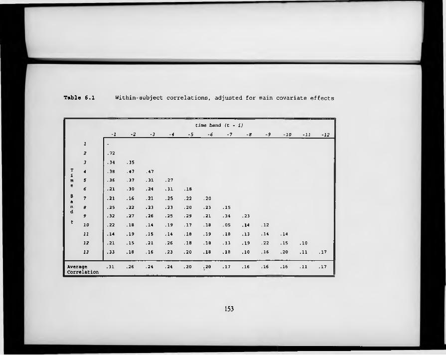
T a b l e 6 . 1 Within-subject correlations, adjusted for main covariate effects

time band (t - i)

-l -2 -3 -4 -5 -6 -7 -8 -9 -10 -11 -12

1 -2 .723 .34 .35

T 4 .38 .47 .47im 5 .36 .37 .31 .27e

« .21 .30 .24 .31 .18B 7 .21 .16 .21 .25 .22 .20an 8 .25 .22 .23 .23 .20 .23 .15d

9 .32 .27 .26 .25 .29 .21 .34 .23t

10 .22 .18 .14 .19 .17 .18 .05 .14 .1211 .14 .19 .15 .14 .18 .19 .18 .13 .14 .1412 .21 .15 .21 .26 .18 .18 .13 .19 .22 .15 .1013 .33 .18 .16 .23 .20 .18 .18 .10 .16 .20 .11 .17

AverageCorrelation

.31 .26 .24 .24 .20 .20 .17 .16 .16 .16 .11 .17 i

153

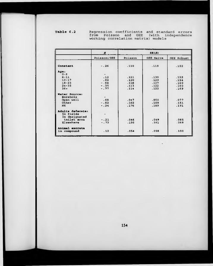
Table 6.2 Regression coefficients and standard errorsfrom Poisson and GEE (with independenceworking correlation matrix) models

ß SK(/S)Poisson/GEE Poisson GEE Naive GEE Robust

Constant - . 26 .110 .119 .152Aga:0-5 -6-11 . 12 . 121 .130 .15212-17 . 02 . 120 .129 . 15418-23 - . 04 .118 .127 . 16024-35 - . 35 .113 . 122 . 16036 + - . 77 . 114 .123 .169Water Source:Borehole -

Open well . 08 . 047 . 050 . 077Other - . 02 .102 . 109 . 151NK - . 34 . 176 . 189 .191Adults defecate:In fields -

In designatedtoilet area - .21 . 046 . 049 .085 !Elsewhere - . 72 .150 .161 .268Animal excretain compound . 12 . 054 . 058 .100

154

Table 6.3 Standard errors from the GEE model using exchangeable and stationary-5 working correlation matrices

SE (0)Exchangeable Stationary-5correlation correlation

Naive Robust Naive RobustConstant .132 . 141 . 136 .142Age:0-56-11 .120 . 138 . 136 . 14612-17 .126 . 144 .145 •13918-23 .135 . 145 .146 . 14624-35 .136 . 148 .142 .14936 + .146 .163 . 146 .157Water Source:Borehole Open well . 065 .061 . 061 . 064Other .122 .121 . 114 .125NK .163 . 154 . 154 .158Adults defecate:In fields In designatedtoilet area .094 . 085 . 079 . 085Elsewhere .308 .271 .247 .264Animal excreta in compound .111 .097 .093 . 097

155

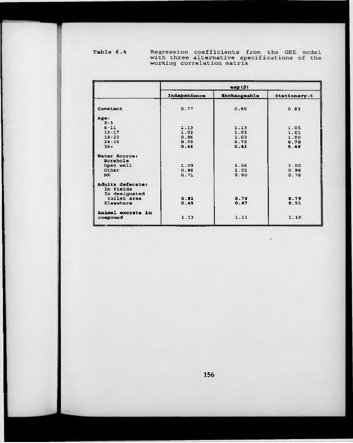
Table 6.4 Regression coefficients from the GEE modelwith three alternative specifications of theworking correlation matrix

exp(/J)Independence Exchangeable Stationary-5

Constant 0.77 0.80 0.83Aga:0-5| 6-11 1.13 1.13 1.0512-17 1.02 1.03 1.01 118-23 0.96 1.03 1.0024-35 0.70 0.72 0.7036 + 0.46 0.41 0.46Hatar Sourca:

1 Borehole Open well 1.09 1.06 1.00Other 0.98 1.02 0.98i NK 0.71 0.80 0.78Adults defecate:In fields In designatedtoilet area 0.81 0.79 0.7 9Elsewhere 0.49 0.47 0.51Animal excreta In compound 1.13 1.11 1.10

156

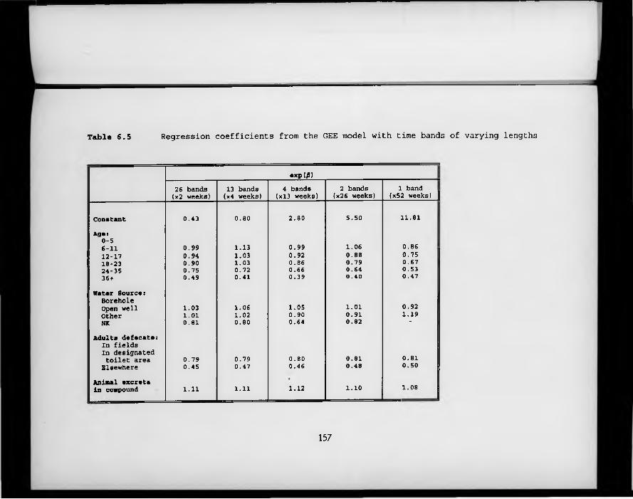
Table 6 .5 Regression coefficients from the GEE model with time bands of varying lengths

exp(/S)26 bands (x2 weeks) 13 bands (x4 weeks) 4 bands (xl3 weeks) 2 bands (x26 weeks) 1 band(x52 weeks) ||

Constant 0.43 0.80 2.80 5.50 11.81.Agsi0-56-11 0.99 1.13 0.99 1.06 0.8612-17 0.94 1.03 0.92 0.88 0.7518-23 0.90 1.03 0.86 0.79 0.6724-35 0.75 0.72 0.66 0.64 0.5336+ 0.49 0.41 0.39 0.40 0.47

Natar Source: Borehole Open well 1.03 1.06 1.05 1.01 0.92Other 1.01 1.02 0.90 0.91 1.19 !NK 0.81 0.80 0.64 0.82 “

Adults dafecate:In fields In designated toilet area 0.79 0.79 0.80 0.81 0.81Elsewhere 0.45 0.47 0.46 0.48 0.50

Animal excreta in compound 1.11 1.11 1.12 1.10 1.08

157

Table 6.6 Residual confounding by age in children classified as aged 0-5 months at the beginning of the one-year follow-up period

Actual age at time Sleep Sleep ---- 1of ALRI episode: inside outside Ratio \AgesO-5 mo.

episodes: 36 11 0.58c h i l d r e n : 137 74

Age = 6 -11 mo.episodes: 11 24 1.71c h i l d r e n : 196 251

Age = 12 -17 mo.episodes: 10 4 0.19c h i l d r e n : 78 164

All agesepisodes: 57 39 0.58c h i l d r e n : 411 489 | 0.38,0.86

Mantel-Haenszel Rate Ratio= 0.74 (0.49-1.13)

158

Table 6.7 Associations with age of the child among the full set of covariates examined in the Ghana study

Variables clearly associated with the age of the child:★ Vaccination status★ History of measles or hospital admission★ Consumption of vitamin A rich foods and breastfeeding★ Anthropometric status; vitamin A status★ Sleeping patterns★ Child's defecation practices★ Source of drinking water and use of soap;

certain handwashing practices★ Knowledge, attitudes and practices re. ORS★ Mother's age and parity; presence of younger sibling

Variables associated with the age of the child in this data set, but unlikely to be associated in other data sets:★ Maternal education★ Twin★ Household possessions and access to dry season farm

Variables not associated with the age of the child:★ Sex of the child★ Birth order★ Survival status of the preceding child★ Father's education★ Household ownership of livestock and design of compound★ Exposure to smoke pollutants★ Certain handwashing practices★ Adult defecation and refuse disposal practices

159

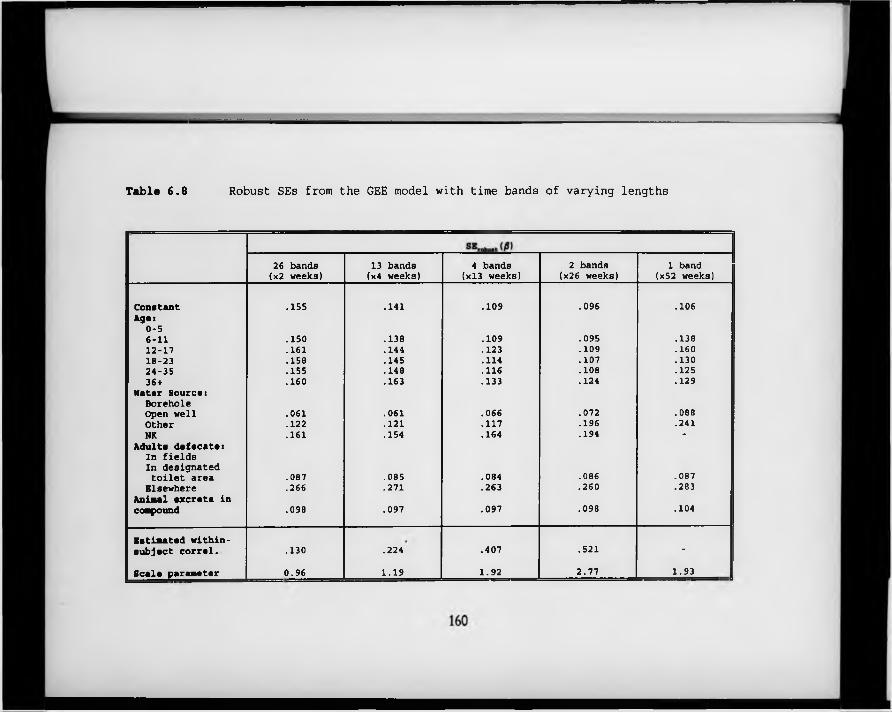
Table 6.8 Robust SEs from the GEE model with time bands of varying lengths

26 bands (x2 weeks)

13 bands (x4 weeks)

4 bands (xl3 weeks)

2 bands (x26 weeks)

1 band (x52 weeks)

Constant .155 .141 .109 .096 .106Ages

0-56-11 .150 .138 .109 .095 .13812-17 .161 .144 .123 .109 .16018-23 .158 .145 .114 .107 .13024-35 .155 .148 .116 .108 .12536+ .160 .163 .133 .124 .129

Hater Source:Borehole Open well .061 .061 .066 .072 .088Other .122 .121 .117 .196 .241NK .161 .154 .164 .194 -

Adults defecate:In fields In designated toilet area .087 .085 .084 .086 .087

Elsewhere .266 .271 .263 .260 .283Animal excreta in compound .098 .097 .097 .098 .104

Estimated within- subject corral. .130 .224 .407 .521 -

Scale parameter 0.96 1.19 1.92 2.77 1.93

Table 6.9 Numbers (and percentages) of time-bands in which the exposure variable is partially misclassified when the value observed at the beginning of the time band is assumed to be correct for the entire duration of that time band

||length of tine bands -> 2 months 3 months 4 months

fraction of time band for which individuals are misclassified for exposure status ->

1/2 1/3 2/3 1/4 1/2 3/4 f |

Exposure variable:Breast feeding 802/8877

( 9 . 0 * )530/5567

( 9 . 5 * )336/5567

( 6 . 0 * )417/4117

( 1 0 . 1 * )266/4117

( 6 . 5 * )191/4117

( 4 . 6 * ) :!Wasted (weight-for-age s -2 z-scores^ 766/8639

( 8 . 9 * )531/5485

( 9 . 7 * )268/5485

( 4 . 9 * )370/4064

( 9 . 1 * )249/4064

( 6 . 1 * )145/4064

( 3 . 6 * )

Sleeping pattern 3680/8874 ( 4 1 . S t )

2013/5570( 3 6 . l t )

1350/5570( 2 4 . 2 * )

1193/4115( 2 9 . 0 * )

1108/4115( 2 6 . 9 * )

791/4115 ! ( 1 9 . 2 * ) j

Father smokes 786/8869( 8 . 9 * )

505/5565 ( 9 . I t )

256/5565( 4 . 6 * )

422/4113( 1 0 . 3 * )

157/4113( 3 . 8 * )

151/4113( 3 . 7 * )

Source of drinking water 1172/8876( 1 3 . 2 * )

692/5570( 1 2 . 4 * )

483/5570( 8 . 7 * )

485/4115( 1 1 . 8 * )

317/4115( 7 . 7 * )

263/4115( 6 . 4 * )

Cooking in compound 218/8871( 2 . 5 * )

117/5568( 2 . 1 t )

74/5568( 1 . 3 * )

111/4114 ( 2 . 7 * )

25/4114( 0 . 6 * )

44/4114 '( 1 . 1 * )

161

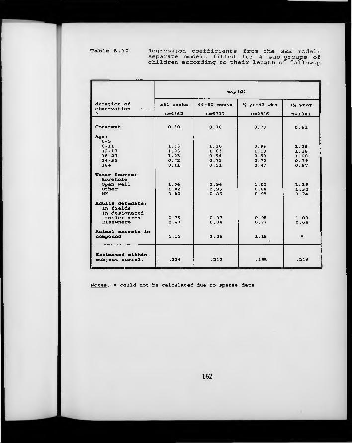
Table 6.10 Regression coefficients from the GEE model: separate models fitted for 4 sub-groups of children according to their length of followup

exp (0)

duration ofobservation -->

*51 weeks n=4862

44-50 weeks n-6717

M yr-43 wks n-2926

sM year n=1041

Constant 0.80 0.76 0.78 0.61A g e :

0-56-11 1.13 1.10 0.96 1.2612-17 1.03 1.03 1.10 1.2618-23 1.03 0.94 0.99 1.0824-35 0.72 0.72 0.70 0.7936 + 0.41 0.51 0.47 0.57

Water S o u r c e:Borehole Open well 1.06 0.96 1.00 1.19Other 1.02 0.93 0.84 1.30NK 0.80 0.85 0.98 0.74

Adults defecate:In fields In designated toilet area 0.79 0.97 0.98 1.03

Elsewhere 0.47 0.84 0.77 0.68Animal excreta incompound 1.11 1.05 1.15 *

Estimated within-subject correl. .224 . 212 .195 .216

Notes : * could not be calculated due to sparse data

162

Table 6.11 Regression coefficients from the GEE model with and without adjustment for seasonality

Notes: * In this model, the constant term refers only to the first month of observation, and is therefore not directly comparable to the model without the seasonal factor

163

Table 6.12 Summary of recommended analytic strategies for correlated response data

Type of covariate

Examples: Importance of confounding by age

Type of modelling strategy preferred

Width of time bands

Occasion-specific

Sleeping patterns (in N . Ghana),Air pollution/ temperature/humidity

May or may not be important; analysis focuses on changes in outcome variable within each individ. as exposure alters

Conditional models As short as possible; determined by frequency of data collection

Changes rapidly with time or age

Breastfeeding,Weight/Age, W/Height Source of drinking water (in N. Ghana), Hygiene practices

Major confounding by age

GEE 1-2 months l

Changes slowly with time or age

Vitamin A dosing status, Height/Age, Immune function

Less severe confounding by age

GEE 4-6 months

Fixed Socio-economic status Demographic characteristics, Parental beliefs

Not associated with age of the child

Poisson regression with standard errors inflated by scale factor derived from residual deviance (or other similar parametric models)

Total follow-up time

164

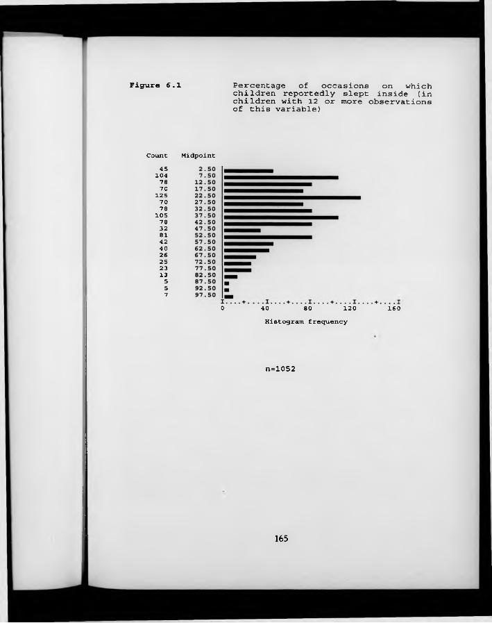
Figure 6.1 Percentage of occasions on which children reportedly slept inside (in children with 12 or more observations of this variable)

Count Midpoint45

104 78 70

1257078

105 78 32 81 42 40 26 25 23 13557

0 40 80 120 160Histogram frequency

n=1052

165

Chapter 7The Analysis of Prevalence Data

7.1 Measures o f prevalence in longitudinal studies

Prevalence is a measure of disease frequency which differs from incidence in that it focuses on disease status rather than on events. It has been defined as "the proportion of people who have a disease at a specific instant" (Rothman, 1986). As such, it is quintessential^ a cross-sectional measure, not normally associated with longitudinal studies. Indeed, as mentioned in Section 1.2, the pioneers of the longitudinal approach in studies of common childhood illnesses felt strongly the need to overcome the severe limitations of the cross-sectional prevalence study as a tool for the study of morbidity and its interactions with nutritional status (Scrimshaw, 1967). Moreover, prevalence is a particularly complex and at times ambiguous outcome measure for those endeavouring to carry out aetiological research, since it reflects determinants of disease duration as well as of disease incidence (Rothman, 1986). On the other hand, io r health service planners, prevalence may be the most relevant of all outcome measures, since it indicates the potential demand for health services at any given moment in time.

Longitudinal studies by definition involve measurements of disease status at many different points in time. It is therefore possible to examine the "proportion of people who have a disease at a specific instant" repeatedly on each occasion that the study population is contacted. Alternatively, one could combine all the available information for all time points and all subjects, and estimate the proportion of all occasions on which disease was recorded. A third possibility is to focus on the individual, calculating the proportion of all days (or other time units) observed on which each individual was recorded as suffering from a given disease. "Each of these three strategies will be examined in turn in this section.

166

The first approach is illustrated in Figure 7.1, which shows the point prevalence (presence of the disease on the day of the interview) of a fever-like complaint known as ‘intolegere’ over each of a total of 65 weeks of data collection in the Ghana VAST Child Health Study, described in Chapter 2. It will be recalled that each child was visited just once a week in this study, so that no more than one observation from each child is included in any of the 65 estimates of the point prevalence of ‘ intolegere’. This type of data, in which a single variable is measured regularly over a prolonged period of time, is known as time series data. The weekly prevalences can be related to other variables which also change over time, such as meteorological measures, or group-level changes in malaria parasitaemia rates, anthropometric status of diet. However, such analyses are complicated by the fact that there are strong correlations between the prevalence rate at time t and the same rate at time t-1 (referred to as lag 1 autocorrelation). This violates the assumptions of ordinary linear regression, and means that special models must be used (Gujarati, 1988). These characteristics of time series data are confirmed by the example of Figure 7.1, which - it can be shown - has the properties of a first-order Markov process (see Section 5.3.1), with a lag 1 autocorrelation coefficient of over 90%.

Moving away from a focus on time to a focus on individuals, an alternative way of analysing data on disease status in longitudinal studies is to calculate what Kleinbaum et al. (1982) have termed ‘episodic prevalence’. This is, for each individual, the number of time units (days, in the current example) with illness divided by the total number of time units under observation. This measure may be interpreted as the probability that a given individual is sick at time t (which can be any time over the course of the period of observation), provided that it can be assumed that the individual’s probability of illness remains constant over the length of the observation period. Each day of observation appears only once in the denominator of this measure, but of course, individual days of sickness/ health are not independent when they are measured on the same individual (see

167

below, Section 7.4.1). It should not therefore be assumed that this measure has the customary binomial variance for proportions. Furthermore, there m ay be some between-individual correlation, where - for example - a number of children live in the same residential unit.

Cobb (1962) has pointed out that the frequency distribution of these episodic prevalences (or, in his terminology, ‘protepV, proportion of time in episode) of all the individuals in a study population provides a full description of disease prevalence in that population over the observation period. Such a distribution is shown in Figure 7.2, which depicts the episodic prevalence of cough in 1103 children with at least 300 days of observation in the Ghana study. Sim ilar distributions are seen for other signs/symptoms in this data set. When analysing these data, it will be important to incorporate information about the proportions of children with very low or very high prevalences, as well as about the ‘average’ prevalence in different groups.

A third approach to the analysis of prevalence data in longitudinal studies is to calculate what I shall call ‘block prevalence’, by dividing all the days of illness over the observation period by the total number of days of observation, for all subjects together. This measure is in fact a weighted average of the time series prevalences, with weights equal to the proportion of the total observation time that each individual unit of time contributes; or, equivalently, a weighted average of the episodic prevalences, with weights equal to the proportion of the total observation time that each study subject contributes. It is not equal to an unweighted average of either measure, unless - by chance or design - a ll the weights are equal (i.e. all the children contribute data from the same period of observation, and there are no missing data). Moreover, the variance o f this measure is not equal to the customary binomial variance of a proportion because the use of repeated measures on the same individual introduces problems of correlated data more serious even than those discussed in the previous sections

168

on measures of disease incidence (Section 5.2.3). The use of this measure is thus best avoided when analysing prevalence data from longitudinal studies.

In this chapter, no further consideration is given to the time series approach to the analysis of prevalence data, since this does not permit the examination of individual-level differences in disease status. Instead, I first consider the significance of episodic prevalence as a potential measure of ‘frailty’, and then consider a variety of statistical techniques which might be used to compare episodic prevalence in different sub-groups of a population. Finally, I consider in more detail the relationship between multiple days of illness/health measured on the same individual, and discuss the implications that these relationships may have for the appropriate analysis of illness prevalence.

7 .2 Episodic prevalence a n d the concept o f 'frailty *

The tabulation of the distribution of episodic prevalences in the whole population, as illustrated in Figure 7.2, suggests that days of illness are not distributed ‘fairly’ between different individuals: some of the children in the Ghana VAST Child Health Study experience very little or no cough during the course of the study year, whilst others experience almost continuous coughing throughout the year. In fact, if days of illness were distributed completely at random, w ith a constant probability of illness for all individuals and all days, the distribution would be binomial with a mean of 7r=.14, as shown in Figure 7.3. The marked difference between this distribution and that observed in Figure 7.2 confirms the existence of important heterogeneity of risk, a concept previously evoked in Section 5.2.3. It is convenient to refer to those children with a higher underlying risk of morbidity as frail, even though this term has hitherto generally been used to describe individuals at increased risk of mortality rather than morbidity (see, for example, Vaupel et al., 1979). An important

169

consideration in extending this term to include individuals at increased risk of specific morbidities - over and above the axiomatic observation that mortality is caused by illness - is the fact that the various environmental and genetic factors that make some children more prone to common infectious illness than others are most unlikely to be specific to individual signs or symptoms. This phenomenon has been discussed in some detail by Mosley and Becker (1991), and is apparent in the Ghana VAST data set, where individuals who experience high episodic prevalences of one sign/symptom are likely to experience high prevalences of other symptoms also.

In addition to its importance as a possible indicator of frailty already established, episodic prevalence may have another role as an indicator of frailty in-the- making. The idea relates to the work of Alter and Riley (1989), who developed the concept of insult accumulation, meaning that "each ‘insult’ from illness or injury leaves the individual more susceptible to disease in the future". The precise mechanisms by which such insults could be brought about are discussed by Solimano and Vine (1980). A number of studies have examined the link between episodic prevalence of illness and anthropometric status, attempting to quantify the impact of illness on ‘acquired frailty’: for example, Lutter and colleagues (1992) have shown, using three different data sets, that each day of diarrhoeal illness between the ages of 0 and 36 months is associated w ith a .03 cm decrease in attained length at 36 months in Colombia; with a .74 cm decrease in attained length at 36 months in Guatemala, and with a significant impact on weight gain between 6 and 12 months in Peru. Rowland et al. (1988) have shown that in the Gambia, both diarrhoea and lower respiratory tract infections were associated with weight faltering in the first, but not the second year of life. All these studies are based on the premise that anthropometric status may be taken as a proxy measure of frailty. The strength of the associations demonstrated suggests that episodic prevalence may be an outcome measure of major clinical relevance in studies of common diseases of childhood.

170

7.3 C om paring distributions o f episodic prevalences between different

groups o f individuals

In order to make a comparison of episodic prevalences between two different groups o f individuals, Cousens and Kirkwood (1990) have suggested dividing the distribution of prevalences into a number of discrete intervals (e.g. no illness; 1-20%, 21-40% and 41-100%) and comparing the groups by means of a chi- squared test for trend. This approach facilitates the visual comparison of the proportions of children with low or high episodic prevalences, and is illustrated in Table 7.1, which shows the distribution of cough prevalences in the Ghana data set in children living in compounds with (n=116) and without (n = 981) an adult w ith a chronic cough. The analysis is restricted to individuals with 300 or more days of observation. In this example, children living in compounds with an adult with chronic cough were much more likely to have high prevalences of cough than children living in compounds without an adult with chronic cough (x2= 12.16 on 1 df; P — 0.0005). Mathematically, the chi-squared test for trend is equivalent to a t-test using consecutive integers to represent each grouped interval instead of the true values. It is thus somewhat wasteful of information, since the actual data values are discarded.

On the other hand, using a simple r-test to compare actual episodic prevalences in the tw o groups is problematic, since the distribution of episodic prevalences is likely to be far from Normal, and the test assumption of equal variances in each group may be violated. In the example of the previous paragraph, the variance of the prevalences of children living in compounds with an adult with a chronic cough was 1.92 times the variance of children living in compounds without such an individual. With large numbers of observations in each group, it is possible to calculate a z-statistic robust to unequal variances (Kirkwood, 1988). In this example, the resulting value of z was 2.75 (P -0.007).

171

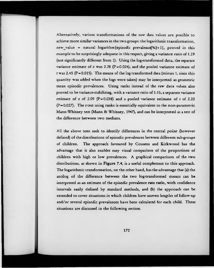
Alternatively, various transformations of the raw data values are possible to achieve more similar variances in the two groups: the logarithmic transformation, new_value = natural logarithm{episodic prevalence[%]+1}, proved in this example to be surprisingly adequate in this respect, giving a variance ratio of 1.19 (not significantly different from 1). Using the log-transformed data, the separate variance estimate of z was 2.28 (P = 0.024), and the pooled variance estimate of t was 2.45 (P = 0.015). The means of the log-transformed data (minus 1, since this quantity was added when the logs were taken) may be interpreted as geometric mean episodic prevalences. Using ranks instead of the raw data values also proved to be variance-stabilising, with a variance ratio of 1.15, a separate variance estimate of z of 2.09 ( P - 0.038) and a pooled variance estimate of t of 2.22 (P = 0.027). The r-test using ranks is essentially equivalent to the non-parametric Mann-Whitney test (Mann & Whitney, 1947), and can be interpreted as a test of the difference between two medians.

All the above tests seek to identify differences in the central point (however defined) of the distributions of episodic prevalences between different sub-groups of children. The approach favoured by Cousens and Kirkwood has the advantage that it also enables easy visual comparison of the proportions of children with high or low prevalences. A graphical comparison of the two distributions, as shown in Figure 7.4, is a useful complement to this approach. The logarithmic transformation, on the other hand, has the advantage that (a) the antilog of the difference between the two log-transformed means can be interpreted as an estimate of the episodic prevalence rate ratio, w ith confidence intervals easily defined by standard methods, and (b) the approach can be extended to cover situations in which children have uneven lengths of follow-up and/or several episodic prevalences have been calculated for each child. These situations are discussed in the following section.

172

7 .3 .1 Uneven lengths o f follow -up, and m ultiple measures o f

episodic prevalence

A practical problem associated with analysing data on episodic prevalences arises when children have differing lengths of follow-up, since episodic prevalences calculated using data on children with a relatively short period of follow-up will be less precisely estimated than those estimated using data on children with a long length of follow-up. This implies that some system of weighting should be used so that the contributions of children with incomplete follow-up are down­weighted in the analysis. Ideally, the inverse of the variance of the individual episodic prevalence estimates should be used, but it is far from clear how the variance of these episodic prevalence estimates should be determined; although the episodic prevalences are nothing more than simple proportions, the conventional binomial variance of a proportion is not appropriate in this case since individual days of sickness/health measured on the same individual are not independent, and, furthermore, the binomial variance is by definition equal to zero when the episodic prevalence is zero or one.

One might argue that the whole concept of within-child variability is not relevant in the consideration of episodic prevalence, since this measure is effectively a score rating the child on a continuum from ‘very healthy’ to ‘very sick’, without any reference to individual days. In this case, the number of days observed for each child divided by the maximum possible number of days of observation is probably an acceptable weighting system (equivalent to weighting cluster-level estimates by cluster size in a cluster-randomised trial). An unweighted analysis, using data from all 1847 children in the Ghana VAST Child Health Study with known values for the presence or otherwise of an adult with chronic cough in their compound, and comparing (log-transformed) episodic prevalences of cough in children living with an adult with chronic cough

173

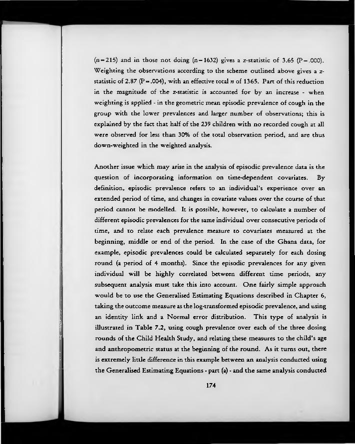
(n = 215) and in those not doing (n=1632) gives a z-statistic of 3.65 (P = .000). Weighting the observations according to the scheme outlined above gives a z- statistic of 2.87 (P = .004), with an effective total n of 1365. Part of this reduction in the magnitude of the z-statistic is accounted for by an increase - when weighting is applied - in the geometric mean episodic prevalence of cough in the group with the lower prevalences and larger number of observations; this is explained by the fact that half of the 239 children with no recorded cough at all were observed for less than 30% of the total observation period, and are thus down-weighted in the weighted analysis.

Another issue which may arise in the analysis of episodic prevalence data is the question of incorporating information on time-dependent covariates. By definition, episodic prevalence refers to an individual’s experience over an extended period of time, and changes in covariate values over the course of that period cannot be modelled. It is possible, however, to calculate a number of different episodic prevalences for the same individual over consecutive periods of time, and to relate each prevalence measure to covariates measured at the beginning, middle or end of the period. In the case of the Ghana data, for example, episodic prevalences could be calculated separately for each dosing round (a period of 4 months). Since the episodic prevalences for any given individual w ill be highly correlated between different time periods, any subsequent analysis must take this into account. One fairly simple approach would be to use the Generalised Estimating Equations described in Chapter 6, taking the outcome measure as the log-transformed episodic prevalence, and using an identity link and a Normal error distribution. This type of analysis is illustrated in Table 7.2, using cough prevalence over each of the three dosing rounds of the Child Health Study, and relating these measures to the child’s age and anthropometric status at the beginning of the round. As it turns out, there is extremely little difference in this example between an analysis conducted using the Generalised Estimating Equations - part (a) - and the same analysis conducted

174

using standard multiple linear regression, treating each round as an independent observation - part (b). This is despite the fact that relatively high within-child correlations were observed (r = 0.367). The effect of malnutrition (weight-for- height z-score less than -2) may have been slightly over-estimated when standard multiple linear regression methods were used.

7 .4 W ithin-child variability in disease status, an d acquired fra ilty

The use of episodic prevalence as the primary outcome measure in the analysis of disease prevalence necessarily implies discarding potentially valuable information about the timing and sequence of days of illness. Any approach which explicitly modelled these features of disease status would need to take each individual day of illness (or health) as the primary unit of analysis, and account for the full set of correlations between one day of illness and another, measured on the same individual. These correlations may be expected to change as the interval between the two days increases. Figure 7.5 shows the observed within- subject correlations between the presence of cough on the first day of the trial period and the presence of cough on subsequent days up to the 50th day of the trial period in the Ghana VAST Child Health Study. It can be seen that the first two days of illness/health were very highly correlated within each child, with an r of over 0.8. These correlations then fell progressively with longer intervals separating the pairs of observations being compared. Rather stable correlations of the order of 0.2 were observed with intervals of two weeks or longer.

In theory, this correlation structure could be modelled using either the Generalised Estimating Equations described in Chapter 6 or the Multi-Level Modelling package ML3 (Section 5.3.2). However, because of the limitations of the current implementations of the Generalised Estimating Equations, it would not be possible to model anything other than exchangeable correlation if there

175

were variable numbers of days of observation per individual. Furthermore, with a full year of follow-up, the equations could only be solved by inverting a 364 x 364 matrix, an undertaking which is completely impracticable using micro­computers. Although methods exist for modelling an exponential decline in intra-subject correlations using the Multi-Level Modelling package ML3, this package has rather restrictive data space specifications, and would be quite incapable of analysing data sets of the size of the Ghana VAST study, with nearly 2000 children and 364 days of observation.

One approach which could more feasibly be applied to the analysis of daily prevalence data in longitudinal studies - if it were considered necessary to incorporate information about the timing and sequence of days of illness - would be to use conditional models (described in Section 5.3.1). These models seek to quantify the probability that an individual w ill experience illness on day t given that s/he did (or did not) experience illness on day t-1. A set of models appropriate for dependent binary outcomes of this kind has been developed by Bonney (1987). In the following section, Bonney’s approach is applied to data from the Ghana Vitamin A Supplementation Trials Child Health Study.

7.4 .1 Logistic regression fo r dependent binary outcomes

In his paper, Bonney attempts to identify the different features of dependence in the outcome variable (presence of illness on day f; coded y, - 1 for illness present, and y ,-0 for illness absent) which need to be considered when modelling daily prevalence data. He introduces a general regression model in which 0„ the logit of the outcome on day t, is related to the illness status on the previous day (day t-1), the number of preceding ‘successes’ (in this case, days with illness), the number of preceding ‘failures’ (days without illness), and other covariates:

176

0, - a + ypZ,_, + y*S*,_, + y (-S',.,) + 0X,

where a is a constant term, Z,_; is a function of the immediately preceding outcome (coded 1 for disease present and -1 for disease absent, so that if y,_, = 1, the odds of y, increases by ey(p), and if yt_, - 0, the odds of y, decreases by the same amount). S*t_, is the number of preceding days of illness, S~,_, is the number of preceding days without illness, and X, is a vector of occasion-specific covariates.

This very general model includes (nested within it) a number of more specific models, such as the simple Markov model which specifies that the current outcome is determined only by the immediately preceding outcome (and other relevant covariates), with no terms relating to the number of previous days with or without illness. Comparison of a variety of models, with different assumptions about the structure of the dependence between successive days of illness or health, should help indicate to what degree the concept of a day of illness has any relevance removed from its context as part of an episode, and also to what degree ‘acquired frailty’ can be demonstrated using prevalence data. With this aim, a variety of models were fitted using data on daily prevalence of cough in 100 children with complete follow-up in the Ghana study, and the results are shown in Table 7.3.

Model 8 is the complete model described in the first paragraph of this section: in this model, the effect of the number of preceding days of illness is allowed to be of a different magnitude to the effect associated with the number of preceding days without illness (i.e. they are not equally predictive), and the immediately preceding outcome is included as a potential determinant of current illness status. This is the best fitting model, with a deviance of 6197 on 36,296 degrees of freedom. Other models were compared to this model by subtracting the deviance of the best model from the deviance of each of the other models, and

177

relating this to the difference in degrees of freedom (equal to the difference in the number of parameters). This is interpreted as a chi-squared statistic (Clayton & Hills, 1993). This analysis shows that four other models with a reduced number of predictor variables (numbers 3 and 5-7) are fairly adequate in describing this data set, though all are significantly less good than the ‘best’ model. All of these models include the variable referring to the child’s illness status on the previous day. The models which do not include this variable (numbers 1, 2 and 4) give a substantially poorer fit to the data.

The final ‘best’ model is given by the equation:

6 , -----1.09 + 2.94 x Z,_, + .012 x S*,_, + .004 x ( - S - ,./)

Because of the logit link, the regression coefficients must be anti-logged before they can be interpreted as odds ratios. Furthermore, since the preceding day’s illness status Z is coded (1,-1) the effect of having cough yesterday relative to not having cough yesterday is obtained b y multiplying the coefficient by two before taking the anti-log. The results thus indicate that a child with cough yesterday is 360 times more likely to have cough today than a child without cough yesterday. A child who has already recorded 3 months of cough is 3 times more likely to have cough today than a child without any previous history of cough, and a child who has already recorded 3 months of no cough is 30% less likely to have cough today than a child without any previous history of days without cough.

178

7.5 Discussion and conclusions

The results of the previous section demonstrate the profound dependence that exists between consecutive days of illness/health recorded on the same individual. Such a finding will hardly come as a surprise to those accustomed to thinking of illness in terms of episodes, but it has major implications for the analysis of prevalence data in longitudinal studies. Conventionally, such data are analysed using techniques - such as the simple chi-squared test for the difference between two proportions - which treat every day of observation as independent. Such techniques are inappropriate since they exaggerate both the precision of stand­alone estimates, such as the proportion of days with illness, and the levels of statistical significance in comparisons between different population sub-groups.

These correlations that exist between different days of observation measured on the same individual cannot easily be accommodated using sophisticated modelling procedures such as Multi-Level Modelling or Generalised Estimating Equations. Indeed, any procedure which treats each child-day as a separate record will soon run into software problems due to the enormous size of the resulting files - these problems may be the result of limited work space or quite simply arithmetic ‘overload’. Conditional models of the type proposed by Bonney (1987) are less problematic to fit, and can incorporate quite sophisticated models of dependence between multiple days of observation on the same individual, but they suffer from all the limitations noted in Section 5.3.1, most notably the impossibility of including any fixed (i.e. child-level) covariates in the analysis. Their practical usefulness is probably limited to the rare occasions when the major covariate of interest changes extremely rapidly with time.

An alternative, and more promising, approach to the analysis of illness prevalence involves moving away from a focus on individual days of

179

illness/health, and basing analysis instead on ‘episodic prevalence’, a measure of the proportion of time each individual spends ill. Whilst this measure was first proposed by Cobb as early as 1962, there was virtually no discussion of how such data should be analysed until the appearance of the guidelines developed by Cousens and Kirkwood in 1990. Cousens and Kirkwood suggested a number of different approaches, including a technique based on the chi-squared test for trend, and standard parametric analyses based on the log-transforms of the original episodic prevalences. I suggest two extensions to the latter parametric approach: firstly, weighting episodic prevalences differentially so as to incorporate information on the duration of follow-up of each individual, and secondly, using the Generalised Estimating Equations to deal with within-subject correlations between episodic prevalences calculated over multiple time periods.

I have suggested that episodic prevalence may play an important role in the epidemiology of childhood disease as an indicator of frailty. Heterogeneity of risk cannot be identified in cross-sectional studies because there is no way of telling whether a particular individual is sick at the time of the survey because they are generally sick more of the time than others, or because they are no different from other individuals, but just happen to be sick at that time. The use of episodic prevalence, calculated from longitudinal studies, offers one way of resolving this dilemma. The possibility that episodic prevalences, calculated over a reasonably long period of time, may be a reliable indicator of true underlying propensities to disease is reinforced by the quite different analysis of Section 7.4.1, which shows that children with 90 days’ previous history of coughing were three times more likely to cough on day r than children with no previous history of cough. Whilst it is not possible to say whether this finding points merely to the existence of an identifiable set of chronic coughers, or whether it really is a a demonstration of ‘acquired frailty’ , the evidence from various studies of the impact of multiple days o f illness on growth does seem to indicate that children are indeed rendered more vulnerable by the accumulation of morbidity insults.

180

R e fe re n c e s

Alter G, Riley JC. Frailty, sickness and death: models of morbidity and mortality in historical populations. Pop Studies 1989; 43:25-45.Clayton D, Hills M. Statistical models in epidemiology. Oxford: Oxford University Press, 1993.Cobb S. A method for the epidemiologic study of remittent disease. Am J Public Health 1962; 52:1119-1125.Cousens SN, Kirkwood BR. Outcome measures in prospective studies of childhood diarrhoea and respiratory infections: choosing and using them. Geneva: World Health Organization, 1990.Gujarati DN. Basic econometrics (2nd ed.). New York: McGraw-Hill, Inc., 1988.Kirkwood BR. Essentials of medical statistics. London: Blackwell Scientific Publications, 1988.Kleinbaum DG, Kupper LL, Morgenstern H. Epidemiologic research: principles and quantitative methods . New York: Van Nostrand Reinhold Co. Inc., 1982.Lutter CK, Habicht J-P, Rivera JA, Martorell R. The relationship between energy intake and diarrhoeal disease in their effects on child growth: biological model, evidence, and implications for public health policy. Food Nutr Bull 1992: 14(l):36-42.Mann HB, Whitney DR. On a test of whether one of two random variables is stochastically larger than the other. Annals Math Stat 1947; 18:50-60.Mosley WH, Becker S. Demographic models for child survival and implications for health intervention programmes. Health Policy Planning 1991; 6(3):218-33.Rothman K. Modern epidemiology. Boston/Toronto: Little, Brown & Co. , 1986.Rowland MGM, Goh Rowland SGJ, Cole TJ. Impact of infection on the growth of children from 0 to 2 years in an urban West African community. Am J Clin Nutr 1988; 47:134-8.Scrimshaw NS, Guzmin MA, Gordon JE. Nutrition and infection field study in Guatemalan villages, 1959-64. I. Study plan and experimental design. Arch Environ Health 1967; 14:657-62.Solimano GR, Vine M. Malnutrition, infection and infant mortality. In: Preston SH (Ed.). Biological and social aspects of mortality and the length of life. Proceedings of IUSSP seminar at Fiuggi, Italy, May 13-16. Liege: IUSSP, 1980.Vaupel JW, Manton KG, Stallard E. The impact of heterogeneity in individual frailty on the dynamics of mortality. Demography 1979; 16 (3) :4 3 9 - 54.

181

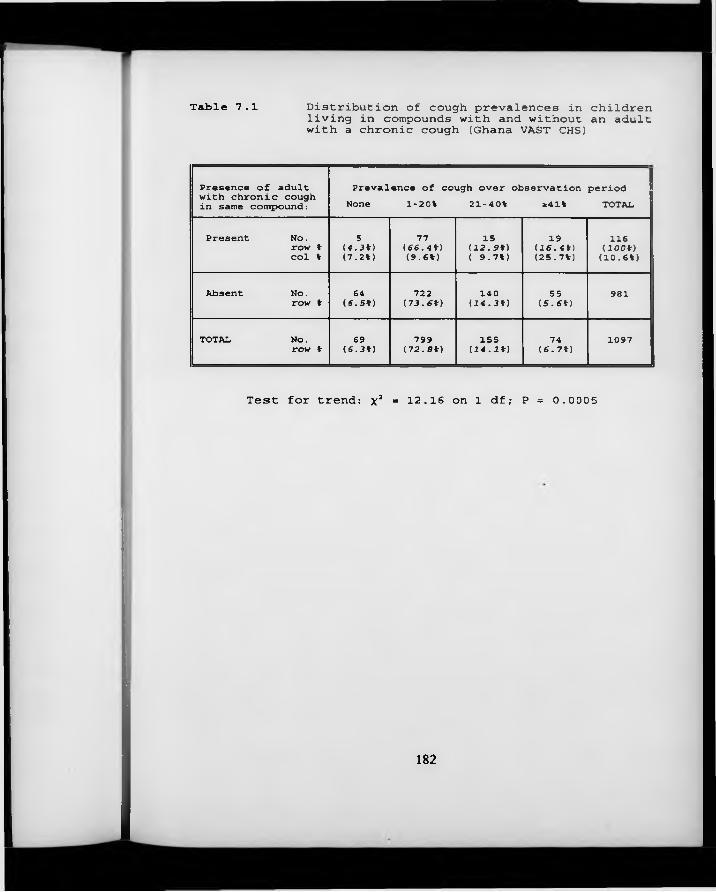
Table 7.1 Distribution of cough prevalences in children living in compounds with and without an adult with a chronic cough (Ghana VAST CHS)

Presence of adult with chronic cough in same compound:

Prevalence of cough over observation period None 1-20% 21-40% 241% TOTAL

1 Present No.row % col %

S(4.3%)(7.2%)

77(66.4%)(9-6%)

15(12.9%) ( 9.7%)

19(16.4%)(25.7%)

116(100%)(10.6%)

Absent No. i row %

64(6.5%)

722(73.6%)

14 0(14.3%)

55(5.6%)

981

TOTAL N o .row %

69(6.3%)

799(72.S%)

155(14.1%)

74(6.7%)

1097

Test for trend: x2 = 12.16 on 1 df; P = 0.0005

182

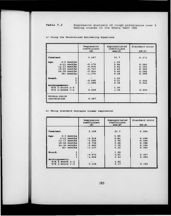
Table 7.2 Regression analysis of cough prevalence over 3 dosing rounds in the Ghana VAST CHS

a) Using the Generalized Estimating Equations

Regressioncoefficient

(0)Exponentiated coefficient

exp(d)Standard error I

SE<0)

Constant 3.167 22.7 0.072Age: 0-5 months _ 1.00

6-11 months -0.179 0.84 O . 08212-17 months -0.474 0.62 O . 09218-23 months -0.717 0.49 O . 09324-35 months -0.914 0.40 O . 08836+ months -1.076 0.34 O . 085

Round: 1 . 1.002 -0.666 0.51 O . 0423 -1.089 0.34 O . 043

Anthropometry:w/H z-score *-2 - 1.00W/H z-score <-2 0.039 1.04 O . 093

Within-childcorrelation 0.367

b) Using standard multiple linear regr ession

Regressioncoefficient

Exponentiatedcoefficient

Standard error03) exp(0) SE (0)

Constant 3.199 23.5 0.080Age: 0-5 months . 1.00

6-11 months -0.214 0.81 O . 09412-17 months -0.548 0.58 O . 09618-23 months -0.732 0.48 O . 09624-35 months -0.942 0.39 O . 084

36+ months -1.137 0.32 0.081Round: 1 - 1.00

2 -0.672 0.51 0.0573 -1.094 0.33 O . 055

Anthropometry:W/H z-score *-2 - 1.00W/H z-score <-2 0.158 1.17 O . 102

183

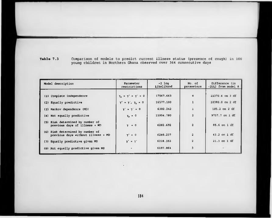
Table 7.3 Comparison of models to predict current illness status (presence of cough) in 100 young children in Northern Ghana observed over 364 consecutive days

Model description Parameterrestrictions

-2 log Likelihood

No. of parameters

Difference (in -2LL) from model 8

(1) Complete independence Yp - y‘ - r - 0 17567.663 0 11370.6 on 3 df(2) Equally predictive 7 * " Y> T p » 0 16577.100 1 10380.0 on 2 df

(3) Markov dependence (MD) Y - r - o 6302.242 1 105.2 on 2 df(4) Not equally predictive 7 p ■ 0 15954.780 2 9757.7 on 1 df(5) Risk determined by number of

previous days of illness + MD r - o 6282.692 2 85.6 on 1 df

(6) Risk determined by number ofprevious days without illness ♦ MD T * - 0 6240.237 2 43.2 on 1 df

(7) Equally predictive given MD Y - Y 6218.353 2 21.3 on 1 df

(8) Not equally predictive given MD - 6197.064 3

184

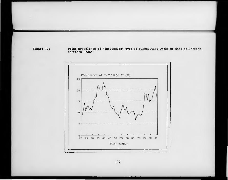
Figure 7.1 Point prevalence of 'intolegere' over 65 consecutive weeks of data collection, northern Ghana

P r e v a le n c e o f " i n t o l e g e r e "

W eek number

185

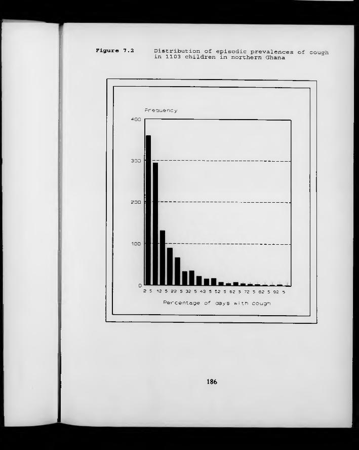
Figure 7.2 Distribution of episodic prevalences of coughin 1103 children in northern Ghana

F r e q u e n c y

4 00 ---------------

3 0 0

200

2 5 1 2 5 2 2 5 3 2 . 5 4 2 5 5 2 5 6 2 . 5 72 5 8 2 5 S2 5

P e r c e n t a g e o f d a y s w i t h c o u g h

186

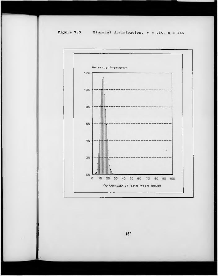
Figure 7.3 Binomial distribution, tt . 14, n 364

R e l a t i v e f r e q u e n c y

P e r c e n t a g e o f d a y s w i t h c o u g h

187

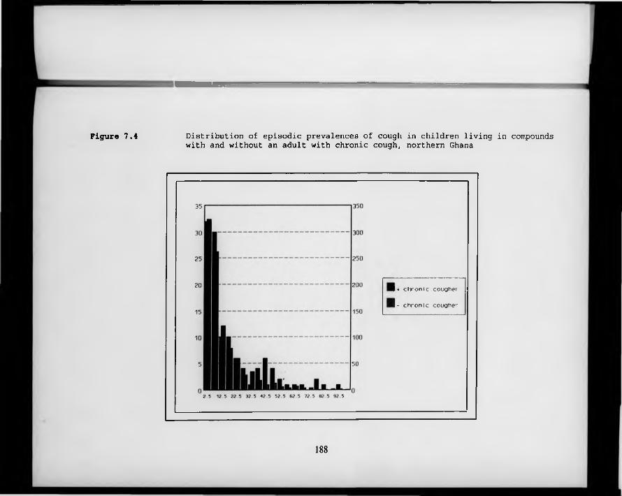
Figure 7.4 Distribution of episodic prevalences of cough in children living in compoundswith and without an adult with chronic cough, northern Ghana

1« c h r o n i c cougher

I - c h r o n ic cougher

188

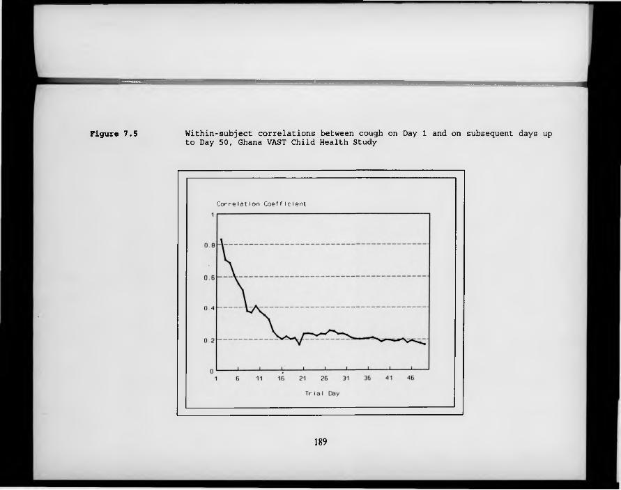
Figure 7.5 Within-subject correlations between cough on Day 1 and on subsequent days up to Day 50, Ghana VAST Child Health Study

C o r r e l a t i o n C o e f f i c i e n t

189

Chapter 8The Analysis of Data on Episode Duration

8 .1 Introduction

If little has been written about the analysis of prevalence data in longitudinal studies of common diseases of childhood, next to nothing has been written about the analysis of data on the duration of illness episodes. Indeed, illness duration has rarely been a major focus of community-based studies of common diseases of childhood, having featured only in a small number of studies which examined the association between anthropometric status and diarrhoea duration in developing countries (Black et al., 1984; Schorling et al., 1990; Thongkrajai et al., 1990; Guerrant et al., 1992). Just two groups have conducted exploratory analyses of risk factors for increased duration of diarrhoea (Househam et al., 1990; Mahalanabis et al., 1991), and no articles could be located describing community-based studies of differentials in the duration of childhood respiratory diseases, or malaria.

On the other hand, a large number of clinical trials have been conducted looking at interventions to reduce the duration of acute watery diarrhoea in children. Many of these have focused on oral rehydration therapies of various descriptions (Ocampo et al., 1993; Bhan et al., 1991; Rahman et al., 1991; Gore et al., 1992). Others have looked at specific feeding practices (Brown et al., 1993; Alarcon et al., 1992; Lembcke & Brown, 1992), micronutrient interventions (Henning et al. 1992; Sachdev et al., 1990; Haffejee, 1988) or drug therapies (Jacobs et al., 1994; Prado et al., 1993; Motala et al., 1990). Clinical trials have also been conducted to investigate the effects of specific interventions on the duration of malaria (Kremsner et al., 1993; Harinsuta et al., 1993) and pneumonia, particularly measles-associated pneumonia (Coutsoudis et al., 1991; Hussey & Klein, 1990).

190

It is important to note that duration data generated by clinical trials may differ in some important respects from that generated in field trials or observational follow-up studies: firstly, since clinical trials are most often conducted in hospitals, there will be relatively little loss to follow-up, with the censoring of duration data that that entails. Secondly, since each child under observation in the field may potentially experience several episodes of diarrhoea, the possibility of within-child correlations in duration outcomes must be borne in mind.

The vast majority of the articles described above have used analytic methods based on Normal distribution theory. Often, untransformed duration data are analysed using t-tests, multiple linear regression or analysis of variance (see, for example, Black et al., 1984, or Mahalanabis et al., 1991). Not only is the underlying conceptual model which would lead to this choice of analytic approach unclear, but the highly asymmetric distribution of episode durations visibly leads to violations of the model assumptions: Black and co-workers, for example, use analysis of variance methods to compare mean durations of E. coli diarrhoea in three groups of children defined by their nutritional status, even though the standard error of the mean duration of E. coli diarrhoea is five times greater in the malnourished children (weight-for-age <60% of the NCHS reference population median) than in their eutrophic peers (weight-for-age >75% of the reference standard). Logarithmic transformations are sometimes used to reduce these imbalances in the within-group variances (Schorling et al., 1990; Bhan et al., 1991), but - as w ill be seen later in this chapter - it is far from clear that this remedial measure is sufficient to eliminate the problem. These methods make no allowance for possible within-subject correlations in the outcome measure, which we have shown in previous chapters to be extremely important in the analysis of disease incidence and prevalence.

The analysis of illness duration is considerably more developed in the area of cancer epidemiology, where ‘duration of response’ (time from documentation of

191

favourable tumour response to documentation of disease progression for the subset of patients who respond to therapy) is often one of the most important variables to be studied (Morgan, 1988). Due to the chronic nature of cancer illness, the response times recorded often run into many months, if not years, and it is not uncommon for a substantial proportion of study subjects to be lost to follow-up before any progression of the illness is seen. This has led to the fairly widespread adoption of survival analysis techniques, which can accommodate these censored observations (some of these methods are described in Breslow and Day, 1987, Chapter 5). In field studies, censoring can be generated by a number of different mechanisms: observation can be curtailed during the middle of an episode, the beginning or end of the observation period can cut through the middle of an illness episode, individuals can move in or out of the study area in the middle of an illness episode, or another outcome (such as hospitalisation) can replace collection of data on the duration of the episode (Bressers et al., 1991). All of these situations occur frequently in longitudinal studies of common diseases of childhood. Depending on the mechanism by which the censoring is generated, the amount of censoring and distribution between different exposure groups, and the precise analytic techniques adopted, Bressers and co-workers have shown that ignoring the problem of censoring by treating censored results as uncensored, or omitting them from the analysis altogether, may lead to seriously erroneous conclusions.

There appears to be little realisation, however, that survival analysis techniques are equally appropriate for the analysis of durations of episodes of the far more common diseases of childhood, even though these illnesses are typically of much shorter duration. Censored illness episodes are quite likely to be in reality more protracted than uncensored ones (both because the most protracted illness is likely to cause the greatest upset to the family’s normal routine, and thus disrupt the surveillance procedures, and because events of long duration offer by definition greater potential for censoring). It is therefore highly desirable that

192

the censoring should be allowed for in the analysis whenever more than a small proportion of all durations are censored. In this chapter, alternative methods for analysing episode duration data are compared. The implications of ignoring the censoring of episode durations, and the possibility of important within-subject correlations are investigated. The relationship between duration and other outcome measures is described, and the biological implications of the findings discussed.

8 .2 D uration data fro m the Lim a R otavirus Vaccine T rial

The discussion of the following pages is illustrated with data drawn from the Lima Rotavirus Vaccine Trial (see Section 2.3 for a description of this study). In this trial, children were visited in their homes and a full retrospective morbidity history taken twice each week, in contrast to the once-weekly visits conducted in the Ghana VAST Child Health Study. Since caretakers may find it difficult to place in time events which occurred several days prior to the interview, accurate information on episode duration is extremely difficult to obtain in community-based studies. The more frequently the interview's are conducted, the more accurately respondents are able to recall the exact starting and ending dates of different symptoms, since recall is limited to a maximum of a few days prior to the interview. For this reason, the Lima study has exceptionally reliable data on episode durations, and was chosen in preference to the Ghana data for the comparative analyses of episode duration. In accordance with the conclusions of Chapter 3, two days without symptoms were deemed necessary to mark the end of a diarrhoea episode. Diarrhoea was defined as three or more liquid or semi-liquid stool motions in the course of a single twenty-four hour period.

When the data were analysed in this way, 15 931 episodes of diarrhoea were

193

recorded during the course of this trial. Only twelve children (out of 800) experienced no episode of diarrhoea during the two-year follow-up period. 804 episodes (5.0%) were of unknown duration due to censoring, either of the start or of the end of the episode. The distribution of durations of those episodes which were not censored is shown in Figure 8.1. 43.7% of these were of just one day’s duration, and over 90% were of 5 days’ duration or less; just 19 episodes were of more than 21 days’ duration.

The form of the distribution resembles that of a negative exponential distribution, previously described in Section 3.3. This is confirmed in Figure 8.2, where the actual durations are plotted against ‘Savage scores’, which are based on the theoretical exponential distribution (see Conover, 1990); a close linear relationship is observed between the two (r=0.9875). The exponential distribution is widely used in engineering applications to describe the lifetime of industrial components, and other similar variables. One can perhaps imagine a parallel between the persistence of a component confronted with a battery of ‘insults’, and the persistence of a pathogenic process in the face of a multi-facetted immune response. The distribution is fully defined by the rate at which components fail (or in this case, symptoms of illness remit), referred to technically as the hazard rate. The close correspondence of the observed distribution to the theoretical model suggests that in this ‘population’ of illness episodes, recovery occurs at an approximately constant rate over tim e (i.e. the likelihood of recovery on the fourth day, given that the illness has lasted three days, is the same as the likelihood of recovery on the third day, given that the illness has lasted two days). The accuracy and biological plausibility of this assumption are examined in subsequent sections.

194

8 .3 M odelling duration data

Various regression techniques have been developed for modelling exponentially distributed data (see Lee, 1992). All of them are able to incorporate information on censored observations. The results cited below are calculated using what has been termed the linear exponential (Lee, 1992), or log linear hazard (Aitkin et al., 1989) model. In this model, mean survival times are related to the vector of covariates by a log link. One of the properties of the exponential distribution is that the mean survival time is equal to the reciprocal of the hazard rate (which, it has already been mentioned, is constant). The following results were obtained from modelling the Lima diarrhoea data:

Exponential regression

Log Likelihood »-20473.363

Number of obs Model chi2(0) Prob > chi2 Pseudo R2

159310 . 0 0 0

0.0000

durât 1 Coef . Std. Err. z P>|z| [95% Conf. Interval]

_cons 1 1.010873 .0081306 124.329 0.000 .9949377 1.026809

The mean survival time is given by the exponentiated coefficient of the constant term, and is equal to 2.75 days. This can be compared with the estimate of the mean survival time which would be derived if censored data were simply excluded from the calculation (2.56 days; an underestimate of 7%), and the estimate which would be derived if the censored data were included, but the censoring ignored (2.61 days; an underestimate of 5%). It is thus moderately important to account for the censored nature of the data, even when censoring affects o n ly a very small percentage of a ll observations, as in this example.

195

As the next step in the analysis of these data, two potentially important covariates were introduced into the model: the A G E of the child at the beginning of the episode, and the child’s S EX . A G E was modelled as a categorical variable with 5 levels. The results are shown in Table 8.1. Negative regression coefficients [/3’s] indicate shorter durations, and positive coefficients indicate longer durations. When exponentiated, these coefficients can be interpreted as ratios of the mean durations in each group, with the constant term referring to the mean duration of illness in the baseline group. The reciprocal of these exponentiated coefficients can be interpreted as a hazard rate ratio, or baseline hazard rate in the case of the constant term. As previously indicated, the hazard rate in this analysis is equivalent to the (instantaneous) rate of recovery from illness. The results show that the recovery rate progressively increases, and therefore the duration of diarrhoeal symptoms progressively decreases, with age in this population, and also that girls have marginally shorter episodes of illness than boys. Although, due to the very large sample size, all the coefficients are highly significant in this analysis, the pseudo R2 (which is simply the log- likelihood value on a scale where 0 corresponds to the constant-only model and 1 corresponds to perfect prediction) is less than 1%, indicating that age and sex are not important determinants of duration of diarrhoeal illness.

It is worth noting that whilst exponential regression is not generally available in the most widely used statistical software, almost identical results can be obtained by using Poisson regression, which is widely available, setting the outcome variable to 1 when the duration of the episode is known and 0 when it is censored, and treating logfduration) as an offset term (Aitkin et al., 1989). This procedure gives identical coefficients to those obtained in exponential regression (though with opposite signs), and very similar (in the case of the current analysis, indistinguishable) standard errors.

It may perhaps be considered surprising that the Lima duration data correspond

196

so well to an exponential distribution, since this implies that the instantaneous rate of recovery from illness (the hazard rate) is the same regardless of how long the illness has already lasted (i.e. the process is memory-less). Another distribution, which allows the hazard rate to vary with the duration of the illness, is the Weibull distribution (see Lee, 1992). Table 8.2 compares the results of the same analysis using Weibull regression with that using exponential regression. The sigma parameter is a shape parameter which describes the change in the hazard rate: if sigma is smaller than 1, the hazard rate is increasing over time; if it is greater than 1, the hazard rate is falling, and if it is equal to 1, the hazard rate is constant (the case of the exponential distribution). In this example, sigma is somewhat smaller than 1, implying that the instantaneous rate of recovery from illness increases with the duration of the illness. The regression coefficients are not appreciably altered by the use of Weibull as opposed to exponential regression, but the standard errors are smaller. The goodness-of-fit statistic (model x2) is considerably greater for the Weibull than for the exponential model, indicating a much better fit.

Also shown in Table 8.2 are the results of conducting the same analysis using the non-parametric Cox Proportional Hazards regression (Cox, 1972). This model has as its dependent variable the natural logarithm of the ratio of the hazard rate for an individual with covariates x, to the hazard rate of an individual with all covariates equal to zero (the baseline hazard rate). This is related to a linear combination of covariates and coefficients, as with any linear model. By holding the x’s constant, the model is able to estimate hazard rate ratios for each of the relevant exposures. It should be noted that since this model estimates hazard ratios rather than group means, the signs of the coefficients are reversed relative to the two previous models.

In the example shown in Table 8.2, Cox Proportional Hazards regression gives similar, though not identical, estimates of covariate effects to those obtained

197

using the parametric models, with standard errors identical to those of the exponential regression model. Since the underlying assumptions of the Cox Proportional Hazards model are more general than those of the parametric models (only proportionality of hazard rates is required), and the models are easily fit using widely available statistical software, this approach may be recommended as an alternative to exponential or Weibull regression.

Table 8.3 shows the results obtained when the durations are transformed to the log scale, and ordinary linear regression is performed. Using this technique, censoring is ignored, and comparisons are of between-group ratios of geometric means. The results are thus quite different from those obtained using any of the approaches which compare hazard rates or maximum likelihood estimates of the means of exponential or Weibull distributions. For a sample well approximated by an exponential distribution, the mean response estimated by exponential regression will be very close to the arithmetic mean of the individual observations in the sample. Likewise, when the sample is well approximated by a Weibull distribution, the sample mean estimated by Weibull regression will be close to the arithmetic mean of the individual observations in the sample. In neither case w ill these values fall anywhere close to the geometric mean, due the extreme skewness of the distributions.

It should be noted that the logarithmic transformation of the duration data was in this case inadequate to completely stabilize the variances in the different age groups, with a between-group maximum-.minimum variance ratio of 1.683 (compared to an even more extreme ratio of 3.325 when the untransformed duration data were used). Between-group differences in linear regression are tested using the equivalent of a pooled estimate of the assumed ‘common’ variance; however, in this case, testing the effect of age group 36+ months versus age group 0-2 months using the more robust separate variance estimates resulted in an increase in the estimated standard error of the difference from 0.0272 to 0.0322 (+18%) compared to the result obtained using the pooled variance

198

estimate. This implies that using linear regression with the log-transformed data would exaggerate the precision of this age effect. The other effect estimates would be less seriously affected.

8 .4 Accounting fo r witkin-child correlation

None of the above methods take into account possible correlations between durations of different episodes experienced by the same child. If child-level characteristics (measured or otherwise) are important in determining the duration of diarrhoea episodes, then this within-child correlation could lead to biases in effect estimates, or mis-estimation of the precision of regression coefficients, in the same way as we have seen with other outcomes.

In order to test this, the Lima data set was analysed using the multi-level modelling package ML3 (see Section 5.3.2). Since this package allows Poisson regression (using algorithms described in Goldstein, 1991), a re-arrangement of the data using log(duration) as an offset term as described above enables a form of exponential regression to be carried out. The results are shown in Table 8.4.

The effect estimates and standard errors are virtually identical to those obtained using ordinary exponential regression (although with the signs reversed, as expected when the Poisson approximation is used). The most interesting feature of these results is the disaggregation of the variance into two distinct components: within- and between-child variability. The within-child component is constrained to take the value 1, indicating Poisson variance. Beside this, however, the between-child variance component is negligible (0.037), indicating an almost complete absence of within-child correlation. Given this extremely low level of correlation, the methods described in the previous section, which do not attempt to partition the variance into different levels, should be adequate. This is fortunate, since use of the Poisson macro in ML3 is cumbersome.

199

8 .5 Discussion a n d conclusions

The duration of illness is determined by a constellation of factors, which may be assumed to include characteristics of the original infection (dose, pathogenicity etc.), characteristics of the host, and characteristics of the child’s environment during convalescence (many of which may be deliberately manipulated by the child’s carers). Although it is known that persistent diarrhoea (of longer than 14 days’ duration) constitutes a major threat to the young child (WHO, 1988), little attention has been devoted to the search for correlates of episode duration. Even less is known about the durations of other common illnesses of childhood.

A ‘natural choice’ model for the analysis of duration data would appear to be some kind of failure-time model. These models allow statements about relative recovery rates in different population sub-groups (or, equivalently, mean durations). They also enable information about episodes whose duration is censored to be included in the analysis, which may be important if a substantial number of episodes have been censored. In the Lima example, the best fit is given by the Weibull model: the shape parameter of this model (sigma < 1) indicates that the longer the disease has already been established, the greater the probability of recovery in the next tim e period. This may reflect a build-up of the immune response in the host, or perhaps increasingly strenuous attempts to combat the illness with external interventions. Exponential models, which assume - unrealistically - a constant rate of recovery with no memory of how long the disease has already been established, also appear, however, to give a reasonably good fit to the data, and to yield very similar estimates of covariate effects. They can be fitted easily w ith standard statistical software, but the efficiency of the estimates is somewhat reduced by the use of this approximation: in the Lima example, standard errors were increased by between 23-28% compared to the more adequate W eibull model. If censoring is not a problem,

200

a less ‘technical’ analysis would consist of transforming the duration data to a logarithmic scale, and conducting the analysis using linear regression. The output from this analysis is not directly comparable to that of the other models, for reasons described above in Section 8.3, and is liable to give exaggerated estimates of the precision of covariate effects when complete stabilisation of variances is not achieved.

Perhaps unexpectedly, there does not appear to be any within-subject correlation in the duration data examined in this section. For the statistician, this implies that standard regression techniques are likely to give satisfactory results, and sophisticated corrections do not need to be applied. For the epidemiologist, these findings are of the utmost importance: they imply that the determinants of disease duration must be sought in the particular circumstances of each episode, rather than in fixed characteristics of the child. It might have been expected that ‘frail’ children who are highly susceptible to new infections would also exhibit the least adequate response to those infections. However, this does not appear to be the case: there is no correlation in the Lima data set between the total number of diarrhoea episodes experienced over the two-year period, and the average duration of those episodes (r«.08). Since the determinants of duration must be sought at the level of the individual episode rather than at the level of the child, it would be inappropriate and highly wasteful of information to undertake analyses based on a summary measure of the average duration of episodes for each child. As yet, little is known about the episode-specific determinants of episode duration, but since it is known that occurrence of diarrhoea episodes of unusually long duration is particularly dangerous for young children, further work on this topic is indicated.

201

R e fe re n c e s

Aitkin M, Anderson D, Francis B, Hinde J. Statistical Modelling in GLIM. Oxford Statistical Science Series, No.4. Oxford: Clarendon Press, 1989.Alarcon P, Montoya R, Rivera J, Perez F, Peerson JM, Brown KH. Effect of inclusion of beans in a mixed diet for the treatment of Peruvian children with acute watery diarrhoea. Ped 1992; 90(1) :58- 65 .Bhan MK, Gore SM, Grange AN et al. Impact of glycine-containing ORS solutions on stool output and duration of diarrhoea: A meta-analysis of seven clinical trials. Bull World Health Org, 1991; 69 (5) : 541-548.Black RE, Brown KH, Becker S. Malnutrition is a determining factor in diarrheal duration, but not incidence, among young children in a longitudinal study in rural Bangladesh. Am J Clin Nutr, 1984; 39(1): 87-94.Breslow NE, Day NE. Statistical Methods in Cancer Research. II. The design and analysis of cohort studies. Lyon: International Agency for Research on Cancer, 1987.Bressers M, Meelis E, Haccou P, Kruk M. When did it really start or stop? The impact of censored observations on the analysis of duration. Behavioural Processes, 1991; 23(l):l-20.Brown KH, Perez F, Peerson JM et al. Effect of dietary fiber (soy polysaccharide) on the severity, duration, and nutritional outcome of acute, watery diarrhea in children. Pediatrics, 1993; 92 (21) : 241-247.Conover WJ. Practical Non-Parametric Statistics. New York: Wiley, 1990 .Coutsoudis A, Broughton M, Coovadia HM. Vitamin A supplementation reduces measles morbidity in young African children: a randomized, placebo-controlled, double-blind trial. Am J Clin Nutr 1991 ; 54:890- 5.Cox DR. Regression models and life tables (with discussion). J Roy Stat Soc, 1972; series B, 34:187-220.Gore SM, Fontaine 0, Pierce NF. Impact of rice based oral rehydration solution on stool output and duration of diarrhoea: Meta-analysis of 13 clinical trials. Brit Med J, 1992; 304 (6822) : 287-291.Guerrant RL, Schorling JB, McAuliffe JF, De Souza MA. Diarrhea as a cause and an effect of malnutrition: Diarrhea prevents catch-up growth and malnutrition increases diarrhea frequency and duration. Am J Trop Med Hyg, 1992; 47 ( II) : 28 - 35.Haffejee IE. Effect of oral folate on duration of acute infantile diarrhoea. Lancet, 1988; 2 ( 8606) : 334-335.

202

Harinasuta T, Bunnag D, Vanijanond S et al. Mefloquine, sulfadoxine, and pyrimethamine in the treatment of symptomatic falciparum malaria: a double-blind trial for determining the most effective dose. Bull World Health Org 1987; 65(3):363-7.Henning B, Stewart K, Zaman K, Alam AN, Brown KH, Black RE. Lack of therapeutic efficacy of vitamin A for non-cholera, watery diarrhoea in Bangladeshi children. Eur J Clin Nutr 1992; 46(6):437-43.Househam KC, Bowie DC, Mann MD, Bowie MD. Factors influencing the duration of acute diarrheal disease in infancy. J Ped Gastroent Nutr, 1990; 10(1) :37-40.Hussey GD, Klein M. A randomized, controlled trial of vitamin A in children with severe measles. New Eng J Med 323 (3) :160-4.Jacobs J, Jimenez LM, Gloyd SS, Gale JL, Crothers D. Treatment of acute childhood diarrhea with homeopathic medicine: a randomized clinical trial in Nicaragua. Ped 1994; 93(5):719-25.Kremsner PG, Winkler S, Brandts C, Graninger W, Bienzle U. Curing of chlorocpaine - resistant malaria with clindamycin. Am J Trop Med Hyg 1993; 49(5):650-54.Lee ET. Statistical Methods for Survival Data Analysis (2nd Ed.). New York: Wiley, 1992.Lembcke JL, Brown KH. Effect of milk-containing diets on the severity and duration of childhood diarrhea. Acta Paed, 1992; 81(381)Supp:8 7- 9 2.Mahalanabis D, Alam AN, Rahman N, Hasnat A. Prognostic indicators and risk factors for increased duration of acute diarrhoea and for persistent diarrhoea in children. Int J Epid, 1991; 20 (4) :1064-1072.Morgan TM. Analysis of duration of response: a problem of oncology trials. Controlled clinical trials, 1988; 9:11-18%Motala C, Hill ID, Mann MD, Bowie MD. Effect of loperamide on stool output and duration of acute infectious diarrhea in infants. J Ped, 1990; 117(3) :467-471.Ocampo PDS, Bravo LC, Rogacion JM, Battad GR. A randomized double­blind clinical trial of a maltodextrin-containing oral rehydration solution in acute infantile diarrhea. J Ped Gastr Nutr 1993; 16 (1) : 23 - 8 .Prado D, Liu H, Velasquez T, Cleary TG. Comparative efficacy of pivmecillinam and cotrimoxazole in acute shigellosis in children. Scand J Inf Dis 1993; 25(6):713-9.Rahman ASMM, Bari A, Molla AM. Rice-ors shortens the duration of watery diarrhoeas. Observation from rural Bangladesh. Trop Geog Med, 1991; 43 (1-2) -.22-21.Rothschild V & Logothetis N. Probability distributions. New York: John Wiley and Sons, 1986:43.Sachdev HPS, Mittal NK, Yadav HS. Oral zinc supplementation in persistent diarrhoea in infants. Annals Trop Paed 1990; 10(1):63-9.

203

Schorling JB, McAuliffe JF, De Souza MA, Guerrant RL. Malnutrition is associated with increased diarrhoea incidence and duration among children in an urban Brazilian slum. Int J Epid, 1990; 19(3) :72 8-73 5.Thongkrajai E, Stoekel J, Thongkrajai P. Nutritional status and the incidence and duration of diarrhoeal disease among children in northeast Thailand. Soc Science Med, 1990; 30 (7) :773 - 776 .World Health Organization. Persistent diarrhoea in children in developing countries: memorandum from a WHO meeting. Bull World Health Organization, 1988; 66(6):709-171.

204

Table 8.1 The effect of age and sex on diarrhoeaduration (exponential regression)

P SE(0) Ratio of means

HazardRatios

Constant 1.50 0.040 VO 0.22*Age (months)

0-2 -3-5 -0.36 0.049 0.70 1.436-11 -0.35 0.046 0.70 1.4312-35 -0.48 0.041 0.62 1.6236 + -0.56 0.042 0.57 1.75

SexMale -Female 1 o o 00 0.016 0.93 1.08

t Mean duration in the baseline group § Baseline hazard rate

205

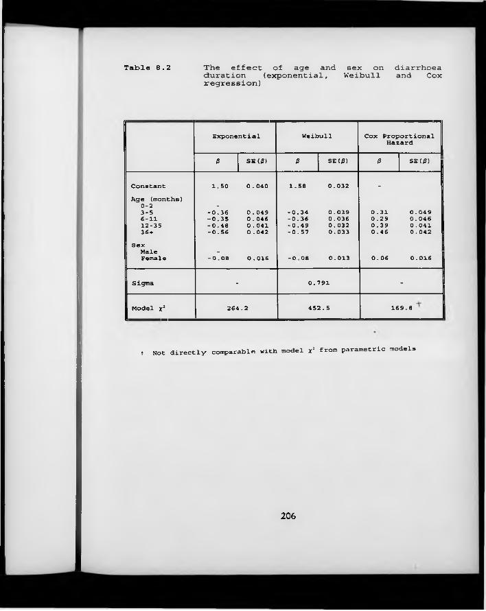
Table 8.2 The effect of age and sex onduration (exponential, Weibullregression)diarrhoea and Cox

Exponential Weibull Cox Proportional Hazard

ß SE(/3) ß SE(/3) ß SE(0)

Constant 1.50 0.040 1.58 0.032 -

Age (months)0-2 -3-5 -0.36 0.049 -0.34 0.039 0.31 0.049 !6-11 -0.35 0.046 -0.36 0.036 0.29 0.04612-35 -0.48 0.041 -0.49 0.032 0.39 0.04136 + -0.56 0.042 -0.57 0.033 0.46 0.042

SexMale -

Female GOOO1 0.016 1 o o 00 0.013 0.06 0.016

Sigma - 0.791 -

Model x2 264.2 4 52.5 169.8

t Not directly comparable with model x2 from parametric models

206

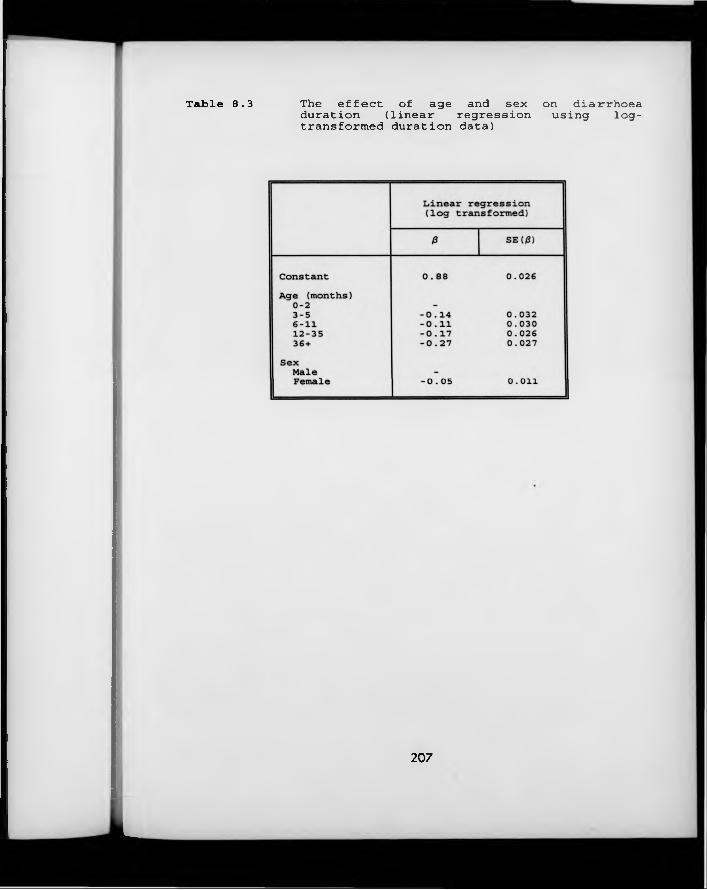
Table 8.3 The effect of age and sex on diarrhoeaduration (linear regression using log-transformed duration data)

207

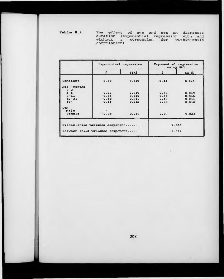
Table 8.4 The effect of age and sex on diarrhoea duration (exponential regression with and without a correction for within-child correlation)

Exponential regression Exponential regression j using ML3 |0 SE(0) 0 SE(/3) j

Constant 1.50 0.040 1 H * * 0.041Age (months)0-2 - -3-5 -0.36 0.049 0.38 0.0496-11 -0.35 0.046 0.36 0.046 112-35 -0.48 0.041 0.49 0.041 i36 + -0.56 0.042 0.58 0.042SexMale - - -

Female GOOO• 0.016 0.07 0.023

Within-child variance component....... 1.000Between-child variance component...... 0.037

208

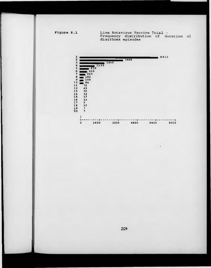
Figure 8.1 Lima Rotavirus Vaccine Trial - Frequency distribution of duration of diarrhoea episodes

12345678 9

1 01112131415161718192 0

1910m 1139 mmmm 639

455m m 263 H 182 H 108M 847549323217

1261077

3468 6613

+-------------+------------- +------------- +------------- +--------------+0 1600 3200 4800 6400 8000

209

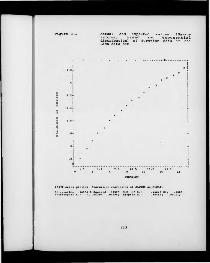
Figure 8.2 Actual and expected values (Savage s c o r e s , based on exponential distribution) of duration data in the Lima data set

++---- +----- +----- +----- ► ---------+ --------- + ----------+ --------- + --------- + ----------+ - R - - + ----------+ --------- -I

+ +--- + —1.5 4.5 7.5 10.5 13.5 16.50 3 6 9 12 15 18DURATION

1SB92 cases plotted. Regression statistics of SAVDUR on DURAT:

Correlation .98754 R Squared .97523 Intercept(S .E.) -1.04639( .00176) S.E. of Est Slope(S.E.) .14846 Siq. .0000.40451( .00051)

210

C h a p t e r 9 Summary, conclusions and recommendations

In this chapter, the findings of this thesis are brought together and summarised. Each specific objective described in Section 1.4 is considered in turn.

9 .1 O utcom e measures in longitudinal studies o f common diseases o f

childhood

Many different outcome measures may be calculated using the data collected in longitudinal studies of common diseases of childhood. These different outcome measures provide descriptions of disease onset, or incidence; of disease status, or prevalence, and of disease duration. In some studies, all three aspects of disease frequency in the population will be of interest; in others, the scientific hypotheses driving the study will naturally suggest a more specific focus on one or other. The choice of primary outcome should generally be made before the data collection phase of any study begins, and is usually based on biological or clinical considerations.

In this thesis, considerable emphasis has been given to questions relating to the analysis of disease I N C I D E N C E . This is because this information is uniquely obtained from intensive, home-based, prospective studies, whereas cross-sectional studies are able to provide information on disease prevalence and duration. Two distinct measures of disease incidence are recognised: the first of these is the risk of any given individual experiencing one or more episodes of disease over a defined period of time, and the second is the instantaneous rate of illness, or force of morbidity. Risk is usually estimated by the calculation of a measure termed cumulative incidence, the proportion of individuals entering a study who experience disease within a specific time period. Strictly, this approximation is

211

only valid for a fixed cohort design with no attrition. It may be biased as a measure of individual risk when levels of attrition from the initial cohort are high, or when a dynamic cohort design is employed. Furthermore, it is wasteful of information, since all information on non-initial episodes is discarded. The related epidemiological measure of association, the cumulative incidence ratio, has the undesirable property of rapidly approaching unity as the time referent increases. For all these reasons, the alternative approach to illness incidence, focusing on the instantaneous rate of illness, is to be preferred.

The incidence density rate is composed of two elements: in the numerator, the number of disease episodes experienced by a child, or group of children; and in the denominator, the number of time periods of observation. In Chapter 3, the issue of how to define an ‘episode’ of a common illness such as diarrhoea was considered, in the light of the observation that where diarrhoea is common, it is theoretically possible for a child to experience two aetiologically distinct bouts of illness separated by just one or two days without illness, so that it could appear that only one protracted bout was experienced. On the other hand, some longer episodes of diarrhoea might genuinely be interrupted by a day or two with milder or even inapparent symptoms. A simulation model was used to develop a pragmatic algorithm for determining how many days without symptoms of illness should be required to elapse in order to define the start of a ‘new’ episode.

The model demonstrated that, with a high incidence of ‘trigger events’ (events provoking clinical symptoms of illness in the immediately ensuing period) and clustering of diarrhoeal illness in a subset of high-risk children, many periods of diarrhoea resulting from genuinely distinct trigger events are separated from each other by intervals of just a few days. On the other hand, where there is no clustering and a relatively low incidence of trigger events, only around 5% of all periods of diarrhoea would be preceded by three or less symptom-free days.

212

Thus, a definition in which two or three symptom-free days are considered sufficient to mark the beginning of a ‘new’ episode of diarrhoea is recommended, with a preference for the two-day definition in areas where the incidence rate is high and/or there is considerable clustering of illness in a small sub-group of children.

With respect to the person-time denominator of incidence rates, two alternative strategies were considered in Section 4.1: either the total number of new cases may be divided by the total person-time under observation, giving an estimate of the incidence of observed episodes, or else the total number of new cases may be divided by the total person-time under observation, minus the summed duration of illness, and minus the summed duration of the symptom-free intervals required to define a new episode. This procedure leads to an estimate of the true incidence of trigger events. The first of these two options is to be preferred: firstly, because the latter approach w ill underestimate the true incidence of trigger events if ever the durations of symptoms associated with consecutive trigger events overlap; secondly, because this approach is inconsistent with the options available for the analysis of episode duration, which must focus on observed durations rather than on the duration of symptoms associated with each trigger event; and thirdly, because the trigger event approach is one step removed from the experience of the child, in that the incidence rate no longer tells us the number of bouts of illness actually experienced, with all the physiological consequences that these m ay entail.

With respect to illness P R E V A L E N C E , three alternative outcome measures were considered in Chapter 7. Firstly, the proportion of individuals suffering from a particular complaint can be calculated separately for each time point at which observations were made (the classic measure of prevalence, but estimated repeatedly). The resulting figures can be treated as a time series, and may be of great interest in describing changes in the community burden of morbidity over

213

time. Secondly, it is possible to calculate the proportion of time that each individual spends ill with a particular symptom over a defined period of time. This measure is not prevalence as classically defined, but is conceptually similar; it has been termed ‘episodic prevalence’ (Kleinbaum et al., 1982). This measure may be a good indicator of ‘frailty’, both because those individuals who experience high episodic prevalences of common diseases must have been in some way particularly ‘susceptible’ at the onset of the observation period, and because the experience of high episodic prevalences of disease is likely to lead to aggravated nutritional status and impaired immune function in the future.

A third possible measure of prevalence is what I have termed ‘block prevalence’: this is simply the sum of all the days on which a particular symptom was reported divided by the sum of all the days of observation. ‘Block prevalence’ is neither a simple average of the time series point prevalences, nor of the episodic prevalences, and is a rather unsatisfactory measure unless it can be assumed that the point prevalence of the symptom has not changed significantly over the observation period. Furthermore, because individual days of illness/health are strongly correlated within any particular individual, the variance of this measure is grossly underestimated if calculated using standard binomial theory.

DURATION is probably the simplest outcome measure to define, once the definition of an episode has been arrived at. Its calculation in longitudinal studies of common diseases of childhood presents no special difficulties, except for the fact that a significant proportion of episodes may be ‘censored’, because observation was interrupted before the illness finally resolved (it is also possible for episodes to be censored because observation began with the episode already in course).

214

In Section 5.2, it was demonstrated that longitudinal studies on common diseases of childhood differ from cross-sectional studies because the outcome measure varies across two dimensions: not only from one study subject to another, but also within subjects from one time period to the next. It was shown that within individuals, the time-to-time variability in disease incidence is well approximated by the familiar Poisson model, which implies random occurrence of trigger events in time. However, the underlying rates of illness differ greatly from one individual to another. This excess of variation in disease incidence from one individual to another, which is referred to as over-dispersion, is partly a consequence of fixed, individual-level characteristics, such as genetic constitution and socio-economic status. However, a large part of the total between-individual heterogeneity cannot be explained, either because the relevant individual-level characteristics are known but intrinsically unmeasurable, or because they are simply not known.

The principal effect of this heterogeneity in individuals’ underlying propensity to illness is that disease rates measured at different points in time on the same individual w ill tend to be more similar than disease rates measured at the same time on different individuals. That is to say, there is within-subject correlation between disease incidence rates in different periods of time. This correlation has the effect of leading to the underestimation of the standard errors of covariate effects, such that the statistical significance of these effects is likely to be exaggerated. Furthermore, in the case of categorical outcome measures, the effect estimates themselves are liable to be biased when within-subject correlations are ignored.

9.2 Statistical features o f longitudinal data on com m on diseases o f

childhood

215

In Section 6.2, it was shown that this within-subject correlation can easily be detected when examining diarrhoea incidence rates in thirteen consecutive one- month periods in young children in northern Ghana. Adjusted correlations of between .11 and .31 are observed for pairs of observations measured on the same individual. In Section 7.4, it was shown that even higher correlations are obtained when disease status is compared over consecutive periods, with a child with cough yesterday 360 times more likely to have cough today than a child without cough yesterday (Ghana VAST Child Health Study). In Section 8.4, however, it was shown that in young children in Lima, there is no within-subject correlation in the duration of diarrhoea episodes.

9 .3 R ecent advances in statistical theory relevant to the analysis o f

correlated, categorical outcomes

Several new techniques for the analysis of correlated, categorical outcomes have been developed in recent years. These were reviewed in Section 5.3. These techniques are, for the most part, fairly general, and can be applied to the analysis of any of disease onset, status or duration.

The first approach to be reviewed was the family of conditional models, widely favoured in econometrics. These models permit the estimation of the probability of a particular health outcome at time t, conditional on the value observed for the same outcome on the same individual at time t-1. This translates into research questions such as "Does the frequency of reported wheezing in children free of wheezing a year earlier vary according to the age of the child?", a rather different kind of question from the more usual type of enquiry about population- averaged associations between disease status and risk factors. Nonetheless, a considerable amount of experience with this type of model has already amassed in the field of environmental risk factors for respiratory infections. These studies

216

have, however, all used continuous response variables, so that the models can be seen basically as extensions of classical multiple linear regression. There is far less experience of modelling categorical outcomes in this manner. A promising approach has been developed by Bonney (1987), discussed in Section 7.4.1. These models require no special computer software, but can be difficult to fit, and require uncomfortable assumptions about the stationarity of transition probabilities over time.

The second class of models to be examined were ‘multi-level models’, developed primarily in the field of education, and only recently beginning to diffuse into other areas of research. These models offer perhaps the most radical departure from traditional approaches, since they estimate ‘components of variability’ in addition to the familiar fixed covariate effects. The models are extraordinarily flexible, in that both intercept terms and effect parameters can be allowed to vary at the level of the individual, any structure of covariances can be allowed for, and important risk factors can be modelled at either, or both of the occasion-specific or the individual levels. Unfortunately, as a result of the flexibility of these models, it is often difficult to decide how any particular model should be set up, and the model output is difficult to interpret. The available software is far from user-friendly, and is known to contain a number of bugs (currently being rectified) in the routines for analysing categorical outcomes. The models also involve crucial assumptions which are difficult to assess other than by analysis of residuals, which can apparently take up to 24 hours to calculate on a standard micro-computer (John Rasbash, personal communication)!

The third set of models to be examined in this section was the extensive family of marginal models. The fully parametric formulations, such as negative binomial regression modelling, have the great disadvantage that only child-level (as opposed to occasion-specific) covariates can be modelled. A much more promising development has been the derivation of so-called ‘Generalised

217

Estimating Equations’ based on quasi-likelihood theory, which yield ‘ robust’ estimates of covariate effects and their variances in the presence of correlation. These models are implemented in a special macro written for the widely-used, but not very user-friendly, analysis package SAS; alternatively, they can be implemented in the newer, and considerably more straightforward modelling package SPIDA. Although the user is required to state as one of the model inputs exactly what the correlation structure of the response variable is expected to be, the model is robust to mis-specification of this parameter. The output looks much like what would be obtained from any standard linear model; an estimate of the working correlation matrix is also obtained. Unfortunately, there is no facility for robust hypothesis testing, although a best-fit model selection option is available in SPIDA.

In Section 5.5, these three approaches to modelling correlated, categorical data were compared and contrasted using a set of five standard criteria proposed in Section 1.5.1. These criteria are based on the applicability of the modelling method to practical epidemiological problems, and the viability of obtaining the required inputs, as well as on the technical properties of the resulting estimators, and the potential for popularisation of the model. This last criterion is judged on the basis of its general ‘user-friendliness’, and the amount of learning tim e and computer resources that would be necessary to start working with it . The Generalised Estimating Equations approach was most favourably evaluated on the basis of these criteria.

218

In Section 5.4, a review of current practice in the analysis of longitudinal studies of common diseases of childhood was carried out, taking as a case-study 19 studies of the efficacy of potential new vaccines against rotavirus diarrhoea. It was apparent from this review that most epidemiologists working on longitudinal studies of common diseases in the field are unfamiliar with the statistical peculiarities of the data they are working with. In their analyses of the effects of the new vaccines on rotavirus-specific illness, 13 of the 19 studies avoided the issue of multiple episodes altogether, by analysing only cumulative incidence. Of the remaining six studies, one presented no data at all on the frequency of rotavirus-related illness, and two used an unspecified chi-squared type test to compare illness rates in the two treatment groups. Chi-squared tests take no account of correlation in the outcome, and are thus liable to overstate the precision of treatment group comparisons. In the three other studies where an attempt was made to incorporate information on clustering of disease, the methods adopted were unsuitable - either because they were premised on assumptions which were visibly violated, or because they were essentially techniques for significance testing, not permitting the estimation of epidemiological measures of effect. Over half of the 19 studies did not even attempt to assess the impact of rotavirus vaccine on all-cause diarrhoea, or else did not specify the analytic technique used.

Very few studies of common diseases of childhood could be located in which disease prevalence was analysed in detail. This presumably reflects the fact that longitudinal studies are generally set up with the aim of estimating incidence rates. On the other hand, several studies were identified in which the episodic prevalence of diarrhoea, or respiratory illness, was examined as a possible

9.4 C u rren t practice in the analysis o f longitudinal studies o f com m on

diseases o f childhood

219

determinant of growth or attained anthropometric status (Section 7.2). Detailed analyses of illness duration were also found to be uncommon in longitudinal studies of common diseases of childhood; in Section 8.1, however, it was shown that in clinical trials, which more frequently have disease duration as a primary outcome, analytic methods such as analysis of variance or multiple linear regression, are almost invariably used. These methods take no account of the censoring, inequality of variances, and possible within-subject correlation which may characterise data of this type.

9 .5 To what degree does the application o f traditional methods lead to

inappropriate conclusions being draw n from the d a ta ?

In Section 6.2, it was shown that ignoring within-subject correlation in the analysis of the incidence of common diseases of childhood is likely to lead to serious underestimation of the magnitude of the standard errors of covariate effects. In the example of diarrhoea incidence in young children in northern Ghana, these standard errors were between 1% and 73% larger (median 34% larger) when estimated by a technique accounting for within,-subject correlation than when this correlation was ignored. Several of the covariate effect would have been deemed ‘significant’ on the basis of the ‘naive’ standard errors, but non-significant when correlation was taken into account. In the same section, it was shown that the effect estimates themselves were only minimally affected by assumptions about the presence and structure of within-subject correlation in the outcome.

In Section 7.4, it was shown that consecutive days of illness/health measured on the same individual are even more highly correlated than disease incidence in consecutive time-bands. It was suggested in this chapter that the level of within- subject correlation in daily disease prevalence is so high, that any attempt to

220

model within-subject variability in daily disease status is probably inappropriate. An approach based on a single measure for each individual was therefore recommended.

In Section 8.3, it was shown that ignoring censoring of duration data will generally lead to bias in the estimation of summary statistics. In the data used, however, only 5% of all episodes were censored, and the magnitude of the bias in the estimate of mean duration was correspondingly small (5-7%). It was also shown in the same section, that even when duration data were transformed to a log scale, sub-group differences in the variance of the outcome measure were sufficiently large to lead to difficulties with traditional techniques such as linear regression; specifically, the standard errors of covariate effects were underestimated by up to approximately 15%. It was found that Cox’ proportional hazards regression, a popular method for analysing time-to-event data, gave a significantly poorer fit to the data than fully parametric techniques such as exponential or Weibull regression.

9 .6 A ppropriate data-handling strategies

Any analysis of longitudinal data on common diseases of childhood is contingent on the data first being arranged in a manner which permits the appropriate manipulation. This was discussed in Section 2.2.6. Essentially, an arrangement in which each child-day of illness/health is represented by a separate record in the data file favours the calculation of prevalence-type measures, and considerably reduces the amount of programming that must be done prior to statistical analysis. This arrangement is recommended for small to moderately large data sets (say, up to 100,000 child-days of observation), especially when the focus of the analysis is on prevalence-type outcomes. The alternative arrangement, in which all the days of illness/health for a particular individual are concatenated

221

in a single string variable, facilitates visual inspection of the data and is more appropriate for the calculation of episodes, but requires considerable amounts of programming in a programming language such as Basic. It is recommended for very large data sets.

Various measures are recommended to ensure high data quality. In the computer centre, duplicate data entry, as well as the regular checking of variable ranges and internal consistency is essential to eliminate typographic or recording errors. W ith longitudinal data, serial consistency must also be checked on variables which change slowly over time, such as height. Ongoing tabulation by individual fieldworker of results such as the distribution of measured breathing rates or body temperature is a powerful quality control approach.

9 .7 Appropriate analytic strategy

9 .7 .1 The analysis o f disease incidence

The choice of appropriate analytic strategy for the analysis of disease incidence depends on two factors: the frequency with which individuals experience the outcome of interest, and the type of covariate which this outcome is being related to. The following steps are recommended:

i. List the covariates which are to be related to the outcome of interest. Classify the covariates according to the following scheme: (A) covariates which do not change with time or age, such as socio-economic status, (B) covariates which evolve slowly with time o r age, such as stunting, (C) covariates which evolve rapidly with time or age, such as breastfeeding status, and (D) covariates which change extremely rapidly from one time point to the next, such as air pollution levels.

222

ii. If the covariates are all of type (A), then each child’s entire morbidity experience can be treated as a single observation. Standard Poisson regression may be used, with one record for each child, and the response variable set equal to the number of incident episodes over the observation period. To allow for unequal periods of observation, an offset term is introduced, equal to the logarithm of the time under observation. Consideration should be given to the possibility that children with very short observation periods (say, less than half the total observation time) may be in some respect unrepresentative of the study population. This can be checked by running a separate model with only these children, and comparing the estimated covariate effects with those estimated on the basis of children with more complete follow-up. If there are strong a priori reasons for believing that these children are different from the others, they may be excluded from the analysis. If, on the other hand, they differ only because of seasonal factors and/or age structure, the total observation period should be divided into shorter bands, and the analysis proceed as in (iii) below.

Model selection may proceed as normal, either by a structured (hierarchical) sequential entry of covariates, or by a procedure based on statistical criteria, such as stepwise inclusion/deletion of covariates. When a final model has been arrived at, a correction must be made to the estimated standard errors, to allow for over-dispersion. A simple correction factor is given by multiplying each standard error by the square root of (the residual deviance divided by its degrees of freedom). If a scaling procedure is available in the software being used, a further stage of model refinement is then possible, removing all non-significant variables. Very similar results w ill be obtained by using negative binomial regression instead of Poisson regression; in this case, no correction factor is required.

223

iii. If some of the covariates are of type (B) or (C), a more complex approach is required because of the necessity of resetting the A G E variable at various points during the course of the observation period. The morbidity experience of each child must be divided into a number of smaller bands, preferably of a fixed length. The exact length needs to be determined with reference to the type of covariate being modelled and the data collection system used - the objective is to keep the bands reasonably long without leading to any serious misclassification of exposure. This probably means bands of length 4-6 months for covariates of type (B), and bands of length 1-2 months for covariates of type (C). These lengths were estimated on the basis of the diarrhoea data from the Ghana VAST data set. Longer bands might be appropriate for rarer disease outcomes.

If the bands are short (type C), individuals with even a short period of missing data may be excluded from the calculations relating to the bands with incomplete information. Thus, all the bands are of equal length, and no offset term is required. If the bands are longer (type B), it is preferable to include individuals absent for up to half the duration of the band, and include an offset term.

Initial model selection is best done using Poisson regression in a user- friendly application. Since significance levels are exaggerated using this technique, only variables which are definitely non-significant w ill be eliminated from the model using this approach. A G E and S E A S O N A L I T Y

must usually be retained in the model to guard against potential confounding. Final model fitting should be done using the Generalised Estimating Equation approach, w ith a log link and variance proportional to the mean. Exchangeable correlation may be assumed, and the ‘robust’ standard errors are used for the calculation of P-values.

2 2 4

iv. If the analysis is of covariates of type (D), consider whether it is the child’s exposure status at time t which determines his/her health status over the following interval, or whether it is the proportion of time that s/he spends in any given state which is important. If the latter is the case, then the relevant new covariates should be calculated, and the analysis proceeds as in (A), (B) or (C). If the former is the case, then conditional models should be used.

9.7.2 The analysis o f disease prevalence

The choice of analysis strategy for the analysis of disease prevalence againdepends on the type of covariate which is being related to the disease outcome.The following strategies are recommended:

i. Where the major covariate of interest changes extremely rapidly with time, and the focus of interest is on changes in the disease status, conditional models are recommended. These models relate the probability of having disease on day t to a series of covariates, conditional on the same individual’s known disease status on day t-1. The models can be implemented using standard logistic regression techniques, coding disease status on day t (the outcome) as 1 - present, 0 - absent, and disease status on day t-1 as 1 —present, -1 —absent. Other measures of between- child heterogeneity, such as the number of days experienced with illness since the first day of follow-up, and/or the number of days experienced without illness since the first day of follow-up can also be included in the model, but are not essential. With many children and/or many days of follow-up, these data sets required for these models become extremely large and unwieldy.

225

ii. In other circumstances, it is recommended that analysis is based on the measure of ‘episodic prevalence’. The distribution of episodic prevalences is conveniently shown using a histogram. Differences between two or more groups can be simply demonstrated by graphical methods (histogram), or by dividing the distribution into a number of intervals and applying a chi-squared test for trend.

Regression modelling is also possible by taking a logarithmic transformation of the episodic prevalences and using standard multiple linear regression. When follow-up times are very unequal, a weighting system should be employed - the optimum weighting system is not known, but the number of days observed divided by the maximum possible number of days of observation is suggested. The period of observation may be divided into several shorter blocks if the inclusion of time-dependent covariates is desired. In this case, the use of Generalised Estimating Equations instead of standard multiple linear regression will ensure that any within-subject correlation was adequately accounted for; in the data examined, however, the use of standard multiple linear regression techniques appeared to give very similar estimates.

9 .7 .3 The analysis o f disease duration

Both parametric Weibull regression, and non-parametric Cox ProportionalHazards regression may be recommended for the analysis of duration data.Weibull Regression:

In this approach, the outcome measure is duration (however measured), and an indicator variable marks the duration as known or censored. The output consists of estimated regression coefficients for differences in mean recovery time - since these are calculated on a logarithmic scale, they may

226

in fact be interpreted as ratio measures. The model can be implemented in statistical packages such as STATA or MINITAB.

Cox Proportional Hazards Regression:The ratio of hazard rates in exposed and non-exposed groups is modelled

Two ‘second-best’ approaches may be used when neither of the above is feasible:Exponential regression, which can be implemented as a special form of Poisson regression by setting the response variable to 1 when the duration is known and 0 when it is censored, and treating logfduration) as an offset term, gives essentially the same coefficient estimates as Weibull regression, but with greater standard errors, due to the poorer fit of the model.

Multiple linear regression, using the log-transformed duration data as the outcome variable, is liable to exaggerate the precision of the regression coefficients when the logarithmic transformation is not adequate to stabilise the variances between groups. This was the case in the data examined in this thesis.

9 .8 Further research needs fo r the second h a lf o f the 1990s

Much of the material presented in this thesis has necessarily been exploratory work based on just one - or at the most, two - data sets. There is no doubt that confirmation of the repeatability of the findings presented in these pages would be of great benefit. This is particularly true, for example, of the discussion of the analysis of data on disease duration, where a strong recommendation was made in favour of the use of a particular parametric model (the Weibull model), based on a single illustrative analysis. This lack of comparative data has not

227

constrained the development of unambiguous guidelines in this respect, for the simple reason that it is clear that a move towards the use of the Weibull model could only be an improvement on the range of analytic strategies currently favoured in the epidemiological literature! It is expected, however, that the availability of other comparative material in the future will enrich and strengthen these guidelines further.

Experimentation w ith a greater range of outcome measures, and discussion of their relative merits, would also be of considerable benefit. Only very few investigators (Pickering and co-workers, 1987, being a notable example) have examined the impact of different choices of outcome measures on conclusions about which are the external factors which pre-dispose to disease in young children. The continued wide use of a measure of prevalence - ‘block prevalence’- which is fraught with statistical difficulties, demonstrates vividly the urgent need for a wider discussion of these issues.

On the theoretical statistical side also, a number of important gaps have been identified: the absence of a procedure for robust hypothesis testing in the Generalised Estimating Equations approach is one of these, and the lack of adequate documentation of the underlying assumptions (and implications of violating these assumptions) of the multi-level modelling strategy is another. User-friendly fronts for both these techniques are required. A clear, non­technical discussion of appropriate weighting strategies when subjects are followed up for differing lengths of time is urgently required, as is further work on the implications of missing data (an area not covered in this thesis).

It is clear that longitudinal studies of common diseases of childhood will be more popular than ever in the second half of the 1990s. It is only to be hoped that the methods for their analysis enjoy a similar burst of interest, so that the benefits that they promise can be enjoyed by all.

228

References

Bonney GE. Logistic regression for dependent binary observations. Biometrics 1987; 43:951-73.

Dwyer JH, Feinleib M. Introduction to statistical models for longitudinal observation. ImDwyer JH, Feinleib M, Lippert P, Hoffmeister H (Eds). Statistical Models for Longitudinal Studies of Health. New York: OUP, 1992.

Kleinbaum DG, Kupper LL, Morgenstern H. Epidemiologic research: principles and quantitative methods. New York: Van Nostrand Reinhold Co. Inc., 1982.

Mosley WH, Becker S. Demographic models for child survival and implications for health intervention programmes. Health Policy & Planning 1991; 6(3) -.218-33.

Pickering H, Hayes RJ, Tomkins AM, Carson D, Dunn DT. Alternative measures of diarrhoeal morbidity and their association with social and environmental factors in urban children in The Gambia. Trans Roy Soc Trop Med Hyg, 1987; 81:853-59.

Scrimshaw NS, Guzman MA, Gordon JE. Nutrition and'infection field study in Guatemalan villages, 1959-64. I. Study plan and experimental design. Arch Environ Health, 1967; 14:657-62.

Selwyn BJ on behalf of the coordinated data group of BOSTID researchers. The epidemiology of acute respiratory tract infection in young children: comparison of findings from several developing countries. Rev Inf Dis 1990; 12(supp 8):S870-S888.

Victora CG, Huttly SRA, Fuchs SC et al. International differences in clinical patterns of diarrhoeal deaths: a comparison of children from Brazil, Senegal, Bangladesh and India. J Diarrhoeal Dis Res 1993; 11(1):25-29.

229