.. .. .. ..

LUNAR SURFACE ENGINEERING PROPERTIES EXPERIMENT DEFINITION

By James K. Mitchell Richard E. Goodman William N. Houston Paul A. Wi t herspoon

SECOND QUA RTE RLY REPORT Contract Number NAS 8-21432 Con trol Number DCN l-8-28-00056(IF) February 20, 1969

Submitted to : National Aeronautics and Space Administration George C. Marshall Space Flight Center

I )

Sciences Laboratory 10, Issue 6

- j - c

C R

UNIVERSITY OF CALIFORNIA, BERKELEY

University of California Berkeley

Geotechnical Engineering

LUNAR SU;RFACE ENGINEERING PROPERTIES EXPERIMENT DEFINITION

by

James K. Mitchell Richard E. Goodman William N. Houston Paul A. Witherspoon

SECOND QUARTERLY REPORT

Contract Number NAS 8-21432

Control Number DCN 1-8--28 .. 00056(IF)

February 20, 1969

Su.bmi tted ·to

National Aeronautics and Space Administration

George c. Marshall Space Flight Center

INTRODUCTION

The objectives of the research under this contract are to define

geological and engineering problems associated with lunar exploration

that depend on the knowledge of the mechanical properties of soil and

rock for solution and to perform critical evaluation of available

information relating to the composition, structure, and engineering

properties of lunar surface materials. This information is being

used to recommend instrumentation and delineate investigations for

determining the strength, deformational characteristics (and general

engineering behavior of lunar materials under in-situ environmental

conditions) during Apollo missions.

The effective date of this contract was June 20, 1968. This

quarterly report describes progress for the period October 1 through

December 31, 1968. Effort during this period was devoted to the following

studies:

I. Lunar soil simulation

(W. N. Houston, L. I. Narniq, and J. K. Mitchell)

II. Friction angle of lunar surface soils estimated from boulder

tracks

(H. J. Hovland and J. K. Mitchell)

III. Trafficability of the lunar surface

(J . B. Thompson and J. K. Mitchell)

IV. Chemical impregnation techniques as related to lunar engineering

applications

(T. s. Vinson and J. K. Mitchell)

v. Failure of a borehole in soil or rock under dilatometer loading

and under borehole jack loading

(T. K. Van and R. E. Goodman)

Appendix - Detailed description of model studies

(K. Drozd, T. K. Van, and R. E. Goodman)

VI. Studies on fluid conductivity of lunar surface materials

(D. F. Katz, D. R. Willis, and P. A. Witherspoon)

Appendix A

Appendix B

This report was prepared by the University of California, Berkeley,

under Contract Number NAS 8-21432, Lunar Surface Engineering Properties

Experiment Definition, for the George C. Marshall Space Flight Center of

the National Aeronautics and Space Administration. The work was administered

under the technical direction of the Space Sciences Laboratory of the

George c. Marshall Space Flight Center.

I. LUNAR SOIL SIMULATION

(W. N. Houston, L. I. Narniq, J. K. Mitchell)

1. INTRODUCTION

As described in the preceding quarterly l;'eport, a simulat:ed lunar

soil has been prepared for study of lunar soil propel:'ties in general

I-1

and study of the use of Apollo hand tools for determination of mechanical

properties in particular. Activities during this quarter have included

(l) further prc>cessing of the basic test soil; (2) performance of confined

compression tes:ts, triaxial shear tests, and trE~nching tests for cohesion

determination; (3) study of soil placement techniques; (4) performance

of boot imprint tests; (5) performance of penetration resistance tests;

and (6) reduction, analysi$, -and- surtlinarization of data. These activities

are described in detail in the following section .

2 • SOIL PROCESSING

To obtain the desired gradationfor the simulated lunar soil itwas

necessary to mix a coarse. basalt sand with a fine powderi obtained by

grinding the coarser sand in a roller mill. It was found that the

percentage .of plus No. 8 in the stock coarse material varied erratically

and that some particles as large as one inch were present. Therefore

it was . neces$ary to sieve approximately one ton of material over the

No. 8 sieve be. fore proceeding with the · nU.xing. This process and subsequent

mixing resulted in a reduction of the amount larger tb.an the No. 8 sieve

size to about 4 or S pe.r cent.

Mixing was accomplished by rolling sealed 55-gal drums in a drum

roller for at least 30 minutes. The barrels were filled to about one-

third capacity with weighed components. After mixing, the gradation

was checked to determine uniformity of mixing. The per cent passing the

No. 200 sieve was always checked by wet sieving. Several hundred pounds

W'ere mixed in this way and the average gradation obtained is shown in

Figure 1. This curve is essentially the same as the one shown in

Fig. 1-1 of the preceding quarterly report, except that the per cent

plus No. 8 is somewhat less for the soil currently being tested.

3. SOIL PLACEMENT

I-2

Several methods of placement in the test bin (2' x 2' x 2') were tried

including (1) sprinkling through a sieve held just above the soil surface,

(2) lifting a sieve through the soil, and (3) sprinkling directly on the

soil surface from a constant height of about 3/4 inch. The third method

was found to be the most satisfactory. The first method is unacceptable

because contact between the sieve and the placed soil is unavoidable.

This contact causes disturbance and qom.pression of the deposited soil.

The second method is unsatisfactory because the archin9 and cohesive

properties of the soil require that the sieve be extremely coarse or it

will not pass through . the soil. The third method seems slightly preferable

to deposition from a mechanical hopper because the qu~ntity of material

to be spri~kled must be low and the.· height of drop small to obtain low

initial dens.ities. The sprinkling method describe~ gives an ave,rage ·density

of 1.32 g/cc for the top h·l.S inches. The lateral uniformity of density

I-3

obtained was checked by filling four containers, side by side, to a depth

of 1-1.5 inches. The lateral variation in density was only about 1 per

cent which is quite acceptable.

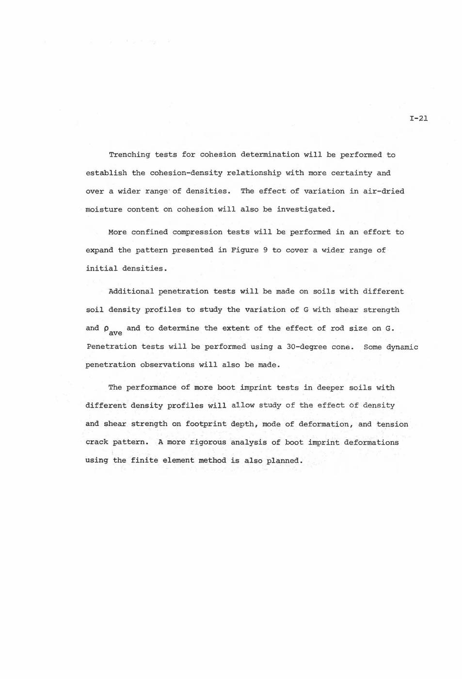
The sprinkling method was tried with heights of drop up to 6 inches.

The relationship between height of drop and average density for the top

1-1.5 inches is shown in Figure 2.

4. DETERMINATION OF ~

The variation of ~ with average density has been determined by means

of vacuum triaxial tests on .air-dried material at confining pressures

ranging from 0.04 kg/cm2 to 0.15 kg/cm2 • The lowest confining pressure

used was 0.04 kg/cm2 because the membrane corrections became too large

compared to the strength for lower confining pressures. A confining

pressure larger than 0.15 kg/cm2 causes too much densification during

isotropic consolidation prior to shearing. Confini.ng pressures much less

than 0.15 kg/cm2 must be used for the very loose specimens if excessive

densification is to be avoided. The reported densities are the values

obtained after consolidation but before sheari.ng.

The range in confining pressure used for vacuum triaxial tests

corresponds to a depth range of about 160 to 600 em for the actual lunar

surface . An effort will be made to measure ~ values for confining pressures

corresponding to much smafler depths ·by performing sliding block tests

to determine soil friction.

As expected, the stress~strain curves for most of the specimens,

especially the looser ones, ·exhibited· a plastic-type behavior. A typical

stress-strain curve for a triaxial test is ·shown in Figure 3.

I-4

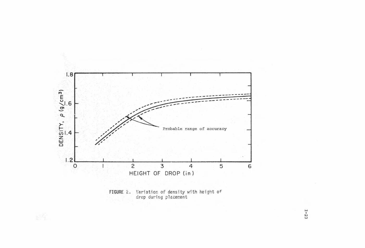
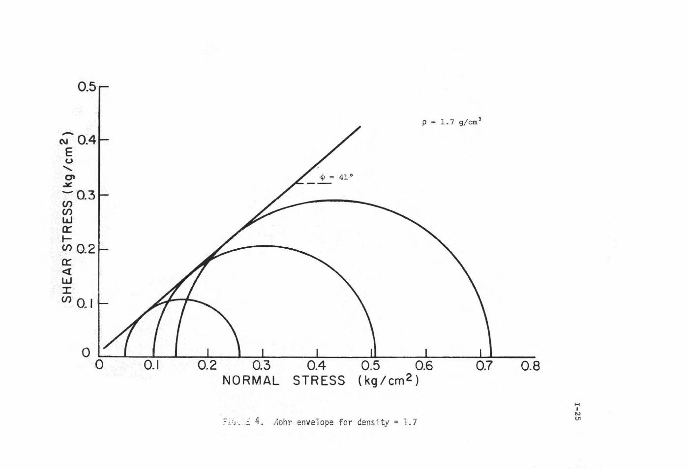
A Mohr envelope for specimens tested at an initial density of

1.7 g/cc is shown in Figure 4 and the variation of <P value with density

is shown in Figure 5. It is quite difficult to perform a triaxial test

on a specimen with an initial density less than 1.6 g/cc because even

small confining pressures cause densification. Probable values of <P

for densities less than 1.6 gjcc have been obtained by extrapolation.

A high degree of accuracy for <P values is difficult to obtain in

testing very loose specimens at very low confining pressures, due to the

relatively low strengths. Subsequent testing will be directed toward

narrowing the range of uncertainty associated with the reported values.

Nonetheless, the values obtained are consistent with those suggested for

actual lunar soil as a result of Surveyor tests.

5. DETERMINATION OF COHESION

The variation of cohesion with average density has been determined

by excavating trenches with vertical walls in samples with different

density. This method is preferable to obtaining the cohesion from usual

strength test results because of the difficulties in determining strength~~

of materials with very low cohesion at very small confining pressures 1

where the failure envelope may be in .. error ·by as much as 100 pe.r cent.

By using the vertical trench wall method, it is believed that errors may

be .kept as low as about 25 . per cent • .

Mariy failures of vertical trench walls were studied and it ·was found

. that the sliding block was ~ss·entially t\ Co\llomb wedge. . Tension cr-acks

usually appeared at the surface,· but they'':gid not appear to cover ~n

I-5

appreciable percentage of the slip surface. Figure 6 shows a photo

of a trench excavation for cohesion determination. A tension crack appears

about midway along the length of the wall. The wall height shown in the

photo is about two inches. Failure has occurred along part of the wall.

The procedure for calculating the cohesion consisted of (1) measuring

the wall height at which failure developed, (2) assuming Coulomb wedge

failure, (3) assigning an appropriate value of ~ and calculating the

shearing resistance force due to friction, and (4) assigning the remaining

resistance required for stability to cohesion. The calculated value of

cohesion was found not to be highly sensitive to either the value of ~

assigned or the inclination of the failure surface.

·A relationship between cohesion, c, and density, p, has been obtaL1ed

by this method for a limited range of densities and is shown in Figure 7.

It should be noted that the value of cohesion is dependent on the ''alue

of the air-dry water content. Additional testing will be done to determine

this dependency.

It is of interest to note that a vertical wall of 2-inch height for \

terrestrial soil corresponds to a vertical wall of about 12-inch height ·

for lunar soil of the same density and cohesion, due to reduced gravity

stresses. This observation indicates that it will probably not be difficult

to excavate around a "cake." . of l'unar soil, forming · four vertical walls.

However, additional testing and analysis is needed to assess ·the ·chances of

being able to scoop the "cake-like" piece of soil up for a density deter.mi-

nation without .brea.king it apart.

The conclusion appears warranted that ·the simulated lunar soil

exhibits· cohesion values appropriate .for tb.e range estimated far the· actual

lunar soil from Surveyor test results~

I-6

6. DETERMINATION OF DENSITY, VERTICAL STRESS, AND SHEAR STRENGTH

VARIATIONS WITH DEPTH

A 16-inch layer of soil was placed in the 2' x 2' x 2' box for the

purpose of conducting trenching tests and other model tests. Placement

was accomplished by sprinkling from a height of about 3/4 inch as

described in the Soil Placement section. In order to estimate the variations

of vertical stress and shear strength with depth it was necessary to know

the variation of density with depth. Confined compression tests were

performed on specimens with different initial densities to provide

compressibility data to be used in computing the needed density values.

The tests were carried out using a 2.8-inch diameter teflon-lined consoli-

dation ring. The initial specimen height was one inch.

The compression curves obtained from these tests are shown in

Figure 8 . The values of intial density·, p,, are shown on the figure. ~

The

curves show that the rebound on load release is extremely small. The same

data plotted in terms of stress and density are shown in Figure 9. The

curves marked L and T were obtained by extrapolation and are discussed in

the following paragraphs.

It is of special interest to note that all the curves merge at a

density of 1.9 g/cc and a stress. of about 1000 g/cm2 , · and that the semi-

log plot shown on Figure 9 indicates a linear variation of density with

. log pressure. These facts make extrapolation arid interpola;tion for other

initial densities possible.

The placement method used ·pioduces a density near the surface of

about 1.32 9/cc. Therefore it w~s des:Lrable to obtain a compression curve

with this initial density. Although confined ·compression specimens coul(l~

I-7

be placed at this initial density, they could not be tested without

significantly increasing the initial density, because the process of

scraping a plane surface on the top of the specimen produced densification.

Therefore it was necessary to obtain the probable position of this

compression curve by extrapolation. Fortunately, the data in Figure 9

show that the desired curve should be a straight line merging with the

other curves at a stress of about 1000 g/cm2 • A second point on the

' Jrve was obtained by using the known value of initial average density

at the surface and assigning an average value of vertical stress due to

the weight of a surficial layer. The compression curve thus obtained is

shown in Figure 9 and marked 11T" to signify its applicability to the

terrestrial soil in the test box.

The straight-line compression curves shown in Figure 9 have equations

of the form:

where (J = vertical compressive stress

p = corresponding density

K1 = value of p for (J = 1

K2 = change in p for one log cycle change in CJ.

Equation (1) can be written in expon~ntial form giving:

whe.re Ks . = 2.303 K2

cr = e

(1)

(2)

It is possible to relate the density to the depth of deposit as follows.

First, it may be assumed that a layer of soil of differential thickness, ·"

dz, is deposited on the bottom of the box at an initial density, p., and 1

that subsequent densification is due only to the compressive stresses

I-8

applied by the weight of additional material placed on top. The increase

in stress, do, due to the addition of a layer of thickness dz is equal to

the thickness of the layer times its density, p .• 1

(3)

In order to develop a relationship between density and depth, it is

necessary to substitute an expression for do in terms of p obtained by

differentiating Equation (2) •

(4)

Substitution in Equation (3) gives

K3 (p - K1) Kae . dp =

Integration gives the following . expression

1 K3 (p - K1) - . e . · -z+c p. . . . 1

(5)

. . . . . .

The constant of inte9rai;ion, c, can be' ev~luated by applying the boundary

condition that p - pi fo.r z - ~ 0; there.£ore , , ·

{{ln[pi(z +c)]+ Kl} dz K3

z

For convenience the constant cis retained in Equation (5), which can be

rewritten as,.

p = ln[pi (z +c)] + Kl

K3

Equation (7) is the desired relationship between density and depth.

I-9

(())

(7)

There is one additional boundary condition which facilitates the evaluation

of p .• The average density, p , of the 16-inch layer of soil was ~ ave

determined by measuring its total volume and weight after placement and

found to be 1.50 g/cc. The use of this value in evaluating p. requires an ~

expression for p in terms of z and p .• The average density for any ave ~

depth of material, z (i.e., the average density for all material between

the surface and depth z), can be obtained by integrating Equation (7) with

respect to z and dividing the result by z.

Integration gives

(8)

Equation (8) is the desired rela_ tionship between p , · p: , and z. Examina-. · ave_ :1.

tion of curve "T" in. Figure 9 shows that K1 = 1.20· and K; = 0.223 fr6rn

which K3 = 10.32 can be. c:a~culated .• - Using these cornpre~si_on parai[\et~rs·

I-10

and the condition that p = 1.50 g/cc for z = 15.7 inches (39.8 em), ave solution of Equation (8) for p. gives p. = 1.30 g/cc. This value of p.

1 1 1

was then used in Eql.lations (7) and (8) to compute the variations of p and

p with depth as shown in Figure lO(a). The vertical stress at any ave depth z is given by

(9)

Equation (9) and the data in Figure lO(a) were used to compute the vertical

stress variation with depth shown in Figure lO(b). The agreement between

the computed stresses and densities shown in Figures IOta) and (b) and the

stress-density relationship given by curve "T" of Figure 9 ind.;i.cates that

the method used and assumptions made are acceptable. An additional

check is provided by the fact that the computed value of p for the upper ave few centimeters compares very well with the value obtained experimentally.

It should be noted that precise agreement between the computed

density-depth relationship shown in Figure 10 and that implied by the

confined compression curve shown in Figure 9 should not be expected for

very small depths because two modes of densification are involved. The

actual soil placement process involves densiflcation due largely to

vibration- resulting ina layer of finite thickness at the surface with

essentially constant density. This surface layer is tnen s11bseqtiently

compressedin accordance with the relationships depict~a in Figure 9.

Howev_er, the calculated density-d~pth relationship shoWn in -- Fig"\U'e 10 (a)

is based on the assumption that _ a!l densification is by static compression

I-ll

alone; i.e. the initially deposited surface layer of density pi has only

differential thickness. The difference caused by this assumption becomes

negligible after the stress exceeds a few grams per cm2 •

Using the data presented in Figures 5, 7, and lO(a,b) it was

possible to compute the variation of cohesion, c, and shear strength

on a horizontal plane, sh, with depth, as shown in Figure lO(c).

Figure lO(c) shows that the shear strength variation is nearly linear,

although not precisely so, and that the contribution due to cohesion

is appreciable for the first 10 to 15 em.

A similar analysis was made to determine the probable variation of

density, vertical stress, and shear strength with depth for th~ actual

lunar surface under conditions of reduced gravity. As in the case of the

terrestrial section of soil, it was necessary to determine a compression

curve relating density and stress. ~rhe position of this curve was deter-

mined by assuming that the lunar soil fits the -compressibility pattern

established in Figure 9. It was further assumed that the average density '

of the top 40 em of lunar soil is 1.50 g/cc, in accordance with estimates

of this property from Surveyor data. Using these two assumptions it was

possible to obtain a probable position for the compressibility curve as

shown in Figure 9 by the curve marked "L" to signify its applicability to

the lunar soil under reduced gravity. The compressibility curve was found

by making a trial and error solution .for K1, K3, and p .• l.

Before discussing the trial and error solution, a preliminary

obse~cvation can be made which -shows · that the curve "L" must ·be appreciably

flatter than curve "T."- If p for the top 40 ern is LSO g/cc, then the · ave

vertical compressive stress due to gravity .at this depth must. be:

I-12

cr (z = 40 em) = (1.50) (40) (1/6) % 10 g/cm 2

since the gravity-induced stress is only 1/6 of the value for the same

soil on the earth's surface. [Note: Although stresses are, by definition,

expressed in dynes/cm2 in the metric system, expression in grams;cm2

is used herein for both terrestrial and lunar applications because

of the better "feel 11 for behavior that is obtained with these units.

For computation of lunar gravitational forces, a density equal to

1/6 of the mass density is used.] In order that p be equ_ al ave ·

to 1.50 g/cc for the top 4D em, it is necessary that the value of

p at a depth of 40 em be appreciably greater than 1.50 g/cc. The preceding

obse-rvation shows that the value of p = 1. 56 g/cc for cr = 10 g/cm2 shown

by Curve L is a reasonable value. The same argument can be used to show

that p, for the actual lunar surface should be greater than p, for the terrestrial ~ ~

section prepared in the test bin if both sections have the same value of

P This relationship is necessary···. because the increase in density with ave·

increase in depth is smaller for the lunar soil due to reduced gravity stresses.

Modifications in the derivations of expressions for p and p to ave account for reduced gravity consist simply of substituting p./6 :Eor p,

~ ~

in cases where gravity stresses are being calculated. Thus, the expression

for dcr, ·.the incremental stress increase due to the weight of a small

additional surface layer, as given by Equation (3) _.becomes:

(3a) _

I-13

and the desired relationships between p, pave' and depth are:

p = ln[ {p ./6) {z + c)] ----~1~-----------+ K1

K3

and

(7a)

{Sa)

However, the boundary condition that p = p. for z = 0 holds for the lunar 1

soil section as it did for the terrestrial soil section; therefore the

expression for the constant of integration, c, is:

c = 6/p. e 1

K3 (p. - K1) 1 (6a)

Solutions of Equations {7a) and (Sa) gave the best agreement between

the computed stress-density relationship and the confined compression

curve ,\'~hen K3 = 13.55, K1 = 1.39, and p , = 1.37 gjcc. Using these values 1

the distributions shown in Figure ll{a) were determined. The variations

of vertical stress, cohesion, and shear strength with depth shown in

Figure ll(b,c) were obtained by combining data from Figures ll(a), 5, and 7.

Under conditions of lunar gravity the cohesion, c, constitutes a very

significant percentage of the total shear strength on a horizontal plane,

sh, as shown by. Figure ll(c). However, the significance of the cohesion

component is likely to be much less in the case of shear induc~d by .

surface loading, because ~f the additional confinement provided by applied

direct stresses. · For example, although_ it is ·difficult to estimate the

I-14

minimum contact pressure to be exerted by the wheels of lunar roving vehicles

at this point in time, it seems likely that this pressure will be greater

than 0.75 psi (absolute pounds force). This contact stress will, of course,

both cause some densification and dis8ipate with depth. Assuming that

most of the deformation occurs within the top 15 to 20 em of material, it

is reasonable to assume that the average normal stress within most of this

zone is at least 0.45 psi (about 30 g/cm2 ). This value of normal stress

would cause densification of tl1e lunar soil to a density of about 1.64 g/cm2

for which cohesion, c = 4.6 g/cm2 and sh = 27.4 g/cm2 • Therefore a conserva-

tive estimate ' of the percentage contribution of cohesion to the shear strengtll

is about 17% for this case.

7. PENETRATION RESISTANCE

Penetration resistance measurements are being considered as a means

by which astronauts may gather data leading to the assessment of lunar

surface soil properties. Approximate values of resistance are needed for

design· of penetrometers that may be utilized on Apollo missions. An

important application of penetration resistance data may be for the design

of lunar .roving vehicles. The Corps of Engineers utilizes cone penetrometer

data for cohesionless soils in trafficabili ty an.3.lysis by o.btaining the slope,

. G, of the penetration resistance (in. psi) versus depth of penetration . (in

·inches). Although the lunar soil is not considered to be completely cohesionless,

it may still be possible to utilize such a modulus. As a first step toward

obtaining penetration data for a si~ulated lunar soil, ~ series of rods

of different sizes were ·used as pene:tr.~'~eters in the soil represented by . .

Figure 10. · The ·rod sizes and the G: ;., ;ue;p . obtained from the~ are shown

in Table I-1 . All rods had flat ends . . In most cases, the rods were simply

allowed · to sink under thei'i own weight.

I-15

TABLE I-1

SUMMARY OF ROD PENETRATION DATA

Rod Diameter

(in.)

Area

( . 1n. 2)

G

#/in. 3

0.50 0.1965 1.9

0.50 0.1965 2.5

0.90 0.636 1.8

0.95 0.71 2.5

1.35 1.43 2.2

1.35 1.43 2.3

2.0 3.14 1.5

4.0 12.6 1.9

'V Ave."' 2.1 ± 0.5

The rod penetration data in Table I-1 show an average value of G = 2.1 #/in. a.

It appears that G is not appreciably aff~~cted by "the rod size , but the

scatter in the data is about ± 0. 5 . #/in. :3 so the 'effect of rod size may be

obscured. An idea of the effect of rod size can be obtained by considering

the rod to be a square footing and equat:ing its bearing capac~ty to the

penetration resistance . .

q .lt = ~ N K1 . + dyN + cNc. ""U 2 Y .. CJ llO) .

where

~lt = bearing capacity

b = width of footing

y

N y

d

N q

c

=

=

=

=

=

=

unit weight

function of <j>

foundation shape

depth of footing

function of <j>

cohesion

factor

N ~ constant (relatively insensitive to depth change) c

I-16

The constants N'Y and N<P are of about the same magnitude and are conside~~ably

larger than Nd. This bearing capacity equation shows t.~at the depth term

should predominate after the depth exceeds a few rod diameters and that the

penetration resistance should become essentially proportional to depth.

However, the rod diameter obviously should have a significant effect on

penetration resistance at very s_hallow depths.

A first approximation of the value of G applicable to the actual

lunar surface (reduced gravity) can be obtained by assuming the penetration

resistance is proportional to the shear strength. A comparison of Figures 10

and 11 showsthat the rate of increase in shear strength with depth for the

simulated lunar soil i$ about five times the rate of increase for the

probable. lunar profile. Therefore,·

G . f\.. 5 G . Earth f\.. Moon·

or

G Moon 2.1

5 = 0.42 ± 0.1 #/in. 3

Note that the units for GM are absolute pounds force per cubic inch. oon

I-17

If GM. ~ 0.4 #/in. 3 , then a 10# (absolute pounds force) vertical load oon ·v

could be used to drive a l-inch-diameter penetrometer about 30 inches

(75 em) into the lunar soil. Therefore, penetrometers of l-inch-diameter

and smaller can probably be used successfully with much smaller loads.

An additional observation of interest made during the performance

of the penetration tests was that the maximum downward thrust that could

be exerted on a rod was about 45 pounds -with hands at chest level and

about 15 inches from the chest.

Figures 5, 7, and 11 show that the initial density profile of the

lunar surface will probably have a very pronounced effect on the compressi-

bility as well as the shear strength. Therefore the effect of variable

density is of importance. It is of interest to estimate the possible

effect of changing the average density about 10 per cent {say 1.5 to 1.65)

on the value of G. The cohesion would be more or less uniformly increased,

but this increase would have little effect on the rate of increase in

shear strength with depth. However, Figure 5 shows that tan cp might

increase by about 20 per cent. Assuming tan cp·were proportional toG;

a 20 per cemt increase in G would result. Similarly a 5 per cent increase

in density might cause an increase of about 10 per cent in G. This

comparison indicates that measured G values for the lunar surfac;e material . . . '

.may, in fact, be good indicators of variation in density and sh~~a:r strength.

I-18

8. ANALYSIS OF FOOTPRINT DATA

Figures 12 and 13 show photographs and sketches of a boot imprint

made by stepping down on the surface of the simulated soil with a weight

of 180 pounds. The profile of the simulated soil is represented in

Figure 10. The dimensioned sketch <>f the boot Used (see Figure 13) shows

that the bearing area is about 45 sq in. Although the stress distribution

under the boot was not €!xpected to be uniform; the average stress was

4 psi. The. observed maximum depth of the footprint was 3. 5 inches.

In order to provide a basis for comparing the depth of footprint

in the simulated lunar soil and in the actual lunar soil, it was assumed

that the boot was a 4-inch-wide strip footing and that the contact stress

dissipated with dep·l:h according to elastic theory (Bous~;inesq solution) •

The va:r·iation C!)f the existing vertical stress and the total vertical stress

including surface load with depth is shown in Figure l4(a). The magnitude

of stress due to surface load which still exists at the bottom of tt,e box

shows that boundary effects were appreciable for this depth of soil. Thi.s

point i$ discussed further subsequently. The compressibility curve T of

Figure 9 was used to deterrnine the variation of final density with depth

as shown in Figul:'e 14 (b) •

depths by

The ·vez:otical strain, e:: . , was calculated at various v

e:: v P1

1--· .. P2,

~rhere p 1 = original density

p 2. = final density

and. plotted in Figure .15. The area.tothe left of the curve gives the

predicted depth of footprint, 2~. 3 inches. The fact that the predicted

b. Lunar surface b.Terrestial surface

= 1.8 2.3 = 0.78

I-19

depth of footprint, 2. 3 inches, does no·t compare well with the observed

value, 3.5 inches, indicates that the assumption of stress dissipation by

elastic theory may not be good . Furthermore, shear deformations were

neglected in making this estimate; only deformations due .. to compression

were considered. Nevertheless, the method used serves as a basis for

comparing depth of footprint in the test bin and the corresponding depth

of footprint for the lunar surface.

The prediction was repeated for the actual lunar surface using the

properties given in Figures 9 and 11, except that the force applied to the

boot was assumed to be 275 earth lb (46 lunar lbs) giving a surface contact

stress of about 1 psi, assuming the same contact area of 45 in. 2 • The

results of this prediction are shown .in Figure 16. The predicted depth of

footprint was 1.8 ·inches , Comparison shows that:

This ratio can now be applied to the observed depth of footprint for the

simulated soil in the test bin. However, the observed depth must first

be corrected for the boundary effects exerted by the bottom of the box.

Figure 15 indicates that the depth of footprint might have been abou·t ·

20 per ·cent greater had the box been infinitely deep, in which case the

observed depth of footprint would have been about 4.2 inches. Dsing this

value, a reasonable estimate of the depth of footprint for the actual

lunar surface, .with p = 1.50 g/cc, can ~e obtained by ave

Depth = (4.2) (0.18). = 3.3 .inches

parar:eters. T'ile results are .shmt'n in ':'able 2 below.

Pave (before loading) Probable Depth of

i'n g/cc footprint in Inches

1.40 4.3

L50 3.3

1.60 2.5

TABLE I-2

These comparisons indicate that depth of footprint may be useful as

an indicator of density and shear strength. This conclusion is only

tentative, however, and will be checked by conducting more footprint

tests on soils with different p values and by making more· ·refined ave ·

analyses, including, for example, shear deformations.

9. PLANNED STUDIES FOR NEXT QUARTER

Additional triaxial tests are required to establish the · ¢-den·sity

relationship over ·a wider range. of densities. and to decrease the

uncertainty associated w;ith cp values reported herein. A small number of

plane strain tests will also be .. performed · to determine the magnitude of

any differences in. ¢. values for ·plane strai.,n and i;.riaxial tests.

Trenching tests for cohesion determination will be performed to

establish the cohesion-density relationship with more certainty and

over a wider range· of densities. The effect of variation in air-dried

moisture content on cohesion will also be investigated.

More confined compression tests will be performed in an effort to

expand the pattern presented in Figure 9 to cover a wider range of

initial densities.

Additional penetration tests will be made on soils with different

soil density profiles to study the variation of G with shear strength

and p and to determine the extent of the effect of rod size on G. ave

I-21

Penetration tests will be performed using a 30-degree cone. Some dynamic

penetration observations will also be made.

The performance of more boot imprint tests in deeper soils with

different density profiles will allow study of the effect Of density

and shear strength on footprint depth, mode of deformation, and tension

crack pattern. A more rigorous analysis of boot imprint deformations

using the finite element method is also planned.

GEOTECHNICAL ENGINEERING UNIVERSITY OF CALIFORNIA_

GRADING ANALYSIS Mu:xons Sieve Sizes

'"1------------~5

-- 10 20' 400270200 too· 50 30 16 8 4 J_" 11" 2" t>l'' 3' 100 .-.. 8 2 "2 100

:::: ' '( ,... J :::: -~

9u I f= f= I 90

t- · : ~

80 I- I : f= -I= - I f= ., t= 70 _) -1-f= / 70

~ 1-; ~v : : 60 I= F L : 60 :

.... I= z "'

~ :x.; L 0 t: a: L ~

"" : : 50 :

f= : w 0.. f= ~

.4(' F ' L v : ...J 40 .... C( != . : 0 I= ~ :

.... f= F 301- / : :

30 I-F ~ :

· I= I= 201- / ~ :

: : : 20

I-I= F

v :

j ~ IOF =

= ;" -'= / 10

= ~

oF L~ I I I I I 1 Ll _l _l _l_l_l _l_l' _l _1 I I I I I I I I I I I I I I I I 1 = =

I 5 10 20/ 400 210200 too so 3o 16 8 4 ~~ 1·~J ~ f2'-.v 325 230 110 1"10 120 10

f so 60 45 40 35 2s i -rr '*' tf zo. 1e 14 12 10 r s s 3f I

M1crons Steve Stzes 5 10 20 50 100 500 1000 ) I ! I I I I I I b.bot I I 't ', '•' 't ~ I , I • I I I I I I I J I I 1 ~~opq I~~~ I I

50000 IQ~bo~ I • ' I t' I I I I j

I 1 Microns

j I l I I I I I I f ' I I j I I I

I I I I I I I I I I I I I I I II I f I I ~ I t I OD05 0.01 0.05 0.1 Q5 I 2 3lnches

FIGURE l. Gradation curve for basic test soil H

r. 8 ....... --........ ------,r-------,r-------,r-----r-------.

, - _ E

... __ _ -----------------

-~~--,1 .6 ...... --------------------

0'

>--....... Probable range of accuracy (f) 1.4

. Z w 0

1.2~~-~------~------~------~------_. ______ ~ 0 2 3 4 5 6

HEIGHT OF DROP (in)

FIGURE t. . Variatior: of density with hsight of d~op during place~ent

H

0.5

w (.) z 0.4 w a:: LLIN LL.E LL.u - ........ 0 ~ 0.3

.::e.

(f)z (/)

Density= 1 . 70 g/cm 3 L&.J­a::_ t- , Confining pressure , = O . l kg/cm2 03

(/) ~ 0.2 ~ 6-a..-u z a:: 0.1 0...

OL-----~----~~----~----~------~ 0 10 20 30 40 50

AXIAL STRAIN, E (ok)

.I • •

FI-GtJRE··,·3 . Triaxial stres·, ,.,.s tra in curve

r - 24

0.5

p = 3 1. 7 g/cm...,._ .

N 0.4 E v

. ' C\ ~

. .

~0.3 en en w a:: . .....

. ·.; .. en · cr::

· 0.2 .

<( w

.. ·I en 0.1 1

0 0 0.1 0.2 0.3 0.4 0.5 0.6 0.7 0.8

NORMAL STRESS (kg/cm2)

?~:; ·_ .. .:: 4. ;•iohr- enveiope for density= 1.7

H

45

40 f/) cv cv ---....;:::::::-..,_ Probable range ~

.0 of acc~acy cv "0

-e-I

35

30~ __ , __ _. ______ ~----~------~------._----~ 1.4 1.5 1.6 1.7 1.8 1.9 2.0

DENSITY. p ( g/crn 3)

FIGURE 5. cp vs density

I-?7

f"IGURE 6 • Trench excavation for cohesion determination.

OJ5 . ...-----~---.,.-----,------.---.-----, 10.2

............ For air-dry water (\J

= -

content 1:8% E ~ 0.10 6.8~

z -0'

u

0 z en . 0

~005 (/)

3.4w :r: 0

u Prob able range o f 0 a.ccura cy u

o~-----~-------~------~----~------~~--~o I. 3 1.4 1.5 1.6 1.7 1.8 1.9 . DENSITY, p (g/cm3)

FI GURE i.. Cohesion vs density

H

p. initial N - 1.2

= density ].

E p. = 3 1.44 g/cm

...... (.)

1.0 ].

-Ol 3 ..¥ p ... I

1. 47g/c J.

=

(/)

~ 0.8 0: t-V>

~ 0.6 ~ a: 0 2 0.4 ...J <(

.._ u

a: 0.2 .UJ >

25

FIGURE 8. Confined compression stress-strain curves for different initial densities

I-29

p. 1 = 1 . 65 gm/cinl.

• p. = 1.47 gm/cm3

-l.

1.2 0 p. = 1.44 gm/cm3 l.. .

·~ ' E '~ T

~ · ·L

-C7' '

1.4 , . ....-....r ', ,,

',~ p = 1.20 + 0.223 log a Q...

~ l-

' ' en 1.6 -

' '-, .-- p = 1.39 + 0.17 log cr z w 0

1 .• 8 . ~

= 3 .. p. 1.65 g / cm

2.0---~----"'-------or=J--------.J....-.-----~ I 10 100 1000 10,000

VERTICAL STRESS, o- (gm/cm 2 )

FIGURE 9. Confined compressive stress vs density H

\ \ \ .

\ \

' ' ' ' - '

.

' -E ' .

I u ' I

' ' - I . p . = 1 ~ 3o·

' a

:I: l. I ~· =10 .32

~ I

25 = c I sh + cr tan 4> L&J kt = 1. 20 1 0 I

I

30 I I I I

~-· c = cohesion p ave .• :-- •

' I I

40 . . I

1.0 ,· 1.2 1.4 L6 1.8 0 20 40 60 80 0 10 20 30 40 50 60 DENSITY ( gicm3)- VERTICAL NORMAL STRESS SHEAR STRENGTH ON A

IN gm/cm 2 HORIZONTAL PLANE IN gm/cm2 (a) ( b ) ( c )

FIGURE 10. Variation of tlensity, vertical stress, and shear st rength with depth fo r simulated lunar soi l

H

0 , \ \

5 \ ·~

' \ \ lO \

-\

' ' ' -E u 15 ' ' ' ' -

~ • pi ;:: 1.37 ' ~

:I:

b: Jr3 = 13.55 ' ' 25 LLJ kl = 1.39 ' ~ 0 • ' t • I

• • 35 Pave I c = cohesion ~

I

' 40~~--~~~~

1.2 1.'3 L4 1.5 1.6 0 5 10 15 20 o 5 r o 15 20 25 30 DENSITY ( g/cm3) VERTICAL NORMAL STRESS SHEAR STRENGTH ON A

IN g /cm·2 HORIZONTAL PLANE IN g/cm2 ( b) ( c )

~rtt'URE· 11 . Estimated variation of density , vertical stress , and shear strength wi th depth for actual i unar soil ( r educed gravity field)

H

I - 33

FIGURE 12. Foot print in simulated lunar soi l.

..,. __ ..._ _ _ _ I 3 . 5 "---------. .....

Contact stress ~ 4 ps~

t lt) .

A r (a)

~, l A

Ver tical wall

BOOT DIMENSIONS

SECTION A~A ~-----------13.5" ------------~ (b)

SCALE: t" =4" -co -. ~ 2 co

Area 45 in • ~

! rt")

t

( c ) J t:I G' U:\ .,E 1-.:S • Footprint details

H

0

5 p after surface loadi~g

E Total vertica·l 0 stress including I s urface load

N 20 :J: ~ 25 0... lJ.J 0

30

35 existing p

40 "!-"'--""'--~-----~~------'. 0 100 200 300 1.0 1.2 1.4 1.6 1.8 2.0

2 VERTICAL · NOR~AL STRESS, (Ty-g/cm DENSITY (gm/cm3) (a} ( b}

FIGURE 14. Varitation of vertica·l stress and density before and after surface loading f or simulated lunar soi l

H

0

8 = 1 ~ P1 E "" 14.6% v . P2 ave where P2 · ~ Pl

--E u

t :I:

25 w 0

L\H = ( 0. 1.46) ( 40) = =

5 . 84 em 2.3 inches

40~--~--~--~--~~------~ 0 10 20 30

VERTICAL STRAIN , €.v (0/o)

FIGURE _15. Variation of verttcal strain with depth for simul ated lunar soi 1

0 = 11.3%

-10

-e 15 u p after surface loading

,:I: ~ 25 Total vertical w stress including 0 surface l oad

,30 e xisting p

35 ~ = (O.ll3){40)=4.5cliH = 1. 8 in

40~--~~--~--~~ 0 20 40 60 80 100 1.3 1.4 1.5 1.6 I. 7 1.8 0 5 10 15 20 VERTICAL NORMAL STRESS

1 DENSITYl ( g/cm3) VERTICAL STRAIN, crv ( g/ c m 2 ) E V (o/o)

(a') (b) ( c ) -FI4.iURE 16. Probable variat.i.o1n of vertical stress, density, and vertical strain before

and ~fter surface· loading for actual lunar soi-l (reduce~ gravity field)

m

H

w

II. FRIC'I.'ION ANGLE OF LUNAR SURFACE SOILS

ESTIMATED FROM BOULDER TRACKS

(H. J. Hovland and J. K. Mitchell)

1. INTRODUCTION

II-1

Among the conspicious and interesting features on the surface of the

moon observed on lunar orbiter photographs are boulders or blocks of

rock and the tracks that some of these boulders left as they rolled

down slopes. Some of these boulders have been studied in previous

investigations (Moore and Martin, 1967; Filice, 1967; Eggleston et al.,

1968).

Early investigations of the relationship between boulder size and

track width were aimed primarily at determining the static bearing capacity

of lunar surface soil. Currently we are investigating the possibility of

deducing strength parameters (cohesion and angle of internal friction) .

A summary of past work done by our group on the study of lunar boulder

tr~oks was presented in the final report for Contract NSR 05-003-189

(Mitchell et al., 1968). In this report, several methods for utilizing

boulder-track data were considered, each giving somewhat different results.

It was recommended that the boulder-track phenomena be further studied, .

and that if variability is to be determined, it is important to use the

same method throughout.

Dr. Henry Moore of the U. S. Geological Survey, Menlo Park, California,

is also performing s~milar studies. It is understood that Dr. Moore has

investigated boulder-track phenomena for Orbiter I~ photographs primarily.

II-2

His results indicate friction angles in the range of 20 to 25 degrees. In

his analysis the bearing capacity required at the point where the boulder

rests, utilizing a full circular bearing area corrected for determinable

flatness of boulder shape is considered. In our analyses an attempt has

been made to relate the boulder to the track at failure and, hence, to

determine a limiting friction angle required for stability. Dr . Moore's

analysis on the other hand determines a friction angle for partially

mobilized resistance. Therefore, his values for ¢ are somewhat lower than

those obtained in the analyses to follow. The present report describes the

status of current studies.

2. METHOD OF ANALYSIS

(a} General:

From observation of boulder-track combinations from orbiter photo-

graphs and terrestrial boulder-track phenomena it appears that boulders

can be nearly spherical, quite rectangular with one distinct shorter

dimension, or intermediate in shape and still form a relatively smooth

track. However, the nearly spherical boulder should leave the smoothest

track. Tracks have been observed to be smooth, chain-like or disconnected

as shown in last year's final report~ These tracks imply either uniform

rol1ing motion or jumping motion with a combination of translation and

rotation both when the boulder is or is not in contact with the ground.

(b) A Rolling Sphere -Theory:

A boulder rolling on a slope where the soil fails, in general shear,

i.e.t the soil behaves essentially as an incompressible material, would

leave a track with a raise~ rim as spown on Fig. 1. For the purpose of

the present analysis, the theory will be developed for a somewhat more

idealized situation, as shown on Fig. 2.

From the above i~lustration, it may be seen that the track depth

will be given by

z = r(l - cose) = r (1 - cos [sin-1 ~]) 2r

Tt1e semicircular soil-boulder contact area may be represented by an

equivalent rectangular area defined by

= = w ~ - v7f = 4 0. 444 w

If a. = O, i.e. a horizontal surface, the resultant force causing

the sphere to move and form the track must naturally be inclined at

some angle with respect to the direction of the weight of the sphere.

Assuming that this resultant goes through the centroid of the soil-

boulder contact area, ·the maximum value of this result«;mt would be

approximately 12 (rt~eight of boulder) when the ratio of W/r is maximum

II-3

or 2. For smaller ratios of tJJ/r and slope angles greater than zero, the

magnitude of the resultant would be more nearly equal to the weight of

the sphere. It will, therefore, be assumed in the following analysis that

the magnitude of the resultant force ~quais the weight of the boulder.

(c) Bearin2 Capacity Theory:

The general bearing capacity equation for a strip footing is (c.f.

Leonards, 1962)

q . = 1.£ N' + eN + q'N 2 y c q

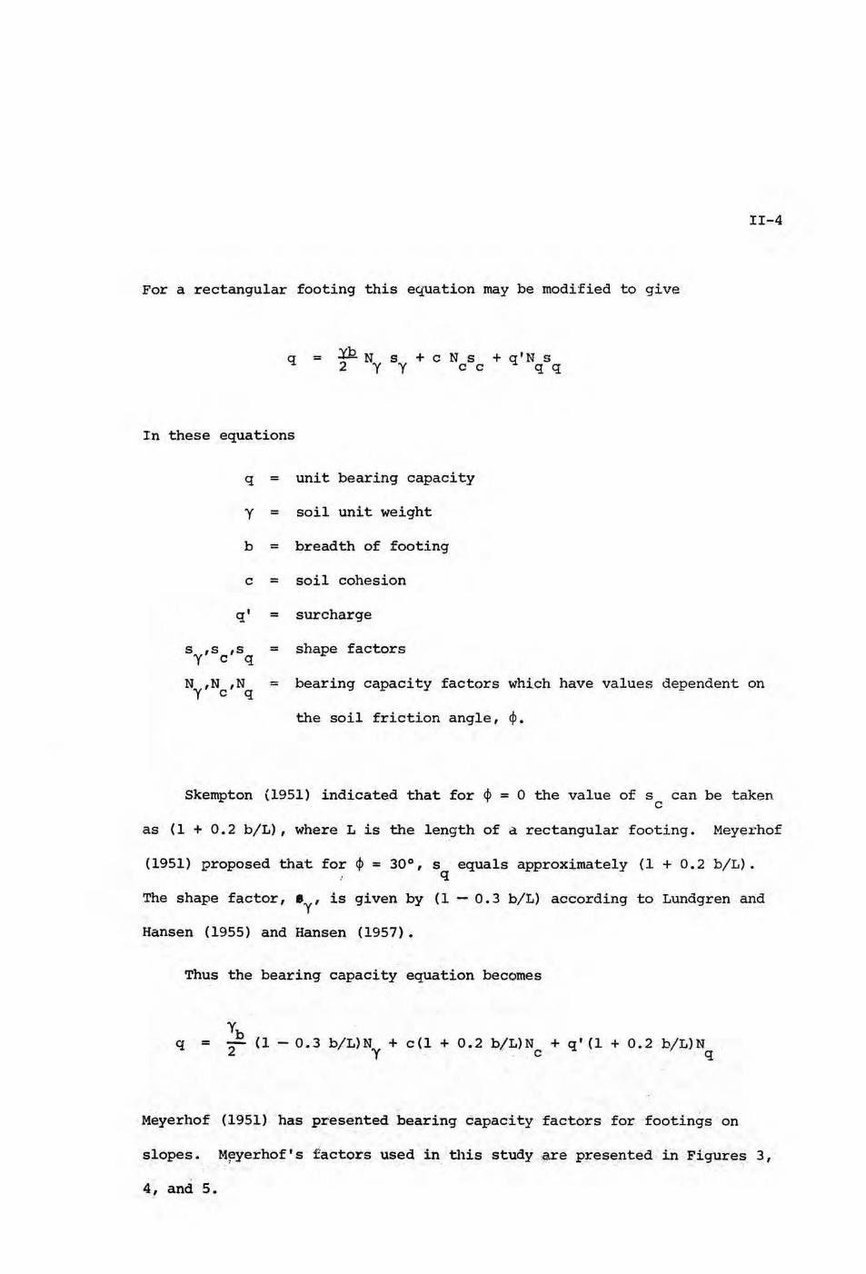
For a rectangular footing this equation may be modified to give

q = .xQ N s + c N s + q 1 N s 2 yy cc qq

In these equations

q = unit bearing capacity

y = soil unit weight

b = breadth of footing

c = soil cohesion

q' = surcharge

s ,s ,s = shape factors y c q

II-4

N ,N ,N = bearing capacity factors which have values dependent on y c q

the soil friction angle, ~ .

Skempton (1951) indicated that for ~ = 0 the value of s can be taken c

as {1 + 0.2 b/L), where L is the length of a rectangular footing. Meyerhof

(1951) proposed that for~= 30°, s equals approximately {1 + 0.2 b/L). q

The shape factor, 'y' is given by (1 - 0.3 b/L) according to Lundgren and

Hansen (1955) and Hansen (1957).

Thus the bearing capacity equation becomes

q y

= -2b (1- 0 .. 3 b/L)N + c(l + 0.2 b/L)N + q' (1 + 0.2 b/L)N y . . c q

Meyerbof (1951) has presented bearing capacity facto;rs for -footings on

slopes. M~yerhof's factors used in this study are presented in Figures 3,

4, and 5.

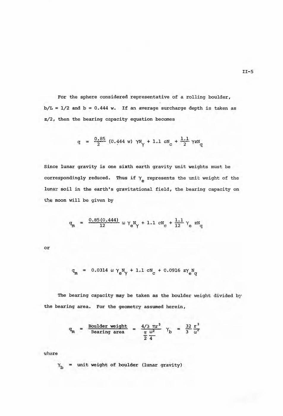
~ = Boulder weight Bearing area = 4/J 1Tr 3

.7T w2. --2 4

For the sphere considered representative of a rolling boulder,

b/L = 1/2 and b = 0.444 w. If an average surcharge depth is taken as

z/2, then the bearing capacity equation becomes

q = £>:8~ (0' .444 W) 1 1 l~l J yN + . eN + ~ yzN .... . y c 2 q

Since lunar gravity is one sixth earth gravity unit weights must be

correspondingly reduced. Thus if y represents the unit weight of the e

lunar. soil in the earth's gravitational field, the bearing capacity on

th~ moon w.ill be given by

q = 0.85(0.444) W y N + l.l eN + 1.1 y zN '"m 12 e y c U e q

or

= 0.0314 W y N + 1.1 eN + 0.0916 zy N e y c e q

The bearing capacity may be taken as the boulder weight divided b1!'

the bearing area. For the geornet1~ assumed herein,

wn~re

yb = unit weight of boulder (lunar gravity)

II-5

II-6

d. Analysis

In applying the above .. theory to lunar boulder tracks it was assumed

that the boulders are spherical. To make this assumption valid only

boulders appearing equidimensional on the lunar orbiter photographs and

having relatively smooth tracks were selected. The most recent estimates,

Mitchell et al. (1968) of average lunar soil properties

c ~ 2.08 psf (value assumed by Dr. H. Moore) and, yb ave

give y ~ 100 pcf, e 62 4 ; l = 2 • 7l-f"- pcf.

By measuring the track width and boulder diameter on the photographs, the

bearing capacity equation was solved by trial for the friction angle.

The results are presented in the following table for 16 boulder tracks

revealed by Orbiter V photographs and one boulder track shown in Orbiter II

photographs.

For most of the above 'boulders it was assumed that the boulder came

to rest on a slope of a= 0°.

It may be seen from these results that \!Thile lunar soil friction

angles in the range of 25° to 45° are required to account for the results,

the ~jority of the values fall between 32° and 38°. An assumption of a

larger value of cohesion, e.g. 20 psf has very little effect on the results

obtained, amounting to a reduction in the requi·red friction angle of about 2°.

3. DISCUSSION

It should be noted that the .assumptions involve.d in computing the

bearing capacity ·"~" are considerably fewer than are requ,ired to deduce

4> from the. ·bearing capac!tyequation ..

Table 1

Boulder Tr ack Slope Frame let <1m Location Frame Diameter Width a <f> (boulder location)* m m (assumed) psf

Hadley Rille V-105H 233 + 9.0 mn, 232 mm 15.3 10 .3 0 4150 31° II 233 + 11.0 nun, 234 nun 14.7 8.8 0 5020 33°

234 + 8.0 IDm, 235 mm 14.7 8.8 0 5020 33° " .. Schroter' s V-204H 221 + 18.0 mm, 161 nnn 12.8 6.1 0 6920 38°

II Valley 210 + 15.0 mm, 242 nun 12.8 7.3 0 4820 34° II 210 + 14.0 mm, 177 mm 11.2 5.5 0 5700 38° II 202 + 7 .0 mm, 253 nun 19.5 12.2 0 6120 33°

So. E part V-95H 957 + 11.5 mm, 164 . 0 mm 8.4 6.0 0 2020 290 of Hyginus 959 + 12 . 5 nnn~> 161.0 nun 8 . 4 4.8 0 3160 34°

962 + 3.0 mm, 167.0 mm 8 . 8 4.5 0 4100 37° 965 + 11 . 0 mm, 239 .0 mm 9.1 4.8 0 4030 37° '

968 + 13.0 mm, 253.0 mm 11.0 3.6 0 12600 45° 970 + 7. 0 mm, 246.0 mm 1!~ .4 9 . 2 0 4300 31° 978 + 13.0 mm, 252 . 0 1l1IIl 6.0 4.8 0 1150 **25°

Large hill so . V- 88H 011 + 8 . 5 mm, 230 mm 19.5 10~6 0 8100 36° of Alexander

Sabine D II-76H 364 + 8.7 6.4 0 1970 28° II-76H 364 + (same) 8 . 7 6.4 13° 32°

No. E part V-96H 092 + 1.0 mm, 46.0 mm 15 . 9 10.6 10° 4380 32° of Hyginus

*Frame1et number, distance from framelet edge, distance from data edge **S = +10° was used on the Meyerhof's charts. H

H I '-l

II-8

Values of the internal friction angle and cohesion are of importance

in advancing our understanding of lunar soils. That the results in the

above table give reasonably consistant and uniform values of ~ within

different areas should imply first, that by analyzing a sufficient number

of boulder-track phenomena an approximate average value of ~ can be

obtained within limits of the theory used and, second, that lunar soils

may be uniform with respect to ~ and c and do not vary greatly from place

to place. It is also to be noted that the results imply that ,lunar soils

appear to behave primarily as cohesionless materials, since cohesion of a

magnitude consistent with Surveyor results gives an insignificCJ.'l.t contribu-

tion in the bearing capacity equation.

4. CONCLUSIONS

Several assumptions were made in the application of the bearing

capacity equation to the boulder problem. Boulder track forma.~iop is

a dynamic problem. Since general bearing capacity theory is ba.·· ~111

statics, it cannot .be expected to hold rigorously for dynamic conditions .

Consequently further theoretical and expe:I'imental studies are being

initiated by us to enable better analysis of the boulder-track features

so common on the lunar surface. The following studies are proposed:

1. Analysis of additional. boulder-track phenomena using the method

described .above and refined as suggested below, so that statis-' tically valid average values of ~ and c can be established

within limits of the theory used.

2. Refinement of the present approach by correcting for boulder

shape., slope, and observable and measurable features. This is

to a c~rtain extent already possiblei for example, it may not

II-9

be necessary to assume that a boulder is equidimensional,

instead boulder dimensions can be checked using plan measurements

and shadow data.

3. Development of additional approaches or equations ~o that an

independent solution for cohesion is possible.

4. Observation of terrestrial boulder tracks to aid in development

of a feel for the variables and the limitations inherent in this

type of study.

5. Development of a theory which describes the dynamic rolling

boulder problem, and verification of this theory by experimental

investigations.

failure surface

track width

Top view Front view

FIGURE 1

failure surface Side view

W = boulder weight

contact area

Side view

equivalent rectanqular.area soil - boulder contact area

Top view (normal to .slope)

FIGUR~ 2

w = track width = 2r sin e

II-10

15· o 10 20 30 40 50 ANGLE OF INTERNAL FRICTION, 4> DEGREES

FIGURE 3. General Bearing Capacity Factor N for Strip ff)undation {after Meyerhoff~ 1951).

II-11

2

2

2

I.Oo 10 20 30 40 50 ANGLE OF INTERNAL FRICTION, ~ DEGREES

FIGURE 4. General Bearing Capacity Factor Ny for Strip Foundation (after Meyerhoff, 1951).

II-12

z •

2

2

1.0 .,;._----------'"""----~--------'------~~ 0 <10 20 30 40 ' 50

ANGLE OF INTERNAL FRICTION, c/> DEGREES

FIGURE 5. General Bearing Capacity Factor N for Strip Foundation (after Meyerhoff~ 1951).

II-13

REFERENCES

1. Eggleston, J. M., Patteson, A. w., Throop, J. E., Arant, w. H. and Spooner, D. L . , "Lunar Rolling Stones," Photographic Engineering, Vol. 34, No. 3, March 1968.

2. Filice, A. L., "Lunar Surface Strength Estimates from Orbiter II Photographs," Science, Vol. 156, p. 1486, 1967.

II-14

3. Hansen, J. B., "Foundations of Structures - (a} General Subjects and Foundations other than Piled Foundations," Proc. of the Fourth Int. Conf. on Soil Mech. & Found . Eng., London, 1957.

4. J .P .L., Cal. Inst. of Tech., "Lunar Traverse Seminar," Document 760-27, July 1968.

5. Leonards, G. A. , "Foundation Engineering," McGraw-Hill Book Co. , Inc . , 1962.

6. Lundgren, H. and Hansen, J. B. , "Geoteknik," Teknisk For lag, Kobenhavn. 1958·.

7 . Meyerhof, G. G., "The Ultimate Bearing Capacity of Foundations," Geotechnique, Vol. II, 1951, p. 301~

8. Mitchell, J. K. et al, "Material Studies Related to Lunar Surface Exploration," Final Report, Contract NSR 05-003-189, University of California, Berkeley, July 1968.

9. Moore, H. and Martin., G. , "Lunar Boulder Tracks , " Orbiter Supporting Data No. 1, 1967.

10. Skempton, A. w. (1951): The Bearing Capacity of Clays, Proc. Bldg. Res. Congr., London 1951.

SYMBOLS

b width of equivalent rectangle

c apparent cohesion

D dian1eter of boulder.

H high resolution

L length of equivalent rectangle

N ,N ,N bearing capacity factors c y q

q uni·t bearing capacity

q' surcharge

qe unit bearing capacity in earth gravity

~ unit bearing capacity in lunar gravity

r r.adius or boulder

s ,s ,s shape factors in the bearing capacity equation c y q

W boulder weight

z sinkage or track depth

a slope angle

~ angle defining equivalent free surface on Meyerhof's charts

y unit weight

·yb boulder unit weight in lunar gravity

Ye ~it weight of soil in earth gravity

~ apparent angle of internal fraction

e angle defining soil-boulder contact

w track width

II orbiter two

V orbiter five

II-15

III-1

III. TRAFFICABILITY OF THE LUNAR SUIU~ACE

(J. B. Thompson and J. K. Mitchell)

1. INTRODUCTION

The current state-of-the-art of vehicle mobility and tr.afficability

prediction a £1 related to the design and operation of lunar roving

vehicles was reviewed and evaluated under contract NSR 05-003-189. It

was noted that there is at present no method that is completely suitable

for the reliable prediction of needed trafficability and vehicle-soil

interaction parameters. Recommendations were made that intensive studies

of both an experim~ntal and theoretical nature be initiated in order to

develop the information necessary for design and performance prediction

of lunar roving vehicles.

On October 8 a.nd 9 a Working Group. meeting was held at NASA Head-

quarters for the purpose of establishing design criteria for a dual mode

lunar roving vehicle. The lack ·Of a proven method for trafficability

analysi~:; 1 even when reasonably close estimates of soil properties are

available, was readily apparent at this meeting. A subsequent meeting

was held on November 15, 1968 at the Jet Propulsion Laboratory to

consider further the problem of soil vehicle interaction. As ~ result

of these meet<Lngs it is understood that a proposal for experimental

model studies has been prepared by the Waterways Experiment Station for

the purposes of establishing the performance parameters of wheel s of a

type proposed for lunar vehicles and answering basic performance

questions such as the maximum slope that may be negotiated on the lunar

st::s:-face. The resl.llts of experimental studies of this type may be useful ' also for the establishment of similitude relationshipS {or lunar

trafficability analysis once cone index values for lunar soils are

available. The essential elements of this method are described in

the Final Report for Contract NSR 05-003-189.

Our group has concerned itself during the past quarter with some

analytical aspects of lunar soil trafficability. As a result of the

discussions at the Working Group Meeting for the Dual Mode Lunar

Roving Vehicle we became concerned with the question "How muc:h

difference is a variation in 1soil conditions likely to make on the

performance par,a."neters of a lunar roving vehicle?" In order to g·ain

insight :u~to this question a ser.ies of analyses have been made using

the Be.":,ker "Soil Value System" method of analysis. That there are

many limitations and i nconsistencies in this method is well recog-

nized. Nonetheless it is about the only quasi-theoretical method

available, and furthermore a considerable body of previous trafficabi-

lity work for lunar exploration purposes has been done using this

method. Consequently, it is believed that the results of the analyses

reported below help to define those soil and wheel characteristics

that will be of greatest concern in further studies of lunar soil

trafficability.

2. BASIC RELATIONSHIPS

III-2

The key relationships that are developed in the ''Soil Value System''

4re for wheel or track thrust, motion resistance, and drawbar pull

(Bekker, 1960). The merits and limitations of the theory underlying

these relationships and the test methods used for the determination of

needed soil param~ters have been discussed at length in the literature

H =(~be+ W tan ~)[1- K ioR.

2n + 2 - n - 1 2n + 1 0 2n + 1

and are summarized in Chapter I of Vol. III of the Final Report for

Contract NSR 05-003-189.

The appropriate relationships are as follows:

Wheel or Track Thrust -

The above equation is applicable for a soil exhibiting a stress-

{1)

III-3

deflection curve in which stress continuously increases ,~ith deflection.

For a soil which exhibits a stress strain curve in which stress falls

off after a certain deflection is reached, another expre:ssion in terms

of two parameters K1 and K2 can be written for thrust. lBecause little

information is available on the stress-strain properties of the lunar

soil, it will be assumed that the soil is of the first t~l{pe. If the

results of the Bevameter annular shear test are plotted ilS the ratio of

the recorded shear stres~3 to the soil shear strength versus the

deflection, K is equal to the inverse of the slope of the curve at zero

deflection. In other words the magnitude of the stress Btrain parameter

indicates the steepness of the stress- strain curve.

Motion Resistance

Rigid ' Wheel -

(2)

III-4

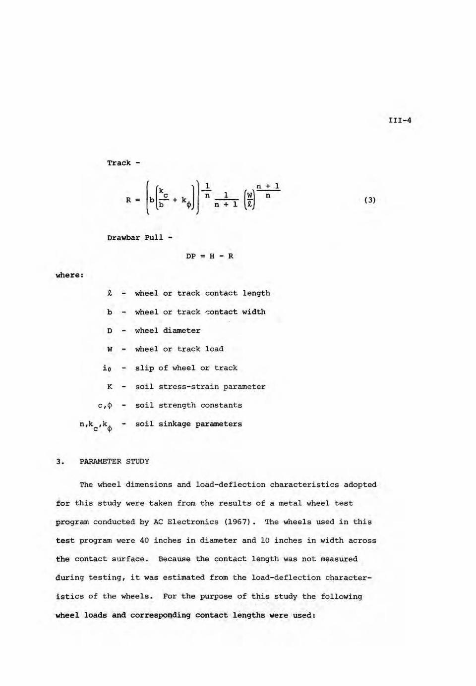
Track -

(3)

Drawbar Pull -

DP = H - R

where:

~ wheel or track contact length

b wheel or track .-:ontact width

D wheel diameter

w wheel or track load

io slip of wheel or track

K soil stress-strain parameter

c,<f> soil strength constants

n,kc,k<t> soil sinkage parameters

3 . PARAMETER STUDY

The wheel dimensions and load-deflection characteristics adopted

for this study were taken from the results of a metal wheel test

program conducted by AC Electronics (1967). The wheels used in this

test program were 40 inches in diameter and 10 inches in width across

the. contact surface. Because the contact length was not measured

during testing, it was estimated from ·the load-deflection character-

istics of the wheels. For the purpose of this study the following

·wheel loads and corresP9~din9 qontact .lengths were u·sed:

c = 0.05 to 0.15 psi

w (lbf.) ~ (in.)

50 14.7

75 16.5

100 18.2

150 20.6

From a consideration of the deflection characteristics of the wheels

studied it mi9ht be anticipated that the motion resistance character-

istics would fall between those of a track and a rigid wheel.

Therefore, equations 2 and 3 should theoretically envelope the

measured motion resistance values. This hypothesis is examined

subsequently.

Values assumed for soil cohesion (c) and angle of internal

friction (~) were as follows, based on available data from the

surveyor program.

The soil sinkage parameters kc' k¢' and n are l~ss certain.

(1968) * reported values for n of 1.0 and 0. 7 c;letermined from load-

Scott

sinkage tests using the surveyor Surface Sampler with the scoop closed

For .the purpose of this study, kc and k<l> were k

arid open respectively.

combined into a single c parameter, k = b + k~ r and the f ,ollowing ranges

of values .for k and n were ~ssumed for this study:

*Verbal· communication as stated at the· ·Lunar Soil Wheel Interactioi-1 Meeting at the Jet Propulsic;m Lab_oratory, November 15-;- 1968 ~

III-5

k c k = b + k¢l - 0 . 5 to 6.0

n = 0.75 to 1.25

Estimates of the soil stress-strain parameter K can be based only

on terrestrial experience as appropriate tests have as yet not been

conducted on the lunar surface. The range assumed was:

K = 0.5 to 1.5

Using the values stated above for the various wheel and soil

parw~eters, the performance indicators wheel thrust, motion resist-

ance (for both rigid wheel and track), and drawbar pull (for both

rigid wheel and track) were calculated. The results are presented in

Figures 1 through 5. The sensitivity of each of these performance

indicators to each of the assumed soil parameters is discul:.Jsed below.

A. Influence of K, Soil Stress-strain Parameter - K affects the

calculated thrust as shown in Figure 1, and consequently drawbar p"ll

as indicated in Figures 4 and 5. The influence is greatest for low

values of K and for high wheel loads. For example, at a slip of

III-6

10 percent and a whe~l l oad of 150 pounds, the variation in the calcula~-

ed thrust over the range of K assumed in this study is 38~5 pounds. For

any given wheel load, the influence of K decreases appreciably with

increasing . slip.

B. Influence of Soil Sinkage Parameters - The assumed values of

the soil sinkage constants affect the calculated motion resistance

(figures 2 and 3) and consequently drawbar pull (Figures 4 and .S) • The

effect of each is discussed separately below.

III-7

i) n - Within the range of k generally considered applicable to

ii)

lunar soil (i.e., 2.5 or greater) , the ef.fect of the assumed

value of n on the calculated motion resistance is seen to be

small in the range of wheel loads studied. This is true

whether the metal wheel is assumed to behave a5 a rigid

wheel or track . The variation in the calculated motion

resistance with n increases with increasi.ng wheel load and

k value and is larges":. in the case of the rigid wheel

assumption. For a wheel load of 150 pounds and a value of k

of 6, the variation in the calculated motion resistance of a

rigid wheel is only 2.2 pounds for the range of n values

studied. Therefore, wheel performance does not appear to be

sensitive to variation in values of n.

An interesting observation from Figures 2 and 3 is that

contrary to the usual way of thinking, larger values of n

result in larger values of motion resistance in the

applicable range of k values. The£efore, a consistently

conservative design should recognize this fact. k c k or ~ + k~ - The effect of k on the motion resistance

increases with .a decrease in the value of the parameter and

an increase in the wheel load and is greatest for the rigid

wheel assumption. For a wheel load of 150 pounds, the

difference between the motion resistance of the rigid wheel

at values for k of 2 and 6 is 7. 7 pounds. The effe·ct of k

on the motion resistance of a track is negligible within the

applicable range of the parameter, and a value of k = 4 was

used in calculating the drawbar pull of a track.

III-8

c. Influence of Soil Strength Const.~ - In order to clearly

present the effect of the other parameters in Figures 1 through 5, the

wheel performance indicators were calculated with the assumed soil

strength values of c = 0.1 psi and ~ = 35 degrees. These two

parameters affect the calculated wheel thrust and consequently

drawbar pull. The influence of the assumed values of c and ¢ can be

seen most easily by examining the thrust equation, Equation 1. For

given values of k, ~' and io the term in brackets has a fixed value

·which is multiplied by another term, in parentheses, whose value is

determined by values of ~' b, c, W, and ~· Therefore, for a given

wheel load, and consequently contact length, and for the wheel width

specified above, it is possible to express in percent the effect of

deviations in values of c and~' from 0.1 psi and 35 degrees

respectively, on the calculated value of thrust.

The percent change in the calculated value of thrust as a function

of the assumed values of c and ~ is shown in Figure 6. Over the range

of c and ~ values of probable significance, that is 0.05 psi < c < 0.15

psi and 33° < ~ < 41°, and over the range of wheel loads studied, the

maximum variations in the calculated thrust are theoretically 30 and 26

percent due to deviations in c and ~ respectively. Therefore, the

assumed soil strength parameters may be expected to have a significant

effect on the vehicle performance. It is noteworthy that the effect of

the wheel load on the percent change in . the calculated value of thrust

is the result of the lof;q-deflect.io'l characteristics of the wheel. If

the wheel load-contact length relationship for the wheel were linear,

the percent change would be independent of the wheel load.

Figure 6 can be used to adjust values of thrust for one assumea

set of strength parameters to another. For example if a given wheel

at a given wheel load is to be tested on several different soils one

would only need to calculate the performance indicators based on one

set of soil strength parameters and then 1) ent·er Figure 6 (a) and (b)

at the revised parameter values and read the percent change, 2) add the

two values together, 3) multiply the thrust calculated for the original

set of strength parameter values by the quantity one plus or minus the

net percent change divided by one hundred, and 4) pl.ot the adjusted

thrust and drawbar pull curves. This approach assumes, of course, that

for each wheel load, there is a corresponding contact length indepen-

dent of the test soil.

The effects of the wheel load, wheel diameter, contact length,

and contact width on the wheel drawbar pull have not been presented in

the preceding graphs. However, study of Equations (1), (2), and (3)

shows that the wheel diameter, contact leng~~, and contact width

should be maximized to maximize drawbar pull. With the exception of

the motion resistance of the track, in the applicable range of k, the

wheel load has a significant effect on the performance indicators

(Figures 1 through 5). An increase in wheel load results in an

increase in the calculated thrust, motjon resistance, and drawbar pull.

An important problem in lunar trafficability investigations is

likely to be the mobility of a rover on slopes. Bekker (1960) stated

that the maximum slope a vehicle can climb is given by the drawbar pull

to weight ratio. Although this conclusion does not consider such

important factors as the general stability of the soil Jnass, it will be

used here as a first ordet: measure of the slope climbing ·capability

III-9

III-10

of a vehicle. Calculated drawbar pull to weight ratios are shown in

Figures 7 and 8. These plots indicate that in spite of the fact that

the heavier wheel loads result in larger values of drawbar pull, the

increase in wheel load is not matched by an increase in hypothetical

slope climbing ability . It appears therefore that for values of slip

greater than approximately 10 percent, the axle load should be

minimized in order to maximize the slope climbing ability of a vehicle.

4. COMPARISON OF THEORY WITH EXISTING TEST RESULTS

The conclusions reached in this parameter study are obviously

only significant if the "Soil Value System" method adequately evaluates

the mobility of any proposed lunar vehicle . Very limited metal wheel

test results that may be used for an evaluation of the accuracy of the

method were reported by AC Electronics (196 7) .

Mobility tests on both wt re mesh and metal elastic wheels were

conducted. Because the performance of both wheel types was nearly

identical, average values of the measured performance indicators are

used in this discussion.

The soil used in this wheel test program was a dry sand with the

following parame·ter values.

c = 0.035 psi

~ = 31°

k = 0 ) c k 16 =

k~ = 6

n = 1

K= (not measured)

III-11

Tests were performed using wheel loads of 50, 75, 100 and 150

ponnds force. The test wheel dimensions t:m d lc;:;~d-deflection

characteristi·cs were the same as those used in perfol!:'Jlling the parameter

study in the previous section . Therefore, the va:rious values of the

performance indicators calculated for the parameter study can be

compared directly with the measured values except that the calculated

thrust and dr~wbar pull values must be corrected to the values of c and

~exhibited by the soil used in this test program. From Fi~ure 6, the

following percent corrections of the c~lculated t hrust are required for

each wheel load.

Table II

Percent Change w (lbf.) in Thrust

~0 -29.2

75 -27.0

100 -24.1

150 -22.6

Plots of the predicted and measured wheel thrust , motion resistance,

and drawbar pull are shown in Figures 9 through 11.

A. Thrust - Unfortunately, t he soil stress-strain parameter, K,

was apparently not measured in this test program. 'rberefore a value

of K of 0 .• 5 was assumed since it resulted in the best fit between the

predicted and measured values of thrust as shown in Figure 9. For the

wheel loads of 50 and 75 pounds force, the predicted and measured

value~ of thrust are quite close. However for the wheel loads of 100

and 150 pounds force the predicted values of thrust are inv;re~lsingly

larger than the measured values. The explanation for this difference

offered by AC Electronics was that slip between the whe~1 and the

III-12

soil occurred and therefore the optimum soil strength was npt, mobilized.

Although this explanatior. seems plausible, a possible ~.nad'equacy of

the "Soil Value System" method should not be overlooked. However, it

is encouraging that the general shape of the predicted and measured

thrust plots correspond quite well.

The apparent slip between the wheel and the soil noticed in this

test program points out an important problem in terrestrial wheel

testing. Since terrestrial wheel-soil friction and adhesion may differ

from those on the moon, lunar conditions may have to be artificially

duplicated in order, to accurately model the wheel-soil interaction.

B. Motion Resistance - The measured, predicted, and corrected

predicted values of motion resistance are plotted in Figure 10.

Because the "Soil Value System" method provides only for the calcnla-

tion of the motion resistance due to the force exerted on the wheel by

the soil, a correction must be made for the inherent resistance of a

given wheel to ~otion. One way of approaching this problem is to

measure the motion resistance of the wheel on a hard flat surface at

specified wheel loads. Values of the inherent wheel motion resistance

were measured by AC Electronics using this method, and the appropriate

corrections have been applied to the preqicted values of motion

resistance.

As predicted in Section 3 the rigid wheel and track mo~ion

resistance assumptions do envelope the measured values of~oti6n

resistance. The measured values of motion resistance are small and the

III-13

test wheels appear to behav~ more like a track than a rigid wheel.

This is of course what one would expect considering that 1) the

reported sinkage was on the order of 1 in., and 2) the contao·t length,

i, was on the order of 15 to 20 in.

c. Drawbar Pull - The predicted and measured values of draw-

bar pull are plotted in Figure 11. The predicted and measured values

'of drawbar pull correspond quite well for the wheel loads of 50 and

75 pounds force but for the wheels loads of 100 and 150 pounds force

the predicted values are increasingly g~~f:!ater than the measured

values.

5 . CONCLUSIONS

The following conclusions may be derived from the study of the

"soil Value System" method parameters. Of course the validity of these

conclusions is entirely dependent on the validity of the Equations (1),

(2) , and (3).

1) The effect of variations of t he soil stress-strain parameter,

K, on the calculated value of thrust is greatest at low values

of slip and increases with increase in wheel load. Because

efficient us~ of available energy will require the opera tion of

the lunar rover at low values of slip, an accurate estimate of

this parameter may be required for. adequate prediction of

vehicle performance .

2) The effect of vari ations of the soil sinkage constant, n, on

the calculated motion resistance is relatively small in the

applicable range of values of k. Therefore, an accurate ' . . '

III-14

estimate of this parameter will not be required to adequately

predict vehicle performance. However, a cons~stently censer-

vative design should adopt the maximum value of n in the range

considered applicable.

3) The effect of variations of the soil sinkage constant, k, on

the calculated motion resistance increases with an increase

in wheel load and is only significant in the case of the rigid

wheel assumption. The required accuracy in the estimation of

this parameter will depend to a great extent on the anticipated

wheel load and wheel deflection characteristics. For the

wheels investigated in this study, an accurate prediction of

this parameter will not be required if wheel loads on the

order of 100 pounds force are anticipated as the maximum

error in motion resistance prediction would only be approxima-

tel y 4 pou•nds •

4) The effect of variations of the soil strength parameters, c

and ~' on the calculated value of thrust is significant and

accurate prediction of these parameters is required if the

vehicle performance is to be adequately evaluated.

5) An inc~ease in the wheel load leads to an increase in the

calculated thrust,. mot;io'n resistance, ' and drawbar puil.

However by taking the drawbar pull-weight ratio as an indicator

of the slPpe climbing ability of a vehicle, the lighter the

whee! load the steeper a slope the vehicle should be able to

climb.

6) The characteristic wheel dimeris~ons of contact .width, cont~ct

III-15

length, and diameter should be maximized from a trafficability

viewpoint.

The comparison of the predicted metal wheel performance indicators

tc those measured by AC Electronics in a test program resulted in the

following conclusions.

1) Fo:r: those wheels tested, the predicted and measured values of

thrust compared quite well at the low wheel loads. However,

the deviation between the predicted and measured values was

considerable for the larger wheel loads.

2) The measured values of the motion resistance of the wheel

were enveloped by the two assumptions a) the wheel behaved as

a rigid wheel and b) the wheel behaved as a track. The wheels

tested exhibited values of motion resistance which suggest

that this type of wheel behaves more like a track than a rigid

wheel.

3) Even though deviations between predicted and measured values

of the performance parameters were evident, the general shape

of the predicted and measured thrust, motion resistance, and

drawbar pull plots were similar.

A conclusive statement can not be mad~ at ~n1s time concerning

the applicability of the "Soil Value System" approach to the prediction

of .the mobility of the proposed lunar roving· vehicle. Although the

metal wheel test results present~y available are encouraging, future

wheel test programs are _required. In addition modifications of the

basic theory should be examined and, if possible, the approach must .be

extended to prediction of mobility. on slopes. studies are proceeding

along these lines.

140

~ ---------------=::==K==~O·~lw= ==------=::::::r,.sJ 1501bft

-100

-~ '+-.J!l -.:.. K=O.~ 0 W=

. 5 IOOibft t-en 80 a:: ::l :t: t-_. UJ UJ 60 :t: ~

- ·K=0.5} w-~ 5~1bft

:t: 40

20 C=O.Ipsi cp=35°

o~ ______ _. ________ ~ ________ ._ ______ ~ 0 25 50 75 100

L- , 0 SLIP (0/o)

FIGURE 1. Wheel .Thrust vs~ ·sl1p.

III-16

6

s ~

4

.:.c. • + . ~.o3

II ~

2

\_----. ""----.v--~ \.---.,,______.;1 W=IOO lbft

___ , v-

0 W=501b ft · W=I501bft ~o-. ~. --~--------~,o~.--------------~·20~-------------3~0------------

R , MOTION RESISTANCE{lbft) ~ H

k H I

FIGURE 2. Motion Resistance vs. ( ~ + k ) for a Rigid Wheel. ~­~

4

6.0 ~+ - - ·\ . II\· . ' , ' ,

5.0 !! \ \ I' . \ \

" . jjl I \ I : \ \ \

. \ \ \ 4.0 ~· \ \ \

i \ \ \ l \ .¥

. \ \

+ •

\. \

\ \ .

~I.e 3.o . \\ · \\ ..::: II\ ~, \'

\,\\ ;2.0 •. .

\\\,\

. '\\ \

'\. \\ \'\\ .. "~ \ . n: 1DO -~ ~,

0 \. I. · \:\-· n= 1.25 '~ ::=: - __ -~+-- ''-"·

. '"" --...... -----.~, n=0~75 -- -._ ·~ · -----------------

. ..._ --- n = 0.75 n:t.oo -. ---.........

~ n::125_ n=~.75 -n=L25 -- ---~

. --W--501bft W=iOOib]l W=l50tb.ft

1.0 2.0 3.0 4.0 5.0 6.0 7.0 R, MOTION RESISTANCE (I b ft )

k FIGURE 3. ~1otion Resistance vs ( ~ + ·kcp) f m·· a Track.

120

k= 6 }K=0.5} w-

-100 ~ -= } K=I.S 1501bft .

-.c

_j

....J 80 ::::> k:§ a.. 2 }K=O.S} w= a:: ~=6 :}K=I.S IOOibft <( ----

2

;so <( 0:: C)

a.. f:.2 L:k=6

k=S }K=O.S} W:

C:l 40 "2 } K=l.5 50tbft

20 . C=O.I psi cp=35°

0 ~------_.--------~-----------------~ 0 25 50 100 • lo, S L I P 1(0/o)

III- l9

FIGURE 4. Orawba r Pull vs. Sli p f or a Ri gi d ·Hhee l

140

120

---.Q

..J

..J

~ 80 0::: <X CD 3: <X 60 0::: 0

... a.. 0 --------------:=:==K=O . .S}

~ W=

40 --------------K= 1.5 501b.ft

20 C=O.I"lJISi ¢=35° k=4

0~------~--------._~~--_.--------~' 0 25 50 75 100

i o , S L I P (0/o)

FIGURE 5. Drawbar Pull vs. ~ lip for a Track.

III-20

w = 50 l b f

vv = 100 lbf w = 150 l b f

I 0 _ 1-

~ 0 a: ~------~------~~------~------~~------0.15 0.20 C(psi) ,__, :c 0 0 UJ t--20 Range of <t probabl e _J

:::>,..30 u _J

t-- significan•::e

<t u z ~ 30 z w = 150 l b f

~ 20 . ~W= 50 l b f

u 1- 10 z LtJ

~ 0~--~--~~~--~~--._--~---------------~ cp (degrees)

-10 Range of

-20 probable significance

-30

FIGURE 6. Percent Change in Ca1culatE~d Thrust vs·. c and $.

I I I - 21

120

-0 ~100' 0 h-<t a: I- 80 :I: (.!)

LLJ 3:

5 I

...J 60

a.:, a: <I Qj

~ 40 a: 0 .. 3: ' a.. 0 20 C=O.llpsi

cp: 35 °

0~------------~--_. ________ _. ________ _. __ __ 0 25 5·0 75 100

l 0 , S L l P (0/o)

· DP FIGURE 7 • . ir• Drawbar Pull - Weight Ratio for .a Ri'gid Wht~e l . ·

III-22

- 100 ~ 2, 0 -~ ~ 80 :r: C)

w 3: ~ _, 60 a. ~ a:· <[ m ~ 40 C=O. I psi Q: 0 cp = 35°

k= 4 ..

3: 20 ....... a. 0

0~------~--------._------~--------~ 0 25 50 75 100 i .SLIP ( 0/o) 0

FIGURE 8. eP, Drawbar Pull- \~e i ght Rati o for a Tr-ack .

III- 23

100 ~--------------------W=I501bf1

- 80 -----W=I501bft

-.... .... /.,---------.Q / ..... I W=IOOtbft

~ 60 I /, ----- ---W=IOOibft

~ a:: p ' / ---- w=751bft w=75tbft

w 40 :I / ,.___.

...J -

LLJ

:=. X y ,.,. .,.,.,. .,.,. ----w=so:hf1

.. y-- W=50tbft

I. 20 PREDICTED K= 0.5

¢~ = '31° ----MEASURED G =0.035psi

0 I 0 25 50 75 100

i • 0 SLIP (0/o)

FIGURE 9. Comparison Between Predicted and Ac.t1ual Wheel Thrust vs. Sl fp,~·~

;[li-24

-Rigid wheel (corrected predict ions)

.... --.... ~ 16 Rigi d wheel , pr edicted L&J u z 14 (/) ~ u; 12 a= LLJ

z 10 .,_ 0

~ 8 .. 6

a: 4 Track (correct ed

pr edictions)

2 k = 6 n = 1

Track , predicted

0 0 50 100 150 200

W, WHEEL LOAD ( L b ft )

FI GURE 10. Compartson BetWf!.en Predi.cted and Actua 1 Motion Resistance vs. Wheel Load.

III - 25

100 ------- ---- --· ~--

----

- ao, ... I

-'+-.Q

/ ;'

;'

W=l50 lbft

...... / ,_....-

...... / ------W=I50tbft ______ , _____ }

...J 60 /

/

~ ,

,_ ~·- __ --

.--W=IOOibft :::l a_ &.::::;;,:::.:---::.--:_------------ W=IOOibft

a: ..oil ~--·

<[ CD

~40 a: 0

p · .,-~

~--:;---:-::--~~::=:-:-=-·· -=----=--=-~w.:.=.2:so~ab~tt:...-_-.;... -_'!"!" ____ -_-_ }w=50tbtt 0.. 0 k=6 tc/:>=310

20 n =I C=Q.035 psi RIGID WHEEL} PREDICTED K=0.5

----- TRACK '

- "'• -- MEASURED

0--------~------~------~--------~' 0 25 50 75 100 l , SLIP (0/o.\ 0

FIGURE 1 L Cornpari son Bet ween Predi.cted ·and Act ual Drav!ba r· Pu l1 'vs·. i' o• s l 'i .p'. .

III-26

Bibliography

1. AC Electronics - Defense Research Laboratories (1967), "Lt.mar Wheel and Drive Experiment Test Program, " 2 vols., Contract NASB-20267, Jwle 1967.

2. Bekker, M. G. (1960).; "Off-the-Road Locomotion," University of Michigan Press, Ann Arbor.

III-27

List of Symbols

b wheel or track contact width

c soil cohesion

D wheel diameter

DP - wheel or track drawbar pull

H wheel or track thrust

j"o - slip of wheel or track

K soil stress-strain parameter

k soil Ct:>mposite load-deflection parameter

k soil load-deflection parameter c

k¢ - soil load-·deflection parameter

i wheel or track contact length

n soil load-deflection parameter

R wheel or track motion resistance

W wheel or track load

¢ soil angle of internal friction

III-28

IV. CHEMICAL IMPREGNATION TECHNIQUES

AS RELATED TO LUNAR ENGINEERING APPLICATIONS

(T. s. Vinson and J. K. Mitchell)

1. INTRODUCTION

In the First Quarterly Report4 it was indicated that potential

applicability of foamed plastics for the stabilization of unconsolidated

lunar surface materials and for sealing of porous rock and soil masses

IV-1

for storage and shielding purposes was under investigation. The possibility

of using foamed plastics for soil stabilization, particularly for lunar

applications is attractive for the following reasons :

a. The density of foamed plastics can be very low, thus providing

the possibility of treatment of large soil and/or jointed rock

masses with smaller quantities of stabilizer than would be

possible using conventional stabilize~s.

b. Reactants of relatively low viscosity may be employe d.

c. The formation of closed-cell foams in soil pores will give

impermeabilization.

d. Foaming action may serve to force the stabilizer into larger soil

volume.s than reached by the. initial .injection.

e. Reaction times are controllable.

f. The economics appear favorable.

IV-2

The current studies are aimed at determining the degree to which

each of these factors may be realized. We are aware of no previous work

with the specific purpose of soil stabilization by injection of foamed

plastics. It is recognized that different potential lunar applications,

e.g., preservation of unconsolidated soil structure for sampling purposes,

treatment of large soil masses for strengthening purposes, sealing of

cavity walls, will place different requirements on the material properties

and injection techniques. It is also recognized that the harsh lunar

environment will undoubtedly lead to differences in foaming action and

treated soil properties from what would be obtained under terrestrial

environment conditions .

Without losing sight of these factors, it has been considered

appropriate first to investigate in some detail the chemistry of foamed

plastics, the properties of the various ingredients in their initial

state, the properties of foams by themselves, and the degree of success

that can be obtained in injection under more favorable conditions than

represented by fine-grained lunar soil and the lunar enviror~ent. As

knowledge and experience accumulate the work will move more in the

direction of actual lunar conditions and applications.

2. CHEMISTRY

As noted in the First Quarterly RepQrt urethane plastics have been

selected as potentially the most useful of the different foam types.

Urethanes are produced by the reaction of polyols with polyisocyanates.

The general reaction is:

[H 0 ·1 I II .

R- WCO + R"'"- OR-+- R N- C OR"" + heat (1)

where,

R - NCO = a polyisocyanate such as toluene diisocyanate

R' - OH = a polyol; more generally any polyhydroxyl compound

(e.g. polyol, glycol, polyester, or polyether)

the urethane linkage

The above reaction involves IOOno-func:tional reactants, however, if

polyfunctional chemicals are used polymers: result. Functionality refers

IV-·3

to the number of reactive sites per molecutle. For example, toluene

diisocyanate (TDI) may be represented as NCO - R - NCO. Since there are

two NCO groups per molecule 1 TDI is said t :o be di-functional. If a tri-

functional polyol is used with a diisocyan1ate then a cross-linked structure

results. This may be ~represented diagrame:trically as follows:

Catalysts, surfactants 1 and blowing a1gents may be incorporated in the

reaction expressed by equation (1). Commc•nly used catalysts are tertiary

amines and tin ·salts and are a¢ided to cont:rol or accelerate the rate of

reaction so that gelation will be syncbron1ized with maximum rise of the

foam. Surfaotants control cell surface te!nsion and thus can render the

foam large-celled or fine-celled. Polygl~rcol-silicone polymers represent

a general glass of compounds that ca.n be Utsed as surfactants.

IV-4

Blowing agents expand to form a gas in the polymer structure hence

they are the agent responsible for the foam-like structure. Two classes

of chemical blowing agents are possible. In the first the gas is

produced by a chemical reaction within the polymer. In the second a chemical

blowing agent decomposes in the presence of the exothermic heat of the

reaction to produce the gas. Water would be in the former class of compounds.

1'he gas produced in this instance is C02. Low boiling fluorocarbons would

be in the latter class of compounds.

The flexibility or rigidity of urethane foamed plastic is controlled

by the functionability and molecular weight of the polyol and isocyanate

used. Rigid foams result when low molecular weight highly functional

polyols are used. Conversely, flexible foams result when high molecular

weight low functional polyols are used. Variations between these two

extremes for specific applications are possible.

Ideally the urethane linkage would be the only one found in the poly-

meric structure. This is not the usual case. There are several other

import.ant linkages that may be present. One of the most conunon subordinate

linkages occurs when water is present. The general reaction is:

H

I R - NCO + HOH -+ R - N - H + C02 t (2)

This reacts with another isocyanate as follows

H 0 H

I II I .R - NH2 + R - NCO -+ R - N - C - N -- R (3)

IV-5

where,

H 0 H I II I

R - N - C - N - R = a urea

Further, a cross-linking reaction will occur when the hydrogen on the

nitrogen atom of the urethane group reacts with an isocyanate group.

This is known as the allophanate linkage and may be represented as follows:

0 H 0

II I II R - 0 - C - N - R + R - NCO + R - C - N - R

I O=C-N-R

I H

{4)

In the general case all of these linkages will be forming simultaneously.

The preceding is intended only as a general presentation of the

chemistry of urethane foamed plastics. More detailed treatments are

presented in references 1, 2, and 5.

3. SELECTION OF URETHANE SYSTEM FOR PRELIMINARY INJECTION TESTS

For lunar engineering application there are three primary criteria

that should be satisfied by a grout: (1) low viscosity, (2) a controllable

gel time, and (3) a high ratio of stabilized volume to transported weight.

Initial studies were concerned with satisfying the latter criterion.

Current efforts are directed at determining the "best" system relative

to the fir5t ~o criteria while still satisfying the latter criterion.

These investigations were made by mixing small quantities of the appropriate

reactants in -different proportions and observing the initial viscosity ,

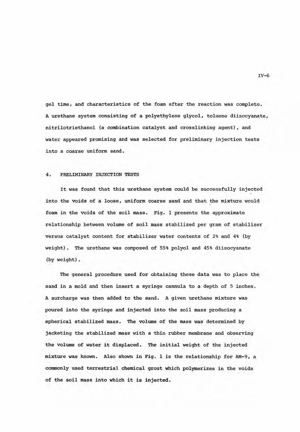
IV-6

gel time, and characteristics of the foam after the reaction was complete.

A urethane system consisting of a polyethylene glycol, toluene diisocyanate,

nitrilotriethanol (a combination catalyst and crosslinking agent), and

water appeared promising and was selected for preliminary injection tests

into a coarse uniform sand.

4. PRELIMINARY INJECTION TESTS

It was found that this urethane system could be successfully injected

into the voids of a loose, uniform coarse sand and that the mixture would

foam in the voids of the soil mass. Fig. 1 presents the approximate

relationship between volume of soil mass stabilized per gram of stabilizer

versus catalyst content for stabilizer water contents of 2% and 4% {by

weight) • The urethane was composed of 55% polyol and 45% diisocyanate

(by weight) •

The general procedure used for obtaining these data was to place the

sand in a mold and then insert a syringe cannula to a depth of 5 inches.

A surcharge was then added to the sand. A given urethane mixture was

poured into the syringe and injected into the soil mass producing a

spherical stabilized mass. The volume of the mass was determined by

jacketing the stabilized mass with a ·thin rubber membrane and observing

the volume of water it displaced. The initial weight of the injected

mixture was known. Also shown in Fig. 1 is the relationship for AM-9, a

commonly used terrestrial chemical grout which polymerizes in the voids

of the soil mass into which it is injected.

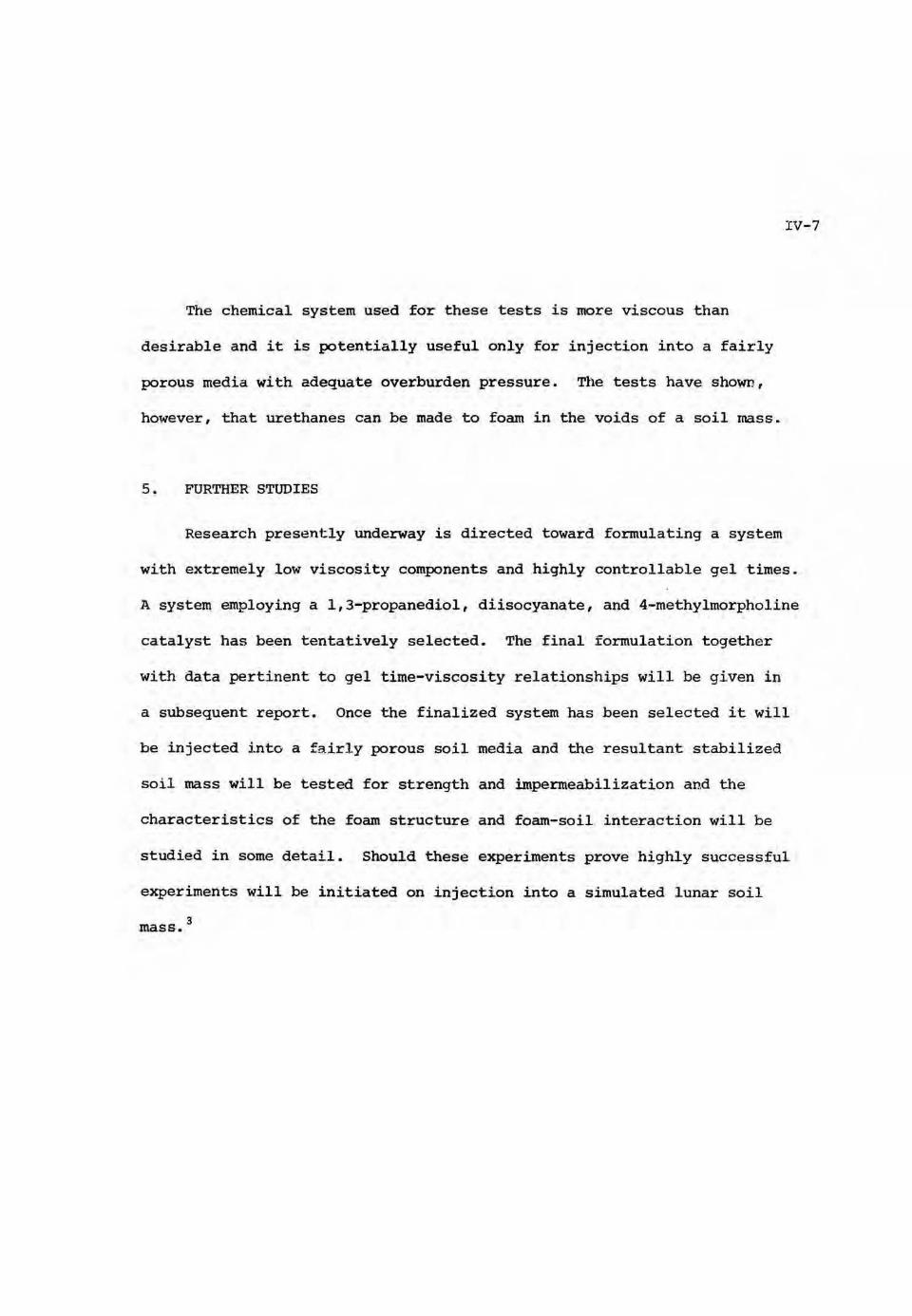
The chemical system used for these tests is more viscous than

desirable and it is potentially useful only for injection into a fairly

porous media with adequate overburden pressure. The tests have shown,

however, that urethanes can be made to foam in the voids of a soil mass.

5. FURTHER STUDIES

rv-7

Research presently underway is directed toward formulating a system

with extremely low viscosity components and highly controllable gel times .

A system employing a 1,3-propanediol, diisocyanate, and 4-methylmorpholine

catalyst has been tentatively selected. The final formulation together

with data pertinent to gel time-viscosity relationships will be given in

a subsequent report. Once the finalized system has been selected it will

be injected into a fairly porous soil media and the resultant stabilized

soil mass will be tested for strength and impermeabilization and the

characteristics of the foam structure and foam-soil interaction will be

studied in some detail. Should these experiments prove highly successful

experiments will be initiated on injection into a simulated lunar soil

mass. 3

-~ 8

-(!)

u ' HzO = 4% u ~

D

0:: 7 -o-C1' IJJ

N

-~ u c m = 2:¥o 6 2

ct ..... C/)

u. 0 .... 5 :I: (.!)

IJJ 3: 4 .... z :J a: 3 ~

AM-9 Chemical Grout 0 w N - 2 -...J m <( t-U) ' -IJJ ~ :::> ...J

~ 0 •, 'I I 6 7 8 9 10 I I

CATALYST

~-BY WEIGHT OF POLYOL SOLUTION)

Figure 1. Volume of ~oil stabilized pe.r gram of stabilizer versus catalyst co.ntertt for stabilizer water contents of 4% and . 2.%.

IV-8

~ERENCES

1Dombrow, B. A., 1963, Polyurethanes, Reinhold Publishing Corporation.

2Ferrigno, T. a., 1963, Rigid Plastic Foams, Reinhold Publishing Corporation.

3Houston, w. N., Mitchell, J. K., Namiq, L. I., 1968, Lunar. Soil

IV-9

Simulation, Lunar Surface Engineering Properties ExperimentDefinition. First Quarterly Report, submitted to National Aeronautics and Space Administration George C. Marshall Space Flight Center, October 1.

~Mitchell, J. K. and s. s. Smith, 1968, Chemical Impregnation Teclmiques as Related to Lunar Engineering Applications, Lunar Surface Engineering Properties Experiment Definition. First Quarterly Report, submitted to National Aeronautics and Space Administration George c. Marshall Space Flight Center, October 1.

5Phillips, L. N. and Parker, D. B. v., 1964, Polyurethanes, The Plastics Institute.

V. FAILURE OF A BOREHOLE IN SOIL OR ROCK UNDER DILATOMETER

LOADING AND .,. UNDER BOREHOLE JACK LOADING.

(T. K. Van and R. E. Goodman)

1. . INTRODUCTION

The failure of an infinitely long circular borehole under

dilatometer loading in an infinite homogeneous mass has been studied

by many investigators. Solutions have been obtained for different

property assumptions and failure criteria, for soils and for rocks.

Solutions to the same problems with borehole jack loading are not

available, to our knowledge. Studies are being made, using finite

element analysis, analytical limit analysis, and also by experi-

mentation in the laboratory.

2. FAILURE OF AN INFINITELY LONG BOREHOLE BY DILATOMETER LOADING

The problem is that of a thick-walled cylinder under internal

pressure, with the outer radius approaching infinity. For a

homogeneous and isotropic medium, due to the condition of symmetry,

radial stress .and circumferential stress are principal stresses. The

solutions were first obtained by Lame (Seely and Smith, 1959) . For

small values of ambient pressure (pressux-e a .t infinity) , p, the

maXimum value of circumferential stress occurs at. the inner surface

and equals th~ applied pressure.. The borehole will fail in tension at

every point on the borehole ·surface when the. applied dilatometer

pressure reaches the tensional strength of ·the medium. As the

V-1

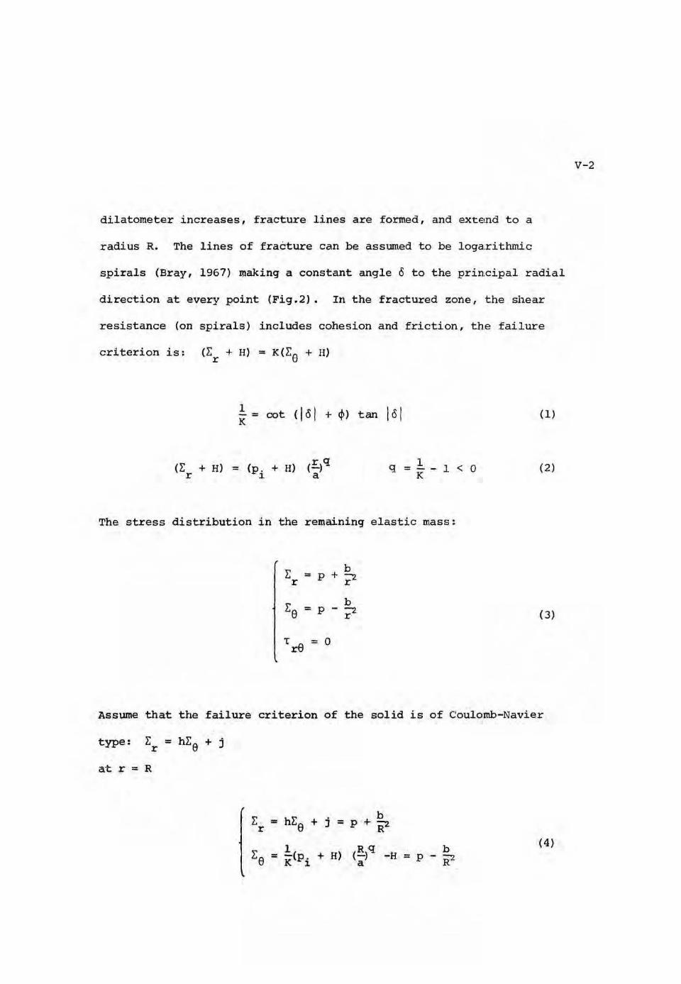
1 - = K cot <lol + ~) tan lol

1 q=--1 <0 K

at r = .R

L: hL:e + j ' b = = p '+ '::'2. r R

1 (RJq b ~e = K(p . + H) -H =p -::2

' l. a R

E + b = p ? r

Ee b = p - ~ r ·

't re = 0

dilatometer increases, fracture lines are formed, and exte!nd to a

radius R. The lines of fracture can be assumed to be logatrithmic

spirals (Bray, 1967) ~aking a constant angle 8 to the principal radial

direction at every point (Fig.2). In the fractured zone, the shear

resistance (on spirals) includes cohesion and friction, the failure

criterion is : (Er +H) = K(E6 + H)

The stress distribution in the remaining elastic mass:

(1)

(2)

( 3)

Ass1,m1e that the failure criterion of the solid is of Coulomb-Navier

(4)

V-2

R = a {K (~p - j) + H(h + 1)}~ (h + 1) (p. + H)

~

b = {(h - 1) E' + j 1 + h

E3 = T s if E1 + m(m - 2) E3 <0

o::1 - E3) 2 2(m- 1) 2 T (1 +

2T8 {<m ; l) 2

_ 1}] E1 + E3 = s Et + E~

(5)

It can be seen that the weaker the material the greater the radius of

the fractured zone. It is a function of angle o which is related to

the failure criterion of the solid mass . Bray suggested thaLt the

V-3

appropriate value foro would be 45~ + ¢s/2, with tan ~s as the friction

constant. The parabolic Griffith criterion of failure, and a

modified form suggested by McClintock and Walsh, composed of the

Griffith parabola and a straight line, do not well approximalte the

actual fracture strength of rock. Fairhurst proposed a more flexible

empirical criterion (Fairhurst, 1964):

or

Mohr's representation of the failure criterion is given by the

equation of the Mohr's envelope

1:2 = (m - 1) 2 T (T - E) s s .

(6)

(7)

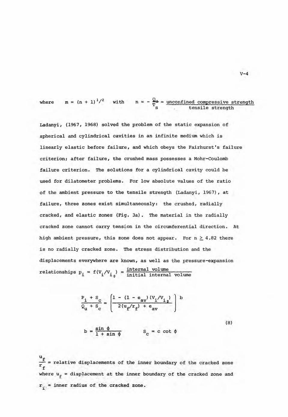
P. + s [1 - (1 - e ) (V. /V. ) b

1 c av . 1 1 o = Qu + s 2 {uf/rf) + e c av

b sin <I> s c cot cp = = 1 + sin <P c

V-4

where m = (n + 1) 1 / 2 with n = ~=unconfined compressive strength s tensile strength

Ladanyi·, (1967, 1968) solved the problem of the static expansion of

spherical and cylindrical cavities in an infinite medium which is

linearly elastic before failure , and which obeys the Fairhurst's failure

criterion; after failure, the crushed mass possesses a Mohr-Coulomb

failure criterion. The solutions for a cylindrical cavity could be

used for dilatometer problems. For low absolute values of the ratio

of the ambient pressure to the tensile strength (Ladanyi, 1967) , at

£ailure, three zones exist simultaneously: the crushed, radially

cracked , and e l astic zones (Fig. 3a). The material in the radially

cracked zone cannot carry tens~on in the circumferential direction. At

high ambient pressure, this zone does not appear. For n ~ 4.82 there

is no radially cracked zone. The stress distribution and the

displacements everywhere are known, as wel l as the pressure-expansion

internal vol ume relationships p. = f(V./V. ) = ~~~~~~~~------1 1 1 0 initial internal volume

l (8)

-:;:: rel ative displacements of the inner boundary of the cracked zone rf where uf = displacement at the inner boundary of the cracked zone and

rt:· = inner radius of the cracked zone .

( 1 - \1) 2 1\1 [ Qu l 2po - 'T s

po + s + c

• G + e av

-b

p. + s l. c

Po + S + Q • G c u av 1. 1.0

[

1 - (1 ,.. e ) [V. /V. 1 lb = [2(1 + V)/E] Qu • G + eav

G = m --!-1 [n~: + 1 - ! (m - 1)2]1/2

Volume of crushed zone after expansion eav = Volume of intact rock in the crushed zone - · 1

v. l. The ultimate internal pressure is that for = oo v.

Pult + 5 c Q + s u 0 (

u l-b = 2....!. + e rf av

l.O

For high values of the ratio C:i?o/-T ) the radially cracked .zone is s absent (Fig. 3b). The pressure-expansion relation is given by:

(9)

with (10 )

The ultimate internal dilatometer pressure (Ladanyi, 1967)

is obtained implicitly as follows:

l (Il)

V-5

It can be seen that the ultimate cavity pressure is controlled by

many factors: the strength parameters in intact and broken states;

deformability (E); the ambient pressure; and the densit y change due to

the change of state (Ladanyi, 1967).

The problems of dilatometer loading and borehole jack loading in

soils are different from those in rocks, mainly due to the plastic

behavior of soils and their inability to carry tension. The inter-

pretation of the failure in soil masses caused by a dilatometer can

be based on a number of available solutions. In the studies of

punching of metals, Bishop, Hill and Mott (1945) solved the p:coblem

of an expanding spherical or cylindrical cavity in an infinite

frictionless medium. In the investigation of the problem of the

dilatometer in clays, Menard (1957), Kerisel, Anderson and Gibson

(1961) solved the cases of an expanding cylindrical cavity in a

cohesionless medium. The same problem ~or an expanding spherical

cavity was obtained by Skempton, Yassin, and Gibson (1953) in the

V-6

study of pile bearing capacity. To deal with the problem of the

expansion of a cavity in a saturated clay medium under undrained

condition, Ladanyi (1963) treated the pLoblem semi-empirically. The

solution is based on stress-strain curves and strain-volume change

relationships obtained .. by conventional triaxial tests. 'fhe problem is

solved by step-by-step numerical integration method, More general

solutions for expanding spherical and cylindr.al cavities in media

possessing both cohesion and friction were obtained by Vesic and

Barksdale (1963), in a study on cratering mechanisms. For special cases,

frictionless or cohesionless media, these solutions +educe to those

obtained by earlier . investigators for th~se cases·-.

The assumptions made by Menard (1957) in the solution for clay

(¢ = 0) were based on observation of the curve relating deformation

to pressure. Within the low initial pressure range, linear elasticity

applies. Radial deformation is obtained by Lame's solution for an

infinitely thick cylinder. Poisson's ratio is taken as 0.50 for

saturated clay. At intermediate pressure range, a zone of plastic

equilibrium develops around the cavity .in uhich the clay is assumed

to be incompressible. Outside this zone, elastic equilibrium exists.

The deformation increases exponentially with pressure in this range

(Fig. 4). For an interval of pressure p - p in the plastic range, 1 2

the average value of the radius of the Mohr's circle is given by

Menard (1957) :

p - p 1 2 R= log u - log u

1 2

where u = displacement

p - p - c u = p 1 + V cp2e o

E c

and c = a constant =S?.u du

There is a stage of the loading where the deformation increases

greatly without any increase in pressure. The deformation becomes

very large compared to the initial cavity radius. The pressure

deformation curve is limited by a vertical asymptote p = pult"

(12)

(13)

V-7

= c(l + K)

F c = (Fq- l) cot4>

sin ~ +sin~

p0

= pressure at zero deformation.

E K = log 2c(l + \1) = relative rigidity

To analyze the cratering caused by a concentrated point charge of

explosive or line charge, Vesic and Barksdale (1963) obtained the

solution of an expanding spherical or cylindrical cavity of zero

radius in a soil mass possessing both friction and cohesion .

At an internal pressure p , plastic deformation takes plac.:e around u

v-a

the cavity until it becomes large enough to maintain equilibrium (Fig. 5).

A zone of plastic equilibrium exists around the borehole (cavity) ; the

rest of the medium is in elastic equilibrium. The solid is assumed to

be rigid-plastic in the plastic zone, and linear-elastic in the zone

outside. The change in cavity volume is equal to the change of volume

in the elastic zone. The infinite medium is subject to a hydrostatic

initial pressure q. The solution for the ultimate pressure can be

rearranged into the form (Vesic, Barksdale, 1963):

= cF + qF c q

F , F = cavity expansion factors. c q

(14)

(15)

E Ir = soil rigidity index, the ratio of soil rigidity 1 + V to initial

shear strength (c + q tan ~) •

The radius of the plastic zone is given by:

(~) =( 2 ~s (16)

For frictionle·ss media ($ = 0) , F c = Ln (~r) + 1, equal to the value found by Gibson and Anderson. The expansion factors for a

spherical cavity are larger than those of a cylindrical one. The slope

effects increase with increasing ~ and increasing I . The actual r

expansion factors for a dilatometer. should be larger than those of an

infinitely long cylinder. The values for the factors are available

for the whole range of 9 and rigidity index (Vesic and Barksdale 1963) •

3. FAILURE OF A BOREHOLE UNDER JACK LOADING

To our· knowledge little had been done with the problems of failure

of a borehole in rocks or in soils under jack loading. There are a

number of factors that complicate the problem. The. problem is not

axisymmetric. The distribution of contact pressure, the induced state

of stress, the deformation, and the mode of failure, are all affected

by the properties o.f the medium, and the geometry of the problem • .

The distribution of contact pressure de~ends on the relative·

rigidity between the bearing plate and the material, the bearing plate

dimensions, the roughness of the borehole wall, the properties of the

material, and the magnitude of the applied pressure. Wyanecki (1968)

V-9

(Fig. 6a) assumed that the contact pressure is purely radial, with the

maximum value at the center of the bearing plate. The distribution

was based on radial and tangential strains measured by strain gages

very close to the edge of the borehole. Goodman, Heuze, and Van (1968)

assumed that the contact pressure is unidirectional and uniform (Fig. 6b) .

For a small bearing plate width, it is reasonable to assume that there

is uni form radial contact pressure. When the medium is soil, the

problem is closer to that for uniform unidirectional displacement,

because the bearing plate is much more rigid than the medium. For sand

the contact pressure at the edges of the bearing plate is small because

of low confinement (Fig. 6c). For clay (~ = O), the minimum value is atthe

center, because at the edges, larger pressure is needed to cause the

same amount of deformation as at the center {Fig. 6d). For c - ~

materials, the minimum contact pressure is at the center of the plate

for low load range, and the maximum contact pressure is at the center

for large loads (Fig. 6e}.

The mode of failure depends on the properties of the medium and

the geometry of the loading. The problems are different for soils and

for rocks.

(a) Failure of solid under borehole jack loading:

Some experimentation done on concrete cylinders and on plaster-

based simulated brittle materials during this project showed that O~£e

mode of failure is tensional cracking. Maximum tensional stresses are

developed at the edge of the borehole, but not necessarily at e = + 90°

(8 = 0° at the center of the bearing plate) because of the non-axisymrnetry

V-11

of the problem. The magnitude and 'the location of the maximum tensional

stress depend on the magnitude, distribution and direction of contact

pressure. For uniforJn unidirectional jack pressure in a homogeneous

elastic, isotropic medium, finite element analysis showed that maximum

·tension occurs very close to the edge of the bearing plate. The

maximum tension occurs at 0 = 90° when the bearing plate is a semi-

circle (2a = ~) . For a given applied load the magnitude of the maximum

tensional stress decreases rapidly and ~e maximum compressional stress,

at the center of the plate increases as the bearing plate width is

reduced. For a given material under jack loading, it is conceivable

that when the width of the bearing plate is small enough, a different

mode of failure occurs before the maximum tensional stress reaches the

tensional strength of the medium. The problem is to find the prope~

failure criterion. It is impractical to solve this intractable problem

analytically.

Finite element analysis is being used to study the problem. The

approach, assumptions and failure criteria are those used by Goodman

(1968) in a study on effects of joints on strength of tunnels. The

rock masses are h.J.ockwise isotropic or orthotropic, linear elast.ic.

The failure criterion is

'[ N + D 1: B for E > 0 = Odt oct oct

(1: t) min = Et for 1: < 0 oc oct

and

where Et = uniaxial tensile strength E0ct and Toct are the octahedral

normal and _shear stresses, and N, 0, _ B are· material properties.

V-12

With the finite element computer program available, both loadings in form

of pressures and point loads can be accommodated. The effects of joints and dif-

ferent materials in the rock mass can be included and the propagation of cracks

can be considered. Study is in progress for a range of material properties.

There is another mode of failure - local punching - which could apply

here. This mode is observed in brittle material under concentrated loading

(Ladanyi, 1968).

(b) Modes of failure of soils under borehole jack loading:

For soils, the problem is different mainly due to plastic behavior and

inability to carry tension. The failure mechanism of a borehole in soil

under jack loading will be proposed here. The validity of the hypo-

thetical mechanism and its solution are to be verified by experimentation.

The me.chansim of failure is different for expanding soils (dense sands

and stiff clays) than for contracting soils (loose sands and soft clays) .

a) Expanding soils. For ~ wide bearing plate, as the load is

increased, tensional stresses are developed in the regions close to the

edges of the plates. Tensional fracturing occurs at the early stage of

loading, creating zones of no stress as shown in Fig. 7. The no-stress

zones extend deeper into the medium as the load is increased and two half

spaces are formed. The material below the plate shears along the surfaces

shown. Probably a crushed zone forms ·below the plate.

With narrow baaring plates, there is no tension failure. The. problem

is that of ~ strip footing on a curved surface.. Both . Prandtl mechanism of

failure and Hill mechanism are possible (Fig ... 8). The Hil.l mechanism is

chosen because it g~ves a more appropriate velocity field (Finn,

l965i Hill, 1951).

V-13

f3) Contr .'-'>::ting soils. Under jack loading, loose sands and soft clays

fail by forming a plastic bulb below the p~ate. The material in the bulb

is in plastic equilibrium, the material outside is in elastic equilibrium

(Fig. 12) .

(c) Upper and lower bound failure solutions i n soils:

Limit analysis method in plasticity is being used to find the solu-

tions for the problems of failure of expanding soils by jack loading by

the proposed mechanisms. In principle, it is difficult ~o find an exact ,

solution, therefore an upper bound and a lower bound are estimated. The

true sol~tion is within their range. If the two bounds coincide, they

are the solution (Finn, 1965; Ladanyi, 1968). To find a lower bound one

tries to guess a statically admissible stress field, then to determine

the load which induces this stress field. For the upper bound, a

kinematically admissible velocity field is guessed. A fail ure mechanism

is assumed based on exferience and intuition, and one finds the load

which causes this failure. A number of stress fields are considered; the

smallest upper bound and the largest lower bound constitute a bracket.

The brackets are narrowed by repeated trials.

a) Uppe-r bound solution for small bearing plate in expanding soils.

For small bearing plate widths, the plate is as~umed to be flat (Fig. 9).

The failure surface includes: the straight line AC, making an angle

(45 + ~/2) with the base AB; a logarithmic spiral CD, making an angle ~

with every radius drawn from B, and a curve which can be approximat~d by

a n~er of straight lines DE, EF, -FG . Radial shear exists in the spiral

zone BCD. The amount of energy dissipated along AC, CD, and within the

deformable zone of radial shear is readily calculated. Th~ remaining

discontinuous velocities are dete~ined gr~phically by a hodograoh.

The energy dissipated on each discontinuous line is equal to cLV cos ¢

where,

c = cohesion

L = length of the line

V = velocity obtained from hodograph

The energy dissipated on CD and in BCD is equal to (Finn, 1965) :

c cot ¢ v BC (e~ tan ¢ - 1) 1

V = velocity for AC. 1

The total energy is minimized by using various assumptions of

discontinuous surfaces AEFG.

V-14

S> Lower bound solution for small bearing plate in expanding soils.

A lower bound solution of a strip foundation at a bottom of a symmetrical

valley, solved by Chen (1966), is adapted to the given problem as shown

in Fig. 10. The lower bound is improved by an improved stress field

which includes stress fields in the trapezoid (FDDF) and the wedge (CDH)

under a unilateral pressure. The trapezoid supports ~ vertical pressure

Q1

which p~oduces a horizontal compression q1

in DDB and compression P1

in the two legs of the trapezoid. In the ve.rtical ·region DDCC below the

p~ate, horizontal and vertical compressions Q2. are arbitrarily added.

The unilateral pressure Q acting on face CD of the wedge CDH has the 2

maximum sale value of {Chen., 1966) :

(17)

+ ~ tan3 [ 45 + t) sin (82 112) (19) sin (82 + }.12)

{4 + sin cp + sin2 cp + (1 + sin $} (4 + sin2 cp} 1 / 2 }

V-15

where cos v = sin cp sin a. 2

The same value was obtained earlier by Shield (16) through the appli-

cation of the general jump condition. The inclination a.1 and stress Pl

~e chosen so that the legs EBDF are plastic. The yield condition and

the value of Q2 give (Chen, 1966) :

and

where

= 4c (sin 4> + cos 2 a. 1) Pl cos cp (1 - sin <P>

sin <ih }12) sin (fh + llv

sin a.1 = cos !_ 2

sin 112 = sin <P sin ~2

(18)

Q1 is obtained by using the condition of equilibrium of forces, the

condition of plastic yeild in DDB, and values of Pl and a.1 obtained

above. The lower bound QL = Q1+ Q2 is given as (Chen, 1966):

y) Solution for large bearing plates in expanding soils.

Due to the presence of the "no-stress" zones, it is assume.dl that two

half spaces are formed. This assumption is more correct when the

bearing plate angl_e 2 (3 is close to _180° ~ For smaller bearing plat.es

the boundary AD deviates from the direction perpendicular t .o the

direction of l-oading. - The failure surface is that of the P'randtl

V-16

mechanism (Fig. 11). The upper bound for c - ~ medium is given by

(Finn, 1965) ~

(20)

The lower bound is given by equation (19) above with S2 The

lower bound becomes (Chen, 1966):

(21)

For smaller bearing plate widths, the upper bound and lower bound are

smaller than those calculated by equation (19) and (20) , because the

surfaces of the half spaces are sloping .

o) Borehole jack loading in contracting soils. A few laboratory

tests conducted in this research project on sand-mica-paraffin mixtures

suggest that contracting soils (relatively loose sands and soft clays) ,

under jack loading, fail by forming a plastic bulb below the plate.

The plastic bulb exerts pressure on the outside elastic mass. A

solution by Vesic and Barksdale (1963) for an expanding cylindrical

c.avi ty in c - ~ material applies here when the plastic bulb is

approximated b¥ half of a circular ring as shown in Fig. 12. The load

against the bearing plate is replaced by the internal pressure pult

against the wall of a cavity of radius equal to the wid·th of the

bearing plate. Assume that the total -force againstthe caiity wall in

the direction of jackin~ is equal to the ultimate load pult:

q = average ultimate pressure against bearing plates, equal to ult

Pult I plate width.

= cF + qF c q (14)

q = initial ambient isotropic pre~sure. The cavity expansion factors

F and F are functions of cohesion , friction, modulus of elasticity, c q

Poisson's ratio, and ambient pr~ssure.

Further literature studiea are in progress as is an experimental

program to define the actual fa.ilu:re modes in all cases and to check

the validity of the proposed mechanisms and their solu.tion.

V-17

.--- --. .---

a ) b)

FIGURE 1. a) Dilatometer loading

b) Borehol~ jack loading

V-18

elastic zone

fractured zone

FIGURE 2·. Logarithmic spiral fracture zone around circular hole under dilatometer loading (after Bray, 1967).

zone

elastic zone

radially cracked zone

FIGURE 3. Rock failure around a cylindrical cavity (after Ladanyi, 1967) .

a) (~] m(m - 2) - 1 < 2

b) (~] m{m - 2) - 1 > . 2

V-19

phase of large deformations

plastic phase

ela:stic phase

pressure p

FIGURE 4. Deformation-pressure re lati onshi p for dil atometers in soils (after Menard. 1957).

V-20

V-21

ambi ent pressure

elastic zone E, V

FIGURE 5 . Expansion of a cylindrical cavity in a c - 4> material (after Ladanyi, 1967) .

e) FIGURE 6. Contact pressure distributi'on a) rock (Wyanecki, 1968.)

b) rock (Goodman et al ~ , 1968) c) ·sand d) clay e) c- 4> soil. ·

V-22

A D zone of no stress

D -------------A ..... A - ·-- D ~-------...- --

FIGURE 7. Failure for large bearing plate.

a) Prandtl mechanism b) ·Hill mechanism

FIGURE ·8. Mechanism of failure for small p 1 ates . ·; n . expa.ndi ng soi-ls.

shear zone

FIGURE 9. Upper bound solution. Velocity field by hodograph. Hill mechanism for small bearing plates on plastic materials.

LOWER BOUND (APPROXIMATION)

J

H H.

-- . -- --G-- --

I F E c

FIGURE 10. Lower bound solution for small bearing plates on plastic materials (after Wai-Fah Chen, 1966·).

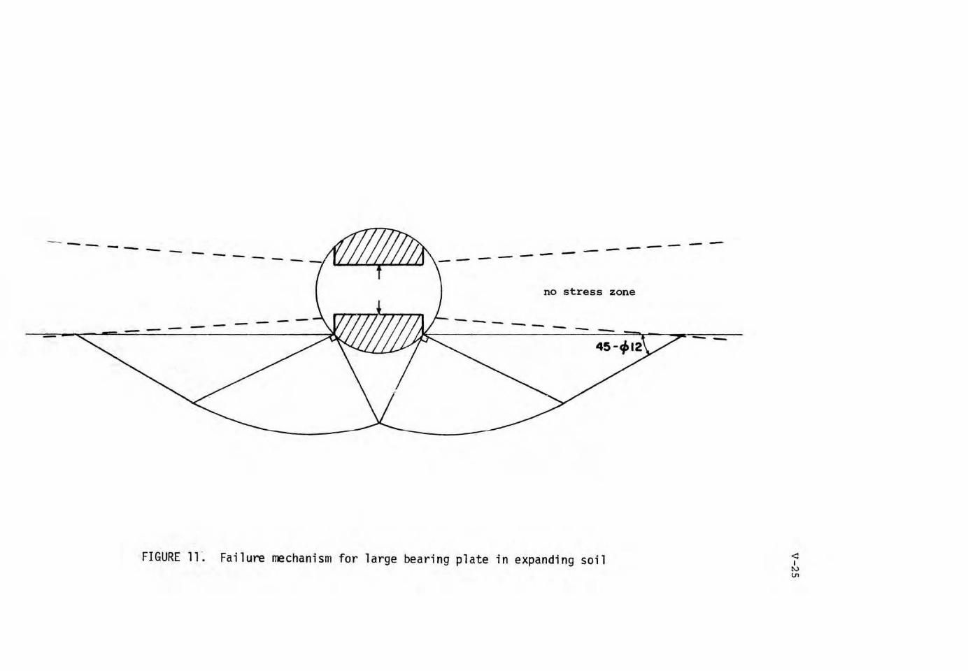
- - --- --- -- --- ----- ---no stress zone

--- --- --- -- --

FIGURE 11 ~ Failure mechanism for large bearing plate in expanding soil

/ / ~.......,~J....U ' \ I \ I

' I \ i '

I '

dealized

' I

plastic zone '

/ /

E , ~t

actual p l ast ic bulb --

FI GURE 12. Mechanism of f ailure i n contrac-~·: n g soils

SOURCES OF REFERENCE

1. Bishop, R. F., Hill, R., and Mott, N. F., "The Theory of Indenta-tion and Hardness Tests", Proceedings of the Physical Society, London, 57/3, pp. 147-159, 1945.

2. Bray, J. W., "A Study of Jointed and Fractured Rocks, Part II, Theory of Limiting Equilibrium", Rock Mech. and Engineering Geology, Vol. 4, 1967.

3. Chen, w. F., "On Solving Plasticity Problems of Relevance to Soil Mechanics ~ The Bearing Capacity of Concrete". Ph.D. Thesis Brown University, 1966.

4. Fairhurst, C., "On the Validity of the Brazilian Test for Brittle Materials", Int. Journal of Hock Mechanics & Mining Sciences, 1, pp. 535-546, 1964.

5 . Finn, W. D. L., "Application of Plasticity in Soil Mechanics". Soil Mechanics and Bituminous Materials Research Laboratory, Univ. of California, Berkeley, August 1965.

6. Gibson, R. E., and Anderson, W. F., "In-situ Measurement of Soil Properties with the Pressuremeter." Civii Engineering & Public Works Review 56, pp. 615-618, 1961.

7. Goodman, R. E., Van, T. K., and Heuze, F., "The Measurement of Rock Deformabili ty in Boreholes.'' Proceedings of the lOth Symposium on Rock Mechanics, AIME, 1968.

8. Goodman, R. E., "Effects of Joints on the Strength of Tunnels, Analysis of Piledriver Drifts." Report of Investigation for u.s. Army Engineer District, Omaha, August 1968.

9. Hill, R., "The Mathematical Theory of Plasticity." Oxford University Press. 1951.

10. Kerisel, J., "La Mecanique des Sols: recherches et investigations recentes." Travaux 42, PP• 874-878, 1968.

V-27

11 . Ladanyi, B .• , "Expansion of a Cavity in Saturated Clay Medium"; Proceedings ASCE, ~Journal of Soil Mechanics and Foundation Division, 89, No. SM-4, pp. 127-161, 1963.

12. , "Expansion of Cavities in Brittle Media", Intern. Journal of Rock Mechanics & Mining Sciences, \Tol. 4, pp. 301-328, 1967.

13. , 1'Rock Failure und~~ Concentrated Loading", Proceedings of the lOth Symposium .on Roc)(. Mechanics·, Texa:s, 1968.

14. Menard, L., "Mesures In-situ des Proprietes ·Physiques des Sols." Annales des Ponts et Ch~ussees, 127, .pp •. 357-377, 1957.

V-28

15. Seeley, F .. B., and Smith, J. o., "Advanced Mechanics of Materials." John Wiley and Sons, Inc., pp. 295-341, New York, 1959.

16. Shield, R. T., "Stress and Velocity Field in Soil Mechanics", Journal of Mathematical Physics, Vol. 33 1 No. 2, pp. 144-156, 1954 .

17. Skempton, A. w., Yassin, A. A., and Gibson, R. E., "'l'heorie de la Force Portante des Pieux dans le Sable", Annales de l'Inst. Tech. Batiment, No. 63-64, p. 285, 1953.

18. Vesic, A. B., and Barksdale 1 R. D. 1 ''Theoretical Studies of Cratering Mechanisms Affecting the Stability of Cratered Slopes.'' Project No. A-655, Eng. Exper. Station, Georgia Inst. of Tech., 1963.

19. Wyanecki , J., "Les Geoextensometres du Centre Experimental de Recherches et d'Etudes du Batiment et des Travaux Publics, Etude Experimentale sur Modeles ~dui ts. " Laboratoire du Batiment e·t Travaux Publics, Supplement aux Annales, No . 246, June 1968.

APPENDIX - DETAILED DESCRIPTION OF MODEL STUDIES

(K. Drozd, T. K. Van, R. E. Goodman)

During the period October 1 to December 31, 1968 research

proceeded in the following domains:

(1) Theoretical determination of the mode of failure taking place,

when a hole in a rock or soil material is uniaxially loaded by

opposed bearing plates.

(2) Model testing to guide and check the theoretical solutions .

V-A-1

The theoretical work (1) was described in the body of the quarterly

report . This appendix describes details of the testing program (2)

conducted during the quarter. The results of these tests will be pre-

sented in the final report of the project.

The research of the fourth quarter of 1968 continued model studies

begun during the summer, in which t:!-1e following e quipment was used:

(1) Uniaxial jack for tests in a circU] .;il- hole 3" in diameter and

1-1/2" deep, equipped with pairs of bearing plates of 4 differ-

ent dimensions. The jack was fitted with a complete hydraulic

device (hydraulic oil pump and lines, manometer for pressures

up to 4000 psi) •

(2) Four model plates made of ·the following mixture (bJt we.ight):

plaster 1.0

celite 0.4

water 1.6

retarder ... .. .. 0.002

The plates were 36"· x 36", 1-1/2" thick, and .. _with a central hole. 3;, ·in

diameter.

(3) Testing bench with base steel plate and upper plexiglass plate

with screws for achieving plain strain condition on the tested

plate.

V-A-2

During th~ conduct of the model tests it became neoessc~y to modify

some of the procedures as the results became available. ThE! modifica-

tions were of four types:

A) Adjustment of the model ja.ck to include a load cell

B) Development of new model. materials and improved fabrication

techniques

C) ·Determination of a convenient method for deformatiorl measure-

ments

D) Preparation of new devices for further model explorations

A. Modification and Adjustment of the Model Jack

During calibration studies the hydraulic pressure meast~ing system

displayed intolerable hysteresis. Therefore a strain gauge dynamometer

was constructed. The dynamometer is a steel ring fitted bet:ween the

hydraulic cylinder and one bearing plate. It has a sensitivrity of

1 micro strain per 2.65 pounds, constantly and reproducibly throughout

the entire 4000 psi ran<3e.

B. Adjustment of Model Plates

The model plates mi;ide of plaster and celite were .cast in a special

font in vertical position . Even if both cast.;ing plates .were stiffened

by frames,. the pressure .of liquid mixture caused a small def'le9tion of

plates, especially in the center part, in the place of the central .. hole.

V-A-3

The deflection amounted to 3/16" over the standard thickness of 1-1/2 ''.

This deflection caused a breaking of one plate during the Test 2 when

the model plate, inserted between steel and plexiglass plate was

loaded by screwing the periphery bolts. We tried to eliminate this

deflection by inserting some thin layers of papers under the model plate.

This arrangement proved to be sufficient but influenced the deformation

in the environment of the loaded bearing plates owing to the high

friction between both units. It was shown that the next model

plates should be cast in a horizontal position directly on the model

table.

At the end of the quarter we tried casting a model plate from a

mixture of sand and parafin. The sand was clean and poorly graded in

the range 0.5 - 1.0 mm {Monterey Sand No. 20). The two components

were mixed hot in a ratio 25:1 {sand:parafin). At the end of the

quarter the characteristic values (~, c, Eo) were not yet available.

The unit weight obtained from three separately made samples was 1.67,

3 1.61, and 1.73 g/cm •

c. Improvement of Deformation Measurements I

Plate displacements were measured with a dial gauge. Owing to the

small thicknes~ of the testing plate, it was not possible to guarantee

parallel movement of both bearing plates. Aiso a small fo} ce in the

spring of the dial gauge indicator increased the deformat.ibns during the

decreasing of load so that the modulus of elasticity of the tested plate

could not be determined. Improvements we~e ~ade to remedy these

deficiencies. Several methods were used to measure borehole deformation.

1) The teste~ area was covered by a brittle coating. This method

failed totally because: a) the coating penetrated the model and changed

its properties; b) the surface of the model plates was insufficiently

smooth; and c) the modulus of elasticity of the plates was too high.

2) The Moire Method of Strain Analysis was used. This method

proved to be quite reliable when plaster-celite plates were used but

proved -inapplicable for plates made of sand-parafin mixture.

3) For parafin-sand plates, regular patterns were created on the

surface of the plates using a mica powder which was sifted over the

surface through a grid of holes. Photogrammetric techniques of

recording and measuring the deformation of grid points were developed.

D. Preparation of New Devices for Further Model E~lorations

V-A-4

The model tests will continue with other materials of varying

properties. Models during this quarter failed either by a tension

cracking, without any visible changes around the hole (plaster-celite

plates) or by a local punching of the bearing plates (sand and parafin

mixture) • Dilatent materials are being prepared to study shear modes of

failure. It is planned to perform tests as well with simulated lunar

soils. The temporary stability of the hole wall will be created by

placing the ~odel under vacuum inside a closed steel frame.

Arrangements started for making a small dilatometer to study

failure modes under this loading configuration as well. A cast was

made for molding the rubber coat of a special polymer. (Adiprene-

Liquid Urethane Elastomer hardened by Moca) •

VI-1

VI. STUDIES ON FLUID ~1NDUCTIVITY OF LUNAR SURFACE MATERIALS

(D. F . Katz, !) , R. Willis, P. A. Witherspoon)

1. INTRODUCTION

In the first quarterly report, the problems in developing a means

of measuring penneability of lunar rocks and soils in situ,using a gas,

were introduced. The design of a lunar permeability probe is dependent

upon a knowledge of the equat ions of motion for a gas flowing through

porous media under lunar C~?Iid i:t ions. Because of the lack of any

atmosphere on the tnoon, the mpecifi9 nature of these equations is not

well understood. Thus, it w.\ls first necessary to develop the fundamental

physics of gaseous flow in lunar soils and rocks.

During the second quarter, theoretical analysis of the physics was

continued. As a result of the physics developed to date,. a general form

of the equations governing flow of gases in lunar soils and rocks has been

deduced. On the basis of only this general form, a simple method has been

developed for measuring lunar permeabilities in situ. The method utilizes

an assumption of local similarity and provides a basis for the first

experimental approach to the problem.

2. LOCAL SIMILARITY ANALYSIS OF 'FLOW IN POROUS MEDIA

In the first quarterly rep~~t~ a general qualitive momentum relation-

ship was described

v = C(p)\i'p (1)

C(p)

VI-2

where~ is the average fluid velocity vector in a pore (see Appendix I),

p is the average pressure, and C is a master diffusion coefficient .

Consider. a steady, isothermal flow field dependent '~pon only one space

variable, denoted by r, i.e. a one-dimensional, cylindrically symmetric ,

or spherically symmetric problem. Henceforth, such flow problems will be

referred to as ''symmetric." Theu Eq. (1) beco)nes

v = C(p)~~ (2)

C(p) can be rendered dimensionless by defining

(3)

'1.1 where ~ is viscosity, C is the dimensionless form of C, and L is an

effective cross-sectional d~.rnension of a pore, the square of which is

termed the permeability, k.

k (4)

~ * It is assumed that C is a function o:t. local pressure (or Knudsen number)

only, as in the Wakao formula described in the first report. This is the

basic local similari't:y assumption. As applied to Eq. (2}, it embodies all

tne necessary physics of the flow field. I'I.J The specific form of C need not

be known.

* Pressure and Knudsen number are inversely proportional. See Appendix B.

Symbol

Type Symmetric Problem

One-Dimensional Cylindrical Spherical

j 0 1 2

"' Q Q/A Q/27f.ll,

---------~----------------------------------------------------------

Q :z

VI-3

Consider now the continuity equation [see .Appendix AJ

(5)

where a. is the area fraction, p the average density, and 0 t.akes on

different values, as shown in Table 1, depending upon the na1t:ure of the

symmetric problem.

TABLE 1

Here Q refers to the dimensional mass flow rate, A is the to·tal cross-

sectional area of the rock in one-dimensional flow, and Jl, is the cylinder

length for cylindrically symmetric flow. Combining Eqs. (2), (3), and (5),

(6)

Assume that the gas is perfect, so that p = PRT, whe1:e R is the ga~

constant and T is average temperature. Then

(7)

VI-4

'U Now, C(p) is dimensionless; hence it can be expressed as a function of a

dimensionless pressure ~:

"' C(p) 1 --F (7;) (8)

'V The particular form of 7; is motivated by the fact that C can be considered

a function of Knudsen number only (see ~ppendix II). Thus

LV 2lJRT p =

1 Kn

where v ·= /B:T·, the mean thermal speed, and Kn is the Knudsen number.

Substituting in Eq. (7) and rearranging,

a.L2 1 rj p ~drd = F(?;) ~lJRT

(9)

(10)

This is a fundamental similarity relatio1n. F (l;) is a "universal" function,

in that data from all symmetric problems, plotted according to Eq. (10),

fall on the same curve. It should be no·t:ed that F (7;) is not the only

possible universal curve. Multiplicatiom by any real ·function of 7;

yields an equally universal curve.

3. METHOD FOR DETERMINING PERMEABILITY AND AREA FRACTION

By developing dimensio~less relatioJnships in this manner, Eq. ( 10)

.can be used to determine both permeabili;t:y, L2 , and the area fraction, a.

For example, if the flow field for -'dle 11llnar probe can be a}>proximated . as

VI-5

spherically symmetric, as has been found by Selim et al. 1 for a related

problem, then j = 2 and ~ = Q/4TI. Equation (10) becomes

'2 [ 4'TT 2 ~] aL Q~RT r P dr = F(l;;) (11)

Since F(l;;) presumably holds for any synunetric flow in porous meda, this

function can be uniquely determined by appropriate experimentation

in the laboratory.

To apply Eq. {11} to an unknown rock sample, one must fix the flow

rate Q and measure temperature T, from which ~ = ~(T) is easily determined.

If pressure taps are appropriately spaced in the skirt of the probe

(cf. Fig. 1 of first quarterly report), then r 2 p ~ ca~ be measured at

two or more different values of r. This enables one to determine two

different values of the bracketed expression in Eq. (11) which are sufficient I

to determine both I. and a.

A simple procedure illustrating the method of calculation can be

outlined as follows. From Eqs. (9) and {11)

ln F(l,;) = 1 [ .: 2 •§.] n r. P dr [

2 4TI J + ln ctL Q~RT

d ln F (l;;} d ln z;; = d ln [r2 p ~]

d ln p

(12a)

(12c)

2~ If follows that curves of F(l,;} vs z;; and r p dr vs p, plotted on identical

log-log scales, differ only in the positions of their respective origin_s

of coordinates. Thus, the two measured -values of r 2 p . d; are plotted· versus ·

p on log-log paper, and F(l;) vs z; is plotted on identical paper. The

two plots are then placed on top of each other, and maneuvered, keeping

respective axes mutually parallel, until the two experimental points

VI-6

lie on the known curve. The coordinates of the origin of the experimental

plot relative to the universal one then clearly yield both a and L.

See Fig. (1).

As drawn in Fig. (1), F(l;) will be a monotonic function of z; .

Ho\>Tever, a problem of uniqueness in determining a and L will arise if

there are regions where, en the log-log scale, F(l;} is locally linear.

If the experimental points correspond to such regions, then the position

of the origin of the experimental plot is not uniquely determined. This

difficulty can, in principle, be circumvented, however, by redefinition

of the universal curve such that it has adequate curvature throughout.

In l In p

~< --DATA POINTS

In (F (€ >) ( 47T 2) In OJLRT aL

FIGURE 1. Example of matching procedure in detennining· permeability and area fraction

A

\ z

FIGUIRE 2

VI-7

VI-8

REFERENC~S

1Selium, M. A., I. Fatt, and W. H. Sanerton, "Temperature Rise in a Semi-Infinite Medium qeated by a Disc Source. Proc. Konkl. Ned. Acad. Wet., Amsterdam, A,~, 5 (November, 1963), pp. 705-720.

2carman, P . c., Flow of Gases Through Porous Media, Academic Press , New York (1956) , pp. 8 and 30.

A -one dimensional

2rrdi - cylindrical symmetry

4rrd2 - spherical symmetry

where

APPENDIX A

In Eq. (5), the area fraction a is defined

"" A

a - f

VI-A-l

(I-1)

(I-2)

(I-3)

Here d is a reference length large compared to a. typical pore length, do

is the diameter of the fluid source (taken to be zero for one-dimensional 'V

flow), and A (r) is the total pore area normal to the flmf/. Thus A p p

represents the pore area, normal to flow, averaged along <i; . and~

is the total cross-sectional·area of the po~ous medium at r =d. The

significance of these quantities will be illustrated for ithe case of one

dimensional flow. Similar descriptions apply to flows wi1th cylindrical or

spherical symmetry.

Consider a one di1nensional flew ~oU:gh a hollow cylinder of cross-

section A, cf .- Fig. ( 2) • · A Cartesian coordinate system r ,, y; z is f _ixed

in the cylinder. The '"average" velo.city and density a.t any st~tion r

are defined, respectively

v(r) - !J J v(r, y, z) dydz A A

- i J J p(r,y,z)dydz p(r) -A

The applied mass flow rate Q is given by

Q = J J p(r,y,z)v(r,y,z)dydz = constant A

pvA

VI-A-2

(I-4)

(I-5)

(I-6a)

(I-6b)

pr represents the average mass flow rate per unit area, and is constant.

Suppose now that the cylinder is filled with a porous material.

A (r) here represents the total pore area projected on a y - z plane, and .p ~ * A is thus the total pore area on an average y - z plane. Now p

Q = P(r,y,z)v(r,y,z)dydz = constant A {r) p

Pv (r) A (r) p

J J

The average velocity and density in a pore are defined

v(r) -1 J J v(r,y,z)dydz

Ap (t·} A {r) p

(I-7a)

(I-7b)

(I-8)

* 'V That is, A is the average of A (r) along the length d on the rock sample, p p where d ·is large compared to a typical pore length so that a large number of differen·t pore cross-sections are · included.

P {r) 1 A (r)

p J J p ( r, y, z) dydz

A (r) p

VI-A-3

(I-9)

Written without the bars, these are the qnanti ties which appear throughout

this report. Similar definitions apply to average pressure and temperature.

Thus far, the continuity equation, cf. Eqs. (I-6b) and {I-7b)l

contains only the product ~v, and is therefore insufficient to be

applicable to the momentum equation! cf. Eq. (2) 1 since ,no distinction is

* made between density and velocity. In order to perform the necessary

separation, some kind of statistical postulate is needed. It is therefore

assumed that

- - 1'\J p(r)v(r)A p

= pv {r)A (r) p

(I-10)

Since Eq. (I-10) must apply to both compressible and incompressible flow, rv it is thus required that A (r) p = A = constant. This has been verified p

experimentally for unconsolidated materials. 2 For consolidated materials,

this assumption is valid for one-dimensional flow; however, for cylindrically

and spherically symmetric flow, it may not hold due to the effects of

anistropy. It follows that

Then, from Eq. (II-7b)

*

pv (r) = p (r)v (r)

- '\i p(~)v(r)A = Q

p

For incompressible flow 1 this problem does not arise 1,\ and the averag.e

(I-ll)

(I-12)

velocity is simply the volumetric flow rate per unit pore area normal to the flow.

Hence, using Eq. (.II-1),

ap(r)v (r) = Q A

vr-A-4

(I-13)

This is the continuity equation for one-dimensional flow in porous meda.

~or a general ·symmetric flow

(I- 14)

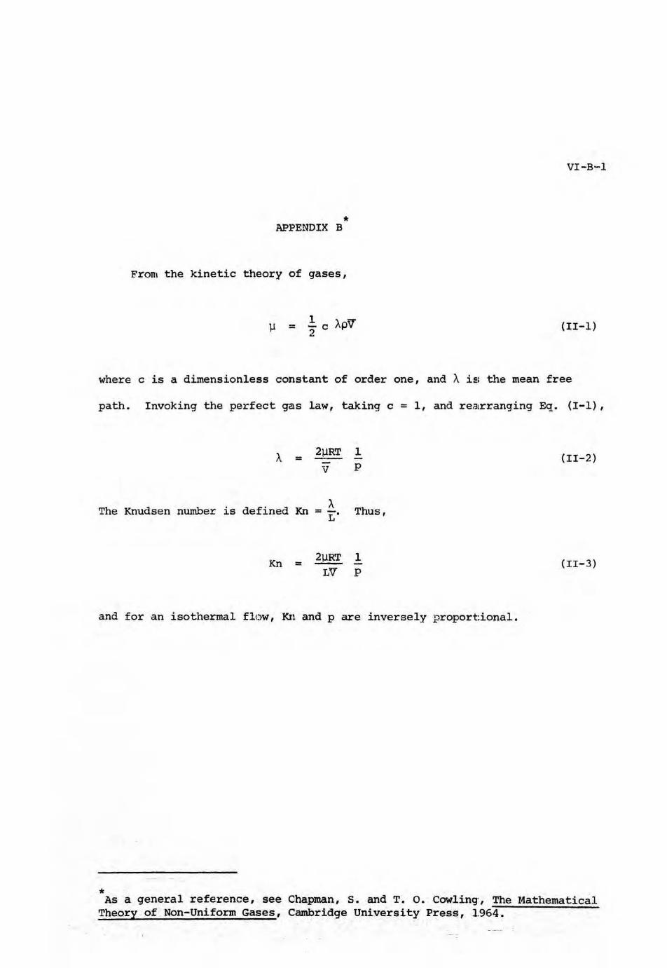
* APPENDIX B

From the kinetic theory of gases,

l.l = I c Ap'V

VI-B-1

(Il-l)

where c i$ a dimensionless constant of order one, and A i~; the mean free

path. Invoking the perfect gas law, taking c = 1, and reatrranging Eq. (I-1),

The Knudsen number is

A 2llRT 1 = v p

defined Kn >.. Thus, = L"

= 2URT 1 LV P

and for an isothermal flow, Kn and p are inversely proport:ional.

*

(II-2)

(II-3)

As a general reference, see Chapman, s. and T. 0. Cowling·,, The Mathematical Theory of Non-Uniform Gases, Cambridge University Press, 1.964.