arX

iv:0

902.

4712

v2 [

astr

o-ph

.CO

] 1

7 M

ar 2

009

Draft version November 3, 2013Preprint typeset using LATEX style emulateapj v. 08/22/09

LYMAN BREAK GALAXIES AT Z ≈ 1.8 − 2.8: GALEX/NUV IMAGING OF THE SUBARU DEEP FIELD1

Chun Ly,2 Matthew A. Malkan,2 Tommaso Treu,3 Jong-Hak Woo,2,4 Thayne Currie,5 Masao Hayashi,6 NobunariKashikawa,7,8 Kentaro Motohara,9 Kazuhiro Shimasaku,6,10 and Makiko Yoshida6

Draft version November 3, 2013

ABSTRACT

A photometric sample of ∼7100 V < 25.3 Lyman break galaxies (LBGs) has been selected bycombining Subaru/Suprime-Cam BV RCi′z′ optical data with deep GALEX/NUV imaging of theSubaru Deep Field. Follow-up spectroscopy confirmed 24 LBGs at 1.5 . z . 2.7. Among the opticalspectra, 12 have Lyα emission with rest-frame equivalent widths of ≈ 5 − 60A. The success rate foridentifying LBGs as NUV-dropouts at 1.5 < z < 2.7 is 86%. The rest-frame UV (1700A) luminosityfunction (LF) is constructed from the photometric sample with corrections for stellar contaminationand z < 1.5 interlopers (lower limits). The LF is 1.7 ± 0.1 (1.4 ± 0.1 with a hard upper limit onstellar contamination) times higher than those of z ∼ 2 BXs and z ∼ 3 LBGs. Three explanationswere considered, and it is argued that significantly underestimating low-z contamination or effectivecomoving volume is unlikely: the former would be inconsistent with the spectroscopic sample at 93%confidence, and the second explanation would not resolve the discrepancy. The third scenario is thatdifferent photometric selection of the samples yields non-identical galaxy populations, such that someBX galaxies are LBGs and vice versa. This argument is supported by a higher surface density of LBGsat all magnitudes while the redshift distribution of the two populations is nearly identical. This study,when combined with other star-formation rate (SFR) density UV measurements from LBG surveys,indicates that there is a rise in the SFR density: a factor of 3− 6 (3− 10) increase from z ∼ 5 (z ∼ 6)to z ∼ 2, followed by a decrease to z ∼ 0. This result, along with past sub-mm studies that find apeak at z ∼ 2 in their redshift distribution, suggest that z ∼ 2 is the epoch of peak star-formation.Additional spectroscopy is required to characterize the complete shape of the z ∼ 2 LBG UV LF viameasurements of AGN, stellar, and low-z contamination and accurate distances.Subject headings: galaxies: photometry — galaxies: high redshift — galaxies: luminosity function —

galaxies: evolution

1. INTRODUCTION

Over the past decade, the number of Lyman breakgalaxies (LBGs; for a review, see Giavalisco 2002) identi-fied at z ∼ 3 − 6 has grown rapidly from deep, wide-field optical imaging surveys (e.g., Steidel et al. 1999;Bouwens et al. 2006; Yoshida et al. 2006). Follow-upspectroscopy on large telescopes has shown that thismethod (called the Lyman break technique or the “drop-out” method) is efficient at identifying high-z star-

Electronic address: chun@astro.ucla.edu1 Based on data obtained at the W.M. Keck Observatory (oper-

ated as a scientific partnership among the California Institute ofTechnology, the University of California, and NASA), the SubaruTelescope (operated by the National Astronomical Observatory ofJapan), and the MMT Observatory (a joint facility of the Univer-sity of Arizona and the Smithsonian Institution).

2 Department of Physics and Astronomy, UCLA, Los Angeles,CA.

3 Department of Physics, UCSB, Santa Barbara, CA.4 Hubble fellow.5 Harvard-Smithsonian Center for Astrophysics, Cambridge,

MA.6 Department of Astronomy, School of Science, University of

Tokyo, Bunkyo, Tokyo, Japan.7 Optical and Infrared Astronomy Division, National Astronom-

ical Observatory, Mitaka, Tokyo, Japan.8 Department of Astronomy, School of Science, Graduate Uni-

versity for Advanced Studies, Mitaka, Tokyo, Japan.9 Institute of Astronomy, University of Tokyo, Mitaka, Tokyo,

Japan.10 Research Center for the Early Universe, School of Science,

University of Tokyo, Tokyo, Japan.

forming galaxies. Furthermore, these studies have mea-sured the cosmic star-formation history (SFH) at z > 3,which is key for understanding galaxy evolution. It indi-cates that the star-formation rate (SFR) density is 10 ormore times higher in the past than at z ∼ 0.

Extending the Lyman break technique to z < 3 re-quires deep, wide-field UV imaging from space, which isdifficult. In addition, [O II] (the bluest optical nebularemission line) is redshifted into the near-infrared (NIR)for z & 1.5 where high background and lower sensitiv-ity limit surveys to small samples (e.g., Malkan et al.1996; Moorwood et al. 2000; van der Werf et al. 2000;Erb et al. 2003). The combination of these observationallimitations has made it difficult to probe z ≈ 1.5 − 2.5.

One solution to the problem is the ‘BX’ method devel-oped by Adelberger et al. (2004). This technique iden-tifies blue galaxies that are detected in U , but show amoderately red U −G color when the Lyman continuumbreak begins to enter into the U -band at z ∼ 2.

Other methods have used NIR imaging to identifygalaxies at z = 1 − 3 via the Balmer/4000A break.For example, selection of objects with J − K > 2.3(Vega) has yielded “distant red galaxies” at z ∼ 2 − 3(van Dokkum et al. 2004), and the ‘BzK’ method hasfound passive and star-forming (dusty and less dusty)galaxies at z ≈ 1.5−2.5 (Daddi et al. 2004; Hayashi et al.2007). The completeness of these methods is not aswell understood as UV-selected techniques, since limitedspectra have been obtained.

2 Ly et al.

In this paper, the Lyman break technique is extendeddown to z ∼ 1.8 with wide-field, deep NUV imaging ofthe Subaru Deep Field (SDF) with the Galaxy EvolutionExplorer (GALEX; Martin et al. 2005). This survey hasthe advantage of sampling a large contiguous area, whichallows for large scale structure studies (to be discussedin future work), an accurate measurement of a large por-tion of the luminosity function, and determining if theSFH peaks at z ∼ 2.

In § 2, the photometric and spectroscopic observa-tions are described. Section 3 presents the color selec-tion criteria to produce a photometric sample of NUV-dropouts, which are objects undetected or very faint inthe NUV, but present in the optical. The removal offoreground stars and low-z galaxy contaminants, andthe sample completeness are discussed in § 4. In § 5,the observed UV luminosity function (LF) is constructedfrom ∼7100 NUV-dropouts in the SDF, and the comov-ing star-formation rate (SFR) density at z = 1.8− 2.8 isdetermined. Comparisons of these results with previoussurveys are described in § 6, and a discussion is providedin § 7. The appendix includes a description of objectswith unusual spectral properties. A flat cosmology with[ΩΛ, ΩM , h70] = [0.7, 0.3, 1.0] is adopted for consistencywith recent LBG studies. All magnitudes are reportedon the AB system (Oke 1974).

2. OBSERVATIONS

This section describes the deep NUV data obtained(§ 2.1), followed by the spectroscopic observations (§ 2.2and 2.4) from Keck, Subaru, and MMT (Multiple Mir-ror Telescope). An objective method for obtaining red-shifts, cross-correlating spectra with templates, is pre-sented (§ 2.3) and confirms that most NUV-dropouts areat z ∼ 2. These spectra are later used in § 3.2 to definethe final empirical selection criteria for z ∼ 2 LBGs. Asummary of the success rate for finding z ∼ 2 galaxies asNUV-dropouts is included.

2.1. GALEX/NUV Imaging of the SDF

The SDF (Kashikawa et al. 2004), centered atα(J2000) = 13h24m38.s9, δ(J2000) = +2729′25.′′9, isa deep wide-field (857.5 arcmin2) extragalactic sur-vey with optical data obtained from Suprime-Cam(Miyazaki et al. 2002), the prime-focus camera mountedon the Subaru Telescope (Iye et al. 2004). It was im-aged with GALEX in the NUV (1750− 2750A) between2005 March 10 and 2007 May 29 (GI1-065) with a totalintegration time of 138176 seconds. A total of 37802objects are detected in the full NUV image down toa depth of ≈27.0 mag (3σ, 7.5′′ diameter aperture).The GALEX-SDF photometric catalog will be presentedin future work. For now, objects undetected or faint(NUV > 25.5) in the NUV are discussed.

The NUV image did not require mosaicking to coverthe SDF, since the GALEX field-of-view (FOV) is largerand the center of the SDF is located at (+3.87′, +3.72′′)from the center of the NUV image. The NUV spa-tial resolution (FWHM) is 5.25′′, and was found tovary by no more than 6% across the region of interest(Morrissey et al. 2007).

2.2. Follow-up Spectroscopy

Fig. 1.— Postage stamps for some NUV-dropouts targeted withLRIS. From left to right is NUV, B, and V . Each image is 24′′ ona side and reveals that optical sources do not have a NUV coun-terpart. Photometric and spectroscopic information are providedin Table 1.

2.2.1. Keck/LRIS

When objects for Keck spectroscopy were selected, theNUV observations had accumulated 79598 seconds. Al-though the selection criteria and photometric catalog arerevised later in this paper, a brief description of the origi-nal selection is provided, since it is the basis for the Kecksample. An initial NUV-dropout catalog (hereafter ver.1) of sources with NUV − B > 1.5 and B − V < 0.5was obtained. No aperture correction was applied tothe 7.5′′ aperture NUV flux and the 2′′ aperture wasused for optical photometry. These differ from the fi-nal selection discussed in § 3.2. The NUV 3σ limit-ing magnitude for the ver. 1 catalog is 27.0 within a3.39′′ radius aperture. Postage stamps (see Figure 1)were examined for follow-up targets to ensure that theyare indeed NUV-dropouts. The Keck Low ResolutionImaging and Spectrograph (LRIS; Oke et al. 1995) wasused to target candidate LBGs in multi-slit mode on2007 January 23−25. The total integration times wereeither 3400, 3600, or 4833 seconds, and 36 NUV-dropoutswere targeted within 3 slitmasks. A dichroic beam split-ter was used with the 600 lines mm−1 grism blazed at4000A and the 400 lines mm−1 grating blazed at 8500A,yielding blue (red) spectral coverage of 3500 − 5300A(6600−9000A), although the coverages varied with loca-tion along the dispersion axis. The slits were 4′′ to 8′′ inlength and 1′′ in width, yielding spectral resolution of≈0.9A at 4300A and ≈1.2A at 8000A.

Standard methods for reducing optical spectra werefollowed in PyRAF where an IRAF script, developed byK. Adelberger to reduce LRIS data, was used. Whenreducing the blue spectra, dome flat-fields were not useddue to the known LRIS ghosting problem. Other LRISusers have avoided flat-fielding their blue spectra, sincethe CCD response is mostly flat (D. Stern, priv. comm).

HgNe arc-lamps were used for wavelength calibrationof the blue side while OH sky-lines were used for thered side. Typical wavelength RMS was less than 0.1A.For flux calibration, long-slit spectra of BD+26 2606(Oke & Gunn 1983) were obtained following the last ob-servation for each night.

Lyman Break Galaxies at z = 1.8 − 2.8 3

In the first mask, three of five alignment stars had coor-dinates that were randomly off by as much as 1′′ from thetrue coordinates. These stars were taken from the USNOcatalog, where as the better alignment stars were fromthe 2MASS catalog with a few tenths of an arcsecondoffsets. This hindered accurate alignment, and resultedin a lower success rate of detection: the first mask had 7of 12 NUV-dropouts that were not identified, while theother two masks had 2/10 and 3/14.

2.2.2. MMT/Hectospec

Spectra of NUV-dropouts from the final photomet-ric catalog were obtained with the multifiber opticalspectrograph Hectospec (Fabricant et al. 2005) on the6.5m MMT on 2008 March 13 and April 10, 11, and14. Compared to Keck/LRIS, MMT/Hectospec has asmaller collecting area and lower throughput in the blue,so fewer detections were anticipated. Therefore, obser-vations were restricted to bright (Vauto = 22.0 − 23.0)sources, which used 21 of 943 fibers from four configu-rations. Each source was observed in four, six, or seven20-minute exposures using the 270 mm−1 grating. Thisyielded a spectral coverage of 4000− 9000A with 6A res-olution. The spectra were wavelength calibrated, andsky-subtracted using the standard Hectospec reductionpipeline (Fabricant et al. 2005). A more detailed discus-sion of these observations is deferred to a forthcomingpaper (Ly et al. 2008, in prep.).

2.3. Spectroscopic Identification of Sources

The IRAF task, xcsao from the rvsao package(Kurtz & Mink 1998, ver. 2.5.0), was used to cross-correlate with six UV spectral templates of LBGs. Forcases with Lyα in emission, the composite of 811 LBGsfrom Shapley et al. (2003) and the two top quartilebins (in Lyα equivalent width) of Steidel et al. (2003)were used. For sources lacking Lyα emission (i.e., pureabsorption-line systems), the spectra of MS 1512-cB58(hereafter ‘cB58’) from Pettini et al. (2000), and the twolowest quartile bins of Steidel et al. (2003) were used.

When no blue features were present, the red end ofthe spectrum was examined. An object could still beat z > 1.5, but at a low enough redshift for Lyα tobe shortward of the spectral window. In this case,rest-frame NUV features, such as Fe II and Mg II, areavailable. Savaglio et al. (2004) provided a compositerest-frame NUV spectrum of 13 star-forming galaxies at1.3 < z < 2. For objects below z ≈ 1.5, optical featuresare available to determine redshift. The composite SDSSspectra (3500 − 7000A coverage) from Yip et al. (2004)and those provided with rvsao (3000− 7000A) are usedfor low-z cases. Note that in computing redshifts, sev-eral different initial guesses were made to determine theglobal peak of the cross-correlation. In most cases, thesolutions converged to the same redshift when the initialguesses are very different. The exceptions are classifiedas ‘ambiguous’.

Where spectra had poor S/N, although a redshift wasobtained for the source, the reliability of identification(as given by xcsao’s R-value) was low (R = 2 − 3).An objective test, which was performed to determinewhat R-values are reliable, was to remove the Lyα emis-sion from those spectra and templates, and then re-run

400000 450000 500000 550000 600000

-0.1

0

0.1

0.2

500000 550000 600000

-0.1

0

0.1

0.2

750000 800000 850000

-0.1

0

0.1

0.2

600000 650000 700000 750000

-0.1

0

0.1

0.2

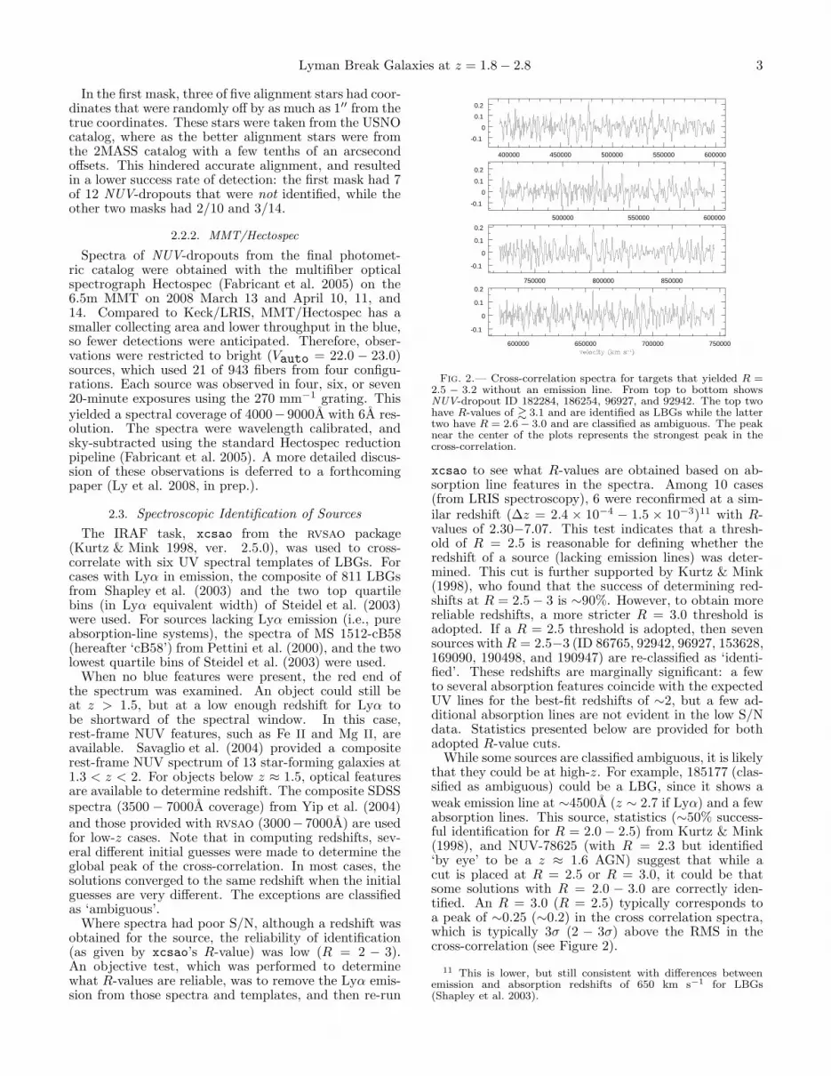
Fig. 2.— Cross-correlation spectra for targets that yielded R =2.5 − 3.2 without an emission line. From top to bottom showsNUV-dropout ID 182284, 186254, 96927, and 92942. The top twohave R-values of & 3.1 and are identified as LBGs while the lattertwo have R = 2.6 − 3.0 and are classified as ambiguous. The peaknear the center of the plots represents the strongest peak in thecross-correlation.

xcsao to see what R-values are obtained based on ab-sorption line features in the spectra. Among 10 cases(from LRIS spectroscopy), 6 were reconfirmed at a sim-ilar redshift (∆z = 2.4 × 10−4 − 1.5 × 10−3)11 with R-values of 2.30−7.07. This test indicates that a thresh-old of R = 2.5 is reasonable for defining whether theredshift of a source (lacking emission lines) was deter-mined. This cut is further supported by Kurtz & Mink(1998), who found that the success of determining red-shifts at R = 2.5 − 3 is ∼90%. However, to obtain morereliable redshifts, a more stricter R = 3.0 threshold isadopted. If a R = 2.5 threshold is adopted, then sevensources with R = 2.5−3 (ID 86765, 92942, 96927, 153628,169090, 190498, and 190947) are re-classified as ‘identi-fied’. These redshifts are marginally significant: a fewto several absorption features coincide with the expectedUV lines for the best-fit redshifts of ∼2, but a few ad-ditional absorption lines are not evident in the low S/Ndata. Statistics presented below are provided for bothadopted R-value cuts.

While some sources are classified ambiguous, it is likelythat they could be at high-z. For example, 185177 (clas-sified as ambiguous) could be a LBG, since it shows aweak emission line at ∼4500A (z ∼ 2.7 if Lyα) and a fewabsorption lines. This source, statistics (∼50% success-ful identification for R = 2.0 − 2.5) from Kurtz & Mink(1998), and NUV-78625 (with R = 2.3 but identified‘by eye’ to be a z ≈ 1.6 AGN) suggest that while acut is placed at R = 2.5 or R = 3.0, it could be thatsome solutions with R = 2.0 − 3.0 are correctly iden-tified. An R = 3.0 (R = 2.5) typically corresponds toa peak of ∼0.25 (∼0.2) in the cross correlation spectra,which is typically 3σ (2 − 3σ) above the RMS in thecross-correlation (see Figure 2).

11 This is lower, but still consistent with differences betweenemission and absorption redshifts of 650 km s−1 for LBGs(Shapley et al. 2003).

4 Ly et al.

2.3.1. LRIS Results

12 (14 with R ≥ 2.5) LBGs are found at 1.7 . z . 2.7out of 36 attempts. Among those, 10 show Lyα in emis-sion, while 2 (4 with R ≥ 2.5) are identified purely byUV absorption lines. Their spectra are shown in Fig-ures 3 and 4, and Table 1 summarizes their photometricand spectroscopic properties. Contamination was foundfrom 3 stars and 5 (7 with R ≥ 2.5) low-z galaxies (shownin Figure 5), corresponding to a 60% success rate (58% ifR > 2.5 is adopted). Four sources showed a single emis-sion line, which is believed to be [O II] at z ∼ 1−1.5, onesource showed [O II], Hβ, and [O III] at z ∼ 0.7, and twosources with absorption lines have R ∼ 2.5 results withz ∼ 0.1 and ∼ 0.5 (these would be “ambiguous” withthe R ≥ 3.0 criterion). The success of identifying z ∼ 2LBGs improves with different color selection criteria thatremove most interlopers (see § 3.2).

Of the remaining 16 spectra (12 with R > 2.5 cut), 8(4 with R > 2.5 cut) were detected, but the S/N of thespectra was too low, and the other 8 were undetected.These objects were unsuccessful due to the short integra-tion time of about one hour and their faintness (averageV magnitude of 24.2).

It is worthwhile to indicate that the fraction of LRISspectra with Lyα emission is high (83%). In comparison,Shapley et al. (2003) reported that 68% of their z ∼ 3spectroscopic sample contained Lyα in emission. If thefraction of LBGs with Lyα emission does not increasefrom z ∼ 3 to z ∼ 2, it would imply that 5 z ∼ 2 galaxieswould not show Lyα in emission. Considering the diffi-culties with detecting Lyα in absorption with relativelyshort integration times, the above 83% is not surprising,and suggests that most of the z > 1.5 ambiguous LRISredshifts listed in Table 1 are correct.

2.3.2. Hectospec Results

Among 21 spectra, 7 objects (2 are AGNs) are iden-tified (R > 3.0; 9 if R > 2.5) at z > 1.5, 2 objects arestars, 1 (2 with R > 2.5) is a z < 1.5 interloper, and 11are ambiguous (8 if R > 2.5 is adopted). These MMTspectra are shown in Figures 6−8, and their propertiesare listed in Table 1.

The spectrum of a RC∼ 22 z ∼ 1.6 LBG detected theFe II and Mg II absorption lines, which indicates thatMMT is sensitive enough to detect luminous LBGs. Infact, since the surface density of bright LBGs is low, slit-mask instruments are not ideal for the bright end. How-ever, the entire SDF can be observed with Hectospec,so all ∼150 Vauto < 23.0 objects can be simultaneouslyobserved.

2.4. Additional Spectra with Subaru/MOIRCS

The BzK technique, which identifies galaxies with awide range (old and young, dusty and unreddened) ofproperties, could include objects that would also be clas-sified as NUV-dropouts. As a check, cross-matching ofspectroscopically identified star-forming BzK’s with theGALEX-SDF photometric catalog was performed. Spec-tra of BzKs were obtained on 2007 May 3−4 with Subaruusing the Multi-Object Infrared Camera and Spectro-graph (MOIRCS; Ichikawa et al. 2006). 44 sources weretargeted and 15 were identified by the presence of Hαand [N II] or [O II], [O III] and Hβ emission. One of the

15 was not in the B-band catalog. Among the 14 ob-jects, 7 are also classified as NUV-dropouts and were notpreviously identified (i.e., LRIS or Hectospec targets).This included 5 galaxies at z > 1.5 and 2 at z = 1− 1.5.Their properties are included in Table 1. Among the 7BzKs that did not meet the NUV-dropout criteria, 2 arebelow z = 1.5 and the other five are at high-z. For twoof the high-z BzKs, one was below the NUV −B = 1.75cut because it is faint (V > 25.3), thus not considereda NUV-dropout, and the other missed the B − V = 0.5selection by having B − V = 0.53.12 The other threesources have low-z neighboring sources that are detectedin the NUV, which influences the NUV photometry tobe brighter. The cause of confusion is due to the poorresolution of GALEX, which is discussed further in § 4.3.The details of these observations and their results aredeferred to Hayashi et al. (2008).

2.5. Summary of Observations

In order to probe 1.5 < z < 3 with the Lyman breaktechnique, deep (>100 ks) GALEX/NUV imaging wasobtained. Spectroscopic observations from Keck andMMT independently confirm that most NUV-dropouts(with their UV continuum detected spectroscopically)are found to be at 1.5 < z < 2.7.

A summary of the number of LBGs, stars, and low-zinterlopers identified spectroscopically is provided in Ta-ble 2. Among the spectra targeting NUV-dropouts (i.e.,excluding MOIRCS spectra), 53% (30/57) were identi-fied, and among those, 63% are at z > 1.5. Includingseven objects with R = 2.5 − 3.0, the percentages are65% and 62%, respectively. These statistics are improvedwith the final selection criteria discussed in § 3.2.

3. PHOTOMETRIC SELECTION OF NUV-DROPOUTS

This section describes the NUV and optical photomet-ric catalogs (§ 3.1) and the methods for merging the twocatalogs. Then in § 3.2, ∼8000 NUV-dropouts are empir-ically identified with the spectroscopic sample to refinethe selection criteria.

3.1. Revised NUV Photometric Catalogs

Prior to any measurements, an offset (∆α = −0.39′′,∆δ = −0.18′′) in the NUV image coordinates was appliedto improve the astrometry for alignment with Suprime-Cam data. The scatter in the astrometric correctionswas found to be σ∆α=0.39′′ and σ∆δ=0.33′′. This onlyresults in a 0.01 mag correction for NUV measurements,and is therefore neglected.

The coordinates of ∼100000 SDF B-band sourceswith Bauto < 27.5 were used to measure NUV fluxeswithin a 3.39′′ (2.26 pixels) radius aperture with theiraf/daophot task, phot. For objects with NUV pho-tometry below the 3σ background limit, the 3σ value isused. This limit is determined from the mode in an an-nulus with inner and outer radii of 22.5′′ and 37.5′′ (i.e.,an area of 1200 pixels), respectively. For sources detectedin the NUV, a point-source aperture correction of a fac-tor of ≈1.83 is applied to obtain the “total” NUV flux.This correction was determined from the point spread

12 If the selection criteria were modified to include this object,no low-z interlopers or stars would have contaminated the criteria.However, a B − V ≤ 0.5 is still adopted for simplicity.

Lyman Break Galaxies at z = 1.8 − 2.8 5

Fig. 3.— LRIS spectra of confirmed NUV-dropouts from the ver. 1 catalog with known redshifts. Most of the LBGs with Lyα emissionare shown here with the remaining in Figure 4. Overlayed on these spectra is the composite template (shown as grey) with the highestR-value (see Table 1) from cross-correlation. Note that these overlayed templates are intended to show the location of spectral features, andis not meant to compare the flux and/or the spectral index differences between the spectra and the templates. The ID number, redshifts,and R-values are shown in the upper left-hand corner of each panel. [See the electronic edition of the Journal for a color version of thisfigure.]

function (PSF) of 21 isolated sources distributed acrossthe image. The NUV catalog is then merged with the B-band catalog from SExtractor (SE; Bertin & Arnouts1996) that contains BV RCi′z′ photometry.

Throughout this paper, “total” magnitudes from theSuprime-Cam images are given by SE mag auto, sincethe corrections between B-band Kron and the 5′′ diame-ter magnitudes were no greater than 0.03 mag for isolated(5′′ radius), point-like (SE class star ≥ 0.8) targets.

The merged catalog was also corrected for galactic ex-tinction based on the Cardelli et al. (1989) extinctionlaw. For the SDF, they are: A(NUV) = 0.137, A(B)= 0.067, A(V ) = 0.052, A(RC) = 0.043, A(i′) = 0.033,and A(z′) = 0.025. Since the Galactic extinction for theSDF is low, the amount of variation in A(NUV) is nomore than 0.02, so all NUV magnitudes are corrected bythe same value.

3.2. Broad-band Color Selection

Using the sample of spectroscopically confirmed z >1.5 LBGs, low-z interlopers, and stars, the color selectionis optimized to minimize the number of interlopers whilemaximizing the number of confirmed LBGs. In Figure 9,known LBGs are identified in the NUV − B versus B −V diagram, where the NUV − B color is given by the“total” magnitude and the B − V is the color within a2′′ aperture. The latter was chosen because of the higherS/N compared to larger apertures. The final empiricalselection criteria for the LBG sample are:

NUV − B ≥ 1.75, (1)

B − V ≤ 0.50, and (2)

NUV − B ≥ 2.4(B − V ) + 1.15, (3)

which yielded 7964 NUV-dropouts with 21.90 ≤ V ≤25.30. Among the Hectospec and LRIS spectra, these

6 Ly et al.

Fig. 4.— Same as Figure 3, but some spectra do not have Lyα emission. The strong line seen in the spectrum of 96927 at ∼5570A isa sky subtraction artifact, and cosmic rays are seen in the spectra of 94093 (at 3780A), 186254 (at 3325A), and 92942 (at 3990A). Thesefeatures are removed in the cross-correlation process. [See the electronic edition of the Journal for a color version of this figure.]

selection criteria included all spectroscopic LBGs and ex-cluded 4/5 stars and 4/6 (4/9 with R > 2.5) interlopers.Therefore, the fraction of NUV-dropouts that are con-firmed to be LBGs with the new selection criteria is 86%(the R = 2.5 cut implies 79%). Note that while theB-band catalog was used (since the B filter is closer inwavelength to the NUV), the final magnitude selectionwas in V , to compare with the rest-frame wavelength(≈1700A) of z ∼ 3 LBGs in the R-band.

To summarize, a NUV-optical catalog was created, andit was combined with spectroscopic redshifts to select7964 NUV-dropouts with NUV − B ≥ 1.75, B − V ≤0.50, NUV − B ≥ 2.4(B − V ) + 1.15, and 21.90 ≤ V ≤25.30. The spectroscopic sample indicates that 14% ofNUV-dropouts are definite z ≤ 1.5 interlopers.

4. CONTAMINATION AND COMPLETENESS ESTIMATES

Prior to constructing a normalized luminosity function,contaminating sources that are not LBGs must be re-moved statistically. Section 4.1 discusses how foreground

stars are identified and removed, which was found to bea 4−11% correction. Section 4.2 describes the methodfor estimating low-z contamination, and this yielded acorrection of 34% ± 17%. These reductions are appliedto the number of NUV-dropouts to obtain the surfacedensity of z ∼ 2 LBGs. Monte Carlo (MC) realizationsof the data, to estimate the completeness and the effec-tive volume of the survey, are described in § 4.3. Thelatter reveals that the survey samples z ≈ 1.8 − 2.8.

4.1. Removal of Foreground Stars

The Gunn & Stryker (1983) stellar track passes abovethe NUV-dropout selection criteria box (as shown in Fig-ure 9). This poses a problem, as objects that are unde-tected in the NUV can be faint foreground stars. A sim-ple cut to eliminate bright objects is not sufficient, be-cause faint halo stars exist in the SDF (as shown later).To reduce stellar contamination, additional photomet-ric information from the SExtractor BV Rci

′z′ catalogsis used. The approach of creating a “clean” sample of

Lyman Break Galaxies at z = 1.8 − 2.8 7

Fig. 5.— Same as Figures 3 and 4, but this shows the z < 1.5 interlopers and galactic stars. [See the electronic edition of the Journalfor a color version of this figure.]

point-like sources, as performed by Richmond (2005), isfollowed. He used the class star parameter and thedifference (δ) between the 2′′ and 3′′ aperture magni-tudes for each optical image. A ‘1’ is assigned whenthe class star value is 0.90 − 1.00 or 0.10 < δ < 0.18,and ‘0’ otherwise for each filter. The highest score is 10[(1+1)×5], which 2623 Vauto = 21.9 − 26.0 objects sat-isfied, and is referred to as “perfect” point-like or “rank10” object. These rank 10 objects will be used to definethe stellar locus, since contamination from galaxies is lessof a problem for the most point-like sample. Then ob-jects with lower ranks that fall close to the stellar locuswill also be considered as stars after the locus has beendefined.

Unfortunately, distant galaxies can also appearpoint-like, and must be distinguished from stars. Thisis done by comparing their broad-band optical colors rel-ative to the stellar locus. Figure 10 shows the B − V ,V −RC, and RC − z′ colors used in Richmond (2005) forthe “clean” sample. The stellar locus is defined by thesolid black lines using brighter (V ≤ 23.0) sources. Fig-ure 10 shows differences in the colors between the stellarlocus defined for point-like SDF stars and those of Gunn-Stryker stars. Richmond (2005) states that this is dueto metallicity, as the SDF and Gunn-Stryker stars areselected from the halo and the disk of the Galaxy, re-spectively.

For each object in the clean sample, the V − RC coloris used to predict the B − V and RC − z′ colors alongthe stellar locus (denoted by ‘S.L.’ in the subscript of thecolors below). These values are then compared to the ob-served colors to determine the magnitude deviation fromthe stellar locus, ∆ = −[(B − V )obs − (B − V )S.L.] +[(RC − z′)obs − (RC − z′)S.L.]. Therefore, an object with∆ ≈ 0 mag is classified as a star. This method is similarto what is done in Richmond (2005), where an objectis considered a star if it is located within the stellar lo-cus “tube” in multi-color space. This approach provides

stellar contamination at faint magnitudes, which is diffi-cult spectroscopically (Steidel et al. 2003). A histogramshowing the distribution of ∆ in Fig. 11a reveals twopeaks: at ∆ ≈ 0 and 0.8 mag. The comparison of ∆versus the V -band magnitude is shown in Fig. 11b, anda source is identified as a star if it falls within the se-lection criteria shown by the solid lines in this figure.A total of 1431 stars V ≤ 26.0 are identified, while theremaining 1192 sources are classified as galaxies. Thesurface density as a function of magnitude for the iden-tified stars agrees with predictions made by Robin et al.(2003) and other surface density measurements near thegalactic pole. When the NUV-dropout selection criteriaare applied13, these numbers are reduced to 336 stars(i.e., a 4% contamination for the NUV-dropout sample)and 230 galaxies with 21.9 ≤ Vauto ≤ 25.3.

Sources that are ranked 7 − 9 are also considered andwere classified as a star or a galaxy using the above ap-proach. Of those that met the NUV-dropout criteria, 535and 252 have the colors of stars and galaxies, respectively.Thus, the photometric sample of NUV-dropouts contains7093 objects after statistically removing 871 stars (11%of the NUV-dropout) that are ranked 7−10. The reasonsfor only considering objects with a rank of 7 or greaterare (1) the stellar contamination does not significantlyincrease by including rank 6 or rank 5 objects (i.e., an-other 128 rank 6 stars or 1.5% and 143 rank 5 stars or1.8%), and (2) comparison of the surface density of rank7−10 stars with expectations from models showed ev-idence for possible contamination from galaxies at thefaint end (V > 24.0; A. Robin, priv. comm.), and theproblem will worsen with rank 5 and 6 objects included.As it will be apparent later in this paper, stellar contam-ination is small and not expected to significantly alterany discussion of differences seen in the luminosity func-

13 The B − V and NUV − B color cuts limit the stellar sampleto spectral types between A0 and G8.

8 Ly et al.

Fig. 6.— Same as Figures 3 and 4, but these are Hectospec observations of LBGs in the final photometric catalog. The cross-correlationtemplate and the typical sky spectrum are shown above and below the spectrum of the source, respectively. [See the electronic edition ofthe Journal for a color version of this figure.]

tion. A hard upper limit by considering objects of rank1 and above as stars would imply an additional (rank 1to 6) stellar contamination of 14.5%.

Among the 5 sources spectroscopically determinedto be stars, 3 of them (71239, 66611, and 149720) areclassified as stars with the ∆ method, and the other twostars (86900 and 178741) fall outside the ∆ selection cri-teria. Among the known LBGs, 8 are rank 8−10 and 3(166380, 78625, and 133660) are classified as not beingstars. Since the spectroscopic sample of rank 10 objectsis small, additional spectra will be required to furtheroptimize the ∆ technique. However, the spectroscopicsample (presented in this paper) indicates that 3 − 7%of NUV-dropouts are stars, which is consistent with the4 − 11% derived with the ∆ method.

4.2. Contamination from z < 1.5 Interlopers

One of the biggest concerns in any survey targetinga particular redshift range is contamination from other

redshifts. The spectroscopic sample of NUV-dropoutsshows that 5% are definite z < 1.5 galaxies. This num-ber increases to an upper value of 51% if the ambiguousNUV-dropouts (that meet the color selection criteria) areall assumed to be low-z interlopers. However, it is un-likely that all unidentified NUV-dropouts are low-z, sinceLBGs without Lyα emission in their spectra14 are likelymissed. A secondary independent approach for estimat-ing low-z contamination, which is adopted later in thispaper, is by using a sample of z < 1.5 emission-line galax-ies identified with narrow-band (NB) filters. Since a de-tailed description of this sample is provided in Ly et al.(2007), only a summary is given below:A total of 5260 NB emitters are identified from their ex-cess fluxes in the NB704, NB711, NB816, or NB921 filtereither due to Hα, [O III], or [O II] emission line in 12

14 Either because they do not possess Lyα in emission or theyare at too low of a redshift for Lyα to be observed.

Lyman Break Galaxies at z = 1.8 − 2.8 9

Fig. 7.— Same as Figure 6. [See the electronic edition of the Journal for a color version of this figure.]

redshift windows (some overlapping) at 0.07 . z . 1.47.These galaxies have emission line equivalent widths andfluxes as small as 20A (observed) and a few ×10−18 ergs−1 cm−2, and are as faint as V = 25.5 − 26.0. Cross-matching was performed with the NUV-dropout sam-ple, which yielded 487 NB emitters as NUV-dropouts.The redshift and V -band magnitude distributions areshown in Figure 12. Note that most of the contami-nating sources are at 1.0 < z < 1.5, consistent with thespectroscopic sample.

Since this sample represents a fraction of the 0.07 .z . 1.5 redshift range, the above results must be inter-polated for redshifts in between the NB redshifts. It isassumed that emission-line galaxies exist at all redshifts,and possess similar properties and number densities tothe NB emitters. One caveat of this approach is thatblue galaxies that do not possess nebular emission lines,may meet the NUV-dropout selection.15 The statistics

15 Red galaxies are excluded by the B − V < 0.5 criterion.

of such objects are not well known, since spectroscopicsurveys are biased toward emission line galaxies, due toease of identification. Therefore, these contamination es-timates are treated as lower limits. A further discussionof this approach is provided in § 7.

Using the redshift distribution shown in Figure 12, thenumber of objects per comoving volume (N/∆V ) is com-puted at each NB redshift window. For redshifts notincluded by the NB filters, a linear interpolation is as-sumed. Integrating over the volume from z = 0.08 toz = 1.5 yields the total number of interlopers to be2490± 1260, which corresponds to a contamination frac-tion of fcontam= 0.34±0.17. The error on fcontam is fromPoissonian statistics for each redshift bin, and are addedin quadrature during the interpolation step for other red-shifts. This is also determined as a function of magni-tude (hereafter the “mag.-dep.” correction), since theredshift distribution will differ between the bright andfaint ends. The fcontam (V -band magnitude range) val-ues are 0.39± 0.20 (22.9−23.3), 0.40± 0.21 (23.3−23.7),

10 Ly et al.

Fig. 8.— Same as Figures 6 and 7, but this shows the low-z interlopers and galactic stars [See the electronic edition of the Journal for acolor version of this figure.]

Fig. 9.— NUV − B and B − V colors for 22.0 < Vauto < 25.3sources. A total of ∼33,000 sources are represented here, but onlyone-third are plotted, for clarity. Sources undetected (at the 3σlevel) in the NUV are shown as grey unfilled triangles while thedetected sources are indicated as dark grey unfilled squares. Filled(unfilled) circles correspond to sources that have been confirmed asLBGs with (without) emission lines. Low-z interlopers are shownas filled squares while stars are shown as unfilled stars. Skeletalstars represent Gunn-Stryker stars. [See the electronic edition ofthe Journal for a color version of this figure.]

0.37 ± 0.21 (23.7−24.1), 0.31 ± 0.16 (24.1−24.5), 0.27 ±0.14 (24.5−24.9), and 0.39 ± 0.19 (24.9−25.3).

4.3. Modelling Completeness and Effective Volume

In order to obtain an accurate LF for NUV-dropouts,the completeness of the sample must be quantified.This is accomplished with MC simulations to calculateP (m, z), which is the probability that a galaxy of ap-parent V -band magnitude m and at redshift z will bedetected in the image, and will meet the NUV-dropoutcolor selection criteria. The effective comoving volumeper solid area is then given by

Veff(m)

Ω=

∫dzP (m, z)

dV (z)

dz

1

Ω, (4)

where dV/dz/Ω is the differential comoving volume perdz per solid area at redshift z. Dividing the numberof NUV-dropouts for each apparent magnitude bin byVeff will yield the LF. This approach accounts for colorselection biases, limitations (e.g., the depth and spatialresolution) of the images (Steidel et al. 1999), and choiceof apertures for “total” magnitude.

In order to determine P (m, z), a spectral syn-thesis model was first constructed from galaxev(Bruzual & Charlot 2003) by assuming a constant SFRwith a Salpeter initial mass function (IMF), solar metal-licity, an age of 1Gyr, and a redshift between z = 1.0and z = 3.8 with ∆z = 0.1 increments. The model

Lyman Break Galaxies at z = 1.8 − 2.8 11

-0.5 0 0.5 1 1.5-0.5

0

0.5

1

1.5

-0.5 0 0.5 1

-0.5

0

0.5

1

1.5

2

2.5

3

Fig. 10.— Two color-color diagrams for rank 10 point-like objects. Grey (small) and black (large) squares represent sources brighter thanVauto = 26.0 and 23.0, respectively. The Gunn-Stryker stars are shown as stars, and the SDF stellar locus of Richmond (2005) is shownas filled squares. The solid lines define the stellar locus for calculating ∆ (see § 4.1). The five sources that have been spectroscopicallyidentified to be stars are shown as filled green circles. [See the electronic edition of the Journal for a color version of this figure.]

ALL

NUV-dropout

Fig. 11.— Photometric properties of rank 10 point-like objects. A histogram of ∆ is shown in (a) while (b) plots ∆ versus V -band Kronmagnitude. The grey histogram and squares are for all point-like sources while those that satisfy the NUV-dropout selection criteria arerepresented in black. The selection of foreground stars is given by the solid lines in (b). The horizontal solid lines represent a minimum ∆at the bright end while the two solid curves are the ±3σ criteria for ∆, as given by −2.5 log [1 ∓ (f2

3σB + f23σV + f2

3σRC+ f2

3σz′)0.5/fV ].

Here fX is the flux density in the X filter.

was reddened by assuming an extinction law followingCalzetti et al. (2000) with E(B − V ) = 0.0− 0.4 (0.1 in-crements) and modified by accounting for IGM absorp-tion following Madau (1995). The latter was chosen overother IGM models (e.g., Bershady et al. 1999) for consis-tency with previous LBG studies. This model is nearlyidentical to that of Steidel et al. (1999).

Figure 13 shows the redshift evolution of the NUV −B

and B − V colors for this model. These models werescaled to apparent magnitudes of V = 22.0−25.5 in incre-ments of 0.25. These 2175 (29×15×5) artificial galaxiesare randomly distributed across the NUV, B, and V im-ages with the appropriate spatial resolution (assumed tobe point-like) and noise contribution with the IRAF tasksmkobject (for optical images) and addstar (using theempirical NUV PSF). Because of the poor spatial resolu-

12 Ly et al.

Fig. 12.— Redshift (top) and V -band magnitude (bottom) distri-butions of 487 NB emitters that meet the NUV-dropout criteria.Note that the redshift bins are made larger to clearly show thehistogram.

tion of GALEX, each iteration of 435 sources (for a givenE[B − V ] value) was divided into three sub-iterations toavoid source confusion among the mock galaxies. Theartificial galaxies were then detected in the same man-ner as real sources. This process was repeated 100 times.Note that 21% of artificial sources did not meet the NUV-dropout criteria (see e.g., Figure 14), as they were con-fused with one or more nearby sources detected in theNUV. This serves as an estimate for incompleteness dueto confusion, and is accounted for in the final LF. Theseresults are consistent with MOIRCS spectra that findsthat 14 − 29% of BzKs with z ≥ 1.5 was missed byNUV-dropout selection criteria with nearby objects af-fecting the NUV flux. In addition, this simulation alsorevealed that among all mock LBGs with z ≤ 1.5, 30%were photometrically scattered into the selection criteriaof NUV-dropouts, which is consistent with the 34% low-z contamination fraction predicted in § 4.2.

Figure 14 shows P (m, z) as a function of magnitudefor E(B − V ) = 0.1, 0.2, and 0.0 − 0.4. The latter is de-termined from a weighted average where the E(B − V )distribution from Steidel et al. (1999) is used for weight-ing each completeness distribution. This corresponds toan average E(B−V ) ∼ 0.15. The adopted comoving vol-ume uses the weighted-average results. Table 3 providesthe effective comoving volume per arcmin2, the averageredshift, the FWHM and standard deviation of the red-shift distribution for subsets of apparent magnitudes.

4.4. Summary of Survey Completeness andContamination

Using optical photometry, 871 foreground stars (i.e.,a 11% correction) were identified and excluded to yield7093 candidate LBGs. Then z < 1.5 star-forming galax-ies, identified with NB filters, were cross-matched withthe NUV-dropout sample to determine the contamina-tion fraction of galaxies at z < 1.5. Redshifts missed bythe NB filters were accounted for by interpolating thenumber density between NB redshifts, and this yielded2490 ± 1260 interlopers, or a contamination fraction of

Fig. 13.— Modelled NUV − B and B − V colors for NUV-dropouts. The solid, dotted, short-dashed, long-dashed, and dotshort-dashed lines correspond to the spectral synthesis model de-scribed in § 4.3 with E(B−V ) = 0.0, 0.1, 0.2, 0.3, and 0.4, respec-tively. The thick solid black lines represent the selection criteria in§ 3.2.

0.34 ± 0.17.To determine the survey completeness, the Veff was

simulated. This consisted of generating spectral synthe-sis models of star-forming galaxies, and then adding ar-tificial sources with modelled broad-band colors to theimages. Objects were then detected and selected asNUV-dropouts in the same manner as the final photo-metric catalog. These MC simulations predict that thesurvey selects galaxies at z ∼ 2.28 ± 0.33 (FWHM ofz = 1.8 − 2.8), and has a maximum comoving volume of2.8 × 103 h−3

70 Mpc3 arcmin−2.

5. RESULTS

This section provides the key measurements for thissurvey: a z ∼ 2 rest-frame UV luminosity function forLBGs (§ 5.1), and by integrating this luminosity func-tion, the luminosity and SFR densities are determined(§ 5.2).

5.1. The 1700A UV Luminosity Function

To construct a luminosity function, a conversion fromapparent to absolute magnitude is needed. The distancemodulus is m1700 − M1700 ≈ 45.0, where it is assumedthat all the sources are at z ≈ 2.28 and the K-correctionterm has been neglected, since it is no more than 0.08mag. The luminosity function is given by

Φ(M1700) =1

∆m

Nraw(1 − fcontam)

Veff(M1700), (5)

where Nraw is the raw number of NUV-dropouts withina magnitude bin (∆m = 0.2), Veff(M1700) is the effectivecomoving volume described in § 4.3, and fcontam is thefraction of NUV-dropouts that are at z < 1.5 (see § 4.2).The photometric LF is shown in Figure 15. For the mag.-dep. fcontam case, the adopted correction factor for V ≤22.9 is fcontam= 0.34 (the average over all magnitudes).

Converting the Schechter (1976) formula into absolute

Lyman Break Galaxies at z = 1.8 − 2.8 13

1 1.5 2 2.5 3 3.5 4 4.50

0.2

0.4

0.6

0.8

1

E(B-V)=0.1

V=22.00-22.50

22.50-23.00

23.00-23.50

23.50-24.00

24.00-24.50

24.50-25.00

25.00-25.50

1 1.5 2 2.5 3 3.5 4 4.50

0.2

0.4

0.6

0.8

1

E(B-V)=0.2

V=22.00-22.50

22.50-23.00

23.00-23.50

23.50-24.00

24.00-24.50

24.50-25.00

25.00-25.50

1 1.5 2 2.5 3 3.5 4 4.50

0.2

0.4

0.6

0.8

1

E(B-V)=0.0-0.4

V=22.00-22.50

22.50-23.00

23.00-23.50

23.50-24.00

24.00-24.50

24.50-25.00

25.00-25.50

Fig. 14.— Monte Carlo completeness estimates as a function of redshift for different apparent magnitude. From left to right is the resultfor E(B − V ) = 0.1, 0.2, and 0.0 − 0.4 (a weighted average assuming the E(B − V ) distribution of Steidel et al. 1999). [See the electronicedition of the Journal for a color version of this figure.]

magnitude, the LF is fitted with the form:

Φ(M1700)dM1700 =2

5ln (10)φ⋆xα+1 exp [−x]dM1700,

(6)where x ≡ 10−0.4(M1700−M

⋆

1700). In order to obtain the

best fit, a MC simulation was performed to consider thefull range of scatter in the LF. Each datapoint was per-turbed randomly 5× 105 times following a Gaussian dis-tribution with 1σ given by the uncertainties in Φ. Eachiteration is then fitted to obtain the Schechter param-eters. This yielded for the mag.-dep. fcontam case:M⋆

1700 = −20.50 ± 0.79, log φ⋆ = −2.25 ± 0.46, andα = −1.05±1.11 as the best fit with 1σ correlated errors.Since these Schechter parameters are based on lower lim-its of low-z contamination (see § 4.2), they imply anupper limit on φ⋆. This luminosity function is plottedonto Figure 15 as the solid black line, and the confidencecontours are shown in Figure 16. With the faint-endslope fixed to α = −1.60 (Steidel et al. 1999) and −1.84(Reddy et al. 2008), the MC simulations yielded (M⋆

1700,log φ⋆) of (−20.95±0.29,−2.50±0.17) and (−21.30±0.35,−2.75± 0.21), respectively.

5.2. The Luminosity and Star-Formation RateDensities

The LF is integrated down to M1700 = −20.11—themagnitude where incompleteness is a problem—to obtaina comoving observed specific luminosity density (LD) oflogLlim = 26.28 ± 0.69 erg s−1 Hz−1 Mpc−3 at 1700A.The conversion between the SFR and specific luminosityfor 1500-2800A is SFRUV(M⊙ yr−1) = 1.4×10−28Lν(ergs−1 Hz−1), where a Salpeter IMF with masses from0.1 − 100M⊙ is assumed (Kennicutt 1998). Therefore,the extinction- (adopted E[B − V ] = 0.15 and Calzettilaw) and completeness-corrected SFR density of z ∼ 2LBGs is log ρstar = −0.99 ± 0.69 M⊙ yr−1 Mpc−3. Us-ing the Madau et al. (1998) conversion would decreasethe SFR by ∼10%. Integrating to L = 0.1L⋆

z=3, whereL⋆

z=3 is L⋆ at z ∼ 3 (M⋆z=3 = −21.07, Steidel et al.

1999), yields logL = 26.52 ± 0.68 erg s−1 Hz−1 Mpc−3

or an extinction-corrected SFR density of log ρstar =−0.75± 0.68 M⊙ yr−1 Mpc−3.16

16 The above numbers are upper limits if the low-z contamina-tion fraction is higher than estimates described in § 4.2.

Fig. 15.— The observed V -band luminosity function for NUV-dropouts. The LF of this work is shown by the thick blacksolid curve with unfilled squares. Grey points are those excludedfrom the MC fit. Steidel et al. (1999) measurements are shownas filled squares with solid thin curve (z ∼ 3) and opened cir-cles with short-dashed thin curve (z ∼ 4). Reddy et al. (2008)BX results are shown as filled circles with long-dashed line, andSawicki & Thompson (2006a) is represented by unfilled trianglesand dotted line. Corrections to a common cosmology were madefor Steidel et al. (1999) measurements, and SFR conversion followsKennicutt (1998). [See the electronic edition of the Journal for acolor version of this figure.]

5.3. Summary of Results

A UV luminosity function was constructed and yieldeda best Schechter fit of M⋆

1700 = −20.50 ± 0.79, log φ⋆ =−2.25±0.46, and α = −1.05±1.11 for z ∼ 2 LBGs. TheUV specific luminosity density, above the survey limit, islogLlim = 26.28± 0.68 erg s−1 Hz−1 Mpc−3. Correctingfor dust extinction, this corresponds to a SFR density oflog ρstar = −0.99 ± 0.68 M⊙ yr−1 Mpc−3.

6. COMPARISONS WITH OTHER STUDIES

Comparisons in the UV specific luminosity densities,LFs, and Schechter parameters can be made with pre-vious studies. First, a comparison is made between thez ∼ 2 LBG LF with z ∼ 2 BX and z ∼ 3 LBG LFs.Then a discussion of the redshift evolution in the UV lu-minosity density and LF (parameterized in the Schechter

14 Ly et al.

-2.6 -2.4 -2.2 -2-2

-1

0

1

-21 -20.5 -20 -19.5 -19

-3 -2.8 -2.6 -2.4 -2.2 -2-22

-21.5

-21

-20.5

-20

-3.5 -3 -2.5 -2-22.5

-22

-21.5

-21

-20.5

Fig. 16.— Confidence contours representing the best-fittingSchechter parameters for the LF. (Top) The mag.-dep. correc-tion where the faint-end slope is a free parameter. The verticalaxes show α while the horizontal axes show log (φ⋆) (left) andM⋆ (right). (Bottom) M⋆ vs. log (φ⋆) for α = −1.6 (left) andα = −1.84 (right). The inner and outer contours represent 68%and 95% confidence levels.

form) is given in § 6.2.The results are summarized in Figures 15, 18, and 19

and Table 4. For completeness, three different UV spe-cific luminosity densities are reported by integrating theLF down to: (1) 0.1L⋆

z=3; (2) Llim, the limiting depth ofthe survey; and (3) L = 0. The latter is the least confi-dent, as it requires extrapolating the LF to the faint-end,where in most studies, it is not well determined.

6.1. UV-selected Studies at z ∼ 2 − 3

In Figure 15, the z ∼ 2 LBG LF at the bright endis similar to those of LBGs from Steidel et al. (1999)and BX galaxies from Sawicki & Thompson (2006a) andReddy et al. (2008); however, the faint end is systemat-ically higher. This is illustrated in Figure 17 where theratios between the binned z ∼ 2 UV LF and the fittedSchechter forms of Steidel et al. (1999) and Reddy et al.(2008) are shown. When excluding the four brightestand two faintest bins, the NUV-dropout LF is a factorof 1.7 ± 0.1 with respect to z ∼ 3 LBGs of Steidel et al.(1999) and z ∼ 2 BX galaxies of Reddy et al. (2008)and Sawicki & Thompson (2006a). The hard upper limitfor stellar contamination (see § 4.1) would reduce thisdiscrepancy to a factor of 1.4 ± 0.1. There appears tobe a trend that the ratio to Reddy et al. (2008) LF in-creases towards brighter magnitudes. This is caused bythe differences in the shape of the two LFs, particu-larly the faint-end slope. The increase in the ratio isless noticeable when compared to Steidel et al. (1999),which has a shallower faint-end slope. Since the LFsof Sawicki & Thompson (2006a) and Reddy et al. (2008)are similar, the comparison of any results between theNUV-dropout and the BX selections will be made di-rectly against Reddy et al. (2008).

All 11 points are 1 − 3σ from a ratio of 1. It has beenassumed in this comparison that the amount of dust ex-tinction does not evolve from z ∼ 3 to z ∼ 2. Evidencesupporting this assumption is: in order for the intrinsic

0.5

1

1.5

2

2.5

3

-20 -21 -22 -231

2

3

4

5

6

Fig. 17.— Comparisons of the LBG LF with other LFs. Theratios of the z ∼ 2 LBG LF to the Schechter fits of Steidel et al.(1999) LF and Reddy et al. (2008) are shown in the top and bottompanels, respectively. On average, the z ∼ 2 LBG LF is a factor of1.7 ± 0.1 higher than these studies.

LBG LFs at z ∼ 2 and 3 to be consistent, the popula-tion of LBGs at z ∼ 2 would have to be relatively lessreddened by ∆E(B − V ) = 0.06 (i.e., E[B − V ] = 0.09assuming a Calzetti extinction law). However, the stel-lar synthesis models, described previously, indicate thatE(B − V ) = 0.1 star-forming galaxies are expected tohave observed B − V ∼ 0.1, and only 15% of NUV-dropouts have B − V ≤ 0.1. This result implies thatdust evolution is unlikely to be the cause for the discrep-ancy seen in the LFs.

To compare the luminosity densities, the binned LFis summed. This is superior to integrating the Schechterform of the LF as (1) no assumptions are made betweenindividual LF values and for the faint-end, and (2) theresults do not suffer from the problem that Schechterparameters are affected by small fluctuations at thebright- and faint-ends. The logarithm of the binned lu-minosity densities for −22.91 < M1700 < −20.11 are26.27±0.16 (this work), 26.02±0.04 (Steidel et al. 1999),and 26.08 ± 0.07 ergs s−1 Hz−1 Mpc−3 (Reddy et al.2008), which implies that the z ∼ 2 LBG UV luminos-ity density is 0.25 ± 0.16 dex higher than the other twostudies at the 85% confidence level.

Since the low-z contamination fraction is the largestcontributor to the errors, more follow-up spectroscopywill reduce uncertainties on the LF. This will either con-firm or deny with greater statistical significance that theluminosity density and LF of z ∼ 2 LBGs are higher thanthe z ∼ 3 LBGs and z ∼ 2 BXs.

6.2. Evolution in the UV Luminosity Function andDensity

The Schechter LF parameters, listed in Table 4, areplotted as a function of redshift in Figure 18. Thereappears to be a systematic trend that M⋆ is less neg-ative (i.e., a fainter L⋆) by ≈1 mag at higher redshiftsfor surveys with α ≤ −1.35. No systematic evolution isseen for φ⋆, given the measurement uncertainties. Lim-ited information are available on the faint-end slope, so

Lyman Break Galaxies at z = 1.8 − 2.8 15

no analysis on its redshift evolution is provided. It is of-ten difficult to compare Schechter parameters, since theyare correlated, and without confidence contours for thefits of each study, the apparent evolution could be in-significant. A more robust measurement is the product(φ⋆ × L⋆), which is related to the luminosity density.

The observed LDs, integrated to 0.1L∗z=3, show a slight

increase of ≈ 0.5 dex from z ∼ 6 to z ∼ 3. How-ever, the two other luminosity densities appear to beflat, given the scatter in the measurements of ≈ 0.5−1.0dex. A comparison between z ∼ 2 and z ∼ 5 stud-ies reveal a factor of 3 − 6 higher luminosity density atz ∼ 2. The extinction-corrected results for Llim = 0and Llim = 0.1L∗

z=3 show a factor of 10 increase fromz ∼ 6 Bouwens et al. (2007)’s measurement to z ∼ 2.Bouwens et al. (2007) assumed a lower dust extinctioncorrection. If an average E(B−V ) = 0.15 with a Calzettilaw is adopted, the rise in the extinction-corrected lumi-nosity density is ≈ 3.

7. DISCUSSION

In this section, the discrepancy between the UV LF ofthis study and two BX studies, shown in § 6.1, is exam-ined. Three possible explanations are considered:1. Underestimating low-z contamination. To es-timate contamination, a large sample of z . 1.5 NBemitters was cross-matched with the NUV-dropout sam-ple. This method indicated that 34% ± 17% of NUV-dropouts are at z < 1.5. However, it is possible thatstar-forming galaxies at z = 1 − 1.5 could be missedby the NB technique, but still be identified as NUV-dropouts. This would imply that the contamination ratewas underestimated. To shift the NUV-dropout LF toagree with Reddy et al. (2008) and Sawicki & Thompson(2006a) would require that the contamination fractionbe more than 60%. However, the spectroscopic sam-ple has yielded a large number of genuine LBGs and asimilar low-z contamination (at least 21% and at most38%). If the large (60%) contamination rate is adopted,it would imply that only 15 of 40 spectra (LRIS andHectospec) are at z > 1.5, which is argued against atthe 93% confidence level (98% with R = 2.5 threshold),since 24 LBGs (1.6 times as many) have been identified.Furthermore, the LRIS and Hectospec observations in-dependently yielded similar low contamination fractions,and the MC simulation (that involved adding artificialLBGs to the images) independently suggested 30% con-tamination from z ≤ 1.5.2. Underestimating the comoving effective vol-ume. The second possibility is that Veff was underes-timated, as the spectral synthesis model may not com-pletely represent the galaxies in this sample, and missesz ∼ 1 − 1.5 galaxies. However, a comparison between atop-hat P (m, z) from z = 1.7 − 2.7 versus z = 1.4 − 2.7(z = 1.0 − 2.7) would only decrease number densities by≈ 20% (37%). Note that the latter value is consistentwith fcontam.3. Differences between LBG and BX galaxies se-lection. This study uses the Lyman break techniquewhile other studies used the ‘BX’ method to identifyz ∼ 2 galaxies. Because of differences in photometricselection, it is possible that the galaxy population iden-tified by one method does not match the other, but in-stead, only a fraction of BX galaxies are also LBGs and

vice versa. This argument is supported by the highersurface density of LBGs compared to BXs over 2.5 mag,as shown in Figure 20a. However, their redshift distribu-tions, as shown in Figure 20b, are very similar.

This scenario would imply that there is an increase inthe LF and number density of LBGs from z ∼ 3 to z ∼ 2,indicating that the comoving SFR density peaks at z ∼ 2,since there is a decline towards z ∼ 0 from UV studies(see Hopkins 2004, and references therein). However, itmight be possible that the selection (NUV−B − V ) ofz ∼ 2 LBGs could include more galaxies than the UnGRcolor selection used to find z ∼ 3 LBGs. Although noreason exists to believe that z ∼ 3 LBG selection is moreincomplete than at z ∼ 2 (nor is there any evidence forsuch systematic incompleteness for z > 4 LBGs), it isdifficult to rule out this possibility for certain. But if so,then the SFR density might not evolve. In addition, theconclusion that z ∼ 2 is the peak in star-formation isbased on UV selection techniques, which are less sensi-tive at identifying dusty (E[B − V ] > 0.4) star-forminggalaxies. However, spectroscopic surveys have revealedthat the sub-mm galaxy population peaks at z ≈ 2.2(Chapman et al. 2005), which further supports the abovestatement that z ∼ 2 is the epoch of peak star-formation.

8. CONCLUSIONS

By combining deep GALEX/NUV and opticalSuprime-Cam imaging for the Subaru Deep Field, a largesample of LBGs at z ∼ 2 has been identified as NUV-dropouts. This extends the popular Lyman break tech-nique into the redshift desert, which was previously dif-ficult due to the lack of deep and wide-field UV imagingfrom space. The key results of this paper are:

1. Follow-up spectroscopy was obtained, and 63%of identified galaxies are at z = 1.6 − 2.7.This confirms that most NUV-dropouts are LBGs.In addition, MMT/Hectospec will complementKeck/LRIS by efficiently completing a spectro-scopic survey of the bright end of the LF.

2. Selecting objects with NUV − B ≥ 1.75, B − V ≤0.5, and NUV −B ≥ 2.4(B−V )+1.15 yielded 7964NUV-dropouts with V = 21.9 − 25.3. The spec-troscopic sample implied that 50−86% of NUV-dropouts are LBGs.

3. Using broad-band optical colors and stellar classi-fication, 871 foreground stars have been identifiedand removed from the photometric sample. Thiscorresponds to a 4 − 11% correction to the NUV-dropout surface density, which is consistent withthe 3 − 7% from limited spectra of stars presentedin this paper.

4. In addition, low-z contamination was determinedusing a photometric sample of NB emitters atz . 1.47. This novel technique indicated thatthe contamination fraction is (at least) on average34% ± 17%, which is consistent with the spectro-scopic samples and predictions from MC simula-tions of the survey.

5. After removing the foreground stars and low-z in-terlopers, MC simulations were performed to es-timate the effective comoving volume of the sur-vey. The UV luminosity function was constructedand fitted with a Schechter profile with M⋆

1700 =

16 Ly et al.

-3.5

-3

-2.5

2 3 4 5 6-20

-20.5

-21

-21.5

-22

2 3 4 5 6

redshift

2 3 4 5 6

Fig. 18.— Compiled Schechter parameters of LBG and BX studies versus redshift. Top and bottom show the the normalization (φ⋆),and the “knee” of the UV LF (M⋆), respectively. Measurements are grouped according to α: ≤ −1.70, between −1.70 and −1.35, and> −1.35. This NUV-dropout work is shown as black filled square (α = −1.05). The color and symbol conventions for studies in Figure 15are identical for this figure. In the legend, Sawicki & Thompson (2006a) is abbreviated as “ST(2006)”. Some points are not shown herebut have luminosity density measurements presented in Figure 19.

−20.50 ± 0.79, log φ⋆ = −2.25 ± 0.46, and α =−1.05 ± 1.11.

6. A compilation of LF and SFR measurements forUV-selected galaxies is made, and there appears tobe an increase in the luminosity density: a factor of3−6 (3 − 10) increase from z ∼ 5 (z ∼ 6) to z ∼ 2.

7. Comparisons between NUV-dropouts with LBGsat z ∼ 3 (Steidel et al. 1999) and BXs at z ∼ 2(Sawicki & Thompson 2006a; Reddy et al. 2008)reveal that the LF is 1.7±0.1 (1.4±0.1 if the hardupper limit of stellar contamination is adopted)times higher than these studies. The summed lu-minosity density for z ∼ 2 LBGs is 1.8 times higherat 85% confidence (i.e., 0.25 ± 0.16 dex).

8. Three explanations were considered for the discrep-ancy with z ∼ 2 BX studies. The possibility ofunderestimating low-z contamination is unlikely,since optical spectroscopy argues against the possi-bility of a high (60%) contamination fraction at the93% confidence. Second, even extending the red-shift range to increase the comoving volume is notsufficient to resolve the discrepancy. The final pos-sibility, which cannot be ruled out, is that a direct

comparison between BX-selected galaxies and LBGis not valid, since the selection criteria differ. It islikely that the BX method may be missing someLBGs. This argument is supported by the simi-lar redshift distribution of BXs and LBGs, but theconsistently higher surface density of LBGs over2.5 mag.

9. If the latter holds with future reduction of low-zcontamination uncertainties via spectroscopy, thenthe SFR density at z ∼ 2 is higher than z & 3 andz . 1.5 measurements obtained via UV selection.Combined with sub-mm results (Chapman et al.2005), it indicates that z ∼ 2 is the epoch wheregalaxy star-formation peaks.

The Keck Observatory was made possible by the gen-erous financial support of the W.M. Keck Foundation.The authors wish to recognize and acknowledge the verysignificant cultural role and reverence that the summit ofMauna Kea has always had within the indigenous Hawai-ian community. We are most fortunate to have the op-portunity to conduct observations from this mountain.We gratefully acknowledge NASA’s support for construc-tion, operation, and science analysis for the GALEX mis-sion. This research was supported, by NASA grant NNG-

Lyman Break Galaxies at z = 1.8 − 2.8 17

redshift

25

25.5

26

26.5

27

27.5

25

25.5

26

26.5

27

27.5

2 4 625

25.5

26

26.5

27

27.5

redshift

25.5

26

26.5

27

27.5

28

25.5

26

26.5

27

27.5

28

2 4 625.5

26

26.5

27

27.5

28

Fig. 19.— The observed (left) and extinction-corrected (right) UV specific luminosity densities as a function of redshift. The luminosityfunction is integrated to three different limits: L = 0 (top panel), L = Llim (the survey’s limit; middle panel), and L = 0.1L∗

z=3. The color

and point-type schemes are the same as Figure 18. The SFR densities are shown on the right axes following Kennicutt (1998) conversion.For the z ∼ 2 LBG luminosity density integrated to L = Llim, only one value is shown, since all the fits with different α are almost identical.

BXs

LBGs

Fig. 20.— Surface densities and redshift distributions for z ∼ 2 BXs and LBGs. In (a), the surface densities of LBGs and BXs are shownas circles and triangles, respectively. Both studies have stellar and low-z contamination corrections applied. This figure reveals that theLBG surface density is systematically higher than the BX’s. The redshift distributions are shown in (b). The shaded (unshaded) histogramcorresponds to BXs (LBGs). For the BX, the redshift distribution is obtained from Reddy et al. (2008) spectroscopic sample, while theLBG is determined from the MC simulations described in § 4.3 for all magnitudes. The similarities in redshifts surveyed by both studiesand the higher surface density of LBGs indicate that the BX technique misses a fraction of LBGs.

06GDD01G. We thank the Hectospec instrument andqueue-mode scientists and the MMT operators for theirexcellent assistance with the observations. Public AccessMMT time is available through an agreement with theNational Science Foundation. C.L. thank A. Shapley,

M. Pettini, and S. Savaglio for providing their compos-ite spectra, and S. C. Odewahn for providing K. Adel-berger’s LRIS reduction code.

Facilities: Keck:I (LRIS), GALEX, MMT (Hectospec),Subaru (MOIRCS, Suprime-Cam)

APPENDIX

A. INDIVIDUAL SOURCES OF SPECIAL INTEREST

In most cases, the confirmed LBGs showed no unique spatial or spectral properties. However, 3 cases are worthmentioning in more detail.

18 Ly et al.

1. SDFJ132431.8+274214.3 (179350). Upon careful examination of the 2-D spectra, it appears that the Lyα emis-sion from this source is offset by ≈1.1′′ (9 kpc at 107 east of north) from the continuum emission, which is shown inFigure 21a. The extended emission appears in the individual exposures of 15 − 30 minutes. The deep (3σ = 28.45)B-band image (Figure 21b) reveals that there are no sources in this direction and at this distance, assuming that thecontinuum emission in the spectrum corresponds to the bright source in the B-band image. The two sources locatedbelow the bright object in Figure 21b are too faint for their continuum emission to be detected with LRIS. Also,absorption features seen in the 1-D spectra (see Figure 3a) are at nearly the same redshift as Lyα. This indicates thatthe Lyα emission is associated with the targeted source, rather than a secondary nearby companion.

Extended Lyα emission galaxies are rare (e.g., Saito et al. 2006, have the largest sample of 41 objects), and theextreme cases are extended on larger (∼ 100 kpc) scales, such as LAB1 and LAB2 of Steidel et al. (2000). In addition,extended Lyα emission has been seen in some cases that show evidence for energetic galactic winds (Mas-Hesse et al.2003). Either this source is a fortuitous discovery from a dozen spectra, or perhaps a fraction of NUV-dropouts haveextended Lyα emission. The physical significance of this source is not discussed here, given limited information.

(a)

2" = 16.5kpc

(b) E

N

Fig. 21.— Optical images for 179350. (a) The 2-D spectrum with wavelength increasing to the right shows Lyα emission offset by≈1′′ from the center of the continuum. The vertical white line corresponds to 2′′. (b) The Suprime-Cam B-band image centered on thetargeted source shows that there are no sources in the direction of the extended emission. The two white vertical lines correspond to theslit, so (b) is rotated to have the same orientation as (a), and the vertical scales are the same. [See the electronic edition of the Journalfor a color version of this figure.]

2. SDFJ132452.9+272128.5 (62056). The 1- and 2-D spectra for this source reveal an asymmetric emissionline, as shown in Figure 22a, but with a weak “bump” about 10A blue-ward from the peak of Lyα emission. TheB-band image (see Figure 23) shows two nearby sources where one is displaced ≈2′′ nearly in the direction of the slitorientation while the other source is displaced in the direction perpendicular to the slit orientation. It may be possiblethat the blue excess is originating from the latter source due to a slight misalignment of the slit to fall between thetwo sources (i.e., they are physically near each other). To confirm this hypothesis, spectroscopy with a 90 rotation ofthe slit would show two sources with Lyα emission ≈800 km s−1 apart.

3. SDFJ132450.3+272316.24 (72012). This object is not listed in Table 1, as it was serendipitously discovered.The slit was originally targeting a narrow-band (NB) emitter. The LRIS-R spectrum showed an emission line at7040A, but the blue-side showed a strong emission line that appears asymmetric at ≈4450A. One possibility is thatthe 4450A feature is Lyα, so that the 7040A emission line is the redshifted C III] λ1909, but at z = 2.6634, C III] isexpected at ≈6994A. This ≈40A difference is not caused by poor wavelength calibration, as night sky and arc-lampslines are located where they are expected in both the blue and red spectra. In Figure 24, the B-band image revealstwo sources, one of which is moderately brighter in the NB704 image, as expected for a NB704 emitter. These twosources were too close for SExtractor to deblend, but the coordinate above has been corrected. Because the NB704emitter is a foreground source, the measured NUV flux for the other source is affected, and results in a weak detectedsource in the NUV. Thus, this source is missed by the selection criteria of the ver. 1 catalog and those described in§ 3.2. It is excluded from the spectroscopic sample discussed in § 2.

This source is of further interest because it also shows a blue excess bump (shown in Figure 22) much like 62056, butweaker. This blue bump does not correspond to a different emission line with the same redshift as the 7040A emissionline. Since the bump is 10A from the strong Lyα emission, it is likely associated with the source producing Lyα.Both 62056 and 72012 were obtained on the second mask. These blue bumps are not due to a misalignment of singleexposures when stacking the images together, as other equally bright sources in the mask with emission lines do notshow a secondary blue peak. Other studies have also seen dual peak Lyα emission profiles (e.g., Tapken et al. 2004,2007; Cooke et al. 2008; Verhamme et al. 2008). In addition, high resolution spectra of 9 LBGs have also revealed 3cases with double-peaked Lyα profile (Shapley et al. 2006), which indicates that such objects may not be rare.

REFERENCES

Adelberger, K. L., Steidel, C. C., Shapley, A. E., Hunt, M. P.,Erb, D. K., Reddy, N. A., & Pettini, M. 2004, ApJ, 607, 226

Bershady, M. A., Charlton, J. C., & Geoffroy, J. M. 1999, ApJ,518, 103

Bertin, E., & Arnouts, S. 1996, A&AS, 117, 393

Bouwens, R. J., Illingworth, G. D., Blakeslee, J. P., & Franx, M.2006, ApJ, 653, 53

Bouwens, R. J., Illingworth, G. D., Franx, M., & Ford, H. 2007,ApJ, 670, 928

Burgarella, D., et al. 2007, MNRAS, 380, 986Bruzual, G., & Charlot, S. 2003, MNRAS, 344, 1000

Lyman Break Galaxies at z = 1.8 − 2.8 19

4450 4500 4550

0

5

4400 4450 4500

0

5

Fig. 22.— (a) One- and (b) two-dimensional spectra for 62056 (top) and 72012 (bottom) centered on the Lyα emission. These objectsappear to show weak emission blue-ward of Lyα. See § A for a discussion. [See the electronic edition of the Journal for a color version ofthis figure.]

2"

NE

Fig. 23.— The B-band image cropped to 20′′ on a side and centered on 62056. The white box with thick lines is the LRIS slit intendedto target the bright object. However, a 1.5′′ offset of the slit in the north-west direction (as shown by the thin white box) may explain theblue excess seen in the 1-D and 2-D spectra (Figure 22) by including both objects.

Fig. 24.— Postage stamp images (10′′ on a side) for 72012. From left to right is NUV, B, RC, and NB704. North is up and east is tothe left. The source on the right shows a weak excess in NB704 relative to the broad-band images.

Calzetti, D., Armus, L., Bohlin, R. C., Kinney, A. L., Koornneef,J., & Storchi-Bergmann, T. 2000, ApJ, 533, 682

Cardelli, J. A., Clayton, G. C., & Mathis, J. S. 1989, ApJ, 345,245

20 Ly et al.

Chapman, S. C., Blain, A. W., Smail, I., & Ivison, R. J. 2005,ApJ, 622, 772

Cooke, J., Barton, E. J., Bullock, J. S., Stewart, K. R., & Wolfe,A. M. 2008, ApJ, 681, L57

Daddi, E., Cimatti, A., Renzini, A., Fontana, A., Mignoli, M.,Pozzetti, L., Tozzi, P., & Zamorani, G. 2004, ApJ, 617, 746

Erb, D. K., Shapley, A. E., Steidel, C. C., Pettini, M.,Adelberger, K. L., Hunt, M. P., Moorwood, A. F. M., & Cuby,J.-G. 2003, ApJ, 591, 101

Fabricant, D., et al. 2005, PASP, 117, 1411Foucaud, S., et al. 2003, A&A, 409, 835Giavalisco, M. 2002, ARA&A, 40, 579Giavalisco, M., et al. 2004, ApJ, 600, L103Gunn, J. E., & Stryker, L. L. 1983, ApJS, 52, 121Hayashi, M., Shimasaku, K., Motohara, K., Yoshida, M.,

Okamura, S., & Kashikawa, N. 2007, ApJ, 660, 72Hayashi, M., et al. 2009, ApJ, 691, 140Hopkins, A. M. 2004, ApJ, 615, 209Mas-Hesse, J. M., Kunth, D., Tenorio-Tagle, G., Leitherer, C.,

Terlevich, R. J., & Terlevich, E. 2003, ApJ, 598, 858Hildebrandt, H., et al. 2007, A&A, 462, 865Ichikawa, T., et al. 2006, Proc. SPIE, 6269,Iwata, I., Ohta, K., Tamura, N., Akiyama, M., Aoki, K., Ando,

M., Kiuchi, G., & Sawicki, M. 2007, MNRAS, 376, 1557Iye, M., et al. 2004, PASJ, 56, 381Kashikawa, N., et al. 2004, PASJ, 56, 1011Kennicutt, R. C. 1998, ARA&A, 36, 189Kurtz, M. J., & Mink, D. J. 1998, PASP, 110, 934Ly, C., et al. 2007, ApJ, 657, 738Madau, P. 1995, ApJ, 441, 18Madau, P., Ferguson, H. C., Dickinson, M. E., Giavalisco, M.,

Steidel, C. C., & Fruchter, A. 1996, MNRAS, 283, 1388Madau, P., Pozzetti, L., & Dickinson, M. 1998, ApJ, 498, 106Malkan, M. A., Teplitz, H., & McLean, I. S. 1996, ApJ, 468, L9Martin, D. C., et al. 2005, ApJ, 619, L1Massarotti, M., Iovino, A., & Buzzoni, A. 2001, ApJ, 559, L105Miyazaki, S., et al. 2002, PASJ, 54, 833Moorwood, A. F. M., van der Werf, P. P., Cuby, J. G., & Oliva,

E. 2000, A&A, 362, 9Morrissey, P., et al. 2007, ApJS, 173, 682Oke, J. B. 1974, ApJS, 27, 21Oke, J. B., & Gunn, J. E. 1983, ApJ, 266, 713Oke, J. B., et al. 1995, PASP, 107, 375

Paltani, S., et al. 2007, A&A, 463, 873Pettini, M., Steidel, C. C., Adelberger, K. L., Dickinson, M., &

Giavalisco, M. 2000, ApJ, 528, 96Reddy, N. A., Steidel, C. C., Pettini, M., Adelberger, K. L.,

Shapley, A. E., Erb, D. K., & Dickinson, M. 2008, ApJS, 175,48

Richmond, M. 2005, PASJ, 57, 969Robin, A. C., Reyle, C., Derriere, S., & Picaud, S. 2003, A&A,

409, 523Saito, T., Shimasaku, K., Okamura, S., Ouchi, M., Akiyama, M.,

& Yoshida, M. 2006, ApJ, 648, 54Savaglio, S., et al. 2004, ApJ, 602, 51Sawicki, M., & Thompson, D. 2006a, ApJ, 642, 653Sawicki, M., & Thompson, D. 2006b, ApJ, 648, 299Schechter, P. 1976, ApJ, 203, 297Shapley, A. E., Steidel, C. C., Pettini, M., & Adelberger, K. L.

2003, ApJ, 588, 65Shapley, A. E., Steidel, C. C., Pettini, M., Adelberger, K. L., &

Erb, D. K. 2006, ApJ, 651, 688Shim, H., Im, M., Choi, P., Yan, L., & Storrie-Lombardi, L. 2007,

ApJ, 669, 749Shimasaku, K., Ouchi, M., Furusawa, H., Yoshida, M.,

Kashikawa, N., & Okamura, S. 2005, PASJ, 57, 447Steidel, C. C., Adelberger, K. L., Giavalisco, M., Dickinson, M.,

& Pettini, M. 1999, ApJ, 519, 1Steidel, C. C., Adelberger, K. L., Shapley, A. E., Pettini, M.,

Dickinson, M., & Giavalisco, M. 2000, ApJ, 532, 170Steidel, C. C., Adelberger, K. L., Shapley, A. E., Pettini, M.,

Dickinson, M., & Giavalisco, M. 2003, ApJ, 592, 728Tapken, C., Appenzeller, I., Mehlert, D., Noll, S., & Richling, S.

2004, A&A, 416, L1Tapken, C., Appenzeller, I., Noll, S., Richling, S., Heidt, J.,

Meinkohn, E., & Mehlert, D. 2007, A&A, 467, 63

Verhamme, A., Schaerer, D., Atek, H., & Tapken, C. 2008, A&A,491, 89

van Dokkum, P. G., et al. 2004, ApJ, 611, 703van der Werf, P. P., Moorwood, A. F. M., & Bremer, M. N. 2000,

A&A, 362, 509Wadadekar, Y., Casertano, S., & de Mello, D. 2006, AJ, 132, 1023Yip, C. W., et al. 2004, AJ, 128, 585Yoshida, M., et al. 2006, ApJ, 653, 988

Lym

an

Brea

kG

ala

xies

at

z=

1.8−

2.8

21

TABLE 1Properties of Spectroscopically Targeted NUV-dropouts and BzKs

B-band IDa Name (SDF) UV and Optical measurements Spectroscopic measurementsNUV − B B − V NUV B V RC i′ z′ redshift R Temp.b F(Lyα) EWo(Lyα)

(1) (2) (3) (4) (5) (6) (7) (8) (9) (10) (11) (12) (13) (14) (15)

With emission lines179350L 132431.8+274214.28 >2.662 0.078 >27.121 24.459 24.366 24.379 24.430 24.500 2.0387 9.72 45 157 5.38170087L 132428.6+274037.95 >2.562 0.128 >27.126 24.564 24.498 23.991 23.880 23.859 2.2992 12.29 45 80.4 58.2062056L 132452.9+272128.50 >2.991 0.107 >27.165 24.174 24.161 24.103 24.182 24.263 2.6903 34.21 43,5 66.4c 37.12c

60962L 132436.7+272118.67 >2.896 0.136 >27.164 24.268 24.110 23.993 23.917 23.527 1.9098 3.06 43,5 20.3 7.1496658L 132521.5+272730.24 >2.605 0.282 >27.158 24.553 24.310 24.193 24.220 24.485 2.5639 3.99 53,4 9.5 5.2187890L 132520.3+272559.22 >3.597 0.278 >27.161 23.564 23.334 23.298 23.335 23.362 2.5747 9.84 23,4,5 28.9 5.5692076L 132507.6+272303.44 >2.666 0.239 >27.143 24.477 24.256 24.130 24.115 24.184 2.1720 3.93 32,5 13.4 6.5289984L 132506.8+272620.75 >3.386 0.246 >27.169 23.783 23.567 23.516 23.436 23.309 2.0894 3.30 21 5.6 4.1194093L 132457.7+272703.10 >3.248 0.129 >27.165 23.917 23.770 23.693 23.674 23.705 2.0025 6.87 52,3,4 56.9 20.7182392L 132454.4+272503.97 >2.941 0.196 >27.166 24.225 24.037 24.025 24.084 24.054 2.6527 28.57 42,3,5 112 45.56

139014M 132417.5+273512.63 2.110 0.238 26.131 24.021 23.863 23.569 23.283 23.109 1.750 . . . . . . . . . . . .140830M 132422.4+273530.21 >2.816 0.100 >27.158 24.342 24.264 24.024 23.821 23.390 1.504 . . . . . . . . . . . .142813M 132414.8+273552.41 >2.552 0.124 >27.160 24.608 24.420 24.401 24.194 23.647 2.018 . . . . . . . . . . . .143960M 132425.5+273603.42 >2.421 0.347 >27.161 24.740 24.436 24.393 23.965 23.682 1.872 . . . . . . . . . . . .166380M 132410.4+273958.51 >2.994 0.356 >27.278 24.284 23.951 23.870 23.745 23.532 2.013 . . . . . . . . . . . .166078M 132418.2+273954.46 >3.332 0.530 >27.138 23.806 23.290 23.081 22.884 22.628 2.044 . . . . . . . . . . . .158464M 132419.6+273842.92 0.597 0.193 >25.235 24.638 24.485 24.162 23.887 23.513 1.506 . . . . . . . . . . . .170958M 132415.8+274043.52 >1.136 0.495 >27.121 25.985 25.489 25.079 24.912 24.690 1.710 . . . . . . . . . . . .171558M 132409.1+274052.82 0.094 0.248 >25.145 25.051 24.842 24.675 24.304 23.936 1.796 . . . . . . . . . . . .188586M 132417.8+274405.52 1.535 0.309 25.720 24.185 24.102 23.725 23.328 22.886 1.719 . . . . . . . . . . . .78625H 132343.4+272426.33 2.625 -0.162 25.171 22.546 22.704 22.225 22.211 22.153 1.6755 2.30 AGN . . . . . .

175584H 132504.3+274147.60 2.405 0.223 25.284 22.879 22.643 22.341 22.084 21.723 2.3902 2.69 43 . . . . . .169311H 132440.0+274040.27 >3.838 0.429 >27.142 23.304 22.949 22.847 22.890 22.875 2.6693 6.72 31,2,4,5 . . . . . .144397H 132422.5+273612.47 3.621 0.421 26.231 22.970 22.541 22.386 22.336 22.326 2.6421 2.60 1 . . . . . .133660H 132507.0+273413.84 2.646 0.175 25.785 23.139 22.970 23.009 22.673 22.609 1.9345 2.52 AGN . . . . . .

Absorption line systems186254L 132442.0+274334.89 >4.032 0.203 >27.145 23.113 22.910 22.833 22.727 22.560 1.7550 3.15 62 . . . . . .62351L 132447.2+272135.84 >3.213 0.221 >27.179 23.966 23.750 23.712 23.610 23.462 1.7921 6.61 61,2 . . . . . .

144516H 132350.8+273614.52 1.915 0.291 25.014 23.099 22.804 22.638 22.243 21.955 1.7488 5.79 56 . . . . . .182284H 132348.4+274301.74 3.560 0.288 26.004 22.444 22.198 21.962 21.774 21.384 1.5926 3.22 76 . . . . . .

Z < 1.5 interlopers and stars179764L 132442.6+274220.19 1.421 0.183 25.673 24.252 24.054 23.970 23.602 23.391 1.0139 9.32 [7]4,5,6 . . . . . .63771L 132452.9+272147.91 >2.767 0.331 >27.163 24.396 24.058 23.832 23.383 22.922 1.0965 10.37 [7]4,5 . . . . . .68765L 132444.4+272237.13 >1.561 0.256 >27.183 25.622 25.336 24.711 24.401 24.404 0.6898 6.29 [5]4,6,7 . . . . . .48542L 132434.6+271901.63 1.725 0.138 26.109 24.384 24.191 23.904 23.680 23.361 1.4220 3.77 [7]4,5 . . . . . .

104403L 132508.4+272853.98 1.544 0.326 26.110 24.566 24.294 24.102 23.752 23.580 0.9921 10.22 [7]4,5,6 . . . . . .136893M 132424.1+273447.28 >2.666 0.346 >27.157 24.491 24.145 23.700 23.300 22.769 1.479 . . . . . . . . . . . .137114M 132416.4+273455.52 1.751 0.245 25.626 23.875 23.669 23.348 23.064 22.504 1.174 . . . . . . . . . . . .163292M 132423.2+273923.57 1.098 0.295 26.278 25.180 24.875 24.544 24.263 23.777 1.498 . . . . . . . . . . . .191435M 132422.3+274421.71 0.673 0.119 23.899 23.226 23.100 22.959 22.788 22.427 1.250 . . . . . . . . . . . .145511H 132429.9+273635.92 3.258 0.148 25.944 22.686 22.539 22.337 22.176 21.765 1.4729 2.82 7 . . . . . .71239L 132453.1+272307.35 >3.984 0.623 >27.183 23.199 22.574 22.301 22.175 22.088 -0.0008 6.32 [2]1,3 . . . . . .66611L 132446.5+272218.81 >4.863 0.532 >27.178 22.315 21.783 21.581 21.485 21.440 -0.0018 9.96 [2]1,3 . . . . . .86900L 132511.5+272303.44 >4.206 0.616 >27.161 22.955 22.341 22.131 22.060 22.033 -0.0015 4.65 [1]2,3 . . . . . .

149720H 132407.7+273704.83 3.621 0.367 26.215 22.594 22.227 22.094 22.061 22.048 0.0006 3.81 [9] . . . . . .178741H 132515.4+274212.36 1.760 0.266 24.286 22.526 22.262 22.268 22.338 22.432 0.0002 1.87 [8] . . . . . .

Ambiguous NUV-dropouts

22

Ly

etal.

TABLE 1 — Continued

B-band IDa Name (SDF) UV and Optical measurements Spectroscopic measurementsNUV − B B − V NUV B V RC i′ z′ redshift R Temp.b F(Lyα) EWo(Lyα)

(1) (2) (3) (4) (5) (6) (7) (8) (9) (10) (11) (12) (13) (14) (15)

185177L 132442.7+274319.52 >3.181 0.128 >27.145 23.964 23.837 23.703 23.630 23.286 2.6739d 2.28 3 . . . . . .165834L 132431.0+273954.97 >4.227 0.181 >27.147 22.920 22.762 22.728 22.649 22.607 2.1348d 2.41 1,6 . . . . . .56764L 132449.4+272029.14 >2.591 0.159 >27.171 24.580 24.320 24.317 24.346 24.192 0.2473d 2.49 [1] . . . . . .80830L 132503.3+272445.16 >2.522 0.226 >27.148 24.626 24.414 24.380 24.360 24.351 2.0855d 2.22 [6] . . . . . .96927L 132523.0+272734.22 >3.255 0.190 >27.162 23.907 23.707 23.621 23.537 23.384 2.6436d 2.98 16 . . . . . .

1.0713 2.68 [3] . . . . . .92942L 132515.7+272653.97 >2.638 0.198 >27.160 24.522 24.253 24.280 24.260 24.236 2.1863d 2.64 6 . . . . . .

0.9496 2.44 [3] . . . . . .169090L 132420.8+274025.74 >3.154 0.164 >27.137 23.983 23.798 23.660 23.461 23.223 0.0932d 2.51 [2]1,3 . . . . . .86765L 132453.3+272545.01 >2.404 0.571 >27.176 24.772 24.215 24.078 24.025 23.759 0.4717d 2.55 [1]2,3 . . . . . .

137763H 132406.1+273502.82 2.547 0.102 25.458 22.911 22.821 22.798 22.801 22.522 0.1367d 1.89 [8] . . . . . .92150H 132505.3+272646.15 3.903 0.498 26.516 22.613 22.117 21.934 21.864 21.855 . . . . . . . . . . . . . . .

176626H 132352.4+274152.41 4.172 0.482 26.852 22.680 22.201 21.972 21.896 21.837 1.6906d 2.64 6 . . . . . .166856H 132442.1+274005.24 >4.160 0.305 >27.286 23.126 22.820 22.625 22.469 22.137 0.0071d 2.39 [1] . . . . . .146434H 132524.8+273631.59 1.864 0.091 24.721 22.857 22.755 22.676 22.630 22.470 2.1028d 2.29 6 . . . . . .183911H 132439.6+274311.57 2.367 0.157 25.361 22.994 22.821 22.562 22.396 22.043 2.0213d 2.97 5 . . . . . .78733H 132346.4+272426.09 4.126 0.367 27.164 23.038 22.683 22.586 22.567 22.575 1.8112d 2.15 7 . . . . . .66488H 132520.4+272220.46 >4.595 0.447 >27.165 22.570 22.126 21.960 21.897 21.833 2.4233d 2.89 5 . . . . . .

190498H 132516.9+274417.26 3.652 0.409 26.211 22.559 22.148 21.999 21.969 21.930 2.3434d 2.84 6 . . . . . .0.8932 2.79 [3] . . . . . .

190947H 132346.0+274419.92 >4.344 0.212 >27.140 22.796 22.597 22.423 22.259 22.081 1.7273d 2.89 3 . . . . . .0.9612 2.38 [3] . . . . . .

153628H 132514.5+273743.52 >4.563 0.457 >27.268 22.705 22.243 22.066 21.993 21.962 0.0551d 2.63 [2] . . . . . .Undetected NUV-dropouts

174747L 132436.7+274129.12 1.951 0.247 26.332 24.381 24.184 24.080 24.028 23.969 . . . . . . . . . . . . . . .182447L 132429.1+274249.80 >2.603 0.385 >27.105 24.502 24.126 23.642 23.192 22.584 . . . . . . . . . . . . . . .180088L 132421.6+274223.22 >2.720 0.129 >27.120 24.400 24.262 24.198 24.040 23.766 . . . . . . . . . . . . . . .172253L 132414.3+274100.26 >2.911 0.224 >27.120 24.209 24.017 23.970 23.960 23.853 . . . . . . . . . . . . . . .184387L 132414.6+274308.58 >2.362 0.173 >27.137 24.775 24.606 24.275 24.109 23.586 . . . . . . . . . . . . . . .63360L 132433.2+272142.21 >2.353 0.443 >27.167 24.814 24.275 23.840 23.600 23.346 . . . . . . . . . . . . . . .

113109L 132514.6+273028.10 >2.478 0.209 >27.158 24.680 24.417 24.408 24.252 24.298 . . . . . . . . . . . . . . .94367L 132459.1+272709.00 >3.386 0.246 >27.169 23.783 23.567 23.516 23.436 23.309 . . . . . . . . . . . . . . .

Note. — Identified sources are based on an R > 3.0 criterion (exceptions are AGNs, stars, and those with emission lines). Col. (1) is the B-band catalog ID, Col. (2) is the J2000coordinates, and magnitudes and colors are given in Cols. (3) to (10). The cross-correlated redshifts and R-values from xcsao are provided in Cols. (11) and (12). The template yielding thehighest R-value is given in Col. (13), where 1-4 correspond to the four spectra of Steidel et al. (2003) from strongest Lyα absorption to emission, and 5 and 6 refer to the Shapley et al. (2003)composite and cB58 spectra, respectively. ‘7’ corresponds to the rest-frame NUV spectra from Savaglio et al. (2004), and ’AGN’ refers to a SDSS QSO template. For interlopers, the six SDSScomposite spectra presented in Yip et al. (2004) correspond to [1] to [6] from strongest absorption-line to strongest emission-line systems. [7], [8], and [9] correspond to the rvsao templates

“femtemp”, “EA”, and “eatemp”, respectively. For objects with Lyα emission, the line flux (in units of 10−18 ergs s−1 cm−2) and rest-frame EWs (in units of A) are given in Cols. (14) and(15), respectively. These were measured using the splot routine.a

The character following the ID number corresponds to the spectrograph used: ‘H’=Hectospec, ‘L’=LRIS, ‘M’=MOIRCS.b

Values in superscript correspond to other templates, which yielded similar cross-correlated velocities with R ≥ 2.5.c

As discussed in § A, this source shows an unusual Lyα profile, so the reported flux and rest-frame EW excluded the blue excess by deblending in IRAF splot.d

The values reported here correspond to the best cross-correlated results, but may be wrong due to the low S/N of the spectra.

Lyman Break Galaxies at z = 1.8 − 2.8 23

TABLE 2Summary of Spectroscopic Observations

Instrument Total LBGs [AGNs] z ≤ 1.5 stars Ambiguous Undetected(1) (2) (3) (4) (5) (6) (7)

LRIS 36 (28) 4 12 2 5 (1) 2 3 (0) 8 (7) -4 8 (8)Hectospec 21 (20) 3 7 [2] 2 1 (1) 1 2 (1) 11 (11) -3 0 (0)MOIRCS 44 10 (5) 4 (2) 0 . . . . . .Total 101 29 (24) [2] 4 10 (4) 3 5 (1) 19 (18) -7 8 (8)

Note. — Sources with z > 1.5 are classified as “LBG”. Values in square brackets are those that appear to be AGNs, and those in parenthesesmeet the final selection criteria in § 3.2. Values in curly brackets represent LBGs that are reclassified as “identified” if a lower (R = 2.5) thresholdis adopted rather than a R = 3.0 cut. None of the LBGs and AGNs was missed by the final selection criteria.

TABLE 3Effective Volume Estimates

V mag zavg σz FWHM(z) Veff/dΩ zavg σz FWHM(z) Veff/dΩ zavg σz FWHM(z) Veff/dΩ(1) (2) (3) (4) (5) (6) (7) (8) (9) (10) (11) (12) (13)

E(B − V ) = 0.0 E(B − V ) = 0.1 E(B − V ) = 0.222.0-22.5 2.422 0.312 1.860−2.962 2.93 2.313 0.318 1.757−2.860 2.89 2.150 0.304 1.627−2.667 2.6922.5-23.0 2.420 0.312 1.865−2.961 2.67 2.304 0.323 1.746−2.859 2.67 2.148 0.307 1.613−2.668 2.4823.0-23.5 2.418 0.317 1.862−2.962 2.36 2.304 0.328 1.738−2.864 2.40 2.146 0.312 1.592−2.664 2.2323.5-24.0 2.401 0.333 1.831−2.969 2.12 2.290 0.339 1.717−2.863 2.20 2.166 0.320 1.585−2.682 1.9724.0-24.5 2.379 0.361 1.772−2.974 2.14 2.261 0.355 1.645−2.846 2.10 2.157 0.331 1.570−2.684 1.9324.5-25.0 2.312 0.369 1.680−2.910 2.14 2.199 0.349 1.575−2.774 2.02 2.104 0.314 1.561−2.631 1.8125.0-25.5 2.220 0.352 1.603−2.788 1.80 2.133 0.325 1.569−2.659 1.44 2.043 0.292 1.560−2.487 1.01

E(B − V ) = 0.3 E(B − V ) = 0.4 E(B − V ) = 0.0 − 0.422.0-22.5 2.074 0.290 1.563−2.569 2.41 1.956 0.236 1.553−2.359 1.78 2.278 0.333 1.752−2.837 2.7922.5-23.0 2.079 0.287 1.573−2.567 2.16 1.952 0.233 1.559−2.352 1.57 2.274 0.335 1.740−2.834 2.5623.0-23.5 2.088 0.291 1.573−2.574 1.88 1.957 0.230 1.562−2.350 1.40 2.273 0.338 1.741−2.832 2.2823.5-24.0 2.077 0.295 1.567−2.572 1.79 1.952 0.232 1.557−2.349 1.34 2.268 0.345 1.711−2.839 2.0724.0-24.5 2.060 0.293 1.559−2.559 1.77 1.934 0.235 1.553−2.313 1.28 2.248 0.360 1.610−2.834 2.0224.5-25.0 2.002 0.279 1.557−2.422 1.29 1.887 0.237 2.131−2.243 0.56 2.194 0.354 1.574−2.762 1.9125.0-25.5 1.898 0.266 1.550−2.004 0.35 1.967 0.334 1.962−2.062 0.08 2.139 0.336 1.571−2.652 1.30

Note. — Results for MC simulations described in § 4.3 for different assumed E(B − V ) values. Col. (1) lists the apparent V -band magnitude.Cols. (2), (6), and (10) show the average redshift (zavg), and Cols. (3), (7), and (11) list the redshift 1σ uncertainties. Cols. (4), (8), and (12)

give the FWHM of the redshift distribution, and the effective comoving volume per area in units of 103h−3

70Mpc3 arcmin−2 are in Cols. (5), (9),

and (13).

24

Ly

etal.

TABLE 4Compilation of UV Luminosity Functions and Luminosity Densities

Reference z N Area λrest CE CL CΦ log φ⋆ M⋆ α logLobs

L ≥ 0.1Lz=3 L ≥ Llim L ≥ 0(1) (2) (3) (4) (5) (6) (7) (8) (9) (10) (11) (12) (13) (14)

Bouwens et al. (2006) 5.90±0.30 506 344.2 1350 1.51 1.000 1.000 -2.69+0.15−0.21 -20.25±0.20 -1.73+0.21

−0.20 26.047 26.224+0.10−0.13 26.567

Bouwens et al. (2007) 3.80±0.35 4671 347 1600 2.692 1.000 1.000 -2.89+0.06−0.07 -20.98±0.10 -1.73±0.05 26.276 26.503±0.05 26.668

5.00±0.35 1416 367 1600 1.995 1.000 1.000 -3.00+0.11−0.16 -20.64±0.13 -1.66±0.09 25.952 26.161±0.06 26.313

5.90±0.30 627 396 1350 1.51 1.000 1.000 -2.85+0.16−0.15 -20.24±0.19 -1.74±0.16 25.885 26.100±0.08 26.421

Burgarella et al. (2007) 1.10±0.20 420 947 1800 3.651 1.000 1.000 . . . . . . . . . . . . 25.738+0.08−0.10 . . .

Foucaud et al. (2003) 3.20+0.02−0.30 1294 1700 1900 . . . 1.000 1.000 . . . . . . . . . . . . . . . . . .

Giavalisco et al. (2004) 3.78±0.34 1115 316 1500 7.48 1.000 1.000 . . . . . . -1.60f . . . 26.212±0.07 . . .4.92±0.33 275 316 1500 7.48 1.000 1.000 . . . . . . -1.60f . . . 26.017±0.14 . . .5.74±0.36 122 316 1500 7.48 1.000 1.000 . . . . . . -1.60f . . . 26.061±0.19 . . .

Hildebrandt et al. (2007) 2.96±0.24 14283 9.99 1650 3.88 1.000 1.000 -3.29±0.08e -22.43±0.11e -1.60ef 26.362 26.097 26.492Iwata et al. (2007) 4.80±0.40 853 1290 1500 7.48 1.000 1.000 -3.39+0.23

−0.53 -21.23±0.30 -1.45+0.38−0.32 25.841+0.06

−0.04 25.679 25.995+0.23−0.09

Madau et al. (1996) 2.75±0.75 69 4.65 1620 3.23 1.108 0.712 . . . . . . . . . . . . <26.101 . . .4.00±0.50 14 4.65 1630 3.23 1.170 0.662 . . . . . . . . . . . . <25.588 . . .

Massarotti et al. (2001) 1.50±0.50 315 5.31 1500 8.10 0.980 0.844 . . . . . . . . . . . . 26.240±0.19 . . .2.75±0.75 232 5.31 1500 12.17 1.108 0.712 . . . . . . . . . . . . 26.259±0.19 . . .4.00±0.50 54 5.31 1500 12.00 1.170 0.662 . . . . . . . . . . . . 25.889±0.24 . . .

Paltani et al. (2007) 3.50±0.50 113 1720 1700 3.80 1.000 1.000 -2.91+0.14−0.22 -21.49±0.19 -1.40f 26.093+0.16

−0.26 . . . 26.499+0.09−0.12

Reddy et al. (2008) 2.20±0.32 10007 1925.8 1700 3.796 1.000 1.000 -2.76+0.13−0.20 -20.97±0.23 -1.84±0.11 26.439+0.06

−0.07 26.256 27.030

Sawicki & Thompson (2006a,b) 2.20±0.32 2417 169 1700 5-15 1.000 1.000 -2.52+0.20−0.26 -20.60+0.38

−0.44 -1.20+0.24−0.22 26.320±0.02 26.314 26.424±0.03

2.96±0.26 1481 169 1700 5-15 1.000 1.000 -2.77+0.13−0.09 -20.90+0.22

−0.14 -1.43+0.17−0.09 26.257±0.01 26.303 26.422±0.03

4.13±0.26 427 169 1700 5-15 1.000 1.000 -3.07+0.21−0.33 -21.00+0.40

−0.46 -1.26+0.40−0.36 25.969±0.03 25.965±0.03 26.061±0.07

Shimasaku et al. (2005) 5.90±0.30 12 767 1425 4.358 1.000 1.000 . . . . . . . . . . . . 24.447+0.11−0.15 . . .

Shim et al. (2007) 3.20±0.14 1088 9468 1550 3.964 1.000 1.000 -2.81e -20.69e -0.83ef 26.027 25.578 26.067Steidel et al. (1999) 2.96±0.26 1270 1046 1700 3.796 1.126 0.693 -2.86 -21.07±0.15 -1.60±0.13 26.462 26.193 26.711

4.13±0.26 207 828 1700 3.796 1.175 0.658 -2.97 -21.11 -1.60f 26.397 25.734 26.640Wadadekar et al. (2006) 2.75±0.75 125 5.67 1850 4.70 0.862 1.249 . . . . . . . . . 26.518 . . . . . .Yoshida et al. (2006) 4.00±0.30 3808 875 1500 3.381 1.000 1.000 -2.84+0.11

−0.12 -21.14+0.14−0.15 -1.82±0.09 26.450+0.06

−0.07 26.343±0.02 26.968

4.70±0.30 539 875 1500 3.381 1.000 1.000 -2.91+0.13−0.11 -20.72+0.16

−0.14 -1.82f 26.138±0.24 25.645+0.03−0.05 26.726

This work 2.28±0.33 7093 857.5 1700 3.796 1.000 1.000 -2.25±0.46 -20.50±0.79 -1.05±1.11 26.519±0.68 26.276±0.68 26.601±0.92-2.50±0.17 -20.95+0.43

−0.29 -1.60f 26.601±0.07 26.293±0.07 26.864±0.07

-2.75±0.21 -21.30±0.35 -1.84f 26.633±0.08 26.305±0.08 27.172±0.08

Note. — Cols. (1) through (5) list the reference, the redshift, the sample size, the area (arcmin2), and the rest-wavelength of measurements (A). Dust extinction correction is provided in

Col. (6), and corrections to a common cosmology for luminosity and number density are shown in Cols. (7) and (8) . Schechter LF parameters are listed in Cols. (9)-(11) in units of Mpc−3

for number density, and finally the observed luminosity densities (erg s−1 Hz−1 Mpc−3) are provided in Cols. (12)-(14) for three different limits of integration.e

These values were not reported in the paper, but was obtained by fitting their LF with data provided in the paper or by the authors. For Shim et al. (2007), the results are not well constrained

given the limited number of degrees of freedom.f

This value was kept fixed, while the other Schechter parameters were fitted.