Embed Size (px)
Citation preview
Machine Learning inDrug Discovery and Drug Design
vorgelegt vonDipl.-Chem. Timon Schroeter
aus Berlin
Von der Fakultat IV – Elektrotechnik und Informatikder Technischen Universitat Berlin
zur Erlangung des akademischen Grades
Doktor der Naturwissenschaften– Dr. rer. nat. –
genehmigte Dissertation
Promotionsausschuss:
Gutachter: Prof. Dr. Klaus-Robert MullerProf. Dr. Gisbert Schneider
Vorsitzender: Prof. Dr. Felix Wichmann
Wissenschaftlichen Aussprache: 3.11.2009
Berlin 2009D 83
Contents
1 Preface 11.1 Acknowledgements . . . . . . . . . . . . . . . . . . . . . . . . 11.2 Parts Published Elsewhere . . . . . . . . . . . . . . . . . . . . 5
2 Introduction 72.1 Drug Discovery and Drug Design . . . . . . . . . . . . . . . . 72.2 Machine Learning . . . . . . . . . . . . . . . . . . . . . . . . . 112.3 Machine Learning in Drug Discovery and Drug Design . . . . 13
2.3.1 State of the Art . . . . . . . . . . . . . . . . . . . . . . 132.3.2 Challenging Aspects and the Author’s Contributions . 15
3 Methods (Utilized / Improved) 213.1 Overview . . . . . . . . . . . . . . . . . . . . . . . . . . . . . 213.2 Data Pre-Processing . . . . . . . . . . . . . . . . . . . . . . . 233.3 Learning Algorithms . . . . . . . . . . . . . . . . . . . . . . . 353.4 Evaluation Strategies . . . . . . . . . . . . . . . . . . . . . . . 423.5 Performance Indicators . . . . . . . . . . . . . . . . . . . . . . 453.6 Incorporating Heterogeneous Types of Information . . . . . . . 473.7 Quantifying Domain of Applicability . . . . . . . . . . . . . . 473.8 Presenting Results to Bench Chemists . . . . . . . . . . . . . 51
4 Methods (Newly Developed) 574.1 Overview . . . . . . . . . . . . . . . . . . . . . . . . . . . . . 574.2 Incorporating Additional Measurements . . . . . . . . . . . . . 584.3 Explaining Individual Predictions . . . . . . . . . . . . . . . . 61
4.3.1 Motivation . . . . . . . . . . . . . . . . . . . . . . . . . 614.3.2 Prerequisites . . . . . . . . . . . . . . . . . . . . . . . 634.3.3 Concepts & Definitions . . . . . . . . . . . . . . . . . . 654.3.4 Examples & Discussion . . . . . . . . . . . . . . . . . . 674.3.5 Conclusion . . . . . . . . . . . . . . . . . . . . . . . . . 79
4.4 Guiding Compound Optimization . . . . . . . . . . . . . . . . 814.4.1 Introduction . . . . . . . . . . . . . . . . . . . . . . . . 814.4.2 Definitions . . . . . . . . . . . . . . . . . . . . . . . . . 834.4.3 Related Work . . . . . . . . . . . . . . . . . . . . . . . 87
ii
Contents iii
5 Results 895.1 Overview . . . . . . . . . . . . . . . . . . . . . . . . . . . . . 895.2 Partition Coefficients . . . . . . . . . . . . . . . . . . . . . . . 905.3 Aqueous Solubility . . . . . . . . . . . . . . . . . . . . . . . . 925.4 Cytochrome P450 Inhibition . . . . . . . . . . . . . . . . . . . 995.5 Metabolic Stability . . . . . . . . . . . . . . . . . . . . . . . . 1055.6 Ames Mutagenicity . . . . . . . . . . . . . . . . . . . . . . . . 1095.7 hERG Channel Blockade Effect . . . . . . . . . . . . . . . . . 1135.8 Local Gradients for Explaining & Guiding . . . . . . . . . . . 119
5.8.1 Ames Mutagenicity . . . . . . . . . . . . . . . . . . . . 1195.9 Virtual Screening for PPAR-gamma Agonists . . . . . . . . . 127
6 Conclusion 133
A Appendix 137A.1 Challenging Aspects of Machine Learning in Drug Discovery . 137
A.1.1 Molecular Representations . . . . . . . . . . . . . . . . 137A.1.2 Covariate Shift . . . . . . . . . . . . . . . . . . . . . . 139A.1.3 Multiple Mechanisms . . . . . . . . . . . . . . . . . . . 141A.1.4 Activity Cliffs . . . . . . . . . . . . . . . . . . . . . . . 142
A.2 Data Used in Modeling Cytochrome P450 Inhibition . . . . . . 143A.3 Descriptors Used in Modelling Cytochrome P450 Inhibition . . 144A.4 Miscellaneous Plots . . . . . . . . . . . . . . . . . . . . . . . . 146A.5 How to Cite this Thesis . . . . . . . . . . . . . . . . . . . . . 147
Bibliography 149


Chapter 1
Preface
1.1 Acknowledgements
The first big ”Thank You!” is dedicated to Prof. Dr. Klaus-Robert Muller.Klaus: Thank you for supervising this work and giving me the opportunityto be part of your research group. As one of my role models, you inspired mein many ways: Your scientific enthusiasm and curiosity, coupled with yourability to empathize & connect with people, make it easy for you to inspirepeople around you, be it members of our group, scientific collaborators orindustrial clients. Thank you for the mix of guidance, support & freedomyou gave me.
Another big ”Thank You!” goes to Prof. Dr. Gisbert Schneider. Gisbert:Thank you for reviewing this thesis and for our fruitful discussions. Yoursupport means a lot to me. Our joint virtual screening project gave me adistinct feeling of success: Two souls, alas, are housed within my breast.After having studied chemistry and then working in computer science forseveral years, it was really great for me to once again work on a projectwhere the most important result was a structural formula & activity.
Anton Schwaighofer and Sebastian Mika were the senior members of myfirst project team. Thank you for patiently teaching me the basics and help-ing me to take my first steps. Learning from you and working together wasproductive and it was fun. I liked our discussions in which many extremeswere represented: Elegant & beautiful vs. quick & dirty, science vs. business- this may sound a bit like a commercial for some credit card: “Having aBayesian and a frequentist on your team - priceless!” ¨
At Fraunhofer FIRST, I shared my first office with Soren Sonnenburg andOlaf Weiss, then moved upstairs to share a two-desk office with Soren. Beingpresent during many of your phonecalls with collaborators from Tubingen Ilearned more about Kernels for DNA, efficiently implementing SVMs & theMLOSS initiative than from any other source. Thank you for the friendlyatmosphere and all our discussions on science & technology, Linux, BSD,PSP and countless other acronyms. Soren: Also thank you for introducingme to Klaus after our initial meeting following Gunnar’s lecture at 21C3!
1

2 Preface
An individual thank you goes to each member of the ChemML team:Katja Hansen, David Baehrens, Fabian Rathke and Peter Vascovic. Katja:Assembling and then later de facto co-leading the team with you was great.The teamwork training we took at the beginning was a good start. I value thevery open and direct way we regularly interact. David, Fabian, Peter: Withyou guys on board and productively working together, we sometimes didwithin a couple of days what one person could hardly have done within weeks.Each one of you surprised me repeatedly with ideas, ways of implementingthings and scientific results of all kinds. Lastly: Even in cooking we are agood team ¨
Pavel Laskov, Konrad Rieck and Patrick Dussel included me in discussionson network protocols and intrusion detection. Thank you for giving me thechance to explore this topic of research for a short and joyful time!
Thank you very much to all present and former members of the IDAgroup at TU-Berlin and Fraunhofer FIRST! To those I met: Thank you forthe friendly and stimulating atmosphere, your support of all kinds and yourcurious questions. To those I didn’t meet: Thank you for paving the way, i.e.providing key insights, software & infrastructure and motivating big footstepsfor all of us to step into! This list of remarkable people includes: BernhardScholkopf, Alex Smola, Gunnar Ratsch, Benjamin Blankertz, Guido Nolte,Stefan Harmeling, Julian Laub, Matthias Krauledat, Guido Dornhege, KojiTsuda, Michael Tangermann, Joaquin Quinonero Candela, Steven Lemm,Jens Kohlmorgen, Motoaki Kawanabe, Gilles Blanchard, Andreas Ziehe,Florin Popescu, Cristian Grozea, Siamac Fazli, Marton Danoczy, Alexan-der Binder, Christian Gehl, Olaf Weiss, Roman Krepki, Christin Schafer,Masashi Sugiyama, Ryota Tomioka, Carmen Vidaurre, Alois Schloegl, Vo-jtech Franc, David Tax, Ricardo Vigario, Keisuke Yamazaki, Takashi On-oda, Noboru Murata, Frank Meinecke, Stefan Haufe, Yakob Badower, ThiloThomas Friess, Patricia Vazquez, Christine Carl, Xichen Sun, Paul von Bu-nau, Petra Philips, Matthias Schwan, Matthias Scholz, Stefan Kruger, DanielRenz, Caspar von Wrede, Bettina Hepp, Irene Sturm, Wenke Burde, MarkusSchubert, Rene Gerstenberger, Nils Plath and all present IDA members pre-viously mentioned in this acknowledgement. Futhermore, I would like tothank Andrea Gerdes, Klaus’ secretary. Andrea: Thank you very much foryour competent engagement!
I would like to thank our collaborators at Bayer Schering Pharma. Work-ing together was productive and it was fun. A special thank you goes to theco-authors on our various journal papers, talks and posters, namely Antoniuster Laak, Nikolaus Heinrich, Detlev Sulzle, Ursula Ganzer, Philip Lienau,Andreas Reichel, Andreas Sutter and Thomas Steger-Hartmann.
Thank you to two members of Prof. Dr. Gisbert Schneider’s research

1.1 Acknowledgements 3
group: Matthias Rupp and Ewgenij Proschak. Thank you for the productiveand very enjoyable work on our joint virtual screening project! Matthias: Itwas good to have you in Berlin for the final part of the implementation andproducing the first results. Thank you for hosting us in Frankfurt! Ewgenij& Matthias: Goslar was fun with you guys ¨
A number of institutions and companies supported this work financiallyand/or by providing office space, computational resources, access to dataetc. The lists of grants and supporting institutions includes: FraunhoferFIRST, University of Potsdam, Idalab GmbH, the German Research Foun-dation DFG (DFG grants MU 987/4-1 and MU 987/2-1), the European Com-munity (FP7-ICT Program, PASCAL2 Network of Excellence, ICT-216886 &the PASCAL Network of Excellence EU #506778), Bayer Healthcare, BayerSchering Pharma, Schering & Bohringer Ingelheim.
Prof. Dr. Arne Luchow deserves a special thank you for joining RWTH-Aachen and promptly creating a special lecture on math & statistics foradvanced students who wanted more and, of course, supervising my diplomathesis on quantum monte carlo methods. Arne: I am so happy that youtaught me so much math & statistics that I felt confident enough to makethe jump from chemistry into computer science. Furthermore, I value theinsights into quantum mechanics: Mystical to many, understandable to onlyfew, most of whom truly enjoy it ¨
Supervised by Prof. Dr. Peter Kroll I worked on one of my four researchprojects that were part of studying at RWTH-Aachen. Peter: Thank you forteaching me density functional theory and the basics of pressure dependentstability of crystal structures. Thank you for taking my initial findings,adding much more and still including my name on what was later going tobe my first scientific publication.
Thank you to everybody who helped improve this text with comments &corrections: Anton Schwaighofer, Katja Hansen, David Baehrens and FabianRathke.
Finally, I want to express my thanks to those who contributed non-scientifically to the completion of this thesis: I would like to thank my par-ents Sibylle and Carl Schroeter for their love and support. Furthermore,thank you Linda, Titus, Julia, Heiko, Tanja, Abiba, Samir, Anton, Estelle,David, Sarah, Simone, Patricia, Maurice, Janne, Andrea, Alexandra, Reikand Christine.

1.2 Parts Published Elsewhere 5
1.2 Parts Published Elsewhere
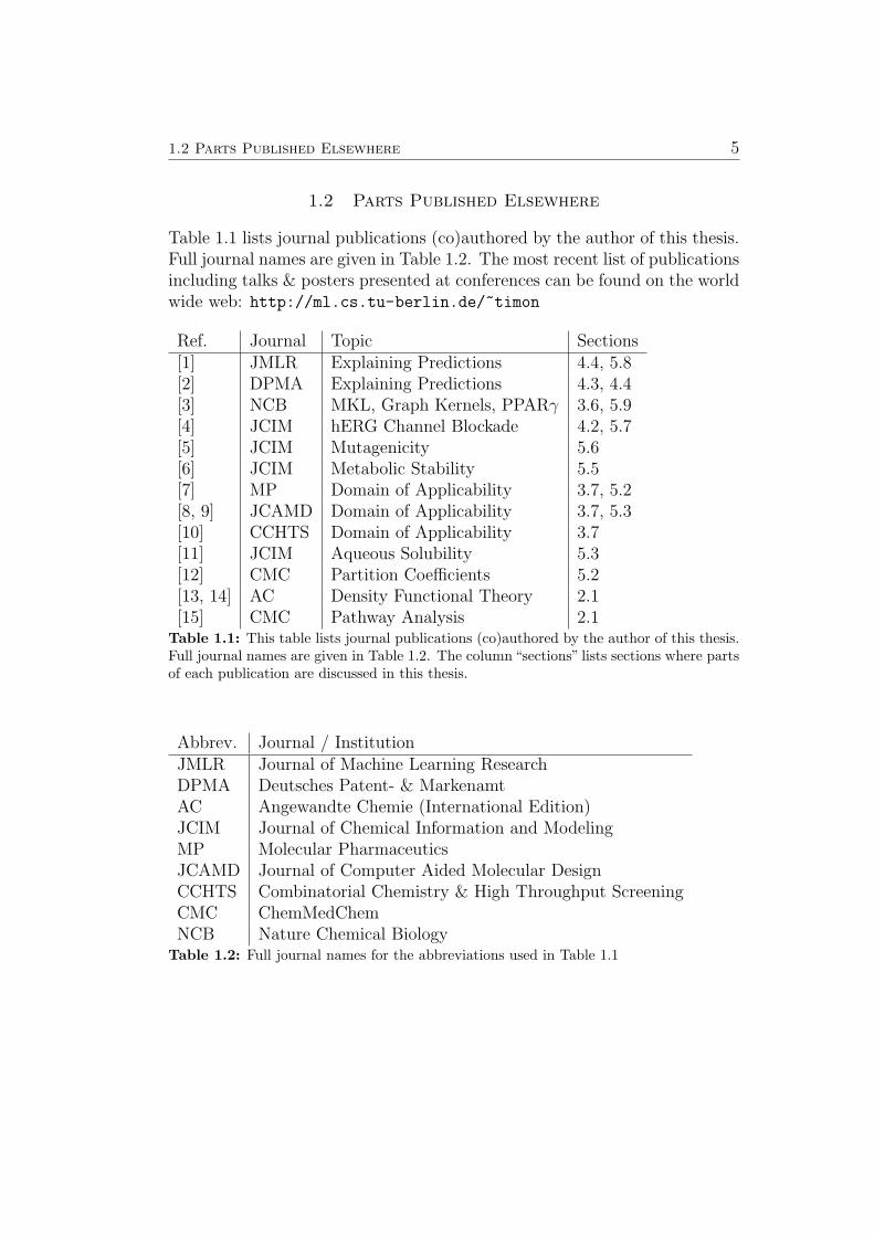
Table 1.1 lists journal publications (co)authored by the author of this thesis.Full journal names are given in Table 1.2. The most recent list of publicationsincluding talks & posters presented at conferences can be found on the worldwide web: http://ml.cs.tu-berlin.de/~timon
Ref. Journal Topic Sections[1] JMLR Explaining Predictions 4.4, 5.8[2] DPMA Explaining Predictions 4.3, 4.4[3] NCB MKL, Graph Kernels, PPARγ 3.6, 5.9[4] JCIM hERG Channel Blockade 4.2, 5.7[5] JCIM Mutagenicity 5.6[6] JCIM Metabolic Stability 5.5[7] MP Domain of Applicability 3.7, 5.2[8, 9] JCAMD Domain of Applicability 3.7, 5.3[10] CCHTS Domain of Applicability 3.7[11] JCIM Aqueous Solubility 5.3[12] CMC Partition Coefficients 5.2[13, 14] AC Density Functional Theory 2.1[15] CMC Pathway Analysis 2.1
Table 1.1: This table lists journal publications (co)authored by the author of this thesis.Full journal names are given in Table 1.2. The column “sections” lists sections where partsof each publication are discussed in this thesis.
Abbrev. Journal / InstitutionJMLR Journal of Machine Learning ResearchDPMA Deutsches Patent- & MarkenamtAC Angewandte Chemie (International Edition)JCIM Journal of Chemical Information and ModelingMP Molecular PharmaceuticsJCAMD Journal of Computer Aided Molecular DesignCCHTS Combinatorial Chemistry & High Throughput ScreeningCMC ChemMedChemNCB Nature Chemical Biology
Table 1.2: Full journal names for the abbreviations used in Table 1.1

Chapter 2
Introduction
2.1 Drug Discovery and Drug Design
The following section provides an overview over the process of drug discoveryand design.1 An in depth introduction can be found in these books [17, 18].Steps in the process that have been treated in this thesis are pointed out inthe last paragraphs.
Solid biological basic research on disease mechanisms is nowadays thebasis of drug discovery and drug design. Ideally, one finds that stimulatingor inhibiting a certain target receptor (usually a protein) will help cure thedisease, ease the pain etc. Due to advances in genomics [19–21], proteomicsand other parts of systems biology, the analysis of signalling pathways [15] iscurrently gaining importance in understanding complex disease mechanisms.This set of methods can greatly facilitate the process of identification andvalidation of drug targets (e.g. receptors).
One of the first steps in discovering a new drug is to develop an exper-iment that allows for testing whether a molecule binds to the target. Thistype of experiment is called assay. Once such an assay has been developed tothe point where it is applicable in an automated way, one chooses compoundsfor investigation in high throughput screening (HTS). The number of com-pounds depends on the budget of the company and can exceed one millioncompounds. These are typically selected from a much larger number of com-pounds that are available in-house or from external vendors. The majoritystems from combinatorial libraries and can be synthesized by machines usinga certain set of chemical reactions to combine predefined suitable buildingblocks [22]. The step of choosing a collection of compounds for screeningfrom a larger set of available/feasible molecules will later be referred to aslibrary design. Results from HTS campaigns are very noisy, the effects of hitcompounds identified in HTS are therefore carefully examined in regular lab-oratories. Out of the confirmed hits, one selects molecules as starting pointsfor developing lead compounds.
1The actual process depends on the company. This summary was partly inspired by[16].
7
8 Introduction
When looking for hits, assessing the potential of compounds using com-putational methods (in silico methods) can be seen as an alternative to highthroughput screening. The most popular group of methods is called virtualscreening [23, 24]. Depending on which information is available, differentvirtual screening protocols can be applied:
If, for example, the 3D structure of the target protein is known, one canexploit it in different ways, commonly referred to as structure based design[25]. One can simulate (or even calculate2) how different molecules fit into theactive site of the target. Depending on the amount of human intervention inevaluating the goodness of the fit, this is either referred to as docking or highthroughput docking. The latter not only requires computationally efficientalgorithms and high performance computers / clusters, but also good scoringfunctions. Alternatively, one can virtually build a molecule out of fragmentsdirectly inside the active site of the protein model, choosing each fragment sothat the fit to the target is optimal. This strategy is called “de novo design”[26–29].
Without a 3D structure of the target protein, one can investigate com-pounds that are similar to know actives (active compounds) [30, 31]. Thesemay be natural products [32], drugs previously developed by other compa-nies that are already on the market but still protected by patents or activesreported in the literature. In the first two cases one looks for molecules wherethe relevant functional groups can adopt 3D structures similar to the knownactive compounds. At the same time, they are supposed to be somewhatdissimilar in a chemical sense, because natural products are often expensiveto synthesize and patents for compounds also cover chemically very similarstructures. Looking for new compounds with similar activity as known ac-tives is called ligand based virtual screening. As explained above, the goal istypically not only to find new actives, but new actives of a different chemotypeor scaffold (hence the often used term scaffold hopping [33, 34] to describethe goal). Pseudoreceptor models can be used to bridge ligand based- and(protein-) structure based virtual screening [35].
Having found hits using any of the above methods, one proceeds to ex-amining these few compounds in the lab and selects or develops [36] leadcompounds (short: leads) that are suitable for further development (see be-low) in so called hit to lead programs.
In the following lead optimization phase, variants of these lead compoundsare synthesized in a more or less systematic way: The many decisions which
2Hybrid methods of molecular mechanics simulations (for most parts of the protein)and efficient quantum mechanical methods like DFT [13, 14] (for the active site) can beused to precisely calculate interaction energies.
2.1 Drug Discovery and Drug Design 9
compound or small batch of compounds to synthesize and test next are oftenmade on the basis of very little information. The experience (and luck) of thepeople making the respective decisions therefore have a lot of influence on theduration of this phase. One continues until one finds a compound that has therequired properties or the project is cancelled. At this stage, compounds aresynthesized by humans. Together with some basic tests the costs can easilyreach 10,000 $ per compound. Some companies regularly stop a predefinedpercentage of all projects to avoid investing too much into dead ends or toodifficult paths. Both for projects and for individual compounds this is some-times referred to as “fail cheap - fail early” paradigm. Sometimes thousandsof compounds are made and tested until one finally succeeds; even 10,000compounds are not uncommon. For promising compounds, extensive toxi-cologic and pharmacologic profiles are done using computational methods,laboratory experiments involving cells (in vitro testing) and in animal mod-els. Finally, drug candidates are selected for first experiments with humans& patent applications are submitted. The duration of the patent protectiondepends on the country. Typical times for the United States and Europe are20 years. Note that time starts running before clinical testing begins, i.e.years before the drug reaches the market.
Clinical testing happens in four phases involving increasing numbers ofboth patients and healthy volunteers (from 20-80 people in phase 1 to 1000-3000 people in phase 3). One determines characteristics like the distributionin the body, suitable dose range, potential side effects and effectiveness of thenew drug. Registration can be done after successful phase 3 trials. Ideally,one then gets the permission to market the drug. After introducing the druginto the market, further studies are performed (phase 4).
The whole process can cost on the order of a billion dollars and in rarecases even exceed two billion dollars. Once the drug is on the market, onecan, in theory, sell it infinitely, but as soon as the patent protecting thecompound runs out, other companies are allowed to “copy” it. Not havinginvested into basic research and development, these generic drug makers cansell it at a very low price and still be profitable.
Speeding up the drug design process is therefore very desirable for thefollowing reasons:
• one can save many millions of euros by avoiding useless experimentsand finding good compounds faster
• one can increase the time that one spends alone on the market, pro-tected by a still running patent and can recover investments into basicresearch and development
10 Introduction
Traditionally, early research was very focussed on the effect on the target.Properties relating to Absorption, Digestion, Metabolism, Excretion & Tox-icity (ADME/Tox ) were investigated late in the lead optimization process.In recent years, most companies have started considering these properties asearly as possible.
The author of this thesis contributed to developing models for the follow-ing properties:
• Partition Coefficients (Sec. 5.2)
• Aqueous Solubility (Sec. 5.3)
• Cytochrome P450 Inhibition (Sec. 5.4)
• Metabolic Stability (Sec. 5.5)
• Ames Mutagenicity (Sec. 5.6)
• hERG Channel Blockade Effect (Sec. 5.7)
These models allow taking the respective properties into account already inearly development stages, i.e. when building libraries for high throughputscreening, in hit to lead programs and at the beginning of lead optimization.Four of these models have been equipped with graphical user interfaces (seeSec. 3.8) and deployed for use by researchers at Schering (now part of BayerHealthcare).
Furthermore, the author of this thesis participated in a ligand based virtualscreening project leading to new PPARγ agonists (Sec. 5.9).
Three new machine learning technologies aimed at lead optimization wereconceived. The first algorithm improves prediction accuracy for new com-pound classes by means of a local bias correction. The other two algorithmscan help human experts in choosing new compounds to investigate: The firstmethod explains individual predictions of kernel based models (Sec. 4.3). Thesecond method identifies the features that are most promising for optimizingeach individual molecule (Sec. 4.4 and 5.8).
2.2 Machine Learning 11
2.2 Machine Learning
The following section introduces general machine learning paradigms andmethods. The next section discusses the state of the art, challenging aspectsand the authors contributions to machine learning in drug discovery and drugdesign.
Machine learning can be regarded as data driven generation of predic-tive models. Supervised machine learning assumes that there is a set of ngiven pairs {(x1, y1), (x2, y2), . . . , (xn, yn)} where xi ∈ Rd denotes the vectorof the d feature (descriptor) values calculated in the pre-processing for theobject (chemical compound) i and yi refers to the corresponding label. Onedistinguishes two types of supervised learning problems, depending on thestructure of y. For classification, y consists of a finite number (very oftentwo, sometimes more) of class labels (i.e. mutagenic vs. non-mutagenic),and the task is to correctly predict the class membership of objects. Forregression, yi ∈ R, and the task is to predict some real valued quantity (i.e.a property like a binding constant) based on the object features. Trainingexamples are assumed as ideally identically distributed samples from a prob-ability distribution PX×Y . One aims to find a function f which can predictthe label for unknown objects represented as feature vectors x.When measuring the quality of f , contradictory aspects have to be consid-ered: On the one hand, the complexity of the function f must be sufficient toexpress the relation between the given labels (y1, y2, . . . , yn) and the corres-ponding feature vectors (x1,x2, . . . ,xn) accurately. On the other hand, theestimating function should not be too complex (e.g. too closely adapted tothe training data) to allow for reliable predictions of unknown objects. Thistradeoff is captured mathematically in the minimization of the regularizedempirical loss function [37]:
minRregemp(f) =
1
n
n∑i=1
`(f(xi), yi)︸ ︷︷ ︸quality of fit
+ λ · r(f)︸ ︷︷ ︸regularizer
. (2.1)
where l : R× R→ R refers to a loss function, r : L→ R to a regularizationfunction and λ to a positive balance parameter. The first term in Equation2.1 measures the quality of the fit of the model on the training data, andthe second term penalizes the complexity of the function f to prevent over-fitting. The parameter λ is used to adjust the influence of the regularizationfunction r. In addition to preventing over-fitting, it is often used to ensurethat the problem in Equation 2.1 is not illposed which is required by variousoptimization methods. The loss function ` determines the loss resulting from
12 Introduction
the inaccuracy of the predictions given by f . Many regression algorithms usethe squared error loss function
`(f(xi), yi) = (f(xi)− yi)2. (2.2)
Most inductive machine learning methods minimize the empirical risk func-tion with respect to different regularization terms r and loss functions `.
Popular supervised learning algorithms include Support Vector Machines[38–42], Gaussian Processes [11, 43, 44], Decision Trees [45] and ArtificialNeural Networks [46–48]. The most commonly used way of representingmolecules is choosing one out of many available tools to calculate a vectorof so called chemical descriptors characterizing the molecule [49]. Standardlearning algorithms for vectorial data can then be applied to these descrip-tors. Sometimes the features of the test set are already available when themodel is trained. I.e. one builds a model based on a training set of chemicalmolecules, intending to apply this model to an already collected/generatedlibrary of molecules. This setting is generally referred to as semi-supervisedmachine learning.3 If a learning machine can suggest which compounds toinvestigate next to achieve the maximum improvement of the model, we arein an active learning scenario [50]. Finally, sometimes no labels exist for acollection of objects and one seeks to detect some type of order in the databased on the features alone. This setting is commonly called unsupervisedmachine learning or clustering [51–57]. More general definitions of machinelearning also include different types of signal processing (e.g. in brain com-puter interface systems [58–64]), and various unsupervised and supervisedprojection and dimensionality reduction algorithms [65–73]. A recent ini-tiative in the machine learning community [74] advocates the use of opensource software for machine learning and points to a free software repositoryestablished to facilitate this move.
In the work leading up to this thesis, non-linear Bayesian regression andclassification using Gaussian Process priors have been applied to differentlearning tasks and are also used as the starting points for newly developedalgorithms for explaining individual predictions and eliciting hints for com-pound optimization. Therefore, a separate section has been devoted to Gaus-sian Processes, namely Sec. 3.3.
3Other definitions of semi-supervised machine learning are more broad and also includeprocedures where any set of unlabeled data is used in the learning process.
2.3 Machine Learning in Drug Discovery and Drug Design 13
2.3 Machine Learning in Drug Discovery and Drug Design
2.3.1 State of the Art
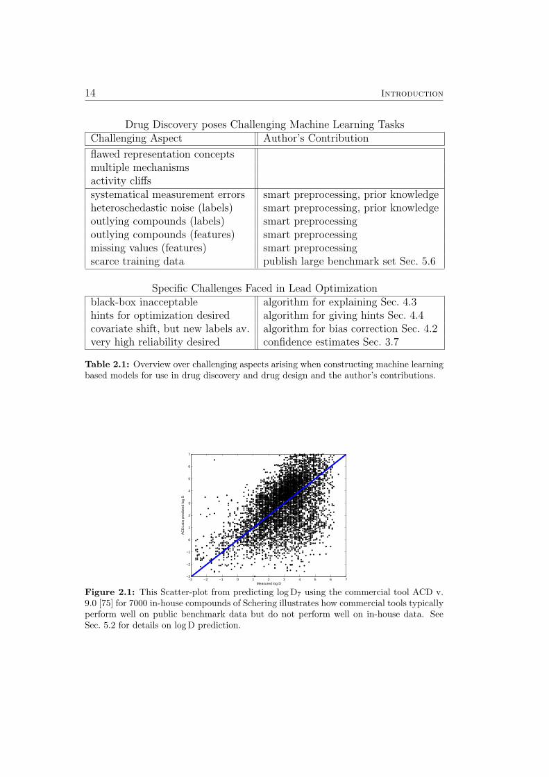
In 2005, when work leading to this thesis commenced, there were no predic-tive models for metabolic stability (Sec. 5.5) and the hERG channel blockadeeffect (Sec. 5.7) available on the market. Existing predictive tools for par-tition coefficients (Sec. 5.2), aqueous solubility (Sec. 5.3) and mutagenicity(Sec. 5.6) performed reasonably well on publicly available benchmark sets ofcompounds, but did not generalize to the in-house compounds of pharma-ceutical companies. Figure 2.1, a scatter-plot from predicting log D7 usingthe commercial tool ACD v. 9.0 [75] for 7013 in-house compounds of Scher-ing, illustrates the problem: We see a lot of compounds where the predictionsdeviate from the true values by several log units. Most of them occur for com-pounds with relatively high log D7. Unfortunately, these are the compoundsthat tend to bind proteins very well and are therefore very interesting in thecontext of drug discovery & design (most drug targets are proteins).
Furthermore, in 2005 none of the existing commercial models for ADME/-Tox properties had the ability to quantify the confidence into each individualprediction. As explained in Sec. 3.7, this is a very desirable feature in drugdiscovery & drug design, where models are often operated outside of theirrespective domains of applicability.
The causes of the anti-inflammatory and anti diabetic effects of bermudagrass (cynodon dactylon) were unknown until our screening for new PPARγagonists (Sec. 5.9) lead to a first hypothesis.
When understandable models for application in lead optimization weresought, researchers resorted to building linear models based on small train-ing sets of compounds represented by small sets of descriptors. Using allavailable training data and/or complex kernel-based models while still beingable to understand each individual prediction were not yet feasible (Sec. 4.3).Furthermore, there was no technology that allowed to elicit hints for com-pound optimization (Sec. 4.4).
14 Introduction
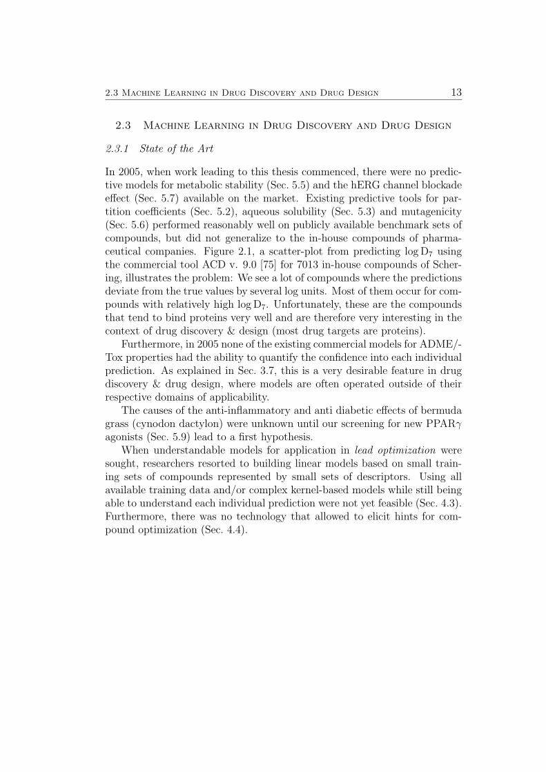
Drug Discovery poses Challenging Machine Learning TasksChallenging Aspect Author’s Contribution
flawed representation conceptsmultiple mechanismsactivity cliffssystematical measurement errors smart preprocessing, prior knowledgeheteroschedastic noise (labels) smart preprocessing, prior knowledgeoutlying compounds (labels) smart preprocessingoutlying compounds (features) smart preprocessingmissing values (features) smart preprocessingscarce training data publish large benchmark set Sec. 5.6
Specific Challenges Faced in Lead Optimizationblack-box inacceptable algorithm for explaining Sec. 4.3hints for optimization desired algorithm for giving hints Sec. 4.4covariate shift, but new labels av. algorithm for bias correction Sec. 4.2very high reliability desired confidence estimates Sec. 3.7
Table 2.1: Overview over challenging aspects arising when constructing machine learningbased models for use in drug discovery and drug design and the author’s contributions.
−3 −2 −1 0 1 2 3 4 5 6 7−3
−2
−1
0
1
2
3
4
5
6
7
Measured log D
AC
DLa
bs p
redi
cted
log
D
Figure 2.1: This Scatter-plot from predicting log D7 using the commercial tool ACD v.9.0 [75] for 7000 in-house compounds of Schering illustrates how commercial tools typicallyperform well on public benchmark data but do not perform well on in-house data. SeeSec. 5.2 for details on log D prediction.
2.3 Machine Learning in Drug Discovery and Drug Design 15
2.3.2 Challenging Aspects and the Author’s Contributions
When constructing machine learning based models for use in drug discov-ery and drug design, many challenging aspects arise. Table 2.1 presents anoverview over these challenges. The next subsection introduces challengingaspects that have not been treated in this thesis and points to more detailedexplanations given in the appendix. The following four subsections are ded-icated to challenging aspects where the author has contributed to progressin the field. This includes newly invented algorithms, algorithms initiallyintroduced into the field, careful pre-processing and publishing a new largebenchmark data set
Challenging Aspects Not Treated
Molecules are dynamical three dimensional objects, exhibiting many differenttypes of flexibility (see Sec. A.1.1). Available representations of moleculesfor machine learning either completely ignore this fact by considering onlyfeatures derived from the two dimensional graph of the molecule, or theyconsider a small arbitrarily chosen number of 3D structures that may or maynot be relevant for the task at hand. Consequently, the accuracy that canbe achieved by machine learning models based on these representations islimited. See Sec. A.1.1 for a more detailed discussion including examples.
As explained in Sec. 2.2, popular machine learning algorithms rely on theassumption that training data and future test data are sampled from thesame underlying probability density, and further assume that the conditionaldistribution of target values given the input features (descriptors) is the samein both test and training data. Violation of the first assumption is often re-ferred to as covariate shift or dataset shift and is encountered in most drugdiscovery applications (see Sec. A.1.2). If new measurements have becomeavailable since the model has been built, bias correction allows to achievebetter generalization performance (see subsection on new algorithms below).As of today, there is no satisfying solution known that allows improving pre-dictions in case of violation of the second assumption (multiple mechanisms,see Sec. A.1.3). In the work leading up to this thesis, datasets contain-ing multiple mechanisms have been encountered in the studies described inSec. 5.5 (Metabolic Stability), Sec. 5.3 (Aqueous Solubility), Sec. 5.4 (Cy-tochrome P450 Inhibition) and Sec. 5.6 (Ames Mutagenicity). See Sec. A.1.3for a more detailed discussion. Considering confidence estimates to identifyreliable predictions can partially alleviate this problem (see separate sectionbelow).
Machine learning in drug discovery and design relies on the assumption
16 Introduction
that similar molecules exhibit similar activity. Unfortunately, many relevantproperties exhibit sudden jumps in activity. The existence of such activitycliffs is not entirely surprising since molecular recognition plays a crucial rolein determining properties like binding to receptors or the active sites of en-zymes. In this thesis, activity cliffs are present in PPARγ binding (Sec. 5.9),Metabolic Stability (Sec. 5.5), Cytochrome P450 Inhibition (Sec. 5.4), AmesMutagenicity (Sec. 5.6), hERG Channel Blockade Effect (Sec. 5.7) and tosome degree even in Aqueous Solubility (Sec. 5.3). See Sec. A.1.4 for moreinformation on activity cliffs.
Data Scarcity Alleviated by New Benchmark Data Set
Today, the academic part of the field of chemoinformatics still suffers froma lack of large high-quality datasets. A new dataset on Ames mutagenicitywas collected from the literature by collaborators at Bayer Schering Pharmaand jointly released to the public (Sec. 5.6). The set attracted the imme-diate attention of numerous researchers. Currently, a joint publication byresearchers from eight different groups across the world is in preparation.
Challenging Aspects Handled in Data Pre-Processing
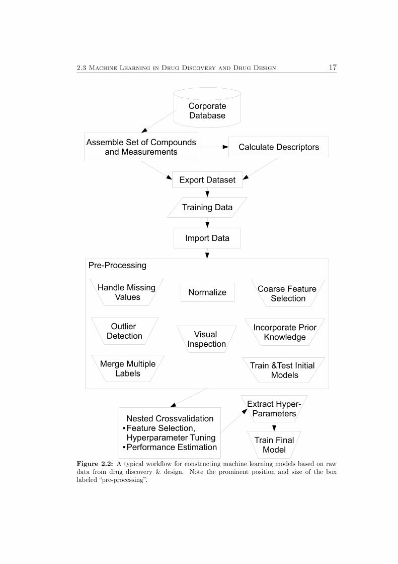
Systematical measurement errors, heteroschedastic noise, compounds withoutlying labels or features or even missing values in some features necessi-tate carefully performing various pre-processing steps before training machinelearning models. A typical workflow for constructing machine learning mod-els based on data from drug discovery & design is indicated in Figure 2.2.Note the prominent position and size of the box labeled “pre-processing”.Therefore, separate sections have been developed to the most important pre-processing steps:
Visualizing many different aspects of new datasets can help detect poten-tial problems (e.g. strong outliers) early and can give hints as to the difficultyof the modeling task, sensible choice of kernels & parameters etc. In the firstsubsection of Sec. 3.2, recent examples are used to illustrate how many usefulhints and pieces of information can already be found using linear principlecomponent analysis (PCA).
In the chemoinformatics community, there exists a widespread belief thatfeature selection or dimension reduction using projection techniques is essen-tial for any modelling task. The second subsection in Sec. 3.2 acknowledgesthat while there are good reasons for doing feature selection, it is definitelynot always necessary and can even be harmful.
2.3 Machine Learning in Drug Discovery and Drug Design 17
Pre-Processing
Assemble Set of Compoundsand Measurements
Calculate Descriptors
Export Dataset
Normalize
Nested Crossvalidation●Feature Selection,Hyperparameter Tuning
●Performance Estimation
Import Data
Training Data
CorporateDatabase
Visual Inspection
Coarse Feature Selection
Handle Missing Values
Incorporate PriorKnowledge
Train &Test Initial Models
Merge MultipleLabels
Outlier Detection
Train FinalModel
Extract Hyper-Parameters
Figure 2.2: A typical workflow for constructing machine learning models based on rawdata from drug discovery & design. Note the prominent position and size of the boxlabeled “pre-processing”.
18 Introduction
The third subsection in Sec. 3.2 discusses detection and analysis of out-liers by visual inspection, using outlier indices in descriptor space, based onprior knowledge and when multiple measurements per compound are avail-able. Furthermore, the identification of outlying predictions with respect tothe predicted confidence estimates of Gaussian Processes and a “reverse en-gineering” exercise of models & training sets for a-posteriori explanation ofthese outlying predictions is presented.
Increasing Reliability of Predictions by Considering Confidence Estimates
As explained in Sec. 2.2, most machine learning algorithms rely on the factthat training data and future test data are sampled from the same underlyingprobability density. This assumption is typically violated in drug discoveryapplications (i.e. they exhibit covariate shift or dataset shift, see Sec. A.1.2).In other words: In drug discovery and drug design, predictive models areoften operated outside of their respective domain of applicability (DOA).Unless some new measurements have been made since the model has beenbuilt (see next subsection for new algorithms developed for this scenario), itmay not be possible to achieve better predictions. In this case, in may bevery helpful to know which predictions are most likely incorrect (outside theDOA) or correct (inside the DOA). Sec. 3.7 explains this concept in moredetail and lists heuristics that have been conceived in the chemoinformaticscommunity.
Gaussian Process models can produce a predictive variance along witheach individual prediction. This variance can be interpreted as an estimateof the confidence in each individual prediction. This concept has been in-troduced to the chemoinformatics community during the work leading up tothis thesis. Sec. 3.3 explains Gaussian Process Models and points to relevantpublications. In this thesis, the practical usefulness of predictive variances isinvestigated in Sec. 5.2 (Partition Coefficients), Sec. 5.3 (Aqueous Solubility),Sec. 5.5 (Metabolic Stability) and in preparing hit-lists in a virtual screeningfor new PPARγ agonists (Sec. 5.9).
Newly Developed Algorithms
As time progresses, new projects are started and new compound classes areexplored. As explained in Sec. 2.2, almost all supervised machine learningalgorithms rely on the fact that training data and future test data are sampledfrom the same underlying probability density. Violation of this assumption(covariate shift) may lead to a bias. More information about covariate shift
2.3 Machine Learning in Drug Discovery and Drug Design 19
can be found in the appendix Sec. A.1.2. In the lead optimization applicationscenario, one question that regularly arises is how to best use the first newmeasurements for compounds belonging to a newly explored compound class,i.e. a new part of the chemical space. New different model selection and biascorrection algorithms are introduced in Sec. 4.2 and an evaluation of thesealgorithms in the context of the hERG Channel Blockade Effect is presentedin Sec. 5.7.
In this thesis, two separate methodologies for explaining individual pre-dictions of (possibly non-linear) machine learning models are presented. Themethod presented in Sec. 4.3 explains predictions by the means of visualiz-ing relevant objects from the training set of the model. This allows humanexperts to understand how each prediction comes about. If a prediction con-flicts with his intuition, the human expert can easily find out whether thegrounds for the models predictions are solid or if trusting his own intuitionis the better idea.
The method presented in Sec. 4.4 utilizes local gradients of the model’spredictions to explain predictions in terms of the locally most relevant fea-tures. This not only teaches the human expert which features are relevantfor each individual prediction, but also gives a directional information. Ab-stractly speaking, one can learn in which direction a data point has to bemoved to increase the prediction for the target value. In the context of leadoptimization, this means that the human expert can obtain a type of guidancein compound optimization.

Chapter 3
Methods (Utilized / Improved)
3.1 Overview
This chapter introduces the methodology that was applied and partially re-fined in the work leading up to this thesis. Methods that have been newlydeveloped are presented in Chapter 4.
The first four sections in this chapter deal with topics that are consideredessential parts of any machine learning study in chemoinformatics. Eachsection focuses on the aspects that are most relevant to this thesis as a wholeand points to the literature for more comprehensive coverage of the respectivetopic.
When first analyzing a new (raw) set of data, many aspects need tobe considered. Systematical measurement errors, heteroschedastic noise,compounds with outlying labels or features or even missing values in somefeatures necessitate carefully performing various pre-processing steps beforetraining machine learning models. Therefore, Sec. 3.2 contains separate sub-sections on important pre-processing steps, namely visual data inspection,feature selection and outlier detection & analysis.
The account of machine learning algorithms (Sec. 3.3) focuses on non-linear Bayesian regression and classification using Gaussian Process priors(GP), because this method was introduced into the field of chemoinformaticsand for the first time, individual confidence estimates were provided basedon a solid theoretical foundation. The section explains how GPs work anddiscusses their advantages in the context of chemoinformatics.
Sec. 3.4 discusses evaluation strategies that allow reaching all the goalsthat one may have in a typical modeling study: Starting from a batch of data,one selects features, chooses a modeling algorithm and tunes free parameters.In the end one seeks to estimate the generalization performance includingor excluding extrapolation. Care has to be taken to both obtain modelsthat generalize well and realistically estimate this achieved generalizationperformance.
The section on performance indicators contains a mostly informal col-lection of the author’s insights regarding various standard loss functions,
21
22 Methods (Utilized / Improved)
modified versions of standard loss functions and a new loss function that wasconceived to express the specific goals of a virtual screening application.
The following three sections deal with more advanced topics.As detailed in Sec. 3.6, multiple kernel learning allows to simultaneously
take different aspects of the same piece of information into account. Further-more, one can use this technique to combine heterogeneous types of informa-tion (e.g. vectorial molecular descriptors & molecular graphs).
A typical challenge for statistical models in the chemical space is to ade-quately determine the domain of applicability, i.e. the part of the chemicalspace where the models’ predictions are reliable. Sec. 3.7 treats both heuris-tics that have been previously used in the chemoinformatics community andrecent probabilistic models.
When trying to establish new computational methodology that can berelevant to the work of bench chemists (who tend to focus on the syntheticaspects of chemistry), it is necessary to adapt to their needs and preferences.Sec. 3.8 describes a graphical user interface that allows easy access to modelsthat have been developed with contributions by the author of this thesis.
3.2 Data Pre-Processing 23
3.2 Data Pre-Processing
A typical workflow for constructing machine learning models based on datafrom drug discovery & design has been introduced in Figure 2.2 on page 17.Note the prominent position and size of the box labeled “pre-processing”. Inthis section, three separate subsections illustrate important pre-processingsteps.
The first subsection lists a number of possible first steps in analyzinga new dataset. Visualizing many different aspects can help detect poten-tial difficulties early and can give hints as to sensible choices of kernels ¶meters and the difficulty of the modeling task.
In the chemoinformatics community, there exists a widespread belief thatfeature selection or dimension reduction using projection techniques is essen-tial for any modelling task. The second subsection acknowledges that whilethere are good reasons for doing feature selection, it is definitely not alwaysnecessary and can even be harmful.
The third subsection discusses detection and analysis of outliers by visualinspection, using outlier indices in descriptor space, based on prior knowledgeand when multiple measurements per compound are available. Furthermore,the identification of outlying predictions with respect to the predicted con-fidence estimates of Gaussian Processes and a “reverse engineering” exerciseof models & training sets for a posteriori explanation of these outlying pre-dictions is presented.
Visual Data Inspection
Research papers tend to focus on the final results of model building & vali-dation, while skipping over some of the preliminaries. This section will list anumber of possible first steps in analyzing a new dataset. Visualizing manydifferent aspects can help detect potential problems (e.g. strong outliers)early and can give hints as to the difficulty of the modeling task, sensiblechoice of kernels & parameters etc. Properties generally useful to visualizeinclude:
• histogram of the target values
• 2/3 D plots of raw/normalized descriptor values
• 2/3 D plots of correlation between descriptors (see Fig. A.4 in Sec. A.4for an example)
• plots of linear/kernelized principle component analysis (PCA) compo-nents of all/most relevant descriptors [76–81]
24 Methods (Utilized / Improved)
−5 −4 −3 −2 −1 0 1 2 3 4
−3
−2
−1
0
1
2
3
4
5
PCA component 1
PC
A c
ompo
nent
2
logD: PCA on best features
−1.5
0.406
1.79
2.75
3.7
5.09
7
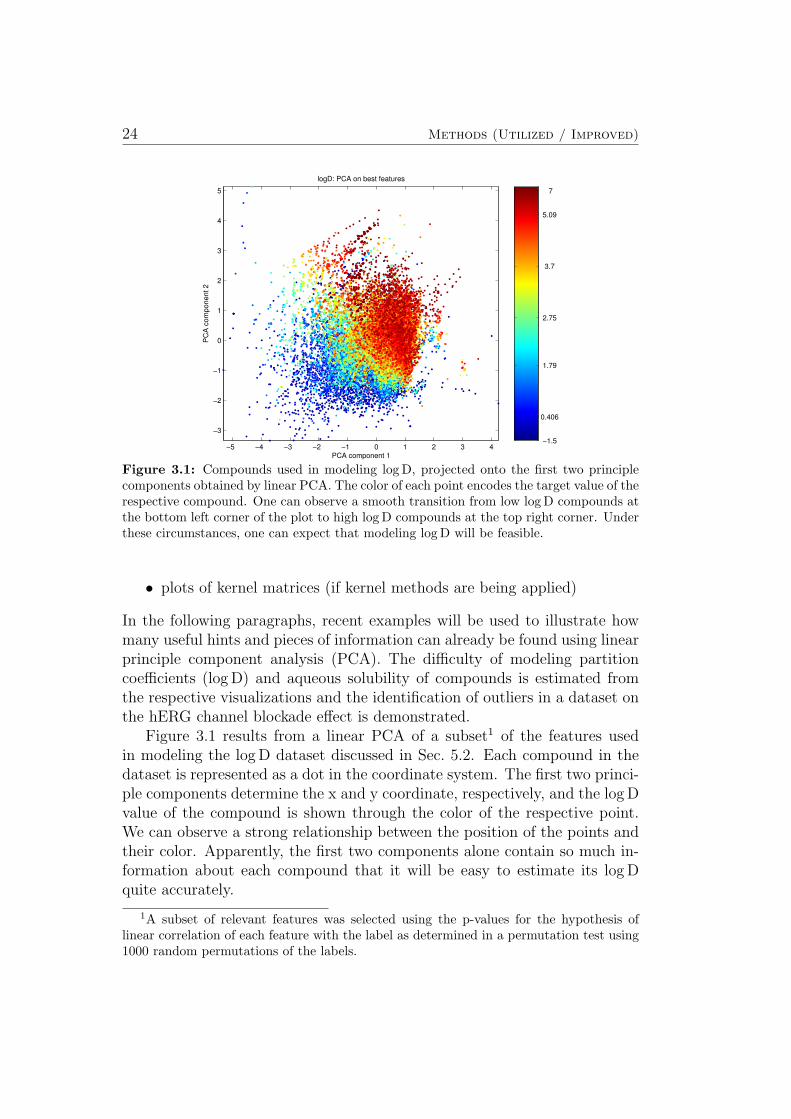
Figure 3.1: Compounds used in modeling log D, projected onto the first two principlecomponents obtained by linear PCA. The color of each point encodes the target value of therespective compound. One can observe a smooth transition from low log D compounds atthe bottom left corner of the plot to high log D compounds at the top right corner. Underthese circumstances, one can expect that modeling log D will be feasible.
• plots of kernel matrices (if kernel methods are being applied)
In the following paragraphs, recent examples will be used to illustrate howmany useful hints and pieces of information can already be found using linearprinciple component analysis (PCA). The difficulty of modeling partitioncoefficients (log D) and aqueous solubility of compounds is estimated fromthe respective visualizations and the identification of outliers in a dataset onthe hERG channel blockade effect is demonstrated.
Figure 3.1 results from a linear PCA of a subset1 of the features usedin modeling the log D dataset discussed in Sec. 5.2. Each compound in thedataset is represented as a dot in the coordinate system. The first two princi-ple components determine the x and y coordinate, respectively, and the log Dvalue of the compound is shown through the color of the respective point.We can observe a strong relationship between the position of the points andtheir color. Apparently, the first two components alone contain so much in-formation about each compound that it will be easy to estimate its log Dquite accurately.
1A subset of relevant features was selected using the p-values for the hypothesis oflinear correlation of each feature with the label as determined in a permutation test using1000 random permutations of the labels.
3.2 Data Pre-Processing 25
−3 −2 −1 0 1 2 3−2
−1
0
1
2
3
4
PCA component 1
PC
A c
ompo
nent
2
Solubility data, color indicating log10(SW
)
−8.61
−6.07
−4.24
−2.96
−1.69
0.147
2.68Test data
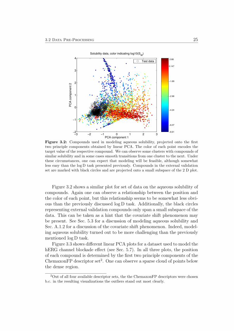
Figure 3.2: Compounds used in modeling aqueous solubility, projected onto the firsttwo principle components obtained by linear PCA. The color of each point encodes thetarget value of the respective compound. We can observe some clusters with compounds ofsimilar solubility and in some cases smooth transitions from one cluster to the next. Underthese circumstances, one can expect that modeling will be feasible, although somewhatless easy than the log D task presented previously. Compounds in the external validationset are marked with black circles and are projected onto a small subspace of the 2 D plot.
Figure 3.2 shows a similar plot for set of data on the aqueous solubility ofcompounds. Again one can observe a relationship between the position andthe color of each point, but this relationship seems to be somewhat less obvi-ous than the previously discussed log D task. Additionally, the black circlesrepresenting external validation compounds only span a small subspace of thedata. This can be taken as a hint that the covariate shift phenomenon maybe present. See Sec. 5.3 for a discussion of modeling aqueous solubility andSec. A.1.2 for a discussion of the covariate shift phenomenon. Indeed, model-ing aqueous solubility turned out to be more challenging than the previouslymentioned log D task.
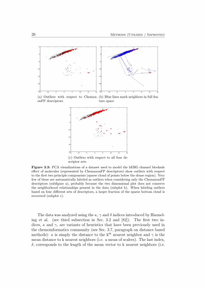
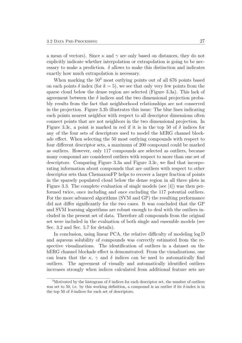
Figure 3.3 shows different linear PCA plots for a dataset used to model thehERG channel blockade effect (see Sec. 5.7). In all three plots, the positionof each compound is determined by the first two principle components of theChemaxonFP descriptor set2. One can observe a sparse cloud of points belowthe dense region.
2Out of all four available descriptor sets, the the ChemaxonFP descriptors were chosenb.c. in the resulting visualizations the outliers stand out most clearly.
26 Methods (Utilized / Improved)
−15 −10 −5 0 5 10 15 20−25
−20
−15
−10
−5
0
5
(a) Outliers with respect to Chemax-onFP descriptors
−15 −10 −5 0 5 10 15 20−25
−20
−15
−10
−5
0
5
(b) Blue lines mark neighbors in full fea-ture space
−15 −10 −5 0 5 10 15 20−25
−20
−15
−10
−5
0
5
(c) Outliers with respect to all four de-scriptor sets
Figure 3.3: PCA visualizations of a dataset used to model the hERG channel blockadeeffect of molecules (represented by ChemaxonFP descriptors) show outliers with respectto the first two principle components (sparse cloud of points below the dense region). Veryfew of these are automatically labeled as outliers when considering only the ChemaxonFPdescriptors (subfigure a), probably because the two dimensional plot does not conservethe neighborhood relationships present in the data (subplot b). When labeling outliersbased on four different sets of descriptors, a larger fraction of the sparse bottom cloud isrecovered (subplot c).
The data was analyzed using the κ, γ and δ indices introduced by Harmel-ing et al. (see third subsection in Sec. 3.2 and [82]). The first two in-dices, κ and γ, are variants of heuristics that have been previously used inthe chemoinformatics community (see Sec. 3.7, paragraph on distance basedmethods): κ is simply the distance to the kth nearest neighbor and γ is themean distance to k nearest neighbors (i.e. a mean of scalers). The last index,δ, corresponds to the length of the mean vector to k nearest neighbors (i.e.
3.2 Data Pre-Processing 27
a mean of vectors). Since κ and γ are only based on distances, they do notexplicitly indicate whether interpolation or extrapolation is going to be nec-essary to make a prediction. δ allows to make this distinction and indicatesexactly how much extrapolation is necessary.
When marking the 503 most outlying points out of all 676 points basedon each points δ index (for k = 5), we see that only very few points from thesparse cloud below the dense region are selected (Figure 3.3a). This lack ofagreement between the δ indices and the two dimensional projection proba-bly results from the fact that neighborhood relationships are not conservedin the projection. Figure 3.3b illustrates this issue: The blue lines indicatingeach points nearest neighbor with respect to all descriptor dimensions oftenconnect points that are not neighbors in the two dimensional projection. InFigure 3.3c, a point is marked in red if it is in the top 50 of δ indices forany of the four sets of descriptors used to model the hERG channel block-ade effect. When selecting the 50 most outlying compounds with respect tofour different descriptor sets, a maximum of 200 compound could be markedas outliers. However, only 117 compounds are selected as outliers, becausemany compound are considered outliers with respect to more than one set ofdescriptors. Comparing Figure 3.3a and Figure 3.3c, we find that incorpo-rating information about compounds that are outliers with respect to otherdescriptor sets than ChemaxonFP helps to recover a larger fraction of pointsin the sparsely populated cloud below the dense region in all three plots inFigure 3.3. The complete evaluation of single models (see [4]) was then per-formed twice, once including and once excluding the 117 potential outliers.For the more advanced algorithms (SVM and GP) the resulting performancedid not differ significantly for the two cases. It was concluded that the GPand SVM learning algorithms are robust enough to deal with the outliers in-cluded in the present set of data. Therefore all compounds from the originalset were included in the evaluation of both single and ensemble models (seeSec. 3.2 and Sec. 5.7 for details).
In conclusion, using linear PCA, the relative difficulty of modeling log Dand aqueous solubility of compounds was correctly estimated from the re-spective visualizations. The identification of outliers in a dataset on thehERG channel blockade effect is demonstrated: From the visualizations, onecan learn that the κ, γ and δ indices can be used to automatically findoutliers. The agreement of visually and automatically identified outliersincreases strongly when indices calculated from additional feature sets are
3Motivated by the histogram of δ indices for each descriptor set, the number of outlierswas set to 50, i.e. by this working definition, a compound is an outlier if its δ-index is inthe top 50 of δ-indices for each set of descriptors.

28 Methods (Utilized / Improved)
considered in the automatic detection procedure.
3.2 Data Pre-Processing 29
Feature Selection vs. Identifying Important Features
In the chemoinformatics community, there exists a widespread belief thatfeature selection (or dimension reduction using projection techniques suchas linear PCA oder Kernel PCA [76–81]) is essential for any modelling task(see [83–85], [86] and references therein). The following section acknowledgesthat while there are good reasons for doing feature selection, it is definitelynot always necessary and can even be harmful [87, 88].
Selecting a small set of features from a given larger set is usually donewith one or both of these goals in mind:
• Reduce the number of features to be used by a given machine learningalgorithm.
• Learn more about a given dataset, i.e. make sure that features thatcorrelate with the target value are not artifacts, but do make sense ina physical / chemical way.
There are different possible reasons why one might want to reduce the numberof features that will be used in learning:
• Some learning algorithms (e.g. plain unregularized linear regression)fail to converge when correlated features are present. Eliminating cor-related features by feature selection or projection methods is thereforeessential.
• In some learning algorithms controlling the complexity of the learnedmodels is made more difficult by using a larger number of features.
• Using a smaller number of features reduces the computational cost ofany learning algorithm. Depending on the algorithm, the differencemay or may not be a good reason to perform feature selection.
When using a learning algorithm that provides an easy way of controlling thecomplexity of the resulting model, like Gaussian Processes or Support VectorMachines, including many features does not have a negative impact on themodels generalization performance, even if they are correlated, misleadingor just noise. This finding was confirmed in a number of studies [3–12].Feature selection algorithms were therefore usually applied to investigate theimportance of individual descriptor dimensions to learn more about the data(see the last paragraphs of this section).
There is a number of ways in which feature selection can have a nega-tive impact on modeling: In the end, one typically wants to estimate the
30 Methods (Utilized / Improved)
generalization performance of the models one constructed. Feature selectioneasily leads to overfitting: The resulting model will be too closely adapted tothe given dataset. This has two big backdraws at the same time: Firstly, theperformance on new data is worse that it could have been with proper featureselection (or maybe no feature selection at all) [87, 88]. Secondly, general-ization estimation based on models that overfit via global feature selectionleads to overoptimistic results, even if the models themselves are evaluatedin a sensible way (see Sec. 3.4 for a discussion).
In the special case of Gaussian Processes we found that using a small sub-set of descriptors sometimes results in only slightly decreased accuracy whencomparing to models built on the full set of set descriptors. The predictivevariances, however, turn out to be too optimistic [7, 8, 12]. In other words:The target value is predicted accurately for most compounds, but the modelcannot correctly detect whether the test compound has, for example, addi-tional functional groups. These functional groups might not have occurredin the training data, and were thus excluded by the feature selection step.In the test case, the information about these additional functional groups isimportant since it helps to detect that these compounds are different fromthose the model has been trained on, i.e., the predictive variance should in-crease. Including whole blocks containing important descriptors leads to bothaccurate predictions and predictive variances. For a GP model with individ-ual feature weights in the covariance function these surplus descriptors canbe given small (but non-zero) weights during training.4 In consequence themodel has more information than it needs for just predicting the target valueand can respond to new properties (functional groups etc.) of molecules byestimating a larger prediction error.
As mentioned in that last paragraph, Gaussian Process models can use co-variance functions with individual weights for each feature dimension. Theseparameters are then automatically set in the learning phase. Unless one usesadequate priors, the algorithm tends to set many feature weights to zero,thereby effectively turning the weighting into an internal feature selectionmechanism. Just as any other feature selection procedure, this will some-times lead to overfitting the data [88]. Nevertheless, this procedure can beused to learn something about the training data: During our studies on aque-ous solubility, and partition coefficients (log D and log P) features with highweights included the number of hydroxy groups, carboxylic acid groups, ketogroups, nitrogen atoms, oxygen atoms and total polar surface area. Thesefeatures are plausible when considering the physics involved, see [7, 11, 12]for details.
4This goal can be achieved by imposing appropriate priors on the feature weights.
3.2 Data Pre-Processing 31
In trying to understand more complex chemical or biological phenomena,a more fine grained analysis of the relevance of individual features may behelpful. A procedure for identifying locally relevant features, i.e. features rel-evant to the prediction produced for each individual molecule, is introducedin Sec. 4.4.
Outlier Detection & Analysis
In the work leading up to this thesis, the following types of detection andanalysis of outliers have been applied:
• Identification of outlying compounds by visual inspection
• Identification of outlying compounds using outlier indices in descriptorspace
• Identification of outlying measurements based on prior knowledge
• Identification of outlying measurements when combining multiple mea-surements per compound
• “Reverse engineering” models & training sets for a posteriori expla-nation of outlying predictions (outlying with respect to the predictedconfidence estimates)
Visual inspection of different aspects of each new dataset is useful in manyways beyond pointing to possible outliers. Therefore, a separate subsectionhas been devoted to this topic, namely the first subsection in Sec. 3.2. Eachof the remaining four topics is discussed in one of the following paragraphs.
Identification of outlying compounds using outlier indices in descriptor space
Many kernel based learning algorithms (if regularized properly) are robustenough to deal with outliers in descriptor space as encountered during thework leading up to this thesis. Therefore it is often not necessary to removeany compounds from these datasets. The following paragraph illustratesthis typical case: While constructing models for the hERG channel blockadeeffect (see Sec. 5.7), visual inspection of the raw descriptors and different PCAvisualizations indicated that several percent of all compounds in the data setmight be outliers (see the first subsection in Sec. 3.2 and [4]). Therefore, itwas decided to analyze the data considering the κ, γ and δ indices introducedby Harmeling et al. [82]. κ and γ are variants of local density estimators
32 Methods (Utilized / Improved)
that are already established in the chemoinformatics community (see Sec. 3.7,paragraph on distance based methods). δ is the length of the mean vectorto k nearest neighboring compounds in descriptor space. It measures locallyjust how much extrapolation is required to make a prediction for each newcompound. As described in the context of visual data inspection (see the firstsubsection in Sec. 3.2), the first modeling experiments have been conductedtwice. Once after removing outliers based on their δ indices and once withall compounds included. Both kernel based algorithms (Gaussian Processregression (GP) and Support Vector regression (SVR)) performed well, evenwith outlying compounds in the training set. It was concluded that the GPand SVR learning algorithms are robust enough to deal with the outliers inthis set of data and all compounds were used throughout the study. SeeSec. 5.7 for details.
Identification of outlying measurements based on prior knowledge
Machine learners (i.e. experts for machine learning) are typically not expertsin every field of science and engineering where they apply their algorithms.However, it is very desirable to understand as much as possible about theproblem to be modeled: Any prior information may be useful in modeling.In the case of predicting the metabolic stability of compounds (see Sec. 5.5),the training set of data was generated by measuring the percentage of eachcompound remaining after incubation with liver microsomes of humans, ratsand mice, respectively (for details on the procedure see [6]). It follows thatmeasurements should span the range between 0 % and 100 %. In practice,however, some values exceed 150 %. Upon noticing this fact in a first visualinspection of the data (first subsection in Sec. 3.2), it was found that mea-surements exceeding 100 % by up to 20 % can be explained by measurementnoise. The most plausible explanation for measurement values exceeding150 % was issues like too slow dissolution: In these cases, the compoundsare only partially dissolved when the incubation is started and continue todissolve during the incubation period. Therefore, it was decided to filter outthe most extreme measurements and otherwise treat metabolic stability as aclassification problem (see Sec. 5.5 for details).
Identification of outlying measurements when combining multiple measure-ments per compound
Datasets with multiple measurements for some of the compounds in the re-spective datasets were available in the studies described in Sections 5.3 and
3.2 Data Pre-Processing 33
5.5. Such measurements are merged to obtain a consensus value for modelbuilding. For each compound, one generates the histogram of experimentalvalues. Characteristic properties of histograms are the spread of values (y-spread) and the spread of the bin heights (z-spread). If all measured valuesare similar (small y-spread), the median value is taken as consensus value. Ifa group of similar measurements and smaller number of far apart measure-ments exists, both y-spread and z-spread are large. In this case one treats thefar apart measurements as outliers, i.e., one removes them and then uses themedian of the agreeing measurements as consensus value. If an equal num-ber of measurements supports one of two (or more) far apart values (highy-spread and zero z-spread), one discards the compound. The only free pa-rameter in this procedure is the threshold between small and large y-spreads.When modeling aqueous solubility, this value was set to the experimentalnoise value (0.5 log-units). In modeling metabolic stability, this thresholdwas chosen as 25 units.
In addition to removing outlying measurements, the merging procedureintroduced in the last paragraph also allows for passing extra informationto learning algorithms capable of using it. Based on the assumption thatconsensus values based on several agreeing measurements will be more re-liable than single measurements one can divide all compounds into groupsencoding consideration of 1, 2 or more agreeing measurements, and pass this“noise group” information to the Gaussian Process learning algorithm. Ina study on aqueous solubility, a noise level of 0.5 log units was learned forthe group of compounds where only one measurement was available. Thisobservation agrees with the prior knowledge about the experimental uncer-tainty. Compared to single measurements, smaller noise values were learnedfor compounds where 2, 3 or more agreeing measurements were available, see[11].
A posteriori explanation of outlying predictions (outlying with respect to thepredicted confidence estimates)
The predictions of GP models are Gaussian distributions, characterized by amean and a variance. The variance can be transformed into a standard devi-ation σ for use as a confidence estimate (see also Sec. 3.7). If all assumptionsconcerning the data and it’s distribution are met (see Sec. A.1.2, A.1.3), 68 %of all predictions should be within 1 ∗σ, 95 % within 2 ∗σ and 99,7 % within3∗σ. Table 3 in [11] lists compounds where the measured solubility is outsidethe 3 ∗ σ interval in more than 5 (out of the 10) cross-validation trials. Witheach test compound, the three training compounds with the highest value

34 Methods (Utilized / Improved)
for the covariance function are listed (i.e. the training compounds with thehighest impact on the respective inaccurate prediction). Interestingly, mostof these predictions can be attributed to misleading measurements in thetraining data (sometimes leading to corrections being made to the respectivedatabase) or limitations in the descriptors (i.e. almost identical descriptorsfor compounds with very different correct measurements of their solubility).See [11] for a discussion of each compound presented.
3.3 Learning Algorithms 35
3.3 Learning Algorithms
Non-linear Bayesian Regression using Gaussian Process Priors
Gaussian Process (GP) models are techniques from the field of Bayesianstatistics. O’Hagan [89] presented one of the seminal work on GPs, a recentbook [43] presents an in-depth introduction. The first application of GPs inthe field of chemoinformatics (including an evaluation of the quality of theconfidence estimates) is documented in our paper on aqueous solubility [11].This paper was quickly followed by a study conducted at BioFocus[90], inwhich blood-brain barrier penetration, hERG inhibition and aqueous solu-bility were modeled. Today, two different very powerful commercial imple-mentations of Gaussian Process training tools are available from BioFocusand idalab GmbH, respectively. A number of free implementations [74] havebeen posted on [91]. This section explains how GPs work, followed by adiscussion of their advantages in the context of chemoinformatics.
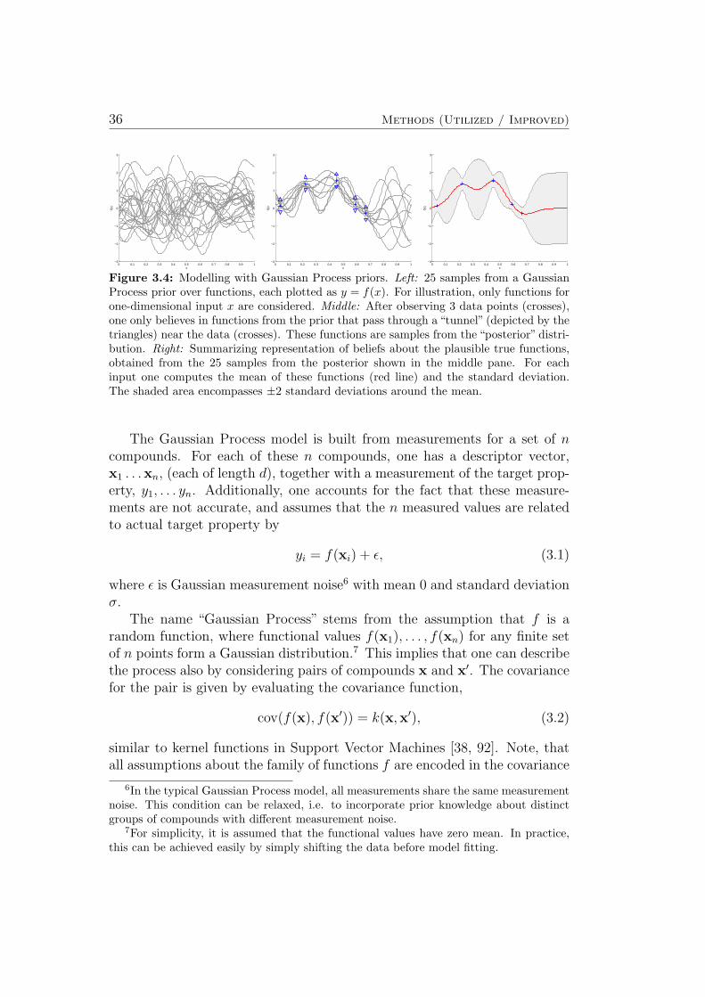
In GP modelling, one considers a family of functions that could potentiallymodel the dependence of the property to be predicted (function output, de-noted by y, also called “target function”, “target property”, or “target”) fromthe features (function input, denoted by x, in chemoinformatics also referredto as “descriptors”). This space of functions is described by a Gaussian Pro-cess prior. 25 such functions, drawn at random from the prior, are shown inFigure 3.4 (left). The prior captures, for example, the inherent variability ofthe target value as a function of the features. This prior belief is then up-dated in the light of new information, that is, the measurements (“labels”) athand. In Figure 3.4 (middle), the available measurements are illustrated bythree crosses. Principles of statistical inference are used to identify the mostlikely posterior function, that is, the most likely target function as a com-bination of prior assumptions and observed data (shown in the right panelof Figure 3.4). The formulation with a prior function class is essential inorder to derive predictive variances for each prediction. Note also that theuncertainty increases on points that are far from the measurements.
The main assumption of a Gaussian Process model is that the targetfunction can be described by an (unknown) function f that takes a vector ofmolecular descriptors as input, and outputs the target. x denotes a vectorof descriptors, which is assumed to have length d. The target property of acompound described by its descriptor vector x can thus be written as f(x).It is assumed that f is inherently random.5
5The notation here is chosen to allow an easy understanding of the material, thusdropping, e.g., a clear distinction between random variables and their outcome.
36 Methods (Utilized / Improved)
0 0.1 0.2 0.3 0.4 0.5 0.6 0.7 0.8 0.9 1−3
−2
−1
0
1
2
3
x
f(x)
0 0.1 0.2 0.3 0.4 0.5 0.6 0.7 0.8 0.9 1−3
−2
−1
0
1
2
3
xf(
x)0 0.1 0.2 0.3 0.4 0.5 0.6 0.7 0.8 0.9 1
−3
−2
−1
0
1
2
3
x
f(x)
Figure 3.4: Modelling with Gaussian Process priors. Left: 25 samples from a GaussianProcess prior over functions, each plotted as y = f(x). For illustration, only functions forone-dimensional input x are considered. Middle: After observing 3 data points (crosses),one only believes in functions from the prior that pass through a “tunnel” (depicted by thetriangles) near the data (crosses). These functions are samples from the “posterior” distri-bution. Right: Summarizing representation of beliefs about the plausible true functions,obtained from the 25 samples from the posterior shown in the middle pane. For eachinput one computes the mean of these functions (red line) and the standard deviation.The shaded area encompasses ±2 standard deviations around the mean.
The Gaussian Process model is built from measurements for a set of ncompounds. For each of these n compounds, one has a descriptor vector,x1 . . .xn, (each of length d), together with a measurement of the target prop-erty, y1, . . . yn. Additionally, one accounts for the fact that these measure-ments are not accurate, and assumes that the n measured values are relatedto actual target property by
yi = f(xi) + ε, (3.1)
where ε is Gaussian measurement noise6 with mean 0 and standard deviationσ.
The name “Gaussian Process” stems from the assumption that f is arandom function, where functional values f(x1), . . . , f(xn) for any finite setof n points form a Gaussian distribution.7 This implies that one can describethe process also by considering pairs of compounds x and x′. The covariancefor the pair is given by evaluating the covariance function,
cov(f(x), f(x′)) = k(x,x′), (3.2)
similar to kernel functions in Support Vector Machines [38, 92]. Note, thatall assumptions about the family of functions f are encoded in the covariance
6In the typical Gaussian Process model, all measurements share the same measurementnoise. This condition can be relaxed, i.e. to incorporate prior knowledge about distinctgroups of compounds with different measurement noise.
7For simplicity, it is assumed that the functional values have zero mean. In practice,this can be achieved easily by simply shifting the data before model fitting.
3.3 Learning Algorithms 37
function k. Each of the possible functions f can be seen as one realizationof an “infinite dimensional Gaussian distribution”.
Let us now return to the problem of estimating f from a data set of ncompounds with measurements of the target property y1, . . . , yn, as describedabove in Eq. (3.1). Omitting some details here (the derivation can be foundin appendix B in [11]), it turns out that the prediction of a Gaussian Processmodel has a particularly simple form. The predicted function for a newcompound x∗ follows a Gaussian distribution with mean f(x∗),
f(x∗) =n∑i=1
αik(x∗,xi). (3.3)
Coefficients αi are found by solving a system of linear equations,k(x1,x1) + σ2 k(x1,x2) . . . k(x1,xn)k(x2,x1) k(x2,x2) + σ2 . . . k(x2,xn)
......
...k(xn,x1) k(xn,x2) . . . k(xn,xn) + σ2
α1
α2...αn
=
y1
y2...yn
(3.4)
In matrix notation, this is the linear system (K+σ2I)α = y, with I denotingthe unit matrix. In this framework, one can also derive that the predictedproperty has a standard deviation of
std f(x∗) =
√√√√k(x∗,x∗)−n∑i=1
n∑j=1
k(x∗,xi)k(x∗,xj)Lij (3.5)
where Lij are the elements of the matrix L = (K + σ2I)−1.
Relations to Support Vector Machines Gaussian Process models sharewith the widely known support vector machines the concept of a kernel (co-variance) function. Support vector machines (SVM) implicitly map the ob-ject to be classified, x, to a high-dimensional feature space φ(x). Classifica-tion is then performed by linear separation in the feature space, with certainconstraints that allow this problem to be solved in an efficient manner. Sim-ilarly, support vector regression [92] can be described as linear regression inthe feature space. Gaussian Process models can as well be seen as linearregression in the feature space that is implicitly spanned by the covariance(kernel) function [43]. The difference lies in the choice of the loss function:SVM regression has an insensitivity threshold, that amounts to ignoring smallprediction errors. Large prediction errors contribute linearly to the loss. GP
38 Methods (Utilized / Improved)
models assume Gaussian noise, equivalent to square loss. As for supportvector machines, the mapping of input space to feature space is never com-puted explicitly. In SVMs and GP models, only dot-products of the form〈φ(x), φ(x′)〉 are used in the algorithm. Such dot products can be evaluatedcheaply via the covariance (kernel) function, since 〈φ(x), φ(x′)〉 = k(x,x′).
Note, however, that SVMs are completely lacking the concept of uncer-tainty. SVMs have a unique solution that is optimal under certain conditions[92, 93]. Unfortunately, these assumptions are violated in some practicalapplications.
Relations to Neural Networks Radial Basis Function networks with acertain choice of prior distribution for the weights yield the same predictionsas a Gaussian Process model [43]. More interestingly, it can be shown that atwo-layer neural network with an increasing number of hidden units convergesto a Gaussian Process model with a particular covariance function [94].
Using GP Models For predicting Partition Coefficients (Sec. 5.2) andAqueous Solubility (Sec. 5.3), a covariance function of the form
k(x,x′) =
(1 +
d∑i=1
wi(xi − x′i)2
)−ν(3.6)
is used (the “rational quadratic” covariance function [43]). k(x,x′) describesthe “similarity” (covariance) of the target property for two compounds, givenby their descriptor vectors x and x′. The contribution of each descriptor tothe overall similarity is weighted by a factor wi > 0 that effectively describesthe importance of descriptor i for the task of predicting the respective targetproperty.
Clearly, one cannot set the weights wi and the parameter ν a priori.Thus, one extends the GP framework by considering a superfamily of Gaus-sian Process priors, each prior encoded by a covariance function with specificsettings for wi. The search is guided through the superfamily by maximiz-ing a Bayesian criterion called the evidence (marginal likelihood). For nmolecules x1, . . . ,xn with associated measurements y1, . . . , yn, this criterionis obtained by “integrating out” everything unknown, namely all the truefunctional values f(xi). Using vector notation for f = (f(x1), . . . , f(xn)) andy = (y1, . . . , yn), one obtains
L = p(y | x1, . . . ,xn, θ) =
∫p(y|f , θ) p(f | x1, . . . ,xn, θ) df . (3.7)
3.3 Learning Algorithms 39
This turns out to be
L = −1
2log det(Kθ + σ2I)− 1
2y>(Kθ + σ2I)−1y − n
2log 2π (3.8)
Here, det denotes the determinant of a matrix, and > is vector transpose. Kθ
is used to explicitly denote the dependence of the covariance matrix K on aset of parameters θ of the covariance function.8 Gradient ascent methods9 cannow be used to maximize L with respect to covariance function parameters θand the measurement variance σ2. References [43, 96] present further details.
The following advantages of Gaussian Processes are relevant for theirapplication in drug discovery & design:
• As illustrated above, Gaussian Process models allow for quantifyingthe confidence in each individual prediction. Since this feature is veryuseful in chemoinformatics, a separate section has been devoted to thistopic, namely Sec. 3.7.
• In GP modeling, heterogeneous types of information about one set ofcompounds can be combined via combined covariance functions. ThisBayesian concept is similar in spirit to the frequentist concept of mul-tiple kernel learning, see Sec. 3.6.
• Data sets for multiple target values (e.g. one set for aqueous solubilityand a different set for partition coefficients) can be treated in a singlelearning procedure. Even if the datasets overlap only partially, infor-mation gained from one set eases solving the remaining task(s) [44]. Inthe machine learning community, this is called multi task learning. Aconcise overview of multi task learning (using a variety of algorithms)in chemoinformatics can be found in this recent article [97].
• When using kernels with separate width parameters for each dimension,the weighting of the features can be optimized by a gradient ascent onthe evidence. Optionally, one can later use this information to reducethe number of features to present to a second GP or other learningalgorithm or to identify important features (see the second subsectionin Sec. 3.2 for a discussion).
• Many types of previous knowledge that one might have about the datacan be included into GP models. In [11], it was known that different
8In the case of Eq. (3.6), θ = {ν, w1, . . . , wd} for a total of d descriptors.9In the actual implementation, the Broyden-Fletcher-Goldfarb-Shanno method [95] is
used.
40 Methods (Utilized / Improved)
subsets of measurements in the training data were moderately reliable,more reliable and very reliable, respectively. We then trained GP mod-els such that a different noise variance was learned for each group ofcompounds. Even without specifying different priors for the groups,the models automatically learned lower noise levels for the more reli-able measurements. See [11] for details.
• The algorithm presented in Sec. 4.3 explains predictions of machinelearning models by the means of visualizing relevant objects from thetraining set of the model. This allows human experts to understandhow each prediction comes about. In case of kernel methods (includingGaussian Processes), the contribution of individual testpoints can becalculated analytically.
• Sec. 4.4 proposes a method that can explain the local decisions takenby arbitrary (possibly) non-linear classification algorithms. In a nut-shell, the estimated explanations are local gradients that characterizehow a data point has to be moved to change its predicted label. Formodels where such gradient information cannot be calculated explic-itly, a probabilistic approximate mimic of the learning machine to beexplained is employed. In the special case of Gaussian Processes, lo-cal gradients of predictions can be calculated analytically. See Sec. 4.4for derivations & illustrations and Sec. 5.8 for an application in drugdiscovery & design.
Due to these advantages, GP regression models were used in the followingstudies: [3–12, 90, 98]. The first use of GP classification models in thecontext of drug discovery and design is described in our study [6], furtherapplications include [1, 5].
Other Learning Algorithms
When introducing new methods, it generally makes sense to compare theirperformance with established models of equal or lesser complexity. Briefintroductions to each method can be found in [10]. The reader is invited toconsult the literature cited directly following each algorithm’s name below tolearn more about the respective method.
• Support Vector Machines [38–42] for regression and classification servedas equally complex but more established [99, 100] type of model in [3–8, 12].

3.3 Learning Algorithms 41
• Random forests [101] (i.e. ensembles of decision trees [45]) have beenpreviously used in drug discovery & drug design. Benchmarks wereincluded in [4, 5, 7, 8, 12].
• k-Nearest-Neighbor models were applied in [5], Sec. 4.3 and 4.4.
• Linear models [102] represent the least complex type of models andwere included as baselines in [3–8, 12].
42 Methods (Utilized / Improved)
3.4 Evaluation Strategies
Many different strategies for evaluating models exist:
• single validation set
• leave one out cross-validation
• leave k-percent out cross-validation
• leave one cluster out cross-validation
• nested cross-validation variants
• blind tests / prospective evaluation
When choosing an evaluation strategy, the most important question has tobe: What is the goal of this evaluation? One may want to
1. select features / descriptors
2. select a modeling algorithm
3. tune model parameters
4. estimate generalization to unseen data following the same distributionas the training data
5. estimate generalization to unseen data following a different distributionthan the training data.
Very often, one wants to do all of the above: Starting from a batch of data,one selects features, chooses a modeling algorithm and tunes free parameters.In the end one seeks to estimate the generalization performance including orexcluding extrapolation.
The most common mistake is trying to estimate the generalization per-formance using data that has been used in model building. If any of the testdata has been used in any of the model building steps (selecting features,algorithm and tuning parameters), estimates of generalization performancewill invariably turn out too optimistic. This means that one needs to splitthe data into at least three sets: The first set is used to train models usingdifferent algorithms, feature sets and parameters. These different models arethen applied to the second set of data. Based on the performance on this set,one selects one (!) model. This final model is then applied to the third set toestimate generalization performance. This is the exact point where mistakes
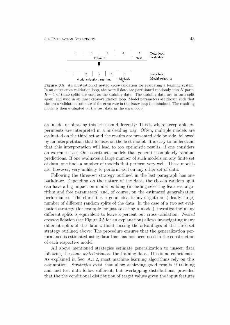
3.4 Evaluation Strategies 43
Figure 3.5: An illustration of nested cross-validation for evaluating a learning system.In an outer cross-validation loop, the overall data are partitioned randomly into K parts.K − 1 of these splits are used as the training data. The training data are in turn splitagain, and used in an inner cross-validation loop. Model parameters are chosen such thatthe cross-validation estimate of the error rate in the inner loop is minimized. The resultingmodel is then evaluated on the test data in the outer loop.
are made, or phrasing this criticism differently: This is where acceptable ex-periments are interpreted in a misleading way. Often, multiple models areevaluated on the third set and the results are presented side by side, followedby an interpretation that focuses on the best model. It is easy to understandthat this interpretation will lead to too optimistic results, if one considersan extreme case: One constructs models that generate completely randompredictions. If one evaluates a large number of such models on any finite setof data, one finds a number of models that perform very well. These modelsare, however, very unlikely to perform well on any other set of data.
Following the three-set strategy outlined in the last paragraph has onebackdraw: Depending on the nature of the data, the chosen random splitcan have a big impact on model building (including selecting features, algo-rithm and free parameters) and, of course, on the estimated generalizationperformance. Therefore it is a good idea to investigate an (ideally large)number of different random splits of the data. In the case of a two set eval-uation strategy (for example for just selecting a model), investigating manydifferent splits is equivalent to leave k-percent out cross-validation. Nestedcross-validation (see Figure 3.5 for an explanation) allows investigating manydifferent splits of the data without loosing the advantages of the three-setstrategy outlined above: The procedure ensures that the generalization per-formance is estimated using data that has not been used in the constructionof each respective model.
All above mentioned strategies estimate generalization to unseen datafollowing the same distribution as the training data. This is no coincidence:As explained in Sec. A.1.2, most machine learning algorithms rely on thisassumption. Strategies exist that allow achieving good results if trainingand and test data follow different, but overlapping distributions, providedthat the the conditional distribution of target values given the input features
44 Methods (Utilized / Improved)
(descriptors) is the same in both test and training data. In the machinelearning community, this scenario is known as covariate shift and corres-ponds to “mild extrapolation”, see Sec. A.1.2 for details. The assumption ofequal conditionals is often violated in drug discovery applications: In newprojects, new compound classes may be investigated. These new compoundscan exhibit new mechanisms of action (see Sec. A.1.3), possibly leading tocomplete failure of previously constructed models.
Imagine a set of measurements for 100 compounds, belonging to 10 struc-tural classes. If we evaluate models on any single random split of the dataor in a number of random splits (e.g. in leave k-percent out cross-validation)it is very likely that for every molecule in every test set, structurally similarcompounds exist in the respective training set. To simulate the effect of newstructural classes being introduced in new projects, one can generate splitswhere the distributions of test and training data differ substantially. One pos-sible way to do this is leave one cluster out cross-validation, see [3, 4, 10, 103]for a description. Alternatively, one can take the temporal structure of thedataset into account, i.e. train on compounds measured before a given dateand test on compounds that were measured after this date. If the evaluationis done by a group of people who were not involved in model building, usingmeasurements that were not available to the modellers, this is called “blindevaluation”. In [5–9, 11, 12] a combination of the two last-mentioned strate-gies was used to evaluate model performance. Models were constructed byresearchers at Fraunhofer FIRST and Idalab. The final evaluation of eachmodel was done by scientists at Bayer Schering Pharma, using new data thathad accumulated over last couple of months, including compounds from newprojects. This way of evaluating models is very similar to a strategy oftenreferred to as “prospective evaluation”. Here, one also applies the models tonewly measured compounds. However, the new compounds were typically se-lected using the same model that is finally evaluated. Depending on the typeof model, this can introduce a bias towards easily predictable compoundsand will (as intended) introduce a bias towards compounds with desirableproperties.
3.5 Performance Indicators 45
3.5 Performance Indicators
In drug discovery & design, performance indicators (or loss functions) areused for a number of different purposes, including:
• steering the process of model fitting inside a learning algorithm
• guiding automatic tuning of hyperparameters of the learning algorithm
• allowing the modeller to assess the quality of a model
• communicating the quality of a model to non-experts
In the work leading up to this thesis, various standard regression, classifica-tion and ranking loss functions were used. This includes mean absolute error,mean squared error, root mean squared error, percentage of prediction withindifferent intervals from the true value, correlation coefficients, Kendall’s τ andarea under the ROC curve. Additionally, modified versions of standard lossfunctions and one completely new loss function were conceived.
Hints for Practitioners
The following subsection contains a somewhat informal collection of findingson loss functions that the author beliefs may be useful for practitioners inthe field of chemoinformatics.
• Loss functions inside learning algorithms can be implicitly containedin the formulation of the optimization problem. One example is thestandard formulation of Gaussian Processes, based on the assumptionof Gaussian noise. This noise-model leads to an implicit squared errorloss function. See paragraph “Relations to Support Vector Machines”on page 37.
• When using loss functions for tuning real valued hyperparameters, dif-ferentiable loss functions have the obvious advantage of enabling theuse of gradient descend methods. If different local minima exist orwhen tuning hyperparameters expressed by integers, network architec-tures etc., grid search algorithms are a good choice. In this case, lossfunctions need not be differentiable, but are required to be informativewith respect to the goal of the optimization.
• In the presence of outliers, the often used mean squared error loss-function can be misleading, because it is easily dominated by small
46 Methods (Utilized / Improved)
numbers of outliers. The mean absolute error is somewhat more robustin this respect, but in the presence of very extreme outliers it will alsobe misleading. Unless other ways of avoiding these far off predictionscan be found (e.g. detection of outliers based on their features, seethird subsection in 3.2), a simple way of avoiding their dominance inparameter tuning is to redefine the loss function to disregard a certainpercentage of least accurate predictions.
• When assessing the quality of a model as a human, it is generally agood idea to not rely on a single number statistic. [104] illustrates howcorrelation coefficients can be misleading. Instead, one should lookat plots such as scatterplots, receiver operating characteristic curves(ROC) and cumulative histograms.
• “Staircase plots” can be very useful for providing a visual impressionof the quality of confidence estimates (see Figure 5.2 in Sec. 5.2 andFigure 5.5 in Sec. 5.3). If a single number statistic is desired, Kendall’sτ [105] can be used.
A New Loss Function for Virtual Screening
It is important to use a loss function that represents the application scenarioas closely as possible. When preparing a virtual screening for new PPARγagonists (see Sec. 5.9) a new loss function was defined to this end: Whenperforming the retrospective evaluation, it was known that the prospectiveevaluation would comprise experimentally investigating the activity of 20or less compounds chosen out of a database containing more than 300.000compounds. Including inactive compounds in the top 20 is very undesirable,whereas errors in the remaining bulk of predictions are irrelevant. Thereforethe loss function “FI20” was defined as the fraction of inactive compounds inthe top 20 ranked compounds. Additionally, standard regression performanceindicators considering the whole set of test data were calculated to find outwhether the newly introduced FI20 loss function actually results in choosingdifferent models. Different models were chosen using different loss functions.The model chosen based on the FI20 loss function turned out to suggest themost promising candidate molecules according to a panel of human experts.The activity of a number of molecules was measured and a number of newPPARγ agonists agonists were identified. Interestingly, the FI20 score forthe actual experiments was almost identical to the score estimated duringthe prospective evaluation. See Sec. 5.9 for details.
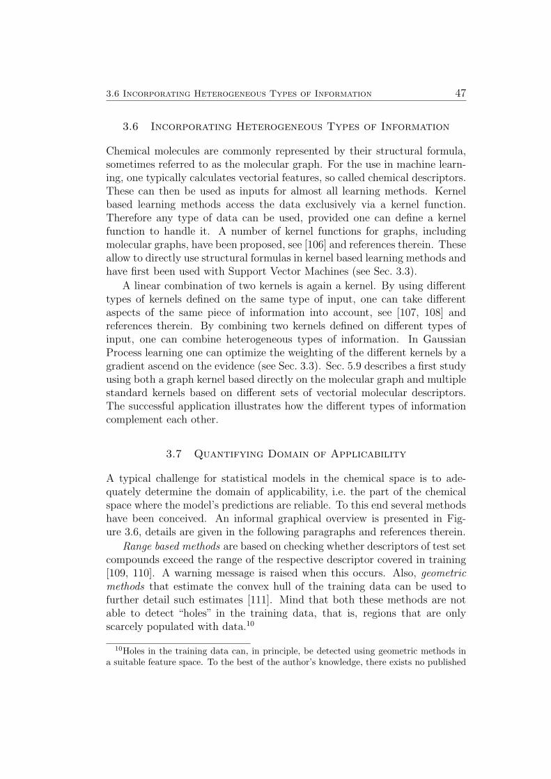
3.6 Incorporating Heterogeneous Types of Information 47
3.6 Incorporating Heterogeneous Types of Information
Chemical molecules are commonly represented by their structural formula,sometimes referred to as the molecular graph. For the use in machine learn-ing, one typically calculates vectorial features, so called chemical descriptors.These can then be used as inputs for almost all learning methods. Kernelbased learning methods access the data exclusively via a kernel function.Therefore any type of data can be used, provided one can define a kernelfunction to handle it. A number of kernel functions for graphs, includingmolecular graphs, have been proposed, see [106] and references therein. Theseallow to directly use structural formulas in kernel based learning methods andhave first been used with Support Vector Machines (see Sec. 3.3).
A linear combination of two kernels is again a kernel. By using differenttypes of kernels defined on the same type of input, one can take differentaspects of the same piece of information into account, see [107, 108] andreferences therein. By combining two kernels defined on different types ofinput, one can combine heterogeneous types of information. In GaussianProcess learning one can optimize the weighting of the different kernels by agradient ascend on the evidence (see Sec. 3.3). Sec. 5.9 describes a first studyusing both a graph kernel based directly on the molecular graph and multiplestandard kernels based on different sets of vectorial molecular descriptors.The successful application illustrates how the different types of informationcomplement each other.
3.7 Quantifying Domain of Applicability
A typical challenge for statistical models in the chemical space is to ade-quately determine the domain of applicability, i.e. the part of the chemicalspace where the model’s predictions are reliable. To this end several methodshave been conceived. An informal graphical overview is presented in Fig-ure 3.6, details are given in the following paragraphs and references therein.
Range based methods are based on checking whether descriptors of test setcompounds exceed the range of the respective descriptor covered in training[109, 110]. A warning message is raised when this occurs. Also, geometricmethods that estimate the convex hull of the training data can be used tofurther detail such estimates [111]. Mind that both these methods are notable to detect “holes” in the training data, that is, regions that are onlyscarcely populated with data.10
10Holes in the training data can, in principle, be detected using geometric methods ina suitable feature space. To the best of the author’s knowledge, there exists no published
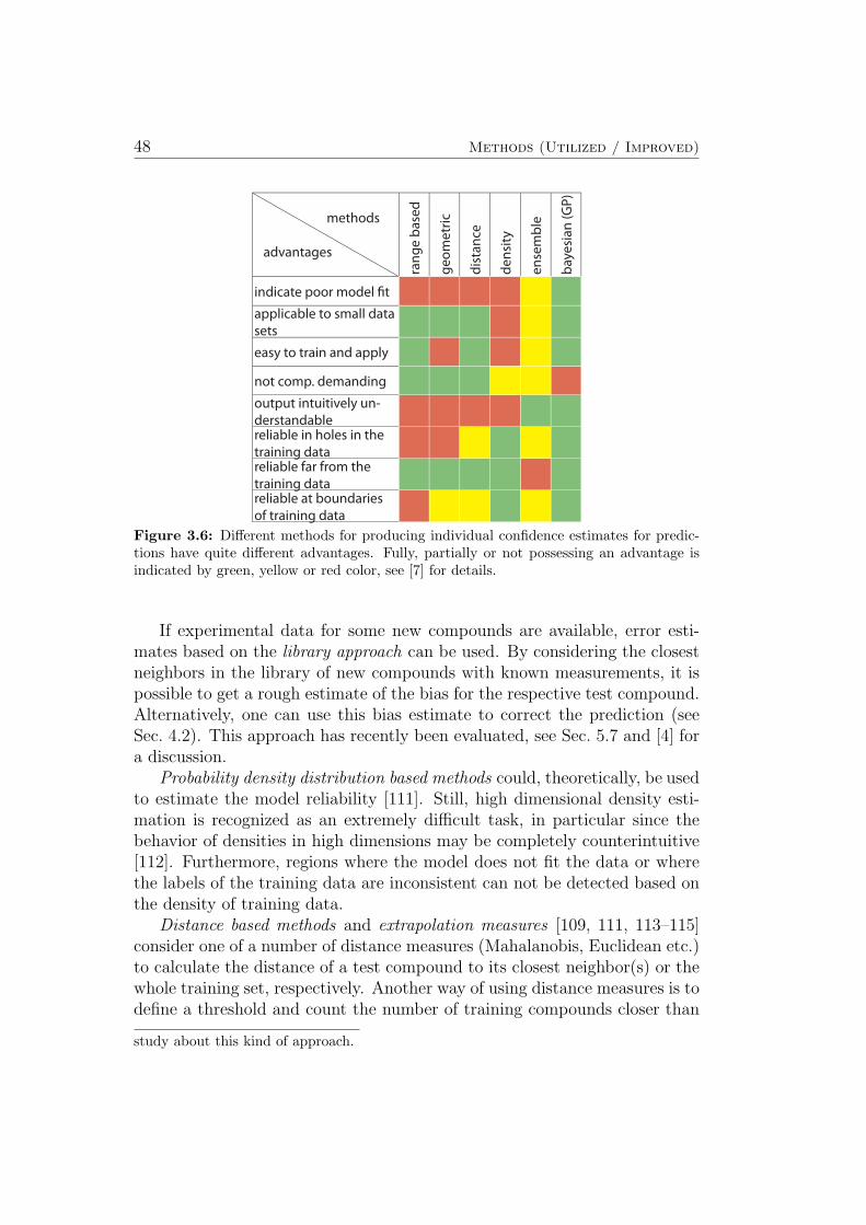
48 Methods (Utilized / Improved)
Background
Results
Domain of Applicability• crucial in drug design
• only inside DOA,
predictions are reliable
• new molecules are often
outside of the DOA
methods
advantages
ran
ge
ba
sed
ge
om
etr
ic
dis
tan
ce
de
nsi
ty
en
sem
ble
bay
esi
an
(G
P)
indicate poor model fi t
applicable to small data
sets
easy to train and apply
not comp. demanding
output intuitively un-
derstandablereliable in holes in the
training datareliable far from the
training datareliable at boundaries
of training data
−10 −8 −6 −4 −2 0 2 4 6 8 10−1.5
−1
−0.5
0
0.5
1
1.5 bad fi t
−10 −8 −6 −4 −2 0 2 4 6 8 10−1.5
−1
−0.5
0
0.5
1
1.5 bayesian (GP)
−10 −8 −6 −4 −2 0 2 4 6 8 10−1.5
−1
−0.5
0
0.5
1
1.5 ensemble
Estimating the Domain of Applicability
for Machine Learning QSAR Models
Quantitative Structure
Activity Relationships• popular in drug design
• predict complex properties of
molecules
• based on measurements and
“descriptors” of a “training” set
of compounds
• machine learning algorithms
allow non-linear generalisation
Aqueous Solubility• training: 650 in-house,
3300 literature compounds
• blind test: 550 in-house
• performance increases when
using GP & focussing on DOA
ReferencesSchroeter, Schwaighofer et al, J. Comp. Aid. Mol. Des., 2007
Schwaighofer, Schroeter et al, J. Chem. Inf. Model. 47(2):407-
424, 2007
−8 −7 −6 −5 −4 −3 −2 −1 0 1−8
−7
−6
−5
−4
−3
−2
−1
0
1
Measured logSW
Pre
dic
ted logS
W
0.25 0.54 0.85 1.580
0.1
0.2
0.3
0.4
0.5
0.6
0.7
0.8
0.9
1
Mean A
bsolu
te E
rror
Model based error bar
Lipophilicity• training:15,000 in-house,
8000 literature compounds
• blind test: 7000 in-house
• performance increases when
using GP & focussing on DOA
ReferencesSchroeter, Schwaighofer et al, ChemMedChem 2007
Schroeter, Schwaighofer et al, Molecular Pharmaceutics
4(4):524-538, 2007
0.1 0.2 0.29 0.4 0.55 0.72 1.260
0.1
0.2
0.3
0.4
0.5
0.6
0.7
0.8
0.9
Me
an
Ab
so
lute
Err
or
Model based error bar
−3 −2 −1 0 1 2 3 4 5 6 7−3
−2
−1
0
1
2
3
4
5
6
7
Measured log d
Pre
dic
ted
lo
g d
Metabolic Stability• training: 2200 in-house
• blind test: 700 in-house
compounds
• performance increases when
using GP & focussing on DOA
ReferencesSchwaighofer, Schroeter et al, J. Chem. Inf. Model. submitted
0 0.2 0.4 0.6 0.8 1
0
0.1
0.2
0.3
0.4
0.5
0.6
0.7
0.8
0.9
1
false positive rate
true p
ositiv
e r
ate
Human m/f
Size of grey area
0 0.2 0.45
0,0
0,5
1,0
Timon Schroeter1, Anton Schwaighofer1, Sebastian Mika2, Antonius Ter Laak3, Nikolaus Heinrich3
Figure 3.6: Different methods for producing individual confidence estimates for predic-tions have quite different advantages. Fully, partially or not possessing an advantage isindicated by green, yellow or red color, see [7] for details.
If experimental data for some new compounds are available, error esti-mates based on the library approach can be used. By considering the closestneighbors in the library of new compounds with known measurements, it ispossible to get a rough estimate of the bias for the respective test compound.Alternatively, one can use this bias estimate to correct the prediction (seeSec. 4.2). This approach has recently been evaluated, see Sec. 5.7 and [4] fora discussion.
Probability density distribution based methods could, theoretically, be usedto estimate the model reliability [111]. Still, high dimensional density esti-mation is recognized as an extremely difficult task, in particular since thebehavior of densities in high dimensions may be completely counterintuitive[112]. Furthermore, regions where the model does not fit the data or wherethe labels of the training data are inconsistent can not be detected based onthe density of training data.
Distance based methods and extrapolation measures [109, 111, 113–115]consider one of a number of distance measures (Mahalanobis, Euclidean etc.)to calculate the distance of a test compound to its closest neighbor(s) or thewhole training set, respectively. Another way of using distance measures is todefine a threshold and count the number of training compounds closer than
study about this kind of approach.
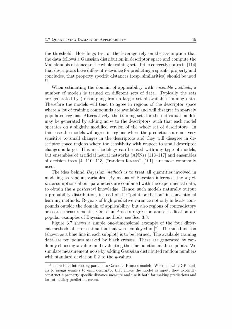
3.7 Quantifying Domain of Applicability 49
the threshold. Hotellings test or the leverage rely on the assumption thatthe data follows a Gaussian distribution in descriptor space and compute theMahalanobis distance to the whole training set. Tetko correctly states in [114]that descriptors have different relevance for predicting a specific property andconcludes, that property specific distances (resp. similarities) should be used11.
When estimating the domain of applicability with ensemble methods, anumber of models is trained on different sets of data. Typically the setsare generated by (re)sampling from a larger set of available training data.Therefore the models will tend to agree in regions of the descriptor spacewhere a lot of training compounds are available and will disagree in sparselypopulated regions. Alternatively, the training sets for the individual modelsmay be generated by adding noise to the descriptors, such that each modeloperates on a slightly modified version of the whole set of descriptors. Inthis case the models will agree in regions where the predictions are not verysensitive to small changes in the descriptors and they will disagree in de-scriptor space regions where the sensitivity with respect to small descriptorchanges is large. This methodology can be used with any type of models,but ensembles of artificial neural networks (ANNs) [113–117] and ensemblesof decision trees [4, 110, 113] (“random forests”, [101]) are most commonlyused.
The idea behind Bayesian methods is to treat all quantities involved inmodeling as random variables. By means of Bayesian inference, the a pri-ori assumptions about parameters are combined with the experimental data,to obtain the a posteriori knowledge. Hence, such models naturally outputa probability distribution, instead of the “point prediction” in conventionallearning methods. Regions of high predictive variance not only indicate com-pounds outside the domain of applicability, but also regions of contradictoryor scarce measurements. Gaussian Process regression and classification arepopular examples of Bayesian methods, see Sec. 3.3.
Figure 3.7 shows a simple one-dimensional example of the four differ-ent methods of error estimation that were employed in [7]. The sine function(shown as a blue line in each subplot) is to be learned. The available trainingdata are ten points marked by black crosses. These are generated by ran-domly choosing x-values and evaluating the sine function at these points. Wesimulate measurement noise by adding Gaussian distributed random numberswith standard deviation 0.2 to the y-values.
11There is an interesting parallel to Gaussian Process models: When allowing GP mod-els to assign weights to each descriptor that enters the model as input, they explicitlyconstruct a property specific distance measure and use it both for making predictions andfor estimating prediction errors.
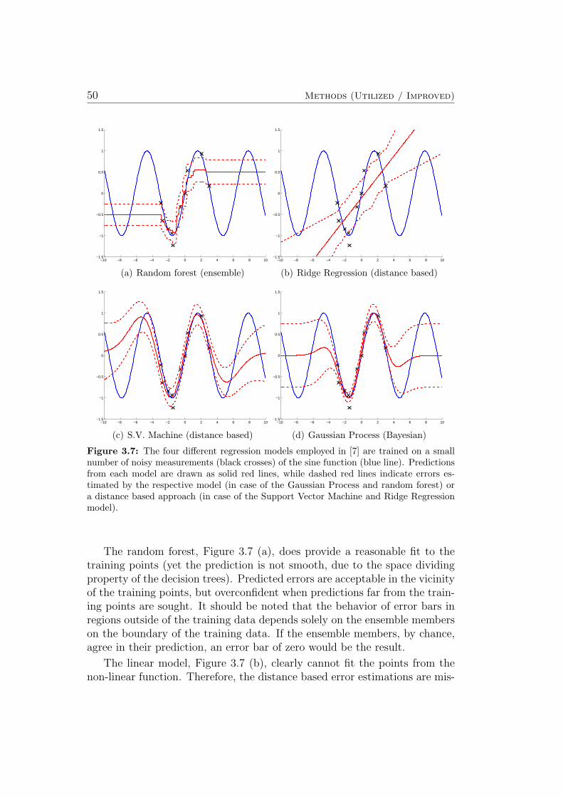
50 Methods (Utilized / Improved)
−10 −8 −6 −4 −2 0 2 4 6 8 10−1.5
−1
−0.5
0
0.5
1
1.5
(a) Random forest (ensemble)
−10 −8 −6 −4 −2 0 2 4 6 8 10−1.5
−1
−0.5
0
0.5
1
1.5
(b) Ridge Regression (distance based)
−10 −8 −6 −4 −2 0 2 4 6 8 10−1.5
−1
−0.5
0
0.5
1
1.5
(c) S.V. Machine (distance based)
−10 −8 −6 −4 −2 0 2 4 6 8 10−1.5
−1
−0.5
0
0.5
1
1.5
(d) Gaussian Process (Bayesian)
Figure 3.7: The four different regression models employed in [7] are trained on a smallnumber of noisy measurements (black crosses) of the sine function (blue line). Predictionsfrom each model are drawn as solid red lines, while dashed red lines indicate errors es-timated by the respective model (in case of the Gaussian Process and random forest) ora distance based approach (in case of the Support Vector Machine and Ridge Regressionmodel).
The random forest, Figure 3.7 (a), does provide a reasonable fit to thetraining points (yet the prediction is not smooth, due to the space dividingproperty of the decision trees). Predicted errors are acceptable in the vicinityof the training points, but overconfident when predictions far from the train-ing points are sought. It should be noted that the behavior of error bars inregions outside of the training data depends solely on the ensemble memberson the boundary of the training data. If the ensemble members, by chance,agree in their prediction, an error bar of zero would be the result.
The linear model, Figure 3.7 (b), clearly cannot fit the points from thenon-linear function. Therefore, the distance based error estimations are mis-
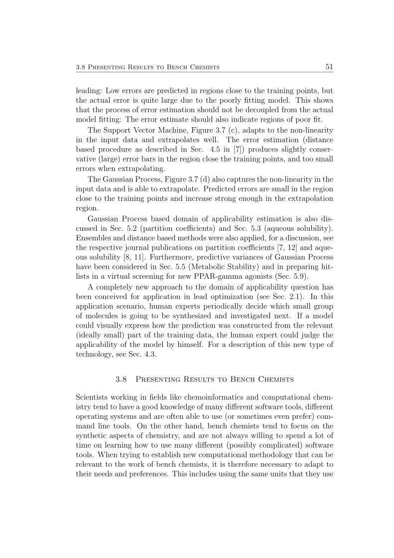
3.8 Presenting Results to Bench Chemists 51
leading: Low errors are predicted in regions close to the training points, butthe actual error is quite large due to the poorly fitting model. This showsthat the process of error estimation should not be decoupled from the actualmodel fitting: The error estimate should also indicate regions of poor fit.
The Support Vector Machine, Figure 3.7 (c), adapts to the non-linearityin the input data and extrapolates well. The error estimation (distancebased procedure as described in Sec. 4.5 in [7]) produces slightly conser-vative (large) error bars in the region close the training points, and too smallerrors when extrapolating.
The Gaussian Process, Figure 3.7 (d) also captures the non-linearity in theinput data and is able to extrapolate. Predicted errors are small in the regionclose to the training points and increase strong enough in the extrapolationregion.
Gaussian Process based domain of applicability estimation is also dis-cussed in Sec. 5.2 (partition coefficients) and Sec. 5.3 (aqueous solubility).Ensembles and distance based methods were also applied, for a discussion, seethe respective journal publications on partition coefficients [7, 12] and aque-ous solubility [8, 11]. Furthermore, predictive variances of Gaussian Processhave been considered in Sec. 5.5 (Metabolic Stability) and in preparing hit-lists in a virtual screening for new PPAR-gamma agonists (Sec. 5.9).
A completely new approach to the domain of applicability question hasbeen conceived for application in lead optimization (see Sec. 2.1). In thisapplication scenario, human experts periodically decide which small groupof molecules is going to be synthesized and investigated next. If a modelcould visually express how the prediction was constructed from the relevant(ideally small) part of the training data, the human expert could judge theapplicability of the model by himself. For a description of this new type oftechnology, see Sec. 4.3.
3.8 Presenting Results to Bench Chemists
Scientists working in fields like chemoinformatics and computational chem-istry tend to have a good knowledge of many different software tools, differentoperating systems and are often able to use (or sometimes even prefer) com-mand line tools. On the other hand, bench chemists tend to focus on thesynthetic aspects of chemistry, and are not always willing to spend a lot oftime on learning how to use many different (possibly complicated) softwaretools. When trying to establish new computational methodology that can berelevant to the work of bench chemists, it is therefore necessary to adapt totheir needs and preferences. This includes using the same units that they use
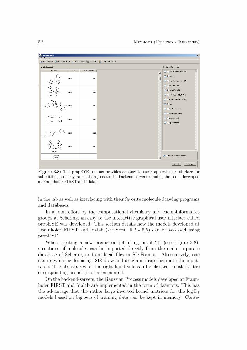
52 Methods (Utilized / Improved)
Figure 3.8: The propEYE toolbox provides an easy to use graphical user interface forsubmitting property calculation jobs to the backend-servers running the tools developedat Fraunhofer FIRST and Idalab.
in the lab as well as interfacing with their favorite molecule drawing programsand databases.
In a joint effort by the computational chemistry and chemoinformaticsgroups at Schering, an easy to use interactive graphical user interface calledpropEYE was developed. This section details how the models developed atFraunhofer FIRST and Idalab (see Secs. 5.2 - 5.5) can be accessed usingpropEYE.
When creating a new prediction job using propEYE (see Figure 3.8),structures of molecules can be imported directly from the main corporatedatabase of Schering or from local files in SD-Format. Alternatively, onecan draw molecules using ISIS-draw and drag and drop them into the input-table. The checkboxes on the right hand side can be checked to ask for thecorresponding property to be calculated.
On the backend-servers, the Gaussian Process models developed at Fraun-hofer FIRST and Idalab are implemented in the form of daemons. This hasthe advantage that the rather large inverted kernel matrices for the log D7
models based on big sets of training data can be kept in memory. Conse-
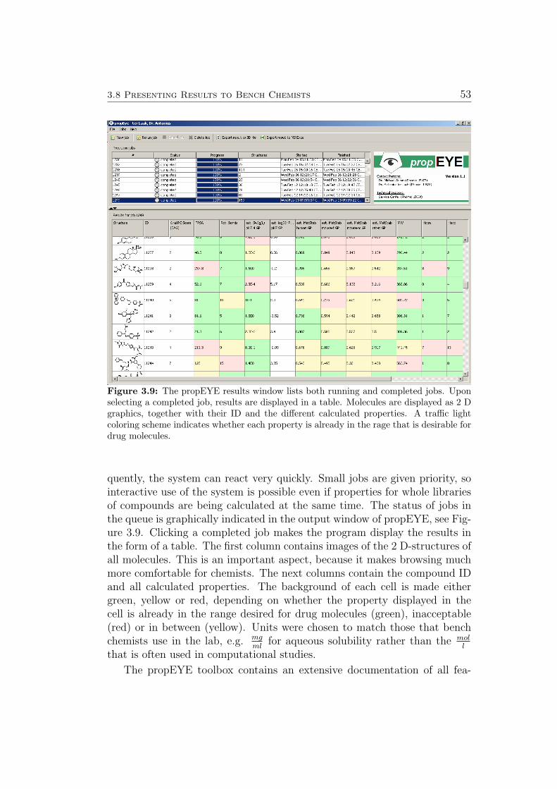
3.8 Presenting Results to Bench Chemists 53
Figure 3.9: The propEYE results window lists both running and completed jobs. Uponselecting a completed job, results are displayed in a table. Molecules are displayed as 2 Dgraphics, together with their ID and the different calculated properties. A traffic lightcoloring scheme indicates whether each property is already in the rage that is desirable fordrug molecules.
quently, the system can react very quickly. Small jobs are given priority, sointeractive use of the system is possible even if properties for whole librariesof compounds are being calculated at the same time. The status of jobs inthe queue is graphically indicated in the output window of propEYE, see Fig-ure 3.9. Clicking a completed job makes the program display the results inthe form of a table. The first column contains images of the 2 D-structures ofall molecules. This is an important aspect, because it makes browsing muchmore comfortable for chemists. The next columns contain the compound IDand all calculated properties. The background of each cell is made eithergreen, yellow or red, depending on whether the property displayed in thecell is already in the range desired for drug molecules (green), inacceptable(red) or in between (yellow). Units were chosen to match those that benchchemists use in the lab, e.g. mg
mlfor aqueous solubility rather than the mol
l
that is often used in computational studies.
The propEYE toolbox contains an extensive documentation of all fea-
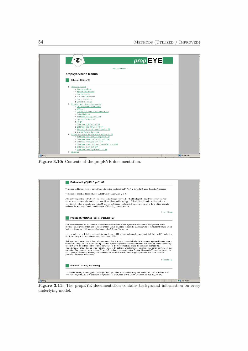
54 Methods (Utilized / Improved)
Figure 3.10: Contents of the propEYE documentation.
Figure 3.11: The propEYE documentation contains background information on everyunderlying model.
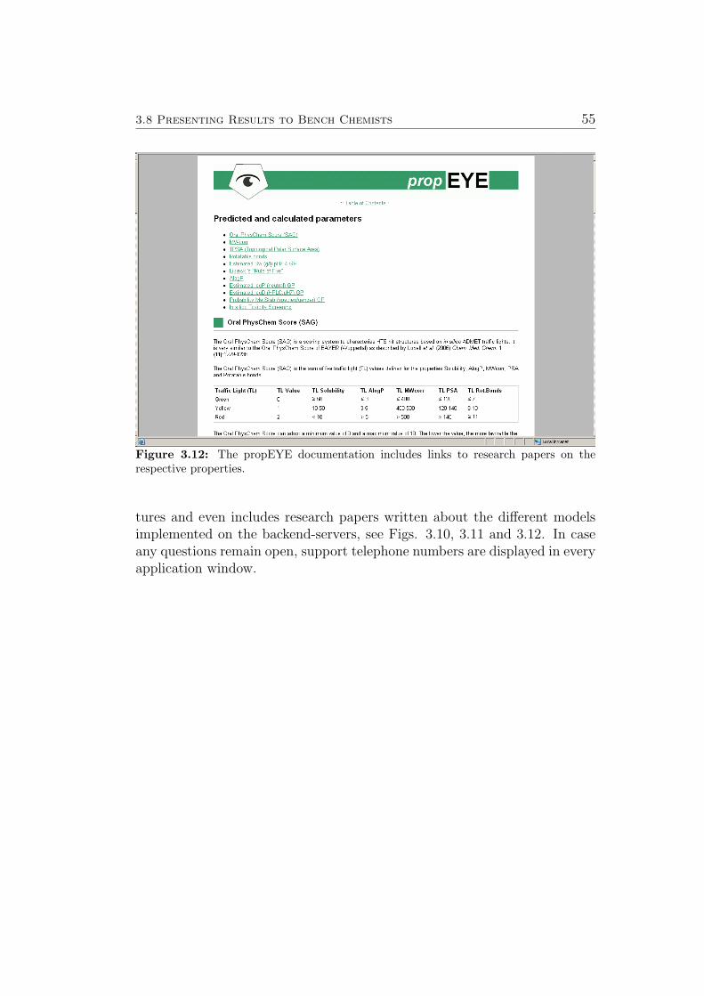
3.8 Presenting Results to Bench Chemists 55
Figure 3.12: The propEYE documentation includes links to research papers on therespective properties.
tures and even includes research papers written about the different modelsimplemented on the backend-servers, see Figs. 3.10, 3.11 and 3.12. In caseany questions remain open, support telephone numbers are displayed in everyapplication window.

Chapter 4
Newly Developed Methods
4.1 Overview
Three new algorithms were developed to cope with the specific requirementsof lead optimization, the most challenging part of the drug discovery process.The first new algorithm can improve the accuracy of models in the earlystages of lead optimization projects. The second new algorithm can explainindividual predictions made by complex models to human experts and thethird new algorithm generates hints for compound optimization.
Imagine a setting where human experts have access to multiple predictivemodels (including commercial black box models) and the first measurementsof compounds from a certain new compound class (e.g. part of the chemicalspace) are available. How can one obtain the best possible predictions fromall these sources of knowledge simultaneously? Sec. 4.2 introduces several en-semble modeling approaches where the most recent measurements are used toeither select the best model from the ensemble, construct a suitable weight-ing of multiple models in the ensemble or even correct a bias that one (ormore) ensemble members may consistently exhibit when making predictionsfor compounds that are similar to certain test compounds.
Two separate methodologies for explaining individual predictions of (pos-sibly non-linear) machine learning models are presented. The method pre-sented in Sec. 4.3 explains predictions by the means of visualizing relevantobjects from the training set of the model. This allows human experts tounderstand how each prediction comes about. If a prediction conflicts withhis intuition, the human expert can easily find out whether the grounds forthe models predictions are solid or if trusting his own intuition is the betteridea [2].
The method presented in Sec. 4.4 utilizes local gradients of the modelspredictions to explain predictions in terms of the locally most relevant fea-tures. This not only teaches the human expert which features are relevantfor each individual prediction, but also gives a directional information. Ab-stractly speaking, one can learn in which direction a data point has to bemoved to increase the prediction for the target value [1]. In the context of
57
58 Methods (Newly Developed)
lead optimization, this means that the human expert can obtain a type ofguidance in compound optimization.
4.2 Incorporating Additional Measurements
In drug discovery & design, modellers typically have access to a number ofpredictive tools for some of the relevant properties. Tools may have beenbought from vendors or trained in-house. For each of these tools, the respec-tive training set may or may not be known, the algorithm used in trainingeach model may or may not be well documented. If re-trainable in-housetools are available, one often has access to measurements for additional com-pounds that have become available after they have been trained last, andthat are not included in any of the commercial tools. An idea originallypublished by Kuhne et al. [118] comprises not just retraining the in-housetools including all new compounds. Instead, they used new compounds tochoose one out of a whole collection of tools that will probably predict acertain unknown compound most accurately. The set of new compounds iscalled“correction set”, and models are evaluated in a leave one compound outcross-validation setting where each compound from the correction set is inturn left out and treated as new. The following section summarizes the selec-tion approach conceived by Kuhne et al. and several ideas going beyond theoriginal publication. An evaluation of these ensemble modeling algorithms ispresented in Sec. 5.7.
Selection by MAE (MAE Model) In this approach the single modelwith the lowest mean absolute error on the neighboring compoundsin the correction set is selected to predict the desired value for the unknowncompound. The calculation of the mean absolute error (MAE) on the knearest neighbors is based on the distance measure introduced in [4]:
MAE(fi) =1
k
k∑j=1
| fi(xj)− yj | . (4.1)
Here fi refers to one of the l trained single models. Chemical compoundsare represented by descriptor vectors xj and the property to be predicted iswritten as yj. The predicted value f ∗(xt) of this ensemble model is given by
f ∗(xt) = fminMAE(xt) with f minMAE = argminfi i=1,..,l
(MAE(fi)). (4.2)
This is the type of algorithm originally proposed by Kuhne et al. [118].
4.2 Incorporating Additional Measurements 59
Weighted Model This model is based on the idea that a weighted sumof all predictions of the different single models can result in a greaterimprovement than selecting the prediction of only one model. The mixingcoefficient of each model υfi
is calculated according to the mean absoluteerror of the model on the neighboring compounds in the correction set:
υfi=
1
MAE(fi)
(l∑
j=1
1
MAE(fj)
)−1
such thatl∑
i=1
υfi= 1 (4.3)
and the predicted value of the weighted model can be written as
f ∗(xt) =l∑
i=1
υfifi(xt). (4.4)
The higher the accuracy of a single model fi in the neighborhood of theunknown compound t the greater the impact of the model fi on the predictionof the weighted model.
Bias Corrected Model In this approach first one single model is selectedwith respect to the mean absolute error on the neighboring compounds, iden-tically to the MAE model. From the prediction of the selected model onesubtracts the mean error on the neighbors in the correction set. To in-corporate the distance between the unknown compound t and its neighborswe define a distance weight for each of the k nearest neighbors as
dj =1
‖ xt − xj ‖red
(k∑i=1
1
‖ xt − xi ‖red
)−1
j = 1, . . . , k. (4.5)
This way close compounds receive high distance weights. The selected modelis now given as
fweightedDist = argminfi i=1,..,l
(1
k
k∑j=1
‖ fi(xj)− yj ‖reddj
). (4.6)
And the prediction is given as the prediction of fweightedDist reduced by theprediction error on the neighborhood
f ∗(xt) = fweightedDist (xt)−1
k
k∑j=1
fweightedDist (xj)− yjdj
. (4.7)
60 Methods (Newly Developed)
Average KNN Model and Random Choice Model These models arebaselines to determine the amount of improvement achieved by applying en-semble models. In the Random Choice Model the prediction of one standardmodel is chosen randomly as the predicted value.Unlike all other models, the Average Model predicts the value for the un-known compound without considering the prediction of the single models.The prediction is the average of the true values of the neighboring com-pounds
f ∗(xt) =1
k
k∑j=1
yj. (4.8)
Results of an evaluation of these algorithms for combining predictionsfrom individual models in the context of the hERG channel blockade effectare described in Sec. 5.7. Details and background information can be foundin [4].
4.3 Explaining Individual Predictions 61
4.3 Explaining Individual Predictions using Objects from theTraining Set
In this thesis, two separate methodologies for explaining individual predic-tions of machine learning models are presented. The method presented inthis section explains predictions by the means of visualizing relevant objectsfrom the training set of the model. This allows human experts to understandhow each prediction comes about. If a prediction conflicts with his intuition,the human expert can easily find out whether the grounds for the modelspredictions are solid or if trusting his own intuition is the better idea [2].
The method presented in Sec. 4.4 utilizes local gradients of the model’spredictions to explain predictions in terms of the locally most relevant fea-tures. This not only teaches the human expert which features are relevantfor each individual prediction, but also gives a directional information. Ab-stractly speaking, one can learn in which direction a data point has to bemoved to increase the prediction for the target value [1]. In the context of leadoptimization, this means that the human expert can obtain a type of guid-ance in compound optimization. For this reason, the two explaining-relatedmethodologies are presented in separate sections.
4.3.1 Motivation
Let us consider lead optimization (see Sec. 2.1). In this application scenariofor machine learning models, human experts periodically decide which smallbatch of molecules is going to be synthesized and investigated next. Modelscan support humans in making such decisions by providing accurate pre-dictions of the relevant properties of the compounds under consideration.However, human experts are not likely to trust a model if its prediction de-viates from their own intuition. This deviation might occur for any of thesereasons:
1. The models prediction is correct.
(a) Its training data includes relevant information that the expertdoesn’t know yet.
(b) It has generalized from known data in a valid way that is notobvious to the human expert.
(c) It has generalized from known data in an invalid way that is notobvious to the human expert, i.e. the correct prediction was alucky strike.
62 Methods (Newly Developed)
2. The human experts intuition is correct. The models predictions iswrong because
(a) The local density of training compounds is not high enough.
(b) The local labeling of training compounds is correct, but inconsis-tent.
(c) The local labeling of training compounds is wrong/inaccurate.
(d) The features (vectorial descriptors, 2D-graphs ...) given to thelearning algorithm do not represent the molecules sufficiently well.
(e) The internal representation of compounds in the learning algo-rithm (e.g. the kernel or covariance function) does not capturethe relevant bits of information.
(f) Hyperparameter selection (if applicable) led to non-optimal pa-rameters.
(g) Learning (model fitting) led to a non-optimal model.
If a model could visually express how each prediction was constructed froma small number of most relevant compounds in the training data, the humanexpert could easily recognize case 1(a). In the following, such visualizationswill be called explanations. By definition, the human expert cannot distin-guish between cases 1(b) and 1(c). To be on the safe side, he should thereforetrust his intuition and not believe the models predictions in cases 1(b,c) and2(a-g). If he learns from the models explanations that case 1(a) applies,his intuition and the model prediction will be in sync again, because he haslearned some decision-relevant new facts from the model.
Relation to Confidence Estimates
Individual confidence estimates, e.g. predictive variances from Gaussian Pro-cess Models (see Sec. 3.3) can, in principle, help to avoid inaccurate predic-tions, because they are often made with lower confidence than correct predic-tions (see Sec. 3.7). Considering the different cases defined above, predictivevariances can help to detect cases 2(a) and 2(b). The remaining cases 2(c-g)can, by definition, not be detected by the model itself. External tools, suchas local density estimators, outlier indices etc. may use different (internal)representations of the data and may be able to detect potentially unreliablepredictions where the model itself predicts confidently. However, the princi-ple difficulties listed in cases 2(c-g) apply to all conceivable external tools inan analog way.
4.3 Explaining Individual Predictions 63
4.3.2 Prerequisites for Obtaining helpful Explanations
The key hypothesis introduced in the motivational first part of this sectionis that sometimes (specifically: case 1(a) in the list above) a human expert’sintuition and a model’s prediction do not match, because the models trainingdata includes relevant information that the expert doesn’t know yet. In thiscase, a visualization of the relevant part of the training data is useful ifthe human expert agrees that the compounds (and metadata) presented asexplanations are indeed relevant to the prediction, because he can then learnsomething new. Consequently, his intuition and the models prediction finallymatch again.
Therefore, the model’s explanations for a certain prediction will be usefulif the following criteria are met:
1. The prediction is correct.
2. The prediction is based on few enough training compounds to allow thehuman expert to grasp the visualization.
3. The prediction is based on training compounds that are similar to thetest compound (according to the perception of the user)
4. At least some of these relevant training compounds (or their labels) arenew to the user.
The following paragraphs present how a study can be set up such that allfour requirements are satisfied. The discussion starts with the easiest re-quirements (no. 4 and no. 1) and then proceeds to the more difficult parts(no. 2 and no. 3).
The fourth requirement can, for the purpose of this present investigation,be satisfied by making the assumption that any compound might be unknownto some human expert who might want to use the system.
To satisfy the first requirement, one can generate predictions for held-out test-compounds with known labels and then choose correctly predictedtest-compounds for in depth investigation.
The second requirement can be made more specific by consulting thepsychological literature. As originally established by Miller [119] and laterconfirmed by many other researchers, humans can efficiently deal with up to7 ± 2 items simultaneously. In this study, the k-nearest-neighbor classifier(KNN) will be used as a baseline method. KNN-predictions are always basedon odd numbers of training compounds. Considering that the user will haveto simultaneously consider the test compound in question together with alltraining compounds relevant to this prediction, choosing k = 7 would result
64 Methods (Newly Developed)
in 7 + 1 = 8 items, i.e. demanding above average cognitive skills on thepart of the user. To be on the safe side while establishing the usefulness ofexplanations, the constraint k ≤ 5 was chosen for this study, resulting in amaximum of 5 + 1 = 6 items. Unlike KNN, more complex machine learningmethods do not have a parameter that limits how many training points willbe taken into account. Furthermore, this number may vary depending on thetest points for which predictions are sought. Hence, a subsection of Sec. 4.3.4is devoted to the question how complex machine learning algorithms can bemodified to operate sufficiently local.
The last requirement depends (by definition) on the user. Ideally, onewould perform an evaluation with a large number of human experts. How-ever, this type of investigation is out of the scope of this work. The initialevaluation presented in the following sections was performed by the authorof this thesis and is considered a starting point for further investigations.
4.3 Explaining Individual Predictions 65
4.3.3 Concepts & Definitions
If unlimited computational resources were available, explanations could begenerated for any machine learning model using a brute force approach alongthese lines:
1. Train a model using the full set of training data.
2. Perform leave-one-out cross-validation on the training data and keepall models.
3. Use each model to generate predictions for the test-compound for whichexplanations are sought.
4. Sort the leave-one-out models by how much the prediction for the testcompound varies when compared to the prediction from the model thatwas trained on the full training set. The compounds left out by themodels at the top of the list cause the largest changes in predictionwhen left out and are therefore the most relevant part of the trainingset.
As discussed in more detail in the next subsection, explanations generated inthis way can be useful if the machine learning algorithm operates sufficientlylocal. Applying the same algorithm to global models (like linear regression)would yield the same explanations for any conceivable test point. There-fore, they cannot lead the user to new insights by pointing out the trainingcompounds that are most relevant to each individual test compound.
In the special case of the k-nearest-neighbor classifier one can directly usethe k nearest neighbors of each test-point to generate explanations.
Kernel methods like support vector machines for classification (SVM) andregression (SVR), Gaussian Process regression (GPR) and kernel ridge regres-sion (KRR) all rely on the following general equation to calculate predictions[120].
f(x) =n∑i=1
αik(xi,x∗) + b (4.9)
Depending on the learning method, n is either the number of support vectors(for sparse methods like SVM, SVR) or the number of all training compounds(in case of GPR, KRR). The weights αi are optimized during model fittingand k(xi,x∗) denotes the kernel function between the respective supportvector / training compound xi an the test compound x∗.
Predictions made by Gaussian Process Classification (GPC) models in-clude the above expression f(x), but additionally take the predictive variance
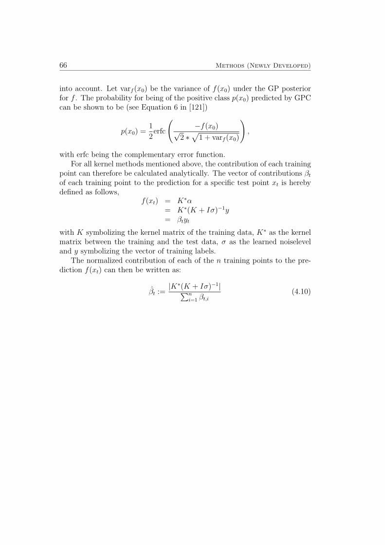
66 Methods (Newly Developed)
into account. Let varf (x0) be the variance of f(x0) under the GP posteriorfor f . The probability for being of the positive class p(x0) predicted by GPCcan be shown to be (see Equation 6 in [121])
p(x0) =1
2erfc
(−f(x0)√
2 ∗√
1 + varf (x0)
),
with erfc being the complementary error function.For all kernel methods mentioned above, the contribution of each training
point can therefore be calculated analytically. The vector of contributions βtof each training point to the prediction for a specific test point xt is herebydefined as follows,
f(xt) = K∗α= K∗(K + Iσ)−1y= βtyt
with K symbolizing the kernel matrix of the training data, K∗ as the kernelmatrix between the training and the test data, σ as the learned noiseleveland y symbolizing the vector of training labels.
The normalized contribution of each of the n training points to the pre-diction f(xt) can then be written as:
βt :=|K∗(K + Iσ)−1|∑n
i=1 βt,i(4.10)
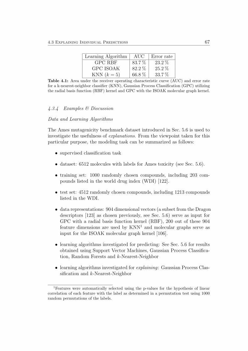
4.3 Explaining Individual Predictions 67
Learning Algorithm AUC Error rateGPC RBF 83.7 % 23.2 %
GPC ISOAK 82.2 % 25.2 %KNN (k = 5) 66.8 % 33.7 %
Table 4.1: Area under the receiver operating characteristic curve (AUC) and error ratefor a k-nearest-neighbor classifier (KNN), Gaussian Process Classification (GPC) utilizingthe radial basis function (RBF) kernel and GPC with the ISOAK molecular graph kernel.
4.3.4 Examples & Discussion
Data and Learning Algorithms
The Ames mutagenicity benchmark dataset introduced in Sec. 5.6 is used toinvestigate the usefulness of explanations. From the viewpoint taken for thisparticular purpose, the modeling task can be summarized as follows:
• supervised classification task
• dataset: 6512 molecules with labels for Ames toxicity (see Sec. 5.6).
• training set: 1000 randomly chosen compounds, including 203 com-pounds listed in the world drug index (WDI) [122].
• test set: 4512 randomly chosen compounds, including 1213 compoundslisted in the WDI.
• data representations: 904 dimensional vectors (a subset from the Dragondescriptors [123] as chosen previously, see Sec. 5.6) serve as input forGPC with a radial basis function kernel (RBF), 200 out of these 904feature dimensions are used by KNN1 and molecular graphs serve asinput for the ISOAK molecular graph kernel [106].
• learning algorithms investigated for predicting: See Sec. 5.6 for resultsobtained using Support Vector Machines, Gaussian Process Classifica-tion, Random Forests and k-Nearest-Neighbor
• learning algorithms investigated for explaining : Gaussian Process Clas-sification and k-Nearest-Neighbor
1Features were automatically selected using the p-values for the hypothesis of linearcorrelation of each feature with the label as determined in a permutation test using 1000random permutations of the labels.
68 Methods (Newly Developed)
Table 4.1 lists the error rate and area under the receiver operating charac-teristic curve (AUC) for the models applied in this study. Results obtainedusing Gaussian Process Classification (GPC) with RBF kernel are on parwith previous results (see Sec. 5.6), despite the fact that in the last study amuch larger fraction of all compounds was used to train the models.2 KNNperforms significantly worse when considering AUC. One reason may be thatKNN does not interpolate as well as GPC. A second reason is that whilebeing a useful single number statistic for classifiers with real valued output(like SVM and GPC), AUC can be misleading when being applied to KNNwith small k.3 The newly introduced GPC with the ISOAK molecular graphkernel performs almost as well as GPC with RBF kernel when consideringboth AUC and error rate.
Initial Explanations & Missing Locality of GPC models
Using these models, initial experiments on generating explanations were per-formed. In line with the previously presented motivation (Sec. 4.3.1) andprerequisites (Sec. 4.3.2), the ten most confidently made predictions for WDIcompounds4 made by each model are identified. Table 4.2, 4.3 and 4.4. listthese ten test compounds together with the five most relevant compoundsfrom the respective training set (explanations).
Inspecting the test compounds predicted most confidently by the KNNmodel with k = 5 (Table 4.2), one finds that they are structurally not verysimilar to the training compounds presented. Therefore, explanations gener-ated in this way will not be convincing in the eyes of a human expert utilizingthis model.5
Next, the ten test compounds predicted most confidently by the GaussianProcess Classification (GPC) model utilizing the ISOAK molecular graphkernel are investigated (Table 4.3). As one would expect when using a graphkernel, the predictions are based on structurally very similar molecules in the
2Previously, a 5-fold cross-validation was performed with additional compounds in astatic training set. Therefore, more than 5000 compounds were used in training eachmodel and only ≈ 1000 compounds were used as respective test set.
3AUC can be misleading when being applied to KNN with small k because AUC isoriginally an indicator of ranking performance. KNN generates a real valued output, butonly 2k+ 1 different values (voting outcomes in the range [−k . . . k]) are possible. Amongtest compounds with the same voting outcome, the order is random, which tends to resultin low AUCs for small values of k.
4When feasible, WDI listed test compounds are chosen for visual inspection, becausethey are the most relevant type of compound.
5Explanations identified by KNN models can potentially be improved by using differentdistance functions and vectorial data representations.
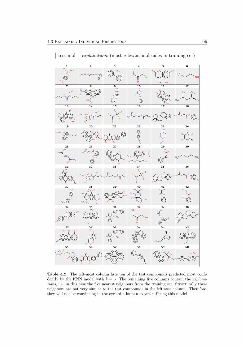
4.3 Explaining Individual Predictions 69
test mol. explanations (most relevant molecules in training set)
Table 4.2: The left-most column lists ten of the test compounds predicted most confi-dently by the KNN model with k = 5. The remaining five columns contain the explana-tions, i.e. in this case the five nearest neighbors from the training set. Structurally theseneighbors are not very similar to the test compounds in the leftmost column. Therefore,they will not be convincing in the eyes of a human expert utilizing this model.
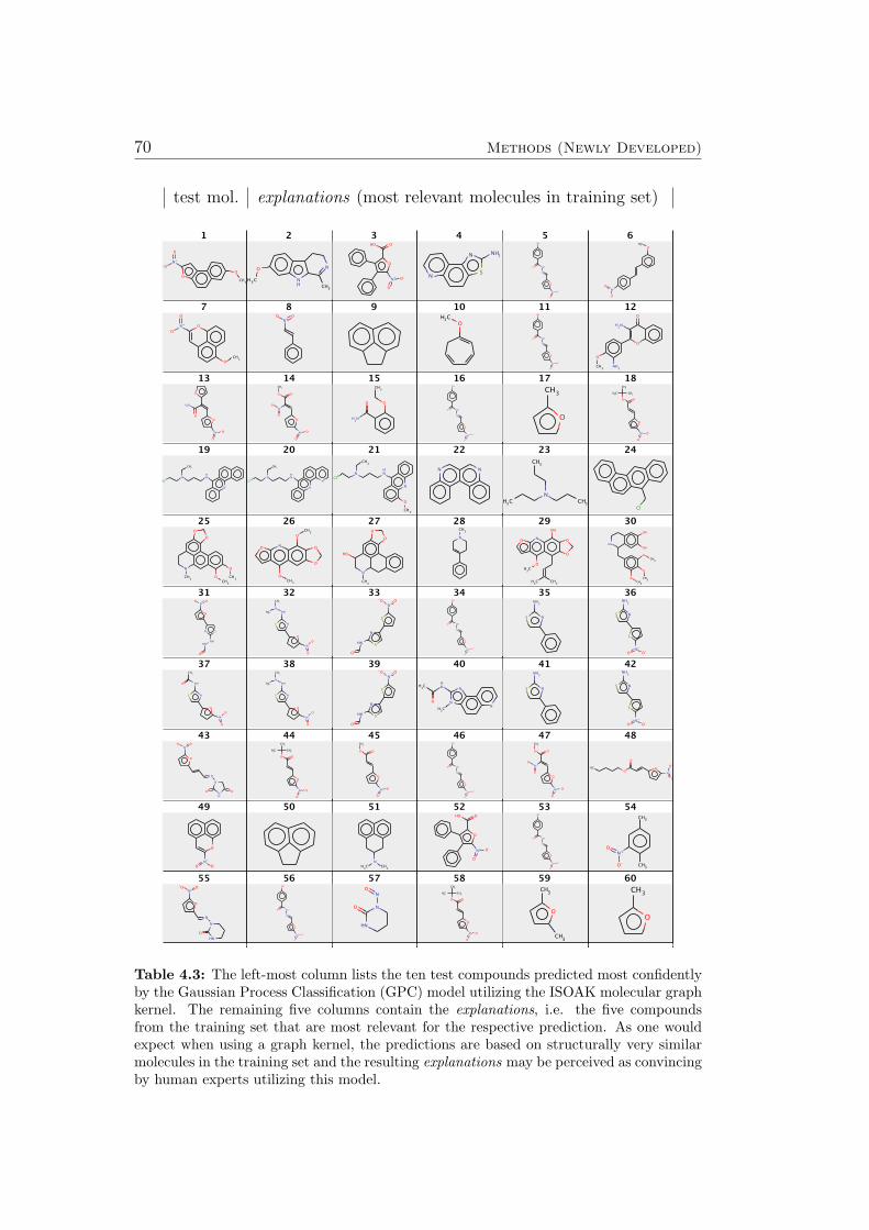
70 Methods (Newly Developed)
test mol. explanations (most relevant molecules in training set)
Table 4.3: The left-most column lists the ten test compounds predicted most confidentlyby the Gaussian Process Classification (GPC) model utilizing the ISOAK molecular graphkernel. The remaining five columns contain the explanations, i.e. the five compoundsfrom the training set that are most relevant for the respective prediction. As one wouldexpect when using a graph kernel, the predictions are based on structurally very similarmolecules in the training set and the resulting explanations may be perceived as convincingby human experts utilizing this model.
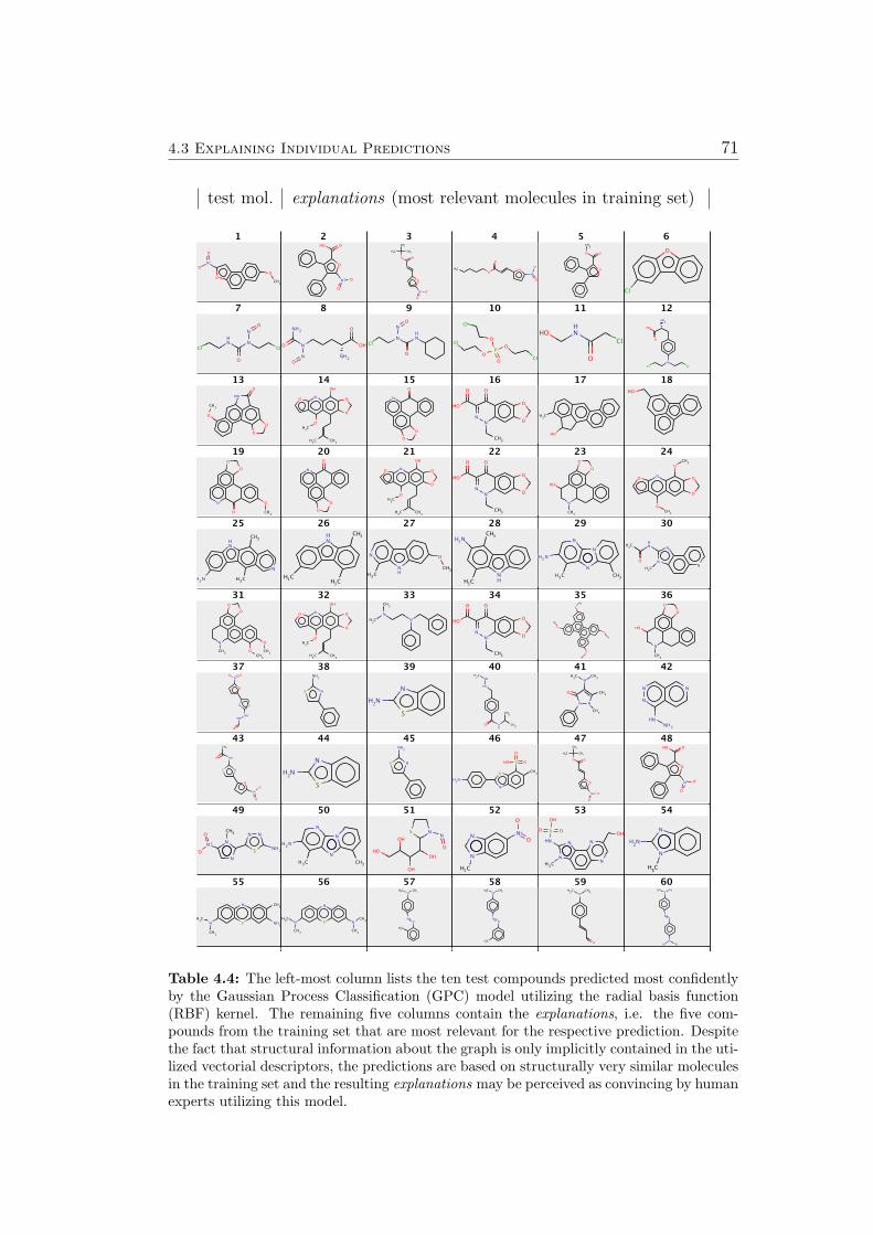
4.3 Explaining Individual Predictions 71
test mol. explanations (most relevant molecules in training set)
Table 4.4: The left-most column lists the ten test compounds predicted most confidentlyby the Gaussian Process Classification (GPC) model utilizing the radial basis function(RBF) kernel. The remaining five columns contain the explanations, i.e. the five com-pounds from the training set that are most relevant for the respective prediction. Despitethe fact that structural information about the graph is only implicitly contained in the uti-lized vectorial descriptors, the predictions are based on structurally very similar moleculesin the training set and the resulting explanations may be perceived as convincing by humanexperts utilizing this model.
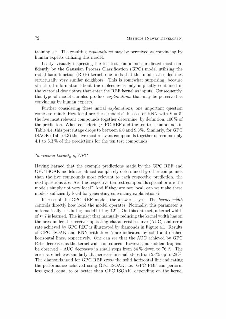
72 Methods (Newly Developed)
training set. The resulting explanations may be perceived as convincing byhuman experts utilizing this model.
Lastly, visually inspecting the ten test compounds predicted most con-fidently by the Gaussian Process Classification (GPC) model utilizing theradial basis function (RBF) kernel, one finds that this model also identifiesstructurally very similar neighbors. This is somewhat surprising, becausestructural information about the molecules is only implicitly contained inthe vectorial descriptors that enter the RBF kernel as inputs. Consequently,this type of model can also produce explanations that may be perceived asconvincing by human experts.
Further considering these initial explanations, one important questioncomes to mind: How local are these models? In case of KNN with k = 5,the five most relevant compounds together determine, by definition, 100% ofthe prediction. When considering GPC RBF and the ten test compounds inTable 4.4, this percentage drops to between 6.0 and 9.3%. Similarly, for GPCISAOK (Table 4.3) the five most relevant compounds together determine only4.1 to 6.3 % of the predictions for the ten test compounds.
Increasing Locality of GPC
Having learned that the example predictions made by the GPC RBF andGPC ISOAK models are almost completely determined by other compoundsthan the five compounds most relevant to each respective prediction, thenext questions are: Are the respective ten test compounds special or are themodels simply not very local? And if they are not local, can we make thesemodels sufficiently local for generating convincing explanations?
In case of the GPC RBF model, the answer is yes: The kernel widthcontrols directly how local the model operates. Normally, this parameter isautomatically set during model fitting [121]. On this data set, a kernel widthof ≈ 7 is learned. The impact that manually reducing the kernel width has onthe area under the receiver operating characteristic curve (AUC) and errorrate achieved by GPC RBF is illustrated by diamonds in Figure 4.1. Resultsof GPC ISOAK and KNN with k = 5 are indicated by solid and dashedhorizontal lines, respectively. One can see that the AUC achieved by GPCRBF decreases as the kernel width is reduced. However, no sudden drop canbe observed – AUC decreases in small steps from 84 % down to 76 %. Theerror rate behaves similarly: It increases in small steps from 23% up to 28%.The diamonds used for GPC RBF cross the solid horizontal line indicatingthe performance achieved using GPC ISOAK, i.e. GPC RBF can performless good, equal to or better than GPC ISOAK, depending on the kernel
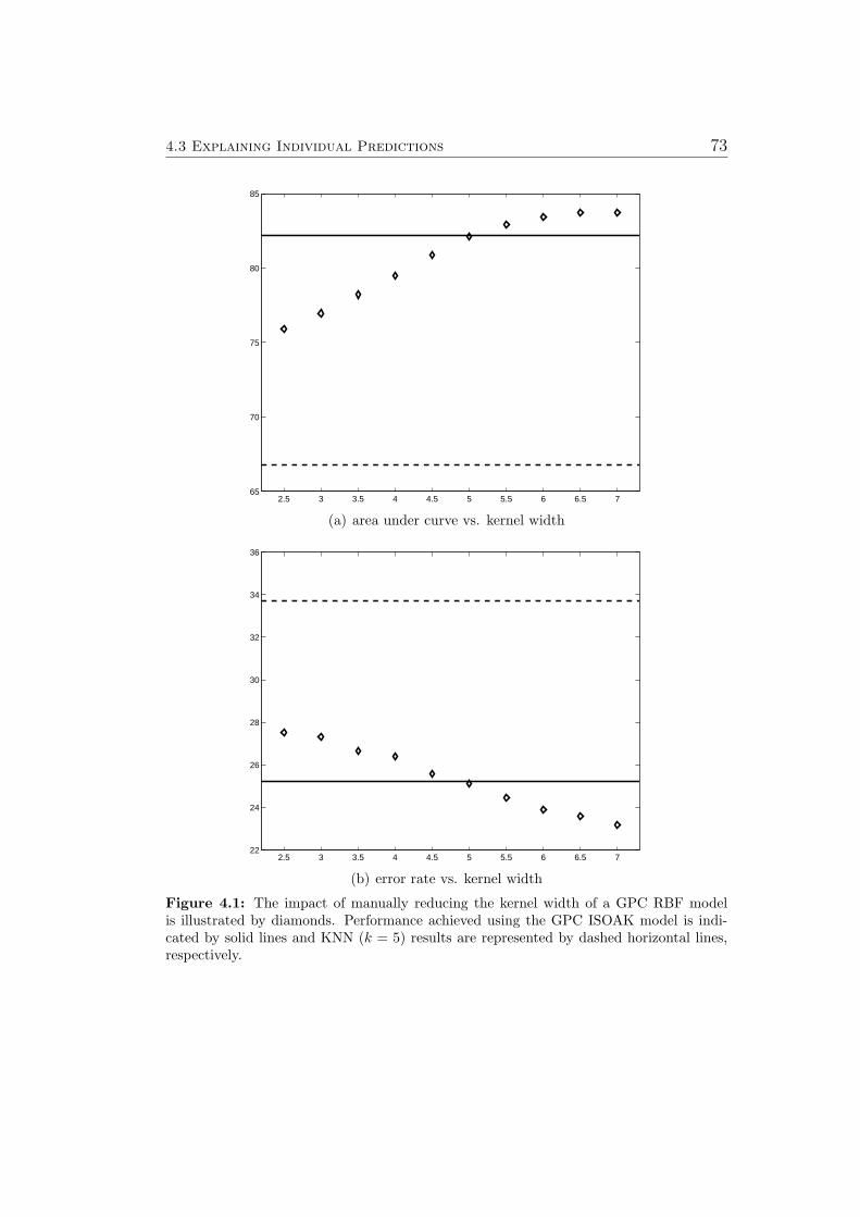
4.3 Explaining Individual Predictions 73
2.5 3 3.5 4 4.5 5 5.5 6 6.5 765
70
75
80
85
(a) area under curve vs. kernel width
2.5 3 3.5 4 4.5 5 5.5 6 6.5 722
24
26
28
30
32
34
36
(b) error rate vs. kernel width
Figure 4.1: The impact of manually reducing the kernel width of a GPC RBF modelis illustrated by diamonds. Performance achieved using the GPC ISOAK model is indi-cated by solid lines and KNN (k = 5) results are represented by dashed horizontal lines,respectively.
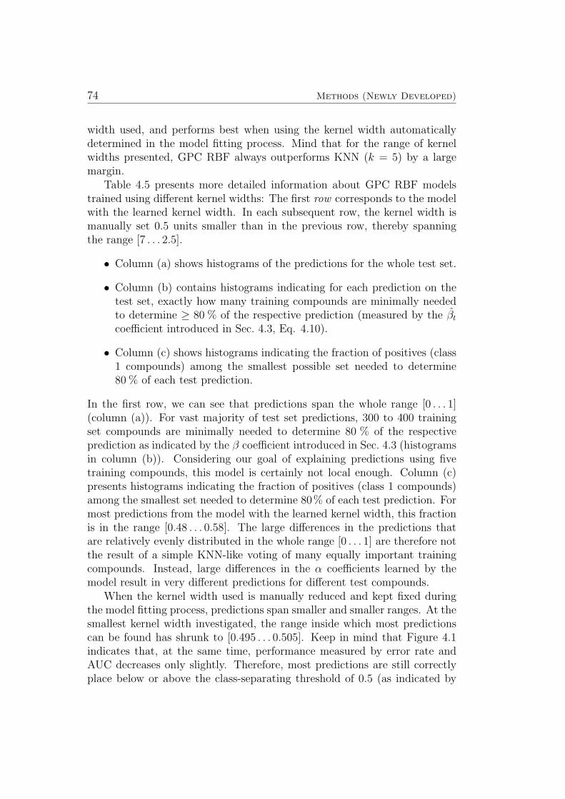
74 Methods (Newly Developed)
width used, and performs best when using the kernel width automaticallydetermined in the model fitting process. Mind that for the range of kernelwidths presented, GPC RBF always outperforms KNN (k = 5) by a largemargin.
Table 4.5 presents more detailed information about GPC RBF modelstrained using different kernel widths: The first row corresponds to the modelwith the learned kernel width. In each subsequent row, the kernel width ismanually set 0.5 units smaller than in the previous row, thereby spanningthe range [7 . . . 2.5].
• Column (a) shows histograms of the predictions for the whole test set.
• Column (b) contains histograms indicating for each prediction on thetest set, exactly how many training compounds are minimally neededto determine ≥ 80 % of the respective prediction (measured by the βtcoefficient introduced in Sec. 4.3, Eq. 4.10).
• Column (c) shows histograms indicating the fraction of positives (class1 compounds) among the smallest possible set needed to determine80 % of each test prediction.
In the first row, we can see that predictions span the whole range [0 . . . 1](column (a)). For vast majority of test set predictions, 300 to 400 trainingset compounds are minimally needed to determine 80 % of the respectiveprediction as indicated by the β coefficient introduced in Sec. 4.3 (histogramsin column (b)). Considering our goal of explaining predictions using fivetraining compounds, this model is certainly not local enough. Column (c)presents histograms indicating the fraction of positives (class 1 compounds)among the smallest set needed to determine 80% of each test prediction. Formost predictions from the model with the learned kernel width, this fractionis in the range [0.48 . . . 0.58]. The large differences in the predictions thatare relatively evenly distributed in the whole range [0 . . . 1] are therefore notthe result of a simple KNN-like voting of many equally important trainingcompounds. Instead, large differences in the α coefficients learned by themodel result in very different predictions for different test compounds.
When the kernel width used is manually reduced and kept fixed duringthe model fitting process, predictions span smaller and smaller ranges. At thesmallest kernel width investigated, the range inside which most predictionscan be found has shrunk to [0.495 . . . 0.505]. Keep in mind that Figure 4.1indicates that, at the same time, performance measured by error rate andAUC decreases only slightly. Therefore, most predictions are still correctlyplace below or above the class-separating threshold of 0.5 (as indicated by
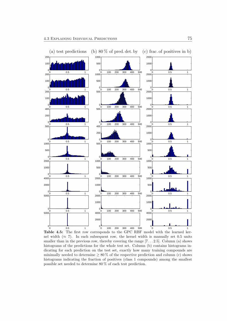
4.3 Explaining Individual Predictions 75
(a) test predictions (b) 80 % of pred. det. by (c) frac. of positives in b)
0 0.5 10
100
200
0 100 200 300 400 5000
500
1000
0 0.5 10
1000
2000
0 0.5 10
100
200
0 100 200 300 400 5000
500
1000
0 0.5 10
1000
2000
0 0.5 10
100
200
0 100 200 300 400 5000
500
0 0.5 10
1000
2000
0 0.5 10
200
400
0 100 200 300 400 5000
500
0 0.5 10
1000
2000
0 0.5 10
500
0 100 200 300 400 5000
200
400
0 0.5 10
1000
2000
0 0.5 10
500
1000
0 100 200 300 400 5000
500
0 0.5 10
500
1000
0 0.5 10
1000
2000
0 100 200 300 400 5000
500
1000
0 0.5 10
500
1000
0 0.5 10
2000
4000
0 100 200 300 400 5000
1000
2000
0 0.5 10
500
1000
0 0.5 10
5000
0 100 200 300 400 5000
1000
2000
0 0.5 10
1000
2000
0 0.5 10
5000
0 100 200 300 400 5000
2000
4000
0 0.5 10
2000
4000
Table 4.5: The first row corresponds to the GPC RBF model with the learned ker-nel width (≈ 7). In each subsequent row, the kernel width is manually set 0.5 unitssmaller than in the previous row, thereby covering the range [7 . . . 2.5]. Column (a) showshistograms of the predictions for the whole test set. Column (b) contains histograms in-dicating for each prediction on the test set, exactly how many training compounds areminimally needed to determine ≥ 80 % of the respective prediction and column (c) showshistograms indicating the fraction of positives (class 1 compounds) among the smallestpossible set needed to determine 80 % of each test prediction.
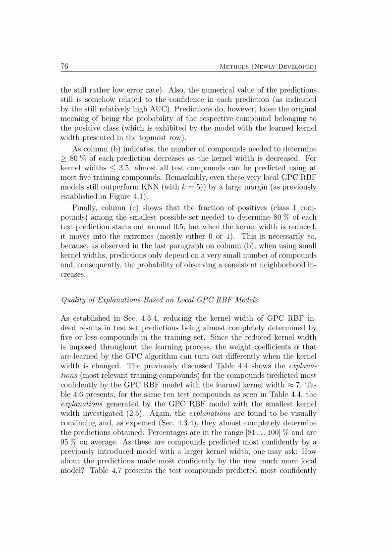
76 Methods (Newly Developed)
the still rather low error rate). Also, the numerical value of the predictionsstill is somehow related to the confidence in each prediction (as indicatedby the still relatively high AUC). Predictions do, however, loose the originalmeaning of being the probability of the respective compound belonging tothe positive class (which is exhibited by the model with the learned kernelwidth presented in the topmost row).
As column (b) indicates, the number of compounds needed to determine≥ 80 % of each prediction decreases as the kernel width is decreased. Forkernel widths ≤ 3.5, almost all test compounds can be predicted using atmost five training compounds. Remarkably, even these very local GPC RBFmodels still outperform KNN (with k = 5)) by a large margin (as previouslyestablished in Figure 4.1).
Finally, column (c) shows that the fraction of positives (class 1 com-pounds) among the smallest possible set needed to determine 80 % of eachtest prediction starts out around 0.5, but when the kernel width is reduced,it moves into the extremes (mostly either 0 or 1). This is necessarily so,because, as observed in the last paragraph on column (b), when using smallkernel widths, predictions only depend on a very small number of compoundsand, consequently, the probability of observing a consistent neighborhood in-creases.
Quality of Explanations Based on Local GPC RBF Models
As established in Sec. 4.3.4, reducing the kernel width of GPC RBF in-deed results in test set predictions being almost completely determined byfive or less compounds in the training set. Since the reduced kernel widthis imposed throughout the learning process, the weight coefficients α thatare learned by the GPC algorithm can turn out differently when the kernelwidth is changed. The previously discussed Table 4.4 shows the explana-tions (most relevant training compounds) for the compounds predicted mostconfidently by the GPC RBF model with the learned kernel width ≈ 7. Ta-ble 4.6 presents, for the same ten test compounds as seen in Table 4.4, theexplanations generated by the GPC RBF model with the smallest kernelwidth investigated (2.5). Again, the explanations are found to be visuallyconvincing and, as expected (Sec. 4.3.4), they almost completely determinethe predictions obtained: Percentages are in the range [81 . . . 100] % and are95 % on average. As these are compounds predicted most confidently by apreviously introduced model with a larger kernel width, one may ask: Howabout the predictions made most confidently by the new much more localmodel? Table 4.7 presents the test compounds predicted most confidently
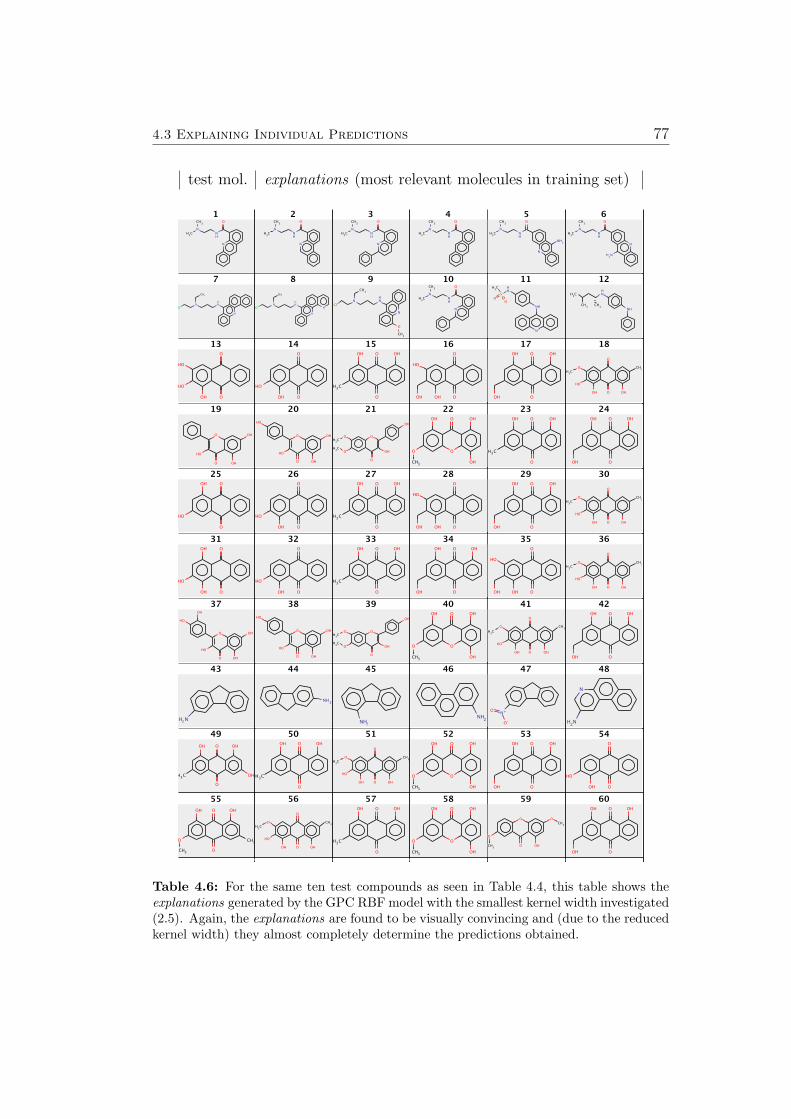
4.3 Explaining Individual Predictions 77
test mol. explanations (most relevant molecules in training set)
Table 4.6: For the same ten test compounds as seen in Table 4.4, this table shows theexplanations generated by the GPC RBF model with the smallest kernel width investigated(2.5). Again, the explanations are found to be visually convincing and (due to the reducedkernel width) they almost completely determine the predictions obtained.
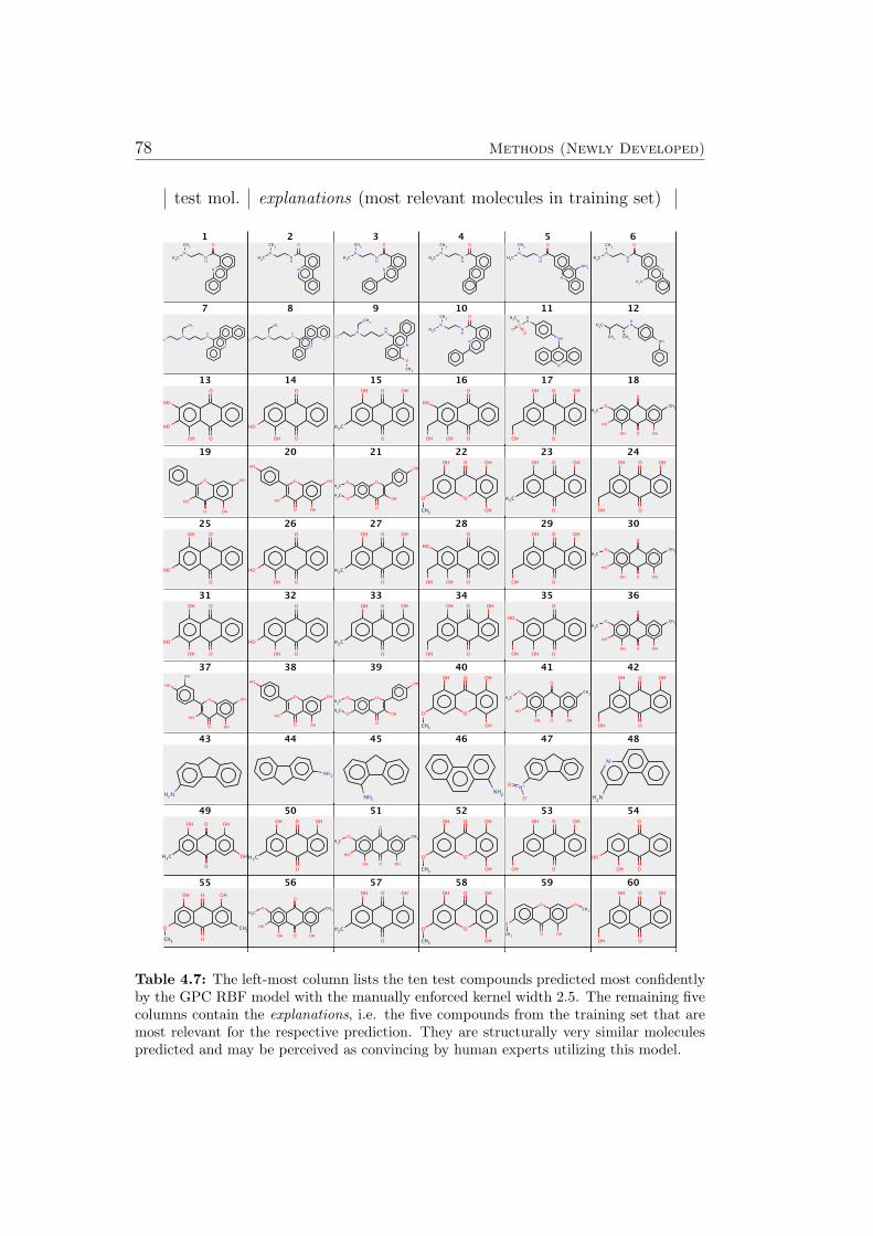
78 Methods (Newly Developed)
test mol. explanations (most relevant molecules in training set)
Table 4.7: The left-most column lists the ten test compounds predicted most confidentlyby the GPC RBF model with the manually enforced kernel width 2.5. The remaining fivecolumns contain the explanations, i.e. the five compounds from the training set that aremost relevant for the respective prediction. They are structurally very similar moleculespredicted and may be perceived as convincing by human experts utilizing this model.
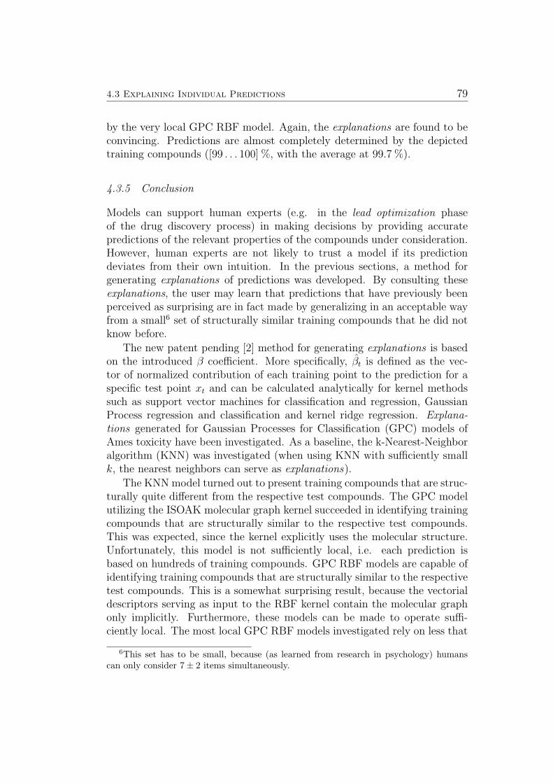
4.3 Explaining Individual Predictions 79
by the very local GPC RBF model. Again, the explanations are found to beconvincing. Predictions are almost completely determined by the depictedtraining compounds ([99 . . . 100] %, with the average at 99.7 %).
4.3.5 Conclusion
Models can support human experts (e.g. in the lead optimization phaseof the drug discovery process) in making decisions by providing accuratepredictions of the relevant properties of the compounds under consideration.However, human experts are not likely to trust a model if its predictiondeviates from their own intuition. In the previous sections, a method forgenerating explanations of predictions was developed. By consulting theseexplanations, the user may learn that predictions that have previously beenperceived as surprising are in fact made by generalizing in an acceptable wayfrom a small6 set of structurally similar training compounds that he did notknow before.
The new patent pending [2] method for generating explanations is basedon the introduced β coefficient. More specifically, βt is defined as the vec-tor of normalized contribution of each training point to the prediction for aspecific test point xt and can be calculated analytically for kernel methodssuch as support vector machines for classification and regression, GaussianProcess regression and classification and kernel ridge regression. Explana-tions generated for Gaussian Processes for Classification (GPC) models ofAmes toxicity have been investigated. As a baseline, the k-Nearest-Neighboralgorithm (KNN) was investigated (when using KNN with sufficiently smallk, the nearest neighbors can serve as explanations).
The KNN model turned out to present training compounds that are struc-turally quite different from the respective test compounds. The GPC modelutilizing the ISOAK molecular graph kernel succeeded in identifying trainingcompounds that are structurally similar to the respective test compounds.This was expected, since the kernel explicitly uses the molecular structure.Unfortunately, this model is not sufficiently local, i.e. each prediction isbased on hundreds of training compounds. GPC RBF models are capable ofidentifying training compounds that are structurally similar to the respectivetest compounds. This is a somewhat surprising result, because the vectorialdescriptors serving as input to the RBF kernel contain the molecular graphonly implicitly. Furthermore, these models can be made to operate suffi-ciently local. The most local GPC RBF models investigated rely on less that
6This set has to be small, because (as learned from research in psychology) humanscan only consider 7± 2 items simultaneously.
80 Methods (Newly Developed)
five training compounds for making each test prediction and still outperformKNN (k = 5) by a large margin.
Interesting directions for future research include investigating explana-tions for other classifiers and regression models. Furthermore, evaluating alarge number of explanations with an (ideally also large) group of experts isconsidered the best possible way of quantifying how useful such explanationscan be in practice.
Note added between grading and publication of Timon Schroeter’sdissertation: In the inital version of this thesis, the author has suggestedevaluating a large number of explanations with an (ideally also large) groupof experts. David Baehrens (who was initially supervised by the author ofthis thesis and later by Katja Hansen and Mikio Braun) has conducted thisevaluation and has published the results in his diploma thesis [124].
In a forced choice paradigm, human users were presented with conflictingpredictions by two models trained on different subsets of the Ames muta-genicity benchmark data set that we published earlier [5]. Forty one (41)students studying pharmaceutical sciences, medicine, chemistry and othersubjects each answered forty (40) questions. The effect of the students sub-ject and the effect of explanations were quantified in terms of conditionalodds ratios. Students studying pharmaceutical sciences were found to choosecorrect predictions with a two-fold increased probability (relative to the ran-dom choice baseline). For students of any subject, explanations were shownto result in a 93 % increased probability of choosing correct predictions. Thelatter result is also statistically significant at a p-value of 0.01.
In conclusion, a large number of explanations has been evaluated using alarge group of experts. Explanations led to a statistically significant (p=0.01)strong increase (93 %) in probability of choosing correct predictions, therbyunderscoring that human users can strongly profit from explanations.
4.4 Guiding Compound Optimization 81
4.4 Guiding Compound Optimization & Explaining Decisionsusing Local Gradients
In this thesis, two separate methodologies for explaining individual predic-tions of (possibly non-linear) machine learning models are presented. Themethod presented in Sec. 4.3 explains predictions by the means of visualiz-ing relevant objects from the training set of the model. This allows humanexperts to understand how each prediction comes about. If a prediction con-flicts with his intuition, the human expert can easily find out whether thegrounds for the models predictions are solid or if trusting his own intuitionis the better idea [2].
The method presented in this section utilizes local gradients of the mod-els predictions to explain predictions in terms of the locally most relevantfeatures. This not only teaches the human expert which features are rele-vant for each individual prediction, but also gives a directional information.Abstractly speaking, one can learn in which direction a data point has tobe moved to increase the prediction for the target value [1]. In the contextof lead optimization, this means that the human expert can obtain a typeof guidance in compound optimization. For this reason, the two explaining-related methodologies are presented in separate sections.
4.4.1 Introduction
Automatic non-linear classification is a common and powerful tool in dataanalysis. Machine learning research has created methods that are practicallyuseful and that can classify unseen data after being trained on a limitedtraining set of labeled examples. Nevertheless, most of the algorithms donot explain their decision. However, in many application scenarios of dataanalysis it is essential to obtain an instance based explanation, i.e. onewould like to gain an understanding what input features made the non-linearmachine give its answer for each individual test object and how one couldmodify this object to optimize its properties.
In the lead optimization phase of the drug discovery process (as intro-duced in Sec. 2.1), variants of the respective lead compounds are synthesizedwith the goal of finally producing a drug candidate that fulfills all require-ments. Reaching this goal typically takes thousands of experiments, eachof which is quite expensive. The many decisions which compound or smallbatch of compounds to synthesize and test next are made by humans, andthey are often made on the basis of very little information. A type of guid-ance in compound optimization that facilitates choosing the most promisingcompounds in each iteration can therefore be of great value.
82 Methods (Newly Developed)
Typically, explanations are provided jointly for all instances of the train-ing set, for example feature selection methods find out which inputs aresalient for a good generalization [125]. While this can give a coarse im-pression about the global usefulness of each input dimension, it is still anensemble view and does not provide an answer on an instance basis. In theneural network literature also solely an ensemble view was taken in algo-rithms like input pruning [126]. The only classification which does provideindividual explanations are decision trees [102].
This section proposes a simple framework that provides local explanationvectors applicable to any classification method in order to help understandingprediction results for single data instances. The local explanation yields thefeatures being relevant for the prediction at the very points of interest in thedata space and is able to spot local peculiarities which are neglected in theglobal view e.g. due to cancellation effects.
The section is organized as follows: Local explanation vectors are techni-cally defined as class probability gradients and an illustration for GaussianProcess Classification (GPC) is given. In the following subsection, the newapproach is contrasted with related work. Some methods output a predictionwithout a direct probability interpretation. For these, our recent publication[1] proposes a way to estimate local explanations.
Results obtained using this new methodology are presented in Sec. 5 andin [1]. More specifically, in section 4 in [1] it is applied to learn distinguish-ing properties of Iris flowers by estimating explanation vectors for a k-NNclassifier applied to the classic Iris dataset. Section 5 in [1] discusses howthe approach applied to a SVM classifier allows to explain how digits ”two”are distinguished from digits ”8” in the USPS dataset. In section 5.8.1 achallenging real world application scenario is presented in which the pro-posed explanation capabilities prove useful: In the lead optimization phaseo the drug discovery process, human experts regularly decide how to modifyexisting lead compounds in order to obtain new compounds with improvedproperties. Models capable of explaining predictions can help in the processof choosing promising modifications. The automatically generated expla-nations match with chemical domain knowledge about toxifying functionalgroups of the compounds in question.
The presentation of results is concluded in the last paragraph of Sec. 4.3.Our recent publication [1] discusses further characteristic properties and lim-itations of the new methodology. Future directions are two-fold: First it isbelieved that the new method will find its way into the tool boxes of practi-tioners who not only want to automatically classify their data but who alsowould like to understand the learned classifier. The second direction is togeneralize this approach to other prediction problems such as regression.
4.4 Guiding Compound Optimization 83
4.4.2 Definitions
This Subsection gives definitions of local explanation vectors in the classi-fication setting. It starts with a theoretical definition for multi-class Bayesclassification and then gives a specialized definition being more practical forthe binary case.
For the multi-class case, suppose one is given data points x1, . . . , xn ∈ <dwith labels y1, . . . , yn ∈ {1, . . . , C} and one intends to learn a function thatpredicts the labels of unlabeled data points. Assuming that the data couldbe modelled as being IID-sampled from some unknown joint distributionP (X, Y ), in theory, one can define the Bayes classifier,
g∗(x) = arg minc∈{1,...,C}
P (Y 6=c | X=x)
which is optimal for the 0-1 loss function [see 127].
For the Bayes classifier one defines the explanation vector of a data pointx0 to be the derivative with respect to x at x = x0 of the conditional proba-bility of Y 6=g∗(x0) given X = x, or formally,
Definition 4.1.
ζ(x0) :=∂
∂xP (Y 6=g∗(x0) | X=x)
∣∣∣∣x=x0
Note that ζ(x0) is a d-dimensional vector just like x0 is. The classifierg∗ partitions the data space <d into up to C parts on which g∗ is constant.Under the usual assumption that P (X =x | Y = c) is for all c smooth in x,ζ(x0) defines on each of those parts a vector field that characterizes the flowaway from the corresponding class. Thus entries in ζ(x0) with large absolutevalues highlight features that will influence the class label decision of x0. Apositive sign of such an entry implies that increasing that feature would lowerthe probability that x0 is assigned to g∗(x0). Ignoring the orientations of theexplanation vectors, ζ forms a continuously changing (orientation-less) vectorfield along which the class labels change. This vector field lets one locallyunderstand the Bayes classifier.
For the case of binary classification we directly define local explanationvectors as local gradients of the probability function p(x) = P (Y = 1 | X =x) of the learned model for the positive class.
So for a probability function p : <d → [0, 1] of a classification modellearned from examples {(x1, y1), . . . , (xn, yn)} ∈ <d × {−1,+1} the explana-tion vector for a classified test point x0 is the local gradient of p at x0:
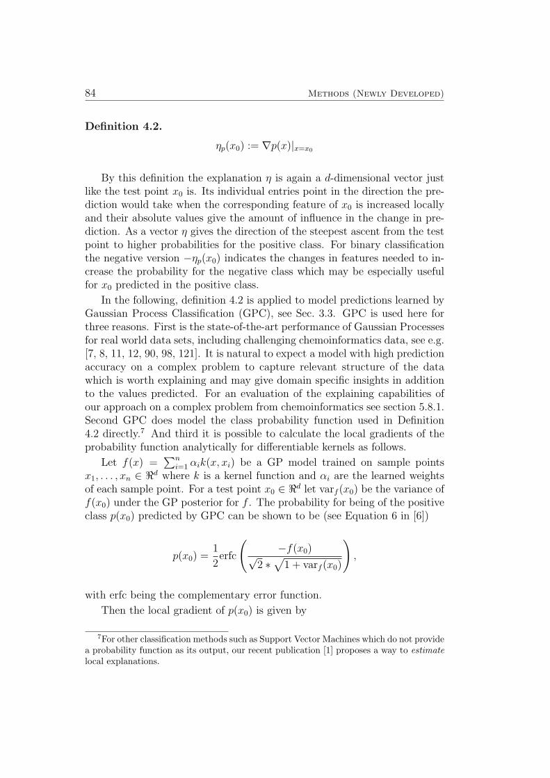
84 Methods (Newly Developed)
Definition 4.2.
ηp(x0) := ∇p(x)|x=x0
By this definition the explanation η is again a d-dimensional vector justlike the test point x0 is. Its individual entries point in the direction the pre-diction would take when the corresponding feature of x0 is increased locallyand their absolute values give the amount of influence in the change in pre-diction. As a vector η gives the direction of the steepest ascent from the testpoint to higher probabilities for the positive class. For binary classificationthe negative version −ηp(x0) indicates the changes in features needed to in-crease the probability for the negative class which may be especially usefulfor x0 predicted in the positive class.
In the following, definition 4.2 is applied to model predictions learned byGaussian Process Classification (GPC), see Sec. 3.3. GPC is used here forthree reasons. First is the state-of-the-art performance of Gaussian Processesfor real world data sets, including challenging chemoinformatics data, see e.g.[7, 8, 11, 12, 90, 98, 121]. It is natural to expect a model with high predictionaccuracy on a complex problem to capture relevant structure of the datawhich is worth explaining and may give domain specific insights in additionto the values predicted. For an evaluation of the explaining capabilities ofour approach on a complex problem from chemoinformatics see section 5.8.1.Second GPC does model the class probability function used in Definition4.2 directly.7 And third it is possible to calculate the local gradients of theprobability function analytically for differentiable kernels as follows.
Let f(x) =∑n
i=1 αik(x, xi) be a GP model trained on sample pointsx1, . . . , xn ∈ <d where k is a kernel function and αi are the learned weightsof each sample point. For a test point x0 ∈ <d let varf (x0) be the variance off(x0) under the GP posterior for f . The probability for being of the positiveclass p(x0) predicted by GPC can be shown to be (see Equation 6 in [6])
p(x0) =1
2erfc
(−f(x0)√
2 ∗√
1 + varf (x0)
),
with erfc being the complementary error function.
Then the local gradient of p(x0) is given by
7For other classification methods such as Support Vector Machines which do not providea probability function as its output, our recent publication [1] proposes a way to estimatelocal explanations.
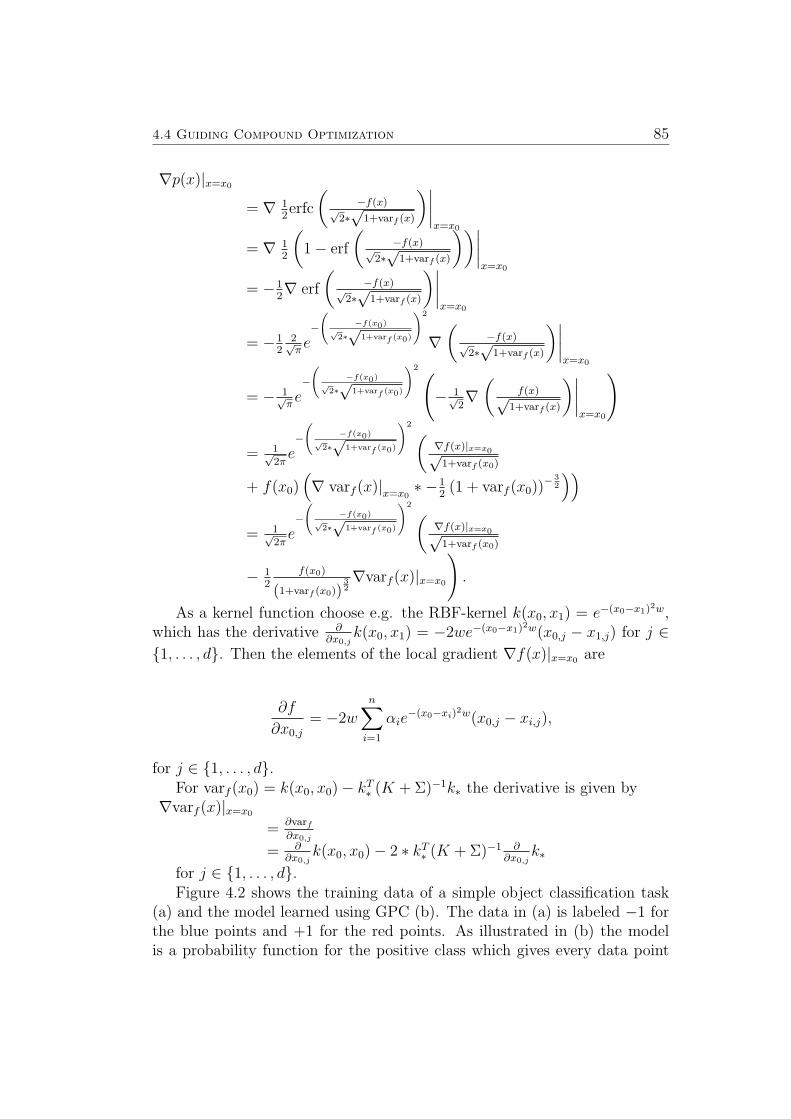
4.4 Guiding Compound Optimization 85
∇p(x)|x=x0
= ∇ 12erfc
(−f(x)
√2∗√
1+varf (x)
)∣∣∣∣x=x0
= ∇ 12
(1− erf
(−f(x)
√2∗√
1+varf (x)
))∣∣∣∣x=x0
= −12∇ erf
(−f(x)
√2∗√
1+varf (x)
)∣∣∣∣x=x0
= −12
2√πe−
−f(x0)√
2∗√
1+varf (x0)
!2
∇(
−f(x)√
2∗√
1+varf (x)
)∣∣∣∣x=x0
= − 1√πe−
−f(x0)√
2∗√
1+varf (x0)
!2 (− 1√
2∇(
f(x)√1+varf (x)
)∣∣∣∣x=x0
)
= 1√2πe−
−f(x0)√
2∗√
1+varf (x0)
!2 (∇f(x)|x=x0√
1+varf (x0)
+ f(x0)(∇ varf (x)|x=x0
∗ −12
(1 + varf (x0))− 3
2
))= 1√
2πe−
−f(x0)√
2∗√
1+varf (x0)
!2 (∇f(x)|x=x0√
1+varf (x0)
− 12
f(x0)
(1+varf (x0))32∇varf (x)|x=x0
).
As a kernel function choose e.g. the RBF-kernel k(x0, x1) = e−(x0−x1)2w,which has the derivative ∂
∂x0,jk(x0, x1) = −2we−(x0−x1)2w(x0,j − x1,j) for j ∈
{1, . . . , d}. Then the elements of the local gradient ∇f(x)|x=x0 are
∂f
∂x0,j
= −2wn∑i=1
αie−(x0−xi)
2w(x0,j − xi,j),
for j ∈ {1, . . . , d}.For varf (x0) = k(x0, x0)− kT∗ (K + Σ)−1k∗ the derivative is given by
∇varf (x)|x=x0
=∂varf
∂x0,j
= ∂∂x0,j
k(x0, x0)− 2 ∗ kT∗ (K + Σ)−1 ∂∂x0,j
k∗
for j ∈ {1, . . . , d}.Figure 4.2 shows the training data of a simple object classification task
(a) and the model learned using GPC (b). The data in (a) is labeled −1 forthe blue points and +1 for the red points. As illustrated in (b) the modelis a probability function for the positive class which gives every data point
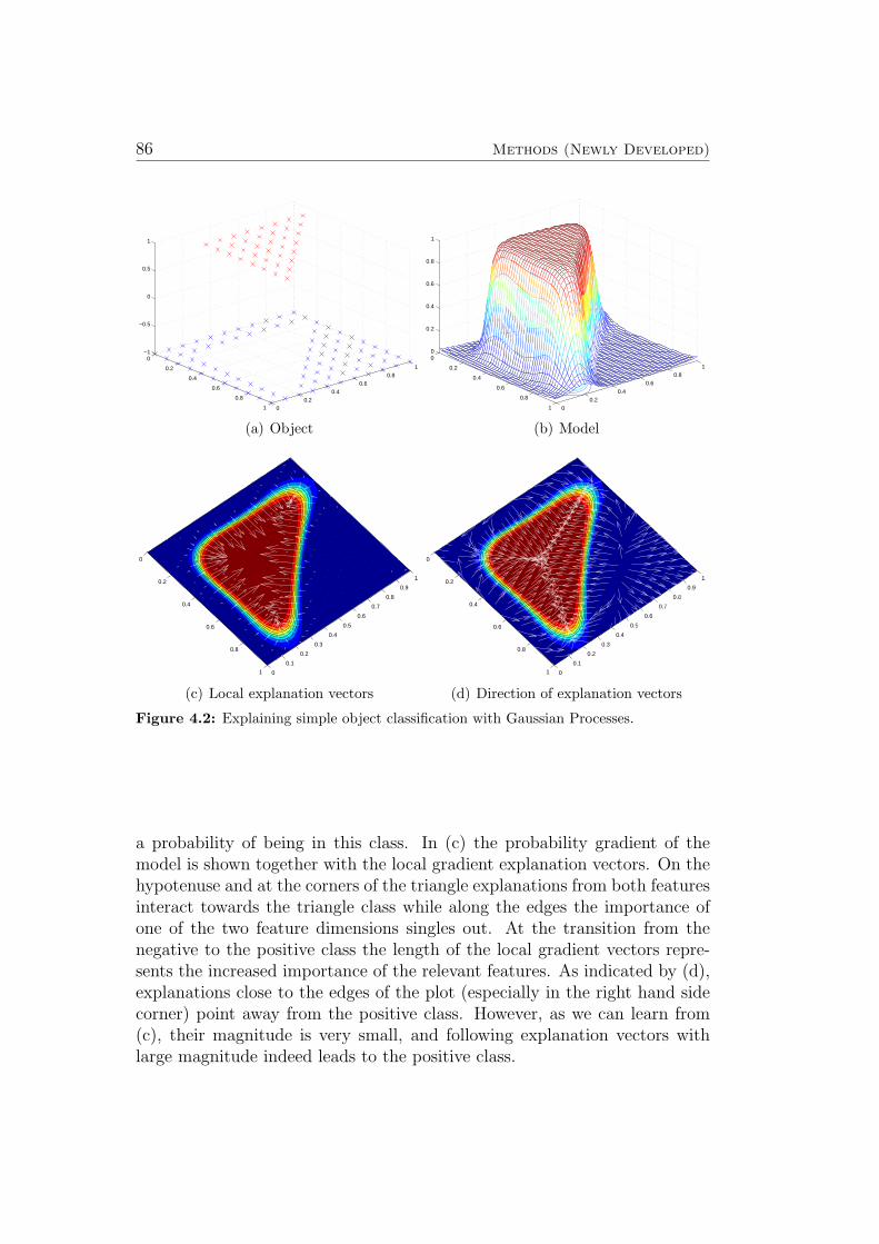
86 Methods (Newly Developed)
0
0.2
0.4
0.6
0.8
1 00.2
0.40.6
0.81
−1
−0.5
0
0.5
1
(a) Object
0
0.2
0.4
0.6
0.8
1 00.2
0.40.6
0.81
0
0.2
0.4
0.6
0.8
1
(b) Model
0
0.2
0.4
0.6
0.8
1 0
0.1
0.2
0.3
0.4
0.5
0.6
0.7
0.8
0.9
1
(c) Local explanation vectors
0
0.2
0.4
0.6
0.8
1 0
0.1
0.2
0.3
0.4
0.5
0.6
0.7
0.8
0.9
1
(d) Direction of explanation vectors
Figure 4.2: Explaining simple object classification with Gaussian Processes.
a probability of being in this class. In (c) the probability gradient of themodel is shown together with the local gradient explanation vectors. On thehypotenuse and at the corners of the triangle explanations from both featuresinteract towards the triangle class while along the edges the importance ofone of the two feature dimensions singles out. At the transition from thenegative to the positive class the length of the local gradient vectors repre-sents the increased importance of the relevant features. As indicated by (d),explanations close to the edges of the plot (especially in the right hand sidecorner) point away from the positive class. However, as we can learn from(c), their magnitude is very small, and following explanation vectors withlarge magnitude indeed leads to the positive class.
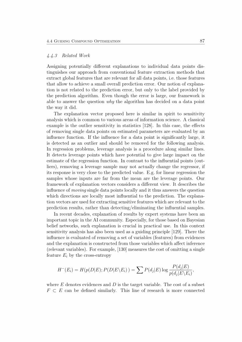
4.4 Guiding Compound Optimization 87
4.4.3 Related Work
Assigning potentially different explanations to individual data points dis-tinguishes our approach from conventional feature extraction methods thatextract global features that are relevant for all data points, i.e. those featuresthat allow to achieve a small overall prediction error. Our notion of explana-tion is not related to the prediction error, but only to the label provided bythe prediction algorithm. Even though the error is large, our framework isable to answer the question why the algorithm has decided on a data pointthe way it did.
The explanation vector proposed here is similar in spirit to sensitivityanalysis which is common to various areas of information science. A classicalexample is the outlier sensitivity in statistics [128]. In this case, the effectsof removing single data points on estimated parameters are evaluated by aninfluence function. If the influence for a data point is significantly large, itis detected as an outlier and should be removed for the following analysis.In regression problems, leverage analysis is a procedure along similar lines.It detects leverage points which have potential to give large impact on theestimate of the regression function. In contrast to the influential points (out-liers), removing a leverage sample may not actually change the regressor, ifits response is very close to the predicted value. E.g. for linear regression thesamples whose inputs are far from the mean are the leverage points. Ourframework of explanation vectors considers a different view. It describes theinfluence of moving single data points locally and it thus answers the questionwhich directions are locally most influential to the prediction. The explana-tion vectors are used for extracting sensitive features which are relevant to theprediction results, rather than detecting/eliminating the influential samples.
In recent decades, explanation of results by expert systems have been animportant topic in the AI community. Especially, for those based on Bayesianbelief networks, such explanation is crucial in practical use. In this contextsensitivity analysis has also been used as a guiding principle [129]. There theinfluence is evaluated of removing a set of variables (features) from evidencesand the explanation is constructed from those variables which affect inference(relevant variables). For example, [130] measures the cost of omitting a singlefeature Ei by the cross-entropy
H−(Ei) = H(p(D|E);P (D|E\Ei) ) =∑
P (dj|E) logP (dj|E)
p(dj|E\Ei),
where E denotes evidences and D is the target variable. The cost of a subsetF ⊂ E can be defined similarly. This line of research is more connected
88 Methods (Newly Developed)
to our work, because explanation can depend on the assigned values of theevidences E, and is thus local.
Similarly [131] and [132] try to explain the decision of trained kNN-,SVM- and ANN-models for individual instances by measuring the differencein their prediction with sets of features omitted. The cost of omitting featuresis evaluated as the information difference, the log-odds ratio or the differenceof probabilities between the model with knowledge about all features andwith omissions respectively. To know what the prediction would be withoutthe knowledge of a certain feature the model is retrained for every choice offeatures whose influence is to be explained. To save the time of combinatorialtraining [131] propose to use neutral values which have to be estimated bya known prior distribution of all possible parameter values. As a theoreticalframework for considering feature interactions, [132] propose to calculate thedifferences between model predictions for every choice of feature subset. Theprincipal differences between our approach and these frameworks are: (i)We consider continuous features and no structure among them is required,while the other frameworks start from binary features and may require dis-cretization steps with the need to estimate parameters for it. (ii) We allowchanges in any direction, i.e. any weighted combination of variables, whileother approaches only consider the omission of a set of variables.
Chapter 5
Results
5.1 Overview
This chapter presents the results of six studies on constructing models forvarious ADME/Tox 1 properties, results obtained using a new algorithm forexplaining predictions & eliciting hints for compound optimization and theresults of a virtual screening study. The results of each individual work havebeen previously published. The respective journal publications are referencedin Table 1.1 in Sec. 1.2 and inside each individual section. More specifically,the ADME/Tox properties investigated in this chapter are:
• Partition Coefficients (Sec. 5.2)
• Aqueous Solubility (Sec. 5.3)
• Cytochrome P450 Inhibition (Sec. 5.4)
• Metabolic Stability (Sec. 5.5)
• Ames Mutagenicity (Sec. 5.6)
• hERG Channel Blockade Effect (Sec. 5.7)
Local gradients for explaining individual classification decisions and elicitingcompound optimization are validated in Sec. 5.8, using two benchmark setsof data that are well known in the machine learning community (IRIS flowersand USPS digits) and was then applied to Gaussian Process Classificationmodels for Ames mutagenicity.
Furthermore, the author of this thesis participated in a virtual screeningstudy that led to the discovery of new PPARγ agonists (Sec. 5.9). Bothretrospective and prospective results are discussed.
1The acronym ADME/Tox stands for properties relating to Absorption, Digestion,Metabolism, Excretion & Toxicity of chemical compounds.
89
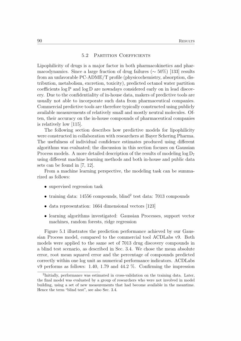
90 Results
5.2 Partition Coefficients
Lipophilicity of drugs is a major factor in both pharmacokinetics and phar-macodynamics. Since a large fraction of drug failures (∼ 50%) [133] resultsfrom an unfavorable PC-ADME/T profile (physicochemistry, absorption, dis-tribution, metabolism, excretion, toxicity), predicted octanol water partitioncoefficients log P and log D are nowadays considered early on in lead discov-ery. Due to the confidentiality of in-house data, makers of predictive tools areusually not able to incorporate such data from pharmaceutical companies.Commercial predictive tools are therefore typically constructed using publiclyavailable measurements of relatively small and mostly neutral molecules. Of-ten, their accuracy on the in-house compounds of pharmaceutical companiesis relatively low [115].
The following section describes how predictive models for lipophilicitywere constructed in collaboration with researchers at Bayer Schering Pharma.The usefulness of individual confidence estimates produced using differentalgorithms was evaluated; the discussion in this section focuses on GaussianProcess models. A more detailed description of the results of modeling log D7
using different machine learning methods and both in-house and public datasets can be found in [7, 12].
From a machine learning perspective, the modeling task can be summa-rized as follows:
• supervised regression task
• training data: 14556 compounds, blind2 test data: 7013 compounds
• data representation: 1664 dimensional vectors [123]
• learning algorithms investigated: Gaussian Processes, support vectormachines, random forests, ridge regression
Figure 5.1 illustrates the prediction performance achieved by our Gaus-sian Process model, compared to the commercial tool ACDLabs v9. Bothmodels were applied to the same set of 7013 drug discovery compounds ina blind test scenario, as described in Sec. 3.4. We chose the mean absoluteerror, root mean squared error and the percentage of compounds predictedcorrectly within one log unit as numerical performance indicators. ACDLabsv9 performs as follows: 1.40, 1.79 and 44.2 %. Confirming the impression
2Initially, performance was estimated in cross-validation on the training data. Later,the final model was evaluated by a group of researchers who were not involved in modelbuilding, using a set of new measurements that had become available in the meantime.Hence the term “blind test”, see also Sec. 3.4.
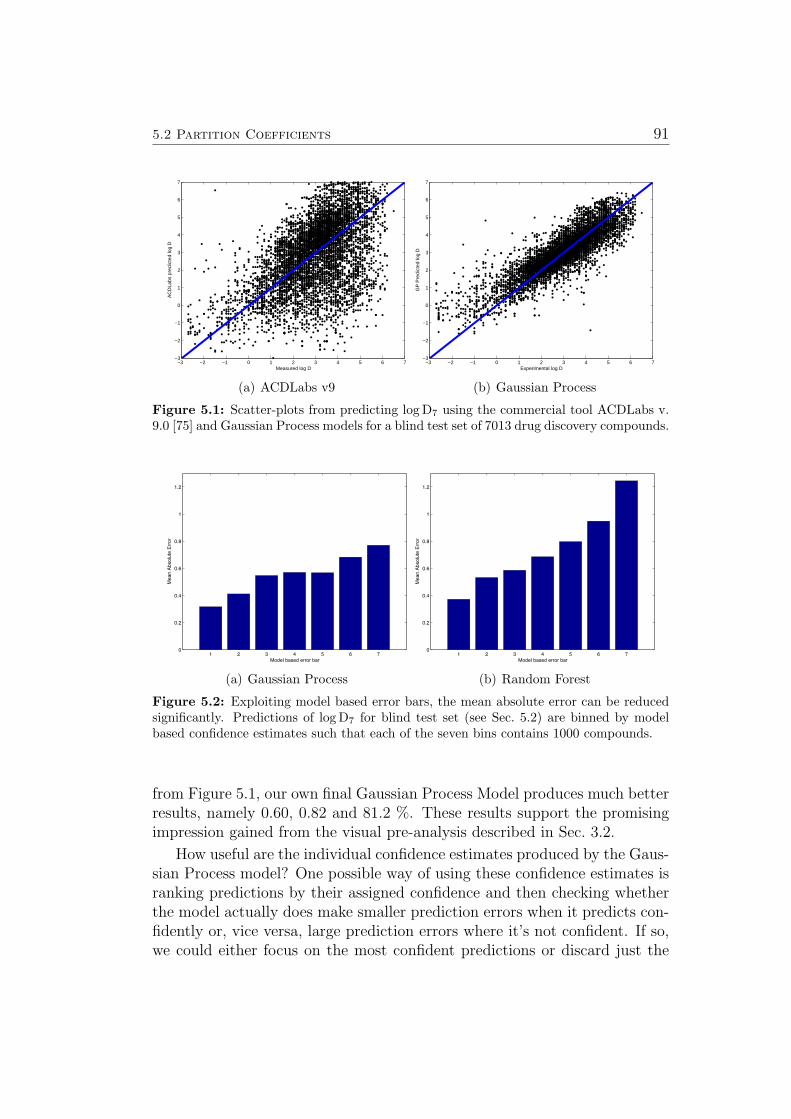
5.2 Partition Coefficients 91
−3 −2 −1 0 1 2 3 4 5 6 7−3
−2
−1
0
1
2
3
4
5
6
7
Measured log D
AC
DLa
bs p
redi
cted
log
D
(a) ACDLabs v9
−3 −2 −1 0 1 2 3 4 5 6 7−3
−2
−1
0
1
2
3
4
5
6
7
Experimental log D
GP
Pre
dict
ed lo
g D
(b) Gaussian Process
Figure 5.1: Scatter-plots from predicting log D7 using the commercial tool ACDLabs v.9.0 [75] and Gaussian Process models for a blind test set of 7013 drug discovery compounds.
1 2 3 4 5 6 70
0.2
0.4
0.6
0.8
1
1.2
Mea
n Ab
solu
te E
rror
Model based error bar
(a) Gaussian Process
1 2 3 4 5 6 70
0.2
0.4
0.6
0.8
1
1.2
Mea
n Ab
solu
te E
rror
Model based error bar
(b) Random Forest
Figure 5.2: Exploiting model based error bars, the mean absolute error can be reducedsignificantly. Predictions of log D7 for blind test set (see Sec. 5.2) are binned by modelbased confidence estimates such that each of the seven bins contains 1000 compounds.
from Figure 5.1, our own final Gaussian Process Model produces much betterresults, namely 0.60, 0.82 and 81.2 %. These results support the promisingimpression gained from the visual pre-analysis described in Sec. 3.2.
How useful are the individual confidence estimates produced by the Gaus-sian Process model? One possible way of using these confidence estimates isranking predictions by their assigned confidence and then checking whetherthe model actually does make smaller prediction errors when it predicts con-fidently or, vice versa, large prediction errors where it’s not confident. If so,we could either focus on the most confident predictions or discard just the
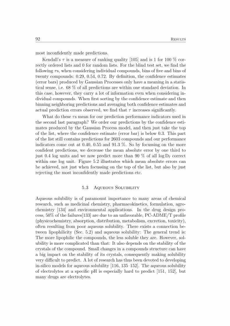
92 Results
most inconfidently made predictions.
Kendall’s τ is a measure of ranking quality [105] and is 1 for 100 % cor-rectly ordered lists and 0 for random lists. For the blind test set, we find thefollowing τs, when considering individual compounds, bins of five and bins oftwenty compounds: 0.29, 0.54, 0.72. By definition, the confidence estimates(error bars) produced by Gaussian Processes only have a meaning in a statis-tical sense, i.e. 68 % of all predictions are within one standard deviation. Inthis case, however, they carry a lot of information even when considering in-dividual compounds. When first sorting by the confidence estimate and thenbinning neighboring predictions and averaging both confidence estimates andactual prediction errors observed, we find that τ increases significantly.
What do these τs mean for our prediction performance indicators used inthe second last paragraph? We order our predictions by the confidence esti-mates produced by the Gaussian Process model, and then just take the topof the list, where the confidence estimate (error bar) is below 0.3. This partof the list still contains predictions for 2603 compounds and our performanceindicators come out at 0.40, 0.55 and 91.3 %. So by focussing on the moreconfident predictions, we decrease the mean absolute error by one third tojust 0.4 log units and we now predict more than 90 % of all log D7 correctwithin one log unit. Figure 5.2 illustrates which mean absolute errors canbe achieved, not just when focussing on the top of the list, but also by justrejecting the most inconfidently made predictions etc.
5.3 Aqueous Solubility
Aqueous solubility is of paramount importance to many areas of chemicalresearch, such as medicinal chemistry, pharmacokinetics, formulation, agro-chemistry [134] and environmental applications. In the drug design pro-cess, 50% of the failures[133] are due to an unfavorable, PC-ADME/T profile(physicochemistry, absorption, distribution, metabolism, excretion, toxicity),often resulting from poor aqueous solubility. There exists a connection be-tween lipophilicity (Sec. 5.2) and aqueous solubility: The general trend is:The more lipophilic the compounds, the less soluble they are. However, sol-ubility is more complicated than that: It also depends on the stability of thecrystals of the compound. Small changes in a compounds structure can havea big impact on the stability of its crystals, consequently making solubilityvery difficult to predict. A lot of research has thus been devoted to developingin-silico models for aqueous solubility [116, 135–152]. The aqueous solubilityof electrolytes at a specific pH is especially hard to predict [151, 152], butmany drugs are electrolytes.
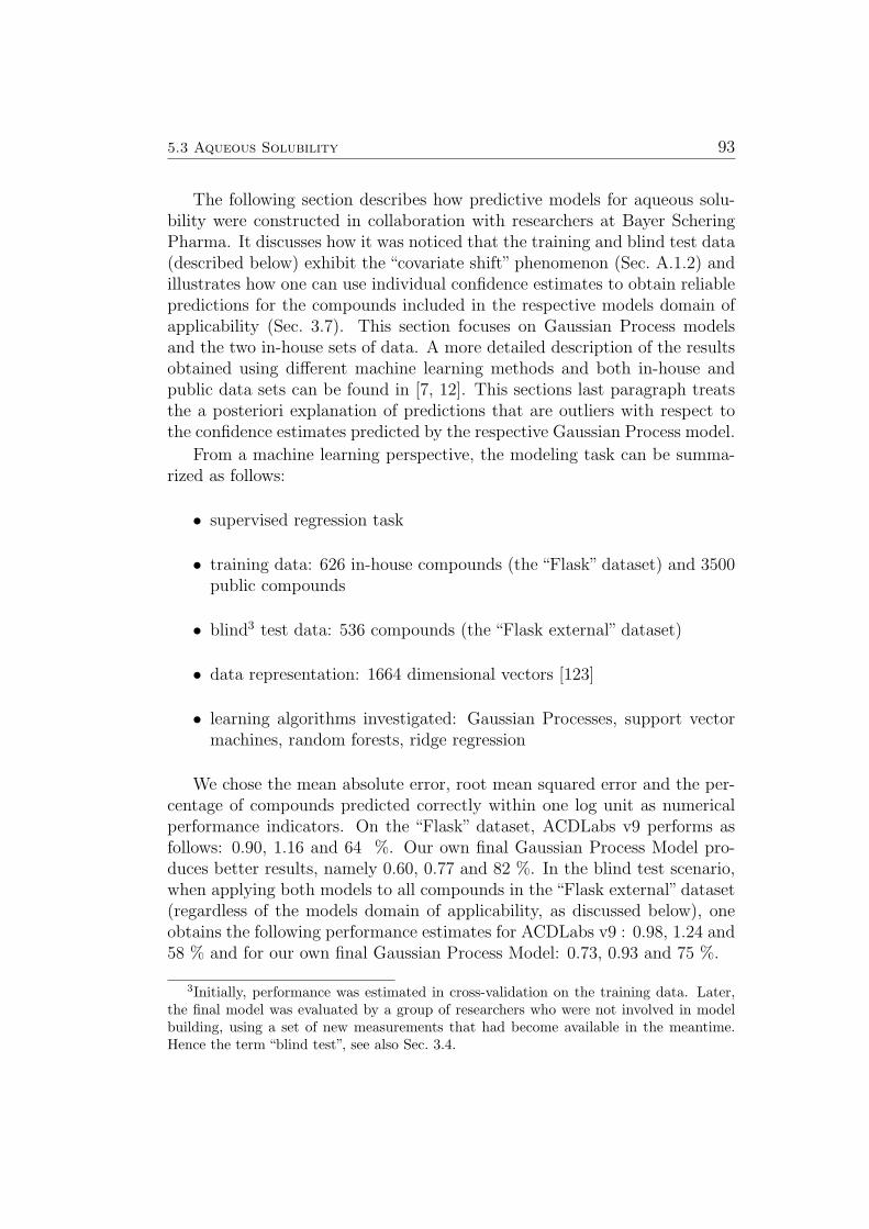
5.3 Aqueous Solubility 93
The following section describes how predictive models for aqueous solu-bility were constructed in collaboration with researchers at Bayer ScheringPharma. It discusses how it was noticed that the training and blind test data(described below) exhibit the “covariate shift” phenomenon (Sec. A.1.2) andillustrates how one can use individual confidence estimates to obtain reliablepredictions for the compounds included in the respective models domain ofapplicability (Sec. 3.7). This section focuses on Gaussian Process modelsand the two in-house sets of data. A more detailed description of the resultsobtained using different machine learning methods and both in-house andpublic data sets can be found in [7, 12]. This sections last paragraph treatsthe a posteriori explanation of predictions that are outliers with respect tothe confidence estimates predicted by the respective Gaussian Process model.
From a machine learning perspective, the modeling task can be summa-rized as follows:
• supervised regression task
• training data: 626 in-house compounds (the “Flask” dataset) and 3500public compounds
• blind3 test data: 536 compounds (the “Flask external” dataset)
• data representation: 1664 dimensional vectors [123]
• learning algorithms investigated: Gaussian Processes, support vectormachines, random forests, ridge regression
We chose the mean absolute error, root mean squared error and the per-centage of compounds predicted correctly within one log unit as numericalperformance indicators. On the “Flask” dataset, ACDLabs v9 performs asfollows: 0.90, 1.16 and 64 %. Our own final Gaussian Process Model pro-duces better results, namely 0.60, 0.77 and 82 %. In the blind test scenario,when applying both models to all compounds in the “Flask external” dataset(regardless of the models domain of applicability, as discussed below), oneobtains the following performance estimates for ACDLabs v9 : 0.98, 1.24 and58 % and for our own final Gaussian Process Model: 0.73, 0.93 and 75 %.
3Initially, performance was estimated in cross-validation on the training data. Later,the final model was evaluated by a group of researchers who were not involved in modelbuilding, using a set of new measurements that had become available in the meantime.Hence the term “blind test”, see also Sec. 3.4.
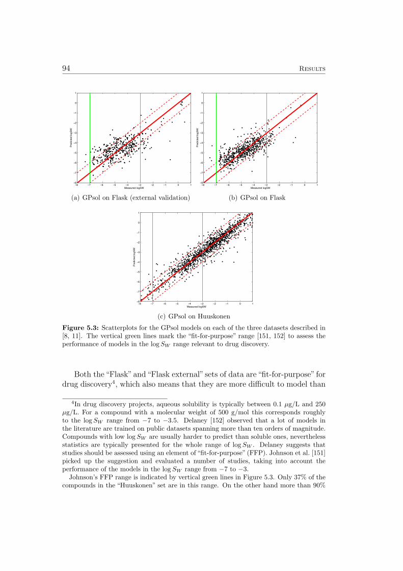
94 Results
−8 −7 −6 −5 −4 −3 −2 −1 0 1−8
−7
−6
−5
−4
−3
−2
−1
0
1
Measured logSW
Pred
icte
d lo
gSW
(a) GPsol on Flask (external validation)
−8 −7 −6 −5 −4 −3 −2 −1 0 1−8
−7
−6
−5
−4
−3
−2
−1
0
1
Measured logSW
Pred
icte
d lo
gSW
(b) GPsol on Flask
−8 −7 −6 −5 −4 −3 −2 −1 0 1−8
−7
−6
−5
−4
−3
−2
−1
0
1
Measured logSW
Pred
icte
d lo
gSW
(c) GPsol on Huuskonen
Figure 5.3: Scatterplots for the GPsol models on each of the three datasets described in[8, 11]. The vertical green lines mark the “fit-for-purpose” range [151, 152] to assess theperformance of models in the logSW range relevant to drug discovery.
Both the “Flask” and “Flask external” sets of data are “fit-for-purpose” fordrug discovery4, which also means that they are more difficult to model than
4In drug discovery projects, aqueous solubility is typically between 0.1 µg/L and 250µg/L. For a compound with a molecular weight of 500 g/mol this corresponds roughlyto the logSW range from −7 to −3.5. Delaney [152] observed that a lot of models inthe literature are trained on public datasets spanning more than ten orders of magnitude.Compounds with low logSW are usually harder to predict than soluble ones, neverthelessstatistics are typically presented for the whole range of logSW . Delaney suggests thatstudies should be assessed using an element of “fit-for-purpose” (FFP). Johnson et al. [151]picked up the suggestion and evaluated a number of studies, taking into account theperformance of the models in the logSW range from −7 to −3.
Johnson’s FFP range is indicated by vertical green lines in Figure 5.3. Only 37% of thecompounds in the “Huuskonen” set are in this range. On the other hand more than 90%
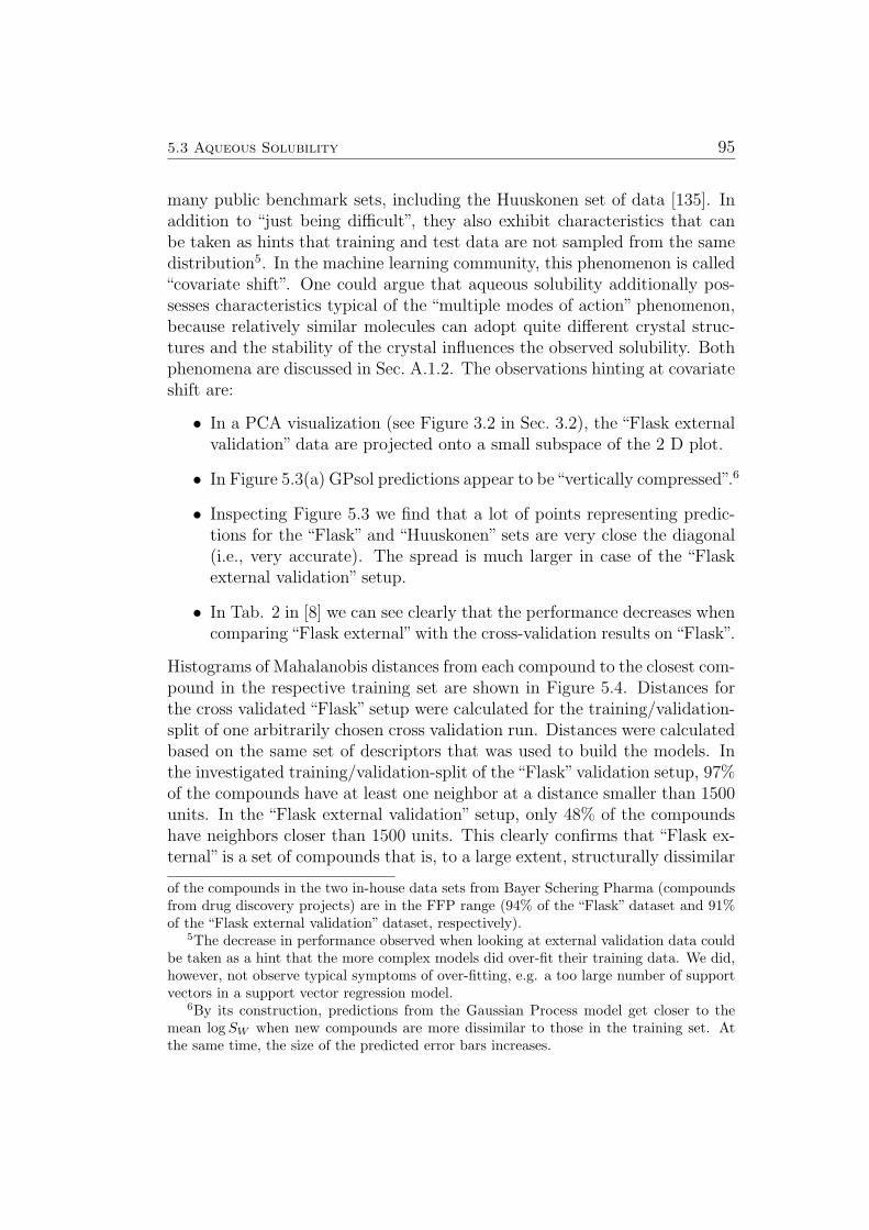
5.3 Aqueous Solubility 95
many public benchmark sets, including the Huuskonen set of data [135]. Inaddition to “just being difficult”, they also exhibit characteristics that canbe taken as hints that training and test data are not sampled from the samedistribution5. In the machine learning community, this phenomenon is called“covariate shift”. One could argue that aqueous solubility additionally pos-sesses characteristics typical of the “multiple modes of action” phenomenon,because relatively similar molecules can adopt quite different crystal struc-tures and the stability of the crystal influences the observed solubility. Bothphenomena are discussed in Sec. A.1.2. The observations hinting at covariateshift are:
• In a PCA visualization (see Figure 3.2 in Sec. 3.2), the “Flask externalvalidation” data are projected onto a small subspace of the 2 D plot.
• In Figure 5.3(a) GPsol predictions appear to be“vertically compressed”.6
• Inspecting Figure 5.3 we find that a lot of points representing predic-tions for the “Flask” and “Huuskonen” sets are very close the diagonal(i.e., very accurate). The spread is much larger in case of the “Flaskexternal validation” setup.
• In Tab. 2 in [8] we can see clearly that the performance decreases whencomparing “Flask external” with the cross-validation results on “Flask”.
Histograms of Mahalanobis distances from each compound to the closest com-pound in the respective training set are shown in Figure 5.4. Distances forthe cross validated “Flask” setup were calculated for the training/validation-split of one arbitrarily chosen cross validation run. Distances were calculatedbased on the same set of descriptors that was used to build the models. Inthe investigated training/validation-split of the“Flask”validation setup, 97%of the compounds have at least one neighbor at a distance smaller than 1500units. In the “Flask external validation” setup, only 48% of the compoundshave neighbors closer than 1500 units. This clearly confirms that “Flask ex-ternal” is a set of compounds that is, to a large extent, structurally dissimilar
of the compounds in the two in-house data sets from Bayer Schering Pharma (compoundsfrom drug discovery projects) are in the FFP range (94% of the “Flask” dataset and 91%of the “Flask external validation” dataset, respectively).
5The decrease in performance observed when looking at external validation data couldbe taken as a hint that the more complex models did over-fit their training data. We did,however, not observe typical symptoms of over-fitting, e.g. a too large number of supportvectors in a support vector regression model.
6By its construction, predictions from the Gaussian Process model get closer to themean logSW when new compounds are more dissimilar to those in the training set. Atthe same time, the size of the predicted error bars increases.
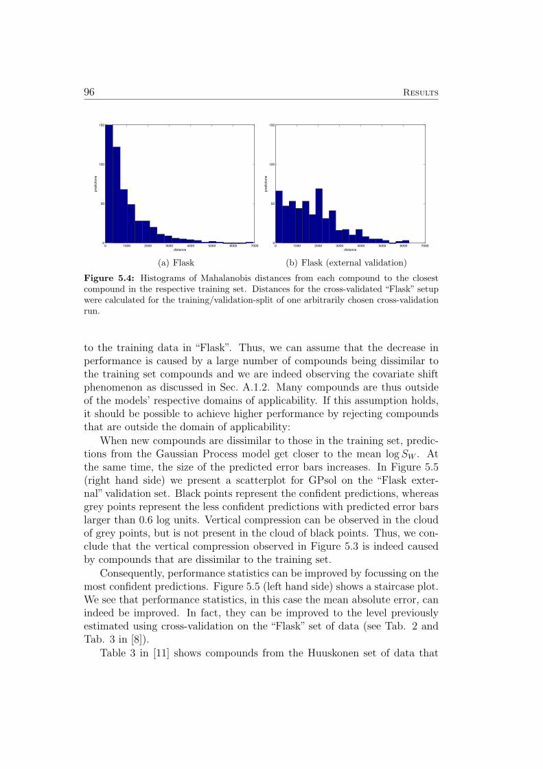
96 Results
0 1000 2000 3000 4000 5000 6000 70000
50
100
150
predictions
distance
(a) Flask
0 1000 2000 3000 4000 5000 6000 70000
50
100
150
predictions
distance
(b) Flask (external validation)
Figure 5.4: Histograms of Mahalanobis distances from each compound to the closestcompound in the respective training set. Distances for the cross-validated “Flask” setupwere calculated for the training/validation-split of one arbitrarily chosen cross-validationrun.
to the training data in “Flask”. Thus, we can assume that the decrease inperformance is caused by a large number of compounds being dissimilar tothe training set compounds and we are indeed observing the covariate shiftphenomenon as discussed in Sec. A.1.2. Many compounds are thus outsideof the models’ respective domains of applicability. If this assumption holds,it should be possible to achieve higher performance by rejecting compoundsthat are outside the domain of applicability:
When new compounds are dissimilar to those in the training set, predic-tions from the Gaussian Process model get closer to the mean logSW . Atthe same time, the size of the predicted error bars increases. In Figure 5.5(right hand side) we present a scatterplot for GPsol on the “Flask exter-nal” validation set. Black points represent the confident predictions, whereasgrey points represent the less confident predictions with predicted error barslarger than 0.6 log units. Vertical compression can be observed in the cloudof grey points, but is not present in the cloud of black points. Thus, we con-clude that the vertical compression observed in Figure 5.3 is indeed causedby compounds that are dissimilar to the training set.
Consequently, performance statistics can be improved by focussing on themost confident predictions. Figure 5.5 (left hand side) shows a staircase plot.We see that performance statistics, in this case the mean absolute error, canindeed be improved. In fact, they can be improved to the level previouslyestimated using cross-validation on the “Flask” set of data (see Tab. 2 andTab. 3 in [8]).
Table 3 in [11] shows compounds from the Huuskonen set of data that
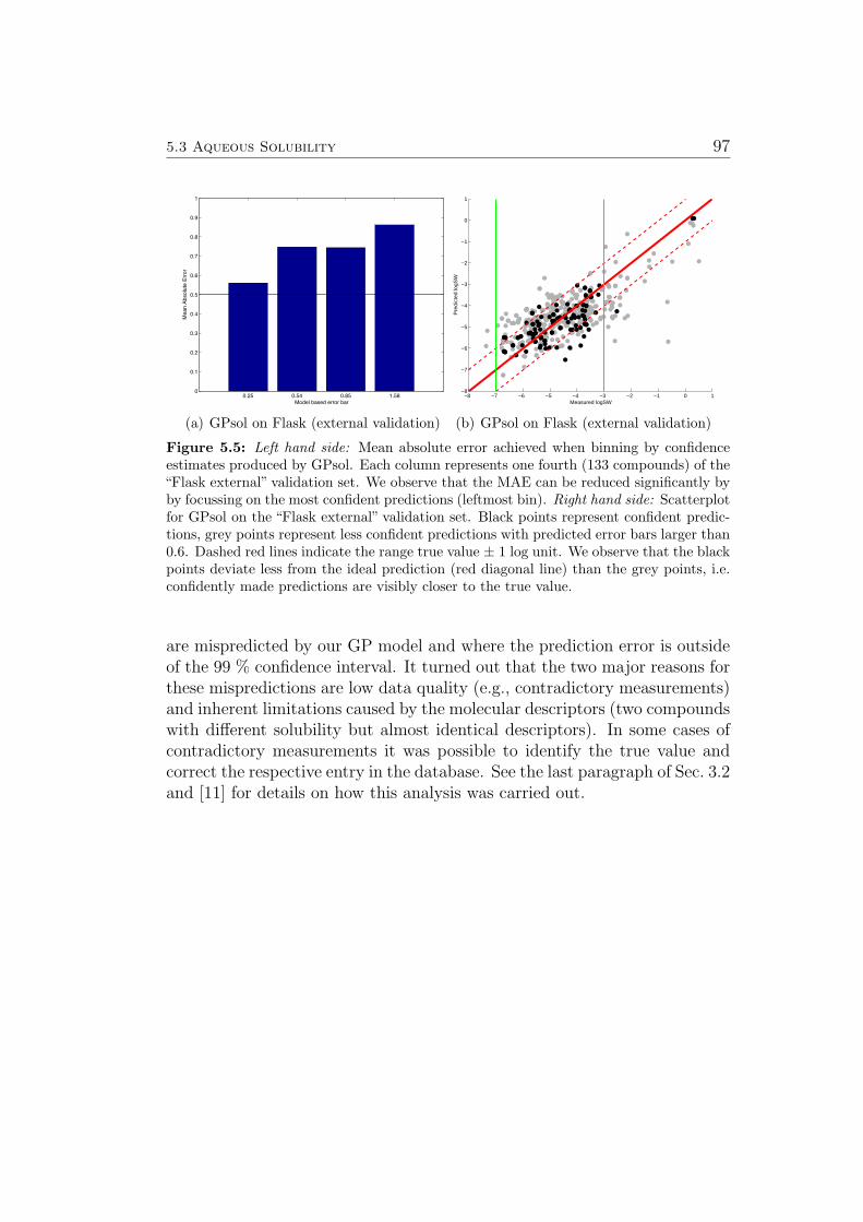
5.3 Aqueous Solubility 97
0.25 0.54 0.85 1.580
0.1
0.2
0.3
0.4
0.5
0.6
0.7
0.8
0.9
1
Mea
n Ab
solu
te E
rror
Model based error bar
(a) GPsol on Flask (external validation)
−8 −7 −6 −5 −4 −3 −2 −1 0 1−8
−7
−6
−5
−4
−3
−2
−1
0
1
Measured logSW
Pre
dict
ed lo
gSW
(b) GPsol on Flask (external validation)
Figure 5.5: Left hand side: Mean absolute error achieved when binning by confidenceestimates produced by GPsol. Each column represents one fourth (133 compounds) of the“Flask external” validation set. We observe that the MAE can be reduced significantly byby focussing on the most confident predictions (leftmost bin). Right hand side: Scatterplotfor GPsol on the “Flask external” validation set. Black points represent confident predic-tions, grey points represent less confident predictions with predicted error bars larger than0.6. Dashed red lines indicate the range true value ± 1 log unit. We observe that the blackpoints deviate less from the ideal prediction (red diagonal line) than the grey points, i.e.confidently made predictions are visibly closer to the true value.
are mispredicted by our GP model and where the prediction error is outsideof the 99 % confidence interval. It turned out that the two major reasons forthese mispredictions are low data quality (e.g., contradictory measurements)and inherent limitations caused by the molecular descriptors (two compoundswith different solubility but almost identical descriptors). In some cases ofcontradictory measurements it was possible to identify the true value andcorrect the respective entry in the database. See the last paragraph of Sec. 3.2and [11] for details on how this analysis was carried out.

5.4 Cytochrome P450 Inhibition 99
5.4 Cytochrome P450 Inhibition
The five most important members of the Cytochrome P450 superfamily ofheme-containing monooxygenases, namely CYP 1A2, 2C19, 2C9, 2D6 and3A4, are responsible for clearance of more than 90% of all marketed drugs[153–156]. Their inhibition can result in unwanted drug-drug interactions,making it desirable to identify problematic compounds as early as possiblein the drug design process. Quantitative Structure Activity Relationships(QSAR), pharmacophore modeling and homology modeling have all beenused to generate predictions for molecules binding either as substrates or in-hibitors. Also, several groups have combined pharmacophores with homologymodels [157]. However, many parts of the mechanisms of catalysis, activationand inhibition are still poorly understood [154]. All of the above mentionedapproaches aim at understanding CYP inhibition via explicit models of theinhibition process. In contrast, approaches based on statistical learning havebeen used in these studies [158–160]. In 2005, the study published by Klesset al. [160] was the only publication about application of machine learningmethods to data about all of the five most important CYP isoenzymes. Thegeneral consensus is that CYP inhibition is a very difficult modeling problem.
The following section describes how predictive models for inhibition ofeach of five cytochrome P450 enzymes were constructed in collaboration withresearchers at Schering. In 2006, CYP 2D6 was first crystallized and its 3Dstructure determined, following the previous discoveries of the 3D structuresof CYP 2C9 and CYP 3A4 [161–163]. This knowledge allows for proteinstructure based approaches (such as docking) to be used in identification ofCYP inhibitors. The study described in the following was started in 2005and employed a ligand based approach.
From a machine learning perspective, the modeling task can be summa-rized as follows:
• supervised multiclass classification / ordinal regression task
• training data: ∼ 800 compounds with labels for each of 5 CYP sub-types, blind7 test data: ∼ 170 compounds with labels for each of 5CYP subtypes
• labels: compounds, are labeled as weak, moderate or potent inhibitorsof the respective CYP subtype, see Sec. A.2 for detailed definitions.
7Initially, performance was estimated in cross-validation on the training data. Later,the final model was evaluated by a group of researchers who were not involved in modelbuilding, using a set of new measurements that had become available in the meantime.Hence the term “blind test”, see also Sec. 3.4.
100 Results
• source: most compounds are in-house compounds of Schering, but forsome compounds, measurements have been curated from the literature(see Sec. A.2 for the exact composition of each dataset). As the litera-ture compounds span a larger part of the chemical space, it is not clearwhether including this data can improve predictions for future in-housecompounds.
• data representation in first modelling effort: The following six vecto-rial representations were used, see Appendix A.3 for a description ofeach type of representation: Ghose-Crippen [164]8, BCUT [166, 167],UNITY fingerprints [168], LogD prediction module from ACD Labs[75], VolSurf [169], GRIND [170]
• data representation in second modelling effort:1664 dimensional vectorsgenerated using the Dragon descriptor generator [123]
• learning algorithms investigated in first modelling effort: decision trees[171], k-Nearest Neighbor (kNN) [172], Gaussian Processes[43], SupportVector Machines (SVM) [38, 173, 174], Linear Programming Machines(LPM) [175, 176].
• learning algorithms investigated in second modelling effort: GaussianProcesses
PCA plots using all descriptors together can be found in Figure 5.6. Somestructure can be recognized, but in two dimensions even the two most differ-ent classes (only weak and potent inhibitors are shown, moderate inhibitorsare omitted) do not look separable. Therefore it is unclear whether classifi-cation using many dimensions will be possible.
For each of the five CYP isoenzymes, two classifiers are build: The firstdiscriminating between weak inhibitors and non-weak (i.e., moderate andpotent) inhibitors (Task 1), the second discriminating between potent andnon-potent (moderate and weak) inhibitors (Task 2). For each of these clas-sifiers, it is not clear which descriptor and learning method is best suitedfor the respective classification task. Thus, classifiers for each combinationof descriptors and learning methods were constructed. As a further subdivi-sion, classifiers from the in-house data, and from the union of in-house andliterature data were investigated.
As on single sets of descriptors the best results were achieved using sup-port vector machines with RBF kernels, this method was also chosen for
8It was checked whether using Fisher Scores [165] of the Ghose-Crippen [164] descriptorsfacilitates modeling. The accuracy achieved was very similar in both cases, therefore theplain Ghose-Crippen descriptors were used in the remaining part of the study.
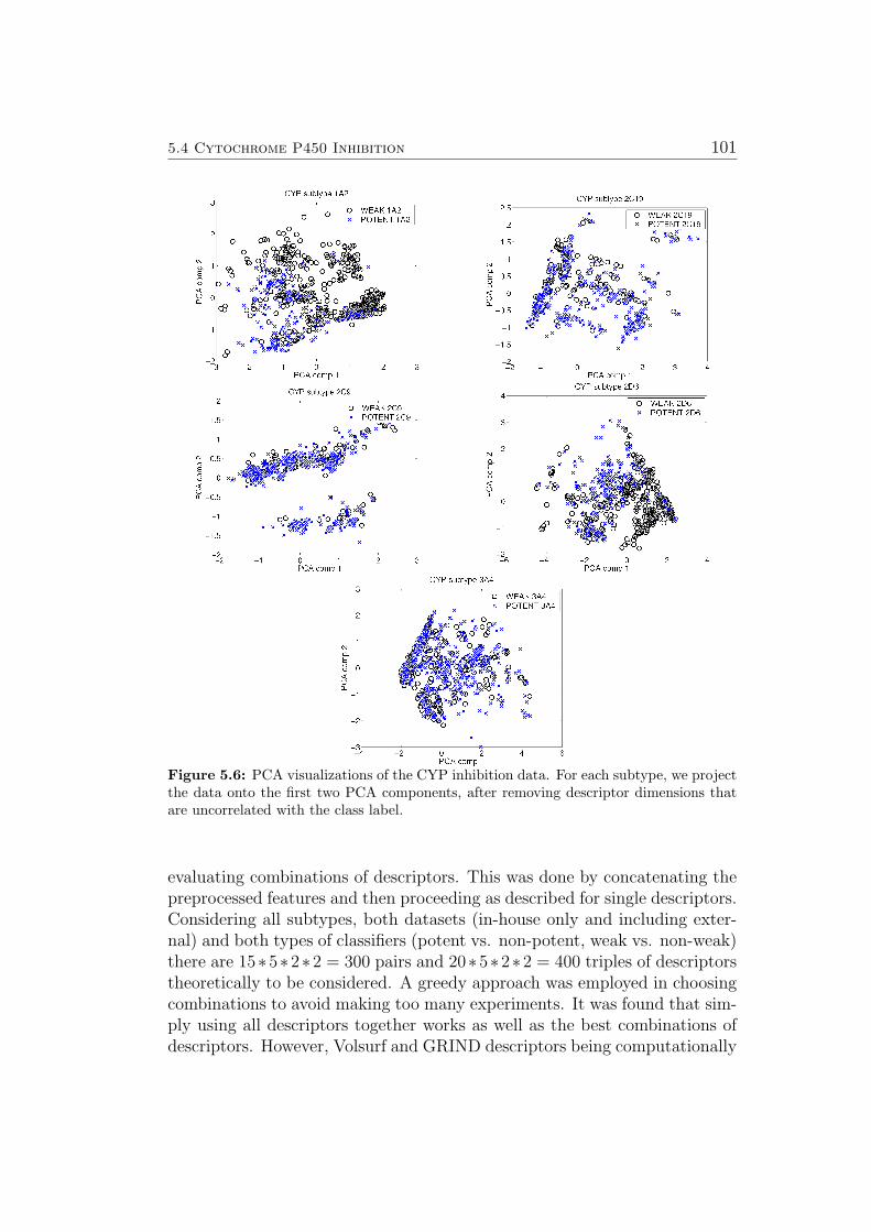
5.4 Cytochrome P450 Inhibition 101
Figure 5.6: PCA visualizations of the CYP inhibition data. For each subtype, we projectthe data onto the first two PCA components, after removing descriptor dimensions thatare uncorrelated with the class label.
evaluating combinations of descriptors. This was done by concatenating thepreprocessed features and then proceeding as described for single descriptors.Considering all subtypes, both datasets (in-house only and including exter-nal) and both types of classifiers (potent vs. non-potent, weak vs. non-weak)there are 15∗5∗2∗2 = 300 pairs and 20∗5∗2∗2 = 400 triples of descriptorstheoretically to be considered. A greedy approach was employed in choosingcombinations to avoid making too many experiments. It was found that sim-ply using all descriptors together works as well as the best combinations ofdescriptors. However, Volsurf and GRIND descriptors being computationally
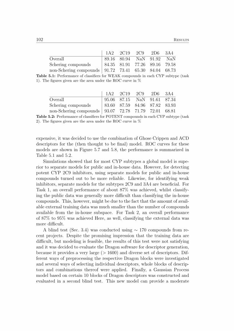
102 Results
1A2 2C19 2C9 2D6 3A4Overall 89.16 80.94 NaN 91.92 NaNSchering compounds 84.35 81.91 77.26 89.16 79.58non-Schering compounds 91.72 73.41 65.30 84.04 68.73
Table 5.1: Performance of classifiers for WEAK compounds in each CYP subtype (task1). The figures given are the area under the ROC curve in %
1A2 2C19 2C9 2D6 3A4Overall 95.06 87.15 NaN 91.61 87.34Schering compounds 83.60 87.59 84.96 87.82 83.93non-Schering compounds 93.07 72.78 71.79 72.01 68.81
Table 5.2: Performance of classifiers for POTENT compounds in each CYP subtype (task2). The figures given are the area under the ROC curve in %
expensive, it was decided to use the combination of Ghose Crippen and ACDdescriptors for the (then thought to be final) model. ROC curves for thesemodels are shown in Figure 5.7 and 5.8, the performance is summarized inTable 5.1 and 5.2.
Simulations showed that for most CYP subtypes a global model is supe-rior to separate models for public and in-house data. However, for detectingpotent CYP 2C9 inhibitors, using separate models for public and in-housecompounds turned out to be more reliable. Likewise, for identifying weakinhibitors, separate models for the subtypes 2C9 and 3A4 are beneficial. ForTask 1, an overall performance of about 87% was achieved, whilst classify-ing the public data was generally more difficult than classifying the in-housecompounds. This, however, might be due to the fact that the amount of avail-able external training data was much smaller than the number of compoundsavailable from the in-house subspace. For Task 2, an overall performanceof 87% to 95% was achieved Here, as well, classifying the external data wasmore difficult.
A blind test (Sec. 3.4) was conducted using ∼ 170 compounds from re-cent projects. Despite the promising impression that the training data aredifficult, but modeling is feasible, the results of this test were not satisfyingand it was decided to evaluate the Dragon software for descriptor generation,because it provides a very large (> 1600) and diverse set of descriptors. Dif-ferent ways of preprocessing the respective Dragon blocks were investigatedand several ways of selecting individual descriptors, whole blocks of descrip-tors and combinations thereof were applied. Finally, a Gaussian Processmodel based on certain 10 blocks of Dragon descriptors was constructed andevaluated in a second blind test. This new model can provide a moderate
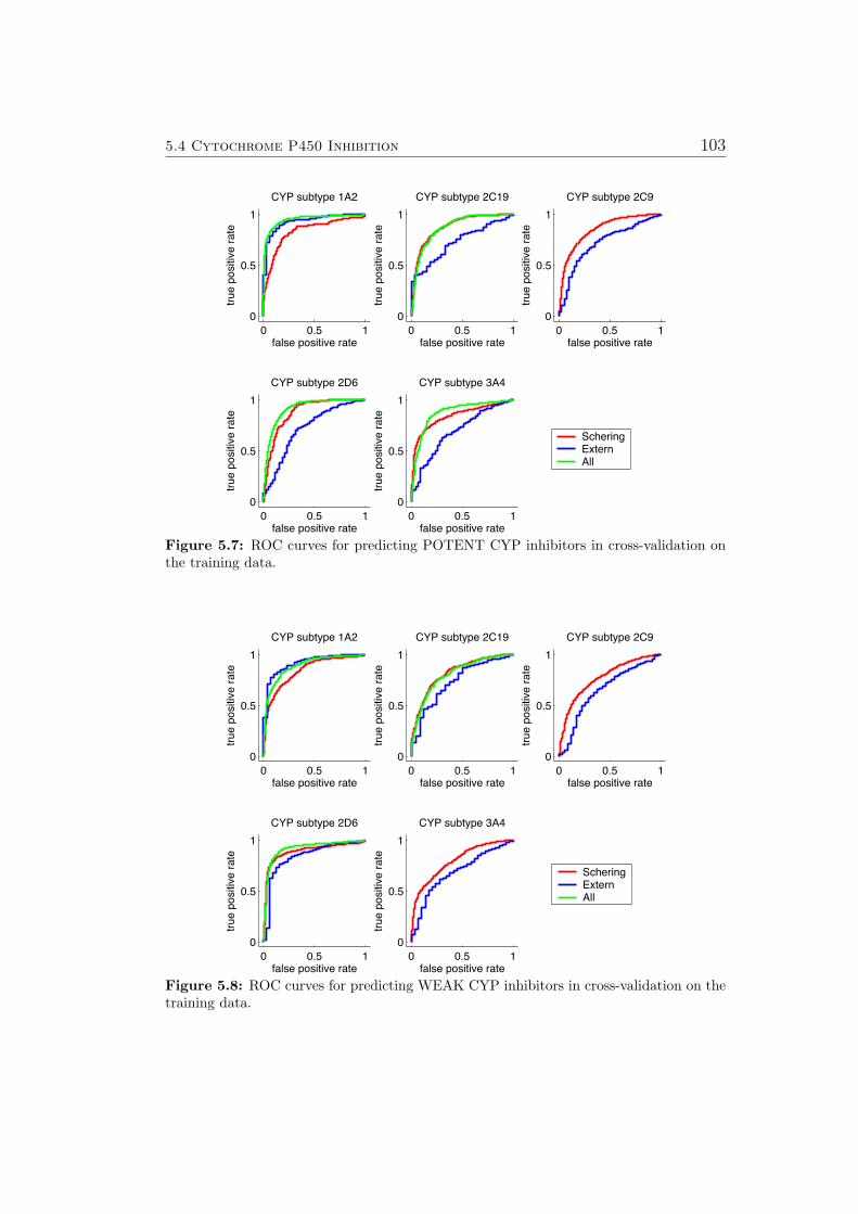
5.4 Cytochrome P450 Inhibition 103
0 0.5 10
0.5
1
false positive rate
true
posi
tive
rate
CYP subtype 1A2
ScheringExternAll
0 0.5 10
0.5
1
false positive rate
true
posi
tive
rate
CYP subtype 2C19
0 0.5 10
0.5
1
false positive rate
true
posi
tive
rate
CYP subtype 2C9
0 0.5 10
0.5
1
false positive rate
true
posi
tive
rate
CYP subtype 2D6
0 0.5 10
0.5
1
false positive rate
true
posi
tive
rate
CYP subtype 3A4
Figure 5.7: ROC curves for predicting POTENT CYP inhibitors in cross-validation onthe training data.
0 0.5 10
0.5
1
false positive rate
true
posi
tive
rate
CYP subtype 1A2
ScheringExternAll
0 0.5 10
0.5
1
false positive rate
true
posi
tive
rate
CYP subtype 2C19
0 0.5 10
0.5
1
false positive rate
true
posi
tive
rate
CYP subtype 2C9
0 0.5 10
0.5
1
false positive rate
true
posi
tive
rate
CYP subtype 2D6
0 0.5 10
0.5
1
false positive rate
true
posi
tive
rate
CYP subtype 3A4
Figure 5.8: ROC curves for predicting WEAK CYP inhibitors in cross-validation on thetraining data.
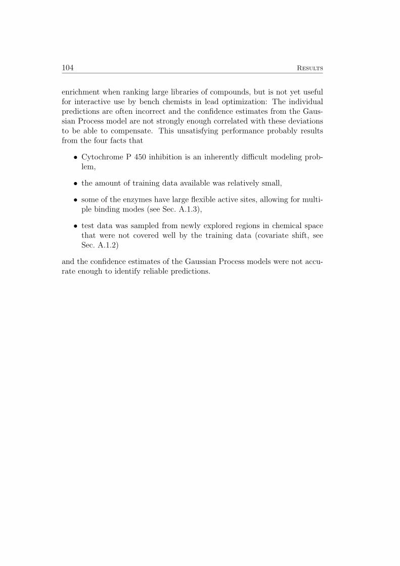
104 Results
enrichment when ranking large libraries of compounds, but is not yet usefulfor interactive use by bench chemists in lead optimization: The individualpredictions are often incorrect and the confidence estimates from the Gaus-sian Process model are not strongly enough correlated with these deviationsto be able to compensate. This unsatisfying performance probably resultsfrom the four facts that
• Cytochrome P 450 inhibition is an inherently difficult modeling prob-lem,
• the amount of training data available was relatively small,
• some of the enzymes have large flexible active sites, allowing for multi-ple binding modes (see Sec. A.1.3),
• test data was sampled from newly explored regions in chemical spacethat were not covered well by the training data (covariate shift, seeSec. A.1.2)
and the confidence estimates of the Gaussian Process models were not accu-rate enough to identify reliable predictions.
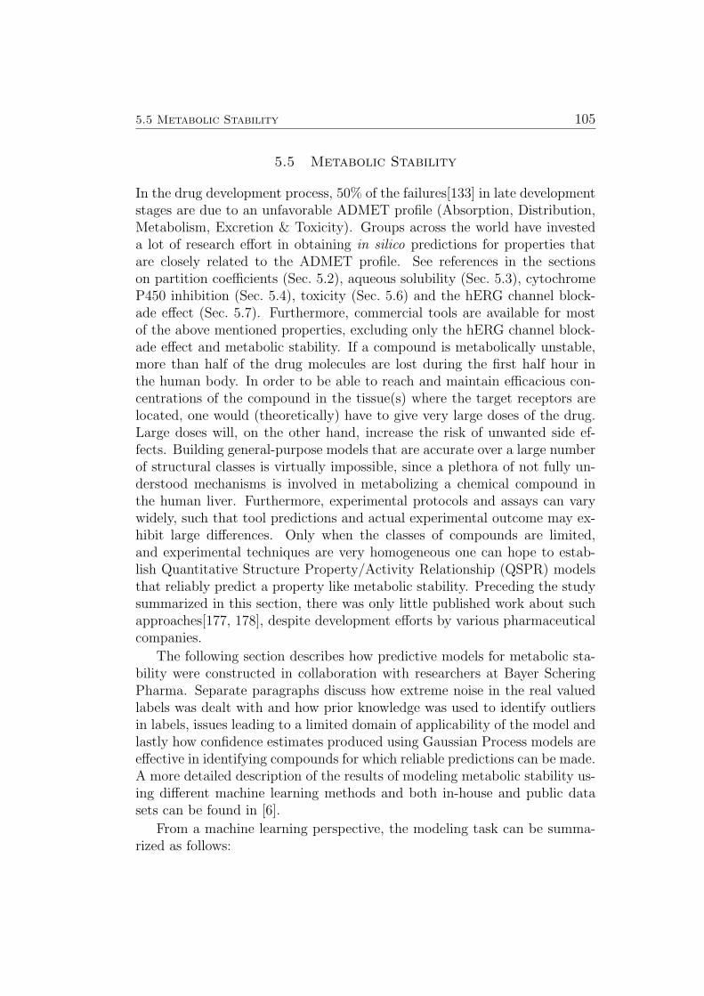
5.5 Metabolic Stability 105
5.5 Metabolic Stability
In the drug development process, 50% of the failures[133] in late developmentstages are due to an unfavorable ADMET profile (Absorption, Distribution,Metabolism, Excretion & Toxicity). Groups across the world have investeda lot of research effort in obtaining in silico predictions for properties thatare closely related to the ADMET profile. See references in the sectionson partition coefficients (Sec. 5.2), aqueous solubility (Sec. 5.3), cytochromeP450 inhibition (Sec. 5.4), toxicity (Sec. 5.6) and the hERG channel block-ade effect (Sec. 5.7). Furthermore, commercial tools are available for mostof the above mentioned properties, excluding only the hERG channel block-ade effect and metabolic stability. If a compound is metabolically unstable,more than half of the drug molecules are lost during the first half hour inthe human body. In order to be able to reach and maintain efficacious con-centrations of the compound in the tissue(s) where the target receptors arelocated, one would (theoretically) have to give very large doses of the drug.Large doses will, on the other hand, increase the risk of unwanted side ef-fects. Building general-purpose models that are accurate over a large numberof structural classes is virtually impossible, since a plethora of not fully un-derstood mechanisms is involved in metabolizing a chemical compound inthe human liver. Furthermore, experimental protocols and assays can varywidely, such that tool predictions and actual experimental outcome may ex-hibit large differences. Only when the classes of compounds are limited,and experimental techniques are very homogeneous one can hope to estab-lish Quantitative Structure Property/Activity Relationship (QSPR) modelsthat reliably predict a property like metabolic stability. Preceding the studysummarized in this section, there was only little published work about suchapproaches[177, 178], despite development efforts by various pharmaceuticalcompanies.
The following section describes how predictive models for metabolic sta-bility were constructed in collaboration with researchers at Bayer ScheringPharma. Separate paragraphs discuss how extreme noise in the real valuedlabels was dealt with and how prior knowledge was used to identify outliersin labels, issues leading to a limited domain of applicability of the model andlastly how confidence estimates produced using Gaussian Process models areeffective in identifying compounds for which reliable predictions can be made.A more detailed description of the results of modeling metabolic stability us-ing different machine learning methods and both in-house and public datasets can be found in [6].
From a machine learning perspective, the modeling task can be summa-rized as follows:
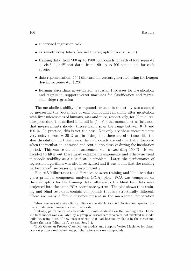
106 Results
• supervised regression task
• extremely noisy labels (see next paragraph for a discussion)
• training data: from 900 up to 1900 compounds for each of four separatespecies9, blind10 test data: from 190 up to 700 compounds for eachspecies
• data representation: 1664 dimensional vectors generated using the Dragondescriptor generator [123]
• learning algorithms investigated: Gaussian Processes for classificationand regression, support vector machines for classification and regres-sion, ridge regression
The metabolic stability of compounds treated in this study was assessedby measuring the percentage of each compound remaining after incubationwith liver microsomes of humans, rats and mice, respectively, for 30 minutes.The procedure is described in detail in [6]. For the moment let us just notethat measurements should, theoretically, span the range between 0 % and100 %. In practice, this is not the case: Not only are these measurementsvery noisy (errors ± 20 % are in order), but there are also issues like tooslow dissolution: In these cases, the compounds are only partially dissolvedwhen the incubation is started and continue to dissolve during the incubationperiod. This can result in measurement values exceeding 150 %. It wasdecided to filter out these most extreme measurements and otherwise treatmetabolic stability as a classification problem. Later, the performance ofregression algorithms was also investigated and it was found that the rankingperformance11 increases only insignificantly.
Figure 5.9 illustrates the differences between training and blind test datavia a principal component analysis (PCA) plot. PCA was computed onthe descriptors for the training data, afterwards the blind test data wereprojected into the same PCA coordinate system. The plot shows that train-ing and blind test data contain compounds that are structurally different.There are many different enzymes present in the microsomal preparation
9Measurements of metabolic stability were available for the following four species: hu-mans, male mice, female mice and male rats.
10Initially, performance was estimated in cross-validation on the training data. Later,the final model was evaluated by a group of researchers who were not involved in modelbuilding, using a set of new measurements that had become available in the meantime.Hence the term “blind test”, see also Sec. 3.4.
11Both Gaussian Process Classification models and Support Vector Machines for classi-fication produce real valued output that allows to rank compounds.
5.5 Metabolic Stability 107
−3 −2 −1 0 1 2−3
−2
−1
0
1
2
3
PCA component 1
PCA
com
pone
nt 2
TrainingBlind test
Figure 5.9: Visualization of training and blind test data for the assay “mouse female” byprincipal component analysis (PCA). The blind test data covers recent projects, and thusfollows a distribution that is different from the training data
0 0.2 0.4 0.6 0.8 1
0
0.1
0.2
0.3
0.4
0.5
0.6
0.7
0.8
0.9
1
false positive rate
true
pos
itive
rat
e
Human m/f
Size of grey area
0 0.2 0.45
0 0.1 0.2 0.3 0.4 0.50
50
100
150
200
250Human m/f
Size of grey area
Num
ber
of e
rror
s
Number of errors% not predicted
0
20
40
60
80
100
Per
−ce
nt n
ot p
redi
cted
Figure 5.10: The output of a Gaussian Process Classification model is close to 0.5 ifpredictions are made inconfidently. ROC curves resulting from rejecting predictions fallinginside “grey areas”, i.e. intervals [0.5−q . . . 0.5+q] are presented in the left hand side plot.At the same time, the number of rejected compounds increases (right hand side plot). Wecan see that the shape of the ROC-curves (left hand side) improves continuously as q isincreased, finally reaching almost 100 % correct classification (red curve at the top).
used for the measurements and some of the enzymes even have different ac-tive sites. Therefore the models are simultaneously facing both a samplingissue (Sec. A.1.2) and multiple mechanisms. The next paragraph explainshow reliable predictions can be identified.
108 Results
The output of a Gaussian Process Classification model is the probabilitythat the compound belongs to class 1. It becomes closer to 0.5 as the distanceto the training set increases and actually is 0.5 for compounds that are farfrom the training set. Therefore a natural way to reject compounds thatare outside of the domain of applicability is to define some desired level ofconfidence and then reject all predictions in the interval [0.5− q . . . 0.5 + q].Receiver operating curves for different values of q in the range [0 . . . 0.45]are shown in Figure 5.10 (left). At the same time, the number of rejectedcompounds increases, see Figure 5.10 (right). We can see that the shapeof the ROC-curves improves continuously as q is increased, finally reachingalmost 100 % correct classification (red curve at the top).
In conclusion, one can use prior knowledge to identify outliers in thetraining data, the domain of applicability of models is limited due to samplingissues and multiple mechanisms, but using a Gaussian Process Classificationmodel one can predict the metabolic stability of compounds in the form ofa probability that the respective compound is stable. By leaving out unsurepredictions where the predicted probability is close to 50 %, performance canbe improved to the point of being almost perfect.
5.6 Ames Mutagenicity 109
5.6 Ames Mutagenicity
The bacterial reverse mutation assay (Ames test [179]) to detect mutagenicityin vitro is of crucial importance in drug discovery and development as an earlyalerting system for potential carcinogenicity and/or teratogenicity. In theAmes test, frame-shift mutations or base-pair substitutions may be detectedby exposure of histidine-dependent strains of Salmonella typhimurium to atest compound. When these strains are exposed to a mutagen, reverse mu-tations to the wild-type histidine-independent form enable bacterial colonygrowth on a medium deficient in histidine (”revertants”). Since many chemi-cals interact with genetic material only after metabolic activation by enzymesystems not available in the bacterial cell, the test compounds are in manycases additionally examined in the presence of a mammalian metabolizingsystem, which contains liver microsomes (with S9 mix, see [5]). Existingcommercial tools suitable for predicting the outcome of the Ames test, suchas DEREK and MultiCASE, provide promising results on several evaluationdata sets and the possibility to derive structure-activity and/or even mech-anistic information from the predictions. Still, these commercial tools arelimited in terms of statistical performance, technical accessibility for benchchemists and adaptability to a company’s chemical space. In the public liter-ature, several approaches have been followed to predict Ames mutagenicity,generally yielding good specificity and sensitivity values (prediction accuracyof up to 85%). Depending on the descriptors and the statistical methodsused, some of the models offer structure-activity information, such as Helmaet al.[180] or Kazius et al. [181], some are however harder to interpret dueto their choice of chemical descriptors, such as Feng et al. [182]. Moreover,different data sets have been used in the respective studies [180–182] withoutdisclosing the splits (training set / test set) used for model evaluation.
The following section describes how a large unique benchmark set wascollected (and published) and predictive models for Ames mutagenicity wereconstructed in collaboration with researchers at Bayer Schering Pharma. Anevaluation of several machine learning algorithms and three commercial toolsis presented. The benchmark data set was used for developing two newframeworks for interpreting results and increasing the acceptance of modelsby bench chemists. Sec. 4.3 explains predictions in terms of the most relevantcompounds in the training set,. In contrast, Sec. 4.4 explains predictions interms of the locally most relevant features. These are identified using localgradients which, at the same time, provide hints that can help in compoundoptimization.
From a machine learning perspective, the modeling task can be summa-rized as follows:
110 Results
• supervised classification task
• evaluation strategy: Five fold cross-validation, each time including astatic training set (see below).
• data representation: 904 dimensional vectors (blocks 1, 2, 6, 9, 12,15, 16, 17, 18 and 20 of DRAGON-X version 1.2 [123] based on a 3Dstructure generated by CORINA version 3.4 [123]
To allow for a reasonable comparison of different methods, we assembleda new benchmark set of 6512 compounds together with their Ames test re-sults from public sources. As described in [5], we make this large uniquebenchmark set - including well-defined random splits - publicly available tofacilitate future comparisons with prediction methods of other researchers.
Using the benchmark data set, four machine learning techniques and threecommercial prediction tools were evaluated. For the non-commercial machinelearning methods we considered a support vector machine, a Gaussian Pro-cess, a random forest and a k-nearest neighbor model. For the machinelearning algorithms, short descriptions and references to the literature canbe found in Sec. 3.3). The commercial tools are described in the following:
• Pipeline Pilot’s Bayesian categorization model[183] provides supervisedBayesian learning for large data collections. In our example, we havecombined this Bayesian classifier with Pipeline Pilot’s ECFP chemicalfingerprint technology (ECFP 4 fingerprints).
• DEREK (Version 10.0.2 Service Pack 3, Knowledge Base Release DfW10.0.0 25 07 2007, Lhasa Ltd., UK) is an expert system providing knownstructure-activity relationships (SARs), each relating to a toxicologicalendpoint. The mutagenicity prediction by DEREK was considered pos-itive if a structure triggered at least one mutagenicity alert, and nega-tive if it did not raise any mutagenicity alerts. Compounds containedas examples in the knowledge base of DEREK were excluded from theevaluation[184].
• MultiCASE (Multicase Inc., USA) is a correlative tool predicting tox-icity on the basis of structural fragments statistically correlated withactivity (QSAR). For mutagenicity prediction, the commercially avail-able AZ2 mutagenicity module was used. Compounds contained in thetraining set of the AZ2 module were excluded from the evaluation[185].
All models were evaluated in a 5-fold cross validation setting. Firstlyall compounds which were verifiably known to DEREK or MultiCASE were
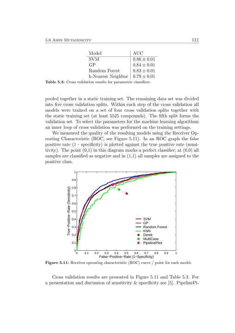
5.6 Ames Mutagenicity 111
Model AUCSVM 0.86± 0.01GP 0.84± 0.01Random Forest 0.83± 0.01k-Nearest Neighbor 0.79± 0.01
Table 5.3: Cross validation results for parametric classifiers.
pooled together in a static training set. The remaining data set was dividedinto five cross validation splits. Within each step of the cross validation allmodels were trained on a set of four cross validation splits together withthe static training set (at least 5525 compounds). The fifth split forms thevalidation set. To select the parameters for the machine learning algorithmsan inner loop of cross validation was performed on the training settings.
We measured the quality of the resulting models using the Receiver Op-erating Characteristic (ROC, see Figure 5.11). In an ROC graph the falsepositive rate (1 - specificity) is plotted against the true positive rate (sensi-tivity). The point (0,1) in this diagram marks a perfect classifier; at (0,0) allsamples are classified as negative and in (1,1) all samples are assigned to thepositive class.
0 0.1 0.2 0.3 0.4 0.5 0.6 0.7 0.8 0.9 10
0.1
0.2
0.3
0.4
0.5
0.6
0.7
0.8
0.9
1
False−Positive−Rate (1−Specificity)
Tru
e−P
ositi
ve−
Rat
e (S
ensi
tivity
)
SVMGPRandom ForestKNNDerekMultiCasePipelinePilot
Figure 5.11: Receiver operating characteristic (ROC) curve / point for each model.
Cross validation results are presented in Figure 5.11 and Table 5.3. Fora presentation and discussion of sensitivity & specificity see [5]. PipelinePi-
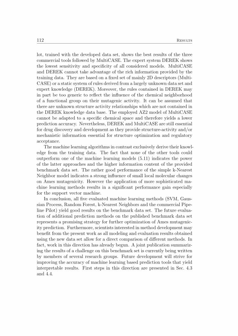
112 Results
lot, trained with the developed data set, shows the best results of the threecommercial tools followed by MultiCASE. The expert system DEREK showsthe lowest sensitivity and specificity of all considered models. MultiCASEand DEREK cannot take advantage of the rich information provided by thetraining data. They are based on a fixed set of mainly 2D descriptors (Multi-CASE) or a static system of rules derived from a largely unknown data set andexpert knowledge (DEREK). Moreover, the rules contained in DEREK mayin part be too generic to reflect the influence of the chemical neighborhoodof a functional group on their mutagenic activity. It can be assumed thatthere are unknown structure activity relationships which are not contained inthe DEREK knowledge data base. The employed AZ2 model of MultiCASEcannot be adapted to a specific chemical space and therefore yields a lowerprediction accuracy. Nevertheless, DEREK and MultiCASE are still essentialfor drug discovery and development as they provide structure-activity and/ormechanistic information essential for structure optimization and regulatoryacceptance.
The machine learning algorithms in contrast exclusively derive their knowl-edge from the training data. The fact that none of the other tools couldoutperform one of the machine learning models (5.11) indicates the powerof the latter approaches and the higher information content of the providedbenchmark data set. The rather good performance of the simple k-NearestNeighbor model indicates a strong influence of small local molecular changeson Ames mutagenicity. However the application of more sophisticated ma-chine learning methods results in a significant performance gain especiallyfor the support vector machine.
In conclusion, all five evaluated machine learning methods (SVM, Gaus-sian Process, Random Forest, k-Nearest Neighbors and the commercial Pipe-line Pilot) yield good results on the benchmark data set. The future evalua-tion of additional prediction methods on the published benchmark data setrepresents a promising strategy for further optimization of Ames mutagenic-ity prediction. Furthermore, scientists interested in method development maybenefit from the present work as all modeling and evaluation results obtainedusing the new data set allow for a direct comparison of different methods. Infact, work in this direction has already begun. A joint publication summariz-ing the results of a challenge on this benchmark set is currently being writtenby members of several research groups. Future development will strive forimproving the accuracy of machine learning based prediction tools that yieldinterpretable results. First steps in this direction are presented in Sec. 4.3and 4.4.
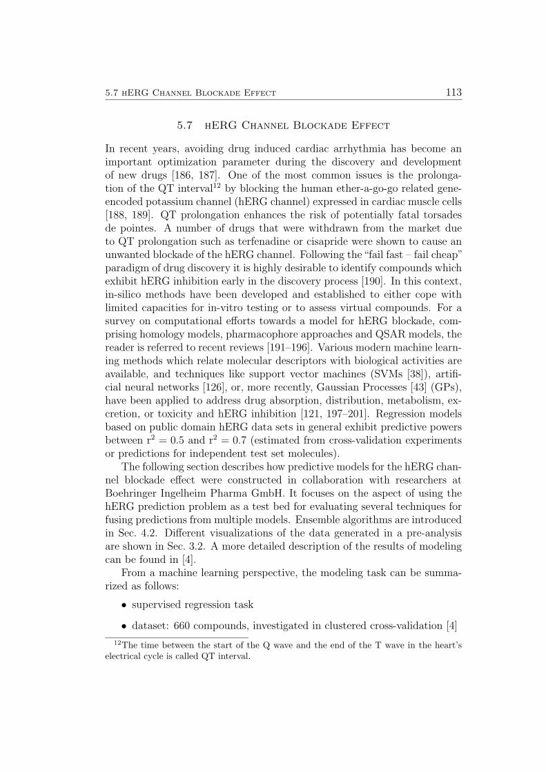
5.7 hERG Channel Blockade Effect 113
5.7 hERG Channel Blockade Effect
In recent years, avoiding drug induced cardiac arrhythmia has become animportant optimization parameter during the discovery and developmentof new drugs [186, 187]. One of the most common issues is the prolonga-tion of the QT interval12 by blocking the human ether-a-go-go related gene-encoded potassium channel (hERG channel) expressed in cardiac muscle cells[188, 189]. QT prolongation enhances the risk of potentially fatal torsadesde pointes. A number of drugs that were withdrawn from the market dueto QT prolongation such as terfenadine or cisapride were shown to cause anunwanted blockade of the hERG channel. Following the“fail fast – fail cheap”paradigm of drug discovery it is highly desirable to identify compounds whichexhibit hERG inhibition early in the discovery process [190]. In this context,in-silico methods have been developed and established to either cope withlimited capacities for in-vitro testing or to assess virtual compounds. For asurvey on computational efforts towards a model for hERG blockade, com-prising homology models, pharmacophore approaches and QSAR models, thereader is referred to recent reviews [191–196]. Various modern machine learn-ing methods which relate molecular descriptors with biological activities areavailable, and techniques like support vector machines (SVMs [38]), artifi-cial neural networks [126], or, more recently, Gaussian Processes [43] (GPs),have been applied to address drug absorption, distribution, metabolism, ex-cretion, or toxicity and hERG inhibition [121, 197–201]. Regression modelsbased on public domain hERG data sets in general exhibit predictive powersbetween r2 = 0.5 and r2 = 0.7 (estimated from cross-validation experimentsor predictions for independent test set molecules).
The following section describes how predictive models for the hERG chan-nel blockade effect were constructed in collaboration with researchers atBoehringer Ingelheim Pharma GmbH. It focuses on the aspect of using thehERG prediction problem as a test bed for evaluating several techniques forfusing predictions from multiple models. Ensemble algorithms are introducedin Sec. 4.2. Different visualizations of the data generated in a pre-analysisare shown in Sec. 3.2. A more detailed description of the results of modelingcan be found in [4].
From a machine learning perspective, the modeling task can be summa-rized as follows:
• supervised regression task
• dataset: 660 compounds, investigated in clustered cross-validation [4]
12The time between the start of the Q wave and the end of the T wave in the heart’selectrical cycle is called QT interval.
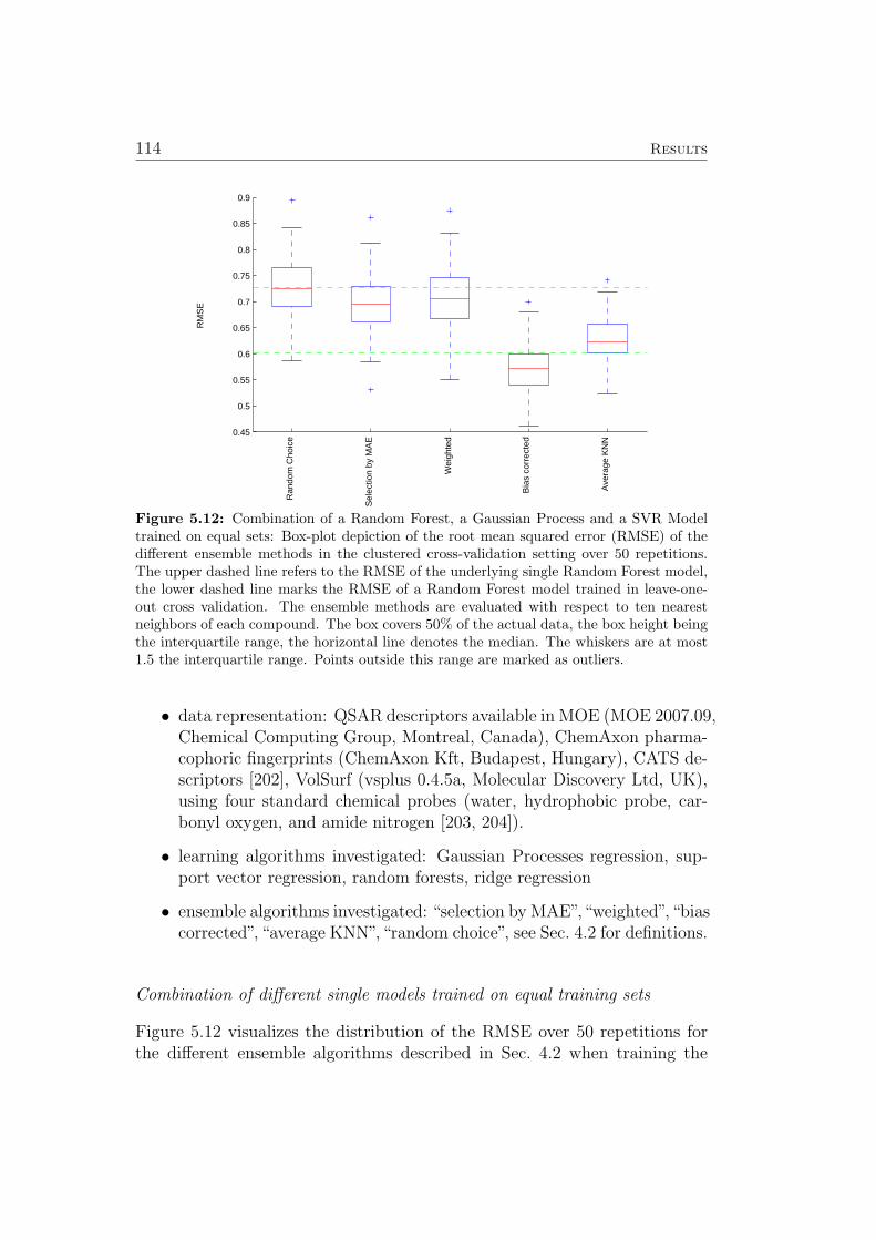
114 Results
0.45
0.5
0.55
0.6
0.65
0.7
0.75
0.8
0.85
0.9R
MS
E
Ran
dom
Cho
ice
Sel
ectio
n by
MA
E
Wei
ghte
d
Bia
s co
rrec
ted
Ave
rage
KN
N
Figure 5.12: Combination of a Random Forest, a Gaussian Process and a SVR Modeltrained on equal sets: Box-plot depiction of the root mean squared error (RMSE) of thedifferent ensemble methods in the clustered cross-validation setting over 50 repetitions.The upper dashed line refers to the RMSE of the underlying single Random Forest model,the lower dashed line marks the RMSE of a Random Forest model trained in leave-one-out cross validation. The ensemble methods are evaluated with respect to ten nearestneighbors of each compound. The box covers 50% of the actual data, the box height beingthe interquartile range, the horizontal line denotes the median. The whiskers are at most1.5 the interquartile range. Points outside this range are marked as outliers.
• data representation: QSAR descriptors available in MOE (MOE 2007.09,Chemical Computing Group, Montreal, Canada), ChemAxon pharma-cophoric fingerprints (ChemAxon Kft, Budapest, Hungary), CATS de-scriptors [202], VolSurf (vsplus 0.4.5a, Molecular Discovery Ltd, UK),using four standard chemical probes (water, hydrophobic probe, car-bonyl oxygen, and amide nitrogen [203, 204]).
• learning algorithms investigated: Gaussian Processes regression, sup-port vector regression, random forests, ridge regression
• ensemble algorithms investigated: “selection by MAE”,“weighted”,“biascorrected”, “average KNN”,“random choice”, see Sec. 4.2 for definitions.
Combination of different single models trained on equal training sets
Figure 5.12 visualizes the distribution of the RMSE over 50 repetitions forthe different ensemble algorithms described in Sec. 4.2 when training the
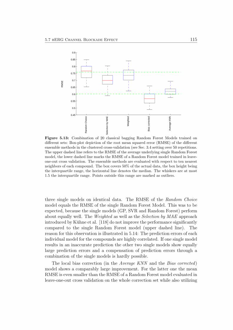
5.7 hERG Channel Blockade Effect 115
0.45
0.5
0.55
0.6
0.65
0.7
0.75
0.8
0.85
0.9
RM
SE
Ran
dom
Cho
ice
Sel
ectio
n by
MA
E
Wei
ghte
d
Bia
s co
rrec
ted
Ave
rage
KN
N
Figure 5.13: Combination of 20 classical bagging Random Forest Models trained ondifferent sets: Box-plot depiction of the root mean squared error (RMSE) of the differentensemble methods in the clustered cross-validation (see Sec. 3.4 setting over 50 repetitions.The upper dashed line refers to the RMSE of the average underlying single Random Forestmodel, the lower dashed line marks the RMSE of a Random Forest model trained in leave-one-out cross validation. The ensemble methods are evaluated with respect to ten nearestneighbors of each compound. The box covers 50% of the actual data, the box height beingthe interquartile range, the horizontal line denotes the median. The whiskers are at most1.5 the interquartile range. Points outside this range are marked as outliers.
three single models on identical data. The RMSE of the Random Choicemodel equals the RMSE of the single Random Forest Model. This was to beexpected, because the single models (GP, SVR and Random Forest) performabout equally well. The Weighted as well as the Selection by MAE approachintroduced by Kuhne et al. [118] do not improve the performance significantlycompared to the single Random Forest model (upper dashed line). Thereason for this observation is illustrated in 5.14: The prediction errors of eachindividual model for the compounds are highly correlated. If one single modelresults in an inaccurate prediction the other two single models show equallylarge prediction errors and a compensation of prediction errors through acombination of the single models is hardly possible.
The local bias correction (in the Average KNN and the Bias corrected)model shows a comparably large improvement. For the latter one the meanRMSE is even smaller than the RMSE of a Random Forest model evaluated inleave-one-out cross validation on the whole correction set while also utilizing
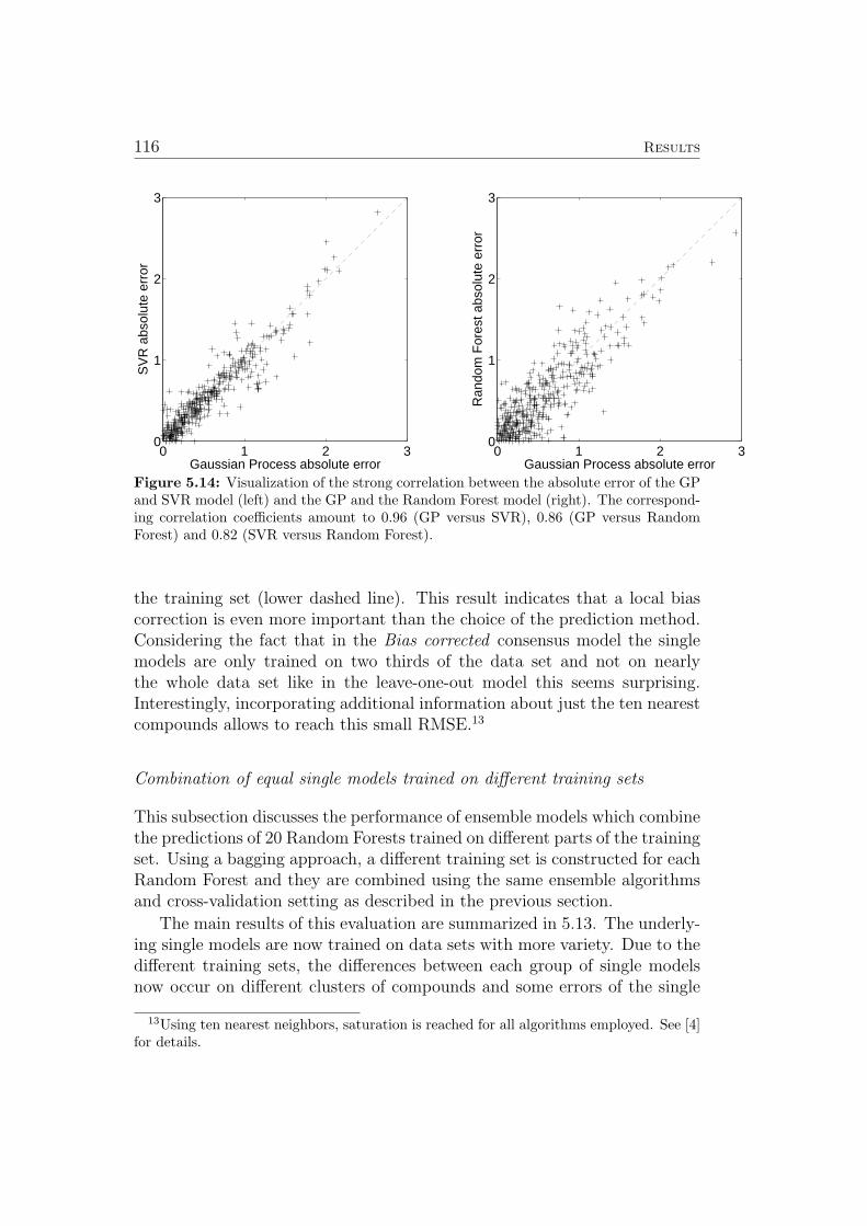
116 Results
0 1 2 30
1
2
3
Gaussian Process absolute error
SV
R a
bsol
ute
erro
r
0 1 2 30
1
2
3
Gaussian Process absolute errorR
ando
m F
ores
t abs
olut
e er
ror
Figure 5.14: Visualization of the strong correlation between the absolute error of the GPand SVR model (left) and the GP and the Random Forest model (right). The correspond-ing correlation coefficients amount to 0.96 (GP versus SVR), 0.86 (GP versus RandomForest) and 0.82 (SVR versus Random Forest).
the training set (lower dashed line). This result indicates that a local biascorrection is even more important than the choice of the prediction method.Considering the fact that in the Bias corrected consensus model the singlemodels are only trained on two thirds of the data set and not on nearlythe whole data set like in the leave-one-out model this seems surprising.Interestingly, incorporating additional information about just the ten nearestcompounds allows to reach this small RMSE.13
Combination of equal single models trained on different training sets
This subsection discusses the performance of ensemble models which combinethe predictions of 20 Random Forests trained on different parts of the trainingset. Using a bagging approach, a different training set is constructed for eachRandom Forest and they are combined using the same ensemble algorithmsand cross-validation setting as described in the previous section.
The main results of this evaluation are summarized in 5.13. The underly-ing single models are now trained on data sets with more variety. Due to thedifferent training sets, the differences between each group of single modelsnow occur on different clusters of compounds and some errors of the single
13Using ten nearest neighbors, saturation is reached for all algorithms employed. See [4]for details.
5.7 hERG Channel Blockade Effect 117
models can be compensated by choosing the best performing model includedin the ensemble model. However, the distribution of the RMSE shows simi-lar tendencies as in the previous setting: For the Random Choice model weobserve a worse performance than a single model (upper dashed line) andthe Weighted Model again only achieves a small improvement. In contrast tothe previous observation, the Selection by MAE Model introduced by Kuhneet al. [118] now achieves a somewhat larger improvement with respect to thesingle Model (RMSE reduced from 0.76 to 0.70). The Bias corrected Modelagain achieves the largest improvement of all ensemble methods (RMSE re-duced from 0.76 to 0.57).
In conclusion, local bias correction may be a good way to cope withthe strong locality of the hERG inhibition problem while still profiting fromglobal trends in the data. Furthermore the experiments indicate practicalhints for the use of machine learning models in drug design: When new mea-surements are added to an existing training set, a simple local bias correctioncan substitute retraining a whole SVR, Gaussian Process or Random Forestmodel on the expanded data set. Further investigation is necessary to evalu-ate in which cases the bias corrected approach is adequate and in which casesretraining should be preferred.

5.8 Local Gradients for Explaining & Guiding 119
5.8 Local Gradients for Explaining Individual ClassificationDecisions & Guiding compound optimization
Overview
In this thesis, two separate methodologies for explaining individual predic-tions of (possibly non-linear) machine learning models are presented. Themethod presented in Sec. 4.3 explains predictions by the means of visualiz-ing relevant objects from the training set of the model. This allows humanexperts to understand how each prediction comes about. If a prediction con-flicts with his intuition, the human expert can easily find out whether thegrounds for the models predictions are solid or if trusting his own intuitionis the better idea.
Sec. 4.4 proposes a method that sheds light into the black boxes of non-linear classifiers. In other words, it introduces a method that can explainthe local decisions taken by arbitrary (possibly) non-linear classification al-gorithms. In a nutshell, the estimated explanations are local gradients thatcharacterize how a data point has to be moved to change its predicted label.For models where such gradient information cannot be calculated explicitly,a probabilistic approximate mimic of the learning machine to be explainedis employed.
To validate the new gradient based methodology, [1] shows how it canbe used to draw new conclusions on how the various Iris flowers in Fisher’sfamous dataset are different from each other (section 4 in [1]) and how toidentify the features with which certain types of digits 2 and 8 in the USPSdataset can be distinguished (section 5 in [1]). In the following Subsection,the method is applied to a challenging drug discovery problem, namely theprediction of Ames mutagenicity (Sec. 5.6). Results fully agree with exist-ing domain knowledge, which was not available to the method. Even localpeculiarities in chemical space (the extraordinary behavior of steroids) wasdiscovered using the local explanations given by the new approach.
5.8.1 Explaining Mutagenicity Classification by Gaussian Processes
In the following section we describe an application of our local gradient ex-planation methodology to a complex real world data set. Our aim is tofind structure specific to the problem domain that has not been fed intotraining explicitly but is captured implicitly by the GPC model in the high-dimensional feature space used to determine its prediction. We investigatethe task of predicting Ames mutagenic activity of chemical compounds. Notbeing mutagenic (i.e. not able to cause mutations in the DNA) is an impor-
120 Results
tant requirement for compounds under investigation in drug discovery anddesign. The Ames test [179] is a standard experimental setup for measuringmutagenicity. The following experiments are based on a set of Ames testresults for 6512 chemical compounds that we published previously.14
GPC was applied as detailed in the following:
• Class 0 consists of non-mutagenic compounds
• Class 1 consists of mutagenic compounds
• Randomly split 6512 data points into 2000 training and 4512 test ex-amples such that:
– The training set consists of equally many class 0 and class 1 ex-amples.
– For the steroid compound class the balance in the train and testset is enforced.
• 10 additional random splits were investigated individually. This con-firmed the results presented below.
• Each example (chemical compound) is represented by a vector of countsof 143 molecular substructures calculated using the Dragon software[205].
• Normalize training and test set using the mean and variance of thetraining set.
• Apply GPC model with RBF kernel
• Performance (84 % area under curve) confirms our previous results [5].Error rates can be obtained from Figure 5.15.
Together with the prediction we calculated the explanation vector (as intro-duced in section 4.4.2 with Definition 4.2) for each test point. The remainderof this section is an evaluation of these local explanations.
In Figures 5.16 and 5.17 we show the distribution of the local importanceof selected features across the test set: For each input feature we generate ahistogram of local importance values, as indicated by its corresponding entryin the explanation vector of each of the 4512 test compounds. As a commonvisual reference, the normal distribution with a standard deviation of 0.02
14See [5] for results of modeling this set using different machine learning methods. Thedata itself is available online at http://ml.cs.tu-berlin.de/toxbenchmark
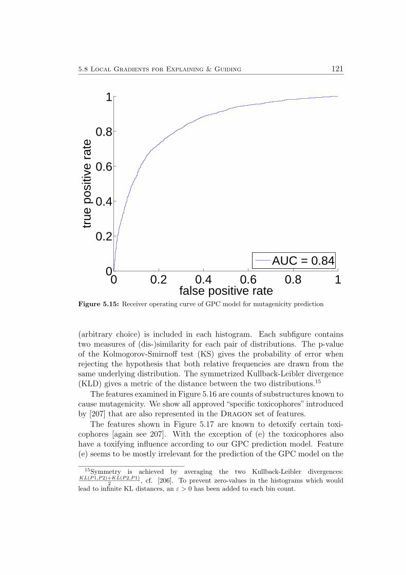
5.8 Local Gradients for Explaining & Guiding 121
0 0.2 0.4 0.6 0.8 10
0.2
0.4
0.6
0.8
1
false positive rate
true
pos
itive
rat
e
AUC = 0.84
Figure 5.15: Receiver operating curve of GPC model for mutagenicity prediction
(arbitrary choice) is included in each histogram. Each subfigure containstwo measures of (dis-)similarity for each pair of distributions. The p-valueof the Kolmogorov-Smirnoff test (KS) gives the probability of error whenrejecting the hypothesis that both relative frequencies are drawn from thesame underlying distribution. The symmetrized Kullback-Leibler divergence(KLD) gives a metric of the distance between the two distributions.15
The features examined in Figure 5.16 are counts of substructures known tocause mutagenicity. We show all approved “specific toxicophores” introducedby [207] that are also represented in the Dragon set of features.
The features shown in Figure 5.17 are known to detoxify certain toxi-cophores [again see 207]. With the exception of (e) the toxicophores alsohave a toxifying influence according to our GPC prediction model. Feature(e) seems to be mostly irrelevant for the prediction of the GPC model on the
15Symmetry is achieved by averaging the two Kullback-Leibler divergences:KL(P1,P2)+KL(P2,P1)
2 , cf. [206]. To prevent zero-values in the histograms which wouldlead to infinite KL distances, an ε > 0 has been added to each bin count.
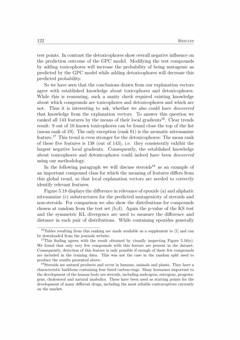
122 Results
test points. In contrast the detoxicophores show overall negative influence onthe prediction outcome of the GPC model. Modifying the test compoundsby adding toxicophores will increase the probability of being mutagenic aspredicted by the GPC model while adding detoxicophores will decrease thispredicted probability.
So we have seen that the conclusions drawn from our explanation vectorsagree with established knowledge about toxicophores and detoxicophores.While this is reassuring, such a sanity check required existing knowledgeabout which compounds are toxicophores and detoxicophores and which arenot. Thus it is interesting to ask, whether we also could have discoveredthat knowledge from the explanation vectors. To answer this question weranked all 143 features by the means of their local gradients16. Clear trendsresult: 9 out of 10 known toxicophores can be found close the top of the list(mean rank of 19). The only exception (rank 81) is the aromatic nitrosaminefeature.17 This trend is even stronger for the detoxicophores: The mean rankof these five features is 138 (out of 143), i.e. they consistently exhibit thelargest negative local gradients. Consequently, the established knowledgeabout toxicophores and detoxicophores could indeed have been discoveredusing our methodology.
In the following paragraph we will discuss steroids18 as an example ofan important compound class for which the meaning of features differs fromthis global trend, so that local explanation vectors are needed to correctlyidentify relevant features.
Figure 5.18 displays the difference in relevance of epoxide (a) and aliphaticnitrosamine (c) substructures for the predicted mutagenicity of steroids andnon-steroids. For comparison we also show the distributions for compoundschosen at random from the test set (b,d). Again the p-value of the KS testand the symmetric KL divergence are used to measure the difference anddistance in each pair of distributions. While containing epoxides generally
16Tables resulting from this ranking are made available as a supplement to [1] and canbe downloaded from the journals website.
17This finding agrees with the result obtained by visually inspecting Figure 5.16(e).We found that only very few compounds with this feature are present in the dataset.Consequently, detection of this feature is only possible if enough of these few compoundsare included in the training data. This was not the case in the random split used toproduce the results presented above.
18Steroids are natural products and occur in humans, animals and plants. They have acharacteristic backbone containing four fused carbon-rings. Many hormones important tothe development of the human body are steroids, including androgens, estrogens, progesta-gens, cholesterol and natural anabolics. These have been used as starting points for thedevelopment of many different drugs, including the most reliable contraceptives currentlyon the market.
5.8 Local Gradients for Explaining & Guiding 123
tends to make molecules mutagenic (see above), we do not observe this effectfor steroids. “Immunity” of steroids to the epoxide toxicophore is an estab-lished fact and has first been discussed by [208]. This peculiarity in chemicalspace is clearly exhibited by the local explanation given by our approach.For aliphatic nitrosamine, the situation in the GPC model is less clear butstill the toxifying influence seems to be less in steroids than in many othercompounds. To our knowledge, this phenomenon has not yet been discussedin the pharmaceutical literature.
In conclusion, we can learn from the explanation vectors that:
• toxicophores tend to make compounds mutagenic (class 1)
• detoxicophores tend to make compounds non-mutagenic (class 0)
• steroids are immune to the presence of some toxicophores (epoxide,aliphatic nitrosamine)
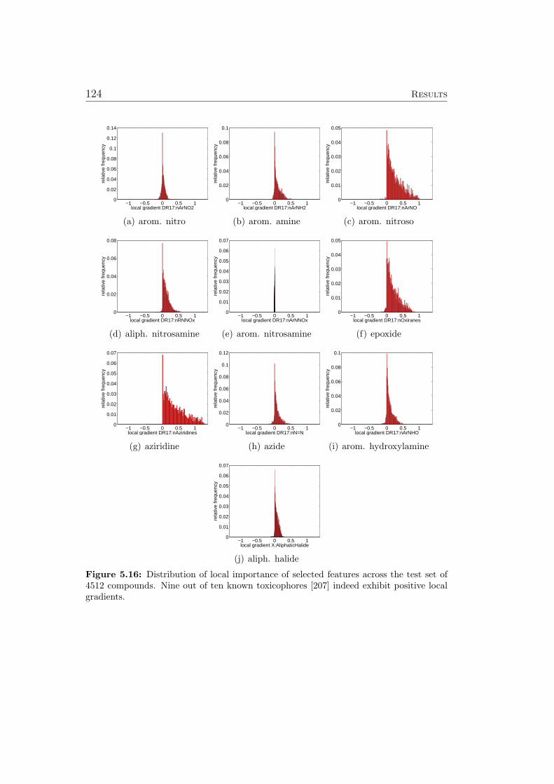
124 Results
−1 −0.5 0 0.5 10
0.02
0.04
0.06
0.08
0.1
0.12
0.14
local gradient DR17:nArNO2
rela
tive
freq
uenc
y
(a) arom. nitro
−1 −0.5 0 0.5 10
0.02
0.04
0.06
0.08
0.1
local gradient DR17:nArNH2re
lativ
e fr
eque
ncy
(b) arom. amine
−1 −0.5 0 0.5 10
0.01
0.02
0.03
0.04
0.05
local gradient DR17:nArNO
rela
tive
freq
uenc
y
(c) arom. nitroso
−1 −0.5 0 0.5 10
0.02
0.04
0.06
0.08
local gradient DR17:nRNNOx
rela
tive
freq
uenc
y
(d) aliph. nitrosamine
−1 −0.5 0 0.5 10
0.01
0.02
0.03
0.04
0.05
0.06
0.07
local gradient DR17:nArNNOx
rela
tive
freq
uenc
y
(e) arom. nitrosamine
−1 −0.5 0 0.5 10
0.01
0.02
0.03
0.04
0.05
local gradient DR17:nOxiranesre
lativ
e fr
eque
ncy
(f) epoxide
−1 −0.5 0 0.5 10
0.01
0.02
0.03
0.04
0.05
0.06
0.07
local gradient DR17:nAziridines
rela
tive
freq
uenc
y
(g) aziridine
−1 −0.5 0 0.5 10
0.02
0.04
0.06
0.08
0.1
0.12
local gradient DR17:nN=N
rela
tive
freq
uenc
y
(h) azide
−1 −0.5 0 0.5 10
0.02
0.04
0.06
0.08
0.1
local gradient DR17:nArNHO
rela
tive
freq
uenc
y
(i) arom. hydroxylamine
−1 −0.5 0 0.5 10
0.01
0.02
0.03
0.04
0.05
0.06
0.07
local gradient X:AliphaticHalide
rela
tive
freq
uenc
y
(j) aliph. halide
Figure 5.16: Distribution of local importance of selected features across the test set of4512 compounds. Nine out of ten known toxicophores [207] indeed exhibit positive localgradients.
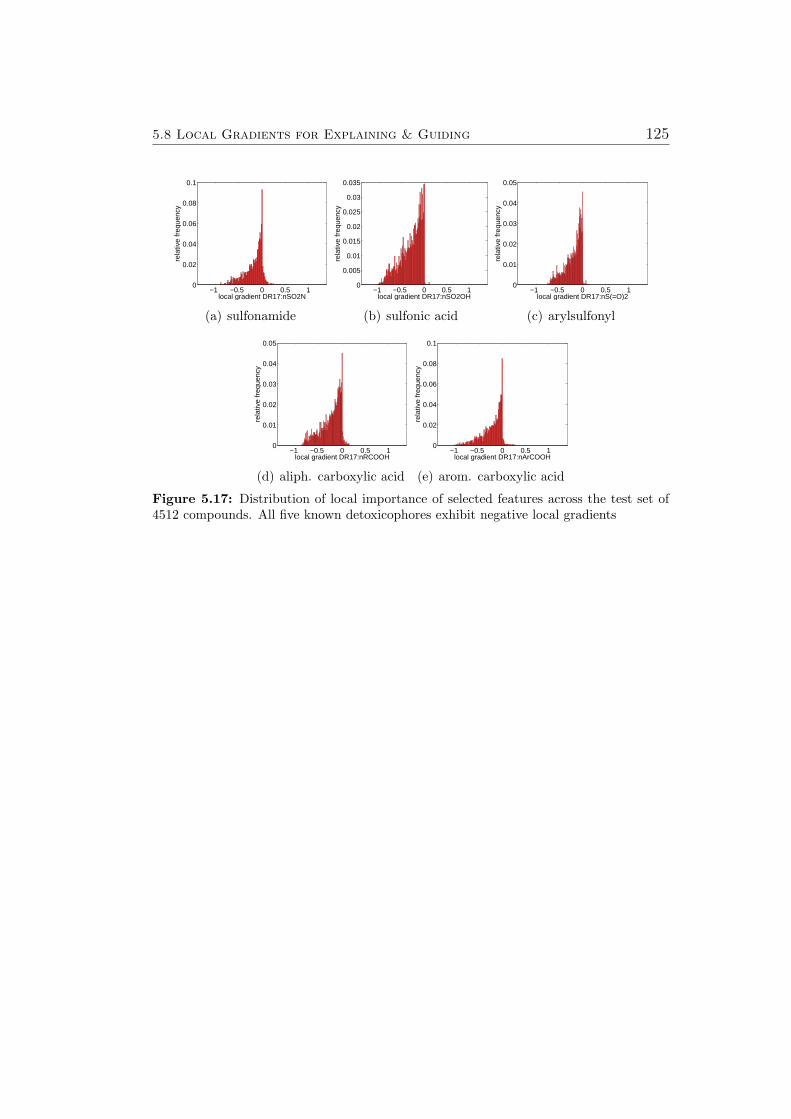
5.8 Local Gradients for Explaining & Guiding 125
−1 −0.5 0 0.5 10
0.02
0.04
0.06
0.08
0.1
local gradient DR17:nSO2N
rela
tive
freq
uenc
y
(a) sulfonamide
−1 −0.5 0 0.5 10
0.005
0.01
0.015
0.02
0.025
0.03
0.035
local gradient DR17:nSO2OH
rela
tive
freq
uenc
y
(b) sulfonic acid
−1 −0.5 0 0.5 10
0.01
0.02
0.03
0.04
0.05
local gradient DR17:nS(=O)2
rela
tive
freq
uenc
y
(c) arylsulfonyl
−1 −0.5 0 0.5 10
0.01
0.02
0.03
0.04
0.05
local gradient DR17:nRCOOH
rela
tive
freq
uenc
y
(d) aliph. carboxylic acid
−1 −0.5 0 0.5 10
0.02
0.04
0.06
0.08
0.1
local gradient DR17:nArCOOH
rela
tive
freq
uenc
y
(e) arom. carboxylic acid
Figure 5.17: Distribution of local importance of selected features across the test set of4512 compounds. All five known detoxicophores exhibit negative local gradients
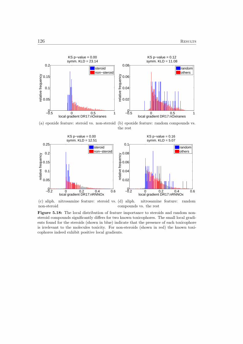
126 Results
−0.5 0 0.5 10
0.05
0.1
0.15
0.2
KS p−value = 0.00symm. KLD = 23.14
local gradient DR17:nOxiranes
rela
tive
freq
uenc
y
steroidnon−steroid
(a) epoxide feature: steroid vs. non-steroid
−0.5 0 0.5 10
0.02
0.04
0.06
0.08
KS p−value = 0.12symm. KLD = 11.08
local gradient DR17:nOxiranesre
lativ
e fr
eque
ncy
randomothers
(b) epoxide feature: random compounds vs.the rest
−0.2 0 0.2 0.4 0.60
0.05
0.1
0.15
0.2
0.25
KS p−value = 0.00symm. KLD = 12.51
local gradient DR17:nRNNOx
rela
tive
freq
uenc
y
steroidnon−steroid
(c) aliph. nitrosamine feature: steroid vs.non-steroid
−0.2 0 0.2 0.4 0.60
0.02
0.04
0.06
0.08
0.1
KS p−value = 0.16symm. KLD = 5.07
local gradient DR17:nRNNOx
rela
tive
freq
uenc
y
randomothers
(d) aliph. nitrosamine feature: randomcompounds vs. the rest
Figure 5.18: The local distribution of feature importance to steroids and random non-steroid compounds significantly differs for two known toxicophores. The small local gradi-ents found for the steroids (shown in blue) indicate that the presence of each toxicophoreis irrelevant to the molecules toxicity. For non-steroids (shown in red) the known toxi-cophores indeed exhibit positive local gradients.
5.9 Virtual Screening for PPAR-gamma Agonists 127
5.9 Virtual Screening for PPARγ Agonists
The peroxisome-proliferator activated receptor family (PPAR) are nuclear re-ceptors acting as transcription factors. They are involved in lipid metabolismand inflammatory response regulation and act as corresponding drug targets.The following section describes how predictive models for PPARγ were con-structed in collaboration with researchers at the University of Frankfurt.It discusses how the training data was used in a clustered cross-validationscheme to evaluate the generalization capability of different combinationsof data representations and learning algorithms. The last two paragraphspresent how the best performing models were applied in screening two largevendor libraries: New PPARγ agonists were discovered, including a PPARγselective compound with a new scaffold. This new compound is especiallyinteresting, because it is almost identical to a natural product in plants thatexhibit anti-diabetic and anti-inflammatory effects. The newly discoveredPPARγ agonist represents a first hint to the cause of these effects. A moredetailed discussion of the results of this virtual screening study can be foundin [3].
From a machine learning perspective, the modeling task can be summa-rized as follows:
• ranking based on real valued labels, implemented as follows:
– supervised regression task
– ranking of unlabeled library by predicted target value & confidence
– experimental investigation of 16 compounds from hitlist
• training data: 144 compounds with real valued labels (binding affinityexpressed as pKi) [209], “leave 50 % of all clusters out” cross-validation
• unlabeled screening library: 360 · 103 compounds from the Asinex[210]Gold and Platinum libraries19
• data representation: molecular graphs, CATS2D[211] topological phar-macophore descriptor (210-dimensional autocorrelation vector), MOE[212]2D descriptors (184 diverse 2d descriptors), Ghose-Crippen fragmentdescriptors[164, 213, 214] (109 substructure counts)
• learning algorithms investigated: Gaussian Processes, support vectormachines, ridge regression
19Asinex[210] Gold (233 · 103 compounds) and Platinum (129 · 103 compounds) librarieswere combined, resulting in 360·103 compounds after removal of duplicates and compoundsnot processable by intermediate other software.
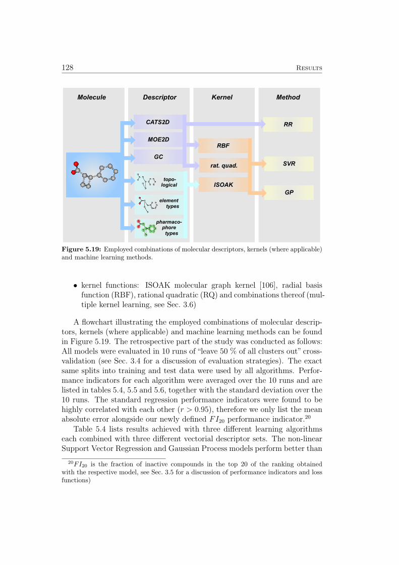
128 Results
MOE2D
CATS2D
GC
Descriptor
RBF
ISOAK
rat. quad.
Kernel MethodMolecule
SVR
GP
RR
topo-logical
elementtypes
pharmaco-phore
types
Figure 5.19: Employed combinations of molecular descriptors, kernels (where applicable)and machine learning methods.
• kernel functions: ISOAK molecular graph kernel [106], radial basisfunction (RBF), rational quadratic (RQ) and combinations thereof (mul-tiple kernel learning, see Sec. 3.6)
A flowchart illustrating the employed combinations of molecular descrip-tors, kernels (where applicable) and machine learning methods can be foundin Figure 5.19. The retrospective part of the study was conducted as follows:All models were evaluated in 10 runs of “leave 50 % of all clusters out” cross-validation (see Sec. 3.4 for a discussion of evaluation strategies). The exactsame splits into training and test data were used by all algorithms. Perfor-mance indicators for each algorithm were averaged over the 10 runs and arelisted in tables 5.4, 5.5 and 5.6, together with the standard deviation over the10 runs. The standard regression performance indicators were found to behighly correlated with each other (r > 0.95), therefore we only list the meanabsolute error alongside our newly defined FI20 performance indicator.20
Table 5.4 lists results achieved with three different learning algorithmseach combined with three different vectorial descriptor sets. The non-linearSupport Vector Regression and Gaussian Process models perform better than
20FI20 is the fraction of inactive compounds in the top 20 of the ranking obtainedwith the respective model, see Sec. 3.5 for a discussion of performance indicators and lossfunctions)
5.9 Virtual Screening for PPAR-gamma Agonists 129
Learning Algorithm Descriptors MAE FI20
SVR rbf ACATS 0.68 ± 0.06 0.33 ± 0.08GC 0.86 ± 0.12 0.41 ± 0.09
MOE 0.69 ± 0.08 0.29 ± 0.14Linear RR ACATS 1.7 ± 0.14 0.80 ± 0.08
GC 1.7 ± 0.08 0.79 ± 0.04MOE 1.45 ± 0.04 0.78 ± 0.05
GP RBF & RQ ACATS 0.66 ± 0.09 0.27 ± 0.14GC 0.86 ± 0.07 0.33 ± 0.12
MOE 0.76 ± 0.06 0.25 ± 0.12Table 5.4: For Support Vector Regression, Linear Ridge Regression and Gaussian Processregression based on ACATS, Ghose Crippen & MOE2D descriptors we list the MeanAbsolute Error and the Fraction of Inactives in the top 20
Learning Algorithm Node & Edge MAE FI20
GP ISOAK none 0.68 ± 0.06 0.33 ± 0.15GP ISOAK Type 0.74 ± 0.06 0.32 ± 0.14GP ISOAK PPP 0.70 ± 0.06 0.38 ± 0.09
Table 5.5: Using atom & bond types (Type) or pharmacophore points (PPP) in additionto the plain graph structure does not improve the performance of ISOAK based GaussianProcess models. See Table 5.4 for abbreviations.
the linear Ridge Regression, indicating that the relationship between activityand the chosen descriptors is indeed non-linear. Non-linear models with thericher MOE2D and ACATS descriptor sets outperform models based on therather simple Ghose Crippen fragment descriptors.
Table 5.5 lists performance indicators obtained when applying variants ofthe ISOAK graph kernel. Interestingly, comparing molecules based on thegraph structure alone results in more accurate predictions than comparingmolecules based on both their graph structure and either atom & bond typesor pharmacophore points.
Learning Algorithm & Descriptors MAE FI20
GP ISOAK, 1 RBF, 1 RQ 0,67 ± 0,08 0,31 ± 0,14GP ISOAK, 1 RBF, 1 RQ, adj. var. 0,66 ± 0,07 0,32 ± 0,15GP ISOAK, 3 RBF, 3 RQ 0,70 ± 0,11 0,21 ± 0,09GP ISOAK, 3 RBF, 3 RQ, adj. var. 0,71 ± 0,12 0,26 ± 0,12
Table 5.6: The Gaussian Process Models based on both ISOAK graph kernels and RBF& RQ kernels with vectorial descriptors yield the lowest MAE and FI20 values observedso far. See Table 5.4 for abbreviations.
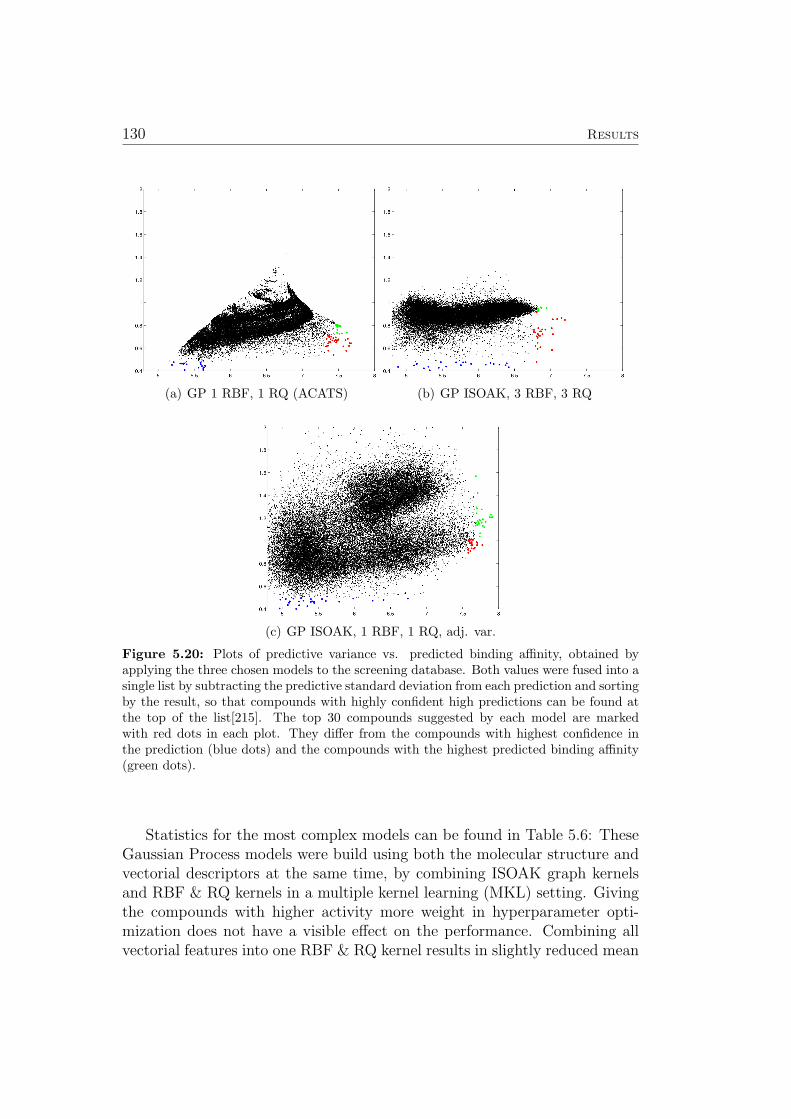
130 Results
(a) GP 1 RBF, 1 RQ (ACATS) (b) GP ISOAK, 3 RBF, 3 RQ
(c) GP ISOAK, 1 RBF, 1 RQ, adj. var.
Figure 5.20: Plots of predictive variance vs. predicted binding affinity, obtained byapplying the three chosen models to the screening database. Both values were fused into asingle list by subtracting the predictive standard deviation from each prediction and sortingby the result, so that compounds with highly confident high predictions can be found atthe top of the list[215]. The top 30 compounds suggested by each model are markedwith red dots in each plot. They differ from the compounds with highest confidence inthe prediction (blue dots) and the compounds with the highest predicted binding affinity(green dots).
Statistics for the most complex models can be found in Table 5.6: TheseGaussian Process models were build using both the molecular structure andvectorial descriptors at the same time, by combining ISOAK graph kernelsand RBF & RQ kernels in a multiple kernel learning (MKL) setting. Givingthe compounds with higher activity more weight in hyperparameter opti-mization does not have a visible effect on the performance. Combining allvectorial features into one RBF & RQ kernel results in slightly reduced mean

5.9 Virtual Screening for PPAR-gamma Agonists 131
absolute errors. However, using individual RBF & RQ kernels for the threeindividual vectorial descriptor sets we obtained the lowest values for the FI20
performance indicator. When grouping models based on their performance,three groups can be identified:
• All linear models were found to be very inaccurate (MAE > 1.45, FI20
> 0.78).
• Both non-linear models based on GC descriptors reach the same MAEof 0.86 ± 0.10. The SVR model exhibits an FI20 of 0.41 ±0.09. Incor-porating the confidence estimates of the Gaussian process model resultsin a slightly reduced FI20 of 0.33 ±0.12, despite equal regression per-formance.
• Non-linear models based on the vectorial MOE or ACATS descriptors,molecular structures or combinations thereof all achieve mean MAEsbetween 0.66 and 0.74. All eleven models reach FI20 below 0.40. Fivemodels even reach FI20 between 0.2 and 0.3.
While the differences between the groups are large, differences within the bestperforming group are as small as the standard deviations across the ten runs.Instead of choosing a single final model for the prospective evaluation basedon these results alone, we first chose a group of three very well performingmodels with different characteristics:
• The GP model with an ISOAK graph kernel and 3 individual RBF& RQ kernels for each respective vectorial descriptor set was chosenbecause it exhibits the lowest FI20 score (0.21 ±0.09) observed in allexperiments, combined with a rather low MAE of 0.70 ±0.11. At thesame time it includes all available information about each compound.
• A GP model with an ISOAK graph kernel and one single RBF & RQkernel for all vectorial descriptor sets taken together was chosen becauseit exhibits the lowest MAE (0.66 ±0.07) observed in all experiments,combined with a reasonable FI20 score of 0.32 ±0.15. It also includesall available information about each compound and gives the activecompounds higher weight in the parameter optimization.
• From the pool of still well performing but less complex models wechose the GP model employing just one RBF & RQ kernel on a singlevectorial descriptor set (ACATS), achieving MAE 0.66 ±0.09 and FI20
0.27 ±0.14.
132 Results
The ASINEX database was then ranked with each of the three modelslisted above. The predictive standard deviation was subtracted from eachprediction, so that compounds with highly confident high predictions canbe found at the top of the list [215]. The top 30 compounds are markedwith red dots in the confidence vs. target value plots for each model inFigure 5.20. From these three lists, 16 compounds were selected by a panelof human experts and experimentally tested, resulting in 8 novel PPARα andPPARγ agonists with EC50 values as low as 9 µmol. Interestingly, 10 out of16 cherrypicked compounds were suggested by this model: “GP with ISOAKand 3 RBF and RQ kernels on the vectorial descriptors” (chosen for best FI20
score), and all 8 compounds exhibiting activity stem from this list.The most potent compound is a known natural product in plants: Ber-
muda grass (cynodon dactylon) is known to be anti-inflammatory, for whichthe PPARγ activity of our compound provides a first possible explanation.A detailed discussion of this finding can be found in [3].
Chapter 6
Conclusion
This thesis presents a collection of seven studies about constructing predictivemodels for application in drug discovery & drug design. Gaussian Processmodels were introduced into the field of chemoinformatics and for the firsttime, individual confidence estimates are provided based on a solid theoreticalfoundation. Furthermore, new algorithms were developed to cope with thespecific requirements of lead optimization, the most challenging part of thedrug discovery process. The first new algorithm can improve the accuracyof models in the early stages of lead optimization projects. The second newalgorithm can explain individual predictions made by complex models tohuman experts and the third new algorithm generates hints for compoundoptimization. Models developed in the above mentioned studies have beendeployed for use by human experts in pharmaceutical companies. A virtualscreening study has not only led to new agonists of PPARγ, but also helpedto understand the anti-diabetic and anti-inflammatory effects of bermudagrass (cynodon dactylon).
From the point of view of machine learning, chemoinformatics is a verychallenging field of endeavor:
Learning algorithms are always based on some representation of objects(in this case: molecules). Molecules are dynamical three dimensional ob-jects, exhibiting many different types of flexibility. Available representationsof molecules for machine learning either completely ignore this fact by consid-ering only features derived from the two dimensional graph of the molecule,or they consider a small arbitrarily chosen number of 3D structures that mayor may not be relevant for the task at hand. Consequently, the accuracy thatcan be achieved by machine learning models based on these representationsis limited.
Machine learning algorithms rely on the assumption that training dataand future test data are sampled ideally identically distributed (i.i.d.) fromthe same underlying probability density, and further assume that the theconditional distribution of labels (measurements) given the input features(descriptors) is the same in both training and test data. Lastly, it is generallyassumed that similar molecules exhibit similar activity.
133
134 Conclusion
In the machine learning community, violation of the first assumption iscalled covariate shift or dataset shift. In the lead optimization applicationscenario, one question that regularly arises is how to best use the first newmeasurements for compounds belonging to a newly explored compound class,i.e. a new part of the chemical space. New different model selection and biascorrection algorithms based on utilizing the labels of the nearest neighborsin the recently measured set of compounds are introduced. An evaluationof these algorithms in the context of the hERG Channel Blockade effectreveals that a locally performed bias correction significantly improves models.Interestingly, previously trained random forests profit so strongly from thebias correction, that they even outperform k-nearest-neighbor models trainedin leave-one-out cross validation on all training and test data simultaneously.
Four out of seven modeling studies conducted in this thesis deal withproperties that have multiple underlying mechanisms that are relevant indifferent parts of the chemical space. These properties are Metabolic Stabil-ity, Aqueous Solubility, Cytochrome P450 Inhibition and Ames Mutagenicity.Training data are typically scarce (e.g. several hundred training compoundsdescribed by about equally many descriptor dimensions (features)). In newprojects, new compound classes are explored, i.e. test data are sampled froma different part of the chemical space than the training data. Because ofthe different underlying mechanisms, this leads to simultaneously violatingboth the assumption of i.i.d. sampling and the assumption of equal con-ditionals. Furthermore, all properties concerned with molecular recognitioncan exhibit sudden extreme changes (activity cliffs). This necessitates com-plex non-linear models and makes generalizing difficult. The six out of sevenstudies conducted in this thesis where activity cliffs need to be consideredare: Metabolic Stability, Cytochrome P450 Inhibition, Ames Mutagenicity,Aqueous Solubility, PPARγ binding and the hERG Channel Blockade Effect.
As indicated in the last paragraph, one has to expect that many predic-tions for test compounds may be incorrect. It is therefore very desirable toobtain some kind of confidence estimate that allows to identify compoundsfor which reliable predictions can be made. To this end, Gaussian Process(GP) models have been introduced into the field of chemoinformatics. Theirpredictive variances can directly serve as individual confidence estimates.The practical usefulness of predictive variances is investigated in detail formodels predicting Partition Coefficients, Aqueous Solubility and MetabolicStability. In each case it is shown that focussing on confidently predictedcompounds indeed significantly increases the accuracy of predictions. In avirtual screening for compounds binding to the PPARγ receptor, predictivevariances of GPs were considered to select compounds with high values ofpredicted binding affinity that are, at the same time, deemed to be very
135
reliable. And indeed, new potent agonists of PPARγ were identified.In addition to the above mentioned fundamental aspects that make chemo-
informatics challenging from the point of view of machine learning, thereare many more points to be considered when not only treating well curatedbenchmark datasets, but really starting the process of model building fromraw datasets that have just been exported out of corporate databases orgathered from (many) separate publications. Systematical measurement er-rors, heteroschedastic noise, compounds with outlying labels or features oreven missing values in some features necessitate carefully performing variouspre-processing steps before training machine learning models. Since differ-ent raw sets of data can vary tremendously, the process of pre-processingis not easily formalized. The first three sections of this thesis describe in-sights gained when transforming raw data into well-behaved training datafor machine learning models.
Two separate algorithms for explaining individual predictions of (possiblynon-linear) machine learning models are presented. The first method explainspredictions by the means of visualizing relevant objects from the training setof the model. This allows human experts to understand how each predic-tion comes about. If a prediction conflicts with his intuition, the humanexpert can easily find out whether the grounds for the models predictionsare solid or if trusting his own intuition is the better idea. Theoretically, abrute force algorithm can be applied to gather this information about any re-trainable model, regardless of the underlying learning algorithm. As shownin this thesis, a much more elegant solution exists for kernel based learningmethods. When the representer theorem can be applied (i.e. in the caseof support vector machines for classification (SVM) and regression (SVR),Gaussian Processes for classification (GPC) and regression (GPR) and ker-nel ridge regression (KRR)) one can calculate the normalized contribution ofeach training data point analytically, and identify the most important pointsto visualize. These are called explanations. GPC models trained using stan-dard procedures were found to tend to rely on more training compounds thanone can use for producing an intuitively understandable visualization. By re-ducing the width-parameter of radial basis function kernels, it is possible toobtain models where predictions for test compounds are almost completelydetermined by very few training compounds, so that intuitively understand-able visualizations can indeed be produced. Furthermore, these explanationswere found to be convincing from a chemists point of view.
In a somewhat similar spirit, a second method utilizes local gradients ofthe model’s predictions to explain predictions in terms of the locally mostrelevant features. This not only teaches the human expert which featuresare relevant for each individual prediction, but also gives a directional infor-
136 Conclusion
mation. Abstractly speaking, one can learn in which direction a data pointhas to be moved to increase the prediction for the label (measurement). Inthe context of lead optimization, this means that the human expert can ob-tain hints for compound optimization. An estimation framework allows toobtain local gradients from any type of model, including k-nearest neighborclassifiers, support vector machines, decision trees or neural networks. How-ever, in case of Gaussian Process models, local gradients can be calculatedanalytically. The new gradient based methodology was validated using twobenchmark sets of data that are well known in the machine learning com-munity (IRIS flowers and USPS digits) and was then applied to GaussianProcess Classification models for Ames mutagenicity. The new approachcorrectly identified toxicophores and detoxicophores. Furthermore, even lo-cal peculiarities in chemical space (the extraordinary behavior of steroids)was discovered based on the local gradients of the predictions.
Future Directions
Today, machine learning based models are firmly established in the earlystages of the drug discovery process, i.e. in library design. In these earlystages, large numbers of compounds are ranked or filtered with respect todifferent properties and any model that can make predictions that are signif-icantly better than random choice has the chance to exert a positive effect,even if the effect is not very large. In later stages of the drug discoveryprocess, more specifically in the lead optimization phase, requirements aremuch higher: Human experts (often bench chemists) regularly decide whichsmall batch of molecules to synthesize and investigate next. They tend tobe very sceptical towards model predictions unless they understand exactlyhow each prediction is generated. This behavior also makes sense, becauseit is the researchers themselves who have to make the decision and bear theresponsibility. Algorithms capable of explaining predictions will be the key toreaching the goal of much increased acceptance of models. Once models areaccepted by the relevant decision makers in lead optimization, technologiesfor guiding compound optimization have the chance to become valuable.
While the lead optimization scenario served as the original motivationand testbed for developing algorithms for explaining individual predictions,both new methods can be applied to a wide range of modeling tasks. Wher-ever human experts are to be supported in making decisions, explanations ofpredictions will be valuable. Therefore, future research will strive for devel-oping and refining algorithms for explaining predictions by machine learningmodels and demonstrating their practical usefulness.
Appendix A
Misc
A.1 Challenging Aspects of Machine Learning in DrugDiscovery
A.1.1 Molecular Representations
The by far most critical aspect to consider when modeling the propertiesof chemical compounds is the fact that state of the art representations ofmolecules are seriously flawed. Chemical compounds are commonly charac-terized by the 2D structure (graph) of their molecules. As an example, the2D-structure and a ball and stick model of acetylsalicylic acid (also known asAspirin) can be found in Figure A.1. This representation has been developedfor use by human experts and is very useful in tasks like developing synthesispaths, because 2D structures can easily be drawn by hand and printed inbooks and they can be used to express chemical reactions or whole seriesof reactions that one can learn to read, write, memorize and apply in thelaboratory. In the 2D-structure Figure A.1(a), each type of edge indicatesa different type of chemical bond: A single line symbolizes a single bond,two parallel lines indicate a double bond and the circle drawn inside the sixmembered ring indicates aromatic bonds. Note how the ensemble of atomssymbolized in the right hand side of subfigure (a) appears in a different posi-tion in subfigure (b). The position of this group of atoms (the acetyl group)with respect to the remaining part of the molecule is arbitrary, because itis connected through a single bond, and single bonds rotate freely. Further-more, bonds can vibrate in different ways, including stretching and bending.When dissolved in water, the acid group depicted in the top left hand cornerof Figure A.1(a) can dissociate its proton (H+ Ion) and later associate withany proton nearby. In more complex molecules, more complex issues arise:Protons can bind to different functional groups within the same molecule,resulting in shift of the positions of alternatingly placed double and singlebonds. This often observed phenomenon is called tautomerism. In summary,molecules can be flexible both in a physical sense (rotation and vibration)and a chemical sense (dissociation & association of protons, tautomerism).
As a result of this flexibility, molecules adopt many different states when
137
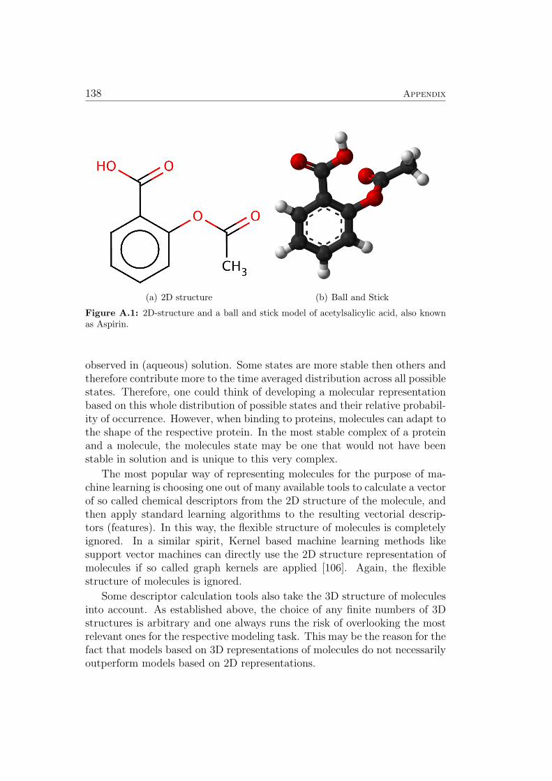
138 Appendix
(a) 2D structure (b) Ball and Stick
Figure A.1: 2D-structure and a ball and stick model of acetylsalicylic acid, also knownas Aspirin.
observed in (aqueous) solution. Some states are more stable then others andtherefore contribute more to the time averaged distribution across all possiblestates. Therefore, one could think of developing a molecular representationbased on this whole distribution of possible states and their relative probabil-ity of occurrence. However, when binding to proteins, molecules can adapt tothe shape of the respective protein. In the most stable complex of a proteinand a molecule, the molecules state may be one that would not have beenstable in solution and is unique to this very complex.
The most popular way of representing molecules for the purpose of ma-chine learning is choosing one out of many available tools to calculate a vectorof so called chemical descriptors from the 2D structure of the molecule, andthen apply standard learning algorithms to the resulting vectorial descrip-tors (features). In this way, the flexible structure of molecules is completelyignored. In a similar spirit, Kernel based machine learning methods likesupport vector machines can directly use the 2D structure representation ofmolecules if so called graph kernels are applied [106]. Again, the flexiblestructure of molecules is ignored.
Some descriptor calculation tools also take the 3D structure of moleculesinto account. As established above, the choice of any finite numbers of 3Dstructures is arbitrary and one always runs the risk of overlooking the mostrelevant ones for the respective modeling task. This may be the reason for thefact that models based on 3D representations of molecules do not necessarilyoutperform models based on 2D representations.
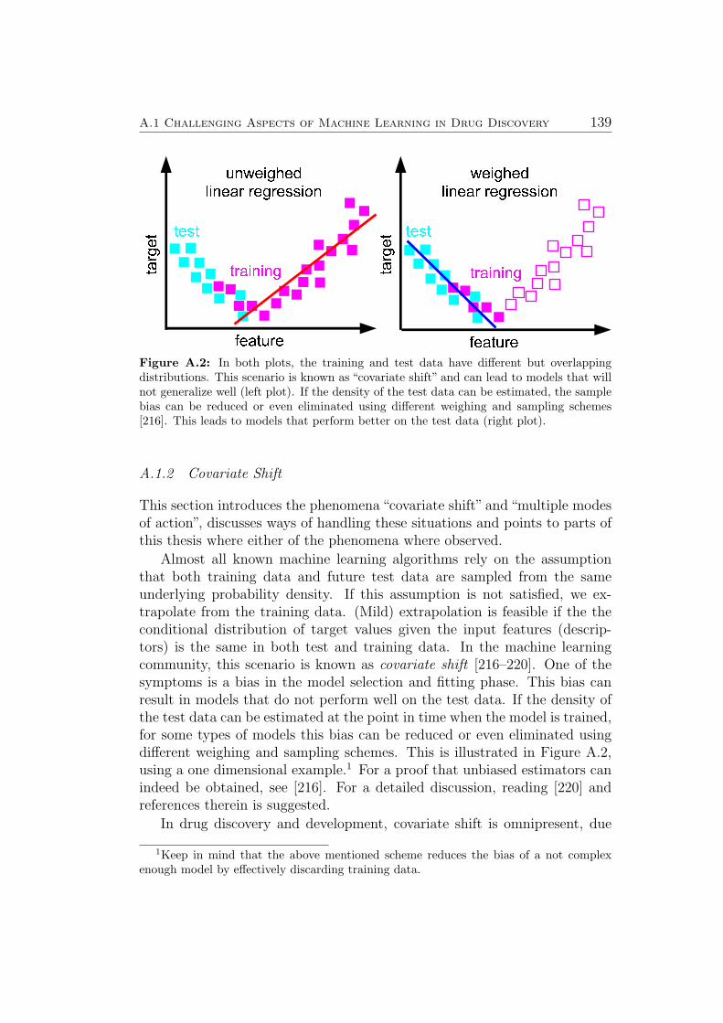
A.1 Challenging Aspects of Machine Learning in Drug Discovery 139
Figure A.2: In both plots, the training and test data have different but overlappingdistributions. This scenario is known as “covariate shift” and can lead to models that willnot generalize well (left plot). If the density of the test data can be estimated, the samplebias can be reduced or even eliminated using different weighing and sampling schemes[216]. This leads to models that perform better on the test data (right plot).
A.1.2 Covariate Shift
This section introduces the phenomena “covariate shift” and “multiple modesof action”, discusses ways of handling these situations and points to parts ofthis thesis where either of the phenomena where observed.
Almost all known machine learning algorithms rely on the assumptionthat both training data and future test data are sampled from the sameunderlying probability density. If this assumption is not satisfied, we ex-trapolate from the training data. (Mild) extrapolation is feasible if the theconditional distribution of target values given the input features (descrip-tors) is the same in both test and training data. In the machine learningcommunity, this scenario is known as covariate shift [216–220]. One of thesymptoms is a bias in the model selection and fitting phase. This bias canresult in models that do not perform well on the test data. If the density ofthe test data can be estimated at the point in time when the model is trained,for some types of models this bias can be reduced or even eliminated usingdifferent weighing and sampling schemes. This is illustrated in Figure A.2,using a one dimensional example.1 For a proof that unbiased estimators canindeed be obtained, see [216]. For a detailed discussion, reading [220] andreferences therein is suggested.
In drug discovery and development, covariate shift is omnipresent, due
1Keep in mind that the above mentioned scheme reduces the bias of a not complexenough model by effectively discarding training data.
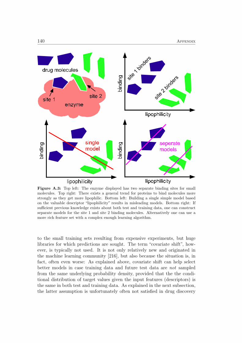
140 Appendix
Figure A.3: Top left: The enzyme displayed has two separate binding sites for smallmolecules. Top right: There exists a general trend for proteins to bind molecules morestrongly as they get more lipophilic. Bottom left: Building a single simple model basedon the valuable descriptor “lipophilicity” results in misleading models. Bottom right: Ifsufficient previous knowledge exists about both test and training data, one can constructseparate models for the site 1 and site 2 binding molecules. Alternatively one can use amore rich feature set with a complex enough learning algorithm.
to the small training sets resulting from expensive experiments, but hugelibraries for which predictions are sought. The term “covariate shift”, how-ever, is typically not used. It is not only relatively new and originated inthe machine learning community [216], but also because the situation is, infact, often even worse: As explained above, covariate shift can help selectbetter models in case training data and future test data are not sampledfrom the same underlying probability density, provided that the the condi-tional distribution of target values given the input features (descriptors) isthe same in both test and training data. As explained in the next subsection,the latter assumption is unfortunately often not satisfied in drug discovery
A.1 Challenging Aspects of Machine Learning in Drug Discovery 141
applications.
A.1.3 Multiple Mechanisms
Figure A.3 illustrates this fact for the problem of protein binding. In thiscase, the protein under consideration is an enzyme, to which small molecules(including drugs) can bind. Our enzyme has two geometrically quite differentactive sites. Therefore, quite different molecules will bind to these differentsites (Figure A.3, top left). Proteins are, generally speaking, quite lipophilic.Consequently, the more lipophilic a molecule, the stronger it binds to a givenprotein. In Figure A.3 (top right) a plot of binding strength vs. lipophilicityis shown. Inside each group (site 1 binders and site 2 binders) the bindingstrength indeed increases as the lipophilicity increases. If we now train asimple linear regression model using all data together (Figure A.3, bottomleft), we obtain a bad fitting model that points in the completely wrong di-rection. This phenomenon is not restricted to enzymes with multiple bindingsites. Some enzymes only have one active site, but if this single site is largeand flexible, different types of molecules can dock into this site in differ-ent orientations or binding modes. In the chemoinformatics community, thisproblem is referred to as multiple mechanisms. Possible ways of obtaininguseful models are:
1. construct individual models for each site or mode of action, as illus-trated in Figure A.3 (bottom right)
2. use a rich feature set and advanced learning algorithms to implicitlyconstruct local models for each mode of action by building a singlesufficiently complex non-linear model
The first option not only requires the knowledge which training moleculebinds into which site etc., but also leads to a number of different models.Ideally, one would have to know the relevant binding site or mode of actionfor each molecule in the test set to apply the adequate model from this setof models. This type of knowledge is usually not available.
Building a single model as illustrated in Figure A.3 (bottom left) onlyfails because this model has a one dimensional feature set and it is not suf-ficiently complex. Imagine a rich feature set, corresponding to a very highdimensional space. If any of the features are relevant for the problem athand, the molecules with different modes of action will automatically end upin different regions of this space. If one now uses a learning algorithm thatcan take local phenomena into account (e.g. a Support Vector Machine orGaussian process with a sufficiently local kernel function) one can succeed in
142 Appendix
training a single model that will perform well despite the different modes ofaction within the same set of training (and test) data. Naturally, this modelwill not be able to make reasonable predictions for the whole vast space offeasible molecules. It is therefore important that models can provide somesort of confidence estimate, that allows assessing whether a given molecule isinside the domain of applicability, see Sec. 3.7.
A.1.4 Activity Cliffs
Machine learning in drug discovery and design relies on the assumption thatsimilar molecules exhibit similar activity. In other words, one hopes that the“activity landscape” is somewhat smooth. However, very similar moleculesmay in some cases possess very different activities leading to what can becalled activity cliffs. Maggiora [221] defines these by the ratio of the differ-ence in activity of two compounds to their distance of separation in a givenchemical space. The existence of such activity cliffs is not entirely surprisingsince molecular recognition plays a crucial role in determining activity.
Figure A.3 shows a simplified example where only the shape of moleculesis relevant. In reality, a small number of functional groups (e.g. hydrogendonor or acceptor groups) in the molecule intensively interacts with theirrespective counterpart in specific spots in the binding pocket. The numberfunctional groups in the molecule may be large, but only very few of them([1...10]) participate in very important interactions. A slight change in themolecular structure may, in general, only cause a small difference in activ-ity, but when one of the key interactions is involved, activity may changecompletely [221, 222].
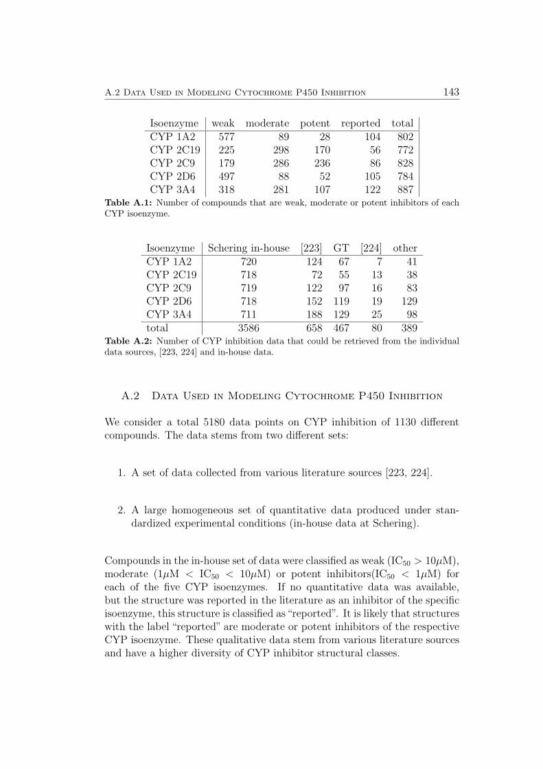
A.2 Data Used in Modeling Cytochrome P450 Inhibition 143
Isoenzyme weak moderate potent reported totalCYP 1A2 577 89 28 104 802CYP 2C19 225 298 170 56 772CYP 2C9 179 286 236 86 828CYP 2D6 497 88 52 105 784CYP 3A4 318 281 107 122 887
Table A.1: Number of compounds that are weak, moderate or potent inhibitors of eachCYP isoenzyme.
Isoenzyme Schering in-house [223] GT [224] otherCYP 1A2 720 124 67 7 41CYP 2C19 718 72 55 13 38CYP 2C9 719 122 97 16 83CYP 2D6 718 152 119 19 129CYP 3A4 711 188 129 25 98total 3586 658 467 80 389
Table A.2: Number of CYP inhibition data that could be retrieved from the individualdata sources, [223, 224] and in-house data.
A.2 Data Used in Modeling Cytochrome P450 Inhibition
We consider a total 5180 data points on CYP inhibition of 1130 differentcompounds. The data stems from two different sets:
1. A set of data collected from various literature sources [223, 224].
2. A large homogeneous set of quantitative data produced under stan-dardized experimental conditions (in-house data at Schering).
Compounds in the in-house set of data were classified as weak (IC50 > 10µM),moderate (1µM < IC50 < 10µM) or potent inhibitors(IC50 < 1µM) foreach of the five CYP isoenzymes. If no quantitative data was available,but the structure was reported in the literature as an inhibitor of the specificisoenzyme, this structure is classified as“reported”. It is likely that structureswith the label “reported” are moderate or potent inhibitors of the respectiveCYP isoenzyme. These qualitative data stem from various literature sourcesand have a higher diversity of CYP inhibitor structural classes.
144 Appendix
A.3 Descriptors Used in Modelling Cytochrome P450Inhibition
Cytochrome P450 Inhibition is a highly complex process, it is thus not clearwhich chemical descriptor can best capture the properties of a chemical com-pound that are indicative of its inhibition behavior. Therefore, we considera total of six different sets of descriptors. These range from conceptuallysimple and computationally cheap pseudo atom counts (Ghose-Crippen de-scriptor) to complex and computationally more demanding 3 D descriptors(VOLSURF). In the following section, each descriptor is explained shortlyand references to the original publications are provided.
The Ghose-Crippen descriptor comprises the numbers of occurrence of 120different pseudo-atoms. It was originally developed to predict the octanol-water partition coefficient [213]. P (octanol/water) is the ratio of the concen-tration of a chemical in octanol and in water at equilibrium and at a specifiedtemperature. Octanol is an organic solvent that is used as a surrogate fornatural organic matter. G. & C. suggest that logP is useful for treatingligand-receptor interaction. G. & C. also used these descriptors to predictmolecular refractivity [214]. The set of descriptors was later extended to al-low prediction of logP for a wider range of compounds [164]. They argue thatthe dispersive force between molecules (or a molecule and a macro-moleculelike a receptor) is related to their polarizability, which is proportional totheir molar refractivity and suggest that this property is therefore useful fortreating ligand-receptor interaction.
The BCUT descriptors are the highest and lowest eigenvalues of atomicconnectivity matrices, where the diagonal elements can be set to the atomsmass, van der Waals volume, electronegativity or polarizability to reflectthe atoms’ ability to form bonds or otherwise interact [167]. They are anextension of the Burden eigenvalues [166]. In our application, we considerthe 16 eigenvalues of largest magnitude and and 16 eigenvalues of lowestmagnitude.
UNITY fingerprints [168] (generated from the default screen2d definitionfile shipped with the software) are represented as string of 988 bits. They weredeveloped to speed up database searches and work similar to hash functions.928 bits are set to indicate the presence of paths of lengths 2 to 6 throughthe molecular graph. The remaining 60 bits indicate the presence of certainpredefined fragments (e.g. rare atoms, or different ring systems).
The logD prediction module from ACD Labs [75] is used to predict logDfor the ten pH values between 2 and 11 and the number of rotable bonds.These eleven numbers are then used as descriptors.
VolSurf descriptors [169] are generated in a three step process: A 3D
A.3 Descriptors Used in Modelling Cytochrome P450 Inhibition 145
structure of the molecule is calculated using Concord [225]. Then different3D molecular interaction fields [226] are created by virtually moving differenthydrophilic or lipophilic probes around the molecule and recording distancesof equal interaction energy. In our cases the H2O, DRY and O probes wereused. These interaction fields are then used to calculate the actual VolSurfdescriptors, including volume, surface, globularity, different descriptors ofhydrophilic and lipophilic regions, interaction energy moment and others.
GRIND descriptors [170] are generated in a four step process. A 3D struc-ture of the molecule is generated using Concord [225] and used to calculatea molecular interaction field (see above). In our case, the DRY, O, N1 andshape probes were used. A fixed number of nodes (e.g., 100) is chosen fromthe grid to maximize the value of a scoring function that depends on thesum of field intensities at all chosen points and the sum of distances betweenall chosen points. The ensemble of these regions for all relevant probes iscalled the virtual reaction site and forms the starting point for calculatingthe actual GRIND descriptors: For each possible pair of nodes the productof their field intensities is calculated. A discrete number of categories, eachrepresenting a small range of distances, is considered. For each category, thehighest product of field intensities is stored. The parameters can be visu-alized by plotting the highest products vs. the distance. If pairs of nodesfrom the same molecular interaction field are considered, this is called auto-correlogram, if the pairs of nodes are from two different molecular interactionfields, this is called a cross-correlogram.
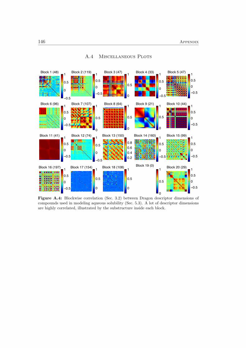
146 Appendix
A.4 Miscellaneous Plots
Block 1 (48)
−0.5
0
0.5
1 Block 2 (119)
−0.5
0
0.5
1 Block 3 (47)
0
0.5
1 Block 4 (33)
−0.5
0
0.5
1 Block 5 (47)
−0.500.51
Block 6 (96)
−0.5
0
0.5
1 Block 7 (107)
0
0.5
1 Block 8 (64)
0
0.5
1 Block 9 (21)
0
0.5
1 Block 10 (44)
−0.500.51
Block 11 (41)
−0.5
0
0.5
1 Block 12 (74)
−0.5
0
0.5
1 Block 13 (150)
0.20.40.60.8
Block 14 (160)
−0.5
0
0.5
1 Block 15 (99)
−0.5
0
0.51
Block 16 (197)
−0.5
0
0.5
1 Block 17 (154)
0
0.5
1 Block 18 (108)
0
0.5
1Block 19 (0)
0
0.5
1 Block 20 (29)
−0.500.51
Figure A.4: Blockwise correlation (Sec. 3.2) between Dragon descriptor dimensions ofcompounds used in modeling aqueous solubility (Sec. 5.3). A lot of descriptor dimensionsare highly correlated, illustrated by the substructure inside each block.

A.5 How to Cite this Thesis 147
A.5 How to Cite this Thesis
Please cite this document as follows:
Timon Schroeter. Machine Learning in Drug Discovery
and Drug Design. PhD thesis, Machine Learning Dept.,
University of Technology Berlin, 2009.
URL http://ml.cs.tu-berlin.de/~timon
Users of LATEX are invited to use the following BibTeX record:
@PhdThesis{Schroeter_2009,
author = {Timon Schroeter},
title = {Machine Learning in Drug Discovery and Drug Design},
school = {Machine Learning Dept.,
University of Technology Berlin},
year = {2009},
url = {http://ml.cs.tu-berlin.de/~timon}
}


Bibliography
[1] David Baehrens, Timon Schroeter, Stefan Harmeling, Motoaki Kawan-abe, Katja Hansen, and Klaus-Robert Muller. How to explain indi-vidual classification decisions. Journal of Machine Learning Research,submitted, 2009.
[2] Timon Schroeter, Klaus-Robert Muller, and Katja Hansen. Method forexplaining the predictions of a mathematical model to its users. PatentApplication at German Patent Office DPMA, 2008.
[3] Matthias Rupp, Timon Schroeter, Ramona Steri, Ewgenij Proschak,Katja Hansen, Oliver Rau, Manfred Schubert-Zsilavecz, Klaus-RobertMuller, and Gisbert Schneider. From virtual screening to natural prod-ucts: New pparγ agonists. ChemMedChem, submitted, 2009.
[4] Katja Hansen, Fabian Rathke, Timon Schroeter, Jan M. Kriegl, andSebastian Mika. Bias-correction of regression models: A case studyon herg inhibition. Journal of Chemical Information and Modelling,in press, 49(6):1486–1496, 2009. URL http://dx.doi.org/10.1021/
ci9000794.
[5] Katja Hansen, Sebastian Mika, Timon Schroeter, Andreas Sutter, An-tonius Ter Laak, Thomas Steger-Hartmann, Nikolaus Heinrich, andKlaus-Robert Muller. A benchmark data set for in silico prediction ofames mutagenicity. Journal of Chemical Information and Modelling,accepted, 49(9):2077–2081, 2009. URL http://dx.doi.org/10.1021/
ci900161g.
[6] Anton Schwaighofer, Timon Schroeter, Sebastian Mika, Katja Hansen,Antonius ter Laak, Philip Lienau, Andreas Reichel, Nikolaus Hein-rich, and Klaus-Robert Muller. A probabilistic approach to classifyingmetabolic stability. Journal of Chemical Information and Modeling,48:785–796, 2008. URL http://dx.doi.org/10.1021/ci700142c.
[7] Timon Schroeter, Anton Schwaighofer, Sebastian Mika, Antonius TerLaak, Detlev Suelzle, Ursula Ganzer, Nikolaus Heinrich, and Klaus-Robert Muller. Machine learning models for lipophilicity and their
149
150 Bibliography
domain of applicability. Mol. Pharm., 4(4):524–538, 2007. URL http:
//dx.doi.org/10.1021/mp0700413.
[8] Timon Schroeter, Anton Schwaighofer, Sebastian Mika, Antonius TerLaak, Detlev Suelzle, Ursula Ganzer, Nikolaus Heinrich, and Klaus-Robert Muller. Estimating the domain of applicability for machinelearning qsar rmodels: A study on aqueous solubility of drug discoverymolecules. Journal of Computer Aided Molecular Design - special issueon ”ADME and Physical Properties”, 21(9):485–498, 2007. URL http:
//dx.doi.org/10.1007/s10822-007-9125-z.
[9] Timon Schroeter, Anton Schwaighofer, Sebastian Mika, Antonius TerLaak, Detlev Suelzle, Ursula Ganzer, Nikolaus Heinrich, and Klaus-Robert Muller. Estimating the domain of applicability for machinelearning qsar rmodels: A study on aqueous solubility of drug discov-ery molecules. Journal of Computer Aided Molecular Design - regu-lar issue, 21(12):651–664, 2007. URL http://dx.doi.org/10.1007/
s10822-007-9160-9.
[10] Anton Schwaighofer, Timon Schroeter, Sebastian Mika, and GillesBlanchard. How wrong can we get? a review of machine learning ap-proaches and error bars. Combinatorial Chemistry & High ThroughputScreening, 12(5):453–468, 2009. URL http://dx.doi.org/10.2174/
138620709788489064.
[11] Anton Schwaighofer, Timon Schroeter, Sebastian Mika, Julian Laub,Antonius ter Laak, Detlev Sulzle, Ursula Ganzer, Nikolaus Heinrich,and Klaus-Robert Muller. Accurate solubility prediction with error barsfor electrolytes: A machine learning approach. Journal of ChemicalInformation and Modelling, 47(2):407–424, 2007. URL http://dx.
doi.org/10.1021/ci600205g.
[12] Timon Schroeter, Anton Schwaighofer, Sebastian Mika, Antonius terLaak, Detlev Sulzle, Ursula Ganzer, Nikolaus Heinrich, and Klaus-Robert Muller. Predicting lipophilicity of drug discovery moleculesusing gaussian process models. ChemMedChem, 2(9):1265–1267, 2007.URL http://dx.doi.org/10.1002/cmdc.200700041.
[13] Peter Kroll, Timon Schroter, and Martina Peters. Prediction of novelphases of tantalum(v) nitride and tungsten(vi) nitride that can be syn-thesized under high pressure and high temperature. Angew. Chem.Int. Ed., 44(27):4249–4254, 2005. URL http://dx.doi.org/10.1002/
anie.200462980.
Bibliography 151
[14] Peter Kroll, Timon Schroter, and Martina Peters. Synthesen bei hohemdruck und hoher temperatur fuhren zu neuen phasen von tantal(v)-nitrid und wolfram(vi)-nitrid. Angewandte Chemie, 117(27):4321–4326,2005. URL http://doi.wiley.com/10.1002/ange.200462980.
[15] Timon Schroeter. Book review: Pathway analysis for drug discovery.ChemMedChem, 4(6):1020, 2009. URL http://dx.doi.org/10.1002/
cmdc.200900107.
[16] Novartis AG. Drug discovery and development process http://www.
novartis.com/research/drug-discovery.shtml, 2009.
[17] Gisbert Schneider and Karl-Heinz Baringhaus. Molecular Design - Con-cepts and Applications. Wiley-Vch, Weinheim, 2008.
[18] Johann Gasteiger and Thomas Engel, editors. Chemoinformatics: ATextbook. Wiley-VCH, 2003.
[19] Asa Ben-Hur, Cheng Soon Ong, Soren Sonnenburg, BernhardScholkopf, and Gunnar Ratsch. Support vector machines and kernelsfor computational biology. PLoS Computational Biology, 4, 2008. URLhttp://svmcompbio.tuebingen.mpg.de. (accepted).
[20] G. Ratsch, S. Sonnenburg, and B. Scholkopf. RASE: recognition ofalternatively spliced exons in c. elegans. Bioinformatics, 21:i369–i377,June 2005.
[21] A. Zien, G. Ratsch, S. Mika, B. Scholkopf, T. Lengauer, and K.-R.Muller. Engineering support vector machine kernels that recognizetranslation initiation sites in DNA. BioInformatics, 16(9):799–807, Sep2000.
[22] K. Grabowski, K.-H. Baringhaus, and G. Schneider. Scaffold diversityof natural-products: Inspiration for combinatorial library design. Nat.Prod. Rep., accepted., 2008.
[23] R. Glen and G. (Eds) Schneider. Special journal issue: Challenges invirtual screening. QSAR & Combinatorial Science, 25(12), 2006.
[24] Thomas Lengauer, Christian Lemmenb, Matthias Rareyc, and MarcZimmermannd. Novel technologies for virtual screening. Drug Dis-covery Today, 9(1):27–34, 2004. URL http://dx.doi.org/10.1016/
S1359-6446(04)02939-3.
152 Bibliography
[25] Martin Weisel, Ewgenij Proschak, Jan M. Kriegl, and Gisbert Schnei-der. Form follows function: Shape analysis of protein cavities forreceptor-based drug design. Proteomics, 9(2):451–459, 2009. URLhttp://dx.doi.org/10.1002/pmic.200800092.
[26] Gisbert Schneider and Uli Fechner. Computer-based de novo design ofdrug-like molecules. Nat Rev Drug Discov, 4(8):1474–1776, 2005. URLhttp://dx.doi.org/10.1038/nrd1799.
[27] Markus Hartenfeller, Ewgenij Proschak, Andreas Schuller, and Gis-bert Schneider. Concept of combinatorial de novo design of drug-like molecules by particle swarm optimization. Chemical Biology &Drug Design, 72(1):16–26, 2008. URL http://dx.doi.org/10.1111/
j.1747-0285.2008.00672.x.
[28] Andreas Schuller, Marcel Suhartono, Uli Fechner, Yusuf Tanrikulu,Sven Breitung, Ute Scheffer, Michael W. Gobel, and Gisbert Schnei-der. The concept of template-based de novo design from drug-derivedmolecular fragments and its application to tar rna. J Comput Aided MolDes, 2008. URL http://dx.doi.org/10.1007/s10822-007-9157-4.
[29] Gisbert Schneider, Markus Hartenfeller, Michael Reutlinger, YusufTanrikulu, Ewgenij Proschak, and Petra Schneider. Voyages to the(un)known: adaptive design of bioactive compounds. Trends inBiotechnology, 27(1):18–26, 2009. URL http://dx.doi.org/10.1016/
j.tibtech.2008.09.005.
[30] Volker Hahnke, Bettina Hofmann, Tomislav Grgat, Ewgenij Proschak,Dieter Steinhilber, and Gisbert Schneider. Phast: Pharmacophorealignment search tool. J. Comput. Chem., 30(5):761–771, 2008. URLhttp://dx.doi.org/10.1002/jcc.21095.
[31] Steffen Renner, Mirko Hechenberger, Tobias Noeske, Alexander Backer,Claudia Jatzke, Michael Schmuker, Christopher G. Parsons, TanjaWeil, and Gisbert Schneider. Searching for drug scaffolds with 3d phar-macophores and neural network ensembles. Angew. Chem. Int. Ed., 46:5336–5339, 2007.
[32] K. Grabowski, E. Proschak, K.-H. Baringhaus, O. Rau, M. Schubert-Zsilavecz, and G. Schneider. Bioisosteric replacement of molecular scaf-folds: From natural products to synthetic compounds. Nat. Prod. Com-mun., 3:1355–1360, 2008.
Bibliography 153
[33] B. Hofmann, L. Franke, E. Proschak, Y. Tanrikulu, P. Schneider,D. Steinhilber, and G. Schneider. Scaffold-hopping cascade yields po-tent inhibitors of -lipoxygenase. ChemMedChem, accepted., 2009.
[34] B. Kruger, A. Dietrich, K.-H. Baringhaus, and G. Schneider. Scaffold-hopping potential of fragment-based de novo design: The chances andlimits of variation. Comb. Chem. High-Throughput Screen., accepted.,2009.
[35] Y. Tanrikulu and G. Schneider. Pseudoreceptor models in drug design:Bridging ligand- and receptor-based virtual screening. Nature Rev.Drug Discov., 7:668–677, 2008.
[36] A. Schuller and G. Schneider. Identification of hits and lead structurecandidates with limited resources by adaptive optimization. J. Chem.Inf. Model., accepted., 2008.
[37] Alexander J. Smola and Bernhard Scholkopf. A tutorial on supportvector regression. Statistics and Computing, 14(3):199–222, 2004. URLhttp://dx.doi.org/10.1023/B:STCO.0000035301.49549.88.
[38] K.-R. Muller, S. Mika, G. Ratsch, K. Tsuda, and B. Scholkopf. An in-troduction to kernel-based learning algorithms. IEEE Neural Networks,12(2):181–201, May 2001.
[39] Vojtech Franc and Soren Sonnenburg. OCAS optimized cuttingplane algorithm for support vector machines. In Proceedings ofthe 25nd International Machine Learning Conference. ACM Press,2008. URL http://ida.first.fraunhofer.de/~franc/ocas/html/
index.html.
[40] Sebastian Mika, Christin Schafer, Pavel Laskov, David Tax, and Klaus-Robert Muller. Support vector machines. In James E. Gentle, WolfgangHardle, and Yasuo Mori, editors, Handbook of Computational Statistics.Springer, Berlin, 2004.
[41] Masashi Sugiyama, Motoaki Kawanabe, and Klaus-Robert Muller.Trading variance reduction with unbiasedness: The regularized sub-space information criterion for robust model selection in kernel regres-sion. Neural Computation, 16(5):1077–1104, 2004.
[42] P. Laskov, C. Gehl, S. Kruger, and K. R. Muller. Incremental supportvector learning: Analysis, implementation and applications. Journal ofMachine Learning Research, 7:1909–1936, September 2006.

154 Bibliography
[43] Carl Edward Rasmussen and Christopher K.I. Williams. Gaussian Pro-cesses for Machine Learning. MIT Press, 2005.
[44] Kai Yu, Volker Tresp, and Anton Schwaighofer. Learning Gaussianprocesses from multiple tasks. In Luc De Raedt and Stefan Wrobel,editors, Machine Learning: Proceedings of the 22nd International Con-ference (ICML 2005). Morgan Kaufman, 2005.
[45] Gilles Blanchard, Christin Schafer, Yves Rozenholc, and Klaus-RobertMuller. Optimal dyadic decision trees. Machine Learning, 66(2–3):209–241, 2007. URL http://dx.doi.org/10.1007/s10994-007-0717-6.
[46] Klaus Pawelzik, Klaus-Robert Muller, and Jens Kohlmorgen. Predic-tion of mixtures. In Artificial Neural Networks – ICANN ’96, pages127–132. Springer, 1996.
[47] K.-R. Muller, N. Murata, A. Ziehe, and S.-I. Amari. On-line learn-ing in Switching and Drifting environments with application to blindsource separation, pages 93–110. On-line learning in neural networks.Cambridge University Press, 1998.
[48] Klaus-Robert Muller, Gunnar Ratsch, Jens Kohlmorgen, AlexanderSmola, Bernhard Scholkpf, and Vapnik Vladimir. Time series predic-tion using support vector regression and neural networks. In T. Higuchiand Y. Takizawa, editors, 2nd International Sympsium on Frontiers ofTime Series Modelling: Nonparametric Approach to Knowledge Di-escovery. Instiute of mathematical statistics publication, 2000.
[49] Roberto Todeschini and Viviana Consonni. Handbook of MolecularDescriptors. John Wiley & Sons, Ltd., 2000.
[50] Burr Settles. Active learning literature survey. Computer SciencesTechnical Report 1648, University of Wisconsin–Madison, 2009. URLhttp://pages.cs.wisc.edu/~bsettles/active-learning/.
[51] Pavel Laskov, Konrad Rieck, Christin Schafer, and Klaus-RobertMuller. Visualization of anomaly detection using prediction sensitiv-ity. In Sicherheit 2005 (Sicherheit-Schutz und Verlasslichkeit), pages197–208, 2005.
[52] P. Laskov, C. Schafer, I. Kotenko, and K.-R. Muller. Intrusion de-tection in unlabeled data with quarter-sphere support vector machines(extended version). Praxis der Informationsverarbeitung und Kommu-nikation, 27:228–236, 2004.
Bibliography 155
[53] Patrick Dussel, Christian Gehl, Pavel Laskov, and Konrad Rieck. Incor-poration of application layer protocol syntax into anomaly detection.In Proc. of International Conference on Information Systems Security(ICISS), pages 188–202, 2008.
[54] Stefan Wahl, Konrad Rieck, Pavel Laskov, Peter Domschitz, and Klaus-Robert Muller. Securing IMS against novel threats. Bell Labs TechnicalJournal, 2009. to appear.
[55] Tammo Krueger, Christian Gehl, Konrad Rieck, and Pavel Laskov. Anarchitecture for inline anomaly detection. In Proc. of European Con-ference on Computer Network Defense (EC2ND), pages 11–18, 2008.
[56] Konrad Rieck and Pavel Laskov. Linear-time computation of similaritymeasures for sequential data. Journal of Machine Learning Research,9(Jan):23–48, 2008.
[57] Pavel Laskov, Konrad Rieck, and Klaus-Robert Muller. Machine learn-ing for intrusion detection. In Mining Massive Data Sets for Security.IOS press, 2008. (in press).
[58] Matthias Krauledat. Analysis of Nonstationarities in EEG signals forimproving Brain-Computer Interface performance. PhD thesis, Tech-nische Universitat Berlin, Fakultat IV – Elektrotechnik und Informatik,2008.
[59] Klaus-Robert Muller, Michael Tangermann, Guido Dornhege, MatthiasKrauledat, Gabriel Curio, and Benjamin Blankertz. Machine learningfor real-time single-trial EEG-analysis: From brain-computer interfac-ing to mental state monitoring. J Neurosci Methods, 167(1):82–90,2008. URL http://dx.doi.org/10.1016/j.jneumeth.2007.09.022.
[60] Carmen Vidaurre, Alois Schlogl, Benjamin Blankertz, Motoaki Kawan-abe, and Klaus-Robert Muller. Unsupervised adaptation of the LDAclassifier for Brain-Computer Interfaces. In Proceedings of the 4th In-ternational Brain-Computer Interface Workshop and Training Course2008. Verlag der Technischen Universitat Graz, 2008. to appear.
[61] Anton Nijholt, Desnay Tan, Gert Pfurtscheller, Clemens Brunner, JoseMillan, Brendan Allison, Bernhard Grainmann, Florin Popescu, Ben-jamin Blankertz, and Klaus-Robert Muller. Brain-computer interfacingfor intelligent systems. IEEE Intelligent Systems, 23(3):72–79, 2008.URL http://dx.doi.org/10.1109/MIS.2008.41.
156 Bibliography
[62] Matthias Krauledat, Michael Tangermann, Benjamin Blankertz, andKlaus-Robert Muller. Towards zero training for brain-computer in-terfacing. PLoS ONE, 3(8):e2967, Aug 2008. doi: 10.1371/journal.pone.0002967. URL http://dx.doi.org/10.1371%2Fjournal.pone.
0002967.
[63] Michael Tangermann, Matthias Krauledat, Konrad Grzeska, Max Sage-baum, Benjamin Blankertz, and Klaus-Robert Muller. Playing pinballwith non-invasive BCI. In Advances in Neural Information ProcessingSystems 21. MIT Press, Cambridge, MA, 2009. in press.
[64] Benjamin Blankertz, Florian Losch, Matthias Krauledat, Guido Dorn-hege, Gabriel Curio, and Klaus-Robert Muller. The Berlin Brain-Computer Interface: Accurate performance from first-session in BCI-naive subjects. IEEE Trans Biomed Eng, 55(10):2452–2462, 2008. URLhttp://dx.doi.org/10.1109/TBME.2008.923152.
[65] Mikio L. Braun, Joachim Buhmann, and Klaus-Robert Muller. On rel-evant dimensions in kernel feature spaces. Journal of Machine LearningResearch, 9:1875–1908, Aug 2008.
[66] Mikio L. Braun. Accurate bounds for the eigenvalues of the kernelmatrix. Journal of Machine Learning Research, 7:2303–2328, Nov 2006.
[67] Mikio L. Braun, Tilman Lange, and Joachim Buhmann. Model selec-tion in kernel methods based on a spectral analysis of label information.In Proc. DAGM, volume 4174 of LNCS, pages 344–353, 2006.
[68] Mikio L. Braun, Joachim Buhmann, and Klaus-Robert Muller. Denois-ing and dimension reduction in feature space. In Advances in NeuralInf. Proc. Systems (NIPS 20), 2007. accepted.
[69] S. Harmeling, A. Ziehe, M. Kawanabe, B. Blankertz, and K.-R. Muller.Nonlinear blind source separation using kernel feature spaces. In T.-W.Lee, editor, Proc. Int. Workshop on Independent Component Analysisand Blind Signal Separation (ICA2001), pages 102–107, 2001.
[70] Frank C. Meinecke, Andreas Ziehe, Motoaki Kawanabe, and Klaus-Robert Muller. Assessing reliability of ICA projections – a resamplingapproach. In T.-W. Lee, editor, Proc. Int. Workshop on IndependentComponent Analysis and Blind Signal Separation (ICA2001), 2001.
[71] S. Harmeling, A. Ziehe, M. Kawanabe, and K.-R. Muller. Kernel fea-ture spaces and nonlinear blind source separation. In T.G. Dietterich,
Bibliography 157
S. Becker, and Z. Ghahramani, editors, Advances in Neural Informa-tion Processing Systems, volume 14. MIT Press, 2002.
[72] S. Harmeling, A. Ziehe, M. Kawanabe, and K.-R. Muller. Kernel-basednonlinear blind source separation. Neural Computation, 15:1089–1124,2003.
[73] Andreas Ziehe, Motoaki Kawanabe, Stefan Harmeling, and Klaus-Robert Muller. Blind separation of post-nonlinear mixtures using lin-earizing transformations and temporal decorrelation. Journal of Ma-chine Learning Research, 4:1319–1338, Dec 2003.
[74] Soren Sonnenburg, Mikio Braun, Cheng Soon Ong, Samy Bengio,Leon Bottou, Geoffrey Holmes, Yann LeCun, Klaus-Robert Muller,Fernando Pereira, Carl Edward Rasmussen, Gunnar Ratsch, Bern-hard Scholkopf, Alexander Smola, Pascal Vincent, Jason Weston, andRobert Williamson. The Need for Open Source Software in Ma-chine Learning. Journal of Machine Learning Research, 8:2443–2466,September 2007.
[75] ACD/Solubility Batch v9.0. Toronto, Canada, 2006.
[76] S. Mika, B. Scholkopf, A.J. Smola, K.-R. Muller, M. Scholz, andG. Ratsch. Kernel PCA and de–noising in feature spaces. In M.S.Kearns, S.A. Solla, and D.A. Cohn, editors, Advances in Neural Inf.Proc. Systems (NIPS 98), pages 536–542. MIT Press, 1999.
[77] B. Scholkopf, S. Mika, C.J.C. Burges, P. Knirsch, K.-R. Muller,G. Ratsch, and A.J. Smola. Input space vs. feature space in kernel-based methods. IEEE Transactions on Neural Networks, 10(5):1000–1017, September 1999.
[78] S. Mika, G. Ratsch, J. Weston, B. Scholkopf, A.J. Smola, and K.-R.Muller. Invariant feature extraction and classification in kernel spaces.In S.A. Solla, T.K. Leen, and K.-R. Muller, editors, Proc. NIPS 12,pages 526–532. MIT Press, 2000.
[79] Gilles Blanchard, Olivier Bousquet, and Laurent Zwald. Statis-tical properties of kernel components analysis. Machine Learn-ing, 66(2-3):259–294, 2007. URL http://dx.doi.org/10.1007/
s10994-006-6895-9.
158 Bibliography
[80] B. Scholkopf, S. Mika, A.J. Smola, G. Ratsch, and K.-R. Muller. KernelPCA pattern reconstruction via approximate pre-images. In L. Niklas-son, M. Boden, and T. Ziemke, editors, Proceedings of the 8th Interna-tional Conference on Artificial Neural Networks, Perspectives in NeuralComputing, pages 147 – 152, Berlin, 1998. Springer Verlag.
[81] Laurent Zwald and Gilles Blanchard. On the convergence of eigenspacesin kernel principal components analysis. In Advances in Neural Inf.Proc. Systems (NIPS 05), volume 18, 2006.
[82] Stefan Harmeling, Guido Dornhege, David Tax, Frank C. Meinecke,and Klaus-Robert Muller. From outliers to prototypes: ordering data.Neurocomputing, 69(13–15):1608–1618, 2006.
[83] Ying Xue Min Wang, Xue-Gang Yang. Identifying herg potas-sium channel inhibitors by machine learning methods. QSAR Comb.Sci., 27:1028–1035, 2008. URL http://dx.doi.org/10.1002/qsar.
200810015.
[84] Aixia Yan, Zhi Wang, and Zongyuan Cai. Prediction of human in-testinal absorption by ga feature selection and support vector ma-chine regression. International Journal of Molecular Sciences, 9(10):1961–1976, 2008. ISSN 1422-0067. doi: 10.3390/ijms9101961. URLhttp://www.mdpi.com/1422-0067/9/10/1961.
[85] Andreas Bender, Hamse Y. Mussa, Robert C. Glen, and StephanReiling. Molecular similarity searching using atom environments,information-based feature selection, and a naive bayesian classifier.Journal of Chemical Information and Computer Sciences, 44(1):170–178, 2004. doi: 10.1021/ci034207y. URL http://pubs.acs.org/doi/
abs/10.1021/ci034207y.
[86] Jorg K. Wegner and Andreas Zell. Prediction of aqueous solubilityand partition coefficient optimized by a genetic algorithm based de-scriptor selection method. Journal of Chemical Information and Com-puter Sciences, 43(3):1077–1084, 2003. doi: 10.1021/ci034006u. URLhttp://pubs.acs.org/doi/abs/10.1021/ci034006u.
[87] Igor V. Tetko, Iurii Sushko, Anil Kumar Pandey, Hao Zhu, Alexan-der Tropsha, Ester Papa, Tomas Oberg, Roberto Todeschini, DenisFourches, and Alexandre Varnek. Critical assessment of qsar mod-els of environmental toxicity against tetrahymena pyriformis: Focusingon applicability domain and overfitting by variable selection. Journal
Bibliography 159
of Chemical Information and Modeling, 48(9):1733–1746, 2008. doi:10.1021/ci800151m. URL http://pubs.acs.org/doi/abs/10.1021/
ci800151m.
[88] Yuan Calan Qi, Thomas P. Minka, and Rosalind W. Picard. Predictiveautomatic relevance determination by expectation propagation. In InProceedings from the International Conference on Machine Learning,pages 4–8, 2004.
[89] Anthony O’Hagan. Curve fitting and optimal design for prediction.Journal of the Royal Statistical Society, Series B: Methodological, 40(1):1–42, 1978.
[90] Olga Obrezanova, Gabor Csanyi, Joelle M.R. Gola, and Matthew D.Segall. Gaussian processes: A method for automatic QSAR modellingof adme properties. J. Chem. Inf. Model., 47(5):1847–1857, 2007. URLhttp://dx.doi.org/10.1021/ci7000633.
[91] Carl Edward Rasmussen. The gaussian process webssite http://www.
gaussianprocess.org/, 2009.
[92] Bernhard Scholkopf and Alex J. Smola. Learning with Kernels. MITPress, 2002.
[93] Vladimir N. Vapnik. The Nature of Statistical Learning Theory.Springer Verlag, 1995.
[94] Radford M. Neal. Bayesian Learning for Neural Networks. SpringerVerlag, 1996.
[95] C. Zhu, R. H. Byrd, and J. Nocedal. L-bfgs-b: Algorithm 778: L-bfgs-b, fortran routines for large scale bound constrained optimization.ACM Transactions on Mathematical Software, 23(4):550–560, 1997.
[96] Radford M. Neal. Regression and classification using Gaussian processpriors. In Jose M. Bernardo, J.O. Berger, A.P. Dawid, and A.F.M.Smith, editors, Bayesian Statistics 6, volume 6, pages 475–501. OxfordUniversity Press, 1998.
[97] Alexandre Varnek, Cedric Gaudin, Gilles Marcou, Igor Baskin,Anil Kumar Pandey, and Igor V. Tetko. Inductive transfer of knowl-edge: Application of multi-task learning and feature net approaches tomodel tissue-air partition coefficients. Journal of Chemical Informa-tion and Modeling, 49(1):133–144, 2009. doi: 10.1021/ci8002914. URLhttp://pubs.acs.org/doi/abs/10.1021/ci8002914.
160 Bibliography
[98] Olga Obrezanova, Joelle M. R. Gola, Edmund J. Champness, andMatthew D. Segall. Automatic qsar modeling of adme properties:blood-brain barrier penetration and aqueous solubility. J. Comput.-Aided Mol. Des., 22:431–440, 2008. URL http://dx.doi.org/10.
1007/s10822-008-9193-8.
[99] Klaus-Robert Muller, Gunnar Ratsch, Soren Sonnenburg, SebastianMika, Michael Grimm, and Nikolaus Heinrich. Classifying ’drug-likeness’ with kernel-based learning methods. J. Chem. Inf. Model,45:249–253, 2005.
[100] M. K Warmuth, J. Liao, G. Ratsch, Mathieson. M., S. Putta, andC. Lemmem. Active learning with Support Vector Machines in thedrug discovery process. Journal of Chemical Information and ComputerSciences, 43(2):667–673, 2003.
[101] Leo Breiman. Random forests. Machine Learning, 45:5–32, 2001. URLhttp://dx.doi.org/10.1023/A:1010933404324.
[102] Trevor Hastie, Robert Tibshirani, and Jerome Friedman. The Elementsof Statistical Learning. Springer Verlag, 2001.
[103] Tapio Pahikkala, Jorma Boberg, and Tapio Salakoski. T.: Fast n-foldcross-validation for regularized least-squares. In In: Proceedings of theNinth Scandinavian Conference on Artificial Intelligence (SCAI, 2006.
[104] Gerard E. Dallal. Correlation coefficients http://www.jerrydallal.
com/LHSP/corr.htm, 1999.
[105] Maurice Kendall. Rank Correlation Methods. Charles Griffin & Com-pany Limited, 1948.
[106] Matthias Rupp, Ewgenij Proschak, and Gisbert Schneider. Kernel ap-proach to molecular similarity based on iterative graph similarity. Jour-nal of Chemical Information and Modelling, 47(6):2280–2286, 2007.
[107] Gunnar Ratsch, Soren Sonnenburg, Jagan Srinivasan, Hanh Witte, RalfSommer, Klaus-Robert Muller, and Bernhard Scholkopf. Improving thec. elegans genome annotation using machine learning. PLoS Computa-tional Biology, 3:e20, 2007.
[108] Soren Sonnenburg, Gunnar Ratsch, Christin Schafer, and BernhardScholkopf. Large Scale Multiple Kernel Learning. Journal of MachineLearning Research, 7:1531–1565, July 2006.

Bibliography 161
[109] Alexander Tropsha. Variable selection qsar modeling, model validation,and virtual screening. In David C. Spellmeyer, editor, Annual Reportsin Computational Chemistry, volume 2, chapter 7, pages 113–126. El-sevier, 2006.
[110] Weida Tong, Qian Xie, Huixiao Hong, Leming Shi, Hong Fang, andRoger Perkins. Assessment of prediction confidence and domain ex-trapolation of two structure-activity relationship models for predictingestrogen receptor binding activity. Environmental Health Perspectives,112(12):1249–1254, 2004.
[111] Tatiana I. Netzeva, Andrew P. Worth, Tom Aldenberg, RomualdoBenigni, Mark T.D. Cronin, Paola Gramatica, Joanna S. Jaworska,Scott Kahn, Gilles Klopman, Carol A. Marchant, Glenn Myatt, NinaNikolova-Jeliazkova, Grace Y. Patlewicz, Roger Perkins, David W.Roberts, Terry W. Schultz, David T. Stanton, Johannes J.M. van deSandt, Weida Tong, Gilman Veith, and Chihae Yang. Current sta-tus of methods for defining the applicability domain of (quantitative)structure-activity relationships. Alternatives to Laboratory Animals, 33(2):1–19, 2005.
[112] Bernard W. Silverman. Density Estimation for Statistics and DataAnalysis. Number 26 in Monographs on Statistics and Applied Proba-bility. Chapman & Hall, 1986.
[113] Robert P. Sheridan, Bradley P. Feuston, Vladimir N. Maiorov, andSimon K. Kearsley. Similarity to molecules in the training set is a gooddiscriminator for prediction accuracy in qsar. J. Chem. Inf. Model., 44:1912–1928, 2004.
[114] Igor V. Tetko, Pierre Bruneau, Hans-Werner Mewes, Douglas C.Rohrer, and Gennadiy I. Poda. Can we estimate the accuracy ofADME-tox predictions? Drug Discovery Today, 11(15/16):700–707,August 2006.
[115] Pierre Bruneau and Nathan R. McElroy. Generalized fragment-substructure based property prediction method. J. Chem. Inf. Model.,46:1379–1387, 2006.
[116] Andreas H. Goller, Matthias Hennemann, Jorg Keldenich, and Timo-thy Clark. In silico prediction of buffer solubility based on quantum-mechanical and hqsar- and topology-based descriptors. J. Chem. Inf.Model., 46(2):648–658, 2006.
162 Bibliography
[117] David T. Manallack, Benjamin G. Tehan, Emanuela Gancia, Brian D.Hudson, Martyn G. Ford, David J. Livingstone, David C. Whitley,and Will R. Pitt. A consensus neural network-based technique fordiscriminating soluble and poorly soluble compounds. J. Chem. Inf.Model., 43:674–679, 2003.
[118] Ralph Kuhne, Ralf-Uwe Ebert, and Gerrit Schurmann. Model selectionbased on structural similarity-method description and application towater solubility prediction. J. Chem. Inf. Model., 46:636–641, 2006.
[119] G. A. Miller. The magical number seven, plus or minus two: Somelimits on our capacity for processing information. Psychological Review,63:81–97, 1956.
[120] Bernhard Scholkopf, Ralf Herbrich, and Alex Smola. A generalizedrepresenter theorem. In Lecture Notes in Computer Science, pages416–426. Springer Berlin / Heidelberg, 2001. URL http://dx.doi.
org/10.1007/3-540-44581-1_27.
[121] Anton Schwaighofer, Timon Schroeter, Sebastian Mika, Katja Hansen,Antonius ter Laak, Philip Lienau, Andreas Reichel, Nikolaus Hein-rich, and Klaus-Robert Muller. A probabilistic approach to classifyingmetabolic stability. Journal of Chemical Information and Modelling,2008. URL http://dx.doi.org/10.1021/ci700142c.
[122] World drug index WDI. World drug index WDI, 1996. version 2/96.
[123] R. Todeschini, V. Consonni, A. Mauri, and M. Pavan. DRAGON v1.2.Milano, Italy, 2006.
[124] David Baehrens. Explaining machine-learned model predictions to sup-port human expert decisions. Diplomarbeit, Machine Learning Dept.,University of Technology Berlin, December 2009.
[125] I. Guyon and A. Elisseeff. An introduction to variable and featureselection. JMLR, 3:1157–1182, 2003.
[126] C.M. Bishop. Neural Networks for Pattern Recognition. Oxford Uni-versity Press, 1995.
[127] L. Devroye, L. Gyorfi, and G. Lugosi. A Probabilistic Theory of PatternRecognition. Number 31 in Applications of Mathematics. Springer, NewYork, 1996.
Bibliography 163
[128] F. R. Hampel, E. M. Ronchetti, P. J. Rousseeuw, and W. A. Stahel.Robust Statistics: The Approach Based on Influence Functions. Wiley,New York, 1986.
[129] E. J. Horvitz, J. S. Breese, and M. Henrion. Decision theory in expertsystems and artificial interigence. Journal of Approximation Reasoning,2:247–302, 1988. Special Issue on Uncertainty in Artificial Intelligence.
[130] H. Suermondt. Explanation in Bayesian Belief Networks. PhD thesis,Department of Computer Science and Medicine, Stanford University,Stanford, CA, 1992.
[131] Marko Robnik-Sikonja and Igor Kononenko. Explaining classificationsfor individual instances. IEEE TKDE, 20(5):589–600, 2008.
[132] Erik Strumbelj and Igor Kononenko. Towards a model independentmethod for explaining classification for individual instances. In I.-Y. Song, J. Eder, and T.M. Nguyen, editors, Data Warehousing andKnowledge Discovery, volume 5182 of Lecture Notes in Computer Sci-ence, pages 273–282. Springer, 2008.
[133] T.J. Hou and X.J. Xu. Adme evaluation in drug discovery. 3. model-ing blood-brain barrier partitioning using simple molecular descriptors.J. Chem. Inf. Comput. Sci., 43(6):2137–2152, 2003.
[134] Eric D. Clarke and John S. Delaney. Physical and molecular proper-ties of agrochemicals: An analysis of screen inputs, hits, leads, andproducts. Chimia, 57(11):731–734, 2003.
[135] Jarmo Huuskonen. Estimation of aqueous solubility for a diverse setof organic compounds based on molecular topology. J. Chem. Inf.Comput. Sci., 40(3):773–777, 2000.
[136] Igor V. Tetko, Vsevolod Y. Tanchuk, Tamara N. Kasheva, and Alessan-dro E.P. Villa. Estimation of aqueous solubility of chemical compoundsusing e-state indices. J. Chem. Inf. Comput. Sci., 41(6):1488–1493,2001.
[137] Aixia Yan and Johann Gasteiger. Prediction of aqueous solubility oforganic compounds by topological descriptors. QSAR Comb. Sci., 22(8):821–829, 2003.
[138] Jorg K. Wegner and Andreas Zell. Prediction of aqueous solubility andpartition coefficient optimized by a genetic algorithm based descriptorselection. J. Chem. Inf. Comput. Sci., 43(3):1077–1084, 2003.
164 Bibliography
[139] Aixia Yan and Johann Gasteiger. Prediction of aqueous solubility oforganic compounds based on a 3d structure representation. J. Chem.Inf. Comput. Sci., 43:429–434, 2003.
[140] Ruifeng Liu, Hongmao Sun, and Sung-Sau So. Development of quan-titative structure - property relationship models for early adme evalu-ation in drug discovery. 1. aqueous solubility. J. Chem. Inf. Comput.Sci., 41(6):1633–1639, 2001.
[141] John S. Delaney. Esol: Estimating aqueous solubility directly frommolecular structure. J. Chem. Inf. Comput. Sci., 44(3):1000 –1005,2004.
[142] Pierre Bruneau. Search for predictive generic model of aqueous solu-bility using bayesian neural nets. J. Chem. Inf. Comput. Sci., 41(6):1605–1616, 2001.
[143] Denise Yaffe, Yoram Cohen, Gabriela Espinosa, Alex Arenas, andFrancesc Giralt. A fuzzy artmap based on quantitative structure-property relationships (qsprs) for predicting aqueous solubility of or-ganic compounds. J. Chem. Inf. Comput. Sci., 41(5):1177–1207, 2001.
[144] Ola Engkvist and Paul Wrede. High-throughput, in silico predictionof aqueous solubility based on one- and two-dimensional descriptors.J. Chem. Inf. Comput. Sci., 42(5):1247–1249, 2002.
[145] Aixia Yan, Johann Gasteiger, Michael Krug, and Soheila Anzali. Linearand nonlinear functions on modeling of aqueous solubility of organiccompounds by two structure representation methods. J. Comput.-AidedMol. Des., 18:75–87, 2004.
[146] T. J. Hou, K. Xia, W. Zhang, and X. J. Xu. Adme evaluation in drugdiscovery. 4. prediction of aqueous solubility based on atom contribu-tion approach. J. Chem. Inf. Comput. Sci., 44:266–275, 2004.
[147] Holger Frohlich, Jorg K. Wegner, and Andreas Zell. Towards optimaldescriptor subset selection with support vector machines in classifica-tion and regression. QSAR Comb. Sci., 23:311–318, 2004.
[148] Matthew Clark. Generalized fragment-substructure based propertyprediction method. J. Chem. Inf. Model., 45:30–38, 2005.
[149] Fred-Reiner Rapp. Das Programmsystem SOLVES zur Suche und Op-timierung von Leitstrukturen. PhD thesis, Fakultat fur Informations-
Bibliography 165
und Kognitionswissenschaften, Eberhard-Karls-Universitat Tubingen,Germany, 2005.
[150] Konstantin V. Balakin, Nikolay P. Savchuk, and Igor V. Tetko. In silicoapproaches to prediction of aqueous and DMSO solubility of drug-likecompounds: Trends, problems and solutions. Curr. Med. Chem., 13:223–241, 2006.
[151] Stephen R. Johnson and Weifan Zheng. Recent progress in thecomputational prediction of aqueous solubility and absorption. TheAAPS Journal, 8(1):E27–E40, 2006. URL http://www.aapsj.org/
articles/aapsj0801/aapsj080104/aapsj080104.pdf.
[152] John S. Delaney. Predicting aqueous solubility from structure. DrugDiscovery Today, 10(4):289–295, 2005.
[153] Carol A. Kempa, Jean-Didier Marechal, and Michael J. Sutcliffe.Progress in cytochrome P450 active site modeling. Arch. Biochem.Biophys., 433:361–368, 2005.
[154] Ilia G. Denisov, Thomas M. Makris, Stephen G. Sligar, and IlmeSchlichting. Structure and chemistry of cytochrome P450. Chem. Rev.(Washington, DC, U.S.), 105:2253–2277, 2005.
[155] Arthur G. Roberts, A. Patricia Campbell, and William M. Atkins. Thethermodynamic landscape of testosterone binding to cytochrome P4503a4: Ligand binding and spin state equilibria. Biochemistry, 44:1353–1366, 2005.
[156] David F. V. Lewis and Maurice Dickins. Substrate sars in human p450s.Drug Discovery Today, 7:918–925, 2002.
[157] Sean Ekins. Predicting undesirable drug interactions with promiscuousproteins in silico. Drug Discovery Today, 9:276–285, 2004.
[158] Jan M. Kriegl, Thomas Arnhold, Bernd Beck, and Thomas Fox. Pre-diction of human cytochrome P450 inhibition using support vector ma-chines. QSAR Comb. Sci., 24:491–502, 2005.
[159] Christian Merkwirth, Harald Mauser, Tanja Schulz-Gasch, OlivierRoche, Martin Stahl, and Thomas Lengauer. Ensemble methods forclassification in cheminformatics. J. Chem. Inf. Comput. Sci., 44:1971–1978, 2004.
166 Bibliography
[160] Achim Kless and Tatjana Eitrich. Cytochrome P450 classification ofdrugs with support vector machines implementing the nearest pointalgorithm. In Knowledge Exploration in Life Science Informatics: In-ternational Symposium KELSI 2004, volume 3303 of Lecture Notes inArtificial Intelligence, pages 191–205. Springer Verlag, 2004.
[161] Paul Rowland, Frank E. Blaney, Martin G. Smyth, Jo J. Jones,Vaughan R. Leydon, Amanda K. Oxbrow, Ceri J. Lewis, Mike G. Ten-nant, Sandeep Modi, Drake S. Eggleston, Richard J. Chenery, and An-gela M. Bridges. Crystal Structure of Human Cytochrome P450 2D6. J.Biol. Chem., 281(11):7614–7622, 2006. doi: 10.1074/jbc.M511232200.URL http://dx.doi.org/10.1074/jbc.M511232200.
[162] Pamela A. Williams, Jose Cosme, Dijana Matak Vinkovic, AlisonWard, Hayley C. Angove, Philip J. Day, Clemens Vonrhein, Ian J.Tickle, and Harren Jhoti. Crystal Structures of Human CytochromeP450 3A4 Bound to Metyrapone and Progesterone. Science, 305(5684):683–686, 2004. URL http://dx.doi.org/10.1126/science.
1099736.
[163] Pamela A. Williams, Jose Cosme, Alison Ward, Hayley C. Angove,Dijana Matak Vinkovi, and Harren Jhoti. Crystal structure of humancytochrome p450 2c9 with bound warfarin. Nature, 424:464–468, 2003.URL http://dx.doi.org/10.1038/nature01862.
[164] Vellarkad N. Viswanadhan, Arup K. Ghose, Ganapathi R. Reyankar,and Roland K. Robins. Atomic physicochemical parameters for threedimensional structure directed quantitative structure-activity relation-ships. 4. additional parameters for hydrophobic and dispersive interac-tions and their application for an automated superposition of certainnaturally occurring nucleoside antibiotics. J. Chem. Inf. Comput. Sci.,29:163–172, 1989.
[165] Tommi Jaakkola and David Haussler. Exploiting generative models indiscriminative classifiers. In In Advances in Neural Information Pro-cessing Systems 11, pages 487–493. MIT Press, 1998.
[166] Frank R. Burden. A chemically intuitive molecular index based on theeigenvalues of a modified adjacency matrix. Quant. Struct. Act. Relat.,16:309–314, 1997.
[167] RobertaS.aPearlman and K.M.aSmith. Novel software tools for chemi-cal diversity. Perspectives in Drug Discovery and Design, 9-11:339–353,1998.
Bibliography 167
[168] U.S.A. Tripos Inc.: St.Louis, MO. Unity reference manual, 2006.
[169] G. Cruciani, P. Crivori, P.-A. Carrupt, and B. Testa. Molecular fields inquantitative structure-permeation relationships: The volsurf approach.THEOCHEM, 503:17–30, 2000.
[170] Manuel Pastor, Gabriele Cruciani, Iain McLay, Stephen Pickett, andSergio Clementi. Grid-independent descriptors (grind): A novelclass of alignment-independent three-dimensional molecular descrip-tors. J. Med. Chem., 43:3233–3243, 2000.
[171] J.R. Quinlan. C4.5: Programs for Machine Learning. Morgan Kauf-mann, 1992.
[172] T.M. Cover and P.E. Hart. Nearest neighbor pattern classifications.IEEE transaction on information theory, 13(1):21—27, 1967.
[173] V.N. Vapnik. The nature of statistical learning theory. Springer Verlag,New York, 1995.
[174] B. Scholkopf and A.J. Smola. Learning with Kernels. MIT Press,Cambridge, MA, 2002.
[175] K.P. Bennett and O.L. Mangasarian. Robust linear programming dis-crimination of two linearly inseparable sets. Optimization Methods andSoftware, 1:23–34, 1992.
[176] T. Graepel, R. Herbrich, B. Scholkopf, A.J. Smola, P.L. Bartlett, K.-R.Muller, K. Obermayer, and R.C. Williamson. Classification on prox-imity data with LP-machines. In D. Willshaw and A. Murray, editors,Proceedings of ICANN’99, volume 1, pages 304–309. IEE Press, 1999.
[177] M. Shen, Y. Xiao, A. Golbraikh, V.K. Gombar, and A. Tropsha. An insilico screen for human S9 metabolic turnover using k-nearest neighborQSPR method. J. Med. Chem., 46:3013–3020, 2003.
[178] Berith F. Jensen, Morten D. Sorensen, Kissmeyer Anne-Marie, FrederikBjorkling, Kim Sonne, Soren B. Engelsen, and Lars Norgaard. Pre-diction of in vitro metabolic stability of calcitriol analogs by QSAR.J. Comput.-Aided Mol. Des., 17(12):849–859, 2003.
[179] Bruce N. Ames, E. G. Gurney, James A. Miller, and H. Bartsch. Car-cinogens as Frameshift Mutagens: Metabolites and Derivatives of 2-Acetylaminofluorene and Other Aromatic Amine Carcinogens. Proceed-
168 Bibliography
ings of the National Academy of Sciences of the United States of Amer-ica, 69(11):3128–3132, 1972. URL http://www.pnas.org/content/
69/11/3128.abstract.
[180] Christoph Helma, Tobias Cramer, Stefan Kramer, and Luc De Raedt.Data mining and machine learning techniques for the identificationof mutagenicity inducing substructures and structure activity rela-tionships of noncongeneric compounds. Journal of Chemical Infor-mation and Computer Sciences, 44(4):1402–11, 2004. doi: 10.1021/ci034254q. URL http://www.ncbi.nlm.nih.gov/pubmed/15272848.PMID: 15272848.
[181] J Kazius, R Mcguire, and R Bursi. Derivation and validation of toxi-cophores for mutagenicity prediction. J. Med. Chem., 48(1):320, 312,2005. URL http://dx.doi.org/10.1021/jm040835a.
[182] Jun Feng, Laura Lurati, Haojun Ouyang, Tracy Robinson, YuanyuanWang, Shenglan Yuan, and S Stanley Young. Predictive toxicol-ogy: benchmarking molecular descriptors and statistical methods.Journal of Chemical Information and Computer Sciences, 43(5):1463–70, 2003. URL http://www.ncbi.nlm.nih.gov/pubmed/14502479.PMID: 14502479.
[183] Accelrys Software Inc. SciTegic Pipeline Pilot v7.0 Help Guide 2009,2008. available at http://accelrys.com/products/scitegic/.
[184] DM Sanderson and CG Earnshaw. Computer prediction of possibletoxic action from chemical structure, the derek system. Hum Exp Tox-icol, 10(4):261–73, jul 1991.
[185] Gilles Klopman. Multicase 1. a hierarchical computer automated struc-ture evaluation program. Quantitative Structure-Activity Relationships,11(2):176–184, 1992.
[186] R.R. Fenichel, M. Malik, C. Antzelevitch, M. Sanguinetti, D.M. Ro-den, S.G. Priori, J.N. Ruskin, R.J. Lipicky, and L.R. Cantilena. Drug-induced torsades de pointes and implications for drug development. J.Cardiovasc. Electrophysiol., 15:475–495, 2004.
[187] M. Recanatini, E. Poluzzi, M. Masetti, A. Cavalli, and F. De Ponti.Qt prolongation through herg k(+) channel blockade: Current knowl-edge and strategies for the early prediction during drug development.Med. Res. Rev., 25:133–166, 2005.
Bibliography 169
[188] B. Fermini and A.A. Fossa. The impact of drug-induced qt interval pro-longation on drug discovery and development. Nat. Rev. Drug Discov.,2:439–447, 2003.
[189] M.C. Sanguinetti and M. Tristani-Firouzi. herg potassium channelsand cardiac arrhythmia. Nature, 440:463–469, 2006.
[190] P.J. Stansfeld, M.J. Sutcliffe, and J.S. Mitcheson. Molecular mech-anisms for drug interactions with herg that cause long qt syndrome.Expert Opin. Drug Metab. Toxicol., 2:81–94, 2006.
[191] A.M. Aronov. Predictive in silico modeling for herg channel blockers.Drug Discov. Today, 10:149–155, 2005.
[192] A.M. Aronov. Tuning out of herg. Curr. Opin. Drug Discov. Devel.,11:128–140, 2008.
[193] C. Jamieson, E.M. Moir, Z. Rankovic, and G. Wishart. Medicinal chem-istry of herg optimizations: Highlights and hang-ups. J. Med. Chem.,49:5029–5046, 2006.
[194] M.C. Hutter. In silico prediction of drug properties. Curr. Med Chem.,16:189–202, 2009.
[195] A. Inanobe, N. Kamiya, S. Murakami, Y. Fukunishi, H. Nakamura, andY. Kurachi. In silico prediction of the chemical block of human ether-a-go-go-related gene (herg) k(+) current. J. Physiol. Sci., 58:459–470,2008.
[196] Britta Nisius and Andreas H. Goller. Similarity-based classifier us-ing topomers to provide a knowledge base for herg channel inhibition.J. Chem. Inf. Model., 49(2):247–256, 2009.
[197] T. Fox and J.M. Kriegl. Machine learning techniques for in silico mod-eling of drug metabolism. Curr. Top. Med. Chem., 6:1579–1591, 2006.
[198] O. Obrezanova, G. Csanyi, J.M. Gola, and M.D. Segall. Gaussianprocesses: a method for automatic qsar modeling of adme properties.J. Chem. Inf. Model., 47:1847–1857, 2007.
[199] K.M. Thai and G.F. Ecker. Predictive models for herg channel blockers:ligand-based and structure-based approaches. Curr Med. Chem., 14:3003–3026, 2007.
170 Bibliography
[200] Britta Nisius, Andreas H. Goller, and Jurgen Bajorath. Combiningcluster analysis, feature selection and multiple support vector machinemodels for the identification of human ether-a-go-go related gene chan-nel blocking compounds. Chem. Biol. Drug Des., 73:17–25, 2009.
[201] Q. Li, F.S. Joergensen, T. Oprea, S. Brunak, and O. Taboureau. hergclassification model based on a combination of support vector machinemethod and grind descriptors. Mol. Pharm., pages 117–127, 2008.
[202] G. Schneider, W. Neidhart, T. Giller, and G. Schmid. ”scaffold-hopping” by topological pharmacophore search: A contribution to vir-tual screening. Angew. Chem Int. Ed Engl., 38:2894–2896, 1999.
[203] G. Cruciani, M. Pastor, and W. Guba. VolSurf: a new tool for thepharmacokinetic optimization of lead compounds. Eur. J. Pharm. Sci.,11 Suppl. 2:29–39, 2000.
[204] Cosimo Gianluca Fortuna, Vincenza Barresi, Giuliano Berellini, andGiuseppe Musumarra. Design and synthesis of trans 2-(furan-2-yl)vinylheteroaromatic iodise with antitumor activity. Bioorg. Med. Chem., 16:4150–4159, 2008.
[205] R. Todeschini, V. Consonni, A. Mauri, and M. Pavan. Dragon forwindows and linux, 2006. URL http://www.talete.mi.it/help/
dragon_help/. accessed May 14th 2006.
[206] Don H. Johnson and Sinan Sinanovic. Symmetrizing the kullback-leibler distance. Technical report, IEEE Transactions on InformationTheory, 2000.
[207] Jeroen Kazius, Ross McGuire, and Roberta Bursi. Derivation andvalidation of toxicophores for mutagenicity prediction. J. Med. Chem.,48:312–320, 2005.
[208] Hansruedi Glatt, Reinhard Jung, and Franz Oesch. Bacterial muta-genicity investigation of epoxides: drugs, drug metabolites, steroidsand pesticides. Mutation Research/Fundamental and Molecular Mech-anisms of Mutagenesis, 111(2):99–118, 1983. ISSN 0027-5107. doi:DOI:10.1016/0027-5107(83)90056-8. URL http://dx.doi.org/10.
1016/0027-5107(83)90056-8.
[209] Christoph Rucker, Marco Scarsi, and Markus Meringer. 2d qsar ofpparγ agonist binding and transactivation. Bioorganic & MedicinalChemistry, 14(15):5178–5195, 2006.
Bibliography 171
[210] Asinex. www.asinex.com, 3 2008.
[211] Gisbert Schneider, Werner Neidhart, Thomas Giller, and GerardSchmid. “scaffold-hopping” by topological pharmacophore search: Acontribution to virtual screening. Angewandte Chemie InternationalEdition, 38(19):2894–2896, 1999.
[212] Canada Chemical Computing Group Inc., Montreal. Moe: The molec-ular operating environment, 2008. URL http://www.chemcomp.com/
journal/descr.htm. accessed July 31st 2008.
[213] Arup K. Ghose and Gordon M. Crippen. Atomic physicochemi-cal parameters for three-dimensional structure-directed quantitativestructure-activity relationships i. partition coefficients as a measure ofhydrophobicity. J. Comput. Chem., 7:565–577, 1986.
[214] Arup K. Ghose and Gordon M. Crippen. Atomic physicochemi-cal parameters for three-dimensional-structure-directed quantitativestructure-activity relationships. 2. modeling dispersive and hydropho-bic interactions. J. Chem. Inf. Comput. Sci., 27:21–35, 1987.
[215] John Guiver and Edward Snelson. Learning to rank with softrankand gaussian processes. In SIGIR ’08: Proceedings of the 31st annualinternational ACM SIGIR conference on Research and development ininformation retrieval, pages 259–266, New York, NY, USA, 2008. ACM.ISBN 978-1-60558-164-4. doi: http://dx.doi.org/10.1145/1390334.1390380. URL http://dx.doi.org/10.1145/1390334.1390380.
[216] Masashi Sugiyama, Matthias Krauledat, and Klaus-Robert Muller. Co-variate shift adaptation by importance weighted cross validation. Jour-nal of Machine Learning Research, 8:1027–1061, 2007.
[217] Shimodaira Hidetoshi. Improving predictive inference under covariateshift by weighting the log-likelihood function. Journal of StatisticalPlanning and Inference, 90:227–244(18), 1 October 2000. doi: doi:10.1016/S0378-3758(00)00115-4.
[218] Masashi Sugiyama, Shinichi Nakajima, Hisashi Kashima, Paul von Bue-nau, and Motoaki Kawanabe. Direct importance estimation with modelselection and its application to covariate shift adaptation. In Advancesin Neural Information Processing Systems 20, Cambridge, MA, 2007.MIT Press.
172 Bibliography
[219] B. Zadrozny. Learning and evaluating classifiers under sample selectionbias. In Proceedings of the 21th International Conference on MachineLearning, 2004. URL citeseer.ist.psu.edu/zadrozny04learning.
html.
[220] J. Quinonero-Candela, M. Sugiyama, A. Schwaighofer, andN. Lawrence, editors. Dataset Shift in Machine Learning. MITPress, Cambridge, MA, 2009.
[221] Gerald M. Maggiora. On outliers and activity cliffs why qsar oftendisappoints. Journal of Chemical Information and Modeling, 46(4):1535–1535, 2006. URL http://dx.doi.org/10.1021/ci060117s.
[222] Rajarshi Guha and John H. Van Drie. Structure-activity landscapeindex: Identifying and quantifying activity cliffs. Journal of ChemicalInformation and Modeling, 48(3):646–658, 2008. URL http://dx.doi.
org/10.1021/ci7004093.
[223] Slobodan Rendic. Summary of information on human CYP enzymes:Human P450 metabolism data. Drug Metabolism Reviews, 34:83–448,2002.
[224] P450 table. http://medicine.iupui.edu/flockhart/table.htm (ac-cessed 14 May 2006), 2006.
[225] R.S. Pearlman. Concord. St. Louis, Missouri, USA, 2005.
[226] P. J. Goodford. A computational procedure for determining energeti-cally favorable binding sites on biologically important macromolecules.J. Med. Chem., 28:849–857, 1985.


