Embed Size (px)
Citation preview

Politecnico di Milano
SCUOLA DI INGEGNERIA INDUSTRIALE E DELL’INFORMAZIONE
Corso di Laurea Magistrale in Aeronautical Engineering - Ingegneria Aeronautica
Machine Learning techniques for evaluating nasal airflow:preliminary results
Relatore
Prof. Maurizio Quadrio
Correlatori
Prof. Marcello RestelliDott. Giacomo Boracchi
Candidato
Gianluca RomaniMatr.875748
Anno Accademico 2017–2018


Ringraziamenti
Sicuramente un primo grazie è per la mia famiglia. In questi anni misiete sempre stati accanto nel modo migliore: aiutandomi nei momenti dibisogno senza mai chiedere nulla in cambio. Grazie mamma, grazie papà,grazie bocia, non sarei qui oggi senza di voi, spero di avervi resi orgogliosi.E grazie nonne, per non avermi mai lasciato morire di fame.
A conti fatti, devo ringraziare un’altra famiglia: quella che mi sonocostruito in questi anni di avventure. Grazie Ale, Sgamby, Toni, Franci,Luca, Ludo e tutti gli altri: con voi Milano è diventata davvero casa.Grazie alla vecchia guardia, gli amici che mi riaccolgono sempre col sorriso:Bule, Marta, Luca, Alice, Ire, Bozzi, Caste, Scap, Gian. È sempre belloritrovarsi e vedere che non è cambiato nulla. Un grazie anche a Cla e Fil,su cui ho sempre potuto contare, a Michi del team porceddu e ad Au,insostituibile psicologa e personal shopper. Grazie al fratello che oggi nonpoteva esserci, ma con cui ho condiviso l’anno di convivenza più ignorantedella storia e giusto un altro paio di cosette: grazie Belie.
Ringrazio di cuore il prof. Quadrio, che mi ha guidato con pazienza esaggezza nel travagliato percorso di questa tesi.
Ad uno ad uno sarebbe impossibile, ma ringrazio, infine, tutti glialtri che hanno reso questa esperienza universitaria incredibile: vi porteròsempre con me.
Milano, April 2019 G. R.
iii


Contents
Introduction 1
1 Machine Learning 51.1 Algorithm overview . . . . . . . . . . . . . . . . . . . . . . 7
2 State of the art 112.1 3D modelling of nasal cavity . . . . . . . . . . . . . . . . . 112.2 Numerical simulation of nasal airflow . . . . . . . . . . . . 17
3 Dataset generation 213.1 Base model . . . . . . . . . . . . . . . . . . . . . . . . . . 21
3.1.1 Airflow comparison on modelled and real geometry 253.2 Anatomical modifications . . . . . . . . . . . . . . . . . . . 283.3 Numerical simulations . . . . . . . . . . . . . . . . . . . . 32
4 Learning from data 354.1 Data mining . . . . . . . . . . . . . . . . . . . . . . . . . . 364.2 Handcrafted feature extraction . . . . . . . . . . . . . . . . 394.3 Feature selection . . . . . . . . . . . . . . . . . . . . . . . 44
4.3.1 Feature selection procedures . . . . . . . . . . . . . 444.3.2 Feature selection results . . . . . . . . . . . . . . . 46
4.4 Predictive model: training and results . . . . . . . . . . . . 50
Conclusions 53
A LES and RANS comparison 55
B Codes and listings 59
Bibliography 65
v


List of Figures
1.1 Decision tree example. Picture taken from [10] . . . . . . . 71.2 Sample splitting at a decision tree node, according to differ-
ent features. Pictures taken from [10] . . . . . . . . . . . . 8
2.1 Human nasal cavity scheme (1). Picture taken from [20] . 122.2 Human nasal cavity scheme (2). Picture taken from [20] . 132.3 Turbinate hypertrophy. Picture taken from [18] . . . . . . 142.4 Synthetic model of human upper airways. Picture taken
from [1] . . . . . . . . . . . . . . . . . . . . . . . . . . . . 16
3.1 Base model . . . . . . . . . . . . . . . . . . . . . . . . . . 223.2 2D sketch of a nasal fossa . . . . . . . . . . . . . . . . . . 233.3 CAD model detail: the nasal valve . . . . . . . . . . . . . 243.4 2D sketch of the inferior and middle meatus . . . . . . . . 243.5 Nasal septum before (a) and after (b) volume subtraction . 253.6 CAD model detail: nasopharynx and laryngopharynx . . . 263.7 Coronal section plot of uy . . . . . . . . . . . . . . . . . . 263.8 Sagittal section plot of p . . . . . . . . . . . . . . . . . . . 273.9 Modification 1: septum lateral position . . . . . . . . . . . 283.10 Modification 2: longitudinal position of superior meatus . . 293.11 Modification 4: section change steepness at inferior meatus
inlet . . . . . . . . . . . . . . . . . . . . . . . . . . . . . . 303.12 Modification 6: head of inferior turbinate hypertrophy . . 303.13 Modification 7: overall inferior turbinate hypertrophy . . . 313.14 Modification 8: head of middle turbinate hypertrophy . . . 313.15 Computational mesh detail: middle meatus . . . . . . . . . 333.16 Typical residual trend . . . . . . . . . . . . . . . . . . . . 34
4.1 Section planes selected for data extraction . . . . . . . . . 374.2 Ring with grid points (a) generating streamlines (b). Stream-
lines are coloured according to velocity magnitude . . . . . 38
vii

viii LIST OF FIGURES
4.3 Mean pressure plot on y-axis . . . . . . . . . . . . . . . . . 394.4 Arrival time histograms of streamlines . . . . . . . . . . . 404.5 Flow distribution across sections b, c, d (left to right) . . . 414.6 Mean values of |u| over sections b, c, d (left to right) . . . 414.7 Centres of gravity of coronal plots . . . . . . . . . . . . . . 424.8 Polynomial fitting of various degrees of the pressure trend
along y-axis . . . . . . . . . . . . . . . . . . . . . . . . . . 434.9 Bar plot of maximum importance per feature group for each
selection strategy. The target output is anterior middleturbinate hypertrophy . . . . . . . . . . . . . . . . . . . . 46
4.10 Feature importance plots for anterior inferior turbinate hy-pertrophy, computed with RFECV method on Extra-Treesalgorithm . . . . . . . . . . . . . . . . . . . . . . . . . . . 47
4.11 Feature importance plots for overall inferior turbinate hy-pertrophy, computed with RFECV method on Extra-Treesalgorithm . . . . . . . . . . . . . . . . . . . . . . . . . . . 48
4.12 Feature importance plots for anterior middle turbinate hy-pertrophy, computed with RFECV method on Extra-Treesalgorithm . . . . . . . . . . . . . . . . . . . . . . . . . . . 48
4.13 Velocity magnitude distribution on section b . . . . . . . . 494.14 Pressure distribution on section d . . . . . . . . . . . . . . 504.15 R2-score and MSE trend for anterior inferior turbinate hy-
pertrophy prediction with number of features varying from1 to 5 . . . . . . . . . . . . . . . . . . . . . . . . . . . . . . 51
4.16 R2-score and MSE trend for overall inferior turbinate hy-pertrophy prediction with number of features varying from1 to 5 . . . . . . . . . . . . . . . . . . . . . . . . . . . . . . 51
4.17 R2-score and MSE trend for anterior middle turbinate hy-pertrophy prediction with number of features varying from1 to 5 . . . . . . . . . . . . . . . . . . . . . . . . . . . . . . 51
A.1 Mesh detail comparison: middle meatus . . . . . . . . . . . 55A.2 Residual trend in the initial transient of LES simulation . . 56A.3 Difference of pressure fields between RANS and LES solu-
tions in a sagittal section . . . . . . . . . . . . . . . . . . . 57A.4 Difference of velocity magnitude fields between RANS and
LES solutions in a sagittal section . . . . . . . . . . . . . . 58A.5 Difference of velocity magnitude fields between RANS and
LES solutions in a coronal section . . . . . . . . . . . . . . 58

Listings
B.1 Automatic data download . . . . . . . . . . . . . . . . . . 59B.2 Post-processing operations including the extraction of coro-
nal sections and streamlines . . . . . . . . . . . . . . . . . 59B.3 Post-processing operations including the extraction of pres-
sure integral values in slices along y-axis . . . . . . . . . . 61
ix


Sommario
Questa tesi si inserisce all’interno di OpenNOSE, un progetto di ricercamultidisciplinare il cui fine è la creazione di uno strumento, open sourcee patient-specific, che affianchi i medici nelle diagnosi e negli interventichirurgici alle cavità nasali per ridurre tempi, costi ed effetti collaterali.L’obiettivo specifico è l’esplorazione di un approccio alla valutazione dellacorretta funzionalità delle cavità nasali mediante tecniche di ML (MachineLearning). Il punto di partenza è stata la creazione di un modello CAD(Computer-Aided Design) semplificato delle cavità nasali. In secondo luogoalcuni parametri geometrici significativi sono stati definiti, insieme agliotorinolaringoiatri dell’Ospedale San Paolo di Milano, e combinati pergenerare 200 geometrie nasali diverse, metà delle quali affette da ipertrofiadei turbinati in varie forme ed entità. Le simulazioni RANS (Reynolds-Averaged Navier-Stokes) hanno permesso di ricostruire l’andamento delflusso d’aria all’interno dei modelli durante la fase di inspirazione. Dai daticosì ottenuti sono state estratte delle features, caratteristiche della correnteche riassumono i campi di velocità e pressione in pochi valori numerici dausare come input per i modelli predittivi. La bontà delle caratteristichescelte è stata verificata con un processo di selezione delle features, basatosu algoritmi di ML. Questa procedura ha inoltre consentito di raccogliereinformazioni utili sul legame tutt’altro che banale tra la corrente fluida e lageometria del modello. Infine un modello finale di regressione ha valutatola reale capacità predittiva delle features scelte.
Parole chiave: cavità nasali, modello CAD, CFD, RANS, ML, dataset,feature, ipertrofia dei turbinati
xi

Abstract
This thesis is part of OpenNOSE, a multidisciplinary research projectaiming at the development of an open source, patient-specific tool tosupport medical personnel in the diagnoses and surgical procedures tothe nasal cavity, to reduce costs and collateral damage. The specific taskconcerns the exploration of a novel approach to the evaluation of nasalairflow quality, based on ML (Machine Learning) techniques. The first stepis the creation of a simplified CAD (Computer-Aided Design) model of thenasal cavity. Secondly, some meaningful geometrical parameters are defined,in close collaboration with the otolaryngology experts at San Paolo Hospitalof Milan, and then combined to generate 200 different nasal geometries, halfof which exhibit some version and degree of turbinate hypertrophy. RANS(Reynolds-Averaged Navier-Stokes) simulations allow the reproduction ofthe airflow inside the models during the inhalation phase. Some flowfeatures are extracted from the raw CFD (Computational Fluid Dynamics)results, summarising the entire flow fields in a few numerical values toemploy as the predictive model input. The quality of the chosen featuresis then tested in a feature selection process, based on ML techniques.Additionally, this procedure allows the gathering of insights about thenon-trivial connection between model geometry and the airflow inside it.Lastly, a final regression model assesses the real predictive value of thechosen features.
Keywords: nasal cavity, CAD model, CFD, RANS, ML, dataset, feature,turbinate hypertrophy
xii

Introduction
Almost a decade after it moved its first steps, the OpenNOSE projecthas grown into a consolidated academic research reality. Among others, itinvolves teams from the Dipartimento di Scienze e Tecnologie Aerospaziali(DAER) of Politecnico di Milano, the Dipartimento di Elettronica, Infor-mazione e Bioingegneria (DEIB) of Politecnico di Milano and the otolaryn-gology department of San Paolo Hospital of Milan. Their final purposeremains the creation of a reliable, patient-specific and open source tool tohelp medical personnel come up with more precise diagnoses and performmore effective surgical procedures. Most of the past years’ work, including[8], has successfully focused on the development of ever improving method-ologies to accurately reproduce the airflow inside the human nasal cavitythrough Computational Fluid Dynamics (CFD): through fine tuning andcontinuous validations, today the replication of nasal airflow is close to anestablished practice, despite some limitations highlighted in [16].
This work represents the first step towards a practical applicationof these methodologies, exploiting one of the most recent products ofinnovation in the computing world: Machine Learning (ML). The mainidea is to train a ML algorithm to recognise different pathological conditionsof the nasal cavity by looking at some features of the simulated airflow.Naturally, the job requires a large dataset, in the order of 103-104 cases,which poses a number of complications. Most of all, collecting suitable CTscans1 is a slow process: it requires strict procedures to ensure the patients’privacy protection and is far from a daily procedure. Moreover, each scanmust be matched to a SNOT (Sino-Nasal Outcome Test), a patient filledquestionnaire asserting the perceived quality of their respiration. Therefore,in the time frame of this thesis, it would be impossible to gather enoughscans. In light of these issues, this work aims at testing the feasibility ofthe idea and at establishing procedures to jumpstart a subsequent attempt
1Computed Tomography scan is a diagnosis technique based on X-ray measurementsto investigate the interior of an object without opening it. It is mostly used for medicalapplications
1

2 Introduction
made with more realistic data.The dataset was built using an artificial model of the air volume inside
the human nose, implemented through CAD (Computer-aided Design).The model developed for this thesis takes into account several previousarticles, like [1], although it is largely of new design due to flow qualityconsiderations. In agreement with the open source logic of OpenNOSE, thechosen software was FreeCAD. The anatomical modifications to generate awide variety of cases were suggested by the otolaryngology team of the SanPaolo Hospital and adapted to the CAD model. In particular, some aim atmodifying the geometry without introducing any pathological condition,while a second group consists of variants of turbinate hypertrophy. Thiswas selected as the pathological state to be identified by the MachineLearning model, due to its wide diffusion and easy modelling. The finaldataset amounts to 200 cases. The CFD task consists of steady-stateRANS (Reynolds-Averaged Navier-Stokes) simulations of the inspirationphase, carried out on the clusters of CINECA2. As previous experience,such as [8], recommends, the chosen turbulence model is k − ω SST .The mesh size is roughly optimised as the best compromise between lowcomputational cost and result accuracy and the computation’s setup isadjusted to fit the present needs. Finally, the resulting data is automaticallyextracted on ParaView, an open source visualisation software. A furtherreduction is necessary to obtain a suitable input for the ML algorithm andit is carried out through the extraction of a few significant, handcraftedflow features, via Python scripting. These undergo a feature selectionprocess, to assess their predictive value and to reduce the ML input sizefor better performance. This task involves techniques and algorithms fromthe Machine Learning field. The top ranked features are finally used totrain and test the ML model to evaluate turbinate hypertrophy. Despiteavoiding some of the issues presented by real life nasal geometries, thisthesis enters uncharted territory and lays a solid groundwork for the nextsteps of the project, developing robust procedures while always aiming forefficiency and automation.
This study is the result of a close collaboration with fellow candidateLuca Butera and his supervising team at DEIB, who led the way in themanipulation of data and in the building of the ML model and helped withinsightful ideas and on-point observations throughout the work. Althoughthey tackle the problem from different angles, both this thesis and [3] sharethe same conclusive discussion.
2A High Performance Computing (HPC) centre, built by a consortium of Italianuniversities for academic research purposes
Introduction 3
Outline
The work is structured as follows.
The first chapter introduces the concepts of Machine Learning.After a general definition and classification of the methods, thealgorithms of interest are presented, generally explaining how theywork and how they are employed.
The second chapter summarises the bibliographical research stand-ing at the base of this thesis. In particular, some fundamental notionsof anatomy and Computational Fluid Dynamics are briefly presented,along with the current state of the art concerning nasal cavity mod-elling and nasal airflow simulation.
The third chapter deals with the creation of the dataset, fromthe model design to the CFD simulations. First off, it thoroughlydescribes the standard CAD model, its main features and the anatom-ical modifications introduced. Then, the modelling choices for theCFD phase are illustrated.
The fourth chapter describes the process leading to the MachineLearning model. It starts by outlining the data extraction from theRANS results, a stage made necessary by their excessive size. Then,the procedures for feature extraction and selection are depicted, alongwith the final training of the ML algorithm. Finally, the results arepresented and discussed.
The conclusive chapter reviews the main steps of the work, in-cluding a critical discussion of the accomplished results and sugges-tions about possible developments.
Appendix A reports a further investigation, aimed at evaluatingthe error introduced by the RANS approach. It is carried out bycomparing the results of a RANS and a LES simulation on the samegeometry.
Appendix B presents the most important listings and codes, im-plemented to automatise post-processing operations.


Chapter 1
Machine Learning
Despite the impressively quick proliferation it is undergoing in an everlarger number of applications and the huge amount of ongoing researchconnected to it, Machine Learning remains an abstract concept in themind of many people. A rather formal definition is the one provided byMitchell in [13]: "A computer program is said to learn from experience Ewith respect to some class of tasks T and performance measure P, if itsperformance at tasks in T, as measured by P, improves with experienceE". In other words, ML is concerned with finding the connection betweensome input data and a desired output, without explicit instructions.
Among the most common ML tasks is Supervised Learning, whichspecifically deals with cases where the output set is specified in advance.In mathematical terms, given a dataset of the form {(xi, yi)|i ∈ (0, N)},where xi ∈ X is an input vector containing M values, called features, andyi ∈ Y an output vector to be predicted, Supervised Learning consistsin finding a function g : X → Y mapping the values in the input spaceX to the ones in the output space Y . The selection criterion is usuallyembodied by a scoring function f : X × Y → R, which assigns a score toevery input/output pair. Therefore the objective becomes finding:
g(x) = arg miny
f(x, y) (1.1)
Practically speaking, f is usually modelled as a loss function, measuringthe distance between the predicted output y = g(x) and the actual one y.
Supervised Learning settings can be of two kinds: classification orregression. The main difference concerns the nature of the output: discretein classification problems and continuous in regression ones. For example,given a set of road vehicles, distinguishing cars from motorcycles and trucks
5

6 Chapter 1. Machine Learning
would require a classification algorithm, whereas the prediction of the costof each vehicle would call for a regression algorithm. In this scenario,an Unsupervised Learning application could consist in figuring out thedifferent types of vehicles in the set, since the algorithm would not begiven any information about the expected nature of the output.
Some vital concepts to understand the structure of a ML model andcorrectly evaluate its performances are bias and variance, i.e. the mainsources of error in the predicting process. The former is caused by incorrectassumptions in the algorithm and possibly leads to missing relevant rela-tions between inputs and outputs, in a phenomenon known as underfitting.The latter is due to sensitivity to fluctuations in the input set and canresult in the algorithm modelling these random fluctuations rather thanthe actual input features. This behaviour is labelled as overfitting. Oftenthe design choices in a ML model are driven by a bias-variance trade-off,since generally a reduction in the bias implies an increase in the varianceand vice versa.
The problem posed in this thesis clearly falls under the SupervisedLearning category and represents a regression problem. The input vectorcan be generally identified as the output of the CFD simulations. Thedesired output consists in the degree of severity of turbinate hypertrophyin every nasal model, which is known in advance since the models areartificially generated via CAD.
A fundamental step in the data processing is related to the featureselection process. As suggested by the name, it consists in the reductionof the initial dataset by means of a selection of the features, according tosome measurement of their significance. In the general frame of MachineLearning methods, feature selection is an essential step when dealing withsmall samples, like the one generated for this work. In fact, given a numberof instances N , where each includes a number of features M , problemsfor which N 6�M are subject to several issues because the data does notfill densely enough the input space X. A further practical advantage offeature selection is the reduction in computational costs, due to the smallersize of the input. With respect to other dimensionality reduction methods,feature selection does not involve an alteration in the nature of the features,thus maintaining their interpretability. This is a key aspect, especially inthe medical field, where features usually carry a physical meaning. Thevalue of a robust feature selection process is further discussed by Saeys in[17].
There are essentially three different strategies to approach a featureselection task: the filter methods, the wrapper methods and the embedded

1.1. Algorithm overview 7
Figure 1.1: Decision tree example. Picture taken from [10]
methods. The filter methods are not related to any ML technique andare simply based on ranking the features according to their correlationto the output values. Unlike them, wrapper methods allow to take intoaccount the possible correlation between the features, repeatedly traininga ML model with different subsets of features and operating a selection,based on which subset leads to the most accurate prediction. Finally,embedded methods exploit the implicit feature evaluation mechanism thatsome algorithm possess, as highlighted in the following section.
1.1 Algorithm overview
In the ever growing universe of Machine Learning algorithms, only afew are suitable for the task at hand.
Decision Trees
Decision Trees algorithms are based on the generation of a branchedstructure, made up of nodes. The main factors determining the shape ofthe tree are the features, i.e. the values included in each input vector xi ofthe sample. At every node, the sample is split, according to the value of acertain feature, in a number of child nodes, each containing a subset of the

8 Chapter 1. Machine Learning
(a) Low IG feature (b) High IG feature
Figure 1.2: Sample splitting at a decision tree node, according to differentfeatures. Pictures taken from [10]
parent node set. The splitting occurs again at every child node, this timeaccording to a different feature, and so on until all features are used or,ideally, every last-generation node only contains instances with the sametarget output. Those last-generation nodes become the leaves of the tree.Figure 1.1 clarifies the building process of a decision tree: at each nodethe sample is split according to the value of features W ,X, Y , Z. Eachbranch terminates when all the instances in its subsample are associatedto a single output A, B, C, D.
The criterion determining which feature drives the split at every nodeusually consists in the maximisation of the IG (Information Gain), whichmeasures the correlation of each feature to the target outputs. Figure 1.2shows two possible sample splits: split (a) is made according to a featurewith null IG, resulting in subsamples with the same variance as the originalsample. Split (b) considers a feature with maximum IG: the resultingsubsamples are associated to a single output value A or B. This way, themost meaningful features are used first, thus offering an ideal strategy fora feature selection task.
One of the main issues presented by the Decision Trees algorithm is theinstability in its predictions, especially when dealing with features that arecorrelated to one another. A widespread solution involves ensemble models.They consist in building many smaller decisional trees, employing differentrandom subsets of features. Then the correct input/output correspondenceis determined by mathematical average among them. The ensemble modelof choice for this work is Extremely Randomised Trees (also known asExtra-Trees). For further information on it, the reader should refer to [5].

1.1. Algorithm overview 9
Lasso
Lasso is based on the classical linear regression problem:
y = Xβ + ε (1.2)
where y is the output vector with N elements, X is the matrix wherethe N rows are the input vectors and the M columns are the features,β is the unknown vector of parameters determining the weight of eachfeature and ε represents the noise. For a common ML problem, the numberof instances N is much larger than the number of features M , thereforeequation 1.2 represents an over-constrained problem, whose solution canbe easily found by means of a least square error approach. As suggestedby Tibshirani in [21], Lasso consists in introducing a penalisation term,based on the L1-norm of the parameter vector β. The solution becomes:
β = arg minβ
N∑i=1
(yi −
∑j
βjxij
)2
+ λ∑j
|βj|
(1.3)
The result of the Lasso regularisation is introducing a non-linearityin the process, which directly tends to assign null value to the weightsof the less meaningful features, highlighting instead the most significant.A consequence of this behaviour is that Lasso-based methods are easilyemployable for feature selection.
Variants include Group Lasso and Sparse Group Lasso, which essentiallyconstrain the standard Lasso to employ user-defined groups of features.For example, in a Group Lasso solution β, all the weights connected to acertain group of features are either null or different from zero.
Gaussian processes
As opposed to the methods presented so far, Gaussian processes can not beused in a feature selection process. Instead, they are a valid alternative forthe final Supervised Learning task. Among their favourable characteristicsare the high degree of interpretability of the results and the fact that, inaddition to the predicted value, they output its variance, thus providingsome measure of uncertainty of the prediction. The disadvantages includean applicability issue: the covariance matrix grows according to the datasetsize and, since the method implementation requires its inversion, a largedataset would entail unsustainable computational costs.
Gaussian processes basically consist in the generalisation of the Gaussiandistribution to the infinite dimension space of functions. Hence, the learning

10 Chapter 1. Machine Learning
process becomes a fitting problem of the sample data on a mean functionand a covariance function, which fully describe the Gaussian process. Amore thorough description of Gaussian processes and their application toMachine Learning tasks can be found in [11].

Chapter 2
State of the art
2.1 3D modelling of nasal cavity
The fact that only in recent years technological advancement madethe CFD simulation of human nasal airflow a concrete possibility says alot about the complexity of the geometry considered. A key factor is theextreme variability it presents, making a patient-specific approach almosta necessity and frustrating any attempt to use common sense to makeup generalised insights on how geometrical features are linked to efficientnasal breathing. In fact, this is the very mission of this project: exploitingthe Machine Learning techniques to offer ENT1 specialists a valid aid totheir experience in the clinical choices they make.
Despite the great anatomical variety, there are some features of thenasal cavity which are common to the vast majority of the human species.They are briefly introduced to contextualise some terms and concepts,which are necessary to describe the modelling efforts later on. For furtherdetails, the reader should refer to [19].
The anatomic portion of interest is located beneath the skull baseand above the oral cavity. For simplicity purposes, it is assumed to besymmetrical with respect to the median plane of the human body, eventhough this is never the case in the real world. The nasal cavity beginswith the nares, two symmetrical openings leading into the nasal vestibulesand ends in the laryngopharynx, the portion of the throat where nasaland oral cavity reconnect before the trachea. The nasal septum, a thinstructure lying approximately on the median plane, separates the first
1Ears, Nose and Throat. It is a branch of the medical field also known as otolaryn-gology
11

12 Chapter 2. State of the art
Figure 2.1: Human nasal cavity scheme (1). Picture taken from [20]
section of the airway in two symmetrical volumes, the nasal fossae, beforethey are rejoined in the nasopharynx.
Each fossa undergoes a relevant section change in the nasal vestibules,developing as a narrow channel enclosed between the septum and the nasallateral wall. This section includes the nasal valve, a point of constrictionalong the passageway due to the overlap of the septum and the lateralwalls. It is responsible for the recirculatory character of the airflow in thetop part of the nasal cavity, which enhances olfactory functions. In fact,this is the area where olfactory sensors are located.
Three long and curled bony structures stand out in the following sectionof each nasal fossa: the turbinates or conchae, unfolding roughly parallelto the flow and attached to the lateral walls. The inferior turbinate isthe largest, running almost the entire way from the vestibules to thenasophariynx. The shorter middle turbinate is located above it and furtherdownstream and the same goes for the superior turbinate with respectto the middle one. The nasal airway develops around the turbinatesin thin ducts known as meatuses, with each meatus lying beneath thecorresponding turbinate. This way, the mucosal surface is extended andfunctions of humidification and heating of the incoming air are carried outmore efficiently by the hypervascular mucosa covering the turbinates.
As anticipated, the two nasal fossae reconnect in the nasopharynx,following the posterior ends of the septum and turbinates. Subsequently,the airway makes a corner and enters the section called laryngopharynx,

2.1. 3D modelling of nasal cavity 13
Figure 2.2: Human nasal cavity scheme (2). Picture taken from [20]
which later turns into the trachea and finally leads into the lungs.
The initial part of this work deals with the creation of a database ofCAD modelled geometries, replicating the anatomical features describedabove. Some of these models are modified to simulate a condition calledturbinate hypertrophy. As the name suggests, it consists in the swelling ofthe turbinates, which leads to a constriction of the meatuses, up to thepoint where the airway can be completely obstructed in the most severecases. It may have a variety of different causes, from allergic rhinitis tosinus inflammation, or it can present itself paired with other pathologicaldeformations of the nasal cavity, like septum deviation2. Turbinate hy-pertrophy can affect one or more turbinates in either of the nasal fossaeand it may involve the full length of the bone or just a portion of it. Thetreatment of choice is often surgical turbinate reduction.
As of today, the design of a synthetic model of the human nasal cavityis not entirely new: in the past ten years, many attempts were madein that direction. Generally, their objective is the same that drives themodelling effort in this work: to obtain a general, simplified geometrywhile reproducing, as accurately as possible, the features of a real nasalairflow.
2Physical condition involving the displacement of the nasal septum. It is verycommon, but does not always implicate breathing difficulties

14 Chapter 2. State of the art
Figure 2.3: Turbinate hypertrophy. Picture taken from [18]
According to a chronological criterion, the first work worth mentioningis the one by Liu et al. [9] from January 2009. This article actually dealswith the creation of a standardised nasal model through an averagingprocess of real nasal geometries obtained from CT-scans. The procedureconsists of a number of different steps, including the alignment and scalingof coarse 3D geometries, the extraction of 2D coronal sections from each,the creation of median sections through image processing and the finalreconstruction of a median 3D model, in accordance with individual mea-surements like nasal volume and area. The most interesting part is the oneconcerning the initial spatial adjustment of the coarse models: in orderto compensate for size difference between individuals, two landmarks aredefined in each one. One is the tip of the AMS (anterior maxillary spine),which is set as the origin of the reference system, while the other is thechoana, the point where the two nasal fossae merge into the nasopharynx.This point lies on the y-axis and the last rotational degree of freedomis set by taking the plane minimising the projected area as the xy-plane.Finally, the coarse model dimensions are normalised to the average distancebetween said landmarks. According to their dataset, the average distance is65.1mm. The resulting model is known in literature as the Carleton-Civicstandardised nasal model.
The work by Javaheri et al. [7] focuses on the creation of an idealisedinfant nasal geometry for experimental studies on particle deposition. Themodel is artificially built with CAD and adopts a number of simplifications,
2.1. 3D modelling of nasal cavity 15
justifying each of them. Perhaps, the most relevant one is the approxima-tion of the nasal septum as a flat plate, following the consideration thatits typical bumps and deviations are on a dimension scale too small tosignificantly affect streamline curvature. Then, the effect of sinuses on theairflow is deemed negligible, making their presence in the model redundant.On the other hand, the article highlights the impact of the nasal valveon the flow characteristics downstream from it. It should be noted thatthese simplifications are considered with respect to their effect on particledeposition, although, in part, they can be extended to a general simulationof the nasal airflow.
In the work by Zhang [23], the modelling of the nasal geometry assumesthe same role as in this thesis: reducing computational costs throughthe use of a simpler geometry. He builds a 3D model for each of thereal geometries in his dataset by extracting characteristic dimensions andcharacteristic points’ positions from every instance and applying themto a template model. He then compares CFD results on both the realgeometries and the synthetic models, in order to gain insights on the mainairflow patterns. Some of the flow features he identifies are consistent withother studies, such as the velocity distribution on the coronal sections, butthe terminal portions of the meatuses appear too empty and might evenhide signs of backflow due to the abundant presence of sharp edges in thegeometry adopted.
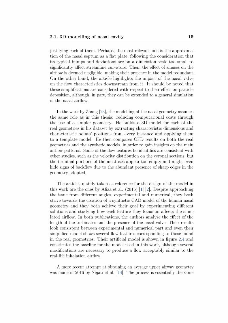
The articles mainly taken as reference for the design of the model inthis work are the ones by Afiza et al. (2015) [1] [2]. Despite approachingthe issue from different angles, experimental and numerical, they bothstrive towards the creation of a synthetic CAD model of the human nasalgeometry and they both achieve their goal by experimenting differentsolutions and studying how each feature they focus on affects the simu-lated airflow. In both publications, the authors analyse the effect of thelength of the turbinates and the presence of the nasal valve. Their resultslook consistent between experimental and numerical part and even theirsimplified model shows several flow features corresponding to those foundin the real geometries. Their artificial model is shown in figure 2.4 andconstitutes the baseline for the model used in this work, although severalmodifications are necessary to produce a flow acceptably similar to thereal-life inhalation airflow.
A more recent attempt at obtaining an average upper airway geometrywas made in 2016 by Nejati et al. [14]. The process is essentially the same

16 Chapter 2. State of the art
Figure 2.4: Synthetic model of human upper airways. Picture taken from [1]
as in [9], but the methods employed are more sophisticated: 2D coronalsections are "skeletonized" using splines and a template model is deformedto fit them, through control point matching. Finally, the control pointsundergo the median-finding step, before reconstruction of the 3D medianmodel, based on the resulting sections. The improvements in this approachinclude an increased robustness to heavier anatomical variations and thepossibility to artificially shape the synthetic model to one’s needs. For theinitial geometry adjustment, the article mostly replicates the proceduredescribed in [9], while using a normalisation length between AMS andchoana of 60mm.
Finally, the article by Xi et al. (2016) [22] eviscerates the effects ofnostril orientation on flow properties. The model used is a real nasalgeometry reconstructed from MRI (Magnetic Resonance Imaging) andthe numerical simulations used are of the LES (Large Eddy Simulation)type. The results suggest that the preservation of the realistic obliquenostril orientation in the modelling process is the best choice. In fact, adownward-directed inlet leads to inaccurate flow distribution in the fossae,while an anterior-directed inlet favours the generation of non-physicalvortices in the initial portion of the nasal cavity. Indeed, this turned outto be a critical aspect in the design of the model used for this work.

2.2. Numerical simulation of nasal airflow 17
2.2 Numerical simulation of nasal airflowThe numerical simulation of the airflow in such a complex geometry as
the human upper airways is no ordinary deal. The difficulties it presentsand the great relevance from the clinical point of view encouraged severalstudies during the past few years, involving any kind of CFD methods. Inthe scope of this thesis, RANS simulations are the preferred choice, whileLES is marginally employed for validation purposes, as more extensivelydescribed in Appendix A.
The incompressible steady-state Reynolds-Averaged Navier-Stokes equa-tions are a set of PDE (Partial Differential Equations) describing the motionof fluids. They are derived from the more general Navier-Stokes equationsby applying the Reynolds decomposition.
While the Navier-Stokes equations accurately describe the fluid motionin most cases, a phenomenon known as turbulence often comes into play.It can be defined as the chaotic behaviour displayed by the flow when itsReynolds number is large enough, which is true for almost any relevantreal-life situation. Since the fluctuations continuously involve every lengthscale, from the flow typical one to the microscopic Kolmogorov scales,and since they all need to be computed for accurate results, the DNS(Direct Numerical Simulation) approach is often deemed prohibitive interms of computational cost. Although it displays wide limitations and itcarries along several sources of error, the statistical approach introducedby Osborne Reynolds still is the most widespread way of tackling theturbulence issue. It results in a new set of PDE, the steady RANS:
∇ · 〈u〉 = 0 (2.1a)
∇ · 〈u〉〈u〉+∇ · 〈u′u′〉+1
ρ∇〈p〉 = ν∇2〈u〉 (2.1b)
In the notation used, u is the velocity vector, p is the pressure and ρis the density. The obtained set of equations is not a closed one. In fact,there is no mathematical relation tying the mean fields 〈u〉 and 〈p〉 to theterm 〈u′u′〉, which is known as Reynolds stresses tensor and includes theeffect of the fluctuating motions on the mean flow field. Closure requiresthe adoption of a model for the Reynolds stresses and the past fifty yearsof research on the subject produced a wide variety of solutions in thatperspective.
In consistency with previous works, such as [8], the model of choicefor the present work is k − ω SST , a two equation eddy-viscosity model,

18 Chapter 2. State of the art
first described by Menter in [12]. It originates from k − ω and k − εclassic models, blending them according to a suitable weighing function, tocapitalise on their respective strengths and mitigate their weaknesses. Inparticular, k − ω is dominant in the near-wall area, where its formulationis particularly convenient. In free-stream regions, k − ε is preferred due toits lower sensitivity to free-stream values of turbulent quantities.
Large Eddy Simulation is based on a spatial filtering operation, whichresults in the following set of equations:
∇ · u = 0 (2.2a)∂u
∂t+∇ · uu +
1
ρ∇p = ν∇2u (2.2b)
Similarly to the Reynolds stress tensor in the RANS approach, the SGS(Sub-Grid Scale) stress tensor τsgs is defined as:
τsgs = uu− u u (2.3)
and accounts for the effect of the sub-grid scale motions on the filteredquantities. The filtered equations 2.2 present the same closure problemas the RANS equations 2.1, requiring the modelling of τsgs. Among themost common models for sub-grid scale stresses is the Smagorinsky model,which is also the one adopted in the present work. In analogy with manyRANS turbulent models, it is based on a fictitious eddy-viscosity.
One of the main features distinguishing a LES from a RANS simulationis the improved accuracy and increased computational cost: the largerturbulent scales are directly calculated, limiting the modelling process tosmaller scales. Furthermore, LES is intrinsically unsteady, requiring anadequate time resolution and deferring a possible average operation to thepost-processing phase. For a more in-depth overview on RANS and LESapproaches, the reader should refer to [15].
The literature review on nasal airflow simulations starts with the ar-ticle by Zhao et al. [25]. The study investigates the connection betweenanatomical variations of the olfactory slit (upper-most part of the nasalfossa) and the olfactory function efficiency. The laminar, steady-state CFDsimulations were carried out on approx. 1.8 million element meshes. Theobjective of the study is, per se, of little relevance to this work, but itremains one of the first attempts at applying CFD to the human upperairways and to do so in a consistent manner, to the point that some of

2.2. Numerical simulation of nasal airflow 19
the procedures it establishes are still valid today. In a subsequent work,Zhao et al. (2006) [26] examine both human and rat nasal airflow in asniffing condition. The increase in the flow rate with respect to the previ-ous study [25] suggests that turbulence might play a role, so the laminarsimulations are paired with others employing turbulent models k− ε, k−ωand Spalart-Allmaras. An interesting aspect in both works concerns theboundary conditions: the flow is driven by a pressure difference imposedbetween the nostrils and the nasopharynx, a similar solution to the oneadopted in this work.
Some interesting considerations about the hypothesis of steady-stateflow are included in the article by Hörschler et al. (2010) [6]. Their CFDsimulations are run on a simplified model and on a real upper airway geome-try, obtained from CT-scans, and further corroborated by rhinomanometry3
measurements. The numerical methods involve a finite-volume methodand a Lattice-Boltzmann method and the flow-driving condition is of thepressure difference type. In order to enhance the unsteady effects, theStrouhal number is set to St = 0.791, while the Reynolds number lies in therange Re ≤ 2900. Results show a significant discrepancy between steadyand unsteady conditions at low and increasing mass-flux conditions, whilethe steady-state hypothesis seems to work adequately in high mass-fluxconditions i.e. in the middle of the inspiration or expiration act.
Works by Zubair et al. (2012) [27] and by Quadrio et al. (2014) [16]highlight how the airflow is largely influenced by a number of factors, whoseeffects are very difficult to account for. In fact, the nasal walls are usuallyconsidered rigid and smooth and the flow incompressible. Despite thesehypotheses, the geometry of a patient’s nasal cavity is far from fixed: thenasal cycle implies an alternate process of congestion and decongestion ofthe nasal fossae, constantly altering the shape of the airway and posturaleffects should be taken into account as well. Furthermore, the nasal mucosais rough and covered with cilia and the heat exchange between the bloodvessels in the nasal walls and the airflow suggests that a thermoaerody-namic approach should be adopted. Although of great importance, suchissues fall outside the scope of this thesis: they constitute a different line ofresearch within OpenNOSE, focusing on the crucial experimental validationof the numerical results obtained so far and described in article [4]. In anycase, plenty of empirical evidence collected over the years corroborates the
3Diagnosis technique adopted for nasal cavity and consisting in the direct measure-ment of pressure and flow

20 Chapter 2. State of the art
validity of the simulation procedures, making these procedures reasonablywell established and robust.
The article by Zhao et al. (2014) [24] finally tries to answer a funda-mental question for the potential clinical value of any CFD-related upperairway study: what is normal nasal airflow? In order to find an answer,they ran their investigation on 22 healthy patients, mostly young Cau-casian individuals, employing a k−ω model to account for turbulent effectsin their steady-state simulations. Despite the relative uniformity of thesample, results showed great variability in the geometries, with volumesand areas roughly varying by up to a factor 2. Some common featureswere identified, but most, like flow distribution across the meatuses, appearquite different even between healthy subjects such as these.

Chapter 3
Dataset generation
The initial step of the actual work consists in producing a simplifiedmodel of the human upper airways, fulfilling the following specifications:firstly, it needs to be simple, to make the CFD computations efficient.Secondly, despite the limited degree of accuracy required, the computedairflow should be qualitatively comparable to the one obtained in a realnasal geometry. Lastly, the necessity to easily introduce some anatomicalvariations calls for great versatility. The model is designed with FreeCAD,a popular open source parametric design software.
3.1 Base model
The base model in figure 3.1 satisfies all the aforementioned require-ments. It represents the air volume, acting as a negative of the bonesand tissues bounding the nasal cavity. As far as possible, the sharp edgesare filleted1 to discourage the formation of recirculation regions and themodel is perfectly symmetric, at least in this standard form. The referencesystem has its origin between the nasal vestibules, for design purposes.The x-axis acts as the frontal axis, the y-axis runs along the sagittal axisand the z-axis represents the vertical axis. About 10− 15mm down they-axis from the origin lies the point corresponding to the AMS, taken asreference in [9], [14]. Also, in compliance to these works, the choana waslocated on the y-axis, 75 mm from the origin and about 60-65 mm fromthe AMS.
1Mechanical engineering term which indicates the rounding of an edge and is com-monly used in CAD
21

22 Chapter 3. Dataset generation
Figure 3.1: Base model
Inlet sphere
The addition to the computational domain of a sphere, centred outsidethe nostrils and intersecting the external nose surface, achieves accuracyand robustness improvements of the CFD simulations. In fact, imposingboundary conditions away from the nasal vestibules has beneficial effectson the stability of the simulation and allows to already obtain an accuratesolution in the beginning portion of the airway. On the other hand, it doesnot entail an important increase in the computational costs, due to thelimited mesh refinement it requires. Only the spherical cap itself acts asan inlet surface, while the cut plane, which the nostrils are connected to,simulates the external nose, where wall boundary conditions are imposed.
Fossa
Figure 3.2 shows the 2D sketch on the yz-plane defining the shapeof the two identical nasal fossae, from the vestibules (on the left) to thenasopharynx (on the right). As anticipated, the general outline recalls theone described in [1]. Its most interesting aspect is the nostril orientation.Following the findings described in [22], nostril orientation is neither vertical,nor anterior. The value of 45◦ guarantees a flow distribution qualitativelysimilar to a real nasal airflow and avoids the presence of backflow in the

3.1. Base model 23
Figure 3.2: 2D sketch of a nasal fossa
terminal portions of the meatuses.
Nasal valve
The nasal valve is designed as a section contraction in the nasalvestibules area, as shown in figure 3.3. The dimensions are defined tooptimise the flow downstream: a more pronounced contraction causes anon-physical recirculation zone right behind the valve, while a less evidentone implies a high velocity flow on the olfactory region, which is actuallya low-velocity area enhancing the olfactory function.
Turbinates
The turbinates are implemented in two steps: firstly, the meatusesare extruded from the sketch in figure 3.4 and suitably smoothed. Thenthe nasal fossa is carved in their correspondence, to compensate for theincrease in CSA (Coronal Section Area). The result can be observed infigure 3.1. The inlet of the inferior meatus deserves a special mention, asit is one of the most critical features for the overall trend of the flow. It isobtained from the union and subtraction of four different blocks, so thatthe fossa and the meatus are connected as harmonically as possible. Themiddle meatus inlet and both outlets are less critical and could be obtainedvia filleting or with the addition of simple volumes. The superior meatus

24 Chapter 3. Dataset generation
Figure 3.3: CAD model detail: the nasal valve
Figure 3.4: 2D sketch of the inferior and middle meatus
is not vital to the general behaviour of the flow, but is mainly introducedto give the model greater versatility: its position can be easily modifiedwithout entailing abrupt changes in the airflow.
Central septum-like structure
This peculiar feature mimics the human nasal septum and serves twopurposes. One concerns flow quality: reducing the width of the mainfossa channel favours a more uniform flow distribution in the meatuses. Inaddition to this, its position along the x-axis becomes the perfect parameterto introduce asymmetry in the model. In figure 3.5 the reader can see theartificial septum besides the main air volume of the fossa and the result oftheir geometrical subtraction.

3.1. Base model 25
(a) (b)
Figure 3.5: Nasal septum before (a) and after (b) volume subtraction
Nasopharynx and laryngopharynx
The nasopharynx and laryngopharynx are implemented as separatevolumes and fused with the two nasal fossae, as shown in figure 3.6. Apartfrom the rounded corners, they do not display any notable detail, since theairflow in these regions is not particularly interesting and the geometryadopted does not have a significant impact on the flow upstream. Themain reason why they are included in the model is to impose more accurateoutlet boundary conditions, replicating the pressure difference generatedby the thoracic diaphragm in the lungs.
3.1.1 Airflow comparison on modelled and real geom-etry
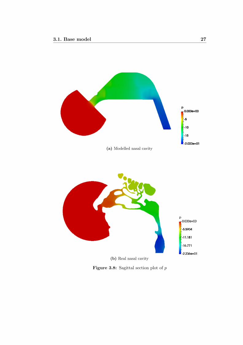
The base model described above is the result of several attempts.The modifications at each step were determined by comparing the CFD-simulated airflow in the model to the one obtained in a real nasal geometry.The final comparison shows the good degree of qualitative accuracy accom-plished, while also preserving properties of simplicity and flexibility. Theimages are obtained on ParaView (5.0.1), an open source visualisation soft-ware, which in recent years has become a standard for the post-processingof fluid dynamics simulations.
Looking at figure 3.7, the reader can notice that the real geometryincludes the sinuses, which are missing in the model for simplicity purposes,as suggested by [7]. The plotted quantity is the y-component of the velocity

26 Chapter 3. Dataset generation
Figure 3.6: CAD model detail: nasopharynx and laryngopharynx
(a) Modelled nasal cavity
(b) Real nasal cavity
Figure 3.7: Coronal section plot of uy
3.1. Base model 27
(a) Modelled nasal cavity
(b) Real nasal cavity
Figure 3.8: Sagittal section plot of p

28 Chapter 3. Dataset generation
Figure 3.9: Modification 1: septum lateral position
vector, normal to the section plane. The range is slightly different, sincethe comparison is purely qualitative, but the maximum values in both casesis around 2m/s. The flow distributions are very similar, with the higherflow-rate regions located in the central part of the fossa, in the middlemeatus and in the initial part of the inferior meatus. As for the pressuredistribution (figure 3.8), the CFD on the model reports quite differentresults from the one run on the real nasal geometry. This is, in part, due tothe higher size of the modelled nostrils, which causes a high velocity flowin the nasal vestibules. Still, the natural shape proves much more efficient:with similar imposed total pressure-over-density difference (20m2/s2 in themodel, 20.5m2/s2 in the real nasal geometry) the volumetric flow rate inthe model is much lower, 10.7l/min against 18.3l/min
3.2 Anatomical modifications
In order to create a wide dataset of diverse geometries and airflows,the following step was applying combinations of anatomical variations tothe base model. The variations introduced are eight, five of which behaveas harmless anatomical differences between healthy individuals, while theremaining three have a pathological impact on the airflow, replicating thecondition known as turbinate hypertrophy described in an earlier chapter.The modifications are defined with the help of the ENT experts of theteam.

3.2. Anatomical modifications 29
Figure 3.10: Modification 2: longitudinal position of superior meatus
1) Septum lateral position (non-pathological)
The first anatomical variation consists in the translation, along the x-axis, of the septum volume described in the previous section. Figure 3.9shows, from a top view, how the modification is practically implementedby reducing it to a single parameter. In the present dataset, the considereddistance varies from 0.3mm to 0.7mm, 0.5mm being the neutral position,which produces a symmetrical model.
2) Longitudinal position of superior meatus (non-pahological)
This modification focuses on the superior meatus and consists in translatingit along the y-axis, without affecting its size, as displayed in figure 3.10.The range adopted for this feature is 30mm to 38mm from the origin ofthe reference system.
3) Vertical position of superior meatus (non-pathological)
Similarly, a third variation is represented by the position of the superiormeatus on the z-axis, ranging between a 20mm and a 28mm distance fromthe origin.
4) Section change steepness at inferior meatus inlet (non-pathological)
The fourth non-pathological variation focuses on the section change, whichappears on the nasal fossa in correspondence of the beginning of theinferior meatus. In particular, the variation concerns the steepness of suchcontraction, varying between 1.1mm (for volume overlap reasons) and3.0mm. It is displayed in figure 3.11.

30 Chapter 3. Dataset generation
Figure 3.11: Modification 4: section change steepness at inferior meatus inlet
Figure 3.12: Modification 6: head of inferior turbinate hypertrophy
5) Nasal valve position (non-pathological)
As suggested by the title, this alteration involves the location of the nasalvalve. The valve is moved along the upper edge of the nasal vestibules,with a vertical distance from the origin of 6mm to 8mm.
6) Head of inferior turbinate hypertrophy (pathological)
As anticipated, the present model acts as a negative of the human nasalcavity: the geometry replicates the air volume of the human upper airways,while the tissues and bones constitute its boundaries. Therefore, thehypertrophy of the inferior turbinate is modelled as a constriction of theairways. The deformation can extend to the entire turbinate or just aportion of it and the sixth modification mimics the hypertrophic conditionof the head (anterior portion) of the inferior turbinate. It is implementedas a carve in the inferior meatus and in the corresponding area of the

3.2. Anatomical modifications 31
Figure 3.13: Modification 7: overall inferior turbinate hypertrophy
Figure 3.14: Modification 8: head of middle turbinate hypertrophy
vertical channel of the nasal fossa, and has width values ranging from0.1mm to 0.7mm, which is about half of the original meatus thickness. Itis displayed in figure 3.12.
7) Overall inferior turbinate hypertrophy (pathological)
This modification, as shown in figure 3.13, exactly replicates the previousone, although it affects the entire length of the inferior meatus, rather thanjust its anterior part. Limit values are still 0.1mm and 0.7mm.
8) Head of middle turbinate hypertrophy (pathological)
The last anatomical variation essentially reproduces the sixth one, butit is applied to the middle turbinate instead of the inferior one. It isalso reduced in size, proportionately to the lower size of the respectiveturbinates, varying from 0.1mm to 0.4mm. For greater variability in thedataset, this modification was applied in combination to either of the othertwo pathological conditions. The result can be seen in figure 3.14.

32 Chapter 3. Dataset generation
The eight modifications described are combined to generate 200 geome-tries, each different from the other. In particular, 100 cases include justthe non-pathological variations, while 100 more also include combinationsof turbinate hypertrophy. This characteristic composition of the datasetachieves an ideal 1:1 ratio of healthy and pathological cases, to guaranteean optimal training base for the Machine Learning algorithms. The modifi-cations corresponding to turbinate hypertrophy conditions are only appliedto the right (positive x-axis direction) nasal fossa, since altering the leftfossa would mostly produce mirrored images. In case a wider sample wasto be obtained, right side hypertrophies could be combined with left sidehypertrophies, leading to more geometries, but for the 200 cases of thiswork it is deemed unnecessary.
3.3 Numerical simulations
The CFD simulations employed are of the RANS type. Because of thehuge computational cost they entail, they are executed on the powerfulclusters of CINECA, via SSH protocol2. The software used is OpenFOAM(v1806+), a widely used open source CFD tool.
The setup of a RANS simulation on OpenFOAM is a delicate operation,especially when dealing with such complex geometries. Apart from the.stl3 files defining the geometry, all the simulations share the same settings.The setup is similar to the one described in a previous thesis on the subjectby Lamberti-Manara [8], whose main focus involved the achievement ofan accurate numerical simulation of the nasal cavity airflow. Despite this,many adjustments are necessary, mostly due to the different behaviourof the model with respect to the real geometry and to the necessity tomake the computations as efficient as possible, while slightly relaxing theaccuracy requirements. As mentioned earlier, the turbulent model adoptedis k − ω SST and air is considered a Newtonian fluid, with kinematicviscosity ν = 1.5 · 10−5m2/s.
Mesh generation
The starting point is the creation of an adequate computational grid. Withrespect to the mesh specifications, the initial block mesh is comprised of
2Secure SHell is a standard cryptographic protocol for networks, usually operatedvia command-line interface
3STereo Lithography is a file format used to describe triangulated surfaces. Widelyused in CAD applications

3.3. Numerical simulations 33
Figure 3.15: Computational mesh detail: middle meatus
cubes of edge length 1mm. This is then refined and deformed aroundthe model surface by means of the snappyHexMesh4 utility. Using ahigher refinement level for nasal walls and a lower one for the sphericalcap boundaries allows to optimise the mesh quality, without excessivelyincreasing its size. A typical final mesh includes 1.0-1.1 million cells.
Boundary conditions
Since these are steady-state RANS simulations and the turbulence modelof choice is a variant of k − ω, the independent variables involved are k,ω, p and u, while eddy viscosity νt is computed at every iteration from kand ω. The boundary condition driving the inspiration flow into the nasalcavity is a total pressure-over-density difference of 20m2/s2 between theinlet, represented by the spherical cap, and the outlet, which is the lowerface of the laryngopharynx, normal to the z-axis. The value was chosen toobtain flow conditions similar to a real nasal cavity airflow. The velocityvector u has a no-slip condition on the solid boundaries and a null normalgradient condition on the inlet and outlet. Boundary values for k and ωare computed according to the criteria defined by Menter in the originalarticle [12] presenting his k − ω SST model.
Numerical settings
The computational grid is subdivided into 8 parts for parallel computing,specifying equal weights since all processors are expected to have equal
4OpenFOAM built-in mesh generation tool. It takes as inputs a uniform block meshand a surface in .stl format and produces a new mesh, deformed around the inputsurface

34 Chapter 3. Dataset generation
Figure 3.16: Typical residual trend
performances. The numerical schemes adopted are first-order for stabilityreasons and the convergence criteria are quite strict, since the steady-flowhypothesis is not very sound for this kind of flow, as remarked by [6].The solver of choice is an OpenFOAM built-in, steady-state algorithm forincompressible flows: simpleFoam.
Convergence results
All the simulations met the convergence criteria in about 20 hours, includingthe meshing, decomposition and reconstruction processes. This correspondsto a number of iterations between 50000 and 60000. A typical residualplot of the variables is displayed in figure 3.16. The slowest variable toreach convergence is typically k, while the residual of p starts oscillatingaround a very low value much earlier than the final convergence.

Chapter 4
Learning from data
After the conclusion of the RANS simulations on the CAD generatedmodels, the dataset is almost ready for the ML model training. A prelimi-nary step is necessary and involves a significant reduction in the data size,which in the present form is unsuitable to train an ML algorithm. At first,this is done by switching from huge 3D scalar and vectorial fields to 2Dsections and other more manageable data structures. A further reductionis then carried out through the extraction of handcrafted features, whichshould summarise all the relevant information about the airflow in a fewbytes. Lastly, a more objective feature selection process is performed,exploiting some ad hoc techniques from the Machine Learning field, beforethe final training of the algorithm and the fine tuning of its parameters.In this setting, the word "feature" refers to both the characteristics of thenasal airflow and to the components of the input vectors of the trainingdataset, as the two concepts end up overlapping. As far as the predictionmodel is concerned, the data structure requires a Supervised Learningapproach. In particular, a regression setting will be adopted: even thoughthe pathological modifications are precisely introduced to 50% of the inputgeometries, some of them show a moderate degree of turbinate hypertrophyand assigning them a "healthy" or "pathological" label seems too sim-plistic an approach. Moreover, in a future perspective where the datasetwill include more realistic nasal models with an increased level of overallvariability, an a priori evaluation of the functionality of a nasal geometry isfar from trivial. Therefore, the ability to predict the severity of turbinatehypertrophy is deemed, in prospect, more useful than the one to distinguisha healthy nose from an unhealthy one.
35

36 Chapter 4. Learning from data
4.1 Data mining
Data reduction represents one of the most important parts of this thesis.On one hand, CFD typically involves huge amounts of data: in fact, forthe dataset considered here, a completed simulation output includes thecomputed airflow fields and the mesh data and weighs on average 210MB.This is valid for steady-state RANS simulations run on a relatively coarsemesh, since the simplified geometry employed allows to relax the meshquality constraints and still robustly reach convergence. Of course, in futuredevelopments, the need for accuracy will increase: the CFD simulationswill become LES or even DNS and the geometrical model used will be morerealistic, probably causing the size of CFD results to increase by up to 2-3orders of magnitude. On the other hand, ML methods generally requirevery large datasets, comprised of cases with a limited number of features.The dataset used in the present work includes 200 instances, which is closeto a lower bound even for a Supervised Learning application. Therefore,the size of every input vector should be at most in the order of some kB,before the feature selection further reduces it to a few numerical values.Clearly, the main obstacle to the application of ML techniques to CFDresults resides in the 5 (possibly more) orders of magnitude between whatone produces and what the other one needs.
The first step towards solving this issue is achieved through some typicalpost-processing operations, replacing 3D fields with a more convenient, lightand interpretable data structure. The software for this job is ParaView,which allows the user to easily automatise operations through Pythonscripting. Three kinds of data are extracted from the raw CFD results: 2Dsections, streamlines and average pressure values along the stream.
1) 2D sections
Slicing a 3D field to obtain 2D representations of the flow is perhaps themost intuitive way to reduce such a complex information, from an AI(Artificial Intelligence) perspective as much as for a human viewer. Infact, one of the advantages of this choice is the easy interpretation of theobtained images, which is a key factor in the medical field, as stated in [17].A total of six section planes, shown in figure 4.1, are chosen. They are allroughly at equal distance from each other and are all approximately normalto the main flow direction. Each section file contains the point coordinatesof the mesh and the field values for each cell. Since the turbulence variablesare not of any interest to the flow general aspect, only u and p fields aresaved, to further optimise data size. The section planes are named a

4.1. Data mining 37
Figure 4.1: Section planes selected for data extraction
through f according to the stream direction: plane a is the one sectioningthe nasal vestibules, the three coronal (normal to the y-axis) planes in theturbinate region are respectively b, c and d, while the oblique planes acrossthe nasopharynx and laryngopharynx are named e and f .
2) Streamlines
Streamlines are a classical visualisation tool in the CFD world, althoughtheir employment as ML input data is far from an established practice. De-spite this, they show considerable potential, introducing a time-dependentinformation in the mix. Naturally, dealing with steady-state RANS simu-lations, time is just a dummy variable generated by numerical integration,but in the future, with time-dependent simulations, the streamline datawill acquire even greater interest.
As displayed in figure 4.2, the streamlines are generated from a roughlyuniform grid on a ring placed upstream of the nostrils, for repeatabilityreasons. The number of streamlines (100), the ring’s position and its sizeare optimised for an efficient description of the airflow. The integrationscheme is a Runge-Kutta 4 (RK4) with a fixed step-length of 1.5 cells.The choice of this non-adaptive scheme is due to robustness considerations:because of numerical errors, only about 70% of the streamlines reach thelaryngopharynx and RK4 ensures the best success rate. The streamlinesdata include all field values at each point of every streamline, includingthe dummy-time produced in the trajectory integration.

38 Chapter 4. Learning from data
(a)
(b)
Figure 4.2: Ring with grid points (a) generating streamlines (b). Streamlinesare coloured according to velocity magnitude

4.2. Handcrafted feature extraction 39
Figure 4.3: Mean pressure plot on y-axis
3) Average pressure trend
This idea lies on the consideration that pressure has a typical decreasingtrend along the direction of the stream, as imposed by the boundaryconditions, while it shows little variability in a generic coronal section.Therefore, each instance is divided in 120 slices by coronal section planes,each thick 0.5mm. The domain portion covered starts downstream of thenasal valve, to avoid too large an influence on the first few slices, and endsin the choana. In each slice, the integral pressure and volume are computedand saved. The number of slices considered is arbitrarily high: with theintegral quantities available, the average pressure can be later computed inany number of slices submultiple of 120. The result is displayed in figure 4.3.
The first step of data mining accomplished a reduction in data sizeof almost 2 order of magnitudes, leading to post-processed instances ap-proximately as big as 3MB. In addition, the data is now in a convenientform for human visualisation as well, allowing a better understanding ofthe general flow behaviour and facilitating a tailored feature extraction tofurther synthesise the CFD results.
4.2 Handcrafted feature extraction
The issue tackled in this section is the extraction of a limited number offlow features, enclosing the overall aspect of the nasal airflow. In this phase,all the possibly significant features are generated: their actual relevanceis evaluated later in the feature selection process. The features shouldbe independent from morphological information and only focus on theflow field: extrapolating geometrical information from geometry-dependentfeatures would result in a trivial problem.

40 Chapter 4. Learning from data
0.000.040.080.120.16seconds
0.0
0.2
0.4
0.6
percen
tage
0.01s bin width
0.000.040.080.120.16seconds
0.02s bin width
0.000.040.080.120.16seconds
0.04s bin width
Figure 4.4: Arrival time histograms of streamlines
1) Arrival time histograms
Having plenty of space-dependent information in the 2D sections, sometime-dependent data is obtained from the streamlines. In detail, thestreamlines are separated from one another according to the dummy timevariable, which is reset to zero at the beginning of each line. Then the totaltime each one takes to get from plane a to plane f is computed and theresults are distributed in a number of bins to generate the histograms shownin figure 4.4. This procedure takes place after a selection of the streamlines:the ones not reaching plane f are discarded to avoid contamination of thevalid data. The optimal number of bins for the histograms is determinedto be four. This allows to preserve some degree of interpretability: thefour values generated can be thought of as the ratio of early, mid-early,mid-late and late arriving streamlines. After a suitable normalisation tothe total number of streamlines reaching plane f , the time-dependentinformation carried by the streamlines is thus condensed in a few floatingpoint numbers.
2) Flow rate distribution along z-axis
This feature is based on the three coronal sections corresponding to planesb, c and d. Firstly, each one is divided horizontally along the yz-plane, inleft and right nasal fossa and vertically in a number of bands along thez-axis. Then, in every one of the resulting 2D regions, the y-componentof the velocity is integrated to compute the volume flow rate across thatsurface. Considering every section plane file includes a matrix UY , whosevalues correspond to the uy evaluated in each pixel, the flow rate percentagein each region Rk is computed as:

4.2. Handcrafted feature extraction 41
Figure 4.5: Flow distribution across sections b, c, d (left to right)
Figure 4.6: Mean values of |u| over sections b, c, d (left to right)
flowratek =
∑(i,j)∈Rk
UY [i, j]∑i
∑j UY [i, j]
(4.1)
As reported in equation 4.1, the flow rate of every region is normalisedto the volume flow rate across the entire section (which naturally is thesame for all three planes), yielding the flow distribution along the z-axisfor each side of every coronal section. The optimal number of horizontalbands is six, as later established by a feature selection process: a biggernumber implies too high a correlation among the features, causing the datavariance to increase excessively, while a smaller number can not describeadequately the flow distribution. An example of this feature is displayedin figure 4.5, where each region is coloured according to its flow rate share.
3) Average field values in low resolution grids
The idea behind this feature is similar to the previous one. The maindifferences concern the grid generation strategy, the physical meaning of thefeatures produced and the quantities they involve. First, sections b, c and dare divided vertically in three regions of equal height and horizontally in sixregions, three on each nasal fossa, as shown in figure 4.6. The output values

42 Chapter 4. Learning from data
Figure 4.7: Centres of gravity of coronal plots
computed in each region are the mean values of pressure p and velocitymagnitude |u|. The number of regions is determined by interpretabilityreasons: the three vertical bands describe the flow behaviour in the lower,middle and upper portion of the fossae, roughly corresponding to themeatuses, while the three horizontal bands separate the vertical duct alongthe septum from the closer and farther part of the meatuses.
4) Centres of gravity on coronal sections
This is the most synthetic feature of the lot and is extracted from eachof the three coronal sections. A centre of gravity (COG) is located in thesection for |u| and p, computing it as follows:
COGq(S) =
∑i
(i ·∑
j Sq[i, j])
∑i
∑j Sq[i, j]
,
∑j
(j ·∑
j Sq[i, j])
∑i
∑j Sq[i, j]
(4.2)
where q is the quantity considered and Sq is the matrix containingits values across section S. In figure 4.7 the reader can see the overallCOG (in red) and the COGs of each fossa computed separately (in green).Additionally, a black dot represents the fixed centre of the image and servesas reference point.

4.2. Handcrafted feature extraction 43
−14
−12
−10pressu
re (m
2 /s2 )
1st degraw
3rd degraw
0.00 0.02 0.04 0.06y coordinate (m)
−14
−12
−10
pressu
re (m
2 /s2 )
6th degraw
0.00 0.02 0.04 0.06y coordinate (m)
8th degraw
Figure 4.8: Polynomial fitting of various degrees of the pressure trend alongy-axis
5) Average pressure polynomial coefficients
This feature is based on the average pressure data described in the previoussection. Directly using the average pressure values on an arbitrary numberof slices would result in highly correlated features, carrying local informa-tion. Instead, the solution adopted consists in computing the coefficientsof a polynomial, which is fitted on the curve employing a classical leastsquares method. This way, the data is reduced to a few floating pointnumbers and each of them is representative of the general trend of thepressure. The degree of the polynomial is empirically chosen to be six, asa compromise between accuracy and feature lightness. Some alternativesare displayed in figure 4.8.
All the 154 values summarising the extracted flow features are con-catenated in arrays and become features in the ML sense, i.e. the valuesforming the input vectors xi. The 200 resulting input vectors are organisedin a matrix, while the values of the three anatomical variations definingthe hypertrophic conditions in the turbinates of the initial geometriesconstitute target output vectors yi. Even before the final feature selectionprocess, the input dataset has been reduced from the initial weight of 108Bper instance, to a more manageable size of 103B per case.
According to their nature, the features can be organised in the following

44 Chapter 4. Learning from data
groups:
• PPT: the coefficients of the polynomial fit of the pressure trend alongthe y-axis ;
• FPd: the flow distribution along the z-axis on section d;
• FPc: the flow distribution along the z-axis on section c;
• FPb: the flow distribution along the z-axis on section b;
• APd: the grid averaged values for p on section d;
• AVd: the grid averaged values for |u| on section d;
• APc: the grid averaged values for p on section c;
• AVc: the grid averaged values for |u| on section c;
• APb: the grid averaged values for p on section b;
• APb: the grid averaged values for |u| on section b;
• AI: the arrival-time histograms.
4.3 Feature selectionThe objective of the this step is establishing which features are most
significant in describing the general flow trend. This process is beneficial intwo ways: on one hand, it generates interpretable insights about the effectsof turbinate hypertrophy on the nasal airflow and, on the other, it reducesthe number of features used in the training process. In fact, as explainedin chapter 1, the number of features used for Supervised Learning tasksshould be limited, especially when dealing with small datasets.
4.3.1 Feature selection procedures
Practically, three separate regression environments are defined, one foreach turbinate hypertrophy version: anterior inferior turbinate hypertro-phy, overall inferior turbinate hypertrophy and anterior middle turbinatehypertrophy. This choice is driven by result interpretation reasons. Foreach target value, a test set including 20% of the cases is set aside, whilethe remaining 80% is used right away as a training set, in a cross valida-tion (CV) frame. This consists in dividing the training set in L subsets
4.3. Feature selection 45
and performing L training tasks on L − 1 subsets of data each, leavingevery time a different one out and using it as a test set. In particular, toavoid generating subsets too small, L is set to 5. This strategy allows toartificially expand the dataset, averaging the results for greater accuracy.Throughout the work, both CV and regression results are evaluated on thebase of the R2-score, defined as:
R2 = 1−∑N
i=1 (yi − yi)2∑Ni=1 (yi − y)2
(4.3)
where i is the sample index, yi is the target value associated to thei-th input vector, yi is the corresponding predicted target value and y isthe mean over all target outputs. The R2-score ranges between 0 and 1and it can be thought of as the amount of variance in the target outputsexplained by the regression model. The algorithms used in this phaseinclude Extra-Trees and Lasso and the feature selection process is carriedout according to three different strategies.
Recursive Feature Elimination with Cross Validation (RFECV)
It falls under the embedded methods class and consists in performingrecursive training attempts of a chosen algorithm, eliminating at each stepfrom the input set the lowest ranked k features, until a minimum numberof features m is reached. In this work, k = 1 and m = 5.
Forward Feature Selection with Cross Validation (FFSCV)
This one belongs to the wrapper methods class: at every step, the featureguaranteeing the highest score increment is added to an initially emptyset. The score is computed through CV by iteratively trying to includein the set every unused feature. The process stops at M = 100 features.This way, the score trend can be observed as each feature is added to theset and used to define in retrospect the optimal subset.
Feature selection on all available data
An additional embedded feature selection task is carried out as a validationstep, training both Lasso and Extra-Trees algorithms with all the availablefeatures and looking at the outcome of their internal feature rankingmechanism.

46 Chapter 4. Learning from data
0.0 0.2 0.4
AIAVbAPbAVcAPcAVdAPdFPbFPcFPdPPT
RFECV
0.00 0.25 0.50
AIAVbAPbAVcAPcAVdAPdFPbFPcFPdPPT
FFS
0.0 0.1 0.2
AIAVbAPbAVcAPcAVdAPdFPbFPcFPdPPT
ALL
(a) Lasso
0.0 0.2
AIAVbAPbAVcAPcAVdAPdFPbFPcFPdPPT
RFECV
0.0 0.2 0.4 0.6
AIAVbAPbAVcAPcAVdAPdFPbFPcFPdPPT
FFS
0.0 0.1
AIAVbAPbAVcAPcAVdAPdFPbFPcFPdPPT
ALL
(b) Extra-Trees
Figure 4.9: Bar plot of maximum importance per feature group for each se-lection strategy. The target output is anterior middle turbinatehypertrophy
4.3.2 Feature selection results
The first relevant outcome of the feature selection process is ratherunexpected: one of the groups of extracted features, the COG position ofp and |u|, shows a very strong correlation to the target output, i.e. theturbinate hypertrophy severity degree. This makes the problem trivial andleads to the exclusion of this feature group from the input set. The reasonis that the COGs are too strongly correlated to the geometry itself, ratherthan to the airflow trend. Additionally, this spurious correlation is likely todisappear when dealing with more realistic nasal geometries, which showgreater geometrical variability than the simplified models employed in thissetting.
A further consideration concerns the effectiveness of the two algorithmschosen for the task: due to its intrinsic linearity, the Lasso regularisationproves unable to recognise the correlation among features, thus producing

4.3. Feature selection 47
Figure 4.10: Feature importance plots for anterior inferior turbinate hypertro-phy, computed with RFECV method on Extra-Trees algorithm
inconsistent results when tested with different feature selection strategies.On the other hand, Extra-Trees shows greater robustness, due to itsensemble nature. Proof of this behaviour is given in figure 4.9: Lassoassigns high importance to different feature types, depending on the methodused, while Extra-Trees is more consistent, at least across the RFECV andAll-features approaches. As for the feature selection strategy adopted, theRecursive Feature Elimination method is deemed more reliable, as ForwardFeature Selection does not show any effect on the R2-score as the featuresare added to the input set.
Figures 4.10, 4.11 and 4.12 report the outcome of the feature selection,relative to each version of turbinate hypertrophy. For each, a bar plotshows the maximum importance in each feature group. On the right-hand side of the figures, the nine feature groups generated from coronalsections b, c and d offer insights on which variables and flow regions aremost significant for every target output. Both arrival-time histograms andpolynomial fit of pressure trend are consistently discarded because of theirlow predictive value. The results appear anything but trivial: every formof turbinate hypertrophy shows correlation to different features and theareas of interest are located both on the right-hand side, which is the onewhere pathological deformations are introduced, and on the left-hand side,suggesting that predictive value indeed resides in the simulated airflow,rather than in the geometry.

48 Chapter 4. Learning from data
Figure 4.11: Feature importance plots for overall inferior turbinate hypertro-phy, computed with RFECV method on Extra-Trees algorithm
Figure 4.12: Feature importance plots for anterior middle turbinate hypertro-phy, computed with RFECV method on Extra-Trees algorithm

4.3. Feature selection 49
(a) Healthy model (b) Slight anterior infe-rior turbinate hyper-trophy
(c) Severe anterior infe-rior turbinate hyper-trophy
Figure 4.13: Velocity magnitude distribution on section b
In detail, a highly relevant feature in the prediction of anterior inferiorturbinate hypertrophy is the pressure value in the inferior meatus of sectionc, which is widely anticipated since it is just downstream of the introducedvariation. More surprisingly, the top ranked feature involves the velocitymagnitude in section b of both fossae. A simple explanation is that thepredictive value is not located separately in the two regions, but in theirdifference, caused by the pathological shape. This is corroborated by figure4.13: the flow in the left fossa is similar across all three cases, but itsdiscrepancy with the right fossa increases as turbinate hypertrophy getsmore severe.
As far as the overall inferior turbinate hypertrophy is concerned, itis best predicted by the flow rate percentage across the lower part ofthe inferior meatus on section b and c: this is not surprising, since thegeometrical deformation affects that exact region, reducing the passagewaywidth and, thus, the flow rate through it. A more unexpected occurrenceamong the top features is the average pressure in the lower d section ofboth fossae. Again, this is probably due to the significance of the differencein the two flow regions. In fact, as displayed in figure 4.14, the difference inpressure distribution between healthy, partially hypertrophic and severelyhypertrophic model is remarkable. The lower part of the fossa has probablybeen chosen over the upper region because it is less heavily impacted bythe middle turbinate hypertrophy.
Finally, the anterior middle turbinate hypertrophy turned out to be themost difficult pathological condition to identify: only a few features showdecisive predicting value and adding more results in a degradation of theregression score. This small significant group mostly concerns the middleand upper part of the right-hand fossa, where the geometrical modification

50 Chapter 4. Learning from data
(a) Healthy model (b) Slight overall inferiorturbinate hypertro-phy
(c) Severe overall infe-rior turbinate hyper-trophy
Figure 4.14: Pressure distribution on section d
occurs. On the other hand, the pressure value in the middle meatus of theleft-hand fossa at section d also shows relevance. The additional difficultyin the prediction of this pathological condition is probably due to thefact that it always presents itself paired with either one of the other twohypertrophy variants. This makes it harder for the model to identify howmiddle turbinate hypertrophy alone affects the airflow.
4.4 Predictive model: training and results
The final prediction model is based on Gaussian Processes. Thischoice is only possible because of the reduced size of the input sample:as anticipated, the covariance matrix inverted in the prediction processgrows with the number of instances in the dataset and a larger samplewould entail excessive computational costs. Among the advantages of thisalgorithm is the higher interpretability of the results. Moreover, a meanvalue and a variance are predicted, thus allowing the evaluation of both theaccuracy and the confidence level of the prediction. The regression tasksare carried out separately for each of the three target outputs and severalruns are made, in order to carefully tune the algorithm parameters and toinvestigate how the prediction quality changes by varying the number offeatures used from 1 to 5. The best features for each regression setting arehandpicked, according to the feature selection outcome reported previously.The results are shown in figures 4.15, 4.16 and 4.17, reporting R2-scoresand the related mean square errors (MSE) of the predictions.

4.4. Predictive model: training and results 51
1 2 3 4 5N° of features
0.2
0.4
0.6
0.8
1.0r2-sco
re
(a)
1 2 3 4 5N° of features
0.0
0.5
1.0
1.5
MSE
(b)
Figure 4.15: R2-score and MSE trend for anterior inferior turbinate hyper-trophy prediction with number of features varying from 1 to5
1 2 3 4 5N° of features
0.800.850.900.951.00
r2-sco
re
(a)
1 2 3 4 5N° of features
0.0
0.2
0.4
MSE
(b)
Figure 4.16: R2-score and MSE trend for overall inferior turbinate hypertrophyprediction with number of features varying from 1 to 5
1 2 3 4 5N° of features
0.4
0.6
0.8
r2-sco
re
(a)
1 2 3 4 5N° of features
0.0
0.5
1.0
MSE
(b)
Figure 4.17: R2-score and MSE trend for anterior middle turbinate hyper-trophy prediction with number of features varying from 1 to5

52 Chapter 4. Learning from data
The outcome looks promising: the R2-score is close to unity, confirmingthe strong correlation between the chosen features and the target values.In particular, the hypertrophic conditions of the inferior turbinate showthe best results, with a very accurate prediction of the target and verylow variance, especially when using all the top five features. On theother hand, middle turbinate hypertrophy proves slightly more difficultto predict: the R2-score is still very high, but its associated MSE is notnegligible as in the other cases. As anticipated, this is probably due to thefact that anterior middle turbinate hypertrophy never occurs as the onlyhypertrophic condition affecting the nasal geometries, making it tougherfor the model to find a clear correlation between flow features and thispathological variation alone. The accomplishment of such high scores, inspite of the fact that pathological modifications are often combined, is quiteimpressive and constitutes further proof of the robustness and accuracy ofthe procedures adopted.

Conclusions
This conclusive chapter is shared by this thesis and the one by LucaButera [3]. This choice highlights the interdisciplinary approach of thiswork, which involved a collaboration between the CFD team of DAER,the ML team of DEIB and the ENT clinical experts of San Paolo Hospital.
Firstly, the main steps of the work are briefly reviewed: according tothe exploratory character of the study, the real nasal geometries are setaside, in favour of a simplified CAD model, with several advantages. Fromthe CFD perspective, a simpler domain facilitates numerical convergence.On the ML side, the variability in the input dataset is reduced becausethe geometries are obtained from local modifications of a single standardmodel. This aspect helps the prediction of the pathological condition, sincevariations in the airflow are imputable to either turbinate hypertrophyor five other harmless geometrical variants. After the input models aregenerated, a RANS simulations is run on each of them. The choice ofRANS is driven by the necessity to keep computational costs to a minimum,to avoid high commitment in a preliminary study such as this. The CFDoutput undergoes a significant size reduction, mostly through the extractionof hand-tailored features. These are chosen for their high interpretability,since black box approaches are widely distrusted in the medical field. Afeature selection task is carried out on the extracted flow characteristics. Itrepresents a key stage: on one hand, it solves the noise issue typical of smallsamples and, on the other, it allows to gather insights about the significanceof the flow features, isolating and ranking the ones with predictive value.Finally, a regression model is trained with the best features, to verify theirpredictivity and to finally assess whether turbinate hypertrophy in a nasalcavity model can be predicted by looking at the CFD simulated airflow.
Despite the preliminary nature of this study, the outcome is encouragingand the procedures established look effective and robust. The achievedprediction scores are remarkably high, but this does not mean that theproblem is trivial. In fact, the results show how even independent patho-logical variations, when combined, are harder to predict. Moreover, the
53

54 Conclusions
top ranked features often concern areas not directly influenced by the geo-metrical modifications, again confirming that the predictive value residesin the airflow, rather than in the geometry itself.
Future perspectivesThe exploratory nature of this work puts great emphasis on future
development. The results achieved show considerable potential, but thefinal objective is still quite far: the implementation of a tool that accuratelypredicts how well a patient’s nasal cavity performs and identifies anypathological state affecting it. This will result in more precise and reliablediagnoses and will help validate surgical procedures.
A way to improve the performance of the ML model consists in generat-ing a larger dataset. This would allow to experiment with fully data-driventechniques, exploiting in a deeper way the informative potential hiddenin the data. A possible alternative is adopting more advanced SupervisedLearning approaches, such as Deep Learning, which need a huge amountof input data, but are able to extrapolate higher level knowledge. A biggersample size would also allow switching to entirely different paradigms, suchas Unsupervised Learning: a large dataset could be clustered to allowa posteriori identification of the important flow features. Moreover, thesample increment will become crucial when dealing with more complexnasal models. In fact, the next suggestions aim at increasing the accuracyof the input data. On the one side, this could be accomplished by devel-oping a more complicated and realistic nasal model, or even by directlyworking with real geometries, depending on the availability of CT scan data.The result would be a significant step towards real-life application: thepredictive models would face the variability and complexity typical of thereal human upper airways. On the other side, the nasal airflow simulationcould involve a different CFD approach: despite the clear advantages of aRANS approach, the results it produces are inherently wrong. Therefore,switching to LES or DNS would entail higher computational costs, but thereliability of the simulation would increase accordingly.
All things considered, it is proven possible to successfully detect anoma-lies in a nose-like structure using simulated airflow data. This representsa solid first step towards the creation of a diagnostic tool based on Ma-chine Learning techniques and CFD simulations, and, ultimately, towardsunderstanding what "good" nasal flow is.

Appendix A
LES and RANS comparison
The necessity to reduce computational costs to a minimum, on onehand, and the limited accuracy required by the use of a simplified geometrywith no clinical value, on the other, leads to the selection of RANS as themost suitable CFD technique. Although widely justified by the preliminarynature of this study, the employment of RANS simulations is one of themain sources of inaccuracy in the dataset generation process. In order toquantify this error, a more accurate Large Eddy Simulation is run on thestandard CAD model depicted in chapter 3.
The simulation is run on OpenFOAM and the main features of itssetup are rapidly reviewed hereby, starting from the computational gridspecifications: the mesh is refined around the model surface, startingfrom a block mesh consisting of cubes of edge length 0.5mm. The finalgrid includes 8.6 million elements. The difference with the coarser meshgenerated for the RANS can be appreciated in figure A.1.
The model for sub-grid scale stress tensor is the classical Smagorinskymodel with Van Driest damping and the solver chosen for the task is
(a) LES (b) RANS
Figure A.1: Mesh detail comparison: middle meatus
55
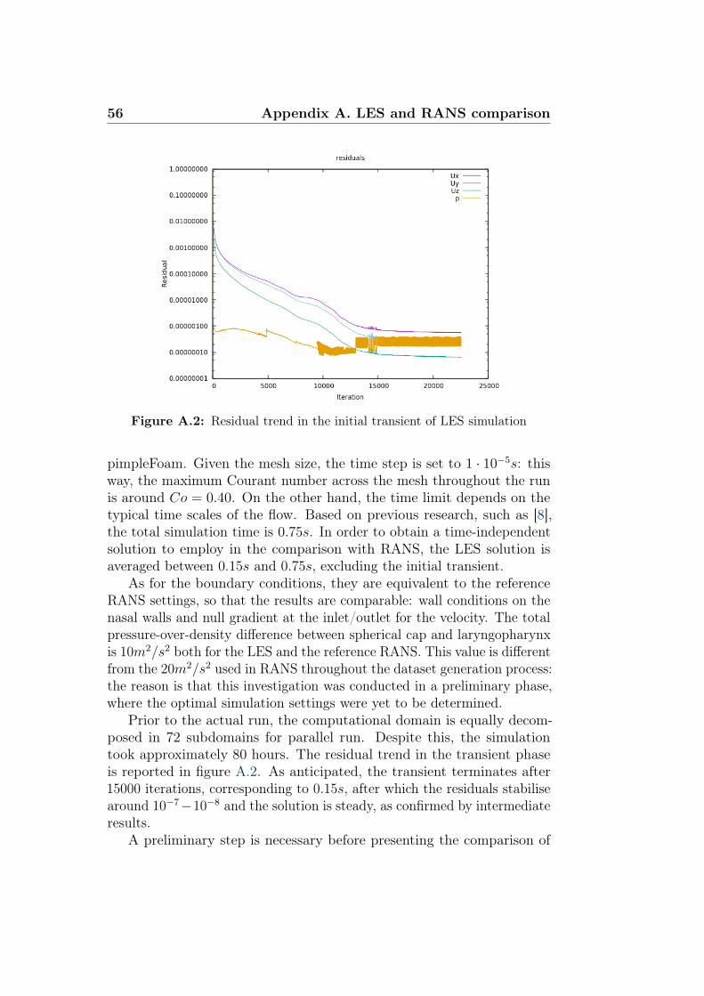
56 Appendix A. LES and RANS comparison
Figure A.2: Residual trend in the initial transient of LES simulation
pimpleFoam. Given the mesh size, the time step is set to 1 · 10−5s: thisway, the maximum Courant number across the mesh throughout the runis around Co = 0.40. On the other hand, the time limit depends on thetypical time scales of the flow. Based on previous research, such as [8],the total simulation time is 0.75s. In order to obtain a time-independentsolution to employ in the comparison with RANS, the LES solution isaveraged between 0.15s and 0.75s, excluding the initial transient.
As for the boundary conditions, they are equivalent to the referenceRANS settings, so that the results are comparable: wall conditions on thenasal walls and null gradient at the inlet/outlet for the velocity. The totalpressure-over-density difference between spherical cap and laryngopharynxis 10m2/s2 both for the LES and the reference RANS. This value is differentfrom the 20m2/s2 used in RANS throughout the dataset generation process:the reason is that this investigation was conducted in a preliminary phase,where the optimal simulation settings were yet to be determined.
Prior to the actual run, the computational domain is equally decom-posed in 72 subdomains for parallel run. Despite this, the simulationtook approximately 80 hours. The residual trend in the transient phaseis reported in figure A.2. As anticipated, the transient terminates after15000 iterations, corresponding to 0.15s, after which the residuals stabilisearound 10−7−10−8 and the solution is steady, as confirmed by intermediateresults.
A preliminary step is necessary before presenting the comparison of

57
Figure A.3: Difference of pressure fields between RANS and LES solutions ina sagittal section
the results and consists in the mapping of the RANS solution to the finercomputational grid used for the LES: this allows to compute difference ofvelocity and pressure fields, which is the most representative and syntheticway to get a full picture of the magnitude of discrepancy between the two.
The resulting differential fields displayed in figures A.3, A.4 and A.5are quite far from the ideal null fields which would be obtained if the twosimulations produced equal outcomes. The difference in the pressure fieldactually remains within 10% throughout the domain, with the exceptionof very local peaks near the wall due to boundary effects, but the velocitymagnitude difference is much more significant, especially in the high velocityregions at the inlet of the inferior meatus and in the lower part of thenasal fossae. The coronal section in figure A.5 shows a consistent velocitydifference along the vertical channel close to the nasal septum. It is in theorder of 0.35m/s, which roughly corresponds to a 15− 20% discrepancy.Additionally, difference of velocity peaks are present at the inferior meatusentrance and are in the order of 100% of the values in the original velocityfields.
Given that LES intrinsically produces a more truthful reconstruction ofthe flow field, by largely reducing the impact of turbulence modelling, thecomparison remarks how the RANS approach limits the accuracy of theresults. The main conclusion drawn by this investigations is the potentialimprovement margin, which can be achieved in the future, by switching tomore advanced CFD techniques.

58 Appendix A. LES and RANS comparison
Figure A.4: Difference of velocity magnitude fields between RANS and LESsolutions in a sagittal section
Figure A.5: Difference of velocity magnitude fields between RANS and LESsolutions in a coronal section

Appendix B
Codes and listings
This section includes the main codes implemented in the automatisationof the post-processing procedures, for a more thorough overview on theprocedures adopted.
Listing B.1: Automatic data download
1 #!/usr/bin/expect2
3 # GRAB PASSWORD4 stty -echo5 send_user -- "Password for username: "6 expect_user -re "(.*)\n"7 send_user "\n"8 stty echo9 set pass $expect_out (1,string)
10
11 # DOWNLOAD12 spawn scp -r [email protected]:/
path_to_file /path_to_folder13 expect "password:"14 send "$pass\n"15 interact
Listing B.1 reports a short Expect script that makes the download (andupload) of data on the CINECA servers more efficient. Expect is a typicaltool to automatise operations on SSH operations. The second part of thecode can be copied and pasted to download and upload several objectsat a time. The uploading version is simply obtained by exchanging thedestination and the source directories.
59

60 Appendix B. Codes and listings
Listing B.2: Post-processing operations including the extraction of coronalsections and streamlines
1 from paraview.simple import *2
3 for i in range (1 ,201):4
5 case = str(i)6 openPath = ’/path_to_folder_case_(i)’7 savePath = ’/path_to_folder_case_(i)’8
9 # create a new ’OpenFOAMReader ’10 a1foam = OpenFOAMReader(FileName=openPath)11 a1foam.MeshRegions = [’internalMesh ’]12 a1foam.CellArrays = [’U’, ’p’]13
14 # get animation scene15 animationScene1 = GetAnimationScene ()16 animationScene1.GoToLast ()17
18 # Slice a19 slice1 = Slice(Input=a1foam)20 slice1.SliceType = ’Plane ’21 slice1.SliceOffsetValues = [0.0]22 slice1.SliceType.Origin = [0.0, 0.0, 0.004]23 slice1.SliceType.Normal = [0.0, 1.0, 1.0]24
25 SaveData(savePath + ’/a.vtm’, proxy=slice1 ,Writealltimestepsasfileseries =1,DataMode=’Binary ’)
26
27 # create StreamTracerWithCustomSource28 disk1 = Disk()29 disk1.InnerRadius = 0.00430 disk1.OuterRadius = 0.01131 disk1.RadialResolution = 332 disk1.CircumferentialResolution = 2533
34 transform1 = Transform(Input=disk1)35 transform1.Transform = ’Transform ’36 transform1.Transform.Translate = [0.0, 0.0005 ,
-0.0065]

61
37 transform1.Transform.Rotate = [-45.0, 0.0,0.0]
38 transform1.Transform.Scale = [0.7, 0.9, 0.0]39
40 streamTracerWithCustomSource1 =StreamTracerWithCustomSource(Input=a1foam ,SeedSource=transform1)
41 streamTracerWithCustomSource1.Vectors = [’POINTS ’, ’U’]
42 streamTracerWithCustomSource1.IntegrationDirection = ’FORWARD ’
43 streamTracerWithCustomSource1.IntegratorType =’Runge -Kutta 4’
44 streamTracerWithCustomSource1.InitialStepLength = 1.5
45 streamTracerWithCustomSource1.MaximumSteps =8000
46 streamTracerWithCustomSource1.MaximumStreamlineLength = 0.3
47 streamTracerWithCustomSource1.ComputeVorticity= 0
48
49 SaveData(savePath + ’/st.csv’, proxy=streamTracerWithCustomSource1)
Listing B.2 on page 59 shows the Python code used to automatically runthe main post-processing operations on Paraview. For synthesis purposes,only the generation of section a is reported: sections b through f share thesame commands.
Listing B.3: Post-processing operations including the extraction of pressureintegral values in slices along y-axis
1 from paraview.simple import *2
3 import csv4
5 for i in range (1 ,201):6
7 case = str(i)8 openPath = ’/path_to_folder_case_(i)’9 savePath = ’/path_to_folder_case_(i)’
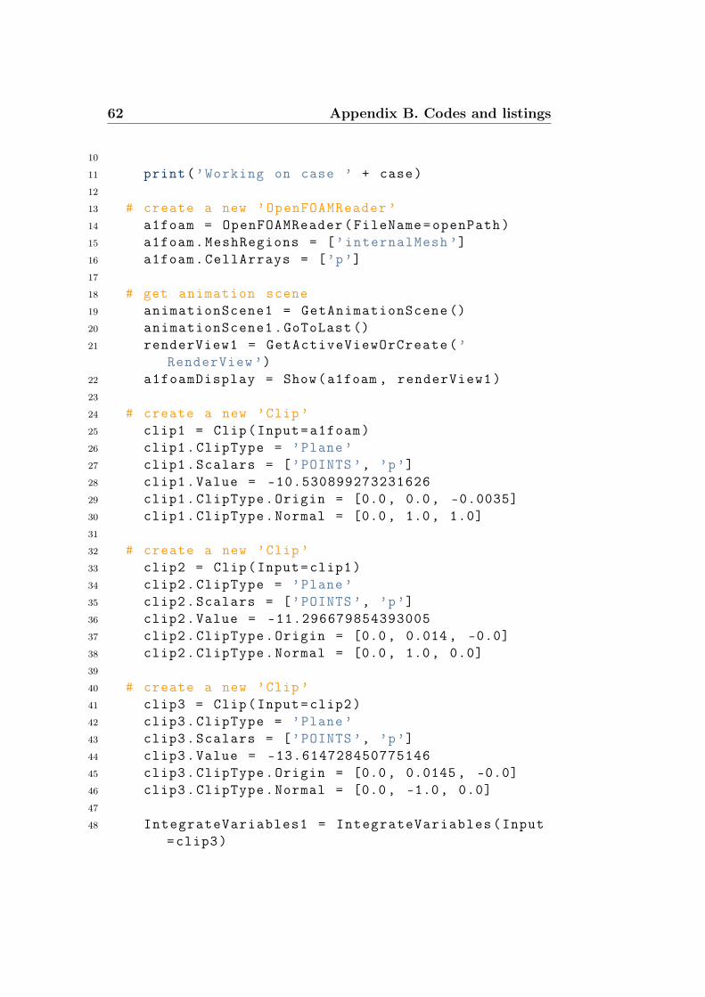
62 Appendix B. Codes and listings
10
11 print(’Working on case ’ + case)12
13 # create a new ’OpenFOAMReader ’14 a1foam = OpenFOAMReader(FileName=openPath)15 a1foam.MeshRegions = [’internalMesh ’]16 a1foam.CellArrays = [’p’]17
18 # get animation scene19 animationScene1 = GetAnimationScene ()20 animationScene1.GoToLast ()21 renderView1 = GetActiveViewOrCreate(’
RenderView ’)22 a1foamDisplay = Show(a1foam , renderView1)23
24 # create a new ’Clip’25 clip1 = Clip(Input=a1foam)26 clip1.ClipType = ’Plane’27 clip1.Scalars = [’POINTS ’, ’p’]28 clip1.Value = -10.53089927323162629 clip1.ClipType.Origin = [0.0, 0.0, -0.0035]30 clip1.ClipType.Normal = [0.0, 1.0, 1.0]31
32 # create a new ’Clip’33 clip2 = Clip(Input=clip1)34 clip2.ClipType = ’Plane’35 clip2.Scalars = [’POINTS ’, ’p’]36 clip2.Value = -11.29667985439300537 clip2.ClipType.Origin = [0.0, 0.014, -0.0]38 clip2.ClipType.Normal = [0.0, 1.0, 0.0]39
40 # create a new ’Clip’41 clip3 = Clip(Input=clip2)42 clip3.ClipType = ’Plane’43 clip3.Scalars = [’POINTS ’, ’p’]44 clip3.Value = -13.61472845077514645 clip3.ClipType.Origin = [0.0, 0.0145 , -0.0]46 clip3.ClipType.Normal = [0.0, -1.0, 0.0]47
48 IntegrateVariables1 = IntegrateVariables(Input=clip3)

63
49
50 finalFile = open(savePath + ’/clip’ + case + ’.csv’,’wb’)
51 fd = csv.writer(finalFile)52
53 fd.writerow ([’p’, ’Volume ’, ’Cell Type’])54
55 writer = CreateWriter(savePath + ’/clip’ +case + ’_tmp.csv’, IntegrateVariables1)
56 writer.FieldAssociation = "Cells"57
58 list = range (0 ,120)59
60 for j in list:61
62 lb = 0.0140 + 0.0005*j63 ub = 0.0145 + 0.0005*j64
65 #Properties modified on clip3.ClipType66 clip3.ClipType.Origin = [0.0, ub , 0.0]67
68 # Properties modified on clip2.ClipType69 clip2.ClipType.Origin = [0.0, lb , 0.0]70
71 # create a new ’Integrate Variables ’72 integrateVariables1 = IntegrateVariables(
Input=clip3)73
74 # writes the integrated variable table tothe tmp file
75 writer.UpdatePipeline ()76
77 # appends the integrated results of thisClip to the final csv file
78 ftmp = open(savePath + ’/clip’ + case + ’_tmp.csv’,’rb’)
79 reader = csv.reader(ftmp , delimiter=’,’)80 row = reader.next()81 row = reader.next()82 fd.writerow(row)83 ftmp.close()

64 Appendix B. Codes and listings
84
85 # destroy integrateVariables186 Delete(integrateVariables1)87 del integrateVariables188
89 # destroy clip390 Delete(clip3)91 del clip392
93 # destroy clip294 Delete(clip2)95 del clip296
97 # destroy clip198 Delete(clip1)99 del clip1
100
101 # destroy a1foam102 Delete(a1foam)103 del a1foam104
105 # close case csv file106 finalFile.close()107 del(writer)
Listing B.3 on page 61 reports the extraction of the pressure and volumeintegral values from thin slices distributed along the y-axis. They are latermanipulated to compute averaged pressure values and, eventually thecoefficients of a polynomial fit as described in chapter 4.

Bibliography
[1] E. Afiza et al. “Airflow Patterns within Real and 3D SimplifiedModels of Nasal Cavities (I. Experimental Study)”. In: Proceedings ofthe School of Engineering, Tokai University. E 40 (2015), pp. 97–108(cit. on pp. 2, 15, 16, 22).
[2] E. Afiza et al. “Airflow Patterns within Real and 3D SimplifiedModels of Nasal Cavities (II. Numerical Study)”. In: Proceedings ofthe School of Engineering, Tokai University. E 40 (2015), pp. 109–119(cit. on p. 15).
[3] L. Butera. “Nasal pathology assessment through Supervised Learningon Computational Fluid Dynamics data: a preliminary study”. MAthesis. Politecnico di Milano (cit. on pp. 2, 53).
[4] F. Cozzi, G. Felisati, and M. Quadrio. “Velocity measurements innasal cavities by means of stereoscopic PIV - Preliminary tests”. In:Journal of Physics: Conference Series 882 (Aug. 2017) (cit. on p. 19).
[5] P. Geurts, D. Ernst, and L. Wehenkel. “Extremely RandomizedTrees”. In: Machine Learning 63 (Apr. 2006), pp. 3–42 (cit. on p. 8).
[6] I. Hörschler, W. Schröder, and M. Meinke. “On the assumption ofsteadiness of nasal cavity flow”. In: Journal of Biomechanics 43.6(Apr. 2010), pp. 1081–1085 (cit. on pp. 19, 34).
[7] E. Javaheri, L. Golshahi, and W.H. Finlay. “An idealized geometrythat mimics average infant nasal airway deposition”. In: Journal ofAerosol Science 55 (Jan. 2013), pp. 137–148 (cit. on pp. 14, 25).
[8] G. Lamberti and F. Manara. “Simulazioni RANS e LES della fluido-dinamica delle cavità nasali”. MA thesis. Politecnico di Milano, 2014(cit. on pp. 1, 2, 17, 32, 56).
[9] Y. Liu et al. “Creation of a standardized geometry of the humannasal cavity”. In: Journal of Applied Physiology 106.3 (Mar. 2009),pp. 784–795 (cit. on pp. 14, 16, 21).
65

66 Bibliography
[10] Machine Learning bites. url: https://medium.com/ machine -learning-bites/machine-learning-decision-tree-classifier-9eb67cad263e (cit. on pp. 7, 8).
[11] D.J.C. MacKay. Information Theory, Inference, and Learning Al-gorithms. Cambridge University Press, 2003, pp. 535–548 (cit. onp. 10).
[12] F.R. Menter. “Two-Equation Eddy-Viscosity Turbulence Modelsfor Engineering Applications”. In: AIAA Journal 32.8 (Aug. 1994),pp. 1598–1605 (cit. on pp. 18, 33).
[13] T. M. Mitchell. Machine Learning. 1st ed. McGraw-Hill, Inc., 1997(cit. on p. 5).
[14] A. Nejati et al. “A deformable template method for describing andaveraging the anatomical variation of the human nasal cavity”. In:BMC Medical Imaging 16 (2016) (cit. on pp. 15, 21).
[15] S.B. Pope. Turbulent Flows. Cambridge University Press, 2000 (cit.on p. 18).
[16] M. Quadrio et al. “Review of computational fluid dynamics in the as-sessment of nasal air flow and analysis of its limitations”. In: EuropeanArchives of Oto-Rhino-Laryngology 271.9 (Sept. 2014), pp. 2349–2354(cit. on pp. 1, 19).
[17] Y. Saeys, I. Inza, and P. Larrañaga. “A review of feature selectiontechniques in bioinformatics”. In: Bioinformatics 23.19 (Aug. 2007),pp. 2507–2517 (cit. on pp. 6, 36).
[18] St. Louis Sinus Center. url: https://www.stlsinuscenter.com/turbinate-reduction/ (cit. on p. 14).
[19] S. Standring and N.R. Borley. Gray’s Anatomy: The AnatomicalBasis of Clinical Practice. ClinicalKey 2012. Churchill Livingstone/El-sevier, 2008 (cit. on p. 11).
[20] The Respiratory System. url: https://www.therespiratorysystem.com/nasal-cavity/ (cit. on pp. 12, 13).
[21] R. Tibshirani. “Regression Shrinkage and Selection via the Lasso”. In:Journal of the Royal Statistical Society. Series B (Methodological)58 (1996), pp. 267–288 (cit. on p. 9).
[22] J. Xi, J. Kim, and X. April Si. “Effects of nostril orientation on airflowdynamics, heat exchange, and particle depositions in human noses”.In: European Journal of Mechanics - B/Fluids 55 (201), pp. 215–228(cit. on pp. 16, 22).

Bibliography 67
[23] J. Zhang. “Characteristic size research of human nasal cavity andthe respiratory airflow CFD analysis”. In: Journal of Biosciences andMedicines 1.2 (2013), pp. 23–27 (cit. on p. 15).
[24] K. Zhao and J. Jianbo. “What is normal nasal airflow? A computa-tional study of 22 healthy adults”. In: International Forum of Allergy& Rhinology 4.6 (June 2014), pp. 435–46 (cit. on p. 20).
[25] K. Zhao et al. “Effect of Anatomy on Human Nasal Air Flow andOdorant Transport Patterns: Implications for Olfaction”. In: ChemicalSenses 29.5 (June 2004), pp. 365–379 (cit. on pp. 18, 19).
[26] K. Zhao et al. “Numerical Modeling of Turbulent and Laminar Airflowand Odorant Transport during Sniffing in the Human and Rat Nose”.In: Chemical Senses 31.2 (Feb. 2006), pp. 107–118 (cit. on p. 19).
[27] M. Zubair et al. “Review: A Critical Overview of Limitations of CFDModeling in Nasal Airflow”. In: Journal of Medical and BiologicalEngineering 32.2 (2012), pp. 77–84 (cit. on p. 19).


