Embed Size (px)
Citation preview

Macroscopic optical response and photonic bands
This article has been downloaded from IOPscience. Please scroll down to see the full text article.
2013 New J. Phys. 15 043037
(http://iopscience.iop.org/1367-2630/15/4/043037)
Download details:
IP Address: 132.248.33.139
The article was downloaded on 30/04/2013 at 19:46
Please note that terms and conditions apply.
View the table of contents for this issue, or go to the journal homepage for more
Home Search Collections Journals About Contact us My IOPscience
Macroscopic optical response and photonic bands
J S Perez-Huerta1, Guillermo P Ortiz2, Bernardo S Mendoza3
and W Luis Mochan1
1 Instituto de Ciencias Fısicas, Universidad Nacional Autonoma de Mexico,Apartado Postal 48-3, 62251 Cuernavaca, Morelos, Mexico2 Departamento de Fısica, Facultad de Ciencias Exactas, Naturales yAgrimensura, Universidad Nacional del Nordeste, Avenida Libertad 5400Campus-UNNE, W3404AAS Corrientes, Argentina3 Division of Photonics, Centro de Investigaciones en Optica, Leon, Guanajuato,MexicoE-mail: [email protected], [email protected], [email protected] [email protected]
New Journal of Physics 15 (2013) 043037 (18pp)Received 21 December 2012Published 19 April 2013Online at http://www.njp.org/doi:10.1088/1367-2630/15/4/043037
Abstract. We develop a formalism for the calculation of the macroscopicdielectric response of composite systems made of particles of one materialembedded periodically within a matrix of another material, each of whichis characterized by a well-defined dielectric function. The nature of thesedielectric functions is arbitrary, and could correspond to dielectric or conducting,transparent or opaque, absorptive and dispersive materials. The geometryof the particles and the Bravais lattice of the composite are also arbitrary.Our formalism goes beyond the long-wavelength approximation as it fullyincorporates retardation effects. We test our formalism through the study ofthe propagation of electromagnetic waves in two-dimensional photonic crystalsmade of periodic arrays of cylindrical holes in a dispersionless dielectric host.Our macroscopic theory yields a spatially dispersive macroscopic responsewhich allows the calculation of the full photonic band structure of the system,as well as the characterization of its normal modes, upon substitution into themacroscopic field equations. We can also account approximately for the spatialdispersion through a local magnetic permeability and analyze the resultingdispersion relation, obtaining a region of left handedness.
Content from this work may be used under the terms of the Creative Commons Attribution 3.0 licence.Any further distribution of this work must maintain attribution to the author(s) and the title of the work, journal
citation and DOI.
New Journal of Physics 15 (2013) 0430371367-2630/13/043037+18$33.00 © IOP Publishing Ltd and Deutsche Physikalische Gesellschaft
2
Contents
1. Introduction 22. General theory 33. Periodic binary systems 44. Recursive method 65. Results 86. Conclusions 15Acknowledgments 16References 16
1. Introduction
The propagation of light within homogeneous materials is completely characterized by usingtheir electromagnetic response. In the optical regime, magnetic effects are typically negligibleso that knowledge of the dielectric response is sufficient for the study of wave propagation [1].However, when the system has spatial inhomogeneities, the behavior of light is not trivial andthis has captured the attention of many researchers [2–11]. As an example, plasmon–polaritonspectra of quasiperiodic superlattices have been investigated [12, 13] and have been shown tohave a fractal character. Novel effects have been obtained, for example, negative refraction,inverse Doppler effect, optical invisibility cloaking and optical magnetism, etc [14–17].4
Effective medium theories [18–26] have been proposed for describing inhomogeneoussystems, such as diluted colloidal suspensions in the quasistatic or long-wavelength limit,in terms of a homogeneous macroscopic response. Further developments on homogenizationof composites have been proposed [27–35] and their limits of validity have been discussed[2, 36, 37].
In this paper, we obtain the macroscopic optical response using a computationally efficientreformulation of a procedure [5, 6] originally developed for accounting for the local field effectof systems with spatial fluctuations. Our main result is that for any system, the macroscopicresponse to an external excitation is simply the average projection of the correspondingmicroscopic response. We apply this general result to Maxwell equations in order to obtainan explicit expression for the macroscopic dielectric response of binary composites. Weillustrate its use with numerical results for a two-dimensional (2D) periodic photonic crystal.As the wavelength of the electromagnetic field becomes comparable with the characteristicmicroscopic spatial lengthscale of the system, retardation effects become important, yielding anon-local [38, 39] macroscopic response, with a strong dependence on the wavevector besidesits usual dependence on frequency. When the full spatial dispersion is taken into account, thephotonic band structure of the system can be obtained and analyzed from its macroscopicresponse.
This paper is organized as follows. In section 2, we formulate a general theory for themacroscopic dielectric response of composite systems. In section 3, we adapt our formulationto periodic systems made of two alternating materials, each characterized by well-defineddielectric functions. In section 4, we develop an efficient computational scheme which allows
4 See the special section on negative refraction and metamaterials for optical science and engineering in [17].
New Journal of Physics 15 (2013) 043037 (http://www.njp.org/)
3
the numerical calculation of the macroscopic response without recourse to explicit operationsbetween large matrices. In section 5, we obtain the non-local macroscopic dielectric tensor anduse it to calculate macroscopically the full band structure of a 2D photonic crystal made up ofnon-dispersive dielectric components; we compare it with exact results as well as with resultswithin a local approximation that partially accounts for spatial dispersion through an effectivemagnetic permeability. Finally, in section 6, we present the conclusions.
2. General theory
Consider a non-magnetic inhomogeneous system characterized by its dielectric responseε, defined through the constitutive equation D = εE, where D and E are the microscopicdisplacement and electric fields, respectively. We designate these fields as microscopic as theyhave spatial fluctuations due to the inhomogeneities of the material. They are not microscopicin the atomic scale, but rather on the scale of the spatial inhomogeneities of the system. We usea caret (ˆ) over a symbol to denote its operator nature and leave implicit the dependence of thedielectric response on position as well as on frequency. Our purpose is to obtain the macroscopicdielectric response of the system, relating the macroscopic displacement and electric fields, fromwhich the fluctuations have been removed.
We start from Maxwell equations for monochromatic microscopic fields. We follow theusual procedure [40] to decouple the magnetic field from the electric field to obtain the second-order wave equation
WE =4πc
iqJ, (1)
where
W = ε−1
q2∇ ×∇× = ε +
1
q2∇
2PT (2)
is the wave operator, q = ω/c is the wavenumber of light in vacuum, ω is the frequency, c isthe speed of light in vacuum and J is the external electric current density. Here we introducedthe transverse projector PT such that the transverse projection of a field F is FT
= PTF. Forcompleteness, we also introduce the longitudinal projector PL such that PL + PT
= 1, with 1 theidentity operator. Note that equation (1) contains both a longitudinal and a transverse part, so itdescribes not only transverse waves, but also allows for the possible excitation of longitudinalwaves such as plasmons [41].
We solve equation (1) formally for E to obtain
E =4πc
iqW−1J. (3)
As we are interested on the macroscopic response of the system, we introduce the average Pa
and fluctuation Pf projectors, such that an arbitrary field F can be written as F = Fa + Ff withFa = PaF its average and Ff = PfF its fluctuating part, and we identify the average field with themacroscopic field Fa ≡ FM. Later, we will provide appropriate explicit definitions for Pa and Pf;here we remark that they must be idempotent P2
a = Pa, P2f = Pf, i.e. the average of the average
is the average, and the fluctuations of the fluctuations are the fluctuations [5]. Furthermore,PaPf = PfPa = 0 and Pa + Pf = 1.
New Journal of Physics 15 (2013) 043037 (http://www.njp.org/)
4
As the macroscopic response would be useless unless the external excitations are devoidof microscopic spatial fluctuations, we assume that the external current has no fluctuations, soJf = 0 and J = JM
= PaJM, where we used the idempotency of Pa. Thus, acting on both sidesof equation (3) with Pa we obtain
EM=
4πc
iqW−1
aa JM. (4)
Here we define Oαβ ≡ PαOPβ , with α, β = a,f for any operator O. As equation (4) relates themacroscopic external electric current to the macroscopic electric field, we may identify themacroscopic inverse wave operator W−1
M ,
EM=
4πc
iqW−1
M JM, (5)
where
W−1M = W−1
aa . (6)
We summarize this result stating that the macroscopic inverse wave operator is simplythe average of the microscopic inverse wave operator. This is a particular case of a moregeneral result: the macroscopic response to an external excitation is simply the average of thecorresponding microscopic response.
From the macroscopic Maxwell equations, we may further relate the macroscopic waveoperator in equations (5) and (6) to the macroscopic dielectric response of the system εM through
WM= εM +
1
q2∇
2PaPT (7)
in analogy to equation (2). Thus, we have to invert the wave operator, average it and invertit again to finally identify the macroscopic dielectric response. Note that we have made noapproximation whatsoever. We remark that as ε relates to two fields, E and D, that have spatialfluctuations, we may not simply average ε to obtain its macroscopic counterpart, i.e. εM
6= εaa.The difference constitutes the local field effect [5].
Our result may easily be generalized to other situations and other response functions. Theprocedure consists of first identifying the response (in our case W−1) to the external perturbation(i.e. J) and then averaging it to yield the corresponding macroscopic response (i.e. W−1
M = W−1aa ),
which may further be related to the desired macroscopic response operator (i.e. εM).
3. Periodic binary systems
In this section, we use equation (6) to obtain the optical properties of an artificial binary crystalmade of two materials A and B with dielectric functions εA and εB . We assume that bothmedia are local and isotropic so that εA and εB are simply complex functions of the frequency.For convenience, we will further assume that εA is real, although this assumption is easilyrelaxed [42].
We introduce the characteristic function B(r) of the inclusions, such that B(r)≡ 1whenever r is on the region B occupied by the inclusions, and B(r)≡ 0 otherwise. Thus, wemay write the microscopic dielectric response as
ε(r)=εA
u(u − B(r)) , (8)
New Journal of Physics 15 (2013) 043037 (http://www.njp.org/)
5
where we defined the spectral variable u ≡ 1/(1 − εB/εA) [19]. The microscopic wave operatorof equation (2) may be written as
W =εA
u(ug−1
− B), (9)
where the characteristic operator B corresponds to multiplication by B(r) in real space, and wedefined
g =
(1 +
∇2PT
q2εA
)−1
, (10)
which, as shown below, plays the role of a metric.Using equation (9) we write equation (6) as
W−1M =
u
εAgaa(u − Bg)−1
aa , (11)
where we have taken advantage of the fact that g is unrelated to the texture of the crystal, so thatit does not couple the average to fluctuating fields.
Using Bloch’s theorem [43], we consider an electric field of the form [21]
Ek(r)=
∑G
EGei(k+G)·r, (12)
where k is a given wavevector, {G} is the reciprocal lattice of our crystal and the coefficientsEG represent the field in reciprocal space. In this representation, all operators may be written asmatrices with vector index pairs G,G′, besides other possible indices, such as Cartesian ones.Thus, we represent the longitudinal projector as the matrix
PLGG′ = δGG′
(k + G)|k + G|
(k + G′)
|k + G′|(13)
with δGG′ the Kronecker’s delta, so the transverse projector becomes PTGG′ = 1δGG′ −PL
GG′ with1 the Cartesian identity matrix. The Laplacian operator in reciprocal space is represented by
∇2→ −(k + G)2δGG′ (14)
and we can define the average projector as a cutoff in the reciprocal space [6]
(Pa)GG′ = δG0δG′0, (15)
so that average fields simply keep the contributions with vector k while all other wavevectorsare filtered out.
As shown by equation (11), we only require
(u − Bg)−1aa = (u − Bg)−1
00 (16)
to obtain the macroscopic inverse wave operator, where the subindices 0 denote the projectiononto the subspace with G = 0.
New Journal of Physics 15 (2013) 043037 (http://www.njp.org/)
6
4. Recursive method
The calculation of equation (16) is analogous to that of a projected Green’s function [44, 45]
Gaa(ε)= 〈a|G(ε)|a〉 (17)
onto a given state |a〉, where
G(ε)= (ε− H)−1 (18)
is the Green’s operator corresponding to some Hermitian Hamiltonian H and ε is a complexenergy. In [28] a similar result was obtained, where the Hamiltonian H was identified withthe longitudinal projection of the characteristic function BL L , the energy ε with the spectralvariable u, and |a〉 with a slowly varying longitudinal wave, and it was shown that thecorresponding projected Green’s function was proportional to the inverse of the longitudinalmacroscopic dielectric function. Haydock’s method may be applied to obtain the projectedGreen’s function (17) in a very efficient way [46, 47], and it has been adapted previously [28]to the calculation of the optical response of nanostructured systems in the long-wavelengthlocal limit. In this section, we generalize the approach of [28] to arbitrary frequencies andwavevectors.
Equations (17) and (18) are similar to equation (16), although the operator product H= Bgthat plays the role of a Hamiltonian does not correspond to a symmetric matrix. Nevertheless,it would correspond to a Hermitian operator if we use g as a metric, that is, if we use 〈ψ |g|φ〉
instead of 〈ψ |φ〉 as the scalar product of two arbitrary states |ψ〉 and |φ〉. Then, it is easyto verify the Hermiticity condition [〈ψ |g(H|φ〉)]∗ = 〈φ|g(H|ψ〉). Note, however, that g is notpositive definite.
According to equation (11), we need the average (u − Bg)−1aa → 〈a|(u − Bg)−1
|a〉, wherewe projected onto an average state |a〉 = b0|0〉 consisting of a plane wave with a givenwavevector k, frequency ω and polarization e. Here, |0〉 is normalized according to the metricg, i.e. 〈0|g|0〉 = g0 = ±1, and the coefficient b0 is a real positive number chosen to guaranteethat |a〉 is normalized in the usual sense 〈a|a〉 = 1. Now, we define | − 1〉 ≡ 0 and we obtainnew states by means of the recursion relation
|n + 1〉 ≡ Bg|n〉 = bn+1|n + 1〉 + an|n〉 + gn−1gnbn|n − 1〉, (19)
where all the states |n〉 are orthonormalized according to the metric g, that is,
〈n|g|m〉 = gnδnm (20)
with gn = ±1 and δnm the Kronecker’s delta function. The requirement of orthonormality yieldsthe generalized Haydock coefficients an, bn+1 and gn+1 given the previous coefficients bn, gn andgn−1. Thus, an are obtained from
〈n|g|n + 1〉 = angn (21)
and bn+1 from
〈n + 1|g|n + 1〉 = gn+1b2n+1 + gna2
n + gn−1b2n, (22)
New Journal of Physics 15 (2013) 043037 (http://www.njp.org/)
7
where we choose the sign gn+1 = ±1 so that b2n+1 is positive and we may choose bn+1 as a real
positive number. In the basis {|n〉}, Bg is represented by a tridiagonal matrix with an along themain diagonal, bn along the subdiagonal and gn−1gnbn along the supradiagonal, so that
u − Bg →
u − a0 −b1g1g0 0 0 · · ·
−b1 u − a1 −b2g2g1 0 · · ·
0 −b2 u − a2 −b3g3g2 · · ·
......
.... . .
. (23)
Note that we may represent the states |n〉 through the corresponding Cartesian field componentsfor each reciprocal vector G or for each position r within a unit cell. Thus, the action of g is atrivial multiplication in reciprocal space, while that of B is a trivial multiplication in real space,and we may repeatedly compute Bg|n〉 and Haydock’s coefficients without performing any largematrix multiplication, by alternatingly fast-Fourier transforming our representation betweenreal and reciprocal space. More explicitly, we represent a state |n〉 through its componentsnG,i = 〈G, i|n〉, where |G, i〉 corresponds to a normalized plane wave with wavevector k + G andpolarization i along the i th Cartesian direction. Then, g|n〉 is represented by φG,i = 〈G, i|g|n〉 =
gi j(G)nG, j , where, according to equation (10),
gi j(G)=εaq2δi j − (ki + G i)(k j + G j)
εaq2 − (k + G)2(24)
is a small Cartesian matrix for each G. Performing a fast Fourier transform, we obtain〈r, i|φ〉 = φr,i in real space, which we then multiply by B(r) to obtain |n + 1〉, representedin real space by (n + 1)r,i = B(r)φr,i . Fourier transforming back into reciprocal space andorthonormalizing, we obtain Haydock coefficients an, bn+1 and gn+1, and the new state |n + 1〉
represented by (n + 1)G,i = 〈Gi|n + 1〉. As discussed above, we iterate this procedure to obtainenough coefficients to converge the continued fraction (25).
According to equation (11), we do not require the full inverse of the matrix (23), but onlythe element in the first row and the first column. Following [28], we obtain that element as acontinued fraction, which when substituted into equation (11) yields
W−1M →
∑i j
ei(W−1M )i j e j =
u
εA
g0b20
u − a0 −g0g1b2
1
u−a1−g1g2b2
2
u−a2−g2g3b2
3
...
. (25)
The right-hand side of equation (25) denotes the macroscopic response projected onto a statewith the given wavevector k, frequency ω and polarization e. Due to the translational invarianceof the homogenized system, the inverse wave operator for a given k corresponds simply to atensor with Cartesian components (W−1
M )i j . Thus, so far we have calculated its inner productswith e, as shown by the second term of equation (25). We may repeat the calculation abovefor different orientations of the (possibly complex) unit polarization vector e and solve theresulting equations for all the individual Cartesian components (W−1
M )i j . Finally, we perform amatrix inversion of this macroscopic tensor and we use equations (6) and (7) to compute themacroscopic dielectric tensor
εMi j (ω,k)=
1
q2(k2δi j − ki k j)+WM
i j (ω,k). (26)
New Journal of Physics 15 (2013) 043037 (http://www.njp.org/)
8
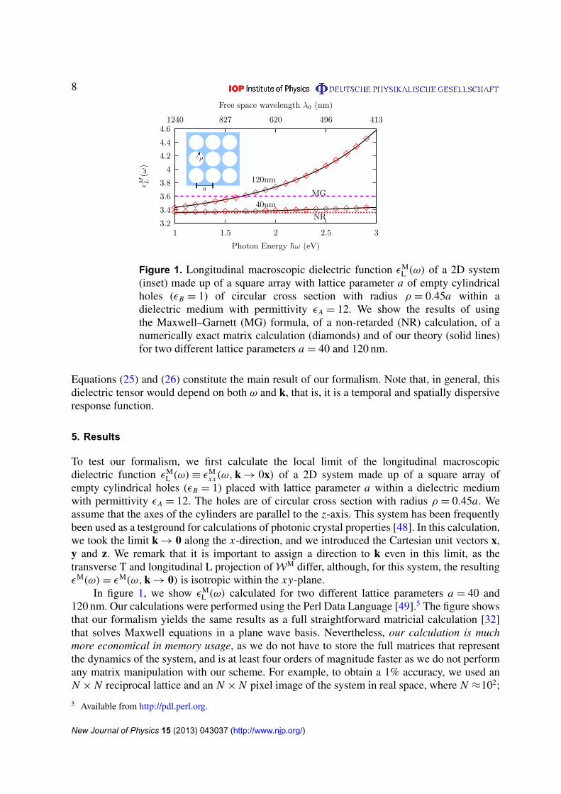
Figure 1. Longitudinal macroscopic dielectric function εML (ω) of a 2D system
(inset) made up of a square array with lattice parameter a of empty cylindricalholes (εB = 1) of circular cross section with radius ρ = 0.45a within adielectric medium with permittivity εA = 12. We show the results of usingthe Maxwell–Garnett (MG) formula, of a non-retarded (NR) calculation, of anumerically exact matrix calculation (diamonds) and of our theory (solid lines)for two different lattice parameters a = 40 and 120 nm.
Equations (25) and (26) constitute the main result of our formalism. Note that, in general, thisdielectric tensor would depend on both ω and k, that is, it is a temporal and spatially dispersiveresponse function.
5. Results
To test our formalism, we first calculate the local limit of the longitudinal macroscopicdielectric function εM
L (ω)≡ εMxx(ω,k → 0x) of a 2D system made up of a square array of
empty cylindrical holes (εB = 1) placed with lattice parameter a within a dielectric mediumwith permittivity εA = 12. The holes are of circular cross section with radius ρ = 0.45a. Weassume that the axes of the cylinders are parallel to the z-axis. This system has been frequentlybeen used as a testground for calculations of photonic crystal properties [48]. In this calculation,we took the limit k → 0 along the x-direction, and we introduced the Cartesian unit vectors x,y and z. We remark that it is important to assign a direction to k even in this limit, as thetransverse T and longitudinal L projection ofWM differ, although, for this system, the resultingεM(ω)= εM(ω,k → 0) is isotropic within the xy-plane.
In figure 1, we show εML (ω) calculated for two different lattice parameters a = 40 and
120 nm. Our calculations were performed using the Perl Data Language [49].5 The figure showsthat our formalism yields the same results as a full straightforward matricial calculation [32]that solves Maxwell equations in a plane wave basis. Nevertheless, our calculation is muchmore economical in memory usage, as we do not have to store the full matrices that representthe dynamics of the system, and is at least four orders of magnitude faster as we do not performany matrix manipulation with our scheme. For example, to obtain a 1% accuracy, we used anN × N reciprocal lattice and an N × N pixel image of the system in real space, where N ≈102;
5 Available from http://pdl.perl.org.
New Journal of Physics 15 (2013) 043037 (http://www.njp.org/)
9
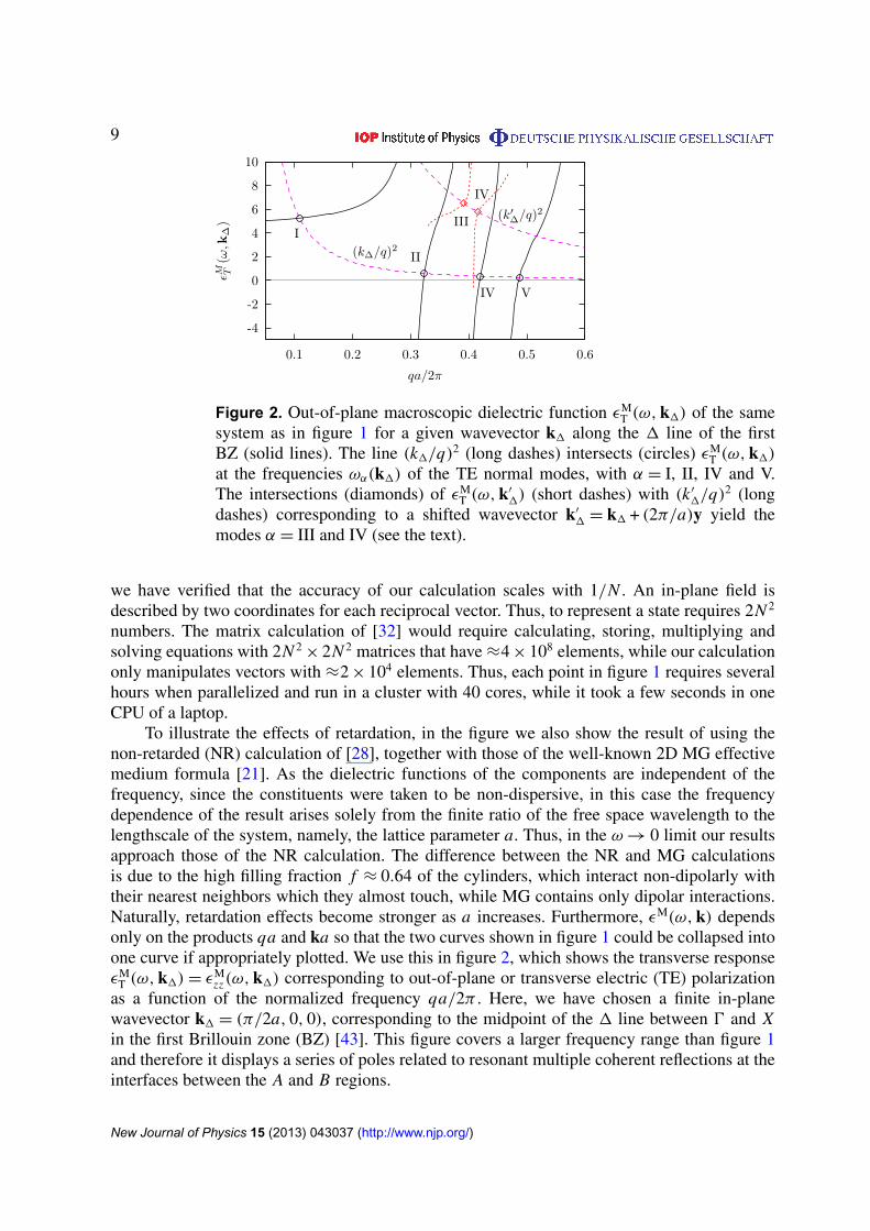
Figure 2. Out-of-plane macroscopic dielectric function εMT (ω,k1) of the same
system as in figure 1 for a given wavevector k1 along the 1 line of the firstBZ (solid lines). The line (k1/q)2 (long dashes) intersects (circles) εM
T (ω,k1)at the frequencies ωα(k1) of the TE normal modes, with α = I, II, IV and V.The intersections (diamonds) of εM
T (ω,k′
1) (short dashes) with (k ′
1/q)2 (long
dashes) corresponding to a shifted wavevector k′
1 = k1 + (2π/a)y yield themodes α = III and IV (see the text).
we have verified that the accuracy of our calculation scales with 1/N . An in-plane field isdescribed by two coordinates for each reciprocal vector. Thus, to represent a state requires 2N 2
numbers. The matrix calculation of [32] would require calculating, storing, multiplying andsolving equations with 2N 2
× 2N 2 matrices that have ≈4 × 10⁸ elements, while our calculationonly manipulates vectors with ≈2 × 10⁴ elements. Thus, each point in figure 1 requires severalhours when parallelized and run in a cluster with 40 cores, while it took a few seconds in oneCPU of a laptop.
To illustrate the effects of retardation, in the figure we also show the result of using thenon-retarded (NR) calculation of [28], together with those of the well-known 2D MG effectivemedium formula [21]. As the dielectric functions of the components are independent of thefrequency, since the constituents were taken to be non-dispersive, in this case the frequencydependence of the result arises solely from the finite ratio of the free space wavelength to thelengthscale of the system, namely, the lattice parameter a. Thus, in the ω→ 0 limit our resultsapproach those of the NR calculation. The difference between the NR and MG calculationsis due to the high filling fraction f ≈ 0.64 of the cylinders, which interact non-dipolarly withtheir nearest neighbors which they almost touch, while MG contains only dipolar interactions.Naturally, retardation effects become stronger as a increases. Furthermore, εM(ω,k) dependsonly on the products qa and ka so that the two curves shown in figure 1 could be collapsed intoone curve if appropriately plotted. We use this in figure 2, which shows the transverse responseεM
T (ω,k1)= εMzz (ω,k1) corresponding to out-of-plane or transverse electric (TE) polarization
as a function of the normalized frequency qa/2π . Here, we have chosen a finite in-planewavevector k1 = (π/2a, 0, 0), corresponding to the midpoint of the 1 line between 0 and Xin the first Brillouin zone (BZ) [43]. This figure covers a larger frequency range than figure 1and therefore it displays a series of poles related to resonant multiple coherent reflections at theinterfaces between the A and B regions.
New Journal of Physics 15 (2013) 043037 (http://www.njp.org/)
10
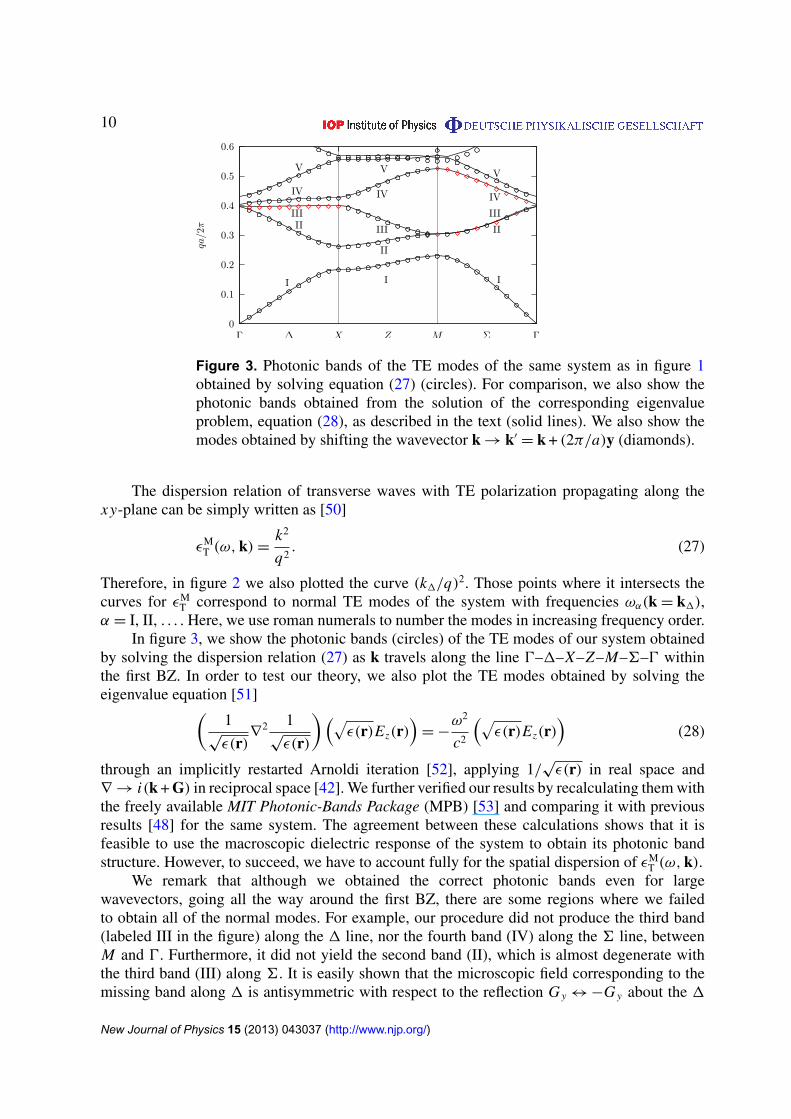
Figure 3. Photonic bands of the TE modes of the same system as in figure 1obtained by solving equation (27) (circles). For comparison, we also show thephotonic bands obtained from the solution of the corresponding eigenvalueproblem, equation (28), as described in the text (solid lines). We also show themodes obtained by shifting the wavevector k → k′
= k + (2π/a)y (diamonds).
The dispersion relation of transverse waves with TE polarization propagating along thexy-plane can be simply written as [50]
εMT (ω,k)=
k2
q2. (27)
Therefore, in figure 2 we also plotted the curve (k1/q)2. Those points where it intersects thecurves for εM
T correspond to normal TE modes of the system with frequencies ωα(k = k1),α = I, II, . . . . Here, we use roman numerals to number the modes in increasing frequency order.
In figure 3, we show the photonic bands (circles) of the TE modes of our system obtainedby solving the dispersion relation (27) as k travels along the line 0–1–X–Z–M–6–0 withinthe first BZ. In order to test our theory, we also plot the TE modes obtained by solving theeigenvalue equation [51](
1√ε(r)
∇2 1√ε(r)
)(√ε(r)Ez(r)
)= −
ω2
c2
(√ε(r)Ez(r)
)(28)
through an implicitly restarted Arnoldi iteration [52], applying 1/√ε(r) in real space and
∇ → i(k + G) in reciprocal space [42]. We further verified our results by recalculating them withthe freely available MIT Photonic-Bands Package (MPB) [53] and comparing it with previousresults [48] for the same system. The agreement between these calculations shows that it isfeasible to use the macroscopic dielectric response of the system to obtain its photonic bandstructure. However, to succeed, we have to account fully for the spatial dispersion of εM
T (ω,k).We remark that although we obtained the correct photonic bands even for large
wavevectors, going all the way around the first BZ, there are some regions where we failedto obtain all of the normal modes. For example, our procedure did not produce the third band(labeled III in the figure) along the 1 line, nor the fourth band (IV) along the 6 line, betweenM and 0. Furthermore, it did not yield the second band (II), which is almost degenerate withthe third band (III) along 6. It is easily shown that the microscopic field corresponding to themissing band along 1 is antisymmetric with respect to the reflection G y ↔ −G y about the 1
New Journal of Physics 15 (2013) 043037 (http://www.njp.org/)
11
line. Similarly, the missing bands along the region 6 are antisymmetric with respect to thereflection Gx ↔ G y about the 6 line. Thus, the reciprocal vector 0 does not contribute to theelectric field for those bands [54], i.e. the missing modes have no macroscopic field componentsand thus, apparently, they may not be obtained from the roots of the macroscopic dispersionrelation (27).
Nevertheless, within our formalism, the wavevector k is actually not restricted to lie withinthe first BZ. Thus, we may calculate the macroscopic dielectric function for wavevectors beyondthe first BZ, and obtain the modes in the extended scheme. In figure 2, we show part of themacroscopic dielectric function εM
T (ω,k′
1) with a wavevector that has been shifted out of thefirst BZ from k1 along the y-direction by the reciprocal vector (2π/a)y, i.e. k′
1 = k1 + (2π/a)y.We remark that εM(ω,k) is not a periodic function of k, as it corresponds to a specific planewave, not to a microscopic Bloch’s wave. The intersection of the curve (k ′
1/q)2 with εM
T (ω,k′
1)
yields the corresponding macroscopic modes. For example, the diamonds in figure 2 illustratetwo of the normal modes that could be obtained using this shifting procedure. One of thesemodes is identical to the mode labeled IV that was obtained previously using the unshiftedresponse εM
T (ω,k1). Nevertheless, another mode, labeled III, appears just below qa/2π = 0.4and corresponds to one of the previously missing modes. We may shift it back into the first BZin order to display it in the reduced zone scheme. Proceeding in this fashion, we have obtainedall of the previously missing bands, shown by diamonds in figure 3. Thus, we have shownthat we can calculate the full photonic band structure for the TE modes from the macroscopicnon-local dielectric function of the composite system. The converse, obtaining the non-localresponse from the dispersion relation [38], can also be attempted, although the results would notbe uniquely defined and are not expected to be valid for wavevectors and frequencies that donot lie in the dispersion relation. Our procedure has no such limitation.
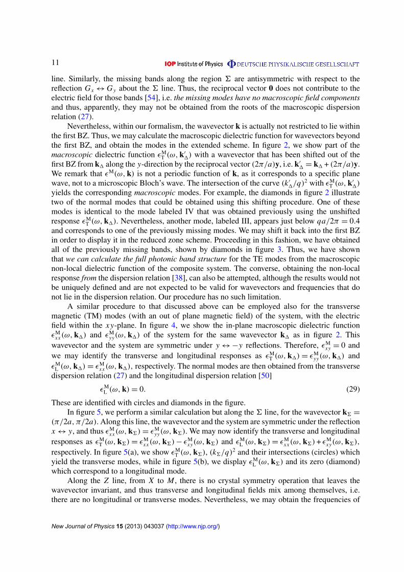
A similar procedure to that discussed above can be employed also for the transversemagnetic (TM) modes (with an out of plane magnetic field) of the system, with the electricfield within the xy-plane. In figure 4, we show the in-plane macroscopic dielectric functionεM
xx(ω,k1) and εMyy(ω,k1) of the system for the same wavevector k1 as in figure 2. This
wavevector and the system are symmetric under y ↔ −y reflections. Therefore, εMxy = 0 and
we may identify the transverse and longitudinal responses as εMT (ω,k1)= εM
yy(ω,k1) andεM
L (ω,k1)= εMxx(ω,k1), respectively. The normal modes are then obtained from the transverse
dispersion relation (27) and the longitudinal dispersion relation [50]
εML (ω,k)= 0. (29)
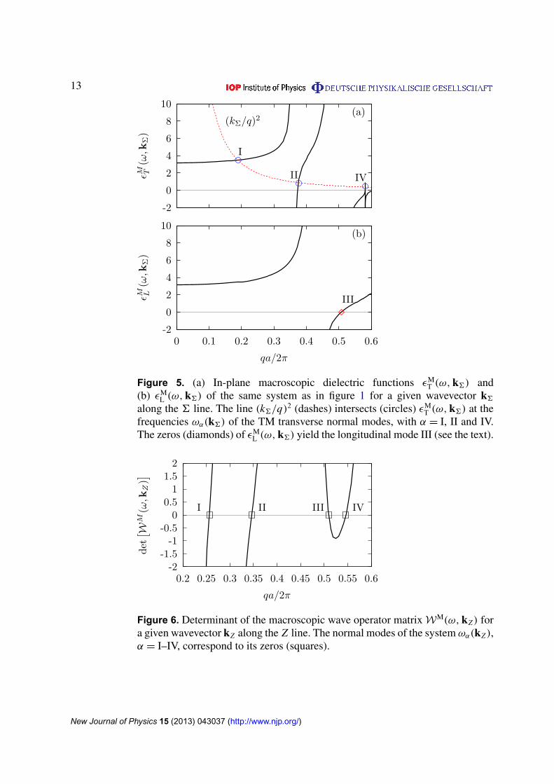
These are identified with circles and diamonds in the figure.In figure 5, we perform a similar calculation but along the 6 line, for the wavevector k6 =
(π/2a, π/2a). Along this line, the wavevector and the system are symmetric under the reflectionx ↔ y, and thus εM
xx(ω,k6)= εMyy(ω,k6). We may now identify the transverse and longitudinal
responses as εMT (ω,k6)= εM
xx(ω,k6)− εMxy(ω,k6) and εM
L (ω,k6)= εMxx(ω,k6)+ εM
xy(ω,k6),respectively. In figure 5(a), we show εM
T (ω,k6), (k6/q)2 and their intersections (circles) whichyield the transverse modes, while in figure 5(b), we display εM
L (ω,k6) and its zero (diamond)which correspond to a longitudinal mode.
Along the Z line, from X to M , there is no crystal symmetry operation that leaves thewavevector invariant, and thus transverse and longitudinal fields mix among themselves, i.e.there are no longitudinal or transverse modes. Nevertheless, we may obtain the frequencies of
New Journal of Physics 15 (2013) 043037 (http://www.njp.org/)
12
Figure 4. (a) In-plane macroscopic dielectric functions εMT (ω,k1) and (b)
εML (ω,k1) of the same system as in figure 1 for the same wavevector k1
as in figure 2. The line (k1/q)2 (dashes) intersects (circles) εMT (ω,k1) at the
frequencies ωα(k1) of the TM transverse normal modes, with α = I, II and IV.The zeros (diamonds) of εM
L (ω,k1) yields the longitudinal mode III (see thetext).
the mixed modes through the singularities of the wave operator matrix
det[WM(ω,k)
]= 0 (30)
as illustrated in figure 6 for a wavevector kZ = (π/a, π/2a) along the Z line.From calculations such as those illustrated by figures 4–6, or more generally, from the
zeros of det[WM(ω,k)
]for arbitrary wavevectors k, we can obtain the full TM photonic band
structure, as shown by figure 7. In order to test our theory, we also plot the TM modes obtainedby solving the eigenvalue equation [51]
∇ ·1
ε(r)∇ Bz(r)= −
ω2
c2Bz(r) (31)
using similar methods [42, 52] as for the TE case and comparing them successfully withprevious results [48] for the same system. The agreement between these calculations showsthat it is also feasible to use the macroscopic dielectric response of the system for obtaining itsphotonic band structure in the TM case.
An approximate band structure could be obtained for transverse waves in the region ofsmall wavevectors k → 0 by expanding the lhs of equation (27) up to second order in k and
New Journal of Physics 15 (2013) 043037 (http://www.njp.org/)
13
Figure 5. (a) In-plane macroscopic dielectric functions εMT (ω,k6) and
(b) εML (ω,k6) of the same system as in figure 1 for a given wavevector k6
along the 6 line. The line (k6/q)2 (dashes) intersects (circles) εMT (ω,k6) at the
frequencies ωα(k6) of the TM transverse normal modes, with α = I, II and IV.The zeros (diamonds) of εM
L (ω,k6) yield the longitudinal mode III (see the text).
Figure 6. Determinant of the macroscopic wave operator matrixWM(ω,kZ) fora given wavevector kZ along the Z line. The normal modes of the system ωα(kZ),α = I–IV, correspond to its zeros (squares).
New Journal of Physics 15 (2013) 043037 (http://www.njp.org/)
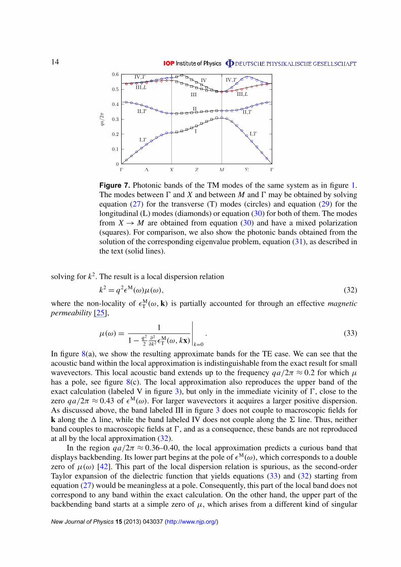
14
Figure 7. Photonic bands of the TM modes of the same system as in figure 1.The modes between 0 and X and between M and 0 may be obtained by solvingequation (27) for the transverse (T) modes (circles) and equation (29) for thelongitudinal (L) modes (diamonds) or equation (30) for both of them. The modesfrom X → M are obtained from equation (30) and have a mixed polarization(squares). For comparison, we also show the photonic bands obtained from thesolution of the corresponding eigenvalue problem, equation (31), as described inthe text (solid lines).
solving for k2. The result is a local dispersion relation
k2= q2εM(ω)µ(ω), (32)
where the non-locality of εMT (ω,k) is partially accounted for through an effective magnetic
permeability [25],
µ(ω)=1
1 −q2
2∂2
∂k2 εMT (ω, kx)
∣∣∣∣∣k=0
. (33)
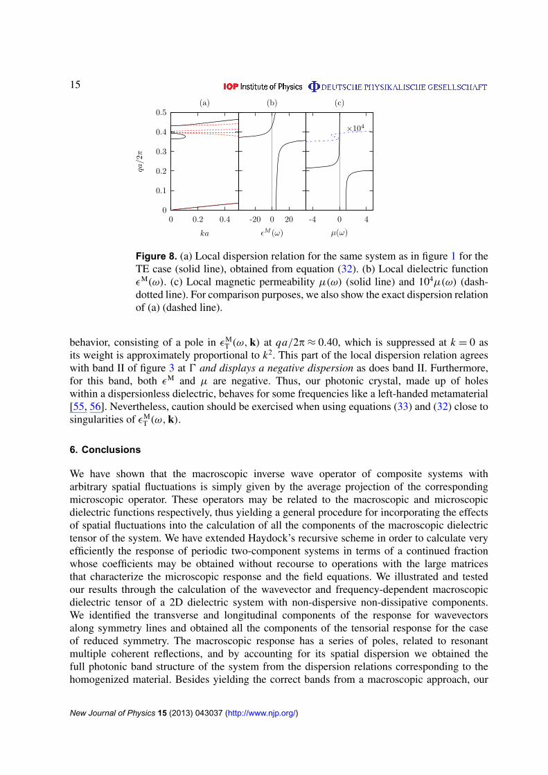
In figure 8(a), we show the resulting approximate bands for the TE case. We can see that theacoustic band within the local approximation is indistinguishable from the exact result for smallwavevectors. This local acoustic band extends up to the frequency qa/2π ≈ 0.2 for which µhas a pole, see figure 8(c). The local approximation also reproduces the upper band of theexact calculation (labeled V in figure 3), but only in the immediate vicinity of 0, close to thezero qa/2π ≈ 0.43 of εM(ω). For larger wavevectors it acquires a larger positive dispersion.As discussed above, the band labeled III in figure 3 does not couple to macroscopic fields fork along the 1 line, while the band labeled IV does not couple along the 6 line. Thus, neitherband couples to macroscopic fields at 0, and as a consequence, these bands are not reproducedat all by the local approximation (32).
In the region qa/2π ≈ 0.36–0.40, the local approximation predicts a curious band thatdisplays backbending. Its lower part begins at the pole of εM(ω), which corresponds to a doublezero of µ(ω) [42]. This part of the local dispersion relation is spurious, as the second-orderTaylor expansion of the dielectric function that yields equations (33) and (32) starting fromequation (27) would be meaningless at a pole. Consequently, this part of the local band does notcorrespond to any band within the exact calculation. On the other hand, the upper part of thebackbending band starts at a simple zero of µ, which arises from a different kind of singular
New Journal of Physics 15 (2013) 043037 (http://www.njp.org/)
15
Figure 8. (a) Local dispersion relation for the same system as in figure 1 for theTE case (solid line), obtained from equation (32). (b) Local dielectric functionεM(ω). (c) Local magnetic permeability µ(ω) (solid line) and 104µ(ω) (dash-dotted line). For comparison purposes, we also show the exact dispersion relationof (a) (dashed line).
behavior, consisting of a pole in εMT (ω,k) at qa/2p ≈ 0.40, which is suppressed at k = 0 as
its weight is approximately proportional to k2. This part of the local dispersion relation agreeswith band II of figure 3 at 0 and displays a negative dispersion as does band II. Furthermore,for this band, both εM and µ are negative. Thus, our photonic crystal, made up of holeswithin a dispersionless dielectric, behaves for some frequencies like a left-handed metamaterial[55, 56]. Nevertheless, caution should be exercised when using equations (33) and (32) close tosingularities of εM
T (ω,k).
6. Conclusions
We have shown that the macroscopic inverse wave operator of composite systems witharbitrary spatial fluctuations is simply given by the average projection of the correspondingmicroscopic operator. These operators may be related to the macroscopic and microscopicdielectric functions respectively, thus yielding a general procedure for incorporating the effectsof spatial fluctuations into the calculation of all the components of the macroscopic dielectrictensor of the system. We have extended Haydock’s recursive scheme in order to calculate veryefficiently the response of periodic two-component systems in terms of a continued fractionwhose coefficients may be obtained without recourse to operations with the large matricesthat characterize the microscopic response and the field equations. We illustrated and testedour results through the calculation of the wavevector and frequency-dependent macroscopicdielectric tensor of a 2D dielectric system with non-dispersive non-dissipative components.We identified the transverse and longitudinal components of the response for wavevectorsalong symmetry lines and obtained all the components of the tensorial response for the caseof reduced symmetry. The macroscopic response has a series of poles, related to resonantmultiple coherent reflections, and by accounting for its spatial dispersion we obtained thefull photonic band structure of the system from the dispersion relations corresponding to thehomogenized material. Besides yielding the correct bands from a macroscopic approach, our
New Journal of Physics 15 (2013) 043037 (http://www.njp.org/)
16
scheme allowed us to classify the polarization of each mode as either transverse, longitudinal ormixed. Even though the macroscopic approach might fail to yield some modes, namely, thosewhich have no coupling to the macroscopic field due to symmetry, they may be recovered byextending the notion of macroscopic state, allowing its wavevector to lie beyond the first BZ.The non-locality of the dielectric response may be partially accounted for through a magneticpermeability which can then be employed in the calculation of the optical properties of thesystem. We compared the band structure obtained through this local approximation to the exactresults and we obtained partial agreement close to 0 for those bands that do couple to longwavelength fields. In particular, we showed that this approach can yield a negative dispersionin frequency regions where both the permittivity and permeability are negative. Nevertheless,we discussed some shortcomings of the local approach. Although here we presented results fordispersionless transparent dielectrics, our calculation does not require that the materials thatmake up the system be non-dispersive or non-dissipative, so that calculations for real dielectricsand metals may be performed with the same low computational costs.
Acknowledgments
JSPH is grateful for a scholarship awarded by CONACYT. This work was partially supportedby ANPCyT grant no. PICT-PRH-135-2008 (GPO), CONACyT grant no. 153930 (BSM) andDGAPA-UNAM grant no. IN108413 (WLM).
References
[1] Bredov M, Rumiantsev V and Toptiguin L 1985 Classical Electrodynamics (Moscow: Mir)[2] Notomi M 2000 Theory of light propagation in strongly modulated photonic crystals: refractionlike behavior
in the vicinity of the photonic band gap Phys. Rev. B 62 10696–705[3] Barrera R G, Reyes-Coronado A and Garcıa-Valenzuela A 2007 Nonlocal nature of the electrodynamic
response of colloidal systems Phys. Rev. B 75 184202[4] Yeh P, Yariv A and Hong C-S 1977 Electromagnetic propagation in periodic stratified media: I. General theory
J. Opt. Soc. Am. 67 423–38[5] Luis Mochan W and Barrera R G 1985 Electromagnetic response of systems with spatial fluctuations: I.
General formalism Phys. Rev. B 32 4984–8[6] Luis Mochan W and Barrera R G 1985 Electromagnetic response of systems with spatial fluctuations: II.
Applications Phys. Rev. B 32 4989–5001[7] Kosaka H, Kawashima T, Tomita A, Notomi M, Tamamura T, Sato T and Kawakami S 1998 Superprism
phenomena in photonic crystals Phys. Rev. B 58 R10096–9[8] Stroud D and Pan F P 1978 Self-consistent approach to electromagnetic wave propagation in composite
media: application to model granular metals Phys. Rev. B 17 1602–10[9] Ortiz G P and Mochan W L 2003 Scaling of light scattered from fractal aggregates at resonance Phys. Rev. B
67 184204[10] Ortiz G P and Mochan W L 2003 Scaling condition for multiple scattering in fractal aggregates Physica B
338 54[11] Hilke M 2009 Seeing Anderson localization Phys. Rev. A 80 063820[12] Vasconcelos M S and Albuquerque E L 1998 Plasmon–polariton fractal spectra in quasiperiodic multilayers
Phys. Rev. B 57 2826–33[13] Albuquerque E L and Cottam M G 1993 Superlattice plasmon–polaritons Phys. Rep. 233 67–135
New Journal of Physics 15 (2013) 043037 (http://www.njp.org/)
17
[14] Chen J et al 2011 Observation of the inverse doppler effect in negative-index materials at optical frequenciesNature Photon. 5 239–45
[15] Zhang B, Luo Y, Liu X and Barbastathis G 2011 Macroscopic invisibility cloak for visible light Phys. Rev.Lett. 106 033901
[16] Lezec H J, Dionne J A and Atwater H A 2007 Negative refraction at visible frequencies Science 316 430–2[17] Urzhumov Y A and Shvets G 2008 Optical magnetism and negative refraction in plasmonic metamaterials
Solid State Commun. 146 208–20[18] Milton G W, McPhedran R C and McKenzie D R 1981 Transport properties of arrays of intersecting cylinders
Appl. Phys. A 25 23–30[19] Bergman D J and Dunn K-J 1992 Bulk effective dielectric constant of a composite with a periodic
microgeometry Phys. Rev. B 45 13262–71[20] Tao R, Chen Z and Sheng P 1990 First-principles Fourier approach for the calculation of the effective
dielectric constant of periodic composites Phys. Rev. B 41 2417–20[21] Datta S, Chan C T, Ho K M and Soukoulis C M 1993 Effective dielectric constant of periodic composite
structures Phys. Rev. B 48 14936–43[22] Alexopoulos A 2010 Effective-medium theory of surfaces and metasurfaces containing two-dimensional
binary inclusions Phys. Rev. E 81 046607[23] Doyle W T 1989 Optical properties of a suspension of metal spheres Phys. Rev. B 39 9852–8[24] Ludwig A and Webb K J 2010 Accuracy of effective medium parameter extraction procedures for optical
metamaterials Phys. Rev. B 81 113103[25] Costa J T, Silveirinha M G and Maslovski S I 2009 Finite-difference frequency-domain method for the
extraction of effective parameters of metamaterials Phys. Rev. B 80 235124[26] Ortiz G P, Lopez-Bastidas C, Maytorena J A and Mochan W L 2003 Bulk response of composite from finite
samples Physica B 338 103[27] Silveirinha M G 2006 Nonlocal homogenization model for a periodic array of epsilon-negative rods Phys.
Rev. E 73 046612[28] Mochan L W, Ortiz G P and Mendoza B S 2010 Efficient homogenization procedure for the calculation of
optical properties of 3D nanostructured composites Opt. Express 18 22119–27[29] Myroshnychenko V and Brosseau C 2010 Analysis of the effective permittivity in percolative composites
using finite element calculations Proc. 8th Int. Conf. on Electrical Transport and Optical Properties ofInhomogeneous Media, ETOPIM-8; Physica B 405 3046–9
[30] Guenneau S, Zolla F and Nicolet A 2007 Homogenization of 3D finite photonic crystals with heterogeneouspermittivity and permeability Waves Random Media 17 653–97
[31] Cabuz A I, Nicolet A, Zolla F, Felbacq D and Bouchitte G 2011 Homogenization of nonlocal wiremetamaterial via a renormalization approach J. Opt. Soc. Am. B 28 1275–82
[32] Ortiz G P, Martınez-Zerega B E, Mendoza B S and Mochan L W 2009 Effective optical response ofmetamaterials Phys. Rev. B 79 245132
[33] Raghunathan S B and Budko N V 2010 Effective permittivity of finite inhomogeneous objects Phys. Rev. B81 054206
[34] Halevi P, Krokhin A A and Arriaga J 1999 Photonic crystal optics and homogenization of 2D periodiccomposites Phys. Rev. Lett. 82 719–22
[35] Reyes-Arendano J A et al 2011 From photonic crystals to metamaterials: the bianisotropic response New J.Phys. 13 073041
[36] Simovski C R 2011 On electromagnetic characterization and homogenization of nanostructuredmetamaterials J. Opt. 13 013001
[37] Menzel C, Paul T, Rockstuhl C, Pertsch T, Tretyakov S and Lederer F 2010 Validity of effective materialparameters for optical fishnet metamaterials Phys. Rev. B 81 035320
[38] Elser J, Podolskiy V A, Salakhutdinov I and Avrutsky I 2007 Nonlocal effects in effective-medium responseof nanolayered metamaterials Appl. Phys. Lett. 90 191109
New Journal of Physics 15 (2013) 043037 (http://www.njp.org/)
18
[39] Barrera R G, Reyes-Coronado A and Garcıa-Valenzuela A 2005 Nonlocal effective medium for theelectromagnetic response of colloidal systems: a t-matrix approach Progress in Electromagnetic ResearchSymp. (Hangzhou, China, 2005) pp 646–9
[40] Jackson J D 1998 Classical Electrodynamics (New York: Wiley)[41] Mochan L W 2005 Plasmons Encyclopedia of Condensed Matter Physics ed G Bassani, G Liedl and P Wyder
p 310–17[42] Perez-Huerta J S, Mendoza B S, Ortiz G and Luis Mochan W in preparation[43] Sakoda K 2004 Optical Properties of Photonic Crystals (Springer Series in Optical Sciences) (Berlin:
Springer)[44] Sutton A P 2004 Electronic Structure of Materials (Oxford: Oxford University Press)[45] Datta S 1997 Electronic Transport in Mesoscopic Systems (Cambridge Studies in Semiconductor Physics and
Microelectronic Engineering) (Cambridge: Cambridge University Press)[46] Haydock R, Heine V and Kelly M J 1972 Electronic structure based on the local atomic environment for
tight-binding bands J. Phys. C: Solid State Phys. 5 2845[47] Haydock R, Heine V and Kelly M J 1975 Electronic structure based on the local atomic environment for
tight-binding bands: II J. Phys. C: Solid State Phys. 8 2591[48] Busch K, von Freymann G, Linden S, Mingaleev S F, Tkeshelashvili L and Wegener M 2007 Periodic
nanostructures for photonics Phys. Rep. 444 101–202[49] Glazebrook K and Economou F 1997 PDL: the Perl data language Dr. Dobb’s J. 9719 45[50] Landau L D and Lifshits E M 1984 Electrodynamics of continuous media Course of Theoretical Physics
(Oxford: Pergamon)[51] Joannopoulos J D, Johnson S G, Winn J N and Meade R D 2008 Photonic Crystals: Molding the Flow of
Light 2nd edn (Princeton, NJ: Princeton University Press)[52] Saad Y 2011 Numerical Methods for Large Eigenvalues Problems (Philadelphia: SIAM)[53] Johnson S G and Joannopoulos J D 2001 Block-iterative frequency-domain methods for Maxwell’s equations
in a planewave basis Opt. Express 8 173–90[54] Robertson W M and Arjavalingam G 1992 Measurement of photonic band structure in a two-dimensional
periodic dielectric array Phys. Rev. Lett. 68 2023[55] Peng L, Ran L, Chen H, Zhang H, Kong J A and Grzegorczyk T M 2007 Experimental observation of left-
handed behavior in an array of standard dielectric resonators Phys. Rev. Lett. 98 157403[56] Vynck K, Felbacq D, Centeno E, Cabuz A I, Cassagne D and Guizal B 2009 All-dielectric rod-type
metamaterials at optical frequencies Phys. Rev. Lett. 102 133901
New Journal of Physics 15 (2013) 043037 (http://www.njp.org/)


