Embed Size (px)
Citation preview
HAL Id: tel-03483203https://hal.archives-ouvertes.fr/tel-03483203
Submitted on 16 Dec 2021
HAL is a multi-disciplinary open accessarchive for the deposit and dissemination of sci-entific research documents, whether they are pub-lished or not. The documents may come fromteaching and research institutions in France orabroad, or from public or private research centers.
L’archive ouverte pluridisciplinaire HAL, estdestinée au dépôt et à la diffusion de documentsscientifiques de niveau recherche, publiés ou non,émanant des établissements d’enseignement et derecherche français ou étrangers, des laboratoirespublics ou privés.
Distributed under a Creative Commons Attribution| 4.0 International License
Magnetic Microrobotics for Biomedical ApplicationsDavid Folio
To cite this version:David Folio. Magnetic Microrobotics for Biomedical Applications: Modeling, Simulation, Control andValidations. Automatic. Université d’Orléans, 2021. tel-03483203

CENTRE VAL DE LOIRE
INSAUNIVERSITÉ D’ORLÉANS
ÉCOLE DOCTORALES MATHÉMATIQUES, INFORMATIQUE, PHYSIQUE THÉORIQUEET INGÉNIERIE DES SYSTÈMES
LABORATOIRE PRISME
MÉMOIRE
Par
David FOLIO
Soutenu le 03 décembre 2021
pour obtenir le grade d’Habilitation à Diriger des Recherches
Discipline: Robotique
MAGNETIC MICROROBOTICS FOR BIOMEDICAL APPLICATIONS:Modeling, Simulation, Control and Validations
Jury:
Michaël Gauthier Directeur de Recherche, CNRS, FEMTO‐ST, Besançon Rapporteur
Sylvain Martel Professeur, Polytechnique Montréal, Canada Rapporteur
Philippe Poignet Professeur des Universités, Univ. Montpellier Rapporteur
Chantal Pichon Professeur des Universités, Univ. Orléans Examinatrice
Christine Prelle Professeur des Universités, UTC Examinatrice
Mohammed Samer Professeur des Universités, Univ. Paris‐Est Creteil Val de Marne Examinateur
Li Zhang Professeur, Dept. MAE, CUHK, Hong Kong Examinateur
Antoine Ferreira Professeur des Universités, INSA Centre Val de Loire Garant


CONTENTS
Contents iii
List of Tables vii
List of Figures ix
Avant Propos (Forewords) xiii
PART I ACTIVITIES BACKGROUND 1
I Presentation 3I.1 Curriculum Vitæ . . . . . . . . . . . . . . . . . . . . . . . . . . . . . . . . . . 3
I.1.1 Identity . . . . . . . . . . . . . . . . . . . . . . . . . . . . . . . . . . . . . 3I.1.2 Current situation . . . . . . . . . . . . . . . . . . . . . . . . . . . . . . . . 3I.1.3 Experience and Graduate Education . . . . . . . . . . . . . . . . . . . . . 4
I.2 Background and Career Overview . . . . . . . . . . . . . . . . . . . . . . . . 4I.2.1 Doctorate degree and post-doctorate . . . . . . . . . . . . . . . . . . . . . 4I.2.2 Tenured as associate professor . . . . . . . . . . . . . . . . . . . . . . . . 5
II Teaching and Administrative Responsibilities 11II.1 Before Tenure . . . . . . . . . . . . . . . . . . . . . . . . . . . . . . . . . . . 11II.2 Since Tenured . . . . . . . . . . . . . . . . . . . . . . . . . . . . . . . . . . . 11II.3 Responsibilities . . . . . . . . . . . . . . . . . . . . . . . . . . . . . . . . . . . 13
III Summary of Research Activities 15III.1 Scientific Projects . . . . . . . . . . . . . . . . . . . . . . . . . . . . . . . . . 15
III.1.1 European Union (EU) and national funding projects . . . . . . . . . . . . 15III.1.2 Cooperation projects . . . . . . . . . . . . . . . . . . . . . . . . . . . . . . 16III.1.3 Regional projects . . . . . . . . . . . . . . . . . . . . . . . . . . . . . . . . 17
III.2 Student Supervision . . . . . . . . . . . . . . . . . . . . . . . . . . . . . . . . 17III.2.1 Master students (M2) . . . . . . . . . . . . . . . . . . . . . . . . . . . . . 17III.2.2 Doctoral students . . . . . . . . . . . . . . . . . . . . . . . . . . . . . . . 18
III.3 Scientific Collaborations . . . . . . . . . . . . . . . . . . . . . . . . . . . . . . 19
iii

Contents
III.3.1 International relationships . . . . . . . . . . . . . . . . . . . . . . . . . . . 20III.3.2 National relationships . . . . . . . . . . . . . . . . . . . . . . . . . . . . . 20
III.4 Scientific Dissemination and Outreach . . . . . . . . . . . . . . . . . . . . . . 20III.4.1 Invitations . . . . . . . . . . . . . . . . . . . . . . . . . . . . . . . . . . . 21III.4.2 Scientific expertise . . . . . . . . . . . . . . . . . . . . . . . . . . . . . . . 21III.4.3 Editorial activities . . . . . . . . . . . . . . . . . . . . . . . . . . . . . . . 21III.4.4 Awards . . . . . . . . . . . . . . . . . . . . . . . . . . . . . . . . . . . . . 22
IV Personal References 23IV.1 Articles . . . . . . . . . . . . . . . . . . . . . . . . . . . . . . . . . . . . . . . 23
IV.1.1 Articles in International peer-reviewed and referenced journals (ACL) . . 23IV.1.2 Articles in unreferenced journals (ACLN) . . . . . . . . . . . . . . . . . . 24
IV.2 Books . . . . . . . . . . . . . . . . . . . . . . . . . . . . . . . . . . . . . . . . 24IV.2.1 Guest Editor (DO) . . . . . . . . . . . . . . . . . . . . . . . . . . . . . . . 25IV.2.2 Book Chapter (OS) . . . . . . . . . . . . . . . . . . . . . . . . . . . . . . 25
IV.3 Proceedings in International Conferences (ACT) . . . . . . . . . . . . . . . . 25IV.4 Oral Communications . . . . . . . . . . . . . . . . . . . . . . . . . . . . . . . 28
IV.4.1 Invited Speaker in International or National Conferences (INV) . . . . . . 28IV.4.2 Communications in International or National Conferences (COM) . . . . 28
PART II SCIENTIFIC CONTRIBUTIONS 29
V Scientific Context and Organization 31V.1 Introduction . . . . . . . . . . . . . . . . . . . . . . . . . . . . . . . . . . . . 31V.2 Positioning of Main Research Activities . . . . . . . . . . . . . . . . . . . . . 32
V.2.1 Working in the microworld . . . . . . . . . . . . . . . . . . . . . . . . . . 32V.2.2 Microrobotics for biomedical applications . . . . . . . . . . . . . . . . . . 33V.2.3 Biomedical microrobotics challenges . . . . . . . . . . . . . . . . . . . . . 35
V.3 Structuring of Activities . . . . . . . . . . . . . . . . . . . . . . . . . . . . . . 38V.3.1 Magnetic microrobotic systems for biomedical applications . . . . . . . . 38V.3.2 Simulation and navigation strategies . . . . . . . . . . . . . . . . . . . . . 40V.3.3 Evaluation and development of magnetic microrobotic systems . . . . . . 41V.3.4 The others research activities . . . . . . . . . . . . . . . . . . . . . . . . . 42
VI Modeling Microrobotic Systems for Endovascular Intervention 45VI.1 Introduction . . . . . . . . . . . . . . . . . . . . . . . . . . . . . . . . . . . . 45VI.2 Endovascular Navigation . . . . . . . . . . . . . . . . . . . . . . . . . . . . . 46
VI.2.1 Fluid mechanics . . . . . . . . . . . . . . . . . . . . . . . . . . . . . . . . 47VI.2.2 Physiology of the cardiovascular system . . . . . . . . . . . . . . . . . . . 50VI.2.3 Discussion . . . . . . . . . . . . . . . . . . . . . . . . . . . . . . . . . . . . 54
VI.3 Biomedical Microrobot Design . . . . . . . . . . . . . . . . . . . . . . . . . . 55VI.3.1 Magnetic microrobot . . . . . . . . . . . . . . . . . . . . . . . . . . . . . . 56VI.3.2 Hydrodynamics of microrobot . . . . . . . . . . . . . . . . . . . . . . . . . 63VI.3.3 Catalytic micromotor . . . . . . . . . . . . . . . . . . . . . . . . . . . . . 66
VI.4 Magnetic Field Generation . . . . . . . . . . . . . . . . . . . . . . . . . . . . 72VI.4.1 Classical electromagnetic coils . . . . . . . . . . . . . . . . . . . . . . . . 72
iv
Contents
VI.4.2 Core-filled electromagnets . . . . . . . . . . . . . . . . . . . . . . . . . . . 75VI.4.3 Electromagnetic actuation setups . . . . . . . . . . . . . . . . . . . . . . . 76
VI.5 Conclusion . . . . . . . . . . . . . . . . . . . . . . . . . . . . . . . . . . . . . 80
VII Magnetically Actuated Microrobots Navigating in a Vascular Network 81VII.1 Introduction . . . . . . . . . . . . . . . . . . . . . . . . . . . . . . . . . . . . 81VII.2 Microrobot in a Vascular Environment . . . . . . . . . . . . . . . . . . . . . . 82
VII.2.1 Dynamic of magnetic microrobots in a microchannel . . . . . . . . . . . . 82VII.2.2 Simulation of microrobot navigating in a vascular network . . . . . . . . . 86VII.2.3 Navigation planning in viscous flow . . . . . . . . . . . . . . . . . . . . . 87
VII.3 Navigation Control Strategies . . . . . . . . . . . . . . . . . . . . . . . . . . . 93VII.3.1 State-space representation . . . . . . . . . . . . . . . . . . . . . . . . . . . 93VII.3.2 Predictive navigation . . . . . . . . . . . . . . . . . . . . . . . . . . . . . 96VII.3.3 Nonlinear optimal control . . . . . . . . . . . . . . . . . . . . . . . . . . . 104VII.3.4 Control of multiple magnetic microrobots . . . . . . . . . . . . . . . . . . 109
VII.4 Conclusion . . . . . . . . . . . . . . . . . . . . . . . . . . . . . . . . . . . . . 113
VIII Development of Experimental Platforms and Validations 115VIII.1 Introduction . . . . . . . . . . . . . . . . . . . . . . . . . . . . . . . . . . . . 115VIII.2 Cardiovascular System Simulator . . . . . . . . . . . . . . . . . . . . . . . . . 115VIII.3 Magnetic Resonant Navigation (MRN) . . . . . . . . . . . . . . . . . . . . . 117
VIII.3.1The clinical MRI setup . . . . . . . . . . . . . . . . . . . . . . . . . . . . 118VIII.3.2MRI-based sensing . . . . . . . . . . . . . . . . . . . . . . . . . . . . . . . 120VIII.3.3MRN experimental results . . . . . . . . . . . . . . . . . . . . . . . . . . . 122
VIII.4 µIRM testbed . . . . . . . . . . . . . . . . . . . . . . . . . . . . . . . . . . . . 124VIII.4.1Platform descriptions . . . . . . . . . . . . . . . . . . . . . . . . . . . . . 124VIII.4.2Results . . . . . . . . . . . . . . . . . . . . . . . . . . . . . . . . . . . . . 126VIII.4.3Discussion . . . . . . . . . . . . . . . . . . . . . . . . . . . . . . . . . . . . 129
VIII.5 OctoRob Platform . . . . . . . . . . . . . . . . . . . . . . . . . . . . . . . . . 130VIII.5.1Platform design specifications . . . . . . . . . . . . . . . . . . . . . . . . . 130VIII.5.2Design of OctoRob . . . . . . . . . . . . . . . . . . . . . . . . . . . . . . . 131VIII.5.3Implementation of the OctoRob prototype . . . . . . . . . . . . . . . . . . 133
VIII.6 Conclusion . . . . . . . . . . . . . . . . . . . . . . . . . . . . . . . . . . . . . 135
Conclusion and Prospects 137
APPENDIX 143
A Three-dimensional controlled motion of a microrobot using magneticgradients (ACL3) 145
B Simulation and planning of a magnetically actuated microrobot navigat-ing in arteries (ACL6) 163
C Catalytic locomotion of core-shell nanowire motors (ACL10 173
v

D Modeling of optimal targeted therapies using drug-loaded magneticnanoparticles for the liver cancer (ACL12) 203
E Mathematical Approach for the Design Configuration of Magnetic Sys-tem with Multiple Electromagnets (ACL15) 215
Index of Terms and Notations 239
Bibliography 245

LIST OF TABLES
II.1 Overview of the various teaching disciplines as associate professor. . . . . . 12
VIII.1 Standard deviations (SD) of the location of different steel balls size usingHASTE and FLASH sequences. [ACL11] . . . . . . . . . . . . . . . . . . . 121
VIII.2 Standard deviations (SD) of the position for different k-space reduction.[ACL11] . . . . . . . . . . . . . . . . . . . . . . . . . . . . . . . . . . . . . . 121
VIII.3 Caracteristics of the µMRI setup coils . . . . . . . . . . . . . . . . . . . . . 124
vii


LIST OF FIGURES
I.1 Timeline of main events and activities since tenure as Associate Professor . 6I.2 Teaching load progress. . . . . . . . . . . . . . . . . . . . . . . . . . . . . . 7I.3 Personal references progress since tenure. . . . . . . . . . . . . . . . . . . . 9
V.1 Scaling down to the microworld . . . . . . . . . . . . . . . . . . . . . . . . . 32V.2 Challenges and opportunities of medical microrobots. . . . . . . . . . . . . 34V.3 Example of actuation mechanisms envisaged for microrobots . . . . . . . . 36V.4 Examples of different microworld imaging modalities . . . . . . . . . . . . . 37
VI.1 Overview of the cardiovascular system . . . . . . . . . . . . . . . . . . . . . 46VI.2 Fluid flow in a pipe . . . . . . . . . . . . . . . . . . . . . . . . . . . . . . . 49VI.3 Relationships among vessel size, cross-sectional area and the blood flow velocity 51VI.4 Pressure, volume and flow rate relationship in the cardiac cycle. . . . . . . 52VI.5 Pulsatile flow profiles in a straight tube . . . . . . . . . . . . . . . . . . . . 53VI.6 In vivo apparent viscosity using the Pries et al. model . . . . . . . . . . . . 55VI.7 Examples of magnetic microrobots . . . . . . . . . . . . . . . . . . . . . . . 56VI.8 Schematic representation of basic magnetic swimming principle . . . . . . . 57VI.9 Magnetization curves of ferromagnetic and superparamagnetic material . . 59VI.10 Representation of spheroidal shapes . . . . . . . . . . . . . . . . . . . . . . 62VI.11 Ellipsoidal and chain-like microrobots in a microchannel. . . . . . . . . . . 65VI.12 Different reported catalytic micro-/nanomotors . . . . . . . . . . . . . . . . 66VI.13 Schematic of the cyclic bubble propulsion mechanism of tubular truncated
conical nanorobot . . . . . . . . . . . . . . . . . . . . . . . . . . . . . . . . 67VI.14 Representation of the microjet and the inner flow under the simplifying
approximations. . . . . . . . . . . . . . . . . . . . . . . . . . . . . . . . . . 68VI.15 Velocity of the microjets against and along flow rates . . . . . . . . . . . . 69VI.16 Self-phoretic propulsion . . . . . . . . . . . . . . . . . . . . . . . . . . . . . 70VI.17 Schematic representation of Ru–Au core-shell nanorod with the different
electrokinetic reaction. . . . . . . . . . . . . . . . . . . . . . . . . . . . . . . 71VI.18 Numerical modeling of Au/Ru core-shell nanorod in the presence of H 2 O 2 . 71VI.19 Representation of the Biot-Savart low applied to a circular loop. . . . . . . 73VI.20 Representation of an Helmholtz (inner red) and Maxwell (outer blue) coils
pair. . . . . . . . . . . . . . . . . . . . . . . . . . . . . . . . . . . . . . . . . 74VI.21 The (a) magnetic fields and (b) its gradient induce with Helmholtz coils. . 74
ix

List of Figures
VI.22 The (a) magnetic fields and (b) its gradient induce with Maxwell coils. . . 75VI.23 Illustration of the magnetic field due to a theoretical magnetic point-dipole. 76VI.24 The concept of EMA system applying for various biomedical applications. . 77VI.25 EMA platforms used in our research . . . . . . . . . . . . . . . . . . . . . . 77VI.26 The diagram of the specifications of EMA system design . . . . . . . . . . 79
VII.1 Representation of a magnetic microrobot navigating in a microchannel. . . 82VII.2 Evolution of microforces acting on a spherical magnetic microrobot in a
microchannel and the relevant microforces. . . . . . . . . . . . . . . . . . . 83VII.3 Hydrodynamic drag forces for spherical, spheroidal and chain-like microrobots. 83VII.4 Magnetophoretic number and the magnetization rate for spherical microrobot 84VII.5 Comparison of magnetophoretic number for an ellipsoidal and a chain-like
microrobots . . . . . . . . . . . . . . . . . . . . . . . . . . . . . . . . . . . . 85VII.6 Load volume as function of the equivalent radius when Cmt = 1 . . . . . . 85VII.7 Clinical MIP image from the MRA obtained for a patient with an isolated
stenosis in the iliac artery . . . . . . . . . . . . . . . . . . . . . . . . . . . . 86VII.8 Simulation results of the blood flow velocity field computation. . . . . . . . 87VII.9 Simulation results of the force field . . . . . . . . . . . . . . . . . . . . . . . 87VII.10 Pulsatile blood flow simulation . . . . . . . . . . . . . . . . . . . . . . . . . 88VII.11 Illustration of the vessel centerline extraction . . . . . . . . . . . . . . . . . 90VII.12 Planning results on varying control action influence for a neodymium micro-
robot of size 250 µm and 750 µm . . . . . . . . . . . . . . . . . . . . . . . 91VII.13 Planning results using the proposed anisotropic cost function for a
neodymium microrobot . . . . . . . . . . . . . . . . . . . . . . . . . . . . . 92VII.14 Representation of spheroidal magnetic microrobot in x0-y0 plane . . . . . . 95VII.15 Illustration of the MRI timeline of acquisition and control and the basic
concept of predictive navigation. . . . . . . . . . . . . . . . . . . . . . . . . 97VII.16 Diagram of the SMPC design. . . . . . . . . . . . . . . . . . . . . . . . . . 98VII.17 Microrobot 3D vascular MRN using SMPC. . . . . . . . . . . . . . . . . . . 99VII.18 3D tracking error with SMPC . . . . . . . . . . . . . . . . . . . . . . . . . 100VII.19 SMPC MRB with blood flow disturbance . . . . . . . . . . . . . . . . . . . 100VII.20 Tracking error with different values of duty cycle . . . . . . . . . . . . . . . 101VII.21 Navigation based-Generalized Predictive Control (GPC) strategy. . . . . . 102VII.22 3D MRN tracking error with GPC . . . . . . . . . . . . . . . . . . . . . . . 103VII.23 GPC MRN with blood flow disturbance . . . . . . . . . . . . . . . . . . . . 103VII.24 Optimal stabilization of a spheroidal microrobot position . . . . . . . . . . 107VII.25 Optimal stabilization of a spheroidal microrobot with singularity crossing 107VII.26 Schematic representation of the principle locoregional therapy for the liver
cancer. . . . . . . . . . . . . . . . . . . . . . . . . . . . . . . . . . . . . . . 108VII.27 Group of magnetic microrobot in a microfluidic environment. . . . . . . . . 109VII.28 Interaction forces fm,12 magnitude between two magnetic microrobot as
function of their separation distance d12. . . . . . . . . . . . . . . . . . . . 110VII.29 Phase portrait of a pair (xi1, vi1) . . . . . . . . . . . . . . . . . . . . . . . . 112VII.30 Optimal stabilization of the three microrobots with different LQI parameters.113VII.31 Optimal stabilization of the 2D positions of two magnetic microrobots . . . 114
VIII.1 Illustration of our cardiovascular system simulator . . . . . . . . . . . . . . 116
x

List of Figures
VIII.2 Example of pulsatile flow generated by the Harvard Apparatus pump. . . . 117VIII.3 Viscosity of aqueous mixtures of glycerin: (a) at fixed T = 20 °C, and (b) for
60 wt.% of glycerin . . . . . . . . . . . . . . . . . . . . . . . . . . . . . . . . 118VIII.4 The Siemens Magnetom® Verio MRI scanner at Pius Hospital, Oldenburg,
Germany, . . . . . . . . . . . . . . . . . . . . . . . . . . . . . . . . . . . . . 119VIII.5 The MRN architecture with the Siemens MRI scanner . . . . . . . . . . . . 119VIII.6 The MRI experimental setups components . . . . . . . . . . . . . . . . . . 120VIII.7 MRI susceptibility artifact imaging experiment . . . . . . . . . . . . . . . . 121VIII.8 Navigation along a planned path of a microrobot with standard FLASH
sequences . . . . . . . . . . . . . . . . . . . . . . . . . . . . . . . . . . . . . 122VIII.9 MRN along a planned path of a microrobot with optimized FLASH sequence
parameters . . . . . . . . . . . . . . . . . . . . . . . . . . . . . . . . . . . . 123VIII.10MRN in Y-shaped microfluidic vessel simulator . . . . . . . . . . . . . . . . 123VIII.11The µIRM EMA platform with its coils pair arrangement. . . . . . . . . . . 124VIII.13Predictive control in a Y-chanel with static flow . . . . . . . . . . . . . . . 126VIII.14Predictive control in a Y-channel with a pulsatile flow . . . . . . . . . . . . 127VIII.15Predictive control in a W-channel with a pulsatile flow . . . . . . . . . . . . 127VIII.16Controlled navigation of soft-magnetic microrobot in W-shaped microchannel 128VIII.17Controlled injection of soft-magnetic microrobots . . . . . . . . . . . . . . . 129VIII.18Microrobot break-up . . . . . . . . . . . . . . . . . . . . . . . . . . . . . . . 130VIII.19 Illustration of the ophthalmic microrobotic MIS system . . . . . . . . . . . 131VIII.20Representation of the geometric arrangement of electromagnetic coils . . . 132VIII.21Evolution of admissible radius and the mobile angle . . . . . . . . . . . . . 133VIII.22Representation of the coils. . . . . . . . . . . . . . . . . . . . . . . . . . . . 133VIII.23The OctoRob prototype . . . . . . . . . . . . . . . . . . . . . . . . . . . . . 134VIII.24Synoptic of OctoRob platform architecture. . . . . . . . . . . . . . . . . . . 134VIII.25Representation of the navigation of a magnetic microrobot (TMMC) navi-
gating in a cardiovascular system. . . . . . . . . . . . . . . . . . . . . . . . 139
xi


AVANT PROPOS (FOREWORDS)
Avant de commencer, il est à noter que bien que cet avant-propos soit rédigé en languefrançaise, le reste de ce mémoire est quant à lui écrit en langue anglaise.
Ce mémoire, rédigé en vue de l’obtention d’une Habilitation à Diriger des Recherches (HDR),décrit mes activités d’enseignement, de recherche, d’encadrement et de collaborations. Cemanuscrit doit donc présenter une synthèse (non exhaustive) de ces activités effectuéesdepuis ma prise de fonction en qualité de maître de conférences en septembre 2008 à l’ENSIde Bourges (aujourd’hui INSA Centre Val de Loire) et au sein de l’équipe Robotique dulaboratoire PRISME. Ce qui est présenté ici est avant tout le résultat d’un travail collectif,issu des interactions avec des collègues enseignant-chercheurs, administratifs et techniques,et aussi d’échange avec des étudiants, avec des scientifiques de divers établissements et desopportunités de projets dans lesquels je me suis investi. Notamment, ce travail n’aurait pas étépossible sans l’enthousiasme et l’implication des jeunes chercheurs que j’ai eu l’opportunité deco-encadrer ou de superviser. Leur contribution est mentionnée tout au long de ce mémoire.Depuis mon recrutement, mes travaux de recherche concernent d’une manière générale l’étudede systèmes robotiques, en vue de proposer des solutions innovantes pour réaliser des tâchesavancées et fiables pour des applications essentiellement biomédicales. Même si j’ai travaillédans différents domaines de la robotique, la grande partie de mes contributions concernentl’étude du comportement de ces systèmes aux échelles microscopiques. Cette thématiqueoriginale est un domaine de recherche en pleine expansion et fortement pluridisciplinaire,associant entre autre la robotique, le biomédical, la mécanique du solide et des fluides,l’électromagnétisme, les microsystèmes… Les applications et les retombés socio-économiquessont potentiellement très prometteuses. Les futurs robots qu’inspirent ces travaux pourraienttransformer significativement la médecine par la possibilité d’aider le diagnostic in situ oude réaliser des thérapies localisées dans des zones aujourd’hui difficiles d’accès autrement quepar une chirurgie invasive. Je me suis ainsi fortement investi dans ce nouvel axe de recherche,ayant ainsi un positionnement scientifique original. Je me suis plus particulièrement intéresséà des problématiques, au sens large, de “modélisation et de commande” de microrobotsmagnétiques évoluant dans le corps humain pour du ciblage thérapeutique. L’émergenceau sein du laboratoire PRISME de cette thématique coïncide avec le démarrage du projeteuropéen NANOMA dont le laboratoire était coordinateur. Plusieurs enseignants-chercheursdu laboratoire PRISME des groupes de recherche de Robotique et d’Automatique se sontimpliqués dans cette thématique autour des aspects de modélisation et de commande.
xiii

Avant Propos (Forewords)
Ce mémoire est organisé en huit chapitres répartis dans deux parties. Comme tout maître deconférences, mes travaux englobent deux composantes principales qui sont liées aux activitésd’enseignement et de recherche. Dans la première partie, quatre chapitres présentent le résuméde ces activités. Ainsi dans le Chapitre I, je présente un bref aperçu de ma carrière et ducontexte de mes activités. Le Chapitre II résume mes responsabilités pédagogiques et admi-nistratives. La synthèse de mes activités de recherche est introduite au Chapitre III, avec unebrève présentation des projets de recherche, des encadrements d’étudiants, des collaborationsscientifiques et des actions de rayonnement. La liste complète de mes publications est indiquéedans le Chapitre IV.
Dans la deuxième partie de ce manuscrit, mes principales contributions scientifiques sontprésentées. Dans un souci de cohérence, j’ai choisi de ne présenter que les réalisationsconcernant le développement des microrobots magnétiques pour des thérapies ciblées, ennavigant à travers le système cardiovasculaire. Cette problématique, fondamentalementpluridisciplinaire, est globalement abordée selon une approche ascendante (dite “bottom-up”), à savoir de la compréhension et de la modélisation du micromonde à la définition destratégies de navigation de haut niveau. C’est notamment en suivant cette approche que laprésentation de mes contributions scientifiques est organisée.Le Chapitre V décrit alors le contexte scientifique de mes travaux de recherche. Comme mesprincipales contributions concernent la microrobotique pour les applications biomédicales, cethème y est introduit. Puis la manière dont mes activités se sont structurées est présentée.Dans le Chapitre VI, les fondements théoriques qui permettent de décrire et de modéliser lesmicrorobots sont introduis. En effet, pour concevoir un système microrobotique efficace etfiable pour une application biomédicale, une bonne compréhension de leur comportement estune étape importante. Il est nécessaire de bien caractériser la manière dont les microrobotsévoluent suivant le type d’environnement biologique et des stimuli externes. Pour cela, nousavons exploré en profondeur les différents éléments qui contribuent majoritairement auxdynamiques dominantes.Sur cette base, dans le Chapitre VII, nous sommes en mesure de pouvoir simuler le comporte-ment des microrobots. Ces simulations ont pour objectif de bien appréhender les spécificitésdes systèmes microrobotiques considérés et de tenter d’anticiper les contraintes et difficultéssusceptibles de les impacter. Nous avons aussi proposé des stratégies de planification pouvantprendre en compte les contraintes de l’application. Cela nous permet d’obtenir une référencequi est effectivement réalisable par le système microrobotique. Nous avons pu alors définirdes stratégies de navigations en fonction des spécificités du système microrobotique et del’application visée.Pour tester et valider les modèles et stratégies choisis, nous avons développé différentesplateformes démontrant les preuves-de-concept. Ces réalistions décrites au Chapitre VIII ontété développées essentiellement au sein du laboratoire PRISME, mais ont bénéficié égalementde collaborations scientifiques avec de nombreux partenaires internationaux (ETH Zurich-Suisse, University of Oldenburgh-Allemagne, KAIST-Corée du Sud…). Notamment, pourévaluer nos stratégies de navigation dans un environnement de type cardiovasculaire, nousavons développé un simulateur qui reproduit au mieux les conditions physiologiques. Puis,pour guider magnétiquement les microbots développés, différentes plateformes d’actionne-ment magnétiques ont été considérées. Tout cela nous a permis d’évaluer et de démontrerexpérimentalement les différents concepts et stratégies que nous avons développés.
xiv

En plus des contributions décrites dans ce mémoire, les perspectives que j’ambitionned’explorer à l’avenir sont également présentées en conclusion de ce mémoire.
xv

Avant Propos (Forewords)
xvi

PART I
ACTIVITIES BACKGROUND


CHAPTER I
PRESENTATION
I.1 CURRICULUM VITÆ
I.1.1 Identity
David FolioBorn September 17, 1979; French nationality
Associate ProfessorMain topic: Microrobotics for biomedical applications.
• Contact informationINSA Centre Val de Loire,
Campus de Bourges, 88 bd Lahitolle;CS 60013; F-18022 Bourges cedex; France– Mobile:+33(0)6 71 30 06 88– Tel.:+33(0)2 48 48 40 75– Fax: +33(0)2 48 48 40 50– email: [email protected]
• Public profiles– Google Scholar: XQVc6JMAAAAJ– Orcid: 0000-0001-9430-6091– ResearchGate: David_Folio– ResearcherID: D-5808-2013– Scopus: 15924858900– Linkedin: david-folio-5b8b43a7
I.1.2 Current situationSince 2008 Associate Professor (maître de conférences), 61st CNU section
Affiliation: INSA Centre Val de Loire, University of Orléans, PRISME LaboratoryEA4229, Bourges, France.
Teaching: member of the teaching team of the Industrial Risk Control (MRI), of theEnergy, Risks, and Environment (ERE), and of the Sciences and Techniques forEngineers (STPI) departments on the Bourges campus of INSA Centre Val deLoire.
Research: member of the Robotics team of the Images, Robotics, Automatic controland Signal (IRAuS) unit of the PRISME Laboratory.
Supervision: 5 Master students (M2) and 6 PhD students, and 3 externals PhD students.Publications: a total of 47 publications, including 15 articles (ACL), 1 guest editorial
(DO), 3 books chapter (OS) and 23 proceedings (ACT).Since 2014
• in charge of the Nuclear Energy option of the 5th year of the Industrial Risk Control(MRI) department.
• French outstanding research award (PEDR)Since 2020 elected member of the council of the Industrial Risk Control (MRI) department.
3

4 Chap. I. Presentation
I.1.3 Experience and Graduate EducationOct.2007 – Aug.2008 Post-Doctorate at Inria Rennes-Bretagne-Atlantique, Rennes, France.
Research on sensory control for unmanned aerial vehicles conducted in Lagadic team,supervised by François Chaumette.
Feb.2007 – Aug.2007 Teaching assistant (ATER), at Paul Sabatier University of Toulouse,France.
Feb.2004 – Aug.2007 Doctorate degree at Laboratory for Analysis and Architecture of Systems(LAAS), CNRS, Toulouse, France. “Multi-sensor-based control strategies and visualsignal loss management for mobile robots navigation”, PhD thesis in Robotic control,of Paul Sabatier University of Toulouse,directed by Viviane CadenatJury • Michel Devy, Senior Research Scientist1 LAAS-CNRS, President
• François Chaumette, Senior Research Scientist Inria, Reviewer• Seth Hutchinson, Professor of University of Illinois, Reviewer• Bernard Bayle, Associate Professor of University of Strasbourg, Examiner• Michel Couredesse, Professor of University of Toulouse, Examiner• Viviane Cadenat, Associate Professor of University of Toulouse, Director• Philippe Souères, Senior Research Scientist LAAS-CNRS, Guest
2003 – 2004 Master of Science (DESS) on Intelligent Systems at Paul Sabatier University ofToulouse, France.
2002 – 2003 Master of Advanced Studies (DEA) on Computer Sciences at Paul SabatierUniversity of Toulouse, France.
1999 – 2002 Scholarship (IUP2, L2-M1) on Intelligent Systems at Paul Sabatier University ofToulouse, France.
1997 – 1999 Bachelor’s degree (L1-L2) in Science and Technology for the Engineer, at Uni-versity of Reunion Island, France.
I.2 BACKGROUND AND CAREER OVERVIEW
I.2.1 Doctorate degree and post‐doctorateI have defended my PhD in Robotics in 2007 within the Robotics, Action, and Perception(RAP) group of the Laboratory for Analysis and Architecture of Systems3 (LAAS), CNRS4,under the supervision of Viviane Cadenat, Associate Professor at the Paul Sabatier Universityof Toulouse, France. Specifically, my PhD thesis was entitled “Multi-sensor-based controlstrategies and visual signal loss management for mobile robots’ navigation”. My thesis subjectwas to design multi-sensor-based control strategies allowing a mobile robot to perform vision-based tasks amidst possibly occluding obstacles. Indeed, the improvement of sensors gaverise to the sensor-based control which allows defining the robotic task in the sensor spacerather than in the configuration space. As cameras provide high-rate meaningful data, visualservoing has been particularly investigated, and can be used to perform various and accuratenavigation tasks [1–3]. My PhD objectives were then to perform reliable navigation tasks,
1Senior Research Scientist refers to in French “ Directeur de Recherche”.2From French “Institut Universitaire Professionnalisé” (IUP)3LAAS is a laboratory depending on the CNRS, http://www.laas.fr4CNRS is the French National Center for Scientific Research, http://www.cnrs.fr
HDR thesis © 2021David FOLIO December 16, 2021

I.2. Background and Career Overview 5
despite the presence of obstacles. Thereby, it is necessary to preserve not only the robotsafety (i.e. ensuring non-collision), but also the visibility of visual features to ensure thevision-based task feasibility. To achieve these aims, we have first proposed techniques able tofulfill simultaneously the mentioned objectives [ACT1,ACT2,ACT3]. However, avoiding bothcollisions and occlusions often over-strained the robotic navigation task, reducing the rangeof realizable missions. This is the reason why we have developed a second approach which letoccurs the loss of the visual features if it is necessary for the success of the task. Using the linkbetween vision and motion, we have proposed different methods (analytical and numerical) tocompute the visual signal as soon it becomes unavailable [ACT4]. We have then applied themto perform vision-based tasks in cluttered environments, before highlighting their interest todeal with a camera failure during the mission [ACT4,ACT5].
In addition, during my doctorate degree, I also had the opportunity to perform teachingactivities, first as temporary teacher (3 years), and then as teaching assistant, specifically inFrench as “Attaché Temporaire d’Enseignement et de Recherche” (ATER, 1 year), both forthe Paul Sabatier University of Toulouse. These global teaching experiences have led to atotal volume of 308 hETD5.
Between 2007 and 2008, I joined the Lagadic team at Inria6 Rennes-Bretagne Atlantiqueas a post-doctoral fellow on sensory control for unmanned aerial vehicles. My postdoctoralfellow has been supported by Sensory Control for Unmanned Aerial Vehicles (SCUAV) ANRproject7. The main objective was to improve multi-sensor-based servoing tasks for unmannedaerial vehicles. The idea was to design robust control law that combine different sensory datadirectly at the control level. Especially, I have contributed to the design of a new onlinesensor self-calibration based on the sensor/robot interaction links [ACT6].
I.2.2 Tenured as associate professorIn 2008, I was recruited as Associate Professor for the 61st CNU section8 at the GraduateEngineering School (ENSI) of Bourges, which is since 2014 the INSA Centre Val de Loire. TheINSA Centre Val de Loire was established following the merger of the Val de Loire NationalEngineering School (ENIVL), Blois and ENSI of Bourges. The Institute was extended in 2015,when it absorbed the National Graduate School for Nature and Landscape, Blois. Like anyINSA engineering school, the first two years are a preparatory cycle (L1 and L2) embeddedin the Sciences and Techniques for Engineers (STPI) department. From the third to the fifthyear, students are enrolled in one of the INSA Centre Val de Loire specialties to becameengineer.
5Equivalent TD hours that is in French heures équivalentes TD (hETD), are the reference hours to calculatethe teaching duties. (see also the index of terms and notations for further definition)
6From French: Institut national de recherche en informatique et en automatique.https://www.inria.fr/centre/rennes
7From French “Agence Nationale de la Recherche” (ANR), which is the French National Research Agency,http://www.agence-nationale-recherche.fr
8From French “Conseil National des Université” (CNU), comprises 57 sections covering differ-ent scientific disciplines. The 61st section involves IT engineering, automation and signal processing.https://www.conseil-national-des-universites.fr
December 16, 2021 HDR thesis © 2021David FOLIO

6C
hap.I.P
resentation
[EU1] NANOMA (FP7-224594)
[PhD4] L. Mellal
[PhD2] K. Belharet [Phd5] R. Cheng
[PhD3] N. Amari
[LP1] Nano-IRM
[PHC2] PROCORE[PHC1] PROCOPE
[LP2] MicroRob [APR IA]US-Probe
[ANR2] PROTEUS[ANR3] PIANHO
[ANR1] PROSIT
2008 2009 2010 2011 2012 2013 2014 2015 2016 2017 2018
postdocfellow
Foundationof INSA CVL
Associate Professor tenure
ENSIB joinsINSA Group
In charge of Nuclear Energy option (MRI5A)
Referent "racism"
PEDR grant #1
ERE Dept.creation
Member of EREDept. council
ENSNP joinsINSA CVL
20202019
[INSERM] MTG
2021
[APR IR]BUBBLEBOT
(PI)
(PI)
Member of MRIDept. council
[EXT1] J. Kim (KAIST, South Korea)
[EXT2] C. Dahmen(Oldenburg Univ., Germany) [EXT4] J. Bumjin
(MSRL, ETH Zurich)
[EXT5] W. Jiaen(MSRL, ETH Zurich)
[PhD1] Tao Li
[Phd6]K. Botros
PEDR grant #2
Figure I.1: Timeline of main events and activities since tenure as Associate Professor. Further information on the different projects, and the supervisions aregiven in Chapter III.
HD
Rthesis
©2021D
avidFO
LIOD
ecember
16,2021

I.2. Background and Career Overview 7
Years
(hET
D)
0
100
200
300
400
2008-2009
2009-2010
2010-2011
2011-2012
2012-2013
2013-2014
2014-2015
2015-2016
2016-2017
2017-2018
2018-2019
2019-2020
2020-2021
196h45
256h40234h40
205h20
302h45299h25
268h10
345h00
304h40
250h40
282h20259h30
330h30
Bachelor's degreesMaster's degreesFollow-upResponsabilities
Figure I.2: Teaching activities progress expressed in equivalent TD hours (hETD).
Since my tenure, I have been regularly involved in the life of the Institute. I contributeat a local level to the scientific animations (e.g. organization of laboratory visits), transferand training-research relationship. For instance, I regularly attend the international relationsdivision by accompanying the different delegations of schools and universities partners duringtheir visits. In March 2017, the direction of the INSA Centre Val de Loire given to me themission of referent racism and antisemitism. Figure I.1 shows the relevant events related withmy activities since tenured as associate professor.
As a lecturer, I am involved, among others, in the development of electronics and electricalsciences teaching activities within the Institute. In particular, I helped to develop all theteaching materials for these courses, tutorials and practices. Since tenured as associateprofessor, my average teaching load is about 272 hETD per year. Figure I.2 presents theevolution of my teaching duty since 2008. These teaching loads varied depending on therecruitment and the choice of engineering students in the different departments in which Iteach. Furthermore, some key events in the life of the Institute have also influenced myteaching loads, as shown in Figure I.1. For instance, since 2012, after the ERE departmentcreation, I have also started to form the apprentices engineers to electrical engineering. Inparallel, I took part in the electronics training for the new preparatory cycle which becamethe Sciences and Techniques for Engineers (STPI) department.Similarly, various responsibilities entrusted to me have also influenced my teaching duties.Since September 2014, I am in charge of the option entitled Nuclear Energy of the 5th year(engineer’s degree, M2) of the Industrial Risk Control (MRI) department. Between 2017and 2020, I have been elected as member of the council department of the Energy, Risksand Environment (ERE); and since November 2020 I am an elected member of the councildepartment of Industrial Risk Control (MRI). Further information on my teaching activitiesand responsibilities are provided in Chapter II.
December 16, 2021 HDR thesis © 2021David FOLIO

8 Chap. I. Presentation
Furthermore, I carry out my research activities with the PRISME Laboratory in the Roboticsteam belonging to the Images, Robotics, Automatic control and Signal (IRAuS) department.The INSA Centre Val de Loire and University of Orléans are jointly responsible for PRISMELaboratory. The laboratory also has hosting agreement with the private School of HighStudies in Engineering (HEI) located in Châteauroux. PRISME Laboratory seeks to carryout multidisciplinary research in the general domain of engineering sciences over a broadrange of subject areas, including combustion in engines, energy engineering, aerodynamics,mechanics, image and signal processing, control and robotics. One of the specificity of thePRISME Laboratory is that it is spread over 3 departments of the administrative RegionCentre Val de Loire, within a total of 7 sites. Within the IRAuS department, the Roboticteam is mainly involved in robotics for biomedical and healthcare applications. Specifically,the Robotics team contributes to the development of methods, tools and techniques for thedesign and control of innovative robotic systems. To achieve these goals, the team comprised10 researchers. The members of the Robotics team are spread over 3 cities: Bourges (5 withIUT and 2 with INSA Centre Val de Loire), Châteauroux (2) and Orléans (1).
Since I have been an associate professor, my field of scientific research mainly focused on themodeling and control for nano and micro-robots in a biomedical context. It should be noticedthat since my PhD degree and post-doctoral fellow, I had to apply a slight evolution on myresearch topics to address the specificity of the microworld. Hence, during the first yearsof taking up my position, I deepened my understanding of microrobotics with a particularattention to their biomedical applications. Indeed, one of my first research activities havebeen mainly related with the European project NANOMA (see also Sections III.1.1 for furtherdetail on projects). This project consisted of designing microrobotic system for targeted drugdelivery through the cardiovascular system. Globally, my main contributions focus on thestudy of magnetic medical microrobots for targeted therapies, and this topic will be thecommon thread in the second part of this manuscript.Meanwhile, I have also contributed to the development of micromanipulation activities of thelaboratory. Firstly, the micromanipulation tasks have been devoted to intracytoplasmic ap-plications [ACT10,ACL5]. Next, these research activities have evolved to micromanipulationof object to be placed in the focus of a light beam within the ANR project PIANHO and thePhD thesis of Nabil Amari [PhD3]. In parallel, I also contributed to projects more relatedto common robotics topic. Specifically, I have helped the Robotic team in the field of medicalrobotics with the development of a tele-echographic platform with the ANR project PROSIT[ACL8]; and in the field of mobile robotics with the ANR project PROTEUS. Thanks to theexperience acquired in participating in these projects, I subsequently obtained the funding ofthe US-Probe and BUBBLEBOT project for which I am the principal investigator (PI).These different research projects in which I have been involved are reported in Figure I.1, andare presented in Section III.1. In addition, I have directly supervised the works of 5 Masterand 6 PhD students, and I also had the opportunity to follow the research works of 3 externalPhD students. Further information about these supervisions are given in Section III.2.
Since tenured in 2008, these various scientific activities have led to 47 publications, including9
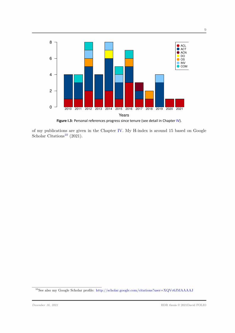
15 articles (ACL), 1 guest editorial (DO), 3 books chapter (OS) and 23 proceedings (ACT).Figure I.3 illustrates the timeline progress of my publishing activities and the detailed list
9The bibliography categories follows the nomenclature proposed by the Hcéres which is an independentadministrative authority for evaluation of research and higher education. http://www.hceres.fr
HDR thesis © 2021David FOLIO December 16, 2021
9
Years
0
2
4
6
8
2010 2011 2012 2013 2014 2015 2016 2017 2018 2019 2020 2021
ACLACTACNDOOSINVCOM
Figure I.3: Personal references progress since tenure (see detail in Chapter IV).
of my publications are given in the Chapter IV. My H-index is around 15 based on GoogleScholar Citations10 (2021).
10See also my Google Scholar profile: http://scholar.google.com/citations?user=XQVc6JMAAAAJ
December 16, 2021 HDR thesis © 2021David FOLIO

10
HDR thesis © 2021David FOLIO December 16, 2021

CHAPTER II
TEACHING AND ADMINISTRATIVERESPONSIBILITIES
In this chapter, the different aspects related to my teaching activities are summarized. Myoverall teaching activities have been solely related with the 61st CNU section which regroupsscientific disciplines from control, IT engineering and signal processing. I taught these teachingactivities as a temporary teacher (3 years), teaching assistant (ATER, 1 year), and then asassociate professor (since 2008). These different teaching experiences are presented in thefollowing sections.
II.1 BEFORE TENUREI have started teaching as a temporary teacher at the Paul Sabatier University of Toulouse,France, during my doctorate (2004 – 2006). Next, I have pursued as teaching assistant,specifically in French as Attaché Temporaire d’Enseignement et de Recherche (ATER, 2007),at the Paul Sabatier University of Toulouse. My teachings were mainly in the fields of robotics,control theory, image processing and real-time systems for students from bachelor’s to masterdegrees. These global teaching experiences have led to a total volume of 308 hETD.
These activities were my first experience in high-graduate education. Those opportunitieshighlighted my interest in the scientific knowledge transmission. They also allowed me tobe familiarized with the different forms of teachings. Indeed, I had then the opportunity tosupervise not only tutorials (TD), practical work (TP), and long-term projects (BE); but alsofew courses. Especially, I also helped the teaching team by writing some TP contents, and inthe students’ evaluation. This first experience confirmed my interest in teaching, leading melogically to apply for an associate professor position.
II.2 SINCE TENUREDUntil now, my teaching activities have been mainly held at INSA Centre Val de Loire onthe Bourges campus. Thus, I am mainly involved in the students’ formation of the MRI,ERE, and STPI departments. After having started with teaching of electronics and electricalengineering, I have participated or organized lessons on signal processing, sensors, controland robotics. These various teaching experiences imply very different pedagogical tasks.Especially, those tasks depend on the type of intervention: courses (C), tutorials (TD),practical works (TP), or tutored projects (P); but also according to the different degreesof scientific maturity and specialization of the concerned students: from bachelor’s (L1) to
11

12 Chap. II. Teaching and Administrative Responsibilities
Table II.1: Overview of the various teaching disciplines as associate professor.
Face time
Disciplines LMDa Studentsb Cc TD TP Dept. Years
Electrokinetics L1 100 18h00 24h00 STPI 2012-2014
Analog Electronics (I) L2 80 8h00 32h00 STPI 2015-present
Analog Electronics (II) L3 70 21h20 21h20 6h00 MRI 2008-2016
Analog Electronics (III) L3 70 10h40 10h40 MRI 2015-present
Electrical engineering L3 70 10h40 10h40 MRI 2008-2016
Electricity - Electricalengineering
L3 78 8h00 14h00 ERE 2016-present
Electricity - Electricalengineering
M1 78 8h00 14h00 ERE 2012-2016
Control and Sensors M1 78 6h 9h ERE 2014-2016
Control and Diagnostic M1 20 10h40 10h40 MRI 2015-present
Signals and Systems M1 20 10h40 10h40 MRI 2014-present
Perception for robotic M2 25 4h MARSS 2012-2018
Robotic M2 50 9h 9h MRI/3EA 2019-present
Students Projects (SA) M1 2 MRI 2008-present
Students Projects (PSI) M1 10 MRI 2008-presenta LMD is the bachelor’s, master’s, doctorate system (in French License-Master-Doctorat) designed
by the Bologna process, with L1-L3: from the 1st to the 3rd year bachelor’s degree; M1-M2: fromthe 1st to the 2nd year master’s degree.
b the average number of students per year.c refer to face time hours for courses (C), tutorials (TD) and practical works (TP).
master’s (M2) degree level. For instance, it can be noticed, that the ERE department trainsengineers through an apprenticeship training. Table II.1 illustrates a synthetic overview ofthe different teaching disciplines for which I am in charge. These responsibilities imply theimplementation of teaching materials and the students evaluations, but also the support ofteaching assistants (e.g. for the TD). As needed, I also intervened to support the teachingactivities of some of my colleagues (e.g. for their TD).
A description of some of these disciplines are summarized hereafter.
Analog electronics (I), (II) and (III): The aim is to provide from basic to high level view of theelementary components that are the heart of electronic circuits. It deal with passivecomponents such as resistors, capacitors and inductors as well as an introduction todiodes, transistors and operational amplifiers, and their use in filters, amplifiers, powersupply circuits.First taught to engineering students (L3) of ENSI of Bourges, this discipline has evolvedsince the creation of INSA Centre Val de Loire and is provided to the STPI (L2) andMRI (L3) departments. This allowed me to develop the teaching of analog electronicsfrom the L3 level to more advanced electronics.
HDR thesis © 2021David FOLIO December 16, 2021

II.3. Responsibilities 13
Electrical engineering: After an introduction to fundamental concepts (e.g. electricity, single-phase and three-phase electric power, etc. ), this teaching is supplemented by casestudies. This allows engineering students to understand the use of tools and models toevaluate the performance of an electrical system, for diagnosis and help in the choice ofmore efficient and sustainable solutions.
Robotics: This course is intended for engineering students from the MRI department (M2)together with the international master degree on Electronics, Electrical Energy andAutomatics (3EA) jointly with the University of Tours. This teaching, in Englishlanguage, allows students to discover new fields of research and to take an interestin the modeling and control of mobile robots.
Student Projects:• Advanced systems projects (SA): a pair have to work over a semester to study
an advanced system, such as a microrobotic system, an electromagnetic actuationplatform, etc.
• Industrial synthesis projects (PSI): a group of about ten students must divide theworkload to study complex processes, such as the viscous flow in channels, themodeling of magnetic fields induced by electromagnetic coils…
II.3 RESPONSIBILITIESIn addition to teaching tasks, various duties are related to associate professor position. First,I am involved in the life and the scientific animation of the Institute. I also participate inthe juries of our engineering students. Similarly, since our establishment have joint the INSAgroup in 2014, I contribute to select and interview the applying students (about 15 studentsper year).
Between 2009 and 2013, I have been member of the Hygiene and Security committee of theof ENSI Bourges.
Since September 2014, I am in charge of the Nuclear Energy option of the 5 year (engineer’sdegree) of the Industrial Risk Control (MRI) department. As such, I coordinate the specificlessons of the option by selecting and recruiting external professional contractors. I alsoorganize visits (nuclear power plant, simulator, etc.) for the engineering students of the option.Since 2018, I took part to panel discussions “support for nuclear training” and “nuclear-jobs-training” which have enabled participants to better understand issues about nuclear energyin France.
Between November 2017 and 2020, I have been an elected member of the ERE departmentcouncil. Next, since 2020, I am an elected member of the Industrial Risk Control (MRI)department council.
In March 2017, the direction of the INSA Centre Val de Loire given to me the mission ofreferent “racism and antisemitism”.
December 16, 2021 HDR thesis © 2021David FOLIO


CHAPTER III
SUMMARY OF RESEARCH ACTIVITIES
This chapter summarizes the different research activities in which I have been involved. Thisincludes research projects, student supervision, scientific collaborations, and outreach.
III.1 SCIENTIFIC PROJECTSMy research activities regularly lead me to contribute to scientific projects. These projectsaim to obtain funds to either recruit young researchers, to design or improve our experimentalplatforms, as well as to help to enhance scientific cooperation. Below are listed the differentprojects in which I have been strongly involved, both in their implementation and in theirachievements. Let us notice that all of these projects have been subject to a process withdeep scientific reviews. The list of unsuccessful applications is equally important.
III.1.1 European Union (EU) and national funding projectsNANOMA Nano-Actuators and Nano-Sensors for Medical Applications
Date 06/2008 – 10/2011Funding 3.3M€, supported by the European Commission under FP7 ICT 2007.3.6,
Micro/nanosystemsSummary The NANOMA was coordinated by Professor Antoine Ferreira, University of
Orléans, PRISME Laboratory. This project aimed at proposing novel controllednanorobotic delivery systems to improve the diagnosis and the administration ofdrugs in the treatment of breast cancer.
Role co-responsible of the workpackage: “object tracking, planning and control in MRI”.PROSIT Robotic Platform for an Interactive Tele-echographic Systems
Date 01/2009 – 09/2012Funding 230k€, supported by ANR Contint programSummary The PROSIT project was coordinated by Professor Pierre Vieyres, University
of Orléans, PRISME Laboratory. The goal was to develop an interactive andcomplex master-slave robotic platform for a medical diagnosis application (i.e. tele-echography) based on a well-defined modular control architecture.
Role co-responsible of the workpackage: “visual servoing”.PROTEUS Robotic platform to facilitate transfer between industries
Date 12/2009 – 12/2013Funding 2.1M€, supported by ANR ARPEGE programSummary The PROTEUS project motivation was to help to organize interactions
between academic and industrial partners of the French robotic community by
15

16 Chap. III. Summary of Research Activities
providing suitable tools and models. One goal was to create a portal for theFrench robotic community as embodied by the GDR Robotique and its affiliatedindustrial partners, in order to facilitate transfer of knowledge and problems amongthis community. To achieve the PROTEUS project 12 partners have been involved.
Role co-responsible of the workpackage: “young challenge”.PIANHO Innovative haptic instrumental platform for 3D nano-manipulation
Date 03/2010 – 03/2014Funding 761k€, supported by ANR P3N program.Summary The PIANHO project motivation is to create a nanomanipulation platform
capable of pick, hold and place nano-objects in the synchrotron radiation beam ofthe ESRF1 (Grenoble, France) via tuneable tool-object interaction.
Role co-responsible of the workpackage: “control of a two-fingered AFM-based nano-manipulation system”.
MTG Microrobots Targeting Glioblastoma (MTG)Date 03/2019 – 03/2022Funding 511.4k€, supported by French National Institute of Health and Medical Re-
search2 (Inserm) “plan cancer” programSummary The MTG objective is to functionalize magnetic microrobot with NFL pep-
tide3 to target glioblastoma (GBM).Role co-responsible of the workpackage: “in vitro and in vivo distribution and tracking
studies using IVIS imaging system to test the capacity of MTG to target glioblas-toma cells versus healthy cells of the nervous system”.
III.1.2 Cooperation projectsPHC PROCOPE Franco-German Hubert Curien4 partnership (PHC)
Date 2010 – 2011Summary Supervision and control of an improved platform for targeted administration
of therapeutic Nanorobots.Partnership Division of Microrobotics and Control Engineering5 (AMiR), university of
Oldenburg, Germany.PHC PROCORE Franco–Hong-Kong Hubert Curien partnership
Date 2014 – 2015Summary Design, fabrication and characterization of the swim of enhanced helical
microrobots.Partnership Department of Mechanical and Automation Engineering6 (MAE), Chinese
university of Hong-Kong (CUHK).1European Synchrotron Radiation Facility (ESRF), https://www.esrf.eu2from French: Institut national de la santé et de la recherche médicale (INSERM), https://www.inserm.fr3NeuroFilament Light subunit that is binding Tubulin (NFL peptide) is capable to penetrate in GBM, block
and inhibit cell division.4PHC, from French Partenariats Hubert Curien, provides support for international scientific and techno-
logical exchange of the Ministry of Foreign Affairs. https://www.campusfrance.org5AMiR, that is from German Abteilung für Mikrorobotik und Regelungstechnik, is a department of the
University of Oldenburg, Germany, headed by Prof. Dr.-Ing. Sergej Fatikov. http://www.amir.uni-oldenburg.de
6MAE is a department of the Chinese University of Hong Kong, with A.Prof. Li Zhang.http://www.mae.cuhk.edu.hk
HDR thesis © 2021David FOLIO December 16, 2021

III.2. Student Supervision 17
III.1.3 Regional projectsNano‐IRM
Date 09/2009 – 08/2012Funding 110k€, supported by Région Centre Val de Loire, the Cher (18) departmental
councils and the agglomeration comity of Bourges.Summary Supervision and control of an improved platform for targeted administration
of therapeutic nanorobots. This project supports the above project NANOMA, byproviding the funding for the PhD thesis of Karim Belharet.
Role co-supervision of the PhD thesis of Karim Belharet.MicroRob
Date 10/2013 – 09/2016Funding 110k€, supported by Région Centre Val de Loire and the agglomeration comity
of Bourges.Summary Modeling and control of magnetic microcarrier for targeted cancer therapy.Role co-supervision of the PhD thesis of Lyes Mellal.
US‐Probe High Definition EchographDate 03/2017 – 03/2018Funding 50k€, supported by Région Centre Val de Loire (APR-IA)Summary Design of novel microrobotic platform with ultrasound imaging.Role Principal Investigator (PI).
BUBBLEBOT Magnetic microbubbles for the targeted delivery of therapeutic agent in the brainDate 10/2020 – 10/2023Funding 210k€, supported by Région Centre Val de Loire (APR-IR)Summary The aim is to combine the progress made in microrobotics with those made
with microbubbles in order to improve the therapeutic targeting of glioblastoma.Role Principal Investigator (PI).
III.2 STUDENT SUPERVISIONMy research work was carried out with the contributions of young researchers whose works Isupervised. I had directly supervised 5 Master (M2) and 6 PhD students. The total rate ofsupervision of defended PhD theses is 200%. In addition, I also had the opportunity to followthe research works of 3 externals PhD students. These different students are listed hereafter,as well as the joint publications.
III.2.1 Master students (M2)Kamel Ncir
Date 03/2010 – 08/2010Title Commande robuste pour le nano-positionnement d’une plateforme instrumentale.Situation Technician at Jubilant HollisterStier LLC, Montréal, Québec, Canada
Nabil AmariDate 03/2011 – 08/2011Title Modélisation et Commande d’une plateforme de nano positionnementSituation Associate Professor HEI, Châteauroux, France
December 16, 2021 HDR thesis © 2021David FOLIO

18 Chap. III. Summary of Research Activities
Bruno SarkisDate 03/2015 – 08/2015Title Modélisation des microjets catalytiques dans des canaux micro-fluidiquesReferences [ACT22,ACL14]
Hadjila MahfoufiDate 03/2018 – 08/2018Title Modélisation, Simulation et Commande de Microrobot CatalytiqueSituation Engineer at Alstom, Paris, France
Oumarou HABOU SOULEDate 03/2019 – 09/2019Title Suivi de Microrobot par Imagerie Echographique
III.2.2 Doctoral studentsIII.2.2.1 Defended theses
[PhD1] Tao LiDate 03/2009 – 02/2013Title Commande d’un robot de télé-échographie par asservissement visuel. Thesis of
university of Rennes 1Supervision 37.5% with Prof. Pierre Vieyres (12.5%), François Chaumette (12.5%) and
Alexandre Krupa (37.5%)References [ACL8]Situation Engineer at Another Brain, Paris, France
[PhD2] Karim BelharetDate 10/2009 – 07/2013Title Navigation prédictive d’un microrobot magnétique : Instrumentation, commande
et validation. Thesis of university of OrléansSupervision 50% with Prof. Antoine FerreiraReferences [ACT8,ACT9,ACT12,ACT14,ACT17,ACT19,ACT21,ACL2,ACL3,
ACL6,OS2]Situation Associate Professor HEI, Châteauroux, France
[PhD3] Nabil AmariDate 10/2011 – 07/2016Title Développement et Commande d’une Plateforme Microrobotique pour la Synchro-
nisation d’un Faisceau de Lumière. Thesis of university of OrléansSupervision 30% with Prof. Antoine FerreiraReferences [ACT15,ACT16,ACT18,ACT20,ACL7,OS3]Situation Associate Professor HEI, Châteauroux, France
[PhD4] Lyès MellalDate 10/2013 – 12/2016Title Modélisation et commande de microrobots magnétiques pour le traitement ciblé
du cancer. Thesis of university of OrléansSupervision 40% with Prof. Antoine Ferreira (30%) and Karim Belharet (30%)References [ACT23,ACT24,ACT25,ACT27,ACL9,ACL12]Situation Teaching assistant at ISEN, Lille, France
HDR thesis © 2021David FOLIO December 16, 2021

III.3. Scientific Collaborations 19
[PhD5] Ruipeng ChenDate 11/2016 – 07/2020Title Design Methodology for Electromagnetic Microrobotic Platforms. Thesis of INSA
Centre Val de LoireSupervision 50% with Prof. Antoine FerreiraReferences [ACT27,ACT28,ACT29,ACL15]Situation Post Doctorate, INSA CVL, Bourges, France
III.2.2.2 Ongoing thesis[PhD6 ]Karim Botros
Date 04/2021 – 03/2024Title Magnetic Micro-robotic Platform Guided by Robotic Ultrasound for Brain Tumor
Targeting. Thesis of INSA Centre Val de LoireSupervision 50% with Prof. Antoine Ferreira
III.2.2.3 External PhD students[Ext1] Junsig Kim
Date 2008 – 2012Title A Study of Oocyte/Embryo Manipulation Using Microfluidics and Robotics. The-
sis of Korea Advanced Institute of Science and Technology (KAIST), South KoreaReferences [ACT10,ACL5]Situation Senior Research Engineer at LG Electronics, South Korea
[Ext2] Christian DahmenDate 2009 – 2013Title Robust Object Tracking for Micro- and Nanorobotics. Thesis of Carl von Ossietzky
Universität OldenburgReferences [ACT11,ACT13,ACL11]Situation Dr. Ing. at Carmeq GmbH, Berlin, Germany
[Ext3] Jang BumjinDate 2015 – 2016Title Magnetic Nano Actuators for Quantitative Analysis. Thesis of ETH Zurich,
SwitzerlandReferences [ACL10]Situation Engineer at Samsung Electronics, South Korea
III.3 SCIENTIFIC COLLABORATIONSMy research works have led to various international and national collaborations. These coop-erations have made possible to investigate complementary approaches to those I have studied,helping me to benefit from supplementary skills. These exchanges were important in viewof the strong multidisciplinary of the achieved works, the variety of physical principles used,and the technologies involved. Hereafter some significant collaborations and partnerships thathave resulted in either joint publications or that are still ongoing.
December 16, 2021 HDR thesis © 2021David FOLIO

20 Chap. III. Summary of Research Activities
III.3.1 International relationships• Department of Mechanical Engineering at Korea Advanced Institute of Science and
Technology (KAIST), South Korea– Team of Prof. Jung Kim– References: [ACT10,ACL5]
• Division of Microrobotics and Control Engineering (AMiR), university of Oldenburg,Germany– Team of Prof. Sergej Fatikow– References: [ACT11,ACT13,ACL11]
• Multi-Scale Robotics Laboratory7 (MSRL), ETH8 Zurich, Switzerland– Team of Prof. Bradley Nelson and Prof. Salvador Pané Vidal– References: [ACT11,ACL10]
• Mechanical and Automation Engineering (MAE) Department of Chinese University ofHong Kong (CUHK), Hong-Kong.– Team of Prof. Li Zhang
III.3.2 National relationships• Inria Rennes–Bretagne Atlantique, IRISA, University of Rennes, France
– Team of senior researcher François Chaumette– Co-supervision of the PhD thesis of Tao Li.– Reference: [ACL8]
• Translational micro and nanomedicines9 (MINT) Laboratory, University of Angers, France– Team of senior researcher Joël Eyer
• Center for Molecular Biophysics10 (CBM), CNRS, Orleans, France– Team “Innovative therapies and nanomedicine” with Prof. Chantal Pichon
• Vermon11 SA, Tours, France– R&D work on development and industrialization to enhance micro-object perception
through ultrasound transducers.
III.4 SCIENTIFIC DISSEMINATION AND OUTREACHThe appreciation of my research works have been effective through various actions that arereported hereafter.
7Multi-Scale Robotics Lab (MSRL) is part of Institute of Robotics and Intelligent Systems (IRIS), ETHZurich, Switzerland. https://msrl.ethz.ch, https://www.iris.ethz.ch
8ETH Zurich is the Swiss Federal Institute of Technology in Zurich, from German “EidgenössischeTechnische Hochschule”. https://ethz.ch
9From French “Laboratoire Micro et Nanomédecines translationnelles”, is funded by the University ofAngers, as well as Inserm and the CNRS. http://mint.univ-angers.fr
10CBM is a research unit of the CNRS affiliate with the University of Orléans.http://cbm.cnrs-orleans.fr11Vermon is a society involved in the design, manufacturing of composite piezoelectric transducer. https:
//www.vermon.com
HDR thesis © 2021David FOLIO December 16, 2021

III.4. Scientific Dissemination and Outreach 21
III.4.1 InvitationsJune 2010 scientific visit in the AMiR division, university of Oldenburg, GermanyMarch 2015 scientific visit in MAE Department of Chinese University of Hong Kong (CUHK),
Hong-Kong.Others I have also been invited as a speaker in international or national conferences,
[INV1,INV2,INV3] which are reported in Section IV.4.1.
III.4.2 Scientific expertise• I have took part in the evaluation process of Generic Call (2019,2020) for the French
National Research Agency (ANR).• I have been member of the recruitment selection committee:
– 2013: associate professor position at University of Orléans;– 2015: associate professor position at INSA Centre Val de Loire;– 2021: associate professor position at INSA Centre Val de Loire;
• In addition to the PhD works that I co-supervised, I was also invited as an examinermember of the PhD thesis defense of:
1. Adrien Durand Petiteville, Navigation référencée multi-capteurs d’un robot mobiledans un environnement encombré, university of Toulouse, December, 2011.
2. Moahmed Dkhil, Modélisation, caractérisation et commande d’un système micro-robotique magnétique à l’interface air/liquide, University of Pierre and Marie Curie,Paris, April, 2016
III.4.3 Editorial activitiesSince 2005 IEEE member (SM’05, AM’08, M’12).Since 2013 Editorial Board member of the International Journal of Advanced Robotic Systems
(IJARS).Since 2015 Member of the program committee of the International Conference on Robotics,
Manipulation, and Automation at Small Scales (MARSS)2012 Oct. Session chairman of the IEEE/RSJ International Conference on Intelligent Robots
and Systems, Vilamoura, Algarve, Portugal, October 20122021 Associate Editor of the 18th International Conference on Ubiquitous Robots, Gangneung-
si, Gangwon-do, Korea, 2021.Regular Reviewer (non-exhaustive list)
• IEEE Transactions on Robotics (TRO);• IEEE robotics and automation letters (RAL);• IEEE Transactions on Biomedical Engineering (TBME);• IEEE/ASME Transactions on Mechatronics (TMECH);• IEEE Transactions on Automation Science and Engineering (TASE);• International Journal of Advanced Robotic Systems (IJARS);• IEEE International Conference on Robotics and Automation (ICRA);• IEEE/RSJ International Conference on Intelligent Robots and Systems (IROS);• IEEE International Conference on Biomedical Robotics and Biomechatronics
(BioRob), …
December 16, 2021 HDR thesis © 2021David FOLIO

22 Chap. III. Summary of Research Activities
III.4.4 AwardsFrench outstanding research award (PEDR) for the periods 2014-2018 and 2018-2022.
HDR thesis © 2021David FOLIO December 16, 2021

CHAPTER IV
PERSONAL REFERENCES
My research activities have led to scientific publications that are listed in this chapter. Thenames of the people for whom I have supervised their works are in bold face. Furthermore,the publications list follows the Hcéres proposed nomenclature.
IV.1 ARTICLES
IV.1.1 Articles in International peer‐reviewed and referenced journals(ACL)
Remark (Remark) — \iffalse Remark (Metrics). Two journal metrics are reported here:journal quartile (Qn) and impact factor (IF). Journal metrics are based on Scopus® data as of April2020. The reported quartile is the metric of the journal in the year of publishing.
[ACL1] David FOLIO, and Viviane Cadenat. “Dealing with visual features loss during avision-based task for a mobile robot”, International Journal of Optomechatronics, 2(3): pp. 185–204, June 2008. doi:10.1080/15599610802301110. Special issue on VisualServoing. (Q2, IF:0.81)
[ACL2] Karim Belharet, David FOLIO, and Antoine Ferreira. “MRI-based microroboticsystem for the propulsion and navigation of ferromagnetic microcapsules”, Mini-mally Invasive Therapy & Allied Technologies, 19 (3): pp. 157–169, June 2010.doi:10.3109/13645706.2010.481402. (Q2, IF:1.0)
[ACL3] Karim Belharet, David FOLIO, and Antoine Ferreira. “Three-dimensional controlledmotion of a microrobot using magnetic gradients”, Advanced Robotics, 25 (8): pp. 1069–1083(15), May 2011. doi:10.1163/016918611X568657. (Q2, IF:1.24)
In 2013 one of the Advanced Robotics most cited articles from 2011 publications.[ACL4] Viviane Cadenat, David FOLIO, and Adrien Durand Petiteville. “A compari-
son of two sequencing techniques to perform a vision-based navigation task in acluttered environment”, Advanced Robotics, 26 (5-6): pp. 487–514, March 2012.doi:10.1163/156855311X617470. (Q2, IF:1.24)
[ACL5] Jungsik Kim, Hamid Ladjal, David FOLIO, Antoine Ferreira, and Jung Kim. “Evalu-ation of telerobotic shared control strategy for efficient single-cell manipulation”, IEEETransactions on Automation Science and Engineering, 9 (2): pp. 402–406, April 2012.doi:10.1109/TASE.2011.2174357 (Q1, IF:4.93)
[ACL6] Karim Belharet, David FOLIO, and Antoine Ferreira. “Simulation andplanning of a magnetically actuated microrobot navigating in arteries”, IEEETransactions on Biomedical Engineering, 60 (4): pp. 994–1001, April 2013.doi:10.1109/TBME.2012.2236092. (Q1, IF:4.42)
23
24 Chap. IV. Personal References
[ACL7] Nabil Amari, David FOLIO, and Antoine Ferreira. “Motion of a mi-cro/nanomanipulator using a laser beam tracking system”, International Journal ofOptomechatronics, 8 (1): pp. 30–46, April 2014. doi:10.1080/15599612.2014.890813 (Q3,IF:0.81)
[ACL8] Alexandre Kruba, David FOLIO, Cyril Novales, Pierre Vieyres, and Tao Li. “Robotizedtele-echography: an assisting visibility tool to support expert diagnostic”, IEEE SystemsJournal, 10 (3): pp. 974–983, April 2014. doi:10.1109/JSYST.2014.2314773 (Q2, IF:3.98)
[ACL9] Lyes Mellal, Karim Belharet, David FOLIO, and Antoine Ferreira. “Optimal struc-ture of particles-based superparamagnetic microrobots: application to MRI guidedtargeted drug therapy”, Journal of Nanoparticle Research, 17 (2): 64, February 2015.doi:10.1007/s11051-014-2733-3 (Q2, IF:2.13)
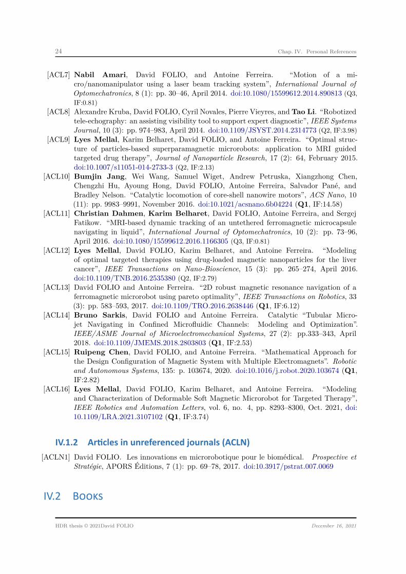
[ACL10] Bumjin Jang, Wei Wang, Samuel Wiget, Andrew Petruska, Xiangzhong Chen,Chengzhi Hu, Ayoung Hong, David FOLIO, Antoine Ferreira, Salvador Pané, andBradley Nelson. “Catalytic locomotion of core-shell nanowire motors”, ACS Nano, 10(11): pp. 9983–9991, November 2016. doi:10.1021/acsnano.6b04224 (Q1, IF:14.58)
[ACL11] Christian Dahmen, Karim Belharet, David FOLIO, Antoine Ferreira, and SergejFatikow. “MRI-based dynamic tracking of an untethered ferromagnetic microcapsulenavigating in liquid”, International Journal of Optomechatronics, 10 (2): pp. 73–96,April 2016. doi:10.1080/15599612.2016.1166305 (Q3, IF:0.81)
[ACL12] Lyes Mellal, David FOLIO, Karim Belharet, and Antoine Ferreira. “Modelingof optimal targeted therapies using drug-loaded magnetic nanoparticles for the livercancer”, IEEE Transactions on Nano-Bioscience, 15 (3): pp. 265–274, April 2016.doi:10.1109/TNB.2016.2535380 (Q2, IF:2.79)
[ACL13] David FOLIO and Antoine Ferreira. “2D robust magnetic resonance navigation of aferromagnetic microrobot using pareto optimality”, IEEE Transactions on Robotics, 33(3): pp. 583–593, 2017. doi:10.1109/TRO.2016.2638446 (Q1, IF:6.12)
[ACL14] Bruno Sarkis, David FOLIO and Antoine Ferreira. Catalytic “Tubular Micro-jet Navigating in Confined Microfluidic Channels: Modeling and Optimization”.IEEE/ASME Journal of Microelectromechanical Systems, 27 (2): pp.333–343, April2018. doi:10.1109/JMEMS.2018.2803803 (Q1, IF:2.53)
[ACL15] Ruipeng Chen, David FOLIO, and Antoine Ferreira. “Mathematical Approach forthe Design Configuration of Magnetic System with Multiple Electromagnets”. Roboticand Autonomous Systems, 135: p. 103674, 2020. doi:10.1016/j.robot.2020.103674 (Q1,IF:2.82)
[ACL16] Lyes Mellal, David FOLIO, Karim Belharet, and Antoine Ferreira. “Modelingand Characterization of Deformable Soft Magnetic Microrobot for Targeted Therapy”,IEEE Robotics and Automation Letters, vol. 6, no. 4, pp. 8293–8300, Oct. 2021, doi:10.1109/LRA.2021.3107102 (Q1, IF:3.74)
IV.1.2 Articles in unreferenced journals (ACLN)[ACLN1] David FOLIO. Les innovations en microrobotique pour le biomédical. Prospective et
Stratégie, APORS Éditions, 7 (1): pp. 69–78, 2017. doi:10.3917/pstrat.007.0069
IV.2 BOOKS
HDR thesis © 2021David FOLIO December 16, 2021

IV.3. Proceedings in International Conferences (ACT) 25
IV.2.1 Guest Editor (DO)[DO1] Ashis Banerjee, David FOLIO, Sarthak Misra and Quan Zhou. Guest editors of
the Special Issue: “Design, Fabrication, Control, and Planning of Multiple MobileMicrorobots”. International Journal of Advanced Robotic Systems, 2014. doi:10.5772/1
IV.2.2 Book Chapter (OS)[OS1] David FOLIO and Viviane Cadenat. Treating Image Loss by using the Vision/Motion
Link: Generic Framework, chapter 4, page 538. I-Tech, Vienna, Austria, November2008. ISBN 978-953-7619-21-3.
[OS2] Karim Belharet, David FOLIO, and Antoine Ferreira. Real-time software platform forin vivo navigation of magnetic micro-carriers using MRI system, chapter 11. Number 51in Biomaterials. Woodhead Publishing, Cambridge, October 2012. ISBN:780857091307.
[OS3] Nabil Amari, David FOLIO, and Antoine Ferreira. Encyclopedia of Nanotechnology,chapter Nanorobotics for Synchrotron Radiation Applications, pp. 1–19. SpringerNetherlands, Dordrecht, 2nd edition, 2016. doi:10.1007/978-94-007-6178-1009270-1
[OS4] Lyès Mellal, Karim Belharet, David FOLIO, and Antoine Ferreira. Modeling Approachof Transcatheter Arterial Delivery of Drug-Loaded Magnetic Nanoparticles, chapter 10.in The Encyclopedia of Medical Robotics. World Scientific, October 2018. ISBN:780857091307. doi:10.1142/9789813232280_0010
IV.3 PROCEEDINGS IN INTERNATIONAL CONFERENCES (ACT)[ACT1] David FOLIO and Viviane Cadenat. Using redundancy to avoid simultaneously
occlusions and collisions while performing a vision-based task amidst obstacles. InEuropean Conference on Mobile Robots (ECMR’05), Ancona, Italy, September 2005.
[ACT2] David FOLIO and Viviane Cadenat. A controller to avoid both occlusions and obstaclesduring a vision-based navigation task in a cluttered environment. In European ControlConference (ECC’05), pages 3898–3903, Seville, Spain, December 2005.
[ACT3] David FOLIO and Viviane Cadenat. A redundancy-based scheme to perform safe vision-based tasks amidst obstacles. In IEEE/RSJ International Conference on Robotics andBiomimetics (ROBIO’06), pages 13–18, Kunming, Yunnan, China, December 2006.doi:10.1109/ROBIO.2006.340252.
Finalist to the T.J. Tarn best paper in Robotics.[ACT4] David FOLIO and Viviane Cadenat. A new controller to perform safe vision-based
navigation tasks amidst possibly occluding obstacles. In European Control Conference(ECC’07), Kos, Greece, July 2007.
[ACT5] David FOLIO and Viviane Cadenat. Using simple numerical schemes to compute visualfeatures whenever unavailable. In IFAC International Conference on Informatics inControl, Automation and Robotics (ICINCO’07), May 2007.
[ACT6] David FOLIO and Viviane Cadenat. A sensor-based controller able to treat total imageloss and to guarantee non-collision during a vision-based navigation task. In IEEE/RSJInternational Conference on Intelligent Robots and Systems (IROS’2008), pages 3052–3057, Nice, France, September 2008. doi:10.1109/IROS.2008.4650743.
December 16, 2021 HDR thesis © 2021David FOLIO

26 Chap. IV. Personal References
[ACT7] Olivier Kermorgant, David FOLIO, and François Chaumette. A new sensor self-calibration framework from velocity measurements. In IEEE International Conferenceon Robotics and Automation (ICRA’2010), pp. 1524–1529, Anchorage, Alaska, May2010. doi:10.1109/ROBOT.2010.5509219
[ACT8] Karim Belharet, David FOLIO, and Antoine Ferreira. 3D MRI-based predictive con-trol of a ferromagnetic microrobot navigating in blood vessels. In IEEE RAS and EMBSInternational Conference on Biomedical Robotics and Biomechatronics (BioRob’2010),pp. 808–813, Tokyo, Japan, September 2010. doi:10.1109/BIOROB.2010.5628063
[ACT9] Karim Belharet, David FOLIO, and Antoine Ferreira. Endovascular navigationof a ferromagnetic microrobot using MRI-based predictive control. In IEEE/RSJInternational Conference on Intelligent Robots and Systems (IROS’2010), pp. 2804–2809, Taipei, Taiwan, October 2010. doi:10.1109/IROS.2010.5650803
[ACT10] Jungsik Kim, Dongjune Chang, Hamid Ladjal, David FOLIO, and Antoine Fer-reira and Jung Kim. Evaluation of telerobotic shared control for efficient ma-nipulation of single cells in microinjection. In IEEE International Conference onRobotics and Automation (ICRA’2011), pp. 3382–3387, Shanghai, China, May 2011.doi:10.1109/ICRA.2011.5979868
[ACT11] David FOLIO, Christian Dahmen, Tim Wortmann, M. Arif Zeeshan, Kaiyu Shou,Salvador Pane, Bradley J. Nelson, Antoine Ferreira, and Sergej Fatikow. MRImagnetic signature imaging, tracking and navigation for targeted micro/nano-capsuletherapeutics. In IEEE/RSJ International Conference on Intelligent Robots andSystems (IROS’2011), pp. 1297–1303, San Fransisco, CA, USA, September 2011.doi:10.1109/IROS.2011.6048651
[ACT12] Karim Belharet, David FOLIO, and Antoine Ferreira. Control of a magneticmicrorobot navigating in microfluidic arterial bifurcations through pulsatile and vis-cous flow. In IEEE/RSJ International Conference on Intelligent Robots and Sys-tems (IROS’2012), pp. 2559–2564, Vilamoura, Algarve, Portugal, October 2012.doi:10.1109/IROS.2012.6386030
[ACT13] Christian Dahmen, David FOLIO, Tim Wortmann, Alexander Kluge, Antoine Fer-reira, and Sergej Fatikow. Evaluation of a MRI based propulsion/control system aimingat targeted micro/nano-capsule therapeutics. In IEEE/RSJ International Conferenceon Intelligent Robots and Systems (IROS’2012), pp. 2565–2570, Vilamoura, Algarve,Portugal, October 2012. doi:10.1109/IROS.2012.6386244
[ACT14] Karim Belharet, David FOLIO, and Antoine Ferreira. Untethered microrobot controlin fluidic environment using magnetic gradients. In International Symposium onOptomechatronic Technologies (ISOT’2012), pp. 1–5, October 2012.
[ACT15] Nabil Amari, David FOLIO, and Antoine Ferreira. Robust laser beam tracking controlusing micro/nano dual-stage manipulators. In IEEE/RSJ International Conference onIntelligent Robots and Systems (IROS’2013), pp. 1543–1548, Tokyo Big Sight, Japan,November 2013. doi:10.1109/IROS.2013.6696554
[ACT16] Nabil Amari, David FOLIO, Karim Belharet, and Antoine Ferreira. Motionof a micro/nanomanipulator using a laser beam tracking system. In InternationalSymposium on Optomechatronic Technologies (ISOT’2013), Jeju Island, Korea, October2013.
[ACT17] Karim Belharet, Yang Chunbo, David FOLIO, and Antoine Ferreira. Model charac-terization of magnetic microrobot navigating in viscous environment. In International
HDR thesis © 2021David FOLIO December 16, 2021

IV.3. Proceedings in International Conferences (ACT) 27
Symposium on Optomechatronic Technologies (ISOT’2013), Jeju Island, Korea, October2013.
[ACT18] Nabil Amari, David FOLIO, and Antoine Ferreira. Robust tracking of a two-fingered micromanipulation system working through the focus of an optical beam. InAmerican Control Conference (ACC’2014), pp. 1613–1618, Portland, OR, USA, June2014. doi:10.1109/ACC.2014.6859244
[ACT19] Karim Belharet, David FOLIO, and Antoine Ferreira. Vision-based forces charac-terization of magnetic microrobot in a viscous environment. In IEEE InternationalConference on Robotics and Automation (ICRA’2014), pp. 2065–2070, Hong Kong,China, May 2014. doi:10.1109/ICRA.2014.6907133
[ACT20] Nabil Amari, David FOLIO, and Antoine Ferreira. Robust nanomanipulation controlbased on laser beam feedback. In IEEE/RSJ International Conference on IntelligentRobots and Systems (IROS’2014), pp. 4674–4679, Chicago, IL, USA, September 2014.doi:10.1109/IROS.2014.6943226
[ACT21] Karim Belharet, David FOLIO, and Antoine Ferreira. Study on rotational andunclogging motions of magnetic chain-like microrobot. In IEEE/RSJ InternationalConference on Intelligent Robots and Systems (IROS’2014), pp. 834–839, Chicago, IL,USA, September 2014. doi:10.1109/IROS.2014.6942656
[ACT22] Bruno Sarkis, David FOLIO, and Antoine Ferreira. Catalytic tubular microjetpropulsion model for endovascular navigation. In IEEE International Conference onRobotics and Automation (ICRA’2015), pp. 3537–3542, Seattle, Washington, USA, May2015. doi:10.1109/ICRA.2015.7139689
[ACT23] Lyes Mellal, David FOLIO, Karim Belharet, and Antoine Ferreira. Magnetic microbotdesign framework for antiangiogenic tumor therapy. In IEEE/RSJ InternationalConference on Intelligent Robots and Systems (IROS’2015), pp. 1397–1402, Hamburg,Germany, September 2015. doi:10.1109/IROS.2015.7353550
[ACT24] Lyes Mellal, David FOLIO, Karim Belharet, and Antoine Ferreira. Optimal controlof multiple magnetic microbeads navigating in microfluidic channels. In IEEE Interna-tional Conference on Robotics and Automation (ICRA’2016), pp. 1921–1926, Stockholm,Sweden, May 2016. doi:10.1109/ICRA.2016.7487338
[ACT25] Lyes Mellal, David FOLIO, Karim Belharet, and Antoine Ferreira. Estimationof interaction forces between two magnetic bolus-like microrobots. In InternationalConference on Manipulation, Automation and Robotics at Small Scales (MARSS’2016),pp. 1–6, Paris, France, July 2016. doi:10.1109/MARSS.2016.7561740
[ACT26] Lyes Mellal, David FOLIO, Karim Belharet, and Antoine Ferreira. Motion controlanalysis of two magnetic microrobots using the combination of magnetic gradient andoscillatory magnetic field. In International Conference on Manipulation, Automationand Robotics at Small Scales (MARSS’2017), pp. 1–6, Montreal, QC, Canada, July 2017.doi:10.1109/MARSS.2017.8001917
[ACT27] Ruipeng Chen, David FOLIO, and Antoine Ferreira Study of robotized electro-magnetic actuation system for magnetic microrobots devoted to minimally invasiveophthalmic surgery, in International Symposium on Medical Robotics (ISMR’2019),pp. 1–7, Atlanta, GA, USA, April 2019. doi:10.1109/ISMR.2019.8710208
[ACT28] Ruipeng Chen, David FOLIO, and Antoine Ferreira Computational Electromag-netics Performances of Magnetic Microrobotics Systems, in International Confer-ence on Robotics and Automation (ICRA’2019), Montreal, QC, Canada, May 2019.doi:10.1109/ICRA.2019.8794092
December 16, 2021 HDR thesis © 2021David FOLIO

28 Chap. IV. Personal References
[ACT29] Ruipeng Chen, David FOLIO, and Antoine Ferreira Performance Metrics for aRobotic Actuation System using Static and Mobile Electromagnets, in IEEE In-ternational Conference on Computational Electromagnetics (ICCEM’2019), pp. 1–3,Shanghai, China, July 2019. doi:10.1109/COMPEM.2019.8778897
IV.4 ORAL COMMUNICATIONS
IV.4.1 Invited Speaker in International or National Conferences (INV)[INV1] David FOLIO. Bio-nanorobotics: A reality for tomorrow? Invited speaker in Interna-
tional R&D Symposium: “biology and communications”, Madrid, Spain, March 2012.Fundación Ramón Areces.
[INV2] David FOLIO. Micro/nano-robots thérapeutique pour le traitement cibler du cancer.Invited speaker in Colloque International: “ Quelles nanotechnologies pour la médecine”,Rabat, Morocco, November 2014.
[INV3] David FOLIO. Innovation en microrobotique pour le biomédical. Invited speaker inColloque “ les futurs de l’innovation”, Bourges, France, June 2015. Prospective etStratégie.
IV.4.2 Communications in International or National Conferences (COM)[COM1] David FOLIO and Viviane Cadenat. A method to safely perform a visually guided
navigation task amidst occluding obstacles. Presented in the 7th International Workshopon Electronics, Control, Modelling, Measurement and Signals (ECMS’2005), May 2005.
[COM2] David FOLIO évitement d’obstacles et gestion des occultations durant une tâche denavigation référencée vision. Presented in the 6ème Congrès des doctorants EDSYS(EDSYS’05), May 2005.
[COM3] David FOLIO and Viviane Cadenat. Gestion des problèmes d’occultation et de collisiondurant une tâche référencée vision. Poster presentes in Journées Nationales de laRecherche en Robotique (JNRR’05), October 2005.
[COM4] David FOLIO and Viviane Cadenat. Dealing with visual features occlusions andcollisions during a vision-based navigation task in cluttered environments. Presented inthe 8th International Workshop on Electronics, Control, Modelling, Measurement andSignals (ECMS’2007), May 2007.
[COM5] Nabil Amari, David FOLIO, and Antoine Ferreira. Robust tracking of a two-fingerednanomanipulation system working through the focus of a X-ray beam. Presented in theWorkshop on Automation of Assembly and Packaging at the Micro/Nano-scale, Trieste,Italy, August 2011.
[COM6] David FOLIO and Antoine Ferreira. Endovascular navigation of magnetic microcarriersusing a MRI system. Presented in the Workshop on Magnetically Actuated MultiscaleMedical Robots, Vilamoura, Algarve, Portugal, October 2012.
[COM7] David FOLIO. Dynamic Modeling Of Self-phoretic Magnetic Janus Microrobot. Pre-sented in the Special session Control of bio-hybrid & bio-inspired microrobotic systemsof the International Conference on Manipulation, Automation and Robotics at SmallScales (MARSS’2019), Helsinki, Finland, June 2019.
HDR thesis © 2021David FOLIO December 16, 2021

APPENDIX


APPENDIX A
THREE‐DIMENSIONAL CONTROLLED MOTION OFA MICROROBOT USING MAGNETIC GRADIENTS
(ACL3)
145

HAL Id: hal-00619080https://hal.archives-ouvertes.fr/hal-00619080
Submitted on 20 Sep 2011
HAL is a multi-disciplinary open accessarchive for the deposit and dissemination of sci-entific research documents, whether they are pub-lished or not. The documents may come fromteaching and research institutions in France orabroad, or from public or private research centers.
L’archive ouverte pluridisciplinaire HAL, estdestinée au dépôt et à la diffusion de documentsscientifiques de niveau recherche, publiés ou non,émanant des établissements d’enseignement et derecherche français ou étrangers, des laboratoirespublics ou privés.
Three-Dimensional Controlled Motion of a Microrobotusing Magnetic Gradients
Karim Belharet, David Folio, Antoine Ferreira
To cite this version:Karim Belharet, David Folio, Antoine Ferreira. Three-Dimensional Controlled Motion of a Micro-robot using Magnetic Gradients. Advanced Robotics, Taylor & Francis, 2011, 25 (8), pp.1069-1083.10.1163/016918611X568657. hal-00619080

3D Controlled Motion of a Microrobot using Magnetic Gradients
Karim Belharet, David Folio and Antoine Ferreira
Institut PRISME, ENSI de Bourges, 88 boulevard Lahitolle, 18020 Bourges, FRANCE;
karim.belharet, david.folio, antoine.ferreira @ensi-bourges.fr
Abstract
This paper presents an endovascular navigation of a ferromagnetic microdevice using MRI-based predictive
control. The concept was studied for future development of microrobot designed to perform minimally invasive
interventions in remote sites accessible through the human cardiovascular system. A system software architec-
ture is presented illustrating the different software modules to allow 3D navigation of a microdevice in blood
vessels, namely: (i) vessel path extraction, (ii) magnetic gradient steering, (iii) tracking and (iv) closed-loop
navigation control. First, the navigation path of the microrobot into the blood vessel is extracted using Fast
Marching Method from the pre-operation images (3D MRI imaging) to guide the microrobot from the injection
point to the tumor area through the anarchic vessel network. Based on the pre-computed path, a Model Predic-
tive Controller is proposed for robust time-multiplexed navigation along a 3D path in presence of pulsative flow.
The simulation results suggest the validation of the proposed image processing and control algorithms.
keywords: Microrobot, gradient controlled motion, endovascular navigation
1 INTRODUCTION
Microrobots designed to perform targeted therapy by navigating in the cardiovascular system are a prolific re-
search area for minimally invasive surgeries [1][2] and treatments efficiency through early diagnosis of diseases
[3]. When microrobots are propelled in the body fluids, especially in the blood circulatory system, a very large
number of remote locations in the human body become accessible. Because the method of propulsion should al-
low such a microrobot to navigate through the cardiovascular system, the use of the normal blood flow itself must
be considered only as a complementary means of propulsion when the travel path is along the direction of the
blood flow. These untethered microrobots have been mainly developed according to three different designs: mag-
netic bead pulling [2], biomimetic flagellated robot [4] and magnetotactic bacteria [5]. Furthermore, navigation
requires observation of the scene in order either to plan the trajectory by off-line mapping, or to correct on-line the
microrobot’s pose error between the planned and the observed trajectory. Recently, magnetic resonance imaging
(MRI)-based medical microrobotic platforms are investigated to reach locations deep in the human body while
enhancing targeting efficacy using real-time navigational and trajectory control [6]. For the position recognition
of the microrobot in the blood vessels, from the pre-operation images, 3D path planning and route optimization

solutions have been proposed. The authors in [7] proposed an endovascular path-planning method based on 3D
potential fields and enhanced breath-first search algorithms based on MR-imaging. Based on these path-planning
techniques, only explorative 2D control strategies have been adopted so far using simple proportional-integral-
derivative (PID) controller [8]. However, stability and robustness are not ensured against important perturbations.
First, pulsatile flow should be taken into account since variations in waveform, amplitude, and frequency exists
from vessels. Second, variation of time-multiplexed sequence parameters (duty cycle of the propulsion gradients,
and repetition time of the tracking sequence) produce important trajectory errors during real-time navigation.
Finally, random imaging signal noise degrades the localization of the microrobot during tracking.
The main objective of this paper is to propose an automated technique based on image processing and control
algorithms for path finding, reconstruction and navigation control of a ferromagnetic microrobot using the MRI
system. The MRI-based control of a ferromagnetic microcapsule presented here is dedicated to macroscale
navigation, which focuses in conveying a microsphere radius of 300 µm in vessels, such as arteries and arterioles
(eg, around 10 to 0.5 mm), as close as possible to the tumor area. Based on slice images provided by an MRI
system, relevant information related to detection of blood vessels is extracted using robust Frangi vesselness
filtering from the pre-operation images. Then, a set of minimal path is predefined, using Fast Marching Method
(FMM), to guide the ferromagnetic microrobot from the injection point to a targeted area through the anarchic
vessel network. Based on the precomputed path, a Model Predictive Controller (MPC) is designed. Hence, we
proposed a control strategy for robust time-multiplexed navigation along a 3D path even in presence of pulsative
flow. The simulation results suggest the validation of the proposed image processing and control algorithms
against perturbations.
2 MRI-based NAVIGATION SYSTEM
2.1 System Overview
The Magnetic Resonant Imaging (MRI)-based microrobotic system is used here for propulsion and navigation
of the microdevice. The propulsion of the ferromagnetic microcapsule in the cardiovascular system is realized
through the induction of force from magnetic gradients provided by the MRI. This MRI system will guide the mi-
crocapsule in vivo through vascular networks to a targeted area. The overview of the software system architecture
is given in Fig. 1.
(i) The graphical user interface module, which comprises input command prompt, 3D-visualization, and
process supervision tools. (ii) The control module, which comprises (a) the high-level controller responsible for
the microcapsule navigation tasks and for the generation of the magnetic field gradients and (b) the low-level
controller (manufacturer MRI controller) responsible for the generation of the desired field gradients and for
the image acquisition tasks. Then, (iii) the controlled hardware, which comprises (a) the MRI hardware and
software systems and (b) the microcapsules that have been injected within the vasculature and are steered by
the magnetic gradients. Finally, (iv) the image processing module, which comprises the MRI data rendering,
the navigation path extraction, and the microdevice recognition/tracking algorithm. In particular, the tracking

procedure, presented in [9], allows to estimate the position and accumulation of the microdevices within the
vasculature, the tissues, and the organs of the human. However as MR-imaging is too slow to gather position of
the microrobot and special MR-tracking algorithm, such as MR-SET, must considered to ensure real time control.
2.2 Navigation in blood vessels
In our context, the problem of navigation in blood vessels within the MRI data can be formulated as finding
the correct way through the data that follows the vessel of interest between its start and end points. Finding a
navigation path within the endovascular network is then an essential, primary, and important step that must be
addressed prior to the control procedure. The problem of vessels extraction has received considerable attention in
the computer vision and medical imaging communities [10]. Hence, several class of methods have been proposed
to find a path from a set of medical imaging, such as using tracking methods [11] [6] [12], path extraction methods
[13][14][15], and so on. Most works based on in vivo MR-tracking methods usually need many user-defined way
points as the input of a controller module for the navigation computation. A major drawback in general remains
when the user must define many points (e.g. way or fiducial points) manually. Hence, for a complex structure
(e.g. colon, small vessels. . . ) the required interactivity can be very tedious. The path extraction is useful for a
range of application domains including medical image analysis, robot navigation, and artificial intelligence. The
path extraction technique needs a very simple initialisation and leads to global minimum of a snake-like energy,
thus avoiding local minima. Moreover, it is fast and accurate. This path finding problem has been studied for
ages by mathematicians, and has been solved numerically using graph theory or dynamic programming. Cohen
and Kimmel [16] solved the minimal path problem in 2D with a front propagation equation between the two
fixed end points, using the Eikonal equation (that physically models wave-light propagation), with a given initial
front. Wink et al.[14] explored different methods to determine the minimum cost path through a pre-defined cost
image, for extraction of vessel centrelines from medical image data. Among them are Dijikstra’s algorithm, the
A⋆ algorithm, which makes use of additional heuristics to steer the search process, and wave front propagation
analysis [15]. Early, Sethian [17] explored the use of Fast Marching Method (FMM) to extract minimal paths.
This method relies on the fact that the gradient of the FMM arrival function has only one local minimum, which
is guaranteed to be global minimum [13]. Therefore, the minimal path can be extracted by back-propagating
from given seeds (e.g. the end point of the desired path) to the starting point implicitly embedded in the arrival
function.
In this work the FMM is adopted to design a set of paths to guide the microdevice from the injection point
to the tumor area through the vessel network. Our aim is to focus on the automation of the path construction,
reducing the need of interaction and improving performance, in a robust way.

3 MRI-BASED PREDICTIVE CONTROL
3.1 Problem formulation
Navigation in blood vessel requires observation of the scene in order either to plan the path by offline mapping,
or to correct online the microrobot pose error between the planned and the observed path. To insure a smooth
conveyance of the microcapsule to destination, collisions and the risk to be trapped by the endothelium, optimal
navigation performance will be affected by external perturbations and MRI technological constraints:
• Nonnegligible pulsatile flow, whose variations in waveform, amplitude, and frequency exist from one vessel
to another (such as arteries and arterioles).
• Magnetic gradients are used both for observation and control purposes in a time-multiplexed sequence. It
requires different trade-offs in terms of refresh rate, duty cycle of the propulsion gradients, and repetition
time of the tracking sequence.
• MRI overheating avoidance leading to limitations on the MRI duty cycle, tends to increase the dispropor-
tional scaling between magnetic forces used for control purpose and perturbation forces (drag forces and
net buoyancy forces).
• Limitations on the magnetic gradient amplitude in available MRI devices.
• Proper delay in the image processing algorithms that renders the navigation control unstable.
3.2 Real-Time Sequence Design
The overall concept of the in-vivo MRI-tracking system is based on the fact that both tracking and propulsion is
possible with the gradient coils of the MRI system. Software based upgrading of a clinical MRI system is the least
expensive approach to convert a platform that is used for imaging to an effective interventional platform. At any
instant only one of the functions could be applied (i.e. either tracking or propulsion), but both will be executed
over the same MRI interface. The MRI interface has therefore to be shared and a time-division-multiple-access
scheme for it has to be developed. Fig. 2 shows an overview of the real-time sequence with time-multiplexed
positioning and propulsion phases introduced by Martel et al. [6]. The main aspect relevant to the controller’s
performance is (i) the duty cycle TProp/Ts that stands for the ratio between the propulsion time and the time be-
tween two successive position requests, and (ii) the synchronization event delay TSync that stands for the minimum
time allowed for image processing and real-time control feedback. First, the duty cycle should be adapted to apply
sufficient magnetic propulsion gradients during a predefined propulsion time TProp to prevent the microrobot from
drifting away from the path. Second, a large time delay TSync produces oscillations as the microrobot approaches
the reference path w leading to position instabilities. Such limitations have been pointed out by Mathieu et al.
[8] when implementing simple proportional-integral-derivative (PID) controller. We proposed a Model Predictive
Controller (MPC) including microrobot’s motion and dynamics with estimation of the pulsative blood flow and
time-multiplexed positioning. A predictive path-tracking control consider a prediction window (cf. Fig. 2). The

propulsion phase starts during TProp seconds at the same initial condition as the prediction phase, recording the
performance of the system according to a prediction horizon. After this phase the system ends after a imaging-
propulsion sequence at a final position Y which is set as the new initial condition of the next prediction output Y .
The proposed navigation based predictive controller offers stability by design and allows the designer to trade-
off performance for (computation) speed, stability margins according to the MRI application and technological
requirements outlined in section 3.1.
3.3 Model description
The linear model used in this work is derived from the nonlinear model developed in a previous study [18]. The
authors used this model to combine the backstepping controller and high-gain observer in order to control the
path of the microrobot inside a vessel using the MRI gradients.
The different forces acting on the microrobot are (see Fig. 3): drag force−→Fd , apparent weight
−→Wa and mag-
netic force−→Fm. The application of Newton’s third law and the projection on the (−→x ,−→y ,−→z ) axes leads to:
mx =−→F dx +
−→F mx
my =−→F dy +
−→F my
mz =−→F dz +
−→F mz +
−→Wa
(1)
where m is the mass of the microrobot modeled by a ferromagnetic sphere with a high saturation magnetization.
Let−→v = (v fx ,v fy ,v fz) denotes the blood flow velocity, and (x,y,z) the robot location in the blood vessel wrt.
to a given frame F (O,−→x ,−→y ,−→z ). Taking the drag coefficient Cd =24Re
, the linear model can be written as follow:
x = α1
(x− v fx
)+α2ux
y = β1
(y− v fy
)+β2uy
z = γ1
(z− v fz
)+ γ2uz
(2)
with the following parameters αi, βi and γi, and the magnetic gradients considered as control inputs ux, uy and uz,
that is:
α1 = −4.5 η cosϕ cosθ
r2ρ, ux =
∥∥∥−→∇ Bx
∥∥∥
β1 = −4.5 η cosϕ sinθ
r2ρ, uy =
∥∥∥−→∇ By
∥∥∥γ1 = −4.5 η sinϕ
r2ρ, uz =
∥∥∥−→∇ Bz
∥∥∥
α1 = β2 = γ2 =mρ
(3)
where ρ is the density of the fluid; η is the fluid viscosity; r is the spherical radius of the microrobot; and
B = (Bx,By,Bz)T is the magnetic field generated by the MRI system.
Finally, the state-space representation is deduced from (2):
(S)
x = vx
vx = α1vx −α1v fx +α2ux
(Sx)
y = vy
vy = β1vy −β1v fy +β2uy
(Sy)
z = vz
vz = γ1vz −β1v fz + γ2uz
(Sz)
(4)

where (vx,vy,vz)T denotes the robot velocity along −→x -axis, −→y -axis and −→z -axis. Assuming that the microrobot
location (x,y,z) can be measured thanks to the MRI system, we denote by Y = (x,y,z)T the process measure. We
can notice that system (S) can be divided into three subsystems (Sx), (Sy) and (Sz), which allow us to define three
independents MPC schemes to track the reference path w in 3D MRI data.
In this paper, we aim to use the system model defined in (4) in a high level MPC scheme in order to follow
efficiently a pre-planed path extracted with the method proposed in section 2.2. The proposed MPC controller
is intended to embed the low level robust controller designed in [18][19] (see Fig. 4). Let us notice that the
low level controller provides1 robustness performances against MRI system constraints (as pulsatile flow, limited
gradient amplitude, and image noise) while the MPC controller is designed to tradeoff time-multiplexed sequence
constraints in terms of refresh-rate, duty cycle of the propulsion gradients, and repetition time of the tracking
sequence.
3.4 Predictive Control
Model Predictive Control (MPC) has become an area of significant research interest over the last past twenty
years. This interest has been powered by a stream of successful industrial applications [21]. When focusing on
linear (and unconstrained) discrete time transfer function models and quadratic cost functions, some of the best
known approaches include the Generalized Predictive Control (GPC) introduced by Clarck et al.[22], and the
inner loop stabilizing Stable Predictive Control [23].
MPC refers to a class of computer control algorithms which use an explicit process model to predict the future
response of the system. One way to design MPC is to use an extended state-space representation, which is given
by:
Xk+1 = AXk +B∆uk
Yk = CXk
(5)
where ∆uk = uk−uk−1 is the discrete difference operator. The predicted state vector at time k+ i is then computed
from [24]:
Xk+i|k = AiXk|k−1 +i−1
∑j=0
A jBuk− j−1 (6)
Then, the future outputs Yk+ j|k can be computed based on the plant for future times starting at time k using a
recursion procedure, defined by:
Yk+i|k =C
(AiXk +
i
∑j=1
Ai− j−1Buk+i− j|k
)(7)
Design criterion is defined for certain interval of predictions (several steps to future). It includes the part of
control error, in which the model of system is covered (insertion of equations of prediction (7)) and the part of
control actions, where the input energy (control actions) is weighted. This part redistributes control errors to
individual steps of predictions and provides coupling within intervals of predictions. Usual form of the criterion
1The interested reader is invited to refer to [18][19][20].

for predictive design is written as follows:
Jk =N2
∑j=N1+1
[Yk+ jW
Tk+ jQYYk+ jWk+ j
]+
Nu
∑j=1
[uT
k+ j−1Quuk+ j−1
](8)
The criterion is expressed in step k. N = N2 −N1 is a horizon of prediction, Nu is the control horizon. QY and Qu
are output and input penalizations. Yk+ j and uk+ j−1 are output and input (full or incremental) values.
Finally, let us note how to construct real control actions at incremental algorithm: after computing a vector
for whole horizon, only first control uk is used; then to obtain the full control actions the second line of equation
(5) is applied.
When using MPC in the state-space formulation, and generally at the use of whichever stat-space control, it
is necessary to solve the question of availability of the state of the system (state vector). If it is not available,
and only system output from the measurement are known, then some state-space estimation has to be considered.
Suitable well-known solution of such estimation is the state-space observer based on Kalman filter.
4 Results
4.1 Navigation Path Extraction
The FMM algorithm, introduced by Sethian [17] is applied here to extract a targeted navigation path within the
vessel network. From the set of 3D MRI data, a speed map is computed (ie. a weighting image map) in order to
enhance the relevant intravascular network. Choosing an appropriate and efficient image cost function is the most
difficult part of the entire process.
We describe in the sequel presented in Fig. 5, the process used to extract the navigation path. First, we
need a relevant cost function which allow to enhance vessel in the image. To this aim, we used some a priori
knowledge about vessel shape and intensity in MRI data (cf. Fig. 5). Vessels are expected to appear as bright
tubular structures in a darker environment. One way to account for the varying size of vessels is by multiscale
analysis. It allows us to detect structures of different sizes according to the scale at which they give maximal
response. In this context, a typical speed image is produced by using a Frangi vesselness filter [25] which uses
the eigenvectors of the Hessian matrix at each voxel of the image to compute the likeliness of an image region to
vessels. This mapping is selected in such a way that vessels regions will have higher speed (high level in speed
image, see Fig. 5). Once the speed map is generated, the user has to select a start and end points (ie. seed points)
in the viewer of the input original image. The FFM will then propagate a front from the start seed and traveling to
the targeted area, thanks to the speed map. Thus, this approach allow to find a minimal navigation path between
the start and targeted seed (cf. Fig. 5).
4.2 Microdevice Navigation using Predictive Control
Simulations conducted here are performed within the scope of actual commonly spread MRI system abilities.
Actually, MRI systems are able to generate magnetic gradients with an intensity of some tens of mT.m−1. Let
us note that this limitation is additionally affected by the gradient coils duty-cycle and by the time-multiplexing
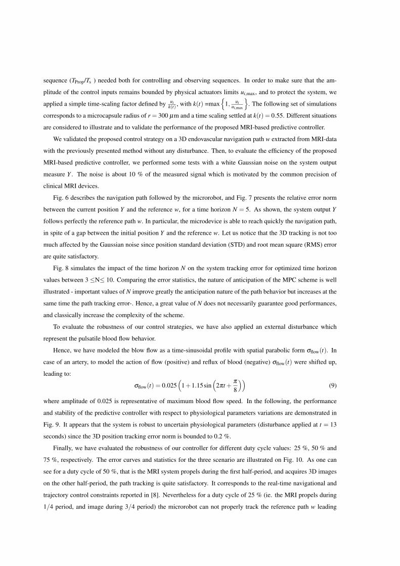
sequence (TProp/Ts ) needed both for controlling and observing sequences. In order to make sure that the am-
plitude of the control inputs remains bounded by physical actuators limits ui,max, and to protect the system, we
applied a simple time-scaling factor defined by ui
k(t) , with k(t) =max
1, uiui,max
. The following set of simulations
corresponds to a microcapsule radius of r = 300 µm and a time scaling settled at k(t) = 0.55. Different situations
are considered to illustrate and to validate the performance of the proposed MRI-based predictive controller.
We validated the proposed control strategy on a 3D endovascular navigation path w extracted from MRI-data
with the previously presented method without any disturbance. Then, to evaluate the efficiency of the proposed
MRI-based predictive controller, we performed some tests with a white Gaussian noise on the system output
measure Y . The noise is about 10 % of the measured signal which is motivated by the common precision of
clinical MRI devices.
Fig. 6 describes the navigation path followed by the microrobot, and Fig. 7 presents the relative error norm
between the current position Y and the reference w, for a time horizon N = 5. As shown, the system output Y
follows perfectly the reference path w. In particular, the microdevice is able to reach quickly the navigation path,
in spite of a gap between the initial position Y and the reference w. Let us notice that the 3D tracking is not too
much affected by the Gaussian noise since position standard deviation (STD) and root mean square (RMS) error
are quite satisfactory.
Fig. 8 simulates the impact of the time horizon N on the system tracking error for optimized time horizon
values between 3 ≤N≤ 10. Comparing the error statistics, the nature of anticipation of the MPC scheme is well
illustrated - important values of N improve greatly the anticipation nature of the path behavior but increases at the
same time the path tracking error-. Hence, a great value of N does not necessarily guarantee good performances,
and classically increase the complexity of the scheme.
To evaluate the robustness of our control strategies, we have also applied an external disturbance which
represent the pulsatile blood flow behavior.
Hence, we have modeled the blow flow as a time-sinusoidal profile with spatial parabolic form σflow(t). In
case of an artery, to model the action of flow (positive) and reflux of blood (negative) σflow(t) were shifted up,
leading to:
σflow(t) = 0.025(
1+1.15sin(
2πt +π
8
))(9)
where amplitude of 0.025 is representative of maximum blood flow speed. In the following, the performance
and stability of the predictive controller with respect to physiological parameters variations are demonstrated in
Fig. 9. It appears that the system is robust to uncertain physiological parameters (disturbance applied at t = 13
seconds) since the 3D position tracking error norm is bounded to 0.2 %.
Finally, we have evaluated the robustness of our controller for different duty cycle values: 25 %, 50 % and
75 %, respectively. The error curves and statistics for the three scenario are illustrated on Fig. 10. As one can
see for a duty cycle of 50 %, that is the MRI system propels during the first half-period, and acquires 3D images
on the other half-period, the path tracking is quite satisfactory. It corresponds to the real-time navigational and
trajectory control constraints reported in [8]. Nevertheless for a duty cycle of 25 % (ie. the MRI propels during
1/4 period, and image during 3/4 period) the microrobot can not properly track the reference path w leading

to great tracking error. The time-multiplexing duty cycle is optimized for a value around 40 %. In the optimal
case, the simulated predictive behavior of the MPC controller suggests better tracking results compared to those
obtained by [8] that should be confirmed by experimentation.
5 CONCLUSIONS
The proposed MRI-based ferromagnetic microcapsule steering and navigation strategy has been developed at milli
and microscale, where endovascular navigation path extraction and predictive controller have been designed. The
main drawback of MRI-based navigation stems from the strong limitations on the magnetic gradient amplitude
of available MRI devices. As magnetic forces used for propelling are volumetric, whereas the drag force is at
best dependent on the microcapsule’s area, the smaller the capsule, the higher the required control forces with
respect to hydrodynamic perturbations. Consequently, this approach is well conditioned for beads whose radius
is up to a few dozen micrometers with actual MRI devices. Targeting aims at focusing these microcarriers and
stopping them through embolization at the arterioles entry close to the occluded blood vessels. Possible releasing
mechanisms could rely on biodegradable polymer and techniques used in hyperthermia where aggregates of
nanocapsules can be heated to melt polymer. Such a solution is actually under experimentation for validation of
the proposed minimally invasive MRI-based microrobotic system.
6 ACKNOWLEDGMENTS
This work was supported by European Union’s 7th Framework Program and its research area ICT-2007.3.6 Mi-
cro/nanosystems under the project NANOMA (Nano-Actuactors and Nano-Sensors for Medical Applications).
The PhD student K. Belharet is supported by the Nano-IRM project, funded by Conseil Gnral du Cher and Ag-
glomeration de Bourges.
References
[1] K. Ishiyama, M. Sendoh, and K. I. Arai, “Magnetic micromachines for medical applications,” J. of Mag-
netism and Magnetic Materials, vol. 242-245, pp. 41–46, 2002.
[2] J. Abbott, Z. Nagy, F. Beyeler, and B. Nelson, “Robotics in the Small,” IEEE Robot. Automat. Mag., p. 92,
2007.
[3] T. A. Cavalcanti, B. Shirinzadeh and S. Ikeda, “Nanorobot for Brain Aneurysm,” Int. J. of Robotic Research,
vol. 28, no. 4, pp. 558–570, 2009.
[4] B. Behkam and M. Sitti, “Design methodology for biomimetic propulsion of miniature swimming robots,”
ASME J. Dyn. Syst. Meas. Control, pp. 36–43, 2006.

[5] S. Martel, M. Mohammadi, O. Felfoul, Z. Lu, and P. Pouponneau, “Flagellated magnetotactic bacteria as
controlled MRItrackable propulsion and steering systems for medical nanorobots operating in the human
microvasculature,” Int. J. Robot. Res., vol. 28, no. 4, pp. 571–582, 2009.
[6] O. Felfoul, J. Mathieu, G. Beaudoin, and S. Martel, “In vivo MR-tracking based on magnetic signature
selective excitation,” IEEE Trans. Med. Imag., vol. 27, no. 1, pp. 28–35, Jan. 2008.
[7] W. Sabra, M. Khousam, and S. Martel, “Use of 3D potential field and an enhanced breath-first search
algorithms for path-planning of microdevices propelled in the cardiovascular system,” in 27th IEEE EMBS
Annual Int. Conf., Shangai, China, 2005, pp. 91 – 100.
[8] S. Tamaz, A. Chanu, J.-B. Mathieu, R. Gourdeau, and S. Martel, “Real-time mri-based control of a ferro-
magnetic core for endovascular navigation,” IEEE Trans. Bio-Med. Eng., vol. 55, no. 7, pp. 1854–1863, July
2008.
[9] T. Wortmann, C. Dahmen, and S. Fatikow, “Study of MRI susceptibility artifacts for nanomedical applica-
tions,” Journal of Nanotechnology in Engineering and Medicine, vol. 1, no. 4, p. 041002, 2010.
[10] C. Kirbas and F. Quek, “A review of vessel extraction techniques and algorithms,” ACM Comput. Surv.,
vol. 36, no. 2, pp. 81–121, 2004.
[11] P. Reuze, J. Coatrieux, L. Luo, and J. Dillenseger, “A 3D moment based approach for blood vessel detection
and quantification in MRA,” Technology and Health Care, vol. 1, pp. 181–188, 1993.
[12] J. Tokuda, G. S. Fischer, S. P. DiMaio, D. G. Gobbi, C. Csoma, P. W. Mewes, G. Fichtinger, C. M. Tempany,
and N. Hata, “Integrated navigation and control software system for mri-guided robotic prostate interven-
tions,” Computerized Medical Imaging and Graphics, vol. 34, no. 1, pp. 3–8, 2010.
[13] T. Deschamps, “Curve and shape extraction with minimal path and level-sets techniques: Applications to
3d medical imaging,” Ph.D. dissertation, University of Paris Dauphine, 2001.
[14] O. Wink, W. J. Niessen, and M. A. Viergever, “Minimum cost path determination using a simple heuristic
function,” Int. Conf. on Pattern Recognition, vol. 3, p. 7010, 2000.
[15] O. Wink, W. Niessen, B. Verdonck, and M. Viergever, “Vessel axis determination using wave front propa-
gation analysis,” Medical Image Computing and Computer-Assisted Intervention, vol. 2208, pp. 845–853,
2001, lecture Notes in Computer Science.
[16] L. Cohen and R. Kimmel, “Global minimum for active contour models: A minimal path approach,” Int. J.
of Computer Vision, vol. 24, no. 1, pp. 57–78, 1997.
[17] J. A. Sethian, Level set methods and fast marching methods. Cambridge University Press, 1999.
[18] L. Arcese, M. Fruchard, and A. Ferreira, “Nonlinear modeling and robust controller-observer for a magnetic
microrobot in a fluidic environment using MRI gradients,” in IEEE/RSJ Int. Conf. on Intel. Robots and
Systems, St. Louis, MO, USA, Oct. 2009, pp. 534–539.

[19] L. Arcese, A. Cherry, M. Fruchard, and A. Ferreira, “High gain observer for backstepping control of a mri-
guided therapeutic microrobot in blood vessels,” in IEEE/RAS-EMBS Int. Conf. on Biomedical Robotics and
Biomechatronics, Tokyo, Japan, Sep. 2010, pp. 349 –354.
[20] L. Arcese, A. Cherry, M. Fruchard, and A. Ferreira, “Dynamic behavior investigation for trajectory control
of a microrobot in blood vessels,” in IEEE/RSJ Int. Conf. on Intel. Robots and Systems, Taipei, Taiwan, Oct.
2010, pp. 5774 –5779.
[21] S. Qin and T. Badgwell, “A survey of industrial model predictive control technology,” Control engineering
practice, vol. 11, no. 7, pp. 733–764, 2003.
[22] D. Clarke, C. Mohtadi, and P. Tuffs, “Generalized predictive control – Part I & II,” Automatica, vol. 23, pp.
137–160, 1987.
[23] B. Kouvaritakis, J. Rossiter, and A. Chang, “Stable generalised predictive control: an algorithm with guar-
anteed stability,” IEE Proceedings Part D Control Theory and Applications, vol. 139, no. 4, pp. 349–362,
1992.
[24] E. Camacho and C. Bordons, Model predictive control. Springer Verlag, 2004.
[25] A. Frangi, W. Niessen, K. Vincken, and M. Viergever, “Multiscale vessel enhancement filtering,” Lecture
Notes in Computer Science, pp. 130–137, 1998.

Figure 1: Overall system overview.
Figure 2: Timeline of acquisition and control prediction.

Figure 3: Forces applied on microrobot navigating in blood vessel.
Figure 4: MRI-based Predictive Control strategy.
Figure 5: 3D Navigation path extraction processing: a) Original MRI data; b) Computed cost function using
Frangi filter (here displayed in red volume); c) Extracted navigation path between the start and end seeds using FFM.

Figure 6: 3D MRI-based microrobot endovascular navigation (N = 5, in mm).
(a) Without noise (b) With white noise
Figure 7: 3D tracking error: ‖Y −w‖ for N = 5.

Figure 8: Tracking error statistics for different time horizons N.
(a) Blood flow disturbance σflow(t).
0 5 10 15 20 250
0.5
1
1.5
Time (sec)
Disturbance
(b) Tracking error.
Figure 9: MRI-based navigation with blood flow disturbance.
75%
50%
25%25% 50% 75%
std 1.5871 0.6860 0.2563
RMS 3.2023 0.9697 0.3628
Figure 10: Tracking error with different values of duty cycle.

162
HDR thesis © 2021David FOLIO December 16, 2021

APPENDIX B
SIMULATION AND PLANNING OF AMAGNETICALLY ACTUATED MICROROBOT
NAVIGATING IN ARTERIES (ACL6)
163

HAL Id: hal-00767787https://hal.archives-ouvertes.fr/hal-00767787
Submitted on 20 Jan 2013
HAL is a multi-disciplinary open accessarchive for the deposit and dissemination of sci-entific research documents, whether they are pub-lished or not. The documents may come fromteaching and research institutions in France orabroad, or from public or private research centers.
L’archive ouverte pluridisciplinaire HAL, estdestinée au dépôt et à la diffusion de documentsscientifiques de niveau recherche, publiés ou non,émanant des établissements d’enseignement et derecherche français ou étrangers, des laboratoirespublics ou privés.
Simulation and Planning of a Magnetically ActuatedMicrorobot Navigating in ArteriesKarim Belharet, David Folio, Antoine Ferreira
To cite this version:Karim Belharet, David Folio, Antoine Ferreira. Simulation and Planning of a Magnetically Actu-ated Microrobot Navigating in Arteries. IEEE Transactions on Biomedical Engineering, Instituteof Electrical and Electronics Engineers, 2013, 60 (4), pp.994-1001. 10.1109/TBME.2012.2236092.hal-00767787
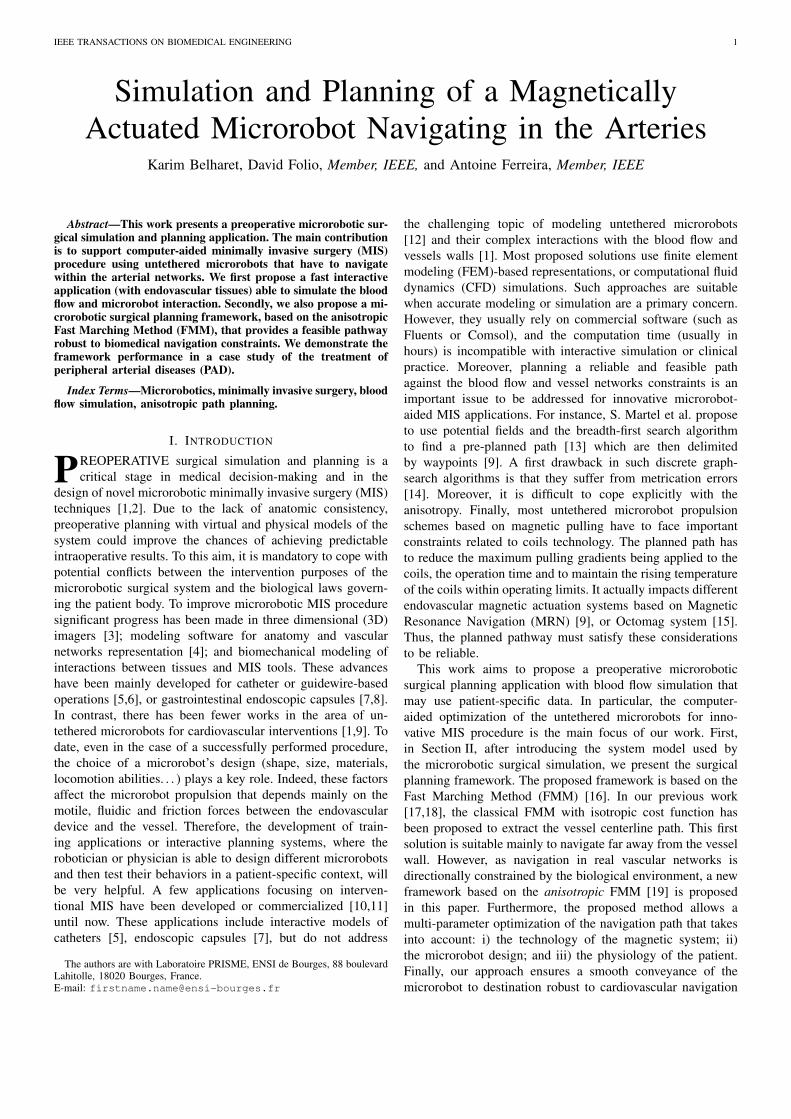
IEEE TRANSACTIONS ON BIOMEDICAL ENGINEERING 1
Simulation and Planning of a MagneticallyActuated Microrobot Navigating in the Arteries
Karim Belharet, David Folio, Member, IEEE, and Antoine Ferreira, Member, IEEE
Abstract—This work presents a preoperative microrobotic sur-gical simulation and planning application. The main contributionis to support computer-aided minimally invasive surgery (MIS)procedure using untethered microrobots that have to navigatewithin the arterial networks. We first propose a fast interactiveapplication (with endovascular tissues) able to simulate the bloodflow and microrobot interaction. Secondly, we also propose a mi-crorobotic surgical planning framework, based on the anisotropicFast Marching Method (FMM), that provides a feasible pathwayrobust to biomedical navigation constraints. We demonstrate theframework performance in a case study of the treatment ofperipheral arterial diseases (PAD).
Index Terms—Microrobotics, minimally invasive surgery, bloodflow simulation, anisotropic path planning.
I. INTRODUCTION
PREOPERATIVE surgical simulation and planning is acritical stage in medical decision-making and in the
design of novel microrobotic minimally invasive surgery (MIS)techniques [1,2]. Due to the lack of anatomic consistency,preoperative planning with virtual and physical models of thesystem could improve the chances of achieving predictableintraoperative results. To this aim, it is mandatory to cope withpotential conflicts between the intervention purposes of themicrorobotic surgical system and the biological laws govern-ing the patient body. To improve microrobotic MIS proceduresignificant progress has been made in three dimensional (3D)imagers [3]; modeling software for anatomy and vascularnetworks representation [4]; and biomechanical modeling ofinteractions between tissues and MIS tools. These advanceshave been mainly developed for catheter or guidewire-basedoperations [5,6], or gastrointestinal endoscopic capsules [7,8].In contrast, there has been fewer works in the area of un-tethered microrobots for cardiovascular interventions [1,9]. Todate, even in the case of a successfully performed procedure,the choice of a microrobot’s design (shape, size, materials,locomotion abilities. . . ) plays a key role. Indeed, these factorsaffect the microrobot propulsion that depends mainly on themotile, fluidic and friction forces between the endovasculardevice and the vessel. Therefore, the development of train-ing applications or interactive planning systems, where therobotician or physician is able to design different microrobotsand then test their behaviors in a patient-specific context, willbe very helpful. A few applications focusing on interven-tional MIS have been developed or commercialized [10,11]until now. These applications include interactive models ofcatheters [5], endoscopic capsules [7], but do not address
The authors are with Laboratoire PRISME, ENSI de Bourges, 88 boulevardLahitolle, 18020 Bourges, France.E-mail: [email protected]
the challenging topic of modeling untethered microrobots[12] and their complex interactions with the blood flow andvessels walls [1]. Most proposed solutions use finite elementmodeling (FEM)-based representations, or computational fluiddynamics (CFD) simulations. Such approaches are suitablewhen accurate modeling or simulation are a primary concern.However, they usually rely on commercial software (such asFluents or Comsol), and the computation time (usually inhours) is incompatible with interactive simulation or clinicalpractice. Moreover, planning a reliable and feasible pathagainst the blood flow and vessel networks constraints is animportant issue to be addressed for innovative microrobot-aided MIS applications. For instance, S. Martel et al. proposeto use potential fields and the breadth-first search algorithmto find a pre-planned path [13] which are then delimitedby waypoints [9]. A first drawback in such discrete graph-search algorithms is that they suffer from metrication errors[14]. Moreover, it is difficult to cope explicitly with theanisotropy. Finally, most untethered microrobot propulsionschemes based on magnetic pulling have to face importantconstraints related to coils technology. The planned path hasto reduce the maximum pulling gradients being applied to thecoils, the operation time and to maintain the rising temperatureof the coils within operating limits. It actually impacts differentendovascular magnetic actuation systems based on MagneticResonance Navigation (MRN) [9], or Octomag system [15].Thus, the planned pathway must satisfy these considerationsto be reliable.
This work aims to propose a preoperative microroboticsurgical planning application with blood flow simulation thatmay use patient-specific data. In particular, the computer-aided optimization of the untethered microrobots for inno-vative MIS procedure is the main focus of our work. First,in Section II, after introducing the system model used bythe microrobotic surgical simulation, we present the surgicalplanning framework. The proposed framework is based on theFast Marching Method (FMM) [16]. In our previous work[17,18], the classical FMM with isotropic cost function hasbeen proposed to extract the vessel centerline path. This firstsolution is suitable mainly to navigate far away from the vesselwall. However, as navigation in real vascular networks isdirectionally constrained by the biological environment, a newframework based on the anisotropic FMM [19] is proposedin this paper. Furthermore, the proposed method allows amulti-parameter optimization of the navigation path that takesinto account: i) the technology of the magnetic system; ii)the microrobot design; and iii) the physiology of the patient.Finally, our approach ensures a smooth conveyance of themicrorobot to destination robust to cardiovascular navigation

IEEE TRANSACTIONS ON BIOMEDICAL ENGINEERING 2
Blood Vessel
Bloodow
Centerlineof the vessel
x
y
z
fv
Bifurcation
fa
fgfd
fe+fv
(distance to wall)
fExt(x)=fe(x)+fv(x)+fg(x)
Fig. 1. Modeling scheme example in case of bead pulled microrobot.
constraints while minimizing the energy expenditure, to reducethe gradient pulling and system overheating. Specifically,we aim to get a feasible path by finding the min-energypathway (which is not necessarily the shortest). Section IIIbriefly describes our developed microrobotic surgical simu-lation and planning application, before illustrating its per-formance. As an illustration, we consider the treatment ofperipheral arterial diseases (PAD), such as artery narrowing(stenosis). For instance, one possible surgical application isto target atherosclerotic plaques in stenosed arteries. Oneof the most common strategies is angioplasty, occasionallywith stent implantation. Despite the high success rate, thesesolutions are not satisfactory, as vessel damage, infection andrestenosis can appear at a later stage. Otherwise, a surgicalmicrorobot for such vascular applications offers some novelsolutions [1]. Specifically, microrobotic intervention based onchemical, mechanical or mechano-chemical could be achievedto treat vascular obstructions [2]. Finally, we discuss someopen issues, evaluate the computational efficiency, and outlinesome future extends in Section IV. This study is concluded inSection V.
II. METHODS
A. A modeling overview
Different types of devices could be used for MIS interven-tions from catheter and guidewires, to wireless microcapsulesor microcarriers [1]. In this framework, any kind of untetheredmicrodevice (termed as microrobot throughout the text) thathas to perform endovascular navigation within blood flow isconsidered. More precisely, we consider any microsystem thatcould be modeled as:
mv = fa(a) + fd(v) + fExt(x) (1)
where v is the velocity of the device; m its mass; fa(a)is the controlled force, that is related to the control actiona ∈ A, with A the admissible controls set; fd(v) denotesthe fluid flow hydrodynamic drag force; and fExt(x) are allother external forces, as depicted Fig. 1. Different externalforces could be added to the model (1), such as the weight(fg), electrostatic (fe), van der Waals (fv), contact or stericforces. The interested reader may refer to [20] for detailedformulation of microforces. Fig.2 illustrates the evolution ofthese microforces with varying microrobot radius r and wrt.its distance to vessel wall δ. In particular, Fig. 2(f) shows thatclose to the centerline of the vessel (δ = R) the electrostatic
5
10
15
20
0.5
1
1.5
0.5
1
1.5
0.1
0.2
0.3
0.4
0.5
0.6
0.050.1
0.51
0.51
1.52
2.5
1
2
3
5
(mm)
r (mm)
fg (mN) fa (mN)
0.10.5
1
0.51
1.52
2.5
5
(mm)r (mm)
fd (mN)
0.10.5
1
0.51
1.52
2.5
5
(mm)
r (mm)
fv (nN)
0.10.5
1
0.51
1.5
2
2.5
5
(mm)
r (mm)
0.05 0.05
0.1 0.5 1 5
(mm)0.050.5
1
1.5
2
2.5
r (mm)
fe (mN)
(mN
)
Distance to wall (in mm)0 0.5 1 1.5 2 2.5 3 3.5 4 4.5 5
10-6
10-3
100
(a) (b) (c)
(d) (e)
(f)
fg
fa
fd
fe
fg
fv
Fig. 2. Microforces evolution: (a) apparent weight fg (b) magnetic forcefa (with ∇B = 200mT/m), (c) drag force fd (with ∥vf∥ = 400mm/s), (d)electrostatic force fe, (e) van der Waals force fv, as function of the distanceto the vessel wall δ in artery (R = 5mm) and wrt. the microrobot radius r.(f) Microforces acting on a microrobot with r = 1mm wrt. the distance tothe vessel wall δ in artery (R = 5mm).
and the van der Waals microforces are negligible comparedto the other relevant forces. In addition, if the microrobot isnever in contact with the vessel wall, the contact force couldbe omitted. Finally, most of the time because of the size of themicrosphere, the effect of Brownian motion is also neglected.
B. Navigation Planning in Flow
1) Minimal Path Planning: Classically, a navigation path-way could be defined as a curve P linking a starting pointx0 to any point x. In the general case, a curve is a minimalpath, also called a geodesic, wrt. the metric ϖ, if it globallyminimizes the energy functional:
Eϖ(P) =
∫Pϖ(P(l), P(l))dl, (2)
with l the arclength parameter. The solution to the mini-mum path finding problem (2) could be obtained through thecomputation of the distance map U : C 7→ R+, defined as:U(x) = minP E(P), for any P linking x to x0 in the domainC ⊂ Rd (with d = 2, 3, 4. . . ). In this context, Sethian [16] hasproposed the Fast Marching Method (FMM). Indeed, the FMMconverges to a smooth solution in the continuous domain evenwhen it is implemented on a sampled environment, contrary todiscrete graph-search algorithms. Especially, in the isotropiccase, the FMM satisfies the Eikonal equation:
∥∇U(x)∥ = w(x), ∀x ∈ CU(x0) = 0
(3)
where the isotropic cost function w : x ∈ C 7→ w(x) ∈ R+
is the metric. As the map U has a single local minimum, thegeodesic can be retrieved with a simple gradient descent on Ufrom a targeted seed xg to x0. The FMM provides a continuoussolution to the minimum path problem by employing upwinddifferences and a causality condition [16]. The key issue of

IEEE TRANSACTIONS ON BIOMEDICAL ENGINEERING 3
the FMM is then to get an appropriate metric w(x) whichdrives the front expansion efficiently to find a geodesic P . Inprevious works [17,18], we have proposed to design such ametric on spatial consideration:
w : x ∈ C 7→ Vesselness(x) ∈ R+ (4)
where Vesselness(x) is a vesselness enhancement function.A typical Vesselness(x) function could be designed usinga multi-scale analysis of the Hessian matrix, as proposed byFrangi [21] or Sato [22]. This approach then allows to find thevessel centerline geodesic Pc, as the considered vesselnessfilter gives their maximal response in the vessel center. Wehave applied this procedure to different sets of data, in 2D[17] as well as in 3D [18].
As mentioned previously the contact, electrostatic and vander Waals microforces are negligible when the microrobotnavigates close to the centerline Pc (cf. Fig. 2). Pc is thenthe best solution to navigate far away from the vessels wall.However, navigation in real vascular networks is constrainedby the biological environment, and can strongly modify thesystem behavior, leading to incompleteness in real intra-operative applications.
2) Anisotropic Path Planning: Navigating in blood flowimplies some directional constraints. When the path findingproblem has some preferred directions of travel it becomesanisotropic, i.e. the solutions depend on the configurationand directional constraints. In [19], the authors noticed thatthe FMM could be applied to isotropic or anisotropic prob-lems, and they provided a numerical scheme to solve staticHamilton-Jacobi equations of the form:
∥∇U(x)∥ = ϖ(x, ∇U(x)∥∇U(x)∥ ), ∀x ∈ C
U(x0) = 0(5)
where the anisotropy expansion is the result of the dependenceof ϖ on ∇U(x). Nevertheless, the computational complexityof the FMM in the anisotropic case is growing significantlywith the amount of anisotropy. The literature provides dif-ferent variants of the FMM to deal with anisotropy, such asusing a recursive approach [23], or iterative schemes [24].Furthermore, in [14] anisotropic cost functions have been alsoproposed. The proposed basic idea is to take advantage of theoriginal FMM efficiency, and to model the anisotropy thanksto a vector f of a field of force F , leading to the followinganisotropic metric:
ϖ : (x, f) ∈ C × F 7→ ϖ(x, f) ∈ R+ (6)
Such an anisotropic cost function leads to anisotropic front-propagation, and gives better geodesic than isotropic FMM. Toembed the directional constraints f within such an anisotropicFMM different specific cost functions have been proposedmainly for autonomous underwater vehicles (AUVs) [14,25].The drag and flow forces have a significant effect on themotion of the AUV, which is a common problem with ourmicrorobot planning problem. However, the proposed solutionmainly deals with either the min-distance or the min-timepath finding problem, and not minimizing directly neither thedynamics nor the motion applied to the system. Moreover,
most existing approaches classically simplify the problem byassuming constant vehicle speed, or only spatially varyingflow fields without time variation. Such limitations can gen-erate physically unfeasible paths. Especially, in the presenceof strong flows, incompleteness or incorrectness issues arereported [25].
3) Minimum-feasible-energy Planning: Most microrobotpropulsion schemes usually require a limitation of the powerconsumption, and have a maximum available power. Moreover,considering only either the min-time or min-distance problemusually leads to compute high motion forces, that is reach thegoal as fast as possible. But in our context, high motion implieshigh drag forces, and then high motion force fa (limited bythe maximum available magnetic forces) to be able to reachthe targeted area. To minimize the energy expenditure, a basicidea is to use a classical power functional expression, that is:
p(x,a) = ⟨f(x,a) · v(x)⟩ (7)
where ⟨·⟩ is the inner product of Rd; v is a velocity; andf(x,a) is the applied resultant force that embeds the controlledaction a ∈ A. Using the optimal control approach, we proposethe following anisotropic cost function:
ϖ(x, f) = maxa∈A
⟨f(x,a) · v(x)⟩ (8)
This anisotropic cost formulation, as in [14,25], naturallyincites the device to move in the direction of the force f .Especially, ϖ(x, f) will imply that the FMM propagation (5)follows the force field constraints, that is ∇U(x)
∥∇U(x)∥ ∝ f .Finally, this new anisotropic formulation (8) using optimalcontrol aspects embeds the system motion wrt. a finite definedadmissible control set A. This ensures that the given geodesicP is really feasible by the system and minimizes energyexpenditure. Indeed, the metric ϖ(x, f) allows to considerboth the biological constraints and the microrobot capabilities.
III. RESULTS
A. Simulation and Planning Tool
The proposed framework has been integrated in a dedicatedinteractive microrobot surgical simulation and planning appli-cation. This application, depicted on Fig. 3, is based on theVisualization Toolkit (VTK) [26], the Insight Segmentationand Registration Toolkit (ITK) [27], and the Qt Toolkit [28].Through the user interface (Fig. 3(b)), the surgeon realizes thefollowing operating mode iteratively:
a) Specifications: The surgeon provides different parametersin the software (in the left panel on Fig. 3(b)) related to:i) the physiology of the patient (blood flow and viscosity,vessel’s size and topology); ii) the technology of the magneticsystem (coil’s slew rate, maximum magnetic gradients, powerlimitations); and iii) the microrobot design (size, density,magnetic saturation).
b) Simulations: The surgeon initiates the simulation andplanning process wrt. the specification constraints.
c) Data analysis: The surgeon analyses the power functionalmapping and force field wrt. microrobot specifications.This iterative process is conducted until the preoperativeplanning of plaque removal specifications are satisfied. We

IEEE TRANSACTIONS ON BIOMEDICAL ENGINEERING 4
(a)
Path
Left
Panel
View Panel
(b)
Fig. 3. Preoperative microrobot surgical simulation and planning application:(a) application workflow; (b) vessel centerline extraction example.
focus in the sequel on the main contributions of this paper thatis the simulation and reliable vascular navigation planning.
B. Case study: peripheral arterial diseases
To assess the overall framework, we have performed a seriesof tests for both the microrobot within blood vessel modelsimulation and preoperative microrobotic MIS planning. Weillustrate the proposed application for the treatment of periph-eral arterial diseases (PAD). One possible application is tolocate atherosclerotic plaque in stenosed arteries. In particular,stenosis implies an abnormal narrowing of the vessel whichcauses a decrease in blood flow. Different plaque removaltasks have already been realized by magnetically actuatedmicrorobots navigating in occluded blood vessels [2]. In [29],shear-targeting of a thrombolytic drug in a mouse arterialthrombosis model using a microcarrier has been successfullytested. In [30], the rotation of the magnetic microrobot isat the origin of a drilling action through an occlusion in avessel. In the following, we propose a preoperative planningof a magnetic microrobot navigating within the vasculatureto the stenosed artery for plaque removal. We will considerhere as case study the real Magnetic Resonance Angiogram(MRA) clinical dataset depicted on Fig. 4. As the proposedframework works in C ⊂ Rd (with d = 2, 3. . . ), for thesake of clarity of the representation, we will only show herea Maximum Intensity Projection (MIP) image of the MRA.Here, the patient has a single level disease represented by anisolated stenosis in the iliac artery. As it is still a challengingissue to identify automatically the patient pathology and itslocation, the PAD is manually defined by the user.
C. Simulation Results
As previously mentioned, the simulation is based on aphysics-based model (presented in details in [20]). When
Fig. 4. Real MIP image from MRA (resolution of N = 384× 384 nodes)obtained in a patient with an isolated stenosis in the iliac artery (the white (A)-arrow), used to illustrate microrobotic MIS treatment simulation and planning.
interactive simulation is required (for training, interventionplanning, etc.), a trade-off between computation time andaccuracy has to be found. In our application, computationalefficiency is more important than small-scale details, as weaim to increase the users interaction capabilities, whereasprecision could be achieved using FEM or CFD simulation.To speed-up either the blood flow velocity or the force fieldssimulation computation, the basic FMM is extended to be ableto compute these vector fields during the front propagation(see Fig. 3(a)). Indeed, using Vesselness(x) isotropic costfunction, the FMM front will extend only within the vascularstructure. This allows to take advantage of the FMM efficiency,without using the whole dataset grids, and significantly reducethe overall computational time.
The blood flow velocity field simulation of the consideredcase study is illustrated on Fig.5. The interactive simulationtool takes into account that blood flow velocity intensity vf
on the vessel centerline decreases wrt. vessels radii, that isfrom about ∥vad
f ∥ ≈ 400 mm/s in descending aorta witha radius R ≈ 6.5 mm, to ∥vei
f ∥ ≈ 250 mm/s in externaliliac artery with a radius R ≈ 3.5 mm. As one can see, theblood flow velocity field is modified in the considered stenosiscase (narrowed vessel on Fig.5). The corresponding forcefield that will act on a neodymium microrobot with a radiusr = 500 µm is shown on Fig.6. In this simulation, only theweight fg (in the −→g -axis direction), drag fd and electrostaticfe forces are calculated. Let us notice that any force that canhave an analytical expression and can be embedded in (1)can easily be added to the application. Finally, the realizedinteractive simulation application is also able to deal withperiodic time-varying pulsatile blood flows, as presented onFig. 7. The user defines the periodic pulsatile blood flowparameters [20], a number of time-steps, and can then browsethe time-frame of either the blood flow velocity or the appliedforce field. Fig. 7(a) illustrates a typical periodic time-varyingpulsatile blood flow that takes place in the descending aorta,and the row 7(b) describes the corresponding velocity field.Fig. 7(c) and 7(d) show the resulting force fields applied onthe microrobot for two case studies, a microrobot of radius ofr = 250µm and r = 1.5mm, respectively. This demonstratesthat when the microrobot’s radius r or weight fg increases, theresultant force becomes more important.

IEEE TRANSACTIONS ON BIOMEDICAL ENGINEERING 5
Fig. 5. Simulation results of the blood flow velocity field computation.
Fig. 6. Simulation results of the force field: f = fd(v)+fe(x)+fg , appliedon a microrobot of r = 500 µm radius.
D. Microrobotic surgical planning demonstration
Once the microrobot is specified (size, materials, etc.), thesystem’s planning step only requires as user’s input the startingx0 and ending points xg. Next, to deal with the anisotropy ofthe media, the blood flow and force fields simulation results areused to compute the power functional map (7). The key issue isthen to generate the controlled force field fa(a), ∀a ∈ A. First,the action magnitude has to be defined wrt. available actuationcommand. The action magnitude is usually the controlledmagnetic gradient (a = ∇B), which implies the followingmagnetic force on a spherical device:
fa(∇B) = Dτm4
3πr3 (M.∇)∇B, (9)
where r is the microsphere radius; τm ∈ [0; 1] is the volumeratio of the magnetic material; M its magnetization; and D∈[0; 1] is the duty-cycle, i.e., the ratio between the durationof the applied magnetic gradient for propulsion to the totalperiod T .
The magnetic gradient used to propel a magnetic microrobotis assumed to be generated from various medical magneticsteering systems: ElectroMagnetic based Actuation (EMA)systems such as the Magnetic Catheter Steering System (alarger version of the Octomag system [15]) or the one de-veloped in [30]; and Magnetic Resonance Navigation (MRN).The EMA systems are capable of generating maximum mag-netic gradient fields up to amax = 350 mT/m in closed-loopnavigation control. In this case, the duty cycle is consideredequal to D = 1 since the imaging modality is provided byeither optical microscopy or X-ray imaging. These systemsare more suitable for the navigation of millimeter-sized hardmagnetic microrobots. The MRN system is based on clinicalMRI systems, without any hardware upgrades. Such magneticsystems are usually limited to maximum values to amax =80 mT/m in closed-loop navigation control. Generally, the
Fig. 7. Pulsatile blood flow simulation: (a) the periodic time-varying velocityin the descending aorta; (b) zoomed view of the blood flow velocity field; (c-d) zoomed view of the force field f = fd + fe + fg acting on a microrobotof: (c) r = 250µm, and (d) r = 1500µm for different time instants.
duty cycle is D < 1, since MR-imaging sequences and MR-tracking are provided by the same scanner to gather feedbackpositional information during MRN [9]. The MRN approach ismore suitable for micrometer-sized soft magnetic microrobots.However, it should be noticed that experimental results haveshown that therapeutic particles (known as TMMC), 50-60 µmdiameter were navigated in arteries (rabbit models) and thatMRN was done with gradient coils (capable of 450 mT/mwith inner diameter suitable for limbs or head interventions)installed in the tunnel of clinical MRI scanners [31].
Our proposed FMM strategy can be adapted to each specificcase by taking into account the duty-cycle D, the slew rateof the magnetic coils, and the maximum temperature coils.Secondly, the action direction should be defined. To this aim,we used some a priori knowledge about the goal direction,defined between x0 and xg, provided by the isotropic FMMusing Vesselness(x) cost function (see Fig. 3(a)). Indeed,this FMM step provides the distance map Uc between x0 andxg (or reciprocally), and then the goal direction field ∇Uc(x).This helps to define the appropriate guidance field G(x) ∝∇Uc(x). Some variations could be added on the goal directionfield to enlarge the guidance field set. The admissible controlset A can then be defined as:
A = A×G, (10)
where A ⊂]0;amax] is a finite set of action magnitudes, andG = G(x) ∼ [0; π
2 ] is the guidance field set. Let usrecall that A could be filtered to consider some technologicalconstraints (such as the duty-cycle, or the magnetic slew rate).
This planning framework has been validated on the casestudy dataset considering different microrobot sizes navigatingwithin arteries. First, Fig. 8 demonstrates the influence of the

IEEE TRANSACTIONS ON BIOMEDICAL ENGINEERING 6
(a)
(b)
Fig. 8. Planning results on varying control action influence for a neodymiummicrorobot of size 250 µm and 750 µm: (a) the energy functional Eϖ(P)wrt. the action magnitude (i.e. the magnetic gradient) and (b) zoomed view ofthe corresponding geodesics: Pc the vessel centerline and Pa the min-energypath for the varying action magnitude.
Fig. 9. Planning results on varying control action influence for a neodymiummicrorobot of size 1.5 mm and 2.5 mm in clinical MRI context.
motion force magnitude on finding the minimum-feasible-energy path. We noticed that as the motion force magnitudeincreased, the required energy Eϖ(P) increased exponentially.This is significant for important microrobot size (r = 750 µmon Fig. 8(a)). Indeed, Fig. 8(b) shows that with much powerthe microrobot is more able to leave the vessel’s centerline Pc
(provided by the isotropic FMM) to reach the goal faster. Iflimited magnetic gradient magnitudes are available to propelthe microrobot, such as in clinical MRI, Fig. 9 shows thatincreasing its size should overcome the power limitation.Therefore, the proposed min-energy path planning has beenevaluated for various microrobot sizes and for EMA andMRN systems, as reported on Fig. 10. We can notice thatfor a microrobot radius bigger than 1.5 mm the curve lengthincreases slightly, and starts to decrease significantly below1 mm (cf. Fig. 10(a)). Furthermore, Fig. 10(b) depicts that theenergy functional decreases significantly with the microrobotradius. In fact, the action force fa(a) decreases following acubic power (L3), minimizing the power budget. Therefore,it is more difficult for neodymium microrobots with a sizebelow 750 µm to overcome the blood flow constraints that takeplace in the artery. Finally, as an illustration of the blood flow
Length
0 0.5 1 1.5 2 2.5 3
359
360
361
Ball radius (mm)
Energ
y f
uncti
onal
0 0.5 1 1.5 2 2.5 30
2
4
6
8
(a)
(b)
amax=350mT/mamax= 80mT/m
Fig. 10. Planning results with varying microrobot radii, for an EMA system(amax = 350mT/m) and a MRN (amax = 80mT/m): (a) the geodesiccurvature length (in mm); and (b) the energy functional.
Fig. 11. Planning results using the proposed anisotropic cost function for aneodymium microrobot with r = 1.5 mm: three targeted point are specified(xg1, xg2 and xg3). The colored map depicted the power functional level.
TABLE IPLANNING RESULTS OF MINIMUM-FEASIBLE-PATH FOR THREE TARGETED
POINT (xg1 , xg2 AND xg3) DEPICTED ON FIG.11
Geodesic # Length (mm) Energy Eϖ(P)P1 360.086 0.6765P2 359.612 0.5118P3 361.735 0.4879
influence, Fig. 11 shows the planning results of our minimum-feasible-path finder for three targeted points (xg1, xg2 andxg3), and Table I lists the curve lengths of their geodesic (P1,P2 and P3) and the energy functional Eϖ(P). The min-energygeodesic is curve P3, while the shortest length is P2. Thismeans that although P3 is longer than P2, P3 consumes lessenergy.
IV. DISCUSSION
The most computationally intensive part of the microroboticsurgical application is the vesselness filter (that providesVesselness(x) cost function) based on a multiscale analysisof the Hessian matrix [21]. This multiscale interpretation ofeigenvalues of the Hessian matrix could be improved thanksto parallelization through GPU implementation. Furthermore,as mentioned, instead of using the overall dataset grid (in thecase study N = 147 456), the vector fields simulations are per-formed on only 18 941 nodes corresponding to the vasculature.Thus, on an Intel Core2 3Ghz processor, one simulation time
IEEE TRANSACTIONS ON BIOMEDICAL ENGINEERING 7
takes less than 150 ms. For the periodic pulsatile blood flow,this allows to compute one cardiac cycle with 50 time-stepsin less than 8 s. Therefore, the combination of the microrobotand the caradiovascular model together with the FMM maybecome accurate enough to support interactive microroboticsurgical planning applications. Finally, in the planning step, themain computational aspect remains on action set A generation.This set A is related to the dimension of the action magnitudeset A and guidance field set G, specified by the users. Forthe case study with dimA = 10× 10, the overall planningprocedure needs a calculation time of about 36 s. This com-putational efficiency ensures a high level of interactivity forpreoperative simulation, planning and navigation.
In the simulation process we have chosen to focus on com-putational efficiency, rather than on accurate blood flow simu-lations. Nonetheless, the vasculature and blood flow modelingare still strongly investigated by the communities, and remainan open issue. In future extends, we will use some analyticalmodeling of vessel bifurcation as in [20], to improve the bloodflow simulation accuracy. Although the visualization of vectorfields is still a challenging issue (especially in 3D), moreintuitive flow rendering (such as streamline, streamribbon, etc.)could also be helpful for the microrobotic surgery applications.
V. CONCLUSION
In this study, a microrobotic surgical simulation and plan-ning has been presented for the treatment of peripheral arte-rial diseases. However, the proposed framework could alsobe applied to other regions of the body, different therapyand various MIS microrobots. Especially, the results showsthat interactive applications can be helpful to design thesuitable microrobot design (e.g. shape, size, materials, etc.)wrt. anatomic consistency to improve microrobotic surgicalapplications. Hence, preoperative surgical planning with bloodflow simulation provides useful information for understandingcardiovascular pathologies, predicting their onset and choosingan optimal therapy strategy for innovative microrobotic MISprocedure.
ACKNOWLEDGMENT
The PhD student K. Belharet is supported by the Nano-IRMproject, founded by Region Centre and City of Bourges.
REFERENCES
[1] B. J. Nelson, I. K. Kaliakatsos, and J. J. Abbott, “Microrobots forminimally invasive medicine,” Annual Review of Bio.med. Eng., vol. 12,no. 1, pp. 55–85, 2010.
[2] P. Miloro, E. Sinibaldi, A. Menciassi, and P. Dario, “Removing vascularobstructions: a challenge, yet an opportunity for interventional microde-vices,” Bio.med. Microdevices, vol. 14, pp. 511–532, 2012.
[3] R. M. Satava, “Virtual reality, telesurgery, and the new world order ofmedicine,” Computer Aided Surgery, vol. 1, no. 1, pp. 12–16, 1995.
[4] K. Sun, Z. Chen, and S. Jiang, “Local morphology fitting activecontour for automatic vascular segmentation,” IEEE Trans. Biomed.Eng., vol. 59, no. 2, pp. 464–473, Feb. 2012.
[5] Y. Ganji and F. Janabi-Sharifi, “Catheter kinematics for intracardiacnavigation,” IEEE Trans. Biomed. Eng., vol. 56, no. 3, pp. 621–632,Mar. 2009.
[6] W. Tang, T. R. Wan, D. A. Gould, T. How, and N. W. John, “A stableand real-time nonlinear elastic approach to simulating guide-wire andcatheter insertions based on cosserat rod,” IEEE Trans. Biomed. Eng.,vol. PP, no. 99, p. 1, 2012.
[7] F. Carpi, N. Kastelein, M. Talcott, and C. Pappone, “Magneticallycontrollable gastrointestinal steering of video capsules,” IEEE Trans.Biomed. Eng., vol. 58, no. 2, pp. 231–234, Feb. 2011.
[8] G. Ciuti, M. Salerno, G. Lucarini, P. Valdastri, A. Arezzo, A. Menciassi,M. Morino, and P. Dario, “A comparative evaluation of control interfacesfor a robotic-aided endoscopic capsule platform,” IEEE Trans. Robot.,vol. 28, no. 2, pp. 534–538, Apr. 2012.
[9] S. Tamaz, A. Chanu, J.-B. Mathieu, R. Gourdeau, and S. Martel,“Real-time MRI-based control of a ferromagnetic core for endovascularnavigation,” IEEE Trans. Biomed. Eng., vol. 55, no. 7, pp. 1854–1863,Jul. 2008.
[10] (2012) Stereotaxis Inc. [Online]. Available: http://www.stereotaxis.com[11] (2012) Sensei(r) x robotic catheter system. Hansen Medical. [Online].
Available: http://www.hansenmedical.com[12] C. Pawashe, S. Floyd, and M. Sitti, “Modeling and experimental
characterization of an untethered magnetic micro-robot,” The Int. J. ofRobot. Research, vol. 28, no. 8, pp. 1077–1094, 2009.
[13] W. Sabra, M. Khouzam, and S. Martel, “Use of 3D potential field andan enhanced breadth-first search algorithms for the path planning ofmicrodevices propelled in the cardiovascular system,” in IEEE Int. Conf.of the Eng. in Med. and Bio. Soc., Apr. 2005.
[14] C. Petres, Y. Pailhas, P. Patron, Y. Petillot, J. Evans, and D. Lane, “Pathplanning for autonomous underwater vehicles,” IEEE Trans. Robot.,vol. 23, no. 2, pp. 331–341, 2007.
[15] M. Kummer, J. J. Abbott, B. E. Kratochvil, R. Borer, A. Sengul, andB. J. Nelson, “Octomag: An electromagnetic system for 5-dof wirelessmicromanipulation,” IEEE Trans. Robot., vol. 26, no. 6, pp. 1006–1017,Sep. 2010.
[16] J. A. Sethian, Level set methods and fast marching methods: evolvinginterfaces in computational geometry, fluid mechanics, computer vision,and materials science. Cambridge University Press, 1999.
[17] K. Belharet, D. Folio, and A. Ferreira, “Endovascular navigation ofa ferromagnetic microrobot using MRI-based predictive control,” inIEEE/RSJ Int. Conf. on Intel. Robots and Syst., Taiwan, Oct. 2010.
[18] ——, “3D MRI-based predictive control of a ferromagnetic microrobotnavigating in blood vessels,” in IEEE RAS & EMBS Int. Conf. onBioMed. Robot. and BioMechatron., Tokyo, Japan, Sep. 2010.
[19] J. A. Sethian and A. Vladimirsky, “Ordered upwind methods forstatic hamilton-jacobi equations: theory and algorithms,” SIAM J. onNumerical Analysis, vol. 41, no. 1, pp. 325–363, 2003.
[20] L. Arcese, M. Fruchard, and A. Ferreira, “Endovascular Magnetically-Guided Robots: Navigation Modeling and Optimization,” IEEE Trans.Biomed. Eng., no. 99, pp. 1–12, Sep. 2011.
[21] A. Frangi, W. Niessen, K. Vincken, and M. Viergever, “Multiscale vesselenhancement filtering,” Lect. Notes in Comp. Scie., pp. 130–137, 1998.
[22] Y. Sato, S. Nakajima, H. Atsumi, T. Koller, G. Gerig, S. Yoshida, andR. Kikinis, “Three-dimensional multi-scale line filter for segmentationand visualization of curvilinear structures in medical images,” Med.Imag. Anal., vol. 2, no. 2, pp. 143–168, 1998.
[23] E. Konukoglu, M. Sermesant, O. Clatz, J.-M. Peyrat, H. Delingette,and N. Ayache, “A recursive anisotropic fast marching approach toreaction diffusion equation: Application to tumor growth modeling,” inInf. Processing in Med. Imag., N. Karssemeijer and B. Lelieveldt, Eds.,vol. 4584. Springer, 2007, pp. 687–699.
[24] F. Bornemann and C. Rasch, “Finite-element discretization of statichamilton-jacobi equations based on a local variational principle,” Com-puting and Visualization in Science, vol. 9, pp. 57–69, 2006.
[25] M. Soulignac, “Feasible and optimal path planning in strong currentfields,” IEEE Trans. Robot., no. 99, pp. 1–10, Feb. 2011.
[26] (2012) The visualization toolkit (VTK). Kitware. [Online]. Available:http://www.vtk.org
[27] (2012) Insight segmentation and registration toolkit (ITK). Kitware.[Online]. Available: http://www.itk.org
[28] (2012) Qt-a cross-platform application and UI framework. Nokia.[Online]. Available: http://qt.nokia.com/
[29] N. Korin, M. Kanapathipillai, B. Matthews, M. Crescente, A. Brill,T. Mammoto, K. Ghosh, S. Jurek, S. Bencherif, D. Bhatta et al.,“Shear-activated nanotherapeutics for drug targeting to obstructed bloodvessels,” Science, vol. 337, no. 6095, pp. 738–742, 2012.
[30] C. Yu, J. Kim, H. Choi, J. Choi, S. Jeong, K. Cha, J. oh Park, andS. Park, “Novel electromagnetic actuation system for three-dimensionallocomotion and drilling of intravascular microrobot,” Sensors and Actu-ators A: Physical, vol. 161, no. 1-2, pp. 297–304, 2010.
[31] P. Pouponneau, J.-C. Leroux, G. Soulez, L. Gaboury, and S. Martel, “Co-encapsulation of magnetic nanoparticles and doxorubicin into biodegrad-able microcarriers for deep tissue targeting by vascular MRI navigation,”Biomaterials, vol. 32, no. 13, pp. 3481–3486, 2011.

172
HDR thesis © 2021David FOLIO December 16, 2021

APPENDIX C
CATALYTIC LOCOMOTION OF CORE‐SHELLNANOWIRE MOTORS (ACL10
173

HAL Id: hal-01410107https://hal.archives-ouvertes.fr/hal-01410107
Submitted on 26 Jan 2017
HAL is a multi-disciplinary open accessarchive for the deposit and dissemination of sci-entific research documents, whether they are pub-lished or not. The documents may come fromteaching and research institutions in France orabroad, or from public or private research centers.
L’archive ouverte pluridisciplinaire HAL, estdestinée au dépôt et à la diffusion de documentsscientifiques de niveau recherche, publiés ou non,émanant des établissements d’enseignement et derecherche français ou étrangers, des laboratoirespublics ou privés.
Catalytic locomotion of Au/Ru core-shell nanowiremotors
Bumjin Jang„ Wang Wei, Samuel Wiget„ Petruska Andrew, XiangzhongChen„ Chengzhi Hu„ Ayoung Hong„ David Folio, Antoine Ferreira, Salvador
Pané, et al.
To cite this version:Bumjin Jang„ Wang Wei, Samuel Wiget„ Petruska Andrew, Xiangzhong Chen„ et al.. Catalyticlocomotion of Au/Ru core-shell nanowire motors. ACS Nano, American Chemical Society, 2016, 10(11), 10.1021/acsnano.6b04224. hal-01410107

Catalytic locomotion of Au/Ru core-shell nanowire
motors
Bumjin Jang*,*,† Wei Wang,‡ Samuel Wiget,† Andrew J. Petruska,† XiangZhong Chen,† ChenzhiHu, † David Folio,§ Antoine Ferreira, § Salvador Pané,*, † and Bradley J. Nelson,†
†Institute of Robotics and Intelligent Systems, ETH Zurich, Zurich, CH8092, Switzerland
‡Shenzhen Key Laboratory for Advanced Materials, School of Material Sciences and
Engineering, Shenzhen Graduate School, Harbin Institute of Technology, University Town,
Shenzhen 518055, China
§ INSA Centre Val de Loire, Universite d’Orléans, PRISME EA 4229, Bourges, France.
KEYWORDS: coreshell nanowires, catalytic micronanomotors, selfelectroosmosis, self
diffusiophoresis, net propulsive force
Fifteen years ago, Whitesides et al. pioneered a work on self-propelled catalytic
millimeter-scale ships,1 triggering a mighty development of synthetic micro and nanomotors.
These devices move autonomously in the presence of a fuel solution by converting chemical to
mechanical energy.2 Most of reported catalytic micro and nanomotors are driven by the
decomposition of hydrogen peroxide, although there are other recent examples using glucose and
urea as fuels.3-5 Several applications for these miniaturized motors have been demonstrated such
1

as electronic circuit healing,6 biosensing,4, 7 nanolithography,8 microfluidic pumping,9 nanocargo
transport10, or environmental remediation (for details, see recent review articles11-16). Most of
these applications require a precise control over the speed and directionality of the motors.17,
which are highly dependent on the motor design parameters, such as its geometry, size and
composition. Understanding the mechanisms involved in the propulsion of catalytic micro and
nanomotors as a function of their design is crucial for controlling their motion. Different
propulsion mechanisms have been identified, such as bubble propulsion, selfelectroosmosis,
selfdiffusiophoresis or interfacial tension.16 In the first mechanism, bubbles are formed on the
catalytic surface and impart momentum to the motor. For example, tubular microjets18, 19 are
driven by oxygen bubble propulsion, caused by the decomposition of H2O2 at the inner catalytic
surface. While bubble propulsion seems at first glance the most intuitive way to explain the
motion of these motors, this mechanism cannot be used to rationalize, for instance, the motion of
bimetallic structures such as Pt/Au or Cu/Pt nanowires (NWs) in H2O2 and I2 solutions
respectively.20, 21 For bimetallic NWs, self-electroosmosis 22, 23 is generally the most accepted
mechanism compared to others21,24. In this case, a selfinduced electric field is generated by
redox reactions occurring on the two different metallic segments. The motion of other micro- and
nanomotors has been explained in terms of self-diffusiophoresis. Several works suggest that
micro- and nanoparticles asymmetrically coated with Pt move due to an O2 concentration
gradient, caused by the asymmetric decomposition of H2O2 along the body of the motor.25-27 28, 29
Recent investigations evaluating more complex motor architectures are pointing towards a
concomitant occurrence of mechanisms.30, 31

Among all micro- and nanomotors’ structures, NWs are particularly appealing due to
their unique physical properties.32 Additionally, NWs can be compartmentalized in several
functional modules by means of segmentation33 or coaxial lithography34 to increase their
capabilities and functionalities. For instance, the trajectory of catalytic NW motor consisting of
Pt/Ni/Au/Ni/Au segments can be controlled by means of magnetic fields.35 However, interfacing
certain building blocks can be detrimental for several applications. For example, the combination
of two dissimilar metallic segments such as Au and Ni can lead to an increase of the corrosion
rate of the magnetic part due to galvanic coupling.36 Also, the interaction of certain materials
(e.g. Ni) with the surrounding environment (e.g.biological or aquatic media) must be avoided to
prevent undesired leakage of toxic ions. Alternatively, coreshell arrangements can provide an
inert housing to prevent certain components to be in direct contact to the surrounding
environment. Coreshell NWs have been manufactured using a wide variety of methods, and
usually they imply two or more steps.37-42
In this work, we capitalize on a recently developed method, which allows for the batch
fabrication of freestanding NWs based on template-assisted electrodeposition and wafer bonding.
As the NWs are self-supported on the wafer after template removal, a second electrodeposition
step can be realized to produce a core-shell architecture. This newly developed method can be
adopted to fabricate core-shell NWs with various material combinations. Here, we have
produced different types of bimetallic core-shell NWs such as Au/Ru, Rh/Au, Au/Rh and we
have investigated for the first time their motion in H2O2 solutions. We observed abnormal
behaviors of these core-shell devices including a speed increase with the length of Au/Ru core-
shell NWs and a large speed difference among Au/Ru, Rh/Au and Au/Rh, which have not been

observed for the segmented (conventional bimetallic) NWs. The experimental results suggest
that self-electroosmosis cannot be the sole mechanism for the locomotion of these architectures.
Indeed, we suggest that self-diffusiophoresis is additionally playing a role as well. Additionally,
magnetically guided motion of a (Au-Ni)/Ru core-shell NW is demonstrated. In this
configuration, the magnetic component is enclosed within the shell, thus preventing the Ni core
to be in contact with the surrounding solution.
Results
Numerical model of electroosmotic mechanism on core-shell NWs. It has previously been
established that the electroosmotic force is the main driving force for locomotion of nanomotors
based on surface redox reactions.43, 44 The redox reaction consists of an oxidation reaction and
reduction reaction as illustrated in Figure 1a. Protons, oxygen molecules, and electrons are
generated in the oxidation process at the anode (Au) by decomposing H2O2. The generated
protons travel by convection, diffusion, and migration to the cathode (Ru), where they react with
electrons, oxygen and H2O2 molecules to produce H2O in the reduction process. As a
consequence of this redox reaction, protons are asymmetrically distributed around the nanomotor
and, accordingly, an asymmetric electric field is developed. This self-generated electric field
causes protons to migrate inside the electrical double layer that naturally formed when the
nanomotor is immerged in a water solution. The proton migration leads to an electroosmotic
flow, which eventually causes the motion of the nanomotor. The influence of the electroosmotic
mechanism on the locomotion of our newly designed nanomotor is simulated using commercial
multiphysics simulation package COMSOL (5.1). Figure S1a shows that the proton
concentration around the Au/Ru coreshell NW is highly asymmetric, as expected. The protons
are highly concentrated at the Au (anode) end the NW, where they are generated, and have a low

concentration at the Ru (cathode) end, where they are consumed. As expected, Figure S1b
shows that the electric potential is also asymmetric because of the asymmetric distribution of
protons. Figure 1b shows that the fluid flows from the anode to the cathode, translating to a
directional motion of the Au/Ru coreshell NW with the anode forward. The simulation also
reveals that the fluid speed is highest at the interface between the cathode and anode of the core
shell NW, where the majority of the electroosmosis flow occurs.
We notice in our simulation (Figure 1b) that near the opposite tip to the anode there is a
convergent flow loop on each side of the rod due to the coupling between the electrosmotic flow
moving from the anode to the cathode, and a flow from the surrounding solution due to the
electric field pointing towards the cathode. We further investigate how the length of Au/Ru core-
shell NW affects the convergent flow. When the length is small enough (~ 500 nm, Figure 1b
(i)), the electric field generated at the anode dominates the overall electroosmotic flow (Figure
S1c), and the disturbance to the fluid flow at the tip of the cathode is negligible. At
approximately 1.5 µm, a flow reversal at the tip occurs, which is caused by the migration of
protons from the surrounding solution to the cathode (Figure 1b (ii)). The reverse flow gains
enough strength to create vortices near the surface of the NW tip. Further increase in length
increase the size of vortices (Figure 1b (iii), (iv)). These vortices represent a local increase in the
fluidic drag at the tail of the NW, according to the observed negative fluidic speed at the tip of
the cathode as seen from the fluid profile along the NW long axis (Figure S1d).
The nanomotor speeds are calculated from the fluid velocities around the core-shell NWs
using the Solomentsev and Anderson model.45 Figure 1c shows the speed as a function of length
of the core-shell NW. The decreased speed with length in the numerical simulation can be

attributed to the increase in drag force of the nanomotor as its length increases, since no-slip
boundary condition was chosen for the nanomotor surface in the simulation.
Design and fabrication of the Au/Ru core shell NWs. The fabrication process is illustrated in
Figure 2a. First, an anodic aluminium oxide (AAO) membrane was transferred onto a Si
substrate via the Au/Au compressive bonding technique previously developed in our group.46
Next, Au was electrodeposited into the pores of the AAO. The AAO was then chemically etched
to obtain a freestanding Au NW array on the Si substrate. Ru was then electrochemically
deposited on the freestanding Au NW array, hence the formation of a coreshell structure. The
strong adhesion between the freestanding array and the Si substrate is able to withstand the
electrophoretic and fluidic forces exerted on the NWs during Ru electrodeposition. We
importantly note that the freestanding NWs must be kept in solution to prevent drying, because
the surface tension forces during drying will cause severe NW aggregation 47 and result in a non
uniform deposition of the Ru shell. After the Ru deposition, the NWs are released by sonication.
A scanning electron microscope (SEM) image obtained using a back-scattered electron
(BSE) detector in Figure 2b shows a typical Au/Ru core-shell NW with an approximate diameter
and a length of 350 nm and 2.5 µm, respectively, where the length varies with the deposition
time of the Au core. Since the intensity of the BSE signal is proportional to the atomic number,
the bright area and the dark area can be assigned to Au and Ru, respectively. The Au core appears
only at the base (left end) as a consequence of being released from the Si substrate. No obvious
defects are observed in the Au/Ru core-shell NW structure as is seen in the high-angle annular
dark field (HAADF) scanning transmission electron microscopy (STEM) image (Figure 2c). The
corresponding energy dispersive X-ray (EDX) mapping verifies that the core-shell NW is

composed of Au and Ru (Figure 2d). For a better understanding of the Ru distribution, we further
selectively etched the Au core in Au etchant. Representative SEM and STEM images (Figure
2e,f) show that the remaining structure after etching is a Ru shell. The Ru shell has an
approximate diameter of 350 nm, which is similar to that of a Au/Ru core-shell NW. A smooth
surface of the nanoshell without holes or cracks on the rod is observed and confirms the uniform
distribution and the conformal growth of the Ru shell. Subsequent EDX mapping verifies that the
nanoshell solely consists of Ru (Figure 2g).
Catalytic propulsion of the Au/Ru core-shell NWs. The catalytic locomotion of the Au/Ru
core-shell NWs (approximate length of 2.5 µm) in H2O2 solution was investigated at various
concentrations (0, 0.1, 0.3, 2.5, 5, 10 and 20 wt %). As expected, the speed of the core-shell NW
increases with the concentration of H2O2 (Figure 3a), showing the maximum speed of 41 ± 7.6
µm/s at 20 wt % H2O2. The positive correlation between the speed of the motor and the
concentration of H2O2 is in accordance with previous findings.48-51 A representative core-shell-
NW trajectory is shown in Figure 3a (i). A large displacement is observed over 4.55 sec in the
presence of H2O2 (5 wt %) in contrast to the control experiment, conducted in the absence of
H2O2, which shows Brownian motion and a very small displacement (Figure 3a (ii)).
To systematically understand the locomotion, we studied the dynamic motion behavior of
the core-shell NW with different lengths (1.8, 2.6 and 3.4 µm). We calculated the mean-square
displacement (MSD) from the recorded motion trajectory (see also supporting movie1) using:
ΔL2 (t )≡ ⟨ [r (t )−r (0 ) ]2 ⟩ (1)
where r (t )=(x (t ) , y (t ) ) .

Similar to catalytic motors of other shapes, the MSD curves in Figure 3b and S2a,b show
sinusoidal oscillations, which indicate that our motors exhibit a circular motion.48, 52, 53 The
translational velocity (v), rotational velocity (ω), translational diffusivity (D) and rotational
diffusivity (Dr) for a moving particle can be extracted by fitting the MSD curves with53:
Δ L2 (t )=4Dt+2v2Dr t
Dr2+ω2
+2v2 (ω2−Dr
2 )Dr2+ω2
+2 v2 eD rt
(Dr2+ω2 )
2 [(Dr2−ω2 )cosωt−2ωDr sinωt ]
For comparison, the translational diffusivity Dt,b and the rotational diffusivity Dr,b of passive
Brownian motion (i.e. in the absence of H2O2) of our core-shell NW are calculated by the
Einstein relation:
Dt , b=k BT
f t ,∥ (3)
ΔL2 (t )=4Dt+2v2Dr t
Dr2+ω2
+2v2(ω2−Dr
2 )Dr2+ω2
+2 v2eD rt
(Dr2+ω2 )
2 [(Dr2−ω2 )cosωt− 2ωDrsinωt ] (4)
where k B is the Boltzmann constant, T is the absolute temperature, f t∥ is the translational
frictional drag force and f r∥ is the rotational frictional drag force parallel to the long axis of
NW with a length (L) and a diameter (d) in a viscous media Dt , b=k BT
f t ,∥ . Dr , b=
k BT
f r∥ are defined as:54
f t∥=
2 πηL
ln (L/d )−0.207+0.980(L/d )
−0.133
(L /d )2 (5)
k B (6)
All of the values, as summarized in Table 1, vary as the length changes. The translational
diffusivity Dt, rotational diffusivity Dr, and rotational velocity decrease with increasing length

which are easy to understood by the Einstein law; as the length increases, both translational and
rotational drag forces increase, which results in a decrease in both the diffusivity and velocity.
However, while Dt is quite close to Dt,b, a discrepancy of several orders of magnitude is observed
between Dr and Dr,b for longer core-shell NWs. The vortices at the tail of the cathode, found in
the numerical modelling (see again Figure 1b) may explain the observed discrepancy between Dr
and Dr,b for a longer NW. This additional fluidic drag caused by the vortices, electrochemically
formed contributes to the large reduction in the rotational diffusivity, hence reducing its
tendency to rotate and, therefore, increasing its motion stability (or directionality.) For a detailed
elucidation, we example macro-scaled flying objects, such as rockets or airplanes. For those
flying objects, it is commonly known that the center of drag force should locate behind the center
of thrust for a directional stability, and the stability further increases with the distance of the two
centers. In our case, the center of thrust locates at the tip of the anode, while the center of drag
force, supposed to be at the center for this rectangular shaped-nanomotor is actually shifted to the
side of the cathode tip due to the additional drag force. The distance of the two centers further
increases with the size of vortex as the length increases.
In addition, the increase in translational velocity (ν) with increasing length is unexpected
and somewhat counter-intuitive. Previous study conducted on Cu/Pt nanomotors show a decrease
in velocity with increasing nanomotor length, most likely due to the increased drag force for a
longer length.20 However, in our experiments the speed of Au-Ru core-shell nanomotor increased
with the nanomotor length, as shown by the averaged measured velocities in Figure 3c for
lengths of 1.5, 2.5 and 3.5 µm (N>8 for each length). Our experimental values show a dissimilar
trend with the numerical simulations (Figure 1c). The increase in speed with length in the
experimental data implies that there might be an extra driving force that increases with length.

This extra driving force superimposes on the main driving force (electroosmotic force), resulting
in increase in the net propulsive force of the nanomotor (Figure 3d). We can assume that the
extra driving force can be related to a self-diffusiophoresis mechanism because O2 concentration
gradient around the motor surface is reinforced as the catalytically reactive surface area (Ru)
increases with length. Although it is intuitively compelling that self-diffusiophoresis due to the
generated O2 concentration on the Ru surface leads to a speed enhancement, the exact magnitude
of such enhancement remains unknown, and it is therefore difficult to directly compare the
relative contribution from the enhanced force due to O2 generation, and the larger viscous drag
that a longer rod would experience slowing down the motor.
Catalytic propulsion of the core-shell NWs with various material combinations and the
prediction of their propulsive force. In order to further investigate the role of diffusiophoresis
in the catalytic propulsion of core-shell naonomtors, we fabricated Au/Rh and Rh/Au core-shell
NWs with a length of 2.5 um. Their motion in the presence of 20 wt% H2O2 were compared with
that of Au/Ru core-shell NW. We note that Ru/Au core-shell NW was not fabricated due to the
growth limit of Ru cores beyond 200 nm in a length. The trajectories of the core-shell NWs are
represented in Figure 4. The speed comparison of these three types of nanomotors was Au/Ru >>
Rh/Au > Au/Rh (See the Supplementary movie2).
Such a trend cannot be explained by existing theory on self-electroosmosis, and we
reason as follows. The speed of a self-electroosmotic nanomotor is in general correlated to a
combination of the surface charge of the nanomotor (zeta potential), and the self-generated
electric field as a result of surface electrochemical reactions. To understand the effects of these
two factors, we first measured the zeta potential of Au/Ru, Rh/Au and Au/Rh core-shell NWs, all

yielding results around ~ -26 mV. This indicates that the observed speed difference among these
three samples cannot be explained solely by the differences in their zeta potential. Secondly, as
far as self-generated electric field is concerned, we believe that the difference among these three
samples are to be insignificant, supported by a previous study by Wang et al.22 showing similar
speed of Au-Ru, Rh-Au and Au-Rh segmented NW motors. To briefly summarize, self-
electroosmosis mechanism would predict similar speeds for these three samples, which is in clear
contrast to what we have experimentally observed.
Given the inadequacy of self-electroosmosis in explaining the observed speed trend, we
attempt to reconcile our results with self-diffusiophoresis. The magnitude of the self-
diffusiophoretic force (extra driving force) depends on the O2 concentration gradient, developed
by the decomposition of H2O2 on the catalytically active layer. According to the previous studies,
the decomposition rate of H2O2 on Ru is twice as high as Rh, while it is 10 times slower on Au
than on Rh.55 This implies that the predicted magnitude of the selfdiffusiophoretic forces on the
coreshell NWs are in the order of Au/Rh >> Rh/Au > Au/Ru core-shell NWs, provided that the
total number of H2O2 decomposition is defined as the product of the decomposition rate and the
reactive surface area. With the regards, diffusiophoretic force directions on Au/Rh, Rh/Au,
Au/Ru core-shell nanomotors can be predicted as Au→Rh, Rh→Au and Au→Ru respectively.
The predicted force magnitudes and directions are illustrated in the left column of Figure 4. We
note that the arrow sizes are relative among three core-shell samples.
To this end,, the relative speeds among three nanomotors are predicted by comparing the
magnitudes of the propulsive forces that is the sum of the self-electroosmotic force and self-
diffusiophoretic force. Since the Au/Ru and Au/Rh core-shell NW exhibits the highest and lowest
propulsive force respectively, the expected speeds for the core-shell NWs decrease in the

following order: Au/Ru > Rh/Au > Au/Rh. This prediction is in accordance with our
experimental observation, confirming our propulsion mechanism.
Magnetic guided motion of (Au-Ni)/Ru core-shell NWs.
In this section, we demonstrate that the trajectory of our core-shell NWs can be
controlled under an applied magnetic field in H2O2 solution. For a magnetically guided motion, a
Ni segment was additionally deposited on a Au segment, and subsequently coated with a Ru shell
(see Figure S3 for SEM images and EDX mapping of the (Au-Ni)/Ru core-shell NWs). A
magnetic guided motion was performed under the magnetic field ( B ) of 1mT with a
negligible magnetic field gradient. Supplementary movie 3 shows rectangular trajectories of two
(Au-Ni)/Ru core-shell NWs when the field orientation is switched counterclockwise with a step
of 90°. Interestingly, the magnetic field only serves to align the motors parallel to the magnetic
field lines, but it does not determine the heading direction along them.
In conclusion, coreshell NWs composed Au/Ru have been fabricated and studied as a
potential catalytic nanomotor when submerged in H2O2. Their maximum speed was observed to
be 41±7.6 µm/s at a 20% H2O2 concentration. Moreover, decreased rotational diffusivity or,
equivalently, enhanced directionality is observed with increased length, which results from the
formation of vortices at the end of the cathode as revealed by the electroosmotic mechanism
based numerical simulation. Experimentally, this nanomotor design exhibits a positive length
speed correlation, which is contrary to what occurs in other designs or in our simulation. In the
case of our coreshell nanostructures, we assume that the propulsion comes from two
simultaneous mechanisms: selfdiffusiophoresis and selfelectroosmosis. When the catalytic

active surface area (Ru) increases with length, the selfdiffusiophoretic force increases due to a
higher O2 concentration gradient. For a coreshell Au/Ru NW, the generated selfdiffusiophoretic
force is superimposed to the selfelectroosmotic force with the same force direction. Therefore,
the net propulsion force is reinforced. The suggested propulsion mechanism also justifies the
large difference in speed among Au/Rh, Rh/Au and Au/Ru coreshell NWs, which has not been
observed for conventional bimetallic NWs. Finally, we have successfully demonstrated
magnetically guided motion of coreshell NWs by inserting a Ni segment in the coreshell
architecture as a magnetic responsive material. The coreshell fabrication method presented here
also allows for the integration of materials within the shell such as magnetic parts, and prevent
them to be in direct contact with the surrounding environment.

Figures

Figure 1. Numerical modeling of Au/Ru core-shell NW in the presence of H2O2: (a) A schematic drawing of theself-electroosmotic model for our Au/Ru core-shell NW. We note the force arrow is represented from the point ofview of the nanomotor, rather than fluid. b) Magnitude of fluid velocity (background), fluid velocity (magentaarrows) and electroosmotic flux (red arrows) of Au/Ru core-shell NW with a length of 2.5 um; the inserts are themagnified images of the magnitude of fluid velocity (background) and fluid velocity field (magenta arrows) for thelength of (i) 0.5 um, (ii) 1.5 um, (iii) 2.5 um and (iv) 3.5 um; the diameter of NWs are fixed to 300 nm, and (c)Speed as a function of lengths.

Figure 2. (a) A schematic drawing of the fabrication of core-shell NWs: the fabrication process includes AAO/Sisubstrate bonding and electrodeposition. BSE images of (b) a Au/Ru core-shell NW and (e) a Ru shell. *Insets in (b)and (e) are schematic drawings of Au/Ru core-shell NW and Ru shell, respectively. HAADF STEM images of (c) aAu/Ru core-shell NW and (f) a Ru shell. TEM-edx maps of (d) a Au/Ru core-shell NW and (g) a Ru shell,respectively.

Figure3. Experimental data of Au/Ru core-shell NW in the presence of H2O2: (a) Averaged speed as a function of theconcentration of H2O2. Speed was averaged from at least 11 samples with an approximate length of 2.5 μm. Inset (i):A tracked path of a core-shell NW at 5 wt % H2O2. And inset (ii): A tracked path of a core-shell NW at 0 wt % H 2O2.(b) a MSD curve of Au/Ru core-shell NWs at the approximate length of 2.5 µm. (c) Speed of Au/Ru core-shellNWs as a function of a length of NWs in the presence of 5 wt % H2O2. *The length of core-shell NWs ranges from 1to 2 µm, 2 to 3 µm and 3 to 4 µm. Averaged speed from at least eight samples for each range. (d) A schematicdrawing of our proposed mechanism for the propulsion of the Au/Ru core-shell NWs. We note the force arrows arerepresented from the point of view of the nanomotor, rather than fluid.

Table 1. Measured parameters (Dt, ν, Dr and ω) and theoretical values (Dt,b and Dr,b) of Au/Ru core-shell NWs
Parameters
Length
Dt (µm2/s) Dt,b
(µm2/s)ν (µm/s) Dr (µm2/rad) Dr,b
(µm2/rad)Ω
(rad/s)
1.8 µm 0.97 0.71 9.83 1.84 2.13 6.97
2.6 µm 0.58 0.58 16.35 0.44 1.52 5.73
3.4 µm 0.31 0.50 27.88 0.0015 1.18 1.43
Figure 4. The predictions of the magnitude and direction of self-electroosmotic and self-diffusiophoretic forces,and the experimentally observed tracked paths of (a) Au/Rh, (b) Rh/Au and (c) Au/Ru core-shell NWs over 4.8 sec.* The arrow size are relatively predicted in three samples and force arrows are represented from the point of view ofthe nanomotor, rather than fluid.

TOC

REFERENCES
(1) Ismagilov, R. F.; Schwartz, A.; Bowden, N.; Whitesides, G. M. Autonomous Movement and
SelfAssembly. Angew. Chem. Int. Ed. Engl. 2002, 41, 652654.
(2) Wang, W.; Duan, W.; Ahmed, S.; Mallouk, T. E.; Sen, A. Small power: Autonomous nano
and micromotors propelled by selfgenerated gradients. Nano Today 2013, 8, 531554.
(3) Mano, N.; Heller, A. Bioelectrochemical Propulsion. J. Am. Chem. Soc. 2005, 127, 11574
11575.
(4) Ma, X.; Jannasch, A.; Albrecht, U. R.; Hahn, K.; MiguelLopez, A.; Schaffer, E.; Sanchez,
S. EnzymePowered Hollow Mesoporous Janus Nanomotors. Nano Lett. 2015, 15, 70437050.
(5) Gaspar, S. Enzymatically induced motion at nano and microscales. Nanoscale 2014, 6,
77577763.
(6) Li, J.; Shklyaev, O. E.; Li, T.; Liu, W.; Shum, H.; Rozen, I.; Balazs, A. C.; Wang, J. Self
Propelled Nanomotors Autonomously Seek and Repair Cracks. Nano Lett. 2015, 15, 70777085.
(7) Dey, K. K.; Zhao, X.; Tansi, B. M.; MendezOrtiz, W. J.; CordovaFigueroa, U. M.;
Golestanian, R.; Sen, A. Micromotors Powered by Enzyme Catalysis. Nano Lett. 2015, 15, 8311
8315.
(8) Li, J.; Gao, W.; Dong, R.; Pei, A.; Sattayasamitsathit, S.; Wang, J. Nanomotor lithography.
Nat. Commun. 2014, 5, 5026.
(9) Kline, T. R.; Paxton, W. F.; Wang, Y.; Velegol, D.; Mallouk, T. E.; Sen, A. Catalytic
Micropumps: Microscopic Convective Fluid Flow and Pattern Formation. J. Am. Chem. Soc.
2005, 127, 1715017151.

(10) Sundararajan, S.; Lammert, P. E.; Zudans, A. W.; Crespi, V. H.; Sen, A. Catalytic Motors
for Transport of Colloidal Cargo. Nano Lett. 2008, 8, 12711276.
(11) Dey, K. K.; Wong, F.; Altemose, A.; Sen, A. Catalytic Motors—Quo Vadimus? Curr.
Opin. Colloid Interface Sci. 2016, 21, 413.
(12) Yadav, V.; Duan, W.; Butler, P. J.; Sen, A. Anatomy of Nanoscale Propulsion. Annu. Rev.
Biophys. 2015, 44, 77100.
(13) Sanchez, S.; Soler, L.; Katuri, J. Chemically powered micro and nanomotors. Angew.
Chem. Int. Ed. Engl. 2015, 54, 14141444.
(14) Wang, W.; Duan, W.; Ahmed, S.; Sen, A.; Mallouk, T. E. From one to many: dynamic
assembly and collective behavior of selfpropelled colloidal motors. Acc. Chem. Res. 2015, 48,
19381946.
(15) Guix, M.; MayorgaMartinez, C. C.; Merkoci, A. Nano/micromotors in (bio)chemical
science applications. Chem. Rev. 2014, 114, 62856322.
(16) Zhou, C.; Zhang, H.; Li, Z.; Wang, W. Chemistry pumps: a review of chemically powered
micropumps. Lab Chip 2016, 16, 17911811.
(17) Colberg, P. H.; Reigh, S. Y.; Robertson, B.; Kapral, R. Chemistry in motion: tiny synthetic
motors. Acc. Chem. Res. 2014, 47, 35043511.
(18) Solovev, A. A.; Mei, Y.; Bermudez Urena, E.; Huang, G.; Schmidt, O. G. Catalytic
microtubular jet engines selfpropelled by accumulated gas bubbles. Small 2009, 5, 16881692.
(19) Huang, W.; Manjare, M.; Zhao, Y. Catalytic Nanoshell Micromotors. J. Phys. Chem. C
2013, 117, 2159021596.

(20) Liu, R.; Sen, A. Autonomous nanomotor based on copperplatinum segmented nanobattery.
J. Am. Chem. Soc. 2011, 133, 2006420067.
(21) Paxton, W. F.; Kistler, K. C.; Olmeda, C. C.; Sen, A.; St. Angelo, S. K.; Cao, Y.; Mallouk,
T. E.; Lammert, P. E.; Crespi, V. H. Catalytic Nanomotors: Autonomous Movement of Striped
Nanorods. J. Am. Chem. Soc. 2004, 126, 1342413431.
(22) Wang, Y.; Hernandez, R. M.; Bartlett, D. J.; Bingham, J. M.; Kline, T. R.; Sen, A.;
Mallouk, T. E. Bipolar Electrochemical Mechanism for the Propulsion of Catalytic Nanomotors
in Hydrogen Peroxide Solutions†. Langmuir 2006, 22, 1045110456.
(23) Pumera, M. Electrochemically powered selfpropelled electrophoretic nanosubmarines.
Nanoscale 2010, 2, 16431649.
(24) FournierBidoz, S.; Arsenault, A. C.; Manners, I.; Ozin, G. A. Synthetic selfpropelled
nanorotors. Chem. Commun. 2005, 4, 441443.
(25) Ma, X.; Hahn, K.; Sanchez, S. Catalytic mesoporous Janus nanomotors for active cargo
delivery. J. Am. Chem. Soc. 2015, 137, 49764979.
(26) Yamamoto, D.; Takada, T.; Tachibana, M.; Iijima, Y.; Shioi, A.; Yoshikawa, K.
Micromotors working in water through artificial aerobic metabolism. Nanoscale 2015, 7, 13186
13190.
(27) Howse, J. R.; Jones, R. A.; Ryan, A. J.; Gough, T.; Vafabakhsh, R.; Golestanian, R. Self
motile colloidal particles: from directed propulsion to random walk. Phys. Rev. Lett. 2007, 99,
048102.
(28) Frankel, A. E.; Khair, A. S. Dynamics of a selfdiffusiophoretic particle in shear flow.
Phys. Rev. E: Stat., Nonlinear, Soft Matter Phys. 2014, 90, 013030.

(29) Golestanian, R.; Liverpool, T. B.; Ajdari, A. Propulsion of a molecular machine by
asymmetric distribution of reaction products. Phys. Rev. Lett. 2005, 94, 220801.
(30) Wilson, D. A.; Nolte, R. J.; van Hest, J. C. Autonomous movement of platinumloaded
stomatocytes. Nat. Chem. 2012, 4, 268274.
(31) Wang, S.; Wu, N. Selecting the swimming mechanisms of colloidal particles: bubble
propulsion versus selfdiffusiophoresis. Langmuir 2014, 30, 34773486.
(32) Hu, J.; Odom, T. W.; Lieber, C. M. Chemistry and Physics in One Dimension: Synthesis
and Properties of Nanowires and Nanotubes. Acc. Chem. Res. 1999, 32, 435445.
(33) NicewarnerPena, S. R.; Freeman, R. G.; Reiss, B. D.; He, L.; Pena, D. J.; Walton, I. D.;
Cromer, R.; Keating, C. D.; Natan, M. J. Submicrometer metallic barcodes. Science 2001, 294,
137141.
(34) Ozel, T.; Bourret, G. R.; Mirkin, C. A. Coaxial lithography. Nat. Nanotechnol. 2015, 10,
319324.
(35) Kline, T. R.; Paxton, W. F.; Mallouk, T. E.; Sen, A. Catalytic Nanomotors: Remote
Controlled Autonomous Movement of Striped Metallic Nanorods. Angew. Chem. Int. Ed. Engl.
2005, 117, 754756.
(36) Hangarter, C. M.; Lee, Y. I.; Hernandez, S. C.; Choa, Y. H.; Myung, N. V. Nanopeapods
by galvanic displacement reaction. Angew. Chem. Int. Ed. Engl. 2010, 49, 70817085.
(37) Lauhon, L. J.; Gudiksen, M. S.; Wang, D.; Lieber, C. M. Epitaxial coreshell and core
multishell nanowire heterostructures. Nature 2002, 420, 5761.

(38) Hwang, J.; Min, B.; Lee, J. S.; Keem, K.; Cho, K.; Sung, M. Y.; Lee, M. S.; Kim, S. Al2O3
Nanotubes Fabricated by Wet Etching of ZnO/Al2O3 Core/Shell Nanofibers. Adv. Mater. 2004,
16, 422425.
(39) Yin, Y.; Lu, Y.; Sun, Y.; Xia, Y. Silver Nanowires Can Be Directly Coated with
Amorphous Silica To Generate WellControlled Coaxial Nanocables of Silver/Silica. Nano Lett.
2002, 2, 427430.
(40) Kong, X. Y.; Ding, Y.; Wang, Z. L. Metal−Semiconductor Zn−ZnO Core−Shell Nanobelts
and Nanotubes. J. Phys. Chem. B 2004, 108, 570574.
(41) Cao, H. Q.; Xu, Z.; Sang, H.; Sheng, D.; Tie, C. Y. Template Synthesis and Magnetic
Behavior of an Array of Cobalt Nanowires Encapsulated in Polyaniline Nanotubules. Adv.
Mater. 2001, 13, 121123.
(42) Hu, J. Q.; Meng, X. M.; Jiang, Y.; Lee, C. S.; Lee, S. T. Fabrication of GermaniumFilled
Silica Nanotubes and Aligned Silica Nanofibers. Adv. Mater. 2003, 15, 7073.
(43) Moran, J. L.; Wheat, P. M.; Posner, J. D. Locomotion of electrocatalytic nanomotors due to
reaction induced charge autoelectrophoresis. Phys. Rev. Lett. E 2010, 81, 065302.
(44) Moran, J. L.; Posner, J. D. Electrokinetic locomotion due to reactioninduced charge auto
electrophoresis. J. Fluid Mech. 2011, 680, 3166.
(45) Wang, W.; Chiang, T. Y.; Velegol, D.; Mallouk, T. E. Understanding the efficiency of
autonomous nano and microscale motors. J .Am. Chem. Soc. 2013, 135, 1055710565.
(46) Jang, B.; Chen, X.Z.; Siegfried, R.; Montero Moreno, J. M.; Özkale, B.; Nielsch, K.;
Nelson, B. J.; Pané, S. Siliconsupported aluminum oxide membranes with ultrahigh aspect ratio
nanopores. RSC Adv. 2015, 5, 9428394289.
(47) Hill, J. J.; Haller, K.; Gelfand, B.; Ziegler, K. J. Eliminating capillary coalescence of
nanowire arrays with applied electric fields. ACS Appl. Mater. Interfaces 2010, 2, 19921998.
(48) Marine, N. A.; Wheat, P. M.; Ault, J.; Posner, J. D. Diffusive behaviors of circleswimming
motors. Phys. Rev. Lett. E 2013, 87.
(49) Lee, T. C.; AlarconCorrea, M.; Miksch, C.; Hahn, K.; Gibbs, J. G.; Fischer, P. Self
propelling nanomotors in the presence of strong Brownian forces. Nano Lett. 2014, 14, 2407
2412.
(50) Demirok, U. K.; Laocharoensuk, R.; Manesh, K. M.; Wang, J. Ultrafast catalytic alloy
nanomotors. Angew. Chem. Int. Ed. Engl. 2008, 47, 93499351.
(51) Laocharoensuk, R.; Burdick, J.; Wang, J. CarbonNanotubeInduced Acceleration of
Catalytic Nanomotors. ACS Nano 2008, 2, 10691075.
(52) Teeffelen, S. V.; Lowen, H. Dynamics of a Brownian circle swimmer. Phys. Rev. E: Stat.,
Nonlinear, Soft Matter Phys. 2008, 78, 020101.
(53) Ebbens, S.; Jones, R. A.; Ryan, A. J.; Golestanian, R.; Howse, J. R. Selfassembled
autonomous runners and tumblers. Phys. Rev. E: Stat., Nonlinear, Soft Matter Phys. 2010, 82,
015304.
(54) Charsooghi, M. A.; Akhlaghi, E. A.; Tavaddod, S.; Khalesifard, H. R. A MATLAB
program to calculate translational and rotational diffusion coefficients of a single particle.
Comput. Phys. Commun. 2011, 182, 400408.
(55) McKee, D. W. Catalytic decomposition of hydrogen peroxide by metals and alloys of the
platinum group. J. Catal. 1969, 14, 355364.

ASSOCIATED CONTENTSupporting Information.
Experimental procedures, numerical modelling procedures, supplementary figures and
supplementary movies are included.
This material is available free of charge via the Internet at http://pubs.acs.org.
AUTHOR INFORMATION
Corresponding Author
*Email: [email protected], [email protected]
Author Contributions
S.P. and B.J.N. initiated the project. S.P. and B.J. designed the fabrication experiments. B.J. and
S.W. fabricated the magnetic nanoswimmers and analyzed their motion. W.W. and B.J.
conducted the simulation experiments. B.J., W.W., A.P., X.C., B.J.N., D.F. and A.F. performed
the analysis of the swimmers and provided theoretical discussion. B.J., W.W., A.P., X.C., S.P.,
and B.J.N. supervised the work and gave critical input. All authors contributed to discussions.
Notes
The authors declare no competing financial interests.

ACKNOWLEDGMENT
Funding support from the European Community’s Seventh Framework Programme (FP7/2007
2013) under grant agreement 296679 (MANAQA) is acknowledged. S.P. acknowledges financial
support by the European Research Council Starting Grant “Magnetoelectric Chemonanomotorics
for Chemical and Biomedical Applications (ELECTROCHEMBOTS)”, by the ERC grant
agreement n. 336456. W.W. is grateful for the financial support from National Natural Science
Foundation of China (Grant No. 11402069) and the city government of Shenzhen (Grant No.
KQCX20140521144102503). We especially thank Prof. Mahmut Selman Sakar from the
Mechanical Engineering (School of Engineering, EPFL), and Carlos C.J. Alcantara and Ayoung
Hong from the MultiScale Robotics Lab (ETH Zürich) for constructive discussions.

202
HDR thesis © 2021David FOLIO December 16, 2021

APPENDIX D
MODELING OF OPTIMAL TARGETED THERAPIESUSING DRUG‐LOADED MAGNETIC
NANOPARTICLES FOR THE LIVER CANCER(ACL12)
203

HAL Id: hal-01305959https://hal.archives-ouvertes.fr/hal-01305959
Submitted on 22 Apr 2016
HAL is a multi-disciplinary open accessarchive for the deposit and dissemination of sci-entific research documents, whether they are pub-lished or not. The documents may come fromteaching and research institutions in France orabroad, or from public or private research centers.
L’archive ouverte pluridisciplinaire HAL, estdestinée au dépôt et à la diffusion de documentsscientifiques de niveau recherche, publiés ou non,émanant des établissements d’enseignement et derecherche français ou étrangers, des laboratoirespublics ou privés.
Modeling of Optimal Targeted Therapies usingDrug-Loaded Magnetic Nanoparticles for the Liver
CancerLyès Mellal, David Folio, Karim Belharet, Antoine Ferreira
To cite this version:Lyès Mellal, David Folio, Karim Belharet, Antoine Ferreira. Modeling of Optimal TargetedTherapies using Drug-Loaded Magnetic Nanoparticles for the Liver Cancer. IEEE Transac-tions on NanoBioscience, Institute of Electrical and Electronics Engineers, 2016, pp (99), pp.10.10.1109/TNB.2016.2535380. hal-01305959

1536-1241 (c) 2015 IEEE. Personal use is permitted, but republication/redistribution requires IEEE permission. See http://www.ieee.org/publications_standards/publications/rights/index.html for more information.
This article has been accepted for publication in a future issue of this journal, but has not been fully edited. Content may change prior to final publication. Citation information: DOI 10.1109/TNB.2016.2535380, IEEETransactions on NanoBioscience
IEEE TRANSACTIONS ON NANOBIOSCIENCE 1
Modeling of Optimal Targeted Therapies usingDrug-Loaded Magnetic Nanoparticles for the Liver
CancerLyes Mellal, David Folio, Karim Belharet and Antoine Ferreira
Abstract—To enhance locoregional therapies for liver cancertreatment, we propose in this study a mathematical model to op-timize the transcatheter arterial delivery of therapeutical agents.To maximize the effect of the treatment and minimize adverseeffects on the patient, different mathematical models of the tumorgrowth are considered in this study to find the optimal numberof the therapeutic drug-loaded magnetic nanoparticles to beadministered. Three types of therapy models are considered, e.g.angiogenesis inhibition therapy, chemotherapy and radiotherapy.We use state-dependent Riccati equations (SDRE) as an optimalcontrol methodology framework to the Hahnfeldt’s tumor growthformulation. Based on this, design optimal rules are derivedfor each therapy to reduce the growth of a tumor through theadministration of appropriate dose of anti-angiogenic, radio- andchemo-therapeutic agents. Simulation results demonstrate thevalidity of the proposed optimal delivery approach, leading toreduced intervention time, low drug administration rates andoptimal targeted delivery.
Index Terms—Magnetic Resonance Navigation; Tumor Growthmodel; Optimal Tumor Control; Optimal drug delivery; Locore-gional therapies.
I. INTRODUCTION
Cancer is known as one of the major causes of morbidityand death worldwide. Especially, the liver cancer continuesto be a major cause of mortality, and its incidence is stillincreasing [1]. Due to a lack of donors, it is even more rarelypossible to perform a liver transplantation or to consider sur-gical procedures [2], [3]. Therefore, transarterial locoregionalinterventions, such as transcatheter arterial chemoembolization(TACE) or radioembolization (TARE), are procedures thatprovide a significant survival benefit [2]–[4]. These minimallyinvasive procedures aim to restrict a tumor’s blood supply (em-bolization) together with a drug delivery (radioembolizationor chemoembolization) into an artery supplying a tumor. Inparticular, the use of drug eluting beads (microspheres) thatcarry the chemotherapeutic agent ensures the delivery a lowerside-effect than systemic chemotherapy [5], [6]. The successof both TACE or TARE procedures requires a critical massof drug eluting beads or radioactive Yttrium-90 microspheresto implant in vessels at the tumor periphery, as illustrated inFig. 1. Due to anatomical size constraints the delivery catheteris limited in terms of accessibility, improper catheter place-ment and insufficient extrahepatic artery embolization. As a
This paper extends the work presented at the IEEE International Conferenceon Intelligent Robotics and Systems, Hamburg, Germany, 2015. L. Mellal, D.Folio and A. Ferreira is with the INSA Centre Val de Loire, Univ. Orleans,K. Belharet is with the HEI Centre, PRISME Laboratory EA 4229, Bourges,F-18020, France. E-mail: [email protected].
i) The tip of the catheter positioned in the upstream of the tumor
ii) the embolizations block the tumor feed
iii) the eluting beads release the therapeutic agent
Tumor
Liver
iv) some beadsend up in the systemic flow
Hepaticartery
Tumor
Catheter
Drug elutingbeads (bolus)
AortaTherapeuticagent
Microvascular networks
Size: 100-300µm
Fig. 1. Schematic representation of the principle locoregional therapy forthe liver cancer. Access is gained from the femoral artery, and the catheter ispassing through the abdominal aorta to the hepatic (liver) artery for deliveringthe therapeutic agents (drug eluting beads) close to the tumor. Then, the beadsare cutting off the blood supply (embolization), as well as delivering thedrugs to the tumor (chemo- or radio-therapy). Without proper control sometherapeutic agents could end up in the systemic flow and cause injuries.
consequence, the current procedures demonstrated insufficientdeposition results close to the tumor vessels promoting tumorgrowth. Furthermore, some therapeutic agents end up in thesystemic flow, and destroy healthy liver tissue via ischemia,radiation damage and/or drug inflammation [7], [8] .
Recently, magnetic navigation using a clinical magneticresonance imaging (MRI) scanner has been introduced as anovel technique to improve the above mentioned loco regionalprocedures. It consists to serially steer single magnetic agents(delivered through the catheter tip) to the disease site toreach a given drug dose or radioactive isotope concentra-tion (Fig. 1). As example, radioactive magnetic biodegradablenanoparticles that incorporate both magnetite and the β-emitter90Y have demonstrated efficient tumor targeting by usingthe superconducting magnet provided by MRI scanner [9].In the same way, Martel et al. have proposed the use of anupgraded clinical MRI scanner to enable magnetic resonancenavigation (MRN) of therapeutic agents to realize direct tumortargeting [10]–[12]. In their experiments, the authors haveused FeCo magnetic particles to carry doxorubicin (cytotoxicdrug) coated with a biodegradable polymer (PLGA) [11].These preliminary trials point out the need to know preciselythe number, the size, the shape and the steering propertiesof the therapeutic agents to be injected with respect to thedevelopmental stage of the tumor [13]. In this study, tomaximize the effect of the treatment and to minimize adverse

1536-1241 (c) 2015 IEEE. Personal use is permitted, but republication/redistribution requires IEEE permission. See http://www.ieee.org/publications_standards/publications/rights/index.html for more information.
This article has been accepted for publication in a future issue of this journal, but has not been fully edited. Content may change prior to final publication. Citation information: DOI 10.1109/TNB.2016.2535380, IEEETransactions on NanoBioscience
IEEE TRANSACTIONS ON NANOBIOSCIENCE 2
effects on the patient, mathematical models of the tumorgrowth are considered to find the number of magnetic agentsto be administered. Indeed, an ultimate goal in the clinicalsetting is to use models to help design optimal therapeuticstrategies. Actually, mathematical modeling offers interestingtools that could give insights into a better understanding andcontrol of these open clinical problems. In particular, modelingof cancer behavior is an active research field for biologists,mathematicians and engineers. Different approaches are usedin the mathematical modeling of cancer and its control [14]–[23]. For instance, some researchers investigated the tumorgrowth model by using cellular automata which can includevery specific characteristics of the tumor, patient and drugeffectively in the model [24], [25]. Most of mathematicalformulations are mainly constructed using ordinary differentialequations (ODE) to exhibit the cancer dynamics and theirresponse to the therapeutic agents [15]–[22]. Therefore, themodeling of tumor treatment is realized for chemotherapy[20], [21], immunotherapy [22], anti-angiogenic therapy [15]–[17], radiotherapy [17] as well as a combination of the above[17]–[19]. For example, de Pillis and Radunskaya [22] setout an ODE system to depict the dynamics of tumor growthby means of the populations of tumor, normal and immunecells. To the best of the author’s knowledge, no studies haveinvestigated the mathematical modeling of locoregional pro-cedures. This is mainly due to modeling difficulties. First, asthe tumor behavior (avascular, vascular, and metastatic stages)and medication level are highly patient-dependent, differenttherapeutical materials may be considered as navigable agents,e.g. drug eluting microspheres, biologically active agents,chemical mediators of cell function, viral vectors or geneticmaterial. Second, a large dispersion of the therapeutic agentsoccurs along the feeding vessels to the tumor(s) that endupin the systemic flow. It renders difficult the estimation ofdrug concentration deposited within the tumor. Third, thetolerability of conventional locoregional therapies seems tobe affected by the type of regimen and the frequency of thetreatment. The model should take into account constraintson drug delivery rates and state of the patient by solvingan optimization problem at regular time intervals. This workaims to fill this gap by extending conventional therapy modelsfor the transcatheter tumor therapy using MRN procedurefor hepatocellular carcinoma (HCC). This paper is organizedas follows: first, Section 2 presents the mathematical modelframework for cancer therapy. Then, Section 3 proposes anoptimal direct targeting therapy optimization problem. Section4 demonstrates the applicability of the design framework inthe context of MRN-assisted procedures. Finally, Section 5discusses the main limitations when translating the theoreticalresults to practical experiments.
II. MATHEMATICAL MODELING OF CANCER
A. BackgroundCancer is a group of diseases involving basically abnormal
cell growth (neoplasia). With over 100 different known formsthat could affect all human organs, cancer is not a uniquepathology. Hence, cancers are classified by the type of malig-nant cell, such as blastoma, carcinoma, sarcoma, lymphoma
PioM
PioM
(i) Avascular stageoriginal primary tumor
(ii) Vascular stage tumor is spread to nearby blood vessels
Endothelial cells
Tumor cells(iii) Mestastases stagetumor cells start to spread to other organs
Lung mestatases
Brain mestastases
VEGFproduction
Fig. 2. Representation of the liver cancer stages: (i)avascular stage: the tumoris small and found in one part of the liver without connection with the bloodvessels or lymph nodes; (ii) vascular stage: tumor has grown into the bloodvessels of the liver; (iii) metastases stage: tumor has spread into other organs.
and leukemia. Therefore, many treatments against cancerexist, including surgery, chemotherapy, radiation therapy, orpalliative care. The chosen treatment(s) depends on the type,location, and grade of the cancer as well as the person’s states.
Thus, the understanding of the cancer evolution is a mainissue in its fight. To this aim, it is mandatory to investigate theneoplasia process. Actually, neoplasia commonly forms a massthat is referred as tumor. Basically, a tumor evolution couldbe described in three stages, as illustrated in Fig. 2. First, atumor appears and starts to grow to obtain its nutriments fromits immediate environment. At this step, known as avasculargrowth, it is usually difficult to detect it through medicalscreening. The tumor could then continue to expand by seekingadditional resources that allows it entering to the secondstage: the vascular growth. At this step, the body providesnew nutriments, and endothelial cells migrate to the tumor toform new microvascular networks. This process, referred asangiogenesis, allows the tumor to continue its development.In this vascular stage, symptoms may appear and the tumorbecomes detectable on medical images. Finally, the tumorcould evolve to the third step: the metastasis stage. In thisstep, the tumor cells are spread to other organs, and it becomesmore difficult to treat them.
B. Tumor Growth Models
Different cancer models have been proposed [14]–[23].One key aspect in the cancer evolution is the angiogenesisprocess. Commonly, in this context, the Hahnfeldt’s tumorgrowth model [15] is considered, as it could be applied fordifferent cancer therapies [17]–[19]. Specifically, the under-lying diffusion of tumor and endothelial cells that stimulateand inhibit angionesis are incorporated into a system ofordinary differential equation (ODE). Different extensions ofthe original Hahnfeldt’s model have been proposed [16]–[19].

1536-1241 (c) 2015 IEEE. Personal use is permitted, but republication/redistribution requires IEEE permission. See http://www.ieee.org/publications_standards/publications/rights/index.html for more information.
This article has been accepted for publication in a future issue of this journal, but has not been fully edited. Content may change prior to final publication. Citation information: DOI 10.1109/TNB.2016.2535380, IEEETransactions on NanoBioscience
IEEE TRANSACTIONS ON NANOBIOSCIENCE 3
0 50 100 150 2000
0.1
0.2
0.3
0.4
0.5
0.6
0.7
250 300 350 400
2
4
6
8
10
12
14
16
450 500 550 600
18
19
20
21
22
23
24
25
26
27
Tumor vol.Endo. vol.
Vol. (
cm3)
Time (day) Time (day) Time (day)
(b) (c) (d)
Tumor vol.Endo. vol.
Tumor vol.Endo. vol.
0 100 200 300 400 500 600
5
10
15
20
25Tumor vol.Endo. vol.
Vol. (
cm3)
Time (day)(a)
Fig. 3. (a) Tumor growth rate changes at different stages of the liver cancer. Evolution of the tumor and endothelial volumes without drug administered: (b)vascular growth from c0 = 20mm3 and e0 = 20mm3; (c) vascular step from the avascular equilibrium point cavasc.,∞ = eavasc.,∞ = 625mm3; and (d)metastasis stage simulation from the vascular equilibrium point cvasc.,∞ = evasc.,∞ = 17 346.5mm3.
Let c denotes the volume of cancer cells, and e the volumeof endothelial cells that supplies the tumor with nutriments.The tumor angiogenesis evolution could be then described bythe following ODE system:
c(t) = −λcc(t) log(c(t)
e(t)
)(1)
e(t) = bc(t)− dc(t)2/3e(t) (2)
with λc the tumor growth rate; b the vascular endothelial cellsbirth rate; and d the vascular endothelial cells death rate.
Especially, the tumor follows a Gompertzian law [15]:its growth saturates at a maximal volume, and we get thefollowing steady-state:
c∞ = e∞ =
(b
d
)3/2
(3)
The endothelial cell birth (b) and death (d) rate dependmainly on the type of tumor and the patient. Obviously, thesystem model states that the tumor cannot increase over c∞volume, and then does not take into account the evolution tothe metastasis stage. As the system model (1)-(2) is mainlydevoted to the vascular stage, to take into account the otherstages the endothelial birth rate b could be considered aspiece-wise continuous. To understand the tumor dynamics, itis important to analyze its growth. The growth parametersset λc, b, d has been identified by Hahnfeldt et al. [15]from experimental data with mice diseased with lung cancer(Lewis lung-carcinoma, LLC) for the vascular stage, and the
TABLE IANGIOGENESIS TUMOR GROWTH PARAMETERS SET.
Param. Value [15] Units
λc 0.192/ log(10) day−1
d 8.73× 10⁻³ day−1 mm−2
b 0.638 day−1
(a)
Stage Avasc. Vasc. [15] Met. Units
b 0.638 5.85 8 day−1
(b)
corresponding values are reported in Table I. Fig. 3a showsthe evolution of the tumor and endothelial volume growthfor each stage. First, we consider that a malignant neoplasmappears with an initial volume c0 = 20mm3. We assumethat nutriments sought by the tumor from its immediateenvironment could be equivalent to an initial volume ofendothelial cells of e0 = 20mm3. Hence, in the avascularstage the endothelial state simulates the resources absorbed bythe tumor (see Fig. 3b). The tumor volume increases with aGompertzian curve, and after 100 days reaches the equilibriumvalue: cavasc.,∞ = eavasc.,∞ = 625mm3, predicted by (3).After 200 days, endothelial cell migrates to the tumor to forma microvasculature networks around the tumor. The avascularequilibrium values is used as the initial condition of thevascular stage (cf. Fig. 3c). Once again, an equilibrium is

1536-1241 (c) 2015 IEEE. Personal use is permitted, but republication/redistribution requires IEEE permission. See http://www.ieee.org/publications_standards/publications/rights/index.html for more information.
This article has been accepted for publication in a future issue of this journal, but has not been fully edited. Content may change prior to final publication. Citation information: DOI 10.1109/TNB.2016.2535380, IEEETransactions on NanoBioscience
IEEE TRANSACTIONS ON NANOBIOSCIENCE 4
reached: cvasc.,∞ = evasc.,∞ = 17 346.5mm3. If no treatmentis administered or it fails to block the growth of the tumor,the metastasis stage could occur (cf. Fig. 3d).
C. Cancer Therapy Modeling
This section addresses the mathematical modeling of tar-geted therapy for optimal administration of drug-loaded mag-netic nanoparticles, namely therapeutic vectors. When atherapeutic vector is delivered to a host, two different types ofprocesses are involved: pharmacokinetics (PK) and pharma-codynamics (PD). The PK model characterizes what the bodydoes with the agent, and is commonly modeled through theconcentration of the therapeutic agents δ(t), in the sampledfluid (e.g. plasma or blood). The agent concentration expres-sion is [15]:
δ(t) =
∫ t
0
u(s) exp (−λδ (t− s)) ds (4)
where u is the rate of administration of the therapeutic agent,and λδ is the elimination rate. The PD describes the effects ofthe agent to the body, and is related to the concentration δ(t)provided by the PK model. The classic PD model is the log-kill effect [15], [22]. The following presents how the PK andPD are related to the tumor growth, according to consideredcancer therapy.
1) Angiogenesis Inhibition Treatment: Basically, for suchtreatment only the endothelial growth (2) will be antagonizedby an anti-angiogenic agent, such as endostatin, whose plasmaconcentration is δa(t), leading to its new formulation [15]:
e(t) = bc(t)− dc(t)2/3e(t)− kaδa(t)e(t) (5)
with ka the angiogenic drug killing parameter. Table III showsthe PK parameters of the endostatin.
2) Chemotherapy Treatment: The literature provides dif-ferent mathematical formulations of the tumor functioning andresponse to chemotherapy [19]–[21]. Here, to model the effectof a cytotoxic chemotherapeutic agent of concentration δx(t)the angiogenesis model is used [19], and is extended as:
c(t) = −λcc(t) log(c(t)
e(t)
)− kcx c(t)δx(t) (6)
e(t) = bc(t)− dc(t)2/3e(t)− kex e(t)δx(t) (7)
with kcx and kex the PD log-kill parameters. The case kex = 0means that the cytotoxic drug does not have any effects on theendothelial cells. Contrarily to angiogenesis inhibition model,no PK-PD parameters kcx, kex, λδ characterized from ex-perimental data are available in the literature.
3) Radiotherapy Treatment: Classically, the so-called tu-mor linear-quadratic (LQ) model [17], [18], [26] is used tocharacterize the effects of ionizing radiation on the tumor andendothelial cells. Thus, the damage of radiation on a cell x ismodeled in the following form [17], [18], [26]:
−x(t)(αx + βx
∫ t
0
(u(s) exp (−µ(t− s)) ds))u(t) (8)
where u(t) represents the fractionation schedule of radiation;αx and βx are positive gains related to the tumor-LQ param-eters; and µ is the cell repair rate. As the radiation damage
the tumor and the endothelial cells, the model for radiotherapycould be expressed with the following ODE set [18]:
c = −c(λc log
( ce
)+ (αc + βcr)u
)(9)
e = bc− e(dc2/3 + (αe + βer)u
)(10)
with r(t) the concentration of the radiation.
III. OPTIMAL DIRECT TARGETING THERAPY
In traditional treatment regimes the amount of administeredtherapeutic agents is very important for patient’s survival.Actually, the therapy does not treat only the tumor, it oftenkills some healthy tissues or causes them serious damage.Hence, the dosage of the therapy must be carefully adjustedto minimize side-effects, while maximizing the capability todestroy the tumor. To address this issue, control theory isbasically employed [27]. In particular, optimal control tech-niques have been applied for antiangiogenic therapy [16], [17],chemotherapy [21], [22], [28] or radiotherapy [17] to definethe optimal treatment and drug dose. This section presents anadaptation of conventional therapies [15]–[19] to the case ofmagnetically controlled drug-loaded nanoparticles.
A. Optimal Control Design
Optimal control deals with the problem of finding a regu-lator such that a certain optimality criterion is achieved [29],[30]. Given cancer models presented in Section II, the issueis to find an optimal control input u to decrease the tu-mor size while minimizing total drug administered. However,the different therapy models exhibit a highly nonlinear andcomplex nature. Thus, different optimization techniques havebeen used for stabilizing tumor growth while minimizing theadministered therapeutic agent [19], [21], [23], [28]. One ofthese approaches consider the state-dependent Riccati equa-tions (SDRE) framework [28], [30], [31]. Actually, SDRE hasemerged as an interesting strategy for direct synthesis of non-linear controllers [30], [31]. This optimal control methodologyhas been applied with the de Pillis et al. cancer model [22]in [28]. However, to the authors’ knowledge, this optimalframework has not been applied to the Hahnfeldt’s tumorgrowth formulation [15] or its extension [16]–[19].
1) SDRE Optimal Regulation: Let us consider a systemrepresented by the following pseudo-linear equations in state-depend coefficient (SDC) form:
x = A(x)x+B(x)u (11)
where x ∈ Rn is the time-dependent state vector, with n thenumber of states; u ∈ Rm is the (drug) control input (m = 1for monotherapy); A(x) ∈ Rn×n and B(x) ∈ Rn×m are state-dependent matrices. In infinite horizon, the continuous-timeSDRE optimization problem is then to minimize the followingquadratic cost functional [29], [30]:
J =
∫ (xTQx+ uTRu
)dt (12)
where the weights (design parameters) are state-dependent,such that Q ∈ Rn×n is positive-definite and R ∈ Rm×m.
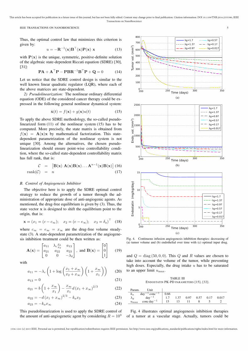
1536-1241 (c) 2015 IEEE. Personal use is permitted, but republication/redistribution requires IEEE permission. See http://www.ieee.org/publications_standards/publications/rights/index.html for more information.
This article has been accepted for publication in a future issue of this journal, but has not been fully edited. Content may change prior to final publication. Citation information: DOI 10.1109/TNB.2016.2535380, IEEETransactions on NanoBioscience
IEEE TRANSACTIONS ON NANOBIOSCIENCE 5
Thus, the optimal control law that minimizes this criterion isgiven by:
u = −R−1(x)B>(x)P(x) x (13)
with P(x) is the unique, symmetric, positive-definite solutionof the algebraic state-dependent Riccati equation (SDRE) [30],[31]:
PA+A>P−PBR−1B>P+Q = 0 (14)
Let us notice that the SDRE control design is similar to thewell known linear quadratic regulator (LQR), where each ofthe above matrices are state-dependent.
2) Pseudolinearization: The nonlinear ordinary differentialequation (ODE) of the considered cancer therapy could be ex-pressed in the following general nonlinear dynamical system:
x(t) = f(x) + g(x)u(t) (15)
To apply the above SDRE methodology, the so-called pseudo-linearized form (11) of the nonlinear system (15) has to becomputed. More precisely, the state matrix is obtained fromf(x) = A(x)x by mathematical factorization. This state-dependent parametrization of the nonlinear system is notunique [30]. Among the alternatives, the chosen pseudo-linearization should ensure point-wise controllability condi-tion, where the so-called state-dependent controllability matrixhas full rank, that is:
C =[B(x) A(x)B(x) . . .An−1(x)B(x)
](16)
rank(C) = n (17)
B. Control of Angiogenesis Inhibitor
The objective here is to apply the SDRE optimal controlstrategy to reduce the growth of a tumor through the ad-ministration of appropriate dose of anti-angiogenic agents. Asmentioned, the drug-free equilibrium is given by (3). Thus, thestate vector x is designed to shift the equilibrium point to theorigin, that is:
x = (x1 = (c− c∞); x2 = (e− e∞); x3 = δa)> (18)
where c∞ = e∞ = x∞ are the drug-free volume steady-state (3). A state-dependent parametrization of the angiogene-sis inhibition treatment could be then written as:
A(x) =
a11 λcx1
x2a13
a21 a22 a230 0 −λδ
, and B(x) =
001
(19)
with
a11 = −λc(1 + log
(x1 + x∞x2 + x∞
)(1 +
x∞x1
))(20)
a13 = 0 (21)
a21 = b
(1 +
x∞x1
)− x∞
x1d (x1 + x∞)
2/3 (22)
a22 = −d (x1 + x∞)2/3 − kax3 (23)
a23 = −kax∞ (24)
This pseudolinearization is used to apply the SDRE control ofthe amount of anti-angiogenetic agent by considering R = 103
200 250 300 3500
100
200
300
400
500
600
700
800λδ=1.7
λδ=1.37
λδ=0.97
λδ=0.57
λδ=0.17
λδ=0.017
Time (days)
Tum
or
vol. (
mm
3)
(a)
200 250 300 350
λδ=1.7
λδ=1.37
λδ=0.97
λδ=0.57
λδ=0.17
λδ=0.017
Time (days)
End
o.
vol. (
mm
3)
0
500
1000
1500
2000
2500
(b)
200 250 300 350Time (days)
End
ost
ati
n
(mg
/kg
/day)
0
5
10
15
λδ=1.7
λδ=1.37
λδ=0.97
λδ=0.57
λδ=0.17
λδ=0.017
(c)
Fig. 4. Continuous infusion angiogenesis inhibition therapies: decreasing of(a) tumor volume and (b) endothelial over time with (c) optimal input drug.
and Q = diag (50, 0, 0). This Q and R values are chosen totake into account the volume of the tumor, while preventinghigh doses. Especially, the drug intake u has to be saturatedto an upper limit umax.
TABLE IIIENDOSTATIN PK-PD PARAMETERS [15], [32].
Param. Unitka day−1 conc−1 0.66λg day−1 1.7 1.37 0.97 0.57 0.17 0.017umax conc day−1 15 13 11 8 5 2
Fig. 4 illustrates optimal angiogenesis inhibition therapiesof a tumor at a vascular stage. Actually, tumors could be
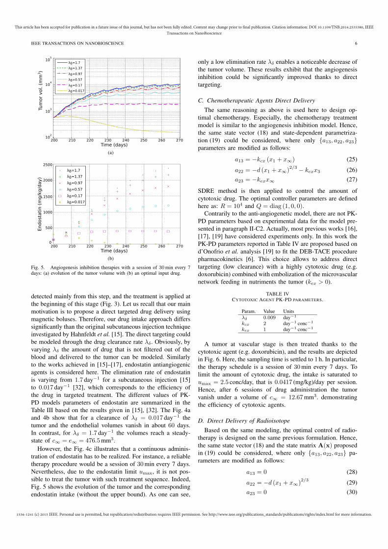
1536-1241 (c) 2015 IEEE. Personal use is permitted, but republication/redistribution requires IEEE permission. See http://www.ieee.org/publications_standards/publications/rights/index.html for more information.
This article has been accepted for publication in a future issue of this journal, but has not been fully edited. Content may change prior to final publication. Citation information: DOI 10.1109/TNB.2016.2535380, IEEETransactions on NanoBioscience
IEEE TRANSACTIONS ON NANOBIOSCIENCE 6
Time (days)
Tum
or
vol. (
mm
3)
200 210 220 230 240 250 260 27010
2
103
104
105
λδ=1.7
λδ=1.37
λδ=0.97
λδ=0.57
λδ=0.17
λδ=0.017
(a)
Time (days)
End
ost
ati
n (
mg
/kg
/day)
200 210 220 230 240 250 260 270
2500
2000
1500
1000
500
0
λδ=1.7
λδ=1.37
λδ=0.97
λδ=0.57
λδ=0.17
λδ=0.017
(b)
Fig. 5. Angiogenesis inhibition therapies with a session of 30min every 7days: (a) evolution of the tumor volume with (b) an optimal input drug.
detected mainly from this step, and the treatment is applied atthe beginning of this stage (Fig. 3). Let us recall that our mainmotivation is to propose a direct targeted drug delivery usingmagnetic boluses. Therefore, our drug intake approach differssignificantly than the original subcutaneous injection techniqueinvestigated by Hahnfeldt et al. [15]. The direct targeting couldbe modeled through the drug clearance rate λδ . Obviously, byvarying λδ the amount of drug that is not filtered out of theblood and delivered to the tumor can be modeled. Similarlyto the works achieved in [15]–[17], endostatin antiangiogenicagents is considered here. The elimination rate of endostatinis varying from 1.7 day−1 for a subcutaneous injection [15]to 0.017 day−1 [32], which corresponds to the efficiency ofthe drug in targeted treatment. The different values of PK-PD models parameters of endostatin are summarized in theTable III based on the results given in [15], [32]. The Fig. 4aand 4b show that for a clearance of λδ = 0.017 day−1 thetumor and the endothelial volumes vanish in about 60 days.In contrast, for λδ = 1.7 day−1 the volumes reach a steady-state of c∞ = e∞ = 476.5mm3.
However, the Fig. 4c illustrates that a continuous adminis-tration of endostatin has to be realized. For instance, a reliabletherapy procedure would be a session of 30min every 7 days.Nevertheless, due to the endostatin limit umax, it is not pos-sible to treat the tumor with such treatment sequence. Indeed,Fig. 5 shows the evolution of the tumor and the correspondingendostatin intake (without the upper bound). As one can see,
only a low elimination rate λδ enables a noticeable decrease ofthe tumor volume. These results exhibit that the angiogenesisinhibition could be significantly improved thanks to directtargeting.
C. Chemotherapeutic Agents Direct Delivery
The same reasoning as above is used here to design op-timal chemotherapy. Especially, the chemotherapy treatmentmodel is similar to the angiogenesis inhibition model. Hence,the same state vector (18) and state-dependent parametriza-tion (19) could be considered, where only a13, a22, a23parameters are modified as follows:
a13 = −kcx (x1 + x∞) (25)
a22 = −d (x1 + x∞)2/3 − kexx3 (26)
a23 = −kexx∞ (27)
SDRE method is then applied to control the amount ofcytotoxic drug. The optimal controller parameters are definedhere as: R = 104 and Q = diag (1, 0, 0).
Contrarily to the anti-angiogenetic model, there are not PK-PD parameters based on experimental data for the model pre-sented in paragraph II-C2. Actually, most previous works [16],[17], [19] have considered experiments only. In this work thePK-PD parameters reported in Table IV are proposed based ond’Onofrio et al. analysis [19] to fit the DEB-TACE procedurepharmacokinetics [6]. This choice allows to address directtargeting (low clearance) with a highly cytotoxic drug (e.g.doxorubicin) combined with embolization of the microvascularnetwork feeding in nutriments the tumor (kex > 0).
TABLE IVCYTOTOXIC AGENT PK-PD PARAMETERS.
Param. Value Unitsλδ 0.009 day−1
kcx 2 day−1 conc−1
kex 1 day−1 conc−1
A tumor at vascular stage is then treated thanks to thecytotoxic agent (e.g. doxorubicin), and the results are depictedin Fig. 6. Here, the sampling time is settled to 1 h. In particular,the therapy schedule is a session of 30min every 7 days. Tolimit the amount of cytotoxic drug, the intake is saturated toumax = 2.5 conc/day, that is 0.0417 (mg/kg)/day per session.Hence, after 6 sessions of drug administration the tumorvanish under a volume of c∞ = 12.67mm3. demonstratingthe efficiency of cytotoxic agents.
D. Direct Delivery of Radioisotope
Based on the same modeling, the optimal control of radio-therapy is designed on the same previous formulation. Hence,the same state vector (18) and the state matrix A(x) proposedin (19) could be considered, where only a13, a22, a23 pa-rameters are modified as follows:
a13 = 0 (28)
a22 = −d (x1 + x∞)2/3 (29)
a23 = 0 (30)
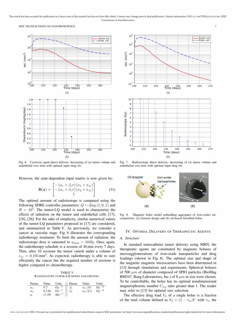
1536-1241 (c) 2015 IEEE. Personal use is permitted, but republication/redistribution requires IEEE permission. See http://www.ieee.org/publications_standards/publications/rights/index.html for more information.
This article has been accepted for publication in a future issue of this journal, but has not been fully edited. Content may change prior to final publication. Citation information: DOI 10.1109/TNB.2016.2535380, IEEETransactions on NanoBioscience
IEEE TRANSACTIONS ON NANOBIOSCIENCE 7
200 210 220 230 240 250 26010
0
101
102
103
104
Tumor vol.Endo. vol.
Time (days)
Vol. (
mm
3)
(a)
Dox
oro
buci
n (
mg
/kg
/day)
200 210 220 230 240 250 260Time (days)
0
0.2
0.4
0.6
0.8
1
1.2
1.4
1.6
1.8
2
(b)
Fig. 6. Cytotoxic agent direct delivery: decreasing of (a) tumor volume andendothelial over time with optimal input drug (b).
However, the state-dependent input matrix is now given by:
B(x) =
− (αc + βcr) (x1 + x∞)− (αe + βer) (x2 + x∞)
1
(31)
The optimal amount of radioisotope is computed using thefollowing SDRE controller parameters: Q = diag (1, 0, 1) andR = 103. The tumor-LQ model is used to characterize theeffects of radiation on the tumor and endothelial cells [17],[18], [26]. For the sake of simplicity, similar numerical valuesof the tumor-LQ parameters proposed in [17] are considered,and summarized in Table V. As previously, we consider acancer at vascular stage. Fig. 6 illustrates the correspondingradiotherapy treatment. To limit the amount of radiation, theradioisotope dose is saturated to umax = 10Gy. Once again,the radiotherapy schedule is a session of 30min every 7 days.Thus, after 10 sessions the tumor vanish under a volume ofc∞ = 0.195mm3. As expected, radiotherapy is able to cureefficiently the cancer but the required number of sessions ishigher compared to chemotherapy.
TABLE VRADIOISOTOPE TUMOR-LQ MODEL PARAMETERS.
Param. Value Units Param. Value Unitsαc 0.7 Gy−1 βc αc/10 Gy−2
αe 0.136 Gy−1 βe αe/2.5 Gy−2
µ 11.09 day−1
Time (days)
Vol. (
mm
3)
Tumor vol.Endo. vol.
200 210 220 230 240 250 260 27010
-1
100
101
102
103
104
(a)
0
1
2
3
4
5
6
7
8
9
10
Rad
iois
oto
pe (
Gy)
Time (days)200 210 220 230 240 250 260 270
(b)
Fig. 7. Radioisotope direct delivery: decreasing of (a) tumor volume andendothelial over time with optimal input drug (b).
Fig. 8. Magnetic bolus model embedding aggregates of iron-oxides mi-croparticles. (a) General design and (b) oil-based ferrofluid bolus.
IV. OPTIMAL DELIVERY OF THERAPEUTIC AGENTS
A. Structure
In standard transcatheter tumor delivery using MRN, thetherapeutic agents are constituted by magnetic boluses ofmicroagglomerations of iron-oxide nanoparticles and drugloadings (shown in Fig. 8). The optimal size and shape ofthe magnetic magnetic microcarriers have been determined in[13] through simulations and experiments. Spherical bolusesof 500 µm of diameter composed of SPIO particles (BioMagBM547, Bang Laboratories, Inc.) of 8 µm in size were chosen.To be controllable, the bolus has its optimal nondimensionalmagnetophoretic number Cmt ratio greater than 1. The readermay refer to [13] for optimal size selection.
The effective drug load Vδ of a single bolus is a fractionof the total volume defined as Vδ = (1 − τm)V with τm the

1536-1241 (c) 2015 IEEE. Personal use is permitted, but republication/redistribution requires IEEE permission. See http://www.ieee.org/publications_standards/publications/rights/index.html for more information.
This article has been accepted for publication in a future issue of this journal, but has not been fully edited. Content may change prior to final publication. Citation information: DOI 10.1109/TNB.2016.2535380, IEEETransactions on NanoBioscience
IEEE TRANSACTIONS ON NANOBIOSCIENCE 8
so-called magnetization rate. When injected in the vascularphantom placed in the tunnel of the MRI scanner, the magneticbolus will take the form of a prolate sphere due to the strongdipole-to-dipole interactions between the nanoparticles. Due tothe B0 field of the scanner, the equivalent magnetization Ms ofthe aggregates is aligned with the B0 field. We consider herethat the magnetic material (Vm) is saturated to its maximalvalue Ms = 56 emu/g under a magnetic field B0 = 3.0 Tesla.The injected magnetic volume τmV is computed as a tradeoffbetween the encapsulated drug volume and the necessarysteering force. Finally, the number of magnetic boluses isestimated from
Nb =
⌈u m
Vδρδ
⌉(32)
where u is the rate of administration of the therapeutic agent;m is the patient weight (considered as m = 60 kg hereafter);and ρδ is the agent load density.
B. Endostatin Angiogenesis Inhibitor
The objective is to determine the amount Nb of requiredboluses to reduce the tumor size by administrating an anti-angiogenic agent. In paragraph III-B endostatin agent is usedas angiogenesis inhibitor. Endostatin is a naturally occurring20 kDa polypeptide, identified as a C-terminal fragment ofcollagen (type 18). Commonly, endostatin agent is available insolution concentration of 1mg ml−1. Hence, considering theupper limit umax given in Table III, the Table VI presents themaximum of required number of magnetic boluses that havebeen to be conveyed continuously. Even in the low clearancecase with λδ = 0.017 day−1 where the endostatin administra-tion rate is lower (umax = 2 conc day−1), Nb = 4661 magneticboluses have to be injected continuously to administrate thedaily dose.
TABLE VIREQUIRED MAGNETIC BOLUSES THAT CARRY ENDOSTATIN TO TREAT A
PATIENT OF AVERAGE WEIGHT m = 60 kg.
Param. Unitumax conc day−1 15 13 11 8 5 2Dose mg day−1 750 650 550 400 250 100Nb 1× 10³ 34.95 30.29 25.63 18.64 11.65 4.66
Similarly, if the considered scheduling of one session everyweek is applied (cf. Fig. 5), Nb = 1.398× 10⁴ boluses haveto be administered at the first session.
C. Cytotoxic Drug (doxorubicin)
Chemotherapy is achieved by direct targeting of highlycytotoxic drug, such as doxorubicin. Doxorubicin is an anthra-cycline tumor antibiotic that works by intercalating DNA. Thisdrug has already shown its efficiency in DEB-TACE proceduresince a decade [5], [6]. The drug eluting beads (DEB) havebeen easily loaded with doxorubicin to a recommended levelof 25mg ml−1, with a maximum loading of 45mg ml−1 [5].Here, we assume that the doxorubicin PK-PD model param-eters is close to the cytotoxic agent given in Table IV. Fora patient of average weight m = 60 kg a maximum dose of
120mg has to be conveyed per session (cf. Fig. 6). Therefore,a maximum of Nb = 1036 magnetic boluses have to beadministered.
D. Radioisotope (Yttrium)
The radiotherapy consists to administrate microspherescontaining a radioisotope. Usually, yttrium-90 (90Y) micro-spheres are administered in directed cancer radiotherapy [4].90Y is a high-energy beta-emitting isotope with no primarygamma emission and a half-life of 2.67 days. For instance,TheraSphere (MDS Nordion, Canada) are biocompatible andnonabsorbable glass microspheres loaded with 90Y. The radiusof TheraSphere beads is about rp = 12.5 ± 2.5µm, and thenone magnetic bolus could embed up to 3147 radioisotopemicrospheres. Each 90Y bead contains an activity of 2500Bq,leading to 7.8675× 10⁻³ GBq per bolus. Assuming an uni-form distribution, the radiation dose intake is computed from
[4] u =49.67A
mlwith A the radioisotope activity (in GBq),
and ml the mass of the liver (in kg). Therefore, the numberof magnetic boluses that carries 90Y beads is obtained from:
Nb =
⌈u ·ml
49.67× 3147× 2.5× 10−6
⌉(33)
We consider that the radioisotope tumor-LQ model parametersgiven in Table V corresponds to TheraSphere. For a typicalpatient with a liver mass of ml = 2 kg, a maximum of Nb = 52boluses have to be administered in one session to carry theupper limit of 10Gy (cf. Fig. 7).
V. DISCUSSION
Locoregional therapies are considered as the best treatmentsin patients with unresectable hepatocellular carcinoma (HCC).The various mathematical models of cancer therapies forHCC that have been evaluated so far describe some interac-tions between tumor cells and blood vessels. However, theinternal cell behavior is not explicitly expressed, whereasfurther sources of complexity arise from its internal cell-to-cell cooperative and competitive interactions [17]. Especially,due to the use of ODE system the model also does notinclude the spatial characteristic of the tumor growth along thesurrounding tissue. Particularly, this work considers medicallyreasonable parameters set given in Table I-to-V taken fromthe literature. Actually, only few data are available to estimatethe parameter sets, especially in the case of human models[16], [17], [22]. Mathematically modeling the dynamics ofa tumor allows us to better understand tumor activity byconsidering critical biological influences, time delays, humanintervention and tumor adaptation. Our model parameters arecomputed on the basis of experimental data given in [15].The environmental factors such as habits, smoking, alcoholconsumption, and infections, have a profound influence oncancer development. As example, it is possible to regulatethe nuclear transcription factor, NF-kB, by controlling thevascular endothelial cells birth rate, b, expressed in the model[33]. Furthermore, the control of the drug input u offersthe possibility to model the drug overdose and/or toxicity.

1536-1241 (c) 2015 IEEE. Personal use is permitted, but republication/redistribution requires IEEE permission. See http://www.ieee.org/publications_standards/publications/rights/index.html for more information.
This article has been accepted for publication in a future issue of this journal, but has not been fully edited. Content may change prior to final publication. Citation information: DOI 10.1109/TNB.2016.2535380, IEEETransactions on NanoBioscience
IEEE TRANSACTIONS ON NANOBIOSCIENCE 9
In the proposed direct targeting therapy, the drug input issaturated to umax values which should be related to the upperbound of the drug concentration umax. For instance, the mostcommonly used dosage of doxorubicin is to not exceed δmax= 2 mg/kg to have a very low risk of overdose. Finally, thetheoretical simulation results point out some benefits whenconsidering MRN-assisted locoregional therapy. At an earlier-stage disease, TACE and TARE treatments are commonlyused. Actual TACE treatments with doxorubicin at baseline(cTACE) or doxorubicin-loaded eluting beads (DEB-TACE)deliver a high dose of drug over a longer period of time (3months) into the tumor. The schedule of treatment is settledto 3 months, 6 months, and then every 6 months thereafter.The size of DEB is chosen according to the particular study,usually with smaller particles (100-to-300 µm) being selectedfirst, followed by larger particles (500-to-700 µm). Whenperforming MRN-assisted procedure using embolic magneticboluses releasing doxorubicin, similar benefits (drug rate andfrequency of treatment) are found but the technique mayprevent bile duct injury by avoiding overembolization thatwill relentlessly lead to nontarget embolization. In the case ofembolic radioembolization in TARE treatment, glass or resinemicrospheres of 20-to-30 µm in size are used. A high numberof aggregated spheres (glass: 1.2 million microspheres/3 GBq;resin: 40-to-60 millions of microspheres/3 GBq) are requiredleading to deposition in the liver as a large number ofdiscrete clusters. The use of MRN could significantly improvethe technique by reducing the number and the timeless ofsequences, and most importantly, by providing heterogeneousradiation dose distribution patterns. At an advanced-stagedisease, Sorafenib, a multikinase inhibitor with antiangiogenicproperties of Sorafenib, in combination with locoregionaltherapy if of increased interest to specialists who care forpatients with unresectable hepatocellular carcinoma [18]. Todemonstrate the feasibility of MRN-assisted procedure, Bigotet al. [12] have demonstrated that the propulsion of Nb = 1530magnetic boluses inside a multi-bifurcation phantom required33min of duration. These experiments are in agreement withour simulation results concerning TACE and TARE treatmentssince only 1036 and 52 magnetic boluses are required.
VI. CONCLUSION
The paper described an optimal design strategy for innova-tive transcatheter arterial magnetic bolus delivery using MRNprocedure. To maximize the effect of the treatment and mini-mize adverse effects on the patient, a mathematical model hasbeen developed to find the number of magnetic boluses withrespect to the growth of a tumor and the carried therapeuticagent. The application of such mathematical design frameworkis the optimization of anti-cancer treatment modalities by itsoptimal use with locoregional tumor therapies. Indeed, thepreliminary results demonstrate that MRN may improve theconventional TACE and TARE treatments by increasing thelocal drug concentration, reducing the number and duration oftreatment sequences, and decreasing the side-effects relatedto toxicity in healthy tissues. Undergoing work considersthe locoregional magnetic bolus delivery of various sizes ofaggregates in small animals.
REFERENCES
[1] R. L. Siegel, K. D. Miller, and A. Jemal, “Cancer statistics, 2015,” CA:a cancer journal for clinicians, vol. 65, no. 1, pp. 5–29, 2015.
[2] J. M. Llovet, M. I. Real, X. Montaa, R. Planas, S. Coll, J. Aponte,C. Ayuso, M. Sala, J. Muchart, R. Sol, J. Rods, and J. Bruix, “Arte-rial embolisation or chemoembolisation versus symptomatic treatmentin patients with unresectable hepatocellular carcinoma: a randomisedcontrolled trial,” The Lancet, vol. 359, no. 9319, pp. 1734–1739, 2002.
[3] A. Forner, J. M. Llovet, and J. Bruix, “Hepatocellular carcinoma,” TheLancet, vol. 379, no. 9822, pp. 1245–1255, 2012.
[4] A. Kennedy, S. Nag, R. Salem, R. Murthy, A. J. McEwan, C. Nutting,A. Benson III, J. Espat, J. I. Bilbao, R. A. Sharma et al., “Recommen-dations for radioembolization of hepatic malignancies using yttrium-90 microsphere brachytherapy: a consensus panel report from theradioembolization brachytherapy oncology consortium,” InternationalJournal of Radiation Oncology* Biology* Physics, vol. 68, no. 1, pp.13–23, 2007.
[5] A. L. Lewis, M. V. Gonzalez, A. W. Lloyd, B. Hall, Y. Tang, S. L. Willis,S. W. Leppard, L. C. Wolfenden, R. R. Palmer, and P. W. Stratford, “DCbead: in vitro characterization of a drug-delivery device for transarterialchemoembolization,” Journal of vascular and interventional radiology,vol. 17, no. 2, pp. 335–342, 2006.
[6] M. Varela, M. I. Real, M. Burrel, A. Forner, M. Sala, M. Brunet,C. Ayuso, L. Castells, X. Montana, J. M. Llovet et al., “Chemoemboliza-tion of hepatocellular carcinoma with drug eluting beads: efficacy anddoxorubicin pharmacokinetics,” Journal of hepatology, vol. 46, no. 3,pp. 474–481, 2007.
[7] T. Matsumoto, J. Endo, K. Hashida, H. Ichikawa, S. Kojima,S. Takashimizu, N. Watanabe, T. Yamagami, and T. Hasabe, “Balloon-occluded transarterial chemoembolization using a 1.8-french coaxialmicroballoon catheter for hcc: Tehnical and safety considerations,”Minimally Invasive Therapy Allied Technologies, vol. 24, no. 2, pp.94–100, 2015.
[8] R. Salem and K. Thurston, “Radioembolization with 90yttrium mi-crospheres: A state-of-the-art brachyterapy treatment for primary andsecondary liver malignancies- part 1: Technical and methodologic con-siderations,” Journal of Vascular Interventional Radiology, vol. 17, pp.1251–1278, 2006.
[9] U. Hafeli, S. Sweeney, B. Beresford, J. Humm, and R. Macklis,“Effective targeting of magnetic radioactive y-microspheres to tumorcells by an externally applied magnetic field. preliminary in-vitro andin-vivo resuls,” Nuclear Medecina and Biology, vol. 22, no. 2, pp. 147–155, 1995.
[10] J.-B. Mathieu, G. Beaudoin, and S. Martel, “Method of propulsion ofa ferromagnetic core in the cardiovascular system through magneticgradients generated by an MRI system,” IEEE Trans. Biomed. Eng.,vol. 53, no. 2, pp. 292–299, 2006.
[11] P. Pouponneau, J.-C. Leroux, G. Soulez, L. Gaboury, and S. Martel, “Co-encapsulation of magnetic nanoparticles and doxorubicin into biodegrad-able microcarriers for deep tissue targeting by vascular MRI navigation,”Biomaterials, vol. 32, no. 13, pp. 3481–3486, 2011.
[12] A. Bigot, C. Tremblay, G. Soulez, and S. Martel, “Magnetic resonancenavigation of a bead inside a three-bifurcation pmma phantom using animaging gradient coil insert,” navigation (MRN), vol. 5, p. 7, 2014.
[13] L. Mellal, K. Belharet, D. Folio, and A. Ferreira, “Optimal structureof particles-based superparamagnetic microrobots: application to mriguided targeted drug therapy,” Journal of Nanoparticle Research, vol. 17,no. 2, pp. 1–18, 2015.
[14] B. Ribba, N. Holford, P. Magni, I. Troconiz, I. Gueorguieva, P. Girard,C. Sarr, M. Elishmereni, C. Kloft, and L. Friberg, “A review of mixed-effects models of tumor growth and effects of anticancer drug treatmentused in population analysis,” CPT: pharmacometrics & systems phar-macology, vol. 3, no. 5, p. e113, 2014.
[15] P. Hahnfeldt, D. Panigrahy, J. Folkman, and L. Hlatky, “Tumor de-velopment under angiogenic signaling a dynamical theory of tumorgrowth, treatment response, and postvascular dormancy,” Cancer re-search, vol. 59, no. 19, pp. 4770–4775, 1999.
[16] A. d’Onofrio and A. Gandolfi, “Tumour eradication by antiangiogenictherapy: analysis and extensions of the model by hahnfeldt et al. (1999),”Mathematical biosciences, vol. 191, no. 2, pp. 159–184, 2004.
[17] A. Ergun, K. Camphausen, and L. M. Wein, “Optimal schedulingof radiotherapy and angiogenic inhibitors,” Bulletin of mathematicalbiology, vol. 65, no. 3, pp. 407–424, 2003.
[18] U. Ledzewicz, A. dOnofrio, and H. Schttler, “Tumor development undercombination treatments with anti-angiogenic therapies,” in Mathematical

1536-1241 (c) 2015 IEEE. Personal use is permitted, but republication/redistribution requires IEEE permission. See http://www.ieee.org/publications_standards/publications/rights/index.html for more information.
This article has been accepted for publication in a future issue of this journal, but has not been fully edited. Content may change prior to final publication. Citation information: DOI 10.1109/TNB.2016.2535380, IEEETransactions on NanoBioscience
IEEE TRANSACTIONS ON NANOBIOSCIENCE 10
Methods and Models in Biomedicine, ser. Lecture Notes on Mathe-matical Modelling in the Life Sciences, U. Ledzewicz, H. Schttler,A. Friedman, and E. Kashdan, Eds. Springer New York, 2013, pp.311–337.
[19] A. d’Onofrio, U. Ledzewicz, H. Maurer, and H. Schattler, “On optimaldelivery of combination therapy for tumors,” Mathematical biosciences,vol. 222, no. 1, pp. 13–26, 2009.
[20] S. Sanga, J. P. Sinek, H. B. Frieboes, M. Ferrari, J. P. Fruehauf, andV. Cristini, “Mathematical modeling of cancer progression and responseto chemotherapy,” Expert Review of Anticancer Therapy, vol. 6, no. 10,pp. 1361–1376, 2006.
[21] L. G. de Pillis, W. Gu, K. R. Fister, T. a. Head, K. Maples, A. Murugan,T. Neal, and K. Yoshida, “Chemotherapy for tumors: An analysis ofthe dynamics and a study of quadratic and linear optimal controls,”Mathematical Biosciences, vol. 209, no. 1, pp. 292–315, 2007.
[22] L. G. De Pillis and A. Radunskaya, “The dynamics of an optimallycontrolled tumor model: A case study,” Mathematical and ComputerModelling, vol. 37, no. 11, pp. 1221–1244, 2003.
[23] L. Kovacs, A. Szeles, J. Sapi, D. A. Drexler, I. Rudas, I. Harmati,and Z. Sapi, “Model-based angiogenic inhibition of tumor growth usingmodern robust control method,” Computer methods and programs inbiomedicine, vol. 114, no. 3, pp. e98–e110, 2014.
[24] A. Kansal, S. Torquato, G. Harsh, E. Chiocca, and T. Deisboeck,“Simulated brain tumor growth dynamics using a three-dimensionalcellular automaton,” Journal of theoretical biology, vol. 203, no. 4, pp.367–382, 2000.
[25] P. Gerlee and A. R. Anderson, “An evolutionary hybrid cellular automa-ton model of solid tumour growth,” Journal of theoretical biology, vol.246, no. 4, pp. 583–603, 2007.
[26] J. F. Fowler, “The linear-quadratic formula and progress in fractionatedradiotherapy,” The British journal of radiology, vol. 62, no. 740, pp.679–694, 1989.
[27] G. W. Swan, “Role of optimal control theory in cancer chemotherapy,”Mathematical biosciences, vol. 101, no. 2, pp. 237–284, 1990.
[28] Y. Batmani and H. Khaloozadeh, “Optimal chemotherapy in cancertreatment: state dependent riccati equation control and extended kalmanfilter,” Optimal Control Applications and Methods, vol. 34, no. 5, pp.562–577, 2013.
[29] K. Zhou, J. C. Doyle, K. Glover et al., Robust and optimal control.Prentice Hall New Jersey, 1996, vol. 40.
[30] C. P. Mracek and J. R. Cloutier, “Control designs for the nonlinearbenchmark problem via the state-dependent riccati equation method,”International Journal of robust and nonlinear control, vol. 8, no. 4-5,pp. 401–433, 1998.
[31] T. Cimen, “Systematic and effective design of nonlinear feedback con-trollers via the state-dependent riccati equation (sdre) method,” AnnualReviews in Control, vol. 34, no. 1, pp. 32–51, 2010.
[32] S.-U. Shin, H.-M. Cho, J. Merchan, J. Zhang, K. Kovacs, Y. Jing, S. Ra-makrishnan, and J. D. Rosenblatt, “Targeted delivery of an antibody–mutant human endostatin fusion protein results in enhanced antitumorefficacy,” Molecular cancer therapeutics, vol. 10, no. 4, pp. 603–614,2011.
[33] P. Anand, A. B. Kunnumakara, C. Sundaram, K. B. Harikumar, S. T.Tharakan, O. S. Lai, and B. B. Aggarwal, “Cancer is a preventabledisease that requires major lifestyle changes,” Pharmaceutical research,vol. 25, no. 9, pp. 2097–2116, 2008.

APPENDIX E
MATHEMATICAL APPROACH FOR THE DESIGNCONFIGURATION OF MAGNETIC SYSTEM WITH
MULTIPLE ELECTROMAGNETS (ACL15)
215

Mathematical approach for the design configuration of magnetic systemwith multiple electromagnets
Ruipeng Chen, David Folio, Antoine Ferreira∗
INSA Centre Val de Loire, Universite d’Orleans, PRISME EA 4229, Bourges, France
Abstract
Magnetic actuation techniques and microrobots have attracted great interest since they have potential inbiomedicine applications. Interventional techniques have emerged as a tool to handle a wide range of mini-mally invasive surgeries (MIS). However, current MIS procedures are constrained by the limitation of manualoperation by surgeon. Thus, various microrobotic solutions including magnetic navigation systems have beenproposed for MIS, which carries many potential benefits such as reduced incision, less intraoperative hemor-rhaging and postoperative pain, and faster recovery time. In recent decades, many electromagnetic actuation(EMA) systems have been reported and involved to general surgery. The EMA system allows to generateefficiently magnetic source for microrobot control when its specifications are further investigated and satis-fied for the desired application. To precisely manipulate the biomedical microrobot, a key issue still relieson the design of a suitable EMA platform. In this paper, we demonstrate a mathematical approach for thedesign configuration of magnetic system with multiple electromagnets. Especially, the required magneticcoil number has been investigated where the heading motion control, magnetic force control and their combi-nation control are discussed respectively. The singular cases of control are pre-evaluated by a mathematicalanalysis of the simulated electromagnetic field. In addition, the placed positions and tilted orientations ofthe applied electromagnets are investigated for the optimization regarding the six typical configurations ofEMA platform with 4, 6 and 8 coils. The various configurations of EMA systems have been comprehensivelyanalyzed. Therefore, with the number of electromagnets and their optimal configuration obtained by theproposed approach, the EMA system can be initially established.
Keywords: Electromagnetic actuation system, Magnetic microrobot, Design methodology, Roboticmagnetic platform
1. Introduction
Minimally invasive surgery (MIS) encompassessurgical techniques that limit the size of incisionsneeded and so lessen wound healing time, asso-ciated pain and risk of infection. MIS proce-5
dures have been enabled by the advance of variousmedical technologies. In particular, several surgi-cal robotics systems have been developed. Suchrobotic platforms already play a significant roleto improve patient care, though it increases sur-10
gical preparation, cost and risk of the MIS ap-proach compared with traditional open surgery[1,
∗Corresponding authorEmail addresses: david.folioinsa-cvl.fr (David
Folio), [email protected] (Antoine Ferreira)
2, 3, 4, 5, 6, 7, 8, 9, 10, 11]. For example,there are the well-known da Vinci surgical assis-tance robots[5, 7], developed by Intuitive Surgical1,15
which improves the surgeon technical skills. More-over, unlike the dependence on using rigid instru-ments with dexterous distal wrists, it is commonlymore attractive to use flexible or adaptive robotictools that access internal anatomy with few skin20
incisions[10, 12, 13, 14, 15, 16, 17]. Especially, themechanical parts of existing medical robotic devicesare still relatively large and rigid to access and treatmajor inaccessible parts of the human body (e.g.in robot-assisted surgery). In parallel, the various25
medical robotics solutions have been developed toimprove the acceptance of the use of robotics sys-tems in clinical practices. In the meanwhile, mi-
Preprint submitted to Robotics and Autonomous Systems July 1, 2021

crorobotics has also emerged as an attractive tech-nology to introduce novel microsystems to further30
reduce trauma, create new diagnosis tools and ther-apeutic procedures.
Indeed, designing miniaturized and versatile mi-crorobotic systems would allow accessing through-out the whole human body; leading to new proce-35
dures down to the cellular level; and offering lo-calized diagnosis and treatment with greater pre-cision and efficiency. For example, untethered mi-croscopic devices, smaller than one millimeter, maynavigate within the body for targeted therapies[18,40
19, 20, 21]. Among the various actuation of mi-crorobots, magnetic actuation is considered to bethe most promising method[9, 18, 22, 23, 24, 25,26, 27, 28, 29, 30, 31, 32, 33, 34]. To this aim, nu-merous electromagnetic actuation (EMA) systems45
have been proposed to control untethered mag-netic microrobots for biomedical applications[18,35, 36, 37, 38, 39, 40, 41, 42, 43, 44, 45, 46, 47].The development of magnetic microrobotic systemscircumvents the need to embed power within the50
microdevice[18, 19, 20]. Magnetic microrobot canbe then remotely powered and actuated preciselyby the use of external electromagnetic fields. Thisenables untethered microrobots to assist the sur-geon to increase precision and dexterity of the MIS55
procedure[10, 18, 34, 42].The paper aims to propose a mathematical ap-
proach for the design configuration of magnetic sys-tem using multiple electromagnets, that improvesMIS procedures since the magnetic manipulation of60
microrobots is one of the most interesting methodto assist researchers in many biomedical applica-tions. To address this issue of designing a properEMA system for a given application, the investiga-tion of the appropriate design configuration carried65
out. The paper is then organized as follows. Sec-tion 2 presents the theoretical foundation of electro-magnetism including the basic principles and nec-essary equations. From this basis, the electromag-netic manipulation of untethered microrobot with70
the magnetic torque and force control is discussed,and the necessary metrics are defined. In Section 3,the analysis of the minimum number of electromag-nets for an EMA platform is investigated. In partic-ular, singular cases are pointed out when magnetic75
field and gradient exhibit some linear dependencies.In Section 4, six typical configurations are simu-lated and evaluated for the efficient motion controlof microrobot. The configuration of EMA system isoptimized with respect to the considered magnetic80
yx
z
2
22
B(p1)
Electromagnets
...
t= (m⨉B)
f=(m·∇)B
∇B(p2)
m2
i2
in
i1
m1
mn
2
N
S
n1
(a)
y
x
z
p
B(p)
m
mxmy
mz
bxby
bz
(b)
∂yby∂xby∂zby
∂zbz
∂xbz∂ybz
∂xbx∂ybx
∂zbx
B(p)
by
bz
∇bx ∇bx
∇bz
pbx
(c)
Figure 1: Electromagnetic manipulation: (a) illustration ofthe use of the magnetic force and torque on untethered mag-netic microrobots; (b) composition of the magnetic field withthe magnetic moment of the microrobot; and (c) the differentcomponents of the magnetic gradient.
control objectives. In Section 5, the comparison ofconfigurations is performed when the magnetic per-formances are summarized regarding the arrange-ment parameters of magnetic system. The paper isconcluded with the Section 6.85
2. Theoretical foundation
The aim of this section is to recall the basic prin-ciples of electromagnetism that serve as a founda-tion of our research works.
2.1. Electromagnetic Manipulation90
Starting from the Maxwell’s equations, and as-suming that charges are either fixed or move as asteady current J , the governing equation of a quasi-static magnetic field can be described by the twofollowing relations [48]:
∇ ·B = 0 (1)
∇×B = µ0J (2)
Next, assuming that the microrobot is a magne-tized body described by its magnetic dipole momentM , that is placed in a magnetic flux B, the inducedmagnetic force and torque are basically expressedfrom [49]:
f = (M · ∇)B (3)
t = (M ×B) (4)
2

xe
me
Ω
F e
d
p
beF 0
mOF 0 x
zy
Figure 2: Schematic representation of a single electromag-net inducing a magnetic flux Be(P ) within the workspace Ω(blue square box).
Obviously, f is related to the magnetic gradient∇B, whereas the magnetic torque t is a function ofthe magnetic field B. Moreover, to actuate the mi-crorobot, the magnetic field must undergo either aspatial change (i.e. exhibit a spatial field gradient),95
or a temporal change, such as through a rotatingmagnetic field, oscillation and so on. Fig. 1 illus-trates these basic principles. Specifically, the mag-netic field and its gradient are generated by a set ofn electromagnets to control the motion of unteth-100
ered microrobots. The orientation of microrobottends to be aligned with the direction of magneticfield B, thus the microrobots are rotated by themagnetic torque t. Moreover, the magnetic gradi-ent ∇B induces the magnetic force f as propulsion105
force to move the microrobot. Hence, the magneticobject can be manipulated through the rotation andtranslation operations using magnetic field and gra-dient, respectively.
Secondly, if we assume there is no electric currentflowing through the workspace occupied by the mi-crorobot, Maxwell’s equation implies that equation(2) becomes ∇ × B = 0. The magnetic force (3)can be then rearranged using vector calculus intothe following form:
f =
∂B
∂x∂B
∂y∂B
∂z
M =
∂bx
∂x
∂by
∂x
∂bz
∂x∂bx
∂y
∂by
∂y
∂bz
∂y∂bx
∂z
∂by
∂z
∂bz
∂z
M = GM
(5)where G ∈ R3×3 denotes the gradient matrix of110
the magnetic field B = (bx, by, bz). Besides, thesubscripts x, y and z explicitly refer to the basisdirections of the Cartesian reference frame F0(O :x, y, z) linked to the workspace Ω, in which all vec-tors are expressed (see Fig. 2).115
The torque on microrobot tends to align the mag-netization vector with the magnetic field. To rep-resent vector cross products, the skew-symmetric
matrix formed of a vector can be employed, that is:
Sk(M) = Sk
mx
my
mz
=
0 −mz my
mz 0 −mx
−my mx 0
(6)
Therefore, the force (3) and torque (4) applied tomagnetic microrobots can be rewritten as:(
ft
)=
((M · ∇)Sk(M)
)B (7)
2.2. Electromagnetic control
For multiple-coil configuration, the magnetic fieldis induced by an EMA system consisting of sev-eral electromagnets. Hence, with a given set of nelectromagnets, each of them creates a magneticfield, Be(P ), at any location of the workspace:∀P ∈ Ω. The magnetic fields and their spatial gra-dients depend linearly on the currents. When ieflows through the coils e, the magnetic field can beexpressed as: Be(P ) = Be(P )ie. The superpositionprinciple is commonly used to compute the overallmagnetic field, that is:
B(P ) =n∑e=1
Be(P )ie =
bx1 . . . bxe . . . bxnby1 . . . bye . . . bynbz1 . . . bze . . . bzn
i
=
Bx(P )By(P )Bz(P )
i = B(P )i (8)
where i = (i1 . . . in)ᵀ
is the current vector, andB(P ) is a 3 × n matrix mapping the currents tothe magnetic fields. Similarly, the magnetic gradi-ent fields could be expressed as:
∂B(P )
∂x=
n∑e=1
∂Be(P )
∂xie = Gx(P )i (9)
∂B(P )
∂y=
n∑e=1
∂Be(P )
∂yie = Gy(P )i (10)
∂B(P )
∂z=
n∑e=1
∂Be(P )
∂zie = Gz(P )i (11)
where each Gx,y,z(P ) is 3 × n matrix mapping thecurrent to the magnetic gradient field in the x, y,and z directions, respectively.
The different mapping matrices B(P ) and120
Gx,y,z(P ) expressions are related to the type and
3

geometry of each electromagnet (e.g. length, ra-dius, numbers of turns). For instance, the mappingfor Helmholtz or Maxwell coils could be easily car-ried out from the Biot-Savart’s law. For the other125
types of electromagnets, especially with a magneticcore, the mapping matrices can be calculated ei-ther from measures of the magnetic field within theEMA system’s workspace or from the simulationsof magnetic field using FEM models [43].130
Finally, the equations of magnetic force andtorque can be rearranged as follows:t
f
=
Sk(M)BMᵀGx(P )MᵀGy(P )MᵀGz(P )
i =
At(M,P )
Af (M,P )
i
= A(M,P )i
(12)
where At(M,P ) and Af (M,P ) are the actuationmatrices mapping the current vector i to the torqueand force, respectively; and A(M,P ) is the 6 × nactuation matrix mapping to the applied magneticwrench. These magnetic actuation matrices depend135
both on the position P ∈ Ω, and on the orientationof the dipole moment M of the microrobot.
According to equations (3)-(4), each column ofthe matrix A(M,P ) represents the wrench on theforce and torque per current unit created by eachelectromagnet. If there are greater than n > 6 elec-tromagnets, the actuation matrix A(M,P ) leadsto a better conditioned matrix, a more isotropicworkspace Ω, a reduction of singularity configura-tions, and lower current requirements [50, 51]. Insuch cases, n > 6, the EMA system could be said”redundant” for the task. Especially, if A(M,P ) isof full rank, for a desired force, f? and torque, t?,the actuation currents i can be calculated from thepseudo-inverse:
i = A+(M,P )
(t?
f?
)(13)
If n < 6, the pseudo-inverse would be a least-squares approximations. Hence, for a controlledforce and torque, the input current can be obtained140
only if the pseudo-inverse of A(M,P ) exists. Thisderivation on the controlled current i can be sim-ilarly extended for controllers that require torqueand/or force control [52].
2.3. Indexes for Electromagnetic System145
To be able to compare such various electromag-netic coils dispositions, it is necessary to define
some metrics to get some quantitative assessmentsof their effectiveness. The basic idea is to set ascore to a given EMA configuration to allow an ef-150
fective comparative analysis. Indeed, with respectto the applications objectives, different indexes canbe defined and considered.
2.3.1. Magnetic Field Indexes
First, the strength and homogeneity of either the155
magnetic field or its gradient in the workspace arethe most significant metrics for medical applica-tions. As example, a strong magnetic field strengthleads to powerful torque t enabling reliable swim-ming of the helical microrobot. In the meantime, it160
should be homogeneous along the workspace to sim-plify the control strategy. Furthermore, the EMAsystem needs to avoid unexpected magnetic forcewhen varying the orientation of microrobot alongwith the magnetic field. Similarly, a strong mag-165
netic gradient provides an effective propulsion forcef , and its uniformity implies a homogeneous netforce on microrobots. To this aim, various indexescan be used from statistical analysis of the fields dis-tributions, such as its maximum, mean, RMS, STD,170
etc. To evaluate the quality of a magnetic fieldor its gradient, we have chosen to consider mainlythe average and the uniformity indexes introducedhereafter.
Average index. In [40], the authors propose to char-acterize the strength of a sampled vector field ϕ byits average (i.e. the arithmetic mean) basically de-fined as:
〈ϕ〉 =1
N
N∑P∈Ω
ϕ(P ) (14)
with N the number of samples, and P the sampling175
location in the workspace Ω. This arithmetic meanvalue reflects the strength of a global vector fieldϕ. It can be utilized to quantify the average of themagnitudes of a magnetic field or its gradient fromthe corresponding samples, and then to evaluate the180
strength of the torque or force in the workspace.
Uniformity index. The isotropy index measuresand yields an intuitive value for the difference be-tween each considered vector of a vector field ϕ dis-tribution. To evaluate the isotropy, various indexescan be considered, such as the basic minimum-to-maximum ratio, or the coefficient of variation. Fora vector field ϕ, the uniformity index γ is usually
4

considered, which is defined as:
γ(ϕ) = 1− 1
2N〈ϕ〉
N∑P∈Ω
|ϕ(P )− 〈ϕ〉| (in %)
(15)where the isotropy index γ should be commonlybounded between 0% and 100%. Then, a unifor-mity index close to 100% indicates that every sam-ple of the field ϕ is almost identical.185
2.3.2. Magnetic Actuation Indexes
In the other hand, the EMA system has to actu-ate a magnetic microrobot in the workspace. Hence,the ability to perform or not certain motion at anylocation and direction is of prime importance. Basi-190
cally, if there are some singularities, some motionscannot be achieved, and the DOFs of the micro-robot is reduced. For an EMA system, this analy-sis can be performed through the examination ofits magnetic actuation matrix A(M,P ). As de-195
scribed in (12), A(M,P ) allows mapping the inputcurrents i to the magnetic torque and force thatare applied to a microrobot possessing a magneticmoment M at the location P ∈ Ω. Hence, theactuation matrix A(M,P ) can be seen as a Jaco-200
bian matrix. Commonly, the Jacobian matrix ofa system is used to characterize the control effi-ciency. Here, the columns of the actuation matrixA(M,P ) represents the wrench on the magnetic mi-crorobot. As long as A(M,P ) is singularity-free or205
merely well-conditioned, the direct mapping will ex-ist and full wrench control of the microrobot canbe achieved in the workspace. Thus, the struc-ture of A(M,P ) has to be analyzed to determinethe ”wrench-kinematic” performance of the EMA210
system. Therefore, the magnetic actuation matrixprovides a similar information as a classic Jacobianmatrix in robotics.
There are numerous studies on the kinematic per-formance indexes of robotic mechanisms [53, 54, 55,215
56]. Most of proposed metrics were derived fromthe definition of manipulability index, introducedby [54].
Manipulability index. From classic robotic kine-matics, measuring the manipulability is a well-known technique for determining the ability to ma-neuver in workspace. Specifically, manipulabilitydescribes the degree to which a robot can freely ap-ply forces and torques in arbitrary directions, andquantifies the ability to perform an action quickly
σ1
σ2σ1
Isotropic
σ1
σ2Easy
Difficult
Difficult
Easy
σ2
Figure 3: 2D illustration of the manipulability ellipsoid: mi-crorobots have better kinematic capacity in the direction ofthe major axis σ1 of the ellipsoid, whereas the minor axis σ2induces worse kinematic performance.
and skillfully [54]. To do so, the manipulability in-dex is defined as a quality measure describing thedistance to singular configurations. The approach isbased on analyzing the manipulability ellipsoid thatis spanned by the singular vectors of the Jacobian.Similarly, we investigate the mapping efficiency be-tween the current input i to the torque and forcewith this standard manipulability ellipsoid. Fig. 3illustrates the manipulability ellipsoid, here in 2D,where the minor axis σ2 represents the directionwith the worse kinematic capacity, whereas the ma-jor axis σ1 gives the easiest direction of force/torquetransmission. Specifically, from the manipulabilityellipsoid, the product of the ellipsoid’s axes leads tothe manipulability index which gives a measure ofthe maneuverability of the EMA system, and it isdefined as [54]:
w(A) =√
det(AAᵀ) (16)
Commonly, the manipulability ellipsoids can becomputed from SVD factorization. Let the SVD ofa matrix A be:
A = UΣVᵀ (17)
where the U and V are orthogonal matrices, withU a 6 × 6 unitary matrix and V a n × n unitarymatrix. In our considered system, Σ is a 6 × nsingular value matrix given as follows:
Σ =
σ1 0 0 0 0 0 0 · · · 00 σ2 0 0 0 0 0 · · · 00 0 σ3 0 0 0 0 · · · 00 0 0 σ4 0 0 0 · · · 00 0 0 0 σ5 0 0 · · · 00 0 0 0 0 σ6 0 · · · 0
(18)
where σ1 ≥ σ2 ≥ . . . ≥ σ6 ≥ 0 are the singularvalues of A. The singular values are significant in-220
dexes for the evaluation of system and that can be
5

considered as a scalar gain by which each input ismultiplied to produce the corresponding output.
Since the singular values give information aboutthe quality of the workspace [54], the product ofall singular values can be used to analyze the con-trol capability of points or configurations in certaindirections. Thereby, the measure of manipulabil-ity index w can be expressed as the product of thesingular values:
w(A) =
n∏e=1
σe (19)
It can be noticed that w is proportional to the vol-ume of the manipulability ellipsoid. Generally, a225
larger measure of w indicates a better conditioningof the actuation matrix A(M,P ), that means aneffective control of the microrobot. Hence, the ma-nipulability index w measures the ”distance” fromsingularities, that represents the capability of the230
EMA system to control efficiently the magnetic mi-crorobot.
Finally, as the above manipulability index (16)depends on the scale or units, the normalized ma-nipulability can be preferred:
wn =w(A(M,P ))
maxP∈Ω
w(A(M,P ))(20)
Condition number. Another way to characterizethe manipulability ellipsoid is to measure itsisotropy. This is commonly achieved by computingthe condition number of a matrix, which is definedas:
κ(A) = ‖A‖‖A†‖ ∈ [1; +∞) (21)
whereA† is the Moore-Penrose pseudo-inverse ofA,and ‖.‖ denotes the Euclidean (or Frobenius) normdefined as:
‖A‖ =√
tr (AWAᵀ) (22)
with W a weighting matrix, and especially, W = Ifor the Euclidean norm.
To evaluate the control accuracy and isotropy ofsystem, the inverse of the condition number of amatrix, also termed as isotropic index, was intro-duced by [53], and is defined as:
1/κ =σmin
σmax=σ6
σ1∈ [0; 1] (23)
The isotropic index indicates how well the micro-235
robot can move in all directions, and characterizes
in some sense the dexterity of the microrobot [56].Therefore, when 1/κ (A(M,P )) is close to 1, its ma-nipulability ellipsoid is more close to be a sphere,which means the EMA system has more capacity to240
transmit the same force or torque in all directions(see also Fig. 3).
Let us notice that the previous indexes are onlylocal metrics for a dedicated location P ∈ Ω. Toevaluate the system efficiency over the workspaceΩ, many global performance indexes have been pro-posed [55, 56]. Classically, to define such globalperformance indexes, the integral of a local perfor-mance index ξ over a domainW is considered givenby (24) or its sampled expression (25):
Γξ(A) =
∫W ξ(A)dW∫W dW
(24)
Γξ(A) =1
N
N∑x∈W
ξ(A, x) (25)
When the domain is the workspace, that is W =Ω ⊂ R3 and x = P , and for ξ = wn, Γwn
(A) leadsto the global manipulability index. Similarly, for245
ξ = 1/κ, Γ1/κ(A) denotes the global isotropic index,also termed as the global conditioning index [55, 56].
mθ
φ
x
y
z
ρ
Figure 4: Spherical coordinates (ρ, θ, ϕ) with ρ the radialdistance, θ the polar angle, and ϕ azimuthal angle.
Likewise, we can evaluate the performance in-dexes for any direction of the magnetic moment Mby considering the 3D rotation group as domain,250
leading to: W = SO(3), where it means the mag-netic moment M has 3D orientations and can bealigned to x-, y- and z-directions. In the following,to express the orientation of the magnetic moment,we will consider the spherical coordinate represen-255
tation, as shown in Fig. 4. Obviously, when both lo-cation P ∈ Ω of the microrobot and the orientationof its magnetic moment M are considered, the do-main is defined accordingly, that isW = Ω×SO(3).
6

In this work, the global performance metrics con-260
sisting of the average index (14), the uniformity in-dex (15), the normalized manipulability index (20),and the (inverse) condition number (23) for EMAsystems are proposed. The considered configura-tion of electromagnets is estimated in relation with265
these proposed performance metrics. Thereby, thevarious configurations can be quantitatively evalu-ated for their magnetic field distribution and actu-ation efficiency.
3. DESIGN AND MODELING270
3.1. The estimation of magnetic coil number
One of the motivation of an EMA platform is toprovide the necessary DOFs for the manipulationof microrobot, mainly depending on the configura-tion and the number n of constituting electromag-275
nets. Intuitively, it can be shown that platformswith different arrangements of electromagnets ex-hibit a wide diversity of operating performances forvarious manipulation tasks [43, 57]. In this sec-tion, we will rigorously analyze the number of elec-280
tromagnets that is required for different magneticmanipulations. Commonly, the manipulation of un-tethered magnetic microrobot includes the controlof its orientation and position. As we mentionedin Fig. 1a, the orientation of microrobot can be285
simply controlled through the magnetic field. Inaddition, its position is reached using drilling forcegenerated by rotating magnetic field or translatingforce generated by magnetic gradient. Thus, the ef-ficient remote magnetic manipulation relies on the290
capability of generating proper magnetic field andgradient. Specifically, the DOFs of wireless micro-robot can be evaluated through the magnetic fieldand its gradient that are generated by the EMAsystem with a given number of electromagnets.295
As demonstrated in [58, 59, 60, 61], at leastn = 3 electromagnets are required to achieve 3DOFs pointing control. Besides, the position con-trol can be effectively realized with at least n = 4magnets in 3D workspace, but up to 5 coils are com-300
monly used to improve the system stability [62]. Ascomputed, 3 DOFs pointing control of the micro-robot can be achieved by 2 DOFs torque manipula-tion. There is no torque that can be applied on themicrorobot about its dipole moment main axis. In-305
deed, some articles have reports several methods toreach 3 DOFs torque control on the designed spe-cial microrobots[63, 64, 65]. For the minimum num-ber of electromagnets, the non-magnetic restoring
forces, such as gravity, play also an important role,310
and will be considered. Moreover, some unexpectedsingularities involving to force control lead to someholonomic constraints, that will be investigated inthe follows.
3.1.1. Heading motion control315
The quasi-static magnetic fields generated byelectromagnets can be defined from the Maxwell’sequations (1)-(2). The magnetic torque and forceacting on a microrobot are described following (12).In current free space, (1) constraints the gradientmatrix of the vector field B to have zero trace; and(2) constraints the gradient matrix of the vectorfield to be symmetric. Hence, the magnetic force(5) can be rearranged as:
f =
∂bx
∂x
∂bx
∂y
∂bx
∂z∂bx
∂y
∂by
∂y
∂by
∂z
∂bx
∂z
∂by
∂z−
(∂bx
∂x+∂by
∂y
)
mx
my
mz
(26)
This rearrangement allows simplifying the numberof magnetic gradient components from nine to five.It is obvious that the magnetic force relies on theapplied magnetic gradient field and the magneticdipole moment of the microrobot. Thus, for a givenmagnetic dipole, the induced magnetic force onlydepends on the magnetic gradient that is controlledby the currents flowing through the electromagnets.The magnetic force equations can be thereby ex-pressed as the follows to highlight the magnetic gra-dients as the controllable parameters:
f =
mx my mz 0 00 mx 0 my mz
−mz 0 mx −mz my
∂bx
∂x∂bx
∂y∂bx
∂z∂by
∂y∂by
∂z
= F(M)g (27)
where F(M) indicates the matrix form of the dipolemoment M of the microrobot; and the vector fieldg includes the five magnetic gradient components.
7

Similarly, the applied magnetic torque is depen-dent on the magnetic field when the dipole momentof the microrobot is determined. Using the skewmatrix (6), the Eq. (7) can be rewritten as:(
tf
)=
(Sk(M)F(M)
)(Bg
)(28)
Considering the current flowing through the nelectromagnetic coils of the EMA system has a lin-early mapping to the magnetic field (8) and gradi-ent (9)-(11), it follows that the (12) can be thenrepresented as:(
tf
)= A(M,P )i =
(At(M,P )Af (M,P )
)i
=
(Sk(M)F(M)
)(B(P )G(P )
)i
(29)
where B is a 3× n matrix and G is a 5× n matrix,that are defined as:
g = G(P )i
=
(∂Bx∂x
∂Bx∂y
∂Bx∂z
∂By∂y
∂By∂z
)ᵀ
i(30)
Besides, both B and G are a function of the locationP of the microrobot in the workspace Ω. Through320
investigating the matrices F(M) and Sk(M), theconditioning of magnetic field and its gradient canbe analyzed.
Since the orientation of microrobot tends to bealigned on the applied magnetic field, it is moreconvenient to linearize the system by specifying thedesired field directly instead of magnetic torque.Hence, the magnetic field and inducing force canbe obtained from:(
Bf
)=
(I OO F(M)
)(B(P )G(P )
)i = Ab(M,P ) i
(31)where I is an identity matrix, and O is a zero matrixin an appropriately size.325
If the microrobot is made of permanent magnet,magnetic torque is linear with the current. If themicrorobot is composed of a soft magnetic mate-rial and it does not reach the magnetic saturation,there is a linear relation between the magnetic mo-330
ment and the magnetic field. Consequently, themagnetic torque becomes quadratic with the cur-rent [66]. Thus, the capability of the EMA system,such as DOFs of manipulation of the microrobot,
can be evaluated from the (31). Similarly to the335
(13), the input currents i can be also here com-puted using the pseudo-inverse of Ab(M,P ) matrixwhen the matrix has full rank.
Furthermore, as the magnetic field and force aredecoupled in (31), they can be first analyzed sep-340
arately. As the magnetic field is linear with thecurrent i, the sole B field control relies on the prop-erties of the matrix B(P ). It can be easily shownthat if the rank of B(P ) is equal to the dimension ofthe workspace ∀P ∈ Ω, that leads to a full control345
of B. In other words, the number of current in-puts i should be equal or more than the dimensionof the workspace Ω. In contrast, the force controlrequires more advanced investigations that are pre-sented hereafter.350
3.1.2. Magnetic force control
The matrix F(M) is a 3 × 5 non-square matrix,and it can be shown that its row rank is full. Thus,F(M) has a right Moore-Penrose inverse which is
expressed by F(M)† = F(M)ᵀ (F(M)F(M)ᵀ)−1
.From (26), the desired magnetic gradient vectors g?
are thereby obtained using the right inverse whenthe magnetic force is required. This leads to:
∂b?x∂x∂b?x∂y∂b?x∂z∂b?y
∂y∂b?y
∂z
=
(mn)mx
mm
−m2xmy
mm
−mz
mnzm3y +mym
2z
mm
m3x +mxm
2z
mm0
(mn)mz
mm
−mxm2z
mm
mx
mnz−mxm
2y
mm
(mn)my
mm
−mz
mnz−mxm
2z
mm
(mn)mz
mm
my
mnz
f
g? = F(M)+f (32)
where mn = m2x + m2
y + m2z, mm = (m2
x + m2y +
m2z)
2− (mxmy)2, and mnz = mn +m2z. As one can
see, the matrix F(M) is a function of the dipolemoment M = (mx,my,mz)
ᵀ of the microrobot.355
Hence, the pseudo-inverse matrix F(M)+ is alsoaffected by the magnetic moment of microrobot.
If the magnetic moment M of the microrobot isfixed (e.g. when a uniform static magnetic field B0
is applied), only three independent magnetic gradi-360
ents of g are required to produce an arbitrary forcef . However, the all five magnetic gradient compo-nents are required for continuous force control if M
8

is changing. Therefore, there are ten linear rela-tions between magnetic gradients.365
For instance, linear dependence between ∂bx∂x and
∂by∂y is considered. Let us express this linear depen-
dence through adding a coefficient α ∈ R∗, thatis:
∂by∂y = α∂bx∂x . The Eq. (26) is written with the
following g matrix:
g =
(∂bx
∂x
∂bx
∂y
∂bx
∂zα ·
∂bx
∂x
∂by
∂z
)T(33)
If the magnetic microrobot is aligned along the z-axis, the magnetic force in z-axis direction is ex-pressed as:
fz = − (1 + α)mz
∂bx
∂x(34)
Obviously, fz equals to zero when: α = −1, that is
for∂by
∂y= −∂bx
∂x.
Let us now assume that the microrobot has amagnetic dipole moment defined by:
M = (m,βm, 0)ᵀ, (m, 0, βm)
ᵀ, (0,m, βm)
ᵀ(35)
with β ∈ R∗ a coefficient term. Then, these val-ues have to be taken into the (32) to investigatethe existence of a solution. The necessary and suf-ficient condition for a matrix reversibility is thatthe determinant is not equal to 0. Since the de-terminant of a matrix is equal to the product ofall of their eigenvalues, all eigenvalues must be notequal to 0 in order to enable the existence of theinverse matrix. Thus, the singularly values of thesystem for the considered linear dependence canbe mathematically analyzed by computing whetherdet (F(M)F(M)ᵀ) = 0. The determinants with re-gard to the magnetic dipole moments of M are ob-tained as:
det (m,βm, 0) = m(α2β6 + α2β4 + 2αβ4 + 2αβ2
+β2 + 1)
(36)
det (m, 0, βm) = m(α2β6 + α2β4 + 2αβ6 + 4αβ4
+2αβ2 + β6 + 3β4 + 3β2 + 1)
(37)
det (0,m, βm) = m(α2β6 + 3α2β4 + 3α2β2 + α2
+2αβ6 + 4αβ4 + 2αβ2 + β6 + β4)
(38)
where det represents the determinant operator,such as det (M) is expressed as the determinant of(F(M)F(M)ᵀ) for the given dipole moment.370
When the determinant becomes 0, the rank ofmatrix F(M) is less than 3 and the inverse matrixdoes not exist, thereby, the system becomes singu-lar. Thus, the system should avoid the relationshipbetween β and α regarding the three dipole mo-ments, respectively, meets the followings:
β = ± 1√α
(39)
β = ± 1√−α− 1
(40)
β = ±√−α (α+ 1)
α+ 1(41)
When the above equations are satisfied, one of mag-netic force components becomes linear dependent toone of the others. For instance, for a dipole momentM = (m,βm, 0)
ᵀ, the basic condition is: α > 0
and not satisfy (39), and then a singularity can be375
avoided. The other singular cases are summarizedin Table. (1).
Table 1: The singular cases caused by the linear dependent
between ∂bx∂x
and∂by∂y
Mᵀ Relationshipbetween βand α
Condition on α
(m,βm, 0) β = ± 1√α
α > 0
(m, 0, βm) β =
± 1
√−α−1
α < −1
(0,m, βm) β =
±√−α(α+1)
α+1
α 6= −1 ∧ α (α+ 1) ≤ 0
Similarly, other nine linearly dependent relations:∂bx∂y = α∂bx∂x , ∂bx
∂x = α∂bx∂z , ∂bx∂x = α
∂by∂z , ∂bx
∂y = α∂bx∂z ,∂bx∂y = α
∂by∂y , ∂bx
∂y = α∂by∂z , ∂bx
∂z = α∂by∂y , ∂bx
∂y = α∂by∂z ,380
and∂by∂y = α
∂by∂z have also been investigated. The
different conditions to enable a linear relationshipbetween the magnetic gradients terms of g are sum-marized hereafter. If these conditions are fulfilled,the matrix F(M) is not always full rank. Thereby,385
the magnetic force control becomes singular be-cause the matrix F(M) is not full rank when anytwo magnetic gradients exist linear dependence. Itmeans that magnetic force f cannot be controlledin some orientations and positions where non-full390
rank happens. To apply an arbitrary force f onthe microrobot in any position P ∈ Ω and orienta-tion requires the all five magnetic gradients, whose
9

terms must be controlled independently.It is obvious that the magnetic gradient is a395
variation in the magnetic field B with respect toposition. Thus, when the magnetic gradients areapplied on a microrobot for providing propulsionforce, it is synchronously placed in a global mag-netic field. According to (4), if the magnetic field B400
is changing, a magnetic torque t is simultaneouslygenerated on the microrobot, which will change itsmagnetic moment orientation and then affect theapplied magnetic force. For an EMA system tocontinuously apply a desired force, it must be capa-405
ble of controlling the microrobot’s orientation, andupdating the magnetic gradients faster than thechange of dipole-moment direction. Therefore, thecontrol of magnetic field should be considered whenapplying magnetic gradient to the microrobot.410
3.1.3. Combined torque and force control
Torque control can be analyzed directly throughthe magnetic field properties, as expressed in (31).Commonly, the three magnetic fields componentsare required to generate magnetic torque to alignmicrorobot to any directions in the workspace Ω.As discussed above, the control of the five indepen-dent magnetic gradients is the necessary and suf-ficient condition for a singular-free force control.Hence, the (31) can be used to analyze the com-bined torque and force control. In addition, fromequation (31), the matrix B and matrix G are com-bined as a 6× 8 matrix defined as:
C(M) =
(I OO F(M)
)(42)
The first three columns are the expansion of theidentity matrix I, thus there is no singular case.The last five columns are relevant to force control.The above matrix C(M) can be reduced to C(M)415
that is a 6 × 7 matrix by replacing a linear combi-nation between one of the first three columns andone of the last five columns. The obtained matrixC(M) describes an EMA system where there is alinear dependence between the magnetic field and420
its gradient.Moreover, the all 10 singular cases have been al-
ready investigated regarding linearly dependent re-lations of magnetic gradients. There is always asingular case if any one of such 10 linear dependen-425
cies exists. Besides, there are 3 linear dependen-cies between magnetic fields. As discussed, these3 linear relations will lead to singular case of field
control. Thus, only the linear dependence betweenthe first three columns and last five columns should430
be considered in the analysis of the matrix C. Infact, there are totally 28 linear dependencies in thematrix C(M).
Consequently, there are 10 dependent relation-ships between each magnetic gradients, and 3 linear435
dependencies between the magnetic fields. Since,there is a total of 28 linear dependencies in thematrix C, thereby, the linear combinations betweenfields and gradients are 15 that will be investigatedhereafter.440
Let us recall that an unrestrained magnetic mi-crorobot will be aligned with the applied field di-rection for quasi-static manipulations. Specifically,we assume that the direction of magnetic momentchanges slower compared to the rotational time of445
the alignment of the microrobot with the magneticfield B.
Once again, we will discuss linear dependencieson the magnetic gradient component ∂bx
∂x as exam-
ples. These dependencies between ∂bx∂x and the mag-
netic field B = (bx, by, bz)ᵀ
are defined with the fol-
lowing formulas: a)∂bx
∂x= αbx, b)
∂bx
∂x= αby, and
c)∂bx
∂x= αbz, with α ∈ R∗ a coefficient. The corre-
sponding matrices can be expressed respectively asfollows:
Ca =
1 0 0 0 0 0 00 1 0 0 0 0 00 0 1 0 0 0 0
αmx 0 0 my mz 0 00 0 0 mx 0 my mz
−αmz 0 0 0 mx −mz my
Cb =
1 0 0 0 0 0 00 1 0 0 0 0 00 0 1 0 0 0 00 αmx 0 my mz 0 00 0 0 mx 0 my mz
0 −αmz 0 0 mx −mz my
(43)
Cc =
1 0 0 0 0 0 00 1 0 0 0 0 00 0 1 0 0 0 00 0 αmx my mz 0 00 0 0 mx 0 my mz
0 0 −αmz 0 mx −mz my
When
∂bx
∂xand bx are linearly dependent, it is ob-
vious that the matrix Ca is not full rank. Themagnetic force on the x-direction is directly re-450
lated to the magnetic field when the dipole mo-ment is M = (mx, 0, 0)
ᵀ. That is the magnitude of
magnetic field will be proportional to the magneticforce required in the dependent direction. However,when the force is applied to a direction, the orien-455
tation of the microrobot may be affected due to the
10

X
y fx
by
mx
Microrobot
NS
Figure 5: The illustration of the contradiction of microrobotorientation and magnetic field for generating magnetic force.
linear dependence between the generated force andthe applied field.
Moreover, there is still an issue on the sign of theforce that can not be changed. Here, the magnetic460
field is used to align the microrobot magnetic mo-ment along the same direction, that is: mx = βbx,with β ∈ R∗ a coefficient. From the above analysis,the x-directed magnetic force is not linearly inde-pendent to the magnegtic field, which is expressed465
as: fx = αbxmx = αβb2x. Hence, the sign of fx cannot be changed because the sign of dipole momentand the sign of field are always the same.
Therefore, such control system requires a non-magnetic restoring force in the x-direction. If a suit-470
able nonmagnetic restoring force exists, the EMAsystem with the linear dependence between ∂bx
∂x andbx can be used to control the microrobot in the de-sired direction and position, thus, at least 7 inputsare required.475
Some other linearly dependent relationships be-tween magnetic field and its gradient can causephysical impossibility. For instance, a contradictionexists between the orientation of the microrobotand the direction of magnetic field. Indeed, the480
orientation of microrobot should be aligned alongdirection of magnetic field as we assumed.
When ∂bx∂x and by are linearly dependent, and if
M = (mx, 0, 0)ᵀ, it is impossible for any EMA sys-
tem to apply a magnetic force in the x-direction.485
In this case, the force is expressed by fx = αbymx.Obviously, it is impossible to apply a magnetic forcein the x-direction . The reason is that it is not fea-sible to align the microrobot along the x-axis whenthe magnetic field is applied in the y-direction. As490
shown in the Fig. 5, the desired magnetic forcerequires that the orientation of the microrobot isaligned in x-direction that demands the appliedmagnetic field is aligned to x-direction. However,the magnetic field is applied to y-direction due to495
y
x
z
OF0
core-filledmagnet
workspace
x1m1
F1
O1
x2m2
F2
O2
p
BF0
m
Ω
xn
mn
Fn
On
Fe
xe
me
Oe
l2
le
lnl1
Figure 6: Schematic representation of a multiple electro-magnets system inducing a magnetic flux B(P ) within theworkspace Ω (blue square box). The length le represents thedistance between the coil center Oe to the workspace centerO.
the assumed linear dependence. Hence, the desiredmagnetic force can not be produced in respect ofsuch dependent relation. Similarly, when ∂bx
∂x andbz are in linear dependence, and dipole momentis M = (mx, 0, 0)
ᵀ, the magnetic force can be ex-500
pressed as fx = αbzmx. This x-direction magneticforce can not be generated due to the constraintthat the magnetic field aligns the microrobot to ap-plied direction.
Other linearly dependent relations have also an-505
alyzed on ∂bx∂y : d) ∂bx
∂y = αbx, e) ∂bx∂y = αby, and f)
∂bx∂y = αbz; on ∂bx
∂z : g) ∂bx∂z = αbx, h) ∂bx
∂z = αby, and
i) ∂bx∂z = αbz; on
∂by∂y : j)
∂by∂y = αbx, k)
∂by∂y = αby,
and l)∂by∂y = αbz; on
∂by∂z : m)
∂by∂z = αbx, n)
∂by∂z = αby, and p)
∂by∂z = αbz. However, the pos-510
sible linear relations only exist at following cases:∂bx∂x and αbx;
∂by∂y and αby; or ∂bx
∂x +∂by∂y and αbz (as
∂bx∂x +
∂by∂y + ∂bz
∂z = 0). Such linear dependencies canobviously reduce the inputs for control system thatrequires less coils. It should be noted that reducing515
the number of coils only works under some certainconditions, for instance the non-magnetic restoringforce is required. In addition, to the study of sin-gularity under the linearly dependencies betweeninput terms, with some advanced control technol-520
ogy application to the magnetic field control, theelectromagnetic field singularity problems still canbe investigated and avoided[67].
3.2. Magnetic field generated in the referenceworkspace525
Considering the EMA system composed of a setof n electromagnets, the generated magnetic fieldF0B(P ) at any point P in the workspace Ω can beillustrated in Fig. 6. This overall magnetic fieldis assumed to be the sum of the contributions of
11

all individual electromagnets. Recall that whenthe current input ie flows through the coils e, thecorresponding magnetic field can be expressed as:Be(P ) = Be(P )ie. A key step is thus to computethe magnetic field produced by the electromag-nets e. Several models, based either on numericalor analytical approaches, have been proposed in theliterature. Numerical models are commonly basedon maps of the magnetic field obtained either fromFEM or from experimental measurement of the fieldBe. The numerical method allows a good accuracybut costs a lot of calculation time. Analytical meth-ods are often based on dipole approximation whichoffers a better computation time, or even on ellipti-cal integrals [68, 69, 70]. Hybrid approaches, usinga map of the magnetic field obtained from FEM anda fitting of an analytical model can be also consid-ered, such as in [43]. The choice of the methodcommonly leads to make the best trade-off betweenspeed and accuracy. As in this work, numerous sim-ulations are realized, we assume that the magneticfield Be(P ) induced by the electromagnet e can beapproximated by the magnetic point-dipole model.Specifically, the point-dipole model expresses themagnetic field FeBe(P ) of the coils e with respectto its own frame Fe(Oe : xe, ye, ze), as shown inFig. 6, and can be written as:
FeBe(P ) =µ0
4π|P |3
(3 (Me · P )
|P |2−Me
)(44)
where Me is the equivalent magnetic dipole momentrelated to the magnet source e for a unit currentinput. Indeed, for the sake of clarity and simplic-ity, we assume that each electromagnet e can beapproximated by its analogous dipole moment Me.530
Hence, the magnetic field is generated by using thepoint-dipole model for computation. The electro-magnet is considered as a theoretical point-dipolemapping to the unit-current contribution, thus theshape or the filled core does not affect the perfor-535
mance analysis of the system. Especially, the ma-nipulability indexes, conditioning indexes and ex-isting singularities are based on the arrangementsof electromagnet instead of input current.
The magnetic field FeBe(P ) can be thus ex-pressed in the reference frame F0(O : x, y, z) linkedto the workspace center using the homogeneoustransformation:
F0Be(P ) = F0TFe × FeBe(P ) (45)
where the homogeneous transformation matrix is
basically defined as:
F0TFe =
( F0RFeF0tFe
0 1
)(46)
where F0RFe and F0tFe denote the rotation and540
translation matrices with respect to the referenceframe F0, respectively.
The overall magnetic field distribution in theworkspace produced by a set of n electromagneticcoils can be superposed, that is:
F0B(P ) =n∑e=1
F0Be(P ) =n∑e=1
F0Be(P )ie
= F0B(P )i =(F0B1(P ) . . . F0Bn(P )
)i (47)
with the input currents i = (i1, i2, . . . , in)ᵀ.
It can be easily shown that the total magneticfield F0B(P ) in the workspace can be changed not545
only thanks to the currents i, but also by varyingthe position and/or orientation of electromagnets.If the electromagnets are dynamically moved fol-lowing a control strategy, a similar current-controlapproach can be designed.550
4. Configurations of magnetic systems withmultiple electromagnets
The arrangement of electromagnets is also a keyissue for the magnetic actuation system. With thenumber of electromagnets computed by the pro-555
posed approach and the derived equations, the sim-ulations of various EMA systems can be performedmathematically. The magnetic characteristics willbe investigated according to different configurationsof electromagnets with the various performance560
metrics mentioned in section. 2.3. Thus, in this sec-tion, several typical configurations of EMA systemswill be quantitatively evaluated.
In a 2D space, the flat configurations of EMAsystems including n = 4, 6 and 8 electromagnets are565
studied. The 3D-placement setups with n = 6 and8 electromagnets are simulated for 3D space. Theseconfigurations as illustrated in Fig.7 are selected toestimate the effectiveness of different arrangementsof electromagnets.570
As shown in Fig.7a-Fig.7c, the considered four-electromagnet system, the six-electromagnet sys-tem and the eight-electromagnet system are or-ganized in axisymmetric configuration around thecenter O of the workspace where their coils sep-575
arated with an offset angle of 90°, 60° and 45°,
12

(a) (b) (c)
(d) (e) (f)
Figure 7: Representation of different basic multi-electromagnet EMA systems: (a) flat four-electromagnetsystem; (b) flat six-electromagnet system; (c) flat eight-electromagnet system; (b) 3D six-electromagnet system; (e)OctoMag system (eight coils) and (f) MiniMag system (eightcoils).
odw
y
x
α52=45°3
6
5
1
2
7
48
α26=45°
(a)
odw
z
xβ3
β6
Lowerset
Upperset
3
65
1
(b)
Figure 8: 3D eight coils EMA systems arrangement: (a) topview on xy-plane and the (b) side view on xz-plane.
respectively. The Fig.7d-Fig.7f illustrate the 3D-arrangement setups where the 3D six-electromagnetsystem, eight-electromagnet OctoMag system andeight-electromagnet MiniMag system are repre-580
sented. The 3D six-electromagnet system consistsof three pairs of opposing electromagnets alignedalong the x, y and z-axis with same distance to thecenter O. The OctoMag and MiniMag systems de-signed and developed at the ETH Zurich [43] are585
both composed of n = 8 electromagnets. Here, theeight electromagnets have been divided into twosets of four coils referred as the upper and lowersets. As presented in Fig.8a, these two sets areequally spaced and organized around the common590
z-axis of rotation with α = 45°, and are pointing atthe center O of the workspace with a fixed distance.For OctoMag system, the lower set is placed in xy-
(a) (b)
(c) (d)
Figure 9: The magnetic field B generated by OctoMag-likeEMA system with dw = 65 mm: (a) a 3D view, (b) the xy-plane, (c) the xz-plane and (d) the yz-plane. The colorbarindicates the magnetic field magnitude.
plane, with βe = 0 (e = 1..4) and the upper aretilted βe = 45° (e = 5..8). Whereas, the lower set595
of MiniMag is rotated to βe = 26° (e = 1..4) fromthe xy-plane, and the upper set is set to βe = 47.5°(e = 5..8).
In our study, the influence of the distance dw be-tween the workspace center O and each electromag-600
net regarding the performance of EMA system isassessed. Also, the impact of tilted angle of theplaced electromagnets is evaluated as well to opti-mize the system performances.
4.1. Optimization regarding working distance dw of605
electromagnets for EMA System
We consider that each coil has the equal dis-tance dw for the considered system as representedin Fig. 8. Different arrangements of EMA systemhave been investigated from numerous simulations,610
and different metrics have been calculated to eval-uate their performances. To sum up, the values ofroot mean square (RMS) and uniformity indexes ofthe magnetic field are synthesized in Table.2, andin Table.3 for its gradient.615
Commonly, long distance dw from the workspacecenter O to the electromagnet leads globally to aslight more uniform magnetic field and gradient, inaddition, the effective control of magnetic micro-robot is improved. Nevertheless, stronger magnetic620
13

Table 2: Metrics of the magnetic field strength: its RMS (mT) and uniformity γ(B) metric (%)
Distance dw (mm)
EMA System 60 65 70 75 80
Flat four-coil (Fig. 7a) 13.13 (71.18) 9.39 (70.97) 6.91 (70.82) 5.21 (70.81) 4.00 (70.88)
Flat six-coil (Fig. 7b) 20.55 (72.55) 14.69 (72.96) 10.80 (73.03) 8.13 (72.96) 6.24 (72.85)
Flat eight-coil (Fig. 7c) 27.41 (73.05) 19.59 (73.26) 14.41 (73.23) 10.85 (73.09) 8.33 (72.92)
3D six-coil (Fig. 7d) 10.08 (51.09) 6.48 (50.00) 4.28 (49.11) 2.90 (48.39) 2.01 (47.80)
OctoMag (Fig. 7e) 24.86 (76.97) 18.61 (79.32) 14.49 (81.32) 11.58 (82.92) 9.44 (84.19)
MiniMag (Fig. 7f) 55.73 (63.86) 42.40 (67.20) 33.21 (69.89) 26.57 (72.12) 21.63 (74.02)
Table 3: Metrics of the magnetic field gradient strength: its RMS (mT/m) and uniformity γ(B) metric (%)
Distance dw (mm)
EMA System 60 65 70 75 80
Flat four-coil (Fig. 7a 1.18 (59.89) 0.78 (64.58) 0.54 (68.95) 0.38 (72.99) 0.28 (76.78)
Flat six-coil (Fig. 7b) 1.48 (64.27) 0.97 (70.66) 0.68 (75.34) 0.50 (78.69) 0.38 (81.21)
Flat eight-coil (Fig. 7c) 1.87 (66.49) 1.27 (71.77) 0.91 (75.60) 0.67 (78.66) 0.51 (81.20)
3D six-coil (Fig. 7d) 1.32 (65.61) 0.84 (66.97) 0.55 (67.50) 0.37 (66.94) 0.26 (66.42)
OctoMag (Fig. 7e) 1.80 (36.68) 1.00 (43.02) 0.59 (49.00) 0.37 (54.40) 0.25 (59.26)
MiniMag (Fig. 7f) 2.17 (56.69) 1.31 (66.02) 0.88 (72.13) 0.63 (76.26) 0.47 (79.18)
field and gradient require a short length dw. Thus,a compromise should be made with respect to thebiomedical applications specifications. Certainly,the value of dw will affect the size of the workspacesince a great length enables larger workspace di-625
mension.
Obviously, EMA setup with n = 8 coils producesstronger magnetic field and gradient than configu-ration with fewer magnets. Furthermore, as pre-sented in the results of tables, MiniMag arrange-630
ment generates the strongest and the most uniformmagnetic field, specially in xy-plane. From theseresults, it confirms that the performances of EMAsystems are not only affected by the number of coilsbut also by their configurations.635
In order to better present the effect of the shifteddistance dw of electromagnet, let us focus on theEMA system with a certain number of coils. Asmentioned in section.3.1, the n = 8 electromag-nets can be applied for the combined force and640
torque singular-free control with 5 DOFs (3-DOF
position and 2-DOF pointing orientation) in a 3Dworkspace. In the following, we only keep onevariable parameter. We have chosen to set thetilted angle similar to the OctoMag EMA setup [43],645
while working distances of dw = 60 mm, 70 mm and80 mm are evaluated, respectively.
As presented in Fig. 9, the magnetic field B dis-tribution is mainly oriented along the z-axis direc-tion. As the OctoMag setup shares the same ar-650
rangement of electromagnets in the xy-plane withthe flat four-electromagnet configuration, the vec-tor field in the xy-plane is quite homogeneous. Thedirections of the magnetic field vectors mainly alongthe z-axis are basically due to the upper set of elec-655
tromagnets.
Fig. 10 shows the magnetic field magnitude ‖B‖in the xy-plane for the different working distances.The magnetic field distribution B looks much lesslike a radial field and becomes stronger for the660
shorter distance dw. However, if a magnetic micro-robot moves outward from the center of xy-plane,
14

(a) (b)
Figure 10: The magnetic field magnitude ‖B‖ in the xy-plane for lengths of (a) dw = 60 mm, and (b) dw = 80 mm.
60 65 70 75 80dw (mm)
-20
-10
0
10
20
30||b||
bx
by
bz
Field(mT)
(a)
60 65 70 75 80dw (mm)
0
20
40
60
80
100
||b||
bx
by
bz
Uniformity(%)
(b)
Figure 11: Magnetic field metrics over the workspace Ω fordw ranging from 60 mm to 80 mm: (a) error-bar showing theaverage and STD values; and (b) the uniformity index γ.
the longer distance dw can make magnetic fieldmore homogeneous in each direction. This meansthat OctoMag system is able to actuate a magnetic665
microrobot to any direction with less interference inlong distances dw. For instance, when the workingdistance is set to dw = 65 mm, the maximum mag-netic intensity decreases from 36.99 mT with the 2Dconfiguration to 35.86 mT with the OctoMag plat-670
form.
The magnetic field metrics are shown in Fig. 11.It appears that the average value 〈‖B‖〉 of the mag-netic field magnitude is equivalent to the flat eight-
Gradient(mT/m)
(a)
Uniformity(%)
(b)
Figure 12: Magnetic field gradient metrics for distance dwranging from 60 mm to 80 mm: (a) the mean and STD values;and (b) the uniformity index γ.
(a) (b) (c)
(d) (e) (f)
Figure 13: Performance metrics of the force actuation ma-trix Af : (a) the manipulability wn and (d) conditioningnumber 1/κ indexes for P ∈ Ω when M is aligned alongthe x-direction; (b) Γwn (Af ) and (e) Γ1/κ(Af ) for the sam-pled orientation of M ; and (c) Γwn (Af ) and (f) Γ1/κ(Af ) asfunction of dw.
electromagnet arrangement, however, its STD value675
is here improved. Furthermore, the uniformity in-dex γ(‖B‖) is more important and is increasingwith the length dw. Therefore, the values confirmthat OctoMag-like arrangement is a promising so-lution to efficiently actuate a magnetic microrobot680
in a 3D workspace.
(a) (b)
600
300
65
50200
(deg) (deg)
100
70
dw (
mm
)
100150
75
0
80
0
0.25
0.5
0.75
1
wn
(c)
(d) (e) (f)
Figure 14: Performance metrics of the torque actuationmatrix At: (a) the manipulability wn and (d) conditioningnumber 1/κ indexes in P ∈ Ω when M is aligned alongthe x-direction; (b) Γwn (At) and (e) Γ1/κ(At) for the sam-pled orientation of M ; and (c) Γwn (At) and (f) Γ1/κ(At) asfunction of dw.
The metrics of the magnetic field gradient areillustrated in Fig. 12. The average of magneticfield gradient behaves equivalently to flat eight-electromagnet configuration. However, as the mag-685
15

netic field becomes more uniform, its gradient is ob-viously lower. Next, it appears that the uniformityof the magnetic gradient is decreasing significantlywith dw, especially, for the component
∂by∂y and ∂bz
∂z .The performance metrics of the force and torque690
actuation matrices in the workspace for the sampledorientations of dipole moment M are presented inFig. 13 and 14, respectively. The manipulabilityindexes wn of the force and torque have better per-formance when the orientation of the microrobot695
magnetic moment M is in the xy-plane (θ = 90°)and along z-axis (θ = 0°). The conditioning in-dexes 1/κ of force and torque reach a high valuewhen the dipole moment M is aligned along the z-axis. From these results, it can be seen that these700
global performance metrics of the both force andtorque control are increasing with dw in the givenOctoMag configuration. Furthermore, the impactof changing the shifting angles of EMA system willbe estimated hereafter.705
4.2. Analysis with respect to the tilted angle β ofelectromagnets for EMA systems
Let us highlight the orientation angle β of elec-tromagnets and fix other parameters. Once again,eight electromagnets are applied to enable reli-710
able combined torque and force singular-free con-trol with 5 DOFs. As it has been shown above thatlong distance dw from the workspace centerO to theelectromagnet leads globally to a slight more uni-form magnetic field and gradient, in addition, the715
effectiveness control of magnetic microrobot is im-proved. Nevertheless, stronger magnetic field andgradient require a short length dw. With a compre-hensive consideration of strength and uniformity,we have set the working distance to dw = 65 mm,720
that is similar to the OctoMag EMA setup [43],and a workspace of Ω = 45 mm × 45 mm × 45 mmis considered throughout the simulations. For thesake of simplicity, the eight electromagnetic coils ofthe EMA platform are divided in two sets: four sta-725
tionary electromagnets: e = 1..4; and four mobilecoils: e = 5..8, as illustrated in Fig. 8. These twosets are arranged around a common axis of rotationwith an azimuth angle αe = 45° (e = 1..8), and arepointing to the common center O of the workspace.730
The mobile sets are able to rotate their polar an-gle βe ∈ [0; 90°) (e = 5..8). Two cases are consid-ered for the stationary coils set where the polar βe(e = 1..4) is fixed to:
1. βe = 0°, that is equivalent to the OctoMag [43]735
configuration;
2. βe = 26°, that is close to the MiniMag [44]arrangement.
Hence, the considered reconfigurable EMA plat-form can vary from one to another of these config-740
urations by changing the orientation of the polarangle βe in their two sets of electromagnets.
In the following sections, the influence of the mo-bile angle βe on the magnetic field and gradientperformance indexes, and on the magnetic actua-745
tion indexes are investigated. As previously stated,each electromagnet is computed with a point dipolemoment magnitude of: ‖Me‖ = 8.178 A m2, andthe microrobot is modeled from its magnetic mo-ment M = (1, θ, ϕ), with a unit magnitude, az-750
imuth ϕ ∈ [0; 360°) and polar angles θ ∈ [0; 180°].Let us recall that the possible collision of the coilsis not taken into account in this study.
4.2.1. Case #1: reconfigurable OctoMag-like setup
This section investigates a reconfigurable EMA755
platform similar to the OctoMag system. Specifi-cally, the mobile set of coils is able to rotate with thesame angle β = βe ∈ [0; 90°) (e = 5..8). To analyzethe performance of such reconfigurable EMA setup,different simulations are conducted, and their re-760
sults are presented hereafter.
Field(m
T)
(a) (b)
Gradient(mT/m
)
(c) (d)
Figure 15: Performance metrics of (a)-(b) the magnetic fieldand (c)-(d) its gradient of reconfigurable OctoMag-like setupwhen the mobile coils set is rotating with β ∈ [0; 90°). Themarkers and envelopes (a)-(c) refer to the mean and standarddeviation (STD) of the fields.
16

(a) Performance metrics of theforce Af
(b) Performance metrics of theforce Af
(c) Performance metrics of thetorque At
(d) Performance metrics of thetorque At
Figure 16: Actuation performance indexes of the (a)-(b)force and (c)-(d) torque actuation matrices for the sampledorientations of the magnetic moment of the microrobot: (a)-(c) the global normalized manipulability index Γwn ; and (b)-(d) the global conditioning index Γ1/κ.
First, the magnetic field performance indexes areanalyzed and shown in Fig. 15, for different mov-ing angles β ∈ [0; 90°). As previously analyzed, theperformance indexes are axisymmetric around the765
z-axis, and the magnetic field and gradient behavesimilarly between the x and y components. In par-ticular, the average values 〈bx〉 and 〈bx〉 of B, and⟨∂bx∂y
⟩,⟨∂bx∂z
⟩and
⟨∂by∂z
⟩of ∇ B are close to zero.
Moreover, from these results, two distinguishing be-770
haviors appear: i) for low angle β . 45°, the mag-netic field gradient is the strongest and more uni-form; whereas ii) for higher value of β, the magneticfield becomes stronger and more uniform. Thus,the reconfigurable OctoMag-like platform exhibits775
a versatility to manipulate either the magnetic fieldor its gradient, which is only driven by simply reg-ulating the orientation βe of some electromagnets.
Table 4: Minimum and Maximum values of the global actu-ation performance indexes.
min (ϕ, θ, β) max (ϕ, θ, β)
Γwn(Af ) 0.241 (0, 0, 89) 0.772 (0, 0, 22)Γ1/κ(Af ) 0.133 (180, 180, 89) 0.739 (0, 0, 32)
Γwn(At) 0.446 (90, 90, 0) 0.889 (0, 0, 0)Γ1/κ(At) 0.227 (210, 90, 0) 0.973 (0, 0, 68)
Fig. 16 shows the global performance indexes forthe sampled orientations of the magnetic moment780
M with different moving β angles. The simulationresults release that if M is parallel to the xy-plane(ie. θ = 90°), the global performance indexes of thetorque t are low, whereas the force f is low whenM is aligned along the z-axis (θ = 0°or180°). To785
further investigate these results, table.4 reports themaximal and minimal values of the global perfor-mance indexes, and the corresponding angles forthe sampled orientations of a unit-strength mag-netic moment. It can be shown that to improve790
the perfromacnes of magnetic actuation, firstly, Mshould be globally aligned along the z-axis. Sec-ondly, the moving angle must be set to β = 32° inorder to maximize the dexterity index 1/κ of theforce, whereas a value around β = 68° is required795
for the torque. In contrast, the normalized manip-ulability of the force and torque needs a low anglebelow β ≤ 22° for improvement.
(a) (b)
Figure 17: Statistical data of the global performance indexesof the force and torque actuation matrices for β ∈ [0; 90°):(a) the mean and STD, and (b) the uniformity γ metrics.
To exhibit the influence of the moving angle βon the magnetic actuation performance, Fig. 17 de-800
picts the mean and uniformity metrics of the globalperformance indexes Γwn
and Γ1/κ. The analysisof the performance indexes reveals that it is moreefficient to control f with low angle, whereas t re-quires a higher β, especially to increase its unifor-805
mity. These simulation results demonstrate thatrotating the moving angle β could make the EMAplatform more flexible to control efficiently eitherthe force f or the torque t.
Finally, the impact of the moving angle β on the810
workspace size has been also investigated. Sincethe indexes are axisymmetric around the z-axis, theanalysis is reported only along this direction. Inparticular, to evaluate the tissue penetration, thelocations behind the workspace Ω could be consid-815
ered. The different performance metrics are shown
17

(a) (b)
(c) (d)
Figure 18: Performance indexes along the z-axis of (a)-(b)the torque and (c)-(d) the force actuation matrices: (a)-(c) the normalized manipulability index wn; and (b)-(d) thedexterity index 1/κ. The black line represents the maximumvalue of the performance indexes.
in Fig. 18. Fig. 18b shows that high angle β leadsto the reliable torque dexterity. Specifically, a highangle β & 50° allows the increasing of the value ofthe conditioning number 1/κ. The good condition-820
ing number of torque means that a reconfigurableEMA system is able to transmit a torque t alongany directions more efficient. However, to enablesufficient force f in the high locations together witha good manipulability index wn, a low angle β . 30°825
is required. Therefore, these results exhibit that todesign a versatile EMA system with both effectiveforce and torque control, it is necessary to be ableto vary the moving angle βe of some coils. Suchdesign objective seems a promising way to achieve830
optimal control of f and t.
4.2.2. Case #2: reconfigurable MiniMag-like setup
The second case corresponds to EMA platform,similar to the MiniMag system. Specifically, themobile set of coils is able to rotate with the same an-835
gle β = βe ∈ [0; 90°) (e = 5..8, as shown in Fig. 8),while the stationary set of coils is fixed to βe = 26°(e = 1..4).
Fig. 19 shows the performance metrics of themagnetic field and its gradient with a moving an-840
gle β ∈ [0; 90°). Similarly, the high moving anglevalue β & 45° provides stronger and more uniform
Field(m
T)
(a) (b)
Gradient(mT/m
)(c) (d)
Figure 19: Performance metrics of (a)-(b) the magneticfield and (c)-(d) its gradient of reconfigurable MiniMag-likesetup when the mobile coils set is rotating with β ∈ [0; 90°).The markers and envelopes (a)-(c) refer to the mean andstandard deviation (STD) of the fields.
magnetic field B. Especially, the reconfigurableMiniMag-like setup induces a larger magnetic fieldstrength along the z-axis than the OctoMag-like one845
(cf. Fig. 15). However, the magnetic field gradi-ent requires a low moving angle β to be strongerand more uniform. In particular, it can be seen inFig. 19d that their uniformity metrics γ are decreas-ing for β < 26°, and increasing again for β > 56°.850
In such case #2, it appears that it is more conve-nient to use high angles around β ≈ 50°–60° to geta suitable uniform magnetic field and gradient.
The performance indexes of the actuation ma-trix A(P,M) are evaluated for different moving β855
angles, and reported in Fig. 20. From these sim-ulation results, it appears that if M is parallel tothe xy-plane (ie. θ = 90°), the global conditioningindexes Γ1/κ of both the force and torque are low,whereas the global normalized manipulability in-860
dexes Γwnare advantageous. Moreover, when M is
aligned along the z-axis (θ = 0° mod 180°), a goodΓwn
is obtained and Γ1/κ has the greatest value.Next, the moving angle β should have a low valueto enable the good global performance indexes Γwn865
of the torque and the force, while their Γ1/κ requirea value around β = 60°. These trends are clearly re-vealed in Fig. 21 that shows the magnetic actuationperformance indexes statistical data and uniformity
18

(a) Performance metrics ofthe force Af
(b) Performance metrics ofthe force Af
(c) Performance metrics ofthe torque At
(d) Performance metrics ofthe torque At
Figure 20: Actuation performance indexes of the (a)-(b)force and (c)-(d) torque actuation matrices for the sampledorientations of the magnetic moment of the microrobot: (a)-(c) the global normalized manipulability index Γwn ; and (b)-(d) the global conditioning index Γ1/κ.
γ.870
The influence of β ∈ [0; 90°) along the z-axis hasbeen evaluated and reported in Fig. 22. To max-imize the performance indexes, the moving angleshould be adjusted with respect to the z-depth posi-tion of the magnetic moment M of the microrobot.875
For instance, Fig. 22d shows that there are two an-gle routes to provide a force with a good dexterity:one with β . 35° and the second with β & 65°.Basically, for deep location, a low angle β enables areliable manipulability wn and conditioning number880
1/κ metrics of both the force and torque. There-
(a) (b)
Figure 21: Statistical data of the global performance indexesof the force and torque actuation matrices for β ∈ [0; 90°):(a) the mean and STD, and (b) the uniformity γ metrics.
fore, the tilted angle of the applied electromagnetcan be determined referring the above analysis fordifferent applications.
(a) (b)
(c) (d)
Figure 22: Performance indexes along the z-axis of (a)-(b)torque and (c)-(d) the force actuation matrices: (c)-(a) thenormalized manipulability index wn; and (d)-(b) the dexter-ity index 1/κ. The black line represents the maximum valueof the performance indexes.
4.3. Discussions885
Based on the numerous simulations, it appearsthat MiniMag-like arrangement provides the great-est magnetic field and gradient, besides, the mosteffective actuation performance can also be per-formed among the various considered configura-890
tions. However, the magnetic field distributionuniformity index Iso of MiniMag-like arrangementis less interesting than OctoMag-like arrangement,implying some difficulties to derive the controlstrategy. The system is capable of providing differ-895
ent performances by setting the positions and ori-entations of electromagnets. Therefore, the choiceof the basic EMA configuration can be motivatedbased on the applications objectives and the desiredmanipulation tasks.900
5. Design analysis
Different configurations of electromagnetic coilscan produce various magnetic field distributions.The flat multi-electromagnet EMA systems are
19

used for 2D manipulation. For the 3D control of mi-905
crorobot, the 3D configurations are applied. In thisstudy, the six different typical systems consistingof flat four-electromagnet, flat six-electromagnet,flat eight-electromagnet, 3D six-electromagnet, Oc-toMag and MiniMag configurations were simulated910
and compared. Based on these results, an optimalconfiguration can be determined for the consideredapplication.
Obviously, the investigated EMA systems all canbe reconfigurable where either the distance dw or915
mobile angle β is adjusted. If either the strongmagnetic field or gradient is required in 2D plane,n = 2 and 3 coils are necessary, respectively. Theflat four-electromagnet system with short distancedw can be applied for this control with redundancy.920
Commonly, if 2D applications require only a weakmagnetic field and its gradient, a minimum of n = 5electromagnets is essential. Thus, the flat six-electromagnet or flat eight-electromagnet systemsset to long distance dw can be used to improve the925
field distribution and the control redundancy.Similarly, the 3D EMA systems are also formu-
lated with different distances dw to achieve the de-sired performances. Especially, the efficiency ofOctoMag-like and MiniMag-like systems has been930
further investigated with respect to the mobile an-gle β. When a strong magnetic field and gradi-ent are of prime importance for the application, dwhas to be set to a short distance. Moreover, to en-hance the magnetic field B, the tilted angle β has935
to be set to an high value. In contrast, to enablea proper magnetic field gradient ∆B, different spe-cific values of β can be considered. Conversely, thelong distance dw leads to a more uniform magneticfield and gradient, higher manipulability of torque940
and force, and higher dexterity of torque and force.Moreover, these performance’s improvements canalso be realized by implementing the correspond-ing tilted angles β to superimpose their advantageswith dw.945
From these results, various system performancescan be obtained, depending on the given design pa-rameters. All these capabilities are summarized inthe chart1 given in Fig. 23 and 24. In Fig.23, it isobserved that the more electromagnets lead to the950
stronger magnetic field strength 〈‖B‖〉. However,the uniformity of field does not change significantby applying more coils. If the magnetic gradient
1For the sake of consistency between the different results,the magnetic field strength and gradient are here normalized.
1.0
0.5
0.0
1/κ (AT)Torque dexterity
1/κ (AF)Force
dexterity
wn (AT)Torque
manipulabity wn (AF)
Force manipulability
γ(||B||) Field uniformity
γ(||∇B||) Gradient uniformity
<||∇B||>
<||B||>Field strength
(a)
1.0
0.5
0.0
1/κ (AT)Torque dexterity
1/κ (AF)Force
dexterity
wn (AT)Torque
manipulabity wn (AF)
Force manipulability
γ(||B||) Field uniformity
γ(||∇B||) Gradient uniformity
<||∇B||>
<||B||>Field strength
(b)
Figure 23: The optimal performances for each EMA systemdesign for (a) short and (b) long distance dw.
is prioritized for control, MiniMag, OctoMag andflat eight-electromagnet configurations are set to955
short working distance dw. Meanwhile, MiniMag,flat eight-electromagnet and 3D six-electromagnetconfigurations are proposed for long distance dw.Considering the uniformity of magnetic field andgradient, MiniMag system has the capability of gen-960
erating both uniform field and gradient. OctoMagsystem can produce more uniform magnetic fieldas well, while its weakness lies in the uniformityof magnetic gradient. Besides, the flat configu-rations are also able to provide uniform magnetic965
gradient. The 3D six-electromagnet and flat four-electromagnet configurations carry the benefit ofthe good manipulability of torque. Especially inlong distance dw, flat four-electromagnet arrange-ment has significant capability of producing better970
manipulability of force than other configurations.With short distance dw, OctoMag system can beused to provide good manipulability of the force.Whereas, the great dexterity of force is producedby using MiniMag system since the eight coils with975
such configuration could lead to more dexterous
20

force control. Such improved phenomenon also oc-curs in the term of the dexterity of torque throughapplying more coils.
1.0
0.5
0.0
1/κ (AT)Torque dexterity
1/κ (AF)Force
dexterity
wn (AT)Torque
manipulabity wn (AF)
Force manipulability
γ(||B||) Field uniformity
γ(||∇B||) Gradient uniformity
<||∇B||>
<||B||>Field strength OctoMag
MiniMag
Low β
OctoMagMiniMag
β=45°
OctoMagMiniMag
High β
Figure 24: The optimal performances for the OctoMag-likeand MiniMag-like designs regrading the mobile angle β value.
The investigation of mobile angle β is further rep-980
resented in Fig. 24. It can be observed that themagnetic field generated by MiniMag-like arrange-ment becomes much more strong than OctoMag-like configuration when the β is set to a high anglevalue. Conversely, the lower mobile angle allows985
OctoMag-like system to produce a stronger andmore uniform magnetic gradient ∆B. Comparingin Fig. 24, MiniMag-like configuration commonlypresents better performance of force and torquecontrol. When β is set to around 45°, MiniMag-990
like configuration has the significant capability toprovide more manipulabilities of force and torque.When β is rotated to higher angle, OctoMag-likesystems is able to achieve high manipulability oftorque control, whereas MiniMag is good at con-995
trolling force. Therefore, for the desired applica-tion and required system performance, the optimalconfiguration or the design inspiration could be ob-tained from them.
6. CONCLUSION1000
In the paper, theoretical foundation of electro-magnetism has been studied, especially, the point-dipole model was analyzed for magnetic field sim-ulation. Moreover, the electromagnetic manipula-tion of the untethered microrobot was investigated1005
where the motion includes translation and rota-tion actuated by magnetic force and torque, respec-tively. Furthermore, the required minimum elec-tromagnetic coils for EMA system were estimated
mathematically. Indeed, the linear dependencies re-1010
garding the applied field and gradient, and theirresulting singular cases have been fully evaluated.
The various configurations of EMA systems havebeen studied and compared. The performance eval-uation of the reconfigurable platform was thereby1015
investigated. Several simulations were proceeded,and performance metrics of the actuated systemwere analyzed under different shifted distance dwand the tilted angle β of electromagnets. Resultsshow that the reconfigurable platform of electro-1020
magnets enables a variety of local magnetic fielddistribution. The evaluations of the force, torque,manipulability and the dexterity indexes demon-strate that the reconfigurable system provides moreflexibility. Overall, the shorter distance dw can be1025
used to generate the strong magnetic field and gra-dient, while their uniformities require longer dis-tance dw. Moreover, the low angle β leads to themore efficient magnetic force control. But the mag-netic torque becomes less controllable as it requires1030
an higher angle β. Thus, when the configuration ofEMA system is stationary, the system design pa-rameters can be determined depend on the aboveresults. If the stationary EMA platform is upgradedto a reconfigurable system by enabling the control1035
of the distance dw and angle β, it will be resource-ful to perform various tasks. Basically, for differentapplications, by using the mathematical approachas we demonstrated for performant electromagneticmicromanipulation platforms, the obtained EMA1040
system could be optimized and improved concern-ing the specific medical application. These wouldhelp to develop more advanced navigation controlstrategy of biomedical magnetic microrobot for dif-ferent micromanipulation tasks. In particular, it1045
can be used for improving the convenience of mini-mally invasive operation.
References
[1] F. Tendick, S. S. Sastry, R. S. Fearing, M. Cohn, Ap-plications of micromechatronics in minimally invasive1050
surgery, IEEE/ASME Trans. Mechatronics 3 (1) (1998)34–42.
[2] M. J. Mack, Minimally invasive and robotic surgery,Jama 285 (5) (2001) 568–572.
[3] S. Purkayastha, T. Athanasiou, R. Casula, S. A. Darzi,1055
Robotic surgery: a review, Hospital Medicine 65 (3)(2004) 153–159.
[4] J. Troccaz, R. Bogue, The development of medical mi-crorobots: a review of progress, Industrial Robot: AnInternational Journal (2008).1060
[5] S. Tsuda, D. Oleynikov, J. Gould, D. Azagury, B. San-dler, M. Hutter, S. Ross, E. Haas, F. Brody, R. Satava,
21

Sages tavac safety and effectiveness analysis: da vinci®surgical system (intuitive surgical, sunnyvale, ca), Sur-gical endoscopy 29 (10) (2015) 2873–2884.1065
[6] S.-J. Baek, S.-H. Kim, Robotics in general surgery:An evidence-based review, Asian journal of endoscopicsurgery 7 (2) (2014) 117–123.
[7] L. Morelli, S. Guadagni, G. Di Franco, M. Palmeri,G. Di Candio, F. Mosca, Da vinci single site© surgical1070
platform in clinical practice: A systematic review, TheInternational Journal of Medical Robotics and Com-puter Assisted Surgery 12 (4) (2016) 724–734.
[8] J. P. Desai, R. V. Patel, A. Ferreira, S. K. Agrawal, En-cyclopedia of Medical Robotics, World Scientific, 2017.1075
[9] G.-Z. Yang, J. Bellingham, P. E. Dupont, P. Fischer,L. Floridi, R. Full, N. Jacobstein, V. Kumar, M. Mc-Nutt, R. Merrifield, et al., The grand challenges of sci-ence robotics, Science robotics 3 (14) (2018).
[10] N. Simaan, R. M. Yasin, L. Wang, Medical technologies1080
and challenges of robot-assisted minimally invasive in-tervention and diagnostics, Annual Review of Control,Robotics, and Autonomous Systems 1 (2018) 465–490.
[11] C. M. Hoang, T. K. Nguyen, V. H. Le, J. Kim,C. S. Kim, Independent electromagnetic field control for1085
practical approach to actively locomotive wireless cap-sule endoscope, IEEE Transactions on Systems, Man,and Cybernetics: Systems (2019) 1–13.
[12] D. Rattner, A. Kalloo, Asge/sages working group onnatural orifice translumenal endoscopic surgery, Sur-1090
gical Endoscopy and Other Interventional Techniques20 (2) (2006) 329–333.
[13] J. R. Romanelli, D. B. Earle, Single-port laparoscopicsurgery: an overview, Surgical endoscopy 23 (7) (2009)1419–1427.1095
[14] M. M. Tiwari, J. F. Reynoso, A. C. Lehman, A. W.Tsang, S. M. Farritor, D. Oleynikov, In vivo miniaturerobots for natural orifice surgery: State of the art andfuture perspectives, World journal of gastrointestinalsurgery 2 (6) (2010) 217.1100
[15] D. Samarasekera, J. H. Kaouk, Robotic single portsurgery: Current status and future considerations, In-dian journal of urology: IJU: journal of the UrologicalSociety of India 30 (3) (2014) 326.
[16] S. U. Bae, W. K. Jeong, S. K. Baek, Current status of1105
robotic single-port colonic surgery, The InternationalJournal of Medical Robotics and Computer AssistedSurgery 13 (1) (2017) e1735.
[17] F. Carpi, C. Pappone, Stereotaxis niobe® magneticnavigation system for endocardial catheter ablation and1110
gastrointestinal capsule endoscopy, Expert review ofmedical devices 6 (5) (2009) 487–498.
[18] B. J. Nelson, I. K. Kaliakatsos, J. J. Abbott, Micro-robots for minimally invasive medicine, Annual reviewof biomedical engineering 12 (2010) 55–85.1115
[19] M. Sitti, Voyage of the microrobots, Nature 458 (7242)(2009) 1121–1122.
[20] M. Sitti, H. Ceylan, W. Hu, J. Giltinan, M. Turan,S. Yim, E. Diller, Biomedical applications of unteth-ered mobile milli/microrobots, Proceedings of the IEEE1120
103 (2) (2015) 205–224.[21] H. Ceylan, J. Giltinan, K. Kozielski, M. Sitti, Mobile
microrobots for bioengineering applications, Lab on aChip 17 (10) (2017) 1705–1724.
[22] T. Honda, K. Arai, K. Ishiyama, Micro swimming1125
mechanisms propelled by external magnetic fields,IEEE Transactions on Magnetics 32 (5) (1996) 5085–
5087.[23] Y. Alapan, O. Yasa, O. Schauer, J. Giltinan, A. F.
Tabak, V. Sourjik, M. Sitti, Soft erythrocyte-based1130
bacterial microswimmers for cargo delivery, ScienceRobotics 3 (17) (2018) eaar4423.
[24] A. Barbot, D. Decanini, G. Hwang, The rotation ofmicrorobot simplifies 3d control inside microchannels,Scientific reports 8 (1) (2018) 1–9.1135
[25] R. W. Carlsen, M. R. Edwards, J. Zhuang, C. Pacoret,M. Sitti, Magnetic steering control of multi-cellular bio-hybrid microswimmers, Lab on a Chip 14 (19) (2014)3850–3859.
[26] F. Carpi, N. Kastelein, M. Talcott, C. Pappone, Mag-1140
netically controllable gastrointestinal steering of videocapsules, IEEE Transactions on Biomedical Engineer-ing 58 (2) (2010) 231–234.
[27] E. Diller, M. Sitti, et al., Micro-scale mobile robotics,Foundations and Trends® in Robotics 2 (3) (2013)1145
143–259.[28] A. Hosney, J. Abdalla, I. S. Amin, N. Hamdi, I. S.
Khalil, In vitro validation of clearing clogged vessels us-ing microrobots, in: 2016 6th IEEE International Con-ference on Biomedical Robotics and Biomechatronics1150
(BioRob), IEEE, 2016, pp. 272–277.[29] S. Jeon, S. Kim, S. Ha, S. Lee, E. Kim, S. Y. Kim, S. H.
Park, J. H. Jeon, S. W. Kim, C. Moon, et al., Mag-netically actuated microrobots as a platform for stemcell transplantation, Science Robotics 4 (30) (2019)1155
eaav4317.[30] V. H. Le, S. Zheng, J. Han, J.-O. Park, et al., Prepara-
tion of tumor targeting cell-based microrobots carryingnir light sensitive therapeutics manipulated by electro-magnetic actuating system and chemotaxis, Journal of1160
Micro-Bio Robotics 14 (3-4) (2018) 69–77.
[31] J. Li, B. E.-F. de Avila, W. Gao, L. Zhang, J. Wang,Micro/nanorobots for biomedicine: Delivery, surgery,sensing, and detoxification, Science Robotics 2 (4)(2017).1165
[32] J. Li, X. Li, T. Luo, R. Wang, C. Liu, S. Chen, D. Li,J. Yue, S.-h. Cheng, D. Sun, Development of a magneticmicrorobot for carrying and delivering targeted cells,Science Robotics 3 (19) (2018) eaat8829.
[33] S. Martel, Microrobotics in the vascular network:1170
present status and next challenges, Journal of Micro-Bio Robotics 8 (1) (2013) 41–52.
[34] J. J. Abbott, E. Diller, A. J. Petruska, Magnetic meth-ods in robotics, Annual Review of Control, Robotics,and Autonomous Systems 3 (2015).1175
[35] F. Carpi, N. Kastelein, M. Talcott, C. Pappone, Mag-netically controllable gastrointestinal steering of videocapsules, IEEE Trans. Biomed. Eng. 58 (2) (2011) 231–234.
[36] S. Park, K. Cha, J. Park, Development of biomedi-1180
cal microrobot for intravascular therapy, InternationalJournal of Advanced Robotic Systems 7 (1) (2010) 1.
[37] K. B. Yesin, K. Vollmers, B. J. Nelson, Modeling andcontrol of untethered biomicrorobots in a fluidic envi-ronment using electromagnetic fields, The International1185
Journal of Robotics Research 25 (5-6) (2006) 527–536.[38] T. W. Fountain, P. V. Kailat, J. J. Abbott, Wireless
control of magnetic helical microrobots using a rotating-permanent-magnet manipulator, in: 2010 IEEE In-ternational Conference on Robotics and Automation,1190
IEEE, 2010, pp. 576–581.[39] A. W. Mahoney, J. J. Abbott, Five-degree-of-freedom
22

manipulation of an untethered magnetic device in fluidusing a single permanent magnet with application instomach capsule endoscopy, The International Journal1195
of Robotics Research 35 (1-3) (2016) 129–147.[40] P. Ryan, E. Diller, Magnetic actuation for full dex-
terity microrobotic control using rotating permanentmagnets, IEEE Transactions on Robotics 33 (6) (2017)1398–1409.1200
[41] W. Amokrane, K. Belharet, M. Souissi, A. B. Grayeli,A. Ferreira, Macro–micromanipulation platform for in-ner ear drug delivery, Robotics and Autonomous Sys-tems 107 (2018) 10–19.
[42] S. Schuerle, S. Erni, M. Flink, B. E. Kratochvil, B. J.1205
Nelson, Three-dimensional magnetic manipulation ofmicro-and nanostructures for applications in life sci-ences, IEEE transactions on magnetics 49 (1) (2012)321–330.
[43] M. P. Kummer, J. J. Abbott, B. E. Kratochvil,1210
R. Borer, A. Sengul, B. J. Nelson, Octomag: An electro-magnetic system for 5-dof wireless micromanipulation,IEEE Transactions on Robotics 26 (6) (2010) 1006–1017.
[44] B. E. Kratochvil, M. P. Kummer, S. Erni, R. Borer,1215
D. R. Frutiger, S. Schurle, B. J. Nelson, Minimag: ahemispherical electromagnetic system for 5-dof wire-less micromanipulation, in: Experimental Robotics,Springer, 2014, pp. 317–329.
[45] S. Jeon, G. Jang, H. Choi, S. Park, Magnetic navigation1220
system with gradient and uniform saddle coils for thewireless manipulation of micro-robots in human bloodvessels, IEEE transactions on magnetics 46 (6) (2010)1943–1946.
[46] H. Choi, K. Cha, J. Choi, S. Jeong, S. Jeon, G. Jang, J.-1225
o. Park, S. Park, Ema system with gradient and uniformsaddle coils for 3d locomotion of microrobot, Sensorsand Actuators A: Physical 163 (1) (2010) 410–417.
[47] A. Pourkand, J. J. Abbott, A critical analysis of eight-electromagnet manipulation systems: The role of elec-1230
tromagnet configuration on strength, isotropy, and ac-cess, IEEE Robotics and Automation Letters 3 (4)(2018) 2957–2962.
[48] D. J. Griffiths, Introduction to Electrodynamics, 4thEdition, Cambridge University Press, 2017.1235
[49] D. Jiles, Introduction to magnetism and magnetic ma-terials, CRC press, 2015.
[50] E. Diller, J. Giltinan, G. Z. Lum, Z. Ye, M. Sitti, Six-degree-of-freedom magnetic actuation for wireless mi-crorobotics, The Int. J. Robot. Res. 35 (1-3) (2016)1240
114–128.[51] E. Diller, J. Giltinan, P. Jena, M. Sitti, Three dimen-
sional independent control of multiple magnetic micro-robots, in: IEEE Int. Conf. on Intel. Robot. and Au-tom., 2013, pp. 2576–2581.1245
[52] S. Schuerle, S. Erni, M. Flink, B. E. Kratochvil, B. J.Nelson, Three-dimensional magnetic manipulation ofmicro-and nanostructures for applications in life sci-ences, IEEE Trans. Magn. 49 (1) (2013) 321–330.
[53] J. K. Salisbury, J. J. Craig, Articulated hands: Force1250
control and kinematic issues, The International journalof Robotics research 1 (1) (1982) 4–17.
[54] T. Yoshikawa, Manipulability of robotic mechanisms,The international journal of Robotics Research 4 (2)(1985) 3–9.1255
[55] S. Kucuk, Z. Bingul, Comparative study of performanceindices for fundamental robot manipulators, Rob. Au-
ton. Syst. 54 (7) (2006) 567–573.[56] J.-P. Merlet, Jacobian, manipulability, condition num-
ber, and accuracy of parallel robots, J. of Mech. Des.1260
128 (1) (2006) 199–206.[57] S. Schurle, B. E. Kratochvil, S. Pane, M. A. Zeeshan,
B. J. Nelson, Generating magnetic fields for controllingnanorobots in medical applications, in: Nanorobotics,Springer, 2013, pp. 275–299.1265
[58] K. Ishiyama, K. Arai, M. Sendoh, A. Yamazaki,Spiral-type micro-machine for medical applications, in:MHS2000. Proceedings of 2000 International Sympo-sium on Micromechatronics and Human Science (Cat.No. 00TH8530), IEEE, 2000, pp. 65–69.1270
[59] R. Dreyfus, J. Baudry, M. L. Roper, M. Fermigier, H. A.Stone, J. Bibette, Microscopic artificial swimmers, Na-ture 437 (7060) (2005) 862–865.
[60] M. N. Faddis, W. Blume, J. Finney, A. Hall, J. Rauch,J. Sell, K. T. Bae, M. Talcott, B. Lindsay, Novel, mag-1275
netically guided catheter for endocardial mapping andradiofrequency catheter ablation, Circulation 106 (23)(2002) 2980–2985.
[61] T. Roberts, W. Hassenzahl, S. Hetts, R. Arenson, Re-mote control of catheter tip deflection: an opportunity1280
for interventional mri, Magnetic Resonance in Medicine:An Official Journal of the International Society for Mag-netic Resonance in Medicine 48 (6) (2002) 1091–1095.
[62] A. J. Petruska, B. J. Nelson, Minimum bounds on thenumber of electromagnets required for remote magnetic1285
manipulation, IEEE Trans. Robot. 31 (3) (2015) 714–722.
[63] C. R. Thornley, L. N. Pham, J. J. Abbott, Reconsid-ering six-degree-of-freedom magnetic actuation acrossscales, IEEE Robotics and Automation Letters 4 (3)1290
(2019) 2325–2332.[64] J. Giltinan, M. Sitti, Simultaneous six-degree-of-
freedom control of a single-body magnetic microrobot,IEEE Robotics and Automation Letters 4 (2) (2019)508–514.1295
[65] E. D. Diller, J. Giltinan, G. Z. Lum, Z. Ye, M. Sitti, Six-degrees-of-freedom remote actuation of magnetic micro-robots., in: Robotics: Science and Systems, 2014.
[66] Z. Nagy, B. J. Nelson, Lagrangian modeling of the mag-netization and the magnetic torque on assembled soft-1300
magnetic mems devices for fast computation and anal-ysis, IEEE transactions on robotics 28 (4) (2012) 787–797.
[67] K. T. Nguyen, M. C. Hoang, G. Go, B. Kang, E. Choi,J.-O. Park, C.-S. Kim, Regularization-based indepen-1305
dent control of an external electromagnetic actuator toavoid singularity in the spatial manipulation of a micro-robot, Control Engineering Practice 97 (2020) 104340.
[68] D. Wong, E. B. Steager, V. Kumar, Independent controlof identical magnetic robots in a plane, IEEE Robotics1310
and Automation Letters 1 (1) (2016) 554–561.[69] M. Etievant, A. Bolopion, S. Regnier, N. Andreff, An
improved control-oriented modeling of the magneticfield, in: 2019 International Conference on Robotics andAutomation (ICRA), IEEE, 2019, pp. 6178–6184.1315
[70] X. Jing, W. Guo, Modeling and configuration design ofelectromagnetic actuation coil for a magnetically con-trolled microrobot, Chinese Journal of Mechanical En-gineering 32 (1) (2019) 63.
23

INDEX OF TERMS AND NOTATIONS
NOTATION RULES
Notations Description
x lower case a scalar
v bold lower case a vector
e bold lower case a unit vector
M bold upper case a matrix or a vector field
f a force vector
t a torque vector
Mt the transpose of matrix M
M−1 inverse of matrix M
M+ pseudo-inverse of matrix M
On×m a zero matrix or null matrix of dimension n × m
In×m identity matrix of dimension n × m
ı imaginary unit: ı2 = −1
∇ gradient operator
a · b dot product between vector a and b
‖a‖ norm of a
〈a(t)〉 mean value of a(t)
Unless explicitly stated otherwise, throughout this document the values are stated in SI units.
239

240 App. E. Index of Terms and Notations
LIST OF SYMBOLS
Symbol Description Units
R Microrobot radius m
Rv Vessel radius m
V Volume m
B Magnetic field flux density T
∇B Magnetic field flux gradient T/m
E Electric field strength V/m
H Magnetic field strength A/m
j Electric current density A/m2
i Electric current A
m Magnetic moment A m2
M Magnetization or magnetic polarization of a magnetic material thatcorrespond to the volumetric density of magnetic moment
A/m
µ Magnetic permeability H/m
µ0 Magnetic permeability of the free space: µ0 = 4π × 10−7 H/m
A Magnetic actuation matrix NA
τm Magnetic volume ratio (τm = Vm/V ) –
fm Magnetic force N
tm Magnetic torque Nm
fd Hydrodynamic drag force N
td Hydrodynamic drag torque Nm
κ Dynamic shape factor –
v Velocity vector m/s
ω Rotational velocity vector rad/s
p pressure vector Pa
Re Reynolds number that corresponds to the ratio of inertial forces toviscous forces within a fluid
–
η Viscosity of a fluid Pa·s
ρ Density of a material kg/m3
HDR thesis © 2021David FOLIO December 16, 2021

241
LISTS OF ACRONYMS2D two-dimension3D three-dimensionCFD computational fluid dynamicsDOF degrees of freedomEMA electro-magnetic actuationENSI École Nationale Supérieur d’IngénieursFMM fast marching methdodFEM finite element methdodGPC generalized predictive controllerHDR Habilitation à Diriger des RecherchesINSA Institut National des Sciences AppliquéeLQI linear quadratic integralLQR linear quadratic regulatorLTI linear time-invariant systemMIS minimally invasive surgeryMNM micro/nano-motorMPC model predictive controllerMRN magnetic resonance navigationMRI magnetic resonance imagingMSRL Multi-Scale Robotics LaboratoryNANOMA Nano-Actuators and Nano-Sensors for Medical ApplicationsNS Navier-Stokes equationsPHC Partenariats Hubert CurienPIANHO Innovative Haptic Instrumental platform for 3D Nano-manipulationPROTEUS Robotic Platform to facilitate transfer between IndustriesPROSIT Robotic Platform for an Interactive Tele-echographic SystemRBC red blood cellRMS root mean squareSD standard deviationSDC state dependent coefficientsSDRE state-dependent Riccati equationSMPC state-space based model predictive controllerSPIO superparamagnetic iron oxideTACE transcatheter arterial chemoembolizationTARE transcatheter arterial radioembolisationTMMC therapeutic magnetic microcarriersUS (medical) ultrasound or ultrasonography
LIST OF TERMSANR French National Research Agency, that is to say in French “Agence Nationale de la
Recherche”. http://www.agence-nationale-recherche.frbiomicromanipulation Biomicromanipulation commonly refers to the manipulation of small
bioligical material such as micro-organsims, cells, tissues, DNA, etc
December 16, 2021 HDR thesis © 2021David FOLIO

242 App. E. Index of Terms and Notations
CNU French National Universities Council, that is to say in French “Conseil National desUniversités”, which comprises 57 sections covering different scientific disciplines. The61st section involve IT engineering, automation and signal processing. https://www.conseil-national-des-universites.fr/cnu/
ETH Swiss Federal Institute of Technology in Zurich, from German “Eidgenössische TechnischeHochschule”. https://ethz.ch
hETD Equivalent TD hours, is the reference hour to calculate the teaching duties. The rulesare as follows: 1h of course = 1.5hETD, while the others, e.g. 1h of tutorial (TD) = 1hof practical work (TP) = 1hETD
INSA CVL The INSA Centre Val de Loire was established on 1st January 2014 following themerger of the Val de Loire ENI (National Engineering School) and Bourges ENSI(Graduate Engineering School). On the Bourges campus two engineering coursesare available to students with the Industrial Risk Control (MRI) and InformationTechnology and Cybersecurity (STI) departments, and one apprenticeship-trainingcourse, Energy Risks and the Environment (ERE), is taught together with the CherChamber of Commerce and Industry (CCI) Hubert Curien CFSA (Apprentice FurtherTraining Centre) in Bourges. https://insa-centrevaldeloire.fr
AMiR Division of Microrobotics and Control Engineering, that is from German “Abteilung fürMikrorobotik und Regelungstechnik”, is a department of the University of Oldenburg,Germany, headed by Prof. Dr.-Ing. Sergej Fatikov. http://www.amir.uni-oldenburg.de
medical robotics A medical robot is a robot used in the medical sciences to help the prac-titioner in diagnosis and treating patients. They include surgical robots, rheabilita-tion/assistive robotics, and so on.
microfluidic Microfluidics deals with the behaviour, precise control and manipulation of fluidsthat are geometrically constrained to a small scale (e.g. typically sub-millimeter) atwhich capillary penetration governs mass transport. It is a multidisciplinary field atthe intersection of engineering, physics, chemistry, biochemistry, nanotechnology, andbiotechnology, with practical applications in the design of systems in which low volumesof fluids are processed to achieve multiplexing, automation, and high-throughputscreening.
micromotor Micromotor is a component of microrobot that can convert energy from varioussources, such as magnetic fields, light, or chemical bonds, to do mechanical work in theform of directional motion.
microrobot Microrobot is commonly seen as a reprogrammable, microscopic machine(e.g. with dimension less than 1mm) with partly or fully self-contained capabilitiesentitled by on-board motion, perception, and learning.
microrobotics Microbotics is commonly referred to the branch of robotics, which deals withthe study and application of miniature ones, such as microscale mobile robots. The termcan also be used for system capable of manipulating micrometer-sized components.While the ‘micro’ prefix has been used subjectively to mean “small”, standardizing onlength scales should avoid confusion. A nanorobot would have characteristic dimensionsat or below L < 1 µm, or manipulate components on the 1 to 1000 nm size range.Similarly, a millirobot would have characteristic length L < 1 cm; and a small-robotwould have dimensions L < 10 cm. Anything above the milli-scale is, here, globallyconsidered as a macroscale robot, where objects or phenomena are large enough to bevisible with the naked eye.
HDR thesis © 2021David FOLIO December 16, 2021

243
microswimmer Microswimmer is a specific locomotion mode of a microrobot that is able topropel and do directional motion in bulk fluid.
MAE Department of Mechanical and Automation Engineering (MAE) of The Chinese Univer-sity of Hong Kong (CUHK). http://www.mae.cuhk.edu.hk
MSRL Multi-Scale Robotics Lab is part of Institute of Robotics and Intelligent Systems (IRIS),ETH Zurich, Switzerland. https://msrl.ethz.ch, https://www.iris.ethz.ch
PRISME Laboratory Laboratoire Pluridisciplinaire de Recherche en Ingénierie des Systèmes,Mécanique, Énergétique. The PRISME Laboratory is from University of Orléans andINSA Centre Val de Loire (EPRES 4229). The PRISME laboratory seeks to carryout multidisciplinary research in the general domain of engineering sciences over abroad range of subject areas, including combustion in engines, energy engineering,aerodynamics, the mechanics of materials, image and signal processing, automaticcontrol and robotics. The laboratory is split in 2 units: i) Fluids, Energy, Combustion,Propulsion (FECP) and ii) Images, Robotics, Automatic control and Signal (IRAUS).There are about 170 research professors, engineers, technicians and PhD. studentsworking for this laboratory across several sites in Bourges, Orléans, Chartres, andChâteauroux. https://www.univ-orleans.fr/fr/prisme
December 16, 2021 HDR thesis © 2021David FOLIO


BIBLIOGRAPHY
[1] S. Hutchinson, G. D. Hager, and P. I. Corke, “A tutorial on visual servo control,” IEEETransactions on Robotics and Automation, vol. 12, no. 5, pp. 651–670, Oct. 1996. doi:10.1109/70.538972.
[2] F. Chaumette and S. Hutchinson, “Visual servo control. Part I. basic approaches,”IEEE Robotics and Automation Magazine, vol. 13, no. 4, pp. 82–90, Nov. 2006. doi:10.1109/MRA.2006.250573.
[3] F. Chaumette and S. Hutchinson, “Visual servo control. Part II. advanced approaches,”IEEE Robotics and Automation Magazine, vol. 14, no. 1, pp. 109–118, Mar. 2007. doi:10.1109/MRA.2007.339609.
[4] S. Fatikow and U. Rembold, Microsystem technology and microrobotics. Berlin Heidel-berg: Springer International Publishing, 1997, isbn: 978-3-662-03450-7. doi: 10.1007/978-3-662-03450-7.
[5] B. J. Nelson, L. Dong, and F. Arai, “Micro/Nanorobots,” in Springer Handbook ofRobotics, B. Siciliano and O. Khatib, Eds., Berlin, Heidelberg: Springer, 2008, pp. 411–450, isbn: 978-3-540-30301-5. doi: 10.1007/978-3-540-30301-5_19.
[6] B. J. Nelson, I. K. Kaliakatsos, and J. J. Abbott, “Microrobots for minimally invasivemedicine,” Annual Review of Biomedical Engineering, vol. 12, no. 1, pp. 55–85, Jul.2010. doi: 10.1146/annurev-bioeng-010510-103409.
[7] M. Sitti, “Miniature devices: Voyage of the microrobots,” Nature, vol. 458, no. 7242,p. 1121, 2009. doi: 10.1038/4581121a.
[8] M. Sitti, Mobile Microrobotics, ser. Intelligent Robotics and Autonomous Agents. MITPress, Jun. 2017, isbn: 9780262036436.
[9] J. J. Abbott, Z. Nagy, F. Beyeler, and B. J. Nelson, “Robotics in the Small, Part I:Microbotics,” IEEE Robotics and Automation Magazine, vol. 14, no. 2, pp. 92–103,Jun. 2007. doi: 10.1109/MRA.2007.380641.
[10] M. J. Mack, “Minimally invasive and robotic surgery,” Jama, vol. 285, no. 5, pp. 568–572, 2001. doi: 10.1001/jama.285.5.568.
[11] P. Gomes, Ed., Medical Robotics: Minimally Invasive Surgery, ser. Woodhead Pub-lishing Series in Biomaterials 51. Cambridge: Elsevier Science, Oct. 2012, isbn:9780857097392.
[12] J. Troccaz, Ed., Medical Robotics, ser. ISTE. Wiley Online Library, Mar. 2013, isbn:9781118563335. doi: 10.1002/9781118562147.
245

246 Bibliography
[13] M. Kroh and S. Chalikonda, Eds., Essentials of robotic surgery. Springer InternationalPublishing, Oct. 27, 2014, 218 pp., isbn: 978-3-319-09564-6.
[14] H. Ryan and S. Tsuda, “History of and current systems in robotic surgery,” inEssentials of Robotic Surgery, M. Kroh and S. Chalikonda, Eds., Springer InternationalPublishing, 2015, pp. 1–12, isbn: 978-3-319-09564-6. doi: 10.1007/978-3-319-09564-6_1.
[15] G. M. Grimsby, M. E. Dwyer, M. A. Jacobs, M. C. Ost, F. X. Schneck, G. M.Cannon, and P. C. Gargollo, “Multi-institutional review of outcomes of robot-assistedlaparoscopic extravesical ureteral reimplantation,” The Journal of urology, vol. 193,no. 5, pp. 1791–1795, 2015. doi: 10.1016/j.juro.2014.07.128.
[16] R. H. Taylor, A. Menciassi, G. Fichtinger, P. Fiorini, and P. Dario, “Medical roboticsand computer-integrated surgery,” in Springer handbook of robotics, B. Siciliano andO. Khatib, Eds., Cham: Springer International Publishing, 2016, pp. 1657–1684, isbn:978-3-319-32552-1. doi: 10.1007/978-3-319-32552-1_63.
[17] J. Li, B. E.-F. de Ávila, W. Gao, L. Zhang, and J. Wang, “Micro/nanorobots forbiomedicine: Delivery, surgery, sensing, and detoxification,” Science Robotics, vol. 2,no. 4, 2017.
[18] H. Alemzadeh, J. Raman, N. Leveson, Z. Kalbarczyk, and R. K. Iyer, “Adverse eventsin robotic surgery: A retrospective study of 14 years of fda data,” PloS one, vol. 11,no. 4, e0151470, 2016. doi: 10.1371/journal.pone.0151470.
[19] N. Simaan, R. M. Yasin, and L. Wang, “Medical technologies and challenges of robot-assisted minimally invasive intervention and diagnostics,” Annual Review of Control,Robotics, and Autonomous Systems, vol. 1, pp. 465–490, 2018.
[20] J. Hwang, J.-y. Kim, and H. Choi, “A review of magnetic actuation systems andmagnetically actuated guidewire- and catheter-based microrobots for vascular inter-ventions,” Intelligent Service Robotics, vol. 13, no. 1, pp. 1–14, Jan. 1, 2020. doi:10.1007/s11370-020-00311-0.
[21] F. Tendick, S. S. Sastry, R. S. Fearing, and M. Cohn, “Applications of micromecha-tronics in minimally invasive surgery,” IEEE/ASME Transactions on Mechatronics,vol. 3, no. 1, pp. 34–42, 1998.
[22] M. C. Carrozza, P. Dario, and L. P. S. Jay, “Micromechatronics in surgery,” Transac-tions of the Institute of Measurement and Control, vol. 25, no. 4, pp. 309–327, 2003.
[23] S.-J. Baek and S.-H. Kim, “Robotics in general surgery: An evidence-based review,”Asian journal of endoscopic surgery, vol. 7, no. 2, pp. 117–123, 2014.
[24] F. Courreges, P. Vieyres, and G. Poisson, “Robotized tele-echography,” in Teleradi-ology, Berlin, Heidelberg: Springer International Publishing, 2008, pp. 139–154, isbn:978-3-540-78871-3. doi: 10.1007/978-3-540-78871-3_13.
[25] S. Kumar and E. Krupinski, Teleradiology. Springer International Publishing, Jul. 25,2008, isbn: 9783540788713.
[26] S. Avgousti, E. G. Christoforou, A. S. Panayides, S. Voskarides, C. Novales, L. Nouaille,C. S. Pattichis, and P. Vieyres, “Medical telerobotic systems: Current status and futuretrends,” BioMedical Engineering OnLine, vol. 15, no. 1, p. 96, Aug. 12, 2016. doi:10.1186/s12938-016-0217-7.
[27] G.-Z. Yang, J. Bellingham, P. E. Dupont, P. Fischer, L. Floridi, R. Full, N. Jacobstein,V. Kumar, M. McNutt, R. Merrifield, et al., “The grand challenges of science robotics,”Science Robotics, vol. 3, no. 14, eaar7650, 2018. doi: 10.1126/scirobotics.aar7650.
HDR thesis © 2021David FOLIO December 16, 2021
Bibliography 247
[28] K. Ishiyama, M. Sendoh, and K. I. Arai, “Magnetic micromachines for medicalapplications,” Journal of Magnetism and Magnetic Materials, Proceedings of the JointEuropean Magnetic Symposia (JEMS’01), vol. 242-245, pp. 41–46, Apr. 1, 2002. doi:10.1016/S0304-8853(01)01181-7.
[29] H. Ceylan, J. Giltinan, K. Kozielski, and M. Sitti, “Mobile microrobots for bioengi-neering applications,” Lab on a Chip, vol. 17, no. 10, pp. 1705–1724, 2017. doi: 10.1039/C7LC00064B.
[30] I. Kassim, L. Phee, W. S. Ng, F. Gong, P. Dario, and C. A. Mosse, “Locomotiontechniques for robotic colonoscopy,” IEEE Engineering in Medicine and BiologyMagazine, vol. 25, no. 3, pp. 49–56, May 2006. doi: 10.1109/MEMB.2006.1636351.
[31] G. Ciuti, A. Menciassi, and P. Dario, “Capsule endoscopy: From current achievementsto open challenges,” IEEE Reviews in Biomedical Engineering, vol. 4, pp. 59–72, 2011.doi: 10.1109/RBME.2011.2171182.
[32] W. Gao, R. Dong, S. Thamphiwatana, J. Li, W. Gao, L. Zhang, and J. Wang, “Artificialmicromotors in the mouse’s stomach: A step toward in vivo use of synthetic motors,”ACS nano, vol. 9, no. 1, pp. 117–123, 2015. doi: 10.1021/nn507097k.
[33] A. Servant, F. Qiu, M. Mazza, K. Kostarelos, and B. J. Nelson, “Controlled in vivoswimming of a swarm of bacteria-like microrobotic flagella,” Advanced Materials,vol. 27, no. 19, pp. 2981–2988, 2015. doi: 10.1002/adma.201404444.
[34] O. Felfoul, M. Mohammadi, S. Taherkhani, D. de Lanauze, Y. Zhong Xu, D. Loghin,S. Essa, S. Jancik, D. Houle, M. Lafleur, L. Gaboury, M. Tabrizian, N. Kaou, M. Atkin,T. Vuong, G. Batist, N. Beauchemin, D. Radzioch, and S. Martel, “Magneto-aerotacticbacteria deliver drug-containing nanoliposomes to tumour hypoxic regions,” NatureNanotechnology, vol. 11, no. 11, pp. 941–947, 11 Nov. 2016. doi: 10.1038/nnano.2016.137.
[35] S. Jeon, S. Kim, S. Ha, S. Lee, E. Kim, S. Y. Kim, S. H. Park, J. H. Jeon, S. W. Kim,C. Moon, B. J. Nelson, J.-y. Kim, S.-W. Yu, and H. Choi, “Magnetically actuatedmicrorobots as a platform for stem cell transplantation,” Science Robotics, vol. 4, no. 30,2019. doi: 10.1126/scirobotics.aav4317.
[36] J. Li and D. J. Mooney, “Designing hydrogels for controlled drug delivery,” NatureReviews Materials, vol. 1, no. 12, p. 16 071, 2016. doi: 10.1038/natrevmats.2016.71.
[37] E. M. Purcell, “Life at low Reynolds number,” American Journal of Physics, vol. 45,no. 1, pp. 3–11, 1977. doi: 10.1119/1.10903.
[38] M. Setti, “Microscale and nanoscale robotics systems: Caracteristics, state of the art,and grand challenges,” IEEE Robotics and Automation Magazine, vol. 14, no. 1, pp. 53–60, Mar. 2007. doi: 10.1109/MRA.2007.339606.
[39] A. A. Solovev, Y. Mei, E. Bermúdez Ureña, G. Huang, and O. G. Schmidt, “Catalyticmicrotubular jet engines self-propelled by accumulated gas bubbles,” Small, vol. 5,no. 14, pp. 1688–1692, 2009. doi: 10.1002/smll.200900021.
[40] A. Ghosh and P. Fischer, “Controlled propulsion of artificial magnetic nanostructuredpropellers,” Nano letters, vol. 9, no. 6, pp. 2243–2245, 2009. doi: 10.1021/nl900186w.
[41] V. Garcia-Gradilla, J. Orozco, S. Sattayasamitsathit, F. Soto, F. Kuralay, A.Pourazary, A. Katzenberg, W. Gao, Y. Shen, and J. Wang, “Functionalized ultrasound-propelled magnetically guided nanomotors: Toward practical biomedical applications,”ACS nano, vol. 7, no. 10, pp. 9232–9240, 2013. doi: 10.1021/nn403851v.
December 16, 2021 HDR thesis © 2021David FOLIO

248 Bibliography
[42] V. Magdanz, M. Medina-Sánchez, Y. Chen, M. Guix, and O. G. Schmidt, “Howto improve spermbot performance,” Advanced Functional Materials, vol. 25, no. 18,pp. 2763–2770, 2015. doi: 10.1002/adfm.201500015.
[43] P. Dario, R. Valleggi, M. Carrozza, M. Montesi, and M. Cocco, “Microactuators formicrorobots: A critical survey,” Journal of Micromechanics and microengineering,vol. 2, no. 3, p. 141, 1992.
[44] J. J. Abbott, K. E. Peyer, L. Dong, and B. J. Nelson, “How should microrobots swim?”In Springer Tracts in Advanced Robotics, vol. 66, Springer Berlin Heidelberg, 2010,pp. 157–167. doi: 10.1007/978-3-642-14743-2_14.
[45] T. Honda, K. Arai, and K. Ishiyama, “Micro swimming mechanisms propelled byexternal magnetic fields,” IEEE Transactions on Magnetics, vol. 32, no. 5, pp. 5085–5087, Sep. 1996. doi: 10.1109/20.539498.
[46] H. Zhou, C. C. Mayorga-Martinez, S. Pané, L. Zhang, and M. Pumera, “MagneticallyDriven Micro and Nanorobots,” Chemical Reviews, Mar. 31, 2021. doi: 10.1021/acs.chemrev.0c01234.
[47] K. B. Yesin, K. Vollmers, and B. J. Nelson, “Modeling and Control of UntetheredBiomicrorobots in a Fluidic Environment Using Electromagnetic Fields,” The Inter-national Journal of Robotics Research, vol. 25, no. 5-6, pp. 527–536, May 2006. doi:10.1177/0278364906065389.
[48] S. Martel, J.-B. Mathieu, O. Felfoul, A. Chanu, E. Aboussouan, S. Tamaz, P. Poupon-neau, L. Yahia, G. Beaudoin, G. Soulez, and M. Mankiewicz, “Automatic navigationof an untethered device in the artery of a living animal using a conventional clinicalmagnetic resonance imaging system,” Applied Physics Letters, vol. 90, no. 11, pp. 11–13, 2007. doi: 10.1063/1.2713229.
[49] T. W. Fountain, P. V. Kailat, and J. J. Abbott, “Wireless control of magnetic helicalmicrorobots using a rotating-permanent-magnet manipulator,” in IEEE InternationalConference on Robotics and Automation (ICRA), IEEE, 2010, pp. 576–581.
[50] B. E. Kratochvil, M. P. Kummer, S. Erni, R. Borer, D. R. Frutiger, S. Schürle, andB. J. Nelson, “MiniMag: A hemispherical electromagnetic system for 5-DOF wirelessmicromanipulation,” Springer Tracts in Advanced Robotics, vol. 79, pp. 317–329, 2014.doi: 10.1007/978-3-642-28572-1_22.
[51] M. P. Kummer, J. J. Abbott, B. E. Kratochvil, R. Borer, A. Sengul, and B. J. Nelson,“Octomag: An electromagnetic system for 5-dof wireless micromanipulation,” IEEETransactions on Robotics, vol. 26, no. 6, pp. 1006–1017, 2010. doi: 10.1109/TRO.2010.2073030.
[52] H. Choi, J.-o. Park, and S. Park, “Electromagnetic Actuated Micro and Nano Robots,”in The Encyclopedia of Medical Robotics, vol. 2, World Scientific, 2018, pp. 1–32. doi:10.1142/9789813232280_0006.
[53] W. Amokrane, K. Belharet, M. Souissi, A. B. Grayeli, and A. Ferreira, “Macro–micromanipulation platform for inner ear drug delivery,” Robotics and AutonomousSystems, vol. 107, pp. 10–19, 2018.
[54] D. Li, F. Niu, J. Li, X. Li, and D. Sun, “Gradient-Enhanced Electromagnetic Actu-ation System With a New Core Shape Design for Microrobot Manipulation,” IEEETransactions on Industrial Electronics, vol. 67, no. 6, pp. 4700–4710, Jun. 2020. doi:10.1109/TIE.2019.2928283.
HDR thesis © 2021David FOLIO December 16, 2021

Bibliography 249
[55] Z. Yang and L. Zhang, “Magnetic Actuation Systems for Miniature Robots: A Review,”Advanced Intelligent Systems, vol. 2, no. 9, p. 2 000 082, 2020. doi: 10 . 1002 / aisy .202000082.
[56] O. Erin, M. Boyvat, M. E. Tiryaki, M. Phelan, and M. Sitti, “Magnetic ResonanceImaging System–Driven Medical Robotics,” Advanced Intelligent Systems, vol. 2, no. 2,p. 1 900 110, 2020. doi: 10.1002/aisy.201900110.
[57] J. Wang, Nanomachines: fundamentals and applications. Wiley Online Library, 2013.[58] S. Pané, J. Puigmartí-Luis, C. Bergeles, X. Z. Chen, E. Pellicer, J. Sort, V. Počepcová,
A. Ferreira, and B. J. Nelson, “Imaging Technologies for Biomedical Micro- andNanoswimmers,” Advanced Materials Technologies, vol. 1800575, pp. 1–16, 2018. doi:10.1002/admt.201800575.
[59] C. R. Reid, H. MacDonald, R. P. Mann, J. A. Marshall, T. Latty, and S. Garnier,“Decision-making without a brain: How an amoeboid organism solves the two-armedbandit,” Journal of The Royal Society Interface, vol. 13, no. 119, p. 20 160 030, 2016.doi: 10.1098/rsif.2016.0030.
[60] R. W. Carlsen and M. Sitti, “Bio-hybrid cell-based actuators for microsystems,” Small,vol. 10, no. 19, pp. 3831–3851, 2014. doi: 10.1002/smll.201400384.
[61] J. A. Sethian, Level Set Methods and Fast Marching Methods: evolving interfacesin computational geometry, fluid mechanics, computer vision, and materials science.Cambridge university press Cambridge, Jun. 1, 1999, 400 pp., isbn: 0521645573.
[62] J.-B. Mathieu, G. Beaudoin, and S. Martel, “Method of propulsion of a ferromagneticcore in the cardiovascular system through magnetic gradients generated by an MRIsystem,” IEEE Transactions on Biomedical Engineering, vol. 53, no. 2, pp. 292–299,2006. doi: 10.1109/TBME.2005.862570.
[63] F. Martini, Fundamentals of Anatomy and Physiology, 11th ed. New York: PearsonEducation, Limited, 2018, 1272 pp., isbn: 9780134396026.
[64] Y. C. Fung, Biomechanics: Mechanical Properties of Living Tissues, 2nd ed. SpringerScience & Business Media, 1993, 585 pp., isbn: 978-1-4757-2257-4.
[65] Y. C. Fung, Biomechanics: Circulation, 3rd ed. Springer Science & Business Media,1997, 587 pp., isbn: 978-1-4757-2696-1.
[66] W. F. Boron and E. L. Boulpaep, Medical Physiology. Elsevier Health Sciences, Dec. 3,2008, 4220 pp., isbn: 978-1-4377-2017-4.
[67] E. Gauger and H. Stark, “Numerical study of a microscopic artificial swimmer,”Physical Review E, vol. 74, no. 2, p. 021 907, Aug. 2006. doi: 10 .1103/PhysRevE.74.021907.
[68] S. Tamaz, R. Gourdeau, A. Chanu, J.-B. Mathieu, and S. Martel, “Real-time MRI-based control of a ferromagnetic core for endovascular navigation,” IEEE Transactionson Biomedical Engineering, vol. 55, no. 7, pp. 1854–1863, 2008. doi: 10.1109/TBME.2008.919720.
[69] L. Arcèse, M. Fruchard, and A. Ferreira, “Endovascular Magnetically-Guided Robots:Navigation Modeling and Optimization,” IEEE Transactions on Biomedical Engineer-ing, vol. 54, no. 4, pp. 977–987, 2012. doi: 10.1109/TBME.2011.2181508>.
[70] R. Dreyfus, J. Baudry, M. L. Roper, M. Fermigier, H. A. Stone, and J. Bibette,“Microscopic artificial swimmers,” Nature, vol. 437, no. 7060, pp. 862–865, 7060 Oct.2005. doi: 10.1038/nature04090.
[71] A. Yamazaki, M. Sendoh, K. Ishiyama, K. Ichi Arai, R. Kato, M. Nakano, and H.Fukunaga, “Wireless micro swimming machine with magnetic thin film,” Journal of
December 16, 2021 HDR thesis © 2021David FOLIO
250 Bibliography
Magnetism and Magnetic Materials, Proceedings of the International Conference onMagnetism (ICM 2003), vol. 272-276, E1741–E1742, May 1, 2004. doi: 10 .1016/ j .jmmm.2003.12.337.
[72] B. Behkam and M. Sitti, “Design Methodology for Biomimetic Propulsion of MiniatureSwimming Robots,” Journal of Dynamic Systems, Measurement, and Control, vol. 128,no. 1, pp. 36–43, Mar. 1, 2006. doi: 10.1115/1.2171439.
[73] K. E. Peyer, L. Zhang, and B. J. Nelson, “Bio-inspired magnetic swimming microrobotsfor biomedical applications,” Nanoscale, vol. 5, no. 4, pp. 1259–1272, 2013. doi: 10.1039/C2NR32554C.
[74] A. F. Tabak and S. Yesilyurt, “Improved kinematic models for two-link helicalmicro/nanoswimmers,” IEEE Transactions on Robotics, vol. 30, no. 1, pp. 14–25, 2014.doi: 10.1109/TRO.2013.2281551.
[75] J. Nam, W. Lee, J. Kim, and G. Jang, “Magnetic Helical Robot for Targeted Drug-Delivery in Tubular Environments,” IEEE/ASME Transactions on Mechatronics,vol. 22, no. 6, pp. 2461–2468, Dec. 2017. doi: 10.1109/TMECH.2017.2761786.
[76] S. Palagi and P. Fischer, “Bioinspired microrobots,” Nature Reviews Materials, vol. 3,no. 6, pp. 113–124, 2018. doi: 10.1038/s41578-018-0016-9.
[77] L. Zhang, J. J. Abbott, L. Dong, K. E. Peyer, B. E. Kratochvil, H. Zhang, C. Bergeles,and B. J. Nelson, “Characterizing the swimming properties of artificial bacterialflagella.,” Nano letters, vol. 9, no. 10, pp. 3663–7, 2009. doi: 10.1021/nl901869j.
[78] S. Martel, M. Mohammadi, O. Felfoul, Zhao Lu, and P. Pouponneau, “Flagellatedmagnetotactic bacteria as controlled MRI-trackable propulsion and steering systemsfor medical nanorobots operating in the human microvasculature,” The InternationalJournal of Robotics Research, vol. 28, no. 4, pp. 571–582, 2009. doi: 10 . 1177 /0278364908100924.
[79] I. S. Khalil, V. Magdanz, S. Sánchez, O. G. Schmidt, L. Abelmann, and S. Misra,“Magnetic Control of Potential Microrobotic Drug Delivery Systems : Nanoparticles, Magnetotactic Bacteria and Self- Propelled Microjets,” in Annual InternationalConference of the IEEE Engineering in Medicine and Biology Society (EMBC), 2013,pp. 5299–5302. doi: 10.1109/EMBC.2013.6610745.
[80] I. S. M. Khalil, V. Magdanz, S. Sanchez, O. G. Schmidt, and S. Misra, “PreciseLocalization and Control of Catalytic Janus Micromotors Using Weak MagneticFields,” International Journal of Advanced Robotic Systems, vol. 12, no. 1, p. 2, Jan.2015. doi: 10.5772/58873.
[81] A. X. Lu, Y. Liu, H. Oh, A. Gargava, E. Kendall, Z. Nie, D. L. DeVoe, and S. R.Raghavan, “Catalytic Propulsion and Magnetic Steering of Soft, Patchy Microcap-sules: Ability to Pick-Up and Drop-Off Microscale Cargo,” ACS Applied Materials &Interfaces, vol. 8, no. 24, pp. 15 676–15 683, Jun. 2016. doi: 10.1021/acsami.6b01245.
[82] D. H. Kim, P. S. S. Kim, A. A. Julius, and Min Jun Kim, “Three-dimensional control ofengineered motile cellular microrobots,” in IEEE International Conference on Roboticsand Automation, May 2012, pp. 721–726. doi: 10.1109/ICRA.2012.6225031.
[83] Y. Alapan, O. Yasa, O. Schauer, J. Giltinan, A. F. Tabak, V. Sourjik, and M. Sitti,“Soft erythrocyte-based bacterial microswimmers for cargo delivery,” Science Robotics,vol. 3, no. 17, eaar4423, Apr. 25, 2018. doi: 10.1126/scirobotics.aar4423.
[84] M. Aubry, W.-A. Wang, Y. Guyodo, E. Delacou, J.-M. Guigner, O. Espeli, A. Lebreton,F. Guyot, and Z. Gueroui, “Engineering E. coli for Magnetic Control and the Spatial
HDR thesis © 2021David FOLIO December 16, 2021

Bibliography 251
Localization of Functions,” ACS Synthetic Biology, vol. 9, no. 11, pp. 3030–3041,Nov. 20, 2020. doi: 10.1021/acssynbio.0c00286.
[85] A. Cavalcanti, B. Shirinzadeh, T. Fukuda, and S. Ikeda, “Nanorobot for BrainAneurysm,” The International Journal of Robotics Research, vol. 28, no. 4, pp. 558–570,Apr. 1, 2009. doi: 10.1177/0278364908097586.
[86] L. P. Chua, J. Zhang, and T. Zhou, “Numerical study of a complete anastomosis modelfor the coronary artery bypass,” International Communications in Heat and MassTransfer, vol. 32, no. 3, pp. 473–482, Feb. 1, 2005. doi: 10.1016/j.icheatmasstransfer.2004.03.016.
[87] A. K. Politis, G. P. Stavropoulos, M. N. Christolis, F. G. Panagopoulos, N. S. Vlachos,and N. C. Markatos, “Numerical modeling of simulated blood flow in idealizedcomposite arterial coronary grafts: Steady state simulations,” Journal of Biomechanics,vol. 40, no. 5, pp. 1125–1136, Jan. 1, 2007. doi: 10.1016/j.jbiomech.2006.05.008.
[88] C. Vlachopoulos, M. O’Rourke, and W. W. Nichols, McDonald’s Blood Flow inArteries: Theoretical, Experimental and Clinical Principles. CRC Press, Jul. 29, 2011,758 pp., isbn: 978-1-4441-2878-9.
[89] M. Zamir, The Physics of Pulsatile Flow. Springer Science & Business Media, Dec. 6,2012, 232 pp., isbn: 978-1-4612-1282-9.
[90] A. Afshari, M. Akbari, D. Toghraie, and M. E. Yazdi, “Experimental investigationof rheological behavior of the hybrid nanofluid of MWCNT–alumina/water (80%)–ethylene-glycol (20%),” Journal of Thermal Analysis and Calorimetry, vol. 132, no. 2,pp. 1001–1015, May 1, 2018. doi: 10.1007/s10973-018-7009-1.
[91] U. Dinnar, Cardiovascular Fluid Dynamics. CRC Press, Aug. 15, 2019, 241 pp., isbn:978-1-00-069688-2.
[92] D. Quemada, “Rheology of concentrated disperse systems II. A model for non-newtonian shear viscosity in steady flows,” Rheologica Acta, vol. 17, no. 6, pp. 632–642,Nov. 1, 1978. doi: 10.1007/BF01522036.
[93] A. R. Pries and T. W. Secomb, “Blood Flow in Microvascular Networks,” in Compre-hensive Physiology, American Cancer Society, 2011, pp. 3–36, isbn: 978-0-470-65071-4.doi: 10.1002/cphy.cp020401.
[94] A. R. Pries, D. Neuhaus, and P. Gaehtgens, “Blood viscosity in tube flow: Dependenceon diameter and hematocrit,” American Journal of Physiology-Heart and CirculatoryPhysiology, vol. 263, no. 6, H1770–H1778, Dec. 1, 1992. doi: 10.1152/ajpheart.1992.263.6.H1770.
[95] A. S. Popel and P. C. Johnson, “Microcirculation and Hemorheology,” Annual Reviewof Fluid Mechanics, vol. 37, pp. 43–69, Jan. 1, 2005. doi: 10.1146/annurev.fluid.37.042604.133933.
[96] O. K. Baskurt and H. J. Meiselman, “Blood rheology and hemodynamics,” Seminarsin Thrombosis and Hemostasis, vol. 29, no. 5, pp. 435–450, Oct. 2003. doi: 10.1055/s-2003-44551.
[97] J. Happel and H. Brenner, Low Reynolds Number Hydrodynamics, ser. Mechanics ofFluids and Transport Processes. Dordrecht: Springer Netherlands, 1983, vol. 1, isbn:978-90-247-2877-0. doi: 10.1007/978-94-009-8352-6.
[98] E. Guyon, J. P. Hulin, L. Petit, and C. D. Mitescu, Physical Hydrodynamics. OxfordUniversity Press, 2015, 547 pp., isbn: 978-0-19-870245-0.
December 16, 2021 HDR thesis © 2021David FOLIO

252 Bibliography
[99] J. R. Womersley, “Method for the calculation of velocity, rate of flow and viscous dragin arteries when the pressure gradient is known,” The Journal of Physiology, vol. 127,no. 3, pp. 553–563, Mar. 28, 1955. doi: 10.1113/jphysiol.1955.sp005276.
[100] D. W. Holdsworth, C. J. D. Norley, R. Frayne, D. A. Steinman, and B. K. Rutt,“Characterization of common carotid artery blood-flow waveforms in normal humansubjects,” Physiological Measurement, vol. 20, no. 3, pp. 219–240, Jan. 1999. doi: 10.1088/0967-3334/20/3/301.
[101] T. S. Anirudhan and S. Sandeep, “Synthesis, characterization, cellular uptake andcytotoxicity of a multi-functional magnetic nanocomposite for the targeted deliveryand controlled release of doxorubicin to cancer cells,” Journal of Materials Chemistry,vol. 22, no. 25, pp. 12 888–12 899, Jun. 6, 2012. doi: 10.1039/C2JM31794J.
[102] S. Kim, F. Qiu, S. Kim, A. Ghanbari, C. Moon, L. Zhang, B. J. Nelson, and H. Choi,“Fabrication and Characterization of Magnetic Microrobots for Three-Dimensional CellCulture and Targeted Transportation,” Advanced Materials, vol. 25, no. 41, pp. 5863–5868, 2013. doi: 10.1002/adma.201301484.
[103] X. Dong and M. Sitti, “Controlling two-dimensional collective formation and coopera-tive behavior of magnetic microrobot swarms,” The International Journal of RoboticsResearch, vol. 39, no. 5, pp. 617–638, Apr. 1, 2020. doi: 10.1177/0278364920903107.
[104] J. J. Abbott, E. Diller, and A. J. Petruska, “Magnetic Methods in Robotics,” AnnualReview of Control, Robotics, and Autonomous Systems, vol. 3, no. 1, pp. 57–90, 2020.doi: 10.1146/annurev-control-081219-082713.
[105] D. J. Griffiths, Introduction to Electrodynamics, 4th ed. Cambridge University Press,Jun. 29, 2017, 624 pp., isbn: 978-1-108-35714-2.
[106] D. Jiles, Introduction to Magnetism and Magnetic Materials. CRC Press, Sep. 18, 2015,616 pp., isbn: 978-1-4822-3888-4.
[107] A. Sommerfeld, Electrodynamics, ser. Lectures on Theoretical Physics. Academic Press,1964.
[108] E. P. Furlani, Permanent magnet and electromechanical devices: materials, analysis,and applications. Academic press, 2001, 540 pp., isbn: 978-0-12-269951-1. doi: 10.1016/B978-0-12-269951-1.X5000-1.
[109] L. D. Landau, J. Bell, M. Kearsley, L. Pitaevskii, E. Lifshitz, and J. Sykes, Electrody-namics of continuous media, ser. Course of Theoretical Physics. Elsevier Science, 1984,vol. 8.
[110] F. M. White, Viscous Fluid Flow, 3rd ed. New York: McGraw-Hill, Jan. 5, 2005.[111] J. W. Maccoll, “Aerodynamics of a spinning sphere,” The Aeronautical Journal, vol. 32,
no. 213, pp. 777–798, Sep. 1928. doi: 10.1017/S0368393100136260.[112] W. L. Haberman and R. M. Sayre, “Motion of rigid and fluid spheres in stationary
and moving liquds inside cylindrical tubes,” 1143, 1958. [Online]. Available: http://hdl.handle.net/1721.3/48988.
[113] R. Chhabra, S. Agarwal, and K. Chaudhary, “A note on wall effect on the terminalfalling velocity of a sphere in quiescent Newtonian media in cylindrical tubes,” PowderTechnology, vol. 129, no. 1-3, pp. 53–58, Jan. 8, 2003. doi: 10.1016/S0032-5910(02)00164-X.
[114] G. Kasper, T. Niida, and M. Yang, “Measurements of viscous drag on cylinders andchains of spheres with aspect ratios between 2 and 50,” Journal of Aerosol Science,vol. 16, no. 6, pp. 535–556, Jan. 1985. doi: 10.1016/0021-8502(85)90006-0.
HDR thesis © 2021David FOLIO December 16, 2021

Bibliography 253
[115] G. V. Madhav and R. P. Chhabra, “Drag on non-spherical particles in viscous fluids,”International Journal of Mineral Processing, vol. 43, no. 1-2, pp. 15–29, Apr. 1995. doi:10.1016/0301-7516(94)00038-2.
[116] A. V. Filippov, “Drag and torque on clusters of N arbitrary spheres at low Reynoldsnumber,” Journal of Colloid and Interface Science, vol. 229, no. 1, pp. 184–195, 2000.doi: 10.1006/jcis.2000.6981.
[117] A. S. Geller, L. Mondy, D. J. Rader, and M. S. Ingber, “Boundary element methodcalculations of the mobility of nonspherical particles-1. Linear chains,” Journal ofAerosol Science, vol. 24, no. 5, pp. 597–609, 1993. doi: 10.1016/0021-8502(93)90017-4.
[118] R. Kehlenbeck and R. D. Felice, “Empirical Relationships for the Terminal SettlingVelocity of Spheres in Cylindrical Columns,” Chemical Engineering & Technology,vol. 22, no. 4, pp. 303–308, 1999. doi: 10.1002/(sici)1521-4125(199904)22:4<303::aid-ceat303>3.0.co;2-8.
[119] N. Kishore and S. Gu, “Wall effects on flow and drag phenomena of spheroid particles atmoderate Reynolds numbers,” Industrial and Engineering Chemistry Research, vol. 49,no. 19, pp. 9486–9495, 2010. doi: 10.1021/ie1011189.
[120] W. Wang, T.-Y. Chiang, D. Velegol, and T. E. Mallouk, “Understanding the efficiencyof autonomous nano-and microscale motors,” Journal of the American ChemicalSociety, vol. 135, no. 28, pp. 10 557–10 565, 2013.
[121] S. Sánchez, L. Soler, and J. Katuri, “Chemically powered micro-and nanomotors,”Angew. Chem. Int. Ed., vol. 54, no. 5, pp. 1414–1444, 2015.
[122] B. Jurado-Sánchez and A. Escarpa, “Milli, micro and nanomotors: Novel analyticaltools for real-world applications,” TrAC Trends in Analytical Chemistry, RecentAdvances and Trends in Analytical Nanoscience and Nanotechnology, vol. 84, pp. 48–59, Nov. 1, 2016. doi: 10.1016/j.trac.2016.03.009.
[123] J. Katuri, X. Ma, M. M. Stanton, and S. Sánchez, “Designing Micro- and Nanoswim-mers for Specific Applications,” Accounts of Chemical Research, vol. 50, no. 1, pp. 2–11,Jan. 17, 2017. doi: 10.1021/acs.accounts.6b00386.
[124] J. Wang and W. Gao, “Nano/Microscale Motors: Biomedical Opportunities andChallenges,” ACS Nano, vol. 6, no. 7, pp. 5745–5751, Jul. 24, 2012. doi: 10.1021/nn3028997.
[125] S. Sanchez, A. A. Solovev, S. Schulze, and O. G. Schmidt, “Controlled manipulationof multiple cells using catalytic microbots,” Chemical Communications, vol. 47, no. 2,pp. 698–700, Dec. 14, 2010. doi: 10.1039/C0CC04126B.
[126] W. Gao, X. Feng, A. Pei, Y. Gu, J. Li, and J. Wang, “Seawater-driven magnesiumbased Janus micromotors for environmental remediation,” Nanoscale, vol. 5, no. 11,pp. 4696–4700, May 16, 2013. doi: 10.1039/C3NR01458D.
[127] R. Golestanian, T. B. Liverpool, and A. Ajdari, “Designing phoretic micro- and nano-swimmers,” New Journal of Physics, vol. 9, no. 5, pp. 126–126, May 2007. doi: 10.1088/1367-2630/9/5/126.
[128] J. Anderson, “Colloid Transport By Interfacial Forces,” Annual Review of FluidMechanics, vol. 21, no. 1, pp. 61–99, 1989. doi: 10.1146/annurev.fluid.21.1.61.
[129] Y. Solomentsev and J. L. Anderson, “Electrophoresis of slender particles,” Journal ofFluid Mechanics, vol. 279, p. 197, Nov. 1994. doi: 10.1017/S0022112094003885.
[130] W. F. Paxton, P. T. Baker, T. R. Kline, Y. Wang, T. E. Mallouk, and A. Sen,“Catalytically Induced Electrokinetics for Motors and Micropumps,” Journal of the
December 16, 2021 HDR thesis © 2021David FOLIO

254 Bibliography
American Chemical Society, vol. 128, no. 46, pp. 14 881–14 888, Nov. 2006. doi: 10.1021/ja0643164.
[131] V. M. Fomin, M. Hippler, V. Magdanz, L. Soler, S. Sánchez, and O. G. Schmidt,“Propulsion mechanism of catalytic microjet engines,” IEEE Transactions on Robotics,vol. 30, no. 1, pp. 40–48, Feb. 2014. doi: 10.1109/TRO.2013.2283929.
[132] A. Klingner, I. S. Khalil, V. Magdanz, V. M. Fomin, O. G. Schmidt, and S. Misra,“Modeling of Unidirectional-Overloaded Transition in Catalytic Tubular Microjets,”The Journal of Physical Chemistry C, vol. 121, no. 27, pp. 14 854–14 863, Jul. 2017.doi: 10.1021/acs.jpcc.7b02447.
[133] L. Li, J. Wang, T. Li, W. Song, and G. Zhang, “Hydrodynamics and propulsionmechanism of self-propelled catalytic micromotors: Model and experiment,” SoftMatter, vol. 10, no. 38, pp. 7511–7518, Jul. 2014. doi: 10.1039/C4SM01070A.
[134] J. R. Howse, R. A. Jones, A. J. Ryan, T. Gough, R. Vafabakhsh, and R. Golestanian,“Self-Motile Colloidal Particles: From Directed Propulsion to Random Walk,” PhysicalReview Letters, vol. 99, no. 4, pp. 3–6, 2007. doi: 10.1103/PhysRevLett.99.048102.
[135] Y. Mei, A. A. Solovev, S. Sanchez, and O. G. Schmidt, “Rolled-up nanotech on poly-mers: From basic perception to self-propelled catalytic microengines,” Chemical SocietyReviews, vol. 40, no. 5, pp. 2109–2119, Apr. 18, 2011. doi: 10.1039/C0CS00078G.
[136] I. S. Khalil, V. Magdanz, S. Sanchez, O. G. Schmidt, and S. Misra, “The control ofself-propelled microjets inside a microchannel with time-varying flow rates,” IEEETransactions on Robotics, vol. 30, no. 1, pp. 49–58, Feb. 2014. doi: 10.1109/TRO.2013.2281557.
[137] S. Sanchez, A. A. Solovev, S. M. Harazim, and O. G. Schmidt, “Microbots swimmingin the flowing streams of microfluidic channels,” Journal of the American ChemicalSociety, vol. 133, no. 4, pp. 701–703, 2010.
[138] J. R. Baylis, J. H. Yeon, M. H. Thomson, A. Kazerooni, X. Wang, A. E. St. John,E. B. Lim, D. Chien, A. Lee, J. Q. Zhang, J. M. Piret, L. S. Machan, T. F. Burke,N. J. White, and C. J. Kastrup, “Self-propelled particles that transport cargo throughflowing blood and halt hemorrhage,” Science Advances, vol. 1, no. 9, pp. 1–8, 2015.
[139] W. Wang, W. Duan, S. Ahmed, T. E. Mallouk, and A. Sen, “Small power: Autonomousnano- and micromotors propelled by self-generated gradients,” Nano Today, vol. 8,no. 5, pp. 531–554, Oct. 2013. doi: 10.1016/j.nantod.2013.08.009.
[140] B. Jang, W. Wang, S. Wiget, A. Petruska, X. Chen, C. Hu, A. Hong, D. Folio, A.Ferreira, S. Pané, and B. Nelson, “Catalytic locomotion of core-shell nanowire motors,”ACS Nano, vol. 10, no. 11, pp. 9983–9991, Nov. 2016. doi: 10.1021/acsnano.6b04224.
[141] J. L. Anderson, M. E. Lowell, and D. C. Prieve, “Motion of a particle generated bychemical gradients Part 1. Non-electrolytes,” Journal of Fluid Mechanics, vol. 117,pp. 107–121, Apr. 1982. doi: 10.1017/s0022112082001542.
[142] D. C. Prieve, J. L. Anderson, J. P. Ebel, and M. E. Lowell, “Motion of a particlegenerated by chemical gradients. Part 2. Electrolytes,” Journal of Fluid Mechanics,vol. 148, pp. 247–269, Nov. 1984. doi: 10.1017/S0022112084002330.
[143] S. Jeong, H. Choi, J. Choi, C. Yu, J.-o. Park, and S. Park, “Novel electromagneticactuation (EMA) method for 3-dimensional locomotion of intravascular microrobot,”Sensors and Actuators A: Physical, vol. 157, no. 1, pp. 118–125, Jan. 1, 2010. doi:10.1016/j.sna.2009.11.011.
HDR thesis © 2021David FOLIO December 16, 2021

Bibliography 255
[144] Y. Ganji \ ast$ and F. Janabi-Sharifi, “Catheter Kinematics for Intracardiac Naviga-tion,” IEEE Transactions on Biomedical Engineering, vol. 56, no. 3, pp. 621–632, Mar.2009. doi: 10.1109/TBME.2009.2013134.
[145] F. Carpi, N. Kastelein, M. Talcott, and C. Pappone, “Magnetically ControllableGastrointestinal Steering of Video Capsules,” IEEE Transactions on BiomedicalEngineering, vol. 58, no. 2, pp. 231–234, Feb. 2011. doi: 10.1109/TBME.2010.2087332.
[146] F. Kirbas C. Quek, “A review of vessel extraction techniques and algorithms,”Computing Surveys, vol. 36, no. 2, pp. 81–121, 2004. doi: 10.1145/1031120.1031121.
[147] O. Felfoul, J.-B. Mathieu, G. Beaudoin, and S. Martel, “In Vivo MR-Tracking Basedon Magnetic Signature Selective Excitation,” IEEE Transactions on Medical Imaging,vol. 27, no. 1, pp. 28–35, 2008. doi: 10.1109/TMI.2007.897375.
[148] J. Tokuda, G. S. Fischer, S. P. DiMaio, D. G. Gobbi, C. Csoma, P. W. Mewes,G. Fichtinger, C. M. Tempany, and N. Hata, “Integrated navigation and controlsoftware system for mri-guided robotic prostate interventions,” Computerized MedicalImaging and Graphics, vol. 34, no. 1, pp. 3–8, 2010, Image-Guided Surgical Planningand Therapy. doi: DOI:10.1016/j.compmedimag.2009.07.004.
[149] T. Deschamps and L. D. Cohen, “Fast extraction of minimal paths in 3D images andapplications to virtual endoscopy,” Medical Image Analysis, vol. 5, no. 4, pp. 281–299,Dec. 2001. doi: 10.1016/S1361-8415(01)00046-9.
[150] O. Wink, A. F. Frangi, B. Verdonck, M. A. Viergever, and W. J. Niessen, “3DMRA coronary axis determination using a minimum cost path approach,” MagneticResonance in Medicine, vol. 47, no. 6, pp. 1169–1175, 2002. doi: 10.1002/mrm.10164.
[151] W. Sabra, M. Khouzam, A. Chanu, and S. Martel, “Use of 3D Potential Field andan Enhanced Breadth-first Search Algorithms for the Path Planning of MicrodevicesPropelled in the Cardiovascular System,” in IEEE Engineering in Medicine andBiology, Jan. 2005, pp. 3916–3920. doi: 10.1109/IEMBS.2005.1615318.
[152] C. Petres, Y. Pailhas, P. Patron, Y. Petillot, J. Evans, and D. Lane, “Path Planningfor Autonomous Underwater Vehicles,” IEEE Transactions on Robotics, vol. 23, no. 2,pp. 331–341, Apr. 2007. doi: 10.1109/TRO.2007.895057.
[153] A. F. Frangi, W. J. Niessen, K. L. Vincken, and M. A. Viergever, “Multiscalevessel enhancement filtering,” in Medical Image Computing and Computer-AssistedIntervention (MICCAI), W. M. Wells, A. Colchester, and S. Delp, Eds., ser. LectureNotes in Computer Science, Berlin, Heidelberg: Springer International Publishing,1998, pp. 130–137, isbn: 978-3-540-49563-5. doi: 10.1007/BFb0056195.
[154] Y. Sato, S. Nakajima, H. Atsumi, T. Koller, G. Gerig, S. Yoshida, and R. Kikinis,“3D multi-scale line filter for segmentation and visualization of curvilinear structuresin medical images,” in International Conference on Computer Vision, Virtual Reality,and Robotics in Medicine-International Conference on Medical Robotics and Computer-Assisted Surgery, J. Troccaz, E. Grimson, and R. Mösges, Eds., ser. Lecture Notesin Computer Science, Berlin, Heidelberg: Springer International Publishing, 1997,pp. 213–222, isbn: 978-3-540-68499-2. doi: 10.1007/BFb0029240.
[155] J. A. Sethian and A. Vladimirsky, “Ordered Upwind Methods for Static Hamilton–Jacobi Equations: Theory and Algorithms,” SIAM Journal on Numerical Analysis,vol. 41, no. 1, pp. 325–363, Jan. 1, 2003. doi: 10.1137/S0036142901392742.
[156] E. Konukoglu, M. Sermesant, O. Clatz, J.-M. Peyrat, H. Delingette, and N. Ayache,“A Recursive Anisotropic Fast Marching Approach to Reaction Diffusion Equation:Application to Tumor Growth Modeling,” in Information Processing in Medical
December 16, 2021 HDR thesis © 2021David FOLIO

256 Bibliography
Imaging, N. Karssemeijer and B. Lelieveldt, Eds., ser. Lecture Notes in ComputerScience, Berlin, Heidelberg: Springer International Publishing, 2007, pp. 687–699, isbn:978-3-540-73273-0. doi: 10.1007/978-3-540-73273-0_57.
[157] F. Bornemann and C. Rasch, “Finite-element Discretization of Static Hamilton-JacobiEquations based on a Local Variational Principle,” Computing and Visualization inScience, vol. 9, no. 2, pp. 57–69, Jun. 1, 2006. doi: 10.1007/s00791-006-0016-y.
[158] R. Marler and J. Arora, “Survey of multi-objective optimization methods for engineer-ing,” Structural and Multidisciplinary Optimization, vol. 26, no. 6, pp. 369–395, Apr. 1,2004. doi: 10.1007/s00158-003-0368-6.
[159] H. Li, J. Tan, and M. Zhang, “Dynamics Modeling and Analysis of a SwimmingMicrorobot for Controlled Drug Delivery,” IEEE Transactions on Automation Scienceand Engineering, vol. 6, no. 2, pp. 220–227, Apr. 2009. doi: 10 .1109/TASE.2008 .917137.
[160] C. Pawashe, S. Floyd, and M. Sitti, “Modeling and Experimental Characterizationof an Untethered Magnetic Micro-Robot,” The International Journal of RoboticsResearch, vol. 28, no. 8, pp. 1077–1094, Aug. 1, 2009. doi: 10.1177/0278364909341413.
[161] Y. Bailly, Y. Amirat, and G. Fried, “Modeling and Control of a Continuum StyleMicrorobot for Endovascular Surgery,” IEEE Transactions on Robotics, vol. 27, no. 5,pp. 1024–1030, Oct. 2011. doi: 10.1109/TRO.2011.2151350.
[162] H. Marino, C. Bergeles, and B. J. Nelson, “Robust Electromagnetic Control ofMicrorobots Under Force and Localization Uncertainties,” IEEE Transactions onAutomation Science and Engineering, vol. 11, no. 1, pp. 310–316, Jan. 2014. doi:10.1109/TASE.2013.2265135.
[163] M. J. Pourmand, S. Taghvaei, R. Vatankhah, and M. M. Arefi, “An UnderactuatedBio-Inspired Helical Swimming Microrobot Using Fuzzy-PI Controller with Novel ErrorDetection Method for 5-DOF Micromanipulation,” Designs, vol. 2, no. 2, p. 18, 2 Jun.2018. doi: 10.3390/designs2020018.
[164] S. P. BANKS and K. J. MHANA, “Optimal control and stabilization for nonlinearsystems,” IMA Journal of Mathematical Control and Information, vol. 9, no. 2, pp. 179–196, Jan. 1, 1992. doi: 10.1093/imamci/9.2.179.
[165] B. Friedland, Advanced Control System Design. Prentice Hall, 1996, 368 pp., isbn:978-0-13-014010-4.
[166] C. P. Mracek and J. R. Cloutier, “Control designs for the nonlinear benchmark problemvia the state-dependent Riccati equation method,” International Journal of Robustand Nonlinear Control, vol. 8, no. 4-5, pp. 401–433, 1998. doi: 10.1002/(sici)1099-1239(19980415/30)8:4/5<401::aid-rnc361>3.0.co;2-u.
[167] T. Çimen, “Survey of State-Dependent Riccati Equation in Nonlinear Optimal Feed-back Control Synthesis,” Journal of Guidance, Control, and Dynamics, vol. 35, no. 4,pp. 1025–1047, 2012. doi: 10.2514/1.55821.
[168] D. W. Clarke, C. Mohtadi, and P. Tuffs, “Generalized predictive control—Part I. Thebasic algorithm,” Automatica, vol. 23, no. 2, pp. 137–148, Mar. 1987. doi: 10.1016/0005-1098(87)90087-2.
[169] D. W. Clarke, C. Mohtadi, and P. Tuffs, “Generalized Predictive Control—Part IIExtensions and interpretations,” Automatica, vol. 23, no. 2, pp. 149–160, Mar. 1987.doi: 10.1016/0005-1098(87)90088-4.
HDR thesis © 2021David FOLIO December 16, 2021

Bibliography 257
[170] L. Grüne and J. Pannek, Nonlinear Model Predictive Control: Theory and Algorithms,2nd ed., ser. Communications and Control Engineering. Springer International Pub-lishing, 2017, isbn: 978-3-319-46023-9. doi: 10.1007/978-3-319-46024-6.
[171] P. Ru and K. Subbarao, “Nonlinear Model Predictive Control for Unmanned AerialVehicles,” Aerospace, vol. 4, no. 2, p. 31, 2 Jun. 2017. doi: 10.3390/aerospace4020031.
[172] P. Hahnfeldt, D. Panigrahy, J. Folkman, and L. Hlatky, “Tumor development underangiogenic signaling: A dynamical theory of tumor growth, treatment response, andpostvascular dormancy,” Cancer Research, vol. 59, no. 19, pp. 4770–4775, Oct. 1, 1999.
[173] E. Diller and M. Sitti, “Three-Dimensional Programmable Assembly by UntetheredMagnetic Robotic Micro-Grippers,” Advanced Functional Materials, vol. 24, no. 28,pp. 4397–4404, 2014. doi: 10.1002/adfm.201400275.
[174] A. Eqtami, O. Felfoul, and P. E. Dupont, “MRI-powered closed-loop control formultiple magnetic capsules,” in IEEE International Conference on Intelligent Robotsand Systems, 2014, pp. 3536–3542. doi: 10.1109/IROS.2014.6943056.
[175] M. Salehizadeh, S. Salmanipour, J. Zhang, and E. Diller, “Controlling MultipleMicrorobots using Homogeneous Magnetic Fields,” in IEEE Conference on Roboticsand Automation, 2018.
[176] K. W. Yung, P. B. Landecker, and D. D. Villani, “An Analytic Solution for the ForceBetween Two Magnetic Dipoles,” Magnetic and Electrical Separation, vol. 9, no. 1,pp. 39–52, 1998. doi: 10.1155/1998/79537.
[177] I. S. M. Khalil, I. E. O. Gomaa, and R. M. A.-K. a. S. Misra, “Magnetic-Based Contactand Non-Contact Manipulation of Cell Mockups and MCF-7 Human Breast CancerCells,” Smart Drug Delivery System, Feb. 10, 2016. doi: 10.5772/61686.
[178] A. Chanu, O. Felfoul, G. Beaudoin, and S. Martel, “Adapting the clinical MRI softwareenvironment for real-time navigation of an endovascular untethered ferromagnetic beadfor future endovascular interventions,” Magnetic Resonance in Medicine, vol. 59, no. 6,pp. 1287–1297, 2008. doi: 10.1002/mrm.21638.
[179] N.-S. Cheng, “Formula for the viscosity of a glycerol-water mixture,” Industrial &engineering chemistry research, vol. 47, no. 9, pp. 3285–3288, 2008. doi: 10 . 1021/ie071349z.
[180] Y.-L. Park, S. Elayaperumal, B. Daniel, S. C. Ryu, M. Shin, J. Savall, R. J. Black,B. Moslehi, and M. R. Cutkosky, “Real-Time Estimation of 3-D Needle Shape and De-flection for MRI-Guided Interventions,” IEEE/ASME Transactions on Mechatronics,vol. 15, no. 6, pp. 906–915, Dec. 2010. doi: 10.1109/TMECH.2010.2080360.
[181] M. Rea, D. McRobbie, H. Elhawary, Z. T. H. Tse, M. Lampérth, and I. Young,“System for 3-D real-time tracking of MRI-compatible devices by image processing,”IEEE/ASME Transactions on Mechatronics, vol. 13, no. 3, pp. 379–382, 2008. doi:10.1109/TMECH.2008.924132.
[182] J.-H. Park, G. von Maltzahn, L. Zhang, M. P. Schwartz, E. Ruoslahti, S. N. Bhatia, andM. J. Sailor, “Magnetic Iron Oxide Nanoworms for Tumor Targeting and Imaging,”Advanced Materials, vol. 20, no. 9, pp. 1630–1635, 2008. doi: 10.1002/adma.200800004.
[183] K. Zhang, F. Maier, A. J. Krafft, R. Umathum, W. Semmler, and M. Bock, “Trackingof an interventional catheter with a ferromagnetic tip using dual-echo projections,”Journal of Magnetic Resonance, vol. 234, pp. 176–183, Sep. 1, 2013. doi: 10.1016/j.jmr.2013.06.020.
December 16, 2021 HDR thesis © 2021David FOLIO

258 Bibliography
[184] O. Felfoul, A. Becker, C. Bergeles, and P. E. Dupont, “Achieving Commutation Controlof an MRI-Powered Robot Actuator,” IEEE Transactions on Robotics, vol. 31, no. 2,pp. 387–399, Apr. 2015. doi: 10.1109/TRO.2015.2407795.
[185] R. Bitter, T. Mohiuddin, and M. Nawrocki, LabVIEW: Advanced Programming Tech-niques, 2nd ed. CRC Press, 2017, isbn: 9781420004915. [Online]. Available: http://www.ni.com/labview/.
HDR thesis © 2021David FOLIO December 16, 2021

259
Magnetic Microrobotics for Biomedical Applications
This research work mainly focuses on the study of the modeling and control of microrobotic systems in abiomedical context. So far, the use of magnetic actuation has been regarded as the most convenient approachfor such achievements. Besides, the cardiovascular system allows to reach most parts of the human body and isthen chosen as the main navigation route. This original topic is a rapidly expanding field whose ambition is tomodernize current therapies by trying to improve therapeutic targeting while improving patient comfort. Toachieve this goal, a good understanding of how microrobots evolve in the human body is an important step. Thetheoretical foundations and the physical laws that make it possible to describe the various phenomena whichact on magnetic microrobots in vascular-like environments have thus been deeply studied. Methodologiesfor dealing with multiphysics approaches combining different sources of hypotheses and uncertainties havebeen developed. Great care has been taken in their validations by experimentation when possible, otherwiseby numerical analysis. This helps to better understand the dominant dynamics, as well as the predominantparameters in the description of magnetic microrobots in a vascular-like environment. This makes it possibleto efficiently characterize and predict their behaviors in a viscous flow and their responses to magnetic fields.On this basis, advanced navigation strategies have been developed. The navigation process can be divided intotwo stages. First, safe and efficient navigation paths are planned (off-line) based on the fast marching method(FMM). With the proposed navigation planning framework, different constraints and objectives can then betaken into account to obtain a truly feasible reference path. Second, control schemes that drive the magneticmicrorobots along the planned reference path to the targeted location are synthesized. To do so, predictiveand optimal control laws have been implemented. All the proposed models and navigation strategies havebeen evaluated through various experiments under different conditions with the platforms developed at thePRISME Laboratory.
Microrobots magnétiques pour des applications biomédicales
Ce travail traite principalement l’étude de la modélisation et du contrôle de systèmes microrobotiques dansun contexte biomédical. Jusqu’à présent, l’utilisation de l’actionnement magnétique est considérée commel’approche la plus prometteuse pour de telles réalisations. Par ailleurs, le système cardiovasculaire permetd’atteindre la plupart des parties du corps humain et est alors choisi comme voie de navigation principale.Cette thématique originale est un domaine en pleine expansion dont l’ambition est de moderniser les thérapiesactuelles en essayant d’améliorer le ciblage thérapeutique tout en améliorant le confort des patients. Pouratteindre cet objectif, une bonne compréhension du comportement des microrobots dans le corps humain estune étape importante. Les fondements théoriques et les lois de la physique permettant de décrire les différentsphénomènes qui agissent sur les microrobots magnétiques dans des environnements de type vasculaire ont ainsiété étudiés en détails. Des méthodologies pour traiter des approches multiphysiques combinant différentessources d’hypothèses et d’incertitudes ont été développées. Un grand soin a été apporté à leurs validationspar l’expérimentation lorsque cela était possible, le cas échéant par des analyses numériques. Cela permetde mieux comprendre la dynamique dominante, ainsi que les paramètres prédominants dans la descriptiondes microrobots magnétiques. Cela permet de caractériser et de prédire efficacement leurs comportementsdans un écoulement visqueux et leurs réponses aux champs magnétiques. Sur cette base, des stratégiesde navigation avancées ont été développées. Le processus de navigation peut être divisé en deux étapes.Premièrement, des chemins de navigation sûrs et efficaces sont planifiés (hors ligne) sur la base de la méthodedu fast marching (FMM). Dans le cadre de la méthode de planification de la navigation proposée, différentescontraintes et objectifs peuvent être pris en compte pour obtenir un chemin de référence véritablement réalisable.Deuxièmement, des stratégies de commande guidant les microrobots magnétiques le long du chemin de référencejusqu’à l’emplacement ciblé sont synthétisées. Pour ce faire, des lois de commande prédictives et optimales ontété mises en œuvre. Tous les modèles et stratégies de navigation proposés ont été évalués à travers diversesexpérimentations dans différentes conditions sur les plateformes développées au Laboratoire PRISME.
December 16, 2021 HDR thesis © 2021David FOLIO


![[Fullerenol – properties and applications in biomedical sciences]](https://img.pdfslide.net/doc/110x75/63124de2c32ab5e46f0be7ef/fullerenol-properties-and-applications-in-biomedical-sciences.jpg)


