Embed Size (px)
Citation preview
arX
iv:1
003.
1323
v2 [
cond
-mat
.mes
-hal
l] 6
Dec
201
1
Magnetotransport in nanostructures: the role of inhomogeneous
currents
Tiago S. Machado1, M. Argollo de Menezes2, Tatiana G. Rappoport3, and Luiz C. Sampaio1
1Centro Brasileiro de Pesquisas Fısicas, Xavier Sigaud,
150, Rio de Janeiro, RJ, 22.290-180, Brazil
2Instituto de Fısica, Universidade Federal Fluminense,
Rio de Janeiro, RJ, 24.210-346, Brazil and
3Instituto de Fısica, Universidade Federal do Rio de Janeiro,
Rio de Janeiro, RJ, 68.528-970, Brazil
(Dated: December 7, 2011)
Abstract
In the study of electronic transport in nanostructures, electric current is commonly considered
homogeneous along the sample. We use a method to calculate the magnetoresistance of magnetic
nanostructures where current density may vary in space. The current distribution is calculated
numerically by combining micromagnetic simulations with an associated resistor network and by
solving the latter with a relaxation method. As an example, we consider a Permalloy disk exhibiting
a vortex-like magnetization profile. We find that the current density is inhomogeneous along the
disk, and that during the core magnetization reversal it is concentrated towards the center of the
vortex and is repelled by the antivortex. We then consider the effects of the inhomogeneous current
density on spin-torque transfer. The numerical value of the critical current density necessary to
produce vortex core reversal is smaller than the one that do not take the inhomogeneity into
account.
1
I. INTRODUCTION
Electric transport in magnetic nanostructures is a useful tool both for probing and for ma-
nipulating the magnetization. In the low current density regime, magnetoresistance curves
are useful for probing the sample’s magnetization state while, in the high current density
regime, magnetization patterns can be modified by a spin-transfer torque [1–3]. Magnetore-
sistance measurements have the advantage of being relatively simple and fast, serving as an
efficient magnetic reading mechanism [4, 5].
Depending on thickness and diameter, small ferromagnetic disks exhibit stable topological
defects called magnetic vortices [6, 7]. These vortices can be manipulated by picosecond
pulses of few (tens of) Oersted in-plane magnetic fields that switch their polarity [8–13],
making them good candidates for elementary data storage units [9].
For their use as storage units, the most viable form of manipulation of the magnetization
is through spin-torque transfer, with the injection of high density electrical currents [1].
The effect of these currents in the magnetization dynamics is described theoretically by
the incorporation of adiabatic and non-adiabatic spin-torque terms in the Landau-Lifshitz-
Gilbert (LLG) equation [14, 15]. These two terms are proportional to the injected current
density and it is normally considered an homogeneous current distribution inside the disk.
Although theoretical predictions using this approach agree qualitatively with experimental
results, there is a lack of quantitative agreement between theoretical and experimental results
regarding to the current densities necessary to modify the magnetic structures [17–19].
In this paper we investigate the effect of non-uniform current distributions on electronic
transport and spin-torque transfer in ferromagnetic systems exhibiting vortices. We calculate
numerically the magnetoresistance (MR) and local current distribution of a ferromagnetic
disk by separating the timescales for magnetic ordering and electronic transport. We consider
an effective anisotropic magnetoresistance (AMR) that depends on the local magnetization.
We discretize the disk in cells and solve the Landau-Lifshitz-Gilbert (LLG) equation [20]
numerically with fourth-order Runge-Kutta [21], obtaining the magnetization profile of the
disk. This pattern is used to calculate the magnetoresistance of each cell as a fixed current
I is applied at two symmetrically distributed electrical contacts, resulting in a voltage drop
and an inhomogeneous current distribution along the disk.
This method couples the electric and magnetic properties of the metallic nanomagnets
2
and can be used to analyze the effect of inhomogeneous current distributions in different con-
texts. First, we discuss the limit of low current density where transport measurements can
be used to probe the magnetic structure. We compare the magnetic structure with magne-
toresistance curves and show how magnetoresistance measurements could be interpreted to
obtain information on the magnetization profile and its dynamics during the vortex core mag-
netization reversal. Moreover, we discuss the consequences of a non-homogeneous current
distribution on spin-torque transfer and find that the critical current density that produces
vortex core reversal is reduced by one order of magnitude whenever such non-inhomogeneity
is taken into account. This result can be seen as a new route to understand why experimen-
tal values of the critical current densities are usually lower than the ones obtained in LLG
calculations [17–19].
This article is organized as follows: In section II we discuss the model and method
for the calculation of the magnetoresistance and current distribution. In section III, we
exemplify the calculations by considering the magnetoresistance and current distributions
of a Permalloy disk exhibiting a magnetic vortex. In section IV, we study the consequences of
a non-homogeneous current distribution on spin-torque transfer. In section V we summarize
the main results.
II. MAGNETORESISTANCE AND CURRENT DISTRIBUTION CALCULA-
TIONS
Let us consider a 36nm-thick Permalloy disk with a diameter of 300 nm discretized into
a grid of 4 × 4 × 4nm3 cells. The dynamics of the magnetization vector associated with
each cell is given by the Landau-Lifshitz-Gilbert equation, which we numerically integrate
with fourth-order Runge-Kutta and discretization step h = 10−4 [21]. The parameters
associated with the LLG equation are the saturation magnetization Ms = 8.6 × 10⁵A/m,
exchange coupling A = 1.3× 10⁻¹¹J/m and Gilbert damping constant α = 0.05 [13].
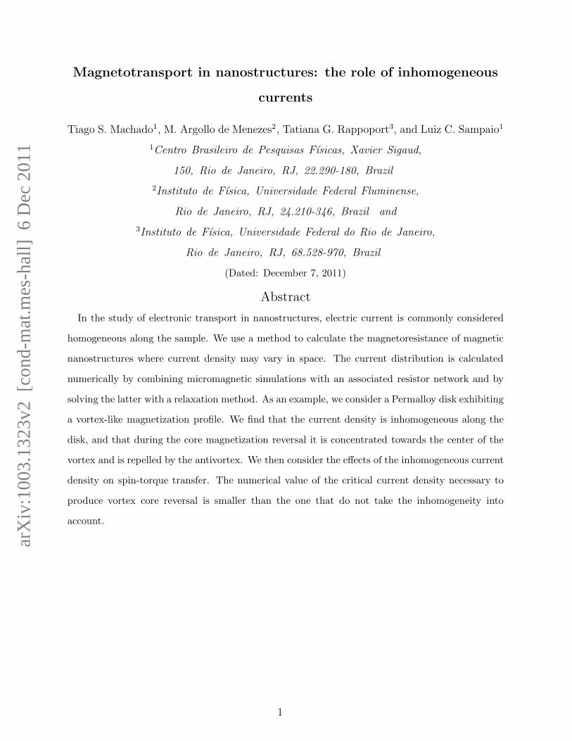
By varying the external in-plane magnetic field H from negative to positive saturation
we obtain a hysteresis curve, as depicted in Fig. 1, which is consistent with experimental
observations [7]. As shown in Fig. 1(a), in static equilibrium and in the absence of magnetic
fields, a vortex structure with a core magnetized perpendicular to the disk plane is formed in
the center of the disk. If a small in-plane magnetic field H is applied, the core is displaced
3
FIG. 1: Magnetic hysteresis obtained with micromagnetics simulation of a Py disk with a diameter
of 300 nm and thickness of 36 nm subject to a static, in-plane magnetic field H. Two configurations
for the vortex core, corresponding to different external fields (0 and 75 mT), are also depicted.
from the center (Fig. 1(b)). At a critical field Hc1 the vortex is expelled from the disk,
resulting in a discontinuity in the hysteresis loop. As the external field H is lowered back,
the vortex structure reappears, but at a lower field Hc2 < Hc1.
In order to investigate the electronic transport on the nanomagnetic disk we consider the
magnetization profile ~Mi, obtained as the stationary solution of the LLG equation, as a
starting point to calculate the magnetoresistance Ri in each cell i of the disk. It is well
established that in relatively clean magnetic metals the main source of magnetoresistance is
the anisotropic magnetoresistance (AMR) [22], which can be expressed as ρ = ρ⊥ + (ρ‖ −
ρ⊥)cos2 φ, where φ is the angle between the local magnetization and the electric current
and ρ⊥ and ρ‖ are the resistivities when the magnetization is perpendicular and parallel
to the current, respectively. We decompose the current into orthogonal components x and
y such that if the normalized projection of the magnetization ~Mi on the current direction
u (u = x, y) is mui = cosφ, and the cell geometrical factor is taken into account, the
magnetoresistance Ri is split into orthogonal components as Rui = R⊥
i + (R‖i −R⊥
i )(mui )
2 in
every cell i of the disk (Fig. 2). Thus, we obtain a resistor network where the resistances
depend on the local magnetization and are assumed to be approximately constant at the
4
time scale of electronic scattering processes.
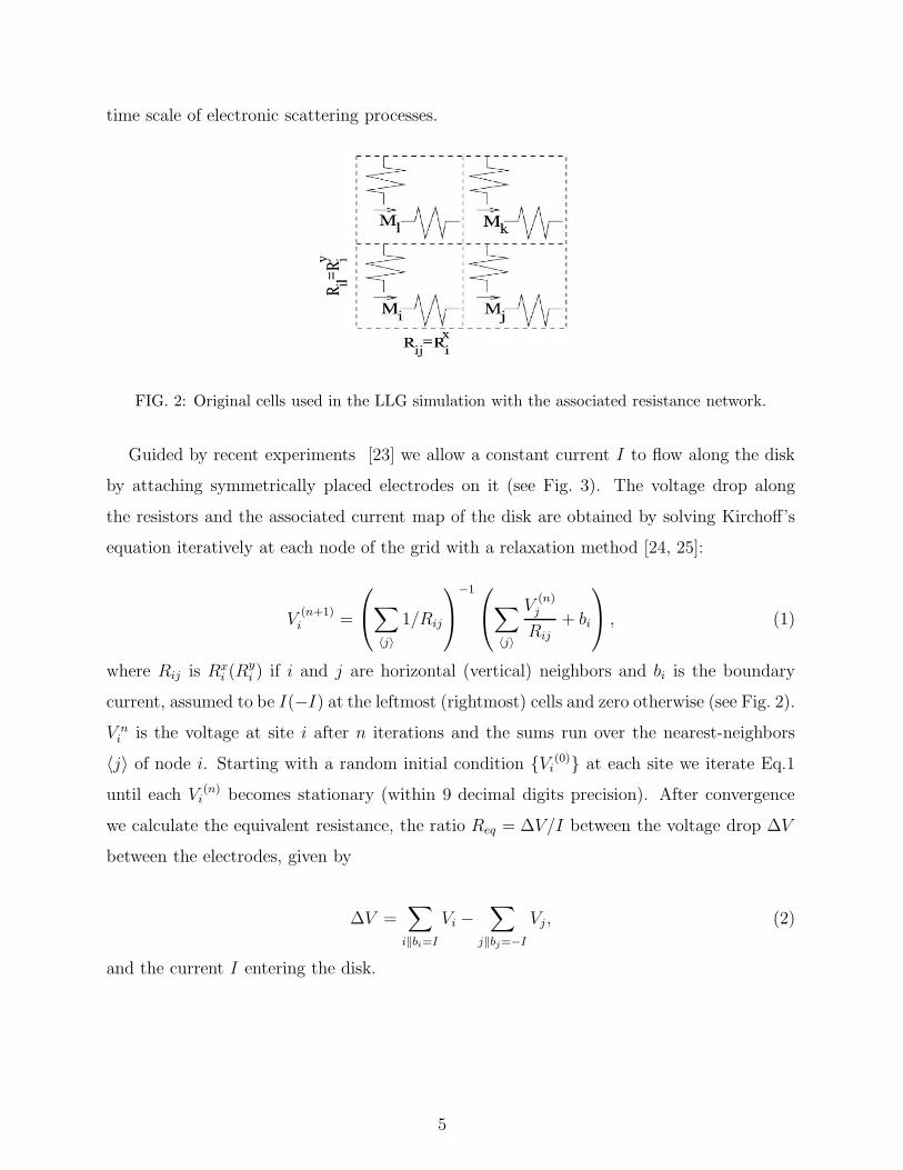
FIG. 2: Original cells used in the LLG simulation with the associated resistance network.
Guided by recent experiments [23] we allow a constant current I to flow along the disk
by attaching symmetrically placed electrodes on it (see Fig. 3). The voltage drop along
the resistors and the associated current map of the disk are obtained by solving Kirchoff’s
equation iteratively at each node of the grid with a relaxation method [24, 25]:
V(n+1)i =
∑
〈j〉
1/Rij
−1
∑
〈j〉
V(n)j
Rij
+ bi
, (1)
where Rij is Rxi (R
yi ) if i and j are horizontal (vertical) neighbors and bi is the boundary
current, assumed to be I(−I) at the leftmost (rightmost) cells and zero otherwise (see Fig. 2).
V ni is the voltage at site i after n iterations and the sums run over the nearest-neighbors
〈j〉 of node i. Starting with a random initial condition Vi(0) at each site we iterate Eq.1
until each Vi(n) becomes stationary (within 9 decimal digits precision). After convergence
we calculate the equivalent resistance, the ratio Req = ∆V/I between the voltage drop ∆V
between the electrodes, given by
∆V =∑
i‖bi=I
Vi −∑
j‖bj=−I
Vj , (2)
and the current I entering the disk.
5
III. MAGNETO-STRUCTURE AND MAGNETORESISTANCE
A. Hysteresis and magnetoresistance
In order to obtain the magnetoresistance curves, the calculation discussed in the previous
section is performed at different fields. Magnetoresistance and current distribution for the
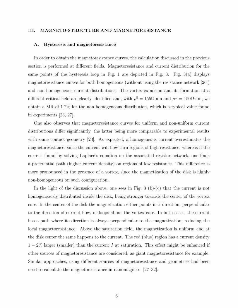
same points of the hysteresis loop in Fig. 1 are depicted in Fig. 3. Fig. 3(a) displays
magnetoresistance curves for both homogeneous (without using the resistance network [26])
and non-homogeneous current distributions. The vortex expulsion and its formation at a
different critical field are clearly identified and, with ρ‖ = 155Ω·nm and ρ⊥ = 150Ω·nm, we
obtain a MR of 1.2% for the non-homogeneous distribution, which is a typical value found
in experiments [23, 27].
One also observes that magnetoresistance curves for uniform and non-uniform current
distributions differ significantly, the latter being more comparable to experimental results
with same contact geometry [23]. As expected, a homogeneous current overestimates the
magnetoresistance, since the current will flow thru regions of high resistance, whereas if the
current found by solving Laplace’s equation on the associated resistor network, one finds
a preferential path (higher current density) on regions of low resistance. This difference is
more pronounced in the presence of a vortex, since the magnetization of the disk is highly
non-homogeneous on such configuration.
In the light of the discussion above, one sees in Fig. 3 (b)-(c) that the current is not
homogeneously distributed inside the disk, being stronger towards the center of the vortex
core. In the center of the disk the magnetization either points in z direction, perpendicular
to the direction of current flow, or loops about the vortex core. In both cases, the current
has a path where its direction is always perpendicular to the magnetization, reducing the
local magnetoresistance. Above the saturation field, the magnetization is uniform and at
the disk center the same happens to the current. The red (blue) region has a current density
1 − 2% larger (smaller) than the current I at saturation. This effect might be enhanced if
other sources of magnetoresistance are considered, as giant magnetoresistance for example.
Similar approaches, using different sources of magnetoresistance and geometries had been
used to calculate the magnetoresistance in nanomagnets [27–32].
6
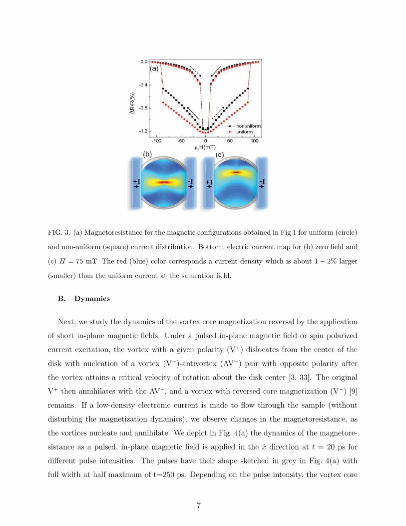
FIG. 3: (a) Magnetoresistance for the magnetic configurations obtained in Fig 1 for uniform (circle)
and non-uniform (square) current distribution. Bottom: electric current map for (b) zero field and
(c) H = 75 mT. The red (blue) color corresponds a current density which is about 1 − 2% larger
(smaller) than the uniform current at the saturation field.
B. Dynamics
Next, we study the dynamics of the vortex core magnetization reversal by the application
of short in-plane magnetic fields. Under a pulsed in-plane magnetic field or spin polarized
current excitation, the vortex with a given polarity (V+) dislocates from the center of the
disk with nucleation of a vortex (V−)-antivortex (AV−) pair with opposite polarity after
the vortex attains a critical velocity of rotation about the disk center [3, 33]. The original
V+ then annihilates with the AV−, and a vortex with reversed core magnetization (V−) [9]
remains. If a low-density electronic current is made to flow through the sample (without
disturbing the magnetization dynamics), we observe changes in the magnetoresistance, as
the vortices nucleate and annihilate. We depict in Fig. 4(a) the dynamics of the magnetore-
sistance as a pulsed, in-plane magnetic field is applied in the x direction at t = 20 ps for
different pulse intensities. The pulses have their shape sketched in grey in Fig. 4(a) with
full width at half maximum of t=250 ps. Depending on the pulse intensity, the vortex core
7
magnetization does not reverse at all (µ0H < 43 mT), reverses once (54 mT< µ0H < 64
mT) or multiple times (µ0H > 64 mT) [12, 13].
FIG. 4: (a) Evolution of magnetoresistance after the application of pulsed, in-plane magnetic
fields (the shape is shown in grey) with different intensities. Snapshots of magnetization (arrows)
and current distribution (color map) for pulse fields without (b) and with (c)-(e) vortex core
magnetization reversal. The white cross shows the position of the disk center. Both current and
magnetic field are applied in the x direction
During the application of a field pulse in the x direction, i.e., parallel to the current
flow, the vortex core is pushed to the y direction breaking the rotation symmetry of the
disk’s magnetization, increasing both the total mx component and the disk’s equivalent
resistance (see Fig. 4(a)). At t = 340 ps the field is practically zero and, from the decay of
magnetoresistance to its equilibrium (initial) value, one can infer whether there was reversal
of the vortex core polarization or not: for pulses that induce reversal, the value of the
magnetoresistance just after the pulse is always larger than its initial value. If there is no
reversal the magnetoresistance attains a minimum value that is lower than its initial value,
i.e., before the application of the pulse, and oscillates about it.
8
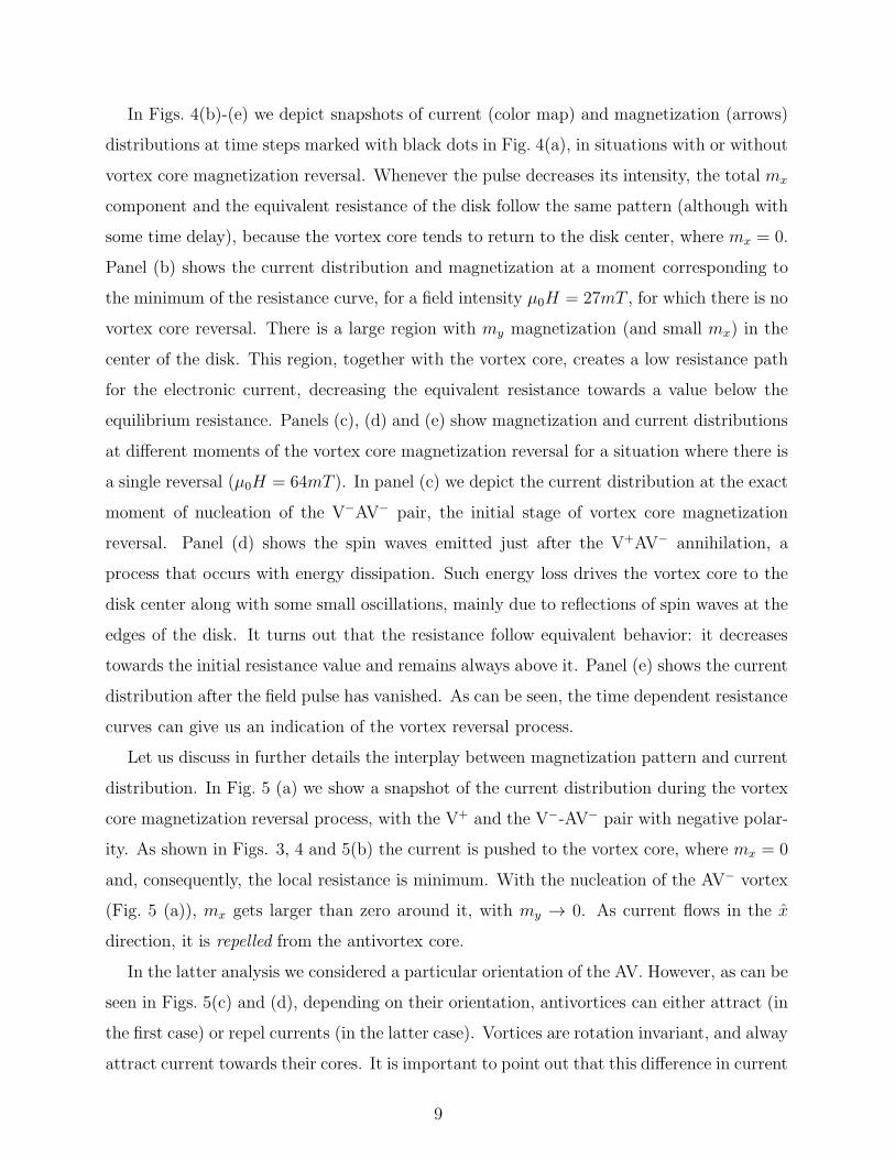
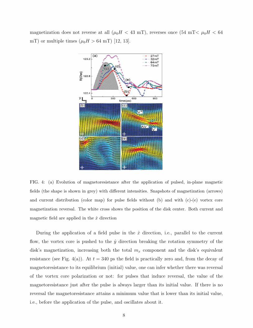
In Figs. 4(b)-(e) we depict snapshots of current (color map) and magnetization (arrows)
distributions at time steps marked with black dots in Fig. 4(a), in situations with or without
vortex core magnetization reversal. Whenever the pulse decreases its intensity, the total mx
component and the equivalent resistance of the disk follow the same pattern (although with
some time delay), because the vortex core tends to return to the disk center, where mx = 0.
Panel (b) shows the current distribution and magnetization at a moment corresponding to
the minimum of the resistance curve, for a field intensity µ0H = 27mT , for which there is no
vortex core reversal. There is a large region with my magnetization (and small mx) in the
center of the disk. This region, together with the vortex core, creates a low resistance path
for the electronic current, decreasing the equivalent resistance towards a value below the
equilibrium resistance. Panels (c), (d) and (e) show magnetization and current distributions
at different moments of the vortex core magnetization reversal for a situation where there is
a single reversal (µ0H = 64mT ). In panel (c) we depict the current distribution at the exact
moment of nucleation of the V−AV− pair, the initial stage of vortex core magnetization
reversal. Panel (d) shows the spin waves emitted just after the V+AV− annihilation, a
process that occurs with energy dissipation. Such energy loss drives the vortex core to the
disk center along with some small oscillations, mainly due to reflections of spin waves at the
edges of the disk. It turns out that the resistance follow equivalent behavior: it decreases
towards the initial resistance value and remains always above it. Panel (e) shows the current
distribution after the field pulse has vanished. As can be seen, the time dependent resistance
curves can give us an indication of the vortex reversal process.
Let us discuss in further details the interplay between magnetization pattern and current
distribution. In Fig. 5 (a) we show a snapshot of the current distribution during the vortex
core magnetization reversal process, with the V+ and the V−-AV− pair with negative polar-
ity. As shown in Figs. 3, 4 and 5(b) the current is pushed to the vortex core, where mx = 0
and, consequently, the local resistance is minimum. With the nucleation of the AV− vortex
(Fig. 5 (a)), mx gets larger than zero around it, with my → 0. As current flows in the x
direction, it is repelled from the antivortex core.
In the latter analysis we considered a particular orientation of the AV. However, as can be
seen in Figs. 5(c) and (d), depending on their orientation, antivortices can either attract (in
the first case) or repel currents (in the latter case). Vortices are rotation invariant, and alway
attract current towards their cores. It is important to point out that this difference in current
9
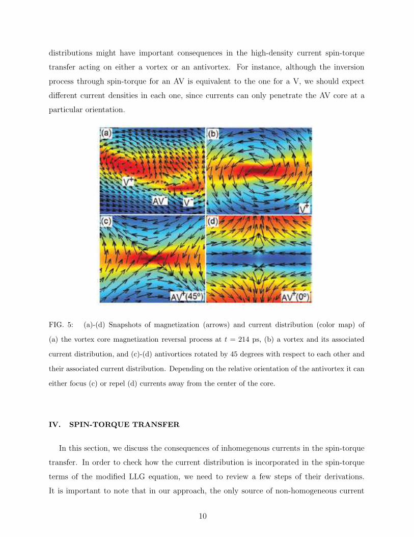
distributions might have important consequences in the high-density current spin-torque
transfer acting on either a vortex or an antivortex. For instance, although the inversion
process through spin-torque for an AV is equivalent to the one for a V, we should expect
different current densities in each one, since currents can only penetrate the AV core at a
particular orientation.
FIG. 5: (a)-(d) Snapshots of magnetization (arrows) and current distribution (color map) of
(a) the vortex core magnetization reversal process at t = 214 ps, (b) a vortex and its associated
current distribution, and (c)-(d) antivortices rotated by 45 degrees with respect to each other and
their associated current distribution. Depending on the relative orientation of the antivortex it can
either focus (c) or repel (d) currents away from the center of the core.
IV. SPIN-TORQUE TRANSFER
In this section, we discuss the consequences of inhomegenous currents in the spin-torque
transfer. In order to check how the current distribution is incorporated in the spin-torque
terms of the modified LLG equation, we need to review a few steps of their derivations.
It is important to note that in our approach, the only source of non-homogeneous current
10
distribution is the anisotropic magnetoresistance, as discussed in section II. All other effects
are neglected.
The itinerant electrons spin operator satisfies the continuity equation
d
dt〈s〉+∇ · 〈J〉 = −
i
~(〈[s, H ]〉) (3)
where J is the spin current operator. The Hamiltonian H is the s-d Hamiltonian (Hsd =
−Jexs · S), where s and S/S = −M/Ms are the spins of itinerant and localized electrons,
and Jex is the exchange coupling strength between them. We define spin current density
J = 〈J〉 = −(gµBP/eMs)je(r) ⊗ M), where je(r) is the current density, and the electron
spin density is given by m = 〈s〉[14]. We use the same approximations, previously used
to calculate the spin-torque [14, 15], with the new ingredient of non-homogeneous current
density. We obtaind
dtm =
µbP
eMs
[M(∇ · je(r)) + (je(r) · ∇)M]
−JexS
Ms
m×M,(4)
where, M is the matrix magnetization, g is the Lande factor splitting, µB is the Bohr
magneton, P is the spin current polarization of the ferromagnet, e is the electron charge.
From the continuity equation for charges, the term containing ∇ · je(r) is always zero, even
if the current density is not constant. As discussed previously, the same divergent is used
to determine the current distribution in section II. This expression is exactly the same
expression obtained previously but with je(r) in the second term of the right side of the
equation varying with r. This current distribution is introduced at the modified LLG that
considers spin-torque transfer. Therefore, we obtain a spin-torque transfer where the current
distribution is not uniform.
To consider spin-torque transfer effects we include adiabatic and non-adiabatic spin torque
terms in the LLG equation,
d
dtm = −γ0m×Heff + αm×
d
dtm
−(u · ∇)m+ βm× [(u · ∇)m],(5)
where, m=M/Ms is the normalized local magnetization, α is a phenomenological damping
constant, γ0 is the gyroscopic ratio, Heff is the effective field, which is composed of the
applied external field, the demagnetization field, the anisotropy field and the exchange field.
The first term describes the precession of the normalized local magnetization about the
11
efective field. The second term describes the relaxation of the normalized local magnetization
and β is a dimensionless parameter that describes the strength of the non-adiabatic term,
which we consider to be 0.5 [15, 16]. The velocity u(r)=(gPµB/2eMs)je(r) is a vector
pointing parallel to the direction of electron flow and je(r) is calculated using the procedure
discussed in section II.
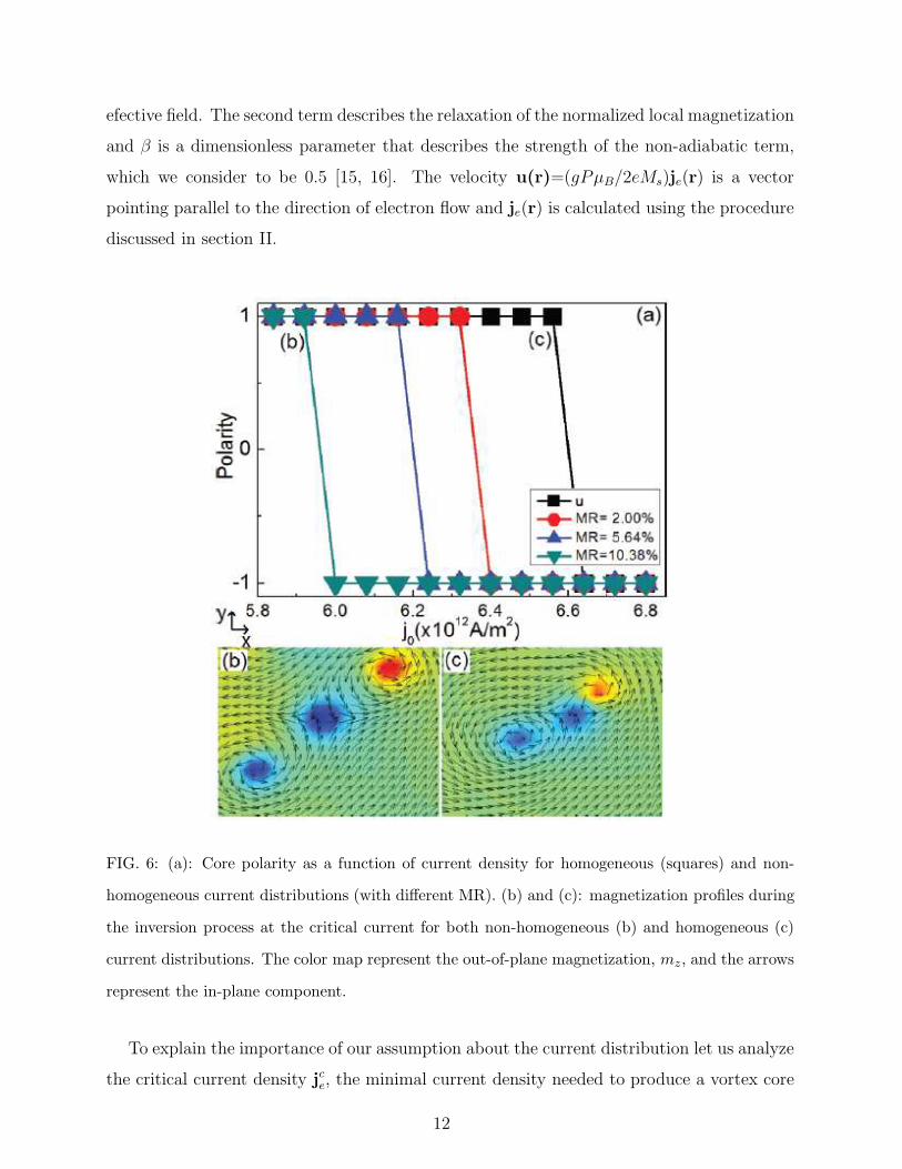
FIG. 6: (a): Core polarity as a function of current density for homogeneous (squares) and non-
homogeneous current distributions (with different MR). (b) and (c): magnetization profiles during
the inversion process at the critical current for both non-homogeneous (b) and homogeneous (c)
current distributions. The color map represent the out-of-plane magnetization, mz, and the arrows
represent the in-plane component.
To explain the importance of our assumption about the current distribution let us analyze
the critical current density jce, the minimal current density needed to produce a vortex core
12
reversal. For this purpose, we simulated the magnetization dynamics of a system subjected
to a DC current with the modified LLG equation (equation 5). In Fig. 6(a) one sees
the vortex core polarity as a function of current density je. The different curves represent
situations of homogeneous current (squares) and of three different values of AMR where
the magnetoresistance ranges from 2% to 10%. Such AMR, as discussed in the previous
sections, shape the degree of current inhomogeneity throughout the disk. One can see that
the critical current density jce in our model is 3 − 10% smaller than the one obtained for
uniform currents. These results suggest a new route, together with the non-adiabatic term,
to explain the discrepancy between experimental results and theoretical calculations of the
critical current density jce.
Our analysis might also have important technological implications, since we observe a
(almost linear) correlation between the current density necessary to produce a core inversion
and the anisotropic magnetoresistance of the material. Thus, by increasing the AMR of the
sample, one can decrease the critical current jce, which is strongly desirable in memory devices
for the sake of low energy comsumption and minimal heat waste.
Panels (b) and (c) of Fig. 6 show the magnetic configurations for the moment just
before the V+-AV− annihilation, at the critical current density, for the model with non-
homogeneous and homogeneous current distributions, respectively. In the case of inhomege-
neous currents, the fact that a V(AV) attracts (repels) the current affects the velocity and
separation distance of the V-AV pair during the vortex core reversal. As antivortices repel
currents, the current density at their core is smaller, making them slower than vortices.
As a result, after the nucleation of the V−-AV− pair their separation occurs faster than in
the case where the current density in the center of a V or an AV is the same, as usually
considered in micromagnetic simulations.
V. CONCLUSIONS
We performed a realistic calculation of magnetoresistance effects in magnetic nanostruc-
tures subject that takes into account inhomogeneous current densities. For that purpose,
we adapted a numerical relaxation scheme for the Laplace equation to the solution of the
LLG equation for the magnetization profile along a Permalloy disk. Our results suggest
that resistance measurements might be useful to probe the dynamics of vortex core mag-
13
netization reversal, induced by short in-plane magnetic pulses. Moreover, we note that the
difference between current distributions close to vortices and anti-vortices have significant
consequences for the spin-torque transfer effect. The inhomogeneous current distribution
inside the magnet reduces substantially the critical current density necessary to produce a
vortex core reversal. We conclude that materials with large anisotropic magnetoresistance
need lower current densities to modify their magnetic structure, a much deasireable feature
for most modern memory devices.
Acknowledgements
This work was supported by CNPq and FAPERJ. LCS and TGR acknowledge the “INCT
de Fotonica” and “INCT de Informacao Quantica”, respectively, for financial support.
[1] J. C. Slonczewski, J. Magn. Magn. Mater. 159, L1 (1996); L. Berger, Phys. Rev. B 54, 9353
(1996).
[2] D. C. Ralph, M. D. Stiles, J. Magn. Magn. Mater 320(7), 1190 (2008).
[3] K. Yamada, S. Kasai, Y. Nakatani, K. Kobayashi, H. Kohno, A. Thiaville, T. Ono, Teruo,
Nat. Mater. 6, 269 (2007).
[4] I. N. Krivorotov, N. C. Emley, J. C. Sankey, S. I. Kiselev, D. C. Ralph, R. A. Buhrman,
Science 307,215 (2005).
[5] S. Choi, K. -S. Lee and S. -K. Kim, Appl. Phys. Lett. 89, 062501 (2006).
[6] T. Shinjo, T. Okuno, R. Hassdorf, K. Shigeto, and T. Ono, Science 289, 930 (2000).
[7] R. P. Cowburn, D. K. Koltsov, A. O. Adeyeye, M. E. Welland, and D. M. Tricker, Phys. Rev.
Lett. 83, 1042 (1999).
[8] M. Weigand, B. Van Waeyenberge, A. Vansteenkiste, M. Curcic, V. Sackmann, H. Stoll, T.
Tyliszczak, K. Kaznatcheev, D. Bertwistle, G. Woltersdorf, C. H. Back, and G. Schutz, Phys.
Rev. Lett. 102, 077201 (2009).
[9] A. Vansteenkiste, K. W. Chou, M. Weigand, M. Curcic, V. Sackmann, H. Stoll, T. Tyliszczak,
G. Woltersdorf, C. H. Back, G. Schtz, and B. Van Waeyenberge, Nature 5, 332 (2009).
[10] B. Van Waeyenberger, A. Puzic, H. Stoll, K. W. Chou, T. Tyliszczak, R. Hertel, M. Fahnle,
14
H. Bruckl, K. Rott, G. Reiss, I. Neudecker, D. Weiss, C. H. Back, and G. Schutz, Nature 444,
461 (2006).
[11] R. Hertel, S. Gliga, M. Fahnle, and C. M. Schneider, Phys. Rev. Lett. 98, 117201 (2007).
[12] S. K. Kim, K. S. Lee, Y. S. Yu, and Y. S. Choi, Appl. Phys. Lett. 92, 022509 (2008); K. S.
Lee, K. Y. Guslienko, J. Y. Lee, and S. K. Kim, Phys. Rev. B 76, 174410 (2007).
[13] T. S. Machado, T. G. Rappoport, and L. C. Sampaio, Appl. Phys. Lett. 93, 112507 (2008).
[14] S. Zhang, and Z. Li, Phys. Rev. Lett. 93, 127204 (2004).
[15] A. Thiaville, Y. Nakatani, J. Miltat, and Y. Suzuki, Europhys. Lett. 69, 990 (2005)
[16] L. Heyne, J. Rhensius, D. Ilgaz, A. Bisig, U. Rudiger, M. Klaui, L. Joly, F. Nolting, L. J.
Heyderman, J. U. Thiele, and, F. Kronast, Phys. Rev. Lett. 105, 187203 (2010).
[17] K. Yamada, S. Kasai, Y. Nakatani, K. Kobayashi, and T. Ono, Appl. Phys. Lett. 93,152502
(2008).
[18] K. Yamada, S. Kasai, Y. Nakatani, K. Kobayashi, and T. Ono, Appl. Phys. Lett. 96, 192508
(2010).
[19] G. S. D. Beach, M. Tsoi and J.L. Erskine, J. Magn. Magn. Mater. 320 1272 (2008).
[20] T.L. Gilbert, Physical Review, 100 1243 (1955).
[21] W.H. Press, B.P. Flannery, B.P. Teukolsky, S.A. Vetterling and T. William, Numerical Recipes
in C: The Art of Scientific Computing(Cambridge University Press, 1992).
[22] R. C. O’Handley, Modern Magnetic Materials (Wiley-Interscience, New York, 1999), Chap.
15.
[23] S. Kasai, Y. Nakatani, K. Kobayashi, H. Kohno, and T. Ono, Phys. Rev. Lett. 97, 107204
(2006).
[24] R. Courant, K. Friedrichs, and H. Lewy, Phys. Math. Ann. 100, 32 (1928).
[25] H. Gould and J. Tobochnik, An Introduction to Computer Simulation Methods (Addison-
Wesley, 1996), Chap. 10.
[26] R. A. Silva, T. S. Machado, G. Cernicchiaro, A. P. Guimaraes, and L. C. Sampaio, Phys. Rev.
B, 79, 134434 (2009).
[27] P. Vavassori, M. Grimsditch, V. Metlushko, N. Zaluzec, and B. Ilic, Appl. Phys. Lett. 87,
072507 (2005).
[28] H. Li, Y. Jiang, Y. Kawazoe, and R. Tao, Phys. Lett. A 298, 410-415 (2002).
[29] M. Bolte, M. Steiner, C. Pels, M. Barthelmess, J. Kruse, U. Merkt, G. Meier, M. Holz, and
15
D. Pfannkuche, Phys. Rev. B 72, 224436 (2005).
[30] M. Holz, O. Kronenwerth, and D. Grundler, Phys. Rev. B 67, 195312 (2003).
[31] Jun-ichiro Ohe, S. E. Barnes, Hyun-Woo Lee, and S. Maekawai, Appl. Phys. Lett. 95, 123110
(2009)
[32] L. K. Bogart and D. Atkinson, Appl. Phys. Lett. 94, 042511 (2009)
[33] K. Y. Guslienko, K. S. Lee, and S. K. Kim, Phys. Rev. Lett. 100, 027203 (2008).
16


