Embed Size (px)
Citation preview
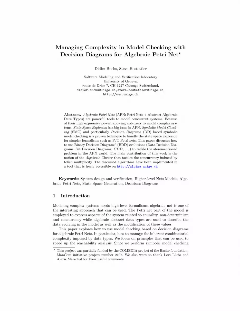
Managing Complexity in Model Checking withDecision Diagrams for Algebraic Petri Net?
Didier Buchs, Steve Hostettler
Software Modeling and Verification laboratoryUniversity of Geneva,
route de Drize 7, CH-1227 Carouge Switzerland,[email protected],[email protected],
http://smv.unige.ch
Abstract. Algebraic Petri Nets (APN: Petri Nets + Abstract AlgebraicData Types) are powerful tools to model concurrent systems. Becauseof their high expressive power, allowing end-users to model complex sys-tems, State Space Explosion is a big issue in APN. Symbolic Model Check-ing (SMC) and particularly Decision Diagrams (DD) based symbolicmodel checking is a proven technique to handle the state space explosionfor simpler formalisms such as P/T Petri nets. This paper discusses howto use Binary Decision Diagrams’ (BDD) evolutions (Data Decision Dia-grams, Set Decision Diagrams, ΣDD, . . . ) to tackle the aforementionedproblem in the APN world. The main contribution of this work is thenotion of the Algebraic Cluster that tackles the concurrency induced bytoken multiplicity. The discussed algorithms have been implemented ina tool that is freely accessible on http://alpina.unige.ch.
Keywords: System design and verification, Higher-level Nets Models, Alge-braic Petri Nets, State Space Generation, Decisions Diagrams
1 Introduction
Modeling complex systems needs high-level formalisms, algebraic net is one ofthe interesting approach that can be used. The Petri net part of the model isemployed to express aspects of the system related to causality, non-determinismand concurrency while algebraic abstract data types are used to describe thedata evolving in the model as well as the modification of these values.
This paper explores how to use model checking based on decision diagramsfor algebraic Petri Nets. In particular, how to manage the inherent combinatorialcomplexity imposed by data types. We focus on principles that can be used tospeed up the reachability analysis. Since we perform symbolic model checking? This project was partially funded by the COMEDIA project of the Hasler foundation,
ManCom initiative project number 2107. We also want to thank Levi Lucio andAlexis Marechal for their useful comments.

and not bounded model checking, we expect the state space to be finite. Theseconcepts can also be applied to more elaborated model checkers such as CTLmodel checkers.
We do not explain here the internal machinery (for more details see [?]) ofthe model checker but we rather focus on its usage. In particular, checking alge-braic nets using symbolic representation based on decision diagrams requires anadditional level of symbolism with respect to P /T Petri nets model checking.This additional layer, called algebraic clusters, is the main contribution of thispaper. Algebraic clusters are clusters [?,?] that are indexed by an algebraic do-main. The advantage of such an approach is that it enables discovery of localitiesof computation and the ability to apply saturation principles. Localities are nolonger only defined based on net structure but also on the algebraic values.
Besides, partial or total unfolding greatly speeds up the exploration of thestate space and saves memory. By unfolding we mean finding all possible values ofa user-defined algebra (if finite) and build specialised operations to handle theminstead of heavy general operations that can handle any value. This last aspectwill not be detailed in this article however interested readers can find moreinformation in [?]. Throughout this paper we mainly explore how the correctuse of algebraic clusters can dramatically improve the construction of the statespace both in terms of memory consumption and processing time. Comparisonto existing approach can be made on two levels:
– Comparable high-level Petri nets analyzers such as Maria[?] and Helena[?]are completely outperformed if clusters can be mapped on significantly in-dependent part of computation (see section 8).
– Decision diagrams on P/T nets with unfolding [?,?] and our approach arelinear in term of performance. However with a significant advantage on ourside for the modeling aspect as well as a clear separation of the heuristics(clustering and unfolding) necessary for doing efficient model checking.
These principles are illustrated in our tool called AlPiNA (Algebraic PetriNet Analyzer). 1
This paper is organized as follows: first we introduce algebraic abstract datatypes and algebraic Petri nets, then we give an example of an algebraic Petrinet that is sufficiently complex to introduce our approach. The fourth sectionshows, using said example, the kind of properties we can check. Section 5 givesan overview of the operational aspects of model checking while the sixth sectionpresents an abstract definition of the decision diagrams as well as the encodingof basic elements and operational principles. The seventh section introduces theidea behind clustering and how algebraic clustering works. Finally, section 8 de-scribes how clusters are applied to the example and some significant benchmarksdemonstrates the approach.
1 The engine is already available, a GUI will be released within a few months.

2 Short Introduction to Algebraic Nets
Algebraic nets [?] are an evolution of P/T Petri nets where tokens belong todomains defined by algebraic specifications. Although not very different fromother extensions of Petri nets such as Coloured Petri Nets [?], APN have severalsignificant advantages:
– The possibility to define any data structures that have first order axiomati-sations (it is the case for usual structures that we find in classical modelingor programming languages: integer, lists, sets,... but not reals for example);
– An abstract level of axiomatization combined with concrete operational tech-niques based on rewriting;
– A formal notation allowing reasoning about data types and their usage. Itcan be particularly useful to automatically perform proofs.
An APN definition is split into two parts: a Petri Net with places holding typedtokens; and a set of ADT (Abstract Algebraic Data Types) representing data.
2.1 Algebraic Abstract Data Type
Algebraic Abstract Data Types (AADT or ADT for simplicity) [?] provide amathematical way to define properties of data types. ADT modules define datatypes by means of algebraic specifications. Each module describes one or moresorts, along with generators and operations on these sorts. The properties of theoperations are given in the axiom section of the modules, by means of positiveconditional equational axioms.
An algebraic abstract data type is then composed of a signature Σ = 〈S,OP 〉where S is the set of sorts and OP the set of operations with their arity. Ingeneral, there are two types of ADTs:
– Primitive data ADTs: boolean, natural, and integer are simple data types.– Container ADTs: set, list, pair, bag, etc. They represent structured data and
allow to construct complex data types and operations. The contained typescan be data ADTs or container ADTs.
Moreover, through equations (Ax) based on terms, defined by the signature(TΣ) and variables (X) to form the term with variables (TΣ,X), the properties aredefined. A specification is given by Spec = 〈Σ,Ax,X〉. There are no predefineddata types in ADT and all used types should be defined by ADT modules. Nev-ertheless, we provide a library of ADTs as part of COOPNBuilder[?]/AlPiNa[?]framework which includes the most commonly used data types: boolean, natu-ral, string, pair, list, etc. These types are fully axiomatized; this allows inferringproperties of models for verification purposes.
A calculus is defined through rewriting techniques [?,?], Rew : TΣ → TΣ ,which provides a normal form for any terms. This procedure can be used fordeciding equalities between terms (the eval function evaluates terms into theirsemantic domains) i.e ∀t, t′ ∈ TΣ , Rew(t) = Rew(t′)⇒ eval(t) = eval(t′). In therest of the paper, we only use term rewriting as semantics of ADT.

It must be noted that while the notation where kept as minimal as possiblewe support a rather powerful and useful algebraic extension of ADT, the ordersorted algebraic specification [?]. A Complete description of the support of ordersorting in our approach can be found in [?].
2.2 APN
Components are described by modular Algebraic Petri Nets which are definedby so-called behavioural axioms, similar to the axioms of an ADT.
An APN spec is noted Apn-spec = 〈Spec, P, T,Beh,X,m0〉 where Spec is thealgebraic specification, P the set of places (with τ : P → S a typing function),T the transitions, Beh the set of behavioural axioms (detailed below) and Xsome variables and , m0 the initial marking. The (behavioural) axioms have thefollowing structure:
Cond⇒ event :: pre→ post
In which each one of the terms has the following meaning: 2
– Cond is a set of equational conditions, similar to a guard. The ` relationdecides based on rewriting if a closed condition is satisfied;
– event ∈ T is the name of a transition;– pre and post are typical Petri net flow relations (indexed by P ) determining
what is consumed and what is produced in the net’s places.– pre and post are built on multiset of terms. Multisets are built with +
(union), - (difference) and singleton [a] operators.
For instance, the multiset with two numbers 1 and 2 using the natural numberADT described Fig. 2 is written [s(0)] + [s(s(0))] or simply [s(0), s(s(0))].
2.3 Semantics of APN
Knowing the semantics of an ADT, we can build the semantics of an APN. Thesemantics of an APN is given by a transition system where labels represent whatis visible from outside i.e. the events. The states (also called the markings) arerepresented by a set of multisets of tokens, indexed by the places, expressed byalgebraic terms of the ADTs.
Let M be the set of markings such that M is a P indexed family of T[Σ],[τ(p)].The [s] extension mean the addition of sort multiset and associated operationsfor each sort of the ADT[?]. This is made with empty set ε and operationssuch as marking union (+), marking difference (-) and comparisons ⊆. Markingsare vector extensions of the similar operation on multisets for describing themarkings.
2 In our tool only input arcs that are labeled by closed term or isolated variables areallowed in pre. Putting a variable in the input arc plus a condition in the guardsimulates composed terms.

Given an axiom Cond ⇒ event :: pre → post and m,m′ ∈ M the markings,event ∈ T , the transitions induced by that behavioural property is:∀σ3, if ` Condσ, Rew(preσ) ⊆ m,m event−−−→ m−Rew(preσ) +Rew(postσ) 4
The resulting construction is the transition system built from the initialmarking by applying this firing rule until reaching a fix point TSapn(m0). Fromthe transition system, we can also consider the reachability set Reachapn(m0).
3 Modeling with apn
The model (Fig. 1) used in the rest of the paper is the distributed database man-ager used by many authors, originally presented by Genrich and Lautenbach in[?], working on Petri net and associated models. This model raises interestingproblems concerning domains. For instance, the number of database is finite(type Databases) while the number of acknowledgments is modeled with naturalnumbers. Limited domains will be enumerated (we say here unfolded) before thestate space computations while the domain of naturals will be explored duringthe state space exploration. We call this combination “partial unfolding”. Alter-natively, the graphical syntax can be replaced by the previous textual syntax.For instance, the “Receive Msg” transition is modeled by the following axiom:db1 = db2⇒ Receive Msg :: 〈([db1])Pending, ([db2])Inactive〉 → 〈([db1])Syncing〉
Inactive[db0, db1,
db2]<db>
Receive MsgUpdate &Send Msg
[db1] [db2]
Mutex[@]
<blacktoken>
Waiting
<db>
[db1]
Pending
< db >
[db1]
Syncing
<db>
Send AckFinishUp
[db1][db1][db1][db1] [@]
acks
[0]
<nat>
count[3]
<natural>prepare
[n]
[dec(n)][processOf(n)]
[@]
[3]
inc(n)
[n]
[2]
[0]
[db1]
[db1]
n > 0
db1 = db2[0]
[db1]
[db1]
Where : db1, db2 : db; n : nat:
Fig. 1. Distributed database Algebraic Petri Net model
3 σ is a term substitution. tσ stands for applying the substition σ to the term t ∈ TΣ,X4 Rew is the evaluation morphism extended to APN structures such as multiset and
vector of places from the algebraic morphism Rew.

In Fig. 2, one can find a simplified version of the ADTs that describe thedata part of the model. Only the operations and axioms that are required for theproblem are written. The algebra of the booleans is composed of true and falsewithout any operation. The natural numbers are described using Peano arith-metic and finally the databases are represented by a structure that is isomorphicto the natural numbers modulo 3.
ADT BooleansSort boolGenerators
true : bool;false : bool;
End Booleans
ADT DatabasesSort dbUse natGenerators
db0 : db;d : db -> db;
OperationsprocessOf : nat -> db;
Axiomsd(d(d(db0))) = db0;processOf(s(x)) = d(processOf(x));
Wherex:nat;
End Databases
ADT NaturalsSort natUse boolGenerators
0 : nat;s : nat -> nat;
Operationsdec : nat -> nat;inc : nat -> nat;> : nat ,nat -> bool;2 : nat;3 : nat;
Axiomsinc(x) = s(x);dec(s(x)) = x;dec(0) = 0;>(s(x), s(y)) = >(x, y);>(s(x), 0) = true;>(0, s(x)) = false;>(0,0) = false;2 = s(s(0));3 = s(s(s(0)));
Wherex,y:nat;
End Naturals
Fig. 2. ADT of the Distributed Databases Protocol
4 The purpose of symbolic model checking
In order to check properties, a dedicated language is offered which check mainlyin CTL temporal logic setting the formula of the shape: AG(atmΣ,P ) i.e. de-termines for a given property at ∈ atmΣ,P if Reachapn(m0) |= AG(at), whereatmΣ,P is an atomic formulae based on signature and place definitions, opera-tion on sets and algebraic conditions. We currently do not support other CTLoperators such as (F , U , ...) as they require the predecessor relation (pre) asdefined in [?]. This restricts the checks to those can be verified by reachabilityanalysis. In our model checker, we gave some possibilities to check more detailedproperties at the atomic proposition level, such as inclusion or exclusion of par-ticular tokens or sets of tokens. The following properties can be checked on themodel of Fig. 1:
– A process is either idle, waiting for other processes to sync or syncing:AG(inactive∩syncing = ∅∧syncing∩waiting = ∅∧waiting∩inactive = ∅)
– At most one database process is the master process: AG(card(wating) ≤ 1)

These properties will be satisfied for a given number of databases, in thebenchmarks we will show how many databases we can handle with our opera-tional method. Please note the whole does not work for an arbitrary number ofdatabases since we have to compute the state space entirely.
5 Basic Operational Techniques
In this section we define the model checking techniques that are used to buildthe set of reachable states. The usual process for computing the state space is tosuccessfully apply transitions on the marking until reaching a fix point. For anaccount of the reachability algorithms, see [?]. Algorithm. 1 describes the bruteforce approach to build the state space.
Algorithm 1: Compute the set of states reachable from m0 using BehInput: m0 the initial state.Input: Beh the set of axioms to apply.Result: the set of states reachable from the states m0 using Behbegin
s, s′ are set of statess := {m0} ;repeat
s′ := s ; // Save the old set of statesforeach beh ∈ Beh do
foreach m ∈ s doforeach σ,` Condbehσ and Rew(prebehσ) ⊆ m do
m′ := m−Rew(prebehσ) +Rew(postbehσ);s := s ∪ {m′};
endend
enduntil s = s′ ; // Until we reach a fixpointreturn s ;
end
Decision diagrams (DD) are very efficient techniques to operationally imple-ment the previous algorithm. Such approaches are both very efficient in termof memory consumption and processing time. In the DD framework, the repeatloop, both for loops as well as the application of the axioms are encoded us-ing so called homomorphisms. The next section gives an overview of the DDframework as well as more details on the operational implementation of saidhomomorphisms. The above procedure is far from being optimized for complexsystems. We will show how to improve it by splitting up the state spaces throughclustering. The pieces are then composed afterwards to build the complete state.

6 Decision Diagrams
Data Decision Diagrams (DDD [?]) and Set Decision Diagrams (SDD [?]) areboth evolutions of the well-known Binary Decision Diagrams (BDD)[?]. WhileBDD is often seen as representing a Boolean function, it can also be seen asa set of sequences of assignments of Boolean values to variables. DDD (resp.SDD) are similar for assignments of any kind of values (resp. sets) of the form(var1 := val1).(var2 := val2) . . . (varn := valn). V al will designate the possiblevalues and V ar the variable names.
p1
p2
1
a
b
1
bb10 2
2 1 0
c
d
1
dd10 2
2 1 0
The SDD on the left side represents the Cartesian productof p1 and p2 that is 9 paths or states. SDD (esdd = {p1, p2})embed DDD (eddd = {a, b, c, d}):
p1a
1−→b1−→1−−−−−−→ p2
c1−→d
1−→1−−−−−−→ 1 + p1a
0−→b2−→1−−−−−−→ p2
c1−→d
1−→1−−−−−−→ 1 +
p1a
2−→b0−→1−−−−−−→ p2
c1−→d
1−→1−−−−−−→ 1 + p1a
1−→b1−→1−−−−−−→ p2
c0−→d
2−→1−−−−−−→ 1 +
p1a
0−→b2−→1−−−−−−→ p2
c0−→d
2−→1−−−−−−→ 1 + p1a
2−→b0−→1−−−−−−→ p2
c0−→d
2−→1−−−−−−→ 1 +
p1a
1−→b1−→1−−−−−−→ p2
c2−→d
0−→1−−−−−−→ 1 + p1a
0−→b2−→1−−−−−−→ p2
c2−→d
0−→1−−−−−−→ 1 +
p1a
2−→b0−→1−−−−−−→ p2
c2−→d
0−→1−−−−−−→ 1Again the power of the SDD lies in the Cartesian productsymbolic encoding. Using SDD, thanks to the sets, we endup with a two-dimensional symbolic encoding.
Fig. 3. SDD
6.1 Abstract definition of Decision Diagrams
A decision diagram (DD) is a structure DD with properties of set and the fol-lowing operations:
– SeqAV ar,V al is the set of sequences of assignments of value V al to variablesV ar. This object will be efficiently represented by DD.
– internal operations (DD × DD → DD) such as the above mentioned setoperations ∪DD, ∩DD, \DD, one constant ∅DD,
– the encoding and decoding operations: encodeDD :⋃SeqAV ar,V al → DD,
decodeDD : DD→⋃SeqAV ar,V al,
– specific internal operations (DD → DD) such as inductive homomorphismshomDD.
Moreover, these operations must have the following properties:
– all operations are homomorphic i.e. op(d ∪DD d′) = op(d) ∪DD op(d′). Thisfundamental property ensures that computations can be made globally on aset avoiding costly value-by-value calculations.

– the domain SeqA is the sequence of assignments specific to the encodedinformation of the domain Val. Sequences of assignments are composablewith concatenation ′.′ or
⊗for an indexed sequence of concatenation. For
instance ’v1:=1.v2:=2.v3:=3’ is a sequence of assignments.– an efficient comparison is provided = : (DD×DD→ B). It works in constant
time due to the canonicity of the representations. This point is very impor-tant in DD and the formal representation given to DD hide this point forsimplicity but the concrete realization must ensure this fundamental prop-erty.
– encoding and decoding are reverse operations: encodeDD ◦ decodeDD =decodeDD ◦ encodeDD = Id.
In the encoding necessary for this paper, we use various structures based ondifferent kind of assignment (defined in the domainSeqAV ar,V al = {(v1 := val1).(v2 := val2)...(vn := valn)}):– DDD (Data Decision Diagrams) where SeqA is based on v := val, v ∈ V ar,val ∈ V alueDomain5
– SDD (Set Decision Diagrams) where SeqAV ar,V al is based on v := val,v ∈ V ar, val ∈ P(V alueDomain)
– MSDD (Multi Set Decision Diagram) where SeqAV ar,V al is based on v :=val, v ∈ V ar, val ∈ PMS(V alueDomain)6
– ΣDD (Signature based Decision Diagrams) k SeqAV ar,V al is based on v :=val, v ∈ S, val ∈ P(TΣ,X) with an homomorphism implementing rewritingRewΣDD compatible with rewriting on terms Rew. The ΣDD [?] structureimplements rewriting on set of terms very efficiently (comparisons with ref-erence implementations such as Maude [?] show real advantages of ΣDDfor large set of terms). This means that we can perform proof of universallyquantified formula on finite domains in a reasonable time.
6.2 Computing reachable states
Computing the state space requires a basic schema of how states are encoded,and the homomorphisms that compute new states from existing states. Withoutentering into a detailed description, we give a sketch of states are encoded.
Encoding The encoding is given for transition systems following its inductivedefinition:
– encodeSDD(m) =⊗
p∈P (p := encodeMSDD(mp))– encodeMSDD(εs) = s := ∅MSDD, s ∈ S– encodeMSDD([t]s) = (s := encodeΣDD({t}))7 , s ∈ S and t ∈ TΣ– encodeMSDD(ms+ms′) = encodeMSDD(ms) ∪MSDD encodeMSDD(ms′)– encodeMSDD(ms−ms′) = encodeMSDD(ms) \MSDD encodeMSDD(ms′)– encodeΣDD : P(TΣ,X)→ SIGDDΣ which encodes a term as a ΣDD [?].
5 Where V alueDomain is the domain of the variables.6 The PMS notation corresponds to the power multi-set.7 The basic encoding element of a sequence.

Homomorphisms Homomorphisms are used to encode the transition relation.We define in [?] homomorphisms for algebraic nets that compute successor statesof given states.
Let Beht = 〈event, pre, Cond, post〉 be a transition behaviour. 8 We defineH−Beht
, CheckBehtand H+
Beht, based on elementary homomorphisms H+ and
H− working on each individual places, [?] by:
– H−Beht=©p∈P H
−(p, prep, event),
– H+Beht
=©p∈P H+(p, postp, event),
– CheckBeht =©〈l,r〉∈Cond check(〈l, r〉).
The homomorphism HomBeh applies the behaviour of all transitions of T bycombining the previous operators: HomBeh =
⋃Beht∈BehH
−Beht
◦ CheckBeht◦
H+Beht
and finally we compute the transitive closure:Hom∗Beh = (HomBeh∪Id)∗.At the end of this process, we obtain a SDD structure building the whole
transition system Reachapn(m0) from an initial marking :⋃m∈Reachapn(m0)
encodeSDD(m) = Hom∗Beh(encodeSDD(m0))
which corresponds to the program schemata given at the beginning. When im-plementing such a procedure we can see that the performance, while interesting,is not as good as those of [?]. Reasons are that the processes are not well cap-tured and non-necessary interleaving of computations are explicitly representedwhile they should have been symbolically represented. In the next section wewill present algebraic clustering to overcome this problem.
7 When axioms can help discovering processes
In this section, we explain the principles that can be used for capturing processesand modules in a model (subparts of independent behaviour) and how theyimpact on the computation of the state space.
Let’s divide the model M of a system into n components such that M =C1× . . .×Cn and thus the complexity of |M | = |C1| · . . . · |Cn|. Hence, in the bestcase, that is when each and every component is independent, we end up with thefull Cartesian product of the states of the different components. This is exactlywhat we get when concatenating decision diagrams representing set of states.Therefore, to efficiently use decision diagrams, we need to split up the system incomponents, consider them locally and then to compose their state space. It isclear that in the general case, components are not completely independent andadjustments must be made.
If well chosen, these clusters help to compute a considerably smaller numberof symbolic values whilst generating the state space. Moreover, the representa-tion of the state space itself is dramatically reduced [?]. In the following we show
8© represent an indexed sequence of compositions.

how to define these subparts with the concept of clusters. This approach extendsthe one of [?,?] and is called algebraic clustering [?].
Notice that previous approaches tackled the problem by splitting up themodel based on structural information [?,?]. Since our work is based on alge-braic nets, we do require managing algebraic values or colors by generalizing theapproach to algebraic values.
Our clustering function will define in an algebraic setting a mapping betweenplace (the structural part of the model) and algebraic values present in theplaces to a dedicated finite algebraic domain of cluster identifiers. The P indexedCl function dispatch the tokens (the algebraic values in place’s sort) in theclusters for each place p ∈ P . Please note that operationally only the syntacticalrepresentation (t ∈ TΣ,τ(p)) of the algebraic values are manipulated.
ClP : TΣ,τ(p) → Clusters
For homogeneity reasons, this function is specified in the same formal frame-work as the algebraic abstract data type. Nevertheless, we will add ‘syntacticsugar’ to the usual syntax in order to simplify the task of the user of the modelchecker tool. In order to easily manage cluster domains, order sorting is used forspecifying that each inductive cluster forms a disjoint subpart of the clusters.This is also true for structural clusters. We will first define the domain Clustersas union of structural (structClusters) and algebraic clusters (algClusters) andthe show how to axiomatize the Cl function.
7.1 Structural clusters
Structural clusters (a.k.a static clusters) are clusters that can be finitely enu-merated. Typically, structural clusters represent modules (and thus the struc-ture) of the model. Such clusters are static with regards to the algebraic valuesthat they contain. In other words, tokens are dispatched among the structuralclusters according to structural information such as the place they belong to.Structural clusters in place p ∈ P have the property that ∃c ∈ Clusters,∀t ∈TΣ,τ(p), Clp(t) = c.
7.2 Algebraic clusters
Algebraic clusters (a.k.a inductive clusters) are finite domains that can be ob-tained by inductive definition limited by a bound formula. Typically, algebraicclusters represent objects or groups of objects that behave together. An inductivecluster is defined by a triple:
algClusteri = 〈clBase, clInductive, clBound〉
Where clBase is a constant, clInductive is a unary operation inductivelydefining cluster names (isomorphic to natural number) and clBound is an alge-braic condition selecting only a finite subpart of these inductively defined set.

The defined set UnboundCli is then the least set satisfying:
clBase ∈ UnboundCli∀c ∈ UnboundCli, clInductive(c) ∈ UnboundCli
Moreover, the bound is used to only keep values that satisfy the clBoundconstraint: Clustersi = {c ∈ UnboundCli | c |= clBound}. In this paper, weassume that such selection can be done easily in order to produce the finite setof clusters that can be exploited in the concrete computations. Decidable logics,that fits with this requirement, have been studied in [?,?].
7.3 Axiomatisation of clustering
Axioms must be given to semantically define the cluster mapping. As mentionedpreviously, for homogeneity reasons, clustering is defined by using the AADTframework. However, for the sake of simplicity, we simplified a bit the axioma-tization and we provide syntactic sugar to easily define clustering properties onset of places. The following examples show some clustering properties:
– cluster of 0 in {p1, p2, p3} is clbase– cluster of succ(x) in {p1, p2, p3} is cluster of x in any
The first property says that the value ’0’ is dispatched in a cluster calledclbase if it occurs in the places {p1, p2, p3}. The second property is inductiveand defines that every token of the form “succ(x)” is dispatched according to“x”. In this case, the clustering dispatched every natural numbers in the samecluster (clbase) if it occurs in the places {p1, p2, p3}. A different set of axiomswould then dispatch values in distinct clusters:
– cluster of 0 in {p4} is clbase– cluster of succ(x) in {p4} is cl(cluster of x in {p4})
7.4 Properties of the clustering
The properties of the cluster functions can be linked to the axioms of the apnunder study, in particular they have to express a notion of independence simi-lar to what we have in reduction methods based on symmetry. Locality is oneimportant aspect. A local transition is a transition that only affects one cluster.So given one axiom Cond ⇒ event :: pre → post, it is local if it is involved inone cluster i.e.:
∀σ,` Condσ ⇒ ∃cl ∈ Clusters,∀p ∈ P,Clmp (prepσ) = Clmp (postpσ) = {cl}.9
Transitions are locals if all their axioms are local. In the example, we canshow that transition Receive Msg is local because we give the cluster function:9 cluster function Cl is naturally extended to multisets with i.e Clmp (ε) = ∅, Clmp ([t]) ={Clp(t)}, Clmp (t+ t′) = Clmp (t) ∪ Clmp (t′)

– cluster of db0 in any is cl0– cluster of db(x) in any is cl(cluster of x in any)
It is then necessary to prove that ∀σ s.t db1 = db2 we have Clmpending([db1]) =Clminactive([db2]) = Clmsyncing([db1]). Using the definition of clusters and ΣDDthis proof is performed by exhaustively instantiating the domain. This will splitthe set of axioms into local and non-local axioms before computing local andglobal fixpoints. Exhaustive proof can be very costly when domains are large. Insome contexts, it would be interesting to have pattern of axiom that are local.For instance, we can prove by induction on the database that we have a localaxiom:
– base case : Clmpending([db0]) = Clminactive([db0]) = Clmsyncing([db0]) = {cl0} isobviously verified.
– induction Clmpending([db(x)]) = Clminactive([db(x)]]) = Clmsyncing([db(x)]]) ={cl(Clpending(x))} = {cl(Clinactive(x))} = {cl(Clsyncing(x))}: which is veri-fied using the induction hypothesis and the substitutivity property.
This pattern of axioms can be generalized to any axiom with input andoutput places of the same sort and same clustering definition, where conditionsmust be neutral. In this case, the axiom is local. This is used to quickly discoverlocalities.
7.5 The computation of the reachability set revisited
Symbolically, instead of computing the reachability set for the whole system,Reachapn(system), we will compute the same state space using the computa-tion of the state space of the clusters.
Algorithm 2 starts by saturating (computing the transitive closure) of eachsubpart of the model then it saturates the model itself. Please note that this is asimplified version of the saturation algorithm. The actual one does first saturatevariables that have been impacted by a previous saturation.
8 A good use of clusters to exploit processes
In our example (the distributed database), it seems natural to dispatch thedifferent database process among different clusters. By doing that, behavioursthat are local to a process that is without side effects on other database processescan be juxtaposed in order to get the Cartesian product of such behaviours.
– cluster of any in {counter, mutex, acks} is semaphore– cluster of db0 in any is cl0– cluster of db(x) in any is cl(cluster of x in any)

Algorithm 2: Compute the clustered set of states reachable from the statesm0 by applying Beh = ∪c∈ClustersBehc ∪ Behglobal with Behc the set oflocal behaviours of the cluster c ∈ Clusters and Behglobal the set of globaltransitions. It first saturates local transitions before global ones.
Input: m0 the initial set of states.Input: HomBehc = (∪b∈BehcencodeHom(b) ∪ Id)∗
Input: HomBehglobal = (∪b∈BehglobalencodeHom(b) ∪ Id)∗
Result: the clustered set of states reachable from the states m0 using Behbegin
s, s′ are clustered set of statess := clusteredEncodeSDD(m0) ; ; // extends encodeSDD to clusters
repeats′ := s ; // Save the old set of states
foreach c ∈ Clusters dos := HomBehc(s) ; // Apply the local axioms to sc
ends := HomBehglobal(s) ; // Apply the global axioms to s
until s = s′ ; // Until we reach a fixpoint
return s ;end
The first axiom tells us that any algebraic values present in one of the fol-lowing places {counter, mutex, acks} must be put in the cluster c0. When theclustering is independent from the algebraic values and only dependant of theplaces, it is typically an example of a structural cluster. In this case, all thevalues shared by all processes (semaphores) are put in the same cluster. Sincethose values are shared, they can be part of any local behaviour. The secondaxiom gives the base case of the algebraic clustering and the third one gives theinductive step. Intuitively, it means that the local behaviour can be computedby only working on a subpart of the model.
AlPiNA Maria HelenaPartial Unfold. Total Unfold.
Model States DD Mem Time DD Mem Time Mem Time Mem TimeSize # # (MB) (s) # (MB) (s) (MB) (s) (MB) (s)10 196821 15336 10 0.8 13402 12.4 1.3 47 44.3 24 915 7.17E7 51E3 32.6 2.6 49E3 41 5.8 - - 1.4E3 7.5E335 5.84E17 993E3 544 69.4 117E4 789 278 - - - -
Table 1. State space generation

We compared our implementation to Maria10[?] and Helena [?], both wellknown in the domain of High Level Petri Net Model Checking. Thanks to clus-tering and unfolding enabled (partial or total) AlPiNA outperforms the othertools. Results are not as good as those for P/T nets from [?] because of theunfolding cost and because some symmetries cannot be exploited due to tokenheterogeneity (can be improved using a symbolic-symbolic approach). However,user gains in expressivity and simplicity since APN models are more tractablethan their P/T equivalents. We used partial unfolding by ignoring naturals andtotal unfolding with a bound that limits naturals numbers to the number ofdatabases. The cost of static analysis (included in total time in the table) startsto be prohibitive for 35 databases and thus the partially unfolded version per-formed better.
When performing explicit model checking, properties can be checked whilstgenerating the state space. This is not the case with the presented techniques.In the later case, properties are checked once the state space generation is com-plete. Table 2 shows the time required to check a property. Times for state spacegeneration and property checking have been cumulated. Again, AlPiNA outper-forms the competition both in terms of speed and in terms of the size of themodel.
AlPiNA Maria HelenaModel Size Prop 1 (s) Prop 2 (s) Prop 1 (s) Prop 2 (s) Prop 1 (s) Prop 2 (s)
10 1 1.4 49 46 10 915 2.9 3.4 - - 7.5E3 7.5E335 76 78 - - - -
Table 2. Property Check
The models we used, our implementation, as well as the programs for Mariaand Helena can be found under http://alpina.unige.ch.
9 Conclusion & Future Work
During this article, we provided the readers with a description on the techniquesand principles that we use for the model checking of complex system speci-fications based on algebraic Petri Nets. We proposed methods that not onlyuse symbolic representation on the place structure but also on subcomponents(structural clusters) and on the multi-flow of computation determined by alge-braic values (algebraic clusters). These principles combined with an adequateencoding of the states and consequently the state space by means of decision
10 with parameters –compile tmp -Y -R -Z

diagrams of various natures leads to very efficient model checking algorithms.Convincing benchmarks have been shown.
In this paper, several topics have been briefly mentioned for the coherence ofthe explanation but never deeply explained. The interested reader is encouragedto consult other papers about decision diagrams [?,?], our recent work on ΣDDfor term representation and computation [?], the detailed description of thehomomorphisms used for encoding and computing state space of algebraic nets[?] and our prototype tool AlPiNA [?].
Future work are planned in various directions: generalizing the use of ΣDD,model checking modular systems such as COOPN, extension of clusters to hier-archy of clusters, saturation control, and prototype tool implementation.
References
1. Didier Buchs and Steve Hostettler. Toward efficient state space generation ofalgebraic petri net. Technical report, Centre Universitaire D’Informatique, Uni-versite de Geneve, January 2009. TR206 - Available as http://smv.unige.ch/
technical-reports/TR206-APNClustering.pdf.2. Ming-Ying Chung and Gianfranco Ciardo. Saturation now. In QEST ’04: Proceed-
ings of the The Quantitative Evaluation of Systems, First International Conference,pages 272–281, Washington, DC, USA, 2004. IEEE Computer Society.
3. J.M. Couvreur and Y. Thierry-Mieg. Hierarchical decision diagrams to exploitmodel structure. In FORTE, pages 443–457, 2005.
4. Modular reachability analyzer. http://www.tcs.hut.fi/Software/maria/.5. S. Evangelista C. Pajault. High level net analyzer. http://helena.cnam.fr/.6. LIP6. Libddd. http://move.lip6.fr/software/libddd.7. Alexandre Hamez, Yann Thierry-Mieg, and Fabrice Kordon. Hierarchical set de-
cision diagrams and automatic saturation. In Petri Nets, pages 211–230, 2008.8. Wolfgang Reisig. Petri nets and algebraic specifications. In Theoretical Computer
Science, volume 80, pages 1–34. Elsevier, 1991.9. K. Jensen. Coloured Petri Nets. Springer, Berlin, 1996.
10. Hartmut Ehrig and Bernd Mahr. Fundamentals of Algebraic Specification 1 : Equa-tions and Initial Semantics, volume 6 of EATC Monographs. Springer-Verlag, 1985.
11. Ali Al-Shabibi, Didier Buchs, Mathieu Buffo, Stanislav Chachkov, Ang Chen, andDavid Hurzeler. Prototyping object oriented specifications. In (ICATPN 2003),LNCS, volume 2679, pages 473–482. Springer-Verlag, June 2003.
12. SMV. Algebraic petri nets analyzer. http://alpina.unige.ch.13. A. J. J. Dick and P. Watson. Order-sorted term rewriting. Comput. J., 34(1):16–19,
1991.14. Enno Ohlebusch. Advanced topics in term rewriting. Springer-Verlag, London,
UK, 2002.15. Joseph A. Goguen and Jose Meseguer. Order-sorted algebra 1: Equational de-
duction for multiple inheritance, overloading, exceptions and partial operations.Theoretical Computer Science, 105(2):217–273, 1992.
16. Didier Buchs and Steve Hostettler. Sigma decision diagrams : Toward efficientrewriting of sets of terms. In Andrea Corradini, editor, TERMGRAPH 2009 :Premiliminary proceedings of the 5th International Workshop on Computing withTerms and Graphs, number TR-09-05, pages 18–32. Universita di Pisa, 2009.

17. H. J. Genrich and K. Lautenbach. The analysis of distributed systems by meansof predicate/ transition-nets. Lecture Notes in Computer Science: Semantics ofConcurrent Computation, 70:123–146, 1979.
18. E. Allen Emerson. Temporal and modal logic. In Handbook of Theoretical ComputerScience, pages 995–1072. Elsevier, 1990.
19. J.-M. Couvreur, E.Encrenaz, E. Paviot-Adet, D. Poitrenaud, and P. Wacrenier.Data decision diagram for petri nets analysis. In 23rd international conference onapplication and theory of Petri Nets (ATPN 2002), jun 2002, Australia., volumeLNCS vol 2360, 2002.
20. R. Bryant. Graph-based algorithms for boolean function manipulation. In Trans-actions on Computers, C-35, pages 677–691. IEEE, 1986.
21. M. Clavel, F. Duran, S. Eker, P. Lincoln, N. Martı-Oliet, J. Meseguer, and J. F.Quesada. Maude: specification and programming in rewriting logic. Theor. Com-put. Sci., 285(2):187–243, 2002.
22. M. Presburger. Ueber die vollstaendigkeit eines gewissen systems der arithmetikganzer zahlen, in welchem die addition als einzige operation hervortritt. In ComptesRendus du I congres des Mathematiciens des Pays Slaves, pages 92–101, 1929.
23. Agnes Arnould, Pascale Le Gall, and Bruno Marre. Dynamic testing from boundeddata type specifications. In EDCC-2: Proceedings of the Second European Depend-able Computing Conference on Dependable Computing, pages 285–302, London,UK, 1996. Springer-Verlag.