Manipulation of particles using dielectrophoresis

Mechanics Research Communications 33 (2006) 108–122

www.elsevier.com/locate/mechrescom

MECHANICSRESEARCH COMMUNICATIONS

Manipulation of particles using dielectrophoresis

J. Kadaksham, P. Singh *, N. Aubry

Department of Mechanical Engineering, New Jersey Institute of Technology, University Heights, Newark, NJ 07102, United States

Available online 5 July 2005

Abstract

A numerical scheme based on the distributed Lagrange multiplier method (DLM) is used to study the motion ofparticles of electrorheological suspensions subjected to non-uniform electric fields. At small Reynolds number, the timetaken by the particles to collect at the minimums or maximums of the electric field is primarily determined by a param-eter defined to be the ratio of the dielectrophoretic and viscous forces. Simulations show that in non-uniform electricfields the collection time is also influenced by a parameter defined by the ratio of the electrostatic particle–particle inter-action and dielectrophoretic forces. The collection time decreases as this parameter decreases because when this param-eter is less than one, particles move to the regions of high or low electric field regions individually. However, when thisparameter is greater than one, particles regroup into chains which then move toward the electric field maximums orminimums without breaking. It is also shown that when the real part of the Clausius–Mosotti factor (b) is negativethe positions of the local minimums of the electric field, and thus also the locations where particles collect, can be mod-ified by changing the electric potential boundary conditions.� 2005 Elsevier Ltd. All rights reserved.

Keywords: Dielectrophoresis; Electrorheological suspensions; Finite-element method; Direct numerical simulations; DistributedLagrange multiplier method

1. Introduction

During the past few decades, the application of dielectrophoresis for collecting, positioning and separat-ing particles suspended in liquids have advanced tremendously due to improvements in the micro-fabrica-tion techniques. These advances have been facilitated by improvements in numerical techniques for solvingthe governing equations for the motion of fluid and particles and for electrostatic forces (Wakeman and

0093-6413/$ - see front matter � 2005 Elsevier Ltd. All rights reserved.doi:10.1016/j.mechrescom.2005.05.017

* Corresponding author.E-mail address: [email protected] (P. Singh).

mailto:[email protected]

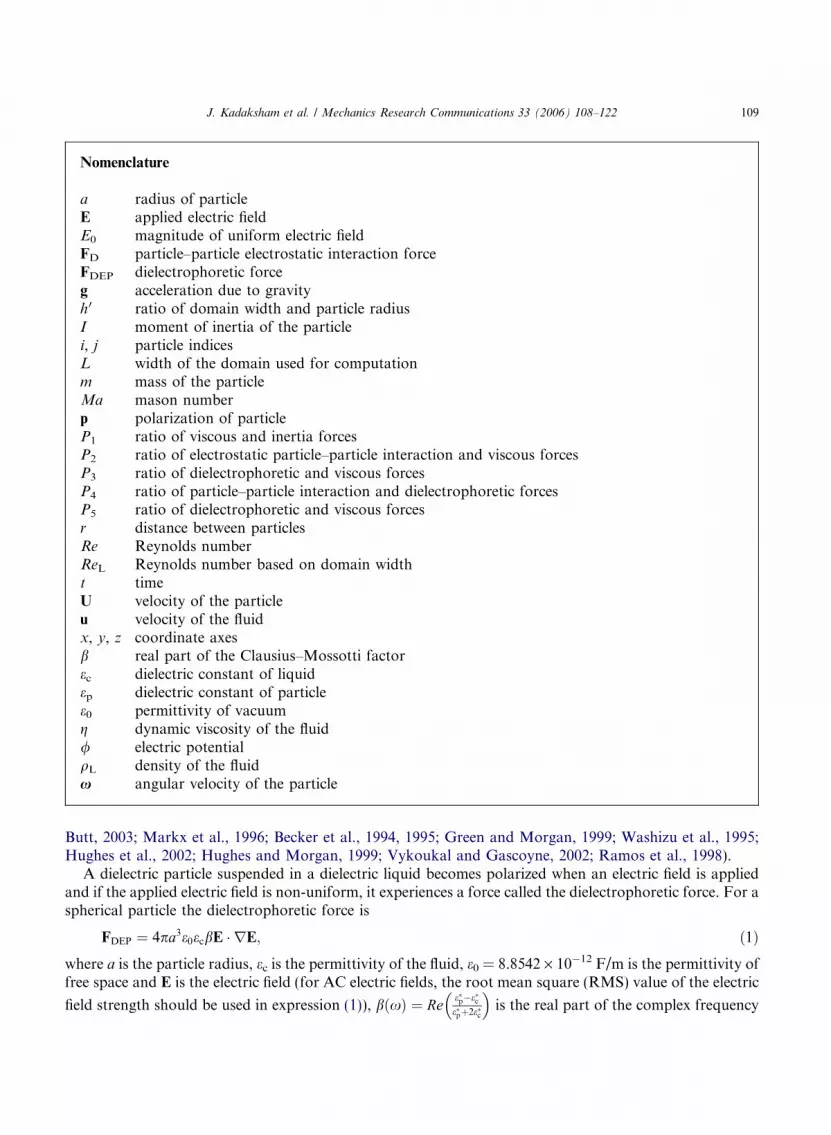
Nomenclature

a radius of particleE applied electric fieldE0 magnitude of uniform electric fieldFD particle–particle electrostatic interaction forceFDEP dielectrophoretic forceg acceleration due to gravityh 0 ratio of domain width and particle radiusI moment of inertia of the particlei, j particle indicesL width of the domain used for computationm mass of the particleMa mason numberp polarization of particleP1 ratio of viscous and inertia forcesP2 ratio of electrostatic particle–particle interaction and viscous forcesP3 ratio of dielectrophoretic and viscous forcesP4 ratio of particle–particle interaction and dielectrophoretic forcesP5 ratio of dielectrophoretic and viscous forcesr distance between particlesRe Reynolds numberReL Reynolds number based on domain widtht timeU velocity of the particleu velocity of the fluidx, y, z coordinate axesb real part of the Clausius–Mossotti factorec dielectric constant of liquidep dielectric constant of particlee0 permittivity of vacuumg dynamic viscosity of the fluid/ electric potentialqL density of the fluidx angular velocity of the particle

J. Kadaksham et al. / Mechanics Research Communications 33 (2006) 108–122 109

Butt, 2003; Markx et al., 1996; Becker et al., 1994, 1995; Green and Morgan, 1999; Washizu et al., 1995;Hughes et al., 2002; Hughes and Morgan, 1999; Vykoukal and Gascoyne, 2002; Ramos et al., 1998).

A dielectric particle suspended in a dielectric liquid becomes polarized when an electric field is appliedand if the applied electric field is non-uniform, it experiences a force called the dielectrophoretic force. For aspherical particle the dielectrophoretic force is

FDEP ¼ 4pa3e0ecbE � rE; ð1Þ
where a is the particle radius, ec is the permittivity of the fluid, e0 = 8.8542 · 10�12 F/m is the permittivity offree space and E is the electric field (for AC electric fields, the root mean square (RMS) value of the electric
field strength should be used in expression (1)), bðxÞ ¼ Ree�p�e�ce�pþ2e�c

� �is the real part of the complex frequency

110 J. Kadaksham et al. / Mechanics Research Communications 33 (2006) 108–122

dependent Clausius–Mossotti factore�p�e�ce�pþ2e�c

� �, e�p and e�c are the complex permittivity of the particles and the

liquid. Here, e� ¼ e � j rf , where r is the conductivity, e is the permittivity, f is the frequency of the applied

electric field and j ¼ffiffiffiffiffiffiffi�1

p. In this paper we will assume that the particles and liquid are perfect dielectrics,

i.e., r � e. In the present work, we also assume that the electrostatic force acting on a particle is given bythe point-dipole approximation (see Klingenberg et al., 1989).

From (1) it is clear that if a particle is more polarizable than the liquid, i.e., b > 0, the force is in thedirection of the gradient of the electric field magnitude and the particle is said to experience positive dielec-trophoresis. In this case, the particle moves to the high electric field region. On the other hand, if b < 0, theparticle experiences negative dielectrophoresis and moves to the low electric field region. Gascoyne et al.(1994) have used this property for separating particles for which the sign of b is different, as the directionof the dielectrophoretic force depends on b.

The polarized particles of a suspension are not only subjected to the applied external electric field, butalso interact with each other electrostatically. This interaction among particles can be of the same order asthe dielectrophoretic force when particles are close to each other, as is the case when they collect in the highor low electric field regions. Thus, the total electrostatic force FE,i acting on the ith particle is given by thesum of these two forces,

FE;i ¼ FDEP;i þ FD;i; ð2Þ
where FDEP,i = 4pa3e0ecb Ei Æ$Ei is the DEP force acting on the ith particle and FD,i is the net electrostaticinteraction force acting on the ith particle, given by FD;i ¼
PNi¼1;i6¼jFD;ij. Here, within the framework of the

point dipole approximation

FD;ij ¼1

4pe0ec

3

r5rijðpi � pjÞ þ ðrij � piÞpj þ ðrij � pjÞpi �

5

r2rijðpi � rijÞðpj � rijÞ

� �; ð20Þ

where pi denotes the dipole moment of particle i (see Appendix A for details). Notice that FD,ij varies in-versely as the fourth power of the distance between the particles.

The goal of this paper is to employ the direct numerical simulation (DNS) approach to study the motionof neutral particles in non-uniform electric fields, using the governing equations of motion for both the par-ticles and the fluid. The fluid is described by the Navier-Stokes equations and the particles by the Newton�ssecond law in which the action of the electric field is modeled by means of the point dipole (PD) approx-imation of (2). We are particularly interested in numerically simulating the phenomenon of particle chain-ing in non-uniform electric fields and its dependence on the parameter values, as well as in investigating itseffect on the particle collection time. The phenomenon of particle chaining under the action of non-uniformelectric fields has been observed in many experiments but, to our knowledge, has not yet been simulated bymeans of DNS.

The particle–particle interaction force FD,i of (2), based on the point-dipole approximation, takes intoaccount the modification of the electric field due to the presence of other particles up to the dipole term,but neglects higher order (multipole) terms. Thus, strictly speaking, the use of the point-dipole approxima-tion should be limited to the case where the particle radius is much smaller than the typical distance overwhich the electric field varies and the distance between particles is large compared to the particle radius. Theexact interaction effects have been included in previous numerical studies, but only for the case of a uniformelectric field in periodic domains (Bonnecaze and Brady, 1992). For the non-uniform electric field problemsinvestigated here, the electric potential boundary conditions on the side walls are mixed which complicatesthe use of the method of images for estimating modifications in the electric force due to the proximity of thewalls and electrodes; the electric potential is prescribed on the electrodes and the normal derivative of theelectric potential is taken to be zero on the remaining side wall. In our numerical scheme these modifica-tions to the electric force are neglected which is a good approximation when the distance of the particle


from the wall is large compared to its radius. The approximation adopted here are appropriate for studiesof particle motions where they are still relatively far from each other and to the prediction of the approx-imate time it takes for the particles to collect (as in Hass, 1993 for the case of a uniform electric field). How-ever, as is the case of a uniform electric field (Baxter-Drayton and Brady, 1996; Resca, 1996), it is probablynot well suited for estimating properties which depend on the behavior of aggregates, such as the viscosityof concentrated suspensions in shear flows, which is not investigated in this paper. We are aware that anerror is introduced in the computation of the time particles take to reach their final destination, but thiserror was found to be relatively small (approximately 14%) in recent calculations involving two particlessubjected to a uniform electric field where the actual electrostatic force was computed from the integrationof the Maxwell Stress tensor on the particle surface (Kadaksham et al., 2004a).

The rest of the paper is organized as follows. In the next section, we present the governing equations andobtain the dimensionless parameters. In Section 3, we present the results for several cases that show theimportance of the electric potential boundary condition and a dimensionless number defined as the ratioof electrostatic particle–particle interaction and dielectrophoretic forces.

2. Governing equations

In this section we first state the governing equations of the motion of fluid and particles, and then theseequations are non-dimensionalized to obtain the dimensionless parameters.

Let us denote the domain containing a Newtonian fluid and N solid spherical particles by X the interiorof the ith particle by Pi(t), and the domain boundary by C. The governing equations for the fluid-particlesystem are

qL

ou

otþ u � ru

� �¼ �rp þr � ð2gDÞ in X n P ðtÞ;

r � u ¼ 0 in X n PðtÞ; ð3Þu ¼ uL on C;

u ¼ Ui þ xi � ri on oP iðtÞ; i ¼ 1; . . . ;N . ð4Þ

Here, u is the fluid velocity, p is the pressure, g is the dynamic viscosity of the fluid, qL is the density of thefluid, D is the symmetric part of the velocity gradient tensor and Ui and xi are the linear and angular veloc-ities of the ith particle. The above equations are solved using the initial condition ujt=0 = u0, where u0 is theknown initial value of the velocity.

The linear velocity Ui and the angualr velocity xi of the ith particle are governed by

midUi

dt¼ Fi þ FE;i;

I idxi

dt¼ Ti; ð5Þ

Uijt¼0 ¼ Ui;0;

xijt¼0 ¼ xi;0; ð6Þ

where mi and Ii are the mass and moment of inertia of the ith particle, Fi and Ti are the hydrodynamic forceand torque acting on the ith particle and FE,i = FDEP,i + FD,i is the electrostatic force acting on the ith par-ticle. As mentioned above, in this work, we will restrict ourselves to the case where the particles are spher-ical, and therefore we do not need to keep track of the particle orientation. The particle positions areobtained from


dXi

dt¼ Ui; ð7Þ

Xijt¼0 ¼ Xi;0; ð8Þ

where Xi,0 is the position of the ith particle at time t = 0. In this work, we will assume that all particles havethe same density qp, and since they have the same radius, they also have the same mass, m.

To calculate the electric field E, we first solve the electric potential problem $2/ = 0, subjected toprescribed boundary conditions, and then calculate E = �$/.

2.1. Dimensionless equations and parameters

Eqs. (3) and (5) are non-dimensionalized by assuming that the characteristic length, velocity, time, stress,angular velocity and electric field scales are a, U, a/U, gU/a, U/a and E0, respectively. The gradient of theelectric field is assumed to scale as E0/L, where L is the distance between the electrodes which is of the sameorder as the domain width. The non-dimensional equations, after using the same symbols for the dimen-sionless variables, are

Reou

otþ u � ru

� �¼ �rp þr � r in X n PðtÞ;

r � u ¼ 0 in X n PðtÞ;ð9Þ

dU

dt¼ 6pga2

mU

Z �pIþ r

6p

� �� ndsþ 4pa4e0ecbjE0j2

mU 2LðE � rEÞ þ 3pe0eca3b

2jE0j2

4mU 2jrijj4ðFDÞ; ð10Þ

dx

dt¼ 5ga2

2mU

Zðx� X Þ � ½ð�pIþ rÞ � n�ds. ð11Þ

Notice that in the first term on the right hand side of (10) a factor of 6p is introduced to ensure that foran isolated particle the quantity inside the integral in the Stokes flow limit is equal to one.

The above equations contain the following dimensionless parameters:

Re ¼ qLUag

; P 1 ¼6pga2

mU; P 2 ¼

3pe0ecb2a3jE0j2

4mU 2; P 3 ¼

4pe0ecba4jE0j2

mU 2Land h0 ¼ L

a. ð12Þ

Here, Re is the Reynolds number, which determines the relative importance of the fluid inertia and viscousforces, P1 is the ratio of the viscous and inertia forces, P2 is the ratio of the electrostatic particle–particleinteraction and inertia forces and P3 is the ratio of the dielectrophoretic and inertia forces. Another impor-tant parameter, which does not appear directly in the above equations, is the solids fraction of the particles;the rheological properties of ER suspensions depend strongly on the solids fraction. We can define anotherReynolds number ReL ¼ qLLU

g based on the channel width L.In order to investigate the relative importance of the electrostatic particle–particle and dielectrophoretic

forces, we define another parameter

P 4 ¼P 2

P 3

¼ 3bL16a

. ð13Þ

Obviously, in most applications of dielectrophoresis L � a because L is comparable to the domain sizeand the particle radius a is smaller than the domain size. However, there are applications in which L is onlya few times larger than a. Expression (13) implies that if b = O(1) and L � a, the particle–particle interac-tion forces will dominate, which is the case in most applications of dielectrophoresis. On the other hand, ifb � 1 and 3bL

16a � 1, the dielectrophoretic force dominates. In this limit, we expect particles to move to the


regions of maximums or minimums of the electric field without forming chains even when they are close toeach other. It is noteworthy that P4 depends linearly on b because according to the point-dipole approxi-mation the dielectrophoretic force depends linearly on b and the particle–particle interaction force dependsquadratically on b.

If the particle and fluid inertia can be set to zero, i.e., Re = 0, the number of dimensionless parametersreduces to three. The dimensionless parameters in this case are the Mason number Ma and P5,

Ma ¼ P 1

P 2

¼ 8gU

e0ecb2ajE0j2

;

P 5 ¼P 3

P 1

¼ 2e0ecba2jE0j2

3gUL

ð14Þ

and h0 ¼ La. The Mason number determines the relative importance of the viscous force and the electrostatic

particle–particle interaction force, and P5 determines the relative importance of the electrostatic dielec-trophoretic and viscous forces.

If there is no imposed bulk flow and the particle motion is caused by the dielectrophoretic force, an obvi-ous choice of the characteristic velocity in this case is obtained by equating the dielectrophoretic force andviscous drag terms (Kadaksham et al., 2004b), which gives

U ¼ 2e0ecba2jE0j2

3gL. ð15Þ

If (15) is taken to be the characteristic velocity, the dimensionless parameters P1 and P3 are the same:P 1 ¼ P 3 ¼ 9pg2L

me0ecbjE0j2, and P5 = 1. The other parameters become: Re ¼ 2qLe0ecba3jE0j2

3g2L ,

P 2 ¼27pg2L2

16me0ecajE0j2and P 4 ¼

3bL16a

¼ 1

Ma.

Assuming that the electric field E0 ¼ VL, where V is the voltage applied to the electrodes, expression (15)

for the characteristic velocity can be written as

U ¼ 2e0ecbV 2

3gLaL

� �2

. ð16Þ

The above expression implies that if a/L, V and the material parameters are held constant, U increaseswith decreasing L. The ratio a/L is considered constant because the device size is decided by the size of theparticles that need to be manipulated. Let us consider the case where g = 0.01 Poise, b = 1.0, ec = 80,qL = 103 kg/m3, a/L = 0.1 and V = 10 V. Substituting these values into (16) for a device withL = 10 lm, we obtain U = 4.72 · 104 lm/s. On the other hand, for a device with L = 1 mm,U = 472 lm/s. Therefore, the velocity is hundred times larger in the smaller device. Also, since the particlesmust be moved over a larger distance in the larger device, we may conclude that the larger sized devices areless effective! This is the case because with increasing particle size the magnitude of the dielectrophoreticforce becomes small compared to that of the viscous drag. In order to overcome this problem, a higher volt-age is usually applied in a larger sized device. For example, in Wakeman and Butt (2003) for the device withL = 20 mm, the applied voltage is as large as V = 10,000 V. The applied voltage however must be less thanthe critical voltage at which the electric discharge occurs.

2.2. Finite element method

The numerical scheme is a generalization of the DLM finite-element scheme described in Glowinski et al.(1998) and Singh et al. (2000). The computational scheme used here is described in detail in Kadaksham


et al. (2004b). In the DLM scheme, the fluid flow equations are solved on the combined fluid-solid domain,and the motion inside the particle boundaries is forced to be rigid-body motion using a distribution ofLagrange multipliers. The fluid and particle equations of motion are combined into a single combined weakequation of motion, eliminating the hydrodynamic forces and torques, which helps ensure stability of thetime integration. The time integration is performed using the Marchuk–Yanenko operator splittingmethod, which is first-order accurate. The electrostatic force is given by (2), based on the point dipoleapproximation. We refer to Kadaksham et al. (2004b) for further details.

3. Results

Fig. 1a shows a typical domain, the initial arrangement of particles and the coordinate system used inour simulations. The dimensions of the box shaped domain are 1.6 mm · 0.8 mm · 2.4 mm in the x-, y-and z-directions. The fluid velocity is assumed to be zero on the sidewalls of the domain and periodic alongthe z-direction. The electric field is also assumed to be periodic in the z-direction. The electrostatic andhydrodynamic forces include contributions from the periodic images in the z-direction. The imposed fluidvelocity and the pressure gradient in the z-direction are assumed to be zero.

The non-uniform electric field is generated by placing two pairs of electrodes on the domain side wallsparallel to the yz-coordinate plane. Let us denote the potential for the bottom left and upper left electrodesby VBL and VUL and those for the bottom right and upper right electrodes by VBR and VUR. For mostcases, the left electrodes are grounded, i.e., VBL = VUL = 0 V, and VBR = VUR = 2000 V. The electric fieldand the gradient of electric field for these boundary conditions are shown in Fig. 1b and c.

Throughout this paper, we assume that the dynamic fluid viscosity g = 0.01 Poise and the particle diam-eter and density are 0.2 mm and 1.01 g/cm3, respectively. The fluid density is qL = 1.0 g/cm3. The gravity isignored, as the density of particles is close to that of the fluid and the particle diameter is small. The initialfluid and particle velocities are set to zero. The domain is discretized using a regular pseudo P2–P1 tetra-hedral mesh and the number of nodes used is 208,065. The time step used is 5 · 10�4 s.

Fig. 1. (a) An oblique view of a typical domain used for simulations. (b) Isovalues of log(jEj) and the direction of E on the domainmidsection are shown. Notice that the electric field is maximum at the electrode tips. The electric field does not vary with y. (c)Isovalues of log (jE.$Ej) and the lines of dielectrophoretic force are shown. E Æ$E does not vary with y.


3.1. Influence of parameter P4

As discussed in Section 2, parameter P 4 ¼ P2

P3¼ 3bL

16a determines the relative importance of the electrostaticparticle–particle and dielectrophoretic forces. As the dielectrophoretic force dominates when P4 < O(1), theparticles are easily separated from neighbors and move individually to the maximums or minimums of theelectric field. On the other hand, when P4 > O(1), the particle–particle interactions dominate which resultsin the formation of particle chains which then move relatively slowly towards the minimums or maximumsof the electric field. In fact, when P4 � O(1) and the particle concentration is sufficiently large, the particlesform chains extending from one electrode to the opposite one, thus preventing the removal of particles. It isworth noting that the chaining behavior of particles does not depend directly on the particle radius, but ona/L, where L is the length scale over which the electric field varies. Also notice that P4 depends on the ratioof the dielectric constants of the liquid and particles which determines b, but not directly on the dielectricconstant of the liquid or the particle.

In our simulations, the value of P4 is varied using two different approaches. In both approaches, onlythose dimensionless parameters that depend on the electrostatic forces are varied and the remaining param-eters are held fixed. In the first approach, P4 is varied by changing b and in the second by changing P2 andP3. Even though P2 and P3 cannot be varied independently for a real ER fluid, the approach is useful foranalyzing the mathematical nature of equations.

We first discuss two cases with b = 0.5 and 0.01. The particle–particle interaction force is expected todominate in the first case and the dielectrophoretic force is expected to dominate in the second. Forb = 0.5, the dielectric constants of the particles and fluid are 10 and 2.5, respectively. The left electrodesare grounded whereas the right ones are at 2000 V. Eighty particles are arranged in the domain in a periodicmanner as shown in Fig. 1a. The solids fraction is 0.118. The values of dimensionless parameters in this caseare Re = 7.2, P1 = 0.618, P2 = 0.927, P3 = 0.618, Ma = 0.67, and P4 = 1.5. Simulations show that att � 0.9 s the particle chains are formed (see Fig. 2a) and then these chains move toward the electrode edgesat a smaller speed than of individual particles. The positions of the particles at t = 3.0 s is shown in Fig. 2b.

For b = 0.01, the dielectric constants of the particles and fluid are 2.576 and 2.5, respectively. In order toensure that the magnitude of the dielectrophoretic force, which depends on b, is the same as for the casedescribed above, i.e., P3 remains 0.618, the electric field strength is increased. The values of dimensionlessparameters are Re = 7.2, P1 = 0.618, P2 = 0.0185, P3 = 0.618, Ma = 33.3, and P4 = 0.03, respectively.Fig. 2c shows the positions of the particles at t = 0.9 s from which it can be seen that the particles in themiddle have already started moving to the electrodes, without forming chains. The position of the particlesat time, t = 3.0 s is shown in Fig. 2d. Notice that most particles, except those in the middle, are attached tothe edges of the electrodes by this time. The vertical chains of particles seen at the middle of the domain areformed due to the presence of the saddle points at (x = 0.8, z = 0.6), (x = 0.8, z = 1.2) and (x = 0.8,z = 1.8). As can be observed from Fig. 1b and c, at these points the dielectrophoretic force is zero, butthe magnitude of the electric field is not locally minimum.

We next describe two cases where the values of parameters P2 and P3 are changed independently. First,we describe the case for which P2 is 99.26. The other dimensionless parameters in this case are Re = 0.40,P1 = 11.12, P3 = 11.12, Ma = 0.112, and P4 = 8.92, respectively. As P4 is much greater than one, the par-ticle–particle interactions dominate and the particles form chains, as can be seen in Fig. 2e at t = 3.0 s. Thechains of particles rearrange and some chains even merge to form longer chains. Notice that some chainsextend from one electrode to the other, and after they are formed remain almost stationary, and theparticles do not collect at the electrode edges.

Next, the magnitude of the parameter P2 is decreased to 0.99. The other dimensionless parameters forthis case are Re = 0.40, P1 = 11.12, P3 = 11.12, Ma = 11.2, and P4 = 0.089, respectively. The particlesmove relatively quickly toward the edges of the electrodes without forming chains, as can be seen inFig. 2f at t = 3.0 s. Here also, as in Fig. 2d, the particles in the middle of the domain are not collected.

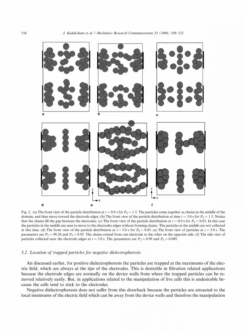
Fig. 2. (a) The front view of the particle distribution at t = 0.9 s for P4 = 1.5. The particles come together as chains in the middle of thedomain, and then move toward the electrode edges. (b) The front view of the particle distribution at time t = 3.0 s for P4 = 1.5. Noticethat the chains fill the gap between the electrodes. (c) The front view of the particle distribution at t = 0.9 s for P4 = 0.03. In this casethe particles in the middle are seen to move to the electrodes edges without forming chains. The particles in the middle are not collectedat this time. (d) The front view of the particle distribution at t = 3.0 s for P4 = 0.03. (e) The front view of particles at t = 3.0 s. Theparameters are P2 = 99.26 and P4 = 8.92. The chains extend from one electrode to the other on the opposite side. (f) The side view ofparticles collected near the electrode edges at t = 3.0 s. The parameters are P2 = 0.99 and P4 = 0.089.


3.2. Location of trapped particles for negative dielectrophoresis

An discussed earlier, for positive dielectrophoresis the particles are trapped at the maximums of the elec-tric field, which are always at the tips of the electrodes. This is desirable in filtration related applicationsbecause the electrode edges are normally on the device walls from where the trapped particles can be re-moved relatively easily. But, in applications related to the manipulation of live cells this is undesirable be-cause the cells tend to stick to the electrodes.

Negative dielectrophoresis does not suffer from this drawback because the particles are attracted to thelocal minimums of the electric field which can be away from the device walls and therefore the manipulation


is contactless. For example, in the so-called field-casting applications the cells are brought together to formaggregates which has many advantages over conventional methods as there is no touching of the cells in-volved. A local minimum of the electric field is also referred to as a ‘‘trap’’ or ‘‘cage’’ (Fuhr et al., 1996;Voldman et al., 2003).

In this subsection, it is shown that the locations of the electric field minimums, and thus also the posi-tions where the particles are collected, can be changed by modifying the electric field boundary conditions.For all cases discussed in this subsection, b = �0.297 and there are forty particles. The solids fraction is0.0545. In the first case, the bottom left and bottom right electrodes are grounded, and the remainingtwo electrodes are charged, i.e., VBL = VBR = 0 V and VUL = VUR = 2000 V. The electric field and the gra-dient of the electric field are shown in Fig. 3a and b. The local minimums of the electric field magnitude,where the particles with negative b collect are at the locations (x = 0.8 mm, z = 1.2 mm), (x = 0.8 mm,z = 0 mm). The dimensionless parameters in this case are Re = 0.40, P1 = 11.12, P2 = 9.93, P3 = 11.12,Ma = 1.12 and P4 = 0.892.

Fig. 3. (a) Isovalues of log (jEj) on the domain midsection are shown. The electric field does not vary with y, and the bottom electrodeon the left and the top electrode on the right are grounded. (b) Isovalues of log (jE Æ$Ej) and the lines of dielectrophoretic force. (c) Thetop view of the particle distribution at t = 2 min 2 s for b = �0.297. (d) The distribution of log (jEj) on the domain midsection. (e) Thepositions of the particles at time t = 2 min 15 s.


As b is negative, all particles move to the local minimums of the electric field and, as shown in Fig. 3c,most are collected by t = 2 min 2 s.

We next describe the case where the positions of the electric field minimums are moved by changing thevoltages at the four electrodes. The applied voltages are: VBL = 400 V, VUL = 1000 V, VBR = 0 V andVUR = 2000 V. The distribution of log jEj is shown in Fig. 3d. The local minimums of the electric fieldare at (x = 0.6 mm, z = 1.05 mm), (x = 0.6 mm, z = 0.15 mm). At t = 2 min 15 s, as shown in Fig. 3e, mostparticles are collected. The collection time is of the same order as before.

The above simulations show that the local minimums of jEj, and thus the regions in which the particleswith b < 0 collect, can be easily moved by changing the electrostatic potential of the electrodes. This canbe important, for example, in applications which require that a cell be moved to a preset location where itcan be manipulated. In fact, by changing the position of the local minimum of jEj, the cell can be movedalong a predetermined trajectory. This is possible because the location of the minimum of jEj is deter-mined by the electric potential boundary conditions which can be changed in a time dependent manner.Also, since the particles near the local minimum can be moved along an arbitrary path by changing theelectric potential boundary condition, at least in principle, an ER suspension can be mixed by draggingthe particles.

3.3. Separation of particles with positive and negative b

Finally, we study the process of separation of particles for which the sign of b is different. This method ofseparation of particles is called the differential DEP affinity separation. In practice, for this technique towork, one must find a suitable liquid such that its dielectric constant is smaller than the dielectric constantof one set of particles and greater than the dielectric constant of the second set of particles. Since the fre-quency dependence of the dielectric constant is different for different materials, it is possible to achieve thisby selecting a suitable frequency. The method is useful if the dielectric properties of the particles are quitedifferent (Morgan et al., 1999; Vykoukal and Gascoyne, 2002).

To numerically study this phenomenon, we consider a mixture containing 20 particles with b = 0.297and 20 particles with b = �0.297 (see Fig. 4a). The electric field and jE � rEj for this case are shown inFig. 1b and c. There are three saddle points at (x = 0.8, z = 0.6), (x = 0.8, z = 1.2) and (x = 0.8,z = 1.8). The minimums of the electric field are on the domain sidewalls equidistant between the two elec-trodes and at the four corners of the domain. The values of the parameters are Re = 0.40, P1 = 11.12,P2 = 9.93, P3 = 11.12, Ma = 1.12 and P4 = 0.892.

Simulations show that the particles with positive b move in the direction of E.$E and are collected in theregions of high electric field strength (see Fig. 4b–d). The particles with negative b, on the other hand, movein the opposite direction of E Æ$E and get collected at the minimums of electric field strength. All particlesare separated and collected at t = 14 s. We may therefore conclude that the particles with different dielectricconstants can indeed be separated.

Next, we discuss the case where the electric potential boundary conditions are changed to: VBL =VBR = 0 Volts and VUL = VUR = 2000 V. The parameters are identical to those of the previous case.The electric field and the gradient of the electric field for these boundary conditions are shown inFig. 4a and b. In this case the two different kinds of particles get separated quickly. The particles with neg-ative b get collected at the electric field minimums at (x = 0.8 mm, z = 1.2 mm), (x = 0.8 mm, z = 0.0 mm)and the particles with positive b get collected at the tip of the electrodes. The position of the particles attime, t = 2 min is shown in Fig. 4e. Notice that the time required for the collection of particles is muchsmaller than in the previous case. This is due to the fact that the electric field minimum at (x = 0.8 mm,z = 1.2 mm) is well separated from the electric field maximums at the electrode tips and the saddle points(x = 0.8, z = 0.6) and (x = 0.8, z = 1.8). This demonstrates that the separation efficiency of a device can beimproved by optimizing the electric field distribution.

Fig. 4. (a) An oblique view of the initial arrangement of particles with b > 0 and b < 0 (painted black). (b) The top view of particledistribution at t = 0.3 s. The particles with b < 0 are attracted toward the regions where the electric field strength is minimum and thosewith b > 0 toward the electrodes edges where the electric field strength is maximum. (c) t = 2.5 s. (d) t = 14 s. The particles with b < 0are collected on the domain sidewalls near the domain center and top, and those with b > 0 (painted white) are collected near the edgesof the electrodes. (e) The positions of the particles at t = 2 min for modified voltage boundary conditions.


4. Conclusions

A numerical scheme based on the distributed Lagrange multiplier method (DLM) (Glowinski et al.,1998; Singh et al., 2000) was used to perform direct numerical simulations of the dynamical behavior ofparticles in ER suspensions. The dynamical behavior of ER suspensions in non-uniform electric field de-pends on the solids fraction, the ratio of the domain size and particle radius, and four additional dimen-sionless parameters which, respectively, determine the relative importance of inertia, viscous,electrostatic particle–particle interaction and dielectrophoretic forces. The simulation results are used toarrive at the following conclusions:

The influence of the parameter P4 on the particle chaining and time it takes for the particle to gettrapped was examined numerically. It was shown that the parameter P4, simply proportional to the ratio


of the Clausius–Mossotti factor and the particle radius non-dimensionalized with the channel width,determines the extent to which particles form chains. The larger P4 is, the stronger are the particle–par-ticle interactions compared to the dielectrophoretic force. In a system where P4 > O(1), the time of par-ticle collection increases with increasing P4 due to the fact that the formation of chains slows thecollection process. In contrast, when P4 < O(1), particles move individually without forming chainsand, thus, the time taken for collection is relatively smaller. It is worth noting that it is not obviouswhether these results obtained using the point dipole approximation would remain true if the electricproblem is also solved exactly. This, in our opinion, is an interesting question in its own right whichshould be investigated. To investigate these issues, we have been developing techniques where the electricproblem is solved exactly (numerically) and the electric forces on particles are obtained by integrating theMaxwell stress tensor.

The phenomenon of field-casting was studied numerically. The regions in which the particles with b < 0aggregates are formed can be changed by modifying the electric potential boundary conditions. By chang-ing the boundary conditions in a time dependent manner, these regions can be moved in a time dependentmanner. The electric field maximum, on the other hand, is always at the electrode corners.

Simulations in this paper have shown that the separation time strongly depends on the positions of max-imums and minimums of the electric fields, and is much smaller when the distance between the maximumsand minimums is larger. The dielectrophoretic effect thus can be used to separate mixtures containing twosets of particles for which the sign of b is different.

Acknowledgments

We gratefully acknowledge the support of the National Science Foundation KDI Grand Challenge grant(NSF/CTS-98-73236), the New Jersey Commission on Science and Technology through the New-JerseyCenter for Micro-Flow Control under Award Number 01-2042-007-25, the W.M. Keck Foundation forproviding support for the establishment of the NJIT Keck laboratory for Electrohydrodynamics of Suspen-sions and the support of the Office of Naval Research under Award Number 992294.

Appendix A. Electrostatic forces

We will assume that the polarization of a particle in a spatially varying electric field depends on the valueof the electric field E at its center. For an isolated spherical particle subjected to E, the polarization is thengiven by

p ¼ 4pe0ecba3E. ðA:1Þ

To obtain the interaction force between two particles, we assume that the electric field strengths at theircenters to be Ei and Ej, respectively. The two particles thus become polarized with dipole moments, pi = 4-pe0ecba

3Ei and pj = 4pe0ecba3Ej. Since the direction of E and its magnitude vary in space, the direction and

magnitude of the polarization of the particles also vary in space. It is easy to show that the x-component ofthe electrostatic interaction force FD,ij between particles i and j is

ðF D;ijÞx ¼1

4pe0ec

3

r5

�xijð3pi1pj1 þ pi2pj2 þ pi3pj3Þ þ yijðpi1pj2 þ pi2pj1Þ þ zijðpi1pj3 þ pi3pj1Þ

� 5

r2xijðpi � rijÞðpj � rijÞ

�. ðA:2Þ


Here, rij = ri � rj where ri and rj, are the position vectors of particles i and j, r = jrijj, xij, yij and zij are thecomponents of rij, pi1, pi2 and pi3 are the components of pi, and pj1, pj2 and pj3 are the components of pj. Theabove expression can be written in vector form as

FD;ij ¼1

4pe0ec

3

r5rijðpi � pjÞ þ ðrij � piÞpj þ ðrij � pjÞpi �

5

r2rijðpi � rijÞðpj � rijÞ

� �. ðA:3Þ

It is easy to show that in a spatially uniform electric field the above expression takes the following well-known form in spherical coordinates,

FD;ijðrij; hijÞ ¼ f0arij

� �4

ðð3cos2hij � 1Þer þ sin 2hijehÞ; ðA:4Þ

where f0 ¼ 12pe0eca2b2E2

0, E0 being the magnitude of the uniform electric field along the z-axis, hij denotesthe angle between the z-axis and the position vector rij.

The net electrostatic interaction force acting on the ith particle is the sum of the interaction forces withall other particles:

FD;i ¼XN

i¼1;i6¼j

FD;ij; ðA:5Þ

where N is the number of particles.Eq. (A.4) implies that the particle–particle interaction force is inversely proportional to the fourth power

of the distance between the particles. It thus decreases rapidly with increasing jrijj and can be ignored whenthe distance between two particles is larger than a few particle diameters.

References

Baxter-Drayton, Y., Brady, J.F., 1996. Brownian electrorheological fluids as a model for flocculated dispersions. Journal of Rheology40, 1027.

Becker, F.F., Wang, X.-B., Huang, Y., Pethig, R., Vykoukal, J., Gascoyne, P.R.C., 1994. The removal of human leukemia cells fromblood using interdigitated microelectrodes. Journal of Physics D: Applied Physics 27, 2659–2662.

Becker, F.F., Wang, X.-B., Huang, Y., Pethig, R., Vykoukal, J., Gascoyne, P.R.C., 1995. Separation of human breast cancer cells fromblood by differential dielectric affinity. Proceedings of the National Academy of Sciences, USA 92, 860–864.

Bonnecaze, R.T., Brady, J.F., 1992. Dynamic simulation of an electrorheological suspension. Journal of Chemical Physics 96, 2183–2204.

Fuhr, G., Zimmermann, U., Shirley, S.G., 1996. Cell motion in time varying fields: principles and potentials. Electromanipulation ofCells, pp. 259–328.

Gascoyne, P.R.C., Noshari, J., Becker, F.F., Pethig, R., 1994. Use of dielectrophoretic collection spectra for characterizing differencesbetween normal and cancerous cells. IEEE Transactions on Industry Applications 30, 829–834.

Glowinski, R.T., Pan, W., Hesla, T.I., Joseph, D.D., 1998. Direct numerical simulation of viscoelastic particulate flows. InternationalJournal of Multiphase Flows 25, 755–794.

Green, N.G., Morgan, H., 1999. Dielectrophoresis of submicrometer latex spheres. 1. Experimental results. Journal of PhysicalChemistry B 103, 41–50.

Hass, K.C., 1993. Computer simulations of nonequilibrium structure formation in electrorheological fluids. Physical Review E 47,3362.

Hughes, M.P., Morgan, H., 1999. Measurement of bacterial flagellar thrust by negative dielectrophoresis. Biotechnology Progress 15,245–249.

Hughes, M.P., Morgan, H., Rixon, J.F., 2002. Measuring the dielectric properties of herpes simplex virus type 1 virions withdielectrophoresis. Biochimica et Biophysica Acta 1571, 1–8.

Kadaksham, J., Singh, P., Aubry, N., 2004a. Direct simulation of electrorheological suspensions. American Society of MechanicalEngineers Annual Meeting. Fluids Engineering Division Publication.


Kadaksham, J., Singh, P., Aubry, N., 2004b. Dynamics of electrorheological suspensions subjected to spatially nonuniform electricfields. Journal of Fluids Engineering 126, 170–179.

Klingenberg, D.J., van Swol, S., Zukoski, C.F., 1989. Simulation of Electrorheological suspensions. Journal of Chemical Physics 91,7888–7895.

Markx, G.H., Dyda, P.A., Pethig, R., 1996. Dielectrophoretic separation of bacteria using a conductivity gradient. Journal ofBiotechnology 51, 175–180.

Morgan, H., Hughes, M.P., Green, N.G., 1999. Separation of submicron bioparticles by dielectrophoresis. BioPhysics Journal 77, 516–525.

Ramos, A., Morgan, H., Green, N.G., Castellanos, A., 1998. AC electrokinetics: a review of forces in microelectrode structures.Journal of Physics D: Applied Physics 31, 2338–2353.

Resca, L., 1996. Exact treatment of the electrostatic interactions and surface effects in electrorheological fluids. Physical Review B 53,2195.

Singh, P., Joseph, D.D., Hesla, T.I., Glowinski, R.T., Pan, W., 2000. A distributed Lagrange multiplier/fictitious domain method forparticulate flows. Journal of Non-Newtonian Fluid Mechanics 91, 165–188.

Voldman, J., Toner, M., Gray, M.L., Schmidt, M.A., 2003. Design and analysis of extruded quadrupolar dielectrophoretic traps.Journal of Electrostatics 57, 69–90.

Vykoukal, J., Gascoyne, P.R.C., 2002. Invited review: particle separation by dielectrophoresis. Electrophoresis 23, 1973–1983.Wakeman, R.J., Butt, G., 2003. An investigation of high gradient dielectrophoretic filtration. Chemical Engineering Research and

Design 81, 924–935.Washizu, M., Kurosawa, O., Arai, I., Suzuki, S., Shimamoto, N., 1995. Applications of electrostatic stretch- and-positioning of DNA.

IEEE Transactions on Industrial Applications 30, 835–843.

Documents

Manipulation of particles using dielectrophoresis