Embed Size (px)
Citation preview

IVA. Eelgrass Restoration Project (July 1, 2004-October 31, 2007) Staff: Project Supervisor: Bruce T. Estrella
AQBII: Alison S. Leschen AQBI: Ross K. Kessler Fisheries Technicians: Kate Lin Taylor, Cate O’Keefe, Theresa Vavrina, Wesley Dukes
Completion Report: Alison S. Leschen, Ross K. Kessler, and Bruce T. Estrella Introduction From 2004-2007, the Massachusetts Division of Marine Fisheries (MarineFisheries) restored eelgrass in Boston Harbor, MA as partial mitigation for assumed impacts to the environment and biota from the construction of the "HubLine" natural gas pipeline across Massachusetts Bay. Pipeline construction activities during 2002-2003 exceeded recommended time-of-year work windows and were determined to potentially impact a number of finfish and invertebrate species including crustaceans, flounders, cod, and anadromous fish. Restoration of eelgrass habitat was chosen as a mitigation option because it had the potential to provide shelter and food and positively impact populations of these species. The ecosystem value of eelgrass (Zostera marina) is well documented. Eelgrass acts to stabilize sediments, buffer wave energy, and provide habitat for juvenile fish and shellfish (Stauffer 1937; Orth et al. 1984; Heck et al. 1989; Hughes et al. 2002; Lazarri and Tupper 2002). Decline of this important marine plant has been tracked throughout its range (Jacobs 1979; Short et al. 1986; Valiela et al. 1992; Short and Burdick 1996). It has been estimated that 90% of eelgrass died off in the 1930s due to an outbreak of wasting disease (Tutin 1942). While wasting disease continues to occur sporadically (Short et al. 1986, 1987), natural re-population has been thwarted by degraded water quality from coastal development, which limits light essential for eelgrass growth (Batuik et al. 2000). This problem is compounded by the limited ability of eelgrass to disperse to suitable areas over long distances.
The clear relationship between eutrophication and eelgrass loss (Kemp et al. 1983; Valiela et al. 1992; Short et al. 1996; Hauxwell et al. 2001, 2003; Cardoso et al. 2004) underscores the futility of attempting restoration where water quality remains poor. In addition, physical and biological changes that can occur in an area when eelgrass is lost may inhibit natural re-vegetation (Rasmussen 1977; Duarte 1995; Short et al. 2002b). In fact, attempts to actively restore eelgrass have met with varied success, and many failures (Homziak et al. 1982; Thom 1990; Fonseca et al. 1998). Just 31% of restoration sites reviewed in Short et al. (2002a) succeeded in establishing eelgrass and many of these were only on a test transplant scale (<0.01 hectares). Careful site-selection is now recognized as an essential precursor to any restoration project (Fonseca et al. 1998; Short et al. 2002a; Kopp and Short 2003) and should improve the poor record of past attempts. Short et al. (2002a) developed a site-selection model with criteria based on some of their most successful transplant sites. Criteria included historical and current eelgrass distribution, proximity to natural eelgrass beds, sediment, wave exposure, water depth, and water quality. Further field testing is done at sites identified by the model, including light measurements and surveys of bioturbators. We used the Short et al. model (hereinafter the Short model) with some modifications as the basis for our site selection process in Boston Harbor. Wastewater management upgrades in Boston Harbor presented an excellent opportunity to assess eelgrass restoration success in an area where most beds had disappeared due to severe eutrophication, but where major water quality improvements could enable its growth. The improvements in water and sediment qualities
68

increased the potential for eelgrass growth, but it was unlikely that this growth would happen naturally on an acceptable time scale. MarineFisheries therefore undertook an eelgrass restoration project in the Harbor with the goal of “jump-starting” the re-colonization of eelgrass to this embayment. Rigorous attention to site selection was essential due to the massive physical and ecological changes which the Harbor had undergone. Eelgrass spreads both vegetatively (rhizome expansion) and non-vegetatively (seeds). Vegetative spreading is limited to adjacent areas, so the natural spread of eelgrass to new areas must be accomplished by the dispersal of seeds. Eelgrass seeds are negatively buoyant and do not travel far within the water column once released from a vegetative shoot (Orth et al. 1994). Detached reproductive eelgrass shoots containing seeds can float long distances, and thus can start new meadows far from the bed of origin (Harwell and Orth 2002a and 2002b). However, such a scenario requires several assumptions: first, that seed shoots are available in the area from existing beds; second, that local currents carry the shoots to an area that is suitable for eelgrass propagation given requirements for water quality, depth (light), and sediment; third, that shoots will sink or the seeds drop out coincident with each shoot’s travel over such an area; and, finally, that any seeds that do sink in suitable areas will germinate and survive burial, grazing, etc. to grow into a viable plant. We took these dynamics into account to determine the likelihood that eelgrass could have naturally re-colonized Boston Harbor, and to focus on areas in our site selection process where eelgrass would become self-spreading. Study Area Boston Harbor is a relatively shallow (4.9m average depth), tide-dominated estuary located on the western edge of Massachusetts Bay within the Gulf of Maine (Figure IVA.1). The 125 km2 area is broken up by numerous small islands. Tidal range averages 2.7 m (Signell and Butman 1992).
The City of Boston (population 590,000) lies directly on the Harbor, and until the 1990’s virtually the entire volume of sewage from the city and surrounding area (population 2 million) was discharged directly into the water body with minimal or no treatment. Prior to 1991, Boston Harbor received well over 100,000 metric tons of suspended solids annually (Knebel 1992; Rex et al. 2002). By the time MarineFisheries’ efforts began in 2004, eelgrass in the Harbor had been reduced to 3 remnant beds Two of these beds had declined in area by over half between the 1995 and 2001 Massachusetts Department of Environmental Protection (DEP) Wetlands Conservancy Program surveys. A fourth bed shown on these surveys had virtually disappeared by the time we surveyed it in 2004. Cause of disappearance in the area was very likely poor water quality (http://www.mass.gov/dep/water/ resources/maps/eelgrass/eelgrass.htm). A massive wastewater collection and treatment project for the Boston area, The Boston Harbor Project, curtailed sludge discharge in 1991. Over the next 9 years, effluent treatment was upgraded to secondary; in 2000, wastewater discharge was diverted from within Boston Harbor, via an outfall pipe extension, to an area 15 km offshore in Massachusetts Bay. Intensive studies conducted by the Massachusetts Water Resources Authority (MWRA), United States Geological Survey (USGS), and others have led to a good understanding of the impacts of the wastewater system upgrades on water and sediment quality in the Harbor. Geometry of the estuary mouth, combined with regional bathymetry, define an ebb tide-dominated system, with net flushing of water from within the Harbor on each outgoing tide (Signell and Butman 1992). This flushing has accelerated water and sediment quality improvements since initiation of the wastewater treatment project. MWRA reported that, five years after the offshore transfer, almost all water-quality parameters had improved for the whole Harbor or for individual stations (Table IVA.1; Taylor 2006).
69

Figure IVA.1. Boston Harbor, Massachusetts.
ubstrate within the Harbor is dominated by epositional sediment (silts, clayey silts, and ndy silts) in a patchy distribution. Gravel is also und within the Harbor (Knebel et al.1991; nebel 1993; Knebel and Circé 1995). Tide- and ind-driven current patterns vary in different
parts of the Harbor (Signell and Butman 1992; Knebel 1993); consequently improvements to both water and sediment have been more rapid in better-flushed areas (Taylor 2006; Tucker et al. 2006).
SdsafoKw
70

Table IVA.1: Summary of differences in selected water-quality parameters in Boston Harbor at aseline and 5 years after outfall went online (adapted from Table 1 in Taylor (2006)). All current alues are considered "improvements" for eelgrass except that shaded in gray. Recommended quirements for eelgrass (Batiuk et al. 2000) are provided for comparison where available (NA= ot available).
Variable
% increase (+) or decrease (-) at 5-y Current value
Recommended requirements for eelgrass
bvreN
Total nitrogen (TN) (μmol l-1) -35 20.2 ± 2.9 NA Dissolved inorganic nitrogen (DIN) (mg l-1) -55 .074 ± .049 <0.15 (mg l-1) Total Phosphorus (TP) -28 1.48 ± 0.31 NA Dissolved inorganic phospohorus (DIP) -15 0.02 ± .0084 <0.02 (mg l-1) Total chlorop1) -26 4.8 ± 2.4 <15
hyll-a (μg l-
Total suspended solids (TSS) (mg l-1) 5 3.8 ± 1.1 <15 Percent organic carbon (POC) as % TSS -33 12 ± 3 NA Secchi depth (m) 4 2.7 ± 0.70 NA Dissolved oxygen (DO) (mg l-1) 5 8.9 ± 1.3 NA
Existing water quality standards for eelgrass were
et in Boston Harbor following the outfall
μM and Total rganic Carbon (TOC) < 5% (Koch 2001). ediment in existing eelgrass beds is often very ne (Wanless 1981; Smith et al. 1988), largely
due to the trapping and settling of suspenparticles by leaves extending into the watcolumn. Acc of organic matterinability of o r into fine sediments oftcentimeter or so in existing eelgrass meadows (Klug 1980; st 1992). Neve e
in unvegetated areas may be problematic for eelgrass transplants. It is easily re-suspended, and
r
in these parameters among stations noted by Tucker et al. (2006), and the wide range of recommended levels in the literature, it was important to conduct sediment quality work as a
ponent of site se
MetMarineFisheries’ Eelgrass Restoration Project efforts were initiated in spring 2004 and conc 200 ey encompassed site selection, permitting, test transplants, large-scale plan e of planting
mdiversion. However, the Harbor is dominated by fine-grained sediment. Sediment guidelines for eelgrass vary widely in the literature, ranging from a silt/clay fraction of <20% (Koch 2001) to < 70% (Short et al. 2002a). Pore water sulfide evels were recommended at <400
can worsen light attenuation; it is also subject tohigh porewater sulfide levels which can lead to H2S toxicity in eelgrass (Barko and Smart 1983; Carlson et al. 1994; Goodman et al. 1995; Holmeet al. 1997; Koch 2001). Because of the variation
lOSfi
ded er and
com
umulation xygen to diffuse very faen creates anoxic sediment below a
Thayer et al. 1984; Huettel a s
nd Gurtheless, very fine-grained diment
lection.
hods
luded in fall 7. Th
tings, developm nt and evaluation
71

methods, survival/expansion assessment, and comparison o en pl and existing eelgrass beds and unvegetated control sites. In addition, an involved a nu er educated the f ms. Estrella (200 gh ne 2005, and Le 7) summarized d 2006 fseasons. Thi formation from the three prev des results from t eld season.
ermitting
f habitat quality betwe anted
outreach component s andmber of hands-on volunte
public in mutiple different oru Ju5) reported activities throu
schen et al. (2006 and 200activities in 2005 an ield s report combines inious reports, and also incluhe 2007 fi
P
t
s
val
MassGIS eelgrass areal coverage was overlaid on Massachusetts Bay nautical charts with townwater boundaries to determine municipal responsibility for each area. The Program Coordinator contacted shellfish constables and conservation commissions from towns surrounding Boston Harbor regarding our intent to harvest and transplant submerged aquatic vegetation (SAV). All constables were called andtheir respective town conservation commissions received a letter of introduction, a description ofwork to be accomplished, and a request for inpuon local permitting guidelines and requirements. Considerable time was spent researching eelgrasrestoration permit requirements with pertinent agencies and submitting appropriate documents. All necessary permit applications were filed including Notices of Intent with the seven affectedtowns (Boston, Hull, Hingham, Weymouth, Quincy, Revere, and Nahant – Winthrop had already been eliminated as a possibility before permitting began) and DEP. A PowerPoint presentation on our eelgrass restoration work wasdeveloped for communication to Town Conservation Commissions during our Notice of Intent hearings. Orders of Conditions were subsequently received from all towns. Approwas also obtained from the Army Corps of Engineers, the Massachusetts Historical Commission, and Board of Underwater
rcheological Resources. A Site selection Initial site selection began simultaneously with permitting process. To narrow planting efforts toareas most likely to support eelgrass,
their suitability as eelgrass habitat (Table IVA.2). All the parameter scores were then multiplied to get a Preliminary Transplant Suitability Index (PTSI) score (Short et al. 2002a) for each cell. Since the model employed a multiplicative index, a score of zero (0 - unsuitable) in any one parameter eliminated the site from further consideration, whereas high parameter scores made it more likely to support eelgrass. Each celwas color-coded to reflect the PTSI scores, whicallowed mapping of areas with the most potenfor eelgrass growth. PTSI results effectively focused the search for suitable sites, thus reducingthe number of areas requiring further
vestigation.
the
environmental data specific to Boston Harbor was acqu ction model produced by Short et al. (2002a) was modified and GIS sis (Estrella 2005; Lesc 06) analysis was based on a gri x 10 lls covering the Boston Harb ven eters were estimated at each cell: depth, exposure, historical eelgrass distr , water qual on ediment type. Parameters were assigned scores ranging from 0-2 (2 be st suitable for eelgrass growth) based on literature values or from conditions at existing local reference eelgrass beds based on
l h
tial
ired (Estrella 2005). The site sele
adapted to ahen et al. 20
analy. This
d of 100 m or area. Se
0 m ceparam
ibution, current eelgrass distributionity, bioturbati , and s
ing the mo
in The parameter estimates came from a variety of sources:
Depth: Average depth at mean low wwas estimated by using point depthmeasurements taken from NOAA Electronic Navigational Chart (data. The depth points, along with MassGIS tidal flats and shoreline data (depth = 0), were spatially interpolated using the Inverse Distance Weighted (IDW) method to obtain depth estimates at each cell.
ater
ENC)
Exposure: The fetch in the NE direction was used as a surrogate for exposure, as it is the prevailing direction of winter storm winds. NE fetch was estimated using the MassGIS 1:25,000 shoreline data. Historical SAV Distribution: Data produced by Mass DEP Wetlands Conservancy Program surveys in 1951,
72

73
al 1971, and 1995 were used for historicSAV distribution. Current SAV Distribution: The most recent survey (2001) was used for current SAV distribution. Water Quality: Water quality scores weremade using point measurements of various water quality criteria taken by theMassachusetts Water Resources Au(MWRA) and later supplementedMarineFisheries Eelgrass ProjecFirst, the median Ap
thority
by t staff.
ril to October value for each water quality criterion was
ted. These median values were estimathen interpolated using the IDW method to obtain estimates at each cell. Bioturbation: Values were badensity of bioturbating organisms such as green crabs and skates which were counted along 2 to 3, 50 m transects persite (2 m swath per transect).
sed on
Sediment Type: Using a polygon layer of sediment types for Massachusetts Bay developed by the U.S. Geological Survey (USGS), the percent composition of easediment type was determined for each grid cell. The predominant sedimfor each cell was then used to derive a
score for the sediment parameter. This score was revised as described below.
The potential transplant sites originally ideby the PTSI output were surveyed in the field. Sites were surveyed for actual depth (corrected for tide), presence of marinas, mooring fields, extensive shore armoring (rip-rap), and proximity to commuter ferry routes (wakes). Underwatesurveys of sediment and bioturbators such as green crabs and skates were undertakeSCUBA divers a
Table IVA.2. PTSI scoring criteria for param(Zostera marina) transplanting.
Parameter PTSI scoreDepth 0 = <0.5m or > 4m
ch
ent type
ntified
r
n by long two to three 50 m transects
t each site (2 m swath transect-1). Sediment
cm long, 4.9 cm diameter flow-through cylindrisieved b A second nt for process (BU) w e using st Our initindicateUSGS w in the shallow depth zone targeted e extrapodecidedthe mod
eters used in lgrass
acores were collected every 5 m along the transectwith a 15
cal core. The sediment was dried and y MDMF for preliminary grain size.
set of samples was collected and seing to a laboratory at Boston Universityhere they were analyzed for grain sizandard methods of Poppe et al. (2000).
ial sediment groundtruth sampling d that the GIS sediment data layer from as inaccurate
for eelgrass restoration because data werlated from deeper water. We therefore to remove the USGS sediment layer from el and instead, conducted extensive
evaluation of site suitability for ee
GIS Data Source Groundtruthing methodAA Navigational Chart, values based on reference s
Depth soundings adjusted to low tide
3m
S USGS Open File 99-439
E Fisheries calculations fro
H P Wetlands ConservancHistorical eelgrass distribution (1
eelgrass distribution (200
C ss DEP Wetlands Conservantorical eelgrass distribution (1
eelgrass distribution (200
W MWRA BHWQM, CSORWM proj
B
figures based on
NObed
1 = 3 - 4m
2 = 0.5 -
ediment type 0 = > gravel and >70% silt/clay
1 = coarse sand to very coarse sand
2 = <70% silt/clay to medium sand
xposure 0 = NE fetch > 2724 (max. fetch of existing bed)
Marine m existing beds Visual: protection from NE
Underwater camera, Ponar grab samples, analysis of sediment cores
1 = 1866 to 2274 m
2 = < 1866 m (average of existing beds
istorical SAV distribution 0 = previously unvegetated Mass DE
current
1 = previously vegetated in 1 survey
2 = previously vegetated in 2 or more surveys
urrent SAV distribution 0 = currently vegetated MaHiscurrent
2 = unvegetated
ater Quality 0 = >1 WQ value does not meet eelgrass requirements*
1 = meet all but one
2 = meet all requirements
ioturbation 0 = >1 crab/m2 none
1 = 1 crab/m2
2 = < 1 crab/m2
y Program (WCP) 951, 1971, 1995) and 1)
Visual inspection with SCUBA
cy Program (WCP) 951, 1971, 1995) and 1)
Visual inspection with SCUBA
ects Light attentuation measured with LICOR 1400 data logger
Davis et al. 199850m sweep with 2m swath bar, counting crabs and skates/rays in each 10m segment

sediment groundtruthing. A Ponar grab sampler and an Atlantis underwater camera allowed quickly assess bottom type in an area. With the camera, rocky sites and areas of high macroalgalgrowth could quickly be eliminated. Gravellyareas were omitted by using the grab sampleblack, anoxic areas noted for later consideration (only if such sediment proved suitable for transplantation). If the sediment did not show obvious problems a core sample was collected via SCUBA for grain size analysis. When high PTscores were upheld after groundtruthing, the area
us to
r, and
SI
as selected for test transplanting.
ny sites was ery fine (silt and clay) with a visible redox layer
below ~2 cm. These observations of possible anoxic sediments in some areas raised concerns about bottom sediment quality, e.g., organic loading and H2S toxicity (Barko and Smart 1983; Koch 2001; Carlson et al. 1994; Goodman et al. 1995). Therefore, we contracted analyses of TOC and pore water sulfide to help refine the transplant site selection process. An additional set of sediment cores was collected for analysis, stored intact and upright in coolers on the boat, and delivered to the Department of Environmental, Coastal and Ocean Sciences Laboratory at the University of Massachusetts, Boston. There they were analyzed immediately according to the methods of Cline (1969) and Hedges and Stern (1984), respectively. Briefly, sulfide in pore water was determined by sectioning the cores,
y
w Sediment grain size obtained at mav
isolating pore water by centrifugation (10,000g), 0.4 μm polycarbonate syringe filtration, and preservation by the addition of 2% zinc acetate (all performed in a nitrogen or argon atmosphere).Sediment for TOC analysis was dried at 60oC, acidified with HCl to remove carbonates and analyzed by a Perkin-Elmer CHN Analyzer. In spring 2007, we contracted Boston Universit(BU) to re-analyze sediment grain size from 12 original test transplant sites and pre-existing remnant beds with more accurate laboratory techniques than previously used. Harvest and test transplants Test transplanting began after potentially suitable sites had been identified and permits obtained. An existing bed north of Boston Harbor, in Lynn
r e
s a donor site since it was not as dense as the
Harbor, Nahant, was adopted as the primary donosite after investigation confirmed it was extensivand dense (Figure IVA.2). (A bed across the channel in Revere was examined, but eliminatedaNahant bed).
Figure IVA.2. Donor beds in Revere and Nahant. Several steps were taken to minimize impact to the donor bed. A GPS-referenced 50 m transect line was used to avoid re-harvest of the same area.
rs
ng
Divers then placed a 1 m2 quadrat adjacent to thetransect and harvested eelgrass shoots in one of two ways: the single-shoot method, described by Davis and Short (1997), or the clump method, adapted from Save the Bay, Rhode Island (Sue Tuxbury, personal communication). In the single shoot method, trained MarineFisheries divers fanned away sediment from the rhizomes and snapped off one shoot at a time with approximately 3-5 cm of rhizome. Shoots were grouped into bundles of 50. Alternatively, divedug small clumps of eelgrass using a garden trowel, leaving sediment intact around the rhizomes of harvested shoots, and placed clumpsin mesh dive bags. No more than 20% of standistock was harvested from each quadrat using either method and quadrats with sparse eelgrass coverage were skipped. The quadrat was then
74
flipped along the transect and harvest continuthis way until enough eelgrass was obtained. Shoot counts were taken approximately every 2 months during the first and second harvest seasons to determine if harvest was having a loterm impact on the donor beds. Ten 0.25 m2
ed in
ng-
uadrats were sampled along transect lines re-laid
t.
ites which warranted primary phase test ERFs™ [weighted
s
ed offset; 1
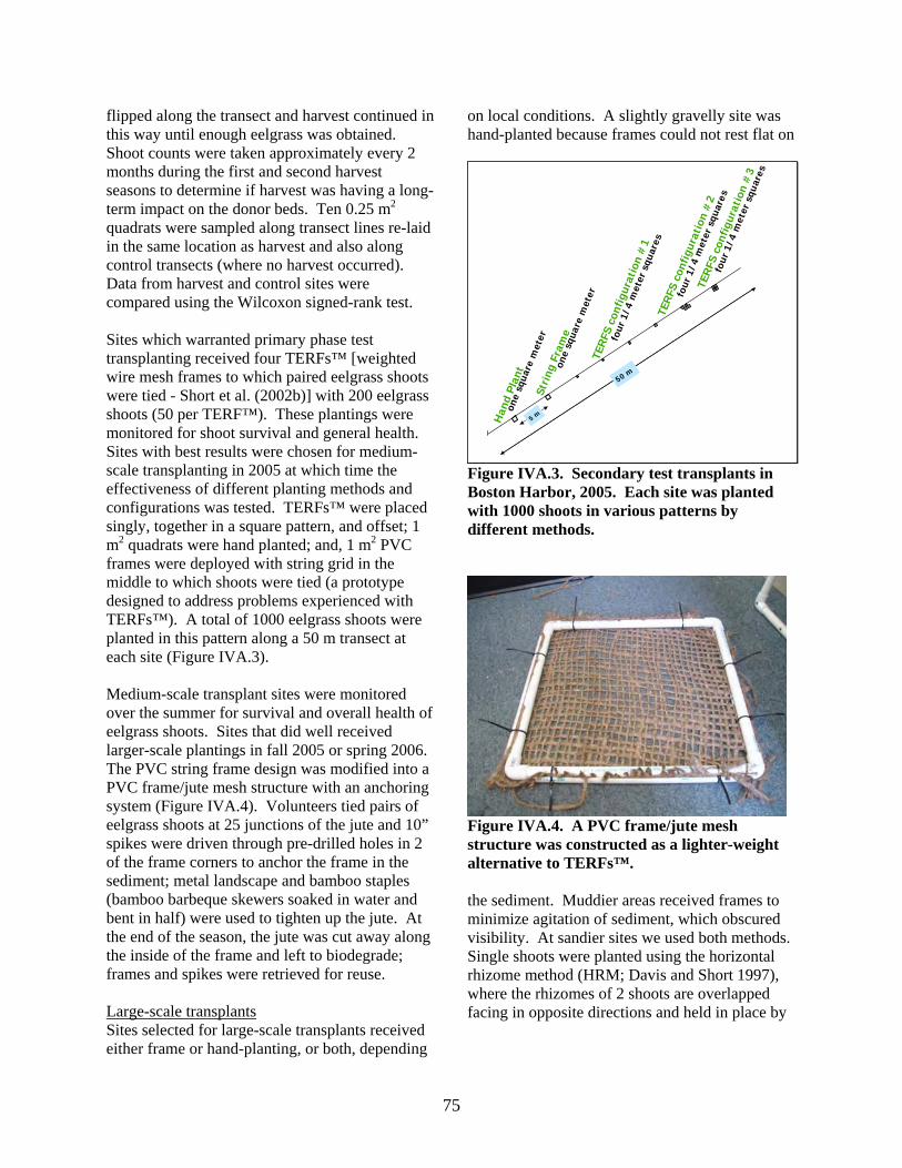
m quadrats were hand planted; and, 1 m2 PVC frames were deployed with string grid in the middle to which shoots were tied (a prototype designed to address problems experienced with TERFs™). A total of 1000 eelgrass shoots were planted in this pattern along a 50 m transect at each site (Figure IVA.3). Medium-scale transplant sites were monitored over the summer for survival and overall health of eelgrass shoots. Sites that did well received larger-scale plantings in fall 2005 or spring 2006. The PVC string frame design was modified into a PVC frame/jute mesh structure with an anchoring system (Figure IVA.4). Volunteers tied pairs of eelgrass shoots at 25 junctions of the jute and 10” spikes were driven through pre-drilled holes in 2 of the frame corners to anchor the frame in the sediment; metal landscape and bamboo staples (bamboo barbeque skewers soaked in water and bent in half) were used to tighten up the jute. At
of the frame and left to biodegrade; ames and spikes were retrieved for reuse.
qin the same location as harvest and also along control transects (where no harvest occurred). Data from harvest and control sites were compared using the Wilcoxon signed-rank tes Stransplanting received four Twire mesh frames to which paired eelgrass shoots were tied - Short et al. (2002b)] with 200 eelgrasshoots (50 per TERF™). These plantings were monitored for shoot survival and general health. Sites with best results were chosen for medium-scale transplanting in 2005 at which time the effectiveness of different planting methods and configurations was tested. TERFs™ were placsingly, together in a square pattern, and
2
the end of the season, the jute was cut away along the insidefr Large-scale transplants Sites selected for large-scale transplants received either frame or hand-planting, or both, depending
on local conditions. A slightly gravelly site was hand-planted because frames could not rest flat on
!
Han
d Pl
ant
5 m
50 m
Stri
ng F
ram
eon
e sq
uare
met
er
one
squa
re m
eter
TER
FS c
onfig
urat
ion
#1
four
1/4
met
er s
quar
esTE
RFS
con
figur
atio
n #
2
four
1/4
met
er s
quar
es
TER
FS c
nfig
urat
ion
#3
four
4
met
er s
quar
es
o 1/
ted Figure IVA.3. Secondary test transplants in Boston Harbor, 2005. Each site was planwith 1000 shoots in various patterns by different methods.
Figure IVA.4. A PVC frame/jute mesh structure was constructed as a lighter-weight alternative to TERFs™. the sediment. Muddier areas received frames tominimize agitation of sediment, which obscured visibility. At sandier sites we used both methods.Single shoots were planted using the horizontalrhizome method (HRM; D
avis and Short 1997), here the rhizomes of 2 shoots are overlapped
y wfacing in opposite directions and held in place b
75

76
n
atural Resources, and others; it is designed to continuous planting of
sessment of test- and medium-scale transplants was based on an assumed count of 50 shoots per square. However, at our large-scale planting sites we conducted baseline shoot counts within two weeks of planting to avoid compromising shoot survival estimates. This method accounted for: 1) bundler counting error, 2) more or less than 50 shoots actually being tied to the frames by volunteers, and 3) loss of shoots between the tying
stage and transport/placement of the string frames on sediment. Seeds
a bamboo staple. Clumps were either tied into bundles of approximately 50 shoots prior to planting or planted "as is” with divers simply pulling them out of the mesh bag and estimating 50 shoots per square. Clumps were held in place using several bamboo staples. Hand-planted squares and string frames were arranged in a checkerboard pattern by alternating eighteen planted and unplanted ¼ m2 quadrats (Figure IVA.5). The planted squares contained approximately 50 shoots each. This pattern was adapted from a strategy used by Save the Bay iRhode Island, the Maryland Department of Ncover more ground than shoots, while providing voids for eelgrass to fill asit spreads. Initially, four to eight of these grid plots, spaced 30-50 m apart, were planted at each large-scale site. More were added later. Survival as
Eelgrass reproduces sexually by producing seeds and also spreads asexually by rhizome expansion. To determine if we could successfully grow eelgrass from seed, twelve fish totes of flowering shoots were harvested from Nahant in July 2005. Flowering shoots are generally longer and lighter-colored than vegetative shoots and can easily be spotted and plucked by divers. Shoots break off near the base so no digging or rhizome
hoots
; Granger et al. 2002).
r
A.6). Sorted seeds were stored in lobster reisels (narrow cylindrical tanks with circulating
disturbance occurs. If left in place, these swould normally senesce and die after dropping their seeds (Orth et al. 1994 Shoots were maintained in flow-through seawatetanks at the Marine Biological Laboratory in Woods Hole for approximately six weeks until seeds ripened and dropped from the leaves. Thereafter, vegetation was discarded and seeds were collected and sorted from detritus using a series of sieves (Granger et al. 2002; Figure IVkwater) until late fall when they were planted. Approximately 300,000 seeds were
g alternating planted and unplanted ¼ m2
lant site. Figure IVA.5. Planting pattern showin
quadrats at a typical large-scale transp

Figure IVA.6. Clockwise from upper left: flowering shoots containing immature seeds; removing vegetation once seeds have dropped out; close-up of mature seeds; measuring seeds into bags for deployment.
collected and distributed at three sites to complement the shoot planting. Divers scratched seeds into the sediment using a small garden claw at two of the sites and simply broadcast the seeds from the boat at the third site. We repeated these methods with approximately the same number of seeds at different sites in 2007. In 2006 we tetechniqussociatlowering shoots were harvested as before, but ere transported directly to the planting site, here they were bundled in handfuls (average 22
hoots/bundle). Bundles were attached at tervals of 0.25-0.5 m along a continuous length
f twine using a simple slip knot (Figure IVA.7a). he lines trailed behind the boat (Figure IVA.7b) nd were staked to the seafloor in a zig-zag attern by divers (Figure IVA.7c).
Monitoring
sted an innovative seed planting e in an attempt to reduce time and costs
ed with the previous year’s methods.
Several measures of habitat structure and function were used to compare habitat function of our transplant sites to that of pre-existing natural beds and an unvegetated control site. Measures included survival and expansion, assessment of faunal communities, and habitat structure. Data were collected in July 2006 and 2007 from four
l beds
and 2006, and an unvegetated control site near some of the planted sites. In 2007 we also conducted monitoring at one of the seeded areas. Shoot density and size of plots were used to assess survival and expansion. Sites were evaluated for these parameters at the end of the summer for spring plantings and the following spring for fall plantings.
aFwwsinoTap
locations: a pre-existing Boston Harbor naturaahant donor site, our transplanted bed, the N
from 2005
77

a b c
undled t
ce per year for the uration of the project.
ned
f
th H) (also
nown as Shannon-Weaver or Shannon-Wiener) measures the chance of correctly predicting the species of the next individual collected. Simpson’s Diversity (1-D) index is the probability that two individuals randomly selected from a sample will belong to different species (Krebs 1999). Though commonly used in ecology, the Shannon index assumes random sampling from an infinitely large population and that all species in the area sampled are present in the sample. These are assumptions that are rarely true in benthic monitoring efforts (Pielou 1975; Magurran 1988; Maciolek et al. 2004). Since infaunal organisms could not be identified to species level in all cases, these analyses of
a,
to be two different, though unidentified, pecies.
of
he percent contribution of the two most important species. We selected several easily-measured proxies to evaluate habitat function (Evans and Short 2005). Three-dimensional structure was measured as shoot density, two-sided leaf area index (LAI), canopy height, and above-ground peak eelgrass biomass. Data were tested using Shapiro-Wilk W test for non-normality. The non-parametric Kruskal-Wallis test was employed for each parameter, and then for all pair-wise comparisons (between sites in each year, and between years for each site) to determine significance at P< 0.05. StatsDirect statistical software version
Figure IVA.7. Handfuls of seed shoots tied in btrailing behind the boat (b). Planting pattern us Thereafter shoot density and areal coverage monitoring continued at least on
es along a length of twine (a). String of bundles o stake down bundles (c).
Calculations of abundance were made for all taxincluding those identified only to higher taxonomic levels. Calculations based on species (i.e., species richness, evenness, diversity, and dominance) included only those taxa identified to species level or those treated as such (67 of 76). For example, Oligochaete spp.1 and Oligochaetespp. 2 were treated as species because they wereknown
d To compare epibenthic/demersal and benthic faunal communities, we examined abundance, species richness, evenness, and diversity among sites and between years. Abundance was defias the total number of organisms found at a site. Species richness (S) refers to the number ospecies found at each site. Evenness (relative abundance of the species present) was calculated using Shannon’s Equitablility (EH) index. Species diversity indices take into account borichness and evenness. Shannon’s (k
diversity were performed with several caveats.
s The top 3 contributors to the percentage of total species at each site were determined. An indexdominance (McNaughton 1967) was calculated asthe sum of t
78

2.6.5, available online, was used m(http://www.statsdirect.co ). Shannon and
also
n was used for hannon’s Equitability.
s in
005
ssed
d
d
over seine or other net urveys for several reasons: depths at the sites
ling
A survey was t was
al ets in
phyte cover.
ached the quadrats, 30
f each organism was sed in analyses. Species with large numbers
access. One of each pair of divers “crawled” a gloved hand along the substrate at each quadrat to
tion of core size and number sampled. wenty 4.9 cm diameter core samples were taken
rab ites, all cores were taken
here eelgrass was growing. Clear flow-through e
brought to the boat, where they were mptied and washed with seawater into a 0.5 mm
and
s fixative to samples in ambient seawater to equal approximately 10% of
and
re
imes into
s
Simpson diversity indices and their SDs werecalculated using StatsDirect. Microsoft Excel Statistical Package Add-iS Survival and expansion Density was based on the mean shoot density count from nine 0.25 m2 quadrats in each plot ± SD. To determine areal cover, we measured and multiplied distance between outermost shootperpendicular directions. Epibenthic and demersal species monitoringTen 1 m2 quadrats were distributed randomly within each site in one of two ways. At our 2and 2006 transplant sites, distribution of the ten quadrats among the plots was determined with arandom numbers table. Quadrats were tofrom the boat into the planted areas at low tide when they were visible. At harvest, natural, control, and seeded sites, quadrats were attacheat random intervals along a 50 m transect line (tofacilitate finding them in poor visibility conditions) and pushed overboard. In all cases, sampling of quadrats was delayed for a minimum of ½ hour after placement to allow any disturbefish and invertebrates to return to the area. A diver survey was chosensmade other methods extremely difficult and planted plots were too small for effective trawwhich could also damage and uproot recent
scare epibenthic fauna out of hiding. Benthic infaunal species monitoring We followed the University of New Hampshire, Jackson Estuarine Lab Standard Operating Procedures and the San Francisco Wetlands Regional Monitoring Plan protocols for samplingbenthic infauna in eelgrass habitats, with modifica
transplants. Since a visual SCUBthe only feasible method in transplant plots, ideployed throughout all sites for consistency. Pratt and Fox (2001) found that underwater visutransects sampled more species than gillnmedium and heavy macro Two divers slowly approquickly assessed the species present in the firstseconds, and then more carefully counted and recorded numbers of each species. The divers observed each quadrat at the same time and the higher-recorded number ou(over 100) were estimated to the nearest 100 up to1000, and then as 1000+. In vegetated plots, eelgrass was parted several times to gain visual
total volume, and several drops of Rose Bengal stain solution (4 g/L) were added to stain organisms and facilitate sorting (Raz-Guzman Grizzle 2001; Holme and McIntyre 1984; Mudroch and MacKnight 1994). Samples weleft in dilute formalin until they were processed inthe laboratory. They were then poured through a 0.25 mm mesh sieve and rinsed several ta waste collection container. After rinsing, samples were returned to jars with tap water in which they were stored in a refrigerator for a maximum 4 days before sorting (most samplewere sorted on the same day as transfer). Samples were sorted in Petri dishes
Tby divers from well-distributed, haphazard locations within each site. This method was chosen to minimize damage to transplanted beds that would have occurred with larger cores or gsamplers. At vegetated swcores were inserted approximately 15 cm into thsediment and capped. Divers capped the bottom of the cores as they removed them from the sediment. Cores wereemesh sieve (Eleftheriou and Holme 1984, Tetra Tech, Inc. 1987). Large pieces such as stonesshell debris were discarded after being rinsed and examined for organisms. Samples remaining afterflushing were washed into labeled collection jars.Buffered formalin (4 oz. borax per gallon 40% formaldehyde) was added a
79

during examination with a dissecting microscope. Animals stood out with Rose Bengal stain and were removed with tweezers to small labeled collection vials containing 70% ethyl alcohol folater identification. Organisms were ide
r ntified to
pecies where possible by ENSR, Inc., Woods
of l.
in g d
”.
t each 1 m2 quadrat, divers placed a 0.25 m2 arting in the
rat each
shoots .
n
tes de or
ere then placed separately in a pre-weighed foil drying oven (60°C).
sHole, MA and data recorded in an Excel spreadsheet. Posterior fragments were discarded. Habitat structure monitoring Faunal presence and diversity in eelgrass beds have been correlated with the physical structurethe habitat (Evans and Short 2005, Fonseca et a1990). Trained divers estimated percent cover of eelgrass, macroalgae, and sessile invertebratesthe same 1 m2 quadrats used to count fauna alontransects. Algae and invertebrates were identifieto species where possible or otherwise recorded as e.g., “un-id’d red algae, un-id’d sponge Aquadrat in a quadrant of the square, stupper left corner and rotating clockwise with eachsuccessive 1 m2 quadrat. This 0.25 m2 quadwas further divided with string into quarters, of which was 0.0625 m2 (Bosworth and Short 1993; Evans and Short 2005). We countedwithin the 0.25 m2 quadrat to obtain shoot densityTo calculate LAI and aboveground biomass we cut and removed all above-ground vegetatiofrom within two of the four 0.0625 m2 subsections. In the lab, ten shoots from each sample were haphazardly chosen; length and width of these leaves were measured to the nearest mm, and leaf area calculated. LAI (m2 leaf per m2 area of seafloor) was calculated as 2-sided leaf area times density (Evans and Short 2005; Hauxwell et al. 2003). To determine epiphyte cover in the field, we estimated percent of the leaf area covered with epiphytes. In the lab, epiphywere scraped from leaves using a glass slidull knife. All leaves and epiphytes from each site wpouch and dried for 48 hr in a Dry leaves and epiphytes were then weighed toobtain biomass in g per m2 (Westlake 1965; Phillips 1990). Canopy height was measured in situ (80% of mean of maximum length shoots from each quadrat).
Efficiency of Harvest and Planting Methods An efficiency analysis of hand- vs. frame-plantingwas conducted by recording the number of person-hou
rs spent by divers, boat handlers, and horeside volunteers, vs. the number of shoots
splanted in this effort. Results were averaged for 2planting days. The efficiency of the "clump harvest method" vs. the single shoot method was investigated. Number of shoots harvested and planted per dive hour (time spent in the water by divers) was calculated for each method. We used the same checkerboard pattern described above with 50 shoots planted in each square. Modeling of seed shoot movement We modeled the movement of seed shoots from pre-existing natural beds to areas which wesuitable for eelgrass in the Harbor in order to determine whether our restoration efforts were redundant, i.e., would eelgrass have colonized the Harbor without our efforts. Our previous field surveys had indicated that existing remnant bthe source of reproductive shoots, may be scarceor non-existent in areas affected by water qualdegradation, thereby severely limiting available seed stock. We also investigated whether seeds from our selected sites were
found
eds,
ity
likely to populate ther suitable areas.
e used the model GNOME™ (General NOAA perations Modeling Environment) to investigate
the potential path of seed shoots that become
se it is de and current driven, it was applicable in our
to
e objects tion
o WO
detached from "parent" plants and float to the surface. GNOME™ is primarily used to simulate the movement of oil after a spill, but becautiresearch question. The model was first run to evaluate the distribution of seed shoots from historical (remnant) beds in Boston Harbor. The simulation was re-run using our successful transplant locations as start points to determine whether seeds from our transplants were likelyre-vegetate other suitable areas. We used Boston Harbor inputs of 1) wind typical for the time of year when seed shoots are maturing (early-mid-July) obtained from the NOAA National Data Buoy Center, 2) floating non-degradabl(representing seed shoots), and 3) 2-week dura
80

(the maximum time eelgrass shoots remain buoyant, and by which time they have dropped two-thirds of their seeds (Harwell and Orth 2002a)). (Massachusetts Bay current data were not included in the model inputs, which maaffect distribution of shoots after they leave Boston Harbor, but they are not considered to significantly impact the results within Boston Harbor. The Nahant/Revere beds were also included in a model run, but did not affect results and were therefore left out of future model runs for simplicity). Results and Discussion
y
Evaluation of Harvest Method Shoot densities measured at harvest and controsites in the Nahant do
l nor bed are presented in
igure IVA.8. Differences were not significant vest
in
F(p>0.05) in all comparisons of control vs. haron any date, suggesting that our harvest methods had no detrimental impact on shoot density donor beds.
Shoot density at harvest and control sites
9/5/2006
Date
0
100
200
300
400
500
600
700
800
7/12/05 9/14/05 11/1/05
Sh
oo
t d
en
sity
(m
-2)
Harvest
Control
Figure IVA.8. Eelgrass shoot densities at donor site in Nahant in 2005. Control and harvest data on each date were compared using the Wilcoxon signed-rank test. Error bars are ± SD. Site selection and test transplants The GIS map generated from the original PTSI scoring (Figure IVA.9A) was a starting point in our site selection process. The majority of the blue area (PTSI score of 0) was the result of unsuitable depth or exposure. This effectively focused our search along shallow segments of theshoreline that were protected from NE storm winds. Of the potential
transplant areas originally entified with the PTSI output, six were
d nd
e
ith the
d
from
dary e
far n
ival at the Thompson Island site as high; however, the grass looked very
ith epiphytes and sily when
ne,
and ing plants looked very healthy. The
significant excavation by crabs (bioturbation) under TERFs™ at Long Island and Peddocks Island SE sites may have caused most of the eelgrass mortality, rather than poor growing conditions. Further planting by alternative methods was therefore pursued at these sites. Four sites, Long Island South (LIS), Peddocks SE (hence also referred to as “Peddocks”), and Weymouth were selected for secondary test transplants in the fall of 2005, with the intention of also planting Long Island North (LIN) in spring 2006.
ideliminated due to presence of a marina, high energy environment, or incorrect depth, i.e., too
shallow or too deep. The boat traffic associatewith marinas makes transplanting impractical apotentially dangerous. Riprap reflects the wakes generated in shipping channels, creating energetic conditions unsuitable for eelgrass growth. FigurIVA.9B shows the PTSI scores once the USGSsediment map layer was removed after groundtruthing revealed its inaccuracy in shallow water. Figure IVA.9C depicts the scoring wMarineFisheries sediment layer created from groundtruthing and the resulting limited area for restoration. Twelve sites remained viable after sediment groundtruthing using Short model guidelines anwere selected to receive test transplants (Figure IVA.10). Shoot survival after primary test transplanting with four (4) TERFs™ ranged5% - 90% (Table IVA.3). However, several factors in addition to shoot survival influenced the decision to continue planting at a site after both primary and secontest transplants were completed. Sediment at thRainford E sites proved unsuitable; there were more rocks and kelp than had been apparent othe initial visit, and despite initial high survival shoots later disappeared and the site was eliminated. Survwunhealthy, was covered wsediment, and up-rooted very eaTERFs™ were removed. Because of these factors, and the prevalence of extremely soft, fianoxic sediment, the Thompson Island site was eliminated as was Lovell Island which was too shallow and gravelly to support eelgrass. Despite mediocre survival rates at some of the Long Islsites, remain
81

82
B A
C
Figure IVA.9. Results of PTSI scoring with USGS sediment layer (A). Higher scores indicate greater suitability for eelgrass growth based on the Short model. PTSI map with problematic USGS sediment layer removed (B) and PTSI scoring with MarineFisheries sediment layer (C).
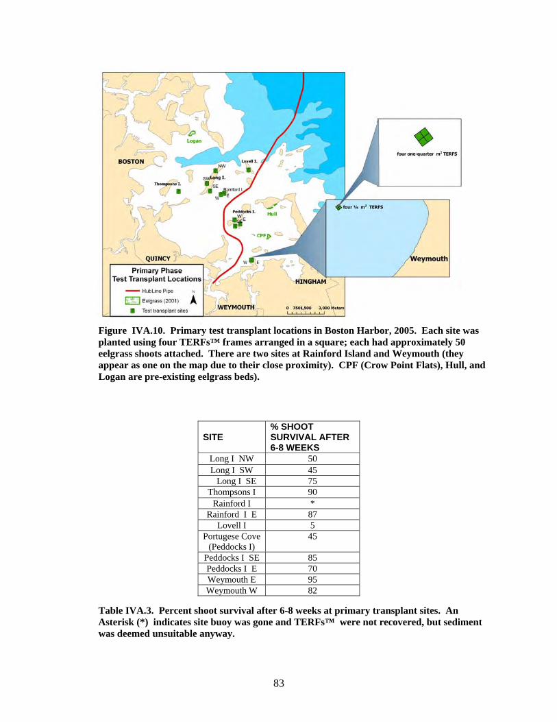
Figure IVA.10. Primary test transplant locations in Boston Harbor, 2005. Each site was planted using four TERFs™ frames arranged in a square; each had approximately 50 eelgrass shoots attached. There are two sites at Rainford Island and Weymouth (they appear as one on the map due to their close proximity). CPF (Crow Point Flats), Hull, and Logan are pre-existing eelgrass beds).
ot survival after 6-8 weeks at primary transplant sites. An Asterisk (*) indicates site buoy was gone and TERFs™ were not recovered, but sediment was deemed unsuitable anyway.
SITE % SHOOT SURVIVAL AFTER 6-8 WEEKS
Long I NW 50 Long I SW 45
Long I SE 75 Thompsons I 90
Rainford I * Rainford I E 87
Lovell I 5 Portugese Cove
(Peddocks I) 45
Peddocks I SE 85 Peddocks I E 70 Weymouth E 95 Weymouth W 82
Table IVA.3. Percent sho
83

Combined shoot survival with TERFs™ at four secondary transplant sites ranged from 54-67%. However, these numbers may be artificially low for two reasons: 1) Percent survival was based on a planned baseline of 50 shoots per 0.25 m2 TERF™, rather than a follow-up baseline count as we did later. The initial survival estimates from test transplants are therefore more useful in relative, rather than absolute, terms. Later survival estimates were more strongly correlated with follow-up baseline counts. 2) In general, we found that hand-planted shoots did much better than those in TERFs™ due to crab bioturbation under TERFs™ and uprooting of shoots during removal of the frames. Prototype string frames showed potential; when they remained anchored, shoots did well and looked healthier than those in the TERFs™. Hand-planted quadrats remained free of excavation and did very well. Evaluation and selection of final sites was therefore subjectively based orather thequipmeseconda
eelgrass was healthy, would be most conducive to eelgrass growth. The pattern in which TERFs™ were planted (Figure IVA.11) appeared to have less effect on survival than the planting technique (i.e., hand plant vs. TERFs™ vs. "string frames"). There was no statistical difference in survival among the single, offset, and square patterns of TERFs™ except at Peddocks (Figure IVA.11). Here the offset arrangement did poorly, but crab excavation was again an important factor in these results. A single-factor ANOVA was used to determine whether differences in survival were evident between planting patterns at each site. Such differences were not significant (P > 0.05) at any site except Peddocks Island, where the offset pattern displayed significantly poorer survival than the other two patterns (p =0.01). This result is also likely due more to crab excavation than TERFs™ arrangement.
n health and vigor of remaining plants an strictly survival. It was felt that once nt and techniques had been perfected, the ry transplant locations, where remaining
Large-scale transplants LIS, LIN, Weymouth, and Peddocks SE were selected for large-scale planting. Some sites winvestigated further which led to additional plantings at Portuguese Cove (Figure IVA.12).
ere
Percent shoots remaining in different TERF arrangements after 2 wk
0
10
20
30
40
50
60
70
80
Weymouth Peddocks SE IN LIS
Perc
ent s
urv
ival
L
single
offset
square
Figure IVA.11. Percent s grass shoo anted in various patterns at four sites in Boston Harbor, 2005. -scale tes ansplant, four TERFS™ were
l.
quare. N=12 at each site.
urvival of eel ts plIn the medium t tr
arranged in each of three patterns at four sites to assess the pattern's effect on surviva"Single" TERFs™ were placed linearly 5 m apart along a transect. "Offset" TERFS™ were laid in a checkerboard pattern. In the "square" pattern, 4 TERFS™ were laid adjacent to each other to form a s
84

Eight grid plots were initially planted at LIS in fall 2005, four hand-planted and four with framesalong two 150 m transects, respectively, boundingapproximately one acre. Peddocks SE (frames) and Weymouth (hand-plant) were each plantwith 4 plots in a square pattern, and encompassed ~ ½ acre per site. In spring 2006, Portuguese Cove and LIN were planted with 6 and 4 plorespectively (plot size varied at these sites bon amount of eelgrass available from harvest), using a combination of hand- and frame-planting. More plots were added at each site through sprin2007. Figure IVA.13 depicts plot configuration.
,
ed
ts, ased
g
his occurred to varying degrees t the other sites.
ing
sy
Much of the area bounded by buoys at LIS filled in with eelgrass; ta String frames PVC string frames (Leschen et al. 2006) plantedin fall 2005 were left in place during the followwinter. Those planted in spring 2006 were retrieved at the end of the summer after eelgrassshoots had rooted. The string frames proved eawith which to work, deploy, and retrieve and their spiked anchoring system effectively prevented frame-shifting (Figure IVA.14).
Figure IVA.12. Large-scale transplant sites planted in 2005 and 2006.
85

Figure IVA.13. Enlargements of each large-scale transplant site and respective areal coverage.
Figure IVA.14. Photos of PVC frame in situ (left) and after frame has been removed (right). Note that jute is silted over.
86

Also, there were few crab excavations events with PVC frames (with the exception of Portuguese Cove), in contrast to our experience with TERFs at these same sites. While restoration efforts in other areas have experienced significant damage from green crabs, this species caused little or no destruction in our study area, despite its presence in low densities. Excavations at our sites were caused by Cancer spp. crabs and juvenile lobsters. The jute mesh silted over fairly rapidly at all sites except Portuguese Cove, allowing eelgrass to root. Eelgrass within the frames generally increased greatly in density. However, expansion beyond the frames was limited since the PVC apparently provided a significant, though not insurmountable, barrier to vegetative spreading. This confinement was primarily a problem for frames planted in spring, which, in the future, could be resolved by removing the frames earlier in the summer. Seeds Initial monitoring of seed germination in late April 2006 appeared to indicate a low germination
rate (<1%) at both Peddocks SE and LIS from seeds planted in 2005. However, our site survey in July 2006 revealed a large, flourishing bed of eelgrass at the LIS seed-planting site. This bed continued to expand throughout the summer and by the end of August covered almost 180 m2 (Figure IVA.15). Assessment in spring 2007 revealed an area of 3100 m2 harboring at least some tufts or bunches of eelgrass which spread from the original 2005 seed planting (Figure IVA.16); by fall 2007 most of the area exhibited fairly dense growth. Growth at Peddocks from the 2005 seed planting was less extensive and harder to measure due to poor visibility, nevertheless, this site showed promising growth and expansion. The LIN site, where seeds were simply broadcasted, covered approximately 100 m2 by fall 2007. This cover was much less than at sites where divers scratched the seeds into the sediment. The additional, minimal effort by divers may have helped to conceal seeds from grazers and facilitated germination.
igure IVA.15. Seed planting progression at LIS; initial sparse germination eventually spread into large, dense bed.
Spring 2006
Summer 2007 Spring 2007
Fall 2006 Summer 2006
Fa
87

(3117)
1000
2000
3000
Are
al c
over
age
(m2)
(181)(60)
0
2005 2006 2007
Year
t
vestigation of these sites over summer 2007 little if any growth. We speculate that
e seeds; hermit crabs were observed carrying oots away while we were staking bundles.
herefore, in 2007, we reverted to the highly ccessful 2005 seeding method.
s of our seed planting efforts corroborates that of other projects (Orth et al. 2006; Pickerell et al. 2005; Maryland Department of Natural Resources). Seeding populated far more ground with eelgrass than our shoot transplant efforts, with a much smaller investment of time and resources. Large numbers of seed shoots can be harvested in 1-2 days, and splanted days. Additional tiexpense are involved in storing the seeds in a flow-through seawater tank and sieving the contents; but, overall, effort per area colonized is much less than transplanting shoots. Restoration efforts must still rely upon the site-selection process and test transplant stages to identify areas where seeds are likely to grow and spread. However, seed planting sho red as
Figure IVA.16. Areal coverage of seeded site aLIS, 2005-2007. In May 2007, the area at LIS which was seeded in 2006 with staked reproductive shoot bundles, showed sparse shoot germination. At LIN only one or two shoots were observed. Further inshowedgrazers, much more active in July when these shoots were staked out, may have eaten most of thshTsu The succes
eeds me and in another 1-2
uld be considean option to enhance the more labor- intensive shoot transplanting method.
Monitoring of Survival and expansion Eelgrass plots planted in 2005 were evaluated in spring 2006. Initial survival of 2005 plantings ranged from 41% (Weymouth) to 89% (PeddockSE). At Weymouth, few shoots survived the winter, and those remaining were in poor condition. We the
s
refore decided to eliminate this ite. Peddocks E and LIS were evaluated for
er,
on. PVC string frame (hereinafter “frame”) and hand planting at LIS 05 yielded similar survival rates. Expansion by the following spring (2006) was variable. For example, Weymouth shoots (frames) declined continuously throughout the monitoring period until only a few shoots remained. At LIS 05, densities in hand-planted plots expanded only 71% vs. 127% for frame plantings, but at Peddocks SE, density in hand-planted quadrats expanded 116%. Initially high density increases in frames at LIS 05 and hand plantings at Peddocks SE slowed by the summer. In contrast, the initial slow density increase at LIS
planted sites accelerated during this riod. As a result, by r 2006, shoot
density was fairly even across all 2005 sites (except Weymouth). Sites planted in spring 2006 showed expansion by the following fall which ranged from 20% to 193% (Table IVA.4). LIN frame plantings did extremely well (193% expansion) while hand plantings doubled (93%). At Portuguese Cove, excavation by crabs and
considerably better (78%expansion) than frames (20%).
sdensity and expansion in spring and again in August/September, 2006. Spring 2006 plantings at LIN and Portuguese Cove were evaluated for survival/shoot density expansion in the summer/fall of that year (Table IVA.4). More plots were added to all of the remaining sites over the 2006 field season, and into 2007. Hereaft2005 and 2006 plantings are distinguished, e.g. LIS 05 represents plots planted at Long Island South in 2005 and LIS 06 plots were planted in 2006. Planting method did not appear to make a difference in survival in 2005 nor was it a consistent determinant of plot expansi
05 hand-pe Septembe
approximately
lobsters resulted in hand-planted areas faring
88

89
Table IVA.4. Survival and shoot density expansi nd "frames" refers to planting method. "Overall" method. "Survival" is the percent of originally plan s the percent increase above the original planting density nitored for expansion in the fall. Eelgrass planted in la survival. NA = planting did not occur at that site ong Island North.
2005 Plantings
on for 2005 and 2006 plantings. "Hand" ais the average of all plantings, regardless of ted shoots remaining alive. "Expansion" i. Eelgrass planted in the spring was mote summer was monitored a month later for and time; LIS=Long Island South; LIN=L
Site Plant method
planting to Oct 05
Survival from Sept 05
Shexfal06
oot density pansion from l 05 to spring
Shoot density expansion from spring 06 to summer 06
Total shoot density expansion since planting
Weymouth frames 40.6% -35.0% -65.7% -86.0% overall 68.2% 95.3% 137.5% 210.4% frames 66.6% 126.7% 25.5% 205.2% LIS hand 69.6% 71.1% 186.4% 241.3%
Peddocks E hand 88.6% 116.2% 93.1% 283.0% 2006 Plantings
Site Plant method
Shexsp06
oot density pansion from ring 06 to fall
Survival from Aug 06 planting to Sept 06
overall 144.1% NA frames 192.9% NA Area A hand 93.2% NA
LIN
Area B hand NA 78.9% Area A hand 61.5% NA
LIS Area B hand NA 81.4%
overall 48.8% NA frames 19.8% NA
Portuguese Cove
hand 77.8% NA

Both LIN and LIS sites planted in August 2006, howed high survival one month later (~80%;
re were 2 plots at the southernmost end of the LIS site which had virtually disappeared. Prevailing currents run north along that area of shoreline, and we speculate that seeds produced in the plots were carried northward, filling in the northern segment of the LIS site, but leaving few seeds to re-populate the southernmbeds. It is also possible these plotcrab damage, becau very cdoing exceptionally plo the s IS h ed with th d by the time plots w red in Se2 t was no lon le to dist e two from one another. The 7 mean areal cover
at LIS 05 excluded that plot and also the plots that had virtually disappeared at the southernmost end.
Both 2005 sites increased significantly in areal covererage each year after planting (P<0.05 in all cases; Figure IVA.17). The difference between Peddocks and LIS 05 sites did not differ significantly in an ensity
ific 20 c dg en h pattern, except that 2006
7 densitie up re w erence be two sit or t in 2007 as signhigher at Peddocks th 5.
sTable IVA.4). In summer 2007, all sites (LIS, Peddocks SE, LIN, and Portuguese Cove) looked healthy and most plots showed substantial shoot density increases and areal expansion (Figure IVA.17), with two exceptions. In one case, the
The second exception was in 4 plots at LIN, where 2 plots had decreased in size, one had expanded slightly, but one had expanded significantly, accounting for the large SD seen in Figure IVA.17 for that site.
ost s had localized lose by were t nearest
se areas well. The
eeded area at L ad merg e seed beere measu ptember
007; i ger possib 200
inguish th
y year. Dantly betweenontinued to trennificantly differe sames did not trend
at Peddocks 05 and 2006, upward, 2007 t from 2006.
ward. The
increased signand, although itdata were not siLIS 05 showed tand 200
as no diff tween the es in 2005 2006, bu density w ificantly
an LIS 0
2005 Plant gs
0
5
10
15
20
5
30
Me
an
are
al c
ove
r (m
2 )
in
2
35
Peddocks
LIS 05
2006 Plantings
0
50
100
ea
n a
rea
l co
ve
150
Mr
(m2 )
Port. Cove
LIN 06
0
20
40
60
80
2005 2006 2007
De
nsi
ty (
sho
ots
0.2
5 m
-2)
100
120
140
160Peddocks
LIS 05
0
50
1
1
2006 2007
nsi
ty (
sho
ots
0.2
5 m
-2)
00
50Port. Co
De
ve
LIN 06
Figure IVA.17. Mean density and areal cover (± SD) over the duration of the project (2005-
2007) of plots planted in 2005 (LIS and Peddocks SE) and 2006 (Portuguese Cove and LIN).
90

At 2006 sites, there were no significant differences in areal cover between sites or yearThere was more crab damage at Portuguese Covthan anywhere else, yet density increased significantly there between years, and was significantly higher than at LIN 06 in 2007.
s. e
ll four large-scale planting sites exhibited
ites. LIS
.
of
ahant. The sites planted in 2006, LIN and Portuguese Cove, showed evidence of between-plot spreading. Again, spreading seemed to be in either density increase (Portuguese Cove) or areal expansion (LIN 06), but not both.
Ahealthy eelgrass, growth, and expansion, however, the patterns of growth differed among sshowed the most between-plot spreading, with all voids within the periphery of planted plots and seeded area filled or filling in (likely via seeds originating from planted plots and the seeded bed). Individual planted plots were also spreading considerably, but with modest density increasesPeddocks SE plots expanded, but there was little between-plot spreading; the length and density the eelgrass at this site exceeded all other transplant sites including the healthy donor bed at
Sediment Monitoring
N
Using results from BU’s sediment analysis, we compared grain size composition among exisbeds, successful transplant sites and 4 that faiThompson Island, two at Rainford (prelimtest transplants), and Weymouth (other sites that failed after preliminary trans
ting led:
inary
plants for reasons uch as gravel, kelp, and boat traffic were
t
vels did not exceed Koch’s recommended levels at any sites except slightly at Thompson Island and Logan (pre-existing bed; Figures IVA.19 and IVA.20). However, levels at our Peddocks sites were higher than the LI sites. TOC levels there were close to those at Weymouth and Thompson, and sulfide levels at the Peddocks sites exceeded those at Weymouth and Thompson.
sexcluded from the analysis). Sites with 35% or less silt/clay were successful. Those with >57% silt/clay failed (Figure IVA.18). All but one of the failed sites had less than Shoret al.’s (2002a) recommended <70% silt/clay (Rainsford, 75%), and would not have been eliminated under that model. Though we had no data points between 35 and 57%, all of our successful sites, and all of the existing beds, had <35% silt/clay. Surprisingly, sulfide and TOC le
Percent silt/clay by site
0
20
40
60
80
LIN
LIS
Peddo
cks S
E.
Portu
gues
e Cov
e
Rainfo
rd S
Rainf
ord
SW
Thom
pson
Wey
mou
th
Crow P
oint F
lats
Hull
Loga
n
Nahan
t
Pe
rce
nt s
ilt/c
lay
Figure IVA.18. Percent silt/clay at successful (white bars) and failed (black bars) transplant sites,and existing beds (gray bars). Top (dashed) line is recommended maximum per Short model. Middle (solid) line is maximum found at our successful sites. Bottom (dotted) line is maximum recommended by Koch (2001).
91

A. Sulfide cosectio
ncentrations of core
n in top and bottom , June 2005
0
Crow Pt. o
utside
Crow Pt. s
parse
Hul
2
4
6
8
Ln
(C
on
cen
trat
ion
+1)
l dense
Hull outsi
de
Hull
e N
W1
ong I NW
Lon sparse
Logan dense
Logan outside
Logan spars
Long I
L
2g I S
E
Long I SW
Peddocks I
E
Peddocks I
SE
PeddW
eock
s I W
Rainford I
Thompson I
Weym
outh E
ymouth W
Top
Bottom
ln Maximum threshold (5.99) Koch (2001)
Sulfide concentraticore
6
8
n +
1)
on in t, Sept
0
2
4
Crow P
t. ou
tside
Crow P
t. sp
arse
Hull d
ense
Hull o
utsid
e
Hull s
pars
e
Loga
n de
nse
Loga
n ou
tside
Loga
n sp
arse
Long
I NW
Long
I SE
Long
I SW
Peddo
cks I
E
Peddo
cks I
SE
Peddo
cks W
Thom
pson
I
Weym
outh
Ln
(C
on
cen
trat
io
op and bottom sections of ember 2005
ln Maximum threshold (5.99)
Koch (2001)
Top
Bottom
B.
Figure IVA.19. Porewater sulfide concentrations (converted to ln) at existing eelgrass beds and potential transplant sites in Boston Harbor in June (A) and September (B) 2005. In existing beds (Hull, Logan, Crow Pt.—see Figure IVA.10), "dense" and "sparse" refer to a dense, central part of the bed and the sparse edges, respectively. "Outside" refers to just beyond the boundary of the bed where there is no eelgrass. "Top section" = upper 5 cm of the core; "Bottom section" = remainder of core (core compossandy/sreplicat
length ranged from 9.4 - 17.5 cm due to collection techniques and sediment ition). Sites where concentration is zero either had too little porewater to test (typical of ilty sediment) or tested below the detectable limit of sulfide, 0.21 μM. (The mean of
exhibited anomalously large differences.) e sample values was graphed when the data
92

93
A. Percent pore water TOC at existing beds and potential transplant sites, June 2005
Max. recommended threshold (5%) (Koch 2001)
0
1
2
3
4
5
6
Crow P
t. ou
tside
Crow P
t. sp
arse
Hull d
ense
Hull o
utsid
e
Hull sp
arse
Loga
n de
nse
Loga
n ou
tside
Loga
n sp
arse
Long
I NW
1
Long
I NW
2
Long
I SE
Long
I SW
Peddo
cks E
Peddo
cks I
SE
Peddo
cks I
W
Rainfo
rd I
Thom
pson
I
Wey
mou
th E
Wey
mou
th W
Per
cen
t T
OC
Top section
Bottom section
B. Percent pore water TOC at existing beds and potential transplant sites, September 2005
Max. recommended threshold (5%) (Koch 2001)
0
1
2
3
4
5
6
Crow P
t. de
nse
Crow P
t. ou
tside
Crow P
t. sp
arse
Hull dens
e
Hull outsi
de
Hull spa
rse
Loga
n de
nse
Loga
n ou
tside
Loga
n sp
arse
Long
I SE
Long
I SW
Long
NW
Peddo
cks I
E
Peddo
cks I
SE
Peddo
cks I
W
Thom
pson I
Weym
outh
Per
cen
t T
OC
Top section
Bottom section
Figure IVA.20. Percent Total Organic Carbon (TOC) at existing beds and potential
transplant sites in Boston Harbor in June (A) and September (B) 2005. The length of the core from the Weymouth E site in June did not permit a bottom section analysis.
Water quality parameters were acceptable at all attempted transplant sites, minimizing macroalgal and epiphytic effects, and grain size composition was the only potential detrimental factor we found in common among failed sites. There were no other obvious similarities between Thompson, Rainford, and Weymouth sites that would account for the transplant failures there. For example, the Weymouth site is in a protected cove exposed to
NW winds, whereas Thompson is more exposed,but to E winds; the Rainford coves have SW and SE exposure. Weymouth receives more ferry and other boat wakes, and although Peddocks SE also receives ferry wakes, its plantings have done very well. Rainford receives little in the way of ferrywakes, but experiences heavy weekend recreational boat traffic. The sediment at Thompson Island was more flocculent than at

Weymouth. None of the sites had large numbers of epibenthic bioturbators when surveyed in 2004, nor did excavation appear to be a problem for transplants at Weymouth or Thompson. Rainford shoots disappeared over the winter, during the absence of monitoring, so we could not determine whether excavation played a role. While it is possible that other unknown factors contributed to eelgrass failure at all three sites, it is more likely that sediment quality may be responsible. The exact mechanism by which high silt/clay content renders an area unsuitable for eelgrass transplant is unclear. Our sulfide analytical results (Figure IVA.19) do not implicate sulfide toxicity per se as the cause for eelgrass decline and death, unless thresholds are less than Koch (2001) recommends (although in that case we might have expected Peddocks SE to do poorly). TOC levels were also acceptable at most sites. Sediment at established eelgrass beds can be rich in organics and have low redox potential without adversely affecting the plants (Smith et al. 1988; Klug 1980; Thayer et al. 1984). It is possible, however, that eelgrass transplants become stressed in reducing environments often found in very fine-grained sediment. Much of the sediment at our failed sites was black-colored with a shallow redox layer indicating anoxic conditions. While eelgrass restoration programs have often used existing beds to determine baseline conditions for site selection, it is possible that transplants have different requirements than established beds. Seagrasses can ameliorate reducing conditions and resultant sulfide toxicity
releasing oxygen from their rhizome and root
Smith exygen
thus neutralizing the effects of high organic content (Koch et al. 2001; Lee and Dunton 2000; Brüchert and Platt 1996; Blackburn et al. 1994; Schlesinger 1991). In addition, if the sediment around the root zone is oxygenated, the plant does not have to continually send oxygen to the roots to maintain respiration in these structures. The supply of oxygen to the roots and surrounding sediment, where some diffuses, is therefore dependent on both the level of photosynthesis occurring in the leaves (Terrados et al. 1999; Smith et al. 1988; Nienhus 1983) and the demand of the roots for oxygen. If individual shoots, or even small clumps of eelgrass are transplanted into anoxic sediment, the net photosynthesizing biomass at the new site would be a fraction of that in the donor bed, thus making it more difficult for transplants to overcome an anoxic environment in very fine grained sediments. A study f Phragmites australis, an invasive salt marsh plant, found that severing rhizomes significantly lowered the photosynthetic rate of the plants, and that this effect was nearly double in anoxic vs. oxygenated sediment (Amsberry et al. 2000). If this effect is also true for eelgrass, severing the rhizomes during harvest would compound the already-diminished level of photosynthesis that occurs at a transplant site. The effort involved in attempting to keep roots oxygenated under these circumstances may stress the transplants to the point of death. Transplants, then, may need more oxygenated sediment than established beds until enough biomass is established to compensate for lower porewater oxygen in finer-grained sediments. The prevalence of unsuitable sediment throughout
ries
bysystems into the sediment (Terrados et al. 1999; Pedersen et al. 1998; Sand-Jensen et al. 1982;
much of Boston Harbor five years after the offshore outfall became operational (Figur
t al. 1984; Lee and Dunton 2000). e
IVA.21) raises concerns about the future Op
is produced in the leaves through possibilities for eelgrass restoration in estuahotosynthesis and delivered through the plant’s
lacunar system (Larkum et al 1989; Pedersen et al.1998; Smith et al. 1984) to the roots to support respiration in these non-photosynthesizing structures (Goodman 1995; Zimmerman et al. 1989). When light and photosynthetic biomass are plentiful, the oxygen released by the roots is able to keep reducing conditions at a minimum,
degraded by eutrophication. In areas where low flushing rates result in long-term deposition of organic matter, it may take years for sediment to recover enough to support eelgrass, even when water quality has improved. This issue will require further study as improvements are made to coastal water quality in other locations.
o
94

95
Figure IVA.21. Sediment type observedunderwater camera, Ponar grab
in B, or by diver
mud around the shoreline and the limited ar
oston Harbor. Data were gathered using an s taking cores. Note the prevalence of anoxic eas of suitable sediment.
Biological Monitoring Epibenthic/demersal species abundance and diversity From 2006 to 2007 Shannon diversity indices (H’for benthic and demersal fish and invertebrates increased at all Boston Harbor sites (Table IVAand Figure IVA.22); by 2007 our 2-year oldgenerated indices which exceeded those at and Hull. (There is no comparative data for the seed bed because it was first assessed in 2007.) The Simpson diversity index (1-D) increasemarkedly at our planted sites; there was little change in reference and control sites. By 2007, indices at our planted sites exceeded those at reference beds.
Evenness, measured by Shannon’s equitability (EH) index, exhibited a similar pattern.
)
.5 beds
Nahant
d
verall, diversity indices for our planted sites
ariation
es
d l, and
ber of individuals per m (N) declined markedly at Peddocks and LIS 05 which was primarily due to greatly reduced numbers of Mysis spp in 2007.
Owere comparable to or exceeded those of natural beds and the Control site. Total number of species (S) showed less vthan diversity between years at our planted sites.It did not change at Peddocks, but increased slightly at all other sites. Total number of speciat planted sites approached or exceeded the healthy natural donor bed at Nahant and exceedeHull and Control sites by 2007. Nahant, HulControl site data also exhibited slight increases in species number across years. Mean num
2

Since Mysis spp. can number in the hundreds or thousands and greatly influence all indices, the data are reported in two ways in Table IVA.5: with and without Mysis spp. A total list of epibenthic/demersal species is presented in Appendix IVA.A. Benthic infaunal species abundance/diversity There was a total of 71 species of infaunal invertebrates found at all the sites in 2006, and 69 in 2007 (Appendix IVA.B). In 2006 Pygosio elegans, a spionid polychaete, was among the top 3 dominant species at all sites except Nahant, and at all sites in 2007 (Table IVA.6 displays 2007 data). It comprised 33.7% and 55.3% of the total infauna in 2006 and 2007, respectively. All spionid polychaetes, combined,
comprised 63% of the top 3 dominants. Control and LIS seed sites exhibited the largest number of individuals (N) in 2007 (Figure IVA.23); they also had the highest dominance index, indicating that these N’s were in large part due to the presence of just 2 species. This dominance is reflected in the lower evenness and diversity indices for these 2 sites. Highest number of species, evenness, and diversity were found at Nahant. These indices were slightly lower at our planted sites. Measures of 3-D habitat function Percent cover of algae and sessile invertebrates was negligible in almost all quadrats, and never exceeded 5%. Epiphytes also comprised immeasurable or minute weight fractions of above-ground biomass at all sites.
Table IVA.5. Diversity indices of benthic and demersal samples at planted, reference and control sites. The LIS seeded site was not sampled until 2007. LIS 05 = Long Island South beds planted in 2005. LIN+LIS 06 represents combined data from Long Island South and North planted in 2006. Numbers in parentheses indicate the index with Mysis spp. excluded from analyses. There were no Mysis spp. seen at Nahant in 2006.
2 6
SPed
LIS 05 1.09 (1.68) 0.40 (.64) 15 (14) 188 (55)LIN06+LIS 06 .92 (1.41) 0.36 (.49) 12 (11) 174 (51)
1.54 0.64 (1.02) 0.56 (.53)
1 (.37) 9)
)82 (49)
).58).54)
Index00
ite Shannon (H') Pielou’s evenness value J' Total no. spp. (S) Number individuals m-2 (N)366 (33)docks 0.44 (1.51) 0.17 (.61) 13 (12)
NahantHull 1.16
11 238 (7) 59 (27)10 (9) 130 (8Control 1.18 (.82) 0.5
2007Peddocks 1.88 (1.72) 0.73 (.69
LIS 05 1.87 (1.97) 0.68 (.73)LIS06+LIN 06 1.67 (1.55) 0.60 (.57)
Nahant 1.55 (1.61) 0.59 (.63)Hull 1.36 (1.31) 0.55 (.55
Control 1.42 (1.39) 0.57 (LIS seeds 1.33 (1.13) 0.61 (
13 (12) 29 (26)16 (15)16 (15) 136 (89)14 (13) 42 (23)12 (11) 131 (67)12 (11) 122 (121)
9 (8) 117 (68)
96

2.0
Figure IVA.22. Indices of species diversity, abundance, evenness, and richness for epibenthic and demersal fish and invertebrates,
006 and 2007. Sites on x-axis are: Peddocks, ahant, LIS & LIN 06, LIS 05, Hull, Control, nd LIS seeds. LIS seeds was not monitored ntil 2007. H’ is Shannon diversity index; 1-D Simpson diversity index; EH is Shannon quitablility; S is number of species found at
ite; N is mean number of individuals per m2.
Figure IVA.23. Indices of species diversity, abundance, evenness, and richness for benthic infauna, 2006 and 2007. Sites on x-axis are: Peddocks, Nahant, LIS & LIN 06, LIS 05, Hull, Control, and LIS seeds. LIS seeds was not monitored until 2007. H’ is Shannon diversity index; 1-D is Simpson diversity index; EH is Shannon Equitablility; S is number of species
und at site; N is mean number of individuals er core.
2NauisEs
fop
0.0
0.4
0.8
1.2
1.6
H'
0
0
0.2
0.4
0.6
0.8
1
1-D
0.0
0.4
0.8
EH
0
5
10
15
20S
1
2
3
H'
0
100
200
300
Peddo
cks
Nahan
t
LIS06
+LIN
06
LIS 0
5Hull
Contro
l
LIS se
eds
N
2006
2007
0.0
0.2
0.4
0.6
0.8
1-D
1.0
0.2
0.4
0.0
0.6
0.8
1.0
Eh
20
30
40
50
S
0
10
0
50
100
150
Peddo
cks
Nahan
t
LINLI
S 06
LIS 0
5Hull
Contro
l
LIS se
eds
N
2006
2007
97

98
Table IVA.6. Top three numerical dominants with percent of total organisms of each species at each site in 2007. All are Annelids (polychaetes) except for Leptocheirus pinguis (Arthropoda/amphipoda). Index of dominance represents the percentage of total standing crops (N) contributed by the top 2 most num rous species (McNaughton 1967).
2006, the healthy reference donor bed in ahant exceeded our then-1 yr old beds in ensity, LAI, and biomass. In 2007, however, our o yr old beds were comparable to or exceeded
ahant, and surpassed Hull with respect to
he one year old beds (LIN/LIS 06) did not yet xhibit the structure of the two year old beds, owever, they are comparable to 2006 easurements at sites planted in 2005; if they
Site Top 3 dominants (% of total (N) at te) Family Index of dominance Peddocks Polydora cornuta (44.1%) Spionidae
Maldanidae spp (22.4%) Maldanidae 66.5 Pygospio elegans (6.6%) SpionidaeClymenella torquata (6.6%) Maldanidae
Nahant Exogone hebes (23.5%) SyllidaePygospio elegans (18.6%) Spionidae 42.1 Aricidea catherinae (7.4%) ParaonidaeMaldanidae spp (7.4%) Maldanidae
LIN/S 06 Pygospio elegans (33.9%) SpionidaePolydora cornuta (20.1%) Spionidae 54.0 Spiophanes bombyx (16.9%) Spionidae
LIS 05 Pygospio elegans (36.2%) SpionidaePolydora cornuta (19.3%) Spionidae 55.5 Spiophanes bombyx (7.3%) SpionidaeTharyx acutus (7.3%) Cirratulidae
Hull Pygospio elegans(34.7%) SpionidaeExogone hebes (32.7%) Syllidae 67.4 Polydora cornuta (12.1%) Spionidae
Control Pygospio elegans (62.2%) SpionidaeLeptocheirus pinguis (6.83%) Amphipoda 69.0 Polydora cornuta (6.7%) Spionidae
LIS seeds Pygospio elegans (72.7%) SpionidaeSpiophanes bombyx (6.7%) Spionidae 79.4 Exogone hebes (6.3%) Syllidae
e
si
InTNedhtwmNcontinue to follow the growth pattern of older transplants, we can expect that, by their second year, they, too, will reach parity with the referencedonor bed. Benthic infaunal composition was typical of healthy sand-mud sediment. Spionids, typically found more in non-complex habitats where a few opportunistic species do very well, were in fact more dominant at the Control and LISseed sites (which were still patchy), and were leastdominant at Nahant.
measures of 3-D habitat function. Peddocks equaled or exceeded Nahant with regard to all four measures: density, aboveground biomass, canopy height, and LAI (Figure IVA.24). LIS 05 equaled Nahant in biomass, canopy height, and density. In 2007, our 1 yr old beds (LINLIS 06) exhibited comparable measures of structure to those of the 2005 plantings, when they were 1 yr old (2006 results). Significance of interactions isgiven in Table IVA.7.

0
50
100
150
200
250
300
350
Ab
oveg
rou
nd b
iom
ass
(g
m-1
)
020406080
100120140160
Peddock
s
Nahan
t
LINLIS
06
LIS 0
5Hull l
Ca
nopy
hei
ght (
m)
Contro
LIS s
eeds
2006
2007
0
1
2
3
4
5
6
LAI
(m2 /m
2)
0
50
100
150
200
250
Sho
ot
den
sity
(sh
oots
/.02
5 m
2)
side
. IS
ce and diversity indicate that our successfully-planted
oach habitat functi ealthy natural donor bed outside Boston Harbor. In contrast, habitat structure decre ur habitat measures at the pre-existi d we monitored within Boston Harbor, i.e, Hull. Eelgrass at that site was patchier with leaves exhibiting more re-settled suspended sediment in 2007locati y well flushed and it may be suffering from localized water quality issues, possib ated by its position in a mooring field. ates tha ceived general trend of im for eelgrass has not been uniform Boston Harbor. It also emph need for ul site selection to locate those limited area reviously degraded estuar ay be conducive to restoration. The LIS seed bed values are diluted because the bed is still patchy; if zeroes are removed from the datasenarro Effici est an ting methods
Figure IVA.24. Measures of 3-D habitat function in areas monitored in 2006 and 2007. Control site = unvegetated. Nahant = healthy reference bedoutside Boston Harbor; Hull = reference bed inBoston Harbor. LIS seeds was seeded in fall 2005LIS 05 and Peddocks were planted in 2005. LIN/L06 were planted in 2006; data from these areas were combined. Error bars are ±SD. Because of the method used to calculate LAI, SD was not computed. Note: the drop in density at Nahant is likely due to the extraordinarily dense area randomly selected in 2006, rather than a decrease indensity of the bed as a whole in 2007.
The improvements in measures of both habitat structure and those of species abundan
beds are appr ing or exceeding theon of the h
ased in all fong natural be
than in 2006. Its on is not ver
ly aggrav This indic t a perproved suitability
throughoutasizes the caref
s in pies which m
t the gap between it and the 2006 beds ws.
ency of harv d plan An ef alysis was conducted to evaluate harvesting rates and hand vs. frame planting (Tabl Practiced divers harvested an average of 671 shoots/h s number dropped to 450 s teer divers participated, likely due to their inexperience. Hand-planting
MarineFisheries personnel was 390 hoots/person h (dive time plus boat helmsman),
g by
fference is
if
ficiency an
e IVA.8). . Thi
hoots/h when volun
rate byscompared to 82 shoots/person h for frame plantinwhich also included number of hours invested dive, boat, and shore personnel. This dimagnified (390 vs. 64) if time invested in stringing the frames is also included. However,only dive hours expended in both planting techniques are counted, hand planting is less efficient than frame planting (441 shoots/h vs. 740 shoots/h, respectively). This gap narrows when dive time for retrieving frames is included (441 shoots/h vs. 542 shoots/h).
99

Table IVA.7. Habitat structure: significance of interactions between sites monitored in 2006 (light gray), in 2007 (dark gray), and at each ite between 2006 and 2007 (white). LIS seeds and LINLIS06 were only monitored in 2007 (**) denotes P< 0.01.
s; (*) denotes significant difference at P < 0.05;
Shoot densityNahant Hull Peddocks LIS 05
.0067** 0.0022**0.9714 0.86240.0263* 0.99990.0447* 0.241.0027** 0.0719 LIS seeds
0.0154* 0.9999 0.0969
eddocks LIS 050.5819 0.24520.8239 0.99990.0209* 0.77690.7506 0.0588.0019** 0.008** LIS seeds
0.0377* 0.4084 0.044**
eddocks LIS 050.8248
Nahant 0.0001** 0.0022** 0Hull 0.0221* 0.0005**Peddocks 0.0134* 0.003**LIS 05 0.9993 0.0499*LIS seeds 0.0373* 0.9982 0LINLIS 06 0.9977 0.0318*
Aboveground biomassNahant Hull P
Nahant 0.4406 0.0933Hull 0.0065** 0.0004**Peddocks 0.6566 0.0021**LIS 05 0.999 0.0112*LIS seeds 0.044* 0.999 0LINLIS 06 0.9347 0.005**
Canopy heightNahant Hull P
Nahant 0.512 0.0007** 0.0353*Hull 0.018* 0.0012** 0 0.0005**Peddocks 0.9925 0.0031**LIS 05 0.8957 0.0049**LIS seeds 0.1293 0.9999 0LINLIS 06 0.5514 0.0402* 0
.0009**0.0139* 0.28020.0526 0.7608.0045** 0.0591 LIS seeds.0043** 0.1738 0.7647
nting methods using trained MarineFisheries r person-hour includes time invested by divers, e-h includes hours invested by divers onl
MF+ shore nteers (frames)
Shoots/dive h only (handplant)
Shoots/dive h only (frames)
441 740
per person hour
plaots pe
hoots/div y.
Table IVA.8. Efficiency of different harvest and(MDMF) personnel and volunteers. Mean shoboat handlers, and shoreside volunteers. S
MDMF only MDMF + volunteer divers
MDMF (handplant)
Planting hours only 671 450 390
Includes time for stringing and retrieving frames
Mean Harvest Plant
MDvolu
82
64 542
shoots
100

101
ome method.
Table IVA.9. Efficiency of single shoot vs. clump harvesting and planting (dive time only). Numbers are mean shoots per person-hour. Percent difference is between the 2 methods. HRM=horizontal rhiz
Plantshoots/h % difference shoots/h % difference
Single shoot/HRM 300* 300
271% 158%Clump 814 475
Harvest
*exactly the number reported in Davis and Short (1997) The "eelgrass clump" method proved much more efficient for both planting and harvesting than the single shoot/HRM methods (Table IVA.9). Divers using the clump method were able to harvest 171% more shoots and plant 58% more shoots per person h than divers employing the single shoot/HRM methods. This analysis did not count time expended in bundling shoots for HRM, an unnecessary step for the clump method, which would increase the time differential between the two methods. The efficiency and apparent lack of negative impact on donor beds of the clump method (Leschen et al. 2006) provide justification for its use in areas where donor beds are sufficiently robust. The survival and eventual expansion of beds planted by the 2 methods should be studied further to determine if results differ significantly, but so far our planted plots how no evidence of a difference.
and planting can be accomplished efficiently by or more experienced divers. On several ccasions, 2 trained MarineFisheries divers ansplanted 1000-3000 shoots (harvest and plant) one day. While larger scale efforts can result in
Frame-planting was much less efficient than hand-planting, based on time invested, because of the number of steps involved. Volunteers are needed to string frames, sort and bundle shoots, and tie shoots in pairs onto the mesh of frames (25 pairs/frame) which are then deployed by divers.
rames must be retrieved at a future date and re-trung for re-use. Conversely, once shoots have een hand-planted, the task is completed (except
onitoring). However, frame planting
provides a means for the non-diving public to be involved, and offers hands-on educational opportunities if within the goals of a restoration effort. Volunteers can also be employed in a hand-planting operation to bundle shoots (Short et al. 2002b; Sue Tuxbury, personal communication), although in our study area the distance between our harvest sites and a suitable shore base made this step prohibitively inefficient. These instances highlight factors that must be considered in deciding which planting method and scale to use. The goals of the restoration program, available time, staff resources, including diving vs. shore-side volunteers, and tidal amplitude and resulting water depth in which volunteers would be working must be taken into account. In some coastal bays and rivers, much of this work can be done by snorkelers or even waders at low tide. This was never an option in Boston Harbor due to the steep tidal amplitude, short period of shallow depth available during low tide, and distance from shore; these factors limited our use of in-water volunteer workers to SCUBA divers.
s H2otrina greater numbers of shoots planted, such efforts also involve more coordination, divers, equipment, and boats.
Modeling of seed shoot movement The paucity of suitable sediment in formerly eutrophic estuaries has implications for natural re-colonization of eelgrass, in addition to limiting possible restoration sites. GNOME™ model results showed it was improbable that seed shoots from existing bed locations would naturally disperse to the most suitable areas within Boston Harbor to grow new beds. During the first simulation, hypothetical “shoots” were “spilled” at existing bed locations and spent 14 days adrift, but few shoots came near Long or
Fsbfor m

Start
Day 5
Day 1
Day 10
Boston Long I.
Peddocks I.
igure IVA.25. Selected output from GNOME™ m
ed b site selecti
re we t in the Harbor (Figure
A.25). According to the model output, the
to
ffort
ts,
ong the western coast Long Island, in the Peddocks SE cove, and
F odel run for 14 days. "Shoots" (black dots) y arrows) in Boston Harbor to ascertain if they
on process as suitable for eelgrass (purple were "spilled" at remnant eelgrass beds (indicatwould spread over areas identified in theovals). Peddocks Islands, the only locations whefound suitable sedimenIVlikelihood that floating reproductive shoots will pass over good eelgrass habitat is low. Furthermore, the probability that those few shoots which approach good sites actually sink and/or drop seeds there, and that those seeds go on germinate and survive, decreases with each step. Since natural re-colonization appears unlikely,
these results support the use of a restoration eto "jump-start" the growth of eelgrass in Boston Harbor. In contrast, when the simulation was re-run using our successful transplant sites as starting poinshoots were delivered throughout the Harbor, including a large number alof some in Portuguese Cove (Figure IVA.26).
102
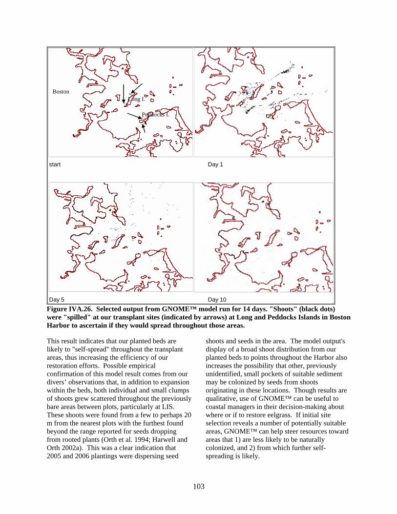
start Day 1
Day 5 Day 10
BostonLong I.
Peddocks I.
Figure IVA.26. Selected output from GNOME™ model run for 14 days. "Shoots" (black dots) were "spilled" at our transplant sites (indicated by arrows) at Long and Peddocks Islands in Boston Harbor to ascertain if they would spread throughout those areas. This result indicates that our planted beds are
kely to "self-spread" throughout the transplant
ur n s
20
d rth 2002a). This was a clear indication that 005 and 2006 plantings were dispersing seed
shoots and seeds in the area. The model output's display of a broad shoot distribution from our
olonized by seeds from shoots
ard
colonized, and 2) from which further self-spreading is likely.
liareas, thus increasing the efficiency of our restoration efforts. Possible empirical confirmation of this model result comes from odivers’ observations that, in addition to expansiowithin the beds, both individual and small clumpof shoots grew scattered throughout the previouslybare areas between plots, particularly at LIS. These shoots were found from a few to perhaps m from the nearest plots with the furthest found beyond the range reported for seeds dropping from rooted plants (Orth et al. 1994; Harwell an
planted beds to points throughout the Harbor also increases the possibility that other, previously unidentified, small pockets of suitable sediment may be c
O2
originating in these locations. Though results are qualitative, use of GNOME™ can be useful to coastal managers in their decision-making about where or if to restore eelgrass. If initial site selection reveals a number of potentially suitable areas, GNOME™ can help steer resources towareas that 1) are less likely to be naturally
103

104
Outreach We received help during this Project from 155 volunteer shore workers and divers who provided 428 hours of assistance with harvesting and planting (Fig. IVA.27). These included volunteers from several corporate groups, Odyssey High School, National Park Service, Boston Single Volunteers, Norfolk County House of Correction, New England Aquarium, Boston’s Environmental Ambassadors to National Parks (BEAN) program, Genzyme, Clear Forest, State St. Corp., Boston University Marine Program, local dive clubs, and many individuals. Many MarineFisheries’ divers also participated. MarineFisheries’ biologists gave presentations to staff at the New England Aquarium; to meetings of a Stellwagen Bank Sanctuary work group; the Massachusetts Bays Program; the Quincy Beaches and Coastal Commission; and also to the public on a catamaran tour of the Harbor sponsored by the National Park Service as part of its “Biodiversity Days”. Other public outreach efforts included a presentation on a day-long biodiversity event for about 50 Earthwatch Institute employees who cruised Boston Harbor while learning about, and participating in, various research and restoration projects occurring there. Our involvement with local school systems included Boston’s Odyssey High School GIS class
which used data from our research efforts as a real-life example to help them learn the mapping software. Members of Odyssey’s after-school program completed the design of a logo which we used on t-shirts supplied to all volunteers. MarineFisheries staff also delivered a presentation to a career explorations class at Hull High School; to a group of Charlestown High School students who participated in the Courageous Sailing Program in Boston; and to Massachusetts Marine Educators at University of Massachusetts, Dartmouth. Children at the Marion Natural History Museum after school program also enjoyed learning about eelgrass from our staff. Eelgrass project personnel appeared on a Martha’s Vineyard cable television program to talk about eelgrass and water quality with several other local biologists. Project activities and results were communicated through updates of the HubLine Eelgrass Restoration Project website and numerous news and magazine articles. Presentations were made to professional peers including a poster at the spring New England Estuarine Research Society meeting in Hull; a poster at the USEPA conference: “Celebrating aquatic habitat restoration in Massachusetts” in Ipswich in May 2007; an invited talk in a special section on urban estuaries at the September 2007 Annual American Fisheries Society meeting in
Figure IVA.27. Some of the many volunteers that helped on this project.

San Francisco; oral and poster presentations at the
mer rs
n .
by ivers from MarineFisheries, EPA, and Metcalf &
n
grass
urvival and expansion rates were recorded at 4 of
new sediment guidelines). Planting technique had no effect on eelgrass survival or expansion. Our light-weight PVC string frames experienced fewer excavations from crustaceans than TERFs™, however, hand-planted plots were free of bioturbation. Seeding populated far more ground with eelgrass than our shoot-transplant efforts with a much smaller
y
a arbor in
even
r
ithin
hat
tal
MarineFisheries’ projects contributed data and/or SCUBA assistance: Coastal Lobster Investigations, Shellfish, and Environmental Impact Assessment. David Taylor and Ken Keay, MWRA kindly provided environmental data, and Charlie Costello, DEP contributed historical SAV distribution information. George Hampson and Pam Neubert provided helpful assistance with initial benthic infaunal investigative procedures.
Estuarine Research Federation conference in November 2007 in Providence, R.I.; talks at the annual meeting of eelgrass scientists and managers at EPA, Boston, and at the sum2007 meeting of the Mass. Shellfish OfficeAssociation on Martha’s Vineyard. A talk wasalso delivered at the Restore America’s Estuaries conference in October 2008. Project staff participated in a multi-agency effort to harvest eelgrass from Gloucester Harbor in aarea targeted for construction of a CSO pipelineApproximately 7000 shoots were harvesteddEddy. Shoreside volunteers from CZM, MIT Seagrant, Winthrop Middle School, Gloucester Maritime Heritage Center, and other interested Gloucester citizens assisted with shoot bundling. These shoots were subsequently planted in BostoHarbor by MarineFisheries divers to augment restoration efforts there. Conclusions We successfully restored over 5 acres of eelto a previously degraded estuary, Boston Harbor,by intensively focusing on site selection, with particular attention to sediment quality. High s5 of our large-scale sites (the exception, Weymouth, would have been eliminated under
investment of time and resources. The efficiencof checkerboard plot planting saved time and effort while allowing transplanted eelgrass to eventually fill in open spaces within the pattern. Planted beds were comparable or exceeded healthy natural bed outside of Boston Hboth habitat function and diversity of species inhabiting them. Our choice of planting locations was severely constrained by unsuitable sediment, which persisted throughout much of Boston Harbor5 years after elevated wastewater treatment andimproved water quality were realized. These results have important implications for otheestuaries where water quality improvement projects are undertaken. Such efforts may need tobe combined with increasing flushing rates wthese areas via dredging or other means in order to clear out accumulated depositional sediment twill impair eelgrass growth. Acknowledgements Dr. Ryan Davis assisted in the collation and evaluation of available Boston area environmendata sets during year #1 of the Eelgrass Restoration Project. A formal, comprehensive GIS analysis of all data layers was developed and initiated with the help of MarineFisheries Research Analyst Micah Dean. Other
105

Literature Cited Amsberry, L., M. A. Baker, P. J. Ewanchuk, M.
D. Bertness. 2000. Clonal integratthe expansion of Phragmites australis. Ecol Appl 10:1110-1118.
Batuik, R. A., P. Bergstrom, M. Kemp, E. Koch,
L. Murray, J. C. Steve
ion and
nson, R. Bartleson, V. Carter, N Rybicki, J. Landwehr, C.
ical .
n crophytes. Ecology
67:1328-1340.
gation l
velopment project in Portsmouth, New Hampshire. New
tion,
w Bay, FL, USA. Geochim Cosmochim Acta 13:2325-2332.
ardoso, P. G. M. A. Pardal, A. I. Lillebø, S. M. Ferreira, D. Raffaelli, J. C. Marques. 2004. Dynamic changes in seagrass assemblages under eutrophication and implications for recovery. J Exp Mar Biol Ecol 302:233-248.
to
aters. Limnol Oceanog 14:454-458.
g
uarte, C. M. 1995. Submerged aquatic vegetation in relation to different nutrient
a 4:87-112.
16. In: os.
ssessment,
vans, N. T. and F. T. Short. 2005. Functional trajectory models for assessment of transplanted eelgrass, Zostera marina L., in the Great Bay Estuary, New Hampshire. Estuaries 28:936-947.
onseca, M. S., W. J. Kenworthy, and G. W. Thayer. 1998. Guidelines for the conservation and restoration of seagrasses in the United States and adjacent waters. Center for Sponsored Coastal Ocean
Gallegos, L. Karrh, M. Naylor, D. Wilcox, K. Moore, S. Ailstock, M. Teichberg. 2000. Chesapeake Bay submerged aquatic vegetation water quality and habitat-based requirements and restoration targets: a second technsynthesis. USEPA, Annapolis, Maryland205 p.
Barko, J. W. and R. M. Smart. 1986. Sediment-
related mechanisms of growth limitatioin submersed ma
Blackburn, T. H., D. B. Nedwell, W. J. Wiebe.
1994. Active mineral cycling in a Jamaican seagrass sediment. Mar Ecol Porg Ser 110:233-239.
Bosworth, W. and F. T. Short. 1993. Miti
plan for the New Hampshire commerciamarine terminal de
Hampshire Department of TransportaPort Authority, Bedford.
Brüchert, V. and L. M. Pratt. 1996.
Contemporaneous early diagenetic formation of organic and inorganic sulfur in estuarine sediments from St. Andre
Carlson, P. R., Jr., L. A. Yarbro, and T. R. Barber. 1994. Relationship of sediment sulfidemortality of Thalassia testudinum in Florida Bay. Bull Mar Sci 54:733-746.
Cline, J. D. 1969. Spectrophotometric
determination of hydrogen sulfide in natural w
C
Davis , R. C. and F. T. Short. 1997. Restorin
eelgrass, zostera marina l., habitat using a new transplanting technique: the horizontal rhizome method. Aquatic Botany 59:1-15.
Davis, R. C., F. T. Short, and D. M. Burdick.
1998. Quantifying the effects of green crab damage to eelgrass transplants. Restoration Ecology 6:297-302.
D
regimes. Opheli Eleftheriou, A. and N. A. Holme. 1984.
Macrofauna techniques. p. 140-2Methods for the Study of Marine BenthN.A Holme and A.D. McIntyre (eds). Blackwell Scientific Publications, London.
Estrella, B. T. 2005. Hubline Impact A
Mitigation and Restoration: Annual Progress Report of the Massachusetts Division of Marine Fisheries to the Executive Office of Environmental Affairs, July 1, 2004-June 30, 2005. 46 pp.
E
F
106

Research, NOAA Coastal Ocean Program. 221 p.
Fonseca
ng natural and transplanted eelgrass Zostera marina
Frederik mer, J.
s in a
uatic
Goodma
n. 1995. Photosynthetic responses of eelgrass (Zostera marina L.) to light
r
Granger, S., M. S. Traber, S.W. Nixon, R. Keyes.
2002. A practical guide for the use of
essing,
ansett, R.I.. 20 pp.
Harwell
. Harwell 2b. Seed-bank
patterns in Chesapeake Bay eelgrass 6-
Hauxwe
(Zostera marina) decline I temperate estuarine ecosystems.
Hauxwe .
ate
fect of light limitation imposed by algae. Mar Ecol Prog Ser 247:59-73.
Heck, J
meadows: Species composition, seasonal rison with
9-
edges, J. I. and J. H. Stern. 1984. Carbon and
Holme, N. A. and A. D. McIntyre, eds. 1984.
Methods for the study of marine benthos,
. Holmer ment
sulfur dynamics related to biomass-a
11-
ine .
Hughes
ver, and A. Wright. 2002. The effects of eelgrass habitat loss on estuarine fish
.
Jacobs, nd
f eelgrass, Zostera marina L., at Roscoff,
Kemp,
he
, M. S., W. J. Kenworthy, D. R. Colby, K. A. Rittmaster, G. W. Thayer. 1990. Comparisons of fauna amo
meadows: criteria for mitigation. Mar Ecol Prog Ser 65:251-264.
sen, M., D. Kruase-Jensen, M. HolS. Laursen. 2004. Long-term changearea distribution fo eelgrass (Zostermarina) in Danish coastal waters. AqBotany 78:167-181.
n, J. L. K. A. Moore, and W. C. Denniso
and sediment sulfide in a shallow barrieisland lagoon. Aquat Bot 50:37-47.
seeds in eelgrass (Zostera marina L.) restoration. Part 1: Collection, procand storage. M. Schwartz (ed.), Rhode Island Sea Grant, Narrag
, M. C. and R. J. Orth. 2002a. Long- distance dispersal potential in a marine macrophyte. Ecology 83:3319-3330
, M. C. and R. J. Orth. 200
(Zostera marina L.). Estuaries 25:1191204.
ll, J., J. Cebrián,, C. Furlong, and I. Valiela. 2001. Macroalgal canopies contribute to eelgrass
Ecology 82:1007-1022.
ll, J., J. Cebrián, and I. Valiela. 2003Eelgrass Zostera marina loss in temperestuaries: relationship to land-derived nitrogen loads and ef
r., K. L., K. W. Able, M. P. Fahay, and C. T. Roman. 1989. Fishes and decapod crustaceans of Cape Cod eelgrass
abundance patterns and compaunvegetated substrates. Estuaries 12:565.
Hnitrogen determinations of carbonate-containing solids. Limnol Oceanog 29:657-663.
2nd ed. Blackwell Scientific Publications, Boston, Oxford
, M. and S. L. Nielsen. 1997. Sedi
density patterns in Zostera marin(eelgrass) beds. Marine Ecology Progress Series 146:163-171.
Homziak, J., M. S. Fonseca, and W. J.
Kenworthy. 1982. Macrobenthic community structure in a transplanted eelgrass (Zostera marina) meadow. Marine Ecology Progress Series 9:2221.
Huettel, M. and G. Gust. 1992. Impact of
bioroughness on interfacial solute exchange in permeable sediments. MarEcology Progress Series 89:253-267
, J. E. , L. A. Deegan, J. C. Wyda, M. J. Wea
communities of southern New EnglandEstuaries 25: 235-249.
R. P. W. M. 1979. Distribution aaspects of the production and biomass o
France. Aquatic Botany 7:151-172.
W. M., Boynton, W. R., Twilley, R. R., Stevenson, J. C., Means, J. C. 1983. T
107

decline of submerged vascular plaChesapeake Bay:
nts in A summary of results
concerning possible causes. Mar. Techn.
Klug, M
llips
em perspective. Garland STPM Press, New
Knebel .
ssachusetts. J Sed Petrol 61: 791-804.
Knebel,
etts
Knebel,
ronments within the Boston Harbor-Massachusetts Bay sedimentary system: a
31-
och, E. W. 2001. Beyond light: physical,
ion
opp, B. S. and F. T. Short. 2003. Status report
1.
ion Program. 62 p.
Krebs, C
arkum, A. W., A. J McComb, and S. A.
of to the
Lazarri, f
w water habitats of demersal fishes and decapod crustaceans in Penobscot
Lee, K.
rewater sulfide concentration in the seagrass Thalassia
as,
eschen, A. S., R. K. Kessler, and B. T. Estrella.
ine
vision of Marine Fisheries to the Executive Office of
Leschen ella.
s). In: Estrella, B.T. (ed). Hubline Impact Assessment, Mitigation, and
rt of ine
006-June 30, 2007. 94 pp.
Maciole
husetts Water Resources Authority. Report 2004-02. 96
Magurr
ress, Princeton.
Soc. J. 17: 78-89.
. J. 1980. Detritus-decomposition relationships, p. 225-246. In R. C. Phiand C. P. McRoy (eds.), Handbook of seagrass biology, an ecosyst
York.
HJ, R. R. Rendigs, and M. H. Bothner1991. Modern Sedimentary Environments in Boston Harbor, Ma
H. J. (1992) Sedimentary environments within a glaciated estuarine-inner shelf system: Boston Harbor and MassachusettsBay. Mar Geol 110:7-30.
Knebel, H. J. 1993. Sedimentary environments
within a glaciated estuarine-inner shelfsystem: Boston Harbor and MassachusBay. Marine Geology 110:7-30.
H. J. and R. C. Circé. 1995. Seafloor envi
regional synthesis. J Coastal Res 11:2251.
Kgeological, and geochemical parameters as possible submersed aquatic vegetathabitat requirements. Estuaries 24:1-17.
Kfor the New Bedford Harbor eelgrasshabitat restoration project, 1998-200Submitted to the New Bedford Harbor Trustee Council and the NOAA Damage Assessment and Restorat
. J. 1999. Ecological Methodology:
Second Edition. Addison Wesley Longman, Inc. Menlo Park, CA.
LShepherd (eds.). 1989. Biology of Seagrasses: A Treatise on the BiologySeagrasses with Special ReferenceAustralian Region. Elsevier, Amsterdam.
M.A. and B. Tupper. 2002. Importance oshallo
Bay, Maine. Env. Biol. Fish 63:57-66.
S. and K. H. Dunton. 2000. Diurnal changes in po
testudinum in Corpus Christi Bay, TexUSA. Marine Ecology Progress Series 143:201-210.
L2006. Eelgrass Restoration Project (status). In: Estrella, B.T. (ed). HublImpact Assessment, Mitigation, andRestoration: Annual Progress Report of the Massachusetts Di
Environmental Affairs, July 1, 2005-June 30, 2006. 92 pp.
, A. S., R. K. Kessler, and B. T. Estr2007. Eelgrass Restoration Project (statu
Restoration: Annual Progress Repothe Massachusetts Division of MarFisheries to the Executive Office of Environmental Affairs, July 1,
k N. J., R. J. Diaz, D. T. Dahlen, C. D. Hunt and I. P. Williams 2004. 2002 Boston Harbor Benthic Monitoring Report. Boston: Massac
p.
an, A.E. 1988. Ecological Diversity and Measurement. Princeton University P
108

McNau
4.
L. Nienhus 1983. Temporal and spatial
patterns of eelgrass (Zostera marina L.) in
rth, R. J., M. Luckenbach, K. A. Moore. 1994.
rth, R. J., K. L. Heck, Jr., and J. van Montfrans.
ries 7: 339-350.
Orth, R
Aquatic Botany 84:26-36.
.
Pickerel
5. Buoy-deployed seeding: Demonstration of a new eelgrass (Zostera
al
ielou, E. C. 1975. Ecological Diversity. Wiley,
New York.
Poppe,
processing, In: USGS East Coast
ratt, T. C. and M. G. Fox. 2001. Comparison of
one biol.
Rasmus
) and its effects on environmental factors and fauna, p. 1-
tific
Raz-Gu
f s.
ethods. F. s.). Elsevier
Science, B.V., Amsterdam.
Rex, A. . E.
s
9.
Sand-Je olm. 1982. Oxygen release from roots of submerged
. Schlesin n
hort, F. T., L. K. Muhlstein, and D. Porter. 1987.
ulletin 173:557-562.
Short, F.T. and D.M. Burdick. 1996. Quantifying eelgrass habitat loss in relation to housing
ghton, J. J. 1967. Relationships among functional properties of Californian grassland. Nature 216:168-169.
Mudroch, A. and S. MacKnight. (Eds). 199
Handbook of Techniques for Aquatic Sediments Sampling, Second Edition. Lewis Publishers, Boca Raton, F
, P. H.
a former estuary in the Netherlands dominated by human activity. Marine Technology Society Journal 17:69-77.
OSeed dispersal in a marine macrophyte: implications for colonization and restoration. Ecology 75:1927-1939.
O1984. Faunal communities in seagrass beds: a review of the influence of plant structure and prey characteristics on predator-prey relationships. Estua
. J., M. Luckenbach, S. R. Marion, K. A. Moore, and D. J. Wilcox. 2006. Seagrass recovery in the Delmarva Coastal Bays, USA.
Pedersen, O., J. Borum, C. M. Duarte, M. D
Fortes. 1998. Oxygen dynamics in the rhizosphere of Cymodocea rotundata. Mar Ecol Prog Ser 169:283-288.
Phillips, R. C. 1990. Transplant methods. In:
Phillips, R. C., McRoy, C. P. (eds). Seagrass Research Methods. UNESCO,Paris, pp.51-54.
l, C., S. Schott, and S. Wyllie-Echeverria. 200
marina L.) planting method. EcologicEngineering 25:127-136.
P
L.J., Eliason, A.H., Fredericks, J.J., Rendigs, R.R., Blackwood, D. and Polloni, C.F., 2000. Grain-size analysis ofmarine sediments – methodology and data
Sediment Analysis: Procedures, Database, and Georeferenced Displays, USGS Open-File Report 00-358.
Ptwo methods for sampling a littoral zfish community. Arch. Hydro152:687-702.
sen, E. 1977. The wasting disease of eelgrass (Zostera marina
52. In C. P. McRoy and C. Helfferich (eds.), Seagrass ecosystems: a scienperspective. Marcel Dekker, New York.
zman, A. and R. E. Grizzle 2001. Techniques for quantitative sampling oinfauna and small epifauna in seagrasIn: Global Seagrass Research MT. Short and R. G. Coles (ed
C., D. Wu, K. Coughlin, M. Hall, KKeay, D. I. Taylor. 2002. The State of Boston Harbor: Mapping the Harbor’Recovery. Boston: Massachusetts Water Resources Authority. ENQUAD 2002-042 p. nsen, K., C. Prahl, H. Stokh
aquatic macrophytes. Oikos 38:349-354
ger, W. H. 1991. Biogeochemistry: AAnalysis of Global Change. Academic Press, San Diego. 443 pp.
SEelgrass wasting disease: cause and recurrence of a marine epidemic. Biological B
109

development and nitrogen loading in Waquoit Bay, Massachusetts. Estuar19:730-739.
ies
hort, F.T., A. C. Mathieson, and J. I. Nelson.
ng re
hort,
227:253-267.
Short, Fased
e Laboratory, University of New
Signell,
on
7:15, 591-15,606.
.
88.
s): ng
sediments. Mar Biol 98:131-141.
Stauffer, R. C. 1937. Changes in the invertebrate
the eelgrass. Ecology 18:427-431.
Taylor, of Deer
ter Resources Authority. Report ENQUAD
errados, J., C. M. Duarte, L. Kamp-Nielsen, N. . D.
reve.
175-
Tetra T ed protocols
for sampling and analyzing subtidal
Thayer, enworthy, and M. S.
Fonseca. 1984. The ecology of eelgrass
.
Thom, R
Pacific Northwest. Northwest Envir. J.
Tucker,
ces Authority. Report ENQUAD 2006-17. 69
Tutin, T
Valiela, I., K. Foreman, M. LaMontagne, D.
Coupling of watersheds and coastal
5:443-457.
. 51:445-
S1986. Recurrence of the eelgrass wastidisease at the border of New Hampshiand Maine, USA. Mar Ecol Prog Ser 29:89-92.
Short, F. T, R. C. Davis, B. S. Kopp, C. A. S
D. M. Burdick. 2002a. Site-selection model for optimal transplantation of eelgrass Zostera marina in the northeastern US. Mar Ecol Prog Ser
. T., C. A. Short, and C. L. Burdick. 2002b. A Manual for community-beelgrass restoration. Jackson Estuarin
Hampshire, Durham.
R. P. and Butman, B. 1992. Modeling tidal exchange and dispersion in BostHarbor. 1992. Journal of Geophysical Research 9
Smith, R. D., A. M. Pregnall, R. S. Alberte. 1984
Role of seagrass photosynthesis in root aerobic processes. Plant Physiol 74:1055-1058.
Smith, R. D., A. M. Pregnall, R. S. Alberte. 19
Effects of anaerobiosis on root metabolism of Zostera marina (eelgrasimplications for survival in reduci
community of a lagoon after disappearance of
D. I. 2006. 5 years after transferIsland flows offshore: an update of water-quality improvements in Boston Harbor. Boston: Massachusetts Wa
2006-16. 77 p.
TS. R. Agawin, E. Gacia, D. Lacap, MFortes, J. Borum, M. Lubanski, T. G1999. Are seagrass growth and survival constrained by the reducing conditions of the sediment? Aquatic Botany 65:197.
ech, Inc. 1987. Recommend
benthic macroinvertebrate assemblages inPuget Sound. For U.S EPA.
G. W., W. J. K
meadows of the Atlantic Coast: a community profile. United States Fish andWildlife Service. FWS/OBS-84/02. 147 p
. M. 1990. A review of eelgrass (Zosteramarina L.) transplanting projects in the
6:121-137.
J., S. Delsey, A. Giblin, and C. Hopkinson. 2006. 2005 Annual Benthic Nutrient Flux Monitoring Report. Boston: Massachusetts Water Resour
p.
. G. 1942. The autecology of Zostera marina in relation to its wasting disease. New Phytology 37:50-71.
Hersh, J. Costa, P. Peckol, B. DeMeo-Anderson, C. D'Avanzo, M. Babione, C.H. Sham, J. Brawley, K. Lajtha. 1992.
waters: sources and consequences of nutrient enrichment in Waquoit Bay, Massachusetts. Estuaries 1
Wanless, H. R. 1981. Fining-upwards sedimentary
sequences generated in seagrass bedsJournal of Sedimentary Petrology 454.
Westlake, D. F. 1965. Some basic data for
investigations of the productivity of
110

111
hitlatch, R. B. 1980. Patterns of resource
Zimmer R. D. Smith, and R. S.
Alberte. 1989. Thermal acclimation and
aquatic macrophytes. Mem. Ist. Ital. Idrobiol (Suppl), 18: 229-248.
Wutilization and coexistence in marine intertidal deposit-feeding communities. J. Mar Res 38:743-763.
man, C. F.,
whole plant carbon balance in Zostera marina L. (eelgrass). Journal of Experimental Marine Biology and Ecology 130:93-109.