arX

iv:g

r-qc

/970

3047

v1 1

8 M

ar 1

997

Submitted toNucl. Phys. B

MPI-PhT/97-20BUTP-97/08gr-qc/9703047March 18, 1997

Mass inflation and chaotic behaviour

inside hairy black holes

Peter Breitenlohner †, George Lavrelashvili ‡ 1

and Dieter Maison †

Max-Planck-Institut fur Physik †

— Werner Heisenberg Institut —Fohringer Ring 6

80805 Munich (Fed. Rep. Germany)

Institute for Theoretical Physics ‡

University of BernSidlerstrasse 5

CH-3012 Bern, Switzerland

Abstract

We analyze the interior geometry of static, spherically symmet-ric black holes of the Einstein-Yang-Mills-Higgs theory. Generi-cally the solutions exhibit a behaviour that may be described as“mass inflation”, although with a remarkable difference betweenthe cases with and without a Higgs field. Without Higgs field theYM field induces a kind of cyclic behaviour leading to repeatedcycles of mass inflation – taking the form of violent explosions –interrupted by quiescent periods and subsequent approaches to analmost Cauchy horizon. With the Higgs field no such cycles occur.In addition there are non-generic families with a Schwarzschildresp. Reissner-Nordstrøm type singularity at r = 0.

1On leave of absence from Tbilisi Mathematical Institute, 380093 Tbilisi, Georgia

1

1 Introduction

Most of the knowledge on the interior geometry of static black holes derivesfrom the well-known exact solutions like the Schwarzschild (S) and Reissner-Nordstrøm (RN) solution. Whereas for the S-solution the radial coordinatestays time-like inside the horizon all the way down to the central singularity,the RN-solution exhibits a second – inner – horizon, behind which the radialcoordinate becomes space-like again. This inner horizon is a so-called Cauchyhorizon, beyond which the evolution of any matter system is influenced bydata causally disconnected from the earlier history [1]. Furthermore, whilethe outer horizon is an infinite redshift surface, the Cauchy horizon is asurface of infinite blueshift. This suggests, that the Cauchy horizon shouldbe unstable against small perturbations and a space-like singularity shouldform replacing the former Cauchy horizon [2]. In fact, perturbative studiesindicate an exponential growth of the mass-function close to the inner horizon– a phenomenon dubbed “mass inflation” [2]. However, as yet no unanimousconclusion about the reliability and genericity of these perturbative resultsseems to have been obtained [3]. In this situation it is definitely of interest toinvestigate the internal structure of black holes with other forms of matterlike Yang-Mills and Higgs fields. This is the subject of the present study.Compared to the previously mentioned perturbative analysis our work is“exact”, although at least partially based on numerical results.

One may summarize these results saying that generically no Cauchy hori-zon forms, because its existence requires fine-tuning of the initial data at theouter horizon. Solutions with a Cauchy horizon are in fact obtained throughsuch fine-tuning, leading to a RN-type singularity at r = 0. Generically,however, the solutions exhibit “mass-inflation”, although with a remarkabledifference between the cases with and without a Higgs field. The behaviour isactually much simpler with the inclusion of a Higgs field. In this case the massfunction shows generically exponential growth all the way down to r = 0.On the other hand in the seemingly simpler case without the Higgs field thesituation is more involved. The YM field induces a kind of cyclic behaviourleading to repeated cycles of mass inflation – taking the form of violent “ex-plosions” – interrupted by quiescent periods and subsequent approaches toan almost Cauchy horizon. This behaviour is particularly spectacular due tothe fantastic growth of the mass function during these explosions by hundredsof orders of magnitude, a phenomenon unprecedented in standard physical

2

problems. Actually, these explosions become exponentially more violent af-ter each cycle such that it is practically impossible to follow more than oneor two of them numerically.

A further novel phenomenon is a kind of chaotic behaviour generatedby a hierarchical structure of families of non-abelian RN-type (NARN) andnon-abelian S-type (NAS) solutions separating generic solutions with cyclic(EYM) or acyclic (EYMH) behaviour.

Our numerical results exhibiting these claims are predominately basedon the EYM system, but we have no doubt that we could easily establishsimilarly convincing evidence in the EYMH case.

In this discussion the global behaviour outside the horizon was ignored.Clearly it is of interest to find out what is the behaviour of asymptotically flatsolutions, which for the EYM theory constitute a discrete set of 1-parameterfamilies – described by curves in the (Wh, rh) plane [4, 5]. Obviously withoutfurther restriction they will show the generic behaviour inside the horizon,although for certain discrete points S-type resp. RN-type singularities atr = 0 are possible.

In a recent paper [6] Donets et al. presented their results on the internalstructure of static, spherically symmetric black holes of the Einstein-Yang-Mills (EYM) theory (without Higgs field). Our results for this particularcase essentially agree with the findings of Donets et al., although we differin some details. In particular the chaotic stucture we find close to the basicNARN solutions was not observed in [6].

2 Ansatz and Field Equations

The contents of this chapter are essentially (up to minor changes in notation)a copy from our earlier paper [7], which we include for the convenience of thereader.

For the static, spherically symmetric metric we use the parametrization

ds2 = A2Bdt2 − dR2

B− r2(R)dΩ2 , (1)

with dΩ2 = dθ2 + sin2 θdϕ2 and three independent functions A, B, r of aradial coordinate R, which has, in contrast to r, no geometrical significance.

3

It is common to express B through the “mass function” m defined by B =1 − 2m/r.

For the SU(2) Yang-Mills field W aµ we use the standard minimal spheri-

cally symmetric (purely ‘magnetic’) ansatz

W aµTadxµ = W (R)(T1dθ + T2 sin θdϕ) + T3 cos θdϕ , (2)

and for the Higgs field we assume the form

ΦaTa = H(R)naTa , (3)

where Ta denote the generators of SU(2) in the adjoint representation. Plug-ging these ansatze into the EYMH action results in

S = −∫

dRA[1

2

(

1 + B((r′)2 +(A2B)′

2A2B(r2)′)

)

− Br2V1 − V2

]

, (4)

with

V1 =(W ′)2

r2+

1

2(H ′)2 , (5)

and

V2 =(1 − W 2)2

2r2+

β2r2

8(H2 − α2)2 + W 2H2 . (6)

Through a suitable rescaling we have achieved that the action depends onlyon the dimensionless parameters α and β representing the mass ratios α =MW

√G/g = MW /gMPl and β = MH/MW (g denoting the gauge coupling

and G Newtons constant).2

We still have to choose a suitable gauge for the radial coordinate R. Themost natural choice is R ≡ r, i.e. Schwarzschild (S) coordinates. However,this choice is singular at a stationary point of r(R) (‘equator’). Such singu-larities are avoided using the gauge B ≡ r−2 for B > 0 resp. B ≡ −r−2 forB < 0. We denote this radial coordinate by τ in order to distinguish it fromthe S coordinate r. With this choice the spatial part of the metric takes thesimple form

ds2 = r2(dτ 2 + dΩ2) , (7)

2 The usual quantum definition of MPl ≡√

hcG

is obtained from our classical expression

replacing the dimensionful classical gauge coupling g2 by the dimensionless g2

hcand putting

the latter equal to one.

4

suggesting to call them isotropic coordinates.Using S coordinates the field equations obtained from (4) are

(BW ′)′ = W (W 2 − 1

r2+ H2) − 2rBW ′V1 , (8a)

(r2BH ′)′ = (2W 2 +β2r2

2(H2 − α2))H − 2r3BH ′V1 , (8b)

(rB)′ = 1 − 2r2BV1 − 2V2 , (8c)

A′ = 2rV1A . (8d)

The equations obtained with isotropic coordinates B ≡ −r−2 are essentiallyEqs. (9) of [7], there are however some sign changes due to B < 0.

r′ = rN , (9a)

N ′ =(κ − N)N − 2U2 − V 2 , (9b)

κ′ =−1 − κ2 + 2U2 +β2r2

2(H2 − α2)2 + 2H2W 2 , (9c)

W ′ = rU , (9d)

U ′ =−W (W 2 − 1)

r− rH2W − (κ − N)U , (9e)

H ′ =V , (9f)

V ′ =−β2r2

2(H2 − α2)H − 2W 2H − κV , (9g)

together with the constraint

2κN = −1 + N2 + 2U2 + V 2 + 2V2 , (10)

and the definitions

N ≡ r′

r, κ ≡ (A2B)′

2A2B+ N , U ≡ W ′

r, and V ≡ H ′ . (11)

3 Singular points

The field Eqs. (8) are singular at r = 0, r = ∞ and for points where Bvanishes. Whereas the former singularities are of geometrical origin (theaction of the rotation group degenerates) the zeros of B turn out to becoordinate singularities, in fact, of two different kinds:

5

1. Points where B = 0, but A2B 6= 0 are stationary points of the functionr(R) and hence choosing r as a coordinate leads to singular derivatives;our second coordinate choice avoids this problem.

2. Points where B = 0 and A2 < ∞ correspond to an horizon; as is wellknown a retarded time coordinate t∗ = t−∫ dr

A|B|avoids this singularity.

As we want to stick to the time coordinate t we have to treat horizons assingular points. In order to guarantee the finiteness of A we have to requirethe regularity conditions

rB′|h = 1 − 2V2|h , B′W ′|h =1

2

∂V2

∂W

∣

∣

∣

∣

∣

h

, r2B′H ′|h =∂V2

∂H

∣

∣

∣

∣

∣

h

. (12)

In general it is not possible to parametrize regular solutions directly bytheir initial data at the singular point. However, as was already discussed in[5, 8, 7] in the present case this is in fact possible, using a sharpened version(Prop. 1 of [5]) of the standard text-book existence theorems [9].Proposition:Consider a system of first order differential Eqs. for m+n functions y = (u, v)

sdui

ds= sfi(s, y) , i = 1, . . . , m , (13a)

sdvi

ds=−λivi + sgi(s, y) , i = 1, . . . , n , (13b)

with constants λi > 0 and let C be an open subset of Rm such that fi, gi areanalytic in a neighbourhood of s = 0, y = (c, 0) for all c ∈ C. There existsan m-parameter family of local solutions yc(s) analytic in c and s for c ∈ C,|s| < s0(c) such that yc(0) = (c, 0).

In order to meet the requirements of this Proposition we may introducethe coordinate s ≡ r − rh and put [8]

u1 ≡ r , u2 ≡ W , u3 ≡ H , (14a)

v1 ≡B

s− 1

u1

(

1 − 2V2

)

, (14b)

v2 ≡BW ′

s− u2

(

u22 − 1

u21

+ u23

)

, (14c)

v3 ≡r2BH ′

s− u3

(

2u22 +

β2

2u2

1(u23 − 1)

)

. (14d)

6

There remain two parameters – Wh and Hh – to describe solutions with aregular horizon at rh. For an event horizon r has to increase as one deviatesfrom the horizon in the direction where B is positive. This requires theinequality

rB′|h = 1 − 2V2|h > 0 , (15)

which for the case without Higgs field reduces to rh > |W 2h − 1|. For V2|h =

1/2 we get B′|h = 0, which looks like the condition for a degenerate horizon.As discussed in [7] the latter is, however, only obtained for 1 − 2V2|h =∂V2/∂W |h = ∂V2/∂H|h = 0; without Higgs field this is satisfied only forrh = 1, Wh = 0 yielding the extremal Reissner-Nordstrøm solution. Initialdata with V2|h = 1/2 but ∂V2/∂W |h 6= 0 and/or ∂V2/∂H|h 6= 0 turn outto describe a non-degenerate horizon, which is simultaneously a maximumof r and therefore has a singularity in S coordinates. In order to avoid thissingular behavior one may use isotropic coordinates, in which the boundaryconditions at the horizon (assumed to be at τ = 0) read [7]

r(τ)= rh

(

1 + N1

(

τ 2

2+ O(τ 4)

)

−(

W 21 +

1

2H2

1

)

τ 4

4

)

+ O(τ 6) , (16a)

N(τ) = N1(τ + O(τ 3)) −(

W 21 +

1

2H2

1

)

τ 3 + O(τ 5) , (16b)

W (τ)= Wh + rhW1τ 2

2+ O(τ 4) , (16c)

H(τ)= Hh + H1τ 2

2+ O(τ 4) , (16d)

where

N1 = −1

2+ V2|h , W1 = −rh

4

∂V2

∂W

∣

∣

∣

∣

∣

h

, H1 = −1

2

∂V2

∂H

∣

∣

∣

∣

∣

h

, (17)

The function κ(τ) has a simple pole at the horizon, but κ(τ)−1/τ is regular.B ≡ −N2, W , and H are analytic in τ 2 and τ 2 is analytic in the S coordinater as long as V2|h 6= 1/2 (i.e., N1 6= 0). For the special case V2|h = 1/2 weobtain

B =−8(W 21 + H2

1/2)1

2 (1 − r/rh)3

2 + O((1 − r/rh)2) , (18a)

W = Wh + rhW1

(

1 − r/rh

W 21 + H2

1/2

)1

2

+ O(1 − r/rh) , (18b)

7

H = Hh + H1

(

1 − r/rh

W 21 + H2

1/2

)1

2

+ O(1 − r/rh) . (18c)

In the following we will use the terms event resp. Cauchy horizon for anyhorizon with B′|h > 0 resp. < 0, although the original meaning of theseterms applies only to asymptotically flat solutions.

Next we turn to the singular behaviour at r = 0, which is of particu-lar relevance for the internal structure of black hole solutions. We have todistiguish two cases, B > 0 and B < 0.

1. B > 0: For black holes this case is only possible, if there is a sec-ond, inner horizon. The generic behaviour of the solutions in isotropiccoordinates without the Higgs field is described by Prop. 13 of [5].Translating to S coordinates and taking into account the Higgs field weget

W (r)=W0 +W0

2(1 − W 20 )

r2 + W3r3 + O(r4) , (19a)

H(r)=H0 + H1r + O(r2) , (19b)

B(r) =(W 2

0 − 1)2

r2− 2M0

r+ O(1) , (19c)

which is a 5-parameter, i.e. generic, family of solutions. In the casewith vanishing Higgs field Prop. 13 of [5] implies the analyticity ofW (r) and r2B(r), i.e. the expressions above are in fact the beginningof a convergent Taylor series. More generally, in the case with a Higgsfield, introducing the variables

u1 ≡W , u2 ≡ (rBW ′ + W (W 2 − 1))/r , (20a)

u3 ≡(

(W 2 − 1)2

r2B− 1

)

/r , (20b)

u4 ≡H , u5 ≡ H ′ , (20c)

it is easy so check that

ru′i = O(r) , i = 1 . . . 5 , (21)

and thus analyticity follows from the Proposition with C = W 20 6= 1.

8

According to the asymptotics of B(r) we may call the singular be-haviour to be of RN-type. The special case W 2

0 = 1, M0 < 0 leads toS-type behavior with a naked singularity. On the other hand W 2

0 =1, H0 = 0, M0 = 0 gives regular solutions.

2. B < 0: This case is more involved, with two disjoint families ofsingular solutions.

2.1 There is a 3-parameter family of solutions with a S-type singularity,characterized by the asymptotics

W (r)= 1 + W2r2 + O(r3) , (22a)

H(r)= H0 + O(r) , (22b)

B(r)=−2M0

r+ O(1) . (22c)

Introducing the variables

u1 ≡BW ′ , u2 ≡1

rB, u3 ≡ H , (23a)

v1 ≡(1 − W 2)

r2+

W ′

2r, (23b)

v2 ≡ rBH ′ − 2H , (23c)

we obtain

ru′i = O(r) , for i = 1 . . . 3 , (24a)

rv′1 =−2v1 + O(r) , rv′

2 = −v2 + O(r) . (24b)

With C = M0 > 0 the analyticity follows again from the Proposition.

Obviously the condition B < 0 (M0 > 0) prevents the existence ofregular solutions in this case.

2.2 There is an additional 2-parameter family of solutions with a pseudo-RN singularity (pseudo because B < 0).

W (r)=W0 ± r + O(r2) , (25a)

H(r)=H0 + O(r2) , (25b)

B(r) =−(W 20 − 1)2

r2± 4W0(1 − W 2

0 )

r+ O(1) . (25c)

9

Introducing the variables

u1 ≡W , u2 ≡ H , (26a)

v1 ≡[

1 ∓(

W ′ − W (W 2 − 1)

rB

)]

/r , v3 ≡ H ′ , (26b)

v2 ≡ ((W 2 − 1)2

r2B+ 1)/r , (26c)

we get

ru′i =O(r) for i = 1, 2 (27a)

rv′1 =−2v1 − 4v2 + O(r) , rv′

2 = v1 − v2 + O(r) , (27b)

rv′3 =−v3 + O(r) . (27c)

With C = W 20 6= 1 the Proposition implies again analyticity. The

negative eigenvalues of the linearized equations are λ1,2 = −1/2(3 ±i√

15) and λ3 = −1. This is a repulsive focal point which will turn outto be important for the cyclic behaviour in the EYM case.

In the case B < 0 we obtained no singular class that has enough parameters(three for EYM and five for EYMH) to describe the generic behaviour. Since,also the appearance of a second, inner horizon is a non-generic phenomenon,one may wonder, what the generic behaviour inside the horizon near r = 0looks like. This question actually is at the origin of our interest in thisproblem. Some insight was obtained by a detailed numerical study, whoseresults will be presented in the next chapter (compare also [6]).

Finally we would like to address the question of geodesic incompletenessinside the horizon expected in view of general singularity theorems [1]. Wewill show that for solutions without a Cauchy horizon (i.e., B < 0 for r < rh)the radial time- and lightlike geodesics are incomplete. Their equations are

gtt

(

dt

dτ

)2

− grr

(

dr

dτ

)2

= ǫ with ǫ = 1 or 0 . (28)

From staticity we get the constancy of gttdt/dτ = E and thus

(

dr

dτ

)2

=E2

A2− ǫB . (29)

10

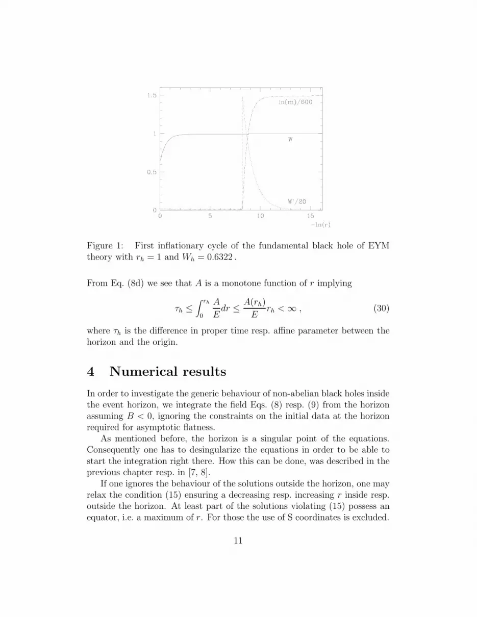
Figure 1: First inflationary cycle of the fundamental black hole of EYMtheory with rh = 1 and Wh = 0.6322 .

From Eq. (8d) we see that A is a monotone function of r implying

τh ≤∫ rh

0

A

Edr ≤ A(rh)

Erh < ∞ , (30)

where τh is the difference in proper time resp. affine parameter between thehorizon and the origin.

4 Numerical results

In order to investigate the generic behaviour of non-abelian black holes insidethe event horizon, we integrate the field Eqs. (8) resp. (9) from the horizonassuming B < 0, ignoring the constraints on the initial data at the horizonrequired for asymptotic flatness.

As mentioned before, the horizon is a singular point of the equations.Consequently one has to desingularize the equations in order to be able tostart the integration right there. How this can be done, was described in theprevious chapter resp. in [7, 8].

If one ignores the behaviour of the solutions outside the horizon, one mayrelax the condition (15) ensuring a decreasing resp. increasing r inside resp.outside the horizon. At least part of the solutions violating (15) possess anequator, i.e. a maximum of r. For those the use of S coordinates is excluded.

11

Figure 2: First two cycles of the solution with rh=0.97 and Wh = 0.2. Forthe second cycle a suitably stretched coordinate x is used.

As one performs the numerical integration one quickly runs into seriousproblems due to the occurence of a quasi-singularity, initiated by a suddensteep raise of W ′ and subsequent exponential growth of B resp. m (compareFigs. 1, 2, and 3 for some examples). This inflationary behaviour of themass function is similar to the one observed for perturbations of the RNsolution at the Cauchy horizon [2]. While this exponential growth continuesindefinitely for the EYMH system, it comes to a stop without the Higgs field.The mass function reaches a plateau and stays constant for a while until itstarts to decrease again. When B has become small enough, i.e. the solutioncomes close to an inner horizon, the same inflationary process repeats itself.Generically this second “explosion” is so violent (we will give estimates onthe increase of m in chapter 5) that the numerical integration procedurebreaks down.

Besides these generic solutions there are certain families of special solu-tions obtained through suitable fine-tuning of the initial data at the horizon.There are two classes of such special solutions. The first class are black holeswith a second, inner horizon, the second are solutions with one of the sin-gular behaviours at r = 0 for B < 0 described in chapter 3. The numericalconstruction of such solutions is complicated by the fact that both boundarypoints are singular points of the equations. The strategies employed to solvesuch problems are well described in our paper on gravitating monopoles [7].Actually, in order to control the numerical uncertainties we used two differ-

12

Figure 3: Inflationary solutions with Higgs fields with α = 0.2, β = 0,rh = 1.2 and Wh = 0.15, Hh = 0.8 resp. Wh = 0.2, Hh = 0.5 .

ent methods, which may be called “matching” and “shooting and aiming”.For matching we integrate independently from both boundary points withregular initial data, tuning these data at both ends until the two branchesof the solution match. For shooting and aiming we integrate only from oneend and try to suppress the singular part of the solution at the other end bysuitably tuning the initial data at the starting point.

As already said, the first class of special solutions consists of black holeswith a second, inner horizon; let us call them non-abelian RN-type (NARN)solutions. As was explained in chapter 3 a regular horizon requires the si-multaneous vanishing of B, BW ′ and BH ′. We have determined two such1-parameter families for the EYM system, shown in Fig. 4, whose signifi-cance will be explained in chapter 5. As may be inferred from Fig. 4, the(dotted) curve 2 corresponding to one such family intersects all (solid) curvesdescribing asymptotically flat solutions except the one for n = 1. In contrastto what is claimed by Donets et al. [6] our curve continues straight throughthe parabola rh = 1 − W 2

h and runs all the way to rh = Wh = 0. As alreadymentioned the branch to the left of the parabola cannot be obtained usingS coordinates. The corresponding curve of Donets et al. makes a suspiciouslysharp turn very close to the parabola and runs to the point rh = 1, Wh = 0.We are convinced that the latter piece of their curve is an artefact of unre-liable numerics caused by the use of S coordinates becoming singular at theparabola (compare the discussion in chapter 3).

13

n=1

n=2n=32

5

1

3

4

6

7

Figure 4: Initial data for special solutions. The solid curves representasymptotically flat solutions with n zeros of W . The other curves representvarious NARN and NAS families.

As already stressed B′ has to be positive at an event horizon. This condi-tion is violated for values of rh < rp, where rp denotes the value of rh wherethe NARN curve 2 intersects the parabola. However it turns out to be ful-filled for the second horizon if rh < rm with rm ≈ 0.112 on the NARN curve.Thus this curve may be divided into three pieces according to 0 < rh < rm,rm < rh < rp and rp < rh. On the first interval the two horizons have ex-changed their roles, whereas on the second interval both of them are Cauchyhorizons with a maximum of r (equator) in between. The only differencebetween the first and the third interval is that Wh > 1 resp. < 1 on theevent horizon.

Our second NARN family (curve 5 of Fig. 4) stays completely to the leftof the parabola and ends at rh ≈ 0.9 close to the curve 3, whose significance

14

Figure 5: A NARN solution and two accompanying NAS solutions withWh = 0.3 and rh = 0.198728 (on curve 5 of Fig. 4), rh = 0.290837 (oncurve 6 with W → +1), and rh = 0.170525 (on curve 7 with W → −1).

will be explained below.The second class are solutions without a second horizon (i.e. B stays

negative) approaching the center r = 0 with one of the two singular be-haviours described in chapter 3, i.e. those with a S-type singularity resp. witha pseudo-RN-type singularity; let us denote them NAS resp. NAPRN solu-tions. We have determined several NAS families represented by the dashed-dotted curves of Fig. 4. The curve 1 staying to the right of the parabolacoincides with the corresponding one of Donets et al., whereas the others,staying essentially to the left of the parabola are new. As will be explainedin chapter 5, the two NAS curves 6 and 7 accompanying the (dotted) NARNcurve 5 are expected to merge with the NAS curve 3 close to rh = 0.9. Someof the NAS curves (e.g., 3 and 4) are expected to extend indefinitely to theright, but numerical difficulties (too violent “explosions”) prevented us fromcontinuing them further to larger values of rh. They will intersect the (solid)curves for asymptotically flat solutions with n = 2, 3, . . . zeros of W andtherefore yield additional asymptotically flat NAS black holes beside thosefound by Donets et al. [6], contradicting their uniqueness claim.

Finally there are the NAPRN solutions, which constitute a discrete setaccording to the number of available free parameters at r = 0. We foundseveral such solutions with W ′(0) = −1 (compare Tab. 1). Only one of themhas no maximum of r and was also found by Donets et al.

15

Table 1: Initial data for several NAPRN solutions with W ′(0) = −1 .

W0 rh Wh # of zeros1 0.9663634 0.7867834 1.54085646 02 0.93306559 1.889087974 0.29197873 03 0.9215847 0.8032373 -2.06670276 14 0.9150108 0.009594267 -0.8037193 1

5 Qualitative Discussion

We shall now give a qualitative picture of the solutions and try to explainour numerical results. Since the generic behaviour of the solutions is ratherdifferent in the cases with and without Higgs field, we shall treat the twocases separately. Let us first concentrate on the case without Higgs field.For simplicity we introduce the notation U ≡ BW ′ and B ≡ rB and useσ ≡ − ln(r) as a radial coordinate. Observe that B ≈ −2m for small r.With these variables the field Eqs. (8) become (a dot denoting d/dσ)

W =−r2 U

B, (31a)

˙U =−WW 2 − 1

r+ 2r2 U3

B2, (31b)

˙B = r(

(1 − W 2)2

r2− 1

)

+ 2r2 U2

B. (31c)

Close to the horizon the first term in the equation for B dominates (sinceU vanishes at r = rh) and thus B becomes negative. Provided W 2 does nottend to 1, this term will, however, change sign as r decreases and B will turnback to zero. Assuming further that U does not tend to zero simultaneously,the second term in the equation for U will grow very rapidly as B approacheszero, leading to a rapid increase of U . This in turn induces a rapid growth ofB (compare Fig. 1). Once the second terms in Eqs. (31b,c) dominate one gets(U/B) ≈ 0 and thus U/B = W ′/r tends to a constant c. As long as (rc)2

is sizable U and B increase exponentially, giving rise to the phenomenonof mass inflation. Eventually this growth comes to a stop when (rc)2 has

16

become small enough. Then U and B stay constant until the first termsin Eqs. (31b,c) become sizable again. As before B tends to zero inducinganother “explosion” resp. cycle of mass inflation (compare Fig. 2).

In the discussion above we made two provisions – that W 2 stays awayfrom 1 and that U does not tend zo zero simultaneously with B. If thefirst condition is violated, i.e. W 2 → 1 we get a NAS solution. If on theother hand U and B develop a common zero we get a NARN solution, i.e. asolution with a second horizon. Both these phenomena can occur after anyfinite number of cycles, giving rise to several NAS resp. NARN curves as inFig. 4. Generically W changes very little during an inflationary cycle, withthe exception of solutions that come very close to a second horizon, i.e. closeto a NARN solution. In this case W may change by any amount, dependingon how small U becomes at the start of the explosion. By suitably fine-tuning the initial data at the horizon one can then obtain new NAS solutionswith W → ±1 or a new NARN solution. In this way each NARN solutionis the ‘parent’ of two NAS and one NARN solution. Fig. 4 shows two suchgenerations: the NARN solutions labelled 2 have the NAS children 3 and 4and the NARN child 5; the curves labelled 6 and 7 are the NAS children of 5(see Fig. 5). Whenever the value of W at the second horizon of a NARNsolution approaches ±1 this NARN curve and its NAS children merge withthe corresponding sibling NAS curve having one cycle less. This hierarchyof special solutions gives rise to a kind of chaotic structure in this region of‘phase space”.

After this qualitative discussion we would like to present a simplifiedquantitative discussion of the solutions, following essentially one completecycle. This will also provide us with a discrete map of the variables W, Uand B from one plateau to the next. Let us denote their initial data atsome plateau by W0, U0 and B0. Since the plateau is characterized by the(effective) vanishing of the second terms in Eqs. (31b,c) involving the factorr2 and the constancy of W , we can easily integrate them to

U = U0 −W0(W

20 − 1)

r, and B = B0 +

(W 20 − 1)2

r, (32)

ignoring the term −r in the B equation. The beginning of the subsequentexplosion is characterized by B ≈ 0, i.e. r ≈ r0 = −(W 2

0 −1)2/B0. Dependingon the value of W0 the value of U at this point is essentially given by U0 or−W0(W

20 − 1)/r0. Whatever it is, let us denote this value again by U0. For

17

the description of the solution through the explosion it is sufficient to solvethe simplified system

W = −r2 U

B, ˙U = 2r2 U3

B2, ˙B = 2r2 U2

B, (33)

implying U/B = c with some constant c. Plugging c back into Eqs. (33) wecan integrate them to get

U = U0 exp(

c2(r20 − r2)

)

, (34a)

B =U0

cexp

(

c2(r20 − r2)

)

, (34b)

W =W0 +c

2(r2 − r2

0) . (34c)

We still have to determine c joining this solution to the one before the ex-plosion. Equating the derivatives of B at r = r0 using the expressions in

Eqs. (32) and (34) we obtain c =(W 2

0−1)2

2U0r3

0

.

In order to obtain the values of W1, U1, B1 after the explosion we maysavely put r = 0 in Eqs. (34) and obtain

U1 = U0e(cr0)2 , B1 =

U0

ce(cr0)2 , (35a)

W = W0 −c

2r20 , with r0 = −(W 2

0 − 1)2

B0

, c =(W 2

0 − 1)2

2U0r30

. (35b)

It is instructive to illustrate these relations on an example. We take thefundamental black hole solution with rh = 1 and Wh = 0.6322 shown inFig. 1. For the first explosion one finds the parameters r0 ≈ 2.7 · 10−4 andc ≈ 1.1 · 105 yielding cr0 ≈ 30 and thus B1 ∼ e900 and W1 − W0 ≈ 4 · 10−3.The subsequent explosion will then take place at the fantastically small valuer0 ∼ e−900 ≈ 10−330.

Since the change of W in one inflationary cycle has an extra factor r0

the function W stays practically constant. If we furthermore concentrate oncases, where the first term in Eq. (31b) can be neglected we may use thesimplified system

W = 0 , ˙U = 2r2 U3

B2, ˙B =

(1 − W 2)2

r+ 2r2 U2

B, (36)

18

also discussed by Donets et al. [6]. Introducing the variables x ≡ rU/B = W ′

and y ≡ −(1 − W 2)2/rB one obtains the autonomous system

W = 0 , x = (y − 1)x , y = y(y + 1 − 2x2) . (37)

Since the first of these equations may be ignored, we can concentrate on thex, y part. As usual for 2-dimensional dynamical systems the global behaviourof the solutions can be analyzed determining its fixed points. Since the “largetime” behaviour σ → ∞ corresponds to the limit r → 0 these fixed pointsare related to the singular solutions at r = 0 discussed in chapter 3. Thereare essentially three different fixed points.

1. For y < 0 there is the fixed point x = 0, y = −1 giving the RNtype singularity. Its eigenvalues are −1 and −2, hence it acts as anattracting center for σ → ∞.

2. Then there is the point x = y = 0, a saddle with eigenvalues ±1.

3. In addition there are the points x = ±1, y = 1 with the eigenvalues1/2(1 ± i

√15), related to the pseudo-RN type singularity. This fixed

point acts as a repulsive focal point, from which the trajectories spi-ral outwards. Since solutions of the approximate system given by theEqs. (37) cannot cross the coordinate axes, solutions in the quadrantsy > 0, x > 0 resp. x < 0 stay there performing larger and larger turnsaround the focal point coming closer and closer to the saddle pointx = y = 0 without ever meeting it. As observed by Donets et al. thisnicely explains the cyclic inflationary behaviour of the solutions in thegeneric case.

Finally we come to the black holes with Higgs field. Apart from thegeneric solutions there are the special ones approaching r = 0 with a singularbehaviour described in chapter 3. On the other hand, the generic behaviouris much simpler than in the previously discussed situation without Higgsfield. An easy way to understand this difference is to derive the analogue ofthe simplified system Eqs. (37). Introducing the additional variable z ≡ −Hand ignoring again irrelevant terms one finds

W =0 , H = −z , (38a)

x =(y − 1)x , z = yz (38b)

y = y(y + 1 − 2x2 − z2) . (38c)

19

Leaving aside the decoupled equations for W and H one may study the fixedpoints of the (x, y, z) system. For z = 0 one clearly finds the previous fixedpoints of the (x, y) system. However, for z 6= 0 the focal point disappearsand the only fixed point for y ≥ 0 is x = y = 0, z = z0 with some constantz0. For z2

0 < 1 this point is a saddle with one unstable mode, whereas forz20 > 1 it is a stable attractor. The latter describes the simple inflationary

behaviour described in chapter 4 and shown in the left part of Fig. 3. So-lutions approaching a fixed point with z2

0 < 1 eventually run away from itagain and ultimately tend to one with z2

0 > 1 as shown in the right part ofFig. 3. In both cases the Higgs field grows logarithmically as r → 0.

Finally let us remark that all these solutions are singular at r = 0, sincea regular origin requires B(0) = 1.

6 Summary

We study the behaviour of the static, spherically symmetric non-abelian blackholes inside their event-horizon. We have chosen a Higgs field in the adjointrepresentation of SU(2), but we expect similar results for Higgs fields in otherrepresentations, because for r → 0 the differences do not seem to be relevant.

In the generic case the solutions inside the horizon show a phenomenonknown as “mass inflation” from perturbations of the Reissner-Nordstrømblack holes at their Cauchy horizon. Whereas for the black holes with a Higgsfield the mass function grows monotonously once the inflation has startedthose without Higgs field run through an infinite sequence of inflationarycycles, which take the form of ever more violent “explosions”. Besides thegeneric solutions there are exceptional ones with a Schwarzschild or Reissner-Nordstrøm type singularity at the center of symmetry. These exceptionalsolutions accumulate in a way that may be interpreted as a kind of “chaotic”behaviour.

Since the typical length scale of these black holes is the Planck length (atleast for values of the gauge coupling g2/hc of order one) one may questionthe physical relevance of these results of the classical theory. However, thereare claims [10] that the phenomenon of mass inflation connected with theReissner-Nordstrøm black hole persists in the quantized theory. Definitelythis subject requires further study.

Apart from that, our results provide a non-perturbative confirmation of

20

the mass inflation phenomenon observed for perturbations of the RN blackhole. Furthermore we believe that our results are of some interest in view ofthe classical singularity theorems of Penrose and Hawking [1].

7 Acknowledgments

G.L. is grateful to Theory Group of the MPI fur Physik for the invitation andkind hospitality during the visit in Nov. 1996, when this work was begun.He also wants to thank P.Hajıcek for critical remarks and comments.

The work of G.L. was supported in part by the Tomalla Foundation andby the Swiss National Science Foundation.

References

[1] Hawking, S.W. and Ellis, G.F.R.: The large scale structure of space-time.Cambridge University Press, 1973.

[2] Poisson,E. and Israel, W.: Phys. Rev. D41 (1990) 1796.

[3] Bonanno, A., Droz, S., Israel, W. and Morsink, S.M.: Phys. Rev. D 50

(1994) 7372.

[4] Kunzle, H.P., and Masood-ul-Alam, A.K.M.: J. Math. Phys. 31 (1990)928;Volkov, M.S., and Gal’tsov, D.V.: JETP Lett. 50 (1989) 346;Bizon, P.: Phys. Rev. Lett. 64 (1990) 2844;Smoller, J.A., Wasserman, A.G., and Yau, S.T.: Commun. Math. Phys.154 (1993) 377.

[5] Breitenlohner, P., Forgacs, P., and Maison, D.: Commun. Math. Phys.163 (1994) 141.

[6] Donets, E.E., Gal’tsov, D.V. and Zotov, M.Yu.: Internal Structure ofEinstein-Yang-Mills Black Holes.gr-qc/9612067.

[7] Breitenlohner, P., Forgacs, P., and Maison, D.: Nucl. Phys. B 442 (1995)126.

21

[8] Breitenlohner, P., Forgacs, P., and Maison, D.: Nucl. Phys. B 383 (1992)357.

[9] Coddington, E.A., and Levinson, N.: Theory of Ordinary DifferentialEquations. New York: McGraw-Hill, 1955.

[10] Oda, I.: Mass Inflation in Quantum Gravity. gr-qc/9701058.

22