Master thesis for the Master of Economic Theory and Econometrics degree

Developmental effects of corruption

Mona Frøystad

May 2007

Department of Economics

University of Oslo

i

In memory of Hedda

To newly born Trygve, a reminder of beauty in life

ii

Preface The experience of living in Argentina almost a year made problems concerning corruption

very clear to me. This stay made me want to learn more about what can be done to reduce

the uncertainty that many people live under.

A number of people were important in the process of writing this thesis. Especially Tina

Søreide should be thanked for excellent and insightful supervision – and for her attentive,

interested, and helpful attitude. I am also grateful to CMI (Christian Michelsen Institute)

who has provided me with a study desk and a roof over my head during my stays in Bergen.

Thanks to my fellow students Sara Cools and Henning Wahlquist for their cheerfulness, even

when the time is close to midnight, and to Kalle Ellingard for helping me with learning

Stata.

Last, but not least, my friends and family should be thanked for always being there for me.

iii

Contents 1. INTRODUCTION .......................................................................................................................................... 1

1.1 CORRUPTION, WHAT IS IT?........................................................................................................................ 3 1.2 FORMS OF CORRUPTION ............................................................................................................................ 5

2. CORRUPTION AND DEVELOPMENT ..................................................................................................... 7 2.1 WHAT ARE THE COMMON CHARACTERISTICS OF COUNTRIES WITH HIGH CORRUPTION? .................. 7 2.2 GROWTH AND DEVELOPMENT .................................................................................................................. 9 2.3 INSTITUTIONS AND CORRUPTION .............................................................................................................. 9 2.4 REVIEW OF EMPIRICAL LITERATURE ON GROWTH, GDP- LEVEL AND CORRUPTION......................... 10

2.4.1 Growth and Corruption.................................................................................................................... 10 2.4.2 Corruption and GDP-level ............................................................................................................... 12

2.5 CAUSALITY .............................................................................................................................................. 12 2.5.1 Causality: Growth and Corruption .................................................................................................. 12 2.5.2 Causality: GDP pr capita and Corruption....................................................................................... 12

2.6. CAUSES OF CORRUPTION ........................................................................................................................ 13 2.7 CORRUPTION AND ITS HARMFULNESS..................................................................................................... 14 2.8 CONCLUSION............................................................................................................................................ 17

3. CORRUPTION INDICES............................................................................................................................ 18 3.1. PERCEPTION BASED INDICES .................................................................................................................. 18

3.1.1 Composite indices ............................................................................................................................ 18 3.1.2 Individual indices ............................................................................................................................. 20 3.1.3 Problems concerning the perception based indices ......................................................................... 21

3.2 ALTERNATIVE SOURCES OF CROSS-COUNTRY INFORMATION ABOUT CORRUPTION ............................. 23 3.2.1 The Business Environment and Enterprise Performance Survey (BEEPS)...................................... 24 3.2.2 World Business Environment Survey (WBES).................................................................................. 24 3.2.3 Problems Concerning Surveys ......................................................................................................... 24

3.3 WHAT DO ALTERNATIVE MEASURES TELL US ABOUT THE EXTENSION OF CORRUPTION? .................... 25 3.4 CONCLUSION............................................................................................................................................ 25

4. THE METHOD AND EMPIRICAL FINDINGS....................................................................................... 26 4.1 EXPECTED FINDINGS ............................................................................................................................... 26 4.2 DATA ........................................................................................................................................................ 26

4.2.1 Bureaucratic corruption (petty corruption) ..................................................................................... 27 4.2.2 Procurement corruption ................................................................................................................... 27 4.2.3 Political corruption .......................................................................................................................... 27

4.3 ORDINARY LEAST SQUARE ...................................................................................................................... 28 4.3.1 Estimation problems likely in the applied dataset............................................................................ 30

4.5 RESULTS................................................................................................................................................... 31 4.5.1 GDP per capita- regressions............................................................................................................ 31 4.5.2 GDP per capita growth-regressions ................................................................................................ 33 4.5.3 Annual growth .................................................................................................................................. 34 4.5.4 The logarithm of GDP per capita growth and GDP per capita ....................................................... 34

4.6 EVALUATION OF RESULTS ....................................................................................................................... 35 4.6.1 Is some types of corruption more harmful than others?.................................................................. 36

5. CONCLUSION ............................................................................................................................................. 38 REFERENCES ................................................................................................................................................. 40 APPENDIX........................................................................................................................................................ 43

1

1. Introduction Corruption is a disturbing problem in many countries because it often leads to the wrong

decisions being made, by high-level politicians as well as among the citizens in general. This

is especially because corruption can lead to the misallocation of resources in that they are not

utilized where they can be used most efficiently. As well, corruption can lower the

profitability of doing legal business, and thus give incentives to going over to corrupt

activities.

Among some early works on corruption, corruption was seen as a way to reduce the time

needed in order to process permits and thus improve efficiency around repressive government

regulations. In this way, and under certain circumstances, corruption could lead to positive

outcomes (Leff 1964) and Huntington 1968). However, nowadays there is a common

consensus among scholars that corruption is harmful to economic and human development.

An emphasis is put on the adverse welfare effects of corruption; rather than being oil in the

machinery corruption fuels the growth of excessive and discretionary regulations (Rose-

Ackerman 1999).

The focus on corruption has increased rapidly the last decade, maybe especially due to

Transparency International’s (TI) contribution; the corruption perception index, which is a

means of measuring the overall perceived level of corruption in different countries.

Seemingly, TI made it possible to compare corruption levels across countries, and, through

the help of media, this way of portraying corruption really put it on the international agenda.

However, as recognized by many scholars and TI itself, neither is the index a good measure of

the relative corruption level across countries, nor can it be used to measure the development

of countries corruption level over time. Further, there are reasons to believe that the measure

of people’s perception about corruption may prove to be a bad measure of the actual level of

corruption.

There is an international will to fight corruption which can be seen in the many international

conventions with corruption on the agenda1. Furthermore, the legal framework and definitions

of the concept corruption are in place. However, there are still problems concerning the

1 Norway is legally bounded by 3 conventions: The UN Convention against Corruption, The Criminal Law and Convention against Corruption and The OECD Convention against Bribery.

2

implementation of the definition of corruption across countries. Corruption has many different

forms and consequences, and due to this it is difficult to define corruption in a manner which

is possible to implement. There are international recognized definitions, but different

definitions entails different interpretation of which acts that are perceived corrupt. Further, an

act which is legal in one country may be perceived corrupt in another (or defined corrupt by

an index). This means that countries can be deemed to have a high perceived level of

corruption even though parts of the estimated level of corruption reflect activities that are

obeying the laws of that country. On the other hand, it has been seen that political leaders

have changed the law in order to make their corrupt actions legal. 2

Even though there is a consensus that corruption has negative effects on development, we

need information about how corruption influences development. Different forms of corruption

exist, and we do not know enough about how they might have different effects on welfare.

Khan (2006) argues that the outcome of corruption is likely to depend on the type of

corruption. Since different types of corruption may have different consequences, composite

corruption indices might hide important insights about the different effect different types of

corruption might have. Corruption indices, such as Transparency International Corruption

Perception Index (CPI), are supposed to measure the overall level of corruption in a country.

As Søreide (2006) expresses it: “Being this all-encompassing, the index [CPI] fails to

distinguish between the forms of corruption that represents welfare problems, and the

corruption that functions as a substitute for prices or public solutions in cases of weak or

absent public institutions” (Søreide 2006:5).

Wedeman (1997) questions how it can be that countries such as China, with a high perceived

level of corruption, can coexist with high levels of economic growth. He argues that such a

fact is not likely to be explained away just by controlling for other variables that might

explain growth. Rather, he argues that it is the type of corruption as well as the distribution of

corruption which is important when explaining the connection between growth and

corruption.

I want to investigate whether it is possible to conclude that some types of corruption are more

harmful than others. Empirically, I will investigate whether different types of corruption have

2 Berlusconi (Italia) is an example.

3

different effects on a country’s GDP growth and GDP level. On the basis of these results and

a literature review, the thesis will add to the discussion about how the consequences of

corruption may depend on the form of corruption.

The data material on specific forms of corruption is weak. The data is new, so there are few

observations, as well as the data have not been collected with the means of investigating

different forms of corruption. Therefore, I have used the data available which seems to be

most likely to measure the indicated form of corruption. Since the empirical basis for analysis

is weak, this study is just as much a literature review.

1.1 Corruption, what is it?

A clear-cut definition on corruption which includes all existing forms of corruption, and

which is possible to implement, does not exist. This is due to the many-faced dimension of

corruption. Aidt (2003) argues that it is important to define corruption precisely in order to

determine what kind of data is being collected and what gets modelled. According to Jain

(2001) “(…) corruption refers to acts in which the power of public office is used for personal

gain in manner that contravenes the rules of the game” (Jain 2001:73). From this definition

Aidt (2003) argues that three conditions are essential for corruption’s commencement and

persistence.

The public official must have authority to deal with rules and regulations in a discretionary

manner, and this power must give him the capability to extract rents. As well, the official

must have incentives to exploit his power. If the institutions in a country are weak, the

chances of being caught in a corrupt act may be low, and even if caught, he may be able to

bribe his way out. Thus, the cost of being corrupt is low when the institutions are weak, and

corruption is more likely to occur (Andvig and Moene 1990). As Svensson (2005) expresses

it, “Corruption is an outcome - a reflection of country’s legal, economic, cultural and

political institutions” (Svensson 2005:20). Even though corruption in some aspects can be

seen as a cultural and individual moral problem, it should, as argued above, rather be seen as a

symptom of fundamental economic, political, and institutional causes (Rose-Ackerman 1999).

The choice of offering bribes is closely linked to risk. There is a risk of being detected in

bribery, and the punishment can be severe. Since bribing is an illegal agreement, the benefits

to be gained are uncertain. The briber is vulnerable to deviations from the agreement because

4

such agreements can generally not be enforced in courts due to their illegality. Further, an

offer of one bribe may lead to demand for more bribes, and thus creating uncertainty whether

the briber ever will get what he wanted in the first place (Søreide 2007). However, being

honest also entails risk and uncertainty. If the business environment is perceived having

widespread corruption, being honest may lead firms to fear loosing contracts because their

competitors are perceived to offer bribes to procure contracts (Ibid).

Rent seeking and corruption is sometimes used interchangeably, but there is a difference.

While corruption involves the use of public office for private gains, rent seeking originates

from the economic concept of rents, which means profits in addition to all relevant costs

(Coolidge and Rose-Ackerman 2000). Corruption entails some kind of secret agreement

which may mutually benefit the agents involved.

Some forms of corruption and lobbyism have common features in that they try to influence

political outcomes. However, there are important differences as well. As argued by Harstad

and Svensson (2006), there are major differences between lobbying and bribing. In many

countries lobbyism is legal and regulated, while bribing is not. If lobbying leads to a change

in a rule, this will typically affect all firms, while bribing is likely to only affect the firm in

question. Governments have relatively a stronger ability to commit than that of an individual

bureaucrat, and therefore lobbyism tends to be more permanent than bribing.

According to the definition of corruption given above, corruption mainly arises in the

interaction between the public and the private. However, corruption may as well arise

between private firms as well as between non-governmental organisations. A typical example

is a firm bribing another firm in order to procure a contract.

It has been argued that corruption may be seen as acting as a tax because it creates a wedge

between actual and bribe-inflated marginal product of capital. However, corruption is much

more harmful than corruption because it creates uncertainty. Wei (1997) argues “(…) that

corruption, unlike tax, is not transparent, not preannounced, and carries a much poorer

enforcement of an agreement between a briber and a bribee” (Wei 1997:1).

5

1.2 Forms of corruption

There are many types of corruption, and I will focus on the most well-known. The section

draws on the typology offered by Gray and Kaufman (1997). Corruption can take the form of

extortion, which is to cause harm or to threaten a person in order to obtain something, that

may be money, services, actions or other kinds of goods. Another form is the illegal

appropriation of property or money entrusted to someone, but owned by others

(embezzlement). Corruption can arise when a political official uses public funds for private

gains (graft). Another variety of corruption is to favor relatives when giving jobs and benefits

to employees (nepotism). In addition, corruption takes place when local public office holders

grant favors, jobs and contracts in return for political support (patronage systems). Such

systems tend to disregard formal rules, and instead give importance to personal channels.

Bribery is often seen as the most common type of corruption, and can be defined as an offer

of money, goods or services in order to gain an advantage. Bribing of a public official by

private agent is a complex matter. Bribes can influence the government’s choice of suppliers

of goods and services, and in this way government contracts can be influenced by the bribes

offered. This can distort the allocation of resources and talents. Bribes can be used to avoid

red tape and thereby speed up government’s granting of different kinds of permissions. Bribes

can influence outcomes of legal and regulatory process, as well as influence the allocation of

benefits such as pensions, subsidies and taxes.

I will concentrate on some main groups of corruption which are practically possible to use for

empirical testing. Those are the following:

Bureaucratic corruption (petty corruption)

Bureaucratic corruption may be defined as corruption in the public administration. This type

of corruption is often considered low level, and can be encountered daily by citizens and firms

in contact with public administration, police, customs and so on (Andvig et al. 2001). One

might be required to pay a fee, a facilitation payment, in order to procure or speed up the

provision of services. One can be entitled to these services, but one must pay a bribe in order

to get hold of them.

6

Political corruption

Political corruption is considered to be high level, and more serious than petty corruption.

Political corruption occurs when politicians at the highest level of political authority are

corrupt. They are at liberty to change and implement the laws in the name of the people

(Andvig et al. 2001). As Amundsen puts it: “(…) political corruption can be for private and

group enrichment, and for power preservation purposes” (Amundsen 2006:1). Political

corruption often derives from political stabilization which entails redistribution of incomes.

Such corruption can take the form of state capture, changes of the law being bought and may

provide explanations of why democracy does not work in certain places (Khan 2006).

Procurement corruption

Public procurement refers to all acquisitions of goods and services by public institutions in a

country, and concerns contracts between the government and the private in many different

areas such as health, military, construction and so on. As Søreide (2002) states: “Corruption

in public procurement makes the officials or the politicians in charge purchase goods or

services form the best briber, instead of choosing the best price-quality combination” (Søreide

2002:1). In addition to the misallocation of resources, the consequences may arise in inflated

prices or in lower quality on the goods or services offered (Ibid).

7

2. Corruption and development “Corruption is widespread in developing and transition countries, not because their people

are different from people elsewhere but because conditions are ripe for it.” (Gray and

Kaufman 1998:1)

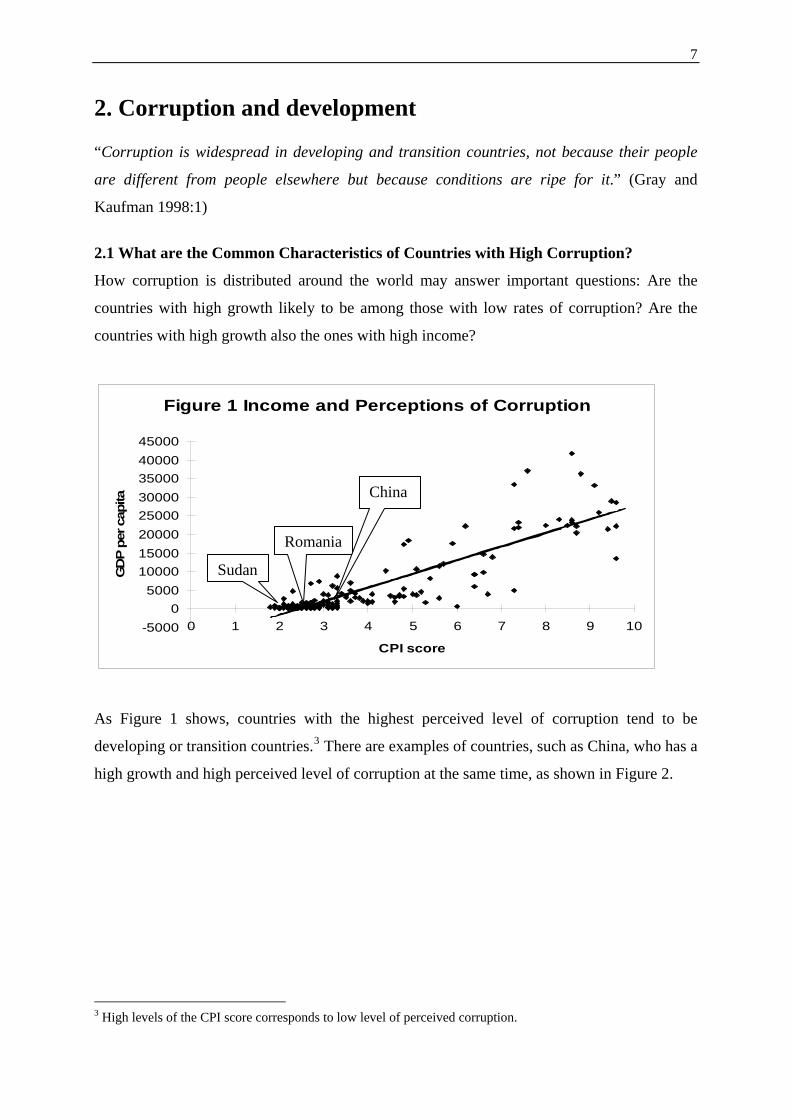
2.1 What are the Common Characteristics of Countries with High Corruption?

How corruption is distributed around the world may answer important questions: Are the

countries with high growth likely to be among those with low rates of corruption? Are the

countries with high growth also the ones with high income?

Figure 1 Income and Perceptions of Corruption

-50000

50001000015000200002500030000350004000045000

0 1 2 3 4 5 6 7 8 9 10

CPI score

GD

P pe

r cap

ita

Romania

China

Sudan

As Figure 1 shows, countries with the highest perceived level of corruption tend to be

developing or transition countries.3 There are examples of countries, such as China, who has a

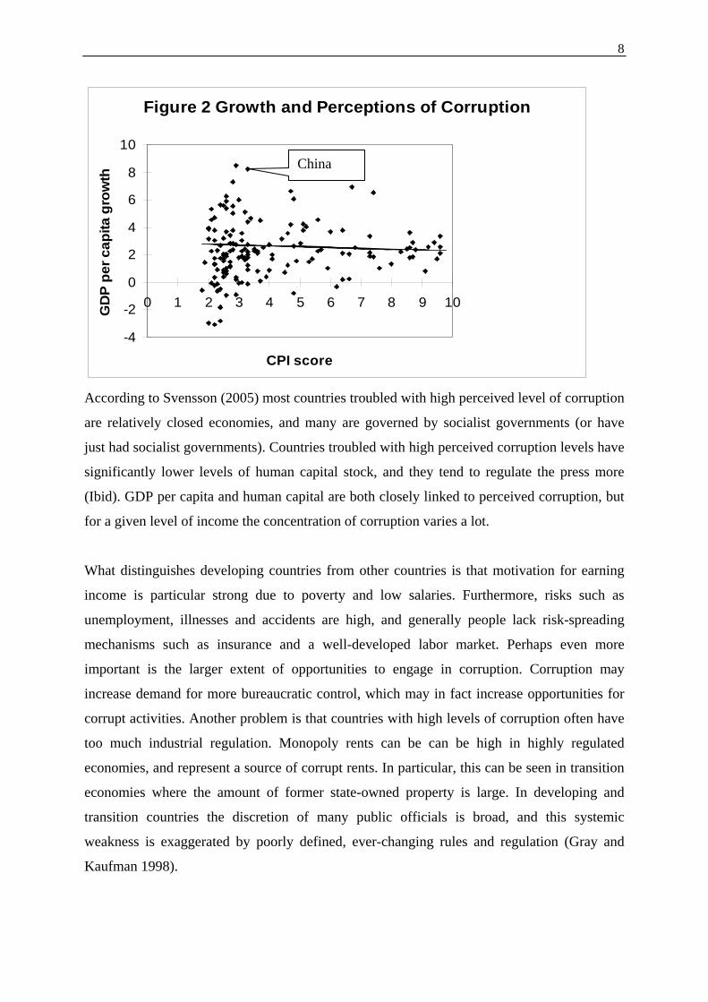
high growth and high perceived level of corruption at the same time, as shown in Figure 2.

3 High levels of the CPI score corresponds to low level of perceived corruption.

8

Figure 2 Growth and Perceptions of Corruption

-4

-2

0

2

4

6

8

10

0 1 2 3 4 5 6 7 8 9 10

CPI score

GD

P pe

r cap

ita g

row

th

China

According to Svensson (2005) most countries troubled with high perceived level of corruption

are relatively closed economies, and many are governed by socialist governments (or have

just had socialist governments). Countries troubled with high perceived corruption levels have

significantly lower levels of human capital stock, and they tend to regulate the press more

(Ibid). GDP per capita and human capital are both closely linked to perceived corruption, but

for a given level of income the concentration of corruption varies a lot.

What distinguishes developing countries from other countries is that motivation for earning

income is particular strong due to poverty and low salaries. Furthermore, risks such as

unemployment, illnesses and accidents are high, and generally people lack risk-spreading

mechanisms such as insurance and a well-developed labor market. Perhaps even more

important is the larger extent of opportunities to engage in corruption. Corruption may

increase demand for more bureaucratic control, which may in fact increase opportunities for

corrupt activities. Another problem is that countries with high levels of corruption often have

too much industrial regulation. Monopoly rents can be can be high in highly regulated

economies, and represent a source of corrupt rents. In particular, this can be seen in transition

economies where the amount of former state-owned property is large. In developing and

transition countries the discretion of many public officials is broad, and this systemic

weakness is exaggerated by poorly defined, ever-changing rules and regulation (Gray and

Kaufman 1998).

9

There are countries that have high levels of corruption while at the same time as they are

exceeding high levels of growth. However, there is reason to believe that those countries with

high growth and high corruption, would have had even higher levels of growth if the did not

have such high levels of corruption.

2.2 Growth and Development

It is difficult to define exactly what development is because it has so many aspects, and it is

necessary to choose what to focus on when talking about development. Important

characteristics of development are often considered to be economic, social, cultural, political

and environmental aspects which are needed in order to obtain sustainable development. Such

a definition will mean that development is something that changes from culture to culture, and

form country to country. It can therefore be difficult to measure and compare development

across cultures as well as country borders (Sen 1995). Development and poverty are closely

interlinked in that poverty is one of many aspects of development, and can be used as an

indicator of development. The lack of poverty can be defined as getting the basic need

satisfied as well as being able to function socially in a society (Sen 1995). The most common

measurement of development is income per capita measured in US dollars. The flaws of this

measurement are that it does not directly measure the standard of living. There can be huge

differences in average age, the health sector etc between countries with same level of GDP

per capita. Further, even if the majority of the population is poor, a small rich minority may

induce a relatively high GDP per capita (Meier and Rauch 2000).

We distinguish between the size and the growth in the GDP. Economic growth refers to how

fast an economy grows in a certain period. Equally essential is how rich a country actually is.

A high GDP today is normally associated with high growth rates in the past. While GDP

growth can be seen as the development of a country’s production, the GDP level says

something about at which stage the economy is. There are interesting differences in the

relationship between corruption and welfare, depending whether one looks at GDP per capita

or growth in GDP.

2.3 Institutions and corruption

Corruption is fundamentally a question about the quality of institutions. As Aidt (2003)

argues, weak institutions are a necessary condition for corruption to be widespread.

Institutions are often described as the rules of the game, or as the constraints that shape human

10

interaction. Acemoglu et al. (2004) argue that economic institutions are seen as “(…) the

structure of property rights and the presence and perfection of markets” (Acemoglu et al.

2004:1). Institutions are important because they influence the structure of economic

incentives and they help allocate resources to their most efficient uses. Acemoglu et al state

that “We think of good economic institutions as those that provide (…) relatively equal access

to economic resources to a broad cross-section of society” (Acemoglu et al. 2004:9). While

the correlation between the quality of institutions and corruption is clear, the determination of

the direction of causality is not that straightforward. Does corruption create bad institutions or

do bad institutions create corruption? Since a prerequisite for the existence of corruption, are

weak institutions, it seems likely that the causality goes from institutions to corruption.

2.4 Review of Empirical Literature on Growth, GDP- level and Corruption

2.4.1 Growth and Corruption

Some early papers on corruption, beginning with Leff (1964) and Huntington (1968), suggest

that corruption might increase economic growth, mainly through two mechanisms. First,

bribes could speed up bureaucracy and in this way avoid delay. Second, bribes may lead

public officials to work more efficiently. Rose-Ackerman (1978) argues that it may be

difficult to limit corruption to certain areas that might seem profitable. Recently, researchers

have come to the conclusion that corruption has a negative effect on growth. It is difficult to

measure the direct effect of corruption on growth, and many researchers have instead focused

on the indirect effects corruption has on growth, particularly through channels such as quality

of governance, trade and investment.

Mauro (1997) demonstrates that perceptions of corruption are likely to reduce growth at a 10

percent significance level. In order to measure corruption and other institutional variables he

uses data from Business International, and creates a sub index, the bureaucratic efficiency

index, consisting of an average of measures of red tape, corruption and the judiciary system.

He argues that this index is likely to be a better measure of corruption than the single measure

of corruption itself, due to possible measurement error in each individual index. He controls

for possible endogeneity between government institutions and growth by using an instrument

for corruption; the ethnolinguistic fractionalization (ELF) index. The ELF index is calculated

by Taylor and Hudson (1972). The macroeconomic data are drawn from Summers and Heston

(1998) and Barro (1991). He uses data from Levine and Renelt (1992) to control for other

11

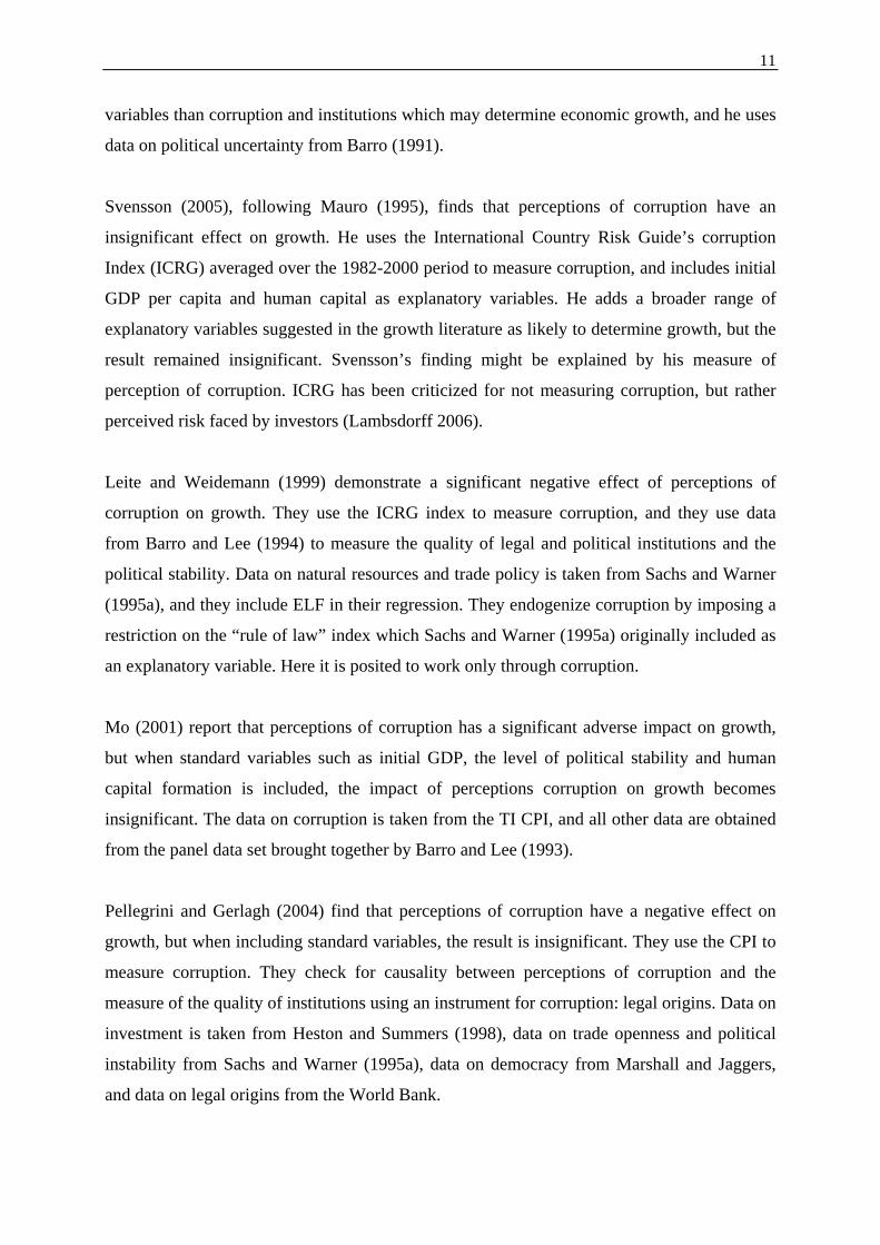
variables than corruption and institutions which may determine economic growth, and he uses

data on political uncertainty from Barro (1991).

Svensson (2005), following Mauro (1995), finds that perceptions of corruption have an

insignificant effect on growth. He uses the International Country Risk Guide’s corruption

Index (ICRG) averaged over the 1982-2000 period to measure corruption, and includes initial

GDP per capita and human capital as explanatory variables. He adds a broader range of

explanatory variables suggested in the growth literature as likely to determine growth, but the

result remained insignificant. Svensson’s finding might be explained by his measure of

perception of corruption. ICRG has been criticized for not measuring corruption, but rather

perceived risk faced by investors (Lambsdorff 2006).

Leite and Weidemann (1999) demonstrate a significant negative effect of perceptions of

corruption on growth. They use the ICRG index to measure corruption, and they use data

from Barro and Lee (1994) to measure the quality of legal and political institutions and the

political stability. Data on natural resources and trade policy is taken from Sachs and Warner

(1995a), and they include ELF in their regression. They endogenize corruption by imposing a

restriction on the “rule of law” index which Sachs and Warner (1995a) originally included as

an explanatory variable. Here it is posited to work only through corruption.

Mo (2001) report that perceptions of corruption has a significant adverse impact on growth,

but when standard variables such as initial GDP, the level of political stability and human

capital formation is included, the impact of perceptions corruption on growth becomes

insignificant. The data on corruption is taken from the TI CPI, and all other data are obtained

from the panel data set brought together by Barro and Lee (1993).

Pellegrini and Gerlagh (2004) find that perceptions of corruption have a negative effect on

growth, but when including standard variables, the result is insignificant. They use the CPI to

measure corruption. They check for causality between perceptions of corruption and the

measure of the quality of institutions using an instrument for corruption: legal origins. Data on

investment is taken from Heston and Summers (1998), data on trade openness and political

instability from Sachs and Warner (1995a), data on democracy from Marshall and Jaggers,

and data on legal origins from the World Bank.

12

Rock and Bonnett (2004) find a negative association between growth and perceptions of

corruption. However, this is after controlling for both country size and the region and/or

country differences in the political economy of corruption. Unless this is done, the

relationship between growth, perceptions of corruption and investment is not very robust.

2.4.2 Corruption and GDP-level

According to Lambsdorff (2003) and (Tanzi and Davoodi (2000), there is a strong correlation

between GDP per capita and corruption. The uncertainty is concerning the direction of

causality.

2.5 Causality

All together this review shows that most studies conclude that perceptions of corruption have

a negative effect on growth as well as on GDP per capita. But this conclusion is valid only if

causality runs from corruption to growth and GDP level, and not the other way around.

2.5.1 Causality: Growth and Corruption

The negative association between perceptions of corruption and growth is consistent with

causality going in both directions. Empirical work proposes that corruption is better explained

by the quality of institutions rather than by growth. Mauro (1995) shows that the correlation

between measures of corruption and other institutional quality indices is high. Acemoglu et al.

(2001) find that institutions are fundamental for economic growth as well as they show that

institutions are very persistent over time. Pellegrini and Gerlagh 2004) use this finding to

argue that perceptions of corruption levels to a large degree are persistent over time, and thus

that it is possible to consider corruption as an exogenous variable when explaining growth

rates.

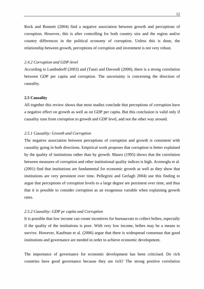
2.5.2 Causality: GDP pr capita and Corruption

It is possible that low income can create incentives for bureaucrats to collect bribes, especially

if the quality of the institutions is poor. With very low income, bribes may be a means to

survive. However, Kaufman et al. (2006) argue that there is widespread consensus that good

institutions and governance are needed in order to achieve economic development.

The importance of governance for economic development has been criticised. Do rich

countries have good governance because they are rich? The strong positive correlation

13

between governance indicators and per capita incomes may reflect this, and not a causal

impact of governance on development. However, according to Kaufmann et al. (2006), it is

unlikely that income can explain the level of governance. Will institutional quality get better

as countries get richer? Kaufmann et al. (2006) argue that causation rather goes from

governance to per capita incomes.

The given discussion points at the importance of good institutions for economic development.

Corruption and the quality of institutions are closely interlinked, and thus the level of

corruption is important for economic development as well.

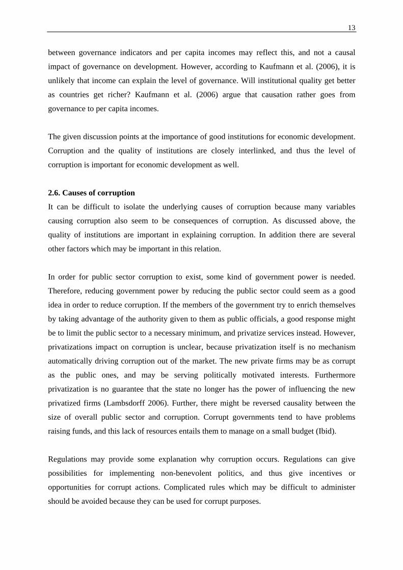
2.6. Causes of corruption

It can be difficult to isolate the underlying causes of corruption because many variables

causing corruption also seem to be consequences of corruption. As discussed above, the

quality of institutions are important in explaining corruption. In addition there are several

other factors which may be important in this relation.

In order for public sector corruption to exist, some kind of government power is needed.

Therefore, reducing government power by reducing the public sector could seem as a good

idea in order to reduce corruption. If the members of the government try to enrich themselves

by taking advantage of the authority given to them as public officials, a good response might

be to limit the public sector to a necessary minimum, and privatize services instead. However,

privatizations impact on corruption is unclear, because privatization itself is no mechanism

automatically driving corruption out of the market. The new private firms may be as corrupt

as the public ones, and may be serving politically motivated interests. Furthermore

privatization is no guarantee that the state no longer has the power of influencing the new

privatized firms (Lambsdorff 2006). Further, there might be reversed causality between the

size of overall public sector and corruption. Corrupt governments tend to have problems

raising funds, and this lack of resources entails them to manage on a small budget (Ibid).

Regulations may provide some explanation why corruption occurs. Regulations can give

possibilities for implementing non-benevolent politics, and thus give incentives or

opportunities for corrupt actions. Complicated rules which may be difficult to administer

should be avoided because they can be used for corrupt purposes.

14

Corruption is by some seen as mirroring the absence of economic competition. Competition

may drive down prices, and public officials therefore have less to sell, and this can reduce

their motivation to seek payoff. Ades and Di Tella (1995, 1997, 1999) show that openness is

negatively associated with perceptions of corruption. Henderson (1999) finds that corruption

is negatively correlated with different indicators of economic freedom. Sandholtz and Gray

(2003) argue that the longer a country has been a part of the major international institutions,

and the more international organizations it belongs to, the lower will the level corruption be.

On the other hand, market restrictions may increase firm’s income and may possibly serve as

a motivation for firms to bribe in order to maintain/obtain such restrictions.

Democracy may limit corruption through increased competition for political mandates. In

theory, competition should allow societies to get rid of those politicians performing

particularly badly. However, the high level of corruption in East European countries which

transformed from socialism to democracy shows that it may take some time for the system to

adjust (Lambsdorff 2006).

Geographical and historical variables, especially natural resources, can in some cases help

explaining why corruption occurs. Leite and Weidemann (1999) show that capital intensive

natural resources are an important determinant of corruption. The existence of natural

resources leads to the existence of potential rents which can be captured. This may serve as a

motivation for corruption, especially if good institutions are lacking. Finally, culture, religion

and values may as well contribute in causing corruption.

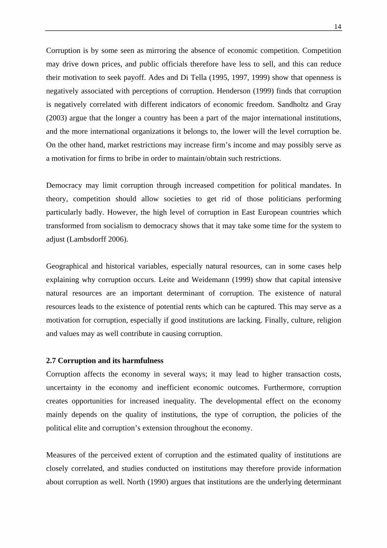
2.7 Corruption and its harmfulness

Corruption affects the economy in several ways; it may lead to higher transaction costs,

uncertainty in the economy and inefficient economic outcomes. Furthermore, corruption

creates opportunities for increased inequality. The developmental effect on the economy

mainly depends on the quality of institutions, the type of corruption, the policies of the

political elite and corruption’s extension throughout the economy.

Measures of the perceived extent of corruption and the estimated quality of institutions are

closely correlated, and studies conducted on institutions may therefore provide information

about corruption as well. North (1990) argues that institutions are the underlying determinant

15

of long-run economic development. But through which channels are institutions affecting

development?

Acemoglu et al. (2004) find that economic institutions encourage economic growth when

political institutions allocate power to groups with interests inn broad-based property rights

enforcement, when they create effective constraints on power-holders, and when there are

relatively few rents to be captured by power holders. Gyimah-Brempong and Traynor (2004)

understand economic growth and political instability as jointly endogenous, and find that

political instability has a direct negative impact on growth, as well as at it decreases long-run

capital accumulation and thus indirectly growth.

The quality of institutions is especially important due to its effect on investment, which again

is important for economic growth. Essential in order to attract investments is to secure the

investors’ property rights, institutions with the ability to enforce laws, and as well the size and

liquidity of the financial market. Mauro (1995) shows that corruption may constitute a

significant obstacle to investment, and further, that this has a negative effect on growth. The

direct relationship between corruption and growth becomes insignificant when investment is

held constant.

Mo (2001) gets an insignificant result of corruption on growth when including a number of

standard variables explaining growth. He argues that this is due to the multicolinearity of

corruption with these variables, and further, that this finding can help identifying the channels

by which corruption affects growth. He demonstrates that more than half of corruption’s

impact on growth is due to its effect on political stability, about 20 percent through its impact

on the ratio of investment to GDP, and 15 percent via its adverse impact on human capital

formation.

The intentions of political leaders matter. Rock and Bonnett (2004) find that corruption has a

negative effect on growth, except in the large East Asian newly industrialized industries. They

argue that due to the developmental policy of the political leaders in the East Asian growth

economies, as well as their long time horizon and centralized business networks, it was

possible to have high levels of corruption and achieve high growth at the same time. Further,

Nye (1964) argues that it is of critical importance if bribes stay in the country or is sent

abroad, and whether they are consumed or invested. It the bribes are exported abroad, the

16

economy will experience a loss of capital which is likely to affect growth negatively. If the

bribes are spent within the country, the effect on growth will depend on the type of potential

investment or consumption.

Shleifner and Vishney (1993) argue that corruption is more harmful when there is a need for

secrecy, and as well when the outcome after bribing is uncertain. Kenny (2006) discusses the

developmental effect of different forms of corruption. He argues that while bribes which

encourage legal activities such as speeding up bureaucratic process are likely to be damaging,

it may be more important to focus on bribes that lead to illegal activities because the

developmental consequences this type of corruption have. Such activities may be unfair

competition for governmental contracts, stealing of property and lower quality on products

produced. The two latter activities have very strong effects in the infrastructure sector, as

shown by a study conducted by Olken (2006).

Unfair competition for governmental contracts can push firms outside the formal sector. This

is likely to reduce the state’s ability to raise revenues and leads to higher tax rates being levied

on fewer and fewer taxpayers. A lower income reduces the state’s capability to provide

essential goods. The result can be a vicious circle of increasing corruption and underground

economics. In this way corruption can undermine the state’s legitimacy (Gray and Kaufmann,

1998). Unfair competition can as well lead to misallocation of resources because they are not

used were they can be utilized most efficiently. This can be seen if a firm procures a contract

(for example delivering a product) because the firm has powerful friends. The point is that the

firm which procures a contract delivering a product at a given quality, should be the one

which can offer the lowest price in the market. If this is not so, resources could be allocated in

a more efficient way.

How widespread corruption is in a society matters for how harmful corruption is for

development. Andvig and Moene (1990) show, using a theoretical model, that if the number

of corrupt agents in an economy exceeds a certain percentage, this will reduce the return of

productive activities, and hence, make rent seeking and corrupt activities more attractive. In

this way otherwise productive economic agents decide doing corrupt actions, and talents

which could be put in amore productive use are misallocated.

17

2.8 Conclusion

The quality of institutions is important to understand how corruption affects growth. But the

extent of corruption and the type of corruption also matters in relation to how damaging

corruption is. The given review of literature points to that the types of corruption that seem to

be most harmful are those leading to misallocation of resources and lowering the quality of

services and goods provided. Public procurement is concerning acquisitions of goods and

services by public institutions, included contracts between the private and the government.

Procurement corruption is therefore potentially very harmful. Political corruption is also

likely to be particularly harmful because the intentions of the political leaders do have effects

on development, and political corruption influences the political stability in a country.

We need more information on how the impacts depend on the type and the extents of

corruption. This is important to develop policy tools, and also to understand what institutional

qualities are particularly important to control the crime. In chapter 4 I will test empirically if

different types of corruption have different effects on development and growth. Before that I

will discuss the estimates of corruption.

18

3. Corruption Indices Corruption takes many forms and tends to have a secretive nature. These features makes is

difficult to get accurate measures of corruption, and any single source of corruption may be

subject to measurement error. Since corruption can be said to reflect underlying institutional

weaknesses, it is likely that different forms of corruption are correlated (Lambsdorff 2006). I

will first start to explain the main differences between the different measures of corruption,

and then look at the criticism of these measures.

3.1. Perception based indices

According to Abramo (2007), the economic meaning of an indicator is a measured amount of

something. In order to be an indicator, a perception index must fulfil three criteria: it must

correspond to a well defined phenomenon (corruption), it must be a precise measurement of

opinions, and it must reflect the actual corruption.

Perception based (subjective) indices of corruption are applied in the lack of better

alternatives. It may be possible to use indirect measures of corruption, but they tend to be

unsuitable as cross-country measures of corruption (Kaufmann et al. 2005). Further,

individual objective measures of governance may provide an incomplete picture even of the

particular aspect that they are intended to measure (Ibid). Several perception based indices

exist, and a main difference lies between the composite indices, and the individual ones. The

composite indices are characterized by that they use many different external sources as a base

for their measure of corruption, while the individual ones use their own sources.

3.1.1 Composite indices

Creating a corruption index based on many sources is motivated by a number of reasons. The

information from one source only may be too narrowly defined in order to measure some

aspect of corruption. With a composite index it can be possible to cover a large number of

countries (Knack 2006). Further, there may be measurement error in each individual index of

corruption, and averaging the individual indices may reduce the measurement error

(Kaufmann et al. 2005). This holds as long as the measurement errors across the different

sources of data are not correlated (Søreide 2006). However, whether these errors are

uncorrelated can be questioned, and I will look into this issue in the evaluation of these

indices.

19

The two most important composite indices are the Transparency International Corruption

Perception Index (CPI) and the Control of Corruption (CC) derived by Kaufmann, Kraay and

Mastruzzi (2003), which is one out of six World Governance Indicators (WGI).

3.1.1. A) Corruption Perception Index4

CPI is created by Transparency International (TI) and was first produced in 1996, with the

intention to measure perceptions of the overall corruption level in different countries. TI is a

politically non-partisan, non-governmental organisation with a global network including more

than 90 locally established national divisions and divisions-in-formation.

The index uses a wide range of sources which span the last two years, and a method of scaling

these data into an index. The data comes from externally conducted polls and surveys, which

are mainly reflecting the perceptions of business people and assessments of country analysts.

A country’s score is calculated as an average of ratings based on these polls and surveys with

equal weight given to each poll/survey.

In order to be included in the index the sources must provide a ranking of countries as well as

they must measure the overall extent of corruption. Furthermore, a country must have three

different sources on corruption in order to be included in the index. TI defines corruption as

“the misuse of entrusted power for private gain”, and it does not distinguish between different

forms of corruption. They find a high correlation between perceptions of political

administrative and political corruption, and use this finding to argue that this shows reliability

of data, and that the overall level of corruption is the most important piece of information

(Ibid). The index ranges from 0 to 10 with 10 indicating a low corruption level, and 0

indicating a highly corrupt country.

3.1.1. B) World Governance Indicators: Controlling Corruption5

The World Bank Control of Corruption indicator is one out of the six indicators measuring

different dimensions of governance in the World Bank’s Worldwide Governance Indicator

(WGI). The WGI goes from 1996-2005, covers 213 countries and territories, and is based on

4 The information about TI is gather from this webpage: http://www.transparency.org/The CPI report 2006 can be found here: http://www.transparency.org/policy_research/surveys_indices/global/cpi5 The aggregate and underlying governance indicators, as well as information about WGI can be found here: www.govindicators.org

20

276 individual variables measuring governance. These are taken from 31 different sources and

produced by 25 different organizations. To construct six aggregate indicators in each period a

method called the unobserved components model is used.6 These aggregate indicators are

weighted averages of the underlying data, with weights reflecting the precision of the

individual data sources. The scores range from -2.5 to 2.5, where -2.5 indicates low perceived

quality of governance and 2.5 indicate high quality . Kaufmann et al. (2006) define corruption

as “(…) the extent to which public power is exercised for private gain, including both petty

and grand forms of corruption, as well as ‘capture’ of the state by elites and private interests”

(Kaufmann et al. 2006:).

3.1.2 Individual indices

Knack (2006) argues that due to the loss of conceptual precision in data, it may be wise to use

data from a single source rather than a composite index (of course, depending on ones

purpose). The most common is the Political Risk Service’s International Country Risk

Guide’s corruption indicator (PRS/ICRG). This index is also broadly defined, but not as broad

as the composite indices. Knack (2006) is arguing that the CPI and the CC are suffering from

varying definitions of corruption due to their many sources. In contrast, with a single broadly-

defined indicator this can be avoided.

International Country Risk Guide7

The ICRG is created by The Political Risk Service Group (PRS) and assess financial,

economic, and political risk. The guide covers a wide range of approximately 140 countries,

and it allows for a time series analysis as the monthly updates of the dataset have been

published regularly since 1980. The ICRG consists of 22 components which are organized

into three subcategories (political, financial and economic) after risk has been assessed. The

components within the categories are added together to provide a risk rating for each

category. The ratings of these categories are then added together, and divided by two to

produce the weights for inclusion in the composite country risk score.

Each component is assigned a maximum value (risk points), with the highest number of points

indicating the lowest potential risk for that component and the lowest number (0) indicating 6 I will not go into detail explaining this model. However, more information about the method can be found in Kaufmann et al. 2004 7 Data on ICRG as well as information about the index can be found here: http://www.prsgroup.com/

21

the highest potential risk. The composite score, ranging form zero to 100, are broken into

categories from Very Low Risk (80 to 100 points) to Very High Risk (zero to 49. 5 points).

The political risk assessments are made on the basis of subjective analysis of the available

information, while the financial and economic risk assessments are made solely on the basis

of objective data. The corruption measure is including different forms of corruption such as

nepotism, patronage and secret party funding.

3.1.3 Problems concerning the perception based indices

A general criticism towards the perception based indices is that there might be a gap between

the actual corruption levels and general perceptions of corruption. Søreide (2006) and Olken

(2006) provide insights about what can explain this gap. Søreide (2006) argues that

measurement errors are likely to be correlated if survey respondents base their responses on

the same sources of information, such as the media and rumours, rather than reporting their

own personal experiences with corruption. Olken (2006) shows that who you are matters for

how you perceive corruption. Olken (2006) finds that personal characteristics of survey

respondents, such as education and sex, were more correlated with perceptions of corruption

than the objective estimation of corruption. This means that ones experiences, education etc.

will colour ones perceptions of corruption more than an actual change in the objective level of

corruption.8

Information from TI is the most applied by the media for reference to corruption, and this may

explain why this institution in particular has been criticized for the downsides of aggregating

sources of corruption. The following section will focus on the CPI, however, some the

criticism can also be directed towards other indices.

Effect of media attention

The CPI raises awareness about corruption on international level, and encourages attempts to

curb corruption. However, as Søreide (2005) argues, the value of the increased media focus

on corruption depends on the perspective. A poor rating sends signals of widespread

corruption, and this can have economic consequences in the form of loss of private investment

8 Olken (2006) conducted a study measuring corruption during road constructions in Indonesia. He used measures of losses as a proxy for the extent of corruption. In order to this, he used the reported physical inputs and costs, surveyed labour inputs and physical audits of outputs. After the project was finished, engineers were used to examine the quality of the roads.

22

and aid. Developing countries are especially vulnerable to damaging misinterpretation of the

CPI.

Ranking not comparable across countries

Especially the ranking of countries according to perceived corruption levels has been

criticized. A country’s rank can change because of methodological changes, or if new

countries enter the index and others drop out. Since the TI is relying on secondary sources it

cannot control countries dropping out of the index.

How to interpret the index

It is difficult to interpret the difference between a country A’s score of 3 compared to a

country B’s score of 6. It does not mean that country A has twice the amount of corruption as

country B; rather one can only say that country A has more corruption than country B

(Søreide 2006).

Not comparable over time

The sources TI has used have changed, as well as the questions asked have been revised, and

the method of aggregating the data has changed. This means that changes in the CPI scores

over time may not only result from changing perceptions, but can be consequence of different

sample and methodology. The CPI should not be used to in time series regressions because it

rather presents a snapshot of how business people and country analysts view corruption.

Supply side of corruption not in focus

Galtung (2005) argues that the CPI only focuses on the bribe receivers and it does not put

emphasis on the major bribe givers and safe havens. Even though the Bribe Payers Index

(constructed by TI) was created in order to account for this problem, this index gets less

attention, and the index has only been updated few times since it was created in 1995 (Ibid).

Since the supply side of corruption is not well accounted for by the CPI, some countries can

be perceived as less corrupt than they really are.

Biased towards private sector

15 of the 17 institutions providing data for the CPI is private sector oriented. While it is

probable that business people are likely to have firsthand experience with some types of

corrupt practices, other groups’ opinions are excluded (Galtung 2005). Since the private

23

sector to a large degree is male and well off economically, this means that the views and

experiences of most women and of the poor are ignored. The informal sector is ignored, and

this sector employs the majority of the population developing countries (Ibid).

What does the index measure?

Galtung (2005) argues that the bribe aspect of corruption has been put on the agenda, at the

expense of the other aspects of corruption. Kenny (2006) and Knack (2006) are arguing that

broad, perception-based corruption assessments appear to primarily measure administrative

corruption. They are both referring to a study conducted by The Business Environment and

Enterprise Performance Survey (BEEPS) which shows that surveyed corruption in contracting

is not significantly linked to the CPI score (or other broad measures of corruption). CPI

correlates more with petty corruption than grand corruption. Further, Kenny refers to Olken’s

(2006) study which shows that perceptions of grand corruption are a weak guide to actual

levels of corruption and subject to systemic biases.

3.2 Alternative sources of cross-country information about corruption

What is the solution if the perception based indices discussed above seem to inaccurately

measure corruption? One solution could be to use direct measures of corruption, such as the

incidence of cases where corruption has been revealed as part of a criminal investigation. This

approach is subject to biases however; how many cases will be put to trial is likely to depend

on the quality the legal system and the form of corruption. For example, given two countries

with equal levels of corruption, it is likely that the country with more focus on anti-corruption

or with a more efficient legal system would have more trials. The type of corruption present is

also important because some types of corruption may be less sophisticated and easier to detect

(Kenny 2006).

Another source of information is the surveys on personal experience in order to get more

direct information about corruption. Surveys such as Business Environment and Enterprise

Performance Survey (BEEPS) and the World Business Environment Survey (WBES) have

collected information from firms. BEEPS focuses on countries in the Eastern Europe and

Central Asia (ECA) region while the WBES includes a larger number of countries.

Information on the influence of commercial interests and national governance is important,

and firms are actually reporting their own influence on the government institutions. Surveys

of firms can be used to track changes in corruption levels over time if the questions are the

24

same and the surveys’ design identically (Knack 2006). This is important in order to provide

information about the development of corruption levels, and to measure the effect of anti-

corruption efforts.

3.2.1 The Business Environment and Enterprise Performance Survey (BEEPS) 9

The BEEPS was developed jointly by the World Bank and the European Bank for

Reconstruction and Development. It was conducted for the first time in 1999-2000, and

covers over 4000 firms in 22 transition countries. BEEPS examines a wide range of

interactions between firms and the state, and is based on face-to-face interviews with firm

managers and owners. The survey includes questions regarding both petty and grand

corruption, and the assumption of the survey is that many of the interviewed firms will be

directly involved in corruption. BEEPS is designed to create comparative measurements in

many areas (included corruption) which can then be related to specific firm characteristics and

firm performance.

3.2.2 World Business Environment Survey (WBES)10

The WBES is a project of the World Bank's Investment Climate and Institute Units. The

project started in 1998, and includes more than 10,000 firms in 80 countries. Batra et al.

(2003) states that the survey “(…) provides a basis for regional comparisons of investment

climate and business environment conditions, and comparisons of the severity of constraints

that affect enterprises according to characteristics, such as size or ownership” (Batra et al.

2003:1). The survey focused on how the quality of the investment climate is shaped by factors

such as infrastructure, governance and quality of public services

3.2.3 Problems Concerning Surveys

To survey firms that are likely to be directly involved in grand corruption will probably

produce more accurate answers than perception indices. However, there can be complications

with these surveys too, especially in relation to honesty and truthful reporting. When asking

business owners directly to account for their costs in relation to paying bribes, this may result

in inaccurate answers. Further, it can be argued that if surveys are very specified, they can be

9 Data on, as well as information about BEEPS can be found here: http://info.worldbank.org/governance/beeps/ 10 Data on, as well as information about WBES can be found here: http://www.ifc.org/ifcext/economics.nsf/Content/ic-wbes

25

a precise, but narrow measure of corruption. In this way there can be a trade-offs between the

precision of measurement and the broadness of measurement of corruption.

3.3 What do alternative measures tell us about the extension of corruption?

Both petty corruption and high level corruption is assumed to be widespread in the

infrastructure industry. Constructions in infrastructure are particularly vulnerable to

corruption in licensing, taxation and obtaining government contracts (Kenny 2006). However,

the BEEPS survey shows a significant variation of petty corruption in infrastructure within

countries. Therefore an aggregate perception based index may not capture the differences

which may exist among different sectors in a country. Further, Olken (2006) argues that

objective measures of corruption, such as inputs and outcomes may capture the real level of

corruption in a sector far better than general perception based sources of corruption,

potentially capturing the impact of both petty and grand corruption. From this one can

conclude that what is needed in order capture the level of corruption in different sectors is

sector based objective measures of corruption.

3.4 Conclusion

In the lack of good alternatives, the composite corruption indices are applied as measures of

corruption even though they are based on perceptions and have important failings. The

correlation between CPI and the World Bank’s Control of Corruption, and the correlation

between the CPI and ICRG are both high, (Svensson 2005), so it may not be that important

which one of the composite indices being used. What distinguishes the use of these indices is

the number of years they include. ICRG is often used for panel data studies because the index

has been around for quite a while.

As broadly discussed, there are reasons to be careful in putting too much confidence in these

indices. In situations with few alternatives, the information provided by the indices is better

than no information at all as long as we are aware of these weaknesses.

26

4. The Method and Empirical Findings

The aim of this section is to investigate whether different types of corruption have different

effects on a country’s GDP growth and GDP level. In order to investigate this problem

empirically, I will use the ordinary least square method on data on different forms of

corruption. Since these data are difficult to obtain, I apply data that are most likely to correlate

with the type of corruption in question. I will now inform about some preliminary

assumptions and decisions, and then present analysis and results.

4.1 Expected findings

A country can have a high growth rate and still be poor if it starts out at a low GDP level. It

could be expected that measures of corruption are less correlated with such growth, because

the growth is not due to a large increase in values; the GDP in absolute terms will not increase

much. Increased values in general are associated with higher corruption levels because there

are more values from which rents can be extracted. Therefore, increases in GDP per capita are

likely to be closer correlated to measures of corruption than annual growth.

I would expect measures of corruption to be closer associated to the GDP pr capita growth

than the measure of annual growth. GDP per capita growth is an estimate of annual growth

divided by annual population growth. The annual growth will thus be discounted by

population growth. The effect of countries having a high growth rate because they have a low

level of GDP to start with is likely to be weaker with this measure. This is due to that poor

countries tend to have high population growth, which will downsize the measure of growth.

Thus, the growth according to this measure is more likely to be caused by other factors than a

low GDP starting point.

4.2 Data

The macro data besides from the data on “rule of law” and data on corruption, is collected

from the Human Development Index, and from 1995-2004. “Rule of law” is one of the six

World Governance Indicators, and the data are produced in the period 1996-2005, annually

since 2002.

27

4.2.1 Bureaucratic corruption (petty corruption)

Because of the lack of objective data measuring this form of corruption, I will follow Knack

(2006) and Kenny (2006) who argue that broad perception based corruption indices measure

petty corruption rather than grand corruption. Thus, there are different sets of data I could use

to measure this type of corruption. As discussed, the correlation between the broad-defined

composite indices is high, so which one I use might not be that important. I choose to use the

CPI11 from 2006. Since this index is subject to flaws, the results are also likely to have some

weaknesses.

4.2.2 Procurement corruption

There is not much data available on corruption in public procurement, and the data that do

exist are new. Therefore it is yet not possible to track changes in corruption levels over time. I

will apply business climate data from the World Business Environment Survey (WBES)12.

Data are drawn from enterprise surveys with focus on many aspects that firms are likely to

meet when doing business. In order to measure procurement corruption I will use data which

describes how much firms need to pay in order to obtain a contract, namely, the value of gifts

expected to secure government contract as a percentage of the contracts.13 The data was

gathered from 2002 to 2006, and I have used the newest data available on each country.

4.2.3 Political corruption

It is also difficult to obtain good data on political corruption. I will use one of the components

in Worldwide Governance Indicator (WGI): “Political Stability and the Absence of

Violence”. This was the most appropriate measure I found which can capture political

corruption. The number of periods in office tends to correlate with political corruption. I used

data from 1996-2005, collected and published by the World Bank.14

11 The CPI can be found here: http://www.transparency.org/policy_research/surveys_indices/cpi/200612World Business Environment Survey data can be found here: http://www.ifc.org/ifcext/economics.nsf/Content/ic-wbes13 Data on procurement corruption from WBES can be found here: http://www.enterprisesurveys.org/ExploreTopics/CompareAll.aspx?topic=corruption14 Data on Worldwide Governance can be found here: http://web.worldbank.org/WBSITE/EXTERNAL/WBI/EXTWBIGOVANTCOR/0,,contentMDK:20771165~menuPK:1866365~pagePK:64168445~piPK:64168309~theSitePK:1740530,00.html

28

4.3 Ordinary least square15

The ordinary least squares (OLS) is a method to estimate a linear correlation between data,

which thus determines how some variables are explained by observed values. The simplest

case is when there are two variables, x and y, and the goal is to understand the relationship

between these two variables. The error term,ε , is assumed to contain measurement error from

y, factors not explained by x (non-explained variation in y), and randomness in human

behaviour. The expectation of ε is assumed zero and the variance is assumed constant, . If

there are N observations indexed by i, then the following relationship holds:

2σ

ii y εβα ++= ix

α and β are numbers we want to estimate, and they are assumed to be constants. β is

interpreted as one unit increase in x leads to a β unit increase in y. ( if there are many

explanatory variables, the interpretation is the effect on y by one unit change in the x in

question, keeping the other x’s constant).

Imagine that only the value of x is known, and we want to get as close to the true value of y as

possible. We then have to guess the values of α and β so that ii yy ˆ− gets as small as

possible, where is an estimator of the true value of y based on estimators of the coefficients y

α and . The most common way to do this is to minimize the squared difference between y

and in order to obtain the ordinary least square estimators. Those estimators will then be the

ones that minimize that difference between y and ;

β

y

y

∑∑==

−−=−N

iii

N

iii yyy

1

2ˆ,ˆ1

2ˆ,ˆ

)ˆˆ(min)ˆ(min βαβαβα

This yields the solutions, the OLS estimators:

xy βα ˆˆˆ −=

∑∑

−

−−=

i i

i ii

xxxxyy

2)())((

β

15 If not indicated otherwise, the information is this section is drawn from Hill et al. (2001).

29

The precision of the estimates are determined by the variances. When working with empirical

data, the x’s are stochastic. Either conditional variances can be calculated or asymptotic

theory can be used to calculate variances if the number of observations is large. We assume

),0(~ 2σε N , and if , then it can be shown that . We normalize

the estimator in order to obtain the test statistic (the same holds for

2)ˆvar( βσβ = ),(~ˆ 2σββ N

α ):

)1,0(~ˆ

2NT

βσ

ββ −= .

The variance of the error term must be calculated, and we get

tT ~ˆ

ˆˆ2

βσ

ββ −=

t is the t-distribution. Now it is possible to test whether the coefficient is significantly

different from zero, i.e. whether they do have effect on the dependent variable.

If the assumptions do not hold, we can get flawed results. Errors may occur if relevant

independent variables are omitted or irrelevant independent variables are included. The error

terms are assumed to have the same variance and not to be correlated with one another. If this

does not hold, two problems may arise:

1. Hetroskedasticity, when the error terms to not all have the same variance. This could

be due to that some observations have larger variance than others or the variance

could be increasing in x.

2. Autocorrelation, when the error terms are correlated with one another. This is a

common problem with time series data (Kennedy 2003).

If some of the independent variables are highly correlated we have multicolinearity, and it is

difficult to say which one of the independent variables that is causing changes in the

dependent variable. A result may be low t-values for both variables, which makes them look

individually insignificant.

30

A problem arises if the relationship between the dependent and independent variables is not

linear, but has another functional form. In some cases this problem can be solved by

transforming either the dependent or the independent variables.

4.3.1 Estimation problems likely in the applied dataset

The data applied on corruption are new, and there are not many observation included. From

these data it is not possible to see how perceptions of corruption have evolved over time, but

it rather presents a snapshot of how perceptions of corruption are distributed. Thus the

regressions provide a snapshot of how different forms are affecting the level and growth of

corruption. Preferably, the independent variable should be older than the dependent one. That

is not possible for this data, however. As argued by Pellegrini and Gerlagh (2004), measures

of the quality of institutions are not likely to change rapidly. Thus, it may not be a significant

problem if the corruption data is slightly newer than the dependent variable.

Multicolinearity is likely to be a problem since estimates of corruption tend to be correlated

with the measures of the quality of institutions. If I do not include a variable on the quality of

institutions, measures of corruption is likely to capture some of the effect quality of

institutions have on GDP level or growth (problem of omitted variables). If I do include such

a variable, the regression is likely to suffer from multicolinearity. I will take this into

consideration when interpreting the coefficients.

Another potential challenge relates to causality problems. Does corruption affect growth, or

does growth affect corruption? Even though I have argued that the effect is likely to go from

corruption to growth, effects the other way around can also occur. One way to deal with this

problem is to use an instrument instead of the measures of corruption. An instrument should

be correlated with the variable it is replacing (here corruption), but not with the variable in

which the original variable was correlated with (here growth or GDP level). In this study, that

would mean one instrument for each of the different types of corruption. Such instruments are

difficult to identify, and have not been applied.

31

A final consideration is concerning hetroskedasticity because some countries will have larger

variance than others. This can be solved by calculating the standard deviations in a different

manner which is robust in relation to hetroskedasticity.16

4.4 Description of the study

1. Stata and Excel were applied to organize data and run regressions.

2. Average values for all the macro data and data on political corruption were created.

3. Countries without observations for GDP were deleted.

4. Corruption data in Excel were organized to fit the macro data concerning the order of

countries.

5. Three dummies were created, one for each of the corruption variables in order to

easily run regressions on different groups of countries.

6. Explanatory variables likely to explain growth were included in the regressions.17

7. I ran regressions which included the different types of corruption, different measures

of GDP and growth, and other variables that are likely to explain growth.

4.5 Results

Initial GDP per capita was included in the regressions to control for economy size. The theory

on convergence states that poor countries will grow faster than richer countries (Barro and

Sala-I-Martin 2004), and when including initial GDP this effect is taken away.

4.5.1 GDP per capita- regressions

Table 1 shows that the measure of CPI is positively correlated which GDP per capita at 1%

significance level. The measure of political is positively correlated with GDP at 5%

significance level, while the measure of procurement corruption is not significant. When

measures of all three types of corruption are included at the same time, none remain

significant. The three first regressions in this table include different number of countries

because the data available on different types of corruption vary from country to country (I will

refer to “red group” when I include all countries available for each measure of corruption).

For instance, regression 1 includes 154 countries with data on bureaucratic corruption,

regression 2 includes 87 countries with data on procurement corruption, and regression 3

16 In Stata this can be done by including the command “robust” in the regressions. 17 I compared articles explaining growth, and got an overview over the most common explanatory variables the authors included.

32

includes 156 countries with data on political corruption. Regression 4 includes only 85

countries which have data available on all three forms of corruption. (I will refer to this group

of countries as “blue group”). I want to compare the effect different types of corruption might

have, and therefore I will look at the same group of countries. This is to make sure that the

results form regressions are not due to different countries included in the data.

In Table 2 only the blue group is included, and then none of the measures of different types

of corruption remain significant. I control for hetroskedasticity for group red, and then the

significance level of the measure of bureaucratic corruption is reduced. The t-value is

increased for both measures of political and procurement corruption, though only measure of

political corruption enters significantly. When the measure of bureaucratic corruption

increases by one unit, thus reducing the corruption level18, GDP per capital will increase by

185.4 units at a 5% significance level. When the measure of political corruption increases by

one unit, thus improving the political situation, the GDP per capita will increase by 152.1

units (Table 3). Controlling for hetroskedasticity does not change the result much for group

blue, other than changing the t-values a bit (Table 4).

I ran regression to see if the quality of institutions had an effect on the result. Different

measures of institutions are likely to be correlated, so I included only one variable to measure

the quality of institutions: the “rule of law”-indicator from WGI. Table 5 and 6 show that

none of the measures of corruption remain significant for neither the red nor the blue group

when “rule of law” is included. “Rule of law” itself does not enter significantly in either of the

groups. The insignificant measures of quality of institutions and corruption indicate that a

multicolinearity problem is likely. When “rule of law” is omitted, the corruption measures are

likely to capture some of the effect which “rule of law” has on the dependent variable. Table 7

and 8 show that when all the other explanatory variables are included, none of the measures of

corruption remains significant in neither the red nor the blue group.

The r-squared, which measures how much of the variation in the dependent variable which is

explained by the explanatory variables, is very high. It lies between 0.98 -0.99 in all

regressions with GDP per capita as the dependent variable. I am sure there are variables that

explain GDP per capita which are not included in the regressions. Further, the r-squared does

18 The bureaucratic corruption is measured by the CPI. An increase in the CPI means that the corruption level is reduced.

33

not change much when including more explanatory variables, or when the number of

countries is changed. A likely explanation is that the variables which are included must

capture a lot of the effect of variables omitted.

4.5.2 GDP per capita growth-regressions

GDP per capita growth captures how GDP growth (referred to as growth in this section)

divided by the population growth interact. Table 9, including red group, shows that all three

types of corruption affect growth significantly. However, when blue group is included, only

the measure of procurement corruption and political corruption remains significant (Table

10).

I control for hetroskedasticity for the red and blue group, and now all three measures of

corruption enter significantly. Measures of bureaucratic and procurement corruption are

significant at the 1% significance level, and political corruption at a 5% significance level

(Table 11 and12). The effect is particularly strong for the measure of bureaucratic corruption

in the blue group, which goes from not being significant, to being significant at a 1%

significance level. For the blue group, and controlling for hetroskedasticity, when the measure

of bureaucratic corruption increases by one unit, the GDP per capita growth increases by

0.690. When the measure of procurement increases by one unit, growth decreases by 0.307

units. When the measure of political corruption increases by one unit, the growth increases by

0.699.

The r-squared is low; it varies from 4% to 13% (when all forms of corruption measures are

included). 8% of the variation in growth is explained by the measure of procurement

corruption. This means that much of the variation of growth is explained by other variables.

Table 13 shows regressions with the red group, and the measure of the quality of institutions

included. Here only procurement corruption remains significant, and it negatively affects

growth (-0,265) at a 5% significance level, thus its effect is a bit lower and the significance

level is reduced. The measure of the quality does not enter significantly, but the r-squared has

increased to 11% (from 8%). The result is not changed much when using the blue group (table

14). The fact that procurement corruption is still significant when controlling for rule of law

indicates that procurement corruption and rule of law are not as correlated as the other types

34

of corruption and rule of law. When controlling for hetroskedasticity, the result is not changed

much (table 15 and 16).

In table 17 other variables which are likely to explain growth are included, and then none of

the corruption variables are significant. This does not change when the blue group is used

(table 18), nor when controlling for hetroskedasticity (table 19 and 20).

4.5.3 Annual growth

The corruption measures are not significant when regressing annual growth and including all

available countries (Table 21). This does not change when I only included “blue group”

(Table 22). None of the measures of corruption remain significant while including red group

and controlling for hetroskedasticity (Table 23). However, when controlling for

hetroskedasticity and including blue group, measures of political corruption and bureaucratic

corruption enter significantly (Table 24). When the measure of bureaucratic corruption

increases by one unit, growth increases by 0.390 units at a 5% significance level. When the

measure of political corruption increases by one unit, growth increases by 0.52 units at a 5 %

significance level. However, when including the measure of the quality of institutions, none

of the measures of corruption enter significantly (Table 41).

4.5.4 The logarithm of GDP per capita growth and GDP per capita

I was advised to use the logarithm on measures of GDP because of its functional form and

nice interpretations. However, when I take the log of growth, none of the corruption variables

remains significant. This holds for both red and blue groups, and controlled for

hetroskedasticity (Table 25, 26, 27 and 28).

I then take the log of GDP per capita and all the measures of corruption enter significantly,

and this holds for both the blue and red group and controlling for, and not controlling for

hetroskedasticity (Table 29, 30, 31 and 32). Controlling for hetroskedasticity and using the

blue group, the measures of bureaucratic and procurement corruption are significant at a 1%

significance level, while political corruption is significant at a 5% level. When regressing log

of GDP per captia on independent variables in levels, a one unit increase in the procurement

corruption variable, leads to a 10.6% decrease in GDP. A one unit’s increase in the measure

of bureaucratic corruption leads to a 31.9% increase in GDP per capita. A one unit increase in

the measure of political corruption leads to a 23.5% increase in GDP per capita.

35

The measure of procurement corruption still remains significant when the measure of the

quality of institutions is included, when including the red/blue group and controlling/not

controlling for hetroskedasticity (Table 33 34, 35 and 36). When all explanatory variables are

included, none of the corruption variables remain significant (Table 37, 38, 39 and 40).

4.6 Evaluation of results

The regressions tell that different types of corruption tend to have different effect on level and

growth of GDP. As well the effect is influenced by what sort of growth in question. This is off

course conditioned on the assumptions I made in the beginning; that bureaucratic corruption

actually is measured by the CPI, that political corruption is captured by the indicator from

WGI, and that procurement corruption is measure by the survey data from the WBES.

As expected, all three types of corruption have strong effects on GDP growth per capita. All

three also had an effect on ln GDP per capita. The measures of bureaucratic and political

corruption also had an effect on annual growth, but this effect is weaker than on growth per

capita. From these regressions it is difficult to conclude whether measures of corruption are

affecting GDP per capita more than annual growth.

Procurement corruption

The regressions show that the measure of this type of corruption does not have effect on GDP

per capita nor on annual growth. This can mean that this type of corruption does not have an

effect on these measures of GDP, but may as well indicate that the measure of procurement

corruption does not capture the whole magnitude of procurement corruption because the data

material is weak.

Procurement corruption enters significantly in the GDP per capita growth and ln GDP per

capita-regressions. The measure of procurement corruption does not seem to be correlated

with the measure of the quality of institutions. It is interesting to note that it seems to be less

correlated with the measure of the quality of institutions than the other types of corruption.

This can indicate that this a type of corruption is likely to be present even if a country has

well-functioning institutions. There might be other aspects in relation to the procurement of

contracts which are more important than geographical lines represented by a countries

36

institutions. It may also indicate that the chances of getting caught in such corrupt activities

are low, and that it can occur in spite of a well-functioning institutional system.

Bureaucratic corruption/ political corruption

These measures have an effect on all the measures of GDP which are included. Using GDP

per capita they enter significantly when the larger red group is included, however, they are not

significant when using the smaller group, called blue. Using GDP per capita growth they

remain significant using blue group and controlling for hetroskedasticity. Using annual

growth they enter significantly only when including blue group and controlling for

hetroskedasticity. This is interesting because here the result is significant when the number of

countries is decreased. At least with this dataset other results obtained when decreasing the

number of observations, or countries, tend to decrease significance of the explanatory

variables. Using ln GDP per capita they enter significantly including blue and controlling for

hetroskedasticity. These measures of corruption seem to be correlated with the measure of the

quality of institutions.

4.6.1 Is some types of corruption more harmful than others?

The regressions show that all three measures have negative effect on GDP per capita growth.

The measures of political and bureaucratic corruption tend to follow each other: if one is

significant, so is the other. Bureaucratic corruption tends to have the strongest negative effect

on different measures of GDP. Political corruption tends to have the second largest effect on

GDP per capita growth, while procurement corruption tends to have the smallest effect on

GDP per capita growth among the three types of corruption. This may be due to that the

different measures have different effects on the explanatory variables, but it may as well be

due to that the measures of bureaucratic and political corruption are indices, while the

measure of political corruption only includes one single question. Hence, it is likely that the

two former measures captures more than the measure of political corruption.

Another question relates to what the data material actually represents. The data material is

mainly based on perceptions of different forms of corruption. It is easier to get respondents to

answer questions concerning political and bureaucratic types of corruption because these two

forms are so well known. In many countries bureaucratic corruption is a part of everyday

business, it may function as an informal price system, and thus we know more about this form

of corruption. Firms and respondents are in general answering willingly to questions

37

concerning this type of corruption. Firms are more reluctant to express their views on

procurement-related corruption and how they might have influenced the award of contracts.

There are also substantial grey zones in the legal definitions of procurement-related

corruption, which may be another reason why it is difficult to assess opinions about the crime

through surveys.

To conclude, this study is indicating that all three forms of corruption are hampering

development. Bureaucratic corruption seems to have the strongest negative effect, however as

discussed, there are reasons to believe that a part of this result is due to the weak data.

38

5. Conclusion This thesis has studied how different types of corruption can have different effects on

development, measured by GDP growth, GDP per capita growth and GDP per capita. Earlier,

typical measures of corruption have been broad, composite indices, and my aim has been to

investigate whether different effects of different forms of corruption could be found when

focusing on specific forms of corruption. Thereby, I wanted to see if some types of corruption

could be concluded as more damaging than others.

The literature review points to that corruption can lead to higher transaction costs, uncertainty

in the economy, and inefficient economic outcomes. The level of corruption and the quality of

institutions are closely linked, and the quality of institutions is important to development in

several aspects. For instance, institutions are found to have a strong influence on private

sector investment, which is important to growth. Investment is attracted by protection of

property rights and enforcement of laws. If institutions are weak, these prerequisites of

investments are less likely to be fulfilled. In general, the effects of corruption which are

especially damaging to development are the misallocation of resources and lower quality of

the goods and services.

This thesis has discussed and empirically tested the consequences of corruption in public

procurement, at political levels, and bureaucratic corruption in terms of facilitation payments.

From the empirical investigation, all types of corruption included had a negative effect on

GDP per capita growth. The perception-based estimates of bureaucratic corruption tend to

have the strongest negative effect on different measures of GDP, while procurement

corruption tends to have the weakest effect of the three. However, given that the measures of

bureaucratic and political corruption are indices, while the measure of procurement corruption

only corresponds to one single question, there is reason to suspect that the two former

measures of corruption captures a broader dimension of corruption.

An interesting result is that procurement corruption seems to be less correlated with the

measure of the quality of institutions than the two other measures of corruption. This finding

suggest that the existence of procurement corruption is less affected by the quality of

institutions, and therefore, that this type of corruption also is likely to be found in well-

developed countries. More information about how corruption in the procurement sector is

39

distributed, what types of firms are involved, the effect of this type corruption has on business

industries, are areas of value for future research.

The causes of corruption are often rooted in fundamental economic, political, and institutional

problems. In order to solve the problem of corruption it will be necessary to solve other

fundamental problems of the state. Further, how to change people’s attitude towards the

governments and politicians, and increasing trust and faith in society are all important factors

in reducing corruption.

40

References Abramo, C. (2007): “Misuses of perceptions”, Transparência Brasil Working Paper. Ades, A. and R. Di Tella (1999): “Rents, competition, and corruption”, American Economic Review, Vol. 89: 982-94. Ades, A. and R. Di Tella (1997): “National champions and corruption: some unpleasant interventionist arithmetic”, Economic Journal, Vol 107: 1032-42. Ades, A. and R. Di Tella (1995): “Competition and Corruption”, draft paper, Keble College, Oxford University. Acemoglu, D., S. Johnson and J. Robinson (2004), “Institutions as the fundamental cause of long-run growth”. NBER Working Paper No. 10481 Acemoglu, D., S. Johnson, and J. Robinson (2001): "The Origins of Comparative Development: An Empirical Investigation". American Economic Review. Vol. 91, No. 5: 1369-1401. Aidt, T. (2003): “Economic Analysis of Corruption: A Survey.” Economic Journal 113 (491), F632-652. Amundsen, I. (2006): “Political Corruption”, Chr. Michelsen Institute, Report 2006:6, CMI, Bergen. Andvig, J. C. and Moene, K.O. (1990): “How corruption may corrupt”, Journal of Economic Behaviour and Organization, Vol. 13(1), pp. 63–76. Andvig, J., Fjeldstad, O.-H., I. Amundsen, T. Sissener, T. and T. Søreide (2001): ”Corruption. A Review of Contemporary Research”, Chr. Michelsen Institute, Report 2001:7, CMI Bergen. Barro R. J. and X. Sala-i-Martin (2004): Economic Growth. Mc-Graw Hill: New York. Batra, G., D. Kaufman and A. H. W. Stone (2003): Investment Climate Around the Word: Voice of the Firms form the World Business Environment Survey, The World Bank. Coolidge, J. and S. Rose-Ackerman (2000): “Kleptocracy and reform in African regimes: Theory and cases” in: Hope, Kempe R. Sir / Chikulu, Bornwell C. (Eds.) (2000): Corruption and Development in Africa. Lessons from Country Case-Studies, New York, pp. 57-86. Galtung, F. (2005): “Measuring the Immeasurable: Boundaries and Functions of (Macro) Corruption Indices” in F. Galtung and C. Sampford (eds.), Measuring Corruption. Gray and Kaufman (1997): “Corruption and Development”, Finance & Development, March 1998. Gyimah-Brempong and Traynor (2004): “Political instability and economic growth in Sub-Saharan Africa”, Journal of African Economics, Vol. 8(1): 52-86. Harstad and Svensson (2006): “Bribes, Lobbying and Development”, CEPR Discussion Paper no. 5759. Centre for Economic Policy Research. Henderson, D. R. (1999): “Power corrupts – editorial comment”, The Wall Street Journal, 19 April. Hill, R.C., Griffiths W.E and Judge G.G. (2001): Undergraduate Econometrics. John Wiley & Sons Inc: Hoboken, NJ. Huntington, S. (1968): Political Order in Changing Societies, New Haven, CT: Yale University Press Jain A. K. (2001): “Corruption: a review”, Journal of Economic Surveys, Vol. 15(1): 71–121. Kaufmann, D., A. Kraay and M. Mastruzzi (2004): “Governance matters IV: Governance Indicators for 1996-2004”, World Bank Policy Research Working Paper 3630, June 2005.

41

Kaufmann, D., A. Kraay and M. Mastruzzi (2006) Measuring Governance Using Cross- Country Perceptions Data in S. Rose-Ackerman International Handbook on the Economics Corruption. Edward Elgar. Kennedy, P. (2003): A Guide to Econometrics. Blackwell Publishing: Oxford. Kenny, C. (2006):”Measuring and reducing the impact of corruption in infrastructure, ” World Bank Policy Research Working Paper 4099, Washington DC: The World Bank. Khan, M. (2006): “Determinants of Corruption in Developing Countries: The Limits of Conventional Economic Analysis” in S. Rose-Ackerman (eds). International Handbook of Economic Corruption, Cambridge, pp. 216-244. Knack, S. (2006): “Measuring Corruption in Eastern Europe and Central Asia: A Critique of the Cross-Country Indicators”, World Bank Policy Research Working Paper 3968. Lambsdorff, G. (2003): “How corruption affects productivity”, Kyklos, Vol.56 (4): 459-476. Lambsdorff, J. (2006): “Causes and consequences of corruption: What do we know from a cross-section of countries?” in S. Rose-Ackerman (eds). International Handbook of Economic Corruption, Cambridge, pp. 3-51. Leite, C. and J. Weidemann (1999): “Does Mother Nature Corrupt? Natural Resources, corruption, and economic growth”, International Monetary Fund Working Paper, 99/85, July. Leff, N. (1964): “Economic development through bureaucratic corruption”, American Behavioural Scientist, Vol. 8(3): 8-14. Mauro, P. (1997): “The effects of corruption on growth, investment, and government expenditure: a cross-country analysis”, in K. Elliott (ed.), Corruption and the Global Economy, Washington, DC: Institute for International Economics, pp. 83-107. Meier G.M. and J.E. Rauch (2000): Leading Issues in Economic Development. Oxford University Press: Oxford. Moe, P.H. (2001): “Corruption and economic growth”, Journal of Comparative Economics, Vol. 29: 66-79. North, D. (1990), Institutions, Institutional change, and Economic Performance, Cambridge University Press, New York Nye (1967): “Corruption and political development: A cost benefit analysis”, The American Political Science Review, Vol. 61, No. 2, 417-427. Olken, B. (2006) “Monitoring Corruption: Evidence from a Field Experiment in Indonesia”, NBER Working Paper 11753. Olken, B. (2006) "Corruption Perceptions vs. Corruption Reality", NBER Working Paper 12561. Pellegrini, L. and R. Gerlagh (2004): “Corruption’s effect on growth and its transmission channels”, Kyklos, Vol. 57(3): 429-456. Rock, M. and H. Bonnett (2004): “The comparative Politics of Corruption: Accounting for the East Asian Paradox in Empirical Studies of Corruption, Growth and Investment”, World Development 32, 6. Rose-Ackerman, S. (1978): Corruption: A Study in Political Economy, New York, Academic Press Rose-Ackerman, S. (1999): Corruption and Government: Causes, Consequences and Reform, Cambridege UK: Cambridge University Press. Sandholtz. W. and M. Gray and (2003): “International integration and national corruption”, International Organization, Vol.57 (4): 761-800. Sen, A. (1995): Inequality re-examined, Oxford University Press.

42

Shleifer, A. and Vishny, R. W. (1993): “Corruption”, Quarterly Journal of Economics, vol. 108, pp. 599–618. Reprinted in Williams et al. (2000) Vol. 1, chapter 13 and in Shleifer and Vishny (1998) chapter 5. Søreide, T. (2002): “Corruption in public procurement. Causes, consequences and cures”, Chr. Michelsen Institute, Report 2002:1, CMI Bergen Søreide, T. (2006): “Is it wrong to rank?”, Chr. Michelsen Institute, Report 2006:1, CMI Bergen Søreide, T. (2007): “Business corruption, uncertainty and risk aversion”, Chr. Michelsen Institute, Report 2007:1. Svensson, J. (2005): “Eight Questions About Corruption”, Journal of Economic Perspectives, Vol. 19,3. Tanzi, Vito and Hamid R. Davoodi (2001): “Corruption, Growth, and Public Finances”, 89-110, in: Arvind K. Jain (ed.), Political Economy of Corruption, Routledge. Wei (1997): “Why is corruption so much more taxing than tax? Arbitrariness kills”, NBER Working Paper Series 6255.

43

Appendix List of variables included

• GDP growth (annual %) (named “growth” in regressions

• GDP per capita (constant 2000 US$) (named “gdppercap” )

• GDP per capita growth (annual %) (named “growthpercap”)

• Population, total (named “pop”)

• School enrolment, secondary (% net) (named “school”)

• General government final consumption expenditure (% of GDP) (named “gcf”)

• Trade (% of GDP) (named “open”)

• Quality of institutions (named “ruleoflaw”)

• Procurement corruption (named “procurement”)

• Bureaucratic corruption (named “cpiscore”)

• Political corruption (named “political”)

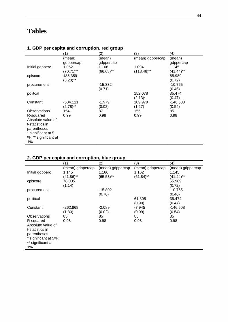
44

Tables 1. GDP per capita and corruption, red group (1) (2) (3) (4) (mean)

gdppercap (mean) gdppercap

(mean) gdppercap (mean) gdppercap

Initial gdpperc 1.062 1.166 1.094 1.145 (70.71)** (66.68)** (118.46)** (41.44)** cpiscore 185.359 55.989 (3.23)** (0.72) procurement -15.832 -10.765 (0.71) (0.46) politcal 152.078 35.474 (2.13)* (0.47) Constant -504.111 -1.979 109.978 -146.508 (2.78)** (0.02) (1.27) (0.54) Observations 154 87 156 85 R-squared 0.99 0.98 0.99 0.98 Absolute value of t-statistics in parentheses

* significant at 5 %; ** significant at 1%

2. GDP per capita and corruption, blue group (1) (2) (3) (4) (mean) gdppercap (mean) gdppercap (mean) gdppercap (mean) gdppercapInitial gdpperc 1.145 1.166 1.162 1.145 (41.86)** (65.58)** (61.84)** (41.44)** cpiscore 78.005 55.989 (1.14) (0.72) procurement -15.802 -10.765 (0.70) (0.46) political 61.308 35.474 (0.90) (0.47) Constant -262.868 -2.089 -7.945 -146.508 (1.30) (0.02) (0.09) (0.54) Observations 85 85 85 85 R-squared 0.98 0.98 0.98 0.98 Absolute value of t-statistics in parentheses

* significant at 5%; ** significant at 1%

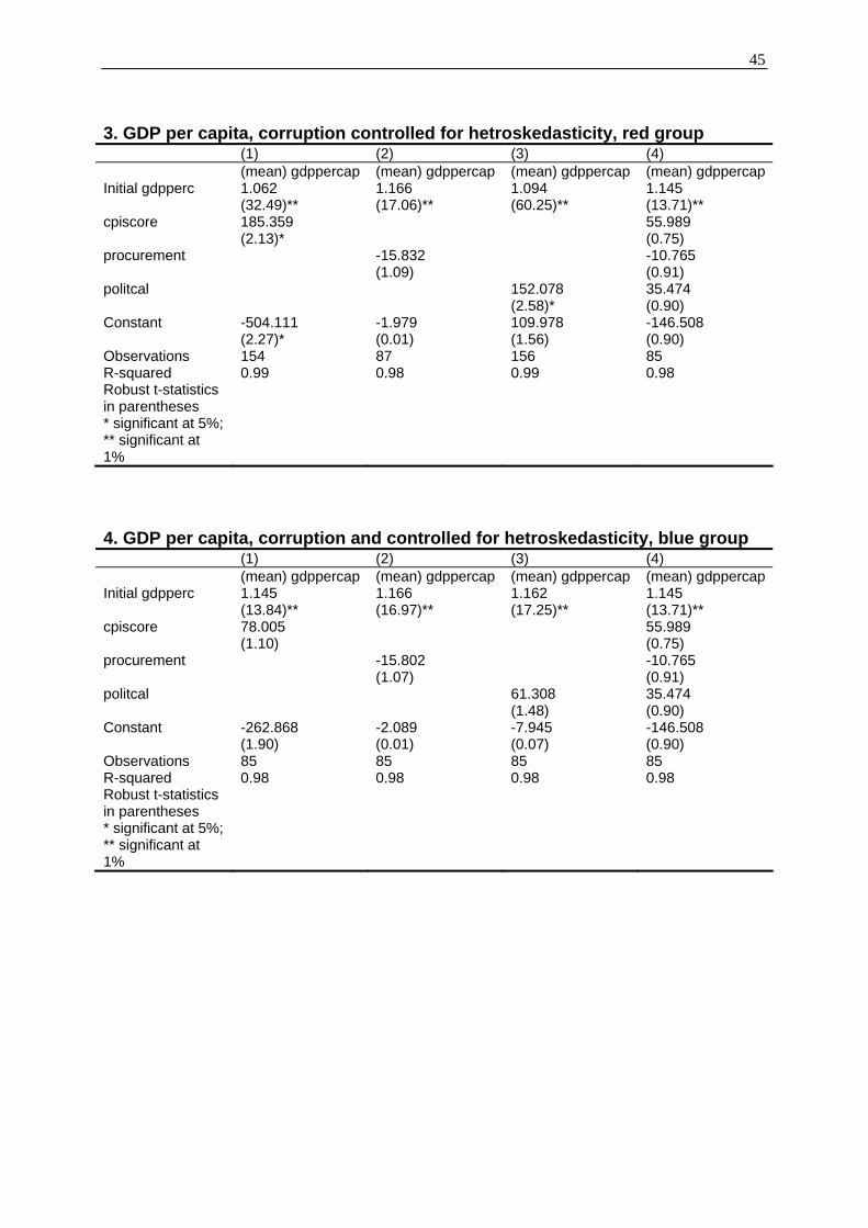
45

3. GDP per capita, corruption controlled for hetroskedasticity, red group (1) (2) (3) (4) (mean) gdppercap (mean) gdppercap (mean) gdppercap (mean) gdppercapInitial gdpperc 1.062 1.166 1.094 1.145 (32.49)** (17.06)** (60.25)** (13.71)** cpiscore 185.359 55.989 (2.13)* (0.75) procurement -15.832 -10.765 (1.09) (0.91) politcal 152.078 35.474 (2.58)* (0.90) Constant -504.111 -1.979 109.978 -146.508 (2.27)* (0.01) (1.56) (0.90) Observations 154 87 156 85 R-squared 0.99 0.98 0.99 0.98 Robust t-statistics in parentheses

* significant at 5%; ** significant at 1%

4. GDP per capita, corruption and controlled for hetroskedasticity, blue group (1) (2) (3) (4) (mean) gdppercap (mean) gdppercap (mean) gdppercap (mean) gdppercapInitial gdpperc 1.145 1.166 1.162 1.145 (13.84)** (16.97)** (17.25)** (13.71)** cpiscore 78.005 55.989 (1.10) (0.75) procurement -15.802 -10.765 (1.07) (0.91) politcal 61.308 35.474 (1.48) (0.90) Constant -262.868 -2.089 -7.945 -146.508 (1.90) (0.01) (0.07) (0.90) Observations 85 85 85 85 R-squared 0.98 0.98 0.98 0.98 Robust t-statistics in parentheses

* significant at 5%; ** significant at 1%

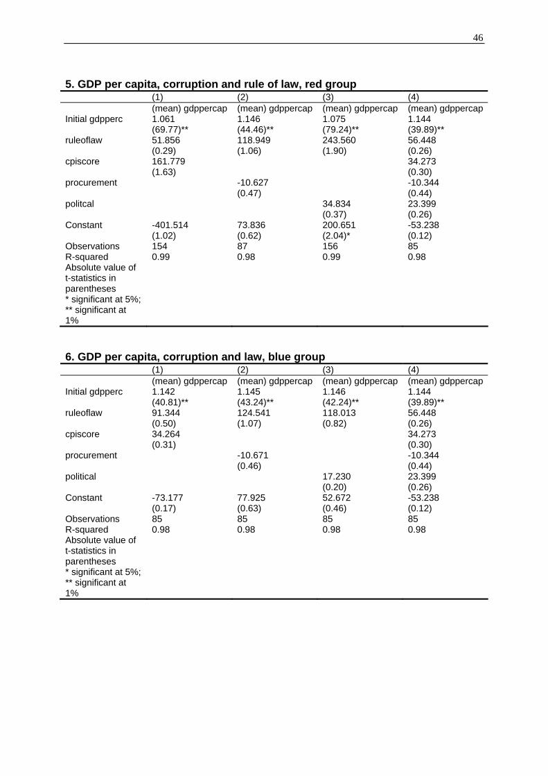
46

5. GDP per capita, corruption and rule of law, red group (1) (2) (3) (4) (mean) gdppercap (mean) gdppercap (mean) gdppercap (mean) gdppercapInitial gdpperc 1.061 1.146 1.075 1.144 (69.77)** (44.46)** (79.24)** (39.89)** ruleoflaw 51.856 118.949 243.560 56.448 (0.29) (1.06) (1.90) (0.26) cpiscore 161.779 34.273 (1.63) (0.30) procurement -10.627 -10.344 (0.47) (0.44) politcal 34.834 23.399 (0.37) (0.26) Constant -401.514 73.836 200.651 -53.238 (1.02) (0.62) (2.04)* (0.12) Observations 154 87 156 85 R-squared 0.99 0.98 0.99 0.98 Absolute value of t-statistics in parentheses

* significant at 5%; ** significant at 1%

6. GDP per capita, corruption and law, blue group (1) (2) (3) (4) (mean) gdppercap (mean) gdppercap (mean) gdppercap (mean) gdppercapInitial gdpperc 1.142 1.145 1.146 1.144 (40.81)** (43.24)** (42.24)** (39.89)** ruleoflaw 91.344 124.541 118.013 56.448 (0.50) (1.07) (0.82) (0.26) cpiscore 34.264 34.273 (0.31) (0.30) procurement -10.671 -10.344 (0.46) (0.44) political 17.230 23.399 (0.20) (0.26) Constant -73.177 77.925 52.672 -53.238 (0.17) (0.63) (0.46) (0.12) Observations 85 85 85 85 R-squared 0.98 0.98 0.98 0.98 Absolute value of t-statistics in parentheses

* significant at 5%; ** significant at 1%

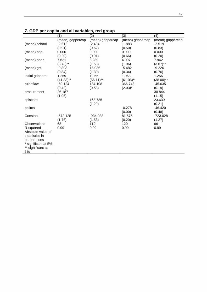
47

7. GDP per capita and all variables, red group (1) (2) (3) (4) (mean) gdppercap (mean) gdppercap (mean) gdppercap (mean) gdppercap(mean) school -2.612 -2.404 -1.883 -2.519 (0.91) (0.62) (0.50) (0.83) (mean) pop 0.000 0.000 0.000 0.000 (0.20) (0.91) (0.66) (0.20) (mean) open 7.621 3.289 4.097 7.942 (3.73)** (1.53) (1.96) (3.67)** (mean) gcf -9.893 15.036 -5.482 -9.226 (0.84) (1.30) (0.34) (0.76) Initial gdpperc 1.259 1.055 1.068 1.256 (41.33)** (56.11)** (61.06)** (38.00)** ruleoflaw -50.124 134.108 366.743 -45.635 (0.42) (0.53) (2.03)* (0.19) procurement 26.187 30.844 (1.05) (1.15) cpiscore 168.785 23.639 (1.29) (0.21) politcal -0.278 -46.420 (0.00) (0.48) Constant -572.125 -934.038 81.575 -723.028 (1.76) (1.53) (0.20) (1.27) Observations 68 119 120 66 R-squared 0.99 0.99 0.99 0.99 Absolute value of t-statistics in parentheses

* significant at 5%; ** significant at 1%

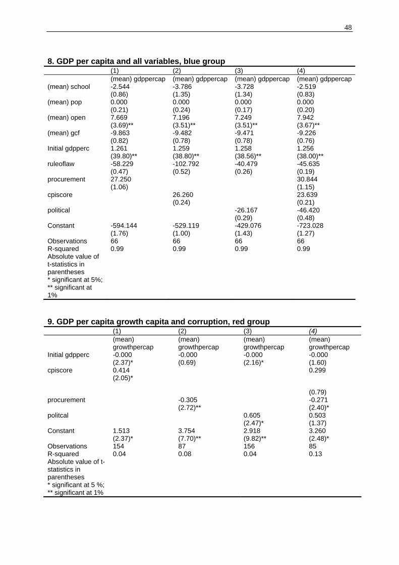
48

8. GDP per capita and all variables, blue group (1) (2) (3) (4) (mean) gdppercap (mean) gdppercap (mean) gdppercap (mean) gdppercap(mean) school -2.544 -3.786 -3.728 -2.519 (0.86) (1.35) (1.34) (0.83) (mean) pop 0.000 0.000 0.000 0.000 (0.21) (0.24) (0.17) (0.20) (mean) open 7.669 7.196 7.249 7.942 (3.69)** (3.51)** (3.51)** (3.67)** (mean) gcf -9.863 -9.482 -9.471 -9.226 (0.82) (0.78) (0.78) (0.76) Initial gdpperc 1.261 1.259 1.258 1.256 (39.80)** (38.80)** (38.56)** (38.00)** ruleoflaw -58.229 -102.792 -40.479 -45.635 (0.47) (0.52) (0.26) (0.19) procurement 27.250 30.844 (1.06) (1.15) cpiscore 26.260 23.639 (0.24) (0.21) political -26.167 -46.420 (0.29) (0.48) Constant -594.144 -529.119 -429.076 -723.028 (1.76) (1.00) (1.43) (1.27) Observations 66 66 66 66 R-squared 0.99 0.99 0.99 0.99 Absolute value of t-statistics in parentheses

* significant at 5%; ** significant at 1%

9. GDP per capita growth capita and corruption, red group (1) (2) (3) (4) (mean)

growthpercap (mean) growthpercap

(mean) growthpercap

(mean) growthpercap

Initial gdpperc -0.000 -0.000 -0.000 -0.000 (2.37)* (0.69) (2.16)* (1.60) cpiscore 0.414

(2.05)* 0.299

(0.79) procurement -0.305 -0.271 (2.72)** (2.40)* politcal 0.605 0.503 (2.47)* (1.37) Constant 1.513 3.754 2.918 3.260 (2.37)* (7.70)** (9.82)** (2.48)* Observations 154 87 156 85 R-squared 0.04 0.08 0.04 0.13 Absolute value of t-statistics in parentheses

* significant at 5 %; ** significant at 1%

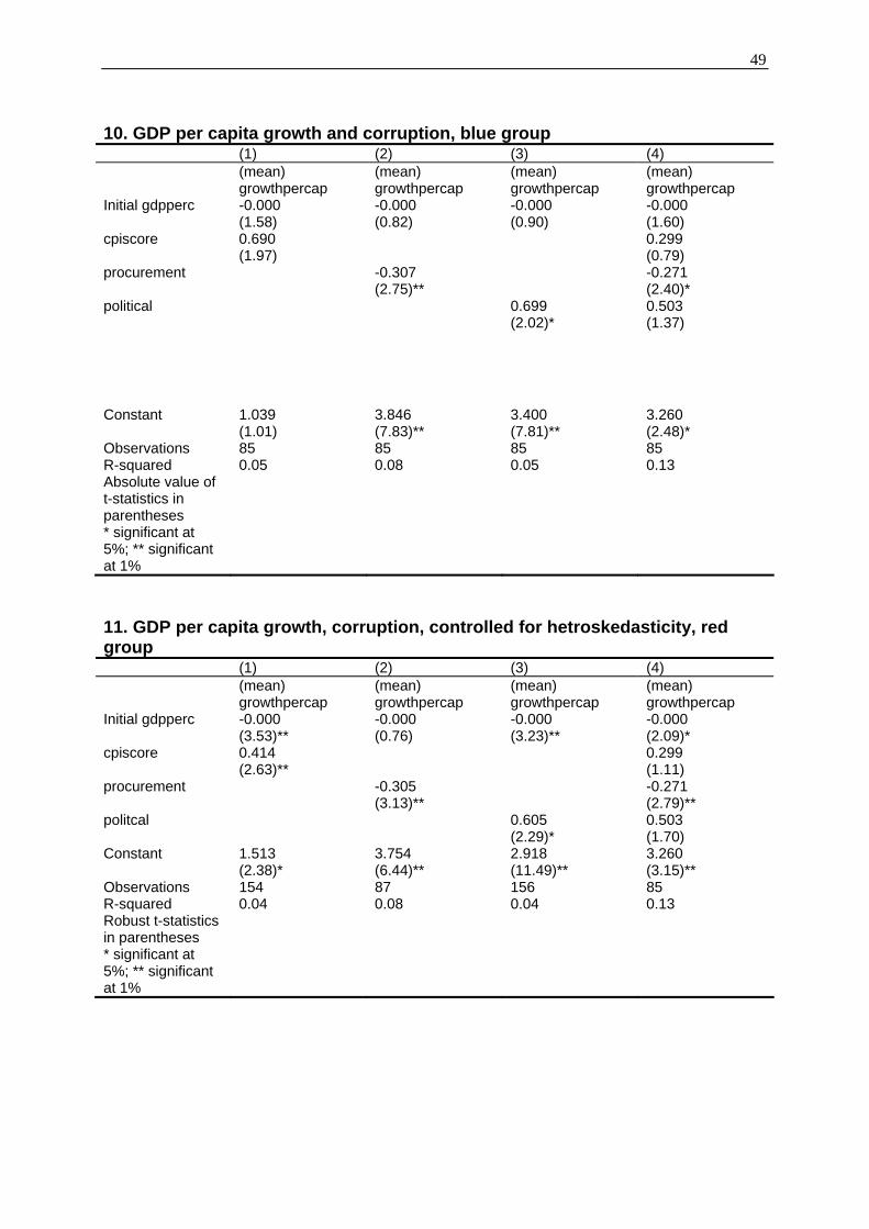
49

10. GDP per capita growth and corruption, blue group (1) (2) (3) (4) (mean)

growthpercap (mean) growthpercap

(mean) growthpercap

(mean) growthpercap

Initial gdpperc -0.000 -0.000 -0.000 -0.000 (1.58) (0.82) (0.90) (1.60) cpiscore 0.690 0.299 (1.97) (0.79) procurement -0.307 -0.271 (2.75)** (2.40)* political 0.699 0.503 (2.02)* (1.37)

Constant 1.039 3.846 3.400 3.260 (1.01) (7.83)** (7.81)** (2.48)* Observations 85 85 85 85 R-squared 0.05 0.08 0.05 0.13 Absolute value of t-statistics in parentheses

* significant at 5%; ** significant at 1%

11. GDP per capita growth, corruption, controlled for hetroskedasticity, red group (1) (2) (3) (4) (mean)

growthpercap (mean) growthpercap

(mean) growthpercap

(mean) growthpercap

Initial gdpperc -0.000 -0.000 -0.000 -0.000 (3.53)** (0.76) (3.23)** (2.09)* cpiscore 0.414 0.299 (2.63)** (1.11) procurement -0.305 -0.271 (3.13)** (2.79)** politcal 0.605 0.503 (2.29)* (1.70) Constant 1.513 3.754 2.918 3.260 (2.38)* (6.44)** (11.49)** (3.15)** Observations 154 87 156 85 R-squared 0.04 0.08 0.04 0.13 Robust t-statistics in parentheses

* significant at 5%; ** significant at 1%

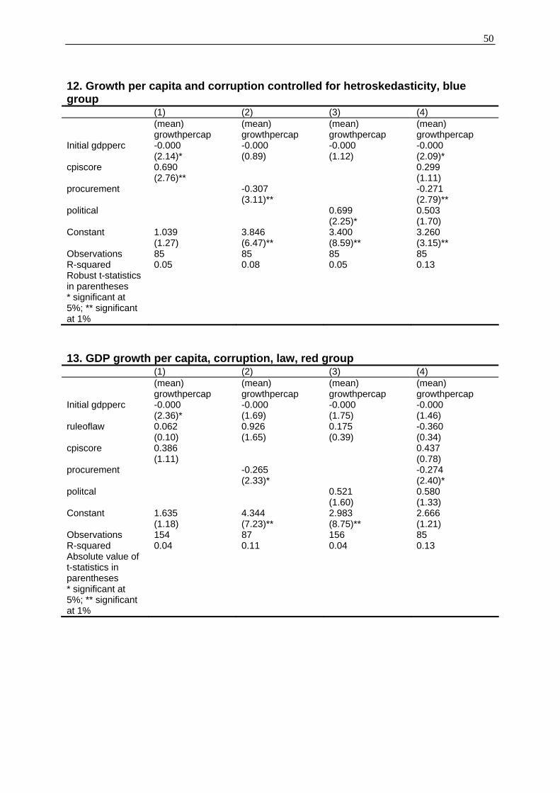
50

12. Growth per capita and corruption controlled for hetroskedasticity, blue group (1) (2) (3) (4) (mean)

growthpercap (mean) growthpercap

(mean) growthpercap

(mean) growthpercap

Initial gdpperc -0.000 -0.000 -0.000 -0.000 (2.14)* (0.89) (1.12) (2.09)* cpiscore 0.690 0.299 (2.76)** (1.11) procurement -0.307 -0.271 (3.11)** (2.79)** political 0.699 0.503 (2.25)* (1.70) Constant 1.039 3.846 3.400 3.260 (1.27) (6.47)** (8.59)** (3.15)** Observations 85 85 85 85 R-squared 0.05 0.08 0.05 0.13 Robust t-statistics in parentheses

* significant at 5%; ** significant at 1%

13. GDP growth per capita, corruption, law, red group (1) (2) (3) (4) (mean)

growthpercap (mean) growthpercap

(mean) growthpercap

(mean) growthpercap

Initial gdpperc -0.000 -0.000 -0.000 -0.000 (2.36)* (1.69) (1.75) (1.46) ruleoflaw 0.062 0.926 0.175 -0.360 (0.10) (1.65) (0.39) (0.34) cpiscore 0.386 0.437 (1.11) (0.78) procurement -0.265 -0.274 (2.33)* (2.40)* politcal 0.521 0.580 (1.60) (1.33) Constant 1.635 4.344 2.983 2.666 (1.18) (7.23)** (8.75)** (1.21) Observations 154 87 156 85 R-squared 0.04 0.11 0.04 0.13 Absolute value of t-statistics in parentheses

* significant at 5%; ** significant at 1%

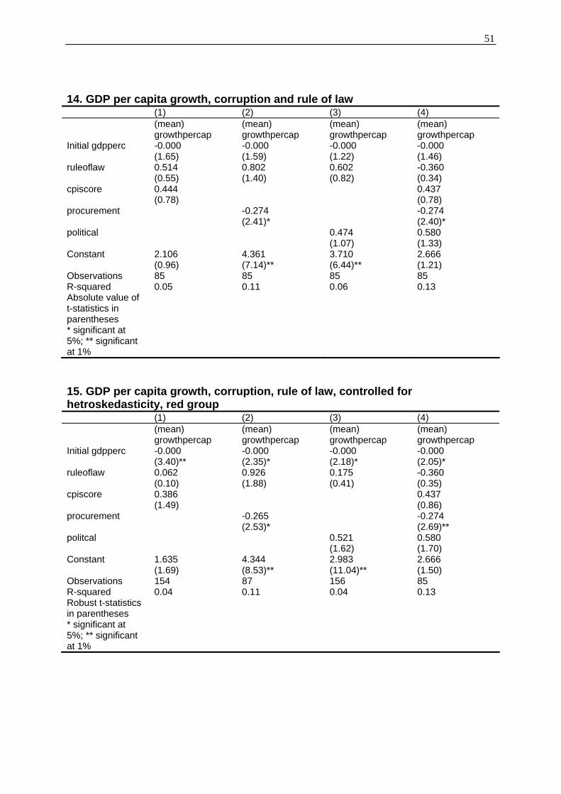
51

14. GDP per capita growth, corruption and rule of law (1) (2) (3) (4) (mean)

growthpercap (mean) growthpercap

(mean) growthpercap

(mean) growthpercap

Initial gdpperc -0.000 -0.000 -0.000 -0.000 (1.65) (1.59) (1.22) (1.46) ruleoflaw 0.514 0.802 0.602 -0.360 (0.55) (1.40) (0.82) (0.34) cpiscore 0.444 0.437 (0.78) (0.78) procurement -0.274 -0.274 (2.41)* (2.40)* political 0.474 0.580 (1.07) (1.33) Constant 2.106 4.361 3.710 2.666 (0.96) (7.14)** (6.44)** (1.21) Observations 85 85 85 85 R-squared 0.05 0.11 0.06 0.13 Absolute value of t-statistics in parentheses

* significant at 5%; ** significant at 1%

15. GDP per capita growth, corruption, rule of law, controlled for hetroskedasticity, red group (1) (2) (3) (4) (mean)

growthpercap (mean) growthpercap

(mean) growthpercap

(mean) growthpercap

Initial gdpperc -0.000 -0.000 -0.000 -0.000 (3.40)** (2.35)* (2.18)* (2.05)* ruleoflaw 0.062 0.926 0.175 -0.360 (0.10) (1.88) (0.41) (0.35) cpiscore 0.386 0.437 (1.49) (0.86) procurement -0.265 -0.274 (2.53)* (2.69)** politcal 0.521 0.580 (1.62) (1.70) Constant 1.635 4.344 2.983 2.666 (1.69) (8.53)** (11.04)** (1.50) Observations 154 87 156 85 R-squared 0.04 0.11 0.04 0.13 Robust t-statistics in parentheses

* significant at 5%; ** significant at 1%

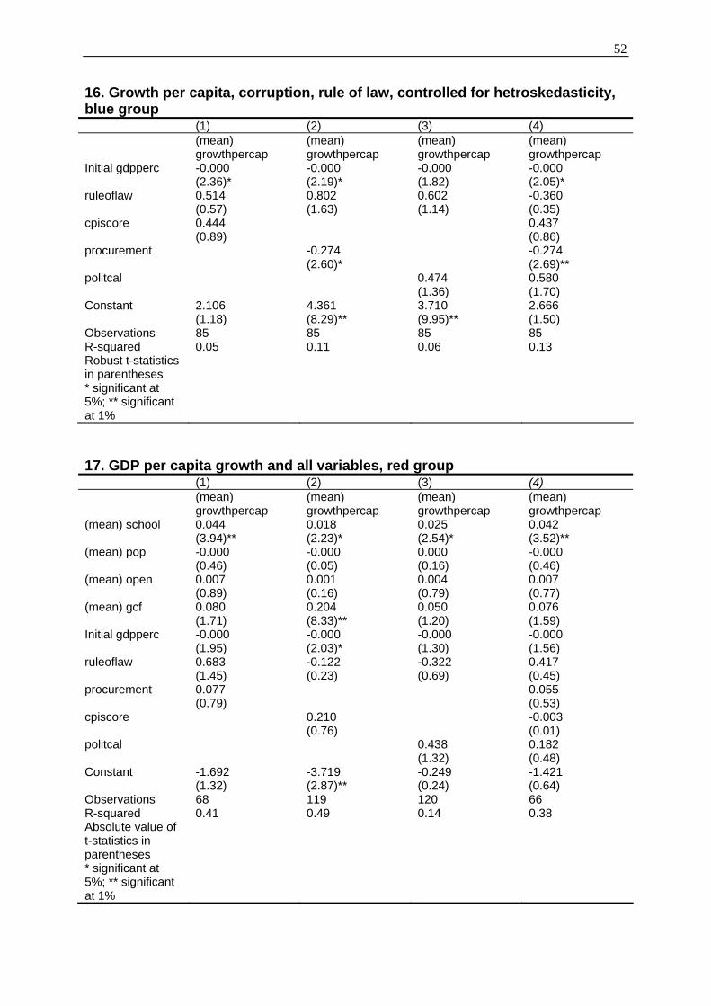
52

16. Growth per capita, corruption, rule of law, controlled for hetroskedasticity, blue group

(1) (2) (3) (4) (mean)

growthpercap (mean) growthpercap

(mean) growthpercap

(mean) growthpercap

Initial gdpperc -0.000 -0.000 -0.000 -0.000 (2.36)* (2.19)* (1.82) (2.05)* ruleoflaw 0.514 0.802 0.602 -0.360 (0.57) (1.63) (1.14) (0.35) cpiscore 0.444 0.437 (0.89) (0.86) procurement -0.274 -0.274 (2.60)* (2.69)** politcal 0.474 0.580 (1.36) (1.70) Constant 2.106 4.361 3.710 2.666 (1.18) (8.29)** (9.95)** (1.50) Observations 85 85 85 85 R-squared 0.05 0.11 0.06 0.13 Robust t-statistics in parentheses

* significant at 5%; ** significant at 1%

17. GDP per capita growth and all variables, red group (1) (2) (3) (4) (mean)

growthpercap (mean) growthpercap

(mean) growthpercap

(mean) growthpercap

(mean) school 0.044 0.018 0.025 0.042 (3.94)** (2.23)* (2.54)* (3.52)** (mean) pop -0.000 -0.000 0.000 -0.000 (0.46) (0.05) (0.16) (0.46) (mean) open 0.007 0.001 0.004 0.007 (0.89) (0.16) (0.79) (0.77) (mean) gcf 0.080 0.204 0.050 0.076 (1.71) (8.33)** (1.20) (1.59) Initial gdpperc -0.000 -0.000 -0.000 -0.000 (1.95) (2.03)* (1.30) (1.56) ruleoflaw 0.683 -0.122 -0.322 0.417 (1.45) (0.23) (0.69) (0.45) procurement 0.077 0.055 (0.79) (0.53) cpiscore 0.210 -0.003 (0.76) (0.01) politcal 0.438 0.182 (1.32) (0.48) Constant -1.692 -3.719 -0.249 -1.421 (1.32) (2.87)** (0.24) (0.64) Observations 68 119 120 66 R-squared 0.41 0.49 0.14 0.38 Absolute value of t-statistics in parentheses

* significant at 5%; ** significant at 1%

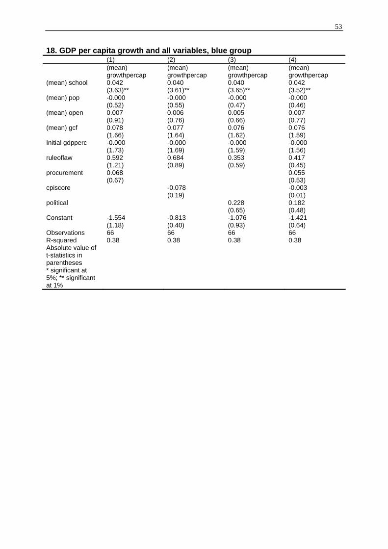
53

18. GDP per capita growth and all variables, blue group (1) (2) (3) (4) (mean)

growthpercap (mean) growthpercap

(mean) growthpercap

(mean) growthpercap

(mean) school 0.042 0.040 0.040 0.042 (3.63)** (3.61)** (3.65)** (3.52)** (mean) pop -0.000 -0.000 -0.000 -0.000 (0.52) (0.55) (0.47) (0.46) (mean) open 0.007 0.006 0.005 0.007 (0.91) (0.76) (0.66) (0.77) (mean) gcf 0.078 0.077 0.076 0.076 (1.66) (1.64) (1.62) (1.59) Initial gdpperc -0.000 -0.000 -0.000 -0.000 (1.73) (1.69) (1.59) (1.56) ruleoflaw 0.592 0.684 0.353 0.417 (1.21) (0.89) (0.59) (0.45) procurement 0.068 0.055 (0.67) (0.53) cpiscore -0.078 -0.003 (0.19) (0.01) political 0.228 0.182 (0.65) (0.48) Constant -1.554 -0.813 -1.076 -1.421 (1.18) (0.40) (0.93) (0.64) Observations 66 66 66 66 R-squared 0.38 0.38 0.38 0.38 Absolute value of t-statistics in parentheses

* significant at 5%; ** significant at 1%

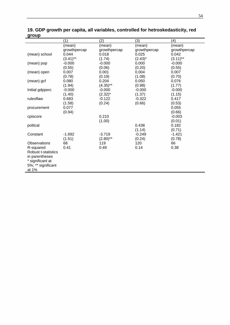
54

19. GDP growth per capita, all variables, controlled for hetroskedasticity, red group (1) (2) (3) (4) (mean)

growthpercap (mean) growthpercap

(mean) growthpercap

(mean) growthpercap

(mean) school 0.044 0.018 0.025 0.042 (3.41)** (1.74) (2.43)* (3.11)** (mean) pop -0.000 -0.000 0.000 -0.000 (0.55) (0.06) (0.20) (0.55) (mean) open 0.007 0.001 0.004 0.007 (0.78) (0.19) (1.08) (0.70) (mean) gcf 0.080 0.204 0.050 0.076 (1.94) (4.35)** (0.98) (1.77) Initial gdpperc -0.000 -0.000 -0.000 -0.000 (1.40) (2.32)* (1.37) (1.15) ruleoflaw 0.683 -0.122 -0.322 0.417 (1.58) (0.24) (0.66) (0.53) procurement 0.077 0.055 (0.94) (0.66) cpiscore 0.210 -0.003 (1.00) (0.01) politcal 0.438 0.182 (1.14) (0.71) Constant -1.692 -3.719 -0.249 -1.421 (1.51) (2.80)** (0.24) (0.78) Observations 68 119 120 66 R-squared 0.41 0.49 0.14 0.38 Robust t-statistics in parentheses

* significant at 5%; ** significant at 1%

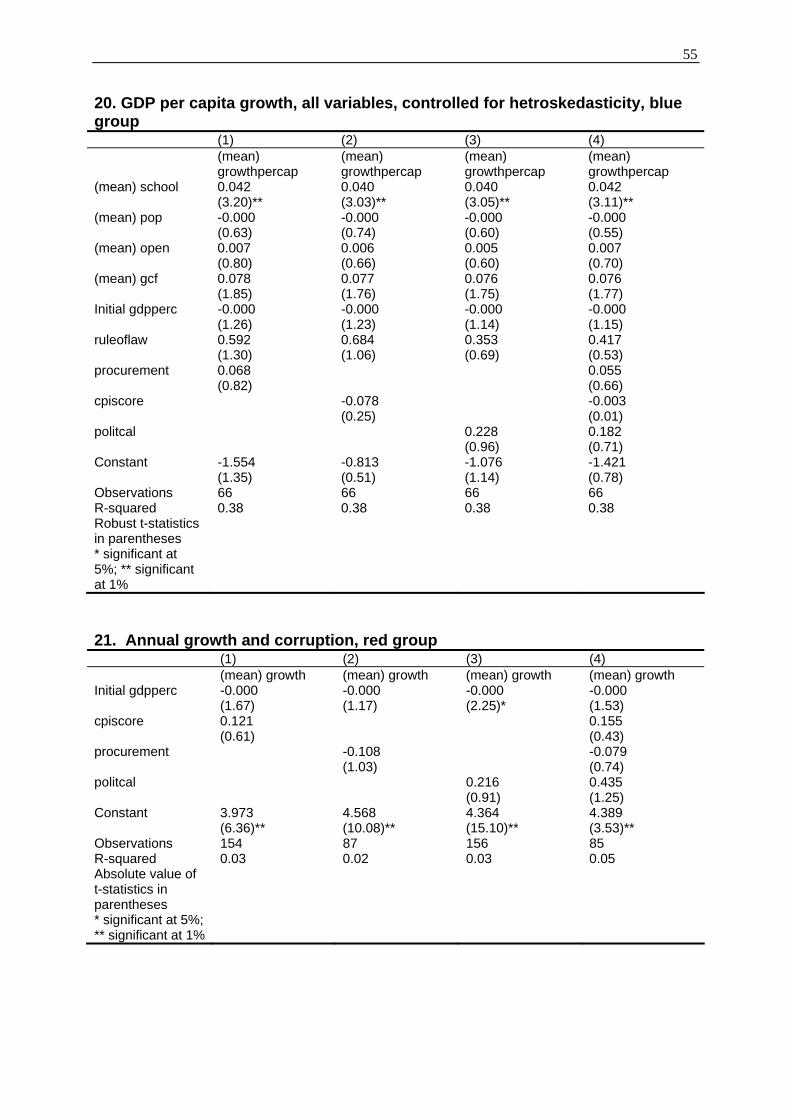
55

20. GDP per capita growth, all variables, controlled for hetroskedasticity, blue group (1) (2) (3) (4) (mean)

growthpercap (mean) growthpercap

(mean) growthpercap

(mean) growthpercap

(mean) school 0.042 0.040 0.040 0.042 (3.20)** (3.03)** (3.05)** (3.11)** (mean) pop -0.000 -0.000 -0.000 -0.000 (0.63) (0.74) (0.60) (0.55) (mean) open 0.007 0.006 0.005 0.007 (0.80) (0.66) (0.60) (0.70) (mean) gcf 0.078 0.077 0.076 0.076 (1.85) (1.76) (1.75) (1.77) Initial gdpperc -0.000 -0.000 -0.000 -0.000 (1.26) (1.23) (1.14) (1.15) ruleoflaw 0.592 0.684 0.353 0.417 (1.30) (1.06) (0.69) (0.53) procurement 0.068 0.055 (0.82) (0.66) cpiscore -0.078 -0.003 (0.25) (0.01) politcal 0.228 0.182 (0.96) (0.71) Constant -1.554 -0.813 -1.076 -1.421 (1.35) (0.51) (1.14) (0.78) Observations 66 66 66 66 R-squared 0.38 0.38 0.38 0.38 Robust t-statistics in parentheses

* significant at 5%; ** significant at 1%

21. Annual growth and corruption, red group (1) (2) (3) (4) (mean) growth (mean) growth (mean) growth (mean) growth Initial gdpperc -0.000 -0.000 -0.000 -0.000 (1.67) (1.17) (2.25)* (1.53) cpiscore 0.121 0.155 (0.61) (0.43) procurement -0.108 -0.079 (1.03) (0.74) politcal 0.216 0.435 (0.91) (1.25) Constant 3.973 4.568 4.364 4.389 (6.36)** (10.08)** (15.10)** (3.53)** Observations 154 87 156 85 R-squared 0.03 0.02 0.03 0.05 Absolute value of t-statistics in parentheses

* significant at 5%; ** significant at 1%

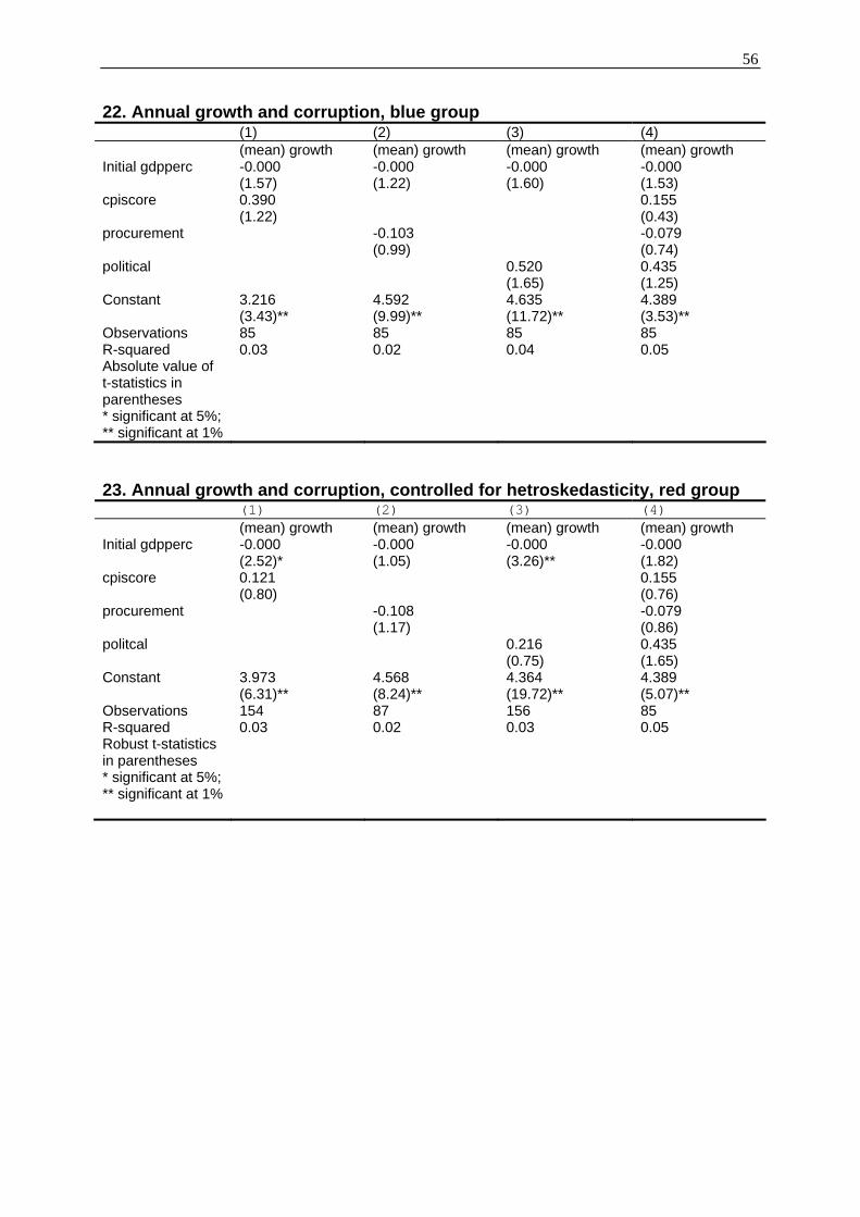
56

22. Annual growth and corruption, blue group (1) (2) (3) (4) (mean) growth (mean) growth (mean) growth (mean) growth Initial gdpperc -0.000 -0.000 -0.000 -0.000 (1.57) (1.22) (1.60) (1.53) cpiscore 0.390 0.155 (1.22) (0.43) procurement -0.103 -0.079 (0.99) (0.74) political 0.520 0.435 (1.65) (1.25) Constant 3.216 4.592 4.635 4.389 (3.43)** (9.99)** (11.72)** (3.53)** Observations 85 85 85 85 R-squared 0.03 0.02 0.04 0.05 Absolute value of t-statistics in parentheses

* significant at 5%; ** significant at 1%

23. Annual growth and corruption, controlled for hetroskedasticity, red group (1) (2) (3) (4) (mean) growth (mean) growth (mean) growth (mean) growth Initial gdpperc -0.000 -0.000 -0.000 -0.000 (2.52)* (1.05) (3.26)** (1.82) cpiscore 0.121 0.155 (0.80) (0.76) procurement -0.108 -0.079 (1.17) (0.86) politcal 0.216 0.435 (0.75) (1.65) Constant 3.973 4.568 4.364 4.389 (6.31)** (8.24)** (19.72)** (5.07)** Observations 154 87 156 85 R-squared 0.03 0.02 0.03 0.05 Robust t-statistics in parentheses

* significant at 5%; ** significant at 1%

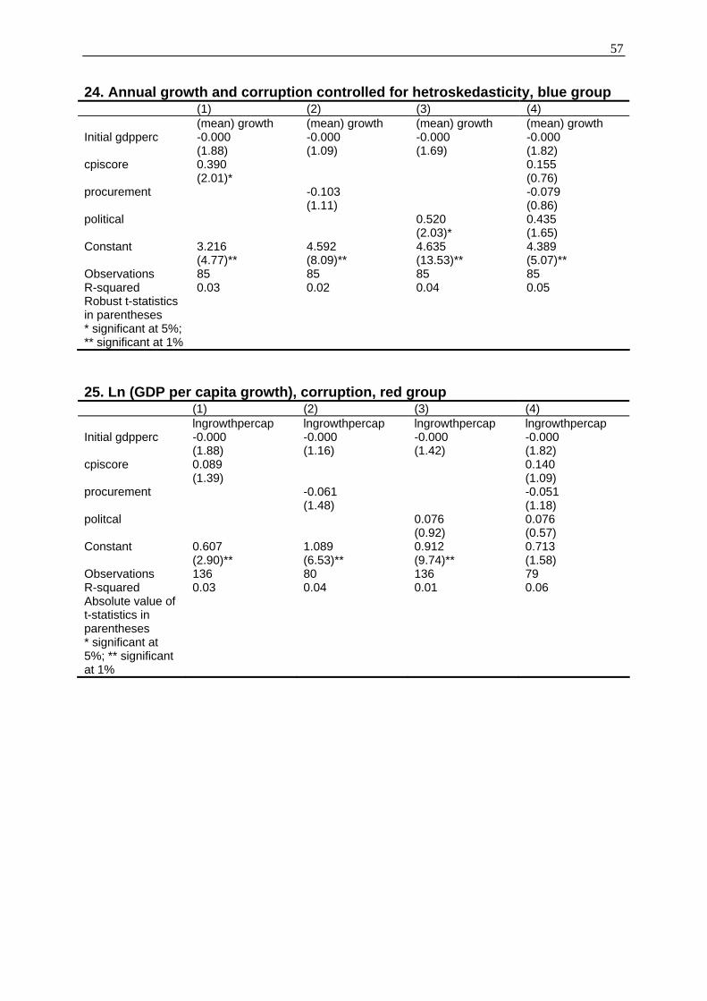
57

24. Annual growth and corruption controlled for hetroskedasticity, blue group (1) (2) (3) (4) (mean) growth (mean) growth (mean) growth (mean) growth Initial gdpperc -0.000 -0.000 -0.000 -0.000 (1.88) (1.09) (1.69) (1.82) cpiscore 0.390 0.155 (2.01)* (0.76) procurement -0.103 -0.079 (1.11) (0.86) political 0.520 0.435 (2.03)* (1.65) Constant 3.216 4.592 4.635 4.389 (4.77)** (8.09)** (13.53)** (5.07)** Observations 85 85 85 85 R-squared 0.03 0.02 0.04 0.05 Robust t-statistics in parentheses

* significant at 5%; ** significant at 1%

25. Ln (GDP per capita growth), corruption, red group (1) (2) (3) (4) lngrowthpercap lngrowthpercap lngrowthpercap lngrowthpercap Initial gdpperc -0.000 -0.000 -0.000 -0.000 (1.88) (1.16) (1.42) (1.82) cpiscore 0.089 0.140 (1.39) (1.09) procurement -0.061 -0.051 (1.48) (1.18) politcal 0.076 0.076 (0.92) (0.57) Constant 0.607 1.089 0.912 0.713 (2.90)** (6.53)** (9.74)** (1.58) Observations 136 80 136 79 R-squared 0.03 0.04 0.01 0.06 Absolute value of t-statistics in parentheses

* significant at 5%; ** significant at 1%

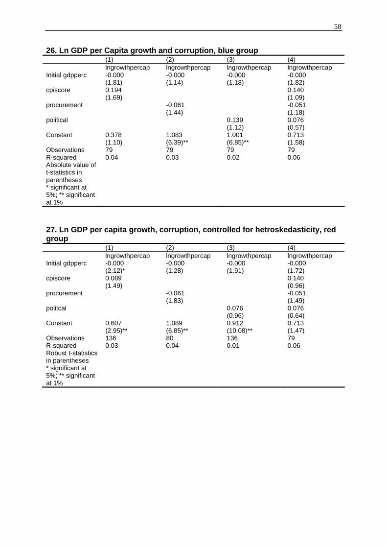
58

26. Ln GDP per Capita growth and corruption, blue group (1) (2) (3) (4) lngrowthpercap lngrowthpercap lngrowthpercap lngrowthpercap Initial gdpperc -0.000 -0.000 -0.000 -0.000 (1.81) (1.14) (1.18) (1.82) cpiscore 0.194 0.140 (1.69) (1.09) procurement -0.061 -0.051 (1.44) (1.18) political 0.139 0.076 (1.12) (0.57) Constant 0.378 1.083 1.001 0.713 (1.10) (6.39)** (6.85)** (1.58) Observations 79 79 79 79 R-squared 0.04 0.03 0.02 0.06 Absolute value of t-statistics in parentheses

* significant at 5%; ** significant at 1%

27. Ln GDP per capita growth, corruption, controlled for hetroskedasticity, red group (1) (2) (3) (4) lngrowthpercap lngrowthpercap lngrowthpercap lngrowthpercap Initial gdpperc -0.000 -0.000 -0.000 -0.000 (2.12)* (1.28) (1.91) (1.72) cpiscore 0.089 0.140 (1.49) (0.96) procurement -0.061 -0.051 (1.83) (1.49) politcal 0.076 0.076 (0.96) (0.64) Constant 0.607 1.089 0.912 0.713 (2.95)** (6.85)** (10.08)** (1.47) Observations 136 80 136 79 R-squared 0.03 0.04 0.01 0.06 Robust t-statistics in parentheses

* significant at 5%; ** significant at 1%

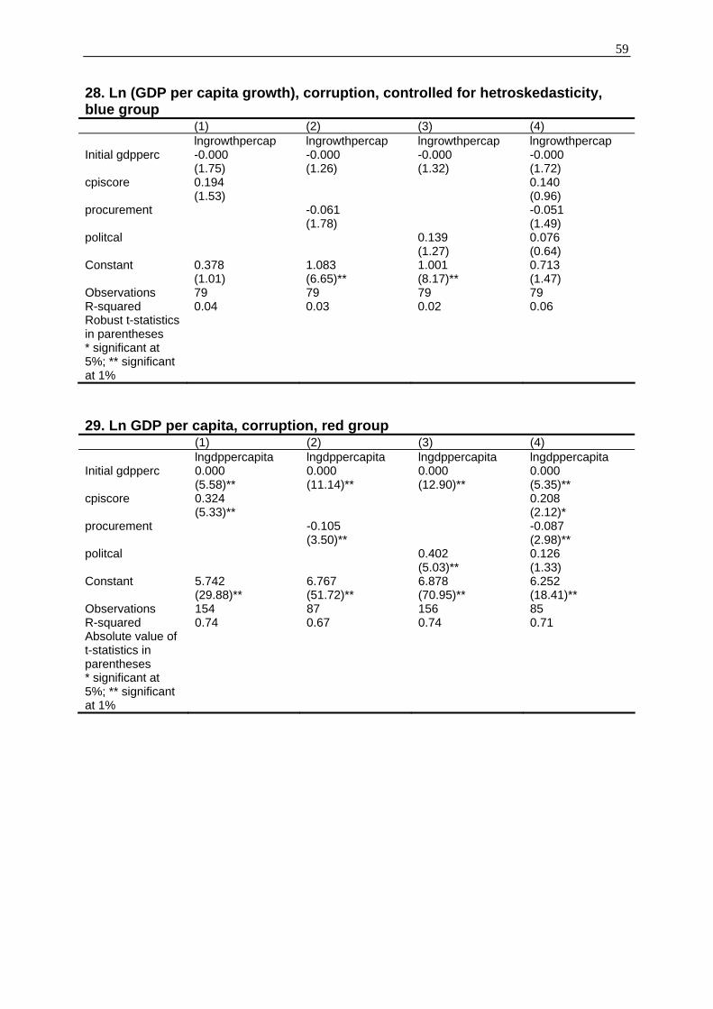
59

28. Ln (GDP per capita growth), corruption, controlled for hetroskedasticity, blue group (1) (2) (3) (4) lngrowthpercap lngrowthpercap lngrowthpercap lngrowthpercap Initial gdpperc -0.000 -0.000 -0.000 -0.000 (1.75) (1.26) (1.32) (1.72) cpiscore 0.194 0.140 (1.53) (0.96) procurement -0.061 -0.051 (1.78) (1.49) politcal 0.139 0.076 (1.27) (0.64) Constant 0.378 1.083 1.001 0.713 (1.01) (6.65)** (8.17)** (1.47) Observations 79 79 79 79 R-squared 0.04 0.03 0.02 0.06 Robust t-statistics in parentheses

* significant at 5%; ** significant at 1%

29. Ln GDP per capita, corruption, red group (1) (2) (3) (4) lngdppercapita lngdppercapita lngdppercapita lngdppercapita Initial gdpperc 0.000 0.000 0.000 0.000 (5.58)** (11.14)** (12.90)** (5.35)** cpiscore 0.324 0.208 (5.33)** (2.12)* procurement -0.105 -0.087 (3.50)** (2.98)** politcal 0.402 0.126 (5.03)** (1.33) Constant 5.742 6.767 6.878 6.252 (29.88)** (51.72)** (70.95)** (18.41)** Observations 154 87 156 85 R-squared 0.74 0.67 0.74 0.71 Absolute value of t-statistics in parentheses

* significant at 5%; ** significant at 1%

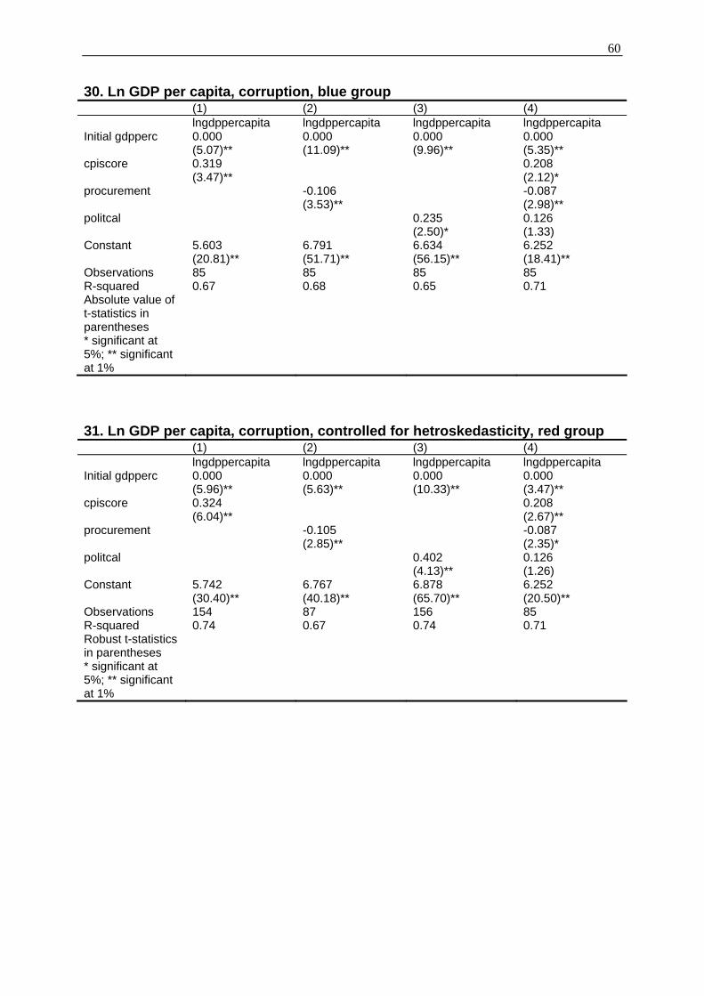
60

30. Ln GDP per capita, corruption, blue group (1) (2) (3) (4) lngdppercapita lngdppercapita lngdppercapita lngdppercapita Initial gdpperc 0.000 0.000 0.000 0.000 (5.07)** (11.09)** (9.96)** (5.35)** cpiscore 0.319 0.208 (3.47)** (2.12)* procurement -0.106 -0.087 (3.53)** (2.98)** politcal 0.235 0.126 (2.50)* (1.33) Constant 5.603 6.791 6.634 6.252 (20.81)** (51.71)** (56.15)** (18.41)** Observations 85 85 85 85 R-squared 0.67 0.68 0.65 0.71 Absolute value of t-statistics in parentheses

* significant at 5%; ** significant at 1%

31. Ln GDP per capita, corruption, controlled for hetroskedasticity, red group (1) (2) (3) (4) lngdppercapita lngdppercapita lngdppercapita lngdppercapita Initial gdpperc 0.000 0.000 0.000 0.000 (5.96)** (5.63)** (10.33)** (3.47)** cpiscore 0.324 0.208 (6.04)** (2.67)** procurement -0.105 -0.087 (2.85)** (2.35)* politcal 0.402 0.126 (4.13)** (1.26) Constant 5.742 6.767 6.878 6.252 (30.40)** (40.18)** (65.70)** (20.50)** Observations 154 87 156 85 R-squared 0.74 0.67 0.74 0.71 Robust t-statistics in parentheses

* significant at 5%; ** significant at 1%

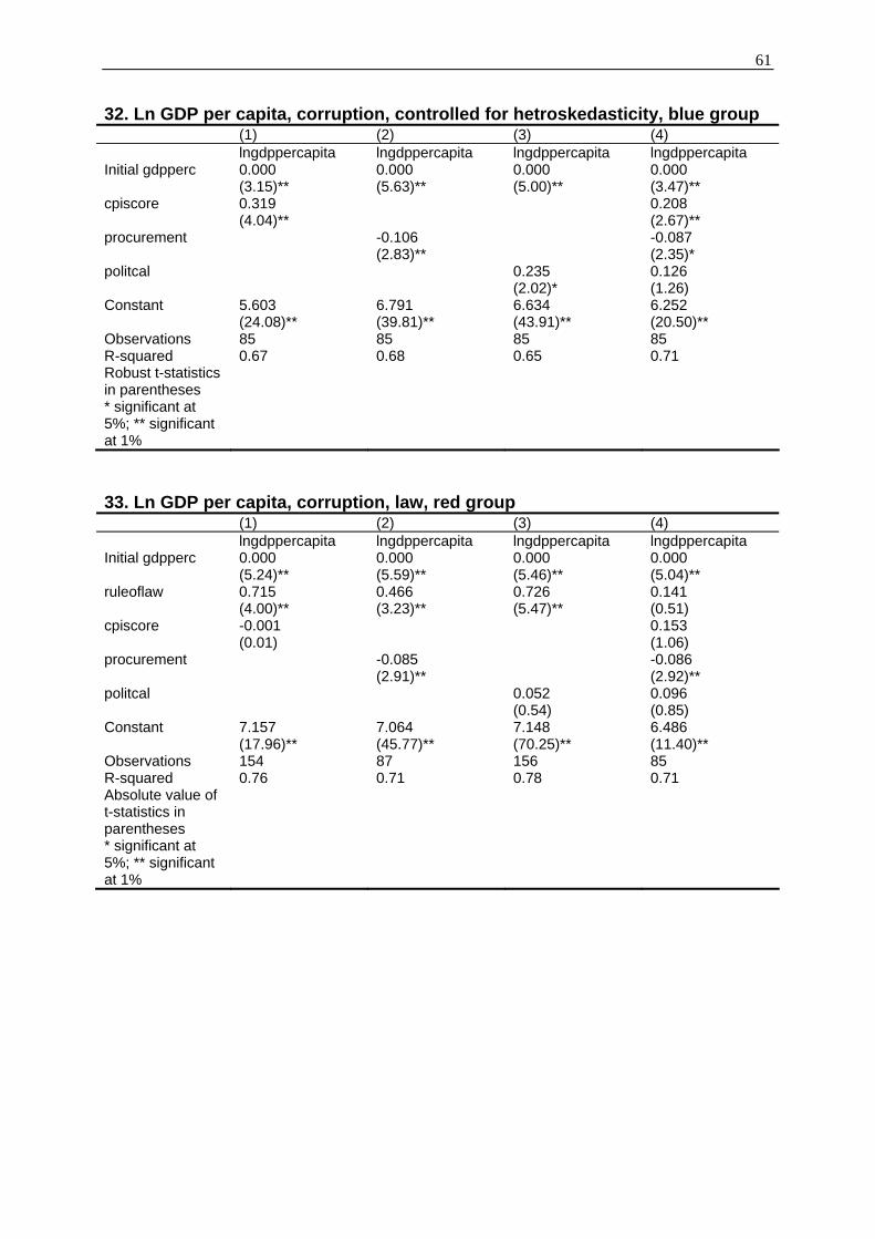
61

32. Ln GDP per capita, corruption, controlled for hetroskedasticity, blue group (1) (2) (3) (4) lngdppercapita lngdppercapita lngdppercapita lngdppercapita Initial gdpperc 0.000 0.000 0.000 0.000 (3.15)** (5.63)** (5.00)** (3.47)** cpiscore 0.319 0.208 (4.04)** (2.67)** procurement -0.106 -0.087 (2.83)** (2.35)* politcal 0.235 0.126 (2.02)* (1.26) Constant 5.603 6.791 6.634 6.252 (24.08)** (39.81)** (43.91)** (20.50)** Observations 85 85 85 85 R-squared 0.67 0.68 0.65 0.71 Robust t-statistics in parentheses

* significant at 5%; ** significant at 1%

33. Ln GDP per capita, corruption, law, red group (1) (2) (3) (4) lngdppercapita lngdppercapita lngdppercapita lngdppercapita Initial gdpperc 0.000 0.000 0.000 0.000 (5.24)** (5.59)** (5.46)** (5.04)** ruleoflaw 0.715 0.466 0.726 0.141 (4.00)** (3.23)** (5.47)** (0.51) cpiscore -0.001 0.153 (0.01) (1.06) procurement -0.085 -0.086 (2.91)** (2.92)** politcal 0.052 0.096 (0.54) (0.85) Constant 7.157 7.064 7.148 6.486 (17.96)** (45.77)** (70.25)** (11.40)** Observations 154 87 156 85 R-squared 0.76 0.71 0.78 0.71 Absolute value of t-statistics in parentheses

* significant at 5%; ** significant at 1%

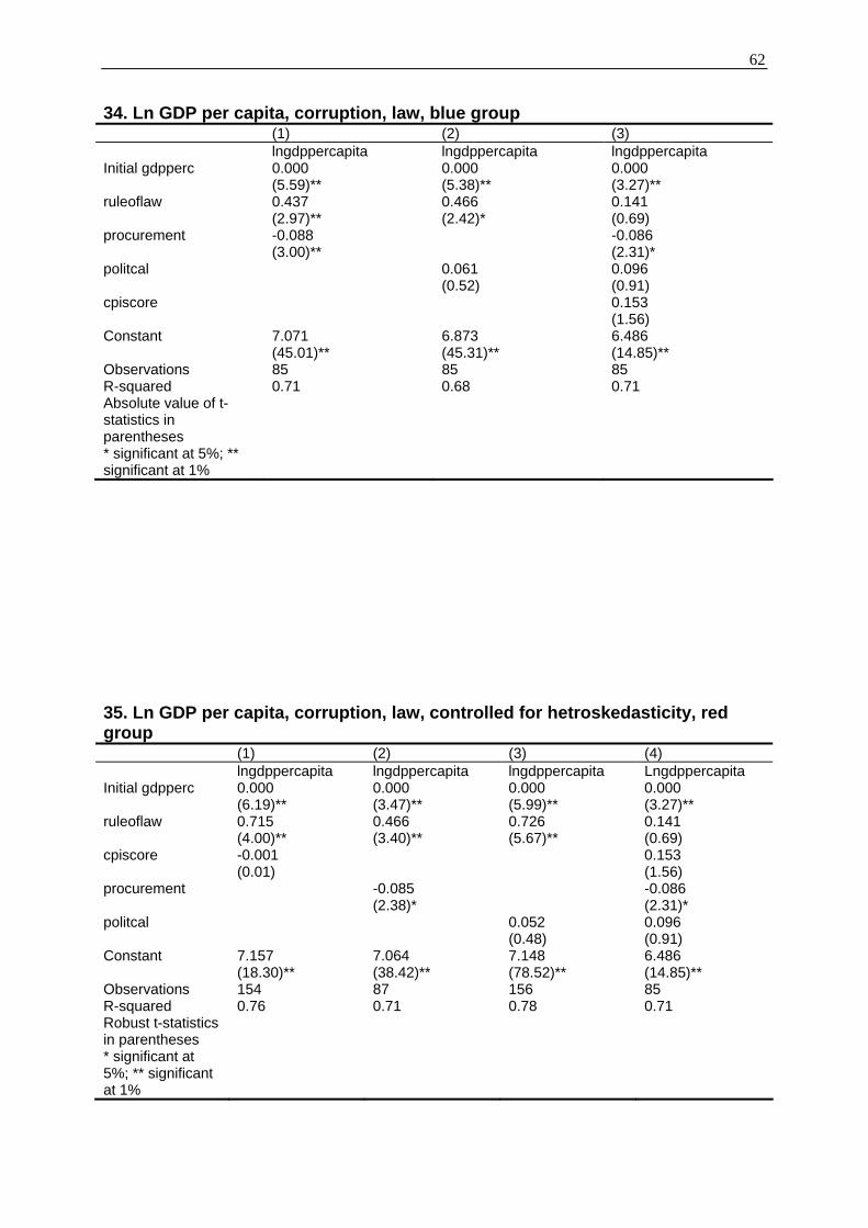
62

34. Ln GDP per capita, corruption, law, blue group (1) (2) (3) lngdppercapita lngdppercapita lngdppercapita Initial gdpperc 0.000 0.000 0.000 (5.59)** (5.38)** (3.27)** ruleoflaw 0.437 0.466 0.141 (2.97)** (2.42)* (0.69) procurement -0.088 -0.086 (3.00)** (2.31)* politcal 0.061 0.096 (0.52) (0.91) cpiscore 0.153 (1.56) Constant 7.071 6.873 6.486 (45.01)** (45.31)** (14.85)** Observations 85 85 85 R-squared 0.71 0.68 0.71 Absolute value of t-statistics in parentheses

* significant at 5%; ** significant at 1%

35. Ln GDP per capita, corruption, law, controlled for hetroskedasticity, red group (1) (2) (3) (4) lngdppercapita lngdppercapita lngdppercapita Lngdppercapita Initial gdpperc 0.000 0.000 0.000 0.000 (6.19)** (3.47)** (5.99)** (3.27)** ruleoflaw 0.715 0.466 0.726 0.141 (4.00)** (3.40)** (5.67)** (0.69) cpiscore -0.001 0.153 (0.01) (1.56) procurement -0.085 -0.086 (2.38)* (2.31)* politcal 0.052 0.096 (0.48) (0.91) Constant 7.157 7.064 7.148 6.486 (18.30)** (38.42)** (78.52)** (14.85)** Observations 154 87 156 85 R-squared 0.76 0.71 0.78 0.71 Robust t-statistics in parentheses

* significant at 5%; ** significant at 1%

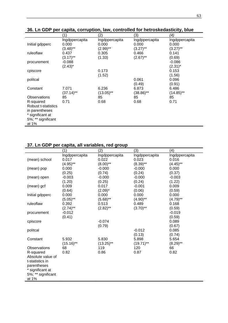
63

36. Ln GDP per capita, corruption, law, controlled for hetroskedasticity, blue (1) (2) (3) (4) lngdppercapita lngdppercapita lngdppercapita lngdppercapita Initial gdpperc 0.000 0.000 0.000 0.000 (3.48)** (2.99)** (3.27)** (3.27)** ruleoflaw 0.437 0.305 0.466 0.141 (3.17)** (1.33) (2.67)** (0.69) procurement -0.088 -0.086 (2.43)* (2.31)* cpiscore 0.173 0.153 (1.52) (1.56) politcal 0.061 0.096 (0.49) (0.91) Constant 7.071 6.236 6.873 6.486 (37.14)** (13.05)** (38.86)** (14.85)** Observations 85 85 85 85 R-squared 0.71 0.68 0.68 0.71 Robust t-statistics in parentheses

* significant at 5%; ** significant at 1%

37. Ln GDP per capita, all variables, red group (1) (2) (3) (4) lngdppercapita lngdppercapita lngdppercapita lngdppercapita (mean) school 0.017 0.022 0.023 0.016 (4.95)** (8.00)** (8.39)** (4.45)** (mean) pop 0.000 -0.000 -0.000 0.000 (0.25) (0.74) (0.24) (0.37) (mean) open -0.003 -0.000 -0.000 -0.003 (1.20) (0.25) (0.24) (1.22) (mean) gcf 0.009 0.017 -0.001 0.009 (0.64) (2.09)* (0.06) (0.59) Initial gdpperc 0.000 0.000 0.000 0.000 (5.05)** (5.68)** (4.90)** (4.79)** ruleoflaw 0.392 0.513 0.489 0.168 (2.74)** (2.82)** (3.70)** (0.59) procurement -0.012 -0.019 (0.41) (0.59) cpiscore -0.074 0.089 (0.79) (0.67) politcal -0.012 0.085 (0.13) (0.74) Constant 5.932 5.830 5.898 5.654 (15.16)** (13.25)** (19.71)** (8.29)** Observations 68 119 120 66 R-squared 0.82 0.86 0.87 0.82 Absolute value of t-statistics in parentheses

* significant at 5%; ** significant at 1%

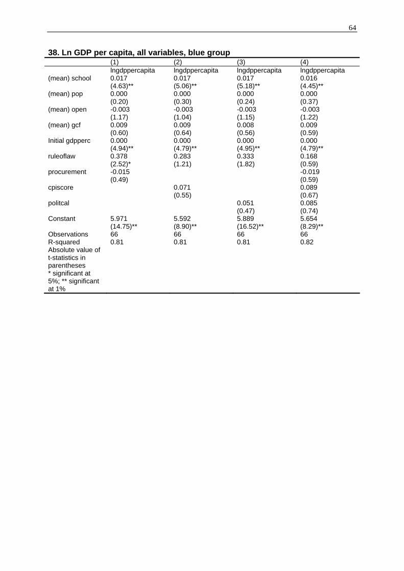
64

38. Ln GDP per capita, all variables, blue group (1) (2) (3) (4) lngdppercapita lngdppercapita lngdppercapita lngdppercapita (mean) school 0.017 0.017 0.017 0.016 (4.63)** (5.06)** (5.18)** (4.45)** (mean) pop 0.000 0.000 0.000 0.000 (0.20) (0.30) (0.24) (0.37) (mean) open -0.003 -0.003 -0.003 -0.003 (1.17) (1.04) (1.15) (1.22) (mean) gcf 0.009 0.009 0.008 0.009 (0.60) (0.64) (0.56) (0.59) Initial gdpperc 0.000 0.000 0.000 0.000 (4.94)** (4.79)** (4.95)** (4.79)** ruleoflaw 0.378 0.283 0.333 0.168 (2.52)* (1.21) (1.82) (0.59) procurement -0.015 -0.019 (0.49) (0.59) cpiscore 0.071 0.089 (0.55) (0.67) politcal 0.051 0.085 (0.47) (0.74) Constant 5.971 5.592 5.889 5.654 (14.75)** (8.90)** (16.52)** (8.29)** Observations 66 66 66 66 R-squared 0.81 0.81 0.81 0.82 Absolute value of t-statistics in parentheses

* significant at 5%; ** significant at 1%

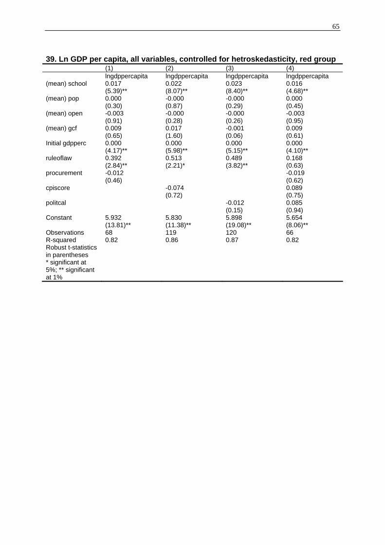
65

39. Ln GDP per capita, all variables, controlled for hetroskedasticity, red group (1) (2) (3) (4) lngdppercapita lngdppercapita lngdppercapita lngdppercapita (mean) school 0.017 0.022 0.023 0.016 (5.39)** (8.07)** (8.40)** (4.68)** (mean) pop 0.000 -0.000 -0.000 0.000 (0.30) (0.87) (0.29) (0.45) (mean) open -0.003 -0.000 -0.000 -0.003 (0.91) (0.28) (0.26) (0.95) (mean) gcf 0.009 0.017 -0.001 0.009 (0.65) (1.60) (0.06) (0.61) Initial gdpperc 0.000 0.000 0.000 0.000 (4.17)** (5.98)** (5.15)** (4.10)** ruleoflaw 0.392 0.513 0.489 0.168 (2.84)** (2.21)* (3.82)** (0.63) procurement -0.012 -0.019 (0.46) (0.62) cpiscore -0.074 0.089 (0.72) (0.75) politcal -0.012 0.085 (0.15) (0.94) Constant 5.932 5.830 5.898 5.654 (13.81)** (11.38)** (19.08)** (8.06)** Observations 68 119 120 66 R-squared 0.82 0.86 0.87 0.82 Robust t-statistics in parentheses

* significant at 5%; ** significant at 1%

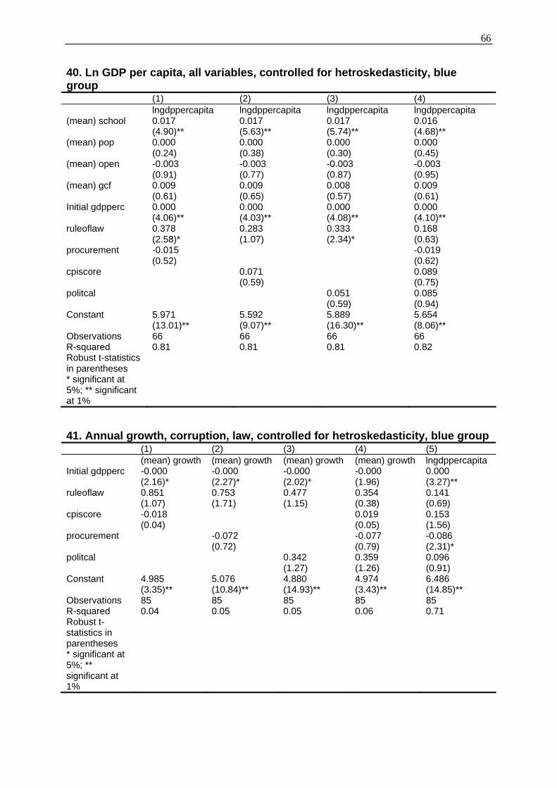
66

40. Ln GDP per capita, all variables, controlled for hetroskedasticity, blue group (1) (2) (3) (4) lngdppercapita lngdppercapita lngdppercapita lngdppercapita (mean) school 0.017 0.017 0.017 0.016 (4.90)** (5.63)** (5.74)** (4.68)** (mean) pop 0.000 0.000 0.000 0.000 (0.24) (0.38) (0.30) (0.45) (mean) open -0.003 -0.003 -0.003 -0.003 (0.91) (0.77) (0.87) (0.95) (mean) gcf 0.009 0.009 0.008 0.009 (0.61) (0.65) (0.57) (0.61) Initial gdpperc 0.000 0.000 0.000 0.000 (4.06)** (4.03)** (4.08)** (4.10)** ruleoflaw 0.378 0.283 0.333 0.168 (2.58)* (1.07) (2.34)* (0.63) procurement -0.015 -0.019 (0.52) (0.62) cpiscore 0.071 0.089 (0.59) (0.75) politcal 0.051 0.085 (0.59) (0.94) Constant 5.971 5.592 5.889 5.654 (13.01)** (9.07)** (16.30)** (8.06)** Observations 66 66 66 66 R-squared 0.81 0.81 0.81 0.82 Robust t-statistics in parentheses

* significant at 5%; ** significant at 1%

41. Annual growth, corruption, law, controlled for hetroskedasticity, blue group (1) (2) (3) (4) (5) (mean) growth (mean) growth (mean) growth (mean) growth lngdppercapita Initial gdpperc -0.000 -0.000 -0.000 -0.000 0.000 (2.16)* (2.27)* (2.02)* (1.96) (3.27)** ruleoflaw 0.851 0.753 0.477 0.354 0.141 (1.07) (1.71) (1.15) (0.38) (0.69) cpiscore -0.018 0.019 0.153 (0.04) (0.05) (1.56) procurement -0.072 -0.077 -0.086 (0.72) (0.79) (2.31)* politcal 0.342 0.359 0.096 (1.27) (1.26) (0.91) Constant 4.985 5.076 4.880 4.974 6.486 (3.35)** (10.84)** (14.93)** (3.43)** (14.85)** Observations 85 85 85 85 85 R-squared 0.04 0.05 0.05 0.06 0.71 Robust t-statistics in parentheses

* significant at 5%; ** significant at 1%

67