Embed Size (px)
Citation preview
Matching 2D and 3D Articulated Shapes using
Eccentricity
Adrian Ion, Nicole M. Artner, Gabriel Peyre, Walter G. Kropatsch, Laurent
D. Cohen
To cite this version:
Adrian Ion, Nicole M. Artner, Gabriel Peyre, Walter G. Kropatsch, Laurent D. Cohen. Match-ing 2D and 3D Articulated Shapes using Eccentricity. 2008. <hal-00365019v1>
HAL Id: hal-00365019
https://hal.archives-ouvertes.fr/hal-00365019v1
Submitted on 2 Mar 2009 (v1), last revised 25 Jan 2011 (v2)
HAL is a multi-disciplinary open accessarchive for the deposit and dissemination of sci-entific research documents, whether they are pub-lished or not. The documents may come fromteaching and research institutions in France orabroad, or from public or private research centers.
L’archive ouverte pluridisciplinaire HAL, estdestinee au depot et a la diffusion de documentsscientifiques de niveau recherche, publies ou non,emanant des etablissements d’enseignement et derecherche francais ou etrangers, des laboratoirespublics ou prives.
International Journal of Computer Vision manuscript No.(will be inserted by the editor)
Matching 2D & 3D Articulated Shapes using Eccentricity
Adrian Ion · Nicole M. Artner · Gabriel Peyre · Walter G. Kropatsch ·
Laurent Cohen
Received: date / Accepted: date
Abstract Shape matching should be invariant to thetypical intra-class deformations present in nature. Themajority of shape descriptors are quite complex andnot invariant to the deformation or articulation of ob-ject parts. Geodesic distances computed over a 2D or3D shape are articulation insensitive. The eccentricitytransform considers the length of the longest geodesics.
It is robust with respect to Salt and Pepper noise, andminor segmentation errors, and is stable in the pres-ence of holes. We present a method for 2D and 3Dshape matching based on the eccentricity transform.Eccentricity histograms make up descriptors insensitiveto rotation, scaling, and articulation. The descriptoris highly compact and the method is straight-forward.
Experimental results on established 2D and 3D bench-marks show results comparable to more complex stateof the art methods. Properties and results are discussedin detail.
Partially supported by the Austrian Science Fund under grantsS9103-N13 and P18716-N13.
Adrian Ion
PRIP, Vienna University of TechnologyE-mail: [email protected]
Nicole M. Artner
ARC, Smart Systems Division, AustriaE-mail: [email protected]
Gabriel Peyre
CNRS, CEREMADE, Universite Paris-Dauphine
E-mail: [email protected]
Walter G. Kropatsch
PRIP, Vienna University of Technology
E-mail: [email protected]
Laurent Cohen
CNRS, CEREMADE, Universite Paris-DauphineE-mail: [email protected]
Keywords Eccentricity Transform · Shape Matching ·Articulation · Geodesic Distance
1 Introduction
The recent increase in available 3D models and acqui-sition systems has seen the need for efficient retrievalof stored models, making 3D shape matching gain at-tention also outside the computer vision community.Together with its 2D counterpart, 3D shape matchingis useful for identification and retrieval in classical vi-
sion tasks, but can also be found in Computer AidedDesign/Computer Aided Manufacturing (CAD/CAM),virtual reality (VR), medicine, molecular biology, secu-
rity, and entertainment (Bustos et al, 2005).
Shape matching requires to set up a signature thatcharacterizes the properties of interest for the recogni-tion (Veltkamp and Latecki, 2006). The invariance ofthis signature to local deformations such as articula-
tions is important for the identification of 2D and 3Dshapes. Matching can then be carried out over this re-duced space of signatures. Most shape descriptors are
computed over a transformed domain that amplifies theimportant features of the object while throwing awayambiguities such as translation, rotation or local defor-mations.
For 2D shapes, the Fourier transform of the bound-
ary curve (Zahn and Roskies, 1972) is an example ofsuch a transformed domain descriptor adapted tosmooth shapes. Shape transformations computed with
geodesic distances (Bronstein et al, 2006) lead to signa-tures invariant to isometric deformations such as bend-ing or articulation. To capture salient features of 2Dobjects, local quantities such as curvature (Mokhtar-ian and Mackworth, 1992) or shape contexts (Belongie
2
et al, 2002) can be computed. They can be extended tobending invariant signatures using geodesic distances(Ling and Jacobs, 2007). More global features includethe Laplace spectra (Reuter et al, 2005) and the skele-
ton (Siddiqi et al, 1999). Some transformations involvethe computation of a function defined on the shape, forinstance the solution to a linear partial differential equa-
tion (Gorelick et al, 2004) or geometric quantities (Os-ada et al, 2002). Geodesic distance information such asthe mean-geodesic transform (Hamza and Krim, 2003)
could also be used.
Among appraoches matching 3D shapes, existingapproaches can be divided into (Bustos et al, 2005):Statistical descriptors, like for example geometric 3D
moments employed by Elad et al (2001); Paquet et al(2000), and the shape distribution (Osada et al, 2002; Ip
et al, 2003). Extension-based descriptors, which are cal-culated from features sampled along certain directionsfrom a position within the object (Vranic and Saupe,2002, 2001a). Volume-based descriptors use the volu-metric representation of a 3D object to extract fea-tures (examples are Shape histograms, Ankerst et al(1999), Model Voxelization, Vranic and Saupe (2001b),
and point set methods, Tangelder and Veltkamp (2003)).Descriptors using the surface geometry compute curva-ture measures and/or the distribution of surface normalvectors (Paquet and Rioux, 1999; Zaharia and Preux,2001). Image-based descriptors reduce the problem of3D shape matching to an image similarity problem bycomparing 2D projections of the 3D objects (Ansary
et al, 2004; Cyr and Kimia, 2004; Chen et al, 2003).Methods matching the topology of two objects (for ex-ample Reeb graphs, where the topology of the 3D objectis described by a graph structure, Hilaga et al (2001);Shinagawa et al (1991)). Skeletons are intuitive objectdescriptions and can be obtained from a 3D object byapplying a thinning algorithm on the voxelization of asolid object like in Sundar et al (2003). Descriptors us-ing spin images work with a set of 2D histograms of theobject geometry and a search for point-to-point corre-spondences is done to match 3D objects (Johnson andHebert, May 1999).
The majority of shape descriptors is quite complexand not invariant to the deformation or articulation ofobject parts.
In Ling and Jacobs (2007) a model of articulated ob-
jects is presented. It is defined as a union of (rigid) partsOi and joints (named ’junctions’ by the authors). Anarticulation is defined as a transformation that is rigidwhen limited to any part Oi, but can be non-rigid onthe junctions. An articulated instance of an object is anarticulated object itself (actually the same object) that
can be articulated back to the original one. The term
articulated shape refers to the shape of an articulatedobject in a certain pose. In the context of shape match-ing it means that shapes that belong to articulationsof the same object, belong to the same class. Assuming
that the size of the junctions is very small compared tothe size of the parts Oi, it is shown that the relativechange of the geodesic distance1 during articulation issmall and that geodesic distances are articulation in-sensitive.
The eccentricity transform of a shape associates toeach of its points the distance to the point furthest
away. It is based on the computation of geodesic dis-tances and thus robust with respect to articulation. Itis in addition robust with respect to Salt and Peppernoise and minor segmentation errors (Kropatsch et al,2006), and stable in the presence of holes. Normalizedhistograms of the eccentricity transform are invariant to
changes in orientation, scale, and articulation. We pro-pose eccentricity histograms as descriptors for 2D and3D shape matching. They require only a simple repre-sentation and can be efficiently matched. Initial resultshave been presented for 2D in Ion et al (2007), andfor 3D (volumetric representation) in Ion et al (2008a).This article presents a common framework with an in
dept analysis of the properties of the approach, sup-ported by promising experimental results and detaileddiscussion. Four variants of the descriptor are used, onefor 2D shapes and three for 3D shapes (volume, bordervoxels, mesh) and compared to state of the art methods.To the best of our knowledge, this is the first approachapplying eccentricity (furthest point distance) to the
problem of shape matching. The presented approachcould be fitted to either of the categories extension-
based or volume-based, and it is a transformation com-
puted with geodesic distances.Like the method in (Ling and Jacobs, 2007), our
method does not involve any part models. The articu-lation model is only for the analysis of the properties
of the geodesic distance. Finding the correspondencesbetween all the parts of two shapes is an NP -completeproblem in graph theory (known also as the ’matching’of two graphs) which relies on the correct decomposi-tion of the unknown object into parts. A one-to-onemapping is not always possible as some parts might be
missing due to, for example, segmentation errors. De-composition of the shapes into parts is not required byour approach.
The paper is organized as follows: Section 2 recallsthe eccentricity transform and discusses used variantsand computation. Section 3 gives the proposed match-ing method and discusses pros and cons of the descrip-
tor (Section 3.1). Section 4 presents details and dis-
1 Called ’inner-distance’ in Ling and Jacobs (2007).
3
cusses the results of the experiments, followed by pa-rameters and improvements in Section 5. Section 6 con-cludes the paper.
2 Eccentricity Transform
The following definitions and properties follow Kropatschet al (2006); Ion et al (2008b), and are extended to n-
dimensional domains.Let the shape S be a closed set in R
n. A path πin S is the continuous mapping from the interval [0, 1]to S. Let Π(p1,p2) be the set of all paths betweentwo points p1,p2 ∈ S within the set S. The geodesicdistance d(p1,p2) between two points p1,p2 ∈ S isdefined as the length λ(π) of the shortest path π ∈
Π(p1,p2)
d(p1,p2) = min{λ(π) | π ∈ Π(p1,p2)}, (1)
where the length λ(π) is
λ(π(t)) =
∫ 1
0
|π(t)|dt,
and π(t) is a parametrization of the path from p1 =π(0) to p2 = π(1). Any shortest path ν ∈ Π(p1,p2),λ(ν) = d(p1,p2) is called a geodesic (path).
The eccentricity transform of S can be defined as,∀p ∈ S
ECC(S,p) = max{d(p,q) | q ∈ S}. (2)
To each point p it assigns the length of the geodesicpath(s) to the points farthest away from it.
The definition above accommodates n-dimensional
objects embedded in Rn as well as n-dimensional ob-
jects embedded in higher dimensional spaces (e.g. the2D manifold given by the surface of a closed 3D ob-ject). The distance between any two points whose con-
necting segment is contained in S, is computed us-ing the ℓ2-norm i.e. distances are not computed on agraph, but are a discretization of the continuous defini-
tion of length. For a definition of the ECC of a graphsee Kropatsch et al (2006).
The ECC is quasi-invariant to articulated motionand robust against salt and pepper noise (which creates
holes in the shape) (Kropatsch et al, 2006). An analysisof the variation of geodesic distance under articulationcan be found in Ling and Jacobs (2007).
An eccentric point is a point q that reaches a max-imum in Equation 2, and for most shapes, all eccentricpoints lie on the border of S (Kropatsch et al, 2006).The center is the set of points that have the smallest(minimum) eccentricity. The diameter of a shape S is
the maximum ECC, which is the length of the longestgeodesic path.
This paper considers the class of 2n-connected dis-crete shapes S defined by points on a square grid Z
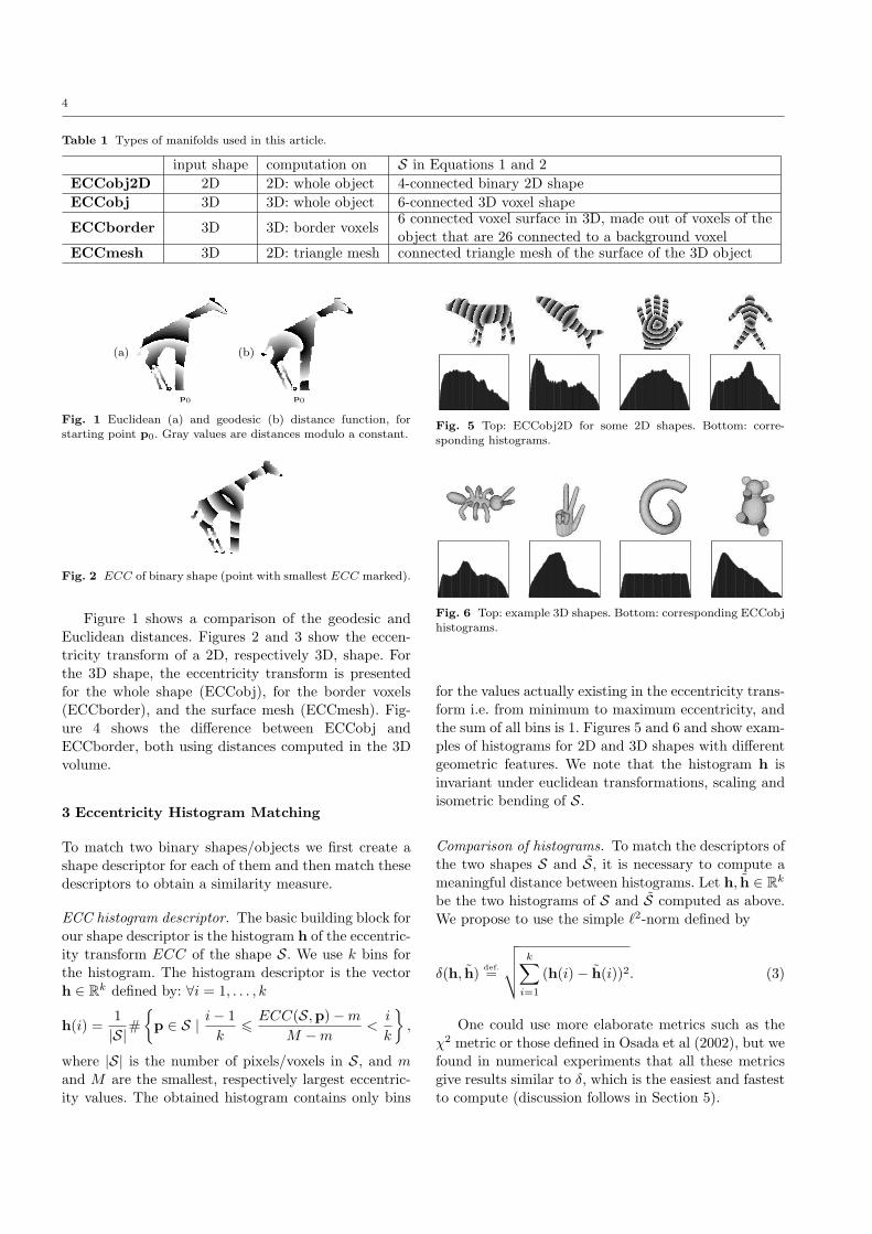
n,n ∈ {2, 3}, as well as connected triangle meshes repre-senting the surface of the 6-connected 3D shapes. Ta-ble 1 shows the types of manifolds used in this article,for which ECC is computed. For ECCobj2D, ECCobj,
and ECCborder, paths need to be contained in the areaof R
n defined by the union of the support squares/cubesfor the pixels/voxels of S. For ECCmesh, paths need to
be contained in the 2D manifold defined by the unionof the triangles of the mesh (including the interior ofthe triangles). If increasing the resolution of the shapes,ECCborder and ECCmesh converge to the same value.
2.1 Computation
One of the first attempts to deal with the problemof furthest point is presented in Suri (1987), wherean algorithm for finding the eccentric/furthest verticesfor the vertices of a simple polygon is given in. LaterMaisonneuve and Schmitt (1989); Schmitt (1993) pro-posed an efficient algorithm for simply connected shapeson the hexagonal and dodecagonal grid. The conceptof eccentricity of a vertex can be found in classicalgraph theory books (Harary, 1969; Diestel, 1997), andthe concept of eccentricity transform2 in recent discretegeometry (Klette and Rosenfeld, 2004) and mathemat-ical morphology books (Soille, 2002). Computation isnot discussed and no references to holes in a shape aremade.
The straight forward computation approach is: foreach point of S, compute the distance to all other pointsand take the maximum. In Ion et al (2008b) fastercomputation and efficient approximation algorithms arepresented. For this paper, the fastest one, algorithm
ECC06 (see Appendix), has been used.
ECC06 relies on the computation of the shape bound-
ed single source distance transform3 DS(p) (Figure 1(b)),which is computed for estimated eccentric point candi-
dates in an iterative manner. DS(p) associates to eachpoint q ∈ S the geodesic distance to p. DS can becomputed using Fast Marching (Sethian, 1999), which
allows for an efficient computation in O(N ∗ log(N))steps, for N = |S| grid points. The complexity for com-puting ECC(S) using ECC06 and Fast Marching isO(K ∗ N ∗ log(N)) where K 6 |∂S| is adapted to the
shape.
2 Known in the mathematical morphology community as the
propagation function.3 Also called geodesic distance function with marker set p.
4
Table 1 Types of manifolds used in this article.
input shape computation on S in Equations 1 and 2
ECCobj2D 2D 2D: whole object 4-connected binary 2D shape
ECCobj 3D 3D: whole object 6-connected 3D voxel shape
ECCborder 3D 3D: border voxels6 connected voxel surface in 3D, made out of voxels of theobject that are 26 connected to a background voxel
ECCmesh 3D 2D: triangle mesh connected triangle mesh of the surface of the 3D object
(a) (b)
p0 p0
Fig. 1 Euclidean (a) and geodesic (b) distance function, forstarting point p0. Gray values are distances modulo a constant.
Fig. 2 ECC of binary shape (point with smallest ECC marked).
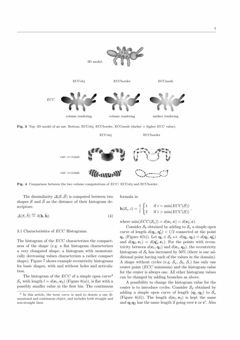
Figure 1 shows a comparison of the geodesic andEuclidean distances. Figures 2 and 3 show the eccen-tricity transform of a 2D, respectively 3D, shape. Forthe 3D shape, the eccentricity transform is presentedfor the whole shape (ECCobj), for the border voxels
(ECCborder), and the surface mesh (ECCmesh). Fig-ure 4 shows the difference between ECCobj andECCborder, both using distances computed in the 3Dvolume.
3 Eccentricity Histogram Matching
To match two binary shapes/objects we first create ashape descriptor for each of them and then match thesedescriptors to obtain a similarity measure.
ECC histogram descriptor. The basic building block forour shape descriptor is the histogram h of the eccentric-ity transform ECC of the shape S. We use k bins for
the histogram. The histogram descriptor is the vectorh ∈ R
k defined by: ∀i = 1, . . . , k
h(i) =1
|S|#
{
p ∈ S |i − 1
k6
ECC(S,p) − m
M − m<
i
k
}
,
where |S| is the number of pixels/voxels in S, and m
and M are the smallest, respectively largest eccentric-ity values. The obtained histogram contains only bins
Fig. 5 Top: ECCobj2D for some 2D shapes. Bottom: corre-sponding histograms.
Fig. 6 Top: example 3D shapes. Bottom: corresponding ECCobj
histograms.
for the values actually existing in the eccentricity trans-form i.e. from minimum to maximum eccentricity, and
the sum of all bins is 1. Figures 5 and 6 and show exam-ples of histograms for 2D and 3D shapes with differentgeometric features. We note that the histogram h isinvariant under euclidean transformations, scaling andisometric bending of S.
Comparison of histograms. To match the descriptors ofthe two shapes S and S, it is necessary to compute ameaningful distance between histograms. Let h, h ∈ R
k
be the two histograms of S and S computed as above.
We propose to use the simple ℓ2-norm defined by
δ(h, h)def.
=
√
√
√
√
k∑
i=1
(h(i) − h(i))2. (3)
One could use more elaborate metrics such as theχ2 metric or those defined in Osada et al (2002), but wefound in numerical experiments that all these metrics
give results similar to δ, which is the easiest and fastestto compute (discussion follows in Section 5).
5
3D model:
ECCobj ECCborder ECCmesh
ECC
volume rendering volume rendering surface rendering
Fig. 3 Top: 3D model of an ant. Bottom: ECCobj, ECCborder, ECCmesh (darker = higher ECC value).
ECCobj ECCborder
cut: x=const.
cut: z=const.
Fig. 4 Comparison between the two volume computations of ECC: ECCobj and ECCborder.
The dissimilarity ∆(S, S) is computed between twoshapes S and S as the distance of their histogram de-scriptors:
∆(S, S)def.
= δ(h, h). (4)
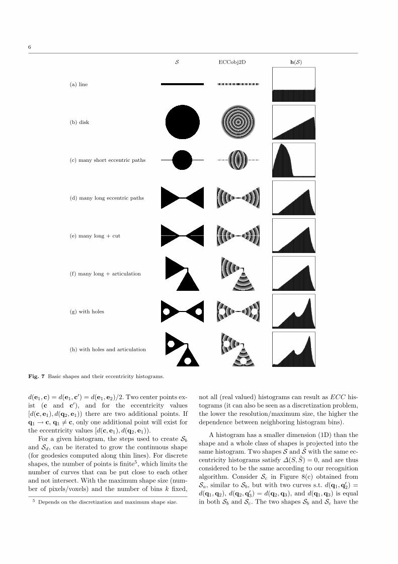
3.1 Characteristics of ECC Histograms.
The histogram of the ECC characterizes the compact-ness of the shape (e.g. a flat histogram characterizesa very elongated shape, a histogram with monotoni-cally decreasing values characterizes a rather compactshape). Figure 7 shows example eccentricity histogramsfor basic shapes, with and without holes and articula-tion.
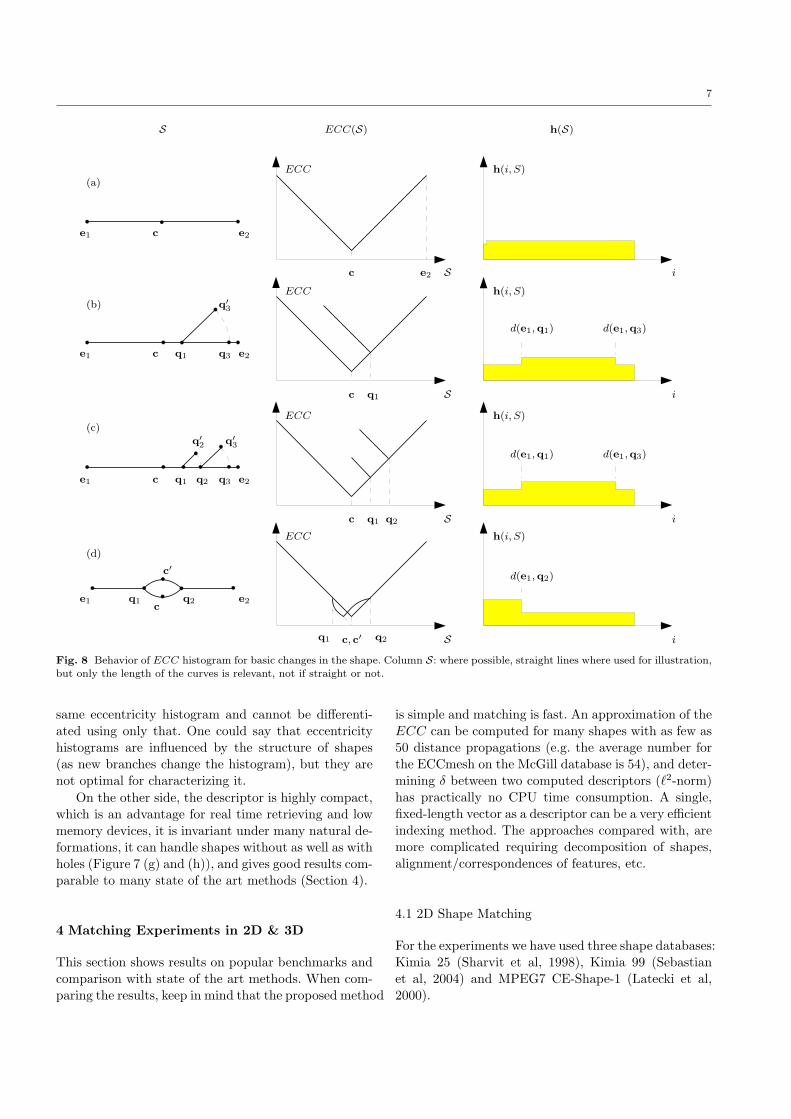
The histogram of the ECC of a simple open curve4
Sa with length l = d(e1, e2) (Figure 8(a)), is flat with a
possibly smaller value in the first bin. The continuous
4 In this article, the term curve is used to denote a one di-mensional and continuous object, and includes both straight and
non-straight lines.
formula is:
h(Sa, i) =1
l
{
1 if i = min(ECC(S))
2 if i > min(ECC(S)),
where min(ECC(Sa)) = d(e1, c) = d(e2, c).
Consider Sb obtained by adding to Sa a simple open
curve of length d(q1,q′3) < l/2 connected at the point
q1 (Figure 8(b)). Let q3 ∈ Sb s.t. d(q1,q3) = d(q1,q′3)
and d(q3, e1) = d(q′3, e1). For the points with eccen-
tricity between d(e1,q1) and d(e1,q3), the eccentricity
histogram of Sb has increased by 50% (there is one ad-ditional point having each of the values in the domain).A shape without cycles (e.g. Sa, Sb, Sc) has only one
center point (ECC minimum) and the histogram valuefor the center is always one. All other histogram valuescan be changed by adding branches as above.
A possibility to change the histogram value for thecenter is to introduce cycles. Consider Sd obtained byadding a simple open curve of length (q1,q2) to Sa
(Figure 8(d)). The length d(e1, e2) is kept the sameand q1q2 has the same length if going over c or c′. Also
6
S ECCobj2D h(S)
(a) line
(b) disk
(c) many short eccentric paths
(d) many long eccentric paths
(e) many long + cut
(f) many long + articulation
(g) with holes
(h) with holes and articulation
Fig. 7 Basic shapes and their eccentricity histograms.
d(e1, c) = d(e1, c′) = d(e1, e2)/2. Two center points ex-
ist (c and c′), and for the eccentricity values[d(c, e1), d(q2, e1)) there are two additional points. Ifq1 → c, q1 6= c, only one additional point will exist for
the eccentricity values [d(c, e1), d(q2, e1)).For a given histogram, the steps used to create Sb
and Sd, can be iterated to grow the continuous shape(for geodesics computed along thin lines). For discreteshapes, the number of points is finite5, which limits thenumber of curves that can be put close to each otherand not intersect. With the maximum shape size (num-
ber of pixels/voxels) and the number of bins k fixed,
5 Depends on the discretization and maximum shape size.
not all (real valued) histograms can result as ECC his-
tograms (it can also be seen as a discretization problem,the lower the resolution/maximum size, the higher thedependence between neighboring histogram bins).
A histogram has a smaller dimension (1D) than theshape and a whole class of shapes is projected into thesame histogram. Two shapes S and S with the same ec-centricity histograms satisfy ∆(S, S) = 0, and are thus
considered to be the same according to our recognitionalgorithm. Consider Sc in Figure 8(c) obtained fromSa, similar to Sb, but with two curves s.t. d(q1,q
′2) =
d(q1,q2), d(q2,q′3) = d(q2,q3), and d(q1,q3) is equal
in both Sb and Sc. The two shapes Sb and Sc have the
7
S ECC(S) h(S)
(a)
e1 e2c
ECC
Sc e2
h(i, S)
i
(b)
e1 e2c q1 q3
q′3
ECC
Sc q1
h(i, S)
i
d(e1,q1) d(e1,q3)
(c)
e1 e2c q1 q2 q3
q′2
q′3
ECC
Sc q1 q2
h(i, S)
i
d(e1,q1) d(e1,q3)
(d)
e1 e2c
c′
q1 q2
ECC
Sc, c′q1 q2
h(i, S)
i
d(e1,q2)
Fig. 8 Behavior of ECC histogram for basic changes in the shape. Column S: where possible, straight lines where used for illustration,
but only the length of the curves is relevant, not if straight or not.
same eccentricity histogram and cannot be differenti-ated using only that. One could say that eccentricityhistograms are influenced by the structure of shapes(as new branches change the histogram), but they arenot optimal for characterizing it.
On the other side, the descriptor is highly compact,
which is an advantage for real time retrieving and lowmemory devices, it is invariant under many natural de-formations, it can handle shapes without as well as withholes (Figure 7 (g) and (h)), and gives good results com-parable to many state of the art methods (Section 4).
4 Matching Experiments in 2D & 3D
This section shows results on popular benchmarks andcomparison with state of the art methods. When com-paring the results, keep in mind that the proposed method
is simple and matching is fast. An approximation of theECC can be computed for many shapes with as few as50 distance propagations (e.g. the average number forthe ECCmesh on the McGill database is 54), and deter-mining δ between two computed descriptors (ℓ2-norm)
has practically no CPU time consumption. A single,fixed-length vector as a descriptor can be a very efficientindexing method. The approaches compared with, aremore complicated requiring decomposition of shapes,alignment/correspondences of features, etc.
4.1 2D Shape Matching
For the experiments we have used three shape databases:Kimia 25 (Sharvit et al, 1998), Kimia 99 (Sebastianet al, 2004) and MPEG7 CE-Shape-1 (Latecki et al,2000).
8
A shape database is composed of q shapes {Si}qi=1
and each shape Si has a label L(i) ∈ {1, . . . , lmax}. Eachlabel value 1 ≤ l ≤ lmax defines a class of shapes Q(l) ={Si | L(i) = l}. The first columns of the three blocks of
Figure 9 show the shapes from the Kimia 25 database,ordered by classes (such as fish, planes, rabbits, etc.).Any shape matching algorithm α assigns to each shapeSi a vector of best matches Φi, where Φi(1) is the shapethe most similar to Si, Φi(2) is the second hit, and soon. Depending on the benchmark, Φi contains all shapes
including the query shape Si (all 2D benchmarks in thisarticle), or leave Si out, i.e. the shape Si is not matchedto itself and Φi has q − 1 elements (all 3D benchmarksin this article).
For the Kimia 25 database lmax = 6 and q = 25, andfor the Kimia 99 database, lmax = 9 and q = 99. Wemeasure the efficiency of various matching algorithmson Kimia databases by the number of correct matchesfor each ranking position k:
Matchk(Φ)def.
=
q∑
i=1
1L(Φi(k))=L(i) 6 q.
Tables 2 and 3 give the value of Matchk for variousshape matching algorithms.
In the case of the MPEG7 database, which containslmax = 70 classes with 20 images each (q = 70 × 20 =
1400), the efficiency of matching algorithms is com-puted using the standard Bullseye test:
Bullseye(Φ)def.
=1
20q
40∑
k=1
q∑
i=1
1L(Φi(k))=L(i)
=1
20q
40∑
k=1
Matchk(Φ).
This test counts the number of correct hits (same class)
in the first 40 hits. For each image there can be at most20 correct hits and a maximum of 20×1400 hits can beobtained during the benchmark and thus Bullseye(Φ) ≤1. Table 4 gives the value of Bullseye for various shapematching algorithms.
The results of the presented approach over bothKimia 25 and Kimia 99, and over MPEG 7 are slightlybellow the state of the art.
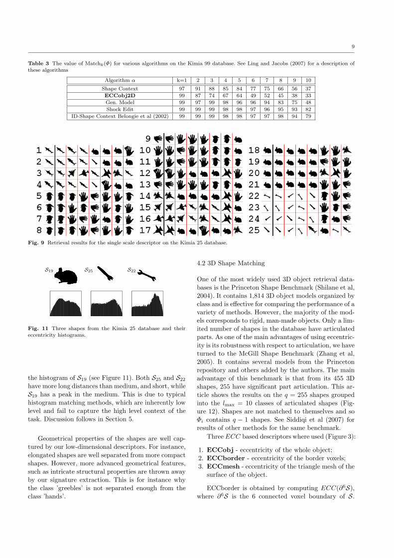
Case Study - Kimia 25. Figure 9 shows the retrieval
results for Kimia 25. The first column shows the 25shapes Si. The following set of shapes forms an array,where the shape at row i and column k is Φi(k), therank-k shape associated to Si.
The Kimia 25 database has shapes from 6 classes: 5classes with 4 images each, and one (hands) with 5 im-ages (1 simulating a segmentation error). The class with
Table 2 The value of Matchk(Φ) for various algorithms on theKimia 25 database. See Ling and Jacobs (2007) for a description
of these algorithms.
Algorithm α k=1 2 3
Sharvit et. al 23 21 20
ECCobj2D 25 20 16
Gdalyahu and Weinshall 25 21 19
Belongie et. al 25 24 22
ID-Shape Context 25 24 25
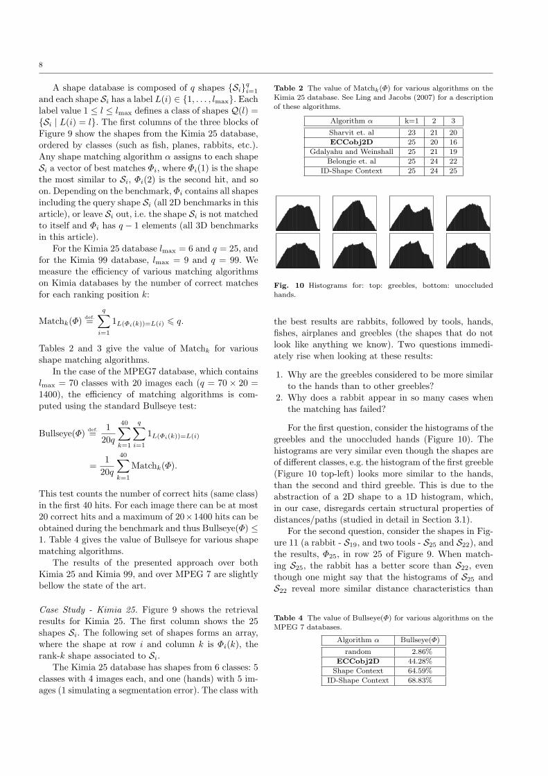
Fig. 10 Histograms for: top: greebles, bottom: unoccluded
hands.
the best results are rabbits, followed by tools, hands,fishes, airplanes and greebles (the shapes that do notlook like anything we know). Two questions immedi-
ately rise when looking at these results:
1. Why are the greebles considered to be more similarto the hands than to other greebles?
2. Why does a rabbit appear in so many cases when
the matching has failed?
For the first question, consider the histograms of thegreebles and the unoccluded hands (Figure 10). Thehistograms are very similar even though the shapes areof different classes, e.g. the histogram of the first greeble
(Figure 10 top-left) looks more similar to the hands,than the second and third greeble. This is due to theabstraction of a 2D shape to a 1D histogram, which,in our case, disregards certain structural properties ofdistances/paths (studied in detail in Section 3.1).
For the second question, consider the shapes in Fig-
ure 11 (a rabbit - S19, and two tools - S25 and S22), andthe results, Φ25, in row 25 of Figure 9. When match-ing S25, the rabbit has a better score than S22, eventhough one might say that the histograms of S25 andS22 reveal more similar distance characteristics than
Table 4 The value of Bullseye(Φ) for various algorithms on the
MPEG 7 databases.
Algorithm α Bullseye(Φ)
random 2.86%
ECCobj2D 44.28%
Shape Context 64.59%
ID-Shape Context 68.83%
9
Table 3 The value of Matchk(Φ) for various algorithms on the Kimia 99 database. See Ling and Jacobs (2007) for a description ofthese algorithms
Algorithm α k=1 2 3 4 5 6 7 8 9 10
Shape Context 97 91 88 85 84 77 75 66 56 37
ECCobj2D 99 87 74 67 64 49 52 45 38 33
Gen. Model 99 97 99 98 96 96 94 83 75 48
Shock Edit 99 99 99 98 98 97 96 95 93 82
ID-Shape Context Belongie et al (2002) 99 99 99 98 98 97 97 98 94 79
Fig. 9 Retrieval results for the single scale descriptor on the Kimia 25 database.
S19 S25 S22
Fig. 11 Three shapes from the Kimia 25 database and theireccentricity histograms.
the histogram of S19 (see Figure 11). Both S25 and S22
have more long distances than medium, and short, while
S19 has a peak in the medium. This is due to typicalhistogram matching methods, which are inherently lowlevel and fail to capture the high level context of thetask. Discussion follows in Section 5.
Geometrical properties of the shapes are well cap-tured by our low-dimensional descriptors. For instance,elongated shapes are well separated from more compactshapes. However, more advanced geometrical features,such as intricate structural properties are thrown awayby our signature extraction. This is for instance why
the class ’greebles’ is not separated enough from theclass ’hands’.
4.2 3D Shape Matching
One of the most widely used 3D object retrieval data-bases is the Princeton Shape Benchmark (Shilane et al,2004). It contains 1,814 3D object models organized by
class and is effective for comparing the performance of avariety of methods. However, the majority of the mod-els corresponds to rigid, man-made objects. Only a lim-ited number of shapes in the database have articulatedparts. As one of the main advantages of using eccentric-ity is its robustness with respect to articulation, we haveturned to the McGill Shape Benchmark (Zhang et al,2005). It contains several models from the Princetonrepository and others added by the authors. The mainadvantage of this benchmark is that from its 455 3Dshapes, 255 have significant part articulation. This ar-ticle shows the results on the q = 255 shapes groupedinto the lmax = 10 classes of articulated shapes (Fig-
ure 12). Shapes are not matched to themselves and soΦi contains q − 1 shapes. See Siddiqi et al (2007) forresults of other methods for the same benchmark.
Three ECC based descriptors where used (Figure 3):
1. ECCobj - eccentricity of the whole object;
2. ECCborder - eccentricity of the border voxels;3. ECCmesh - eccentricity of the triangle mesh of the
surface of the object.
ECCborder is obtained by computing ECC(∂6S),where ∂6S is the 6 connected voxel boundary of S.
10
10 60 110 160 2100
0.2
0.4
0.6
0.8
1
10 60 110 160 2100
0.2
0.4
0.6
0.8
1
10 60 110 160 2100
0.2
0.4
0.6
0.8
1
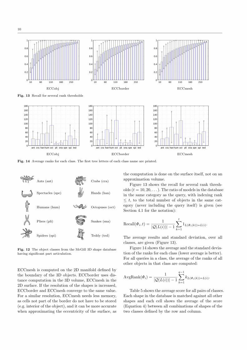
ECCobj ECCborder ECCmesh
Fig. 13 Recall for several rank thresholds
ant cra han hum oct pli sna spe spi ted0
20
40
60
80
100
120
140
160
180
ant cra han hum oct pli sna spe spi ted0
20
40
60
80
100
120
140
160
180
ant cra han hum oct pli sna spe spi ted0
20
40
60
80
100
120
140
160
180
ECCobj ECCborder ECCmesh
Fig. 14 Average ranks for each class. The first tree letters of each class name are printed.
Ants (ant) Crabs (cra)
Spectacles (spe) Hands (han)
Humans (hum) Octopuses (oct)
Pliers (pli) Snakes (sna)
Spiders (spi) Teddy (ted)
Fig. 12 The object classes from the McGill 3D shape databasehaving significant part articulation.
ECCmesh is computed on the 2D manifold defined bythe boundary of the 3D objects. ECCborder uses dis-tance computation in the 3D volume, ECCmesh in the2D surface. If the resolution of the shapes is increased,
ECCborder and ECCmesh converge to the same value.For a similar resolution, ECCmesh needs less memory,as cells not part of the border do not have to be stored(e.g. interior of the object), and it can be more accuratewhen approximating the eccentricity of the surface, as
the computation is done on the surface itself, not on anapproximation volume.
Figure 13 shows the recall for several rank thresh-olds (t = 10, 20, . . . ). The ratio of models in the databasein the same category as the query, with indexing rank≤ t, to the total number of objects in the same cat-egory (never including the query itself) is given (see
Section 4.1 for the notation):
Recall(Φi, t) =1
|Q(L(i))| − 1
t∑
k=1
1L(Φi(k))=L(i).
The average results and standard deviation, over allclasses, are given (Figure 13).
Figure 14 shows the average and the standard devia-tion of the ranks for each class (lower average is better).For all queries in a class, the average of the ranks of allother objects in that class are computed:
AvgRank(Φi) =1
|Q(L(i))| − 1
q−1∑
k=1
kL(Φi(k))=L(i).
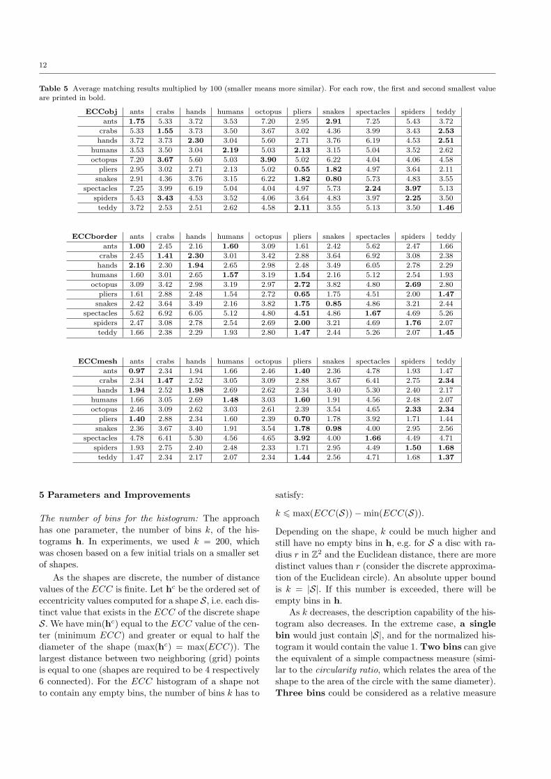
Table 5 shows the average score for all pairs of classes.Each shape in the database is matched against all othershapes and each cell shows the average of the score(Equation 4) between all combinations of shapes of thetwo classes defined by the row and column.
11
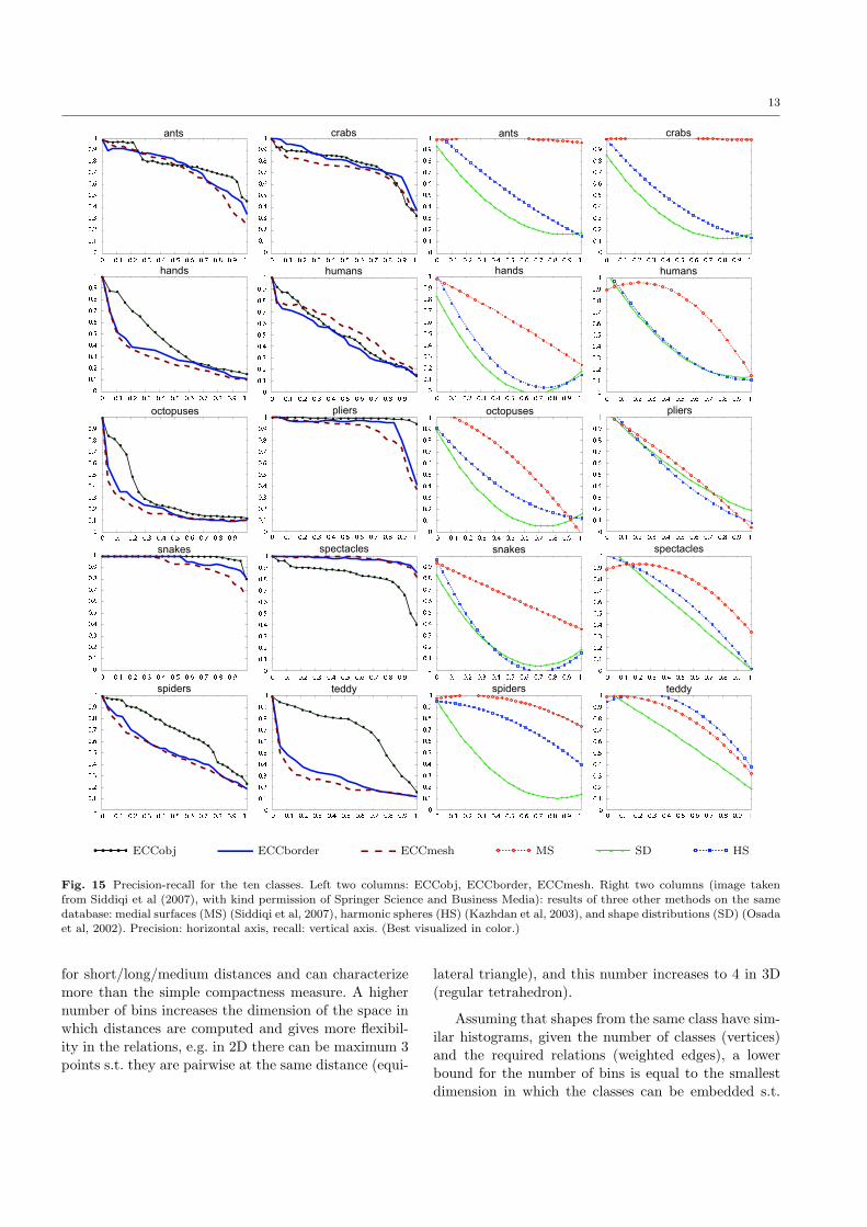
Figure 15 shows the precision-recall curves for eachof the 10 classes. Precision and recall are common in in-formation retrieval for evaluating retrieval performance.They are usually used where static document sets can
be assumed. However, they are also used in dynamic en-vironments such as web page retrieval (Fawcett, 2006).Precision refers to the ratio of the relevant shapes re-trieved, to the total number retrieved:
Precision(Φi, t) =1
t
t∑
k=1
1L(Φi(k))=L(i).
Precision-recall curves are produced by varying the pa-rameter t. Better results are characterized by curvescloser to the top, i.e. recall = 1 for all values of preci-
sion.As can be seen in Figures 13, 14, and 15, and Ta-
ble 5, ECCobj does in most cases a better job than EC-
Cborder and ECCmesh. The recall of the three meth-ods is comparable, with slightly better results from EC-Cobj. With respect to the average ranks, ECCobj doesbetter with the hands, octopus, pliers, snakes, spiders,teddy, is worse then one of ECCborder and ECCmeshwith the ants, crabs, humans, and slightly worse thanboth other methods with the spectacles. None of thethree variants produces an average class rank higherthan 50%. All three methods have the smallest averageclass distance (highest similarity) correct for 8 out of10 classes, with ECCobj having the correct class as thesecond smallest one for the other two, the humans andoctopus (see Table 5).
Figure 15 shows comparative precision-recall resultsof ECCobj, ECCborder and ECCmesh, and three othermethods:
– medial surfaces (MS) (Siddiqi et al, 2007);– harmonic spheres (HS) (Kazhdan et al, 2003);– shape distributions (SD) (Osada et al, 2002).
ECCobj, ECCborder, and ECCmesh are compara-
ble, except for the teddy bears, where ECCobj is supe-rior to the other two. The best results (higher precisionvs. recall) are reached by the ECC variants for the
snakes, by MS for the ants, and HS and SD for teddy.For these best results the MS has the best precision-recall followed by the ECC based methods, followedby HS and SD. The worst results are achieved by EC-Cobj, ECCborder, and ECCmesh for the octopus, MSfor the pliers, and HS and SD for the hands. The resultsof MS for the pliers are superior to ECCobj, ECCbor-der and ECCmesh for the octopus, which are in turnsuperior to the HS and SD for the hands. In comparisonto all other three methods (MS, HS, SD), the eccentric-ity based methods score better on the pliers, spectaclesand snakes.
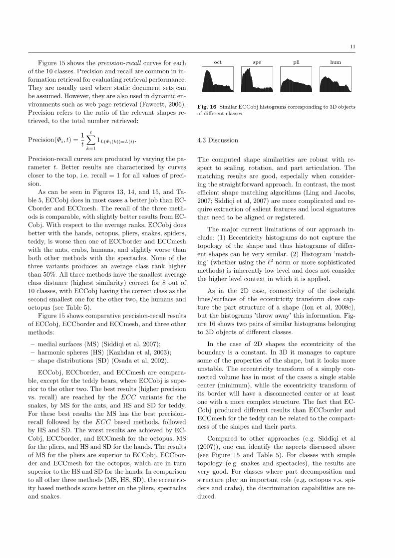
oct spe pli hum
Fig. 16 Similar ECCobj histograms corresponding to 3D objects
of different classes.
4.3 Discussion
The computed shape similarities are robust with re-spect to scaling, rotation, and part articulation. Thematching results are good, especially when consider-ing the straightforward approach. In contrast, the most
efficient shape matching algorithms (Ling and Jacobs,2007; Siddiqi et al, 2007) are more complicated and re-quire extraction of salient features and local signaturesthat need to be aligned or registered.
The major current limitations of our approach in-clude: (1) Eccentricity histograms do not capture the
topology of the shape and thus histograms of differ-ent shapes can be very similar. (2) Histogram ’match-ing’ (whether using the ℓ2-norm or more sophisticatedmethods) is inherently low level and does not consider
the higher level context in which it is applied.
As in the 2D case, connectivity of the isoheightlines/surfaces of the eccentricity transform does cap-ture the part structure of a shape (Ion et al, 2008c),but the histograms ’throw away’ this information. Fig-ure 16 shows two pairs of similar histograms belongingto 3D objects of different classes.
In the case of 2D shapes the eccentricity of the
boundary is a constant. In 3D it manages to capturesome of the properties of the shape, but it looks moreunstable. The eccentricity transform of a simply con-nected volume has in most of the cases a single stable
center (minimum), while the eccentricity transform ofits border will have a disconnected center or at leastone with a more complex structure. The fact that EC-
Cobj produced different results than ECCborder andECCmesh for the teddy can be related to the compact-ness of the shapes and their parts.
Compared to other approaches (e.g. Siddiqi et al(2007)), one can identify the aspects discussed above(see Figure 15 and Table 5). For classes with simpletopology (e.g. snakes and spectacles), the results arevery good. For classes where part decomposition andstructure play an important role (e.g. octopus v.s. spi-
ders and crabs), the discrimination capabilities are re-duced.
12
Table 5 Average matching results multiplied by 100 (smaller means more similar). For each row, the first and second smallest valueare printed in bold.
ECCobj ants crabs hands humans octopus pliers snakes spectacles spiders teddy
ants 1.75 5.33 3.72 3.53 7.20 2.95 2.91 7.25 5.43 3.72
crabs 5.33 1.55 3.73 3.50 3.67 3.02 4.36 3.99 3.43 2.53
hands 3.72 3.73 2.30 3.04 5.60 2.71 3.76 6.19 4.53 2.51
humans 3.53 3.50 3.04 2.19 5.03 2.13 3.15 5.04 3.52 2.62
octopus 7.20 3.67 5.60 5.03 3.90 5.02 6.22 4.04 4.06 4.58
pliers 2.95 3.02 2.71 2.13 5.02 0.55 1.82 4.97 3.64 2.11
snakes 2.91 4.36 3.76 3.15 6.22 1.82 0.80 5.73 4.83 3.55
spectacles 7.25 3.99 6.19 5.04 4.04 4.97 5.73 2.24 3.97 5.13
spiders 5.43 3.43 4.53 3.52 4.06 3.64 4.83 3.97 2.25 3.50
teddy 3.72 2.53 2.51 2.62 4.58 2.11 3.55 5.13 3.50 1.46
ECCborder ants crabs hands humans octopus pliers snakes spectacles spiders teddy
ants 1.00 2.45 2.16 1.60 3.09 1.61 2.42 5.62 2.47 1.66
crabs 2.45 1.41 2.30 3.01 3.42 2.88 3.64 6.92 3.08 2.38
hands 2.16 2.30 1.94 2.65 2.98 2.48 3.49 6.05 2.78 2.29
humans 1.60 3.01 2.65 1.57 3.19 1.54 2.16 5.12 2.54 1.93
octopus 3.09 3.42 2.98 3.19 2.97 2.72 3.82 4.80 2.69 2.80
pliers 1.61 2.88 2.48 1.54 2.72 0.65 1.75 4.51 2.00 1.47
snakes 2.42 3.64 3.49 2.16 3.82 1.75 0.85 4.86 3.21 2.44
spectacles 5.62 6.92 6.05 5.12 4.80 4.51 4.86 1.67 4.69 5.26
spiders 2.47 3.08 2.78 2.54 2.69 2.00 3.21 4.69 1.76 2.07
teddy 1.66 2.38 2.29 1.93 2.80 1.47 2.44 5.26 2.07 1.45
ECCmesh ants crabs hands humans octopus pliers snakes spectacles spiders teddy
ants 0.97 2.34 1.94 1.66 2.46 1.40 2.36 4.78 1.93 1.47
crabs 2.34 1.47 2.52 3.05 3.09 2.88 3.67 6.41 2.75 2.34
hands 1.94 2.52 1.98 2.69 2.62 2.34 3.40 5.30 2.40 2.17
humans 1.66 3.05 2.69 1.48 3.03 1.60 1.91 4.56 2.48 2.07
octopus 2.46 3.09 2.62 3.03 2.61 2.39 3.54 4.65 2.33 2.34
pliers 1.40 2.88 2.34 1.60 2.39 0.70 1.78 3.92 1.71 1.44
snakes 2.36 3.67 3.40 1.91 3.54 1.78 0.98 4.00 2.95 2.56
spectacles 4.78 6.41 5.30 4.56 4.65 3.92 4.00 1.66 4.49 4.71
spiders 1.93 2.75 2.40 2.48 2.33 1.71 2.95 4.49 1.50 1.68
teddy 1.47 2.34 2.17 2.07 2.34 1.44 2.56 4.71 1.68 1.37
5 Parameters and Improvements
The number of bins for the histogram: The approachhas one parameter, the number of bins k, of the his-tograms h. In experiments, we used k = 200, whichwas chosen based on a few initial trials on a smaller setof shapes.
As the shapes are discrete, the number of distancevalues of the ECC is finite. Let hc be the ordered set of
eccentricity values computed for a shape S, i.e. each dis-tinct value that exists in the ECC of the discrete shapeS. We have min(hc) equal to the ECC value of the cen-ter (minimum ECC) and greater or equal to half thediameter of the shape (max(hc) = max(ECC)). Thelargest distance between two neighboring (grid) pointsis equal to one (shapes are required to be 4 respectively
6 connected). For the ECC histogram of a shape notto contain any empty bins, the number of bins k has to
satisfy:
k 6 max(ECC(S)) − min(ECC(S)).
Depending on the shape, k could be much higher andstill have no empty bins in h, e.g. for S a disc with ra-dius r in Z
2 and the Euclidean distance, there are moredistinct values than r (consider the discrete approxima-tion of the Euclidean circle). An absolute upper boundis k = |S|. If this number is exceeded, there will be
empty bins in h.As k decreases, the description capability of the his-
togram also decreases. In the extreme case, a single
bin would just contain |S|, and for the normalized his-togram it would contain the value 1. Two bins can givethe equivalent of a simple compactness measure (simi-lar to the circularity ratio, which relates the area of the
shape to the area of the circle with the same diameter).Three bins could be considered as a relative measure
13
ECCobj ECCborder ECCmesh MS SD HS
Fig. 15 Precision-recall for the ten classes. Left two columns: ECCobj, ECCborder, ECCmesh. Right two columns (image taken
from Siddiqi et al (2007), with kind permission of Springer Science and Business Media): results of three other methods on the same
database: medial surfaces (MS) (Siddiqi et al, 2007), harmonic spheres (HS) (Kazhdan et al, 2003), and shape distributions (SD) (Osadaet al, 2002). Precision: horizontal axis, recall: vertical axis. (Best visualized in color.)
for short/long/medium distances and can characterizemore than the simple compactness measure. A highernumber of bins increases the dimension of the space inwhich distances are computed and gives more flexibil-ity in the relations, e.g. in 2D there can be maximum 3points s.t. they are pairwise at the same distance (equi-
lateral triangle), and this number increases to 4 in 3D(regular tetrahedron).
Assuming that shapes from the same class have sim-ilar histograms, given the number of classes (vertices)and the required relations (weighted edges), a lowerbound for the number of bins is equal to the smallestdimension in which the classes can be embedded s.t.
14
the weights of the edges corresponding to the distancebetween the vertices. If the variation inside classes in-creases the number of classes that can be discriminatedwill decrease.
Describing topology: One of the problems identified inSection 3.1 and during the experiments (Sections 4.1and 4.2) is that the histograms do not capture the ex-act structure of the shape. Classical methods to de-scribe the topology of a shape (e.g. Reeb graphs, Reeb(1964), and homology generators, Munkres (1993)) fail
to capture the geometrical aspects. An approach to dealwith this problem is presented in Aouada et al (2008).To describe a shape, two descriptors are used: a geomet-ric one, based on the Global Geodesic Function(GCF),which is defined for a point as the sum of the geodesicdistances to all points of the shape multiplied by a fac-tor, and a topological one, the Reeb graph of the shape
using the GCF as the Morse function.
Initial steps in combining the eccentricity transformwith Reeb graphs have been presented in Ion et al
(2008c).
A better histogram matching: The problem of having a
descriptor matching function that is aware of the con-text in which it is applied can be approached in twoways: use expert knowledge about the context to createan algorithm that considers the proper features, or learn
the important features by giving a set of representativeexamples. In Yang and Jin (2006); Yang et al (2006),a survey of current distance metric learning methods
is given. The purpose of distance metric learning is tolearn a distance metric for a space, from a given collec-tion of pairs of similar/dissimilar points. The learneddistance is supposed to preserve the distance relation
among the training data. Example training data wouldbe: S1 is more similar to S2 than to S3. The result isa distance function that would replace the ℓ2-norm inEquation 3 with a new measure which is adapted to thetask of eccentricity histogram distance computation asgiven by the training examples.
Higher dimensional data: 4D data has started to beavailable in the medical image processing community(e.g. 3D scans of a beating heart, over time). The pre-sented method is general and should be able to discrim-inate between any metric space. This includes 4D, butalso gray scale images (e.g. gray values can determinethe distance propagation speed in the respective cells).
A study in this direction is planned.
6 Conclusion
We have presented a novel method for matching 2D
and 3D shapes. The method is based on the eccentric-ity transform, which uses maximal geodesic distances,and is insensitive to articulation, Salt and Pepper noise,and robust with respect to minor segmentation errors.Descriptors are normalized histograms of the eccentric-ity transform, compact, and easy to match. The methodis straight-forward but still efficient, with experimental
results comparable to more complex state of the artmethods. Experimental results on popular 2D and 3Dshape matching benchmarks are given, with computa-tion on binary 2D images, binary 3D voxel objects, and3D triangle meshes. The experiments are preceded by adetailed analysis of the properties of the descriptor andfollowed by in depth discussion of results, parameters,and improvement possibilities.
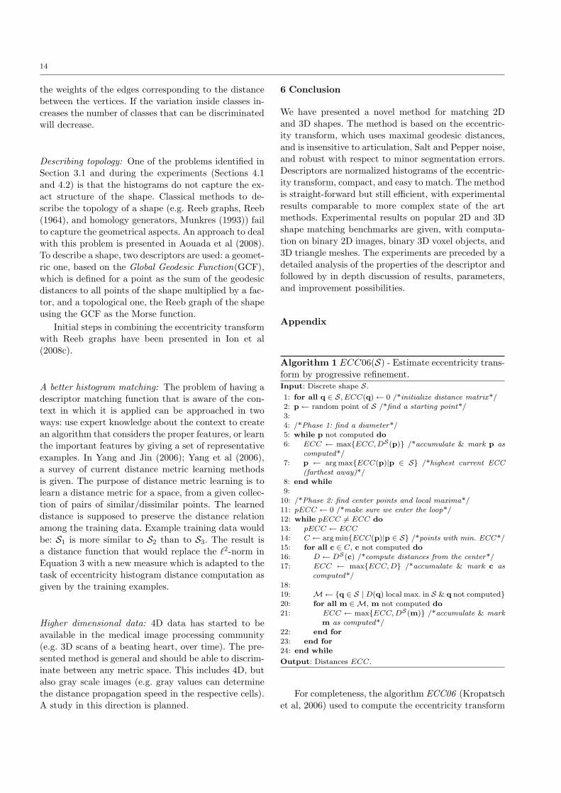
Appendix
Algorithm 1 ECC06(S) - Estimate eccentricity trans-form by progressive refinement.Input: Discrete shape S.
1: for all q ∈ S, ECC(q)← 0 /*initialize distance matrix*/
2: p← random point of S /*find a starting point*/3:
4: /*Phase 1: find a diameter*/
5: while p not computed do
6: ECC ← max{ECC, DS(p)} /*accumulate & mark p as
computed*/
7: p ← arg max{ECC(p)|p ∈ S} /*highest current ECC(farthest away)*/
8: end while
9:10: /*Phase 2: find center points and local maxima*/
11: pECC ← 0 /*make sure we enter the loop*/12: while pECC 6= ECC do
13: pECC ← ECC
14: C ← arg min{ECC(p)|p ∈ S} /*points with min. ECC*/15: for all c ∈ C, c not computed do
16: D ← DS(c) /*compute distances from the center*/
17: ECC ← max{ECC, D} /*accumulate & mark c ascomputed*/
18:
19: M← {q ∈ S | D(q) local max. in S & q not computed}20: for all m ∈M, m not computed do
21: ECC ← max{ECC, DS(m)} /*accumulate & mark
m as computed*/22: end for
23: end for
24: end while
Output: Distances ECC.
For completeness, the algorithm ECC06 (Kropatschet al, 2006) used to compute the eccentricity transform
15
for the shapes in our experiments is included (see Ionet al (2008b) for an analysis of the speed/error perfor-mance). ECC06 (Algorithm 1) tries to identify pointsof the geodesic center (minimum ECC) and use those
to find eccentric point candidates. Computing DS(c)for a center point c ∈ C(S) is expected to create lo-cal maxima where eccentric points lie. In a first phase,the algorithm identifies at least two diameter ends byrepeatedly ’jumping’ (computing DS(p)) for the pointthat had the highest value in the previous estimation.
In the second phase, the center points ci are estimatedas the points with the minimum eccentricity and all lo-cal maxima m of DS(c) are marked as eccentric pointcandidates. For all m, DS(m) is computed and accu-mulated. When no new local maxima are found (i.e.with DS(m) not previously computed), the algorithmstops.
References
Ankerst M, Kastenmuller G, Kriegel HP, Seidl T(1999) 3d shape histograms for similarity search andclassification in spatial databases. In: 6th Interna-tional Symposium on Advances in Spatial Databases,
Springer, London, UK, pp 201–226Ansary T, Vandeborre JP, Mahmoudi S, Daoudi M
(2004) A bayesian framework for 3d models retrievalbased on characteristic views. 2nd International Sym-posium on 3D Data Processing, Visualization andTransmission, 2004 3DPVT 2004 pp 139–146
Aouada D, Dreisigmeyer DW, Krim H (2008) Geomet-
ric modeling of rigid and non-rigid 3d shapes us-ing the global geodesic function. In: NORDIA work-shop in conjunction with IEEE International Confer-
ence on Computer Vision and Pattern Recognition(CVPR08), IEEE, Anchorage, Alaska, USA
Belongie S, Malik J, Puzicha J (2002) Shape matchingand object recognition using shape contexts. IEEE
Transactions on Pattern Analysis and Machine Intel-ligence 24(4):509–522
Bronstein AM, Bronstein MM, Bruckstein AM, Kim-
mel R (2006) Matching two-dimensional articu-lated shapes using generalized multidimensional scal-ing. In: Conference on Articulated Motion and De-formable Objects, Springer, Mallorca, Spain, LNCS,vol 4069, pp 48–57
Bustos B, Keim DA, Saupe D, Schreck T, Vranic DV(2005) Feature-based similarity search in 3d objectdatabases. ACM Comput Surv 37(4):345–387
Chen DY, Ouhyoung M, Tian XP, Shen YT, Ouhy-oung M (2003) On visual similarity based 3d modelretrieval. In: Eurographics, Granada, Spain, pp 223–232
Cyr CM, Kimia BB (2004) A similarity-based aspect-graph approach to 3d object recognition. Interna-tional Journal of Computer Vision 57(1):5–22
Diestel R (1997) Graph Theory. Springer, New YorkElad M, Tal A, Ar S (2001) Content based retrieval of
vrml objects: an iterative and interactive approach.In: Eurographics Workshop on Multimedia, Springer,New York, pp 107–118
Fawcett T (2006) An introduction to roc analysis. Pat-tern Recognition Letters 27(8):861–874
Gorelick L, Galun M, Sharon E, Basri R, Brandt A(2004) Shape representation and classification usingthe poisson equation. In: CVPR (2), pp 61–67
Hamza AB, Krim H (2003) Geodesic object representa-tion and recognition. In: DGCI: International Work-shop on Discrete Geometry for Computer Imagery
Harary F (1969) Graph Theory. Addison WesleyHilaga M, Shinagawa Y, Kohmura T, Kunii TL (2001)
Topology matching for fully automatic similarity es-timation of 3d shapes. In: SIGGRAPH ’01: Proceed-ings of the 28th Conference on Computer Graphicsand Interactive Techniques, ACM, New York, USA,pp 203–212
Ion A, Peyre G, Haxhimusa Y, Peltier S, Kropatsch
WG, Cohen L (2007) Shape matching using thegeodesic eccentricity transform - a study. In: W Pon-weiser CB M Vincze (ed) The 31st Annual Workshopof the Austrian Association for Pattern Recognition(OAGM/AAPR), OCG, Schloss Krumbach, Austria,pp 97–104
Ion A, Artner NM, Peyre G, Lopez Marmol SB,Kropatsch WG, Cohen L (2008a) 3d shape match-ing by geodesic eccentricity. In: Workshop on Searchin 3D (in conjunction with CVPR 2008), IEEE, An-chorage, Alaska
Ion A, Kropatsch WG, Andres E (2008b) Euclideaneccentricity transform by discrete arc paving. In:Coeurjolly D, Sivignon I, Tougne L, Dupont F (eds)14th IAPR International Conference on Discrete Ge-ometry for Computer Imagery (DGCI), Springer,
Lyon, France, Lecture Notes in Computer Science,vol LNCS 4992, pp 213–224
Ion A, Peltier S, Alayrangues S, Kropatsch WG (2008c)Eccentricity based topological feature extraction. In:
Alayrangues S, Damiand G, Fuchts L, Lienhardt P(eds) Workshop on Computational Topology in Im-age Context, Poitiers, France
Ip CY, Regli L W C Sieger, Shokoufandeh A (2003)Automated learning of model classifications. In: 8thACM Symposium on Solid Modeling and Applica-tions, ACM Press, New York, pp 322–327
Johnson A, Hebert M (May 1999) Using spin imagesfor efficient object recognition in cluttered 3d scenes.
16
IEEE Transactions on Pattern Analysis and MachineIntelligence 21(5):433–449
Kazhdan M, Funkhouser T, Rusinkiewicz S (2003) Ro-tation invariant spherical harmonic representation of
3d shape descriptors. In: SGP ’03: Proceedings ofthe 2003 Eurographics/ACM SIGGRAPH Sympo-sium on Geometry Processing, Eurographics Asso-ciation, pp 156–164
Klette R, Rosenfeld A (2004) Digital Geometry. MorganKaufmann
Kropatsch WG, Ion A, Haxhimusa Y, Flanitzer T(2006) The eccentricity transform (of a digitalshape). In: 13th International Conference on DiscreteGeometry for Computer Imagery (DGCI), Springer,Szeged, Hungary, pp 437–448
Latecki LJ, Lakamper R, Eckhardt U (2000) Shape de-scriptors for non-rigid shapes with a single closedcontour. In: IEEE International Conference on Com-puter Vision and Pattern Recognition, Hilton Head,SC, USA, pp 1424–1429
Ling H, Jacobs DW (2007) Shape classification usingthe inner-distance. IEEE Transactions on PatternAnalysis and Machine Intelligence 29(2):286–299
Maisonneuve F, Schmitt M (1989) An efficient algo-
rithm to compute the hexagonal and dodecagonalpropagation function. Acta Stereologica 8(2):515–520
Mokhtarian F, Mackworth AK (1992) A theory of mul-tiscale, curvature-based shape representation for pla-nar curves. IEEE Transactions on Pattern Analysisand Machine Intelligence 14(8):789–805
Munkres JR (1993) Elements of Algebraic Topology.Addison-Wesley
Osada R, Funkhouser T, Chazelle B, Dobkin D (2002)Shape distributions. ACM Transactions on Graphics21(4):807–832
Paquet E, Rioux M (1999) Nefertiti: A tool for 3-d shape databases management. SAE transactions108:387–393
Paquet E, Murching A, Naveen T, Tabatabai A, RiouxM (2000) Description of shape information for 2-dand 3-d objects. Signal Processing: Image Communi-cation 16(1–2):103–122
Reeb G (1964) Sur les points singuliers d’une formede pfaff complement integrable ou d’une fonction
numerique. Annales de l’institut Fourier, 14 no 114(1):37–42
Reuter M, Wolter FE, Peinecke N (2005) Laplace-
spectra as fingerprints for shape matching. In:Kobbelt L, Shapiro V (eds) Symposium on Solid andPhysical Modeling, ACM, pp 101–106
Schmitt M (1993) Propagation function: Towards con-stant time algorithms. Acta Stereologica: Proceed-ings of the 6th European Congress for Stereology,
September 7-10, Prague 13(2)Sebastian TB, Klein PN, Kimia BB (2004) Recognition
of shapes by editing their shock graphs. IEEE Trans-actions on Pattern Analysis and Machine Intelligence26(5):550–571
Sethian J (1999) Level Sets Methods and Fast MarchingMethods, 2nd edn. Cambridge Univ. Press
Sharvit D, Chan J, Tek H, Kimia B (1998) Symmetry-based indexing of image databases. In: IEEE Work-shop on Content-based Access of Image and Video
Libraries, pp 56–62Shilane P, Min P, Kazhdan MM, Funkhouser TA (2004)
The princeton shape benchmark. In: InternationalConference on Shape Modeling and Applications(SMI), Genova, Italy, IEEE Computer Society, pp167–178
Shinagawa Y, Kunii T, Kergosien Y (1991) Surface cod-
ing based on morse theory. Computer Graphics andApplications, IEEE 11(5):66–78
Siddiqi K, Shokoufandeh A, Dickinson S, Zucker SW(1999) Shock graphs and shape matching. Interna-tional Journal of Computer Vision 30:1–24
Siddiqi K, Zhang J, Macrini D, Shokoufandeh A, BouixS, Chen R, Dickinson S (2007) Retrieving articulated
3-d models using medial surfaces. Machine Vision andApplications
Soille P (2002) Morphological Image Analysis, 2nd edn.Springer
Sundar H, Silver D, Gagvani N, Dickinson S (2003)Skeleton based shape matching and retrieval. Shape
Modeling International, 2003 pp 130–139Suri S (1987) The all-geodesic-furthest neighbor prob-
lem for simple polygons. In: Symposium on Compu-tational Geometry, pp 64–75
Tangelder JWH, Veltkamp RC (2003) Polyhedral modelretrieval using weighted point sets. In: Shape Model-ing International, IEEE, Seoul, Korea, pp 119–129
Veltkamp RC, Latecki L (2006) Properties and perfor-mance of shape similarity measures. In: Proceedingsof the 10th IFCS Conference on Data Science andClassification, Slovenia
Vranic D, Saupe D (2001a) 3d model retrieval withspherical harmonics and moments. In: 23rd DAGM-Symposium on Pattern Recognition, Springer, Lon-
don, UK, pp 392–397Vranic D, Saupe D (2001b) 3d shape descriptor based
on 3d fourier transform. In: EURASIP Conference
on Digital Signal Processing for Multimedia Com-munications and Services, Comenius University, pp271–274
Vranic D, Saupe D (2002) Description of 3d-shape usinga complex function on the sphere. In: InternationalConference on Multimedia and Expo, IEEE, pp 177–
17
180Yang L, Jin R (2006) Distance metric learn-
ing: A comprehensive survey. Tech. rep., De-partment of Computer Science and Engineering,
Michigan State University, http://www.cse.msu.edu/˜yangliu1/frame survey v2.pdf
Yang L, Jin R, Sukthankar R, Liu Y (2006) An effi-cient algorithm for local distance metric learning. In:The Twenty-First National Conference on ArtificialIntelligence and the Eighteenth Innovative Applica-
tions of Artificial Intelligence Conference, July 16-20,2006, Boston, Massachusetts, USA, AAAI Press
Zaharia T, Preux F (2001) Three-dimensional shape-based retrieval within the mpeg-7 framework. In:SPIE Conference on Nonlinear Image Processing andPattern Analysis XII, pp 133–145
Zahn CT, Roskies RZ (1972) Fourier descriptors for
plane closed curves. IEEE Transactions on Computer21(3):269–281
Zhang J, Siddiqi K, Macrini D, Shokoufandeh A, Dick-inson SJ (2005) Retrieving articulated 3-d models us-ing medial surfaces and their graph spectra. In: 5thInternational Workshop Energy Minimization Meth-ods in Computer Vision and Pattern Recognition,
EMMCVPR 2005, Springer, LNCS, vol 3757, pp 285–300