Embed Size (px)
Citation preview
DIGITAL COMPUTER LABORATORY
UNIVERSITY OF ILLINOIS
URBANA, ILLINOIS
INTRODUCTION TO THE THEORY OF DIGITAL MACHINES
Math., E.E. 294 Lecture Notes
by
w. J~ Poppelbaum

CHAPI'ER I
DIG ITAL COMPUl'ERS AND NUMBER SYSTEMS
1.1 Ana.log Computers and Digital Computers
A computer is a calculating machine capable of accepting numerics.l
data and performing upon them mathematical operations such as addition, taking
the square root, etc. The computer can also accept non-numerical data by
establishing, via a code, a correspondence between the information at its
input and the numbers used inside o The mechanism involved in computation
can use anyone of the common phySical agents (mechanics, electricity, etc.).
The data inside the machine can be in the form of continuously
variable mea.surements, such a,s voltages in a given range .. angles; we then
talk of a.n ana.log computer (example: slide-rule) , If the da.ta are in the
form of discrete numbers (assembly of a finite number of multi-valued digits),
we speak of a digital computer (example ~ desk calculator) " With such a computer
nearly unlimited precision can be obtained even when standar.d hardware is used,
while the results of pure analog computation are usually only known within a
fr.action of a per cento It should be remarked that combinations of the two
princip1es are possible and used in some installations.
General Organization of a Digital Machine
A digital computer can take the simple form of a desk calculator
using toothed wheelso In the decimal system these wheels would have ten
discrete positions, 0 000 9. Individual operations are then controlled by a.
human operator, customarily using a. writing pad which contains the list of
instructions to be perfor.med, the numbers to pe operated on and the intermediate
results 0 The time for multiplying two numbe":'f' of 10 dec1mal digits each is of
the order of 10 seconds~ the time necessary to write down the result and for
pushing the keys can be almost neglected 0
In an electronic computer the digits are represented by the electrical
states of electronic circuits, ioe., circuits using transistors. Usually these
circuits (called flipflops and assembled in registers) have two states (e.g., a
high qoltage output or a low voltage output), which means tha~ only two discrete
-1-
values, 0 and 1, are availa.ble per digit. We must then use the b1n!t;l system
in which th~ numbers 1, 2, 3, 4, 5 etc. are represented by 1, 10, 11, 100, 101
etc ..
The ttme for multiplying two numbers of 30 binary digits (~in
precision to lO decimal digits) is of the order of 10 ~ 100 microseconds;
manual control and the use of a pad to jot down intermediate results would be very inefficient. The writing pad is replaced by a. memorl (in principle a. grea.t
number of flipflop resisters) which stores from the outset the list of instruc
tions and which, by way of a control-unit, established the electrica.l connections
necessary to perform the operationso The memory is also used to store back the
1ntermedia.te results. An electronic ma.chine will be automa.tic at the same time,
in the sense that it proceeds a.ll on its own through the problem due to the
stored program. The part of the machine corresponding to the desk ca.lcula.tor 1s
called the a.rithmetic unit. The la.tter is usually connected to the input-output
equipment ( ta.pes with holes or magnetic coating With rea.ding and writing devices).
As the name implies, this input-output equipment allows the machine to'communicat~
with the outside world, eego, store numbers in the memory after ha~ing read holes
punched in tapes (or cards), or punch hcles corresponding to the memory aontents
a.t the end of a problemt This general layout of the computer is the same for
installa.tions as .widely different a.s the '.' Illiac" and the IBM 6500
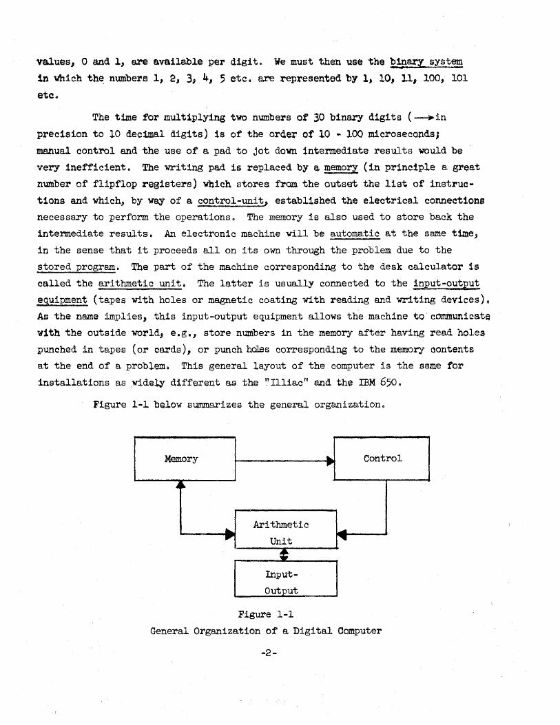
Figure 1-1 below summarizes the general organiza.tion 0
Memory .... Control ,....
~~
Arithmetic ..... .... .... Unit .,
~
Input-
Output
Figure 1-1
General Organization of a Digital Computer
-2-
The "Thinkips" Ability of Computers
The astonishing usefulness ot a modern computer is due to the possibility
of ha.ving it ma.ke simple decisions. . These are usually ot the f'ollowing torm:
1. It number in register A > number in register B, tollow instructions stored in list 1 in memory (e. g. , locations 56, 57, 58 ••. );
2. If number in register A < number in register B, follow instructions stored in list 2 in memory (e.g., locations 82, 83, 84 .•• ).
The transfer from one list to another depending on the contents of registers is
called a conditional transfer, jump or branch.
Example 1
Ta,ke the numeri~al calculation of' the value of' a function expressed
as a series. The number of terms we have to take in order to obtain a fixed
precision varies with the value of the argument. We can decide that we are
going to calculate up to the nth term where this term is smaller than a given
quanti ty 5. After being through with the calculations of each term, we shall
test and see if it is bigger than 5. If'so, we shall go on to the next term;
if not, we 'shall f'orm.-the sum ot-all the terms calculated up to this stage, and
then proceed with the rest of the problem.
Example 2
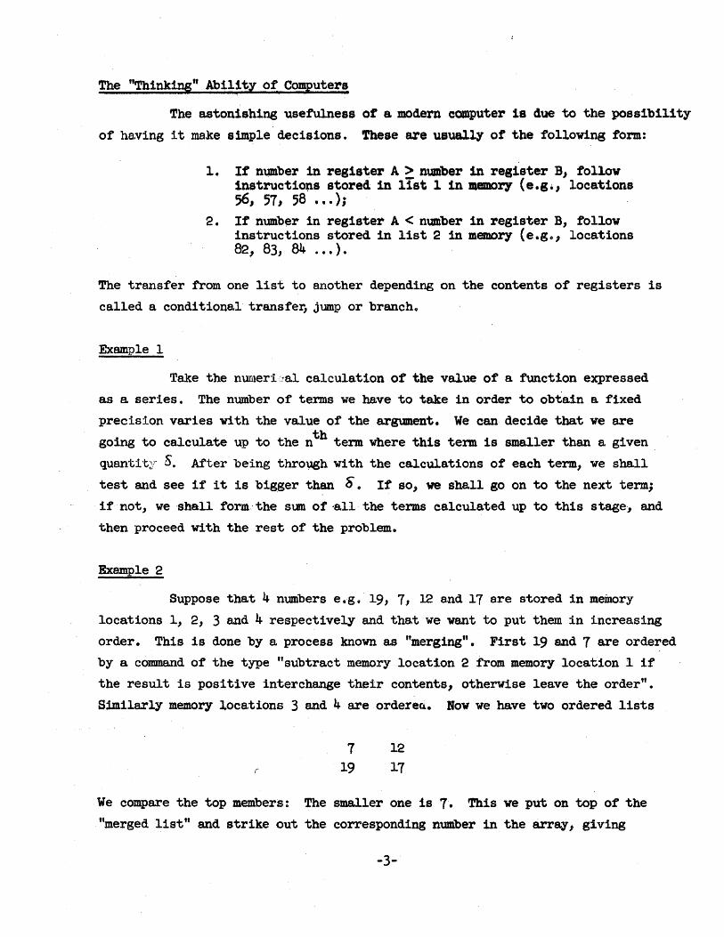
Suppose tha.t 4 numbers e.g 0 19, 7, 12 a,nd 17 a.re stored in memory
locations 1, 2, 3 and 4 respectively and that we want to put them in increa.sing
order. This is done by a process known as "merging". First 19 and 7 are ordered
by a command of the type "subtract memory location 2 from memory location 1 if
the result is positive interchange their contents, otherwise leave the order".
Similarly memory locations 3 and 4 are ordere~. Now we have two ordered lists
r
7 19
12
17
We compare the top members: The smaller one is 7. This we put on top of the
"merged list" and strike out the corresponding number in the array, giving
-3-
12
19 17
We know that 17 follows 12 (t~is list being partially ordered) so the only
question is: does 19 follo~ 12 or 171 This can be decided by two more decisions
of the type used before and the problem is solved in a language suitable for a
computer.
The ability to exercise "judgment" and to choose between two alter
natives saves a. great amount of time,but, of course, the programmer must write
down the details of what to do in each case before the computation starts.. It
is possible to extend this ability to judge in such a way that the computer
virtually assembles its own program (list of instructions) once the list of
subroutines is given and the general method of calculation 1sprescribed in
symbolic form. This is called automatic programming.
1.2 Fundamental Computer Vocabulary
Serial and Parallel Machines
As mentioned, the numbers are stored in register, i.e., sets of flip
flops. In order to calculate, the digital computer shifts the digits from one
register to another, adds, subtracts, multiplies or divides the contents of
two registers and transfers the result to a third.. We can see that all arith
metic operations can be performed if we provide an adder, equipment which ta.kes
the negative of a number held in a register (subtracting the digits means adding
the negative) and shift facilities which transfer into another register and
simultaneously give a displacement of digits by one digit pOSition to the right
or left. Since multiplication is a series of additions and shifts, and division
a. series of subtra.ctions and shifts, such an arithmetic unit would be ca.pable of
performing the four operations of arithmeticeo
There are two fundamenta.lly different methods for transmitting the
digits from one register to the other (or through the a.dder). If a. separate
'Wire is used for each digit and all digits are transmitted simultaneously, we
speak of parallel operation. If the digits are "sensed" one after the other
and transmitted through a single wire, we speak of serial operationc To illus-
.. 4-
trate the la.tter case, we can think of a selector mechanism which alW3's connects
the flipflops having the same position in the order 1-1, 2-2, 3-3 eo. n-n.
Telephone systems use serial transfer of 1nfor.mationo
It turns out that para,llel operation gives higher computation speeds,
while serial operation cuts down the amount of equipment used. It is difficult
to a,scertain the proportion in which we gain speed or reduce equipment in going
from one system to the othere For n digital positions the gain is certainly
less than a factor n.
Synchronous and Asynchronous Operation
In a synchronous machine there exists a central unit called a clock
which determines by its signals the moment at which the steps ,necessary to
perform an operation (such as addition, shifts, etc.) are initiated and ter
minated. For each type of operation we need a fixed number of cycles of the
clock whether, in practice, the intermediate steps vere long or short (the
length usually depends on the numbers involved).
In an asynchronous machine there is no clock to sequence the steps.
This can be atta.ined by having ea.ch step send out an nend signal" which initiates
the next step (kinesthetic machine)o There are systems of various degrees of
a.synchronism, ranging from those in which the times of action of a set of circuits
~re simulated in a delay device (i.e., in which the end signa.l or reply-back
signal is simply the previous end signal delayed by a sufficient amount of time
to allow the set of circuits to opera.te properly; this amounts to a loca,l clock),
to systems in which the operation of each set of circuits is examined by a
checking circuit which gives end signals if, and only if, the operation has
r'eaJ.lY been performed.. A special type of asynchronous machine is the "speed
independ.ent It machine in which an element may react a.s slowly as it likes without
upsetting the end result. One way to obtain speed independence is to build a
"totally sequential" machine in which only one element acts at a. time; this
would have to be a serial machine~
It should be mentioned that often only a part of the computer is
asynchronous. In III11iac", for exampleJ the arithmetic unit is asynchronous
while the (electrostatic) memory is synchronouso In the IBM 650, both the
arithmetic unit and the (drum) memory are synchronous It
-5-
Two-Level DC and Pulse Representation
Information, ioe., digit values l can be represented Insldethe machine
by two different methods. Suppose that we have agreed upon a binary machine
using only the values "0" and "1" for each digit. We can then decide to represent
these values by sending pulses (of approximately rectangular sha.pe and a. duration
of the order of 0.1 - 10 ~s) from one register to the other. In such a pulse
machine the presence of a pulse would mean "1", the a.bsence, "0", (the inverse
convention could be made too). Usually these pulses are sent (or not sent) at
fixed intervals, i.e .. , a pulse ma.chine is, in most cases, a synchronous machine
(example: IBM 650)0
In a direct-coupled machine we would represent the values of a digit
by a given dc level. For instance, "1" would mean -20v and "0" would mean Ov
(Illlac system).. Any other correspondence would, of course, be just a.s good,
The name Itdirect-coupled" stems from the fact that, contrary to pulse machines,
no coupling capacitors ma.y be used in the circuits for these cannot transmit
dc levels. Note that current levels can be substituted for voltage levels in a
dc representation.
Which design philosophy is chosen in a given machine depends on whether
we would like to have simple circuits which are harder to service (pulse machines)
or more elaborate circuits whlchare very convenient when it somes to checking
their operation (dc-coupled machines). In a pulse machine we must inject pulses
and observe their combinations and modifications a.s they go through the circuits.
In a dc-coupled machine we only have to check for the proper behavior of ea.ch
element using a voltmeter.
It is sometimes a.lleged that the two level de representation allows
:faster operation since the signal only has to change once in orde~ to transmit
one E..!i (= binary digit) of information, while in a. pulse the signa.l has to go
up and down 0 This view is erroneous because the duty cycle of the active elements
(transistors, tubes) is as much as "1" in a de system (i.e., these elements can
be on all the time) and less than 0" 5 in a pulse system (rise time ,...Jfa.ll time,
no tops and valleys in a. fa.st system!). At equal average power dissipa.tion, the
speeds of the two systems are comparable"
-6-
1.3 Memory Systemso Single and Multiple Address Machines
At a first glance it may seem to be useful to have separate memories
for numbers and orders (instructions) 0 But if we ta,ke account of the fact that
the memory stores also :i.ntermedia,te results and that conditiona,l transfers of
control often make the sequentia.l read-out of orders impossible anywa,y, it seems
preferahle to use the same memory for both orders or numbers (common name "words").
Each order then ha,s to specify the locations of the numbers it has to operate upon;
the numerica.l specification of a memory location is called an address 0 The storage
of orders and numbers in the same memory also makes possible modifications of orders
during the calcula.tiono .
These memories·or stores as they are also called .• are divided into two
kinds: so-called "random a,ccess" memories in which any word can be directly
attained and the "back-up" memories in which a given word is contained in a long
list which must be scann~do Typically the random access memory consists of
magnetized cores (number of bits per word x number of word cores!) the state of
magnetization of which represents 0 or 1. Reading out such a memory consists
in setting the cores to a standard state and observing the change of magnetization
by induced voltageso Another way of storing information in a random access memory
is to transform ea.ch word into a sequence of dim or bright spots on a. TV tube~
these cathode-ray-tube mem?ries (8.l.so called Williams-tube memories) must be
regenerated periodically be.cause they are volatile.,
Back-up memories _consist almost invariably of magnetic drums or
magnetic tapeso In both cases each word is transformed into a sequence of
magnetized or unmagnetized spots on a ma.gnetic coating i.e .. we have really a
glorified tape-recordere It is evident that both these systems are sequential
in nature because we must wa,i t for the drum (ta.pe) to be in the correct position
in order to start reading by means of a series of fixed reading'headso
Many modern computers contain a buffer memory between the arithmetic
unit and the random access memory in which ~. c~rtain amount of advanced processing
can be done 0 These "memory plus simplified arithmetic unit" systems are called
"look aheads" or "advanced control"" They use as their stora.ge medium simplified
flipflops ("flow-gating t in I111ac II) or specially fast core memories ..
Since all arithmetic operations invo1ve two numbers, a and b, and give
a result, c:J (c = a + b, a. - b, ab, alb), we woUld need in the general case five
pieces of information for each order:
-7-
1) the address of aj
2) the address of b;
3) the kind of operation to be performed;
4) the address to which c shall be sent; '\".~" ..
5) the a.ddress oof the next order.
For obvious reasons the a,bove system is ca.lled a "4-a.ddress systemft•
One can simpli'fy the procedure enormously by introducing certain conventions:
1) the address of a, is a fixed register in the arithmetic unit (which one may depend on the type of order);
2) the address of b is to be given a.s above;
3) the kind of opera.tion is specified as before;
4) c is left in a fixed register unless the order specifies that it is to be sent to the memory, in which case a is taken to be in a, fixed register;
5) the address of the next order is the number immediately following, unless a. specific order to "transfer control" is given. The only a.ddress specified is then that of the next order; a., b and c are not involved.
A system which uses the above conventions is called a. single-address
system. It is easy to see that making only part of these conventions, one can
obtain two-a.ddress and three-address systems ..
1.4 Past and Present Digital Computers
Calculators of' the mechanical type date back to Pascal, who, in 1642 invented an adding machine using toothed wheels to represent numbers. Leibnitz,
in 1671, extended the principles used to obtain multiplication. The first time
desk calculator was produced by Thomas de Colmar in 1820.
At this time Charles Babbage in England conceived the idea of using
punched cards to direct a giant desk calculator in its efforts. The idea of
storing programs for looms on cards had been introduced by J. M. Jaccard in
1804: patterns were produced by operating the weft selectors a.ccording to rows
of' punched holes in an endless belto This machine ha.d such advanced features as
-8-
transfers of control. On demand the machine would ring a bell an attendant
would present to it tables of logarithms, s mea etc., again in the form of
punched cards. Unhappily the project was abandoned after having spent about
$200,000 on it.
The first working model ot a stored program computer was built by
Howard Aiken at Harvard: The Harvard Automatic Sequence Control Calculator
Mark I. It was used during World War II. It contained a 60' shaft to drive
the diverse mechanic~l units. Bell Laboratories then produced several computers
using rel~s rather than toothed wheels. All these were superseded by ENIAC,
built by the MOore School of Electronics at the University of Pennsylvania using
tubes exclusively (1946). .Remington Rand soon eame out With a commercial machine,
Univac I and IBM, with some some delay, with its model 650 which is still widely
used. Meanwhile John von Neumann, Burks and Goldstine made plans for a very
comprehensive machine for the lAS in Princeton: Illiac I is a copy of this
machine.
Recently three still more ambitious projects have been completed.
IBM has designed its STRm'CH computer (150,000 transistors), Remington Rand the
LARC (60,000 transistors) and the University of Illinois Illiac II or NIC
(30,000 transistors). All these machines have gone to the extreme ,limit of
speed where their dimensions (via the propagation time of electrical signals
of 1 ~s/foot) set a bound to their times: All three machines can multiply
in less then 10 ~s.
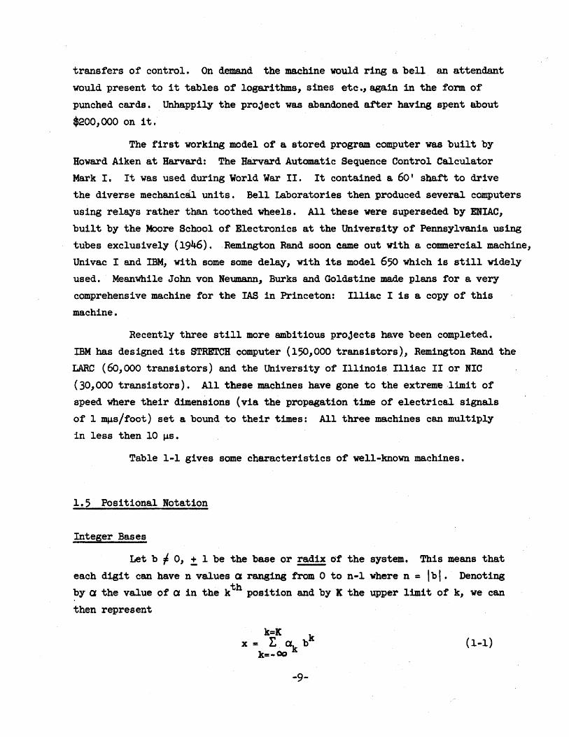
Table 1-1 gives some characteristics of well-known machines.
1.5 Positional Notation
Integer Bases
Let b , 0, ±. 1 be the base or radix of the system. This means that
each digit can have n values a ranging from 0 to n-1 where n = I b I. Denoting
by a the valueot a in the kth position and byK the upper limit of k, we can
then represent
k=K x = E a b
k
k=-Oo k
-9-
(1-1)
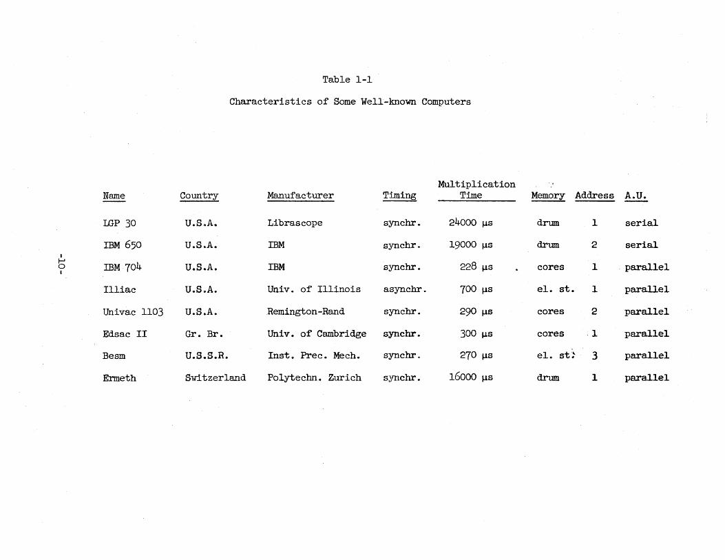
Table 1-1
Cha.racteristics of Some Well-known Computers
Multiplication - . Name Country Manufa.cturer Timing Time Memory Address A.U.
LGP 30 U.S .. A. Libras cope synchr. 24000 J.Ls drum 1 serial
IBM 650 U.S.A. IBM synchr. 19000 J.l.S drum 2 serial I I-'
IBM 704 IBM synchr. 228 J.l.S 1 . parallel 0 U.S.A. cores I
Illiac U.S.A. Univ. of Illinois asynchr. 700 J.LS el. st. 1 parallel
Univac 1103 U.S.A. Remington-Rand synchr. 290 J..I.S cores 2 parallel
Edsac II Gr. Br. Univ. of Cambridge synchr. 300 f,.LS cores ·1 pa.rallel
Besm U.S.S.R. Inst. Frec. Mech. synchr. 270 J.l.S el. st~ 3 para.llel
Ermeth Switzerland Polytechn. Zurich synchr. 16000 f,.LS drum 1 para.llel
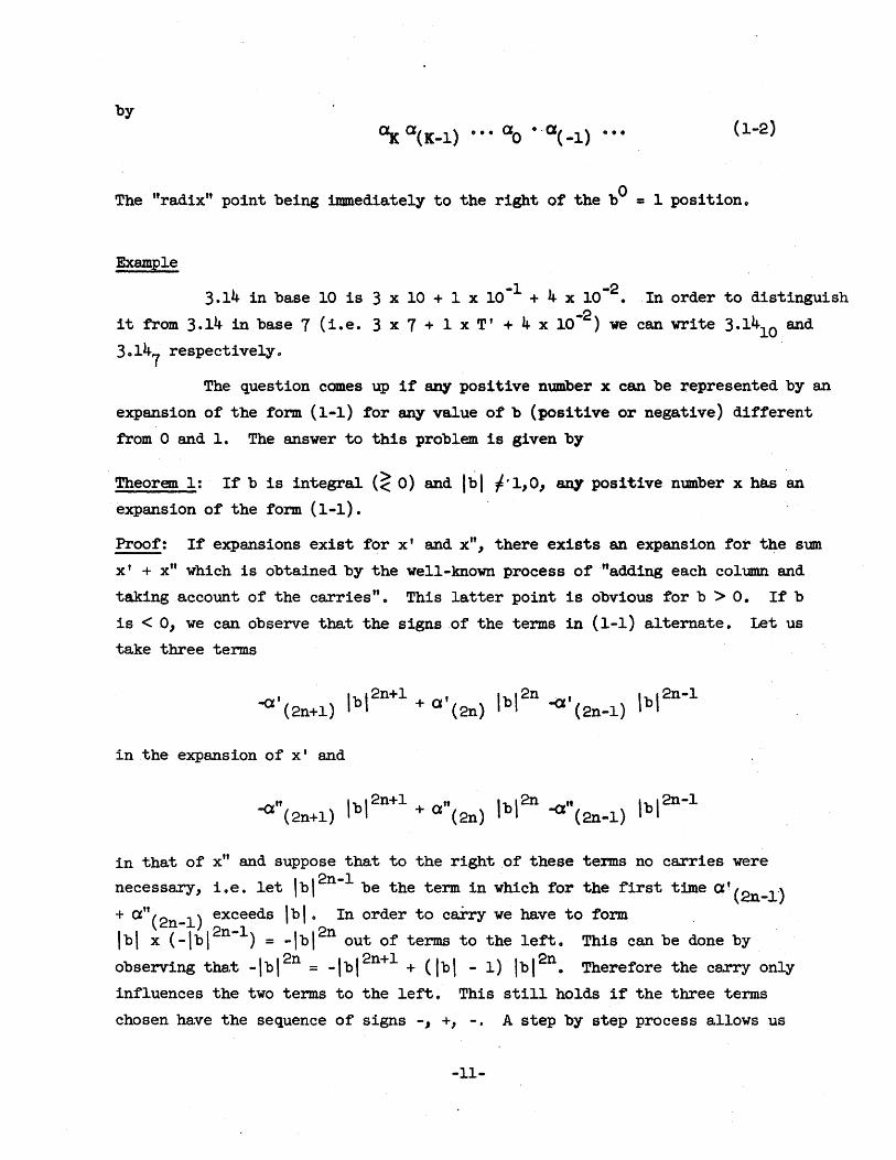
by (1-2)
The "radix" point being immediately to the right ot the bO = 1 position.
Example
3.14 in base 10 is 3 x 10 + 1 x 10.1 + 4 x 10.2• In order to distinguish
it from 3.14 in base 7 (i.e. 3 x 7 + 1 x T' + 4 x 10⁻² ) we can write 3.1410 and
30147 respectively.
The question comes up if any positive number x can be represented by an
expansion of the form (1-1) for any value ot b (posl t1ve or nega.tive) different
from 0 and 1. The answer to this problem is given by
Theorem 1: If b is integral (~O) and Ibl ,'1,0, arr¥ positive number x has an
expansion of the form (1-1) ..
Proof: If expanSions exist for x' and x", there exists an expansion for the sum
x' + XU which is obtained by the well-known process of "adding each column and
taking account of the carries It • This latter point is obvious for b > O. If b
is < 0, we can observe that the signs of the terms in (1-1) alternate. Let us
take three terms
, Ib I2n+1 , Ibl 2n ...;,y' lbl 2n-1 -ex (2n+1) + a (2n) ~ (2n-1)
in the expansion ·of x' and
in that of x" and suppose that to the right of these terms no carries were
necessary, i .. e. let Ibl 2n-1 be the term in which for the first time a'(2n-J..)
+ a"(2n-1) exceeds Iblo In order to carry we have to form .
Ibl x (_lbl 2n- l ) = -lbl 2n out of terms to the left. This can be done by
observing that _lbl 2n = _lbI 2n+l + (fbi - 1) Ibl2n. Therefore the carry only
influences the two terms to the left.. This still holds if the three terms
chosen have the sequence of signs -, +, -. A step by step process allows us
-11-
therefore to absorb all carries when we form x' + x"" i. e., we can write down
explicitly the expansion of the sum. Now we only have to prove that there is
* always an x > 0 as small a,s we like in the set of all expansions of the form
(l ... l)~ this is quite obvious. By summing a, sufficient number of these "small
* x ... expansions" we can then come as close as we like to a given x.
Positive Fractional Bases. The Most Economical Base
It is.not hard to prove that we can extend the above arguments to
positive bases of any kind (rational or irrational) if we take
1) b ~ 0.5 (still excluding 1)
2) n = 2 minimum and generally n ::;: 2 + [b] ... [2 + [b] ... b)) where [b) is the greatest integer contained inb. (The above function gives the next highest integer!)
We can then supplement Theorem 1 by
Theorem 2: If b is any non ... integral positive number, any arbitrary number x
has an expansion of the form (1-1).
Proof: We can always scale down x by division by bm (m = integer) in such a
wa.y that x < 1. Furthermore by the transformation B = lib we can reduce the
case b < 1 to the case b > 1. Then the expansion will only start to the right
of the point and we can find thea's by multiplying both sides by b and com
paring integral parts.
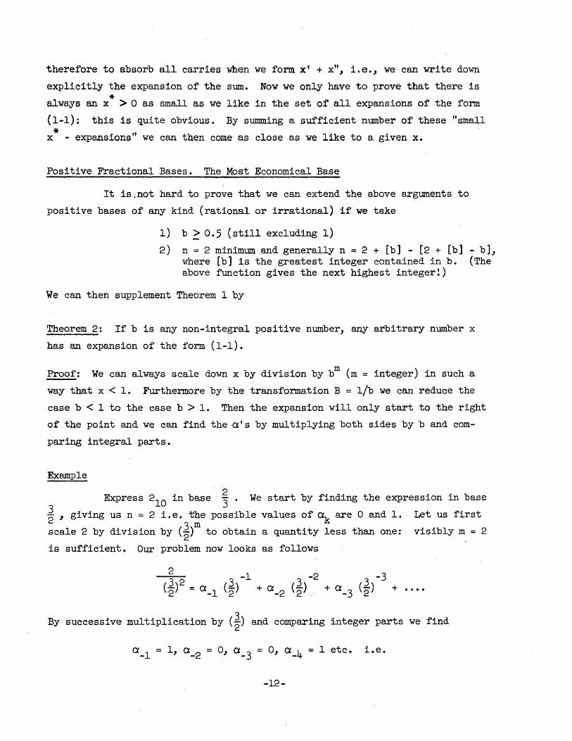
Example
2 Express 210 in base ''3. We start by finding the expression in base
~ , giving us n = 2 i.e. the possible values of Ok are 0 and 1. Let us first
scale 2 by division by (~)m to obtain a quantity less than one: visibly m = 2
is sufficient. Our problem now looks as follows
By successive multiplicaxion by (~) and comparing integer parts we find
-12-
or -1 0 1 2
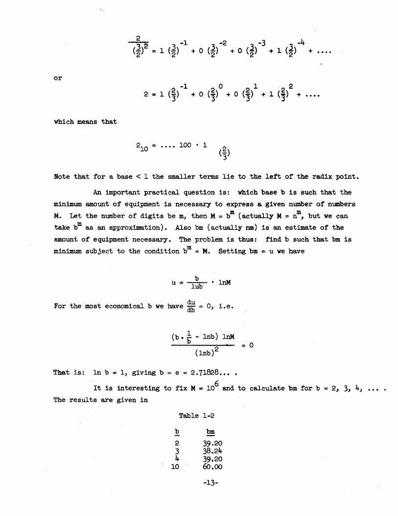
2 = 1 (~) + 0 (~) + 0 (~) + 1 (~) + ....
which means that
210 = •..• 100 0 ~
Note that for a base < 1 the smaller terms lie to the lett o~ the radix pointo
An important practical question is: which base b is such that the
minimum amount of equipment is necessary to express a given .number of numbers
M. Let the number of digits be m, then M = bm (actually M = nm, but we can
take bm as an approxilDation). Also bm (actually nm) is an estimate of the
amount of equipment necessary. The problem is thus: find b such that bm is
minimum subject to the condition ~ = M.Setting bm = u we have
u = b
lub ·lnM
du For the most economical b we have db = 0, i.e.
(b • ! - lnb) 1nM b
2 , (lnb) = 0
That is: In b = 1, giving b = e = 2071828 ••• 0
6 It is interesting to fix M = 10 and to calc~ate bmfor b = 2, 3, 4J 000 0
The results are given in
Table 1-2
b bm
2 39020 3 38024 4 39.20
10 60.00
-13-
We see therefore tha.t ba.se 2 is B. good choice: for once the system dictated
by the electronic nature of the number representation is also nearly the most
effioient.
Arithmetic in Other Bases
One can show quite easily that all arithmetic opera.tions can be
performed in other bases (see F. E. Hohn, "Applied Boolean Algebra") as long
as we take account of the modification of the addition and multipl~cation table.
Example
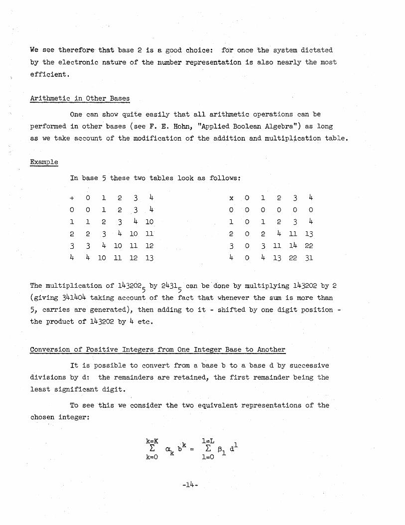
In base 5 these two tables look as follows:
+ 0 1 2 3 4 x 0 1 2 3 4
0 0 1 2 3 4 0 0 0 0 0 0
1 1 2 3 4 10 1 0 1 2 3 4
2 2 3 4 10 11 2 0 2 4 11 13
3 3 4 10 11 12 3 0 3 11 14 22
4 4 10 11 12 13 4 0 4 13 22 31
The multiplication of 1432025 by 24315 can be· done by multiplying 143202 by 2
(giving 341404 taking account of the fact that whenever the sum. is more than
5, carries are generated), then a.dding to it - shifted by one digit position -
the product of 143202 by 4 etc.
Conversion of Positive Integers from One Integer Base to Another
It is possible to convert from a base b to a base d by successive
divisions by d: the remainders a.re retained, the first remainder being the
least significant digit.
To see this we cons:ider the two equivalent representa.tions of the
chosen integer:
-14-
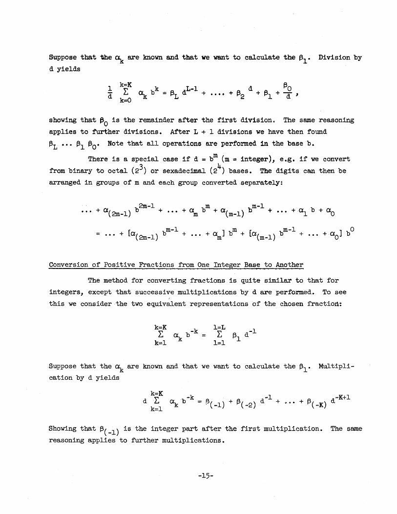
Suppose that ~e ~ are known and that we want to calculate the 131 • Division by
d yields
d 130 •••• + ~2 + ~l + (f ,
showing that ~O is the remainder s,fter the first division. The same reasoning
applies to further divisions. After L + 1 divisions we have then found
~L ••• ~l ~O· Note that all operations are performed in the base b.
There is a specia,l case if d = bm (m = integer), e.g. if we convert
from binary to octal (23) or sexadecimal (24) bases. The digits can then be
arranged in groups of m and ea.ch group converted .sepa.rately:
[ m-l ] m [ m-l ] 0 = ••• +O(2m_l) b + ••• + Om b + O(m_l) b + ••• +00 b
Conversion of Positive Fractions from One Integer Ba,se to Another
The method for converting fractions is quite similar to that for
integers, except that successive multiplications by d are performed. To see ..
this we consider the two equivalent representations of the chosen fraction:
k=K l=L La 0: b -k = L, 13 d-l
k=l k 1=1 1
Suppose that the ~ .are known and that we want to calculate the f3l • Mul tipli
cation by d yields
Showing that f3(_1) is the integer part after the first multiplication.
reasoning applies to further multiplications.
-15-
The same
1.6 Representation of Numbers in Computers
Fixed Point and Floating Point Computers
If the ba.se of the number system is b (integral), the registers in the
computer contain, for each digit, devices having either b states or a number of
combinations of states > b, b out of which are used. The important thing is to
ha.ve a, one to one correspondence between the numerical value of a, digit and the
states (or combination.of states). If m is the number of digits used, all in
tegers between 0 and bm can then be represented by combina,tions of digit-values.
Usually of course, the representation is such tha.t the successive devices indica.te
the numerics.l value of the digits in posi tiona.! notation.
Rational fractions could be represented by indicating two integers in a
given order. Practically this would not be convenient. Since irrationalqua.n
tities must be represented by a.pproximations anyway, it is usual to use a limited
number of digits in the expansion of the rationa.l or irrational quantity to the
base b.
Since the product of two numbers of m digits will have more than m
digits, the result of multiplications could not always be held in the registers.
To avoid the difficulty, a.ll numbers in a problem can be scaled down so that
their absolute value is less than one: this means·that a "radix point lt (decimal
paint, binary point) is placed in a fixed position in the register and that
all admissible numbers must be such that their non-zero digits lie to the right
of this point. It should be noted tha,t "overflOW" can still occur in division:
it is the task of the programmer to a:void this overflow by proper scaling. A
computer using the above system of representation is called a fixed point
computer for obvious reasons. Often it is possible to consider a given device
as an integral computer (representing only integers, point to the right of the
least Significant digit) or a,s a, fractional computer ( with all numbers scaled
down, point to the left of the most significant digit) at will: only the
interpretation of the digits ha,s to be modified.
In a floating pOint computer each number x (fraction ~ integer) is
divided into two parts and written in the form
X= zbY with Izi < 1.
-16-
The registers are then split up and hold z and y separately. Of course, there
are limits to the magnitude of the numbers one can represent, since y < m
(number of digits in the register). Note that the sign of y must be recorded
too.
Floating-paint computers are most useful when the magnitude of the
numbers involved in a ca,lculation varies widely or when this magnitude is not
too well known a,t the outset, meaning that accurate scaling becomes difficult.
Their disadvantage is that fundamental operations like addition or subtra,ction
become quite involved: a,ugend and addend must first be shifted so that their
exponents are the same.
Illiac is a fixed-point computer, but it is possible to make it beha~e
like a (slower) floating-point computer by special programming.
Representation of Negative Numbers in Computers
There a.re two common ways of representing negative numbers in a
positive base-system (for negative bases the problem is trivial)~ as signed
absolute values or as complements.
The signed absolute value system is difficult to apply·in computers
(especially of the parallel type). There are two reasons: in a subtraction
the computer has no means of recognizing which term has the higher absolute
value, meaning that the sign of the difference may ha~e to be changed after
the operation. Furthermore the simple process of "counting down" becomes
awkward: one has to sense the passage through zero and then change from sub
tractions to additions, modifying the sign indication. It is interesting to
note that the absolute value system implies a "schizophrenic zero": + 0 = - 0 0
In the complement-system the fact is used tha.t the numbers in the
registers are always finite, e.g. a 10-decimal-digit integral machine can hold
1010
-1 = 9999 999 999 but not 1010
: it performs operations modulo 1010
• We 10 can therefore add 10 to any number and the machine representation will not
change; to represent a given number initially outside the range we can therefore
add or subtract integral multiples of 1010 •. For example we can represent -3 by
-3 + 1010 = 0 000 000 007. As can be seen easily all operations of addition and
subtraction can then be performed without contradiction.
-17-
10 Instead of taking the complement with respect to 10 (called ten's
complement), we can take the complement with respect to 1010 -1 (called nine's
complement). This has some technical advantages: all the digits are treated
alike 0 We see that the ten t s complement can be obtained from the nine' s
complement by adding one unit in the least significant digit. Using the nine's
complement introduces a It schizophrenic zero" since 0 000 000 000 and 9 999 999 999
represent the same number.
When the sum of two numbers exceeds 1010 -1 the machine no longer
indica.tes the sum modulo 1010 -1 but modulo 1010: we can correct this state
of a.ffairs by adding one unit to the extreme right-hand digit. This procedure
is called end-around carry.
All reasonings in the preceding paragraphs can be applied in the b"1nary
. system. The two interesting complements are then the two's complement and the
one's complement. The latter again necessitates the end-around carry and a
schizophrenic zero. It has however the advantage that complemedtation simply
means changing zeros to ones and vice-versa: this can be done without going
through the a.dder •
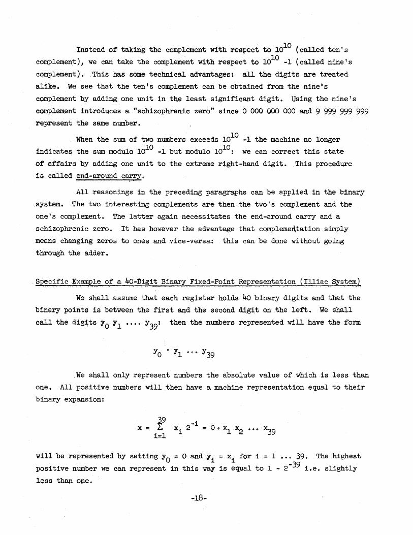
. Specific Example of a 40-Digit Binary Fixed-Point Representation (Illiac System)
We shall assume tha.t each register holds 40 binary digits and that the
binary points is between the first and the second digit on the left" We shall
call the dig~ts Yo Yl 'QOO Y39: then the numbers represented will have the form
We shall only represent numbers the absolute value of which is less than
one. All positive numbers will then have a machine representation equal to their
binary expansion:
x = ~9 -i Lt Xi 2 =
i=l
will be represented by setting YO = 0 and Yi = Xi for i = 1 00. 39. The highest
positive number we can represent in this way is equal to 1 - 2-39 i.e. slightly
less than one 0
-18-
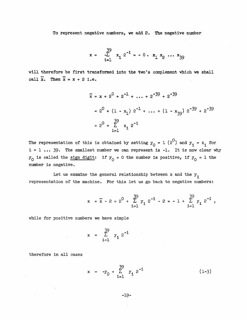
To represent negative numbers, we add 2. The negative number
will therefore be first transformed into the two's complement which we shall
callx. ,Then x = x + 2 i.e.
2° + (1 - xl) -1 ••• + (1 - x ) 2-39 + 2-39 = 2 + 39
2° + 39
2-i = L zi
i=l
The representation of this is obtained by setting YO = 1 (2°) and Yi = zi for
1 = 1 ••• 390 The smallest number we can represent is -1. It is now clear why
YO 1s called the sign digit: if YO = ° the number is positive, if YO = 1 the
number is negative.
Let us examine the general relationship between x and the Yi representation of the machine. For this let us go back to negative numbers:
2° + 39 i 39 -i x = x - 2 = L Y
i2- - 2 = - 1 + L Yi 2
i=l i=l
while for positive numbers we have simple
39 -i x = L yi 2 i=l
therefore in all cases
39 -i x = -y + L Yi 2 (1-3) ° i=l
-19-
,
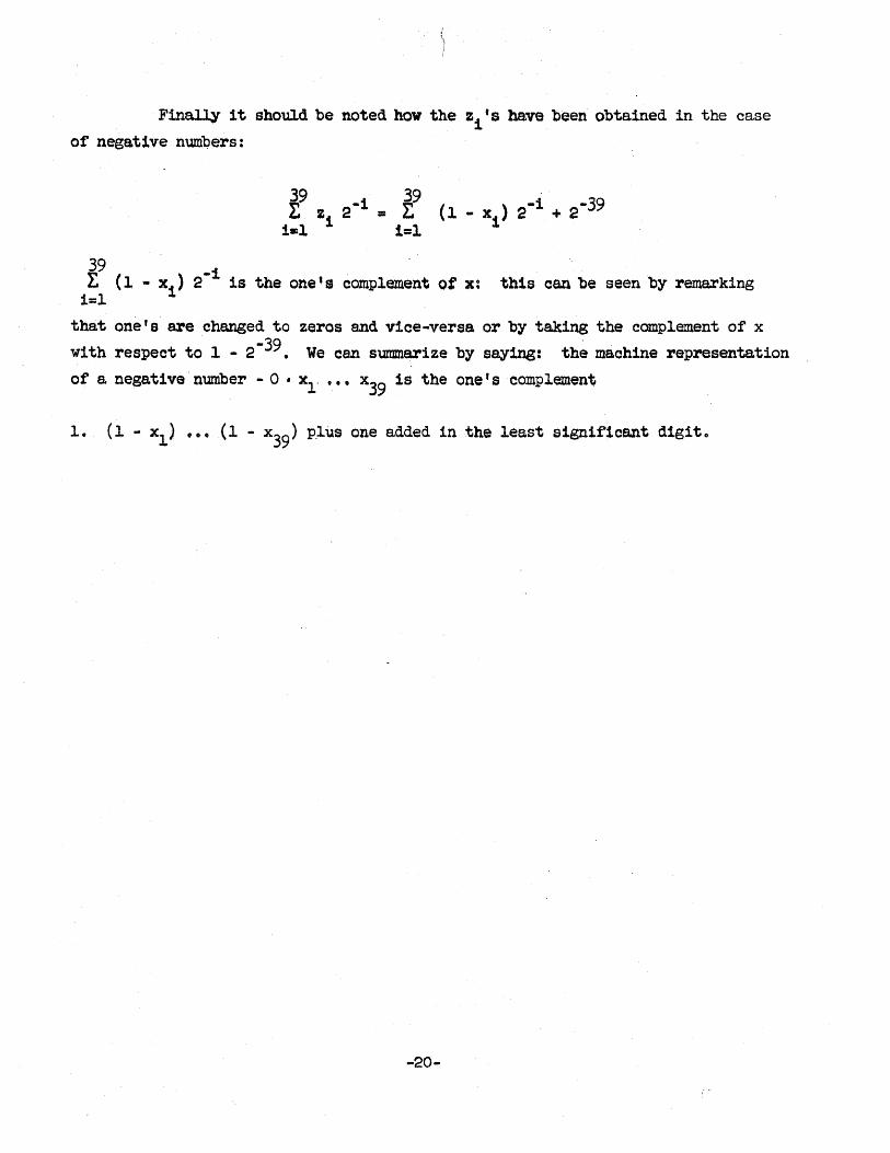
Finally it should be noted how the zits have been obtained in the case
of negative numQers:
39 E (1- x ) 2-1 is the one's complement of x: this can be seen 'by remarking
i=l 1
that one's are changed to zeros end vice-versa or by taking the complement of x
with respect to 1 ~ 2-39 • We can summarize by saying: th~ machine representation
of a. negat1 va' number - 0 0 xl' ••• x39 is the one's complement
1. (1 - Xl) ••• (1 - x39 ) p'lus one added in the least signif1cant digit.
-20-
· CHAPl'ER II
LOGICAL ELEMENTS AND THEm .cONNECTION
2.1 The Fundamental Logical .Elements
We shall call "logical element" or '''decision element" a circuit
having minputs xl ••• xm and n outputs y 1 •••• y n' each input and each
output existing only at two possible voltage levelsvO and vI' which
will be called "0" level and "1" level respectively. It will be supposed
for the moment tha,t a;llelem.ents are dc-coupled and tha,t the circuits are
a.synchronous. All lines and nodes can then only exist B,t the "0" or· "Itt
level.
Each logical element can be defined in a static sense by giving
its equilibrium table, i.e. the complete list of simultaneously possible
input and output va.lues. This does not necessarily imply tha.t different
input combinations give different output combinations or that the output
is uniquely determined by the input combination: the element may be a
stor.a,ge element and retain information.
If the equilibrium table contains all possible input combinations
and the outputs are uniquely determined by the inputs, we shall speak of
a "truth table" and of the element as a, Itsimple logical element It (or
combinational.element).
In practice the ,ItO" and "1" levels for different lines may be
different and instead of associating nO" with the level Vo and ttl" with
level vI it may be necessary to associate "0" with a voltage range
(vO' vO) and "1" with a voltage range (VI' VI)' the ranges being non
overlapping •. Aleo it may be necessary to.speak.of current ranges instead
of voltage ranges.
-21-
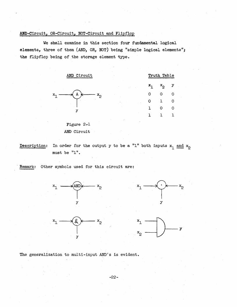
AND-Circuit, OR-Circuit, NOT-Circuit and Flipflop
We sha.ll examine in this section four fundamenta.l logical
elements, three of them (AND, OR, NOT) being "simple logica.l elements";
the flipflop being of .the stora.ge element type.
AND Circuit Truth Table
xl x2 y
Xl {? x2
y
0 0 0
0 1 0
I 0 0
I 1 1
Figure 27."1
AND·Circuit
Description: In order for the output y to be a. "1" both inputs Xl and x2 must be "1" •
. Rema.rk: Other symbols used for this circuit are:
y y
#---- Y
y
The genera.liza.tion to multi-input AND's is evident.
-22-
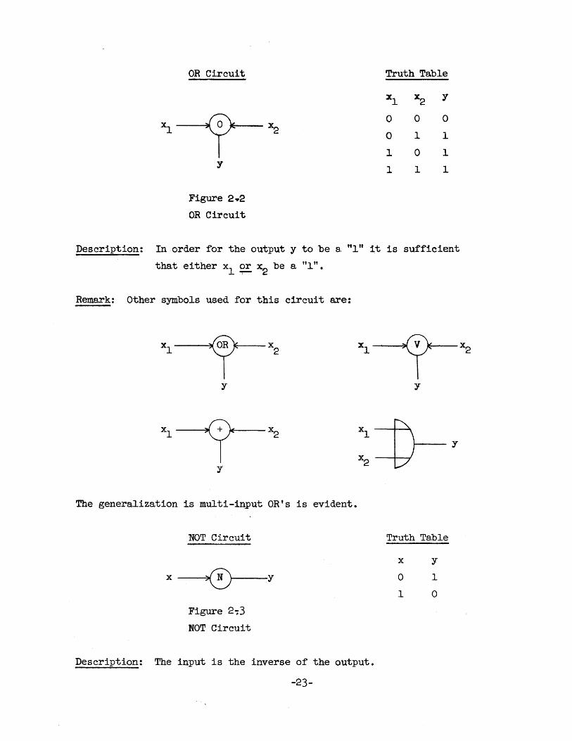
OR Circuit
y
Figure 2 .. 2
OR Circuit
Truth Table
xl x2 y
0 0 0
0 1 1
1 0 1
1 1 1
Description: In order for the output y to be a. "ltt it is sufficient
tha.t either xl $!. x2 be a "1".
Remark: Other symbols used for this circuit are:
y y
....--- y
y
The generalization 1s multi-in~ut OR's is evident.
NOT Circuit Truth Table
x y
x >® y 0 1
1 0
Figure 2-;3
NOT Circuit
Description: The input is the inverse of the output.
-23-
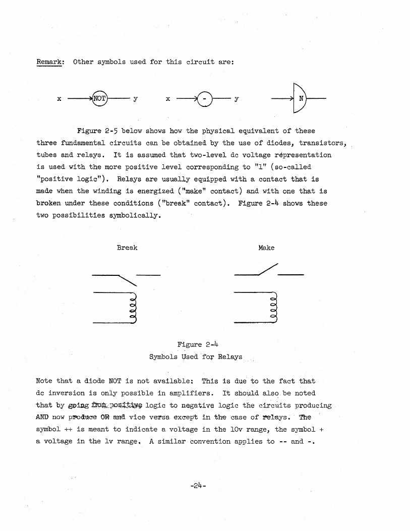
Remark: Other symbols used for this circuit are:
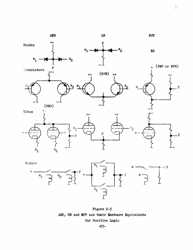
x --~@I---y x-D-y Figure 2-5 below shows how the physical equivalent of these
three fundamental circuits can be obtained by the use of diodes, transistors,
tubes and relays. It is assumed that two-level dc voltage representation
is used with the more positive level corresponding to "1" (so-called
"positive logic ft). Rela.ys are usually equipped with a conta.ct that is
made when the winding is energized ("make" contact) and with one tha,t is
broken under these conditions ("break tt contact). Figure 2-4 shows these
two possibilities symbolically.
Brea.k
Figure 2-4
Symbols Used'fo+Relays
Make
Note that a diode NOT is not available: This is due to the fact that
dc inversion is only possible in amplifiers. It should also be noted
tha.t 'by ge>1;Qg~l;\?,"lJ.O~ . .t:e);;;){e logic to nega.tive logic the circuits producing
AND now p:f!to<iuC'e OR and. vice vers'a. ex~ept in the' ca.se of ~la.yS'. The
symbol ++ is meant to indicate a voltage in the IOv range, the symbol +
a voltage in the Iv range. A similar convention applies to -- and -
-24-
AND
++ Diodes
x 1
ri.::.~ans iators y
(PNP)
Tubes
OR
Y
xl
.~
++ (NPN) ++
++ ++
" "2
x--'
Figure 2-5 AND, OR and NOT and their Hardware Equiva.lents
for Positive Logic
-25-
NOT
lfA
+ (PNP Ol" NPN)
++
y
y
Flipflop Truth Table
xl x2 Yl Y2
xl Y1 (nO Side Output") 0 1 0 1
(ltl Side Output") 1 0 1 0 x2 Y2 0 0 Last state
1 1 disallowed
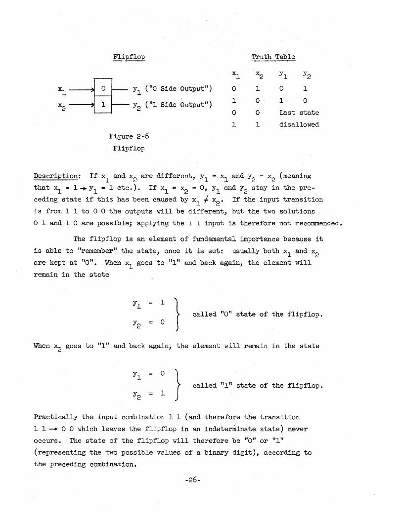
Figure 2-6
Flipflop
Description: If xl and x2 are different, Yl =xl and Y2 ;:: x2 (meaning
that xl = l-+Yl = 1 etc.). If xl = x2 ;:: 0, Yl and Y2 sta.y in the pre
ceding state if this has been caused by Xl f x2 • If the input transition
is from lIto 0 0 the outputs will be differ~nt, but the two solutions
Oland 1 0 are possible; applying the 1 1 input is therefore not recommended.
The flipflop is an element of fundamental importance because it
is able to "remember" the state, once it is set: usua.lly both Xl a.nd x2 are kept at nott. . When Xl goes to ttl" and ba.ckaga.in, the element will
remain in the state
I
1 called ItO" state of the flipflop. = o
Whenx2 goes to "Itt and back again, the element will remain in the state
o } called ttl" state of the flipflop. = 1
Practically the input combination I 1 (and therefore the transition
1 1 -+0 0 which leaves the flipflop in an indeterminate state) never
occurs. The state of the flipflop will therefore be "0" or· "In
(representing the two possible values of a binary digit), according to
the preceding combination.
-26-
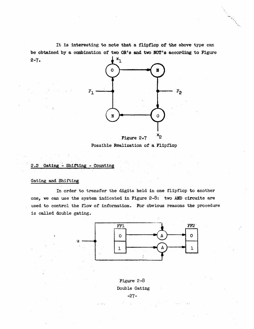
It is interesting to note that a flipflop ot the above type can
be obtained by a combination of two OR' s end two NOT,' s according to Figure
2-7.
,Figure 2'1'7
Possible Realization of a Flipflop
2.2 ,Gating - Shi:rt~ - COWlting
Gating and Shiftins
In order' to transfer the digits held in one flipflop to another
one, we can use the system indicated in Figure 2-8: two AND circuits are
used to control the flow of ,informationo For obvious reasons the procedure
is called double gatingo
u--a
FFl
o
1
Figure 2-8
Double Gating
-21-
FF2
o
1
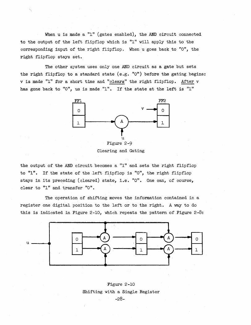
When u is ma.de a "lit (gates enabled), the AND circuit connected
to the output of the left flipflop which is "1" will apply this to the
corresponding input of the right flipflop. When .. u goes ba.ck to "0 It, the
right flipflop stays set.
The other system uses only one .AND circuit a.s a gate but sets
the right flipflop to a. standard state (e~g. "Olt) before the gating begins:
v is made Itl" for a. short time and It clears" the right flipflop. After v
has gone back to "ott, us is made 111". If the state at the left is "1ft
FFl FF2
a v o
1 1
u Figure 2-9
Clearing and Gating
the output of the AND cireui t becomes a "1" and sets the right flipflop
to ttl'·. If the sta.te of the left flipflop is nOn, the right flipflop
stays in its preceding (cleared) state, i.e. nO". ·One can, of course,
clear to "1" and transfer· nO n •
The operation of shifting moves the informa.tion contained in a
register one digital position to the left or to the right. A way to do
this is indicated in Figure 2-10, which repeats the pattern of Figure 2-8:
u ___ •
·Figure 2-10
Shifting with a Single Register
-28-
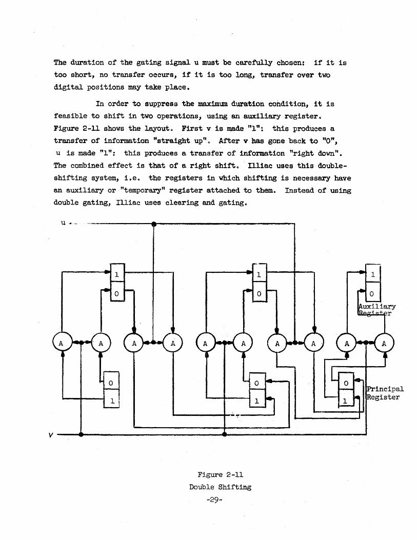
The dura,tion of the gating signal u must be carefully chosen: if it is
too short, no transfer occurs, if it is too long, transfer over two
digital positions may take place.
In order to suppress the maximum duration condition, it is
feasible to shift in two operations, using an auxiliary register.
Figure 2-11 shows the layout. First v is made "1": this produces a
transfer of' information "straight up" 0 After v has gone back to "0",
u is made "1": this produces a transfer of information "right down".
The combined effect is that of a. right shift. n11ac uses this double
shifting system, i • eo the registers in which shifting is necessary have
an a,uxiliary or· "temporary" register attached to them. Instead of using
double gating, Illiac uses clearing and gating.
u •.. -
v ----~----------------------------~~--------------------------~
Figure 2-11
Double Shifting
-29-
Counting
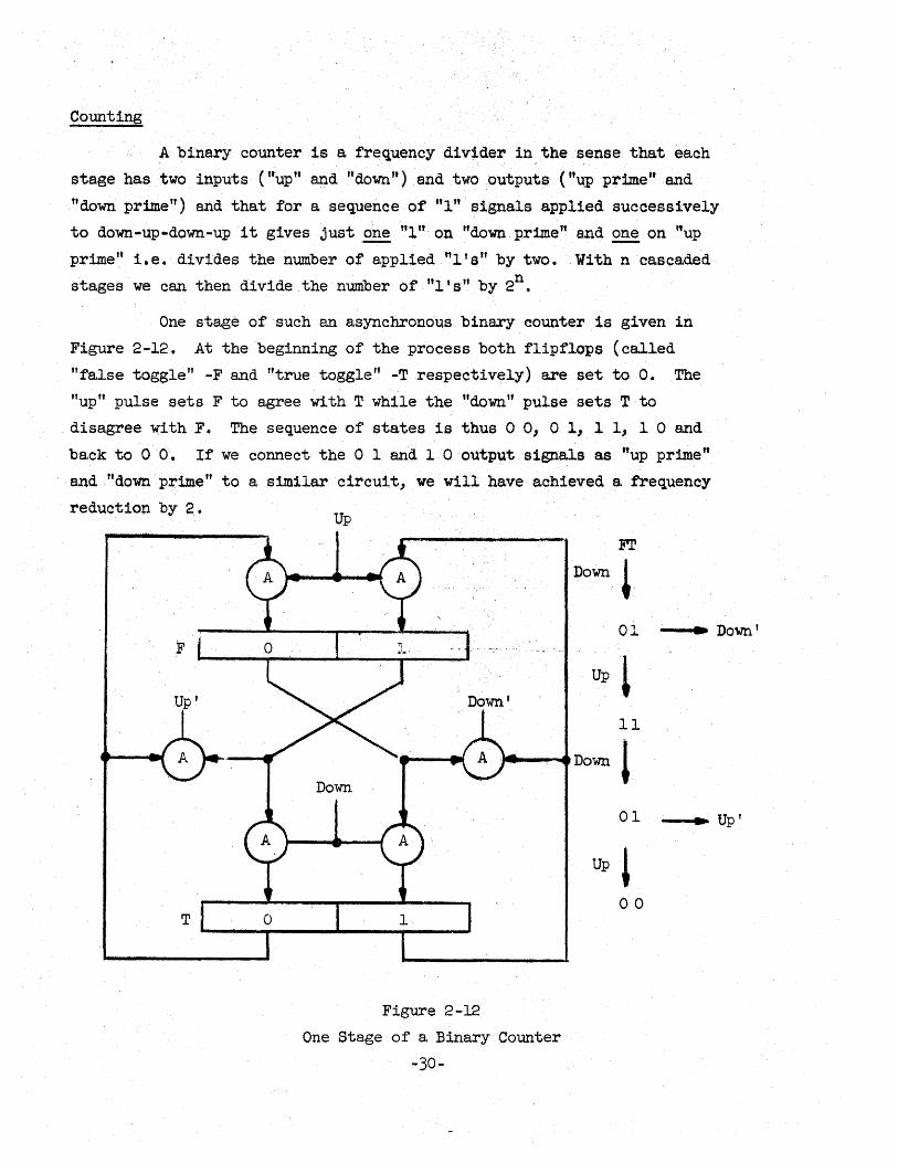
A binary counter is a. frequency divider in ,the sense that each
stage has two inputs ("up" a,nd ftdown") and two outputs ("up pr:Lme" end
"down prime") and that for a sequence of' "1" signals applied successively
to down-up-down-upit gives just,~ 'lIft, on "down pr1me't and ~ on "up
prime ft i. e. divides the number of applied "1 f S It by two • With n ea.s caded
sta,ges we can then divide the number of nl's" by 2n.
One stage of' such an a,synchronous binary counter is given in Figure 2-12. At the beginning of the process both flipflops (called
"false toggle" -F and "true toggle" -Trespectively) are set to O. The
"up" pulse sets F to agree with T while the ttdown" pulse sets T to
disagree with FII The sequence of states is thus 0 0, 0 1, 1 1, 1 0 and
back to 0 O. If we connect the Oland 1 0 output, signals as ttup prime"
and "down prime" to a. s1m1larcircuit, we will have achieved a. frequency
reduction by 2. Up
Figure 2-12
One Stage of s, Binary Counter
-30-
liT
Down ,
01 --t ... Down'
Up 1 11
Down 1 01 - ........ Up'
Up , 00
2.3 Adding and Subtracting
When adding two binary digits x. and y. we obtain a sum digit l l·
si and a carry digit ci _1 . The relation between xi' Yi' si and ci _l is
given by the table below.
Binary Addition Table
x. y. s. ci
_l l l l
0 0 0 0
0 1 1 0
1 0 1 0
1 1 0 1
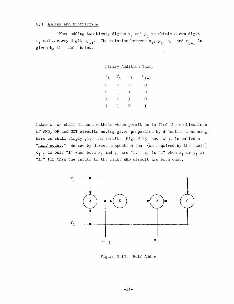
Later on we shall discuss methods which permit us to find the combinations
of AND, OR and NOT circuits having given properties by deductive reasoning.
Here we shall simply give the result: Fig. 2-13 shows what is called a
"half adder." We see by direct inspection that (as required by the table)
c is only "lH when both x. and y. are "1." s. is "111 when x. or y. is i-I l l l l l
"1," for then the inputs to the right AND circuit are both ones.
x. l
y. l
Figure 2-13. Half-Adder
-31-
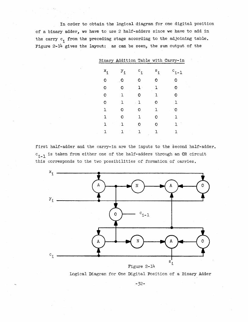
In order to obtain the logical diagram for one digital position
of a binary adder, we have to use 2 half-adders since we have to add in
the carry ci from the preceding stage according to the adjoining table.
Figure 2 .. 14 gives the layout: as can be seen, the sum output of the
Binary Addition Table with Carry-in
x. Yi c. 1 1 si c. 1 1-
0 0 0 0 0
0 0 1 I 0
0 I 0 1 0
0 1 I 0 1
I 0 0 1 0
1 0 I 0 I
I 1 0 0 1
I 1 1 I 1
first half-adder and the carry~in are the inputs to the second half-adder.
c i _l is taken from either one of the half-adders through an OR circuit
this corresponds to the two possibilities of formation of carries.
c. 1
c. 1 1-
Figure 2-14 S.
1
Logical Diagram for One Digital Position of a Binary Adder
-32-
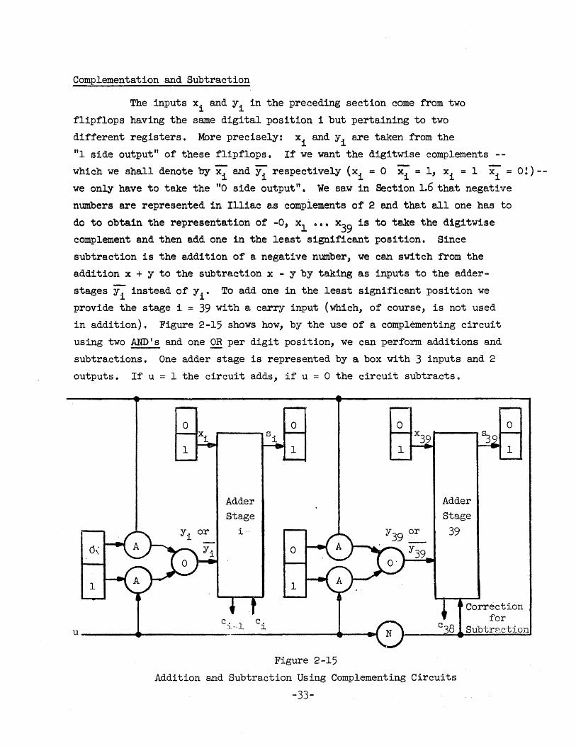
Complementation and Subtra,ction
The inputs xi and Yi in the preceding section come from two
flipflops having the same digital position i but pertaining to two
different registers. MOre precisely: xi and Yi are taken from the
"1 side output" of these flipflopso If we want the digitwise complements
which we shall denote by ~ and Yi respectively (xi = 0 xi = 1, xi = 1 xi = O!)-
we only have to take the "0 side output It 0 We saw in Section 106 tha,t nega,ti ve
numbers are represented in Illia,c a,s complements of 2 and tha,t all one ha,s to
do to obtain the representation of -0, xl 00. x39 is to ts,ke the digitwise
complement and then a,dd one in the lea,st significant position. Since
subtra,ction is the a,ddition of a, nega,tive number, we cain switch from the
a,dditionx + Y to the subtra.ction x - y by taking as inputs to the a.dder-
stages Yi instead of Yi • To add one in the least significant position we
provide the stage i = 39 with a carry input (which, of course, is not used
in addition). Figure 2-15 shows how, by the use of a complementing circuit
using two AND's and one OR per digit position, we can perform additions and
subtra.ctions. One adder stage is represented by a box with 3 inputs and 2
outputs. If u = 1 the circuit adds, if u = 0 the circuit subtractso
Adder Sta.ge
i
c:i.,"l c. l
u __________ --------------------------------4~--4M
Figure 2-15
Adder Sta.ge
39
Correction for
Subtrp.ct:ton
Addition and Subtraction Using Complementing Circuits
-33-
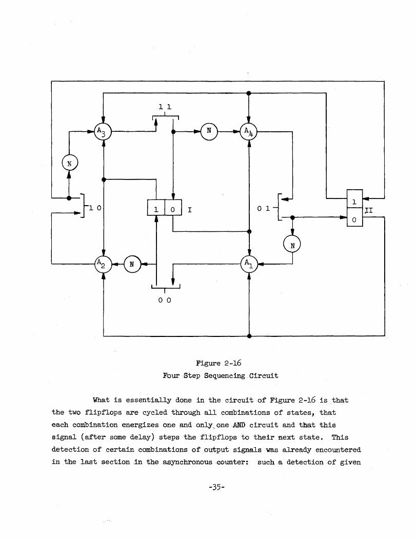
2.4 Decoding and Sequencing
In 2.2 we examined the clearing and gating procedure o It
happens very often in an asynchronous computer of the I11iac type that
a sequence of 4 signals "clear-gate-clear-gate" is required, these
signals being non-overlapping and the next step being initiated only
after we know that the preceding one has been completed. The four-step
sequencing circuit of Figure 2-16 shows how the desired result is obtained.
First consider the combina.tion of flipflops and four AND circuits
Al 0 o. A4 i. eo lea.ve the NOT circui ts aside.. The flipflops give 4 different
combinations and for each combination one and only one AND circuit has a Itl"
output:
FFI FF II Al A2 A3 A4
0 0 1 0 0 0
1 0 0 1 0 0
1 1 0 0 1 0
0 1 0 0 0 1
This output goes out into other parts of the machine and comes back with
a "return-signal" or ,"reply-back-signal" •. We can imagine that a certain
group of gates is enabled and that one of the gate outputs is used as a.
return signal.. This return signal modifies one and only one flipflop and
therefore produces the next combination, i.e. energizes the next AND
circuit. If we now put in the NOT circuits (making 3 input AND circuits
out of 2 input AND circuits) the next AND circuits can only give a "lIt
output, if the return signal of the preceding operation ha.s gone ba.ck to
"0": this guarantees non-overlapping "1" signals at the output of the
AND circuits. Notice that connecting the returns to the outputs gives a
"free-running" pulserwith a 4 pha,se output.
-34-
1 1
I o 0
I
Figure 2-16
Four 'Step Sequencing Circuit
What is essentially done in the circuit of Figure 2-16 is ,that
the two f1ipflops are cycled through all combinations of states, that
1
o
each com,binationenergizes one and . only,.: one AND circuit and that this
signal (after some delay) steps the flip flops to their next sta.te. This
detection of certain combinations of output signals was already encountered
in the last section in the.asynchronous ~ounter: such a detection of given
-35-
;I: I
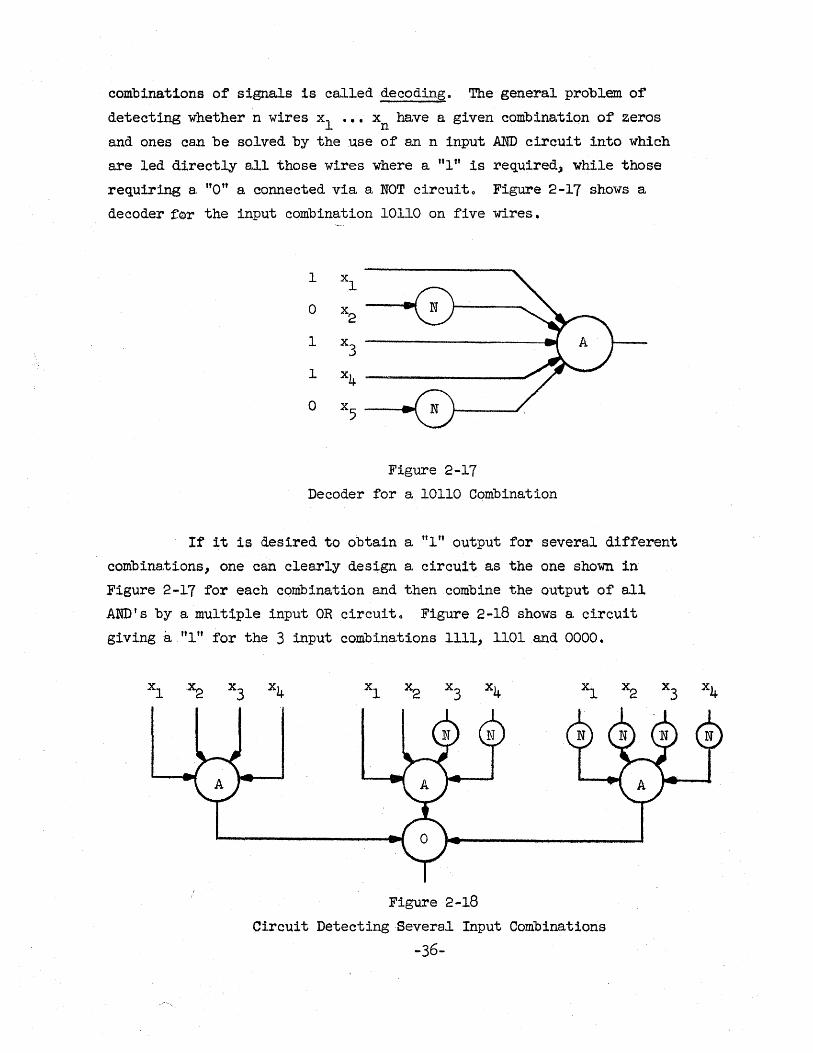
combinations of signals is called decoding.. The genera.l problem of
detecting whether n wires xl ••• xn have 8, given combination of zeros
and ones can be solved by the use of an n input AND circuit into which
are led directly all those wires where a 1t1 tt is required, while those
requiring a. "ott a, connected via. a, NOT circuit.. Figure 2-17 shows a
decoder for the input combination 10110 on five wires.
1
o
1
1
o
Xl
x2
x3
x4 ------------------~ x5 --..-01
Figure 2-17
Decoder for a 10110 Combina.tion
If it is desired to obtain a 1t1" output for several different
combinations, one can clearly design a circuit as the one shown in Figure 2-17 for each combination and then combine the output of all
AND's by a multiple input OR circuit.. Figure 2-18 shows a. circuit
giving a "1" for the 3 input combinations 1111, 1101 and 0000.
Figure 2-18
Circuit Detecting Several Input Combinations
-36-
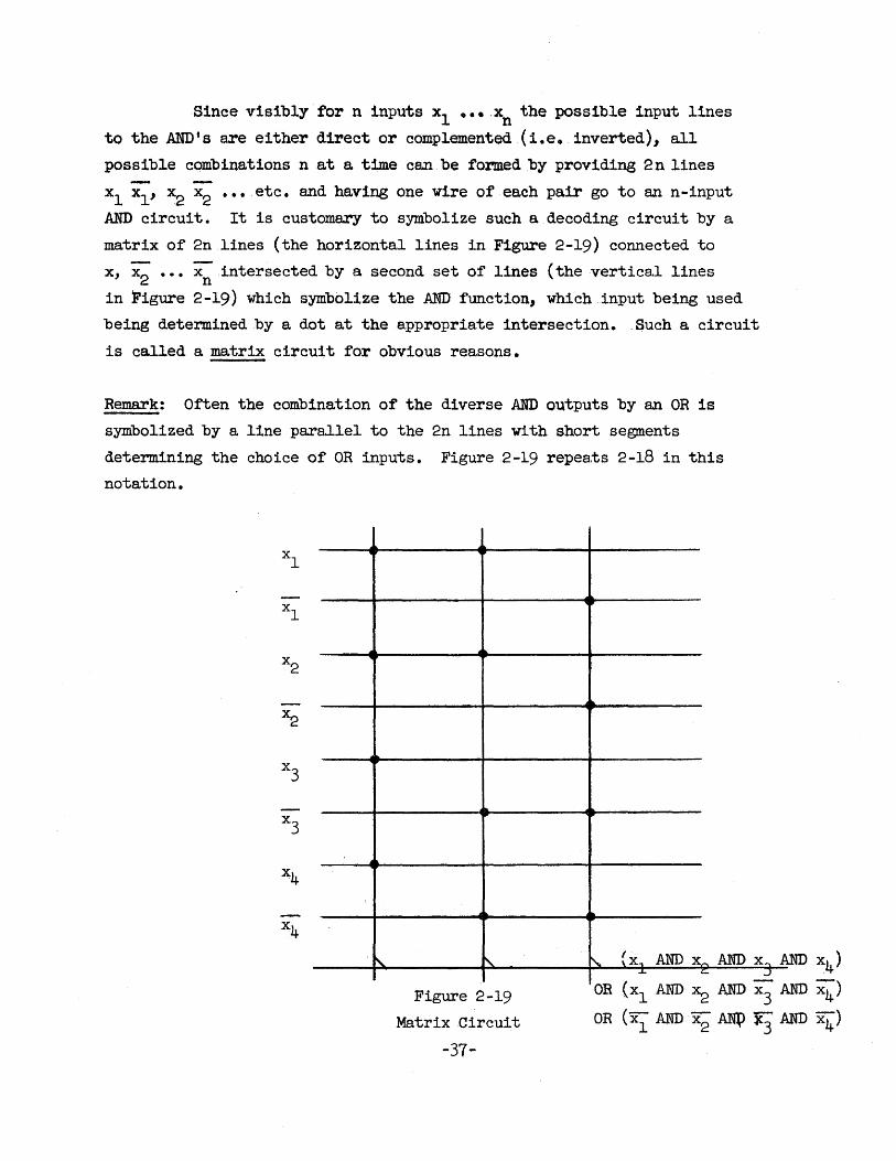
Since visibly for n inputs xl ••• . xn the possible input lines
to the AND's are either direct or complemented (i.e. inverted), all
possible combinations nat a time can be f'ormedby providing 2 n lines
xl xl' x2 x2 ••• etc. and having one wire of each pair go to an n-input
AND circuit. It is customary to symbolize such a decoding circuit by a
matrix of 2n lines (the horiZontal lines in Figure 2-19) connected to
x, x2
••• xnintersected by a second set of lines (the vertica.l lines
in Figure 2-19) which symbolize the AND function, which input being used
being determined by a dot at the a.ppropriate intersection •. Such a circuit
is called a matrix circuit for obviQUS reasons.
Remark: Often the combination of the diverse AND outputs by an OR is
symbolized by a line para.llel to the 2n lines with short segments
determining the choice of OR inputs. Figure 2-19 repea.ts 2-18 in this
notation.
., , Figure 2-19
Ma.trixCircuit
-37-
" ex .. AND x,... AND x,., ..L '- .2.
AND x4)
OR (xl AND x2 AND x3 AND x4)
OR (Xl AND x2 ~ lC3 AND x4)
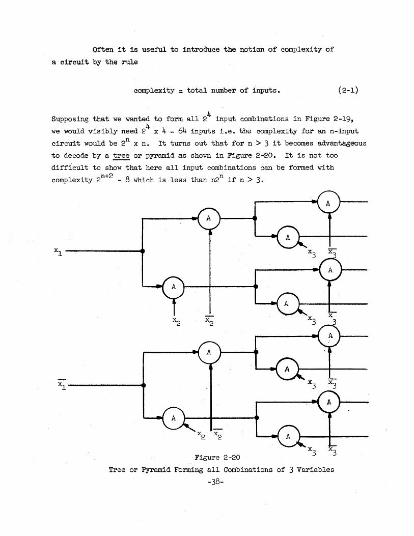
Often it is useful to introduce the notion of complexity of
a circuit by the rule
complexity.: tota.l number of inputs, (2-1)
Supposing that we wanted to form all 24 input combina.tions in Figure 2-19,
we would visibly need 24 x 4 = 64 inputs iqe. the complexity for an n-input
circuit would be 2n x n. It turns out that for n > 3 it becomes advantageous
to decode by a. tree or pyramid a.s sho"Wll in Figure 2-20. It is not too
difficult to show that herea.ll input combina.tions can be formed with
complexity 2n+2 - 8 which is less than n2n if n> 3.
Xl ---------e
xl ---------------·
Figure 2-20
Tree or Pyramid Forming all Combinations of 3 Variables
-38-
2.5 ComplexLogicalElements
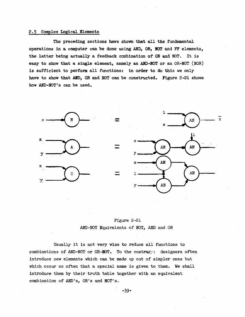
The preceding sections have shown that all the fundamental
operations in a. computer can be done using AND, OR, KOT and FF elements,
the latter being actually a feedback combination of OR and NOT. It is
ea.sy to show that a single element, namely an AND-NOT or an OR-NOT (NOR)
is sufficient to perfor.m all functions: in order to do this we only
ha.ve to show that AID, OR and NOT can be constructed. Figure 2-21 shows
how AND-NOT's can be used.
1 B--x --- x
x·
B- x
tV ~' y y
x x
!V- 1
'''f Y
Figure 2-21
AND-NOT Equiva.lents of NOT, AND and OR
Usua.lly it is not very wise to reduce a.11 functions to
combina.tions of AND-NOT or OR-BOT. To the contrar:,'": designers often
introduce new elements which can be made up out of simpler ones but
whicb occur so often that a special name is given to them. We shall
introduce them by their .truth table together with an equivalent
combination of AND's I OR's and NOT ' s.
-39-
x
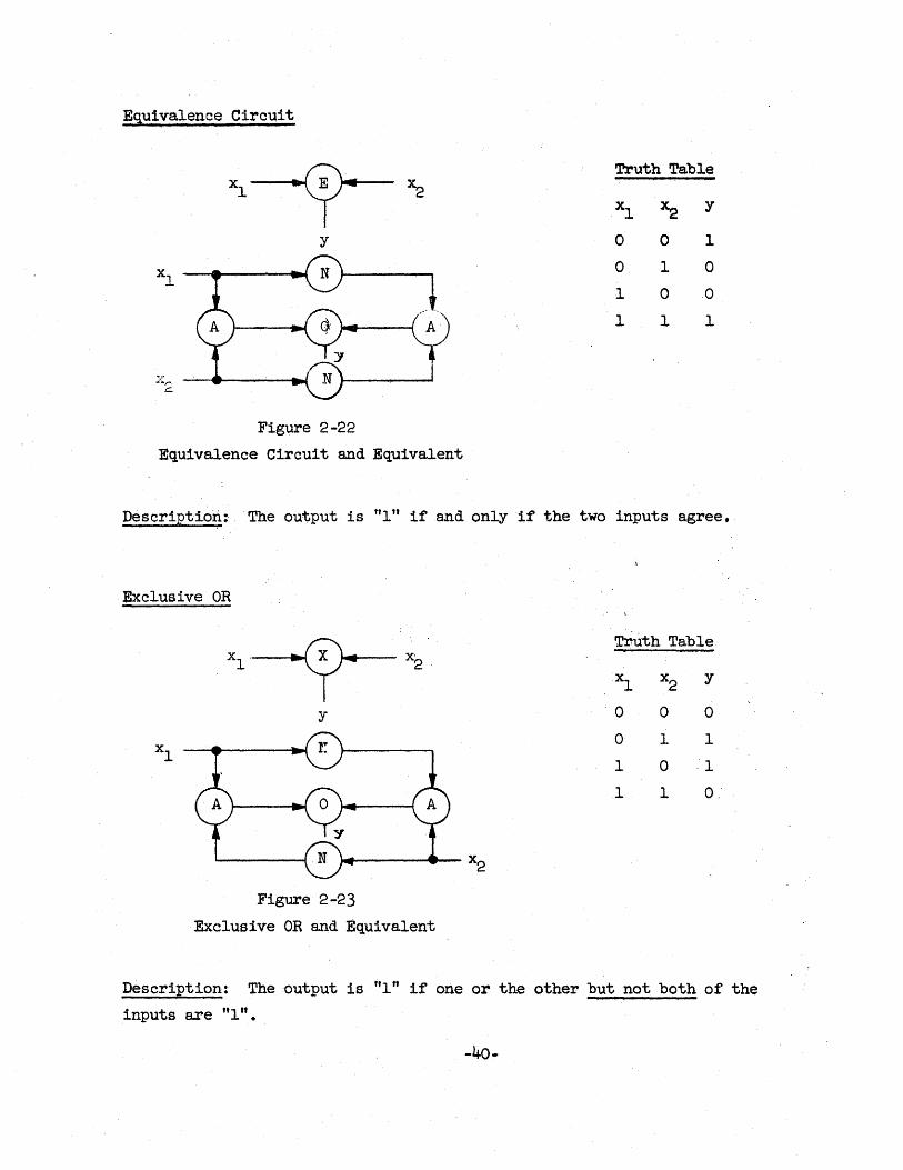
Equivalence Circuit
y
Figure 2-22
Equivalence Circuit and Equivalent
Truth Table
xl x2 y
0 0 1
0 1 0
1 0 0
1 1 1
Description:. The output is "Itt if and only if the two inputs agree.
Exclusive OR
xl
xl' ~C?~ X· 2,
y
Figure 2-23
Exclusive OR and Equivalent
Truth Tahle
xl x2 y
'0 0 0
0 1 1
1 0 ,'1
I 1 0
Description: The output is "1" if one or the other but not both of the inputs are ttltt.
-40-
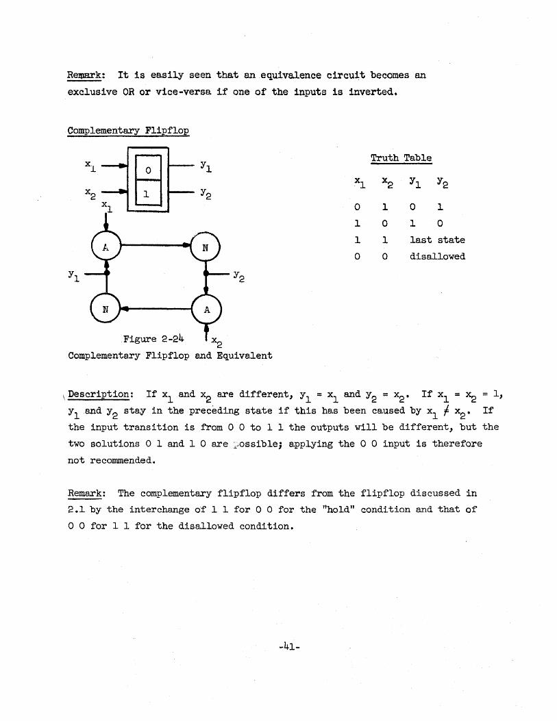
Re~k: It is easily seen that anequlvalence circuit becomes an
exclusive OR or vice-versa. if one of the inputs i6 inverted.
Complementary Flipflop
Truth Table
xl x2 Y1 Y2
0 1 0 1
I 0 1 0
1 1 la.st state
0 0 disallowed
Y2
Figure 2-24 x2 Complementary Flipflop and Equivalent
\ Description: If xl and x2 are different, Yl ; xl and Y2 = x2 ' If xl = x2 = 1,
Y 1 and y 2 stay in the preceding state if this has been ca,used by xl -I x2 • If
the input transition is from 0 0 to 1 1 the outputs will be different, but the
two solutions 0 land 1 0 are ~ossible; a~plying the 0 0 input is therefore
not recommended.
Remark: The complementary flipflop differs from the flipflop discussed in
2.1 by the interchange of 1 1 for 0 0 for the "hold" condition and that of
o 0 for 1 1 for the disallowed condition.
-41-
xl
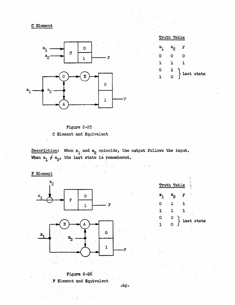
C Element ----,.....~
Truth Table
~ I I xl 0 xl ~ y
C 0 0 0 ~ 1 y
1 1 1
0 1 } last
1 0
0 Xr"\
c.
1 y
Figure 2-25
C Element'andEquivalent
Descript,ion: When xl and ~ cp'incide, tp.e output follows the input.
When xl {: x2, the laet state ia,remembered.
F Element
Truth Table
Xl • r 0 1''"\ .. F \....../ ~
1
xl ~ y
y 0 1 1
1 1 1
0 0
I~ :
,..
f~
state
} 1ast" state
x o
1
Figure 2'!O26
FElementand Equivalent
'1 0
y
-42-
Description: If' x2 = l~ the output tollows the input xl' If' x2 = 0, the
last state is remembered.
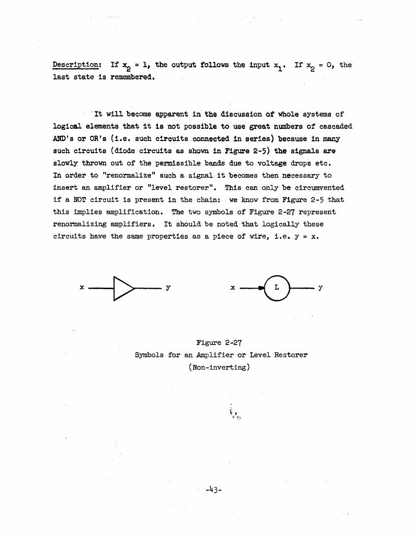
'It will become apparent in the discussion ot whole systems of
logical elements that it is not possible to use grea.t numbers of cs,sca.ded
AND's or OR's (i.e, such circuits connected in series) beca.use in many
such circuits (diode circuits as shown in Figure 2-5) the signals are
slowly thrown out of the permissible bands due to voltage drops etc.
In order to "renorma,lize" such a signa.11t becomes then necessary to
insert an amplifier or "level restorer". This can only be circumvented
if a NOT circuit is present in the chain: we know from Figure 2-5 that
this implies amplification. The two symbols of Figure 2-27 represent
renormalizing amplifiers. It should be noted that logica,lly these
circuits have the same properties a,s a piece of wire, i.e.y = x.
X --.... [>>--- y x ----41{).. L 1---- Y
Figure 2-27
Symbols for an Amplifier or Level Restorer
(Non-inverting)
-43-
2.6 Sophisticated Adding, Counting and Sequencing
Separate Carry Storage
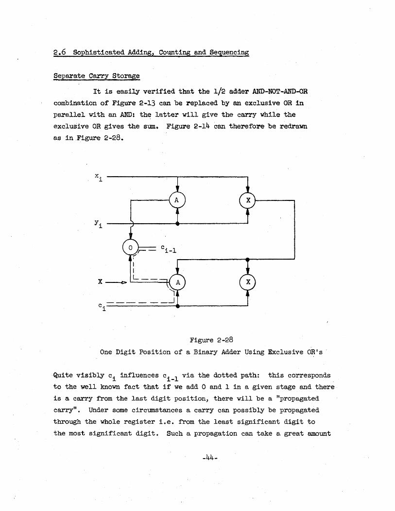
It is es.sily verified tha.t the 1/2 adder AND-NOT-AND-OR
combination of Figure 2-13 can be replaced by an exclusive OR in
para.lle~ with an AND: th~ latter will give the ca:rry while the
exclusive OR gives the sum. Figure 2-14 can therefore be redrawn
as in Figure 2-28.
x. J.
I I
X ---i> L __
c. I ~-
Figure 2-28
One Digit Position of a Binary Adder Using Exclusive OR's -
Quite visib~ ci influences ci _l via the dotted path: this corresponds
to the well known fact tha.t if we add 0 and 1 in a given stage and there
is a. carry from the last digit position, there will be a. "propa.gated
carry" • Under some circumstances a carry can possibly be propagated
through the whole register i.e. from the least significant digit to
the most significant digit. Such a propagation can take a great amount
-44-
of time and operat1ons1n which repeated additions occur (like multiplication)
are excessively slowed down. A way around th1sdif'ficulty is to sever the
carry propaga.tion path in .Xanddump the output of' the AND into a separate
flipflop. If we make the input to the OR "0" we shall then simply have a
"pseudo-sum" coming out of si while the carry 1s stored separately;
considering the Whole adder and its registers we would then have a register
holding Xi'S, one holding Yi's, a "pseudo-sum" register ·holding the s1's
and finally a carr.y storage register holding the output - s~ bi _l - of the
lower Am>. At each moment the read sum ·could be obtained by adding the
"pseudo-sum" to the separate carries.
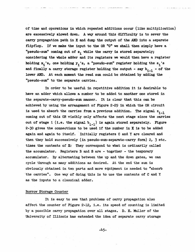
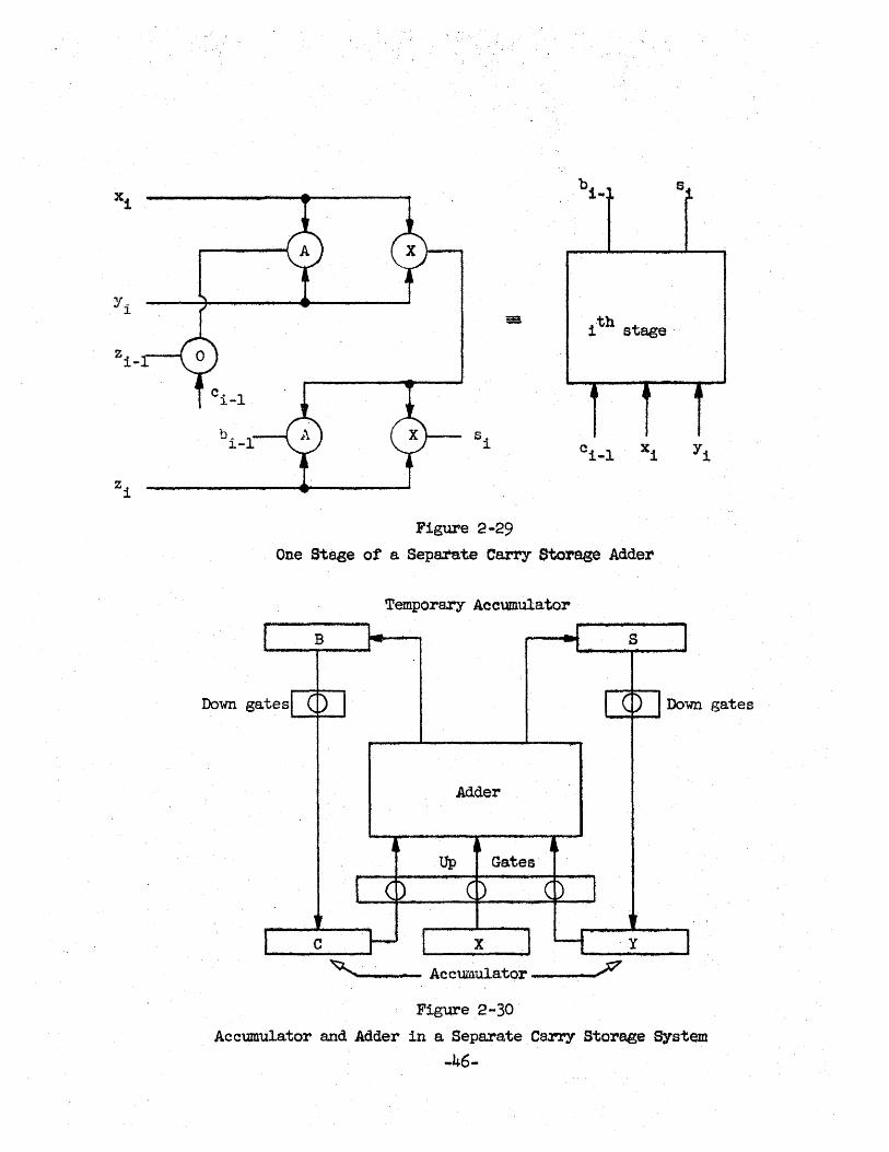
In order to be useful in repetitive addit10nit is desirable to
have an adder which allows a number to be added to another one stored in
the separate-carry-pseudo-sum manner. It is clear that tbis can be
achieved by using the arrangement of Figure 2-29 in which the OR circuit
is used to absorb the carries fram a previous addition. The signal zi_l
coming out of this OR visibly onlY affects the next stage since the carries
out of stage i (i.e. the signal bi _l ) is aga.instored separately •. Figure
2-30 gives the connections to be used if the number in X is to be added
again and aga.in to itself. Initially registers C and Yare cleared and
then they hold successively (in pseudo-sum-separate-carry form) 2, 3 etc.
times the contents of. X: They correspond to what is ordinarily called
the accumulator. ·Registers B and Sare - together - the temporary
accumulator. . By alternating between the up and the down gates, we can
cycle through as many additions as desired. At the end the sum is
obviously obtained in two parts and more equipment is needed to "absorb
the carries". One way of doing this is to use the contents of C and Y
as the inputs to a classical a.dder.
Borrow Storage Counter
It is easy to see that problems of carry propagation also
affect the counter of Figure 2-12, i.e. its speed of counting is limited
by a possible carry propagation over all stages. ·D.E. Muller of the
University of Illinois has extended the idea of separate carry storage
-45-
s. ~
Figure 2-29
;1th stage
One Stage of a Sepa.:rnte Carry Storage Adder
Temporary Accumulator
B S
Down gates
Adder
......... _- Accumula.tor __ .....,
Figure .2-30
Down gates
Accumulator and Adder in a Separate Ca~ Storage System
-46-
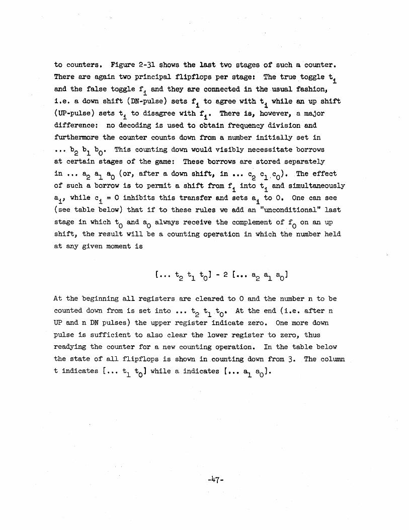
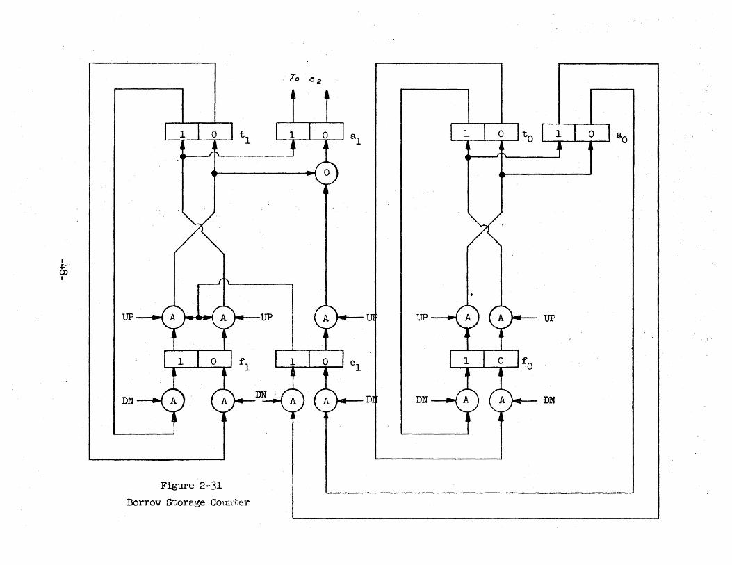
to counters. Figure 2-31 shows the last two stages of such a counter.
There are again two principal f11pflops per stage: The true toggle t1
and the false toggle fiand they are connected 1n the usual fashion,
i.e. a down shift (DN-pulse) sets fi to a.gree with t 1 while an up shift
(UP-pulse) sets ti to disagree with t i , There is, however, s, major
difference: no decoding is used to obtain frequency division and
furthermore the counter counts down from a number initia.lly set in
••• b2 bl bot This counting down would visibly necessitate borrows
a.t certa.in stages of the game: These borrows are stored .sepa,rately
in ••• a'2 a'l aO (or, a.fter a down shift, in ••• c2 cl.cO), . The effect
of such a borrow is to permit a shift trom f i into ti a.nd simultaneously
a'l' while ci = 0 inhibits this transfer and sets ai to 0, One can see
(see table below) that if to these rules we add an "unconditional" last
stage in which to and a.O always receive the complement of fO on an up
shift, the result will be a counting operation in which the number held
at any given moment is
At the beginning all registers are cleared toO and the number n to be
counted down from is set into ••• t2 tltO. At the end (i.e. after n
UP and n DN pulses) the upper register indicate zero. One more down
pulse is sufficient to also clear the lower register to zero, thus
readying the counter for a new counting operation. In the table below
the state of all flipflops is shown in counting down from 3. The column
t indicates [ •••. tl tol while a. indicates [ ••• a1 ao]'
-47-
70 <::2
t1 a1 , to L ___ - ao
I
g; I
UP UP UP
DN DN DN
Figure 2-31
Borrow St.orage COiL:1-;:,er
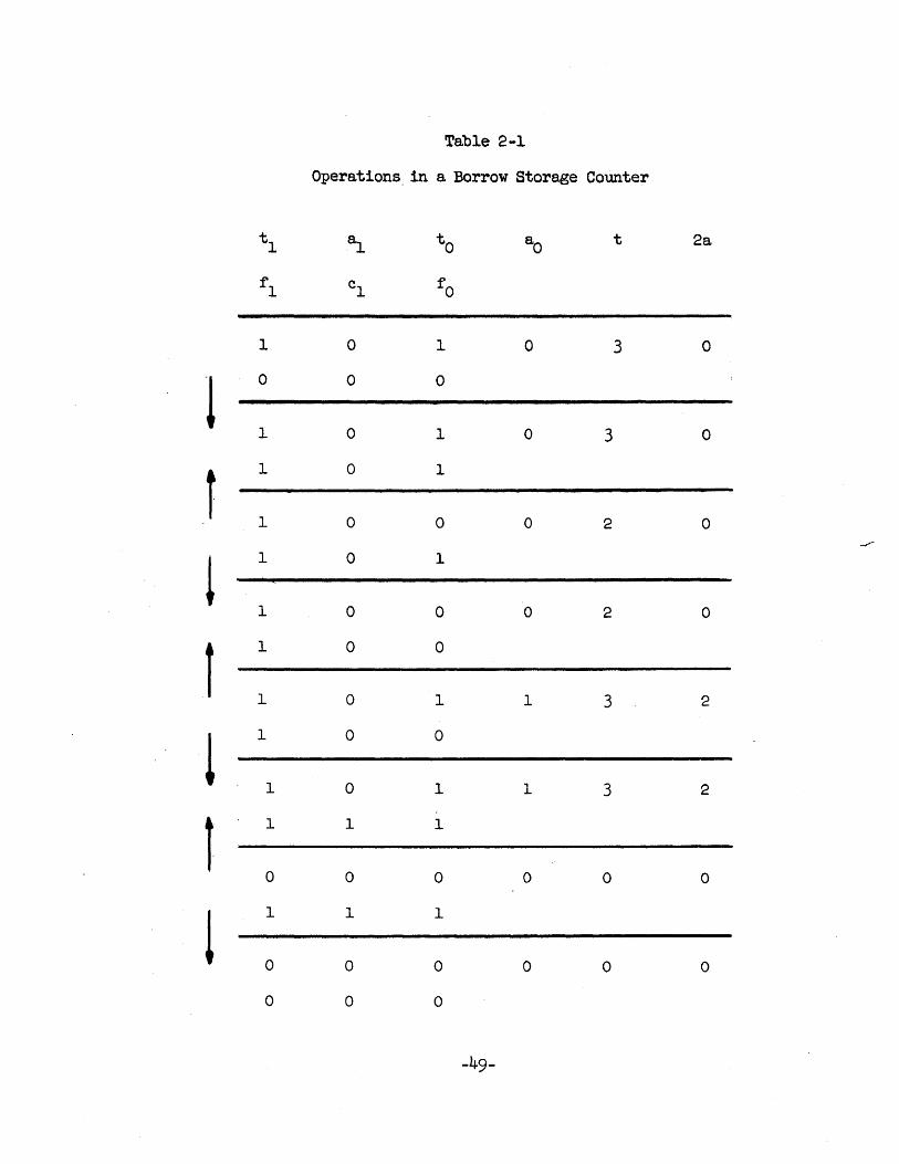
Table 2 .. 1
Operations. in a Borrow Storage CoUnter
tl a1 to aO t 2a
fl c1 fO
1 0 1 0 3 0
1 0 0 0
1 0 1 0 3 0
r 1 0 1
1 0 0 0 2 0 -~
l 1 0 1
1 0 0 0 2 0
f 1 0 0
1 0 1 1 3 2
! 1 0 0
1 0 1 1 3 2
1 1 1 1
0 0 0 0 0 0
! 1 1 1
0 0 0 0 0 0
0 0 0
-49-
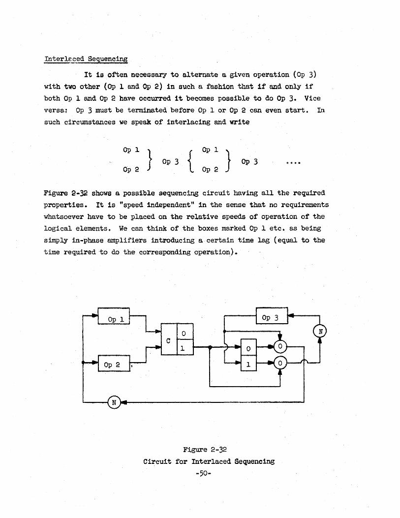
Interle.cedSequenci~
It is often necessary to alternate a given operation (Op 3)
with two other (Op 1 and Op 2) in such a fashion tha.t if and only if
both Op 1 and Op 2 have occurred it becomes possible to do Op 3. Vice
versa.: Op 3 must be terminated before Op 1 or Op 2 can even start. In
such circumstances we speak of interla.cing and write
Op 1 }
Op2 Op3 . " ..
Figure 2-32 shows a possible sequencing circuit having all the required
properties. It 1s "speed independent" in the sense that no requirements
whatsoever have to be placed on the relative speeds of operation of the
logical elements" We can think of the boxes marked Op 1 etc. a.s being
simply in-phase amplifiers introducing a. certain time lag (equal to the
time requiredt.o do the corresponding operation) e
c o
1
----~ N ~---------------------------------------
Figure 2-32
Circuit for Interlaced Sequencing
-50-
The op era.t ion of this circuit is as follows. Suppose thatOp 1 and Op 2
have occurred, injecting two "1ft signals into the C-element: The output
of this element now sets the flipflop into the "On state thus making the
input to the lower NOT ttl" and the input to Op landOp 2 "0" (after some
time this makes the upper input to the flipflop nO" aga.in). As the
flipflop changes state, its lower output becomes zero and this zero,
together with reply back zero mentioned above, fina.lly allows the upper
NOT to energize the input to Op 3. This sets the flipflop back into the
one state, thus cutting.off the input toop 3 anda.fter the output of
Op 3 ha.s also gone ba.ck to zero the lower NOT receives a zero input and
starts up Op 1 and Op 2 again.
2 .7 Dynamic (Synchronous) Logic
Up to now no major difficulties resulted from the fact that
no information concerning the opera.tion time of individual logical
elements was available: we talked essentially about a.synchronous
circuitry •. Very oftensaNings in both time and equipment can be
obtained by specifying the delays signals suffer in the logical circuitry,
at least to the extent of making sure that an ordering relationship is
known i.e. if two parallel signa.l paths are present it is known which
one is faster. Often such an ordering is obtained by inserting into
one of them suitably chosen delay elements. We shall discuss below
some of the more common dynamic circuits •
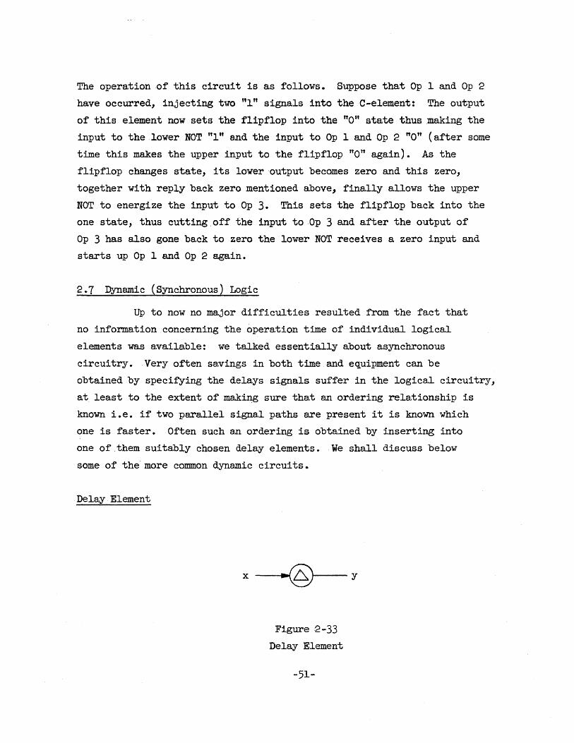
. Delay Element
x --..!-@I----y
Figure 2-33 Delay Element
-51-
The delay element shown .in Figure 2 .. 33 is essentially anamp11fier
which is slowed down by ca.pacitive loading of the output or intermediary
points or it is a, transmission line formed of lumped L and C elements
a,djusted to give a given delay between the input and the output. In the
following discussions we sha.ll a,ssume that delay elements have amplifica.tion.
Often ~ indica.tes the time delay in seconds 0
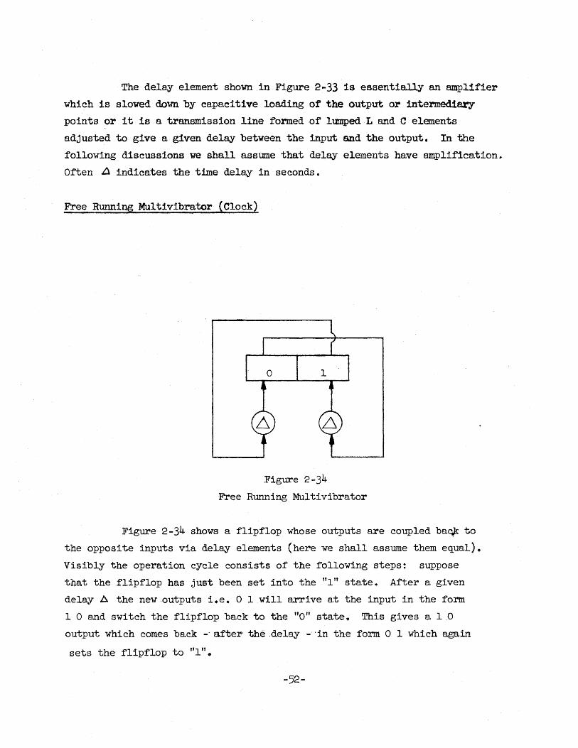
Free Running MUlt1vibrator (Clock)
Figure 2-34 Free Running Multivibrator
Figure 2-34 shows a flipflop whose outputs are coupled ba.¥ to
the opposite inputs via delay elements (here we shall assume them equal).
Visibly the operation cycle consists of the following steps: suppose
that the flipflop has just been set into the "1" state. After a given
delay A the new outputs i.e. 0 1 will arrive at the input in the form
1 0 and switch the flipflop ba.ck to the "a" state o This gives a 10
output which comes ba.ck -" after the "delay -" 'in the form 0 1 which again
sets the flipflop to "1".
-52-
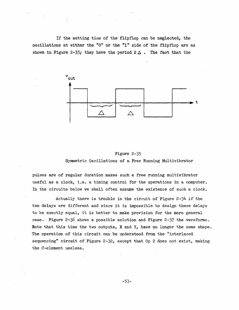
If the setting tline of the flipflop can be neglected, the
oscillations at either the "0" or the "1" side ·of the flipflop are as
shown in Figure 2 -35; they have the period 2 1l. The fact that the
v out ~~
~
6.
.. -\- J ., L..
Figure 2-35 Symmetric Oscillations of a. Free Running Multivibrator
t
pulses are of regular dura.tion makes such a free running multivibrator
useful a.s a. clock, i.e •. a timing control for the operations in a computer.
In the circuits below we sha.ll often assume the existence of such a clock.
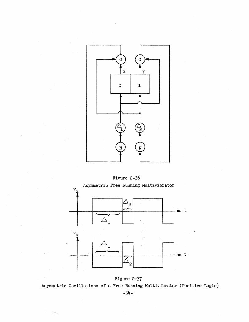
Actually there is trouble in the circuit of Figure 2-34 if the
two delays a.re different and since it is impossible to design these delays
to be exactly equa.l, it is better to make provision for the more general
case 0 Figure 2-36 shows a possible solution and Figure 2-37 the wa~eformso
Note that this time the two outputs, X and Y, have no longer the same shape.
The operation of this circuit can be understood from the '''interlaced
sequencing" circuit of Figure 2-32, except that Op 2 does not exist, making
thee-element useless.
-53-
v "-
II
v y; ,
o 1
Figure 2-36
Asymmetric Free Running Multivibra,tor
~2 ~ -- t
. '----v---" b 1 "-- ~
L1 - -,. ...
"I .. ~ - t
Ll2
Figure 2-37 Asymmetric Oscillations of a Free Running Mu1tivibrator (Positive Logic)
-54-
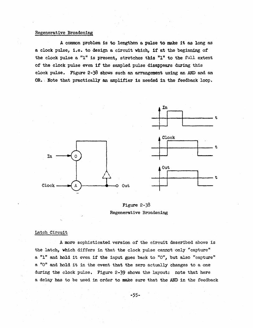
Regenerative Broaden1ng
A common problem is to lengthen a pulse to ~e it as long as
a clock pulse, i.e. to design a circuit which, 1fat the beginning of
the clock pulse a "1" is present, stretches this 'tl" to the full extent
of the clock pulse even if the sampled pulse disappears during this
clock pulse. . Figure 2 -38 shows such an arrangement using an AND and an
.OR., Note that pra.ctically an amplifier 1s needed in the feedback loop.
1m
I
In
I Clock
I
rut I \ '- ~
Cloc~ Out I
Figure 2-38 Regenerative Broadening
Latch·Circuit
t
t
t
A more sophisticated version of the circuit described above is
the latch, which differs in that the clock pulse cannot -,only "c.apture ft
a "1" and hold it even if the input goes back to "0", but also tlcapture"
a "0" and hold it in the event that the zero actually changes to a one
during the clock pulse. Figure 2-39 shows the layout; note that here
a delay has to be used in order to make sure that the AND in the feedback
-55-
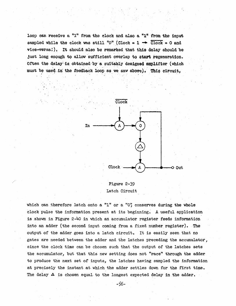
loop oan receive a. "1" from theelock and also a, "1 " from the input sampled while the clock was still t'O'" ,(Clock == 1 -,..Clock = 0 and
v1ce-versa:)o It should ,also be r~~ed, that this delay should be just long enoughtQ allow 'suttie1~nt overlap to ataft regenerat1ono
,Often the, ,d,elSJ'"is, obtaJ.ned;.by'a su1ta.'l)lYdea'1gned'em;.lif1Sl' (whioh , . ,,' . '.
must b~ us~4,1rf the fee4:b&.ck loop e.s we saW's.bo'Y"e) 0' ~:L$ Q1:ro~1~l f . • .. 'j .... • ~
.,',
....
In
'Clock
O:l!ock '--...t
Figure 2 .... 39 La.tch Circuit
I---~ __ -O Out
which can therefore la.tch onto a ttltt or a. "0'; conserves during the whole
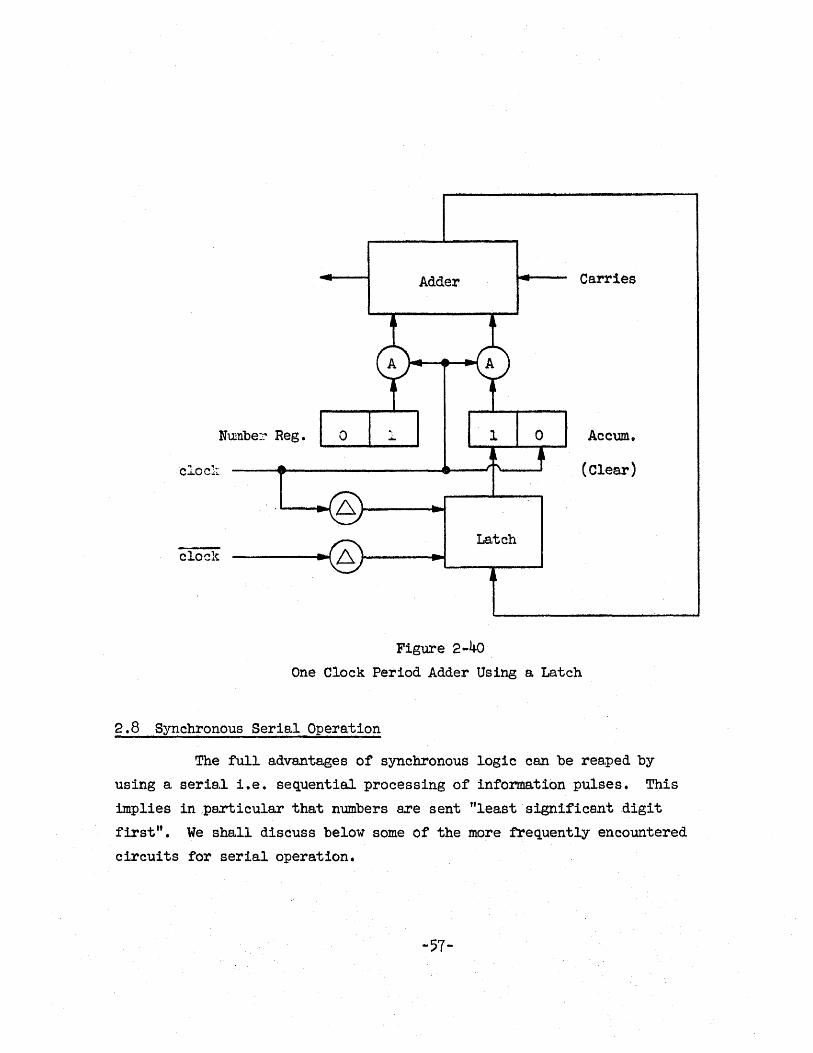
clockpuls,e theinforma.tion present a.t its beginning 0' ,A useful applica.tion
is shown in Figure 2-40 in which an accumulator register feeds information
into an adder (the ;second input coming from a fixed number, register) {I The
output of the a.dder goes into a la.tch circuito It is ea.sily seen that no
ga.tes are needed between the a.dder and the' la.tches preceding the accWTlulator I
since the clock time can be chosen such that the output of the latches sets
the a.ccumula.tor j but that .this new setting does not "ra.ce" through the a.dder
to produce the next set of inputs, the l~.tches ha:ving sampled the information
a.t precisely the instant at which the ad<ier settles down for the first time ..
The dela,y l1. is chosenequa~, to the longest expected delay in the adder.
-56-
Adder Carries
Numbe::- Reg. Accum.
clocl;: (Clear)
Latch clocl-t
Figure 2-40
One Clock Period Adder Using a Latch
2.8 Synchronous Seria,l Opel'B,tion
The full a.dvantages of synchronous logic can be rea.ped by
using a seria.l i.e. sequentia~ processing of information pulses. This
implies in particular tha.t numbers are sent "least significant -digit
firsttt. We shall discuss below some of the more frequently encountered
circuits for serial operation.
-57-
Delay Lines (Recil"cul.~.l~ing Registers)
It is possible to use a tzoe.nsm:i.ssion line of sufficient length
to store sequences of pulses 0 Such a. line can be thought of as a. cha.in
of delay elements~ in order to store n pulses we need n times a delay
equal to the period of the clocko The chain usually c.ontains at its end
a circuit for regenera.tlve broadening 0 This has for effect not only to
give to pulses a standard shape and lengthj) but a~so to resynchronize
them with the clock, ioeo to make sure tha.t all pulses are still equally
spaced after an indefinitely great number of passages through the lineo
It should be remarked that delay lines are often of the accustic type in
order to circumvent size problems one would encounter with electric lines
storing 1000 or more bits 0 The a.ccustic delay line is simply a sound
propagating rod connected between a. loudspeaker and a. microphone (called
"tra.nsducers") at megacycle frequ.encies; b~",:"sts of sine waves are used
rather than the modu.lating pulses themselves~ This simplifies the design
of the transducerso
The two main problems with recircu.lating registers are 1) to
"load't the line by establishing in it a train of pulses conveying the
information initially present in a. set of flipflops 2) to "unload" the
line by dumping into a set of flipflops the dynamic informa.tion u:running
off the end" of the lineo
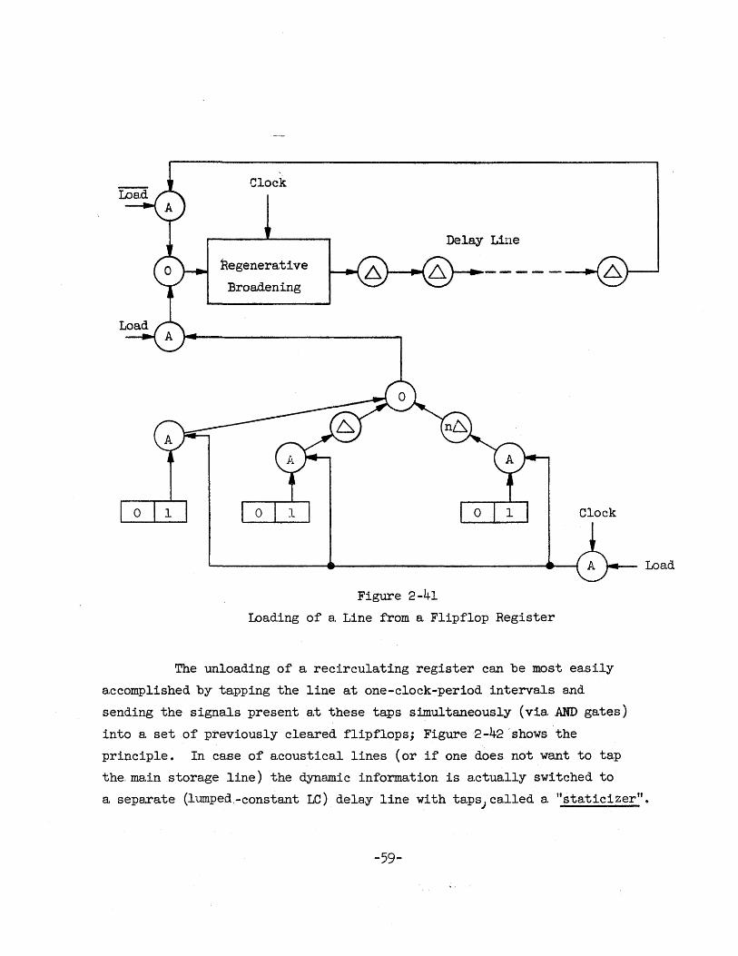
Figure 2-41 shows a. possible loading mechan:i.smo .When both the
load signa.l and 8.. clock pulse occur JI the informa.ti.on in the flipflops is
ma.de a:'"/ailable to the line "'Ii.a. the input OR in front of (or a.s one can
see from Figul"e 2-38 a.ctu.ally pa.rt of) the regenera.tive broadening circuit
which feeds the line (represented. 'by 23. series of dela.y elements) 0 Dela.ys
equa.l to one, two etco times the clock period are inserted between the
one-side output of the flipflops and a. common collecting OR circuito The
latter goes into the input OR mentioned above via. an AND which disconnects
the flipflops in case no loa.ding signal is present~ in the absence of the
load signa.l the upper AND closes the loop and ma.kes sure tha.t no information
is lost 0 Note that more than one wo:rd can be stored and that a counter is
required to time the loa.d signal correctly so that a. new word does not
start in the middle of one already being recirculated 0
Clock
Regenera.ti ve
Broadening
Delay Line
Figure 2-41
Loa.ding of' a. Line from a. Flipflop Register
Clock
The unloading of a recirculating register can be most easily
accomplished by tapping the line at one-clock-period intervals and
sending the signa.ls present a.t these taps simultaneouslY (via . .AND gates)
into a set of previously cleared f'lipflops; Figure 2-42 'shows the
principle. In case of' acoustica.l lines (or if one does not want to tap
the .. main storage line) the dynamic information is actually switched to
Loa.d
a separa.te (lumped.-constant LC) delay line with taps; called a "staticizer".
-59-
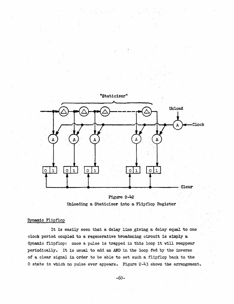
"Static1zer"
~-----------------~~----------~,
. Clock
~----~~----~'-------------~~-----4~--------- Clear
Figure 2-42
Unloa.ding aStaticizer into a Flipflop Register
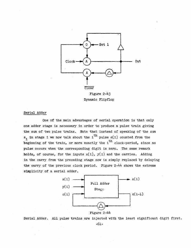
Dynamic Flipflop
It is easily seen that a de~ line ,giving a delay equal to one
clock period coupled to a'regenera.tive broadening circuit is s1m,ply a
dynamic flipflop: once a pulse is trapped in this loop it will reappear
periodically. It is usual to add an AND in the loop fed by the inverse
of a clear signal in order to be able to set such a flipflop back to the
o state in which no pulse ever appears. Figure 2~43 shows the a~rangement.
-60-
Clock
Serial Adder
Set 1
Figure 2-43
Dynamic Flipflop
Out
One of the ma,in advantages of serial operation is that only
one adder stage is necessary in order to produce a pulse train giving
the sum of two pulse trains. Note that instea.d of speaking of the sum
si in stage i we now talk about the ith pulse sCi) counted from the th beginning of the train, or more exa.ctly the i clock-period, since no
pulse occurs when the corresponding digit is zero. The same remark
holds, of course, for the inputs xCi), y(i) and the carries. Adding
in the carry from the preceding stage now is simply replaced by delaying
the carry of the previous clock period. Figure 2-44 shows the extreme
simplicity of a serial adder.
x(i)
y(i)
c(i)
-Full Adder
Sta.g;~
L -Figure 2-44
sCi)
e(i-l)
Serial Adder. All pulse trains a.re injected with the least significant digit first.
-61-
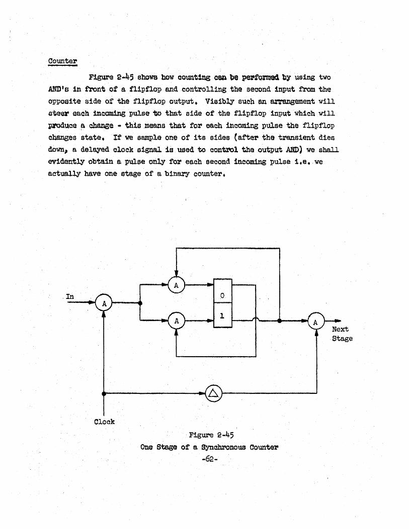
Counter •
Figure 2-45 shows bow count1ng oan be pei'tomed by using two AND's in front of a flipflop and .controlling theseaond1nput fram the oPPosite side ot the flipflop output. VisiblY auoh an arrangement will s"e~ each incam1ng pulse to that side of the flipflop inputwh1chwil1.
produce .~ ~e • thlsmeana that for each incoming pulse the flipflop changes state. It we sample one of its sides (after the transient dies
down, e. delayedolocksignaJ. is used to contX'Ol the output AND) we shall evidently obta.ins. pulse only fol' ea,ch second inooming pulse i.e •. we
e,ctue.ll;yo have one stage of a binary counter •
. In
Cloak
Figure 2-45
One Stase ota. Synahronous Countel'
-62-
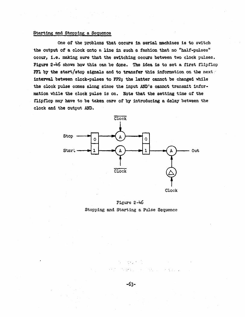
Starting and Stopping a Sequence
One of the problems that occurs in serial machines is to switch
·the output ot a. clock onto a line in such eo fashion that no "half-pulses"
occur" i.e. ma.k1ng sure that the sntching occurs between two clock pulses. Figure 2·46 shows how this can be done. The idea is to set a first flipflop PTl by the start/stop signals ancl to transfer this 1ntorma.t1on on the next .. ,
interval between clock-pulses to FF2J the latter cannot be changed while the clock pulse comes along since the input AND's cannot transmit information while the clock pulse is on. Note that the setting time of' the flipflop may have to be taken care ot by introduoins a delay between the clock and the output AND.
Clock
Stop
t--- Out
Clock
Figure 2-46 Stopping and Starting a Pulse Sequence
.' •. I
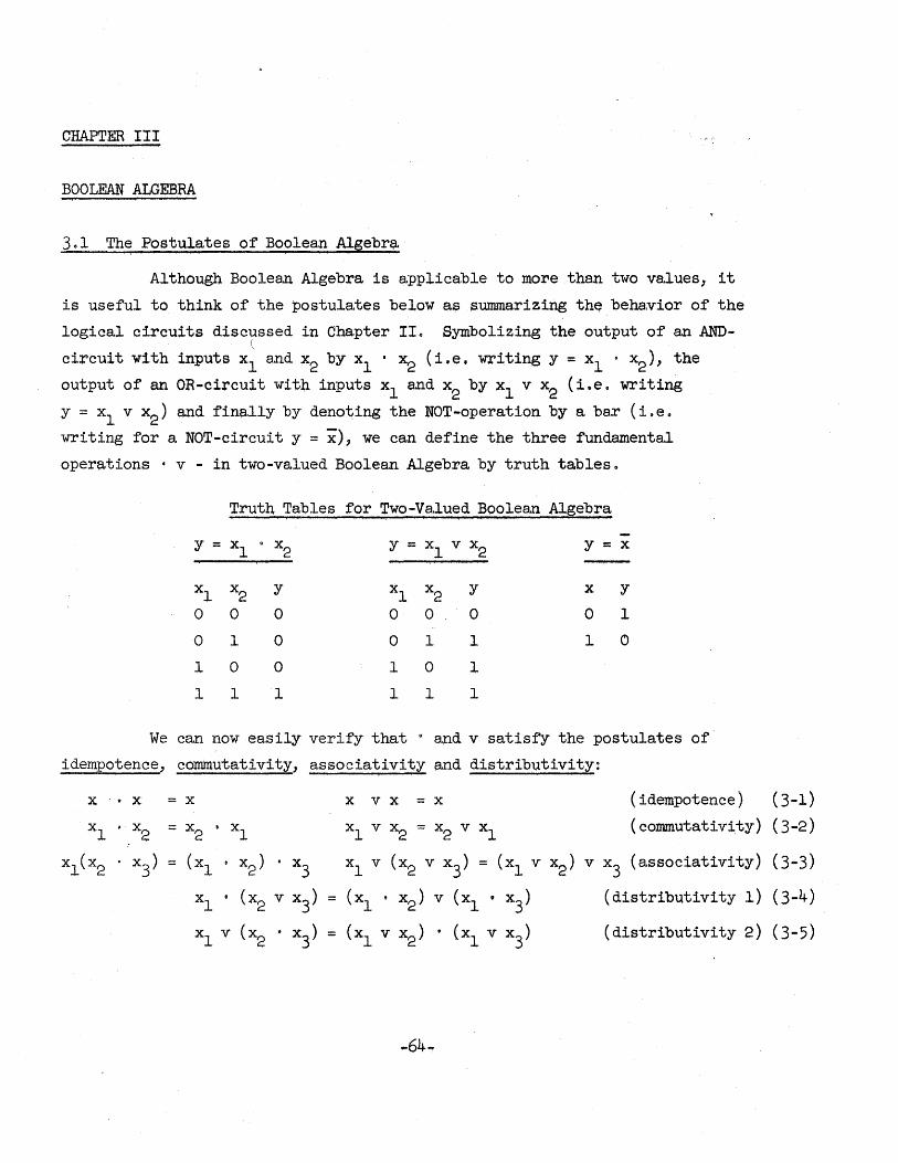
CHAPTER III
BOOLEAN ALGEBRA
3.1 The Postulates of Boolean Algebrl:;l.
Although. Boolean Algebra is applicable to more than two va,lues, it
is useful to think of the postulates below as summa.rizing th~ behavior of the
logical circuits discussed in Cha,pter IIo Symbolizing the output of an AND-(
circuit with inputs xl and x2 by xl • x2 (i.e, writing y = xl · x2 ), the
output of an OR-circuit wit~ inputs xl and x2 by xl v x2 (i.e. writing
y = xl v X2
) and fin~,lly by denoi:ring the NOT-operation by a bar (i. e.
writing for a NOT-circuity == X'), we ca,n define the three fundamental
operations · v - in two-valued Boolean Algebra by truth tables$
Trutn Ta:bles for Two-Valued Boolean Algebra
y == Xl oX 2 Y == Xl v x2 Y == X
Xl x2 Y Xl x2 Y X Y
0 0 0 0 0 0 0 1
0 1 0 0 1 1 I 0
1 0 0 1 0 1
I I I 1 I 1
We can now easily verify that 0 and v sa.tisfy the postulates of
idempotence, commutativity, associa.tivity and distributivity:
X-.X ==X x v x == x (idempotence)
Xl · Xz == x2 ~ Xl Xl v x2 == x2 v Xl (commutativity)
Xl v (x2 v x3 ) == (xl v x2 ) v x3 (associa.tivity)
(3-1) (3-2)
(3-3) Xl (x2 . x3) = (xl · x2 ) • x3
Xl • (x2 v x3)
Xl v (x2 • x3)
== (xl • x2 ) v (Xl • x3) (distributivity 1) (3-4)
= (xl v X2 ) • (xl v X3) (distributivity 2) (3-5)
-64"r
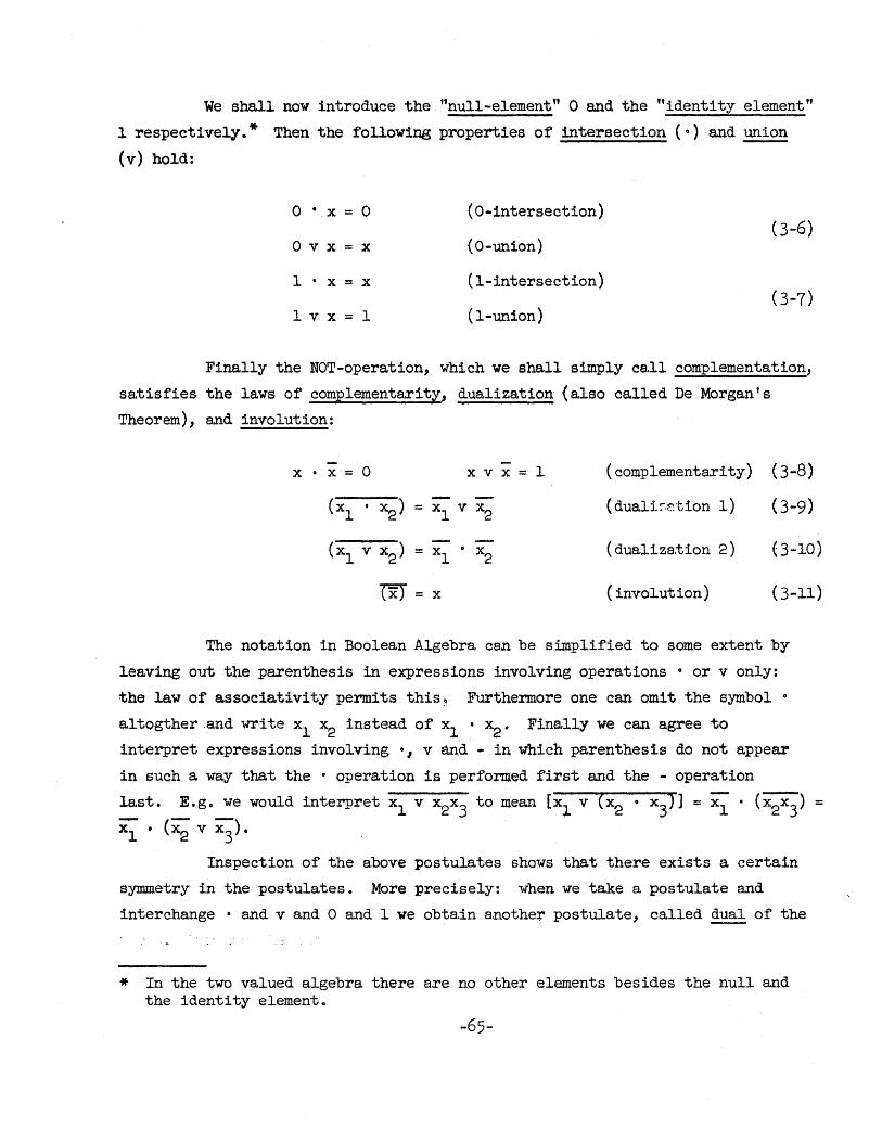
We shall now introduce the "null-element" 0 and the "identity element"
1 respectively.* Then the following properties of intersection (.) and union
(v) hold:
o ·x = 0
o v x = x
I · x = x
1 v x = 1
(O-intersection)
(O-union)
(I-intersection)
(I-union)
(3-6)
Finally the NOT-operation, which we shall simply ca.ll complementation,
satisfies the laws of complementarity, dua.liza.tion (also ca.lled De Morgan t s
Theorem), and involution:
x · x = a x v x :::; 1 (complementarity) (3-8)
(xl • X2 ) = Xl v x2 (dualj.~.etion 1) (3-9)
(xl v X2 ) = Xl • x 2 (dualiza.tion 2) (3-10)
(x) :::; x (involution) (3-11)
The notation in Boolean Algebra can be simplified to some extent by
leaving out the parenthesis in expressions involving operations • or v only:
the law of associativity permits this~ Furthermore one can omit the symbol 0
a1 togther :and wr·i te Xl x2
instea.d of Xl • x2
• Finally we can a.gree to
interpret expressions involving °1 v and ... in which parenthesis do not appear
in such a way that the • operation is performed first and the - operation
last. E.g. we would interp~et Xl v x2x3 to mean [Xl v (x2 • x3)] :::; Xl • (x2x3) = Xl • (x2 v x3)·
Inspection of the a.bove postulates shows that there exists a certain
symmetry in the postulates. More precisely: when we take a postulate and
interchange • and v and 0 and lwe obtain another postulate, called dual of the
* In the two valued algebra there a.re no other elements besides the null and the identity e1emento
-65-
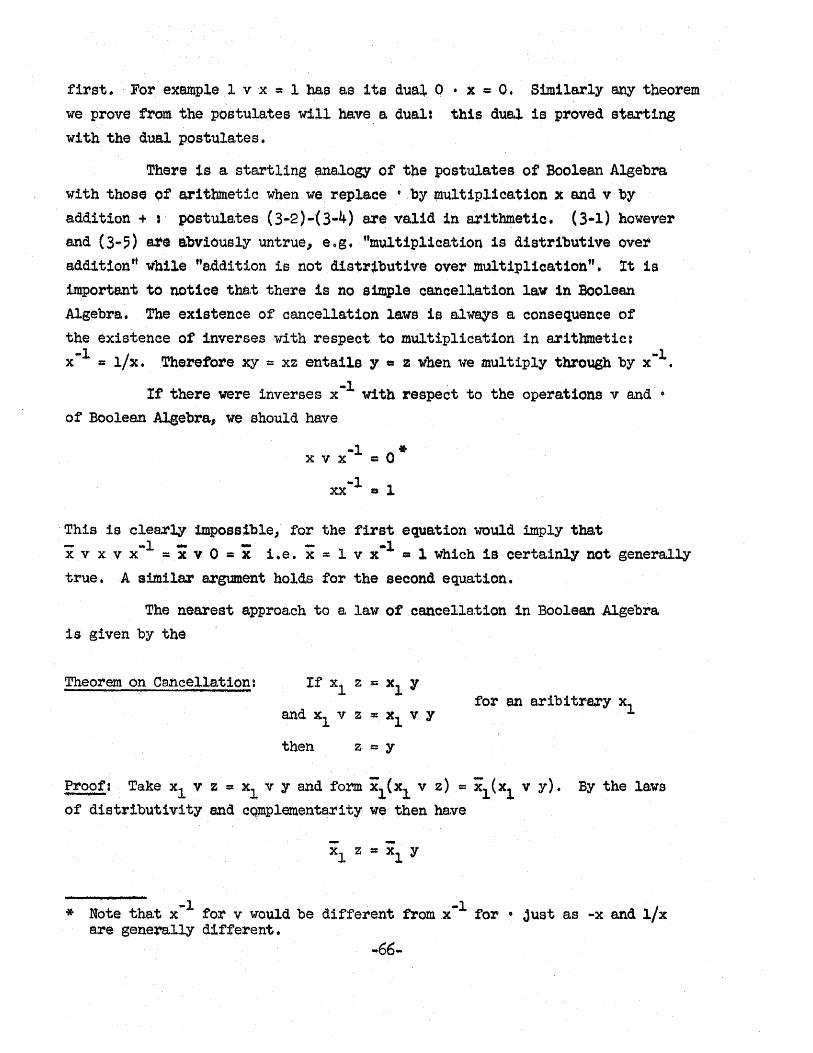
first. For example 1 vx = 1 bas as its dua+ 0 • x = 0. Similarly any theorem
we prove from the postulates rill have a. dual: th1sduel is proved starting
with the Q.ua.l postula.tes.
There is a. startling ~na.logy of the postulates of Boolean Algebra.
with those Qt arithmetic when we repla.ce 'by ~ultip11ca.t1on x and v by
a.ddi tion +: postUla.tes (3-2) -( 3 ... 4) are vs,lid in sri thmetio. (3 ... 1) however
and (3-5) are abv10usly untrue, eos, "multiplica.tion is distributive oveX'
a.d.dition'· wbile "a.ddition is not distr1but1ve over multiplica.tion". it is
important to notice the,t there is no simple cancella.tion la.w in Boolean
Algebra.. Tbe existenee of cancella.tion la.ws is always a consequence of the existence of inverses with :respect to multiplication in arithmetic:
x-1 = l/x.Therefore xy = xz entails y = z when we multiply through by x·l •
If there were inverses x·l with respect to the operations v and 0
of Boolean Algebra, we should have
x v x·1 = 0 * xx-l = 1
'This is clearly tmposs1ble, for the first equation would imply that ..... -1.. .... ...... ·-1 x v x V x = x v 0 = x i.e. x = 1 v x = 1 which is oertainly not generally true. A. similar a.rgument holds tor the second equation.
The nearest a.pproa.ch to a law of . eancella.tion in Boolean Algebra.
is given by the
Theorem on Cancellation: If Xl Z = Xl Y
andx1vz=x1VY for an aribi tre.ry Xl
then z = y
Proof: Take Xl V Z = Xl v y and for.m i1(X1 v z) = i1(X1 v y). By the laws
of distribut1vity and cQmplemente~ity we then ha~e
* Note that x-I tor v would be different fromx-l for • Just as -x and l/x e,re gene:rally different 0
~66-
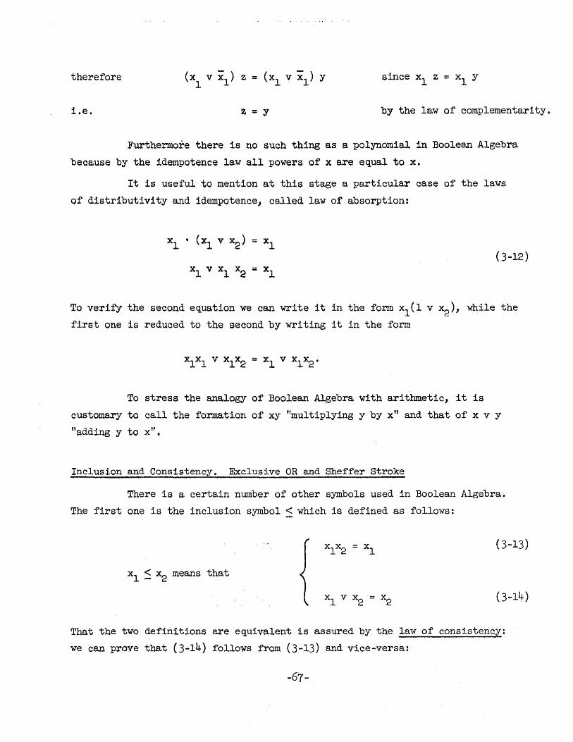
therefore
i.e. z = y by the laM of complementarity.
Furthermore there 1s no such thing as a, polynomia.l in Boolean Algebra
because by the Idempotence law all powers of x are equal to x.
It is useful to mention at this stage a pa.rticu1ar case of the la.ws
of distributivlty and idempotence, called la,w of absorption:
(3-12 )
To verify the second equation we can write it in the form x1(1 v x2), while the
first one is reduced to the second by writing it in the form
To stress the analogy of Boolean Algebra with arithmetic, it is
customary to call the formation of xy "multiplying y by x" and that of x v Y
" a.dding y to x".
Inclusion and Consistency 0 Exclusive OR and Sheffer Stroke
There is a certain number of other symbols used in Boolea.n Algebra.
The first one is the inclusion symbol :s which is defined a.s follows:
(3-13)
(3-14)
That the two definitions are equivalent is assured by the law of consistency:
we can prove that (3-14) follows from (3-13) a,nd vice-versa.:
-67-
Assume
Then by substitution
=~ by absorption
Assume
Then by substitution
'by absorption.
From the definition of :s we can easily see that this operation
sB,t1sfies the laws of ref1exivitYJ anti-symmetry and transitivity and tha.t
of universal bounds:
x < x (reflexitivity)
'If x ~ y and y ::s x, th~n x = y (anti-symmetry)
If x ~ y and y :s z, then x ~ z (transitivity)
O<x<l (universal bounds)
(3-15)
(3-16)
(3-17)
(3-18)
The first two equations are verified biY a.pplying the definition of <. The third -follows from thefa,ct ·tbatJWehB.'V~ simultaneously
xy = x
y v z = z
••• xz = x(y v z) = xyvxz = x y xz = x •
The fourth equation finally simply restates (3-6) and (3-7).
Another operational symbol useful in Boolean Algebra is (3 called
"exclusive or" * ana defined by
* Often the . symbol A is used. -68-
x 0 y=xyvxy
The grea.t usefulness of this operation a.rises from the fact that it allows us
to form binary sums. Another important point is that in equations involving
only ~ the ordinary laws of cancellation hold. This is due to the fact that
every element x has a,n inverse x -1 with respect to the e operation such that
1'7:\ -1 x 0 x = 0 (existence of an inverse) (3-20)
Before we prove this la,tter point, let us note that 0 sa,tisfies a.
number of the properties discussed in the last section:
xl (£) x2 = x2 ® xl (commutativity) (3-21)
xl e (x2 (£) x3
) = (xl 0 x2 ) 0 X3 (associa,tivity) (3-22)
xl (x2 (£) x3) = xl x2 (:) xl x3 (distributivity) (3-23)
These properties ce,n be established from the definition of (£) also gives us immediately the equation
this definition
o (.£) x=x (existence of a zero) * (3-24)
To prove (3-20) it is sufficient to verify that we cap set x·l = x:
x 6 X=xXVXx=o
•• x(~ y=x0 Z~Y=Z
(3-25)
( 3 ... 26)
for we can "a.dd" (with the operation ®) x to both sides, which leaves y = z.
It is useful to join to equation (3-24) and (3-25) the pair
x 0 1 = i x ~ x = 1 (3-27)
* Equations (3-20) - (3-24) together with the commutative la,w for • are the postula.tes of a. .Itring"; eJ is therefore often os,lled "ring-sum".
-69-
and ,x (t) 1= i ~ Y (3-28)
We shall finally introduce a last operation: 'l'beShetfer Stroke /i by def1n1t1onr
It oan then be easily seen that
i;; x/x
xl~ = (Xl/X2)/(Xl/~J
xl v x2 = (~/Xl)I(X2/~)
xl ® xa = [xl/(X2/~) 1/[x1/x1)/x21,
whioh means that a.ll theoperationsdef1nedeo ta:r can be deduced trom the
Sheffer Stroke.*
3.2 Canonica.l l8s!?ansions
(3-29)
(3-30)
(3-31)
, (3-32)
(3-33)
The pui'poee of this section is to show that all Boolean functions of a given number of variables Xl x2 ••• Xn can be written in a certain standard
form ca.l~ed "canonica.l e3Pansion".. Before we prove this let us extend. the dualization laws to nvariables.
DeMbr~an's Theorem 1:
-00. VX : '=:'~l"~( XI"\' •• ',',X
n '" t:: "n
Proof: Call'x2 v .0. Xn for short X, then xl'v x == Xl i by (3-10). This
process of reduction finally leads to (3-34)0
(3 .. 34)
* This corresponds, of course, to the well known fact that all logica.l networks ca.n·be synthesized from AND ... NOT circuitso
-70-
DeMorgan's Theorem 2:
" .. VX n (3-35)
Proof: This theorem is the dual of the preceding one. The proof is the dua~
of the preceding proof.
We shall now introduce the notion of m1ntermand maxterm. Given the
n v6,riables Xl x2 ••• xn a. m1nterm is the product of all n variables, uncom
plemented, partially complemented or all complemented. Such a complemented
or uncomplemented variable is called a "literal". There are clearly 2n = N
minterms which we shall callmo ml ••• mu_loWe can order these terms by
the following:
Convention: Let kl ~ •• 0 kn be the binary expression for k. Then
For example the minterms of two variables Xl and x2
are l in the order
mO ml m2 m3: Xl X21 Xl x2 ' Xl X2J Xl x2 • Similarly we can define the maxterms of'n'var1ables~ they are the sums of all n va.riables, uncomplemented, partially
complemented or all complemented. There are clearly 2n ::: N maxtenns which we
shall call MO Ml ••• M.N_lo We can order these terms by the following
Convention: Let kl ~ ••• kn be the binary expression for k. Then
For example the maxterms of two variables Xl and X2
are, 1n the order
MO Ml M2: M3: Xl v X;-, XlV x2, Xl v X;-, Xl v ~.
These definitions being accepted, we can restate DeMorgan's Theorems
by the
-71-
Theorem on the Relaxio~sh1p of MBxterms and Minterms:
(3-38)
(3-39)
where (3-40)
Proof: The binary expression of k is clearly theone's complement of that of
k. So Mk will have a complemented variable whenever ~ had.· an uncomplemented
one andvice-versa o Furthermore the passage from a minterm to a maxterm and
vice-versa replaced AND' B by OR's' and·:vice"'v.er~ao This is therefore precisely
the process described .inDeMorgan's Theoremso
Now let us look at all·~the possible sums of minterm.s~ There is 1 = NCO
sum not involving a,ny minterms, (i.e. the ffsum" 0 itself) N = Nel involving one
minter.m; NC2 involving two minterms etc •. The number of different sums (i~eo combinations) is therefore NcO + NCl + .00 + NCN = (1 + l)N = 2N = 22n
o We
shall call these 2N sums the elemental OR forms.
Theorem on Elemental OR Forms:
2n No two of the 2 elemental OR forms are equal 0
Proof: Let F and Gbe two different elemental OR for.ms~ ThenG (say) contains
at least one term m. not contained in F ~ . Choose values of Xl D.... X .such that J n
m. = 1, then all m. f m. will be zero~ For these values therefore F , G~ J l J
Another way of stating this theorem is to write
. (3-41)
In the same way we can discuss the possible products of maxterms: the
number of different products isaga.in 2N = 22n. We shall call these 2N products
the elemental AND forms o
-72-
Theorem on Elemental AND Forms:
2n No two of the 2 elemental AND forms axe equal.
Proof: This theorem is the dual of the preceding one; the proof is dual.
Another i.,vay of stating this theorem is to write
(3-42)
We can now prove important theorems on the sum of all minterms and
the product of all maxter.ms~
Theorem on the Sum of All Minter.ms:
= 1 (3-43)
Theorem on the Product of All Maxterms:
(3-44)
Proof: It will be sufficient to prove (3-43), since (3-44) is the dual. Consider
therefore mO v ~ v '.0 v ~-l = m (s~). There will be 2n
-1 terms containing
d 2n-1 t t .. - . Xl a.n erms con al.nl.ng Xl l..e.
m = ( Xl • 0 0 .) v ( Xl • • 0 .) •••• v ( Xl • ...) v (-;z;. 0 ...)
collecting terms.
But by symmetry Xl = X2, therefore
where Xl does not contain Xl or Xl' Pursuing this reduction process we shall
fina.lly come to m = Xn_1 where Xn_l does not contain xl'.' xn_l or their
complements. This means that X I = X v X = 1. This proves the theorem. n- n n
Before we can discuss the central theorem of this section we need
two more Lemmas. -73-
~xponential COmposition Theorem for Minterms~
Let f be an arbitra,ry function and v anarbitra,ry number of variables 0
~hen the sum of the product of f with all the minterms formed- from the ~ va,ri-ables is f ~
Exponential Composition Theorem for Maxterms:
Let f be a,n a,rbi trary function and V an a,rbi trary number of
variables. Then the product of the sums of f with all the maxterms formed
from the v variables 1:6 f:
Proof: It will be sufficient to prove (3-45), since (3-46) is the dual 0
(3-45) is evident when we collect terms:
since (3-43) can be applied 0
·We now state the two theorems about canonical expansions.
Theorem on Canonical Expansions Using Minterms~ b
Every Boolean function f involving the symbols c, v and - can be
represented a,s one and only one product of maxterms, ice ~ as one and only
one elemental AND forma
Proof: Again it will be sufficient to prove the first theorem of this dual
pair. To make things easier we shall consider a particular example: it is
easy to see how the process is applied in general. Let
-74-
(3-46)
The complementing bar can alwa.ys be moved inside the parenthesis by applying
DeMorgan's Theoremo This gives
(n = 3)
We can now "multiply out", i.e. apply the distributive laws. There will
result an expression which is a sum of products. In our example
We can now a,pply the idempotence la.w and the law of complementarity:
= 0
This gives in our example
Now we can use the exponential composition theorem to "infla.te" every term
which does not contain all n variables into 2 y minterms, where v is the
number of variables not contained in the term: we multiply this term by 1 in the form of the sum of all possible minterms of the v variables. In our
example x2 is missing in xlX30 We multiply by x2 v X2 giving
i.e.
In this way f is expressed as a sum of minterms. We finally
replace the sum of all identical minterms by one minterm. In our example
-75-

It is now evident that this reduction of f to a sum of minterms 1nunique:
if.there were two different canonlcalexpansions, two different elemental
OR forms would be equa,lo This is impossible by a theorem proved beforeo
It is very useful to know that the reduction process of f to an
elemental OR form is sufficient to find the elemental AND form and vice
versa. The transformation .from .one to the other is given by the following
theorems.
Theorem on the OR-to-AND ·Transforma,tion:
Suppose that f has been expressed as a sum.of minterms f m .= L, mi (L, means of course applying theoperat1on v!) and tha.t we wish to express
f as a product of maxterms fM = ffMj (7T means of course applying the
opera.tion •. !). Let L, * m. be the sum of minterms not in f. Then J -- m
""":7'1 - t:""r. f = I m. = ~I Mr mJ u
(3-47)
In words: in the sum of minterms not infm, interchange • and v and reverse
~he complementation.
Theorem on the AND-to-OR Transformation:
Suppose that f has been expressed a,s a. product of maxterms fM = ff'Mi a,ndthat we wish to express r as a sum. of minterms f=L. m
j• . Let f!* M. be
m. J the product of maxterms not in fMo Then
f = LM. = L.m~ m J J
In words: in the product.of maxterms not in.fM, interchange v and • and reverse the complementation 0
. Proof: As usual it is sufficient to prove the first theoremo Now clearly
L, m. v L * m. = 1 by (3-43) ioeo 1. J
-76-
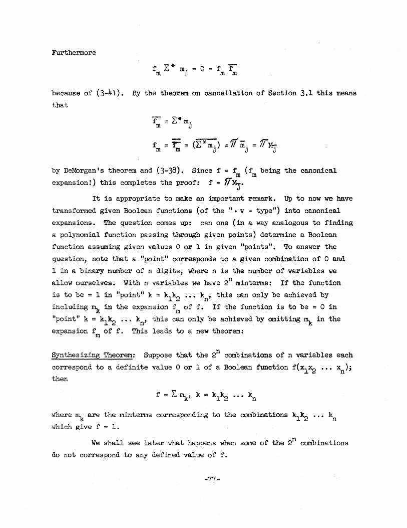
Furthermore
fL.* =O=ff m mj m m
because of (3-41). By the theorem on cancellation of Section 3.1 this means
that
- ~* f = I..J m. m J
f' = r = (L:*m.) =1Tm. = 1T~ m m J J J
by DeMorgan's theorem and (3-38). Since f = f (r being the canonical m m expansion!) this completes the proof: r = fi~.
It is appropriate to make an important remark. Up to now we have
transformed given Boolean functions (of the" • v - type") into canonical
expansions. The question comes up: can one (in a way analogous to finding
a. polynomial function passing through given points) determine a Boolean
function assuming given values 0 or 1 in given "points". To answer the
question, note that a "point" corresponds to a given combination of 0 and
1 in a binary number of n digits, where n is the number of variables we
allow ourselves. With n variables we have 2n minterms: If the function
is to be = 1 in "point II k = kl k2 .... kn' this can only be achieved by
including ~ in the expansion fm of f. If the function is to be = 0 in
"point" k = kl k2 ••• kn' this can only be aChieved, by omitting ~ in the
expansion f of f. This lea.ds to a new theorem: m
Synthesizing Theorem: Suppose that the 2n combinations of n variables each
correspond to a definite value 0 or 1 of a Boolean function f(xl~ •• , xn);
then
where ~ are the minterms corresponding to the combinations klk2
which give f = 1.
••• k n
We shall see later ~hat ha~pens when some of the 2n combinations
do not correspond to any defined value of f.
-77-
It turns out that the synthesizing theorem 1s so easy to apply, that
1 t is often advanta.geous to calculate the values of f( Xl 0 ~. xn) for a~l
combine.tions of the variables and then form the sum of the minterms correspond
ing to the·"onesul>
Finally it is clear that the synthesizing theorem ha.s a dua.l. It is
left to the rea.der to discuss the la.tter point.
J.3 Simplification of Boolean Expressions. Harvard Chart.
First of all we must define what we mean by "s inl:Plifica,t ion" : It
means reducing a. given expression (for instance a. canonica.l expansion) to a.
form in which there is a. minimum of variable occurrence. In this section
we shall show that a.ny given f can be reduced to a. "minimum v polynomia~"
i.e. a. sum of terms, each being the product of complemented or uncomplemented
variables, without being necessarily a mlnterm. The expression "minimum"
here means: each term ha.ving as few variables as possible and the polynomia.l
having as few v signs as possible.
It is evident that by dual considerations we could discuss "minimum
• polynomials" 0 Again it will be left to the reader to generalize the
processes.
The reduction of a. minimum v polynomial to simpler expression can
often be achieved by" collecting terms" 1. e •. "undistribution": if f has
been reduced to xy v xz we can write f = x(y v z); visibly this latter
expression is not a v polynomialo This reduction of a minimum v polynomial
to an expression having fewer variable occurrences is by no means straight
forward: skill and flair (meaning: expanding terms or adding terms which
do not change the function, so called "non-essential terms U) are often
necessary. . This can be seen in the following:
Example: f = tuy v tuwz v twxy v 'WXz
This can be written
f = tu(y v wz) v wx (ty v z)
-78-
But using the idempotence law we can rewrite the first expression
f = ttuy v tuwz v twry v wwxz
= tu(ty vwz) v wx(ty v wz)
= (tu v wx) (ty v wz)
This second expression is certainly simpler. Therefore an a.pparent initial
complication leads to a simpler end result.
The reduction of f to a. minimum - v - polynomial is, however, a
straightforward process and we shall discuss one method of reduction: the
Harvard Chart • It is often faster to use direct simplifice,tion, a,s described
la.ter in this section, but the Harvard Chart is an easy way to a,ccomplish the
first step in an automatic fashion.
To simplify, let us take the reduction of functions of three
variables Xl x2 x3
• The chart then contains:
1. 23 = 8 rows, ee,ch one corresponding to a possible
minterm of f.
2. 23 == 8 columns, the columns corresponding to a.
combination of variables one, two and three at a.
time and to the values of f a.t the 8 "points"
000, 001 •••• , 111.
Figure 3-1 gives the aspect of the three variables chart for the example
Remark: If f is not given as a, canonical expansion, we can calculate
f(OOO), f(OOl) etc. and use the synthesizing theorem of the last section.
The seventh column of the cha,rt contains the eight possible
minterms in order, the eighth column indicates by a and 1 which minter.ms
occur in the canonical expansion and which do not. Columns 1-6 are filled
-79-
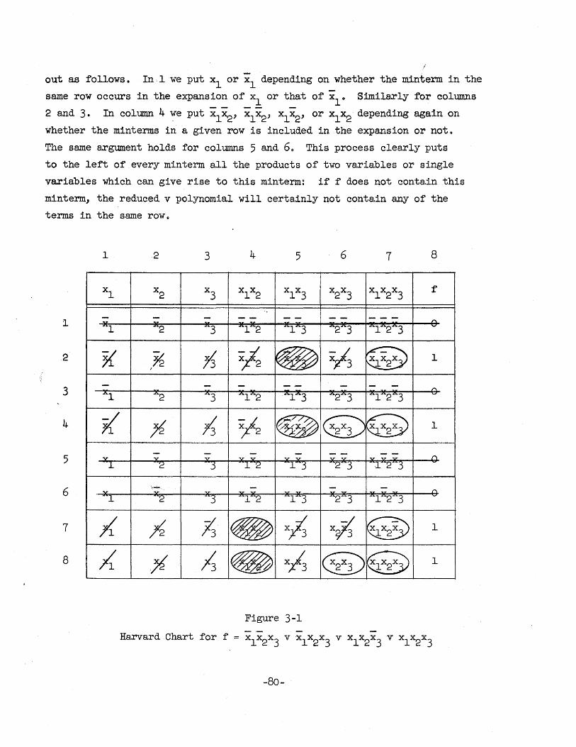
out as follows. In.l we put xl or xl depending on whether the minterm in the
same row occurs in the expansion of xl or that of xlo Similarly for columns
2 and 3. In column 4 -v:e put x;x2,xlx2' xlx2' or xl x2 depending again on
whether the minterms in a given row is included in the expansion or not~
The same argument holds for columns 5 and 60 This process clearly puts
to the left of every minterm a.ll the products of two variables or single
variahles which can give rise to this minterm: if f does not contain this
minterm, the reduced v polynomial will certainly not contain any of the
terms in the same rowo
1 2 3 4 5 6 7 8
Xl x2 x3 xl x2 xl x3
x2x3
xl x2x3
f
- - - - - - - - - - --1 " ..... ... , ..... ··1 ... .. 2 ··3 ··1'·2 .... 1 ..... 3 ..... 2 ..... 3 .... 1 .... 2 .... 3 .....
K ~ t§ ~ ~ y; G 1 I ~
2
- - - -- - - - .f""'.c
""1 ""2 ""3 .... 1 .... 2 · .... 1 .... 3 ..... 2 .... 3 00-1 .... 2·"3 "" 3
4 i ;6 ~ Y2 9 ~%~/. 0 @ 1
- - - - - - - - f'\ v v .V v- ..... v- 'V" " " " " v-l. 2 -3 -l' -2 -.1' -j 2 -j 12 "3 5
":; - - - li ,V' " .. ........ ,.. ... ..., ..... ... .. 1 2 3 1 2 .... 1 .... 3 .... 2 .... 3 .. .. 1 .... 2 .... 3 ~ 6
7 ,{ fi ~ • x;; x~ ~Xij 1
8 ;{ ,~ ~ ~ xA ® ~~y 1
Figure 3-1
Harvard Chart for f = x1x2x3
v xl X2
X3
v xI x2x3 v xl x2x
3
-80-
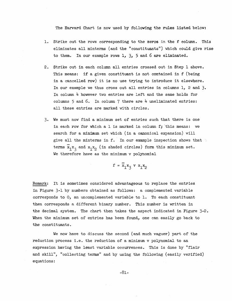
The Harvard Chart is now used by following the rules listed below:
1.. Strike out the rows corresponding to the zeros in the f column. This
eliminates all minterms (and the "constituants") which could give rise
to them. In our example rows 1, 3, 5 and 6 are eliminated.
2. Strike out in each column all entries crossed out in Step 1 above.
This means: if a given consti tua,nt is not contained in f (being
in a cancelled row) it is no use trying to introduce it elsewhere.
In our example we thus cross out all entries in columns 1, 2 and 3. In column 4 however two entries are left and the same holds for
columns 5 and 6. In column 7 there a.re 4 uneliminated entries:
all these entries are marked with circles.
3. We must now find a minimum set of entries such that there is one
in each row for which a 1 is marked in column f; 'this means: we
search for a minimum set which (in a canonical expansion) will
give all the minterms in f. In our example inspection shows that
terms xl x3
and xl x2 (in shaded circles) form this minimum. set.
We therefore ha:ve a.s the minimum v polynomial
Remark: It is sometimes considered advantageous to replace the entries
in Figure 3-1 by numbers obtained as follows: a complemented variable
corresponds to 0, an uncomplemented variable to I. To each constituant
then corresponds a different binary number. This number is written in
the decimal system. The chart then takes the aspect indicated in Figure 3-2. When the minimum set of entries has been found, one can easily go back to
the constituants.
We now have to discuss the second (and much vaguer) part of the
reduction process i.e .. the reduction of a minimum v polynomial to an
expression having the least variable occurrences. This is done by "flair
and skill", "collecting terms" and by using the following (easily verified)
equations:
-81-
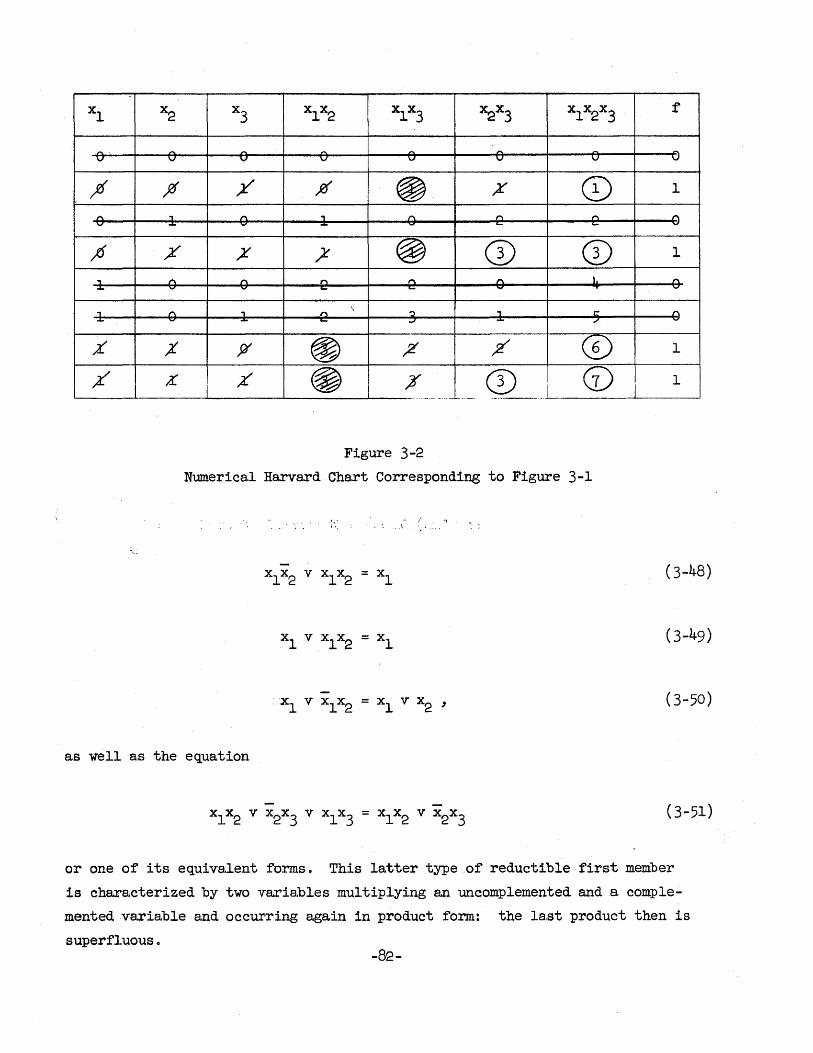
-
xl x2 x3 x1x2 xl x3 ~x3 xl x2x3
f
" . " ,.. ..... - ,.. ,..
v v v 'V v \wi V V
j1 jO ~ jO' ~ ~ CD 1
" "I " "I " 1""1 ,... ,... v - ... - ..., ... .... ...,
)f 7 ,X ,x @ CD 0) 1
'i " ,... 1"'1 " " I. ,...
.... ..., v - -= -- ...,
\ "I " "I ,... ") , c: ,... - ..., - - ..., - ./
...,
;( ,X ~ ® :z 7 (0 1
,X' 4' ,r @ 7' CD (j) I
1 _.<, . __ .'-- •.. ~.- .. -- . __ . ___ .. L
Figure 3-2 Numerical Harvard Chart Corresponding to Figure 3-1
- /.
(3-48)
(3-49)
(3-50 )
as well as the equation
(3-51)
or one of its equivalent forms 0 This latter type .of reductible first member
is characterized by two variables multiplying an uncomplemented and a, comple
mented variable and occurring again in product form: the last product then is
superfluous 0
-82-
It is sometimes useful to apply a test for a. superfluous term by
a.pplying the following Rule for Superfluous Terms: if a term is suspected
to be superfluous, take va.lues of the variables which make this term equal
to one. Insert these va.lues in all other terms: if the rema.inder of the
terms also gives a one, the term tested is superfluous.
Take for example equation (3-51) and set xl = 1, x3 = I then
xl x2 v x2x3
= 1, .'. xl x3 is superfluous.
Finally it should be remarked that elimina.ting terms may very well
lead to a. "trap" situtation similar to that described at the beginning of
the section: an expression ma.y contain no superfluous terms and appear no
longer reductible. Adding a superfluous term may permit further s~pli
fication.
3 . 4 Q~ine_' s Method
It is easily seen that a Harvard Cha.rt for 4 variables has 16
rows (because of 24 minterms), excluding the one containing the headings.
It also has 16 columns for the constituants, excluding the two last ones
for the minterms themselves .arid the value of f: such S, chart is obviously
cumbersome. For 5 variables the size gets entirely out of hand. McCluskey
and Quine have developed a method in which a.n arbitrary Boolean function
given in canonical form is first reduced to prime implicants i.e. essentially
a. possible set of constituailts. The actual choice of the set to be used is
then ma.de on a very much simplified ·Harvard Chart called "Prime Implicant
Chart". To simplify matters still further, a numerical shorthand is used
in which all terms are denoted by their corresponding binary number and
the notion of index is introduced: the index is the number of lIs in the
binary number. The search for prime implicants then follows this pa.ttern:
1. Write down all minterms in f (in bina.ry shorthand) dividing them
into groups. The first group has the lowest index (not necessarily
O!), the second group the next highest index etc. This is done by
dividing the vertical list by horizontal lines where the index
changes.
-83-
2. Compare groups of indices differing by 1 (i.e" neighboring groups)
to find terms differing inane digit only. Write down in a second
column the."reduced terms" obtained by replacing the digit which
differs by a da.sh" . Check off the terms used in this process ~
(E.g. in a 3-variable problem involving X1X2X3
and x1x2x3 denoted
by 001 and 000 we write a.s the reduced term 00- )
3. Divide the second column again into groups by horizontal lines~
the first group containing those reduced terms stemming from the
first two groups ot the orig:1nal list, the second group those
stemming from the comparison of group 2 and group 3 of the original
list etc. These new groups visibly have increasing numbers of l's.
4. The second columnaga1n has its a.dja.cent groups compared: now
doubly reduced terms appear (written with two dashes) when two
reduced terms only differ in one digit. The doubly reduced terms
are put down in a third column and divided into groups according
to which combination of groups in column 2 they stem from 0 Again
the terms used in column 2 are checked off.
5,. The process stops when no new columns can be formed. All terms
which ha~e not been checked off are the prime implicants.
Visibly we have done in a somewhat automatic manner what amounts
to the combination of terms of the fom. Xx v XX into X until no further
reduction is possible. This is simila.r to the search for constituants in
the Harvard Chart Q It can a.ctually be show.n that the two methods give
identical resultso
The next step is to draw up a. prime implicant chart having a.s
many columns as there are minterms in f (ioeo by no means corresponding to
all the mintem.s) and as many rows as there are prime implicants" The
problem is now to choose that set of prime implicants which is mintmum
(in number of primeimplicants) and at the same time gives rise to all
minterms usedo Often this chart is drawn in the form of numbers giving
-84-
the minterms connected to vertical lines and the prime implicants connected to
horizontal lines; a. cross marks those minterms Which occur in the expansion of
a given prime implicant.
It can happen that there are columns with one cross only: the
corresponding prime implicants are called basic prime iInplicants and their
row is called a primary basis rowo If some minterms are left over, there
are often secondary prime implicants (and secondary basis rows) which account
for all minterms included in two other rows. The simplified expression then
contains the sum of the basic prime implicants plus the sum of the secondary
prime implicants plus a ( sometimes arbitrary) choice of remaining prime
implicants to account for the remaining minterms.
The example below, taken from S. H. Caldwell, "Switching Circuits
and Logical Design" shows how a 5-varia:ble situation is handled. It may be
interesting to note that the search for prime implicants can be programmed
for a digital computer with relative facility.
Example: Consider a :canonical'.expression for a function f of 5-va.riables
given by
or in a more convenient notation
f = ~ 0, 1, 3, 8, 9, 13, 14, 15, 16, 17, 19, 24, 25, 27, 31
The search for the prime imp1icants then takes 4 columns. To simplify we
have indicated at the left the decimal subscript of m and in the reduced
terms the decimal subscripts of the terms used.
-85-
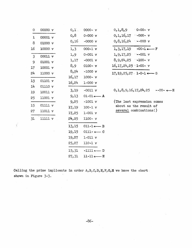
a 00000 v 0,1. 0000- v 0,1,8,9 "'o-oo~ v
1 00001 v 0,8 0-000 v 0,1,16,17 "'-000- v
8 01000 v 0,16 -0000 v 0,8,16,24 . '--000 v
16 10000 v 1,} 000-1 v 1,3,17,19 -00·~·1. +-- F
3 00011 v 1,9 0-001 v 1,9,17,25 . '- .. 001 v
9 01001 v 1,17 -0001 v 8,9,24,25 ., '-100- v
17 10001 v 8,9 0100- v 16,17,24,25 ··.·1··'00- v
24 11000 v 8,,?4 -1000 v 17,-:19,25,27· 1-0:"1 +-- G 16,17 1000- v
13 01101 v 16,24 1-000 v 14 01110 v
19 10011 v 3,19 -0011 v 0,1,8,9,16,17,24,25 --00- ~H
25 11001 v 9,13 01-01~A
9,25 -1001 v (The last expression comes 15 01111 v
17,19 100-1 v about as the result of
27 11011 v 17,25 1-001 v
several combinations~)
31 11111 v .24,25 1100- v
13,15 011-1~B
19,15 0111- +-- C
19,27 1-011 v
25,27 110-1 v
15,31 -1111~D
27,31 11-11~E
Calling the prime imp1icants in order A,B,C,D,E,F,G,H we have the chart
shown in Figure 3~3o
-86-
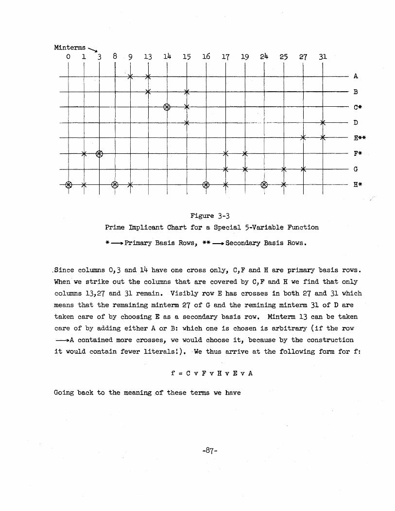
Minterms ~ 013
... 1 .... J('" "I' Xi:>'
A~ ,l.-'<)I 1'1'
8 9 13 14 15 16 17 19 24 25 21
, '" ,l.-
" '1'
,~ ,I.-'1' '1'
1<:>- , '<>' 'I'
, ..•... __ 0 ••
'1'
,It! .... 1'
'v ,!t_ .... 1' '1'
,[.f ,I.- l.-'1' '1' .... 1' '1'
A: 2\ '" I<:~ It' --~ ~-- " '<>' 1" '<~ '1' '1' ! !
Figure 3-3
Prime Implicant Cha.rt for a, Special 5-Variable Function
* --. Primary Ba,s is Rows, ** ---+ Secondary Ba.s is Rows •
31
A
B
c* ,I.-'1' D
i.f '1' E**
F*
G
H*
. Since columns 0,3 and 14 have one cross only, C,F and H are primary basis rows.
When we strike out the columns that are covered by C, F and H we find tha.t only
columns 13,27 and 31 remain. Visibly row E has crosses in both 27 and 31 which
means that the remaining minterm 27 of G and the remining minterm 31 of D are
taken care of by choosing E as a, secondary ba,sis row. Minterm 13 can be taken
care of by adding either A or B: which one is chosen is arbitrary (if the row
~A contained more crosses, we would choose it, beca.use by the construction
it would contain fewer literals!). ,We thus arrive at the following form for f:
f=CvFvHvEvA
Going back to the meaning ,of these terms we have
-87-
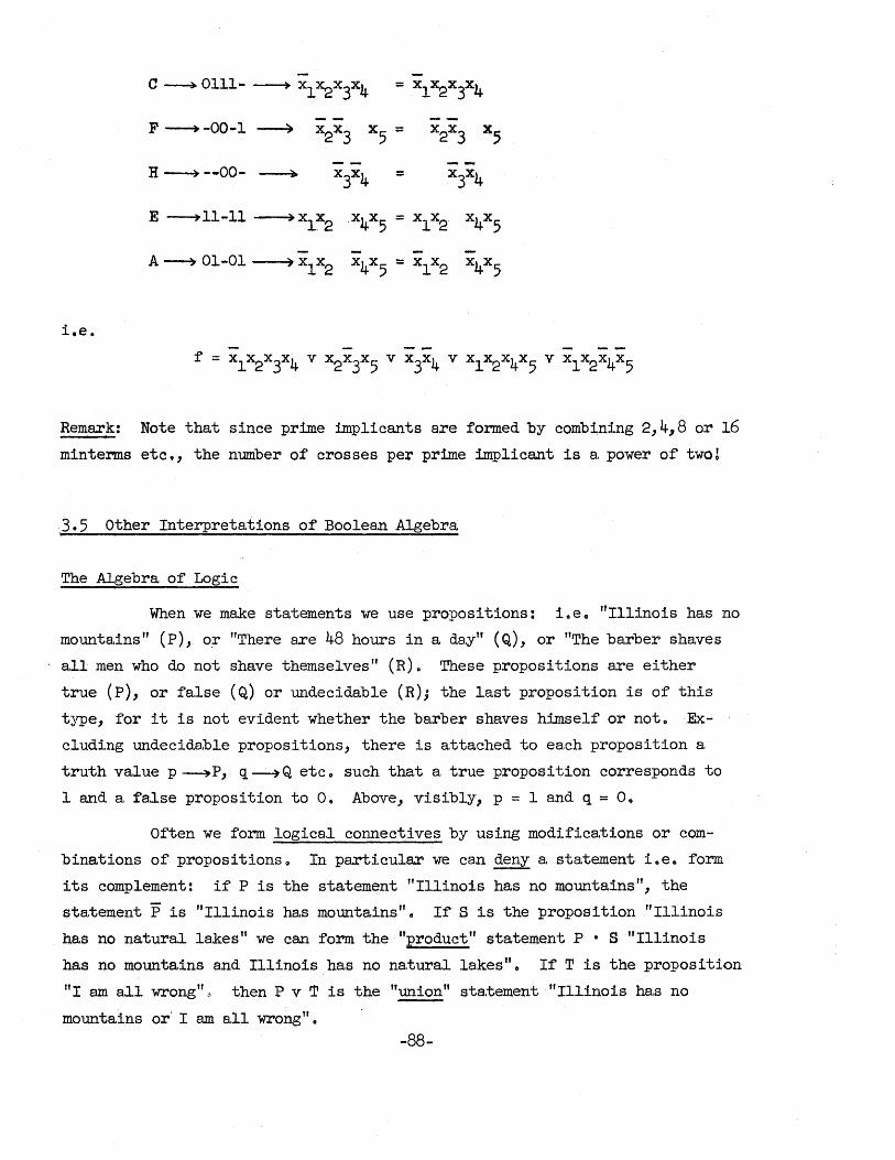
i.e.
F ---+ -00-1 --4
H ---+--00- ~ =
E ~ll .. ll ----+xl~2 x4x5 = xl x2, x4x5
A ~ 01-01 ~ xl x2 x4x5 = xl x2 x4x5
Remark: Note that since prime implicants are formed by combining 2,4,,8 or 16
minter.ms etc., the number of crosses per prime implicant is a power of two!
3.5 other Interpretations of Boolean Algebra
The Algebra of Logic
When we make statements we use propositions: i.e o "Illinois has no
mounta.ins" (p), or "There are 48 hours in a day" (Q), or "The barber shaves
all men who do not shave themselves" (R)o These propositions are either
true (p), or false (Q) or undecidable (R); the last proposition is of this
type, for it is not evident whether the barber shaves himself or not o Ex
cluding undecidable propositions, there is attached to each proposition a
truth value p ~P, q~Q etc" such that a true proposition corresponds to
1 and a false proposition to O. Above, visibly, p = 1 and q = O.
Often we form logical connectives by using modifications or com
binations of propositions~ In particular we can deny a. statement i.e. form
its complement: if P is the statement "Illinois ha.s no mountains", the
statement P is "Illinois has mounta.ins"" If S is the proposition "Illinois
has no natural lakes" we can form the "product" statement P " S "Illinois
he.s no mountains and Illinois has no na.tural la.kes"" If T is the proposition
"I am all wrong" then P v T is the "union" sta.tement "Illinois has no
mountains or'I am all wrongtl" -88-
The use of • and v shows that there is a relationship between
Boolean.Algebra and logic. One sees easily that this is the following:
if we call truth va,lue x of a complex proposition X involving v and • a
variable which is 1 if X is true and 0 of X is false, then
gives rise to
Example:
The statement X
x = f (p Q, R involving v and .)
x = f (p q r invol v1ng v and .)
P = "Modern cars a.re slow"
Q = "Modern cars are underpowered"
R = "Modern cars ea,t a lot of gas"
= (p vQ,) R then reads:
"It is not true that modern cars are slow or tha.t modern cars are underpowered. Modern cars eat a lot of gas."
Let us examine x = (p v q) r. Looking a.t P Q and R we see that p = 0,
q = 0, r = 1. Therefore x = (0 v 0),1 = I i.e. X is a true true statement.
Note that here (p vQ)= P • Q!
There are other symbols for operations ("connectives") tha.t we
have used that reappear in the algebra of logic. Especially P ::: Q means
"either P is fa.lse or, if P is true, Q is true". Now we remember that
p ::: q was defined a.s p • q = p (or by the consistency principle p v q = q!)
Q,uite visibly the proposition P ::: Q corresponds to the relationship p ::: q
between the truth values. We could similarly talk about G ' /. etc. but
a discussion would only lead to a reiteration of the postulates of Boolean
Algebra. We leave it to the reader to verify that these postulates are
sa.tisfied by propositions,
-89-
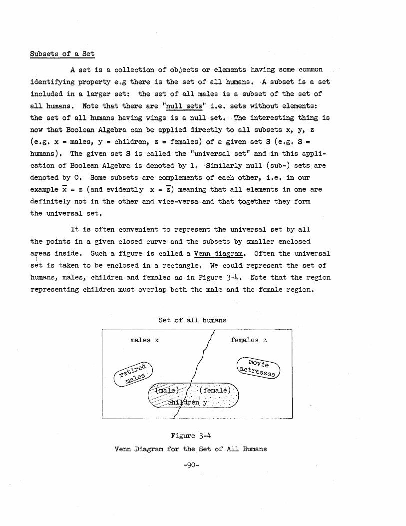
Subsets of a Set
A set is a collection of objects or elements having some 'common
identifying property eog there is the set of all humans~ A subset is a. set
included in a larger set: the set of all males is a subset of the set of
a.11 hums.ns. Note that there are "null sets" ioe. sets without elements:
the set of a.11 humans having wings is a null set 0 . The interesting thing is
now that Boolean Algebra can be a.pplied directly to all subsets x, y, z
(e,g, x = males, y = children, z = females) of a. given set S (e.go S = humans). The given set S is called the "universal set" and in this a.ppli ...
ca.tion of Boolean Algebra, is denoted by 10 Similarly null (sub-) sets are
denoted by 00 Some subsets a,re complements of each other, iDeo in our
example x = z (and evidentl y x = z) meaning that a,ll elements in one are
definitely not in the other and vice-versa"and that together they form
the universal set.
It is often convenient to represent the universal set by all
the points in a given closed curve and the subsets by smaller enclosed
area,s inside 0 Such a figure is called a Venn diagramo Often the universal (
set is taken to be enclosed in a rectangle. We could represent the set of
humans, males, children and females as in Figure 3-4. Note that the region
representing children must overlap both the male and the female region.
Set of all humans
males x females z
'-----_. __ ....
Figure 3-4
Venn Dia.gram for the Set of All Humans
-90-
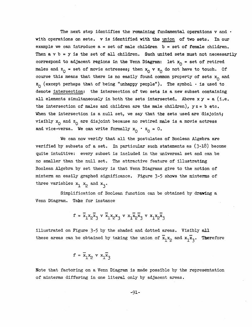
The next step identifies the remaining fundamental operations v and •
with operations on sets. v is identified with the union of two sets. In our
example we can introduce a = set of male children b = set of female children.
Then a vb = y is the set of all children 0 Such united sets must not necessarily
correspond to adjacent regions in the Venn Diagram: let Xo = set of retired
males and Zo = set of movie actresses; then Xo v Zo do not have to touch. Of
course this means that there is no easily found common property of sets Xo and
zo (except perha.ps that of being "unhappy people"). The symbol, is used to
denote intersection: the intersection of two sets is a new subset containing
a.ll elements s imul taneously in both the sets intersected. Above x y = a. (i. e •
the intersection of males and children are the male children), y z = b etc.
When the intersection is a. null set, we say tha.t the sets used are ·'disjoint;
visibly Xo and Zo are disjoint because no retired male is a. movie actress
and vice-versa., We can write forma.lly Xo • Zo = O.
We can now verify that all the postulates of Boolean Algebra are
verified by subsets of a set. In particular such statements a.s (3-:-18). become
quite intuitive: every subset is included in the universal set and can be
no smaller than the null set, The attra.ctive feature of illustrating
Boolean Algebra by set theory is that Venn Diagrams give to the notion of
minterm an easily graphed significance. Figure 3-5 shows the minterms of
three variables Xl x2 and x3'
Simplifica.tion of Boolean function can be obtained by drawing a
Venn Diagram. Talte for instance
illustrated on Figure 3-5 by the shaded and dotted areas. Visibly all
these areas can be obta.ined by taking the union of Xl x2 and x{x3' Therefore
Note that factoring on a. Venn Diagram is made possible by the representation
of minterms differing in one literal only by a.dja.cent areas.
-91-
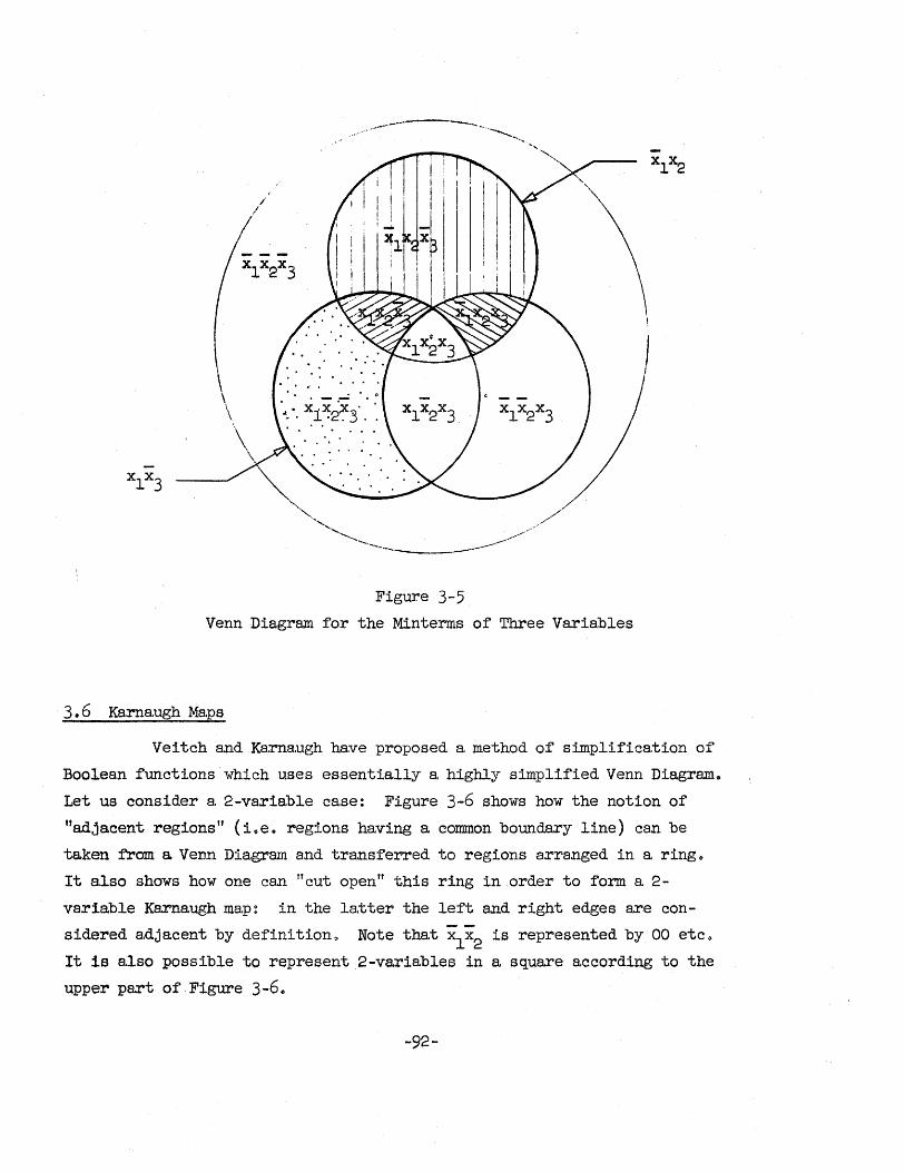
.. ~--.-.. ----------- .. ~ --........... ,.,.
/
//
\ \ \
Figure 3-5 Venn Diagram for the Minterms of Three Variables
3.6 Karnaugh Maps
Veitch and Karna.ugh have proposed a method of simplification of
Boolean functions which uses essentially a highly simplified Venn Diagram.
Let us consider a 2-variable case: Figure 3-6 shows how the notion of
"adjacent regions" (ioe. regions having a common boundary line) can be
taken from a Ven.n Dia.gram and transferred to regions arranged in a ringo
It also shows how one can "cut open" this ring in order to form a 2-
variable Karnaugh map: in the latter the left and right edges are con
sidered adja.cent by definition" Note tha.t X1X2 is represented by 00 etc~
It 1s a.lso possible to represent 2-va.ria.bles in a square a.ccording to the
upper part of Figure 3-60
-92-
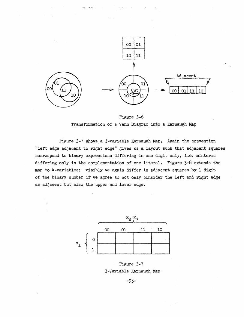
GJ;J GLJ
~ Ad Ja.cent
~ I --t> I 00 I 01111.-11.9J
Figure 3-6
Tra.nsforma.tion of a. Venn Diagram into a. Karna.ugh Map
Figure 3-7 shows,. a 3-variable Karnaugh Map. Again the convention
"left edge adjacent to right edge" gives us a layout such tha.t adjacent squares
correspond to binary expressions differing in one digit only, i.e. minterms
differing only in the complementation of one literal. Figure 3-8 extends the
map to 4-variables: visibly we again differ in adja.cent aqua.res by 1 digit
of the binary number if we agree to not only consider the left and right edge
as adja.cent but also the upper a.nd lower edge.
00 01 11 10
Figure 3-7
3-Variable Kaxnaugh Map
-93-
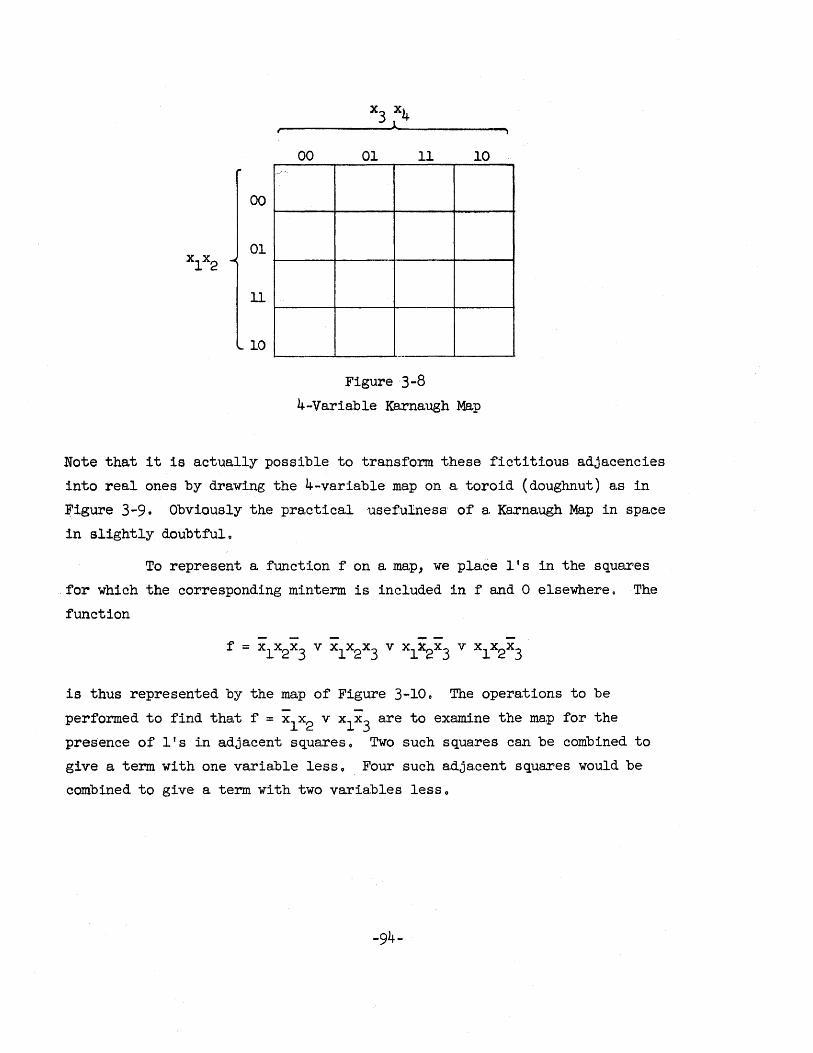
00
01
11
10
00 01 11 10
Figure ·3-8
4-Variable Karnaugh Map
Note that it is actually possible to transform these fioti tious adja.cencies
into real ones by drawing the 4-variahle map on a toroid (doughnut) a.s in
Figure 3-9. Obviously the practical 'Usefulness' of a. Karnaugh Map in space
in slightly doubtful.
To represent a function f on a map, we place lIs in the squares
for which the corresponding minterm is included in f and 0 elsewhere. The
function
- - - - -f = xl x2x3
vxl x2x3
v xl x2x3
v xl x2x3
is thus represented by the map of Figure 3-10~ The operations to be
performed to find that :f = x1x2 v xlx3 are to examine the map for the
presence of Its in adjacent squares 0 Two such squares can be combined to
give a. term with one variahle less 'I Four such a.djacent squares would be
combined to give a. term with two variahles less o
-94-
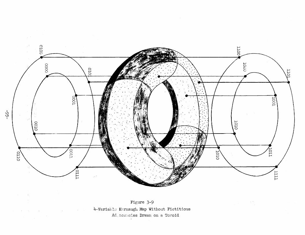
I \0 \)1
I
Figure 3~9
4·-Va,ria:blc KGrn8.ugh Map Without Fictitious
Ad,_ ace:teies Drawn on a Toroid
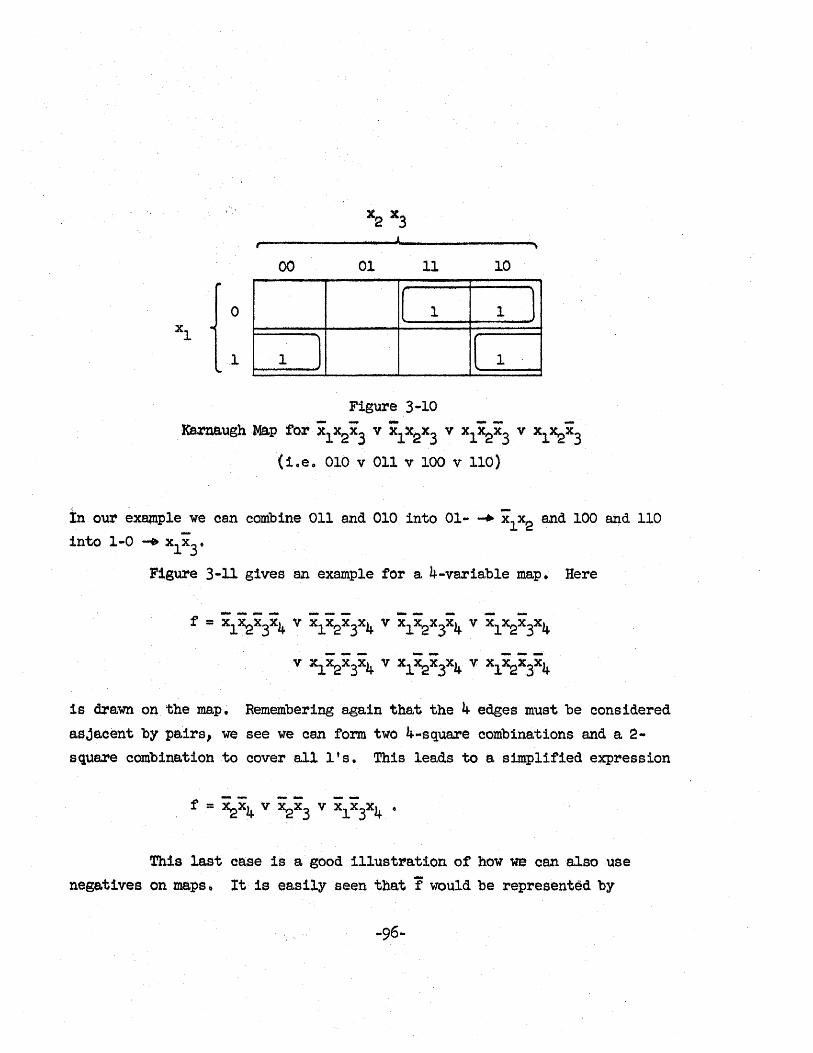
j t ,
00 01 11 10
o II 1 1 1 1 1 ) [ 1
Figure 3-10
Karna.ughMap fOr.xl x2x3 v x1x2x3 v x1x2x3 v xl~x3
(i.eo 010 v 011 v 100 v 110)
In our ex~p1e we can combine 011 and 010 into 01- ~ x1x2 and 100 and 110
into 1-0 ... x{x3-Figure 3-11 gives an example for a. 4-variahle map. Here
is drawn on the map~ Remembering again that the 4 edges must be considered
asjacent by pa.irs, we see we can rom two 4-square combina.tions and a 2-square combina.tion to cover all 1 t s. This lea.ds to 8. simplified expression
This 1a.st ca.se is a. good illustra.tion of how we cana.lsouse
negatives on ma.PSo It is ea.s11y seen tha.t f would be represented by
-96-
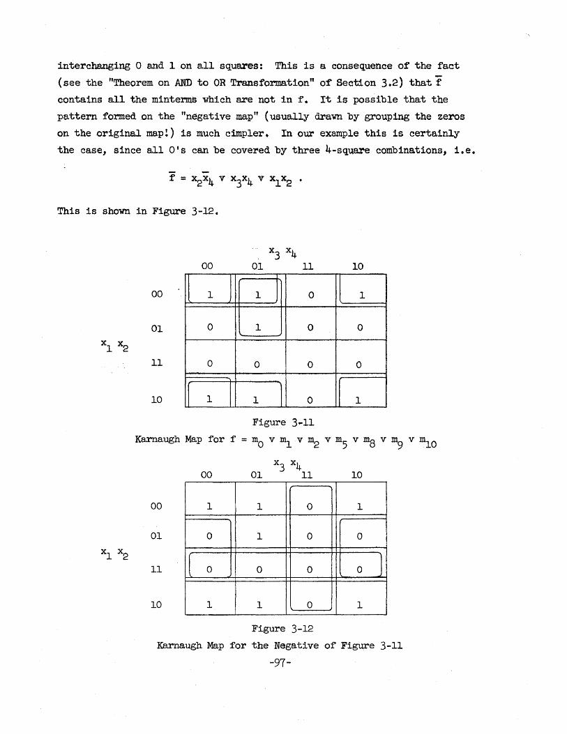
interchanging 0 and 1 on all squares: This is a consequence ,of the fact
(see the "Theorem on AND to OR Transformation" of" Section 3.2) that f. contains all the minterms which are not in f. It is possible that the
pa.ttern formed on the "nega.tive map" (usually drawn by grouping the zeros
on theorig1nal map!) is much cimpler. In our example this is certainly
the case, since all O's can be covered by three 4-square combinations, i.e.
This is shown in Figure 3-12.
00 10
00 1 1 0 1
01 0 1 0 0
11 0 0 0 0
10 1 1 0 1
Figure 3 .. 11
Karna.ugh Map for f = mO v m1 ,v m2 v mS v ma v m9 v m10
00 x3 x4
01 11 10
00 1 1 0 1
01 0 1 0 0
11 ( 0 0 0 0 J
10 1 1 0 1
Figure 3-12
Karnaugh Map for the Negative of Figure 3-11
-97-
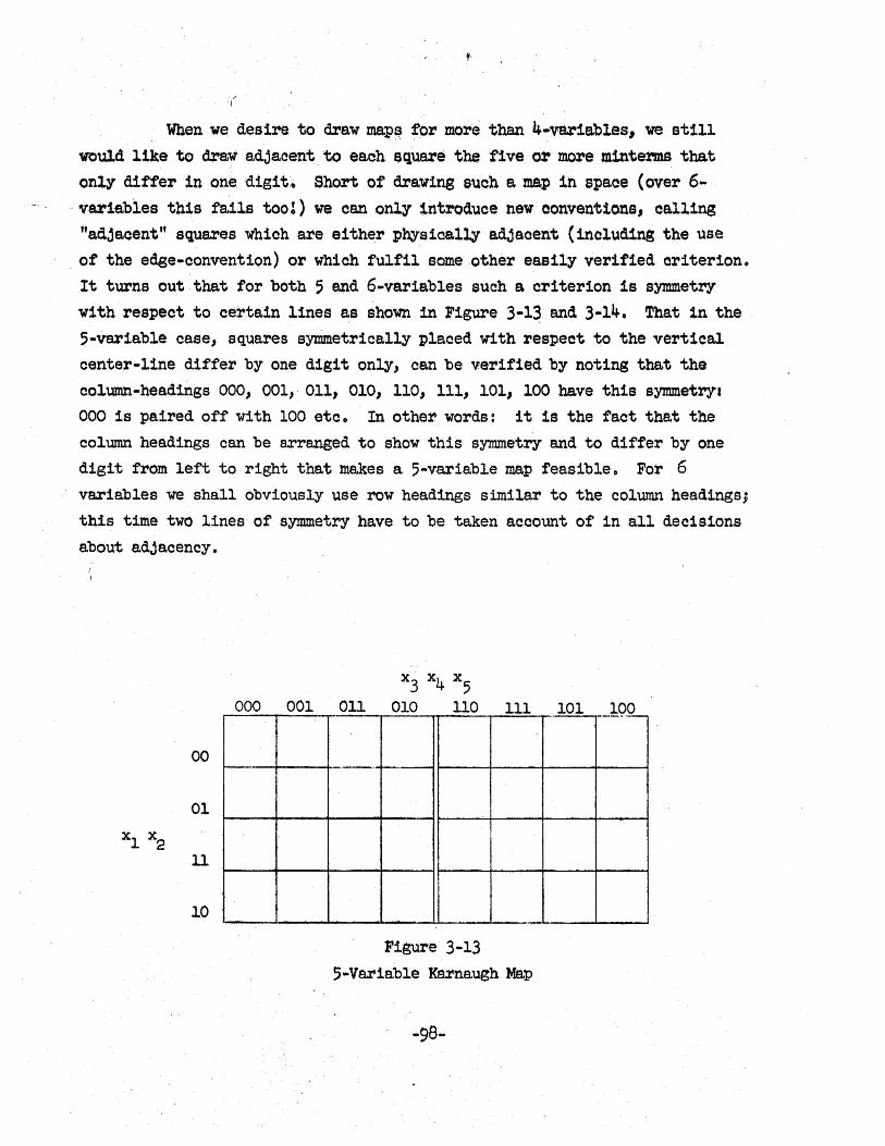
,-i
When we desire to draw map~ for more than 4-va.riables, we still
would like to draw adjacent to ea.ch square the f1ve 01' more m1nterms that only differ in onedigi t.. Short of drawing suoh So map in spa.oe (over 6-
. va.r1·e.bles this fails too!) we can only introduce new oonvent1ons, oa.lling "adjacent" squares which are either physioa.lly adjs,oent (including the use
of the edge-convention) or which fulfil some other easily verified oriteriono It turns out that for both 5 and6-variablessuch a criterion is symmetry
with respect to certain lines as shown 1n Figure 3-1~ and 3-14. Ths.t 1n the 5-variable case, squs,res symmetrically pla.ced with respect to the vertical center-line differ by one digit only, can be verified by noting that the
column-headings 000" 001,·. 011, 010, 110" 111, 101.. 100 have this symmetry. 000 is paired off with 100 etco In other words: it is the faot that the column hea,dings can be arranged. to show this symmetry and to differ by one digit from left to right tha.t ma.kes a 5-va.risble map fea.sible 1\ For 6 variables we sha,ll obviously use row hea.dings similar to the column hea,dings;
this time two lines of symmetry have to be taken account of in all decisions about adjacency.
X3 x4 x5 000 r-__ ~ __ ~ ____ ~0_1_0~ __ ll_0~~1~1~1~101 001 011 100
-.---~
00
01
11
10
Figure 3-13 5 ... Va.riable Karnaugh Map
-98-
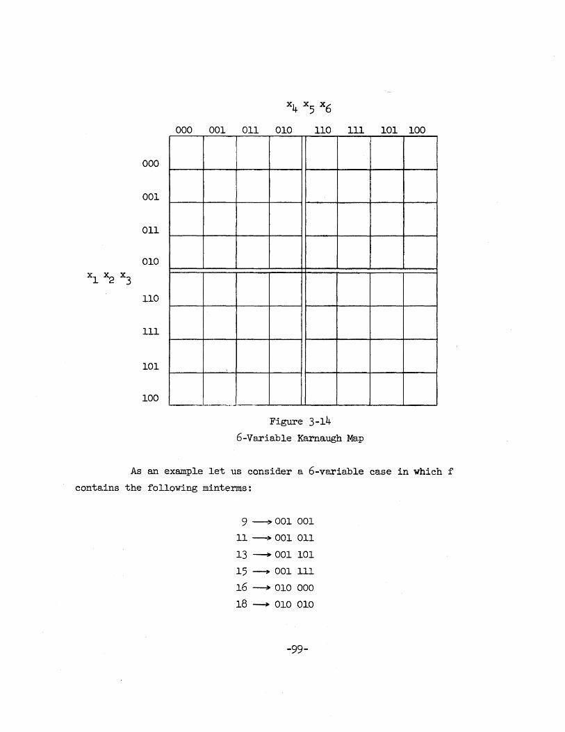
000
001
011
010
xl x2 x3
110
III
101
100
000 001 011 010 110 111 101 100
Figure 3-14
6-Variab1e Karnaugh Map
As an example let us consider a. 6-variable case in which f
contains the following minterms:
9 ~001 001
11 ~ 001 011
13 ~ 001 101
15 ~ 001 III
16 ~ 010 000
18 ---. 010 010
-99-
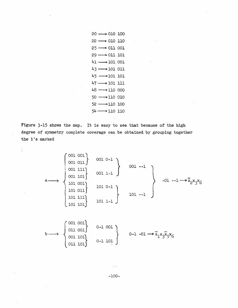
20 ---. 010 100
22 ---+ 010 110
25 ---+ 011 001
29~011 101
41~101 001
43 ----+ 101 011
45 ~101 101
47 ---+ 101 III
48 ~110 000
50 ~110 010
52 ~110 100
54 --) 110 110
Figure 3-15 shows the mapo It is easy to see that because of the high
degree of synunetry complete covera.ge can be obtained by grouping together
the l's marked
a,~
r 001 001}
001 011
001 Ill} 001 101
101 001}
101 011
101 Ill} 101 101
001001}
011 001
001 101}
011 101
001 0-1 }
001 1-1
101 0-1 }
101 1-1
0-1 001 }
0-1 101 ,
-100-
001 --1
101 --1
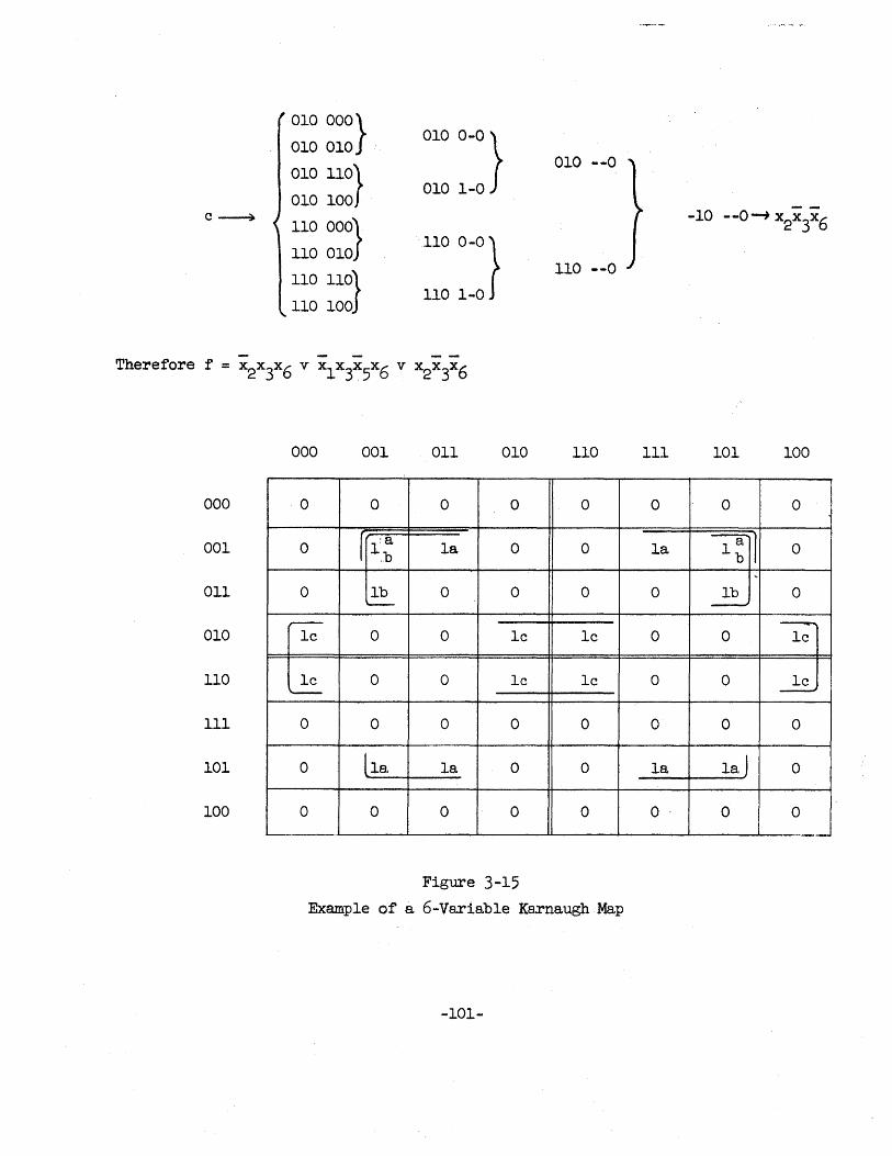
010 OOO} 010 O-O} 010 010
010 nO} 010 1-0
010 100
010 --0
e -----7
110 OO~} .110 O-O} 110 010
110 110} 110 1-0
110 100
110 --0
000 001 011 010 110
000 0 0 0 0 0
001 0 r l~~ la 0 0
011 0 Ib 0 0 0 ~
r--
010 Ie 0 0 Ie Ie
110 Ie 0 0 Ie Ie '---
III 0 0 0 0 0
101 0 lls. la 0 0
100 0 0 0 0 0
Figure 3-15
Example of a 6-Variable Karnaugh Map
-101-
III
0
la
0
0
0
0
la
0-
-10 --o~ x x X6 2 3
101 100
0 0
~l 0 ,
Ib 0 ----.J
-0 Ie
0 Ie --0 0
la. J 0
0 0
----
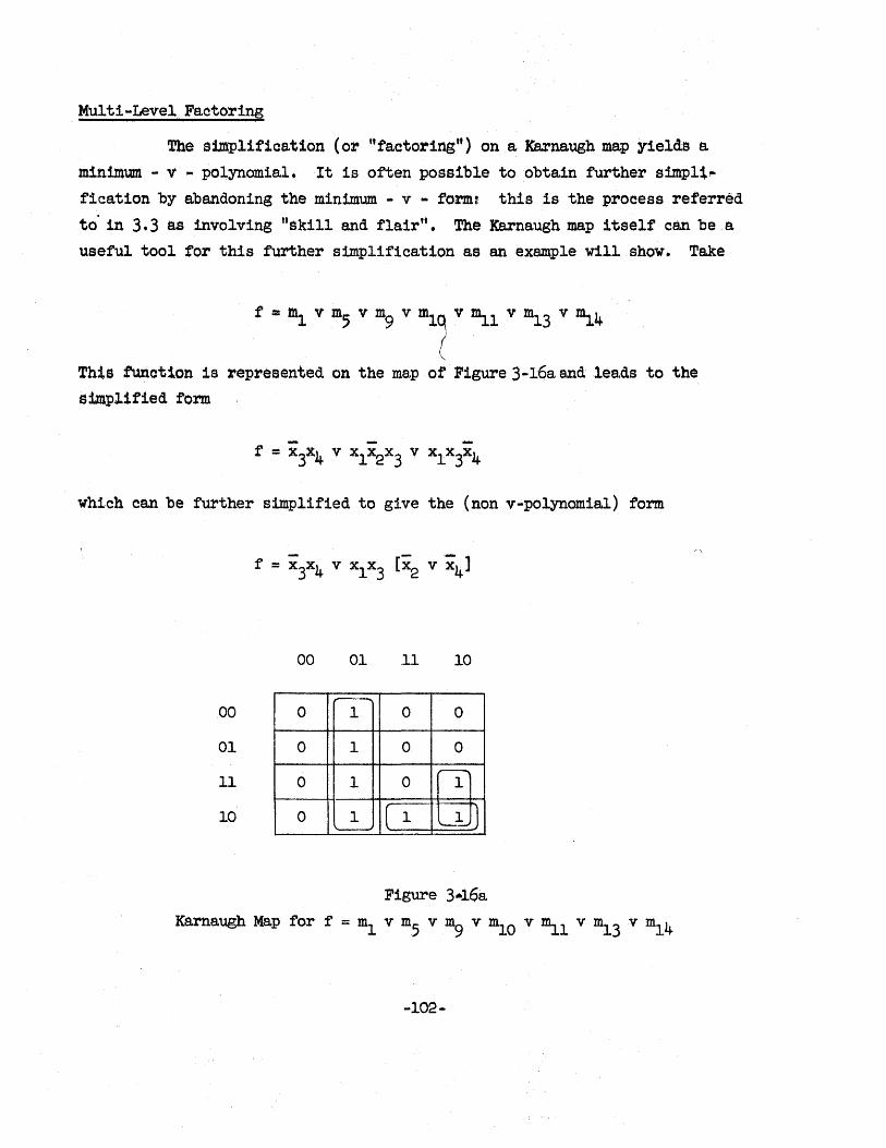
Multi-Level Factoring
'!'he amplifica.tion (or "factoringtt) on a. Karnaugh map yields a.
m1n~um - v ~ polynomial. It is often possible to obtain further simpl~~
f'icat1on by abandoning the minimum ... v - form:- this is the process referred
to' in 3.3 as involving "skill and fla.ir". The Karna,ugh map itself can be e, useful tool tor this further simplification as an example will show. Take
f = ~ v m5 v ~ v ml( v ~l v m13 v ~4
This function is represented on the map of -Figure 3-168. and lea,ds to the simplified torm
which can be further simplified to give the (non v-polynomial) form
00 01 11 10
,..----
00 0 1 0 0
01 0 1 0 0 ,----..,
11 0 1 0 1
0 1 ( 1 ,-~J '------"
10
Figure 3 .. 168.
Karnaugh Map for f = m1 v m5 v m9 v mlO v mll v m13 v m14
-102-
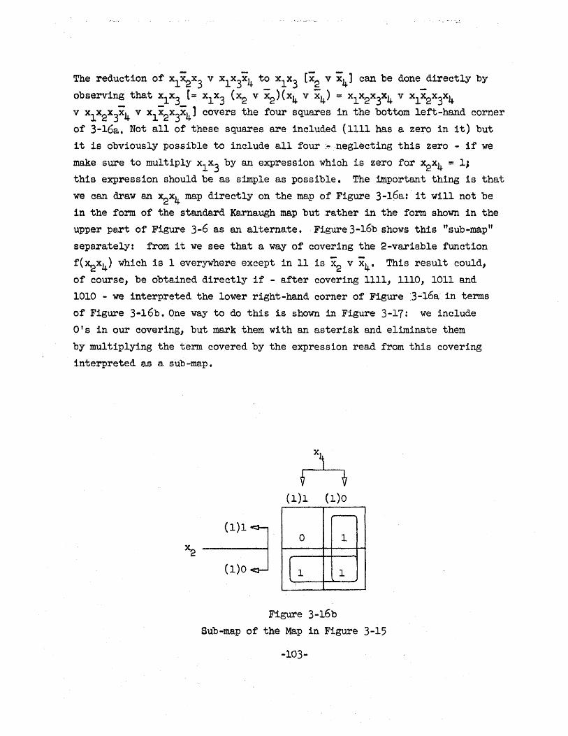
The reduction of X1X2X3 v X1X3X4 to x1x3
[x2 v x4] can be done directly by
observing tha.t xl x3 [= x1x3 (x2 v X2)(X4 v x4) = xr2x3X4 v XIX2X3X4
v X1X2X3X4 v X1X2X3X4] covers the four squares in the bottom left-hand corner
of 3-l6a.. Not a,ll of these squares are included (1111 he,s a zero in it) but
it is obviously possible to include a,ll four ~~ .neglecting this zero ... if we
make sure to multiply x1x3 by an expression which is zero for x2x4 = 1;
this expression should be as simple a,s possible. The important thing is tha,t
we can draw an ~x4 ma,p directly on the ma,p of Figure 3-19a,: it will not be
in the form of the standard Karnaugh map but rather in the form shown in the
upper part of Figure 3-6 a,s an alterna,te. Figure 3-16b shows this "sub-ma.p"
separately: from it we see that a, way of covering the 2-variable function
f(~x4) which is 1 everywhere except in 11 is X2 v x4. This result could,
of course, be obtained directly if - after covering 1111, 1110, 1011 ana 1010 - we interpreted the lower right-hand corner of Figure :3~16a' in terms
of Figure 3-l6b • One way to do this is shown in Figure 3-17: we include
O's in our covering, but mark them with an asterisk and elimins,te them
by multiplying the term covered by the expression res,d from this covering
interpreted a,s e, sub -me,p •
,....--
0 1
[ 1 1
Figure 3-16b Sub-map of the Map in Figure 3-15
-103-
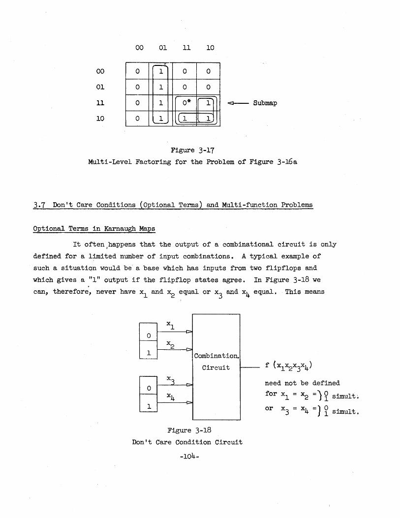
00 01 11 10
~ 00 0 1 0 0
01 0 1 0 0
11 0 1 0* ~ <J--Submap
10 0 1 ( 1 1 '-----'
Figure 3-17
Multi-Level Factoring for the Problem of Figure 3-16a.
3.7 Don't Ca.re Conditions (Optional Terms) and Multi-function Problems
Optional Terms in Ka.rnaugh Maps
It often/happens that the output of a. combina.tional circuit is only
defined for a. l:troi ted number of input combina.tions. Atypica.lexample of
such a. situa.tion would bel a base which has inputs from two flipflops and
which gives a. "1" output if the flipflop sta.tes agree. In Figure 3-18 we . can, therefore, never have xl and x2 equa.l or x3 and x4 equa.l. This means
Xl 0
x2
1 Comb ina.t ion.
Circuit X
need not be defined 0
x4 for Xl = x2 =)~ simult~ 1 or x3 = x4 =) ~ simult 0
Figure 3-18
Don't Care Condition Circuit
-104-
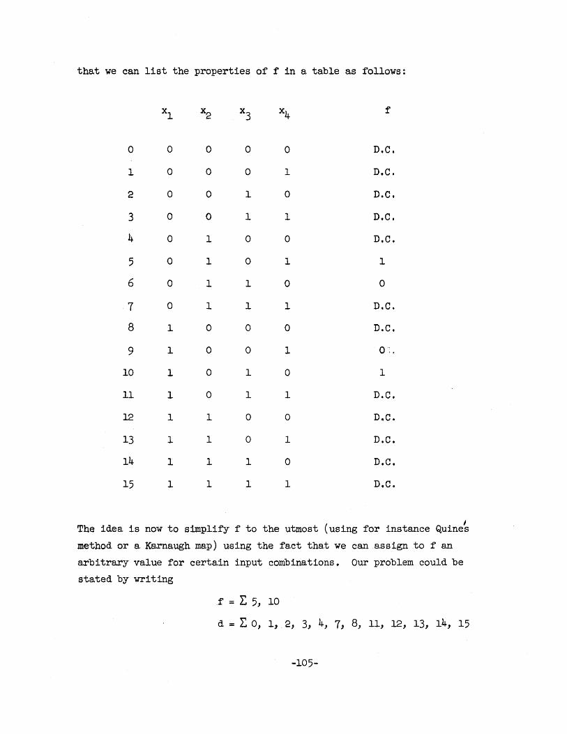
that we can list the properties of f in e, table as follows:
Xl x2 x3 x4 f
0 0 0 0 0 D.C.
1 0 0 0 1 D.C.
2 0 0 1 0 D.C.
3 0 0 1 1 D.C.
4 0 1 0 0 D.C.
5 0 1 0 1 1
6 0 1 1 0 0
1 0 1 1 1 D.C.
8 1 0 0 0 D.C.
9 1 0 0 1 - 0;.
10 1 0 1 0 1
11 1 0 1 1 D.C.
12 1 1 0 0 D.C.
13 1 1 0 1 D.C.
14 1 1 1 0 D.C.
15 1 1 1 1 D.C.
The idea is now to simplify f to the utmost (using for instance Quine~ method or a, Ka,rna,ugh map) using the fact that we can _ assign to f an
arbitrary value for certain input combinations. Our problem could be
stated by writing
f = L: 5, 10
d = L: 0, 1, 2, 3, 4, 7, 8, 11, 12, 13, 14, 15
-105-
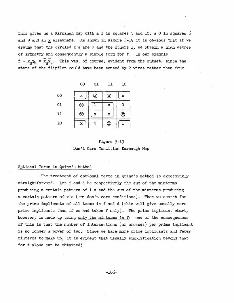
This gives us a, Karna,ugh map with a 1 in squares 5 and 10, a 0 in squares 6
and 9 and an ! elsewhere. As shown in Figure 3-19 it. is obvious that if we
assume tha,t the circled x' s are 0 and the others 1, we obtain a, high degree
of sytbmetry and consequently a simple form for f. In our example
f = x2~ v x2x4. This was, of course, evident from the outset,. since the
state of the flj.pflop could have been sensed by 2 wires rather than four.
00 01 11 10
00 xJ ® ® l x --01 ® 1 ·x 0
11 ® x x ® 10 x 1 0 ® r 1
Figure 3-19 Don't Care Condition Karnaugh Map
Optional Terms in Quine's Method
The treatment of optional terms in Quine's method is exceedingly
straightforward. Let f and d be respectively the sum of the minterms
producing a certain pattern of lIs and the sum of the minterms producing
a certain pattern of x' s (-+ don't care conditions) 0 Then we search for
the prime implicants of all terms in f and d (this will give usually more
prime implicants than if we had taken f only). The prime -implicant chart,
however, is made up using only the minterms in f~ one of the consequences
of this is tha,t the number of intersections (or crosses) per prime implicant
is no longer a power of two. Since we have more prime implicants and fewer
minterms to make up, it is evident that usually simplification beyond that
for f alone can be obtained!
-i06-
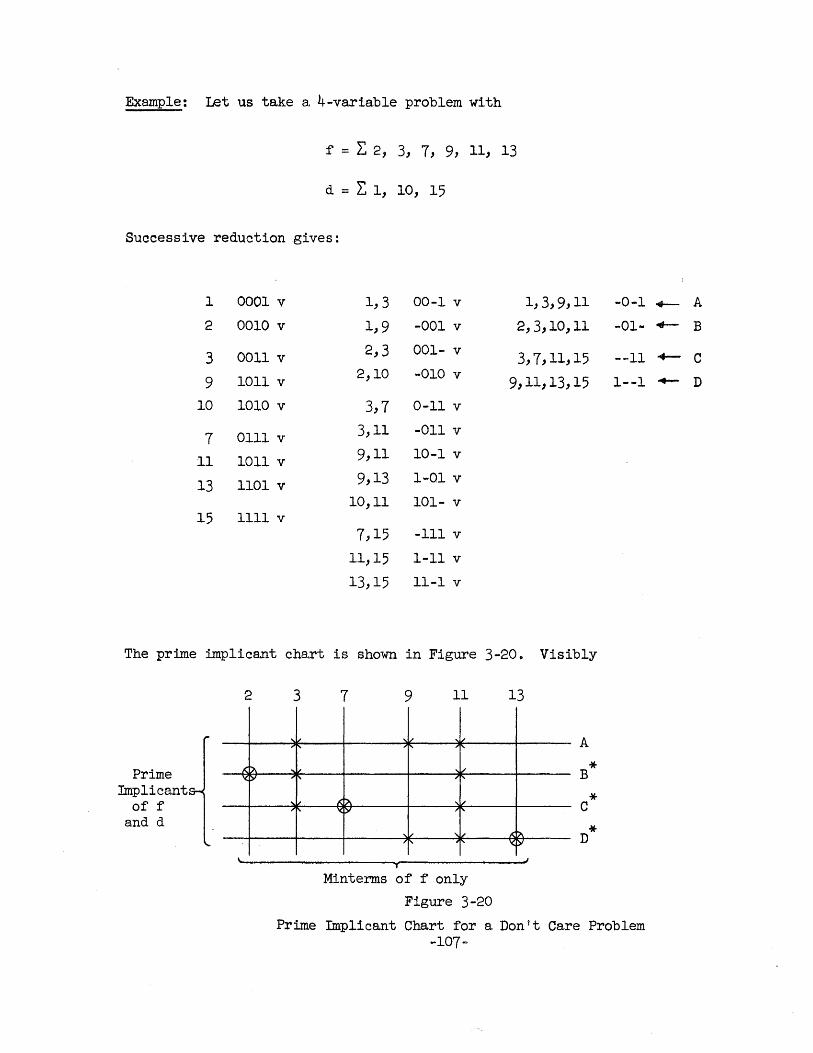
Example: Let us take a 4-variable problem with
f = ~ 2, 3, 7, 9, 11, 13
d = L. 1, 10, 15
Successive reduction gives:
1 0001 v 1,3 00-1 v 1,3,9,11
2 0010 v 1,9 -001 v 2,3,10,11
3 0011 v 2,3 001- v 3,7,11,15
9 1011 v 2,10 -010 v 9,11,13,15
10 1010 v 3,7 0-11 v
7 0111 v 3,11 -011 v
11 1011 v 9,11 10-1 v
13 1101 v 9,13 1-01 v
10,11 101- v 15 1111 v
7,15 -111 v
11,15 1-11 v
13,15 11-1 v
The prime implicant chart is shown in Figure 3-200 Visibly
Prime Implicant
of f and d
2
JC:i)..
'<f>'
3
, ,.
...
"''' ,1/ "'I'
7 9 11
, ..... ,/
':'- 'I'
,1/ ,
,<~ ,'" '<I>' "I'
"j ,,1/ '!'
Minterms of f only
Figure 3-20
13
..<1>1. '<I>'
A
* B
* C
* D
-0-1
-01-
--11
1--1
Prime Implicant Chart for a Don I t Care Problem -107-
+-- A
...- B
+- C ..- D
the function can be formed by taking B, C and D only i.e.
Simultaneous Simplification of Several Functions
A very common problem is to design a box having inputs xl.·· xn
a,nd several outputs fl (xl · o. xn ), f2 (xl .... Xn) 00" fm (Xl 0." xn ) ..
Aga,inwe would like the contents of this box to be as simple a,s possible.
Unluckily no general methods are known. A method which is sometimes quite
useful is the method of assumed form in which one assumes that fl ... 0 fm
contain a common factor ¢ such that
fl = ¢ (Xl x ) n
X ) n
The problem is then to find a set ¢ Flo .• Fm which ma,kes all functions very
simple. The obvious difficulty is that in most cases ¢ can be simplified a,t
the expense of Flo. 0 F m and vice -versa: which choice is best can only be
determined by trial and error.
The idea is now to represent f 1 ..... fm ¢ and Fl •• 0 F m by Karnaugh
maps.. Those for flo 0 0 fm are determined by the problem" In order to find
the .other ones we use the following
Theorem: If f. has a zero in a given square, then either ¢ of F. must have l l
a. zero in the corresponding squares It If f. has a one ina given square, then l
both ¢ and F. must have a. one in the corresponding squares. l
Proof: The theorem is evident, since all it says is that
that for a given combination of inputs (-.. to a square on
means both ¢ = 1 and f. = 1, while f. = 0 is satisfied if l l
-108-
fi = ¢ .. Fi implies
the map) f i = 1
¢ = 0 or F. = o. l
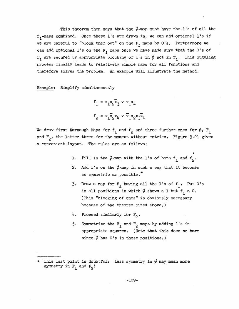
This theorem then says that the ~-map must have the lIs of all the
f i -ma.ps combined. Once these l' s a.re drawn in, we can add optiona.l l' s if
we are careful to "block them out" on the F i maps by 0' s 0 Furthermore we
can add optional l' s on the F i ma.ps once we h~.ve made sure that the 0' s of
fi are secured by appropriate blocking of lIs in ¢ not in f i - This juggling
process finally leads to relatively simple maps for all functions and
therefore solves the problem. An example will illustrate the method.
Example: Simplify simultaneously
We draw first Karnaugh Maps for fl and f2 and three further ones fQr ¢, Fl
and F2, the latter three for the moment without entries. Figure 3-21 gives
a convenient layout. The rules are as follows:
1. Fill in the ¢-ma~ with the lIs of both fl and f 2 •
2. Add lIs on the ¢-map in such a way that it becomes
as symmetric as possible.*
3. Draw a ma,p for Fl having all the l' s of flO Put 0' s
in all positions in which ¢ shows a 1 but fl a O.
(This "blocking of ones" is obviously necessary
because of the theorem cited above:)
4. Proceed similarly for F2 •
5. Symmetrize the Fl and F2 ma~s by adding l's in
appropriate squares. (Note that this does no harm
since ¢ has O's in those positions.)
* This last point is doubtful: less symmetry in ~ may mean more symmetry in Fl and F2!
-109-
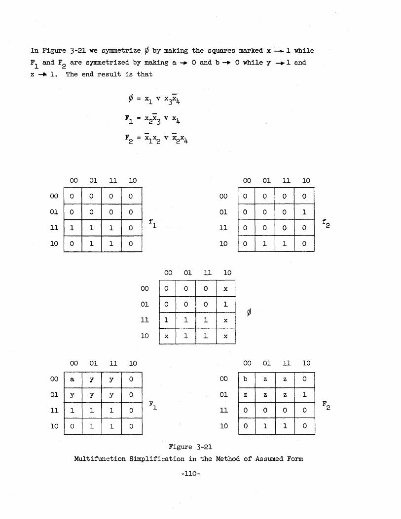
In Figure 3-21 we symmetrize ¢ by making the squares marked x ~ 1 while
F 1 and F 2 are symmetrized by making a ..". 0 and b -+ 0 while y -+ 1 and
Z -II> I. The end result is tha.t
00
01
11
10
F1 = x2x3 v x4
F2 = x1x2 v x2x4
00 01 11 10
0 0 0 0
0 0 0 0
1 1 1 0
0 1 1 0
00
01
11
10
00 01 11 10
00 0 0 0 x
01 0 0 0 1
11 1 1 1 x
10 x 1 1 x
00 01 11 10
00 a y y 0 00
01 y y y 0 01
11 1 1 1 0 11
10 0 1 1 0 10
Figure 3-21
00 01 11 10
0 0 0 0
0 0 0 1
0 0 Q 0
0 1 1 0
00 01 11 10
b z z 0
z z z 1
0 0 0 0
0 1 1 0
Multifunction Simp1ifica.tion in the Method of Assumed Form
-110-
CHAPI'ER IV
OPERATION OF A DIG !TAL COMPUTER SYSTEM
4.1 The Illia.c I Arithmetic Unit
Figure 4-1 gives the general layout of the arithmetic unit in a - - 3 rather typica.l computer i.eo Illiac Ie A, A, Q, Q, Rand R3 are registers
holding 40 binary digits ea.ch. The names commonly given to these registers
are:
A: accumulator register
A: temporary a.ccumulator register
Q: multiplier-quotient register
Q: temporary multiplier-quotient register
R3: number register
R3: order register
In the diagram we symbolize any kind of gate (or group of gates) by
a circle conta.ining a combination of a letter and G or a G with 8. subscript.
R, 0, B, Y and G stand for red, orange, black, yellow and green. When anyone
of the group of gates RG, OG, BG or YG is open, the effects are a shift between
A and A and (except for OG) simulta.neously between Q and 'Q. More specifica.lly
RG shifts left down
OG shifts straight down
BG shifts right down
YG shifts straight up.
The group of gates GG connect the output of the adder to Ao The in
puts to the a.dder come from A (connected permanently) and from R3: when u = 0,
the contents are transferred directly to the adder, while u = 1 entails comple
mentation (two's complement, formed as in Figure 2-15).
-111-
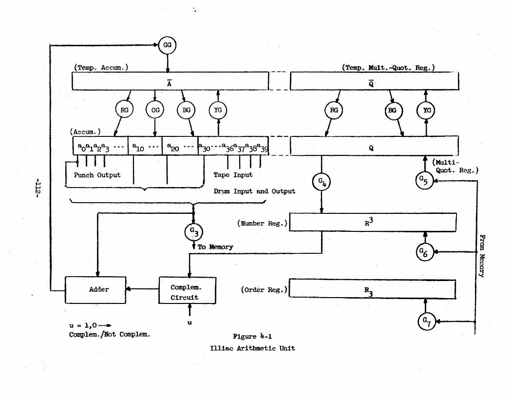
• ~ •
(Tempo Accumo)
A
(ACCUIno)
s0818 2a3 .,., <> I ~O .,,,,, I 8 20 .. e 0 r30°· .. a3~37a38a3
Punch Output
Adder
u=1,O---. Complemo /Not Complemo
Complem ..
Circuit
u
Tape Input
l>rJml Input and Output
(Number Reg .. )
(Ord~r Reg.,)
Figure 4-1
IlliacAritbmetic Unit
(Temp.Mu! t .. -Quat., Reg.)
Q-
Q
R3
(Multi r •
Quot .. Reg.,)
~ .. .8
~
if ~ o ~
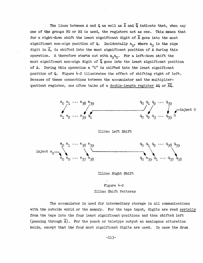
The lines between A and Q as well as A and Q indica.te that, when any
one of the groups RG or BG is used, the registers act a.s one 0 This means that
for a right-down shift the least significant digit of A goes into the most
significant non-sign position of Q~ Incidentally 8,0' where aO is the sign
digit in A, is shifted into the most significant position of A during this
opera.tion 0 A therefore starts out with aOaO
' For a left-down shift the
most significant non-sign digit of Q goes into the least significant position
of Ao During this operation a "0" is shifted into the least significant
position of Q. Figure 4-2 illustrates the effect of shifting right of left.
Because of these connections between the accumulator and the multiplier
quotient register, one often talks of a double-length register AQ or AQo
I1liac Left Shift
a 38 a39 Clo ql ~
\ \'------~, \ a37 8,38 Clo a 39 ql
Illiac Right Shift
Figure 4-2
Illiac Shift Patterns
q39
J ,.-inject a q39 0
The accumulator is used for intermediary storage in all communications
with the outside world or the memory. For the tape input, digits are read serially
from the tape into the four least significant"~posi tions and then shifted left
(passing through A)o For the punch or teletype output an a.nalogous situration
holds, except that the four most significa.nt digits are usedo In :case the drum
-113-
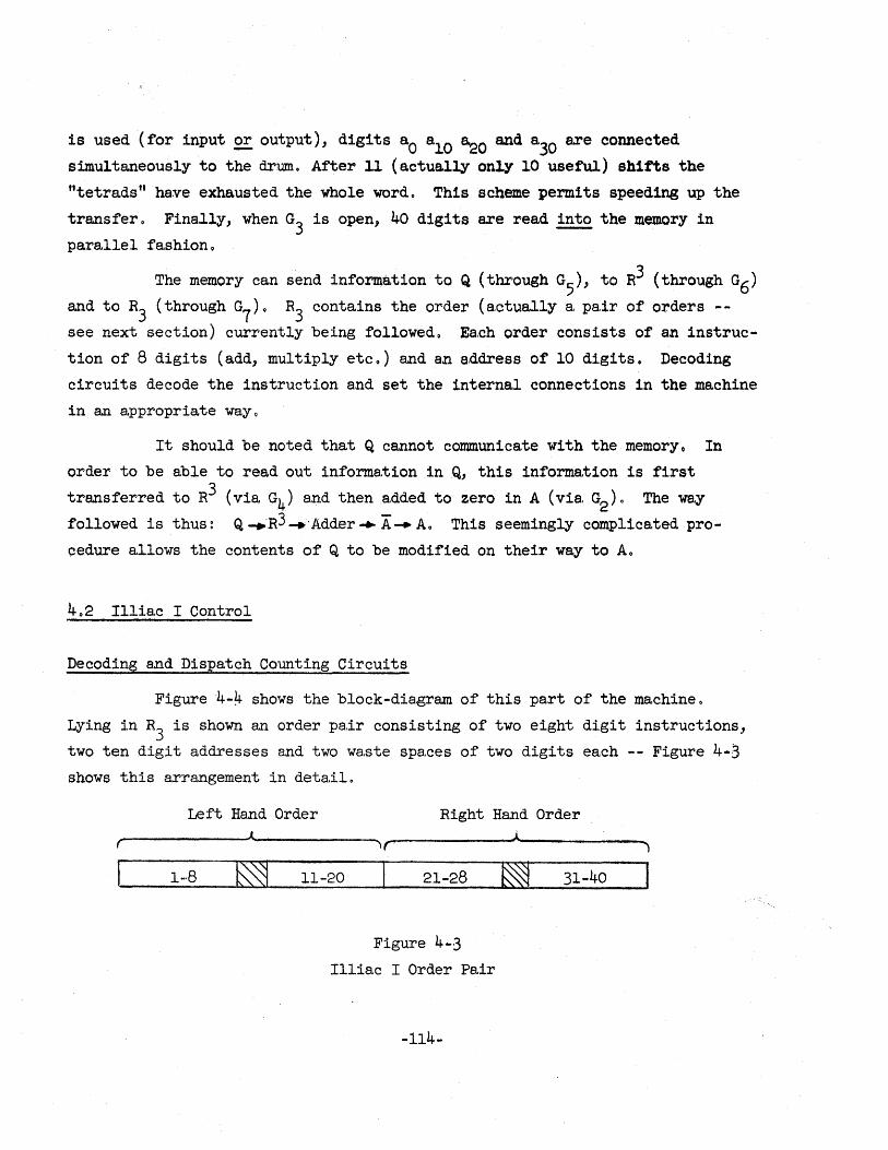
is used (for input 2!. output) , digits aO alO 8.20 and a30
are connected
simultaneously to the drum. After 11 (actua.lly only 10 useful) shifts the
"tetrads" ha:ve exhausted the whole word. This scheme permits speeding up the
transfer. Fina.lly, when G3
is open, 40 digits are read ~ the memory in
parallel fashion 0
The memory can send information to Q (through G5), to R3 (through G6) and to R3 (through G
1)o R3 contains the order (actually a pair of orders -
see next section) currently being followed 0 Ea.ch order consists of an instruc
tion of 8 digits ( a.dd, multiply etc 0) and an s,ddress of 10 digits. Decoding
circuits decode the instruction a.nd set the internal connections in the machine
in an appropriate waYQ
It should be noted that Q cannot communicate with the memoryo In
order to be able to rea.d out information inQ, this information is first
transferred to R3 (via G4) and then added to zero in A (via. G2 ). The wa.y
followed is thus: Q -+'R3 ... "Adder .... A ... Ao This seemingly complica.ted pro
cedure allows the contents of Q to be modified on their way to Ao
402 111iac I Control
Decoding and Dispatch Counting Circuits
Figure 4-4 shows the block-diagram of this part of the machine.
Lying in R3 is shown an order pair consisting of two eight digit instructions,
two ten digit a.ddresses a.nd two wa.ste spaces of two digits each -- Figure 4·3
shows this
r
arrangement in detail.
Left Hand Order Right Hand Order J.
1-8 ~
"\('
11-20 21-28
Figure 4-3
111iac I Order Pair
-114-
J..
~ 31-40
')
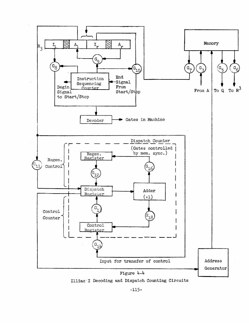
Instructlon Sequencing
Begin --.......... ~~----' Signa.l to Sta.rt/Stop
End Signal From Sta.rt/St p
Ga.tes in Machine
Dispa~ch Counter ----- ---, ( Ga.te s controlled I
..... ___ b_y_m_e_ID_o sync 0 ) I Regen.
Control ~~~~~ I
Control Counter
Adder (+1)
I I l
__ ...1
Input for transfer of control
Figure 4-4
Illiac.' I. Decoding and Dispa.tch Counting Circuits
-115-
Memory
From A To Q To R3
Address
Generator
This order pair has been brought into R3 in the following~. The
control register contains the address of the location of the order pair9 This address is ga.ted into the dispatch register and sets the a.ddress generatoro
The address generator chooses the memory location, the contents of which are
transferred to R3 via. G1
0 Now one unit is added to the a.ddress in the dispa.tch
register and the result is ga.ted into the control registero
Next the instruction sequencing counter puts the left hand address
into the decoder, a. device which sets certain flipflops in the machine and
opens certain paths a.ccording to the type of instructionc Simultaneously
the left hand address is gated into the dispatch registero
If the instruction ha.ppens to involve a. transfer of control, the
new a.ddress is transferred to the control register via. G14 and then gated
into the dispatch register upon the arrival of an end-signal. The process
described above then occurs a. second timeo If there is no transfer of
control, the left hand a.ddress is put into the dispa.tch register and sets
up the necessa.ry memory connections via the address generatoro The machine
then executes tne given instruction, the instruction sequencing counter
being tied to the start/staR control 0 Upon the arriva.l of the end-signa.l
of the operation, the instruction sequencing counter gates the right ha.nd
instruction into the decoder and simultaneously the right hand address into
the part of the register previously occupied by the left hand a.ddress! the
:right hand address thus goes into the dispa.tch register Q A transfer of
control operates a.s before 0 If there is no transfer" the right hand instruc ..
tion is executed 0 The end-signal again causes the contents of the control
register to be gated into the dispatch registero If there was no transfer
of control in the two instructions~ the contents of the control register at
this time axe the address of the previous order pa.ir increa,sed by one: the
ma.chine goes through the memory location' in sequenceo It is clea.r that
programming errors can cause number locations to be interpreted a.s order
1ocations o
As the memory sys·tem in Illiac I is regenera,tive, i.eo since
all :memory locat1ons must be scapnedperiodically and renewed, there is
a regeneration register atta.ched to the dispa.tch register 0 During the
-116-
regeneration cycle the contents of this register, increased by one, are gated
into the dispatch register and determine, via. the address generator, the
location of the next word to be renewed.
Control for the Arithmetic Unit
As indicated in Figure 4-5, there are 4 principal parts in this
section of Illiac I: the shift control, composed of the shift sequencing
unit (See Section 2.4) and the clear and ga.te selector, a shift counter
(as described in Section 2.2), a recognition circuit and a. start/stop control.
The recognition circuit has a dual purpose o If the instruction in R3 is a shift instruction, the address part gives the number of shifts to be
performed. The recognition circuit then compares the number of shifts as
counted by the shift counter to this predetermined number and, upon coincidence, (
acts on the start/stop control~ If the instruction in R3 is a multiply or
division instruction, the machine must go through 39 add-and-shift or subtract
and-shift cycles. This time the recognition circuit acts on the start/stop
control upon the advent of 39 shifts.
Notice that the shift· counter has a. "reset" input:' this clears
a.ll counter flipflops to zero before operations commence. The "up" and
"down" pulses are taken directly from the gates between A, A, and Q a.nd Q: red, orange or bla.ck ga.tes give a "down" signa.l while the yellow gate gives
an "up" signal. Which group of ga.tes is actually chosen depends upon the
signals from the decoder, i.e. upon the instruction followed.
4.3 Illiac Memory Circuits and Interplay Control
Figure 4-6 shows the layout of the memory circuits and what is
called the "interplay control", ioe. the part of the machine which directs
the transfer of information from the (synchronous) memory to the (asynchronous)
registers and vice-versa..
-117-
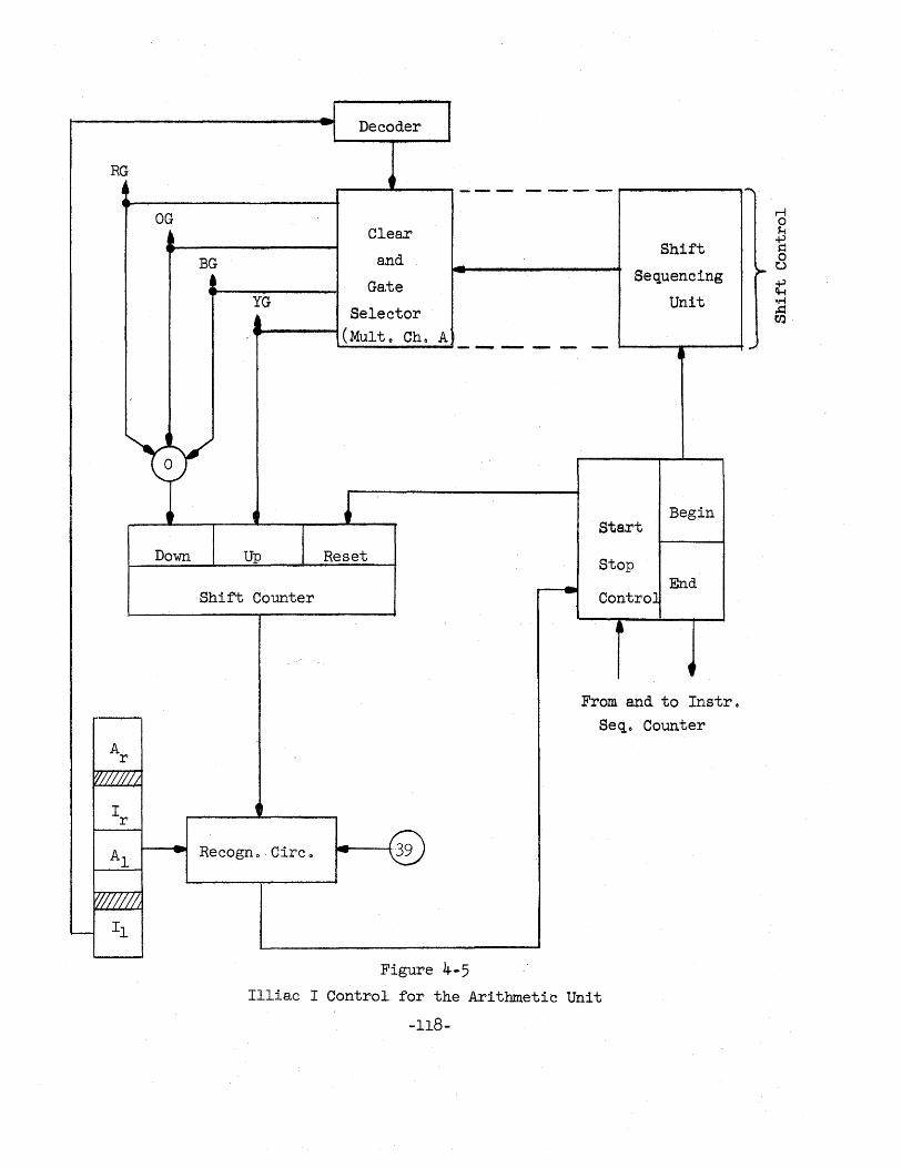
RG
•
----A r
Iflllili/
I r
Al
Ij/////~
I-- II
OG t ,..-
~
o
J
Down
-
BG !
YG jl
Up
Shift Counter
~
Recogno' Circ ..
J I -l Decoder
4,
Clea.r
and
Ga.te
Selector (Multo Cho A
Reset
r- 39
------ ....... ---
-
---- ~-
Shift
Sequencing
-
Start
Stop
Contro]
•
Unit
•
Begin
End
From and to Instre Seqo Counter
Figure 4-5 Illia.c I Control for the Arithmetic Unit
-118-
, .....
r-l 0 H
~ 0
>- t:.>
~ eM
~ .....
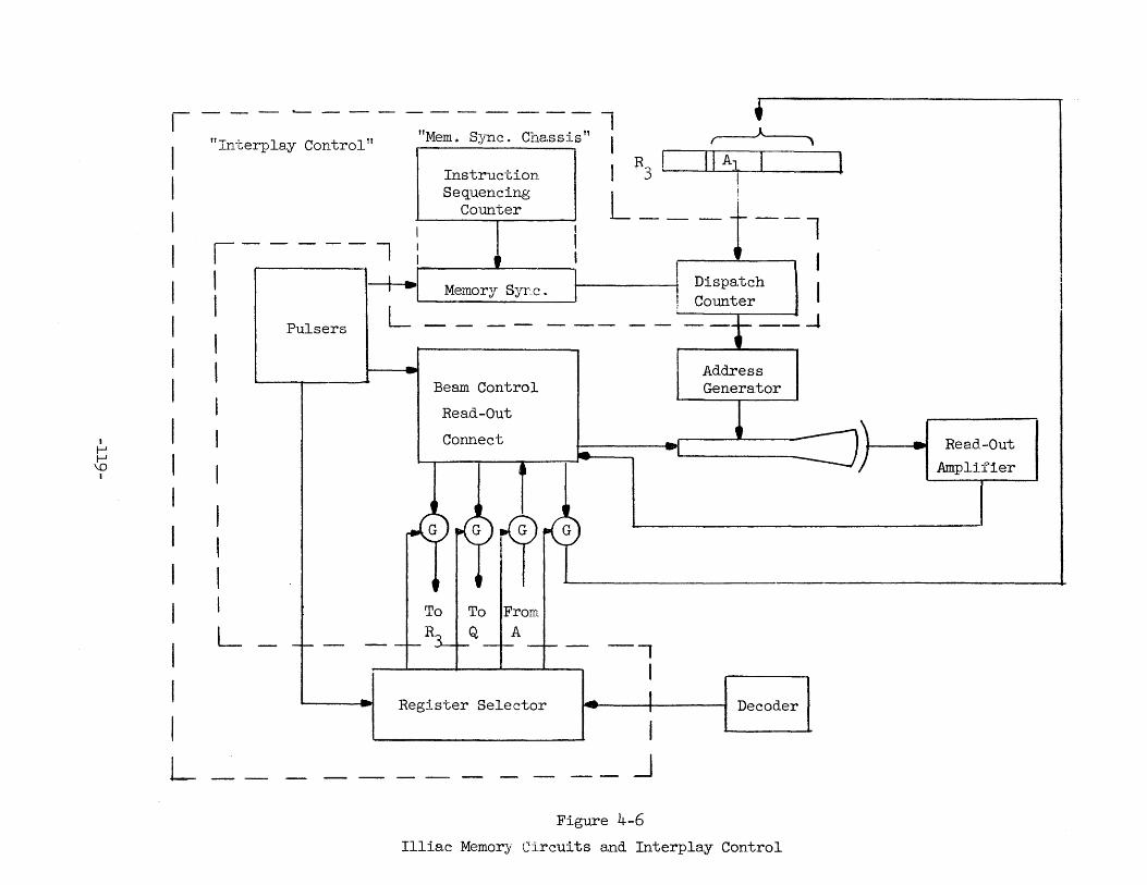
I I-' I-' ~
I
1--------"Mem. Sy-nc. Cha.ssis" ~
I I I I I I I I I I I
I I I
I I ,
L
fTInt.erplay Control"
Instruction Sequencing
Counter
R r II A1 3 .
!
I- ----l t I .r-----t
I Pulsers
I
I
I I Dispatch I--! Memory Syre. : ! Counter
L - - - - - - - ----1
---Beam Control
Read-Out
Connect , I- -
Address Generator
~ ~I~--------------------
f---..... .t.. Read-Out
Amplifier
I I I rr~ ____ -----+-
J G ~
• , I
L -;- -
To To IFrom
_ -i- R:W-Q -l-A -+- _ -, I
-- Register Selector 1- --.
I ___ .J
Figure 4-6
Decoder
Illiac Memory Circuits and Interplay Control
The Illiac memory uses cathode ray tubes as storage elements, each
one of the 40 digits in a. word coming from a different storage tube. The
storage of a "1" is obtained by brightening up anyone of the sports in a.
32 x 32 ra.ster ~ there are therefore memory locations numbered from 0 through
10230 By measuring the beam current when the beam is directed to a given
location by the address genera.tor (all beams are controlled in parallel!),
one can determine whether a "0" or a "1" has been storedo A read-out
amplifier detects the signal when the beam-control turns on the beam: a
pulse corresponding to a "1" sets a flipflop (previously cleared) in the
beam-controle Depending upon the state of this flipflop, a "1" or a. "0"
is written back immedia.tely to eliminate loss of information 0
As mentioned before, the memory can be in either one of two modes:
an a.ction-cycle (read or write) or a regenera.tion-cycle (transformation of
"fair" charge distributions in the cathode ray tubes to "good" distributions)o
In order to read out of the memory, one only has to examine the state of the
40 output flipflops mentioned ahovee For writing into the memory the restoring
process described above is used~ a "1" is always written back and writing a
"0" involves an additional motion of the beamo This additional motion is
suppressed if a "1" is to be writteno The regeneration cycle is :fundamentally
the same as the "read-and-restore" processo
The decoder acts on a register selector which in turn establishes
the connections for the transfer of signals to the registerso It is, however,
important to remember that the memory is synchronous and contains a clock and
a pulser chain 0 These pulses control the moment of transfer of informa~ion
through the register selector cha.ssis 0 They also control the action of the
dispatch counter ~con:trolcounter and regeneration counter) eoge when regen
eration occurs the address is stepped up by one unit by means of a clock
pulse; the other input of the memory synchronization comes from the instruction
sequencing counter 0 Often the la.tter two units are called the "memory
synchronization chassis".
404 Illiac Input-Output Circuits
The input-output circuitry of Illiac I is given in block-form in
Figure 4-70 As mentioned before, the right hand side of A (a,ctua.lly the 4
-120-
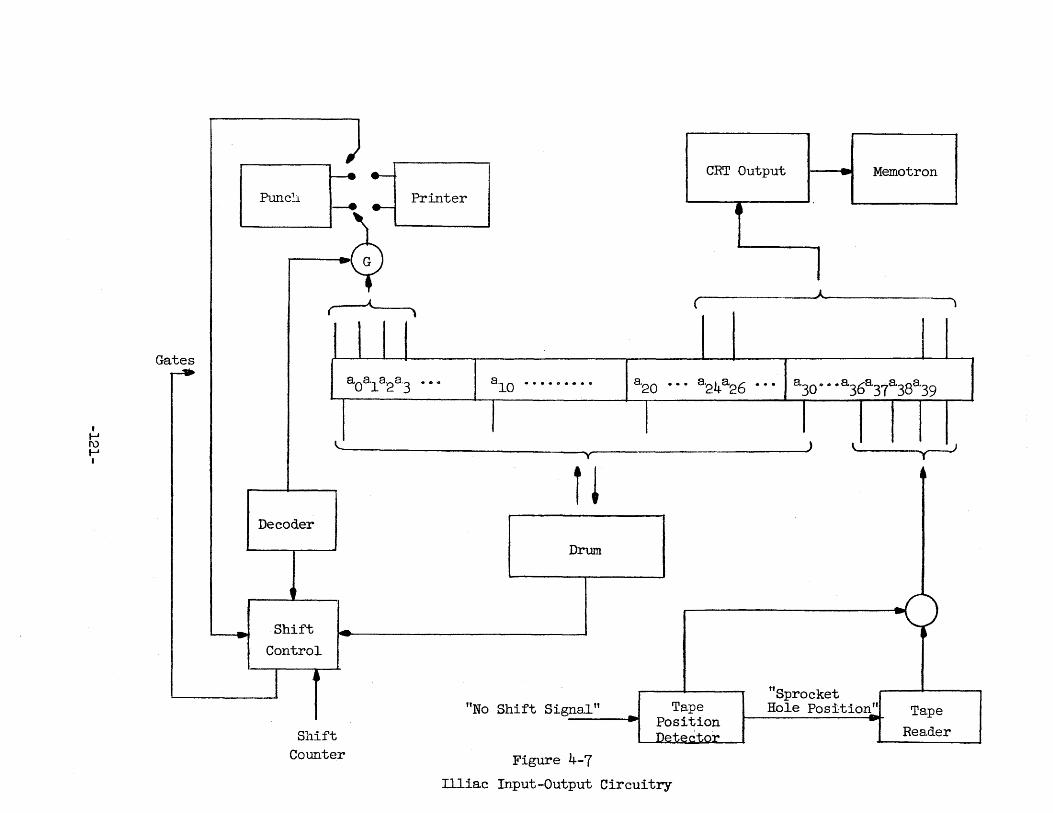
I ...... I\) t--' I
Gates
PunC~l Printer
CRT Output 1 Memotron
I ~
A (-----------~-------------)
a08.1
8.28.3
•• 0 8'10 •••• 0 •• • • 8.20 ••• a24a26 ••• I a30•• .a368,378,388.39
~. ) ~
Decoder
Shift Control
Shift Counter
y
i ~ Drum
"No Shift Signal" ---~~ ...
Figure 4-7
Tape Position
teet
Illiac Input-Output Circuitry
"Sprocket Hole Position" • Tape
Reader
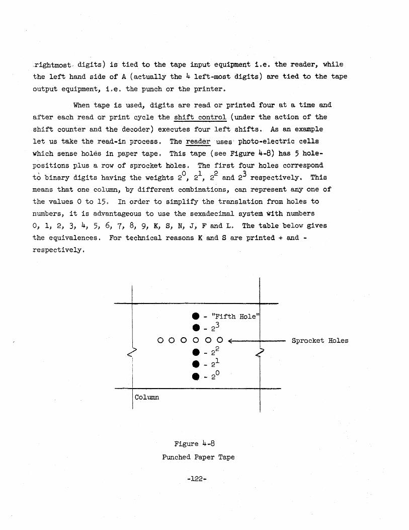
.rightmost ~ digits) is tied to the tape input equipment i. e. the reader, while
the left hand side of A (a.ctually the 4 left-most digits) are tied to the tape
output equipment, ioeQ the punch or the printer~
When tape is used, digits are rea.d or printed four at a time and
after each read or print cycle the shift control (under the a,ction of the
shift counter and the decoder) executes four left shifts. As an example
let us take the read .. in process 0 The readeruse:;.r photo-electric cells
which sense holes in pa,per ta.pe 0 This tape (see Figure 4-8) ha.s 5 hole
positions plus a row of sprocket holes. The first four holes correspond
to bina.ry digits having the weights 2°, 21, 22 and 23 respectively. This
means that one column, by different combinations, can represent anyone of
the va.lues ° to 15. In order to simplify the translation from holes to
numbers, it is advantageous to use the sexa.decimal system with numbers
0, 1, 2, 3, 4, 5, 6, 7, 8, 9, K, S, N, J, F and Lo The table below gives
the equiva.lences. For technical reasons K and S a.re printed + and -
respectively.
• - "Fifth Hole"
• _ 23
00 o 0 0 0 +-~---I---
Column
• _ 22
• _ 21
• _ 2°
Figure 4-8
Punched Paper Tape
-122-
Sprocket Holes
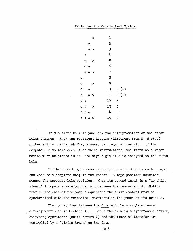
Table for the Sexadecimal System
0 1
0 2
o 0 3 0 4
0 0 5
o 0 6
000 7 0 8
0 0 9 0 0 10 K (+)
0 o 0 11 S ( -)
o 0 12 N
o 0 0 13 J
000 14 F
o 0 0 0 15 L
If the fifth hole is punched, the interpretation of the other
holes changes: they can represent letters (different from K, S etc.),
number shifts, letter shifts, spaces, carriage returns etc. If the
computer is to take account of these instructions, the fifth hole infor
mation must be stored in A: the sign digit of A is assigned to the fifth
hole.
The tape reading process can only be ca.rried out when the tape
ha.s come to a complete stop in the reader~ a. tape position detector
senses the sprocket-hole position. When its second input is a "no shift
signa.l" it opens a gate on the path between the reader and Ae Notice
that in the case of the output equipment the shift control must be
synchronized with the mechanical movements in the punch or the printer.
The connections between the drum and the A register were
already mentioned in Section 4.1. Since the drum is a synchronous device,
switching operations (shift control!) and the times of transfer are
controlled by a "timing track" on the drum.
-123-
A cathode-ray-tube output with a 256 x 256 raster (set -up through
an address genera.tor connected to a'32 . o. a39
for horizonta.l positioning and
a'24 00" 8031 for vertical positioning) allows the display of curves etc.. To
this purpose the computer is programmed to 11ght:.up .. specifl.c:. points ,of the
ra.stero A memotron, connected to the same e,ddress generator, gives a. per
sistent image of the CRT curves.
4.5 The Rela.tive Size of Memories
Problems Involving Large Amounts of Stora,ge
By definition data processing involves simple computations on a
large number of words (non-cumulative errors) while scientific calculations
involve complicated computations on a small number of words (cumulative
errors). Modern scientific calculations tend towards data processing
because complicated tabulations and searches are involved while the
fundamental iterative loop is simple o
Let us estimate the storage space required for some typica.l
scientific problems.
Hyperbolic Differential Equations. These often occur in hydrodynamic
problems in m dimensions o UsUally the va.lues of 2m + 1 variables Xi
(ioeo ql. o. ~, PI 000 Pm' S) s,t time t + At are deduced from their
values s,t time t in e. region with A Xi >ca to The number M of mesh
pOints per Xi (10 :s M :s 100 usually) determines the amount of data, to
be stored a.t anyone time ~ a.pprOXimatelyJim+l words are necessary 0
Intera.ctions Between Atoms in a La.ttice. Here .it is customary to employ
a tabulation method in which all atoms (M3 where M is the number in each
dimension, again 10 < M< 100) are listed and successive a,pproximatlons
change the values o;m p~.rameters of interest.. Visibly mM3 words have
to be stored.
-124-
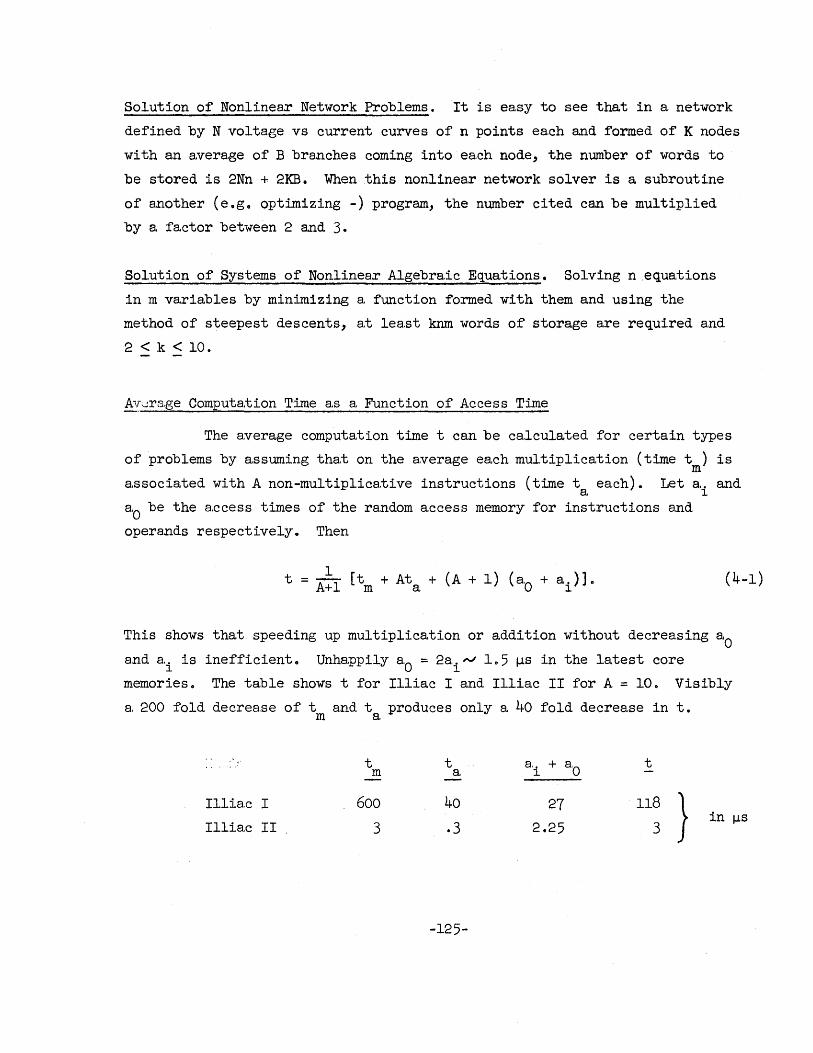
Solution of Nonlinear Network Problems. It is easy to see that in a network
defined by N volta.ge vs current curves, of n points each and formed of K nodes
with an a.verage of B branches coming into each node, the number of words to
be stored is 2Nn + 2KB. When this nonlinear network solver is a subroutine
of another (e.g. optimizing -) program, the number cited can be multiplied
by a. factor between 2 and 3.
Solution of Systems of Nonlinear Algebraic Equations. Solving nequations
in m varia:bles by minimizing a function formed with them and using the
method of steepest descents, at least knm words of storage are required and
2 < k < 10.
A'!.~\,~r8..ge Computation Time as a Function of Access Time
The average computation time t can be calculated for certain types
of problems by assuming that on the average each multiplication (time t ) is m
associated with A non-multiplicative instructions (time teach). Let a .. and a 1
800 be the access times of the random access memory for instructions and
operands respectively. Then
(4-1)
This shows that speeding up multiplication or addition without decreasing aO and 8.i is inefficient. Unhappily 80
0 = 2ai ,..j 105 IJ.s in the latest core
memories. The table shows t for Illiac I and Illiac II for A = 10. Visibly
a 200 fold decrease of t and t produces only a 40 fold decrease in t. m a.
t t a. + 800 t
m 8. 1
Illiac I 600 40 27 118 } in Illiac II 3 .3 2.25 3
-125-
JlS
Paralleling of Operations. Buffer Memories
In the calculations above it was assumed that all operations are
done sequentially~ if n operations with individual times Ti are required
in a process, the time for the process is ~ Tf" Evidently it is theoretically
possible to reduce this time to Max (T.) when all operations are paralleled. l
In practice it must be realized that the ideal time, Max (T.), cannot be l
attained because of supplementary control times necessi ta.ted by the more
complex nature of the control problem~
The bottleneck described is alleviated in Illiac II by using a.
very fast access memory directly connected to the arithmetic unit and called
the "buffer". This serves a double purpose: 1) the factor A is reduced
since short loops do not have to go outside the "buffer"; and 2) paralleling
of information transfer into the "buffer" and a.ctual calcula.tion becomes
possible. The usefulness of the 10 word "buffer" in Illia.c II is guaranteed
by its .2 IJ.s a.ccess time. A specia.l design ma.kes the realization in the form
of flipflop registers economically feasible.
Optimum Size of the Random Access Memory
For problems of the kind discussed at the beginning the main
random access memory must be connected to a back-up memory (drum, tapes),
since a 20-30,000 word core memory is too expensive. The cost of such a.
back-up memory - per bit stored - is reduced by serializing information
transfer~ blocks are transferred with an access time 0: per block (random
address) and then a time t3 per word read serially within the block. Always
0: » t3.
The question as to the relative sizes of these memories can only
be partially answered, even when the type of problem to be solved is known.
The back-up store can be assumed to be of a size sufficient to contain all
the information encountered in a problem; it is sometimes useful to assume
tha.t it is actually part of the input-output equipment. We shall calcula.te
the number of words (n) in the random access memory for which any further
increase in n no longer corresponds to an appreciable decrease of the total
calculation time.
-126-
Consider problems in which N initial words are reduced to AN words
(A. ,....., .5 or less) and an average calculation time t is required per operation ..
If the random access memory holds all N words, the total calculation time is
evidently TN :::: Nt. If, however, only n words are available in the random
access memory, to and fro transfers are necessary. It is easily seen that
T = T + 2aN + t3N(2-A.). n N n
Suppose that we do not wa.nt to increase the calculation time by more than a
factor of five by choosing n < N. Then
5 2aN @N(2-A) 1 + nNt + Nt
For t = 3 IlS, A. :::: . 5, O! :::: 18,000 Ils, t3 :::: 6 IlS we then have n :::: 12))00 ~ Note
that Tn/TN has a lower bound of 1 + t3(2-A.)/t: This means that is is very
time consuming to transfer information as soon as the calculation time is
of the order of the word-time ~.
General Design Criterion. Reliability
For the memory - as for any other equipment involving a great
number of similar elements (transistors, cores, etc.) - the relationship
between the decrease in reliability with increasing complexity and the
decrease in total calculation time can be established. Idealizing by
assuming that there are N elements with an average life of T hours
(meaning that the machine breaks down every T/N hours on the average)
and that the computation time lost per brea.kdown is L(N) hours, a problem
needing 9N
hours of faultless time with this N-element machine will in
reality necessitate
G' N
NL(N) GN [1 + T ] hours.
-127-
(4-2)
For M > N elements
G' = G [1 + ML(M)] hours. M M T
But obviously M/N computers of the N-element type can solve the problem in
NGN/M hours; the increase in hardware is therefore.only justified if
The best possible design therefore minimizes
Neglecting N~~Wi th respect to L (i. e. repa.ir time rv indep. of N!), this
means that
It seems not unreasonable to put N = 20, 000, T = 60, 000 hours and L(N),y .5
hours~ Then the optimum memory has the property that a 1% increase in N
produces a 1 .. 2% increase in speed.
4.6 Addition, Subtraction, Multiplication and Division in Illiac I
Addition and Subtra.ction (Order Type L)
(4-3)
The only difference between addition and subtraction is the setting
of the complementing circuit:
augend x + addend y = sum z
minuend x - subtrahend y = difference z
-128-
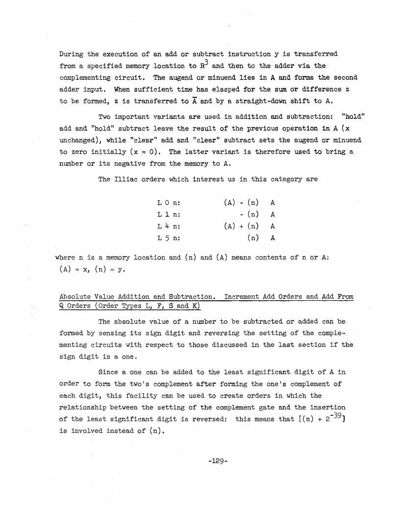
During the execution of an add or subtract instruction y is transferred
from a specified memory location to R3 and then to the adder via the
complementing circuit. The augend or minuend lies in A and forms the second
adder input. When sufficient time ha,s els,sped for the sum or difference z
to be formed, Z is transferred to A and by a. stra,ight-down shift to Ao
Two important va.riants are used in a.ddition and subtraction: "hold"
add and "hold" subtract leave the result of the previous operation in A (x
unchanged), while "clear" add and "clear" subtract sets the augend or minuend
to zero initially (x :;; 0). The latter v8,riant is therefore used to bring a
number or its negative from the memory to A.
The Illiac orders which interest us in this ca.tegory are
L 0 n: (A) - (n) A
L I n: - (n) A
L 4 n: (A) + (n) A
L 5 n: (n) A
where n is a memory location and (n) and (A) means contents of n or A~
(A) = x, (n) = y.
Absolute Value Addition and Subtraction. Increment Add Orders and Add From Q Orders (Order Types L, F, Sand K)
The absolute value of a number to be subtracted or added can be
formed by sensing its sign digit and reversing the setting of the comple
menting circuits with respect to those discussed in the last section if the
sign digit is a one.
Since a one can be added to the least significant digit of A in
order to form the two's complement after forming theone's complement of
each digit, this facility can be used to create orders in which the
relationship between the setting of the complement gate and the insertion
of the least significant digit is reversed: this means that [(n) + 2-39J is involved instead of (n) 0
-129-
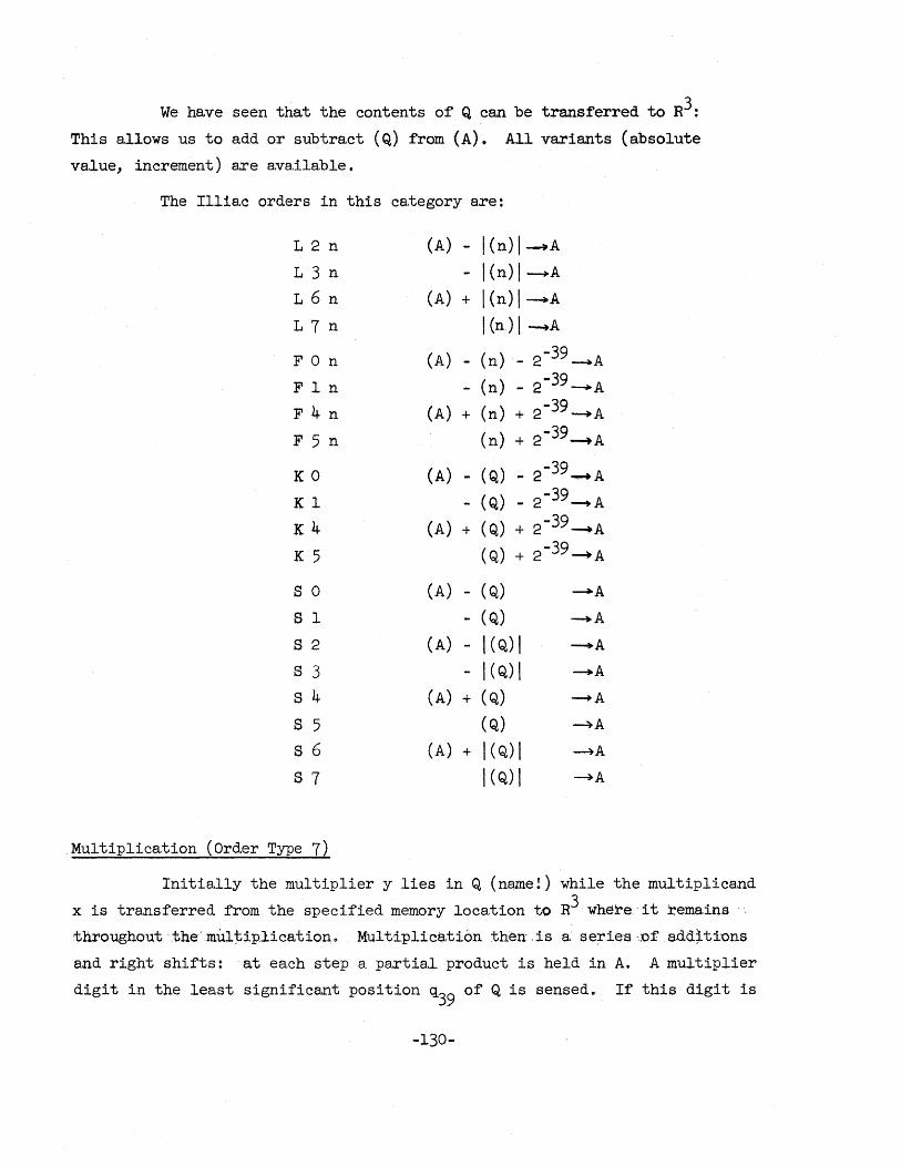
We have seen that the contents of Q can be transferred to R3:
This allows us to a.dd or subtract (Q) from (A). All variants (absolute
va.lue, increment) a.re available.
The Illiac orders in this category are:
L 2 n (A) - I (n) I ~A L 3 n - I (n) I-+A
L 6 n (A) + I (n) I---+A
L 7 n I (n) I ---.A
F 0 n (A) - (n) - 2-39 ~A FIn - (n) - 2-39 --..A
F 4 n (A) + (n) + 2-39~A
F 5 n (n) + 2-39~A
KO (A) - (Q) - 2-39 -+A
Kl - (Q) - 2-39 --+ A
K4 (A) + ( Q) + 2-39 --..A
K 5 ( Q) + 2-39~A
S 0 (A) - (Q) --.loA
S 1 - (Q) --+A S 2 (A) - I (Q) I --+A S 3 - I (Q) I --+A
S 4 (A) + ( Q) -+A
S 5 (Q) -4A S 6 (A) + I (Q) I ~A
S 7 I (Q) I ~A
Multiplication (Order Type 7)
Initially the multiplier y lies in Q (name!) while the multiplicand
x is transferred from the specified memory location to R3 where,' it rema.ins
throughout '.the"mulj,ip:lication" Mult:iplica,tiori then ,is a se~ies "of a.dd~ti:ons
a.nd right shifts: at each step a partial product is held in A. A multiplier
digit in the least significant position q39 of Q is sensed. If this digit is
-130-
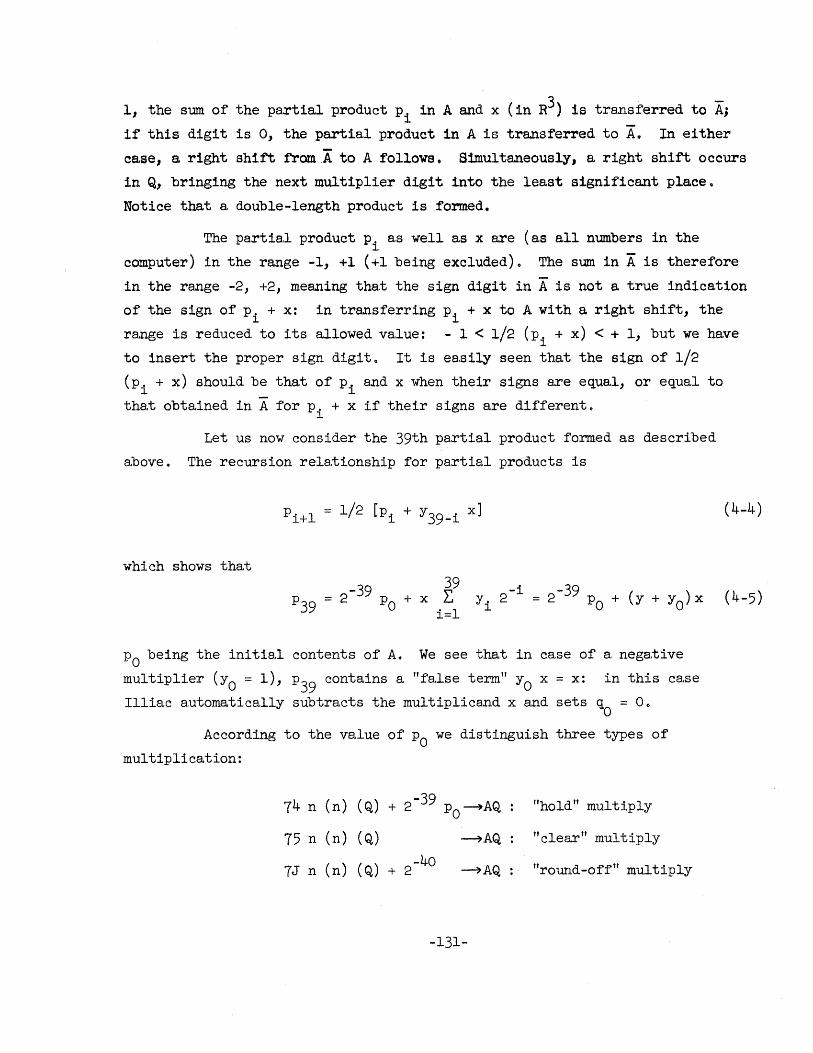
1, the sum of the partial product Pi in A and x (in R3) is transferred to Aj
if this digit is 0, the partial product in A is transferred to Aft In either
case, a right shift framA to A follows. Simultaneously, a right shift occurs
in Q, bringing the next multiplier digit into the least significant placeo
Notice that a double-length product is formed.
The partial product Pi as well as x are (as all numbers in the
computer) in the range -1, +1 (+1 being excluded) 0 The sum in A is therefore
in the range -2, +2, meaning that the sign digit in A is not a true indication
of the sign of Pi + x: in transferring Pi + x to A with a right shift, the
ra.nge is reduced to its allowed value: - 1 < 1/2 (Pi + x) < + 1, but we ha;ve
to insert the proper sign digito It is ea.sily seen that the sign of 1/2
(P. + x) should be that of p. and x when their signs are equal, or equal to l l
that obtained in A for p. + x if their signs are different o l
Let us now consider the 39th partia.lproduct formed as described
above. The recursion relationship for partia.l products is
which shows that
= 2-39 p o 39
+ x L, i=l
-i _ 2-39 p ( ) y i 2 - 0 + y + YO x
Po being the initial contents of A. We see that in case of a negative
multiplier (YO = 1), P39 contains a "false term" YO x = x: in this case
Illiac automatically subtracts the multiplicand x and sets q = 00 o According to the value of Po we distinguish three types of
multiplication:
74 n (n) (Q) + 2-39 p --...,AQ o 75 n (n) (Q) ~AQ
7J n (n) (Q) + 2-40 --7AQ
-131-
"hold" multiply
"clear" multiply
"round-off" multiply
(4-4)
(4-5)
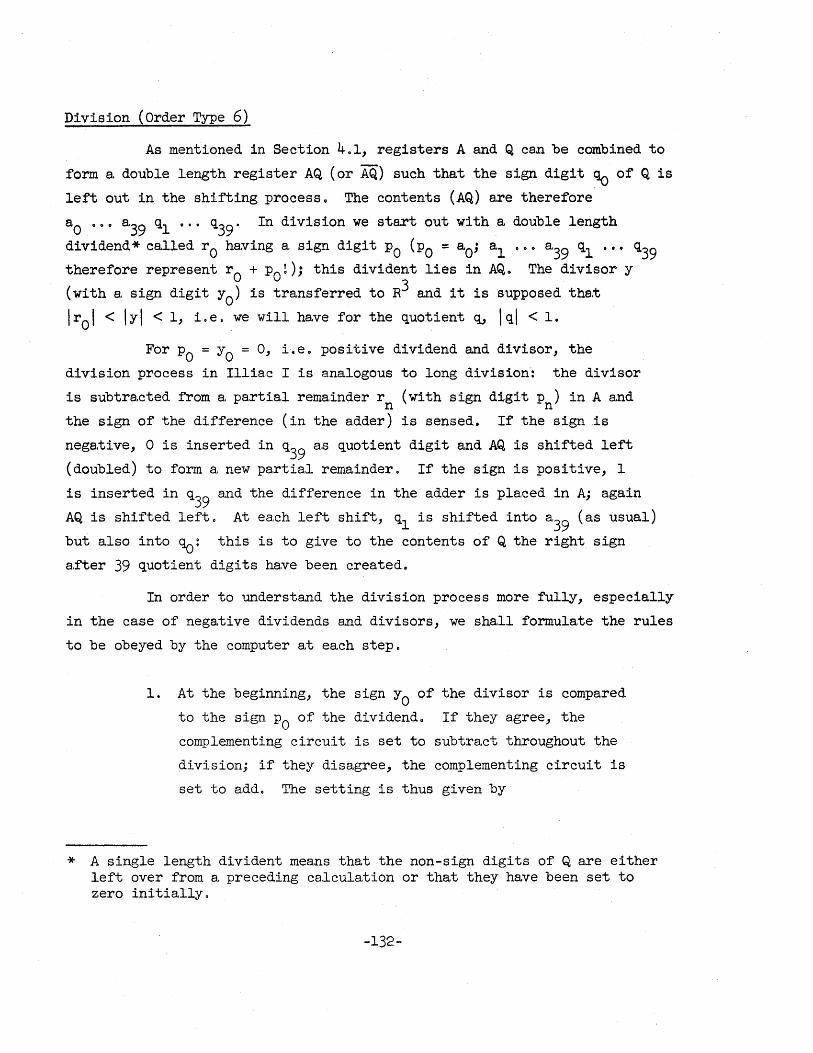
Division (Order Type 6)
As mentioned in Section 401, registers A and Q can be combined to
form a. double length register AQ (or AQ) such tha.t the sign digit Clo of Q is
left out in the shifting process o The contents (AQ) a.re therefore
a·O ••• a'39 Q,l •.. q39· In di vis ion we sta.rt out with a double length
dividend* called rO ha;ving a sign digit Po (PO = a.0; a'l 0'. a.39 Q.l ••• Q.39 therefore represent rO + PO!); this divident lies in AQ. The divisor y
(with a sign digit yo) is transferred to R3 a.nd it is supposed tha.t
I rO I < I YI < 1, i. e. we will have for the quotient Q" I Q,I < 1.
For Po = YO = 0, i.e .. positive dividend and divisor, the
division process in Illiac I is a.nalogous to long division: the divisor
is subtra.cted from a partial remainder r (with sign digit p ) in A and n n
the sign of the difference (in the adder) is sensed. If the sign is
nega.ti ve, 0 is inserted in Q,39 as quotient digit and AQ is shifted left
(doubled) to form a new partial remainder. If the sign is positive, 1
is inserted in Q,39 and the difference in the adder is placed in A; again
AQ is shifted left. At each left shift, Q,l is shifted into a39
(as usual)
but also into~: this is to give to the contents of Q the right sign
a.fter 39 quotient digits have been created,
In order to understand the division process more fully, especia.lly
in the case of negative dividends and divisors, we shall formulate the rules
to be obeyed by the computer at each step.
1. At the beginning, the sign yo of the divisor is compared
to the sign Po of the dividend. If they agree, the
complementing circuit is set to subtract throughout the
division; if they disagree, the complementing circuit is
set to add. The setting is thus given by
* A single length divident means that the non-sign digits of Q are either left over from a preceding calculation or that they have been set to zero initially.
-132-
p +y , (~l) 0 0 = cr-' (say).
2. A tentative partia.l remainder s ( with sign digit t ) n n
3.
is obtained by forming
If the sign t of s agrees with the sign Po of the n n dividend, the tentative partial remainder is transferred
from the adder to A. If they disagree, the partial
:remainder .. :Ln A is transferred to Ao (This choice between
a. tentative partial remainder and the old partial remainder
is a special feature of Illiac, made possible by the fact
that the partial rema.inder in A is not destroyed when the
tenta.tive partial remainder is formed) 0 The new partial
remainder - after a. left shift - is then given by
4. If the sign t of the tentative partial remainder agrees n
with the sign YO of the divisor, 1 is inserted in q39
(39th position of Q)o If they disagree, 0 is inserted 0
Call the quotient digit thus obtained ~o Then
yo+t ~ = 1/2 [1 + (-1) n]
5. (A) and (Q) are transferred to A andQ with a. left shift 0
6. At the end q39 is set to 1.
By us ing (4 -8 ), we find that
-133-
( 4-6)
( 4-7)
( 4-8)
(4-9)
(4-10)
(4-9) gives the non-sign part of the quotient q (using rule 6)
i.e. the arithmetica,1 value of the quotient is
(4-11)
Now we define a. remainder r by
(4-12)
In order to show tha.t q is the quotient, we mu'st show that r is of
order unity 0 Using (4-11) and (4-12)
since
But
and
y +p = 2-1 [1 - (-1) 0 0] since Po F to by our hypothesis
Irol < IYI < 1.
-1 [ =2 1-CS-]
-134-
Therefore
( ) -39 [( -39) { ( )Po ( )Ya} ~8( )tn 2-n ] r - r 39 . 2 = y 1-2 CT + 1 - (J - 1 + a-' -1 - -l ~-1
= y [_239 (J - {} L]
Now
{} YO 2PO = (-1) [(-1) - 1] = 0
Po+Yo since by definition (j' = (-1)
a.nd it follows tha.t
r = r39 - a- y
Since r39 and y both have absolute values less than one and since
~ = ~ 1, the absolute value of r cannot exceed 2, meaning that
(4-l3)
(Actually it can be shown by a. more deta.iled examina.tion tha.t IrO - qyl ::: 2-39 !)
The Illiac division order is written 66 n and as we have seen its
effect is to put
4.7 Other Methods of Multiplica.tion and Division
The lAS Method of Multiplica.tion
This method, used in the Princeton machine, multiplies only the
non-sign digits of the multiplier y and the multiplicand x: suitable
corrections have to be madeo Let Xo and xl be the sign and non-sign digits
of x:
-135-
In the same way y ;;: -Yo + Y1 and
This shows that a correction is required in two cases:
l, If yo ;;: 1, x + Xo must be subtracted s.t the end.
2. If Xo ;;: 1, y must be subtracted at the end.
(4-14)
The latter operat1.on is quite diff1cult, since the digits of the multiplier
are destroyed in the multiplication process. In order to circumvent this
difficulty, a piecewise insertion ot the dig1twise complement of the non
sign digits of y is used; a.t the end .1 + 2-39 is a.dded to the final product,
in order to obtain the two's complement. The following rules describe the
opera.tion!
1. At eB,ch step if q39 = 0 add Xo to the partial product Pi
and if q39 ;;: 1 add the non-sign digits of the multiplicand,
i.e. (x + xO) to Pi. In case Xo is 1, a,dd the d1g1tw1se
complement of Y39-i i.e. (1·Y39-i)' Transfer the results to A and the non-sign digits of Q to Q.
2" Shift right from A to A and from Q to Q, inserting 0 as
sign digit in A.
3~ If the multiplier wa.s negative, subtract x a.t the end a.nd
if the multiplicand wa.s nega.t1ve" add -1 + 2"'39.
Formula.ting these rules ma.tbematica.lly
It follows tha.t
-136-
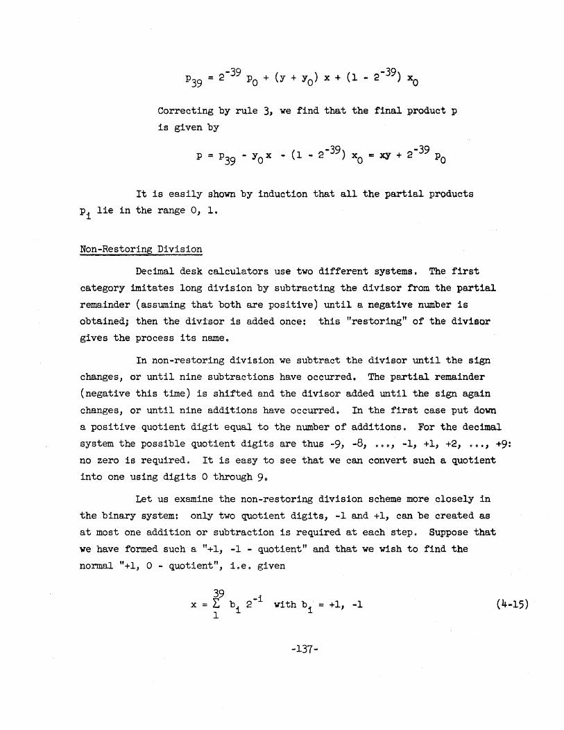
Correcting by rule 3, we find that the final product p
is given by
It is easily shown by induction that all the partial products
Pi lie in the range 0, 1.
Non-Restoring Division
Decimal desk calculators use two different systems. The first
category imitates long division by subtracting the divisor from the partial
remainder (assuming that both are positive) until a negative number is
obtained; then the divisor is added once: this "restoring" of the divisor
gives the process its nameo
In non-restoring division we subtract the divisor until the sign
changes, or until nine subtractions have occurred. The partial remainder
(negative this time) is shifted and the divisor added until the sign aga1n
changes, or until nine a.dditions have occurred. In the first case put down
a. positive quotient digit equal to the number of additions. For the decimal
system the possible quotient digits are thus -9, -8, 000, -1, +1, +2, 000, +9: no zero is required. It is ea.sy to see that we can convert such a quotient
into one using digits 0 through 9~
Let us examine the non-restoring division scheme more closely in
the binary system: only two quotient digits, -1 and +1, can be created as
at most one addition or subtraction is required at each step. Suppose that
we have formed such a "+1, -1 - quotient" and that we wish to find the
normal "+1, 0 - quotient", ioe o given
-137-
(4-15)
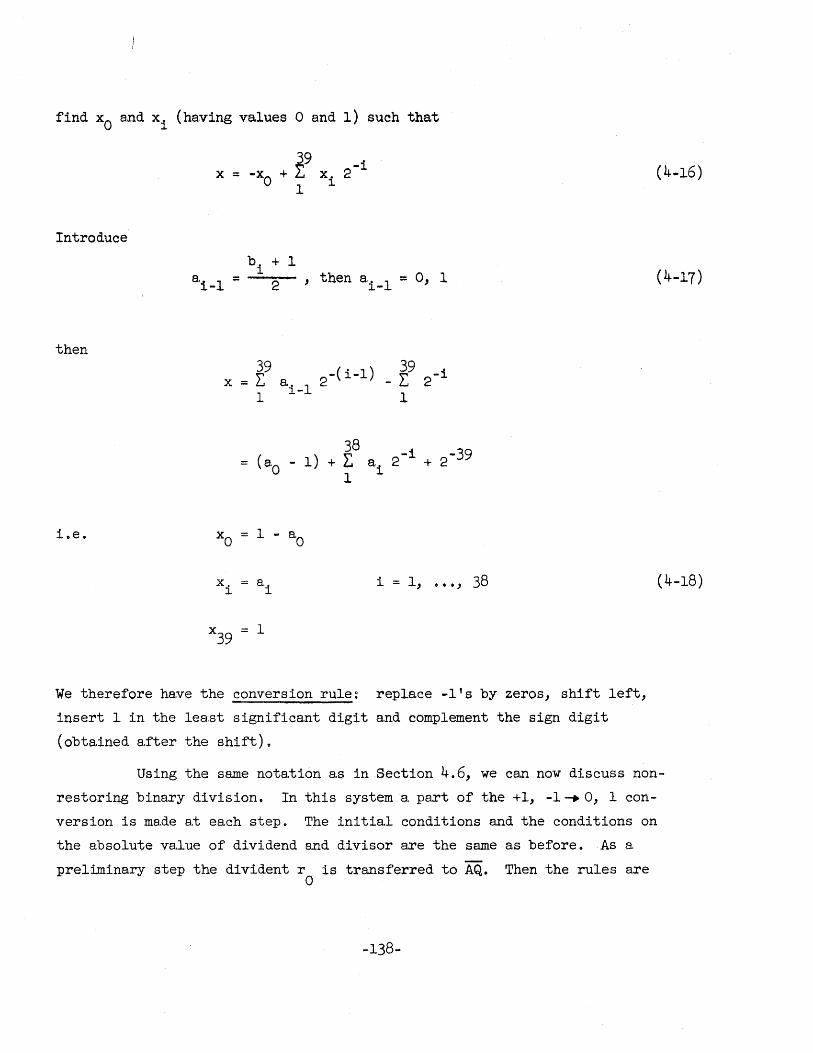
find Xo and xi (having values 0 a.nd 1) such that
Introduce
then
i.e.
39 -1 x = -xo + E x. 2
1 l.
bi
+ 1 a1 _1 = 2 ' then a i _1 = 0, 1
~9 -(i-I) ~9 -i x = w a. 1 2 - ~ 2
1 l.- 1
38 ( 1) ~ a 2-1 + 2-39
eO - + ~ 1 1
Xo = 1 - a,O
x. a'1 i = 1, ... , 1.
x39 = 1
38
We therefore have the conversion ru1e~ replace -1's by zeros, shift left,
insert 1 in the lea.st significant digit and complement the sign digit
(obtained a.fter the shift) 0
(4-16)
(4-17)
(4-18)
Using the same notation a.s in Section 4.6, we can now discuss non
restoring binary division. In this system a, pa.rt of the +1, -1 ..... 0, 1 con
version is made at each step. The initial conditions and the conditions on
the absolute value of dividend a.nd divisor are the same as before. As a
preliminary step the divident r is transferred to AQ. Then the rules are o
-138-
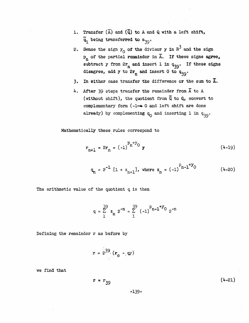
1. Transfer (A:) and ("Q) to A and Q with a left shift,
ql being transferred to a39 0
2~ Sense the sign YO of the divisor y in R3 and the sign
Pn of the partie.l remainder in A, If these signs agreel
subtract y from 2rn end insert 1 in q39~ If these signa
disagree, add y to 2rn and insert 0 to Q39'
3. In either case transfer the difference or the sum to Ao
4, After 39 steps transfer the rema.inder from A to A
(without shift), the quotient from Q to Q, convert to
complementary form (-1 ...... 0 and left shift are done
already) by complementing ~ and inserting 1 in Q390
Mathema.tica11y these, rules correspond to
P +YO r 1 = 2r = (-1) n y n+ n
-1] P 1+YO ~ = 2 [1 + zn+l ' where zn = (-1) n-
The arithmetic value of the quotient q is then
39 39 p +y q = ~ z 2-n = L (-1) n-1 °2-n
1 n 1
Defining the remainder r a.s before by
'"39 r = 2·,· (r -.qy) . '. 0
we find that
r = r39
-139-
(4-19)
(4 ... 20)
(4-21)
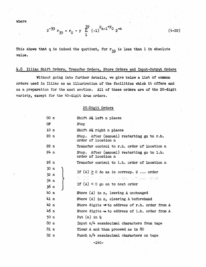
where 39 p +Y
2~39 r = rO - y E (-1) n-l 0 2-n 39 1
(4-22)
This shows that q is indeed the quotient, for r39 is less than 1 in absolute
value.
4.8 Illiac Shift Orders, Transfer Orders, Store Orders and InRut-Output Orders
Without going into further details, we give below a list of common
orders used in Illiac as an illustra.tion of the fa,cilities which it offers and
as a prepara,tion for the next section. All of these orders are of the 20-dig1t
variety, exoept for the 40-digit drum orders.
00 n
OF
10 n
20 n
22 n
24 n
26 n
30 n
f 32 n
34 n
36 n J 40 n
41 n
42 n
46 n
50 n
80 n
81 n
82 n
20-Digit Orders
Shift AQ left n places
stop
Shift AQ right n places
Stop. After (manual) restarting go to r.h. order of locs,tion n
Transfer control to r.h. order of loc8,tion n
Stop 0 After (manual) restarting go to l.h. order of location n
Transfer control to loh. order of location n
If (A) 2: 0 do a,s in corresp. 2 e •• order
If (A) < 0 go on to next order
Store (A) in n, leaving A unchanged
store (A) in n, clearing A beforehand
Store digits .... to a.ddress of r.h. order from A
Store digits .... to a.ddress of l.h. order from A
Put (n) 1n Q
Input n/4 sexadecimal characters from tape
Clear A and then proceed as 1n 80 Punch n/4 sexadecimal characters on tape
-140-
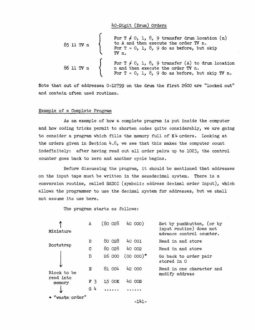
85 11 TV n
86 11 TV n
{ {
40-Digit (Drum) Orders
For T f. 0, 1, 8, 9 transfer drum:.locatlon (n) to A and then execute the order TV no For T = 0, 1, 8, 9 do as before, but skip TV n.
For T f 0, 1, 8, 9 transfer (A) to drum location n and then execute the order TV no For T = 0, 1, 8, 9 do as before, but skip TV no
Note that out of addresses 0-12799 on the drum the first 2600 are "locked out"
and contain often used routineso
Example of a Complete Program
As an example of how a complete program is put inside the computer
and how coding tricks permit to shorten codes quite conSiderably, we are going
to consider a program which fills the memory full of K4orderso Looking at
the orders given in Sec~ion 4.6, we see that this makes the computer count
indefinitely: after having read out all order pairs up to 1023, the control
counter goes back to zero and another cycle beginso
Before discussing the program, it should be mentioned that addresses
on the input tape must be written in the sexadecimal system 0 There is a.
conversion routine, called SADOI (symbolic address decimal order input), which
a.llows the progra.rmner to use the decimal system for a.ddresses, but we sha.ll
not assume its use here.
The program starts as follows:
i A (80 028 40 000) Set by pushbutton, (or by
Miniature input routine) does not advance control counter 0
B 80 028 40 001 Read in and store Bootstrap
C 80 028 40 002 Read in and store
1 D 26 000 (00 000)* Go back to order pair stored in 0
E 81 004 42 000 Read in one character and Block to be modify address read into
40 OOS memory F 3 L5 OOK
t G 4 •••• 0 • loe6e&
* "wa.st~;,-order" -141-
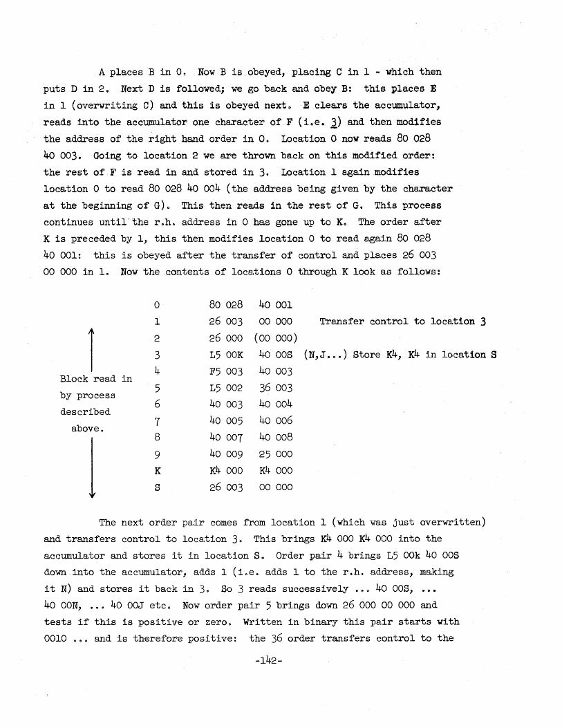
A places B in 0.. Now B is obeyed, placing C in 1 .. which then
puts D in 20 Next D is followed; we go back and obey B: this places E
in 1 (overwriting C) and this is obeyed next .. ·Eclears the accumulator,
reads into the accumulator one character of F (ioe .. l) and then modifies
the a,ddress of the right hand order in 0.. Location 0 now reads 80 028
40 0030 Going to location 2 we are thrown back on this modified order:
the rest of F is read in and .stored in 3. Location 1 agalnmodlfles
loca.tion 0 to read 80 028 40 004 (the address being given by the chara.cter
at the beginning of G).. This then reads in the rest of Go This process
continues until'the roh. address in 0 has gone up to Ko The order after
K is preceded by 1, this then modifies location 0 to read again 80 028
40 001: this is obeyed after the transfer of control and places 26 003
00 000 in 10 Now the .contents of locations 0 throughK look as follows:
0 80 028 40 001
I 26 003 00 000 Transfer control to location 3
I 2 26 000 (00 000)
3 L5 OOK 40 OOS (N,J • .,o) Store K4, K4 in location S
4 F5 003 40 003 Block read in
5 L5 002 36 003 by process
6 40 003 40 004 described
7 40 005 40 006 above ..
8 40 007 40 008
9 40 009 25 000
K K4 000 K4 000
s 26 003 00 000
The next order pair comes from loca.tion I (which was just overwritten)
and transfers control to location 30 This brings K4 000 K4 000 into the
accumulator and stores it in location So Order pair 4 brings L5 Oak 40 OOS
down into the accumulator, adds I (ioe. a.dds l to the r.h. address, making
it N) and stores it back in 3. So 3 rea.ds successively DO" 40 OOS,
40 OON, .".. 40 OOJ etc., Now order pair 5 brings down 26 000 00 000 and
tests if this is positive or zero.. Written in binary this pair starts with
0010 .... 0 and is therefore positive: the 36 order transfers control to the
-142-
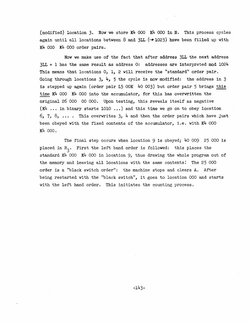
(modified) location 3. Now we store K4 000 K4 000 in No This process cycles
a.gain until a.ll locations between 8 and 3LL (.....p 1023) have been filled up with
K4 000 K4 000 order pairs.
Now we make use of the fact that after a.ddress 3LL the next address
3LL + 1 has the same result as a.ddress 0: a.ddresses are interpreted mod 1024
This means that locations 0, 1, 2 will receive the "standard tt order pair.
Going through locations 3, 4, 5 the cycle is now modified: the address in 3 is stepped up again (order pa.ir L5 OOK 40 003) but order pair 5 brings this
time K4 000 K4 000 into the accumulator, for this has overwritten the
original 26 000 00 000. Upon testing, this revea.ls itself a.s negative
(K4 .•• in binary starts 1010 • 0 0) and this time we go on to obey location
6, 7, 8, 000 • This overwrites 3, 4 and then the order pairs which have just
been obeyed with the fixed contents of the a.ccumulator, i.e. with K4 000
K4 000.
The final step occurs when loca.tion 9 1s obeyed; 40 009 25 000 1s
pla.ced in R30 First the left band order 1s followed: this places the
standardK4 000 K4 000 in location 9, thus draMing the whole program out of
the memory and leaving all locations with the same contents! The 25 000
order is a. "black switch order": the machine stops and clears AD· After
being restarted with the "bla.ck switch", it goes to location 000 and starts
with the left hand order. This initia.tes the counting process.
-143-
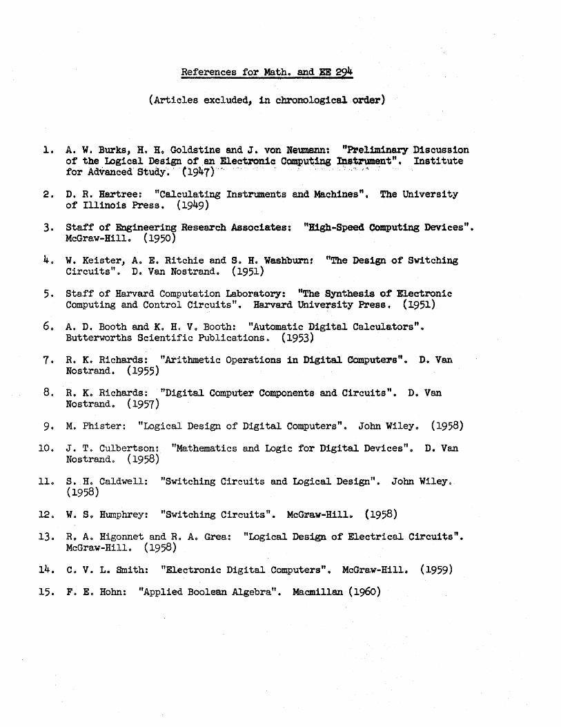
References for Math. and EE 294
(Articles excluded, in chronolog1calorder)
1. A. W. Burks, H. Ho Goldstine and J" von Neumann: "Preliminary Discussion of the Logics,l Design of en ElectJ'On1c Oompvt'~1ng ~'tnment". Institute for Advanced Study!~ !' (1947)" '. '."" . ",~'
2. D. R. Ha.rtree: "Ca.leula,ting Instruments and Machines". The University of Illinois Press, (1949)
3. Staff of Engineering Research Associates: "1I1gb--Speed Computing Devices". McGraw-Hill. (1950)
40 W. Keister, Ao E. Ritchie and S. H. Wa.shburn: "The Design of Switching Circuits"o D. Van Nostrand. (1951)
5. Staff of Harvard Computa,tion Laboratory: "The Synthesis of Electronic Computing and Control Circuits If. Harvard Un! versi ty Press. (1951)
6. A, D. Booth and K. Ho V Q Booth: "Automatic Digital Calculators" 0
Butterworths Scientific Publica~ionso (l953)
7. Ro K. Richards: "Arithmetic Opera.tiona in DigittU Computers". D. Van Nostrand. (1955)
8. R. K. Richards: "Digital Computer Components and Circuits". Do Van Nostrand. (1957)
9. M. Phister: "Logical Design of Digital Computers". John Wiley. (1958)
10. J. To Culbertson: "Mathematics and Logic for Digital Devices". D. Van Nostrand. (1958)
11. S. H. Caldwell: "Switching Circuits and Logical Design". John Wileyo (1958)
12 0 W 0 S. Humphrey: "Switching Circuits 11 • McGra.w-Hillo (1958)
130 R. Ao Higonnet and Ro A. Grea.: "lDgical Design of Electrical Circuits". McGraw-Hill. (1958)
14. Co V. Lo Smith: "Electronic Digita~ Computers". McGraw-Hill. (1959)
15. Fa Eo Hohn: "Applied Boolean Algebra". Macmillan (1960)
CHAPrER V
ABSTRACT MErHODS
5.1 Groups, Rings, Fields and B. A.
1. SEMIGROUP
Let some common property of the elements a, b, c •.• define a set
S = {a, b, c •.• }, also let us define a. binary operation * on the members of
the set, "binary" meaning here "involving two elements." Now a * b = x ma.y
or may not belong to the set S. If for any two elements (a, b) of the set
a * b does belong to S, we sa.y that S is closed with respect to the operation *p
Also" if for all a., b, c c:S (~meaning; belonging to)
(a. * b) * c = a * (b * c), ( 5-0)
the operation * is called associative in S.
Definition: A semigroup is a.n associative, closed set S with respect to a.n
operation *.
Rema.rk: A set can be:
2. GROUP
discrete finite
discrete infinite
continuous
f o} \+1, -1,
{all integers}
{all numbers}
Definitioti: A group G is a se~igroup with a unit a.nd inverses where the unit
and the inverse a.re defined as follows:
The unit e satisfies a * e = e * a. a
1 -1 The: inverse a - to a satisfies a. * a
Theorem 10 The unit is unique.
pOroof: Let el
, e2
both be units
then
e1 * e = e
1 80lso e1 * e2 2
hence
el
e2 QED.
-145-
=
-1 a * a.
e2
e
( 5-1)
( 5-2)
Theorem 2. The inverse is unique.
Proof:: Assume that there exist inverses a-I, b.
Then by definition a.*b=e -1
i. e.,
a. * a. e
B. * b - * -1 - a. a,
-1 operating on the left by a we halve
(80-1 * a) * b = (a.- l * a)
hence
or
e * b = e * al
-1 b = a
-1
-1 * a
Defini.tion': A group is said to be commutative or Abelian if a. * b
The order of a group is the number of elements in it.
3. RING
b * a.
A ring R is a set which is a commutative group with respect to one
binary opera.tion (say +) and a semigroup with respect to a. second binary opera
tion (say.). Also, the ,following distribution relations hold for all a, b, c
cR
a. . (b + c) ab + a.c (where ab means a. • b, etc.)
ana (5-3)
(80'+ b) ~ C =ac + bc
J);:f'ini tion: 1 We shall ca.ll z the unit of the opera.tion +, and we shall ca.ll a
the inverse of a with respect to z:
1 1 a. +8,=a+a =Z
a+z=z+a a.
Example: {all integers} forms a ring.
Special Rings:
(1) Ring with a. unit (unit e for the second operation).
(2) Commutative ring: ab = ba for the second opera,tion.
-146-
(5-4 )
4. FIELD
A field F is a. ring with a. unit e and inverses a-I for the second
binary operation (called' • above). The existence of a. unit and an inverse
with respect to + is gua.ranteed by the :fact tha.t the field is a ring. We
could say tha.t a. field is a. "double group."
Example: f real numbers 1
5. BOOLEAN RING
A Boolee.n ring BR is a ring with a uni t ('W.r. t. .) in which the
idempotency law holds:
for every a c BR
Theorem 30 a + a = z ina BR. --Proof:
but
there:fore
or
(e. + b) • (a + b) = aa + ba + ab +- bb
LHS = (a + b) by the idempot. law
RHS = a + be. + ab + b by the same la.w
,:. a + b = a. + ba + a.b + b
1 1 a. + a = z, b + b = z
a.l
+ bl + (a + b) = al + b
i + a. + ba + ab + b
z = ba + ab
Now let a = b, then
z = aa. +: aa.,
or by the idempot. 1a~
z = a + a QED.
Theorem 4. 81 = a. in a. BR.
Proof: 1 z = a. + a and z = a + a
Thus
1 1 1 a. a + z = a. + a. + a. =.a. QED.
-147-
( 5-5)
(5-6)
( 5-7)
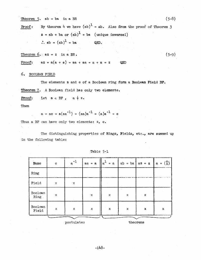
Theorem 5. a.b = ba in a BR ( 5-8)
ProOf: By theorem 4 we have (ab) 1 :;: ab. Also from the proof of Theorem 3
'., ·1 Z :;: ab + be, or (ab) :;: be. (unique inverse!)
:. e.b = (ab) 1 = be. QED.
Theor.em 6.: .. 1. az = z in a, BR. ( 5-9)
pr.oof': a,z = a,C a. + a) = a.a, + a.a = a + a. = z QED
6. BOOLEAN FIELD
The elements z and e of a Boolean ring form a. Boolean Field BF.
Theorem 7. A Boolea.n field he,s only two elements.
Proof: Let a c. BF , a f Z.
Then
a = ae = a ( aa -1 ) = (aa) a -1 = (a) 8. -1 e
Thus a BF can ha.ve only two elements: z, e.
The distinguishing properties of Rings, Fields, etc., are summed up
in the following table:
Ta.ble 5-1
Name -1 1 ab ba. a,Z (~) e a a.a = 8, a = a = c· Z 8, = .----
Ring -"._-- --~-1---,,-,'"'---'-''' ":,,...,...~ .... ~.-."' .. ,,, ."."' ~ •... ~ . -,
Field x x .
Boolea.n Ring x x x x x
Boolea.n Field x x x x x x x
_.--,.
""'--------~----_./ \.'-------~------_./ postulates theorems
-148-
7. BOOLEAN AIGEBRA
Two more operations a.re introduced, called
-Complementation: a = a. + e and (5-10 )
Conjunction: avb =8 +b+a.b
Rema.rk: It is evident from the definitions that we have
avb=bva. (commutativity) ( 5-11)
and
(a v b) v c = a. v (b v c) (associa.tlvity) (5-12 )
Theorem 8. a v a = a (5-13)
Proof': a· v a = a + a + aa, = (a. .... a) + a z + a == a.
Theorem 9. a,(b v c) = ab v a.c ( 5-14)
ProoI': e.(b v c) == a(.b + c + be) = (ab) + (ac) + (ab)(ac) .= a,b v e.c
Theorem 10. a v b c = (a v: b) (a v c) (5-15)
Proo'f: RHS = (a + b + a.b) (a + c + ac)
= a. + ac + ac + be. + bc + abc + ab + a.bc + abc
= a. + bc + a.bc + (ac + ae) + (a,b + ba.) + (abc + abc)
(a) + (be) + (a)(be)
a v be = LHS QED.
Intersection a:nd Union.
z • e. == z (5- 9 )
e.s proved a.bove ~
zva =a ( 5-16)
since z v a. z + a + a,z a)
e • a = a (5-17)
by definition of e
eva.=e (5-18 )
since e v a == e + a. + ae = e + a. + a = e + ~ = e •
Complementa.tiOh ahd Dti8.11:ty·.
aa = z (5-19) sinceaa = a(a + e) = ~a + ae = a + a = z
a v b = s.b ( 5 -20 )
also
since ~ v £ = (a + e) + (b + e) + (a + e)(b + e)
= a. + e + b + e + a,b + a,e + eb + e
= ab + e + (a + a) + (b + b) + (e + e)
a.b + e == (ab)
since a v b = e + a ~ b + ab ~ (e + alee + b) = a • £ ( 5-21)
We now see that the algebra. of a. ring with a. unit, sa.tisfying
id~potemcy and including the operations of complemen~ation and conjunction
i9 formally the same as a Boolean a.lgebra:
e < >1
z < >0
+ is simply the operation E> defined in Chapter III. Again it should be
eniphasized that Boolean algebra. is not restricted to values 1 and 0 for the
va.riables as is shown by the fo110wing example:
8. EXAMPLE OF.A BOOLEAN ALgEBRA-OF .MORE,]HAN'WOV ARIAl3LES
Take the most genera.l function f(X]? x2
) of two (two-va.lued) Boolean
varfa.bles. There must bee. canonica.l expansion (see Cha.pter III) a,nd therefore
where ~,.b, c, d a.re also Boolea.n variables with the values 0 a.nd 1. Visibly
any combina.tion of four zeros and ones corresponds to a different f: There
a.re 16 different functions of two 'varia.bles.
Now take a.s the elements of a. new, multi-valued a~gebra._ the sixteen
types of f, setting
f(OOOO) = 0
f(OOOl)= A
, f(llll) 1
f(lllO) = L
-150-
and call x a variable that can take anyone of these 16 valueso It is then
quite clear that all postulates of Boolean algebra are satisfied, e.g.,
x . x = 0, x v X = 1,
the latter two simply expressing that the minterms in x and those in x are
mutually exclusive and that the product of anyone in x with anyone in x is
zero since they are orthogonal (see Chapter III).
-151-
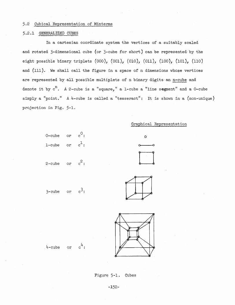
5.2 Cubical Representation of Minterms
5.2.1 GENERALIZED CUBES
In a cartesian coordinate system the vertices of a suitably scaled
and rotated 3-dimensional cube (or 3-cube for short) can be represented by the
eight possible binary triplets (000), (001), (010), (all), (100), (101) .. (110)
and (111). We shall call the figure in a space of n dimensions whose vertices
are represented by all possible multiplets of n binary digits an n-cube and
denote it by en. A 2-cube is a "square," a I-cube a "line segment" and a a-cube
simply a "point." A 4-cube is called a "tesseract": . It is shown in a (non-unique)
projection in Fig. 5-1.
Graphical Representation
a-cube a or c : 0
I-cube 1 or c : 0 0
2-cube 2 0 or c :
3-cube or
4-cube or 4 c :
-152~
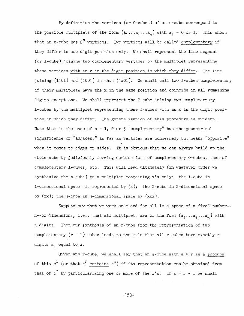
By definition the vertices (or O-cubes) of an n-cube correspond to
the possible multiplets of the form (al " .. a ...• a ) with a. = 0 or 1. This shows l n l
that an n-cube has 2n vertices. Two vertices will be called complementary if
they differ in one digit position only. We shall represent the line segment
(or l-cube) joining two complementary vertices by the multiplet representing
these vertices with an x in the digit position in which they differ. The line
joining (1101) and (1001) is thus (lxOl). We shall call two l-cubes complementary
if their multiplets have the x in the same position and coincide in all remaining
digits except one. We shall represent the 2-cube joining two complementary
l-cubes by the multiplet representing these l-cubes with an x in the digit posi-
tion in which they differ. The generalization of this procedure is evident.
Note that in the case of n = 1, 2 or 3 "complementary" has the geometrical
significance of "adjacent" as far as vertices are concerned, but means "opposite" \
when it comes to edges or sides. It is obvious.that we can always build up the
whole cube by judiciously forming combinations of complementary O-cubes, then of
complementary l-cubes, etc. This will lead ultimately (in whatever order we
synthesize the n-cube) to a multiplet containing x's only: the l-cube in
l-dimensional space is represented by (x); the 2-cube in 2-dimensional space
by (xx); the 3-cube in 3-dimensional space by (xxx).
Suppose now that we work once and for all in a space of a fixed number--
n--of dimensions, i.eo, that all multiplets are of the form (alo .. a. o.oa ) with l n
n digits. Then our syntheSis of an r-cube from the representation of two
complementary (r - l)-cubes leads to the rule that all r-cubes have exactly r
digits a. equal to x. l
Given any r-cube, we shall say that an s-cube with s < r is a subcube
of this cr (or that cr contains cS) if its representation can be obtained from
r that of c by particularizing one or more of the XIS. If s = r - 1 we shall
-153-
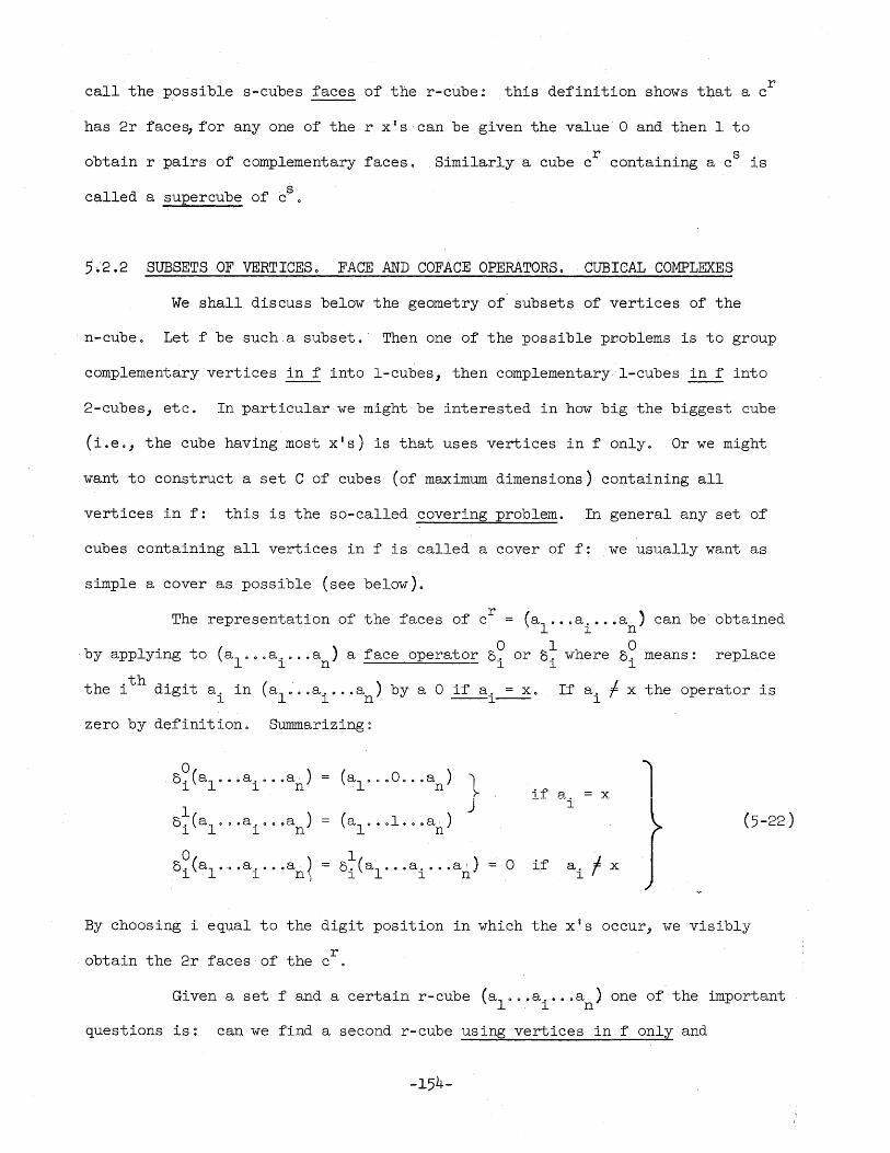
call the possible s-cubes faces of the r-cube; this definition shows that a cr
has 2r face~ for anyone of the rx's can be given the value 0 and then 1 to
obtain r pairs of complementary faces. Similarly a cube cr containing a CS is
s called a supercube of c' •
5.:2.2 SUBSETS OF VEHTICESo FACE AND COFACE OPERATORS. CUBICAL COMPLEXES
We shall discuss below the geometry of subsets of vertices of the
n-cube. Let f be such a subset. Then one of the possible problems is to group
complementary. vertices in f into I-cubes, then complementary I-cubes in f into
2-cubes, etc. In particular we might be interested in how big the biggest cube
(i.e., the cube having most XiS) is that uses vertices in f only. Or we might
want to construct a set C of cubes (of maximum dimensions) containing all
vertices in f: this is the so-called covering problem. In general any set of
cubes containing all vertices in f is called a cover of f: we usually want as
simple a cover as possible (see below).
The representation of the faces of cr = (al ... a .... a) can be obtained l n
b 1 · t ( ) f t 0 .1 hOI Y app ylng 0 al ... a .... a a ace opera or 5. or 5. were 5. means: rep ace l n l l l
the i th digit a. in (al " 0 .a. o •• a ) by a 0 if a. = x. If a. f x the operator is l l n ----l---- l
zero by definition. Summarizing:
if R x l --i (5-22)
o 5. (alo .. a. 0 •• a )
l l n
I 5. (alo 0 • a .•.. a )
l l n
o 5. (al"·o • a .... a)
l l n) 0 if a. f x l
By choosing i equal to the digit position in which the XiS occur, we visibly
r obtain the 2r faces of the c .
Given a set f and a certain r-cube (alo .. a .... a ) one of the important l n
questions is: can we find a second r-cube using vertices in f only and
-154-
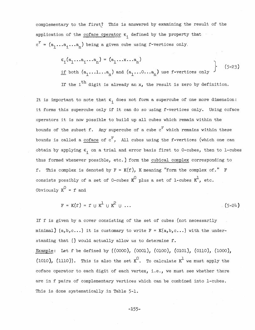
complementary to the first? This is answered by examining the result of the 11.-,
application of the coface operator E. defined by the property that l
cr ~ (al ... a ...• a ) being a given cube using f-vertices only, l n
E . (al ... a .... a ) ~ ( a l .•. x ... a ) } l l n n
if both (al ... l ... a ) and (al ... O ... a ) use f-vertices only --- n n
If the ith digit is already an x, the result is zero by definition.
It is important to note that E. does not form a supercube of one more dimension: l
it forms this supercube only if it can do so using f-vertices only. Using coface
operators it is now possible to build up all cubes which remain within the
bounds of the subset f. Any supercube of a cube cr which remains within these
bounds is called a coface of' cr., All cubes using the f-vertices (which one can
obtain by applying E. on a trial and error basis first to O-cubes, then to l-cubes l
thus formed whenever possible, etc.) form the cubical complex corresponding to
f. This complex is denoted by F = K(f), K meaning "form the complex of." F
consists possibly of a set of O-cubes KO plus a set of l-cubes r, etc.
Obviously KO = f and
F K(f) fUrU~U ••• (5-24 )
If f is given by a cover consisting of the set of cubes (not necessarily
minimal) (a,b,c •.• ) it is customary to write F = K[a,b,coo.} with the under-
standing that [} would actually allow us to determine f.
Example: Let f be defined by (0000), (0001), (0100), (0101), (0110), (1000),
(1010), (1110)}. This is also the set KO. To calculate ~ we: must apply the
coface operator to each digit of each vertex, i.e., we must see whether there
are in f pairs of complementary vertices which can be combined into I-cubes.
This is done systematically in Table 5-1.
-155-
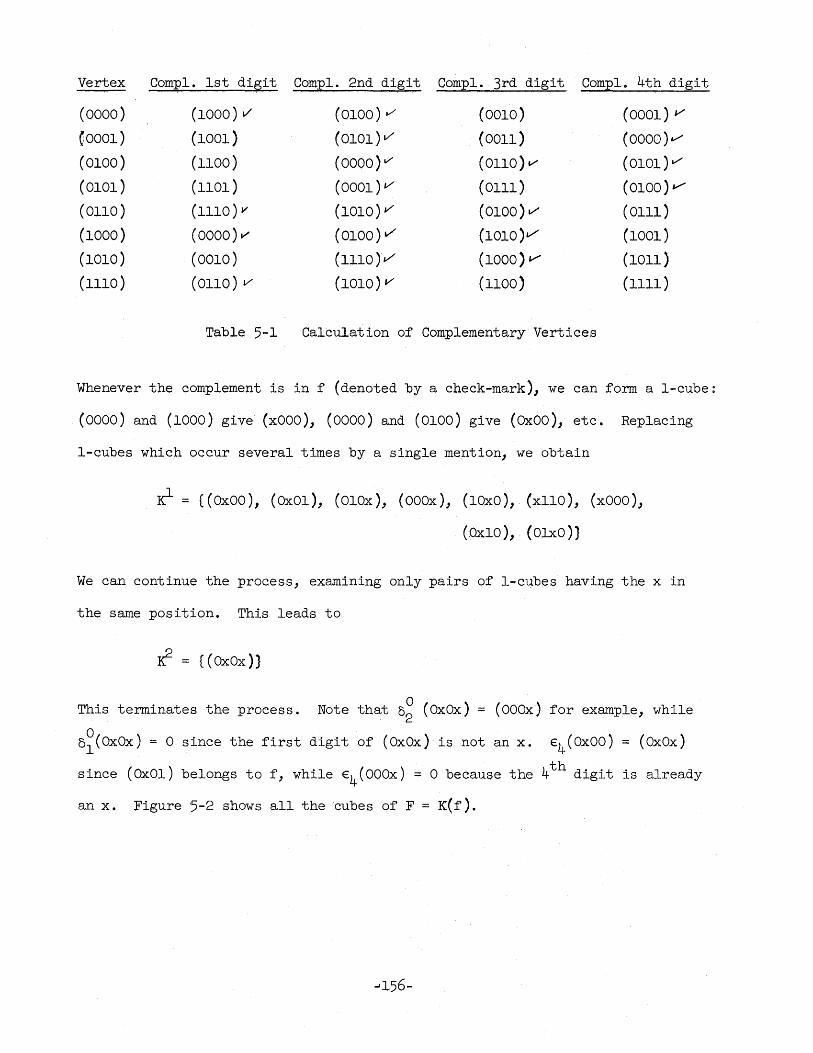
Vertex CampI. 1st disit Compl. 2nd digit Compl. 3rd digit Compl. 4th digit
(0000) (1000) v (0100) v (0010) (0001) v
(0001) (1001) (0101)&/ (0011) (OOOO)v
(0100) (1100) (OOOO)v (0110) v (0101) v-
(0101) (1101) (0001) v- (0111) (0100) v
(0110) (1110) v (1010) v (0100) v- (alII)
(1000) (0000) V' (0100) v (lOlO)v (1001)
(1010) (0010) (lllO)v (1000) v (1011)
(1110) (0110) v (1010) v (1100) (1111)
Table 5-1 Calculation of Complementary Vertices
Whenever the complement is in f (denoted by a check-mark), we can form a I-cube:
(0000) and (1000) give (xOOO)~ (0000) and (0100) give (OxOO), etc. Replacing
I-cubes which occur several times by a single mention, we obtain
12- = {(OxOO), (OxOl), (OlOx), (OOOx), (lOxO), (xllO), (xOOO),
(.oxlO), (OlxO)}
We can continue the process, examining only pairs of l~cubes having the x in
the same position. This leads to
~ = {(OxOx»)
This terminates the process. Note that o~ (OxOx) = (OOOx) for example, while
5~(OXOx) = a since the first digit of (OxOx) is not an x. E4 (OXOO) = (OxOx)
since (OxOl) belongs to f, while E4 (000X) = a becauqe the 4th digit is already
an x. Figure 5-2 shows all the cubes of F = K(f) .
..1156-
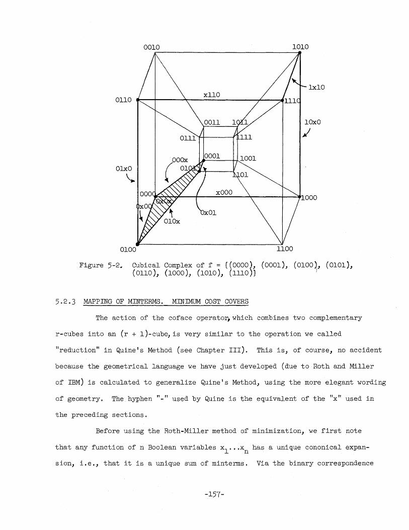
0010 1010
lxlO
0110
lOxO
~
OlxO
\.
0100 1100
Figure 5-2. Cubical Complex of f = {(OOOO), (0001), (0100~, (0101), (0110), (1000), (1010), (1110))
5.2.3 MAPPING OF MINTERMS. MINThIDM COST COVERS
The action of the coface operato~which combines two complementary
r-cubes into an (r + I)-cube, is very similar to the operation we called
"reduction" in Quine's Method (see Chapter III). This is, of course, no accident
because the geometrical language we have just developed (due to Roth and Miller
of IBM) is calculated to generalize Quine's Method, using the more elegant wording
of geometry. The hyphen " " used by Quine is the equivalent of the "x" used in
the preceding sections.
Before using the Roth-Miller method of minimization, we first note
that any function of n Boolean variables xl .•• xn has a unique cononical expan-
sion, i.e., that it is a unique sum of minterms. Via the binary correspondence
-157-
introduced in 3.4 each minterm corresponds to a multiplet of nbinary digits
(~~ 0, x. ~l) and thus to a well defined vertex of an n-cubeo This means l l
that the set of vertices f [and F = K(f)!] is known as soon as the Boolean
function is given. Because of the complete equivalence of the set of vertices
and the function, we shall denote both by the same letter f.
The fundamental problem of simplifying a Boolean function now becomes
equivalent to finding a set C of cubes covering f and causing (for the equivalent
physical circuit) minimum costo If C contains a number go of O-cubes (corres
ponding to AND's with n inputs), gl l-cubes (corresponding to AND's with n-l
inputs), etc., the criterion for minimizing the cost is usually
n n n L g (n - r) + L g
r=O r r=O r L g Cn - r + 1)
r=O r min. (5-25)
wherethe first term gives the total number of AND-inputs and the second term
the number of inputs of the "c.ollecting" OR: CAO gives the number of arrowheads
in the sense of Chapter III. We are thus led to a search for as few cubes of F
as possible, each having the maximum dimensions.
In case we have to cover f, but may cover f v g, i.e., in case f gives
the "care" conditions and g the "don't care" conditions (see Chapter III1, one
problem is to find a mi.nimum cost subset of K(f v g) which covers K(f) only 0
Let K(C) denote the c.omplex of cubes using the vertices in the cover Conly
and let C be the set-theoretical inclusion; then obviously
F K(f) C K(C) C K(f v g) = M(say) (5-26)
5.3 Cocycles and Extremals
5.3.1 THE EXPANSION AND INTERSECTION OPERATORS
Let us take two cubes in n-space
-158-
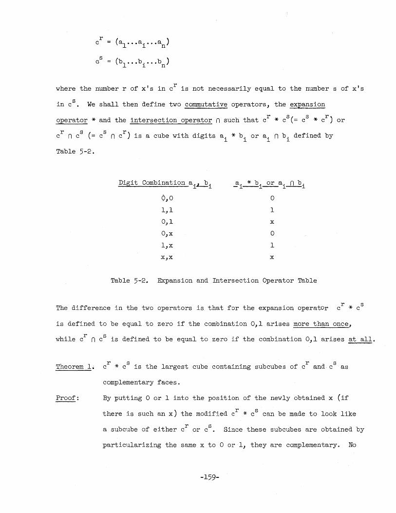
cr (al· ••• a .•.• a ) l n
CS
(blo .• b .•.• b ) l n
where the number r of x's in c r is not necessarily equal to the number s of x's
in c S• We shall then define two commutative operators, the expansion
operator * and the intersection operator n such that cr * cS (= CS * c
r) or
cr n CS (= C
S ncr) is a cube with digits a. * b. or a. n b. defined by l l l l
Table 5-2.
Digit Combination a . .L.E.. a. * b. or a. n b. l l -l----l---- l----l
0,0 ° 1,1 1
0,1 x
O,x ° l,x 1
x,x x
Table 5-2. Expansion and Intersection Operator Table
The difference in the two operators is that for the expansion operator cr * CS
is defined to be equal to zero if the combination 0,1 arises more than once,
while cr n CS is defined to be equal to zero if the combination 0,1 arises at all.
Theorem 1. cr * C
S is the largest cube containing subcubes of cr and CS as
Proof:
complementary faces.
By putting ° or 1 into the position of the newly obtained x (if
there is such an x) the modified cr * CS can be made to look like
a subcube of either cr or cs • Since these subcubes are obtained by
particularizing the same x to ° or-I, they are complementary. No
-159-
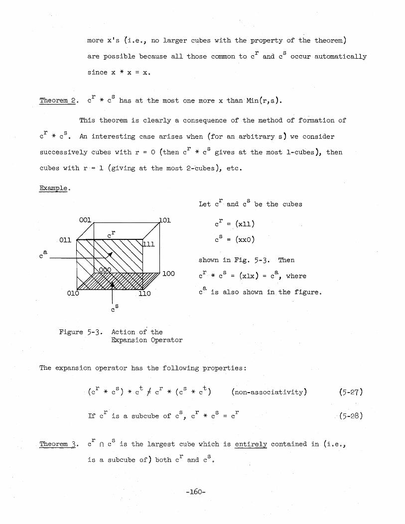
more XIS (i.e., no larger cubes with the property of the theorem)
are possible because all those common to cr and CS occur automatically
since x * x = x.
Theorem 2. cr * cS
has at the most one more x than Min (r, s.).
This theorem is clearly a consequence of the method of formation of
Cr * c S
._ () An interesting case arises when for an arbitrary s we consider
successively cubes with r = 0 (then cr * CS gives at the most I-cubes), then
cubes with r = 1 (giving at the most 2-cubes), etc.
Example.
a c
__ ------------~Ol
011
Let cr and CS be the cubes
cr (xlI)
c S = (xxo)
shown in Fig. 5-3. Then
100 cr * CS
= (xlx) = ca , where
s c
Figure 5-3. Action of the Expansion Operator
a c is also shown in the figure.
The expansion operator has the following properties:
(cr * cs ) * ct ~ r (s t) i c * c * c
r s r s If c is a subcube of c ,c * c
(non-associativity)
r c (5-28 )
Theorem 3. cr n cS is the largest cube which is entirely contained in (i.eo,
is a subcube of) both cr and CS
0
-160-
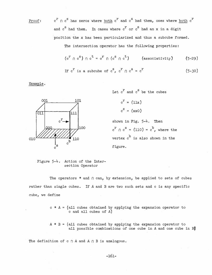
Proof:
Example ~
001
r s r s r c n c has zeros where both c and c had them, ones where both c
and CS had them. In cases where cr or C
S had an x in a digit
position the x has been particularized and thus a subcube formed.
s c
The intersection operator has the following properties:
r s r s If c is a subcube of c , c n c
(associativity)
r c
Let cr and CS be the cubes
shown in Fig. 5-4. Then
cr n C
S = (110) = cb
, where the
b vertex c is also shown in the
figure.
(5-29)
(5-30)
Figure 5-4. Action of the Intersection Operator
The operators * and n can, by extension, be applied to sets of cubes
rather than single cubes. If A and B are two such sets and c is any specific
cube, we define
c * A
A * B
{all cubes obtained by applying the expansion operator to c and all cubes of A}
{all cubes obtained by applying the expansion operator to all possible combinations of one cube inA and one cube in BJ
The definition of c n A and A n B is analogous.
-161-
5.3e2 COCYCLES
Suppose that we have a covering problem with an initial set of vertices
f giving rise to a cubical complex F. We found F in an example in 5.2.2 using
coface operators, but it is also apparent that one can use the expansion
operator, applying it first to all pairs of vertices (and the result being zero
if the pairs are not complementary!), then to pairs of I-cubes having the x in
the same position) etc. The reason for the success of the first step of this
process is, of course, that in our case Theorem 1 states that the result of the
expansion operator is "the largest cube containing the vertices as complementary
faces." Whatever our :procedure (i.e., E. or *) we shall end up with a great l
number of combinations and a great number of cubes, namely all cubes in Fp It
is, however, quite useless in a covering problem to have all cubes in F available:
we only want those which are not contained in larger cubes. A cube of F which
is not a subcube of a larger cube of F is called a cocyle. It is clear that the
minimum cost cover is a combination of cocycles.
We shall now indicate how the set Z of cocycles (consisting of the set
ZO of vertices not contained in I-cubes of F) the set Zl of I-cubes not con-
tained in· 2-cubes of F, etc.) can be found. It has become customary to
generalize the problem slightly by not giving f but an arbitrary initial cover
~ of f, not necessarily minimal: ~ is thus a collection of cubes covering
F without regard to cost.
The first step is to subtract from ~all of those cubes which are
contained in bigger cubes of DO (i.e., not bigger cubes of the complex formed
with the vertices of @ but cubes actually present in @)o Let D6 be the
set of these cubes contained in bigger·- cubes. We then form
o Let d be any O-cube left in DO.
-162-
Remark: D~ = (c/c C d; c,d € ~) in more abstract notation. This is read:
D~ is the set of cubes c such that (symbol: I) c is a subcube of d (symb61:
c C d) and both c and d belong (symbol: E) to ~.
Theorem 4. The O-cocycles are those O-cubes of DO which cannot be combined
with parts of higher order cubes of DO to form I-cubes.
Proof:
o 0/ 0 ~ Z = (d d * DO ~ any I-cube)
dO * DO forms at most 1.- cubes by Theorem 2. The set () above rules
out explicitly those dO,s which actually succeed in forming a I-cube;
i. e., none of the dO,s above have cofaces. This means that ZO c {}
since DO is certainly a cover and must therefore include all neces
sary O-cubes to cover f and, in particular, those in ZO which are
"unexpandable." Now assume that there is a dO in {}--say d for
short--which is not a cocycle. Then there is an E.-operator such l
that Eid = e, where e is a I-cube covered by DO. The complement
of d" which has been used to form e , must also be covered by DO" i"e",
d * DO must contain e: d should have been eliminated in the first
place! Hence all elements of () are cocycles.
We now form the union (or sum) of the set DO and DO * DO:
We again take away the set Dr of cubes of ~ contained in larger
cubes of ~and consider
Dr - {all O-cubes of (jJ
It is clear that Dl is not a cover of F = K(f) but that Dl U ZO is.
The question now arises whether Dl actually contains all I-cubes of
-163-
F (or their cofaces), so that we can search for Zl, i.,eo, all
l-cubes in F not contained in larger ones using Dl only., The
answer is given by
Theorem 50 Dl contains all the I-cubes of F or the cofaces of these cubes.
Proof: Suppose that a certain I-cube dl or its coface is in DO. Then by
definition of DI dl must also be in DI because it was not taken from
DO U DO * DO as a O-cube and if it was taken away inDf it was a
subcube of a larger cube which is still inDlo
I Now suppose that d was not in DO; then there are two comple-
1 mentary faces a and b which, together, form d and which are both
covered by DO. This means that DO contains two cubes a ~ a and
~ ~ b: DO * DO will then contain a * ~ which is a coface of dl
.,
The procedure for .finding ZO can now be extended to z~, Z2, etc." as
can Theorems 4 and 5. The iterative procedure is as follows: from D ·we form r
DUD * D r r r (5-31)
and
D 1 = 01
- D* 1 - {all 0-,1-, .• 0, (r-l)- and r-cubes of ·~l } r+~r+ ~
- (5-32)
where D;+l denotes all (r+l)-cubes contained in larger cubes OfS. The
(r+l)-cocycles are obtained from
r+l/ r+l -t.. ( ) {d d * D 1 ~ any. r+2 -cube} r+
where dr + 1 is a cube of D 1" This iteration is followed until D 1 is empty 0 r+ r+
It is usual to arrange the calculations of DO * DO' etc., in the form of tri
angular arrays as shown in the example below.
-164-
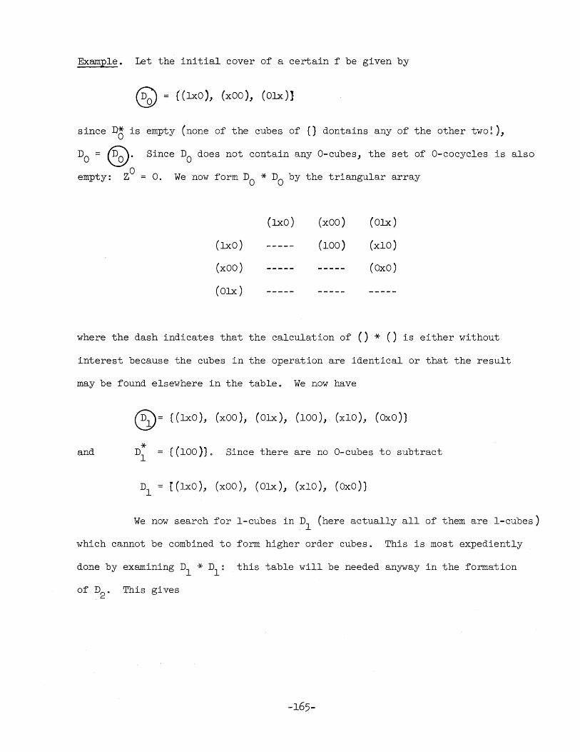
Example. Let the initial cover of a certain f be given by
~ = ((lxO), (xOO), (Olx)}
since DO is empty (none of the cubes of {} dontains any of the other two!),
DO =~. Since DO does not contain any O-cubes, the set of O-cocycles is also
empty: ZO = O. We now form DO * DO by the triangular array
(lxO)
(xOO)
(Olx)
(lxO) (xOO)
(100)
(Olx)
(xlO)
(OxO)
where the dash indicates that the calculation of () * () is either without
interest because the cubes in the operation are identical or that the result
may be found elsewhere in the tableo We now have
(5)= ((lxO), (xOO), (Olx), (100), (xlO), (OxO))
and ((100)). Since there are no O-cubes to subtract
Dl = r(lxO), (xOO), (Olx), (xlO), (OxO))
We now search for I-cubes in Dl (here actually all of them are I-cubes)
which cannot be combined to form higher order cubes. This is most expediently
done by examining DI * DI : this table will be needed anyway in the formation
of D2 " This gives
-165-
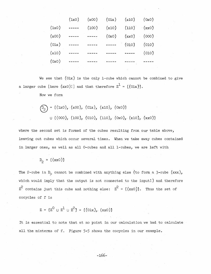
(lxO) (xOO) (Olx) (xlO) (OxO)
(lxO) (100) (xlO) (110) (xxO)
(xOO) (OxO) (xxO) (000)
(Olx) (010) (010)
(xlO) (010)
(OxO)
We see that (Olx) is the only I-cube which cannot be combined to give
a larger cube [here (xxO)!] and that therefore Zl = L! Olx)} .
Now we form
(§) :::: ((lxO), (xOO), (Olx), (xlO), (OxO))
u (( 000), (100), (010), (110)" (OxO), (xlO) J (xxO)}
where the second set is formed of the cubes resulting from our table above,
leaving out cubes which occur several times. When we take away cubes contained
in larger ones, as well as alIa-cubes and all I-cubes, we are left with
D2 :::: {(xxO))
The 2-cube in D2 cannot be combined with anything else (to form a 3-cube (xxx)~
which would imply that the output is not connected to the input·l) and therefore
Z2 contains just this cube and nothing else: Z2 = {(xxO)). Thus the set of
cocycles of f is
z { (Olx), (xxO)}
It is essential to note that at no point in our calculation we had to calculate
all the minterms of f. Figure 5-5 shows the cocycles in our example"
-166-
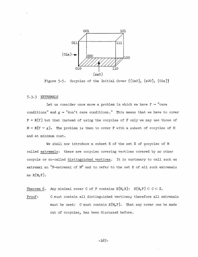
001 101
011
(Olx )---.
010 110
(xxO)
Figure 5-5. Cocycles of the Initial Cover ((lxO), (xOO), (Olx))
5.3.3 EXTREMALS
Let us consider once more a problem in which we have f " ~. care
conditions" and g ~ "don't care conditions." This means that we have to cover
F = K(f) but that instead of using the cocycles of F only we may use those of
M = K(f v g). The problem is then to cover F with a subset of cocycles of M
and at minimum cost.
We shall now introduce a subset E of the set Z of ~ocycles of M
called extremals: these are cocycles covering vertices covered by no other
cocycle or so-called distinguished. vertices 0 It is customary to call such an
extremal an rtF-extremal of M" and to refer to the set E of all such extremals
as E(M, F).
Theorem 6. Any minimal cover C of F contains E(M,R): E(M,F) C C c Z.
Proof: C must contain all distinguished vertices; therefore all extremals
must be used: C must containE(M,F). That any cover can be made
out of cocycles, has been discussed beforeo
-167-
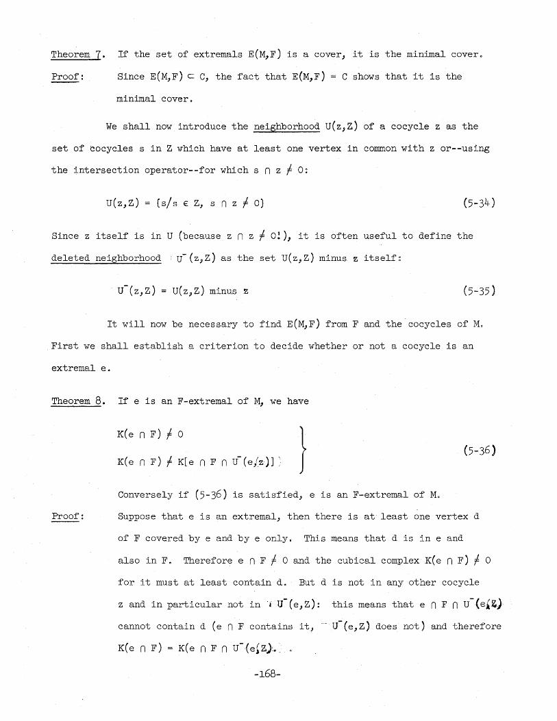
Theorem 7. If the set of extremals E(M,F) is a cover, it is the minimal covero
Proof: Since E(M,F) C C, the fact that E(M,F) = C shows that it is the
minimal covero
We shall now introduce the neighborhood U(z,Z) of a cocycle z as the
set of cocycles s in Z which have at least one vertex in common with z or--using
the intersection operator--for which s n z f 0:
U(z,Z) {sIs E Z, s n z f O} (5- 34)
Since z itself is in U (because z n z f O!), it is often useful to define the
deleted neighborhood ~. u- (z,Z) as the set U(z,Z) minus. z itself~
U(z,Z) minusz (5-35 )
It will now be necessary to findE(M,F) from F and the co cycles of M.
First we shall establish a criterion to decide whether or not a cocycle is an
extremal e.
Theorem 8. If e is an F-extremal of M, we have
K(e n F) f 0 } (5-36 ) K(e n F) f K[e n F n U- (e j z)] :'
Conversely if (5-36) is satisfied, e is an F-extremal of Mo
Proof: Suppose that e is an extremal, then there is at least one vertex d
of F covered by e and by e only. This means that d is in e and
also in F. Therefore e n F f 0 and the cubical complex K(e n F) f 0
for it must at least contain d. But d is not in any other cocycle
z and in particular not in OJ U- (e, Z): this means that e n F n U- (e'~J
cannot contain d (e n F contains it, U-(e,Z) does not) and therefore
K(e n F) = K(e n F n U-.(e~Z):~ ~ .
-168-
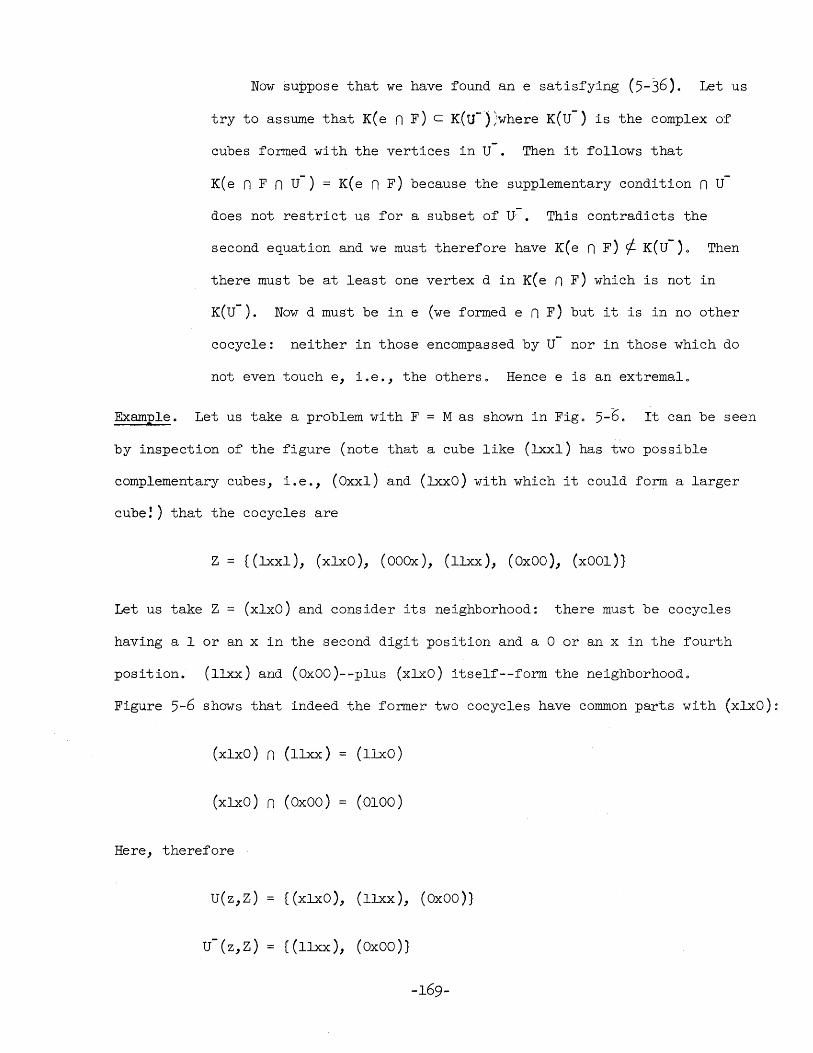
Now suppose that we have found an e satisfying (5-36). Let us
try to assume that K( e n F) C K(U-) ::where K(U-) is the complex of
cubes formed with the vertices in U-. Then it follows that
K(e n F n U-) = K(e n F) because the supplementary condition n U
does not restrict us for a subset of~. This contradicts the
second equation and we must therefore have K(e n F) ¢ K(U-)o Then
there must be at least one vertex d in K(e n F) which is not in
K(U-). Now d must be in e (we formed e n F) but it is in no other
cocycle: neither in those encompassed by U- nor in those which do
not even touch e, i.e., the others. Hence e is an extremalo
Example. Let us take a problem with F = M as shown in Figo 5-b. It can be seen
by inspection of the figure (note that a cube like (lxxl) has two possible
complementary cubes, i.e., (Oxxl) and (lxxO) with which it could form a larger
cube!) that the cocycles are
Z {(lxxl), (xlxO), (OOOx), (llxx), (OxOO), (xOOl)}
Let us take Z = (xlxO) and consider its neighborhood: there must be cocycles
having a 1 or an x in the second digit position and a 0 or an x in the fourth
position. (llxx) and (OxOO)--plus (xlxO) itself--form the neighborhood.
Figure 5-6 shows that indeed the former two cocycles have common part.s with (xlxO):
(xlxO) n (llxx ) (llxO)
(xlxO) n (OxOO) (0100 )
Here, therefore
U(z,Z) {(xlxO ), (llxx), (OxOO )}
U- (z, Z) { (llxx), (OxOO) }
-169-
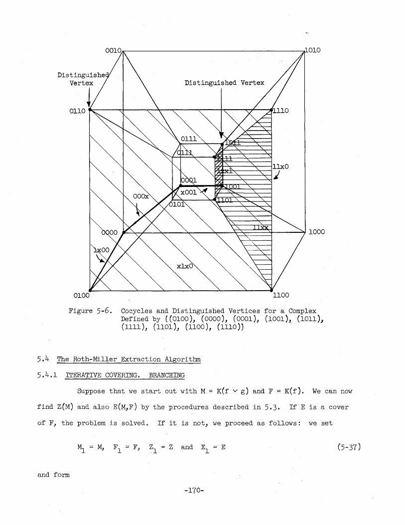
~--------------------------------------~010
Distinguished Vertex
0110~----~----~~--~----~---+~--~~--'
0100 1100
Figure 5-6. Cocycles and Distinguished Vertices for a Complex Defined by {(0100), (0000), (0001), (1001),,(1011), (1111), (1101), (1100), (1110))
5.4 The Roth-Miller Extraction Algorithm
5.401 ITERATIVE COVERING. BRANCHING
Suppose that we start out with M ~ K(f v g) and F = K(f). We can now
find Z(M) and also E(M,F) by the procedures described in 5~3. If E is a cover
of F, the problem is solved. If it is not, we proceed as follows: we set
and form
-170-
(these are the left-over cocycles) (5-38)
and F2 ; Fl - subcomplex covered by El
(5-39) K{left-over vertices}
Let u and v be cubes in ~ and consider u n F2 and v n F2 " Suppose that
u n F2 c v n F2, i.e., that as far as F2 is concerned, v covers all that is
covered by u. Furthermore suppose that cost u > cost v: then v is called a
nonmaximal cube and eliminated. In case the costs are equal, we shall still
retain the cube covering more of F2
0
Now we continue our process/setting
Z2 = ~- nonmaximal cubes (5-40)
~ = K(Z2) (5-41)
E2 = E(M2, F2 ) (5-42)
Continuing this operation we find El , E2, ... , until there are no further extremalso
If El U E2 U ... forms a cover of F, the problem is solved. Very often, however)
we do not attain a cover and yet there are no distinguished vertices left: this
is the so-called irreducible case. In such a case one examines the two covers
obtained by branching: the first branch assumes that one particular cocycle of
the remaining cocycles is in the cover, while the second branch assumes that it
is not ° The cost of the two branches is then compared and the lower cost one
chosen. It is, of course, quite possible to have multiple branching, i.eo,
branching within each branch.
Example 1. Using Fig. 5-6 we find that there are two distinguished vertices:
(1011) and (0101). We have seen that
-17l-
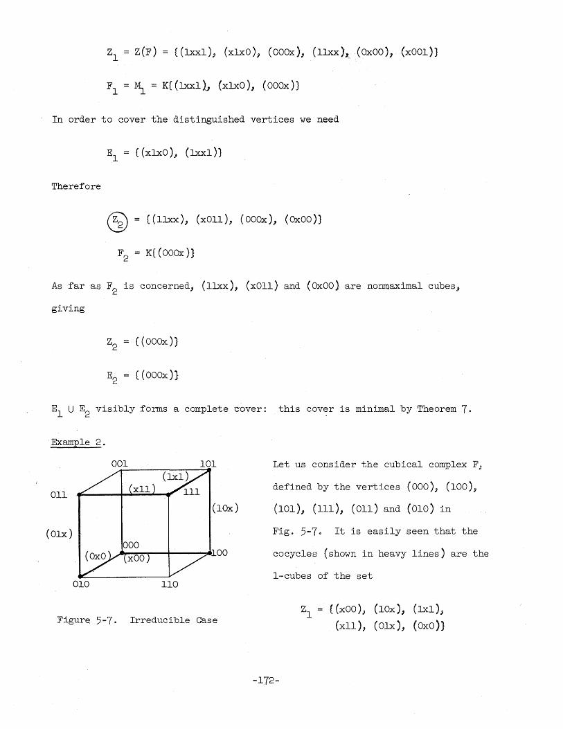
Zl = Z(F) = {(lxxl)J (xlxO), (OOOx), (llxx),: (OXOO), (x001))
Fl = ~ = K{ (lxxl1., (xlxO), (OOOx))
In order to cover the distinguished vertices we need
El = {(xlxO), (lxxl)}
Therefore
~ = {(llxx), (xOll), (OOOx), (OxOO)}
F 2 = K { ( OOOx ) }
As far as F2 is concerned, (llxx), (xOll) and (OxOO) are nonmaximal cubes,
giving
Z2 = {( OOOx ) )
E2 = {( OOOx ) }
El U E2 visibly forms a complete eover: this cover is minimal by Theorem 7.
Example 2.
001 101
011 (lOx)
(Olx) 000 ~~~--+-----~iOO
010 llO
Figure 5-7. Irreducible Case
Let us consider the cubical complex F3
defined by the vertices (000); (100)3
(101), (111), (011) and (010) in
Fig. 5-70 It is easily seen that the
cocycles (shown in heavy lines) are the
l-cubes of the set
-172-
Zl = {(xOO), (lOx); (lxl),
(xll), (Olx), (OxO)}
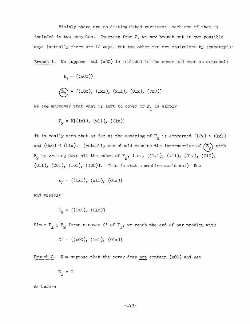
Visibly there are no distinguished vertices: each one of them is
included in two cocycles. Starting from Zi we now branch out in two possible
ways (actually there are 12 ways, but the other ten are equivalent by symmetry/~):
Branch 1. We suppose that (xOO) is included in the cover and even an extremal:
El {(xOO))
C§) = {(lax), (lxl), (xll), (Olx), Coxa)}
We see moreover that what is left to cover of Fl is simply
F2 = K{ (lxl), (xll), (Olx)}
It is easily seen that as far as the covering of F2 is concerned (lax) < (lxl)
and (OXO) < (Olx). (Actually one should examine the intersection of ~ with
F2 by writing down all the cubes of F2, i.e., {(lxl), (xll), (Olx), (010),
(all), (001), (101), (loa)}. This is what a machine would dO!) Now
Z2 {(lxl), (xll), (Olx)}
and visibly
Since El U E2 forms a cover Cf of Fl , we reach the end of our problem with
Cf = {(xOO), (lxl), (Olx)}
Branch 2. Now suppose that the cover does not contain (xOO) and set
As before
-173-
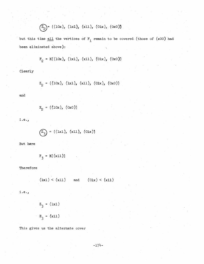
but this time all the vertices of Fl remain to be covered (those of (xOO) had
been eliminated above):
F2 = K{ (lOx), (lxl)) (xlI), (Olx), (OxO»)
Clearly
Z2 {(lOx), (lxl), (xll),(Olx), (Oxo))
and
E2 = {(lOx), (Oxo»)
i.e.,
(5) :;:: {(lxl), (xlI)., (Olx)}
But here
F 3 :;:: K{ (xIl)}
Therefore
(lxl) < (xlI) and (Olx) < (xlI)
i. e. J
E3 = (xlI)
This gives us the alternate cover
-174-
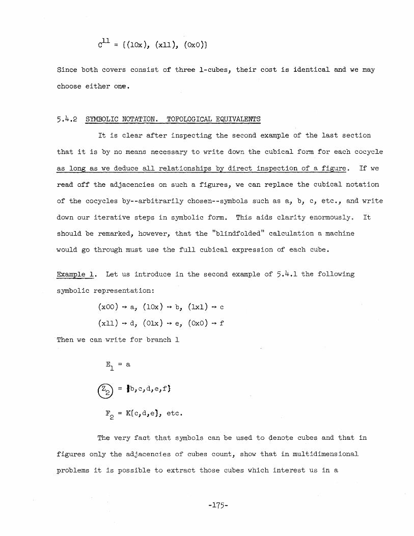
Cll ( (lOx) , (XII) , ( Ox 0 ) }
Since both covers consist of three I-cubes, their cost is identical and we may
choose either one.
5.4.2 SYMBOLIC NOTATION. TOPOLOGICAL EQUIVALENTS
It is clear after inspecting the second example of the last section
that it is by no means necessary to write down the cubical form for each cocycle
as long as we deduce all relationships by direct inspection of a figure. If we
read off the adjacencies on such a figures, we can replace the cubical notation
of the cocycles by--arbitrarily chosen--symbols such as a, b, c, etc., and write
down our iterative steps in symbolic form. This aids clarity enormously. It
should be remarked, however, that the "blindfolded" calculation a machine
would go through must use the full cubical expression of each cube.
Example 1. Let us introduce in the second example of 5.4.1 the following
symbolic representation:
(xOO) ~ a, (lOx) ~ b, (lxl) ~ c
(xlI) ~ d, (Olx) ~ e, (OxO) ~ f
Then we can write for branch 1
E :::;: a 1
F2 :::;: K(c,d,e}, etc.
The very fact that symbols can be used to denote cubes and that in
figures only the adjacencies of cubes count, show that in multidimensional
problems it is possible to extract those cubes which interest us in a
-175-

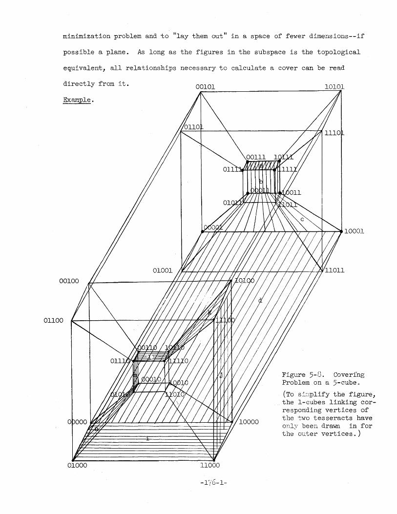
minimization problem and to "lay them out" in a space of fewer dimE;nsions--ii'
possible a plane. As long as the figures in the subspace is the topological
equivalent, all relationships necessary to calculate a cover can be read
directly from it. 00101 10101
Example.
00100
01100
01000 11000
Figure 5-0. Coverfng Problem on a 5-cubeo
(To s ij~lplify the figure, the I-cubes linking corresponding vertices of the two tesseracts have on1 \'. been drawn in for the' outer vertices.)
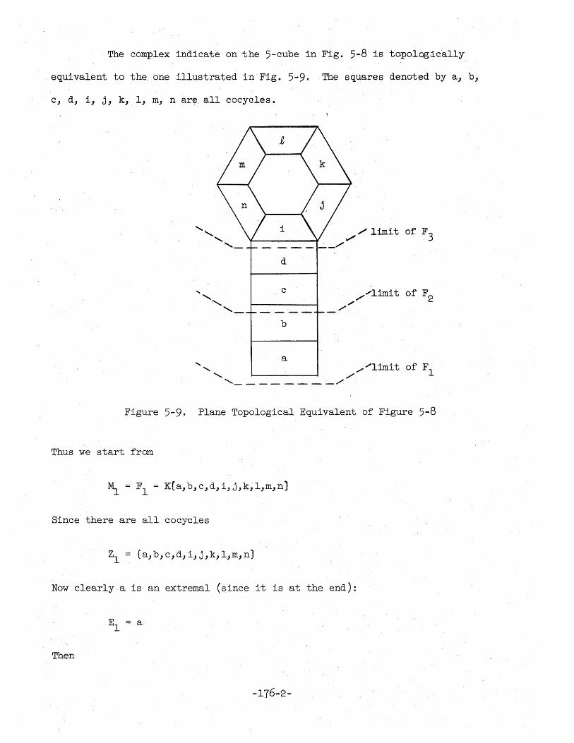
The complex indicate on the 5-cube in Fig. 5-8 is topolOgically
equivalent to the. one illustrated in Fig. 5-9. The squares denoted by a) b,
c, d, i, j) k, 1) m, n are all cocycles.
.// limit of F 3 -----"" d
c
b
a " ",,"'limit of FI
.......... "" ,-------_/
Figure 5-9. Plane Topological Equivalent of Figure 5-8
Thus we start from
Since there are all cocycles
Now clearly a is an extremal (since it is at the end):
Then
and
As far as F2 is concerned b < c and
Z2 = (c,d,i,j,k,l,m,n)
But this makes c an extremal:
~2 = c;
Now
But again, as far as F3 is concerned, d < c and
This is now an irreducible case: the remaining cocycles form a sort of ring
and we must branch. Following the general branching procedure, we find
Branch 1. Assume that i is in the cover, i.e.,
E3 i
C§) Z - i = 3
(j,k,l,m,n)
F4 K{k,l,m}
Clearly
-176-3-
j < k, n < m
and
Now
C9 = {I)
But F5 = 0 since all is covered, and we obtain a cover
Branch 2. Here we assume that i is not in the cover. Then
E = 0 3
Consequently
Since j and n are now at the end
Removing n,j from Z4' we find
,..176-4-
This means that k < 1 and m< 1 and
and
E ::; 1 5
It is also clear that the sum of all extremals gives a cover
1 11 Again the 'cost of the two covers C and C is identical. We can choose either
one.
5~4.3o THE ROTH-MILLER EXTRACTION ALGORITHM
Whether we program a machine in order to perform the iterative steps
or whether we examine by inspection a topologically equivalent figure' using a
symbolic notation, the steps we have to perform always 'follow the same pattern.
This is described by Roth and Miller as follows:
We start with (Ml,Fl ) and form Zl(Ml ), E1;(Ml,Fl ). Then(§) ::;Zl - El
is formed as well as F2 ::; Fl - complex covered by El and after the elimination
of nonmaximal cubes Z2 ::; ~ - nonmaximal cubes is formed. This process is
iterated until either a complete cover is obtained or until branching is neces-
sary_ Formally the step r ~r + l is as follows:
,1. Z is known as well as F. In case extremals exist, we find E • r r r
2. We form
-176-5~
Fr+l ; Fr - cubes covered by Er; K (vertices in F r
vertices covered by E} r (5-44 )
Zr+l = ~ - nonmaximal cubes. with respect to Fr+l
E ; extremals of Z r+l r+l
(5-46)
3. If there are no extremals, we branch by comparing:
3a.
3b.
Assume a given cocycle, a, of Z is part of the cover. We set r
E ::c a and form r
Z r
E r
We have to cover the complex F minus the cubes covered by a; call r
this Fl 10 r+ We eliminate nonmaximal cubes from Z 1 and examine Zl r+ r+l
for extremals 0 This brings us back to a ste'p like 2 or 3.
Assume cocycle a above is not part of the cover.
and form (as above)
We set E r
o
11 This time, however, we have to cover F 1; F since no simplification r+ r
has been obtained in the preceeding stepo This will give us aZll r+l
which differs from Zl above, but we are also back to steps like r+l
2 or 3.
5.4.4 THE SHARP OPERATOR (SUBTRACTION OPERATOR)
The reader may have noted that in the formation of F 1 from F by r+ r
the use of (5-44) we had to fall back on an explicit enumeration of "left-over
vertices" in order to form the new complex. This is highly undesirable~ in
the calculation of cocycles we already formulated a method which starts with
-176-6- ) /
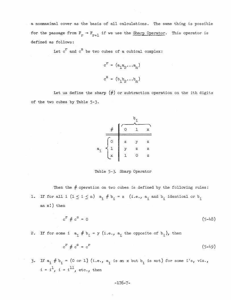
a nonmaximal cover as the basis of all calculations. The same thing is possible
for the passage from F ~F 1 if we use the Sharp Operator. This operator is r r+
defined as follows:
Let cr and cS be two cubes of a cubical complex:
Let us define the sharp (#) or subtraction operation on the ith digits
of the two cubes by Table 5-3.
b. l ,----A---,
# 0 1 x
ro z y z
a. -< 1 y z Z l
Lx 1 0 z
Table 5-3. Sharp Operator
Then the # operation on two cubes is defined by the following rules:
1. If for all i (1 ~ i ~ n) a. # b. = z (i.e., a. and b. identical or b. l l l l l
an x!) then
r #c
s 0 (5-48) c
2. If for some i a. # b. Y (i.e., a. the oppos i te of b.), then l l l l
r #c
s r (5 .. 49) c = c
3. If a. # b. = (0 or 1) (i.e., a. is an x but b. is not) for some i's, viz., l l l l
. .1. .11 t th l = l , l = l ,e co, en
-176-7-
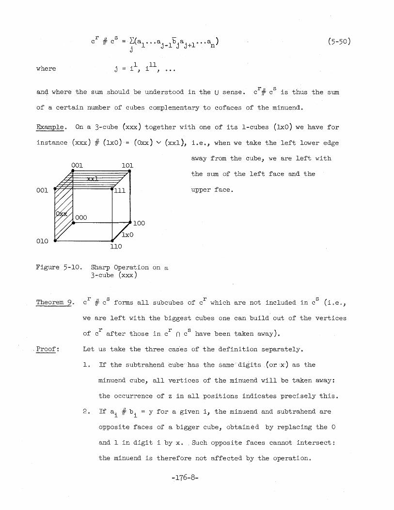
where
l:( a l .... a. . 11) . a. 1 0 •• a ) . J- J J+ . n J
. .1 J ::; l , .11 l ,
(5-50)
anq where the sum should be understood in the U sense. cr # CS is thus the sum
of a certain number of cubes complementary to cofaces of the minuend.
Example. On a 3-cube (xxx) together with one of its I-cubes (lxO) we have for
instance (xxx) # (lxO)'::; (Oxx) v (xxI), i.eo, when we take the left lower edge
away from the cube, we are left with 001 101
the sum of the left face and the
001 III upper face.
000 ---------+--~100
010 110
Figure 5-100 Sharp Operation on a 3-cube (xxx)
Theorem 9. cr # c S forms all subcubes of cr which are not included in C
S (ioeo)
we are left with the biggest cubes one can build out of the vertices
f r ft th . r s h b t k ) o c a er ose In c n cave een a en away 0
, Proof ~ Let us take the three cas'es of the definition separately ..
1. If the subtrahend 'cube'has the same" digits, (or. :x') as the
minuend cube, all vertices of the minuend will be taken away:
the occurrence of z in all positions indicates precisely this.
2. If a. # b. ::; y for a given i, the minuend and subtrahend are l l
opposite faces of a bigger cube, obtained by replacing the 0
and 1 in digit i by x .. Such opposite faces cannot intersect:
the minuend is therefore not affected by the operation.
-176-8-
3, If a a or 1 occurs, there was an x-digit in the minuend: the
operation forms the other face (complement in the digit position!)
of the bigger cube (~to x in position i) still left over. For
several XIS, we take the sum of all complementary cubes.
The sharp operator has the following properties:
r #c
s r if r s 0 (5-51) c c c n c
r #c
s c c r (5-52 ) c
r #c
s f s # c
r (5-53) c c
(cr
# cs
) # c t
(cr
# cs
) U (cs
# ct
) (5-54 ) :::;
(cr # Cs ) # c t f cr # (cs # c t) (5-55)
(cr # c,s) # c t :::; (c r #ct ) #cs (5-56)
The proof of these properties follows more or less immediately from
the definition of the sharp operator. Note that (5-56) can be generalized by
saying: it is allowed to subtract a set of cubes in any order from a given
cube--no brackets have to be used and (cl
# c2
) # c3 •.. can be written
c1 # c2 # c3 ·
The F ~ F 1 step is now described by r r+
Theorem 10. If F K(cl,o .• ,cn } r
and E :::; (el,o .• ,em} then r
cl # e l # e2 e ill
F :::; K c2 #el # e2 I/=e r+l
-176-9-
m (5-57)
Proof: cl # e l # e2 00 a # em contains all vertices of cl not contained
in theextremals eloooemo Hence by the definition of Kthe right
hand side equals F . I" r+
Let us now introduce some further definitions:
20 Let
Then by definition
cOl # Cl
Co # Cl = c
O2 # Cl
cOn # Cl
Now we simply write
F = K{F # E } r+l r r
The sharp operator is useful too when we want to decide on the
equivalence of two covers because we have
Theorem II. Two covers Co and Cl cover the same complex if and only if
Proof: Co # Cl contains all vertices of Co not in Cl
and Cl
# Co all
vertices of Cl not in COo
-176-10-
(5-58)
(5-59)
5.5 Partially Ordered Sets
1. DEFINITION OF POSETS
Sets can be totally ordered ("toset"), partially ordered ("poset")
or unordered: it is, of course, necessary to define the relationship with
respect to which ordering occurs. ~_amples will illustrate the three cases .
. E4amFle 1. The peights of mountains inside the continental confines of the
U. S. A. can be totally ordered by the relationship "higher than" or "lower
than."
Example 2. The successive generations of a family can be ordered by the
relationship "is a descendant of,. I' Figure 5-11 shows a family tree: it is
what is called later on a "Hasse diagram" of the poset in question.
-177-
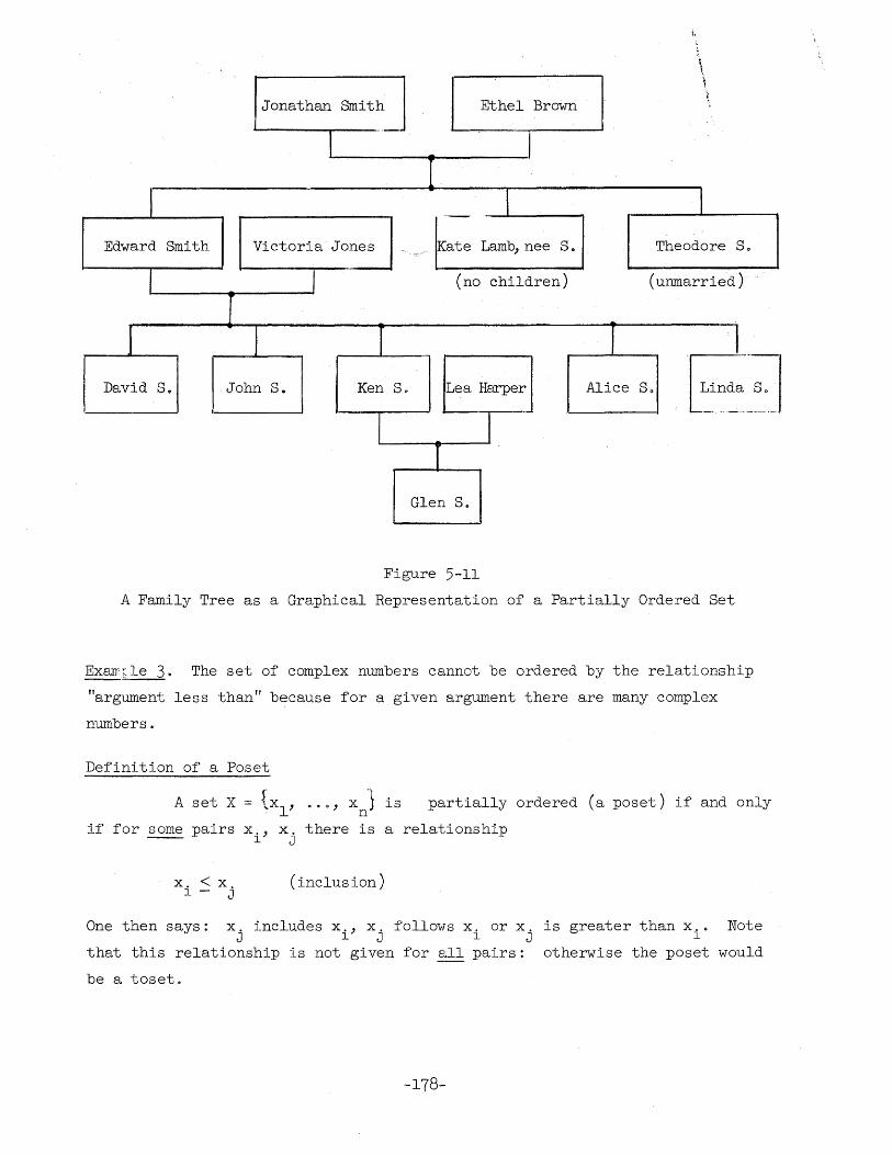
\
I I ,
Jonathan Smith Ethel Brown i.
--I I
I l I --
Edward Smith Victoria Jones ~ate Lamb, nee S. Theodore So ._/
I I (no children) (unmarried)
J
J f I ~-.-David S. John S. Ken So Lea Harper Alice So ~i~~~_ So __
I I
Glen So
Figure 5-11 A Family Tree as a Graphical Representation of a Partially Ordered Set
EXaIT;le 3. The set of complex numbers cannot be ordered by the relationship
"argument less than" because for a given argument there are many complex
numbers.
Definition of a Poset
A set X = (Xl' .. 0' Xn"} is partially ordered (a poset) if and only
if for some pairs Xi' Xj there is a relationship
x. < X l - j
(inclusion)
One then says: x. includes x., x. follows x. or x. is greater than X.. Note J l J l J l
that this relationship is not given for all pairs: otherwise the poset would
be a toset.
-178-
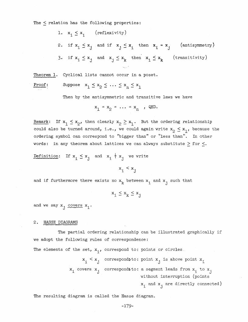
The < relation has the following properties:
1. x. < x. l - l
(reflexivity)
2. if x. < x. and if x. < x. then x. ; X. l - J J - l l J
(antisymmetry)
3. if x. < x. l - J
and then xi:: xk (transitivity)
Theorem 1. Cyclical lists cannot occur in a poset.
Proof:
Then by the antisymmetric and transitive laws we have
x ,QED. n
Remark: If xl :s x2 ' then clearly x2 .:: xl. But the ordering relationship
could also be turned around, i.e., we could again write x2 ~ xl' because the
ordering symbol can correspond to "bigger than" or "less than". In other
words: in any theorem about lattices we can always substitute> for <.
Definition: If x. < x. and x. f x. we write l - J l J
x. < X. l J
and if furthermore there exists no xk between Xi and Xj such that
and we say x. covers x .. J l
2 • HASSE DIAGRAMS
x.<Xk<x. l - - J
The partial ordering relationship can be illustrated graphically if
we adopt the following rules of correspondence:
The elements of the set, x. J correspond to: points or circles l
correspond)to: point x. is above point x. J l
correspondsto: a segment leads from x. to X. l J
x. covers ~x. l J
without interruption (points
x. and x. are directly connected) l J
The resulting diagram is called the Hasse diagram.
-179-
Remark: Note that if an element x. covers x.~ they cannot both be covered by l J
an element k nor can they both cover such an element. Suppose that k covers x. . l
(which covers x.): J
Then k > x. > X., i.e., x. is between kand Xj and conse-l J l
quently k cannot cover x .. In the Hasse Diagram this means that no triangles J
can occur. More generally: if xi covers Xj there cannot be any side-branch
(passing through more than one element) leading from x. to X.O l J
Example. Take all functions of two Boolean variables xl' x2 as was shown in
$ection 5.1. They can be written in the form
Let fl r(al , bl
, cl ' dl
)
f2 f(a2, b2
, c2 ' d2
)
then fl :s f2 is defined as meaning that
1. fl . f 2 fl
or 2. fl v f2 = f 2
As was shown in Chapter 3 these two definitions are mutually con
sistent and one follows from the other.
The corresponding Hasse diagram is then as shown in Figure 5-120
-180-
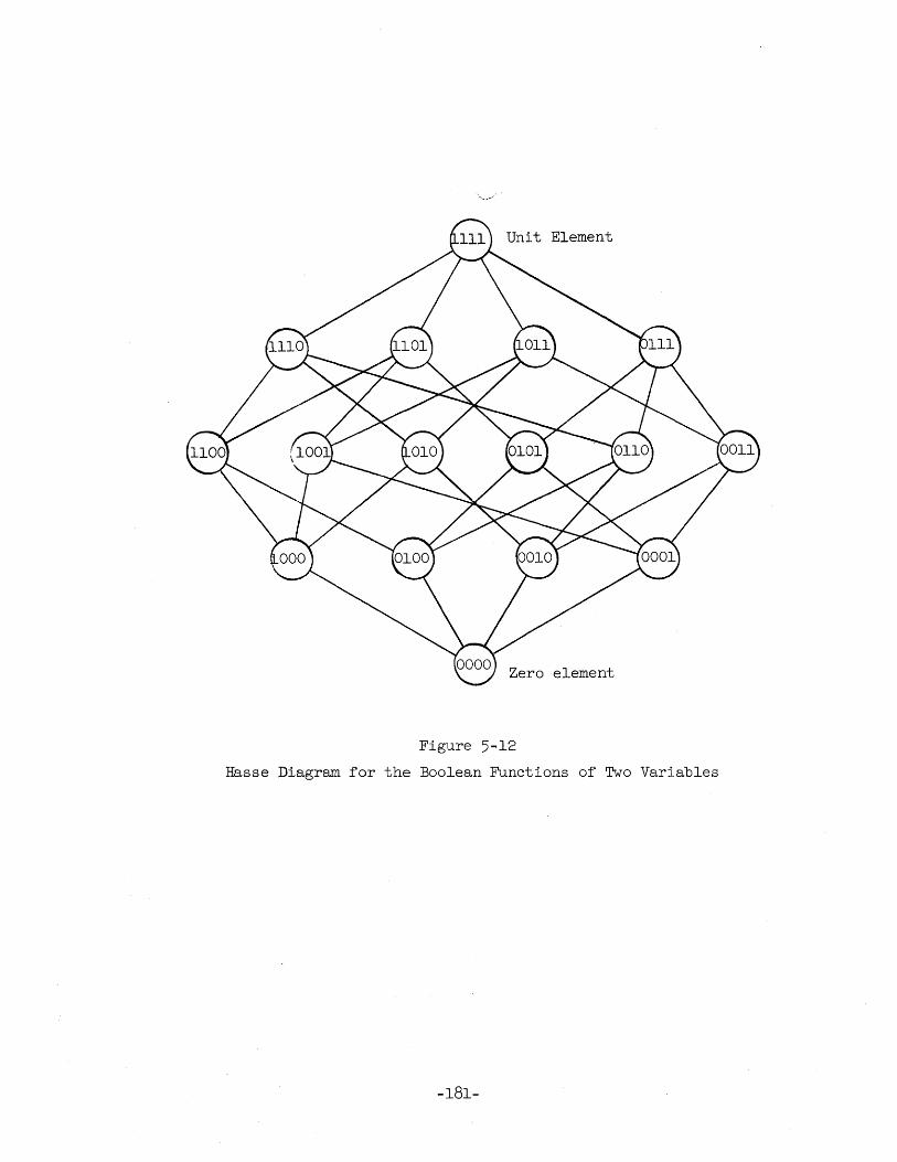
Unit Element
Zero element
Figure 5-12
Hasse Diagram for the Boolean Functions of Two Variables
-181-
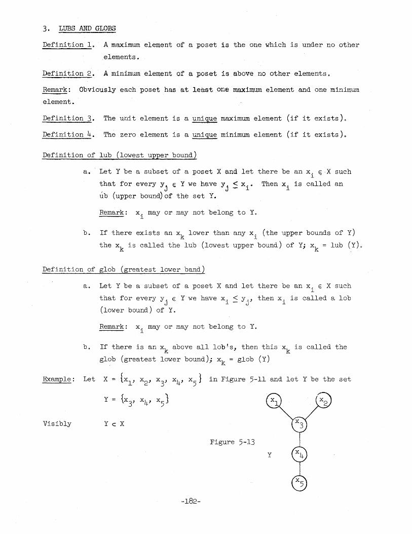
3. LUBS AND GLOBS
Definition 1. A maximum element of a poset is the one which is under no other
elements.
Definition 2. A minimum element of aposet is above no other elements.
Remark: Obviously each poset has at leas~ one maximum element and one minimum
element.
Definition 3. The unit element is a unisue maximum element (if it exists)o
Definition 4. The zero element is a unique minimum element (if it exists)o
Definition of lub (lowest upper bound)
a. Let Y be a subset of a poset X and let there be an xi ~·X such
that for every y. E Y we have Yj
< x .• Then x. is called an I J - 1 1
ub (upper bound) of the set Y.
Remark: x. mayor may not belong to Y. 1
b. If there exists an xk
lower than any xi (the upper bounds of Y)
the xk
is called the lub (lowest upper bound) of Y; xk
= lub (Y).
Definition of glob (greatest lower band)
a. Let Y be a subset of a poset X and let there be an x. E X such 1
that for every y. E Y we have x. < Y., then x. is called a lob J 1 - J 1
(lower bound) of Y.
Remark: x. mayor may not belong to Y. 1
b. If there is an xk
above all lob~s, then this xk
is called the
glob (greatest lower bound); xk = glob (Y)
Example: Let X = {Xl' x2 ' x3, x4' X
5} in Figure 5-11 and let Y be the set
Visibly Y c X
Figure 5-13
-182-
Here xl x2 and X3 are upper bounds of Y. The lub is x3 and here
belongs to Y. The glob of Y is clearly x5
. Note that this poset has a zero
(namely x5
) but no unit: There are two maximum elements.
Remark: The lub and glob of a subset Y of a poset X are unique if they exist.
This stems from the fact that if xl and''-~2 for example are both lubs, xl :::: x2 and x2 ~ xl' i.e., xl = x2 ·
5.6 Lattices
1. DEFINITION OF LATTICES
Defini tion L A lattice is a poset in which every arbitrary pair x., x. has a l J
Def:inition 2.
,Theorem 1.
Proof:
lub and a glob, i.e., there are two other elements of the lattice
Xu and x ~ such that
x. < x } x t ::: xi } l - u and x. <x x~ < x. -l U - J-
and there are no lower x 's and no higher x ~ , s . u
This of that ". " " going down" in a means, course, gOlng up or
Hasse diagram for a lattice, we shall converge, for any pair of
points, on a ",single' nearest common point" both above and below.
An example is visibly furnished by all 'Switching functions of two
variables as shown in Figure 5-12.
We shall introduce the symbols U and n (not to be confused
at this stage with v and A) by the following
lub (x., x.) l J
glob (xi' x j )
x. U X. l J
x. (\ X. l J
} (5-60)
If x. V x. (or x. A x.) equals one of the factors for all i, j, the l J l J
paset is a totally ordered set (toset).
Suppose for instance that
x = x. U x. = lub (x., x.) i l J l J
This implies that x. < x. by the definition of lub; thus for all l J
i, j either x. > x. or x. < x., hence the elements are totally l - J l - J
ordered. -183-
Theorem 20 In a lattice L each finite subset Y has a lub and a glob.,
Pt90f: The proof can be given by ind~ction:
1. Suppose Y1 = t~1; then visibly glob Yl ::;: lub Y1 = ~, ioe.,
the .theorem holds.
2. Suppose Y2 = lXlc
, xk+1l, then by" the ·defin1 tion of a lattice,
the theorem is satisfied.
3. Suppose Yn ::;: {xk
, .•• 0, ~+n} and suppose that the theorem.
holds for this Y , i.e., that lub (Y ) ::;: xk
i and glob (Y ) ::;: n n + n
xk+j
exist. Let
Yn+l {Yn, xk+n+l }
then clearly
lub (Yn+l ) ::;: lub (lub Y, xk 1) n +n+
Since xk
. and xk
1 are elements of L, the lub exists by the +l +n+
definition of a lattice. Similarly glob (Y 1)::;: glob (g1obY , n+ n x ) exists and thus the theorem is true for all n, hence it
k+n+l is true for all lattices.
Theorem 3. Every finite lattice contains a unit and a zero.
Proof: By the definition of L we have a lub for all pairs of elements of
L, and by an iterative process we clearly can find an element
which is a lub of all elements of L. This element satisfies the
requirements of a unit. By 'simila:r reasoning,' one can show that a
zero element exists ..
It is quite obvious from the definition of lub and glob that
we have
o () x. O} l
0 U x. x. l l
1 n x. Xi} l
1 U x. 1 l
-184-
2. PROPERTIES OF LATTICES
In. eV.ery lattice the following identities hold for the glob and lub
operations:
L xi U Xj : Xj V xi }
and x. " x.. - x. (\ X. 1 J 1 1
2 . (x i U x j) U xk
and x. n (x. () xk
) 1 J
3. x. (l x. = x. U x. = Xl' 1 1 1 1
':,. . .,... ..
4. (x. n x.) U x. = x. = (x. V x.) f\ X. 1 J 1 1 1 J 1
(5-64 )
(5-66)
All of these properties are nearly self-evident except (5-66): from the definition of a glob we have
x. () x. < X. 1 J - 1
hence (x. n x.) V x. = lub [glob (x., x.), x.] = lub (x., x.) = X. 1 J 1 1 J 1 11 1
Remark: It will be shown later that a Boolean Algebra is a special type of
lattice if V and n operations correspond to the OR and AND operations respec
tively.
Theorem 4. Any set in which two operations U and ~ are defined and satisfy
properties (5-63) to (5-66) is a lattice.
Proof: Let us define the ".:S" relation by
x. < x. if and only if x. U x. = X. 1 - J 1 J J
Now we have to show that the poset postulates hold for the <
relation as defined and furthermore that glob (x., x.) = x. n x. 1 J 1 J
and lub (x., x.) = x. U x . with respect to this relationo 1 J 1 J
Effectively we have
1. Refl exi ti vi ty: x. < x. since x. tJ x. = X. 1 - 1 1 1 1
2. Antisyrnmetry: x. < x. and x. <x. imply that 1 - J J - 1
X. U x. = x. and x. UX. = X. 1 J J J 1 1
-185-
x. lJ x. = x. U X., hence l J J ~
3. Transitivity:
Let x. < x. ' and Xj: < xk
implying that x. U x. = X. l - J-~' -, l J J
and that Xj U xk = Xklt By property (5-64) we can
write
x. U xk
= x. V (x U Xk
) = (x. U x.) U xk
= x. U xk = x l l j l J J l{
but this implies that xi S xk
' thus transitivity holds.
for the relation.
Now consider that
x. V (x. V x.) l l J
(x. U x.) U x = x. U X. l l j l J
but this implies that x. < x. U X. l - l J
and x. < x. u x. J - l J
hence x V x. is an upper bound of (x., x.). It remains to be i J l J
shown that x. U x. is actually the lub; let xk
be another upper l J
bound of x., x., i.e., 1 J
implying that
and
Then we have
(x. U x.) V xk
= x. V (x. V xk
) l J l J
hence from the definition of "<"
x.ux.<xk l J -
i . e., x. U x. is lower than any other upper bound xk
' hence it is l J
the 1 ub of t x ., x.). The proof of the theorem can be completed by l J
using similar arguments to show that
xi n Xj = glob (xi' x j )
-186-
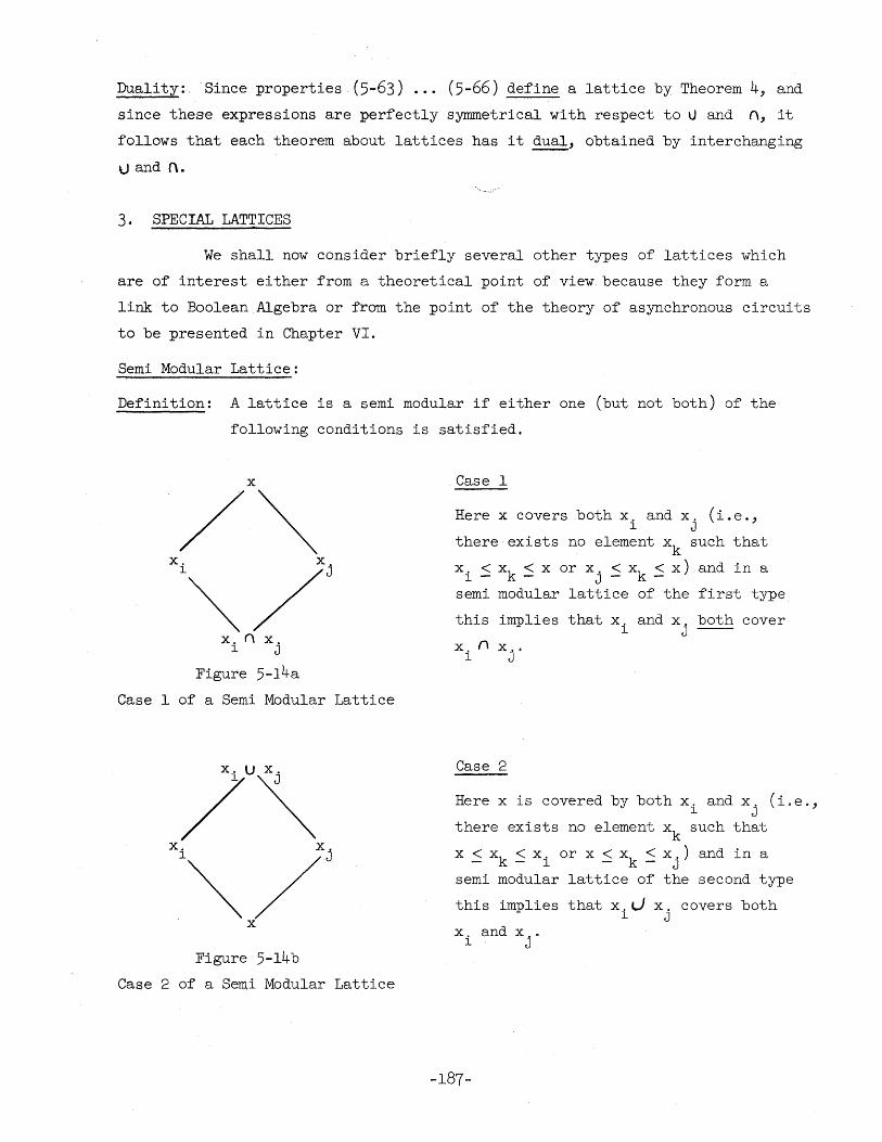
Duality:. Since properties (5-63) ... (5-66) define a lattice by Theorem 4, and
since thes'e expressions are perfectly symmetrical with respect to U and n, it
follows that each theorem about lattices has it dual, obtained by interchanging
U and n.
3. SPECIAL LATTICES
We shall now consider briefly several other types of lattices which
are of interest either from a theoretical point of view because they form a
link to Boolean Algebra or from the point of the theory of asynchronous circuits
to be presented in Chapter VI.
Semi Modular Lattice:
Definition: A lattice is a semi modular if either one (but not both) of the
following conditions is satisfied.
x
/~ Xi~/j
x. () x. l J
Figure 5-14a
Case 1 of a Semi Modular Lattice
Figure 5-l4b
Case 2 of a Semi Modular Lattice
Case 1
Here x covers both x. and x. (i.e., l J
there exists no element xk
such that
x. < xk < x or x. < xk < x) and in a l - - J - -
semi modular lattice of the first type
this implies that x. and x. both cover l J
x n x .. i J
Case 2
Here x is covered by both x. and x. (i.e., l J
there exists no element xk
such that
x < xk < x. or x < xk
< x.) and in a - - l - - J
semi modular lattice of the second type
this implies that x.LI x. covers both l J
x. and x .. l J
-187-
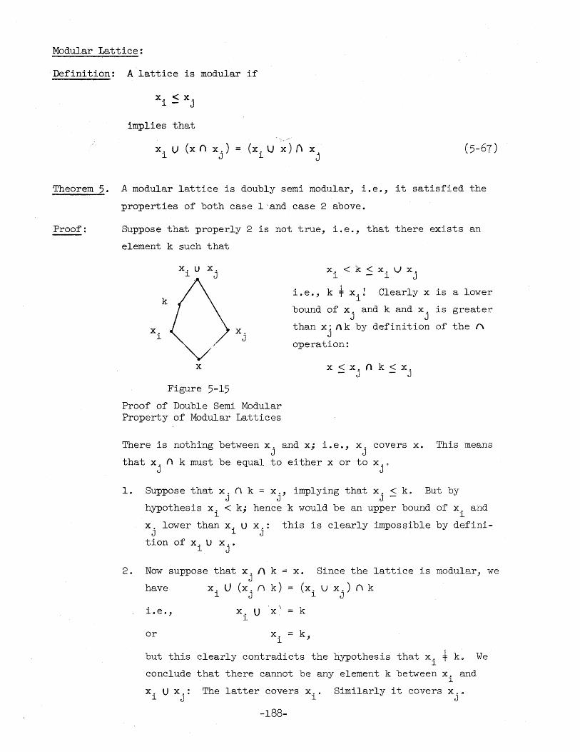
Modular Lattice:
Definition: A lattice is modular if
x. <: x. 1 - J
implies that
x. U (x() x.) = (x. U x){'\ X 1 J 1 j
(5-67)
Theorem 5. A modular lattice is doubly semi modular, i.e., it satisfied the
properties of both case 1 'and case 2 above.
Proof: Suppose that properly 2 is not true, i.e., that there exists an
element k such that
X. 1
k
x
Figure 5-15
x. J
i. e.,
x. < k < x. V X. 1 - 1 J
k t x.! 1
Clearly x is a lower
bound of x. and k and x. is greater J J
than x: Il k by definition of the" J
operation:
x < x. fl k < x. - J J
Proof of Double Semi Modular Property of Modular Lattices
There is nothing between x. and x; i.e., x. covers x. This means J J
that x. n k must be equal to either x or to x .. J J
1.
2.
Suppose that x. (\ k = x., implying that x. < k. But by J J J -
hypothesis x. < k; hence k would be an upper bound of x. and 1 1
x. lower than x. U x.: this is clearly impossible by defini,-J 1 J
tion of x. U x .. 1 J
Now suppose that x. () k = x. J
Since the lattice is modular, we
have
i. e.,
or
x. U (x. (\ k) 1 J
X. 1
(x. U x.) (\ k 1 J
k
k,
but this clearly contradicts the hypothesis that x. t ko We 1
conclude that there cannot be any element k between x. and 1
x. U x.: 1 J
The latter covers x .. 1
-188-
Similarly it covers x.o J
Distributive Lattice:
Definition: For a distributive lattice we have be definition
x. n· (x. U Xk
) = (x. n x.) U (xi r\ Xk
) 1 J 1 J
(5-68)
(Note similarity of this equation and the distributive property
of a Boolean Algebra when tr~ · and \J ~ v).
Theorem 6. Ina distributive lattice
Proof:
x. V (x. () xk
) = (x. U x.) (\ (x. U xk
) 1 J 1 J 1
(5-69)
and conversely: if a lattice has this property, then it is a
distributive lattice.
by (5-66)
:;: x. lJ [(x. n xk
) U (x. (\ xk
)] 1 1 J
by (5-64)
x. U [xk
{\ (x. V x. ) ] 1 1 J
[(x. U x.) n x.] V lXk n (x. U x. ) ] 1 J 1 1 J
by (5-66)
(x. V x.) ('\ (x. U xk
) 1 J 1
QED.
4. COMPLEMENTED LATTICES AND BOOLEAN ALGEBRA
Definition: In a lattice with 0 and 1 (e.g., every finite l.attice) ~ comple--ment x. of x. is defined by
1 1
x. U X. 1 1
x.- n x. 1 1
(5-68)
Example: The lattice of all subsets of a set is a complemented lattice as we
have seen in Chapter 3 in the discussion of Venn Diagrams.
-189-
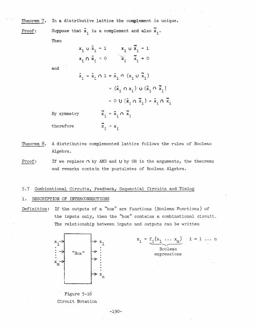
Theorem 7. In a distributive lattice the complement is unique.
Proof: Suppose that i. is a comple~ent and also x .• l l
Then
and
x. U l
xi ()
x. l
By symmetry
therefore
x. l
x. l
x. l
1
0
(\1 =
=
x. l
x. l
-x. U x. = 1 l l
-. '-:-...-, -x. x. = 0
l l
- n (x. lJ ~. ) x. l l l
(i. () x. ) l l
u (i. () l
~. ) l
0 (i. () i. ) x.A -\J = x. l l l l
x. (\ ,."
x. l l
x. l
Theorem 8. A distributive complemented lattice follows the rules of Boolean
Algebra.
Proof: If we replace n by AND and U by OR in the arguments, the theorems
and remarks contain the postulates of Boolean Algebra.
5.7 Combinational Circuits,' Feedback,; Sequential Circuits and."Timing
1. DESCRIPTION OF INTERCONNECTIONS
Definition: If the outputs of a "box" are functions (Boolean Functions) of
the inputs only, then the "box" contains a combinational circuit 0
The relationship between inputs and outputs can be written
"Box"
~z n
Figure 5-16 Circuit Notation
-l90-
z. l
f.(xl
000 x) i- 1 0 O. n ~ m~. _______ r
Boolean expressions
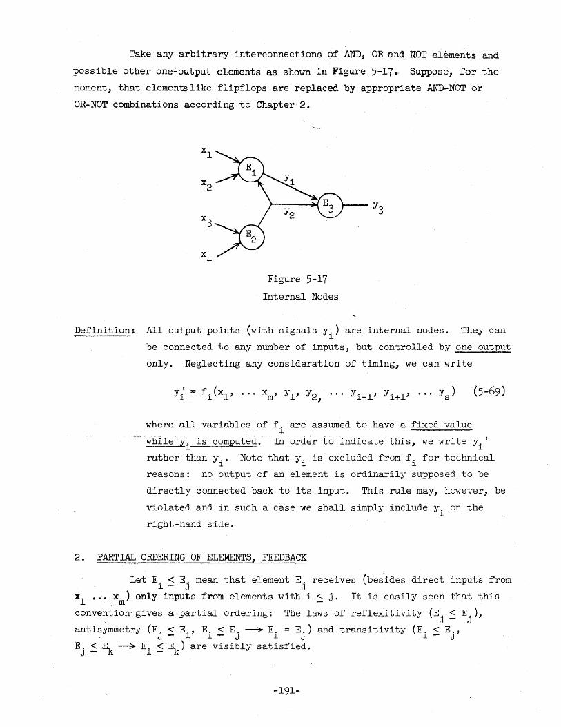
Take any arbitrary interconnections of AND, OR and NOT elements and
possible other one;;'output elements as shown in Figu:re 5-17., Suppose, for the
moment, that elements like flipflops are replaced by appropriate AND-NOT or
OR-NOT combinations according to Chapter 20
Figure 5-17 Internal Nodes
Definition: All output points (with signals y.) are internal nodes. They can l
be connected to any number of inputs, but controlled by one output
only. Neglecting any consideration of timing, we can write
y.' l
f. (Xl' 0'. X , Yl' Y2 . .. y. l' y. l' .•. y ) l m , l- l+ S
where all variables of f. are assumed to have a fixed value l
(5-69)
while y. is computed.' . In order to 'indicate this, we write y. I -------l l
rather than y.. Note that y. is excluded from f. for technical l l l
reasons: no output of an element is ordinarily supposed to be
directly connected back to its input. This rule may, however, be
violated and in such a case we shall simply include y. on the l
right-hand side.
2. PARTIAL ORDERING OF ELEMENTS, FEEDBACK
Let E. < E. mean that element E. receives (besides direct inputs from l - J J
Xl ••• ,Xm) only inputs from elements with i ::: j. It is easily seen that this
convention- gives a partial ordering: The laws of reflexitivity (E. < E.), J - J
antisymmetry (E. < E., E. < E. --7 E. = E.) , J l l J l J
and transitivity (E. < E., l - J
E. < Ek ~ E. < Ek ) are visibly satisfied. J - l -
-191-
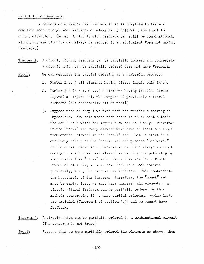
Definition of Feedback
A network of elements has feedback if it is possible to trace a
complete loop through some sequence of elements by following the input to
output direction. (Note: A circuit with feedback can still be combinational,
although these circuits can always be reduced to an equivalent form not having
feedback. )
Theorem 1. A circuit without feedback can be partially ordered and conversely
a circuit which can be partially ordered does not have feedback.
Proof: We can describe the partial ordering as a numbering process:
1. Number 1 to j all elements having direct inputs only (x's).
2. Number j+n (n = 1,2 .00) n elements having (besides direct
inputs) as inputs only the outputs of previously numbered
elements (not necessarily all of them!)
3. Suppose that at step k we find that the further numbering is
impossible 0 Now this means that there is no element outside
the set 1 to k which has inputs from one to k only. Therefore
in the "non-k" set every element must have at least one input
from another element in the "non-k" set. Let us start in an
arbitrary node p of the "non-k" set and proceed "backwards"
in the out-in direction. Because we can find always an input
coming from a "non-k" set element we can trace a path step by
step inside this "non-k" set. Since this set has a finite
number of elements, we must come back to a node covered
previously, ioe., the circuit has feedback. This contradicts
the hypothesis of the theorem: therefore, the "non-k" set
must be empty, i.eo, we must have numbered all elements: a
circuit without feedback can be partially ordered by this
method; conversely, if we have partial ordering} cyclic lists
are excluded (Theorem 1 of section 505) and we cannot have
feedback.
Theorem 2. A circuit which can be partially ordered is a combinational circuit.
(The converse is not true.)
Proof: Suppose that we have partially ordered the elements as above; then
-192-
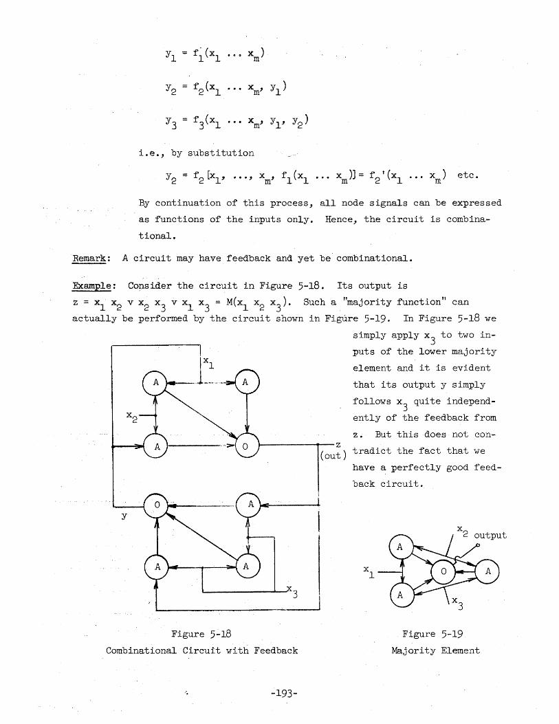
i.e., by substitution
By continuation of this process, all node signals can be expressed
as functions of the inputs only. Hence, the circuit is combina
tional.
Remark: A circuit may have feedback and yet be combinational.
Example: Consider the circuit in Figure 5-18. Its output is
Z = Xl x2 v x2 x3 v Xl x3 = M(xI x2 X3
). Such a "majority function" can
actually be performed by the circuit shown in Figure 5-19. In Figure 5-18 we
simply apply X3 to two in
puts of the lower majority
element and it is evident
that its output y simply
follows x3 quite independ
ently of the feedback from
z.. But this does not con-1------...-- Z
(out) tradict the fact that we
y
Figure 5-18 Combinational Circuit with Feedback
... -193-
have a perfectly good feed
back circuit.
Figure 5-19 Majority Element
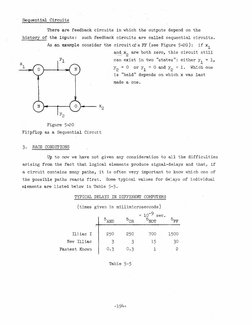
Sequential Circuits
There are feedback circuits in which the outputs depend on the
history of the inputs: such feedback circuits are called sequential circuits.
x 1
As an example consider the circuit of a FF (see Figure 5-20) ~ if xl
Figure 5-20
q.!1:~/x2 are both zero, this circuit still
can exist in two "states": either Yl
= 1,
Y2 = 0 or Yl = 0 and Y2 = 10 Which one
is "held" depends on which x was last
made a one.
Flipflop as a Sequential Circuit
3. RACE CONDITIONS
Up to now we have not given any consideration to all the difficulties
arising from the fact that logical elements produce signal-delays and that, if
a circuit contains many paths, it is often very important to know which one of
the possible paths reacts first. Some typical values for delays of individual
elements are listed below in Table 5-5.
TYPICAL DELAYS IN DIFFERENT COMPUTERS
(times given in millimicroseconds)
10-9 sec o
° AND °OR °NOT OFF
Illiac I
New Illiac
Fastest Known
250
3
0.3
250
3
0.3
Table 5-5
-194-
700
15
1
1500
30 2
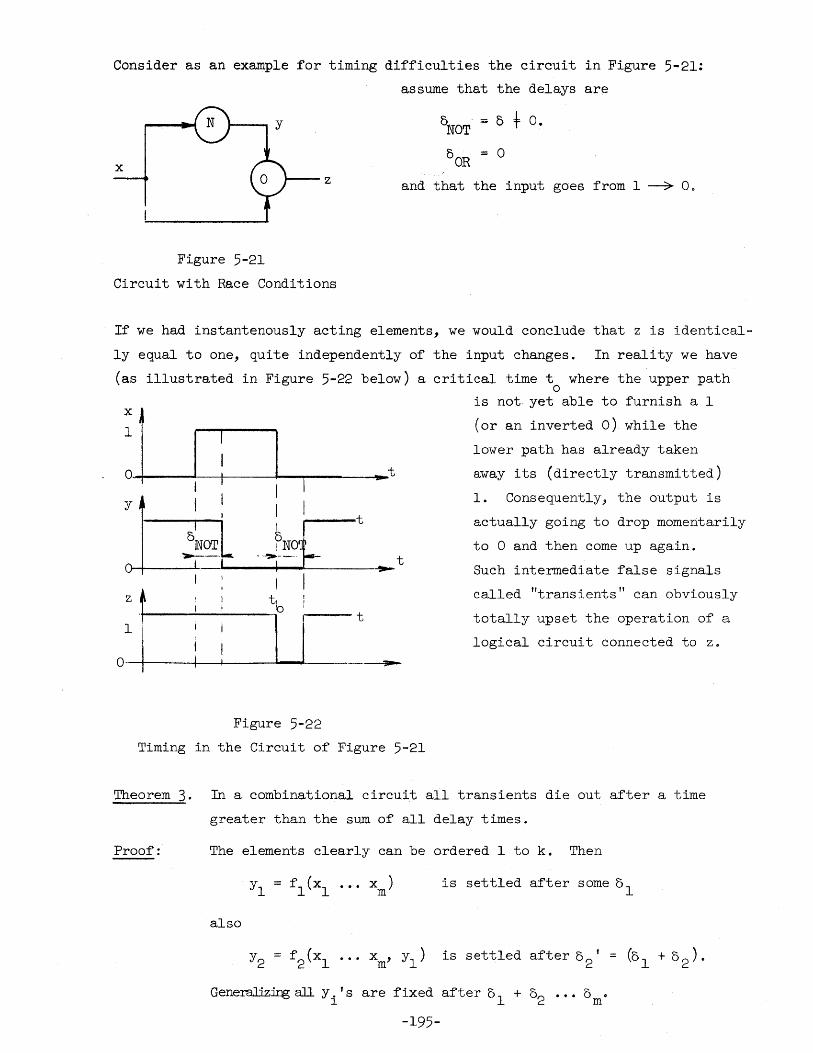
Consider as an example for timing difficulties the circuit in Figure 5-21:
assume that the delays are
5 f O.
= 0 x
z and that the input goes from 1 ---7 O.
Figure 5-21
Circuit with Race Conditions
If we had instantenously acting elements, we would conclude that z is identical
ly equal to one, quite independently of the input changes. In reality we have
(as illustrated in Figure 5-22 below) a critical time t where the upper path o
X is not yet able to furnish a 1
(or an inverted 0) while the I
1 I lower path has already taken
away its (directly transmitted) I
0 I t I I I I Jjl I I
~orL I
I I .~O~,.
I I I I
t
t ......
1. Consequently, the output is
actually going to drop momentarily
to 0 and then come up again.
Such intermediate false signals
called "transients" can obviously
totally upset the operation of a
logical circuit connected to z.
I
z t tl \:)
t
] I
0
1
I I
Figure 5-22
Timing in the Circuit of Figure 5-21
Theorem 3. In a combinational circuit all transients die out after a time
greater than the sum of all delay times.
Proof: The elements clearly can be ordered 1 to k. Then
Y 1 = f I (Xl ••• xm) is settled after some 01
also
Generalizing all Y i f S are fixed after 01 + O2 .•• 0 m 0
-195-
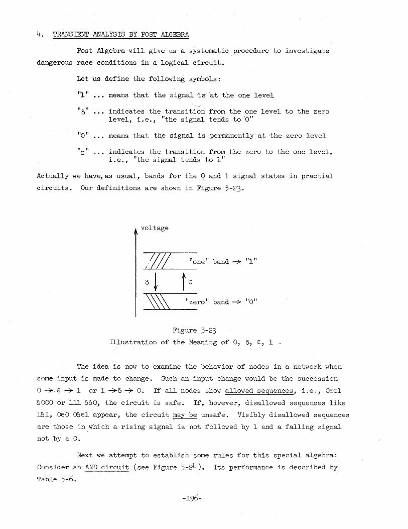
4. TRANSIENT ANALYSIS BY POST ALGEBRA
Post Algebra will give us a systematic procedure to investigate
dangerous race conditions in a logical circuit.
Let us define the following symbols:
"1" means that the signal-is 'at the one level
"0" indicates the transition from the one level to the zero level, i.e., "the signal tends to '0"
"0" means that the signal· is permanently at the zero level
"E: " _ indicates the trans i tion from the zero to the one level, i.e., "the signal tends to 1"
Actually we hav~as usual, bands for the a and 1 signal states in practial
circuits. Our definitions are shown in Figure 5-23.
voltage
?l!J II " one band ~ "1"
o ! tE
'\'\\ "zero" band ~ "0"
Figure 5-23 Illustration of the Meaning of 0, 0, E:, 1
The idea is now to examine the behavior of nodes in a network when
some input is made to change. Such an input change would be the succession
a ~s ~ 1 or 1 -70 -7 O. If all nodes show allowed sequences, i.eo, OEE:l
5000 or III 050, the circuit is safe. If, however, disallowed sequences like
151, OE:O 05E:l appear, the circui~ may be unsafe. Visibly disallowed sequences
are those in which a rising signal is not followed by 1 and a falling signal
not by a O.
Next we attempt to establish some rules for this special algebra:
Consider an AND circuit (see Figure 5-24). Its performance is described by
Table 5-6.
-196-
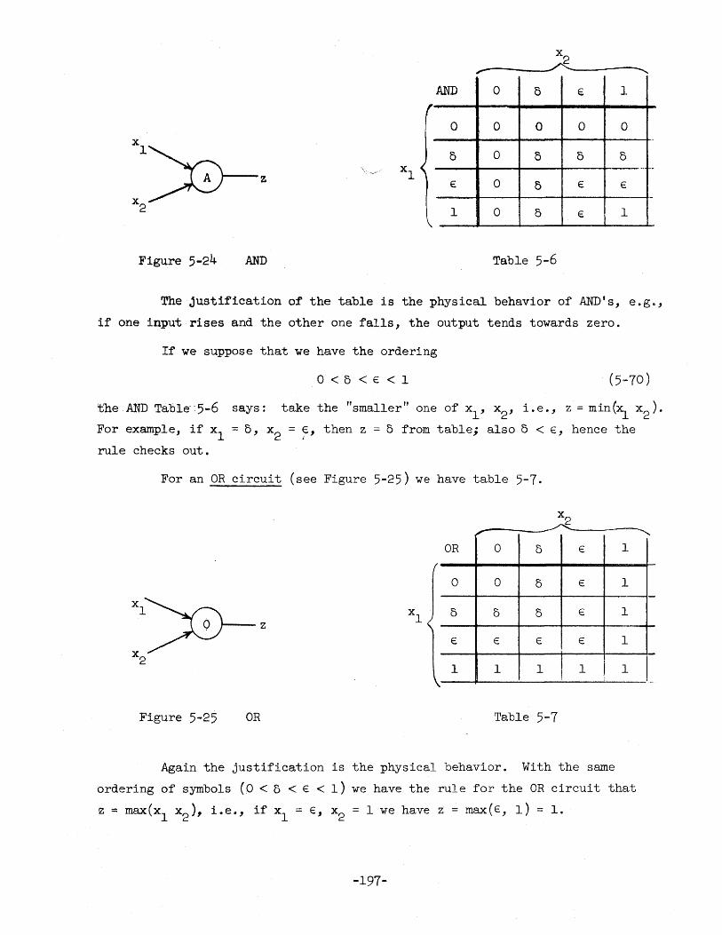
X2
,----------~---------" AND 0 0 E: 1 ,
0 0 0 a 0
0 0 0 0 5 ~~ ...
z € 0 0 € €
I 0 0 € I
Figure 5-24 AND Table 5-6
The justification of the table is the physical behavior of AND's, e.ge,
if one input rises and the other one falls, the output tends towards zero.
If we suppose that we have the ordering
0<5<E<1 (5-70)
the AND Tab1.eoo 5-6 says: take the "smaller" one of Xl' x2 ' i.e., z = min(x:t x2 ).
For example, if Xl = 5, x2 = ~, then z = 5 from table; also 5 < E, hence the
rule checks out.
For an OR circuit (see Figure 5-25) we have table 5-7.
, -OR 0 5 E I
/
0 0 5 E I .0_-
5 5 5 E I
€ E E E I
I I I ! I ! I
Figure 5-25 OR Table 5-7
Again the justification is the physical behavior. With the same
ordering of symbols (0 < 5 < E < I) we have the rule for the OR circuit that
Z = max(x1 x2 ), i.e., if Xl = E, x2 = I we have z = ma.x(E, 1) = 1.
-197-
, -0
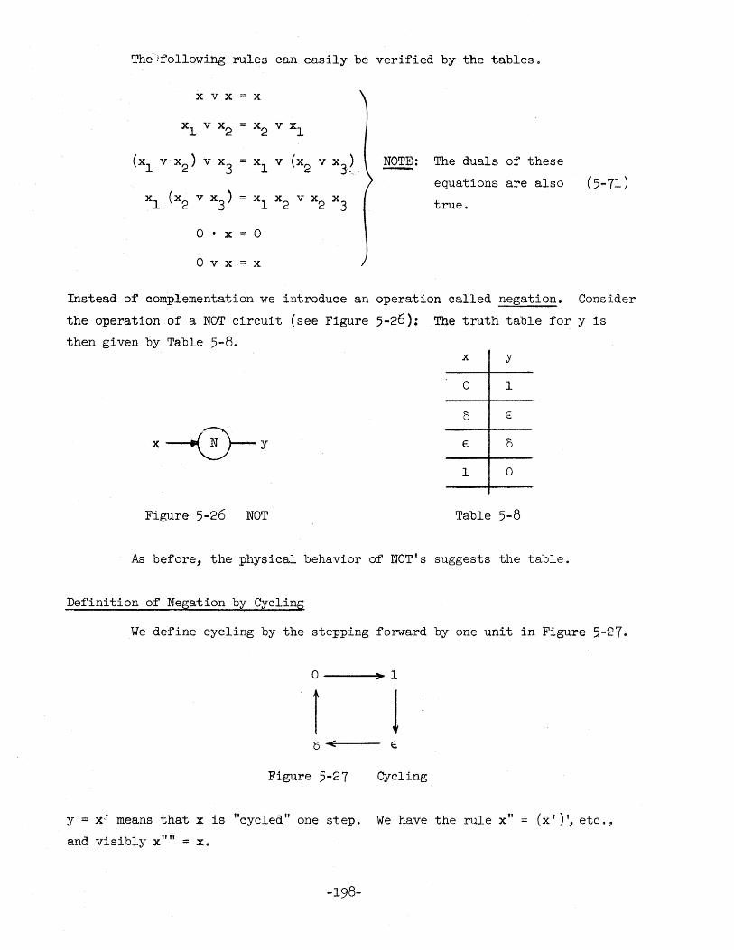
Thejfollowihg rules can easily be verified by the tables.
x v x = x
(Xl v x2 ) v x3 xl v (x2 v x3J
xl (x2 v x3 ) = xl x2 v x2 x3
o · X = a
o v x = x
NOTE: The duals of these -equations are also
true.
(5-71 )
Instead of complementation we introduce an operation called negation. Consider
the operation of a NOT circuit (see Figure 5-26): The truth table for y is
then given by Table 5-8. x y
a 1
6 E
x--0- y €
1 a
Figure 5-26 NOT Table 5-8
As before, the physical behavior of NOT's suggests the table.
Definition of Negation by Cycling
We define cycling by the stepping forward by one unit in Figure 5-27.
a > I
I 1 6 < €
Figure 5 .. 27 Cycling
y = x" means that x is "cycled" one step. We have the rule x" = (x I )', etc.,
and visibly x"" = x.
-198-
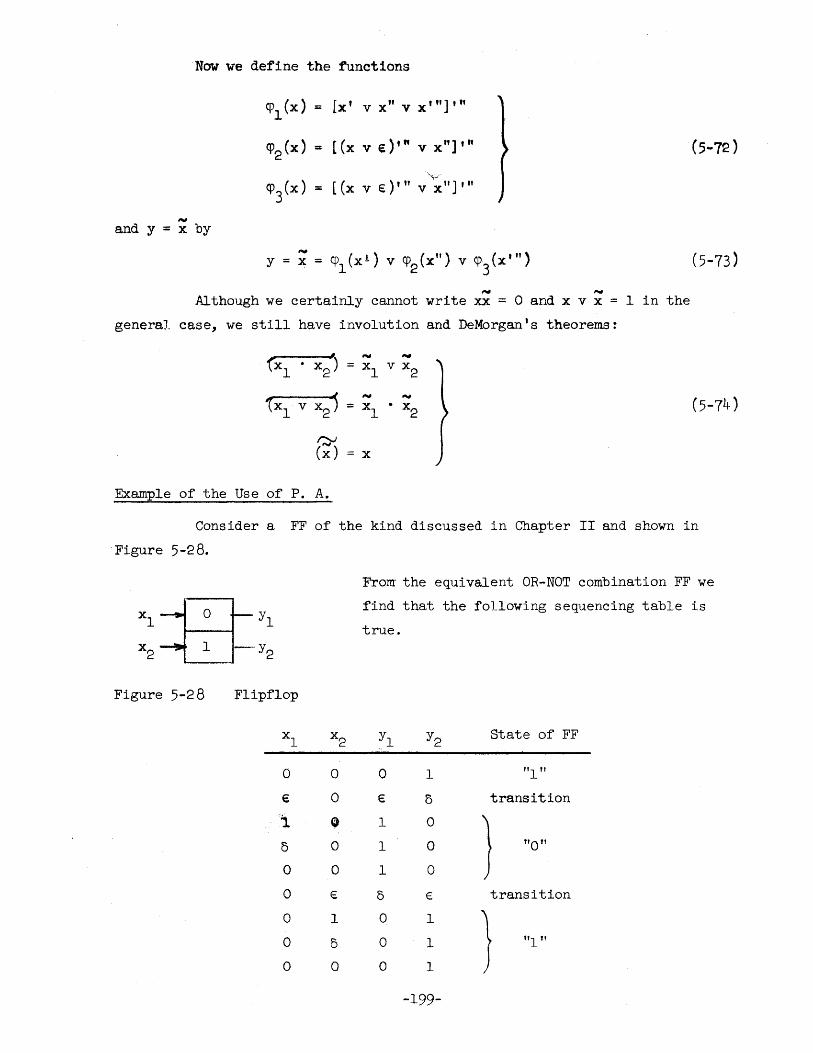
Now we define the functions
'PI (x) = Ix' v x" v X·,,],·f
-and y = x by
~ ,... Although we certainly cannot write xx = 0 and x v x = 1 in the
general case, we still have involution and DeMorgan's theorems:
tXI x2
') - ..., . xl v x
2
1Xl v x2~ - -= xl . x2 (5-74 )
~
(~) = x
Example of the Use of P. A.
Consider a FF of the kind discussed in Chapter II and shown in
. Figure 5 -28.
Figure 5-28 Flipflop
o e
1-o o a
a
o o
X2
0
0
0 0
0
€
1
5
0
From the equivalent OR-NOT combination FF we
:find that the following sequencing table is
true.
~l Y2 State of FF
0 1 "1 tI
€ 0 transition
1 0
} 1 0 "0"
1 0
0 E transition
0 1 } 0 1 "1 "
0 1
-199-
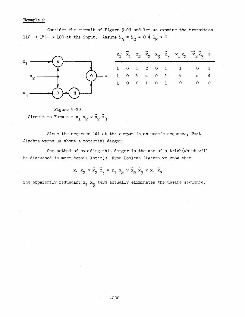
Example 2
Consider the circuit of Figure 5-29 and let us examine the transition
110 -? 150 -? 100 at the input. Assume 5 A = 50 :: 0 + oN > 0
- - .I'WI -~/
1 xl x2 x2 x3 x3 xl x2 x 2 x
3 xl
1 0 1 0 0 1 1 0
x2 z 1 0 5 € 0 1 5 E
1 0 0 1 0 1 0 0
X3
Figure 5-29 Circuit to Form z = xl x2 v x2 x3
Since the sequence l~l at the output is an unsafe sequence, Post
Algebra warns us about a potential danger 0
One method of avoiding this danger is the use of a trick(which will
be discussed in more detail later):: From Boolean Algebra we know that
The apparently redundant xl X3 term actually eliminates the unsafe sequence.
-200-
z
1
E
0
Bibliography for Cha.pter V·
(in chronological order)
1. E. L. Post: "Introduction to a General Theory of Elementary Propos1t1ons"o AJM 43 (163-185) (1921)
\' 2. B. L. Vander Waerden: "Modern Algebra". Springer. (1931)
3. G. Birkhoff: "Lattice Theory", American Mathematical Society Colloquium Publication, Vol. 25 (1948)
4. G. Birkhoff and S. MacLane: "A Survey of Modern Algebra". Macmillan. (1948)
5. M. L. Dubreil-Jacotin, L. Lesieur, R. Croisot: "The'orie des Trei11is des Structures Alge'briques Ordonn~es et des Treillis Ge'ometriques". GauthierVillars. (1953)
6. H. Hermes: "Einf"uhrung in die Verbandstheorie". Springer. (1955)
7. G. A. Metze: "Many-Valued Logic and the Design of Switching Circuits"o Master's Thesis at University of Illinois. (1955)
8. E. J. McCluskey, Jr.: "Minimiz.ation of Boolean Functions". BSTJ 35/6 (Nov. 1956)
9. S. H. Caldwell: " Swi tching Circuits and Logical Des ign" • Wiley. (1958)
10. D. E. Muller. Lecture Notes for "University of illinois Math-EE 391"0 ("Boolean Algebras with Applications to Computer Circuits I") (1958)
11. J. P. Roth: Systems, I". (July 1958)
"Algebraic Topological Methods for the Synthesis of Switching Transactions of the American Mathematical Society, 88/2
12. J. P. Roth: "Algebraic Topological Methods in Synthesis". Proceedings of an Intern. Symposium on the Theory of Switching" Vol. 29, Annals of Computation Laboratory of Harvard University (1959)
13. T. H. Matt, Jr.: "Determination of the Irredundant Normal Forms of a Truth Function by Iterated Consensus of the Prime Implicants". IRE Transactions on EC, Vol. 9. (1960 )
14. R. E. Miller: "Switching Theory and Logical Design of Automatic Digital Computer Circuits". IBM Report Rc-473 (1961) Also, equivalent ··~riiversity of Illinois Math-EE 394 Lecture Notes". (1960)
15. F. E. Hohn. Lecture Notes for "University of Illinois Math-EE 391"0 (Boolean Algebras with Applications to Computer Circuits I") (1958)

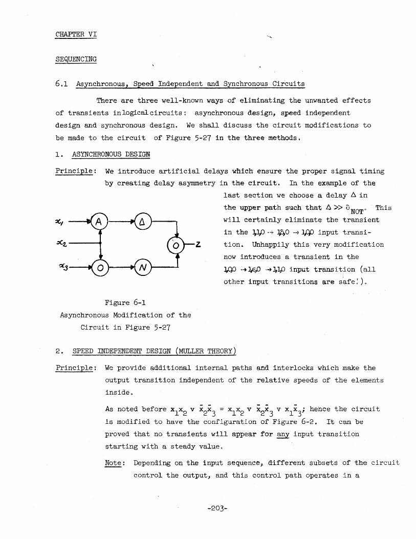
CHAPTER VI " ....
SEQUENCING
6.1 Asynchronous, Speed Independent and Synchronous Circuits
There are three well-known ways of eliminating the unwanted effects
of transients inlogicalcircuits~ asynchronous design, speed independent
design and synchronous design. We shall discuss the circuit modifications to
be made to the circuit of Figure 5-27 in the three methods.
1. ASYNCHRONOUS DESIGN
Principle: We introduce artificial delays ,which ensure the proper signal timing
~,
"'.t---'"
X.,.3--_
by creating delay asynunetry in the circuit. In the example of the
last section we choose a delay ~ in
z
the upper path such that A» 0NOTo This
will certainly eliminate the transient
in the 3,1,0 -~ :lAO ~ ~0jJ input trans i
tiona Unhappily this very modification
now introduces a transient in the
J,qo ..... .l;q.O .~ J,1,G input trans i tion (all
other input transitions are safe!).
Figure 6-1 Asynchronous Modification of the
Circuit in Figure 5-27
20 SPEED INDEPENDENT DESIGN (MULLER THEORY)
Principle: We provide additional internal paths and interlocks which make the
output transition independent of the relative speeds of the elements
inside.
As noted before xl x2
v x2x
3 = xl x2 v X2X
3 v x
lx
3; hence the circuit
is modified to have the configuration of Figure 6-2~ It can be
proved that no transients will appear for any input transition
starting with a steady value.
f\1ote: Depending on the input sequence, dlfferentsubsets of the circuit
control the output, and this control path operates in a
-203-
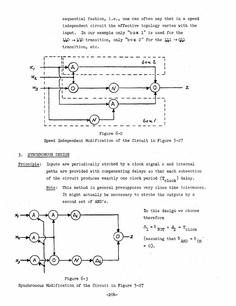
sequential fashion, i.eo, one can often say that in a speed
independent circuit the effective topology varies with the
input 0 In our example only "box 1" is used for the
J.,J.,O ~ J,qG transition, only "b'o x.. 2" for the J,J,1 ~ Wtransition, etc ..
-- --- -. ............ ....,., -- -_ ....... ...,.-, , I
....- _ ...... _ ....... - - - - ___ ............... ,........ - - - --I
, l ____ _
L ___ _
Figure 6-2
6o~/,
I I I I I I -'
z.
Speed Independent Modification of the Circuit in Figure 5-27
3. SYNCHRONOUS DESIGN
Principle: Inputs are periodically strobed by a clock signal c and internal
paths are provided with compensating delays so that each subsection
of the circuit produces ex~ctly one clock period (Tcl0Ck) delay ..
~: This method in general presupposes very close time toleranceso
It might actually be necessary to strobe the outputs by a
second set of AND's.
Figure 6-3
In this des~gn we choose
therefore
6;:::0 +~::;T 1 NOT ~ clock
(assuming that 5 AND == 0 OR'~'
= 0).
Synchronous Modification of the Circuit in Figure 5-27
~204-
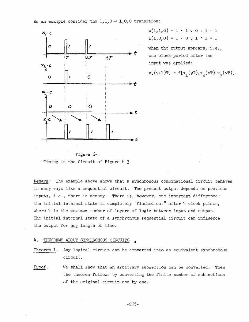
As an example consider the 1,1,0-> 1,0,0 transition:
z(l,I,O) = I .. Iv ° I I x/.,
1° z(I,O,O) = I " ° v 1 o I 1
~I ~I when the output appears, i. e. J
-. t I, Iz.r Igr one clock period after the
I input was applied: ~." I I
1°
t
~I I z[(v+I)T] = f[xl (vT),x2 (VT), X
3(VT)]. :0
.. -t
J: , j I
0 iC)
.t Z'C~i ~ ~
1 IT' ~I ~, .&
Figure 6-4
Timing in the Circuit of Figure 6-3
Remark: The example above shows that a synchronous combinational circuit behaves
in many ways like a sequential circuit. The present output depends on previous
inputs, i.e., there is memory. There is, however, one important difference~
the initial internal state is completely "flushed out" after V clock pulses~
where V is the maximum number of layers of logic between input and output.
The initial internal state of a synchronous sequential circuit can influence
the output for any length of time.
40 THEOREMS ABOUT SYNCHRONOUS CIRCUITS • Theorem 10 Any logical circuit can be converted into an equivalent synchronous
circuit.
Proof 0 We shall show that an arbitrary subsection can be converted. Then
the theorem follows by converting the finite number of subsections
of the original circuit one by one.
-205-
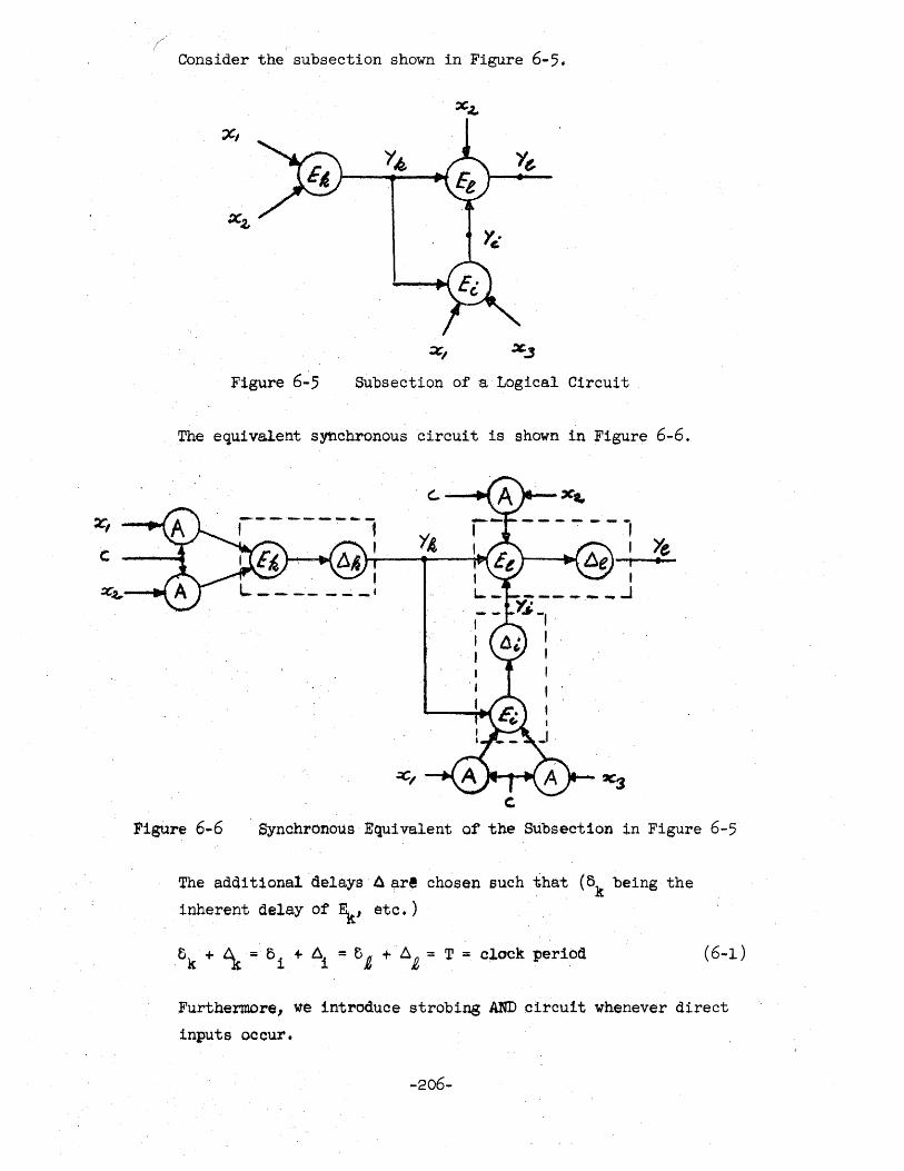
Consider the subsection shown in Figure 6-5.
:XI ~.J
Figure 6-5 Subsection of a Logical Circuit
The equivalent synchronous circuit is shown in Figure 6-6.
Ye •
~I
Figure 6-6 Synchronous Equivalent of the Subsection in Figure 6-5
The additional 'delays A are chosen such that (8k being the
inherent delay of Ek, etc.)
(6-1)
Furthermore, we introduce strobing AND ci~cuit whenever direct
inputs occur.
-206-
New· Definition of y'
In synchronous circuits we shall designate by y'the value one
clock period later rather than the "value if all arguments were fixed" as we
did in the last chapter:
y~(VT) ~ y[(V+l)T] = f.[XI(VT), ... , y (VT)] 11· S
(6-2 )
In the example we have
y~ (T) 1
fi[Xl(O), x3
(0), yk(O)]
f k LXI ( 0), x2 ( 0 ) J
The Qlock period will be dropped from the argument in what follows, i.e., we
shall write
y(VT) == y(V) (6-3)
If now we assume that the initial state is known, i.e.,.that all signal values
of the internal nodes are given at t = 0 (as well as the inputs), we have
Yk(l) y~(O) = fk[Xl(O), x2 (0)]
Yi(l) y~(O) = fi[xl(O), X3
(0), Yk(O)l
and
From the y's at time T and the input at T(i.e., the set yk(l), Yi (1), y£ (1)
and x1(1), X2
(1), etc.) we can 'calculate the next motions of the circuit, ioe.,
the internal states at time 2T, etc.
At this pOint it becomes convenient to introduce vectors to represent
input combinations, the set of signals at the internal nodes and finally the
output combinations. These vectors may be thought of as column vectors,
although other interpretations may be useful.
s m n Definition: Let S = 2 ,M = 2 and N = 2 where s is the number of internal
nodes, m the number of input lines and n the number of output lines.
If x .. II
Xmi is a given input, Yij 0.0 Ysj a given internal state
-207-
and Za .. '" znk a given Qutput,ve define input vectors Xi' state'v.ctors Y ;' and output· vectors~ Z. by ....... -----~-. j J - . -:x _
x == {Xli' 00" , x.} i • 1 .M i ml
Yj
::: {YlJl o o· 0, 1Sj} J 5 1 s
~. :: f!tnl c·,,·., 11 Ink } k :;: 1 N
(6.4)
If we vent to indicate· val~es at clock period y. we may also write
x(v) = {X1(V), b i 9 J Xm(V)}
1(v} = (11 (v), " • q ~ y s (v)} . (6-5)
Z(v) = {%1 (v-), -0 0 s)". Zn(V}}
Symbolically our eqv.a.t1ons . (6 .. 2) : or the equi valen~ (5 -69) can now
. be written
(6-.6 )
We· see, then, how successive 1nterhal states can be constructed
iteratively. It is, however, not clear ho~ the outputs can be .
. obtainede· It is sometimes useful to consider the z's as forming
together with the y's a new set of node~ but this can lead to
. conf.usion. : We $hall theref'oreunt11 further notice make the
following.
Convention: It will be assumed that we have an ln~tt:l.nta.neous decoder (ioe." a.n infinitely fa.st combinationsl clrcui t) wbich forms the z' s either from
tbe yls al.one (~ore machin4;t) or trom the y's and x's (Mealy machine).
SYmbol i cal.ly
or
Z(V) = G[Y(v)]
Z(v)? H[X(v), iev)]
(Moore)
(Mealy)
-208-
(6-7 )
(6·8)
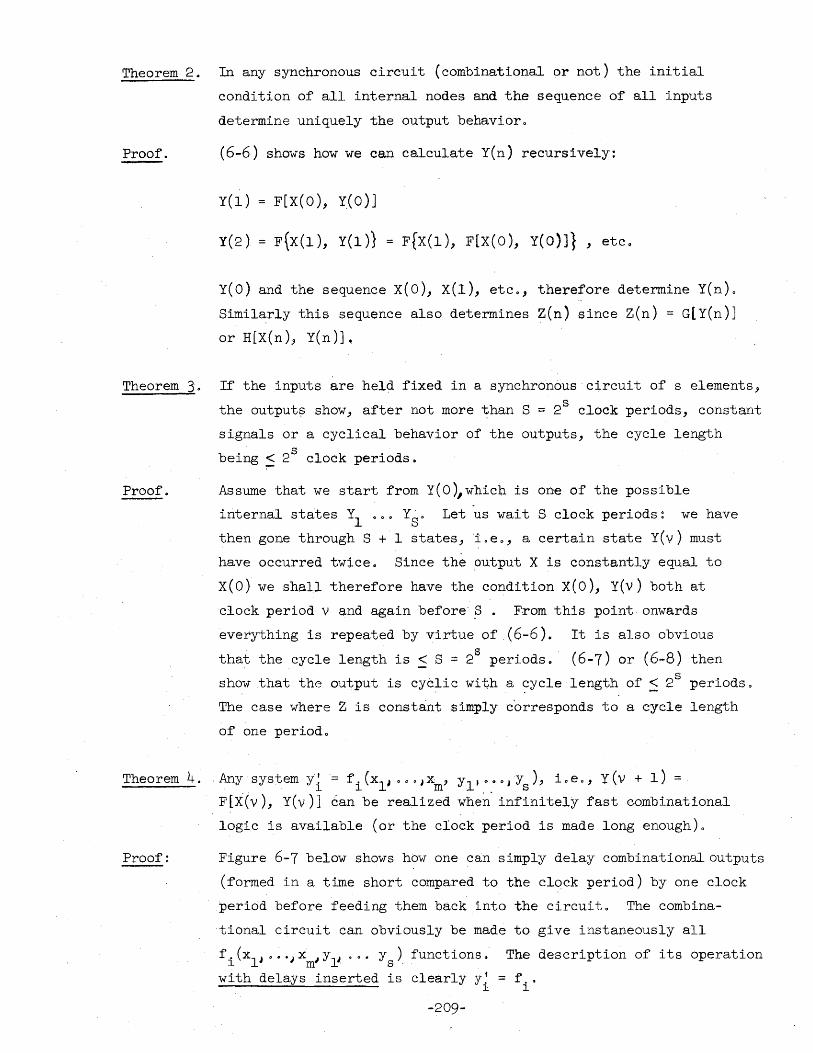
Theorem 2. In any synchronous circuit (combinational or not) the initial
condition of all internal nodes and the sequence of all inputs
determine uniquely the output behavior.
Proof. (6-6) shows how we can calculate Y(n) recursively:
Y(l) F[X(O), Y(O)J
Y(2) F\X(I), Y(l)} = F[X(I), F[X(O), Y(O)]} , etc.
y(o) and the sequence X(O), X(l), etc., therefore determine Y(n).
Similarly this sequence also determines Z(n) since Z(n) = G[Y(n)]
or H[X(n), Y(n)]~
Theorem 3. If the inputs are held fixed in a synchronous circuit of s elements,
Proof.
s the output~ show, after not more than S =- 2 clock periods, constant
signals or a cyclical behavior of the outputs, the cycle length
being ~ 2s clock periods.
Assume that we start from Y(O~which is one of the possible
internal states Yl .0. Ys. Let us wait S clock periods: we have
then gone through S + 1 states, i.e., a certain state Y(v) must
have occurred twice. Since the ~utput X is constantly equal to
X(O) we shall therefore have the condition X(O), Y(v) both at
clock period v and again before'.8. From this point onwards
everything is repeated by virtue of (6-6). It is also obvious
that the cycle length is ~ S ~ 28 periods.' (6-7) or (6-8) then s show that the output is cyclic with a cycle length of ~ 2 periods.
The case where Z is constant simply c'orresponds to a cycle length
of one periodo
Theorem 4. ,Any system i~= f'(XIJ ,o'Jx , Yl' •• oIY ), ioe., Y(v + 1) =. 11m . s
Proof:
F[X(v), Y(v)] can be realized when" infinitely fast c-ombinational
logic is available (or the clock period is made long enough).
Figure 6-7 below shows how one can simply delay combinational outputs
(formed in a time short compared to the clock period) by one clock
period before feeding them back into the circuit. The combina
tional circuit can obviously be made to give instaneously all
f. (xIJ ••. J X I y,1 ... y ) functions. The description of its operation 1 m~' s . with delays inserted is clearly y~ = f ..
1 1
-209-
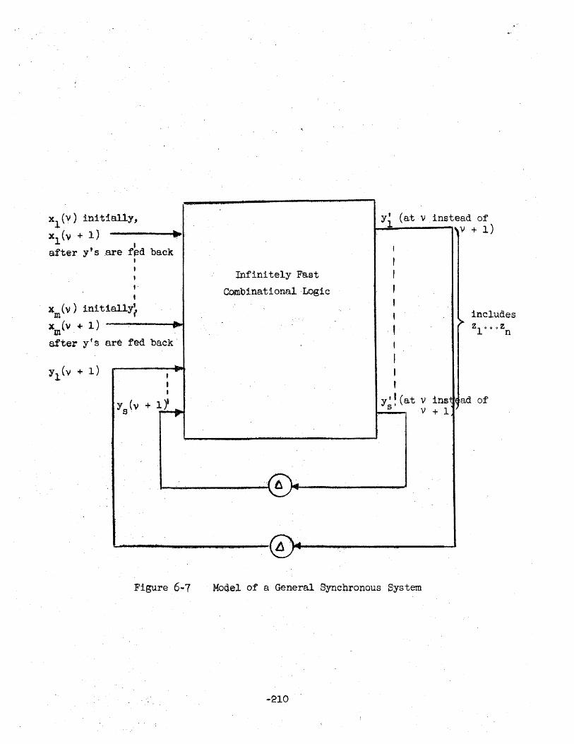
:lally,
.... X1(v) init
xl (V + 1)
after y'6 ,
,are f~d back , , , t·
• JC: (V) ini t
III 1a11Y,
X (v 1- 1) . 111 .
... ....
after y's are fed ba.ck '
... t ......
I
• ys(v + 14
Figure 6 ... 7
Yi (at v
, , Infinitely Fa.st ,
Comb1nat 1 onal Logic , t ,
. , , I t ,
y,J(at v s· v
Q ~
A' ..
Moqel of a General Synchronous System
-210
inste ad of + 1) I'V
' .
insir~ + 1
> includes zl 0 Q • zn
ad of
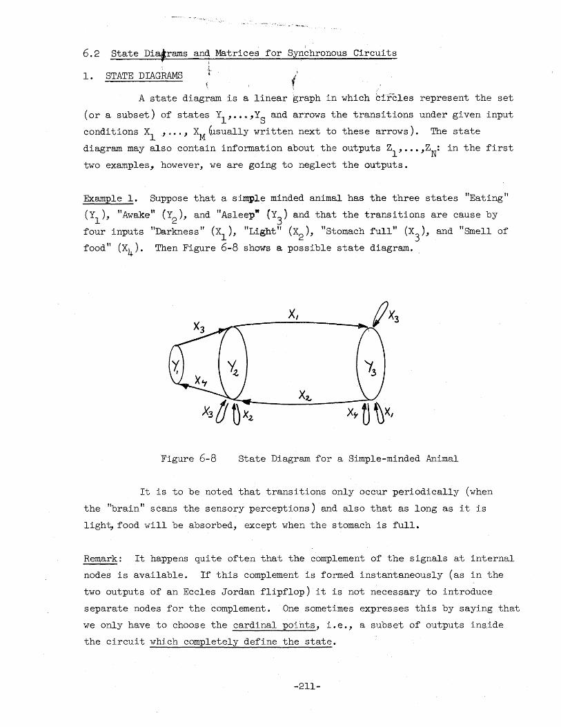
.~". --. -.~ ~ .
6.2 State Dia_rams and Matrices for Synchronous Circuits i
i !
( 1. STATE DIAGRAMS
A state diagram is a linear graph in which bircles represent the set
(or a subset) of states YI, •• o,YS
and arrows the transitions under given input
conditions Xl'." J XM ~sually written next to these arrows). The state
diagram may also contain information about the outputs Zl"",ZN: in the first
two examples, however, we are going to neglect the outputs.
Example 1. Suppose that a silTll'le minded animal has the three states "Eating"
(Yl
), "Awake" (Y2
), and "Asleep· (Y3
) and that the transitions are cause by
four inputs "Darkness" (Xl)' "Light" (X2
), "Stomach full" (X3
), and "Smell of
food" (X4 ). Then Figure 6-8 sho'Ws a possible state diagram.
X,
X.t,
Figure 6-8 State Diagram for a Simple-minded Animal
It is to be noted that transitions only occur periodically (when
the "brain" scans the sensory perceptions) and also that as long as it is
ligh~ food will be absorbed, except when the stomach is full.
Remark: It happens quite often that the complement of the signals at internal
nodes is available. If this complement is formed instantaneously (as in the
two outputs of an Eccles Jordan flipflop) it is not necessary to introduce
separate nodes for the complement. One sometimes expresses this by saying that
we only have to choose the cardinal points, i. e., a subset of outputs ins.ide
the circuit which completely define the state.
-211-
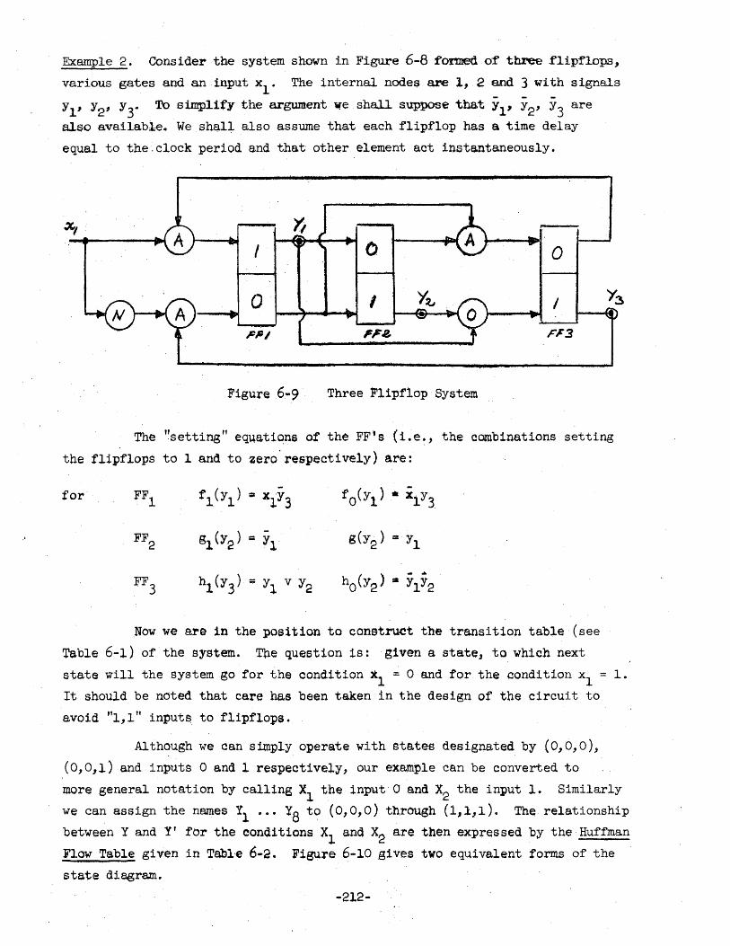
Example 2" Consider the system shown in Figure 6-8 formed 01' three flip-flops,
various gates and an input xl" The internal nodes are 1, 2 and 3 with signals
Y1, Y2, Y3· To simplify the argument we shall suppose that Y1, Y2' Y3 are
also available. We sh~ll also assume that each flipflop has a time delay
equal to the ,clock period and that other element act instantaneously •
. XI
I o o
I I
FF3
Figure 6"'9 Three Flipflop System
The "setting" eq~atiqn6 of the FF's (i.e., the combinations setting
the flipflops to 1 and tozero'respectively) are:
for FFl f 1(Yl) == XiY3 fO(Y1 ) * X1Y3
FF2 Sl (Y2) - g(y ) =y = y 1 2 1
FF3 h1 (Y3) :;;: Y1 v Y2 hO(Y2) :t YlY2
Now we are in the position to construct the transition table (see
Table 6-1) of the system. Tne question is: given a stateJ to which next
state will the system go for the condition xl = ° and for the condition xl = 1.
It should be noted that care has been taken in the design of the circuit to
avoid "1,1" input$ to flipflops.
Although we can simply operate with states designated by (0,0,0),
(0,0,1) and inputs ° a.nd 1 respectively, our example can be converted to
more general notation by calling Xl the input a and X2 the input 1. Similarly
we can assign the names 11 ••• Y8 to (0,0,0) through (1,1,1). The relationship
between Y and Y' for the conditions Xl and X2 are then expressed by the Huffman
Flow Ta.ble given in Tabl'e 6 .. 2. Figure 6-10 gives two equivalent forms of the
state diagram.
-212-
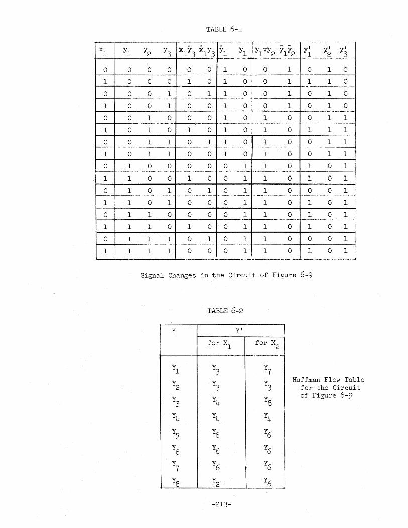
x 1
a 1
a 1
a 1
a 1
a 1
a 1
a 1
a 1
TABLE 6-1
--- "-'. ----- .. ~- - .. - -.•..... --. .. ,- . - -- .. - - - - -Y~ Y~ y' Y1 Y2 Y3 x1Y3
x1Y3 Yl Yl Y1vY2 Y1 Y2 3
1---- - . .- ~.- .-... _._.-.,_ .. ~ -..--- - -_. _._--- --- -... _.-.-
a a a a 0 1 a 0 1 a 1 0 .-a 0 a 1 a 1 0 0 1 1 1 0
,,- ._- -.. --.-.---.,..~~ -..... -_.
a 0 1 a 1 1 a 0 1 0 1 0 -- f--.--.. ------1--......... _ .. - . . -._'",---- t---
0 a 1 0 0 1 a '0 1 a 1 0 -...... ~ ... --.. -. _.- .. _- .. ...4'··.· .... _ .... · .... _
a 1 a a a 1 0 1 0 a 1 1 .- ------ --.----.-.-.. ~-.. - .- .... ,---_ ..••.. -.". .. _-_.---
a 1 a 1 a 1 a 1 0 1 1 1
a 1 1 0 1 1 0 1 a 0 1 1 ------------ -.-.. --- .. -- .. - ---_._-_.- ----_.-
a 1 1 a a 1 0 1 0 a 1 1
1 0 a 0 0 a 1 1 0 1 a 1 .... -.- -...... _.-"-- . - -'-"' - ..... .... _ .. ,- --'.---.--._.- . --.. -- ..... -----
1 a a 1 a 0 1 1 a 1 0 1
1 a 1 0 1 0 1 1 0 a a 1 . ...... - .. ~- . - ._--_.'- . '--'''-- .- - -.... --- .. _.' . •. .-._- -_ ... _ .. - -- ... ---.......... -.- .. -~.- ....... - .... _--_ . ., -_ .... ..--.-. __ ._.-
1 a 1 a a a 1 1 a 1 a 1 ;
1 1 0 a a 0 1 1 0 1 a 1 ---- ... - ----.•. - -_ .. _-- -"---'-'--'-" ~--.,.
1 1 a 1 a a 1 1 a 1 a 1 I 1 1 1 a 1 0 1 1 0 0 0 1 I ---.~ .. -_ .... _- -.. - .-.. __ ..... _. __ ... _ .. - .. ---.-1 1 1 a a 0 1 1 0 1 0 1
..... _-_. -.--....... ...:......----- .. ~ .- -._-__ -- -.' ..... --_ ... _.-i
Signal Changes in the Circuit of Figure 6-9
y
Yl
Y2
Y3
Y4 Y5
Y6
Y7
Y8
TABLE 6-2
y'
for Xl for X2
--~ -_ .. _--_. _.
Y3 Y7
Y3 Y
3 Y4 Y8
Y4 Y4
Y6 Y6 Y6 Y6
Y6 Y6
X2 Y6
-213-
;
Huffman Flow Table for the Circuit of Figure 6-9
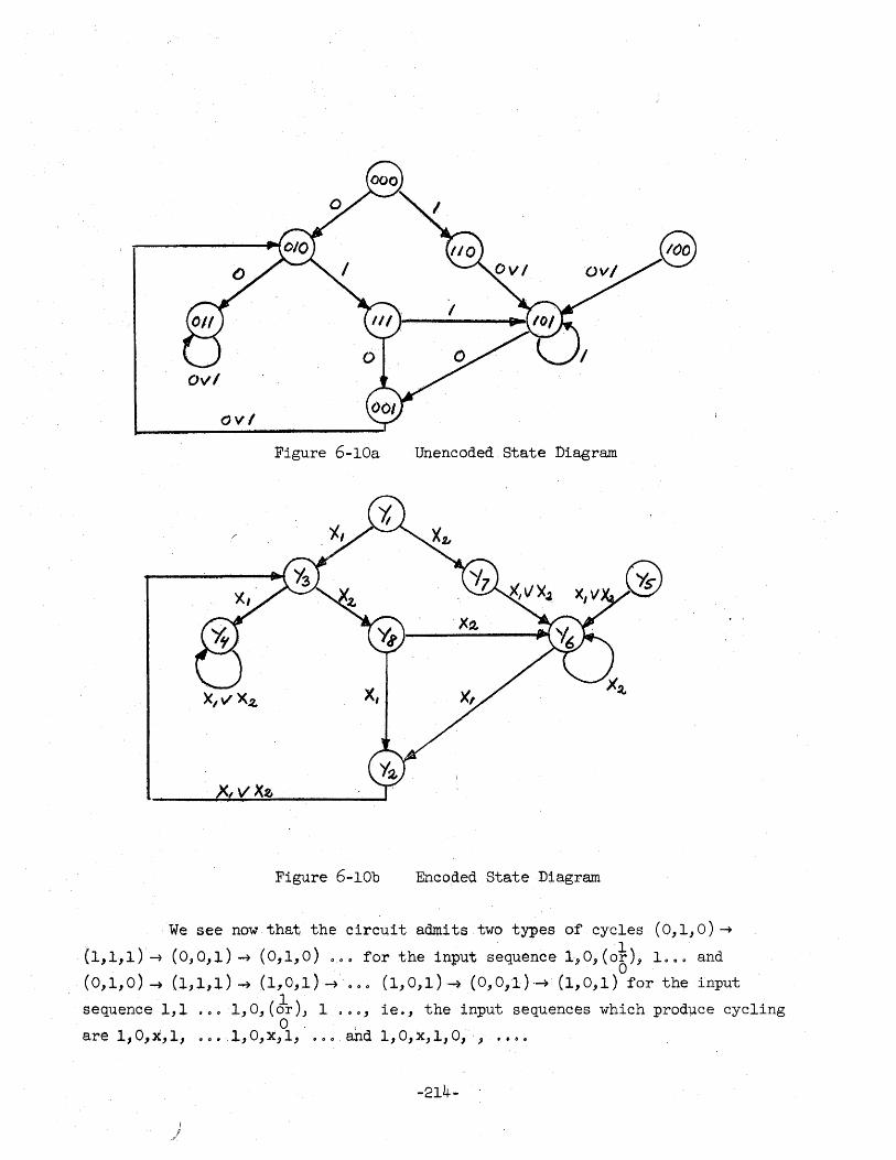
Figure 6-10a Unencoded State Diagram
I V X.e
Figure 6-10b Encoded State Diagram
We see now that the circuit admits two types of cycles (0,1,0) ~
(1,1,1) ~ (0,0,1)·~ (0,1,0) 0.0. for the input sequence 1,0, (o~), 1. 0 0 and a (0,1,0) -+ (1,1,1) -+ (1,0,1)-+ .0. (1,0,1)·~ (0,0,1)--+ (1,0,1) for the input
sequence 1,1 1,0,(Jr), 1 . 00, ie., the input sequences which prod~ce cycling a .
are 1, 0, x, 1, . o. 1, 0, x, 1, arid 1, 0, x, I, 0, ., •• ••
-214-
)
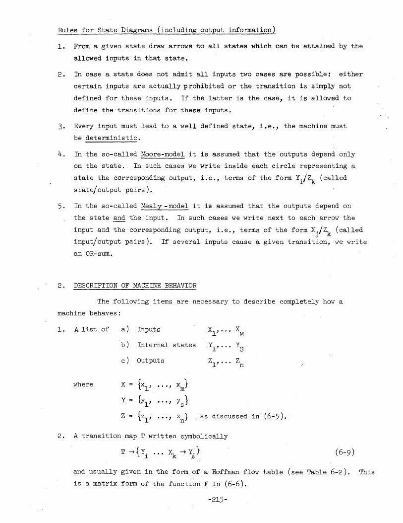
Rules for State Diagrams (including output information)
1. From a given state draw arrows to all states which can be attained by the
allowed inputs in that state.
2. In case a state does not admit all inputs two cases are possible: either
certain inputs are actually prohibited or the transition is simply not
defined for these inputs. If the latter is the case, it is allowed to
define the'transitions for these inputs.
3. Every input must lead to a well defined state, i.e., the machine must
be deterministic.
4. In the so-called Moore-model it is assumed that the outputs depend only
on the state. In such cases we write inside each circle representing a
state the corresponding output, i.e., terms of the form Yi/Zk (called
state/output pairs).
5. In the so-called Mealy -model it is assumed that the outputs depend on
the state and the input. In such cases we write next to each arrow the
input and the corresponding output, i.e., terms of the form Xj/Zk (called
input/output pairs). If several inputs cause a given transition, we write
an OR-sum.
2. DESCRIPTION OF MACHINE BEHAVIOR
The following items are necessary to describe completely how a
machine behaves:
1.
2.
A list of a) Inputs Xl' •. • X M
b) Internal states Yl , .. • Ys c) Outputs Zl' • .. Z
n (
where X = {Xl' · .. , x } m
Y = {Yl' · ... , Ys1
Z {zl' · .. , z } as discussed in (6- 5). n
A transition map T written symbolically
T -) {Yi ... Xk --7 Y,e} (6-9 )
and usually given in the form of a Hoffman flow table (see Table 6-2). This
is a matrix form of the function F in (6-6).
-215-
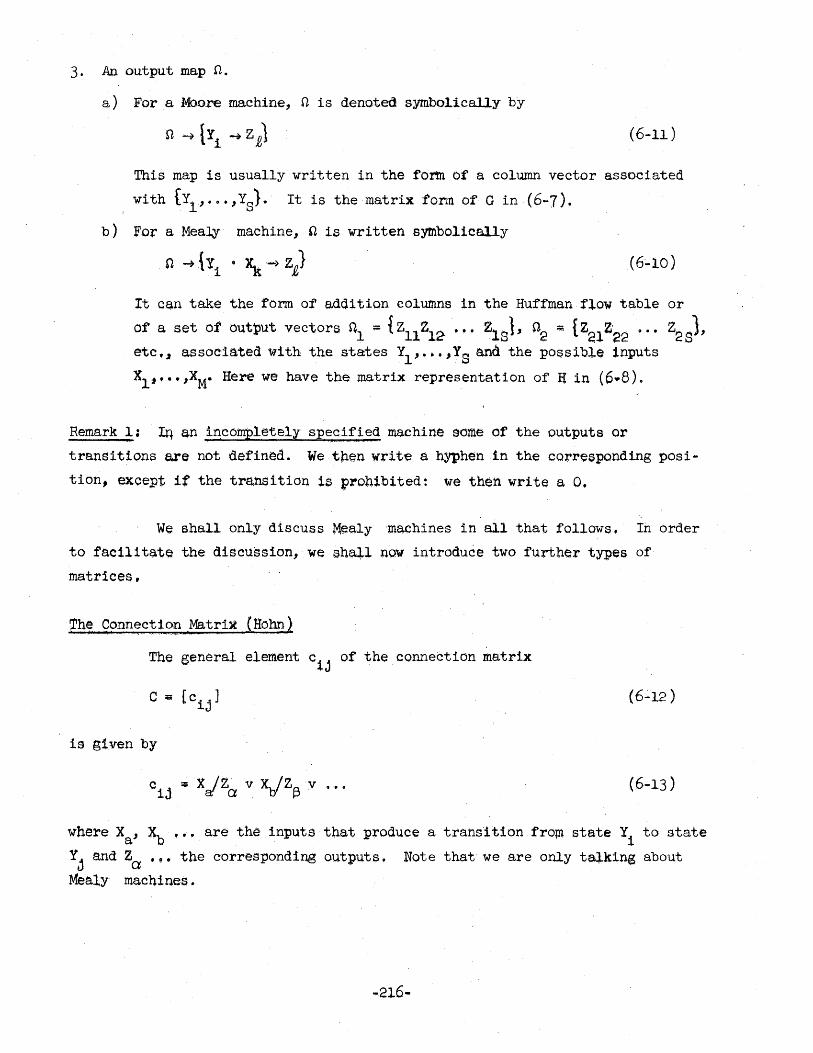
3. An output map n.
a) For a Moore machine, n is denoted symbol.ically by
(6-11 )
This map is usually written in the fo~ of a column vector associated
with {Yl' eo., Ys}. It is the matrix form of G in (6-7).
b) For a Mealy machine, n is written symbolical.ly
It c~n tak~ the tonm of addition columns in the Huffman flow table or
of a set ot outi1ut vectors 01 ;: {Zll Zl2- ••• ZlS 1, 02 :;; {Z~l Z'22 •.• Z2S)' etc., associated with the states Yl, •• "YS and the possible inputs
Xl~""XM' Here we have the matrix representation of a in (6.8).
Remark 1: Iq an incompletely specified machine some of the outputs or
transitions are not defined. We tp.en writ-e So hyphen 1n the corresponding posi ..
tion, except if the transition i~ prohibited: we then write a O.
We shall only discuss M~aly 'machines in all that follows. In order
to facilitate the discussion, we sha.+1 now introduce two further types of
matrices.
The Connection Matri~ {Hahn}
The general element cij
of the connection matrix
is g1venby
(6-13 )
where Xa, ~ .... are the inputs that :produce a transl tion from state Y1 to state
Yj and Za .,. the corresponding outputs. Note that we are only talking about
Mealy machines.
-216 ..
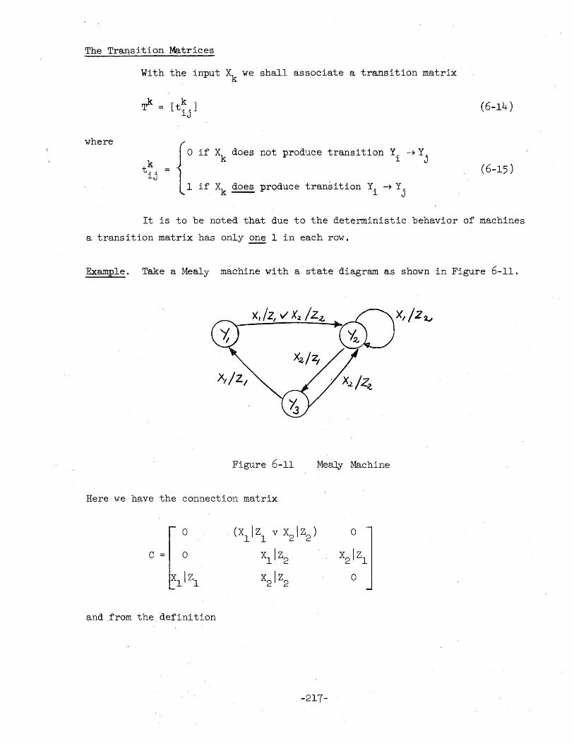
The Transition Matrices
where
With the input Xk
we shall associate a transition matrix
k t .. lJ
if Xk
does not produce transition Yi
-? Yj
if Xk
does produce transition Y. -~ Y. --- l J
(6-14 )
(6-15)
It is to be noted that due to the deterministic behavior of machines
a transition matrix has only ~ 1 in each row.
Example. Take a Mealy machine with a state diagram as shown in Figure 6-11.
Figure 6-11 Mealy Machine
Here we have the connection matrix
a
c = o
and from the definition
(Xl! Zl v X2 ! Z2)
Xl !Z2
X2 !Z2
-217-
o
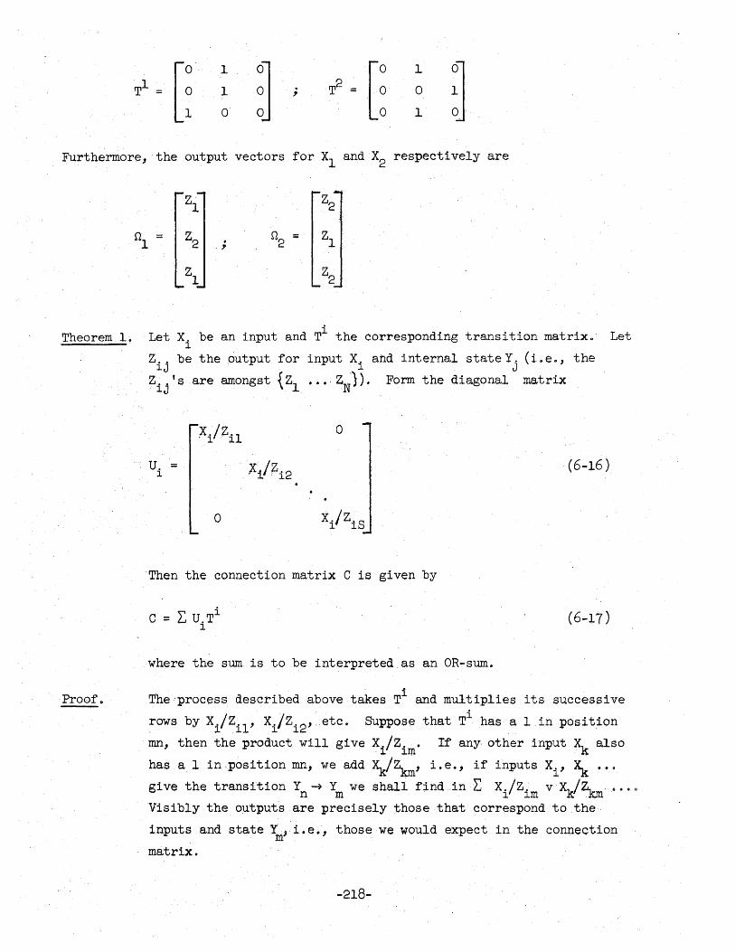
[: 1
~] [~ 1
~] ~ = 1 ; T2 ::;:: 0
0 1
Furthermore, the output vectors for Xl and X2 respectively are
Z1 Z2
n1
= Z2 n ::;:: Zl . 2 . ?
Zl Z2
Theorem 1. Let Xi be an input and Ti the corresponding transition matrixo Let
Z.. be the output for input X. and internal state Y. (i 0 e., the ~J. 1 J
Proof.
Zij 's are amongst {Zl •.• ZN)). Form the diagonal matrix
u. = ~
o
o
·Then the connection matrix C is given by
where the sum is to be interpreted as an OR-sum.
(6-16 )
(6-17)
The process described above takes Ti and multiplies its successive
rows by x./Z. 1, X./Z'I"'l'. etc. Suppose that Ti has a 1 in position 1 ~ ~ ~c:
mn, then the product will give X./Z.. If any other input Xk
also ~ ~m
bas a 1 in position Inn, we add ~/Zkrn' i.e., if inputs Xi' ~ •• 0
give the transition y~ Y we shall find in .r, X./Z. v Xk/Z-. ·.0000 n m . ~ m -~
Visibly the o~tputs are precisely those that correspond to the
inputs and state Ym, i.eo, those we would expect in the connection
matrix.
-218-
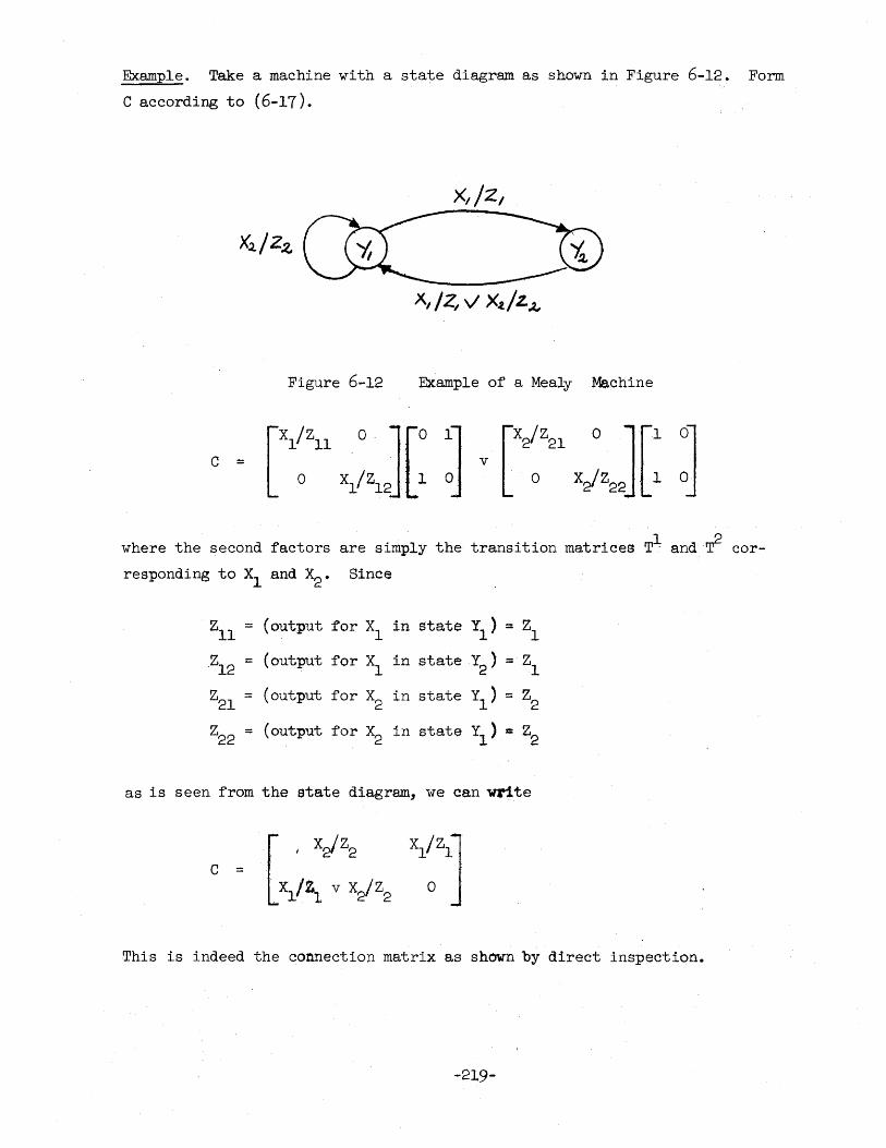
Example. Take a machine with a state diagram as shown in Figure 6-12. Form
C according to (6-17).
X2./ Z2.,
Figure 6-12 Example of a Mealy Machine
C =
where the second factors are simply the transition matrices T~ and·~ cor
responding to Xl .snd x2 • Since
Zll = (output for Xl in state Y1 ) = Zl
Z12 = (output for Xl in state Y2
) = Zl
Z2l = (output for X2
in state Y1 ) = Z2
Z22 =:: (output for X2 in state Y1 ) = Z2
as is seen from the state diagram, we can write
c =
This is indeed the connection matrix as shown by direct inspection.
-219-
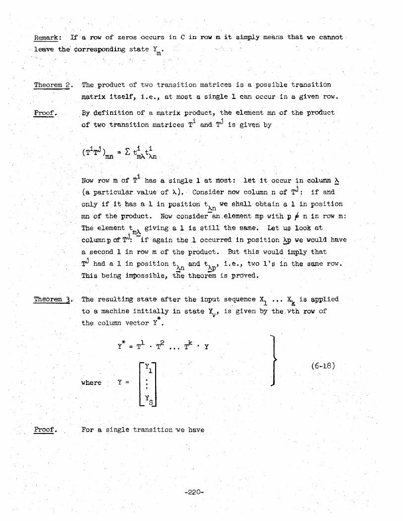
Remark: If' a row of zeros occurs in C in row m it simply means that we cannot··
leave the' corresponding state Y . m
,', "
Theorem 2. The product of two transition matrices is a possible transition
matrix itself, i.e., at most a singlel can occur in a given row •
Proof. . By ~efinition of a matrix ~roduct, the element ron ,of the p~oduct
of twotrahs'i tionmatrices Ti and Tj is gi veri by
. . i Now row m of T has a single 1 at most: l~t it occur ~n column ~
(a particular value of A),· Consider now column n of TJ: if and
only if it ha.s a,·l in position t"-n ¥t€ shall obtain a 1 in position
ron of the, product. Now conSider-an ,el~ment rtlp with P ~ n in ro~ In:
The €lement :mA giving' a 1 is still the s~e. Let us look at
colwnnp of TJ: -if again the .l occurred in position ~ we would have
a seco,nd 1 ih row m of' the product. But this would imply that
TV had a 1 in.positiont). and tA ' i.e., twol's in the same row. I\n . p
This being impossible, the theorem is pr-dved.
Theorem 3., 'rhe· resulting state after the input sequence Xl ~ ~. ~ is ~pplied
to a machine initially in state Yv' is given by the.vth row of
* the. column vector Y •
(6-18)
where y ==
Proof. For a singletransi tion'We have
-220 ...
S 1 L tl,Y,
j=l J J
S 1 L ts'Y'
j=l J J
1 Suppose now that we start from yV and that tv~ = 1, i.e., that under I
the influence of XII Yv ..... Y>,.' Then our assertion is that
S 1 L tv' Y'
j=l J J
which is correct. Now for two transitions we have
Suppose that we, start in state Yv and that under the influence of Xli
Y ~ YT}' i. e., that t l n = 1. Also suppose that under the influence
V ,V'I 2 . ' of X2, YT} -? YIJ.' 1. e., that tT}1J. = 1. Then ObV1ously Yv -) YIJ. under the
influence of Xl' followed be X2 •
Consider the vth row of Y* :;: TIT2y, i.e.,
1 t
vT} • t
2 Y 0 0 0 v v v •••
T}IJ. IJ.
1 · 1 · Y Y IJ. IJ.
Again this agrees with our direct observation. Clearly this method
can be generalized to any number of transitions, i.e., the theorem
is true.
-221-
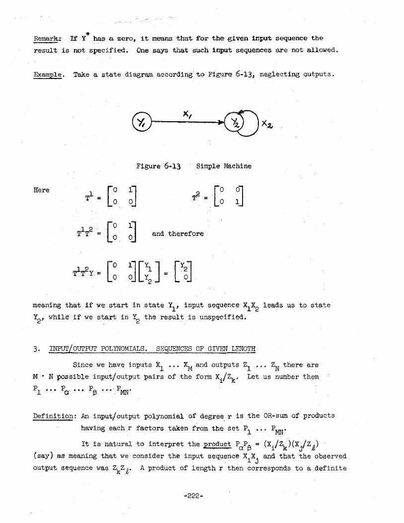
*' Remark: If Y has- a zero, it means that. :for the .given input, sequence the
result is not speci:fied. One says that such input sequences are not allowed.
Example. Take a state diagram accord!ng:to Figure 6-13~ neglecting outputs.
Here
=.[. ,0. IJ . ° 0
F:l.gure 6"'13 Simple Machine
T2- _[0 01 - 0 IJ
and therefQre
x 2, -
meaning that if we start in state Y1' input sequence X1X2 leads ~~, to state
Y2' whl1-e if we st~:rt in 12 the result lquns:p.eeified.
3. ,INPUT/OUTPUT POLYNOMIALS.. SEQUENCES OF GIVEN LENGTH
Si:q.ce we have inputs Xl •• " XM .and outputs Zl .. 0.. ZN there are
M • N possible inl'ut/output pairs of the formXi/Zk .. Let us number them
P r" ... ~a ••• l? e ".-.', P MIt
Definition: An inpu.t/ output polynomial of degree. 'r -1s the OR-s'l.l!llof products
having each r fae-tors taken from the- set PI .... PMN
,
It is natural to interpret the pr?,duct PaP~ = (xi/zk)(Xj/Z£) (say) as meaning that we consider the input seq'lJence XiX
j and that the observed
output sequence wa~ ZkZ£. A product of length r then co:;rresponds to a .definite
input sequence involving r-inputs and adefini te output sequence involving r
outputs, i.e., each term of the OR-sum in the input/output polynomial represents
a certain input/output sequence of "length r."
In a similar way we -shall interpret the OR-sum Pa v P t3 = (Xi/Zk
) v
(xj/Zt) as meaning that input Xi ~ input Xj has been applied, the output
being Zk ~ Z.e depending on the case, More generally an OR-sum of r-factors
shall mean that the input/output sequence corresponding to the first term
or that corresponding to the second term, etc., has been applied.
It is easily seen that we can operate with these input/output
polynomials according to a set of laws not unlike· those of Boolean Algebra:
There is a O-element, namely a polynomial "0" corresponding to no further
stepping forward of the clock time. There is, however, no analog of a l-element.
Rules for Input/Output Polynomials
Let f,g and h be possible polynomials. Then
1. f v g ; g v f (commutativity w.r.t. v)
2. fg f gf (non-commutativity w.r.t .. )
3. f v f f (idempotency w.r.t. v)
4. f v 0 o v f f (0 is the unit element for v)
5. f· 0 o · f o (zero annuls a sequence)
6. (f v g) v h = f v (g v h) (associativity for v)
7. (fg)h=f(gh) (associativity for .)
8. (f v g)h fh v gh (distributivity)
9. f(g v h) fg v fh (distributivity)
(6-19 )
(6-20 )
(6-21 )
(6-22 )
(6-23)
(6-24 )
(6-25 )
(6-26 )
(6-27 )
Remark 1: (6-23) may astonish at first sight. All it means is that a sequence
represented by f (say of length r) cannot be made into any longer sequence
when the clock is stopped.
Remark 2: The set S of all input/output polynomials is (comparing to the
definitions in 5.1) a commutative idempotent semi-group (with a unit) with
respect to v. It is a non-commutative, non-idempotent semi-group (with a zero)
with respect to 0.
-223-
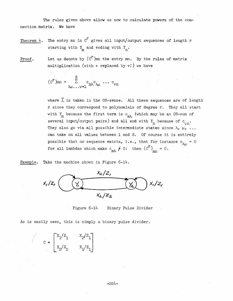
The rules given above allow us now to calculate powers of the con
nection matrix. We have
Theorem 4. The entry mn in Cr gives all input/output sequences of length r
starting with Y and ending with Y • m n
Proof. Let us denote by (Cr)mn the entry mn. By the rules of matrix
multiplication (with + replaced by v! ) we have
• • • 'cv ·n
where L.is taken in the OR-sense. '. All these sequences are of length
r since they correspond to polynomials of degree 'r o They all start
with Y because the first term is c , (which may be an OR-sum of m m/~
several input/output pairs) and all end with Y because of c . n vn
They also go via all possible intermediate states since "A., J-L, 0 ••
can take on all values between 1 and S. Of course it is entirely
possible that no sequence exists, i.e., that for instance cAJ-L = 0
.i (CT) for all lambdas which make cmA rO: then mn = O.
Example. Take the machine shown in Figure 6-14.
Figure 6-14 Binary Pulse Divider
As is easily seen, this is simply a binary pulse divider •
... 224-
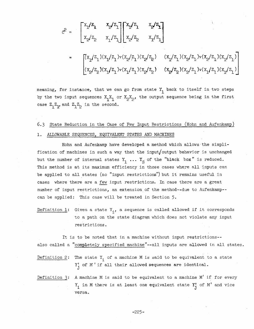
::;: ~XI/Zl ) (X1/Z1 )v(x,j'h )(x,j~)
~X,jZ2 ) (X1/Z1 )v(XiZl ) (X,jZ2 )
(Xl,/ Zl ) (X,j Zl.)V (X,j Zl) (xi Zl ~
(x,jZ2 )(X,jZl )V(X1/Z1 )(xiZl d meaning, for instance, that we can go from state Y
l back to itself in two steps
by the two input sequences XlXl
or X2X2
, the output sequence being in the first
case ZlZ~ and Zl Z2 in the secondo
6.3 State Reduction in the Case of Few Input Restrictions (Hohn and Aufenkamp)
1. ALLOWABLE SEQUENCES, EQUIVALENT STATES AND MACHINES
Hohn and Aufenkamp have developed a method which allows·the simpli
fication of machines in such a way that the input/output behavior is unchanged
but the number of internal states Yl
••• YS' of the "black box" is reduced 0
This method is at its maximum efficiency in those cases where all inputs can
be applied to all states (no "input restrictions lt) but it remains useful in
cases where there are a few input restrictions. In case there are a great
number of input restrictions, an extension,of the method--due to Aufenkamp-
can be applied: This case will be treated in Section 50
Definition 1: Given a state Y., a sequence is called allowed if it corresponds l
to a path on the state dia~r~ which does not violate any input
restrictions.
It is to be noted that in a machine without input restrictions--
also called a "completely specified machine"--all inputs are allowed in all states.
Definition 2: The state Y. of a machine M is said to be equivalent to a state l
Y~ of' M ' if all their allowed sequences are identical. J
Defini tion 3: A machine M is s.aid to be equivalent to a machine M' if for every
Yi
in M there is at least one equivalent state Yj of M' and vice
versa.
-225-
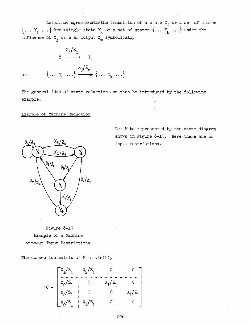
Let us now agree to write the transition of a state Y. or a set of' states l
{ .• " Yi
•.• 1 into a single state Yk or a set of states \... Yk .. o} under the
influence of X. with an output Z symbolically J m
X.jz J m
Y. :> Yk l
X.jz t e ••
J ... m { eo.
• • 0 1 or Y. H.}- < ) Yk l
The general idea of state reduction can then be introduced by the following
example.
Example of Machine Reduction
X,ji.,
Figure 6-15 Example of a Machine
without Input Restrictions
Let M be represented by the state diagram
shown in Figure 6-15. Here there are no
input restrictions.
The connection matrix of M is visibly
Xl/Zl I I X2/Zl
0 0
_1-
X2/Zl I 0 Xl/Zl
0 C ::: 1
X2/Z1 1 0 0 Xl/Zl
X2/Z
l X1/Zl 0 0
-226-
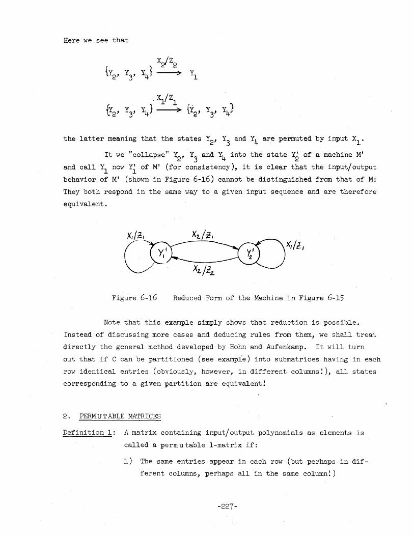
Here we see that
the latter meaning that the states Y2' Y3
and Y4 are permuted by input Xl·
It we "collapse" Y2
, . Y3
and Y4 into the state Y2 of a machine Mt
and call Yl
now Y1 of Mt (for consistency), it is clear that the input/output
behavior of M' (shown in Figure 6-16) cannot be distinguished from that of M:
They both respond in the same way to a given input sequence and are therefore
equivalent.
Figure 6-16 Reduced Form of tne Machine in Figure 6-15
Note that this example simply shows that reduction is possible.
Instead of discussing more cases and deducing rules from them, we shall treat
4irectly the general method developed by Hohn and Aufenkamp. It will turn
out that if C can be partitioned (see example) into submatrices having in each
row identical entries (obviously, however, in different columns!), all states
corresponding to a given partition are equivalent!
2. PERM.UTABLE MATRICES
Definition 1: A matrix containing input/output polynomials as elements is
. called a perm utable I-matrix if:
1) The same entries appear in each row (but perhaps in dif
ferent columns, perhaps all in the same column!)
-227-
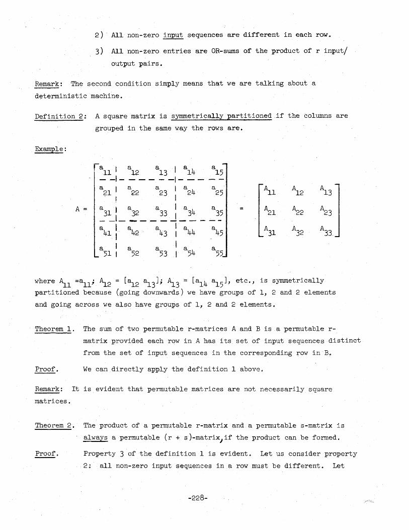
2) . All non-zero input sequences are different in each row o
3) All non-zero entries are OR-sums of the product of r input/
output pairs.
Remark: The second condition simply means that we are talking about a
deterministic machine.
Definition 2: A square matrix is symmetrically partitioned if the columns are
grouped in the same way the rows are.
Example:
A =
a l5 r all I a12 a13 I a14
- -I - - - - - -1- - -a
21 I a a I a
24 a
22 23 1
25 I
a 1 a a I a a 31 I 32 33 I 34 35 --~------- - --
a I a'42 a43
I a44 ~45 ·41 I I
a I a a I ~54 a'55 '51 I 52 '53 I
All A A13 12
= A2l A22 A23
A3l A32 A33
where All :o;;all; ~2 = [a12 a13 J; A13 = [a14 a15 J, etc., is symmetrically
partitioned because (going downwards) we have groups of 1, 2 and 2 elements
and going across we also have groups of 1, 2 and 2 elements.
Theorem 1. The sum of two permutable r-matrices A and B is a permutable r
matrix provided each row in A has its set of input sequences distinct
from the set of input sequences in the corresponding row in Bo
Proof. We can directly apply the definition 1 above.
Remark: It is evident that permutable matrices are not necessarily square
matrices.
Theorem 2. The product of a permutable r-matrix and a permutable s-matrix is
always a permutable (r + s)-matrix,if the product can be formed.
Proof. Property 3 of the definition 1 is evident. Let us consider property
2: all non-zero input sequences in a row must be different.. Let
-228-
A [a .. J, B lJ
[b .. J lJ
Then element ij of the product is given by (L. --) OR-sum)
(We shall omit the limits for A in all calculations: they are 1
and S respectivel~) We want to show that if J f J the input
sequences in (AB) .. are different from those in (AB) .. and that lJ lJ
for a given j all sequences in (AB) .. are different for the dif-- lJ
ferent values of~. The latter point is evident since the
sequences :in ai~ f the sequences:in aiA. when~ f ~, A being a
permutable r-matrix and the interpretation of ai~bA.j is "sequences
in aiA. followed by sequences in b~j": The ai~-part being different
the whole sequences must be different. This argument still holds
when we consider J f ~ and different ""s. The only new case is
then an identical A and ~ f~: Then the sequences in b~l f from
the sequences in bAj
because B is a permutable s-matrix and because
of the above mentioned interpretation of ai~b~j'
Lastly we want to show that property 1 holds, i.e., that the set of
all entries in a row is the same for each row. To this end consider
a certain term t = ai~b~j in row i. Then the part alA. ~ust also
occur in another (arbitrarily chosen) row ~ as ai~ since A is
permutable. Similarly the part b~j must occur inrow ~ of B as b~
since B is permutable. Hence t appears as ai~b~j in row i. ==
Remark: We shall use below an interesting property of two symmetrically
partitioned square matrices A = [a .. J and B = Lb .. J where the partitioning is lJ lJ
identical: one proves easily that in forming the product it is allowed to
multiply the submatrices together as if they were single elements. It is also
noteworthy that all submatrices multiplied in the operation are conformable
(i.e., the number of columns in the first factor equals the number of rows in
the second one).
-229-
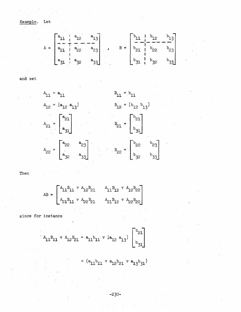
Example. Let
all : al2 al3
A ::: , --T--'--a21 I a22 , a23
I I a3l, a
32 a
33
and set
All = ~ll BIl = b11
A12 = [al2
a13
] B12 = [b12
b13
]
~l= [21J B21 ::: [b21J a
31 b
31
A22 = [22
a32
a23]
a33
" ,B22
= [b22 b
32
b23] b
33
Then
since for instance
-230-
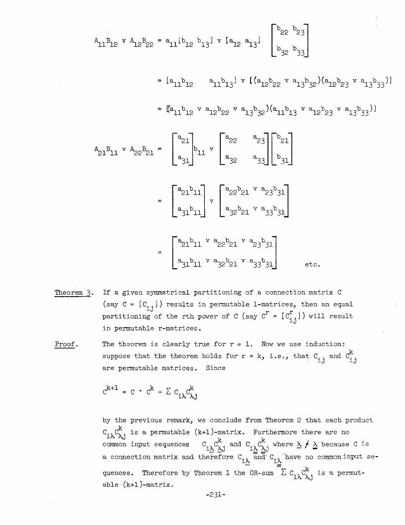
Theorem 3. If a given symmetrical partitioning of a connection matrix C
(say C = [CijJ) results in permutable l-matrices, then an equal
partitioning of the rth power of C (say Cr = [C~.J) will result
lJ
Proof.
in permutable r-matrices.
The theorem is clearly true for r= 1. Now we use induction:
suppose that the theorem holds for r = k, i.e., that C .. and ~. lJ lJ
are permutable matrices. Since
by the previous remark, we conclude from Theorem 2 that each product
CiA~j is a permutable (k+1)-matrixo Furthermore there are no
common input sequences C .• C~. and C .• C~. where A J A because C is l~ I~J l" ~J - T =
a connection matrix and the;efore C. '\ ~nd' C .,\':have no common input se-l~ . l/~"
= . k quences. Therefore by Theorem 1 the OR-sum L,Ci,,-CJ.,.j is a permut-
able (k+1)-matrix~ -231-
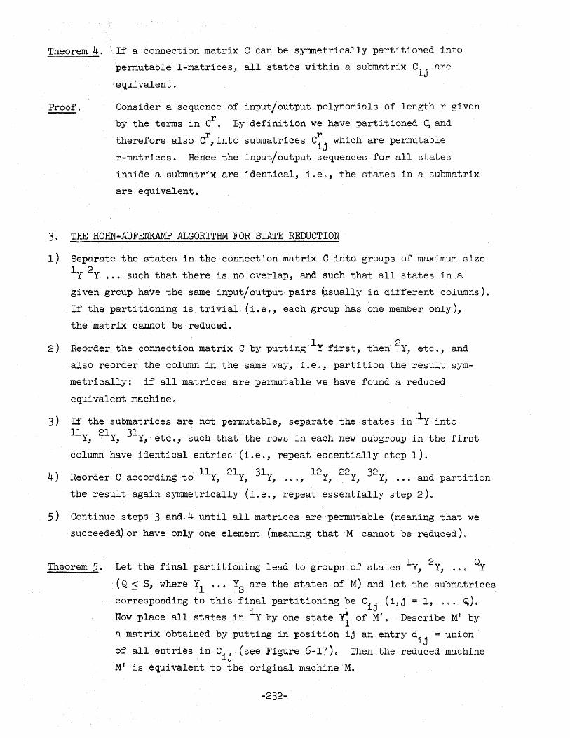
Theorem 4. If a connection matrix C can be symmetrically partitioned into
permutable I-matrices, all states within a submatrix C .. are lJ
Proof.
equivalent.
Consider a sequence of input/output polynomials of length r given
by the terms in Cr. By definition we have partitioned ~ and
therefore also Cr,into submatrices C~. which are permutable lJ
r-matrices. Hence the input/output sequences for all states
inside a submatrix are identical, i.e., the states in a submatrix
are equivalent.
3. THE HOHN-AUFENKAMP ALGORITHM FOR STATE REDUCTION
1) Separate the states in the connection matrix C into groups of maximum size 1 2 Y Y , •• such that there is no overlap, and such that all states in a
given group have the same input/output,pairs ~sually in different columns).
If the partitioning is trivial (i.e., each group has one member only),
the matrix cannot be reduced.
2) Reorder the connection matrix C by puttinglYfirst, then' ~Y, etc., and
also reorder the column in the same way, i.e., partition the result sym
metrically: if all matrices are permutable we have found a reduced
equivalent machine.
-3) If the submatrices are not permutable, separate the states in .1y into
lly, 2lr, 3l y, etc., such that the rows in each new subgroup in the first
column have identical entries (i.e., repeat essentially step 1).
4) Reorder Caccordingto 11y, 21y, 31y, 000, 12y, 22y, 32y, ... and partition
the result again symmetrically (i.e., repeat essentially step 2).
5) Continue steps 3 and 4 until all matrices are permutable (meaning that we
succeeded) or have only one element (meaning that M cannot be reduced) 0
Theorem 5. Let the final partitioning lead to groups of states ly, 2y, .•• ~ (Q~ S, where Yl 0 •• YS are the states of M) and let the submatrices
corresponding to this final partitioning be C.. (i, j = 1, 0 Q. Q) ~
Now place a.ll states in iy by one state Y! of l~, 0 Describe M' by ~
a matrix obtained by putting in position
of all entries in C .. (see Figure 6-17). _ lJ
ij an entry d .. = union' lJ
Then the reduced machine
M' is equivalent to the original machine M.
-232-
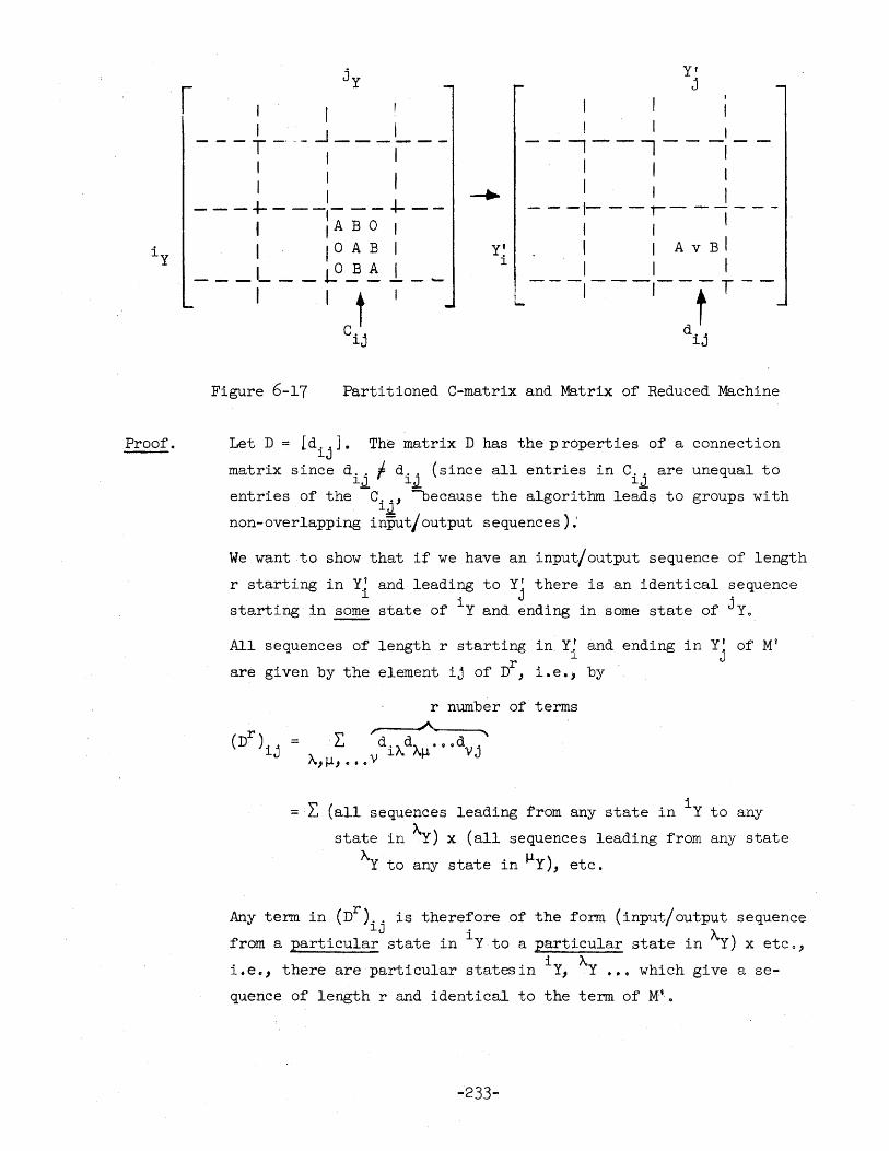
Proof.
I I ___ + _. __ -.J ___ 1 __ _
I I I I 1 I
I - - - +- - - -1- - - .t- --t I ABO I lOA B I lOB A I
------~-----I I t I
Cij
yf i
yl j
I 1
- - -, - - I - - -: -1 I I I I I
---1---,------I I I A v B I I I ~
L - - -,- - -1- - f T - -
dij
Figure 6-17 Partitioned C-matrix and Matrix of Reduced Machine
Let D = [dijJ. The matrix D has the properties of a connection
matrix since d .. f d. ~ (since all entries in C.j
are unequal to lJ l~ l
entries of the -C .. , ~ecause the algorithm leads to groups with lJ . non-overlapping input/output sequences);
We want to show that if we have an input/output sequence of length
r starting in Y! and leading to y! there is an identical sequence l . J .
starting in ~ state of ly and ending in some state of J y •
All sequences of length r starting in Y! and ending in yl of M' l j
are given by the element ij of Dr, i.e., by
r number of terms
= L (all sequences leading from any state in iy to any
state in ~y) x (all sequences leading from any state
~Y to any state in ~y), etc.
Any term in (Dr) .. is therefore of the form (input/output sequence
from a particula~J state in iy to a particular state in ~y) x etco,
i.e., there are particular statesin iy, Ay ••• which give a se
quence of length r and identical to the term of Mt ..
-233-
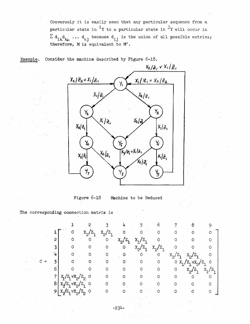
Conversely it is easily seen that any particular sequence from a
partic1llar state in iy to a particular state in j Y will occur in
L. d. ~ d').lIo 0 0 d . because d .. is the union of all possible entries; 1", '''tA' V J lJ
therefore, M is equivalent to M' 0
Example. Consider the machine described by Figure 6-18.
Xz./1:/ V' 'X// i I
Figure 6-18 Machine to be Reduced
The corresponding ~onnection matrix is
1 2 3 4 5' 6 7 8 9 1 0 X1/Zl X2/Z1 0 0 0 0 0 0
2 0 0 0 X2/Z1 'Xl /z1 0 0 0 0
3 a 0 0 0 X2!Zl X1/Z1 0 0 0
:4 0 a 0 0 0 0 XI!Zl X2/Z1 0
C = 5 0 0 0 0 0 0 o X1/Z1VX2!ZI 0
6 0 0 0 0 0 0 0 X2/Z1 XI /Z1
7 \1;vX2/Z2 0 0 0 0 0 0 0 0
8 xjZl vX2/Z1 0 0 0 0 0 0 0 0
9 X/ZI vX2/Z2 0 0 0 0 0 0 0 0
-234-
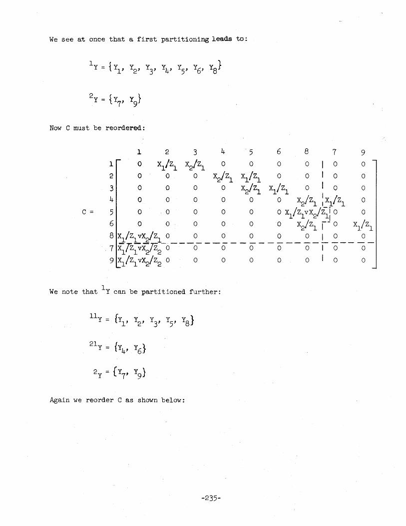
We see at once that a first partitioning leads to:
Now C must be reordered:
1 2 3 4 568 7 9
1 0 X1/Z1
X2/Z1 a a a a 0 0
2 0 0 0 X2/Z1 x1/z1 0 0 0 ° 3 0 0 0 0 X2/Z1 X1/Z1 0 0 ° 4 0 0 0 0 00 X2/Zl :x1/zl 0
c = 5 0 0 0 0 0 0 xl/zlvX2/Z~: 0 ° 6 0 a a 0 a 0 x2/ ZI 1- 0 xII Zl
a X1/Z1 VX2/Z1 a a a a a a I 0 ° 7 x;.Tz
1vx
2Tz
2"-o---O- - - 0" - - 0 - - 0 -- 0-1 0-- 0-
9Xl/zlvX2!Z2o 0 a a ° ° I 0 0
1 We note that Y can be partitioned further:
11y = [Y1
, Y2 , Y3' Y5, Ya}
21y = {Y4' Y6}
2y = {Y7' Y9
}
Again we reorder C as shown below:
-235-
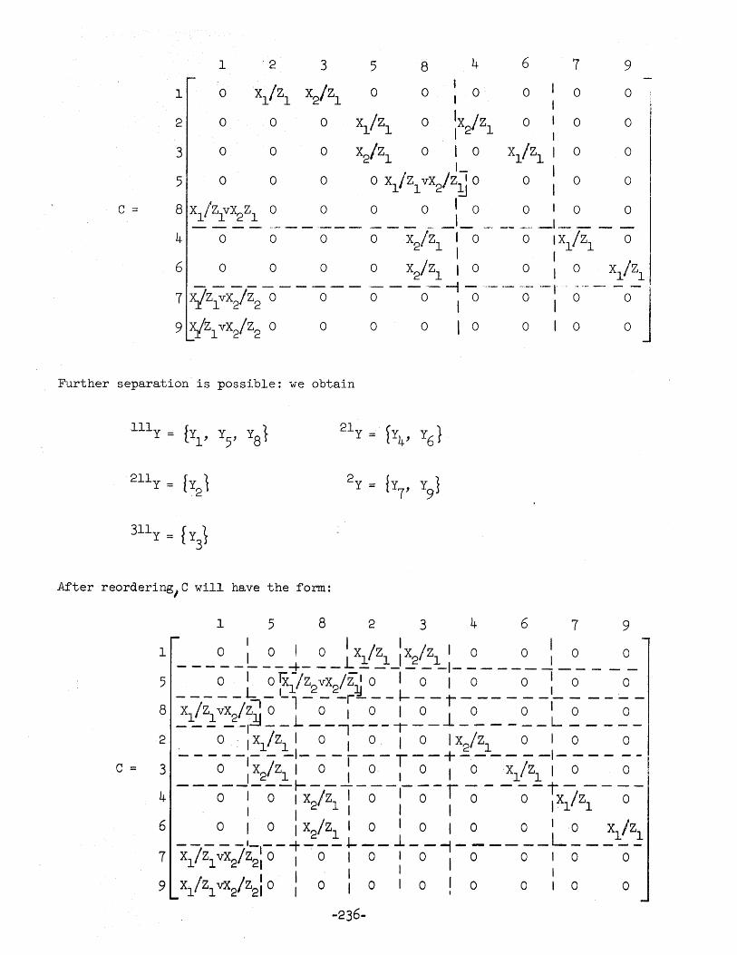
1 3 5 8 4 6 7 9
I 0 xl/zl X2/Z1 0 0 I 0 0 0 0
2 0 0 0 X/Zl 0 :X/Zl 0 1 0 0
3 0 0 0 X2!ZI 0 I 0 XI!Zl I 0 0
1- I 5 0 0 0 0 XI/ZI VX2/Z~ 0 0 I 0 0 I
c = 8 XlZlv~Zl 0 0 0 0 I 0 0 1 0 0 - - - - .. -~ - - ._ - - - - - _. - - __ .. , __ ._ .... _1", ___ _
4 0 0 0 0 X2/Z1 I 0 0 1 xII Zl 0 I I
6 0 0 0 0 X2/Z1 1 0 0 I 0 Xl/Zl - - - - - - - - - -- - - -- -i - .... - -- _ ... - --I' . _ .. , _ .. - -7 xjZlvX2/Z2 0 0 0 0 I 0 0 I 0 0
9 xjZl VX2!Z2 0 0 0 0 I 0 0 1 0 0
Further separation is possible: we obtain
Illy = {y y y? l' 5' 8 r
211y = [y 1 .2 {
After reordering/C will have the form:
1 582 346 7 9
C =
I I I! I I 1 I 1 0 1 0 , 0 LXI Zl I X2 Zl 0 0 1 0 0 - -- - -- -- 4- -- - -- - - -1- _.- ---- -- - --
5 0 1 0 iX;z vX /z I 0 I 0 I 0 0 I 0 0 - - - - -1:.. - L l_2 -2_rJL - - I-- - - "I - - - - - _1- - - - - -
8 Xl!ZI VX2/Z1' 0 0 I 0 I 0 0 0 I 0 0 _____ 111_ - L - -,- - - 'I - _.1 - - - - - - L - - - - -
2. 0 .: I Xl/ZI 1 0 1 O. I 0 I X2/Zl 0 I 0 0 - - - --,- - -1- -'-1- - T--+-'--- - -1- -- - --
3 0 I X2/Zl I 0 I 0 I 0 I OXl/Z1 I 0 0 --------~---·------r - - ---1-- ----
4 0 I 0 ,X2!Zl I 0 I 0 0 0 I X1!Zl 0 I I I I
6 0 I 0 I X2/Z1 1 0 I 0 I 0 0 I '0 X1!Zl --- - _1-_- -f-~--.l- __ .1_ - -i - - -- __ L - - - --
7 X1/Z1 VX2/Z2: 0 I 0 I 0 I 0 I 0 0 I 0 0 I I I I I
9 X1!Zl VX2/Z21 0 I 0 I 0 I 0 ! 0 0 I 0 0
-236-
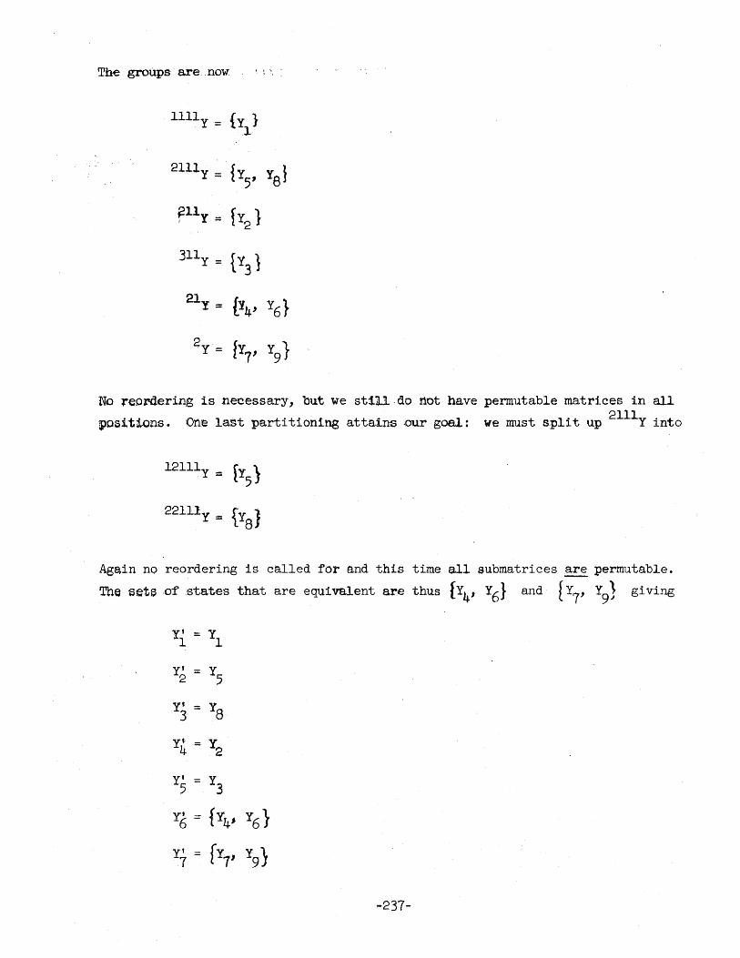
The groups are .. now • I "
lIlly = {Yll
211ly = {Y5' yS}
~lly = {Y2
}
311y = {13 1 2ly= {Y4' Y6}
~y = {Y7' Y9}
No :reordering is necessary, but we still·do rtot have permutable ma.trices in all
pos:i .. tlons.. One last parti tioning attain~ .QUI' goal: we must s.pIi t up 2111y into
12111y = fy5
)
22111y::: {YS}
Again no reordering is c~lled for and this time all submatrices ~ permutable.
The sets .of .states that are equivalent are thu.s {Y4, Y6} and f Y7' Y9} giving
Y' ::: Y 1 I
Y' = Y5 2
Y' ::: J Y8
Y4- = Y2
Y' = Y3 5
Yl ::: {Y4' Y6 }
Y+ = [Y7' Y9}
... 237-
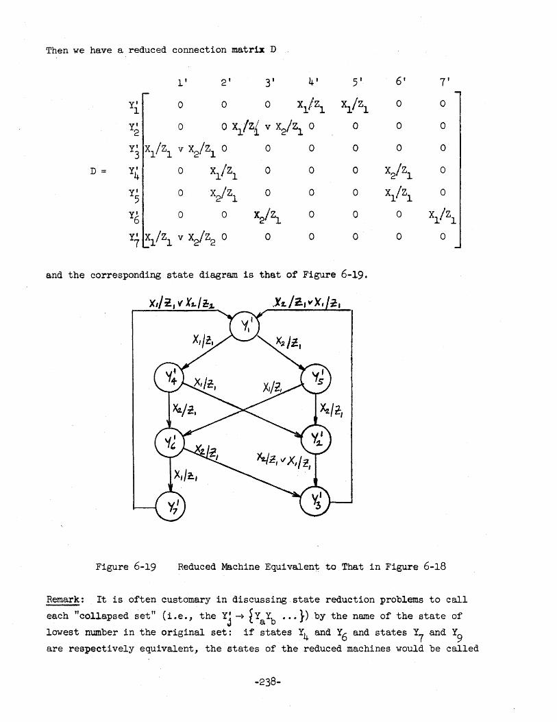
Then we have a reduced connection matrix D
l' 2' 3' 4' 5' 6' 7'
Y' 0 0 0 X1!Zl X1/Z1 0 0
1 Y' 2
0 o X1/Zi v X2/Zl 0 0 0 0
Y' 3
X1/Z1 v X2/Z1 0 0 0 0 0 0
D = Y' 4 0 xl/zl 0 0 0 X2/Z1 0
Y' 5
0 X2/Z1 0 0 0 X1!Zl 0
Y' 6 0 0 X2/Z1 0 0 0 x1/zl
y' 7 X1/Zl v X2/Z2 0 0 0 0 0 0
and the corresponding state diagram 1s that of Figure 6-19.
X,Ji.,,, X2-/t:J. ,.Xf. /'2:., v 'X, ~,
Figure 6-19 Reduced Machine Equivalent to That in Figure 6-18
Remark: It is often, customary in discussing ,state reduction problems to call
each "collapsed set" (i.e., the Yj ~ ~YaYb •• 0 })by the name of the state of
lowest number in the original set: if states Y4 and Y6 and states Y7 and Y9 are respectively equivalent, the states of the reduced machines would be called
-238-
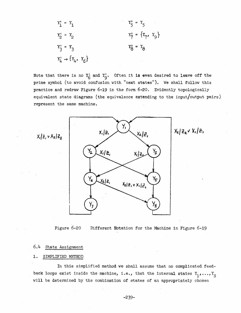
y' 1
Y1
Y' ::::; 5 Y5
Y' = Y2 Y' ::: {Y7, Y9} 2 7
Y' = Y3 Y,' = Y8 3 8
Y4 .... [Y4' Y6}
Note that there is no Y6 and Y9' Often it is even desired to leave off the
prime symbol (to avoid confusion with "next states"). We shall follow this
practice and redraw Figure 6-19 in the form 6·20. Evidently topologically
equivalent state diagrams (the equivalence ~xtending to the input/output pairs)
represent the same machine.
Figure 6-20 Different Notation for the Machine in Figure 6-19
6.4 State Assignment
1. SIMPLIFIED METHOD
In this simplified method we shall aSsume that no complicated feed
back loops exist inside the machine, i.e., that the internal states Y1
,8 .. ,YS will be determined by the combination of states of an appropriately chosen
... 239-
number flipflops--say t--and that we only have to design the AND and OR gates
combining the inputs XI,.",XM with the outputs of these flipflops. We shall
furthermore assume that each flipflop is set at each clock period, independ
ently of whether it may actually already be in the right state or not. That
such a simplification is possible will be shown by the success of the method.
The first question is: how many secondary· variables YI'.'.'Yt
(representing the flipflop states, or more precisely· the signal on the "I"-output
side) are necessary. We shall include the answer in'the State Assignment
Algorithm.
State Assignment Algorithm
1. For a machine with S states take t flipflops w~ere
but (6-28 )
(i.eo, the number of combinations of flipflops states must be at least
equal to the number of internal states!).
This fixes the number of secondary variables y·l ·, ••• , Y t • Note that we have
chosen t rather than s since there is not necessarily any relationship
between the number of nodes (s) and the number of flipflops (t).
2. Associate arbitrarily (we shall improve on this in the next section) the
combinations of the y'swith the Y's by some coding scheme:
i = 1 ... S· . (6-29)
Ob;viously there may be many combinations of y's which are unused. When
they occur in a table wei may consider the corre.spondingY's to be don't-
cares.
3. Repeat steps 1 and 2 for Xl' .,.,Xm and ZI, .. o,Zn' i.e., determine the
appropriate number of binary input variables m and the appropriate number
of binary output variables n such that we can establish an (arbitrary)
code
k 1 M (6-30)
j 1 ••• N (6- 31)
-240-
4. From the connection matrix C write down a modified Huffman Flow Table using
secondary variables. Besides the usual "next state" columns, write down
for each input XI""'~M YI""Yt as column headings twice and mark the
5.
two parts fO and fl' Mark an * under fO and Yi in group Xk if this input
correspoilds to y. = 0 in the "next state" part of the table. Mark an * l
under fl and Yi if Yi = 1 under the influence of ~,
Determine the functions fo(Yi ) and fl(yi ) which are necessary to set the
flipflops from the table in step 4 and the encoding of the inputs (6-30). Note that fO(Yi ) means the "O"·setting function for flipflop i, This
function will generally depend on Yl""'Yt and xl"",xm'
6. Simplify the fO and fl functions by appropriate methods (Roth, Karnaugh).
Note that under the assumptions of the present method
so that we can actually just determine the fl-functions.
7. Design a decoder such that for each combination (Xl,···,xm)(yl , .•• ,Yt ) we
obtain the correct (zl"",zn) when (6-29), (6-30) and (6-31) are used.
This is a (in theory simple) combinational problem.
Example. Let us reconsider the machine of the last example, drawn in the form
of Figure 6-20.
Steps 1-3: We have only two inputs Xl and X2 and two outputs Zl and Z2' There
fore we have m = 1 and n = 1, i.e., one input variable Xl and one outputvari-
able zl suffice. Let us encode as follows:
o
= 1
o
1
To represent seven states we need three flipflops, i.e., three secondary
variables Yl Y2Y3' Let us encode as follows
-241-
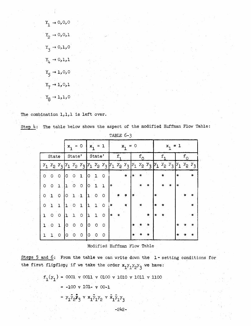
· Y2 ~ 0,0,1
The combination 1,1,1 is left over.
Step 4: The table below shows the aspect of the modified Huffman Flow Table:
'IIABLE 6-3
x = 0 x == 1 xl = 0 x :;: 1 1 1 1
State State' State' fl fo fl fO
Y1 Y2 Y3 Y1 Y2 Y3 Yl Y2 Y3 Y1 Y2 Y3 Yl Y2 Y3 Yl Y2 Y3 Y1 Y2 Y3
0 0 0 0 0 1 0 1 0 * * * * * * 0 0 1 1 0 a a 1 1 * * * * * * a 1 0 a 1 ·1 1 0 0 ¥ '* ~ * .* * 0 1 1 1 0 1 1 1 0 i* * * * * * 1 0 0 1 1 a 1 1 0 * * * * * * 1 0 1 0 0 0 a a 0 * * .* * * * 1 1 0 0 0 0 0 a 0 * * * * * *
Modified Huffman Flow Table
Steps 5 and 6: From the table we can write down the l-setting conditions for
the first flipflop; if we take the order xIYIY2Y3we have:
f1(Y1 ) = 0001 v 0011 v 0100 v 1010 v 1011 v 1100
= -100 v 101- v 00-1
-242-
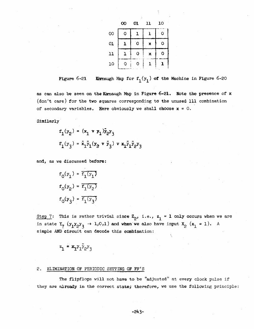
00 01 11 10 _ ....... -
00 0 1 1 0
01 1 0 x 0
11 1 0 x 0 -----1·._··,· i
r .. '- --.---
0 I
0 1 1 I __ .... 1, ...
10
Figure 6-21 KBmaugh Map for fl (Y1) of the Machine in Figure 6-20
as can also be seen on the Karnsugh Map 1n Figure 6 .. 21. Note the presence of' lC
(don't care) for the two equares corresponding to the unused 111 combination
of secondary variables. Here obviously we shall choose x :; o.
Similarly'
f 1(Y2) = (Xl v Yl)Y2Y3
f 1(Y3) = X1Y1 (Y2 v Y3) v X1Y1Y2Y3
and, as we discussed before:
fO(Y1 ) = f 1 (Yl)
f O(Y2 ) = fl (Y2)
1'O(Y3) = f 1 (Y3'
Step 7: This is rather trivial since Z2' i.e., Zl :; 1 only occurs when we are
in state Y7 (YIY2Y3 -+ ,l,D"l) and when'we also have input X2 (Xl;;; 1). A
simple ANDclrcuit can decode thi-s combination: \
2. ELIMINATION OF PERIODIC SETTING OF FF' S
The flipflops will not have to be "adjusted" at every clock pulse if
they are already in the correct state; therefore, we use the following principle:
-243-
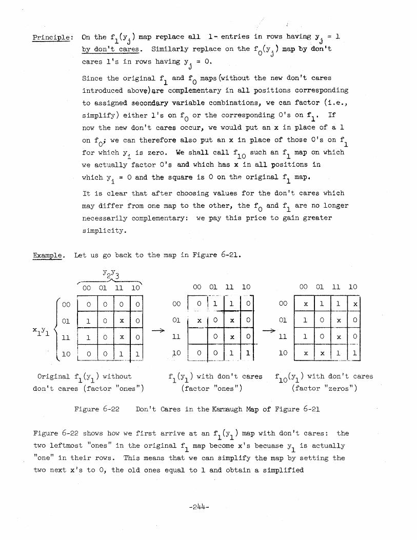
Principle: On the fl (Yj
) map replace all 1- entries in rows having Yj
= 1
by don 1 t cares. Similarly replace on the fO(Yj
) map by don't
cares lIs in rows having y. = o. J
Since the original fl and fO maps (without the new don't cares
introduced above)&re complementary in all positions corresponding
to assigned secondary variable combinations, we can factor (i.eo,
simplify) either lis on fO or the corresponding O's on f l - If
now the new don't cares occur, we would put an x in place of a 1
on fO; we can therefore also put an x in place of those a's on fl
for which Yi is zero. We shall call flO such an fl map on which
we actually factor 0" s and which has x in all positions in
which Yi
= 0 and the square is 0 on the original fl map.
It is clear that after choosing values for the don't cares which
may differ from one map to the other, the fO and fl are no longer
necessarily complementary: we pay this price to gain greater
simplicity.
Example. Let us go back to the map in Figure 6-21.
Y2Y3 r'~----~------'
00 01 11 10 00 01 11 10 00 11 01
0 0 0 0 00 Ior~-- .. -
00 1 0 00 x 1 1 ....... _-
01 1 0 x 0 01 x 0 x 0 01 I 0 x --
I 1 0 x 0 11 ~ ~
11 0 x 0 11 1 0 x
! : 0 0 1 1 10 10 I 0 0 .1 1 10
I x x 1
10
x --
0
0 ..
1 L. __ --l ____ . __ .... __ f--.. __ I L_. __ ._ --... ~.~. -- - ... --.. -.-
Original fl(Yl ) without
don't cares (factor "ones")
fl(Yl) with don't cares
(factor "ones")
flO(Yl ) with don't cares
(factor "zeros")
Figure 6-22 Don't Cares in the KffiT.augh Map of Figure 6-21
Figure 6-22 shows how we first arrive at an fl(Yl ) map with don't cares: the
two leftmost "ones" in the original fl map become XiS becuase Yl
is actually
"one" in their rows. This means that we can simplify the map by setting the
two next x's to 0, the old ones equal to 1 and obtain a simplified
-244-
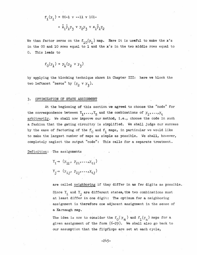
-; xIYlY3 v Y2Y3 v xI YI Y2
. We than factor zeros on the flO (Y l) map. Here it is useful to make the x' s
in the 00 and 10 rows equal to 1 and the x's in the two middle rows equal to
O. This leads to
by applying the blocking technique shown in Chapter III: here we block the
two leftmost "zeros" by (Y2 v Y3).
3. OPTIMIZATION OF STATE ASSIGNMENT
At the beginning of this section w·e agreed to choose the "code" for
the correspondence between Y1, •.. ,Ys and the combinations of YI'''''''Yt arbitrarily. We shall now improve our methOd, i.e., choose the code in such
a fashion that the ga.ting circuitry is simplified. We shall judge our success
by the ease of factoring of the ~O and fl maps, in particular we wOllld like
to make the largest number of maps as simple as possible. We shall, however,
completely neglect the output "code": This calls for a separate treatment.
Definition: The assignments
are called neighporing if they differ in as few digits as possible.
Since Y. and Y. are different states, the. two combinations must l J
at least differ in one digit: The optimum for a neighboring
assignment is therefore one adjacent assigmtlent in the sense of
a Karnaughmap.
The idea is now to cons ider the foe Y m) and f l( Y n) maps for a
gi ven assignme.nt of the form (6-29). We shall also go back to
our assumption that the flipflops are set at each cycle,
-245-
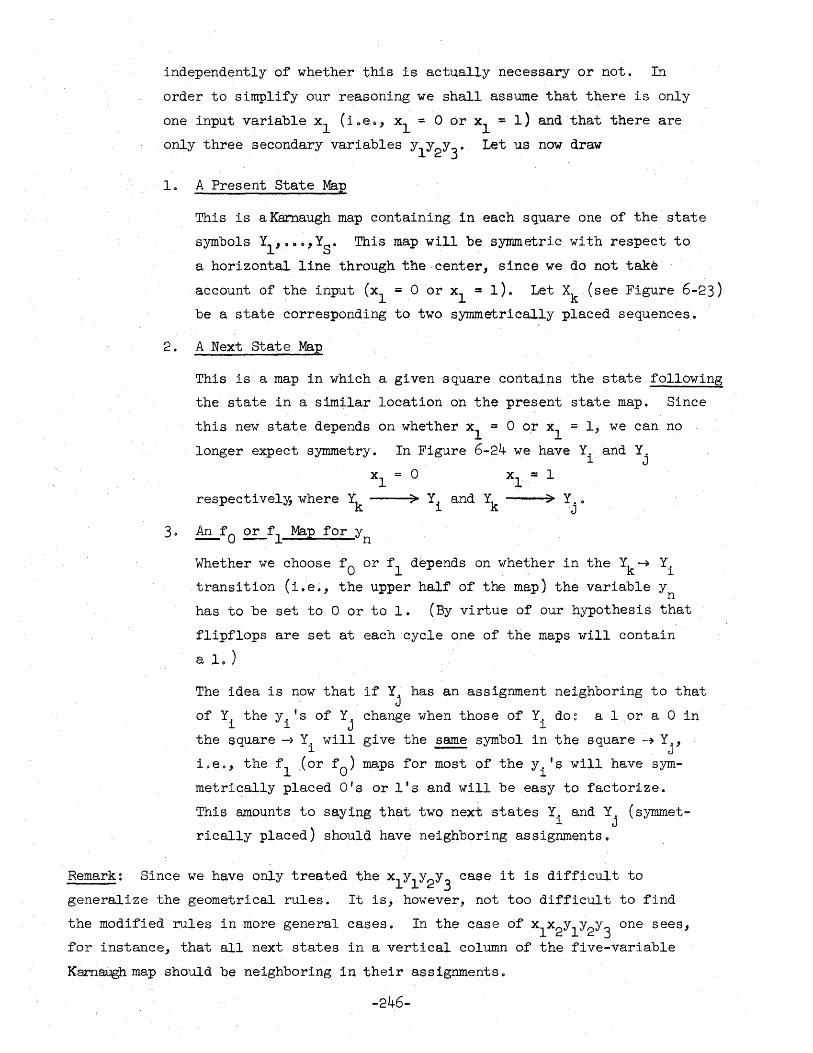
independently of whether this is actually necessary or not. In
order to simplify our reasoning we shall assume that there is only
one input variable xl ( i 0 eo, xl = 0 or xl ::: l) and that there are
only three secondary variables YlY2Y3e Let us now draw
1. A Present State Map
This is aKarnaugh map containing in each square one of the state
symbols YI'o~~,YS. This map will be symmetric with respect to
a horizontal line through the center, since we do not take
account of the input (Xl = 0 or xl ::: l)~ Let Xk (see Figure 6-23)
be a state corresponding to two symmetrically placed sequences.
2. A Next State Map
3.
This is a map in which a given square contains the state following
the state in a similar location on the present state map. Since
this new state depends on whether xl ::: 0 or Xl = 1, we can no
longer expect symmetry. In Figure 6-24 we have Y. and Y. ]. J
Xl 0 Xl ::: I
respectivel~ where Yk
:;;. Y1
and Yk ~ Y.o
J
An fa 2!-fl Map for Yn
Whether we choose fO or fl depends on whether in the Yk~ Yi transition (i.e., the upper half of the map) the variable y
n has to be set to 0 or to 1. (By virtue of our hypothesis that
flipflops are set at each cycle one of the maps will contain
a I. )
The idea is now that if Y.has an assignment neighboring to that . J
of Yi
the y. 's of Y. ]. J
the square -> Y. will ].
i 0 eo, the f l( 0 r f 0 )
change when those of Yi
do: a 1 or a 0 in
give the same symbol in the square -~ Yo, J
maps for most of the y. 's will have sym-].
metrically placed 0 I S or I' s and will be easy to factorize 0
This amounts to saying that two next states Y. and Y. (symmet-]. J
rically placed) should have neighboring as signments.o
Remark: Since we have only treated the xlYIY2Y3 case it is difficult to
generalize the geometrical rules. It is, however, not too difficult to find
the modified rules in more general cases. In the case of xl x2YlY2Y3 one sees,
for instance, that all next states in a vertical column of the five-variable
Karnaugh map should oe neighboring in their assignments.
-246-
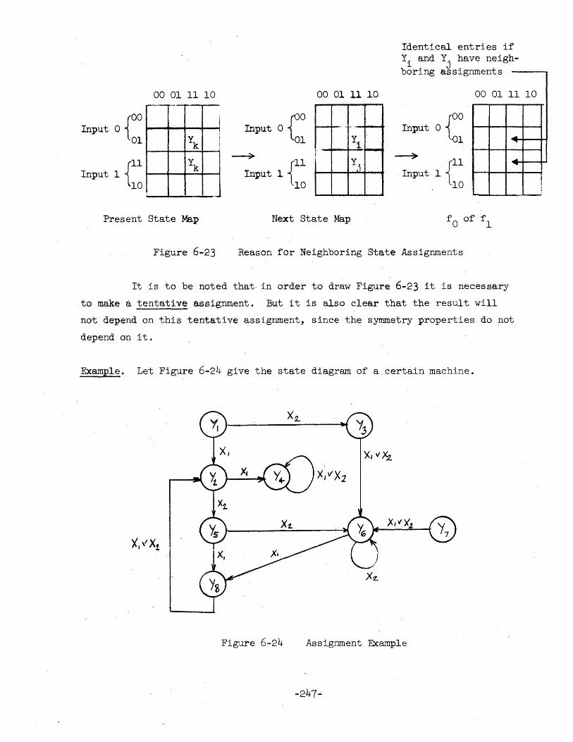
A {
OO Input
01
{
II Input 1
10
00 01 11 10 --
Yk
Yk
--Present State Map
Figure 6-23
I I i
00 01 11 10
Input o~: f-- ...-,':
Y1
~ {Il Input 1 .
10
I'
!
Y.;
Next State Map
Identical entries if Y. and Y. have neigh-b
l . J. t orlng asslgnm en s
00 01 11 10
Input oro 01 ..
---7 {ll Input 1 10
~ ..
Reason for Neighboring State Assignments
It is to be noted that in order to draw Figure 6-23 it is necessary
to make a tentative assignment. But it is also clear that the result will
not depend on this tentative assignment, since the symmetry properties do not
depend on it.
Example. Let Figure 6-24 give the state diagram of a,certain machine.
X, " X2.
X," 'X.2,
X,VX1
Figure 6-24 Assignment Example
-247-
I
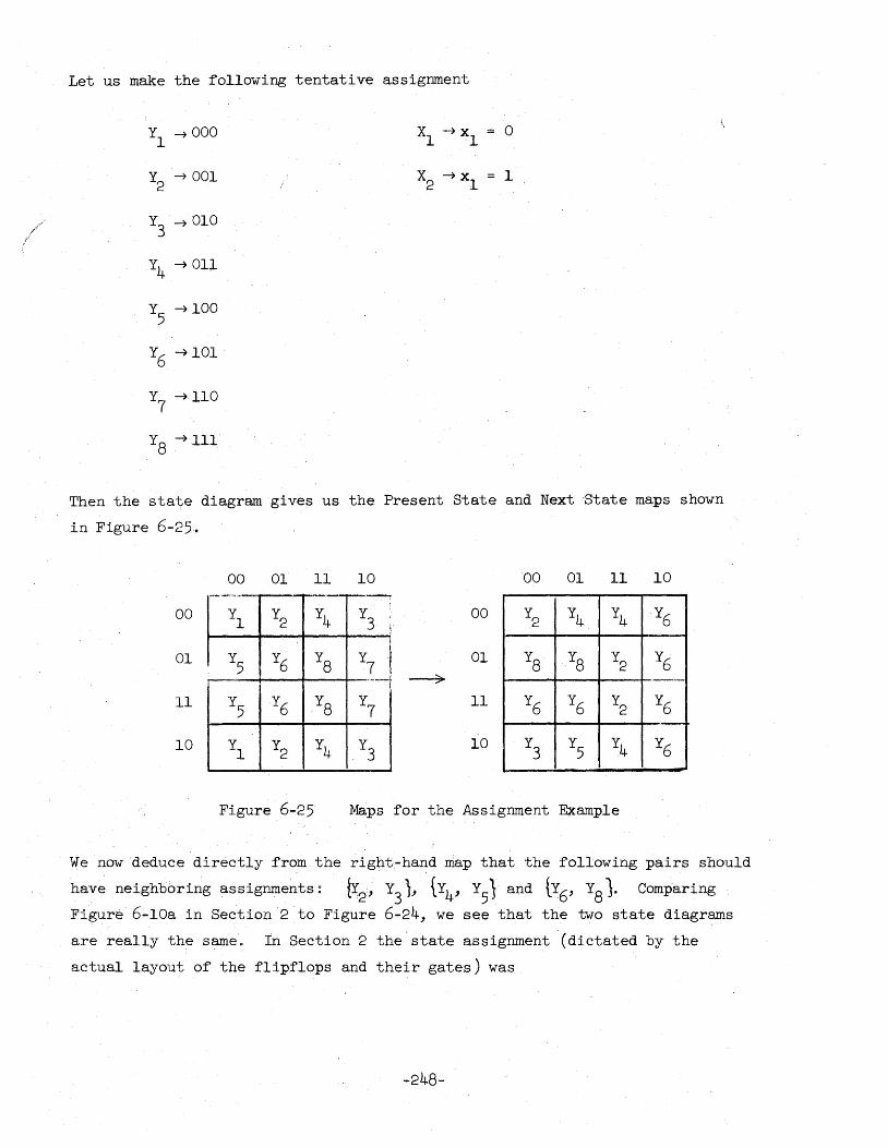
Let us make the following tentative assignment
Yl
-7000 o
Y2
-7001 1
Y3
-7010
Y4 -7 OIl
Y5
-7100
Y6 -7101
Y7
-7110
Y8
-7111
Then the state diagram gives us the Present State and Next Btate maps shown
in Figure 6-25.
00 01 11 10 00 01 11 10 .... --... ,~.~ ... .,----, ,
00 Yl
Y2 Y4 Y
3 00 Y
2 Y
4 Y4
Y6 I
01 Y5 Y6 Y8 Y7 I 01 Y
8 Y8 Y
2 Y6 f ---,
11 Y5
Y6 Y8
Y7
11 Y6 Y6
Y2
Y6
10 Yl Y2 Y4 Y
3 10 Y
3 Y5
Y4 Y6
Figure 6-25 Maps for the Assignment Example
We now deduce directly from the right,-hand map that the following pairs should
have neighboring assignments: {Y2" Y3
), tY4, Y51 and tY6, Y81. Comparing
Figure 6-10a in Section 2 to Figure 6-24, we see that the two state diagrams
are really the same. In Section 2 the state assignment (dictated by the
actual layout of the flipflops and their gates) was
-248-
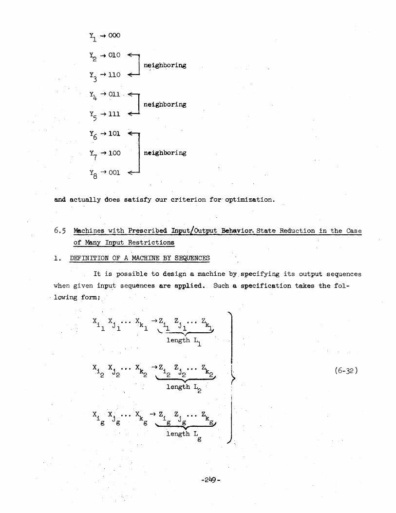
. Y4 ~ all· J neighbortng
Y5 ~ll1
neighboring
and actually does sa.tisfy our criterion for'optimization.
6.5 Machines with Prescribed Input/Output Behavior. State Reduction in the Case
of Many Input Restrictions
1. DEFINITION OF A MACHINE BY SEQUENCES
It is possible to design a machine by. specifying its output sequences
when given input sequ.ences are applied •. Such a specification takes the fol-
. lowing form:
11 1 1 11 J l X. Xj ••• X.k -7Z'~' •. 00 .
\....
length Ll
X. XJ .••• Xk ...... Z. Zj .0. ~2 I (6-32) .l2 2· . 2 \..
12 2
> V ~.
length L2
X. Xj ••• Xk -7 Zi Z. •• 0 ~ 1 g g . g \" g J g gl
..... ·V length L
g
-249-
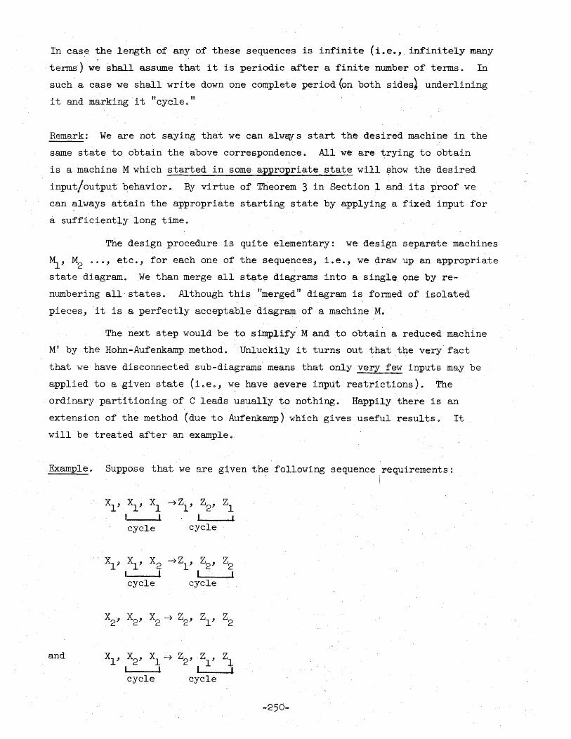
In case the length of any of these sequences is infinite (i.e., infinitely many
terms) we shall assume that it is periodic after a finite number of terms 0 In
such a case we shall write down one complete period (on both sides~ underlining
it and marking it "cycle."
Remark: We are not saying that we can alwSlfs start the desired machine in the
same state to obtain the above correspondence. All we are trying to obtain
is a machine M which started in some appropriate state will show the desired
input/output behavior. By virtue of Theorem 3 in Section I and its proof we
can ~lways attain the appropriate starting state by applying a fixed input for
a sufficiently long time.
The design procedure is quite elementary: we design separate machines
MI, M2 .•. , etc., for each one of the sequences, i.e., we draw up an appropriate
state diagram. We than merge all stat~ diagrams into a single, one by re
numbering all states. Although this "merged" diagram is formed of isolated
pieces,it is ,a perfectly acceptablediagra.m. of e. machine M.
The next step would be to simplify M and to obtain a reduced machine
M' by the Hohn-Aufenkarnp method. Unluckily it turns out that tl1.e ve'ry' fact
that we have disconnected sub-dia~rams means that only very few inputs may be
applied to a given state (iee., we have severe input restrictions). The
ordinary partitioning of C leads usually to nothing. Happily there is an
extension of the method (due to Aufenkamp) which gives useful results. It
will be treated after an example ..
Example. Suppose that we are given the following sequence requirernents~ !
Xl' Xl' Xl ,4> Z1' Z2' Zl I I I , cycle cycle
Xl' Xl' X2 ~Zl' Z2' Z2 I I I I cycle cycle
and
-250-
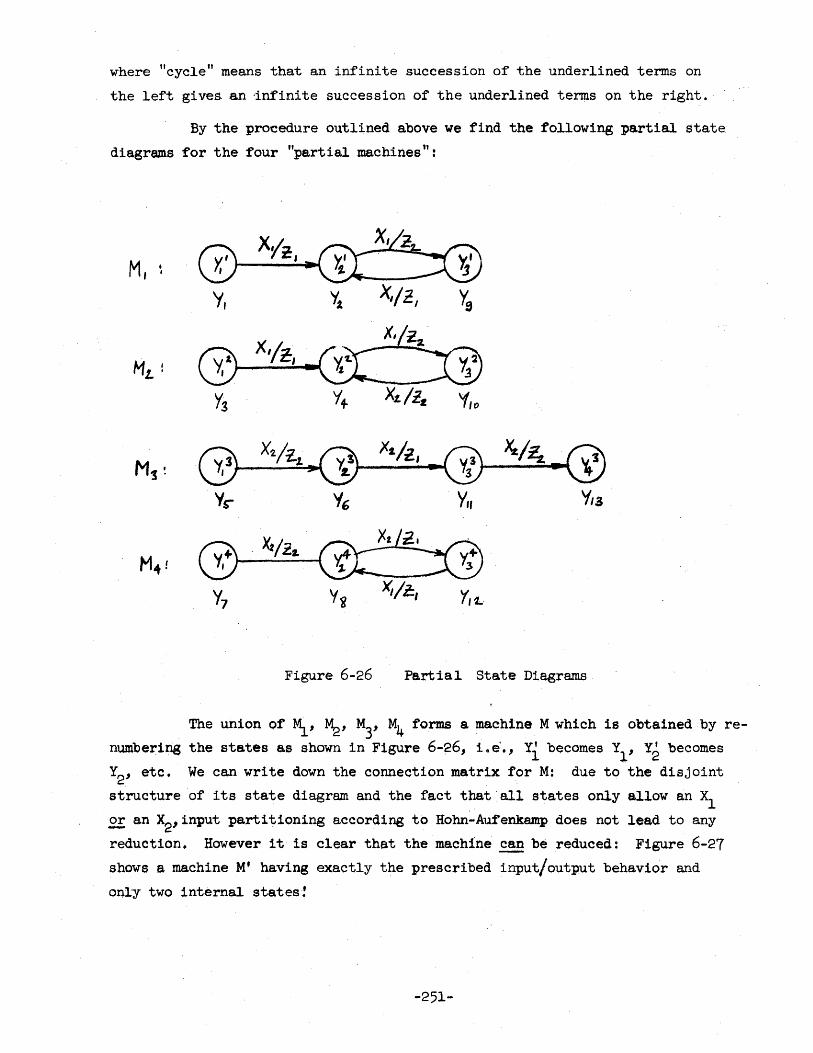
wnere "cycle" means that an infinite succession of the underlined terms on
the left gives. an -infinite succession of the underlined te~s on the right.
By the procedure outlined above we find the following partial state.
diagrams for the four "partial machines":
M, @ y, )'t
M!, l @ Y3 'f,o
M1 ~ X'l.!i.z. X"/i., ~/~
y~ 'I, y" '113
Ha1! @ X,/21. (fil:i£~ Y7 Y g 'X,/i:., '{,t-.
Figure 6-26 Partial State Diagrams
The union of ~, ~, M3, M4 forms a machine M which 1s obtained by re
number1ns the sta.tes as shown in Figure 6-26, i 0 e'., Yi becomes Y1
, Y2 becomes
Y2' etc. We can wr'1te down the connection matrix for M: due to the disjoint
structure of its state diagram and the fact t~tall states only allow an Xl
£!: an X2,input partitioning according to Hohn-Auf"enkamp does not lead to any
reduction. However it is clear that the machine.£!!! be reduced: Figure 6-27
shows a machine M' having exactly the prescribed input/output behavior and
on]:y two internal states!
-251-
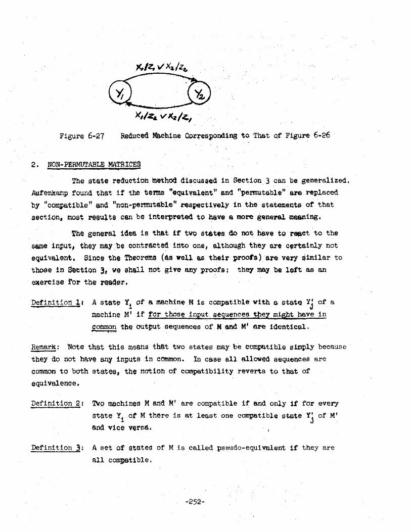
Figure 6-27 Red.uced Machine Cor;res:pond1ng t~Tha.t QfFigur~ 6-26
2. NON .. P!RMUTABLE MATRIC~S Ii, W
The stete reduct10h methotl d1~cus$eti in Section,3 can be g.enerali~edo
Aurenkamp foun~ tha.t if the terms tt.qu1vs!ent tt and "permuta.ble" are repla.ced
by "compstible" ana t1nQn",permutE1ble tt respectively in tbe statements of 'that
.section, moet ~ij~l.ts can be interpreted to h$ve Et, more S4inerel meaning,
The senera~ idee. is that if' two s'tates 40 not h$.ve to rS(aet to the
same input, they mBy:oe contracted into one, although they are c,rta1nly not
equivalent. S1nce the Theot'ems (~s .ell a.s their proote),areve'lY $1m11ar to
tboEle in Seet10n 3" ,W~ shall not give any pro,?fs: they ma1 'be lett a.s an
ellerciae for the rea<1~:r,
Defini tion ~. A state Yj. of a machin~ M is compatible vith {3, s·tete;} YJ of e.
machine M' if for those inRut sesuencee t~el might have in
common tbe output sequenC~$ of M e.nd Nt ere 1<l:ent1cel. 0
, · .•• · .. rS ... c:
Remark: Note tha.t this' mea-hS thf:lt tw-o states maybe eompat1ble eunply because
they do not hav~ any, inputs in common. In case all allowed sequences are
common to both Eltates, the not1oh of compatibility r~ve"a to thet of
equiva1.ence t
Defini tion :2, ~o machines M e;rid Mt are compat,ible if and only it for every
st&te YiotM thare is a.t least one compatible ~te.te Yj of' Mt
and vice verss'e
Definition 3~ A set of states of M is called pseudo-equivalent if they are
all COmpEltibleo
-252-
Definition 4: A matrix containing input/output polynomials as elements is
called a non-permutable r-matrix if
1.. whenever two rows happen to have "the same input sequence, they are
associated with the same output sequence. (In the permutable
case all input/output sequences would occur in each row.)
2. in a row all non-zero input sequences must be different.
3. all non-zero entries are OR-sums of the product of r input/
output pairso
Using these definitions, the following theorems can be stated (The proofs
are analogous to those given in Section 3; hence, will not be given here.):
Theorem 1. The sum of two non-permutable r-matrices A and B is another non
permutable r-matrix if the entries in each row in A are different
from those of the corresponding row in B and if furthermore when
ever an input appears in different rows in both matrices, it is
associated with'the same output.
Theorem 2. The product of a non-permutable r-matrix and a non-permutable s
matrix is a non-permutable r + s matrix if it can be formed 0
Theorem 3. If a given symmetrical partitioning of a connection matrix
C = [Cij ] gives non-permutable I-matrices and furthermore all
submatrices in a row have different sets of entries, the rth
power of C,partitioned in the same way (i.eo, C~j),has as its
submatrices non-permutable r-matrices and the submatrices in a
row again have different setsof entries.
Theorem 4. If C can be symmetrically partitioned such that all submatrices
are non-permutable I-matrices and such that all submatrices in a
row hay disjoint input sequences, then all states in a submatrix
are pseudo-equivalent.
3. THE AUFENKAMP ALGORITHM
1. Parition the states Yl
0.0 Ys in the connection matrix C into groups of
maximum size ly, 2y 00. such that there is no overlap and such that the
-253-
rows in each set fonn non-permutable I-matrices, 'and such that if two
groups are united, the result is no longer a non-permutable I-matrix 0
(There usually is more than one solution 0) If the p~itioning is tri ial,
the matrix cannot be 'reduced Q
20 Reorder the connection matri~ by putting ly first,~h~n 2y, etc., and
part1 tion symmetricall~:. if all 6ubmatricesa,:re non"'perrnutable l-matrices
~nd ell submatr1ces in ~ ~ow have. disjoint lhput seQuQnces we terminate:
4.
all state~ 1~oa part1t1bn are pseudo-equivalent,
If the submatrices a:f't:er Step 2 are not non-permutable l'!"matrices" repartition 1 2" '1../ - "
inside of I, Y, OQ~II ~ ~he res~lt istr1v1al,there are no pseudo ...
equivalent states.
~f the partitioning 1s Step 3 is successful, reo·rde.rand partition the G
matri~ symmetri cally 0
/ 5. Continue Steps 3 and 4 until all matric~S' a.re ·nol'1 .... pennutable l~'matrices
(meaning that we succeeded) or have only one elamen~ (m$aning that M
cannot be reduced).
Theorem 5. If th~ pseudo-equivalent sta.tes of M obtaine~ by the Aufenkamp
algorithm are replaced' by a single st~te ofa machine M' and the
connection matrix C' ofM' is obtained by forming the union (OR
sum) of the entries in the submatrices of C after the final
parti tioriing, then M' is compatible with M. (Thta means" of course,
that for those input sequences they may have 1~.common~ the output
, sequenc~a will be ~denticaJ.~' )
Theorem 60 The reduced mach~ne M'can a.cce:ptall input seQ.uences of M but
not vic~ "ersao
Proof ,'" This rather "importa.nt fa.ct , (the reductiohwoUld. pewi thout . sense
otherwise) simply follows. from the red}1ctionmethod~ no inputs
are lost in the partitioning and. the format1ort ot the firial OR
sumo
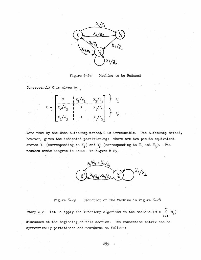
Figure 6-28 Machine to be Reduced
Consequently C is given by
C =
Note that by the Hohn-Aufenkamp metho~ C is irreducible. The Aufenkamp method,
however, gives the indicated partitioning: there are two pseudo-equivalent
states Yl (corresponding to Yi) and Y2 (corresponding to Y2 and Y3
). . The
reduced state diagram is shown in Figure 6-29. .
Figure 6-29 Reduction ofth~ Machine in Figure 6-28
4 Example 2. Let us apply the Aufenkamp algorithm to the machine (M = L Mi )
i=l
discussed at the beginning of this section. Its connection matrix can be
symmetrically partitioned and reordered as follows:
-255-
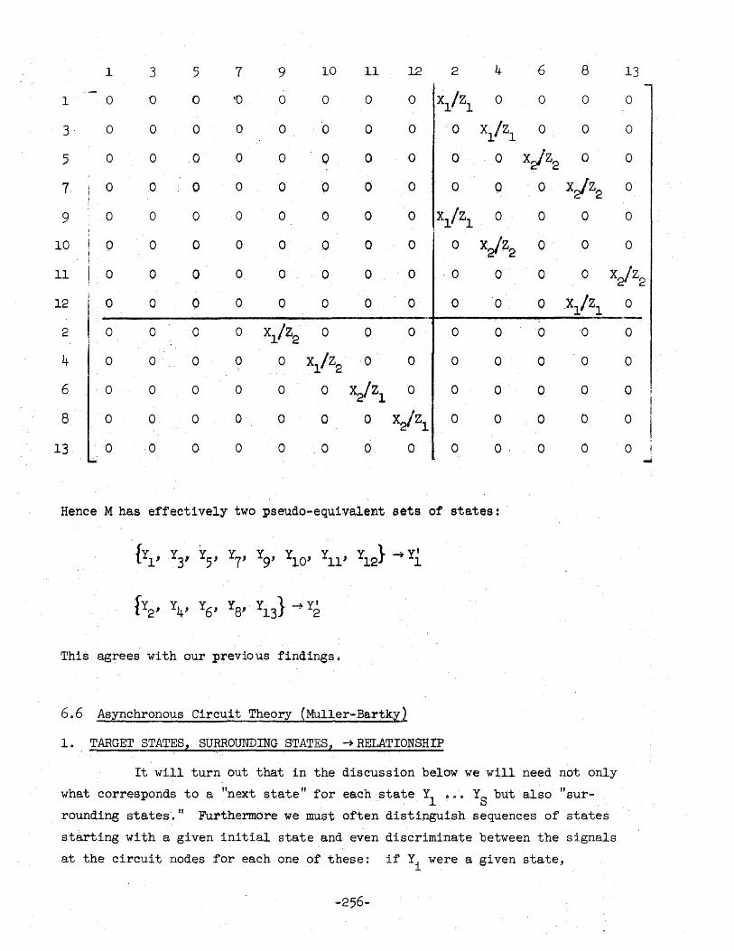
1 3 5 7 9 10 11 .12 2 4 6 8 13
1 0 0 0 '0 0 0 0 0 X1/Z1 0 0 0 0
3· 0 0 0 0 0 ·0 0 0 0 Xl/Z1 0 0 0
5 0 0 0 0 0 Q 0 .0 0 0 X,jZ2 0 0
7 0 0 0 0 0 0 0 0 0 0 0 X,jZ'2' 0
9 0 0 0 0 0 0 0 0 X1!ZI 0 0 0 0
10 0 0 0 0 0 0 0 0 0 XJ'?2 Q 0 0
11 0 0 0 0 a 0 0 0 0 0 0 0 X2!Z2
12 0 0 0 0 0 0 0 0 0 0 0 X1/Z1
'2 0 0 0 0 xl/z2 0 0 0 0 0 0 '0
4 0 o· 0 0 0 Xl /Z2 ·0 0 0 0 0 0
6 0 0 0 0 0 0 X,jZl 0 0 0 0 0
8 0 0 0 0 0 0 0 X,jZl 0 0 0 0
13 0 ·0 0 0 0 .0 0 0 0 0, 0 0
Hence M has effectively two pseudo-equivalent sets of states:
This agrees ~ith our previous find1ngso
6.6 Asynchronous Circu.1t Theory (Muller-Bartky)
10 TARGET STATES, SURROUNDING STATES,-+ RELATIONSHIP
It will turn out that in the disc'Ussion below we will need not only
what corresponds to a '''next state" for each state Y1
0 0 '. Ys but also "SUl"
rounding sta.teso" Furthermore we must often distinguish sequences of states
starting with a given initial state and even discriminate between the signals
at the circuit nodes for each one of these: if Yi were a given state,
-256-
0
0
0
0
0
0 -'
surrounding states would have to have two indices Yik, the signals Yl .00 Ys
three indices, ioe., Yik = (Ylik, Y2ik 000 Ysik ) and a node signal for a
sequence a fourth index. In order to simplify matters we shall often call
the states A, B, 000 Y ••• Z (we will not be concerned with outputs and can
use X and' Z for states), i. e., A = Yl , B = Y2
••• etc 0 The" surrounding"
relationship will be indicated without using a subscript, a sequence of
states starting with A will be written as A(O) A(l) ••• A(n) ••• and the
internal signals of A(n) by (al (n) a2 (n) 0 •• as(n)).
In synchronous circuit theory we had the equation
Yi' = f.(xl,···,x , Yl'·o~,y ) . 1 m·· 6
In asynchronous circuit theory we assume that the input & ar~'held constant
while we examine the transitions of the machine, i6e., that we actually have
(6-33)
The inputs may be thought of as parameters that can only be changed after the
machine has settled down. We suppose, as usual, that it is always possible
to choose appropriate internal nodes or "cardinal points" such that the state
of the {input-independent) machine is completely ,specified by their signals.
Definition 1: The state Y' = (Yl' , •• 0' y') defined by (6-33) will be called . s the target state of Y = (Yl" •• 'Ys ).
Remark: The target state Y' of an asynchronous machine is defined in the
same way as the next state Y' of a synchronous machine. In the present
case, however, there is no guarantee that the machine will ever attain Y'
because of internal races.
Definition 2: A state W = (wI' 0 •• , w ) "surrounds" state Y::; (Yl' Q 0 ., y ) with . s s target state Y' = (Yl' ••• 'Y~) if i.ts signals agree with those
of Yand y' whenever the latter agree:
y' 1 if Y = y'
i . i
-257- '
Otberwi se we,.6halJ.. -allow· w. to have either value, i 0 e . , . 1
Yi Wi :: { if y. I y ~ (6- 34 )
.11 or Yi
·· .
(Note that (6-34) contains· the case Y i = Y ~ :, For such a state
W surrounding Y we shall write Y .... W· (W surrounds Y or Y .is
s'I.lrrounded:.bY' 'W),. with the explicit understanding that W.~
come after Y but must not and that there was no intervening
state.
Remark 1: The -~relatlon5hip is denot.eq 'byte in Mull.er's original papers. Also
his de:r1nltions incl.ude the case 6f more than two sienal values.
Remark 2: It is clear from the definition that Y -~ y' and Y --) Y. However it
is usually ~ true that Y ~ W imp11~s W ..... Yo
Remark 3: If Y' diff'ers from Y in k: digit positions (i.e., signals), Y is
surrounded by 2k states (includingYand Y' themselves'.
Theorem 1. Any state following Y di:r~ctly must surround Y.
Proof. It is clear that the next state after Y will corresponq to a change
in none, some or a~l the ~1~nals, exceptifig those which. remain
constantin :passing. trom Y to Y' 0 A following state is theref'bl:te
a surrounding state.
Example.· Let Y = (0,0,0,0) and·Y' = (0,,1,1,1). Then the states su;rrounliing
Y (an~ l from Yand y.) are (0,0,0,1), (0,,0,1,0),(0,1,0,0), (O,O,l,l),
(0,1,1,0) and (Q,l,O,l), i.~ .• ,they are obt~ined by changing the dj.gits one
at the tim.e, two at the time, etco Fisur~ 6,,30 shows this relationsp,ipon a
tesseract. One can sa.y tha~ all surrounding states lie on a cub~ pa.ssing
through the initial state and·the ta;ra~t $tate~
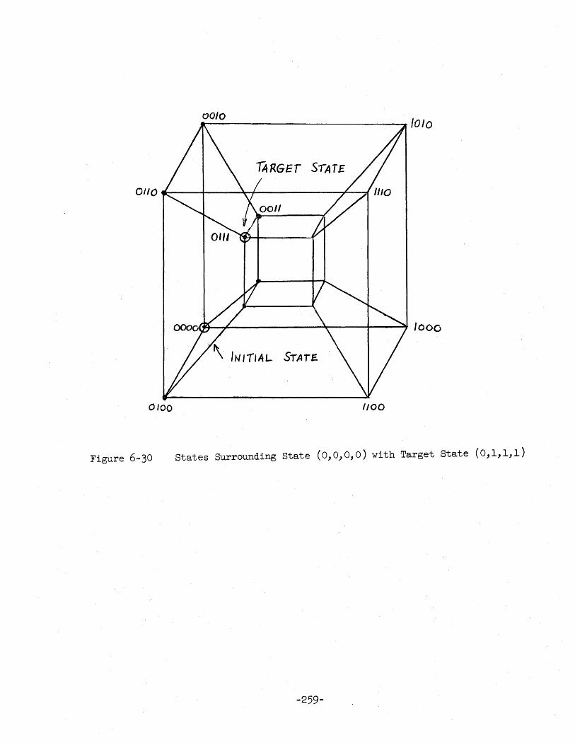
00/0 ~------------------------IOIO
TARGET SlATE
OliO Ik---;--~-I------~~-J
~~------------~----~--~~Jooo
'\ INlrlAL STATE.
0100 1100
Figure 6-30 States Surrounding State (0,0,0,0) with Target State (0,1,1,1)
-259-
Theorem 2. A machine is in equilibrium if and o~y if Y = Y'.
Proof. If Y = Y' there are no surrounding states I Y: the following state
can therefore only be Y and this means equilibrium. If the
machine is in equilibrium all surrounding states must be the same;
now Y' always surrounds Y, therefore Y = Y'.
Definition 3: A sequence of states yeO), Y(2), 0 •• Y(j), Y(j+l) ••• is an
allowed sequence if and only if it satisfied the following
conditions:
I. Y(j) ~ Y(j+l)
(Y(j+l) surrounds Y(j ))
2. Y(j+l) I Y(j)
(Y(j+l) differs from Y(j ))
3. For no internal node i can we
Yi (j) constantly < Yi (j) .
or Y. (j) constantly> Y! (j) . } 1 ~
(target condition)
(6- 35)
(6-36 )
have for all j > 0
(6-37 )
(Here> and'< are taken in the Boolean sense, which simply
reduce to the ordinary numerical 0 < 1 and 1 > 0).
Remark 1: The second condition eliminates the trivial case when the machine
hangs up in one state.
Remark 2: The third condition simply means this: when for a given node the
signal in the target state is different from the signal in the present state
and "pUlls" constantly in the same direction, the n a de will finally " give
in" and change in the direction of the "force." This excludes by no means the
possibility of the target state pulling sometimes in one direction and some
times in the ··other. In such a case we shall say that node i is variably forced.
A sequence of different states following each other and variably forced for
all nodes (or simply '''variably forced") is always an allowed sequence.
-260-
Remark 3: A cyclic sequence is perfectly allowed if its states are variably
forced.
Remark 4: A subsequence of finite length in which (6-37) is not necessarily -
verified, is called a partial allowed sequence or simply a sequence.
Defini tion 4: We ·shall say that a state K "follows" a state A if there is a
sequence A = A(O), A(l), 000 containing K. We shall then
write A:FKo (There are, usually, many intermediate states.) This
sequence does not necessarily satisfy the target condition.
Theorem 3. For any state A there is at least one allowed sequence starting with
it except if A = A' (equilibrium!).
Proof: A' surrounds A and we can form A(O), A(l), 000 by making A(O) = A,
'A(l) = At = A'(0),'A(2) = A'(l), etc'. It must come to an equilibrium
state or go into a cycle: in both cases the target condition is
satisfied (aI(j) = ai(j+l)!)
Theorem 4. An allowed finite sequence ends with an equilibrium state o
Proof: There would be a continuing allowed sequence from the last state K
(say) if K f K'.
2. EQUIVALENT, TERMINAL, FINAL AND PSEUDO-FINAL SETS
Definition 5: If two states A and B are "reversibly joined", i.e., if A8f3 and
B~A we shall say that they are in the same equivalent set and
write A~Bo
From the definition it follows that the ~·relationship satisfies the
following rules:
A~A (6-38)
A~B --7 P4A (6- 39)
A~B and Ee'C ~~ AtC (6-40 )
Let us denote the equivalence sets by Greek letters a,f3 .... Note that their
number is finite since the number of states S is finite.
-261-
Definition 6: We shall write o::1f3 if there is a state A* in a and a state Bit- in
~ such that A~B*o
Theorem 5. If A is any state in 0; and B any state in ~ and aJ~, then A1Bo
Proof: There is an A* in 0; and & B* in .~ with A*~B*o Also by definition
. AeA* and BeB*, There are, therefore, sequences from A to A*, from
A* to B* and from B* to Bo
Remark: Clearlya7t3 does not imply t3Ja, for then all states in a and ~ would
be reversibly joined and the sets a and t3 should have been collapsed into ,a
single set.
Theorem 6. The equivalence sets 0;, t30 9' form a poset.
Proof: ~ in the ordering of 0;, t30 9 0 can he replaced by :s in the rules for
a poset in 505g
~A (reflexivity)
Agt3 and t33a -~ a = t3 (anti-symmetry, see remark above)
@t3 and ~, -) 0;".1-, (transitivity)
Definition 7: A final set ~ is a set such that there is no set ~* with ~~~*o
Theorem 7. For any' equivalence set 0; there is at least one final set j.l such
that ~9
Proof~ This follows from the partial ordering: any poset has at least one
maximum and one minimum element.
Definition 8: A pseud.o-final set is an equivalence set of states containing
more than one. state--which is not final and variably forced.
(The last conditiori means, as usual, that no node i may have Pin
constantly < p~ or p. constantly> p! for all n~ where' In In In ' P = (P1n'o .. , p )! ) n sn
Definition 9: If an allowed sequence yeO), Y(j), Y(j+l)ooo has the property
thatfoJ;" j 2: m all states are in the same equivalence set T,
thi$ equ1 valence set 1s called the terminal set of the sequence 0 .
-262-
Theorem. 80 Any allowed sequence attains a terminaJ. set.,
Proof: The number of equivalence sets is finite and they are partially
ordered: after having left a certain set as we go along in one
sequence we are never allowed to go back to ito So the sequence
slowly exhausts all equivalence sets and must, after some time, be
trappeq in a last one.
Theorem 9. The terminal set of an allowed sequence is either p6eud~-final (in
this case we have a cycle in it) or final (in this case we have
several states and a cycle or just one state and equilibrium).,
Figure 6-31 shows all these possibillties.
Proof: Suppose that ~ is final. If it has one state K, this means that
we cannot go anywhere from Ko But we always have K .-~ Ki: we must
have K = Ki, i.e., equilibrium. Conversely if we go to equilibrium
in a state K of 1', K must be the only sta.te in "t': any other state
M preceding K (and in T) as we go towards K must be reversibly
joined to K (since both are in T). K being an equilibrium state,
we cannot go anywhere from K, in particular not to M. Therefore
M does not exist. The target condition is satisfied since we have
equilibrium.
If we still suppose that T is final but contains more than one
state, we can evidently have a cycle. Then the variable f9rcing
condition must be satisfied for the states of the cycle since we
have an allowed sequence.
Now we shall suppose that T is not final~ then it is an intermediate
set with more than one state. (One state K would mean equilibrium":'
since T is terminal--and then K = K'means that there are no states
surrounding K~ . we cannot leave K and T would be final.) Since
it contains an allowed sequence the target condition becomes the
variable forcing condition and the set must be pseudo-final."
-263-
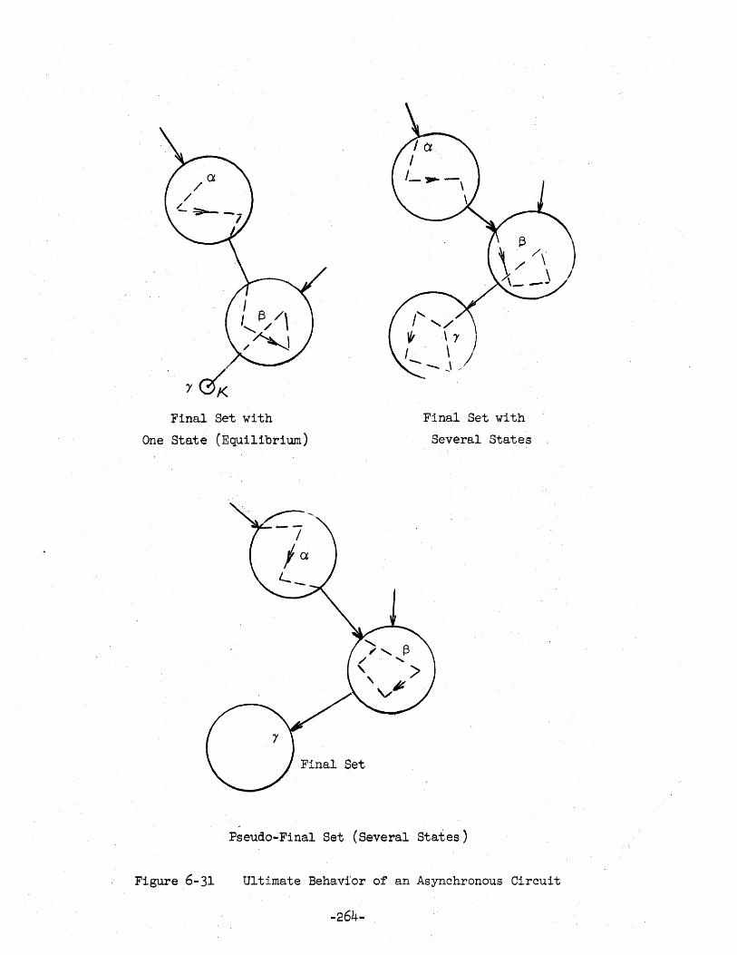
F1nal Set with
One State (Equilibrium)
Final Set with
Several States
Pseudo-Final Set (Several States)
Figure 6-31 Ultimate Behavi'or of an Asynchronous Circuit
-264-
Theorem 10. !f A is a state in a and ~ is any final or pseudo-final set fol
lowing a (ioeo, ~~), there is an allowed sequence A; A(O), A(l),ooo
whose terminal set ~ is ~o
Proof: If ~ is final, this is evident,for we can go from A to a certain F*
in~. From F* onwards we can take the target ~tate sequence: this
is trapped in <:p since it is final an d it is allowed (as are all
target state sequences!). If ~ is pseudo-final we can still go
from A to F* in ~Q Let F* ; P of ~c From P we can go to P I . n p n+ (since they are in the samE;!eq,uivalence set), from Pn+l to Pn+2,
etc., 00. up to Pro From Pr ~e go back to PO. T,hiS sequence
p(O) ,=Pn, P(l) ::: next state on path from Pn'to Pn+1, etco,. is
cyclic, has all different adjacent terms, is entirely in ~ and
satisfies the target condition because the states in ~ satisfy the
variable forcing condition. ~ is therefore a possible terminal
set T of this allowed sequence.
3. METHODS FOR FINDING . EQUIVALENT STATES
The discu·ssion of an asynchronous machine amounts essentially to
finding the equivalence sets of all its states. This can be done by the
following algorithm.
Equivalence Algorithm.
1. Choose the necessary number of cardinal points (say s) inside the logical
diagram.andestablish (fo!' a given fixed input) the relationships between
states and target states, ioeo, determine
2. Assign states Y1
, 0 • 0, Y .to all the possible combinations of y¥ S Q
. S
Draw up a table of target states by list·ing alongside each present state Y. J
the corresponding (Yl' 0 0 o,y ). combination and calculating from it the y. IS. . S 1
List the y. IS in order on the same line and via the assignment of Step 2 1
determine the target state corresponding to Yj , i. e ., Yjo
4. Varying all signals differing in Yj
and Yj one at the time,two at the time,
etc., calculate all other states surrounding Y. and draw up a table of J .
surrounding states.
5. Take a state, say YjJ and investigate how it is connected to its surrounding
sta.tes, i.e., if Yj ~.Yk,investigate whether there is a sequence from Yk
back to Yj
(meaning that Yj 9Yk ~ Yk~Yj' that is Yj~Yk)' To this effect
draw upa stepping diagram as follows;
ao The first column contains Y .• J
b. The second column contains all states surrounding Yj
except Yj
itself.
co Examine this column and strike out all equilibrium states or states
leading solely to equilibrium states in a few steps (scan the table of
surrounding states for thiS!).
do Next strike out in this same column all states leading to other states
in the column or to the left of it in very few steps.
e. Finally strike out in this column all states leading to the same states
as another entry in the column in very few steps. Do not stri~e out
this other entry.
)
f. Iterate steps c. through e. after having formed a third column containing
all states surrounding the states in the second column (except for these
states themselves!)o
6. The process in Step 5 will reduce the possibilities for a path back to Y .. J
As soon as we find such a path, we terminate the process and we know that
Y'~Yk' 'If, however, we find only paths that avoid Y. (in particular if we J J
only find a closed cycle leading back to Yk without touching Yj
) we know
that Yk is in another equivalence set.
Example. Take the circuit shown in Figure 6-32 in which the element r is
defined by the fact that for it
output = (input 1 v input 2)(input 3)
We clearly need four cardinal pOints (namely the outputs of the four elements)
and the circuit equations are
.. 266 ..
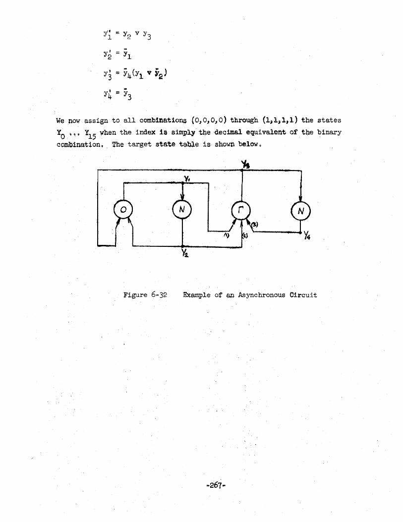
y' = y 2 1
Y3 = Y4(Yl V;2)
Y4 = Y3
We ,now assign to all combinations (0,0,0,0) through (l,ljl,l) the states
YO "'1 9 Y15 when the index is simply'the ,decimal equivalent. of,tbe ~1nary
combination. , The target state table is shown belowo
It)
Yt,
Figure 6-32 Example of all Asynchronous Circuit
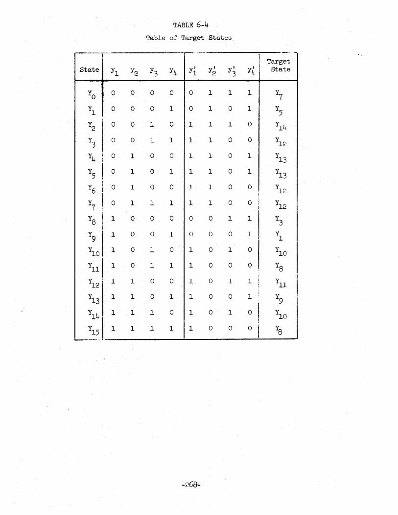
'l1ABLE 6-4
Table of Target States,
I --,.,....-_ .... -_._-,- ,--, ." ......
1 Target I
State Yl Y2 Y3 Y4 Y' 1 y'
2 y'
3 Y4 State
YO 0 0 0 0 0 1 1 1 Y7
Y1
0 0 0 1 0 1 0 1 Y5
Y2 I 0 0 1 0 1 1 1 0 Y
14
Y3
0 0 1 1 1 1 0 0 Y12
I Y4 0 1 0 0 1 1 0 1 Y
13 f
Y5 I 0 1 0 1 1 1 0 1 Y13
Y6 i 0 1 0 0 1 1 0 0 Y
12
Y7 0 1 1 1 1 1 0 0 Y12
Y8 I 1 0 0 0 0 0 1 1 Y3
Y9
1 0 0 1 0 0 0 1 t Y1
Y10
1 0 1 0 1 0 1 0 Y10
Y11 1 0 1 1 1 0 0 0 Y8
Y12
1 1 0 0 1 0 1 1 Y11
Y13
1 1 0 1 1 0 0 1 Y9
Y14
1 1 1 0 1 0 1 0 Y10
Y15j 1 1 1 1 1 0 0 0 Y8 """-M __ '_' .,.
-268 ...
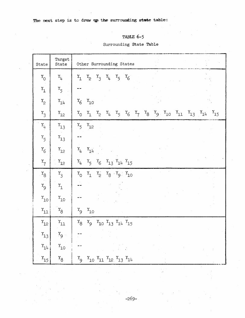
The next step is to drav qp the surrOUDding state table:
TABLE 6-5
Surrounding State Table
.~~-.......... --- .•. ,-,-_.,------.---_._-Target
State State Other Surrounding States of"'''''- ._. _ ....... , .... _ ..... , .. __ •. _ •. - ........ ~. __
YO Y4 Y1 Y2
Y3
Y4 Y5
Y6
Y1 Y5 --
Y2 Y14 Y6 Y10 . ,
Y3
Y12 YO Y1 Y2 Y4 Y5
Y6 Y7
Ys Y9
Y10 Y11 Y13
Y14 Y15
.~.~,.-'--
Y4 Y13
Y5
Y12
Y5 Y13 --
Y6 Y12 Y4
Y14
Y7
'. Y12 Y4 Y5
Y6 Y13
· Y14 Y
15
Ys Y3 YO Xl Y·
2 Ys ' Y9
Y10
Y9
Y1 --
Y10 YlO
I --
I ! , i , ! Ys Y
9 Y10 I Y11 1
Y12 Y11 1S Y9
Y10 Y13 Y14 Y15
Y13 Y9 I
--
Y14 i YlO --. , i
Y15! YS I Y9 Y10 Yl1 Y12 Y
13 Y14
.. -
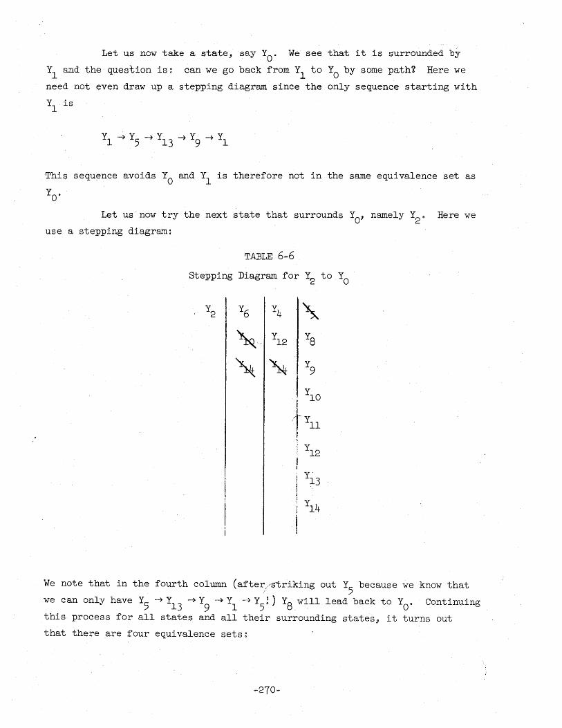
Let us now take a state, say YOo We see that it is surrounded by
YI and the question is: can we go back from YI
to YO by some path? Here we
need not even draw up a stepping diagram since the only sequence starting with
YI
is
This sequence avoids YO and YI is therefore not in the same equivalence set as
YO'
Let us now try the next state that surrounds YO' namely Y2
0 Here we
use a stepping diagram:
TABLE 6-6
Stepping Diagram for Y2 to YO
Y2 Y6 Y4 " ~-- Y
l2 Ys
~ ~ Y9
I YIO
'IYIl , Yl2
~ : j Yi3 t . ~
1 Y14
We note that in the fourth column (after/striking out Y5
because we know that
we can only have Y5
--7 Yl3
-.:, Y --7 Y -) Y !) Ys will lead back to Y 0 Continuing 9 I 5 .. 0
this process for all states and all their surrounding states, it turns out
that there are four equivalence sets~
-270-
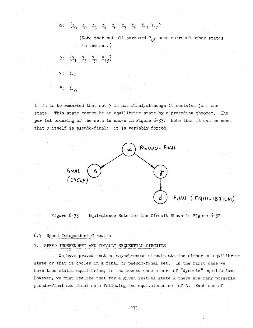
(Note that not all surround Yo; some surround other states
in. the set. )
t3: {Yl Y5
Y9 Y13}
r: Y14
0: YIO
It is to be remarked that set l is not final,although it contains just one
state. This state cannot be an equilibrium state by a preceding theorem. The
partial ordering of the sets is shown in Figure 6-33. Note that it can be seen
that a itself is pseudo-final: it is variably forced.
FINAL
(CYCLE)
'PSEUDO - FINAL
fU.JAL (EQUI1- I 13RIUM)
Figure 6-33 Equivalence Sets for the Circuit Shown in Figure 6-32
66 7 Speed Independent Circuit s
1. SPEED INDEPENDENT AND TOTALLY SEQUENTIAL CIRCUITS i
We' .. have proved that an asynchronous circuit attains either an equilibrium
state or that it cycles in a final or pseudo-ftnal set. In the first case we
have true static equilibrium, in the second case a sort of "dynamic" equilibrium.
However, we must realize that for a given initial state A there are many possible
pseudo-final and final sets following the equivalence set of A. Each one of
-271-
them i~ a potential candidate for the terminal set of an allowed sequence
starting with A. This means that in ~eneral a given initial state can lead
t.o almost a.ny machine behavior 0 We shall now introduce "speed independence,"
ioeo, a foreseeable machine behavior by a new definition.
Defini tion 10: A circuit is fI speed independent t, with respect to an initial
state A (we shall then write si(A» if every allowed sequence
starting with A ends up in the same terminal set To
Theorem II. A circuit is si(A) if and only if the equivalence set aof A is
followed by a single final set and ~pseudo-final set.
Proof: Let cp be the single final set. Then there is an allowed sequence
beginning in A which is ultimately trapped in~. Since there are
. no pseudo-final sets it cannot get trapped on its way to ~ and
there can be no other sequences leaving A and not attaining ~
because they would have to end in a pseudo-final set (and there
is none which follows a) or a final set (and there is none different
from ~)~ It is seen that the condition is not only sufficient
but that it is necessary by a similar reasoning.
Definition ll~ A circuit is "totally sequential" with respect to an initial
state A (we shall then write ts(A)) if there is only one
allowed sequence starting with A.
Theorem 12. A circuit which is ts(A) is also siCA).
Proof: The only allowed sequence leaving A will (as any allowed sequence
be trapped after some time in a terminal set. This must be a
unique final set (for if there had been another one, there would
have been another allowed sequence leading into it) and there
cannot be any pseudo-final sets in between because then there
would be two allowed sequences: the one trapped in the pseudo
final set and the on trapped in the final seto
Theorem 13. In a totally sequential circuit on~y one signal changes at a time
(i. eo, parallel action is excluded!).
Proof: Since the target state sequence can always be constructed, it
is clear that in a totally sequential circuit the one and only
-272-
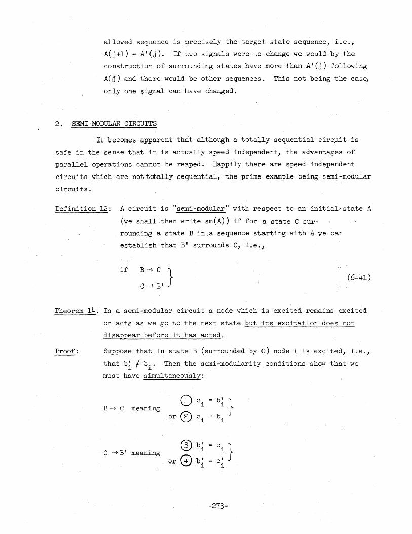
allowed sequence is precisely the target state sequence, i.eo,
A(j+l) ::; A'(j). If two signals were to change we would by the
construction of surrounding states have more than A'(j) following
A(j") and there would be other sequences. This not being the case,
- only one 9ignal can have changed.
2. SEMI-MODULAR CIRCUITS
It becomes apparent that although a totally sequential circ~it is
safe in the sense that it is actually speed independent, the advantages of
parallel operations cannot be reaped. Happily there are speed independent
circui ts which are not totally sequential, the prime example being semi-modular
circuits.
Definiti-on 12: A circuit is "semi-modular" with respect to an initial- state A
(we shall then write sm(A)) if for a state C sur~
rounding a state Bin.a sequence starting with A we can
establish that B' surrounds C, i.e.,
if B --7 C }
C -) B' (6-41 )
Theorem 14. In a semi-modular circuit a node which is excited remains excited
or acts as we go to the next state but its excitation does not
disappear before it has acted.
Proof: Suppose that in state B (surrounded by C) node i is excited, i.e.,
that b ~ f. b." Then the semi-modularity conditions show that we l- l
must have simultaneously:
[) c. b~ } B -7 C meaning l l
or ® c. b. l l
0) b~ c. } C -?B' meaning l l
or ® b' ::; c~ l l
-273-
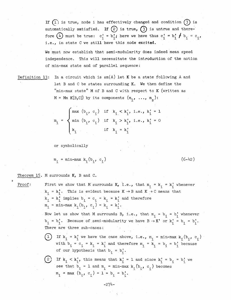
If Q'l is true, node i has effectively changed and condi tion (~). is
automatically satisfied. If (§) is true, ~ is untrue and there~ fore f4\ must be true: c~ = b! " here we have thus c' = b ~1 b.· = c \.V l l i l i l i' i.e., in state C we still have this node' excited.
We ~~st now establish that semi-modularity does indeed mean speed
independence. This will necessitate the introduction of the notion
of min-max state and of p~rallel sequence:
Definition 13: In a circuit which is sm(A) let K be a state following A and
let Band C be states surrounding K. We then define the
"min-max state" M of Band C with respect to K (written as
M = Mrn K[B,C]) by its oomponents (TItl , · 0 ., ms ):
max (b. , c.) if k. < k~, i. eo, k! = 1 l l l l l
m. min (b. , c. ) if k. > k! , i.e., k! = 0 l l l l l l
k. if k. k~ l l l
or symbolically
m. = min-max k. (b., c.) l l l l
(6-42 )
Theorem 15. M surrounds K, B and C.
Proof: First we show that M surrounds K, i.eo, that m. = k. = k~ whenever l l l
k. l
k! . This is evident because K 4 Band K --~ C means that l
k. = k! implies b. = C. l l l l
. m. l
= min-max k. (b., c.) 'l l l
k. = k~ arid therefore l l
k. = l
k~ 0
l
Now let us show that M surrounds B~ i .. e 0' that m. = b. = b ~ whenever l l l
b: = b~. Because of semi -modularity we have B -> K I or k' b. b I l l i l i
O
There are three sub-cases~
If k. = k~ we have the case above; i oe. J m. = min-max l l l
withb. = c. = k. = k~ and therefore m. k. b. l l l l l l l
of our hypothesis that b. = b! 0
l l·
this means that k! = 1 and since k~ = b. If k i < k~,
see that b. = . l
l l l
1 and m. = min-max k. (b., c.) becomes l l l l
m. == max (b. ~ l l
c.)=l=b. b~o l l l.
-274-
b' l
k. (b., l l
c. ) l
because
b ~ we l

If k. > k~, this means that k~ = a and since k~ = b. l l l l l
see that b. = 0 and m. = min-max k.(b., c.) becomes l l . l l l
m. = min (b., c.) = 0 = b. = b!o l l l l l
b~ we l
Definition 14: Suppose that we have a sequence (not necessarily satisfying the
target condition and therefore not necessarily allowed!) B(O),
B(l), B(2), 000 B(j), B(j+l) 000 and that B(O) is surrounded
by a state C(O) f B(O). We can then construct iterative+y a
"parallel sequence" as follows: take BeO), B(l) and C(O) and
take
C(l) = Mm B{b)[B(l), C(O)]
C(2) = Mm B(1)[B(2), C(l)]
C(j+l) == Mrn B(j )(B(j+l), C(j)J t
obtaining
B(O) ~ B(l) ~ B(2) ~,J, ,J,
C(O) -~ C(l) ~ C(2)
-7 B(j) ~ B(j+l) -7 00.
J, "- J, -7 C(j) -~ C(j+l) -7 .00
where the arrows have their usual significance of "surrounded
by" by virtue of Theorem 15.
We see·. that the parallel sequence we have formed has the
property that each of its terms surrounds the preceding term
of the new sequence and also the two corresponding terms in
the original sequence 0
Theorem 16. Let pea), 000 Per), p(O) be a cyclic sequence (not necessarily
allowed, ioe., not necessarily fulfilling the target condition)
and Q(O), .. ., 0 Q(r), Q(O) the parallel sequence constructed by
(6-43). Then for any node i for which
1. p. (j) = q. (j) we also have p. (j+l) = q.(j+l) l l l l
2. P. (j) < q. (j) we also have p. (j+l) <: q. (j+l) (in this case l l l l
P.(j) < p!(j)!) l
-275-
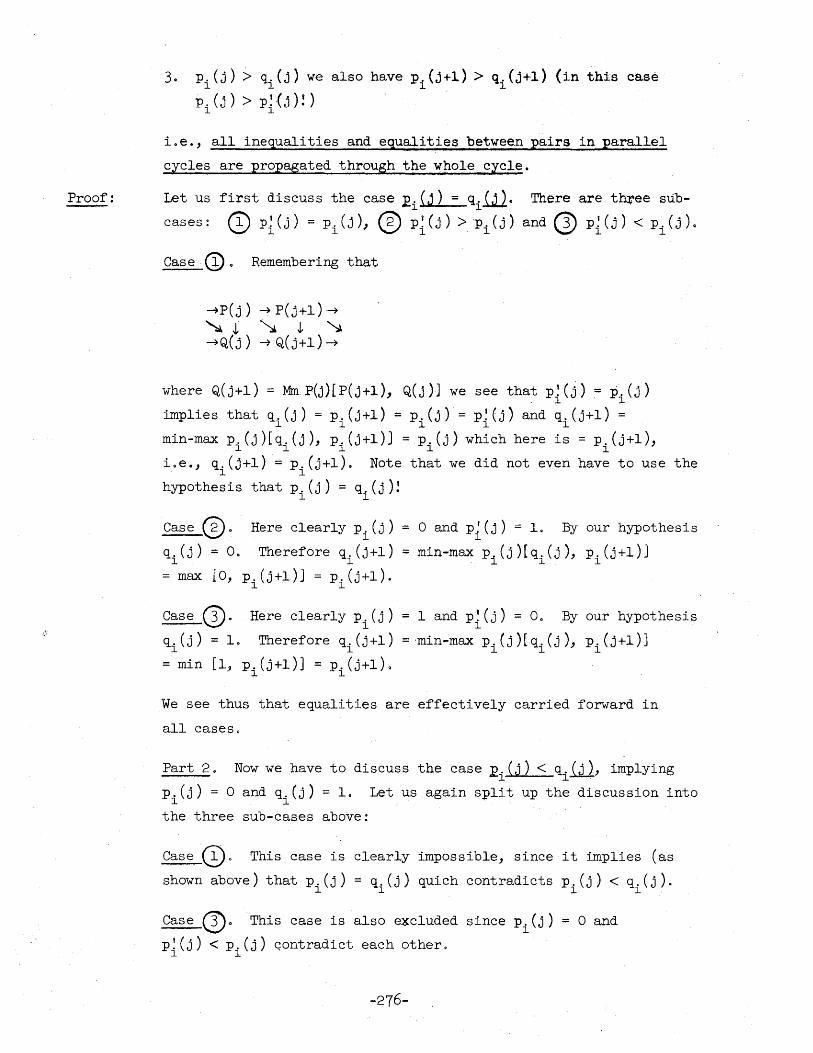
Proof:
3. P.(j». q.(j) we also have p.(j+l) > q.(j+l) (in this case . l II l
P.(j) > p~.(j)!) l l
i.e., all inequalities and equalities between pairs in parallel
cycles are propagated through the whole cycle.
Let us first discuss the case ~i(j) = qiiJl. There are th~ee sub
cases: CD p ~ (j) = Pi (j ) I ® P ~ (j ) >p i (j) and Q) p ~ (j) < Pi (j ) •
Case CD. Remembering that
~p(j) ~ P(j+l) ~ ~J. ~ t ~ ~Q(j) ~ Q(j+l) ~
where Q(j+l) = Mm p(j)[P(j+l), Q(j)] we see that P~ (j) = :Pi (j)
implies that q.(j) = p.(j+l) = P.(j) = p~(j) and q.(j+l) = l l l l l
min-max P.(j)[q.(j), p.(j+l)J = P.(j) which here is = P (j+l), l l l l i
i 0 e. J q. (j+l) .= p. (j+l L Note that we did not even have to use the l l
hypothesis that p. (j) = q.(j)! l l
Case 0. Here clearly Pi(j) 0 and p{(j) = 1. By our hypothesis
q.(j) = O. Therefore q.(j+l) = min-max Pi(j)[q.(j), p.(j+l)J l l l l
= max [0, p. (j+l)J = p. (j+l). l l
~~. Here clearly Pi(j) = 1 and p~(j) = O. By our hypothesis
q.(j) = 10 Therefore q.(j+l) ='min-max P.(j)[q.(j), p.(j+l)] l l l l l
= min [ 1, p. (j +1 ) ] = p. (j +1 ) • l l
We see thus that equalities are effectively carried forward in
all cases.
Part 2. Now we have to discuss the case .:e.(j) < q.(j), implying l l~
p.(j) = 0 and q.(j) = 1. Let us again split up the discussion into l l
the three sub-cases above:
Case~o This case is clearly impossible, since it implies (as
shown above) that Pi(j) = qi(j) quich contradicts Pi(j) < qi(j)·
Case ~o This case is also e~cluded since Pi(j) = 0 and
p~(j) < Pi(j) Gontradict each other.
-276-
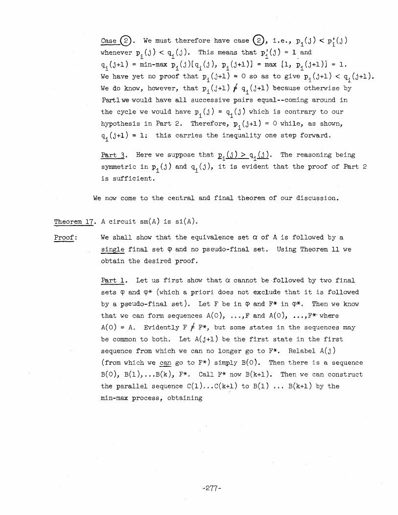
Case 12\. We must therefore have case 12', i.e., p.(j) < p!(j) ----~ ~ l l
whenever Pi(j) < qi(j)· This means that p~(j) = l,and
q. (j+l) = min-max p. (j )[q. (j), p. (j+l)] :: max [1, p. (j+l)] = 1. l l· l l l
We have yet no proof that p.(j+l) = 0 so as to give p.(j+l) < q.(j+l). l l l
We do know, however, that p.(j+l) I q.(j+l) because otherwise by l l
. Part 1 we would have all successive pairs equal--coming around in
the cycle we would have P.(j) = q.(j) which is contrary to our l l
hypothesis in Part 2. Therefore, p.(j+l) = 0 while, as shown, l
q.(j+l) = 1: this carries the inequality one step forward. l
Part 3. Here we suppose that p.(j) > q. (j). The reasoning being -l l-
symmetric in P.(j) and q.(j), it is evident that the proof of Part 2 l l
is sufficient.
We now come to the central and final theorem of our discussion.
Theorem 17. A circuit sm(A) is siCA).
Proof: We shall show that the equivalence set a of A is followed by a
single final set ~ and no pseudo-final seto Using Theorem 11 we
obtain the desired proof.
Part 1. Let us first show that a cannot be followed by two final
sets ~ and ~* (which a priori does not exclude that it is followed
by a pseudo-final set). Let F be in q> and F* in ~* 0 Then we know
that we can form sequences A(O), .. o,F and A(O), .• o,F*-where
A(O) = Ao Evidently F !F*, but some states in the sequences may
be common to both. Let A(j+l) be the first state in the first
sequence from which we can no longer go to F*. Relabel A(j)
(from which we ~ go to F*) simply B(O). Then there is a sequence
B(O), B(l), .ooB(k), F*o Call F* now B(k+l). Then we can construct
the parallel sequence C(l)o .. C(k+l) to B(l) .00 B(k+l) by the
min-max process, obtaining
-277-
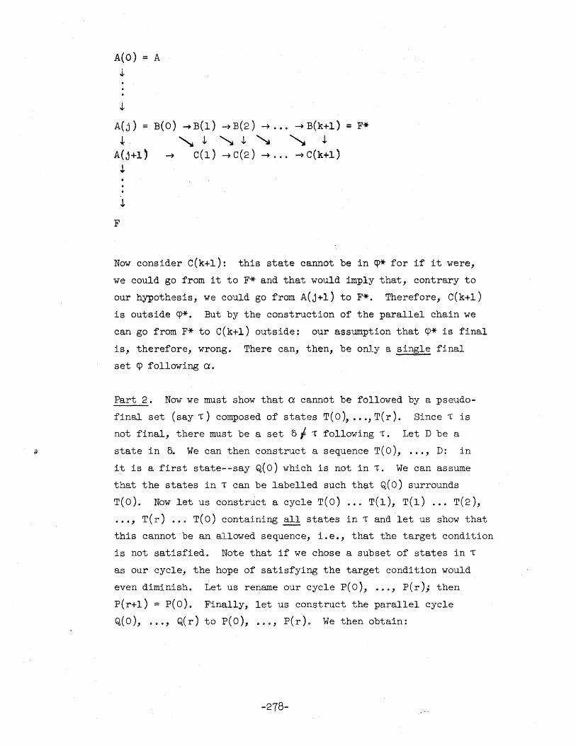
A(O) = A
J,
A(j) =
* A(j+l' J,
J,
F
B ( 0) -+ B ( l) -+ B (2) -+ • •• -+ B (k + 1) = F*
~J, ~J,~ ~ J,
-+ C(l)-+C(2)-+ ••• -+C(k+l)
Now consider C(k+l): this state cannot be in cp* for if it were,
we could go from it to F* and that would imply that, contrary to
our hypothesis, we could go from A(j+l) to F*. Therefore, C(k+l)
is outside CP*. But by the construction of the parallel chain we
can go from F* to C(k+l) outside: our assumption that cP* is final
is, therefore, wrong. There can, then, be only a single final
set cp following o.
Part 2. Now we must show that a cannot be followed by a pseudo
final set (say T) composed of states T(O), •.. ,T(r). Since L is
not final, there must be a set 0 f. T following T. Let D be a
state in 00 We can then construct a sequence T( 0), • 0 ., D: in
it is a first state--say Q(O) which is not in T. We can assume
that the states in T can be labelled such th~t Q(O) surrounds
T(O). Now let us construct a cycle T(O) •.. T(l), T(l) .•. T(2),
T(r) ••. T(O) containing all states in T and let us show that
this cannot 'be an allowed sequence, i.e., that the target condition
is not satisfied. Note that if we chose a subset of states in T
as our cycle, the hope of satisfying the target condition would
even diminish. Let us rename our cycle P(O), .'0, P(r); then
P(r+l) = p(O). Finally, let us construct the parallel cycle
Q( 0), 0 0 0' Q( r) to p( 0), 0 •• ' p( r ) 0 We then obtain:
-278-
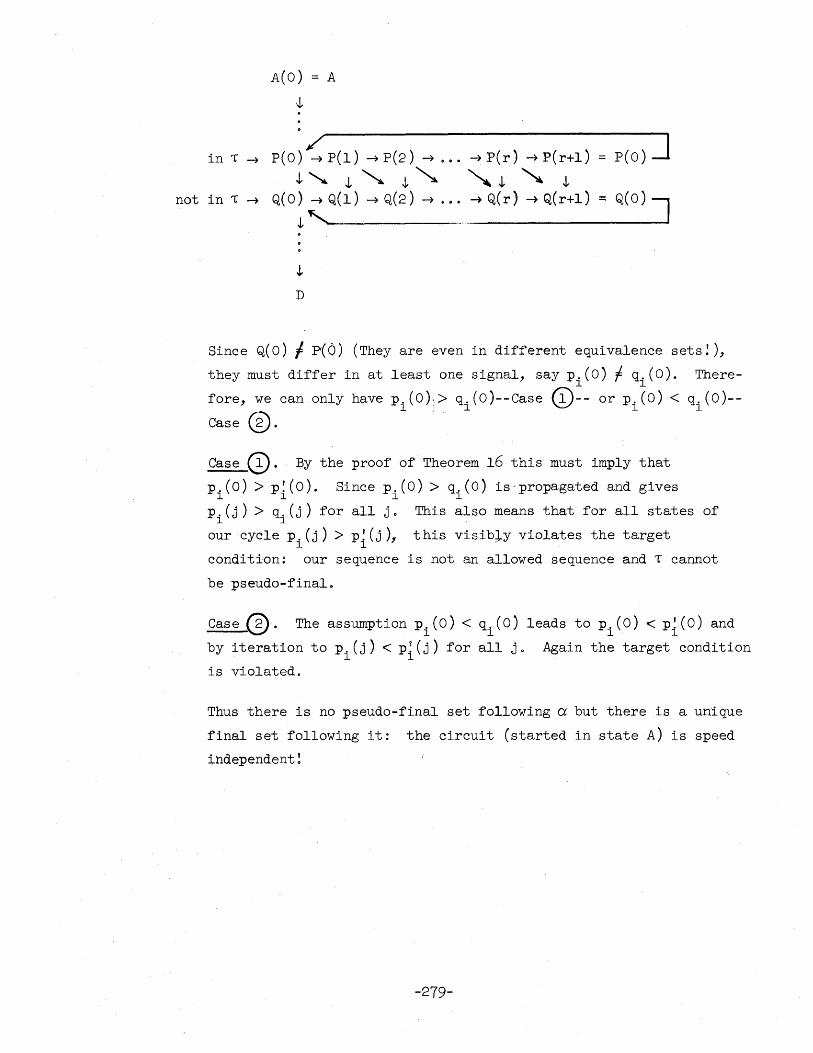
A(O) A
. .1
= p(o) ] in 't ~ /
P ( 0) ~ P (1) ~ P (2) ~ . •. ~ P ( r) ~ P ( r+ 1 )
.1~ .1 ~.1~ "'.1 ~ .1 not in 't ~ Q(O) ~Q(l) ~Q(2) ~ .0. ~Q(r) ~Q(r+l) ::;
.1 '--------
J.
D
Since Q( 0) f p( 0) (They are even in different equivalence sets!),
they must differ in at least one signal, say p.(O) f q.(O). There-1 1
fore, we can only have P.(O)I> q.(O)--Case fi\-- or p.(O) < q.(O)--1 1 \.::J 1 1
Case (0.
Case ~. By the proof of Theorem 16 this must imply that
p.(O) >p!(O). Since p.(O) > q.(O) is-propagated and gives 1 1 1 1
P.(j) > q.(j) for all jo This also means that for all states of 1 1
our cycle P.(j) >p!(j), this visib~y violates the target 1 1
condition: our sequence is not an allowed sequence and 't cannot
be pseudo-finalo
Case r:;}\. The assumptionp. (0) < q. (0) leads to p. (0) < p! (0) and ~ 1 1 1 1
by iteration to p. (j) < p~(j) for all j. Again the target condition 1 1
is violated.
Thus there is no pseudo-final set following a but there is a unique
final set following it: the circuit (started in state A) is speed
independent!
-279-
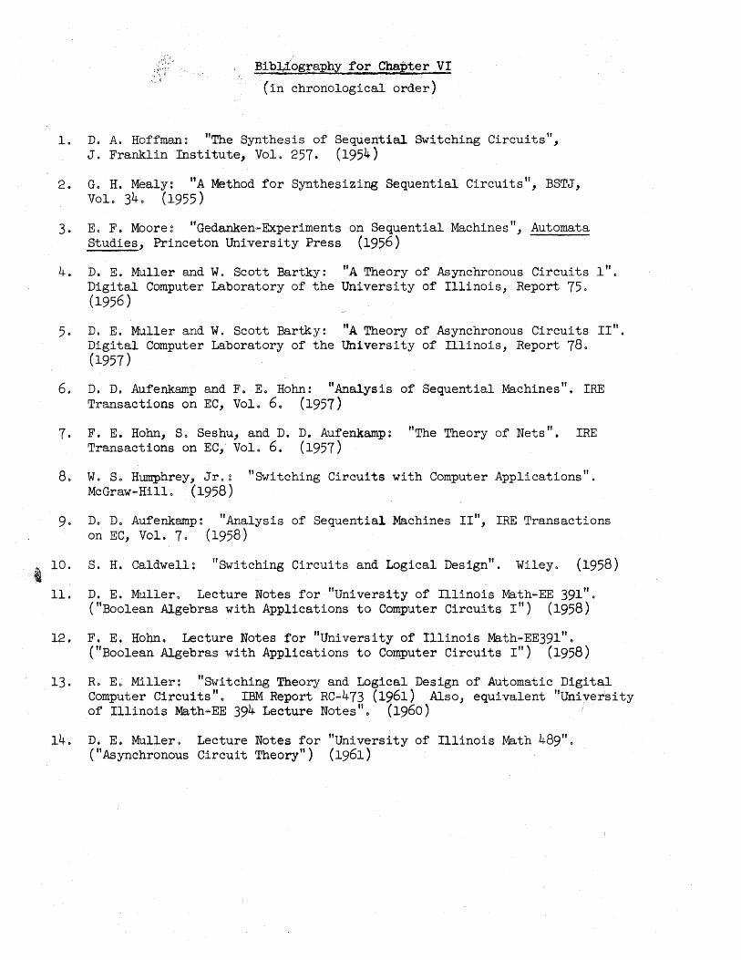
t
I
BibUography for Chapter VI
(in chronological order)
1. D. A. Hoffman: "The Synthesis of Sequential Switching CirCUits", J. Franklin Institute, Vol. 257. (1954)
2. Go H. Mealy: ttA Method for Synthesizing Sequential Circuits", BSTJ, Vol. 340 (1955)
3. E. Fe Moore~ "Gedanken-Experiments on Sequential MaChines", Automata Studies, Princeton University Press (1956)
4. D. E. Muller and W. Scott Bartky: "A Theory of Asynchronous Circuits 1". Digital Computer Laboratory of the University of Illinois, Report 75. (1956 )
5. D. E. Muller and W. Scott Bartky: ttA Theory of Asynchronous Circuits II". Digital Computer Laboratory of the University of Illinois, Report 78. (1957)
6. D. Do Aufenkamp and F. Eo Hohn: ffAnalysis of Sequential Machines". IRE Transactions on EC, Volo 60 (1957)
7. F. E. Hohn, S. Seshu, and D. D. Aufenkamp: " h If T e Theory of Nets 0 IRE
80
9.
10.
11.
12.
13.
Transactions on EC, Vol. 6. (1957)
w. So Humphrey, Jr.g "Switching Circuits with Computer Applications". McGraw-Hill. (1958)
Do Do Aufenkamp: "Analysis of Sequential Machines II", IRE Transactions on EC, Vol. 7. (1958)
S. H. Caldwell: "Switching Circuits and Logical Design". Wiley. (1958)
D. E. Muller. Lecture Notes for "University of Illinois Math-EE 391". ("Boolean Algebras with Applications to Computer Circuits lit) (1958)
F. E. Hohno Lecture Notes for "University of Illinois Math-EE39l"0 ("Boolean Algebras with Applications to Computer Circuits r") (1958)
R. ED Miller: "Switching Theory and Logical Design of Automatic Digital Computer Circuits". IBM Report Rc-473 (1961) Also, equivalent "University of Illinois Math-EE 394 Lecture Notesilo (1960)
14. D. E .. Muller. Lecture Notes for "University of Illinois Math 489". ("Asynchronous Circuit Theory") (1961)