Matricial R-circular systems and random matrices

arX

iv:1

311.

6420

v2 [

mat

h.O

A]

27

Jan

2014

MATRICIAL R-CIRCULAR SYSTEMS AND RANDOM MATRICES

ROMUALD LENCZEWSKI

Abstract. We introduce and study matricial R-circular systems of operators whichplay the role of matricial analogs of circular operators. They are obtained from cano-nical decompositions of ‘matricial circular systems’ studied recently in the contextof the Hilbert space realization of the asymptotic joint *-distributions of symmetricblocks of independent block-identically distributed Gaussian random matrices with re-spect to partial traces. As compared with those systems, matricial R-circular systemsdescribe the asymptotic joint *-distributions of blocks rather than those of symmetricblocks. We prove that they are *-symmetrically matricially free with respect to thecorresponding array of states. We also study their cyclic cumulants defined in termsof cyclic non-crossing partitions as well as the corresponding cyclic R-transform.

1. Introduction

Circular and semicircular systems of operators were introduced by Voiculescu [14] inthe context of random matrices and their asymptotics and applied to free group fac-tors. This result followed his fundamental asymptotic freeness result for independentHermitian and non-Hermitian Gaussian random matrices with complex i.i.d. entries,respectively [13]. Decomposition of these matrices into blocks corresponds to decom-positions of circular and semicircular operators into circular and semicircular systems,respectively.

Recently, we obtained related results in the case when the considered independentGaussian random matrices have independent block-identically distributed complex en-tries, which we abbreviate i.b.i.d. [5,7]. We showed that in order to give an operatorialmodel for the asymptotic joint (*-) distributions of blocks of these matrices under partialtraces rather than under the ‘complete’ trace, one needs to replace (*-) free summandsin the decompositions of (circular) semicircular operators by their matricial counter-parts, related to each other by a matricial generalization of (*-) freeness with respectto an array of scalar-valued states.

The underlying concept of independence is that of matricial freeness [4] which canbe described by means of the intuitive equation

matricial freeness “ freeness & matriciality

and its symmetrized version called symmetric matricial freeness [5] which also plays animportant role in our developments. A connection between these concepts and blocksof large random matrices was established in [5] for one matrix and in [7] for an ensembleof independent matrices.

2010 Mathematics Subject Classification: 46L53, 46L54, 15B52Key words and phrases: free probability, random matrix, matricial freeness, circular system, matricialR-circular system, cyclic R-transform

1

http://de.arxiv.org/abs/1311.6420v2

2 R. LENCZEWSKI

For instance, if we are given an ensemble of independent non-Hermitian nˆn randommatrices tY pu, nq : u P U u whose entries are suitably normalized i.b.i.d. complex Gauss-ian random variables with zero mean for each natural n, then the mixed *-moments oftheir symmetric blocks tTp,qpu, nq : 1 ď p ď q ď r, u P U u converge under partial tracesto arrays of certain bounded non-self-adjoint operators, which we write informally

limnÑ8

Tp,qpu, nq “ ηp,qpuq,

and the operators ηp,qpuq are called matricial circular operators. The whole family

tηp,qpuq : 1 ď p ď q ď r, u P U u

will be called a matricial circular system. Let us remark that our approach allows us totreat all rectangular blocks, including those which are unbalanced or evanescent [7]. Wewould also like to mention that the first operatorial treatment of the asymptotic distri-butions under the ‘complete’ trace of Gaussian random matrices with non-identicallydistributed entries is due to Shlyakhtenko [11], who used free probability with operator-valued states for that purpose.

The array of C˚-algebras Ap,q, each generated by the matricial circular operatorsindexed by p, q and by the corresponding unit, are related to each other by symmetricmatricial freeness. In a similar result for i.b.i.d. Hermitian Gaussian random matrices(in the Hermitian case, we understand that variables are block-identically distributed ifthe covariances of complex variables are equal within blocks), one obtains C˚-algebrasgenerated by matricially free Gaussian operators or their symmetrizations, symmetrizedGaussian operators [5,7]. An application of this scheme to products of independent ran-dom matrices leads to multivariate Fuss-Narayana polynomials and free multiplicativeconvolutions of Marchenko-Pastur laws [8].

All our operators, including matricially free Gaussian operators, symmetrized Gauss-ian operators as well as matricial circular operators, live in the matricially free Fockspace of tracial type (Definition 2.1), where each summand is built by the ‘matricial’action of free creation operators onto a unit vector Ωq, where 1 ď q ď r. This Fockspace gives a canonical model for a matricial circular system. We associate the state

Ψq : BpMq Ñ C by Ψqpaq “ xaΩq,Ωqy

with each Ωq as it is always done for vector states. The presence of a family of vacuumvectors allows us then to compute distributions with respect to the state

Ψ “rÿ

q“1

dqΨq,

where d1 ` . . . ` dr “ 1, which corresponds to the canonical normalized trace of largerandom matrices. In general, we are interested in (*-) distributions with respect to anyΨ of the above form, for which it suffices to determine those with respect to all vectorstates Ψq.

MATRICIAL R-CIRCULAR SYSTEMS AND RANDOM MATRICES 3

We also use them to construct the array of states on BpMq with respect to whichmatricial freeness or symmetric matricial freeness is proved, namely

pΨp,qq “

¨˚˝

Ψ1 Ψ2 . . . Ψr

Ψ1 Ψ2 . . . Ψr

. .. . . .

Ψ1 Ψ2 . . . Ψr

˛‹‹‚.

In the present paper, we can identify Ψq with Φq “ ϕ b ψq, where ϕ is the vacuumexpectation on the C˚-algebra A generated by a system of free circular operators and ψq

is the state associated with the basis vector epqq of Cr. Under the symmetry assumptionon the covariance matrices, the considered matricial circular operators ηp,qpuq havecircular *-distributions with respect to the two associated states Ψp and Ψq, whichexplains why we call them ‘circular’. Another reason is that the arrays pηp,qpuqq arematricial analogs of circular operators even in the case when the covariance matricesare not symmetric (see Proposition 4.3).

One can use circular systems of Voiculescu (more generally, generalized circular sys-tems) to find their matrix realization. Let A be the C˚-algebra generated by the systemof free (generalized) circular operators

tgpp, q, uq : 1 ď p, q ď r, u P U uand define operators

ζp,qpuq “ gpp, q, uq b epp, qq P MrpAqfor any p, q, u. Then, the matricial circular operators can be identified with

ηp,qpuq “"ζp,qpuq ` ζq,ppuq if p ă q

ζq,qpuq if p “ q,

which also explains why we call them ‘matricial’. The arrays pζp,qpuqq which arisein these decompositions are the main objects of our study. Note that they are thegenerators of free group factors used by Voiculescu in his proof of free group factorsisomorphisms [14, Theorem 3.3].

In particular, we prove that both arrays, pηp,qpuqq and pζp,qpuqq, are *-symmetricallymatricially free with respect to pΨp,qq for any u P U . The proof reminds that forsymmetrized Gaussian operators in [7, Proposition 3.5]. However, in the present paper,we use the matricial realization given above, which allows us to phrase it in the languageof free probability. In our previous papers on matricial systems of operators [5,7], werelied on the Hilbert space approach and its implications for random matrix theory.

The diagonal operators ζq,qpuq are clearly circular under the corresponding statesΨq. The off-diagonal ones ζp,qpuq correspond to canonical decompositions of circularoperators ηp,qpuq. The family

tζp,qpuq : 1 ď p, q ď r, u P U uwill be called a matricial R-circular system and its elements will be called matricialR-circular operators since their cyclic R-transforms defined by cyclic cumulants givecanonical decompositions of the R-transform for circular operators. In the simplestcase of an off-diagonal pair ζ1 “ ζp,qpuq and ζ2 “ ζq,ppuq, the cyclic R-transform oftζ1, ζ˚

1 u and tζ2, ζ˚2 u in the state Ψq assume the form

Rζ1,ζ˚

1pz1, z2; qq “ z2z1 and Rζ2,ζ

˚

2pz1, z2; qq “ z1z2

4 R. LENCZEWSKI

if the covariances are equal to one, respectively. Thus, by multilinearity of cumulants,the cyclic R-transform of tη, η˚u in the state Ψq, where η “ ηp,qpuq, takes the form

Rη,η˚pz1, z2; qq “ z1z2 ` z2z1

and thus it agrees with its R-transform in that state. Similar formulas are obtainedfor the state Ψp, whereas the remaining cyclic R-transforms of the above operators, allof which are labelled by p, q, are identically equal to zero. This formalism allows usto show that the cyclic R-transform of matricial R-circular systems become ‘hermitianforms’ in the corresponding arrays of non-commutative indeterminates.

Moreover, we show in this paper that the arrays of R-circular operators are of impor-tance in random matrix theory. To catch a glimpse of that importance, let us go backto non-Hermitian Gaussian random matrices with i.b.i.d. entries. Write each matrixY “ Y pu, nq in the block form

Y “

¨˚˝

S1,1 S1,2 . . . S1,r

S2,1 S2,2 . . . S2,r

.. . . .

Sr,1 Sr,2 . . . Sr,r

˛‹‹‚

and consider the asymptotic joint *-distributions of blocks Sp,q “ Sp,qpu, nq under partialtraces and their realizations on M. We assume that, for any given n, the dimensionsof blocks do not depend on u and we identify each block with its image under theembedding in the algebra of nˆ n matrices.

The operators ζp,qpuq describe the asymptotic joint *-distributions of blocks Sp,qpu, nqas n Ñ 8 with sizes of blocks growing proportionately to n or slower. Namely, we showthat their limit joint *-distributions under partial traces coincide with the corresponding*-distributions of ζp,qpuq, which we write informally

limnÑ8

Sp,qpu, nq “ ζp,qpuq,

for any u P U and 1 ď p, q ď r. Since blocks Sp,qpuq refer to the most general modelof i.b.i.d. Gaussian random matrices, the systems of R-circular operators comprisethe basic constituents of the asymptotic operatorial models. Clearly, we can also usethem to reproduce the results on the asymptotics of symmetric random blocks of i.b.i.d.Gaussian random matrices [7]. In the special case when Y pu, nq has i.i.d. entries andwe divide it into blocks, we obtain in the large n limit a matricial decomposition of thestandard circular operator in terms of R-circular ones and its R-transform decomposesas the sum of cyclic R-transforms.

Voiculescu’s asymptotic freeness result allowed him to show that a decompositionof square Gaussian random matrices with i.i.d. complex entries into blocks leads to anatural decomposition of circular operators into a circular system, and that a similarconnection holds for Hermitian matrices and semicircular systems [14] (see also [15]).Triangular random matrix models and the corresponding decompositions of circularoperators and more general operators called DT-operators were found by Dykema andHaagerup [2,3]. Our approach in [5,7] can be treated as a (symmetric) block refinementof Voiculescu’s result and the present paper goes one step further by giving the mappingbetween arbitrary blocks and R-circular operators [14]. Some implications concerningthe triangular operator will be given in a forthcoming paper. In general, one of ourmain goals in [5,7] and in the present paper is to construct a universal operator system


describing the asymptotic *-distributions of a large class of random matrices, includingtheir sums and products, which would not make it necessary to return to classicalprobability for different random matrix models.

The paper is organized as follows. In Section 2, we recall the definitions of certainmatricial systems of operators from [7] and we introduce matricial R-circular oper-ators. We also establish a connection between C˚-algebras generated by matriciallyfree creation operators and Cuntz-Krieger algebras [1]. In Section 3, we find matrixrealizations of our matricial systems of operators, using systems of operators in freeprobability. Section 4 is devoted to computations of *-distributions of circular and R-circular operators in the corresponding states. In Section 5, we show that their arraysare *-symmetrically matricially free with respect to the array pΨp,qq. In Section 6, westudy the joint *-distributions of R-circular operators. Their cyclic cumulants and thecyclic R-transforms are determined in Section 7. The moment series and their rela-tion to the cyclic R-transforms is studied in Section 8. Finally, in Section 9, we showthat *-distributions of blocks of i.b.i.d. Gaussian random matrices under partial tracesconverge to the *-distributions of the R-circular operators.

2. Operators constructed from partial isometries

Our study of the asymptotic distributions of random matrices in [5] and [7] was basedon the construction of the appropriate Hibert space of Fock type, in which ‘matriciality’is added to ‘freeness’ and in which certain systems of operators called matricially freeGaussian operators replace semicircular systems. This Hilbert space is the matriciallyfree Fock space of tracial type and is derived from the slightly simpler matricially freeFock space and the matricially free product of Hilbert spaces introduced in [4]. In thissection, after recalling some definitions, we show a connection between the system ofmatricially free Gaussian operators and Cuntz-Krieger algebras [1].

In the general case, we assume that J Ď rrs ˆ rrs, where rrs :“ t1, 2, . . . , ru, althoughin this paper we will mainly deal with the situation when these sets are equal. However,passing from rrs ˆ rrs to any proper subset presents no difficulty and can be achievedby setting certain operators to be zero. Moreover, we will consider another finite set ofindices U , setting for convenience U “ rts for some integer t. To each pp, qq P J andu P U we then associate a Hilbert space Hp,qpuq. Using this family of Hilbert spaces,we can construct our Fock space, a matricial version of the free Fock space.

Definition 2.1. By the matricially free Fock space of tracial type we understand thedirect sum of Hilbert spaces

M “rà

q“1

Mq,

where each summand is of the form

Mq “ CΩq ‘8à

m“1

àp1,...,pmu1,...,un

Hp1,p2pu1q b Hp2,p3pu2q b . . .b Hpm,qpumq,

endowed with the canonical inner products.

Note that this definition is equivalent to the one in [7], but it is considerably simplersince it does not use boolean and free Fock spaces associated with the off-diagonal anddiagonal pairs of indices, respectively. Observe also that the neighboring Hilbert spaces

6 R. LENCZEWSKI

can coincide if and only if they have diagonal indices. This shows that there is anessential difference between the diagonal Hilbert spaces and the off-diagonal ones inthis structure.

Proposition 2.1. If Hp,qpuq “ Cep,qpuq for any p, q, u, where ep,qpuq is a unit vector,the canonical orthonormal basis B of the matricially free Fock space M consists of

ep1,p2pu1q b ep2,p3pu2q b . . .b epm,qpumqwhere p1, . . . , pm, q P rrs, u1, . . . , um P U and m P N, and of vacuum vectors Ω1, . . . ,Ωr.

Proof. This fact is obvious.

Let us recall the definition of the matricially free creation operators. In this work,we prefer to give a concrete definition by showing their action onto the basis vectors.An equivalent, more abstract definition was given in [7].

Definition 2.2. Let Bpuq “ pbp,qpuqq be an array of positive real numbers for anyu P U . We associate with each such matrix the matricially free creation operatorswhose non-trivial action onto the basis vectors is

℘p,qpuqΩq “bbp,qpuqep,qpuq

℘p,qpuqpeq,tpsqq “bbp,qpuqpep,qpuq b eq,tpsqq

℘p,qpuqpeq,tpsq b wq “bbp,qpuqpep,qpuq b eq,tpsq b wq

for any p, q, t P rrs and u, s P U , where eq,tpsq b w is a basis vector. Their actions ontothe remaining basis vectors give zero. The corresponding matricially free annihilationoperators are their adjoints denoted ℘˚

p,qpuq. If bp,qpuq “ 1 we will call the associatedoperators standard.

Definition 2.3. A symmetrization procedure leads to symmetrized creation operatorsof the form

p℘p,qpuq “"℘p,qpuq ` ℘q,ppuq if p ‰ q

℘q,qpuq if p “ q

and their adjoints are called symmetrized annihilation operators (in general, we do notassume that the matrices Bpuq are symmetric).

Definition 2.4. Certain linear combinations of the matricially free creation and anni-hilation operators are of special interest:

(1) matricial R-semicircular operators

ωp,qpuq “ ℘p,qpuq ` ℘˚p,qpuq,

(2) matricial semicircular operators

pωp,qpuq “ p℘p,qpuq ` p℘˚p,qpuq,

(3) matricial R-circular operators

ζp,qpuq “ ℘p,qp2u ´ 1q ` ℘˚q,pp2uq,

(4) matricial circular operators

ηp,qpuq “ p℘p,qp2u ´ 1q ` p℘˚p,qp2uq,


where u P U “ rts and p, q P rrs. The corresponding families of arrays of operatorswill be called matricial R-semicircular, semicircular, R-circular and circular systems,respectively.

Remark 2.1. Let us make a few comments on the above definition.

(1) The operators ωp,qpuq were called matricially free Gaussian operators in [5,7]since they play the role of the Gaussian operators in matricially free probabilityand they are matricially free with respect to the array of states pΨp,qq. Here,we prefer the name ‘matricial R-circular operators’ since they have a specialform of the cyclic R-transform (the corresponding terms in free probability arefor instance: ‘free semicircular operators’ and ‘free Gaussian operators’ for thesame objects).

(2) Similarly, the operators pωp,qpuq were called symmetrized Gaussian operators in[5,7]. Moreover, the arrays of both matricial semicircular and circular operatorsare symmetric and it would suffice to use upper-triangular arrays as far as theoperators are concerned. However, with any off-diagonal operator indexed bypp, qq we will associate two states, Ψp and Ψq, and in some cases it will beconvenient to keep square arrays in order to use two operators, one indexed bypq, pq and the other indexed by pp, qq.

(3) As in the case of circular operators studied by Voiculescu [14], who used 2k cre-ation and annihilation operators to find a nice realization of k circular operators

ℓ2j´1 ` ℓ˚2j ,

where j “ 1, . . . , k, we need to double the number of creation and annihilationoperators to produce arrays of matricial circular operators in a similar fashion.Thus, we need to take a pair of symmetrized creation operators for any u P U .For convenience, understanding that U “ rts, we label them by 2u ´ 1 and 2u,respectively. Recall from [7] that this procedure requires that

Bp2u ´ 1q “ Bp2uqfor any u P rts, even if these matrices are not symmetric.

(4) In the case when we want to consider proper subsystems of the above systems, itis convenient to set bp,qpuq “ 0, although we then avoid applying the terminologyof Definition 2.4 to single operators if they are trivial.

We close this section with showing that the C˚-algebras generated by the matriciallyfree creation and annihilation operators are closely related to Cuntz-Krieger algebras.In fact, they are C˚-algebras of Toeplitz-Cuntz-Krieger type, each with a projectiononto the r-dimensional vacuum space. We obtain a Cuntz-Krieger algebra if we takethe quotient by the two-sided ideal generated by this projection.

Theorem 2.1. Denote µ “ pp, q, uq and let us suppose that bp,qpuq “ 1 for any pp, qq PJ Ď rrs and u P U , where U is finite. Let

Sµ “ ℘p,qpuq for any µ “ pp, q, uq P J ˆ U .Then

(1) each Sµ is a partial isometry and the C˚-algebra T generated by the familytSµ : µ P J ˆU u is a Toeplitz-Cuntz-Krieger algebra with a rank r projection pΩ

onto the vacuum space,

8 R. LENCZEWSKI

(2) if I is the two-sided ideal generated by pΩ, then the quotient C˚-algebra C “ T Iis the Cuntz-Krieger algebra associated with the matrix

Apν, µq “"

1 if ν „ µ

0 otherwise

where ν “ pi, j, uq „ pk, l, sq “ µ if and only if j “ k.

Proof. It follows from the definition of Sµ “ ℘p,qpuq that it is a partial isometry,where µ “ pp, q, uq. Its range projection sµ “ SµS

˚µ is the orthogonal projection onto

Nµ “8à

m“1

àµ„µ1„...„µm

Hµ b Hµ1b . . .b Hµm

where Hµ “ Hp,qpuq and similar notations are used for other Hilbert spaces. Thecorresponding source projection rµ “ S˚

µSµ is the orthogonal projection onto

Kµ “ CΩq ‘àµ„ν

Nν ,

for µ “ pp, q, uq, where the direct sumÀ

µ„ν is understood as the sum over those νwhich are matricially related to µ in the given order, i.e. µ „ ν. It can be observedthat rµ depends only on q. Now, the above formulas lead to the relations between rangeand source projections of the form

ÿ

ν„µ

sµ “ rν ´ pΩq

ÿ

µ

sµ “ 1 ´ pΩ

for any ν “ pp, q, uq, where pΩqand pΩ are the orthogonal projections onto CΩq and

onto the vacuum space Ω “ Àq CΩq, respectively. We can write the first relation in

the form ÿ

ν

Apν, µqsµ “ rν ´ pΩq,

using the matrix A defined above. This proves that the C˚-algebra T generated bypartial isometries Sµ is the Toeplitz-Cuntz-Krieger algebra with the projection pΩ ofrank r. This algebra has a two-sided ideal I generated by pΩ. The quotient algebraT I is clearly the Cuntz-Krieger algebra associated with the matrix A, which completesthe proof.

Example 2.1. One of the simplest examples of Cuntz-Krieger algebras obtained in theframework of matricial freeness is that associated with U consisting of one element and

A “

¨˚˝

1 1 0 00 0 1 11 1 0 00 0 1 1

˛‹‹‚

where we take the basis vectors µ “ pp, qq in the following order: p1, 1q, p1, 2q, p2, 1q, p2, 2q.For bigger r, we obtain matrices with similar patterns of ones and zeros. Of course,

if we consider J to be a proper subset of rrs ˆ rrs or consider larger sets U , then we canobtain a much larger class of Cuntz-Krieger algebras.


3. Matricial realizations

Instead of the Hilbert space approach used in [5,7], we will find matricial realizationsof our systems of operators by using circular and semicircular systems [14]. In thisrealization, all operators are obtained by taking linear combinations of tensor productsof free creation and annihilation operators and matrix units.

In our study of distributions of the matricial systems of Definition 2.4, we use thefamily of vector states Ψq on BpMq of the form

Ψqpaq “ xaΩq,Ωqy,where q P rrs. The states Ψq are then used to construct the array pΨp,qq defined in theIntroduction, needed when considering the definition of matricial freeness or symmetricmatricial freeness.

We have shown in [5] that one array pωp,qq is matricially free with respect to pΨp,qqand that the corresponding array ppωp,qq is ‘symmetrically matricially free’. In [7], thisresult was generalized to the corresponding arrays of collective operators obtained bysumming over u P U . Another proof which uses free probability rather than Hilbertspace methods will be given in Section 5. In order to be able to use this new language,we will find new realizations of the considered matricial systems of operators.

Let A be a unital *-algebra and let ϕ be a state on A. We then obtain a *-probabilityspace pA, ϕq. Consider then the algebra of matrices MrpAq – A b MrpCq with thenatural involution

pab epp, qqq˚ “ a˚ b epq, pqfor any a P A and p, q P rrs. Consider the states Φ1, . . . ,Φr on MrpAq of the form

Φq “ ϕ b ψq

for any q P rrs, where ψqpbq “ xbepqq, epqqy and ep1q, . . . , eprq is the canonical orthonor-mal basis in Cr. If A is a C˚-algebra, we can work in the category of C˚-probabilityspaces.

We would like to compare the (*-) distributions of the operators defined in Definition2.4 in the states Ψq with the corresponding (*-) distributions of certain elements ofMrpAq in the states Φq, respectively. When speaking of (*-) distributions of a family ofelements of a *-algebra equipped with a family of states we shall understand the familyof all mixed (*-) moments of these elements in all states from this family.

For that purpose, let us suppose that in the given C˚-probability space pA, ϕq wehave a family of free creation operators,

tℓpp, q, uq : p, q P rrs, u P U uwhich is *-free with respect to ϕ, with ℓpp, q, uq˚ being the free annihilation operatorcorresponding to ℓpp, q, uq, for which

ℓpp, q, uq˚ℓpp1, q1, u1q “ δp,p1δq,q1δu,u1bp,qpuq,for any p, q, u, p1, q1, u1, where the corresponding matrices Bpuq “ pbp,qpuqq consist ofnon-negative numbers. Thus, in general, we do not assume that our free creation andannihilation operators are standard since the entries of Bpuq do not have to be equal toone. The number bp,qpuq will be called the covariance of ℓpp, q, uq. A family of arraysof the above form will be called a system of free creation operators. If it contains onlystandard free creation operators, we will say that this system is standard.

10 R. LENCZEWSKI

By a generalized circular element of a *-probability space pA, ϕq we understand anelement whose *-distribution agrees with the *-distribution of the sum of the form

c “ ℓ1 ` ℓ˚2 ,

where ℓ1 and ℓ2 are free creation operators with covariances α ą 0 and β ą 0, respec-tively, which are *-free with respect to ϕ. If we need to be more specific, we will callthe above element an pα, βq-circular element. In particular, when α “ β, it is calledthe circular element with covariance α. If α “ 1, the circular element will be calledstandard. Let us point out that if we have a family of states on a given *-algebra, thestate with respect to which a given element has (generalized) circular *-distribution hasto be specified. If A is a C˚-algebra, it is customary to speak of operators instead ofelements.

We shall use the above system of free creation operators as well as semicircular and(generalized) circular systems [14]. By a (generalized) circular system in pA, ϕq we shallunderstand the family

tgpp, q, uq : p, q P rrs, u P U uwhere each gpp, q, uq is a (generalized) circular element and the whole family is *-freewith respect to ϕ. We will also use a semicircular system in pA, ϕq of the form

tfpp, uq : p P rrs, u P U uwhere each fpp, uq is a semicircular element and the whole family is free with respect toϕ. We will understand, as in [14, Proposition 2.8], that this semicircular system is freefrom the (generalized) circular system defined above. In fact, one can construct bothsystems from one semicircular family as in [14]. The same terminology will be used forsubfamilies of these families.

We are ready to give matricial representations of the matricial systems of Definition2.4. In particular, this will enable us to observe that the R-circular operators aregenerators of free group factors used by Voiculescu [14, Theorem 3.3].

Lemma 3.1. With the above notations, suppose that the covariance of each ℓpp, q, uqis bp,qpuq and that each gpp, q, uq is pα, βq-circular, where α “ bp,qpuq and β “ bq,ppuq.

(1) The joint distributions of the operators

ℓpp, q, uq b epp, qq ` ℓpp, q, uq˚ b epq, pq,where p, q P rrs and u P U , agree with the joint distributions of the correspondingmatricial R-semicircular operators ωp,qpuq.

(2) The joint distributions of the operators"gpp, q, uq b epp, qq ` gpp, q, uq˚ b epq, pq if p ă q

fpp, uq b epp, pq if p “ q,

where p, q P rrs with p ď q and u P U , agree with the joint distributions of thecorresponding matricial semicircular operators pωp,qpuq.

(3) The joint *-distributions of operators"gpp, q, uq b epp, qq ` gpq, p, uq b epq, pq if p ă q

gpp, p, uq b epp, pq if p “ q

where p, q P rrs with p ď q and u P U , agree with the joint *-distributions of thecorresponding matricial circular operators ηp,qpuq.


(4) The joint *-distributions of the operators

gpp, q, uq b epp, qqwhere p, q P rrs and u P U , agree with the joint *-distributions of the correspond-ing matricial R-circular operators ζp,qpuq.

Here, (*-) distributions of the given operators in the states Φq are compared againstthose of Definition 2.4 in the states Ψq.

Proof. Let us first show that the *-distributions of the arrays

tℓpp, q, uq b epp, qq : p, q P rrs, u P U uwith respect to the states Φq agree with the corresponding *-distributions of the arraysof matricially free creation operators

t℘p,qpuq : p, q P rrs, u P U uwith respect to the states Ψq, respectively. For that purpose, we shall use the isometricembedding of the second underlying Hilbert space into the first one as described below.To obtain shorter formulas, we restrict ourselves to the case when all elements of Bpuqare equal to one for all u P U . Let FpHq be the free Fock space over

H “à

1ďp,qďr

àuPU

Hpp, q, uq,

where Hpp, q, uq “ Cepp, q, uq for any p, q, u with each epp, q, uq being a unit vector anddenote by Ω the vacuum vector in this Fock space. The embedding

τ : M Ñ FpHq b Cr

is given by the formulas

τpΩqq “ Ω b epqqτpep1,p2pu1q b . . .b epn,qpunqq “ epp1, p2, u1q b . . .b eppn, q, unq b epp1q,

for any q, p1, . . . , pn and u1, . . . , un, where tep1q, . . . , eprqu is the canonical basis in Cr.We then have

τ℘p,qpuq “ pℓpp, q, uq b epp, qqqτsince

τp℘p,qpuqΩqq “ τpep,qpuqq “ epp, q, uq b eppq“ pℓpp, q, uq b epp, qqqpΩ b epqqq “ pℓpp, q, uq b epp, qqqτpΩqq

and

τp℘p,qpuqpeq,p2pu1q b . . .b epn,tpunqq“ τpep,qpuq b eq,p2pu1q b . . .b epn,tpunqq“ epp, q, uq b epq, p2, u1q b . . .b eppn, t, unq b eppq“ pℓpp, q, uq b epp, qqqpepq, p2, u1q b . . .b eppn, t, unq b epqqq“ pℓpp, q, uq b epp, qqqτpeq,p2pu1q b . . .b epn,tpunqq

for any values of indices and arguments, whereas the actions onto the remaining basisvectors gives zero. This proves that ℘p,qpuq intertwines with ℓpp, q, uq b epp, qq. There-fore, the *-distributions of ℘p,qpuq under the states Ψk agree with the corresponding*-distributions of ℓpp, q, uq b epp, qq under the states Φk, respectively, which finishes the

12 R. LENCZEWSKI

proof of (1). Now, the remaining operators are linear combinations of the matriciallyfree creation and annihilation operators. If we identify these with ℓpp, q, uqbepp, qq andℓpp, q, uq˚ b epq, pq, respectively, we obtain

pωp,qpuq “ pℓpp, q, uq ` ℓpq, p, uq˚q b epp, qq` pℓpq, p, uq ` ℓpp, q, uq˚q b epq, pq“ gpp, q, uq b epp, qq ` gpp, q, uq˚ b epq, pq,

for any p ă q and any u, where

gpp, q, uq “ ℓpp, q, uq ` ℓpq, p, uq˚

is a generalized circular operator. The realization for diagonal operators is

fpp, uq “ ℓpp, p, uq ` ℓpp, p, uq˚

for any p, u. Clearly, *-freeness with respect to ϕ of the system consisting of circularoperators gpp, q, uq for all p ă q and u and semicircular ones fpp, uq for all p, u followsfrom *-freeness of the system of creation operators ℓpp, q, uq for all p, q, u, which gives(2). Similarly,

ηp,qpuq “ pℓpp, q, 2u´ 1q ` ℓpq, p, 2uq˚q b epp, qq` pℓpq, p, 2u´ 1q ` ℓpp, q, 2uq˚q b epq, pq“ gpp, q, uq b epp, qq ` gpq, p, uq b epq, pq,

wheregpp, q, uq “ ℓpp, q, 2u´ 1q ` ℓpq, p, 2uq˚

are generalized circular operators for any p ă q and any u P rts. We need to rememberhere that in the procedure of doubling the number of creation and annihilation operatorswe assume that Bp2u ´ 1q “ Bp2uq. This leads to ℓpp, q, 2u ´ 1q and ℓpp, q, 2uq withthe same covariances, say bp,qpuq, for any p, q P rrs, but possibly different from thecovariances of ℓpq, p, 2u´ 1q and ℓpq, p, 2uq, equal to, say bq,ppuq. Again, the realizationfor diagonal operators and *-freeness with respect to ϕ of the whole family of circularoperators are obvious, which proves (3). Finally, it easily follows from this that

ζp,qpuq “ gpp, q, uq b epp, qqwith exactly the same gpp, q, uq as above, where the family of circular operators is *-freewith respect to ϕ, which proves (4).

4. Distributions and *-distributions

Let us collect certain facts about the (*-) distributions of the matricial operators.Some of them were proved in [5] and [7], but most facts are new.

In order to use the language of free probability, we will use the realizations of Lemma3.1 and thus we will speak of the (*-) distributions in the states Φq.

Proposition 4.1. Let p, q, u be arbitrary.

(1) If p ‰ q, the distribution of ωp,qpuq in the state Φq is the Bernoulli law withmean zero and variance bp,qpuq.

(2) If p “ q, the distribution of ωp,qpuq in the state Φq is the semicircle law withmean zero and variance bq,qpuq.


(3) If bp,qpuq “ bq,ppuq, then the distributions of pωp,qpuq in the states Φp and Φq aresemicircle laws with mean zero and variance bp,qpuq.

(4) If bp,qpuq “ bq,ppuq, then the *-distributions of ηp,qpuq in the states Φp and Φq

are circular laws with mean zero and covariance bp,qpuq.Proof. For (1)-(3), see [7, Proposition 2.3 and Proposition 3.5]. For instructive

reasons, let us show how to prove these, using the language of free probability andmatrix calculus instead of the canonical Hilbert space representation. If we identify anoff-diagonal ωp,qpuq with

ℓpp, q, uq b epp, qq ` ℓpp, q, uq˚ b epq, pq,we can observe that its only non-trivial *-moments are equal to

Φqpppℓpp, q, uq˚ b epq, pqqpℓpp, q, uq b epp, qqqqkq “ pbp,qpuqqk

and therefore only these contribute to the moments of even orders of ωp,qpuq, whichproves (1). In turn, the action of a diagonal ωq,qpuq on Mq can be identifed withthe action of a free Gaussian operator of mean zero and variance bq,qpuq on the freeFock space, which proves (2). In a similar manner we prove (3). To prove (4) for theoff-diagonal case (the diagonal one is obvious), fix p ‰ q and identify ηp,qpuq with

η1 ` η˚2

` η3 ` η˚4,

where

η1 “ ℓ1 b epp, qq, η2 “ ℓ2 b epq, pq, η3 “ ℓ3 b epq, pq, η4 “ ℓ4 b epp, qq,where ℓ1, ℓ2, ℓ3, ℓ4 are free creation operators with respect to ϕ and their covariancesare all equal. Let us show that there is a bijection between the *-moments of ηp,qpuqand the *-moments of a circular operator of the form ℓ1 ` ℓ˚

2 . When we compute the*-moments of ηp,qpuq in the state Φq, we obtain mixed *-moments of the form

Φqpηǫ1i1 ηǫ2i2. . . ηǫmim q,

where i1, . . . , im P t1, 2, 3, 4u and ǫ1, . . . , ǫm are either ˚ or no symbol. The non-vanishingmixed *-moments of this form are in bijection with the non-vanishing mixed *-moments

ϕpℓǫ1k1ℓǫ2k2. . . ℓǫmkmq,

where the bijection is implemented by the mapping

ℓ1 Ñ"η1 at even positionsη3 at odd positions

ℓ2 Ñ"η2 at odd positionsη4 at even positions

and positions in words are counted from the left. The starred operators ℓ˚1, ℓ˚

2are

mapped onto the corresponding η˚1 , η

˚2 , η

˚3 , η

˚4 , respectively, with the odd positions inter-

changed with the even ones. Note that the definition of this bijection follows from thefact that operators with odd and even positions, respectively, must have matrix unitsepq, pq and epp, qq, respectively. An analogous proof holds for Ψp and thus the proof of(4) is completed.

Remark 4.1. If bp,qpuq “ γ1 and bq,ppuq “ γ2 are not the same, then the *-distributionsof ηp,qpuq in the states Ψp and Ψq are neither circular nor generalized circular. In the

14 R. LENCZEWSKI

proof of Proposition 4.1 we have to replace standard free creation operators by thosewith covariances

ϕpℓ˚1ℓ1q “ ϕpℓ˚

4ℓ4q “ γ1 and ϕpℓ˚

2ℓ2q “ ϕpℓ˚

3ℓ3q “ γ2.

Then the *-distribution of an off-diagonal ηp,qpuq in the state Φq does not agree withthe *-distribution of an pα, βq-circular operator. In order to see this, it suffices to usethe bijection described in the proof of Proposition 4.1, where ℓ1 is replaced either byη1 or η3 and ℓ2 by η2 or η4 depending on the positions of these operators in the given*-moments and both these pairs have different covariances. In the computation of *-moments of an pα, βq-circular operator c “ ℓ1 ` ℓ˚

2it is not the case and the pairings

ℓ1, ℓ˚1and ℓ2, ℓ

˚2contribute α and β, respectively, irrespective of their positions in the

*-moments. Instead of a formal proof, we shall present a simple example below.

Example 4.1. Consider one off-diagonal operator η “ ηp,q of the form

η “ pℓ1 ` ℓ˚2q b epp, qq ` pℓ3 ` ℓ˚

4q b epq, pq.

where ϕpℓ˚1ℓ1q “ ϕpℓ˚

4ℓ4q “ γ1 and ϕpℓ˚

2ℓ2q “ ϕpℓ˚

3ℓ3q “ γ2. We obtain

Φqpη˚ηη˚ηq “ ϕpℓ˚1ℓ1ℓ˚1ℓ1q ` ϕpℓ˚

1ℓ˚2ℓ2ℓ1q “ γ2

1` γ1γ2

Φqpηη˚ηη˚q “ ϕpℓ˚4ℓ4ℓ˚4ℓ4q ` ϕpℓ˚

4ℓ˚3ℓ3ℓ4q “ γ2

1` γ1γ2

Φqpη˚η˚ηηq “ ϕpℓ˚1ℓ

˚3ℓ3ℓ1q “ γ1γ2

Φqpηηη˚η˚q “ ϕpℓ˚4ℓ˚2ℓ2ℓ4q “ γ1γ2

and it can be seen that these *-moments do not agree with the corresponding *-momentsof any generalized circular operator if γ1 ‰ γ2. A similar result is obtained for Φp.

Remark 4.2. Under the same assumptions as in Remark 4.1, we also obtain generaliza-tions of semicircle distributions. As we showed in [7, Example 5.2] (see also [7, Corollary3.2]), the distribution of pωp,qpuq in the state Ψq is associated with the 2-periodic sequenceof Jacobi coeeficients pγ1, γ2, γ1, γ2, . . .q, where γ1 “ bq,ppuq and γ2 “ bp,qpuq, and will becalled the pγ1, γ2q-semicircle law, or simply a generalized semicircle law.

Let us finally study the *-distributions of the R-circular operators.

Proposition 4.2. Let ζ :“ ζp,qpuq, ζ˚ :“ ζ˚p,qpuq and suppose that b :“ bp,qpuq “ bq,ppuq

for fixed p, q, u.

(1) If p “ q, then the *-distribution of ζ with respect to Φq is circular with meanzero and covariance b.

(2) If p ‰ q, then the *-distributions of ζ with respect to Φq and Φp are given by*-moments of the form

Φqppζ˚ζ qkq “ Φpppζζ˚qkq “ Ckbk

where C0 “ 1 and Ck is the kth Catalan number for k P N, with the remaining*-moments equal to zero.

Proof. By Lemma 3.1, we can use the realization

ζ “ cb epp, qq


where c is a circular operator with covariance b with respect to ϕ. Thus, the computationof the *-distribution of ζ reduces to the computation of the *-distribution of c. In thediagonal case, when ζ “ ζq,qpuq, we obtain

Φqpζǫ1 . . . ζǫkq “ ϕpcǫ1 . . . cǫkqfor any ǫ1, . . . , ǫk P t1, ˚u and k P N, which proves (1). In the off-diagonal case, whenζ “ ζp,qpuq, the non-trivial *-moments of ζ in the state Φq are alternating since ζ2 “ 0and must end with ζ since ζ˚Ωq “ 0. Thus, they are of the form

Φqppζ˚ζqkq “ ϕppc˚cqkq “ Ckbk

where k P N. The remaining *-moments vanish; in particular, Φqppζζ˚qkq “ 0 for anyk P N. A similar computation gives the *-distribution of ζ with respect to Φp, exceptthat the non-trivial *-moments must end with ζ˚, which completes the proof of (2).

It is well known that a circular operator can be represented as a square matrix of*-free circular operators, which follows from a generalization of [13, Proposition 2.8]to circular families. In our approach, it is a consequence of [7, Theorem 9.1], whichleads to the representation of a circular operator as a sum of R-circular operators. Ananalogous result for a semicircular operator is a consequence of [7, Theorem 5.1].

The random matrix context on which we concentrated in [7] involves the so-calleddimension matrix

D “ diagpd1, . . . , drqconsisting of the asymptotic dimensions of blocks of a given sequence of random matrices(see Section 9). The limit (*)-distributions of blocks are described in terms of varioussystems of operators with (co)variances bp,qpuq, where the corrsponding matrices are ofthe form

Bpuq “ DV puq,where V puq is a matrix of block (co)variances. If we assume that the considered randommatrices have i.i.d. instead of i.b.i.d. variables, we can set all these (co)variancesto be equal to one. Then bp,qpuq “ dp for any p, q, u, which explains why we useasymptotic dimensions when describing decompositions of the semicircular and circularoperators of the form given below (a slight generalization of the well known Voiculescu’sdecomposition of semicircular and circular operators [14]).

Proposition 4.3. Let tgpp, qq : p, q P rrsu be a generalized circular system, where gpp, qqis pdp, dqq-circular, *-free from a semicircular system tfpq, qq : q P rrsu, where fpq, qqhas variance dq, in a C˚-probability space pA, ϕq. Then the matrix

¨˚˝

fp1, 1q gp1, 2q . . . gp1, rqgp1, 2q˚ fp2, 2q . . . gp2, rq

. . .gp1, rq˚ gp2, rq˚ . . . fpr, rq

˛‹‹‚

has the standard semicircular distribution and the matrix¨˚˝

gp1, 1q gp1, 2q . . . gp1, rqgp2, 1q gp2, 2q . . . gp2, rq

. . .gpr, 1q gpr, 2q . . . gpr, rq

˛‹‹‚

16 R. LENCZEWSKI

has the standard circular distribution with respect to the state Φ “ řr

q“1dqΦq on

MrpAq – A b Mr.

Proof. It is well known that a Hermitian Gaussian random matrix Y pnq “ Y pu, nqwith i.i.d. complex entries with covariances one, where u is fixed (and thus omitted)converges under the trace to the standard semicircular operator. On the other hand, ifwe divide Y pnq into blocks and use [7, Theorem 5.1], we obtain

Y pnq Ñrÿ

p,q“1

ωp,q

as k Ñ 8 under the trace, where convergence is in the sense of *-moments under anypartial trace and thus under the trace to the *-moments of the operator on the right-hand side with respect to Φ, where ωp,q has the variance bp,q “ dp. By Lemma 3.1(2),we obtain the desired matrix representation of the limit operator.

We obtain the standard circular distribution in the non-Hermitian case in a similarway. Dividing Y pnq “ Y pu, nq into blocks and using [7, Theorem 9.1] gives

Y pnq Ñrÿ

p,q“1

ζp,q

as k Ñ 8 under the trace. By Lemma 3.1(4), we obtain the desired matrix represen-tation of ζ . This completes the proof. In particular, if we set dq “ 1r for each q, weobtain the representation in Voiculescu’s paper [14].

Let us also describe the decomposition of an off-diagonal circular operator as the sumof two R-circular ones in a free probability framework. For that purpose, we shall usethe free Fock space

FpCe1 ‘ Ce2q “ F1 ‘ F2,

where

F1 “8à

k“1

pCe1 ‘ Ce2qbp2k´1q

F2 “ CΩ ‘8à

k“1

pCe1 ‘ Ce2qbp2kq

are its odd and even subspaces, respectively, with P1 and P2 denoting the associatedorthogonal projections. We denote by ϕ the vacuum expectation.

Proposition 4.4. Under the assumptions of Proposition 4.2, the joint *-distributionof the off-diagonal pair tζp,q, ζq,pu with respect to Φq agrees with that of the pair

tcP2, cP1uwith respect to ϕ, where c is a circular operator with mean zero and covariance b.

Proof. In the proof of Proposition 4.1, we used the decomposition

ηp,q “ ζp,q ` ζq,p “ pℓ1

` ℓ˚2q b epp, qq ` pℓ

3` ℓ˚

4q b epq, pq.

Invoking the bijection described in that proof, we can observe that when the covari-ances are symmetric and we compute the joint *-distribution of the pair tζp,q, ζq,pu inthe state Φq, we can replace ℓ3 ` ℓ˚

4 by ℓ1 ` ℓ˚2 and observe that ζq,p corresponds to the


action of c “ ℓ1 ` ℓ˚2 onto the odd subspace F1, whereas ζp,q corresponds to the action

of c onto the even subspace F2, which completes the proof.

One can also derive a canonical product realization of each R-circular operator. Forthat purpose, we can use the fact that any so-called R-diagonal element y (its definitionis given in Section 7) in a C˚-probability space can be realized in the form of a producty “ vw of two elements of some C˚-probability space pA, ϕq, where v is a Haar unitaryand w is positive with distribution

?y˚y and v, w are *-free. In particular, the circular

elements c are of this type and if c has covariance one, w is the so-called quarter-circulardistribution given by density

1

π

?4 ´ t2 dt

on r0, 2s. Recall that by a Haar unitary we understand a unitary v such that ϕpvnq “ δn,0for any n P Z. Of course, all *-moments of a Haar unitary can be easily determinedsince v commutes with v˚ and thus, by unitarity, ϕpvkpv˚qlq “ δk,l. The frameworkof W ˚-probability spaces offers the advantage of v, w being the elements of the samespace. This decomposition for circular elements (in theW ˚-probability case called polardecomposition) is due to Voiculescu [14]. For a more general setting of R-diagonalelements, see [10].

Proposition 4.5. Let c be a standard circular element in a W ˚-probability space witha faithful trace ϕ and let Φq “ ϕ b ψq. Then the *-distribution of ζ “ c b epp, qq withrespect to Φq can be realized in the form θχ, where θ is a partial isometry and χ ispositive with the quarter-circular distribution. Moreover, if p “ q, then the pair pθ, χqis *-free, and if p ‰ q, then the pair pθ, χq is *-monotone independent.

Proof. Let c “ vw, where v is a Haar unitary and w is positive with a quarter circulardistribution with respect to ϕ. Therefore, we obtain the decomposition

ζ “ θχ

where

θ “ v b epp, qq and χ “ w b epq, qq.In fact, this type of decomposition was used by Voiculescu in the construction of gen-erators of free group factors [14, Theorem 3.3]. It is easy to see that θ is a partialisometry with the range and source projections

θθ˚ “ 1 b epp, pq and θ˚θ “ 1 b epq, qq,respectively. Moreover, χ is positive and has the quarter-circular distribution withrespect to Φq since w has these properties with respect to ϕ. Let us now prove theproperties related to independence of θ and χ. The diagonal case easily follows from*-freeness of v and w. Let us consider the off-diagonal case. A *-polynomial in θ is ofthe form

a “ αpv b epp, qqq ` βpv˚ b epq, pqq ` γp1 b epq, qqq ` δp1 b epp, pqqwhere we used the properties of the matrix units and unitarity of v. In turn, a polyno-mial in χ is of the form

b “ ppwq b epq, qq

18 R. LENCZEWSKI

where ppwq is a polynomial in w. If a1, . . . , an are *-polynomials in θ and b1, . . . , bn´1

are polynomials in χ, we obtain

Φqpa1b1a2 . . . bn´1anq “ γ1γ2 . . . γnΦqpp1pwq . . . pn´1pwq b epq, qqq“ Φqpa1qΦqpa2q . . .ΦqpanqΦqpb1 . . . bn´1q

which gives *-monotone independence of θ and χ.

Remark 4.3. An R-diagonal partial isometry is called an pα, βq-Haar partial isometrywith respect to ϕ if ϕpv˚vq “ α and ϕpvv˚q “ β [10]. Using this terminology, theR-diagonal isometry θ can be called a p1, 0q-Haar partial isometry with respect to Φq.At the same time, θ is a p0, 1q-Haar partial isometry with respect to Φp.

We already know from Proposition 4.1 that if bp,qpuq “ bq,ppuq, each operator ηp,qpuqis circular and thus its polar decomposition is well known. However, one can also useProposition 4.4 to derive it as a consequence of the polar decompositions of R-circularoperators.

Corollary 4.1. Under the assumptions of Proposition 4.4, the *-distribution of ηp,qpuqwith respect to Φq can be realized in the form θχ, where θ is a Haar unitary and χ ispositive with the quarter-circular distribution. Moreover, θ and χ are *-free with respectto Φq.

Proof. Since ζq,qpuq “ ηq,qpuq, the polar decomposition of ζq,qpuq coincides with thatfor the circular operator ηq,qpuq. In the off-diagonal case, we have

ηp,qpuq “ ζp,qpuq ` ζq,ppuqand we can use Proposition 4.4 for both summands and realize the *-distributions ofζp,qpuq and ζq,ppuq in the form

θp,qχp,q “ pu1 b epp, qqqpw1 b epq, qqqθq,pχq,p “ pu2 b epq, pqqpw2 b epp, pqq.

respectively, where u1, u2 are *-free and w1, w2 are free with respect to ϕ. The *-distribution of ηp,qpuq agrees with that of θχ, where

θ “ u1 b epp, qq ` u2 b epq, pqχ “ w1 b epq, qq ` w2 b epp, pq

since cross multiplications give zero. Now, it is not hard to show that θ is a Haarunitary with respect to Φq. Namely,

θ˚θ “ u˚1u1 b epq, qq ` u˚

2u2 b epp, pq “ 1 b epq, qq ` 1 b epp, pq

which can be identified with the unit in the unital *-algebra generated by ηp,qpuq. Asimilar equation holds for θθ˚. Moreover,

Φqpθnq “ ϕpui1 . . . uinq “ 0

where i1 ‰ . . . ‰ in and a similar equation gives Φqppθ˚qnq “ 0. Next, it is easy to seethat χ has the quarter circular distribution with respect to Φq. Finally, the proof that θand χ are *-free with respect to Φq follows from *-freeness of u1, u2, w1, w2 (the detailsare omitted). This completes the proof of our assertions.


Remark 4.4. Proposition 4.5 can be generalized to ζ “ c b epp, qq, where c is ageneralized circular element. A polar decomposition of p1, βq-circular elements hasbeen found by Shlyakhtenko [12] for 0 ă β ă 1. Namely, again c “ vw, where v, ware *-free, except that v is now a p1, βq-Haar partial isometry and w is positive withdistribution of

?c˚c, where

a4λ ´ pt ´ p1 ` λqq2

2πλtdt

is the distribution of c˚c (all moments except the zeroth moment agree with 1λ timesthe moments of the Marchenko-Pastur law with shape parameter λ.). Using this de-composition, one can derive a decomposition of ζ in the general case (to treat the casewhen c is pα, βq-circular, a suitable rescaling is needed).

5. Matricial freeness and symmetric matricial freeness

We would like to recall that the elements of each matricial system of operators arerelated to each other through the concept of matricial freeness, the definition of whichis given below.

Let A be a unital algebra, equipped with r normalized linear functionals ϕ1, . . . , ϕr,from which we construct the array ϕp,q “ ϕq for any p, q. Let pAp,qq be an array of(in general, non-unital) subalgebras of A. When considering products of elements fromdifferent algebras, we shall need the sets of ‘matricially free tuples’ of various lenghts,

K m “ tppp1, p2q, pp2, p3q . . . , ppm, qmqq : pp1, p2q ‰ pp2, p3q ‰ . . . ‰ ppm, qmqu,where the neighboring pairs of indices are not only different (as in free products), butare related to each other as in matrix multiplication. Finally, each Ap,q is equipped withan internal unit 1p,q, for which 1p,q a “ a1p,q “ a for any a P Ap,q and by I we denotethe subalgebra of A generated by all internal units, assumed to be commmutative. IfA is a *-algebra or a C˚-algebra, we make additional natural assumptions that thefunctionals are positive and the units are projections.

Definition 5.1. The array p1p,qq is a matricially free array of units if for any q it holdsthat

(a) ϕqp1k,lq “ 1q,l for any q, k, l,(b) ϕqpb1ab2q “ ϕqpb1qϕqpaqϕqpb2q for any a P A and b1, b2 P I,(c) if ar P Apr,qr X Kerϕpr,qr , where 1 ă r ď m, then

ϕqpa1p1,q1a2 . . . amq “"ϕqpaa2 . . . amq if ppp1, q1q, . . . , ppm, qmqq P K m

0 otherwise.

where a P A is arbitrary and pp1, q1q ‰ . . . ‰ ppm, qmq.Definition 5.2. We say that the array pAp,qq is matricially free with respect to pϕp,qqif the array of internal units p1p,qq is the associated matricially free array of units and

ϕqpa1a2 . . . anq “ 0 whenever ak P Apk,qk X Kerϕpk,qk

for any state ϕq, where pp1, q1q ‰ . . . ‰ ppm, qmq. The variables pap,qq in a unital (*-)algebra A are said to be (*-) matricially free with respect to the given array if thecorresponding array of (*-) subalgebras pAp,qq, where each Ap,q is (*-) generated by ap,qand 1p,q, is matricially free.

20 R. LENCZEWSKI

One can prove matricial freeness of pωp,qpuqq, using the language of free probabilityand Lemma 3.1 instead of applying the Hilbert space methods as in [7].

Theorem 5.1. Let pA, ϕq be a noncommutative *-probability space and let

tℓpp, q, uq : 1 ď p, q ď r, u P U ube a standard system of free creation operators in pA, ϕq, where U is finite. Let Mp,q

be the *-subalgebra of MrpAq generated by

tℓpp, q, uq b epp, qq : u P U u Y t1p,qu,where the units are

1p,q “ tpp, qq b epp, pq ` 1 b epq, qqand

tpp, qq “" ř

uPU ℓpp, q, uqℓpp, q, uq˚ if p ‰ q

0 if p “ q

for any p, q. Then the array pMp,qq is matricially free with respect to the array pΦp,qq,where Φp,q “ ϕbψq for any p, q, where ψq is the vector state on MrpCq associated withthe basis unit vector epqq P Cr.

Proof. First, let us show that the array p1p,qq is a matricially free array of units in thesense of Definition 5.1. Each 1p,q is indeed an internal unit in Mp,q since any productof the generators and their adjoints is in one of the following forms:

w1 b epp, qq, w2 b epp, pq, w3 b epq, pq, w4 b epq, qqwhere the last two are preserved by 1 b epq, qq and killed by the tpp, qq b epp, pq due tomultiplication of matrix units, whereas the first two are preserved by tpp, qq b epp, pqsince words w1 and w2 begin with a creation operator of type ℓpp, q, uq and are killedby 1b epq, qq. A similar reasoning holds when we multiply such terms by the unit fromthe right. Moreover,

ϕqp1k,lq “ ϕqptpk, lq b epk, kq ` 1 b epl, lqq “ δq,l

since eitherϕpℓpk, l, uqℓpk, l, uq˚q “ 0

for any k ‰ l and any u and thus condition (a) of Definition 5.1 is satisfied, or k “ l

and then tpk, lq “ 0. For the same reason both tpk, lq and tpl, sq are eliminated fromthe equation

ϕqp1k,la1r,sq “ ϕqpp1 b epl, lqqap1 b eps, sqq“ δq,lδq,sϕqpaq“ ϕqp1k,lqϕqpaqϕqp1r,sqq

for any q, k, l, r, s and any a P MrpAq, which gives condition (b) of Definition 5.1. Inorder to show (c), we need to compute the moments

ϕqpa1p1,q1a2 . . . amq,where the product a2 . . . am is in the matricially free kernel form. In order to act with1p1,q1 onto a2 . . . am from the left, note that the latter is a linear combinations of elementsof the form

a “ w b epp2, qmq


where w is a word which begins with ℓpp2, q2, uq for some u P U . In fact, one can alwaysuse the relations between creation and annihilation operators to reduce w to such aform. This means that

p1 b epq, qqqa “ a and ptpp, qq b epp, pqqa “ 0

whenever q “ p2 since 1 preserves w and qp,q kills it since tpp, qq ends with operators ofthe form ℓpp, q, sq˚ which are free from ℓpq, q2, uq for any s, u P U . This proves that thearray p1p,qq is a matricially free array of units. It remains to show that the condition ofDefinition 5.2 is satisfied. This is actually quite straightforward since products a1 . . . amfor which

(1) if pp1, q1q ‰ . . . ‰ ppm, qmq but pp1, q1q, . . . ppm, qmq R Km we get zero momentssince the associated product of matrix units vanishes,

(2) if ppp1, q1q, . . . ppm, qmqq P Km, we also get zero moments since in this case themoment ϕqpa1 . . . amq is a sum of moments of type ϕpaq b ψqpepp1, qmqq, wherea P Kerϕ, so even if q “ p1 “ qm, we get zero.

Therefore, our proof has been completed.

Remark 5.1. The sums of matricially free Gaussian operators called Gaussian pseu-domatrices in [5,7] decompose as

ωpuq “ÿ

p,q

ωp,qpuq “ Lpuq ` Lpuq˚

for any u, where Lpuq, Lpuq˚ are generalizations of matrices studied by Shlyakhtenko[12, Theorems 5.1-5.2] since

Lpuq “ÿ

p,q

ℓpp, q, uq b epp, qq

by Lemma 3.1. Thus, if bp,qpuq “ dp for any p, q, u andř

q dq “ 1, the operators Lpuq areof the same form as those in [12] since dp is the covariance of ℓpp, q, uq (Definition 2.2).In particular, the fact that these operators have the same joint *-distributions withrespect to Φ “ ř

q dqΦq as free creation and annihilation operators is a consequenceof the decomposition of the Gaussian random matrix with i.i.d. complex entries intoblocks of asymptotic dimensions d1, . . . , dr.

It follows from the definition of matricial freeness that if an array pap,qq is (*-) ma-tricially free with respect to pϕp,qq, then the joint (*-) distribution of this array withrespect to any state ϕp,q is uniquely determined by the array of (*-) distributions ofthe variables ap,q with respect to the corresponding states ϕp,q, respectively. Thus, thesituation is similar to that in free probability, where the joint (*-) distribution of a (*-)free family with respect to a distinguished state ϕ is uniquely determined by the familyof (*-) distributions of all members of this family.

The same property holds for (*-) symmetrically matricially free arrays, whose defini-tion is recalled below. This notion is a kind of symmetrization of matricial freeness andit was introduced in [5] (with a correction of the definition of the array of symmetrizedunits in [7]). In this setting, we need to distinguish odd and even elements.

22 R. LENCZEWSKI

Definition 5.3. In the setting used for matricial freeness, assume in addition that thearrays pAp,qq and p1p,qq are symmetric. If, for some a P A0

p,q, where p ‰ q, it holds that

ϕqpb1p,p aq “ ϕqpbaq and ϕqpb1q,q aq “ 0

or

ϕqpb1q,q aq “ ϕqpbaq and ϕqpb1p,p aq “ 0

for any b P A0

p,q, then we will say that a is odd or even, respectively. The subspacesof A0

p,q spanned by even and odd elements will be called even and odd, respectively.Since two states, ϕp and ϕq, are associated with Ap,q, we understand that the aboveproperties hold for both states. If each off-diagonal A0

p,q is a vector space direct sum ofan odd subspace and an even subspace, the array pAp,qq will be called decomposable.

There was a slight imprecision concerning indices in this definition in [7] and that iswhy we wrote the conditions using two equations instead of one. In the framework ofmatrices with operatorial entries, odd and even elements have a quite natural interpre-tation shown in the proposition given below.

Proposition 5.1. Let pA, ϕq be a noncommutative probability space. If a is a productof an odd (even) number of elements taken from the set

tc b epp, qq, cb epq, pq : c P Auwhere p ‰ q are fixed, then a is odd (even), where

1p,q “"

1 b epp, pq ` 1 b epq, qq if p ‰ q

1 b epq, qq if p “ q

defines the array of units and the states are of the form Φq “ ϕ b ψq, where q P rrs.Proof. If we compute moments in the state Φq, it suffices to consider the following

alternating products of matrix units:

epp, qqepq, pq . . . epp, qq “ epp, qqepq, pqepp, qq . . . epp, qq “ epq, qq.

Now, 1p,p preserves products of the form a :“ c1 . . . c2k´1 b epp, qq acting on Ω b epqqand 1q,q kills it, which proves that

Φqpb1p,p aq “ Φqpbaq and Φqpb1q,q aq “ 0

which proves our claim for a odd. The proof for a even is similar. In fact, analogousequations are obtained for Φp,

The main difference between matricial freeness and symmetric matricial freeness isthat ordered pairs of indices of type pp, qq are replaced by sets tp, qu. In the definition,we need to consider the tuples

pK m “ tptp1, q1u, . . . , tpm, qmuq : tpk, qku X tpk`1, qk`1u ‰ H for 1 ď k ď m´ 1uwhere m P N. We will also use the abbreviated notation w k “ tpk, qku. Another im-portant difference is that we have to use decomposable arrays in the sense of Definition5.3. Using the above notations and definitions, one can write the conditions on thesymmetrically matricially free array of units.


Definition 5.4. Assume that the array pAp,qq is symmetric and decomposable. We saythat a symmetric array p1p,qq is a symmetrically matricially free array of units if for anystate ϕq it holds that

(1) ϕqpu1au2q “ ϕqpu1qϕqpaqϕqpu2q for any a P A and u1, u2 P I,(2) ϕqp1k,lq “ 2´1pδq,k ` δq,lq for any q, k, l,

(3) if ar P Apr,qr X Kerϕpr,qr , where 1 ă r ď m and pw 1, . . . , wmq P pK m, then

ϕqpa1p1,q1a2 . . . amq “ ϕqpaa2 . . . amqfor any a P A, whenever one of the following cases holds:(a) w 1 X w 2 ‰ w 2 X w 3 and a2 is odd,(b) w 1 X w 2 “ w 2 X w 3 and a2 is diagonal or even,where we set w 3 “ tq, qu for m “ 2, and for any other w 1 ‰ . . . ‰ wm themoment vanishes.

The above definition seems to be somewhat technical due to the abstract formulation,but in the framework of matrices with operatorial entries studied in this paper it reflectsthe action of the natural units of Proposition 5.1 onto their entries. More explicitly,this can be seen in the proof of Theorem 5.2.

Definition 5.5. We say that a symmetric decomposable array pAp,qq is symmetricallymatricially free with respect to pϕp,qq if

(1) for any ak P Kerϕpk,qk X Apk,qk , where k P rms and w 1 ‰ . . . ‰ wm and for anystate ϕq it holds that

ϕqpa1a2 . . . amq “ 0

(2) p1p,qq is the associated symmetrically matricially free array of units. The vari-ables pap,qq in a unital (*-) algebra A are said to be (*-) symmetrically ma-tricially free with respect to the given array if the corresponding array of (*-)symmetric subalgebras pAp,qq, where each Ap,q is (*-) generated by ap,q and 1p,q,is symmetrically matricially free.

We have shown in [7, Proposition 3.4] that matricial symmetrized Gaussian operatorsare symmetrically matricially free. Here, we prove a more general theorem, which allowsus to extend this result to three different matricial systems of operators studied in thispaper.

Theorem 5.2. Let pA, ϕq be a noncommutative *-probability space and let

tℓpp, q, uq : p, q P rrs, u P U ube a standard system of free creation operators in pA, ϕq, where U is finite. Let Mp,q

be the *-subalgebra of MrpAq generated by

tℓpp, q, uq b epp, qq, ℓpq, p, uq b epq, pq : u P U ufor any fixed p, q P rrs. Then the array pMp,qq is symmetrically matricially free withrespect to pΦp,qq, where Φp,q “ ϕ b ψq for any p, q, with the array of symmetrized unitsof Proposition 5.1.

Proof. It is immediate that the units defined in Proposition 5.1 belong to the *-subalgebras Mp,q and are indeed their internal units (the algebra generated by themis clearly commutative). The proof that they satisfy the conditions of Definition 5.4 issimilar to that of Theorem 5.1. In particular, checking (1) and (2) is easy. In order to

24 R. LENCZEWSKI

prove (3), notice that the array Mp,q is decomposable and even as well as odd elementscan be easily determined by Proposition 5.1. Suppose now that tp1, q1u X tp2, q2u ‰tp2, q2u X tp3, q3u and that a2 is odd, for instance p :“ q1 “ p2 and q :“ q2 “ p3 withp ‰ q. Then a2 is of the form

αc1 b epp, qq ` βc2 b epq, pqbut the second expression can be dropped since it kills a3, whereas the first one ispreserved by 1p1,q1. In turn, if a2 is even, it is of the form

αc1 b epp, pq ` βc2 b epq, qqand again the first expression can be dropped since it kills a3, whereas the second oneis killed by 1p1,q1. Suppose now that tp1, q1u X tp2, q2u “ tp2, q2u X tp3, q3u and a2 iseven, for instance p :“ q1 “ p2 “ p3 and q :“ q2. Then a2 is of the form

αc1 b epp, pq ` βc2 b epq, qqand the second expression can be dropped since it kills a3, whereas the first one ispreserved by 1p1,q1. In turn, if a2 is odd, it is of the form

αc1 b epp, qq ` βc2 b epq, pqand the first expression can be dropped since it kills a3, whereas the second one is killedby 1p1,q1. The case when a2 is diagonal is obvious. This proves that the array of unitssatisfies the conditions of Definition 5.4. The proof of the first condition of Definition5.5 is straightforward and similar to that in the case of matricial freeness.

Let us remark that the essential difference between matricial freeness of arrays inTheorem 5.1 and symmetric matricial freeness of those in Theorem 5.2 is that in thefirst case we have free creation operators associated only with off-diagonal matrix unitsof one type, namely epp, qq, whereas in the second case the free creation operators areassociated with two off-diagonal matrix units, namely epp, qq and epq, pq.Corollary 5.1. Let pMp,qq be the array of *-subalgebras of MrpAq such that one of thefollowing cases holds:

(1) each Mp,q is generated by tpωp,qpuq : u P U u,(2) each Mp,q is generated by tηp,qpuq : u P U u,(3) each Mp,q is generated by tζp,qpuq : u P U u,

and let the array of units be given by Proposition 4.1. Then pMp,qq is symmetricallymatricially free with respect to pΦp,qq, where Φp,q “ ϕ b ψq for any p, q.

Proof. It is obvious that all three matricial systems of operators give arrays of *-algebras of the form required by Theorem 5.2 or arrays of *-subalgebras of such *-algebras and that implies symmetric matricial freeness.

6. Mixed *-moments of R-circular operators

The combinatorics of mixed *-moments of R-circular operators is similar to that formatricial circular operators [7]. However, there are some differences resulting from thefact that the latter are sums of two R-circular operators. Mixed moments of matricialsemicircular and R-semicircular operators were computed in [5,7].


If π is a non-crossing pair-partition of the set rms, wherem is an even positive integer,which is denoted π P NC2

m, the set

Bpπq “ tπ1, π2, . . . , πsuis the set of its blocks, where m “ 2s. If πi “ tlpiq, rpiqu and πj “ tlpjq, rpjqu are twoblocks of π with left legs lpiq and lpjq and right legs rpiq and rpjq, respectively, thenπi is inner with respect to πj if lpjq ă lpiq ă rpiq ă rpjq. In that case πj is outer withrespect to πi. It is the nearest outer block of πi if there is no block πk “ tlpkq, rpkqusuch that lpjq ă lpkq ă lpiq ă rpiq ă rpkq ă rpjq. It is easy to see that the nearestouter block, if it exists, is unique, and we write in this case πj “ opπiq. If πi doesnot have an outer block, it is called a covering block. In that case we set opπiq “ π0,where π0 “ t0, m ` 1u is the additional block called imaginary. The partition of theset t0, 1, . . . , m ` 1u consisting of the blocks of π and of the imaginary block will bedenoted by pπ.

Before we go into more details, let us compute a simple mixed *-moment of R-circularoperators, in which non-crossing partitions start to play a role. This computationalso shows the difference between matricial R-circular operators and matricial circularoperators whose mixed *-moments were computed in [7]

Example 6.1. Consider one off-diagonal R-circular operator ζp,q of the form

ζp,q “ pℓ1 ` ℓ˚2q b epp, qq

where p ‰ q and ℓ1, ℓ2 are free creation operators with covariances γ1 and γ2, respec-tively. We have

Φqpζ˚p,qζp,qζ

˚p,qζp,qq “ ϕpℓ˚

1ℓ1ℓ˚1ℓ1q ` ϕpℓ˚

1ℓ˚2ℓ2ℓ1q “ γ2

1` γ1γ2

whereas all remaining *-moments of ζp,q in the state Φq vanish. Of course, the *-moments of ζp,q ` ζq,p add up to give those of ηp,q in Example 4.1.

Definition 6.1. The tuple pepp1, q1q, . . . , eppm, qmqq of matrix units in MrpCq will becalled cyclic if

q1 “ p2, q2 “ p3, . . . , qm “ p1.

We will say that π P NCm is adapted to pepp1, q1q, . . . , eppm, qmqq if this tuple andall tuples associated with the blocks of π are cyclic. The set of all non-crossing pairpartitions adapted to the tuple pepp1, q1q, . . . , eppm, qmqq, where p1 “ qm, will be denotedby NCmpepp1, q1q, . . . , eppm, qmqq.Example 6.2. For a tuple of off-diagonal matrix units pepp, qq, epq, pq, epp, qq, epq, pqq,there are only two non-crossing partitions which are adapted to it, namely

tt1, 2, 3, 4uu and tt1, 2u, t3, 4uusince only the tuples of matrix units associated to these partitions are cyclic. In turn,the partitions

tt1, 2, 5u, t3, 4uu, tt1, 2, 3, 4, 5uu and tt1, 2, 3u, t4, 5uu.are the only non-crossing partitions adapted to the tuple of off-diagonal matrix unitsof the form pepp, qq, epq, tq, ept, pq, epp, tq, ept, pqq.

26 R. LENCZEWSKI

0 1 2 3 4 5

i

j

k

0 1 2 3 4 5

i j

k

0 1 2 3 4 5 6 7

k

i

j

l

0 1 2 3 4 5 6 7

i j

k

l

bi,jbj,k bi,kbj,k bi,jbj,lbk,l bi,kbj,kbk,l

Figure 1. Colored non-crossing pair partitions

Definition 6.2. If we are given aj “ cj b eppj, qjq P MrpAq for j “ 1, . . . , m, wherecj P A, we will denote by

NCmpa1, . . . , amqthe set of non-crossing partitions of rms which are adapted to pepp1, q1q, . . . , eppm, qmqq.These partitions will be called adapted to the tuple pa1, . . . , amq. Its subset consistingof pair partitions will be denoted NC

2

mpa1, . . . , amq.

In order to find combinatorial formulas for the mixed moments of the operatorsζp,qpuq, we need to use colored non-crossing pair partitions. It will suffice to color eachπ P NC

2

m, where m is even, by numbers from the set rrs. We will denote by Frpπqthe set of all mappings f : Bpπq Ñ rrs called colorings. By a colored non-crossing pairpartition we then understand a pair pπ, fq, where π P NC

2

m and f P Frpπq. The set ofpairs

Bpπ, fq “ tpπ1, fq, pπ2, fq, . . . , pπk, fquwill play the role of the set of its blocks. We will always assume that also the imaginaryblock is colored by a number from the set rrs and thus we can speak of a coloring of pπ.Examples of colored non-crossing pair partitions are given in Fig.1.

For any given rˆr covariance matrix Bpuq, there is a natural way to assign its entriesto the blocks of non-crossing pair partitions colored by the set rrs. By multiplicativ-ity over the blocks, we can then define the associated functions on non-crossing pairpartitions.

Definition 6.3. Let a covariance matrix Bpuq “ pbp,qpuqq P MrpRq be given for anyu P U . For any π P NC2

m and f P Frpπq, let

bqpπ, fq “sź

k“1

bqpπk, fq

where

bqpπk, fq “ bs,tpuq,whenever πk “ ti, ju is colored by s, its nearest outer block opπkq is colored by t andui “ uj “ u and we assume that the imaginary block is colored by q P rrs, and otherwisewe set bqpπk, fq “ 0.

It remains to determine which colorings are natural for R-circular operators. It isconvenient to introduce the following definition.


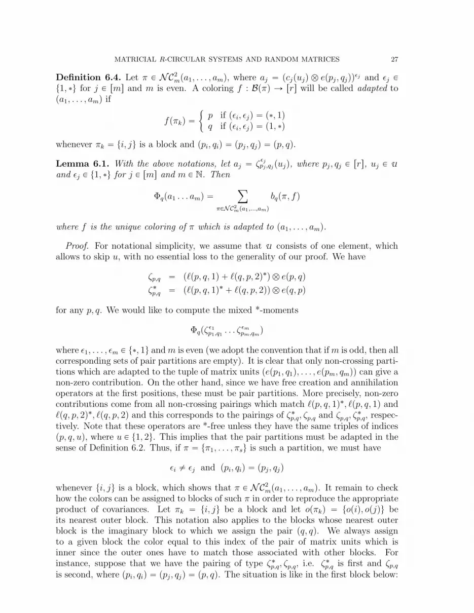
Definition 6.4. Let π P NC2

mpa1, . . . , amq, where aj “ pcjpujq b eppj , qjqqǫj and ǫj Pt1, ˚u for j P rms and m is even. A coloring f : Bpπq Ñ rrs will be called adapted topa1, . . . , amq if

fpπkq “"p if pǫi, ǫjq “ p˚, 1qq if pǫi, ǫjq “ p1, ˚q

whenever πk “ ti, ju is a block and ppi, qiq “ ppj , qjq “ pp, qq.

Lemma 6.1. With the above notations, let aj “ ζǫjpj,qjpujq, where pj , qj P rrs, uj P U

and ǫj P t1, ˚u for j P rms and m P N. Then

Φqpa1 . . . amq “ÿ

πPNC2mpa1,...,amq

bqpπ, fq

where f is the unique coloring of π which is adapted to pa1, . . . , amq.

Proof. For notational simplicity, we assume that U consists of one element, whichallows to skip u, with no essential loss to the generality of our proof. We have

ζp,q “ pℓpp, q, 1q ` ℓpq, p, 2q˚q b epp, qqζ˚p,q “ pℓpp, q, 1q˚ ` ℓpq, p, 2qq b epq, pq

for any p, q. We would like to compute the mixed *-moments

Φqpζǫ1p1,q1 . . . ζǫmpm,qmq

where ǫ1, . . . , ǫm P t˚, 1u andm is even (we adopt the convention that ifm is odd, then allcorresponding sets of pair partitions are empty). It is clear that only non-crossing parti-tions which are adapted to the tuple of matrix units pepp1, q1q, . . . , eppm, qmqq can give anon-zero contribution. On the other hand, since we have free creation and annihilationoperators at the first positions, these must be pair partitions. More precisely, non-zerocontributions come from all non-crossing pairings which match ℓpp, q, 1q˚, ℓpp, q, 1q andℓpq, p, 2q˚, ℓpq, p, 2q and this corresponds to the pairings of ζ˚

p,q, ζp,q and ζp,q, ζ˚p,q, respec-

tively. Note that these operators are *-free unless they have the same triples of indicespp, q, uq, where u P t1, 2u. This implies that the pair partitions must be adapted in thesense of Definition 6.2. Thus, if π “ tπ1, . . . , πsu is such a partition, we must have

ǫi ‰ ǫj and ppi, qiq “ ppj, qjq

whenever ti, ju is a block, which shows that π P NC2

mpa1, . . . , amq. It remain to checkhow the colors can be assigned to blocks of such π in order to reproduce the appropriateproduct of covariances. Let πk “ ti, ju be a block and let opπkq “ topiq, opjqu beits nearest outer block. This notation also applies to the blocks whose nearest outerblock is the imaginary block to which we assign the pair pq, qq. We always assignto a given block the color equal to this index of the pair of matrix units which isinner since the outer ones have to match those associated with other blocks. Forinstance, suppose that we have the pairing of type ζ˚

p,q, ζp,q, i.e. ζ˚p,q is first and ζp,q

is second, where ppi, qiq “ ppj, qjq “ pp, qq. The situation is like in the first block below:

28 R. LENCZEWSKI

color p

ℓpp,q,1q˚ b epq,pq ℓpp,q,1q b epp,qq

color q

ℓpq,p,2q˚ b epp,qq ℓpq,p,2q b epq,pq

The corrresponding second matrix unit is eppj , qjq “ epp, qq and the color assigned tothe block is p. Here, qj is the second index associated with the right leg of the consideredblock. It must agree with the first matricial index assigned to the right leg of the nearestouter block (not shown in the above picture). This is obvious if the nearest outer blockis immediately after the given block. If there is a sequence πk1, . . . , πks of blocks of thesame depth in between the given block πk and its nearest outer block opπkq when wemove from left to right, then the matricial agreement of the corresponding matrix unitsmust ‘transfer’ qj as the index to be matched to the right leg of the nearest outer block.A similar argument applies to pairings of type ζp,q, ζ

˚p,q, to which the second block in

the above picture refers. Therefore, these two kinds of pairings contribute

Φqpζ˚p,qζp,qq “ bp,q and Φppζp,qζ˚

p,qq “ bq,p,

respectively, where we use the fact that the covariances assigned to 1 and 2 are equal(of course, in general we would say that of 2u ´ 1 and 2u). It can be seen that thesecontributions correspond to the way covariances are assigned to blocks in the sense ofDefinitions 6.3 and 6.4 for one value of u. As we remarked, treating an arbitrary U isdone in a similar fashion. Therefore, our proof is completed.

7. Cyclic R-transform for R-circular systems

We would like to examine R-circular operators from the point of view of cumulants.First, let us recall some definitions from free probability referring to free cumulants andR-diagonal elements [10].

If a is a random variables in a *-probability space pA, ϕq, then a free cumulantκ2npa1, . . . , a2nq with arguments from the set ta, a˚u is called alternating if there doesnot exist any ai (1 ď i ď 2n ´ 1) with ai`1 “ ai. Cumulants with an odd numberof arguments are considered as not alternating. A random variable a P A is calledR-diagonal if for all n P N

κnpa1, . . . , anq “ 0

whenever its arguments are not alternating.The R-transform of r elements a1, . . . , ar of the *-probability space pA, ϕq is a formal

power series in noncommutative indeterminates z1, . . . , zr of the form

Ra1,...,arpz1, . . . , zrq “8ÿ

n“1

rÿ

i1,...,in“1

κnpai1 , . . . , ainqzi1 . . . zin .

In particular, the R-transform of the pair ta, a˚u in the case when a is R-diagonal is aformal series in noncommuting indeterminates z1, z2 of the form

Ra,a˚ pz1, z2q “ fpz1z2q ` gpz2z1q,


where

fpzq “8ÿ

n“0

αnzn and gpzq “

8ÿ

n“0

γnzn

and αn, βn are alternating *-cumulants of a and a˚.Circular elements are important examples of R-diagonal elements. If c is a standard

circular element (i.e. has covariance one), then the R-transform of c, c˚ takes the simpleform

Rc,c˚pz1, z2q “ z1z2 ` z2z1

since the only non-vanishing cumulants for c and c˚ are κ2pc, c˚q “ κ2pc˚, cq “ 1.We will examine matricial R-circular operators from a similar point of view. In

particular, we will study the distributions of theR-circular operators ζp,qpuq with respectto the array pΦp,qq, where Φp,q “ Φq and

Φq “ ϕ b ψq

for any p, q P rrs, where ψq is associated with the basis unit vector epqq P C r. However,we will need a new concept of cumulants. Of course, the situation is rather clear withthe cumulants of diagonal operators with respect to the corresponding diagonal statessince they are circular with respect to these states. However, the off-diagonal onesexhibit new features.

Naturally, this situation should lead to a family of cumulants indexed by q and forthat reason our cumulants will have the additional parameter q.

Definition 7.1. A family of multilinear functions κπr . ; qs, where q P rrs, of matricialvariables

aj “ cj b eppj , qjq P MrpAq,where m P rrs, will be called cyclically multiplicative over the blocks π1, . . . , πs of π PNCmpa1, . . . , amq if

κπra1, . . . , am; qs “sź

j“1

κpπjqra1, . . . , am; qpjqs,

for any a1, . . . , am, where

κpπjqra1, . . . , am; qpjqs “ κspai1 , . . . , ail; qiplqqfor the block πl “ pip1q ă . . . ă iplqq, i.e. qpjq is equal to the last matrix indexin the block, where tκsp.; qq : s ě 1, q P rrsu is a family of multilinear functions. Ifπ R NCmpa1, . . . , amq, then we set κπra1, . . . , am; qs “ 0 for any q.

Definition 7.2. With the above notations, by the cyclic cumulants we shall understandthe family of multilinear cyclically multiplicative functionals over the blocks of non-crossing partitions

π Ñ κπr . ; qs,defined by r moment-cumulant formulas

Φqpa1 . . . amq “ÿ

πPNCmpa1,...,amq

κπra1, . . . , am; qs,

where q P rrs and Φq “ ϕ b ψq are states on MrpAq as defined before.

30 R. LENCZEWSKI

The cyclic cumulants remind similar objects defined for R-cyclic matrices by Nica,Shlyakhtenko and Speicher [9,10]. We have a similar restriction on the non-crossingpartitions (cyclicity), but we consider a family of states rather than one state. Itis convenient to think of the cyclic cumulants labelled by q as of cumulants ‘undercondition q’. In fact, their values depend on the index q which labels the correspondingstate. When speaking of cumulants, we will always mean ‘cyclic cumulants’ and theusual ones will be called ‘free cumulants’.

Example 7.1. We would like to compute simple cumulants for one off-diagonal R-circular operator ζ “ ζp,q and its adjoint,

ζp,q “ pℓ1 ` ℓ˚2q b epp, qq and ζ˚

p,q “ pℓ˚1 ` ℓ2q b epq, pq,

considered before in Example 6.1. Using the properties of the free creation and annihi-lation operators, we can easily see that all odd cumulants vanish. Now, the non-trivialsecond order cumulants are

κ2pζ˚p,q, ζp,q; qq “ Φqpζ˚

p,qζp,qq “ ϕpℓ˚1ℓ1q “ γ1

κ2pζp,q, ζ˚p,q; pq “ Φppζp,qζ˚

p,qq “ ϕpℓ˚2ℓ2q “ γ2

whereas all fourth order cumulants vanish. For instance,

κ2pζ˚p,q, ζp,q, ζ

˚p,q, ζp,q; qq “ Φqpζ˚

p,qζp,qζ˚p,qζp,qq ´ κ2pζ˚

p,q, ζp,q; qqκ2pζ˚p,q, ζp,q; qq

´κ2pζ˚p,q, ζp,q; qqκ2pζp,q, ζ˚

p,q; pq“ γ2

1` γ1γ2 ´ γ2

1´ γ1γ2 “ 0,

where we used the moment computed in Example 6.1. It is not hard to observe that thiscumulant vanishes due to the fact that we used Definition 7.2 and not the definitionof free cumulants with one state. If we used the latter (computed with respect toΦq), we would not get zero since κ2pζp,q, ζ˚

p,q, pq “ γ2 would have to be replaced byκ2pζp,q, ζ˚

p,q, qq “ 0.

In fact, all cumulants of matricial R-circular operators of orders higher than twovanish. This fact is proved in the theorem given below, where we we derive a formulafor the family of cyclic R-transforms of the array ζ :“ pζp,qq of matricial R-circularoperators and the array of their adjoints ζ˚ :“ pζ˚

p,qq. These are formal power series in

2r2 noncommuting indeterminates arranged in arrays z :“ pzp,qq and z˚ :“ pz˚p,qq of the

form

Rζ,ζ˚pz, z˚; qq “8ÿ

n“1

ÿ

p1,...,pnq1,...,qn

ÿ

ǫ1,...,ǫn

κnpζǫ1p1,q1, . . . , ζǫnpn,qn; qqzǫ1p1,q1 . . . zǫnpn,qn,

where it is understood that p1, . . . , pn, q, q1, . . . qn P rrs and ǫ1, . . . , ǫn P t1, ˚u with1 playing the role of ‘no symbol’. The theorem proved below shows that the cyclicR-transforms are the canonical transforms of R-transform type to describe R-circularsystems (the first indication of that fact was Example 7.1).

Theorem 7.1. If ζ :“ pζp,qq is the square array of matricial R-circular operators andζ˚ :“ pζ˚

p,qq, then its cyclic R-transforms are of the form

Rζ,ζ˚pz, z˚; qq “rÿ

p“1

pbp,qz˚p,qzp,q ` bp,qzq,pz

˚q,pq


for any q P rrs, where bp,q “ κ2pξ˚p,q, ξp,q; qq “ κ2pξq,p, ξ˚

q,p; qq for any p, q.

Proof. It suffices to consider cumulants of even orders since the odd ones vanish. Thenon-vanishing cumulants of second order of the off-diagonal operators ζp,q, ζ

˚p,q were

computed in Example 7.1. The case of diagonal operators is easy since this case isreduced to the circular one. We have

Φqpζǫ1p1,q1 . . . ζǫmpm,qmq “

ÿ

πPNCmpζǫ1p1,q1

,..., ζǫmpm,qm q

κπrζǫ1p1,q1, . . . , ζǫmpm,qm; qs

where

κπrζǫ1p1,q1, . . . , ζǫmpm,qm; qs “

sź

k“1

κpπkqrζǫ1p1,q1, . . . , ζǫmpm,qm; qpkqs.

The contribution from an adapted pair-partition is a product of cumulants of order twoand it takes the form

κpπkqrζǫ1p1,q1, . . . , ζǫmpm,qm; qpkqs “

$’’’’&’’’’%

κ2pζ˚pi,qi

, ζpi,qi; qiq if ppi, qiq “ ppj , qjqand pǫi, ǫjq “ p˚, 1q

κ2pζpi,qi, ζ˚pi,qi

; piq if ppi, qiq “ ppj , qjqand pǫi, ǫjq “ p1, ˚q

0 otherwise

for any block πk “ ti, ju of π, where i ă j. In order to obtain the result in terms ofcovariances bp,q, we substitute

κ2pζ˚p,q, ζp,q; qq “ ϕpℓpp, q, 1q˚ℓpp, q, 1qq “ bp,q

andκ2pζp,q, ζ˚

p,q; pq “ ϕpℓpq, p, 2q˚ℓpq, p, 2qq “ bq,p

for any p, q. Now, comparing the expression that we obtained here with the formula formixed moments of Lemma 6.1, we can see that all non-crossing pair parititons which areadapted to the given tuple pζǫ1p1,q1, . . . , ζǫmpm,qm

q appear in the expression for their mixedmoment as well as in the moment-cumulant formula. By induction, this suffices to claimthat all mixed cumulants of orders higher than two vanish since in the moment-cumulantformula for any mixed moment of even order m there is one cumulant of order m andproducts of cumulants of even orders smaller than m. To begin with, all cumulantsof order four vanish since the products of cumulants of order two which correspondto non-crossing pair partitions adapted to pζǫ1p1,q1, . . . , ζǫmpm,qm

q and under condition q

appear in the formula for the moment and in the sum of cumulants associated with pairpartitions. Continuing this process, we obtain our claim. That proves that the onlynon-vanishing cumulants are of order two. We have already computed them above andit suffices to exchange p with q in the second cumulant since we want to compute thecyclic R-transform associated with the state Φq. If we fix q and multiply all of theseby the noncommutative variables zp,q and z

˚p,q corresponding to ξp,q and ξ

˚p,q, we obtain

the desired expression for the cyclic R-transforms.

Corollary 7.1. If η “ pηp,qq is the upper triangular array of matricial circular operatorsand η˚ “ pη˚

p,qq, then their cyclic R-transforms are of the form

Rη,η˚pz, z˚; qq “qÿ

p“1

pbp,qz˚p,qzp,q ` bp,qzp,qz

˚p,qq

32 R. LENCZEWSKI

`rÿ

p“q`1

pbq,pz˚q,pzq,p ` bq,pzq,pz

˚q,pq

where q P rrs and bp,q “ κ2pη˚p,q, ηp,q; qq “ κ2pηp,q, η˚

p,q; qq for any p ď q.

Proof. We can use Theorem 7.1 and the multilinearity of the cumulants since

ηp,q “ ζp,q ` ζq,p and ηq,q “ ζq,q

for any p ă q, which gives

κ2pη˚p,q, ηp,q; qq “ κ2pζ˚

p,q, ζp,q; qq “ bp,q

κ2pηp,q, η˚p,q; qq “ κ2pζq,p, ζ˚

q,p; qq “ bp,q

for p ď q and similar computations give bq,p for the cumulants of ηq,p, η˚q,p under condition

q. Thus, it suffices to put zp,q “ zq,p for p ą q in Theorem 7.1 to obtain Rη,η˚ pz, z˚; qq(for upper-triangular arrays) from Rζ,ζ˚pz, z˚; qq (for square arrays). This gives thedesired form of the cyclic R-transforms.

In the results given above, we dealt with cyclic R-transforms of square r ˆ r arraysof R-circular operators. However, one can also consider pairs consisting of one fixedoperator and its adjoint. In the off-diagonal case, we then obtain two non-trivial cyclicR-transforms of this pair and they take a very simple form.

Corollary 7.2. If p, q P rrs are fixed and p ‰ q, then

(1) the non-trivial cyclic R-transforms of h :“ ζp,q, h˚ :“ ζ˚

p,q are

Rh,h˚pz1, z2; qq “ bp,qz2z1 and Rh,h˚pz1, z2; pq “ bq,pz1z2,

(2) the non-trivial cyclic R-transform of c :“ ζq,q, c˚ “ ζ˚

q,q is

Rc,c˚pz1, z2; qq “ bq,qpz1z2 ` z2z1q,(3) the non-trivial cyclic R-transforms of η :“ ηp,q, η

˚ :“ η˚p,q are

Rη,η˚pz1, z2; qq “ bp,qpz1z2 ` z2z1qRη,η˚ pz1, z2; pq “ bq,ppz1z2 ` z2z1q.

Proof. The formulas for these cyclic R-transforms are obtained from Theorem 7.1 orCorollary 7.2 by taking suitable subarrays.

Remark 7.1. It seems natural that the cyclic R-transforms of ηp,q, η˚p,q in the states Φq

and Φp coincide with the R-transforms of circular operators since the *-distributionsof ηp,q in these states are circular by Proposition 4.1. However, cyclic R-transformsare defined differently than the usual R-transforms and thus we prefer to treat thisproperty as a decomposition of the R-transform of circular operators in terms of cyclicR-transforms of R-circular operators rather than an obvious fact. A more generaldecomposition property of this type is formulated below.

Corollary 7.3. If bp,q “ dp for any p, q, then c :“ řp,q ζp,q is circular with respect to

Φ “ řr

q“1dqΦq and the corresponding R-transform takes the form

Rc,c˚pz1, z2q “rÿ

q“1

dqRζ,ζ˚pz, z˚; qq,


where Rζ,ζ˚pz, z˚; qq is the cyclic R-transform of Theorem 7.1 in which all entries ofarrays z and z˚ are identified with z1 and z2, respectively.

Proof. If we assume that all block variances in [7, Theorem 9.1] are equal to one,the moments of the matrix Y pnq converge under the normalized trace to those of thestandard circular operator c :“ ř

p,q ζp,q under Φ by Proposition 4.3. We have

κ2pc˚, cq “ Φpc˚cq and κ2pζ˚p,q, ζp,q; qq “ Φqpζ˚

p,qζp,qq,where we denote by κn the free cumulants with respect to Φ. Since

Φpc˚cq “rÿ

p,q“1

dqΦqpζ˚p,qζp,qq,

we obtain

κ2pc˚, cq “rÿ

q“1

dqκ2pc˚, c; qq.

A similar decomposition holds if we interchange c and c˚. Free cumulants of c, c˚ ofhigher orders vanish since c is circular. The cyclic cumulants of higher orders of c, c˚

also vanish by multilinearity in view of Theorem 7.1. Therefore, the R-transform forc, c˚ has the desired decomposition in terms of their cyclic R-transforms which can beidentified with Rζ ,ζ˚pz, z˚; qq for q P rrs, where zp,q “ z1 and z˚

p,q “ z2 for any p, q. Ofcourse, both sides of this equation are equal to z1z2 ` z2z1.

We proceed in a similar way in the case of matricial R-semicircular and semicircularoperators. The corresponding cyclic R-transforms become ‘quadratic forms’ similar tothose for the matricial R-circular and circular operators.

Theorem 7.2. If ω :“ pωp,qq is the square array of matricial R-semicircular operators,then its cyclic R-transforms are of the form

Rωpz; qq “rÿ

p“1

bp,qz2

p,q

for any q P rrs, where z “ pzp,qq and bp,q “ κ2pωp,q, ωp,q; qq for any p, q.

Proof. The proof is similar to that of Theorem 7.1. The only non-vanishing cycliccumulants under condition q are of the form κ2pωp,q, ωp,q; qq “ bp,q, where p, q are arbi-trary, which gives the desired equation.

Corollary 7.4. If pω :“ ppωp,qq is the upper triangular array of matricial semicircularoperators, then its cyclic R-transforms are of the form

Rpωpz; qq “qÿ

p“1

bp,qz2

p,q `rÿ

p“q`1

bq,pz2

q,p

where we use the notations of Theorem 7.2.

Proof. The only non-vanishing cyclic cumulants under condition q are of the formκ2ppωp,q, pωp,q; qq “ bp,q for p ď q and κ2ppωq,p, pωq,p; qq “ bq,p for p ą q, which gives thedesired equation.

34 R. LENCZEWSKI

Corollary 7.5. If bp,q “ dp for any p, q, then s :“ řp,q ωp,q is semicircular with respect

to Φ “ řr

q“1dqΦq and the corresponding R-transform takes the form

Rspwq “rÿ

q“1

dqRωpz; qq,

where the Rωpz; qq are the cyclic R-transform of Theorem 7.2 in which all entries of thearray z are identified and denoted by w.

Proof. The proof is similar to that of Corollary 7.3 except that we use [7, Theorem5.1]. The moments of the matrix Y pnq converge then under the normalized trace tothose of the standard semicircular operator s :“ ř

p,q ωp,q under Φ by Proposition 4.3.

Remark 7.2. For simplicity, we considered so far the case of one array and its adjoint.However, one can easily extend the results of this section to a finite number of arrayspζp,qpuqq and pζ˚

p,qpuqq, where u P U . In that case, in order to avoid lenghty notations,we replace the triples pp, q, uq by one symbol µ, as in Section 2. We then have a familyof arrays of R-circular operators

ζ :“ tζµ : µ P rrs ˆ rrs ˆ U uand, denoting the corresponding family of their adjoints by ζ˚, we can define the cor-responding family of cyclic R-transforms

Rζ,ζ˚pz, z˚; qq “8ÿ

n“1

ÿ

µ1,...,µn

ÿ

ǫ1,...,ǫn

κnpζǫ1µ1, . . . , ζǫnµn

; qqzǫ1µ1. . . zǫnµn

where q P rrs and z :“ pzµq, z˚ :“ pz˚µq. It can be proved that these cyclic R-transforms

take the formRζ,ζ˚pz, z˚; qq “

ÿ

µ“pp,q,uq

bµz˚µzµ `

ÿ

µ“pp,q,uq

bµzµtz˚µt,

where the summation runs over all triples of the form µ “ pp, q, uq, with µt “ pq, p, uqand bµ “ bp,qpuq for any p, q, u. In fact, the proof is identical to that of Theorem 7.1since operators labelled by u and u1 cannot be paired if u ‰ u1 and the proof given herefor one array does not change if we take more arrays. Thus, we get additivity of thecyclic R-transforms corresponding to different pairs of arrays labelled by u and theiradjoints.

One can also observe that all systems of operators considered in this paper (see Def-inition 2.4) are matricial analogs of R-diagonal operators, which requires us to replacethe R-transform by the cyclic R-transforms. Moreover, matricial R-circular operatorscan also be viewed as non-tracial analogs of circular operators.

A general treatment of cyclic cumulants and cyclic R-transforms in the frameworkof matricial freneess and symmetric matricial freeness goes beyond the scope of thisarticle. We expect a close relation here, similar to that between free cumulants andR-transform and the notion of freeness. The concept of the matricial R-transformintroduced in [6] seems to be different since the latter refers to a slightly differentconcept of independence called strong matricial freeness. Actually, this is the mainreason why we used the term ‘cyclic R-transforms’ instead of ‘matricial R-transform’.Nevertheless, a unified approach to both concepts seems to be possible.


8. Moment series for R-circular systems

The matricial moment series for the arrays ζ “ pζp,qq and ζ˚ “ pζ˚p,qq is the family of

formal series of the form

Mqpz, z˚q “8ÿ

m“1

ÿ

p1,q1,...,pm,qmǫ1,...,ǫm

Φqpζǫ1p1,q1 . . . ζǫmpm,qmqzǫ1p1,q1 . . . zǫmpm,qm

where q P rrs and z “ pzp,qq and z˚ “ pz˚p,qq are the arrays of 2r2 noncommuting

indeterminates.

Proposition 8.1. The moment series for the arrays ζ, ζ˚ satisfy the relations

Mq “ 1 `rÿ

p“1

bp,qpz˚p,qMpzp,qMq ` zq,pMpz

˚q,pMqq

for any q P rrs, where Ms “ Mspz, z˚q for any s P rrs.Proof. We can express each moment Φqpζǫ1p1,q1 . . . ζǫmpm,qm

q in terms of cumulants ac-cording to the formula

Φqpζǫ1p1,q1 . . . ζǫmpm,qmq “

ÿ

πPNC2mpζ

ǫ1p1,q1

,..., ζǫmpm,qm q

κπrζǫ1p1,q1, . . . , ζǫmpm,qm; qs,

where each partitioned cumulant κπr.; qs is a product of cumulants over the 2-blocks ofπ. In order to find a typical relation between moment series, it now suffices to singleout in each π the 2-block containing 1, say t1, ku. The cumulant corresponding tothis block is bp,q for some p and the corresponding matrix units must be epq, pq andepp, qq, respectively. All cumulants corresponding to the inner blocks of this block arecollected in the seriesMppz, z˚q since they correspond to the mixed moments of variableslying in between ζǫ1p1,q1 and ζǫkpk,qk computed ‘under condition p’ since the correspondingproduct of matrix units must be epp, pq. In turn, all cumulants correponding to theblocks involving numbers greater than q are collected in the series Mqpz, z˚q since theycorrespond to the mixed moments of ζ

ǫk`1

pk`1,qk`1, . . . , ζǫmpm,qm

and the corresponding productof matrix units must be epq, qq. Of course, zp,q is assigned to ζ˚

q,p and zp,q is assignedto its adjoint ζ˚

p,q and, since our indeterminates do not commute, we have to place theseries Mppz, z˚q in between them if t1, ku is associated with the pairing pζ˚

p,q, ζp,qq. Inturn, the series Mppz, z˚q is placed in between zq,p and z˚

p,q if t1, ku is associated withthe pairing pζq,p, ζ˚

q,pq. This gives the formula

Mq “ 1 `rÿ

p“1

bp,qpz˚q,pMpzp,qMq ` zq,pMpz

˚p,qMqq

where Ms “ Mspz, z˚q for any s.

One can express the functional formulas of Proposition 8.1 in terms of the cyclicR-transforms of ζ, ζ˚. For that purpose, it is convenient to replace the array z˚ by itstranspose w “ pwp,qq, where wp,q “ z˚

q,p for any p, q P rrs. Moreover, let

Mpz, wq : “ diagpM1, . . . ,MrqRpz, wq : “ diagpR1, . . . , Rrq,

36 R. LENCZEWSKI

where Mq “ Mqpz, wq and Rq “ Rζ,ζ˚pz, w; qq for any q P rrs and we abuse the notationin the sense that we replace each z˚

p,q by wq,p and we still write w as the second argumentof each Mq and Rq.

Corollary 8.1. With the above notations, let

Rqpz, wq “rÿ

p“1

bp,qpwq,pzp,q ` zq,pwp,qq

for any q P rrs. Then, the functional equation holds

Mpz, wq “ I ` RpzMpz, wq, wMpz, wqq,where zMpz, wq and wMpz, wq are products of arrays.

Proof. We can substitute zs,t Ñ zs,tMt “ pzMqs,t and ws,t Ñ ws,tMt “ pwMqs,t fors, t P tp, qu, which gives the formula of Proposition 8.1. This completes the proof.

From the formulas of Proposition 8.1 we can obtain a concise formula for the diagonalmatrix of moment series for ζ “ ř

p,q ζp,q in the states Ψq. Let D : MnpAq Ñ MnpAqbe the linear mapping given by

DpAq “ diagpA1, . . . , Arqfor any A P MrpAq, where

Aq “rÿ

p“1

ap,q

for any q. This formula will be similar to that derived in [7] for the moment series forthe sums of matricial R-semicircular (or, semicircular) operators ω “ ř

p,q ωp,q.

Corollary 8.2. Let M “ diagpM1, . . . ,Mrq, where each Mq is given by

Mqpz, z˚q “8ÿ

m“1

ÿ

ǫ1,...,ǫm

Φqpζǫ1 . . . ζǫmqzǫ1 . . . zǫm

for the sum ζ “ řp,q ζp,q. Then M satisfies the functional equation

M “ I ` Dpz˚MBzM ` zMBz˚Mq,where B “ pbp,qq and z, z˚ are two noncommuting variables.

Proof. We set zs,t “ z and z˚s,t “ z˚ for any s, t in the formulas of Proposition 8.1,

which gives

Mq “ 1 `rÿ

p“1

pz˚Mpbp,qzMq ` zMpbp,qz˚Mqq

for any q, where we put bp,q between Mp and Mq to anticipate the product of matricesMp, B,Mq. Now, it is easy to see that z˚Mpbp,qzMq is the pp, qq-th entry of the matrixz˚MBzM , where z and z˚ are to be understood as diagonal matrices with z and z˚ onthe diagonal, respectively. Similarly, zMpbp,qz

˚Mq is the pp, qq-th entry of zMBz˚M .In turn, summation over p for fixed q corresponds to the mapping D, which completesthe proof.


The formulas of Proposition 8.1 for the moment series for arrays of R-circular opera-tors as well as those of Corollary 8.2 for the moment series for their sums are equivalentto the definition of their cumulants (which are recursions for moments) and thus it is notsurprising that their solutions can be found in the form of recursions analogous to thosefor Catalan numbers. For simplicity, we restrict our attention to the case discussed inCorollary 8.1.

Proposition 8.2. The matrix-valued moment series M of Corollary 8.2 takes the form

Mpz, z˚q “8ÿ

m“0

ÿ

ǫ1,...,ǫ2m

Cmpǫ1, . . . , ǫ2mq zǫ1 . . . zǫ2m ,

where the coefficients are diagonal r ˆ r matrices satisfying the recurrences

Cmpǫ1, . . . , ǫmq “ÿ

j`k“m´1

DpCjpǫ2, . . . , ǫ2j´1qBCkpǫ2j`1, . . . , ǫ2mqq

for any m P N, with C0 “ I, where we set Cmpǫ1, . . . , ǫmq “ 0 whenever pǫ1, . . . , ǫmq isnot associated with a non-crossing pairing consisting of p1, ˚q and p˚, 1q. These recur-rences have a unique solution.

Proof. It suffices to substitute Mpz, z˚q in the above form to the equation for M ofCorollary 8.2 and observe that if pǫ1, ǫ2jq “ p˚, 1q, then Cjpǫ2, . . . , ǫ2j´1q comes from thefirst M in the product z˚MBzM and Ckpǫ2j´1, . . . , ǫ2mq comes from the second M inthat product. All terms for which pǫ1, ǫ2jq “ p1, ˚q correspond to the product zMBz˚M

in a similar way. This gives the desired recurrence for the matrix-valued coefficients. Itis obvious that these recurrences have a unique solution.

Corollary 8.3. If bp,q “ dp for any p, q P rrs, then the moment series M0 “ M0pz, z˚qfor the circular operator ζ “ ř

p,q ζp,q associated with Φ “ řr

q“1dqΦq satisfies the func-

tional equationM0 “ 1 ` z˚M0zM0 ` zM0z

˚M0

Proof. It holds that

M0pz, z˚q “8ÿ

m“1

ÿ

ǫ1,...,ǫm

Φpζǫ1 . . . ζǫmqzǫ1 . . . zǫm “rÿ

q“1

dqMqpz, z˚q

and it suffices to take the sum over q of the equation in the proof of Corollary 8.2 andset bp,q “ dq to obtain the desired equation.

Remark 8.1. The moment series for a family of arrays labelled by u is defined ina similar way. Accordingly, all results of this section hold for such families, but wedo not formulate them in the whole generality for the sake of simplicity. In order toobtain the general formulation it suffices to label each pair ζp,q, ζ

˚p,q by an additional

argument u and use the fact that two operators corresponding to any 2-block ti, juof any non-crossing pair partition give a non-trivial contribution to the moment seriesand to the cyclic R-transforms only if they are labelled by the same u. The effect isthat the definition of the series Mq aquires additional summations over u1, . . . , um P Uand appropriate additional summations appear in the formulas of Proposition 8.1 (over

38 R. LENCZEWSKI

u), Corollary 8.1 (over u), Corollary 8.2 (over u1, . . . , um) and Proposition 8.2 (overu1, . . . , u2m).

Remark 8.2. The recurrence of Proposition 8.2 reminds that for Catalan matrices in[7, Theorem 8.3]. Note, however, that the latter involved the matrix of K-transforms

Kpzq “ diagpK1,1pzq, . . . , Kr,rpzqqand not the corresponding matrix of moment generating functions Mj,j. Nevertheless,the sequence of Catalan matrices pCmqmě0 can be viewed as the matricial analog ofthe sequence of Catalan numbers since that recurrence involves a nice bracketing ruleand, after all, the K-transform of the standard semicircle law agrees with its Cauchytransform. Clearly, the matrix of moment series can be computed from Kpzq as in thescalar-valued case, namely

Mpzq “ diagpM1,1pzq, . . . ,Mr,rpzqq “8ÿ

m“0

pzKp1zqqm.

Its matrix-valued coefficients satisfy a different recurrence than that for Catalan matri-ces. Of course, these coefficients give another sequence of matricial analogs of Catalannumbers which is directly related to moments.

Instead of using convolutions and K-transforms [7], let us now briefly state the resultsfor the moment series for matricial R-semicircular operators in the same spirit as wedid for the matricial R-circular operators in this section. It is not hard to see that weobtain functional equations similar to those in Proposition 8.1 and Corollary 8.1. Westate these results without proofs since they are very similar to those given above.

Proposition 8.3. The moment series for the array pωp,qq of the form

Mqpzq “8ÿ

m“1

ÿ

p1,q1,...,pm,qm

Φqpωp1,q1 . . . ωpm,qmqzp1,q1 . . . zpm,qm

where z “ pzp,qq is the array of r2 noncommuting indeterminates, satisfy the relations

Mqpzq “ 1 `rÿ

p“1

bp,qzp,qMppzqzp,qMqpzq

for any q P rrs.Corollary 8.4. The matrix-valued moment series M “ diagpM1, . . . ,Mrq for the sumω “ ř

p,q ωp,q, where each Mq “ Mqpzq is given by

Mqpzq “8ÿ

m“1

Φqpωmqzm,

satisfies the functional equation

Mpzq “ I ` z2DpMpzqBMpzqq,where B “ pbp,qq and z is a variable. Its unique solution is of the form

Mpzq “8ÿ

m“0

Cmz2m,


where the coefficients are diagonal r ˆ r matrices satisfying the recurrence

Cm “ÿ

j`k“m´1

DpCjBCkq

for any m P N, with C0 “ I.

Remark 8.3. One can also consider the moment series for the arrays of matricialcreation and annihilation operators ℘ “ p℘p,qq and ℘˚ “ p℘˚

p,qq of the form

Mqpz, z˚q “8ÿ

m“1

ÿ

p1,q1,...,pm,qmǫ1,...,ǫm

Φqp℘ǫ1p1,q1

. . . ℘ǫmpm,qm

qzǫ1p1,q1 . . . zǫmpm,qm

where q P rrs and z “ pzp,qq and z˚ “ pz˚p,qq are the arrays of 2r2 noncommuting

indeterminates. Then the corresponding cyclic R-transforms are of the form

R℘,℘˚pz, z˚; qq “rÿ

p“1

bp,qz˚p,qzp,q

and the functional equation for the matrix-valued moment series takes the same formas for the matricial R-circular operators in Corollary 8.1, namely

Mpz, wq “ I ` RpzMpz, wq, wMpz, wqq,where w “ pwp,qq is the transpose of z, i.e. wp,q “ z˚

q,p. If we set z˚p,q “ zp,q, we can write

in the same form the functional equation for the R-semicircular operators involving thecyclic R-transforms of Theorem 7.2.

9. Asymptotics of random blocks

Matricial semicircular (circular) operators give operatorial realizations of the limitjoint distributions (*-distributions) under partial traces of symmetric random blocks ofHermitian (non-Hermitian) random matrices with i.b.i.d. complex entries, respectively[5,7].

By partial traces we understand normalized traces composed with classical expecta-tions of the form

τqpnq “ 1

|Nq|ptrq ˝ Eq

where q P rrs :“ t1, 2, . . . , ru and trq is the trace over the sets of basis vectors of Cn

indexed by Nq, whererns :“ N1 Y . . .YNr

is a partition into disjoint non-empty intervals (their dependence on n is supressed).Further, it is assumed that

limnÑ8

|Nq|n

“ dq ě 0 for any q,

where D is the dimension matrix.The following theorem has been proved in [7] (see also [5] for the case of one matrix).

Theorem 9.1. Let tY pu, nq : u P U u be a family of Gaussian random matrices withi.b.i.d. complex entries, each with symmetric blocks pTp,qpu, nqq and symmetric blockvariance matrix V puq and associated matrix Bpuq “ DV puq. Then

40 R. LENCZEWSKI

(1) if the matrices are Hermitian,

limnÑ8

Tp,qpu, nq “ pωp,qpuq,

(2) if the matrices are non-Hermitian, then

limnÑ8

Tp,qpu, nq “ ηp,qpuq,

for any 1 ď p ď q ď r and u P U , where convergence is in the sense of mixed momentsand *-moments under partial traces, respectively.

We would like to complete this picture with the asymptotics of blocks

Sp,qpu, nq “ÿ

i,jPNpˆNq

Yi,jpu, nq b ei,jpnq

where p, q P rrs, from which the symmetric blocks are constructed:

Tp,qpu, nq “"Sp,qpu, nq ` Sq,ppu, nq if p ‰ q

Sq,qpu, nq if p “ q.

Of course, the right framework is non-Hermitian since we do not want to assume anydependence among the entries. It is natural to expect that R-circular operator will givethe asymptotics of blocks Sp,qpu, nq.Theorem 9.2. Let tY pu, nq : u P U u be a family of Gaussian random matrices withi.b.i.d. complex entries, each with blocks pSp,qpu, nqq and symmetric block covariancematrix V puq and associated matrix Bpuq “ DV puq, respectively. Then

limnÑ8

Sp,qpu, nq “ ζp,qpuq

for any 1 ď p, q ď r and u P U , where convergence is in the sense of mixed *-momentsunder partial traces.

Proof. We need to show that

limnÑ8

τqpnqpS ǫ1p1,q1

pu1, nq . . . S ǫmpm,qm

pum, nqq “ Ψqpζǫ1p1,q1pu1q . . . ζǫmpm,qmpumqq

for any ǫ1, . . . , ǫm P t1, ˚u, u1, . . . , um P U and q, p1, q1, . . . , pm, qm P rrs. Here, thesymbol Sp,qpu, nq denotes the block consisting of variables indexed by pi, jq P Np ˆ Nq

and S˚p,qpu, nq is its adjoint (we identify blocks with the subbblocks of nˆ n matrices).

By [7, Theorem 9.1], we have

limnÑ8

τqpnqpT ǫ1p1,q1

pu1, nq . . . T ǫmpm,qm

pum, nqq “ Ψqpηǫ1p1,q1pu1q . . . ηǫmpm,qmpumqq

for any ǫ1, . . . , ǫm P t1, ˚u, u1, . . . , um P U and q, p1, q1, . . . , pm, qm P rrs. By definition,

ηǫp,q “"ζǫp,qpuq ` ζǫq,ppuq if p ‰ q

ζǫq,qpuq if p “ q

for any p, q, u, ǫ. It suffices to analyze the contributions from various mixed *-momentsof R-circular operators to the combinatorial formula for the mixed *-moments of opera-tors ηp,qpuq given in [7, Proposition 9.1]. Namely, letNC

2

m,qppw 1, u1, ǫ1q, . . . , pwm, um, ǫmqqbe the set of those π P NC2

m which are adapted to ppw 1, u1, ǫ1q, . . . , pwm, um, ǫmqqand to the number q, where w k “ tpk, qku for any k. This means that if ti, ju is


a block of π, where i ă j, then there exists a tuple ppv1, u1q, . . . , pvm, umqq, wherevk P tppk, qkq, pqk, pkqu for any k, such that

v i “ vj , ui “ uj, ǫi ‰ ǫj and qj “ popjq

where topiq, opjqu is the nearest outer block of ti, ju, where opiq ă opjq and it is under-stood that we assign tq, qu to the imaginary block. Then

Ψqpηǫ1p1,q1pu1q . . . ηǫmpm,qmpumqq “

ÿ

πPNC2m,qppw1,u1,ǫ1q,...,pwm,um,ǫmqq

bqpπ, fq,

where f is the coloring of π defined by ppw 1, u1, ǫ1q, . . . , pwm, um, ǫmqq and by the numberq. Therefore, is suffices to identify the limit contributions from various mixed *-momentsof the blocks Sp,qpn, nq with the corresponding mixed *-moments of the operators ζp,qpuq.The diagonal blocks and the diagonal operators are the same as in [7, Theorem 9.1] andthus it suffices to analyze the off-diagonal ones. By definition, we have

ηp,qpuq “ ζp,qpuq ` ζq,ppuq,where

ζp,qpuq “ ℘p,qp2u ´ 1q ` ℘˚q,pp2uq

ζq,ppuq “ ℘q,pp2u ´ 1q ` ℘˚p,qp2uq

for any p ‰ q and any u. If ti, ju is a block of π P NC2

m,qppw 1, u1, ǫ1q, . . . , pwm, um, ǫmqqand pǫi, ǫjq “ p˚, 1q, then η˚

pi,qipuiq, ηpj ,qjpujq forms a pairing and thus there are two

possible pairings of R-circular operators which may contribute:

ζ˚pi,qi

puiq, ζpj ,qjpujq or ζ˚qi,pi

puiq, ζqj ,pjpujq.The choice of the ‘right’ pairing depends on the vector of Cr onto which ηpi,qjpujq issupposed to act. Depending on whether it is epqjq or eppjq, the first or the secondpairing contributes, respectively. Observe that these pairings must correspond to thepairings of blocks

S˚pi,qi

pui, nq, Spj ,qjpum, nq or S˚qi,pi

pui, nq, Sqj,pjpum, nq,respectively, since in a given pair of symmetric blocks T ˚

pi,qipui, nq, Tpj ,qjpuj, nq we get

a non-trivial action of the second member of these pairs of subblocks onto vectors ofC

n indexed either by k P Nqj or k P Npj , respectively. A similar correspondence holdsif pǫi, ǫjq “ p1, ˚q and thus our formula for the limit mixed *-moments of R-circularoperators is proved.

References

[1] J. Cuntz, W. Krieger, A class of C˚-algebras and topological Markov chains, Invent. Math. 56

(1980), 251-268.[2] K. Dykema, U. Haagerup, DT-operators and decomposability of Voiculescu’s circular operator,

Amer. J. Math. 126 (2004), 121-189.[3] K. Dykema, U. Haagerup, Invariant subspaces of Voiculescu’s circular operator, J. Funct. Anal.

209 (2004), 332-366.[4] R. Lenczewski, Matricially free random variables, J. Funct. Anal. 258 (2010), 4075-4121.[5] R. Lenczewski, Asymptotic properties of random matrices and pseudomatrices, Adv. Math. 228

(2011), 2403-2440.[6] R. Lenczewski, Matricial R-transform, J. Funct. Anal. 262 (2012), 1802-1844.[7] R. Lenczewski, Limit distributions of random matrices, arXiv:1208.3586 [math.OA], 2012.

http://de.arxiv.org/abs/1208.3586

42 R. LENCZEWSKI

[8] R. Lenczewski, R. Sa lapata, Multivariate Fuss-Narayana polynomials with appplication to randommatrices, Electron. J. Combin. 20 (2013), Issue 2.

[9] A. Nica, D. Shlyakhtenko, R. Speicher, R-cyclic families of matrices in free probability, J. Funct.Anal. 188 (2002), 227-271.

[10] A. Nica, R. Speicher, Lectures on the Combinatorics of Free Probability, Cambridge UniversityPress, Cambridge 2006.

[11] D. Shlyakhtenko, Random Gaussian band matrices and freeness with amalgamation, Int. Math.

Res. Notices 20 (1996), 1013-1025.[12] D. Shlyakhtenko, Free quasi free states, Pac. J. Math. 177 (1997), 329-367.[13] D. Voiculescu, Limit laws for random matrices and free products, Invent. Math. 104 (1991),

201-220.[14] D. Voiculescu, Circular and semicircular systems and free product factors, Progress in Math. 92,

Birkhauser, 1990.[15] D. Voiculescu, K. Dykema, A. Nica, Free random variables, CRM Monograph Series, No.1, A.M.S.,

Providence, 1992.

Romuald Lenczewski,

Instytut Matematyki i Informatyki, Politechnika Wroc lawska,

Wybrzeze Wyspianskiego 27, 50-370 Wroc law, Poland

E-mail address : [email protected]

Documents

Matricial R-circular systems and random matrices