Maximum Battery Capacity Routing to Prolong Network Operation Lifetime in Wireless MESH Network alongside the OLSR Protocol

(IJCSIS) International Journal of Computer Science and Information Security,

Vol. 11, No. 9, September 2013

Maximum Battery Capacity Routing to Prolong Network Operation Lifetime

in Wireless MESH Network alongside the OLSR Protocol

Ramezanali Sadeghzadeh

Faculty of Electrical and Computer

Engineering, K.N. Toosi University

of Technology

Tehran, Iran

[email protected]

Asaneh Saee Arezoomand Dept. of Electrical and Computer

Engineering, Science and Research

Branch, Islamic Azad University

Tehran, Iran

[email protected]

Mohammad Zare

Dept. of Electrical and Computer

Engineering, Science and Research Branch, Islamic Azad University

Tehran, Iran [email protected]

Abstract— A wireless mesh network (WMN) is a

communications network made up of radio nodes

organized in a mesh topology. Wireless mesh networks

often consist of mesh clients, mesh routers and gateways.

The mesh clients operate on batteries such as cell phone, laptop and .., while the mesh routers forward traffic to

and from the gateways which may, but need not, connect

to the Internet. To maximize the lifetime of mesh mobile

networks, the power consumption rate of each node

must be evenly distributed, it is essential to prolong each

individual node (mobile) lifetime since the lack of mobile

nodes can result in partitioning of the network, causing

interruptions in communications between mobile nodes,

and finally the overall transmission power for each

connection request must be minimized. In this article we

propose a new metric to find a proper route in wireless Mesh network and beside it we study OLSR protocol

that it can be used in Ad hoc network.

Keywords- Wireless Mesh; Ad hoc Network; Energy

Consumption; Power Control; OLSR protocol

I. INTRODUCTION

Wireless mesh architecture is a first step towards providing cost effective and dynamic high-bandwidth networks over a specific coverage area [1], [2].

Mesh networks may involve either fixed or mobile devices. The solutions are as diverse as communication needs, for example in difficult environments such as emergency situations, tunnels, oil rigs, battlefield surveillance, high speed mobile video applications on board public transport or real time racing car telemetry. An important possible application for wireless mesh networks is VoIP. By using a Quality of Service scheme, the wireless mesh may support local telephone calls to be routed through the mesh.

The term 'wireless mesh networks' describes wireless networks in which each node can communicate directly with one or more peer nodes. It is a multi-hop wireless network [8] and consists of two types of nodes: mesh routers and mesh clients. Mesh routers have minimal mobility and form the backbone of WMNs, some of them are called gateway nodes and connected with a wired network. Client mesh networks comprise of energy-limited, mobile devices such as laptops and IP Phones. The mesh clients have mobility

requirements as well as energy constraints, thus making communication challenging.

Dependence of power-consumption constraints on the type of mesh nodes. Mesh routers work by the endless power energy from backbone Internet and mesh clients by the limited battery, so we focus on the routing of the mesh clients. The lack of mobile clients can result in partitioning of the network, causing interruptions in communications between mobile clients. Since most mobile clients today are powered by batteries, efficient utilization of battery power is more important than in cellular networks. It also has an important influence on the overall communication performance of the network.

II. POWER-EFFICIENT ROUTING PROTOCOLS

In this section, we present a brief description of the relevant

energy-aware routing algorithms proposed recently.

A. Minimum Battery Cost Routing (MBCR)

This metric reduce the total power consumption of the overall network. But, it has a critical disadvantage, it does not reflect directly on the lifetime of each client. If the minimum total transmission power routes obtain via a specific client, the battery of this client will be exhausted quickly, and this client will die of battery exhaustion soon. So, the remaining battery capacity of each client is a more accurate metric to describe the lifetime of each client [10].

Let f�(c��) be the battery cost function of a client ni. Now,

suppose a node’s willingness to forward packets is a

function of its remaining battery capacity. As proposed, one

possible choice for fi is

��(�) = �

�� (1)

Where c�� is the battery capacity of a client n at time t.

The battery cost Rj for route j, consisting of D nodes, is

�� = ∑ ��(�)

�� . (2)

Therefore, to find a route with the maximum remaining

battery capacity, we should select a route i that has the

minimum battery cost.

�� = �� ∈ !" (3)

where A is the set containing all possible routes. Since only the summation values of battery cost

functions is considered, a route containing nodes with little

remaining battery capacity may still be selected, which is

undesirable.

24 http://sites.google.com/site/ijcsis/ ISSN 1947-5500



B. Minimum Total Transmission Power Routing

In the MTPR mechanism, the total transmission energy

for the route is calculated as: P(r&) = ∑ T(n� + n�*�)&�� .

Where a function T(n�, n,) denoting the energy consumed in

transmitting over the hop (n�, n,) and generic route is

r& = n�, n�, … n&, where n� is the source node and n& is the destination node.

The optimal route r. satisfies the following condition: P(r.) = min12∈1∗ P(r,) (4)

Where r∗ is the set of all possible routes.

C. Min-Max Battery Cost Routing (MMBCR)

Equation (2) can be modified to make sure that no node will be overused, as indicated in [4]. Battery cost R, for

route j is redefined as R, = max�∈1.7�8_, f�(c�

�) (5)

Similarly, the desired route i can be obtained from the equation

R� = min�R,�j ∈ A"

As MMBCR always tries to avoid the route with nodes having the least battery capacity among all nodes in all possible routes, the battery of each host will be used more fairly than in previous metrics. But, there is no guarantee that minimum total transmission power paths will be selected under all circumstances.

III. OUR PROPOSED NEW ROUTING MODEL

Nodes in Wireless Mesh Network (WMN), especially in client topology, are battery driven. Therefore, they suffer from limited energy level problems. In such an environment there are two important reasons that result in partitioning of the network: 1) Node dying of energy exhaustion, and 2) Node moving out of the radio range of its neighboring node. Hence, to achieve the best route in WMNs, node stability is essential. According to previous discussions, our goal is to maximize the lifetime of each node and use the battery fairly. But, in this new model we consider both hop-counts and remaining battery capacity together to achieve a proper route. In other words, battery capacity defines as a cost function with spot a number of hops. WangBo proposed [5] new energy consumption model that considers the hops too. So, energy consumption of each node will be use fairly and energy distribution implement better over more hops. To represent new model are four different conditions:

• Equal number of hops with different total cost.

• Different number of hops with equal total cost.

• Different number of hops with different total cost.

• Equal number of hops with equal total cost.

f�(c��) is the battery cost function (BCF) of a client n�

that defines as Equation (1) in MBCR, i.e. f�(c��) = �

�� .

Where c�� is the battery capacity of a client n� at time t. But,

in new model the battery cost R, is different from equation

(2). Since we consider the number of hops the battery cost R, , consisting of M nodes, is redefined as follows:

R, = �

;∑ f�(c�

�)<2�� (6)

where H denote the number of hops. So, to find a route with the maximum remaining battery capacity, the favorite route i can be obtained from the equation

R� = min�R,�j ∈ A" (7).

This model prevents the nodes in the routing with consideration their cost which have a less battery capacity and balance the energy consumption of each node.

IV. PERUSE THE NEW MODEL WITH AN EXAMPLE

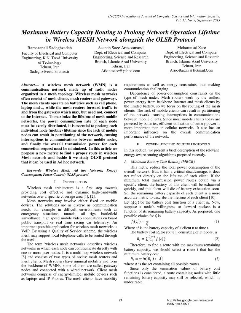
In order to illustrate the new model, we give an example (Fig. 1) to express it.

In figure 1 if source node is S and destination node is D, there are three routes between them. First, battery cost �� is

calculated for three routes. Then, according to equation (7) the best route is elected. To compare these three routes we consider three different conditions as mentioned in previous section. Since we consider critical states in the example, we compare two steps of conditions. 1) Route 1 and route 2 show the state 2, i.e. Different number of hops with equal total cost. If the prior metric implemented to select the route, the route with minimum hops was selected i.e. route 1 while the node 3 in this route has a little energy capacity, which is undesirable. But, whit this new metric route 2 is elected that have enough energy capacity and distributed energy has done well. Although route 2 has an end-to-end delay higher than route 1, route 2 restrains interruptions in communications between mobile clients. 2) Route 2 and route 3 show the state 3, i.e. Different number of hops with different total cost. Again if the prior metric implemented like MBCR, the route 3 was selected that has a minimum total energy, it can consume more power to transmit user traffic from a source to a destination, which actually reduces the lifetime of all nodes. But with new metric after calculate

the �� , route 2 is selected. In addition, more hops can reduce

the total transmission power consumption and balance the energy consumption of each node.

Most of the previous metrics have surveyed on equal hops. But, this new metric has studied on different hops to find a proper route which has shown in figure 1.

V. THE STRUCTURE OF OUR SIMULATOR

Different routing protocols have been proposed for mesh wireless networks. Some use conventional routing metrics such as minimum hop, while others consider new routing metrics such as power consumption. To better understand

Figure 1: Example of the algorithm




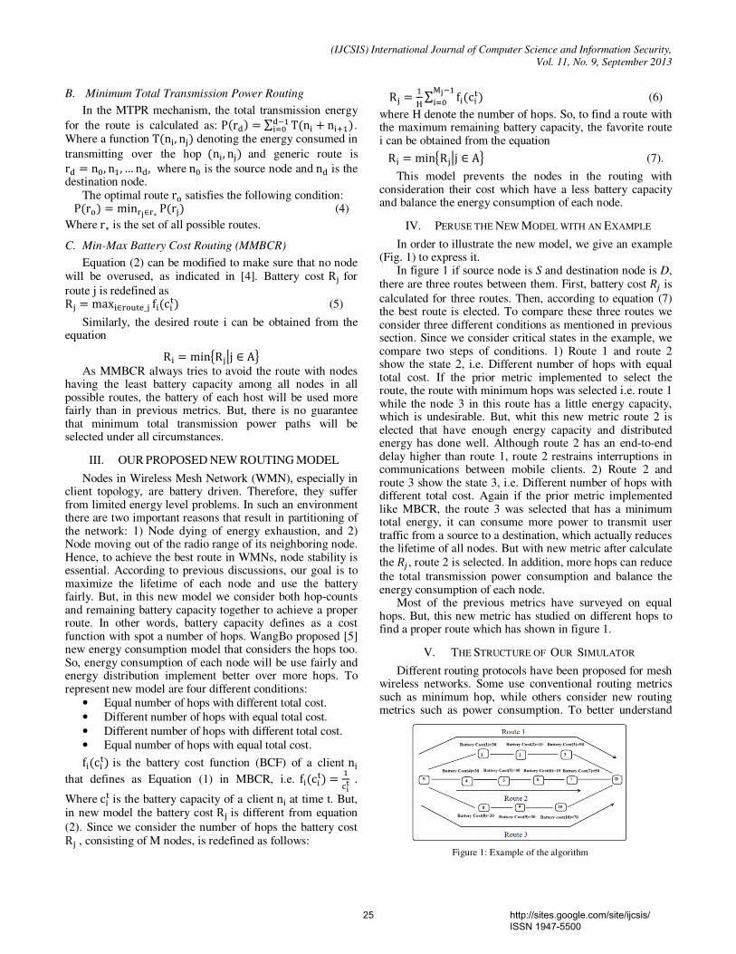
their performance in terms of power efficiency, we perform simulations. Fig. 2 demonstrates these steps.

VI. SIMULATION SETTINGS

Simulations were done using the OPNET v14.5 Simulator

and Matlab R2007b to analyze the performance of the

proposed metric. OPNET is excellent simulation software.

However, there are a number of simple tasks that are often

not so simple to do in OPNET. So, we combine the power

of Matlab as a backend to OPNET simulations using the Matlab Engine. The proposed metric was implemented in

DSR and its performance was compared to the standard DSR

protocol that uses the minimum hop metric and OLSR protocol

applied to another scenario separately.

A. Network scenario

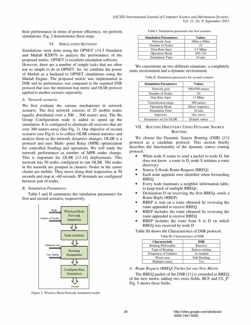
We first evaluate the various mechanisms in network

scenario. The first network consists of 25 mobile nodes

equally distributed over a 500 _ 500 meters area. The Rx Group Configuration node is added to speed up the

simulation. It is configured to eliminate all receivers that are

over 300 meters away (See Fig. 3). Our objective of second

scenario (see Fig.4) is to collect OLSR related statistics and

analyze them as the network dynamics changes. OLSR is a

protocol and uses Multi- point Relay (MPR) optimization

for controlled flooding and operations. We will study the

network performance as number of MPR nodes change.

This is important for OLSR [12-14] deployments. This

network has 50 nodes configured to run OLSR. The nodes

in the network are grouped in clusters. Nodes in the center cluster are mobile. They move along their trajectories at 50

seconds and stop at ~60 seconds. IP demands are configured

between pair of nodes.

B. Simulation Parameters

Table I and II summarize the simulation parameters for first and second scenario, respectively.

Table I. Simulation parameters for first scenario

Simulation Parameters Values

Network Area 500m x 500m

Number of Nodes 25

Data Rate (bps) 5.5 Mbps

Operation Mode 802.11b

Simulation Time 10 min

We concentrate on two different situations: a completely

static environment and a dynamic environment.

Table II. Simulation parameters for second scenario

Simulation Parameters Values

Network grid 500×500 meters

Number of Nodes 50

Data Rate (bps) 11 Mbps

Transmission range 300 meters

Operation Mode Direct sequence

Simulation Time 10 min

trajectory olsr_move

Parameters set for OLSR Default values

VII. ROUTING DISCOVERY USING DYNAMIC SOURCE

ROUTING

We choose the Dynamic Source Routing (DSR) [11] protocol as a candidate protocol. This section briefly describes the functionality of the dynamic source routing protocol.

• When node S wants to send a packet to node D, but does not know a route to D, node S initiates a route discovery

• Source S floods Route Request (RREQ)

• Each node appends own identifier when forwarding RREQ

• Every node maintains a neighbor information table, to keep track of multiple RREQs

• Destination D on receiving the first RREQ, sends a Route Reply (RREP)

• RREP is sent on a route obtained by reversing the route appended to receive RREQ

• RREP includes the route obtained by reversing the route appended to receive RREQ

• RREP includes the route from S to D on which RREQ was received by node D

Table ІII shows the Characteristics of DSR protocol.

Table III. Characteristics of DSR

Characteristic DSR

Routing Philosophy Reactive

Type of Routing Source routing

Frequency of Updates As needed

Worst case Full flooding

Multiple routes Yes

A. Route Request (RREQ) Packet for our New Metric

The RREQ packet of the DSR [11] is extended as RREQ of the new metric adding two extra fields, BCF and CL_P. Fig. 5 shows these fields.

Figure 2: Wireless Mesh Network simulation model




SA DA T ID TTL BCF HOPs P CL_P

Figure 5: The RREQ packet

SA (Source Address) field carries the source address of

node. DA. (Destination Address) field carries the destination address of node. T (Type) field indicates the type of packet, TTL (Time To Live) field is used to limit the lifetime of packet, by default, it contains zero. BCF (Battery Cost Function) field carries inverse battery capacity of each node. HOP field carries the hop count, initially, this field contains zero value. P (PATH) field carries the path accumulations, when packet passes through a node; its address is appended at end of this field. CL_P field calculates the battery cost (like equation 6) at the end of route.

B. Destination Node

In this case with new metric, when the destination receives multiple RREQs it selects the path has the minimum digit that has calculated in CL_P power, i.e. the path with the maximum remaining battery capacity.

VIII. PERFORMANCE STUDY

In first scenario, we epitomize our study on estimating the halt-time, of nodes. The halt-time (Expiration time) expresses how long a node has been active before it halts due to lack of battery capacity. The halt-time of nodes directly affects the lifetime of an active route and possibly of a connection. Then we evaluate the traffic routing received/sent by each node with different transmit power in static and dynamic environments.

In the dynamic environment we used the “random waypoint” model to simulate nodes movement. The motion is characterized by the maximum speed. Each node starts moving from its initial position to a random target position selected inside the simulation area. The node speed is uniformly distributed between 0 and the maximum speed.

In second scenario, we study four states:

A. MPR count statistics

This statistic shows the number of nodes selected as MPRs in the network. Initially (0-50 seconds), “MPR count”

increases and then converges to 1. In the transient phase,

each node has partial information about network topology.

Hence each node tries to select MPR based on partial

topology information. As nodes receive topology

information, MPRs are re-elected and finally converges at

steady state. Note that node_56 becomes MPR by default

(due to its willingness parameter) and since it is the only

required MPR, rest of nodes do not become MPR. Since the

transmission range is 300 meters, one hop is required for

communication for the nodes at opposite ends of the

network. Node_56 being in center cluster has more “reachability” than nodes in edge clusters. For time period

after 50 seconds, the nodes in middle cluster starts moving

and reach the upper right edge. Since there is no single best

candidate for MPR (in terms of reachability), each node

finds different MPRs to reach two hop neighbor. That is why we see higher MPR count. The MPR that is

selected in each cluster is the node with its willingness parameter set to high (Node_19, node_28, node_25, node_64). Since there are 5 clusters, 5 MPRs will remain in the steady state (Fig. 6).

B. TC Traffic sent (bits/sec)

Topology control (TC) messages are periodically sent out only by MPR nodes in the network. For time period 0-50 seconds, there was only 1 MPR node. After 50 seconds, the number of MPRs in network increases, hence TC Traffic Sent increases (See Fig.6).

C. Hello Message Sent

Hello message are periodically sent by each node in the network. It contains the list of neighbors and their quality.

Figure 3: First Network Scenario

Figure 4: Second Network Scenario




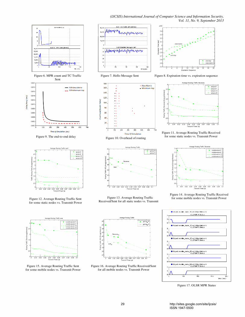
Statistics “Hello Message Sent (Fig.7)” shows the number of hello messages sent in the network. It does not change even after 50 second time as each node continues sending hello message. However, the “Hello Message Sent (bits/seconds)” statistics changes with node movement. The number of neighbors for each node decreases when the nodes in center cluster moves away, hence the size of each hello message reduces.

D. MPR status

This statistic indicates (Fig.17) if a node is elected as an MP. It generates a square wave graph with values 1 and 0, where value 1 indicates the time when this node becomes an MPR.

IX. SIMULATION RESULTS

In our simulations, two different route selection schemes are considered: 1) Minimum Hop (MH) and 2) New Metric (NM).

Note: Since a client can forward packets only when its battery capacity is above zero, the value of the cost function will always be finite. Fig. 8 demonstrates the expiration time of nodes and of connections. The expiration times are sorted in ascending order. In Minimum Hop approach, the times of some first nodes exhausting theirs battery are much earlier than that of some last nodes since this metric does not take the battery capacity of each node into consideration and selects route with minimum hop. So, there is no guarantee to extend the lifetime of nodes. But, expiration sequences for New Metric preliminary nodes have the longer lifetime than that of the first nodes in MH because NM chooses the path that has the nodes with proper remaining battery capacity.

Fig. 9 displays the end to end delay of system. Delay of our

network is compared with minimum hop which has a more

delay of MH metric. The reason of it is, since new metric

needs to obtain power’s information about its own

neighbourhood and it is down periodically in system. So, it

takes a few times to gather this information and increase the end to end delay system. To save the information temporary,

this method needs a routing table causes the overhead of

routing (see Fig.10). But, in this scenario prolonging

network operation is more important than other issue. Fig. 11 and fig. 12 illustrate the routing traffic received

and routing traffic sent for static environment for some nodes in different positions respectively (see Fig.3). Transmit power for each node is increased and the average value of routing traffic is recorded. As these figures have shown, the routing traffic decreases when the transmit power of each node increases. Because, when the transmit power of node is little node cannot route the packet better therefore retransmission mechanism occur and cause the traffic.

Fig. 13 represents the average routing traffic received/sent for 25 nodes in the network. (Global statistics)

Fig. 14, fig. 15 and fig. 16 illustrate the routing traffic received, sent and global for dynamic environment respectively.

X. CONCLUSION

In this paper, we first presented previous work on power-aware routing. Then we proposed a new energy consumption model, chiefly for the mesh clients (because mesh clients have limited battery resources and must consume battery power more efficiently to prolong network operation lifetime), to be used to predict the lifetime of nodes according to current traffic conditions. The main goal of this new metric is to extend the lifetime of each node. Alongside this new work, we simulate the network scenario by using OLSR protocol and we study their statistics. Using OPNET simulator and MATLAB, we implemented OLSR protocol in wireless mesh network and new proposed metric and we compared it with minimum hop mechanism. Finally, we studied the routing traffic vs. transmit power in static and dynamic environment and observed the traffic increased when transmit power decreased.

REFERENCES

[1] I.F. Akyildiz and X. Wang,” A Survey on Wireless Mesh Networks,” in IEEE communication Magazine, September 2005.

[2] J. Jun and M. L. Sichitiu, “The Nominal Capacity of Wireless Mesh

Networks,” in IEEE Wireless Communications, October 2003.

[3] C.-K. Toh, “Maximum battery life routing to support ubiquitous mobile computing in wireless ad hoc networks,” IEEE

Communications Magazine, vol. 39, no. 6, pp. 138–147, June 2001.

[4] S.Singh, M. Woo, and C. Raghavendra, “Power-aware routing in mobile ad hoc networks,” in MobiCom ’98: Proceedings of the 4th

annual ACM/IEEE international conference on Mobile computing and networking.New York, NY, USA: ACM Press, 1998, pp. 181

190.

[5] WangBo and Li Layuan, “Maximizing Network Lifetime in Wireless

Mesh Networks,” IEEE Wireless Communications, 2008.

[6] D.K.Kim, J. Garcia-Luna-Aceves, K. Obraczka, J.-C. Cano, and P. Manzoni, “Routing mechanisms for mobile ad hoc networks based on

the energy drain rate,” IEEE Transactions on Mobile Computing, vol. 2,no. 2, pp. 161–173, 2003.

[7] C.-K. Toh, “Maximum Battery Life Routing to Support Ubiquitous

Mobile Computing in Wireless Ad Hoc Networks,” IEEE Comm. Magazine, June 2001.

[8] Held, Gilbert, Wireless mesh networks, Taylor & Francis Group,

USA, March 2005.

[9] K. Scott and N. Bambos, “Routing and Channel Assignment for Low Power Transmission in PCS,” Proc. IEEE Int’l Conf. Universal

Personal Comm., 1996.

[10] S. Singh, M. Woo, and C. S. Raghavendra, “Power- Aware Routing in Mobile Ad Hoc Networks,” Proc. MobiCom ’98, Dallas, TX, Oct.

1998.

[11] David B. Johnson, David A. Maltz, & Josh Broch, "DSR: The

Dynamic Source Routing Protocol for Multi-Hop Wireless Ad Hoc Networks", (2001), Ad Hoc Networking, Addison- Wesley , pp. 139-

172

[12] T. Clausen, P. Jacquet, "RFC3626: Optimized Link State Routing Protocol (OLSR)"

[13] A. Qayy , L. Viennot, A. Laouiti, "Multipoint relaying: An efficient

technique for flooding in mobile wireless networks", 35t Hawaii International Conference on System Sciences (HICSS’2001)

[14] T. Clausen, C. Dearlove, J. Dean, C. Adjih, \RFC5444: Generalized

Mobile Ad Hoc Network (MANET) Packet/Message Format", Std. Track, http://www.ietf.org/rfc/rfc5444.txt




Figure 6. MPR count and TC Traffic

Sent

Figure 7. Hello Message Sent Figure 8. Expiration time vs. expiration sequence

Figure 9. The end-to-end delay Figure 10. Overhead of routing

Figure 11. Average Routing Traffic Received

for some static nodes vs. Transmit Power

Figure 12. Average Routing Traffic Sent

for some static nodes vs. Transmit Power

Figure 13. Average Routing Traffic

Received/Sent for all static nodes vs. Transmit

Figure 14. Average Routing Traffic Received for some mobile nodes vs. Transmit Power

Figure 15. Average Routing Traffic Sent

for some mobile nodes vs. Transmit Power

Figure 16. Average Routing Traffic Received/Sent for all mobile nodes vs. Transmit Power

Figure 17. OLSR MPR Status


Documents

Maximum Battery Capacity Routing to Prolong Network Operation Lifetime in Wireless MESH Network alongside the OLSR Protocol