Embed Size (px)
Citation preview

MAXENT ROC 1
Running head: MINIMAL SDT
Bits of the ROC:Signal Detection as Information Transmission
Peter R. Killeen & Thomas J. Taylor
Arizona State University
Correspond with:
Peter KilleenDepartment of PsychologyBox 1 1 0 4Arizona State UniversityTempe, AZ 85287-1104
email: [email protected]: (480) 965-8544Voice: (480) 965-2555

MAXENT ROC 2
Abstract
The framework for detection and discrimination called Signal
Detection Theory (SDT) is reanalyzed from an information-theoretic
perspective. Receiver-operating characteristics (ROCs) for the iso-
informative processor describe arcs in the unit square, and lie close t o
those described by constancy of A’. Necessary and sufficient condit ions
for performance to fall on these arcs is that the p a y off matrix be hones t ,
and that as bias shifts changes in the information expected from yes
responses are complemented by those from n o responses. Asymmetric
ROCs require further characterization of the underlying distributions.
The simplest maximum-entropy distributions on the evidence axis a r e
exponential, and yield power-law ROCs that describe many data. T h e
success of ROCs constructed from confidence ratings shows that m o r e
information is available from the signal than the experimenter’s b ina ry
classification lets pass. Such ratings comprise category scaling of signal
strength. Power operating characteristics are consistent with Weber’s
law. Where Weber’s law holds, channel capacity on a dimension equals
the logarithm of its Weber fraction.
MAXENT ROC 3
Bits of the ROC:
Signal Detection as Information Transmission
Signal Detection Theory (SDT) and Information Theory (IT) were t h e
jewels in the crown of 2 0t h century experimental psychology. As a n
avatar of statistical decision theory, SDT provided a technique fo r
reducing a 2x2 table of relations between stimulus and response in to
measures of detectability and bias, of sensitivity and selectivity, t he reby
untangling a 100-year old confound. It has been well popularized b y
Swets (e.g. Swets, Dawes & Monahan, 2000) and thoroughly analyzed b y
Macmillan and Creelman (1991). Information theory, the bril l iant
invention of Claude Shannon (Shannon, 1949), provided algorithms fo r
quantifying the amount of information t r ansmitted by a response.
Although both theories were formulated at the same time (the la te
1940s), and both concern similar phenomena (quantifying the accuracy
of imperfect discriminations), there has been very little use of o n e
theory to reinforce and complement the other. By the end of the 2 0t h
century, SDT remains an important theory while IT is rarely ment ioned.
Classic SDT (here, CSDT) is an application of Thurstone scaling (see,
e.g., Juslin & Olsson, 1997; Lee, 1969; Luce, 1977; Luce, 1994). Whereas many stimuli a r e
susceptible to measurement in physical units, such as decibels o f
intensity, some are not. These latter are often of most central concern t o
society, involving measures of complex stimuli such as beauty, qual i ty
MAXENT ROC 4
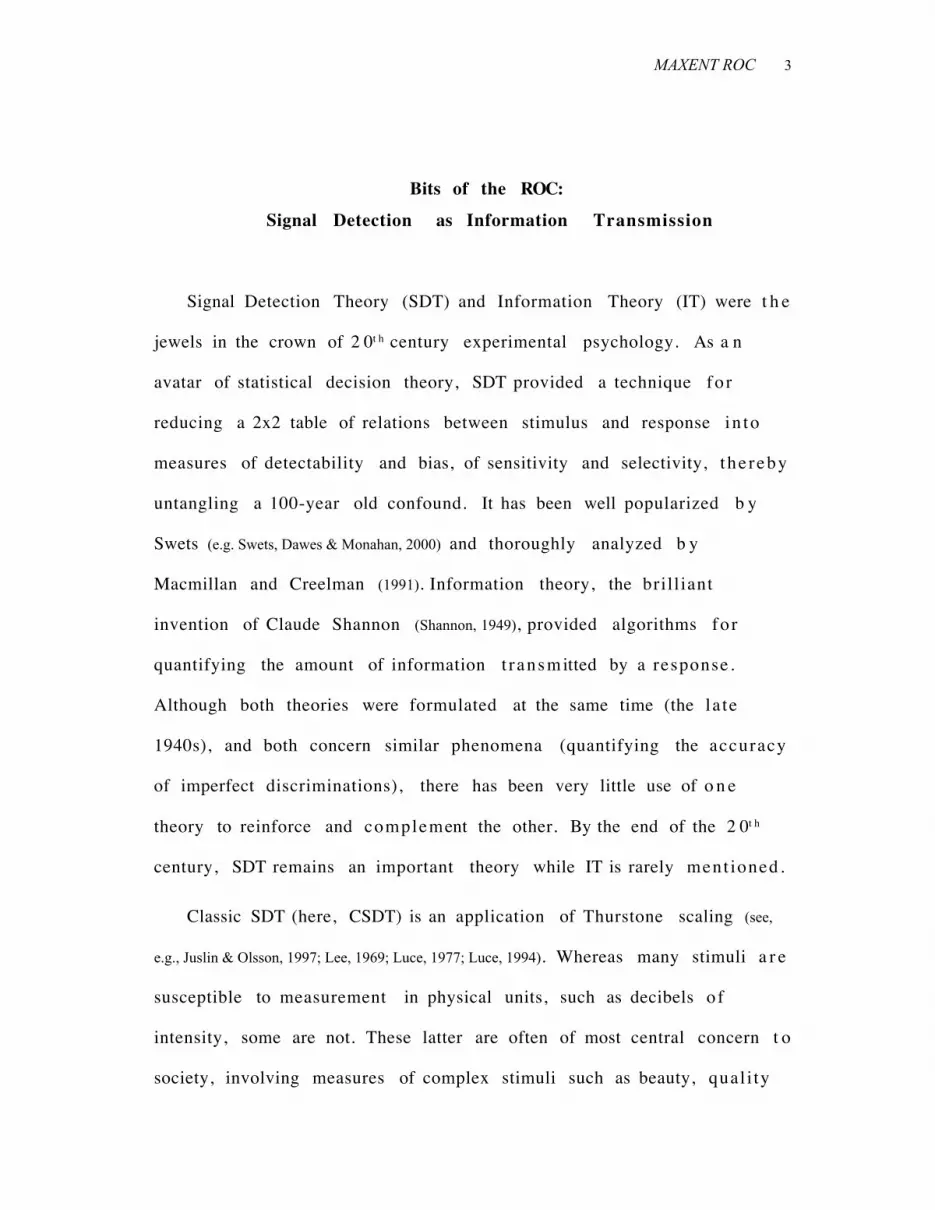
of life, impac t of punishment. Thurstone suggested a metric for t h e
distance between stimuli that would embrace both the simple a n d
complex: The unit of distance between stimuli would be the s t a n d a r d
deviation of the percept associated with the stimulus. Thurstone called
the distribution of perceptions issuing from a stimulus a “discriminal
process”, and its standard deviation σ the “discriminal dispersion”. Two
such processes are shown in Figure 1, issuing from two stimuli.
++ Figure 1 (discrim disp) and Table 1 (calc) about here ++
Tables 1 and 2 give the data from which such machinery is inferred.
Table 1 shows the joint probabilities of signals and responses. In Table
2, these are divided by the row marginals to give the condit ional
probabilities of responding “A” or “B” given the stimulus value.
Although here viewed as a symmetric discrimination, the origin of CSDT
was in detection tasks, where Sa was the background, or noise st imulus.
This gave rise to the terminology of Correct Rejection (CR) for responses
in the RaSa cell, and Misses (M) for responses in the RaSb cell.
++ Tables 2 & 3 about here ++
Table 2 descr ibes the performance from the perspective of a n
experimenter, one who knows the stimulus condition and assays t h e
probability of a response. It is useful for characterizing the behavior o f
the detector. In the applications of SDT, we are usually given t h e
response--the verdicts of radiologists, juries, and children who c r y
“wolf”-- and wish to know the probability that a signal was in fact
present. This requires dividing the cells in Table 1 by their co lumn

MAXENT ROC 5
marginals, yielding Table 3. One may go between Tables 2 & 3 by using
Bayes’ theorem to convert the arguments of a conditional probabili ty.
Table 3 is more user-friendly, in that consumers of SDT analyses a r e
seldom given the state of nature, and wish to evaluate that state, n o t
characterize the detector. The impact of these different
conditionalizations can be quite different: A child who always cries
“wolf” when their prevalence is 1% will be assigned a hit rate of 100 %
by the conventional Table 2, but only 1% by Table 3. No matter h o w
Table 1 is conditionalized it has two degrees of freedom, and n o
evaluation of a discrimination is complete without reporting b o t h
accuracy of affirmatives and accuracy of negatives. Table 3 is o f ten
more convenient for information-theoretic analyses.
CSDT invokes normal discriminal processes to translate t h e
probabilities in Table 2 into the two measures of theoretical interest (d’
and C). Other distributions are reviewed by Egan (1975). The data a r e
often consistent with these assumptions. However, the discr iminal
processes are never observed, and carry more degrees of freedom t h a n
the data they represent. There are five degrees of freedom available i n
constructing Figure 1: The means and standard deviations of signal a n d
noise distributions, and the location of the criterion. These over-
endowed distributions are then slimmed down by stipulating an origin
and unit for the perceptual abcissae. The origin is set either at the m e a n
of the first percept, or halfway between the means of the two percepts
(as inferred from the data). The unit--the standard deviation--is set t o
1.0. This leaves the scale value of the second stimulus, d’ and t h e

MAXENT ROC 6
location of the criterion, C, as the recovered parameters that re-present
the information found in the hit and false alarm rates. For the data i n
Table 1, d’ = 0.385 - (-0.675) = 1.06. If the origin is placed at the m e a n
of the two distributions, then C = -(z(H) + z(F))/2. Macmillan a n d
Creelman (1991, Equation 2.2) include the factor 1/2 so that the range of t h e
bias statistic is the same as that of d’. For the data in Table 2, C = -
(0.385 -0.675) = 0.29. As shown in Figure 1, the criterion is slightly
above the mean of the percepts, indicating a conservative criterion: T h e
observer is more likely to reject a marginal perception as noise than t o
accept it as a signal.
CSDT was a trail breaking innovation. Now standing near t h e
summit, a glance back shows that CSDT did not pick out the most d i rec t
route to the goal of representing discrimination performance. Too m u c h
that is unverifiable is assumed, only to be later nullified. Alternative
nonparametric measures of sensitivity and bias have been developed
out of a condign sense of parsimony. Macmillan and Creelman (1996)
reviewed these alternatives in an article whose title h e d g e d
“nonparametric”, because the measures reviewed either made subt le
assumptions of underlying distributions or mechanisms--or were at least
consistent with such distributions.
Subsumption Psychophysics
It this paper we m a ke assumptions about mechanisms a n d
distributions in incremental fashion, in the style of Brooks (1991), w h o
coined the term subsumption archi tecture to describe such a bottom-up

MAXENT ROC 7
approach. Build until it breaks, then see what additional is necessary.
The conceptual tool that permits this approach to be applied to signal
detection theory is the maximum entropy formalism (MEFJaynes, 1986;
Skilling, 1989; Tribus, 1969). The MEF stipulates that inference should be ba sed
on statements of everything known, with all other constraints maximally
random (i.e., having maximum entropy). If they are not maximally
random, then we are implicitly making additional inferences about the i r
nature. It is the goal of MEF to make all such knowledge explicit, leaving
nothing hidden in implicit assignments of parameters or distr ibutions.
We instantiate the MEF for detection by (a) describing a detect ion
theory that makes no assumptions concerning underlying distributions;
then (b) describing one t h a t invokes underlying one-parameter
distributions of signal strengths; and then (c) describing one t h a t
invokes underlying two-parameter distributions of signal s t rength.
Minimal SDT
Assume that observers attempt to maximize performance, given t h e
constraint imposed by limits on the information available from t h e
stimuli. This goal is equivocal until “maximal performance” is defined.
Value. Whenever an experimenter stipulates proper behavior for a n
observer (e.g., “Respond B only when you are sure you have observed
the stimulus”), they are imposing an index of merit for t he i r
performance. Often this is vague, as in the example given. One of t h e
many important contributions of CSDT was its emphasis on the explicit
assignment of indices of merit to per formance. An example is given i n

MAXENT ROC 8
Table 4, where the entries indicate the values assigned to each of t h e
outcomes. For instance, an experimenter may provide points ,
convertible into goods, for performance in the following manner: v(CR)
= v(H) = +5; v(F) = -3; v(M) = -1. This would generate a slightly
conservative bias in subjects attempting to maximize their expected
payoff. The perceived utility of the goods is, however, often a nonl inear
function of the points assigned (Kornbrot, Donnelly & Galanter, 1981). Some
subjects, motivated by a sense of propriety that outweighs the payoff
matrix, may attempt to maximize their % correct. Because of t h e
potential ambiguity of what subjects may be maximizing, po in t
predictions are seldom made. Instead, what is predicted is the nature o f
the curve that describes the locus of points p(H), p (F) in the u n i t
square, and the changes in parameters of that curve, or of t h e
observer’s location on it, with changes in the payoff matrix or t h e
discriminability of the s t imulus (see Figure 2) .
++ Insert Figure 2 (ROC) and Table 4 (payoff) around here +++
Symmetry. Consider the case in which there is no reason to t h ink
that Sa is qualitatively different than Sb, so that it is arbitrary which is
called A and which B, and thus arbitrary which conditional probabil i ty
in Table 2 is called hit and which correct rejection. Switching those
labels gives the open circle shown in Figure 2 as an equally valid locus
for the data; it is where the data would be found if the only impor ta n t
distinction between the two stimuli were the labels the exper imenter
assigned to them, and those could be arbitrarily reassigned. What these
two data points have in common is that they convey an equal amount o f

MAXENT ROC 9
information from the stimulus through the observer to t h e
experimenter. We now generalize this relation.
Information
The related concepts of randomness (entropy) and its reduc t ion
(information) have been given explicit formulation only in this cen tu ry
by Brillouin, Cox, Jaynes, Weiner, and most importantly, Shannon. Brief
histories of these ideas by major contributors are (Tribus, 1979) and (Jaynes,
1979). In particular, Jaynes reformulated both statistical mechanics a n d
inferential statistics using MEF and Bayes’s Theorem. Because
information is the central concept in this regrounding of SDT, i t
requires explication.
Entropy is a thermodynamic measure of disorder, which changes a s
a function of the energy added to a system relative to its temperature. I t
is intimately related to information, which is a measure of the reduc t ion
of entropy by some operation. Shannon’s (1949) key insight was t h e
development of entropy theory for the measurement of informat ion
transmission. “Shannon’s paper ... takes its rightful place alongside t h e
works of Newton, Carnot, Gibbs, Einstein, Mendeleev and the o t h e r
giants of science on whose shoulders we all stand (Tribus, 1979, p. 10).
Information is a relative concept; it is relative to context, and to t h e
state of the receiver. A coded message may look completely r a n d o m
until we are given a key (context), which permits the extraction o f
useful information. The amount of information is not the same as i ts
value. Small amounts of information may be of greater value than t h a t
derivable from encyclopedias: Lamps in a belfry may be inscrutable

MAXENT ROC 10
without the key “One if by land, two if by sea”, in which context t h e y
provide approximately one bit of very important information. They
would provide less than a bit if the route of invasion were a l ready
known, or known with some probability; they would provide more t h a n
a bit if the timing or color or brightness of the signal conveyed
additional information, such as distance or magnitude of the force.
Because information is defined as change--either as a difference i n
discrete systems or as a differential in continuous systems--it is a
process/behavioral construct, rather than a content/cognitive
construct. Information does not reside in the source, nor in t h e
message, nor in the communication channel; nor in the receiver. I t
resides nowhere. Information is the reduction in the uncer ta in ty
(entropy) of a response by use of a stimulus. Books do not conta in
information. Books may reduce the uncertainty--entropy--of t h e
reader’s response to questions such as “who killed the white whale”.
The book informs the response, but does not conta in information. T h e
book is a key that permits the student to decipher the correct answer t o
the question. The font of the text is un in fo rmative. Unless the ques t ion
concerns typography. The number of chapters is uninformative. Unless
the game is trivial pursuit. No specification of the information value of a
stimulus such as a book can be made without knowledge of the range o f
possible ques tions and answers (their entropy), and the degree to which
the answers are less random than they would be without that st imulus.
To say a book is informative means that it will permit the reader t o
respond to a wide range of relevant (to the reader) quest ions in a non-

MAXENT ROC 11
U x p pi i( ) log ( )= −∑ 2
random manner. An observer in a psychophysical experiment does n o t
so much have information, but rather t ransmits information f r o m
stimulus to the experimenter, who measures it by evaluating Table 1 .
Entropy tells us how much variability a system, or parts of it, contains.
Information is a relation between the entropy of two or more parts of a
system: it tells us how much of the variability in one part is correla ted
with the variability in ano ther .
Measuring information. The Shannon-Weiner measure of the
information transmitted from stimulus to response, t h e
transinformation (T), is the amount by which the channel reduces t h e
maximum entropy--or uncertainty (U)--in a stimulus-response matrix. If
there were no correlation between stimuli and r e s ponses (i.e., no s h a r e d
information), the cell entries in Table 1 could be predicted b y
multiplying the marginal probabilities, obtaining p(CR) = p(M) = .275;
p(F) = p(H) = .225. This is the same tactic used to calculate the expected
cell entries in calculating a chi-square statistic. To calculate the en t ropy
of such an uninformative matrix, apply the classic informat ion
transformation to the cells:
1 .
and then reapply it to the actual matrix. The difference between these is
the information transmitted b y the response. This may be concisely
written as:

MAXENT ROC 12
An alternate way of calculating information transmission provides a
different perspective on its meaning. Transinformation (T) is t h e
amount by which our uncertainty concerning a stimulus is reduced by a
response:
2 . T = U (S) - U(S|r)
U(S) is the entropy of the stimulus as measured by Equation 1. For
the data shown in Figure 2, the probability of a signal was constant a t
.5, giving a value of 1 bit for U(S). The variable U(S|r) tells us h o w
uncertain we are about the presence of a stimulus once we know which
response occurred; it is called the equivocation of transmission (see,
e.g., Attneave, 1959). It is calculated by applying Equation 1 to t h e
conditional probabilities in Table 3 1. The equivocation depends on t h e
expected equivocation from both yes and n o responses (Equation 3):
3 . T = U (S) - [ p(y )U(S|y) + p ( n )U(S|n)]
1 It is also possible to calculate T from Table 2, as the entropy of the response less the expectedambiguities (U(r|S)) of the stimuli. Because U(S) is often fixed for an experimentl condition, Equation 3is more interpretable.
Ti,j = ∑
i
pipj∑j
log2
pi, j
pipj

MAXENT ROC 13
Application to the data in Table 3 yields a value of T = 0.12 bits.
Conserving informat ion. The transinformation that the observer
communicates from stimulus to response is T. If the stimuli a r e
indiscriminable, T = 0. If two equiprobable stimuli are perfectly
discriminated, T = 1. The observer might choose to communicate less
information if so motivated by the payoff schedule. Call a payoff matr ix
honest if, in Table 4, v(CR) > v(F), and v(H) > v(M). An honest payoff
matrix is one that rewards the observer more for telling the truth t h a n
for lying. A dishonest payoff matrix could generate data that fell below
the diagonal in Figure 2, as could confusion concerning the appropr ia te
use of response categories. In such cases of disinformation, T does n o t
go negative (as does d’). The performance of the observer remains
informative; it merely requires that the experimenter understand t h a t
yes means n o, and vice versa; examples abound .
Under what conditions will an observer operating at the filled circle
in Figure 2 move to an operating point closer to the diagonal? Assume
the payoff remains honest and effective, as does t he discriminability o f
the stimuli. If the observer decreases the hit rate while holding CR r a t e
constant, payoff will decrease; if the observer increases false alarm r a t e
while holding hit rate constant, payoff will decrease. There is neve r
motivation to operate inside the observed (maximum) level o f
performance. Honest payoff matrices force the observers away from t h e
bottom right corner of the graph to the limit of their ability. This l imit
is called the channel capacity.

MAXENT ROC 14
Under honest payoff matrices, it is thus always to the subject’s
advantage to respond in a manner that maximizes informat ion
transmission. Figure 2 shows as dots the loci that do this for an observer
transmitting 0.12 bits, and for another transmitting 0.50 bits.
Characteristics of T. The relation between the traditional measure d’
and T is shown in Figure 3. For d’s of less than 3, the informat ion
transmitted, T, is approximately 10% of the square of d’. Isoinformation
contours are very similar to Pollack and Norman’s (1964) nonparamet r ic
ROC: The smooth curves in Figure 2 describe the performance t h a t
maintains a constant A’.
Transmitted information T is approximately distributed as chi-
square, knT ≈ Χ2, were n is the number of observations and k = 2ln[2] ≈
1.386 (McGill, 1954). If the data in Table 1 were based on 100 observations,
then with T = 0.12, Χ2 ≈ 16.6, which for 2 degrees of freedom is
significantly greater than zero (p < .01). The exact chi-square for th i s
matrix is Χ2 = 16.2. Measured values of T are biased estimators of i ts
true value. Miller (1955) has shown that T’ = T - (r-1)(c- 1 ) / k provides
an unbiased estimate when n is not too small; r is number of rows, c
number of columns, and k is 2ln[2].
+++ Insert Figure 3 (d’ vs. H) around here +++
Conditions for constancy of T. What accomplishes the shift along t h e
Information Operating Characteristic (IOC) in Figure 2? As payoff varies,
observers can maximize their earnings by shifting the proportion of yes
and n o responses, which affects the informativeness of those responses.

MAXENT ROC 15
For transmitted information (T) to remain constant, as the probabil i ty
of a yes response changes, any concommitant gains or losses i n
p ( y )U(S|y) must balance the losses or gains in p ( n )U(S|n). For t h e
isoinformation loci shown as dots in Figure 2, these complements a r e
plotted in Figure 4 .
++ Insert Figure 4 around here +++
More generally we may state that, given constant signal
probabilities, in order for T to remain constant over shifts in bias
requires that the change in the expected equivocation of yes responses
complement any changes in the expected equivocation of n o responses:
d [ p(y )U(S|y)] /d[ p(y)] = - d[ p( n )U(S|n)] /d[ p(y)]
This is a strong constraint: it requires symmetric, congruen t
densities, such as those shown in Figure 1 .
Bias. When the payoff is increased for yes responses the observer
can maximize payoff by increasing the number of yes responses. But if
the probability and discriminability of the stimuli don’t change, so t h a t
U(S) and T remain constant, then Equation 3 shows that as p (y )U(S|y)
increases p ( n )U(S|n) must decrease. An equilibrium will be f o u n d
somewhere on the IOC that maximizes payoff. The difference be tween
the average equivocations of yes and n o responses provides a measure
of bias:
4 . B = p [n]U[S|n] - p [y]U[S|y].

MAXENT ROC 16
B is positive for conservative biases, zero on the negative diagonal o f
the ROC, and negative for liberal biases. It may be normalized to r ange
between -1 and +1 by dividing it by the entropy of the stimulus m i n u s
the transinformation, U(S) - T:
4’. B’ = B/ ( U(S) - T) .
For the exemplary data in Figure 2, B’ = B/(1.0-0.12). Figure 4
shows that as bias shifts, the transfer of uncertainty from yes to n o
responses falls along a diagonal with a slope o f -1, thus conserving
transinformation--the distance between the locus of the points and t h e
diagonal. Conversely, for information to be conserved, the change i n
information from a yes response as its probability is varied must equa l
the complement of that from a n o response. Isoinformative opera t ing
characteristics effectively describe some experimental data, as shown i n
Figure 5. The loci of isoinformative points in this space closely
approximate the arc of a circle. The function is not visually
discriminable from that described by the nonparametric statistic A’
(Grier, 1971; Pollack & Norman, 1964).
+++ Insert Figure 5 (G&S symmetric) around here +++
There are, however, many data not well described by isoinformation
contours, such as some reported Green and Swets in their Figure 4-5,
and replotted in Figure 6. The deviations from isoinformation occur
both as skew, shown there, and as performance that is more concave

MAXENT ROC 17
than permitted by isoinformative curves. To deal with these deviations
it is necessary to impute structure to the information processor.
+++ Insert Figure 6 (G&S skewed) around here +++
Imputing Mechanism
The isoinformation contour shown in Figure 6 misses the d a t a
systematically. This indicates that the observer is not able to main ta in
constant information transmission while increasing the proportion o f
“yes” responses. The assumption of symmetry of stimuli has failed:
there is some intrinsic order to the stimuli that makes it impossible t o
conserve information under a symmetric change in bias. What is t h e
minimal structure that can be added to similarly hobble the i m p u t e d
discrimination mechanism? The dependent variables in these
experiments are a pair of probabilities; such probabilities are funct ions
on random variables. It has sufficed to describe the stimuli as a rb i t ra ry
binary variables. It no longer does.
Knowing nothing about the stimuli (the random variables) that gave
rise to p(H) and p (F) other than that they assume a finite set of values,
the most general assumption that one can make about their dis t r ibut ion
is that it is uniform--if the variable can take k values, the probability o f
any one is 1/k. The distribution in ROC-space that minimizes deviat ion
from this distribution is a straight line issuing from 0,0 to the d a t a
point, and then extending to 1,1. But once such an operating point is i n
hand, it provides an estimate of the mean of both distributions. Given
this estimate, the most general, least constrained a posteriori

MAXENT ROC 18
distribution is the geometric (Kapur, 1989). The geometric distribution is
also the maximum entropy (maxent) distribution for a random variable
that can assume a countably infinite number of states, given
specification of the mean. In the continuous limit, the geometric
approaches the exponential, which is the maxent distribution on t h e
positive continuum, given knowledge of the mean. In the case of a finite
upper limit, the maxent distribution is a renormalized exponential .
Figure 7 shows the imputed distribution of two s t imuli about which all
we know is their means .
+++ Insert Figure 7 around here +++
On each trial of the detection experiment an event--stimulus o r
noise--is presented to the observer, on whom then impinges some
instance of the random variable drawn from o ne of these distr ibutions.
Because the observer does not know a priori which distribution was
sampled, she confronts a distribution that is a mixture of these two,
looking like the average of the ordinates of the two curves shown i n
Figure 7. If the observer employs the standard decision-theoretic
strategy of responding yes whenever the event exceeds some cri ter ion
value (e.g., a value of C = 7 in Figure 7) and n o otherwise, a s imple
version of CSDT results. The probability of a hit, p(y|S), is the integral o f
the Signal distribution to the right of C: exp(-C/µ S), where µS is the m e a n
of the signal distribution. The probability of a false alarm, p(y|N), is t h e
integral of the noise distribution to the right of C: exp(-C/µ N). Solving
for C and substituting gives the equation for the ROC:

MAXENT ROC 19
5 .
The probability of a hit is a power function of the probability of a
false alarm, with an exponent β equal to the ratio of the mean of t h e
signal distribution to that of the noise distribution. When these a r e
equal, t he ROC lies along the major diagonal, as no discrimination is
possible. When the signal to noise ratio is large, the ROC rises quickly
toward the upper left corner before bending over toward 1,1. T h e
dashed line through the data in Figure 6 is a power ROC.
Green and Swets (1966, p. 69)recognized the importance of t h e
exponential as an underlying discriminal process:
an exponential distribution has, we feel, many advantages
over the Gaussian assumption with unequal variance.
First, the decision axis is monotonic with likelihood rat io.
Second, this distribution arises in a natural way in m a n y
counting processes and may, therefore, genera te
interesting hypotheses about the sensory mechanisms.
Third, and equally important, it is a one-parameter
distribution, and thus the ROC curve can be summar ized
by one parameter rather than by two.
Why was the exponential not pursued? Their next sentence tells:
“The parsimony gained, however, entails the risk that the n e w
distribution may fit fewer data than the two-parameter models.”
p y|S = p y|N1/β
with β = µS/µN

MAXENT ROC 20
Possibly; but Figures 8 and 9 show that the exponential assumption is i n
fact robus t23.
+++ Insert Figures 8 & 9 (Swets, Norman) around here +++
Characteristics of the power ROC. The parameter of the power
function β is the r atio of the means of the inferred signal and noise
distributions. As described below, its logarithm gives the entropy of t h e
ROC. It conveys the same information as d’, as it increases from 0 a s
discriminability improves. Using a logistic approximation to the normal ,
for unbiased observers and processes with equal dispersions, a measure
equivalent to d’ is ln[H/ (1 -H)] (Luce, 1 9 6 3 ). Figure 10 shows t h e
square of this index plotted as a function of the parameter of the power
characteristic, f or hit rates ranging from .5 to .95. An alternate index o f
merit is the area under the ROC, A. Green and Swets ( 1966) showed
that under very general considerations, this area predicts the pe rcen t
correct in a two-alternative forced choice task. Integrating the power
function gives:
6 . A = µS /(µ S + µN) = β/(1 + β).
Conversely, the parameter of the power function can be infer red
from the percent correct as:
β = A/(1-A) ,
3 The ROC curves shown in these figures minimize the sum of squares deviation between data andcurve on each axis. This was accomplished by appending to the data files a replicate with ordinates andabcissae exchanged, and simultaneously minimizing the error variance around p(F) = p(H)^β for thatappendix.

MAXENT ROC 21
where A is estimated from the 2AFC task. Egan (1975) provides a
thorough analysis of power ROCs. Equations 4 and 4’ continue to b e
useful as a measure of bias in the information transmitted. Information
transmission is greater for conservative biases, where the ROC is t h e
greatest distance from the diagonal. To maximize informat ion
transmission the observer cannot be unbiased.
+++ Insert Figure 10 (d’ vs. beta) around here +++
The entropy of the inferred signal-to-noise ratio, ln [β], is plotted i n
Figure 11 as a function of the relative amplitude of signal and noise fo r
the data of two of Norman’s (1963) observers. Notice that in the bes t
case the entropy approaches 4 bits (β ≈ 16); but with observers
restricted to a binary judgment, the most information that can b e
transmitted is 1 bit .
+++ Insert Figure 11 (Norman’s info vs. dB) around here +++
Weber’s law. In studies of sensory discrimination it is often f o u n d
that the dispersion of judgements is p ropor t ional to the mean of t h e
stimuli: Over a large range, the coefficient of variation of judgments is
constant. The Thurstone paradigm shown in Figure 1 assumes equal-
variance for these processes (this assumption of independent r a n d o m
variables with equal variance is known as Case V). Weber’s law is
inconsistent with this simplifying assumption. In CSDT studies t h e
MAXENT ROC 22
standard deviation of the inferred signal distribution is often found t o
be proportional to the mean signal strength (e.g., Green & Swets, 1966 ,
p. 407; (Jeffress, 1970; Markowitz & Swets, 1967), consistent with Weber’s law.
Symmetric densities such as the normal or logistic appear as s t ra ight
lines on probability axes, with slopes of m = σN/ σS and intercepts of I =
(µS - µN)/ σS. Under Weber’s law, σ = w µ; it follows that m = 1 - w I: Slopes
should be a linearly decreasing function of discriminability. This is also
true for power ROCs, which are slightly concave up in logit coordinates,
and have slopes of m = 1 /β at the intercept, which flatten as t h e
intercept increases, as m = ln(1-e-I] / ln[2] .
The unequal-variance normal distributions typically used as t h e
inferred discriminal process have the inconvenient property that t he i r
densities cross at two points, entailing that performance must fall below
the major diagonal for sufficiently liberal criteria. Such improper ROCs
are seldom observed (cf. Blough, 1967). This is why Green and Swets
admired the “monotonic decision axis” of the exponential, which b o t h
entails Weber’s law and remains proper in modeling it. Thus, t h e
standard implementation of CSDT reinforces Weber’s law, which in turn
undermines that standard implementation. For exponential processes,
the standard deviation automatically increases with the mean, wi thout
forcing improper ROC curves. This is also true for the Rayleigh a n d
Weibull distributions, which are discussed below.
Symmetry vs. simplicity. Power ROCs arise from the simplest o f
assumptions--a maxen t distribution on the positive line with known
means--but they cannot be symmetric. Although the current analysis

MAXENT ROC 23
was introduced with the assumption of symmetry of signal types, s u c h
symmetry makes a stronger demand on the state of nature: The signal
distribution must be the square root of a measure-preserving
transformation of the noise distribution. A translation composed with a
reflection is a simple example. If a distribution is symmetric, as the case
for the Gaussian distributions in Figure 1, the reflection will g o
unnot iced.
Form vs. substance. The present analysis is formal, asking what t h e
least constraining ROC curves are under a variety of assumptions. If t h e
stimuli are multidimensional, then the central limit theorem indicates
that the sum of values on each of the dimensions will approach t h e
normal. If decisions are based on the sums or extrema or convolutions
of multidimensional features, then the simple predictions fo r
unidimensional stimuli evolve toward more interesting ones. If, f o r
instance, an observer attends to the most distinctive feature on one o f
several dimensions (or to the least distinctive feature) the discriminal
processes will be extreme value distributions (Killeen, 2001). The difference
of two extreme value processes has a logistic distribution, which is t h e
form assumed by Luce (1959; 1963) in his theory of signal detection. It is
the discriminal process that is predicted if the observer is compar ing
two stimuli on the basis of most or least distinctive features, as t h e y
might in a police l ineup.
In the case of recognition memory, comparison of various theoretical
models is economically effected with ROC curves (Lockhart & Murdock, 1970).
Some models of recognition memory r e q uire constancy of slope, o the r s

MAXENT ROC 24
that it take a value of 1.0, and yet others that it be correlated with t h e
intercept. The empirical ROC curves support one or another theory as a
function of the methods used for manipulating detectability of o l d
versus new words. In some cases, conformance to the constraint for a
Weberian continuum (m = 1 - w I ) is good. Key references are (e.g., Clark &
Gronlund, 1996; Glanzer, Kim, Hilford & Adams, 1999; Ratcliff, McKoon & Tindall, 1994; Shiffrin &
Steyvers, 1997).
Extracting more Information from the Experiment
The maximum information that can be conveyed in the CSDT
paradigm is 1 bit, and this is achieved only when performance is
perfect. The data shown in Figures 8 and 9 required many sessions o f
experimentation to establish reliable estimates at several points in t h e
information space. It was inevitable that more efficient methods would
be soon devised. In recent reviews of SDT (Swets, 1986a; Swets, 1986b; Swets et al.,
2000), as well as analysis of recognition memory, almost all of the ROCs
were derived by the confidence rating technique.
The confidence rating ROC. If, instead of a binary response, subjects
are encouraged to qualify their decisions by rating how confident t h e y
are in their judgment, the matrices shown in Tables 1-3 expand to a
version of Table 5. In that table, positive responses are taken t o
designate stimulus B, with confidence greatest for responses of n a n d
decreasing to 1. Negative responses are taken to designate Stimulus A,
with confidence in that designation increasing with absolute value o f
the response.

MAXENT ROC 25
+++ Insert Table 5 around here +++
In constructing a scale from such data it is assumed that t h e
observer partitions the decision axis--the x-axis of Figure 7 (or some
monotone function of it). Assume that n = 5. Then a rating of -5 is close
to the origin: The magnitude of the event that was perceived was small--
or the depth of the quiet that was sensed was great. If a payoff schedule
convinced an observer to place the criterion between the -5t h and -4t h
categories, then all events of magnitude below that criterion would b e
called “A”, and contribute to the calculation of correct rejections a n d
misses. Events of magnitude falling above that criterion would be called
“B,” and all of the columns from -4 through +5 would be pooled, t o
contribute to the calculation of hits and false alarms. Knowing whe the r
a stimulus was present or not, we could calculate the true positives a n d
false positives around that criterion. The procedure is continued b y
successively aggregating on either side of the criteria separating each o f
the columns of Table 5 .
Representative early data were published by Emmerich (1968), w h o
had observers move a slider over a range o f 13.5 inches. Locations t o
the left of a central mark indicated degree of certainty that no signal
had been presented, and ones to the right indicated degree of cer ta inty
that a signal had been presented. Emmerich aggregated the data into n
= 10 confidence ratings on either side of the center. One of the d o z e n
data sets he presented is displayed as Figure 12. There is a deviation
from these power curves evident as an over-prediction for the lower

MAXENT ROC 26
parts of the curves. This deviation was also present in other figures, a n d
equally evident in fits of unequal-variance normal distributions. It m a y
be due to lack of symmetry in the response modality: A response 4
inches to the left of center (moderate confidence n o) might not h a v e
meant the same as a responses 4 i nches to the right of the cen te r
(moderate confidence yes). There is, none-the-less, a fair amount o f
order in the data. The inset shows that the logarithm of β is a linear
function of the logarithm of the signal-to-noise ratio, as was the case fo r
Norman’s pedestal experiment (Figure 11; the use of energy rather t h a n
voltage/amplitude merely changes the scale on the x-axis).
+++ Insert Figure 12 around here +++
Signal detection as category scaling. The ROC is a graph of o n e
cumulative probability d i s t ribution as a function of another, as a n
argument (here, the criterion) ranges from the highest limits to t h e
lowest. This display is also called a Q-Q plot (a quantile-quantile plot;
Chambers, Cleveland, Kleiner & Tukey, 1983). Statistics are available fo r
specific hypotheses about ROCs (e.g., Metz & Kronman, 1980); Smith,
Thompson, Engelgau & Herman, (1996) provide a generalized l inear
model and references to other models.
Symmetric densities that differ only in their means genera te
symmetric ROCs. The information displayed consists of probabilities,
not measures of physical or psychological spaces. Yet the derivation o f
measures such as d’ from probabilities assumes an underlying interval-
scale (the z-score map to probabilities) for the random variables.

MAXENT ROC 27
Observers can transmit the maximum information if categories are u s e d
accurately and with equal frequency; they attempt to achieve both these
goals, with performance usually a compromise between them (Parducci,
1983). On Weberian continua, equal use of categories requires t h a t
category widths be an increasing function of the magnitude of t h e
stimuli. Plotted against the magnitude of the stimuli, optimal category
scales should be concave, as they are (Eisler & Montgomery, 1974;
Marks, 1974; Stevens & Galanter, 1957). If the categories are imposed
without respecting the nonlinearity of the category scale, for example
by dictating either assignments or anchors--such as centering t h e
confidence rating on the equiprobable point--then the category scale
will be warped and information transmission decreased (Killeen, 1998;
Stevens, 1955). Rating-scale ROCs should permit the observers use of a n
unrestricted category scale, rather than one anchored at the midpoint .
Balakrishnan (1998) shows that the sum of the differences be tween
p(H) and p (F) for each of the categories provides a measure o f
sensitivity that is superior to traditional measures .
Entropy of the Signal
The judgments of Emmerich’s (1968) observers contained more than 1
bit of entropy. Had the observers used each of the 20 categories in t h a t
experiment with equal probability, the response distribution would
have 4.32 bits of entropy, the theoretical maximum information t h a t
they could transmit. The maximum achievable by such scaling is
probably less than this: Hake and Garner (1951) found that the channe l

MAXENT ROC 28
capacity for judgment of position of a marker on a line was 3.3 bits.
Since this is the best in the simple case of localizing a point on a line
(under these circumstances), use of a point on a line to measure o t h e r
variables is unlikely to be more informative. In any case, Emmerich’s
observers demonstrably had access to more than the 1 bit o f
information expended by the experimenter when the latter classified
the stimuli as either signal or noise. Where did this information come
from, and how is it lost from CSDT?
The entropy of a binary signal is a simple function of its probability
distribution (Equation 1). As the number of states of the signal increases
beyond 2, so also may the entropy of the signal. A continuous signal h a s
an infinity of possible states, and thus can potentially convey an infinite
amount of information. But the ability of an observer to process th i s
information is limited by a finite perceptual “grain”--the just-noticeable
difference, or j n d. Call the limiting grain size ∆x. Then the entropy of a
continuous distribution on the variable x is (Norwich, 1993):
7 .
The integral is known as the differential entropy. It is a function o f
characteristics of the signal. For an exponential distribution, f(x) = exp(-
x/µ ). The differential entropy of the exponential distribution with m e a n
µS is log2( e µS). The rightmost “limit” in Equation 7 represents t h e
increasing information that becomes available as the grain-size is
reduced. It grows without bound as ∆x goes to zero. Call this componen t
g(∆) .
U = – f(x) log2[f(x)] dx0
∞
+ lim∆x → 0
log2[1/∆x]

MAXENT ROC 29
On any trial the observer is p r e sented with a stimulus from a
mixture of signal and noise distributions--an average of those shown i n
Figure 7. On such a trial we may ask how much entropy is derived f r o m
the signal, over and above that from the noise. The difference i n
entropies of signal and noise is:
8 .
Thus, as long as the signal and noise densities are parsed with t h e
same grain size, then the component of information due to the gra in
cancels out, leaving a measure of the maximum information available
from the signal in this mixture .
Digitization Loss
When an experimenter classifies an event into categories, h e
performs the same task as the observer in his experiment: He is
mapping a complex stimulus onto a binary representation (e.g., t h e
nomination “S” vs. “N”). The only difference is that the exper imenter
has an additional source of information (the position of a switch, or t h e
printout of a computer). But it is not the position of a switch that is
presented to the observer: It is the raw stimulus that the exper imenter
categorized as S or N, and which now the observer must categorize. T h e
stimulus may be as simple as the presence of a tone in a background o f
noise, or as complex as the presence of a tumor in an x-ray. Both t h e
experimenter and the observer are part of an information sys tem
US –UN = log2[eµS] + g(∆) – log2[eµN] + g(∆)
= log2[µS/µN]

MAXENT ROC 30
(Figure 13). There are three sources of entropy: the experimenter, t h e
stimulus, and the observer. The transmission between the stimulus a n d
a binary experimenter is at most 1 bit. The transmission between t h e
stimulus and the observer may be more than 1 bit, as seen in the ra t ing
scale paradigm. By limiting his nomination of the stimulus to 2 states,
however, the experimenter limits information transmission between
himself and the observer to 1 bit.
The stimulus, whether a masked tone, a PET scan, or a n
encyclopedia, may have arbitrarily large entropy. It is the three-way
interaction of the signaler, the signal, and the receiver that consti tutes
the proper object of analysis. Attneave (1959) and McGill (1954) p rovide
the models. The three way interaction may occur even where t h e r e
appears to be fewer entities, as in a conversation: A speakers’ face m a y
be an open book to his listener, even though closed to himself. To
“know oneself” an observer must map a most complex stimulus onto a
reduced vocabulary in a manner that conveys information to the self a s
listener.
+++ Insert Figure 13 (icon) around here +++
The quantization loss incurred by using less than the max imum
capacity of a signal to transmit information was graphed by Harmon
(1963), and is reproduced as Figure 14. If all the experimenter knows is a
binary state, 1 bit is the best that she can do. Knowing the m e a n
stimulus value she might estimate the differential entropy of t h e
stimulus. But the experimenter may have limited control of the noise,

MAXENT ROC 31
components of which may be internal to the observer, or limited control
of the sample drawn by the observer on any one trial from the s t imulus
population. Thus it is often the experimenter, not the observer, t h a t
forms the bottleneck in the communication channel .
+++ Insert Figure 14 (Harmon) around here +++
Theory of the Ideal Observer
The ideal observer utilizes all of the information available in a signal
to make a decision. If the r a n d om variable is voltage or amplitude of a
signal, then its variance, σ2, corresponds to the power of the signal. T h e
distribution with known average power and maximum randomness is a
Gaussian, with a differential entropy of log2[ 2 πeσ2]/2 (Shannon, 1949). If
more than one frequency is involved, the maxent signal has Gaussian
amplitude at each frequency, and is called white noise. In a channel
with noise added to the signal, the net entropy of the signal is log2[ (σS +
σN)/ σN] = log2[1 + S/ N]. If observers are sensing differences i n
amplitude, then this equation specifies the most entropy that they c a n
convert into information. This is the reason for the ubiquitous use o f
the logarithm of the signal-to-noise ratio as a common x-axis i n
psychoacoustics (the decibel), and of white noise as a masker. T h e
decibel is compared to other measures by Grantham (1982).
What is the observer observing? Even in the case of simply detect ing
a tone in a background of other tones, or of white noise, it is not easy t o
say just what an observer is basing his or her decision upon--that is, t h e
nature of the decision axis corresponding to the x-axis in Figure 7. A

MAXENT ROC 32
Gaussian distribution of signal voltages or sound pressures is o f ten
assumed as the discriminal process (Figure 1) because it corresponds t o
the signal that, given specification of average power (σ2), is m o s t
random, and which therefore has the potential to convey the m o s t
information. The addition of one Gaussian random variable to another--
their convolution--yields another Gaussian--the signal plus noise
distribution, resulting in the icon of CSDT shown4 in Figure 1 .
But what if observers are detecting differences in power--the
amplitude squared? Then the resulting discriminal processes--the
convolution of the squares of Gaussian processes--are chi-square (Χ2)
distributions. The degrees of f reedom of the Χ2 correspond to t h e
number of normal processes that are involved. If these component ia l
distributions have different means, then the resulting non-central chi-
square distribution is known as the Rayleigh-Rice distribution (Evans,
Hastings & Peacock, 1993). Laming (1986) has made a good case for the Χ2 as t h e
fundamental discriminal process for energetic stimuli, as has Jeffress
(1964) for auditory stimuli. With a large number of degrees of f reedom
(or a large non-centrality parameter), Χ2 processes are essentially
normal, looking much like those pictured in Figure 1. In the case of a
small number of degrees of freedom, they are approximately no rma l
when plotted on a logarithmic axis.
Finally, consider the Weibull distribution, 1 - exp[(-x/µ )γ]. For γ = 1
its density is the exponential process of Figure 7; for γ = 2 it is t h e
4 Figure 1, although representative of this scenario, is euphemistic. For the distribution on the right to besignal plus noise, its variance must be larger than the one on the left by the rms of their variances. Thus,asymmetric ROCs are entailed by this standard assumption.

MAXENT ROC 33
Rayleigh density; and for γ = 3 it is a symmetric distribution t h a t
resembles the normal. It has been used as a model for the psychometr ic
function (Fay & Coombs, 1992; Nachmias, 1981; Relkin & Pelli, 1987). For all values of γ,
the ROC of the Weibull is given by Equation 5 with β raised to the power
γ. Thus the ROC remains a power function. It is clear that the shape o f
the operating characteristic is only weakly constrained by assumptions
about the nature of the underlying discriminal processes.
Channel Capacity for Weberian Stimuli
The derivation of Equation 8 from Equation 7 treated noise a s
perturbing the signal and thus undermining the information that can b e
extracted from it. This is a pragmatic assumption because it cancels o u t
the infinite term in the integration, reducing the differential entropy t o
an absolute one. The origin of the noise may reside not so much in t h e
signal, but in the ruler against which the signal is measured: Each n e w
signal may perturb psychological representations by a m o u n t s
proportional to the signal’s magnitude. With stimuli presented i n
random order, the resulting per tu rba t ions will be approximately
Gaussian (Killeen, 1991). It is known from the empirical literature that t h e
standard deviations of the perturbations are approximately
proportional to the mean of the stimuli, σ = wµ, where w is the Weber
coefficient. Killeen and Taylor (2000) provide one mechanism for s u c h
proportional error. If the signal is also assumed to have a Gaussian
distribution, then the maximum information available from the signal is
the difference in entropy of signal and noise:
MAXENT ROC 34
9 .
Weber coefficients usually assume values between 0.25 and 0.05 fo r
various sensory continuua, for which the channel capacities a r e
predicted to be between 2 and 4.3 bits, consistent with data on absolu t e
judgments. The same result follows if both signal and noise are a s sumed
exponential. In the case that the signal is exponentially distributed a n d
the noise Gaussian, the channel capacity will be lower by log2[2π] / 2 ,
approximately 1.3 bits.
Summary and Conclusions
Observers in SDT tasks are conveying information concerning a
stimulus to an experimenter. For the binary detection task, t h e
information is limited by the binary categorization of the experimenter .
The entropy of the stimulus may be greater than 1 bit, and this may b e
revealed by subjects who are given the opportunity to rate t h e
likelihood that a stimulus was present. If the underlying distributions o f
perceptions are symmetric and congruent, the observer will be able t o
maintain constant information transmission while shifting bias to favor
one or the other response category. The resulting iso-informative
operating characteristics are approximately arcs of a circle.
US –UN = log2[2πeµS2]/2 + g(∆) – log2[2πew2µS
2]/2 + g(∆)
= – log2[w]

MAXENT ROC 35
Often subjects are unable to m a i n tain constancy of informat ion
transmission while shifting bias, implying anisotropy in the under ly ing
continuum. The discriminal process that makes the least assumpt ions
beyond an estimate of its mean is the exponential. The opera t ing
characteristics that result from this assumption are power functions, a s
are those resulting from the generalization of the exponential known a s
the Weibull distribution. Power-law operating characteristics a r e
characterized by the parameter β, the inferred signal-to-noise rat io,
which is closely related to d’.
Most contemporary ROCs are constructed using the confidence
rating technique. Inferences concerning discriminations are thus ba sed
on category scales, often without recognition of th i s fact, or wi thout
optimizing performance based on the scaling l i terature.
The entropy of a stimulus, and thus the maximum informat ion
available to the observer, may vary as a function of its mean. T h e
measure of entropy depends on the number of states of the r a n d o m
variable, and for continuous distributions can be infinite. This p rob lem
of infinitesimal grain size is avoided if discussion is limited to n e t
entropy, with another source of entropy, such as noise, canceling o u t
the infinitesimal. For both exponential and normal discriminal
processes, the maximum information available from a signal is
proportional to the logarithm of the signal-to-noise rat io.
On the line, entropy is determined up to an arbitrary grain size; i n
this wise, it reflects our finite ability to resolve differences, whether in a
physical measurement or a psychological one. If the grain size is

MAXENT ROC 36
determined by the noise attendant on measurement, and this is
proportional to signal magnitude--as is the case for continua on which
Weber’s l aw holds--then the channel capacity for a continuum is a
function of its Weber fraction alone.

MAXENT ROC 37
References
Attneave, F. (1959). Applications of information theory to psychology. New
York: Holt, Rineheart, and Winston.
Blough, D. S. (1967). Stimulus detection as signal detection in pigeoons.
Science, 1 5 8, 940-941.
Brooks, R. (1991). Intelligence without representation. Artificial Intelligence, 47, 139-
159 .
Clark, S. E., & Gronlund, S. D. (1996). Global matching models o f
recognition m e m ory: How the models match the data. Psychonomic Bulletin &
Review, 3 , 37-60.
Egan, J. P. (1975). Signal detection theory and ROC analysis. New York:
Academic Press.
Eisler, H., & Montgomery, H. (1974). On theoretical and realizable ideal
conditions in psychophysics: Magnitude and category scales and their relation.
Perception & Psychophysics, 1 5, 157-168.
Emmerich, D. S. (1968). Receiver-operating characteristics determined u n d e r
several interaural conditions of listening. Journal of the Acoustical Society o f
America, 4 3, 298-307.
Evans, M., Hastings, N., & Peacock, B. (1993). Statistical Distributions (2nd ed.) .
NY: Wiley.
Fay, R. R., & Coombs, S. L. (1992). Psychometric functions for level
discrimination and the effects of signal duration in the goldfish (Carassius
au ra tu s): Psychophysics and neurophysiology. Journal of the Acoustical Society
of America, 9 2, 189-201.
Glanzer, M., Kim, K., Hilford, A., & Adams, J. K. (1999). Slope of t h e
receiver-operating characteristic in recognition memory. Journal o f
Experimental Psychology: Learning, Memory, and Cognition, 2 5, 500-513.
Grantham, D. W., & Yost, W. A. (1982). Measures of intensi ty
discrimination. Journal of the Acoustical Society of America, 7 2, 406-410.
Green, D. M., & Swets, J. A. (1966). Signal detection theory a n d
psychophysics. New York: Wiley.

MAXENT ROC 38
Grier, J. B. (1971). Nonparametric indices for sensitivity and bias:
Computing formulas. Psychological Bulletin, 7 5, 424-429.
Hake, H. W., & Garner, W. R. (1951). The effect of presenting various
numbers of discrete steps on scale reading accuracy. Journal of Experimental
Psychology, 4 2, 358-366.
Harmon, W. W. (1963). Principles of the statistical theory o f
communicat ion. New York: McGraw-Hill.
Jaynes, E. T. (1979). Where do we stand on maximum entropy? In R. D.
Levine & M. Tribus (Eds.), The maximum entropy formalism, (Vol. 15-118, ) .
Cambridge, MA: Masachussetts Institute of Technology.
Jaynes, E. T. (1986). Bayesian methods: An introductory tutorial. In J. H.
Justice (Ed.), Maximum entropy and Bayesian methods in applied statistics, .
Cambridge: Cambridge University Press.
Jeffress, L. A. (1964). Stimulus-oriented approach to detection. Journal o f
the Acoustical Society of America, 3 6, 766-774.
Jeffress, L. A. (1970). Masking. In J. V. Tobias (Ed.), Foundations of m o d e r n
auditory theory, (pp. 87-114). New York: Academic Press.
Juslin, P., & Olsson, H. (1997). Thurstonian and Brunswikian origins o f
uncertainty in judgment: A sampling model of confidence in sensory
discrimination. Psychological Review, 1 0 4, 344-366.
Kapur, J. N. (1989). Maximum entropy models in science and engineering. New
York: Wiley.
Killeen, P. R. (1991). Paying attention limits channel capacity. In G. R.
Lockhead (Ed.), Fechner Day 91; Proceedings from the Seventh Annual Meeting
of the International Society for Psychophysics, (pp. 27-32). Durham, NC, USA.
Killeen, P. R. (1998). Fechner's magic. In S. Grondin & Y. Lacouture (Eds.),
Fourteenth Annual Meeting of the International Society for Psychophysics, ( p p .
1-9). Quebec, Canada: Université Laval.
Killeen, P. R. (2001). Writing and overwriting short-term memory .
Psychonomic Bulletin & Review, in p ress.
Killeen, P. R., & Taylor, T. J. (2000). How the propagation of error t h r o u g h
stochastic counters affects time discrimination and other psychophysical
judgments. Psychological Review, 1 0 7, 430-459.

MAXENT ROC 39
Kornbrot, D. E., Donnelly, M., & Galanter, E. (1981). Estimates of util i ty
function parameters fom signal detection experiments. Journal of Experimental
Psychology: Human Perception a nd Performance, 7 , 441-458.
Laming, D. (1986). Sensory Analysis. New York: Academic Press.
Lee, W. (1969). Relationship between Thurstone category scaling and signal
detection theory. Psychological Bulletin, 7 1, 101-107.
Lockhart, R. S., & Murdock, B. B. (1970). Memory and the theory of signal
detection. Psychological Bulletin, 7 4, 100-109.
Luce, R. D. (1959). Individual choice behavior. New York: Wiley.
Luce, R. D. (1963). Detection and recognition. In R. D. Luce, R. R. Bush, & E.
Galanter (Eds.), Handbook of Mathematical Psychology, (Vol. 1, pp. 103-189) .
New York: Wiley.
Luce, R. D. (1977). Thurstone's discriminal processes fifty years later .
Psychometrika, 42, 461-489.
Luce, R. D. (1994). Thurstone and sensory scaling: Then and now.
Psychological Review, 1 0 1, 271-277.
Macmillan, N. A., & Creelman, C. D. (1991). Detection theory: A user's
gu ide. Cambridge, England: Cambridge University Press.
Macmillan, N. A., & Creelman, C. D. (1996). Triangles in ROC space: History
and theory of "nonparametric" measures of sensitivity and bias. Psychonomic
Bulletin & Review, 3 , 164-170.
Markowitz, J., & Swets, J. A. (1967). Factors affecting the slope of empirical
ROC curves: comparison of binary and rating responses. Perception &
Psychophysics, 2 , 91-100.
Marks, L. E. (1974). On scales of sensation: Prolegomena to any fu tu re
psychophysics that will be able to come forth as science. Perception &
Psychophysics, 1 6, 358-376.
McGill, W. J. (1954). Multivariate information transmission. Psychometrika,
1 9, 97-116.
Metz, C. E., & Kronman, H. B. (1980). Statistical significance tests fo r
binormal ROC curves. Journal of Mathematical Psychology, 2 2, 218-243.
MAXENT ROC 40
Nachmias, J. (1981). On the psychometric function for contrast detection.
Vision Research, 2 1, 215-223.
Norman, D. A. (1963). Sensory thresholds and response bias. Journal of t h e
Acoustical Society of America, 3 5, 1432-1441.
Norwich, K. W. (1993). Information, sensation, and perception. New York:
Academic Press.
Parducci, A. (1983). Category ratings and the relat ional character o f
judgment. In H. G. Geissler (Ed.), Modern issues in perception, (Vol. 11, p p .
262-282). Amsterdam: Elsevier.
Pollack, I., & Norman, D. A. (1964). A nonparametric analysis of recognit ion
experiments. Psychonomic Science, 1 , 125-126.
Ratcliff, R., McKoon, G., & Tindall, M. (1994). Empirical generality of d a t a
from recognition memory receiver-operating characteristic functions a n d
implications for the global memory models. Journal of Experimental
Psychology: Learning, Memory, and Cognition, 2 0, 763-785.
Relkin, E. M., & Pelli, D. G. (1987). Probe tone thresholds in the aud i to ry
nerve measured by two-interval forced-choice. Journal of the Acoustical Society
of America, 8 2, 1679-1691.
Shannon, C. E. (1949). A mathematical theory of communication. In C. E.
Shannon & W. Weaver (Eds.), The mathematical theory of communicat ion.
Urbana, IL: University of Illinois Press.
Shiffrin, R. M., & Steyvers, M. (1997). Model for recognition memory: REM -
Retrieving effectively from memory. Psychonomic Bulletin & Review, 4 , 145-
166 .
Skilling, J. (1989). Maximum entropy and Bayesian methods. Dordrecht ,
The Netherlands: Kluwer Academic Publishers.
Smith, P. J., Thompson, T. J., Engelgau, M. M., & Herman, W. H. (1996). A
generalized linear model for analysing receiver operating characteristic curves.
Statistics in Medicine, 1 5, 323-333.
Stevens, S. S. (1955). On the averaging of data. Science, 1 2 1, 113-116.
Stevens, S. S., & Galanter, E. (1957). Ratio scales and category scales for a
dozen perceptual con t inuua. Journal of Experimental Psychology, 5 4, 377-
411 .

MAXENT ROC 41
Swets, J. A. (1986a). Form of empirical ROCs in discrimination and diagnostic
tasks: Implications for theory and measurement of performance. Psychological
Bulletin, 9 9, 181-198.
Swets, J. A. (1986b). I n dices of discrimination or diagnostic accuracy: Their
ROCs and implied models. Psychological Bulletin, 9 9, 100-117.
Swets, J. A., Dawes, R. M., & Monahan, J. (2000). Psychological science c a n
improve diagnostic decisions. Psychological Science in the Public Interest, 1 , 1 -
2 6 .
Swets, J. A., Tanner, W. P., & Birdsall, T. G. (1964). Decision processes i n
perception. In J. A. Swets (Ed.), Signal detection and recognition by h u m a n
observers, (pp. 3-57). New York: John Wiley & Sons, Inc.
Tribus, M. (1969). Rational descriptions, decisions and designs. New York:
Pergamon.
Tribus, M. (1979). Thirty years of information theory. In R. D. Levine & M.
Tribus (Eds.), The maximum entropy formalism, (pp. 1-14). Cambridge, MA:
Masachussetts Institute of Technology.

MAXENT ROC 42
Table 1. The joint probabilities from a discrimination exper iment
Response:Stimulus
Ra Rb
Sa . 375 .125 p(Sa) = . 5 0Sb . 175 .325 p(Sb) = . 5 0
p(Ra) = .55 p(Rb) = . 4 5 1 . 0
Table 2. Stimulus-conditional probabilities --p(Ri|Sj)--derived from Table1
Response:Stimulus
Ra Rb
Sa p(CR) = . 750 p(F) = . 250 1 .0Sb p(M) = . 350 p(H) = . 650 1 .0
Table 3. Response-conditional probabilities --p(Si|Rj)--derived from Table1
Response:Stimulus
Ra Rb
Sa p(CR’) = . 682 p(F’) = .278Sb p(M’) = . 318 p(H’) = . 722
1 . 0 1 . 0
Table 4. The payoff matrix.
Response:
Stimulus
Ra Rb
Sa v(CR) v(F)
Sb v(M) v(H)

MAXENT ROC 43
Table 5. The rating scale ROC data matrix.
Response:Stimulus
- n … - 3 - 2 - 1 + 1 + 2 + 3 … + n
Sa
Sb

MAXENT ROC 44
Figure 1 . The machinery of CSDT. The discriminal processes a r e
Gaussian densities representing the probability that a stimulus will give
rise to a perceptual event of a particular magnitude. The observer says
“B” whenever a percept exceeds a criterion C, represented by the vertical
line. Normally an Sb stimulus gives rise to a percept that falls above t h e
criterion, and the affirmative response is called a hit (H). Sometimes an Sa
stimulus gives rise to a percept that exceeds the criterion, and t h e
affirmative response is then called a false a l a rm (F). The discriminability
of two stimuli is given by the difference of their z-scores, as inferred f r o m
the accuracy of their performance. In particular, d’ = -[z(H) - z(F)].
250 500 750 1000 1250
Pro
babi
lity
Den
sity
Stimulus Value
Percept Value
Sa S
b
1
Pa
Pb
C

MAXENT ROC 45
Figure 2 . The data from Table 1 plotted as a filled circle in the u n i t
square. The open circle is derived by assuming symmetry of signals. T h e
curves are drawn through points that conserve the informat ion
transmitted by the observer.
0
0.2
0.4
0.6
0.8
1
0 0.2 0.4 0.6 0.8 1
p(H
)
p(F)
T = 0.50 T = 0.12
Isoinformation ROCs

MAXENT ROC 46
Figure 3 . The relation between transinformation and detectabili ty
measured as d’.
0.001
0.01
0.1
1
0.1 1
Tra
nsin
form
atio
n (b
its)
d'
T ≈ 0.1d'2
MAXENT ROC 47
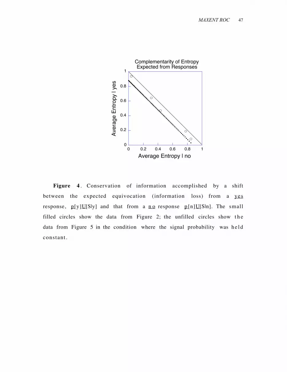
Figure 4 . Conservation of information accomplished by a shift
between the expected equivocation (information loss) from a yes
response, p[y]U[S|y] and that from a n o response p [n]U[S|n]. The small
filled circles show the data from Figure 2; the unfilled circles show t h e
data from Figure 5 in the condition where the signal probability was h e l d
constant .
0
0.2
0.4
0.6
0.8
1
0 0.2 0.4 0.6 0.8 1
Ave
rage
Ent
ropy
| ye
s
Average Entropy | no
Complementarity of EntropyExpected from Responses

MAXENT ROC 48
Figure 5 . Data reported by Green and Swets for an observer b iased
by varying the signal presentation probability (squares; their Figure 4-1)
and by varying the payoffs (circles; their Figure 4-2). The curve is t h e
isoinformation ROC, which is not visually discriminable from that fo r
constant A’ (also drawn through the points) .
0
0.2
0.4
0.6
0.8
1
0 0.2 0.4 0.6 0.8 1
p(H
)
p(F)
T = 0.05
IsoinformationROC
Green & Swets (1966)
MAXENT ROC 49
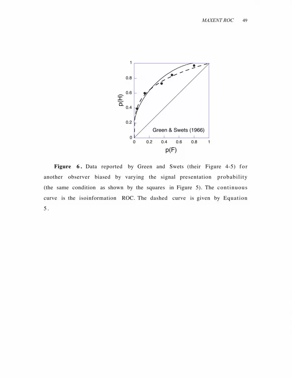
Figure 6 . Data reported by Green and Swets (their Figure 4-5) fo r
another observer biased by varying the signal presentation probabil i ty
(the same condition as shown by the squares in Figure 5). The cont inuous
curve is the isoinformation ROC. The dashed curve is given by Equation
5 .
0
0.2
0.4
0.6
0.8
1
0 0.2 0.4 0.6 0.8 1
p(H
)
p(F)
Green & Swets (1966)

MAXENT ROC 50
Figure 7 . Maxent exponential distributions of two random variables
on the positive line in the continuous case. The variable with the smaller
mean is called Noise, and the other Signal.
Signal
0 5 10 15 20 25 30
Stimulus
Pro
babi
lity
Noise

MAXENT ROC 51
Figure 8 . Data from 4 observers detecting brief flashes of light, f r o m
(Swets, Tanner & Birdsall, 1964). Performance was manipulated b y
varying the payoff matrices.
0
0.2
0.4
0.6
0.8
1
0 0.2 0.4 0.6 0.8 1
p(H
)
p(F)
2
0
0.2
0.4
0.6
0.8
1
0 0.2 0.4 0.6 0.8 1
p(H
)
p(F)
1
0
0.2
0.4
0.6
0.8
1
0 0.2 0.4 0.6 0.8 1
p(H
)
p(F)
3
0
0.2
0.4
0.6
0.8
1
0 0.2 0.4 0.6 0.8 1
p(H
)
p(F)
4
Swets, Tanner & Birdsall (1964)

MAXENT ROC 52
Figure 9 . Data from one observer detecting brief increments in t h e
intensity of tones (Norman, 1963). Each panel shows the data for a
different signal-to-noise ratio. Bias was varied with differential payoffs.
0
0.2
0.4
0.6
0.8
1
0 0.2 0.4 0.6 0.8 1
p(H
)
p(F)
A: ∆v/v = 0.017 0
0.2
0.4
0.6
0.8
1
0 0.2 0.4 0.6 0.8 1
p(H
)
p(F)
B: ∆v/v = 0.019
0
0.2
0.4
0.6
0.8
1
0 0.2 0.4 0.6 0.8 1
p(H
)
p(F)
C: ∆v/v = 0.022 0
0.2
0.4
0.6
0.8
1
0 0.2 0.4 0.6 0.8 1
p(H
)
p(F)
D: ∆v/v = 0.023
0
0.2
0.4
0.6
0.8
1
0 0.2 0.4 0.6 0.8 1
p(H
)
p(F)
E: ∆v/v = 0.0290
0.2
0.4
0.6
0.8
1
0 0.2 0.4 0.6 0.8 1
p(H
)
p(F)
F: ∆v/v = 0.033
Norman (1963)

MAXENT ROC 53
Figure 1 0 . The equivalence of the indices of merit for logistic SDT
and power ROCs. The x-axis is the parameter β.
0
1
2
3
4
5
6
0 1 2 3 4 5 6
Two indices of meritcompared
2*ln
[H/(
1-H
)] ≈
d'2
log2(S/N)

MAXENT ROC 54
Figure 1 1 . Beta, the ratio of the exponential means inferred f r o m
power functions fit to the data of 2 observers, versus the relative
increment in signal voltage associated with them. Data from (Norman,
1 9 6 3 ).
1
10
1.02 1.03 1.04 1.05
Parameter of IOCsas a Function of
Relative Signal Amplitude
µ S/µ
N
(∆v+v)/v

MAXENT ROC 55
Figure 1 2 . Rating scale operating characteristics. The inset shows
the parameter of the power function against the signal-to-noise ratio i n
dB. Each datum along a curve is obtained by re-aggregating the d a t a
around successive ratings, as though different ratings corresponded t o
different criteria.
0
0.2
0.4
0.6
0.8
1
0 0.2 0.4 0.6 0.8 1
p(r|
S)
p(r|N)
Emmerich (1968)
1
10
6 8 10 12
µ S/µ
N
10 log(E/N0)

MAXENT ROC 56
Figure 1 3 . The entropy of stimuli such as an encyclopedia or a
medica l measurement may be indefini tely large. Information
transmission is limited by the variable with the smallest entropy. This
may be the stimulus, the experimenter or the observer. If t h e
experimenter imposes a binary classification, the maximum informat ion
that may transmitted between observer and experimenter is 1 bit, even
though the observer may be able to make finer discriminations.

MAXENT ROC 57
Figure 1 4. Digitization loss increases with the relative entropy of t h e
signal. C is channel capacity for a continuous Gaussian signal, and w h e n
encoding is restricted to binary signals; W is the bandwidth of t h e
signal, and S/ N is the signal-to-noise ratio. Reprinted from (Harmon,1 9 6 3 ), with permission.


