Embed Size (px)
Citation preview

Measurement of the Charged-Hadron Multiplicity in
Proton-Proton Collisions at LHC with the CMS Detector
by
Yen-Jie Lee
M.S., National Taiwan University (2004)
Submitted to the Department of Physicsin partial fulfillment of the requirements for the degree of
Doctor of Philosophy
at the
MASSACHUSETTS INSTITUTE OF TECHNOLOGY
© Massachusetts Institute
MASSAOHK
Lu' RA R I ES~
ARCHIVES
April 2011
of Technology 2011. All rights reserved.
Author ........................... ..Department of Physics
April 30th, 2011
Certified by ...............Wit Busza
Francis Friedman Professor of Physics
, Thesis Supervisor
Accepted by ............' Krishna Rajagopal
Associate Department Head for Education

Measurement of the Charged-Hadron Multiplicity in Proton-Proton
Collisions at LHC with the CMS Detector
by
Yen-Jie Lee
Submitted to the Department of Physicson April 30th, 2011, in partial fulfillment of the
requirements for the degree ofDoctor of Philosophy
Abstract
Charged-hadron pseudorapidity densities and multiplicity distributions in proton-proton collisions at s= 0.9, 2.36, 7.0 TeV were measured with the inner tracking sys-tem of the CMS detector at the LHC. The charged-hadron yield was obtained by count-ing the number of hit-pairs (tracklets). The charged-particle multiplicity per unit ofpseudorapidity dNch/dr7 II ||<0.5 at s = 7.0 TeV is 5.78 i 0.01(stat.) i 0.23(syst.) for non-single-diffractive events, higher than predicted by commonly used models. The relativeincrease in charged-particle multiplicity from js = 0.9 to 7 TeV is 66.1% ± 1.0%(stat.) ±4.2%(syst.) and strong KNO violation is observed in the multiplicity distributions. Re-sults are compared with low energy measurements.
Thesis Supervisor: Wit Busza
Title: Francis Friedman Professor of Physics


Contents
1. Introduction 15
1.1. The Standard M odel ........................................ 16
1.2. p+ p collisions ............................................ . 19
1.2.1. Physics picture of p+p collisions .......................... 19
1.3. Experim ental observables .................................... 20
1.3.1. Particle production processes ............................ 21
1.4. Theoretical concepts related to p+p collisions ..................... .23
1.4.1. Fermi-Landau M odel .................................. 23
1.4.2. Feynm an Scaling ..................................... 25
1.4.3. Limiting fragmentation ................................ 27
1.4.4. Koba-Nielsen-Olesen (KNO) Scaling ....................... .29
1.4.5. Negative binomial distributions .......................... 30
1.4.6. Saturation m odel ..................................... 34
1.5. Event Generators .......................................... 35
1.5.1. The PYTHIA Generator ................................. 36
1.5.2. The PHOJET Generator ................................ 38
2. Previous Measurements 39
2.1. Experim ents .............................................. 39
2.1.1. Cosmic ray experiments ................................ 39
2.1.2. Experiments at the National Accelerator Laboratory (NAL) ....... .39
2.1.3. Experiments at the Intersecting Storage Rings ...... .......... .40
2.1.4. Experiments at the SppS ................................ 41
2.1.5. Experiments at the Tevatron ............................. 42
2.1.6. Experiments at the Relativistic Heavy Ion Collider ............. .43
2.2. dNch/dr7 distributions ...................................... 46
2.2.1. Fragm entation region .................................. 46

2.2.2. Energy dependence of the pseudorapidity density at the mid-
rapidity ............................................ 48
2.2.3. Comparison between data and PHOJET .................... 49
2.3. M ultiplicity distributions ..................................... 53
2.3.1. Validity of KNO scaling ................................. 53
3. The Large Hadron Collider 57
3.1. Design and Layout of LHC .................................... 57
3.2. Experiments at the LHC ..................................... .58
3.3. Startup .................................................. 59
4. The CMS detector 61
4.1. CM S design concept ........................................ 61
4.2. M agnet ................................................. 62
4.3. Inner tracking system ....................................... 63
4.3.1. Pixel tracker ......................................... 64
4.3.2. Silicon Strip tracker(SST) ............................... .64
4.4. M uon system ............................................. 65
4.5. Electromagnetic calorimeter .................................. 66
4.6. Hadron calorim eter ........................................ 67
4.7. Beam monitoring system .................................... 68
4.7.1. Beam Pick-up Timing for the eXperiments (BPTX) ............. .68
4.7.2. Beam Scintillator Counters (BSC) ......................... .69
4.8. Trigger system ............................................ 70
4.8.1. Level 1 Trigger ....................................... 71
4.8.2. High Level Trigger .................................... 71
4.8.3. Triggers used at the startup .............................. 73
4.9. Sim ulations .............................................. 74
5. Event selection 77
5.1. Online Trigger ............................................ 77
5.2. Event Vertex Reconstruction .................................. 78
5.2.1. Cluster Vertex reconstruction ............................ 78
5.2.2. Tracklet Vertex reconstruction ........................... .80
5.2.3. Agglomerative Vertex reconstruction ....................... 81
5.3. Perform ance .............................................. 82

5.4. Event Selection ............................................
5.4.1. Selecting Collision Events ...............................
5.4.2. Rejecting beam halo events .............................
5.4.3. Rejecting high occupancy events .........................
5.5. Trigger and selection efficiency studies ..........................
5.5.1. Event selection efficiency ...............................
5.5.2. MC event selection efficiencies ...........................
6. Pseudorapidity distribution measurement
6.1. Tracklet m ethod ...........................................
6.1.1. Tracklet reconstruction .................................
6.1.2. Event M ultiplicity .....................................
6.1.3. Combinatorial background subtraction .....................
6.1.4. Efficiency and Acceptance Correction ......................
6.2. dN /d rl study .............................................
6.3. Results ................................................
6.4. System atic Uncertainties .....................................
6.4.1. Systematic error of the trigger efficiency ....................
6.4.2. Systematic uncertainties from algorithmic efficiency correction ...
6.4.3. Systematic uncertainties due to the extrapolation to low PT ......
6.4.4. Systematic uncertainties due to vertex resolution .............
6.4.5. Systematic uncertainties from MC efficiency correction and single
diffractive fraction ........... . . . . . . . . . . . . . . . . . . . . . . . . . 111
Systematic uncertainties due to the tracklet selection .......... .111
Systematic uncertainties from secondary contribution ......... .111
Systematic uncertainties from misalignment ................. 112
Systematic uncertainties from low Pr loopers, beam halo and
event pile-up ........................................ 112
Systematic uncertainties from pixel hit reconstruction .......... 112
Cross-checks from magnetic field off sample ................. 112
7. Multiplicity distribution measurement7.1. Raw spectrum reconstruction .......................
7.2. Correction of detection effects .......................
7.2.1. General concept of unfolding problem ...........
7.2.2. Bayes' Theorem ............................
115
.......... 116
.......... 116
.......... 116
.......... 118
83
83
84
84
90
91
92
95
95
97
98
99
101
103
106
107
107
108
110
111
6.4.6.
6.4.7.
6.4.8.
6.4.9.
6.4.10.
6.4.11.

7.2.3. Unfolding procedure .................................
7.3. Multiplicity distribution measurement .........................
7.4. System atic Check .........................................
7.4.1. Uncertainty due to the algorithmic efficiency and acceptance cor-
rections ...........................................
7.4.2. Uncertainty due to the unfolding procedure ................
7.4.3. Uncertainty due to the event selection and SD fraction correction
Cross-checks between different layers ............
Cross-checks between magnetic field on / off sample
Uncertainty due to event pile-up................
.......... 122
.......... 122
.......... 122
8. Results 1298.1. Comparison between different methods ......................... 129
8.1.1. Pseudorapidity distributions ............................. 129
8.1.2. Multiplicity distributions ............................... 130
8.2. Comparison with other experiments ............................ 132
8.2.1. Results from other LHC experiments ....................... 132
8.2.2. Comparison between experiments ........................ 134
8.3. D iscussions .............................................. 134
8.3.1. dNch/drl structure and the central platau ................... 134
8.3.2. vlf dependence ...................................... 135
8.3.3. Limiting fragmentation and extended longitudinal scaling ....
8.3.4. KN O violation ....................................
8.3.5. Comparison with event generators .....................
9. Conclusion
A. Kinematic Variables
A. 1. The CMS coordinate system ...............................
A.2. M om entum ...........................................
A.3. Four-m om entum .......................................
A.4. M andelstam variables ....................................
A.5. Rapidity and Pseudorapidity ...............................
B. Negative binomial distribution
. . . 137
... 137
... 139
145
149
... 149
. . . 149
... 149
... 150
... 151
153
C. Pomeron and Reggeon
7.4.4.
7.4.5.
7.4.6.
119
120
120
120
121
121
155

C.1. S-Matrix and optical theorem ................................. 155
C.2. Reggeon and Pomeron ...................................... 156
D. BSC MIP Efficiency Measurement 159D.1. Circulating beam sample .................................... 159
D.2. M IP efficiency ............................................ 160
E. List of Acronyms 163
Bibliography 165

OutlineOn 20 Nov 2009, the Large Hadron Collider (LHC) [1], the world's largest particle ac-
celerator, successfully delivered the first p+p collision at s= 900 GeV. In 2010, the LHC
also delivered collisions at 2.36 TeV and 7.0 TeV, which were the highest energy collisions
ever achieved by any particle accelerator and opened a new era of high energy physics
research. The LHC was designed to deliver high energy p+p and Pb+Pb collisions to
cover a very wide range of research topics, from the discovery of the Higgs boson, or
super-symmetric particles, to the studies of the quark-gluon plasma.
In my field, the medium created in Pb+Pb collisions is particularly interesting. In
order to understand the Pb+Pb collisions, it is crucial to understand the particle pro-
duction in p+p collisions, such as the angular distribution of the produced particles, av-
erage abundance, and event-by-event multiplicity distributions. These measurements
provide an essential reference for Pb+Pb collisions in order to study the properties of
the quark-gluon plasma. It is also crucial to understand the bulk of the particle produc-
tion in the case of p+p collisions in order to discover new phenomena. p+p collisions
are primarily governed by the soft processes, which involve non-perturbative QCD and
can only be modeled phenomenologically. Therefore the studies of the particle produc-
tion not only provide valuable background knowledge to the new discoveries, but also
are intriguing in themselves and provide crucial guidance to the commonly used event
generators and analytical models.
In this thesis, two studies of the particle production in p+p collisions with the Com-
pact Muon Solenoid (CMS) experiment [2] are described. The first is the study of the
pseudorapidity distribution of charged particles (dNch/dr ). It involves the measure-
ment of the average abundance of particles produced in different emission angles, and
can be performed in the early stage of the experiment. Although this measurement
averages over different events and different processes, it can already provide good sep-
aration between models. The second is the study of the event-by-event multiplicity,
which gives information about the fluctuation in the particle production process and
provides more details about the particle production mechanism. The analyses in both
studies are based on the tracklet method (hit-pairs in the CMS pixel detector), which is a
proven technique from the PHOBOS experiment [3]. The technique developed and im-
proved in this thesis was applied to the first collision data and led to the first publication
of the CMS experiment.
The increase of the pseudorapidity particle density from 0.9 to 2.36 (to 7.0) TeV is
found to be much larger than the predictions from the commonly used event generators

and models. This means that the energy dependence of the predictions from multiple
parton interaction models are not accurate. Modifications and tunings are necessary.
The pseudorapidity distribution measurement also provides crucial information during
the detector commissioning phase because the occupancy and the distribution of the
particles which pass through the detector is the starting point in the understanding of
all data.
The outline of this thesis is the following: Chapter 1 gives the theoretical framework,
related to the understanding of particle production in p+p collisions. A review of the
dNch/dr and multiplicity distribution measurements performed in previous experi-
ments is compiled in the Chapter 2. Chapter 3 and 4 give an introduction to the LHC and
the CMS detector. Chapter 5 discusses the event triggering and selection. The tracklet
reconstruction and pseudorapidity distribution measurement are described in Chapter
6. Chapter 7 extends the application of the tracklet analysis technique to the multiplicity
distribution measurement, and the systematic uncertainty studies. In the last chapter,
the results from the p+p collision studies at v/s = 0.9, 2.36 and 7.0 TeV are summarized
and discussed.


1. Introduction
As mentioned in the outline, the main goal of this thesis is to provide a useful p+p ref-
erence for the study of the Pb+Pb collisions. The lead ions contain 208 nucleons and
the first step of the Pb+Pb collisions involve many nucleon-nucleon scatterings. Since
so many collisions happen at the same time in a small space, they create a medium
with extremely high energy density and may lead to the state known as the quark-gluon
plasma, consisting of deconfined quarks and gluons. However, the nucleon-nucleon
scattering is not simple itself. The nucleons are extended objects which contain struc-
ture. Moreover, the scattering involves the soft processes, which cannot (yet) be calcu-
lated reliably from first principles. The description of the soft processes has to rely on
phenomenological models.
In order to understand the first steps of Pb+Pb collisions, it is important to measure
the particle production in p+p collisions and provide inputs to the models. The results
in p+p can also be compared to Pb+Pb collisions to study the property of the produced
medium. Furthermore studies of particle production in p+p collision are interesting in
themselves. They can be used to improve our understanding of soft processes and the
incalculable part of the hadronic interaction. In this thesis, the pseudorapidity den-
sity and charged hadron multiplicity distributions are measured and discussed. The
pseudorapidity density contains the space and time information of the particle pro-
duction, while the multiplicity distributions give information about fluctuations and
correlations.
This chapter briefly discusses theoretical and experimental concepts which are re-
lated to the multi-particle production in p+p collisions. The chapter begins with an
introduction to the building blocks of matter and the Standard Model which describes
the interactions between the elementary particles.
Since the proton is a complicated system, the inelastic collision events can be classi-
fied into several event classes, such as diffractive and non-diffractive events. The event
classification of the p+p collisions will be introduced, and the connection to the physi-
cal picture will be described. The theoretical and phenomenological description of the
1. Introduction
multiplicity distributions and charged hadron spectra will also be discussed.
Experimentally, simulations of the detector response to the p+p collision rely on
event generators. An introduction to the common used generators, PHOJET [4, 5] and
PYTHIA [6], for event simulation will be presented. Calculations and predictions at LHC
energies from these generators will also be presented. In Chapter. 8, they are compared
with the experimental results presented in this thesis.
1.1. The Standard Model
What are the building blocks of matter? How do they interact with each other? These are
the questions that drive the development of science. There are four known interactions
in nature: the gravitational force which is responsible for the falling of apples; the elec-
tromagnetic force which enables us to touch and to grab objects around us; the strong
force which is the source of the nuclear power, and is responsible for the interaction
between the hadrons; finally the weak force which governs the transitions from one
quark flavor to another and the interaction between neutrinos and other elementary
particles. The Standard Model is so far the most successful gauge theory that describes
the interaction between fundamental particles, including electromagnetic, weak and
strong interactions. Gravitational force is not yet integrated in the Standard Model.
In the Standard Model, the building blocks of matter are point-like particles, which
carry a spin of 1/2. They are usually grouped into three families; each family consists of
two leptons and two quarks. The properties of these elementary particles are summa-
rized in Table. 1.1. For each particle, there is an associated antiparticle with the same
mass but opposite quantum numbers. Leptons participate in weak and electromag-
netic (if it carries electromagnetic charge) interactions. Quarks carry "color charges",
which means that quarks also participate in the strong interaction. Color charges are
the strong interaction version of charges, which have no relation to the real colors of
daily life. There are three color charges, usually denoted by blue (B), red (R) and green
(G). Experimentally, all particle states observed in nature are "colorless" or " white". This
is called the color confinement. The quarks cannot appear freely and have to group to-
gether in the form of hadrons, which are colorless. Hadrons observed in the lab can
be classified into baryons and mesons. Baryons consist of three quarks (qqq), or three
anti-quarks (4q4). The colors of the quarks inside a baryon are RGB (R+G+B=white),
which satisfies the requirement of color confinement. Mesons consist of a quark and ananti-quark (qq). The colors of the quarks inside a meson are B5, GC and RR (The sum

1.1. The Standard Model
of the color and anti-color is white).
The interactions between particles are mediated by gauge bosons. The photons are
responsible for the electromagnetic interaction between charged particles, which is
formulated as Quantum Electrodynamics (QED). The weak interactions, mediated by
th W* and Z0 bosons, are described by the electroweak theory. The strong force be-
tween hadrons is mediated by gluons, which is described by Quantum Chromodynam-
ics (QCD). The forces and the mediators are summarized in Table. 1.2. The coupling
constants of the weak and electromagnetic forces are small, and enabled the application
of the perturbation techniques to perform accurate calculations. However, in the case
of strong interaction, the coupling constant in soft processes (low momentum trans-
fer) is large such that calculation based on perturbation theory is not reliable. Since
the direct calculation can not (yet) be carried out, the studies of the general property
of hadron-hadron collision, such as p+p collisions, are of fundamental importance and
provide necessary guidance to the development of the theoretical models.

Table 1.1.: The properties of the quarks and leptons. [7]
Strong Electromagnetic Weak Gravitational
Mediator Gluon (g) Photon (r) WA,Z GravitonSpin-Parity 1- 1- 1-, 1+ 2+
Range [m] < 10-15 0o 10-18 00Relative Strength 1 10-2 10-13 10-38
Table 1.2.: The fundamental force carriers and properties.
Generation Quarks Leptons
Name Symbol Charge Mass Name Symbol Charge Mass
First Up u +2/3 1.5 - 4.5 MeV Electron e- -1 0.511 MeVDown d -1/3 5.0 - 8.5 MeV Electron neutrino Ve 0 < 2 x 10⁻⁶ MeV
Second Charm c +2/3 1.0 - 1.4 GeV Muon P- -1 105.7 MeVStrange s -1/3 80 - 155 MeV Muon neutrino vp 0 < 0.19 MeV
Third Top t +2/3 174.3 5.1 GeV Tau T - -1 1777 MeVBottom b -1/3 4.0 - 4.5 MeV Tau neutrino vT 0 < 18.2 MeV

1.2. p+p collisions
1.2. p+p collisions
1.2.1. Physics picture of p+p collisions
Figure 1.1.: Schematic view of the proton in the parton model.
From e+p scattering [8, 9], we know that protons are extended objects. In the study
of the p+p scattering, the structure of the proton should be taken into account. In
the framework of the parton model, the constituents of the proton, when it is probed
by a hard scattering at virtuality scale Q2, can be described by the structure function
(F(x, Q2), x is the momentum fraction of the parton). The structure function of the pro-
ton is determined by fits to e+p and p+p collision data. From this point of view, the
p+p collisions are actually interactions between two bags of partons. Assuming the fac-
torization of the proton structure holds, the 2 -42 differential cross-sections of the p+p
scattering can be written in the following form:
do-i- diri-d dx1f dx2Fi(x 1,Q2)F jx 2,Q2) Rdt -j Xjdt(1)
where t is one of the the Mandelstem variable which describes the interaction in-
volving the exchange of an intermediate particle through t-channel with squared four-
momentum t. The definition of t can be found in Section. A.4, i, j are the index of
the parton species (quarks and gluons) and r is the cross-section from matrix element
calculations. However, this is not the whole story. The first problem of this equation
is that the differential cross-section diverges in the t --> 0 limit, and regularization is
needed. Secondly, the scattered partons have to be translated to hadron level to be

1. Introduction
compared with the experimental results. This involves branching / showering (splitting
of the partons) and hadonization (picking up another parton to make a final state par-
ticle which is colorless). However, the hadronization process of the scattered partons is
not yet understood from the first principle and can only be modeled phenomenologi-
cally. Moreover, in the high-energy p+p collisions, the initial momenta of the protons
are high enough such that many partonic interactions can occur in one collision, which
makes the picture even more complicated. The high-energy collisions also involved the
interactions between low x partons (x < 10-4) where the uncertainty of the structure
function is large from the current knowledge of the collision data.
Apart from some theoretical insights that describe the general properties of the col-
lisions, there is no straightforward analytical calculation, starting from first principles,
which can give a complete description of the p+p collision. Practically, the description
of the particle production relies on the Monte Carlo generator based on factorization
and phenomenological models. A further discussion of event generators will be given
in Sec. 1.5. Based on these reasons, the measurements of the charged particle produc-
tion will be important tests on the physics picture we have and provides useful guidence
to the model building.
1.3. Experimental observables
In the study of the particle production in p+p collisions, the abundance of the charged
particles and their angular distributions are the simplest observables. The coordinate
system and kinematic variables are summarized in Appendix. A. Instead of the angle
(0), the rapidity y is a better variable because it is an additive quantity in the Lorentz
transformation (relativistic version of velocity). However, it is difficult to measure the
energy (or the mass) of each charged particle in the experiment. The pseudorapidity
(q) is usually used to characterize the emission angle of the charged particles because
it is closely related to rapidity (y). To justify this, the dNch/dy and dNch/dr) from
PYTHIA generator are plotted together and shown in Fig. 1.2. A short introduction to
the PYTHIA generator is given in Sec. 1.5.1. There is a dip at mid-rapidity, which is due
to the Jacobian transformation from rapidity to pseudorapidity This transformation
also widens the distribution. The generated dNch/dri |1,i1o is roughly 16%(18%) lower
than the dNch/dy |y|~o at ls = 53 (7000) GeV and the ratio of the two distributions at
mid-rapidity (IrI < 1.0) is only weakly dependent on the collisional energy.
The pseudorapidity density (dNch/dr ) is an averaged quantity over all kinds of dif-

1.3. Experimental observables
-3 2.5. - I . --: :. .I. .1 1. .I 11 . --:; 5 'I
PYTHIA 53 GOV
z dN/dy 2.5 z
-2
Z 15 3
1.5 -
1 -2
0.5 -pyTA 0.2ev 1 PYTHIA 7 TeV050.5 - dNdri dNdY
-- dN/dy -dNldy
10 -2 0 2 4 6 8 10 -10 -8 -6 -4 -2 0 2 4 6 10 910 8 -6 -4 -2 0-2 4 6 8 10
f (y) l (Y) M(Y)
Figure 1.2.: The comparison between dNch/dr) and dNch/dy from PYTHIA D6TTune [10] at i = 53, 200 and 7000 GeV.
ferent events created in the p+p collisions. It shows the averaged event shape of the
collisions. The pseudorapidity density at I ~ 0 increases as a function of v/~ and can
be described by a 1 (or 2) degree polynomial of logs. Sudden changes in the trend may
indicate new phenomena in low PT particle production.
The distribution of the event-by-event multiplicity Neh characterizes the fluctuation
of the charged hadron abundance. The multiplicity distribution P(Neh) characterizes
the amount of correlation in the particle production. If there is no correlation between
the creations of final-state charged hadrons, the distribution is Poissonian. A wider dis-
tribution implies positive correlations.
1.3.1. Particle production processes
The bulk of the particle production in p+p collisions arises from the soft interactions,
which contains elastic and inelastic scatterings. The elastic scattering involves the ex-
change of virtual mesons or virtual photons. Experimentally, due to the small momen-
tum transfer and high beam energy, the scattered proton usually passes through the
very forward region of the detector and is undetected. In this thesis, the elastic pro-
cesses are not further discussed.
The soft inelastic interactions are typically classified into diffractive processes and
non-diffractive scattering. In Good and Walker's picture [11], one can expand the initial-
state proton in terms of a complete set of states. During the proton-proton scattering,
the large number of states of the projectile is absorbed by the target and diffractively
dissociates into a collection of particles. This diffractive system has the same intrinsic
quantum numbers as the original proton, i.e. the same charge, isospin, baryon number

1. Introduction
Single-Diffractive Dissociation Double-Diffractive Dissociation
Diffractive System
p p
Pomeron Pomeron {
p pDiffractive System Diffractive System
Figure 1.3.: The schematic view of single-diffractive dissociation (SD) and double-diffractive dissociation (DD).
and etc. The target receives a small momentum transfer from the projectile proton andremain unchanged, as shown in Fig. 1.3. Between the diffractive system and the target alarge gap in rapidity is created and devoid of particles. This is called a single-diffractive(SD) collision. In some cases, both of the protons are turned into diffractive systemsas shown in Fig. 1.3. This is called the double-diffractive dissociation (DD). In the non-diffractive (ND) collisions, there are parton-parton interactions with larger momentumtransfer as well as the exchange of quantum numbers. No diffractive systems are cre-ated. Usually, non-diffractive collisions create more particles and lack rapidity gaps.
Fig. 1.4 shows the charged hadron pseudorapidity distributions of those processes at7 TeV predicted by PYTHIA [6] and PHOJET [4, 5]. Short descriptions of these generatorsare in Section. 1.5. The single-diffractive distribution features an asymmetric pseudo-rapidity distribution, which has a peak around the initial pseudorapidity of the protonbeam and the contributions of the particles emitted from the diffractive system. Usu-ally, the emitted particles only appear on one side of the detector and a requirement ofcoincident in both side of the detector will lead to suppression of the single diffractivecomponent. The double-diffractive distribution is more symmetric and has a dip in themid-rapidity. The non-diffractive distribution has many particles produced in the mid-rapidity and the density decreases in the high pseudorapidity region. The PYTHIA and

1.4. Theoretical concepts related to p+p collisions
P YTHIA D6T 7 TeV SD PYTHIA D6T 7 TeV DD PYTHIA D6T 7 TeV ND5 PHOJET 7 TeV SD 5 PHOJET 7 TeV DD 5 PHOJET 7 TeV ND
4- 4 4
3 -3 37-
2 22 j
000-10 -5 0 5 10 -10 -5 0 5 10 -10 -5 0 5 10
Tj (SD) T (DD) a (ND)
Figure 1.4.: The dN/dr distributions from single-diffractive (SD), double-diffractive(DD), and non-diffractive (ND) processes generated by PYTHIA and PHO-JET generator. The parameter used in PYTHIA is the D6T tune [10].
PHOJET gives quite different predictions on the properties of the diffractive processes,including the diffractive fractions and average multiplicity.
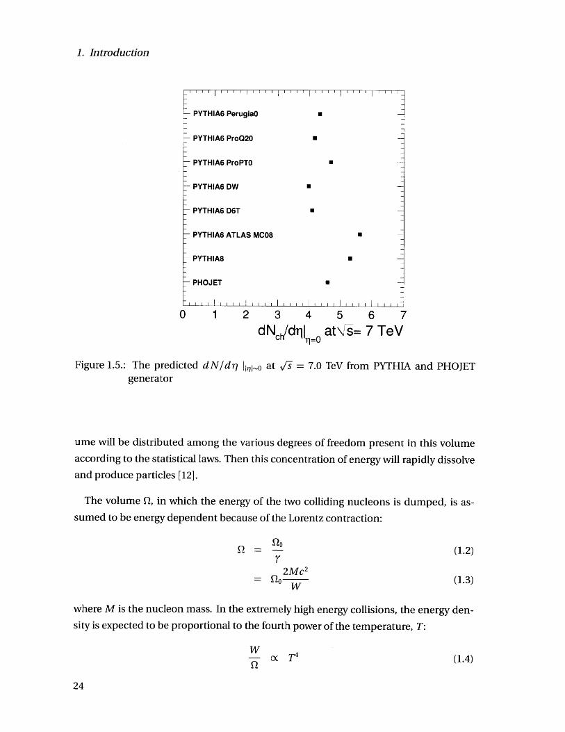
Although these generators are tuned with the data from low energy measurements,the uncertainty of the dNch/d r due to the parameters used in the generator is still large.Fig. 1.5 shows the predictions from different parameter tunes and generators. The pre-dicted dNch/drl ,0 is 3.5 - 5.6. The measurement from LHC will be able to eliminatethe unsuitable tunes.
In this thesis, we present the results from the inelastic non-single-diffractive (NSD)interactions, which are based on an event selection that retains a large fraction of theND and DD events, while SD processes are suppressed.
1.4. Theoretical concepts related to p+p collisions
1.4.1. Fermi-Landau Model
In 1950, Fermi and Landau proposed a statistical way for the description of high energycollisions of hadrons [12, 13]. The main assumption is that the interactions betweenthe hadrons are so strong such that the incident hadrons stopped each other. All theenergy carried by the hadrons are deposited in a small volume and produce a fireball. Astatistical equilibrium is reached during the collision.
When two nucleons collide with very high energy in their centre-of-mass frame, thisenergy will suddenly be released in a small volume surrounding the two nucleons. Sincethe interactions of the pion field are strong, the energy W which is deposit in this vol-
1. Introduction
PYTHIA6 PerugiaO U
PYTHIA6 Pro020 -
PYTHIA6 ProPTO
PYTHIA6 DW
PYTHIA6 D6T
PYTHIA6 ATLAS MC08
PYTHIA8 -
PHOJET
0 1 2 3 4 5 6 7
dNch/dnl at\ s= 7 TeV
Figure 1.5.: The predicted dN/drj 11,i-O at Vs = 7.0 TeV from PYTHIA and PHOJETgenerator
ume will be distributed among the various degrees of freedom present in this volumeaccording to the statistical laws. Then this concentration of energy will rapidly dissolveand produce particles [12].
The volume Q, in which the energy of the two colliding nucleons is dumped, is as-sumed to be energy dependent because of the Lorentz contraction:
Q = -- (1.2)r2Mc 2
=Qo W (1.3)
where M is the nucleon mass. In the extremely high energy collisions, the energy den-sity is expected to be proportional to the fourth power of the temperature, T:
W-- - c T4(1.4)

1.4. Theoretical concepts related topp+p collisions
From Eq. 1.2 we have:
W W2 2
- oc T4 (1.5)Q 2MC 2QO
Woc T2 (1.6)
According to the standard calculation of statistical mechanics, the density of the parti-
cles turns out to be proportional to the third power of the temperature:
n oc T3 (1.7)
From Eq. 1.5 and Eq. 1.7, the number of particles produced is
N = nxQ (1.8)
X Wi/ 2 (1.9)
This means that the total number of particles produced in the collisions will be propor-
tional to Wi/ 2 (or s1/ 4).
Fermi-Landau's picture is an extreme case which assumes that the interaction be-
tween the two proton is so strong such that a thermalized state is created. However, it is
found experimentally that the particle abundance is actually growing slower than this
power law (Eq. 1.9). The transverse momentum distribution is found to be much nar-
rower than the longitudinal momentum distribution which suggests that the interac-
tion between the protons is weak. These experimental results imply that the interaction
between two protons is not strong enough to create a fully thermalized system.
1.4.2. Feynman Scaling
In 1969, Feynman predicted the character of the hadron production in very high-energy
collisions of hadrons [14] from phenomenological arguments. The conclusion was that
the total number of particles created in the collision rises logarithmically with [s.
(N) oc ln v/s oc ln W (1.10)
where W = v/s/2, which is the total energy of the incoming particle in the center-of-
mass frame. He suggested that the ratio of longitudinal momentum pz to the total avail-
able W (x = p,/W) and the transverse momenta PT are the appropriate variables to use

1. Introduction
for the various outgoing particles in comparing experiments at various values of W in
the c.m. system.
Two-body interaction involved in the exchange of currents carry quantum numbers
such as the isospin. The fields, which are connected to those currents, are expected to
radiate and produce particles (analogous to bremsstrahlung). In the limit of W -> 00,
by Lorentz transformation, the fields to be radiated are becoming a 5 function in the z
direction. This means that the field energy is uniform in pz and the mean number of
particles of fixed PT is distributed as dpz/E for not too large x.
From the argument above, the probability of finding a particle
verse momentum PT and mass m can be expressed in this form:
P(PT, x) oc fi(PT, x) d 2PTE
of kind i with trans-
(R.11)
where
E = AV/m2+p2 +p2T =
= WJx2+ 2W
(1.12)
(1.13)
where mT = m 2 + p2. Since PT/E becomes dx/x in the large W limit, P(pT,x) be-
comes independent of W. The fi(pr,x) factorizes approximately (found experimen-
tally) and can be expressed as
fi(pr, x) = gipr)fi(x) (1.14)
with a normalization of gi chosen to be:
gi(pT)d 2pr = 1 (1.15)
The mean total number of particles produced is:

1.4. Theoretical concepts related top+p collisions
(Ni) = fi(pT,x)dp z d 2pT (1.16)
F' dx= fi(x) (1.17)
Feynman assumed that for XF = 0, a finite limit(C) is reached. Therefore:
dx (1 dxMf(x) < 2 C (1.18)
MT)2 x2±+(M)2
- 2Cln x+ x2+( )2 (1.19)
= 2C In 1+ l+(m) +lnMT (1.20)1 l+( Y) .
In the large W limit, (Ni) oc In W cx In -1s. Since the width of the rapidity distribution
is also a proportional to In 1K and assume that the produced particles are evenly dis-
tributed in rapidity, it follows that the dN/dy near the mid-rapidity is independent of
Ks as shown in Fig. 1.6.
In 1971, the first hadron collider, the Intersecting Storage Rings (ISR) commenced
operation, colliding p+p(P) at 1K= 30.4 to 62.2 GeV However, it was observed at ISR
energies that the pseudorapidity density at the mid-rapidity (r7 ~ 0) increased as a func-
tion of 1K and the results implied that the interaction between hadrons can not be ex-
plained by wee parton interactions. A review of the pseudorapidity density is given in
Section. 2.2.
Feyman's picture is another extreme case which assumes that the interaction between
partons are weak. Compared to Fermi-Landau model, this picture is closer to the ex-
perimental data. The missing ingredients are the contributions from gluon radiations
(which was not known at that time).
1.4.3. Limiting fragmentation
While Feynman scaling gave some insights to the particle production in the mid-
rapidity, the hypothesis of limiting fragmentation of the target and of the projectile is
proposed by Benecke et al. [11] which focuses on the fragmentation region. The authors
suggest the rest frame of the projectile (P) and of the target (L) give more insight for the

1. Introduction
increasing s
Figure 1.6.: Demonstration of the Feynman scaling of the inclusive particle productionA + B - X in the rest frame of B.
description of a collision. In the L system, the projectile passes through the target andturns the target into an excited state. The excited state then breaks into several pieces.This is quite similar to the picture which Good and Walker proposed in the diffractiveprocess. In the rest frame of the target, the projectile is highly relativistic. Due to thetime dilation, the fast components (the projectile) can't change. The only part whichstart to radiate particles is the slow components in the collision (the target). The dis-tributions of the broken-up fragments of the target reach a limiting distribution, basedon kinematical arguments. One obvious example is that the target proton is turned intoa A particle and emits a pion. Clearly, conservation laws limit the kinematic distribu-tion of the pion. The same discussions can apply to the projectile in the P system. Theparticles created in the pionization process that are slow in the centre-of-mass frame,which correspond to the particles produced in the mid-rapidity, do not contribute tothe limiting distributions. A schematic plot of the limiting fragmentation is shown inFig. 1.7.
The limiting fragmentation is observed in p+p(p+p) and heavy-ion collisions exper-imentally. The dN/drj distributions from different energies in the rest frame of thetarget line up in a common curve before reaching the central plateau. Moreover, it wasfirst observed in p+A collisions [15, 16] and later in Au+Au collisions [17] that this scal-ing continues to hold in a larger rapidity range (for instance, Fig. 1.8). The origin of thisscaling effect is not understood. It was later called "Extended Longitudinal Scaling" byMark Baker of the PHOBOS Collaboration [18].
The results of limiting fragmentation and extended longitudinal scaling in p+p (p+p)collisions are reviewed in Section. 2.2.1.

1.4. Theoretical concepts related top+p collisions
Target In the rest frameof tha tar et
Collision
Excited target Excited projectileMIM
1 li i -"
Fragments fromthe projectile
A"
Figure 1.7.: Demonstration of the limiting fragmentation of the inclusive particle pro-duction A + B -+ X in the rest frame of B.
1.4.4. Koba-Nielsen-Olesen (KNO) Scaling
Inspired by the Feynman scaling and early data, the KNO scaling was suggested by Koba,
Nielsen, and Olsen [19] for the description of the multiplicity distribution. They suggest
that if the multiplicity distribution is expressed in the variable z =Nh/ < Nch >, the
distribution '(z) =< Nch > P(z) is a universal function in the high energy limit.
Although the original assumption of Feynman scaling turned out to be wrong, KNO
scaling is found to hold at NAL and ISR energies [20-22] (See Section 2.3.1). In high-
energy collisions at SppS and Tevatron, the KNO scaling is found to be violated. Com-
parisons of the multiplicity distributions in KNO variable are reviewed in Section. 2.3
Projectile
g
..................................................... ...............................................................................

- a) 0-6% b) 0-6% c) 0-6% Au+Au -
200 GeV130 "
- e--____ 0 0
- JP0 0
0 0
800
600
Z 400
200
0200
0 2 4 6 8
+ybeam
e) 35-40%
- 0
I |I
10 -10 -8 -6 -4 -2
lybeam
0 2
I I II I I I~f) 35-40% PHOBOS-
- -0000 --
- e~~ --
- --
-4 -2 0 2
-91 ybeam
Figure 1.8.: Example of Extended Longitundinal scaling in the 0-6% and 35-40% cen-trality Au+Au collisions from the PHOBOS collaboration [17].
1.4.5. Negative binomial distributions
From the p+p collision data taken at the NAL [20], ISR [22] and SppS [24] energies, itis found that the charged particle multiplicity distributions in p+p collisions deviatesfrom the Poisson distribution. The widths of the distributions are larger than Pois-son distribution indicates positive correlation between charged particles. For instance,the decay of the unstable particles and the showering of the partons. Further analysesshow that the distributions can be described by a negative binomial distribution (NBD),which is defined as:
f(n)(k+n
-1 (1.21)
which gives the probability number of n fails in a sequence of independent Bernoullitrials before a specified number k success occurs. Further discussions of the negativebinomial distribution are given in Appendix. B. In the study of the charged hadron mul-tiplicity, the NBD is usually expressed as
1. Introduction
I I i I
- d) 35-40%
- 0 0
- 0
*.
I I I i 0
150
100
50
0-2
. i
*-
l

1.4. Theoretical concepts related to p+p collisions
z
10-2
10-3
10-4
10~5
' ' ' ' ' ' ' ' ' ' ' ' ' ' ' ' ' ' ' ' ' ' ' ' ' ' '', i '' . i, L i 1 0 ~65 10 15 20 25 30 35 40 C
NCh20 40 60 80 100 120
Nch
Figure 1.9.: The multiplicity distributions in the full phase space from the SFM exper-iment at the ISR [22] and the UA5 collaboration at SppS [23]. The distribu-tions are fit with a negative binomial distribution (NBD), a Poisson distribu-tion or two NBDs.
f(n)= (kn)F(n+1)F(k)
n "
(k
-n-k+ -) (1.22)
where the average multiplicity of the distribution is (h = k/p - 1). Fig. 1.9 shows thatthe NBD distribution describes the ISR data reasonable well, while the Poisson distri-bution doesn't describe the data.
Initial Parton Initial Parton
Branch Branch
------
Probability = p Recapture the virtual particles
Figure 1.10.: Schematic view of the parton evolution
z
10-2
10-3
10o-4
10~5' -0
0 pp UA5 NSD 546 GeV-....... Negative Binomial Distribution-------- Two Negative Binomial Distribution-
..... Poission Distribution
-
-------------------------------------- ------------------------------------- -------------------------------------------------------
---------------------------- --------
---------------------------
1. Introduction
Initial Parton Hadronize
BranchCollision
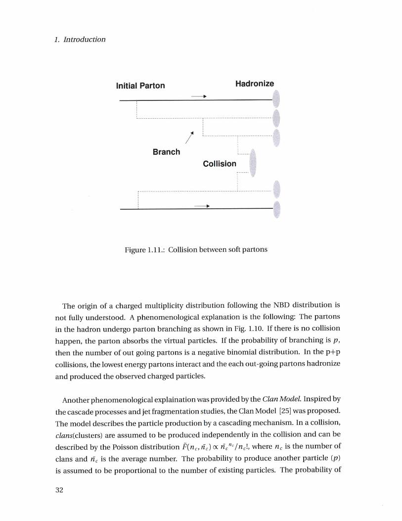
Figure 1.11.: Collision between soft partons
The origin of a charged multiplicity distribution following the NBD distribution is
not fully understood. A phenomenological explanation is the following: The partons
in the hadron undergo parton branching as shown in Fig. 1.10. If there is no collision
happen, the parton absorbs the virtual particles. If the probability of branching is p,
then the number of out going partons is a negative binomial distribution. In the p+p
collisions, the lowest energy partons interact and the each out-going partons hadronize
and produced the observed charged particles.
Another phenomenological explaination was provided by the Clan Model. Inspired by
the cascade processes and jet fragmentation studies, the Clan Model [25] was proposed.
The model describes the particle production by a cascading mechanism. In a collision,
clans(clusters) are assumed to be produced independently in the collision and can be
described by the Poisson distribution F(nc, ,e) oc tenc/nc!, where ne is the number of
clans and te is the average number. The probability to produce another particle (p)
is assumed to be proportional to the number of existing particles. The probability of
-------------------------------------

1.4. Theoretical concepts related to p+p collisions
producing Neh particles in a clan F(Neh) is characterized by the following relations:
F(O) = 0 (1.23)
(Nch +1)F(Nch +1) =p x NchF(Nh) (1.24)
Eq. 1.23 corresponds to the fact that a cluster contains at least one particle. F(Nh) can
be expressed as:
F(1)pNch-1F(Nch)= Nch (1.25)
Neh
And the multiplicity distribution is:
Nch
P(Nch)= F(x, dc)ZF(N)F(Nz ... F(Nx) (1.26)x=O
whereXE* denotes the sum over all partitions with Nch = n 1+n 2+...nx. It is shown in [25]
that Eq. 1.26 is a negative binominal distribution. The average number of particles per
clan hch and the average number of clans fic can be directly derived from the negative-
binomial parameters:
hch = /ln(1+ ) (1.27)k k
e= skln(1+ ) (1.28)
From the experiments at SppS collider, it is found that the multiplicity distribution
deviates from the NBD distribution [23]. Fig. 1.9 shows the measurement at /s = 546
GeV [23], there are additional structures found around the peak when the distribution
is compared with NBD fit. It is clear that a fit with two NBDs works much better in the
description of the high-energy collisions. Also in the fit of the lower energy data, the
two-components fit also works better. It has to be noted that each NBD distribution
describes one kind of event class or production mechanisms so that there is no inter-
ference between the two components. Fits with two NBDs can be performed without
constraints (as shown in the Fig. 1.9), or with constrains in the parameters which char-
acterize the soft and semi-hard components [26]. The soft component which doesn't
contain mini-jets follows the KNO scaling. The semi-hard component violates the KNO
scaling. Experimental efforts are also made for the investigation of the relative fraction
of the two different components [27].

1. Introduction
Another possible explanation to this deviation is the contribution from the multiple
parton interaction. The events with two parton-parton scatterings form another event
class which extend the tail part of the multiplicity distribution. This can also explain
why the deviation from a single NBD distribution increases as a function of collisional
energy because the probability of multiple parton interaction increases.
1.4.6. Saturation model
In the framework of parton model as described in Sec. 1.2.1, the proton are bags of
partons and the distributions of the partons are described by the parton distribution
function. The violation of the Feynman scaling shows the importance of the gluon con-
tribution in the low x region. To get the full description of the proton-proton collision,
one must include the lowest x partons in the picture.
At small x, by the uncertainty principle the interaction develops over large longitudi-
nal distance z - 1/(mx), where m is the nucleon mass [28]. When the x is sufficiently
small, z becomes larger than the nucleon diameter. The incident probe interacts with
all the partons within the transverse area ~1/Q2 determined by the momentum trans-
fer Q. Since the probe interacts with partons with cross-section o- as/Q 2, the number
of partons (N) is proportional to Q2:
S1N ~. S ~ Q2R2 (1.29)
o- as(Q2)
where S, is the transverse area of the nucleon SP ~ irR2 . The density of the parton is
given by:
p xF(xQ 2 ) (1.30),z R2
In case of up >> 1, we deal with a dense parton system. At very high gluon density, the
anniliation process of the gluons limits the growth of the gluon density and the number
of gluon is related to the geometry of the nucleon. The saturation scale Q2 which defines
the scale of the gluon saturation can be determined by the condition o-p ~ 1:
x F(x, Q2)Q2 ~ as (Q2) 2 (1.31)S S irR

1.5. Event Generators
Therefore the number of gluons is given by:
Q2xF(x,Q2 ) )~ c (1.32)x F~i" S as(Q2)
where c is a constant. Assuming the number of hadrons in the system is proportional
to the number of the scattered partons (detailed discussions can be found in [29]), we
get:
d Noc xF(x, Q) (1.33)
Q2Dc - S(1.34)
as(Q2)
From r*p scattering data at HERA, it is found that the saturation scale Q2 is propor-
tional to v/s [30-32], where A ~0.27 - 0.29 [32]. Therefore we get:
dN(vs) AsA/ 2
(1.35)d rl
It would be interesting to check if this parametrization describe the data and the ex-
tracted A parameter can be compared with the values obtained from the HERA data [33].
1.5. Event Generators
From the discussions in the last section, there are two important missing pieces which
are needed to explain the experimental results. (1) The inclusion of the gluon radiation
is necessary in order to explain the raising pseudorapidity density. (2) Implementation
of the multiple parton interaction models is necessary to explain the measured charged
hadron multiplicity fluctuations. Other than those missing elements, the discussions
and calculations usually stay in the parton level. The translation from partons to hadron
level is also needed in order to compare the theoretical prediction to the experimental
observables. Those complications make the calculation directly from first principles
difficult.
To describe the p+p collisions, Monte Carlo technique is usually used to generate
events with the best guess from models. The goal is to produce the events at the hadron
level as the input to the full detector simulation. This helps to understand the expected

1. Introduction
signal and possible background components in the collisions. The hard collisions in-
volve high momentum transfer can be described by perturbative QCD (pQCD). How-
ever, the majority of the events come from soft interactions in the minimum-bias events
triggered by the detector. The coupling constant as of the strong force is 0(1) in scat-
tering with low Q2 and the perturbation method is not valid. Usually, additional phe-
nomenological models are added to the generator for the description of the soft com-
ponent
Due to the color confinement, the out-going partons hadronize and produce color-
less final state particles. This transition is not yet understood from first principle calcu-
lations and has to be described by phenomenological models. In this section, we will
give a brief introduction to the event generators used in this thesis.
1.5.1. The PYTHIA Generator
The PYTHIA [6] generator tries to combine calculations from the pQCD to phenomeno-
logical models in order to provide a complete description of the soft and hard processes
in the p+p collisions. In the A + B -> X process, total cross-section is divided according
to:
01AB = AR 0 AB +1AR 0 AR 1.6ot el S0D DD+JND (.6
The total cross-section 0 -tot is calculated by the Reggeon based method which is de-scribed in Appendix C.2 and Eq. C.10. The elastic cross-section -ei is estimated byoptical theorem and subtracted from the total cross-section. The inelastic collisions areclassified into the single-diffractive (SD), double-diffractive (DD) and non-diffractive
(ND) processes. Higher order diffractive processes such as central diffraction with dou-
ble Pomeron exchange are not included in the PYTHIA (version 6.4) simulation. The
diffractive cross-sections are described by parametrizations motivated by the Regge
theory [34]. The non-diffractive cross-section is given by Eq. 1.36 with elastic and
diffractive components subtracted.
The non-diffractive process is described phenomenologically, but closely related to
the pQCD. Starting from Eq. 1.1, the QCD cross-section for hard 2 - 2 processes, as a
function of the p2 scale is given by [34]:
d o- d9.kjdx dx dtF(x 2 )F(x 2 2 (d (1.37)dPT f~ dxJ d 2J (X,~ 2,) dt (1.37

1.5. Event Generators
Since the differential cross-section diverge roughly like dp /p', a parameter PTmin is
introduced. The hard-scattering cross-section above a given PTmin is
J'hard (P Tmin>{ s1 d1p 2 (1.38)U h a d i p m i n P T i n T
The Uhard can be larger than the total non-diffractive cross-section otot, which means
there are several parton-parton interactions in a single event. This is the concept of the
multiple parton interaction. The event multiplicity is sensitive to the p2min. The number
of the parton-parton interactions is given by:
Nint = Uhard (1.39)UND
There are two models which describe the fluctuation of the Nint. The old model as-
sumes that there is no correlation between the parton-parton interactions and the Nint
is assumed to be Poissonian. A fit to the UA5 data [35] gives PTmin - 1.6 GeV. In the
new model, the Nint is characterized by the overlap of two disks (the incoming pro-
tons) with varying impact parameter. The density of the partons p(r) in each disk
is described by a exponential form (p(b) cx exp (-bd)) or a double Gaussian(p(b) c
exp -) +aI exp (- ). The width and the relative fraction of the two Gaussiana, ( 1 1 2a
are tunable parameters. For each impact parameter, the fluctuation of the Nint is as-
sumed to be a Poisson distribution.
Starting from the hard interaction, initial- and final-state radiation corrections are
added. In PYTHIA, the branching of the outgoing parton is modeled by a parton shower
approach. A shower may be viewed as a sequence of 1 -> 2 branchings. In the PYTHIA,
those sequence includes q -* qg, g -+ gg, g -> qq, q -+ q and 1 - 1r. In those
branching processes a -+ bc, the mother a branches into two daughter, with parton b
carrying a fraction z and parton c carrying a fraction 1 - z. The branching probabilities
Pa-bc(z) are given by DGLAP evolution equations [36, 37]. The energy and momentum
are conserved at each step of the showering process and the shower cut off is at a mass
scale of 1 GeV.
In order to compare with experimental observable, PYTHIA uses the Lund model [38]
to describe the hadronization process. The Lund model describes the transition from a
scattered parton to final state hadrons with a string fragmentation model. Starting with
a qq pair, as the distance between the quarks increases, another q171 pair may be cre-
ated from the vacuum fluctuation. The qj 1 pair hadronizes and creates a meson, while
1. Introduction
qi continues the fragmentation process. The qi may (or may not) pair off with a q-2. The
algorithm continues iteratively. In the Lund string fragmentation model, the tunneling
mechanism is assumed to create each new qigq pair. The fragmentation function which
describe how qqj pairs are creates and the hadronization of multiparton systems are
proposed in the model. Details of the model can be found in [38]. If a produced par-
ticle is unstable, it decays into stable particles by the decay table implemented in the
PYTHIA generator.
Since PYTHIA gives reasonable description of the existing data, especially the hard
scattering part, the PYTHIA generator is used as the main generator for trigger efficiency
and correction studies.
1.5.2. The PHOJET Generator
Compared to PYTHIA, whose starting point is a hard scattering and tries to extend the
model to describe soft interactions, PHOJET focuses on the soft part of the p+p collision
and approaches the question from a different angle.
The PHOJET generator is based on the ideas of the Dual Parton Model (DPM). A
review of the DPM can be found in [39]. The DPM is a phenomenological model of
large number of charge (Nc) and flavor (Nf) expansion of QCD. This model relates the
parameters used to describe the cross-sections directly to multi-particle production.
In DPM, the proton proton scattering can be described by the exchange of Pomerons
and Reggeons. Some short discussions are given in Appendix C.2. In DPM, Pomerons
are virtual quasi-particle which carried quantum numbers of vacuum. A Pomeron ex-
change diagram corresponses to exchange of several gluons between the partons, with
total quantum numbers equal to the vacuum quantum numbers. The p+p scattering
is dominated by single Pomeron scattering, which includes elastic or diffractive scatter-
ing. PHOJET also tries to implement the hard scattering in the language of Pomeron in
order to give a consistent description between hard and soft scattering processes.
The hadronization process from partons to hadrons is also based on the Lund string
fragmentation model. The PHOJET generator has been tuned to give good descrip-
tion of the charged hadron multiplicity and diffractive processes. Comparison between
PHOJET and previous measurements is summarized in Sec. 2.2.3.
In this thesis, the Monte Carlo simulated events with PHOJET generator are used as a
cross-check on the trigger and efficiency corrections.

2. Previous Measurements
Charged-hadron production has been studied extensively, from cosmic ray, fixed target
experiments to hadron colliders. It has to be noted that although those experiments
were trying to measure the same quantity, there were different techniques, triggers and
kinematic reaches involved. These differences should be taken into account when re-
sults are compared.
In this chapter, the multiplicity measurements from experiments are reviewed. The
techniques and detectors, which were used for those measurements, are summarized.
2.1. Experiments
2.1.1. Cosmic ray experiments
Charged particle production was first studied with cosmic rays (for instance, [40]) to un-
derstand the property of the hadronic interaction. The analysis methods and variables
proposed in the cosmic ray studies were adapted in the later hadron collider experi-
ments.
Due to the nature of the cosmic ray studies, there was less control on the incident
particle. It was difficult to determine the initial energy and the type of the incident
particle. Careful event selections are needed to select hadronic interaction. Moreover,
most of the data were from emulsion experiment and the target was usually a mixture
of different nuclei. This made the interpretation of the results non-trivial. In this data
review, we focus on the results from fixed target and collider experiments.
2.1.2. Experiments at the National Accelerator Laboratory (NAL)
Inclusive p+p collisions were studied by the 30-in. hydrogen bubble chamber at
the National Accelerator Laboratory (NAL). The chamber had been exposed to pro-
ton beams with pBeam = 102, 205, 303, 405 GeV/c, which corresponded to s =
13.8,19.6,23.8,27.6 GeV/c [20]. About (1 - 7) x 103 pictures were taken in each energy,

2. Previous Measurements
which corresponded to 3-10k events. The bubble chamber had a 47T solid-angle accep-tance and was used to study the inclusive particle production in the collisions.
The multiplicity distributions were shown to satisfy the KNO scaling. The experiment
also measured the pseudorapidity and rapidity distribution of the pion at Vs = 205 GeV.
The dN/dr, showed a dip at q ~0 in the center-of-mass frame while dN/dy was found
to be flat [20]. The experiment also measured inclusive cross-section measurement.
2.1.3. Experiments at the Intersecting Storage Rings
0 . 0. 0
0:
OtA AO
o 0 0 0
('0 69:9 :0: 69
61 69- - 6 .
0 pp ISR INEL 45.2 GeVY'
:0
00~ pp ISR INEL 53.2 GeV
2.2
2
1.8
1.6
1.4
1.2
1
0.8
0.6
0.4
0.2
-4 -3 -2
7
I I I I I
O0
I I
-1 0 1 2 3 4 5fl
Figure 2.1.: Inclusive inelastic dNch/dr) from ISR energies with statistical errors.
A detector based on streamer chamber (SCD) at the CERN-ISR measured the inelas-
tic charged particle multiplicity at /s = 23.6, 30.8, 45.2, 53.2 and 62.8 GeV. This ex-
40
0I iii'I
pp ISR INEL 62.8 GeV
I I 1 1 1 1 1 1 | 1 1 1U-5
. . . . . . . . . . . . . .
2.1. Experiments
periment contained two streamer chambers which covered a range of nIr/ < 4 which
corresponded to ~ 90% of the total solid angle. The measurement was performed with-
out magnetic field, which is sensitive to pions with PT > 45 MeV/c. A good rejection
of charged secondaries not pointing to the production vertex could also be achieved.
Data taking was triggered by a coincidence between large scintillator hodoscopes on
each side of the interaction region. A total of 2300 to 7400 events, were taken in the five
ISR-energies and used for further analysis. The most interesting results from this ex-
periment were the evidence for a violation of Feynman scaling [21]. KNO scaling of the
multiplicity distribution in the range Ir/i < 1.5 was found to be valid in the ISR energies
and the distributions significantly deviated from Poisson distribution. The experiment
also confirmed the increasing p+p total cross section as a function of /s.
The Split Field Magnet detector (SFM) at the CERN-ISR measured the NSD and in-
elastic p+p collisions at s = 30.4, 44.5, 52.6 and 62.2 GeV In SFM, an inclusive trig-
ger was used instead of a left-right coincidence from counters in the forward direction.
Triggered events were classified as SD and NSD events if there was a track with a Feyn-
man x > 0.8, or there was no track in one of the two rapidity hemispheres. If the number
of reconstructed multiplicity was larger than 7, the event was also treated as a non-
diffractive event. The measurements were also corrected for the secondaries, contam-
inations from leptons and the geometrical acceptance. The experiment also demon-
strated the KNO scaling holded in the NSD events at the ISR energies.
2.1.4. Experiments at the SppS
The UA1 (Underground Area 1) experiment measured the NSD p+p collisions at Vs
= 200 - 900 GeV during the Pulsed Collider run at the SppS in March 1985 [41]. There
were a total of 188k events collected, 18% at the lowest energy l = 200 GeV, and 34%
at the highest energy v = 900 GeV. The minimum-bias trigger used was a two-arm
trigger that required at least two charged particles in opposite rapidity hemispheres in
the range 1.5 < Ir1| < 5.5. Only tracks with PT > 0.15 GeV/c were retained for analy-
sis. Corrections on track finding efficiency, detector acceptance, secondaries and pho-
ton conversion were applied. The overall systematic errors including luminosity, event
selection and corrections were 15 %. UAl also measured the dN/drJ distribution at
/s= 540 GeV which used 8000 events taken without magnetic field [42]. This setup re-
duced the amount of the particles lost at low-momenta to about 1%. A systematic error
of 5% was quoted for this measurement.
The UA5 (Underground Area 5) experiment was operated at the ISR and the SppS

2. Previous Measurements
collider. UA5 performed detailed d Nch/d q measurements, including inelastic and NSDresults from p+p collisions at s = 53, 200, 546, 900 GeV [23, 23, 24]. UA5 also compared
p+p and p+p collisions at v/i = 53 GeV [43]. UA5 had two large streamer chambers
which provided large solid angle coverage. The low momentum reach for pions was
~ 45 MeV/c such that smaller than 1% of the charged particles were lost. However,
there were no systematic errors assigned in those measurements.
UA5 also measured the multiplicity distributions with different r -regions. The result
was also extrapolated to full phase space. There were 4000 events used for analysis at
v/s= 200 GeV, and 7000 events each for 540 and 900 GeV [35, 44, 45]. The most interest-
ing results from the UA5 measurement were the violation of the KNO scaling in the full
phase space, and the multiplicity distributions deviatedfrom a single negative binomial
distribution.
A Forward Silicon Micro-Vertex detector (P238) was a forward geometry silicon
micro-vertex detector which was proposed as a part of a hadronic B-physics experiment
(P238) [46]. The minimum-bias trigger was a coincidence of the 2 scintillation counter
in the forward region. The collaboration reported the dNch/dr) of charged particlesproduced in 630 GeV p+p collisions at CERN SpPS collider in the range 1 < 1| < 6. The
results were based on 3 x 10⁶ triggers. The correction for fake tracks and secondaries
were each about 2%. The single diffractive interaction correction was about 0.5%. The
corrections were obtained from a PYTHIA simulation which was tuned with UA5 data.
The biggest uncertainty was the overall normalization error (5%) which was from the
inconsistency when x, y data were used simultaneously in tracking compared to the
results where only the x or y information was used. The result from P238 gave a com-plementary check on the UA5 results obtained at similar collisional energies.
2.1.5. Experiments at the Tevatron
The CDF (Collider Detector at Fermilab) experiment at the Tevatron collider measured
the dNch/drl within I7|< 3.5 in p+p collisions at v/ = 630, 1800 GeV during the 1987run [47]. The study used data from the vertex time-projection chamber (VTPC), which
provided charged-particle tracking. The beam-beam counter (BBC) was used to trig-
ger the detector readout. The BBC consisted of two sets of scintillation counters whichcovered the pseudorapidity range 3.2 < |r| < 5.9. The VTPC was sensitive to particleswith transverse momentum greater than 50 MeV/c. The detector trigger required atleast one hit in each set of BBC counters in coincidence with the beam crossing. Therewere 30000 triggers at 1800 GeV and 9400 triggers at 630 GeV collected for this analysis.

2.1. Experiments
The event selection retained events that pass either of the following tests: (1) a mini-
mum of four tracks in the VTPC with at least one in each of the forward and backward
hemispheres (2) an interaction point derived from VTPC information within 16 cm of
that determined from BBC time of flight. Those trigger and event selections were rel-
ative insensitive to SD events. The CDF result showed that the increase of dNch/d at
q ~ 0 is faster than ln Vs. However, the authors did not correct for events missed by
the trigger or selection procedure, which is quite surprising because this procedure can
change the results dramatically. This choice makes it hard to compare CDF results to
other experiments.
CDF also measured the multiplicity distribution at both energies with a large sam-
ple [48]. The tracks were reconstructed with a central tracking chamber (CTC). How-
ever, the study considered only tracks with a PT greater than 400 MeV/c. The measure-
ment was also done with two separate samples [27], where a hard event had a jet which
deposited at least 1.1 GeV in the calorimeter towers and a soft event was the one that
contained no jets. The results showed that the KNO scaling holded in the "soft" sample
while violated in the "hard" sample.
The E735 experiment at the Tevatron collider measured the multiplicity distribution
of NSD events in p+p collisions at V = 300, 546, 1000 and 1800 GeV [49]. The multi-
plicities were determined from the number of hits in an array of 240 scintillators which
covered the range of Ir7I< 3.25. Time of flight counters covered a range of 1.6 < lI < 3.25
were used for trigger. The results were extrapolated to full phase space by UA5 simula-
tion, which was tuned to the UA5 data, and PYTHIA. Sample size and corrections were
not mentioned in the paper.
2.1.6. Experiments at the Relativistic Heavy Ion Collider
The PHOBOS experiment at RHIC had a charged particle multiplicity detector covering
a large fraction of the total solid angle. The charged particle reconstruction in this ex-
periment was based on the silicon detector. The PHOBOS experiment measured inclu-
sive p+p collision at s = 200 and 410 GeV in the range I1r| < 5.4. The charged particle
multiplicity was reconstructed with a Hit Counting method, which used the segmen-
tation of the silicon multiplicity detector. The large acceptance also provided checks
on the existing measurements at /= 200 GeV The results were consistent with UA5
measurement on p+p collisions.
The STAR experiment measured the NSD p+p collisions at Vs = 200 GeV at RHIC.
The main detector of the STAR experiment was the time projection chamber which

2. Previous Measurements
covered a pseudorapidity range of 1r71 < 1.8. The trigger used was a coincidence of thesignals from the zero degree calorimeters and beam-beam counters. A data set of 3.9million was collected during 2002. Tracks with PT > 0.2 GeV/c are retained for analy-sis. Corrections on tracking efficiency, secondaries and SD contribution were based onPYTHIA simulation.

Table 2.1.: Summary of the experiments before the startup of the LHC. The symbol o indices that measurements of d Nch/dr) (or
multiplicity distributions) is available in this experiment.
Exp. fs (GeV) Type dNch/d r Multi. Trigger Ne v PT reach 1 Ref.
NAL 13.8,19.6,23.8,27.6(p+p) INEL o o incl. 26k Full [20, 50]
SCD 23.6,30.8,45.2,53.2 INEL o o incl. 2k-7k 45 MeV [21]
SFM 30.4,44.5,52.6,62.2 INEL/NSD o incl. [22]
UA1 200,500,900(p+p) NSD 0 2-arm 150 MeV |r}|< 5.5 [41]
540(p+p) NSD o [42]
UA5 53(p+p p+p) INEL o o 2-arm 4k 45 MeV I| <3.5 [43]
53,200,546,900 (p+p) INEL/NSD o [24]
546(p+p) INEL/NSD a o [23]
540(p+p) NSD 0 [35]
200,900(p+p) NSD a 2-arm 4k, 7k |r}l < 5.0 [44, 45]
P238 630(p+p) NSD a 2-arm 3M 1 < |r| <6 [46]
CDF 630,1800(p+p) Uncor. a 2-arm 9k, 30k 50 MeV Il <3.5 [47]
630,1800(p+p) NSD 0 2-arm 9k, 30k 50 MeV nri|< 2.5 [48]
630,1800(p+p) NSD o 2-arm 3M, 4M 400 MeV I < 1.0 [27]
E735 300,500,1000,1800(p+p) NSD a 2-arm rIl <3.25 [49]
1800(p+p) NSD o 2-arm 5M |r|il <3.25 [51]
PHOBOS 200,410(p+p) INEL/NSD o 1(2)-arm |r|il <5.4 [52]
STAR 200(p+p) NSD o [53]

2. Previous Measurements
2.2. dNch/dq distributions
The measurement of charged hadron angular distribution was first carried out in the
studies of cosmic rays and later performed in the collider experiments. The pseudo-rapidity distributions of p + p(p) collisions had been measured from NAL to Tevatron
energies, which spaned almost three orders of magnitudes. The results from differentenergies were similar in shape, but with width and height increased as a function of S.It has been observed from the NAL data that the distributions consisted of a flat plateaunear the mid-rapidity and decreased to 0 in the forward region. There was a dip neari = 0, which was from the Jacobian transformation from the rapidity to the pseudora-
pidity (See Sec. 1.3 for more details).
Fig. 2.1 shows the dNh/drl from ISR energies. It is clear the the dNch/dr atmid-rapidity is increasing, which indicates that Feynman scaling is violated. The au-thors also confirmed the substantial violation by converting the observed dNch/dr) todNch/dy [21]. The data didn't show an increase in width and the distributions stopsat r - 4, which could be from the effect of limited detector sensitive to very forwardparticles. Although the correction on geometrical acceptance was apply, the correctionfactor due to the acceptance for rlJ|> 3.5 was 1-10 [21] which may lead to larger system-atic error.
Fig. 2.2 and 2.3 show the dNch/dr distributions of inclusive and NSD p+p (p+p)collisions from ISR to Tevatron energies. At several center-of-mass energies, the distri-butions were measured by several experiments and the results were found to be con-sistent with each other. The data showed a clear trend of widening in rI, which wasproportional to the rapidity of the beam (yBeam).
The CDF data showed a large central dip in the mid-rapidity. It has to be noted thatthe results were uncorrected for the events which missed the trigger and there werelarge systematic uncertainties quoted by the authors for the data in the range of lI|> 1.
2.2.1. Fragmentation region
In order to test the limiting fragmentation hypothesis, the distributions are plotted inthe lab frame of the incoming proton beam, which is shown in Fig. 2.4 for inclusivep+p(p) collisions and in Fig. 2.5 for NSD events. The distributions from higher energiestend to join an universal curve at the region of low rl - yBeam, which suggest that thelimiting fragmentation holds in the forward region. It seems that the limiting fragmen-tation distribution follows a straight line. It is also found that the scaling continues to

2.2. dNeh/dri distributions
-o .5
3
2.5
2
1.5
1
0.5
0-E3 61l
Figure 2.2.: Inclusive inelastic dNch/drl from ISR to Tevatron energies.
hold in larger q - yBeam where the produced particles are not expect to come from the
fragmentation of the projectile. This phenomenon is called the extended longitudinal
scaling [18]. The cause of the scaling is not yet understood. Busza [18] interpreted it as
direct evidence of some kind of saturation, akin to that in the Color Glass Condensate
picture of particle production.
The spread of the data points in the fragmentation region is roughly 20% for inclusive
distributions and 10% for NSD distributions. In the collider experiments, the fragmen-
tation region corresponds to very forward region of the experiment, where large accep-
tance corrections were applied to the raw data. Part of the large variation can also come
from the difficulty of event triggering.
00 0r
- q:L
-4
0 p P
0 0 a A5NE 546 6e 0' ' &' ' ppUA5 0EL90GeV6
00
-~~~ 0 pPOO NL40 e
A p :A5NE54Ge
- (:0 0CI II 0 p~A rL0 0 .6 0. 0
2. Previous Measurements
0 0
00666
0
O 9
* 6 0
0:
0 O O
WO,
Do0~
0 e 00 :AA c
0.0 A
0
0 0
0A
0
-4 -2
I I I I I
A 0
A,00
0
I I I I
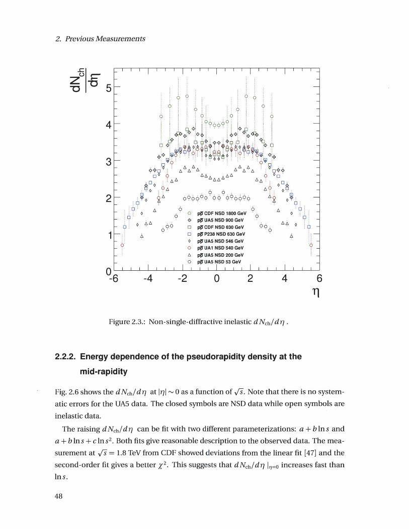
Figure 2.3.: Non-single-diffractive inelastic dNch/dr).
2.2.2. Energy dependence of the pseudorapidity density at themid-rapidity
Fig. 2.6 shows the dNch/d at I ~ 0 as a function of Vs. Note that there is no system-
atic errors for the UA5 data. The closed symbols are NSD data while open symbols are
inelastic data.
The raising dNch/d can be fit with two different parameterizations: a + bIns and
a + bins + cln s 2 . Both fits give reasonable description to the observed data. The mea-
surement at V1 = 1.8 TeV from CDF showed deviations from the linear fit [47] and the
second-order fit gives a better y2. This suggests that dNch/dr 11=0 increases fast than
In s.
48
0-
0 -
0--6 6
il
pp CDF NSD 1800 GeVpp UA5 NSD 900 GeVpP CDF NSD 630 GeVpp P238 NSD 630 GeVpp UA5 NSD 546 GeVpp UA1 NSD 540 GeVpp UA5 NSD 200 GeVpp UA5 NSD 53 GeVI I I I I I

2.2. dNch/d rj distributions
_r__
Z-3.5
3-
2.5-
2-
1.5
1
0.5
070
I I
0
A
-0
*0
-0
0
4A4b0
I I I I I I I 1 1 1 I I1 I I I I I I I I I I I I Ipp ISR INEL 23.6 GeV
pp ISR INEL 30.8 GeV
pp ISR INEL 45.2 GeV
pp ISR INEL 53.2 GeV
pp UA5 INEL 53 GeV o
pp ISR INEL 62.8 GeV 0
pp PHOBOS INEL 200 GeV
pI UA5INEL 200 GeV [
pp PHOBOS INEL 410 GeV El
pp UA5 INEL 546 GeV Oopp UA5 INEL 900 GeV
60
-
--1
A
1 2 3 4 5 6 7 E+YBeam
Figure 2.4.: Inclusive inelastic dNch/dr) in the rest frame of the proton beam.
Since the two empirical fits gives quite different extrapolations at LHC energies (up to25%), the measurement at high energy will help to identify the correct parameterization.
2.2.3. Comparison between data and PHOJET
Fig. 2.7 shows the comparison between NSD dNeh/dr and the results from the PHOJET
generator. The PHOJET generator describes the dNeh/drl reasonably well up to v/s =
1800 GeV The consistency between data and MC is at the 5% to 10% level except theCDF data in the range of rf l > 1. The generated dNch/dr from PHOJET is higher than
data at v/= 53 - 630 GeV and lower than the CDF measurement at s= 1800 GeV. The
dip structure at mid-rapidity is also reproduced by the PHOJET generator.
I I I I I I I
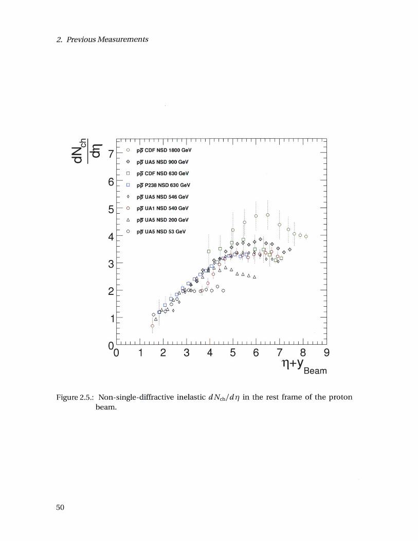
7
6
5
4
3
2
1
0) 1 2 3 4 5 6 7 8 9fyBeam
Figure 2.5.: Non-single-diffractive inelastic dNch/dr in the rest frame of the protonbeam.
2. Previous Measurements
_1 1| 1 i ii 1 1 i11 i 1 1 i i 11 1 1 11 111 I I i I 1 110 pp CDF NSD 1800 GeV
0 pp UA5 NSD 900 GeV
- 0 pp CDF NSD 630 GeV
0 pp P238 NSD 630 GeV
- pp UA5 NSD 546 GeV
- 0 pp UA1 NSD 540 GeV
a 9- A pp UA5 NSD 200 GeV 0
0-- 0 pp UA5 NSD 53 GeV 0 -
000--' ' ''
00 a00E~1~00
00
6Ot:OOO
.-
z" -9

2.2. dNeh/drl distributions
I I I I 1I I1II1
X UA1 NSD
V STAR NSD
A UA5NSD
N CDFNSD
I I I I
0 NAL B.C. ine
0 ISR inel.
A UA5 inel.
O PHOBOS
--------- 1.462 - 0.064 In s +-------- -0.406 - 0.282 In s
0.554 - 0.094 In s + 0-0.043 - 0.227 In s
i l i l l I I I i l l
~I.
I---
.0154 In2 s -
.0068 In2 s
i i I I I l
10 102N s [GeV]
Figure 2.6.: dNch/drl as a function of v~s. The solid lines are fits to the inclusive datawhile dashed lines are fits to the NSD data. The systematic errors are shownwhen available.
0
z
10 3 104

2. Previous Measurements
5-0"
-o 4.5
4
3.5
3
2.5
2
1.5
1
0.5
0 -6 -4 -2 0 2 4 6
Figure 2.7.: Non-single-diffractive inelastic dNch/dr compared with PHOJETgenerator.
0 ? 00 0
0 0-
< i 0 0
0. 0
OO 06-9, O .-DFND0 30Ge
Sp PN6 Ge 0
0 pOUANSD56%e
A p- UA -N(? A A ,
Q1. 0 00 6 0o66' o 00'
A%. I
0 p15CDF NSD 1800OGeV 6'k, '
0 o p15UA5 NSD 900GeVA,6 EJ pISCDF NSD 630OGeV%
'A0 plSP238 NSD 630OGeV A'
0I P15UA5 NSD 546 GeVA ppSUA5 NSD 200 GeVk
0 pp UA5 NSD 53 GeV
PHOJET- -l - - I I i

2.3. Multiplicity distributions
2.3. Multiplicity distributions
5 10 15 20 25 30 35 40
z
10.2
10-3
10-5045 5 10 15 20 25 30 35
Nch
Figure 2.8.: The multiplicity distributions measured in the NAL and ISR energies. (LeftPanel) The distributions from inclusive events. (Right Panel) The distribu-tions from NSD events.
Multiplicity distributions measured in full phase space from NAL and ISR are shown
in Fig. 2.8. Increasing the energy resulted in an increase in total multiplicity. Studies
were done in inclusive events and NSD events. By comparing the distributions from
both event selections, one can see that the single-diffractive events are populated in
low multiplicity region of the distribution.
2.3.1. Validity of KNO scaling
To assess the validity of KNO, the multiplicity distributions are expressed using KNO
variable z = Neh/ < Nh >, which is shown in Fig. 2.9. The distributions from different
energies (j s < 63 GeV) and different experiments join an universal curve, which can be
described as a negative binomial function. Although the Feynman scaling is broken, it
is clear that the KNO scaling is hold in the ISR and NAL energies.
Fig. 2.10 shows the multiplicity distributions before the startup of the LHC, including
SppS and Tevatron data. It is evident that the KNO scaling is violated between lowest
energy and highest energy dataset. The data with v/ > 100 GeV show a extended high
multiplicity tail which can not be described by a single NBD. The extended high multi-
plicity tail seems to grow smoothly as a function of /~s.
z
10-
10-4
10-5
00
- pp ISR INEL 30.4 GOV
0 pp ISR INEL 44.5 GeV
A ppISR INEL 52.6 GeV
pp ISR INEL 62.2 GeV
o pp NAL INEL 13.8 GeV
o pp NAL INEL 19.6 GeV
- pp NAL INEL 23.8 GeV
-'' pp'ISR NSD 44.5 GeV'''''
- A
0 AA
pp ISR NSD 30.4 GeV I?
0 pp ISR NSD 44.5 GeV -
A pp ISR NSD 52.6 GeV
pp ISR NSD 62.2 GeV
40 45NCh
' '
0

2. Previous Measurements
1 1.5 2 2.5 3 3.5 4 4.5
The multiplicity distributions measured in the NAL and ISR energies andfit by a negative binominal function. The distributions are normalized andexpressed using KNO variables. (Left Panel) The distributions from inclusiveevents. (Right Panel) The distributions from NSD events.
For the low z region, the height of the peak from higher energies is lowered because
< Nch > is increasing faster due to the high multiplicity tail. In E735 data, a large un-
certainty was shown in the low multiplicity region which was due to the correction and
rejection of the beam background.
The distributions in UA5 can be described by a fit with two NBD (Fig. 1.9). This in-
dicates that there are two independent classes in the multiplicity distribution. Each of
the class follows a NBD. But the origin of the shoulder structure is not yet understood.
Possible explanations are the contributions from mult2iple parton interactions, or in-
creasing contributions from the hard processes involve in the production of high PT
jets.
1 0-1
10-2
10~3
10-40
o pp ISR INEL 30.4 GeV
o pp ISR INEL 44.5 GeV 4a pp ISR INEL 52.6 GeV
- pp ISR INEL 62.2 GeV
o pp NAL INEL 13.8 GeV
0 pp NAL INEL 19.6 GeV
a pp NAL INEL 23.8 GeV
0.5
o pp ISR NSD 30.4 GeV \
o pp ISR NSD 44.5 GeV
pp ISR NSD 52.6 GeV
- pp ISR NSD 62.2 GeV
Figure 2.9.:

2.3. Multiplicity distributions
API
PHPH
P1
3 p
p
epI
0 20 40 60 80 100120
ISR NSD 30.4 GeV --
p ISR NSD 44.5 GeVp ISR NSD 52.6 GeVp ISR NSD 62.2 GeV
p UA5 NSD 200 GeVpUA5 NSD 546 GeV -p UA5 NSD 900 GeV -p E735 NSD 1800 GeV-
k --
c -
10 -2
10-3
10-4
10-5140 160 180 200Nch
0.5 1 1.5 2 2.5 3 3.5
Figure 2.10.: The multiplicity distributions measured in multiplicity variables (leftpanel) and in KNO variables (right panel).
zI--
101
10 2
10-3
10-4
10-5
04
pp ISR NSD 30.4 GeV
pp ISR NSD 44.5 GeV
pp ISR NSD 52.6 GeV
pp ISR NSD 62.2 GeV
pp UA5 NSD 200 GeV
p1 UA5 NSD 546 GeV
pp UA5 NSD 900 GeV
pp E735 NSD 1800 GeV
4 4.5 5


3. The Large Hadron Collider
The Large Hadron Collider (LHC) [1] is a two-ring-superconducting-hadron acceleratorand collider installed in the existing 26.7 km tunnel that was constructed between 1984and 1989 for the CERN LEP accelerator. It is designed to collide proton beams with acenter-of-mass energy of 14 TeV and luminosity of 1034 cm-2 s-1. It also collides leadions with an energy of 2.76 TeV per nucleon and a peak luminosity of 1027 cm-2 s-1. Inthis chapter, a brief description of the LHC is presented.
3.1. Design and Layout of LHC
nrtdmae to Grani Sas.o
3 73 km0
Figure 3.1.: Schematic layout of the LHC (Beam 1 - clockwise, Beam 2 - anticlockwise)
The LHC is a synchrotron that accelerates two counter-rotating beams in separatebeam pipes. It has eight arcs and eight straight sections and the basic layout is shownin Fig. 3.1. There are 4 beam crossing points which contain the experiments (point 1, 2,

3. The Large Hadron Collider
5 and 8). The injection systems from SPS to LHC for Beam 1 and Beam 2 are located at
Point 2 and Point 8. Insertions at Points 3 and 7 each contain two collimation systems
for beam cleaning. The RF systems which accelerate the particles are located at Point 4.
There are 1232 superconducting dipole magnets that bend the beam trajectories and
392 quadrupole magnets that are used to keep the beams focused. The superconduct-
ing magnets are kept at the operating temperature of 1.9 K with liquid helium. The
dipole magnets are operated with a current of 11.85 kA and provide a field of 0.54 T
during injection and a nominal field of 8.33 T during nominal collisions with beam en-
ergy of 7 TeV. RF systems provide a RF voltage of 8 - 16 MV/beam which accelerates the
particle, compensate the synchrotron radiation loss (7 keV/turn).
The protons(lead ions) are grouped in cylindrical bunches with a radius of 16.6(15.9)
pm and a length of 7.55(7.94) cm with a bunch spacing of 25(100) ns in the nominal
operation. The design bunch intensity is 1.15 x 10¹¹ for protons and 7 x 1o for lead ions.
The maximum bunches per ring is 2808(592) for nominal proton-proton(Pb+Pb) runs.
3.2. Experiments at the LHC
There are six experiments that operates at the LHC:
1. CMS (Compact Muon Solenoid) [54] and ATLAS (A Toroidal LHC Apparatus) [55]
are two general-purpose detectors that are built to study both p+p and Pb+Pb
collisions. The focus of the two experiments are the verification of the Stan-
dard Model, search for the Higgs boson, physics beyond the Standard Model, and
heavy ion physics. The detector is optimized for high-PT physics to enhance the
discovery potential of new heavy particles postulated by various of models such
as the supersymmetric extensions (SUSY) of the Standard Model, and the use of
the high-PT probes in the study of the quark-gluon plasma. The analysis in this
thesis is based on the CMS detector and the details are described in Chap. 4
2. ALICE (A Large Ion Collider Experiment) [56] is a dedicated heavy-ion which is
optimized to study heavy ion collisions. The strength of the detector is in the
low-PT observables such as the particle multiplicity measurement, particle iden-
tification.
3. LHCb (The Large Hadron Collider beauty experiment) [57] studies the CP-violation
in the b-quark systems produced in the proton-proton collisions.
3.3. Startup
4. TOTEM (TOTal Elastic and diffractive cross section Measurement) [58] is designed
for the measurement of total cross section, elastic scattering and diffractive proec-
sses in the p+p collisions, which is located in the forward region of the CMS de-
tector.
5. LHCf (Large Hadron Collider forward) [59] is a special-purpose detector to study
the particles generated in the forward region of collisions which is located close to
the ATLAS experiment. The LHCf is designed to measure the energy and number
of 70 , which will help explain the origin of high energy cosmic rays.
3.3. Startup
On 10th September 2008, the proton beam at LHC was successfully circulated in the
main ring of the LHC for the first time. The machine is ready for collisions at Vs = 900
GeV However, during the 10 TeV magnet commissioning, a short circuit occurred and
resulted damage of magnets. The repairing of the magnet and installation of additional
protection features was done during 2009. On 20th November 2009, the proton beams
were successfully circulated with injection energy 450 GeV per beam again, with the first
proton-proton collisions at 900 GeV
On 30 November 2009, the LHC became the highest-energy particle accelerator in the
world with 1.18 TeV per beam, which was a record held by the Tevatron at Fermilab in
the Unite States. After the 2009 winter shutdown, the accelerator ramped up the beam
energy to 3.5 TeV on 19th March 2010 and delivered the first collisions at 7.0 TeV on 30th
March 2010.
During the startup, the initial collision rate was 5 - 50 Hz (corresponds to L ~1 - 10 x
1026 cm-2 s-1) and the expected number of pile-up is less than 0.3%.


4. The CMS detector
The CMS detector is a multi-purpose detector which provides capability to study p+p
and heavy-ion collisions. A detailed description of the CMS experiment can be found in
Ref. [60]. An important aspect driving the detector design and layout is the choice of the
magnetic field configuration in order to measure precisely the momentum of charged
particles. A compact design is chosen and this results in a choice of high magnetic field
which provides a large bending power.
In the multiplicity analysis, the crucial parts of the CMS detector is the pixel tracker,
which is used to reconstruct the charged particles, forward calorimeter (HF) and Beam
Scintillator Counters (BSCs) [60, 61] in the forward region, which are used for triggering
and event selection. In this chapter, the design and performance of the CMS detector
will be described.
4.1. CMS design concept
The overall layout of CMS is shown in Fig. 4.1. The central feature of the CMS appara-
tus is a superconducting solenoid of 6 m internal diameter, providing a uniform mag-
netic field of 3.8 T. Immersed in the magnetic field are the pixel tracker, the silicon-strip
tracker (SST), the lead-tungstate crystal electromagnetic calorimeter (ECAL) and the
brass/scintillator hadron calorimeter (HCAL). In addition to barrel and end-cap detec-
tors for ECAL and HCAL, the steel/quartz-fibre forward calorimeter (HF) covers the re-
gion of Jri between 2.9 and 5.2. Muons are measured in gas-ionization detectors embed-
ded in the steel return yoke. Two elements of the CMS detector monitoring system, the
Beam Scintillator Counters and the Beam Pick-up Timing for the eXperiments (BPTX)
devices [60, 62], were used to trigger the detector readout. In the following sections, the
sub-detectors will be described in detail.

4. The CMS detector
Compact Muon Solenoid
Figure 4.1.: The overall layout of the CMS detector. The beam monitoring system in theforward region is not shown.
4.2. Magnet
In order to provide unambiguous determination of the sign of the muons with a mo-
mentum up to 1 TeV/c in the reconstruction of the decaying new particles, it requires
a momentum resolution of Ap/p ~ 10% at p = 1 TeV/c [63]. CMS chose a large super-
conducting solenoid, the design parameters of which are given in Table 4.1 [64]. A large
bending power can be obtained for a modestly-sized solenoid, albeit a high-field super-
conducting one, as the bending starts at the primary vertex. The main feature of the
CMS solenoid are the use of a high-purity aluminum-stabilised conductor and indirect
cooling (by thermosyphon) together with full epoxy impregnation.
During the data taking in 2009-2010, the magnetic field was set to 3.8 T for the most
of the beam time. A small data set was also taken with B= 0 at v/~= 7 TeV.
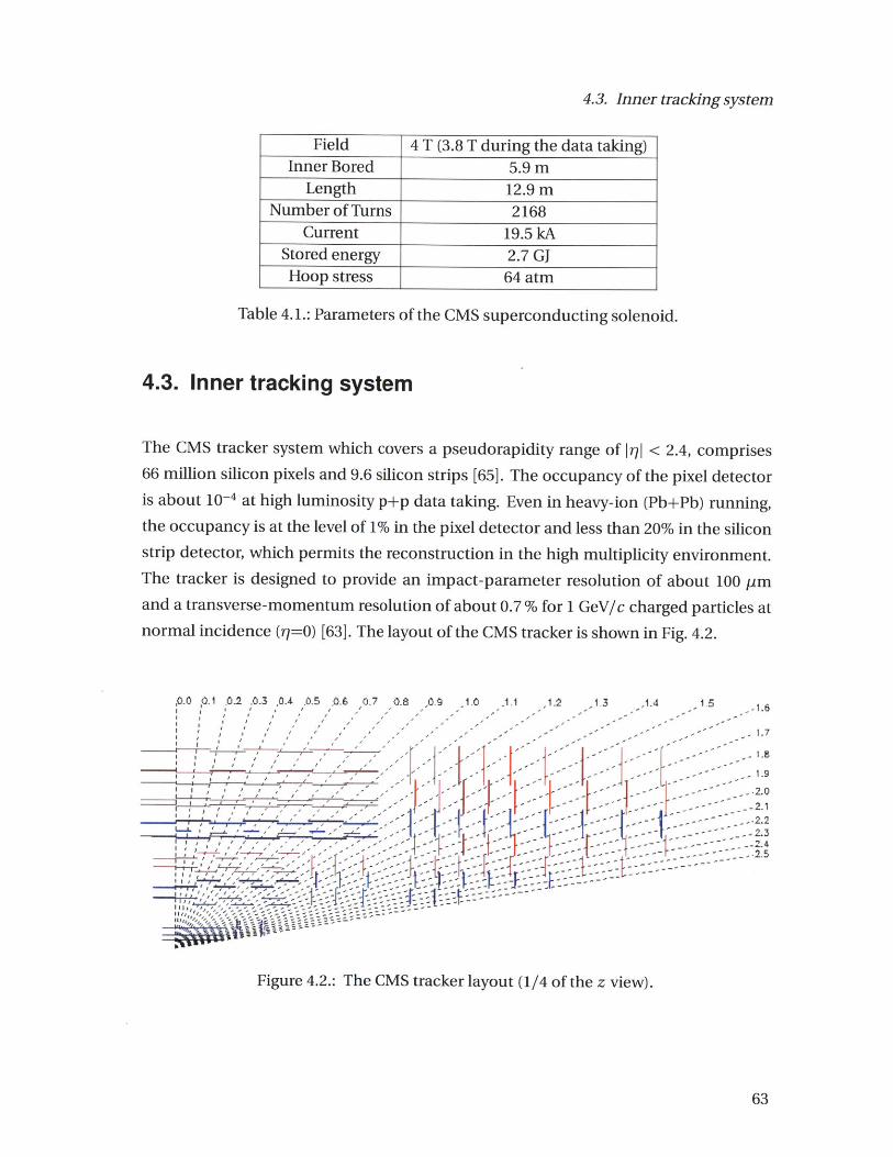
4.3. Inner tracking system
Field 4 T (3.8 T during the data taking)Inner Bored 5.9 m
Length 12.9 mNumber of Turns 2168
Current 19.5 kAStored energy 2.7 GJHoop stress 64 atm
Table 4.1.: Parameters of the CMS superconducting solenoid.
4.3. Inner tracking system
The CMS tracker system which covers a pseudorapidity range of IrI < 2.4, comprises66 million silicon pixels and 9.6 silicon strips [65]. The occupancy of the pixel detectoris about 10-4 at high luminosity p+p data taking. Even in heavy-ion (Pb+Pb) running,the occupancy is at the level of 1% in the pixel detector and less than 20% in the siliconstrip detector, which permits the reconstruction in the high multiplicity environment.The tracker is designed to provide an impact-parameter resolution of about 100 Pmand a transverse-momentum resolution of about 0.7 % for 1 GeV/c charged particles atnormal incidence (rl=O) [63]. The layout of the CMS tracker is shown in Fig. 4.2.
,00 .01 .0.2 A03 ,0.4 0AS 0.6 0.7 0.8 S 1. .. 1
I - I'
.........
................... - - -
771____ - -- K,
17
4 25
Figure 4.2.: The CMS tracker layout (1/4 of the z view).
21 3
4

4. The CMS detector
4.3.1. Pixel tracker
The pixel detector consists of 3 barrel layers with 2 endcap disks on each side on them
(Fig.4.3) [65]. The 3 barrel layers are located at mean radii of 4.4 cm, 7.3 cm and 10.2 cm,
and have a length of 53 cm. This means that CMS is capable to detect charged pions
with transverse momentum greater than ~ 50(70) MeV/c with the first(second) pixel
barrel layer with a magnetic field of 3.8 Tesla. The 2 end disks, extending from 6 to 15
cm in radius, are placed on each side at IzI = 34.5 cm and 46.5 cm. The recorded hits in
the barrel layers are used for tracklet reconstruction for charged multiplicity study. The
details are described in Chap. 6.
Figure 4.3.: The CMS Pixel Detector layout.
4.3.2. Silicon Strip tracker(SST)
The barrel tracker region is divided into 2 parts: a TIB (Tracker Inner Barrel) and a TOB
(Tracker Outer Barrel) [63, 65]. The TIB is made of 4 layers and covers up to |zI <65 cm
and The TOB comprises 6 layers with a half-length of Izi < 110 cm. The first 2 layers
of TIB and TOB are made with "stereo" modules in order to provide a measurement in
both r - # and r - z coordinates. A stereo angle of 100 mrad has been chosen.
The endcaps are divided into TEC (Tracker End Cap) and TID (Tracker Inner Disks).
Each TEC comprises 9 disks that extend into the region 120cm < zl < 280cm, and each
TID comprises 3 small disks that fill the gap between the TIB and the TEC. The TEC

4.4. Muon system
and TID modules are arranged in rings, centered on the beam line, and have strips that
point towards the beam line, therefore have a variable pitch. The first 2 rings of the TID
and the inner most 2 rings and the fifth ring of the TEC have "stereo" module. The spec
and performance of the silicon sensors used in the strip detectors are summarized in
Table. 4.2.
During the data-taking period, 98.4% of the pixel and 97.2% of the SST channels were
operational. The fraction of noisy pixel channels was less than 10-5. The signal-to-noise
ratio in the SST depends on the sensor thickness and was measured to be between 28
and 36, consistent with the design expectations and cosmic-ray measurements [63, 66].
The tracker was aligned as described in Ref. [67] using cosmic ray data prior to the LHC
commissioning. The precision achieved for the positions of the detector modules with
respect to particle trajectories is 3-4 pm in the barrel for the coordinate in the bending
plane. This allowed us to perform the first physics measurement with an already aligned
detector.
part No. detectors thickness (pm) mean pitch (pm) r - #(z) resolution (pm)TIB 2724 320 81/118 23-34(23)
TOB 5208 500 81/183 35-52(52)TID 816 320 97/128/143TEC 2512 320 96/126/128/143
TEC(2) 3888 500 143/158/183
Table 4.2.: Detector types in the silicon tracker.
The CMS tracker gives a transverse momentum resolution of 0.5-7.0% and 95% re-
construction efficiency for muons with PT of 1-100 GeV/c. [63]
4.4. Muon system
The Layout of the muon system is shown in Fig. 4.4. Three types of gaseous detectors are
used to identify and measure muons [63, 68]. The choice of the detector technologies
has been driven by the very large surface to be covered and by the different radiation
environments. In the barrel region (II < 1.2), where the neutron induced background
is small, the muon rate is low and the residual magnetic field in the chamber is low,
drift tube (DT) chambers are used. In the 2 endcaps, where the muon rate as well as
the neutron induced background rate is high, the magnetic field is also high, cathode
strip chambers (CSC) are deployed and cover the region up to Ir| < 2.4. In addition

4. The CMS detector
to this, resistive plate chambers (RPC) are used in both barrel and the endcap regions.
The RPCs are operated in avalanche mode to ensure good operation at high rates (up to
10kHz/cm 2). The typical momentum resolution of the muons is from 0.7% (p -10 GeV)
to 10% (p ~1 TeV). [63]
800
700
600
500
400
300
200
100' /-
0 200 400 600 800 1000 1200Z (cm)
Figure 4.4.: The Layout of the CMS Muon system.
4.5. Electromagnetic calorimeter
The Electromagnetic Calorimeter (ECAL) is a hermetic, homogeneous calorimeter com-
prising 61200 lead tungstate (PbWO4) crystals mounted in the central barrel part, closed
by 7324 crystals in each of the 2 endcaps. [69] The goal of the ECAL to reconstruct the
electromagnetic objects such as electrons and photons, as well as the EM component of
the jets. Lead tungstate scintillating crystals are chosen in order to have short radiation
(Xo = 0.89 cm) and Moliere (2.2 cm) lengths, are fast (80% of the light is emitted within
25 ns) and radiation hard (up to 10 Mrad). Silicon avalanche photodiodes (APDs) and

4.6. Hadron calorimeter
vacuum phototriodes (VPTs) are used for signal amplification. The layout of the CMS
ECAL is shown in Fig. 4.6.
Preshower (ES)
-- - ~~~ 3. ~~~ Endcap
~ Z ECAL (EE)
Figure 4.5.: The Layout of the CMS Electromagnetic Calorimeter system.
The ECAL Barrel (EB) covers a pseudorapidity interval of 0 < IqI < 1.479. The inner
radius is 129 cm, which means that a charged particle should have a PT of at least ~1.5
GeV/c to reach the EB [63, 69]. Each crystal have a front face cross-section of ~ 22 x
22mm 2, which covers 0.0174 in AO and Arl, and a length of 230 mm, corresponding to
25.8 Xo.
The ECAL Endcaps (EE) are two "Dees" at a distance of 314 cm from the center of
the CMS and covering a pseudorapidity range of 1.479 < IrI < 3.0. The endcap crystals
are all identical and have a front face cross section of 28.6 x 28.6mm 2 and a length of
220 mm (2 4 .7Xo). A preshower device is placed in front of the crystal calorimeter over
much of the endcap pseudorapidity range in order to provide better separation power
between nO and photons. The active elements of this device are 2 planes of silicon strip
detectors, with a pitch of 1.9mm, which lie behind disks of lead absorber at depths of 2
Xo and 3Xo.
4.6. Hadron calorimeter
The goal of the hadron calorimeter (HCAL) [70] is to minimize the non-Gaussian tails
in the jet energy resolution and to provide good containment and hermetricity for the

4. The CMS detector
missing transverse energy (E"is") measurement. Due to the choice of the CMS mag-net, the HCAL design maximizes material inside the magnet coil in terms of interactionlengths.
In the pseudo-rapidity range of Irj| < 3.0, brass/scintillator sampling calorimeter ischosen. Brass has a reasonably short interaction length and is non-magnetic and thescintillator tiles with wavelength-shifting (WLS) fiber minimize the space devoted tothe active medium. The photodetection readout is based on multi-channel hybrid pho-todiodes (HPDs). The hadron barrel (HB) part of HCAL consist of 32 towers coveringthe pseudorapidity range of IqI < 1.4, resulting in 2304 towers with a segmentation ofA 3 x A# = 0.087 x 0.087. The hadron endcap (HE) of HCAL covers the pseudorapidityregion 1.3 < jr7| < 3.0. For the 5 outermost towers at smaller rj), the # segmentationis 5 .and the rj segmentation is 0.087. For the 8 innermost towers the # segmentationis 100, whilst the q segmentation varies from 0.09 to 0.35 at the highest q. The totalnumber of HE tower is 2304. In order to sample the energy from penetrating hadronshowers leaking through the rear of the calorimeters and improve the E"iss resolution,the hadron outer (HO) detector is placed outside the magnet. It contains scintillatorswith a thickness of 10 mm and covers the pseudorapidity region II < 1.26.
In the forward region, the hadron forward (HF) calorimeter covers the pseudorapidityrange 3.0 < |jj< 5.0. The HF is located 11.2 m from the interaction point and is madeof steel absorber and embedded radiation hard quartz fibers, which provide a fast col-lection of Cherenkov light. There are 13 towers in T7, all with a size given by Aq ~ 0.175,except for the lowest-rl tower with Ar ~ 0.1 and the highest-rl tower with Ar ~ 0.3. The# segmentation of all towers is 100, except for the highest-ri tower which has A# - 200.The hadron forward detector served as an important detector in the dN/drj analysiswhich provides good selection on the collisional events.
4.7. Beam monitoring system
4.7.1. Beam Pick-up Timing for the eXperiments (BPTX)
In order to monitor the beam condition, the two Beam Pick-up Timing for the eXperi-ments (BPTX) devices, located around the beam pipe at a distance of ±175 m from theIP on either side, are designed to provide precise information on the bunch structureand timing of the incoming beam, with better than 0.2 ns time resolution [62]. TheBPTX detector uses two standard LHC beam position monitors (BPM) each comprising

4.7. Beam monitoring system
Figure 4.6.: The Layout of the CMS Hadronic Calorimeter system.
of four electrostatic button electrodes positioned symmetrically around the beam-pipe.
The BPTX is measured to be fully efficiency in detecting the beam with bunch inten-
sity greater than 109 which provides valuable inputs to the Level 1 trigger.
4.7.2. Beam Scintillator Counters (BSC)
The two Beam Scintillator Counters (BSCs) are located at a distance of +10.86 m
from the nominal interaction point (IP) and are sensitive in the Irl range from 3.23 to
4.65 [61]. The scintillators for the BSC1 station are mounted on the inner surface of the
HF detectors on both sides of the IR The flight time between the IP and BSCl is 36.5 ns.
Each BSC is a set of 16 scintillator tiles. The structure and location of the BSC are shown
in Fig. 4.7.
The four segments in each outer petal are grouped to two PMTs (PMT = photo-
multiplier tube), providing a segmentation in two halves, one for each end. The scin-
tillator rings provide eight signals on each side. This gives in total 2 x (8+8)= 32 BSC 1
channels.
Earlier measurements have shown a time resolution around 3 ns for these scintillators
taken from the OPAL mini-plug detector. With the routing of the signal cables to the

4. The CMS detector
BSC1 Tiles
I 932 mm
Segmentation:- 8 x per ring- 2 x per pedal (vertical split)
Figure 4.7.: Location and schematic of BSC detector [61]
readout in USC55, a resolution around 5 ns is expected. The scintillators (BC408), read
out through photo-multipliers via wavelength shifting fibers, are expected to provide 14
photo-electrons per traversing MIP.
The readout of the BSC counters is implemented using commercial electronics lo-
cated in NIM and VME crates in rack S1E08. Signals from the PMT-s are discriminated
and then combined using off-the-shelf logical NIM units (e.g. LeCroy) to implement the
required coincidence logic and delays. This requires NIM to LVDS units for signal con-
version in the end. The LVDS signals are routed to the GT rack via 4x2 wire commercial
Ethernet cables.
The BSC elements have an average minimum-ionizing-particle(MIP) detection effi-
ciency of 95.7%. The signal from BSC are also designed to provide hit and coincidence
rates as inputs to the Level 1 trigger. The efficiency of the BSC segments was measured
based on the MIP peak in the scintillators. The details of the efficiency determination
can be found in Appendix. D.
4.8. Trigger system
The bunch crossing rate at LHC is 40 MHz which leads to - 109 interactions/sec at de-
sign luminosity, which makes full event recording impossible. The trigger system is de-
signed to provide filter with a rejection factor of nearly 106 to select interesting events.
The CMS trigger system can be divided into two parts: The Level 1 Trigger (LI), which
use custom electronics, provides fast decision. The High Level Trigger (HLT) system,
which relies upon commercial processor, perform reconstruction on the Li accepted

4.8. Trigger system
events and make decisions from more detailed information [2, 63]. The triggers used in
this analysis will be discussed in Chapter 5.
4.8.1. Level 1 Trigger
The CMS Li trigger electronics itself is pipelined and deadtimeless, and can render a
decision on every bunch crossing (40 MHz), synchronised to the LHC clock. The LI trig-
ger involve calorimetry and muon systems as well as some correlation of information
from these systems. The L1 decision is based on the presence of local objects such as
photons, electrons, muons and jets, using information from the calorimeters and muon
systems. Detailed description of the Li Trigger system can be found in Ref. [2]. During
the startup, the Zero-Bias and Minimum-Bias Triggers are also implemented based on
the BPTX coincidence or activities in BSCs which will be described in Sec. 4.8.3.1.
The Li pipeline data storage time is 3.2 ps which included the signal propagation
delays. This means that the Li trigger calculations must be done in many cases in less
than 1 ps. The schematic plot of the Li Trigger is shown in Fig. 4.9. The Li Global
Trigger (GT) collects and synchronises the information from the calorimeters and muon
systems and make a decision to keep or reject an event. Once the L1 trigger generates
an accept, all data which used as input to the Li trigger system are moved to the DAQ
along with the event readout data for storage and will be processed by the High Level
Triggers [2]. Typically, the event rate is reduced by a factor of O(1000).
4.8.2. High Level Trigger
Events which pass the LI trigger are processed by the High-Level Trigger system(HLT) [2].
Only data accepted by the HLT are recorded for offline physics analysis. The rate of
events accepted by the HLT should be within limits allowed by the data recording tech-
nology (O(100) Hz) and thus a rejection factor of O(1000) is needed. In traditional 3-level
trigger systems, this is achieved in two stages: a hardware/software-based Level-2 trig-
ger which quickly provides the large rejection factor and a Level-3 processor farm which
makes decisions based on more sophisticated algorithms. The CMS HLT hardware con-
sist of a single processor farm called the "Event Filter Farm". The farm comprises PCs
mounting 2.66 GHz dual quad-core Intel processors and a total of 16 GB RAM (as of
2010). The CMS HLT combines the rejection power and speed of a Level-2 trigger with
flexibility and sophistication of Level-3 in a single processor farm [2].
The full detector data (~I MB) accepted by the Li Trigger are read out by the DAQ

4. The CMS detector
Global Muon Trigger
'D (RK,ECAL,)tem +O. HCAL.MUJ
Figure 4.8.: Overview of Level 1 Trigger [2]
system at a rate up to 100 kHz. The assembling of the event fragments coming fromeach detector front-end module takes place in two stages. First, the front end data areassembled into larger fragments (super-fragments) which are then delivered to Read-out Units (RU) in eight different and independent sets (DAQ slides) in a round-robinscheme, such that all super-fragments of an event are delivered to the same DAQ slice.In each DAQ slice the super-fragments are managed by the Event Builder where they arefinally assembled into complete events. From the BU, the events are handed to the Fil-ter Units (FU), the applications which runs the actual High Level Trigger reconstructionand selection. Events accepted by the HLT are forward to the Storage Managers(SM)and then stream event data on storage [71]. In the FU, the high level objects such asECAL clusters, jets and muons are reconstructed for event filter determination.
The CMS HLT is highly flexible. The HLT Triggers can be as simple as "mark and pass",or involved in complicated physics object reconstruction. For the MinBias triggers usedin the thesis, the HLT paths are seeded by BPTX and BSC-based Li triggers and no fur-ther event reconstruction are needed in the HLT stage.

4.8. Trigger system
Detectors
Digitizers
LV1 Front end pipelines
Readout buffers
Switching networks
HLT Processor farm
sec
Figure 4.9.: Overview of Level 1 Trigger [72]
4.8.3. Triggers used at the startup
In this section contains information concerning the triggers used at startup for minimum-bias studies, which are based on BPTX and BSCs. The goal of those triggers is to provideZero-Bias / 'Empty-Target'/ minimum-bias data sets which can be used to understandthe trigger efficiencies and beam background.
4.8.3.1. BPTX-based triggers
During the commissioning in 2009, the BPTX is found to be fully efficient for the detec-tion of the crossing of the filled proton bunches with an intensity > 109. This enables usto use the readout of the BPTX signal as L1 trigger.
The most important trigger based on the BPTX is the Zero-Bias trigger, which is thecrossing of two filled proton bunches. There is also a trigger that requires only one filledand one empty bunch crossing; this is sometimes called 'empty target' trigger and willbe used for corrections for beam gas and halo.

4. The CMS detector
4.8.3.2. BSC-based triggers
The main purpose of the BSC system is to provide collision/background monitoring
information for CMS. Besides the monitoring goals, signal pulses are also extracted from
the readout of the BSC and BPTX detectors for triggering.
The Global Trigger (GT) has 64 so-called technical trigger inputs (LVDS) to which sim-
ple signals (pulses) from the BSC and BPTX are routed. The required logic (fanning in
the 32 individual BSC signals in logical "or"s and "and"s) for these signals before enter-
ing the GT is fully implemented. There are 8 technical and 4 extra algo trigger bits from
the BSC, and 7 technical and 4 algo bits from the BPTX provided for the General Trigger.
The relevant trigger bits for this analysis are listed in table 4.3. The BSC halo trigger
use the timing information of the BSC inner ring or outer paddle. The trigger bit 36-39
fires if the timing between the signals from both side of the BSC detector is consistent
with beam halo passing through the CMS. The single-sided BSC MinBias trigger bit fires
if there is a hit in the BSC (bit 34). The coincidence BSC MinBias trigger bits fires if there
is at least one hit in both side of the BSC detector in time coincidence.
The BSC halo bits are used for beam gas and beam halo tagging and rejection, while
the BSC MinBias triggers are used to select collisional events.
4.9. Simulations
The detailed Monte Carlo (MC) simulation of the CMS detector response is based on
GEANT4 [73]. The position and width of the beam spot in the simulation were adjusted
to that determined from the data. Simulated events were processed and reconstructed
in the same manner as collision data.

Table 4.3.: BSC Li bit assignments.
Bit number Bit Name DescriptionTechnical bits
34 LITechBSCminBiasOR there is at least one hit in the BSC36 L1TechBSChalobeam2_inner beam 2 halo, inner37 LiTechBSChalobeam2_outer beam 2 halo, outer38 LiTechBSChalobeamlinner beam 1 halo, inner39 LiTechBSChalobeamiouter beam 1 halo, outer40 LiTechBSCminBiasthresholdi at least one hit in time coincidence
41 LiTech BSC minBiasthreshold2 at least two hits in time coincidence
Algorithm bits124 LiBscMinBiasORBptxPlusORMinus at least one BSC hit in time with one BPTX


5. Event selection
During the data taking, three different data sets are taken for the studies. The first sam-
ple is a Zero-Bias sample which is taken whenever a collision is possible, i.e., two filled
bunches. This sample has no bias due to the online trigger. However, it also contains
empty events and beam backgrounds. The second sample is an Empty-Target sample,
which require only one filled bunch. The empty-target sample will only contain empty
events and beam background. The third sample is a Minimum-Bias (MinBias) sam-
ple based on a 1-arm trigger. This trigger requirement rejects most of the beam back-
grounds, while retains most of the collisional sample.
With the three different samples, one can estimate the contamination from the beam
gas and beam halo in order to develop useful strategy for the background rejection. The
Zero-Bias sample is used for trigger efficiency validation. Those studies are detailed and
discussed in this chapter.
In this chapter, the details of the event selections are presented. The online trigger is
discussed first, followed by event vertex reconstruction and beam background rejection.
5.1. Online Trigger
As discussed in Chapter. 1, the p+p scattering we focus on is the NSD collisions in order
to reduce the uncertainty due to the modeling of the SD event and reduce the contam-
ination from the beam background. To minimize the bias imposed on such an analysis
by the trigger strategy it is essential to optimize the trigger to accept a large fraction
of the NSD cross section while reject most of the SD cross-section. Furthermore, it is
essential to study the relative contributions of single-diffractive, double-diffractive and
non-diffractive collisions as well as the admixture of non-collisional background such
as beam gas interactions and beam halo.
In order to study collisional and beam-gas events, it is important to have a Zero-Bias
trigger and an Empty-Target trigger in the Level 1 Trigger menu. The Zero-Bias trigger is
based on the coincidence of the BPTX signal which triggers on the crossing of two filled

5. Event selection
colliding bunches, therefore contains collision sample and beam background contribu-
tion. The empty-target trigger requires only one filled and one empty bunch crossing
based on BPTX. No collisional events are expected in the empty-target sample.
To achieve high trigger efficiency on the MinBias sample, the CMS readout is triggered
by a signal in any of the BSC segments(see Fig. 4.7), coincident with a signal from either
BPTX indicating a beam or a bunch crossing the IP The three data sets are summarized
in Table. 5.1.
Table 5.1.: The three different data sets used in this thesis.
Name Event content Trigger selectionZero-Bias Empty, beam gas, collisions Coincidence of BPTX
Empty-target Empty, beam gas BPTX XOR signalMin-Bias Empty, beam gas, collisions Coincidence of BPTX, any hit in the BSC
5.2. Event Vertex Reconstruction
A valid primary vertex is useful for beam-background rejection and provide the ref-
erence point for the tracklet reconstruction. In this analysis, there are three differentmethods used for the event vertex determination. The cluster vertex method uses infor-mation from single layer, which is a simple algorithm without using correlation between
different detector layers. The tracklet vertex method is a quick algorithm which corre-
lates two layers of the pixel detector. This algorithm works also on data taken without
magnetic field. The agglomerative vertex reconstruction [74] uses fully reconstructed
tracks, which provides robust and accurate vertex positions. This method is also usedin the final analysis on data taken with magnetic field. With different complexity in al-
gorithm and different vertexing efficiency and resolution, the three methods are used
for various of cross-checks.
5.2.1. Cluster Vertex reconstruction
When a charged particle pass through the pixel detector, the width of the cluster alongthe beam line (w) is proportional to the amount of material it passes through (Fig. 5.1.The expected width (wv) can be calculated with the following relation:
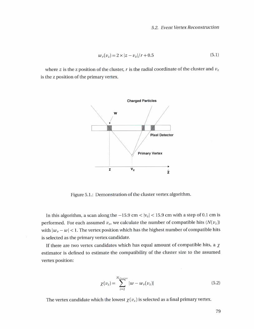
5.2. Event Vertex Reconstruction
wo(vz)=2 x Iz - vzI/r +0.5 (5.1)
where z is the z position of the cluster, r is the radial coordinate of the cluster and vz
is the z position of the primary vertex.
Charged Particles
w
Pixel Detector
Primary Vertex
Vzz
Figure 5.1.: Demonstration of the cluster vertex algorithm.
In this algorithm, a scan along the -15.9 cm < Ivzl < 15.9 cm with a step of 0.1 cm is
performed. For each assumed vz, we calculate the number of compatible hits (N(vz))
with Iw - w I < 1. The vertex position which has the highest number of compatible hits
is selected as the primary vertex candidate.
If there are two vertex candidates which has equal amount of compatible hits, a X
estimator is defined to estimate the compatibility of the cluster size to the assumed
vertex position:
Ncl uster
X(-= IW-W(Vw)I (5.2)
The vertex candidate which the lowest X(vz) is selected as a final primary vertex.

5. Event selection
5.2.2. Tracklet Vertex reconstruction
In order to have a better vertex position resolution while keeping the algorithm rela-
tively simple, a tracklet-based vertex reconstruction technique is introduced. This algo-
rithm is used for magnetic field off analysis.
Figure 5.2.: The definition of A# of the proto-tracklet in vertex reconstruction. The qangle is calculated with respect to the center of the CMS detector (0,0,0).
The first step in reconstructing the primary vertex is to take a first layer hit and loop
over the second layer hits. If the difference in azimuthal angle (A#) between the twohits is smaller than Aoct, this pair is saved as a proto-tracklet. This procedure is re-peated for each first layer hit to get a collection of proto-tracklets. The algorithm is
demonstrated in Fig. 5.3
The expected z vertex position of such proto-tracklets is given by the following ex-pression:
z=zi-pi x(z 2 -zi)/(p2-pi) (5.3)
where z 1( 2) is the z position of the first (second) layer hit in the proto-tracklet, and
P1(2) is the radius in cylindrical coordinates. The calculated z positions are saved to acollection of vertex candidates.
The second step is to determine the primary vertex position from the vertex candi-dates. Looping through the vertex candidates in the collection, the z position of each

5.2. Event Vertex Reconstruction
Layer2
\ \ ///\ I
Layer1V< -A /_
Figure 5.3.: Left The reconstructed proto-tracklets in the X-Z plane. Right: The recon-structed proto-tracklets in the r-#q plane.
is compared to all other candidates. If the difference |Az| between two candidates is
smaller than Azcar, they are grouped together into a vertex candidate cluster. The clus-
ter with the highest number of candidates is selected as the primary vertex; its z position
is determined from the average z position of the cluster.
In this analysis, the optimized parameters were found to be Aocut = 0.08 and Az,,, =
0.14.
The resolution of the pixel tracklet method is found to be only slightly worse than the
pixel triplet method and significantly better than the cluster method.
5.2.3. Agglomerative Vertex reconstruction
The x and y positions of the luminous region where protons of both beams interact,
from here on referred to as beam spot, are constant within a given data set. The beam
spot for each data set is obtained from three-dimensional vertex fits based on tracks
reconstructed with PT > 0.9 GeV/c, using the full event sample. The tracks are recon-
structed as described in [74]. The RMS of the beam spot in both directions was found to
be less than 0.1 mm.
The z position and shape of the beam spot is obtained in a similar manner, using
the event-by-event primary vertex reconstructed as described below. Due to the low
collision rate, the probability for more than one inelastic collision to occur in the same
bunch crossing is less than 0.5%.
To reconstruct the z coordinate of the primary vertex for each event, tracks consisting

5. Event selection
of triplets of pixel hits are formed. The minimal transverse momentum of these tracksis - 75 MeV/c. The tracks are required to originate from the vicinity of the beam spotwith a transverse impact parameter (dT) smaller than 0.2cm. Of these, only tracks withdT< 4 0rT, where oT is the quadratic sum of the uncertainty of dT and the RMS of thebeam spot in the transverse direction, are used in the vertex reconstruction.
The vertex-reconstruction algorithm uses the z coordinate of the tracks at the point ofclosest approach to the beam axis and the corresponding estimated measurement un-certainty (o-z). It performs an agglomerative clustering by adding tracks to form groups.These groups (denoted the ith and fh group) are then merged based on their normal-ized distance, dh2 = (z, - zj)2/(o2 + oj) where o- and o- are the uncertainties of the ziand z; positions, with a fast nearest-neighbor search algorithm [74]. The z position andits uncertainty o-z for the newly joined group are calculated using a weighted average.The clustering process stops when the smallest normalized distance between the re-maining groups gets larger than 12, where the stopping condition was optimized usingsimulated events. Only vertices formed from at least two tracks are considered furtherexcept when there is only one track reconstructed in the event. In this case the vertexposition is given by the point of closest approach of the track to the beam axis. Thefraction of single-track vertices in the data sample is 1.7% at 0.9 TeV, 1.3% at 2.36 TeVand 0.9% at 7 TeV The overall vertex reconstruction efficiency, evaluated from the dataafter all other event selection cuts, is 99.2% and the probability of reconstructing morethan one primary vertex candidate is 5.0% (7.4%) at 0.9 TeV (2.36 TeV). When more thanone vertex candidate is reconstructed, the vertex composed of the largest set of tracks ischosen. This selection is safe since in the startup, the average number of collisions perbunch crossing is <1 which no event pile-up is expected.
The distribution of the reconstructed vertex positions along the beam axis is shownin Fig. 5.4, and compared with that obtained from the simulation, adjusted to the mea-sured beam spot in three dimensions.
5.3. Performance
The performance of vertex resolution as a function of hit multiplicity among the threeavailable vertexing methods are shown in Fig. 5.5. The agglomerative vertexing givesthe best resolution in sample with magnetic field on, but doesn't work in the magneticfield off case. This method is used in the final analysis of the magnet field on sample.The tracklet vertexing also works in the sample without magnetic field, and has a better

5.4. Event Selection
0zP, [cm]
Figure 5.4.: The distribution of the reconstructedthe 7 TeV data (symbols), compared tosimulation (lines).
z position of the primary vertex inthe same distribution from PYTHIA
performance compared to Cluster vertexing. This algorithm is used for B=0 analysis.
Cluster vertexing has less sensitivity to the detector condition or misalignment and itwas used for cross-checks and systematic studies.
5.4. Event Selection
This analysis uses LHC collision data sets collected at LHC startup. The collision ratewith p+p collision are about 11, 3, and 50 Hz at vs =0.9, 2.36, 7.0 TeV respectively.The fraction of events with two or more collisions is negligible (< 0.3%). After all eventselections described in the following section, there are 40320 (0.9 TeV) 10837 (2.36 TeV)
and 55100 (7.0 TeV) events which enter the analysis.
5.4.1. Selecting Collision Events
To select valid collisions, we select events with a BPTX coincidence, indicating a filledbunch from either beam crossing the IP at the same time based. Events which have atleast 1 hit in all of the BSC segments are selected, which pass the Level 1 trigger.
In order to suppress the single-diffractive component and keep most of the non-

5. Event selection
EE
C-luster Vertex - 101 -Cluster VertexTracklet Vertex
Tracklett Vertex- Agglomerative Vertex Tracklet Vertex
0 20 40 60 80 100 120 140 0 20 40 60 80 100 120 140NHits (Layer 1) NHits (Layer 1) B=0 sample
Figure 5.5.: The vertex resolution as a function of hit multiplicity in the 7 TeV PYTHIAMonte Carlo sample.
single diffractive events, we select events that contain a coincidence of at least one
calorimeter tower containing a total energy great than 3 GeV in the positive and neg-
ative HF, i.e on either side of the IP
A valid vertex is required for this analysis. The main analysis uses the agglomerative
vertex which is described in 5.2.3. Data sample reconstructed with cluster vertexing and
tracklet vertexing are used for cross-checks.
5.4.2. Rejecting beam halo events
The selected collision candidate events still contain a contribution from beam induced
background events that can pass the collision trigger. Beam halo events were rejected
based on the BSC beam halo bits (Techical Bit 36, 37, 38, and 39) as described in Sec-
tion. 4.8.3.2.
5.4.3. Rejecting high occupancy events
Another type of beam background events are very high pixel multiplicity events present
in the data set. The number of pixel hits in one pixel layer can go up to several thou-
sands, however, in non-collisional like distributions. An example event is shown in Fig-
ure 5.6 that looks like a shower traversing the full longitudinal extent of the pixel system
84
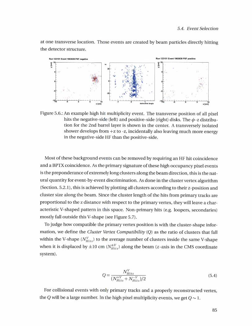
5.4. Event Selection
at one transverse location. Those events are created by beam particles directly hittingthe detector structure.
Run 123151 Event 1903639 PXF negative Run 123151 Event 1903639 PXF positive110 10
20-
-10 5 0~ 5 10 -0 1-L 0 5 *10- [cm- Azimuthal Angle - 1 1
Figure 5.6.: An example high hit multiplicity event. The transverse position of all pixelhits the negative-side (left) and positive-side (right) disks. The # -z distribu-tion for the 2nd barrel layer is shown in the center. A transversely isolatedshower develops from +z to -z, incidentally also leaving much more energyin the negative-side HF than the positive-side.
Most of these background events can be removed by requiring an HF hit coincidenceand a BPTX coincidence. As the primary signature of these high occupancy pixel eventsis the preponderance of extremely long clusters along the beam direction, this is the nat-ural quantity for event-by-event discrimination. As done in the cluster vertex algorithm(Section. 5.2.1), this is achieved by plotting all clusters according to their z-position andcluster size along the beam. Since the cluster length of the hits from primary tracks areproportional to the z distance with respect to the primary vertex, they will leave a char-acteristic V-shaped pattern in this space. Non-primary hits (e.g. loopers, secondaries)mostly fall outside this V-shape (see Figure 5.7).
To judge how compatible the primary vertex position is with the cluster-shape infor-mation, we define the Cluster Vertex Compatibility (Q) as the ratio of clusters that fallwithin the V-shape (NVyts) to the average number of clusters inside the same V-shapewhen it is displaced by +10 cm (Ngy,) along the beam (z-axis in the CMS coordinatesystem).
NVQ= Hits (5.4)
NHits +Nt,,/
For collisional events with only primary tracks and a properly reconstructed vertex,the Q will be a large number. In the high pixel multiplicity events, we get Q ~ 1.

5. Event selection
Fig. 5.8(a) shows the correlation of Q and the number of pixel hits (Nhits) from theMinBias sample at s = 0.9 TeV This can be compared to Monte Carlo simulationswhere only collisions are present (Figure 5.8(c)) and empty-target sample where onlybeam background is present (Figure 5.8(b)). The collisions typically have good clustervertex compatibility (large Q). On the other hand, the high hit multiplicity beam back-ground events are populated around Q - 1. It is clear that a simple diagonal cut can beeffective in cleaning up the sample in data without cutting much at all into the overallefficiency.
It should be noted that the HF coincidence requirement itself is also effective in re-moving beam background, as another prominent feature of the background is signifi-cant asymmetry in the energy deposits between the forward and negative hemispheres.The vertex quality distributions in 0.9 TeV MinBias sample after all other selections havebeen applied (including the HF coincidence) are shown in Figure 5.9(a) for the collisionbunches and Figure 5.9(b) for the empty-target bunches. Only a few high-multiplicitybeam-background events remain in the collision events, which are clearly removed withthe diagonal cut (indicated by the red line). Furthermore, it is evident from the very fewentries to the left of the cut in Figure 5.9(b) that only a tiny fraction (per mille level at 0.9and 2.36 TeV; less than 2x10- 5 at 7 TeV) of beam-gas events survive the complete eventselection.
The implementation used in the event selection for the dN/drj and dN/dpT analy-ses at s = 7 TeV differs slightly from the cut used at 0.9 and 2.36 TeV to accommodatehigher multiplicity real collision events. The definition of quality events, indicated bythe lines in Figure 5.9(a) and Figure 5.9(c), is as follows:
Q >(a x Nfits)| NHits < b || Q > c. (5.5)
In case of 7 TeV collisions, the parameters are set to a = 0.0045, b = 150 and c =2.In addition to the higher multiplicity reach of 7 TeV collisions that is evident in Fig-
ure 5.9(c), it is also apparent that the beam conditions are 'cleaner' than at the lowerenergies, i.e. there are proportionately fewer events in the low-quality tail than in Fig-ure 5.9(a). This is because of the much higher collision rate in 7 TeV data taking com-pared to low energy runs.

5.4. Event Selection
z [cm]
(a) Valid collision, 204 layer 1 hits
0 30z [cm]
(c) Beam background, 204 layer 1 hits
(b) Valid collision, 311 layer 1 hits
20 30z [cm]
(d) Beam background, 311 layer 1 hits
Figure 5.7.: The example distribution of pixel clusters according to their z-position andcluster length along the beam, shown with the V-shaped selection of clusterscompatible with primary particles coming from the collision vertex. Thedashed lines show the shifted V-shape for compatibility estimation. (a) A 7TeV Collision with 204 hits in the first pixel barrel layer. (b) A 7 TeV collisionwith 311 hits in the first pixel barrel layer. (c) Beam background event with204 hits in the first pixel barrel layer.(d) Beam background event with 311hits in the first pixel barrel layer.
z [cm]

5. Event selection
Run 124023 - BPTX_AND, no BSC halo, BSC_OR, pixel vertex Run 124023 - BPTXXOR, no BSC halo, BSCOR, pixel vertex
10 103 10 103collBeams singleBeam
Entries 48435 Entries 1040
Mean x 131.6 Mean x 719.9
- 8 Mean y 4.406 8 Mean y 1.625
o RMS x 147.4 RMS x 381.80 RMS y 1.614 210 RMS y 0.9703 2X X
6 6 ,"6
4 4
10 10
2 2
500 1000 1500 0 500 1000 1500# of pixel hits # of pixel hits
(a) 0.9 TeV MinBias sample (b) Empty-target sample
PYTHIA ATLAS tune - BSCOR, pixel vertex
10 103
pythiaATLASEntries 41394Mean x 95.71
8 Mean y 4.644
o RMS x 79.85RMS y 1.909 10 2
X0 6
10
2
500 100 1500 1
# of pixel hits
(c) 0.9 TeV PYTHIA MC events
Figure 5.8.: (a) The distribution of vertex compatibility (Q) versus hit multiplicity af-
ter applying all the selections from Table 5.2 except the HF coincidence.The quality selection cut is indicated by the red line. (c) The same quan-tity for PYTHIA Monte Carlo simulated events and (b) data events triggeredby empty-target trigger.

5.4. Event Selection
Run 124023 - BPTXAND, no BSC halo, BOSC OR, pixel Vertex, HF coinc
10Co
EntMeg
CL 8 MeeEMe0 RMI
X RMt
6 6
4
1000 151# of pixel hits
(a) 0.9 TeV MinBias sample
ftun t3e - WITX.AM n WBC We, BSC.OA pixWe ven
10
18
6
4
f7lK''0 500
Run 124023 - BPTX_XOR, no BSC halo, BSCOR, pixel vertex, HF coinc
# of pixel hits
(b) Empty-target sample
r coai, CcoliBSOMsEntrims 51273M.... 134.1Nen y 4.434RMS x 152.7RMS y 1.35
101 1 01 0
No
* 10
1000 1500# of pixel hits
(c) 7 TeV MinBias sample
Figure 5.9.: (a) The distribution of vertex compatibility (Q) versus hit multiplicity afterapplying all the selections from Table 5.2 including the HF coincidence at
~s = 0.9 Te V. The quality selection cut is indicated by the red line. (b)The same selection applied to data events triggered in empty-target bunchcrossings (i.e. those when only one beam was crossing the IP). (c) The sameselection applied to 7 TeV collision events, where the dashed line indicatesthe updated cut position.
I .

5. Event selection
5.5. Trigger and selection efficiency studies
The efficiency of the event selection used in this analysis is estimated from a MC study.
MC events are generated using the Pythia event generator and then processed by a full
GEANT 4 simulation [75] including detector response simulation. For each data run
a separate set of simulated events is generated with matching energy and beam spot
parameters.The total number of collision events and the number of collision events passing each
subsequent requirement are listed in Table 5.2.
Table 5.2.: Number of events per data sample used in this analysis. The offline event se-lection criteria are subsequently applied, i.e. each line includes the selectionof the lines above.
Beam Energy 0.9 GeV 2.36 TeV 7.0 TeVRun Number 124023 124120 132440Magnetic Field 3.8 T 3.8 T 3.8 TSelectionBPTX Coincidence + one BSC Signal 72637 18074 68512One Pixel Track 51308 13029 62097HF Coincidence 40781 10948 55322Beam Halo Rejection 40741 10939 55309Beam Background Rejection 40647 10905 55301Valid Event Vertex 40320 10837 55100
Table 5.3.: Check on the non-collisional events. The offline event selection criteria aresubsequently applied, i.e. each line includes the selection of the lines above.
Beam Energy 7.0 TeVSelectionBPTX XOR + one BSC Signal 3167One Pixel Track 336HF Coincidence 15Beam Halo Rejection 10Beam Background Rejection 5Valid Event Vertex 0

5.5. Trigger and selection efficiency studies
5.5.1. Event selection efficiency
Inelastic p+p collisions at 7 TeV simulated by PYTHIA consist of an admixture of 19.2%
SD, 12.9% DD and 80.8% NSD processes. The efficiency of the event selection for the
different processes is determined to be 26.7% for SD, 33.6% for DD and 86.3% for NSD.
Based on our cross checks with data (looking at diffraction signals in the HF), we assign
a relative 20% error on these SD and DD efficiencies. The event selection efficiency for
NSD and SD events (symbols) is shown in Fig. 5.10 as a function of simulated charged
particle multiplicity in the 1J1 < 2.5 range, together with the distribution of the same
multiplicity (lines).
The magnitude of the correction of the measurements to the NSD part of the p+p
cross section depends on the fraction of SD processes accepted by the event selec-
tion. Based on the PYTHIA process composition we estimate the fraction of selected
SD events relative to selected events to be 5.8% at 7 TeV.
20 40 60 80 100 120 140
Charged-particle multiplicity0 10 20 30 40 50 60
Charged-particle multiplicity
Figure 5.10.: (a) Generated multiplicity distributions of primary charged hadrons in therange Iq| < 2.5 for Fs = 7 TeV after the event selection is applied to thereconstructed events, using inelastic events from the PYTHIA (histogram)and PHOJET (symbols) event generators. (b) The event selection efficiencyexpected for NSD events from the PYTHIA (histogram) and PHOJET (sym-
bols) event generators as a function of generated charged hadron multi-plicity in the region rI< 2.5.

5. Event selection
5.5.2. MC event selection efficiencies
The MC event selection efficiencies are shown in Table. 5.4. The SD fraction is droppingas a function of s in both generator, while the DD and ND fraction is increasing. Sincethe event multiplicity is increasing, the event selection efficiency increases as a functionof center-of-mass energy. The selected SD fraction in PYTHIA is higher than PHOJET,and the difference is up to 1.8%. This difference is from the ways of modeling the SDevents and is taken into account in the systematic uncertainty.

Table 5.4.: Expected fractions of SD, DD, ND and NSD processes ("Frac.") obtained from the PYTHIA and PHOJET event genera-
tors before any selection and the corresponding selection efficiencies ("Sel. Eff.") determined from the MC simulation.
PYTHIA
Energy 0.9 TeV 2.36 TeV 7.0 TeV
Frac. Sel. Eff. Sel. Frac. Frac. Sel. Eff. Sel. Frac. Frac. Sel. Eff. Sel. Frac.
SD 22.5% 16.1% 5.2% 21.0% 21.8% 6.3% 19.2% 26.7% 6.8%
DD 12.3% 35.0% 6.2% 12.8% 33.8% 5.9% 12.9% 33.6% 5.8%
ND 65.2% 95.2% 88.7% 66.2% 96.4% 87.8% 67.9% 96.4% 87.4%
NSD 77.5% 85.6% 94.8% 79.0% 86.2% 93.6% 80.8% 86.3% 93.1%
PHOJET
Energy 0.9 TeV 2.36 TeV 7.0 TeV
Frac. Sel. Eff. Sel. Frac. Frac. Sel. Eff. Sel. Frac. Frac. Sel. Eff. Sel. Frac.
SD 18.9% 20.1% 4.9% 16.2% 25.1% 5.0% 13.8% 30.7% 5.0%
DD 8.4% 53.8% 5.9% 7.3% 50.0% 4.5% 6.6% 48.3% 3.8%
ND 72.7% 94.7% 89.2% 76.5% 96.5% 90.5% 79.6% 97.1% 91.2%
NSD 81.1% 90.5% 90.9% 83.8% 92.4% 89.5% 86.2% 93.4% 95.0%


6. Pseudorapidity distribution
measurement
The pseudorapidity distributions are measured by three different methods with the
CMS detector: pixel counting technique, tracklet reconstruction from this thesis, and
full tracking [76, 77]. The pixel counting method uses pixel hits from a single pixel layer
has good sensitivity to low PT particles, but it's more sensitive to the background con-
tamination. The full tracking method involves a more complicated algorithm and is
insensitive to background hits and low PT loopers. The three methods are complemen-
tary to each other and are useful for the understanding of systematic uncertainties. In
this thesis, the tracklet method will be presented and the results will be compared with
other methods in Chapter. 8.
In this chapter, the measurement of the charged hadron pseudorapidity distribution
in NSD p+p collisions with the CMS pixel detector is presented. The reconstruction of
hit-pairs (tracklets), which is used to characterized the event multiplicity, is described
in Sec. 6.1. The corrections of detector effects, such as the reconstruction efficiency,
contributions from the secondary particles which comes from the weak decays, 5 ray
and photon conversions have to be applied to the raw spectra. The effect of trigger-
ing efficiencies, contribution from the SD process and MC model dependence are also
studied.
6.1. Tracklet method
Tracklets are two hit combinations in consecutive layers of the pixel detector consis-
tent with a track originating at the primary vertex. In the CMS experiment, the pixel
hits are reconstructed from the clusters of energy deposit in the pixel detector, which
is described in [66]. The reconstructed hits are used in the tracklet reconstruction. The
tracklet analysis makes use of the correlation between hit positions in the first two layers
of the pixel detector. Pairs of hits produced by the same charged particle will have only

6. Pseudorapidity distribution measurement
small differences in the pseudorapidity (rj) and the azimuthal angle (q5) with respect to
the primary vertex.
This analysis uses the first three tracker layers in the CMS silicon pixel barrel [66].The first layer is located at a distance between 3.6 and 5.2 cm from the beam line, the
second layer is between 6.6 and 8.0 cm and the third layer is between 9.4 and 10.8 cm.
For a homogeneous magnetic field of 3.8 Tesla, charged pions with transverse momen-
tum greater than -50(70) MeV/c can reach the first(second) pixel layer. That allows the
reconstruction of tracklets from all but the lowest PT particles.
With the three layers of the pixel detector, there are three possible combinations:
1st+2nd, 1st+3rd and 2nd+3rd layers. The combination of 1st+2nd layer provides the
lowest PT reach, but it's more sensitive to the beam-pipe induced background. The
combination of 2nd+3rd have a higher PT threshold and less sensitive to the possible
low PT background, however, it needs a larger correction on the strangeness content
and secondary production. The three combinations are complement to each other and
the results are useful for layer-by-layer systematic checks.
For each tracklet, the pseudorapidity is calculated from the hit position in the first
layer. The differences in pseudorapidity (AZr) and azimuthal angle (A#) are important
for characterizing the tracklet and are calculated by:
AT =71 - J2 (6.1)
A# =#1 - #2 (6.2)
where T1( 2) is the pseudorapidity of the first(second) hit with respect to the primary ver-
tex, and #1(2) is the azimuthal angle.
In addition to primary charged particles, the tracklet collection will also include con-
tributions from low-PT "loopers", secondary interactions in the beam-pipe, and parti-
cles from weak decays. We do not apply a hit selection on the reconstructed hits, i.e. all
pixel hits are used in the analysis. This design is to minimize the systematics due to de-
tailed pixel detector simulation. "Combinatorial background tracklets" are defined as
combinations from looper hits, secondary hits and hits from different primary tracks.
The background fraction can be estimated by a data driven method, which will be de-scribed in Sec. 6.1.3. The looper contribution can be suppressed by a selection on A77.The tracklets from secondary particles cannot be removed, and the correction for this
contribution relies on MC simulation. In the following sections, we describe the detailsof the tracklet analysis.

6.1. Tracklet method
Layer2
2 #
Layer1 I1I
Primary Vertex
Primary Vertex
Figure 6.1.: The definition of Arl and Ap of the tracklet.
6.1.1. Tracklet reconstruction
Tracklets are pairs of pixel hits in each of the first two pixel layers. In this analysis, track-lets are reconstructed in four steps:
1. The primary vertex is reconstructed with the method described in Chapter 5.2.3.An event is used only if there is at least one reconstructed primary vertex. If morethan one is found, the vertex with more associated tracks is chosen. To ensurethis analysis to be insensitive to acceptance correction, all reconstructed verticeslie within IvI <20cm (see Fig. 5.4).
2. For each reconstructed hit, we calculate the pseudorapidity, ri (2 ), for the first (sec-ond) layer using the primary vertex location. This design gives a better resolutionon the pseudorapidity.
3. Starting with a reconstructed hit in the first pixel layer and looping over the re-constructed hits in the second layer we save all possible combinations as proto-tracklets.
4. We sort the proto-tracklets by Arl = (rh - r72), which is the difference in pseudo-
rapidity of the first and second layer hits. If a second layer hit is matched severaltimes, the proto-tracklet with the smallest Arl is kept. The selected proto-trackletsare final reconstructed tracklets. (Fig. 6.2)

6. Pseudorapidity distribution measurement
5. To ensure the reconstructed tracklets are consistent with the primary vertex,
tracklets with IAiI| <0.1 are selected in the multiplicity analysis.
Layer2
Layer1Primary Vertex
Figure 6.2.:
Layer2
Layer1
Primary Vertex
Layer2
Primary Vertex
Demonstration of the tracklet reconstruction algorithm. (Left pannel) Re-constructed proto-tracklets. The red dots are the reconstructed hits in thepixel detector and the lines show all possible combinations between the hitsin the two pixel layers (Proto-tracklets) (Central panel) Reconstructed track-lets after cleaning. Now all the hits are only used once. Sometimes thereare still hits with large Arj reconstructed as the cleaned tracklets. Therefore,further selections are needed to reject those tracklets. (Right panel) Recon-structed tracklets with IAr7|< 0.1 requirement.
The reason that the tracklets are ranked by Ar7 is because the magnetic field in the
CMS detector bends the trajectory of the charged particles in the # direction which
makes the A# width much larger than the Arl width. The Arl, A# distribution of the
reconstructed tracklets is shown in Figure 6.3 and Figure 6.4. From Monte Carlo study,
the typical widths of the Arl and A# from the charged particle are 0.004 and 0.05 if the
distribution is fit by a Gaussian distribution.
6.1.2. Event Multiplicity
Since the event selection efficiency, tracklet reconstruction efficiency and background
level are dependent on the event multiplicity, a event multiplicity variable (M) is impor-
tant for this analysis. Several possible multiplicity variables are
1. pixel hit multiplicity in the first layer (Nhiti)
2. Number of reconstructed tracklets (N Rawkler
3. Number of background subtracted tracklets (NTracklet)
Z'X/z)
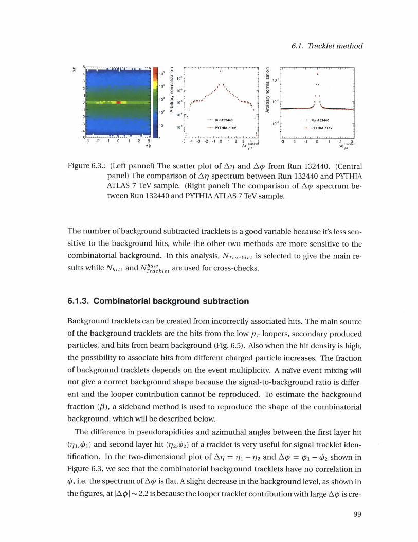
6.1. Tracklet method
5
4
3
2
1
0
-1
-2
-3
-4
10. 0
10 -1
10"10' .- ' 'e.104 E EC
10 1* ->10 10 a . 10- -.10'3-2 0
2<10 10-
10 - Run132440 10-- Run132440
10 - - PYTHIA 7TeV PYTHIA 7TeV
~-3 -2 -1 0 1 2 3 -5-4 -3 -2-1 0 12 3 45 -3 -2 -1 0 1 2Take
Afl Tracklet A rcl
Figure 6.3.: (Left pannel) The scatter plot of Arl and A# from Run 132440. (Centralpanel) The comparison of Arl spectrum between Run 132440 and PYTHIAATLAS 7 TeV sample. (Right panel) The comparison of A# spectrum be-tween Run 132440 and PYTHIA ATLAS 7 TeV sample.
The number of background subtracted tracklets is a good variable because it's less sen-
sitive to the background hits, while the other two methods are more sensitive to the
combinatorial background. In this analysis, NTracklet is selected to give the main re-sults while Nhitl and NRak1et are used for cross-checks.
6.1.3. Combinatorial background subtraction
Background tracklets can be created from incorrectly associated hits. The main sourceof the background tracklets are the hits from the low PT loopers, secondary producedparticles, and hits from beam background (Fig. 6.5). Also when the hit density is high,the possibility to associate hits from different charged particle increases. The fraction
of background tracklets depends on the event multiplicity. A naive event mixing will
not give a correct background shape because the signal-to-background ratio is differ-
ent and the looper contribution cannot be reproduced. To estimate the background
fraction (#), a sideband method is used to reproduce the shape of the combinatorial
background, which will be described below.
The difference in pseudorapidities and azimuthal angles between the first layer hit
(r91,#)1 ) and second layer hit (W2,# 2 ) of a tracklet is very useful for signal tracklet iden-
tification. In the two-dimensional plot of A7 = ?1 - T72 and A# = #1 - #2 shown in
Figure 6.3, we see that the combinatorial background tracklets have no correlation in
#, i.e. the spectrum of A# is flat. A slight decrease in the background level, as shown inthe figures, at |A# I - 2.2 is because the looper tracklet contribution with large A# is cre-
4MMMMW Mw rwuwvu
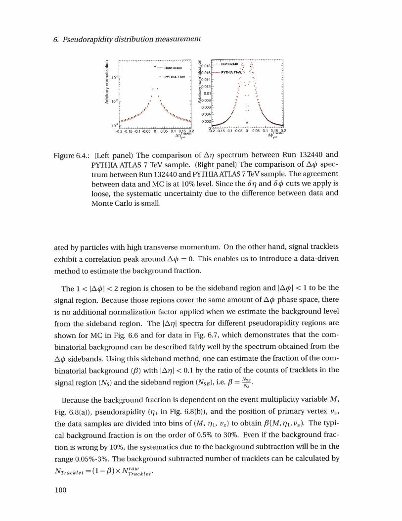
6. Pseudorapidity distribution measurement
--- Run1324400Run32440 =0.018 344N N
=0.016 PYTHIA 7TeY.E 101 -PYTHIA 7TOV Eo 10.014*
0012.012*
0.01a a-
<a a.0.0067
age ,Is0.004 -
0.002
-- 0.2 -0.15 -0.1 -0.05 0 0.05 0.1 1 2All Yak, fA rake
11.2 1P2
Figure 6.4.: (Left panel) The comparison of ALr spectrum between Run 132440 andPYTHIA ATLAS 7 TeV sample. (Right panel) The comparison of A# spec-trum between Run 132440 and PYTHIA ATLAS 7 TeV sample. The agreementbetween data and MC is at 10% level. Since the 6Yj and 6# cuts we apply isloose, the systematic uncertainty due to the difference between data andMonte Carlo is small.
ated by particles with high transverse momentum. On the other hand, signal tracklets
exhibit a correlation peak around A# = 0. This enables us to introduce a data-driven
method to estimate the background fraction.
The 1 < IA#|P < 2 region is chosen to be the sideband region and JA#~ |< 1 to be the
signal region. Because those regions cover the same amount of A# phase space, there
is no additional normalization factor applied when we estimate the background level
from the sideband region. The |AriI spectra for different pseudorapidity regions are
shown for MC in Fig. 6.6 and for data in Fig. 6.7, which demonstrates that the com-
binatorial background can be described fairly well by the spectrum obtained from the
A0 sidebands. Using this sideband method, one can estimate the fraction of the com-
binatorial background (P) with IAr)| < 0.1 by the ratio of the counts of tracklets in the
signal region (Ns) and the sideband region (NSB), i.e. - NSB-
Ns~
Because the background fraction is dependent on the event multiplicity variable M,
Fig. 6.8(a)), pseudorapidity (rj1 in Fig. 6.8(b)), and the position of primary vertex v2,
the data samples are divided into bins of (M, ?1, vz) to obtain # (M, r1, vz). The typi-
cal background fraction is on the order of 0.5% to 30%. Even if the background frac-
tion is wrong by 10%, the systematics due to the background subtraction will be in the
range 0.05%-3%. The background subtracted number of tracklets can be calculated by
NTracklet = (1 - #) x Nraw
100

6.1. Tracklet method
Loopers
Secondary Particle
Primary Particle
Figure 6.5.: Demonstration of difference sources of pixel hits.
6.1.4. Efficiency and Acceptance Correction
To calculate the number of hadrons, an efficiency correction has to be applied. Tocorrect for the reconstruction efficiency and detector acceptance, the correction factora(M, r,, vz) is introduced and defined as:
(6.3)a(M, fM, vz)= .awomC rVA(1 -#(M , r], vz))NC Ta e(M, T1, Vz)
where Ng (M, q, vz) is the number of charged hadrons in the simulated sample(Monte Carlo Truth). The a(M, q, vz) is evaluated by a large number of simulated eventsand is used to calculate the charged hadron spectra from the measured backgroundsubtracted tracklets. The typical correction factors are close to 1 because of the high hitreconstruction efficiency. For high pseudo-rapidity region, the correction factors startto increase due to the limited acceptance. The extrapolation to PT = 0 is also includedin this a correction. The calculated a correction factors are shown in Fig. 6.9 and 6.10.
The q acceptance range as a function of the primary vertex position is shown inFig. 6.11 and the range of the primary vertex position used in different pseudo-rapiditybins are summarized in Table. 6.1.
101

6. Pseudorapidity distribution measurement
1
010-1C i
=10-2
0310
10
10 2 2.5 3 3.5 4 4.5 5
C
21 0
010-2
10 o
10 -6
0 0
kAil| PYTHIA 7TeV
CMS Preliminary9 All trackletsc Combinatorial Background
a Tracklets with Background Subtracted
me @.ae e
a.,
*a
69E
Ca-
0.5 1 1.5 2 2.5 3 3.5 4 4.5 5
jA PYTHIA 7TeV
Figure 6.6.: The Arj spectra for |i| < 0.5 (left) and 1.0 < Irjj < 1.5 (right) in the 7 TeVPYTHIA sample from the 1st+2nd layers.
C10101
NCC 10-2
0 3Z10-
CIS~:10~
|AT1 Run132440
C1o101
INia10 .2
0 3Z10
C10-42U
0 0.5 1 1.5 2 2.5 3 3.5 4 4.5 5
|AM| Run132440
Figure 6.7.: The Arl spectra for I <0.5 (left) and 1.0 < I ||< 1.5 (right) in the data sample(Run 132440) from the lst+2nd layers.
102
0.5 1 1.5
CMS Preliminary* All trackletso CombInatorial Backgroundo Tracklets with Background Subtracted
~0S. 00
e1
.11

6.2. dN/drj study
0.09
0.08
0.07
0.06
0.05
0.04
0.03
0.02
0.01
0
C0
N 0.03
E0.0250C:
2 0.02CZ
P0.015
0.01
0.005
0
Tracklets with bkg subtracted per event (M)
(a)
-3 -2 -1 0 1 2 3Tracklet
11)2
(b)
Figure 6.8.: (a) Number of background subtracted tracklets per event. The backgroundfraction is estimated by a sideband method which is described in the text.(b) Pseudorapidity distribution of raw tracklets from the data sample (Run132440) and PYTHIA ATLAS 7 TeV.
6.2. dN/drj study
The pseudo-rapidity distribution of charged particles is obtained from the measurednumber of tracklets (NTackle t) after background subtraction, efficiency and acceptancecorrection and normalization to the number of selected events.
Using the correction factor a and background fraction p, the dNeh/d r of the selectedevents can be calculated by:
r bins [-2.0, -1.5] [-1.5, -1.0] [-1.0, -0.5] [-0.5,0.0]1st+2nd 14 range (cm) [-10,12] [-16,12] [-16,12] [-16,12]1st+3rd 14 range (cm) [-2,12] [-14,12] [-16,12] [-16,12]2nd+3rd 14 range (cm) [-2,12] [-14,12] [-16,12] [-16,12]
r; bins [0.0,0.5] [0.5,1.0] [1.0,1.5] [1.5,2.0]lst+2nd Vz range (cm) [-16,12] [-16,12] [-16,12] [-16,10]lst+3rd Vz range (cm) [-16,12] [-16,12] [-16,12] [-16,2]
2nd+3rd Vz range (cm) [-16,12] [-16,12] [-16,12] [-16,2]
Table 6.1.: The selected 14 range of the primary vertex for different pseudo-rapidity binsfor tracklets from three different combinations.
103
0 20 40 60 80 100
Run132440
PYTHIA 7TeV
A--
-I I
Run132440
PYTHIA 7TeV -
.. . . . . . . .
. I . . . I . ! 9 ! !
--" I- ' ' ' '
-
-
.
'4
-

6. Pseudorapidity distribution measurement
-2.0< l<-.
-0.6 < I <0.00.0 <T .
06< <1.01.0 < 1 <1.51.5 <j<2.0
U'k8cO 102
O ( m 102?(-4 cm <v z< -2 cm)
--- 2.0 < Yj < -1.5
-1.5 < < -1.0
-1.0 < q < -0.5--- 0.5 < Tj < 0.0-+-0.0 <,I < 0.5
-0.5 <T < 1.0- 1.0 < < 1.5
1.5 < q < 2.0*2.0 < <2.6
-s il i e is ll i i i~ I 1 1
1X(-6 cm < v < -4 cm)
0.0 <<0.50.5 <<1.0
*1.0O< ip<1.5
1 2U-2cm <v z<0 cm)
The calculated correction factors (a) with 2M 7.0 TeV MC in bins of vz for-8<|VZ|<O.
dNe ~(M,V~z)a(MTVV)(1-fi(M, g,Vz))NTracklet(M, V )w(M)
d ( (1+fuSD) IM Nselected(M)()ST)w(M)(6.4)
where Nselected(7) is the number of selected events used in each 17 bin and 56r is the
bin width. Due to the requirement that there has to be a reconstructed primary ver-
tex, the events with no activity in the pixel detector are essentially lost and the event
selection efficiencies c(M) should also be accounted. To get the total NSD dN/dj, cor-
rections on the event weighting (w(M)) and fraction of events with M = 0(fSSD) for the
effect of the event selection is necessary, where w(M) and fNSDare defined as:
104
Figure 6.9.:

6.2. dN/drj study
--- 2.0 < Ta < -1.5
-- 1.5 < q < -1.0
-- 1.0 < TJ < -0.5
--- 0.5 < q < 0.00.0 < < 0.50.5< <1.01.0 < Tj < 1.5 -
1.5 < < 2.0
1 1n 102
M(0 CM < v Z< 2 cm)
-2.5 < q < -2.0-2.0 < < -1.5-1.5 < <-1.0
-+ 1.0 < 9 < -0.5--- 0.5 < <J 0.0
-- 0.0 < TJ< 0.5-- 0.5 < Tj< 1.0+-1.0 < Tj< 1.5
1.5 < Tj< 2.0
+ ++
1f (c 102(4 cm < v < 6 cm)
-2.5 < < -2.0-2.0 < < -1.5-1.5 < < -1.0
---- 1.0 < Tj < -0.5-0.5 < 7 < 0.00.0 <T .0.5 1.01.0 1.51.5 <1<2.0
M(2 cm < v 4cm)
S-2.5 < < -2.0--- 2.0 < Tj< -1.5
-- 1.5 < 71<-1.0
-1.0 < < -0.5-0.5 < Tj< 0.00.0 < 71< 0.50.5 < < 1.01.0 < < 1.51.5 < < 2.0
M (6 cm < v < 8 cm)
Figure 6.10.: The calculated correction factors (a) with 2M 7.0 TeV MC in bins of vz for0<|Vz|<8.
w(M) = (1 fsD(M))ENSD(M)
No
fSD NSDkD-NNSD
(6.5)
(6.6)
w(M) and fOsD are estimated from PYTHIA D6T sample and the size of those correc-
105
and
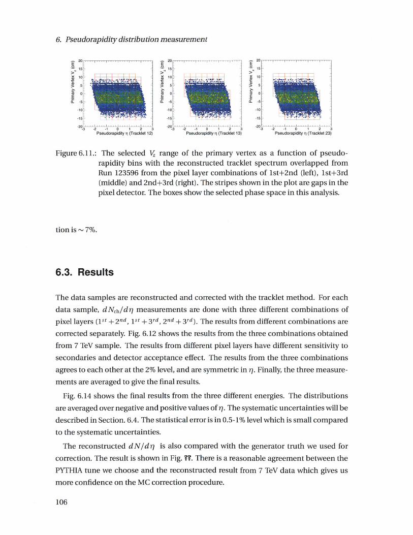
6. Pseudorapidity distribution measurement
201
15
( 10- -5 ~(~
c0 -ME E
CL-5 - C
-10-
-15 s L -udori 11 (rLe 12)
-20 *
Pseudorapidity 11(Tracklet 12)
2015-
10
-5
-10d
-15 L -T _ ' ' "7 _ f -J
-2 0 ' ' ''' ' '' ' ' ' ' 3
Pseudorapidity Tj (Tracklet 13)
20
15
102
5-
0
-5-
-10-
-15
-3 2 -1 0 1 2 3Pseudorapidity il (Tracklet 23)
Figure 6.11.: The selected V range of the primary vertex as a function of pseudo-rapidity bins with the reconstructed tracklet spectrum overlapped fromRun 123596 from the pixel layer combinations of lst+2nd (left), 1st+3rd(middle) and 2nd+3rd (right). The stripes shown in the plot are gaps in thepixel detector. The boxes show the selected phase space in this analysis.
tion is ~ 7%.
6.3. Results
The data samples are reconstructed and corrected with the tracklet method. For each
data sample, dNch/dq measurements are done with three different combinations of
pixel layers (1s + 2 nd, 1 st + 3 rd, 2 nd + 3 rd). The results from different combinations are
corrected separately. Fig. 6.12 shows the results from the three combinations obtained
from 7 TeV sample. The results from different pixel layers have different sensitivity to
secondaries and detector acceptance effect. The results from the three combinations
agrees to each other at the 2% level, and are symmetric in q. Finally, the three measure-
ments are averaged to give the final results.
Fig. 6.14 shows the final results from the three different energies. The distributions
are averaged over negative and positive values of q. The systematic uncertainties will be
described in Section. 6.4. The statistical error is in 0.5-1% level which is small compared
to the systematic uncertainties.
The reconstructed dN/dr, is also compared with the generator truth we used for
correction. The result is shown in Fig. ??. There is a reasonable agreement between the
PYTHIA tune we choose and the reconstructed result from 7 TeV data which gives us
more confidence on the MC correction procedure.
106
..................... . ....... 11 ................................................................................ ................ ...... " I .......... ....... .... ... . ... ....

6.4. Systematic Uncertainties
6-
5
4 -
zZ~ 33--
2-Run132440
- Reconstructed (1 st+2nd layers)1 A Reconstructed (1 st+3rd layers)
-3 Reconstructed (2nd+3rd layers)o ' . I
-3 -2 -1 0 1 2 31l
Figure 6.12.: The reconstructed dN/drl from three different combinations of pixel lay-ers (s'+2nd, 1st+ 3 rd, 2 nd + 3 rd) from Run 132440 (v/=7 TeV). The errorsshown in the figure are dominated by the systematic uncertainties.
6.4. Systematic Uncertainties
6.4.1. Systematic error of the trigger efficiency
To estimate the systematic error of the Monte Carlo based trigger efficiency evaluation
we performed a series of studies.
6.4.1.1. Variation of the diffractive component
To understand the effect of the diffractive component, we vary the fraction of the
diffractive process in the Monte Carlo sample. If we decrease the single-diffractive frac-
tion, the correction factor fSD(M) will be smaller and lead to a larger dNch/drj . The
same trend also applies to the double-diffractive component. If we remove the single-
diffractive component completely, the effect is found to be 6%.
107

6. Pseudorapidity distribution measurement
6- -I I
4-_
2-_ Final result---- 7.0 TeV p+p
o2.36 TeV p+p-+-900 GeV p+p
0 ' ' ' ' ' ' ' ''11 1 1 1 1 1 1 1 1-3 -2 -1 0 1 2 3
1l
Figure 6.13.: The reconstructed dN/dr7 from trackdet method with the final system-
atic uncertainty. The results are symmetrized in rl. The error shown in the
figure is dominated by the systematic uncertainties.
6.4.1.2. Different event selection
We selected the NSD enriched events by requiring a coincidence of energy deposit in the
HF towers (See Section. 5.4). One can change this requirement to BSC based trigger, i.e.
selection on the BSC tirgger bit 40. This requires at least one hit in the both side of the
BSC counter. The selected events are analyzed and corrected with the same procedure
as the HF based analysis.
Fig. 6.15 shows the results from this study. The results are consistent with each other
within 2%.
6.4.2. Systematic uncertainties from algorithmic efficiency correction
The scale factor a which corrects for the reconstruction efficiency, secondary particle
production and acceptance. There are two factors which change the algorithmic effi-
ciency: event mean transverse momentum and tracklet multiplicity.
Events with low mean transverse momentum contain less particles which arrive the
pixel layer and need higher a correction. The effect of the event mean Pr is studied
108
............

6.4. Systematic Uncertainties
7
6-
5-
4-
0 3-
2-Run132440
1 ---- 7.0 TeV p+p by Tracklet (CMS)- e- 7.0 TeV PYTHIA ATLAS tune
-3 -2 -1 0 1 2 3
Figure 6.14.: The reconstructed dN/dr; from tracklet method with the final systematicuncertainty compared with the generator truth from PYTHIA ATLAS tuneat 7 TeV.
by comparing MC samples with different mean PT and samples produced by differentgenerators (PHOJET and PYTHIA). If the mean PT is changed by 10%, the effect is foundto be 0.7%.
Events with high tracklet multiplicity tend to have lower tracklet reconstruction effi-ciency because the probability to connect hits from different charged hadron increases.A proper multiplicity variable is necessary to characterize the event multiplicity. How-ever, different multiplicity variables have different event-by-event resolution and dif-ferent sensitivities to background hits. To study the systematics due to the choice ofmultiplicity variable, the results are checked by using different event multiplicity def-
initions: (1). number of first layer hits, (2). number of tracklets, and (3). number ofbackground subtracted tracklets. The effect is estimated to be 1.0%.
The effect due to the event topology is checked by HYDRO events, which generates
random particles and provides events with different topology compared to PYTHIA gen-erator. The generated events are corrected by PYTHIA MC and the effect due to the
event topology is found to be 0.2%.
We sum the systematic uncertainties due to the algorithmic efficiency linearly and a
109

6. Pseudorapidity distribution measurement
z0
-2 -1 0 1 2 3
Figure 6.15.: The reconstructed dN/dr from tracklet method on MC samples usingBSC bit 40 selection vs using HF coincidence selection. The difference is in
2% level.
1.9% uncertainty is assigned for this. The 0.9 and 2.36 TeV analysis were performed in
an earlier stage of the experiment and a larger uncertain was quoted for the efficiency
correction (3%).
6.4.3. Systematic uncertainties due to the extrapolation to low PT
The extrapolation correction is included in the a correction factor. The agreement be-
tween results from different pixel layer combinations is at the 2% level as shown in
Fig. 6.12. Since the corrections of the PT extrapolation for different combinations are
different, this give us confidence that the systematics due to this extrapolation is small.
We estimate the systematic uncertainties due to the extrapolation to low PT by com-
paring the results from different MC. We quote a 0.2% systematic uncertainty for the
correction.
110
I I I III I I
Run1 32440-ATLAS-7TeV-HF1
7.0 TeV p+p by Tracklet HF Coincidence(CMS)
7.0 TeV p+p by Tracklet BSC Bit4O(CMS)I IO
i e i i i
I I I
_si
:
i
............................................................... .... ................. I
6.4. Systematic Uncertainties
6.4.4. Systematic uncertainties due to vertex resolution
In this analysis, a valid primary vertex is essential and the systematic uncertainty due to
the vertex resolution is checked by smearing the vertex z position by a Gaussian with a
width of 20 microns. The effect is found to be negligible. (<0.5%)
6.4.5. Systematic uncertainties from MC efficiency correction and single
diffractive fraction
The event selection correction factors w, f~sD are obtained from the MC. The uncer-
tainty due to event selection and SD fraction is estimated by varying the SD fraction(fsD(M))
and cross-checked by PHOJET generator. A 3.0%(3.5%) uncertainty is assigned for this
in 0.9 and 2.36 TeV (7 TeV) analysis.
6.4.6. Systematic uncertainties due to the tracklet selection
The effect of the signal region definition is checked by varying the Ar7 and A# selection
criteria. The effect is found to be < 0.1% for changing Aq cut from 0.1 to 0.2. The ef-
fect of signal region and sideband region definition is studied by changing the selection
criteria. If the signal region definition is changed to |A#I < 1.5 and sideband region def-
inition is changed to 1.5 < IA#|< 3.0, the reconstructed d N/d q is changed by 0.5%. A
0.5% systematic uncertainty is assigned for this.
6.4.7. Systematic uncertainties from secondary contribution
The systematic uncertainties from secondary contribution is checked in two ways. The
effect of secondary produced particle from the interaction between charged hadrons
and pixel detectors is checked by changing the GEANT production cut off. The effect is
found to be negligible. (<0.5%)
The effect of secondary particles from strange particles are checked by varying the
fraction of the strange particles. Increasing the strangeness content by 40% will change
the reconstructed dN/drl by 1%.
From those studies, we assign a 1% uncertainty for this.
111

6. Pseudorapidity distribution measurement
6.4.8. Systematic uncertainties from misalignment
The r and # correlations between the first and second layer hits of the pixel detectorare used in the tracklet reconstruction, thus the effect of misalignment becomes moreimportant, i.e. the width of the signal correlation peak will be dependent on the mis-alignment.
Uncertainty due to the misalignment is estimated by comparing the hit distributionsbetween data and MC. The difference in acceptance is found to be in 2% level and wequote this difference as the systematic uncertainty. The uncertainty due to the wideningof the correlation peak is estimated to be in 1% level.
6.4.9. Systematic uncertainties from low PT loopers, beam halo andevent pile-up
To test the effect from the hits of low PT loopers and beam halo, 10 random hits wereadded to the first layer (flat as a function of rj). This increases the average number ofhits in the first layer by 30%. The effect on the final measurement is at the 1% level. Themonitoring of the hit multiplicity as a function of time is important for us to understandthe effect from the beam background.
6.4.10. Systematic uncertainties from pixel hit reconstruction
There is a chance that the pixel reconstruction efficiency in data is actually differentfrom that of the Monte Carlo simulation. To study this effect, we remove reconstructedhits with a probability of 0.5%. The difference in the result is found to be at the 1% level.
For tracks with a very shallow angle, there is a non-negligible probability that the pixelhit will be split into two separate hits. This effect is studied by artificially splitting thepixel hits with a probability of 1%. The effect is found to be 0.4%.
We also check the systematic uncertainty from the hit reconstruction algorithm. Wetune the pixel hit reconstruction algorithm with different templates and thresholds. Thedifference is found to be 0.1%.
6.4.11. Cross-checks from magnetic field off sample
We checked the tracklet reconstruction performance in Run 133242, which is collectedwithout magnetic field at 7 TeV. PYTHI-A MC with ATLAS tune is generated with the same
112

6.4. Systematic Uncertainties
condition for correction. This check allows us to investigate the systematics due to the
loopers and PT extrapolation.
The reconstructed tracklet spectra are shown in Fig. 6.16. We now see a narrow corre-
lation peak in A#. The data and MC are in good agreement.
We follow the same procedure to reconstruct dN/d rl from this sample Fig. 6.17 shows
the results from this run. The results are consistent with Run 132440 which is taken with
magnetic field B = 3.8 T at 2% level.
101 -
10-2
10-3
-0.2 -0.15 -0.1 -0.05
PYTHIA 7.OTeV -
4 I
0 0.05 0.1 0 15 2Tracklet
C:.2 0.I.-CZN
o.0C
2!nCu
25
.2
15
0.05[
0.2 -0.15 -0.1 -0.05 0 0.05 0.1 A0 '15cle 02
,1+2
Figure 6.16.: (Left panel) The comparison of Ar7 spectrum between Run 133242 andPYTHIA ATLAS 7 TeV sample. (Right panel) The comparison of A# spec-trum between Run 133242 and PYTHIA ATLAS 7 TeV sample.
The systematic uncertainties discussed in this section are summarized in Table 6.2.
The estimated total systematic uncertainty for the d N/d q measurement is 4.6%.
113
Run133242
-~ .. 1.. .1.
- Run133242
PYTHIA 7.OTeV
- -i

6. Pseudorapidity distribution measurement
Run133242 B=0-E) 7.0 TeV p+p by Tracklet (CMS)---- 7.0 TeV p+p by Tracklet HF (CMS)
3 - 1 I I I I
3 -2 -1 0 1 2 3
Figure 6.17.: The comparison between magnetic field on (3.8T) and magnet field offresults. The reconstructed dN/d q from Run132440 (B=3.8T) are shown asblack dots while the results from Run 133242 (B=0) are shown as the blackcircles.
Table 6.2.: Summary of systematic uncertainties.
114
Source Correction 0.9 TeV 2.36 TeV 7 TeV (%)Algorithmic efficiency a 3.0 3.0 1.9
PT extrapolation a 0.3 0.3 0.3Pixel hit reconstruction efficiency a 1.0 1.0 1.0
Pixel hit splitting a 0.4 0.4 0.4Acceptance uncertainty a 1.0 1.0 1.0
Correction of secondary particles a 1.0 1.0 1.0Selection and background subtraction #8 0.5 0.5 0.5
Misalignment a, # 1.0 1.0 1.0Correction of looper hits a, # 1.0 1.0 1.0
Random hit from beam halo a, # 0.2 0.2 0.2Effect of event pile-up a, p 0.1 0.1 0.1
Correction on event selection w, fNsD 3.0 3.0 3.5Total 4.9 4.9 4.6

7. Multiplicity distribution measurement
The multiplicity distributions are measured by tracklet (in this thesis) and tracking
methods with the CMS tracker [78]. The tracklet method has lower PT reach such that
the extrapolation correction to zero PT is small. Due to the statistical nature of the
tracklet method, the event-by-event multiplicity resolution is worse than the tracking
method. The tracking method has low fake rate and better resolution on the event mul-
tiplicity. But the requirement of hits in the strip detector limits the low PT reach to - 100
MeV/c such that it has larger uncertainty due to the extrapolation.
This chapter describes a tracklet-based analysis method for the measurement of the
charged hadron multiplicity distribution. In this analysis, the same event selection and
tracklet reconstruction algorithm as the pseudorapidity distribution measurement are
used for the selecting and reconstructing NSD events in p+p collisions. Details can be
found in Section 6.1. Compared to pseudorapidity density analysis which is an mea-
surement of the integrated quantity over all events with different charged hadron mul-
tiplicity, this analysis provides a more detailed information about the multiplicity fluc-
tuation. In order to correct the observed raw spectrum to the multiplicity distribution,
an unfolding procedure which use the information from the Monte Carlo simulation is
necessary.
This analysis contains three major steps:
1. Raw spectrum reconstruction
2. Bayesian unfolding
3. Event selection correction and single-diffraction component subtraction.
They will be discussed in detail in the following sections. The systematic uncertainty
studies are detailed in Section 7.4.
115

7. Multiplicity distribution measurement
7.1. Raw spectrum reconstruction
The multiplicity distribution requires a multiplicity variable for each event in order
to extract the multiplicity fluctuation. For each event, reconstructed tracklets with
|Ar/|<O.1 are selected for analysis. In order to estimate the background contribution,the 1 < |A#|I < 2 region is chosen to be the sideband region for combinatorial back-
ground estimation and |AL I < 1 to be the signal region. Using this sideband method,
one can estimate the uncorrected event by event multiplicity(M) by:
M=NS-NSB (7.1)
where NS(SB) is the number of tracklets in the signal(sideband) region. The event by
event multiplicity M is used as an input to the unfolding process to get the correct mul-
tiplicity distributions.
Fig. 7.1 shows the uncorrected tracklet multiplicity spectrum with the first and second
pixel layers for the three different energies. The raw spectrum needs to be corrected for
the effects due to the detection.
7.2. Correction of detection effects
In order to correct the effect of tracklet reconstruction efficiency, contribution from the
secondaries and detector acceptance, Bayesian unfolding technique is selected to cor-
rect the tracklet multiplicity distributions to the true multiplicity distributions. Since
this method is an iterative process and unfolded results usually converge very quickly,
it can avoid complicated matrix inversion procedure as well as computing intensive fit-
ting (such as 2 unfolding method). However, due to its iterative nature, one needs to
check the statistical uncertainty carefully.
7.2.1. General concept of unfolding problem
The ultimate goal of the physics measurement is to get the physics quantity with de-
tector effect removed. If one has a true spectrum (T) as a function of physics quantity
(t), the observed spectrum (M) as a function of detection variable (m) is recorded in the
detector level. The observed spectrum is usually convoluted by detector effects such
as detector efficiency, detector resolution, and transportation which is demonstrated in
Fig. 7.2. The relation between the true spectrum and observed can be written as the
116

7.2. Correction of detection effects
following:
Mm ZRmt T (7.2)t
where Rmt is the response matrix which accounts for the detector effects. From the
expression above, the true spectrum can be calculated by:
Ut ZR-tMm (7.3)
However, the inverse matrix may not exist because Rmt can be singular. Even if the
response matrix can be inverted, the unfolded result (Ut) from Eq. 7.3 usually exhibit
oscillation behavior due to the amplification of the statistical fluctuation during the cal-
culation.
Another option is to use numerical approach to solve this problem. For example, one
can use a X2 minimization method to obtain the unfolded results. A X2 function can be
defined by
X2(U= (Mm - Rmt Ut) (7.4)t m
and a minimization program is used to tune the Ut until the minimum x2 is found. If
the Ut is the same as T, the X2 will be 0. This approach is usually computing intensive
because of the large number of the tunable parameters. If the X2 minimization is per-
formed without proper regularization, the unfolded distribution will still exhibit strong
oscillation behavior.
In the following sections, an unfolding method which is based on the Bayes' theorem
will be discussed. The advantage of this method is that it is an iterative algorithm which
is not involved in numerical minimization or matrix inversion. Usually, the conver-
gence of the result is very quick, and limited number of iterations provides an implicit
regularization.
117

7. Multiplicity distribution measurement
7.2.2. Bayes' Theorem
Bayes' theorem expresses the conditional probability in terms of the prior probabili-
ties (or called unconditional probabilities), which is widely used to calculate the inverse
probability from a known conditional probability. For example, there is a measurement
(M) and a physics input (T). If M has a non-zero probability, the conditional probabili-
ties satisfies the following relation:
P(TIM) = P(MI T)P(T)P(M)
where P(M) and P( T) are the prior probabilities of M and T, P(MI T) is the conditional
probability of M given T, P( TIM) is the conditional probability of T given M.
As shown in Fig. 7.3, the conditional probabilities can be expressed as:
P(TIM) = P(MnT) (7.6)P(M)
P(MIT) P(M n T)P(T)
By using Eq. 7.6 and Eq. 7.7, we can derive the Bayes' theorem:
P(TIM)P(M) = P(MnT) = P(MIT)P(T) (7.8)
P(T|M) = P(MIT)P(T) (7.9)P(M)
In case of several independent physics inputs (T, t = 1, 2, ... , n,) and several mea-
sured values (Mm, m = 1, 2, ..., n m), the Bayes' theorem can be stated as:
P(TIMm) = P(MmIP(T) (7.10)P(Mm)
t P(Mm I TP(t) (7.11)
However, the P(T) is the unknown which is to be extracted, as suggested in [79, 80],an unfolding procedure is introduced as follows. If we assume that P( T) is known in thebeginning (Po(Tt)), then based on the Eq. 7.12 the conditional probability P(TtIMm) can
118

7.2. Correction of detection effects
be calculated by:
P, P(Mm|I Tt)Po(NT)
where Po(T/) is the initial prior probability, which can be an uniform distribution or
a distribution predicted by generator. The unfolded distribution after the first iteration
can be calculated by
P1(T) = jP(TlMm)P(Mm) (7-13)
One can repeat this procedure to calculate the unfolded distribution P, for the nth
iteraction. From the Monte Carlo study, it is shown that Pn(T) is moving closer to the
real spectrum P(T).
7.2.3. Unfolding procedure
In this analysis, the physical quantities t is the charged hadron multiplicity, the mea-
surement m is the event by event tracklet multiplicity. From the discussion in the last
section, one can recognize that P( T) is the charged hadron multiplicity distribution (Tt)
and P(Mm) is the raw spectrum(Mm). P(Mm ITt) is the response matrix(Rmt) which de-
scribes the physics and detector effects. This unfolding procedure contains the follow-
ing four steps:
1. Start with the PYTHIA generator multiplicity distribution (or a flat distribution for
cross-check) as a prior distribution (Pt), calculate the smearing matrix (Rtm) by
f = RmtPt (7.14)" L, Rmt'Pt'
2. Calculate the unfolded distribution with the smearing matrix by using the mea-
sured tracklet multiplicity spectrum (Mm):
Ut =Z htmMm (7.15)m
119

7. Multiplicity distribution measurement
3. Replace the prior distribution Pt by Ut and go back to step 1 for several iterations.4. After the unfolded distribution converges (changes between iterations are much
smaller than statistical error), the event selection efficiency(et) and single-diffractivefraction(ftD) corrections are applied to get the final multiplicity distributions U':
(1 -ffD)
U,'= - Ut (7.16)Et
Fig. 7.4 shows the event selection efficiency Et and single-diffractive fraction ffD. Theevent selection efficiency is mainly driven by the vertex reconstruction efficiency. Thesingle-diffractive fraction correction only affects the low multiplicity part and the typi-cal correction factor is 0 - 20%.
7.3. Multiplicity distribution measurement
Tracklet multiplicity spectra from the 1st+2nd, 2nd+3rd and lst+3rd layers are cor-rected and averaged to obtain the final multiplicity distributions. The charged particlemultiplicity distributions are measured in increasing bins of pseudorapidity.
The statistical error is checked by varying the raw spectrum according to the Poissondistribution around the center value of each bin to study the effect of statistical fluctu-ation. Each generated raw spectrum is unfolded with 50 iterations because in the largeiteration limit, the unfolded result will be approaching the exact solution from matrixinversion method. The statistical errors are determined by a Gaussian fit on the pulldistributions obtained from the pseudo-experiments.
The fully corrected results from 0.9, 2.36, 7.0 TeV samples are shown in Fig. 7.5. Theerror bar shown in the plots included the statistical and systematical uncertainty whichwill be discussed in the next section.
7.4. Systematic Check
7.4.1. Uncertainty due to the algorithmic efficiency and acceptancecorrections
The uncertainties associated to the algorithmic efficiency and acceptance correctionsare summarized in table 7.1. The total systematic error from reconstruction efficiency
120

7.4. Systematic Check
correction is found to be 2.6%(2.9%) with (without) magnetic field.
In order to check the effect of the efficiency uncertainty to the multiplicity distri-
bution measurement, a Toy MC study is performed by varying the reconstruction effi-
ciency by 2.6%. The differences of the reconstructed results are quoted as the systematic
errors. The systematic uncertainty as a function of Neh is shown in Fig. 7.6 and obtain
the final uncertainty in the multiplicity distribution.
Source 7 TeV (%)Algorithmic efficiency 1.6
PT extrapolation 0.3Pixel hit reconstruction efficiency 1.0
Pixel hit splitting 0.4Acceptance uncertainty 1.0
Correction of secondary contribution 1.0Tracklet selection and background subtraction 0.5
Misalignment 1.0Random hit from beam halo 0.2
Total 2.6
Table 7.1.: Summary of systematic uncertainties related to thetance correction.
efficiency and accep-
7.4.2. Uncertainty due to the unfolding procedure
The unfolding procedure is checked by varying the number of iterations. The effect is
found to be 0 - 5% level which is much smaller than the other uncertainty. The effect
of the prior assumption is also checked by using a flat prior distribution, the effect is
found to be in 0 - 5% level.
7.4.3. Uncertainty due to the event selection and SD fraction correction
The uncertainty due to the event selection efficiency and SD fraction correction is stud-
ied by comparing the corrected result with PHOJET MC and with PYTHIA MC because
these two models have pretty different SD definitions. We quote the difference as the
systematic error. The systematic uncertainty as a function of Nch is shown in Fig. 7.6 for
7 TeV and Irl< 2.0. This uncertainty is the dominant systematics in the low multiplicity
region.
121

7. Multiplicity distribution measurement
7.4.4. Cross-checks between different layers
The results from 1st+2nd, 1st+3rd and 2nd+3rd pixel layers are obtained indepen-
dently by different response matrices and are compared to each other. This check helps
to understand the uncertainty due to the algorithmic efficiency, PT extrapolation and
the correction of the secondary produced particles. Fig. 7.7 shows the results from 7
TeV sample. The agreement is found to be within 10-20% in the high multiplicity region
which is well covered by the total systematic uncertainty.
7.4.5. Cross-checks between magnetic field on / off sample
In order to check the effect of looper hits and magnetic field, results with and without
magnetic field are checked. The unfolded distributions from the two samples at 7 TeV
in the high multiplicity region are consistent within 25 % level which is covered by the
total systematic uncertainty.
7.4.6. Uncertainty due to event pile-up
The systematics due to the event pile-up is studied by randomly merging two event with
a probability of 2%. The contribution from the pile-up event is largely rejected in the
tracklet reconstruction procedure. The uncertainty due to the event pile-up is found to
be negligible compared to other systematics.
122

7.4. Systematic Check
~tiI~jI .1 I
0 20 40 60 80 100 120 140hb<2.0 (0.9TeV B=3.8T)
0 20 40 60 80 100 120 140h|<2.0 (7.OTeV B=3.8T)
10--
Figure 7.1.: Raw multiplicity distributions from 0.9, 2.36, 7.0 TeV samples taken with orwithout magnetic field.
123
0 20 40 60 80 100 120 140
hl<2.0 (2.36TeV B=3.8T)
lt,
,I , ,
0 20 40 60 80 100 120 140h|<2.0 (7.OTeV B=O)
10-3
10-4
1U5
10-2
10-3

7. Multiplicity distribution measurement
0 20 40 60 80 100120140160180
Nch (h|<2 .0)
0.3
0.20.10
Figure 7.2.: The response matrix obtained from PYTHIA 7 TeV MC.
Figure 7.3.: Venn diagram of the measurement(M) and physics input(T) in the proba-bility space (.2))
124
0.9
0.8
0.7

7.4. Systematic Check
- -
0 5 10 15 20 25 30Nch (7.0 TeV)
.8-
.6-
.4-
. - 0S 0
0L I ,,~,I:,~.I,
0 5 10 15 20 25 30NCh (7.0 TeV)
Figure 7.4.: (Left Panel) The event selection efficiency (c) as a function of Nch with
Irjl<2.0. (Right Panel) The single-diffractive fraction (fSD) as a function ofNch with J1<2.0.
125

7. Multiplicity distribution measurement
1 2'0 102z(L 10
1
2--0U-
10-1
10-2
10-3
10~4
10-5
10-6
10-7 0)
0z
00L-
20 40 60 80 100
b102 ' ''
z 7.0 TeVCL 10-
1
+--+ 1q32.0 (x 1000).0 04 -
n 10-10++ I1-5 .1O0) -I-C- 10-2 +
10-3 ._I<. ++ 10 +-
10-4 - h (x 1) ++t -+ t
10-5 +106t t-tt10-
0 20 40 60 80 100 120 140 160 180NCh
Nch
Figure 7.5.: Corrected multiplicity distributions from 0.9, 2.36, 7.0 TeV samples takenwith or without magnetic field.
126
0.9 TeV
<MI2.0 (x 1000)
- <111.5 (x 100)
ITik1.0(x 10) --
+ $1<05 (x 1)-t- +-+
- - + -
1--tt
r I I I I f

7.4. Systematic Check
o 1.5
414-C,
z
1.3-
1.2 --
0.9 ''' '0 20 40 60 80 100 120 140 160 180
Nch (7.0 TeV)
Figure 7.6.: The ratio of P(Nh) with lr/<2.0 before and after varying the reconstructionefficiency by 2.6%.
1za- 10-1
10 -2
10 3
10-4
10-5
10-6
1 20 40 60 80 100 120 140 160 180
3 9 (1st+ard) / (1st.2nd)-ch ch
N(2nd+
3rd) / (1 st2nd)
ch ch
0 20 40 60 80 100 120 140 160 180Nch
Figure 7.7.: (Left Panel) Reconstructed Nch from three different combinations with 7TeV data sample. (Right Panel) Ratios of reconstructed Nch.
127
7.0 ToV, hl<2.0Reconstructed (1 st
- Reconstructed (1 stReconstructed (2nd
I, 1 1 1. . 1 L J lI. c .I , , , I I . - ,
+2nd layers)+3rd layers)+3rd layers)
,I l I I I I I ,

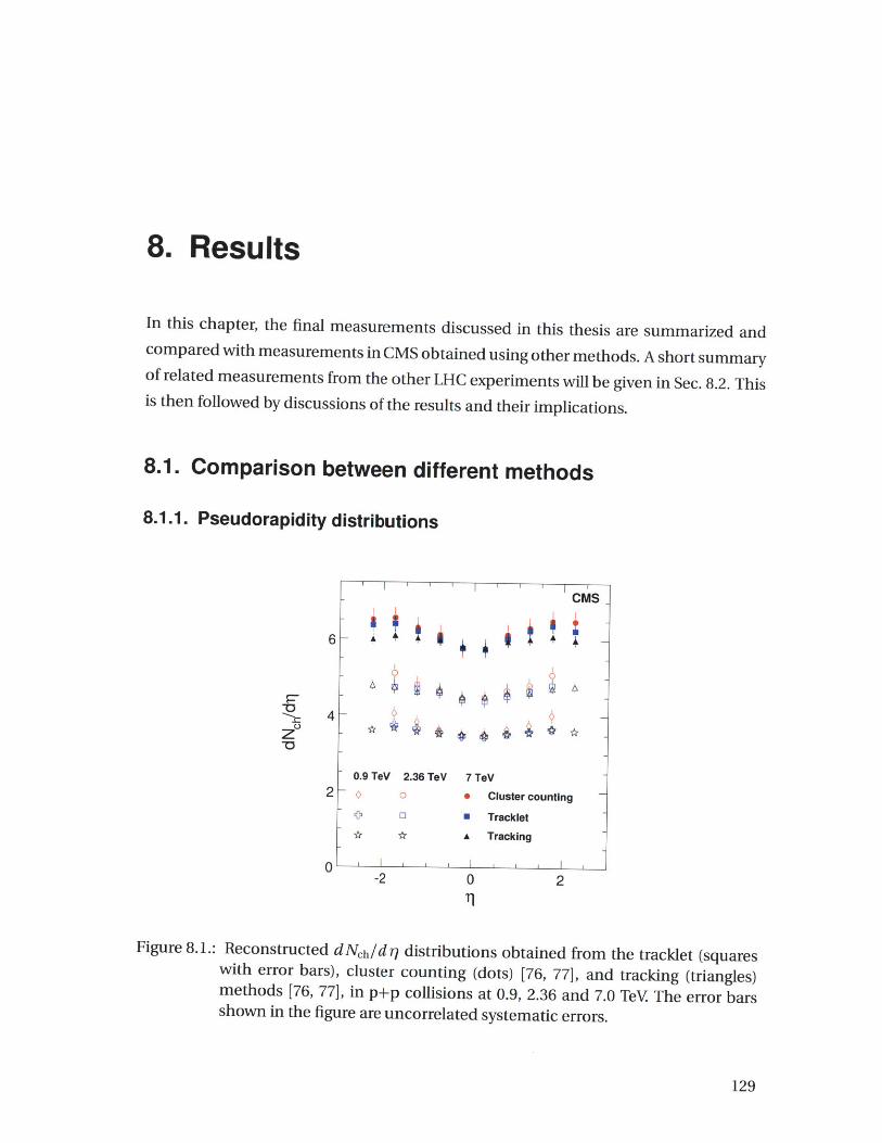
8. Results
In this chapter, the final measurements discussed in this thesis are summarized and
compared with measurements in CMS obtained using other methods. A short summary
of related measurements from the other LHC experiments will be given in Sec. 8.2. This
is then followed by discussions of the results and their implications.
8.1. Comparison between different methods
8.1.1. Pseudorapidity distributions
P,-o
11
Figure 8.1.: Reconstructed dNch/dr) distributions obtained from the tracklet (squareswith error bars), cluster counting (dots) [76, 77], and tracking (triangles)methods [76, 77], in p+p collisions at 0.9, 2.36 and 7.0 TeV. The error barsshown in the figure are uncorrelated systematic errors.
129
CMSI I | I
0.9 TeV 2.36 TeV 7 TeV
0 0 Cluster counting
40 [ 0 Tracklet
* * A Tracking

8. Results
The measured dNch/dri from the tracklet method in this thesis are compared with
the pixel cluster counting method [76] and tracking method [76]. The strengths and
weaknesses of each method are discussed in Chapter. 6. Fig. 8.1 shows the summary
of results on pseudorapidity density distributions. The three methods are consistent
within 4%. There is a trend of increasing discrepancy as a function of pseudorapidity.
This may come from the increasing fraction of the background hits in the forward region
and the acceptance correction.
To minimize the systematic uncertainties, results from the three methods are aver-
aged to produce the final result in the publication [76, 77]. The averaged CMS results
are shown in Fig. 8.2 and compare with other experiments.
0gZ."a
Figure 8.2.: Distributions of dNch/d q, averaged over the three measurement methodsand compared with data from UA5 [24] (p+p, with statistical errors only)and ALICE [81] (with statistical and systematic uncertainties). The shadedband shows systematic uncertainties of the CMS data. The CMS and UA5data are averaged over negative and positive values of rj.
8.1.2. Multiplicity distributions
In Fig. 8.3, the measured multiplicity distributions from the tracklet method is com-
pared to the tracking method [78]. At Is =7 TeV, the tracklet measurement are higher
than the tracking results in the high multiplicity region at v =7 TeV, but the difference
130
CMS
7 TeV 9
2.36 TeV
0jg dGO 00 9@Pj
0.9 TeV
- 0 CMSNSD
A ALICE NSD
0 UA5 NSD
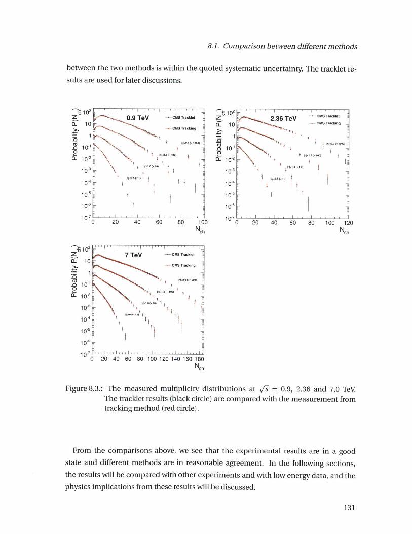
8.1. Comparison between different methods
between the two methods is within the quoted systematic uncertainty. The tracklet re-sults are used for later discussions.
102Z - 0.9 TeV CMS TrackletCL 10 r1 - CMS Tracking
0 10 -
0 10-2
10-3
10-4 -
10-5
10~6
10 -7 ' ' ' '' ' '
0 20 40 60 80 100Nch
z
-
-0
0-
102
10
1
10-1
10-2
10-3
104
10-5
10-6
10-7 0 20 40 60 80 100 120
'102z
Q. 10
D 14-0 10-20
10-2
10-5
10-6
10-70
2.36 TeV -CMCM
. \61
20 40 60 80 100 120
Nch
140 160 180NCh
Figure 8.3.: The measured multiplicity distributions at 1~s = 0.9, 2.36 and 7.0 TeVThe tracklet results (black circle) are compared with the measurement fromtracking method (red circle).
From the comparisons above, we see that the experimental results are in a goodstate and different methods are in reasonable agreement. In the following sections,the results will be compared with other experiments and with low energy data, and thephysics implications from these results will be discussed.
131
S Tracklet
S Tracking
In1k2
.0(. 1000)
z-I~
7 TeV CMS Tracklet
CMS Tracking
jiIj2.0(x 1000)
| 1<1.5(x100)
09 1 .0 ( 10)t
IiI<0.0 (x 4
- -~
I I I

8. Results
8.2. Comparison with other experiments
8.2.1. Results from other LHC experiments
The ALICE (A Large Ion Collider Experiment) detector measured inclusive and NSDcharged hadron multiplicity distributions and dNch/drl from p+p collisions at v =0.9 and 2.36 TeV during the commissioning of the LHC [81]. The main detector usedin the analysis was the Silicon Pixel Detector (SPD), which covered a range of IqI < 1.4,and the two scintillation hodoscopes (VZERO), which covered the region 2.8 < rl < 5.1and -3.7 < rl < -1.7. The minimum-bias trigger used in ALICE was at least 1 hit in theSPD or VZERO and in coincidence with the signals from the two beam pick-up coun-ters indicating the presence of two passing proton bunches. During the 2.36 TeV datataking, the VZERO detector was not turned on. Therefore, the trigger conditions anduncertainties differ slightly from the 0.9 TeV analysis [81]. For the NSD measurement at
s = 0.9 TeV, a subset of the sample were selected by requiring a coincidence betweenthe two sides of the VZEROs to minimize the contamination from the SD events.
The charged particle multiplicity was reconstructed with a tracklet method, which issimilar to the technique used in the PHOBOS experiment and in this thesis. This alsolimited the pseudorapidity reach to the acceptance range of the SPD. The results werecorrected for tracking efficiency, detector acceptance, and secondaries. The multiplicitydistributions were measured by an unfolding technique based on a regularized y2 fit.The results were cross-checked by a Bayesian unfolding method.
The ATLAS (A Toroidal LHC Apparatus) detector measured charged hadron multi-plicity distribution and d Nch/drl from p+p collisions at VI = 900 GeV during the com-missioning of the LHC [82]. The events were triggered by a single-arm trigger and atotal of 455,593 events were collected. The measurement was done with the inner track-ing system. However, the measurement was mainly for PYTHIA model tunning. Onlycharged particles with PT > 500 MeV/c were included in the measurement in orderto minimize the model dependence of the event classification, diffractive componentand PT extrapolation. The results were compared with calculation from several PYTHIAtunes and the PHOJET generator [82]. This choice made comparison to previous ex-periments and analytical models impossible. The results from ATLAS are not furtherdiscussed.
132

Table 8.1.: Summary of the LH C experiments. The symbol o indices that measurements of d Nch/dTj (or multiplicity distributions)
is available in this experiment.
Exp. s (GeV) Type dNch/drY Multi. Trigger Nev PT reach Ref.
CMS 900,2360(p+p) NSD o incl./2-arm 40k, Ilk 30 MeV [76]7000(p+p) NSD o incl./2-arm 55k 30 MeV [77]900,2360,7000(p+p) NSD 0 incl./2-arm 100 MeV [78]
ALICE 900,2360(p+p) INEL/NSD o o incl./2-arm 150k,40k [81]
ATLAS 900(p+p) other o o 1-arm 456k 500 MeV [82]

8. Results
8.2.2. Comparison between experiments
Fig. 8.4 shows the comparison between the CMS NSD dNch/dr and previous experi-
ments as well as the ALICE measurement. Our result on p+p collisions at /s = 0.9 TeV
agrees with UA5 measurement (p+p) at the 1-3% level. This shows that the averaged
charged hadron production is similar in p+p and p+p collisions.
The ALICE collaboration also measured the inelastic and NSD p+p collisions at V =
0.9 and 2.36 TeV. The 0.9 TeV results are slightly higher than our results, while the two
experiments are in good agreement at /s = 2.36 TeV. It has to be noted that different
trigger conditions were used in the two ALICE measurements. Overall, the dNch/dr
results from ALICE are consistent with our results at the 1-5% level and the differences
are within the quoted systematic uncertainties.
We also compared the multiplicity distribution measurements with results from UA5
and ALICE, which are shown in Fig. 8.5. Generally the results are consistent between
different experiments. The results from CMS and ALICE have a peak at Nh = 0 which is
different from the UA5 results. This is because of the different treatment of the diffrac-
tive component, i.e., CMS and ALICE used the PYTHIA definition for the correction,
while UA5 used their own event generator. At [s = 2.36TeV, there are wavy structures
at Neh(Ir| < 1.0) ~ 30 and Nch(I)| < 0.5) ~ 30 which are due to statistical fluctuations.
There is no wavy structure found in the 7 TeV result.
8.3. Discussions
8.3.1. dNch/drl structure and the central platau
The dNch/drl results from 0.9, 2.36 and 7.0 TeV shows a dip at the mid-rapidity (|I -0),
which is similar to the behavior in lower energy measurements. The only dNch/dq
measurements which show a flat pseudorapidity distribution without a dip are the re-
sults from UA5 at vs = 53 GeV. From a PYTHIA generator study (Fig. 1.2), it is found
that the width of the dNch/dy is narrow such that the transformation from dNch/dy
to dNch/d q accidentally flattened the distribution. The ratio between dN/d q at |rqI=2
and 0 is similar to the previous measurements from 0.2 - 0.9 TeV, unlike the large dip
seen in CDF results at #= 0.63 and 1.8 TeV.
The ratio between dNch/dq at |rj| = 0 and |q| = 2 is ~ 0.92 at V = 7.0 TeV. The
PYTHIA and PHOJET generator (See Sec. 1.3) studies give ratios between 0.82 and 0.84
if the dNch/dy is flat as a function of y. It implies that the dNch/dy at |yl ~ 0 is
134

8.3. Discussions
-6 -4 -2 0 2 4 6
Il
Figure 8.4.: dNch/dr7 distribution compared with lower energy data
roughly 10% higher than at ly I - 2. There is no evidence of a flat platau in dNch/dy in
p+p collisions at Ks =7 TeV.
8.3.2. v/s dependence
From Fig. 8.4, it is evident that the dNch/d?7 in the CM frame is increasing in all pseu-dorapidity ranges as a function of centre-of-mass energy of the collision. Also the dis-tribution becomes wider because of the increasing rapidity difference between the two
protons.
Fig. 8.6 shows the dNch/dr) 11qI1o as a function of I. Clearly, Feynman scaling isviolated. At 0.9 TeV, the p+p result from this thesis can be compared with UA5 mea-surement on p+p collisions. At 2.36 and 7.0 TeV, the raising dNch/dq continues anddeviates from the linear parameterization a + b lns significantly. The second order
135
I1 I I I 1 1 1 1 1 1 1 1 I_ e pp CMS NSD 7000 GeV
M pp CMS NSD 2360 GeV~ 0 pp ALICE NSD 2360 GeV- A pp CMS NSD 900 GeV * --A pp ALICE NSD 900 GeV
- 0 pP CDF NSD 1800 GeV *-0 pp UA5 NSD 900 GeV-0 plYCDF NSDB630 GeVo pl P238 NSD 630 GeV
~ p5 UA5 NSD 546 GeV-0 ppUA1 NSD 540 GeV- A pP UA5 NSD 200 GeV -
0 pT UA5 NSD 53 GeV T6
~- 0 065 OO~I 0 060
- 6 666666
- o:~AA 0 66. AA
*0 0A AA
( 0 0 AA 0
-I AA AA A AA IA0

0
-0
0-
>6102
C. 10
10-
M 10.10
CL 1O-2
10 3
10
10-5
102
10
1
10-2
102
106
10-720 40 60 80 100 120
Nch
The measured multiplicity distributions at vi = 0.9 and 2.36 TeV. The re-
sults are compared with the data from ALICE (pp) [81] and UA5 (p+p) [44,
45] at the same energy.
parametrization a + b in s + c in S2 describes the observed data reasonable well.
In the figure we also included the fit with a x s I, which was motivated by the Satura-
tion Model described in Sec. 1.4.6. More details can be found in [33].The dashed blue
line is the result from a fit to all available NSD data, while the green solid line is from a fit
to CMS NSD data only in order to check the validity of the extrapolation from high en-
ergies to lower energies. The blue line shows nice description of the experimental data
and the extrapolated value at ~s =14 TeV is close to the result from second order Ins.
The green line which uses only CMS data also gives reasonable description to the low
energy data, but starts to under-predict the dNch/drj at 'F~ 100 GeV. The extracted
A value, which describes the energy dependence of the saturation scale Qsat ~ 1/XA, is
~ 0.23 - 0.25 which is slightly lower than the value (0.288) determinated by the HERA
data.
The successful description of the existing data from a + b lns + c ln s2 and Satu-
ration model motivated parametrization also strengthen the extrapolation to p+p at
~s= 14TeV (dNch/dr q- 6.5-6.8) and interpolation at I = 2.76 TeV (d Nch/dr - 4.54)
and F = 5.5 TeV (dNh/d q ~ 5.3). The agreement between data and Saturation mod-
els also gives us more confidence to the prediction (extrapolation) of the dNch/dr) of
Pb+Pb collisions at s = 2.76 and 5.5 TeV.
136
8. Results
20 40 60 80 100Nch
Figure 8.5.:
-236 TeV scEALICE
4--
4 +
M120t00
I I00I
' '
'

8.3. Discussions
0
0
z-o
102 N/ [\!S [GeV]
1Wo
Figure 8.6.: dNch/dl l1,1o as a function of v/s.
8.3.3. Limiting fragmentation and extended longitudinal scaling
Fig. 8.7 shows the dNch/drl distributions plotted in the rest frame of one of the protonbeams. Although the pseudorapidity range in this measurement is limited in Iril < 2.5and can not probe the fragmentation region directly, it is clear that if the Extended Lon-
gitudinal Scaling still holds, the the limiting curve is not a straight line.
8.3.4. KNO violation
The results from 0.9 and 7 TeV are plotted in the KNO variables. Fig. 8.8 shows the com-
parison between the multiplicity distributions in three different pseudorapidity ranges
from UA5 data at v/~ = 0.2 TeV [45] and CMS measurements. The KNO scaling seems tohold between the three energies if we limit ourselves in IrlI <0.5.
Strong KNO violation is observed in the pseudorapidity ranges of Jil < 1.5 and 2.0.With increasing energy, the peak of the distribution moves closer to 0 while the tail part
137
-- K UA1 NSD CMS- V STAR NSD
- A UA5 NSD
- U CDFNSD
_ * ALICE NSD
CMS NSD
- -------- 2.716 - 0.307 In s + 0.0267 In
--------- -0.406 - 0.282 In s
---------- 3.60 ( s )0.1144
1000
3.59 S \o.1237100 /
2

8. Results
0
-0
0
-- A
- a
-- 0O
I I I I
pp CMS NSD 7000 GeVpp CMS NSD 2360 GeVpp ALICE NSD 2360 GeVpp CMS NSD 900 GeVpp ALICE NSD 900 GeVp5 CDF NSD 1800 GeVpp UA5 NSD 900 GeVpp CDF NSD 630 GeVpp P238 NSD 630 GeV 6 0
pp UA5 NSD 546 GeV 6 6 11:pp UA1 NSD 540 GeV 0pp UA5 NSD 200 GeV 006pp UA5 NSD 53 GeV Q
:0 " R:0
II I
1 2 3 4 5 6 7 8 9l+YB
10
eam
Figure 8.7.: d Nch/d7 distribution in the lab frame of the proton beam.
becomes wider. Also the distribution at 7 TeV shows a kink structure at z ~ 1. Appar-
ently, the distribution at 7 TeV can not be described by two NBD fit. More NBD com-
ponents may be needed to describe the extended tail, which may correspond to event
classes with large number of multiple parton interactions. More detailed studies are
needed to understand the extended tail.
It's not obvious why the physics near l ~ 0 should be different from 0.5 < Ir|j < 1.5
in high energy p+p collisions. One possible explanation of the KNO scaling in |n| <
0.5 is the following: In case of limited acceptance range, the mean of the multiplicity
distribution is closer to zero. There will be limited separation power to distinguish two
NBDs from a single NBD such that it's hard to extract information about the dynamics
from it. In the limit of zero acceptance, the multiplicity distribution will always look
similar no matter how many event classes are present in the data.
138

8.3. Discussions
1 0 -5 1' '' '' ' ''I I I I0 1 2 3 4 5 6 7 8 9
-- 10-4
10-510 0 1 2 3 4 5 6 7 8 9 10
z
i - 1 , , , I .. .I . . I , , I . I I , , I .. .
0 1 2 3 4 5 6 7 8 9 10z
Figure 8.8.: The measured multiplicity distributions in KNO variable. The results fromCMS are compared with the measurement from UA5 at vs =0.2 TeV [45].
8.3.5. Comparison with event generators
Fig. 8.9 shows the comparison between the CMS measurements and the model predic-
tions. A summary of the predictions (posdictions) from extrapolations, generators, and
analytical models is given in Fig. 8.10. The extrapolation by a second order polyno-
mial of logs gives good description of the data, while the extrapolation from a + b logs
under-predict the pseudorapidity density and the ratio of the d Nh/d r at s= 0.9 and
7.0 TeV.
The commonly used PYTHIA D6T [10] and Perugia-0 [83] tunes, which was tuned
with CDF data, predicted a much lower dNch/d r than the experimental data at v/s =0.9, 2.36 and 7.0 TeV The PYTHIA ATLAS tune [84] and PYTHIA8 (default) describe the
139
|7|<0.50 pP UA5 NSD 200 GeV
0 pp CMS NSD 900 GeV -
pp CMS NSD 7000 GeV-
006
-1|<1.5
0 pp UA5 NSD 200 GeV
o pp CMS NSD 900 GeV -
pp CMS NSD 7000 GeV
-E
fg|<2.0pp CMS NSD 900 GeV
pp CMS NSD 7000 GeV

8. Results
observed dNch/dr) and the ratio reasonably well from 0.9 to 7.0 TeV, but underestimate
the dNch/dr for p+p collisions at vs < 0.9 TeV The dNch/dq from PHOJET roughly
increases linearly as a function of logs which follows the raising of the dNch/dr) from
53 GeV to 0.9 TeV, but doesn't describe the rapid raising from 0.9 TeV to 7.0 TeV.
0Z
zo
102 10 3\/s [GeV]
104
Figure 8.9.: dNch/dr) 11,|~-o as a function of /s compared to PYTHIA and PHOJET.
The multiplicity distribution in PYTHIA is controlled by the infrared cutoff (Qo) of the
parton-parton scattering cross sections and the shape of the proton. Those factors are
closely related to the average number of the multiple parton interaction(MPI) and its
fluctuations. Changing the parton distribution function from CTEQ5L to CTEQ6L has
little effect on the multiplicity distribution.
To characterize the parton spatial distribution inside the proton, the PYTHIA Perugia-
0 chooses a exponential form, while the D6T, ATLAS, Z2 and PYTHIA8 use a double-
Gaussian. The parton spatial distribution in Perugia-0 and D6T features a narrower
parton spatial distribution, while ATLAS and Z2 tune are wider. The infrared cutoff(Qo)
in Perugia-0 and D6T are higher and describe the multiplicity fluctuation measured in
140
- ) UA1 NSD - PYTHIA ATLAS CMSV STAR NSD - PYTHIA D6T
A UA5NSD
N CDF NSD - PYTHIA8 Default
- * ALICE NSD - PHOJET
CMS NSD
--------- 2.716 - 0.307 In s + 0.0267 In2 sI I Iii 'I I I t I II

8.3. Discussions
0 1 2 3 4
Figure 8.10.:
5 6 7
dNWdh '=O
-PYTHIA6 Perugiao -- PYTHIA6 ProQ2O -
-PYTHIA6 ProPTO U
- PYTHIA6 DW -
-PYTHIA6 D6T -
- PYTHIA6 ATLAS MCOB -
-PYTHIA8 -
- PHOJET -
-Kaidalov, Poghosyan (QGSM) *- Gotsman, Levin, Maor (GLMM) --Levin, Rezatan (Gluon Saturation) -- Likhoded, Luchinsky (Reggeon) --Sarkisyan, Sakharov (Energy dissipation) ---
- ln4s extrapolation -+---Busza (Extrapolation) -- HIJING INEL u-ALICE INEL,,h,, h-
- CMS NSD a -
-0.4 -0.2 0 0.2 0.4 0.6 0.8 1
(dN /dIl 7TeV)/(dN /Chi .9TeVch 1=0 ch T1=0
(Left Panel) dNch/drj l|rjV-o at v/s = 7.0 TeV compared to theoreti-cal and phenomenological calculation. (Right Panel) The increase ofdNch/dr} from /~s = 0.9 TeV to 7.0 TeV compared to theoretical and phe-nomenological calculation [85-89].
CDF [10, 83], while the cutoff in ATLAS, Z2 and PYTHIA8 are lower which allows moreMPIs.
Fig. 8.11 shows the multiplicity distributions at vl = 7 TeV compared with the pre-dictions from PYTHIA and PHOJET generators. The PYTHIA D6T, Perugia-0, and PHO-JET predicted smaller multiplicity fluctuation than data which is due to the higher in-frared cutoff. The ATLAS tune over-estimates the multiplicity fluctuation. The PYTHIA8,which contains new diffraction model and lower infrared cutoff, describes the high mul-tiplicity tail reasonably well. The Z2 tune, which is created after the 7 TeV measurementwas made, also features a lower Qo and reproduce the observed multiplicity fluctua-tion. The PYTHIA D6T and Perugia-0 tunes also under-predict the dNch/drj by ~ 40%at K =7 TeV.
Fig. 8.12 shows the zoom-in of the multiplicity distributions at low Neh region. The
region contains contributions from the double-diffractive process. The PYTHIA6 tunes
used a simple model for the diffractive processes which doesn't include central diffrac-tion and hard diffractive events, while the PYTHIA8 generator used a improved diffrac-tion model which is closer to the implementation in PHOJET. It is found that the D6Ttune has the best agreement with the data. The predictions from PYTHIA8 and PHOJETare similar at low Neh region, under-predict the Neh < 3 region.
141
PYTHIA6 Perugiao- PYTHIA6 ProO20- PYTHIA6 ProPTO a- PYTHIA6 DW a
PYTHIA6 D36T MPYTHIA6 ATLAS MC08PYTHIA8PHOJET
- Troshin, TyurinKaidalov, Poghosyan (QGSM) 0
- Gotsman, Levin, Maor (GLMM) 0- Tokarev, Zborovsky (z-scaling)- Levin, Rezaian (Gluon Saturation)
Likhoded, Luchinsky (Reggeon)
- Sarkisyan, Sakharov (Energy dissipation)
In24s extrapolation
- Busza (Extrapolation)
- CMS~, I I .I
U
1 ! , i , , , i i l I , I I I , , ,I

8. Results
In summary, the observed multiplicity distributions feature large MPI fluctuation,
which can be reproduced by lowering the infrared cutoff. However, those tunes (ie.
ATLAS and PYTHIA8) usually under-estimate the dNch/dr/ of the p+p collision with
i < 0.9 TeV. More detailed tuning are needed to reproduce the distribution at low mul-
tiplicity region.
0
Cz
00.
CL
102
10
1
10-1
-~- I..5 (x 10)
10-5- kl<0.5 (x 1)
0 20 40 60 80 100 120 140 160 180Nch
Figure 8.11.: The measured multiplicity distributions at v/s = 7 TeV The results arecompared with predictions from different event generators and tunes.
142

8.3. Discussions
z 7.0 TeV1,91<2.0 (x 1000)
- |3|I<0.5 (x 1)-
10-2 PYTHIA D6T TunePYTHIA ATLAS Tune
PYTHIA Perugia-0 Tune-. - -- PYTHIA Z2 Tune
10-3 PHOJETPYTHIAB Default
10-1 1 10 1Qch
Figure 8.12.: The measured multiplicity distributions at ,s = 7 TeV. The results arecompared with predictions from different event generators and tunes (thex-axis in log scale).
143


9. Conclusion
In this thesis, the theoretical background of the particle production in p+p(p+p) colli-
sions is briefed to give the picture of the charged hadron multiplicity studies. In order to
compare experimental results to theoretical descriptions, a complete data review on the
pseudorapidity density and multiplicity distribution measurements in p+p(p+p) colli-
sions from fixed target and collider experiments is presented. Since the trigger strategies
and detector capabilities affect the measurement significantly, experimental methods
and analysis procedures from those experiments are summarized and compared. We
measured the pseudorapidity densities and multiplicity distributions in p+p collisions
at V's = 0.9, 2.36 and 7.0 TeV, which are the first results from the world highest energy
p+p collisions. The analysis techniques developed and used in this thesis can be ap-
plied in the future studies of the p+p and Pb+Pb collisions.
The observed dNch/dr) is different from Fermi-Landau's picture, which predicts a
much narrower q distribution if the system is completely thermalized and particles are
radiated isotropically. This suggests the interaction between the protons is weak.
The important features of the dNch/dy distributions predicted by Feynman are the
flat platau near the mid-rapidity in the CM frame and scaling of dNch/dy at mid-
rapidity in different collisional energies. The dNch/d r distributions measured in the
three different energies shows a central-dip around rj - 0. This structure is understood
to be from the effect of the transformation from dNch/dy to dNch/drl from gener-
ator studies. However, the size of the dip is small which implies that the dNch/dy
at ly| - 0 is actually 10% higher than dNch/dy at y ~I 2 (as discussed in Sec. 8.3.1).
We conclude that there is no central platau in dNch/dy . It is also evident that the
dNch/dy (dNch/d r )is growing as a function of v's, which violated the Feynman scal-
ing.
The measurements are also compared with low energy data and plotted in the center-
of-mass frame of the incoming proton. Although the measurement is limited by the
detector acceptance, we can still extract some information about the Extended Longitu-
dinal Scaling. If the extended longitudinal scaling still holds, the universal curve of this
145

9. Conclusion
scaling will no longer be a straight line.
The dNch/drJ at |r|~ 0 is clearly rising faster than logs and also exceeds the expec-
tations of the commonly used event generators. This implies that the current models
of the multiple parton interaction are not accurate and tunings are needed in order to
describe the experimental data. The rising dNch/drl can be describe by an empirical
parameterization a + b logs + c log2 s or a x sA/2 which was motivated by the Saturation
Model. The extracted 2L value is close to the extracted value from the e+p deep inelastic
scattering data from HERA and supports the picture of gluon saturation in the limit of
low x. It will be very interesting to measure the dNch/drl in p+p collisions at 14 TeV to
check the validity of the Saturation Model.
The multiplicity distribution at the three energies are measured in different pseudo-
rapidity intervals and compared with low energy measurements in KNO variables. The
data shows a violation of KNO scaling in the pseudorapidity interval of |il < 1.5. The
observed data deviates from the Poisson distribution and can not be described by a
single negative binomial distribution (NBD) or a two-NBD. This implies more indepen-
dent event classes in the collisions. The distributions were compared with PYTHIA and
PHOJET generator. The generator tunes with larger number of multiple parton interac-
tion are closer to the observed large event-by-event fluctuation in data, but none of the
tunes give a complete description of the multiplicity distributions. Detailed studies on
the moments of the multiplicity distribution are ongoing in CMS and will be published
soon. Those results will provide valuable inputs to the parameter tunings in the mod-
els. More studies on the high multiplicity tails may provide more information about the
event class and the physics of collisions with large number of multiple parton interac-
tions.
Since the increase of the multiplicity is faster than extrapolation from the existing
models, empirical parameterizations are used to fit the rising dNch/dr l, which provide
reliable interpolations and extrapolations at s = 2.76, 5.5 and 14 TeV The extrapolated
values will be compared with the measurements in Pb+Pb collisions at the LHC and
help with the interpretation of the heavy ion collisions. The extrapolation to F = 14
TeV also helps the preparation of the data taking. Furthermore, those measurements
give constraints on the phenomenological models which is used to simulate the ultra-
high energy cosmic showers [90].
Although it will be hard experimentally, measurement of dNch/drl at forward region
will be interesting to check the validity of the extended longitudinal scaling. It is also
interesting to identify the charged particles and perform multiplicity measurement on
146

n7, k and p to provide more detailed information of the hadron production.
147


A. Kinematic Variables
In this appendix the kinematic variables used in this thesis are introduced.
A.1. The CMS coordinate system
The origin of the CMS coordinate sytem is the CMS collision point. The x axis is hori-
zontal, pointing south to the LHC center, the y axis is vertical pointing upwards and the
z axis is horizontal poing west. The beam axis is parallel to the z axis.
A.2. Momentum
The momentum of a particle can be expressed as i = (px, py, pz), where Px, p, and pz
are the momentum in the x, y, z direction.
The momentum can be divided into two components, the logitudinal momentum
(PL) and transverse momentum (PT) which can be written as:
Pi = Pz (A.1)
Pt = p2+P2 (A.2)
A.3. Four-momentum
A particle with momentum p and energy E can be expressed as
EP = (-, px, py, pz) (A.3)C
where P is a four-momentum in spacetime and c is the speed of light. Four-
momentum is a Lorentz vector in the spacetime and follow the Lorentz transformations.
149

A. Kinematic Variables
The particle's proper mass (m) can be expressed by
M2 1P12 =_ 1 1SC
2
which is invariant under Lorentz transform.
A.4. Mandelstam variables
PC
Figure A. 1.: Two particles with incoming momenta PA and PB interact and then producetwo particles with outgoing momenta Pc and PD
In a 2 -+ 2 process, such as AB-+CD shown in Fig. A.1, the Mandelstam variables are
introduced by Stanley Mandelstam in 1958 in order to describe the scattering process.
The variables s, t,u are defined by:
B)2 = (p(pA+pS = D)2C+p
Ap D)2C)2 = (pt (p Bp
D)2 = (p BpApU (p C)2
(A.5)
(A.6)
(A.7)
where I is usually known as the center-of-mass energy and vY is known as the
momentum-transfer.
150
(A.4)

A.5. Rapidity and Pseudorapidity
A.5. Rapidity and Pseudorapidity
The rapidity y is an alternative to speed in relativity which is defined by:
y = In pc (A.8)2 E-pic
In one-dimensional space, rapidities are additive. Experimentally, the energy of the
unidentified particle is usually not measured. Alternatively, the pseudorapidity rJ is de-
fined by:
1P+Pi= In (A.9)
2 p-pl
- -- n tan - (A.10)2.
which can be determined by the measurement of the particle trajectory and can be
used to characterize the emission angle (0, with respect to the beam pipe) of the parti-
cle. In the relativistic limit, pseudorapidity is approximately the same as rapidity.
151


B. Negative binomial distribution
The negative binomial distribution (NBD) is a discrete distribution of the number of
fails n in a sequence of independent Bernoulli trials before a specified number k suc-
cess occurs. For instance, the number of exams that a student can fail before he passes.
If the probability of success is p in each Bernoulli trails, the probability density func-
tion of the negative binomial distribution is:
f(n) = >p"(1 - p)k (B.1)k - 1
F(k+ n) - p) (B.2)F(n + 1)F(k)
In the description of the multiplicity distribution, the NBD is expressed in the two
independent parameters: The average multiplicity (h = k/p -1) of the distribution and
a parameter k which describe the shape of the distribution. Replacing p by k/(n + 1),
the functional form becomes:
T (k + n ) "h~ n1 f-"-kf(n)= k 1 +- (B.3)
Q~n + 1)F(k) k k
If k is a negative integer, the distribution become a binomial distribution. In the limit
k -+ o, the negative binomial distirbution reduces to the Poisson distribution.
153


C. Pomeron and Reggeon
In this appendix, the optical theorem and reggeon theory are briefly discussed in order
to provide necessary theoretical background to the inclusive cross-section of the proton
proton collisions.
C.1. S-Matrix and optical theorem
Before the development of QCD, the scattering of hadrons involved in the strong in-
teraction were studied by S-matrix approach. Since the strength of the strong force is
much greater than the other forces, the electromagnetic and weak interactions are ne-
glected. In a 2 -->2 scattering, for instance, A+B --> C+D, the in-state la > (t --- 0c) and
out-state < bI (t -4++oo) are assumed to be free particle states The S-matrix is defined as
Sab =< alb > (C.1)
The scattering amplitude Aab(S, t) from I a > to I b > is related to the S-matrix by
Sab(S, t) - Sab + i(2 ITS'4 EZpa -EPb Aab(S, t) (C.2)
The 5 function ensure the conservation of 4-momentum. From the unitarity of the S-
matrix, one get
2ImAab(S, t) =(27c)64 Pa - Pb Aac(s, t)A'b(s,t) (C.3)
where c is an intermediate state. The Eq. C.3 relate the imaginary part of the amplitude
a -4 b to the sum of all amplitudes of a - c and c -> b. This is known as Cutkosky rules.
One important special case of the Cutkosky rules is the optical theorem. If the initial
155

C. Pomeron and Reggeon
state and the final state are the same (a -- a), Eq. C.3 becomes:
2ImliAaa(s, 0) = (2Z)5 pa -ZPfJ ZIAa-n(S, 0)12 = Fo-ot(s)(a f n
(C.4)
where F is the flux factor. The optical theorem relates the imaginary part of the ampli-tude to the total cross-section. In the limit of high energy scattering (Vs >> m), F isshown to be ~ 2s. The Eq. C.4 becomes
u' 0t(s) - 2IMAaa(S, 0)2s (C.5)
C.2. Reggeon and Pomeron
YAC
Reggeon(t)
YBD
Figure C.1.: Diagram of A + B -- C + D in the language of Reggeon theory.
Regge theory was based by the S-matrix approach and partial wave expansion. Theamplitudes are expressed as combinations of partial waves with complex angular mo-mentum (J). The final scattering amplitudes in the s -* c limit can be related to thesingularities in the J-plane (a(t)), which is called Regge-poles.
In the language of Regge theory, the scattering amplitude of the reaction A+B -> C+Dcan be viewed as the exchange in the t-channel of an object with angular momen-tum equal to a(t) with couplings of r(t). This object is call a Reggeon. Fig. C.1 shows
156

C.2. Reggeon and Pomeron
a Reggeon exchange diagram. The scattering amplitude is expressed as:
A(s, t) = i+e- a())AtrBt s at (C.6)2sinnta(t) F(a(t))
where r is -1 or -1. When a(t) takes an integer value for some value of t, then the am-
plitude in Eq. C.6 has a pole. For positive integers (Ji), the corresponse to the exchange
of a resonance particle (mi) with integer spin. In this case, a(m2) = fr. For negative
integers, it is cancelled by the factor 1/F(a(t)) which is vanishing.
In 1961, Chew and Frautschi plotted the square of mass of the mesons as a function
of the Ji. The data points lie in a straight line. This means that the Reggeon trajectories
a(t) a linear function of t:
a(t)= ao + a't (C.7)
If we insert the trajectories a(t) into Eq. C.6, the differential cross in the large s limit is
given by:
do(s, t) Oc s2ao-2a't-2 (C.8)d t
From the optical theorem (Eq. C.5), the total cross-section o-tot in the large s limit can
be written as:
o tot (S) c S (ao-1) (C.9)
In the Regge theory, the p+p collisions are exchanges of Reggeon trajectories, or the
mesons on the trajectories and the total cross-section is an exponential function of s.
From the linear fit to the Chew-Frautschi diagrams, the ao is found to be smaller than 1
and the total cross-section is expected to vanish in the limit of s -> 00. Indeed, the total
cross-section of the p+p collision is found to be falling at the region VI <20 GeV.
However, it was found that the p+p total cross-section reach a minimum around V =
20 GeV and rise slowly as s increases. We can attribute this rise to the exchange of a
single Regge pole with ao>1. This trajectory is called the Pomeron, which carries the
quantum number of the vacuum. The functional form [91] of the total cross-section is
0- _ C(aRO) + C2 S(aPO-1) (C. 10)
157

C. Pomeron and Reggeon
10 102 103 104
Figure C.2.: The total cross-sections of p+pplot are taken from [91].
and p+p collisions. The fits shown in the
The two terms in Eq. C. 10 characterize the contribution from the Reggeon and Pomeron.
Fig. C.2 shows the rising total cross-section of the p+p (p+p) collision and the quality
of the fits of Eq. C.10 [91].
158
140E
1200C
0i 100
0o 80
0H-60
- e pp 21.70s"" +56.08s-0
.2
--- + pi 21.70sOos+98.39s-o.2s
10 5sqrt{s}
|

D. BSC MIP Efficiency Measurement
The siganl from BSC scintillation counter served as one of the most important minimum-
bias trigger of the CMS experiment. It is important to understand the MIP detection
efficiency of the BSC. In this appendix, the method which is used to commission the
BSC scintillation counter is briefed. The averaged MIP efficiency of the BSC segments
is found to be 95.7%. This study also provide important input to the MC simulation
tuning.
D.1. Circulating beam sample
The efficiency of the BSC scintillator segments was measured based on the measure-
ment of the MIP peak in the scintillators. The measurement was done on the 26th and
29th of March, with circulating proton beams, just before the first collision data taking
on 30th of March, 2010. The BSC has a standalone readout based on CAEN VME V1721
8-bit digitizers (called ADC-s in this section). These can measure the pulse shape in 2
ns steps. All the ADC's are calibrated with a known pulse shape, so the ADC counts and
the voltage is related to each other with < 1% precision. The ADC's use 6dB attenuators
as well, and those are also calibrated using pulse generators and measuring them with
oscilloscope, also with < 1% precision.
In this measurement, self-triggering was used with 5 ADC unit threshold. The
pedestal of the readout signal is estimated event by event. After pedestal subtraction,
the pulse (-to pedestal) height was measured for each pulse. Part of these pulses are
from MIPs crossing the scintillator layer, while other part is from noise (including am-
bient gamma radiation and cosmic rays).
To eliminate the noise contribution, a correlation method is used to estimation the
background shape. The ADC's have the BPTX signal connected, so events can be se-
lected off-line where BPTX was firing, giving the MIP distribution. The random coinci-
dences from noise were subtracted carefully (small contribution), using off-time signals
with respect to the BPTX signal. The result of the MIP measurement for a typical seg-
159

D. BSC MIP Efficiency Measurement
ment is plotted in Fig. D. 1.
The final, subtracted MIP peak was fitted with a convolution of the Landau and Gaus-sian distribution, see Fig. D.1, and the relative fraction of its area above the hardwarediscriminator threshold set for triggering, which was 31 ±1 mV (that was converted toADC units for each channel separately using the calibration, and the fit function wasintegrated above this ADC value corresponding to the threshold).
D.2. MIP efficiency
The resulting segment efficiencies are given in Table D.1. The measured MIP efficiencywere included in the Monte Carlo simulation to estimate the impact of the MIP ineffi-ciency. The difference of the reconstructed dN/d rl between the Monte Carlo with 95%and 100% MIP efficiencies is found to be smaller than 1%.
X2 /
ndf 34.57/12
- 300 'I' i Prob 0.0005487
:D Width 4.074 + 0.213
500 -MP 10.36 0.23Area 4.407e+04 802
GSigma 0.8262 1.5787
<2000 -
1500-
1000 -
500 lm
0
0 10 20 30 40 50 60Pulse Height (ADC)
Figure D.1.: MIP peak in the BSC. Black: all signals, blue: background (out-of-time), red:subtracted spectrum, line: Landau*Gaussian fit.
160

D.2. MIP efficiency
Table D. 1.: Measured efficiencies of the BSC segments. Mean: 95.7%.for positive and negative z side from the IP. D and P meanand paddles (outer segments).
segment eff. (%) segment eff. (%) segment eff. (%)
+ and - stands
disk (inner ring)
segment eff. (%)+D1 98 -D1 92 +P1 92 -P1 90+D2 98 -D2 98 +P2 92 -P2 96+D3 98 -D3 95 +P3 98 -P3 97+D4 96 -D4 94 +P4 96 -P4 96+D5 99 -D5 92 +P5 94 -P5 91+D6 98 -D6 99 +P6 92 -P6 98+D7 99 -D7 96 +P7 95 -P7 94+D8 98 -D8 96 +P8 98 -P8 98
161


E. List of Acronyms
Facilities:
CERN European Organization for Nuclear Research - Conseil Europden pour la
Recherche Nucldaire (http://public.web.cern.ch/public/)
HERA Hadron Elektron Ring Anlage
ISR Intersecting Storage Rings
LHC Large Hadron Collider (http://lhc.web.cern.ch/lhc/)
RHIC Relativistic Heavy Ion Collider (http://www.bnl.gov/RHIC/)
SPS Super Proton Synchrotron
(http://ab-dep-op-sps.web.cern.ch/ab-dep-op-sps/)
Physics Terminology:
KNO Koba-Nielsen-Olesen
NLo Next-to-leading Order
NNLO Next-to-next-to-leading Order
pQCD perturbative Quantum Chromodynamics (QCD)
QCD Quantum Chromodynamics
QED Quantum Electrodynamics
QGP Quark Gluon Plasma
Hardware:
163

E. List ofAcronyms
ADC Analog-to-Digital Converter
DAQ Data Acquisition
Experimental Terminology:
MC Monte Carlo
MinBias Minimum Bias
MIP Minimum Ionizing Particle
NSD Non-Sigle-Diffractive
RMS Root Mean Square
164

Bibliography
[1] Lyndon Evans, (ed.) and Philip Bryant, (ed.). LHC Machine. JINST, 3:S08001, 2008.
doi: 10.1088/1748-0221/3/08/S08001.
[2] The TriDAS Project Technical Design Report, Volume 1: The Trigger Systems.
CERN-LHCC, 2000-038, 2000.
[3] B. B. Back et al. Charged-particle multiplicity near midrapidity in central a u + a u
collisions at ,s-= 56 and 130gev. Phys. Rev. Lett., 85(15):3100-3104, Oct 2000.
doi: 10.1103/PhysRevLett.85.3100.
[4] Fritz W. Bopp, R. Engel, and J. Ranft. Rapidity gaps and the PHOJET Monte Carlo,
version 1.12-35. 1998.
[5] R. Engel, J. Ranft, and S. Roesler. Hard diffraction in hadron-hadron interactions
and in photoproduction. Phys. Rev., D52:1459, 1995. doi: 10.1103/PhysRevD.52.
1459.
[6] Torbjorn Sjdstrand, Stephen Mrenna, and Peter Skands. PYTHIA 6.4 Physics and
Manual; v6.420, tune ATLAS. JHEP, 05:026, 2006.
[7] K. Namura et al. Review of Particle Physics. J. Phys., G37:075021, 2010. doi: 10.
1088/0954-3899/37/7A/075021.
[8] R. W. McAllister and R. Hofstadter. Elastic scattering of 188-mev electrons from the
proton and the alpha particle. Phys. Rev., 102(3):851-856, May 1956. doi: 10.1103/
PhysRev. 102.85 1.
[9] E. D. Bloom, D. H. Coward, H. DeStaebler, J. Drees, G. Miller, L. W. Mo, R. E. Taylor,
M. Breidenbach, J. I. Friedman, G. C. Hartmann, and H. W. Kendall. High-energy
inelastic e - p scattering at 6* and 10*. Phys. Rev. Lett., 23(16):930-934, Oct 1969.
doi: 10.1103/PhysRevLett.23.930.
165

Bibliography
[10] Paolo Bartalini, (ed. ) et al. Proceedings of the First International Workshop onMultiple Partonic Interactions at the LHC (MPI08). 2010.
[11] M. L. Good and W. D. Walker. Diffraction dissociation of beam particles. Phys. Rev.,
120 (5):1857-1860, Dec 1960. doi: 10.1103/PhysRev.120.1857.
[12] Enrico Fermi. High-energy nuclear events. Prog. Theor. Phys., 5:570-583, 1950.
[13] L. D. Landau. On the multiparticle production in high-energy collisions. Izv. Akad.
Nauk SSSR Ser Fiz., 17:51-64, 1953.
[14] Richard P. Feynman. Very high-energy collisions of hadrons. Phys. Rev. Lett., 23:1415-1417, 1969. doi: 10.1103/PhysRevLett.23.1415.
[15] C. Halliwell, J. E. Elias, W. Busza, D. Luckey, L. Votta, and C. Young. Energydependence of the pseudorapidity distributions in proton-nucleus collisions be-tween 50 and 200 gev/c. Phys. Rev. Lett., 39(24):1499-1502, Dec 1977. doi:10.1 103/PhysRevLett.39.1499.
[16] I. Otterlund et al. Nuclear interactions of 400 gev protons in emul-sion. Nuclear Physics B, 142(4):445 - 462, 1978. ISSN 0550-3213. doi: DOI:10.1016/0550-3213(78)90223-7. URL http: / /www.sciencedirect.com/science/article/B6TVC-4719JKC-RF/
2/d6994f55f04776f83f3f57bb2627c4cc.
[17] B.B. Back et al. The phobos perspective on discoveries at rhic. Nuclear PhysicsA, 757(1-2):28 - 101, 2005. ISSN 0375-9474. doi: DOI:10.1016/j.nuclphysa.2005.
03.084. URLhttp: //www. sciencedirect. com/science/article/
B6TVB-4FY28CF-1/2/9b988946dbeeb263171a46b244b94dc.
First Three Years of Operation of RHIC.
[18] Wit Busza. Extended longitudinal scaling: Direct evidence of satura-tion. Nuclear Physics A, In Press, Corrected Proof:-, 2011. ISSN 0375-9474. doi: DOI:10.1016/j.nuclphysa.2010.12.015. URL http: / /www.sciencedirect . com/science/article/B6TVB-51XH97B-1/
2/a98e0efc7c091b2c7c378998da360098.
[19] Z. Koba, Holger Bech Nielsen, and P Olesen. Scaling of multiplicity distributionsin high-energy hadron collisions. Nucl. Phys., B40:317-334, 1972. doi: 10.1016/0550-3213(72)90551-2.
166

Bibliography
[20] C.P Ward, D.R. Ward, R.E. Ansorge, J.R. Carter, W.W. Neal e, J.G. Rushbrooke, B.Y
Oh, M. Pratap, G.A. Smith, J. Whitmore a nd R. Raja, and L. Voyvodic. General fea-
tures of charged particle production in p interactions at 10 0 gev/c. Nuclear Physics
B, 153:299 - 333, 1979. ISSN 0550-3213. doi: DOI:10.1016/0550-3213(79)90603-5.
URL http://www.sciencedirect.com/science/article/
B6TVC-4968W15-J/2/7be45437a4c0add32829141fd4e4l551.
[21] Charged Particle Multiplicity Distributions in pp Collisions at ISR Energies. Nucl.
Phys., B129:365, 1977. doi: 10.1016/0550-3213(77)90122-5.
[22] A. Breakstone et al. Charged Multiplicity Distribution in p p Interactions at ISR
Energies. Phys. Rev., D30:528, 1984. doi: 10.1103/PhysRevD.30.528.
[23] G. J. Alner et al. UA5: A general study of proton-antiproton physics at i = 546-
GeV. Phys. Rept., 154:247-383, 1987. doi: 10.1016/0370-1573(87)90130-X.
[24] G. J. Alner et al. Scaling of Pseudorapidity Distributions at c.m. Energies Up to
0.9-TeV. Z. Phys., C33:1-6, 1986. doi: 10.1007/BF01410446.
[25] Alberto Giovannini and L. Van Hove. Negative binomial multiplicity distributions
in high energy hadron collisions. Z. Phys., C30:391, 1986. doi: 10. 1007/BFO 1557602.
[26] Alberto Giovannini and Roberto Ugoccioni. On signals of new physics in global
event properties in pp collisions in the TeV energy domain. Phys. Rev., D68:034009,
2003. doi: 10.1103/PhysRevD.68.034009.
[27] Darin E. Acosta et al. Soft and hard interactions in pp collisions at s = 1800-GeV
and 630-GeV. Phys. Rev., D65:072005, 2002. doi: 10.1103/PhysRevD.65.072005.
[28] Dmitri Kharzeev and Eugene Levin. Manifestations of high density QCD in the first
RHIC data. Phys. Lett., B523:79-87, 2001. doi: 10.1016/SO370-2693(01)01309-0.
[29] Nestor Armesto, Carlos A. Salgado, and Urs Achim Wiedemann. Relating high-
energy lepton hadron, proton nucleus and nucleus nucleus collisions through ge-
ometric scaling. Phys. Rev. Lett., 94:022002, 2005. doi: 10.1103/PhysRevLett.94.
022002.
[30] Krzysztof J. Golec-Biernat and M. Wusthoff. Saturation effects in deep inelastic
scattering at low Q**2 and its implications on diffraction. Phys. Rev., D59:014017,
1998. doi: 10.1103/PhysRevD.59.014017.
167

Bibliography
[31] Krzysztof J. Golec-Biernat and M. Wusthoff. Saturation in diffractive deep inelasticscattering. Phys. Rev., D60:114023, 1999. doi: 10.1103/PhysRevD.60.114023.
[32] A. M. Stasto, Krzysztof J. Golec-Biernat, and J. Kwiecinski. Geometric scaling forthe total gamma* p cross-section in the low x region. Phys. Rev. Lett., 86:596-599,2001. doi: 10.1103/PhysRevLett.86.596.
[33] Larry McLerran and Michal Praszalowicz. Saturation and Scaling of Multiplicity,Mean PT and PT Distributions from 200 GeV < sqrts < 7 TeV - Addendum. Acta
Phys. Polon., B42:99, 2011. doi: 10.5506/APhysPolB.42.99.
[34] Gerhard A. Schuler and Torbjorn Sjostrand. Towards a complete description ofhigh-energy photoproduction. Nucl. Phys., B407:539-605, 1993. doi: 10.1016/0550-3213(93)90091-3.
[35] G. J. Alner et al. Scaling Violation Favoring High Multiplicity Events at 540-GeVCMS Energy. Phys. Lett., B138:304, 1984. doi: 10.1016/0370-2693(84)91666-6.
[36] V. N. Gribov and L. N. Lipatov. Deep inelastic e p scattering in perturbation theory.Sov. J. Nucl. Phys., 15:438-450, 1972.
[37] Guido Altarelli and G. Parisi. Asymptotic Freedom in Parton Language. Nucl. Phys.,B126:298, 1977. doi: 10.1016/0550-3213(77)90384-4.
[38] Bo Andersson, G. Gustafson, G. Ingelman, and T. Sjostrand. Parton Fragmentationand String Dynamics. Phys. Rept., 97:31-145, 1983. doi: 10.1016/0370-1573(83)90080-7.
[39] A. Capella, U. Sukhatme, C-I Tan, and J. Tran Thanh Van. Dual parton model. Phys.Rept., 236:225-329, 1994. doi: 10.1016/0370-1573(94)90064-7.
[40] C. M. G. Lattes, Y. Fujimoto, and S. Hasegawa. Hadronic interactions of highenergy cosmic-ray observed by emulsion chambers. Physics Reports, 65(3):151 - 229, 1980. ISSN 0370-1573. doi: DOI:10.1016/0370-1573(80)90165-9.URL http://www.sciencedirect.com/science/article/
B6TVP-46TYOGN-N/2/baf60d087fb5aa47f39282729c7870a3.
[41] C. Albajar et al. A Study of the General Characteristics of pp Collisions at I = 0.2-TeV to 0.9-TeV. Nucl. Phys., B335:261, 1990. doi: 10.1016/0550-3213(90)90493-W.
168

Bibliography
[42] G. Arnison et al. CHARGED PARTICLE MULTIPLICITY DISTRIBUTIONS IN PRO-
TON ANTI-PROTON COLLISIONS AT 540-GeV CENTER-OF-MASS ENERGY. Phys.
Lett., B123:108, 1983. doi: 10.1016/0370-2693(83)90969-3.
[43] K. Alpgard et al. COMPARISON OF p anti-p and p p INTERACTIONS AT s**(1/2)
53-GeV. Phys. Lett., B112:183, 1982. doi: 10.1016/0370-2693(82)90325-2.
[44] G. J. Alner et al. Scaling Violations in Multiplicity Distributions at 200- GeV and
900-GeV. Phys. Lett., B167:476-480, 1986. doi: 10.1016/0370-2693(86)91304-3.
[45] R. E. Ansorge et al. Charged Particle Multiplicity Distributions at 200-GeV and 900-
GeV Center-Of-Mass Energy. Z. Phys., C43:357, 1989. doi: 10.1007/BF01506531.
[46] R. Harr et al. Pseudorapidity distribution of charged particles in p p collisions at Vf
= 630-GeV. Phys. Lett., B401:176-180, 1997. doi: 10.1016/SO370-2693(97)00385-7.
[47] Pseudorapidity distributions of charged particles produced in pp interactions at
s = 630 GeV and 1800 GeV. Phys. Rev., D41:2330, 1990. doi: 10.1103/PhysRevD.
41.2330.
[48] E Rimondi. Multiplicity distributions in pp interactions at VI = 1800-GeV. To
be published in the proceedings of 23rd International Symposium on Ultra-High
Energy Multiparticle Phenomena, Aspen, CO, 12-17 Sep 1993.
[49] T. Alexopoulos et al. The role of double parton collisions in soft hadron interac-
tions. Phys. Lett., B435:453-457, 1998. doi: 10.1016/SO370-2693(98)00921-6.
[50] J. Whitmore. Experimental Results on Strong Interactions in the NAL Hydrogen
Bubble Chamber. Phys. Rept., 10:273, 1974. doi: 10.1016/0370-1573(74)90046-5.
[51] Clark S. Lindsey et al. Results from E735 at the tevatron pp collider with F =
1.8-TeV. Nucl. Phys., A544:343-356, 1992. doi: 10.1016/0375-9474(92)90585-8.
[52] Joseph E Sagerer. Proton-Proton multiplicity distributions at the relativistic heavy
ion collider. 2008.
[53] Systematic measurements of identified particle spectra in p p, d-Au and Au-Au col-
lisions at the STAR detector. Phys. Rev., C79:034909, 2009. doi: 10.1103/PhysRevC.
79.034909.
[54] CMS, the Compact Muon Solenoid: Technical proposal. . CERN-LHCC-94-38.
169

Bibliography
[55] W W. Armstrong et al. ATLAS: Technical proposal for a general-purpose p p exper-
iment at the Large Hadron Collider at CERN. CERN-LHCC-94-43.
[56] ALICE: Technical proposal for a large ion collider experiment at the CERN LHC.
CERN-LHCC-95-71.
[57] S. Amato et al. LHCb technical proposal. CERN-LHCC-98-04.
[58] V. Berardi et al. TOTEM: Technical design report. Total cross section, elastic scat-
tering and diffraction dissociation at the Large Hadron Collider at CERN. CERN-
LHCC-2004-002.
[59] 0. Adriani et al. Technnical proposal for the CERN LHCf experiment: Measurement
of photons and neutral pions in the very forward region of LHC. CERN-LHCC-
2005-032.
[60] R. Adolphi et al. The CMS experiment at the CERN LHC. JINST, 3:S08004, 2008.
doi: 10.1088/1748-0221/3/08/S08004.
[61] Alan James Bell. Design and Construction of the Beam Scintillation Counter for
CMS. Master's thesis, University of Canterbury, Christchurch, New Zealand, 2008.
[62] Thomas Aumeyr. Beam Phase and Intensity Monitoring for the Compact Muon
Solenoid Experiment. Master's thesis, Vienna University of Technology, Austria,
2008.
[63] CMS Physics TDR: Volume I, Detector Performance and Software. CERN-LHCC,
2006-001, 2006.
[64] G. Acquistapace et al. CMS, the magnet project: Technical design report. CERN-
LHCC-97-10, CMS TDR1.
[65] CMS, tracker technical design report.. CERN-LHCC-98-06, CMS TDR5, Addendum
CERN/LHCC 2000-016.
[66] Commissioning and Performance of the CMS Pixel Tracker with Cosmic Ray
Muons. to be published in JINST, 2009.
[67] Alignment of the cms silicon tracker during commissioning with cosmic rays. to
appear in JINST, 2009.
170

Bibliography
[68] CMS, the Compact Muon Solenoid. Muon technical design report. . CERN-LHCC-
97-32, CMS TDR3.
[69] CMS: The electromagnetic calorimeter. Technical design report. . CERN-LHCC-
97-33, CMS TDR4, Addendum CERN/LHCC 2002-027.
[70] CMS: The hadron calorimeter technical design report. . CERN-LHCC-97-31, CMS
TDR2.
[71] L. Agostino, G. Bauer, B. Beccati, U. Behrens, J. Berryhil, K. Biery, T. Bose, A. Brett,
J. Branson, E. Cano, H. Cheung, M. Ciganek, S. Cittolin, J. A. Coarasa, B. Dahmes,
C. Deldicque, E. Dusinberre, S. Erhan, D. Gigi, E Glege, R. Gomez-Reino, J. Gut-
leber, D. Hatton, J. Laurens, C. Loizides, E Ma, E Meijers, E. Meschi, A. Meyer,
R. K. Mommsen, R. Moser, V. O'Dell, A. Oh, L. Orsini, V. Patras, C. Paus, A. Petrucci,
M. Pieri, A. Racz, H. Sakulin, M. Sani, P Schieferdecker, C. Schwick, J. E S. Margal-
eff, D. Shpakov, S. Simon, K. Sumorok, A. S. Yoon, P Wittich, and M. Zanetti. Com-
missioning of the CMS High Level Trigger. Journal of Instrumentation, 4:10005-+,
October 2009. doi: 10.1088/1748-0221/4/10/P10005.
[72] Serguei Chatrchyan et al. Commissioning of the CMS High-Level Trigger with Cos-
mic Rays. JINST, 5:T03005, 2010. doi: 10.1088/1748-0221/5/03/T03005.
[73] Geant4: a simulation toolkit. Nucl. Instrum. and Methods, A506:250, 2003. doi:
10.1016/S0168-9002(03)01368-8.
[74] Ferenc Sikl r. Study of clustering methods to improve primary vertex finding for
collider detectors. 2009. doi: 10.101 6/j.nima.2010.04.058.
[75] S. Agostinelli et al. G4-a simulation toolkit. Nucl. Instrum. Meth. A, 506(3):
250 - 303, 2003. ISSN 0168-9002. doi: DOI:10.1016/S0168-9002(03)01368-8.
URL http://www.sciencedirect.com/science/article/
B6TJM-48TJFY8-5/2/23ea98096ce11c1be4468 50 c0 4 cfa 4 9 8 .
[76] Transverse-momentum and pseudorapidity distributions of charged hadrons in
pp collisions at vs = 0.9 and 2.36 TeV. JHEP, 02:041, 2010. doi: 10.1007/
JHEP02(2010)041.
[77] Vardan Khachatryan et al. Transverse-momentum and pseudorapidity distribu-
tions of charged hadrons in pp collisions at sqrt(s) = 7 TeV. Phys. Rev. Lett., 105:
022002, 2010. doi: 10.1103/PhysRevLett.105.022002.
171

Bibliography
[78] Vardan Khachatryan et al. Charged particle multiplicities in pp interactions atsqrt(s) = 0.9, 2.36, and 7 TeV. JHEP, 01:079, 2011. doi: 10.1007/JHEPO1(2011)079.
[79] G. D'Agostini. A multidimensional unfolding method based on bayes'theorem. Nucl. Instrum. Meth. A, 362(2-3):487 - 498, 1995. ISSN 0168-9002. doi: DOI:10.1016/0168-9002(95)00274-X. URL http: / /www.sciencedirect.com/science/article/B6TJM-3YRNXOH-5K/
2/3e3a92555a7955c7f4ab989fa99baef7.
[80] G. D'Agostini. Bayesian reasoning in high-energy physics: Principles and applica-tions. CERN Yellow Report, CERN-YELLOW-99-03, 1999.
[81] Charged-particle multiplicity measurement in proton-proton collisions at Is =0.9 and 2.36 TeV with ALICE at LHC. 2010.
[82] Charged-particle multiplicities in p p interactions at F = 900 GeV measured withthe ATLAS detector at the LHC. Phys. Lett., B688:21, 2010. doi: 10.1016/j.physletb.2010.03.064.
[83] Peter Z. Skands. The Perugia Tunes. 2009.
[84] A. Moraes, C. Buttar, and I. Dawson. Prediction for minimum bias and the un-derlying event at LHC energies. Eur Phys. J., C50:435, 2007. doi: 10.1140/epjc/s10052-007-0239-1.
[85] A. B. Kaidalov and M. G. Poghosyan. Predictions of Quark-Gluon String Model forpp at LHC. Eur. Phys. J., C67:397-404, 2010. doi: 10.1140/epjc/s10052-010-1301-y.
[86] E. Gotsman, E. Levin, and U. Maor. QCD motivated approach to soft interactionsat high energy: inclusive production. Phys. Rev., D81:051501, 2010. doi: 10.1103/PhysRevD.81.051501.
[87] A. K. Likhoded, A. V. Luchinsky, and A. A. Novoselov. Light hadron productionin inclusive pp-scattering at LHC. Phys. Rev., D82:114006, 2010. doi: 10.1103/PhysRevD.82.114006.
[88] Edward K. G. Sarkisyan and Alexander S. Sakharov. Relating multihadron pro-duction in hadronic and nuclear collisions. Eur Phys. J., C70:533-541, 2010. doi:10.1140/epjc/s10052-010-1493-1.
172

Bibliography
[89] Wit Busza. Trends in multiparticle production and some 'predictions' for pp and
PbPb collisions at LHC. J. Phys., G35:044040, 2008. doi: 10.1088/0954-3899/35/4/
044040.
[90] David d'Enterria, Ralph Engel, Tanguy Pierog, Sergey Ostapchenko, and Klaus
Werner. Constraints from the first LHC data on hadronic event generators for ultra-
high energy cosmic-ray physics. 2011.
[91] A. Donnachie and P. V. Landshoff. Total cross-sections. Phys. Lett., B296:227-232,
1992. doi: 10.1016/0370-2693(92)90832-0.
173


List of Figures
1.1. Schematic view of the proton in the parton model................... 19
1.2. The comparison between dNch/dr} and dNch/dy from PYTHIA D6T
Tune [10] at /s =53, 200 and 7000 GeV .......................... 21
1.3. The schematic view of single-diffractive dissociation (SD) and double-
diffractive dissociation (DD)................................... 22
1.4. The d N/d r distributions from single-diffractive (SD), double-diffractive
(DD), and non-diffractive (ND) processes generated by PYTHIA and PHO-
JET generator. The parameter used in PYTHIA is the D6T tune [10] . ..... 23
1.5. The predicted dN/drj I|qIo at Vs = 7.0 TeV from PYTHIA and PHOJET
generator ................................................ 24
1.6. Demonstration of the Feynman scaling of the inclusive particle produc-
tion A + B --+ X in the rest frame of B. ........................... .28
1.7. Demonstration of the limiting fragmentation of the inclusive particle pro-
duction A + B --> X in the rest frame of B .......................... 29
1.8. Example of Extended Longitundinal scaling in the 0-6% and 35-40% cen-
tralityAu+Au collisions from the PHOBOS collaboration [17]. ......... .30
1.9. The multiplicity distributions in the full phase space from the SFM ex-
periment at the ISR [22] and the UA5 collaboration at SppS [23]. The dis-
tributions are fit with a negative binomial distribution (NBD), a Poisson
distribution or two NBDs..................................... 31
1.10. Schematic view of the parton evolution .......................... 31
1.11. Collision between soft partons ................................ 32
2.1. Inclusive inelastic dNch/d7 from ISR energies with statistical errors. . . . . 40
2.2. Inclusive inelastic dNch/drl from ISR to Tevatron energies. ........... .47
2.3. Non-single-diffractive inelastic dNch/dn . ....................... 48
2.4. Inclusive inelastic dNch/dr/ in the rest frame of the proton beam . ...... 49
175

List of Figures
2.5. Non-single-diffractive inelastic dNeh/dr in the rest frame of the proton
beam ............ ........ .. ............... .. ......... .... 50
2.6. d Nch/d r as a function of 'fs. The solid lines are fits to the inclusive data
while dashed lines are fits to the NSD data. The systematic errors are
shown when available . ...................................... 51
2.7. Non-single-diffractive inelastic dNh/d7 compared with PHOJET gener-
ator. . .. .. . . . . .. . . . . . . . .. . . ... .. . . . . . .. . . . . . . . . . . . . . . . . . . 52
2.8. The multiplicity distributions measured in the NAL and ISR energies.
(Left Panel) The distributions from inclusive events. (Right Panel) The
distributions from NSD events................................. 53
2.9. The multiplicity distributions measured in the NAL and ISR energies and
fit by a negative binominal function. The distributions are normalized
and expressed using KNO variables. (Left Panel) The distributions from
inclusive events. (Right Panel) The distributions from NSD events....... .54
2.10. The multiplicity distributions measured in multiplicity variables (left
panel) and in KNO variables (right panel)......................... 55
3.1. Schematic layout of the LHC (Beam 1 - clockwise, Beam 2 - anticlockwise) 57
4.1. The overall layout of the CMS detector. The beam monitoring system in
the forward region is not shown ................................ 62
4.2. The CMS tracker layout (1/4 of the z view). ....................... .63
4.3. The CMS Pixel Detector layout ................................. 64
4.4. The Layout of the CMS Muon system ............................ 66
4.5. The Layout of the CMS Electromagnetic Calorimeter system........... .67
4.6. The Layout of the CMS Hadronic Calorimeter system. ............... .69
4.7. Location and schematic of BSC detector. [61] ...................... 70
4.8. Overview of Level 1 Trigger [2] ................................. 72
4.9. Overview of Level 1 Trigger [72] ................................ 73
5.1. Demonstration of the cluster vertex algorithm...................... 79
5.2. The definition of A# of the proto-tracklet in vertex reconstruction. The
#5 angle is calculated with respect to the center of the CMS detector (0,0,0). 80
5.3. Left. The reconstructed proto-tracklets in the X-Z plane. Right. The re-
constructed proto-tracklets in the r- # plane....................... 81
176

List of Figures
5.4. The distribution of the reconstructed z position of the primary vertex
in the 7 TeV data (symbols), compared to the same distribution from
PYTHIA simulation (lines). ................................... 83
5.5. The vertex resolution as a function of hit multiplicity in the 7 TeV PYTHIA
Monte Carlo sample. ....................................... 84
5.6. An example high hit multiplicity event. The transverse position of all pixel
hits the negative-side (left) and positive-side (right) disks. The # -z distri-
bution for the 2nd barrel layer is shown in the center. A transversely iso-
lated shower develops from +z to -z, incidentally also leaving much more
energy in the negative-side HF than the positive-side. ............... .85
5.7. The example distribution of pixel clusters according to their z-position
and cluster length along the beam, shown with the V-shaped selection of
clusters compatible with primary particles coming from the collision ver-
tex. The dashed lines show the shifted V-shape for compatibility estima-
tion. (a) A 7 TeV Collision with 204 hits in the first pixel barrel layer. (b) A
7 TeV collision with 311 hits in the first pixel barrel layer. (c) Beam back-
ground event with 204 hits in the first pixel barrel layer.(d) Beam back-
ground event with 311 hits in the first pixel barrel layer .............. 87
5.8. (a) The distribution of vertex compatibility (Q) versus hit multiplicity after
applying all the selections from Table 5.2 except the HF coincidence. The
quality selection cut is indicated by the red line. (c) The same quantity
for PYTHIA Monte Carlo simulated events and (b) data events triggered
by em pty-target trigger ...................................... 88
5.9. (a) The distribution of vertex compatibility (Q) versus hit multiplicity after
applying all the selections from Table 5.2 including the HF coincidence
at vi = 0.9 Te V. The quality selection cut is indicated by the red line.
(b) The same selection applied to data events triggered in empty-target
bunch crossings (i.e. those when only one beam was crossing the IP). (c)
The same selection applied to 7 TeV collision events, where the dashed
line indicates the updated cut position........................... 89
177

List of Figures
5.10. (a) Generated multiplicity distributions of primary charged hadrons in
the range Iri < 2.5 for i = 7 TeV after the event selection is applied to
the reconstructed events, using inelastic events from the PYTHIA (his-
togram) and PHOJET (symbols) event generators. (b) The event selec-
tion efficiency expected for NSD events from the PYTHIA (histogram) and
PHOJET (symbols) event generators as a function of generated charged
hadron multiplicity in the region qI <2.5......................... 91
6.1. The definition of Arl and A# of the tracklet . ...................... 97
6.2. Demonstration of the tracklet reconstruction algorithm. (Left pannel) Re-
constructed proto-tracklets. The red dots are the reconstructed hits in the
pixel detector and the lines show all possible combinations between the
hits in the two pixel layers (Proto-tracklets) (Central panel) Reconstructed
tracklets after cleaning. Now all the hits are only used once. Sometimes
there are still hits with large A7j reconstructed as the cleaned tracklets.
Therefore, further selections are needed to reject those tracklets. (Right
panel) Reconstructed tracklets with IlAqI <0.1 requirement . .......... 98
6.3. (Left pannel) The scatter plot of Arl and A# from Run 132440. (Central
panel) The comparison of A77 spectrum between Run 132440 and PYTHIA
ATLAS 7 TeV sample. (Right panel) The comparison of A# spectrum be-
tween Run 132440 and PYTHIA ATLAS 7 TeV sample................. .99
6.4. (Left panel) The comparison of A7 spectrum between Run 132440 and
PYTHIA ATLAS 7 TeV sample. (Right panel) The comparison of AO spec-
trum between Run 132440 and PYTHIA ATLAS 7 TeV sample. The agree-
ment between data and MC is at 10% level. Since the 6rl and 6# cuts we
apply is loose, the systematic uncertainty due to the difference between
data and Monte Carlo is small . ................................ 100
6.5. Demonstration of difference sources of pixel hits . .................. 101
6.6. The Aq spectra for |I| < 0.5 (left) and 1.0 < jr|j < 1.5 (right) in the 7 TeV
PYTHIA sample from the 1st+2nd layers.......................... 102
6.7. The Ar) spectra for II| < 0.5 (left) and 1.0 < |I < 1.5 (right) in the data
sample (Run 132440) from the lst+2nd layers ...................... 102
6.8. (a) Number of background subtracted tracklets per event. The back-
ground fraction is estimated by a sideband method which is described
in the text. (b) Pseudorapidity distribution of raw tracklets from the data
sample (Run 132440) and PYTHIA ATLAS 7 TeV .................... 103
178

List of Figures
6.9. The calculated correction factors (a) with 2M 7.0 TeV MC in bins of vz for
-8<1V1<0. ....................................... 104
6.10. The calculated correction factors (a) with 2M 7.0 TeV MC in bins of vz for
0<VzI<8................................................ 105
6.11. The selected Vz range of the primary vertex as a function of pseudo-
rapidity bins with the reconstructed tracklet spectrum overlapped from
Run 123596 from the pixel layer combinations of 1st+2nd (left), 1st+3rd
(middle) and 2nd+3rd (right). The stripes shown in the plot are gaps in
the pixel detector. The boxes show the selected phase space in this anal-
ysis. ........................................... ........ 106
6.12. The reconstructed dN/d from three different combinations of pixel
layers (1s' + 2 nd, 1st + 3 rd, 2 nd + 3 rd) from Run 132440 (Ks = 7 TeV). The
errors shown in the figure are dominated by the systematic uncertainties. . 107
6.13. The reconstructed dN/dl from tracklet method with the final system-
atic uncertainty. The results are symmetrized in r1. The error shown in
the figure is dominated by the systematic uncertainties ............... 108
6.14. The reconstructed dN/d a from tracklet method with the final system-
atic uncertainty compared with the generator truth from PYTHIA ATLAS
tune at 7 TeV............................................. 109
6.15. The reconstructed dN/d7 from tracklet method on MC samples using
BSC bit 40 selection vs using HF coincidence selection. The difference is
in 2% level................................... ............. 110
6.16. (Left panel) The comparison of Ar spectrum between Run 133242 and
PYTHIA ATLAS 7 TeV sample. (Right panel) The comparison of A# spec-
trum between Run 133242 and PYTHIA ATLAS 7 TeV sample........... 113
6.17. The comparison between magnetic field on (3.8T) and magnet field off
results. The reconstructed dN/drj from Run132440 (B=3.8T) are shown
as black dots while the results from Run 133242 (B=0) are shown as the
black circles............................. ................ 114
7.1. Raw multiplicity distributions from 0.9, 2.36, 7.0 TeV samples taken with
or without m agnetic field. ................................... 123
7.2. The response matrix obtained from PYTHIA 7 TeV MC . .............. 124
7.3. Venn diagram of the measurement(M) and physics input(T) in the prob-
ability space ( )) ........................................... 124
179

List of Figures
7.4. (Left Panel) The event selection efficiency (e) as a function of Nch with
Ir)<2.0. (Right Panel) The single-diffractive fraction (fSD) as a function of
Nch with Iri<2.0 . ......................................... 1257.5. Corrected multiplicity distributions from 0.9, 2.36, 7.0 TeV samples taken
with or without magnetic field................................. 1267.6. The ratio of P(Neh) with lql<2.0 before and after varying the reconstruc-
tion efficiency by 2.6% ....................................... 1277.7. (Left Panel) Reconstructed Nch from three different combinations with 7
TeV data sample. (Right Panel) Ratios of reconstructed Nh. .............. 127
8.1. Reconstructed dNch/d q distributions obtained from the tracklet (squareswith error bars), cluster counting (dots) [76, 77], and tracking (triangles)methods [76, 77], in p+p collisions at 0.9, 2.36 and 7.0 TeV. The error barsshown in the figure are uncorrelated systematic errors . .............. 129
8.2. Distributions of dNch/drl , averaged over the three measurement meth-ods and compared with data from UA5 [24] (p+p, with statistical errorsonly) and ALICE [81] (with statistical and systematic uncertainties). Theshaded band shows systematic uncertainties of the CMS data. The CMSand UA5 data are averaged over negative and positive values of r. ........ 130
8.3. The measured multiplicity distributions at V = 0.9, 2.36 and 7.0 TeV. Thetracklet results (black circle) are compared with the measurement fromtracking method (red circle) ................................... 131
8.4. dNch/dr7 distribution compared with lower energy data ............. .1358.5. The measured multiplicity distributions at i = 0.9 and 2.36 TeV The re-
sults are compared with the data from ALICE (pp) [81] and UA5 (p+p) [44,45] at the sam e energy . ...................................... 136
8.6. d Nch/dr I r|o as a function of I ................................ 1378.7. d Nch/d q distribution in the lab frame of the proton beam ............. 1388.8. The measured multiplicity distributions in KNO variable. The results
from CMS are compared with the measurement from UA5 at , =0.2TeV [45] ................................................. 139
8.9. d Nch/d q I l~qo as a function of s compared to PYTHIA and PHOJET. . . . . 1408.10. (Left Panel) dNch/drl |00 at v/ = 7.0 TeV compared to theoretical and
phenomenological calculation. (Right Panel) The increase of d Nch/d r fromi= 0.9 TeV to 7.0 TeV compared to theoretical and phenomenological
calculation [85-89] . ........................................ 141
180

List of Figures
8.11. The measured multiplicity distributions at vd = 7 TeV The results are
compared with predictions from different event generators and tunes. . . . 142
8.12. The measured multiplicity distributions at /s = 7 TeV. The results are
compared with predictions from different event generators and tunes
(the x-axis in log scale) ....................................... 143
A.1. Two particles with incoming momenta PA and PB interact and then pro-
duce two particles with outgoing momenta Pc and PD ............... 150
C.1. Diagram of A + B --+ C + D in the language of Reggeon theory. ......... 156
C.2. The total cross-sections of p+p and p+p collisions. The fits shown in the
plot are taken from [91] ...................................... 158
D.1. MIP peak in the BSC. Black: all signals, blue: background (out-of-time),
red: subtracted spectrum, line: Landau*Gaussian fit................. 160
181


List of Tables
1.1. The properties of the quarks and leptons. [7] ...................... 18
1.2. The fundamental force carriers and properties . .................... 18
2.1. Summary of the experiments before the startup of the LHC. The symbol o
indices that measurements of dNch/dr (or multiplicity distributions) is
available in this experiment................................... 45
4.1. Parameters of the CMS superconducting solenoid................... 63
4.2. Detector types in the silicon tracker . ............................ 65
4.3. BSC LI bit assignm ents. ..................................... 75
5.1. The three different data sets used in this thesis..................... 78
5.2. Number of events per data sample used in this analysis. The offline event
selection criteria are subsequently applied, i.e. each line includes the se-
lection of the lines above . .................................... 90
5.3. Check on the non-collisional events. The offline event selection criteria
are subsequently applied, i.e. each line includes the selection of the lines
above................................................... 90
5.4. Expected fractions of SD, DD, ND and NSD processes ("Frac.") obtained
from the PYTHIA and PHOJET event generators before any selection and
the corresponding selection efficiencies ("Sel. Eff.") determined from the
M C simulation. ........................................... 93
6.1. The selected V range of the primary vertex for different pseudo-rapidity
bins for tracklets from three different combinations . ................ 103
6.2. Summary of systematic uncertainties............................ 114
7.1. Summary of systematic uncertainties related to the efficiency and accep-
tance correction............................................ 121
183

8.1. Summary of the LHC experiments. The symbol o indices that measure-ments of dNch/drl (or multiplicity distributions) is available in this ex-periment ................................................. 133
D.1. Measured efficiencies of the BSC segments. Mean: 95.7%. + and - standsfor positive and negative z side from the IP. D and P mean disk (innerring) and paddles (outer segments).............................. 161
184

Acknowledgments
This thesis would not have been possible without generous assistances and supports of
many people.
First and foremost, I would like to express my deep and sincere gratitude to my advi-
sor, Professor Wit Busza, who helped me through my graduate studies. Wit guided me
through all the difficulties I faced in the research and when I needed to make choices.
He was always patient and good at explaining complicated physics concepts. What I
learned from him changed my way of thinking about physics questions. He also en-
couraged me to take some time to think about the available measurements and theory
to enjoy and understand the physics implications of the data. That was proven to be
one of the most important thing I learned in my graduate studies. I also learned a lot
from him about the philosophy of life.
I would like to thank my thesis committee, Professor Gunther Roland and Professor
Janet Conrad for their comments and suggestions. Janet is helpful and kind. I would like
to thank to her comments and suggestions on my thesis. As the leader of the CMS Heavy
Ion program, Gunther has been very helpful on all fronts and he always points out the
most important task to be done in order to finish the analysis. Due to Gunther's organi-
zation and planning, we started a very ambitious program to study the particle produc-
tion and aimed for the first physics publication on collision data. The plan worked out
really nicely and this is a unforgettable experience I have during my life.
I would like to thank my academic advisor, Professor Bolek Wyslouch. He made sure
that the fractions of time I spent on courses, service works and thesis works were nicely
balanced. He also gave me the first culture shock of the MIT standard. Bolek always
played the key role in the leadership and ensured good communication between vari-
ous of CMS detector groups.
It is my pleasure to be educated at MIT and work with talented people in the heavy ion
group. Constantin Loizides was always helpful and due to his high standard, my pro-
gramming skill improved significantly. From him, I learned how to organize the analysis
and the philosophy that one should try to solve problems nicely to save time. Christof
185

Roland was the trigger expert and ensured the useful data was collected. From him, Ilearned how to plan the data samples we want to use, and how to design and under-
stand the complicated trigger paths. Ivan Cali was the expert of the silicon tracker that
I can consult with. George Stephans was my source of knowledge about the heavy ion
physics. I would like to thank my senior fellow students, Edward Wenger, Wei Li, Burak
Alver and Siarhei Vaurynovich. Edward and Wei were already Postdoc researcher in our
group. Edward was the soul of the reconstruction of the heavy ion events. Under his or-
ganization, the heavy ion analysis framework worked beautifully. Wei ensured the MIT
Tier2 was working nicely to make the analysis possible. Burak and Siarhei were always
helpful on the discussions and improved my knowledge of the heavy ion physics. My
friends and colleagues, Yetkin Yilmaz, Andre Yoon, and Frank Ma have been working
closely with me. We moved to CERN together and had a new life here. We also suc-
cessfully survived through the first p+p data taking, the first analysis of p+p data, and
the first Pb+Pb data taking. It was really a pleasure to work with them. I also want to
thank my younger fellow students, Yongsun Kim, Yi Chen, Yongsoo Park, Arya Tafvizi,
and Dragos Velicanu who helped me and made our office at CERN full of fun. In the end,
I would like to thank to Anna Maria Convertino, our secretary, for elegantly arranging
all our administrative affairs. It is hard to imagine how we could survive without your
help.
I had the great privilege of working in the CMS collaboration. First of all, I would like
to thank to Gabor Veres, Krisztian Krajczar, Ferenc Sikler and Alan Bell who I worked
closely with on the first p+p analysis. I worked on the Beam Scintillation Counter with
Gabor and Alan. It was my first hardware project and I learned a lot from them. Gabor
was also the source of knowledge and his suggestions were always to the right point. He
was full of nice ideas and I learned how to think from him. Alan helped me on English
and he always made the work of a lot of fun. I worked closely with Krisztian and Ferenc
on the multiplicity analysis. Krisztian was always calm and accurate. Ferenc's expe-
rience and knowledge also broadened my view. I will never forget the time I worked
with them during the first p+p data taking. I would like to thank Xavier Janssen and
Romain Rougny. We worked on the multiplicity distribution analysis together and the
discussions and cross-checks were very useful.
I want to thank the CMS heavy ion group convenors David d'Enterria, Raphael
Granier De Cassagnac, Olga Kodolova for their guidence, and all my collaborators in
the CMS Heavy Ion group, Catherline Silvestre, Marguerite Tonjes, Victoria Zhukova,
Dong-Ho Moon, Eric Appelt and many others for their encouragements and supports.
186

I also would like to express my gratitude to Vivian O'dell, Albert De Roeck, Gigi Rolandi
and Joe Incandela for their help and management, and all the heroes who built and
maintained the CMS detector.
I would like to thank my friends from Taiwan: Professor Chia-Ming Kuo, Shin-Shan
Yu, Rong-Shyang Lu, Yeng-Ming Tzeng, Syue-Wei Li who helped me though the difficult
time. My life in CERN would have been intolerable without so many great friends I
met here, Yeong-Jyi Lei, Kai-Yi Kao, Yun-Ju Lu, Yu-Wei Chang, Gianni Pucciani, Karolin
Kokaz, Daniele Kruse made living in Geneva great fun.
Finally, I owe everything to my family. My parents, Chien-Kun Lee and Ruoh-Pyng
Wu, have been constantly providing me selfless love, support and guidance that could
not be expected more by any other child, and my brother Yen-Fu Lee who have been
encouraged me and provide essential supports from Taiwan. I would like to appreciate
all the sacrifices made by my girl friend, Hui-Jing Lai. Although being apart thousands of
miles away and a 6-hour difference in time-zone, she had been my the most important
support. She had to wake up very early in the morning in Taiwan and I had to sleep very
late in Geneva in order to meet on the internet and to share our life. I will never forget
about it. None of this work would have been possible without them.
187


Published papers
189

PUBLISHED FOR SISSA BY 41 SPRINGER
RECEIVED: February 4, 2010ACCEPTED: February 7, 2010
PUBLISHED: February 10, 2010
Transverse-momentum and pseudorapiditydistributions of charged hadrons in pp collisions at
Vs- = 0.9 and 2.36 TeV
CMS Collaboration
ABSTRACT: Measurements of inclusive charged-hadron transverse-momentum and pseudo-rapidity distributions are presented for proton-proton collisions at v/s = 0.9 and 2.36 TeV.The data were collected with the CMS detector during the LHC commissioning in Decem-ber 2009. For non-single-diffractive interactions, the average charged-hadron transversemomentum is measured to be 0.46 ± 0.01 (stat.) ± 0.01 (syst.) GeV/c at 0.9 TeV and0.50 ± 0.01 (stat.) ± 0.01 (syst.) GeV/c at 2.36 TeV, for pseudorapidities between -2.4and +2.4. At these energies, the measured pseudorapidity densities in the central region,dNch/dlIrj1<0. 5, are 3.48 ± 0.02 (stat.) ± 0.13 (syst.) and 4.47± 0.04 (stat.) ± 0.16 (syst.),respectively. The results at 0.9 TeV are in agreement with previous measurements and con-firm the expectation of near equal hadron production in pp and pp collisions. The resultsat 2.36 TeV represent the highest-energy measurements at a particle collider to date.
KEYWORDS: Hadron-Hadron Scattering
ARXIV EPRINT: 1002.0621
OPEN ACCESS, COPYRIGHT CERN,FOR THE BENEFIT OF THE CMS COLLABORATION
doi: 10. 1007/JHEP02(2010)041

The CMS Collaboration
Yerevan Physics Institute, Yerevan, Armenia
V. Khachatryan, A.M. Sirunyan, A. Tumasyan
Institut fur Hochenergiephysik der OeAW, Wien, Austria
W. Adam, T. Bergauer, M. Dragicevic, J. Er6, M. Friedl, R. Friihwirth, V.M. Ghete,
J. Hammer,' S. Hdnsel, M. Hoch, N. H6rmann, J. Hrubec, M. Jeitler, G. Kasieczka,
M. Krammer, D. Liko, I. Mikulec, M. Pernicka, H. Rohringer, R. Sch6fbeck, J. Strauss,
A. Taurok, F. Teischinger, W. Waltenberger, G. Walzel, E. Widl, C.-E. Wulz
National Centre for Particle and High Energy Physics, Minsk, Belarus
V. Mossolov, N. Shumeiko, J. Suarez Gonzalez
Universiteit Antwerpen, Antwerpen, Belgium
L. Benucci, E.A. De Wolf, M. Hashemi, X. Janssen, T. Maes, L. Mucibello, S. Ochesanu,
R. Rougny, M. Selvaggi, H. Van Haevermaet, P. Van Mechelen, N. Van Remortel
Vrije Universiteit Brussel, Brussel, Belgium
V. Adler, S. Beauceron, J. D'Hondt, 0. Devroede, A. Kalogeropoulos, J. Maes, M.U. Mozer,
S. Tavernier, W. Van Doninck, P. Van Mulders, I. Villella
Universite Libre de Bruxelles, Bruxelles, Belgium
E.C. Chabert, 0. Charaf, B. Clerbaux, G. De Lentdecker, V. Dero, A.P.R. Gay,
G.H. Hammad, P.E. Marage, C. Vander Velde, P. Vanlaer, J. Wickens
Ghent University, Ghent, Belgium
M. Grunewald, B. Klein, A. Marinov, D. Ryckbosch, F. Thyssen, M. Tytgat, L. Vanelderen,
P. Verwilligen, S. Walsh
Universit6 Catholique de Louvain, Louvain-la-Neuve, Belgium
S. Basegmez, G. Bruno, J. Caudron, E. Cortina Gil, J. De Favereau De Jeneret, C. Delaere,
P. Demin, D. Favart, A. Giammanco, G. Gr6goire, J. Hollar, V. Lemaitre, F. Maltoni,
0. Militaru, S. Ovyn, K. Piotrzkowski, 1 L. Quertenmont, N. Schul
Universit6 de Mons, Mons, Belgium
N. Beliy, T. Caebergs, E. Daubie, P. Herquet
Centro Brasileiro de Pesquisas Fisicas, Rio de Janeiro, Brazil
G.A. Alves, M.E. Pol, M.H.G. Souza
Universidade do Estado do Rio de Janeiro, Rio de Janeiro, Brazil
W. Carvalho, E.M. Da Costa, D. De Jesus Damiao, C. De Oliveira Martins,
S. Fonseca De Souza, L. Mundim, V. Oguri, A. Santoro, S.M. Silva Do Amaral, A. Sznajder,
F. Torres Da Silva De Araujo
Instituto de Fisica Teorica, Universidade Estadual Paulista, Sao Paulo, Brazil
F.A. Dias, M.A.F. Dias, T.R. Fernandez Perez Tomei, E. M. Gregores, 2 F. Marinho,
S.F. Novaes, Sandra S. Padula

Institute for Nuclear Research and Nuclear Energy, Sofia, BulgariaJ. Damgov, N. Darmenov, 1 L. Dimitrov, V. Genchev, 1 P. Jaydjiev, S. Piperov, S. Stoykova,G. Sultanov, R. Trayanov, I. Vankov
University of Sofia, Sofia, BulgariaR. Hadjiiska, V. Kozhuharov, L. Litov, M. Mateev, B. Pavlov, P. Petkov
Institute of High Energy Physics, Beijing, ChinaG.M. Chen, H.S. Chen, C.H. Jiang, D. Liang, S. Liang, X. Meng, J. Tao, J. Wang, J. Wang,X. Wang, Z. Wang, J. Zang, Z. Zhang
State Key Lab. of Nucl. Phys. and Tech., Peking University, Beijing, ChinaY. Ban, S. Guo, Z. Hu, Y. Mao, S.J. Qian, H. Teng, B. Zhu
Universidad de Los Andes, Bogota, ColombiaC.A. Carrillo Montoya, B. Gomez Moreno, A.A. Ocampo Rios, J.C. Sanabria
Technical University of Split, Split, CroatiaN. Godinovic, K. Lelas, R. Plestina, D. Polic, I. Puljak
University of Split, Split, CroatiaZ. Antunovic, M. Dzelalija
Institute Rudjer Boskovic, Zagreb, CroatiaV. Brigljevic, S. Duric, K. Kadija, S. Morovic
University of Cyprus, Nicosia, CyprusA. Attikis, R. Fereos, M. Galanti, J. Mousa, A. Papadakis, F. Ptochos, P.A. Razis,D. Tsiakkouri, Z. Zinonos
National Institute of Chemical Physics and Biophysics, Tallinn, EstoniaA. Hektor, M. Kadastik, K. Kannike, M. Mintel, M. Raidal, L. Rebane
Department of Physics, University of Helsinki, Helsinki, FinlandP. Eerola
Helsinki Institute of Physics, Helsinki, FinlandS. Czellar, J. Hirk6nen, A. Heikkinen, V. Karimski, R. Kinnunen, J. Klem,M.J. Kortelainen, T. Lampen, K. Lassila-Perini, S. Lehti, T. Lind6n, P. Luukka,T. Menpss, E. Tuominen, J. Tuominiemi, E. Tuovinen, D. Ungaro, L. Wendland
Lappeenranta University of Technology, Lappeenranta, FinlandK. Banzuzi, A. Korpela, T. Tuuva
Laboratoire d'Annecy-le-Vieux de Physique des Particules, IN2P3-CNRS,Annecy-le-Vieux, FranceD. Sillou
DSM/IRFU, CEA/Saclay, Gif-sur-Yvette, FranceM. Besancon, M. Dejardin, D. Denegri, J. Descamps, B. Fabbro, J.L. Faure, F. Ferri,S. Ganjour, F.X. Gentit, A. Givernaud, P. Gras, G. Hamel de Monchenault, P. Jarry,

E. Locci, J. Malcles, M. Marionneau, L. Millischer, J. Rander, A. Rosowsky, D. Rousseau,
M. Titov, P. Verrecchia
Laboratoire Leprince-Ringuet, Ecole Polytechnique, IN2P3-CNRS, Palaiseau,
France
S. Baffioni, L. Bianchini, C. Broutin, P. Busson, C. Charlot, L. Dobrzynski, S. Elgammal,
R. Granier de Cassagnac, M. Haguenauer, P. Min6, P. Paganini, Y. Sirois, C. Thiebaux,
A. Zabi
Institut Pluridisciplinaire Hubert Curien, Universite de Strasbourg, Univer-
sit4 de Haute Alsace Mulhouse, CNRS/IN2P3, Strasbourg, France
J.-L. Agram,3 A. Besson, D. Bloch, D. Bodin, J.-M. Brom, M. Cardaci, E. Conte,3
F. Drouhin,3 C. Ferro, J.-C. Fontaine, 3 D. Gel6, U. Goerlach, S. Greder, P. Juillot,
A.-C. Le Bihan, Y. Mikami, I. Ripp-Baudot, J. Speck, P. Van Hove
Universit4 de Lyon, Universit6 Claude Bernard Lyon 1, CNRS-IN2P3, Insti-
tut de Physique Nucleaire de Lyon, Villeurbanne, France
C. Baty, M. Bedjidian, 0. Bondu, G. Boudoul, D. Boumediene, H. Brun, N. Chanon,
R. Chierici, D. Contardo, P. Depasse, H. El Mamouni, F. Fassi,4 J. Fay, S. Gascon,
B. Ille, T. Kurca, T. Le Grand, M. Lethuillier, L. Mirabito, S. Perries, S. Tosi, Y. Tschudi,
P. Verdier, H. Xiao
E. Andronikashvili Institute of Physics, Academy of Science, Tbilisi, Georgia
V. Roinishvili
RWTH Aachen University, I. Physikalisches Institut, Aachen, Germany
G. Anagnostou, M. Edelhoff, L. Feld, N. Heracleous, 0. Hindrichs, R. Jussen, K. Klein,
J. Merz, N. Mohr, A. Ostapchuk, D. Pandoulas, A. Perieanu, F. Raupach, J. Sammet,
S. Schael, D. Sprenger, H. Weber, M. Weber, B. Wittmer
RWTH Aachen University, III. Physikalisches Institut A, Aachen, Germany
0. Actis, W. Bender, P. Biallass, M. Erdmann, J. Frangenheim, T. Hebbeker, A. Hinzmann,
K. Hoepfner, C. Hof, M. Kirsch, T. Klimkovich, P. Kreuzer,l D. Lanske, t M. Merschmeyer,
A. Meyer, H. Pieta, H. Reithler, S.A. Schmitz, M. Sowa, J. Steggemann, D. Teyssier,
C. Zeidler
RWTH Aachen University, III. Physikalisches Institut B, Aachen, Germany
M. Bontenackels, M. Davids, M. Duda, G. Fliigge, H. Geenen, M. Giffels, W. Haj Ahmad,
D. Heydhausen, T. Kress, Y. Kuessel, A. Linn, A. Nowack, L. Perchalla, 0. Pooth,
P. Sauerland, A. Stahl, M. Thomas, D. Tornier, M.H. Zoeller
Deutsches Elektronen-Synchrotron, Hamburg, Germany
M. Aldaya Martin, U. Behrens, K. Borras, A. Campbell, E. Castro, D. Dammann,
G. Eckerlin, A. Flossdorf, G. Flucke, A. Geiser, J. Hauk, H. Jung, M. Kasemann,
I. Katkov, C. Kleinwort, H. Kluge, A. Knutsson, E. Kuznetsova, W. Lange, W. Lohmann,
R. Mankel, 1 M. Marienfeld, A.B. Meyer, J. Mnich, J. Olzem, A. Parenti, R. Schmidt,
T. Schoerner-Sadenius, N. Sen, M. Stein, D. Volyanskyy, C. Wissing

University of Hamburg, Hamburg, GermanyC. Autermann, J. Draeger, D. Eckstein, H. Enderle, U. Gebbert, K. Kaschube, G. Kaussen,R. Klanner, B. Mura, S. Naumann-Emme, F. Nowak, C. Sander, P. Schleper, M. Schr5der,T. Schum, H. Stadie, G. Steinbriick, J. Thomsen, R. Wolf
Institut fur Experimentelle Kernphysik, Karlsruhe, GermanyJ. Bauer, P. Bhim, V. Buege, A. Cakir, T. Chwalek, D. Daeuwel, W. De Boer,A. Dierlamm, G. Dirkes, M. Feindt, M. Frey, J. Gruschke, C. Hackstein, F. Hartmann,M. Heinrich, K.H. Hoffmann, S. Honc, T. Kuhr, D. Martschei, S. Mueller, Th. M6ller,M. Niegel, 0. Oberst, A. Oehler, J. Ott, T. Peiffer, D. Piparo, G. Quast, K. Rabbertz,M. Renz, A. Sabellek, C. Saout,' A. Scheurer, P. Schieferdecker, F.-P. Schilling, G. Schott,H.J. Simonis, F.M. Stober, J. Wagner-Kuhr, M. Zeise, V. Zhukov, 5 E.B. Ziebarth
Institute of Nuclear Physics "Demokritos", Aghia Paraskevi, GreeceG. Daskalakis, T. Geralis, K. Karafasoulis, A. Kyriakis, D. Loukas, A. Markou, C. Markou,C. Mavrommatis, E. Petrakou, A. Zachariadou
University of Athens, Athens, GreeceA. Agapitos, L. Gouskos, P. Katsas, A. Panagiotou, K. Saganis, E. Xaxiris
University of Iodnnina, Iodnnina, GreeceI. Evangelou, P. Kokkas, N. Manthos, I. Papadopoulos, F.A. Triantis
KFKI Research Institute for Particle and Nuclear Physics, Budapest, HungaryA. Aranyi, G. Bencze, L. Boldizsar, G. Debreczeni, C. Hajdu,1 D. Horvath, 6 A. Kapusi,K. Krajczar, A. Laszlo, F. Sikler, G. Vesztergombi
Institute of Nuclear Research ATOMKI, Debrecen, HungaryN. Beni, J. Molnar, J. Palinkas, Z. Szillasi,1 V. Veszpremi
University of Debrecen, Debrecen, HungaryP. Raics, Z.L. Trocsanyi, B. Ujvari
Panjab University, Chandigarh, IndiaS. Bansal, S.B. Beri, V. Bhatnagar, M. Jindal, M. Kaur, J.M. Kohli, M.Z. Mehta, N. Nishu,L.K. Saini, A. Sharma, R. Sharma, A.P. Singh, J.B. Singh, S.P. Singh
University of Delhi, Delhi, IndiaS. Ahuja, S. Bhattacharya,7 S. Chauhan, B.C. Choudhary, P. Gupta, S. Jain, S. Jain,A. Kumar, K. Ranjan, R.K. Shivpuri
Bhabha Atomic Research Centre, Mumbai, IndiaR.K. Choudhury, D. Dutta, S. Kailas, S.K. Kataria, A.K. Mohanty, L.M. Pant, P. Shukla,P. Suggisetti
Tata Institute of Fundamental Research - EHEP, Mumbai, IndiaT. Aziz, M. Guchait, 8 A. Gurtu, M. Maity,9 D. Majumder, G. Majumder, K. Mazumdar,
A. Nayak, A. Saha, K. Sudhakar, N. Wickramage
Tata Institute of Fundamental Research - HECR, Mumbai, IndiaS. Banerjee, S. Dugad, N.K. Mondal
- lv -

Institute for Studies in Theoretical Physics & Mathematics (IPM), Tehran, Iran
H. Arfaei, H. Bakhshiansohi, A. Fahim, A. Jafari, M. Mohammadi Najafabadi, A. Moshaii,
S. Paktinat Mehdiabadi, M. Zeinali
University College Dublin, Dublin, Ireland
M. Felcini
INFN Sezione di Bari,a Universite di Bari,b Politecnico di Bari,' Bari, Italy
M. Abbrescia,ab L. Barbone,a A. Colaleo,a D. Creanza,a,c N. De Filippis,a M. De Palma,a,b
A. Dimitrov, F. Fedele,a L. Fiore,' G. Iaselli,',c L. Lusito,a,b,l G. Maggi,ac M. Maggi,a
N. Manna,a,b B. Marangelli,"'b S. My,',c S. Nuzzo,a,b G.A. Pierro,a G. Polese, A. Pompili,ab
G. Pugliese,ac F. Romano,a,c G. Roselli,ab G. Selvaggi,,,b L. Silvestris,a S. Tupputi,a
G. Zito'
INFN Sezione di Bologna,' Universite' di Bologna,b Bologna, Italy
G. Abbiendi,a D. Bonacorsi,a S. Braibant-Giacomelli, ,b P. Capiluppi,,'b F.R. Cavallo,"
G. Codispoti,ab M. Cuffiani,a,b G.M. Dallavallea', F. Fabbri,a A. Fanfani,a,b D. Fasanella,"
P. Giacomelli,a M. Giuntaa', C. Grandi,a S. Marcellini,a G. Masetti,a,b A. Montanari,a
F.L. Navarria, ,b F. Odorici,a A. Perrotta,a A.M. Rossi,a,b T. Rovelli,a,b G. Sirolia,b
R. Travaglini'b
INFN Sezione di Catania,a Universith' di Catania,b Catania, Italy
S. Albergo,",, M. Chiorboli,ab S. Costaa,b R. Potenza,a,b A. Tricomi,ab C. Tuve'
INFN Sezione di Firenze,a Universite' di Firenze,b Firenze, Italy
G. Barbagli," G. Broccolo,a,b V. Ciulli,,'b C. Civinini,a R. D'Alessandro,ab E. Focardi,a
S. Frosali, ,b E. Gallo,a C. Genta,a,b G. Landi,a,b P. Lenzia,b,l M. Meschini,a S. Paoletti,"
G. Sguazzoni,a A. Tropianoa
INFN Laboratori Nazionali di Frascati, Frascati, Italy
S. Bianco, S. Colafranceschi, 10 F. Fabbri, D. Piccolo
INFN Sezione di Genova, Genova, Italy
P. Fabbricatore, R. Musenich
INFN Sezione di Milano-Biccoca,a Universith' di Milano-Bicocca,b Milano, Italy
A. Benaglia,a G.B. Ceratia,b,l F. De Guio,a A. Ghezzia', P. Govoni,,'b M. Malbertia,b,l
S. Malvezzi," A. Martelli,a D. Menasce,a V. Miccio,ab L. Moroni,a P. Negri,a,b
M. Paganoni,a,b D. Pedrini,a A. Pullia,ab S. Ragazzi,ab N. Redaelli,a S. Sala,a R. Salerno, a
T. Tabarelli de Fatis,a,b V. Tancini,ab S. Taronia b
INFN Sezione di Napoli,' Universith di Napoli "Federico 11 ",b Napoli, Italy
A. Cimminoa,b,l M. De GruttolaAl F. Fabozzia,l A.O.M. Iorioa L. Lista,a P. Noli,a,b
P. Paoluccia
INFN Sezione di Padova,' Universith di Padova,b Universith' di Trento
(Trento),c Padova, Italy
P. Azzi,a N. Bacchettaa P. Bellana,b,1 M. Biasottoa, 12 R. Carlin,a,b P. Checchia,a
M. De Mattia,ab T. Dorigo,a F. Fanzago," F. Gasparini,,'b P. Giubilato,ab F. Gonella,"

A. Gresele,a,c M. Gulminia,12 S. Lacapraraa,12 I. Lazzizzera,'c G. Marona,12 S. Mattiazzo,'bA.T. Meneguzzo,ab M. Passaseoa M. Pegoraro,a N. Pozzobon,'b P. Ronchese,"'E. Torassaa M. Tosi,ab S. Vanini,a,b S. Venturaa p. Zottoa,b
INFN Sezione di Pavia,a Universita di Pavia,b Pavia, Italy
P. Baesso,a,b U. Berzano,a D. Paganoab S.P. Ratti,a,b C. Riccardi,'b P. Torre,"''P. Vitulo)a,b C. Vivianiab
INFN Sezione di Perugia,a Universitai di Perugia,b Perugia, Italy
M. Biasini,a G.M. Bilei,a B. Caponeri,a L. Fan6,a P. Lariccia,a,b A. Lucaroni,aG. Mantovani,ab A. Nappi,ab A. Santocchia'a,b L. Servolia R. Volpea'b'l
INFN Sezione di Pisa,a Universith' di Pisa,b Scuola Normale Superiore
di Pisa,c Pisa, Italy
P. Azzurri,a'c G. Bagliesi,a J. Bernardini,a T. Boccali,a A. Boccia,c R. Castaldi,aR. Dell'Orso,a S. Dutta,a F. Fiori,ab L. Foi, ' S. Gennai, a' A. Giassi,a A. Kraan,a
F. Ligabue,'c T. Lomtadze,' L. Martini,' A. Messineo,a,b F. Palla,a F. Palmonari,aS. Sarkar a G. Segneria A.T. Serbana P. Spagnoloal R. Tenchinia,l G. Tonelli',bl
A. Venturi,a P.G. Verdinia
INFN Sezione di Roma,a Universite di Roma "La Sapienza",b Roma, Italy
L. Barone,ab F. Cavallaria,l D. Del Re'a,b E. Di Marco,a,b M. Diemoz,a D. Franci,a,b
M. Grassi,a E. Longo,ab G. Organtini,'b A. Palma,a,b F. Pandolfi,a,b R. Paramattia,1
S. Rahatlou,a, C. Rovellia
INFN Sezione di Torino," Universite di Torino,b Universite del Piemonte Ori-
entale (Novara),c Torino, Italy
N. Amapane,ab R. Arcidiacono,ab S. Argiro,ab M. Arneodo,a,c C. Biino,a M.A. Borgiaa,b
C. Botta,a,b N. Cartiglia,a R. Castello,'ab M. Costa,'a,b G. Dellacasaa N. Demariaa
A. Graziano, ab C. Mariotti,a M. Marone,a,b S. Maselli,a E. Migliore,a~b G. Mila,a,bV. Monaco, a,b M. Musich,ab M.M. Obertino,a,'c N. Pastrone,a A. Romeroab M. Ruspa,ac
R. Sacchi,ab A. Solano,a,b A. Staianoa D. Trocino,ab A. Vilela Pereiraa,b,l
INFN Sezione di Trieste,a Universite di Trieste,b Trieste, Italy
F. Ambroglini,ab S. Belforte," F. Cossuttia G. Della Ricca'a,b B. Gobbo,a A. Penzoa
Kyungpook National University, Daegu, Korea
S. Chang, J. Chung, D.H. Kim, G.N. Kim, D.J. Kong, H. Park, D.C. Son
Chonnam National University, Kwangju, Korea
Zero Kim, S. Song
Konkuk University, Seoul, Korea
S.Y. Jung
Korea University, Seoul, Korea
B. Hong, H. Kim, J.H. Kim, K.S. Lee, D.H. Moon, S.K. Park, H.B. Rhee, K.S. Sim
Seoul National University, Seoul, Korea
J. Kim
- Vi -

University of Seoul, Seoul, KoreaM. Choi, I.C. Park
Sungkyunkwan University, Suwon, Korea
S. Choi, Y. Choi, Y.K. Choi, J. Goh, Y. Jo, J. Kwon, J. Lee, S. Lee
Vilnius University, Vilnius, Lithuania
M. Janulis, D. Martisiute, P. Petrov, T. Sabonis
Centro de Investigacion y de Estudios Avanzados del IPN, Mexico City, Mexico
H. Castilla Valdez,1 A. SAnchez Hernindez
Universidad Iberoamericana, Mexico City, Mexico
S. Carrillo Moreno
Benemerita Universidad Autonoma de Puebla, Puebla, Mexico
H.A. Salazar Ibarguen
Universidad Aut6noma de San Luis Potosi, San Luis Potosi, MexicoE. Casimiro Linares, A. Morelos Pineda
University of Auckland, Auckland, New Zealand
P. Allfrey, D. Krofcheck
University of Canterbury, Christchurch, New Zealand
T. Aumeyr, P.H. Butler, T. Signal, J.C. Williams
National Centre for Physics, Quaid-I-Azam University, Islamabad, Pakistan
M. Ahmad, I. Ahmed, M.I. Asghar, H.R. Hoorani, W.A. Khan, T. Khurshid, S. Qazi
Institute of Experimental Physics, Warsaw, Poland
M. Cwiok, W. Dominik, K. Doroba, M. Konecki, J. Krolikowski
Soltan Institute for Nuclear Studies, Warsaw, Poland
T. Frueboes, R. Gokieli, M. G6rski, M. Kazana, K. Nawrocki, M. Szleper, G. Wrochna,P. Zalewski
Laborat6rio de Instrumentagdo e Fisica Experimental de Particulas, Lisboa,Portugal
N. Almeida, P. Bargassa, A. David, P. Faccioli, P.G. Ferreira Parracho, M. Gallinaro,P. Musella, P.Q. Ribeiro, J. Seixas, P. Silva, J. Varela,1 H.K. W6hri
Joint Institute for Nuclear Research, Dubna, Russia
I. Altsybeev, I. Belotelov, P. Bunin, M. Finger, M. Finger Jr., I. Golutvin, A. Kamenev,V. Karjavin, G. Kozlov, A. Lanev, P. Moisenz, V. Palichik, V. Perelygin, S. Shmatov,V. Smirnov, A. Vishnevskiy, A. Volodko, A. Zarubin
Petersburg Nuclear Physics Institute, Gatchina (St Petersburg), Russia
Y. Ivanov, V. Kim, P. Levchenko, G. Obrant, Y. Shcheglov, A. Shchetkovskiy, I. Smirnov,V. Sulimov, S. Vavilov, A. Vorobyev

Institute for Nuclear Research, Moscow, Russia
Yu. Andreev, S. Gninenko, N. Golubev, A. Karneyeu, M. Kirsanov, N. Krasnikov,V. Matveev, A. Pashenkov, A. Toropin, S. Troitsky
Institute for Theoretical and Experimental Physics, Moscow, Russia
V. Epshteyn, V. Gavrilov, N. Ilina, V. Kaftanovf M. Kossov, 1 A. Krokhotin, S. Kuleshov,A. Oulianov, G. Safronov, S. Semenov, I. Shreyber, V. Stolin, E. Vlasov, A. Zhokin
Moscow State University, Moscow, Russia
E. Boos, M. Dubinin,1 3 L. Dudko, A. Ershov, A. Gribushin, 0. Kodolova, I. Lokhtin,S. Petrushanko, L. Sarycheva, V. Savrin, I. Vardanyan
P.N. Lebedev Physical Institute, Moscow, Russia
I. Dremin, M. Kirakosyan, N. Konovalova, S.V. Rusakov, A. Vinogradov
State Research Center of Russian Federation, Institute for High Energy
Physics, Protvino, Russia
I. Azhgirey, S. Bitioukov, K. Datsko, V. Kachanov, D. Konstantinov, V. Krychkine,V. Petrov, R. Ryutin, S. Slabospitsky, A. Sobol, A. Sytine, L. Tourtchanovitch, S. Troshin,N. Tyurin, A. Uzunian, A. Volkov
Vinca Institute of Nuclear Sciences, Belgrade, Serbia
P. Adzic, M. Djordjevic, D. Maletic, J. Puzovic1 4
Centro de Investigaciones Energeticas Medioambientales y Tecnol6gicas(CIEMAT), Madrid, Spain
M. Aguilar-Benitez, J. Alcaraz Maestre, P. Arce, C. Battilana, E. Calvo, M. Cepeda,M. Cerrada, M. Chamizo Llatas, N. Colino, B. De La Cruz, C. Diez Pardos,C. Fernandez Bedoya, J.P. Ferndndez Ramos, A. Ferrando, J. Flix, M.C. Fouz, P. Garcia-Abia, 0. Gonzalez Lopez, S. Goy Lopez, J.M. Hernandez, M.I. Josa, G. Merino,J. Puerta Pelayo, L. Romero, J. Santaolalla, C. Willmott
Universidad Aut6noma de Madrid, Madrid, SpainC. Albajar, J.F. de Troc6niz
Universidad de Oviedo, Oviedo, SpainJ. Cuevas, J. Fernandez Menendez, I. Gonzalez Caballero, L. Lloret Iglesias,J.M. Vizan Garcia
Instituto de Fisica de Cantabria (IFCA), CSIC-Universidad de Cantabria, San-tander, Spain
I.J. Cabrillo, A. Calderon, S.H. Chuang, I. Diaz Merino, C. Diez Gonzalez,J. Duarte Campderros, M. Fernandez, G. Gomez, J. Gonzalez Sanchez, R. Gonzalez Suarez,C. Jorda, P. Lobelle Pardo, A. Lopez Virto, J. Marco, R. Marco, C. Martinez Rivero,P. Martinez Ruiz del Arbol, F. Matorras, T. Rodrigo, A. Ruiz Jimeno, L. Scodellaro,M. Sobron Sanudo, I. Vila, R. Vilar Cortabitarte
CERN, European Organization for Nuclear Research, Geneva, Switzerland
D. Abbaneo, E. Auffray, P. Baillon, A.H. Ball, D. Barney, F. Beaudette, 15 B. Beccati,
- Viii -

A.J. Bell, 16 R. Bellan, D. Benedetti, C. Bernet, W. Bialas, P. Bloch, S. Bolognesi,
M. Bona, H. Breuker, K. Bunkowski, T. Camporesi, E. Cano, A. Cattai, G. Cerminara,
T. Christiansen, J.A. Coarasa Perez, R. Covarelli, B. Cure, T. Dahms, A. De Roeck,
A. Elliott-Peisert, W. Funk, A. Gaddi, H. Gerwig, D. Gigi, K. Gill, D. Giordano,
F. Glege, S. Gowdy, L. Guiducci, J. Gutleber, C. Hartl, J. Harvey, B. Hegner,
C. Henderson, H.F. Hoffmann, A. Honma, M. Huhtinen, V. Innocente, P. Janot, P. Lecoq,
C. Leonidopoulos, C. Lourengo, A. Macpherson, T. Mdki, L. Malgeri, M. Mannelli,
L. Masetti, F. Meijers, P. Meridiani, S. Mersi, E. Meschi, R. Moser, M. Mulders, M. Noy,
T. Orimoto, L. Orsini, E. Perez, A. Petrilli, A. Pfeiffer, M. Pierini, M. Pimis, A. Racz,
G. Rolandi, 17 M. Rovere, V. Ryjov, H. Sakulin, C. Schifer, W.D. Schlatter, C. Schwick,
I. Segoni, A. Sharma, P. Siegrist, M. Simon, P. Sphicas, 18 D. Spiga, M. Spiropulu, 13
F. St6ckli, P. Traczyk, P. Tropea, A. Tsirou, G.I. Veres, 19 P. Vichoudis, M. Voutilainen,
W.D. Zeuner
Paul Scherrer Institut, Villigen, Switzerland
W. Bertl, K. Deiters, W. Erdmann, K. Gabathuler, R. Horisberger, Q. Ingram,
H.C. Kaestli, S. K6nig, D. Kotlinski, U. Langenegger, F. Meier, D. Renker, T. Rohe,
J. Sibille, 20 A. Starodumov 21
Institute for Particle Physics, ETH Zurich, Zurich, Switzerland
L. Caminada, 22 M.C. Casella, Z. Chen, S. Cittolin, S. Dambach, 22 G. Dissertori,
M. Dittmar, C. Eggel, 22 J. Eugster, K. Freudenreich, C. Grab, A. Herv6, W. Hintz,
P. Lecomte, W. Lustermann, C. Marchica, 22 P. Milenovic, 23 F. Moortgat, A. Nardulli,
F. Nessi-Tedaldi, L. Pape, F. Pauss, T. Punz, A. Rizzi, F.J. Ronga, L. Sala, A.K. Sanchez,
M.-C. Sawley, D. Schinzel, V. Sordini, B. Stieger, L. Tauschert, A. Thea, K. Theofilatos,
D. Treille, P. Triib,22 M. Weber, L. Wehrli, J. Weng
Universitiit Zurich, Zurich, Switzerland
C. Amsler, V. Chiochia, S. De Visscher, M. Ivova Rikova, C. Regenfus, P. Robmann,
T. Rommerskirchen, A. Schmidt, H. Snoek, D. Tsirigkas, L. Wilke
National Central University, Chung-Li, Taiwan
Y.H. Chang, E.A. Chen, W.T. Chen, A. Go, C.M. Kuo, S.W. Li, W. Lin, M.H. Liu, J.H. Wu
National Taiwan University (NTU), Taipei, Taiwan
P. Bartalini, P. Chang, Y.H. Chang, Y. Chao, K.F. Chen, W.-S. Hou, Y. Hsiung, Y.J. Lei,
S.W. Lin, R.-S. Lu, J.G. Shiu, Y.M. Tzeng, K. Ueno, C.C. Wang, M. Wang
Cukurova University, Adana, Turkey
A. Adiguzel, A. Ayhan, M.N. Bakirci, S. Cerci, Z. Demir, C. Dozen, I. Dumanoglu,
E. Eskut, S. Girgis, E. Gurpinar, T. Karaman, A. Kayis Topaksu, G. Onengit, K. Ozdemir,
S. Ozturk, A. Polatdz, 0. Sahin, 0. Sengul, K. Sogut'24 B. Tali, H. Topakli, D. Uzun,
L.N. Vergili, M. Vergili
Middle East Technical University, Physics Department, Ankara, Turkey
I.V. Akin, T. Aliev, S. Bilmis, M. Deniz, H. Gamsizkan, A.M. Guler, K. Ocalan, M. Serin,
R. Sever, U.E. Surat, M. Zeyrek

Bogazigi University, Department of Physics, Istanbul, TurkeyM. Deliomeroglu, D. Demir,25 E. Giilmez, A. Halu, B. Isildak, M. Kaya,26 0. Kaya,26
S. Ozkorucuklu, 27 N. Sonmez28
National Scientific Center, Kharkov Institute of Physics and Technol-ogy, Kharkov, UkraineL. Levchuk
University of Bristol, Bristol, United KingdomP. Bell, F. Bostock, J.J. Brooke, T.L. Cheng, D. Cussans, R. Frazier, J. Goldstein,M. Hansen, G.P. Heath, H.F. Heath, C. Hill, B. Huckvale, J. Jackson, L. Kreczko,C.K. Mackay, S. Metson, D.M. Newbold, 29 K. Nirunpong, V.J. Smith, S. Ward
Rutherford Appleton Laboratory, Didcot, United KingdomL. Basso, K.W. Bell, C. Brew, R.M. Brown, B. Camanzi, D.J.A. Cockerill, J.A. Coughlan,K. Harder, S. Harper, B.W. Kennedy, C.H. Shepherd-Themistocleous, I.R. Tomalin,W.J. Womersley, S.D. Worm
Imperial College, University of London, London, United KingdomR. Bainbridge, G. Ball, J. Ballin, R. Beuselinck, 0. Buchmuller, D. Colling, N. Cripps,G. Davies, M. Della Negra, C. Foudas, J. Fulcher, D. Futyan, G. Hall, J. Hays,G. Iles, G. Karapostoli, L. Lyons, B.C. MacEvoy, A.-M. Magnan, J. Marrouche, J. Nash,A. Nikitenko, 21 A. Papageorgiou, M. Pesaresi, K. Petridis, M. Pioppi,30 D.M. Raymond,N. Rompotis, A. Rose, M.J. Ryan, C. Seez, P. Sharp, M. Stoye, A. Tapper, S. Tourneur,M. Vazquez Acosta, T. Virdee,' S. Wakefield, D. Wardrope, T. Whyntie
Brunel University, Uxbridge, United KingdomM. Barrett, M. Chadwick, J.E. Cole, P.R. Hobson, A. Khan, P. Kyberd, D. Leslie, I.D. Reid,L. Teodorescu
Boston University, Boston, U.S.A.T. Bose, A. Clough, A. Heister, J. St. John, P. Lawson, D. Lazic, J. Rohlf, L. Sulak
Brown University, Providence, U.S.A.J. Andrea, A. Avetisyan, S. Bhattacharya, J.P. Chou, D. Cutts, S. Esen, G. Kukartsev,G. Landsberg, M. Narain, D. Nguyen, T. Speer, K.V. Tsang
University of California, Davis, Davis, U.S.A.R. Breedon, M. Calderon De La Barca Sanchez, D. Cebra, M. Chertok, J. Conway,P.T. Cox, J. Dolen, R. Erbacher, E. Friis, W. Ko, A. Kopecky, R. Lander, H. Liu,S. Maruyama, T. Miceli, M. Nikolic, D. Pellett, J. Robles, M. Searle, J. Smith, M. Squires,M. Tripathi, R. Vasquez Sierra, C. Veelken
University of California, Los Angeles, Los Angeles, U.S.A.V. Andreev, K. Arisaka, D. Cline, R. Cousins, S. Erhan,' C. Farrell, J. Hauser,M. Ignatenko, C. Jarvis, G. Rakness, P. Schleint, J. Tucker, V. Valuev, R. Wallny
University of California, Riverside, Riverside, U.S.A.J. Babb, A. Chandra, R. Clare, J.A. Ellison, J.W. Gary, G. Hanson, G.Y. Jeng, S.C. Kao,

F. Liu, H. Liu, A. Luthra, H. Nguyen, B.C. Sheni, R. Stringer, J. Sturdy, R. Wilken,
S. Wimpenny
University of California, San Diego, La Jolla, U.S.A.
W. Andrews, J.G. Branson, E. Dusinberre, D. Evans, F. Golf, A. Holzner, R. Kelley,
M. Lebourgeois, J. Letts, B. Mangano, J. Muelmenstaedt, M. Norman, S. Padhi,
G. Petrucciani, H. Pi, M. Pieri, R. Ranieri, M. Sani, V. Sharma,' S. Simon, A. Vartak,
F. Wiirthwein, A. Yagil
University of California, Santa Barbara, Santa Barbara, U.S.A.
D. Barge, M. Blume, C. Campagnari, M. D'Alfonso, T. Danielson, J. Garberson,
J. Incandela, C. Justus, P. Kalavase, S.A. Koay, D. Kovalskyi, V. Krutelyov, J. Lamb,
S. Lowette, V. Pavlunin, F. Rebassoo, J. Ribnik, J. Richman, R. Rossin, D. Stuart, W. To,
J.R. Vlimant, M. Witherell
California Institute of Technology, Pasadena, U.S.A.
A. Apresyan, A. Bornheim, J. Bunn, M. Gataullin, V. Litvine, Y. Ma, H.B. Newman,
C. Rogan, V. Timciuc, J. Veverka, R. Wilkinson, Y. Yang, R.Y. Zhu
Carnegie Mellon University, Pittsburgh, U.S.A.
B. Akgun, R. Carroll, T. Ferguson, D.W. Jang, S.Y. Jun, M. Paulini, J. Russ, N. Terentyev,
H. Vogel, I. Vorobiev
University of Colorado at Boulder, Boulder, U.S.A.
J.P. Cumalat, M.E. Dinardo, B.R. Drell, W.T. Ford, B. Heyburn, E. Luiggi Lopez,
U. Nauenberg, K. Stenson, K. Ulmer, S.R. Wagner, S.L. Zang
Cornell University, Ithaca, U.S.A.
L. Agostino, J. Alexander, F. Blekman, D. Cassel, A. Chatterjee, S. Das, N. Eggert,
L.K. Gibbons, B. Heltsley, W. Hopkins, A. Khukhunaishvili, B. Kreis, J.R. Patterson,
D. Puigh, A. Ryd, X. Shi, W. Sun, W.D. Teo, J. Thom, J. Vaughan, Y. Weng, P. Wittich
Fairfield University, Fairfield, U.S.A.
A. Biselli, G. Cirino, D. Winn
Fermi National Accelerator Laboratory, Batavia, U.S.A.
M. Albrow, G. Apollinari, M. Atac, J.A. Bakken, S. Banerjee, L.A.T. Bauerdick,
A. Beretvas, J. Berryhill, P.C. Bhat, M. Binkleyt, I. Bloch, F. Borcherding, K. Burkett,
J.N. Butler, V. Chetluru, H.W.K. Cheung, F. Chlebana, S. Cihangir, M. Demarteau,
D.P. Eartly, V.D. Elvira, I. Fisk, J. Freeman, E. Gottschalk, D. Green, 0. Gutsche,
A. Hahn, J. Hanlon, R.M. Harris, E. James, H. Jensen, M. Johnson, U. Joshi,
B. Klima, K. Kousouris, S. Kunori, S. Kwan, P. Limon, L. Lueking, J. Lykken,
K. Maeshima, J.M. Marraffino, D. Mason, P. McBride, T. McCauley, T. Miao, K. Mishra,
S. Mrenna, Y. Musienko,3 1 C. Newman-Holmes, V. O'Dell, S. Popescu, 0. Prokofyev,
E. Sexton-Kennedy, S. Sharma, R.P. Smithi, A. Soha, W.J. Spalding, L. Spiegel, P. Tan,
L. Taylor, S. Tkaczyk, L. Uplegger, E.W. Vaandering, R. Vidal, J. Whitmore, W. Wu,
F. Yumiceva, J.C. Yun
- x1 -

University of Florida, Gainesville, U.S.A.D. Acosta, P. Avery, D. Bourilkov, M. Chen, G.P. Di Giovanni, D. Dobur, A. Drozdetskiy,R.D. Field, Y. Fu, I.K. Furic, J. Gartner, B. Kim, S. Klimenko, J. Konigsberg, A. Korytov,K. Kotov, A. Kropivnitskaya, T. Kypreos, K. Matchev, G. Mitselmakher, Y. Pakhotin,J. Piedra Gomez, C. Prescott, V. Rapsevicius, R. Remington, M. Schmitt, B. Scurlock,D. Wang, J. Yelton, M. Zakaria
Florida International University, Miami, U.S.A.C. Ceron, V. Gaultney, L. Kramer, L.M. Lebolo, S. Linn, P. Markowitz, G. Martinez,J.L. Rodriguez
Florida State University, Tallahassee, U.S.A.T. Adams, A. Askew, J. Chen, W.G.D. Dharmaratna, B. Diamond, S.V. Gleyzer, J. Haas,S. Hagopian, V. Hagopian, M. Jenkins, K.F. Johnson, H. Prosper, S. Sekmen
Florida Institute of Technology, Melbourne, U.S.A.M.M. Baarmand,3 2 S. Guragain, M. Hohlmann, H. Kalakhety, H. Mermerkaya, R. Ralich,I. Vodopiyanov
University of Illinois at Chicago (UIC), Chicago, U.S.A.M.R. Adams, I.M. Anghel, L. Apanasevich, V.E. Bazterra, R.R. Betts, J. Callner,R. Cavanaugh, C. Dragoiu, E.J. Garcia-Solis, C.E. Gerber, D.J. Hofman, S. Khalatian,C. Mironov, E. Shabalina, A. Smoron, N. Varelas
The University of Iowa, Iowa City, U.S.A.U. Akgun, E.A. Albayrak, B. Bilki, K. Cankocak, 33 K. Chung, W. Clarida, F. Duru,C.K. Lae, E. McCliment, J.-P. Merlo, A. Mestvirishvili, A. Moeller, J. Nachtman,C.R. Newsom, E. Norbeck, J. Olson, Y. Onel, F. Ozok, S. Sen, J. Wetzel, T. Yetkin,K. Yi
Johns Hopkins University, Baltimore, U.S.A.B.A. Barnett, B. Blumenfeld, A. Bonato, C. Eskew, D. Fehling, G. Giurgiu, A.V. Gritsan,Z.J. Guo, G. Hu, P. Maksimovic, S. Rappoccio, M. Swartz, N.V. Tran
The University of Kansas, Lawrence, U.S.A.P. Baringer, A. Bean, G. Benelli, 0. Grachov, M. Murray, V. Radicci, S. Sanders,J.S. Wood, V. Zhukova
Kansas State University, Manhattan, U.S.A.D. Bandurin, A.F. Barfuss, T. Bolton, I. Chakaberia, K. Kaadze, Y. Maravin, S. Shrestha,I. Svintradze, Z. Wan
Lawrence Livermore National Laboratory, Livermore, U.S.A.J. Gronberg, D. Lange, D. Wright
University of Maryland, College Park, U.S.A.D. Baden, M. Boutemeur, S.C. Eno, D. Ferencek, N.J. Hadley, R.G. Kellogg, M. Kirn,K. Rossato, P. Rumerio, F. Santanastasio, A. Skuja, J. Temple, M.B. Tonjes, S.C. Tonwar,E. Twedt
- xii

Massachusetts Institute of Technology, Cambridge, U.S.A.
B. Alver, G. Bauer, J. Bendavid, W. Busza, E. Butz, I.A. Cali, M. Chan, D. D'Enterria,
P. Everaerts, G. Gomez Ceballos, M. Goncharov, K.A. Hahn, P. Harris, Y. Kim, M. Klute,
Y.-J. Lee, W. Li, C. Loizides, P.D. Luckey, T. Ma, S. Nahn, C. Paus, C. Roland, G. Roland,
M. Rudolph, G.S.F. Stephans, K. Sumorok, K. Sung, E.A. Wenger, B. Wyslouch, S. Xie,
Y. Yilmaz, A.S. Yoon, M. Zanetti
University of Minnesota, Minneapolis, U.S.A.
P. Cole, S.I. Cooper, P. Cushman, B. Dahmes, A. De Benedetti, P.R. Dudero, G. Franzoni,
J. Haupt, K. Klapoetke, Y. Kubota, J. Mans, D. Petyt, V. Rekovic, R. Rusack,
M. Sasseville, A. Singovsky
University of Mississippi, University, U.S.A.
L.M. Cremaldi, R. Godang, R. Kroeger, L. Perera, R. Rahmat, D.A. Sanders, P. Sonnek,
D. Summers
University of Nebraska-Lincoln, Lincoln, U.S.A.
K. Bloom, S. Bose, J. Butt, D.R. Claes, A. Dominguez, M. Eads, J. Keller, T. Kelly,
I. Kravchenko, J. Lazo-Flores, C. Lundstedt, H. Malbouisson, S. Malik, G.R. Snow
State University of New York at Buffalo, Buffalo, U.S.A.
U. Baur, I. Iashvili, A. Kharchilava, A. Kumar, K. Smith, M. Strang
Northeastern University, Boston, U.S.A.
G. Alverson, E. Barberis, D. Baumgartel, 0. Boeriu, S. Reucroft, J. Swain, D. Wood
Northwestern University, Evanston, U.S.A.
A. Anastassov, A. Kubik, R.A. Ofierzynski, A. Pozdnyakov, M. Schmitt, S. Stoynev,
M. Velasco, S. Won
University of Notre Dame, Notre Dame, U.S.A.
L. Antonelli, D. Berry, M. Hildreth, C. Jessop, D.J. Karmgard, J. Kolb, T. Kolberg,
K. Lannon, S. Lynch, N. Marinelli, D.M. Morse, R. Ruchti, N. Valls, J. Warchol, M. Wayne,
J. Ziegler
The Ohio State University, Columbus, U.S.A.
B. Bylsma, L.S. Durkin, J. Gu, P. Killewald, T.Y. Ling, G. Williams
Princeton University, Princeton, U.S.A.
N. Adam, E. Berry, P. Elmer, D. Gerbaudo, V. Halyo, A. Hunt, J. Jones, E. Laird,
D. Lopes Pegna, D. Marlow, T. Medvedeva, M. Mooney, J. Olsen, P. Pirou6, D. Stickland,
C. Tully, J.S. Werner, A. Zuranski
University of Puerto Rico, Mayaguez, U.S.A.
J.G. Acosta, X.T. Huang, A. Lopez, H. Mendez, S. Oliveros, J.E. Ramirez Vargas,
A. Zatzerklyaniy
Purdue University, West Lafayette, U.S.A.
E. Alagoz, V.E. Barnes, G. Bolla, L. Borrello, D. Bortoletto, A. Everett, A.F. Garfinkel,
Z. Gecse, L. Gutay, M. Jones, 0. Koybasi, A.T. Laasanen, N. Leonardo, C. Liu,
- x1ii -

V. Maroussov, P. Merkel, D.H. Miller, N. Neumeister, K. Potamianos, A. Sedov, I. Shipsey,D. Silvers, H.D. Yoo, Y. Zheng
Purdue University Calumet, Hammond, U.S.A.P. Jindal, N. Parashar
Rice University, Houston, U.S.A.V. Cuplov, K.M. Ecklund, F.J.M. Geurts, J.H. Liu, M. Matveev, J. Morales, B.P. Padley,R. Redjimi, J. Roberts
University of Rochester, Rochester, U.S.A.B. Betchart, A. Bodek, Y.S. Chung, P. de Barbaro, R. Demina, H. Flacher,A. Garcia-Bellido, Y. Gotra, J. Han, A. Harel, S. Korjenevski, D.C. Miner, D. Orbaker,G. Petrillo, D. Vishnevskiy, M. Zielinski
The Rockefeller University, New York, U.S.A.A. Bhatti, L. Demortier, K. Goulianos, K. Hatakeyama, 34 G. Lungu, C. Mesropian, M. Yan
Rutgers, the State University of New Jersey, Piscataway, U.S.A.0. Atramentov, Y. Gershtein, E. Halkiadakis, D. Hits, A. Lath, K. Rose, S. Schnetzer,S. Somalwar, R. Stone, S. Thomas
University of Tennessee, Knoxville, U.S.A.G. Cerizza, M. Hollingsworth, S. Spanier, Z.C. Yang, A. York
Texas A&M University, College Station, U.S.A.J. Asaadi, R. Eusebi, J. Gilmore, A. Gurrola, T. Kamon, V. Khotilovich, C.N. Nguyen,J. Pivarski, A. Safonov, S. Sengupta, D. Toback, M. Weinberger
Texas Tech University, Lubbock, U.S.A.N. Akchurin, C. Jeong, S.W. Lee, Y. Roh, A. Sill, I. Volobouev, R. Wigmans, E. Yazgan
Vanderbilt University, Nashville, U.S.A.E. Brownson, D. Engh, C. Florez, W. Johns, P. Kurt, P. Sheldon
University of Virginia, Charlottesville, U.S.A.M.W. Arenton, M. Balazs, M. Buehler, S. Conetti, B. Cox, R. Hirosky, A. Ledovskoy,C. Neu, R. Yohay
Wayne State University, Detroit, U.S.A.S. Gollapinni, K. Gunthoti, R. Harr, P.E. Karchin, M. Mattson
University of Wisconsin, Madison, U.S.A.M. Anderson, M. Bachtis, J.N. Bellinger, D. Carlsmith, S. Dasu, J. Efron, K. Flood,L. Gray, K.S. Grogg, M. Grothe, R. Hall-Wilton,' P. Klabbers, J. Klukas, A. Lanaro,C. Lazaridis, J. Leonard, D. Lomidze, R. Loveless, A. Mohapatra, D. Reeder, A. Savin,W.H. Smith, J. Swanson, M. Weinberg
Xiv -

t: Deceased1: Also at CERN, European Organization for Nuclear Research, Geneva, Switzerland
2: Also at Universidade Federal do ABC, Santo Andre, Brazil
3: Also at Universit6 de Haute-Alsace, Mulhouse, France
4: Also at Centre de Calcul de l'Institut National de Physique Nucleaire
et de Physique des Particules (IN2P3), Villeurbanne, France
5: Also at Moscow State University, Moscow, Russia
6: Also at Institute of Nuclear Research ATOMKI, Debrecen, Hungary
7: Also at University of California, San Diego, La Jolla, U.S.A.
8: Also at Tata Institute of Fundamental Research - HECR, Mumbai, India
9: Also at University of Visva-Bharati, Santiniketan, India
10: Also at Facolth Ingegneria Universith di Roma "La Sapienza", Roma, Italy
11: Also at Universith della Basilicata, Potenza, Italy
12: Also at Laboratori Nazionali di Legnaro dell' INFN, Legnaro, Italy
13: Also at California Institute of Technology, Pasadena, U.S.A.
14: Also at Faculty of Physics of University of Belgrade, Belgrade, Serbia
15: Also at Laboratoire Leprince-Ringuet, Ecole Polytechnique, IN2P3-CNRS,Palaiseau, France
16: Also at Universit6 de Geneve, Geneva, Switzerland
17: Also at Scuola Normale e Sezione dell' INFN, Pisa, Italy
18: Also at University of Athens, Athens, Greece
19: Also at E6tv6s Lor~nd University, Budapest, Hungary
20: Also at The University of Kansas, Lawrence, U.S.A.
21: Also at Institute for Theoretical and Experimental Physics, Moscow, Russia
22: Also at Paul Scherrer Institut, Villigen, Switzerland
23: Also at Vinca Institute of Nuclear Sciences, Belgrade, Serbia
24: Also at Mersin University, Mersin, Turkey
25: Also at Izmir Institute of Technology, Izmir, Turkey
26: Also at Kafkas University, Kars, Turkey
27: Also at Suleyman Demirel University, Isparta, Turkey
28: Also at Ege University, Izmir, Turkey
29: Also at Rutherford Appleton Laboratory, Didcot, United Kingdom
30: Also at INFN Sezione di Perugia; Universiti di Perugia, Perugia, Italy
31: Also at Institute for Nuclear Research, Moscow, Russia
32: Also at Institute for Studies in Theoretical Physics & Mathematics (IPM),
Tehran, Iran
33: Also at Istanbul Technical University, Istanbul, Turkey
34: Also at Baylor University, Waco, U.S.A.
- xv

Contents
The CMS Collaboration i
1 Introduction 1
2 The CMS detector 2
3 Event selection 3
4 Reconstruction algorithms 54.1 Primary vertex reconstruction 74.2 Pixel cluster counting method 74.3 Pixel-tracklet method 94.4 Tracking method 10
5 Results 115.1 Systematic uncertainties 115.2 Charged hadron transverse-momentum distributions 135.3 Charged hadron pseudorapidity density 14
6 Discussion 15
7 Summary 16
1 Introduction
Measurements of transverse-momentum (PT) and pseudorapidity (7) distributions are re-ported for charged hadrons produced in proton-proton (pp) collisions at centre-of-massenergies (V/§) of 0.9 and 2.36 TeV at the CERN Large Hadron Collider (LHC) [1]. Thedata were recorded with the Compact Muon Solenoid (CMS) experiment in December2009 during two 2-hour periods of the LHC commissioning, demonstrating the readiness ofCMS in the early phase of LHC operations. The results at vs = 2.36 TeV represent the
highest-energy measurements at a particle collider to date.
The majority of pp collisions are soft, i.e., without any hard scattering of the partonicconstituents of the proton. In contrast to the higher-pT regime, well described by pertur-bative QCD, particle production in soft collisions is generally modelled phenomenologicallyto describe the different pp scattering processes: elastic scattering, single-diffractive anddouble-diffractive dissociation, and inelastic non-diffractive scattering [2].
- 1 -

The measurements presented in this paper are the inclusive primary charged-hadron
multiplicity densities (dNch/dPT and dNch/dri) in the pseudorapidity range |7| < 2.4, where
PT is the momentum of the particle transverse to the beam axis, and where Nch is the
number of charged hadrons in any given T7 or PT interval. The pseudorapidity 'q is defined
as - ln[tan(6/2)), where 0 is the polar angle of the particle with respect to the anti-clockwise
beam direction.
Primary charged hadrons are defined as all charged hadrons produced in the interac-
tions, including the products of strong and electromagnetic decays, but excluding products
of weak decays and hadrons originating from secondary interactions. In this paper, the
multiplicity densities are measured for inelastic non-single-diffractive (NSD) interactions
to minimize the model dependence of the necessary corrections for the event selection,and to enable a comparison with earlier experiments. The event selection was therefore
designed to retain a large fraction of inelastic double-diffractive (DD) and non-diffractive
(ND) events, while rejecting all elastic and most single-diffractive dissociation (SD) events.
Measurements of dNch/dPT and dNch/d7 distributions and their Vs dependence are
important for understanding the mechanisms of hadron production and the relative roles of
soft and hard scattering contributions in the LHC energy regime. Furthermore, the mea-
surements at the highest collision energy of 2.36 TeV are a first step towards understanding
inclusive particle production at a new energy frontier. These measurements will be partic-
ularly relevant for the LHC as, when it is operated at design luminosity, rare signal events
will be embedded in a background of more than 20 near-simultaneous minimum-bias col-
lisions. These results will also serve as a reference in the measurement of nuclear-medium
effects in PbPb collisions at the LHC. The differences in these distributions between ppand pp collisions are expected to be smaller than the attainable precision of these measure-
ments [3]. The results reported here at fs = 0.9 TeV can therefore be directly compared
to those previously obtained in pp collisions.
This paper is organized as follows. In section 2, the elements of the CMS detector
relevant to this analysis are outlined. In sections 3 and 4, the event selection and recon-
struction algorithms are described. Results on dNch/dPT and dNch/dq are presented in
section 5 and compared with previous pp and pp measurements in section 6.
2 The CMS detector
A detailed description of the CMS experiment can be found in ref. [4]. The central feature
of the CMS apparatus is a superconducting solenoid of 6 m internal diameter, providing a
uniform magnetic field of 3.8 T. Immersed in the magnetic field are the pixel tracker, the
silicon-strip tracker (SST), the lead-tungstate crystal electromagnetic calorimeter (ECAL)
and the brass/scintillator hadron calorimeter (HCAL). In addition to barrel and end-cap
detectors for ECAL and HCAL, the steel/quartz-fibre forward calorimeter (HF) covers the
region of Ig| between 2.9 and 5.2. The HF tower segmentation in ' and azimuthal angle #(expressed in radians) is 0.175x0.175, except for [q| above 4.7 where the segmentation is
0.175x0.35. Muons are measured in gas-ionization detectors embedded in the steel return
yoke.

The tracker consists of 1440 silicon-pixel and 15 148 silicon-strip detector modules andmeasures charged particle trajectories within the nominal pseudorapidity range 171 < 2.5.The pixel tracker consists of three 53.3 cm long barrel layers and two end-cap disks on
each side of the barrel section. The innermost barrel layer has a radius of 4.4 cm, while
for the second and third layers the radii are 7.3 cm and 10.2 cm, respectively. The tracker
is designed to provide an impact-parameter resolution of about 100 pm and a transverse-momentum resolution of about 0.7 % for 1 GeV/c charged particles at normal incidence(i=0) [5].
During the data-taking period addressed by this analysis, 98.4% of the pixel and 97.2%of the SST channels were operational. The fraction of noisy pixel channels was less than10-5. The signal-to-noise ratio in the SST depends on the sensor thickness and was mea-sured to be between 28 and 36, consistent with the design expectations and cosmic-raymeasurements [5, 6]. The tracker was aligned as described in ref. [7] using cosmic ray dataprior to the LHC commissioning. The precision achieved for the positions of the detectormodules with respect to particle trajectories is 3-4 pm in the barrel for the coordinate inthe bending plane.
Two elements of the CMS detector monitoring system, the Beam Scintillator Counters(BSCs) [4, 8] and the Beam Pick-up Timing for the eXperiments (BPTX) devices [4, 9],were used to trigger the detector readout. The two BSCs are located at a distance of±10.86 m from the nominal interaction point (IP) and are sensitive in the |J| range from3.23 to 4.65. Each BSC is a set of 16 scintillator tiles. The BSC elements have a timeresolution of 3 ns and an average minimum-ionizing-particle detection efficiency of 96.3%,and are designed to provide hit and coincidence rates. The two BPTX devices, locatedaround the beam pipe at a distance of ±175 m from the IP on either side, are designed toprovide precise information on the bunch structure and timing of the incoming beam, withbetter than 0.2 ns time resolution.
The CMS experiment uses a right-handed coordinate system, with the origin at thenominal interaction point, the x axis pointing to the centre of the LHC, the y axis pointingup (perpendicular to the LHC plane) and the z axis along the anticlockwise-beam direction.The azimuthal angle, #, is measured in the (x,y) plane, where # = 0 is the +x and = rr/2is the +y direction.
The detailed Monte Carlo (MC) simulation of the CMS detector response is based onGeant4 [10]. The position and width of the beam spot in the simulation were adjusted tothat determined from the data. Simulated events were processed and reconstructed in thesame manner as collision data.
3 Event selection
This analysis uses two LHC collision data sets collected with pp interaction rates of about11 and 3 Hz at v = 0.9 and 2.36 TeV, respectively. At these rates, the probability formore than one inelastic collision to occur in the same proton bunch crossing is less than2 x 10-4 at both collision energies.

Table 1. Numbers of events per data sample used in this analysis. The offline event selectioncriteria are applied in sequence, i.e., each line includes the selection of the lines above.
Events were selected by a trigger signal in any of the BSC scintillators, coincident witha signal from either of the two BPTX detectors indicating the presence of at least oneproton bunch crossing the IP. From these samples, collision events were selected offline byrequiring BPTX signals from both beams passing the IP and at least one reconstructed
charged particle trajectory in the pixel detector originating from within 0.2 cm of the beamposition in the transverse direction (section 4.1). The total number of collision events andthe numbers of collision events passing each requirement are listed in table 1.
To select NSD events, a coincidence of at least one HF calorimeter tower with more
than 3 GeV total energy on each of the positive and negative sides of the HF was required.
Events containing beam-halo muons crossing the detector were identified by requiring thetime difference between any two hits from the BSC stations on opposite sides of the IPto be within 73 ± 20 ns. Such events were removed from the data sample. Beam-inducedbackground events producing an anomalously large number of pixel hits were excluded byrejecting events with pixel clusters (section 4.2) inconsistent with a pp collision vertex. Thisrejection algorithm was only applied for events with more than 150 pixel clusters, providinga clean separation between collision events and beam background events. Finally, eventswere required to contain at least one reconstructed primary vertex, as described in section 4.
To study beam-induced background, the event selection criteria were also applied to adata sample obtained by selecting events with only a single unpaired bunch crossing the IP.The contamination of background events in the colliding-bunch data sample was estimatedby taking into account the total unpaired and paired bunch intensities and was found to
be negligible (<0.1%). The total number of cosmic-ray muons in the selected data sample
was estimated to be less than one event, and was also neglected.
The event selection criteria are expected to have high efficiency for the NSD part of the
pp cross section, while rejecting a large fraction of the SD component of pp interactions.
The efficiency of the event selection for the different processes and centre-of-mass energies
was determined using simulated events obtained from the PYTHIA [11] (version 6.420, tune
D6T, [12]) and PHOJET [13, 14 (version 1.12-35) event generators processed with a MCsimulation of the CMS detector response (hereafter simply called PYTHIA and PHOJET). In
the case of PHOJET, the discussion and numerical values concerning the DD process given
-4
Centre-of-mass Energy 0.9 TeV 2.36 TeV
Selection Number of Events
BPTX Coincidence + one BSC Signal 72637 18074One Pixel Track 51308 13029HF Coincidence 40781 10948
Beam Halo Rejection 40741 10939Beam Background Rejection 40647 10905Valid Event Vertex 40320 10837
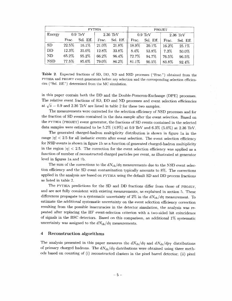
PYTHIA PHOJET
Energy 0.9 TeV 2.36 TeV 0.9 TeV 2.36 TeVFrac. Sel. Eff. Frac. Sel. Eff. Frac. Sel. Eff. Frac. Sel. Eff.
SD 22.5% 16.1% 21.0% 21.8% 18.9% 20.1% 16.2% 25.1%DD 12.3% 35.0% 12.8% 33.8% 8.4% 53.8% 7.3% 50.0%ND 65.2% 95.2% 66.2% 96.4% 72.7% 94.7% 76.5% 96.5%NSD 77.5% 85.6% 79.0% 86.2% 81.1% 90.5% 83.8% 92.4%
Table 2. Expected fractions of SD, DD, ND and NSD processes ("Frac.") obtained from thePYTHIA and PHOJET event generators before any selection and the corresponding selection efficien-cies ("Sel. Eff.") determined from the MC simulation.
in this paper contain both the DD and the Double-Pomeron-Exchange (DPE) processes.The relative event fractions of SD, DD and ND processes and event selection efficienciesat Is = 0.9 and 2.36 TeV are listed in table 2 for these two samples.
The measurements were corrected for the selection efficiency of NSD processes and forthe fraction of SD events contained in the data sample after the event selection. Based onthe PYTHIA (PHOJET) event generator, the fractions of SD events contained in the selecteddata samples were estimated to be 5.2% (4.9%) at 0.9 TeV and 6.3% (5.0%) at 2.36 TeV.
The generated charged-hadron multiplicity distribution is shown in figure la in therange 17| < 2.5 for all inelastic events after event selection. The event selection efficiencyfor NSD events is shown in figure lb as a function of generated charged-hadron multiplicityin the region rj| < 2.5. The correction for the event selection efficiency was applied as afunction of number of reconstructed charged particles per event, as illustrated at generatorlevel in figures la and 1b.
The sum of the corrections to the dNch/dy measurements due to the NSD event selec-tion efficiency and the SD event contamination typically amounts to 8%. The correctionsapplied in the analysis are based on PYTHIA using the default SD and DD process fractionsas listed in table 2.
The PYTHIA predictions for the SD and DD fractions differ from those of PHOJET,and are not fully consistent with existing measurements, as explained in section 5. Thesedifferences propagate to a systematic uncertainty of 2% in the dNch/dy measurement. Toestimate the additional systematic uncertainty on the event selection efficiency correctionresulting from the possible inaccuracies in the detector simulation, the analysis was re-peated after replacing the HF event-selection criterion with a two-sided hit coincidenceof signals in the BSC detectors. Based on this comparison, an additional 1% systematicuncertainty was assigned to the dNch/d?7 measurements.
4 Reconstruction algorithms
The analysis presented in this paper measures the dNch/dr and dNch/dPT distributionsof primary charged hadrons. The dNch/drl distributions were obtained using three meth-ods based on counting of (i) reconstructed clusters in the pixel barrel detector; (ii) pixel

n e * PHOJET 0.9 TeV
0.04 _ o PHOJET2.36TeV C
C oSO 0.50 .2 0.
CO0.02- o ().0 -- PYTHIA 0.9 TeV
-C/) ----- PYTHIA 2.36 TeV
.0- - aPHOJET 0.9 TeV0
, o PHOJET 2.36 TeV
0 0 ' ' '0 10 20 30 40 50 60 0 10 20 30 40 50 60
Charged-particle multiplicity Charged-particle multiplicity
Figure 1. (a) Generated multiplicity distributions of primary charged hadrons in the range 17| < 2.5for 9/s = 0.9 TeV (solid dots and histogram) and 2.36 TeV (open circles and dashed histogram) afterthe event selection is applied to the reconstructed events, using inelastic events from the PYTHIA(histograms) and PHOJET (symbols) event generators. (b) The event selection efficiency expectedfor NSD events from the PYTHIA (histograms) and PHOJET (symbols) event generators as a function
of generated charged hadron multiplicity in the region lrj < 2.5.
tracklets composed of pairs of clusters in different pixel barrel layers; and (iii) tracks re-
constructed in the full tracker volume, combining the pixel and strip hits. The cluster
counting method provides an independent measurement for each pixel barrel layer, and the
tracklet method for each pair of layers. The third method also allows a measurement of
the dNch/dpT distribution. All three methods rely on the reconstruction of the primary
vertex (PV) described in section 4.1.
The pixel-cluster-counting method has the advantage of having the largest PT ac-
ceptance down to small transverse momentum (30 MeV/c), is insensitive to geometrical
misalignment of the detector and does not require detailed knowledge of the primary ver-
tex position resolution. A potential disadvantage is the sensitivity to backgrounds from
collisions with residual gas in the beam pipe (beam-gas collisions), from secondary particles
produced in the detector material and from low-pT particles curling in the axial magnetic
field (loopers). The pixel-tracklet method is capable of measuring and correcting for the
combinatorial background and has a PT threshold of 50 MeV/c. The third method uses
the tracker (pixel and SST) to build tracks. It requires at least two pixel hits in different
layers, has the largest PT threshold (~100 MeV/c) and algorithmic complexity, but is the
most robust against background hits produced by particles not originating from the col-
lision. The charged-particle multiplicity was corrected in all three methods for the small
contamination (< 1%) of primary charged leptons. The measured dNch/dq values were
evaluated by extrapolating or correcting to PT = 0 for all the three analysis methods.
The three reconstruction methods are described in sections 4.2-4.4.

4.1 Primary vertex reconstruction
The x, y and z positions of the luminous region where protons of both beams interact,hereafter referred to as beam spot, are obtained for each data set from three-dimensional
vertex fits based on tracks reconstructed with PT > 0.9 GeV/c, using the full event sample.
The RMS of the beam spot in the transverse directions was found to be less than 0.05 cm.
The beam spot position and dimensions were found to be stable within a given data set.
To reconstruct the z coordinate of the PV for each event, tracks consisting of tripletsof pixel hits were formed. The minimum transverse momentum of these tracks is ~ 75MeV/c. The tracks were required to originate from the vicinity of the beam spot with atransverse impact parameter (dT) smaller than 0.2cm. Of these tracks, only those with
dT <4 T, where UT is the quadratic sum of the uncertainty in dT and the RMS of thebeam spot in the transverse direction, were used in the vertex reconstruction.
The vertex-reconstruction algorithm uses the z coordinate of the tracks at the pointof closest approach to the beam axis and the corresponding estimated measurement un-certainty (o-z). It performs an agglomerative clustering by adding tracks to form groups.These groups (denoted the ith and jth group) are then merged based on their normal-ized distance, d = (z, - zj) 2/(o0 + o?) where o and oj are the uncertainties of thezi and z1 positions, with a fast nearest-neighbour search algorithm [15]. The z positionand its uncertainty cz for the newly joined group are calculated using a weighted average.The clustering process stops when the smallest normalized distance between the remaininggroups gets larger than 8.0, where the stopping condition was optimized using simulatedevents. Only vertices formed from at least two tracks were considered except when onlyone track was reconstructed in the event. In the latter case the PV position was defined asthe point of the closest approach of the track to the beam axis. The fraction of single-trackvertices in the selected data sample is 1.7% (1.3%) at 0.9 TeV (2.36 TeV). The overall PVreconstruction efficiency, evaluated from the data after all other event selection cuts, is inexcess of 99% and the fraction of events with more than one primary vertex candidate is5.0% (7.4%) at 0.9 TeV (2.36 TeV). In the rare case of multiple PV candidates, the vertexcomposed of the largest set of tracks was chosen.
The reconstructed primary vertex resolution in the z direction is a function of the asso-ciated track multiplicity (N) and was found to be parameterized adequately as 0.087 cm /NO.6using simulated events.
The distribution of the reconstructed z position of the PV is shown in figure 2a.Overlaid is the PV distribution in simulated events, the position and RMS of which wereadjusted to reproduce the beam spot measured in data.
4.2 Pixel cluster counting method
The pseudorapidity distribution of primary charged hadrons produced in a pp collision canbe measured by counting the number of clusters they create when traversing each of thethree pixel barrel layers and applying appropriate corrections, as described in this section.
The energy deposited by charged particles traversing a pixel detector layer is spreadover multiple pixels. Adjacent pixels with a charge measurement above a readout threshold
-7-

PYTHIA 0.9 TeV -' PYTHIA 0.9 TeVC -- PYTHIA 2.36 TeV - - - PYTHIA 2.36 TeV
U)
0 -30.03
0 C0.05- -2 0.02 .
CZ CZLL LL
0.01-0 00
-20 -10 0 10 20 0 20 40 60 80zP, [cm] Angle-corrected cluster charge [ke]
Figure 2. (a) The distribution of the reconstructed z position of the primary vertex in the data(dots), compared to that from the PYTHIA simulation (histogram). (b) Distribution of the clustercharge multiplied by |sin 01 in the data (dots) and the simulation (histogram), for the clustersselected for analysis.
of typically 2740 electrons are combined into pixel clusters to integrate the total chargedeposit [6]. The cluster size and charge depend on the incident angle of the particle withrespect to the active detector surface. The cluster length along the z axis ranges from 1-2pixels at normal incident angle up to 14-16 pixels at shallow crossing angles. Figure 2bshows the measured distribution of cluster charge multiplied by Isin 0| (or 1/coshr) afterthe cluster selection discussed below, compared to the simulation. Here, 0 is the polarangle of the straight line connecting the PV to the cluster.
The peak position is consistent with the expected charge of 22 ke, while the width ofthe distribution is slightly larger in the data than in the simulation due to gain calibrationnon-uniformities.
The cluster counting method correlates the observed pixel-cluster length in the z di-rection, expressed in number of pixels, with the expected path length traveled by a primaryparticle at a given 77 value. For primary particles the cluster length in z is proportional tocot 01 (or |sinh 1) as displayed in figure 3a. Small clusters at large 17l are due to loopers,
secondary particles and daughters of long-lived hadrons. Clusters from these backgroundparticles were efficiently removed by the cluster-length cut represented by the solid line infigure 3a. To allow for an efficient background rejection, only the barrel part of the pixeldetector was used, where the detector units are parallel to the beam axis, as opposed to thepixel end-caps. Furthermore, the 71 range for the cluster counting was restricted to Ig| < 2to avoid acceptance problems due to the slightly off-centred position of the luminous region.
The event selection efficiency and the SD contribution for a given total multiplicityof selected clusters (M) for each pixel barrel layer can be determined from Monte Carlosimulation. The overall change of the dNch/dq value due to this correction is 9% for bothcollision energies.

'Wi 2 0 I! .1 - ' ' I '. . I , '. ' I i ' ' ' ' -.1 --_Ms (b) CMSC W .
18 --. Data 0.9 Tev16 -o Data 2.36 Tev.. 16 .PYTHIA 0.9 TeV14 -...... ,PYTHIA 2.36 TeV
0. ,. 1210 --- Primaries in MC
10 -.. ..... ' 0
6 0
8 ,.Nl .......mne~fllh .. ...
- , .... ... .. ... ...... . . .. .... 11nn U l lD . -- - U 10 -26 __ __........... __ ___ __.......I .....
-3 -2 -1 0 1 2 3 -0.2 -0.1 0 0.1 0.2
:3 gul .......... A1l
Figure 3. (a) Pixel cluster length along z as a function of 77 for the 900 GeV data. The solid line
illustrates the cut applied in the cluster counting method. (b) The Zog distribution of clusters ontracklets in the data (dots and circles), together with the distribution obtained from the PYTHIA
simulation (solid and dotted lines), for both 0.9 and 2.36 TeV collision energy. The dashed line showsthe A77 distribution of clusters for primary charged-particle tracks in the Monte Carlo simulationat 0.9 TeV. The tail of the A77 distribution comes from the combinatorial background.
The fraction of clusters created by loopers above the cluster-length cut (1% and 5% for
S=2 and ry = 0.5, respectively) can be estimated by measuring the total number of clusters
below the cut in data, corrected by the ratio of looper clusters below and above the cut in
simulated events. The number of clusters eliminated by the cluster-length cut was found
to be higher in data than in simulated events by 10-20% due to a slightly larger abundance
of secondary particles and loopers, while the observed number and length distributions of
clusters above the cut was found to agree with the simulation.
The corrections for absorption in the beam pipe and detector material, secondary
particles, daughters of long-lived hadrons, delta-ray electrons and double hits caused by
geometrically overlapping detector units were all evaluated, in bins of rg and M, with
simulated data. The size of these corrections is 10%, 23% and 41% for the first, second
and third detector layer, respectively. Varying the charged-particle multiplicity in the event
generator by 50% only causes a ±3% relative change in these corrections. Their dependence
on y and pixel-cluster multiplicity is similarly small.
4.3 Pixel-tracklet method
This method was first used to measure charged-hadron multiplicities by the PHOBOS
experiment at RHIC [16]. Pixel tracklets are constructed from combinations of two pixel
hits in any two pixel barrel layers. The difference in the angular positions of the two clusters
with respect to the PV, A77 and A#f, are calculated for each tracklet. If two tracklets share
a hit, the tracklet with the larger A77 is discarded. The A77 distribution of reconstructed
-9-

tracklets is shown in figure 3b, together with the corresponding distribution from simulated
data and a separate distribution for simulated primary particles only. Tracklets from
primary particles display a sharp peak at A1 = 0, while the tracklets from the combinatorial
background have an extended tail. The simulated Aq distributions are in good agreement
with data.
To suppress the combinatorial background, only tracklets with lAJ < 0.1 and JA#| <1.0 were selected. Since the combinatorial background is flat in A#, the remaining fraction
of background tracklets in the signal region |A#| < 1.0 can be estimated from tracklets
with 1.0 < |A0# < 2.0. This data-driven estimate of the background accurately describes
the raw A71 distribution of tracklets for lA?| > 2, where no signal from primary particles
is expected from the MC simulation. Typical values of this estimated background fraction
in the signal region increase with jf from 2% to 30%. The 71 range for the tracklet method
was restricted to HqJ < 2 to avoid a large acceptance correction.
The contribution from secondary particles, reconstruction efficiency and geometrical
acceptance needs to be accounted for to determine the number of primary charged hadrons.
These correction factors were calculated using PYTHIA simulations for background-subtract-
ed tracklets in bins of z position of the PV, pseudorapidity, and tracklet multiplicity. The
magnitude of the correction varies with JqJ from 0 to 20%. The correction factors were also
cross-checked by PHOJET simulations and only cause a 2-3% change in the dNch/dq result.
The correction for the event selection efficiency and the SD contribution was deter-
mined for each tracklet multiplicity bin. The overall change in the dNch/dl value due to
this correction is about 8% at ? 0.
4.4 Tracking method
Pixel and SST detectors were used to reconstruct tracks, including both barrel and end-
cap layers. The acceptance was limited to ?17 < 2.4 to avoid edge effects. The iterative
reconstruction procedure described below follows refs. [17, 18], but was further optimized
for primary-track reconstruction in minimum bias events.
In the first step of track reconstruction, tracks with three pixel hits (triplets) are built
using the x and y positions of the beam spot and the z coordinate of the primary vertex
as constraints. These clean pixel tracks are used as seeds for the Kalman-filter-based
trajectory-building algorithm in the SST. The resulting trajectories are stored. Before the
second tracking step, the pixel and strip hits associated with the tracks found in the first
step are removed from further consideration. The second step uses pixel triplet seeds as
well, but does not require a vertex constraint and has a looser transverse impact parameter
requirement than in the first step. After removal of hits associated with tracks found in
the second step, the third tracking step finds primary tracks seeded by two hits in the pixel
detector. At least three hits were required for a track to be accepted.
Tracks found during the three iterative steps were collected and a second iteration
of the PV reconstruction, as described in section 4.1, was performed to refine primary
vertex position determination. Finally, the tracks were refit with the corresponding vertex
constraint, thus improving their q and PT resolution.

In this analysis, a reconstructed track was considered as a primary-track candidate if
it is compatible with originating from the PV (dT < min(4 oT, 0.2 cm) and dz < 4a, where
dz is the distance between the point of the closest approach of the track to the beam axis
and the PV along the z direction).Studies with simulated events showed that the combined geometrical acceptance and
reconstruction efficiency for the tracking method exceeds 50% around PT ~ 0.1, 0.2 and0.3 GeV/c for pions, kaons and protons, respectively. The efficiency is about 96% in the
1,I < 1 region for PT > 0.25 GeV/c, and is above 80% for pions at PT = 0.15 GeV/c. Byrequiring the geometrical shapes of the pixel clusters to be consistent with the crossingangle and direction of the track, the fraction of fake tracks was kept below 1%. Thefraction of duplicated tracks (e.g., from loopers) was estimated to be about 0.1% in thecentral region, rising to 0.5% at large |j7.
The measured yield in data was corrected, based on MC simulation and comparisonswith data, for geometrical acceptance (2% correction for PT > 200 MeV/c), efficiency of thereconstruction algorithm (5-10% for PT > 300 MeV/c), fake and duplicate tracks (<1%each). The contamination of less than 2% from decay products of long-lived hadrons,photon conversions and inelastic hadronic interactions with the detector material was alsosubtracted. To obtain the dNch/dq result from the PT spectrum, an extrapolation to PT = 0was necessary, resulting in an increase of 5% in the estimated number of charged hadrons.
Corrections based on the average hit efficiency of pixel layers, size of the beam spot,longitudinal and transverse impact-parameter resolutions of pixel tracks were validatedwith data. As an example, the average number of pixel and strip hits found on tracksin the range |77 < 1 is shown in figures 4a and 4b, together with the expectation fromPYTHIA. Somewhat fewer particles are predicted with PT < 500 MeV/c than seen in thedata, which results in the small difference in the number of tracks with few SST hits infigure 4b. This small difference, which originates from limitations of the PYTHIA generator,does not affect the final measurement. The correction for the event selection efficiency andthe SD contribution was determined for each track multiplicity bin, and has an overallmagnitude of 8.3%.
5 Results
5.1 Systematic uncertainties
Various corrections and their event-selection and model dependence contribute to the sys-tematic uncertainties of the measured quantities. A summary of these systematic uncer-tainties averaged over q and PT is given in table 3 and discussed below.
The uncertainties related to the trigger bias and to the event selection are common toall the analysis methods. The efficiency of the trigger and event-selection was correctedfor by the prediction of the PYTHIA D6T event generator combined with the full Geant4simulation of the CMS detector. The material description relevant for this analysis wasverified by studies of photon conversion probabilities in the data, found to be in agreementwith those obtained from the simulation.
- 11 -

(a) CMS 0.14 (b) CMS0.9
0 Data 0.9 TeV - Data 0.9 TeV0.8- PYTHIA 0.9 TeV 0.12 * PYTHIA 0.9 TeV
Cl) Of)32 0.7 - , -C .) - ' 0.1
. :0.6-00 O30.08
0.2 -
0 0--0.4--r 0.06 -
L"L0.3 L .400.04
0.200.1 0.02
2 3 4 5 0 5 10 15 20Number of pixel hits on track Number of strip hits on track
Figure 4. (a) The distribution of the number of pixel hits attached to reconstructed tracks inthe region of Ir/| < 1 (closed circles), compared to the CMS detector simulation (histogram). (b)The distribution of the number of hits in the SST detector attached to reconstructed tracks in theregion of Ir/| < 1 (closed circles), compared to the CMS detector simulation (histogram).
Because single- and double-diffractive pp collisions have much smaller charged-hadronmultiplicities per event than non-diffractive events, they contribute to the uncertaintyin the measured dNch/d?7 mostly through the uncertainty in the fraction of SD and DDevents passing the event selection criteria. The fractions of SD events for V/s = 0.9 TeVin PYTHIA and PHOJET (table 2) are 23% and 19%, respectively. The UA5 experimentmeasured 15.5% for this fraction [19]. Based on the simulated trigger efficiencies for thedifferent event types, only 5.5% of events passing the analysis event selection are expectedto be single-diffractive events. From the aforementioned variations of SD fractions, anuncertainty of ±1% is attributed to this correction. The contribution of the uncertaintyof the fraction of DD events was estimated similarly to be +1%. Since underestimatedDD and SD fractions both lead to an underestimated dNch/dr result, a conservative linearsum of 2% was assigned to the above systematic uncertainty. The trigger efficiency of theBSC is more than 98% for events with a valid vertex, and even a 5% uncertainty in single-particle detection efficiency of its individual segments results in a negligible uncertainty inthe final result. The trigger efficiency of the BSC and the event selection efficiency of theHF detector were both measured from data and found to be consistent within 1% with theMC simulation. The total systematic uncertainty from propagating all event selection andtrigger related uncertainties is 3%. The measurement of the average transverse momentumis less sensitive to the trigger selection efficiency. A smaller, 1% uncertainty was thereforeassigned to that result.
The geometrical acceptance was studied by comparing the hit occupancy of the pixelbarrel with the predictions from the simulation. The efficiency of the pixel hit recon-struction was estimated using tracks propagated from the SST to the pixel detector and
- 12 -

by extrapolating pixel tracklets to the unused pixel barrel layer. The measured pixel hit
efficiency was found to exceed 99% with a 0.5% uncertainty from both methods, which
propagates into 0.5% uncertainty in the pixel-counting-based, 1% in the tracklet-based,and 0.3% in the track-based results. If the collected charge in one or more pixels in a clus-
ter remains below the threshold, the cluster may be split. The splitting rate was estimated
from the geometrical distance distributions of close-by pixel clusters found in the data and
in the Monte Carlo simulation and found to be 0.5-0.9% in the simulation and 1.0-1.5% in
data.
The uncertainty related to the cluster and tracklet selections was estimated by varying
the selection cuts. An additional 3% and 2% uncertainty was assigned to the tracklet and
track reconstruction algorithm efficiencies, respectively. Corrections for loopers and sec-
ondary particles are simulation dependent; the tracklet- and pixel-counting-based methods
have low rejection power compared to the tracking method, thus carry a larger systematic
uncertainty (as shown in table 3).The effects of the geometrical misalignment of the pixel barrel detector were simulated
and a 1% uncertainty was assigned to the results from the tracklet-based method. Hits frombeam-induced backgrounds coinciding with the collision were estimated to be very rare,and a conservative 1% random hit contribution was propagated to obtain the uncertainty ofthe results. The corrections for multiple track counting and fake track rate were estimated
from the Monte Carlo simulation and found to be less than 1%. The uncertainty of the
extrapolation to the full PT-range depends on the low-pT reach of the three methods and
varies between 0.2 and 0.5%. While the sources of uncertainties are largely independentfrom each other, they are correlated among all the data points.
5.2 Charged hadron transverse-momentum distributions
Tracks with |q| < 2.4 and PT > 0.1 GeV/c were used for the measurement of dNch /dpT. Themeasured average charged-hadron yields per NSD event are shown in figure 5a, as a function
of PT in bins of Iql. The yields were fit by the Tsallis function (eq. (5.1)), which empiricallydescribes both the low-pT exponential and the high-pT power-law behaviours [20, 21]:
E 1 = d2 Nh = C(n, T, m)dNch ( 1 + n(5.1)dp3 2 ,rPT p d?7dpr dy nT '
where y = 0.5 ln[(E + pz)/(E - pz)] is the rapidity; C(n, T, m) is a normalization constant
that depends on n, T and m; ET = m2 + p2 - m and m is the charged pion mass. Thisfunction provides both the inverse slope parameter T, characteristic for low PT, and theexponent n, which parameterizes the high-pr power-law tail. These fit parameters changeby less than 5% with 77, thus a fit to the whole region 171 < 2.4 was performed. The PTspectrum of charged hadrons, 1/(27rpT)d 2Nch/dqdpT, in the region 177 < 2.4, was also fit
with the empirical function (eq. (5.1)) and is shown in figure 5b. The PT resolution of
the CMS tracker was found to have a negligible effect on the measured spectral shapeand was therefore ignored in the fit function. For the 0.9 TeV data, the inverse slopeparameter and the exponent were found to be T = 0.13 ± 0.01 GeV and n 7.7 ± 0.2.
For the 2.36 TeV data, the values were T = 0.14 ± 0.01 GeV and n = 6.7 ± 0.2. Theaverage transverse momentum, calculated from the measured data points adding the low-

Source Pixel Counting [%] Tracklet [%] Tracking [%)Correction on event selection 3.0 3.0 3.0 (1.0)Acceptance uncertainty 1.0 1.0 1.0Pixel hit efficiency 0.5 1.0 0.3Pixel cluster splitting 1.0 0.4 0.2
Tracklet and cluster selection 3.0 0.5 -Efficiency of the reconstruction 3.0 2.0
Correction of looper hits 2.0 1.0 -Correction of secondary particles 2.0 1.0 1.0Misalignment, different scenarios - 1.0 0.1Random hits from beam halo 1.0 0.2 0.1Multiple track counting - - 0.1
Fake track rate - - 0.5
PT extrapolation 0.2 0.3 0.5Total, excl. common uncertainties 4.4 3.7 2.4
Total, incl. common uncert. of 3.2% 5.4 4.9 4.0 (2.8)
Table 3. Summary of systematic uncertainties. While the various sources of uncertainties arelargely independent, most of the uncertainties are correlated between data points and between theanalysis methods. The event selection and acceptance uncertainty is common to the three methodsand affects them in the same way. The values in parentheses apply to the (pr) measurement.
and high-PT extrapolations from the fit is (PT) = 0.46 ± 0.01 (stat.) ± 0.01 (syst.) GeV/cfor the 0.9 TeV and 0.50 ± 0.01 (stat.) ± 0.01 (syst.) GeV/c for the 2.36 TeV data.
The dNch/d spectrum was obtained by summing the measured differential yields
for 0.1 < PT < 3.5 GeV/c and adding the result to the integral of the fit function for
PT < 0.1 GeV/c and PT > 3.5 GeV/c. The latter term amounts to 5% of the total.
5.3 Charged hadron pseudorapidity density
The summary of results on the pseudorapidity density distribution of charged hadrons is
shown in figure 6. The dNch/d7 results for the three layers in the cluster-counting method
and the three layer-pairs in the pixel-tracklet method are consistent within 3%. These
results from the various layers and from the different layer pairs were combined to provide
one set of data from each analysis method, as shown in figure 6a. The error bars include
the systematic uncertainties of about 2.4-4.4% specific to each method, estimated from the
variations of model parameters in the simulation used for corrections and the uncertainties
in the data-driven corrections. The systematic uncertainties common to all the three
methods, which amount to 3.2%, are not shown. The results from the three analysis
methods are in agreement. The larger fraction of background hits in the data compared
to simulation affects the cluster-counting method differently from the other two, which
results in a small difference at high q, well accounted for by the systematic uncertainty of
the measurement.
14 -

1050 0 Data 0.9 TeV
--- =2.3 1 -0 Data 2.36 TeV
~0
2 0 ---- --------- ---- -- -- - =.
=0. 10
---- --- --- ---- -- - - 1 = 0 .7
10 -- =0.1 5 I 10-4 - *20 ' --- ' ----------- '-- ' -- ' - 4 10-3 '
0 0.5 1 1.5 2 00.511.522.533.54
pT [GeV/c] pT [GeV/c]
Figure 5. (a) Measured differential yield of charged hadrons in the range [7| < 2.4 in 0.2-unit-widebins of 1,q for the 2.36 TeV data. The measured values with systematic uncertainties (symbols)and the fit functions (eq. (5.1)) are displayed. The values with increasing 7 are successively shiftedby four units along the vertical axis. (b) Measured yield of charged hadrons for 17| < 2.4 withsystematic uncertainties (symbols), fit with the empirical function (eq. (5.1)).
6 Discussion
The average transverse-momentum and pseudorapidity densities of charged hadrons derivedfrom the measured data can be compared to results from earlier experiments as a functionof the collision energy. The average transverse momentum of charged hadrons was obtainedfrom the fits (eq. (5.1)) to the transverse-momentum spectrum (figure 5b). At low energiesthe energy dependence of (PT) can be described by a quadratic function of In s. The (PT)from this measurement, shown in figure 7a, follows the general trend. At 0.9 TeV it issimilar to the results from pp collisions at the same energy [22].
The dNch/dq distribution was calculated as the weighted average of the data from thethree reconstruction methods, taking into account their systematic uncertainties, excludingthe common ones, as listed in table 3. The averaged result is shown in figure 6b andcompared to measurements at the same accelerator (ALICE, pp [23]) and to previousmeasurements at the same energy but with different colliding particles (UA5, pp [24]).
The shaded error band on the CMS data indicates systematic uncertainties, while the
error bars on the data from UA5 and ALICE display statistical uncertainties only. No
significant difference is observed between the dNch/d?7 distributions measured in pp and
pp collisions at Vs = 0.9 TeV.
The dNch/dn distribution is weakly q-dependent, with a slow increase towards higherq values, and an indication of a decrease at |q| > 2 for the 0.9 TeV data. At 2.36 TeV, the
entire distribution is wider due to the increased collision energy hence the larger ?7 range
15 -

bI(a) CMS (b) CMS
5 - 5-
4- 4- _00
3*:~ 3Z Z
2 0.9 TeV 2.36 TeV 2 0.9 TeV 2.36 TeV
- o Cluster counting 0 0 CMS NSD
1 a Tracklet A ALICE NSD
A A Tracking a UA5 NSD
0 ' 0 ' '' '-2 0 2 -2 0 2
Figure 6. (a) Reconstructed dNch/d? distributions obtained from the cluster counting (dots witherror bars), tracklet (squares) and tracking (triangles) methods, in pp collisions at 0.9 TeV (filledsymbols) and 2.36 TeV (open symbols). The error bars include systematic uncertainties (as dis-cussed in the text), excluding those common to all the methods. (b) Reconstructed dNch/ddistributions averaged over the cluster counting, tracklet and tracking methods (circles), comparedto data from the UA5 [24] (open squares) and from the ALICE [23] (open triangles) experimentsat 0.9 TeV, and the averaged result over the three methods at 2.36 TeV (open circles). The CMSand UA5 data points are symmetrized in q. The shaded band represents systematic uncertaintiesof this measurement, which are largely correlated point-to-point. The error bars on the UA5 andALICE data points are statistical only.
available for inclusive particle production. For Iy < 0.5, the corrected results average to
dNch/dr = 3.48±0.02 (stat.) ± 0.13 (syst.) and dNch/dj = 4.47±0.04 (stat.) ± 0.16 (syst.)
for NSD events at di = 0.9 and 2.36 TeV. The increase of (28.4 ± 1.4 ± 2.6)% from
0.9 to 2.36 TeV is significantly larger than the 18.5% (14.5%) increase predicted by the
PYTHIA (PHOJET) model tunes used in this analysis. The collision energy dependence of
the measured dNch/dnr/o is shown in figure 7b, which includes data from the NAL Bubble
Chamber [25], the ISR [26], and UAl [22], UA5 [24], CDF [27], STAR [28], PHOBOS [29]
and ALICE [23]. The dNch/dq measurement reported here is consistent with the previously
observed trend.
7 Summary
Inclusive measurements of charged-hadron densities, dNch/dPT and dNh/dl, have been
presented based on the first pp collisions recorded at Vs = 0.9 and 2.36 TeV by the
CMS experiment during LHC commissioning in December 2009. The numerical val-
ues of the data presented in this paper can be found in ref. [30]. For NSD interac-

(a) CMS (b) CMS- ISR inel. -* UA1 NSD 0 NAL B.C. inel.
0.55 * UA1 NSD V STAR NSD @ ISR inel.
- A UA5 NSD n UA5 Inel.-UM CDFNSD 0 CF NSD o PHOBOS Inel.
- 0.5 0 CMS NSD (I |<2.4) * ALICE NSD A ALICE inel.
eCS NSD
W4-0 0.45 -
z.0.4-
-2--0.35 -- 0.161 + 0.201 In(s)
0.35--- - -- - --- 2.42 - 0.244 In(s) + 0.0236 In2(s)
- 0.425 - 0.0197 In(s) + 0.00156 1n2(s) 1.54 - 0.096 In(s) + 0.0155 In
2(S)
0 .3 ' j ' ' 1 ' ' " ' ' ' " I ' ' ' 11 ' ' " ' 101 1 1 1 1 1 1 '10 102 103 104 10 102 103 104
/s [GeV] \ s [GeV]
Figure 7. (a) Energy dependence of the average transverse momentum of charged hadrons. TheCMS data points are evaluated for the range Ir/4 < 2.4. Data of other experiments are taken fromrefs. [22, 31-33]. The curve shows the fit to the data points of the form (PT) = 0.425 - 0.0197 In(s) +0.001561n 2 (s) with (PT) in GeV/c and s in GeV2. The error bars on the CMS data points includesystematic uncertainties. (b) Charged-hadron pseudorapidity density in the central region as afunction of centre-of-mass energy in pp and pp collisions including lower energy data from refs. [22-29], together with various empirical parameterizations fit to the data corresponding to the inelastic(solid and dotted curves with open symbols) and to the NSD (dashed curve with solid symbols)event selection. The error bars indicate systematic uncertainties, when available.
tions, the average charged-hadron transverse momentum has been measured to be 0.460.01 (stat.) ± 0.01 (syst.) GeV/c at 0.9 TeV and 0.50 ± 0.01 (stat.) ± 0.01 (syst.) GeV/cat 2.36 TeV. The three reconstruction methods employed for the dNch/dq measurementhave yielded consistent results, demonstrating the excellent performance and detailedunderstanding of the CMS tracker. The pseudorapidity density in the central region,dNch/d| 1 <o.5 , has been measured to be 3.48 ± 0.02 (stat.) ± 0.13 (syst.) at 0.9 TeV and4.47 ± 0.04 (stat.) ± 0.16 (syst.) at 2.36 TeV. The results at 0.9 TeV have been foundto be in agreement with previous measurements in pp and pp collisions. With the newmeasurements at 2.36 TeV, which show a steeper-than-expected increase of charged-hadronmultiplicity density with collision energy, the study of particle production in pp collisionshas been extended into a new energy regime.
Acknowledgments
We congratulate and express our gratitude to our colleagues in the CERN acceleratordepartments for the excellent performance of the LHC. We thank the technical and admin-istrative staff at CERN and other CMS Institutes, and acknowledge support from: FMSR
- 17 -
(Austria); FNRS and FWO (Belgium); CNPq, CAPES, FAPERJ, and FAPESP (Brazil);
MES (Bulgaria); CERN; CAS, MoST, and NSFC (China); COLCIENCIAS (Colombia);
MSES (Croatia); RPF (Cyprus); Academy of Sciences and NICPB (Estonia); Academy
of Finland, ME, and HIP (Finland); CEA and CNRS/IN2P3 (France); BMBF, DFG, and
HGF (Germany); GSRT (Greece); OTKA and NKTH (Hungary); DAE and DST (India);
IPM (Iran); SFI (Ireland); INFN (Italy); NRF (Korea); LAS (Lithuania); CINVESTAV,
CONACYT, SEP, and UASLP-FAI (Mexico); PAEC (Pakistan); SCSR (Poland); FCT
(Portugal); JINR (Armenia, Belarus, Georgia, Ukraine, Uzbekistan); MST and MAE (Rus-
sia); MSTDS (Serbia); MICINN and CPAN (Spain); Swiss Funding Agencies (Switzerland);
NSC (Taipei); TUBITAK and TAEK (Turkey); STFC (United Kingdom); DOE and NSF
(USA). Individuals have received support from the Marie-Curie IEF program (European
Union); the Leventis Foundation; the A. P. Sloan Foundation; and the Alexander von
Humboldt Foundation.
Open Access. This article is distributed under the terms of the Creative Commons
Attribution Noncommercial License which permits any noncommercial use, distribution,
and reproduction in any medium, provided the original author(s) and source are credited.
References
[1] L. Evans and P. Bryant eds., LHC Machine, 2008 JINST 3 S0800I [SPIRES].
[2] W. Kittel and E.A. De Wolf, Soft Multihadron Dynamics, World Scientific, Singapore (2005).
[3] J.G. Rushbrooke and B.R. Webber, High energy anti-particle-particle reaction differences
and annihilations, Phys. Rept. 44 (1978) 1 [SPIRES].
[4] CMS collaboration, R. Adolphi et al., The CMS experiment at the CERN LHC, 2008 JINST
3 S08004 [SPIRES].
[5] CMS collaboration, CMS Physics TDR: Volume I, Detector Performance and Software,
CERN-LHCC 2006-001 (2006).
[6] CMS collaboration, Commissioning and Performance of the CMS Pixel Tracker with Cosmic
Ray Muons, arXiv:0911.5434 [SPIRES].
[7] CMS collaboration, Alignment of the CMS Silicon Tracker during Commissioning with
Cosmic Rays, arXiv:0910.2505 [SPIRES].
[8] A.J. Bell, Design and Construction of the Beam Scintillation Counter for CMS, Master's
thesis, University of Canterbury, Christchurch, New Zealand, (2008).
[9] T. Aumeyr, Beam Phase and Intensity Monitoring for the Compact Muon Solenoid
Experiment, Master's thesis, Vienna University of Technology, Austria, (2008).
[10] GEANT4 collaboration, S. Agostinelli et al., Geant4: a simulation toolkit, Nucl. Instrumn.
Meth. A506 (2003) 250.
[11] T. Sj6strand, S. Mrenna and P.Z. Skands, PYTHIA 6.4 Physics and Manual, J[HEP 05
(2006) 026 [hep-ph/0603175] [SPIRES].
[12] Proceedings of Multiple Parton Interactions at the LHC, 1st Workshop, Perugia, Italy,
October 27-31, 2008 [DESY-PROC-2009-06].
[13] F.W. Bopp, R. Engel and J. Ranft, Rapidity gaps and the PHOJET Monte Carlo,
hep-ph/9803437 [SPIRES].
[14] R. Engel, J. Ranft and S. Roesler, Hard diffraction in hadron-hadron interactions and in
photoproduction, Phys. Rev. D 52 (1995) 1459 [hep-ph/9502319] [SPIRES].
- 18

[15] F. Sikler, Improved primary vertex finding for collider detectors, arXiv:0911. 2767 [SPIRES].
[16] PHOBOS collaboration, B.B. Back et al., Charged particle multiplicity near mid-rapidity incentral Au + Au collisions at _ = 56 and 130 A/GeV, Phys. Rev. Lett. 85 (2000) 3100[hep-ex/0007036] [SPIRES).
[17] S. Cucciarelli et al., Track reconstruction, primary vertex finding and seed generation withthe pixel detector, CMS Note 2006/026 (2006).
[18] T. Speer et al., Track reconstruction in the CMS tracker, Nucl. Instrum. Meth. A559 (2006)143.
[19] UA5 collaboration, R.E. Ansorge et al., Diffraction Dissociation at the CERN Pulsed p p-barCollider at c.m. Energies of 900 and 200 GeV, Z. Phys. C 33 (1986) 175 [SPIRES].
[20] C. Tsallis, Possible generalization of Boltzmann-Gibbs statistics, J. Stat. Phys. 52 (1988) 4179
[SPIRES].
[21] G. Wilk and Z. Wlodarczyk, Power laws in elementary and heavy-ion collisions: A Story offluctuations and nonextensivity?, Eur. Phys. J. A 40 (2009) 299 [arXiv:0810.2939][SPIRES].
[22] UA1 collaboration, C. Albajar et al., A Study of the General Characteristics ofProton-Antiproton Collisions at 0.2 to 0.9 TeV, Nucl. Phys. B 335 (1990) 261 [SPIRES].
[23] ALICE collaboration, K. Aamod et al., First proton-proton collisions at the LHC asobserved with the ALICE detector: measurement of the charged-particle pseudorapiditydensity at F = 900 Ge V, Eun. Phys. J. C 65 (2010) 111 [arXiv:0911.5430] [SPIRES].
[24] UA5 collaboration, G.J. Alner et al., Scaling of pseudorapidity distributions at c.m. energiesup to 0.9 Te V, Z. Phys. C 33 (1986) 1 [SPIRES].
[25] J. Whitmore, Experimental Results on Strong Interactions in the NAL Hydrogen BubbleChamber, Phys. Rept. 10 (974) 273 [SPIRES].
[26] AACHEN-CERN-HEIDELBERG-MUNICH collaboration, W. Thome et al., Charged ParticleMultiplicity Distributions in p p Collisions at ISR Energies, Nuc. Phys. B 129 (1977) 365[SPIRES].
[27] CDF collaboration, F. Abe et al., Pseudorapidity distributions of charged particles producedin pp interactions at \s = 630 Ge V and 1800 Ge V, Phys. Rev. D 41 (1990) 2330 [SPIRES.
[28] STAR collaboration, B.I. Abelev et al., Systematic measurements of identified particlespectra in p+p, d+Au and Au+Au collisions at the STAR detector, Phys. Rev. C 79 (2009)034909 [arXiv:0808.2041] [SPIR ES].
[29] PHOBOS collaboration, R. Nouicer et al., Pseudorapidity distributions of charged particlesin d+Au and p+p collisions at sNN = 200 GeV, J. Phys. G 30 (2004) S 1133[nucl-ex/0403033] [SPIRES].
[30] CMS collaboration, Numerical values of the data presented in this paper, available at JHEP02 (2010) 041 as supplemental material.
[31] A.M. Rossi et al., Experimental Study of the Energy Dependence in Proton Proton InclusiveReactions, NucL. Phys. B 84 (1975) 269 [SPIRES].
[32] T. Alexopoulos et al., Multiplicity dependence of the transverse momentum spectrum forcentrally produced hadrons in antiproton - proton collisions at F= 1.8 Te V, Phys. Rev. Lett.60 (1988) 1622 [SPIRES].
[33] CDF collaboration, F. Abe et al., Transverse momentum distributions of charged particlesproduced in )5p interactions at ,s =630 GeV and 1800 GeV, Phys. Reo. Lett. 61 (1988)1819 [SPIRES].
- 19 -

PRL 105, 022002 (2010) PHYSICAL REVIEW LETTERS
Transverse-Momentum and Pseudorapidity Distributions of Charged Hadronsin pp Collisions at fs = 7 TeV
V. Khachatryan et al. *
(CMS Collaboration)(Received 18 May 2010; published 6 July 2010)
Charged-hadron transverse-momentum and pseudorapidity distributions in proton-proton collisions at.,= 7 TeV are measured with the inner tracking system of the CMS detector at the LHC. The charged-hadron yield is obtained by counting the number of reconstructed hits, hit pairs, and fully reconstructedcharged-particle tracks. The combination of the three methods gives a charged-particle multiplicity perunit of pseudorapidity dNCh/d7)lj<0o. 5 = 5.78 ± 0.0 l(stat) ± 0.23(syst) for non-single-diffractive events,higher than predicted by commonly used models. The relative increase in charged-particle multiplicityfrom / = 0.9 to 7 TeV is [66.1 ± 1.0(stat) ± 4.2(syst)]%. The mean transverse momentum is measuredto be 0.545 ± 0.005(stat) ± 0.015(syst) GeV/c. The results are compared with similar measurements atlower energies.
DOI: 10.1 103/PhysRevLett.105.022002
Introduction.--Measurements of particle yields and kin-ematic distributions are an essential first step in exploring anew energy regime of particle collisions. Such studiescontribute to our understanding of the physics of hadronproduction, including the relative roles of soft and hardscattering contributions, and help construct a solid founda-tion for other investigations. In the complicated environ-ment of LHC pp collisions [I], firm knowledge of the ratesand distributions of inclusive particle production is neededto distinguish rare signal events from the much largerbackgrounds of soft hadronic interactions. They will alsoserve as points of reference for the measurement ofnuclear-medium effects in Pb-Pb collisions in the LHCheavy ion program.
The bulk of the particles produced in pp collisions arisefrom soft interactions, which are modeled only phenom-enologically. Experimental results provide the criticalguidance for tuning these widely used models and eventgenerators. Soft collisions are commonly classified as elas-tic scattering, inelastic single-diffractive (SD) dissociation,double-diffractive (DD) dissociation, and inelastic nondif-fractive (ND) scattering [2]. (Double-Pomeron exchange istreated as DD in this Letter.) All results presented hererefer to inelastic non-single-diffractive (NSD) interactions,and are based on an event selection that retains a largefraction of the ND and DD events, while disfavoring SDevents.
The measurements focus on transverse-momentum PTand pseudorapidity 7j distributions. The pseudorapidity,
*Full author list given at the end of the article.
Published by the American Physical Society under the terms ofthe Creative Commons Attribution 3.0 License. Further distri-bution of this work must maintain attribution to the author(s) andthe published article's title, journal citation, and DO.
PACS numbers: 13.85.Ni
commonly used to characterize the direction of particleemission, is defined as Y7 = - In tan(6/2), where 6 is thepolar angle of the direction of the particle with respect tothe anticlockwise beam direction. The count of primarycharged hadrons Nch is defined to include decay productsof particles with proper lifetimes less than 1 cm. Productsof secondary interactions are excluded, and a percent-levelcorrection is applied for prompt leptons. The measure-ments reported here are of dNch/dq and dNchdpT inthe pseudorapidity range 171 < 2.4 and closely followour previous analysis of minimum-bias data at lowercenter-of-mass energies of ,Is = 0.9 and 2.36 TeV as re-ported in Ref. [3].
The data for this study are drawn from an integratedluminosity of 1.1 pb- 1 recorded with the Compact MuonSolenoid (CMS) experiment [4] on 30 March 2010, duringthe first hour of the LHC operation at vs = 7 TeV. Theseresults are the highest center-of-mass energy measure-ments of the dNch/d77 and dNch/dpT distributions con-ducted at a particle collider so far and complement theother recent measurements of the ALICE experiment at7 TeV [5].
Experimental methods.-A detailed description of theCMS experiment can be found in Ref. [4]. The detectorsused for the present analysis are the pixel and silicon-striptracker, covering the region 1|q| < 2.5 and immersed in a3.8 T axial magnetic field. The pixel tracker consists ofthree barrel layers and two end-cap disks at each barrelend. The forward calorimeter (HF), which covers the re-gion 2.9 < 1771 < 5.2, was also used for event selection.The detailed Monte Carlo (MC) simulation of the CMSdetector response is based on GEANT4 [6].
The event selection and analysis methods in this Letterare identical to those used in Ref. [3], where more detailscan be found. The inelastic pp collision rate was about50 Hz. At these rates, the fraction of events in the data,
@ 2010 CERN, for the CMS Collaboration
week ending9 JULY 2010
0031-9007/ 10/105(2)/022002(14) 022002-1

PRL 105, 022002 (2010) PHYSICAL REVIEW LETTERS
TABLE I. Numbers of events passing the selection cuts. Theselection criteria are applied in sequence, i.e., each line includesthe selection from the previous ones.
Selection Number of events
Colliding bunches + one BSC signal 68 512Reconstructed PV 61 551HF coincidence 55 113Beam-halo rejection 55 104Other beam-background rejection 55 100
where two or more minimum-bias collisions occurred inthe same bunch crossing, is estimated to be less than 0.3%and was neglected. Any hit in the beam scintillator coun-ters (BSC, 3.23 <| r71 <4.65) coinciding with collidingproton bunches was used for triggering the data acquisi-tion. A sample mostly populated with NSD events wasselected by requiring a primary vertex (PV) to be recon-structed with the tracker, together with at least one HFtower in each end with more than 3 GeV total energy.Beam-halo and other beam-background events were re-jected as described in Ref. [3]. The remaining fraction ofbackground events in the data was found to be less than2 X 10-5. The numbers of events satisfying the selectioncriteria are listed in Table I.
The event selection efficiency was estimated with simu-lated events using the PYTHIA [7,8] and PHOJET [9,10] eventgenerators. The relative event fractions of SD, DD, and NDprocesses and their respective event selection efficienciesare listed in Table II. The fraction of diffractive events ispredicted by the models to decrease as a function ofcollision energy, while the selection efficiency increases.At fs = 7 TeV, the fraction of SD (DD) events in theselected data sample, estimated with PYTHIA and PHOJET,are 6.8% (5.8%) and 5.0% (3.8%), respectively, somewhathigher than at /s = 0.9 and 2.36 TeV [3]. With PYTHIA, theoverall correction for the selection efficiency of NSDprocesses and for the fraction of SD events remaining inthe data sample lowers the measured charged-particlemultiplicity by 6% compared with the uncorrecteddistribution.
The dNch/drJ distributions were obtained, as in Ref. [3],with three methods, based on counting the following quan-tities: (i) reconstructed clusters in the barrel part of the
pixel detector; (ii) pixel tracklets composed of pairs ofclusters in different pixel barrel layers; and (iii) tracksreconstructed in the full tracker volume. The third methodalso allows a measurement of the dNch/dpT distribution.All three methods rely on the reconstruction of a PV [11].The PV reconstruction efficiency was found to be 98.3%(98.0%) in data (MC), evaluated after all other event se-lection cuts. In case of multiple PV candidates, the vertexwith the largest track multiplicity was chosen. The threemethods are sensitive to the measurement of particlesdown to PT values of about 30, 50, and 100 MeV/c,respectively. Only 0.5, 1.5, and 5% of all charged particlesare estimated to be produced below these PT values, re-spectively, and these fractions were corrected for.
The measurements were corrected for the geometricalacceptance (=2%), efficiency (-5%-10%), fake (<1%)and duplicate tracks (<0.5%), low-PT particles curling inthe axial magnetic field (<1%), decay products of long-lived hadrons (<2%) and photon conversions (<1%), andinelastic hadronic interactions in the detector material(~ 1 %-2%), where the size of the corrections in parenthe-ses refers to the tracking method. The PYTHIA parameter setfrom Ref. [8] was chosen to determine the corrections,because it reproduces the dNeh/d77 and charged-particlemultiplicity distributions, as well as other control distribu-tions at 7 TeV, better than other available tuning parametersets. Although the corrections do not depend significantlyon the model used, it is indeed important that the simulateddata set contains a sufficient number of high-multiplicityevents to determine these corrections with the desiredaccuracy.
Results.-For the measurement of the dNch/dpT distri-bution, charged-particle tracks with PT in excess of0.1 GeV/c were used in 12 different 171 bins, from 0 to2.4. The average charged-hadron yields in NSD events areshown in Fig. I as a function of PT and |7l. The Tsallisparametrization [12-14],
EdNch -1 E d2Nch .CdNh I Er) -dp3 21rP p dy dPT dy n T
where y =0.5ln[(E + pz)/(E - p)], Er = m2 p -m,
and m is the charged pion mass, was fitted to the data. The
PT spectrum of charged hadrons, 1/(27rPr)d 2Nch/dij dPT,measured in the range |71| < 2.4, is shown in Fig. 2 for data
TABLE 1I. Fractions of SD, DD, ND, and NSD processes obtained from the PYTHIA and PHOJET event generators before anyselection, and the corresponding selection efficiencies determined from the MC simulation.
PYTHIA PHOJET
Fractions Selection efficiencies Fractions Selection efficiencies
SD 19.2% 26.7% 13.8% 30.7%DD 12.9% 33.6% 6.6% 48.3%ND 67.9% 96.4% 79.6% 97.1%NSD 80.8% 86.3% 86.2% 93.4%
022002-2
week ending9 JULY 2010

PRL 105, 022002 (2010)
-,
01-
zC\j
-a
70
60
50
40
30
20
10
00
o 7TeV PND
PHYSICAL REVIEW LETTERS
CMS-Tsallis fit
00
S 00
S 0------------------- ---- -
-0------ ------------ ---- ------
-0------- - ------------------- ----- ----
0
-- - - - - - - - - --- - - - - - - -
- 0~
-0------. -------------------- ----- -----
- 0-
---- - ---------
- - - - - - - - - - - - --- -- ---- - - - - - - - -
-0------ ---------------- ---
0.5
hll=2.3
11112.1
hj1=1.9
h11=1.7
h11=1.5
h11=1.3
111=1.1
h11=0.9
hI1=0.7
hll=0.5
h11=0.3
h11=0.1
1 1.5 2
pT [GeV/c]
FIG. 1. Differential yield of charged hadrons in the range|i; < 2.4 in 0.2-unit-wide bins of 1r71 in NSD events. The solidcurves represent fits of Eq. (1) to the data. The measurementswith increasing r7 are successively shifted by six units along thevertical axis.
at 0.9, 2.36, and 7 TeV. The high-pT reach of the data islimited by the increase of systematic uncertainties with PT.The fit to the data [Eq. (1)] is mainly used for extrapola-tions to PT = 0, but is not expected to give a good descrip-tion of the data in all -q bins with only two parameters. Theparameter T and the exponent n were found to be T =0.145 ± 0.005(syst) GeV and n = 6.6 0.2(syst). Theaverage PT, calculated from a combination of the measureddata points and the low- and high-pT contributions asdetermined from the fit, is (PT) = 0.545 ± 0.005(stat)
0.015(syst) GeV/c.Experimental uncertainties related to the trigger and
event selection are common to all the analysis methods.The uncertainty related to the presence of SD (DD) eventsin the final sample was estimated to be 1.4% (1.1%), basedon consistency checks between data and simulation fordiffractive event candidates. The total event selection un-certainty, which also includes the selection efficiency ofthe BSC and HF, was found to be 3.5%. Based on studiessimilar to those presented in Ref. [3], additional 3% and2% uncertainties were assigned to the tracklet and trackreconstruction algorithm efficiencies, respectively.Corrections at the percent level were applied to the finalresults to extrapolate to PT = 0. The uncertainty on theseextrapolation corrections was found to be less than 1%. Allother uncertainties are identical to those listed in Ref. [3].The dNch/d- measurements were repeated on a separate
0 1 2 3 4
pT [GeV/c]5 6
FIG. 2. Charged-hadron yield in the range I r7 < 2.4 in NSDevents as a function of PT; the systematic uncertainties aresmaller than the symbols. The measurements at f= 0.9 and2.36 TeV [3] are also shown. The solid lines represent fits of Eq.(1) to the data.
data sample without any magnetic field, for which almostno PT extrapolation is needed, and gave results consistentwithin 1.5%. The final systematic uncertainties for thepixel counting, tracklet, and track methods were found tobe 5.7%, 4.6%, and 4.3%, respectively, and are stronglycorrelated.
For the dNch/d7 measurements, the results for the threeindividual layers within the cluster-counting method werefound to be consistent within 1.2% and were combined.The three layer pairs in the pixel-tracklet method providedresults that agreed within 0.6% and were also combined.Finally, the results from the three different measurementmethods, which agree with the combined result within 1%to 4% depending on -q, were averaged. The final dNch/d77distributions are shown in Fig. 3 for f = 0.9, 2.36, and7 TeV. The CMS results are compared with measurementsmade by other experiments. In the ATLAS Collaborationanalysis [15], events and particles were selected in a differ-ent region of phase space, which makes a direct compari-son difficult. Their results are therefore not included in thefigure.
The results can also be compared to earlier experimentsas a function of ,I. The energy dependence of the averagecharged hadron PT can be described by a quadratic func-tion of Ins [16]. As shown in Fig. 4, the present measure-
022002-3
week ending9 JULY 2010
cy 10
aD 1
_0z 10-1
10-4
i om
CMS -
- 7 TeV pp, NSD
o 2.36 TeV pp, NSD -
o 0.9 TeV pp, NSD
-_- Tsallis fits -
- -
I ' ' ' ' | ' ' ' I

PRL 105, 022002 (2010) PHYSICAL REVIEW LETTERS
Z0
FIG. 3. Distributions of dNch/d??, averaged over the threemeasurement methods and compared with data from UA5 [23](pp, with statistical errors only) and ALICE [24] (with system-atic uncertainties). The shaded band shows systematic uncer-tainties of the CMS data. The CMS and UA5 data are averagedover negative and positive values of 77.
0.65
0.6
0.55
> 0.5a1)
0.45
0.4
0.35
0.3102 10 3
\Js [GeV]10 4
FIG. 4. Average PT of charged hadrons as a function of thecenter-of-mass energy. The CMS measurements are for I j <2.4. Also shown are measurements from the ISR [25] (pp), E735[26] (pp), and CDF [27] (pp) for |,| < 0.5, and from UAl [16](pp) for l 71 < 2.5. The solid line is a fit of the functional form(PT) = 0.413 - 0.0171 Ins + 0.001 431n 2s to the data. The errorbars on the CMS data include the systematic uncertainties.
CMS
7TeV 0 0
0 *
2.36 TeV
0.9 TeV
- 0 CMSNSDA ALICE NSD
0 UA5NSD
0
(.7z
104102 103
\s [GeV]FIG. 5. Average value of dNeh/dj in the central '7 region as afunction of center-of-mass energy in pp and pp collisions. Alsoshown are NSD and inelastic measurements from the NALBubble Chamber [28] (pp), ISR [29] (pp), UAl [16] (pp),UA5 [23] (pp), CDF [30] (pp), STAR [31] (pp), PHOBOS [32](pp), and ALICE [24] (pp). The curves are second-order poly-nomial fits for the inelastic (solid) and NSD event selections(dashed). The error bars include systematic uncertainties, whenavailable. Data points at 0.9 and 2.36 TeV are slightly displacedhorizontally for visibility.
022002-4
week ending9 JULY 2010
ment follows this trend. The choice of the 17|1 interval caninfluence the average PT value by a few percent.
For |17| <0.5, the average charged multiplicity densityis dNch/d) = 5.78 1 0.01(stat) - 0.23(syst) for NSDevents. The s dependence of the measured dNch/di|,Io is shown in Fig. 5, which includes data fromvarious other experiments. The dNh/d-q results reportedhere show a rather steep increase between 0.9 and 7 TeV,which is measured to be [66.1 ± 1.0(stat) ± 4.2(syst)]%.Using a somewhat different event selection, the ALICECollaboration has found a similar increase of [57.6 -0.4(stat)1 3 6 (syst)]% [5]. The measured charged-particlemultiplicity is accurate enough to distinguish amongmost sets of event-generator tuning parameter values andvarious models. The measured value at 7 TeV significantlyexceeds the prediction of 4.57 from PHOJET [9,10], and thepredictions of 3.99, 4.18, and 4.34 from the DW [17],PROQ20 [18], and Perugia0 [19] tuning parameter valuesof PYTHIA, respectively, while it is closer to the predictionof 5.48 from the PYTHIA parameter set from Ref. [8] and tothe recent model predictions of 5.58 and 5.78 fromRefs. [20,21]. The measured excess of the number ofcharged hadrons with respect to the event generators isindependent of 71 and concentrated in the PT < I GeV/c
CM-
~ @ ISR inel.
- *UA1 NSDA E735NSD
_ N CDFNSD
- 0 CMS NSD
- -
----0.413 - 0.0171 In s + 0.00143 In 2 s
X UA1 NSD 0 NAL B.C. inel. CMSV STAR NSD 0 ISR inel. -
A UA5NSD A UA5 inel.N CDF NSD 0 PHOBOS inel.
ALICE NSD fr ALICE inel.
CMS NSD
2.716 - 0.307 In s + 0.0267 In2 s -
1.54 - 0.096 In s + 0.0155 In2 s

PRL 105, 022002 (2010) PHYSICAL REVIEW LETTERS
range. These differences indicate the need for a continuedmodel development and simulation tuning. Work on up-dated event generators based on LHC data is currentlyunder way.
Summary.-Charged-hadron transverse-momentum andpseudorapidity distributions have been measured inproton-proton collisions at s = 7 TeV. The numericalvalues of the data presented in this Letter can be found inthe HEPDATA database [22]. The combined result for thecentral pseudorapidity density, from three mutually con-sistent methods of measurement, is dNch/d7jjlj<0o. 5 =
5.78 ± 0.01(stat) ± 0.23(syst) for non-single-diffractiveevents. This value is higher than most predictions andprovides new information to constrain ongoing improve-ments of soft particle production models and event gener-ators. The mean transverse momentum has been measuredto be 0.545 ± 0.005(stat) ± 0.015(syst) GeV/c. Thesestudies are the first steps in the exploration of particleproduction at the new center-of-mass energy frontier, andcontribute to the understanding of the dynamics in softhadronic interactions.
We congratulate and express our gratitude to our col-leagues in the CERN accelerator departments for the ex-cellent performance of the LHC. We thank the technicaland administrative staff at CERN and other CMS institutes,and acknowledge support from the following: FMSR(Austria); FNRS and FWO (Belgium); CNPq, CAPES,FAPERJ, and FAPESP (Brazil); MES (Bulgaria); CERN;CAS, MoST, and NSFC (China); COLCIENCIAS(Colombia); MSES (Croatia); RPF (Cyprus); Academy ofSciences and NICPB (Estonia); Academy of Finland, ME,and HIP (Finland); CEA and CNRS/IN2P3 (France);BMBF, DFG, and HGF (Germany); GSRT (Greece);OTKA and NKTH (Hungary); DAE and DST (India);IPM (Iran); SF1 (Ireland); INFN (Italy); NRF and WCU(Korea); LAS (Lithuania); CINVESTAV, CONACYT, SEP,and UASLP-FAI (Mexico); PAEC (Pakistan); SCSR(Poland); FCT (Portugal); JINR (Armenia, Belarus,Georgia, Ukraine, Uzbekistan); MST and MAE (Russia);MSTDS (Serbia); MICINN and CPAN (Spain); SwissFunding Agencies (Switzerland); NSC (Taipei);TUBITAK and TAEK (Turkey); STFC (U.K.); DOE andNSF (U.S.).
[1] L. Evans and P. Bryant, JINST 3, S08001 (2008).[2] W. Kittel and E. A. DeWolf, Soft Multihadron Dynamics
(World Scientic, Singapore, 2005), ISBN 981-256-295-8.[3] V. Khachatryan et al. (CMS Collaboration), J. High
Energy Phys. 02 (2010) 041.
[4] S. Chatrchyan et al. (CMS Collaboration), JINST 3,S08004 (2008).
[5] K. Aamodt et al. (ALICE Collaboration),arXiv: 1004.3514.
[6] S. Agostinelli et al. (GEANT4 Collaboration), Nucl.Instrum. Methods Phys. Res., Sect. A 506, 250 (2003).
[7] T. Sj6strand, S. Mrenna, and P. Skands, J. High EnergyPhys. 05 (2006) 026.
[8] A. Moraes, C. Buttar, and I. Dawson, Eur. Phys. J. C 50,435 (2007).
[9] F. W. Bopp, R. Engel, and J. Ranft, arXiv:hepph/9803437.[10] R. Engel, J. Ranft, and S. Roesler, Phys. Rev. D 52, 1459
(1995).[11] F. Sikl6r, Nucl. Instrum. Methods Phys. Res., Sect. A (in
press).[12] C. Tsallis, J. Stat. Phys. 52, 479 (1988).[13] G. Wilk and Z. Wlodarczyk, Eur. Phys. J. A 40, 299
(2009).[14] T. S. Bir6, G. Purcsel, and K. Urmd6ssy, Eur. Phys. J. A 40,
325 (2009).[15] G. Aad et al. (ATLAS Collaboration), Phys. Lett. B 688,
21 (2010).[16] C. Albajar et al. (UA1 Collaboration), Nucl. Phys. B335,
261 (1990).[171 R. Bernhard et al., in Proceedings of the First International
Workshop on Multiple Partonic Interactions at the LHCMPI'08, Perugia, Italy, 2008, edited by P. Bartalini and L.Fan6 (arXiv: 1003.4220).
[18] A. Buckley et al., Eur. Phys. J. C 65, 331 (2010).[191 P. Z. Skands, arXiv:0905.3418.[20] E. Levin and A. H. Rezaeian, arXiv: 1005.0631.[21] A. K. Likhoded, A. V. Luchinsky, and A. A. Novoselov,
arXiv: 1005.1827.[221 Available at HEPDATA, http://hepdata.cedar.ac.uk/view/
irn8656010.[23] G. J. Alner et al. (UA5 Collaboration), Z. Phys. C 33, 1
(1986).[24] K. Aamodt et al. (ALICE Collaboration), arXiv: 1004.3034
[Eur. Phys. J. C (to be published)].[25] A. M. Rossi et al., Nucl. Phys. B84, 269 (1975).[26] T. Alexopoulos et al. (E735 Collaboration), Phys. Rev.
Lett. 60, 1622 (1988).[27] F. Abe et al. (CDF Collaboration), Phys. Rev. Lett. 61,
1819 (1988).[281 J. Whitmore, Phys. Rep. 10, 273 (1974).[29] W. Thom6 et al. (Aachen-CERN-Heidelberg-Munich
Collaboration), Nucl. Phys. B129, 365 (1977).[30] F. Abe et al. (CDF Collaboration), Phys. Rev. D 41, 2330
(1990).[31] B. I. Abelev et al. (STAR Collaboration), Phys. Rev. C 79,
034909 (2009).[32] R. Nouicer et al. (PHOBOS Collaboration), J. Phys. G 30,
SI 133 (2004).
V. Khachatryan,' A. M. Sirunyan,' A. Tumasyan,' W. Adam,2 T. Bergauer,2 M. Dragicevic,2 J. Er6,2 C. Fabjan,2
M. Friedl,2 R. Friihwirth, 2 V. M. Ghete,2 J. Hammer,2 ,b S. Hansel,2 M. Hoch,2 N. H6rmann,2 J. Hrubec,2 M. Jeitler,2
G. Kasieczka,2 W. Kiesenhofer, 2 M. Krammer, 2 D. Liko,2 I. Mikulec, 2 M. Pernicka, 2 H. Rohringer, 2 R. Sch6fbeck, 2
022002-5
week ending9 JULY 2010

week endingPRL 105, 022002 (2010) PHYSICAL REVIEW LETTERS 9 JULY 2010
J. Strauss, 2 A. Taurok,2 F. Teischinger, 2 W. Waltenberger,2 G. Walzel, 2 E. Widl, 2 C.-E. Wulz, 2 V. Mossolov, 3
N. Shumeiko,3 J. Suarez Gonzalez, 3 L. Benucci, 4 L. Ceard,4 E. A. De Wolf,4 M. Hashemi, 4 X. Janssen,4 T. Maes, 4
L. Mucibello,4 S. Ochesanu,4 B. Roland,4 R. Rougny,4 M. Selvaggi,4 H. Van Haevermaet, 4 P. Van Mechelen, 4
N. Van Remortel,4 V. Adler,5 S. Beauceron, S. Blyweert,5 J. D'Hondt,5 0. Devroede,5 A. Kalogeropoulos, J. Maes,5
M. Maes,5 S. Tavernier,5 W. Van Doninck,5 P. Van Mulders,5 I. Villella,5 E. C. Chabert,6 0. Charaf,6 B. Clerbaux, 6
G. De Lentdecker,6 V. Dero,6 A. P. R. Gay,6 G. H. Hammad,6 P. E. Marage,6 C. Vander Velde,6 P. Vanlaer, 6
J. Wickens,6 S. Costantini, 7 M. Grunewald,7 B. Klein,7 A. Marinov, 7 D. Ryckbosch, 7 F. Thyssen,7 M. Tytgat,7
L. Vanelderen,7 P. Verwilligen, 7 S. Walsh, 7 N. Zaganidis, 7 S. Basegmezi G. Bruno,8 J. Caudron 8
J. De Favereau De Jeneret,8 C. Delaere,8 P. Demin,8 D. Favart,8 A. Giammanco,8 G. Gr6goirej J. Hollar,8
V. Lemaitre,8 0. Militaru,8 S. Ovyn,8 D. Pagano,8 A. Pin,8 K. Piotrzkowski, 8b L. Quertenmont,8 N. Schul,8 N. Beliy,9
T. Caebergs, 9 E. Daubie,9 G. A. Alves, " M. E. Pol,' 0 M. H. G. Souza,' 0 W. Carvalho," E. M. Da Costa, 1
D. De Jesus Damiao," C. De Oliveira Martins," S. Fonseca De Souza," L. Mundim," V. Oguri," A. Santoro,"S. M. Silva Do Amaral," A. Sznajder," F. Torres Da Silva De Araujo," F. A. Dias,12 M. A. F. Dias,
T. R. Fernandez Perez Tomei,12 E. M. Gregores,12 F. Marinho, 2 S. F. Novaes, 2 Sandra S. Padula, 2 N. Darmenov, 13,b
L. Dimitrov,' 3 V. Genchev, 13 b P. Iaydjiev,13 S. Piperov,13 S. Stoykova,13 G. Sultanov, 3 R. Trayanov,' 3 I. Vankov,13
M. Dyulendarova,' 4 R. Hadjiiska,14 V. Kozhuharov, 14 L. Litov,' 4 E. Marinova, 1 M. Mateev,14 B. Pavlov,' 4
P. Petkov,14 J. G. Bian,15 G. M. Chen, 5 H. S. Chen,' 5 C. H. Jiang, 5 D. Liang, 5 S. Liang,15 J. Wang,' 5 J. Wang,15
X. Wang,' 5 Z. Wang,' 5 M. Yang, 5 J. Zang,15 Z. Zhang,15 Y. Ban,16 S. Guo,16 Z. Hu,' 6 Y. Mao, 16 S. J. Qian, 6
H. Teng,16 B. Zhu,' 6 A. Cabrera,' 7 C. A. Carrillo Montoya, 7 B. Gomez Moreno, 7 A. A. Ocampo Rios, 7
A. F. Osorio Oliveros,' 7 J. C. Sanabria, 7 N. Godinovic,' 8 D. Lelas,' 8 K. Lelas,' 8 R. Plestina,1'c D. Polic,' 8
I. Puljak,' 8 Z. Antunovic,' 9 M. Dzelalija,'9 V. Brigljevic, 2 0 S. Duric, 20 K. Kadija,2 0 S. Morovic, 2 0 A. Attikis,2'
R. Fereos,2 1 M. Galanti, 2 J. Mousa, 2 1 C. Nicolaou, 2 1 A. Papadakis, 2 1 F. Ptochos, 2 P. A. Razis,2 ' H. Rykaczewski, 2 1
D. Tsiakkouri, 2 1 Z. Zinonos,21 M. Mahmoud,22 A. Hektor,23 M. Kadastik,2 3 K. Kannike2 3 M. MUntel,23 M. Raidal, 3
L. Rebane,23 V. Azzolini, 24 P. Eerola, 24 S. Czellar,2 5 j. Hark6nen,25 A. Heikkinen,2 5 V. Karimaki,25 R. Kinnunen,25
J. Klem 25 M. J. Kortelainen,25 T. Lamp6n,25 K. Lassila-Perini,25 S. Lehti, 5 T. Lind6n, 5 P. Luukka,25 T. Maenp a,25
25 ~~~25 2 52 62E. Tuominen, 5 J. Tuominiemi, E. Tuovinen, D. Ungaro, L. Wendland, K. Banzuzi,26 A. Korpela,26
T. Tuuva,26 D. Sillou, 27 M. Besancon, 28 M. Dejardin, 28 D. Denegri 28 J. Descamps, 28 B. Fabbro,28 J. L. Faure, 28
F. Ferri,28 S. Ganjour,28 F. X. Gentit,28 A. Givernaud, 28 P. Gras,28 G. Hamel de Monchenault, 28 P. Jarry, 2 8 E. Locci,2 8
J. Malcles, 28 M. Marionneau,28 L. Millischer,28 J. Rander, 28 A. Rosowsky, 28 D. Rousseau, 28 M. Titov,28
P. Verrecchia, 28 S. Baffioni,29 L. Bianchini,2 9 M. Bluj, 29.d C. Broutin,29 P. Busson,29 C. Charlot,29 L. Dobrzynski,29
S. Elgammal, 29 R. Granier de Cassagnac,29 M. Haguenauer,29 A. Kalinowski, 29 P. Min6,2 9 P. Paganini,2 9 D. Sabes,29
Y. Sirois,"9 C. Thiebaux,2 9 A. Zabi,29 J.-L. Agram,30 A. Besson,3 0 D. Bloch, 0 D. Bodin,30 J.-M. Brom,30
M. Cardaci,3 0 E. Conte,3 0( F. Drouhin,30 C. Ferro, 0 J.-C. Fontaine,3 0 D. Gel6, 3 U. Goerlach,30 S. Greder, 30P. Juillot,30 M. Karim,30 A.-C. Le Bihan, 30 Y. Mikami,30 J. Speck,30 P. Van Hove,30 F. Fassi,; D. Mercier;
C. Baty,32 N. Beaupere,32 M. Bedjidian,3 2 0. Bondu,3 2 G. Boudoul,32 D. Boumediene,? H. Brun,3 2 N. Chanon,32
R. Chierici,3 D. Contardo, 2 P. Depasse, 2 H. El Mamouni, 32 J. Fay, S. Gascon,3 B. Ille, T. Kurca,T. Le Grand,32 M. Lethuillier,32 L. Mirabito,32 S. Perries,32 S. Tosi,32 Y. Tschudi,3 2 P. Verdier,32 H. Xiao,3 2
V. Roinishvili,3 3 G. Anagnostou, 34 M. Edelhoff,34 L. Feld,34 N. Heracleous, 34 0. Hindrichs, 34 R. Jussen,34
K. Klein, 34 J. Merz, 34 N. Mohr,34 A. Ostapchuk,34 A. Perieanu, 34 F. Raupach, 34 J. Sammet,34 S. Schael, 34
D. Sprenger,34 H. Weber,34 M. Weber,34 B. Wittmer, 34 0. Actis,35 M. Ata,3 5 W. Bender,3 5 P. Biallass, 3 5
M. Erdmann,35 J. Frangenheim, 35 T. Hebbeker,35 A. Hinzmann,35 K. Hoepfner,35 C. Hof,35 M. Kirsch,35
T. Klimkovich,3 5 P. Kreuzer,35'b D. Lanske,3 5 ,a C. Magass,35 M. Merschmeyer,35 A. Meyer,3 5 P. Papacz,35 H. Pieta,35
H. Reithler,35 S. A. Schmitz,35 L. Sonnenschein.35 M. Sowa,3 5 J. Steggemann,35 D. Teyssier,3 5 C. Zeidler, 3 5
M. Bontenackels,36 M. Davids,3 6 M. Duda,36 G. Fligge,3 6 H. Geenen,3 6 M. Giffels, 36 W. Haj Ahmad,3 6
D. Heydhausen, 36 T. Kress, 36 Y. Kuessel,36 A. Linn,36 A. Nowack, 36 L. Perchalla, 36 0. Pooth, 36 P. Sauerland, 36
A. Stahl,36 M. Thomas,36 D. Tornier,3 6 M. H. Zoeller,36 M. Aldaya Martin, W. Behrenhoff,3 7 U. Behrens,M. Bergholz,3 7 K. Borras, 7 A. Campbell, 7 E. Castro, D. Dammann, G. Eckerlin," A. Flossdorf,37 G. Flucke,
A. Geiser,3 J. Hauk, 7 H. Jung,3 M. Kasemann, I. Katkov, 37 C. Kleinwort, H. Kluge,37 A. Knutsson,37
E. Kuznetsova,3 7 W. Lange,3 7 W. Lohmann,3 7 R. Mankel, 37 M. Marienfeld,3 7 I.-A. Melzer-Pellmann, 37
A. B. Meyer,37 J. Mnich,37 A. Mussgiller,37 J. Olzem,37 A. Parenti,37 A. Raspereza,37 R. Schmidt,37
T. Schoerner-Sadenius, 37 N. Sen,37 M. Stein,37 J. Tomaszewska,37 D. Volyanskyy,37 C. Wissing,37 C. Autermann, 38
022002-6

week endingPRL 105,022002 (2010) PHYSICAL REVIEW LETTERS 9 JULY 201 )
J. Draeger,3 8 D. Eckstein,38 H. Enderle, 8 U. Gebbert,3 8 K. Kaschube,3 8 G. Kaussen, 8 R. Klanner,3 8 B. Mura,38
S. Naumann-Emme, 38 F. Nowak, 38 C. Sander,38 H. Schettler,38 P. Schleper,38 M. Schr6der,38 T. Schum,38
J. Schwandt,38 H. Stadie, 38 G. Steinbruck,38 J. Thomsen,33 R. Wolf,38 J. Bauer,3 V. Buege,3 A. Cakir,39
T. Chwalek, 9 D. Daeuwel,3 W. De Boer,3 9 A. Dierlamm,39 G. Dirkes,39 M. Feindt,3 J. Gruschke, C. Hackstein,
F. Hartmann,39 M. Heinrich, 39 H. Held,39 K. H. Hoffmann, 39 S. Honc,39 T. Kuhr,3 9 D. Martschei, 39 S. Mueller,39
Th. Mnller,39 M. Niegel, 39 0. Oberst, 39 A. Oehler,39 j. Ott,39 T. Peiffer 39 D. Piparo, 39 G. Quast,39 K. Rabbertz, 39
F. Ratnikov,39 M. Renz,39 A. Sabellek, 39 C. Saout,39 'b A. Scheurer,39 P. Schieferdecker, 39 F.-P. Schilling,39
G. Schott, 39 H. J. Simonis,39 F. M. Stober,39 D. Troendle, 9 J. Wagner-Kuhr, 39 M. Zeise, 39 V. ZhukoV, 3 9,
E. B. Ziebarth, 39 G. Daskalakis, 40 T. Geralis,40 A. Kyriakis, 40 D. Loukas, 40 I. Manolakos, 40 A. Markou, 40
C. Markou,40 C. Mavrommatis,40 E. Petrakou,40 L. Gouskos,41 P. Katsas,4 A. Panag iotou,41' I. Evangelou,42
P. Kokkas,42 N. Manthos, 42 I. Papadopoulos,42 V. Patras, 42 F. A. Triantis, 4 2 A. Aranyi, 43 G. Bencze,4 3 L. Boldizsar,4 3
G. Debreczeni, 4 3 C. Hajdu,43' D. Horvath, 43 .' A. Kapusi,43 K. Krajczar, 43 A. Laszlo, 43 F. Sikler,43
G. Vesztergombi, 43 N. Beni, 44 J. Molnar,44 j. Palinkas, 44 Z. Szillasi,44.b V. Veszpremi,44 P. Raics, 4 5 Z. L. Trocsanyi, 45
B. Ujvari,45 S. Bansal, 46 S. B. Beri,46 V. Bhatnagar,46 M. Jindal,46 M. Kaur,46 j. M. Kohli,46 M. Z. Mehta,46
N. Nishu, 4 6 L. K. Saini,4 6 A. Sharma, 4 6 R. Sharma,4 6 A. P. Singh,4 6 J. B. Singh,4 6 S. P. Singh,4 6 S. Ahuja, 47
S. Bhattacharya, 7'. S. Chauhan,47 B. C. Choudhary,47 P. Gupta,47 S. Jain,47 S. Jain,47 A. Kumar,47 K. Ranjan,47
R. K. Shivpuri, 47 R. K. Choudhury,48 D. Dutta,4 8 S. Kailas, 48 S. K. Kataria,48 A. K. Mohanty,48 L. M. Pant,48
P. Shukla,48 P. Suggisetti, 48 T. Aziz,49 M. Guchait,49,h A. Gurtu,49 M. Maity,49 D. Majumder,4 9 G. Majumder,49
K. Mazumdar,49 G. B. Mohanty, 49 A. Saha,49 K. Sudhakar,49 N. Wickramage, 49 S. Banerjee,50 S. Dugad, 50N. K. Mondal, 50 H. Arfaei, 5 1 H. Bakhshiansohi, 5 1 A. Fahim,5' A. Jafari, 5 M. Mohammadi Najafabadi 5
S. Paktinat Mehdiabadi, 5 B. Safarzadeh, 51 M. Zeinali, 5 M. Abbrescia, 52a,52b L. Barbone,52 a A. Colaleo 52a
D. Creanzas 2 a,5 2 c N. De Filippis,5a M. De Palma,52a 52b A. Dimitrov, 2 a F. Fedeles 2 a L. FioreS2 a G. IaselliS2 a, 2 c
L. Lusito,52a,52bb G. Maggi,52a. 52c M. Magg 2i,a N. Manna 52a.52b B. Marangelli,5 2a,52b S. My,52 a,52c S. Nuzzo,52a,52b
G. A. Pierro, 52a A. Pompili,52a,5 2b G. Puglieses 2 a.52c F. Romano 52a.52c G. Roselli, 52a,52b G. Selvaggi,52a,52b
L. Silvestris,52 a R. Trentadue,52 a S. TUPPUti,5 2 a,52b G. Zito,5 2 a G. Abbiendi 3 a A. C. Benvenuti 53a D. Bonacorsi,53 a
S. Braibant-Giacomelli, 53a,53b A. Castro 53a,53b F. R. Cavallo 53a G. Codispoti,53a,5 3b G. M. Dallavalle, 53a.b
F. Fabbri,53 a A. Fanfani,53a,53b D. Fasanella 53 a P. Giacomelli,5a M. Giunta s3aab C. Grandi 5 3S. Marcellini 53a
G. Masetti 53a,53b A. Montanari,5 3 a F. L. Navarria 53a.53h F. Odorici'53 a A. Perrottas 3a A. M. Rossi,53a,53b
T. Rovelli,53a,5 3b G. Siroli,53a,53b R. Travaglini, 53a,53b S. Albergo,54a,54b G. Cappello,54a,54b M. Chiorboli, 54a,54b
S. Costa s4a,54b A. Tricomi,54a,54b C. Tuve,5 4a G. Barbagli,ssa G. Broccolo,ssa,ssb V. CiUlli,ssa.ssb C. Civinini,5a
R. D'Alessandro, 55a,55b E. Focardi ,55a,ssb S. Frosali;'5sa,ss E. Gallo;5a C. Gentassa.ssb p. Lenzi ssa,sb,b
M. Meschini,sa S. Paoletti,5 5a G. Sguazzoni,55 a A. Tropiano,sa L. Benussi, 56 S. Bianco,56 S. Colafranceschi,56
F. Fabbri, 56 D. Piccolo, 56 P. Fabbricatore,57 R. Musenich,57 A. Benaglia,ssa,5 b G. B. Cerati 58a,58bb F. De Guio, 58a.58b
L. Di Matteo 8 a,5ssb A. Ghezzi, 5a,58b.b P. Govonisa,5 8 b M. Malberti5 a.ssb.b S. Malvezzi 58 a A. Martelli,5 a5 8b,c
A. Massironi ssa,ssa D. Menasce,58a V. Micciossa,ssa L. Moroni58a P. Negri,58 a,58 b M. Paganoni,s8
a,s8b D. Pedrinissa
S. Ragazzi, sa,58b N. Redaelli, 5a S. Sala s8a R. Salerno ssa-ssa T. Tabarelli de Fatis,58 a,58b V. Tancini,58 a,5 8 b
S. Taroni,ssa"ssa S. Buontempos9 a A. Cimmino,59 a,59b A. De Cosa,59a,59 bb M. De Gruttola,59a,59bb F. Fabozzi,59aA. 0. M. Iorio,59a L. Lista, 59a P. Noli, 5 9a,59 b P. Paolucci,5 9 a P. Azzio60 N. Bacchetta, 60 a P. Bellan,60 a,60 b.b
M. Bellato,60 a M. Biasotto,6 0 a D. Bisello,6a,60b R. Carlin,6 0 a,60b P. Checchiaw6 0a M. De Mattia, 60a,60b T. Dorigooa
F. Fanzago,60 a F. Gasparini,6 oa.6 ob P Giubilato,60a.6ob A. Gresele,6Oa6 c S. Lacaprara, I. Lazzizzera,60a,60c
M. Margoni, 60a.60b G. Maron,6 oa A. T. Meneguzzo, 6oa,6ob M. Nespolo,60 a L. Perrozzi 60a N. Pozzobon, 60 a, 6 0b
P. Ronchese, oa,6ob F. Simonetto soa,6ob E. Torassa,6 0a M. ToSi, 60 a,6 0 b A. Triossi,60 a S. Vanini, oa,60b G. Zumerle,6oa,6ob
P. Baesso, 6 1a 6 1b U. Berzano, 61a C. Riccardi, 6 1a, 6 1b P. Torre, 61a,61 b P. Vitulo,61 a.6Ib C. Viviani, 61a,61 M. Biasini,62a,62b
G. M. Bilei,62 a B. Caponeri,62a,62 b L. Fanb6 2a P. Lariccia, A. Lucaroni 62a,6 2b G. Mantovani,62 a,62
M. Menichelli, 62a A. Nappi,62a.62b A. Santocchia, 62a,62b L. Servoli, 62a M. Valdata, 62a R. Volpe 62a.62b,b
P. Azzurri,63 a63 c G. Bagliesi,63 a J. Bernardini,63a,63bh T. Boccali,63a R. Castaldi,63 a R. T. Dagnolo,63a,63c
R. DelOrso, 63a F. Fiori, 6 3 a. 63 b L FoA 6 3 a,6 3 c A. Giassi, 63a A. Kraan, 63a F. Ligabue,63a,63c T. Lomtadze, 63a
L. Martini, 63a A. Messineo, 63a,63b F. Palla,63a F. Palmonari, 63a G. Segneri, 63a A. T. Serban, 63a p. Spagnolo, 63ab
R. Tenchini 63a.b G. Tonelli,63a,63b,b A. Venturi,63a P. G. Verdini, 6 3a L. Barone, 64a,64b F. Cavallari,64a,b
D. Del Re 64a,64b E. Di Marco,64a,64b M. Diemoz,64 a D. Franci, 64a,64b M. Grassi,6 4 a E. Longo,64a,64b
G. Organtini,64a.64b A. Palma,64 a 64b F. Pandolfi, 64a,64b R. Paramatti, 64a,b S. Rahatlou 64a,64bb N. Amapane,6 5 a,65b
022002-7

PRL 105, 022002 (2010) PHYSICAL REVIEW LETTERS 9w J nU 2n
6a6b65a.65b 65,c6a 65a,65b 65aR. Arcidiacono,65 "'65b S. Argiro, M. Arneodo, sa,seC. Biino,6 sa C. Botta, N. Cartiglia,
R. Castello,65 a,65b M. Costa 65a,65b N. Demaria,65 a A. Graziano,6 5 a,6 5b C. Mariotti,6 5 a M. Marone 65a,65b S. Maselli,65 aE. Migliore,65 a.65b G. Mila ssa.65b V. Monaco, 65a.65b M. Musich,6 5 a,6 5 b M. M. Obertino,65a.65c N. Pastrone,6 5 aM. Pelliccioni,65a.65b,b A. Romero65a,65b M. Ruspa,as65s R. Sacchis65a.65b A. Solano,sa6 5s A. Staiano ,sa
D. Trocino, 65a.65b A. Vilela Pereira,65 a.6 5bb F. Ambroglini,66a,66b S. Belforte,66a F. Cossutti,66a G. Della Ricca, 66a.66b
B. Gobbo,66a D. Montanino, 66a A. Penzo,6 6a S. Chang,67 J. Chung,67 D. H. Kim,67 G. N. Kim,67 J. E. Kim, 67
D. J. Kong, 67 H. Park, 67 D. C. Son,67 Zero Kim, 68 j. y Kim, 68 S. Song,68 B. Hong,69 H. Kim, 69 J. H. Kim, 69
T. J. Kim,69 K. S. Lee,69 D. H. Moon, 69 S. K. Park,69 H. B. Rhee,69 K. S. Sim, 69 M. Choi, 70 S. Kang,70 H. Kim, 70
C. Park, 70 I. C. Park,70 S. Park,7 0 S. Choi,'' Y. Choi, 7' Y. K. Choi,' J. Goh, 7 1 J. Lee,' S. Lee,7 ' H. Seo,7 ' I. Yu,7'S72 72 V7 72 '3b07
M. Janulis, D. Martisiute, P. Petrov,72 T. Sabonis, H. Castilla Valdez,73-b E. De La Cruz Burelo,7 3
R. Lopez-Fernandez,73 A. Sinchez Hermindez,73 L. M. Villasehor-Cendejas, 73 S. Carrillo Moreno,74
H. A. Salazar Ibarguen, 75 E. Casimiro Linares, 76 A. Morelos Pineda,76 M. A. Reyes-Santos, 76 P. Allfrey,77
D. Krofcheck, 77 J. Tam,77 T. Aumeyr,78 P. H. Butler'7 8 T. Signal,78 J. C. Williams, 78 M. Ahmad,79 I. Ahmed,79
M. I. Asghar,79 H. R. Hoorani, 79 W. A. Khan, 79 T. Khurshid,79 S. Qazi, 79 M. Cwiok,80 W. Dominik," K. Doroba,0M. Konecki,8 0 J. Krolikowski, 80 T. Frueboes,8 ' R. Gokieli,"' M. G6rski,"' M. Kazana,8 1 K. Nawrocki,8 1
M. Szleper,8' G. Wrochna,8 ' P. Zalewski, 8 ' N. Almeida,82 A. David,82 P. Faccioli,8 2 P. G. Ferreira Parracho, 82
M. Gallinaro, 82 G. Mini, 82 P. Musella,8 2 A. Nayak, 82 L. Raposo, 82 P. Q. Ribeiro, 82 J. Seixas,82 P. Silva, 82 D. Soares, 82
J. Varela,82 , H. K. W6hri,82 I. Altsybeev, 83 I. Belotelov,83 P. Bunin,8 3 M. Finger,83 M. Finger, Jr.,83 I. Golutvin,8 3
A. Kamenev, 83 V. Karjavin, 83 G. Kozlov, 83 A. Lanev, 83 P. Moisenz, 83 V. Palichik,83 V. Perelygin 8 3 S. Shmatov, 83
V. Smirnov,83 A. Volodko, 83 A. Zarubin, 83 N. Bondar, 84 V. Golovtsov,84 Y Ivanov, 84 V. Kim, 84 P. Levchenko, 84
I. Smirnov,84 V. Sulimov, 84 L. Uvarov, 84 S. Vavilov, 84 A. Vorobyev, 84 Yu. Andreev, 85 S. Gninenko,85 N. Golubev, 85
M. Kirsanov,85 N. Krasnikov,8 5 V. Matveev,8 5 A. Pashenkov,85 A. Toropin, 85 S. Troitsky,85 V. Epshteyn, 86
V. Gavrilov,8 6 N. Ilina,86 V. Kaftanov, 86.a M. Kossov, 86'b A. Krokhotin, 86 S. Kuleshov, 86 A. Oulianov,86
G. Safronov, 86 S. Semenov, 86 I. Shreyber,86 V. Stolin,86 E. Vlasov, 86 A. Zhokin, 86 E. Boos, 87 M. Dubinin,87JL. Dudko, 87 A. Ershov,87 A. Gribushin, 87 0. Kodolova, 87 I. Lokhtin,8 7 S. Obraztsov,87 S. Petrushanko, 87
L. Sarycheva, 87 V. Savrin,87 A. Snigirev,87 V. Andreev,8 I. Dremin,88 M. Kirakosyan,88 S. V. Rusakov,A. Vinogradov,88 I. Azhgirey,8 9 S. Bitioukov, 9 K. Datsko,89 V. Grishin, 89, V. Kachanov, 9 D. Konstantinov,8 9
V. Krychkine,89 V. Petrov,89 R. Ryutin,89 S. Slabospitsky,89 A. Sobol, 89 A. Sytine,89 L. Tourtchanovitch,8 9
S. Troshin,8 9 N. Tyurin,89 A. Uzunian, 89 A. Volkov,89 P. Adzic, 90 M. Djordjevic,90 D. Krpic, 90 D. Maletic, 9()J. Milosevic, 90 J. Puzovic,90 M. Aguilar-Benitez, 91 J. Alcaraz Maestre, 9 ' P. Arce,9' C. Battilana,9 ' E. Calvo,9 '
M. Cepeda,9 1 M. Cerrada,9 1 M. Chamizo Llatas,9 ' N. Colino,9 1 B. De La Cruz,9' C. Diez Pardos,91C. Fernandez Bedoya, 9 ' J. P. Fernindez Ramos, 9 ' A. Ferrando,9 ' J. Flix,9' M. C. Fouz,9' P. Garcia-Abia,9'
0. Gonzalez Lopez,9' S. Goy Lopez,9' J. M. Hemandez, 9' M. I. Josa,9' G. Merino,9 ' J. Puerta Pelayo,9'91 19929 92 93I. Redondo,91 L. Romero,91 J. Santaolalla,91 C. Willmott,9 C. Albajar, J. F. de Troc6niz, J. Cuevas,
J. Fernandez Menendez,9 3 I. Gonzalez Caballero,93 L. Lloret Iglesias,9 3 J. M. Vizan Garcia,93 I. J. Cabrillo,94
A. Calderon, 94 S. H. Chuang, 94 I. Diaz Merino, 94 C. Diez Gonzalez, 94 J. Duarte Campderros, 94 M. Fernandez, 94
G. Gomez, 94 J. Gonzalez Sanchez,94 R. Gonzalez Suarez,94 C. Jorda,94 P. Lobelle Pardo,94 A. Lopez Virto,94
J. Marco, 94 R. Marco,9 4 C. Martinez Rivero,94 P. Martinez Ruiz del Arbol, 94 F. Matorras,94 T. Rodrigo,94
A. Ruiz Jimeno,94 L. Scodellaro, 94 M. Sobron Sanudo, 94 I. Vila,94 R. Vilar Cortabitarte, 94 D. Abbaneo,9 5
E. Auffray,95 P. Baillon,95 A. H. Ball, 95 D. Barney,95 F. Beaudette,95- A. J. Bell,95 R. Bellan,9 5 D. Benedetti, 95
C. Bernet,95-' W. Bialas, P. Bloch, A. Bocci, 95 S. Bolognesi,95 H. Breuker, G. Brona, K. Bunkowski,T. Camporesi, 95 E. Cano, 95 A. Cattai,95 G. Cerminara,95 T. Christiansen, 95 J. A. Coarasa Perez,95 R. Covarelli, 95
B. Cur6,95 T. Dahms,95 A. De Roeck,9 5 A. Elliott-Peisert,95 W. Funk,95 A. Gaddi,95 S. Gennai,95 H. Gerwig, 95
D. Gigi,95 K. Gill,9 5 D. Giordano,95 F. Glege,95 R. Gomez-Reino Garrido,95 S. Gowdy,95 L. Guiducci,9 5 M. Hansen, 95
C. Hartl, 95 J. Harvey,95 B. Hegner,95 C. Henderson,95 H. F. Hoffmann, 95 A. Honma,95 V. Innocente, 95 P. Janot, 95
P. Lecoq,95 C. Leonidopoulos, 95 C. Lourengo, 95 A. Macpherson, 9 5 T. Maki, 95 L. Malgeri, 95 M. Mannelli,95
L. Masetti, 95 G. Mavromanolakis, 95 F. Meijers,95 S. Mersi,9 5 E. Meschi, 95 R. Moser,95 M. U. Mozer,9 5 M. Mulders,95
E. Nesvold, 95-b L. Orsini,95 E. Perez, 95 A. Petrilli,9 5 A. Pfeiffer,95 M. Pierini,9 5 M. Pimii,9 A. Racz,9 5 G. Rolandi,9 5
C. Rovelli, 95 j M. Rovere, 95 V. Ryjov, 95 H. Sakulin,95 C. Schifer,95 C. Schwick,95 I. Segoni,9 5 A. Sharma,95
P. Siegrist, 95 M. Simon, 95 P. Sphicas, 95-' D. Spiga,95 M. Spiropulu, 95J F. Stbckli, 95 P. Traczyk, 95 P. Tropea,9 5
A. Tsirou,95 G. I. Veres,95 P. Vichoudis, 95 M. Voutilainen,9 5 W. D. Zeuner,95 W. Bertl, 96 K. Deiters, 96 W. Erdmann, 96
022002-8

week endingPRL 105, 022002 (2010) PHYSICAL REVIEW LETTERS 9 JULY 2010
K. Gabathuler, 96 R. Horisberger,96 Q. Ingram, 96 H. C. Kaestli, 96 S. K6nig,96 D. Kotlinski,96 U. Langenegger, 96
F. Meier,96 D. Renker,96 T. Rohe, 96 J. Sibille,96'" A. Starodumov,96 '" L. Caminada, 97'" Z. Chen, 97 S. Cittolin,97
G. Dissertori,7 M. Dittmar,97 J. Eugster,97 K. Freudenreich,97 C. Grab,97 A. Herv6,97 W. Hintz,97 P. Lecomte,97
W. Lustermann,97 C. Marchica, 97" P. Meridiani, 97 P. Milenovic, 97 F. Moortgat, 97 A. Nardulli, 97 F. Nessi-Tedaldi, 97
L. Pape,97 F. Pauss,97 T. Punz,97 A. Rizzi, 97 F. J. Ronga,97 L. Sala,9 7 A. K. Sanchez, 97 M.-C. Sawley,9 7 D. Schinzel, 97
V. Sordini, 97 B. Stieger,97 L. Tauscher,97,a A. Thea,97 K. Theofilatos, 97 D. Treille,97 M. Weber,97 L. Wehrli, 97
J. Weng,97 C. Amsler,9 8 V. Chiochia, 98 S. De Visscher,98 M. Ivova Rikova,9 8 B. Millan Mejias,98 C. Regenfus, 98
P. Robmann,9 8 T. Rommerskirchen, 98 A. Schmidt,98 D. Tsirigkas, 98 L. Wilke,98 Y. H. Chang,99 K. H. Chen, 99
W. T. Chen, 99 A. Go, 99 C. M. Kuo,99 S. W. Li, 99 W. Lin,99 M. H. Liu,99 Y J. Lu, 99 J. H. Wu, 99 S. S. Yu, 99
P. Bartalini,' 00 P. Chang,100 Y. H. Chang,100 Y.W. Chang,100 Y. Chao,0 0 K. F. Chen,' 0 0 W.-S. Hou,' 00 Y. Hsiung,' 00
K. Y. Kao,' 0 0 Y. J. Lei,' 00 S. W. Lin,' 00 R.-S. Lu,"' J. G. Shiu,' 00 Y. M. Tzeng,100 K. Ueno,' 00 C. C. Wang,100M. Wang,0 0 J. T. Wei,' 00 A. Adiguzel,'" A. Ayhan,'"' M.N. Bakirci,' 0 ' S. Cerci,"O' Z. Demir,101 C. Dozen, 0 1
I. Dumanoglu,'O' E. Eskut,'O' S. Girgis,"'" G. Gdkbulut,' 0 ' Y. Giuler,101 E. Gurpinar,' 0 I. Hos,'' E.E. Kangal,10'T. Karaman,' 0 ' A. Kayis Topaksu,' 0' A. Nart,' 0 ' G. Onengiit,' 0 ' K. Ozdemir,'"' S. Ozturk,'0 ' A. Polat6z,' 0 '0. Sahin,' 0 ' 0. Sengul,' 0 ' K. Sogut,'0 ' B. Tali,'"0 H. Topakli,' 0 ' D. Uzun,'0 ' L.N. Vergili,' 0 ' M. Vergili,' 0 '
C. Zorbilmez,' 0 ' I. V. Akin,' 0 2 T. Aliev,10 2 S. Bilmis,' 0 2 M. Deniz,10 2 H. Gamsizkan,102 A. M. Guler, 0 2
K. Ocalan,10 2 A. Ozpineci,"o2 M. Serin,102 R. Sever,10 2 U. E. Surat, 0 2 M. Zeyrek,102 M. Deliomeroglu,10 3
D. Demir,'0 3 E. Gulmez,' 03 A. Halu,10 3 B. Isildak,103 M. Kaya,103 0. Kaya, 0 3 M. Ozbek,103 S. Ozkorucuklu, 0 3
N. Sonmez,103 L. Levchuk,10 4 P. Bell,105 F. Bostock,' 05 J. J. Brooke,' 05 T. L. Cheng,'0 5 D. Cussans,10 5 R. Frazier, 0 5
J. Goldstein,105 M. Hansen, 0 5 G. P. Heath,' 05 H. F. Heath,' 05 C. Hill,10 5 B. Huckvale,10 5 J. Jackson,105L. Kreczko,10 5 C. K. Mackay,10 5 S. Metson,105 D. M. Newbold,105 K. Nirunpong,105 V. J. Smith,105 S. Ward, 05
L. Basso,106 K. W. Bell,106 A. Belyaev,1o 6 C. Brew,' 06 R. M. Brown,'06 B. Camanzi,106 D. J. A. Cockerill,"' 6
J. A. Coughlan,' 0 6 K. Harder,10 6 S. Harper,10 6 B. W. Kennedy,10 6 E. Olaiya,106 B. C. Radburn-Smith,106
C. H. Shepherd-Themistocleous,1 06 I. R. Tomalin,106 W. J. Womersley, 0 6 S. D. Worm,106 R. Bainbridge,'' 7
G. Ball,107 J. Ballin,10 7 R. Beuselinck,107 0. Buchmuller,' 0 7 D. Coiling,10 7 N. Cripps,107 M. Cutajar,107 G. Davies, 0 7
M. Della Negra,107 C. Foudas,107 J. Fulcher,10 7 D. Futyan,10 7 A. Guneratne Bryer,107 G. Hall, 107 Z. Hatherell, 0 7
J. Hays,10 7 G. Iles,1 7 G. Karapostoli,107 L. Lyons, 1 07 A.-M. Magnan,' 07 J. Marrouche,107 R. Nandi,107 J. Nash, 0 7
A. Nikitenko, 107 " A. Papageorgiou,107 M. Pesaresi,10 7 K. Petridis,10 7 M. Pioppi,107q D. M. Raymond, 1 07
N. Rompotis, 107 A. Rose, 0 7 M. J. Ryan,10 7 C. Seez,107 P. Sharp,107 A. Sparrow,107 M. Stoye,' 7 A. Tapper,' 0 7
S. Tourneur,107 M. Vazquez Acosta,107 T. Virdee,107,b S. Wakefield,107 D. Wardrope,107 T. Whyntie,107 M. Barrett,' 08
M. Chadwick,' 0 " J. E. Cole,'0 8 P. R. Hobson,108 A. Khan,' 0 8 P. Kyberd,' 0 8 D. Leslie, 108 I. D. Reid,10 8
L. Teodorescu,108 T. Bose,1'9 A. Clough,'10 9 A. Heister,109 J. St. John,109 P. Lawson,'09 D. Lazic,' 09 J. Rohlf,'09L. Sulak,' 09 J. Andrea, 10 A. Avetisyan, S. Bhattacharya, " 0 J. P. Chou," 0 D. Cutts,'"0 S. Esen, 10 U. Heintz, 10
S. Jabeen," 0 G. Kukartsev," 0 G. Landsberg," 0 M. Narain," 0 D. Nguyen," 0 T. Speer," 0 K. V. Tsang," 0
M. A. Borgia," R. Breedon,"' M. Calderon De La Barca Sanchez,' " D. Cebra,"' M. Chertok," ' J. Conway,"'P. T. Cox,"' J. Dolen,' R. Erbacher,"' E. Friis,"' W. Ko,"' A. Kopecky,"' R. Lander, "' H. Liu,'"
S. Maruyama,' " T. Miceli," M. Nikolic,'" D. Pellett, "' J. Robles,"' T. Schwarz, 1" M. Searle, t"1 J. Smith,11M. Squires,"' M. Tripathi,' R. Vasquez Sierra,' 11 C. Veelken,"' V. Andreev,1 2 K. Arisaka," 2 D. Cline,'1 2
R. Cousins,"2 A. Deisher,12 S. Erhan, 12,b C. Farrell," 2 M. Felcini," 2 J. Hauser," 2 M. Ignatenko,n2 C. Jarvis,12C. Plager," 2 G. Rakness," 2 P. Schlein,"1 2 ,a J. Tucker," 2 V. Valuev,1 2 R. Wallny," 2 J. Babb,'' 3 R. Clare, 13
J. Ellison," 3 J. W. Gary,1 3 G. Hanson," 3 G. Y. Jeng,"' 3 S. C. Kao," 3 F. Liu," 3 H. Liu,'' 3 A. Luthra," 3
H. Nguyen," 3 G. Pasztor,' 13,r A. Satpathy," 3 B. C. Shen, 1 3,a R. Stringer," 3 J. Sturdy," 3 S. Sumowidagdo,'3
R. Wilken," 3 S. Wimpenny," 3 W. Andrews,' 14 J. G. Branson," 4 E. Dusinberre,' 14 D. Evans,' 4 F. Golf,'4A. Holzner," 4 R. Kelley,1 4 M. Lebourgeois' 114 J. Letts," 4 B. Mangano,' 14 j. Muelmenstaedt," 4 S. Padhi,' 1 4
C. Palmer,' 14 G. Petrucciani, 14 H. Pi,' 14 M. Pieri, 1 4 R. Ranieri,' 4 M. Sani, 1 4 V. Sharma,' 14,b S. Simon," 4 Y. Tu, 14A. Vartak," 4 F. Wfirthwein," 4 A. Yagil," 4 D. Barge," 5 M. Blume," 5 C. Campagnari," 5 M. D'Alfonso," 5
T. Danielson,' 15 J. Garberson, 15 j. Incandela,' 15 C. Justus," 5 P. Kalavase," 5 S. A. Koay,' 15 D. Kovalskyi,' 15V. Krutelyov," 5 J. Lamb," 5 S. Lowette,' 15 V. Pavlunin, 5 F. Rebassoo,"15 J. Ribnik," 5 J. Richman," 5 R. Rossin,1 1 5
D. Stuart,'5 W. To,'5 J. R. Vlimant,"5 M. Witherell," 5 A. Bornheim,'16 J. Bunn,' M. Gataullin," D. Kcira, 16
V. Litvine," i6 y Ma," 6 H. B. Newman,' 16 C. Rogan,' 16 K. Shin, 6 V Timciuc,' 16 j. Veverka,' 16 R. Wilkinson, 16
Y. Yang,116 R. Y. Zhu,1 6 B. Akgun," 7 R. Carroll," 7 T. Ferguson,l17 D. W. Jang," 7 S. Y. Jun,' 7 M. Paulini,1 7
022002-9

week endingPRL 105, 022002 (2010) PHYSICAL REVIEW LETTERS 9 JULY 2010
J. Russ,17 N. Terentyev," 7 H. Vogel," 7 I. Vorobiev,"7 J. P. Cumalat, " M. E. Dinardo," B. R. Drell, "8
W. T. Ford,'" 8 B. Heyburn, "' E. Luiggi Lopez,1 8 U. Nauenberg, "8 J. G. Smith,' 18 K. Stenson,"18 K. A. Ulmer," 8
S. R. Wagner,"18 S. L. Zang,1 8 L. Agostino, "9 J. Alexander, "9 F. Blekman," 9 A. Chatterjee,1 9 S. Das,"19
N. Eggert,'19 L. J. Fields,"9 L. K. Gibbons,' 19 B. Heltsley," 9 W. Hopkins," 9 A. Khukhunaishvili,' 19 B. Kreis, 19
V. Kuznetsov,1 19 G. Nicolas Kaufman,119 J. R. Patterson,' 19 D. Puigh, "9 D. Riley," 9 A. Ryd,"9 X. Shi," 9
W. Sun,'" 9 W. D. Teo," 9 J. Thom,11 9 J. Thompson," 9 J. Vaughan,11 9 Y. Weng," 9 P. Wittich, "9 A. Biselli, 2 0
G. Cirino,' 2 0 D. Winn, 2 0 S. Abdullin,' 2 M. Albrow,' 2 ' J. Anderson, 2 ' G. Apollinari,' 2 ' M. Atac,' 2 1
J. A. Bakken,' 2 1 S. Banerjee,12 ' L. A. T. Bauerdick,12 ' A. Beretvas,12 1 J. Berryhill,12 1 P. C. Bhat,' 2 1 I. Bloch,' 2 '
F. Borcherding,' 2 ' K. Burkett,' 2 1 J. N. Butler,' 2 V. Chetluru,' 2 H. W. K. Cheung,' 2 F. Chlebana,12' S. Cihangir,' 2 1
M. Demarteau, 2 ' D. P. Eartly,12 V. D. Elvira, I. Fisk,12 J. Freeman, 21 Y. Gao,' 2 ' E. Gottschalk,' 2 D. Green,
o. Gutsche,12 A. Hahn, 2 1 J. Hanlon,' 2 R. M. Harris,12 E. James,' 2 H. Jensen,' 2 ' M. Johnson,' 2 ' U. Joshi,' 2 '
R. Khatiwada,' 2 B. Kilminster,12 ' B. Klima, 2 ' K. Kousouris,12' S. Kunori,12 ' S. Kwan,12 1 P. Limon,12 1
R. Lipton,' 2 ' J. Lykken,121 K. Maeshima,12 1 J. M. Marraffino,' 2 ' D. Mason,12 ' P. McBride,12 ' T. McCauley,' 2'
T. Miao,12 ' K. Mishra,12 1 S. Mrenna, 2 1 Y. Musienko,121,s C. Newman-Holmes,' 2 ' V. O'Dell,12' S. Popescu,12'
R. Pordes,12 1 0. Prokofyev,' 2 ' N. Saoulidou,12 1 E. Sexton-Kennedy, 21 S. Sharma,12 ' R. P. Smith, 2 1,a A. Soha,121
W. J. Spalding,' 2 1 L. Spiegel,12' P. Tan,12 ' L. Taylor, 2' S. Tkaczyk,12 1 L. Uplegger,' 2 E. W. Vaandering, 2'
R. Vidal,' 2 1 J. Whitmore,12 ' W. Wu,12' F. Yumiceva,12' J. C. Yun,' 2 ' D. Acosta,' 2 2 P. Avery,' 2 2 D. Bourilkov,'2 2
M. Chen,' 22 G. P. Di Giovanni,' 22 D. Dobur, 2 2 A. Drozdetskiy,' 22 R. D. Field,' 22 Y. Fu,' 2 2 I. K. Furic,' 22
J. Gartner, B. Kim,m S. Klimenko,' 2 2 J. Konigsberg, 22 A. Korytov,' 22 K. Kotov,12 2 A. Kropivnitskaya, 2 2
T. Kypreos,12 K. Matchev, G. Mitselmakher,' 2 2 Y. Pakhotin, 22 j. Piedra Gomez,' 22 C. Prescott,12
R. Remington, M. Schmitt,<2 B. Scurlock,12 P. Sellers, D. Wang, 2 2 J. Yelton,' 22 M. Zakaria,' 2 2 C. Ceron,13
V. Gaultney,123 L. Kramer,' 23 L. M. Lebolo,' 2 3 S. Linn,' 23 P. Markowitz,' 2 3 G. Martinez,' 23 D. Mesa, 23
J. L. Rodriguez,' 2 3 T. Adams,12 4 A. Askew, 2 4 J. Chen,124 B. Diamond,' 2 4 S. V. Gleyzer, 2 4 J. Haas,124
S. Hagopian, 4 V. Hagopian,' 4 M. Jenkins, 4 K. F. Johnson, 4 H. Prosper,' 4 S. Sekmen,4 4 V. Veeraraghavan, 4
M. M. Baarmand,125 S. Guragain,125 M. Hohlmann,12 5 H. Kalakhety,12 5 H. Mermerkaya,12 5 R. Ralich,12 5
I. Vodopiyanov,' 2 5 M. R. Adams,' 2 6 I. M. Anghel,12 6 L. Apanasevich,12 6 V. E. Bazterra,12 6 R. R. Betts, 126
J. Callner,126 R. Cavanaugh,126 C. Dragoiu, 2 6 E. J. Garcia-Solis,126 C. E. Gerber,126 D. J. Hofman, 126
S. Khalatian,126 F. Lacroix,126 E. Shabalina,126 A. Smoron, 2 6 D. Strom,126 N. Varelas,' 2 6 U. Akgun,12 7
E. A. Albayrak,' 27 B. Bilki,' 2 7 K. Cankocak,' 2 7 W. Clarida,' 2 7 F. Duru,' 2 7 C. K. Lae,12 7 E. McCliment,12 7
J.-P. Merlo,12 7 A. Mestvirishvili,12 7 A. Moeller,'27 J. Nachtman,' 27 C. R. Newsom,' 2 7 E. Norbeck, 2 7 J. Olson, 2 7
Y. Onel,' 2 7 F. Ozok,127 S. Sen,' 27 J. Wetzel,1 27 T. Yetkin,' 2 7 K. Yi,' 27 B.A. Barnett,12 8 B. Blumenfeld,128
A. Bonato,128 C. Eskew, 12 D. Fehling,12 8 G. Giurgiu,128 A. V. Gritsan,128 Z. J. Guo,128 G. Hu,128 P. Maksimovic, 128S. Rappoccio,' 28 M. Swartz,128 N.V. Tran,128 A. Whitbeck, 128 P. Baringer, A. Bean, 129 G. Benelli,129
0. Grachov,12 9 M. Murray,12 9 V. Radicci, S. Sanders, 129 J. S. Wood, - V. Zhukova,129 D. Bandurin,"O
T. Bolton, 30 I. Chakaberia,'" 0 A. Ivanov, 3 01 K. Kaadze,130 Y. Maravin, 30 S. Shrestha,130 I. Svintradze, 3 0 Z. Wan,' 30
J. Gronberg,'1 D. Lange,' D. Wright,' D. Baden, 3 M. Boutemeur,'3 S. C. Eno,'" D. Ferencek,' 2
N.J. Hadley,' 32 R. G. Kellogg,' 32 M. Kirn, A. Mignerey,' 32 K. Rossato,' 3 2 P. Rumerio, 2 F. Santanastasio,12
A. Skuja,13 2 J. Temple,' 3 2 M. B. Tonjes,' 32 S. C. Tonwar,' 32 E. Twedt,13 2 B. Alver,'3 3 G. Bauer,'3 3 J. Bendavid,133
W. Busza, 'm3 E. Butz, 33 .A. Cali, 3 3 M. Chan,13 3 D. D'Enterria, 33 P. Everaerts, 3 3 G. Gomez Ceballos,' 3 3
M. Goncharov, 33 K. A. Hahn,' 33 P. Harris,' 33 Y. Kim,' 33 M. Klute, 3 3 Y.-J. Lee,' 3 3 W. Li,' 33 C. Loizides,133
P. D. Luckey,' 33 T. Ma,' 33 S. Nahn, 3 3 C. Paus, 3 3 C. Roland,' 33 G. Roland,' 3 3 M. Rudolph, 3 3 G. S. F. Stephans, 33
K. Sumorok, 3 3 K. Sung,' 33 E. A. Wenger, 33 B. Wyslouch,' 33 S. Xie, 33 Y. Yilmaz,13 3 A. S. Yoon,' 3 3 M. Zanetti,13 3
P. Cole,' 3 4 S.I. Cooper,' 3 4 P. Cushman,13 4 B. Dahmes,' 3 4 A. De Benedetti,13 4 P.R. Dudero,13 4 G. Franzoni,134
J. Haupt,13 4 K. Klapoetke,13 4 Y. Kubota,13 4 J. Mans,' 3 4 D. Petyt,13 4 V. Rekovic,13 4 R. Rusack,13 4 M. Sasseville,' 34
A. Singovsky,134 L. M. Cremaldi, 35 R. Godang,13 5 R. Kroeger,135 L. Perera, 35 R. Rahmat,13 5 D.A. Sanders,' 3 5
P. Sonnek, 35 D. Summers,' 3 5 K. Bloom,' 3 6 S. Bose,136 J. Butt,' 3 6 D. R. Claes,' 3 6 A. Dominguez,136 M. Eads,136
J. Keller,136 T. Kelly,136 I. Kravchenko, 136 J. Lazo-Flores,13 6 C. Lundstedt,136 H. Malbouisson,136 S. Malik, 36
G. R. Snow,136 U. Baur,13 7 I. Iashvili,137 A. Kharchilava,13 7 A. Kumar, 3 7 K. Smith,137 M. Strang,137 j. Zennamo, 37
G. Alverson,138 E. Barberis,13" D. Baumgartel,' 38 O. Boeriu, 38 S. Reucroft,138 j. Swain,138 D. Wood,138 J. Zhang,138
A. Anastassov, 3 9 A. Kubik,' 39 R. A. Ofierzynski,13 9 A. Pozdnyakov,' 39 M. Schmitt,139 S. Stoynev, 3 9 M. Velasco,1 39
S. Won,' 39 L. Antonelli,14 0 D. Berry,14 0 M. Hildreth,14 0 C. Jessop,140 D. J. Karmgard,14 0 J. Kolb,14 0 T. Kolberg,14 0
022002-10

week endingPRL 105, 022002 (2010) PHYSICAL REVIEW LETTERS 9 JULY 2010
K. Lannon,140 S. Lynch,140 N. Marinelli,'14 0 D. M. Morse,140 R. Ruchti,140 J. Slaunwhite,140 N. Valls, 140J. Warchol,' 4 0 M. Wayne, 140 J. Ziegler,' 4 0 B. Bylsma,14' L. S. Durkin,14 ' J. Gu,141 P. Killewald,14' T. Y. Ling,' 4 '
G. Williams,14' N. Adam,142 E. Berry,142 P. Elmer,142 D. Gerbaudo,142 V. Halyo,14 2 A. Hunt,142 J. Jones,142
E. Laird,14 2 D. Lopes Pegna,142 D. Marlow,142 T. Medvedeva,142 M. Mooney,142 J. Olsen,142 P. Pirou6,142
D. Stickland,14 2 C. Tully,142 J. S. Werner,14 2 A. Zuranski,'142 J. G. Acosta,' 43 X. T. Huang,' 43 A. Lopez, 4 3
H. Mendez,143 S. Oliveros,14 3 J. E. Ramirez Vargas,143 A. Zatzerklyaniy,143 E. Alagoz,144 V. E. Barnes,144
G. Bolla,144 L. Borrello,144 D. Bortoletto,144 A. Everett,144 A. F. Garfinkel,144 Z. Gecse,144 L. Gutay,144 M. Jones,144
0. Koybasi,144 A. T. Laasanen,144 N. Leonardo,144 C. Liu,144 V. Maroussov,144 P. Merkel,144 D. H. Miller, 14 4
N. Neumeister,144 K. Potamianos, 44 I. Shipsey,144 D. Silvers,'44 H. D. Yoo,144 J. Zablocki,144 Y. Zheng,144
P. Jindal,145 N. Parashar,145 V. Cuplov,146 K. M. Ecklund,146 F. J. M. Geurts,' 46 J. H. Liu,146 J. Morales,146
B. P. Padley,14 6 R. Redjimi,' 4 6 J. Roberts,14 6 B. Betchart,147 A. Bodek,14 7 Y. S. Chung,14 7 P. de Barbaro,14 7
R. Demina,147 H. Flacher,147 A. Garcia-Bellido,1 4 7 Y. Gotra,147 J. Han,147 A. Harel,147 D. C. Miner,147 D. Orbaker,147
G. Petrillo,147 D. Vishnevskiy,147 M. Zielinski,147 A. Bhatti,'148 L. Demortier,148 K. Goulianos,148 K. Hatakeyama,14 8
G. Lungu,148 C. Mesropian,148 M. Yan,148 0. Atramentov,'149 Y. Gershtein,14 9 R. Gray,149 E. Halkiadakis,14 9
D. Hidas,149 D. Hits,149 A. Lath,149 K. Rose,' 4 9 S. Schnetzer,149 S. Somalwar,149 R. Stone,149 S. Thomas,149
G. Cerizza, 5 0 M. Hollingsworth,' 5 0 S. Spanier,150 Z. C. Yang,' 50 A. York,' 5 0 J. Asaadi, 5 ' R. Eusebi,15 1
J. Gilmore,' 5 ' A. Gurrola,151 T. Kamon,15
1 V. Khotilovich,' 5' R. Montalvo,15' C. N. Nguyen,' 5 ' J. Pivarski 151
A. Safonov,15 1 S. Sengupta,' 5 ' D. Toback,' 5 1 M. Weinberger, N. Akchurin,15 C. Bardak,' 5 2 J. Damgov,' 5 2
C. Jeong,' 5 2 K. Kovitanggoon,' 5 2 S. W. Lee,' 52 P. Mane,' 5 2 Y. Roh,' 52 A. Sill,' 5 2 I. Volobouev,' 52 R. Wigmans,15 2
E. Yazgan, 5 2 E. Appelt,' 5 3 E. Brownson, 5 3 D. Engh,' 53 C. Florez,' 53 W. Gabella,' 5 3 W. Johns,' 5 3 P. Kurt,' 53
C. Maguire,' 5 3 A. Melo,' 53 P. Sheldon,15 3 J. Velkovska, 5 3 M. W. Arenton, 5 4 M. Balazs, 5 4 M. Buehler,154
S. Conetti,' 5 4 B. Cox, 5 4 R. Hirosky,' 5 4 A. Ledovskoy,15 4 C. Neu,15 4 R. Yohay,' 5 4 S. Gollapinni, 1 K. Gunthoti, 1
R. Harr,' P. E. Karchin, 5 M. Mattson,'55 C. Milstene, A. Sakharov, M. Anderson, 56 M. Bachtis, 56
J. N. Bellinger,"5 D. Carlsmith," 6 S. Dasu,' 6 S. Dutta,'5 J. Efron,' 6 L. Gray,"5 K. S. Grogg,' 56 M. Grothe,' 56
R. Hall-Wilton,156-b M. Herndon,156 P. Klabbers,156 J. Klukas,' 56 A. Lanaro,' 56 C. Lazaridis,156 J. Leonard,' 5 6
D. Lomidze,15 6 R. Loveless, 5 6 A. Mohapatra,156 G. Polese,156 D. Reeder,156 A. Savin,' 56 W. H. Smith, 56
J. Swanson,15 6 and M. Weinberg' 56
(CMS Collaboration)
Yerevan Physics Institute, Yerevan, Armenia2 lnstitut flir Hochenergiephysik der OeAW Wien, Austria
3National Centre for Particle and High Energy Physics, Minsk, Belarus4 Universiteit Antwerpen, Antwerpen, Belgium5 Vrije Universiteit Brussel, Brussel, Belgium
6Universiti Libre de Bruxelles, Bruxelles, Belgium7Ghent University, Ghent, Belgium
"Universiti Catholique de Louvain, Louvain-la-Neuve, Belgium9 Universiti de Mons, Mons, Belgium
'(Centro Brasileiro de Pesquisas Fisicas, Rio de Janeiro, Brazil"Universidade do Estado do Rio de Janeiro, Rio de Janeiro, Brazil
12Instituto de Fisica Teorica, Universidade Estadual Paulista, Sao Paulo, Brazil1Institute for Nuclear Research and Nuclear Energy, Sofia, Bulgaria
14 University of Sofia, Sofia, Bulgaria
5 nstitute of High Energy Physics, Beijing, China16State Key Laboratory of Nuclear Physics and Technology, Peking University, Beijing, China
17Universidad de Los Andes, Bogota, Colombia'8Technical University of Split, Split, Croatia
'9 University of Split, Split, Croatia20Institute Rudjer Boskovic, Zagreb, Croatia21 University of Cyprus, Nicosia, Cyprus
22Academy of Scientific Research and Technology of the Arab Republic of Egypt, Egyptian Network of High Energy Physics,Cairo, Egypt
2 3National Institute of Chemical Physics and Biophysics, Tallinn, Estonia24Department of Physics, University of Helsinki, Helsinki, Finland
022002-11

PRL 105, 022002 (2010) PHYSICAL REVIEW LETTERS 9 JUYi01
2Helsinki Institute of Physics, Helsinki, Finland2 6Lappeenranta University of Technology, Lappeenranta, Finland
2 7Laboratoire d'Annecy-le-Vieux de Physique des Particules, 1N2P3-CNRS, Annecy-le-Vieux, France28DSM/1RFU, CEA/Saclay, Gif-sur-Yvette, France
29Laboratoire Leprince-Ringuet, Ecole Polytechnique, IN2P3-CNRS, Palaiseau, France30Institut Pluridisciplinaire Hubert Curien, Universiti de Strasbourg, Universite de Haute Alsace Mulhouse, CNRS/1N2P3,
Strasbourg, France32 Centre de Calcul de l'Institut National de Physique Nucleaire et de Physique des Particules (IN2P3), Villeurbanne, France
Universiti de Lyon, Universiti Claude Bernard Lyon 1, CNRS-!N2P3, Institut de Physique Nucljaire de Lyon, Villeurbanne, France33 E. Andronikashvili Institute of Physics, Academy of Science, Tbilisi, Georgia
34RWTH Aachen University, I. Physikalisches Institut, Aachen, Germany3 5RWTH Aachen University, III. Physikalisches Institut A, Aachen, Germany36RWTH Aachen University, III. Physikalisches Institut B, Aachen, Germany
3 7Deutsches Elektronen-Synchrotron, Hamburg, Germany38University of Hamburg, Hamburg, Germany
39 Institut flir Experimentelle Kernphysik, Karlsruhe, Germany401nstitute of Nuclear Physics "Demokritos," Aghia Paraskevi, Greece
4 1University of Athens, Athens, Greece42 University of Iodnnina, Ioannina, Greece
43KFKI Research Institute for Particle and Nuclear Physics, Budapest, Hungary44Institute of Nuclear Research ATOMKI, Debrecen, Hungary
4 5 University of Debrecen, Debrecen, Hungary46Panjab University, Chandigarh, India
4 7 University of Delhi, Delhi, India48Bhabha Atomic Research Centre, Mumbai, India
49Tata Institute of Fundamental Research-EHEP, Mumbai, India50Tata Institute of Fundamental Research-HECR, Mumbai, India
5 'Institute for Studies in Theoretical Physics & Mathematics (IPM), Tehran, Iran2aINFN Sezione di Bari, Bari, Italy52bUniversiti di Bari, Bari, Italy52 cPolitecnico di Bari, Bari, Italy
53aINFN Sezione di Bologna, Bologna, Italy53bUniversitai di Bologna, Bologna, Italy
54aINFN Sezione di Catania, Catania, Italy54bUniversitti di Catania, Catania, Italy
55aINFN Sezione di Firenze, Firenze, Italy55bUniversitd di Firenze, Firenze, Italy
56INFN Laboratori Nazionali di Frascati, Frascati, Italy57 INFN Sezione di Genova, Genova, Italy
58aINFN Sezione di Milano-Biccoca, Milano, Italy58bUniversitt di Milano-Bicocca, Milano, Italy
59aINFN Sezione di Napoli, Napoli, Italy
59bUniversita di Napoli "Federico II," Napoli, Italy60aINFN Sezione di Padova, Padova, Italy
60blUniversita di Padova, Padova, Italy60cUniversita di Trento (Trento), Padova, Italy
61aINFN Sezione di Pavia, Pavia, Italy6 lbUniversita di Pavia, Pavia, Italy62aINFN Sezione di Perugia, Perugia, Italy62blUniversitd di Perugia, Perugia, Italy63aINFN Sezione di Pisa, Pisa, Italy
63bUniversiti di Pisa, Pisa, Italy63cScuola Normale Superiore di Pisa, Pisa, Italy
64aINFN Sezione di Roma, Roma, Italy64bUniversita di Roma "La Sapienza,", Roma, Italy
65aINFN Sezione di Torino, Torino, Italy65bUniversitN di Torino, Torino, Italy
65cUniversitd del Piemnonte Orientale (Novara), Torino, Italy66aINFN Sezione di Trieste, Trieste, Italy66bUniversita di Trieste, Trieste, Italy
67Kyungpook National University, Daegu, Korea
022002-12

week endingPRL 105, 022002 (2010) PHYSICAL REVIEW LETTERS 9 JULY 2010
68Chonnam National University, Institute for Universe and Elementary Particles, Kwangju, Korea69Korea University, Seoul, KoreaUniversity of Seoul, Seoul, Korea
7 1Sungkyunkwan University, Suwon, Korea72Vilnius University, Vilnius, Lithuania
7 3 Centro de Investigacion y de Estudios Avanzados del IPN, Mexico City, Mexico74Universidad Iberoamericana, Mexico City, Mexico
7 5Benemerita Universidad Autonoma de Puebla, Puebla, Mexico76 Universidad Aut6noma de San Luis Potosi, San Luis Potosi, Mexico
University of Auckland, Auckland, New Zealand78University of Canterbury, Christchurch, New Zealand
79National Centre for Physics, Quaid-I-Azam University, Islamabad, Pakistan80Institute of Experimental Physics, Warsaw, Poland
81Soltan Institute for Nuclear Studies, Warsaw, Poland82Laborat6rio de Instrumentagdo e Fisica Experimental de Particulas, Lisboa, Portugal
83Joint Institute for Nuclear Research, Dubna, Russia8 4Petersburg Nuclear Physics Institute, Gatchina (St. Petersburg), Russia
85Institute for Nuclear Research, Moscow, Russia86Institute for Theoretical and Experimental Physics, Moscow, Russia
87Moscow State University, Moscow, Russia88P N. Lebedev Physical Institute, Moscow, Russia8
9 State Research Center of Russian Federation, Institute for High Energy Physics, Protvino, Russia"Vinca Institute of Nuclear Sciences, Belgrade, Serbia
9 1Centro de Investigaciones Energeticas Medioambientales y Tecnol6gicas (CIEMAT), Madrid, Spain92Universidad Aut6noma de Madrid, Madrid, Spain
93Universidad de Oviedo, Oviedo, Spain9 4Instituto de Fisica de Cantabria (IFCA), CSIC-Universidad de Cantabria, Santander, Spain
9 5CERN, European Organization for Nuclear Research, Geneva, Switzerland96 Paul Scherrer Institut, Villigen, Switzerland
97Institute for Particle Physics, ETH Zurich, Zurich, Switzerland98Universitdt Zdrich, Zurich, Switzerland
99National Central University, Chung-Li, Taiwano0oNational Taiwan University (NTU), Taipei, Taiwan
101Cukurova University, Adana, Turkey102Physics Department, Middle East Technical University, Ankara, Turkey
0 3Department of Physics, Bogazigi University, Istanbul, Turkey1 4National Scientific Center; Kharkov Institute of Physics and Technology, Kharkov, Ukraine105 University of Bristol, Bristol, United Kingdom
0 6Rutherford Appleton Laboratory, Didcot, United Kingdoml1 7Imperial College, University of London, London, United Kingdom
l0 8Brunel University, Uxbridge, United Kingdom1"9Boston University, Boston, Massachusetts 02215, USA
"'"Brown University, Providence, Rhode Island 02912, USA"'University of California, Davis, Davis, California 95616, USA
n 2 University of California, Los Angeles, Los Angeles, California 90095, USA11
3 University of California, Riverside, Riverside, California 92521, USA" 4 University of California, San Diego, La Jolla, California 92093, USA
" University of California, Santa Barbara, Santa Barbara, California 93106, USA116Calif ornia Institute of Technology, Pasadena, California 91125, USA
"7 Carnegie Mellon University, Pittsburgh, Pennsylvania 15213, USA118University of Colorado at Boulder, Boulder, Colorado 80309, USA
'9 Cornell University, Ithaca, New York 14853-5001, USA20Fairfield University, Fairfield, Connecticut 06824, USA
121Fermi National Accelerator Laboratory, Batavia, Illinois 60510-0500, USA
2 University of Florida, Gainesville, Florida 32611-8440, USA12 3Florida International University, Miami, Florida 33199, USA
1 2 4Florida State University, Tallahassee, Florida 32306-4350, USA12 5Florida Institute of Technology, Melbourne, Florida 32901, USA
12 6 University of Illinois at Chicago (UIC), Chicago, Illinois 60607-7059, USA
2 7 The University of Iowa, Iowa City, Iowa 52242-1479, USA128Johns Hopkins University, Baltimore, Maryland 21218, USA
022002-13

PRL 105, 022002 (2010) PHYSICAL REVIEW LETTERS 9w J nUY2010
129The University of Kansas, Lawrence, Kansas 66045, USA3 0Kansas State University, Manhattan, Kansas 66506, USA
131Lawrence Livermore National Laboratory, Livermore, Calhibrnia 94720, USA
13 2UUniversity of Maryland, College Park, Maryland 20742, USA
13 3Massachusetts Institute of Technology, Cambridge, Massachusetts 02139, USA
13 4 University of Minnesota, Minneapolis, Minnesota 55455, USA13 5 University of Mississippi, University, Mississippi 38677, USA
136University of Nebraska-Lincoln, Lincoln, Nebraska 68588-0111, USA1
3 7 State University of New York at Buffalo, Buffalo, New York 14260-1500, USA138Northeastern University, Boston, Massachusetts 02115, USA139Northwestern University, Evanston, Illinois 60208-3112, USA140 University of Notre Dame, Notre Dame, Indiana 46556, USA
"'The Ohio State University, Columbus, Ohio 43210, USA142Princeton University, Princeton, New Jersey 08544-0708, USA
43University of Puerto Rico, Mayaguez, Puerto Rico 00680'4Purdue University, West Lafayette, Indiana 47907-1396, USA14 5Purdue University Calumet, Hammond, Indiana 46323, USA
146Rice University, Houston, Texas 77251-1892, USA147 University of Rochester, Rochester, New York 14627-0171, USA
14 8 The Rockefeller University, New York, New York 10021-6399, USA149Rutgers, The State University of New Jersey, Piscataway, New Jersey 08854-8019, USA
15 0 University of Tennessee, Knoxville, Tennessee 37996-1200, USA
15 1Texas A&M University, College Station, Texas 77843-4242, USA
'5 2 Texas Tech University, Lubbock, Texas 79409-1051, USA153 Vanderbilt University, Nashville, Tennessee 37235, USA
5 4 University of Virginia, Charlottesville, Virginia 22901, USA155 Wayne State University, Detroit, Michigan 48202, USA
156University of Wisconsin, Madison, Wisconsin 53706, USA"Deceased.bAlso at CERN, European Organization for Nuclear Research, Geneva, Switzerland.cAlso at Laboratoire Leprince-Ringuet, Ecole Polytechnique, IN2P3-CNRS, Palaiseau, France.dAlso at Soltan Institute for Nuclear Studies, Warsaw, Poland.'Also at Moscow State University, Moscow, Russia.
Also at Institute of Nuclear Research ATOMKI, Debrecen, Hungary.'Also at University of California, San Diego, La Jolla, CA, USA.hAlso at Tata Institute of Fundamental Research-HECR, Mumbai, India.'Also at California Institute of Technology, Pasadena, CA, USA.'Also at INFN Sezione di Roma, Universita di Roma "La Sapienza," Roma, Italy.kAlso at University of Athens, Athens, Greece.'Also at The University of Kansas, Lawrence, KS, USA.
"'Also at Institute for Theoretical and Experimental Physics, Moscow, Russia."Also at Paul Scherrer Institut, Villigen, Switzerland."Also at Vinca Institute of Nuclear Sciences, Belgrade, Serbia.PAlso at Rutherford Appleton Laboratory, Didcot, United Kingdom.qAlso at INFN Sezione di Perugia, UniversitA di Perugia, Perugia, Italy.rAlso at KFKI Research Institute for Particle and Nuclear Physics, Budapest, Hungary.'Also at Institute for Nuclear Research, Moscow, Russia.
022002-14


![Charged-Particle Multiplicity Density at Midrapidity in Central Pb-Pb Collisions at sqrt[s_{NN}]=2.76 TeV](https://img.pdfslide.net/doc/110x75/63493046b88fb0854f02d9eb/charged-particle-multiplicity-density-at-midrapidity-in-central-pb-pb-collisions-1699764820.jpg)


![Identified charged hadron production in p+p collisions at sqrt[s]=200 and 62.4 GeV](https://img.pdfslide.net/doc/110x75/635091c5275cc44f4c092cf5/identified-charged-hadron-production-in-pp-collisions-at-sqrts200-and-624-gev.jpg)
