Measurements of transionospheric radio propagation parameters using the FORTE satellite

Radio Science, Volume 33, Number 6, Pages 1739-1753, November-December 1998

Measurements of transionospheric radio propagation parameters using the FORTE satellite

Robert S. Massey, • Stephen O. Knox, 1 Robert C. Franz, 2 Daniel N. Holden, and Charley T. Rhodes •

Abstract. We report initial measurements of ionospheric propagation parameters, particularly the total electron content (TEC), using the recently launched FORTE satellite. FORTE, which orbits the Earth at an altitude of 800 km and an inclination of 70 ø, contains a set of wideband radio receivers whose output is digitally recorded. A specialized triggering circuit identifies transient, broadband radio events, which include radiation from lightning, transionospheric pulse pairs, and man-made sources. Event data are transmitted to the ground station for analysis. In this paper we examine signals transmitted from an electromagnetic pulse generator operated at Los Alamos. The transmitter produces nearly impulsive signals in the VHF range. The received signal is dispersed by the ionosphere, and the received signal can be analyzed to deduce the total electron content along the path. By comparing the slant TEC thus measured with results from a ray-tracing code, we can deduce the vertical TEC to 800 km. Data from eight passes are presented. These types of data (in larger quantities) are of interest to operators of radar altimeters, who need data to corroborate their corrections for the ionospheric TEC. The combination of FORTE TEC data to 800 km and TEC measurements to 20,000 km (the Global Positioning System orbital altitude) can provide useful information for assessing the validity of models of plasmaspheric electron density. Initial estimates of the plasmaspheric density, on two daytime passes, are about 6 TECU. The signal received by FORTE, which is linearly polarized at the transmitter, is split into two magnetoionic modes by the ionosphere. The receiving antenna is also linearly polarized and therefore receives both modes. By measuring the beat frequency between the two modes, we can deduce the product of the geomagnetic field and the cosine of the angle between the field and the propagation vector. The possibility of using the measured slant TEC and the beat frequency to geolocate impulsive signals is discussed.

1. Introduction

On August 29, 1997, a space vehicle named FORTE was placed into a circular orbit with an altitude of 800 km and an inclination of 70 ø by a Pegasus launch vehicle. FORTE is an acronym for fast onboard recording of transient events, and the satellite includes two major payloads. The primary payload is a set of tunable wideband radio receivers followed by fast digitizers. The secondary payload, comprising an imaging camera and a fast photodiode detector, will not be discussed in this paper. One of the purposes for the radio payload is to provide data

1 Space and Atmospheric Sciences Group, Los Alamos National Laboratory, Los Alamos, New Mexico.

2 Space Engineering Group, Los Alamos National Laboratory, Los Alamos, New Mexico.

Copyright 1998 by the American Geophysical Union.

Paper number 98RS02032. 0048-6604/98/98RS-02032511.00

on the propagation of wideband radio signals through the ionosphere. The wideband signals are produced by an electromagnetic pulse generator called LAPP, located at Los Alamos, New Mexico (35.87øN, 106.33øW). The useful bandwidth of the LAPP pulse extends from below 30 MHz to above 200 MHz. The

high-frequency components of the nearly impulsive signals produced by LAPP are dispersed as they pass through the ionosphere and are received by a set of crossed, nadir pointing, log-periodic antennas on the FORTE satellite. The signals are bandpass-filtered and digitized and transmitted back to the ground for analysis. Because the transmitted signals are nearly impulsive, the received signals are essentially the time domain ionospheric transfer function for radio propagation for the observed frequency band. By analyz- ing these signals, we can obtain information about the ionosphere along the propagation path. In particular, by measuring the dispersion of the signal, we can estimate the total electron content (TEC) along the

1739

1740 MASSEY ET AL.: TRANSIONOSPHERIC PROPAGATION MEASUREMENTS

propagation path. We can operate FORTE at frequencies low enough that the dispersion is easy to measure but high enough that refractive bending and other high-order effects in the dispersion relation are small and can be compensated. The accuracy afforded by these observations make the data useful to groups [see Ho et al., 1997] who operate global networks of Global Positioning System (GPS) receivers that provide measurements of TEC to the GPS altitude

(20,000 km). These groups are frequently asked to estimate the TEC to low Earth orbits (LEO), so they need measurements to a LEO satellite like FORTE

to test their models for the plasmaspheric contribution to the TEC. Other groups are directly interested in improving plasmaspheric models, and the combination of GPS and FORTE data provides measurements of interest to them. One of the purposes of the measurements reported here is to determine the minimum elevation angle that provides reasonably accurate measurements of vertical TEC in order to

guide future measurement campaigns. In addition to the signals transmitted from LAPP,

FORTE receives hundreds to thousands of impulses per day that are either transionospheric pulse pairs (TIPPs) [Holden et al., 1995; Massey and Holden, 1995], lightning spherics, or other signals. By itself, FORTE cannot locate the source of these signals, but some location information may be derived from the dispersion of the signals, provided that there are nearly impulsive components within the signal. To do this, we need independent information about the ionosphere beneath the satellite. The technique to use this information will be described below. The

received signal can also be analyzed, under some circumstances, to infer the product of the geomagnetic field and the cosine of the angle between the field and the propagation vector. This information can be used to further constrain the locus of possible source locations.

In the sections to follow we will discuss the theo-

retical basis of the measurements and data analysis and then describe the transmitter and receivers systems used. Data from four passes will be described in detail. The possibility of geolocating signals of unknown origin will be described in further detail, and we will identify needs for further research.

2. Theory and Data Analysis Electromagnetic waves propagating through the

ionosphere obey a dispersion relation given by the

Appleton-Lassen equation, which can be expressed as [Budden, 1985]

x(v-x)

1 y2 sin 2 •7 y4 y2 2 U(U-X)-• (/3)_ + sin4(/3) + cos (/3) (U-X) 2

where X -- fp2/f2; fp is the plasma frequency; U -= 1 - iv/f, where v is the effective collision frequency; Y =- fc/f; fc -= 2•'eB/m is the electron cyclotron frequency (B is the magnitude of the magnetic field vector B); and/3 is the angle between k and B. The derivation of (1) makes several approximations (it neglects thermal effects and assumes that collision rates are independent of electron energy, for exam- ple), but these are well justified for ionospheric propagation at frequencies of interest in this paper. The sign in the denominator depends on the mode: It is positive for the "ordinary" mode and negative for the "extraordinary" mode. For frequencies well above the plasma frequency (as well as the collision and cyclotron frequencies), equation (1) can be expanded in terms of l/f, and one can calculate the leading- order terms for the group delay (assuming that/3 is not very close to a right angle, an approximation called the quasilongitudinal, or QL, approximation):

tg =--+ ''' c (f-+ fc cos (/3))2 + • + (2)

Ne is the line integral of the electron density (the TEC) along the propagation path (which is just the geometric line between the transmitter and receiver in this approximation); R is the distance between the transmitter and receiver; c is the speed of light; and a is 1.34 x 10 -7 when all quantities are expressed in mks units. In this derivation we assume that the

electron density varies slowly over a wavelength (the WKB limit) and that the magnetic field is constant. The next terms in the expansion (of order (fp/f)4) are positive definite, so as the frequency decreases, the actual group delay will begin to exceed that predicted by the first-order expansion. The use of the first-order expansion to estimate N e will therefore result in an overestimate of the true value.

Solving (2) for the frequency arriving at a time t, we find

MASSEY ET AL.: TRANSIONOSPHERIC PROPAGATION MEASUREMENTS 1741

xl t•Ne f= •t-to +_ f• cos (/3) (3)

where to is the time at which the signal would have arrived in the absence of plasma. Equation (3) can be integrated to find the phase of the signal as a function of time:

4) = -4rr X/c•Ne(t- to) +- 2*rfc cos (/3)(t- to) + 4)o (4) The impulse response function for the ionosphere [Roussel-Dupr•, 1995], which should be a good approximation to the signals received from LAPP, is

S(t) oc cos (2,rfc cos (/3)(t- to))

c•NeJl (4*r •/c•Ne(t - to)) x

4,r •/o•Ne(t - to)

for the case where the transmitting and receiving antennas are parallel and are perpendicular to k. If the receiving antenna is perpendicular to the transmitting antenna, the first cosine is replaced by a sine. By using the large-argument asymptotic form for the Bessel function, we can rewrite (5) as

S(t) • (o•Ne(t - to))3/4

x cos (2,rf• cos (t3)(t- to))

X cos (4rr x/aNe(t - to)) (6)

The first term in this product specifies the reduction in power as the chirped signal spreads energy over progressively longer times. The second term is the amplitude modulation caused by interference between ordinary and extraordinary waves arriving at the antenna. The third term is the high-frequency chirped "carrier," whose phase history is given by (4). The importance of this result is that it shows how to separate the effect of the magnetic field (which appears only in the slowly varying amplitude modulation) from the effect of the TEC, which appears in the high-frequency term.

3. Description of the Electromagnetic Pulse Generator

The electromagnetic pulse (EMP) generator used for these experiments was designed specifically to produce nearly impulsive signals in the VHF part of the radio spectrum, with very high power. It consists of a coaxial marx bank which erects to 1 MV in about

a nanosecond and delivers about 500 kV to a wide-

band bow-tie antenna (for these experiments). This antenna is at the feed point of a 14-m-diameter parabolic dish antenna that is in turn mounted on an azimuth-elevation positioner, which can track the satellite. The radiated power spectral density is approximately 1 W/Hz. For these experiments the pulser was fired once a minute.

4. Description of the FORTE Radio Receivers

The radio payload is divided into two subsystems: a 90-MHz analog-bandwidth receiver that can be tuned from 30 to 300 MHz and a pair of 20-MHz analog- bandwidth receivers with the same tuning range. In this paper, only data from the latter receivers will be discussed. The 20-MHz receivers, called TATRs, are double-conversion superheterodyne systems with a first intermediate frequency (IF) of 670 MHz. The second IF is baseband (2-22 MHz). Each receiver's output is continuously recorded by a 12-bit digitizer at 50 megasamples per second. "Events" to be transmitted to the ground are selected by a multiband trigger unit, which consists of eight video-detected, 1-MHz- bandwidth channels evenly spread across the 20-MHz bandwidth of each TATR receiver (for a total of 16 trigger channels). The trigger unit can be programed from the ground, with a variety of requirements available. Typically, for the data presented here, an event requires six out of the eight channels to trigger within a coincidence window of 160/•s. This configuration reliably triggers on pulser signals from LAPP.

The FORTE antenna is a pair of orthogonally mounted log-periodic arrays, with 10 elements in each polarization. The elements are mounted on a 10-m- long boom and are pitched forward by 20 ø . The largest elements are 5 m long. The dispersion of the signal imposed by the antenna is negligible compared with the ionospheric dispersion at the frequencies used for these data. One TATR receiver is connected

to one of the linearly polarized LPA antennas, and the other receiver is connected to the second LPA

antenna, with the orthogonal polarization.

5. Data Analysis There are several ways to analyze the data from

FORTE to extract ionospheric parameters. Two techniques are employed in this paper. The first technique, which we call the "phase-detection" technique, is based on (6). The second technique, which we refer

1742 MASSEY ET AL.' TRANSIONOSPHERIC PROPAGATION MEASUREMENTS

o>o 2

• 1

z

o • o

-2000

E -4ooo

m • -6000

' i

-8000 ............................

-2o -lb 6 lo 2b ......

TIME (MICROSECONDS)

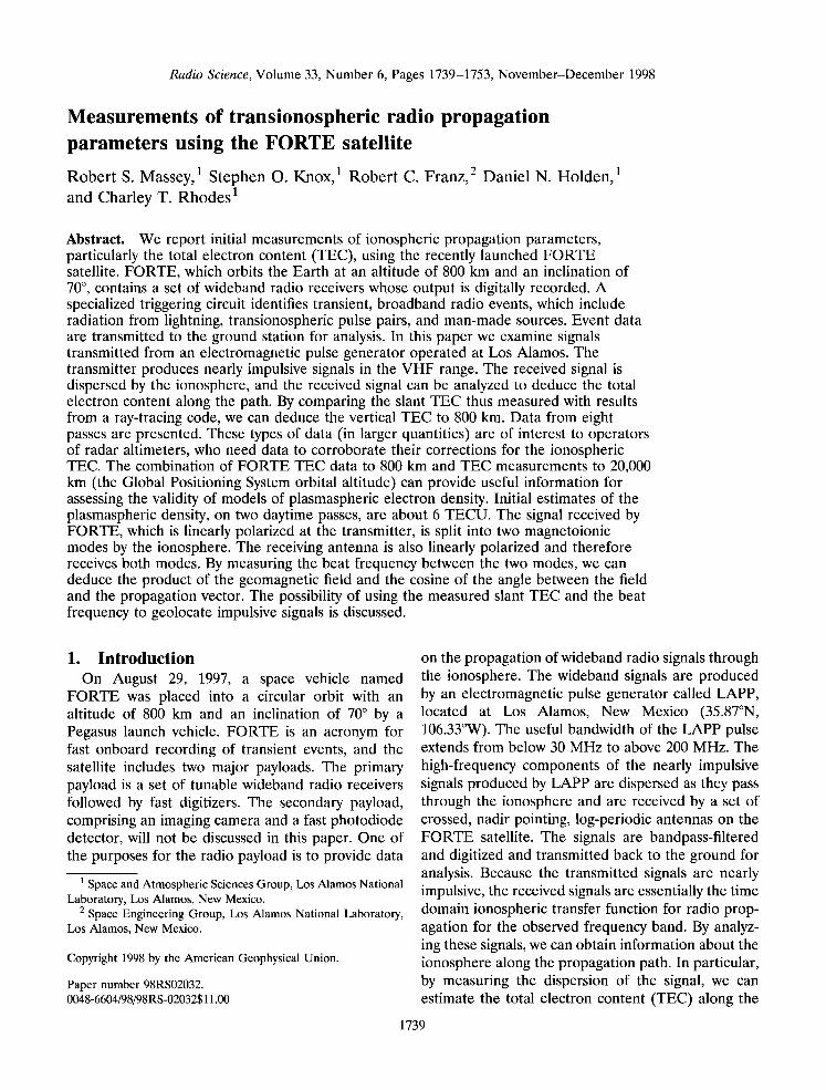
Figure 1. Waveform data from November 5, 1997' (a) basebanded electric field, (b) magnitude of Hilbert transform, and (c) phase from Hilbert transform with fitted points.

to as the "time-of-arrival," or TOA, technique, in- volves fitting (2) to the measured times of arrival at a comb of frequencies.

5.1. Phase-Detection Technique Figure 1 shows waveform data from an event on

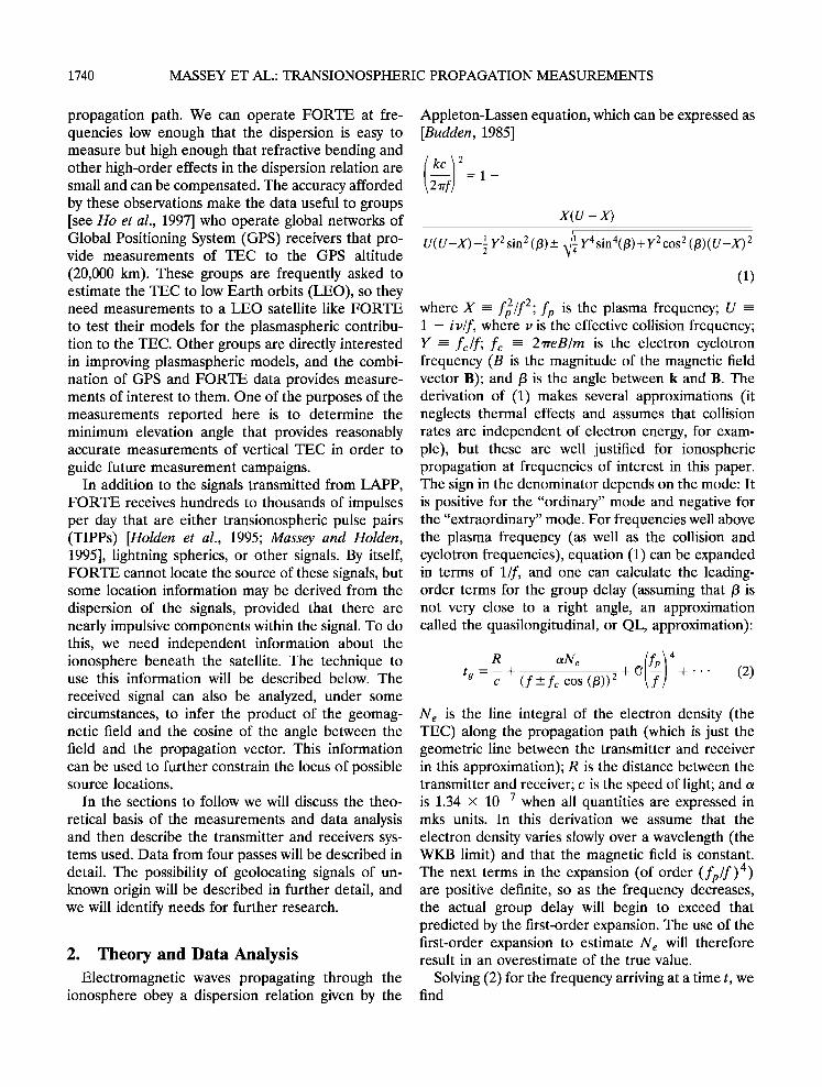
November 5, 1997. Figure l a shows the basebanded electric field waveform. For the phase-detection analysis we take the Hilbert transform of this signal, and from the transform and the data we compute the magnitude and the phase of the corresponding ana- lytic signal. Figure lb shows the magnitude thus calculated. The amplitude modulation predicted by (6) is very clear in the magnitude plot. By Fourier transforming the magnitude, we can readily identify the beat frequency and thereby obtain •r c cos (/3)1. This technique depends on the dispersed pulse lasting for many beats for this technique to work, which in turn requires that the TEC not be too low. Figure l c shows the phase with fitted points. The fit is to (4),

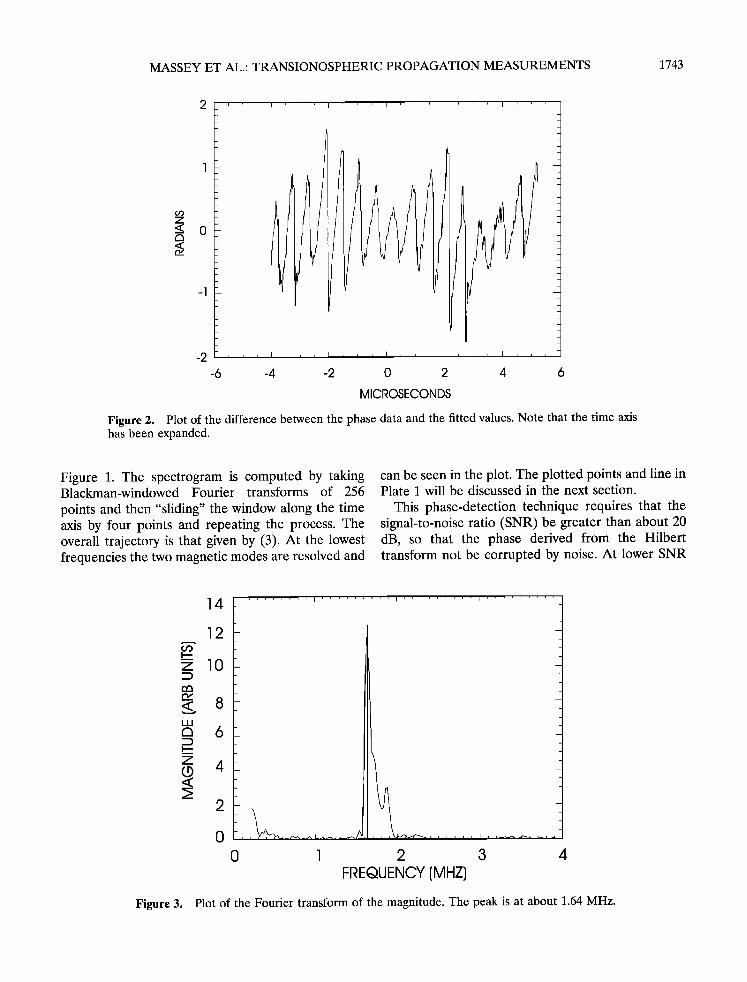
omitting the second term, whose effect appears in the amplitude modulation rather than in the fast varying phase. The differences between the data and the fit are shown in Figure 2. The residual errors are less than 2 rad and exhibit an oscillation at 1.67 MHz, with little or no obvious trend. The TEC coefficient was

13.8 (all values of TEC reported here are in units of 10 ]6 m -2, or TECU). The formal (statistical) error in the TEC is usually a few tenths of a TECU. System- atic errors from higher-order terms are a more im- portant limitation (see discussion below).

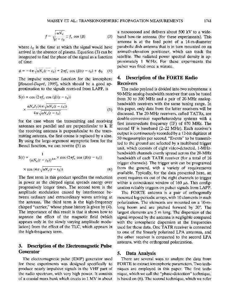
The Fourier transform of the magnitude is shown in Figure 3. The peak is at about 1.64 MHz, which implies that •c cos (/3)1 is about 820 kHz (taking the absolute magnitude doubles the apparent beat frequency). The 1.67-MHz oscillation seen in Figure 2 is probably caused by higher-order terms in the dispersion relation that appear at 2•c cos (/3)l.

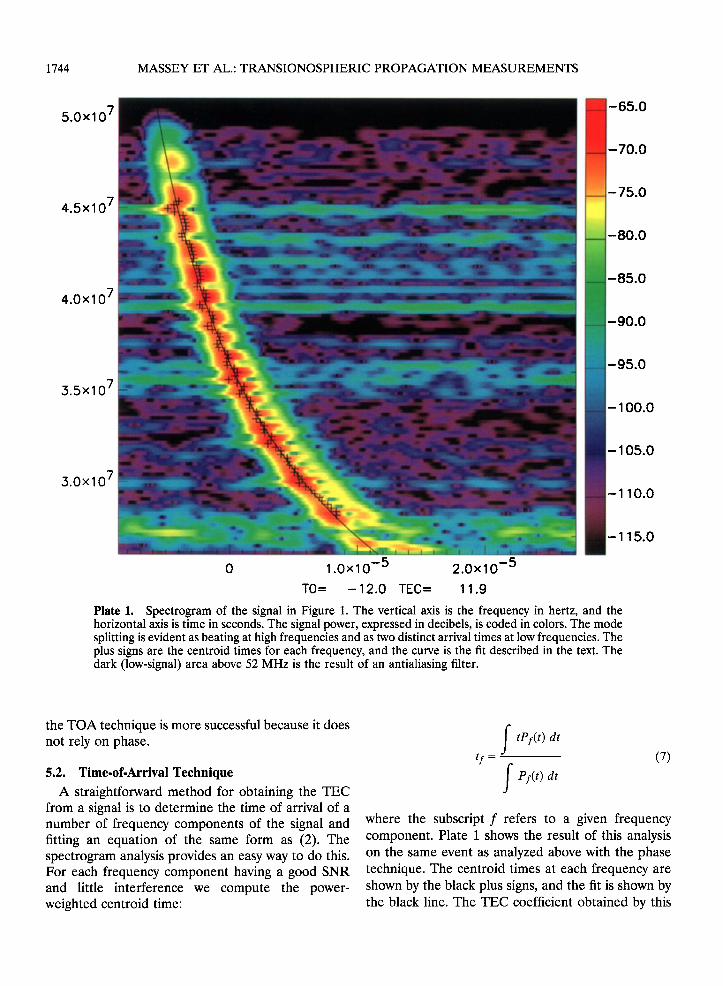
Plate i shows the spectrogram of the signal from


-6 -4 -2

i i I i i i

i

o

I ' i i I

i

2 4 6

MICROSECONDS

Figure 2. Plot of the difference between the phase data and the fitted values. Note that the time axis has been expanded.

Figure 1. The spectrogram is computed by taking Blackman-windowed Fourier transforms of 256

points and then "sliding" the window along the time axis by four points and repeating the process. The overall trajectory is that given by (3). At the lowest frequencies the two magnetic modes are resolved and

can be seen in the plot. The plotted points and line in Plate 1 will be discussed in the next section.

This phase-detection technique requires that the signal-to-noise ratio (SNR) be greater than about 20 dB, so that the phase derived from the Hilbert transform not be corrupted by noise. At lower SNR

14

12

0 1 2 3 4 FREQUENCY (MHZ)

Figure 3. Plot of the Fourier transform of the magnitude. The peak is at about 1.64 MHz.

1744 MASSEY ET AL.' TRANSIONOSPHERIC PROPAGATION MEASUREMENTS

5.0x10 -65.0

-70.0

7 4.5x10

4.0x10 7

3.5x10 7

-75.0

-80.0

-85.0

-90.0

-95.0

-1oo.o

-105.0

7 3.0x10

-11o.o

-115.0

0 1.0x10 -5 2.0x10 -5 TO= -12.0 TEC= 11.9

Plate 1. Spectrogram of the signal in Figure 1. The vertical axis is the frequency in hertz, and the horizontal axis is time in seconds. The signal power, expressed in decibels, is coded in colors. The mode splitting is evident as beating at high frequencies and as two distinct arrival times at low frequencies. The plus signs are the centroid times for each frequency, and the curve is the fit described in the text. The dark (low-signal) area above 52 MHz is the result of an antialiasing filter.

the TOA technique is more successful because it does not rely on phase.

5.2. Time-of-Arrival Technique

A straightforward method for obtaining the TEC from a signal is to determine the time of arrival of a number of frequency components of the signal and fitting an equation of the same form as (2). The spectrogram analysis provides an easy way to do this. For each frequency component having a good SNR and little interference we compute the power- weighted centroid time:

f tPf(t) dt tZ = (7)

f ?z(t) dt where the subscript f refers to a given frequency component. Plate 1 shows the result of this analysis on the same event as analyzed above with the phase technique. The centroid times at each frequency are shown by the black plus signs, and the fit is shown by the black line. The TEC coefficient obtained by this

MASSEY ET AL.' TRANSIONOSPHERIC PROPAGATION MEASUREMENTS 1745

method is 13.7, in excellent agreement with the value obtained by the phase technique.

5.3. Effects of Higher-Order Terms

At the lower frequencies used to obtain the data reported below, the effects of the higher-order terms in the dispersion relation cannot be ignored if the TEC coefficient is to be interpreted as the line integral of the electron density. The fact that there were no obvious systematic differences between the fit and the data does not mean that the higher-order terms are insignificant, because those terms are highly correlated with the 1/f 2 term. For that reason we will in the rest of this paper refer to the coefficient of 1If 2 in fitted data as the "pseudo-TEC." Because we want to know the true TEC, we used a three-dimensional ray-tracing code called TRACKER [Argo et al., 1992], which uses the Appleton-Hartree form for the dispersion relation. TRACKER incorporates the ionospheric conductivity and electron density (ICED) model [Tascione et al., 1988]. We use TRACKER by specifying the transmitter location and receiver (FORTE) location and the date and time of the event. TRACKER computes the group delay for a comb of frequencies across the FORTE channel, and we use the same fitting routine as used in the TOA algorithm described above to predict the measured pseudo-TEC. We adjust the sunspot number input to TRACKER until the modeled pseudo-TEC agrees with the measured pseudo-TEC at the highest elevation angle. We used no other adjustable parameters in this ionospheric model. ICED allows for inputs of the planetary magnetic index Kp and the auroral Q index, but for simplicity we used the default values and varied only the sunspot number. For this reason we do not expect the fitted sunspot number to agree precisely with the actual sunspot number, nor do we expect that the computed profiles are very accurate. In fact, we will see (below) that the predicted pseudo- TEC (and group delay) at angles far from zenith do not agree well with the measured values. We believe that this disagreement is mostly caused by errors in the electron density profiles away from the zenith used in the model.

TRACKER outputs the ionospheric density profile above the transmitter, which we integrate to 800 km to find the "true" TEC to that altitude. The true TEC

obtained in this way is systematically less than the pseudo-TEC, as would be expected from the neglect of the higher-order terms in (2).

5.4. Model for Beat Frequency To predict the beat frequency along a given path,

we use a simple model that evaluates the geomagnetic field at the point where the line of sight passes through an altitude of 250 km. The magnetic field model used is a tilted dipole, with an axis tilted to 78.6øN at 69.8øW. The beat frequency is just twice the product of the electron cyclotron frequency (fce = 2.80 X 10 6 B, with B in gauss and fce in hertz) and the cosine of the angle between the magnetic field and the propagation vector. The beat frequency does not depend on other ionospheric parameters, but unless the TEC is high enough that the dispersed signal lasts several beats, the beat frequency is diffi- cult to observe or measure.

6. Data

We have analyzed data from eight FORTE passes over Los Alamos. Data from four of these passes will be presented in some detail, to give a flavor of the technique and results. Two of these four passes occurred in local daytime, one near local dawn and one in local nighttime.

6.1. October 31, 1997, Data On October 31, both receivers were tuned to the

26- to 46-MHz band but were connected to different

antennas. The times at Los Alamos were from 0739 to

0744 LT, just after sunrise. The phase-detection technique was used to determine the slant pseudo-TEC and the magnetic-mode beat frequency for each received waveform. The results are summarized in

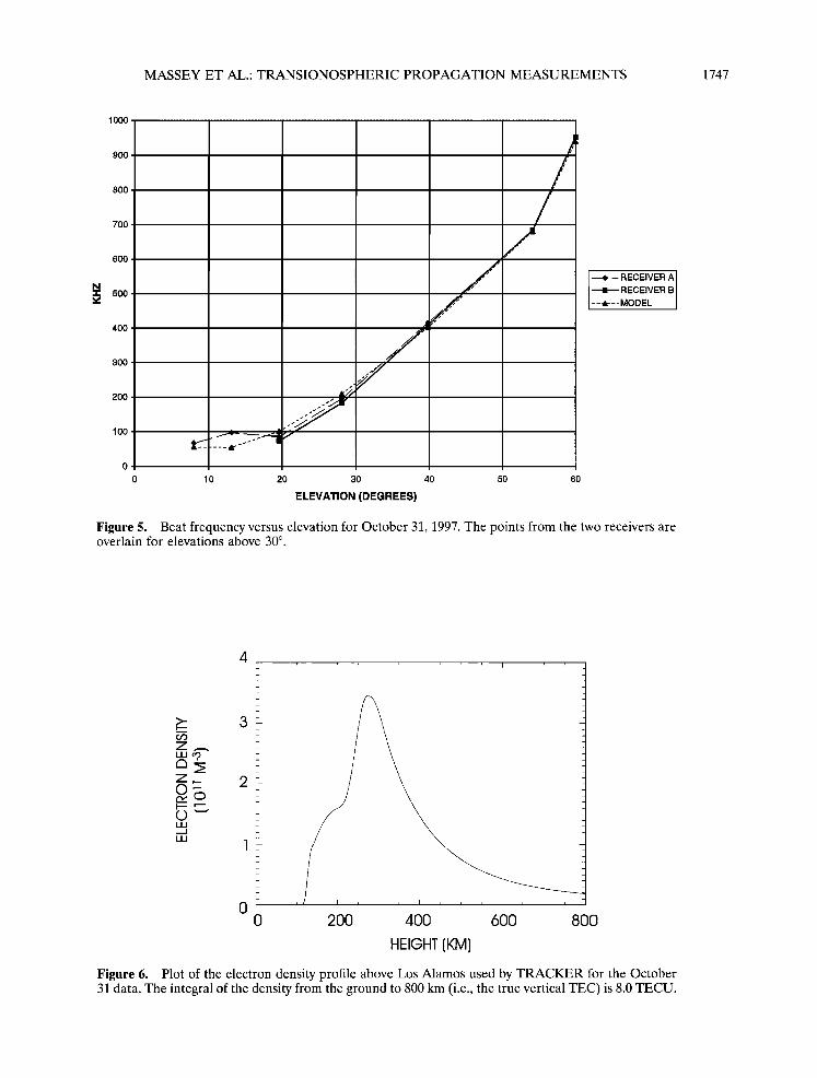
Table 1. The pseudo-TEC data and beat frequency data are plotted in Figures 4 and 5, respectively. A sunspot number (SSN) of 10 was used in the TRACKER calculations for all points. The World Data Center C-1 sunspot number for October 31 was 35 and was 43 for November 1. Agreement between the magnetic field model and the beat frequency data is excellent. The pseudo-TECs derived for the two receivers agree quite well, but the TRACKER predictions of the pseudo-TEC at low elevations fall systematically below the data, implying that the computed profile was in error to some degree.

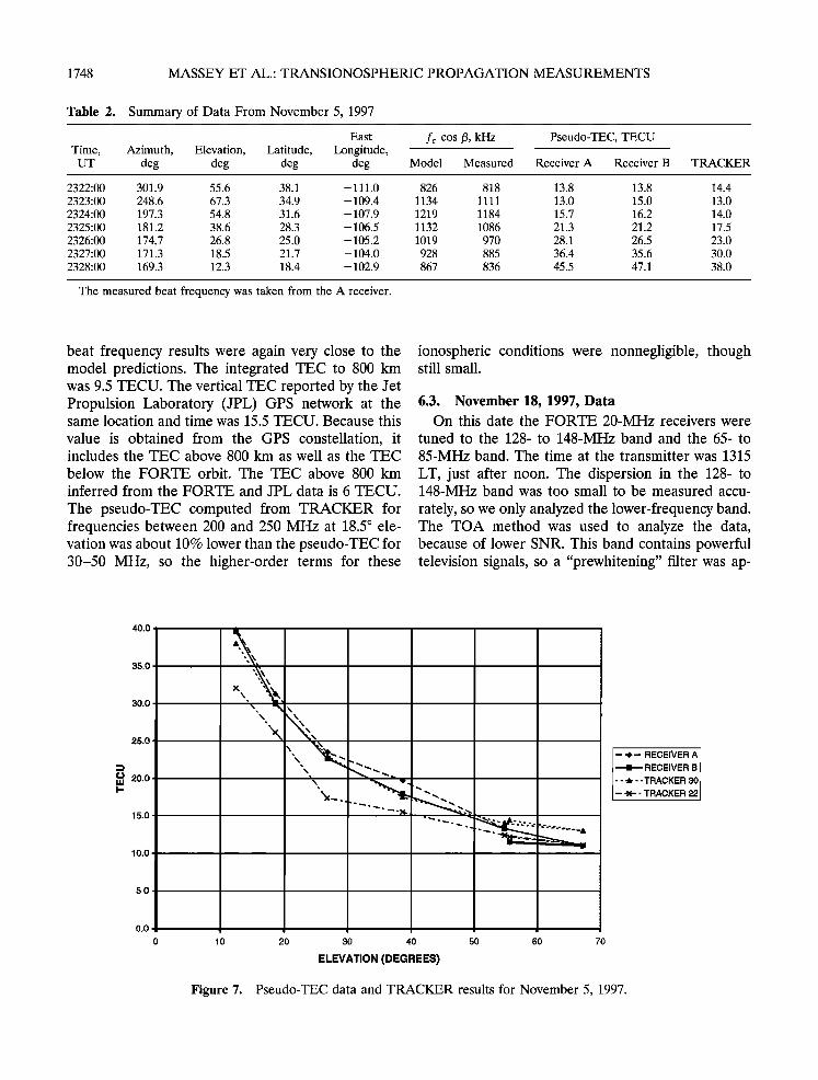
The density profile above Los Alamos computed by TRACKER is shown in Figure 6. The TEC in this profile to 800 km is 8.0 TECU. The pseudo-TEC from the TRACKER code to 800 km for the 26- to 46-MHz

band was 8.2 TECU, implying that the higher-order terms do not contribute much error at vertical angles. TRACKER does not compute slant TECs directly,


Table 1. Summary of Data for October 31, 1997

Receiver A Receiver B East

Time, Azimuth, Elevation, fc cos/3, Latitude, Longitude, Pseudo-TEC, fc cos/3, Pseudo-TEC, fc cos/3, TRACKER UT deg deg kHz deg deg TECU kHz TECU kHz Pseudo-TEC

1439:00 283.7 59.9 940 36.7 -110.8 9.0 952 9.0 952 9.1 1440:00 332.7 54.1 680 39.9 - 109.0 9.9 684 9.9 684 9.4

1441:00 355.4 39.8 401 43.1 -107.1 12.3 415 12.7 409 11.2 1442:00 5.3 28.1 209 46.2 - 105.0 15.0 195 15.0 183 13.0 1443:00 10.6 19.6 101 49.3 -102.5 19.1 85 20.2 73 17.2

1444:00 13.9 13.1 55 52.3 -99.7 23.4 977 23.5 19.6

The columns, from left to right, are the universal time for the event; the clockwise azimuth from north from the electromagnetic pulse generator, LAPP, to the satellite, in degrees; the elevation above the horizon of the satellite, in degrees; the predicted beat frequency, in kilohertz; the latitude and east longitude of the subsatellite point, in degrees; the pseudo-TEC and the beat frequency from the A receiver, in hertz; the pseudo-TEC and beat frequency from the B receiver; and the pseudo-TEC from the TRACKER code, for a sunspot number of 10.

but we reran it for frequencies between 200 and 250 MHz to derive a pseudo-TEC that should have much less susceptibility to high-order terms. The result for the geometry at 19.7 ø elevation was 16.9 TECU, compared with 17.2 TECU from the 30- to 50-MHz band. We conclude that the higher-order dispersion terms are small for these ionospheric conditions and geometry.

6.2. November 5, 1997, Data

On November 5, FORTE was configured as it was for October 31, and the same analysis techniques

were used. The time at the transmitter was 1625 LT, in the late afternoon. The results are summarized in

Table 2. Two different values for the sunspot number were used. To best fit the high-elevation points, a sunspot number of 22 was used, but at lower elevation angles the TRACKER results fell below the data. A sunspot number of 30 better fit the low-elevation data, at the expense of overestimating the pseudo- TEC at high elevations. The World Data Center sunspot number for this date was 51. The TEC and beat frequency data are shown in Figures 7 and 8. The

25.0

20.0

15.0

10.0

5.0

7. * RECEIVERA .•- RECEIVER B

ß a,- - - TRACKER 10

SSN =10

0.0

0 0 20 30 40 5( 60

ELEVATION (DEGREES)

Figure 4. Pseudo-TEC data for October 31, 1997. The pseudo-TECs are in units of 1016 rn -2

MASSEY ET AL.' TRANSIONOSPHERIC PROPAGATION MEASUREMENTS 1747

1000

900

8oo

700

600

N .-r- 500

400

3OO

200

100

10 20 30 40 50 60

ELEVATION (DEGREES)

----e -- RECEIVER A

- RECEIVER B

--.--- MODEL

Figure 5. Beat frequency versus elevation for October 31, 1997. The points from the two receivers are overlain for elevations above 30 ø .

200 400 600 800

HEIGHT (KM]

Figure 6. Plot of the electron density profile above Los Alamos used by TRACKER for the October 31 data. The integral of the density from the ground to 800 km (i.e., the true vertical TEC) is 8.0 TECU.


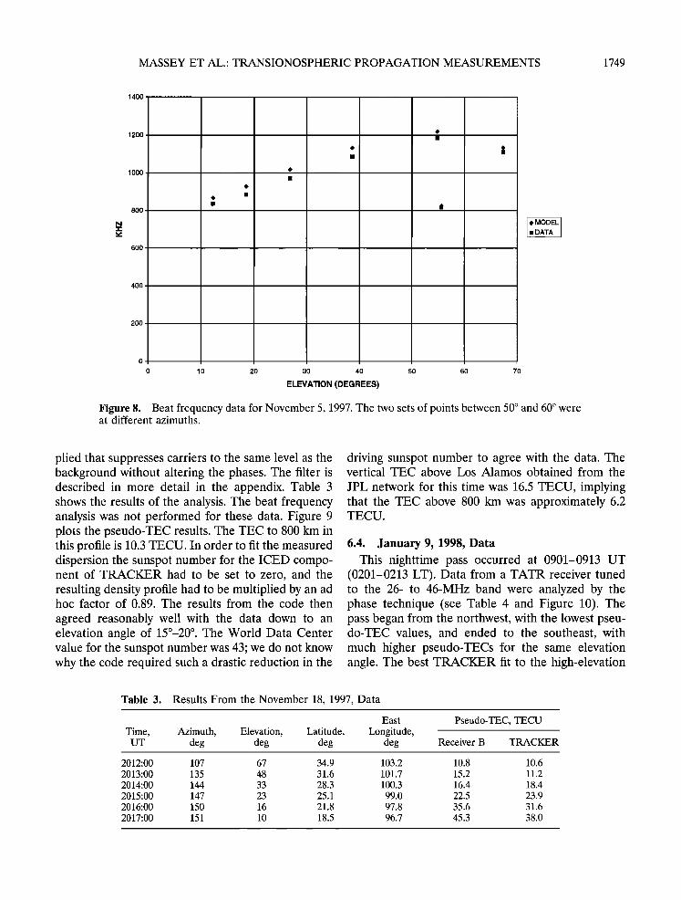
Table 2. Summary of Data From November 5, 1997

East fc cos/3, kHz Pseudo-TEC, TECU Time, Azimuth, Elevation, Latitude, Longitude, UT deg deg deg deg Model Measured Receiver A Receiver B TRACKER

2322:00 301.9 55.6 38.1 -111.0 826 818 13.8 13.8 14.4 2323:00 248.6 67.3 34.9 - 109.4 1134 1111 13.0 15.0 13.0 2324:00 197.3 54.8 31.6 - 107.9 1219 1184 15.7 16.2 14.0 2325:00 181.2 38.6 28.3 - 106.5 1!32 1086 21.3 21.2 17.5

2326:00 174.7 26.8 25.0 - 105.2 1019 970 28.1 26.5 23.0 2327:00 171.3 18.5 21.7 - 104.0 928 885 36.4 35.6 30.0 2328:00 169.3 12.3 18.4 - 102.9 867 836 45.5 47.1 38.0

The measured beat frequency was taken from the A receiver.

beat frequency results were again very close to the model predictions. The integrated TEC to 800 km was 9.5 TECU. The vertical TEC reported by the Jet Propulsion Laboratory (JPL) GPS network at the same location and time was 15.5 TECU. Because this

value is obtained from the GPS constellation, it includes the TEC above 800 km as well as the TEC

below the FORTE orbit. The TEC above 800 km

inferred from the FORTE and JPL data is 6 TECU.

The pseudo-TEC computed from TRACKER for frequencies between 200 and 250 MHz at 18.5 ø elevation was about 10% lower than the pseudo-TEC for 30-50 MHz, so the higher-order terms for these

ionospheric conditions were nonnegligible, though still small.

6.3. November 18, 1997, Data On this date the FORTE 20-MHz receivers were

tuned to the 128- to 148-MHz band and the 65- to

85-MHz band. The time at the transmitter was 1315

LT, just after noon. The dispersion in the 128- to 148-MHz band was too small to be measured accu-

rately, so we only analyzed the lower-frequency band. The TOA method was used to analyze the data, because of lower SNR. This band contains powerful television signals, so a "prewhitening" filter was ap-

40.0

35.0

30.0

25.0

20.0

15.0

10.0

5.0

0.0

0 10 20 30 40 50 60 70

ELEVATION (DEGREES)

- -,- RECEIVER A I -- RECEIVERBI

- - * - -TRACKER 30 - -x- - TRACKER 22

Figure 7. Pseudo-TEC data and TRACKER results for November 5, 1997.


1400

1200

lOOO

800

6O0

400

2O0

MODEL ID• ATA •

0 10 20 30 40 50 60 70

ELEVATION (DEGREES)

Figure 8. Beat frequency data for November 5, 1997. The two sets of points between 50 ø and 60 ø were at different azimuths.

plied that suppresses carriers to the same level as the background without altering the phases. The filter is described in more detail in the appendix. Table 3 shows the results of the analysis. The beat frequency analysis was not performed for these data. Figure 9 plots the pseudo-TEC results. The TEC to 800 km in this profile is 10.3 TECU. In order to fit the measured dispersion the sunspot number for the ICED component of TRACKER had to be set to zero, and the resulting density profile had to be multiplied by an ad hoc factor of 0.89. The results from the code then

agreed reasonably well with the data down to an elevation angle of 15ø-20 ø . The World Data Center value for the sunspot number was 43; we do not know why the code required such a drastic reduction in the

driving sunspot number to agree with the data. The vertical TEC above Los Alamos obtained from the

JPL network for this time was 16.5 TECU, implying that the TEC above 800 km was approximately 6.2 TECU.

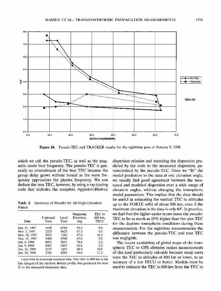
6.4. January 9, 1998, Data

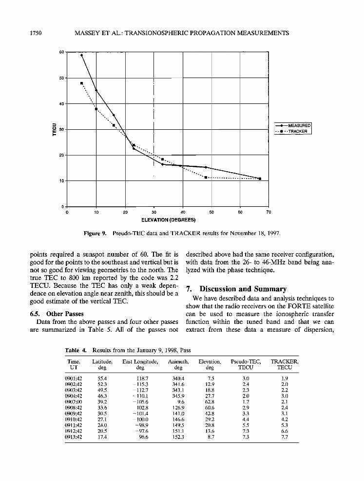
This nighttime pass occurred at 0901-0913 UT (0201-0213 LT). Data from a TATR receiver tuned to the 26- to 46-MHz band were analyzed by the phase technique (see Table 4 and Figure 10). The pass began from the northwest, with the lowest pseudo-TEC values, and ended to the southeast, with much higher pseudo-TECs for the same elevation angle. The best TRACKER fit to the high-elevation

Table 3. Results From the November 18, 1997, Data

Time, Azimuth, Elevation, Latitude, UT deg deg deg

East

Longitude, deg

Pseudo-TEC, TECU

Receiver B TRACKER

2012:00 107 67 34.9 103.2 2013:00 135 48 31.6 101.7 2014:00 144 33 28.3 100.3

2015:00 147 23 25.1 99.0 2016:00 150 16 21.8 97.8 2017:00 151 10 18.5 96.7

10.8 10.6

15.2 11.2 16.4 18.4 22.5 23.9

35.6 31.6

45.3 38.0


60

50

40

(..) 30

20

MEASUREDJ TRACKER

0 10 20 30 40 50 60 70

ELEVATION (DEGREES)

Figure 9. Pseudo-TEC data and TRACKER results for November 18, 1997.

points required a sunspot number of 60. The fit is good for the points to the southeast and vertical but is not so good for viewing geometries to the north. The true TEC to 800 km reported by the code was 2.2 TECU. Because the TEC has only a weak depen- dence on elevation angle near zenith, this should be a good estimate of the vertical TEC.

6.5. Other Passes

Data from the above passes and four other passes are summarized in Table 5. All of the passes not

described above had the same receiver configuration, with data from the 26- to 46-MHz band being analyzed with the phase technique.

7. Discussion and Summary We have described data and analysis techniques to

show that the radio receivers on the FORTE satellite

can be used to measure the ionospheric transfer function within the tuned band and that we can

extract from these data a measure of dispersion,

Table 4. Results from the January 9, 1998, Pass

Time, Latitude, East Longitude, Azimuth, UT deg deg deg

Elevation, deg

Pseudo-TEC, TECU

TRACKER, TECU

0901:42 55.4 -118.7 340.4 0902:42 52.3 -115.3 341.6

0903:42 49.5 - 112.7 343.1 0904:42 46.3 - 110.1 345.9

0907:00 39.2 - 105.6 9.6 0908:42 33.6 - 102.8 126.9

0909:42 30.5 -101.4 141.0

0910:42 27.1 - 100.0 146.6 0911:42 24.0 -98.9 149.5

0912:42 20.5 -97.6 151.1 0913:42 17.4 -96.6 152.3

7.5 12.9

18.8

27.7

62.8

60.6

42.8

29.2 20.8

13.6

8.7

3.0 2.4

2.3

2.0

1.7

2.9

3.3

4.4

5.5

7.3

7.3

1.9

2.0

2.2

3.0

2.1

2.4

3.1

4.2

5.3 6.6

7.7


8.0

7.0

6.0

5.0

O m 4.0

3,0

2.0

1.0

0.0

PHI TEC I -TRACKER

SSN=60

0.0 10.0 20.0 30.0 40.0 50.0 60.0 70.0

ELEVATION (DEGREES)

Figure 10. Pseudo-TEC and TRACKER results for the nighttime pass of January 9, 1998.

which we call the pseudo-TEC, as well as the magnetic mode beat frequency. The pseudo-TEC is gen- erally an overestimate of the true TEC because the group delay grows without bound as the wave frequency approaches the plasma frequency. We can deduce the true TEC, however, by using a ray-tracing code that includes the complete Appleton-Hartree

Table 5. Summary of Results for All High-Elevation Passes

Maximum TEC to

Universal Local Elevation, 800 km, Date Time Time deg TECU

Oct. 31, 1997 1439 0739 59.9 8.0 Nov. 5, 1997 2323 0623 67.3 9.5 Nov. 18, 1997 2012 1312 67.0 10.3 Dec. 18, 1997 1400 0700 87.6 2.8 Jan. 8, 1998 0931 0231 76.6 2.2 Jan. 9, 1998 0907 0207 62.8 2.2 Jan. 14, 1998 2157 1457 68.9 10.0 Jan. 21, 1998 2102 0702 56.0 11.2

Local time is mountain standard time. The TEC to 800 km is the

line integral of the electron density profile that produced the best fit to the measured dispersion data.

dispersion relation and matching the dispersion predicted by the code to the measured dispersion, pa- rameterized by the pseudo-TEC. Once we "fit" the model prediction to the data at one elevation angle, we usually find good agreement between the measured and modeled dispersion over a wide range of elevation angles, without changing the ionospheric model parameters. This implies that the data should be useful in estimating the vertical TEC to altitudes up to the FORTE orbit of about 800 km, even if the maximum elevation in the data is only 60 ø . In practice, we find that the higher-order terms cause the pseudo- TEC to be as much as 10% higher than the true TEC for the daytime ionospheric conditions during these measurements. For the nighttime measurements the difference between the pseudo-TEC and true TEC was negligible.

The recent availability of global maps of the ionospheric TEC to GPS altitudes makes measurements of this kind particularly valuable because many users want the TEC to altitudes of 800 km or lower, to an accuracy of a few TECU or better. Models must be used to estimate the TEC to 800 km from the TEC to


20,000 km, and data are needed to judge the accuracy of these models. By combining the GPS TEC data with the FORTE TEC data, we should be able to evaluate models for the plasmaspheric contribution to TEC. The accuracy of the estimates of vertical TEC is probably limited by systematic errors, but the errors may be as low as a few TECU. Further modeling will be required to make a better estimate of these errors.

Our preliminary determinations of plasmaspheric TEC may be compared with those reported by Ciraolo and Spalla [1997], who looked at the differences between the TEC measurements to the GPS constel-

lation and those to the Navy Navigation Satellite System (NNSS). They reported a median difference (during a year) in those TEC values of 3.2 TECU, with a standard deviation of 2 TECU. The NNSS

satellites are in a higher orbit (1100 km altitude) than FORTE, so their measurements might be expected to fall below ours. A fair comparison with their results can only be made after we have obtained many more data.

We also find very good agreement between the measured beat frequency between the two magnetic modes and a model based on a tilted dipole with a fixed ionospheric height. We would therefore expect that given the beat frequency of a source of unknown location, we could determine a locus of points on the Earth's surface that should contain the source. Fur-

ther constraining the locus of possible source points depends on obtaining accurate estimates of the electron density profile to 800 km in the vicinity of the subsatellite point. The JPL network of GPS receivers is a likely source of such data if the plasmaspheric contribution can be accurately removed. FORTE data can help evaluate how well plasmaspheric models perform this needed function.

Appendix: Description of the Prewhitening Filter

Interference from communication signals is en- countered in many of the frequency bands above 30 MHz (one person's signal is another person's interference). Most of the power in these signals is con- fined to a spectrally narrow carrier that has nearly constant amplitude for the 200- to 500-•s records we typically record. We can suppress these carriers by using a frequency domain filter. The first step in constructing the filter is the computation of a spectrogram with 1024-point windows (513 positive fre-

quencies). The average power in each of these 513 frequency bins is computed. The original signal is Fourier transformed, and the transform is converted into magnitude and phase arrays. For each frequency component in these arrays the magnitude is divided by a value obtained by splining the 513-point array of average powers. The resulting magnitude array is approximately constant. The phase array is not mod- ified. We reconstruct the filtered signal by reconvert- ing the magnitude and phase arrays into a complex array and taking the inverse Fourier transform. The reconstructed time series retains any transient signals from the original data, but continuous signals are suppressed.

Acknowledgments. The authors thank the FORTE engineering team, in particular Don Enemark, Marty Shipley, Michael Pigue, Glenn Thornton, and Steve Wallin, and Tim Murphy, who was project scientist during the design of the satellite. We are also indebted to the operations team led by Diane Roussel-Duprd, with members at Los Alamos and at Sandia National Laboratory in Albuquerque. The software/ data team, especially Phil Klingner, Diana Esch-Mosher, and Michael Carter, made access to the RF data look easy. Gary Stelzer operated the LAPP facility at odd hours of the day and night. We also thank Xiaoqing Pi and Byron Iijima of NASA's Jet Propulsion Laboratory for providing data from their GPS receiver network. This work was performed at the Los Alamos National Laboratory under the auspices of the U.S. Department of Energy. We especially thank Robert Waldron and Stan Rudnick of the DOE for their

long-term support of this program.

References

Argo, P., T. J. Fitzgerald, and R. Carlos, NICARE I HF propagation experiment results and interpretation, Radio Sci., 27(2), 289-305, 1992.

Budden, K. G., The Propagation of Radio Waves, Cambridge Univ. Press, New York, 1985.

Ciraolo, L., and P. Spalla, Comparison of ionospheric total electron content from the Navy Navigation Satellite Sys- tem and the GPS, Radio Sci., 32(3), 1071-1080, 1997.

Ho, C. M., B. D. Wilson, A. J. Mannucci, U. J. Lindqwister, and D. N. Yuan, A comparative study of ionospheric total electron content measurements using global ionospheric maps of GPS, TOPEX radar, and the Bent model, Radio Sci., 32(4), 1499-1512, 1997.

Holden, D. N., C. P. Munson, and J. C. Devenport, Satellite observations of transionospheric pulse pairs, Geophys. Res. Lett., 22(8), 889-892, 1995.

Massey, R. S., and D. N. Holden, Phenomenology of transionospheric pulse pairs, Radio Sci., 30(5), 1645- 1659, 1995.


Roussel-Dupr6, R. A., RF propagation in the atmosphere, in Introduction to Ultra-Wideband Radar Systems, edited by J. D. Taylor, chap. 7, pp. 325-364, CRC Press, Boca Raton, Fla., 1995.

Tascione, T. F., H. W. Kroehl, R. Creiger, J. W. Freeman Jr., R. A. Wolf, R. W. Spiro, R. V. Hilmer, J. W. Shade, and B. A. Hausman, New ionospheric and magneto- spheric specification models, Radio Sci., 23(3), 211-222, 1988.

D. N. Holden, S. O. Knox, R. S. Massey, and C. T. Rhodes, Space and Atmospheric Sciences Group, Los Alamos National Laboratory, Los Alamos, NM 87545. (e-mail: [email protected])

R. C. Franz, Space Engineering Group, Los Alamos National Laboratory, Los Alamos, NM 87545.

(Received March 4, 1998; revised June 10, 1998; accepted June 16, 1998.)

Documents

Measurements of transionospheric radio propagation parameters using the FORTE satellite