Measuring Symmetry, Asymmetry and Randomness in Neural Network Connectivity

Measuring Symmetry, Asymmetry and Randomness inNeural Network ConnectivityUmberto Esposito1, Michele Giugliano1,2,3, Mark van Rossum4, Eleni Vasilaki1,2*

1 Department of Computer Science, University of Sheffield, Sheffield, United Kingdom, 2 Theoretical Neurobiology and Neuroengineering Laboratory, Department of

Biomedical Sciences, University of Antwerp, Wilrijk, Belgium, 3 Laboratory of Neural Microcircuitry, Brain Mind Institute, Ecole polytechnique federale de Lausanne,

Lausanne, Switzerland, 4 School of Informatics, University of Edinburgh, Edinburgh, United Kingdom

Abstract

Cognitive functions are stored in the connectome, the wiring diagram of the brain, which exhibits non-random features, so-called motifs. In this work, we focus on bidirectional, symmetric motifs, i.e. two neurons that project to each other viaconnections of equal strength, and unidirectional, non-symmetric motifs, i.e. within a pair of neurons only one neuronprojects to the other. We hypothesise that such motifs have been shaped via activity dependent synaptic plasticityprocesses. As a consequence, learning moves the distribution of the synaptic connections away from randomness. Our aimis to provide a global, macroscopic, single parameter characterisation of the statistical occurrence of bidirectional andunidirectional motifs. To this end we define a symmetry measure that does not require any a priori thresholding of theweights or knowledge of their maximal value. We calculate its mean and variance for random uniform or Gaussiandistributions, which allows us to introduce a confidence measure of how significantly symmetric or asymmetric a specificconfiguration is, i.e. how likely it is that the configuration is the result of chance. We demonstrate the discriminatory powerof our symmetry measure by inspecting the eigenvalues of different types of connectivity matrices. We show that aGaussian weight distribution biases the connectivity motifs to more symmetric configurations than a uniform distributionand that introducing a random synaptic pruning, mimicking developmental regulation in synaptogenesis, biases theconnectivity motifs to more asymmetric configurations, regardless of the distribution. We expect that our work will benefitthe computational modelling community, by providing a systematic way to characterise symmetry and asymmetry innetwork structures. Further, our symmetry measure will be of use to electrophysiologists that investigate symmetry ofnetwork connectivity.

Citation: Esposito U, Giugliano M, van Rossum M, Vasilaki E (2014) Measuring Symmetry, Asymmetry and Randomness in Neural Network Connectivity. PLoSONE 9(7): e100805. doi:10.1371/journal.pone.0100805

Editor: Sergio Martinoia, University of Genova, Italy

Received December 31, 2013; Accepted May 29, 2014; Published July 9, 2014

Copyright: � 2014 Esposito et al. This is an open-access article distributed under the terms of the Creative Commons Attribution License, which permitsunrestricted use, distribution, and reproduction in any medium, provided the original author and source are credited.

Funding: This work was partly supported by the European Commission (FP7 Marie Curie Initial Training Network ‘‘NAMASEN’’, grant n. 264872 (EV, MG), the RoyalSociety travel grant JP091330-2009/R4 (EV, MG), the Interuniversity Attraction Poles Program (IUAP), initiated by the Belgian Science Policy Office (MG), the FutureEmerging Technology programme project ‘‘BRAINLEAP’’ grant n. 306502 (MG), the Engineering and Physical Sciences Research Council (EPSRC), grant n. EP/J019534/1 (EV) and the EPSRC e-futures award EFXD12003/EFXD12004 (EV). The funders had no role in study design, data collection and analysis, decision topublish, or preparation of the manuscript.

Competing Interests: The authors have declared that no competing interests exist.

* Email: [email protected]

Introduction

It is widely believed that cognitive functions are stored in the so-

called connectome [1,2], the wiring diagram of the brain. Due to

improvements in technology, experimental techniques and com-

putational paradigms [3,4], the investigation of the connectome,

known as connectomics, has generated great excitement [5] and

has made significant progress [6–9] resulting in a rapid

proliferation of neuroscience datasets [10–13].

Studies on the brain wiring diagram have shown that connectivity

is non-random, highlighting the existence of specific connectivity

motifs at the microcircuit level, see for instance [14–17]. Of particular

interest are the motifs that exhibit bidirectional (reciprocal) and

unidirectional (non-reciprocal) connections between pairs of neurons.

More specifically, theoretical work [18] studied the development of

unidirectional connectivity due to long-term plasticity in an artificial

network of spiking neurons under a temporal coding scheme, where it

is assumed that the time at which neurons fire carries out important

information. This finding is correlated to unidirectional connectivity

observed in somatosensory cortex, see [19]. In [18] the development

of bidirectional connectivity in the same network under a frequencycoding scheme, where information is transmitted in the firing rate of

the neurons, was also studied and correlated to bidirectional

connectivity found in the visual cortex [14]. Complementary to this

work, in [20,21] the authors explored the experimentally identified

correlation of bidirectional and unidirectional connectivity to short-

term synaptic dynamics, see [22], by studying the development of

connectivity in networks with facilitating and depressing synapses due

to the interaction of short-term and long-term plasticities. The role of

synaptic long-term plasticity in structures formation within networks

has been also investigated in [23–25].

Similar to [18] and [20,21], we hypothesise that the above

mentioned motifs have been shaped via activity dependent synaptic

plasticity processes, and that learning moves the distribution of the

synaptic connections away from randomness. Our aim is to provide

a global, macroscopic, single parameter characterisation of the

statistical occurrence of bidirectional and unidirectional motifs. To

this end:

PLOS ONE | www.plosone.org 1 July 2014 | Volume 9 | Issue 7 | e100805

http://creativecommons.org/licenses/by/4.0/

http://crossmark.crossref.org/dialog/?doi=10.1371/journal.pone.0100805&domain=pdf

We define a symmetry measure that does not require any a

priori thresholding of the weights or knowledge of their

maximal value, and hence is applicable to both simulations

and experimental data.

We calculate the mean and variance of this symmetry measure

for random uniform or Gaussian distributions, which allows us

to introduce a confidence measure of how significantly

symmetric or asymmetric is a specific configuration, i.e. how

likely it is that the configuration is the result of chance.

We demonstrate the discriminatory power of our symmetry

measure by inspecting the eigenvalues of different types of

connectivity matrices, given that symmetric matrices are

known to have real eigenvalues.

We show that a Gaussian distribution biases the connectivity

motifs to more symmetric configurations than a uniform

distribution and that introducing a random synaptic pruning,

mimicking developmental regulation in synaptogenesis, biases

the connectivity motifs to more asymmetric configurations,

regardless of the distribution. Our statistics of the symmetry

measure allows us to correctly evaluate the significance of a

symmetric or asymmetric network configuration in both these

cases.

Our symmetry measure allows us to observe the evolution of a

specific network configuration, as we exemplify in our results.

We expect that our work will benefit the computational

modelling community, by providing a systematic way to

characterise symmetry and asymmetry in network structures.

Further, our symmetry measure will be of use to electrophysiol-

ogists that may investigate symmetric or asymmetric network

connectivity.

Methods

In what follows, we first define a novel measure that quantifies

the degree of symmetry in a neuronal network with excitatory

synaptic connections. More specifically, we describe the strength of

the synaptic efficacies between the neurons by the elements of a

square matrix, i.e. the connectivity matrix, to which we associate a

number that quantifies the similarity of the elements above the

matrix diagonal to those below the diagonal. We further study this

measure from a statistical point of view, by means of both

analytical tools and numerical simulations. Aiming to associate a

significance value to the measure, i.e. the probability that a certain

symmetric or non-symmetric configuration is the result of chance,

we consider random synaptic efficacies drawn from uniform and

Gaussian distributions. We also study how our symmetry measure

is affected by the anatomical disconnection of neurons in a

random manner, i.e. zeroing some entries in the connectivity

matrix. Finally, we anticipate that connectivity distributions are

modified by activity-dependent processes and we describe the

structure of the network we use as a demonstrative example in the

Results section.

DefinitionsLet us consider the adjacency (or connectivity) matrix W of a

weighted directed network [26], composed of N vertices and

without self-edges. The N vertices represent the neurons, with

N N{1ð Þ possible synaptic connections among them. The

synaptic efficacy between two neurons is expressed as a positive

element wji in the adjacency matrix. W is thus composed by

positive elements off-diagonal, taking values in the bounded range

0,wmax½ �, and by zero diagonal entries. We define s as a measure of

the symmetry of W:

s~1{2

N N{1ð Þ{2M

XN

i~1

XN

j~iz1

Dwij{wji Dwijzwji

ð1Þ

where M is the number of instances where both wij and wji are

zero, i.e. there is no connection between two neurons. The term

q~N N{1ð Þ{2M

2is a normalisation factor that represents the

total number of synaptic connection pairs that have at least one

non-zero connection. A value of s near 0 indicates that there are

virtually no reciprocal connections in the network, while a value of

s near 1 indicates that virtually all connections are reciprocal. We

exclude (0,0) pairs from our definition of the symmetry measure.

Mathematically such pairs would introduce undefined terms to Eq.

(1). In addition, conceptually, we expect that small weights will not

be experimentally measurable. It is then reasonable to exclude

them, expecting to effectively increase the signal to noise ratio.

Pruning and Plasticity. We assume that a connection wij is

permanently disconnected and set to 0 with probability

2pruning~a [ 0, 1½ Þ: Consequently, the probability that two

neurons i and j are mutually disconnected, i.e. wij~wji~0, is

a2: When a connection is permanently pruned in such a way, its

efficacy remains 0 all the time, whereas the off-diagonal non-

pruned values of the adjacency matrix W change slowly in time, as

a result of activity-dependent synaptic plasticity. We consider that

this procedure correlates with developmental mechanisms associ-

ated with or following synaptogenesis.

Unidirectional and Bidirectional connection pairs. We

associate the quantity Zij~Dwij{wji Dwijzwji

, i.e. the term of the

summation in the Eq. (1) to the neuronal pair i,j: This term maps

the strength of the connections between two neurons to a single

variable. Each connection pair can therefore be bidirectional if

wij^wji, unidirectional if wij%wji or wij&wji, or none of the two.

As a consequence, a network can be dominated by bidirectional

connectivity, by unidirectional connectivity, or it may exhibit

random features.

Weight Bounds. In what follows we consider the case of

wmax~1: Due to the termDwij{wji Dwijzwji

, this can be done without loss

of generality.

Statistics of sLet us consider a large number of n instances of a network

whose connection weights are randomly distributed. Each

adjacency matrix can be evaluated via our symmetry measure.

We rewrite Eq. 1 as:

s~1{1

q

XN

i~1

XN

j~iz1

Zij~1{1

q

Xq

k~1

Zk, ð2Þ

where k is a linear index running over all the q non-zero

‘‘connection pairs’’ within the network. We can then estimate the

mean ms and variance s2s of s over all n networks as:

ms:En s½ �~1{En Z½ � ð3Þ

s2s:Varn(s)~

1

qVarn(Z) ð4Þ

Measuring Symmetry, Asymmetry and Randomness in Synaptic Connectivity


1

2

3

4

5

where the notation En:½ � and Varn(:) implies that the expected

value and variance are computed along the n different represen-

tations of the network.

Eq. (3), (4) allow us to transfer the statistical analysis from s to Z:To derive theoretical formulas for mean value and variance of Z

we use the fact that its probability density function (PDF), f (Z),can be written as a joint distribution, f (Z1,Z2) where we have

introduced the notation Z1~Dwij{wji D, Z2~wjizwji :

E Z½ �~ð1

0

dZ Z f (Z)~

ð ðD

dZ1 dZ2Z1

Z2f (Z1, Z2) ð5Þ

within the range D defined by 0ƒZ1ƒ1 and Z1ƒZ2ƒ2{Z1:Similarly, we can calculate the variance as follows:

Var(Z)~

ð1

0

dZ Z{E Z½ �ð Þ2 f (Z)

~

ð ðD

dZ1 dZ2Z1

Z2{E Z½ �

� �2

f (Z1, Z2) :

ð6Þ

We note that mean value and variance of Z can be numerically

estimated either by using a large set of small networks or on a

single very large network: What matters is that the total number of

connection pairs, given by the product n:q, is sufficiently large to

guarantee good statistics and that connection pairs are indepen-

dent of each other. In the calculations below, we assume a very

large adjacency matrix.

Adjacency matrix with uniform random valuesWe first consider a network with randomly distributed

connections without pruning, followed by the more general case

where pruning is taken into account.

Fully connected network. For the uniform distribution

f u(w)~1 for w[ 0, 1½ �, see Fig. 1A. The probability of having

wij~wji~0 for at least one pair (i, j) is negligible, hence M~0: It

is straightforward to derive the distributions f u2 (Z2) and f u

1 (Z1),

depicted in Fig. 1B,C correspondingly:

f u1 (Z1)~

{2Z1z2 for Z1 [ 0, 1½ �0 otherwise

�ð7Þ

f u2 (Z2)~

Z2 for Z2 [ 0, 1½ �{Z2z2 for Z2 [ 1, 2½ �0 otherwise

8><>: : ð8Þ

We can therefore obtain the joint PDF (Fig. 1D):

f u12(Z1,Z2)~

1 for Z1, Z2½ � [ D

0 otherwise

�: ð9Þ

Pruning. Introducing pruning to the elements of the adja-

cency matrix, with probability a, corresponds to a discontinuous

probability distribution function of w, that can be written as a sum

of a continuous function and of a Dirac’s Delta centred in w~0(see also Fig. 1E):

f ua (w)~(1{a)f u(w)za d (0) : ð10Þ

Now the (0, 0) pairs have to be explicitly excluded from the

distributions of Z1 and Z2: Also, the number of pairs of the type

(w, 0) increases, resulting in the appearance of a uniform

contribution in the region 0, 1½ � in both the PDF of Z1 and Z2:Their final exact profile can be obtained by considering the

possible combinations of drawing wij and wji from the above

pruned distribution and their corresponding probability of

occurrence. There are four contributions: f u(w)|f u(w),f u(w)|d(0), d(0)|f u(w), d(0)|d(0): The last term, which

describes the (0, 0) pairs, has to be subtracted and the remaining

expression has to be renormalised. The results are graphically

shown in Fig. 1F, 1G and are mathematically described by the

following expressions:

f u1,a(Z1)~

{21{a

1zaZ1z

2

1zafor Z1 [ 0, 1½ �

0 otherwise

8<: ð11Þ

f u2,a(Z2)~

1{a

1zaZ2z

2a

1zafor Z2 [ 0, 1½ �

{1{a

1zaZ2z2

1{a

1zafor Z2 [ 1, 2½ �

0 otherwise

8>>>><>>>>:

ð12Þ

The joint PDF is a mixture of two uniform distributions: the

unpruned distribution f u12(Z1, Z2) and the contribution from the

pruning, f upeak(Z1, Z2), which is a delta peak along the line

Z1~Z2, see Fig. 1H. To obtain f ua (w), the two unitary

distributions are mixed with some coefficients c2 and c1, satisfying

the normalisation condition c1zc2~1: With the same arguments

used for f u1,a(Z1) and f u

2,a(Z2), we can derive the relation between

c1, c2 and a, so that we can finally write:

f u12,a(Z1, Z2)~c1 f u

12(Z1, Z2)zc2 f upeak(Z1, Z2)

~1{a

1zaz

2a

1zad(Z1{Z2) for Z1, Z2½ � [ D :

ð13Þ

Expected value and variance of Z. We can calculate mean

value and variance of Z by plugging Eq. (13) into Eqs (5) and (6):

Eu Z½ �~ 1{a

1za(2 ln 2{1)z

2a

1zað14Þ

Varu(Z)~1{8 ln 2 1{að Þz7a{5

1za{

2 1{að Þ 1{ ln 2ð Þ1za

� �2

:ð15Þ

Expected value and variance of s. By combining the above

results with Eqs (3) and (4), we can derive the final formulas for the

expected value and variance of s :

mus:Eu s½ �~1{

1{a

1za(2 ln 2{1){

2a

1zað16Þ



Figure 1. Probability density functions for the case of uniformly distributed connections. A Distribution of the uniform variable w: BDistribution of the sum Z2 of two uniform variables. C Distribution of the absolute difference Z1 of two uniform variables. D Joint distribution of Z2

and Z1: E, F, G The same as A, B and C but with pruning a~0:1: H The same as D but with pruning a~0:01: In all figures, Grey shaded area:histograms from simulations, Black lines and surfaces: theoretical results (see Eq. (7)–(13)).doi:10.1371/journal.pone.0100805.g001



s2� �u

s:Varu(s)

~1

q1{

8 ln 2 1{að Þz7a{5

1za{

2 1{að Þ 1{ ln 2ð Þ1za

� �2" # ð17Þ

Adjacency matrix with Gaussian-distributed randomvalues

The procedure described above to derive the joint PDF of Z1

and Z2 is applicable to any distribution. In what follows, we

consider a network with initial connections drawn by a truncated

Gaussian distribution.

Distribution of connections. Whereas the uniform distri-

bution is well defined in any finite interval, the Gaussian

distribution requires some considerations. Strictly speaking, any

Gaussian distribution is defined over the entire real axes. For

practical reasons, however, for any finite network Nv?, the

maximum and the minimum values of the weights, wmax and wmin,are always well defined, and therefore the actual distribution is a

truncated Gaussian. To be able to consider the truncated Gaussian

distribution as Gaussian with satisfactory accuracy, we require that

the portion of the Gaussian enclosed in the region wmin, wmax½ � is

as close as possible to 1: This means that the distribution has to be

narrow enough with respect to the interval of definition

½wmin, wmax�: Also, by definition, the distribution has to be

symmetric in ½wmin, wmax�: Because we are considering only

excitatory connections then wmin~0, so as the mean value has to

be mw~wmax

2: On the other hand, the narrowness imposes a

condition on the standard deviation of the distribution:

sw%Dw~wmax: Since we can set wmax~1 without loss of

generalization, the entire study on all the possible Gaussian

distributions can be limited to a special class, m~1

2, s%1

� �:

The choice of s. To guarantee a good approximation of a

Gaussian distribution, we define the truncated Gaussian distribu-

tion such that points within 5s fall in [0, 1] leading to sw~1

10and

a truncation error Etr~1{Ð 1

0N wð Þ dw^10{4:

Fully connected network. For the truncated Gaussian

distribution defined above, the distribution of connections without

pruning is (see also Fig. 2A):

f g(w)~N w; mw~1

2, sw~

1

10

� �

~1ffiffiffiffiffiffiffiffiffiffiffiffiffiffi

2p :12p exp {

w{0:5ð Þ2

2|0:12

!for w [ 0, 1½ �

ð18Þ

where N denotes the normal distribution. Since combinations of

Gaussian distributions are also Gaussian distributions, we can

immediately derive the PDF of Z2 and Z�1~wij{wji: Then,

fg

1 (Z1) is simply the positive half of f�g1 (Z�1), but scaled by a factor

of two because of the normalization. We obtain (Fig. 2B,C):

fg

1 (Z1)~N 1=2 Z1; m1~0, s1~ffiffiffi2p

sw

� for Z1 [ 0, 1½ � ð19Þ

fg

2 (Z2)~N Z2; m2~2mw, s2~ffiffiffi2p

sw

� for Z2 [ 0, 2½ � ð20Þ

where N 1=2 identifies the normalised (positive) half of a normal

distribution. Similarly, the joint distribution fg

12(Z1,Z2) can be

easily derived from the bivariate Gaussian of Z�1 and Z2 (Fig. 2D):

fg

12(Z1,Z2) ~N B1=2 Z1, Z2; m1,2, 1,2

� ð21Þ

with N B1=2 being the normalised half (where Z1w0) of a bivariate

normal distribution.Pruning. When taking pruning into account, each PDF can

be considered as a mixture of the unpruned distribution and the

contribution coming from the pruning. We can therefore write:

f ga (w)~(1{a)N (w; mw, sw)za d (0) , ð22Þ

fg

1,a(Z1)~1{a

1zaN 1=2(Z1; m1, s1)z

2a

1zaN (w; mw, sw) for Z1 [ 0, 1½ �

ð23Þ

fg

2,a(Z2)~1{a

1zaN (Z2; m2, s2)z

2a

1zaN (w; mw, sw) for Z2 [ 0, 2½ �

ð24Þ

The above distributions are plotted in Fig. 2E, 2F, 2G.

Finally, the joint PDF is again a mixture model, with a

univariate Gaussian peak profile on the line Z1~Z2 (Fig. 2H).

Note that this peak can be described by the intersection of the

plane Z1~Z2 with the full unpruned bivariate normal distribution

N Btransformed to have its mean in mw,mwð Þ: This operation

implies a re-normalisation by Z~ 4ps22

� �{1=2of the resulting

univariate Gaussian. Then, we can write:

fg

12,a(Z1, Z2) ~1{a

1zaN B

1=2 Z1, Z2; m1,2,1,2

!

z2a

1za

1

ZNB

Z1, Z2; mw, w,1,2

!d(Z1{Z2)

for Z1, Z2½ �[D

ð25Þ

Correlation in the bivariate Gaussian. The correlation rbetween Z1 and Z2, appearing in the off-diagonal terms of 1,2,

can be computed by running a numerical simulation. We

estimated r as a mean value over 105 representations of a 10-

neuron network with random connections distributed according to

N (w; mw, sw) and with no pruning, i.e. a~0: The result is

r^7|10{4, which allows to treat Z1 and Z2 as independent

variables and then to factorise the bivariate normal distribution

Eq. (21) in the product of the two single distributions. Indeed, by

introducing the Heaviside step function H(x) and the re-

normalisation parameter R~2, we can write:



Σ

Σ

G

Σ

Σ

0

Figure 2. Probability density functions for the case of Gaussian-distributed connections. A Distribution of the Gaussian variable w: BDistribution of the sum Z2 of two Gaussian-distributed variables. C Distribution of the absolute difference Z1 of two Gaussian-distributed variables. DJoint distribution of Z2 and Z1: E, F, G, H The same as A, B, C and D but with pruning a~0:1: In all the figures, Grey shaded area: histograms fromsimulations, Black lines and surfaces: theoretical results (see Eq. (19)–(25)).doi:10.1371/journal.pone.0100805.g002



N B1=2 Z1, Z2; 1,2,

1,2

!

~RN BZ1, Z2; 1,2, 1,2

� H Z1{m1ð Þ

^RN Z1; m1, s1ð ÞN Z2; m2, s2ð ÞH Z1{m1ð Þ

~N 1=2 Z1; m1, s1ð ÞN Z2; m2, s2ð Þ :

ð26Þ

We note that the pruning case does not require a different

calculation and can be treated as the a~0 case. This is because we

are describing the effect of the pruning with a separate (univariate)

function, i.e. the halved bivariate normal distribution describes

only the unpruned part of the network, see Eq. (25).

The suitability of this approximation is also certified by

Fig. 2D,H, where the agreement between simulation results and

theoretical fit with Eq. (26) is excellent.

Expected value and variance of Z. Now we can insert the

expression of the joint distribution, Eq. (25), into Eq. (3) and Eq.

(4):

Eg Z½ �~ 1{a

1za

ð1

0

dZ1 Z1

ð2{Z1

Z1

dZ21

Z2N B

1=2 Z1, Z2; 1,2,1,2

!z

2a

1za

ð27Þ

Varg(Z) ~1{a

1za

ð1

0

dZ1

ð2{Z1

Z1

dZ2Z1

Z2{Eg Z½ �

� �2

N B1=2 Z1, Z2; m1,2,

1,2

!

z2a

1za

1

Z

ð1

0

dZ1 1{Eg Z½ �ð Þ2N BZ1, Z1; mw,w,

1,1

! ð28Þ

To calculate the above expression we use symbolic integration.

Expected value and variance of s. By plugging the above

results into Eq. (3), (4), we obtain:

mgs:Eg s½ �~1{

1{a

1za

ð1

0

dZ1 Z1

ð2{Z1

Z1

dZ21

Z2N B

1=2 Z1, Z2; 1,2,1,2

!{

2a

1za

ð29Þ

s2� �g

s:Varg(s) ~

1

q

1{a

1za

ð1

0

dZ1

ð2{Z1

Z1

dZ2Z1

Z2{Eg Z½ �

� �2

N B1=2 Z1, Z2 ; m1,2 ,

1,2

!(

z2a

1za

1

Z

ð1

0

dZ1 1{Eg Z½ �ð Þ2N BZ1, Z1 ; mw,w,

1,1

!) ð30Þ

The four formulas Eq. (16), (17), (29), (30) are the final result of

the statistical analysis and they will be discussed in the Results

section.

Model network with plastic weightsBelow we describe the model neural network on which we will

apply our symmetry measure.

Single-neuron dynamics. We simulated N~30 leaky inte-

grate-and-fire neurons [27] with a firing threshold of

Vthr~{50mV : The sub-threshold dynamics of the electrical

potential Vi is given by:

tm

dVi

dt~{ Vi(t){Vrestð ÞzRIi(t) , ð31Þ

where tm is the membrane time constant, Vrest is the resting

potential, R is the membrane resistance and Ii(t) is the input

signal. We chose tm~10 ms, Vrest~{70 mV , R~1 KV: To

introduce noise in the firing process of neurons, we implemented

the escape noise model [28]. At each time-step Dt the probability

that the neuron i fires is given by:

2fdt Við Þ~1{ exp {Dtr0 exp

Vi{Vthr

DV

� �� ð32Þ

where r0~0:1 ms{1 and DV~5 mV : Once a neuron fires, its

membrane potential is reset to the resting value.

Synaptic and External Inputs. The input Ii(t) to each

neuron has two components: a synaptic part, coming from the

action potentials of the other neurons, and an external part, which

is defined by the applied protocol:

Ii(t)~Isyni (t)zIext

i (t)

~asynXj=i

wijd t{tfj {

� zaextd t{text

i

� �:ð33Þ

In the synaptic term, wij are the synaptic weights, tfj is the firing

time of the presynaptic neuron j and E is a small positive number

accounting for the delivering time of the electrical signal from the

presynaptic to the postsynaptic neuron. The term texti is the time

course of the injected input, which is different from neuron to

neuron and depends on the protocol we use (see Results section).

Finally, the amplitudes asyn and aext are fixed to the same value for

all neurons. We chose asyn~1 mA|s and aext~30 mA|s, so

that each external input forces the neurons to fire.

Plasticity. The efficacy of the synaptic connections is activity-

dependent. Therefore, the unpruned elements of the adjacency

matrix wij in Eq. (33) change in time by Spike-Timing Dependent

Plasticity (STDP) mechanisms, i.e. passively driven by the input

protocol and emerging internal dynamics, without the presence of

a supervisory or reinforcement learning signal [29–31]. More

specifically, we implemented the triplet STDP rule [18,32,33] with

parameters from [32] (Visual cortex, nearest neighbour dataset),

see Table 1, and we constrain the connections in 0, 1½ �: In this

model, each neuron has two presynaptic variables r1, r2 and two

postsynaptic variables o1, o2: In the absence of any activity, these

variables exponentially decay towards zero with different time

constants:

tr 1

dr1i

dt~{r1

i tr2

dr2i

dt~{r2

i

to 1

do1i

dt~{o1

i to 2

do2i

dt~{o2

i

ð34Þ

whereas when the neuron elicits a spike they increase by 1 :

r1i ?r1

i z1 r2i ?r2

i z1 o1i ?o1

i z1 o2i ?o2

i z1 : ð35Þ

ð28Þ

ð30Þ



m

m

Σ

Σ

m Σ

Σ

Σ

ε

m Σ

Σ

Σ

Then, assuming that neuron i fires a spike, the STDP

implementation of the triplet rule can be written as follows:

wji?wji{c o1j tð Þ A{

2 zA{3 r2

i t{Eð Þ �

wij?wij{c r1j tð Þ Az

2 zAz3 o2

i t{Eð Þ �

(ð36Þ

where c is the learning rate and E is an infinitesimal time constant

to ensure that the values of r2i and o2

i used are the ones right before

the update due to the spike of neuron i: The learning rate used is 1for the frequency protocol, 7 for the sequential protocol (see

Results).

Reproducibility of results. All simulations were performed

in MATLAB (The Mathworks, Natick, USA). Code is available

from ModelDB [34], accession number: 151692.

Results

We recall the definition of the symmetry measure s (Eq. 1):

s~1{2

N N{1ð Þ{2M

XN

i~1

XN

j~iz1

Dwij{wji Dwijzwji

, ð37Þ

where wij is the positive synaptic connection from neuron j to

neuron i, N is the total number of neurons and M is the number

of instances where both wij and wji are zero, i.e. there is no

connection between two neurons. The term q~N N{1ð Þ{2M

2is

a normalisation factor that represents the total number of synaptic

connection pairs that have at least one non-zero connection.

By using this definition, we were able to estimate the expected

value and the variance of s on random matrices (uniform and

truncated Gaussian), see Eq. (16)–(17) and (29)–(30) correspond-

ingly. This provides us a tool to estimate the significance of the

‘‘symmetry’’ or ‘‘asymmetry’’ of the adjacency matrix of a given

network, shaped by learning, given the initial distribution of the

synaptic connections prior to the learning process. The statistical

analysis is particularly useful in cases where the developed

configuration is not ‘‘clear-cut’’, i.e. all connections have been

turned to either bidirectional or unidirectional resulting in a

symmetry measure almost 1 or 0, which is probably an artificial

scenario, but rather in the intermediate cases, where we need a

measure of how far away the value of the symmetry measure of a

specific configuration is from that of a random configuration.

Though here we focused on two specific random distributions, our

methodology is applicable to other distribution choices.

Hypothesis testHaving calculated the mean and variance of the symmetry

measure s over random networks of a specific connectivity

distribution, we are now able to directly evaluate the symmetry

measure ss of a specific connectivity structure and conclude

whether the symmetric or asymmetric structure observed is due to

chance or it is indeed significant. A simple test is, for instance, to

calculate how many standard deviations ss is away from ms:Equivalently, we can form the hypothesis that the configuration ss

is non-random and calculate the p-value by:

Table 1. List of parameters used for the case study.

Symbol Description Value

N Number of neurons 30

tm Membrane time constant 10 ms

R Membrane resistance 1 KV

Vrest Resting and after-spike reset potential 270 mV

Vthr Threshold potential for spike emission 250 mV

asyn Voltage increase due to a presynaptic event 1 mV

aext Voltage increase due to an external event 30 mV

wmin Lower bound for synaptic weights 0

wmax Higher bound for synaptic weights 1

mw Mean value of Gaussian-distributed initial weights 0.5

sw Variance of Gaussian-distributed initial weights 0.01

Az2

Amplitude of weights change - pair term in Long-Term Potentiation 4.6|10{3

Az3

Amplitude of weights change - triplet term in Long-Term Potentiation 9.1|10{3

A{2 Amplitude of weights change - pair term in Long-Term Depression 3.0|10{3

A{3 Amplitude of weights change - triplet term in Long-Term Depression 7.5|10{9

tr1Decay constant of presynaptic indicator r1 16.8 ms

tr2Decay constant of presynaptic indicator r2 575 ms

to1Decay constant of postsynaptic indicator o1 33.7 ms

to2Decay constant of postsynaptic indicator o2 47 ms

c Learning rate for STDP f1,7gdt Discretisation time step 1 ms

Niter Number of independent repetitions of the experiment 50

STDP parameters are as in the nearest-spike triplet-model, described in [32].doi:10.1371/journal.pone.0100805.t001



p{value~+2

ð+?

ss

N ms,ssð Þds , ð38Þ

where we implicitly assume that the distribution of the symmetry

measure s over all random networks is Gaussian. We can compare

this result with the significance level we fixed, typically ps~0:05,and we can then conclude the nature of the symmetry of the

Figure 3. Final statistics of the symmetry measure. A Expected value and standard deviation of the symmetry measure as a function of thepruning for different types of networks with uniform weights distribution. The total length of each bar is two times the standard deviation. Dashedlight grey line: simulations for symmetric networks, Dash dotted light grey line: simulations for asymmetric networks, Solid dark grey line: simulations forrandom networks, Dashed black line: theoretical results for random networks. B The same as A but with Gaussian-distributed random weights. CExample of an adjacency matrix in a particular random network with uniform weights distribution and pruning parameter a~0:4: For this examples^0:260: D The same as C but with Gaussian-distributed random weights. For this example s^0:322:doi:10.1371/journal.pone.0100805.g003

Table 2. Mean value and standard deviation of the symmetry measure as obtained from the theoretical analysis.

a mus+su

s mgs +sg

s

0:0 0:614+0:042 0:885+0:013

0:1 0:502+0:052 0:724+0:053

0:2 0:409+0:056 0:590+0:064

0:3 0:331+0:058 0:476+0:070

0:4 0:263+0:058 0:379+0:072

0:5 0:205+0:057 0:295+0:072

0:6 0:153+0:056 0:221+0:072

0:7 0:108+0:055 0:156+0:071

0:8 0:068+0:053 0:098+0:070

0:9 0:032+0:052 0:047+0:068

Column 1. Value of the pruning parameter a: Column 2. Uniform distribution. Column 3. Gaussian distribution. These values are obtained with n~105 random networksof N~10 neurons and are plotted in Fig. 3.doi:10.1371/journal.pone.0100805.t002



network with a confidence level equal to ps or reject the

hypothesis.

Pruning biases the network towards asymmetryTo demonstrate the validity of our analytical results, we

compare them to simulation results. We generated a sample of

n~105 networks with N~10 neurons with random connections

with synaptic efficacies varying from 0 to 1: We evaluated the

symmetry measure on each network by applying directly the

definition of Eq. (37), and then we computed the mean value and

variance of that sample. This process was repeated ten times, each

one for a different value of the pruning parameter,

a~ 0,0:1,0:2, . . . 0:9f g: The final results are shown in Fig. 3A,B,

together with the analytical results, see Eq. (16) and Eq. (29). Since

numerical and analytical results overlap, we used a thicker (black)

line for the latter. The agreement between theoretical findings,

listed in Table 2, and numerical evaluations is excellent.

We also considered two extreme cases, symmetric and

asymmetric random networks, which respectively represent the

upper and lower bound for the symmetry measure defined in Eq.

(37). Symmetric random networks have been generated as follows:

we filled the upper triangular part of the N|N weights matrix

with random values from the uniform/Gaussian distribution. We

then mirrored the elements around the diagonal so as to have

wij~wji: In the asymmetric case, instead, we generated a random

adjacency matrix with values in 0:1, 1½ � for the upper triangular

part and in 10{3| 0:1, 1½ � for the lower triangular part, so as to

have wij%wji: Then, we shuffled the adjacency matrix.

In Fig. 3A,B we contrast our results on random networks with

numerical simulations of symmetric and asymmetric random

networks: the dashed, light grey line (top line) shows the upper

extreme case of a symmetric random network wij~wji

Vi,j~1 . . . N, whereas the dash-dotted, light grey line (bottom

line) shows the lower extreme case of a asymmetric random

network wij%wji for iwj:

When we introduce pruning, the lower bound of s remains

unchanged, whereas the more we prune the more a symmetric

network appears as asymmetric.

Gaussian-distributed synaptic efficacies bias the networktowards symmetry

In Fig. 3C,D, we show the adjacency matrix W for a random

pruned network with pruning parameter a~0:4: A network with

uniformly distributed initial connectivity is shown in Fig. 3C and a

network with Gaussian-distributed initial connectivity is shown in

Fig. 3D. Black areas represent zero connection, wij~0: The

‘‘Gaussian’’ network has most of the connections close to the mean

value mw, resulting in higher values for the symmetry measure than

in the case of a uniform distribution, compare Fig. 3B with Fig. 3A.

This difference in the mean values of s depending on the shape

of the distribution implies that for example a weight configuration

that would be classified as non-random under the hypothesis that

the initial connectivity, before learning, is uniform, is classified as

random under the hypothesis that the initial distribution of the

connections is Gaussian. To more emphasise this point, we show

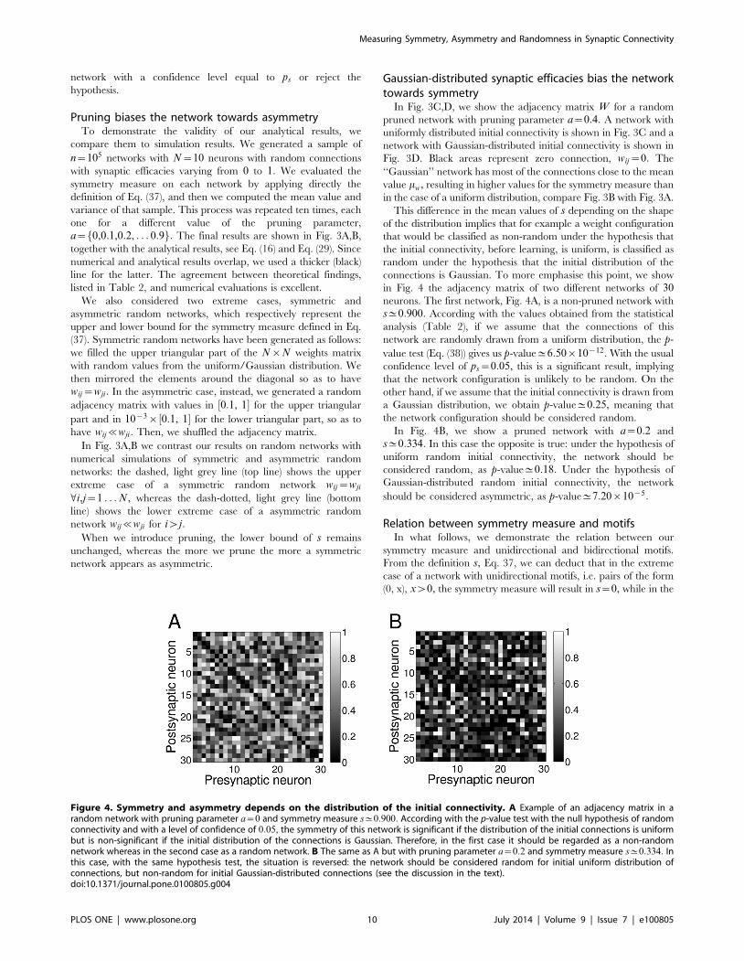
in Fig. 4 the adjacency matrix of two different networks of 30neurons. The first network, Fig. 4A, is a non-pruned network with

s^0:900: According with the values obtained from the statistical

analysis (Table 2), if we assume that the connections of this

network are randomly drawn from a uniform distribution, the p-

value test (Eq. (38)) gives us p-value^6:50|10{12: With the usual

confidence level of ps~0:05, this is a significant result, implying

that the network configuration is unlikely to be random. On the

other hand, if we assume that the initial connectivity is drawn from

a Gaussian distribution, we obtain p-value^0:25, meaning that

the network configuration should be considered random.

In Fig. 4B, we show a pruned network with a~0:2 and

s^0:334: In this case the opposite is true: under the hypothesis of

uniform random initial connectivity, the network should be

considered random, as p-value^0:18: Under the hypothesis of

Gaussian-distributed random initial connectivity, the network

should be considered asymmetric, as p-value^7:20|10{5:

Relation between symmetry measure and motifsIn what follows, we demonstrate the relation between our

symmetry measure and unidirectional and bidirectional motifs.

From the definition s, Eq. 37, we can deduct that in the extreme

case of a network with unidirectional motifs, i.e. pairs of the form

(0, x), xw0, the symmetry measure will result in s~0, while in the

Figure 4. Symmetry and asymmetry depends on the distribution of the initial connectivity. A Example of an adjacency matrix in arandom network with pruning parameter a~0 and symmetry measure s^0:900: According with the p-value test with the null hypothesis of randomconnectivity and with a level of confidence of 0:05, the symmetry of this network is significant if the distribution of the initial connections is uniformbut is non-significant if the initial distribution of the connections is Gaussian. Therefore, in the first case it should be regarded as a non-randomnetwork whereas in the second case as a random network. B The same as A but with pruning parameter a~0:2 and symmetry measure s^0:334: Inthis case, with the same hypothesis test, the situation is reversed: the network should be considered random for initial uniform distribution ofconnections, but non-random for initial Gaussian-distributed connections (see the discussion in the text).doi:10.1371/journal.pone.0100805.g004



case of bidirectional motifs i.e. pairs of the form (x, x), the

symmetry measure will result in s~1: By inverting Eq. 3, we can

derive the mean value for connection pairs mZ:En Zk½ �~1{ms:We can use now this value to define connection pairs in a network

as unidirectional or bidirectional: if Zk§mZ than Zk is a

unidirectional motif, otherwise it is a bidirectional motif. In this

way we relate unidirectional and bidirectional motifs to what is

traditionally called single edge motif and second-order reciprocal

motif, respectively. It is then expected that when s increases, the

fraction of bidirectional motifs increases towards 1, whereas the

percentage of unidirectional motifs decreases towards 0:

We show this relation in simulations by generating 103 networks

of 15 neurons each, with uniformly distributed random connec-

tions in 0, 1½ � and no pruning. In this case the mean value of the

symmetry measure is mus^0:614: Using Eq. 3, we have

muZ^0:386, which is the value used to decide whether a

connection pair is unidirectional or bidirectional. For each of

these networks, we calculated the value of the symmetry measure

and the fraction of unidirectional and bidirectional motifs and we

plotted the results in Fig. 5A as a scatter plot (black circles -

bidirectional motifs, grey circles - unidirectional motifs). Also, un

Fig. 5B we show the analogous results obtained when we prune the

connections with a~0:4: In both cases, a linear relation between sand motifs is evident.

Note that in both figures the restricted domain on the s-axis: this

is determined by the range of s values that correspond to random

networks. If we want to extend this range, we need to consider

networks that are not random any more. We achieve this by fixing

a distribution for connection pairs Z: Once we decide on the

desirable value of s, in our case the whole zero to one spectrum,

we can use a distribution (e.g. Gaussian) with mean mZ~1{ms

and a chosen variance to draw the values of all the connection

pairs in the network. Following this procedure, we fill the upper

triangular part of the 15|15 weights matrix with random values

from the uniform/Gaussian distribution, and derive the other half

of the weights by inverting the definition of Z: As a PDF(Z) we

chose a Gaussian distribution around mZ with s~0:1, except for

the extreme cases (near s~0, s~1) where s~0: With this

technique of creating networks, we sampled the entire domain of s

in steps of 0:01: For each value, we again generated 103 networks

of 15 neurons with (half of the) weights uniformly distributed, and

then we computed the mean value and standard deviation. Results

are shown in Fig. 5C,D respectively for unpruned and pruned

(with a~0:4) networks (black line - bidirectional motifs, grey line -

unidirectional motifs). We can see that Fig. 5C,D correctly

reproduce the linear regime observed in Fig. 5A,B for values of s

close enough to mus :

Due to the method by which we generated networks, the shape

of the distribution of half of the weights does not affect the shape of

the dependence in Fig. 5C,D. Indeed, if we choose half of the

connections to be Gaussian-distributed, we will observe only a shift

in both curves as they have to cross at mgs ~0:885 (results not

shown).

Figure 5. Symmetry measure reflects motifs formation. A Scatter plot of fraction of unidirectional and bidirectional motifs as a function of thesymmetry measure for 103 networks with uniform random connections and a~0: Black dots: bidirectional motifs, Grey dots: unidirectional motifs. Forthis typology mu

s^0:614: B The same as A but with pruning parameter a~0:4: In this case mus^0:263: C Mean value and standard deviation (each bar

is twice the standard deviation) of fraction of unidirectional and bidirectional motifs as a function of the symmetry measure for 103 networks with halfof the connections uniformly distributed and a~0: The second half of the connections were derived from the values of connection pairs Z, drawnfrom a Gaussian distribution with mean 1{s and standard deviation 0:1: Black line: bidirectional motifs, Grey line: unidirectional motifs. D The sameas C but with pruning parameter a~0:4:doi:10.1371/journal.pone.0100805.g005



Symmetry measure and eigenvaluesIn the definition of our symmetry measure we have deliberately

excluded (0,0) connection pairs. This was a conscious decision for

mathematical and practical reasons, see Methods. As a conse-

quence, pairs of the form (0,0) do not contribute to the evaluation

of the symmetry of the network. Instead, pairs of the form (0,E),with E very small, contribute to the asymmetry of the network

according to our specific choice of symmetry measure (leading to

Z~1, see Methods). Here we further motivate this choice via a

comparison of our measure to the evaluation of the symmetry via

the matrix eigenvalues, for three types of networks: (i) symmetric,

where each connection pair consists of synapses of the same value,

(ii) asymmetric, where every connection pair has one connection

set to a small value E, and (iii) random, where connections are

uniformly distributed. We demonstrate that our measure has a

clear advantage over the eigenvalues method, in particular when

pruning is introduced. This difference in performance lays in the

different ways that (0,0) and (0,E) are treated by our measure.

A crucial property of the real symmetric matrices is that all their

eigenvalues are real. Fig. 6A depicts the fraction of complex

eigenvalues vs the pruning parameter a for a symmetric (dash-

dotted, light grey line) asymmetric (dotted, dark grey line) and

random (dashed, black line) matrix with uniformly distributed

values, similar to Fig. 3A, with the same statistics (105 networks of

10 neurons). As expected, if no pruning takes place (a~0),

symmetric matrices have no complex eigenvalues and are clearly

distinguishable from random and asymmetric matrices. On the

contrary, both random and asymmetric matrices have a non-zero

number of complex eigenvalues, which increases with a higher

degree of asymmetry, leading to a considerable overlap between

these two cases, differently from what happens with our measure

in Fig. 3A.

As we introduce pruning, the mean of the complex eigenvalues

of the three distinctive types of network moves towards the same

value, an increase for the symmetric network and decrease for the

random and non-symmetric networks. This is expected as pruning

specific elements will make the symmetric network more

asymmetric while it will increase the symmetry of the asymmetric

network by introducing pairs of the form (0,E) or (0,0): The (0,E)pairs are due to the construction of the asymmetric network, where

half of the connections are stochastically set to very low values.

This continues till a~0:5, after which further pruning reduces the

number of complex eigenvalues of all networks: a high level of

pruning implies the formation of more (0,E) or (0,0) pairs for the

asymmetric network and more (0,0) pairs for the symmetric

network. In Fig. 6B we show the dependence of the fraction of

complex eigenvalues for uniform random matrices on their size.

Comparing Fig. 6A to Fig. 3A, we observe that our symmetry

measure offers excellent discrimination between the symmetric,

asymmetric and random matrices for e.g. a~0:4: This is despite

the fact that the structure of the asymmetric matrix per se has

become less asymmetric and the structure of the symmetric matrix

has become more asymmetric due to the pruning, as it is

confirmed by the overlapping fraction of complex eigenvalues for

asymmetric and random matrices (Fig. 6A). In our measure (0,E)pairs are treated as asymmetric, (0,0) pairs are ignored, and the

bias that pruning introduces is taken into account allowing for

good discrimination for all types of matrices, even beyond a~0:4:

Case study: Monitoring the connectivity evolution inneural networks

We demonstrate the application of the symmetry measure to a

network of neurons evolving in time according to a Spike-Timing

Dependent Plasticity (STDP) ‘‘triplet rule’’ [32] by adopting the

protocols of [18]. These protocols are designed to evolve a network

with connections modified according to the ‘‘triplet rule’’, to either

a unidirectional configuration or bidirectional configuration, with

the weights being stable under the presence of hard bounds. We

have deliberately chosen a small size network as a ‘‘toy-model’’

that will allow for visual inspection and characterisation at the

mesoscopic scale.

We simulated N~30 integrate-and-fire neurons (see Methods

section for simulation details) initially connected with random

weights wij [ 0, 1½ � drawn from either a uniform (Fig. 7) or a

Gaussian (Fig. 8) distribution (see Table 1 for parameters). Where

a pruning parameter is mentioned, the pruning took place prior to

the learning procedure: with a fixed probability some connections

were set to zero and were not allowed to grow during the

simulation.

Our choice allows us to produce an asymmetric or a symmetric

network depending on the external stimulation protocol applied to

the network. Since the amplitude of the external stimulation we

Figure 6. Eigenvalues and network structure. A Expected value and standard deviation of the fraction of complex eigenvalues as a function ofthe pruning for different types of networks of N~10 neurons with uniform weight distribution. The total length of each bar is two times the standarddeviation. Dotted, dark grey line: simulations for asymmetric networks, Dashed, black line: simulations for random networks, Dash-dotted, light grey line:simulations for symmetric networks. B Fraction of complex eigenvalues as a function of network size for random networks with uniform weightsdistribution. Pruning parameter a~0:doi:10.1371/journal.pone.0100805.g006



chose (aext~30mV ) is large enough to make a neuron fire every

time it is presented with an input, the firing pattern of neurons

reflects the input pattern and we can indifferently refer to one or

another. The asymmetric network has been obtained by using a

‘‘sequential protocol’’, in which neurons fire with the same

frequency in a precise order one after the other, with 5 ms delay,

see also [18]. The symmetric network is produced by applying a

‘‘frequency protocol’’, in which each neuron fires with a different

frequency from the values 15, 16, 17, . . . , 44 Hzf g: In both

cases, the input signals were jittered in time randomly with zero

mean and standard deviation equal to 2% of the period of the

input itself for the frequency protocol, to 25% of the delay for the

sequential protocol. Depending on the protocol, we expect the

neurons to form mostly unidirectional or bidirectional connections

during the evolution.

The time evolution for both protocols and initial distributions is

shown in Figs 7A,D (uniform) and 8A,D (Gaussian). Each panel

represents the evolution of the symmetry measure averaged over

50 different representations for both fully connected networks

(a~0, solid black line) and pruned networks (e.g. a~0:4, dashed

grey line). The shaded area represents the standard deviation. The

time course of the symmetry measure can be better understood

with the help of the Fig. 3. At the beginning, the values of s reflect

what we expect from a random network. Afterwards, as the time

passes, the learning process leads to the evolution of the

connectivity. As expected, the frequency protocol induces the

formation of mostly bidirectional connections, leading to the

saturation of s towards its maximum value, depending on the

degree of pruning. On the other hand, when we apply the

sequential protocol, connection pairs develop a high degree of

Figure 7. Evolution of networks with STDP and initially uniform weights distribution. A Time evolution of the symmetry measure when afrequency protocol is applied on a network, shown as average over 50 representations. The shaded light grey areas represent the standard deviation(the total length of height of each band is twice the standard deviation). Solid black line: no pruning, Dashed grey line: with pruning a~0:4: B Exampleof an adjacency matrix at the end of the learning process for a network with the frequency protocol and no pruning. For this example s^0:921: C Thesame as B but with pruning a~0:4: For this example s^0:427: D, E, F The same as A, B and C but with the sequential protocol applied. Theconnectivity matrix in panel E has s^0:393: The connectivity matrix in panel F has s^0:141:doi:10.1371/journal.pone.0100805.g007



asymmetry, the values of s decreasing towards its minimum.

Connections were constrained to remain inside the interval 0, 1½ �:The final connectivity pattern can be inspected by plotting the

adjacency matrix W : In Fig. 7B,C and 8B,C we give an example

of W at the end of the evolution for one particular instance of the

50 networks when the frequency protocol is applied. Similarly, in

Fig. 7E,F and 8E,F we show the results for the sequential protocol.

The corresponding values of s for each of the examples in the

figures are listed in Table 3. In the case that a~0, a careful

inspection of Fig. 7B, 8B indicates that connectivity is bidirection-

al: all-to-all strong connections have been formed. On the other

hand, In Fig. 7E, 8E, trying to determine if there is a particular

connectivity emerging in the network starts to be considerably

tough. However, by using our symmetry measure (see values in

Table 3) we can infer that the connectivity is unidirectional. In the

pruned networks, however, see Fig. 7C, 8C and Fig. 7F, 8F, the

formation of bidirectional and unidirectional connection pairs is

not as obvious as for a~0: We therefore refer again to the Table 3

and compare the values of s with mrands and with masym

s or msyms ,

depending on the case. We can then verify that the learning

process has significantly changed the network and its inner

connections from the initial random state.

We can rigorously verify the above conclusions via a statistical

hypothesis test such as the p-value test, which in essence quantifies

how far away the value of our symmetry measure s of our final

configuration is from the initial, random configuration (see also

Methods). In Table 3 we show the p-values corresponding to the

null hypothesis of random connectivity for the examples in the

Fig. 7, 8. Once we set the significance level at ps~0:05, we can

verify that, except for the case of pruned network with initially

Gaussian-distributed connections where a frequency protocol has

Figure 8. Evolution of networks with STDP and initially Gaussian-distributed weights. A Time evolution of the symmetry measure when afrequency protocol is applied on a network, shown as average over 50 representations. The shaded light grey areas represent the standard deviation(the total length of height of each band is twice the standard deviation). Solid black line: no pruning, Dashed grey line: with pruning a~0:4: B Exampleof an adjacency matrix at the end of the evolution for a network with frequency protocol and no pruning. For this example s^0:963: C The same as Bbut with pruning a~0:4: For this example s^0:456: D, E, F The same as A, B and C but with the sequential protocol applied. The connectivity matrixin panel E has s^0:426: The connectivity matrix in panel F has s^0:153:doi:10.1371/journal.pone.0100805.g008



been applied (i.e. GFa0:4), the p-values are significant, implying

the rejection of the null hypothesis. This is also justified by Fig. 3A,

B: when we increase the pruning, the mean value of the symmetry

measure of the fully symmetric network approaches that of the

pruned random network and in particular for the case where the

weight are randomly Gaussian-distributed.

Summary

The study of the human brain reveals that neurons sharing the

same cognitive functions or coding tend to form clusters, which

appear to be characterised by the formation of specific connec-

tivity patterns, called motifs. We, therefore, introduced a

mathematical tool, a symmetry measure s, which computes the

mean value of the connection pairs in a network, and allows us to

monitor the evolution of the network structure due to the synaptic

dynamics. In this context, we applied it to a number of evolving

networks with plastic connections that are modified according a

learning rule. After the network connectivity reaches a steady state

as a consequence of the learning process, connectivity patterns

develop. The use of the symmetry measure together with the

statistical analysis and the p-value test allow us both to quantify the

connectivity structure of the network, which has changed due to

the learning process, and observe its development. It also allows

for some interesting observations. (i) Introducing a fixed amount of

pruning in the network prior to the learning process biases the

adjacency matrix towards an asymmetric configuration. (ii) A

network configuration that appears to be symmetric under the

assumption of a uniform initial distribution is random under the

assumption of a Gaussian initial distribution.

Statements on non-random connectivity in motifs experimental

work, e.g. [14,20] are supported by calculating the probability of

connectivity in a random network and then distributing it

uniformly: this becomes the null hypothesis. This was a most

suitable approach given the paucity of data. If, however, the null

hypothesis consisted of a Gaussian-distributed connectivity, then a

higher number of bidirectional connections would be expected, as

suggested by our analysis.

It is also possible that in a large network, learning processes are

only modifying a subset of the connections, forming motifs that

might be unobserved if the symmetry measure is applied to the

whole adjacency matrix. In such cases, algorithms of detecting

potential symmetric or asymmetric clusters would detect the area

of interest and the symmetry measure presented here reveals the

evolution of the structure and its significance.

Acknowledgments

We are grateful to the anonymous reviewers for their comments.

Author Contributions

Conceived and designed the experiments: EV UE. Performed the

experiments: UE EV. Analyzed the data: UE EV. Contributed reagents/

materials/analysis tools: MG MvR. Wrote the paper: UE EV. Edited the

manuscript: MG MvR.

References

1. Sporns O, Tononi G, Ktter R (2005) The human connectome: A structural

description of the human brain. PLoS Comput Biol 1: e42.

2. Lichtman JW, Sanes JR (2008) Ome sweet ome: what can the genome tell us

about the connectome? Curr Opin Neurobiol 18: 346–353.

3. Smith SJ (2007) Circuit reconstruction tools today. Curr Opin Neurobiol 17:

601–608.

4. Luo L, Callaway EM, Svoboda K (2008) Genetic dissection of neural circuits.

Neuron 57: 634–660.

5. Seung HS (2009) Reading the book of memory: sparse sampling versus dense

mapping of connectomes. Neuron 62: 17–29.

6. White JG, Southgate E, Thomson JN, Brenner S (1986) The structure of the

nervous system of the nematode caenorhabditis elegans. Philos Trans R Soc

Lond B Biol Sci 314: 1–340.

7. Varshney LR, Chen BL, Paniagua E, Hall DH, Chklovskii DB (2011) Structural

properties of the caenorhabditis elegans neuronal network. PLoS Comput Biol 7:

e1001066.

8. Briggman KL, Helmstaedter M, Denk W (2011) Wiring specificity in the

direction-selectivity circuit of the retina. Nature 471: 183–188.

9. Bock DD, Lee WCA, Kerlin AM, Andermann ML, Hood G, et al. (2011)

Network anatomy and in vivo physiology of visual cortical neurons. Nature 471:

177–182.

10. Koetter R (2001) Neuroscience databases: tools for exploring brain structure-

function relationships. Philos Trans R Soc Lond B Biol Sci 356: 1111–1120.

11. Koslow SH, Subramanian S (2005) Databasing the brain: From data to

knowledge (Neuroinformatics). Wiley.

12. Insel TR, Volkow ND, Li TK, Battey JF, Landis SC (2003) Neuroscience

networks: data-sharing in an information age. PLoS Biol 1: E17.

13. Briggman KL, Denk W (2006) Towards neural circuit reconstruction with

volume electron microscopy techniques. Curr Opin Neurobiol 16: 562–570.

14. Song S, Sjstrm PJ, Reigl M, Nelson S, Chklovskii DB (2005) Highly nonrandom

features of synaptic connectivity in local cortical circuits. PLoS Biol 3: e68.

Table 3. Symmetry measure and p-value for different types of network.

Type s mrands +srand

s p-value ms=as +ss=a

s

UFa0 0:921 0:614+0:042 1:82|10{13 1:000+0:000

UFa0:4 0:427 0:263+0:058 4:50|10{3 0:429+0:081

USa0 0:393 0:614+0:042 1:21|10{7 0:003+0:387|10{3

USa0:4 0:141 0:263+0:058 3:46|10{2 0:001+0:352|10{3

GFa0 0:963 0:885+0:013 3:30|10{9 1:000+0:000

GFa0:4 0:456 0:379+0:072 2:85|10{1 0:429+0:081

GSa0 0:426 0:885+0:013 0 0:002+0:256|10{3

GSa0:4 0:153 0:379+0:072 1:70|10{3 0:001+0:260|10{3

Column 1. Network type. U = Uniform distribution, G = Gaussian distribution, F = Frequency protocol, S = sequential protocol, a0 = No prune, a0:4 = pruning of 0:4:Column 2. Value of the symmetry measure for one instance of each type. Column 3. Results from the previous statistical analysis on random networks. Column 4.Corresponding p-value from Eq. 38. Column 5. Results from the previous statistical analysis for the corresponding closest extreme case – symmetric network forfrequency protocol and asymmetric network for sequential protocol. s means symmetric and a asymmetric.doi:10.1371/journal.pone.0100805.t003



15. Wang Y, Markram H, Goodman PH, Berger TK, Ma J, et al. (2006)

Heterogeneity in the pyramidal network of the medial prefrontal cortex. NatNeurosci 9: 534–542.

16. Silberberg G, Markram H (2007) Disynaptic inhibition between neocortical

pyramidal cells mediated by martinotti cells. Neuron 53: 735–746.17. Perin R, Berger TK, Markram H (2011) A synaptic organizing principle for

cortical neuronal groups. Proc Natl Acad Sci U S A 108: 5419–5424.18. Clopath C, Buesing L, Vasilaki E, Gerstner W (2010) Connectivity reects coding:

a model of voltage-based stdp with homeostasis. Nat Neurosci 13: 344–352.

19. Lefort S, Tomm C, Sarria JCF, Petersen CCH (2009) The excitatory neuronalnetwork of the c2 barrel column in mouse primary somatosensory cortex.

Neuron 61: 301–316.20. Vasilaki E, Giugliano M (2014) Emergence of connectivity motifs in networks of

model neurons with short- and long-term plastic synapses. PLoS One 9: e84626.21. Vasilaki E, Giugliano M (2012) Emergence of connectivity patterns from long-

term and shortterm plasticities. In: ICANN 2012 - 22nd International

Conference on Artificial Neural Networks, Lausanne, Switzerland.22. Pignatelli (2009) Structure and Function of the Olfactory Bulb Microcircuit.

Ph.D. thesis, Ecole Polytechnique Federale de Lausanne.23. Babadi B, Abbott LF (2013) Pairwise analysis can account for network structures

arising from spike-timing dependent plasticity. PLoS Comput Biol 9: e1002906.

24. Bourjaily MA, Miller P (2011) Excitatory, inhibitory, and structural plasticityproduce correlated connectivity in random networks trained to solve paired-

stimulus tasks. Front Comput Neurosci 5: 37.

25. Bourjaily MA, Miller P (2011) Synaptic plasticity and connectivity requirements

to produce stimulus-pair specific responses in recurrent networks of spikingneurons. PLoS Comput Biol 7: e1001091.

26. Newman MEJ (2010) Networks: an Introduction. New York: Oxford University

Press.27. Dayan P, Abbott L (2001) Theoretical neuroscience: Computational and

mathematical modeling of neural systems. The MIT Press: Cambridge,Massachusetts.

28. Gerstner Kistler (2002) Spiking Neuron Models. Cambridge University Press.

29. Vasilaki E, Fusi S, Wang XJ, Senn W (2009) Learning exible sensori-motormappings in a complex network. Biol Cybern 100: 147–158.

30. Vasilaki E, Fremaux N, Urbanczik R, Senn W, Gerstner W (2009) Spike-basedreinforcement learning in continuous state and action space: when policy

gradient methods fail. PLoS Comput Biol 5: e1000586.31. Richmond P, Buesing L, Giugliano M, Vasilaki E (2011) Democratic population

decisions result in robust policy-gradient learning: a parametric study with gpu

simulations. PLoS One 6: e18539.32. Pfister JP, Gerstner W (2006) Triplets of spikes in a model of spike timing-

dependent plasticity. J Neurosci 26: 9673–9682.33. Clopath C, Ziegler L, Vasilaki E, Bsing L, Gerstner W (2008) Tag-trigger-

consolidation: a model of early and late long-term-potentiation and depression.

PLoS Comput Biol 4: e1000248.34. Hines M, Morse T, Migliore M, Carnevale N, Shepherd G (2004) ModelDB: A

database to support computational neuroscience. J Comput Neurosci 17: 7–11.



Documents

Measuring Symmetry, Asymmetry and Randomness in Neural Network Connectivity