Measuring the VC-dimensionof a Learning MachineVladimir Vapnik, Esther Levin, Yann Le CunAT&T Bell Laboratories101 Crawfords Corner Road, Holmdel, NJ 07733AbstractA method for measuring the capacity of learning machines is described. The method is based on�tting a theoretically derived function to empirical measurements of the maximal di�erence between theerror rates on two separate data sets of varying sizes. Experimental measurements of the capacity ofvarious types of linear classi�ers are presented.1 Introduction.Many theoretical and experimental studies have shown the in uence of the capacity of a learning machine onits generalization ability (Vapnik, 1982; Baum and Haussler, 1989; Le Cun et al., 1990; Weigend, Rumelhartand Huberman, 1991; Guyon et al., 1992; Abu-Mostafa, 1993). Learning machines with a small capacitymay not require large training sets to approach the best possible solution (lowest error rate on test sets).High-capacity learning machines, on the other hand, may provide better asymptotical solutions (i.e. lowertest error rate for very large training sets), but may require large amounts of training data to reach acceptabletest performance. For a given training set size, the di�erence between the training error and the test errorwill be larger for high-capacity machines. The theory of learning based on the VC-dimension predicts thatthe behavior of the di�erence between training error and test error as a function of the training set size ischaracterized by a single quantity {the VC-dimension{ which characterizes the machine's capacity (Vapnik,1982).In this paper, we introduce an empirical method for measuring the capacity of a learning machine. Themethod is based on a formula for the maximum deviation between the frequency of errors produced by themachine on two separate data sets, as a function of the capacity of the machine and the size of the datasets. The main idea is that the capacity of a learning machine can be measured by �nding the capacity thatproduces the best �t between the formula and a set of experimental measurements of the frequency of errorson data sets of varying sizes.In the paradigm of learning from examples, the learning machine must learn to approximate as well aspossible an unknown target rule, or input-output relation, given a training set of labeled examples. The linput-output pairs composing the training set (x; !); x 2 X � Rn; ! 2 f0; 1g,(x1; !1); :::; (xl; !l)are assumed to be drawn independently from an unknown distribution function P (x; !) = P (!jx)P (x). HereP (x) describes the region of interest in the input space, and the distribution P (!jx) describes the targetinput-output relation. The learning machine is characterized by the set of binary classi�cation functionsf(x; �); � 2 � (� is a parameter which speci�es the function, and � is the set of all admissible parameters)To appear in Neural Computation. 1994Copyright c 1994 AT&T 1

that it can realize (indicator functions). The goal of learning is to choose a function f(x; ��) within that setwhich minimizes the probability of error, i.e., the probability of disagreement between the value of ! andthe output of the learning machine f(x; �)p(�) = Ej! � f(x; �)j;where the expectation is taken with respect to the probability distribution P (x; !).The problem is that this distribution is unknown, and the only way to assess p(�) is through the frequencyof errors computed on the training set �l(�) = 1l lXi=1 j!i � f(xi; �)j:Many learning algorithm are based on the so-called \principle of empirical risk minimization", whichconsists in picking the function f(x; �l) that minimizes the number of error on the training set.In (Vapnik, 1982) it is shown that for algorithms that minimize the empirical risk, the knowledge ofthree quantities allows us to establish an upper bound on the probability of error p(�). The �rst quantityis the capacity of the learning machine, as measured by the VC-dimension h of the set of functions it canimplement. The second one is the frequency of errors on the training set (empirical risk) �(�). The thirdone is the size of the training set l. With probability 1� �;, the boundp(�) � �(�) +D(l; h; �(�); �) (1)is simultaneously valid for all � 2 � (including the �l that minimizes the empirical risk �(�) ). The functionD is of the formD(l; h; �(�); �) = ch(ln(2l=h) + 1)� ln�2l s1 + 4l�(�)c(h(ln(2l=h) + 1) � ln �) + 1! (2)where c is a universal constant less than 1. It can be interpreted as a con�dence interval on the di�erencebetween the training error and the \true" error.There are two regimes in which the behavior of the function D simpli�es. The �rst regime is when thetraining error happens to be small (large capacity, or small training set size, or easy task), then D can beapproximated by D(l; h; �(�l); �) � h(ln(2l=h) + 1)� ln�l :When the training error is large (near 1/2), D can be approximated byD(l; h; �(�l); �) �rh(ln(2l=h) + 1)� ln �l :Unfortunately, theoretical estimates of the VC-dimension have been obtained for only handful of simpleclasses of functions, most notably the class of linear discriminant functions. The set of linear discriminantfunctions is de�ned by f(x; �) = �((x � �) + �0);where (x � �) is dot-product of the vectors x and �, and � is the threshold function:�(u) = � 1 if u > 00 otherwise ;The VC-dimension of the set of linear discriminant functions with n inputs is equal to n+1 (Vapnik, 1982).Attempts to obtain the exact value of the VC-dimension for other classes of decision rules encounteredsubstantial di�culties. Most of the estimated values appear to exceed the real one by a large amount. Suchpoor estimates result in rather crudely overestimated evaluations of the con�dence interval D.This article considers the possibility of empirically estimating the VC-dimension of a learning machine.The idea that this might be possible was inspired by following observations.2

It was shown in (Vapnik and Chervonenkis, 1989) that a learning algorithm that minimizes the empiricalrisk (i.e. minimizes the error on the training set) will be consistent if and only if the following one-sideduniform convergence condition holds liml!1Pfsup�2�(p(�)� �(�)) > "g = 0In other words the one-sided uniform convergence (within a given set of function) of frequencies to proba-bilities is a necessary and su�cient condition for the consistency of the learning process.In the 30s Kolmogorov and Smirnov found the law of distribution of the maximal deviation between adistribution function and an empirical distribution function for any random variable. This result can beformulated as follows. For the set of functionsf�(x; �) = �(x � �); � 2 (�1;1)the equality Pfsup�2�(p�(�)� ��(�)) > "g = expf�2"2lg � 2 1Xn=2(�1)n expf�2"2n2lgholds for su�ciently large l, where p�(�) = Ef�(�) and ��(�) = 1l Pli=1 f�(xi; �). This equality is inde-pendent of the probability measure on x. Note that the second term is very small compared to the �rstone.In (Vapnik and Chervonenkis, 1971) it was shown that for any set of indicator functions f(x; �); � 2 �with �nite VC-dimension h, the rate of uniform convergence is bounded as followsPfsup�2�(p(�)� �(�)) > "g < min�1; exp��c1 ln 2l=h+ 1l=h � c2"2� l��where c1 and c2 are universal constants such that c1 � 1 and c2 > 1=4. As above, this inequality isindependent of the probability measure. A direct consequence is that for any given � there exists an l0 =l0(h; �; ") such that for any l > l0, the inequalityPfsup�2�(p(�)� �(�)) > "g < expf�(c2 � �)"2lgholds. In (Vapnik and Chervonenkis, 1971) it was shown that c2 is at least 1=4. The result was laterimproved to c2 = 2 by (Devroye, 1982). Interestingly, for c2 = 2, the above inequality is close to theKolmogorov-Smirnov equality obtained for a simple set of functions. This means that, although the above isan upper bound, it is asymptotically close to the exact value. Tightening the upper bound on the value ofc1 is theoretically very di�cult, because the term it multiplies is not the main term in the exponential forlarge values of l=h.Now, suppose that there exists a value for the constant c1, 0 < c1 � 1, for which the above upper bound(which is independent of the probability measure) is tight. Furthermore, suppose that the bound is tightnot only for large numbers of observations, but also for smaller numbers (statisticians commonly use theasymptotic Kolmogorov-Smirnov test starting with l = 30 and the learning processes usually involves severalhundreds of observations). In this case, one can expect the function ��(l=h) de�ned by��( lh ) = E(sup�2�(p(�)� �(�)) = Z 10 Pfsup�2�(p(�) � �(�)) > "gd"to be independent of the probability measure, even for rather small values of l=h.Now, assuming we know a functional form for ��, then we can experimentally estimate the expectedmaximal deviation between the empirical risk and expected risk for various values of l, and measure hby �tting �� to the measurements. The remainder of the paper is concerned with �nding an appropriatefunctional form for ��, and applying it to measuring the VC-dimension of various learning machines.A learning algorithm is said to be consistent if the probability of error on the training set converges to the true probabilityof error when the size of the training set goes to in�nity. 3

In practice, rather than measuring the maximum di�erence between the training set error and the erroron an in�nite test set, it is more convenient to measure the maximum di�erence between the error ratesmeasured on two separate sets �l = fsup�2�(�1(�) � �2(�))g;where �1(�) and �2(�) are frequencies of error calculated on two di�erent samples of size l.We will introduce an approximate functional form for the right hand side �(l=h) of the relationE�l � �(l=h)which we will use for a wide range of values of l=h. To construct this approximation we will determine inSection 2 two di�erent bounds for E�l: the bound valid for large l=h and the bound valid for small l=h.In section 3, we introduce the notion of e�ective VC-dimension, which re ects some weak properties ofthe unknown probability distribution. The e�ective VC-dimension does not exceed the VC-dimension, andwe show that the functional form of the bounds on E�l obtained for the VC-dimension are valid for thee�ective VC-dimension. As a consequence, the bounds obtained with the e�ective VC dimension are tighter.In section 4 we introduce a single functional form inspired by bound (2), and by the bounds on E�l forboth small and large l=h. We hypothesize that this function describes well the expectations E�l in termof e�ective VC-dimension. Assuming this hypothesis is true, section 5 proposes a method for measuringthe e�ective VC-dimension of a learning machine. In section 6 we demonstrate the proposed method ofmeasuring VC-dimension for various classes of linear decision rules.2 Estimation of the Maximum Deviation.In this section we �rst establish the formal de�nition of the VC-dimension, and then give the bounds on themaximum deviation between frequencies of error on two separate sets.De�nition: The VC-dimension of the set of indicator functions f(x; �), � 2 �, is the maximal numberh of vectors x1; : : : ; xhfrom the set X that can be shattered by f(x; �), � 2 �.The vectors x1; : : : ; xh are said to be shattered by f(x; �), � 2 � if, for any possible partition of these vec-tors into two classes A and B, (there are 2h such partitions) there exists a function f(x; ��) that implementsthe partition, in the sense that f(x; ��) = 0 if x 2 A and f(x; ��) = 1 if x 2 B.To estimate a bound on the expectation of the random variable �l we need to de�neZ2l = x1; !1; : : : ;x2l; !2las a random independent sample of vectors (the x's) and their class (the !'s, (! = 0; 1)). We denote byZ(2l) the set of all samples of size 2l.Let us denote by � l1(Z2l; �) the frequency of erroneous classi�cations of the vectorsx1; : : : ; xlof the �rst half-sample of Z2l, obtained by using the decision rule f(x; �):� l1(Z2l; �) = 1l lXi=1 j!i � f(xi; �)j:Let us denote by � l2(Z2l; �) the frequency of erroneous classi�cation of the vectorsxl+1; : : : ; x2lobtained using the same decision rule f(x; �):� l2(Z2l; �) = 1l 2lXi=l+1 j!i � f(xi; �)j:4

We study the properties of the random variable�2l = �(Z2l) = sup�2�(� l1(Z2l; �)� � l2(Z2l; �)); (3)which is the maximal deviation of error frequencies on the two half-samples over a given set of functions.There exists an upper bound for the expectation of this random value �(Z2l) for varying sample size l.Consider three cases.Case 1 (l=h � 0:5). For this case we use the trivial bound:E sup�2�(� l1(Z2l; �)� � l2(Z2l; �)) � 1:Case 2 (0:5 < l=h � g; g is small). Let the supremum of the di�erence� l1(Z2l; �)� � l2(Z2l; �)be attained on the function f(x; �?), where �? = �?(Z2l). Consider the eventB� = fZ2l : (� l1(Z2l; �?)� � l2(Z2l; �?))(�(Z2l; �?) + 1=2l)(1 + 1=2l � �(Z2l; �?)) > �g; (4)where �(Z2l; �?) = � l1(Z2l; �?) + � l2(Z2l; �?)2 :We denote the probability of this event by P (B�). In Appendix 1 we prove the following theorem :Theorem 1. Let the set of indicator functions f(x; �), � 2 � have VC-dimension h. Then the followingbound of the conditional expectation of �(Z2l)Efsup�2�(� l1(Z2l; �)� � l2(Z2l; �))jB�g � 4� � ln(2l=h) + 1l=h + 1� lnP (B�)l � : (5)is valid.From (5) and from the fact that the deviation of the frequencies on two half-samples does not exceed 1we obtainEfsup�2�(� l1(Z2l; �)� � l2(Z2l; �))g � 4P (B�)� � ln(2l=h) + 1l=h + 1� lnP (B�)l �+ (1� P (B�)): (6)This bound should be used when � is not too small (e.g. � > 0:5) and when the probability PfB�g isclose to one. Such a situation seems to arise when the ratio l=h is not too large and when l is large. In thiscase, when P (B�) is close to one, l=h is not large and l is large, the boundEfsup�2�(� l1(Z2l; �)� � l2(Z2l; �))g � C1 ln(2l=h) + 1l=his valid, where C1 is a constant.In the following, we shall make use of this bound for small l=h when constructing an empirical estimateof the expectation.Case 3 (l=h is large). In appendix 1 we show that for the set of indicator functions with VC-dimensionh the following bound holds:Efsup�2�(� l1(Z2l; �)� � l2(Z2l; �))g � C2s ln(2l=h) + 1l=h : (7)where C2 is a constant. This bound is true for all l=h. We shall use it only for large l=h, where the boundof case 2 is not valid.From the conducted experiments described in the section 6 we �nd that g � 8.5

3 E�ective VC-dimension.According to the de�nition, the VC-dimension does not depend on the input probability measure P (x). Ourpurpose here is to introduce a concept of e�ective VC-dimension which re ects a weak dependence on theproperties of the probability measure. Let the probability measure P be given on X and let the subset X?of the set X have a probability measure which is close to one, i.e.P (X?) = 1� �for small �.Let the set of indicator functions f(x; �), � 2 � with VC-dimension h be de�ned on X, and let the sameset of functions on X? � X have VC-dimension h?. In Appendix 2 we prove the following theorem.Theorem 2. For all l > h for which the inequality� < 12l �2elh? �h? � h2el�h (8)is ful�lled, the following boundsEfsup�2�(� l1(Z2l; �)� � l2(Z2l; �))jB�g < 4=�� ln(2l=h?) + 1l=h? + 1� lnP (B�)l � ; (9)Efsup�2�(� l1(Z2l; �)� � l2(Z2l; �))g <s ln(2l=h?) + 1l=h? + 3plh?(ln(2l=h?) + 1) (10)are valid.Remark. If � ! 0 the inequalities are true for all l > h. Note that in this case the left hand side ofinequalities (9) and (10) do not depend on X�, but the right hand side does. Therefore the tightest inequalitywill be achieved for the X� with the smallest h�.De�nition. The e�ective VC-dimension of the set f(x; �); � 2 �, (for the given measure P ) is theminimal VC-dimension of this set of functions de�ned on all subsets X? � X whose measure is almost one(�(X?) > 1� �?, where �? > 0 is a small value).As in the previous section, from (9) we obtain that for the e�ective VC-dimension h? the followinginequality is trueEfsup�2�(� l1(Z2l; �)� � l2(Z2l; �))g < 4P (B�)� � ln(2l=h?) + 1l=h? + 1� lnP (B�)l �+ (1� P (B�)): (11)For the case when P (B�) is close to one, the quantity l=h? is small, and l is large we obtainEfsup�2�(� l1(Z2l; �)� � l2(Z2l; �))g < C ln(2l=h?) + 1l=h? :where C is a constant. Since the bounds (9) and (10) have the same form as the bounds (5) and (7), tosimplify our notation we use h in the next sections to denote the effective VC-dimension.4 The Law of the largest deviations.In section 2 we gave several bounds, for di�erent cases, on the expectation of the largest deviation overthe set of decision rules. In this section we �rst give a single functional form that re ects the properties ofthe bounds. Then we conjecture that the same functional form approximates the expectation of the largestdeviation.The bounds given in the previous section are summarized as followsEfsup�2�(� l1(Z2l; �)� � l2(Z2l; �))g � 8><>: 1 if l=h � 0:5C1 ln(2l=h)+1l=h if l=h is smallC2q ln(2l=h)+1l=h if l=h is large. (12)6

Consider the following continuous approximation of the right side of the bound (12)�(� ) = ( 1 if � < 0:5a ln(2�)+1��k (q1 + b(��k)ln(2�)+1 + 1) otherwise ; (13)where � = l=h. The function �(� ) has two free parameters a and b. The third parameter k < 0:5 is chosenfrom the conditions of continuity at point � = 0:5: �(0:5) = 1. Note that the function �(� ) has the samestructure as the con�dence interval (2), except that the frequency �(�) is replaced by a constant.For small � , (0:5 < � < g), �(� ) behaves asC�1 ln(2� ) + 1� � k ;and for large � as C�2r ln(2� ) + 1� � k :The constants a and b determine the regions of \large" and \small" values of � .We make the hypothesis that there exist constants a; b that are only weakly dependent upon the propertiesof the input probability measure, such that the function �(� ) approximates the expectation su�ciently wellfor all l > h: Efsup�2�(� l1(Z2l; �)� � l1(Z2l; �))g � �(� ): (14)The constants can be found empirically by �tting � to experimental data using a machine whose VC-dimension is known. If we assume that the constants obtained are universal, we can then use the function� obtained this way to measure the capacity of other learning machines.5 Measuring the E�ective VC-Dimension of a Classi�erIf the function �(� ) approximates the expectation with su�cient accuracy, then the e�ective VC-dimensionof the set of indicator functions realizable by a given classi�er can be estimated on the basis of the followingexperiment. First, we generate a random independent set of size 2l,Z2li = xi1; !i1; : : : ;xil; !il ;xil+1; !il+1; : : : ;xi2l; !i2l: (15)using a generator of random vectors P (x) and a (possibly non-deterministic) generator of labels P (!jx).Using this sample, we measure the quantity�(Z2li ) = sup�2�(� l1(Z2li ; �)� � l2(Z2li ; �)): (16)by approximating the expectation by an average over N independently generated sets of size 2l.�(l) = 1N NXi=1 �(Z2li )Repeating the above procedure for various values of l, we obtain the set of estimates �(l1); : : : ; �(lk).The e�ective VC-dimension of the set of functions f(x; �); � 2 �, can then be approximated by �ndingthe integer parameter h? which provides the best �t between �(l=h) and the �(li)'s:h? = argminh kXi=1(�(li)� �(li=h))2:The accuracy of the obtained VC-dimension estimate, and in fact, the validity of the approach presented inthis paper, depend crucially on how well the function �(l=h) describes the expectation (14).7

To estimate the expectation of the largest deviation empirically one must be able to de�ne for every �xedsample (15) the value of the largest deviation (16). This can be done by considering a modi�ed training setwere the labels of the �rst half of the set have been reversedx1; $1; : : : ;xl; $l;xl+1; !l+1; : : : ;x2l; !2lwhere $ denotes the opposite class of !. As shown in Appendix 3, evaluating (16) can be done by minimizingthe functional R(�) = 1l lXi=1($i � f(xi; �))2 + 1l 2lXi=l+1(!i � f(xi; �))2 (17)6 Empirical measurement of the e�ective VC dimensionIn this section, we illustrate the method of measuring the VC-dimension by applying it various types oflinear classi�ers. Our method relies on several assumptions which must be checked experimentally:� The expected deviation Ef�lg is largely independent of the generator distribution P (!jx).� The expected deviation Ef�lg depends on the choice of a learning machine only through the parameterh.� The expected deviation Ef�lg can be well described by the function �(l=h) in equation (13) with �xedparameters a and b.� The values of the free parameters a and b have constant values over wide classes of learning machines.Experiments with learning machine that implement various subsets of the set of linear classi�cationfunctions were conducted to check these hypotheses. The VC-dimension of the set of linear classi�ers(without bias) is known from theory to be equal to the dimension of the input space n. The experimentsdescribed here were conducted with n = 50, x = (x1; :::; x50). Additional experiments with various values ofn ranging from 25 to 200 were performed with similar results.Since no e�cient algorithm is known for minimizing the classi�cation error of linear threshold units, wetrained the machine by minimizing the mean squared error between the labels and the output of a unit wherethe hard threshold was replaced by a sigmoid function This procedure does not ensure that the classi�cationerror is minimized, but it is known empirically to give good approximate solutions in the separable andnon-separable cases. After training, the output labels were computed by thresholding the output of thesigmoid.6.1 Independence of Average Deviations from the Task Di�cultyA set of experiments was performed to assess the in uence of the di�culty of the task (an important propertyof the conditional probability distribution P (!jx)) on the deviation. Three ensembles of training sets weregenerated such that the expected frequency of errors using a linear classi�er would be respectively 0, 0.25and 0.5. First, we randomly selected a set of 50-dimensional input vectors with coordinates independentlydrawn with a uniform distribution over the [�1; 1] interval. Then, the labels for the three experiments weregenerated by picking a 50-dimensional vector of coe�cients �� at random, and by generating the labelsaccording to the following three conditional probability distributionsP1(!jx) = � 1 for ! = �(�� � x),0 for ! = 1� �(�� � x),P2(!jx) = � 0:75 for ! = �(�� � x),0:25 for ! = 1� �(�� � x),P3(!jx) = � 0:5 for ! = �(�� � x),0:5 for ! = 1� �(�� � x),8

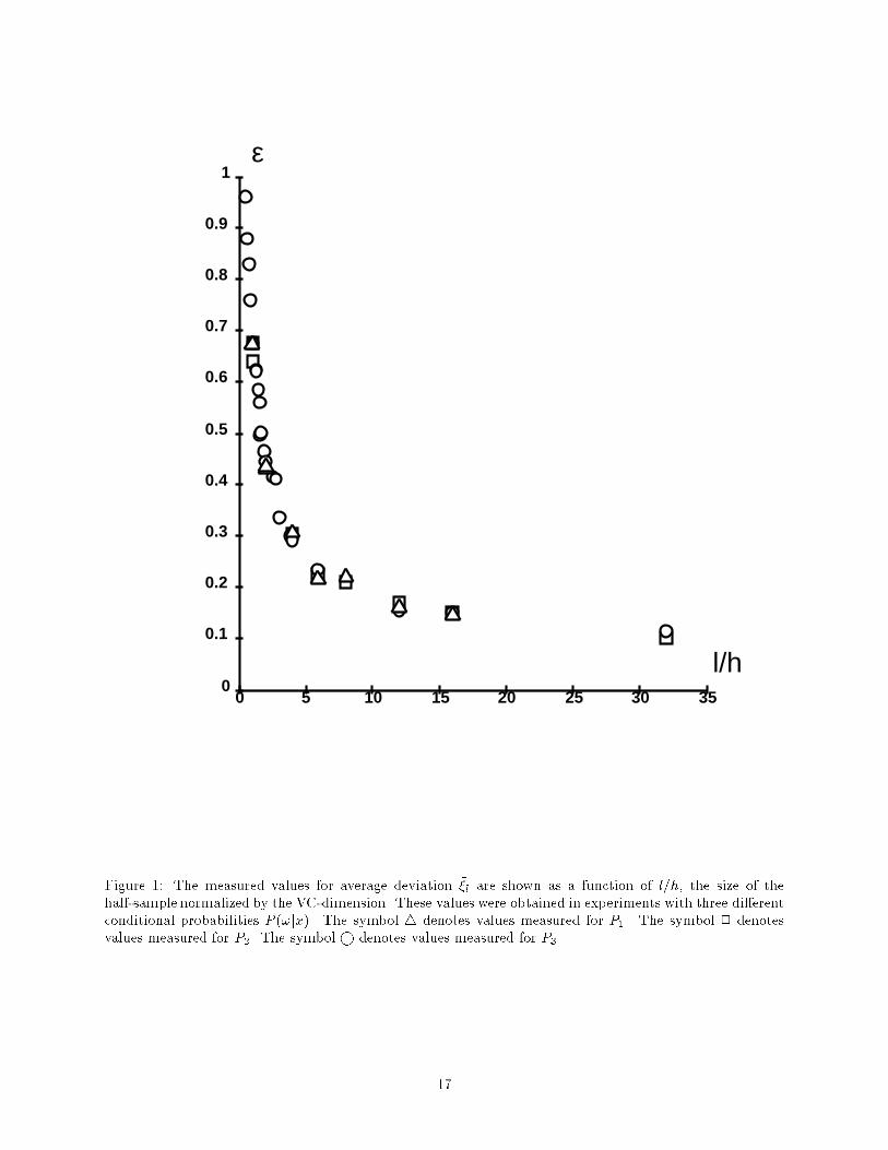
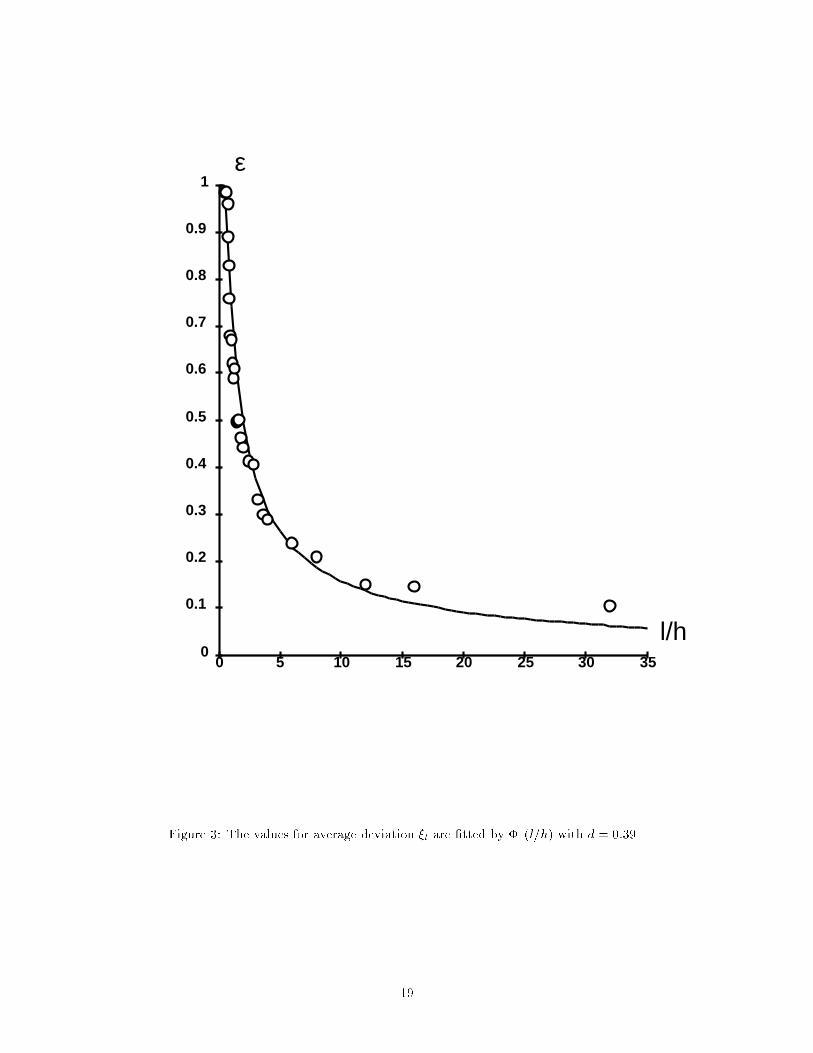
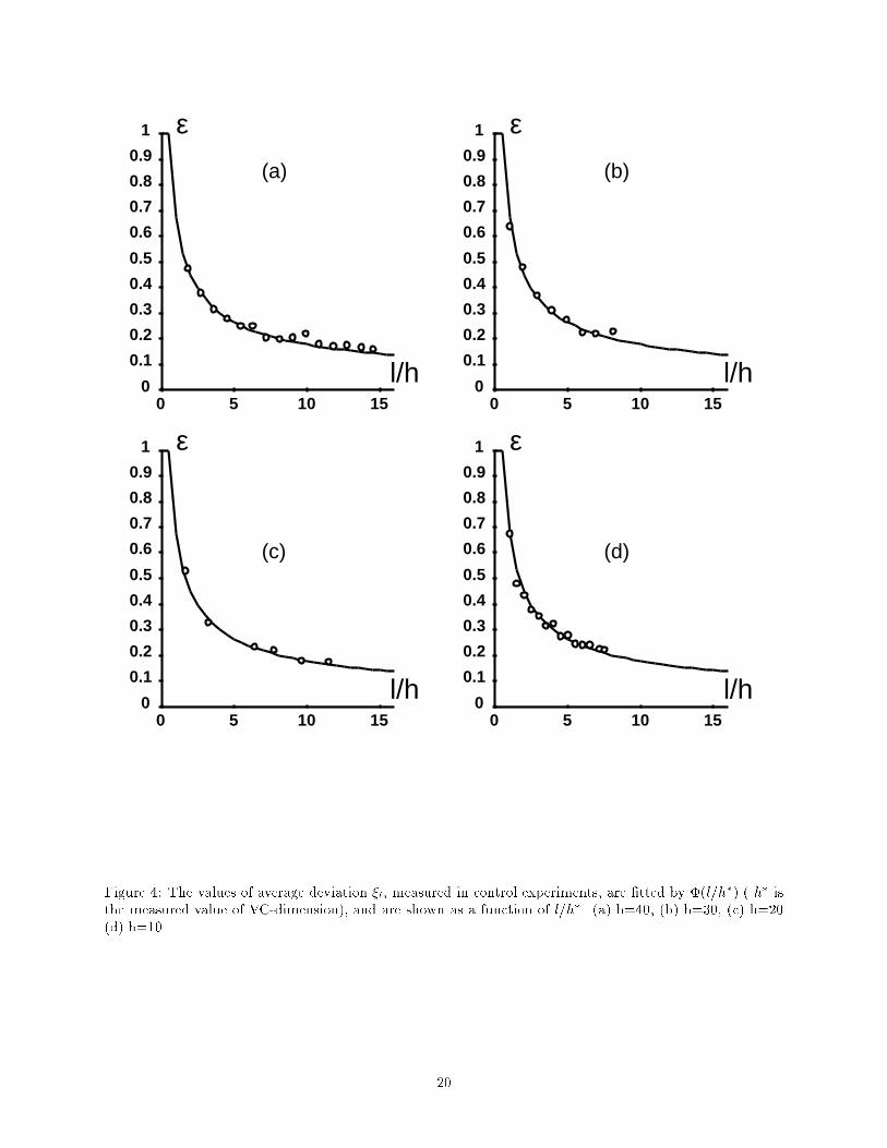
P1 corresponds to a linearly separable task (no noise), P3 to a random classi�cation task (random labels, nogeneralization is expected), P2 to a task of intermediate di�culty.Figure 1 shows the average values of the deviations as a function of l, the size of the half-set, for the threeconditional probabilities. Each average value was obtained from 20 realizations of the deviations. As canbe seen on the �gure, the results for the three cases practically coincide, demonstrating the independence ofthe E�i from the di�culty of the task. In further experiments only the conditional probability P3(!jx) wasused.6.2 Estimation of the free parameters a and b in �( lh)The value of the free parameters a and b in �( lh ) (eq 13) can be determined if we �t equation (13) to a setof experimentally obtained values of the average maximal deviation produced by a learning machine witha known capacity h. Assuming the optimal values a� and b� thereby obtained are universal, we can simplyconsider them constant, and use them for the measurement of the capacity of other learning machines.Figure 2 shows the approximation of the empirical data by �( lh ), given in (13) with parameters set toa� = 0:16; b� = 1:2. Note how well the function � describes the average maximal deviation throughout thefull range of training set sizes used in our experiments (0:5 < lh < 32). Experiments with various input sizesyielded consistent values for the parameters.A simpler functional form for the deviation �1( lh ),�1( lh ) = d ln(2 lh ) + 1lh + d� 0:5 ;inspired by the bound for small l=h, describes the data well for small l=h (up to l=h < 8). Figure 3 showsthe approximation of the empirical data by �1 using d = 0:39.The values a = 0:16 and b = 1:2 obtained with the experiment of �gure 2 were used for all the experimentsdescribed below.6.3 Control ExperimentsFor further validation of the proposed method, a series of control experiments were conducted. In theseexperiments we used the above-described method to measure the e�ective VC-dimension of several learningmachines, and compared it to their theoretically known values.The learning machine we used was composed of a �xed preprocessor which transformed the n-dimensionalinput vector x into another n-dimensional vector y using a linear projection onto a subspace of dimensionk. The resulting vector y was then fed to a linear classi�er with n inputs.It is easy to see that the theoretical value of the e�ective VC-dimension is k, as this can be reduced toa linear classi�er with k inputs. Table 1, which shows the estimated VC-dimension for k = 10; 20; 30; 40,indicates that there is a strong agreement between the estimated e�ective VC-dimension, and the theoreticallypredicted dimension.E�ective VC dim. 40 30 20 10Estimated VC dim. 40 31 20 11Table 1: The true and the measured values of VC-dimension in 4 control experimentsFigures 4a-d demonstrate how well the function �( lh� ), where h� is the estimate of the e�ective VC-dimension, describes the experimental data.6.4 Smoothing experimentsIn this section, we measure the e�ect of \smoothing" the input on the capacity. Contrary to the previ-ous section, this e�ect was not predicted theoretically. As in the previous section, the learning machine9

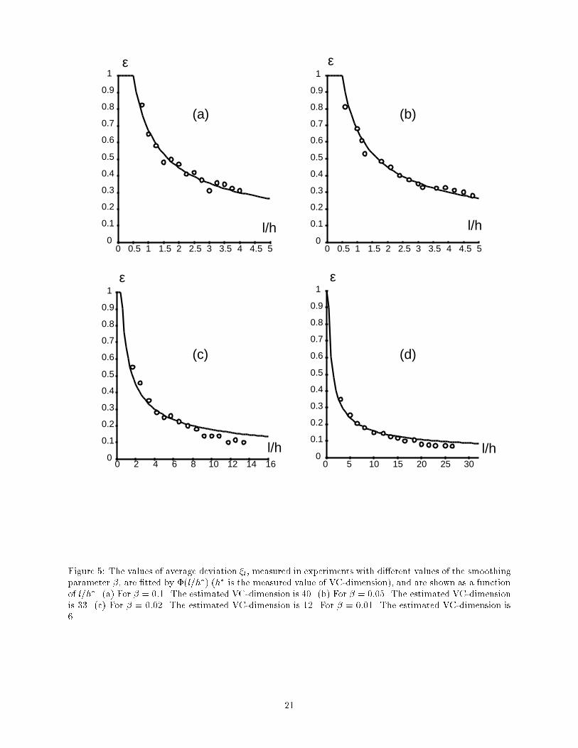
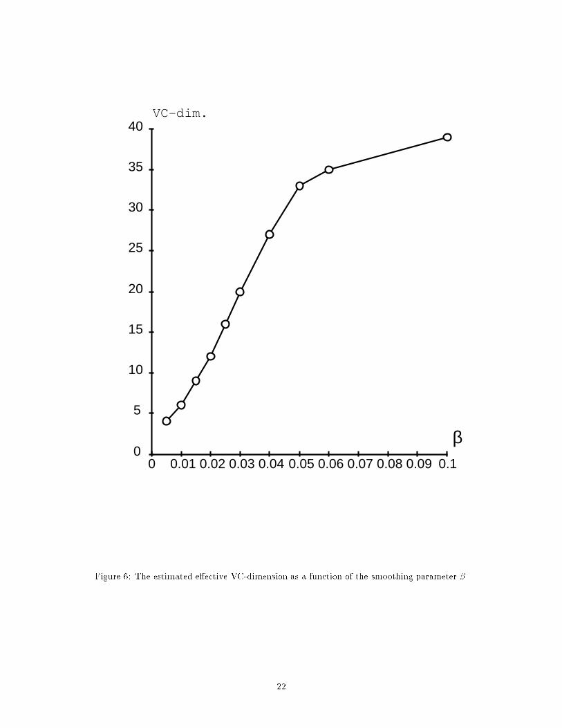
incorporated a linear preprocessor which transformed x into y by a smoothing operation:yi = nXj=1 xjexpf��jj � ijng;where jj � ijn = � j � i for 1 � i < jj + n� i for i � jAs described previously, the classi�er was trained with gradient descent, but a very small \weight decay"term was added (the reason for the weight decay will be explained below).The parameter � determines the amount of smoothing: for very large �, the components of the vectory are virtually independent, and the VC-dimension of the learning machine is close to n. As the value of� decreases, strong correlations between input variables start to appear. This causes the distribution ofpreprocessed vectors to have a very small variance in some directions. Intuitively, an appropriate weightdecay term will make these dimensions e�ectively \invisible" to the linear classi�er, thereby reducing themeasured e�ective VC-dimension. The measured VC-dimension decreases down to 1 for � = 0. When �takes non-zero values, there is no theoretically known evaluation of the VC-dimension, and the success ofthe method can be measured only by how well the experimental data is described by the functional �.Figures 5(a-c) show the average maximal deviation as a function of l, for di�erent smoothing parameters�, and demonstrates how well the function �( lh� ), where h� is the estimate of the e�ective VC-dimension,approximates the experimental data. Figure 6 shows the estimated value of the VC-dimension as a functionof the smoothing parameter �.7 ConclusionWe have shown that there exist three di�erent regimes for the behavior of the maximum possible deviationbetween the frequencies of error on two di�erent sets of examples. For very small values of l=h (< 1=2), themaximal deviation is � 1, for small values of l=h (from 1/2 up to about 8), it behaves like log(2l=h)=(l=h),for large values it behaves like plog(2l=h)=(l=h).We have introduced the concept of e�ective VC-dimension, which takes into account some weak propertiesof probability distribution over the input space. We prove that the e�ective VC-dimension can be used inplace of the VC-dimension in all the formulae obtained previously. This provides us with tighter bounds onthe maximal deviation.Based on the functional forms of the bounds for the three regimes, we propose a single formula thatcontains two free parameters. We have shown how the value of these parameters can be evaluated experi-mentally. We show how the formula can be used to estimate the e�ective VC-dimension.We illustrate the method by applying it to various learning machines based on linear classi�ers. Theseexperiments show good agreement between the model and the experimental data in all cases.Interestingly, it appears that, at least within the set of linear classi�ers, the values of the parameters areuniversal. This universality was con�rmed by recent results obtained since the �rst version of this paperwith linear classi�ers trained on real-life tasks (image classi�cation). Excellent �t with the same values ofthe constants were obtained even when the classi�ers were trained by minimizing the empirical risk subjectto various types of constraints. This included simple constraints, such as a limit on the norm of the weightvector (equivalent to weight decay), and more complex ones which improve the invariance of the classi�erto distortions of the input image by limiting the norm of some Lie derivatives (Cortes, 1993; Guyon et al.,1992).The extension of the present work to multilayer networks faces the following di�culties. First, the theoryis derived for methods that minimize the empirical risk. However, existing learning algorithms for multilayernets cannot be viewed as minimizing the empirical risk over entire set of functions implementable by thenetwork. Because the energy surface has multiple local minima, it is likely that, once the initial parametervalue is picked, the search will be con�ned to a subset of all possible functions realizable by the network.The capacity of this subset can be much less than the capacity of the whole set (which may explain whyneural nets with large numbers of parameters work better than theoretically expected). Second, because10

the number of local minima may change with the number of examples, the capacity of the search subsetmay change with the number of observations. This may require a theory which considers the notion ofnon-constant capacity associated with an \active" subset of functions.8 Appendix 1. Proof of Theorem 1.Let the random independent sampleZ2l = x1; !1; : : : ; xl; !l; xl+1; !l+1; : : : ; x2l; !2l (18)be given.Call the classes of equivalence of the set f(x; �); � 2 � on the sample (18) the subset of indicator functionsf(x; �); � 2 �? that take the same value on the vectors x from (18). Denote the number of di�erent classesof equivalence given on the sample (18) by��(Z2l) = ��(x1; !1; : : : ; x2l; !2l):Consider the eventA� = fZ2l : sup�2�(� l1(Z2l; �)� � l2(Z2l; �)) > �g = fZ2l : � l1(Z2l; �?) � � l2(Z2l; �?) > �gand the event B� de�ned as in equation (4). The following lemma is trueLemma. P (A�B�) � E��(x1; !1; : : : ; x2l!2l) expf���l4 gThe proof of this lemma will follow the same scheme as the proof of Theorem A2 in (Vapnik, 1982) pp.170-172. Write the probability in the evident formP (A�B�) = (19)ZZ(2l) �f(� l1(Z2l; �?)� � l2(Z2l; �?))� �g�f (� l1(Z2l; �?)� � l2(Z2l; �?))(�(Z2l; �?) + 12l )(1 + 12l � �(Z2l; �?)) � �gdP (Z2l)whereZ(2l) is the space of samples Z2l,�(Z2l; �?) = 12[� l1(Z2l; �?) + � l2(Z2l; �?)];and f(x; �?) is the function which attains the maximumdeviation of frequencies in two half-samples. Denoteby Ti (i = 1; 2; : : : ; (2l)!) the set of all possible permutations of the elements of the sample (18). Denote also�(TiZ2l; �?) = � l1(TiZ2l; �?)� � l2(TiZ2l; �?);�2(TiZ2l; �?) = (�(TiZ2l; �?) + 1=2l)(1 + 1=2l � �(TiZ2l; �?)):It is obvious that the equalityP (A�B�) = ZZ(2l) �f�(TiZ2l; �?)� �g�f �(TiZ2l; �?)�2(TiZ2l; �?) � �gdP (Z2l) = (20)ZZ(2l) 1(2l)! (2l)!Xi=1 �f(�(TiZ2l; �?)� �g�f �(TiZ2l; �?)�2(TiZ2l; �?) � �gdP (Z2l):is true.Note that for any �xed Z2l and Ti the following inequality is true:�f�(TiZ2l; �?)� �g�f �(TiZ2l; �?)�2(TiZ2l; �?) � �g �11

X�j2��(Z2l) �f�(TiZ2l; �j)� �g�f �(TiZ2l; �j)�2(TiZ2l; �j) � �gUsing this bound, one can estimate the integrand of the right-hand side of the equality (20). It does notexceed the value X�j2��(Z2l)24 1(2l)! (2l)!Xi=1 �f(�(TiZ2l; �j � �g�f �(TiZ2l; �j)�2(TiZ2l; �j) � �g35 : (21)The expression in the brackets is the fraction of the number of permutations Ti for which the two events(� l1(TiZ2l; �j)� � l2(TiZ2l; �j) > �;and � l1(TiZ2l; �j)� � l2(TiZ2l; �j)(�(TiZ2l; �j) + 1=2l)(1 + 1=2l � �(TiZ2l; �j)) > �hold simultaneously, among all possible (2l)! permutations. It is equal to the following value� =Xk CkmCl�k2l�mCl2l ;where m = l(� l1(Z2l; �) + � l2(Z2l; �))and the summation is performed on all k satisfying the inequalitieskl � m � kl > �; (22)kl � m � kl > ��m + 12l (1� m � 12l )� : (23)We now estimate the value �. The derivation of the estimate of � repeats the derivation of similar estimatesin (Vapnik, 1982) pp. 173-176.ln �=2 < ( � 4(l+1)(m+1)(2l�m+1) (k� � m2 + 1)2 if m is an even number� 4(l+1)(m+1)(2l�m+1) (k� � m�12 + 1)(k� � m�12 ) if m is an add number (24)where k� is the least integer satisfying the conditionk�l � m2l > �2 : (25)From (23) and (24) we obtain ln �=2 < ��2(k� �m=2):And from this inequality and (25) we obtain ln�=2 < �� �l4 :Substitute now the estimate of the value � into right-hand side of the inequality (20). We obtainPfA�B�g � Z X�j2��(Z2l) expf���l4 gdP (Z2l) = E��(Z2l) expf���l4 :g (26)12

The lemma is proved.Note now that the inequality E��(Z2l) < maxZ2l ��(Z2l) = m�(2l)is true. The function m�(2l) known as the growth function is estimated by means of the VC-dimension(Vapnik, 1982): m�(2l) < (2leh )h:Therefore PfA�B�g < (2leh )he� ��l4 :Then PfA�jB�g < (2leh )h e� ��l4P (B�) :Estimate now the conditional expectationE(A�jB�) = Z 10 Pfsup�2�(� l1(�;Z2l)� � l2(�;Z2l)) > �jB�gd�:For this estimation divide the interval area into two parts: (0,u), where we use the trivial estimate ofconditional probability P (A�jB�) = 1, and the area (u;1), were we use the estimate (26). We obtainE(A�jB�) < Z u0 d�+ (2leh )h 1P (B�) Z 1u expf���l4 gd� = u+ (2leh )h 4l�P (B�) expf��ul4 gThe minimum of the right-hand side of the inequality is attained whenu = 4h(ln(2l=h) + 1)� lnP (B�)�l :In such a way we obtain the estimateE(A�jB�) < 4h(ln(2l=h) + 1)� lnP (B�) + 1�l :The theorem is proved.Now we want to obtain the estimate of the expectation of the random value (4) for an arbitrary l=h. Forthis we use the inequality (Vapnik, 1982) p.172Pfsup�2� j� l1(�;Z2l)� � l2(�;Z2l)j > �g < 3(2leh )h expf��2lgAs in the case above we getEfsup�2� j� l1(�;Z2l) � � l2(�;Z2l)jg < Z u0 d�+ 3(2leh )h Z 1u expf��2lgd� <u+ 3(2leh )h Z 1u expf��ulgd� = u+ 3(2leh )h 1lu expf�ulgFor u =s ln(2l=h) + 1l=hwe obtain the estimateEfsup�2� j� l1(�;Z2l)� � l2(�;Z l)jg <s ln(2l=h) + 1l=h + 3plh(ln(2l=h) + 1) < Cs ln(2l=h) + 1l=h :13

9 Appendix 2. Proof of Theorem 2.We �rst prove the �rst part of the theorem. By the lemma proved in Appendix 1, the inequalityP (A�B�) � E��(Z2l) expf���l4 g (27)is true. Then it follows thatP (A�jB�) � E��(Z2l)P (B�) expf���l4 g = ZZ(2l)�(Z2l)dP (Z2l)! expf� ��l4 gP (B�) : (28)Divide the integration domain Z(2l) into two parts: �2l and Z(2l)=�2l, where �2l is a sample space all ofwhose elements belong to X?. Thenexpf���l4 g ZZ(2l)��(Z2l)dP (Z2l) = (29)expf���l4 g Z�2l ��(Z2l)dP (Z2l) + ZZ(2l)=�2l ��(Z2l)dP (Z2l)! :According to the conditions of the theorem, in area �2l the bound��(Z2l) < �2leh� �h� (30)holds, and in the area Z(2l)=�2l the bound ��(Z2l) < �2leh �h (31)holds. Thus from (29), (30) and (31) it follows thatP (A�jB�) < expf� ��l4 gP (B�) �(2leh� )h� + �(2leh )h� (32)where � is the measure of Z(2l)=�2l.Note that � < 1� (1� �)2l < 2l�where 1� � is the measure of the set X�. According to the condition of the theorem the inequality� < 12l (2leh� )h� ( h2le )hholds. We then derive � < (2leh� )h� ( h2le )h (33)Substituting (33) into (32) we obtain P (A�jB�) < (2leh� )h� expf� ��l4 gP (B�)Then, as in Appendix 1, we obtain the estimate of the expectation (10).We can derive the estimate (11) similarly. 14

10 Appendix: Estimation of the Maximum Error Rate Di�er-ence on Two Half-SamplesWe would like to estimate the value of the maximal error rate di�erence of a learning machine on two half-sets(maximal deviation). Denote by �Z2l a sequence obtained from the set Z2l of equation (15) by changing thevalues of !i for the �rst half set.�Z2l = x1; �!1;x2; �!2; :::; xl; �!l ; xl+1; !l+1; :::;x2l; !2l; (34)�!i = 1� !i:We will use �Z2l as a training set for the learning machine. In this case, training results in the minimizationof R(�) = 1l lXi=1(�!i � f(xi; �))2 + 1l lXi=1(!i � f(xi; �))2 (35)It is easy to see that the minimum of (36) is obtained for the same function f(x; ��) that maximizes thedeviation. Since ! and f(x; �) have binary values,(�!i � f(xi; �))2 = 1� (!i � f(xi; �))2: (36)From (35) and (36) it follows thatR(�) = 1� 1l lXi=1(!i � f(xi; �))2 + 1l lXi=1(!i � f(xi; �))2: (37)Therefore, minimizing R(�) is equivalent to maximizing�R(�) = 1l lXi=1(!i � f(x; �))2 � 1l lXi=1(!i � f(xi; �))2 = (�1(�;Z2l)� �2(�;Z2l)): (38)To summarize, the maximization of deviation is obtained by training the learning machine with the trainingset �Z2l. The value of the maximal deviation is related to the minimum of the training functional through�R(�) = 1� R(�):ReferencesAbu-Mostafa, Yaser, S. (1993). Hints and the VC Dimension. Neural Computation, 5(2).Baum, E. B. and Haussler, D. (1989). What Size Net Gives Valid Generaliztion? Neural Computation,1:151{160.Cortes, C. (1993). personnal communication.Devroye, L. (1982). Bounds for the uniform deviations of empirical measures. Journal of MultivariateAnalysis, 12:72{79.Guyon, I., Vapnik, V., Boser, B., Bottou, L., and Solla, S. (1992). Structural Risk Minimization for CharacterRecognition. In Moody, J., Hanson, S., and Lippmann, R., editors, Advances in Neural InformationProcessing Systems 4, Denver, CO. Morgan Kaufman.Le Cun, Y., Denker, J. S., Solla, S., Howard, R. E., and Jackel, L. D. (1990). Optimal Brain Damage.In Touretzky, D., editor, Advances in Neural Information Processing Systems 2, Denver, CO. MorganKaufman.Vapnik, V. (1982). Estimation of Dependencies Based on Empirical Data. Springer-Verlag, New York.15

Vapnik, V. and Chervonenkis, D. (1971). 1971] On the uniform convergence of relative frequencies of eventsto their probabilities. Theory of Probability and Applications, 16:264{280.Vapnik, V. and Chervonenkis, D. (1989). The necessary and su�cient conditions for consistency of empiricalrisk minimization method. Pattern recognition and Image Analysis, 1(3):283{305.Weigend, A., Rumelhart, D., and Huberman, B. (1991). Generalization by weight elimination with appli-cation to forecasting. In Lippmann, R., Moody, J., and Touretzky, D., editors, Advances in NeuralInformation Processing Systems 3, Denver, CO. Morgan Kaufman.

16

0 5 10 15 20 25 30 350

0.1

0.2

0.3

0.4

0.5

0.6

0.7

0.8

0.9

1

tl/h

ε

Figure 1: The measured values for average deviation ��l are shown as a function of l=h, the size of thehalf-sample normalized by the VC-dimension. These values were obtained in experiments with three di�erentconditional probabilities P (!jx). The symbol 4 denotes values measured for P1. The symbol 2 denotesvalues measured for P2. The symbol denotes values measured for P3.17

0 5 10 15 20 25 30 350

0.1

0.2

0.3

0.4

0.5

0.6

0.7

0.8

0.9

1

l/h

ε

Figure 2: The values for average deviation ��l are �tted by �(l=h) with parameter values a = 0:16; b = 1:2.18

0 5 10 15 20 25 30 350

0.1

0.2

0.3

0.4

0.5

0.6

0.7

0.8

0.9

1ε

l/h

Figure 3: The values for average deviation ��l are �tted by �1(l=h) with d = 0:39.19

5 10 150

0.1

0.2

0.3

0.4

0.5

0.6

0.7

0.8

0.9

1 ε

l/h0 5 10 15

0

0.1

0.2

0.3

0.4

0.5

0.6

0.7

0.8

0.9

1 ε

l/h

0 5 10 150

0.1

0.2

0.3

0.4

0.5

0.6

0.7

0.8

0.9

1 ε

l/h0 5 10 15

0

0.1

0.2

0.3

0.4

0.5

0.6

0.7

0.8

0.9

1 ε

l/h

(a) (b)

(c) (d)

0

Figure 4: The values of average deviation ��l, measured in control experiments, are �tted by �(l=h�) ( h� isthe measured value of VC-dimension), and are shown as a function of l=h�. (a) h=40, (b) h=30, (c) h=20(d) h=10. 20

00

0.1

0.2

0.3

0.4

0.5

0.6

0.7

0.8

0.9

1ε

0.5 1 1.5 2 2.5 3 3.5 4 4.5 5

l/h0 0.5 1 1.5 2 2.5 3 3.5 4 4.5 5

0

0.1

0.2

0.3

0.4

0.5

0.6

0.7

0.8

0.9

1

l/h

ε

0 2 4 6 8 10 12 14 160

0.1

0.2

0.3

0.4

0.5

0.6

0.7

0.8

0.9

1

l/h

ε

0 5 10 15 20 25 300

0.1

0.2

0.3

0.4

0.5

0.6

0.7

0.8

0.9

1

l/h

ε

(a) (b)

(c) (d)

Figure 5: The values of average deviation ��l, measured in experiments with di�erent values of the smoothingparameter �, are �tted by �(l=h�) (h� is the measured value of VC-dimension), and are shown as a functionof l=h�. (a) For � = 0:1. The estimated VC-dimension is 40. (b) For � = 0:05. The estimated VC-dimensionis 33. (c) For � = 0:02. The estimated VC-dimension is 12. For � = 0:01. The estimated VC-dimension is6. 21

0 0.01 0.02 0.03 0.04 0.05 0.06 0.07 0.08 0.09 0.10

5

10

15

20

25

30

35

40

qVC−dim.

β

Figure 6: The estimated e�ective VC-dimension as a function of the smoothing parameter �.22