MEG-SIM: A Web Portal for Testing MEG Analysis Methodsusing Realistic Simulated and Empirical Data

C. J. Aine1,2, L. Sanfratello1,2, D. Ranken3, E. Best2, J. A. MacArthur2, T. Wallace1, K.Gilliam2, C. H. Donahue1, R. Montaño1, J. E. Bryant1, A. Scott2, and J. M. Stephen2

1University of New Mexico School of Medicine, Albuquerque, New Mexico2The Mind Research Network, Albuquerque, New Mexico3Los Alamos National Laboratory, Los Alamos, New Mexico

AbstractMEG and EEG measure electrophysiological activity in the brain with exquisite temporalresolution. Because of this unique strength relative to noninvasive hemodynamic-based measures(fMRI, PET), the complementary nature of hemodynamic and electrophysiological techniques isbecoming more widely recognized (e.g., Human Connectome Project). However, the availableanalysis methods for solving the inverse problem for MEG and EEG have not been compared andstandardized to the extent that they have for fMRI/PET. A number of factors, including the non-uniqueness of the solution to the inverse problem for MEG/EEG, have led to multiple analysistechniques which have not been tested on consistent datasets, making direct comparisons oftechniques challenging (or impossible). Since each of the methods is known to have their own setof strengths and weaknesses, it would be beneficial to quantify them. Toward this end, we areannouncing the establishment of a website containing an extensive series of realistic simulateddata for testing purposes (http://cobre.mrn.org/megsim/). Here, we present: 1) a brief overview ofthe basic types of inverse procedures; 2) the rationale and description of the testbed created; and 3)cases emphasizing functional connectivity (e.g., oscillatory activity) suitable for a wide assortmentof analyses including independent component analysis (ICA), Granger Causality/Directed transferfunction, and single-trial analysis.

IntroductionThere has been increased interest in the use of noninvasive functional imaging techniquesfor characterizing cognitive deficits in clinical populations. Furthermore, there has beenrenewed appreciation of the benefits for characterizing the fine temporal dynamics of thesedeficits. For example, one cannot learn about the direction of information flow through thebrain, or information processing stages known to occur in various memory functions (e.g.,identification, maintenance, recognition), without both excellent spatial and temporalresolution. Although magnetoencephalography (MEG) and electroencephalography (EEG)methods offer excellent temporal resolution, they face the greatest challenge to sourcelocalization of the neuroimaging techniques since the well-known “inverse problem” (i.e.,the reconstruction of the current distribution inside the brain based on measurements madeoutside the head) is not as straightforward for MEG/EEG as it is for functional magneticresonance imaging (fMRI) and positron emission tomography (PET) methods, due to the

Contact Information: Cheryl J. Aine, PhD Department of Radiology, MSC10 5530 University of New Mexico School of MedicineAlbuquerque, NM 87131 Phone: 505 272-5557 Fax: 505 272-8002 aine@unm.edu.

Furthermore, the authors declare that they have no conflict of interest.

NIH Public AccessAuthor ManuscriptNeuroinformatics. Author manuscript; available in PMC 2013 April 01.

Published in final edited form as:Neuroinformatics. 2012 April ; 10(2): 141–158. doi:10.1007/s12021-011-9132-z.

$waterm

ark-text$w

atermark-text

$waterm

ark-text

physics of the problem. The inverse problem for MEG and EEG is mathematically ill-posed;that is, it has no unique solution in the most general, unconstrained case (Hämäläinen et al.1993). Therefore, suitable constraints have to be applied to render the solution unique(Baillet et al. 2001).

For a number of reasons, discussed later, results from the varied inverse procedures havenever been tested and compared using a standard testbed of realistic simulated data. It isstandard practice in the MEG field to create computer-simulated data in order to test a newlydeveloped or revised inverse procedure, using data where the ground truth (i.e., the solution)is known before testing it on empirical data where the ground truth cannot be known. Sinceeach of the MEG analysis methods is known to have its own set of strengths and weaknesses[for some examples see (Liljestrom et al. 2005)], it would be beneficial to the community toqualify and quantify them. Therefore, we are announcing the establishment of a websitecontaining a series of realistic simulated data for testing purposes (http://cobre.mrn.org/megsim/). If an algorithm provides reasonable solutions to simulations then it is standardpractice to use the algorithms in simple sensory empirical data where the literature providesinformation on the expected locations and time-courses of sources (e.g., non-human primatestudies) before attempting analysis of cognitive datasets where it is impossible to know theground truth. Therefore, we acquired simple somatosensory, auditory, and visual sensorydata on several participants for this purpose since it is best if the same empirical datasets areshared across the community for comparison. If an algorithm fails to identify the simulatedsources and time-courses under realistic conditions (e.g., similar signal-to-noise ratio orSNR as empirical data and real artifacts occurring at random intervals), then one cannotexpect to obtain correct or reasonable results in empirical data. The rationale and descriptionof the testbed created along with sample simulated cases emphasizing functionalconnectivity and oscillatory activity are presented here. The single-trial datasets describedare suitable for a wide assortment of analyses including independent component analysis(ICA), Granger Causality/Directed transfer function, and single-trial analysis.

Inverse ProceduresFor investigators new to this field, we briefly outline the most common inverse methodsbelow. The source models and associated inverse algorithms fall into four broad categories.First, there are models that use a relatively low-order parametric description of the currentsin order to produce an over-determined problem, i.e., the number of parameters to beestimated in the model is less than the number of recording sites. The most frequently usedsource model in MEG for clinical studies is a fixed set of equivalent current dipoles (ECDs)located at various cortical locations whose moments (ECD amplitudes) vary with time(Scherg and Von Cramon 1986; Mosher et al. 1992; Ermer et al. 2000). The term equivalentmeans that coherent activation of a large number of pyramidal cells can be represented by apoint source at the detectors. Second, there are current reconstruction models that employ agrid of elementary sources in a volume or on the cortical surface such that the number ofparameters to be estimated in the model is typically much greater than the number ofmeasurements. Because the solution, in this case, is under-determined, the weighted least-squares criterion requiring that the prediction error is minimized, must be augmented withan additional constraint to select the “best” current distribution among those capable ofexplaining the data. In the case of the basic L2 minimum norm approach the mathematicalcriterion is the solution that minimizes the power (L2-norm) of the dipole moment (Wang etal. 1992; Dale and Sereno 1993; Hämäläinen and Ilmoniemi 1994; Ioannides et al. 1994;Pascual-Marqui et al. 1994; Grave de Peralta-Menendez and Gonzalez-Andino 1998; Uutelaet al. 1999). The L1 minimum norm solution selects the source configuration that minimizesthe absolute value of the source strength (Uutela et al. 1999; Huang et al. 2006). Third, thereare spatial filter (e.g., beamformer) approaches that estimate activity at points or regions of

Aine et al. Page 2

Neuroinformatics. Author manuscript; available in PMC 2013 April 01.

$waterm

ark-text$w

atermark-text

$waterm

ark-text

interest, independent of one another. Beamformer output, for example, is a linearcombination of the external field measurements at each time sample, constructed with therequirement that the focus is on the source of interest while minimizing contributions fromall other sources (Van Veen et al. 1997; Vrba and Robinson 2000; Sekihara et al. 2001).That is, it allows signals of interest to pass through each volume grid node or cortical surfacelocation while suppressing noise and signals from other locations (i.e., spatial filter). Finally,there are probabilistic approaches to the MEG/EEG source localization problem based onBayesian inference [e.g., (Jun et al. 2005; Wipf et al. 2010)]. Some of these approachesresult in a single best solution to the problem, while others use Markov Chain Monte Carloto produce a large number of likely solutions that both fit the data and any prior information[e.g.,(Schmidt et al. 1999)].

Limitations of Inverse ProceduresEach of the inverse procedures has limitations associated with it. Critics of the earlier dipolemodeling approaches emphasize the difficulties in: 1) accurately localizing more than one ora few point current dipoles; 2) using point current dipoles to localize extended sources; and3) determining the number of sources to be included in the search a priori (Liu et al. 1998;Fuchs et al. 1999; Uutela et al. 1999; Huang et al. 2006; Lin et al. 2006; Mattout et al. 2006).Our greatest concern for the multidipole, spatiotemporal modeling methods is that under-estimation of the number of true sources can severely compromise location and time-courseaccuracy for the identified sources (Supek and Aine 1997; Greenblatt et al. 2005). This isbecause multidipole modeling methods attempt to account for the entire measured signal viaa given number of sources, and the omission of one source will generally change theposition and/or magnitude of other sources to account for the signal from the omitted source.This is not true for the minimum norm, beamformer, or Bayesian methods. In contrast,critics of the minimum norm-based approaches state that: 1) the results often appearsmeared, even for point current sources and at times may become split across lobes whichproduce spurious or ghost sources leading to imprecise estimated dynamics (David et al.2002; Michel et al. 2004; Lin et al. 2006); 2) the constraints introduced are purelymathematical with no physiological justification (Michel et al. 2004); 3) the solution isbiased toward superficial source locations leading to the application of depth weightings bysome groups (Ioannides et al. 1990; Lin et al. 2006); 4) the smeared or broadened effectbecomes more pronounced with a decrease in signal-to-noise, potentially leading to falsepositive sources (Wischmann et al. 1995); and 5) it is severely under-determined therebyrequiring the use of regularization methods to restrict the range of possible solutions.Although, the linearly-constrained minimum variance (LCMV) beamformer has higherresolution than minimum norm-based methods when cortical sources are focal, theunderlying assumption is that neural sources are incoherent. Coherent signals will cause thebeamformer to fail in finding locations of other coherent sources due to partial cancellation(Hui et al. 2010) which is a potential problem for cognitive data where coherence typicallyabounds (i.e., working memory tasks). For example, in working memory studies, activitytends to synchronize across many widespread brain regions for seconds (Aine et al. 2003).However, several groups have recently introduced variants of the beamformer that canreportedly deal with coherent sources, with some restrictions [e.g., (Dalal et al. 2006;Brookes et al. 2007; Diwakar et al. 2011; Moiseev et al. 2011)]. Secondly, Hui and Leahy(2006; Hui et al. 2010) also noted that beamformers may not be appropriate, in their currentform, for directly examining functional connectivity or cortical interactions, given the robustcross-talk present in the data. The latter is true for minimum norm-based methods as well.However, the general advantages of minimum norm and beamformer methods are that theyrequire less analysis time making them quicker to use and the number of sources to bemodeled does not need to be known a priori. Finally, less seems to be known about Bayesianmethods since they have not been widely applied to real experiments (Luck 2005). In part

Aine et al. Page 3

Neuroinformatics. Author manuscript; available in PMC 2013 April 01.

$waterm

ark-text$w

atermark-text

$waterm

ark-text

this may be due to a need for large computational resources since some versions utilize aMarkov Chain Monte Carlo approach to generate sets of activity parameters that aredistributed according to the posterior distribution (Schmidt et al. 1999).

The simulated datasets described here are designed to provide a wide range of realisticexamples which emulate brain activity. We specifically tried to design these simulationssuch that a particular approach would not always be favored. We hope developers willutilize these data to further develop and refine MEG analysis methods. Similarly, we hopethat users of the algorithms will compare and contrast their favored approaches with others.Because we are avid users of a semi-automated, multidipole, spatiotemporal approach[Calibrated Start Spatio-Temporal or CSST; (Ranken et al. 2002; Ranken et al. 2004)],solutions shown throughout this document are from the CSST algorithm, for immediatebenchmark comparisons.

Barriers Addressed by Creating Realistic Simulated DatasetsOne barrier encountered in the area of software development for electromagnetic measuresis the lack of an extensive, realistic simulated testbed for determining the success of thealgorithms and for comparing algorithmic performance with others (i.e., standardization).Often developers test their algorithms using one or a few test cases that may or may notclosely emulate real brain activity and often these test cases are not readily amenable forother developers to use. For example, white noise is often added to the data to simulate noisenormally contained in data. The addition of real brain noise (e.g., ongoing backgroundrhythms not related to the task) is more appropriate since real brain noise can have adramatic effect on the localization ability of algorithms. Furthermore, users of algorithmswould like to know how various analysis methods work in the modalities they areinvestigating (e.g., auditory, visual, somatosensory) or in the specific areas of their researchinterests (e.g., sensory or cognitive studies). Our realistic simulated datasets also showtremendous differences in SNR across participants for similar source locations, due to signalcancellation and summation associated with differences in cortical geometry [e.g., (Aine etal. 1996; Amunts et al. 2000; Stephen et al. 2003)]. An algorithm may work well in one ofthe scenarios listed above but may be less than optimal in others. The creation of realisticdatasets ranging from sensory to cognitive studies in auditory, somatosensory, and visualmodalities and from a number of participants can help developers tremendously inunderstanding behaviors of their algorithms.

An additional barrier for MEG investigators is the fact that MEG systems made by differentmanufacturers have different pickup coils, sensor arrays, noise cancellation methods, as wellas different software packages for data analysis. Many of the software implementations arespecific to one particular data storage format or noise cancellation method as well. Thesefactors make it extremely difficult to compare results or pool data across laboratories. If onedeveloper creates a simulated data set using the sensor geometry of the Elekta Neuromag306 system, for example, then investigators using the VSM MedTech CTF 275 systemusually cannot use it because of file formatting barriers. We have been working on softwarethat is machine-independent (E. Best and D. Ranken) that can convert from one MEGsystem format to another. A standard testbed that can be used by all developers and userswould be of great help to the MEG community, and hopefully to the EEG community in thefuture.

Structural and Functional ConnectivityA current emphasis in neuroimaging is on structural and functional connectivity (e.g., theNIH Human Connectome Project) including the role oscillatory activity plays duringcognition. Evidence now indicates that: 1) local field potentials, which provide a measure of

Aine et al. Page 4

Neuroinformatics. Author manuscript; available in PMC 2013 April 01.

$waterm

ark-text$w

atermark-text

$waterm

ark-text

mainly postsynaptic dendritic responses, show strong sub-threshold synchrony of ongoingfluctuations in the cell's membrane potentials (Lampl et al. 1999); 2) local networks aremodulated by coordinated sub-threshold excitability changes (Engel et al. 2001); and 3)action potentials generated by cortical cells align with the oscillatory rhythm enablingneurons participating at the same oscillatory rhythm to synchronize their discharges withhigh precision across cortical regions (Gray et al. 1989). Although the specific roles theserhythmic activities play are still debated, numerous studies in monkeys and humans suggestthat oscillatory activity plays an important role in integrating neural activity from distantcortical areas [e.g. (Jensen and Lisman 1998; Canolty et al. 2006; de Lange et al. 2008;Osipova et al. 2008)], such as prefrontal and parietal cortices (von Stein et al. 2000). Othersadd that these internally generated coherent fluctuations of excitability may also providecontext to sensory information and predictions about forthcoming events (top-downprocessing) in order to guide behavior (Engel et al. 2001). Because of this increased interestin functional connectivity, we present cases of realistic simulations using both short- andlong-range oscillatory activity (gamma and beta band) and cases where activity is correlatedduring later intervals (e.g., simulating working memory).

Methods and ResultsSimulated data were created using MRIVIEW and MEGAN software. A brief description ofthese tools is provided below. MRIVIEW (Ranken and George 1993; Ranken et al. 2002) isa software tool (http://cobre.mrn.org/megsim/tools/mriview/mriview.shtml) for integratingvolumetric MRI head data with functional information (e.g., EEG, MEG, fMRI). It providestools for visualizing MRI data in a variety of 2D and 3D formats, the latter of which is anobject-based environment that is used to combine structural MRI data with variousrepresentations of brain functional data. A Coordinate Transformation interface allows usersto quickly perform MEG/EEG to MRI transformations, needed for both showing MEG/EEGresults on MRI based anatomy, and for setting up MEG/EEG forward models.

A Segmentation Interface module provides automatic and manual segmentation proceduresto support a variety of segmentation tasks, including: variable resolution grid creation forCSST, gray/white matter segmentation, extraction of 3-layer surface models for BEManalyses, and 5 (or more) tissue-type classifications for Finite Element Models (FEM) orFinite Difference Head Models (FDM). A Forward Simulator is included for creatingmultiple MEG and/or EEG focal or distributed-source regions of arbitrary size andorientation for testing various inverse procedures (see Figure 1A). User-specified, ellipsoidregions of gray/white matter boundary can be labeled and used to create simulated regionsof activity. We have used these tools previously for simulating epileptic spikes that werethen embedded in spontaneous activity from each subject (Stephen et al. 2003; 2005). In theexample shown in Figure 1A, a Freesurfer-segmented gray matter/white matter boundary forthe simulations (shown in red) was imported into MRIVIEW. The EEG forward solutionuses the Sun algorithm (1997) and the MEG forward solution uses the Sarvas formula(1987). The simulated activation time-courses can be generated using multiple Gaussians ora sinusoid (Fig. 1B), or they can be read from a file. Sensor geometries used by the majormanufacturers of MEG whole-head arrays (e.g., Elekta Neuromag Ltd, VSM MedTech CTFSystems, 4-D Neuroimaging) for generating the forward fields are obtained from a sistersoftware package, MEGAN (E. Best), which organizes the data from the different MEGsystems into a consistent data format, netMEG, a self-documenting and highly portable file,written using netCDF format. The simulated sensor measurements are obtained by summingthe forward fields from all of the simulated sources. Either simulated noise or real noisefrom MEG/EEG acquisitions (Fig. 1C) can be added to the calculated forwards to generatebetter simulations of empirical MEG/EEG data (Fig. 1D). MEGAN, http://cobre.mrn.org/megsim/tools/MEGAN, is also written in IDL and allows one to conduct preliminary

Aine et al. Page 5

Neuroinformatics. Author manuscript; available in PMC 2013 April 01.

$waterm

ark-text$w

atermark-text

$waterm

ark-text

analyses on data from different MEG systems such as deletion of bad channels, digitalfiltering and artifact rejection for retrospective averaging relative to a stimulus or responserecord, visualization of a variety of forms (e.g., static field distributions, temporal waveformdisplays and movie formats), and temporal analysis. The netMEG output file format can beused by CSST, constrained linear inverse procedures, and Bayesian Inference analysis.

CSST (Calibrated Start Spatio-Temporal) AnalysisThis multi-dipole, spatio-temporal approach has been automated, i.e., it takes the traditionalstarting parameter guesses out of the hands of the investigator. CSST uses the Nelder-Meadnon-linear downhill simplex procedure to perform a spatial search (Nelder and Mead 1965)and utilizes information based on a singular value decomposition (SVD) of the data matrixfor determining a range of number of sources to be localized. Advantages of the newerCSST automated algorithm, compared to MSST (Multi-Start Spatio-Temporal) (Harrison etal. 1996; Huang et al. 1998; Aine et al. 2000), lie in the fact that more fits to the data can beaccomplished in less time, while still employing a reduced chi-square statistic as the costfunction for obtaining the best fits to the data. CSST runs multiple instances of a downhillsimplex search from random combinations of MR-derived starting locations from within thehead volume, on a Linux PC cluster. General steps for processing the MEG and MRI dataare shown in Figure 2. A two stage simplex procedure is used to first rule out sub-optimalsolutions (i.e., it utilizes a coarse convergence criterion in the simplex procedure), and thento refine the remaining solutions using a fine convergence setting. A parallel version ofCSST is currently running on the Linux clusters at the Mind Research Network (MRN),using MPI to distribute the calculations across the processors, which could eventuallyprovide real-time, multi-dipole MEG analysis through the use of Graphics Processing Unitson multicore personal processors. CSST has been used extensively with both Neuromag 122and CTF 275 MEG systems (Stephen et al. 2003a; 2003b; Stephen et al. 2005; Stephen et al.2006; Aine et al. 2010). CSST has also been used to analyze Neuromag Vectorview 306-channel data and has been thoroughly tested on EEG data (Susac et al. 2010; Golubic et al.2011; Susac et al. 2011). Additional information on our analysis methods can be found inAine et al. 2010. Sphere and overlapping-spheres forward models are options withinMRIVIEW (Huang et al. 1999) but a Forward Interpolation capability (Ermer et al. 2001)has also been implemented in CSST, allowing it to be used with BEM or FEM/FDMforward models. CSST accuracy tests were performed on CTF 275 data obtained from a dry-phantom current dipole generator, demonstrating 1 mm dipole source localization accuracy.

Simulated Data SetsEmpirical MEG/MRI datasets have been acquired for 5 participants under a partnershipformed between the MRN, Massachusetts General Hospital, University of Minnesota/Veterans Affairs in Minneapolis, University of New Mexico, and Los Alamos NationalLaboratory. Data were acquired using 3 different MEG systems (VSM MedTech 275,Elekta-Neuromag 306, 4-D Neuroimaging 3600) and 3 different sensory paradigms (visual,auditory and somatosensory) for each participant. These empirical data will be madeavailable via the MEG-SIM portal and will be discussed more completely later. A grantfrom NIMH (R21MH080141) allowed us to then create realistic simulated data derived fromthe real noise contained in the collected data and to establish a web portal for others toaccess these simulated datasets. We refer to the testbed as ‘realistic’ simulated data because:1) colored noise is used is most examples (i.e., spontaneous data containing correlatednoise); 2) the time-courses and source locations simulated are based on findings fromempirical data; 3) different-sized cortical patches are created from MRIs of individualparticipants (i.e., the SNR and orientation of sources differ across participants); and 4) insome cases each of the unique single trials, mimicking actual data acquisition, are provided.

Aine et al. Page 6

Neuroinformatics. Author manuscript; available in PMC 2013 April 01.

$waterm

ark-text$w

atermark-text

$waterm

ark-text

Focal vs. Extended SourcesExamining source extent in the simulated and empirical studies is important for evaluatingthe suggestion that ECD modeling is limited due to its proposed inability to deal effectivelywith extended sources (Dale et al. 2000; Hillebrand and Barnes, 2002; Lin et al. 2006;Ahlfors et al. 2010; Golubic et al. 2011). The simulated data sets were constructed using twodifferent-sized patches of cortex determined via MRI (~4 mm2 and ~20 mm2) producing twodifferent source strengths (30 and 50 nAm). We used these values because: 1) our previousempirical results suggest that those current strengths are typical of what is encountered insensory studies [e.g., figure 3 and table 2 in (Aine et al. 2006) and figure 4 and table 3 in(Aine et al. 2005) show similar peak amplitudes for visual and auditory studies] and 2) thesensory visual paradigm used to acquire data at each MRN partner site utilized small andlarge stimuli (1.0° and 5.0° of visual angle) designed to activate ~4 mm2 of tissue and ~20mm2 of tissue in primary visual cortex, according to the cortical magnification factorspresented in Rovamo and Virsu (1979). We attempted to equate the simulated and empiricalparameters since the goal was to produce both focal and extended activity. Thesomatosensory study used electrical stimulation of the median nerve and the index finger, inorder to produce focal vs. extended sources. The auditory study used 3 pure tones and burstsof white noise to evoke focal vs. extended activity.

Physiologically Plausible Time-coursesFigure 3 shows sample time-courses from both a monkey and a human (left and rightcolumns) in response to Walsh stimuli (visual). This spike-like activity followed by a slowsustained response is quite common for sensory and cognitive studies. Recent monkeystudies suggest that the initial feedforward flow of information (i.e., the spike-like activity)establishes the neuron's classical receptive field and its basic tuning properties typicallyassociated with pre-attentive processes (within 100 ms) (Lamme and Roelfsema 2000).Visual cortical neurons remain active after their participation in the feedforward sweepwhich allows information from horizontal and feedback connections to be incorporated intothe response (i.e., the slow sustained response); massive feedback projections carryinformation from higher-order regions to forward projecting pyramidal cells of lower-orderareas (Cauller 1998). Attention and memory processes influence lower-level responses viathese horizontal and feedback connections which affects the late sustained activity followingthe initial burst (Lamme and Roelfsema 2000; Mehta et al. 2000; Bisley et al. 2004). Thistype of response profile is evident in many MEG visual and auditory studies (Portin et al.1999; Aine et al. 2003; Vanni et al. 2004; Aine et al. 2005; Kovacevic et al. 2005) and weretherefore modeled in the simulated data for physiological reality.

Simulated Visual DataNine simulated visual datasets (1-sec epochs including equal pre- and poststimulus intervals)were generated consisting of a range of source configurations from simple to complex usingsmall and large cortical patches. The locations and timing of the 3-7 simulated sources (seeTable 1) were generated based on our previous basic visual (Stephen et al. 2002) and visualworking memory studies (Aine et al. 2006). For example, time-courses associated with eachcortical source in visual cortex was delayed by 10 ms, as shown in table 1 in (Stephen et al.2002). We varied the synchronicity of the latter portion of the time-courses across sets inorder to determine an algorithm's sensitivity to fine temporal changes. Parameters that varywithin and across datasets include: number of sources, focal vs. extended sources, currentstrengths, and degree of synchronicity of sources and noise level or type of noise (whitenoise or spontaneous noise). These 7 sets are being produced for 5 participants which resultin datasets derived from different cortical geometries and different SNRs. In addition, theyare being produced using CTF Omega 275, Vectorview 306, and Magnes 248configurations. In each case, 100 single trials of real spontaneous background activity were

Aine et al. Page 7

Neuroinformatics. Author manuscript; available in PMC 2013 April 01.

$waterm

ark-text$w

atermark-text

$waterm

ark-text

averaged as a noise trial for each of 5 participants and for each of 3 MEG systems. Atpresent, a spherical head model was used for the simulations and modeled data; however, aboundary element model (BEM) is available for future EEG and MEG simulations.

Visual Source Locations, Timing and StrengthsThe following visual areas were approximated on the cortical surface of the participants; V1,V2/V3, inferior lateral occipital gyrus (I.LOG), and intraparietal sulcus (IPS) (Stephen et al.2002; Aine et al. 2006). To simulate a cognitive dataset three additional cortical regionswere added, dorsolateral prefrontal cortex (DLPFC), right hippocampus (RH), and anteriorcingulate (AC) since they have been shown to be responsive to visual working memorytasks (Aine et al. 2003; Nyberg et al. 2003; Aine et al. 2006) and they provide a good test forlocalizing deeper sources.

Visual Data Set 1 (A-B)This set represents the simplest case where all 3 sources are asynchronous (10 ms delays inonset times). In Set 1.A all sources are small cortical patches (4 mm2, 30 nAm) while in Set1.B all sources are large cortical patches (20 mm2, 50 nAm). See Figure 4 (top row).

Visual Data Set 2Two synchronous sources with one source half the intensity of the other (30 and 15 nAm),overlapped with an asynchronous source (onsetting 10 ms later and 30 nAm strength) ismodeled in this set (see Figure 4 middle row). This source configuration has been used by usextensively in the past since it provides a good test for resolving synchronous activity(Supek and Aine 1997; Huang et al. 1998), but the present implementation is more realisticin terms of the shapes of the time-courses and use of real noise. Note, binaural stimulationalso activates coherent sources of activity; only the sources are not as closely spaced (i.e.,left and right Heschl's gyrus).

Visual Data Set 3 (A-B)This set contains initial asynchronous activity (same as Set 1 A-B) from 3 sources whichbecome synchronous later in time (Figure 4 bottom row). There has been recent interest inusing MEG to identify large-scale interactions between brain regions in cognitive tasks(neural networks) (David et al. 2002; Aine et al. 2003); synchronous late activity is oftenwitnessed in these types of tasks. As noted by David and colleagues (2002) some inverseprocedures are not designed to localize coherent sources (e.g., some LCMV beamformerapproaches). Our visual working memory studies usually reveal late synchronous activity(Aine et al. 2003; 2006).

Visual Data Sets 4-6In Set 4, six sources of activity are modeled where one pair of sources is synchronous (onesmall and one large cortical patch with consequent differences in intensity). This type ofprofile builds off of Set 3 by making it more consistent with our working memory studieswhere initial asynchronous activity is followed by late activity in several disparate brainregions (including dorsolateral prefrontal cortex, anterior cingulate and superior lateraloccipital gyrus) that become synchronous over time (Aine et al. 2003). Singer (1999), alongwith many others, suggests that synchronous neuronal firing provides one mechanism forbinding the different features/attributes of stimuli across widespread cortical areas. Table 2shows actual source locations, CSST estimated source locations, and errors when eithernoise was absent (no-noise) or real noise was present. Average error across the 6 sourceswas 0.1 mm for the no-noise condition and 6.8 mm for the real noise condition. This tabledemonstrates that the presence of real noise does significantly affect source localization

Aine et al. Page 8

Neuroinformatics. Author manuscript; available in PMC 2013 April 01.

$waterm

ark-text$w

atermark-text

$waterm

ark-text

accuracy; however, our CSST solution for the real noise condition was still good for thiscomplicated dataset and inconsistent with previous critiques of dipole modeling approachesthat state dipole methods cannot accurately localize more than a few point sources ofactivity.

Set 5 is the same as Set 4 with the addition of a source in right hippocampus (7 sources ofactivity). Set 6 (not shown in Table 1) is a case where late activity (e.g., 400-600 ms) wassynchronous across four cortical sites (V1, I. LOG, IPS, and DLPFC), also seen in workingmemory studies. The upper left panel of Figure 5 displays the locations of the corticalpatches (cortical patches are located at the cross-hairs) while the time-courses provided tothe cortical patches are shown beneath the MRIs. The averaged waveforms (128 trials withsignals embedded in real spontaneous noise) seen across 275 channels are shown in themiddle left column. CSST source locations are shown in the upper right panel (see tabledvalues). The table shows the coordinates of the actual sources, the estimated sourcelocations, and the errors using Euclidean distance. Net source orientation errors (polarcoordinates) were 42.0° for V1, 58.2° for I. LOG, 20.9° for IPS and 48.0° for the DLPFsources. The middle right panel shows the estimated time-courses and source locations. Theaverage error across all 4 sources was 6.7 mm with the greatest error for the I. LOG source.The cross-correlations between time-courses are shown in the bottom row of this figure. Weexamined early activity first (200-350 ms--bottom left panel) which shows that V1 activitycorrelated highly with I. LOG (dark blue tracing), regions showing the initial spike-likeactivity (~280 ms). IPS and DLPF cross-correlations were also highly correlated and nearthe zero-lag (orange tracing). The maximal correlation coefficients of the other pairs ofsources were lower in value and were not near the zero-lag. In contrast, the late activity(350-600 ms—bottom right panel) shows higher zero-lag correlation coefficients for activitybetween the 4 brain regions (i.e., late activity was synchronous across brain regions) withIPS and DLPFC revealing the highest correlation coefficient (orange tracing). These data arealso suitable for examining basic coherence between sensors.

Single-trial and Oscillatory Datasets (Sets 7-9)Single-trial datasets reflecting functional connectivity in a working memory task werecreated with and without oscillatory activity and are suitable for most types of analyses (i.e.,ICA, time-frequency analysis, Granger Causality, etc). In each case, sources embeddedwithin 128 single trials of noise were jittered about their mean latency and amplitude. Set 7is similar to Set 6 (VSM-CTF MEG System) only now each of the 128 single trials isavailable. Again, the four cortical sites were: 1) primary visual cortex (V1); 2) inferiorlateral occipital gyrus (I.LOG); 3) intraparietal sulcus (IPS); and 4) dorsolateral prefrontalcortex (DLPFC). The cortical patch current strengths were initially assigned values similarto those we observe in our visual working memory studies (30-50nAm peaks) using theMRIVIEW Forward Simulator (Ranken and George 1993; Ranken et al. 2002) and werethen randomly jittered about those values by up to +/- 50% across the single trials. Peaklatencies were also jittered across each trial by a randomly selected value up to +/- the fullwidth at half maximum (FWHM) divided by 2. To allow for traditional source analysis ofaveraged evoked responses, the 128 single trials were then averaged together and written outto the netCDF file format.

In Set 8, oscillatory activity was added to Set 7 time-courses (Figure 6). For the time-lockedoscillatory activity, V1, I. LOG, and IPS oscillated between 30-60 Hz (gamma band) acrossthe 128 trials while IPS and DLPFC oscillated between 14-28 Hz (beta band). Oscillatoryactivity for DLPFC was delayed by 20 ms relative to IPS and IPS gamma activity wasdelayed by 10 ms relative to IPS beta activity (see schematic in Fig. 6.A). The delays weremeant to reflect normal time delays between visual areas (Stephen et al. 2003). Gammaactivity mimicked local circuitry activity between V1, I. LOG, and IPS while beta activity

Aine et al. Page 9

Neuroinformatics. Author manuscript; available in PMC 2013 April 01.

$waterm

ark-text$w

atermark-text

$waterm

ark-text

mimicked long-range connections between IPS and DLPFC. For both beta and gammaoscillations, the amplitudes were set at 10 nAm and were then jittered between 5-15 nAmacross the 128 trials. Note that the latencies, and therefore the phase of the oscillations, werekept constant between brain regions, and also between trials. As with the first simulated dataset, the time-courses were constructed within MRIVIEW, however, they had to beconstructed independently; i.e., one time-course contained the evoked response plus realnoise while the other time-course contained the oscillations without noise. The two time-courses were then added together using Matlab. Again, to allow for source analysis of theaveraged responses, the 128 single trials were averaged together to create a single averagedtrial, and were then written out to a netCDF file. Datasets for two subjects were created thisway.

Figure 6.B. shows the input signal at the sensor level across sources before oscillatoryactivity was added. Sample single-trials are shown where peak amplitudes (of both theevoked and oscillatory activity), peak latencies (of the evoked activity only), and frequencyof the oscillatory activity were jittered across trials so each single trial is unique. Finally, theaverage of the 128 single trials is shown beneath. Figure 6.C and 6.D shows the output ofthe CSST algorithm. CSST provides both the locations of the dipoles and the reconstructedtime-courses of activity. Table 3 contains the results of this analysis for the two visual/working memory data sets that were created for the first subject (i.e., single trials averagedwith and without oscillatory activity). Our results show that CSST accurately reconstructsboth temporal and spatial characteristics of the simulated data sets, even with noisy andoscillating sources. Time-frequency plots are shown in Figure 6.E for gamma and betabands. Gamma band activity is primarily seen in dipoles located in V1, I.LOG and IPS,which is consistent with the simulated data. No gamma activity was provided to DLPFC andcorrespondingly, gamma activity during this interval of time is essentially non-existent. Itappears that the initial spike-like activity in the time-course has a predominantly betacomponent to it as seen in the V1 and I.LOG beta band plots. IPS and DLPFC, in contrast,reveal beta band activity throughout the interval, which is consistent with the simulated data.Our realistic simulated oscillatory activity will provide a very nice data set for testingvarious frequency analyses and inverse procedures. Again, these data also come with all 128unique individual trials for investigators wishing to try single trial analysis methods.

For the final simulated data set to be discussed (Set 9), the same set as Set 8 was createdwith the difference that the noise trials and sensor configuration were taken from theempirical resting data acquired using the Neuromag 306 system. In this case, a Matlabprogram utilized the netCDF toolbox for manipulating the opening and closing of thenetCDF files containing the individual evoked waveforms and the individual oscillatorywaveforms, which were created at cortical locations similar to Set 7. The simulated datawere again created using MRIVIEW and MEGAN. Matlab was used to import the time-courses of the individual areas of evoked activity which were then jittered (in the same wayas mentioned above) and combined with randomly selected instances of Neuromag 306noise which was read into Matlab using Fieldtrip functions (http://fieldtrip.fcdonders.nl/).One hundred single trials were created in this way, containing evoked and oscillatoryactivity from DLPFC, V1, IPS, and ILOG. This was, therefore, an automation of what wasinitially done with the previous single-trial data, Set 8. The 100 single trials were thenaveraged together and saved to a netCDF file, to be used with CSST analyses, and to aNeuromag 306 system fif file to be used with Curry, a commercial software package(Compumedics Neuroscan, Charlotte, NC http://www.neuroscan.com/) for sLORETA andSWARM analyses (Wagner et al. 2007). This is just one example of the different versions ofsingle-trial simulations that can be created and which will be placed on the MEG-SIMwebsite. Others to be included can have a variety of intra- and inter-trial variability, and/orcan be created for different brain regions altogether. As additional examples, we have

Aine et al. Page 10

Neuroinformatics. Author manuscript; available in PMC 2013 April 01.

$waterm

ark-text$w

atermark-text

$waterm

ark-text

created simulations with: 1) random jitter across sources within-trials for both inducedoscillatory and evoked activity; 2) constant phase across sources within-trial but jitteredacross trials for both induced and evoked activity; and 3) constant phase lag between twooscillating brain sources with a third source that has a random phase lag, in reference to theother two active areas, in each trial. We have also created simulations in continuous fifformat with triggers indicating where the activity begins. This last example will beespecially useful for software packages that cannot read in single trial simulations.

Multidipole, spatiotemporal source localization was conducted for subject #2 (M072) usingthe CSST algorithm for simulated data Sets 8 and 9 (CTF and Neuromag systems,respectively). Table 4 shows the results from these analyses. Once again CSST appears todetermine the locations of the active cortical areas with a good degree of accuracy. We dofind obvious differences between the results for the CSST dipole fits for the two differentsubjects. This was not surprising since the simulations were 1) created using each subjects’MRI, therefore, the exact location of the cortical patch differs somewhat between subjectswhich will result in different waveform distributions at the sensor level for the differentMEG systems; and 2) the V1 source was given a smaller initial amplitude (30nAm versus50nAm) in subject #2 (M072), making it more difficult to identify. Furthermore, there isalso a slight variation in how accurately each source is located depending on the MEGsystem used to collect the empirical data from which the noise trials were taken to create thesimulated data.

We next report the results of two L2 minimum norm-based current distribution analyses,sLORETA and SWARM, available in Curry for the datasets made for subject #2 (M072). Incurrent distribution models, the cortex is divided up into a large number of elements, whichform the solution space. Since the primary source of the MEG signal is assumed to beassociated with postsynaptic currents, a current dipole is assigned to each of the many tensof thousands of tessellation elements. Additionally, since the problem is under-determined(i.e. there are fewer equations than unknowns), the weighted least-squares criterion requiringthat the prediction error is minimized must be augmented with an additional constraint toselect the best current distribution among those capable of explaining the data. In the case ofthe basic L2 minimum norm approach, the mathematical criterion is the solution thatminimizes the power (L2-norm) of the dipole moment. After adding noise normalization,statistical significance of current estimates relative to the level of noise can be determinedusing “dynamic statistical parametric” maps; sLORETA is a variation of this approach(Pascual-Marqui et al. 1994; 1999; Dale et al. 2000; Pascual-Marqui 2002; Wagner et al.,2004; 2008), while SWARM (Wagner et al., 2007; 2008) is an sLORETA-based methodthat provides current estimates instead of probabilities. Simulated data was read into theCurry software package using either .ds files (for the CTF simulations) or .fif files (for theNeuromag simulations). This allowed Curry to identify the correct coordinate system to usewhen importing the data and additionally allowed digitized fiducials in the files to be usedfor accurate alignment with the subjects MRI, which was also imported into Curry.

Figure 7 shows the results of the sLORETA and SWARM analyses carried out using theCurry software package. The simulations made using the CTF system show results that aremore distributed in the IPS/I.LOG/V1 areas in both sLORETA and SWARM in comparisonto the simulations made with the Neuromag system, which shows more focal solutions. Thisis not particularly surprising based on the fact that planar gradiometers are more sensitive tosignals directly below the sensors. We additionally provide the results at two differentcutoffs, to show that some activation may not be seen if the cutoff is too high, e.g. comparethe CTF sLORETA results in Figure 7, where the DLPFC area of activity is lost at thehigher cutoff. Figure 7 also shows that sLORETA was unable to find DLPFC activity ateither cutoff in the Neuromag data. It is also possible to extract time-course activation from

Aine et al. Page 11

Neuroinformatics. Author manuscript; available in PMC 2013 April 01.

$waterm

ark-text$w

atermark-text

$waterm

ark-text

the SWARM analysis. Although Curry software provides time-course extraction via “CDRdipoles” it also contains the functionality to save the SWARM results into a mat file, whichmay then be read into Matlab for further investigation. We utilized the latter method. As afirst step to show how time-courses can be extracted from the SWARM data we chose toidentify areas of activation as simply as possible. To this end we had Matlab identify theareas of highest activation from the SWARM data that Curry created and plot the time-courses at those locations (right portion of Figure 7), the only constraint was that theindependent sources be greater than 2.0 cm apart. Note that the added oscillations can beeasily identified. We have less experience with the two L2 minimum norm-based analyses,therefore they should be considered preliminary at best; consequently, no tables of errorvalues are offered. We present a preliminary report here hoping to stimulate others toinvestigate these areas further using these data. It is clear that these simulated data sets arealready providing a reasonable challenge for a variety of analysis methods, which is ourgoal.

Somatosensory and Auditory Data SetsSimulating median nerve stimulation (Figure 8) provides one of the simplest cases. Thisactivity consists of contralateral primary somatosensory (SIcontra), contralateral secondarysomatosensory (SIIcontra), and ipsilateral secondary somatosensory cortex activity (SIIipsi).And finally, an auditory data set (Figure 9) provides a simple example of initialsynchronous, bilateral activity in auditory cortex. This set also includes asynchronousactivation of the temporo-parietal junction and cingulate cortex (4 cortical sources).

Empirical DataAs mentioned previously, visual, somatosensory and auditory data have already beenacquired from 5 participants. Details regarding these data are described below.

Visual StudySmall visual patterns of two sizes (1.0° and 5.0° of visual angle) were presented at 3.8°eccentricity in the left and right visual fields. The small stimulus was designed to activate ~4mm2 of tissue in primary visual cortex (at 3.8° eccentricity) according to the corticalmagnification factors presented in Rovamo and Virsu (1979) while the large stimulus wasdesigned to activate ~20 mm2 of cortex (focal vs. extended sources). The backgroundmatched the mean luminance of the bullseye patterns. Participants passively viewed a smallfixation point at the center of the screen while the stimuli were randomly presented to theleft and right visual fields for a duration of 500 ms and at a rate of 800–1300 ms (slightlyrandomized to avoid expectation). Two hundred individual responses for each of twostimulus conditions were averaged together. Visual stimuli were projected onto abackprojection screen using a DLP projector (Projection Design FX1+) outside themagnetically shielded room. The same projector and notebook computer were flown to eachsite. Stimulus sequences were generated using Presentation software (NeurobehavioralSystems, http://www.neurobs.com/). Eccentricities and visual angle subtended by the stimuliwere kept constant across sites by adjusting the stimulus size based on the path lengthsmeasured at each site.

Somatosensory Study—An S88 dual channel stimulator with PSISU7 optical stimulusisolation units (Grass Instruments, West Warwick, RI, USA) was used for thesomatosensory study. Electrical stimuli were delivered to the median nerve and to the indexfinger of the right and left hands with an ISI varying between 1.5 and 2 s. The intensity ofmedian nerve stimulation was adjusted to produce a mild thumb twitch and the intensity was

Aine et al. Page 12

Neuroinformatics. Author manuscript; available in PMC 2013 April 01.

$waterm

ark-text$w

atermark-text

$waterm

ark-text

kept the same for index fingers and median nerves. Initial analyses of these data werepresented by Weisend et al. (2007).

Auditory Study—In this empirical study, three pure tones of different frequencies (500Hz, 2000 Hz, and 4000 Hz) were presented to obtain a tonotopic map. In addition whitenoise was also presented intermixed with the tones (focal vs. extended source conditions).White noise contains spectral energy over a wide frequency range in contrast to pure tones,and thus increases the size of the activated cortical patch (Pickles 1988). The cochlea isorganized tonotopically and this organization is propagated to primary auditory cortex,where low frequencies are represented rostrally and high frequencies caudally (Schwartz1986). White noise should stimulate extended tissue covering a range of frequencies. Thetones and white noise (200 trials for each stimulus) were randomly presented at an averageinter-stimulus interval of 1000 ms. Auditory stimuli were generated using Presentationsoftware and were presented via a Creative Labs Soundblaster audio card. The sound wasdelivered to the subject's ear canal using sound transducers connected with plastic tubing toergonomically designed earplugs. A dB attenuator was used to adjust the intensity of thetones.

DiscussionOne goal of this effort is to offer developers of MEG methods, and hopefully EEG methodsin the future, an opportunity to directly compare results from their analysis routines withothers by using this extensive realistic simulated and empirical testbed of data establishedfor the purpose of quantifying strengths and limitations of each method (standardization).This will aid in the refinement and further development of algorithms. Second, we are allaware that some analysis procedures are better-suited for certain types of studies while otheranalysis procedures are better-suited for other studies. The extensive testbed of realisticsimulated data provided at the web portal (http:/cobre.mrn.org/megsim/) includes sampledatasets emulating sensory through working memory-related processes across visual,auditory, and somatosensory modalities. Users of MEG analysis procedures should be ableto make informed decisions as to which analysis tools are best-suited for their data byworking with these datasets. The direct comparison of different analysis techniques isnecessary for moving the MEG (and EEG) field forward in the neuroimaging arena.

The creation of single-trial simulated data sets permit a wider variety of MEG analysis toolsto be compared. Construction of single trials that mimic the differences between epochs ofreal data allow the use of analysis techniques such as ICA to be used in conjunction withvarious source modeling techniques to identify functional networks. These results can thenbe compared with traditional source analysis conducted on averaged data. With the additionof oscillations to the simulated data sets, analyses of the accuracy of functional connectivitymeasures between various brain areas can also be investigated. This is important since it isincomplete to know, for example, that certain brain locations are active without informationabout which areas onset first, their durations, and whether cross-frequency oscillatoryactivity is evident across multiple disparate brain regions or not. Furthermore, the simulateddata sets described here are available in a variety of file formats, including netCDF,Neuromag .fif, CTF .ds, and Curry (Compumedics, Neuroscan). Hopefully, the creation ofthese new data sets and formats, including novel single trial simulations, will fosteralgorithm performance comparisons and facilitate cross-site collaborations. All data sets andsingle trials discussed herein are currently available at the web portal (http://cobre.mrn.org/megsim/).

Aine et al. Page 13

Neuroinformatics. Author manuscript; available in PMC 2013 April 01.

$waterm

ark-text$w

atermark-text

$waterm

ark-text

Information Sharing StatementAll data necessary to reproduce our analyses are located on the web portal available to allinterested parties (http://cobre.mrn.org/megsim/). MRI (MPRAGE), segmented MRI,cortical surfaces, BEM surfaces and ground truth source distributions are available. Whereappropriate, IDL utilities will be supplied to write data to text formats. A free MATLAButility exists that permits reading netCDF format into MATLAB. The web portal has links todownload MRIVIEW and MEGAN as well as functions that import data from netMEG filesinto C or IDL so that additional simulations can be constructed by others.

AcknowledgmentsThis work was funded by NIH grants R21MH080141-02, 1P20 RR021938-03, and R01AG029495-03. It was alsosupported in part by the Department of Energy under Award Number DE-FG02-99ER62764 to the Mind ResearchNetwork. We thank M. Weisend, S. Ahlfors, M. Hämäläinen, J. Mosher, A. Leuthold, and A. Georgopoulos fortheir help when the initial partnership between institutions was established which permitted the acquisition of thesedata. The content of this study is solely the responsibility of the authors and does not necessarily represent theofficial views of the National Institutes of Health.

ReferencesAhlfors SP, Han J, Lin FH, Witzel T, Belliveau JW, Hämäläinen MS, Halgren E. Cancellation of EEG

and MEG signals generated by extended and distributed sources. Hum Brain Mapp. 2010; 31:140–9. [PubMed: 19639553]

Aine C, Adair J, Knoefel J, Hudson D, Qualls C, Kovacevic S, Woodruff C, Cobb W, Padilla D, LeeR, Stephen J. Temporal dynamics of age-related differences in auditory incidental verbal learning.Cognitive Brain Research. 2005; 24:1–18. [PubMed: 15922153]

Aine C, Huang M, Stephen J, Christner R. Multistart algorithms for MEG empirical data analysisreliably characterize locations and time courses of multiple sources. Neuroimage. 2000; 12:159–72.[PubMed: 10913322]

Aine CJ, Bryant JE, Knoefel JE, Adair JC, Hart B, Donahue CH, Montano R, Hayek R, Qualls C,Ranken D, Stephen J. Different strategies for auditory word recognition in healthy versus normalaging. Neuroimage. 2010; 49:3319–3330. [PubMed: 19962439]

Aine CJ, Stephen JM, Christner R, Hudson D, Best E. Task relevance enhances early transient and lateslow-wave activity of distributed cortical sources. J Comput Neurosci. 2003; 15:203–21. [PubMed:14512747]

Aine CJ, Supek S, George JS, Ranken D, Lewine J, Sanders J, Best E, Tiee W, Flynn ER, Wood CC.Retinotopic organization of human visual cortex: departures from the classical model. Cereb Cortex.1996; 6:354–61. [PubMed: 8670663]

Aine CJ, Woodruff CC, Knoefel JE, Adair JC, Hudson D, Qualls C, Bockholt J, Best E, Kovacevic S,Cobb W, Padilla D, Hart B, Stephen JM. Aging: Compensation or Maturation? NeuroImage. 2006;32:1891–1904. [PubMed: 16797187]

Amunts K, Malikovic A, Mohlberg H, Schormann T, Zilles K. Brodmann's areas 17 and 18 broughtinto stereotaxic space-where and how variable? Neuroimage. 2000; 11:66–84. [PubMed: 10686118]

Baillet S, Mosher J, Leahy R. Electromagnetic brain mapping. IEEE Signal Processing Magazine.2001:14–30.

Bisley JW, Krishna BS, Goldberg ME. A rapid and precise on-response in posterior parietal cortex. JNeurosci. 2004; 24:1833–8. [PubMed: 14985423]

Brookes MJ, Stevenson CM, Barnes GR, Hillebrand A, Simpson MI, Francis ST, Morris PG.Beamformer reconstruction of correlated sources using a modified source model. Neuroimage.2007; 34:1454–65. [PubMed: 17196835]

Canolty RT, Edwards E, Dalal SS, Soltani M, Nagarajan SS, Kirsch HE, Berger MS, Barbaro NM,Knight RT. High gamma power is phase-locked to theta oscillations in human neocortex. Science.2006; 313:1626–8. [PubMed: 16973878]

Aine et al. Page 14

Neuroinformatics. Author manuscript; available in PMC 2013 April 01.

$waterm

ark-text$w

atermark-text

$waterm

ark-text

Cauller LJ. Backward Cortical Projections to primary somatosensory cortex in rats extend longhorizontal axons in layer I. J Comp Neurol. 1998; 390:297–310. [PubMed: 9453672]

Dalal SS, Sekihara K, Nagarajan SS. Modified beamformers for coherent source region suppression.IEEE Trans Biomed Eng. 2006; 53:1357–63. [PubMed: 16830939]

Dale AM, Liu AK, Fischl BR, Buckner RL, Belliveau JW, Lewine JD, Halgren E. Dynamic statisticalparametric mapping: combining fMRI and MEG for high-resolution imaging of cortical activity.Neuron. 2000; 26:55–67. [PubMed: 10798392]

Dale AM, Sereno MI. Improved localization of cortical activity by combining EEG and MEG withMRI cortical surface reconstruction: A linear approach. J. Cognitive Neurosci. 1993; 5:162–176.

David O, Garnero L, Cosmelli D, Varela FJ. Estimation of neural dynamics from MEG/EEG corticalcurrent density maps: Application to the reconstruction of large-scale cortical synchrony. IEEEBME. 2002; 49:975–987.

de Lange FP, Jensen O, Bauer M, Toni I. Interactions between posterior gamma and frontal alpha/betaoscillations during imagined actions. Front Hum Neurosci. 2008; 2:7. [PubMed: 18958208]

Diwakar M, Huang MX, Srinivasan R, Harrington DL, Robb A, Angeles A, Muzzatti L, Pakdaman R,Song T, Theilmann RJ, Lee RR. Dual-Core Beamformer for obtaining highly correlated neuronalnetworks in MEG. Neuroimage. 2011; 54:253–63. [PubMed: 20643211]

Engel AK, Fries P, Singer W. Dynamic predictions: oscillations and synchrony in top-downprocessing. Nat Rev Neurosci. 2001; 2:704–16. [PubMed: 11584308]

Ermer JJ, Mosher JC, Baillet S, Leah RM. Rapidly recomputable EEG forward models for realistichead shapes. Phys Med Biol. 2001; 46:1265–81. [PubMed: 11324964]

Ermer JJ, Mosher JC, Huang M, Leahy RM. Paired MEG data set source localization using recursivelyapplied and projected (RAP) MUSIC. IEEE Trans Biomed Eng. 2000; 47:1248–60. [PubMed:11008426]

Fuchs M, Wagner M, Kohler T, Wischmann HA. Linear and nonlinear current density reconstructions.J Clin Neurophysiol. 1999; 16:267–95. [PubMed: 10426408]

Golubic SJ, Susac A, Grilj V, Ranken D, Huonker R, Haueisen J, Supek S. Size matters: MEGempirical and simulation study on source localization of the earliest visual activity in the occipitalcortex. Med Biol Eng Comput. 2011; 49:545–54. [PubMed: 21476049]

Grave de Peralta-Menendez R, Gonzalez-Andino SL. A critical analysis of linear inverse solutions tothe neuroelectromagnetic inverse problem. IEEE Trans Biomed Eng. 1998; 45:440–8. [PubMed:9556961]

Gray CM, Konig P, Engel AK, Singer W. Oscillatory responses in cat visual cortex exhibit inter-columnar synchronization which reflects global stimulus properties. Nature. 1989; 338:334–7.[PubMed: 2922061]

Greenblatt RE, Ossadtchi A, Pflieger ME. Local linear estimators for the bioelectromagnetic inverseproblem. IEEE Trans on Signal Processing. 2005; 53:3403–3412.

Hämäläinen M, Hari R, Ilmoniemi R, Knuutila J, Lounasmaa O. Magnetoencephalography? Theory,instrumentation, and applications to noninvasive studies of the working human brain. Rev. Mod.Phys. 1993; 65:413–497.

Hämäläinen MS, Ilmoniemi RJ. Interpreting magnetic fields of the brain: minimum norm estimates.Med Biol Eng Comput. 1994; 32:35–42. [PubMed: 8182960]

Harrison R, Aine C, Chen H-W, Flynn E. Comparison of minimization methods for spatio-temporalelectromagnetic source localization using temporal constraints. Neuroimage. 1996; 3:S64.

Hillebrand A, Barnes GR. A quantitative assessment of the sensitivity of whole-head MEG to activityin the adult human cortex. Neuroimage. 2002; 16:638–50. [PubMed: 12169249]

Huang M, Aine CJ, Supek S, Best E, Ranken D, Flynn ER. Multi-start downhill simplex method forspatio-temporal source localization in magnetoencephalography. Electroencephalogr ClinNeurophysiol. 1998; 108:32–44. [PubMed: 9474060]

Huang MX, Dale AM, Song T, Halgren E, Harrington DL, Podgorny I, Canive JM, Lewis S, Lee RR.Vector-based spatial-temporal minimum L1-norm solution for MEG. Neuroimage. 2006; 31:1025–37. [PubMed: 16542857]

Huang MX, Mosher JC, Leahy RM. A sensor-weighted overlapping-sphere head model and exhaustivehead model comparison for MEG. Phys Med Biol. 1999; 44:423–40. [PubMed: 10070792]

Aine et al. Page 15

Neuroinformatics. Author manuscript; available in PMC 2013 April 01.

$waterm

ark-text$w

atermark-text

$waterm

ark-text

Hui, HB.; Leahy, RM. Linearly constrained MEG beamformers for MVAR modeling of corticalinteractions. 3rd IEEE International Symposium on Biomedical Imaging: Macro to Nano; 2006. p.237-240.

Hui HB, Pantazis D, Bressler SL, Leahy RM. Identifying true cortical interactions in MEG using thenulling beamformer. Neuroimage. 2010; 49:3161–74. [PubMed: 19896541]

Ioannides AA, Bolton JP, Clarke CJS. Continous probabilistic solutions to the biomagnetic inverseproblem. Inverse Problems. 1990; 6:523–542.

Ioannides AA, Fenwick PB, Lumsden J, Liu MJ, Bamidis PD, Squires KC, Lawson D, Fenton GW.Activation sequence of discrete brain areas during cognitive processes: results from magnetic fieldtomography. Electroencephalogr Clin Neurophysiol. 1994; 91:399–402. [PubMed: 7525237]

Jensen O, Lisman JE. An oscillatory short-term memory buffer model can account for data on theSternberg task. J Neurosci. 1998; 18:10688–99. [PubMed: 9852604]

Jun SC, George JS, Paré-Blagoev J, Plis SM, Ranken DM, Schmidt DM, Wood CC. SpatiotemporalBayesian inference dipole analysis for MEG neuroimaging data. Neuroimage. 2005; 28:84–98.[PubMed: 16023866]

Kovacevic S, Qualls C, Adair J, Hudson D, Woodruff C, Knoefel J, Lee R, Stephen J, Aine C. Age-related effects on superior temmporal gyrus activity during an oddball task. Neuroreport. 2005;16:1075–1079. [PubMed: 15973151]

Lamme VA, Roelfsema PR. The distinct modes of vision offered by feedforward and recurrentprocessing. Trends Neurosci. 2000; 23:571–9. [PubMed: 11074267]

Lampl I, Reichova I, Ferster D. Synchronous membrane potential fluctuations in neurons of the catvisual cortex. Neuron. 1999; 22:361–74. [PubMed: 10069341]

Liljestrom M, Kujala J, Jensen O, Salmelin R. Neuromagnetic localization of rhythmic activity in thehuman brain: a comparison of three methods. Neuroimage. 2005; 25:734–45. [PubMed:15808975]

Lin FH, Witzel T, Ahlfors SP, Stufflebeam SM, Belliveau JW, Hämäläinen MS. Assessing andimproving the spatial accuracy in MEG source localization by depth-weighted minimum-normestimates. Neuroimage. 2006; 31:160–71. [PubMed: 16520063]

Liu AK, Belliveau JW, Dale AM. Spatiotemporal imaging of human brain activity using functionalMRI constrained magnetoencephalography data: Monte Carlo simulations. Proc Natl Acad Sci U SA. 1998; 95:8945–50. [PubMed: 9671784]

Luck, SJ. An Introduction to the Event-Related Potential Technique. MIT Press; 2005.

Mattout J, Phillips C, Penny WD, Rugg MD, Friston KJ. MEG source localization under multipleconstraints: An extended Bayesian framework. Neuroimage. 2006; 30:753–67. [PubMed:16368248]

Mehta AD, Ulbert I, Schroeder CE. Intermodal selective attention in monkeys. II: physiologicalmechanisms of modulation. Cereb Cortex. 2000; 10:359–70. [PubMed: 10769248]

Michel CM, Murray MM, Lantz G, Gonzalez S, Spinelli L, Grave de Peralta R. EEG source imaging.Clin Neurophysiol. 2004; 115:2195–222. [PubMed: 15351361]

Moiseev A, Gaspar JM, Schneider JA, Herdman AT. Application of multi-source minimum variancebeamformers for reconstruction of correlated neural activity. Neuroimage. 2011; 58:481–9.[PubMed: 21704172]

Mosher JC, Lewis PS, Leahy RM. Multiple dipole modeling and localization from spatio-temporalMEG data. IEEE Trans Biomed Eng. 1992; 39:541–57. [PubMed: 1601435]

Nelder J, Mead R. A simplex method for function minimization. Computer Journal. 1965; 7:308–313.

Nyberg L, Marklund P, Persson J, Cabeza R, Forkstam C, Petersson KM, Ingvar M. Commonprefrontal activations during working memory, episodic memory, and semantic memory.Neuropsychologia. 2003; 41:371–7. [PubMed: 12457761]

Osipova D, Hermes D, Jensen O. Gamma power is phase-locked to posterior alpha activity. PLoS One.2008; 3:e3990. [PubMed: 19098986]

Pascual-Marqui RD. Standardized low-resolution brain electromagnetic tomography (sLORETA):technical details. Methods Find Exp Clin Pharmacol. 2002; 24(Suppl D):5–12. [PubMed:12575463]

Aine et al. Page 16

Neuroinformatics. Author manuscript; available in PMC 2013 April 01.

$waterm

ark-text$w

atermark-text

$waterm

ark-text

Pascual-Marqui RD, Lehmann D, Koenig T, Kochi K, Merlo MC, Hell D, Koukkou M. Low resolutionbrain electromagnetic tomography (LORETA) functional imaging in acute, neuroleptic-naive,first-episode, productive schizophrenia. Psychiatry Res. 1999; 90:169–79. [PubMed: 10466736]

Pascual-Marqui RD, Michel CM, Lehmann D. Low resolution electromagnetic tomography: a newmethod for localizing electrical activity in the brain. Int J Psychophysiol. 1994; 18:49–65.[PubMed: 7876038]

Pickles, JO. An introduction to the physiology of hearing. 2nd Edition. Academic Press; San Diego:1988.

Portin K, Vanni S, Virsu V, Hari R. Stronger occipital cortical activation to lower than upper visualfield stimuli. Neuromagnetic recordings. Exp Brain Res. 1999; 124:287–94.

Ranken, D.; Best, E.; Schmidt, DM.; George, JS.; Wood, CC.; Huang, M. MEG/EEG forward andinverse modeling using MRIVIEW. In: Nowak, H.; Jaueisen, J.; Giebler, F.; Huonker, R., editors.Proceedings of the 13th International Conference on Biomagnetism.; 2002. p. 785-787.

Ranken, D.; George, JS. Proceedings of the IEEE Visualization '93. IEEE Computer Society Press;1993. MRIVIEW: an interactive computational tool for investigation of brain structure andfunction; p. 324-331.

Ranken DM, Stephen JM, George JS. MUSIC seeded multi-dipole MEG modeling using theConstrained Start Spatio-Temporal modeling procedure. Neurol Clin Neurophysiol. 2004;2004:80. [PubMed: 16012631]

Rovamo J, Virsu V. An estimation and application of the human cortical magnification factor. ExpBrain Res. 1979; 37:495–510. [PubMed: 520439]

Sarvas J. Basic mathematical and electromagnetic concepts of the biomagnetic inverse problem. PhysMed Biol. 1987; 32:11–22. [PubMed: 3823129]

Scherg M, Von Cramon D. Evoked dipole source potentials of the human auditory cortex.Electroencephalogr Clin Neurophysiol. 1986; 65:344–60. [PubMed: 2427326]

Schmidt DM, George JS, Wood CC. Bayesian inference applied to the electromagnetic inverseproblem. Hum Brain Mapp. 1999; 7:195–212. [PubMed: 10194619]

Schwartz, AM. Auditory nerve and spiral ganglion cells: morphology and organization. In: Altschuler,RA.; Bobbin, RP.; Hoffman, DW., editors. Neurobiology of hearing: The cochlea. Raven Press;New York: 1986. p. 271-282.

Sekihara K, Nagarajan SS, Poeppel D, Marantz A, Miyashita Y. Reconstructing spatio-temporalactivities of neural sources using an MEG vector beamformer technique. IEEE Trans Biomed Eng.2001; 48:760–71. [PubMed: 11442288]

Singer W. Neuronal synchrony: a versatile code for the definition of relations? Neuron. 1999; 24:49–65. 111–25. [PubMed: 10677026]

Stephen JM, Aine CJ, Christner RF, Ranken D, Huang M, Best E. Central versus peripheral visualfield stimulation results in timing differences in dorsal stream sources as measured with MEG.Vision Res. 2002; 42:3059–74. [PubMed: 12480075]

Stephen JM, Aine CJ, Ranken D, Hudson D, Shih JJ. Multidipole analysis of simulated epileptic spikeswith real background activity. J Clin Neurophysiol. 2003; 20:1–16. [PubMed: 12684553]

Stephen JM, Davis LE, Aine CJ, Ranken D, Herman M, Hudson D, Huang M, Poole J. Investigation ofthe normal proximal somatomotor system using magnetoencephalography. Clin Neurophysiol.2003; 114:1781–92. [PubMed: 14499739]

Stephen JM, Ranken D, Best E, Adair J, Knoefel J, Kovacevic S, Padilla D, Hart B, Aine CJ. Agingchanges and gender differences in response to median nerve stimulation measured with MEG. ClinNeurophysiol. 2006; 117:131–143. [PubMed: 16316782]

Stephen JM, Ranken DM, Aine CJ, Weisend MP, Shih JJ. Differentiability of simulated MEGhippocampal, medial temporal and neocortical temporal epileptic spike activity. J ClinNeurophysiol. 2005; 22:388–401. [PubMed: 16462195]

Sun M. An efficient algorithm for computing multishell spherical volume conductor models in EEGdipole source localization. IEEE BME. 1997; 44:1243–1252.

Supek S, Aine C. Spatio-temporal modeling of neuromagnetic data: I. Multisource location vs.timecourse estimation accuracy. Human Brain Mapping. 1997; 5:139–53. [PubMed: 20408212]

Aine et al. Page 17

Neuroinformatics. Author manuscript; available in PMC 2013 April 01.

$waterm

ark-text$w

atermark-text

$waterm

ark-text

Susac A, Ilmoniemi RJ, Pihko E, Ranken D, Supek S. Early cortical responses are sensitive to changesin face stimuli. Brain Res. 2010; 1346:155–64. [PubMed: 20510886]

Susac A, Ilmoniemi RJ, Ranken D, Supek S. Face activated neurodynamic cortical networks. Med BiolEng Comput. 2011; 49:531–43. [PubMed: 21305361]

Uutela K, Hämäläinen M, Somersalo E. Visualization of magnetoencephalographic data usingminimum current estimates. Neuroimage. 1999; 10:173–80. [PubMed: 10417249]

Van Veen BD, van Drongelen W, Yuchtman M, Suzuki A. Localization of brain electrical activity vialinearly constrained minimum variance spatial filtering. IEEE Trans Biomed Eng. 1997; 44:867–80. [PubMed: 9282479]

Vanni S, Dojat M, Warnking J, Delon-Martin C, Segebarth C, Bullier J. Timing of interactions acrossthe visual field in the human cortex. Neuroimage. 2004; 21:818–28. [PubMed: 15006648]

von Stein A, Chiang C, Konig P. Top-down processing mediated by interareal synchronization. ProcNatl Acad Sci U S A. 2000; 97:14748–53. [PubMed: 11121074]

Vrba, J.; Robinson, SE. Linearly constrained minimum variance beamformers, synthetic aperturemagnetometry, and MUSIC in MEG applications.. IEEE Conference Record of the 34th AsilomarConference on Signals, Systems and Computers; 2000. p. 313-317.

Wagner M, Fuchs M, Kastner J. Evaluation of sLORETA in the presence of noise and multiplesources. Brain Topogr. 2004; 16:277–80. [PubMed: 15379227]

Wagner, M.; Fuchs, M.; Kastner, J. SWARM: sLORETA-weighted accurate minimum-norm inversesolutions; Proceedings of the 15th International Conference on Biomagnetism; Vancouver, BCCanada. 2007. p. 1300Elsevier ICS

Wagner, M.; Fuchs, M.; Kastner, J. sLORETA, eLORETA, and SWARM in the presence of noise andmultiple sources. In: Kakigi, R.; Y., K.; Kuriki, S., editors. Biomagnetism: InterdisciplinaryResearch and Exploration. Hokkaido University Press; 2008. p. 74-76.

Wang JZ, Williamson SJ, Kaufman L. Magnetic source images determined by a lead- field analysis:the unique minimum-norm least-squares estimation. IEEE Trans Biomed Eng. 1992; 39:665–75.[PubMed: 1516933]

Weisend M, Hanlon FM, Montano R, Ahlfors S, Leuthold AC, Pantazis D, Mosher JC, GeorgopoulosAP, Hämäläinen M, Aine CJ. Paving the way for cross-site pooling of magnetoencephalography(MEG) data. International Congress Series. 2007; 1300:615–618.

Wischmann, HA.; Fuchs, M.; Wagner, AD.; Doessel, O. Current density imaging: a time seriesreconstruction implementing a “best fixed distributions” constraint.. In: Baumgartner, C.; Deecke,L.; Stroink, G.; Williamson, SJ., editors. Biomagnetism: Fundamental Research and ClinicalApplications. IOS Press; Amsterdam: 1995. p. 427-432.

Wipf DP, Owen JP, Attias HT, Sekihara K, Nagarajan SS. Robust Bayesian estimation of the location,orientation, and time course of multiple correlated neural sources using MEG. Neuroimage. 2011;49:641–655. [PubMed: 19596072]

Aine et al. Page 18

Neuroinformatics. Author manuscript; available in PMC 2013 April 01.

$waterm

ark-text$w

atermark-text

$waterm

ark-text

Fig 1.A Freesurfer-segmented gray matter/white matter boundary for the simulations (shown inred) was imported into MRIVIEW from which patches (A) of simulated activity (B) weregenerated. 100 passes of spontaneous activity or noise (C) were identified using CTFsoftware (Data Editor) and averaged together using MEGAN. The simulated activity wasembedded within the averaged noise file (D) and saved in netCDF format (i.e., a netMEGfile in MEGAN).

Aine et al. Page 19

Neuroinformatics. Author manuscript; available in PMC 2013 April 01.

$waterm

ark-text$w

atermark-text

$waterm

ark-text

Fig. 2.MEGAN is used for preprocessing the MEG data. These data are saved in netCDF formatand used as input for the CSST algorithm. (A): averaged simulated visual responses (Sim1.B) - whole head array; (B): averaged simulated visual responses for each sensor areoverlaid (200-600 ms interval was analyzed). MRIVIEW was used for: 1) segmenting thecortical volume (C); 2) conducting a least squares fit between the points digitized on thehead surface and the reconstructed MR surface (D); 3) determining the starting locations(red dots) and best-fitting sphere head model (E); and 4) setting-up the CSST fits anddisplaying the CSST source localization results (F). Multistart algorithms analyze thousandsof fits to the data, as opposed to a single fit, enhancing the probability of reaching the globalminimum and obtaining statistically adequate and accurate solutions (e.g., 15,000 fits to thedata were conducted for this 4-dipole model). Portions of this figure (examples shown in C-D) were taken from Aine et al., Neuroimage, 49(4): 3319-3330, 2010, with Permission fromElsevier.

Aine et al. Page 20

Neuroinformatics. Author manuscript; available in PMC 2013 April 01.

$waterm

ark-text$w

atermark-text

$waterm

ark-text

Fig. 3.A. Single unit activity from monkey area V1 evoked by a Walsh function visual stimulus. B.MSST human time-course from area V1 evoked by a Walsh function stimulus.

Aine et al. Page 21

Neuroinformatics. Author manuscript; available in PMC 2013 April 01.

$waterm

ark-text$w

atermark-text

$waterm

ark-text

Fig. 4.Sample source locations and time-courses for 3 of the simulated cases. Note the subtledifferences in temporal dynamics between these test cases.

Aine et al. Page 22

Neuroinformatics. Author manuscript; available in PMC 2013 April 01.

$waterm

ark-text$w

atermark-text

$waterm

ark-text

Fig. 5.Simulation results for a 4-source model where all sources became synchronous during thelater interval (see upper left panels for source locations (cross-hairs) and time-courses of thesources). Amplitudes and peak latencies were jittered across each of 128 single trials. Theaveraged waveforms seen at the sensor level for the CTF system are shown beneath theinput time-courses. Upper right table shows CSST actual locations and error associated withmodeled source locations. The middle panel shows location and time-course plots of theCSST solutions. Bottom row shows cross-correlations between source time-courses for anearly interval (left) when there was some asynchrony across sources and a later interval(right) when all sources became synchronous.

Aine et al. Page 23

Neuroinformatics. Author manuscript; available in PMC 2013 April 01.

$waterm

ark-text$w

atermark-text

$waterm

ark-text

Fig. 6.Simulated visual working memory study with long-range beta band and short-range gammaband oscillatory activity (see A schematic). DLPFC and IPS oscillated at 15-20 Hz whileIPS, I. LOG, and V1 oscillated at 30-80 Hz. IPS generated both beta and gamma bandoscillations. B. The averaged input signal without noise is shown followed by sample single-trials and the averaged data as seen at the sensors of the CTF system. C. CSST locationestimates and their associated time-courses (D) are shown. E. Time-frequencyrepresentations using Morlet wavelets for the CSST solutions shown above. Frequency wasnormalized to the Nyquist frequency = ½* sampling frequency (600 Hz). Oscillatory activitywas given 10 nAm on average across trials, which is fairly weak activity.

Aine et al. Page 24

Neuroinformatics. Author manuscript; available in PMC 2013 April 01.

$waterm

ark-text$w

atermark-text

$waterm

ark-text

Fig. 7.A. sLORETA results using Curry at two different cutoff values (30% and 50%) for the sameactive cortical areas mixed with spontaneous noise files from the CTF and Neuromagsystems. B. SWARM results using Curry at two cutoff values for the same active corticalareas and noise files used in A. C. Time-course reconstructions from SWARM usingsimulated data sets in B (both CTF and Neuromag).

Aine et al. Page 25

Neuroinformatics. Author manuscript; available in PMC 2013 April 01.

$waterm

ark-text$w

atermark-text

$waterm

ark-text

Fig. 8.Primary somatosensory (SIc), contra- and ipsi-lateral secondary somatosensory cortices(SIIc and SIIi) were activated in this example.

Aine et al. Page 26

Neuroinformatics. Author manuscript; available in PMC 2013 April 01.

$waterm

ark-text$w

atermark-text

$waterm

ark-text

Fig. 9.Simulated auditory data based on 4 regions of activation (Left and right Heschl's gyrus orLHG and RHG; temporo-parietal junction or TPJ; and anterior cingulate or AC).

Aine et al. Page 27

Neuroinformatics. Author manuscript; available in PMC 2013 April 01.

$waterm

ark-text$w

atermark-text

$waterm

ark-text

$waterm

ark-text$w

atermark-text

$waterm

ark-text

Aine et al. Page 28

Tabl

e 1

Ons

et la

tenc

ies

and

ampl

itude

s of

sou

rces

in d

iffe

rent

vis

ual a

reas

use

d fo

r ea

ch s

imul

ated

dat

a se

t.

V1

V2/

V3

I. L

OG

IPS

S. L

OG

DL

PF

CA

CR

HC

Set

1.A

80 m

s30

nA

m90

ms

30 n

Am

100

ms

30 n

Am

1.B

80 m

s50

nA

m90

ms

50 n

Am

100

ms

50 n

Am

Set

290

ms

15 n

Am

90 m

s30

nA

m10

0 m

s30

nA

m

Set

3.A

80 m

s30

nA

m90

ms

30 n

Am

100

ms

30 n

Am

3.B

80 m

s50

nA

m90

ms

50 n

Am

100

ms

50 n

Am

Set

490

ms

15 n

Am

90 m

s30

nA

m10

0 m

s20

nA

m10

0 m

s30

nA

m30

0 m

s*

20 n

Am

400

ms*

30 n

Am

Set

590

ms

15 n

Am

90 m

s30

nA

m10

0 m

s20

nA

m10

0 m

s30

nA

m30

0 m

s*

20 n

Am

400

ms*

30 n

Am

80 m

s51

nA

m

Not

e th

at S

et 3

dif

fers

fro

m S

et 1

in h

avin

g sy

nchr

onou

s la

te a

ctiv

ity. S

et 1

.B a

nd 3

.B d

iffe

r fr

om 1

.A a

nd 3

.A in

dip

ole

stre

ngth

s (i

.e.,

larg

er c

ortic

al p

atch

es).

Not

e, th

ese

late

ncie

s ar

e m

odel

ed a

fter

empi

rica

l vis

ual s

tudi

es b

ut th

ey w

ere

embe

dded

in th

e no

ise

file

so

that

~20

0 m

s w

as e

ffec

tivel

y tr

eate

d as

pre

stim

ulus

bas

elin

e w

ith ~

200

ms

post

-stim

ulus

(i.e

., th

e ac

tivity

was

cen

tere

d in

the

nois

e fi

les)

.

* DL

PFC

and

AC

wer

e tr

eate

d as

ram

ping

act

ivity

pea

king

late

r in

tim

e.

Neuroinformatics. Author manuscript; available in PMC 2013 April 01.

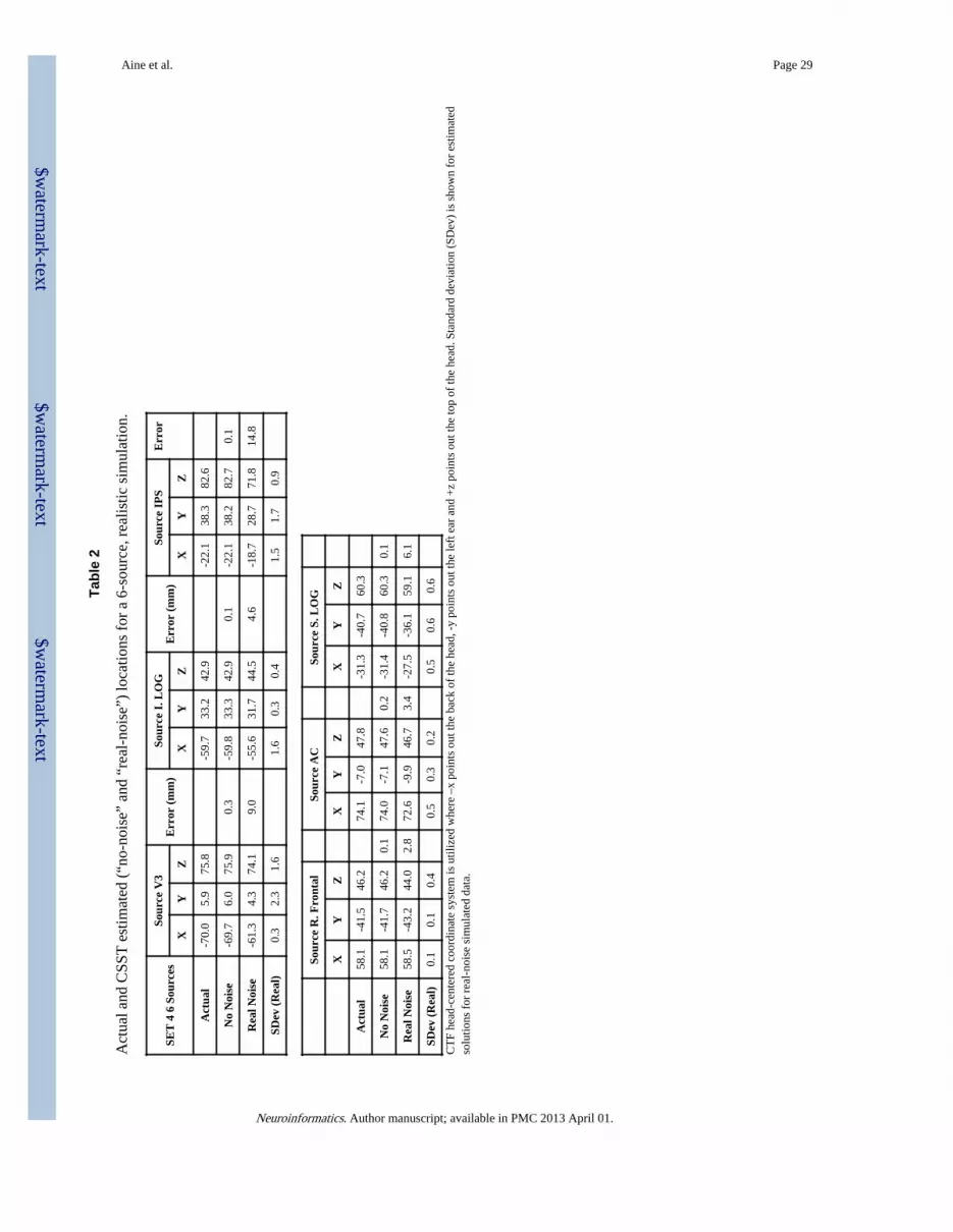
$waterm

ark-text$w

atermark-text

$waterm

ark-text

Aine et al. Page 29

Tabl

e 2

Act

ual a

nd C

SST

est

imat

ed (

“no-

nois

e” a

nd “

real

-noi

se”)

loca

tions

for

a 6

-sou

rce,

rea

listic

sim

ulat

ion.

SET

4 6

Sou

rces

Sour

ce V

3E

rror

(m

m)

Sour

ce I

. LO

GE

rror

(m

m)

Sour

ce I

PS

Err

or

XY

ZX

YZ

XY

Z

Act

ual

-70.

05.

975

.8-5

9.7

33.2

42.9

-22.

138

.382

.6

No

Noi

se-6

9.7

6.0

75.9

0.3

-59.

833

.342

.90.

1-2

2.1

38.2

82.7

0.1

Rea

l Noi

se-6

1.3

4.3

74.1

9.0

-55.

631

.744

.54.

6-1

8.7

28.7

71.8

14.8

SDev

(R

eal)

0.3

2.3

1.6

1.6

0.3

0.4

1.5

1.7

0.9

Sour

ce R

. Fro

ntal

Sour

ce A

CSo

urce

S. L

OG

XY

ZX

YZ

XY

Z

Act

ual

58.1

-41.

546

.274

.1-7

.047

.8-3

1.3

-40.

760

.3

No

Noi

se58

.1-4

1.7

46.2

0.1

74.0

-7.1

47.6

0.2

-31.

4-4

0.8

60.3

0.1

Rea

l Noi

se58

.5-4

3.2

44.0

2.8

72.6

-9.9

46.7

3.4

-27.

5-3

6.1

59.1

6.1

SDev

(R

eal)

0.1

0.1

0.4

0.5

0.3

0.2

0.5

0.6

0.6

CT

F he

ad-c

ente

red

coor

dina

te s

yste

m is

util

ized

whe

re –

x po

ints

out

the

back

of

the

head

, -y

poin

ts o

ut th

e le

ft e

ar a

nd +

z po

ints

out

the

top

of th

e he

ad. S

tand

ard

devi

atio

n (S

Dev

) is

sho

wn

for

estim

ated

solu

tions

for

rea

l-no

ise

sim

ulat

ed d

ata.

Neuroinformatics. Author manuscript; available in PMC 2013 April 01.

$waterm

ark-text$w

atermark-text

$waterm

ark-text

Aine et al. Page 30

Table 3

CSST results for 4 visual sources without oscillatory activity (top section) and with oscillatory activity(bottom section) for subject #1 (M545).

CTF Subj. M545

Source Loc. Error (mm) Lat. Error (ms) Amp. Error (nAm)

Single Trials (Set 7):

V1 1.5 6 2.5

I.LOG 9.4 4 3.2

IPS 3.7 3 7.9

DLPF 8.9 13 6.8

Single Trials with Oscillations (Set 8):

V1 4.7 6 9.8

I.LOG 9.7 1 4.8

IPS 7.0 1 11.2

DLPF 4.9 16 2.4

Neuroinformatics. Author manuscript; available in PMC 2013 April 01.

$waterm

ark-text$w

atermark-text

$waterm

ark-text

Aine et al. Page 31

Table 4

CSST results for subject #2 (M072) for both CTF and Neuromag systems. Location was considered “notfound” if it was ≥ 50.0 mm from the true source.

Source CTF Subj. M072 Neuromag Subj. M072

Single Trials & Oscillations: Loc. Error (mm) Loc. Error (mm)

V1 not found 9.9

I.LOG 7.5 3.7

IPS 4.2 2.8

DLPF 2.1 4.7

Neuroinformatics. Author manuscript; available in PMC 2013 April 01.