MERIDIONAL CIRCULATION IN SOLAR AND STELLAR CONVECTION ZONES

Draft version February 3, 2015Preprint typeset using LATEX style emulateapj v. 5/2/11

MERIDIONAL CIRCULATION IN SOLAR AND STELLAR CONVECTION ZONES

Nicholas A. FeatherstoneJILA, University of Colorado, Boulder, CO 80309-0440

Mark S. MieschHigh Altitude Observatory, National Center for Atmospheric Research, Boulder, CO, 80307-3000, USA: [email protected]

Draft version February 3, 2015

ABSTRACT

We present a series of 3-D nonlinear simulations of solar-like convection, carried out using theAnelastic Spherical Harmonic (ASH) code, that are designed to isolate those processes that drive andshape meridional circulations within stellar convection zones. These simulations have been constructedso as to span the transition between solar-like differential rotation (fast equator/slow poles) and “anti-solar’ differential rotation (slow equator/fast poles). Solar-like states of differential rotation, arisingwhen convection is rotationally constrained, are characterized by a very different convective Reynoldsstress than anti-solar regimes, wherein convection only weakly senses the Coriolis force. We find thatthe angular momentum transport by convective Reynolds stress plays a central role in establishingthe meridional flow profiles in these simulations. We find that the transition from single-celled tomulti-celled meridional circulation profiles in strong and weak regimes of rotational constraint islinked to a change in the convective Reynolds stress, a clear demonstration of gyroscopic pumping.Latitudinal thermal variations differ between these different regimes, with those in the solar-like regimeconspiring to suppress a single cell of meridional circulation, whereas the cool poles and warm equatorestablished in the anti-solar states tend to promote single-celled circulations. Though the convectiveangular momentum transport becomes radially inward at mid-latitudes in anti-solar regimes, it isthe meridional circulation that is primarily responsible for establishing a rapidly-rotating pole. Weconclude with a discussion of how these results relate to the Sun, and suggest that the Sun may lienear the transition between rapidly-rotating and slowly-rotating regimes.

1. INTRODUCTION

Mean (longitudinally-averaged) flows play an essentialrole in all recent models of the solar activity cycle. Differ-ential rotation (the mean zonal flow) generates toroidalfield from poloidal field and amplifies it, tapping the ki-netic energy of shear. This is the well-known Ω-effect andit is generally held responsible for the observed dispar-ity between the toroidal flux inferred from bipolar activeregions and the much smaller poloidal flux inferred fromhigh-latitude magnetograms.

The role of the mean meridional circulation (MC) inthe operation of the solar dynamo is more controversialbut potentially no less profound. As discussed in §2.1,mean-field dynamo models have shown that the ampli-tude and structure of the MC can have a substantialinfluence on cycle properties, and in particular, it maylargely regulate the cycle period.

Yet, despite the central role that mean flows play insolar and stellar dynamo models, their existence is oftentaken for granted. Most mean-field dynamo models pub-lished in the literature are kinematic in the sense thatthe velocity field is specified so the origin of mean flowslies outside the scope of the model. Non-kinematic mean-field models do exist but many take a heuristic approach,introducing parameterizations for convective momentumand energy transport that produce mean flows with pre-conceived amplitudes and profiles (e.g. Rempel 2006).

The utility of these kinematic and heuristic approaches

[email protected]

to dynamo modeling rests on the availability of suffi-cient observational data to constrain the mean flows thatare employed. However, this observational data is lim-ited. Global helioseismic inversions provide a reliablemeasure of the time-averaged angular velocity profileΩ(r, θ) throughout most of the solar convection zone (CZ,Thompson et al. 2003; Howe 2009), but as discussed in§2.2 relatively little is known about the MC. Even lessis known about mean flows in other stars (see §7). Yet,stars provide an invaluable test of dynamo models; anyviable model of the solar activity cycle must also accountfor cyclic magnetic activity in solar-like stars.

Without some theoretical guidance as to what merid-ional and zonal flows one should expect to find in solarand stellar convection zones, kinematic dynamo modelscannot completely account for observed patterns in solarand stellar magnetic activity. Furthermore, theoreticalguidance is needed to help motivate and interpret ongo-ing observational investigations of the solar meridionalcirculation (§2.2) which seek to probe more generally theinternal dynamics of the Sun and the origins of solarmagnetic activity.

In a previous paper, (Miesch et al. 2012, hereafter Pa-per 1), we sought such theoretical guidance based onlyon the observed structure of solar mean flows and ro-bust dynamical balances obtained from the fundamen-tal magnetohydrodynamic (MHD) equations. From thisalone we were able to identify gyroscopic pumping asthe principle physical mechanism that maintains the so-lar MC. This work is summarized in §2. However, fur-

arX

iv:1

501.

0650

1v1

[as

tro-

ph.S

R]

26

Jan

2015

mailto:[email protected]

2 Featherstone & Miesch

ther progress requires an understanding of turbulent so-lar convection and in particular the convective angularmomentum transport. To this end, in this paper, wehave initiated a series of global convection simulationsdesigned to elucidate the nature of convective transportin rotating, stratified, spherical shells and the mean flowsit produces. We focus here on solar-like stars with con-vective envelopes but similar dynamics are likely to occurin other types of stars with different convection zone ge-ometries.

In §2 we survey how this series of simulations fits withinthe context of previous theoretical and observationalwork and in §3 we discuss the motivation and method-ology behind how the numerical experiments were setup. We then present an overview of our results in §4,identifying two distinct dynamical regimes that exhibitqualitatively different mean flows. As in previous stud-ies (see §2.3), the dynamical regimes are distinguishedby the degree of rotational influence on the convection,as quantified by the Rossby number Ro = U/(2Ω0L),where U and L are characteristic convective velocity andlength scales and Ω0 is mean rotation rate. Fast rotatorsproduce solar-like Ω profiles (fast equator, slow poles)with multi-celled MC profiles while slow rotators pro-duce anti-solar Ω profiles (slow equator, fast poles) withsingle-celled MC profiles (poleward flow in the upper CZand equatorward in the lower CZ). We demonstrate thatthese slow and fast regimes can be achieved not only bychanging the rotation rate but also by changing the me-chanical and thermal dissipation, which in turn impactsthe buoyancy driving. In §5 we interpret the resultingMC profiles as a consequence of the changing nature ofthe convective Reynolds stress, within the context of gy-roscopic pumping. We address the establishment andsignificance of thermal gradients in §6.

Which regime is the Sun in? Since it has a solar-likeΩ profile by definition, one would expect it to be classi-fied as a rapid rotator. However, the situation is moresubtle than this. In §7 we demonstrate that the tran-sition between solar and anti-solar differential rotationis intimately linked to the MC and may be sensitive tothe complex dynamics occurring in the boundary layers,namely the tachocline and the near-surface shear layer.The Sun lies very close to this transition, which mayimply that it has somewhat atypical mean flow profiles.This in turn has important implications for solar dynamomodels and their application to other stars. These issuestoo are addressed in §7 and our principle results and con-clusions are summarized in §8.

2. THEORETICAL AND OBSERVATIONAL BACKGROUND

2.1. Meridional Circulation and the Solar Dynamo

The potential significance of the MC to the opera-tion of the solar dynamo is apparent from the observedevolution of the radial magnetic flux in the solar pho-tosphere. In particular, the cyclic polarity reversals ofpolar fields observed at the solar surface are often at-tributed to the poleward transport of the trailing mag-netic flux in emerging active regions due to the com-bined action of the meridional flow and turbulent dif-fusion (Sheeley 2005; Baumann et al. 2006; Schrijver &Liu 2008). Though the timing of the most recent northpolar reversal in 2012 challenges this paradigm (Shiota

et al. 2012), it is clear that the meridional flow plays animportant role in redistributing the magnetic flux thatthreads through the solar surface.

These observations and models of surface flux trans-port help to justify the prominent role that the MC playsin many recent dynamo models of the solar cycle. Thisrole is most dramatic in a class of models known as flux-transport (FT) dynamo models, in which the equator-ward advection of toroidal flux by the meridional flowin the CZ and tachocline accounts for the observed mi-gration of sunspots toward the equator over the courseof a cycle, known as the solar butterfly diagram (Wang& Sheeley 1991; Dikpati & Charbonneau 1999; Kukeret al. 2001; Dikpati & Gilman 2006; Yeates et al. 2008;Munoz-Jaramillo et al. 2009; Jouve & Brun 2007). Byregulating the solar butterfly diagram, the MC also reg-ulates the cycle period.

In a subset of flux-transport dynamo models that op-erate in the so-called advection-dominated regime, theMC plays another important role. In practice, most ex-isting advection-dominated flux-transport (FT) dynamomodels are also Babcock-Leighton (BL) dynamo modelsin which the main source of poloidal flux lies in the buoy-ant destabilization, emergence and subsequent dispersalof toroidal flux (Dikpati & Gilman 2009; Charbonneau2010). Mean-field parameterizations of the BL mecha-nism typically take the form of a poloidal source termconfined to the surface layers (Dikpati & Charbonneau1999; Rempel 2006; Munoz-Jaramillo et al. 2010, e.g.).Thus, in order for the dynamo to operate, there mustbe a coupling mechanism that transports magnetic fluxfrom the poloidal source region near the surface to theregion where the toroidal field is generated, which gener-ally lies in the lower CZ. In advection-dominated BL/FTdynamo models, this coupling mechanism is the MC.

Changes in the amplitude and structure of the merid-ional flow in FT dynamo models can have a dramaticeffect on the length and amplitude of magnetic cycles.Faster meridional flows or multiple cells in latitude canshorten the cycle period and influence the polar fieldstrength while slower flows can lengthen cycles and sup-press activity, potentially inducing a grand minimum(Dikpati & Charbonneau 1999; Jouve & Brun 2007;Schrijver & Liu 2008; Jiang et al. 2009; Karak 2010).Multiple cells in radius can have an even greater impact,disrupting the operation of the dynamo and potentiallyreversing the sense of the butterfly diagram (Jouve &Brun 2007).

The profound role of the MC in contemporary solardynamo models has motivated intense, ongoing observa-tional efforts to probe the meridional flow structure in thedeep CZ. However, this is a formidable challenge, largelybecause the flow is expected to be so weak; typical am-plitudes used in FT dynamo models are only 2-3 m s−1

near the base of the CZ. Thus, observational constraintsare currently limited but may improve with more data,as we now address.

2.2. Observational Context

One of the most notable triumphs of helioseismologyhas been the mapping of the internal solar rotation profileΩ as a function of radius r and colatitude θ (Thompsonet al. 2003; Howe 2009). These helioseismic rotation in-versions span most of the solar convection zone, though

Meridional Circulation in Stars 3

they become less reliable near the poles and in the deepinterior due both to the coarser resolution of the inver-sion kernels and the smaller amplitude of the intrinsicfrequency splitting near the rotation axis. They reveal amonotonic decrease of Ω by about 30% from equator topole that persists throughout most of the CZ, with lit-tle radial variation apart from two boundary layers nearthe bottom and top, known as the tachocline and thenear-surface shear layer respectively.

The most well-established result for the solar MC,meanwhile, is the existence of a systematic poleward flowof 10-20 m s−1 at the surface at latitudes below about ±50-60. However, different techniques often give differentresults as to the subsurface structure, the high-latitudestructure, and even the low-latitude amplitude. For ex-ample, measurements of the meridional flow based onthe correlation tracking of magnetic features generallygive somewhat lower flow speeds than those based onDoppler shifts and local helioseismic inversions (Ulrich2010). Dikpati et al. (2010b) attribute this difference tothe effects of turbulent diffusion. Much of the variation inamplitude estimates arises from the intrinsic variabilityof the flow itself, which is known to change with the solarcycle (Ulrich 2010; Basu & Antia 2010; Hathaway 2010;Hathaway & Rightmire 2011). However, these solar cy-cle variations can be understood as perturbations abouta persistent background circulation (poleward near thesurface at low-mid latitudes) that are induced by surfacemagnetism and its impact on radiative cooling. In thispaper we are interested only in the persistent backgroundcirculation so we disregard the solar cycle variations.

At higher latitudes the results are less clear. The recentDoppler analysis by Ulrich (2010) suggests the possiblepresence of a high-latitude counter-cell with equatorwardsurface flow at latitudes above about 60. This featureis most apparent near solar minimum and may be in-termittent. Indeed, Dikpati et al. (2010a) argue thatthe absence of such a high-latitude counter cell throughmuch of solar cycle 23 may account for the relativelydeep minimum of 2008-2009 and the delayed onset of so-lar cycle 24. However, evidence for such a high-latitudecounter-cell based on feature tracking and helioseismicinversions has so far been lacking, with the former sug-gesting that poleward flow may persist all the way to thepoles (Rightmire-Upton et al. 2012) and the latter beingthus far inconclusive (Zhao et al. 2012). Further insightinto this question should be possible in the coming yearswith the availability of longer time series from the Helio-seismic Magnetic Imager (HMI) on the Solar DynamicsObservatory (SDO), which has the higher spatial resolu-tion needed to minimize limb effects, and also with theadvent of future missions such as Solar Orbiter, whichwill have a high-latitude vantage point.

Of these three principle techniques for measuring themeridional flow (Doppler measurements, feature track-ing, and local helioseismic inversions), only helioseismicinversions and feature tracking can probe the meridionalflow below the surface. While the observational consen-sus is that there is a systematic poleward flow of about10-20 m s−1 at latitudes below about 60 in the near-surface layers of the Sun, the subsurface structure is morecontroversial. The first studies based on SOHO/MDIdata by Giles et al. (1997) suggested that the polewardflow extended down to at least 0.96R. Subsequent stud-

ies suggested that this poleward flow may extend signif-icantly deeper, spanning at least the upper half of theCZ (Braun & Fan 1998; Chou & Dai 2001). However,more recent observations and inversions based on longertime series, new analysis techniques, and new data fromHMI/SDO have begun to cast doubt on this conclusion.

Hathaway (2012b) argued based on surface featuretracking that the return equatorward flow required formass conservation may occur as shallow as 0.93R. In-ferring subsurface flows with feature tracking relies onthe hypothesis that larger horizontal scales in the pho-tosphere trace convective structures that extend deeperinto the CZ and may thus be advected by deeper meanflows (Hathaway 2012a). Hathaway (2012a,b) tests thishypothesis by comparing inferred zonal flows to helio-seismic rotational inversions and then applies it to inferthe meridional flow. Results suggest a flow reversal frompoleward to equatorward at a depth of roughly 50 Mm(r ∼ 0.93, where R is the solar radius). This is notablyshallow compared to earlier estimates obtained from lo-cal helioseismic inversions.

More recent helioseismic investigations, fueled by thehigh-quality data from HMI/SDO and by the availabilityof long time series from GONG and SOHO/MDI1, sug-gest that this picture may be changing. Time-distancehelioseismic inversions by Zhao et al. (2013), taking intoaccount systematic center-to-limb effects on the inver-sions, appear to support this conclusion, showing evi-dence for multiple reversals in the latitudinal flow com-ponent, the shallowest of which being 0.91 R (see alsoMitra-Kraev & Thompson 2007). However, such a shal-low reversal is not found in global inversions of low-orderoscillation modes where the meridional flow enters ashigher-order effect (Schad et al. 2012).

Given the high stakes from the perspective of solarand stellar dynamo theory, the current uncertainty withregard to the meridional flow structure in the deep con-vection zone, and the vibrancy and promise of ongoingobservational efforts, further theoretical insight is sorelyneeded. Here we seek such insight from convection sim-ulations, after a brief overview of the fundamental pro-cesses involved (§2).

2.3. Dynamical Models

As noted above, kinematic mean-field dynamo modelscannot provide any insight into the origin and structureof the MC. For this, dynamical models are required. Suchmodels must address the transport of energy and momen-tum by convection and the subsequent nonlinear feed-backs involving the MC, differential rotation, and ther-mal stratification (Miesch & Toomre 2009). This can bedone either explicitly through global 3-D convection sim-ulations or implicitly through non-kinematic mean-fieldmodels that include parameterizations for the turbulenttransport.

Global convection simulations have revealed two dis-tinct dynamical regimes characterized by qualitativelydifferent differential rotation (DR) profiles (Gilman 1976,1977; Glatzmaier & Gilman 1982; Aurnou et al. 2007;Brun & Palacios 2009; Matt et al. 2011; Gastine et al.

1 the Global Oscillations Network Group (GONG) and theMichelson Doppler Imager (MDI) on the Solar and HeliosphericObservatory (SOHO)


2013; Guerrero et al. 2013a; Gastine et al. 2014; Kapylaet al. 2014). At strong rotational influence Ro . 1the differential rotation is “solar-like” in the sense thatthe equator spins faster than the poles. In other words∆Ω ≡ Ωeq −Ωp > 0 where Ωeq is the equatorial rotationrate at the outer boundary of the domain, and Ωp is somemeasure of the rotation rate at high latitudes, polewardof 70. For the weakly rotating regime, Ro & 1, the dif-ferential rotation is referred to as “anti-solar”, meaning∆Ω < 0. The anti-solar regime has often been attributedto the tendency for the convection to conserve angularmomentum locally, spinning up as motions approach therotation axis (Gilman 1977; Aurnou et al. 2007).

Though these regimes can be achieved by varyingthe rotation rate Ω (or its non-dimensional equivalent),several studies have demonstrated that the transitionfrom solar to anti-solar differential rotation can also beachieved by keeping Ω (or its non-dimensional equiva-lent) fixed and changing the convective driving throughthe Rayleigh number (Gastine et al. 2014; Kapyla et al.2014). This tends to increase Ro by decreasing the con-vective turnover time L/U . In other words, convectivevelocity scales increase while length scales decrease. Nearthe solar/anti-solar transition, Gastine et al. (2014) andKapyla et al. (2014) also find that the DR exhibits bista-bility, with both solar and anti-solar regimes possible de-pending on initial conditions and hysteresis.

Many of these studies reported a qualitative change inthe MC profile in the two regimes (Matt et al. 2011; Guer-rero et al. 2013a; Gastine et al. 2013, 2014; Kapyla et al.2014). The anti-solar regime (Ro < 1) often exhibitsa single circulation cell per hemisphere, with polewardflow in the upper CZ and equatorward flow in the lowerCZ. Meanwhile, the solar regime (Ro > 1) often exhibitsmultiple cells in latitude and radius, aligned with therotation axis outside the tangent cylinder2.

Recent high-resolution models have also begun to cap-ture aspects of the solar near-surface shear layer (NSSL)wherein small-scale convection in the surface layers es-tablishes an inward Ω gradient (Guerrero et al. 2013b;Hotta et al. 2014). As suggested by Miesch & Hindman(2011), the NSSL in these simulations is established bya radially inward angular momentum transport, is main-tained by meridional Reynolds stress, and is intimatelylinked to a poleward meridional flow. This will be dis-cussed further in §7.2 below.

The solar and anti-solar regimes in global convectionsimulations stand in stark contrast to mean-field modelswhich typically produce solar-like DR profiles (e.g. Kukeret al. 2011; Kitchatinov 2012; Kitchatinov & Olemskoy2012). Anti-solar profiles generally only occur if thereis a strong, baroclinic, single-celled meridional flow in-duced by additional factors such as polar starspots ortidal forcing from a binary companion (Kitchatinov &Rudiger 2004; Rudiger & Kitchatinov 2007).

Mean-field models of solar-like stars generally exhibitsingle-celled MC profiles but their origin and structurevary depending on the modeling approach. One ap-proach is to seek steady-state solutions of the mean-field equations with heuristic or model-based prescrip-tions for the convective Reynolds stress and heat trans-

2 The tangent cylinder is a cylindrical surface parallel to therotation axis and tangent to the base of the CZ

port. In such models the MC profile is largely deter-mined by departures from thermal wind balance due tothe meridional Reynolds stress, which is typically mod-eled as a turbulent diffusion (Kitchatinov 2012; Dikpati2014). This can lead to nonlocal driving of the MC fromthe upper and lower boundary layers (Kitchatinov 2012)or to high-latitude counter-cells for steep density stratifi-cations (Dikpati 2014). However, in this case, the form ofthe MC profile is sensitive to the nature of the turbulentviscosity profile that is imposed. This alone breaks thedegeneracy of the thermal wind balance equation withrespect to the meridional flow (see §5.1 below).

When the full time-dependent mean-field equations aresolved, the driving of the meridional flow is fundamen-tally different. Here the MC profile is determined mainlyby the non-diffusive component of the convective angu-lar momentum transport, which is typically modeled bythe Λ-effect in the zonal momentum equation (Rempel2005, 2007). This is the process of gyroscopic pumpingthat will be described in detail in §5.1 and that is re-sponsible for the establishment of MC in our convectionsimulations, as demonstrated in §5.2.

3. DESCRIPTION OF NUMERICAL CONVECTIONEXPERIMENTS

We present a series of numerical experiments designedto examine solar-like convection and its resulting meanflows under conditions that span a range of rotationalconstraints and convective efficiency. We model the so-lar convection zone using the anelastic approximation(Gough 1969; Gilman & Glatzmaier 1980). Such anapproach is appropriate in deep stellar interiors whereplasma motions are subsonic and perturbations to ther-modynamic variables are small compared to their mean,horizontally averaged values. As thermodynamic per-turbations are small, thermodynamic variables are lin-earized about a spherically symmetric reference statewith density ρ, pressure P , temperature T . and specificentropy S. Fluctuations about this state are denoted asρ, P, T, and S. In the uniformly-rotating reference frameof the star, the anelastic equations under these assump-tions may be expressed as

∇ · (ρv) = 0, (1)

ρ

[Dv

Dt+ 2Ω0 × v

]= −∇P + ρg −∇ · D, (2)

and

ρTDS

Dt=∇ · [κρT∇S + κrρcp∇(T + T )]

+ 2ρν

[eijeij −

1

3(∇ · v)2

].

(3)

The velocity v expressed in spherical coordinates isv = (vr, vθ, vφ) relative to a frame rotating at constantangular velocity Ωo, g is the gravitational acceleration,and D is the viscous stress tensor given by

Dij = −2ρν

[eij −

1

3(∇ · v)δij

], (4)


where eij is the strain rate tensor. The kinematic viscos-ity is denoted by ν and the thermal diffusivity by κ. Theradiative diffusivity is indicated by κr, cp is the specificheat at constant pressure, and D/Dt is the advectivederivative. κr and cp remain constant in time.

This set of equations is closed by assuming the ther-modynamic fluctuations satisfy the linear relations

ρ

ρ=P

P− T

T=

P

γP− S

cp, (5)

assuming the ideal gas law

P = RρT , (6)

where R is the gas constant.We evolve the anelastic equations using the anelastic

spherical harmonic (ASH) code, details of which may befound in Clune et al. (1999) and Brun et al. (2004). ASHsolves the 3-D MHD equations in a rotating, sphericalshell using a pseudo-spectral approach. Spherical har-monics are employed in the horizontal dimension, and4th-order finite-differences in the radial direction. ASHemploys a poloidal/toroidal decomposition for the massflux vector to satisfy the divergence-free constraint of eq.1, with

ρv = ∇×∇× (Wer) +∇× (Zer). (7)

Here W and Z are the poloidal and toroidal stream-functions respectively, and are the quantities that areexplicitly evolved in time (as opposed to the individualcomponents of v). The unit vector in the radial directionis indicated by er.

The suite of convection zone models that we exam-ine are identical in all respects save for the diffusivitiesand the rotation rate. The reference state temperature,pressure, and functional form of κr are derived from aone-dimensional solar structure model (Brun et al. 2002).While the specific heat cp of the one-dimensional struc-ture model varies weakly throughout the solar convec-tion zone, we have adopted a constant value of cp, takenfrom the base of that model. This requires us to itera-tively solve for the reference state density ρ, using the 1-D model density as an initial guess, until a density profilethat satisfies both hydrostatic balance and our equationof state is reached. Our simulated convection zones spanfrom 0.72 R to 0.965 R, extending to 25 Mm belowthe solar surface, and encompassing roughly 3.5 densityscale heights. Convective perturbations about this refer-ence state remain small throughout the simulation, andthus we choose not to update the reference state, holdingit fixed throughout each calculation.

As the microscopic viscous and thermal diffusivitiesappropriate for plasma motions within the convectionzone are beyond the capabilities of current computationalmodels, our models should be viewed as large eddy sim-ulations. We adopt a radial profile for ν and κ with eachquantity diminishing in depth as ν ∼ ρ−1/2. Simulationsare thus more diffusive near the surface where we ex-pect the unresolved scales of convective motion to playa prominent role in the transport of heat and momen-tum. This formulation does not, however, capture anynon-dissipative behavior of the unresolved scales.

Impenetrable and stress free boundary conditions are

adopted for each simulation such that

vr =∂(vθ/r)

∂r=∂(vφ/r)

∂r= 0|r=rbot,rtop . (8)

The radial entropy gradient is forced to vanish at thelower boundary of the convection zone, and the entropyperturbations are forced to vanish at the upper boundary,with

∂S

∂r= 0|r=rbot , S = 0|r=rtop . (9)

Thus, there is no diffusive entropy flux across the lowerboundary. Heat is transported across this boundary bythe radiative heat flux instead, ∝ κr∇T , which drops tonear zero at the upper boundary (see Fig. 10 below). Thevanishing of the entropy gradient at the lower boundaryimplies that this is, by definition, the base of the CZ,with no overshoot region. The entropy gradient steepenstoward the top of the domain, where most of the convec-tive driving occurs. This will be discussed further in §6.With the value of entropy pinned at the upper boundary,the entropy gradient there is free to vary with time. Asthe simulation equilibrates, this gradient attains a sta-tistically steady value that is sufficient to expel one solarluminosity through the upper boundary via thermal dif-fusion.

A summary of our input parameter space for thosecases rotating at the solar rate of Ω=2.6×10−6 s−1 isprovided in Table 3. We vary the viscosities by a fac-tor of four and the thermal diffusivities by a factor oftwo for these simulations. The naming convention issuch that the letter denotes the level of thermal diffu-sion, with A corresponding to the highest thermal diffu-sivity of 3.2×1013 cm2 s−1 and C corresponding to thelowest level (1.6×1013 cm s−1). The numbers 0–3 indi-cate the level of viscous diffusion, with 0 correspondingto the lowest kinematic viscosity (2×1012 cm s−1), and3 corresponding to the highest value of 8×1012 cm s−1.Case B2, which lies in the center of our parameter space,serves as the point around which rotation rate is variedfor the results presented in §4. We have also provideda summary of the resulting energy balances, as well astheir relative ratios, for these cases in Table 2. There,we report on the globally-averaged (over the full spher-ical shell) convective kinetic energy density (CKE), theenergy associated with the differential rotation (DRKE),and the energy associated with the meridional circulation(MCKE). We define these as

CKE =1

2ρ[(vr − 〈vr〉)2 + (vθ − 〈vθ〉)2 + (vφ − 〈vφ〉)2

],

(10)

MCKE =1

2ρ[〈vr〉2 + 〈vθ〉2

], (11)

and

DRKE =1

2ρ[〈vφ〉2

], (12)

where the brackets denote averages over longitude.Each model discussed in this paper has been evolved

for several thousand days, with elapsed simulated timeranging from 7,000 days to 14,000 days depending onthe individual case. This corresponds to several hundred


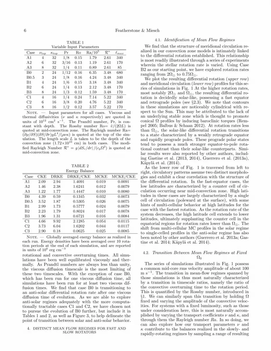
TABLE 1Variable Input Parameters

Case νtop κtop Pr Ro Ra/105 R∗ `max

A1 4 32 1/8 0.15 1.79 2.61 340A2 6 32 3/16 0.13 1.19 2.61 170A3 8 32 1/4 0.11 0.89 2.61 85

B0 2 24 1/12 0.16 6.35 3.48 680B0.5 3 24 1/8 0.16 4.24 3.48 340B1 4 24 1/6 0.15 3.18 3.48 340B2 6 24 1/4 0.13 2.12 3.48 170B3 8 24 1/3 0.12 1.59 3.48 170

C1 4 16 1/4 0.24 7.14 5.22 340C2 6 16 3/8 0.20 4.76 5.22 340C3 8 16 1/2 0.12 3.57 5.22 170

Note. — Input parameters for all cases. Viscous andthermal diffusivities (ν and κ respectively) are quoted inunits of 1012 cm2 s−1. The Prandtl number, Pr, is con-stant with depth. The Rossby number Ro= v/(2ΩL) isquoted at mid-convection zone. The Rayleigh number Ra=(∂ρ/∂S)(∂S/∂r)gL4/(ρνκ) is quoted at the top of the sim-ulation. The length scale L is taken to be the depth of theconvection zone (1.72×1010 cm) in both cases. The modi-fied Rayleigh Number R∗ = g |dSc/dr| /(cpΩ2) is quoted atmid-convection zone.

TABLE 2Energy Balance

Case CKE DRKE DRKE/CKE MCKE MCKE/CKE

A1 2.09 2.94 1.4091 0.019 0.0091A2 1.46 2.38 1.6241 0.012 0.0079A3 1.22 1.77 1.4447 0.010 0.0080

B0 4.39 0.59 0.1345 0.032 0.0073B0.5 3.52 1.87 0.5305 0.026 0.0075B1 2.99 1.73 0.5777 0.024 0.0079B2 2.23 1.79 0.8024 0.017 0.0078B3 1.96 1.31 0.6721 0.016 0.0084

C1 4.66 9.92 2.1285 0.054 0.0115C2 3.73 6.04 1.6202 0.044 0.0117C3 2.90 0.18 0.0625 0.025 0.0085

Note. — Globally averaged energy balance as realized ineach run. Energy densities have been averaged over 10 rota-tion periods at the end of each simulation, and are reportedin units of 106 erg cm−3

rotational and convective overturning times. All simu-lations have been well equilibrated viscously and ther-mally. As Prandtl numbers are always less than unity,the viscous diffusion timescale is the most limiting ofthese two timescales. With the exception of case B0,which has been run for one viscous diffusion time, allsimulations have been run for at least two viscous dif-fusion times. We find that case B0 is transitioning toan anti-solar differential rotation rate after one viscousdiffusion time of evolution. As we are able to exploreanti-solar regimes adequately with the more computa-tionally tractable cases C1 and C2, we have chosen notto pursue the evolution of B0 further, but include it inTables 1 and 2, as well as Figure 3, to help delineate thepoint of transition between solar and anti-solar behavior.

4. DISTINCT MEAN FLOW REGIMES FOR FAST ANDSLOW ROTATORS

4.1. Identification of Mean Flow Regimes

We find that the structure of meridional circulation re-alized in our convection zone models is intimately linkedto the differential rotation established. This relationshipis most readily illustrated through a series of experimentswherein the stellar rotation rate is varied. Using CaseB2 as our starting point, we have explored rotation ratesranging from 2Ω to 0.75Ω.

We plot the resulting differential rotation (upper row)and meridional circulation (lower row) profiles for this se-ries of simulations in Fig. 1 At the higher rotation rates,most notably 2Ω and Ω, the resulting differential ro-tation is decidedly solar-like, possessing a fast equatorand retrograde poles (see §2.3). We note that contoursin these simulations are noticeably cylindrical with re-spect to the Sun. This may be attributed to the lack ofan underlying stable zone which is thought to promoteconical Ω profiles by inducing baroclinic torques (Rem-pel 2005; Balbus & Schaan 2012). At rotation rates lessthan Ω, the solar-like differential rotation transitionsto a state characterized by a weakly retrograde equatorand rapidly prograde poles. These prograde polar statestend to possess a much stronger equator-to-pole rota-tional contrast than their solar-like counterparts. Simi-lar results were also reported by other authors, includ-ing Gastine et al. (2013, 2014), Guerrero et al. (2013a),Kapyla et al. (2014).

As the lower row of Fig. 1 is traversed from left toright, circulatory patterns assume two distinct morpholo-gies and exhibit a clear correlation with the structure ofthe differential rotation. In the fast-equator cases, thelow latitudes are characterized by a counter cell of cir-culation occurring near mid-convection zone. High lati-tudes in these cases are largely characterized by a singlecell of circulation (poleward at the surface), with somehints of multi-cellular behavior at high latitudes for thecase with the fastest rotation. As the rotation rate of thesystem decreases, the high latitude cell extends to lowerlatitudes, ultimately supplanting the counter cell in theequatorial regions for rotation rates lower than Ω. Theshift from multi-cellular MC profiles in the solar regimeto single-celled profiles in the anti-solar regime has alsobeen noted by other authors (Guerrero et al. 2013a; Gas-tine et al. 2014; Kapyla et al. 2014).

4.2. Transition Between Mean Flow Regimes at FixedΩ0

The series of simulations illustrated in Fig. 1 possessa common mid-core rms velocity amplitude of about 100m s−1. The transition in mean-flow regimes spanned bythose simulations is thus most naturally characterizedby a transition in timescale ratios, namely the ratio ofthe convective overturning time to the rotation period.This is quantified by the Rossby number, introduced in§1. We can similarly span this transition by holding Ωfixed and varying the amplitude of the convective veloc-ities. For systems with a fixed luminosity, such as thoseunder consideration here, this is most naturally accom-plished by varying the transport coefficients ν and κ, andthrough them the Rayleigh number Ra. In so doing, wecan also explore how our transport parameters ν andκ contribute to the balances realized in the slowly- andrapidly-rotating regimes by sampling a range of resulting


Fig. 1.— (a-e) Differential rotation profiles (Ω−Ωframe) for cases rotating at different fractions of the solar rotation rate Ω0 (indicated)achieved by spinning up and spinning down case B2, which rotates at the solar rate. Rotation rate decreases from left to right, and units areindicated in nHz. (f -j ) Meridional circulation profiles corresponding to each of the differential rotation profiles in the upper row. Red tonesdenote counter-clockwise motion, and blue tones, clockwise. Profiles have been averaged in time over roughly 200 days in each instance. Asthe Sun is spun down, the polar regions develop prograde rotation, and the equatorial regions retrograde. Similarly, multi-cellular profilesof meridional circulation transition into single-celled profiles at low rotation rates.

Reynolds numbers.Others have shown that the transition between the so-

lar and anti-solar rotation regimes can be achieved by fix-ing the rotation rate and changing the convective drivingby varying the Rayleigh number (Gilman 1977; Aurnouet al. 2007; Guerrero et al. 2013a; Gastine et al. 2014;Kapyla et al. 2014). The key parameter in determin-ing the transition is the Rossby number. However, sincethis is an output of the simulation rather than an input,the transition is often described in terms of the modifiedRayleigh number R∗ (see Table 3), which is a measureof the relative strengths the buoyancy and Coriolis force(Gastine et al. 2013). The simulations presented in thissection will be used in sections 5 to explore the structureand origin of the meridional circulation, a topic that hasreceived less attention in previous studies. While ourdemonstration of the solar/anti-solar transition is itselfnot new, we find it useful to revisit some aspects of thistransition as they also bear on the resulting meridionalcirculation.

It is worth mentioning that the Rayleigh number insystems such as these, where entropy is held fixed at oneboundary, and the entropy gradient fixed at the other,possesses an implicit dependence on κ not found in clas-sical Rayleigh-Benard convection (RBC). The entropy

contrast in models such as ours, analogous to the temper-ature contrast in RBC systems, is not held fixed, but isan output quantity, much as the Reynolds number. Thisentropy contrast is built entirely in the upper boundarylayer, resulting from the entropy gradient realized thereand the width of that boundary layer. Convective driv-ing is thus accomplished primarily in the upper boundarylayers of these systems, a situation more analogous to theSun than RBC flow where driving occurs at the upperand lower boundaries.

While entropy is fixed at the top, the entropy gradientis implicitly determined by the solar luminosity, beingforced to satisfy, in a time-averaged sense, the relation

ρT κ∂s

∂r|r=rtop =

L4πr2top

. (13)

We thus choose to define the our Rayleigh numbers using∂s/∂r at the upper boundary because this quantity is awell-defined simulation input. The consequence is thatour Rayleigh number now varies as κ−2 instead of themore traditional κ−1.

The variation of differential rotation for each case isillustrated in Fig. 2. There, profiles of angular velocity,averaged over several overturning times, are laid out ina grid, with κ increasing along the vertical axis and ν


Fig. 2.— Differential rotation profiles (Ω−Ω) for the a,b, and c series of simulations. Case names are indicated and are arranged suchthat viscosity ν increases from left to right, and thermal diffusivity κ increases from bottom to top. The most laminar case (A3) appearsin the upper right, and the most turbulent case (C1) appears in the lower left. Profiles have been averaged in time over roughly 200 daysin each instance. A clear transition between solar-like and anti-solar rotation occurs between the middle and bottom rows (i.e. betweenthe B and C series cases.)

increasing along the horizontal axis. The upper row iscomprised by simulations from Series A, and the lowerrow by Series C simulations. Convection models from Se-ries A and B each exhibit solar-like differential rotation,whereas series C tends to exhibit anti-solar rotation, withcase C3 (lower right) possibly representing a transitionpoint between the fast equator and fast pole regimes.Variation of the differential rotation with ν is present,but the effect is greatly reduced with respect to that ofκ. This can be attributed to the ν−1κ−2 scaling of the

Rayleigh number noted above.As noted above, the key parameter in determining the

transition between mean flow regimes is the Rossby num-ber Ro. Fig. 3 shows the relative differential rotation,∆Ω/Ω0 = (Ωeq−Ωpole)/Ω0, in all simulations versus Ro,exhibiting a clear transition at Ro ∼ 0.17. This transi-tional value is lower than the Ro ∼ 1 value quoted inprevious papers (e.g. Gastine et al. 2013, 2014). We at-tribute this discrepancy to the ambiguity in defining Ro.Here we use the depth of the CZ as the length scale L


0.10 0.15 0.20 0.25

Ro

-1.5

-1.0

-0.5

0.0

0.5

∆Ω

/Ω

Fig. 3.— Pole-to-equator differential rotation contrast ∆Ω/Ω asa function of Rossby number Ro for the A−C series of simulations.Transitional case B0.5 is indicated with a hollow diamond. Theslightly more turbulent case B0, which is transitioning to an anti-solar state, is indicated by the red triangle. Ro was computed atmid-convection zone in all cases. Equatorial and polar rotationrates were calculated by averaging zonal velocity in both longitudeand depth, and then over a latitude range of 0N-20N latitudeand 70N-90N respectively. Anti-solar cases tend to arise whenRo is greater than about 0.163.

and the rms value of the non-axisymmetric velocity inthe mid-CZ v′rms as the velocity scale U . By contrast,(Gastine et al. 2014) use the volume-averaged value ofv′rms for U and a value of L based on the peak of thekinetic energy spectrum. This tends to shift U higherand L lower, resulting in a larger value of Ro. We referthe reader to (Gastine et al. 2014) for a discussion of howthe transitional value of Ro depends on precisely how Rois defined.

The meridional circulation profiles corresponding tothe simulations shown in Fig. 2 are shown in Fig. 4. Theyexhibit a correlation with the differential rotation similarto that discussed in §4.1. Single-celled profiles of circula-tion appear in all of the C-series cases (i.e. those systemswith fast poles), while those of the A-B series are multi-cellular in the equatorial regions.

Convection in the solar and anti-solar regimes exhibitsnoticeably different morphologies as well. Fig. 5 il-lustrates the radial velocities in the upper and mid-convection zones of case C1 (a,c) and case A3 (b,d). CaseC1, which possess a anti-solar-like differential rotation,also exhibits velocity amplitudes that are roughly twicethat of A3. Elongated convective cells in the equatorialregions tend to tilt in the negative φ-direction for caseC1. In addition to lower velocity amplitudes, Case A3possesses much more prominent columnar structuring ofits convection, with a tilting evident in the positive φ-direction.

An additional effect is evident when comparing theflows of case A3 to those of case C1, namely that the con-vection exhibits a much broader range of spatial scales.Case C3 is thus both more turbulent and more stronglydriven.

4.3. A Transitional Regime

One might ask if the transition in mean-flow regimesis purely a result of rotational constraint, or if the levelof turbulence might also play some role. In particular,by admitting much smaller spatial scales into the sim-ulation, are the correlations of vr and vφ necessary toestablish a fast equator being disrupted? In other words,might the Reynolds number Re = UL/ν play a role inaddition to the Rayleigh number? In order to explorethese questions we have extended the simulations of Fig.2 to include the case B0.5. This case possesses a κ identi-cal to the other B-series cases, but a ν that is lower thanany of of the C-series. Case B0.5 was initiated by lower-ing the diffusivity in the mature case B1, which had itselfbeen evolved for a total of two viscous diffusion times.

An overview of the flows in Case B0.5 is shown in Fig.6. The convective patterns are small-scale in nature, likeC3, but do not exhibit the retrograde tilting character-istic of the patterns in this case. Case B0.5 possessesa decidedly solar-like differential rotation, but, surpris-ingly, seems to exhibit a single circulation cell withineach hemisphere. Moreover, the flow amplitudes indi-cated near the surface are similar to those of case C3,as are the mid-convection zone velocities (not shown).Case B0.5 does possess a somewhat lower Rayleigh num-ber, and a different Prandtl number than case C3, how-ever, and so the differences between these two cases arelikely to be subtle ones. It would seem that case B0.5 isjust straddling the transition between the solar-like andanti-solar regimes of differential rotation.

Gastine et al. (2014) and Kapyla et al. (2014) haverecently shown that the behavior of the differential ro-tation near the solar/anti-solar transition can depend onthe history of the simulation, representing a type of hys-teresis. For a given transitional Ro, the simulation mayexhibit either solar or anti-solar DR. Though we have ob-served unusual mean flows near the transition with caseB0.5, we have not searched explicitly for this bistabilityand hysteresis. It is possible that case B0.5 itself is slowlyundergoing a transition from solar-like to anti-solar dif-ferential rotation. However, this case has been run for18,000 days, about a factor of four longer than the timescale for viscous diffusion across the convection zone, andwe see no signs yet that it is undergoing such a transi-tion. The globally-averaged energy densities associatedwith the differential rotation (DRKE) and meridional cir-culation (MCKE) for case B0.5 are shown in Fig. 7. Themean flows have varied by as much as 30% over this in-terval, but with no apparent long-term trends. We willdiscuss the significance of case B0.5 further in §7.

5. MAINTENANCE OF MEAN FLOWS

In this section we argue that the distinct mean flowregimes described in §4 arise from a change in the natureof the convective angular momentum transport. Further-more, we argue that it is the convective angular momen-tum transport that largely determines the mean merid-ional flow profiles in simulations as well as stars.

5.1. Dynamical Balances and Gyroscopic Pumping

In an anelastic (low Mach number) system, the massflux ρv is divergenceless and the time evolution of themean meridional flow ρ 〈vm〉 is governed by the zonalvorticity equation, which may be written as (Miesch &


Fig. 4.— Contours of meridional circulation streamlines, with streamfunction underlay, for cases in the A-C series as indicated withineach panel. The layout and time averaging are as in Fig. 2. Red tones denote counter-clockwise flow, and blue tones clockwise. As withcases where the rotation rate is varied, multi-cellular circulations arise whenever solar-like differential rotation profiles are present.

Hindman 2011, hereafter MH11)

∂

∂t〈ωφ〉 = λ

∂Ω2

∂z− g

rCP

∂ 〈S〉∂θ

+ . . . , (14)

where ωφ = (∇×vm)·φ is the zonal component of themean vorticity, λ = r sin θ and z = r cos θ are the radialand axial coordinates in a (rotating) cylindrical coordi-nate system, and Ω = Ω0 + λ−1 〈vφ〉 is the total angu-lar velocity, including uniform and differential rotationcomponents. We have adopted the convention that asubscript m on a vector denotes the radial r and latitu-

dinal θ components of a vector. We have focused hereon the two dominant contributors to the meridional forc-ing, namely the inertia of the differential rotation andthe baroclinicity of the mean stratification, which makeup the first and second terms on the right-hand-side of(14) respectively. These are sufficient to illustrate theessential dynamics. We have neglected the meridionalcomponents of the Reynolds stress (〈ρv′mv′m〉; primesdenote fluctuations about the longitudinal mean), thebaroclinicity of thermal fluctuations, the viscous stress,and quadratic terms in vm. All of these are thought tobe negligible in simulations and stars. We have also ne-


a

-/+ 85

b

-/+ 45

c

-/+ 150

d

-/+ 85

- +

Fig. 5.— Radial velocity at one instant in time following equilibration for cases C1 (left column) and A3 (right column). The upper andlower rows correspond to radial velocity near the surface and in the mid CZ respectively. Convective cells in the solar-like case A3 exhibita prograde tilt in the φ-direction. Those in anti-solar case C1 are tilted in the opposite sense. The limits of the color table normalizationare indicated adjacent to each image, with units provided in m s−1.

glected the Lorentz force, which is less justified in starsbut appropriate here since the simulations we considerare non-magnetic. Full expressions are given in MH11(see also Kitchatinov & Rudiger 1995; Rempel 2005).

In a steady state eq. (14) gives the familiar thermalwind balance (TWB) equation (Kitchatinov & Rudiger1995; Elliott et al. 2000; Robinson & Chan 2001; Brun &Toomre 2002; Rempel 2005; Miesch et al. 2006; Balbuset al. 2009; Brun et al. 2010)

∂Ω2

∂z=

g

λrCP

∂ 〈S〉∂θ

. (15)

Here the two dominant meridional forcing terms bal-ance, and latitudinal thermal gradients can sustain non-cylindrical rotation profiles as in the Sun (∂Ω/∂z 6= 0).

It is important to note that in a steady state the merid-ional flow itself drops out of equation (15). Thus, it can-not be used to determine the MC profile even if otherquantities such as Ω and S are known. This ceases tobe the case if other terms are included in the balance,most notably the meridional components of the Reynoldsstress. In mean field theory, this term is often representedas a turbulent diffusion. In short, inclusion of a turbu-lent diffusion term breaks the degeneracy of eq. (15) withrespect to the meridional flow and can largely determinethe MC profile that is achieved in many mean-field mod-els (Kuker et al. 2011; Kitchatinov 2012; Dikpati 2014).However, such solutions are sensitive to the nature ofthe imposed parameterizations, such as the depth de-pendence of the turbulent viscosity and departures fromTWB in the upper and lower boundary layers, where vis-

cous stresses can ultimately determine the global struc-ture and amplitude of the flow.

There is an alternative way to break the degeneracy ofeq. (15) that provides a better explanation for how theMC is established in our 3-D, time-dependent convec-tion simulations. The mechanism is known as gyroscopicpumping and can be illustrated by considering the zonalforce balance which can be expressed as (MH11)

ρ 〈vm〉 ·∇L = F ≈ −∇·FRS , (16)

where L = λ2Ω is the specific angular momentum, F isthe net axial torque given by

F = −∇·[ρλ⟨v′mv

′φ

⟩− ρνλ2∇Ω

]= −∇· [FRS + FV D] ,

(17)and FRS is the convective transport of angular momen-tum, given by

FRS = ρλ⟨v′mv

′φ

⟩. (18)

In stars and in recent high-resolution convection simula-tions such as those presented here, the Reynolds stresscomponent FRS generally dominates over the viscouscomponent FV D. The dynamical balances (15) and (16)should be regarded as temporal averages as well as lon-gitudinal averages, concerning the persistent mean flowsthat exist amid stochastic fluctuations.

In convection simulations and in helioseismic inver-sions, ∇L is oriented away from the rotation axis, parallelto the cylindrical radius ∇λ (MH11). Thus, a conver-gence of the convective angular momentum flux (F > 0)will induce a meridional flow 〈vm〉 directed away from


a

-65 m s-1

65 m s-1

-40 nHz

40 nHz

b

CW

CCW

c

Fig. 6.— Sampling of flows for transitional case B0.5. (a) Radialvelocity snapshot near the upper boundary, Upflows are indicatedin yellow, downflows in blue. (b) Accompanying differential ro-tation (Ω − Ω), time-averaged over 1800 days at the end of thesimulation, with prograde rotation shown in red, and retrograderotation in blue. (c) Meridional circulation streamlines for thesame time period. Clockwise flow is indicated by blue underlay,and counter-clock wise flow by red underlay. This case demon-strates a prograde rotating equator in the absence of multi-cellularmeridional circulations within each hemisphere.

the rotation axis and a divergence (F < 0) will induce aflow toward the rotation axis. This is the phenomenonof gyroscopic pumping as discussed in a solar context byMH11 (see also Haynes et al. 1991; McIntyre 1998, 2007;Garaud & Arreguin 2009; Garaud & Bodenheimer 2010;Miesch et al. 2012).

Gyroscopic pumping is mediated by the axial compo-nent of the rotational shear ∂Ω/∂z, but it can be sus-tained even if the steady-state rotation profile is strictlycylindrical; for an analytic illustration, see Appx. B ofMH11. Indeed, this is also demonstrated in the simu-lations presented here; many exhibit Ω profiles that arenearly cylindrical yet sustain persistent, well-establishedmeridional flow profiles (e.g. Fig. 1). Intuitively, one canattribute this to the efficiency and robustness of Taylor-Proudman balance; in the barotropic limit (∂ 〈S〉 /∂θ =0) any axial variation of the net torque (∂F/∂z 6= 0)will induce a transient axial shear (∂Ω/∂z 6= 0) that

will almost immediately3 be wiped out by an inducedmeridional flow, via equation (14). In this way, a steadymeridional flow can be maintained that continually re-plenishes angular momentum extracted or imparted bythe net torque F by advecting angular momentum acrosslocal L isosurfaces as expressed by eq. (16).

Eq. (16) predicts a direct link between the meridionalflow profile and the angular momentum transport by theconvective Reynolds stress. This link is strongest for thelow-Rossby number limit in which the uniform rotationcomponent of Ω dominates L. In this limit we have

Ψ(λ, z) =1

2λΩ0

∫ z

zb

F(λ, z′) dz′ , (19)

where zb = (R2−λ2)1/2 (MH11) and Ψ is the cylindricalmass flux streamfunction, defined by

〈ρvλ〉 =∂Ψ

∂z, 〈ρvz〉 = − 1

λ

∂

∂λ(λΨ) . (20)

Recall that λ is the cylindrical radius (λ = r sin θ). Notethat Ψ is related to the mass flux streamfunction W asfollows

Ψ =1

r

∂ 〈W 〉∂θ

. (21)

In summary, there are two competing mechanisms forbreaking the degeneracy of (15) and establishing thesteady-state MC; we will refer to them as the meridionalReynolds stress (RS) and gyroscopic pumping. Both relyon the RS tensor Rij = ρ

⟨v′iv′j

⟩. However, the first

mechanism relies on the meridional components of R(Rrr, Rθr, Rφr, Rrθ, Rθθ, Rφθ), whereas the secondrelies on the zonal components (Rrφ, Rθφ, Rφφ). Inthe next section we will demonstrate that it is this lat-ter mechanism, namely gyroscopic pumping, that deter-mines the MC profiles in our convection simulations.

However, before proceeding, we first elaborate on thesetwo mechanisms within the context of mean-field mod-els. In our convection simulations we capture all of theRS components explicitly so both of these mechanismsoccur naturally. Both mechanisms may also be capturedin mean-field models by parameterizing the RS basedon convection simulations as presented here or on alter-native phenomenological arguments or turbulence mod-els. As mentioned above, the meridional RS mechanismmay be captured by solving the steady-state zonal vortic-ity equation (Kuker et al. 2011; Kitchatinov 2012; Dik-pati 2014). However, in order to capture the gyroscopicpumping mechanism it is essential to include the zonalmomentum equation and to follow the time-dependentapproach to the steady state Rempel (2006).

Though both mechanisms can and have been realizedin mean-field models, the gyroscopic pumping mecha-nism is less sensitive to imposed mean-field parameteri-zations. There are two reasons for this. First, the merid-ional MC mechanism relies on second-order departuresfrom the primary meridional force balance, which in thebulk of the convection zone is TWB, eq. (15). By con-trast, the zonal RS enters into the lowest-order zonalforce balance, eq. (16). The second reason is that the

3 on a timescale τ ∼ (2Ω)−1 ∼ Prot/(4π), where Prot is therotation period. For the Sun this is about 2.2 days.


0 5 10 15 180Time (103 Days)

5.0•105

1.0•106

1.5•106

2.0•106

En

erg

y D

en

sity (

erg

/cm

3)

DRKE

MCKE

Fig. 7.— Evolution of mean-flow energy densities for transitional case B0.5. The energy in the differential rotation (DRKE) is depictedin black, and that of the meridional circulation (MCKE) in red. DRKE exhibits large (roughly 30%) variations with respect to the meanover this interval, but no long-term trends are evident.

meridional MC mechanism is sensitive to the functionalform of the RS parameterization, R(Ψ,Ω). Thus, im-plementing results from a convection simulation wouldrequire parameterizing the computed RS tensor. How-ever, in the gyroscopic pumping mechanism one mustonly know the axial torque F . This may in principle bedecoupled from the mean flows without the need for anyexplicit parameterizations. The zonal components of theRS do likely depend on the amplitude of the differen-tial rotation, however, and a realistic mean-field modelshould take this into account.

5.2. Convective Angular Momentum Transport

In §5.1 we argued that the meridional flow profiles inour simulations are largely maintained by the convectiveangular momentum transport FRS through the mecha-nism of gyroscopic pumping. In this section we assessthis argument and its implications by exploring the de-tailed nature of FRS and how it relates to the meridionalflow profiles we find in the simulations.

In our discussion, we find it instructive to introduce aHelmholtz decomposition of the convective angular mo-mentum transport FRS as follows:

FRS = ∇χ+∇×(

Λφ)

. (22)

Such a decomposition is valid for any arbitrary two-dimensional (axisymmetric) vector. Its utility is appar-ent when we see that only the first term contributes tothe gyroscopic pumping equation (16). More generally,only the divergent component of the angular momentumflux can contribute to the time evolution of Ω, and thusthe mean flow profiles that are ultimately achieved. Onecan derive the transport potential χ from FRS by takingthe divergence of (22) and solving a Poisson equation:

∇2χ =∇·FRS . (23)

Figure 8 demonstrates the nature of the convective an-gular momentum transport in two representative cases,chosen to illustrate the low and high Rossby numberregimes (upper and lower rows respectively). The trans-port potential χ is illustrated in the left column (framesa, f ). This is derived from the divergence of the convec-tive angular momentum transport shown in frames (b, g)via eq. (23) and helps to elucidate its origin.

In the slowly-rotating regime the angular momentumtransport at mid latitudes is radially inward. This can

be seen from the nearly horizontal orientation of the χcontours in Fig. 8f, increasing from top to bottom (ra-dially inward ∇χ). Since the radial component of FRSvanishes at the (impermeable) top and bottom bound-aries, this implies a divergence of the convective angularmomentum transport in the upper CZ and a convergencein the lower CZ, as seen in the red and blue layers of Fig.8g.

At low latitudes, ∇χ turns equatorward (Fig. 8f ), pro-ducing a convergence of FRS at the equator (Fig. 8g).Though this convergence of the convective angular mo-mentum flux at the equator tends to establish a solar-like differential rotation, it does not succeed in doing so.Rather, it is offset by the radially outward transport ofangular momentum by the induced meridional flow (Fig.8j ). This induced meridional flow, together with theradially inward angular momentum transport at higherlatitudes is responsible for the anti-solar differential ro-tation profile that is ultimately achieved. We discuss thisissue further in §5.3.

This scenario emphasizes the subtle nonlinear, non-local nature of the dynamical balances discussed in §5.1.The convective angular momentum transport FRS is es-sential for establishing the differential rotation ∇Ω butit does not uniquely determine the resulting Ω profile.Rather, FRS induces a meridional flow (mediated by theCoriolis force) that plays an essential role in establishingthe differential rotation.

The role of the convective angular momentum trans-port in establishing the meridional circulation is illus-trated in Fig. 8h. As expressed by eq. (16), a convergenceof FRS (blue) induces a flow away from the rotation axis(white arrows) and a divergence of FRS (red) induces aflow toward the rotation axis (black arrows). Mass con-servation then requires these flows to form closed circula-tion cells, as reflected by the actual meridional flow pat-tern shown in Fig. 8i. Due to the nature of FRS (whichcan ultimately be traced to the χ profile in Fig. 8f ), theinduced meridional flow has a single-celled nature, dom-inated by one large cell in each hemisphere that extendsfrom the equator to a latitude of at least 70 and spansthe entire CZ. These cells exhibit poleward flow in theupper CZ and equatorward flow in the lower CZ. The ad-vection of angular momentum by this induced flow nearlybalances the convective angular momentum transport asexpressed by eq. (16). This can be seen by comparingFigs. 8g and 8j. Small imbalances are due to viscous


Fig. 8.— Maintenance of meridional flow. Illustrative examples are shown for the rapidly-rotating regime (upper row, case C1) and theslowly-rotating regime (lower row, case A3). (a, f ) Transport potential χ, increasing from -1026 g cm s−2 (blue) to 1026 g cm s−2 (red).(b, g) Divergence of the convective angular momentum transport, ranging from -107 g cm−1 s−2 (blue) to 107 g cm−1 s−2 (red). (c, h)same as frames (b, g) but with arrows indicating the direction of the induced meridional flows. Slanted lines in the northern hemispheredelineate high and low-latitude regimes. (d, i) Meridional flow shown as streamlines of the mass flux Ψ. Red denotes clockwise flow (Ψ > 0)and blue denotes counter-clockwise flow (Ψ < 0). Values of Ψ range from ±4× 1011 g cm−1 s−1 in (d) and ±9× 1010 g cm−1 s−1 in (i).(e, j ) Angular momentum transport by the meridional flow which approximately balances the Reynolds stress divergence in frames (b, g),as expressed in eq. (16). Color table as in frames (b, g).

torques [eq. (17)] and unsteady fluctuations.Similar arguments hold for the rapidly-rotating regime

in the upper row of Fig. (8). Here the χ contours at highlatitudes are again nearly horizontal, signifying a radiallyinward angular momentum transport. However, outsidethe tangent cylinder, the angular momentum transport iscylindrically outward, away from the rotation axis. Thisis reflected by the cylindrical nature of the χ contoursat low latitudes. There is also an equatorward contribu-tion to ∇χ, particularly at mid-latitudes near the outerboundary. This χ profile produces a Reynolds stress di-vergence pattern that reverses sense at high and low lat-itudes, as seen in the red and blue regions of Fig.8b. Athigh latitudes the pattern is similar to the high-Ro case,with a divergence and convergence in the upper and lowerCZ respectively. At low latitudes this reverses, exhibit-ing a convergence in the upper CZ and a divergence inthe lower.

The implications of this χ profile for the meridionalcirculation are profound. Inside the tangent cylinder, asingle cell is established much like the high-Ro case (Figs.

8h,i). However, outside the tangent cylinder, a multi-cell profile is induced with 2-3 distinct cells spanningthe CZ (Fig. 8d). This can be attributed largely to thecylindrically-outward angular momentum transport nearthe equator which induces upward and downward flowin the upper and lower CZ respectively (Figs. 8c). Asin the high-Ro regime, the advective angular momentumtransport by this induced meridional flow largely bal-ances the convective angular momentum transport (Figs.8b,e), with small departures primarily due to the contri-bution of viscous diffusion to the zonal force balance.

The dramatic difference between the convective angu-lar momentum transport at high and low latitudes canbe appreciated by considering the structure of the con-vective flow and how it is influenced by rotation. At highlatitudes, convection is dominated by a quasi-isotropic,interconnected network of downflow lanes near the sur-face that break up into more isolated lanes and plumesdeeper down (Fig. 5). As these downflows travel down-ward, the Coriolis force deflects them in a prograde direc-tion, inducing a negative correlation between v′r and v′φ


that produces an inward angular momentum transport(FRS).

At low latitudes, outside the tangent cylinder, the pre-ferred convection modes for low Ro are banana cells,columnar convective rolls that are aligned with the rota-tion axis near the equator (e.g., Miesch 2005). In simula-tions with large density stratification and moderate val-ues of Ro, these banana cells are manifested as a promi-nent north-south alignment of downflow lanes near theequator that often trail off eastward at higher latitudeswhere they are distorted by the differential rotation (Fig.5b; see also Miesch et al. 2008).

In their simplest manifestation at low Ro and moder-ate density stratification, banana cells are approximatelyaligned with the rotation axis with little variation in theaxial (z) direction. The combined action of the sphericalgeometry, the density stratification, and positive nonlin-ear feedback from the differential rotation they establish,tends to produce a systematic tilt such that cylindri-cally outward flows (vλ > 0, where λ is the cylindricalradius) are deflected westward and cylindrically inwardflows (vλ < 0) eastward (Busse 2002; Aurnou et al. 2007).

This establishes a negative⟨v′λv′φ

⟩correlation that is re-

sponsible for the cylindrical orientation of the χ contoursat low latitudes in Fig. 8a (i.e. the cylindrically outwardangular momentum transport). The effects of densitystratification, the outer spherical boundary, and moder-ate (but still low) Ro tend to cause banana cells to bendaway from the z axis toward a more horizontal orienta-tion, with axes more parallel the θ dimension. This tends

to establish positive⟨v′θv′φ

⟩correlations (in the northern

hemisphere, negative in the southern) that transport an-gular momentum equatorward (Gilman 1983; Glatzmaier1984; Miesch 2005).

Thus, banana cells can account for both the cylindri-cally outward angular momentum transport at low lat-itudes in the low-Ro regime (Fig. 8a) and the equator-ward angular momentum transport at low latitudes inthe high-Ro regime (Fig. 8f ). Though the region out-side the tangent cylinder contains the banana cells, aclose look at Fig. 8a indicates that this region does notstrictly delineate the transition between the high andlow-latitude regimes for the angular momentum trans-port. Rather, the region of inward transport at highlatitudes shifts equatorward with increasing Ro, as in-dicated schematically with the solid black lines at midlatitudes in Figs. 8c and 8h.

This equatorward shift of the transition between highand low-latitude behavior can be understood by consid-ering a downflow plume spawned from the upper bound-ary layer. Though such a plume is subject to a range offorces including pressure gradients, buoyancy, nonlinearadvection and viscous diffusion, it is instructive to con-sider a ballistic trajectory subject only to the Coriolisforce. Then a downflow plume with initial velocity −vprwill be deflected in a prograde direction with an initialradius of curvature given by

rc =

∣∣∣∣∣ v2p∂vφ/∂t

∣∣∣∣∣ =vp

2Ω0 sin θ. (24)

The value of rc relative to D, the depth of the CZ, is a

measure of the local, latitude-dependent Rossby numberexperienced by a downflow plume:

Rθ =rcD

=vp

2Ω0D sin θ. (25)

Intuitively, eq. (25) can be interpreted based on whetheror not a downflow plume on a ballistic trajectory will tra-verse the CZ before being deflected by the Coriolis force.If Rθ >> 1 then the plume could in principle (in the ab-sence of other forces) reach the base of the CZ with onlya small prograde (positive φ) deflection. This Coriolis-induced deflection reflects the tendency for the plumeto conserve its angular momentum conservation and it

is responsible for the negative⟨v′rv′φ

⟩correlation that

transports angular momentum inward at high latitudesas seen in Figs. 8a and f.

For Rθ << 1 the plume will not make it to the base ofthe CZ (again, considering the simplified case of a bal-listic trajectory). Rather, the convective flow will haveto restructure itself in order to provide the requisite heattransport. This is the realm of banana cells. This sug-gests that the transition between the two regimes shouldoccurs where Rθ ≈ 1. However, we found above thatthe actual transition occurs at a lower threshold Rossbynumber of Rt ∼ 0.16 when Ro is defined based on therms velocity and the depth of the CZ (cf. Fig. 3). Inthe present context this implies that the transition tothe rapid-rotation regime occurs when a ballistic plumeis deflected well before it reaches the base of the CZ;rc < RtD. This suggests a transition colatitude of

θ0 ≈ sin−1(

vp2Ω0D

)≈ sin−1

(Ro

Rt

), (26)

where Ro is the global Rossby number defined in §1 andwhere we have assumed that vp ∼ vrms. For the solar-like case A3 (Ro = 0.11), this corresponds to a transitionlatitude of 50. This estimate agrees well with the actualtransition latitude indicated in Fig. 8c.

Equation (26) should be regarded only as a loose ruleof thumb for accounting for why the transition betweenpolar and equatorial regimes for the convective angularmomentum transport shifts equatorward with increas-ing Ro. It formally breaks down for Ro ≥ Rt whereRθ ≥ Rt at all latitudes. Yet, even in this regime, ba-nana cells contribute equatorward angular momentumtransport near the equator as seen in Fig. 8f.

In summary, we find that the angular momentumtransport by the convective Reynolds stress, FRS , playsa central role in establishing the meridional flow profilesin our simulations. In particular, we find a transitionfrom single-celled to multi-celled meridional circulationprofiles in the high and low Ro regimes that is directlylinked to a change in the nature of FRS .

This conclusion is supported by the recent high-resolution simulations of Hotta et al. (2014). There theyfind that inward angular momentum transport by small-scale convection in the surface layers induces a polewardmeridional flow as envisioned by MH11. As in our sim-ulations, this is a clear demonstration of MC profiles es-tablished by gyroscopic pumping (see also §7.2).

5.3. The Solar-Anti-solar Transition


In §5.2 we demonstrated that the convective angularmomentum transport FRS , plays a central role in regu-lating the MC profile in both the high and the low Roregimes. In this section we demonstrate that FRS alsoregulates the transition between the two regimes and thatthe induced MC plays a key role in this transition.

We focus primarily on the anti-solar (high Ro) regimewhere the convective angular momentum transport is ra-dially inward at most latitudes (Fig. 8f ). As discussed in§5.2 and as shown in Fig. 8i, this induces a single-celledMC that is counter-clockwise in the northern hemisphere(NH) and clockwise in the southern hemisphere (SH).This MC transports angular momentum that offsets theconvective angular momentum transport (Fig. 8j ).

However, the MC induced by gyroscopic pumping alsotransports entropy. Since the stratification of the CZ issuperadiabatic (∂S/∂r < 0), the upflows and downflowsat low and high latitudes tend to establish an equator-ward entropy gradient (∂S/∂θ positive in the NH andnegative in the SH). This gives rise to a baroclinic forcingthat further enhances the MC. Baroclinicity thus pro-vides a positive feedback that amplifies the MC estab-lished by gyroscopic pumping. Essentially, the mechani-cal forcing due to FRS triggers an axisymmetric convec-tion instability that feeds back on the mean flows by re-distributing both angular momentum and entropy. Thisaxisymmetric mode is superposed on the preferred non-axisymmetric modes for convection in rotating spheri-cal shells (Miesch & Toomre 2009, e.g.). Though rota-tion plays an essential role in exciting this axisymmetricconvective mode through the Coriolis-induced Reynoldsstress, it may have some bearing on similar large-scalecirculations observed in laboratory experiments and sim-ulations of non-rotating turbulent Rayleigh-Benard con-vection (Ahlers et al. 2009).

This is demonstrated in Fig. 9, which illustrates howthe anti-solar differential rotation in Case C1 is estab-lished. Shown in blue is the time evolution of L, which isthe angular momentum of the north polar region relativeto the rotating reference frame:

Lp =

∫ r2

r1

∫ θp

0

∫ 2π

0

ρr3 sin2 θvφdrdθdφ , (27)

where θ0 = π/6, corresponding to a latitude of 60. InFig. 9, L is normalized by L0, the total amount trans-port poleward by meridional circulations over this inter-val. The stress-free boundaries exert no torques so thetotal angular momentum [obtained by replacing θ0 withπ in eq. (27)] is conserved. Thus, the time evolution re-sults from the integrated angular momentum flux acrossa latitude of 60. This flux includes contributions fromthe convective Reynolds stress, the meridional circula-tion, and the viscous diffusion, represented in Fig. 9 by adashed line, a solid black line, and a red line respectively.

The first thing to note in Fig. 9 is that the convec-tive angular momentum transport is not strictly radial.Rather, it includes a weak equatorward component thatacts to spin up the equator even at mid latitudes. Overthe first 4000 days of evolution, this is approximately bal-anced by the meridional circulation, which transports an-gular momentum poleward. However, eventually the MCoverwhelms the Reynolds stress, spinning up the polesuntil viscous diffusion sets in to help limit the growth of

0 2000 4000 6000 8000Time (Days)

-1.0

-0.5

0.0

0.5

1.0

L/L

0

Fig. 9.— Polar-spinup in anti-solar case C1. Total angular mo-mentum transported poleward across 60 N latitude, as a functionof time, is shown in blue. The individual contributions to thistransport by the meridional circulations (black line), convectiveReynolds Stresses (dashed line), and viscous stresses (red line) areindicated as well. Polar spin-up in case C1 arises from an im-balance in transport by Reynolds stresses, which work to spin upthe equator, and transport by meridional circulations, which workto spin up the poles. Equilibration occurs around day 6000 as vis-cous stresses associated with strong rotational shear become strongenough to help counter the effect of meridional circulation.

the cyclonic polar vortex.Thus, it is the meridional circulation that ultimately

establishes the anti-solar differential rotation, not theReynolds stress directly, although the latter induces theformer. The transition from solar to anti-solar differen-tial rotation is triggered by the inward angular momen-tum transport but mediated by the strong, single-celledMC. This stems from the tendency for the MC to homog-enize angular momentum, spinning up the poles relativeto the equator (Paper 1) and is consistent with the pole-ward angular momentum transport by the MC reportedin many global convection simulations (Brun & Toomre2002; Miesch et al. 2008; Kapyla et al. 2011).

The role of the MC in establishing anti-solar DR pro-files has previously been emphasized in mean-field mod-els by Kitchatinov & Rudiger (2004) (see also Rudiger &Kitchatinov 2007). However, in these models the MC isnot established by convective transport. Rather, otherprocesses such as the suppression of high-latitude con-vection by polar starspots or tidal forcing from a bi-nary companion induce baroclinic torques that in turninduce global circulations. By contrast, in our convec-tion models, the MC is established by a radially inwardconvective angular momentum transport and reinforcedself-consistently by baroclinicity.

6. CONVECTIVE HEAT TRANSPORT IN SOLAR ANDANTI-SOLAR CASES

In §5.1-§5.2 we argued that it is the convective an-gular momentum transport that ultimately determinesthe gross differential rotation contrast ∆Ω as well as theMC profile. However, we have also seen that baroclin-icity can play an important role as well, both in estab-lishing anti-solar DR profiles by spinning up the poles(§5.3) and in shaping the Ω contours through thermal


0.75 0.80 0.85 0.90 0.95Radius (cm)

-0.5

0.0

0.5

1.0

1.5

L/L

sun

5.0•1010 5.5•1010 6.0•1010 6.5•1010

Radius (cm)

-0.5

0.0

0.5

1.0

1.5

L/L

sun

a

b

Fig. 10.— Energy flux balance in cases B1 (a; our most turbulentsolar-like case) and C1 (b; the most strongly driven anti-solar case).Fluxes have been integrated over the shell to yield a luminosity.Enthalpy flux is shown in blue, radiative flux in red, conductiveflux in solid black, and inward kinetic energy flux in dotted black.A dashed line has been plotted at unity for reference. Convectiontends to transport additional heat in the anti-solar case relativeto the solar case, compensated for by an increased inward kineticenergy flux.

wind balance, eq. (15). Though most convection andmean-field models agree that TWB is responsible for theconical Ω profiles in the solar CZ (§5.1), the origin ofthis baroclinicity is not well understood. Early modelsattributed it to the influence of rotation on convectiveheat transport (Kitchatinov & Rudiger 1995; Robinson& Chan 2001; Brun & Toomre 2002) but thermal cou-pling to the tachocline may also play an important role(Rempel 2005; Miesch et al. 2006). Here we consider theformer by investigating the inhomogeneous nature of theconvective heat flux in the solar and anti-solar regimes.

A sense of the energy flux balance in the rapidly-rotating and slowly-rotating regime may be found byexamining Figure 10. Plotted in Figure 10 are the con-vective enthalpy flux Fe, the radiative heat flux Fr, thekinetic energy flux Fk, and the conductive heat flux Fc,defined as

Fe = ρcpvrT ′, (28)

Fr = −κrρcpdT

dr, (29)

Fk =1

2ρvrv2, (30)

0.72 0.80 0.90 1.00r/Rsun

0

2000

4000

6000

Sp

ecific

En

tro

py (

erg

g-1 K

-1)

0.72 0.80 0.90 1.00r/Rsun

0

2000

4000

6000

8000

10000

Sp

ecific

En

tro

py (

erg

g-1 K

-1)

a

b

Fig. 11.— Variation of entropy in the (a) low Rossby number(case A3) and (b) high Rossby number (case C1) regimes. Thespherically symmetric component of the entropy perturbations isplotted in black for each case. Cuts at the equator and a latitudeof 85 have been plotted in blue and red respectively. Variationsabout the spherically symmetric mean have been amplified by afactor of 3 for visibility. Convection is more efficient at high lat-itudes in the low Rossby number regime, signified by the steeperentropy gradient near the surface and the nearly adiabatic inte-rior in those regions. For the low Rossby number regime of (b),convection is more efficient at low latitudes.

and

Fc = −ρT κ∂S∂r. (31)

Each of these fluxes has been integrated over horizon-tal surfaces and normalized by the solar luminosity. Theoutward convective transport of heat and inward trans-port of kinetic energy dominate the flux balance at mid-convection zone in either system. The rapidly rotatingsystem B1 (Figure 10a) has somewhat less efficient con-vection than the slowly-rotating system (Figure 10b),and thus possesses a stronger contribution from conduc-tion at mid-convection zone. This behavior is typicalof other rapidly rotating systems; namely a strong ro-tational constraint tends to inhibit the convective effi-ciency. The latitudinal averaging that has gone into Fig-ure 10 belies significant differences in the convective stateachieved by these systems, however.

The convective transport of heat achieved in either thesolar or anti-solar regimes is highly anisotropic latitudi-nally, with the nature of that anisotropy depending onwhich rotational state the convection is in. Due to theimpenetrable outer boundary present in these systems,transport of heat across the upper boundary is accom-


-/+ 200

a

-/+ 400

b

Fig. 12.— Longitudinally averaged entropy perturbations, withspherically symmetric mean subtracted at each radius, for solar-likecase A3 and anti-solar case C1. The solar-like cases tend to developpolar regions that warm with respect to the equator. By contrast,the anti-solar case exhibits a warm equator. These longitudinalaverages have also been time-averaged over a period of roughly200 days.

plished by conduction. It is in this region where thesuper-adiabaticity of the system is established, resultingfrom the development of a conductive boundary layer.As we have chosen to fix the value of entropy at the up-per boundary, the entropy gradient there is free to varyin time, and also in latitude. Fig. 11 illustrates the typ-ical thermal background realized in the rapidly rotating(Fig. 11a; case A3) and slowly-rotating (Fig. 11b; caseC1) regimes. The spherically symmetric entropy profileis plotted in black alongside cuts of the axisymmetricentropy profiles at the equator (red) and 85 (blue). Athigh latitudes, super-adiabaticity in the entropy gradi-ent is confined to a thin boundary layer for the solar-likecase, implying efficient convection. The situation is theopposite at low latitudes, where much of the convectionzone is super-adiabatic, albeit with a lower overall adia-bat. This situation, with efficient polar convection andinefficient equatorial convection is typical of the rapidly-rotating regime and arises from the prominent role playedby the Coriolis force, which tends to inhibit radial down-drafts more efficiently at the equator than at the poles.

The slowly-rotating regime exhibits an even more pro-nounced dichotomy between pole and equator, but in-verted. Here convection is most efficient at the equa-tor, with a super-adiabatic stratification at high latitudes(Fig. 11b). Here the convection is suppressed by thestrong prograde polar vortex that is characteristic of theanti-solar regime. Down-welling plumes are quickly de-flected in the prograde direction by the strong rotationalshear and the cylindrically outward Coriolis force. Thepolar vortex also acts as a transport barrier for merid-ional momentum, suppressing the meridional flow as canbe seen by examining the C cases in Fig. 4.

The thermal anisotropies realized in the two different

regimes have implications for the establishment of merid-ional circulation as well. Profiles of the axisymmetric en-tropy perturbations are plotted in Fig. 12 where, in orderto emphasize the latitudinal variation of the entropy per-turbations, we have subtracted out the spherically sym-metric mean. In case A3 (Fig. 12a), the polar regionsare warm with respect to the equator. In isolation, thiseffect alone would drive a circulation that is equatorwardat the surface. This is not the nature of the circula-tion realized in the rapidly rotating regime. In thesesimulations, the warm poles thus serves to suppress themeridional circulations realized. The meridional circula-tions in the rapidly-rotating regime are thus not driventhermally. The same can be said of the Sun (Paper 1).

The situation at the surface of C1 is reversed, how-ever, and the effect is to augment any poleward circu-lations already established in the near-surface layers bygyroscopic pumping. This reflects the excitation of anaxisymmetric convective mode as discussed in §5.3. Herebaroclinicity is unable to achieve thermal wind balanceand viscous forces are needed to establish equilibrium. Inactual stars where viscous forces are negligible, this rolemay be played by magnetic fields, which would inhibitthe development of a polar vortex.

7. APPLICATION TO THE SUN AND STARS

7.1. What Regime is the Sun in?

What do our results imply about the meridional cir-culation in the Sun? Is it single-celled or multi-celled?Since its rotation profile is solar-like, by definition (∆Ω >0), we might readily place it in the rapidly-rotatingregime and we might therefore expect that it should havea multi-celled profile. However, the situation is moresubtle than this simple categorization suggests. The dif-ficulty lies with the conical nature of the Sun’s Ω profile.

There is a clear difference between the “solar-like” dif-ferential rotation profiles in the low-Rossby number sim-ulations presented in §4 and the actual internal rotationprofile of the Sun inferred from helioseismology. Like theSun, the simulations in the rapidly rotating regime ex-hibit a fast equator and slow pole (∆Ω > 0). However,unlike the Sun, the simulations exhibit rotation profilesthat are approximately cylindrical, such that ∇Ω is di-rected away from the rotation axis. By contrast, helio-seismic rotational inversions suggest that rotation pro-files are more conical in nature, such that ∇Ω is pri-marily equatorward, with nearly radial Ω isosurfaces atmid-latitudes as shown in Fig. 13a (see also Thompsonet al. 2003; Howe 2009). The presence of these conicalprofiles may signify that the Sun is near the transitionbetween the two mean flow regimes.

To illustrate why this is the case, we must first un-derstand why the Ω profile in the Sun is conical ratherthan cylindrical. As discussed in section 5.1, a diversevariety of modeling efforts including convection simula-tions, mean-field models, and theoretical arguments haveconverged on a common explanation. They attributethe conical nature of the solar rotation profile to ther-mal gradients, which contribute a baroclinic forcing tothe zonal vorticity equation that can effectively offsetmeridional flows induced by the inertia of the differentialrotation that would otherwise establish cylindrical pro-files in accordance with the Taylor-Proudman theorem.


This robust balance between baroclinicity and inertia isexpressed by the thermal wind equation (15), which im-plies

Ω∂Ω

∂z∝ ∆S (32)

where ∆S is the entropy difference between pole andequator. How the differential rotation profile changesas the global rotation rate Ω is increased ultimately de-pends on the scaling of ∆S with rotation rate.

The mean-field models of Hotta & Yokoyama (2011),which include thermal coupling to the tachocline, suggestthat ∆S does not scale steeply enough with Ω to main-tain a conical differential rotation for fast rotators. Thesemodels exhibit an increasingly cylindrical differential ro-tation profile as Ω is increased. Similarly, simulations ofG-type stars by Brown et al. (2008) and recent mean-fieldmodels by Kuker et al. (2011) also show nearly cylindri-cal alignment at rapid rotation rates. However, in mean-field models (Kuker & Rudiger 2005) and 3-D simulations(Augustson et al. 2012) of convection in F-type stars withthinner convection zones, thermal gradients are able toscale with rotation gradients, maintaining a significantconical orientation over nearly an order of magnitude inΩ.

If Ω profiles do become more cylindrical at faster ro-tation rates, then the conical Ω profile of the Sun sug-gests that it is in a low-Rossby number (rapidly-rotating)regime but perhaps only marginally. What does this im-ply about the meridional flow profile?

In section 5 we argued that the multi-cell merid-ional flow profile at low latitudes in rapid rotators canbe attributed to cylindrically outward angular momen-tum transport by columnar convective modes (“bananacells”). This tends to produce not only a multi-cell cir-culation profile but also a cylindrical Ω profile with aprominent ∂Ω/∂r at the equator (see Fig. 1).

The solar rotation profile exhibits a weak ∂Ω/∂r nearthe equator with the same sense (positive) as in therapidly-rotating solar models. This may indicate thatsome cylindrically outward angular momentum transportis indeed occurring. However, the angular velocity con-trast ∆Ω across the CZ at the equator (10-20 nHz) issmall compared to the contrast between the equator andmid-latitudes (50-60 nHz), suggesting that the convectiveangular momentum transport may be more equatorwardrather than cylindrically outward.

We do indeed find equatorward angular momentumtransport by convection at low latitudes in the slowlyrotating regime, as demonstrated by the nearly radial χcontours adjacent to the equator in Fig. 8f. This conver-gence of angular momentum flux at the equator tends toaccelerate the rotation nearly uniformly throughout theCZ. Furthermore, through the mechanism of gyroscopicpumping, it establishes a single-cell meridional circula-tion profile, with radially outward flow at the equatorthat veers poleward at the surface.

In the slowly rotating regime, the convergence of theconvective angular momentum flux at the equator is notsufficient to establish a solar-like differential rotation pro-file. Rather, the radially inward angular momentumtransport at higher latitudes and the meridional flowit establishes efficiently spin up the poles, producing ananti-solar profile. However, there might be situations in

which equatorward angular momentum transport (as op-posed to cylindrically outward) can sustain a solar-likeΩ profile.

One such example is our transitional case B0.5 dis-cussed in section 4.3. As shown in Figure 6, this caseexhibits a solar-like Ω profile (∆Ω > 0) with a single-cell meridional flow. The convective angular momentumtransport in this case is shown in Fig. 14. As in theanti-solar regime (Fig. 8f ), it is radially inward at highlatitudes and equatorward at low latitudes. Yet here theΩ profile is solar-like.

Another way to approach this issue is to turn the prob-lem around, as described by Miesch (2005). Using thesolar rotation profile inferred from helioseismology, wecan ask what Reynolds stress would be needed to main-tain it for a given meridional flow profile. Fig. 13 showsthe result for a single-celled profile. In other words, Fig.13d shows the Reynolds stress that would be needed toestablish a single-celled MC profile in the Sun, expressedin terms of the transport potential χ. This looks notablysimilar to the χ contours in the transitional case B0.5,shown in Fig. 14a. The latter are more radial at low lati-tudes but this is sensitive to the precise form of the MC;what matters here is the qualitative similarity. Also, theΩ profile in case B0.5 is not completely analogous to theSun in that it is cylindrical rather than conical. How-ever, this discrepancy may have to do with the absenceof a tachocline, as discussed in §7.3.

Our results suggest that the Sun may be near the tran-sition between the fast and slow rotating regimes. Thisis consistent with previous estimates of the Rossby num-ber of the Sun, which lie just below unity (Paper 1). Wepredict that G-type stars rotating faster than the Sunshould have cylindrical Ω profiles with multi-cell merid-ional circulation profiles and those rotating much slowerthan the Sun should have anti-solar Ω profiles and single-cell meridional flow profiles. However, the Sun is closeenough to the transition that we cannot definitively sayfrom these simulations alone whether it has a multi-cellor single-cell profile.

It is interesting to note that if the mean flows of theSun are in a transitional regime and thus atypical relativeto other stars with faster or slower rotation rates, thenthis should be reflected in its observed patterns of mag-netic activity. Both the differential and the meridionalcirculation play an essential role in most recent dynamomodels of the solar cycle (e.g. Charbonneau 2010). Ifthese are atypical, then the solar cycle should be too.Although data on stellar cycles is limited and sometimesambiguous, there is some evidence that the period of thesolar cycle relative to its rotation rate is indeed atypical,lying between the active and inactive dynamo branchesdescribed by Bohm-Vitense (2007).

Further insight must come from continuing solar andstellar observations, helioseismic inversions, and from theconsideration of factors such as boundary conditions andmagnetism, which can influence the solar/anti-solar tran-sition and the structure of mean flows. We address theseissues in the following subsections.

7.2. The Near-Surface Shear Layer

The simulations reported on here lack a notable com-ponent of the solar convection zone: a near-surface shearlayer (NSSL). This region of shear, located within the


Fig. 13.— Inferred angular momentum transport for the Sun, assuming a single-cell meridional circulation profile (after Miesch 2005).(a) Angular velocity Ω based on RLS inversions of GONG data for four non-overlapping intervals in 1996, provided by R. Howe (Howeet al. 2000; Schou et al. 2002). (b) Hypothetical single-celled meridional circulation profile, shown in terms of the streamlines of the massflux, used in the flux-transport dynamo models of Dikpati (2011). Blue denotes counter-clockwise circulation; the amplitude is arbitrary forour purposes. (c) Mean axial torque required to sustain these mean flows, from equation (16): F = ρ 〈vm〉 ·∇L. Red denotes a divergenceof the angular momentum flux (F < 0) and blue denotes convergence. (d) Corresponding χ contours, as in Fig. 8.

Fig. 14.— Convective angular momentum transport in the tran-sitional case, B0.5. Shown are (a) the transport potential χ and (b)the negative divergence of FRS (cf. Fig. 8, frames a, b, f, and g).Color tables are as in Fig. 8 with saturation levels of (a) 1.4×1026

g cm s−2 and (b) 2.1 ×107 g cm−1 s−2.

outer 5% of the solar interior, is characterized by a de-crease in angular velocity with radius (∂Ω/∂r < 0) ofabout 2-4% (Thompson et al. 2003; Howe 2009). Oursimulations lack an NSSL comparable to the Sun likelybecause of the simplified upper boundary condition andthe lack of small-scale surface convection (recall from §3that our simulations only extend to 0.965R). However,the insight gained from these simulations as discussedin §5 can help guide the interpretation of helioseismicinversions.

As discussed by MH11, the existence of the solar NSSLis often attributed to the inward transport of angularmomentum by small-scale convection in the solar surfacelayers where the effective Rossby number is high. Thephenomenon of gyroscopic pumping links the differentialrotation and meridional flow in the NSSL and can, atleast in part, account for the poleward flow near the so-

lar surface. In particular, the inward angular momentumtransport by solar surface convection gives a retrogradetorque (flux divergence) that sustains the poleward flowthrough equation (16). Much of this inward angular mo-mentum transport likely arises from convective plumesthat are driven by photospheric cooling and that are de-flected in a retrograde direction by the Coriolis force asthey propagate downward, as described in §5.2. If theseplumes penetrate to a radius of rp, then one would ex-pect a requisite convergence of the angular momentumflux which would then induce an equatorward flow nearrp as expressed by the gyroscopic pumping equation (16).

Thus, the recent detection of a shallow equatorwardreturn flow at r ∼0.91-0.93R may reflect the penetrationdepth of convective plumes that originate in the pho-tosphere. This is consistent with the interpretation ofHathaway (2012b) who attribute the shallow return flowto the presence of the NSSL and the Reynolds stress asso-ciated with supergranular convection. Furthermore, thismay account for why the shallow return flows reported byHathaway (2012b) and Zhao et al. (2013) reverse direc-tion along surfaces that are nearly horizontal while thereversal surfaces in our multi-celled low-Rossby numbersimulations are more cylindrical (see Fig. 1f). It will beinteresting to see if future inversions show any signs ofcylindrical alignment in deeper layers where the Rossbynumber is low.

More generally, helioseismic inversions that focus onthe NSSL region may reflect local dynamics that have lit-tle bearing on the deeper dynamics responsible for main-taining the solar-like differential rotation (∆Ω > 0) and,by extension, the deep meridional flow. Since the processof gyroscopic pumping is intrinsically nonlocal (MH11),the presence of the NSSL may influence the meridionalcirculation profile throughout the convection zone. How-ever, the lower CZ is certainly not passive; this much isclear from the nature of the Ω profile, which is almostcertainly not maintained solely by high-Rossby numbersurface convection. Thus, even if there is a shallow re-turn flow above 0.9R, this tells us little about the meancirculation at the base of the convection zone, which ismost relevant for solar and stellar dynamo models (e.g.Charbonneau 2010).

7.3. The Role of the Tachocline


Much as the upper boundary layer of the CZ mightinfluence the meridional circulation profile of the solarconvection zone, so too might the lower boundary layer,where the transition to a sub-adiabatic radiative zoneoccurs. In §5.3 we attributed the spin-up of the polesin the high Rossby number regime to the poleward ad-vection of angular momentum by the extended single-cellmeridional circulation. The circulation was attributed togyroscopic pumping induced by an inward angular mo-mentum transport but positive feedback from an equa-torward entropy gradient amplified it, quickly establish-ing an anti-solar Ω profile. Balance was only achievedwhen the shear became large enough for subgrid-scalediffusion to suppress further growth.

In actual stars where (microscopic) diffusion is negli-gible, the balance may be achieved quite differently. Forinstance, thermal coupling to the tachocline can inducea baroclinicity throughout the CZ that helps warm thepoles and thus suppresses the formation of a counter-clockwise (clockwise) circulation cell in the northern(southern) hemisphere (Rempel 2005; Miesch et al. 2006;Brun et al. 2011). This baroclinicity is primarily due tothe downward circulation at high-latitudes which bur-rows down into the steep sub-adiabatic stratification ofthe overshoot region and radiative interior. This down-ward advection of relatively low entropy fluid from theCZ induces a strong poleward entropy gradient in thetachocline that establishes an approximate thermal windbalance with the differential rotation as expressed in eq.(15). Convective heat transport may then transmit thisstrong poleward entropy gradient vertically, back up intothe CZ where it could mitigate the equatorward entropygradient that helps drive the runaway convective modediscussed in §5.3.

In addition to maintaining conical Ω profiles through-out the CZ, this mechanism of thermal coupling may alsosuppress the strong CCW meridional circulation cell thathelps to regulate the transition between solar and anti-solar rotation regimes. In short, the same mechanismthat maintains the conical Ω profile in the Sun mightalso help maintain the fast equator and slow pole thatdefines the solar-like profile (∆Ω > 0), shifting the anti-solar transition (∆Ω > 0) toward lower Rossby number.The conical Ω profile of the Sun may thus signify thatis is close to the solar/anti-solar transition, as discussedin §7.1. We are currently investigating these issues withconvection simulations that include a subadiabatic over-shoot region and radiative zone, to be described in futurepapers.

7.4. Magnetism and Mean-Flow Regimes

Another issue that warrants further research is the roleof magnetism. Magnetism may suppress shear and thusassume the role of SGS diffusion in the limit of low mi-croscopic diffusivity (e.g. Nelson et al. 2013). By sup-pressing shear, the Lorentz force (and in particular theMaxwell stress component) tends to partially offset thezonal components of the Reynolds stress (Brun et al.2004; Nelson et al. 2013). This has the effect of reduc-ing the net axial torque F in equation (16), which inturn can reduce the amplitude of the meridional flow.This might account for why the presence of the magneticfield was found to shift the solar/anti-solar transition to-ward lower Rossby number in recent global convection

simulations by Fan & Fang (2014). By suppressing themeridional flow, magnetism may inhibit the polar spin-up associated with the anti-solar regime.

The inhomogeneous spatial distribution of magneticstresses can also suppress or alter meridional flow pat-terns. To illustrate the potential consequences of this,consider the rapidly-rotating regime, where the cylindri-cally outward angular momentum transport at low lat-itudes maintains a multi-cell meridional flow as shownin Fig. 8c. The region of divergence near the equator(red) is cylindrically aligned but its amplitude decreaseswith increasing distance from the equatorial plane. It isthis axial variation in the Reynolds stress (parallel to therotation axis) that helps establish the multi-cellular cir-culation profile. In recent simulations of convection in F-type stars, Augustson et al. (2013) find that the Lorentzforce exerts a retrograde torque (flux divergence) at mid-latitudes that supplements the lower-latitude Reynoldsstress, and diminishes its axial variation. The resultingmeridional circulation at the equator in the lower CZshifts from inward to outward, though the overall pro-file remains multi-celled. The presence of magnetism isthus likely to effect the detailed meridional flow profilesand the precise value of the transitional Rossby numberbetween mean flow regimes, but it should not changeour principle conclusion that rapid rotators should ex-hibit multi-cell meridional flow profiles while slow rota-tors should exhibit single-cell profiles.

8. SUMMARY

In this paper we report on a series of solar convec-tion simulations spanning a range of rotational influ-ences, as quantified by the Rossby number Ro. As inprevious work (Gastine et al. 2013, 2014; Guerrero et al.2013a; Kapyla et al. 2014), we find two distinct dynam-ical regimes of differential rotation (DR). One regime ischaracterized by solar-like DR (∆Ω > 0) at low Rossbynumber (Ro) and the other by anti-solar DR (∆Ω < 0) athigh Ro, where ∆Ω = Ωeq −Ωpole is the pole-to-equatorrotational contrast. Our transitional value of Ro ∼ 0.16is lower than that reported in previous studies but we at-tribute this to a difference in howRo is defined. The mostnovel aspect of the present work is a focus on the merid-ional circulation (MC) in the two dynamical regimes, in-cluding how it is established and maintained, its resultingcellular structure, and its role in defining the transitionbetween regimes.

We find a clear link between the DR and MC, withmulti-cell MC profiles in the solar-like regime and single-cell MC profiles in the anti-solar regime. We attributethis to the convective angular momentum transport (i.e.the zonal component of the convective Reynolds stress,FRS), which both establishes the DR contrast ∆Ω andinduces meridional flows through the mechanism of gyro-scopic pumping. In the solar-like regime, the positive ∆Ωis maintained by a cylindrically outward transport (FRSdirected away from the rotation axis) at low latitudes.This induces a multi-cell MC profile outside the tangentcylinder, with two or more cells spanning the convectionzone (CZ) at low latitudes, approximately aligned withthe rotation axis. At high latitudes radially inward angu-lar momentum transport establishes a single circulationcell, with poleward flow in the upper CZ and equator-ward flow in the lower CZ.


As the rotational influence decreases, the qualitativenature of FRS changes. We demonstrate this change byintroducing a transport potential χ that highlights theorientation of FRS . In particular, the high-latitude re-gion of inward angular momentum transport extends toprogressively lower latitudes as Ro is increased, whilethe low-latitude transport becomes equatorward. Thisestablishes a single-celled MC profile throughout the CZwhich is enhanced by baroclinic forcing. Poleward an-gular momentum transport by this induced circulationis mainly responsible for reversing the sign of ∆Ω andpushing the system into the anti-solar regime.

Thus, though FRS ultimately regulates the transitionbetween mean flow regimes, it is the angular momen-tum transport by the MC, and not the Reynolds stressitself, that leads to the spin-up of the polar regions inanti-solar states. This implies that additional factors im-pacting the efficiency of angular momentum transport bythe MC, outside the purview of the simulations presentedhere, may play an important role in determining whethera particular star may attain an anti-solar state. Thesefactors include magnetism and subtle boundary layer in-fluences involving the tachocline and near-surface shearlayer. The dynamics near the transition are subtle. Thisis clear from the transitional case B0.5, which exhibitscharacteristics from both regimes, namely a solar-like DRand a single-celled MC. Though we did not investigate itexplicitly here, we expect our simulations (and perhapsreal stars) may also exhibit bistability near the transi-tion as reported by Gastine et al. (2014) and Kapylaet al. (2014).

We emphasize that FRS is the dominant factor thatdetermines the MC profiles in our simulations throughthe mechanism of gyroscopic pumping. This mechanismcan operate even if thermal wind balance (TWB), eq.(15) is satisfied everywhere. Thus, it is notably differ-

ent than in mean-field models where meridional flowsare established by deviations from TWB due to merid-ional Reynolds or Maxwell stresses (Kitchatinov 2012;Dikpati 2014). These deviations are often localized inthe boundary layers, which can have a disproportionateinfluence on the global MC profile. Real stars likely havesignificant contributions from both mechanisms, furtherincreasing the challenge of predicting the MC profiles forindividual stars. This is particularly the case for our ownSun, which may lie close to the transition between meanflow regimes. Indeed, the shallow return flow inferredfrom recent helioseismic inversions and photospheric fea-ture tracking may be a boundary-layer effect, reflect-ing the penetration depth of surface-driven convectiveplumes (sec. 7.2).

Nevertheless, the results presented here suggest that atthe extremes of the rotation spectrum, the convective an-gular momentum transport is likely the dominant driverof DR and meridional circulation. While the precise lo-cation of the transitional Ro may depend on a number offactors, solar-like stars rotating significantly faster thanthe Sun should thus have cylindrical, solar-like DR pro-files (∆Ω > 0) and multi-celled MC profiles while thoserotating significantly slower than the Sun should haveanti-solar DR profiles (∆Ω < 0) and single-celled MCprofiles.

This work is supported by NASA grants NNH09AK14I(Heliophysics SR&T), NNX10AB81G, NNX09AB04G,NNX14AC05G, NNX13AG18G, and NNX08AI57G (He-liophysics Theory Program). Additionally, Featherstonewishes to thank the High Altitude Observatory, whosegracious support and hospitality made this work possi-ble. The National Center for Atmospheric Research issponsored by the National Science Foundation. All sim-ulations presented here were run on the Pleiades super-computer at NASA Ames.

REFERENCES

Ahlers, G., Grossmann, S. & Lohse, D., 2009, Rev. Mod. Phys.,81, 503

Augustson, K., Brun, A. S., & Toomre, J. 2013, ApJ, submittedAugustson, K. C., Brown, B. P., Brun, A. S., Miesch, M. S., &

Toomre, J. 2012, ApJ, 756, 169 (23pp)Aurnou, J., Heimpel, M., & Wicht, J. 2007, Icarus, 190, 110Balbus, S. A., Bonart, J., Latter, H. N., & Weiss, N. O. 2009,

MNRAS, 400, 176Balbus, S. A. & Schaan, E. 2012, MNRAS, 426, 1546Barnes, J. R., Cameron, A. C., Donati, J.-F., James, D. J.,

Marsden, S. C., & Petit, P. 2005, MNRAS, 357, L1Basu, S. & Antia, H. M. 2010, ApJ, 717, 488Baumann, I., Schmitt, D., & Schussler, M. 2006, A&A, 446, 307Bohm-Vitense, E. 2007, ApJ, 657, 486Braun, D. C. & Fan, Y. 1998, ApJ, 508, L105Brown, B. P., Browning, M. K., Brun, A. S., Miesch, M. S., &

Toomre, J. 2008, ApJ, 689, 1354Brun, A. S., Antia, H. M., & Chitre, S. M. 2010, A&A, 510, A33Brun, A. S., Antia, H. M., Chitre, S. M., & Zahn, J.-P. 2002,

A&A, 391, 725Brun, A. S., Miesch, M. S., & Toomre, J. 2004, ApJ, 614, 1073—. 2011, ApJ, 742, 79 (20pp)Brun, A. S. & Palacios, A. 2009, ApJ, 702, 1078Brun, A. S. & Toomre, J. 2002, ApJ, 570, 865Busse, F. H. 2002, Phys. Fluids, 14, 1301Charbonneau, P. 2010, Living Reviews in Solar Physics, 7,

http://www.livingreviews.org/lrsp-2010-3Chou, D.-Y. & Dai, E.-C. 2001, ApJ, 559, L175Collier Cameron, A. 2007, Astron. Nach., 328, 1030Dikpati, M. 2011, ApJ, 733, 90 (7 pp)—. 2014, MNRAS, 438, 2380

Dikpati, M. & Charbonneau, P. 1999, ApJ, 518, 508Dikpati, M. & Gilman, P. A. 2006, ApJ, 649, 498—. 2009, Space Sci. Rev., 144, 67Dikpati, M., Gilman, P. A., de Toma, G., & Ulrich, R. K. 2010a,

Geophys. Res. Let., L14107, (6 pp)Dikpati, M., Gilman, P. A., & Ulrich, R. 2010b, ApJ, 722, 774Donahue, R. A., Saar, S. H., & Baliunas, S. L. 1996, ApJ, 466, 384Elliott, J. R., Miesch, M. S., & Toomre, J. 2000, ApJ, 533, 546Fan, Y. & Fang, F., 2014, ApJ, 789, 35Garaud, P. & Arreguin, L. A. 2009, ApJ, 704, 1Garaud, P. & Bodenheimer, P. 2010, ApJ, 719, 313Gastine, T., Wicht, J., & Aurnou, J. M. 2013, Icarus, 225, 156Gastine, T., Yadav, R. K., Morin, J., Reiners, A., & Wicht, J.

2014, MNRAS, 438, L76Giles, P. M. 1999, Time-Distance Measurements of Large-Scale

Flows in the Solar Convection Zone, ph.D. Thesis, StanfordUniv., Stanford, USAhttp://soi.stanford.edu/papers/dissertations/giles/thesis/PDF

Giles, P. M., Duvall, T. L., Scherrer, P. H., & Bogart, R. S. 1997,Nature, 390, 52

Gilman, P. A. 1976, in Basic Mechanisms of Solar Activity, ed.V. Bumba & J. Kleczek (Dordrecht: D. Reidel Pub. Co.),207–228

Gilman, P. A. 1977, Geophys. Astrophys. Fluid Dyn., 8, 93—. 1983, ApJS, 53, 243Glatzmaier, G. A. 1984, J. Chem. Phys., 55, 461Glatzmaier, G. A. & Gilman, P. A. 1982, ApJ, 256, 316Guerrero, G., Smolarkiewicz, P. K., Kosovichev, A. G., &

Mansour, N. N. 2013a, ApJ, 779, 176 (13pp)

http://www.livingreviews.org/lrsp-2010-3

http://soi.stanford.edu/papers/dissertations/giles/thesis/PDF


Guerrero, G., Smolarkiewicz, P. K., Kosovichev, A. G., &Mansour, N. N. 2013b, in Solar and Astrophysical Dynamosand Magnetic Activity (Cambridge: Cambridge Univ. Press),417–425, proc. IAU Symposium 294

Hathaway, D. H. 2010, Living Reviews in Solar Physics, 7,http://www.livingreviews.org/lrsp-2010-1

—. 2012a, ApJ, 749, L13 (4pp)—. 2012b, ApJ, 760, 84 (6pp)Hathaway, D. H. & Rightmire, L. 2011, ApJ, 729, 80Haynes, P. H., Marks, C. J., McIntyre, M. E., Shepherd, T. G., &

Shine, K. P. 1991, J. Atmos. Sci., 48, 651Hotta, H., Rempel, M., & Yokoyama, T. 2014, ApJ, in pressHotta, H. & Yokoyama, T. 2011, ApJ, 740, 12 (9pp)Howe, R. 2009, Living Reviews in Solar Physics, 6,

http://www.livingreviews.org/lrsp-2009-1Howe, R., Christensen-Dalsgaard, J., Hill, F., Komm, R. W.,

Larsen, R. M., Schou, J., Thompson, M. J., & Toomre, J. 2000,Science, 287, 2456

Jiang, J., Cameron, R., Schmitt, D., & Schussler, M. 2009, ApJ,693, L96

Jouve, L. & Brun, A. 2007, A&A, 474, 239Kapyla, P., Mantere, M., & Brandenburg, A. 2014, A&A, in pressKapyla, P., Mantere, M., Guerrero, G., Brandenburg, A., &

Chatterjee, P. 2011, aap, 531, A162 (17pp)Karak, B. B. 2010, ApJ, 724, 1021Kitchatinov, L. L. 2012, in Solar and Astrophysical Dynamos and

Magnetic Activity, Proc. IAU Symposium No. 294, ed. A. G.Kosovichev, E. M. de Gouveia Dal Pino, & Y. Yan (IAU), inpress, arXiv:1210.7041

Kitchatinov, L. L. & Olemskoy, S. V. 2012, MNRAS, 423, 3344Kitchatinov, L. L. & Rudiger, G. 1995, A&A, 299, 446—. 2004, Astron. Nachr., 325, 496Kuker, M. & Rudiger, G. 2005, A&A, 433, 1023Kuker, M., Rudiger, G., & Kitchatinov, L. 2011, A&A, 530, A48

(10pp.)Kuker, M., Rudiger, G., & Schultz, M. 2001, A&A, 374, 301Matt, S., Do Cao, O., Brown, B. P., & Brun, A. 2011, Astron.

Nachr, 332, 897McIntyre, M. E. 1998, Prog. Theor. Phys. Supl., 130, 137,

corrigendum, Prog. Theor. Phys., 101, 189 (1999).McIntyre, M. E. 2007, in The Solar Tachocline, ed. D. W.

Hughes, R. Rosner, & N. O. Weiss (Cambridge: CambridgeUniv. Press), 183–212

Miesch, M. S. 2005, Living Reviews in Solar Physics, 2,http://www.livingreviews.org/lrsp-2005-1

Miesch, M. S., Brun, A. S., DeRosa, M. L., & Toomre, J. 2008,ApJ, 673, 557

Miesch, M. S., Brun, A. S., & Toomre, J. 2006, ApJ, 641, 618Miesch, M. S., Featherstone, N. A., Rempel, M., & Trampedach,

R. 2012, ApJ, 757, 128 (14pp)Miesch, M. S. & Hindman, B. W. 2011, ApJ, 743, 79 (25pp)Miesch, M. S. & Toomre, J. 2009, Ann. Rev. Fluid Mech., 41, 317Mitra-Kraev, U. & Thompson, M. J. 2007, Astronom. Nachr.,

328, 1009Munoz-Jaramillo, A., Nandy, D., & P.C.H.Martens. 2009, ApJ,

698, 461Munoz-Jaramillo, A., Nandy, D., P.C.H.Martens, & Yeates, A. R.

2010, ApJ, 720, L20Nelson, N. J., Brown, B. P., Brun, A. S., Miesch, M. S., &

Toomre, J. 2013, ApJ, 762, 73 (20pp)Reiners, A. 2006, A&A, 446, 267Reiners, A. & Schmitt, J. H. M. 2003, A&A, 398, 647Rempel, M. 2005, ApJ, 622, 1320—. 2006, ApJ, 647, 662—. 2007, ApJ, 637, 1135Rightmire-Upton, L., Hathaway, D. H., & Kosak, K. 2012, ApJ,

in pressRobinson, F. J. & Chan, K. L. 2001, MNRAS, 321, 723Rudiger, G. & Kitchatinov, L. L. 2007, in The Solar Tachocline,

ed. D. W. Hughes, R. Rosner, & N. O. Weiss (Cambridge:Cambridge Univ. Press), 129–144

Rudiger, G., Rekowski, B. V., Donahue, R. A., & Baliunas, S. L.1998, ApJ, 494, 691

Schad, A., Timmer, J., & Roth, M. 2012, Astron. Nachr., 333, 991Schou, J., Howe, R., Basu, S., Christensen-Dalsgaard, J.,

Corbard, T., Hill, F., Komm, R., Larsen, R. M., Rabello-Soares,M. C., & Thompson, M. J. 2002, ApJ, 567, 1234

Schrijver, C. J. & Liu, Y. 2008, Solar Physics, 252, 19Sheeley, N. R. 2005, Living Reviews in Solar Physics, 2,

http://www.livingreviews.org/lrsp-2005-5Shiota, D., Tsuneta, S., Shimojo, M., Sako, N., Suarez, D. O., &

Ishikawa, R. 2012, ApJ, 753, 157 (8pp)Thompson, M. J., Christensen-Dalsgaard, J., Miesch, M. S., &

Toomre, J. 2003, ARA&A, 41, 599Ulrich, R. K. 2010, ApJ, 725, 658Wang, Y. M. & Sheeley, N. R. 1991, ApJ, 375, 761Yeates, A. R., Nandy, D., & Mackay, D. H. 2008, ApJ, 673, 544Zhao, J., Bogart, R. S., Kosovichev, A. G., & Duvall, Jr., T. L.

2013, in preparationZhao, J., Nagashima, K., Bogart, R. S., Kosovichev, A. G., &

Duvall, T. L. 2012, ApJ, 749, L5 (6pp)



http://de.arxiv.org/abs/1210.7041



Documents

MERIDIONAL CIRCULATION IN SOLAR AND STELLAR CONVECTION ZONES