Embed Size (px)
Citation preview
Finite Elements in Analysis and Design 47 (2011) 1326–1336
Contents lists available at ScienceDirect
Finite Elements in Analysis and Design
0168-87
doi:10.1
� Tel.
E-m
journal homepage: www.elsevier.com/locate/finel
Mesh-size-objective XFEM for regularizedcontinuous–discontinuous transition
Elena Benvenuti�
Dipartimento di Ingegneria, Universit �a di Ferrara, via Saragat 1, I-44100 Ferrara, Italy
a r t i c l e i n f o
Article history:
Received 1 February 2011
Received in revised form
14 July 2011
Accepted 1 August 2011
Keywords:
Regularized XFEM
Continuous–discontinuous transition
Concrete-like bulk
Mesh independence
4X/$ - see front matter & 2011 Elsevier B.V.
016/j.finel.2011.08.001
: þ39 0532 974935.
ail address: [email protected]
a b s t r a c t
The focus is on a Regularized eXtended Finite Element Model (REXFEM) for modeling the transition
from a local continuum damage model to a model with an embedded cohesive discontinuity. The
discontinuity surface and the displacement jump are replaced by a volume, whose width depends on a
regularization length, and by a regularized jump function, respectively. By exploiting the property that
the stress–strain work spent within the regularized discontinuity, for vanishing regularization, is
equivalent to the traction–separation work dissipated in a zero-width discontinuity surface, a mesh-
size independent transition from the continuous displacement regime to the discontinuous displace-
ment regime is obtained. Sub-elemental enrichment is considered, leading to a localization band
restricted to a single layer of finite elements, like in the smeared-crack approach. Therefore, a
comparison in the two-dimensional case with a literature model and with a commercial code which
are based on the smeared-crack approach is presented.
& 2011 Elsevier B.V. All rights reserved.
1. Introduction
Simulation of the whole structural behavior of elements madeof quasi-brittle materials, such as concrete, should be able toconjugate early-stage strain localization with subsequent crackinception and propagation [1,2]. While strain-localization isusually modeled by means of regularized continuum damagemodels, such as non-local models [3–8] or viscous models [9–11],cracking is reproduced through discontinuous models, where thedisplacement discontinuity is either located at the inter-elementboundaries [12], or embedded at the element level. Embeddeddiscontinuity models are currently preferred, as they offer thepossibility of inserting discontinuities independently of the geo-metry and the alignment of the mesh. The Enhanced AssumedStrain (EAS) model [13–15]), and the eXtended Finite ElementModel (XFEM) [16,17], also seen as a PUFEM variant [18], aremajor competitors for primacy in embedded discontinuity mod-els. A comparative study between the EAS method and the XFEMwas performed by Oliver et al. [15]. Fries and Belytschko providedan exhaustive review of the manifold applications of the XFEM[19]. Viscous regularized continuum damage models have beenbridged with the EAS method by Oliver and Huespe [20], and withthe XFEM by Areias and Belytschko [11]. Strategies for thetransition from non-local continuum damage models to XFEM
All rights reserved.
models were proposed by Comi et al. [21], Simone et al. [22].Continuous–discontinuous transition approaches based on non-local continuum damage models, however, require non-standardboundary conditions, in the case of gradient models, while theycan arbitrarily shift the peak stress at a notch tip, if integralaverages are performed [23]. Moreover, the load–displacementresults obtained through the existing transition approaches areprone to sudden loss of stiffness, as the switch from continuumdamage model to a discontinuous model is carried out [21,22].One possible explanation relies on the fact that embeddeddiscontinuity models lack of a material length, and this can causea non-smooth continuous–discontinuous transition. As an alter-native regularized continuummodel, the smeared crack approach,where the discontinuity is smeared over the element andincluded in the constitutive law, can be adopted [24,25]. Smearedcrack models, however, can exhibit pathological mesh biasdependency, which can be avoided if the mixed smeared modelproposed by Cervera et al. is adopted [26]. An example ofintegration between AES model and smeared crack was proposedby Jirasek and Zimmermann [27].
The present study deals with a regularized XFEM approach(REXFEM), which overcomes the continuous/discontinous model-ing dualism, and makes possible a smooth transition from a localcontinuum damage model to a cohesive discontinuous model. Thewidth of the zone where dissipation takes place is governed by alength scale, while the local structure of all variables is retained.On the one hand, the implementation is simplified and thecomputational burden of the early-stage analysis is reduced with
E. Benvenuti / Finite Elements in Analysis and Design 47 (2011) 1326–1336 1327
respect to non-local models. On the other hand, the structure ofthe model governing the discontinuous regime is analogous tostandard XFEM formulations. The variables are modeled viacontinuous functions. Unlike standard XFEM, therefore, REXFEMmakes the adoption of standard Gauss quadrature possible,provided that the grid of integration points is sufficiently fine[31,28]. The REXFEM-based approach was first proposed forelastic interfaces in elastic bodies by Benvenuti et al. [28], andsubsequently applied to the case of cohesive interfaces byBenvenuti [29]. A consistent finite element model for the transi-tion from a continuum damage model to a discontinuous modelin an elasto-damaging bulk has been recently presented byBenvenuti and Tralli [30]. In the present study, the influence ofthe constitutive parameters on the structural response is exten-sively discussed, while mesh independency is proved. Subele-mental enrichment was used. The strain localization band is thusrestricted to a single layer of finite elements. Hence, an analogywith the smeared crack approach can be established. Therefore, inorder to discuss the ability of REXFEM to produce a consistentdissipation along the discontinuity surface, a comparison with theresults obtained by means of an mixed smeared crack approachby Cervera et al. [26] and those obtained by using the widelydiffused commercial code TNO DIANA is provided.
−1 −0.5 0 0.5 1−1
−0.8
−0.6
−0.4
−0.2
0
0.2
0.4
0.6
0.8
1
x
H �
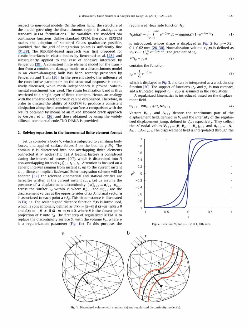
Fig. 2. Function Hr for r¼ 0:2, 0:1, 0:02 mm.
2. Solving equations in the incremental finite element format
Let us consider a body V, which is subjected to vanishing bodyforces, and applied surface forces f on the boundary @Vf . Thedomain V is discretized into non-overlapping finite elementsconnected at N nodes (Fig. 1a). A loading history is consideredduring the interval of interest [0,T], which is discretized into N
non-overlapping intervalsSN
k ¼ 1½tk�1,tk�. Attention is focused on ageneric interval ranging from instant tn up to the current instanttnþ1. Since an implicit Backward Euler integration scheme will beadopted [32], the relevant kinematical and statical entities arehereafter written at the current instant tnþ1. Let us assume thepresence of a displacement discontinuity 1uUnþ1 ¼ uþnþ1�u�nþ1
across the surface Sd within V, where uþnþ1 and u�nþ1 are thedisplacement values at the opposite sides of Sd. A normal vector nis associated to each point xASd. This circumstance is illustratedin Fig. 1a. The scalar signed distance function dðxÞ is introduced,which is conventionally defined as dðxÞ :¼ 9x�x9 if ðx�xÞ � nðxÞZ0and dðxÞ :¼ �9x�x9 if ðx�xÞ � nðxÞo0, where x is the closest pointprojection of x onto Sd. The first step of regularized XFEM is toreplace the discontinuity surface Sd with the volume Vr, where ris a regularization parameter (Fig. 1b). To this purpose, the
Sd
f
n
Fig. 1. Discretized volume with standard (a)
regularized Heaviside function Hr
HrðdðxÞÞ ¼1
Vr
Z dðxÞ
0e�9x9=r dx¼ signðdðxÞÞð1�e�9dðxÞ9=rÞ ð1Þ
is introduced, whose shape is displayed in Fig. 2 for r¼ 0:2,0:1, 0:02 mm [28–30]. Normalization volume VrðxÞ is defined asVrðxÞ ¼
R þ1�1
e�9x9=r dx. The gradient of Hr
rHr ¼ grn ð2Þ
contains the function
gr ¼1
Vre�9x9=r ð3Þ
which is displayed in Fig. 3, and can be interpreted as a crack densityfunction [30]. The support of functions Hr and gr is non-compact,and a truncated support ‘r ¼ 20r is assumed in the calculations.
A regularized kinematics is introduced based on the displace-ment field
unþ1 ¼NVnþ1þHrNAnþ1 ð4Þ
Vectors Vnþ1 and Anþ1 denote the continuous part of thedisplacement field, defined in V, and the intensity of the regular-ized displacement jump, defined in Vr, respectively. They collectthe N nodal values Vnþ1 ¼ fV1,V2, . . . ,VN gnþ1 and Anþ1 ¼ fA1,A2, . . . ,AN gnþ1. The displacement field is interpolated through the
f
Sρ
Sd
n
and regularized discontinuity model (b).
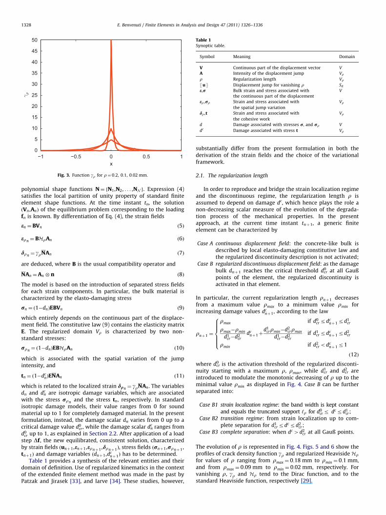
Table 1Synoptic table.
Symbol Meaning Domain
V Continuous part of the displacement vector V
A Intensity of the displacement jump Vr
r Regularization length Vr
1uU Displacement jump for vanishing r Sd
e,r Bulk strain and stress associated with V
the continuous part of the displacement
er ,rr Strain and stress associated with Vr
the spatial jump variation
dr ,t Strain and stress associated with Vr
the cohesive work
d Damage associated with stresses r, and rr V
dc Damage associated with stress t Vr
−1 −0.5 0 0.5 10
5
10
15
20
25
30
35
40
45
50
x
γ�
Fig. 3. Function gr for r¼ 0:2, 0:1, 0:02 mm.
E. Benvenuti / Finite Elements in Analysis and Design 47 (2011) 1326–13361328
polynomial shape functions N¼ fN1,N2, . . . ,NN g. Expression (4)satisfies the local partition of unity property of standard finiteelement shape functions. At the time instant tn, the solutionðVn,AnÞ of the equilibrium problem corresponding to the loadingfn is known. By differentiation of Eq. (4), the strain fields
en ¼ BVn ð5Þ
ern ¼ BHrAn ð6Þ
drn ¼ grNAn ð7Þ
are deduced, where B is the usual compatibility operator and
NAn ¼An � n ð8Þ
The model is based on the introduction of separated stress fieldsfor each strain components. In particular, the bulk material ischaracterized by the elasto-damaging stress
rn ¼ ð1�dnÞEBVn ð9Þ
which entirely depends on the continuous part of the displace-ment field. The constitutive law (9) contains the elasticity matrixE. The regularized domain Vr is characterized by two non-standard stresses:
rrn ¼ ð1�dnÞEBHrAn ð10Þ
which is associated with the spatial variation of the jumpintensity, and
tn ¼ ð1�dcnÞENAn ð11Þ
which is related to the localized strain dqn ¼ grNAn. The variablesdn and dn
c are isotropic damage variables, which are associatedwith the stress rrn and the stress tn, respectively. In standardisotropic damage models, their value ranges from 0 for soundmaterial up to 1 for completely damaged material. In the presentformulation, instead, the damage scalar dn varies from 0 up to acritical damage value d0
cr , while the damage scalar dcn ranges from
d0cr up to 1, as explained in Section 2.2. After application of a load
step Df, the new equilibrated, consistent solution, characterizedby strain fields ðunþ1,enþ1,ernþ1,drnþ1Þ, stress fields ðrnþ1,rrnþ1,tnþ1Þ and damage variables ðdnþ1,dc
nþ1Þ has to be determined.Table 1 provides a synthesis of the relevant entities and their
domain of definition. Use of regularized kinematics in the contextof the extended finite element method was made in the past byPatzak and Jirasek [33], and Iarve [34]. These studies, however,
substantially differ from the present formulation in both thederivation of the strain fields and the choice of the variationalframework.
2.1. The regularization length
In order to reproduce and bridge the strain localization regimeand the discontinuous regime, the regularization length r isassumed to depend on damage dc, which hence plays the role anon-decreasing scalar measure of the evolution of the degrada-tion process of the mechanical properties. In the presentapproach, at the current time instant tnþ1, a generic finiteelement can be characterized by
Case A
continuous displacement field: the concrete-like bulk isdescribed by local elasto-damaging constitutive law andthe regularized discontinuity description is not activated;Case B
regularized discontinuous displacement field: as the damagebulk dnþ1 reaches the critical threshold d0cr at all Gaußpoints of the element, the regularized discontinuity isactivated in that element.
In particular, the current regularization length rnþ1 decreasesfrom a maximum value rmax to a minimum value rmin forincreasing damage values dc
nþ1, according to the law
rnþ1 ¼
rmax if d0cr rdc
nþ1rd1cr
rmax�rmin
d1cr�d2
cr
dcnþ1þ
d1crrmin�d2
crrmax
d1cr�d2
cr
if d1cr rdc
nþ1rd2cr
rmin if d2cr odc
nþ1r1
8>>>><>>>>:
ð12Þ
where d0cr is the activation threshold of the regularized disconti-
nuity starting with a maximum r, rmax, while d1cr and d2
cr areintroduced to modulate the monotonic decreasing of r up to theminimal value rmin as displayed in Fig. 4. Case B can be furtherseparated into:
Case B1
strain localization regime: the band width is kept constantand equals the truncated support ‘r for d0cr r dc rd1cr;
Case B2
transition regime: from strain localization up to com-plete separation for d1cr rdc rd2cr;
Case B3
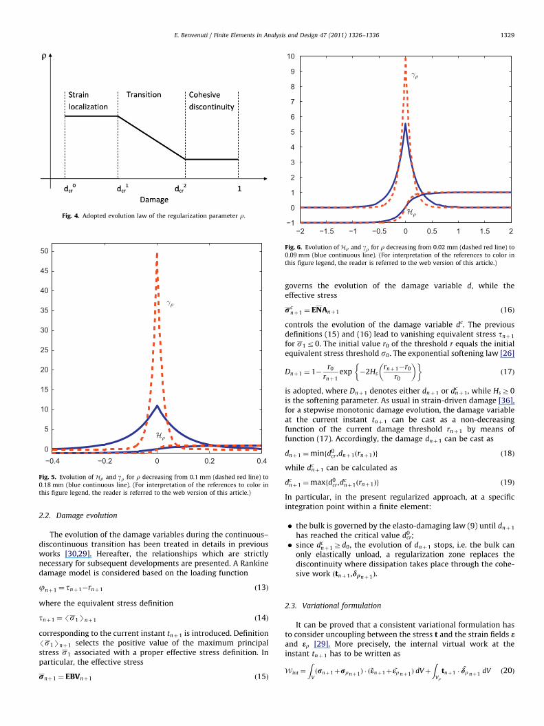
complete separation: when dc 4d2cr at all Gauß points.The evolution of r is represented in Fig. 4. Figs. 5 and 6 show theprofiles of crack density function gr and regularized Heaviside Hrfor values of r ranging from rmax ¼ 0:18 mm to rmin ¼ 0:1 mm,and from rmax ¼ 0:09 mm to rmin ¼ 0:02 mm, respectively. Forvanishing r, gr and Hr tend to the Dirac function, and to thestandard Heaviside function, respectively [29].
−0.4 −0.2 0 0.2 0.40
5
10
15
20
25
30
35
40
45
50
γ�
H�
Fig. 5. Evolution of Hr and gr for r decreasing from 0.1 mm (dashed red line) to
0.18 mm (blue continuous line). (For interpretation of the references to color in
this figure legend, the reader is referred to the web version of this article.)
−2 −1.5 −1 −0.5 0 0.5 1 1.5 2−1
0
1
2
3
4
5
6
7
8
9
10
γ�
H�
Fig. 6. Evolution of Hr and gr for r decreasing from 0.02 mm (dashed red line) to
0.09 mm (blue continuous line). (For interpretation of the references to color in
this figure legend, the reader is referred to the web version of this article.)
Fig. 4. Adopted evolution law of the regularization parameter r.
E. Benvenuti / Finite Elements in Analysis and Design 47 (2011) 1326–1336 1329
2.2. Damage evolution
The evolution of the damage variables during the continuous–discontinuous transition has been treated in details in previousworks [30,29]. Hereafter, the relationships which are strictlynecessary for subsequent developments are presented. A Rankinedamage model is considered based on the loading function
jnþ1 ¼ tnþ1�rnþ1 ð13Þ
where the equivalent stress definition
tnþ1 ¼/s1Snþ1 ð14Þ
corresponding to the current instant tnþ1 is introduced. Definition/s1Snþ1 selects the positive value of the maximum principalstress s1 associated with a proper effective stress definition. Inparticular, the effective stress
rnþ1 ¼ EBVnþ1 ð15Þ
governs the evolution of the damage variable d, while theeffective stress
rcnþ1 ¼ ENAnþ1 ð16Þ
controls the evolution of the damage variable dc. The previousdefinitions (15) and (16) lead to vanishing equivalent stress tnþ1
for s1r0. The initial value r0 of the threshold r equals the initialequivalent stress threshold s0. The exponential softening law [26]
Dnþ1 ¼ 1�r0
rnþ1exp �2Hs
rnþ1�r0
r0
� �� �ð17Þ
is adopted, where Dnþ1 denotes either dnþ1 or dcnþ1, while HsZ0
is the softening parameter. As usual in strain-driven damage [36],for a stepwise monotonic damage evolution, the damage variableat the current instant tnþ1 can be cast as a non-decreasingfunction of the current damage threshold rnþ1 by means offunction (17). Accordingly, the damage dnþ1 can be cast as
dnþ1 ¼minfd0cr ,dnþ1ðrnþ1Þg ð18Þ
while dcnþ1 can be calculated as
dcnþ1 ¼maxfd0
cr ,dcnþ1ðrnþ1Þg ð19Þ
In particular, in the present regularized approach, at a specificintegration point within a finite element:
�
the bulk is governed by the elasto-damaging law (9) until dnþ1has reached the critical value d0cr;
�
since dcnþ1Zd0, the evolution of dnþ1 stops, i.e. the bulk canonly elastically unload, a regularization zone replaces thediscontinuity where dissipation takes place through the cohe-sive work ðtnþ1,dqnþ1Þ.
2.3. Variational formulation
It can be proved that a consistent variational formulation hasto consider uncoupling between the stress t and the strain fields eand er [29]. More precisely, the internal virtual work at theinstant tnþ1 has to be written as
W int ¼
ZVðrnþ1þrrnþ1Þ � ð
~enþ1þ ~ernþ1Þ dVþ
ZVr
tnþ1 �~dr nþ1 dV ð20Þ
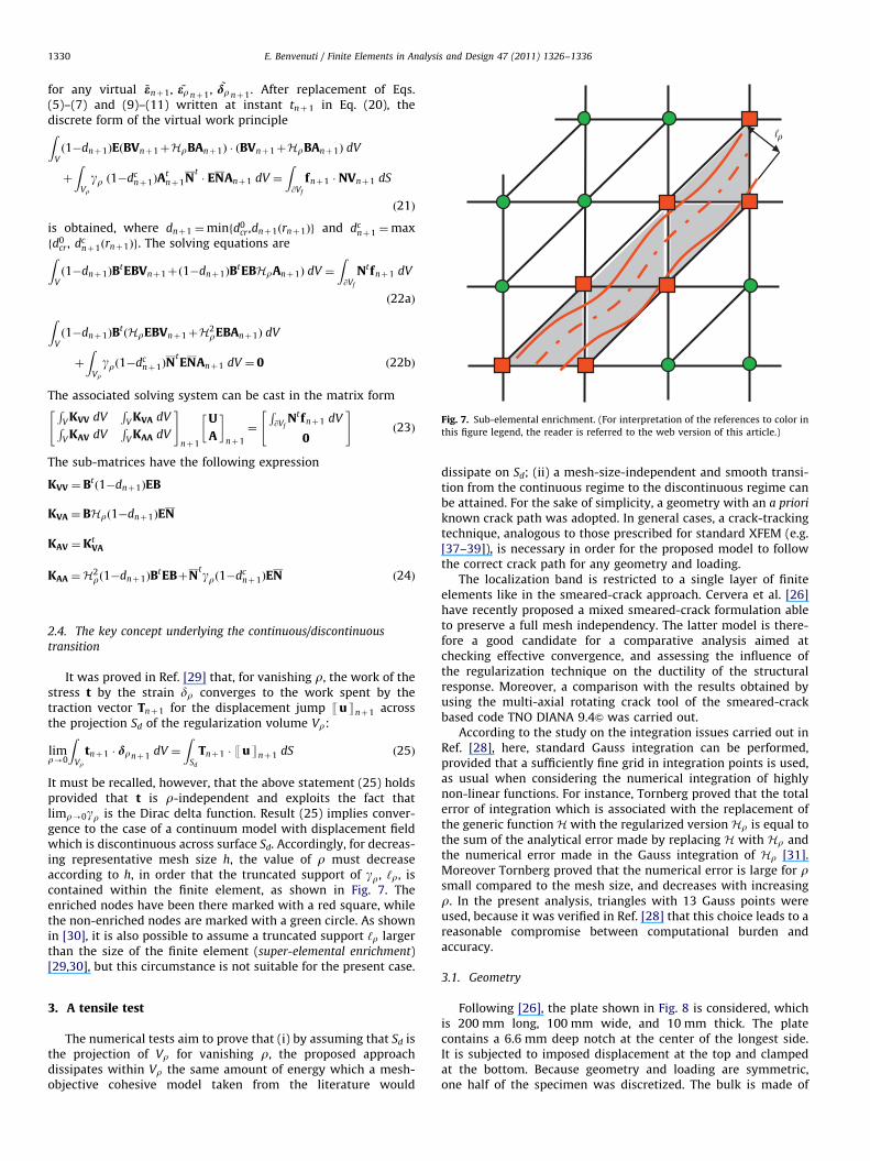
Fig. 7. Sub-elemental enrichment. (For interpretation of the references to color in
this figure legend, the reader is referred to the web version of this article.)
E. Benvenuti / Finite Elements in Analysis and Design 47 (2011) 1326–13361330
for any virtual ~enþ1, ~er nþ1, ~drnþ1. After replacement of Eqs.(5)–(7) and (9)–(11) written at instant tnþ1 in Eq. (20), thediscrete form of the virtual work principleZ
Vð1�dnþ1ÞEðBVnþ1þHrBAnþ1Þ � ðBVnþ1þHrBAnþ1Þ dV
þ
ZVr
gr ð1�dcnþ1ÞA
tnþ1N
t� ENAnþ1 dV ¼
Z@Vf
fnþ1 � NVnþ1 dS
ð21Þ
is obtained, where dnþ1 ¼minfd0cr ,dnþ1ðrnþ1Þg and dc
nþ1 ¼maxfd0
cr , dcnþ1ðrnþ1Þg. The solving equations areZ
Vð1�dnþ1ÞB
tEBVnþ1þð1�dnþ1ÞBtEBHrAnþ1Þ dV ¼
Z@Vf
Ntfnþ1 dV
ð22aÞ
ZVð1�dnþ1ÞB
tðHrEBVnþ1þH2
rEBAnþ1Þ dV
þ
ZVr
grð1�dcnþ1ÞN
tENAnþ1 dV ¼ 0 ð22bÞ
The associated solving system can be cast in the matrix formRV KVV dV
RV KVA dVR
V KAV dVR
V KAA dV
" #nþ1
U
A
� �nþ1
¼
R@Vf
Ntfnþ1 dV
0
" #ð23Þ
The sub-matrices have the following expression
KVV ¼ Btð1�dnþ1ÞEB
KVA ¼ BHrð1�dnþ1ÞEN
KAV ¼KtVA
KAA ¼H2rð1�dnþ1ÞB
tEBþNtgrð1�dc
nþ1ÞEN ð24Þ
2.4. The key concept underlying the continuous/discontinuous
transition
It was proved in Ref. [29] that, for vanishing r, the work of thestress t by the strain dr converges to the work spent by thetraction vector Tnþ1 for the displacement jump 1uUnþ1 acrossthe projection Sd of the regularization volume Vr:
limr-0
ZVr
tnþ1 � drnþ1 dV ¼
ZSd
Tnþ1 � 1uUnþ1 dS ð25Þ
It must be recalled, however, that the above statement (25) holdsprovided that t is r-independent and exploits the fact thatlimr-0gr is the Dirac delta function. Result (25) implies conver-gence to the case of a continuum model with displacement fieldwhich is discontinuous across surface Sd. Accordingly, for decreas-ing representative mesh size h, the value of r must decreaseaccording to h, in order that the truncated support of gr, ‘r, iscontained within the finite element, as shown in Fig. 7. Theenriched nodes have been there marked with a red square, whilethe non-enriched nodes are marked with a green circle. As shownin [30], it is also possible to assume a truncated support ‘r largerthan the size of the finite element (super-elemental enrichment)[29,30], but this circumstance is not suitable for the present case.
3. A tensile test
The numerical tests aim to prove that (i) by assuming that Sd isthe projection of Vr for vanishing r, the proposed approachdissipates within Vr the same amount of energy which a mesh-objective cohesive model taken from the literature would
dissipate on Sd; (ii) a mesh-size-independent and smooth transi-tion from the continuous regime to the discontinuous regime canbe attained. For the sake of simplicity, a geometry with an a priori
known crack path was adopted. In general cases, a crack-trackingtechnique, analogous to those prescribed for standard XFEM (e.g.[37–39]), is necessary in order for the proposed model to followthe correct crack path for any geometry and loading.
The localization band is restricted to a single layer of finiteelements like in the smeared-crack approach. Cervera et al. [26]have recently proposed a mixed smeared-crack formulation ableto preserve a full mesh independency. The latter model is there-fore a good candidate for a comparative analysis aimed atchecking effective convergence, and assessing the influence ofthe regularization technique on the ductility of the structuralresponse. Moreover, a comparison with the results obtained byusing the multi-axial rotating crack tool of the smeared-crackbased code TNO DIANA 9.4& was carried out.
According to the study on the integration issues carried out inRef. [28], here, standard Gauss integration can be performed,provided that a sufficiently fine grid in integration points is used,as usual when considering the numerical integration of highlynon-linear functions. For instance, Tornberg proved that the totalerror of integration which is associated with the replacement ofthe generic function H with the regularized version Hr is equal tothe sum of the analytical error made by replacing H with Hr andthe numerical error made in the Gauss integration of Hr [31].Moreover Tornberg proved that the numerical error is large for rsmall compared to the mesh size, and decreases with increasingr. In the present analysis, triangles with 13 Gauss points wereused, because it was verified in Ref. [28] that this choice leads to areasonable compromise between computational burden andaccuracy.
3.1. Geometry
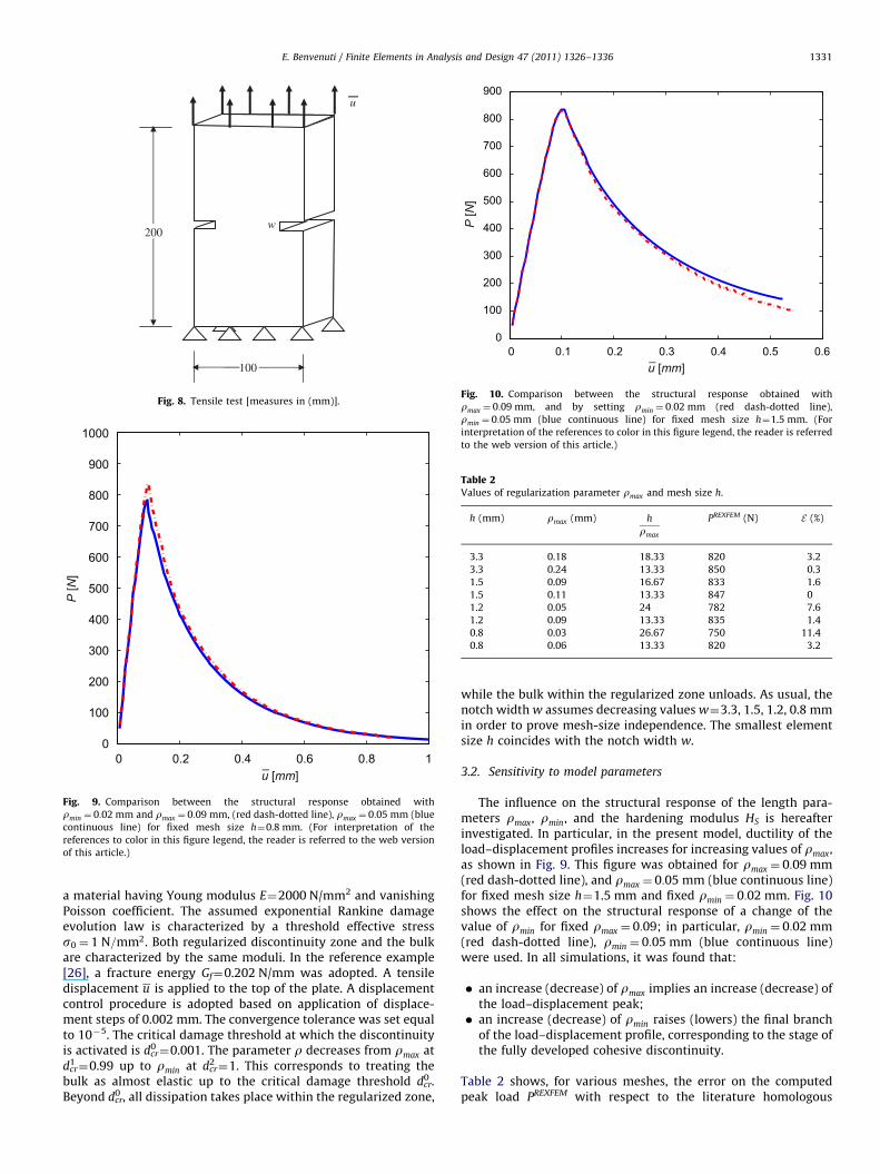
Following [26], the plate shown in Fig. 8 is considered, whichis 200 mm long, 100 mm wide, and 10 mm thick. The platecontains a 6.6 mm deep notch at the center of the longest side.It is subjected to imposed displacement at the top and clampedat the bottom. Because geometry and loading are symmetric,one half of the specimen was discretized. The bulk is made of
u
w
100
200
Fig. 8. Tensile test [measures in (mm)].
0 0.2 0.4 0.6 0.8 10
100
200
300
400
500
600
700
800
900
1000
¯
P [N
]
u [mm]
Fig. 9. Comparison between the structural response obtained with
rmin ¼ 0:02 mm and rmax ¼ 0:09 mm, (red dash-dotted line), rmax ¼ 0:05 mm (blue
continuous line) for fixed mesh size h¼0.8 mm. (For interpretation of the
references to color in this figure legend, the reader is referred to the web version
of this article.)
0 0.1 0.2 0.3 0.4 0.5 0.60
100
200
300
400
500
600
700
800
900
P [N
]
u [mm]
Fig. 10. Comparison between the structural response obtained with
rmax ¼ 0:09 mm, and by setting rmin ¼ 0:02 mm (red dash-dotted line),
rmin ¼ 0:05 mm (blue continuous line) for fixed mesh size h¼1.5 mm. (For
interpretation of the references to color in this figure legend, the reader is referred
to the web version of this article.)
Table 2Values of regularization parameter rmax and mesh size h.
h (mm) rmax (mm) h
rmax
PREXFEM (N) E (%)
3.3 0.18 18.33 820 3.2
3.3 0.24 13.33 850 0.3
1.5 0.09 16.67 833 1.6
1.5 0.11 13.33 847 0
1.2 0.05 24 782 7.6
1.2 0.09 13.33 835 1.4
0.8 0.03 26.67 750 11.4
0.8 0.06 13.33 820 3.2
E. Benvenuti / Finite Elements in Analysis and Design 47 (2011) 1326–1336 1331
a material having Young modulus E¼2000 N/mm2 and vanishingPoisson coefficient. The assumed exponential Rankine damageevolution law is characterized by a threshold effective stresss0 ¼ 1 N=mm2. Both regularized discontinuity zone and the bulkare characterized by the same moduli. In the reference example[26], a fracture energy Gf¼0.202 N/mm was adopted. A tensiledisplacement u is applied to the top of the plate. A displacementcontrol procedure is adopted based on application of displace-ment steps of 0.002 mm. The convergence tolerance was set equalto 10�5. The critical damage threshold at which the discontinuityis activated is d0
cr¼0.001. The parameter r decreases from rmax atd1
cr¼0.99 up to rmin at d2cr¼1. This corresponds to treating the
bulk as almost elastic up to the critical damage threshold d0cr.
Beyond d0cr, all dissipation takes place within the regularized zone,
while the bulk within the regularized zone unloads. As usual, thenotch width w assumes decreasing values w¼3.3, 1.5, 1.2, 0.8 mmin order to prove mesh-size independence. The smallest elementsize h coincides with the notch width w.
3.2. Sensitivity to model parameters
The influence on the structural response of the length para-meters rmax, rmin, and the hardening modulus HS is hereafterinvestigated. In particular, in the present model, ductility of theload–displacement profiles increases for increasing values of rmax,as shown in Fig. 9. This figure was obtained for rmax ¼ 0:09 mm(red dash-dotted line), and rmax ¼ 0:05 mm (blue continuous line)for fixed mesh size h¼1.5 mm and fixed rmin ¼ 0:02 mm. Fig. 10shows the effect on the structural response of a change of thevalue of rmin for fixed rmax ¼ 0:09; in particular, rmin ¼ 0:02 mm(red dash-dotted line), rmin ¼ 0:05 mm (blue continuous line)were used. In all simulations, it was found that:
�
an increase (decrease) of rmax implies an increase (decrease) ofthe load–displacement peak; � an increase (decrease) of rmin raises (lowers) the final branchof the load–displacement profile, corresponding to the stage ofthe fully developed cohesive discontinuity.
Table 2 shows, for various meshes, the error on the computedpeak load PREXFEM with respect to the literature homologous
0 0.2 0.4 0.6 0.8 10
100
200
300
400
500
600
700
800
900
1000
h = 3.3 mm, ρmax = 0.24mm, ρmin = 0.1mm; h = 1.2 mm, ρmax = 0.09mm, ρmin = 0.02mm h = 0.8 mm, ρmax = 0.06mm, ρmin = 0.02mm
u [mm]
P [N
]
Fig. 12. Comparison between the structural response obtained with fixed ratio
rmax=h¼ 13:33 h¼3.3 mm (green continuous line), rmax ¼ 0:24 mm and
rmin ¼ 0:1 mm; h¼1.2 mm (red dash-dotted line) with rmax ¼ 0:09 mm and
rmin ¼ 0:02 mm; h¼0.8 mm (blue dashed line) with rmax ¼ 0:06 mm and
rmin ¼ 0:02 mm. (For interpretation of the references to color in this figure legend,
the reader is referred to the web version of this article.)
E. Benvenuti / Finite Elements in Analysis and Design 47 (2011) 1326–13361332
quantity P [26]
E ¼ 9PREXFEM�P9
P
where P ¼ 847 N is the value of the peak load obtained by Cerveraet al. [26]. In particular, the value of h=rmax ¼ 13:33 makes itpossible to correctly reproduce the peak load computed inreference solution [26] for all the meshes which were considered.This value does not influence the effective mesh independence ofthe proposed approach for decreasing mesh size. Mesh indepen-dent load–displacement results were indeed obtained by adopt-ing other values of the ratio h=rmax, such as those indicated in thethird column of Table 2.
Various values of the hardening parameter HS were used and itwas found that, for any mesh size, the value of HS¼0.002 MPamakes it possible to recover the same energy dissipated by theliterature model [26]. It can be interesting to note that the presentassumption leads to an increase of specific fracture energy of aboutthe 50% with respect to the specific fracture energy assumed byCervera et al. [26], where the hardening modulus HS¼0.003 MPawas assumed, corresponding to a specific fracture energygf ¼ Gf =h¼ 0:202=3:3 N=m over a band width equal to h¼3.3 mm,in the case of the uniform mesh with representative element sizeh¼3.3 mm. In Fig. 11, the load–displacement results obtained byassuming HS¼0.002 MPa and 0.003 MPa are shown, by assuming auniform mesh with h¼3.3 mm and rmax ¼ 0:18 mm andrmin ¼ 0:1 mm. Unlike the usual praxis adopted in smeared crackmodels, here, the hardening modulus has not to be adjustedaccording to the mesh size.
3.2.1. Mesh-size dependence analysis
In order to investigate the capacity to give objective load–displacement results for decreasing width of the regularizeddomain, the case of specimens with decreasing finite elementsize h in the notch area is considered. In the case of sub-elementalenrichment, the regularization requires that the truncated sup-port ‘r is contained within the smallest finite element size h.
A vast number of simulations was carried out. The mostrelevant results have been selected and hereafter reported. Aspreviously shown, the peak load is influenced by the value of the
0 0.2 0.4 0.6 0.8 10
100
200
300
400
500
600
700
800
900
1000
u [mm]
P [N
]
Fig. 11. Comparison between the structural response obtained with r decreasing
from rmax ¼ 0:24 mm to rmin ¼ 0:1 mm (b), by assuming H¼0.002 MPa (blue
continuous line), and H¼0.003 MPa (red dash-dotted line), mesh size h¼3.3 mm.
(For interpretation of the references to color in this figure legend, the reader is
referred to the web version of this article.)
parameter rmax, while it does not affect the final branch. It shouldbe noted that, although in the latter reference a smaller mesh sizewas not considered, Cervera et al. have proved, however, meshindependence of their model in a different paper [35]. Meshindependent results are shown in Fig. 12, which displays thestructural responses obtained with: the uniform mesh character-ized by h¼3.3 mm (green continuous line) with r varying fromrmax ¼ 0:24 mm to rmin ¼ 0:1 mm, the refined mesh characterizedby h¼1.2 mm (red dash-dotted line) with r varying fromrmax ¼ 0:09 mm and rmin ¼ 0:02 mm, and the refined mesh withh¼0.8 mm (blue dashed line) with r varying rmax ¼ 0:06 mm tormin ¼ 0:02 mm. All these set of parameters obey the rulermax=h¼ 1=13:33. It is emphasized that this rule makes it possibleto dissipate the same quantity of energy of the reference solution[26], whereas mesh-size independent results can be obtained alsofor other values of the ratio rmax=h¼ 1=13:33. Obviously, thechoice of sub-elemental enrichment forces the (truncated) sup-port of function gr to be contained within the finite element layerin order for the regularization to be effective.
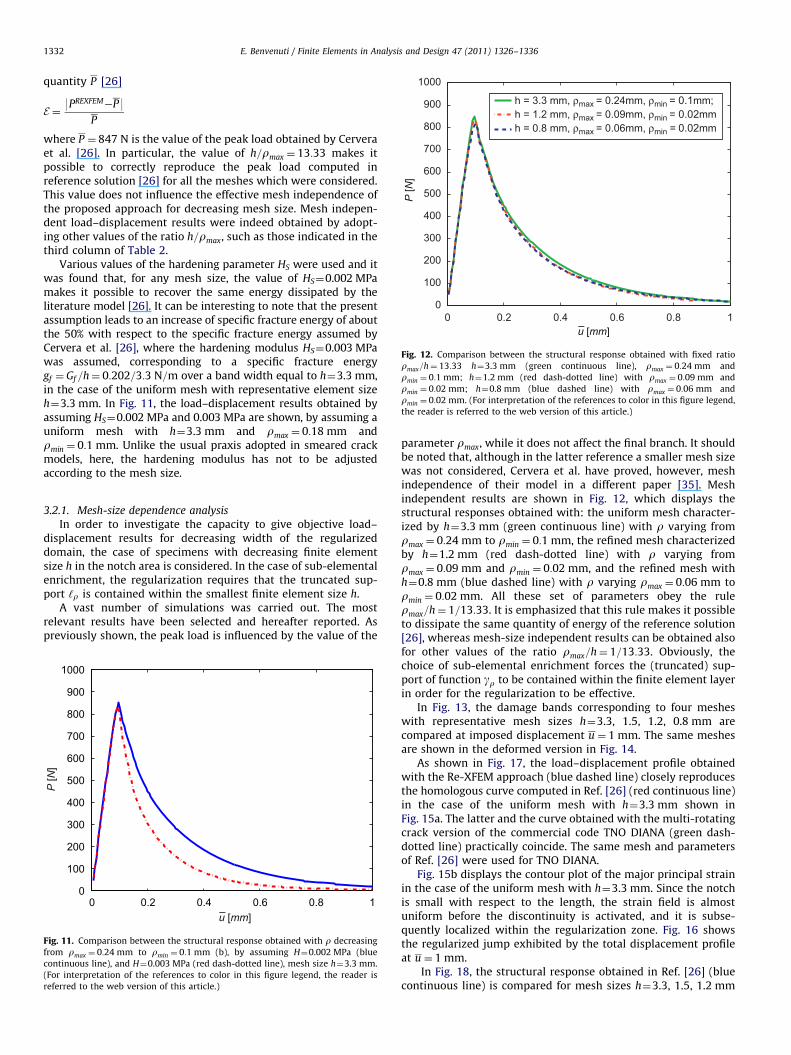
In Fig. 13, the damage bands corresponding to four mesheswith representative mesh sizes h¼3.3, 1.5, 1.2, 0.8 mm arecompared at imposed displacement u ¼ 1 mm. The same meshesare shown in the deformed version in Fig. 14.
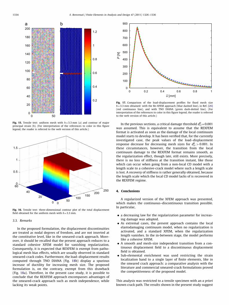
As shown in Fig. 17, the load–displacement profile obtainedwith the Re-XFEM approach (blue dashed line) closely reproducesthe homologous curve computed in Ref. [26] (red continuous line)in the case of the uniform mesh with h¼3.3 mm shown inFig. 15a. The latter and the curve obtained with the multi-rotatingcrack version of the commercial code TNO DIANA (green dash-dotted line) practically coincide. The same mesh and parametersof Ref. [26] were used for TNO DIANA.
Fig. 15b displays the contour plot of the major principal strainin the case of the uniform mesh with h¼3.3 mm. Since the notchis small with respect to the length, the strain field is almostuniform before the discontinuity is activated, and it is subse-quently localized within the regularization zone. Fig. 16 showsthe regularized jump exhibited by the total displacement profileat u ¼ 1 mm.
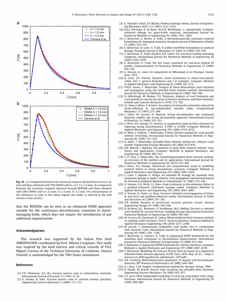
In Fig. 18, the structural response obtained in Ref. [26] (bluecontinuous line) is compared for mesh sizes h¼3.3, 1.5, 1.2 mm
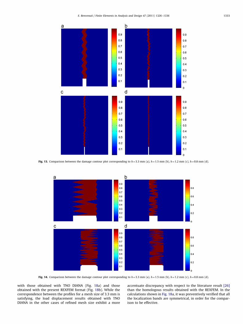
Fig. 13. Comparison between the damage contour plot corresponding to h¼3.3 mm (a), h¼1.5 mm (b), h¼1.2 mm (c), h¼0.8 mm (d).
Fig. 14. Comparison between the damage contour plot corresponding to h¼3.3 mm (a), h¼1.5 mm (b), h¼1.2 mm (c), h¼0.8 mm (d).
E. Benvenuti / Finite Elements in Analysis and Design 47 (2011) 1326–1336 1333
with those obtained with TNO DIANA (Fig. 18a) and thoseobtained with the present REXFEM format (Fig. 18b). While thecorrespondence between the profiles for a mesh size of 3.3 mm issatisfying, the load displacement results obtained with TNODIANA in the other cases of refined mesh size exhibit a more
accentuate discrepancy with respect to the literature result [26]than the homologous results obtained with the REXFEM. In thecalculations shown in Fig. 18a, it was preventively verified that allthe localization bands are symmetrical, in order for the compar-ison to be effective.
0.2
0.4
0.6
0.8
1
1.2
0 500
20
40
60
80
100
120
140
160
180
200
Fig. 15. Tensile test: uniform mesh with h¼3.3 mm (a) and contour of major
principal strain (b). (For interpretation of the references to color in this figure
legend, the reader is referred to the web version of this article.)
050
100150
200250
0
2040
600
0.5
1
1.5
Fig. 16. Tensile test: three-dimensional contour plot of the total displacement
field obtained for the uniform mesh with h¼3.3 mm.
0 0.2 0.4 0.6 0.8 10
100
200
300
400
500
600
700
800
900
P [N
]
u [mm]
Fig. 17. Comparison of the load-displacement profiles for fixed mesh size
h¼3.3 mm obtained: with the Re-XFEM approach (blue dashed line), in Ref. [26]
(red continuous line), and with TNO DIANA (green dash-dotted line). (For
interpretation of the references to color in this figure legend, the reader is referred
to the web version of this article.)
E. Benvenuti / Finite Elements in Analysis and Design 47 (2011) 1326–13361334
3.3. Remarks
In the proposed formulation, the displacement discontinuitiesare treated as nodal degrees of freedom, and are not inserted atthe constitutive level, like in the smeared-crack approach. More-over, it should be recalled that the present approach reduces to astandard cohesive XFEM model for vanishing regularization.Consequently, it is expected that REXFEM is exempt from patho-logical mesh bias effects, which are usually observed in standardsmeared-crack codes. Furthermore, the load–displacement resultscomputed through TNO DIANA (Fig. 18b) display a spuriousincrease of ductility for increasing mesh size. The proposedformulation is, on the contrary, exempt from this drawback(Fig. 18a). Therefore, in the present case study, it is possible toconclude that the REXFEM approach encompasses advantages ofthe smeared-crack approach such as mesh independence, whilelacking its weak points.
In the previous sections, a critical damage threshold dcr0¼0.001
was assumed. This is equivalent to assume that the REXFEMformat is activated as soon as the damage of the local continuummodel starts to develop. It has been verified that, for the currentlyinvestigated case, the peak values of the load–displacementresponse decrease for decreasing mesh sizes for d0
cr 40:001. Inthese circumstances, however, the transition from the localcontinuum damage to the REXFEM format remains smooth, asthe regularization effect, though late, still exists. More precisely,there is no loss of stiffness at the transition instant, like thosewhich can occur when going from a non-local CD model with alength scale to a cohesive-crack model where such a length scaleis lost. A recovery of stiffness is rather generally obtained, becausethe length scale which the local CD model lacks of is recovered inthe REXFEM regime.
4. Conclusions
A regularized version of the XFEM approach was presented,which makes the continuous–discontinuous transition possible.In particular,
�
a decreasing law for the regularization parameter for increas-ing damage was adopted. � As extremal cases, the present approach contains the localelastodamaging continuum model, when no regularization isactivated, and a standard XFEM, when the regularizationlength vanishes. In the in-between stage, the model performslike a cohesive XFEM.
� A smooth and mesh-size independent transition from a con-tinuous displacement field to a discontinuous displacementfield is obtained.
� Sub-elemental enrichment was used restricting the strainlocalization band to a single layer of finite elements, like inthe smeared crack approach: a comparative analysis with theliterature and commercial smeared-crack formulations provedthe competitiveness of the proposed model.
This analysis was restricted to a tensile specimen with an a priori
known crack path. The results shown in the present study suggest
0
100
200
300
400
500
600
700
800
900
1000DIANA h = 1.5 mmDIANA h = 1.2 mmDIANA h = 3.3 mmCervera et al.
0 0.2 0.4 0.6 0.8 10
100
200
300
400
500
600
700
800
900
1000h = 1.5 mmh = 1.2 mmh = 3.3 mmCervera et al.
P [N
]
u [mm]
0 0.2 0.4 0.6 0.8 1u [mm]
P [N
]
Fig. 18. (a) Comparison between the structural response obtained by Cervera et al.
[26] and those obtained with TNO DIANA with h¼3.3, 1.5, 1.2 mm; (b) comparison
between the structural response obtained through REXFEM and those obtained
with TNO DIANA with h¼3.3 mm, h¼1.5 mm, h¼1.2 mm. (For interpretation of
the references to color in this figure legend, the reader is referred to the web
version of this article.)
E. Benvenuti / Finite Elements in Analysis and Design 47 (2011) 1326–1336 1335
that the REXFEM can be seen as an enhanced XFEM approachsuitable for the continuous–discontinuous transition in elasto-damaging bulks, which does not require the introduction of anyadditional regularization.
Acknowledgments
This research was supported by the Italian Prin fund2009XWLFKW coordinated by Prof. Alberto Corigliano. This studywas inspired by the kind interest and critical remarks of Prof.Miguel Cervera of the Technical University of Catalonia. OttaviaVitarelli is acknowledged for the TNO Diana simulations.
References
[1] F.H. Wittmann, X.Z. Hu, Fracture process zone in cementitious materials,International Journal of Fracture 51 (1991) 3–18.
[2] K. Otsuka, H. Date, Fracture process zone in concrete tension specimen,Engineering Fracture Mechanics 5 (2000) 111–131.
[3] G. Pijaudier-Cabot, Z.P. Bazant, Nonlocal damage theory, Journal of Engineer-ing Mechanics ASCE 113 (1987) 1512–1533.
[4] R.H.J. Peerlings, R. de Borst, W.A.M. Brekelmans, S. Ayyapureddi, Gradient-enhanced damage for quasi-brittle materials, International Journal forNumerical Methods in Engineering 39 (1996) 3391–3403.
[5] E. Benvenuti, G. Borino, A. Tralli, A thermodynamically consistent nonlocalformulation for damaging materials, European Journal of Mechanics A/Solids21 (2002) 535–553.
[6] E. Benvenuti, B. Loret, A. Tralli, A unified multifield formulation in nonlocaldamage, European Journal of Mechanics A: Solids 23 (2004) 539–559.
[7] E. Benvenuti, A. Tralli, Iterative LCP solvers for non-local loading-unloadingconditions, International Journal for Numerical Methods in Engineering 58(2003) 2343–2370.
[8] E. Benvenuti, A. Tralli, The fast Gauss transform for non-local integral FEmodels, Communications in Numerical Methods in Engineering 22 (2006)505–533.
[9] G. Duvaut, J.L. Lions, Les inequations en Mecanique et en Physique, Dunod,Paris, 1972.
[10] B. Loret, J.H. Prevost, Dynamic strain localization in elasto-visco-plasticsolids. Part 1: general formulation and 1-D examples, Computer Methodsin Applied Mechanics and Engineering 83 (1990) 247–273.
[11] P.M.A. Areias, T. Belytschko, Analysis of three-dimensional crack initiationand propagation using the extended finite element method, InternationalJournal for Numerical Methods in Engineering 63 (2005) 760–788.
[12] A. Hillerborgh, M. Modeer, P.E. Petersson, Analysis of crack formation andcrack growth in concrete by means of fracture mechanics and finite elements,Cement and Concrete Research 6 (1976) 773–782.
[13] J.C. Simo, J. Oliver, F. Armero, An analysis of strong discontinuities induced bystrain-softening in rate-independent inelastic solids, ComputationalMechanics 12 (1993) 277–296.
[14] J. Oliver, M. Cervera, O. Manzoli, Strong discontinuities and continuumplasticity models: the strong discontinuity approach, International Journalof Plasticity 15 (1999) 319–351.
[15] J. Oliver, A.E. Huespe, P.J. Sanchez, A comparative study on finite elements forcapturing strong discontinuities: E-FEM vs X-FEM, Computer Methods inApplied Mechanics and Engineering 195 (2006) 4732–4752.
[16] N. Moes, J. Dolbow, T. Belytschko, A finite element method for crack growthwithout remeshing, International Journal for Numerical Methods in Engi-neering 46 (1999) 131–150.
[17] N. Moes, T. Belytschko, Extended finite element method for cohesive crackgrowth, Engineering Fracture Mechanics 69 (2002) 813–833.
[18] J.M. Melenk, I. Babuska, The partition of unity finite element method: basictheory and applications, Computer Methods in Applied Mechanics andEngineering 39 (1996) 289–314.
[19] T.-P. Fries, T. Belytschko, The extended/generalized finite element method:an overview of the method and its applications, International Journal forNumerical Methods in Engineering 84 (2010) 253–304.
[20] J. Oliver, A.E. Huespe, Theoretical and computational issues in modellingmaterial failure in strong discontinuity scenarios, Computer Methods inApplied Mechanics and Engineering 193 (2004) 2987–3014.
[21] C. Comi, S. Mariani, U. Perego, An extended FE strategy for transition formcontinuum damage to mode I cohesive crack propagation, International Journalfor Numerical Analytical Methods in Geomechanics 31 (2007) 213–238.
[22] A. Simone, G.N. Wells, L.J. Sluys, From continuous to discontinuous failure ina gradient-enhanced continuum damage model, Computer Methods inApplied Mechanics and Engineering 192 (2003) 4581–4607.
[23] A. Simone, H. Askes, L.J. Sluys, Incorrect initiation and propagation of failurein non-local and gradient-enhanced media, International Journal of Solidsand Structures 41 (2004) 351–363.
[24] Y.R. Rashid, Analysis of prestressed concrete pressure vessels, NuclearEngineering Design 29 (1968) 334–344.
[25] R. de Borst, J.J.C. Remmers, A. Needleman, M.A. Abellan, Discrete vs smearedcrack models for concrete fracture: bridging the gap, International Journal forNumerical Methods in Engineering 28 (2004) 583–607.
[26] M. Cervera, M. Chiumenti, R. Codina, Mixed stabilized finite element methodsin nonlinear solid mechanics. Part II: strain localization, Computer Method inApplied Mechanics Engineering 199 (2010) 2571–2589.
[27] M. Jirasek, T. Zimmermann, Embedded crack model. Part II: combinationwith smeared crack, International Journal for Numerical Methods in Engi-neering 50 (1996) 1291–1305.
[28] E. Benvenuti, G. Ventura, A. Tralli, A regularized XFEM framework for thetransition from continuous to discontinuous displacements, InternationalJournal for Numerical Methods in Engineering 74 (2008) 911–944.
[29] E. Benvenuti, A regularized XFEM framework for cohesive interfaces, ComputerMethods in Applied Mechanics and Engineering 197 (2008) 4367–4378.
[30] E. Benvenuti, Modelling the Fracture Process Zone by means of a regularizedeXtended Finite Element approach, ECCM, Paris, 2010, May 16–21, /https://www.eccm-2010.org/abstract_pdf/abstract_1475.pdfS.
[31] A.K. Tornberg, Multi-dimensional quadrature of singular and discontinuousfunctions, BIT Numerical Mathematics 42 (2002) 644–669.
[32] J.C. Simo, T.J.R. Hughes, Computational Inelasticity, Springer Verlag, 1998.[33] B. Patzak, M. Jirasek, Process zone resolution by extended finite elements,
Engineering Fracture Mechanics 70 (2003) 957–977.
[34] E.V. Iarve, Mesh independent modeling of cracks by using higher order shapefunctions, International Journal for Numerical Methods in Engineering 56(2003) 869–882.

E. Benvenuti / Finite Elements in Analysis and Design 47 (2011) 1326–13361336
[35] M. Cervera, M. Chiumenti, R. Codina, Mesh objective modelling of cracksusing continuous linear strain and displacement interpolations, InternationalJournal for Numerical Methods in Engineering 87 (2011) 962–987.
[36] E. Benvenuti, Damage integration in the strain space, International Journal ofSolids and Structures 41 (2004) 3167–3191.
[37] P. Jager, P. Steinmann, E. Kuhl, Modeling three-dimensional crack propaga-tion: a comparison of crack path cracking strategies, International Journal forNumerical Methods in Engineering 76 (2008) 1328–1352.
[38] J.F. Unger, S. Eckardt, C. Konke, Modelling of cohesive crack growth inconcrete structures with the extended finite element method, ComputerMethods in Applied Mechanics and Engineering 196 (2007) 4087–4100.
[39] G. Meschke, P. Dumstorff, Energy-based modeling of cohesive and cohesion-less cracks via X-FEM, Computer Methods in Applied Mechanics and
Engineering 196 (2007) 2338–2357.


