Metropolis

A modern beamer theme

Matthias Vogelgesang

November 2, 2019

Center for modern beamer themes

Introduction

Title formats

Elements

Conclusion

2

Introduction

3

Metropolis

The metropolis theme is a Beamer theme with minimal visual noiseinspired by the hsrm Beamer Theme by Benjamin Weiss.

Enable the theme (in LATEX) by loading

\documentclass{beamer}\usetheme{metropolis}

Note, that you have to have Mozilla’s Fira Sans font and XeTeX installed toenjoy this wonderful typography.

In R you can of course use this package directly, see its documentation.

4

Sections

Sections group slides of the same topic

## Elements

for which metropolis provides a nice progress indicator …

5

Title formats

6

Metropolis title formats

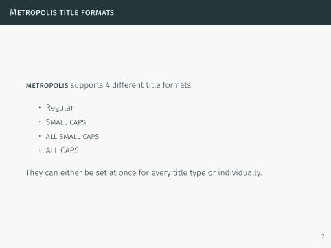
metropolis supports 4 different title formats:

• Regular• Small caps• all small caps• ALL CAPS

They can either be set at once for every title type or individually.

7

Elements

8

Typography

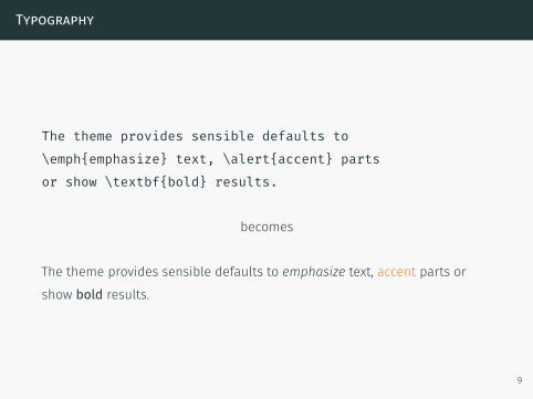
The theme provides sensible defaults to\emph{emphasize} text, \alert{accent} partsor show \textbf{bold} results.

becomes

The theme provides sensible defaults to emphasize text, accent parts orshow bold results.

9

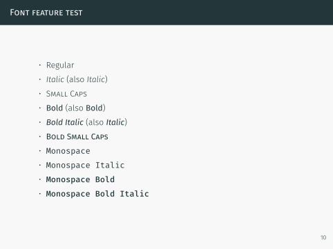
Font feature test

• Regular• Italic (also Italic)• Small Caps• Bold (also Bold)• Bold Italic (also Italic)• Bold Small Caps• Monospace• Monospace Italic• Monospace Bold• Monospace Bold Italic

10

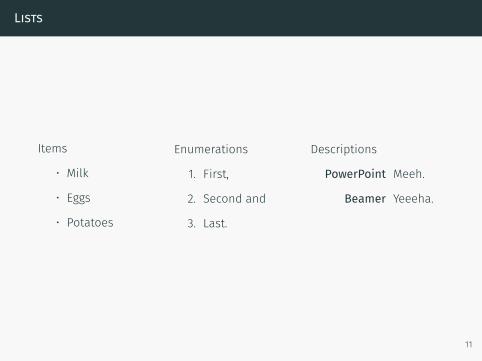
Lists

Items

• Milk

• Eggs

• Potatoes

Enumerations

1. First,

2. Second and

3. Last.

Descriptions

PowerPoint Meeh.

Beamer Yeeeha.

11

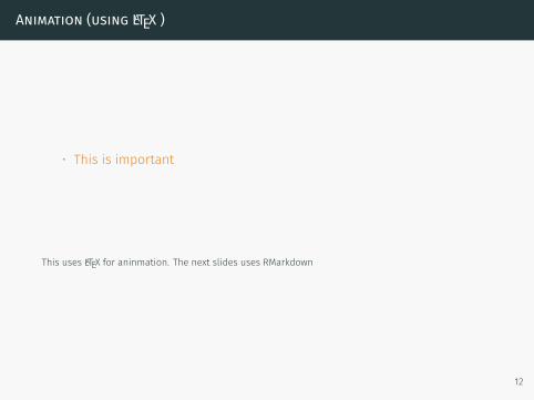
Animation (using LATEX )

• This is important

• Now this

• And now this

This uses LATEX for aninmation. The next slides uses RMarkdown

12

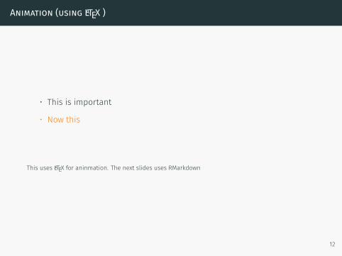
Animation (using LATEX )

• This is important

• Now this

• And now this

This uses LATEX for aninmation. The next slides uses RMarkdown

12

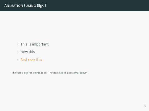
Animation (using LATEX )

• This is important

• Now this

• And now this

This uses LATEX for aninmation. The next slides uses RMarkdown

12

Animation (using LATEX )

• This is really important

• Now this

• And now this

This uses LATEX for aninmation. The next slides uses RMarkdown

12

Animation (using RMarkdown, plus one LATEX trick)

• This is important

• Now this• And now this

13

Animation (using RMarkdown, plus one LATEX trick)

• This is important• Now this

• And now this

13

Animation (using RMarkdown, plus one LATEX trick)

• This is important• Now this• And now this

13

Animation (using RMarkdown, plus one LATEX trick)

• This is really important• Now this• And now this

13

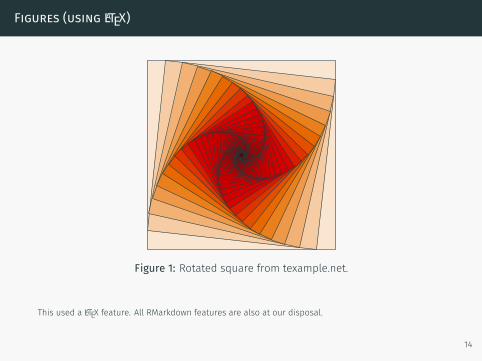
Figures (using LATEX)

Figure 1: Rotated square from texample.net.

This used a LATEX feature. All RMarkdown features are also at our disposal.

14

Tables (using LATEX})

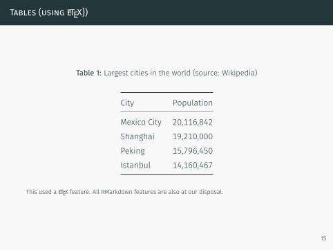
Table 1: Largest cities in the world (source: Wikipedia)

City Population

Mexico City 20,116,842Shanghai 19,210,000Peking 15,796,450Istanbul 14,160,467

This used a LATEX feature. All RMarkdown features are also at our disposal.

15

Blocks

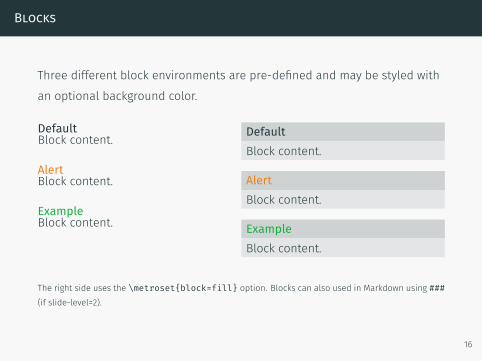
Three different block environments are pre-defined and may be styled withan optional background color.

DefaultBlock content.

AlertBlock content.

ExampleBlock content.

DefaultBlock content.

AlertBlock content.

ExampleBlock content.

The right side uses the \metroset{block=fill} option. Blocks can also used in Markdown using ###(if slide-level=2).

16

Math

e = limn→∞

(1+

1n

)n

17

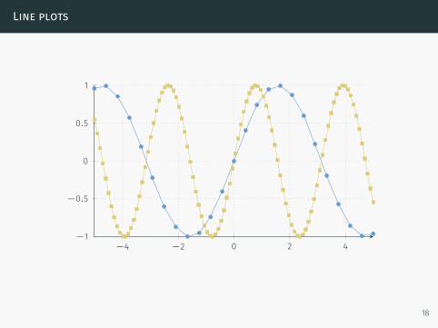
Line plots

−4 −2 0 2 4−1

−0.5

0

0.5

1

18

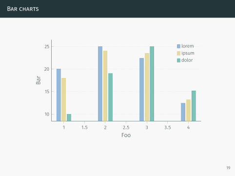
Bar charts

1 1.5 2 2.5 3 3.5 4

10

15

20

25

Foo

Bar

loremipsumdolor

19

Quotes

Veni, Vidi, Vici

20

References

Some references (Knuth, 1992; Graham et al., 1989; Simpson, 2003; Erdős,1995; Greenwade, 1993)

allowframebreaks is not used or needed, also changed \cite to \citep, and defaulted natbib tooption [round].

21

Notes

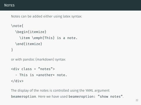
Notes can be added either using latex syntax:

\note{\begin{itemize}

\item \emph{This} is a note.\end{itemize}

}

or with pandoc (markdown) syntax:

<div class = ”notes”>- This is *another* note.

</div>

The display of the notes is controlled using the YAML argumentbeameroption. Here we have used beameroption: ”show notes”.

22

Notes

Notes can be added either using latex syntax:

\note{\begin{itemize}\item \emph{This} is a note.

\end{itemize}}

or with pandoc (markdown) syntax:

<div class = ”notes”>- This is *another* note.

</div>

The display of the notes is controlled using the YAML argumentbeameroption. Here we have used beameroption: ”show notes”.

2019-11-02

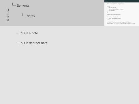
Elements

Notes

• This is a note.

• This is another note.

Conclusion

23

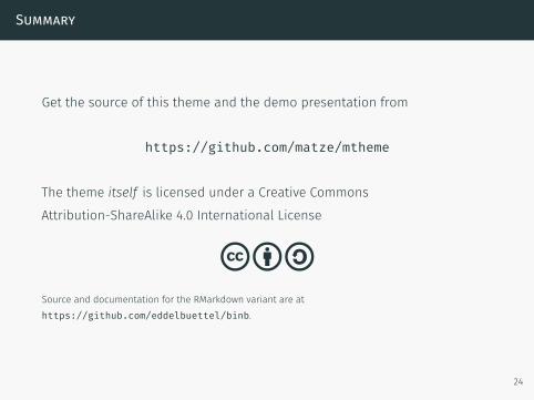
Summary

Get the source of this theme and the demo presentation from

https://github.com/matze/mtheme

The theme itself is licensed under a Creative CommonsAttribution-ShareAlike 4.0 International License

cba

Source and documentation for the RMarkdown variant are athttps://github.com/eddelbuettel/binb.

24

Questions?

25

Backup slides

Sometimes, it is useful to add slides at the end of your presentation to referto during audience questions.

The best way to do this is to include the appendixnumberbeamer packagein your preamble and call \appendix before your backup slides.

metropolis will automatically turn off slide numbering and progress barsfor slides in the appendix.

Calling \appendix currently leads to an error in when using binb.

26

R Appendix: R Figure Example

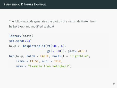
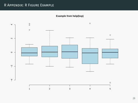
The following code generates the plot on the next slide (taken fromhelp(bxp) and modified slightly):

library(stats)set.seed(753)bx.p <- boxplot(split(rt(100, 4),

gl(5, 20)), plot=FALSE)bxp(bx.p, notch = FALSE, boxfill = ”lightblue”,

frame = FALSE, outl = TRUE,main = ”Example from help(bxp)”)

27

R Appendix: R Figure Example

1 2 3 4 5

−4

−2

02

4

Example from help(bxp)

28

R Appendix: R Table Example

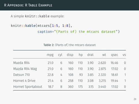
A simple knitr::kable example:

knitr::kable(mtcars[1:5, 1:8],caption=”(Parts of) the mtcars dataset”)

Table 2: (Parts of) the mtcars dataset

mpg cyl disp hp drat wt qsec vs

Mazda RX4 21.0 6 160 110 3.90 2.620 16.46 0Mazda RX4 Wag 21.0 6 160 110 3.90 2.875 17.02 0Datsun 710 22.8 4 108 93 3.85 2.320 18.61 1Hornet 4 Drive 21.4 6 258 110 3.08 3.215 19.44 1Hornet Sportabout 18.7 8 360 175 3.15 3.440 17.02 0

29

P. Erdős. A selection of problems and results in combinatorics. In Recenttrends in combinatorics (Matrahaza, 1995), pages 1–6. Cambridge Univ.Press, Cambridge, 1995.

R. Graham, D. Knuth, and O. Patashnik. Concrete mathematics.Addison-Wesley, Reading, MA, 1989.

G. D. Greenwade. The Comprehensive Tex Archive Network (CTAN). TUGBoat,14(3):342–351, 1993.

D. Knuth. Two notes on notation. Amer. Math. Monthly, 99:403–422, 1992.

H. Simpson. Proof of the Riemann Hypothesis. preprint (2003), available athttp://www.math.drofnats.edu/riemann.ps, 2003.

30