Embed Size (px)
Citation preview

Acknowledgments
The Mexico Emissions Inventory Program Manuals were the result of efforts by severalparticipants. The Binational Advisory Committee (BAC) guided the development of thesemanuals. The members of the BAC were:
Dr. John R. Holmes, State of California Air Resources BoardMr. William B. Kuykendal, U.S. Environmental Protection AgencyMr. Gary Neuroth, Arizona Department of Environmental QualityDr. Victor Hugo Páramo, Instituto Nacional de EcologíaMr. Gerardo Rios, U.S. Environmental Protection AgencyMr. Carl Snow, Texas Natural Resource Conservation Commission
The Western Governors’ Association (WGA) was the lead agency for this project. Mr. John T.Leary was the WGA Project Manager. Funding for the development of the workbook wasreceived from the United States Environmental Protection Agency (U.S. EPA). RadianInternational prepared the manuals under the guidance of the BAC and WGA.

DCN 96-670-017-01RCN 670017 5104
MEXICO EMISSIONS INVENTORY PROGRAM MANUALS
VOLUME II – EMISSIONS INVENTORY FUNDAMENTALS
FINAL
Prepared for:
Western Governors' AssociationDenver, Colorado
and
Binational Advisory Committee
Prepared by:
Radian International LLC10389 Old Placerville Road
Sacramento, CA 95827
December 1997

Mexico Emissions Inventory Program i
PREFACEAir pollution can negatively impact public health when present in the atmosphere
in sufficient quantities. Most rural areas rarely experience air quality problems, while elevated
concentrations of air pollution are found in many urban environments. Recently, there has been
an increasingly larger degree of urbanization and industrial activity throughout Mexico, resulting
in air quality impairment for several regions.
Air pollution results from a complex mix of literally thousands of sources ranging
from industrial smoke stacks and motor vehicles, to the individual use of grooming products,
household cleaners, and paints. Even plant and animal life can play an important role in the air
pollution problem. The complex nature of air pollution requires the development of detailed
plans on a regional level that provide a full understanding of the emission sources and methods
for reducing the health impacts associated with exposure to air pollution. Example air quality
planning activities include:
! Application of air quality models;
! Examination of source attribution for emissions control where deemed
necessary;
! Development of emission projections to examine possible changes in
future air quality;
! Analysis of emission trends; and
! Analysis of emissions transport from one region to another.
Development of fundamentally sound emissions inventories is a key need for each
of these air quality management and planning functions.

Volume II - Emissions Inventory Fundamentals Final, December 1997
Mexico Emissions Inventory Programii
Developing emission estimates to meet air quality planning needs requires
continual development and refinement; "one time" inventory efforts are not conducive to the air
quality planning process. For lasting benefit, an inventory program must be implemented so that
accurate emission estimates can be developed for all important geographic regions, refined over
time, and effectively applied in the air quality planning and monitoring process. Consequently, a
set of inventory manuals will be developed that can be used throughout the country to help
coordinate the development of consistent emission estimates. These manuals are intended for
use by local, state, and federal agencies, as well as by industry and private consultants. The
purpose of these manuals is to assist in implementing the inventory program and in maintaining
that program over time so that emissions inventories can be developed in periodic cycles and
continually improved.
The manuals cover inventory program elements such as estimating emissions,
program planning, database management, emissions validation, and other important topics.
Figure 1 shows the series of manuals that will be developed to support a complete inventory
program. The main purpose of each manual or volume is summarized below.
Volume I—Emissions Inventory Program Planning. This manual addresses
the important planning issues that must be considered in an air emissions inventory program.
Program planning is discussed not as an "up-front" activity, but rather as an ongoing process to
ensure the long-term growth and success of an emissions inventory program. Key Topics:
program purpose, inventory end uses, regulatory requirements, coordination at federal/state/local
levels, staff and data management requirements, identifying and selecting special studies.
Volume II—Emissions Inventory Fundamentals. This manual presents the
basic fundamentals of emissions inventory development and discusses inventory elements that
apply to multiple source types (e.g., point and area) to avoid the need for repetition in multiple
volumes. Key Topics: applicable regulations, rule effectiveness, rule penetration, pollutant
definitions (excluding nonreactive volatile), point/area source delineation, point/area source
reconciliation.

Final, December 1997 Volume II - Emissions Inventory Fundamentals
Mexico Emissions Inventory Program iii
Fig
ure
1. M
exic
o E
mis
sion
s In
vent
ory
Pro
gram
Man
uals
ME
X2.
CD
R -
7/5
/96
- JH
- S
AC

Volume II - Emissions Inventory Fundamentals Final, December 1997
Mexico Emissions Inventory Programiv
Volume III—Basic Emission Estimating Techniques. This manual presents the
basic methodologies used to develop emission estimates, including examples and sample
calculations. Inventory tools associated with each methodology are identified and included in
Volume XI (References). Key Topics: source sampling, emissions models, surveying, emission
factors, material balance, and extrapolation.
Volume IV—Emissions Inventory Development: Point Sources. This manual
provides guidance for developing the point source emissions inventory. A cross-reference table
is provided for each industry/device type combination (e.g., petroleum refining/combustion
devices) with one or more of the basic methodologies presented in Volume III. Key Topics:
cross-reference table, stack parameters, control devices, design/process considerations,
geographic differences and variability in Mexico, quality assurance/quality control (QA/QC),
overlooked processes, data references, and data collection forms.
Volume V—Emissions Inventory Development: Area Sources (Includes
Non-Road Mobile). This manual provides guidance for developing the area source emissions
inventory. After the presentation of general area source information, a table is provided to cross-
reference each area source category (e.g., asphalt application) with one or more of the basic
methodologies presented in Volume III. Then, source category-specific information is discussed
for each source category defined in the table. Key Topics: area source categorization and
definition, cross-reference table, control factors, geographic differences and variability in
Mexico, QA/QC, data references, and data collection forms (questionnaires).
Volume VI—Emissions Inventory Development: Motor Vehicles. Because
motor vehicles are inherently different from point and area sources, the available estimation
methods and required data are also different. To estimate emissions from these complex sources,
models are the preferred estimation tool. Many of these models utilize extensive test data
applicable to a given country or region. This manual focuses primarily on the data development
phase of estimating motor vehicle emissions. Key Topics: available estimation methods,

Final, December 1997 Volume II - Emissions Inventory Fundamentals
Mexico Emissions Inventory Program v
primary/secondary/tertiary data and information, source categorization, emission factor sources,
geographic variability within Mexico, and QA/QC.
Volume VII—Emissions Inventory Development: Natural Sources. This
manual provides guidance for developing a natural source emissions inventory (i.e., biogenic
volatile organic compound [VOC] and soil nitrogen oxide [NOx]). In addition, this manual
includes the theoretical aspects of emission calculations and discussion of specific models. Key
Topics: source categorization and definition, emission mechanisms, basic emission algorithms,
biomass determination, land use/land cover data development, temporal and meteorological
adjustments, and emission calculation approaches.
Volume VIII—Modeling Inventory Development. This manual provides
guidance for developing inventory data for use in air quality models and addresses issues such as
temporal allocation, spatial allocation, speciation, and projection of emission estimates. Key
Topics: definition of modeling terms, seasonal adjustment, temporal allocation, spatial
allocation, chemical speciation, and projections (growth and control factors).
Volume IX—Emissions Inventory Program Evaluation. This manual consists
of three parts: QA/QC, uncertainty analysis, and emissions verification. The QA/QC portion
defines the overall QA/QC program and is written to complement source specific QA/QC
procedures written into other manuals. The uncertainty analysis includes not only methods of
assessing uncertainty in emission estimates, but also for assessing uncertainty in modeling values
such as speciation profiles and emission projection factors. The emissions verification section
describes various analyses that can be performed to examine the accuracy of the emission
estimates. Examples include receptor modeling and trajectory analysis combined with specific
data analysis techniques. Key Topics: description of concepts and definition of terms, inventory
review protocol, completeness review, accuracy review, consistency review, recommended
uncertainty methodologies, and applicable emission verification methodologies.

Volume II - Emissions Inventory Fundamentals Final, December 1997
Mexico Emissions Inventory Programvi
Volume X—Data Management. This manual addresses the important needs
associated with the data management element of the Mexico national emissions inventory
program. Key Topics: general-purpose data management systems and tools, specific-purpose
software systems and tools, coding system, confidentiality, electronic submittal, frequency of
updates, recordkeeping, Mexico-specific databases, and reports.
Volume XI—References. This manual is a compendium of tools that can be
used in emissions inventory program development. Inventory tools referenced in the other
manuals are included (i.e., hardcopy documents, electronic documents, and computer models).
Mexico Emissions Inventory Program vii
CONTENTSSection Page
PREFACE . . . . . . . . . . . . . . . . . . . . . . . . . . . . . . . . . . . . . . . . . . . . . . . . . . . . . . . . . . . . . . . . . . . i
1.0 INTRODUCTION . . . . . . . . . . . . . . . . . . . . . . . . . . . . . . . . . . . . . . . . . . . . . . . . . . . . . 1-1
2.0 TECHNICAL STEPS OF EMISSIONS INVENTORY DEVELOPMENT . . . . . . . . . 2-1
3.0 PURPOSE OF AN EMISSIONS INVENTORY . . . . . . . . . . . . . . . . . . . . . . . . . . . . . . 3-1
4.0 INVENTORY POLLUTANTS . . . . . . . . . . . . . . . . . . . . . . . . . . . . . . . . . . . . . . . . . . . 4-1
4.1 Total Organic Gases/Reactive Organic Gases . . . . . . . . . . . . . . . . . . . . . . . . . . 4-24.2 Carbon Monoxide . . . . . . . . . . . . . . . . . . . . . . . . . . . . . . . . . . . . . . . . . . . . . . . 4-54.3 Nitrogen Oxides . . . . . . . . . . . . . . . . . . . . . . . . . . . . . . . . . . . . . . . . . . . . . . . . . 4-54.4 Sulfur Oxides . . . . . . . . . . . . . . . . . . . . . . . . . . . . . . . . . . . . . . . . . . . . . . . . . . . 4-64.5 Particulate Matter . . . . . . . . . . . . . . . . . . . . . . . . . . . . . . . . . . . . . . . . . . . . . . . . 4-74.6 Ozone . . . . . . . . . . . . . . . . . . . . . . . . . . . . . . . . . . . . . . . . . . . . . . . . . . . . . . . . 4-114.7 Visibility Species . . . . . . . . . . . . . . . . . . . . . . . . . . . . . . . . . . . . . . . . . . . . . . . 4-114.8 Air Toxics/Hazardous Air Pollutants . . . . . . . . . . . . . . . . . . . . . . . . . . . . . . . . 4-134.9 Greenhouse Gases . . . . . . . . . . . . . . . . . . . . . . . . . . . . . . . . . . . . . . . . . . . . . . 4-14
5.0 SOURCE CATEGORIES . . . . . . . . . . . . . . . . . . . . . . . . . . . . . . . . . . . . . . . . . . . . . . . 5-1
5.1 Point Sources . . . . . . . . . . . . . . . . . . . . . . . . . . . . . . . . . . . . . . . . . . . . . . . . . . . 5-15.1.1 Point/Area Source Delineation . . . . . . . . . . . . . . . . . . . . . . . . . . . . . . . 5-15.1.2 Level of Detail . . . . . . . . . . . . . . . . . . . . . . . . . . . . . . . . . . . . . . . . . . . . 5-5
5.2 Area Sources . . . . . . . . . . . . . . . . . . . . . . . . . . . . . . . . . . . . . . . . . . . . . . . . . . . 5-55.3 Point and Area Source Reconciliation . . . . . . . . . . . . . . . . . . . . . . . . . . . . . . . . 5-85.4 Motor Vehicle Sources . . . . . . . . . . . . . . . . . . . . . . . . . . . . . . . . . . . . . . . . . . 5-115.5 Natural Sources . . . . . . . . . . . . . . . . . . . . . . . . . . . . . . . . . . . . . . . . . . . . . . . . 5-135.6 Typical Source Category Checklist . . . . . . . . . . . . . . . . . . . . . . . . . . . . . . . . . 5-14
6.0 OTHER EMISSIONS INVENTORY CHARACTERISTICS . . . . . . . . . . . . . . . . . . . . 6-1
6.1 Base Year . . . . . . . . . . . . . . . . . . . . . . . . . . . . . . . . . . . . . . . . . . . . . . . . . . . . . . 6-16.2 Time Characteristics . . . . . . . . . . . . . . . . . . . . . . . . . . . . . . . . . . . . . . . . . . . . . 6-16.3 Spatial Characteristics . . . . . . . . . . . . . . . . . . . . . . . . . . . . . . . . . . . . . . . . . . . . 6-26.4 Species Resolution . . . . . . . . . . . . . . . . . . . . . . . . . . . . . . . . . . . . . . . . . . . . . . . 6-56.5 Quality Assurance . . . . . . . . . . . . . . . . . . . . . . . . . . . . . . . . . . . . . . . . . . . . . . . 6-86.6 Data Management . . . . . . . . . . . . . . . . . . . . . . . . . . . . . . . . . . . . . . . . . . . . . . . 6-8

Volume II - Emissions Inventory Fundamentals Final, December 1997
Mexico Emissions Inventory Programviii
6.7 Projections . . . . . . . . . . . . . . . . . . . . . . . . . . . . . . . . . . . . . . . . . . . . . . . . . . . . . 6-96.8 Uncertainty Estimation . . . . . . . . . . . . . . . . . . . . . . . . . . . . . . . . . . . . . . . . . . . 6-9
7.0 ITERATION OF INVENTORY PROCESS . . . . . . . . . . . . . . . . . . . . . . . . . . . . . . . . . 7-1
8.0 REFERENCES . . . . . . . . . . . . . . . . . . . . . . . . . . . . . . . . . . . . . . . . . . . . . . . . . . . . . . . 8-1
APPENDIX A: NON-REACTIVE HYDROCARBONS
APPENDIX B: HAZARDOUS AIR POLLUTANTS

Mexico Emissions Inventory Program ix
FIGURES AND TABLESFigures Page
1 Mexico Emissions Inventory Program Manuals . . . . . . . . . . . . . . . . . . . . . . . . . . . . . . . iii
2-1 Technical Steps of Emissions Inventory Development . . . . . . . . . . . . . . . . . . . . . . . . . 2-2
3-1 Identification of the Inventory Purpose . . . . . . . . . . . . . . . . . . . . . . . . . . . . . . . . . . . . . 3-3
4-1 Description of Hydrocarbon Definitions . . . . . . . . . . . . . . . . . . . . . . . . . . . . . . . . . . . . 4-4
4-2 Primary and Secondary Particulate Matter . . . . . . . . . . . . . . . . . . . . . . . . . . . . . . . . . . . 4-8
4-3 TSP, PM10, and PM2.5 . . . . . . . . . . . . . . . . . . . . . . . . . . . . . . . . . . . . . . . . . . . . . . . . . . 4-10
5-1 Different Point Source Inventory Levels . . . . . . . . . . . . . . . . . . . . . . . . . . . . . . . . . . . . 5-6
5-2 Hypothetical Point and Area Source Reconciliation for Graphic Arts Solvents . . . . . 5-10
5-3 Motor Vehicle Emission Processes . . . . . . . . . . . . . . . . . . . . . . . . . . . . . . . . . . . . . . . 5-12
6-1 Hypothetical U.S. Temporal Distribution of Motor Vehicle Activity . . . . . . . . . . . . . . 6-3
6-2 Hypothetical Inventory Domain and Spatial Distribution of Various Source Types . . . 6-4
6-3 Hypothetical HAPs Speciation . . . . . . . . . . . . . . . . . . . . . . . . . . . . . . . . . . . . . . . . . . . . 6-7
7-1 Emissions Inventory Iterations . . . . . . . . . . . . . . . . . . . . . . . . . . . . . . . . . . . . . . . . . . . . 7-2
Tables Page
5-1 Emission Mechanisms for Various Area Source Categories . . . . . . . . . . . . . . . . . . . . . 5-9
5-2 Example Checklist of Inventory Source Categories and Their Primary Pollutants . . . 5-16

Mexico Emissions Inventory Programx
ACRONYMSARB Air Resources Board
Btu British thermal unit
C Celsius
CAS Chemical Abstract Service
CATEF California Air Toxics Emission Factor Database
Cd cadmium
CFC chlorofluorocarbon
CFR Code of Federal Regulations
CH4 methane
CO carbon monoxide
CO2 carbon dioxide
Cu copper
EC elemental carbon
EtO ethylene oxide
F Fahrenheit
FIRE Factor Information Retrieval System
g gram
H2SO4 sulfuric acid
HAP hazardous air pollutant
HC hydrocarbons
HCFC hydrochlorofluorocarbon
HDDV heavy duty diesel vehicle
HDGV heavy duty gas vehicle
HFC hydrofluorocarbon
Hg mercury
hr hour
kg kilogram
km kilometer

Final, December 1997 Volume II - Emissions Inventory Fundamentals
Mexico Emissions Inventory Program xi
LDDT light duty diesel truck
LDDV light duty diesel vehicle
LDGT light duty gas truck
LDGV light duty gas vehicle
LPG liquefied petroleum gas
MC motorcycle
Mg megagram (i.e., 106 g = 1 metric ton)
N2 nitrogen
N2O nitrous oxide
NH3 ammonia
NH4NO3 ammonium nitrate
(NH4)2SO4 ammonium sulfate
NMHC non-methane hydrocarbons
NMOC non-methane organic compounds
NMOG non-methane organic gases
NO nitric oxide
NO2 nitrogen dioxide
NOx nitrogen oxides
O3 ozone
OC organic carbon
ODS ozone depleting substances
OH hydroxyl radical
Pb lead
PFC perfluorocarbon
PM particulate matter
PM2.5 particulate matter of aerodynamic diameter or 2.5 microns or less
PM10 particulate matter of aerodynamic diameter or 10 microns or less
POTW publicly owned treatment works
ppm parts per million

Volume II - Emissions Inventory Fundamentals Final, December 1997
Mexico Emissions Inventory Programxii
QA quality assurance
QC quality control
ROG reactive organic gases
SO2 sulfur dioxide
SO3 sulfur trioxide
SO42- sulfate
SOx sulfur oxides
SP suspended particulate
THC total hydrocarbons
TOC total organic compounds
TOG total organic gases
TSP total suspended particulate
U.S. United States
U.S. EPA United States Environmental Protection Agency
UTM Universal Transverse Mercator
VMT vehicle miles traveled
VOC volatile organic compounds
yr year
µ micrometer (micron)
Mexico Emissions Inventory Program 1-1
1.0 INTRODUCTIONThis manual presents fundamental concepts that underlie the development of
emissions inventories. In general, these concepts apply to every emissions inventory -- from
facility-level emission estimates to large-scale regional modeling inventories. These fundamental
concepts represent basic background information that should be established prior to beginning
actual data collection and emissions estimation. Some concepts will be used in every type of
inventory, while other concepts may only be used in certain limited types of inventories. Specific
details will vary for individual inventories, as well as the total level of effort. However, these
fundamental concepts should be considered in every inventory effort to ensure a successfully
completed inventory.
The remainder of this manual is organized as follows:
• Section 2.0 presents the technical steps of emissions inventorydevelopment and provides a brief explanation of each step;
• Section 3.0 addresses the importance of identifying the purposes of anemissions inventory;
• Section 4.0 provides a detailed description of various inventorypollutants;
• Section 5.0 discusses the various inventory source categories;
• Section 6.0 presents other necessary inventory characteristics;
• Section 7.0 discusses the concept of emissions inventory improvementthrough iteration; and
• Section 8.0 contains references.
Mexico Emissions Inventory Program 2-1
2.0 TECHNICAL STEPS OFEMISSIONS INVENTORYDEVELOPMENT
The technical steps conducted during emissions inventory development are
presented in Figure 2-1. The following paragraphs briefly describe each of these steps and
identify other manuals from this series that can be consulted for further information.
Supplemental information can be found in U.S. Environmental Protection Agency (U.S. EPA)
documents (U.S. EPA, 1991a; EIIP, 1997).
Identify purpose of emissions inventory. As the first technical step of
inventory development, it is crucial to identify the purpose or end use of the emissions inventory.
The overall purpose will help determine many of the other subsequent steps. If the purpose is not
clearly identified, then it is possible that the completed inventory will not meet its required needs.
For example, the data needs for the development of a modeling inventory are significantly
different than those for other types of inventories. Consideration should also be given to future
inventory uses, as well as uses on a larger geographic scale. Further discussion of this step can
be found in Section 3.0 of this manual.
Define needed emissions inventory characteristics. Every emissions
inventory has several characteristics that describe the fundamental nature of the inventory (e.g.,
pollutant types, source types, base year, etc.). Ten separate inventory characteristics are
identified in Figure 2-1. Some inventories may require conducting activities for only a few of
these characteristics, while others may need all of them. Most of these characteristics will be
determined by the purpose of the inventory (e.g., an ozone inventory will need to include TOG,
CO, and NOx as inventoried pollutants). Therefore, decisions are made that define each of the

Volume II - Emissions Inventory Fundamentals Final, December 1997
Mexico Emissions Inventory Program2-2
Identify purpose of emissions inventory
Define needed emissions inventory characteristics
Un
ce
rta
inty
Es
tim
atio
n
Pro
jec
tio
ns
Da
taM
an
ag
em
en
t
Qu
alit
y
As
sura
nc
e(Q
A)
Sp
ec
ies
Re
solu
tio
n
Sp
ati
al
Ch
ara
cte
ris
tic
s
Tim
eC
ha
rac
teri
sti
cs
Ba
se
Ye
ar
So
urc
eTy
pe
s
Po
lluta
nt
Typ
es
Determineemissions inventory
data sources
Select emissionestimating techniques
and methods
Collect emissions-related data
Collectactivity data
QA QA
Calculate emissionestimates
QA
Perform necessaryinventory modeling
QA
Evaluate the reasonablenessand uncertainty of
emissions inventory results
Store electronic data
Document results
Figure 2-1. Technical Steps of Emissions Inventory Development
E IDE VLP7.CDR - VMG 12/1 7 /97 S A C 1
Final, December 1997 Volume II - Emissions Inventory Fundamentals
Mexico Emissions Inventory Program 2-3
characteristics for an inventory. Additional information regarding the characteristics of
emissions inventories is provided in Sections 4.0, 5.0, and 6.0.
Determine emissions inventory data sources/Select emission estimating
techniques and methods. Once the required characteristics have been established, it is
necessary to determine the sources of emissions-related data and select the emission estimating
techniques and methods. These two steps are usually interrelated. In some situations, data
availability will determine which estimating methods are feasible. In other instances, a desired
technique will indicate which types of data must be collected. Data sources are discussed in
detail in Volumes IV-VII of the Manual series (Point Source, Area Source, Motor Vehicle, and
Natural Source Inventory Development). Specific emission estimating techniques are described
in Volume III of the Manual series (Basic Emission Estimating Techniques).
Collect emissions-related data/Collect activity data. After the data sources
and estimation methodologies have been identified, it is appropriate to collect relevant data.
Emissions-related data include emissions factors, source test data, and emission factor model
parameters. Some emissions-related data may already exist; other data may need to be developed
for use in a specific inventory. Activity data typically include information such as hours of
operation, fuel consumption, and other measures of process activity for identified sources.
Because both emissions-related data and activity data are needed to estimate emissions, these two
steps are often performed simultaneously. Both emissions-related data and activity data are
discussed in detail in Volumes IV-VII of the Manual series (Point Source, Area Source, Motor
Vehicle, and Natural Source Inventory Development).
Calculate emission estimates. Once all necessary data have been collected, it
is necessary to perform the specific emission calculations. These calculations are performed as
required by the selected emission estimating technique or methodology. Typically, these
emission calculations are done electronically, particularly for more complex emissions
inventories. Details related to emission calculations can be found in Volumes IV-VII of the

Volume II - Emissions Inventory Fundamentals Final, December 1997
Mexico Emissions Inventory Program2-4
Manual series (Point Source, Area Source, Motor Vehicle, and Natural Source Inventory
Development). Issues related to emission calculations, such as rule effectiveness and rule
penetration, are also discussed in Volume III of the Manual series (Basic Emission Estimating
Techniques). Rule effectiveness quantifies the ability of a regulatory program to achieve the
required emissions reductions, while rule penetration measures the extent to which a regulation
covers emissions from all sources within a source category.
Perform necessary modeling. After the emissions have been calculated,
inventory modeling is performed if necessary. The modeling may include spatial and temporal
distribution, species resolution, and emissions projections. Further discussion of modeling can
be found in Volume VIII of the Manual series (Modeling Inventory Development).
Quality assurance. Quality assurance (QA) is not included as its own box in
Figure 2-1 because it is an integral element of the entire emissions inventory development
process. QA should be performed throughout the emissions inventory process. In particular, it
should begin with the collection of emissions-related and activity data and continue through the
emission calculations and the entire modeling process. This concept is indicated with multiple
“QA checkmarks” in Figure 2-1. QA is discussed in Volume IX of the Manual series (Emissions
Inventory Program Evaluation).
Evaluate the reasonableness and uncertainty of emissions inventory
results. After the inventory has been completed, it is necessary to examine the inventory and
evaluate the reasonableness and uncertainty of the results. Comparisons to expectations,
previous experience, and similar inventories developed previously or for other geographic
regions would be valuable at this time. Also, an examination of the inventory’s uncertainty will
reveal its strong areas, as well as those areas that could be the focus of future improvements.
These issues are discussed in Volume IX of the Manual series (Emissions Inventory Program
Evaluation).

Final, December 1997 Volume II - Emissions Inventory Fundamentals
Mexico Emissions Inventory Program 2-5
Store electronic data. One of the final steps of emissions inventory
development is the electronic storage of the inventory and related data. The integrity of the
emissions inventory must be maintained as the basis for future inventory development.
Electronic storage of data is addressed in Volume X of the Manual series (Data Management).
Document results. The last step of emissions inventory development is the
documentation of results. In addition to the actual inventory results, the documentation should
also include the methodologies, data, and assumptions that were used in the development
process. In general, enough documentation should be provided to allow others to reproduce and
analyze the inventory results. Inventory documentation serves as an important reference for
future inventory efforts.
As can be seen by the brief descriptions given above, the Mexico Emissions
Inventory Program Manuals provide comprehensive support for the technical steps associated
with emissions inventory development.

Mexico Emissions Inventory Program 3-1
3.0 PURPOSE OF ANEMISSIONS INVENTORY
As previously shown in Figure 2-1, the first technical step of emissions
inventory development is the identification of the inventory purpose. Defining the inventory
purpose is crucial to the success of inventory development, and it is important that it not be
overlooked in the “rush” to begin the emissions inventory. The general nature as well as most of
the characteristics of an emissions inventory are ultimately determined by its purpose. In many
instances, an inventory will be constructed to meet two or three major purposes.
The purpose to be achieved by an emissions inventory will define the
inventory’s characteristics as well as subsequent steps of data collection and potential inventory
modeling. For this reason, it is critical to reach agreement on all of the potential uses for the
inventory. It is also important that the purpose of the inventory be identified before any
substantive work is begun on the inventory. Otherwise, some of the work performed may not be
of value for the inventory.
Furthermore, it is critical that the purpose of an emissions inventory be
explicitly identified. This purpose is the “guiding principle” of the inventory and defines all of
the appropriate steps to be performed during development of the inventory. A complete
assessment of the inventory’s purposes will ensure that the inventory proceeds along a
development path fully consistent with its intended uses. Typically, the purposes of an inventory
are described in a planning document that is prepared at the beginning of an emissions inventory
effort. This planning document is sometimes termed a work plan or inventory protocol. In
addition to the inventory purpose, the planning document will include a description of relevant
inventory characteristics, as well as proposed technical steps. The planning document provides
up-front guidance for the inventory developers and helps ensure successful inventory
development.

Volume II - Emissions Inventory Fundamentals Final, December 1997
Mexico Emissions Inventory Program3-2
There are many different inventory purposes which will vary depending upon
specific needs and circumstances. For example, the purpose of an inventory for a single
manufacturing facility is significantly different from the purpose of a large-scale regional
modeling inventory. The inventory for the manufacturing facility might be used to determine
compliance with specific regulations, whereas the regional modeling inventory might be
constructed to support an air quality assessment of multiple source impacts. Several common
reasons for developing inventories include the following:
• To estimate air quality impacts through modeling studies;
• To determine the applicability of permit and other regulatoryrequirements;
• To determine source compliance with permit conditions;
• To estimate changes in source emissions for permit applications;
• To determine the technical specifications of emission controlequipment;
• To track emission levels over time;
• To identify emission contributions by source category or specificsource;
• To identify potential emission trading opportunities;
• To meet emission reporting requirements; and
• To satisfy regulations requiring the development of comprehensiveemission inventories.
All of the reasons given above for developing emissions inventories ultimately
contribute to the process of air quality management.
As shown in Figure 3-1, the identification of the inventory purpose requires the
input and opinions of many people. First, the input of the end-users of the emissions inventory is

Final, December 1997 Volume II - Emissions Inventory Fundamentals
Mexico Emissions Inventory Program 3-3
crucial. The desired end use, as well as the ease of use, often will be significant factors for
consideration in the development of an emissions inventory. Moreover, because emissions
inventories play a central role in air quality planning, the input of regulatory and governmental
agencies responsible for air quality and related policy should be solicited. In many situations,
these agencies’ needs and objectives will be the key driving force behind a specific inventory.
Relevant Mexico air quality regulations are discussed in Volume I of this Manual series,
Emissions Inventory Program Planning. Finally, the input of those constructing the emissions
inventory, including government, industry, and contractor staff, will be important. These
individuals must clearly understand the purposes of the inventory so that their inventory results
will meet each of the needs. In the end, the synthesis of all participants’ ideas will define the
purposes for the inventory.
Who are the primary
end-users ?
What types of
modeling ?Will the inventoryneed to support
modeling ?
ME
XT
HIN
K.C
DR
- V
MG
1
1/1
3/9
7 S
AC
1
What is the purposeof the inventory ?
?
??
??
?
?
?
?
Figure 3-1. Identification of the Inventory Purpose

Volume II - Emissions Inventory Fundamentals Final, December 1997
Mexico Emissions Inventory Program3-4
Further, the purpose of an emissions inventory should address present and
future air quality needs. An attempt should be made to identify future air quality needs during
the scoping of the inventory. Sometimes these future needs will be difficult to project. In other
cases, however, future needs will be clearer, and a small expansion of resources might
significantly increase the ultimate utility of the inventory.
The determination of the purposes of an emissions inventory need not require a
significant level of effort. A reasonable amount of time and effort invested at the beginning of
the process to identify uses and establish the inventory purpose will help ensure the development
of useful inventory data and information. With explicit purposes identified, the resulting
inventory is much more likely to satisfy each of the expected uses of the data set.

Mexico Emissions Inventory Program 4-1
4.0 Inventory PollutantsIn general, an air pollutant may be defined as any substance released to the
atmosphere that alters the air's natural composition and may result in adverse effects to humans,
animals, vegetation, or materials. The established purposes of an emissions inventory will
determine which pollutants should be included in the inventory. For example, a criteria pollutant
inventory would include total organic gases (TOG), carbon monoxide (CO), nitrogen oxides
(NOx), sulfur oxides (SOx), particulate matter with an aerodynamic diameter less than 10 microns
(PM10), and lead (Pb). An ozone inventory, however, would focus on the precursors of ozone,
namely TOG, CO, and NOx. Finally a visibility inventory would include SOx, NOx, fine
particulate matter (aerodynamic diameter less than 2.5 microns—PM2.5), elemental carbon (EC),
organic carbon (OC), and ammonia (NH3) emissions.
Once it has been determined which pollutants should be included in the
inventory, it is important to clearly define each pollutant. It is essential that each pollutant be
clearly defined so that all collected data are consistent and yield accurate emission results of the
desired pollutant. Though “conventional pollutant terminology” exists, it is recommended that all
pollutants be clearly defined in writing at the beginning of an inventory effort, in order to reduce
confusion regarding pollutants to be inventoried. Also, many pollutants are defined by their
chemical names, which often may have synonyms and trade names. Trade names are often given
to mixtures by manufacturers to obscure proprietary information, and the same components may
have several trade names. For example Freon 11 is the commercial name for
trichlorofluoromethane (CFC-11). In order to guarantee use of the proper chemical
identification, the Chemical Abstract Service (CAS) number for the chemical should be
consulted along with the list of synonyms. Finally, suppose it is only stated that a given
inventory is to include “particulate” emissions. Then, different inventory developers might
develop emission estimates of total particulate matter (PM), particulate matter with an
aerodynamic diameter less than 10 microns (PM10), or PM2.5. A significant amount of extra time
and effort would be required to convert these different types of “particulate” emissions to the

Volume II - Emissions Inventory Fundamentals Final, December 1997
Mexico Emissions Inventory Program4-2
desired common basis. By explicitly defining the pollutants at the start of the inventory, this
wasted effort could be avoided.
Sections 4.1—4.9 provide detailed definitions for commonly inventoried
pollutants or pollutant categories.
4.1 Total Organic Gases/Reactive Organic Gases
Many different sources emit organic gases to the atmosphere. In general,
however, organic gases are emitted from either combustion sources or evaporation sources.
Collectively, the compounds that comprise hydrocarbon emissions are known as total organic
gases (TOG). The concept of TOG includes all carbonaceous compounds except carbonates,
metallic carbides, CO, carbon dioxide (CO2), and carbonic acid. TOG are sometimes also
referred to as total organic compounds (TOC), but usually only when discussed in an air quality
context.
Some of the compounds in this pollutant category include aldehydes such as
formaldehyde and acetaldehyde which are respiratory tract irritants as well as cancer-causing
chemicals. Benzene, also a cancer-causing chemical, may be present as well. Short-term
exposure to these chemicals may result in irritation of the respiratory tract. The potential for
increased cases of cancer also exists for long-term exposures to some TOG species.
From an air quality perspective, it is important to note that some of the TOG
emitted to the atmosphere have limited, or no, photochemical reactivity. Consequently, they do
not participate in the formation of ozone. The U.S. EPA has identified the following compounds
that have negligible, or no, photochemical reactivity:
• Methane;• Ethane;• Acetone;

Final, December 1997 Volume II - Emissions Inventory Fundamentals
Mexico Emissions Inventory Program 4-3
• Perchloroethylene (tetrachloroethylene);• Methylene chloride (dichloromethane);• Methyl chloroform (1,1,1-trichloroethane);• Various chlorofluorocarbons (CFCs);• Various hydrochlorofluorocarbons (HCFCs);• Various hydrofluorocarbons (HFCs); and• Various perfluorocarbons (PFCs).
Additional information on these compounds, and a listing of a few more
uncommon non-photochemically reactive compounds, can be found in the U.S. Code of Federal
Regulations (CFR, 1997). This listing of non-reactive compounds is updated periodically as U.S.
EPA designates new non-reactive compounds. The current listing is provided in Appendix A.
Chemicals considered to be photochemically reactive are termed reactive
organic gases (ROG). By definition, therefore, ROG is a subset of TOG. ROG are
photochemically reactive chemical gases, composed of hydrocarbons that may contribute to the
formation of smog.
ROG are also sometimes referred to as volatile organic compounds (VOC).
Emission factors published in U.S. EPA’s AP-42 (AP-42, 1995) are presented almost exclusively
for VOC. Other hydrocarbon definitions that occasionally appear in air quality and emission
factor literature include: non-methane organic gases (NMOG), non-methane hydrocarbons
(NMHC), total hydrocarbons (THC), and hydrocarbons (HC). Figure 4-1 graphically illustrates
the relationship between these various hydrocarbon definitions. The shaded areas in Figure 4-1
indicate the compounds included in each definition. The definitions for NMOG, NMHC, THC,
and HC are generally used for combustion processes only.

Volume II - Emissions Inventory Fundamentals Final, December 1997
Mexico Emissions Inventory Program4-4
MEXVENN.CDR - VMG 12/17/97 SAC 3
Ca
rbo
na
tes
Me
talli
c C
arb
ide
sC
arb
on
Mo
no
xid
e (
CO
)C
arb
on
Dio
xid
e (
CO
)C
arb
on
ic A
cid
2
Ac
eto
ne
Pe
rch
loro
eth
yle
ne
Me
thyl
en
e C
hlo
rid
eM
eth
yl C
hlo
rofo
rmC
FC
sH
CF
Cs
HF
Cs
PF
Cs
Be
nze
ne
Xy
len
eTo
lue
ne
Eth
yl B
en
zen
eP
rop
an
eO
the
r H
yd
roc
arb
on
s
Ald
eh
yde
sEth
an
e
Me
tha
ne TO
G/T
OC
Ca
rbo
na
tes
Me
talli
c C
arb
ide
sC
arb
on
Mo
no
xid
e (
CO
)C
arb
on
Dio
xid
e (
CO
)C
arb
on
ic A
cid
2
Be
nze
ne
Xy
len
eTo
lue
ne
Eth
yl
Be
nze
ne
Pro
pa
ne
Oth
er
Hyd
roc
arb
on
s
Ald
eh
yd
esE
tha
ne
NM
OG
/NM
OC
Ca
rbo
na
tes
Me
talli
c C
arb
ide
sC
arb
on
Mo
no
xid
e (
CO
)C
arb
on
Dio
xid
e (
CO
)C
arb
on
ic A
cid
2
Be
nze
ne
Xy
len
eTo
lue
ne
Eth
yl B
en
zen
eP
rop
an
eO
the
r H
yd
roc
arb
on
s
Ald
eh
yde
sEth
an
e
Me
tha
ne
TH
C/H
C
Ca
rbo
na
tes
Me
talli
c C
arb
ide
sC
arb
on
Mo
no
xid
e (
CO
)C
arb
on
Dio
xid
e (
CO
)C
arb
on
ic A
cid
2
Be
nze
ne
Xy
len
eTo
lue
ne
Eth
yl
Be
nze
ne
Pro
pa
ne
Oth
er
Hyd
roc
arb
on
s
Ald
eh
yd
esE
tha
ne
Me
tha
ne
NM
HC
Ca
rbo
na
tes
Me
talli
c C
arb
ide
sC
arb
on
Mo
no
xid
e (
CO
)C
arb
on
Dio
xid
e (
CO
)C
arb
on
ic A
cid
2
Ac
eto
ne
Pe
rch
loro
eth
yle
ne
Me
thyl
en
e C
hlo
rid
eM
eth
yl C
hlo
rofo
rmC
FC
sH
CF
Cs
HF
Cs
PF
Cs
Be
nze
ne
Xy
len
eTo
lue
ne
Eth
yl B
en
zen
eP
rop
an
eO
the
r H
ydro
ca
rbo
ns
Ald
eh
yde
sEth
an
e
Me
tha
ne
RO
G/R
OC
/VO
C
Fig
ure
4-1.
Des
crip
tion
of
Hyd
roca
rbon
Def
init
ions
Ac
eto
ne
Pe
rch
loro
eth
yle
ne
Me
thy
len
e C
hlo
rid
eM
eth
yl C
hlo
rofo
rmC
FC
sH
CF
Cs
HF
Cs
PF
Cs
Ac
eto
ne
Pe
rch
loro
eth
yle
ne
Me
thy
len
e C
hlo
rid
eM
eth
yl C
hlo
rofo
rmC
FC
sH
CF
Cs
HF
Cs
PF
Cs
Ac
eto
ne
Pe
rch
loro
eth
yle
ne
Me
thy
len
e C
hlo
rid
eM
eth
yl
Ch
loro
form
CF
Cs
HC
FC
sH
FC
sP
FC
s
Me
tha
ne

Final, December 1997 Volume II - Emissions Inventory Fundamentals
Mexico Emissions Inventory Program 4-5
It is recommended that both TOG and ROG emission estimates be developed,
so that the user may have the flexibility to choose the pollutant group that is needed for a
particular inventory purpose. If emission factors for other less common hydrocarbons are used,
they must be adjusted to TOG and ROG to account for the presence/absence of methane, ethane,
and aldehydes as shown in Figure 4-1. At first it may seem unnecessary to inventory TOG, but
developing TOG emission estimates can facilitate a number of reporting functions for such
emissions as greenhouse gases and air toxics. In addition, TOG emissions are better suited for
use in three dimensional grid models used to simulate ozone and aerosol formation. This is
because the models contain chemical mechanisms that use emission estimates based upon
speciated TOG profiles.
4.2 Carbon Monoxide
Carbon monoxide (CO) is a colorless, odorless gas resulting from the
incomplete combustion of fossil fuels. A significant amount of the CO emitted in urban areas is
produced by motor vehicles. Exposure of non-smokers to CO at levels below 15 to 20 ppm does
not appear to produce adverse health effects. At levels above this, the carboxyhemoglobin in the
blood rises causing adverse effects on the nervous system and the cardiovascular system.
Smokers have a higher carboxyhemoglobin level to begin with, so they may experience adverse
effects from lower ambient levels of CO.
4.3 Nitrogen Oxides
Nitrogen oxides (NOx) is a general term that includes nitric oxide (NO),
nitrogen dioxide (NO2), and other less common oxides of nitrogen. Nitrogen oxides are typically
created during combustion processes and are ozone precursors. They are usually removed from
the atmosphere by wet and dry deposition. NO is not expected to cause any adverse health effects
at ambient air concentrations. Exposure to NO2 can cause irritation of the respiratory tract and if
the exposure continues, decrements in lung function can occur.

Volume II - Emissions Inventory Fundamentals Final, December 1997
Mexico Emissions Inventory Program4-6
The primary NOx combustion product is NO. However, NO2 and other
nitrogen oxides are usually emitted at the same time, and these may or may not be distinguishable
in available test data. They are usually in a rapid state of flux, with NO2 being the ultimate
oxidation product emitted or formed shortly downstream of the combustion process. The general
convention followed is to report the pollutant distinctions wherever possible, but to report total
NOx on the basis of the molecular weight of NO2.
NOx is formed in external combustion in primarily two ways: thermal NOx and
fuel NOx. Thermal NOx is formed when nitrogen and oxygen in the combustion air react at high
temperatures in the flame. Fuel NOx is formed by the reaction of any nitrogen in the fuel with
combustion air. Thermal NOx is the primary source of NOx in natural gas and light oil
combustion, and the most significant factor affecting its formation is flame temperature. Excess
air level and combustion air temperature also are factors in the formation of thermal NOx. Fuel
NOx formation is dependent on the nitrogen content of the fuel and can account for as much as
50% of the NOx emissions from the combustion of high-nitrogen fuels, primarily coal and heavy
oils.
4.4 Sulfur Oxides
Sulfur oxides (SOx) is a general term pertaining to compounds of sulfur dioxide
(SO2), and other oxides of sulfur. Sulfur dioxide is a strong smelling, colorless gas that is formed
by the combustion of sulfur-containing fossil fuels. Sulfur oxides are respiratory irritants and can
cause an asthma-like response or aggravate an existing asthma condition. Signs of exposure to
high ambient concentrations can include coughing, runny nose, and shortness of breath. These
responses may be more severe in smokers.
Power plants, which may use coal or fuel oil high in sulfur content, can be
major sources of SO2. Emitted SO2 sometimes oxidizes to sulfur trioxide (SO3) and then to
sulfuric acid (H2 SO4) or sulfate (SO42-) aerosols. The general convention is to report the

Final, December 1997 Volume II - Emissions Inventory Fundamentals
Mexico Emissions Inventory Program 4-7
pollutant distinctions wherever possible, but to report total SOx on the basis of the molecular
weight of SO2. The quantity of SOx emissions from combustion sources is dependent upon the
sulfur content of the fuel used.
Sulfur oxides contribute to the problem of acid deposition. Acid deposition is a
comprehensive term for the ways that acidic compounds deposit from the atmosphere to the
earth’s surface. It can include wet deposition by means of acid rain, fog, and snow; and dry
deposition of acidic particles (aerosols). Acid rain refers to precipitation that has a pH of less
than 5.6. Neutral precipitation would have a pH of 7; however, the “natural” activity of
rainwater has been estimated to be pH 5.6 when in equilibrium with the average atmospheric
concentration of CO2 (330 ppm) (Seinfeld, 1986). Principal components of acid rain typically
include nitric and sulfuric acid. These may be formed by the combination of nitrogen and sulfur
oxides with water vapor in the atmosphere. In addition, sulfate particles also tend to have a small
size (0.2—0.9 µm diameter). Consequently, they can be a significant component of fine
particulate and adversely affect visibility.
4.5 Particulate Matter
Particulate matter (PM) refers to any airborne solid or liquid particles of soot,
dust, aerosols, fumes, and mists. Some classifications of PM include total particulate; primary
and secondary particulate; total suspended particulate (TSP), suspended particulate (SP), PM10
and PM2.5; and filterable and condensable particulate.
Primary particulate matter includes solid, liquid, or gaseous material emitted
directly from the process or stack that would be expected to become a particulate at ambient
temperature and pressure. Secondary particulate matter is an aerosol that was formed from
gaseous material through atmospheric chemical reactions. Figure 4-2 illustrates the concepts of
primary and secondary particulate matter. All PM emission factor references (e.g., AP-42)

Volume II - Emissions Inventory Fundamentals Final, December 1997
Mexico Emissions Inventory Program4-8
At Sta
ck
Tem
pera
ture
and P
ressure
MEXPSPM.CDR - VMG 11/17/97 SAC
At A
mbie
nt
Tem
pera
ture
and P
ressure
After
Chem
ical R
eactions
Solid
Liq
uid
Gas
Prim
ary
PM
Prim
ary
PM
Secondary
PM
Fig
ure
4-2.
Pri
mar
y an
d Se
cond
ary
Par
ticu
late
Mat
ter

Final, December 1997 Volume II - Emissions Inventory Fundamentals
Mexico Emissions Inventory Program 4-9
contain emission factors for primary particulate matter; therefore, the term “total PM” is used to
describe emissions that represent only primary particulate matter.
TSP consists of all matter emitted from sources as solid, liquid, and vapor
forms, but existing or “suspended” in the air as particulate solids or liquids. TSP may include
particles with an aerodynamic diameter up to 100 micrometers (µm); particles larger that 100 µm
tend to settle out rapidly and should not be considered air emissions. Particles between 30 and
100 µm in diameter also typically undergo impeded setting. SP is usually defined as all particles
with diameter less than 30 µm and is often used as a surrogate for TSP. PM10 describes primary
particulate matter emissions smaller than 10 µm in aerodynamic diameter. Similarly, PM2.5 is
primary particulate matter smaller than 2.5 µm in aerodynamic diameter. TSP, PM10, and PM2.5
are demonstrated in Figure 4-3. The small size of PM10 or PM2.5 particles allows them to easily
enter the air sacs deep in human lungs where they may be deposited and result in adverse health
effects. PM may cause coughing, wheezing, and respiratory function changes as well as changes
in the lung itself. Increased levels of PM are believed to be responsible for increased mortality
and morbidity in those with preexisting cardiovascular and/or respiratory conditions. However, it
has been difficult to establish levels at which adverse effects occur because of other chemicals
present which may be responsible for some of the adverse effects seen. In addition, PM2.5
emissions are also a visibility concern.
In AP-42, total particulate emission factors may be split into filterable and
condensable particulate emission factors. The filterable portions include material that is smaller
than the stated size and is collected on the filter of the particulate sampling train. Unless noted, it
is reasonable to assume that the emission factors in AP-42 for processes that operate above
ambient temperatures are for filterable particulate, as defined by U.S. EPA Method 5 or its
equivalent (a filter temperature of 121C [250°F]). The condensable portions of the particulate
matter consist of vaporous matter at the filter temperature that is collected in the sampling train
impingers and is analyzed by U.S. EPA Method 202 or its equivalent. Total particulate emission
factors are the sum of filterable and condensable particulate emission factors.

Volume II - Emissions Inventory Fundamentals Final, December 1997
Mexico Emissions Inventory Program4-10
TSP
PM1 0
PM2 . 5
ME
XP
MS
Z.C
DR
- V
MG
1
2/1
7/9
7 S
AC
Figure 4-3. TSP, PM , and PM1 0 2 . 5
(Includes all particulate matter 2.5 m)< m
(Includes all particulate matter < 1 0 m)m
(Includes all particulate matter < 1 00 m)m
=
=
=

Final, December 1997 Volume II - Emissions Inventory Fundamentals
Mexico Emissions Inventory Program 4-11
4.6 Ozone
Ozone (O3) is a strong smelling, pale blue, reactive toxic chemical gas
consisting of three oxygen atoms. It is the most abundant photochemical oxidant. Ozone and
other photochemical oxidants are not directly emitted to the atmosphere; instead, they are formed
by the chemical reactions of hydrocarbons, CO, and NOx in the presence of sunlight. Therefore,
ozone is not estimated in emissions inventories. Its precursors, however, are estimated.
The general chemical equations describing ozone formation are presented
below:
HO + RH à H2O + R (R = alkyl group)
R + O2 à RO2
RO2 + NO à RO + NO2
NO2 + h< à NO + O (h< = ultraviolet photon)
O + O2 + M à O3 + M (M = third-body molecule)
Ozone and other photochemical oxidants are irritants that can have adverse effects
on the lung. Exposure to high ambient levels can cause decrements in lung function. Shallow,
rapid breathing; bronchitis; and emphysema are among the adverse health effects that may occur
as a result of exposure to ozone. In addition, ozone is very effective in deteriorating rubber and
other materials.
4.7 Visibility Species
Visibility degradation is caused by fine particles that absorb or scatter light in a
direction different from that of the incident light. Some of these particles (primary particles) are
emitted directly to the atmosphere; others (secondary particles) are formed in the atmosphere
from gaseous precursors.
Volume II - Emissions Inventory Fundamentals Final, December 1997
Mexico Emissions Inventory Program4-12
The extinction coefficient, the fraction of light that is attenuated by scattering or
absorption as the light beam traverses a unit of atmosphere, is used in visibility measurements.
The extinction coefficient indicates the rate at which energy is lost or redirected due to
interactions with gases and suspended particles in the atmosphere. Particles with higher
extinction coefficients will cause more visibility degradation.
The magnitude of these visibility degradation effects depends on several factors
such as the size and composition of the particles and the wavelength of the incident light.
Therefore, not all species have the same impact on visibility. The major sources of visibility
impairment are organic carbon (OC), elemental carbon (EC) or soot, sulfates, and nitrates.
Organic carbon and elemental carbon are significant sources of visibility degradation because
they both scatter and absorb light. OC and EC are emitted as primary particles. All of the other
visibility species mainly scatter light and are typically secondary particles formed from gaseous
precursors. Sulfates and nitrates are primarily the results of various chemical reactions on SOx
and NOx emissions. Ozone precursors may be also important because secondary aerosol is one of
the end products from the photochemical smog cycle. Finally, ammonia (NH3) is frequently
considered as a visibility species because of its interaction with SOx and NOx to form ammonium
sulfate, (NH4)2 SO4, and ammonium nitrate, NH4NO3.
Particles and their precursors can remain in the atmosphere for several days and
can be carried great distances downwind from their sources to affect visibility in remote areas.
The emissions from many sources may mix together during transport to form a uniform
widespread haze commonly known as regional haze. Changes in meteorological conditions,
sunlight, and the size and proximity of emission sources are a few of the factors that will vary the
degree of visibility impairment over time and from place to place.

Final, December 1997 Volume II - Emissions Inventory Fundamentals
Mexico Emissions Inventory Program 4-13
4.8 Air Toxics/Hazardous Air Pollutants
Air toxics is a general term used to refer to a harmful chemical or group of
chemicals in the air. They are sometimes called hazardous air pollutants (HAPs). They are
considered air toxics because they either have shorter term (acute) effects or long term (chronic)
effects. This pollutant category encompasses many chemicals with varying effects and
concentrations at which those effects might occur. They range from cancer-causing chemicals
such as 1,3-butadiene and vinyl chloride, to chemical solvents such as toluene and ethylbenzene
which, at the concentrations found in ambient air, are likely to be limited to irritant effects.
Air toxics can exist in gaseous or particulate form. A few examples of common
gaseous air toxics are benzene, toluene, xylene, and ethylbenzene. There are also a limited
number of gaseous hazardous or toxic compounds that may not be TOG such as ammonia and
chlorine. Many of the particulate air toxics are heavy metals such as lead, chromium, and
cadmium. Appendix B contains a listing of the 189 U.S. Federal Hazardous Air Pollutants.
This listing is not an exhaustive list of air toxics; in some inventory applications, other chemicals
may need to be considered as HAPs.
Air toxics emissions should ideally be estimated using source test data or
emission factors. Two possible sources of emission factors are U.S. EPA’s Factor Information
Retrieval System (FIRE) (U.S. EPA, 1995) and California Air Resources Board’s (ARB)
California Air Toxics Emission Factor Database (CATEF) (ARB, 1996). Additional engineering
judgment is required to determine whether a particular emission factor is applicable for a given
source. When air toxic emission factors are not available, then it is necessary to combine the
total TOG or PM emission estimates with speciation profiles to estimate emissions of individual
air toxics. However, because speciation profiles were not developed with the intent of estimating
individual air toxics emissions, this approach is not generally recommended.

Volume II - Emissions Inventory Fundamentals Final, December 1997
Mexico Emissions Inventory Program4-14
4.9 Greenhouse Gases
The greenhouse effect is the trapping of incoming solar radiation by a
combination of radiatively active gases (i.e., greenhouse gases). Light energy from the sun (short
wavelength radiation) that passes through the earth’s atmosphere is absorbed by the earth’s
surface and re-radiated into the atmosphere as heat energy (long wavelength radiation). The heat
energy is then trapped by the atmosphere, creating a situation similar to what occurs in a
greenhouse or a car with its windows rolled up. Many scientists believe that the emission of
greenhouse gases (carbon dioxide [CO2], methane [CH4], nitrous oxide [N2O],
chlorofluorocarbons [CFCs] and others) into the atmosphere may increase the greenhouse effect
and contribute to global warming. Each of these greenhouse gases is described below.
Carbon dioxide (CO2) is a colorless, odorless gas that occurs naturally in the
earth’s atmosphere. Significant quantities are also emitted into the air by fossil fuel combustion.
The second most important source of global CO2 emissions is from land use change and forests.
Forests and other vegetation absorb CO2 while growing. Therefore, loss of forest area (i.e.,
deforestation) leads to a reduction of CO2 incorporation in future years or, in other words, a net
increase of atmospheric CO2. Cultivation or the burning and/or clearing of land for agricultural
purposes can also result in an increase in the natural release or storage of CO2 from soils (IPCC,
1993).
Methane (CH4) is the most abundant and stable hydrocarbon gas in the
atmosphere. The latest estimate of the atmospheric lifetime of methane is 11 years (IPCC, 1993).
Chemical reactions involving methane in the troposphere can lead to ozone production, and
reaction with the hydroxyl radical (OH) in the stratosphere results in the production of water
vapor. This is important, because both ozone and water vapor are greenhouse gases, as is the
final oxidation product of methane, carbon dioxide. Some important anthropogenic sources of
methane emissions are coal mining operations, natural gas production, rice paddies, livestock,

Final, December 1997 Volume II - Emissions Inventory Fundamentals
Mexico Emissions Inventory Program 4-15
and biomass burning. Methane is also formed by decomposition of organic material by bacteria
under anaerobic conditions (e.g., animal waste, domestic sewage treatment, and landfills).
Nitrous oxide (N2O) is an important greenhouse gas with an atmospheric lifetime
of about 110—168 years (WMO, 1992). After release it is practically inert and seldom involved
in any chemical reactions in the troposphere. Nitrous oxide is also the primary source of NOx in
the stratosphere which is contributing to the depletion of stratospheric ozone. Over 20 percent of
the total global N2O emissions and 50 percent of the total N2 emissions may be due to natural
terrestrial emissions (IPCC, 1993). The most important anthropogenic source of N2O is the
increased use of nitrogen fertilizers. Nitrous oxide is produced naturally in soils by
denitrification (i.e., the reduction of nitrite or nitrate to gaseous nitrogen as N2 or as a nitrogen
oxide) and nitrification (i.e., the oxidation of ammonia to nitrate). Commercial nitrogen
fertilizers provide an additional nitrogen source, thereby increasing the emissions of nitrous
oxide from the soil. Other potentially significant sources of N2O include fossil fuel combustion,
biomass burning, and adipic acid production for the nylon industry. Recently, the importance of
mobile combustion as a source of N2O emissions has been increasing due to the use of three-way
catalysts to reduce NOx emissions (De Soete, 1989).
Chlorofluorocarbons (CFCs) are any of a number of manmade substances
consisting of chlorine, fluorine, and carbon. Some examples include dichlorodifluoromethane
(CFC-12) and trichlorotrifluoroethane (CFC-113). CFCs are extremely stable due to full
halogenation. They are also non-flammable and generally non-toxic at low doses. However,
they have been identified as greenhouse gases, as well as ozone depleting substances (ODS).
Because of the potential of ozone depletion, virtually all worldwide production of CFCs has
ceased as set forth in the Montreal Protocol. CFCs have appropriate boiling points to make them
excellent refrigerants. Their low surface tension and low viscosity make them ideal cleaning
solvents. They also exhibit high evaporation rates and leave no residue. They are also used as
inert carriers in ethylene oxide (EtO) sterilizers.

Mexico Emissions Inventory Program 5-1
5.0 Source CategoriesAir pollution results from a complex mix of literally thousands of sources, ranging
from industrial smoke stacks and motor vehicles to the individual use of household cleaners and
paints. Even plant and animal life can play an important role in the air pollution problem. For
emissions inventory purposes, emission sources are typically grouped into four different source
types:
• Point sources;
• Area sources;
• Motor vehicle sources; and
• Natural sources.
This section provides a general description of these different types of emission
sources, explains the concept of point/area source reconciliation, and presents a checklist of
source categories that should be included (or at least considered) in every emissions inventory.
5.1 Point Sources
Volume IV of this Manual series, Point Source Inventory Development, presents
detailed information about point sources. However, before beginning to develop a point source
inventory, two important decisions must be made. First, a "point source" must be clearly defined
(i.e., a point/area source delineation must be established). Second, the desired level of detail
must be determined.
5.1.1 Point/Area Source Delineation
The division of emissions sources into "point" and "area" sources is arbitrary but
necessary to allow for the efficient collection of information needed to support air quality

Volume II - Emissions Inventory Fundamentals Final, December 1997
Mexico Emissions Inventory Program5-2
programs. This division has important implications for both the development of regulatory
programs and the amount and type of information needed to support those programs.
Detailed information on every "point" at which emissions are discharged to the
atmosphere is desirable. While this would allow a detailed understanding of the characteristics
of each such emission source, there is no practical way that such information can be collected.
Treating all facilities as point sources may increase the accuracy of the inventory, but will require
substantially more resources to compile and maintain the point source inventory. An alternative
approach is to collect information on a simpler basis by aggregating related sources (e.g., all
automobiles, all bakeries) into a single "area source."
In Mexico, point sources are defined in Article 6 of the General Law for the
Ecological Equilibrium and Environmental Protection on Air Pollution Control and Prevention
as any facility that is established in one place only, with the purpose of developing industrial or
commercial processes, service works, or activities that generate or can generate air pollutant
emissions (Fuente fija. Es toda instalación establecida en un solo lugar, que tenga como
finalidad desarrollar operaciones o procesos industriales, comerciales, de servicios o actividades
que generen o puedan generar emisiones contaminantes a la atmósfera).
As indicated in Article 111Bis of the General Law for the Ecological Equilibrium
and Environmental Protection and Article 11 of the Regulation of the General Law for the
Ecological Equilibrium and Environmental Protection on Air Pollution Control and Prevention,
point sources under Federal jurisdiction include:
• The following industrial sectors: chemical, petroleum and petrochemical,paint and ink, automobile, cellulose and paper, iron and steel, glass,electricity generation, asbestos, cement and lime, and hazardous wastetreatment;
• All facilities, projects, or activities (industrial, commercial, or service)conducted by Federal Public Administration entities;

Final, December 1997 Volume II - Emissions Inventory Fundamentals
Mexico Emissions Inventory Program 5-3
• Facilities located in the Federal District adjoining zone; and
• Sources affecting the ecological equilibrium in an adjoining state orcountry.
These facilities must solicit a permit to operate through the Secretary
(SEMARNAP). In addition, they must annually submit emission estimates and/or stack
measurements for the facility.
Certain companies that have a microindustry certificate may be exempt from the
licensing and operating certificate requirements for point sources if their activities are exempted
in the Agreement by which Point sources considered to be Small Businesses (microindustries) in
Terms of the Law of the matter Published 17 May 1990 are Exempted from the Requirement of
obtaining an Operating License (el Acuerdo por el que se Exceptúan del Trámite para la
Obtención de la Licencia de Funcionamiento, a las Fuentes Fijas consideradas como Empresas
Microindustriales en los Términos de la Ley en la materia publicado el 17 de Mayo de 1990).
Point sources could also be specified in a number of other ways. These include
defining a point source as follows (with all other sources included as area):
• Source of a given type (e.g., Fluidized Catalytic Cracking unit) or bothtype and size (e.g., boiler with heat input >10,000 British thermal units[Btu]/hr);
• Source that emits more than a specific amount of emissions determined onsome consistent basis (e.g., boilers emitting more than 100 tons per year ofNOx);
• Every source (regardless of type, size or emissions) that is located in afacility of a given type (e.g., petroleum refinery) or type and size (e.g.,steel foundry with steel production more than 1,000 tons/year); and
• Every source (regardless of type, size or emissions) that is located in afacility with more than a specified amount of emissions determined onsome consistent basis.

Volume II - Emissions Inventory Fundamentals Final, December 1997
Mexico Emissions Inventory Program5-4
Some examples of a consistent basis for determining the amount of emissions are:
• Actual emissions (what was actually emitted in some prior time period);
• Allowable emissions (the maximum that could be emitted under regulatorylimits); and
• Potential emissions (what would be emitted if operated full time withoutcontrol equipment).
In addition, these definitions can vary by regulatory region to account for different
levels of severity of the air quality problem and/or the stringency of the regulatory program. As
an example, a specific basis has been set in the United States for areas that exceed various
ambient air quality standards. Depending upon the exceedance severity, the point source
emissions cut-off is set at a different level. As a result, areas with the worst air quality have the
lowest point source emissions cut-off. Furthermore, individual states have been encouraged to
inventory sources below these cutoffs on an individual basis. The decision to set a lower cutoff
depends on a number of local factors, usually available resources to obtain and manage the data.
Environmental programs in the United States have often used the last definition
(i.e., facility-wide emission thresholds) based on actual emissions. These sources have been
designated as "stationary sources" and are subject to more stringent regulations than sources that
emit less. The United States Environmental Protection Agency (U.S. EPA) has expanded this
regulatory definition into the realm of data management. U.S. EPA requires that state agencies
submit data on the regulatory-defined stationary sources as "point sources"; all data on the
remaining facilities must be submitted in aggregated form as "area sources."
As the Mexico emissions inventory program evolves, the established point source
definition may be modified to add new significant sources that are identified or to eliminate
insignificant sources. Again, the goal is to maximize the overall accuracy of the comprehensive
emissions inventory (i.e., point, area, motor vehicle, and nature sources) within the allotted
amount of available resources.

Final, December 1997 Volume II - Emissions Inventory Fundamentals
Mexico Emissions Inventory Program 5-5
5.1.2 Level of Detail
Information on point sources is usually gathered by surveys. Point sources can be
inventoried at the following three levels of detail (which are illustrated in Figure 5-1):
• Plant level, which denotes a plant or facility that could contain severalpollutant-emitting activities;
• Point/stack level, where emissions to the ambient air occur; and
• Process level, representing the emission unit operations of a sourcecategory.
Whenever possible, emissions should be inventoried at the process level in order
to support air quality activities such as regulatory development, compliance, tracking, and
permitting. For example, identifying the processes or devices to which a future regulation might
apply and then estimating the impact (i.e., costs and benefits) of that regulation would typically
require estimating emissions for each process or device. Another equally important reason for
collecting data at this level of detail is that it provides the agency with the information required to
verify the facility-wide emissions estimates provided by the facility operators. Resource
limitations, however, may dictate that emissions should be inventoried at the plant or point/stack
level.
5.2 Area Sources
Area sources represent the emissions from sources that are too numerous and
dispersed to efficiently include in a point source inventory. Collectively, however, area sources
are significant emitters of air pollutants, and such pollutants must be included in an emissions
inventory to ensure completeness. For example, gasoline stations and dry-cleaning
establishments are often treated as area sources. Such facilities are typically not included in point

Volume II - Emissions Inventory Fundamentals Final, December 1997
Mexico Emissions Inventory Program5-6
Fig
ure
5-1.
Dif
fere
nt
Poi
nt S
ourc
e In
vent
ory
Lev
els
MEXPOINT.CDR - VMG 11/14/97 SAC
Pla
nt
Lev
el(e
.g.,
1 P
lan
t)
Po
int/
Sta
ck L
evel
(e.g
., 5
Sta
cks)
OR
Pro
cess
Lev
el(e
.g.,
9P
roce
sses
)
OR

Final, December 1997 Volume II - Emissions Inventory Fundamentals
Mexico Emissions Inventory Program 5-7
source inventories because of the extensive effort that would be required to gather data and
estimate emissions for each individual facility. Non-road mobile sources (e.g., industrial
equipment, construction equipment, etc.) are often included with stationary area sources
primarily because the methods used to estimate area and non-road mobile emissions are very
similar. In contrast, the inventory methodology applied to motor vehicles is significantly
different. More detailed information about area sources may be found in Volume V of this
manual series, Area Source Inventory Development. Area source issues related specifically to
emission calculations, such as rule effectiveness and rule penetration, are also discussed in
Volume III of this Manual series, Basic Emission Estimating Techniques.
Instead of distinguishing between individual facilities and emitting devices as is
done in point source inventories, area source inventories place emissions from similar sources
into categories. An area source inventory generally consists of the following broad categories:
• Stationary source fuel combustion;• Non-road mobile sources;• Solvent use;• Petroleum product storage and transport;• Light industrial/commercial sources;• Agriculture sources;• Waste management sources; and• Miscellaneous area sources.
Each of these categories is comprised of more specific source categories (e.g.,
organic solvent use includes commercial/consumer solvent use, dry cleaning, surface cleaning)
that are defined by similar emission processes or a similarity in the methods that best estimate
emissions. A comprehensive area source inventory may contain 150 or more individual source
categories. For example, dry cleaning is typically represented by two or more source categories
to account for the different solvents that are used (i.e., perchloroethylene versus petroleum-based
solvents). Likewise, surface coating may have many source categories to account for the many
different applications that exist (e.g., metal cans, metal coils, machinery, wood furniture, etc.).

Volume II - Emissions Inventory Fundamentals Final, December 1997
Mexico Emissions Inventory Program5-8
Emissions from the broad source categories are produced through various
mechanisms. Table 5-1 presents the different mechanisms associated with each broad area
source category; sample specific source categories are also included.
5.3 Point and Area Source Reconciliation
When a point source inventory and an area source inventory include emissions
from the same process, the possibility of double-counting emissions exists. In these situations,
the area source emission estimate should be adjusted downward, if appropriate. Certain area
source categories such as commercial/consumer solvent use and architectural surface coating do
not require any point source adjustments. Other categories, such as fuel combustion, and solvent
utilization, may share processes with point sources. To avoid double-counting, the point source
activity is subtracted from the total activity for the combined point and area source categories.
The resulting area source activity is shown in the following equation:
Area Source Activity = Total Activity of Source Category - Sum of Point Source Activity
If the resulting area source activity is less than zero, the point source data should
be reviewed for errors, and any errors found should be corrected. If area source activity is still
less than zero, the area source activity is assumed to be equal to zero, with emissions only from
point sources.
For example, if the area source emissions are calculated using employment, the
number of employees at the point sources must be subtracted from the inventory region
employment to give the area source employment. Likewise, if fuel sales statistics are used to
estimate fuel use for area industrial fuel combustion, then fuel used at point source facilities
should be subtracted from the overall fuel statistics. Another example illustrating graphic arts
solvent use is presented in Figure 5-2.

Table 5-1
Emission Mechanisms for Various Area Source Categories
Source Category Combustion Evaporation MechanicalDisturbance
BiologicalProcess
Stationary Source Fuel Use T(Residential Fuel
Combustion)Non-Road Mobile Sources T
(ConstructionEquipment)
T(RecreationalEquipment)
Solvent Use T(Degreasing)
Petroleum Product Storage and Transport T(Gasoline
Distribution, LPGLeaks)
Light Industrial/Commercial Sources T(Brick
Manufacturing)
T(Building
Construction)
T(Bakeries)
Agricultural Sources T(Agricultural
Burning)
T(Pesticide
Application)
T(Agricultural Tilling)
T(Animal Waste)
Waste Management Sources T(Incineration)
T(Publicly OwnedTreatment Works
[POTWs])Miscellaneous Area Sources T
(Wildfires)T
(Road Dust)T
(LivestockAmmonia)

Volume II - Emissions Inventory Fundamentals Final, December 1997
Mexico Emissions Inventory Program5-10
ME
XS
OLV
T.C
DR
- V
MG
12
/17
/97
SA
C 1
Figure 5-2. Hypothetical Point and Area Source Reconciliation for Graphic Arts Solvents
After reconciliation,area source solventuse is 180 Mg/yr
= 10 Mg/yr
From survey information, point sources use 120 Mg of solvent per year
From solvent balance, all sources collectively use 300 Mg of solvent per year
Area Source
PointSource

Final, December 1997 Volume II - Emissions Inventory Fundamentals
Mexico Emissions Inventory Program 5-11
A point source adjustment is sometimes made by subtracting point source
emissions from total source emissions, although this should be the method of last resort. If this
method is used, uncontrolled emissions (from total combined sources and point sources) should
be used. Any emission control adjustments needed for the area sources should be made after the
point source adjustment.
5.4 Motor Vehicle Sources
On-road motor vehicles are those vehicles, such as autos, trucks, and buses,
designed to operate on public roads. In most urban areas, on-road motor vehicles are major
contributors of emissions of TOG, CO, NOx, SOx, PM, air toxics, and visibility-reducing species.
Due to their large emissions magnitude and the special considerations required to develop
emission estimates, on-road motor vehicles are addressed separately from other area sources.
More detailed information about motor vehicle sources may be found in Volume VI of this
manual series, Motor Vehicle Inventory Development.
Motor vehicle emissions consist of a large number of pollutants resulting from a number
of different processes (see Figure 5-3). The most commonly considered are exhaust emissions, which
result from fuel combustion and are emitted from the vehicle exhaust tailpipe, and a variety of
evaporative emission processes. Evaporative emission processes result in TOG emissions only. These
evaporative emissions include:
• Hot soak emissions – Emissions occurring due to volatilization of fuel in thefuel delivery system following engine shut-off. Residual engine heat volatilizesthe fuel.
• Running evaporative emissions – Evaporative emissions from liquid or vaporfuel leaks occurring while the engine is operating.
• Diurnal emissions – Emissions from the vehicle fuel tank due to higher bulkliquid temperatures and fuel vapor pressure. These result from rising ambienttemperatures, heat input from the vehicle’s exhaust system, or heat reflectedfrom the road surface.
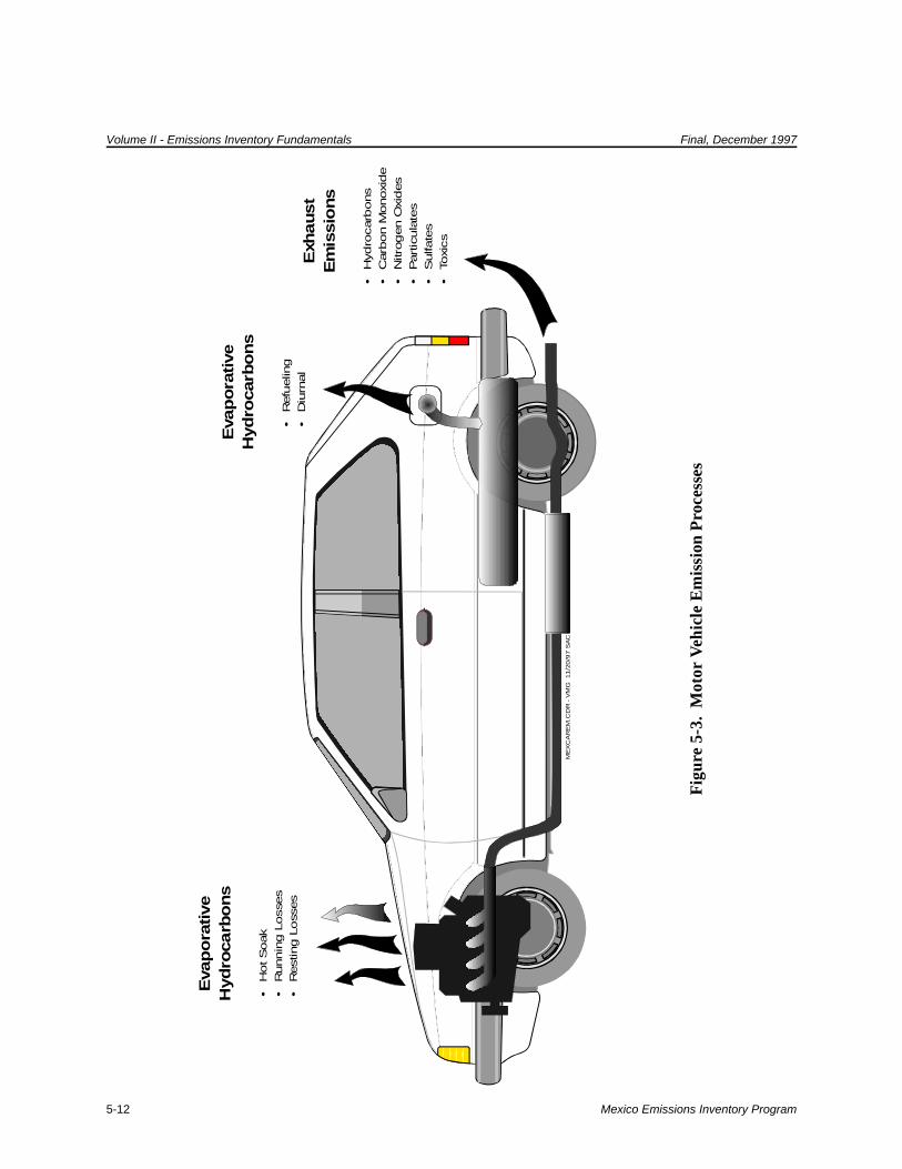
Volume II - Emissions Inventory Fundamentals Final, December 1997
Mexico Emissions Inventory Program5-12
Fig
ure
5-3.
Mot
or V
ehic
le E
mis
sion
Pro
cess
es
ME
XC
AR
EM
.CD
R -
VM
G
11
/20
/97
SA
C
Evapora
tive
Hydro
carb
ons
Evapora
tive
Hydro
carb
ons
Exh
aust
Em
issio
ns
•
Ho
t S
oa
k•
R
un
nin
g L
os
ses
•
Re
sti
ng
Lo
sse
s•
R
efu
elin
g•
D
iurn
al
•
Hy
dro
ca
rbo
ns
•
Ca
rbo
n M
on
oxi
de
•
Nit
rog
en
Oxi
de
s•
P
art
icu
late
s•
S
ulfa
tes
•
Toxi
cs

Final, December 1997 Volume II - Emissions Inventory Fundamentals
Mexico Emissions Inventory Program 5-13
• Resting evaporative emissions – Evaporative emissions other than hot soak,diurnal, and refueling emissions that occur while the engine is not operating. Resting losses occur primarily from fuel leaks and permeation of vapor throughfuel lines.
• Refueling evaporative emissions – Evaporative emissions displaced from thevehicle fuel tank during refueling. While the vehicle is the source of theemissions, they occur while the vehicle is stationary and at known locations,such as gasoline stations. Therefore, refueling emissions are typically treated asan area source and discussed in Volume V: Area Source Inventory Development. Refueling emission factors can either be estimated using the MOBILE model orobtained from other sources such as AP-42.
Interest in obtaining estimates of the on-road motor vehicle contribution to regional
emissions inventories in Mexico has been increasing, leading to the development of motor vehicle
emissions inventories for Mexico City, Monterrey, Ciudad Juárez, Guadalajara, and Toluca (Espinosa, et
al., 1996). In order to account for potentially different vehicle fleets and driving behavior in Mexico, the
U.S.-based MOBILE model has been modified for the Mexico City, Monterrey, and Ciudad Juárez
metropolitan areas. The MOBILE model estimates motor vehicle emission factors, which then must be
combined with appropriate activity data. Multiple modifications to the MOBILE model have been
performed, because it is known that vehicle fleet mix, fuels used, and driving behavior/conditions are not
homogeneous throughout Mexico. For example, in the border regions, the Mexican fleet may contain
more U.S. vehicles and larger quantities of U.S. fuels may be used. As another example, the high altitude
in Mexico City affects the fuel combustion process and, therefore, the emissions from motor vehicles.
5.5 Natural Sources
In addition to human activities, natural phenomena and plant and animal life can play an
important role in the air pollution problem. In some areas where natural source emissions may be
significant to the overall inventory, it is important to understand the contribution of natural sources, since
implementing control strategies generally can not readily reduce these emissions. Two significant natural
sources commonly considered in air emissions inventory efforts are described below.
Biogenic emissions. A number of researchers have established that vegetation (e.g.,
grass, crops, shrubs, forests, etc.) emits significant quantities of hydrocarbons to the atmosphere. Several

Volume II - Emissions Inventory Fundamentals Final, December 1997
Mexico Emissions Inventory Program5-14
studies (e.g., Pierce et al., 1990 and Robinson and Robbins, 1968) have shown that biogenic emissions
may be comparable to, or exceed, the emissions of nonmethane hydrocarbons (NMHC) from
anthropogenic sources in certain areas.
Emissions from soils. As mentioned earlier in the discussion about greenhouse gases in
Section 4.9, nitrous oxide (N2O) is produced naturally in soils by denitrification (i.e., the reduction of
nitrite or nitrate to gaseous nitrogen as N2 or NOx) and nitrification (i.e., the oxidation of ammonia to
nitrate). Commercial nitrogen fertilizers provide an additional nitrogen source, thereby increasing the
emissions of N2O from the soil. The rate of NOx emissions from soils is also dependent on other
variables such as soil type, moisture, temperature, season, crop type, and other agricultural practices.
Emissions of NOx from soils are estimated to be as much as 16 percent of the global amount of NOx in
the troposphere, and as much as 8 percent of the NOx in North America (U.S. EPA, 1993).
Wind erosion is another natural phenomenon that generates emissions. However,
because wind erosion emissions typically are associated with disturbed land, they are sometimes treated
as area sources. More detailed information on wind erosion emissions is presented in Section 11.5 of
Volume V of this Manual series, Area Source Inventory Development.
Some other smaller categories of natural sources include termites (CH4), lightning (NOx),
and volcanoes and other goethermal activity (SOx). More detailed information about natural sources may
be found in Volume VII of this Manual series, Natural Source Inventory Development.
5.6 Typical Source Category Checklist
The sources to be included in the inventory should be prioritized based on their
importance in the inventory. Resources should be allocated preferentially to the sources that are most
important in meeting the end-uses of the inventory. High priority sources include those that are known to
be significant contributors of air pollution, are known to be sources of specific targeted pollutants (e.g.,
PM10), or are most likely to impact air quality.
Table 5-2 is a typical checklist of source categories that might be included in an
inventory effort. For each source category, the primary expected emissions are presented by pollutant.

Final, December 1997 Volume II - Emissions Inventory Fundamentals
Mexico Emissions Inventory Program 5-15
Please note that this checklist should only be used as a tool to begin the process of identifying the
source categories to be included in an inventory. Region-specific conditions will likely lead to
additions or deletions to this checklist in order to obtain a complete inventory. For example,
bus/truck terminal, small scale brick manufacturing, charbroiling, and street vendors are not source
categories that are typically inventoried in the U.S., but they have been added to the checklist as potential
source categories for Mexico.

Table 5-2Example Checklist of Inventory Source Categories and Their Primary Pollutants
Source CategoryInventory Pollutants
TOG ROG CO NOx SOx PM PM10 PM2.5 NH3 EC OC HAPs CO2 N2O CH4 CFCs
Point Sources
Electric Utility T T T T T T T T T T T T T T T
Chemical Manufacturinga T T T T T T T T T T T T
Petroleum Refininga T T T T T T T T T T
Primary Metal Productiona T T T T T T T
Secondary Metal Productiona T T T T T T
Cement Productiona T T T T T T T T T
Miscellaneous Mineral Productiona T T T T T T
Automotive Industrya T T T
Wood Pulping Operationsa T T T T T T T T T
Oil and Gas Productiona T T T T
Printing and Publishing T T T
Surface Coating T T T
Bulk Terminals T T T
Mining and Quarryinga T T T T
Wood Products Manufacturea T T T T T T
Sugar Productiona T T T T T T
Tanning and Finishinga T T T
Glass Productiona T T T T T T
Rubber and Plastic Parts Productiona T T T
Fabricated Metal Productiona T T T T T T
Textile Productsa T T T T T T
Landfills T T T T T T T
Municipal Incinerators T T T T T T T T T T T T T T
Open Waste Burning T T T T T T T T T T T T T T
Asphalt Plantsa T T T T T T

Table 5-2(Continued)
Source CategoryInventory Pollutants
TOG ROG CO NOx SOx PM PM10 PM2.5 NH3 EC OC HAPs CO2 N2O CH4 CFCs
Food and Agriculturea T T T T T T T
Point Source Fuel Combustion T T T T T T T T T T T T T T T
Area Sources
Industrial and Commercial/Institutional Fuel Combustion
T T T T T T T T T T T T T T T
Residential Fuel Combustion(Commercial Fuels)
T T T T T T T T T T T T T T T
Residential Fuel Combustion(Biomass or Waste-derived Fuels)
T T T T T T T T T T T T T T T
Locomotives T T T T T T T T T T T T T T
Commercial Marine Vessels T T T T T T T T T T T T T T
Aircraft T T T T T T T T T T T T T T
Other Non-Road Mobile Equipment(Construction, Industrial,Recreational, etc.)
T T T T T T T T T T T T T T
Border Crossings T T T T T T T T T T T T T T
Bus/Truck Terminals T T T T T T T T T T T T T T
Industrial Surface Coating T T T
Auto Body Refinishing T T T
Architectural Surface Coating T T T
Traffic Paints T T T
Industrial Surface Cleaning(Degreasing)
T T T
Dry Cleaning T T T
Graphic Arts T T T
Asphalt Application T T T
Commercial/Consumer Solvent Use T T T

Table 5-2(Continued)
Source CategoryInventory Pollutants
TOG ROG CO NOx SOx PM PM10 PM2.5 NH3 EC OC HAPs CO2 N2O CH4 CFCs
Gasoline Distribution T T T
Aircraft Refueling T T T
LPG Distribution T T T
Bakeries T T T
Brick Manufacturing T T T T T T T T T T T T T T
Construction Activities T T T T T T
Charbroiling T T T T T T T T T T T T T T
Street Vendors T T T T T T T T T T T T T T
Pesticide Application T T T
Beef Cattle Feedlots T T T T T
Agricultural Burning T T T T T T T T T T T T T T T
Fertilizer Application T T T
Animal Waste T T T T T
Agricultural Tilling T T T T T T
On-Site Incineration T T T T T T T T T T T T T T T
Waste Management – Open Burning T T T T T T T T T T T T T T T
Wastewater Treatment T T T T T
Open Channel Sewage andWastewater
T T T T T
Wildfires/Prescribed Fires T T T T T T T T T T T T T T T
Structure Fires T T T T T T T T T T T T T T T
Paved Road Dust T T T T T T
Unpaved Road Dust T T T T T T
Wind Erosion T T T T T T
Domestic Ammonia Emissions T T
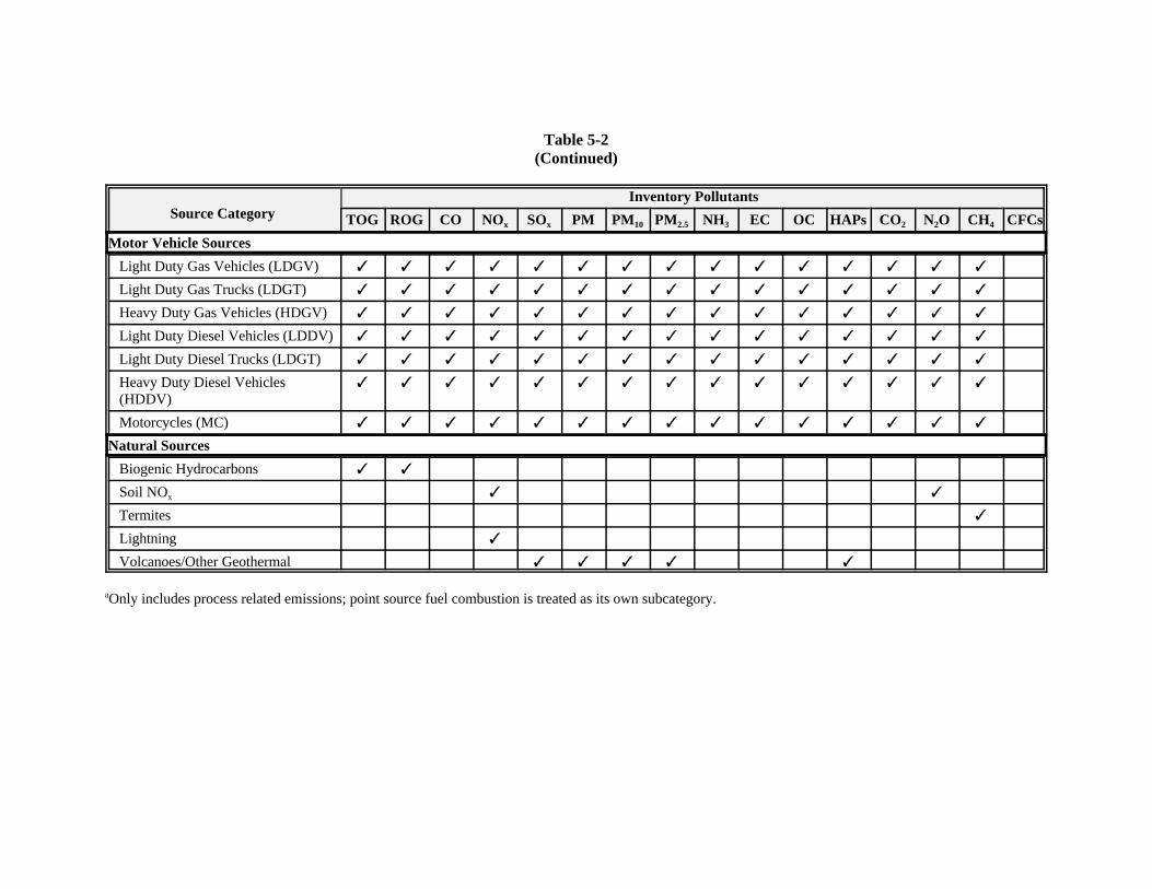
Table 5-2(Continued)
Source CategoryInventory Pollutants
TOG ROG CO NOx SOx PM PM10 PM2.5 NH3 EC OC HAPs CO2 N2O CH4 CFCs
Motor Vehicle Sources
Light Duty Gas Vehicles (LDGV) T T T T T T T T T T T T T T T
Light Duty Gas Trucks (LDGT) T T T T T T T T T T T T T T T
Heavy Duty Gas Vehicles (HDGV) T T T T T T T T T T T T T T T
Light Duty Diesel Vehicles (LDDV) T T T T T T T T T T T T T T T
Light Duty Diesel Trucks (LDGT) T T T T T T T T T T T T T T T
Heavy Duty Diesel Vehicles(HDDV)
T T T T T T T T T T T T T T T
Motorcycles (MC) T T T T T T T T T T T T T T T
Natural Sources
Biogenic Hydrocarbons T T
Soil NOx T T
Termites T
Lightning T
Volcanoes/Other Geothermal T T T T T
aOnly includes process related emissions; point source fuel combustion is treated as its own subcategory.

Mexico Emissions Inventory Program 6-1
6.0 Other Emissions InventoryCharacteristics
Two of the ten emissions inventory characteristics (pollutant types and source types)
were described in Sections 4.0 and 5.0. The remaining eight characteristics are described below. The
definition of these characteristics is determined primarily by the established purpose of the inventory.
6.1 Base Year
The base year of an inventory identifies the year for which emissions are estimated and
fixes an inventory’s position in time. This provides a benchmark against which previous and subsequent
inventories can be compared. It is important to establish a base year, so that all emission estimates have
a common basis and represent activities occurring during the same period of time.
Any year can be used as the inventory base year, but it is usually determined by the
established purpose of the inventory. For example, if it is desired to see the effects of recently
implemented control strategies, then the base year will be some year prior to the implementation of
control strategies. A comparison of current emission levels to historic levels might use a base year in the
past. The base year of an inventory might also be dictated by various regulatory requirements. The main
reason for this is so that emissions inventories from different regions can be easily compared with each
other and regulatory standards. In other cases, data availability might determine what the inventory base
year is. For example, it might be desired to develop an inventory for 1997, but if statistics to be used as
activity data have only been compiled through 1995, then 1995 would probably be a better base year than
1997.
6.2 Time Characteristics
There are two main time characteristics that must be considered for every inventory: time
period and temporal variability. Other minor time characteristics may be applicable for some inventories.
Time period refers to the length of time represented by the inventory. Inventory emissions will be
presented in units of mass of pollutant per inventory time period (e.g., kg CO/yr). For many large-scale
Volume II - Emissions Inventory Fundamentals Final, December 1997
Mexico Emissions Inventory Program6-2
inventories, the time period will typically be one year. However, some specialized inventory applications
may require shorter periods of time (e.g., one day, one month, the summer ozone season, the heating
season, etc.).
Temporal variability describes the variability of emissions over time. If emissions are
constant over time, then temporal variability is not of much concern. However, most emissions do
change over time. Depending upon the inventory requirements associated with the inventory purpose,
the emissions variations might need to be described on a seasonal, monthly, or daily basis. Specialized
inventories may even need emissions on an hourly (or shorter time period) basis. For instance, emissions
from on-road motor vehicles are variable over different time periods due to different levels of activity.
Weekday motor vehicle emissions might be higher than weekend emissions because of high levels of
vehicle activity associated with commuting to and from work. Also, as shown in Figure 6-1, emissions in
the morning and early evening are likely to be higher than emissions at noon or midnight because those
times are characterized by heavy commuting traffic. Because the temporal distribution for motor vehicle
activity presented in Figure 6-1 is U.S.-specific, Mexico motor vehicle activity may be distributed
differently. Depending upon the purpose of the inventory, one or more of these temporal variabilities
may need to be considered.
6.3 Spatial Characteristics
There are two primary spatial characteristics in any inventory: inventory domain and
spatial resolution. The inventory domain represents the area for which air pollutant sources will be
inventoried. The inventory domain is sometimes determined by the inventory purpose.
Often, the inventory domain follows political, geographic, or air quality agency
boundaries. Depending upon the inventory application, sources external to the defined inventory domain
that exert influence upon air quality within the domain due to meteorological transport may also need to
be addressed. A square hypothetical inventory domain measuring 25 km on a side is presented in
Figure 6-2.

Final, December 1997 Volume II - Emissions Inventory Fundamentals
Mexico Emissions Inventory Program 6-3
ME
XG
RA
PH
.CD
R -
VM
G
12
/17
/97
SA
C
Evening CommuteMorning Commute

Volume II - Emissions Inventory Fundamentals Final, December 1997
Mexico Emissions Inventory Program6-4

Final, December 1997 Volume II - Emissions Inventory Fundamentals
Mexico Emissions Inventory Program 6-5
Spatial resolution describes how specifically the geographic location of pollution sources
must be defined. Basic inventories will sometimes provide pollutant totals only for the entire inventory
domain. More complex inventories, particularly those associated with air quality modeling efforts, will
often require a more detailed description of emissions distribution. The resolution of area, motor vehicle,
and natural sources within an inventory domain is usually done using grid cells. The inventory domain
presented in Figure 6-2 contains 25 grid cells measuring 5 km on a side. Typically, the desired air quality
accuracy determines the required grid cell size. However, in general, the required grid cell size is also
indicated by the domain size – large inventory domains will have grid cells that typically measure several
kilometers on a side, while smaller inventory domains can have grid cells that measure a few hundred
meters on a side. From Figure 6-2, the following spatial distribution of emissions can be seen:
• Population/Residential Area Sources: Cells A1 and A2;
• Agricultural Area Sources: Cells B3, B4, C3, C4, D3, and D4;
• Marine Sources: Cells A3, A4, A5, and B5;
• Motor Vehicles: Cells A1, A2, B1, B2, C2, D2, D3, D4, E2, E4, and E5; and
• Natural Biogenic Sources: Cells C5, D5, E1, E2, E3, and E4.
For most types of inventories, point sources will need to be geographically located using
either latitude and longitude coordinates or Universal Transverse Mercator (UTM) coordinates. For
some complex inventory efforts, the required geographical accuracy for point source locations may be as
close as ±10 meters. In Figure 6-2, the three point sources located in cells B1, C1, and C2 will require
detailed location coordinates.
6.4 Species Resolution
Species resolution refers to disaggregating an inventory pollutant (e.g., TOG, PM, etc.)
into its individual chemical components (e.g., toluene, lead, EC, OC, etc.) or into specific groups (e.g.,
paraffins, aromatics, etc.). The need for species resolution, as well as the specific methodology, is
determined by the inventory purpose. Species resolution is primarily performed using speciation profiles
that describe the fraction of individual chemical species. Many inventories will not include detailed
species resolution; other specialized inventory applications will require it. These applications include air

Volume II - Emissions Inventory Fundamentals Final, December 1997
Mexico Emissions Inventory Program6-6
toxics inventories, photochemical modeling, and chemical mass balance modeling used for source
attribution.
As discussed in Section 4.8, air toxics inventories seek to quantify the amount of
hazardous air pollutants (HAPs) that are emitted. Ideally, this would be performed using emission
factors for individual HAPs. Although there are some HAP emission factors for combustion and other
sources, emission factors often do not exist. As a result, individual HAP species frequently are
disaggregated from TOG and PM by using speciation profiles. As mentioned in Section 4.8, this is not
the preferred approach for estimating HAPs emissions. If this approach is used, it often results in an
overestimation of HAPs. This approach is demonstrated in Figure 6-3.
In photochemical modeling, speciation is needed because emitted hydrocarbon species
have different photochemical reactivities. Total hydrocarbon emissions are calculated and then speciated
into different hydrocarbon groups. In order to properly represent the chemical reactions occurring in the
atmosphere, each species group is assigned an appropriate level of photochemical reactivity.
Finally, source attribution (or receptor modeling) through the use of a chemical mass
balance requires fairly detailed species resolution. Source attribution can be determined working
backward from measured TOG and particulate concentrations at a monitoring site using computerized
linear algebra matrix calculations. In this instance, species resolution provides the unique chemical
content (usually for metals and hydrocarbons) of the emissions for each source type. This chemical
content serves as the “fingerprint” for the presence of material from that source in ambient sample data at
the receptor. Without species resolution, implementation of this application is impossible. More
information on source attribution can be found in some recent source attribution studies (Watson et al.,
1984; Chow et al., 1992; and Scheff et al., 1984).

Final, December 1997 Volume II - Emissions Inventory Fundamentals
Mexico Emissions Inventory Program 6-7
Annual PM Emissions
(250 Mg/yr)1 0
= 5 Mg/yr
Speciation Profile
Cu (8%)
Cd (4%)
Hg (2%)
Non-HAP PM (86%)1 0
Cu Cd Hg
Non-HAP PM1 0
Cu
Cd
Hg
Non-HAPPM
1 0
20 Mg/yr
10 Mg/yr
5 Mg/yr
215 Mg/yr
Figure 6-3. Hypothetical HAPs Speciation
ME
XH
AP
S.C
DR
- V
MG
1
1/1
7/9
7 S
AC

Volume II - Emissions Inventory Fundamentals Final, December 1997
Mexico Emissions Inventory Program6-8
6.5 Quality Assurance
Quality assurance (QA) is an indispensable element of any emissions inventory.
Regardless of what type of inventory is being conducted, QA is necessary. The amount and focus of QA,
however, will be variable depending upon the specific inventory purpose. For instance, a detailed large-
scale modeling inventory will typically require significantly more QA than a facility-level reporting
inventory would. Also, if one particular source type had been preliminarily identified as a large pollutant
source, then more QA resources could be directed at this source type rather than at some of the more
minor source types.
QA should be conducted throughout the development of the inventory rather than as an
afterthought conducted at the last minute. Some example QA activities include:
• Using a source category checklist (such as the one presented in Table 5-2),confirm that all necessary source categories have been included in the inventory;
• Check sampling results and activity data for “outliers” prior to emissioncalculations;
• Confirm that all emission calculations have been performed properly; and
• Compare inventory results with emissions inventories in similar regions.
There are also many other QA activities not listed above that can be devised which will
help ensure a high quality emissions inventory.
Although the results of an inventory might affect how QA is conducted later in the
inventory effort, QA resources should be identified at the beginning. To the greatest extent possible, the
type of QA (e.g., detailed “line-by-line” QA or high-level QA) and areas requiring concentrated QA
should be designated at the outset of the inventory effort.
6.6 Data Management
Another essential emissions inventory characteristic is the data management required for
the inventory. With the widespread use of computers and increasing inventory data requirements,

Final, December 1997 Volume II - Emissions Inventory Fundamentals
Mexico Emissions Inventory Program 6-9
virtually all inventory data are currently handled electronically. Consideration should be given to
whether data management should be performed using a spreadsheet-type application or a database
application. Spreadsheets tend to be easier to use, but databases are much more powerful. The method
of transfer of inventory-related information and any data confidentiality requirements should also be
established early in the inventory development process. The inventory purpose will help determine what
type of data management is required. For instance, an inventory used as an air quality model input might
require different data management than an inventory designed for regulatory compliance. Also, expected
future uses of the inventory might influence the type of data management selected.
6.7 Projections
Projections forecast a base year inventory forward or backward in time. The use of
projections is primarily determined by the inventory purpose. Many inventories will not develop
projected emissions. Projections are mainly used to track past and future emission trends due to activity
growth and implemented control strategies. Projections are also used extensively in theoretical analyses
of various control strategies proposed for future implementation. For example, projections could be used
to estimate future motor vehicle emissions based upon expected population growth. Likewise,
projections could be used to track estimated emission reductions due to the proposed phase-in of
reformulated paints that contain lower levels of solvents. Growth projections of emissions are usually
based upon growth projections of other surrogates (e.g., population, economic activity). Control
projections, on the other hand, are often based on estimated reductions from control strategies.
Projection methodologies and required data should be established early in the inventory development
process. U.S. EPA has published guidance regarding emissions projection that contains various
references and methodologies (U.S. EPA, 1991b).
6.8 Uncertainty Estimation
The final emissions inventory characteristic is uncertainty estimation. Uncertainty
estimates are a valuable tool to assess the accuracy of an emissions inventory.
Uncertainty can be estimated quantitatively or qualitatively. Quantitative uncertainty
estimates are unusual. There are several reasons for this. First of all, there is no agreed upon method for

Volume II - Emissions Inventory Fundamentals Final, December 1997
Mexico Emissions Inventory Program6-10
making quantitative estimates of uncertainty. Also, the derivation of quantitative uncertainty estimates
can become very statistically complex. Finally, a large number of assumptions typically are required to
make quantitative uncertainty estimates.
In general, when uncertainty estimates are made, they are most commonly qualitative in
nature. Qualitative estimates of uncertainty may focus on methodologies, activity data, emission-related
data, underlying assumptions, or other components of inventory development. For example, an inventory
assumption that emissions from surface coating operations are limited only to solvent contained in the
applied surface coating (and not from surface preparation and/or cleanup solvents) will almost certainly
lead to an underestimate of TOG emissions in the inventory. In a similar manner, an assumption that all
point sources use the same fuel and operate on the same operating schedule will generate uncertainty in
the inventory, although it may not be clear if this would result in an overestimate or an underestimate.
Although qualitative estimates do not statistically calculate the uncertainty of an emissions inventory,
they are valuable because they point out potential weaknesses in the inventory.

Mexico Emissions Inventory Program 7-1
7.0 Iteration of InventoryProcessThe technical steps of emissions inventory development were previously shown in
Figure 2-1. These steps begin with the identification of the inventory purpose and end with the
documentation of the inventory results. It is important to note that even if all of the steps presented in
Figure 2-1 are properly implemented during inventory development, it simply represents one iteration of
emissions inventory development. Multiple iterations are usually required for the development of high
quality emissions inventories. This iteration concept is represented by the puzzles presented in
Figure 7-1. Early inventories will be characterized by missing information and other imperfections;
subsequent updated inventories will gradually improve in quality.
The end goal is to develop an emissions inventory that is a comprehensive, accurate, and
current accounting of air pollutant emissions and associated data from sources within a given geographic
area over a specific time interval. However, practical limitations necessitate an iterative approach to
accomplish this objective. Systematic, iterative inventory development, over time, will reduce the
amount of inventory uncertainty and improve the overall quality of the emissions inventory.
An emissions inventory should be comprehensive, which is to say that all sources of the
identified inventory pollutants should be included. Limited resources may reduce the number of
inventoried sources to a subset of the total existing sources. Likewise, some emission sources may be
unnoticed or overlooked during the initial inventory process. Subsequent inventory revisions are used to
fill in missing sources.
To the greatest extent possible, an emissions inventory should also be accurate.
Incorrect data or overly simplistic assumptions will introduce inaccuracies into the inventory. These
inaccuracies can be corrected in later inventory iterations with more complete or improved information.

Volume II - Emissions Inventory Fundamentals Final, December 1997
Mexico Emissions Inventory Program7-2
MEXCYCLE.CDR - VMG 12/17/97 SAC 1
Fig
ure
7-1.
Em
issi
ons
Inve
ntor
y It
erat
ions
INIT
IAL
EM
ISS
ION
SIN
VE
NTO
RY
EM
ISS
ION
SIN
VE
NTO
RY
FIR
ST
RE
VIS
ION
SE
CO
ND
RE
VIS
ION

Final, December 1997 Volume II - Emissions Inventory Fundamentals
Mexico Emissions Inventory Program 7-3
Finally, an emissions inventory should represent current emissions. Some inventory
applications will be updated every year and will require current information for that specific year. These
inventories will be updated annually to track the increase of emissions due to growth in the emission-
producing activity or the decrease of emissions due to the implementation of various emission control
strategies. Outdated data and information should be updated in later inventory iterations.

Mexico Emissions Inventory Program 8-1
8.0 ReferencesAP-42, 1995. Compilation of Air Pollution Emission Factors (AP-42) - Volume I: Stationary Point andArea Sources, Fifth Edition. U.S. Environmental Protection Agency, Office of Air Quality Planning andStandards, Research Triangle Park, North Carolina. January.
ARB, 1996. California Air Toxics Emission Factor (CATEF) Database, Version 1.2. California AirResources Board, Sacramento, California. April.
CFR, 1997. U.S. EPA definition of VOC. 40 Code of Federal Regulations (CFR) 51.100(s). Latestamendment: Federal Register, Vol. 62, No. 164. August 25, 1997. pp. 44900 - 44903.
Chow, J.C., J.G. Watson, D.H. Lowenthal, P.A. Solmon, K.L. Magliano, S.D. Ziman, and L.W. Richards,1992. “PM10 Source Apportionment in California’s San Joaquin Valley,” Atmospheric Environment26A:3335-3354.
De Soete, G., 1989. Updated Evaluation of Nitrous Oxide Emissions from Industrial Fossil FuelCombustion. Report to the European Atomic Energy Community. Institute Francais du Petrole, Ref. 37-559.
EIIP, 1997. Emissions Inventory Improvement Program technical reports. Internet address -http://www.epa.gov/ttn/chief/eiip/techrep.htm.
Espinosa, M.E., V.H. Páramo, and J. Sarmiento, 1996. Mobile Sources Inventories in Mexico, Paper 96-RA108A.02. Presented at the 89th Annual Meeting of the Air & Waste Management Association,Nashville, Tennessee. June.
IPCC, 1993. Preliminary IPCC National GHG Inventories: In-Depth Review, Part III. Intergovernmental Panel on Climate Control. Presented at IPCC/OECD Workshop on National GHGInventories: Transparency in Estimating and Reporting. The Hadley Centre, Bracknell, United Kingdom. 1 October.
Pierce, T.W., B.K. Lamb, and A.R. Van Meter, 1990. Development of a Biogenic Emissions InventorySystem for Regional Scale Air Pollution Models, Paper 90094.3. Presented at the 83rd Annual Meetingof the Air and Waste Management Association, Pittsburgh, Pennsylvania, June 24-29.
Robinson, E., and R.C. Robbins, 1968. Sources, Abundance, and Fate of Gaseous AtmosphericPollutants. Report SRI Project PR6755, Stanford Research Institute, Menlo Park, California, pp. 1-122.
Scheff, P.A., R.A. Wadden, D.M. Kenski, and J. Chang, 1984. Receptor Model Evaluation of theSEMOS Ambient NMOC Measurements, Paper 84-72.3. Presented at the 77th Annual Meeting of the AirPollution Control Association, San Francisco, California. June.
Seinfeld, J.H., 1986. Atmospheric Chemistry and Physics of Air Pollution. John Wiley & Sons, Inc.,New York.

Volume II - Emissions Inventory Fundamentals Final, December 1997
Mexico Emissions Inventory Program8-2
U.S. EPA, 1991a. Procedures for the Preparation of Emission Inventories for the Preparation ofEmission Inventories for Carbon Monoxide and Precursors of Ozone. Volume I: General Guidance forStationary Sources. U.S. Environmental Protection Agency, Office of Air Quality Planning andStandards, Research Triangle Park, North Carolina. EPA-450/4-91-016.
U.S. EPA, 1991b. Procedures for Preparing Emissions Projections. U.S. Environmental ProtectionAgency, Office of Air Quality Planning and Standards, Research Triangle Park, North Carolina. EPA450/4-91-019. Internet address - http://www.epa.gov/ttn/chief/ei_guide.html.
U.S. EPA, 1993. Air Quality Criteria For NOx, Volume I, U.S. Environmental Protection Agency,Research Triangle Park, North Carolina. EPA 600/8-91/049a, pp. 4-11 to 4-14.
U.S. EPA, 1995. Factor Information Retrieval System (FIRE), Version 4.0. U.S. EnvironmentalProtection Agency, Office of Air Quality Planning and Standards, Research Triangle Park, NorthCarolina. June.
Watson, J.G., J.A. Cooper, and J.J. Huntzicker, 1984. “The Effective Variance Weighting for LeastSquares Calculations Applied to the Mass Balance Receptor Model,” Atmospheric Environment 18:1347-1355.
WMO, 1992. Scientific Assessment of Ozone Deletion: 1991. WMO/UNEP, WMO Global OzoneResearch and Monitoring Project, Report No. 25, Geneva, Austria.
Mexico Emissions Inventory Program A-1
APPENDIX A
NON-REACTIVE HYDROCARBONS

Volume II - Emissions Inventory Fundamentals Final, December 1997
Mexico Emissions Inventory ProgramA-2
U.S. EPA Photochemically Non-Reactive Compounds
Chemical Synonym
methane
ethane
methylene chloride dichloromethane
1,1,1-trichloroethane methyl chloroform
1,1,2-trichloro 1,2,2-trifluoroethane CFC–113
trichlorofluoromethane CFC–11
dichlorodifluoromethane CFC–12
chlorodifluoromethane HCFC–22
trifluoromethane HFC–23
1,2-dichloro 1,1,2,2-tetrafluoroethane CFC–114
chloropentafluoroethane CFC–115
1,1,1-trifluoro 2,2-dichloroethane HCFC–123
1,1,1,2-tetrafluoroethane HFC–134a
1,1-dichloro 1-fluoroethane HCFC–141b
1-chloro 1,1-difluoroethane HCFC–142b
2-chloro 1,1,1,2-tetrafluoroethane HCFC–124
pentafluoroethane HFC–125
1,1,2,2-tetrafluoroethane HFC–134
1,1,1-trifluoroethane HFC–143a
1,1-difluoroethane HFC–152a
parachlorobenzotrifluoride PCBTF
cyclic, branched, or linear completely methylated siloxanes
acetone
perchloroethylene tetrachloroethylene
3,3-dichloro-1,1,1,2,2-pentafluoropropane HCFC–225ca
1,3-dichloro-1,1,2,2,3-pentafluoropropane HCFC–225cb
1,1,1,2,3,4,4,5,5,5-decafluoropentane HFC–43–10mee
difluoromethane HFC–32
ethylfluoride HFC–161
1,1,1,3,3,3-hexafluoropropane HFC–236fa
1,1,2,2,3-pentafluoropropane HFC–245ca
1,1,2,3,3-pentafluoropropane HFC–245ea
1,1,1,2,3-pentafluoropropane HFC–245eb

Final, December 1997 Volume II - Emissions Inventory Fundamentals
Mexico Emissions Inventory Program A-3
U.S. EPA Photochemically Non-Reactive Compounds(Continued)
Chemical Synonym
1,1,1,3,3-pentafluoropropane HFC–245fa
1,1,1,2,3,3-hexafluoropropane HFC–236ea
1,1,1,3,3-pentafluorobutane HFC–365mfc
chlorofluoromethane HCFC–31
1-chloro 1-fluoroethane HCFC–151a
1,2-dichloro 1,1,2-trifluoroethane HCFC–123a
1,1,1,2,2,3,3,4,4-nonafluoro-4-methoxy-butane C4F9OCH3
2-(difluoromethoxymethyl) 1,1,1,2,3,3,3-heptafluoropropane (CF3)2CFCF2OCH3
1-ethoxy 1,1,2,2,3,3,4,4,4-nonafluorobutane C4F9OC2H5
2-(ethoxydifluoromethyl) 1,1,1,2,3,3,3-heptafluoropropane (CF3)2CFCF2OC2H5
perfluorocarbon compounds which fall into these classes:
(i) Cyclic, branched, or linear, completely fluorinated alkanes;
(ii) Cyclic, branched, or linear, completely fluorinated etherswith no unsaturations;
(iii) Cyclic, branched, or linear, completely fluorinated tertiaryamines with no unsaturations; and
(iv) Sulfur containing perfluorocarbons with no unsaturationsand with sulfur bonds only to carbon and fluorine.
Source: Federal Register, Vol. 62, No. 164. August 25, 1997. pp. 44900 – 44903.
Mexico Emissions Inventory Program B-1
APPENDIX B
HAZARDOUS AIR POLLUTANTS

Volume II - Emissions Inventory Fundamentals Final, December 1997
Mexico Emissions Inventory ProgramB-2
United States Federal Hazardous Air Pollutants(from Clean Air Act – Section 112(b))
CAS Number Chemical Name
75-07-0 Acetaldehyde
60-35-5 Acetamide
75-05-8 Acetonitrile
98-86-2 Acetophenone
53-96-3 2-Acetylaminofluorene
107-02-8 Acrolein
79-06-1 Acrylamide
79-10-7 Acrylic acid
107-13-1 Acrylonitrile
107-05-1 Allyl chloride
92-67-1 4-Aminobiphenyl
62-53-3 Aniline
90-04-0 o-Anisidine
1332-21-4 Asbestos
71-43-2 Benzene (including benzene from gasoline)
92-87-5 Benzidine
98-07-7 Benzotrichloride
100-44-7 Benzyl chloride
92-52-4 Biphenyl
117-81-7 Bis(2-ethylhexyl)phthalate (DEHP)
542-88-1 Bis(chloromethyl) ether
75-25-2 Bromoform
106-99-0 1,3-Butadiene
156-62-7 Calcium cyanamide
105-60-2 Caprolactam
133-06-2 Captan
63-25-2 Carbaryl
75-15-0 Carbon disulfide
56-23-5 Carbon tetrachloride
463-58-1 Carbonyl sulfide
120-80-9 Catechol
133-90-4 Chloramben
57-74-9 Chlordane
7782-50-5 Chlorine

Final, December 1997 Volume II - Emissions Inventory Fundamentals
Mexico Emissions Inventory Program B-3
United States Federal Hazardous Air Pollutants(Continued)
CAS Number Chemical Name
79-11-8 Chloroacetic acid
532-27-4 2-Chloroacetophenone
108-90-7 Chlorobenzene
510-15-6 Chlorobenzilate
67-66-3 Chloroform
107-30-2 Chloromethyl methyl ether
126-99-8 Chloroprene
1319-77-3 Cresol/Cresylic acid (mixed isomers)
95-48-7 o-Cresol
108-39-4 m-Cresol
106-44-5 p-Cresol
98-82-8 Cumene
94-75-7 2,4-D (including salts and esters)
72-55-9 DDE
334-88-3 Diazomethane
132-64-9 Dibenzofuran
96-12-8 1,2-Dibromo-3-chloropropane
84-74-2 Dibutyl phthalate
106-46-7 1,4-Dichlorobenzene
91-94-1 3,3'-Dichlorobenzidine
111-44-4 Dichloroethyl ether (Bis[2-chloroethyl]ether)
542-75-6 1,3-Dichloropropene
62-73-7 Dichlorvos
111-42-2 Diethanolamine
121-69-7 N,N-Dimethylaniline
64-67-5 Diethyl sulfate
119-90-4 3,3'-Dimethoxybenzidine
60-11-7 4-Dimethylaminoazobenzene
119-93-7 3,3'-Dimethylbenzidine
79-44-7 Dimethylcarbamoyl chloride
68-12-2 Dimethylformamide
57-14-7 1,1-Dimethylhydrazine
131-11-3 Dimethyl phthalate
77-78-1 Dimethyl sulfate

Volume II - Emissions Inventory Fundamentals Final, December 1997
Mexico Emissions Inventory ProgramB-4
United States Federal Hazardous Air Pollutants(Continued)
CAS Number Chemical Name
N/A 4,6-Dinitro-o-cresol (including salts)
51-28-5 2,4-Dinitrophenol
121-14-2 2,4-Dinitrotoluene
123-91-1 1,4-Dioxane (1,4-Diethyleneoxide)
122-66-7 1,2-Diphenylhydrazine
106-89-8 Epichlorohydrin (l-Chloro-2,3-epoxypropane)
106-88-7 1,2-Epoxybutane
140-88-5 Ethyl acrylate
100-41-4 Ethyl benzene
51-79-6 Ethyl carbamate (Urethane)
75-00-3 Ethyl chloride (Chloroethane)
106-93-4 Ethylene dibromide (Dibromoethane)
107-06-2 Ethylene dichloride (1,2-Dichloroethane)
107-21-1 Ethylene glycol
151-56-4 Ethylene imine (Aziridine)
75-21-8 Ethylene oxide
96-45-7 Ethylene thiourea
75-34-3 Ethylidene dichloride (1,1-Dichloroethane)
50-00-0 Formaldehyde
76-44-8 Heptachlor
118-74-1 Hexachlorobenzene
87-68-3 Hexachlorobutadiene
77-47-4 Hexachlorocyclopentadiene
67-72-1 Hexachloroethane
822-06-0 Hexamethylene diisocyanate
680-31-9 Hexamethylphosphoramide
110-54-3 Hexane
302-01-2 Hydrazine
7647-01-0 Hydrochloric acid (Hydrogen chloride [gas only])
7664-39-3 Hydrogen fluoride (Hydrofluoric acid)
123-31-9 Hydroquinone
78-59-1 Isophorone
N/A Lindane (all isomers)
108-31-6 Maleic anhydride
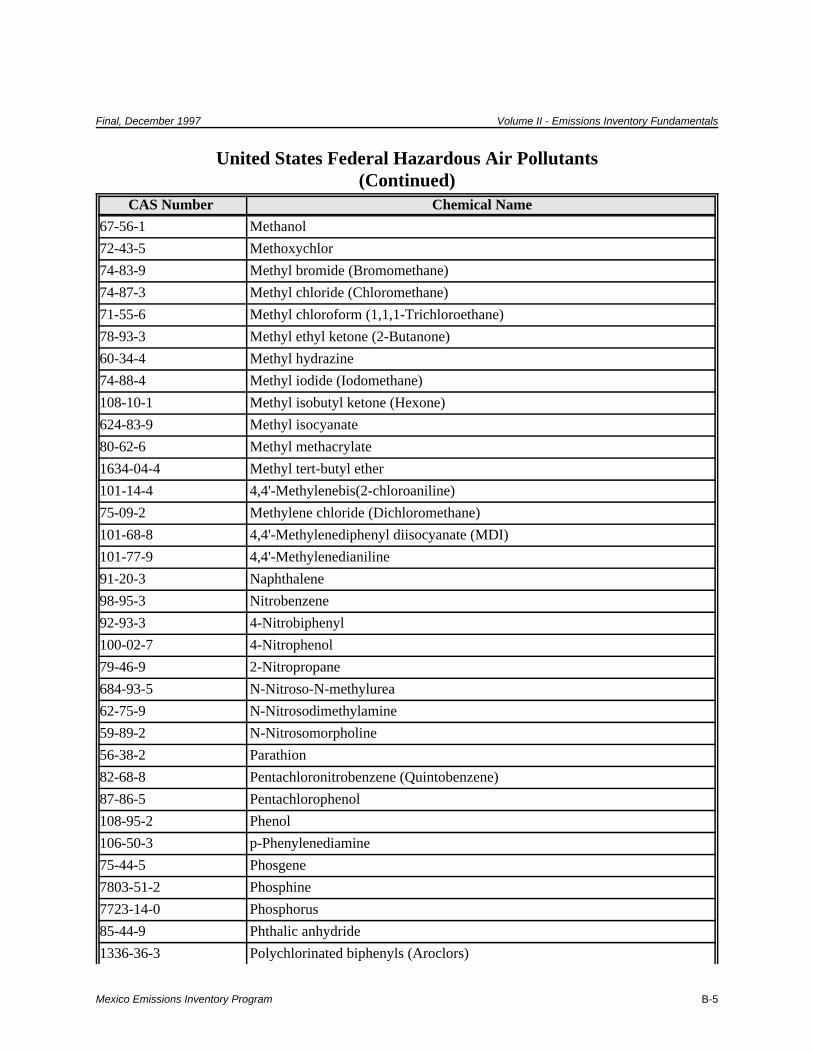
Final, December 1997 Volume II - Emissions Inventory Fundamentals
Mexico Emissions Inventory Program B-5
United States Federal Hazardous Air Pollutants(Continued)
CAS Number Chemical Name
67-56-1 Methanol
72-43-5 Methoxychlor
74-83-9 Methyl bromide (Bromomethane)
74-87-3 Methyl chloride (Chloromethane)
71-55-6 Methyl chloroform (1,1,1-Trichloroethane)
78-93-3 Methyl ethyl ketone (2-Butanone)
60-34-4 Methyl hydrazine
74-88-4 Methyl iodide (Iodomethane)
108-10-1 Methyl isobutyl ketone (Hexone)
624-83-9 Methyl isocyanate
80-62-6 Methyl methacrylate
1634-04-4 Methyl tert-butyl ether
101-14-4 4,4'-Methylenebis(2-chloroaniline)
75-09-2 Methylene chloride (Dichloromethane)
101-68-8 4,4'-Methylenediphenyl diisocyanate (MDI)
101-77-9 4,4'-Methylenedianiline
91-20-3 Naphthalene
98-95-3 Nitrobenzene
92-93-3 4-Nitrobiphenyl
100-02-7 4-Nitrophenol
79-46-9 2-Nitropropane
684-93-5 N-Nitroso-N-methylurea
62-75-9 N-Nitrosodimethylamine
59-89-2 N-Nitrosomorpholine
56-38-2 Parathion
82-68-8 Pentachloronitrobenzene (Quintobenzene)
87-86-5 Pentachlorophenol
108-95-2 Phenol
106-50-3 p-Phenylenediamine
75-44-5 Phosgene
7803-51-2 Phosphine
7723-14-0 Phosphorus
85-44-9 Phthalic anhydride
1336-36-3 Polychlorinated biphenyls (Aroclors)

Volume II - Emissions Inventory Fundamentals Final, December 1997
Mexico Emissions Inventory ProgramB-6
United States Federal Hazardous Air Pollutants(Continued)
CAS Number Chemical Name
1120-71-4 1,3-Propane sultone
57-57-8 beta-Propiolactone
123-38-6 Propionaldehyde
114-26-1 Propoxur (Baygon)
78-87-5 Propylene dichloride (1,2-Dichloropropane)
75-56-9 Propylene oxide
75-55-8 1,2-Propylenimine (2-Methylaziridine)
91-22-5 Quinoline
106-51-4 Quinone (p-Benzoquinone)
100-42-5 Styrene
96-09-3 Styrene oxide
1746-01-6 2,3,7,8-Tetrachlorodibenzo-p-dioxin
79-34-5 1,1,2,2-Tetrachloroethane
127-18-4 Tetrachloroethylene (Perchloroethylene)
7550-45-0 Titanium tetrachloride
108-88-3 Toluene
95-80-7 Toluene-2,4-diamine
584-84-9 2,4-Toluene diisocyanate
95-53-4 o-Toluidine
8001-35-2 Toxaphene (chlorinated camphene)
120-82-1 1,2,4-Trichlorobenzene
79-00-5 1,1,2-Trichloroethane
79-01-6 Trichloroethylene
95-95-4 2,4,5-Trichlorophenol
88-06-2 2,4,6-Trichlorophenol
121-44-8 Triethylamine
1582-09-8 Trifluralin
540-84-1 2,2,4-Trimethylpentane
108-05-4 Vinyl acetate
593-60-2 Vinyl bromide
75-01-4 Vinyl chloride
75-35-4 Vinylidene chloride (1,1-Dichloroethylene)
1330-20-7 Xylene (mixed isomers)
95-47-6 o-Xylene

Final, December 1997 Volume II - Emissions Inventory Fundamentals
Mexico Emissions Inventory Program B-7
United States Federal Hazardous Air Pollutants(Continued)
CAS Number Chemical Name
108-38-3 m-Xylene
106-42-3 p-Xylene
N/A Antimony Compoundsa
N/A Arsenic Compoundsa (inorganic including arsine)
N/A Beryllium Compoundsa
N/A Cadmium Compoundsa
N/A Chromium Compoundsa
N/A Cobalt Compoundsa
N/A Coke Oven Emissions
N/A Cyanide Compoundsa,b
N/A Glycol ethersc
N/A Lead Compoundsa
N/A Manganese Compoundsa
N/A Mercury Compoundsa
N/A Fine mineral fibersd
N/A Nickel Compoundsa
N/A Polycyclic Organic Mattere
N/A Radionuclides (including radon)f
N/A Selenium Compoundsa
a For all listings above which contain the word "compounds" and for glycol ethers, the following applies: Unless otherwise specified, theselistings are defined as including any unique chemical substance that contains the named chemical (i.e., antimony, arsenic, etc.) as part of thatchemical's infrastructure.
b X'CN where X = H' or any other group where a formal dissociation may occur. For example, KCN or Ca(CN)2.
c Includes mono- and di- ethers of ethylene glycol, diethylene glycol, and triethylene glycol R-(OCH2CH2)n-OR'
where:n = 1, 2, or 3R = alkyl or aryl groups R' = R, H, or groups which, when removed, yield glycol ethers with the structure: R-(OCH2CH2)n-OH.Polymers are excluded from the glycol category.
d Includes mineral fiber emissions from facilities manufacturing or processing glass, rock, or slag fibers (or other mineral derived fibers) ofaverage diameter 1 micrometer or less. e Includes substituted and/or unsubstituted polycyclic aromatic hydrocarbons and aromatic heterocycle compounds, with two or more fusedrings, at least one of which is benzenoid in structure. Polycyclic Organic Matter is a mixture of organic compounds containing one or more ofthese polycyclic aromatic chemicals. Polycyclic Organic Matter is generally formed or emitted during thermal processes including (1)incomplete combustion, (2) pyrolysis, (3) the volatilization, distillation or processing of fossil fuels or bitumens, or (4) the distillation or thermalprocessing of non-fossil fuels.
f A type of atom which spontaneously undergoes radioactive decay.


