Migration Equilibrium

Anna Nagurney

Isenberg School of Management

University of Massachusetts

Amherst, MA 01003

c©2002

Migration Equilibrium

Human migration is a topic that has received atten-tion from economists, demographers, sociologists, andgeographers. In this lecture, we focus on the develop-ment of a network framework using variational inequalitytheory in an attempt to formalize this challenging prob-lem domain. In particular, we explore the utilization ofvariational inequality theory in conceptualizing complexproblems in migration networks.

A series of migration models is presented of increasing

complexity and generality. We assume that each class

of migrant has a utility associated with locations, where

the utilities are functions of the population distribution

pattern. The framework is similar in spirit to the one

developed by Beckmann (1957), who also focused on

migratory flows and assumed that the attractiveness of

a location was a function of the population distribution

pattern.

1

Costless Migration

We first describe a model of human migration, whichis shown to have a simple, abstract network structurein which the links correspond to locations and the flowson the links to populations of a particular class at theparticular location.

Assume a closed economy in which there are n loca-

tions, typically denoted by i, and J classes, typically

denoted by k. Assume further that the attractiveness

of any location i as perceived by class k is represented

by a utility uki . Let pk denote the fixed and known pop-

ulation of class k in the economy, and let pki denote the

population of class k at location i. Group the utilities

into a row vector u ∈ RJn and the populations into a

column vector p ∈ RJn. Assume no births and no deaths

in the economy.

2

The conservation of flow equation for each class k isgiven by

pk =n∑

i=1

pki (1)

where pki≥0, ∀k=1, . . . , J; i=1,. . . , n. Equation (1) states

that the population of each class k must be conservedin the economy.

Let K ≡ {p|p ≥ 0, and satisfy (1)}.Assume that the migrants are rational and that migra-tion will continue until no individual of any class hasany incentive to move since a unilateral decision will nolonger yield an increase in the utility. Mathematically,hence, a multiclass population vector p∗ ∈ K is said tobe in equilibrium if for each class k; k =1,. . .,J:

uki

{= λk, if pk

i∗

> 0≤ λk, if pk

i∗= 0.

(2)

Equilibrium conditions (2) state that for a given class

k only those locations i with maximal utility equal to

an indicator λk will have a positive volume of the class.

Moreover, the utilities for a given class are equilibrated

across the locations.

3

The function structure is now addressed. Assume that,in general, the utility associated with a particular loca-tion as perceived by a particular class, may depend uponthe population associated with every class and every lo-cation, that is, assume that

u = u(p). (3)

Note that in allowing the utility to depend upon thepopulations of the classes, we are, in essence, usingpopulations as a proxy for amenities associated witha particular location; at the same time, such a utilityfunction can handle the negative externalities associ-ated with overpopulation, such as congestion, increasedcrime, competition for scarce resources, etc.

The above migration model is equivalent to a network

equilibrium model with a single origin/destination pair

and fixed demands. Indeed, make the identification as

follows. Construct a network consisting of two nodes,

an origin node 0 and a destination node 1, and n links

connecting the origin node to the destination node (cf.

Figure 1).

4

m

m

1

0

R U

1 2 · · · n−u1

1, . . . ,−uJ1 −u1

n, . . . ,−uJn

p1 =∑n

i=1 p1i , . . . , pJ =

∑ni=1 pJ

i

Network equilibrium formulation of costlessmigration

5

If we associate then with each link i, J costs: −u1i , . . . ,−uJ

i ,and link flows represented by p1

i , . . . , pJi . This model is,

hence, equivalent to a multimodal traffic network equi-librium model with fixed demand for each mode, a singleorigin/destination pair, and J paths connecting the O/Dpair. Of course, one can make J copies of the network,in which case each k-th network will correspond to classk with the cost functions on the links defined accord-ingly. This identification enables us to immediately writedown the following:

Theorem 1 (Variational Inequality Formulation ofCostless Migration Equilibrium)

A population pattern p∗ ∈ K is in equilibrium if and onlyif it satisfies the variational inequality problem:

〈−u(p∗), p − p∗〉 ≥ 0, ∀p ∈ K. (4)

6

Qualitative Properties and Computation of Solu-tions

Existence of an equilibrium then follows from the stan-dard theory, since the feasible set K is compact, assum-ing that the utility functions are continuous. Uniquenessof the equilibrium population pattern also follows fromstandard variational inequality theory, provided that the−u function is strictly monotone. In the context of ap-plications, this monotonicity condition implies that theutility associated with a given class and location is ex-pected to be a decreasing function of the population ofthat class at that location; hence, for uniqueness to beguaranteed, “congestion” of the system is critical.

This model is amenable to solution by a variety of algo-

rithms, including, the projection method. The projec-

tion method will resolve the solution of variational in-

equality (4) into separable quadratic programming prob-

lems, if the matrix G is chosen to be diagonal, which

can then, in turn, be solved exactly, and in closed form,

using the fixed demand market exact equilibration algo-

rithm.

7

Note that the network equilibrium equivalent of the above

model is constructed over an abstract network in that

the nodes do not correspond to locations in space; in

contrast, the links are identified with locations in space.

8

Migration with Migration Costs

Now a network model of human migration equilibrium isdeveloped, which allows not only for multiple classes butfor migration costs between locations. In this frameworkthe cost of migration reflects both the cost of trans-portation (a proxy for distance) and the “psychic” costsassociated with dislocation.

The importance of translocation costs in migration decision-making is well-documented in the literature from boththeoretical and empirical perspectives.

Economic research, however, has emphasized the devel-

opment of equilibrium models in which the population is

assumed to be perfectly mobile and the costs of migra-

tion insignificant. In such models, as in the model just

described, individuals and/or households are assumed to

select a location until the utilities are equalized across

the economy.

9

Assume, as before, a closed economy in which thereare n locations, typically denoted by i, and J classes,typically denoted by k. Further, assume that the at-tractiveness of any location i as perceived by class k isrepresented by a utility uk

i . Let pki denote the initial fixed

population of class k in location i, and let pki denote the

population of class k in location i. Group the utilitiesinto a row vector u ∈ RJn and the populations into acolumn vector p ∈ RJn. Again, assume the situation inwhich there are no births and no deaths in the economy.

Associate with each class k and each pair of locations i, ja nonnegative cost of migration ck

ij and let the migrationflow of class k from origin i to destination j be denotedby fk

ij.

The migration costs are grouped into a row vector c ∈RJn(n−1) and the flows into a column vector f ∈ RJn(n−1).

Assume that the migration costs reflect not only the

cost of physical movement but also the personal and

psychic cost as perceived by a class in moving between

locations.

10

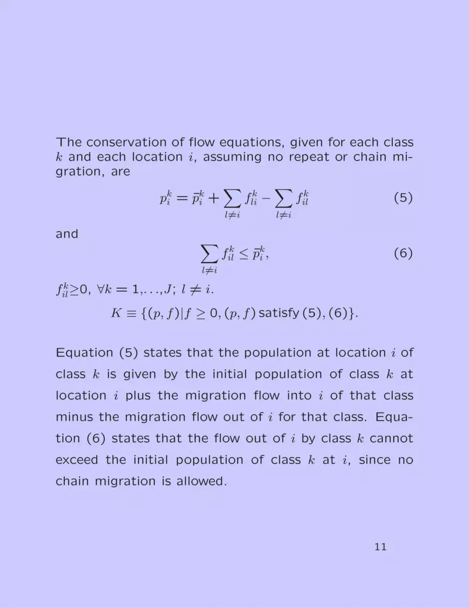
The conservation of flow equations, given for each classk and each location i, assuming no repeat or chain mi-gration, are

pki = pk

i +∑l 6=i

fkli −

∑l 6=i

fkil (5)

and ∑l 6=i

fkil ≤ pk

i , (6)

fkil≥0, ∀k = 1,. . .,J; l 6= i.

K ≡ {(p, f)|f ≥ 0, (p, f) satisfy (5), (6)}.

Equation (5) states that the population at location i of

class k is given by the initial population of class k at

location i plus the migration flow into i of that class

minus the migration flow out of i for that class. Equa-

tion (6) states that the flow out of i by class k cannot

exceed the initial population of class k at i, since no

chain migration is allowed.

11

The multiclass network model with migration costs is

now constructed. In particular, construct n nodes, i =

1, . . . , n, to represent the locations and a link (i, j) con-

necting each pair of nodes. There are, hence, n nodes

in the network and n(n − 1) links. With each link (i, j)

associate k costs ckij and corresponding flows fk

ij. With

each node i associate k utilities uki and the initial pos-

itive populations pki . A graphic depiction of a three-

location migration network is given in Figure 2, where

the classes are layered. Of course, rather than a mul-

ticlass network, one can construct J copies of the net-

work topology given in Figure 2 to represent the classes

where the costs on the links and the utilities are defined

accordingly.

12

� ��

� ��

� ��

� ��

� ��

� ��

2 3

1 2 3

1

-�

-�

������

�� AA

AKAAAU

������

�� AA

AKAAAU

u12 u1

3

u11 uJ

2 uJ3

uJ1

c132

c121 c131 cJ32

cJ21 cJ

31

· · ·· · ·

The multiclass migration networkwith three locations

13

We are now ready to state the equilibrium conditions.As before, assume that migrants are rational and thatmigration will continue until no individual has any incen-tive to move since a unilateral decision will no longeryield a positive net gain (gain in utility minus migra-tion cost). Mathematically, the multiclass equilibriumconditions are stated as follows. A multiclass popula-tion and flow pattern (p∗, f∗) ∈ K is in equilibrium, if foreach class k; k = 1, . . . , J, and each pair of locations i, j;i = 1, . . . , n; j 6= i:

uki + ck

ij

{= uk

j − λki , if fk

ij∗

> 0

≥ ukj − λk

i , if fkij∗= 0

(7)

and

λki

{ ≥ 0, if∑

l 6=i fkil∗= pk

i

= 0, if∑

l 6=i fkil∗

< pki .

(8)

14

Equilibrium conditions (7) and (8), although similar instructure to the equilibrium conditions governing themulticommodity spatial price equilibrium problem, differsignificantly in that the indicator λk

i is present. Thenecessity of λk

i , and, in particular, condition (8), arenow interpreted.

Observe that, unlike spatial price equilibrium problems

(or the related traffic network equilibrium problem with

elastic demand), the level of the population pki may not

be large enough so that the gain in utility ukj − uk

i is ex-

actly equal to the cost of migration ckij. Nevertheless,

the utility gain minus the migration cost will be maximal

and nonnegative. Moreover, the net gain will be equal-

ized for all locations and classes which have a positive

flow out of a location. In fact, λki is exactly the equalized

net gain for all individuals of class k of location i.

15

First, the function structure is discussed and then thevariational inequality formulation of the equilibrium con-ditions (7) and (8) is derived.

Assume, as before, that the utility associated with aparticular location and class can depend upon the pop-ulation associated with every class and every location,that is,

u = u(p). (9)

Assume also that the cost associated with migratingbetween two locations as perceived by a particular classcan depend, in general, upon the flows of every classbetween every pair of locations, that is,

c = c(f). (10)

16

The variational inequality formulation of the migrationequilibrium conditions is given by:

Theorem 2 (Variational Inequality Formulation ofMigration Equilibrium with Migration Costs)

A population and migration flow pattern (p∗, f∗) ∈ Ksatisfies equilibrium conditions (7) and (8) if and only ifit satisfies the variational inequality problem

〈−u(p∗), p − p∗〉+ 〈c(f∗), f − f∗〉 ≥ 0, ∀(p, f) ∈ K. (11)

Proof: We first show that if a pattern (p∗, f∗) satis-fies equilibrium conditions (7) and (8), subject to con-straints (5) and (6), then it also satisfies the variationalinequality in (11).

Suppose that (p∗, f∗) satisfies the equilibrium conditions.Then

fkij∗ ≥ 0 and

∑l 6=i

fkil∗ ≤ pk

i , ∀i, j, k.

17

For fixed class k we define Γk1 = {l|fk

il∗

> 0} and Γk2 =

{l|fkil∗= 0}. Then

∑l 6=i

[uk

i (p∗) + ck

il(f∗) − uk

l (p∗)

] × [fk

il − fkil∗]

=∑l∈Γk

1

[uk

i (p∗) + ck

il(f∗) − uk

l (p∗)

] × [fk

il − fkil∗]

+∑l∈Γk

2

[uk

i (p∗) + ck

il(f∗) − uk

l (p∗)

] × [fk

il − fkil∗]

≥ −λki

∑l∈Γk

1

(fkil − fk

il∗) +

∑l∈Γk

2

(−λki )(f

kil)

= −λki (

∑l 6=i

fkil −

∑l 6=i

fkil∗)

{= 0, if

∑l 6=i f

kil∗

< pki

≥ 0, if∑

l 6=i fkil∗= pk

i

holds for all such locations i.

Therefore, for this class k and all locations i, fkil∗≥0,∑

l 6=ifkil∗≤pk

i , and

n∑i=1

∑l 6=i

[uk

i (p∗) + ck

il(f∗) − uk

l (p∗)

] × [fk

il − fkil∗] ≥ 0. (12)

18

But inequality (12) holds for each k; hence,

J∑k=1

n∑i=1

∑l 6=i

[uk

i (p∗) + ck

il(f∗) − uk

l (p∗)

] × [fk

il − fkil∗] ≥ 0.

(13)

Observe now that inequality (13) can be rewritten as:

J∑k=1

n∑l=1

ukl (p

∗) × ((∑j 6=l

fklj −

∑j 6=l

fkjl) − (

∑j 6=l

fklj∗ −

∑j 6=l

fkjl∗))

+J∑

k=1

N∑i=1

∑l 6=i

ckil(f

∗) × (fkil − fk

il∗) ≥ 0. (14)

Using constraint (5), and substituting it into (14), oneconcludes that

−J∑

k=1

n∑l=1

ukl (p

∗)×(pkl −pk

l∗)+

J∑k=1

n∑i=1

∑l 6=i

ckil(f

∗)×(fkil−fk

il∗) ≥ 0,

(15)or, equivalently, in vector notation,

〈−u(p∗), p−p∗〉+〈c(f∗), f−f∗〉 ≥ 0, ∀(p, f) ∈ K. (16)

19

We now show that if a pattern (p∗, f∗) ∈ K satisfies vari-ational inequality (11), then it also satisfies equilibriumconditions (7) and (8). Suppose that (p∗, f∗) satisfiesvariational inequality (5.11). Then

〈−u(p∗), p〉+〈c(f∗), f〉 ≥ 〈−u(p∗), p∗〉+〈c(f∗), f∗〉, ∀(p, f) ∈ K.

Hence, (p∗, f∗) solves the minimization problem

Min(p,f)∈K〈−u(p∗), p〉 + 〈c(f∗), f〉, (17)

or, equivalently, (17) may be expressed solely in termsof f , that is,

Minf ′∈K1〈−u(Af∗), Af〉 + 〈c(f∗), f〉 (18)

where K1 ≡ {f |f ≥ 0, satisfying (5.6)}, A is the arc-nodeincidence matrix in (5), and u(Af∗) ≡ u(p∗).

Since the constraints in K are linear, one has the fol-lowing Kuhn-Tucker conditions: There exist

λ = (λki ) ≥ 0, (19)

such that

λki (

∑l 6=i

fkil∗ − pk

i ) = 0 (20)

and

uki − uk

j + ckij + λk

i ≥ 0 (21)

(uki − uk

j + ckij + λk

i )fkij∗= 0. (22)

Clearly, equilibrium conditions (7) and (8) follow from

(19) – (22). The proof is complete.

20

Qualitative Properties

Existence of at least one solution to variational inequal-ity (11) follows from the standard theory of variationalinequalities, under the sole assumption of continuity ofthe utility and migration cost functions u and c, sincethe feasible convex set K is compact. Uniqueness ofthe equilibrium population and migration flow pattern(p∗, f∗) follows under the assumption that the utility andmovement cost functions are strictly monotone, that is,

−〈u(p1) − u(p2), p1 − p2〉 + 〈c(f1) − c(f2), f1 − f2〉 > 0,

∀(p1, f1), (p2, f2) ∈ K, such that (p1, f1) 6= (p2, f2).(23)

We now interpret monotonicity condition (23) in termsof the applications. Under reasonable economic situa-tions, the monotonicity condition (23) can be verified.

Essentially, it is assumed that the system is subjectto congestion; hence, the utilities are decreasing withlarger populations, and the movement costs are increas-ing with larger migration flows.

Furthermore, each utility function uki (p) depends mainly

on the population pki , and each movement cost ck

ij(f) de-

pends mainly on the flow fkij. Mathematically, the strict

monotonicity condition will hold, for example, when −∇u

and ∇c are diagonally dominant.

21

Migration with Class Transformations

A network model of human migration equilibrium is nowdeveloped, which allows not only for multiple classesand migration costs between locations but also for classtransformations.

In this model users select the class/location combinationthat will yield the greatest net gain, where the net gainis defined as the gain in utility minus the migration cost.

The cost here reflects both the cost associated with

translocation and the cost associated with training, ed-

ucation, and the like, if there is migration across classes

either within a location or across locations. This model

may also be viewed as a framework for labor move-

ments.

22

As in the preceding two migration models, assume aclosed economy in which there are n locations, typicallydenoted by i, and J classes, typically denoted by k. Theutility functions and the population vectors are as de-fined for the preceding model. However, now associatewith each pair of class/location combinations k, i and l, ja nonnegative cost of migration ckl

ij and let the migrationflow of class k from origin i to class l at destination jbe denoted by fkl

ij .

Note that in the case where the destination class l isidentical to the origin class k, then the migration cost ckk

ijrepresents the cost of translocation, which includes notonly the cost of physical movement but also the psychiccost as perceived by this class in moving between thepair of locations.

On the other hand, when the destination location j is

equal to the origin location i, the cost cklii represents

the cost of transforming from class k to class l while

staying in location i. Hence, the migration cost here is

interpreted in a general setting as including the cost of

migrating from class to class. The migration costs are

grouped into a row vector c ∈ RJn(Jn−1), and the flows

into a column vector f ∈ RJn(Jn−1).

23

The conservation of flow equations are given for eachclass k and each region i, assuming no repeat or chainmigration, by

pki = pk

i +∑

(l,h)6=(k,i)

flkhi −

∑(l,h)6=(k,i)

fklih (24)

and ∑(l,h)6=(k,i)

fklih ≤ pk

i , (25)

where fklih ≥ 0, for all (k, l); k=1, . . . , J; l=1, . . . , J, (h, i);

h = 1, . . . , n; i=1, . . . , n. Let K ≡{(p, f)|f ≥ 0, and sat-isfy (24), (25).

Equation (24) states that the population in location i

of class k is given by the initial population of class k in

location i plus the migration flow into i of that class and

transformations of other classes into that class from this

and other locations minus the migration flow out of i

for that class and transformations of that class to other

classes at this and other locations. Equation (25) states

that the flow out of i by class k cannot exceed the initial

population of class k at i, since no chain migration is

allowed.

24

The general network model with class transformationsis now presented. For each class k, construct n nodes,(k, i); i = 1, . . . , n, to represent the locations and a link(ki, kj) connecting each such pair of nodes.

These links, hence, represent migration links within aclass. From each node (k, i) construct Jn−1 links joiningeach node (k, i) to node (l, h) where l 6= k; l = 1, . . . , J;h = 1, . . . , n.

These links represent migration links which are classtransformation links. There are, hence, a total of Jnnodes in the network and Jn(Jn − 1) links. Note thateach node may be interpreted as a state in class/locationspace.

With each link (ki, lj) associate the cost cklij and the

corresponding flow fklij . With each node (k, i) associate

the utility uki and the initial positive population pk

i . A

graphical depiction of a two-region, three-class migra-

tion network is given in Figure 3.

25

����

����

����

����

����

����

2,2

2,1

1,2

1,1

3,2

3,1

- -

- -��

��? ? ?

666

-

- �

�

? ?

6 6

Location 1

Location 2

@@

@@I

@@

@@

@@

@@

@@

@@R

��

��

��

��

��

��

��

���

@@

@@I

@@

@@

@@

@@

@@

@@R

��

��

��

��

��

��

��

���

The transformation network for twolocations and three classes

26

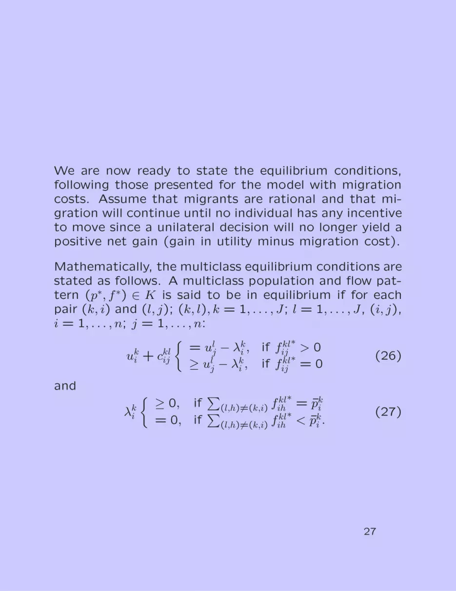
We are now ready to state the equilibrium conditions,following those presented for the model with migrationcosts. Assume that migrants are rational and that mi-gration will continue until no individual has any incentiveto move since a unilateral decision will no longer yield apositive net gain (gain in utility minus migration cost).

Mathematically, the multiclass equilibrium conditions arestated as follows. A multiclass population and flow pat-tern (p∗, f∗) ∈ K is said to be in equilibrium if for eachpair (k, i) and (l, j); (k, l), k = 1, . . . , J; l = 1, . . . , J, (i, j),i = 1, . . . , n; j = 1, . . . , n:

uki + ckl

ij

{= ul

j − λki , if fkl

ij∗

> 0

≥ ulj − λk

i , if fklij

∗= 0

(26)

and

λki

{ ≥ 0, if∑

(l,h)6=(k,i) fklih

∗= pk

i

= 0, if∑

(l,h)6=(k,i) fklih

∗< pk

i .(27)

27

Observe that the population pki may not be large enough

so that the gain in utility ulj − uk

i is exactly equal to

the cost of migration cklij . Nevertheless, the utility gain

minus the migration cost will be maximal and nonneg-

ative. Moreover, the net gain will be equalized for all

classes/locations which have a positive flow out of a

location of that class. In fact, λki is exactly the equal-

ized net gain for all individuals of class k in location

i. In the case where no class transformations are al-

lowed, in other words, l = k, then the above equilibrium

conditions collapse to those given for the model with

migration costs.

28

Assume that, in general, the utility associated with aparticular location and class can depend upon the pop-ulation associated with every class and every location,as similarly assumed in the preceding migration models.

Also assume that, in general, the cost associated with

migrating between two distinct pairs of classes/locations

as perceived by a particular class can depend, in gen-

eral, upon the flows of every class between every pair

of locations, as well as the flows between every pair of

classes.

29

The equilibrium conditions are illustrated through thefollowing example.

Example 1

Consider the migration problem with two classes andtwo locations where the utility functions are:

u11(p) = −p1

1 + 5 u21(p) = −p2

1 − .5p11 + 20

u12(p) = −p1

2 + 15 u22(p) = −p2

2 + .5p11 + 10

and assume that the migration cost functions are:

c1211(f) = f1211 + .5f12

12 + 1 c2111(f) = f2111 + 1

c1112(f) = f1112 + .2f12

12 + 10 c1121(f) = f1121 + 10

c1212(f) = f1212 + .1f11

12 + 5 c2121(f) = f2121 + 20

c2212(f) = f2212 + .3f12

21 + 2 c2221(f) = f2221 + 3

c2112(f) = f2112 + 15 c1221(f) = f12

21 + .2f1121 + 15

c1222(f) = f1222 + 10 c2122(f) = 3f21

22 + 2f2111 + 1.

30

The fixed populations are:

p11 = 1 p2

1 = 5 p12 = 1 p2

2 = 3,

with associated initial utilities

u11 = 4 u2

1 = 15 u12 = 14 u2

2 = 7.

The equilibrium populations and the flow pattern are:

p11∗= 0 p2

1∗= 7 p1

2∗= 2 p2

2∗= 1

f1211

∗= f22

21∗= f21

22∗= 1, all other fkl

ij∗= 0,

and with associated equilibrium utilities

u11 = 5 u2

1 = 13 u12 = 13 u2

2 = 9.

31

We now verify that this population and flow patternsatisfies equilibrium conditions (26) and (27).

Class 1, Location 1

Observe that in this case the final population is p11∗= 0,

and, hence, the original population was exhausted. Notethat

u11+c1211 = 5+2 = u2

1 = 13−λ11, whereλ1

1 = 6and f1211

∗> 0

u11 + c1212 = 5 + 5 ≥ u2

2 = 9, and f1212

∗= 0

u11 + c1112 = 5 + 10 ≥ u1

2 = 13, and f1112

∗= 0.

Class 2, Location 2

Note that here the final population is p22∗

= 1, and,hence, this population is not exhausted. Note also that

u22 + c2221 = 9 + 4 = u2

1 = 13, and f2221

∗> 0

u22 + c2122 = 9 + 4 = u1

2 = 13, and f2122

∗> 0

u22 + c2121 = 9 + 20 ≥ u1

1 = 5, and f2121

∗= 0.

32

Both class 1, location 2 and class 2, location 1 have

zero migration flow out with the equilibrium conditions

uki + ckl

ij ≥ ulj holding, as is easy to verify. Thus, the

above population and flow distribution patterns satisfy

the migration equilibrium conditions (26) and (27), and

the conservation of flow equations (24) and (25) also

hold.

33

The variational inequality formulation of the above mi-gration equilibrium conditions is given below. The prooffollows from similar arguments as given in the proof ofthe preceding variational inequality.

Theorem 3 (Variational Inequality Formulation ofMigration Equilibrium with Class Transformations)

A population and migration flow pattern (p∗, f∗) ∈ Ksatisfies equilibrium conditions (26) and (27) if and onlyif it satisfies the variational inequality problem

〈−u(p∗), p − p∗〉+ 〈c(f∗), f − f∗〉 ≥ 0, ∀(p, f) ∈ K, (28)

where K ≡ {(p, f)|f ≥ 0, and (p, f) satisfy (24), (25)}.

34

Existence of at least one solution to variational inequal-ity (28) is again guaranteed by the standard theory un-der the sole assumption of continuity of the utility andmigration cost functions u and c, since the feasible setK is compact. Uniqueness of the equilibrium populationand migration flow pattern follows from the assumptionthat the utility and migration cost functions are strictlymonotone.

The above model can be further interpreted in the con-text of the migration network model described beforeas follows. If one makes the identification that eachnode in the network model (cf. Figure 3) is, indeed,a “location,” albeit a location in class/location space,then the model developed here with J classes and n re-gions is structurally isomorphic to the human migrationmodel of Section 2 in the case of a single class and Jnlocations, in which asymmetric utility functions and mi-gration cost functions are, of course, permitted. Themodel just described, nevertheless, is the richer modelconceptually and more general from an application pointof view.

Furthermore, the development here illustrates and yet

another network equilibrium model in which the net-

work representation is fundamental to the formulation,

understanding, and, as shall be demonstrated in the sub-

sequent section, the ultimate solution of the problem at

hand.

35

Computation of Migration Equilibria

The variational inequality decomposition algorithm forthe solution of the multiclass human migration equi-librium problem is now presented. Note that, as dis-cussed above, the network model with class transforma-tions can be reformulated as the model with migrationcosts with the appropriate identification between nodescorresponding to locations and nodes corresponding toclass/location combinations. Hence, the algorithm de-scribed below is applicable to both models. The de-composition algorithm is based crucially on the specialstructure of the underlying network (cf. Figure 2).

In particular, note that the feasible set K for variationalinequality (11) can be expressed as the Cartesian prod-uct

K =J∏

k=1

Kk, (29)

where Kk ≡ {(pk, fk)|pk = {pki ; i = 1, . . . , n}}; fk = {fk

ij, i =

1, . . . , n; j = 1, . . . , n; j 6= i}, and satisfying (5) and (6).

36

One can, hence, decompose the variational inequalitygoverning the multiclass migration network equilibriumproblem into J simpler variational inequalities in lowerdimensions. Each variational inequality in the decom-position corresponds to a particular class which, afterlinearizing, is equivalent to a quadratic programmingproblem and can be solved by the migration equilibrationalgorithm developed in Nagurney (1989).

That algorithm is a relaxation scheme and proceeds

from location (node) to location (node), at each step

computing the migratory flow out of the location exactly

and in closed form. This can be accomplished because

the special network structure of the problem lies in that

each of the paths from an origin location to the n − 1

potential destination locations are disjoint.

37

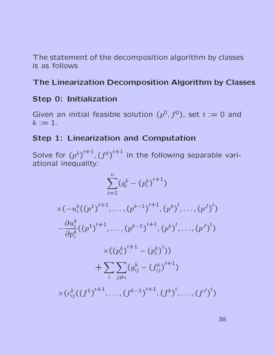
The statement of the decomposition algorithm by classesis as follows

The Linearization Decomposition Algorithm by Classes

Step 0: Initialization

Given an initial feasible solution (p0, f0), set t := 0 andk := 1.

Step 1: Linearization and Computation

Solve for (pk)t+1

, (fk)t+1

in the following separable vari-ational inequality:

n∑i=1

(qki − (pk

i )t+1

)

×(−uki ((p

1)t+1

, . . . , (pk−1)t+1

, (pk)t, . . . , (pJ)

t)

−∂uki

∂pki

((p1)t+1

, . . . , (pk−1)t+1

, (pk)t, . . . , (pJ)

t)

×((pki )

t+1 − (pki )

t))

+∑

i

∑j 6=i

(gkij − (fk

ij)t+1

)

×(ckij((f

1)t+1

, . . . , (fk−1)t+1

, (fk)t, . . . , (fJ)

t)

38

+∂ck

ij

∂fkij

((f1)t+1

, . . . , (fk−1)t+1

, (fk)t, . . . , (fJ)

t)

×((fkij)

k+1 − (fkij)

t)) ≥ 0 (30)

∀qki ≥ 0, gk

ij ≥ 0,

such that∑

j 6=i gkij ≤ pk

i and qki = pk

i − ∑j 6=i(g

kij − gk

ji).

If k < J, then let k := k+1, and go to Step 1; otherwise,go to Step 2.

Step 2: Convergence Verification

If equilibrium conditions (7) and (8) hold for a givenprespecified tolerance ε > 0, then stop; otherwise, lett := t + 1, and go to Step 1.

39

The global convergence proof for the above linearizeddecomposition algorithm is now stated. In addition, suf-ficient conditions that guarantee the convergence arealso given.

Let

A(p, f) =

A1(p, f)

. . .AJ(p, f)

(31)

where

Ak(p, f) =

−∂uk1

∂pk1 . . .

−∂ukn

∂pkn . . .

∂ckij

∂fkij

. . .

n2×n2

(32)

and (p, f) is feasible.

40

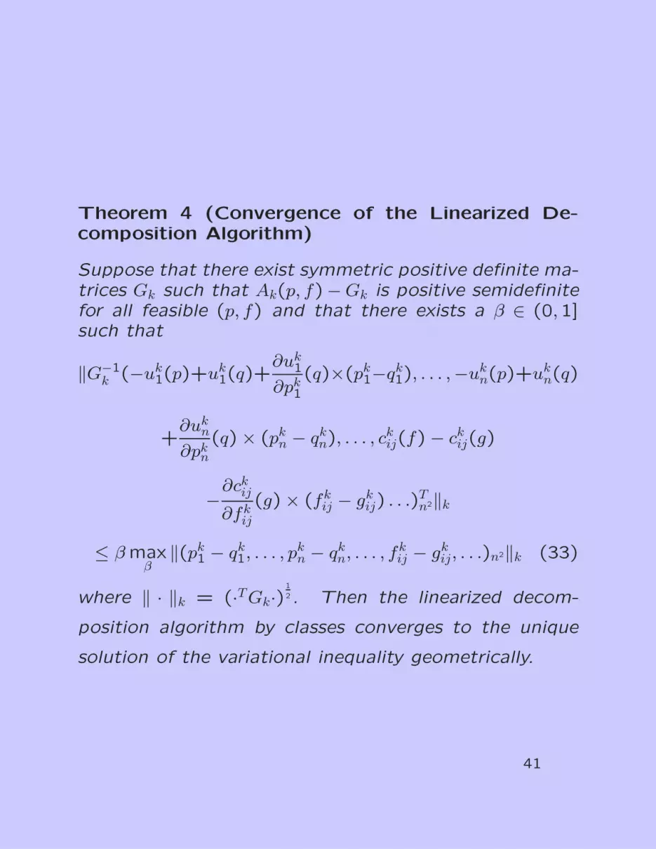
Theorem 4 (Convergence of the Linearized De-composition Algorithm)

Suppose that there exist symmetric positive definite ma-trices Gk such that Ak(p, f)− Gk is positive semidefinitefor all feasible (p, f) and that there exists a β ∈ (0,1]such that

‖G−1k (−uk

1(p)+uk1(q)+

∂uk1

∂pk1

(q)×(pk1−qk

1), . . . ,−ukn(p)+uk

n(q)

+∂uk

n

∂pkn

(q) × (pkn − qk

n), . . . , ckij(f) − ck

ij(g)

−∂ckij

∂fkij

(g) × (fkij − gk

ij) . . .)Tn2‖k

≤ β maxβ

‖(pk1 − qk

1, . . . , pkn − qk

n, . . . , fkij − gk

ij, . . .)n2‖k (33)

where ‖ · ‖k = (·TGk·)1

2 . Then the linearized decom-

position algorithm by classes converges to the unique

solution of the variational inequality geometrically.

41

In the case when −u, c are separable, that is,

uki (p) = uk

i (pki ), ck

ij(f) = ckij(f

kij), (34)

the positive semidefiniteness of Ak(p, f)−Gk is equivalentto the strong monotonicity of (−uk, ck) for each blockk.

In fact, if Ak(p, f) − Gk is positive semidefinite, then

n∑i=1

(−uki (p) + uk

i (q)) × (pki − qk

i )

+n∑

i=1

∑j 6=i

(ckij(f) − ck

ij(g)) × (fkij − gk

ij)

=n∑

i=1

(−∂uki

∂pki

(η)) × (pki − qk

i )2 +

∑i,j 6=i

∂ckij

∂fkij

(ζ) × (fkij − gk

ij)2

≥ α(n∑

i=1

(pki − qk

i )2+

n∑i=1

∑j 6=i

(fkij − gk

ij)2), (35)

that is, (−uk, ck) is strongly monotone. The converse is

clear from the above inequality.

42

The norm inequality condition is actually a measure of

linearity of −u and c. In particular, when −u, c are linear

and separable, the inequality is automatically satisfied,

since the lefthand side is zero. Of course, the variational

inequality can be solved for each class by the migration

equilibration algorithm in this extremal case. A not-too-

large perturbation from this case means not-too-strong

interactions among classes and locations.

43

Numerical Results

The numerical results for the decomposition algorithmare presented in this section.

The algorithm was implemented in FORTRAN and com-piled using the FORTVS compiler, optimization level 3.The special-purpose migration equilibration algorithmoutlined in Nagurney (1989) was used for the embed-ded quadratic programming problems. The system usedwas an IBM 3090/600J at the Cornell National Super-computer Facility. All of the CPU times reported areexclusive of input/output times, but include initializa-tion times. The initial pattern for all the runs was setto (p0, f0) = 0. The convergence tolerance used wasε = .01, with the equilibrium conditions serving as thecriteria.

We first considered migration examples without classtransformations with asymmetric and nonlinear utilityand migration cost functions. The utility functions wereof the form

uki (p) = −αkk

ii (pki )

2 −∑l,j

aklijp

lj + bk

i , (36)

and the migration cost functions were of the form

ckij(f) = γk

ijij(fkij)

2+

∑l,rs

gklijrsf

lrs + hk

ij. (37)

44

The data were generated randomly and uniformly in theranges as follows: αkk

ii ∈ [1,10] × 10−6,γkkijij ∈ [.1, .5, ] ×

10−6,−akkij ∈ [1,10], bk

i ∈ [10,100], gkkijij ∈ [.1, .5], and

hkij ∈ [1,5], for all i, j, k, with the diagonal terms gener-

ated so that strict diagonal dominance of the respectiveJacobians of the utility and movement cost functionsheld, thus guaranteeing uniqueness of the equilibriumpattern (p∗, f∗).

The number of cross-terms for the functions (5.36) and

(37) was set at five. The initial population pki was gen-

erated randomly and uniformly in the range [10,30], for

all i, k.

45

Numerical results for nonlinearmulticlass migration networks

Number of Number of ClassesLocations 5 10

CPU Time in sec. (# of Iterations)

10 .24(4) .41(3)20 1.18(4) 2.38(4)30 3.87(4) 9.73(4)40 8.73(4) 17.01(5)50 16.22(5) 33.07(4)

46

In Table 1 we varied the number of locations from 10through 50, in increments of 10, and fixed the numberof classes at 5 and 10.

As can be seen from the Table 1, the decomposition

algorithm by classes required only several iterations for

convergence. As expected, the problems with 10 classes

required, typically, at least twice the CPU time for com-

putation as did the problems with 5 classes. Finally, note

that, although the decomposition algorithm by classes

implemented here was a serial algorithm, the parallel

version converges under the same conditions as given

in Theorem 4. Hence, the parallel analogue allows for

implementation on parallel computers. We now turn to

the computation of large-scale migration network equi-

librium problems with class transformations and present

numerical results for the linearization decomposition al-

gorithm.

47

We now report the numerical results for multiclass mi-gration problems with class transformations in Table 2.As in the previous examples, we considered exampleswith asymmetric and nonlinear utility and migration costfunctions, that is, the utility functions were of the form

uki (p) = −αk

i (pki )

2 −∑l,j

aklijp

lj + bk

i , (38)

and the migration cost functions were of the form

cklij(f) = γkl

ij (fklij )

2+

∑uv,rs

gkluvijrs fuv

rs + hklij . (39)

The data were generated in a similar fashion to thepreceding examples, i.e., randomly and uniformly in theranges as follows: αk

i ∈ [1,10]×10−6, γklij ∈ [.1, .5]×10−6,

akkii ∈ [1,10], bk

i ∈ [10,100], gklklijij ∈ [.1, .5], and hkl

ij ∈ [1,5],for all i, j, k, l, with the off-diagonal terms generated sothat strict diagonal dominance of the respective Jaco-bians of the utility and migration cost functions held,thus guaranteeing uniqueness of the equilibrium pattern(p∗, f∗). However, the Jacobians were asymmetric.

The number of cross-terms for the functions (38) and

(39) was set at 5. The initial population pki was gener-

ated randomly and uniformly in the range [10,30], for

all i, k.

48

Numerical results for nonlinear multiclassmigration networks with class transformations

Number of Number Number of CPU Time in sec.

Locations of Classes (Nodes; Links) (# of Iterations)

10 5 (50; 2,450) 2.70(4)20 5 (100; 9,900) 16.89(4)30 5 (150; 22,350) 80.40(5)40 5 (200; 39,800) 171.95(6)50 5 (250; 72,250) 321.06(5)10 10 (100; 9,900) 23.71(4)20 10 (200; 39,800) 131.63(5)30 10 (300; 89,700) 512.03(4)

49

In Table 2 the problems ranged in size from 10 regions,5 classes through 50 regions, 5 classes, to 30 regions,10 classes. The problems, hence, ranged in size from50 nodes and 2,450 links to 300 nodes and 89,700 links.The number of nodes and the number of links for eachproblem are also reported in the tables.

As can be seen from the two tables, the linearization de-composition algorithm required only several iterationsfor convergence. The problems solved here representlarge-scale problems from both numerical as well asapplication-oriented perspectives. Although the classtransformation problems solved here cannot directly becompared to those solved without class transformations,some inferences can, nevertheless, be made.

The problems in Table 2 are more time-consuming to

solve for a fixed number of locations and classes. This

is due, in part, to the fact that a problem with J classes

and n locations, in the absence of class transformations,

has only Jn(n − 1) links, whereas a problem with the

same number of classes and regions in the presence of

class transformations has the number of links now equal

to Jn(Jn − 1).

50

Hence, the dimensionality of a given problem now in-creases in terms of the number of links by a factor onthe order of the number of classes J.

The largest problem solved in Table 1 had 50 regions

and 10 classes and consisted of 24,500 links, whereas

the largest problem solved in Table 2 consisted of 30

regions and 10 classes and had 89,700 links.

51

The literature on human migration is extensive and spansdisciplines ranging from economics through geographyto sociology. Some precursors to a network formal-ism are the contributions of Beckmann (1957), Tobler(1981), and Dorigo and Tobler (1983). Tobler (1981)and Dorigo and Tobler (1983) establish connections be-tween migration problems and transportation problems.The importance of migration cost in migration decision-making has been documented in the literature fromboth theoretical and empirical perspectives (cf. To-bler (1981) and Sjaastad (1962), and the referencestherein), and such costs are explicitly included in ourmore general migration models. Some surveys of themigration literature are Greenwood (1975, 1985).

A related problem has been studied by Faxen and Thore

(1990) who utilize a network analysis for studying la-

bor markets and discuss the relationship between their

model and classical spatial price equilibrium models. Here

our emphasis has been on developing the fundamentals

of a unifying network framework for the study of human

population movements. Of course, our model of class

transformations captures labor movements as well.

52

Below we include the references to the above materialas well as additional ones for the interested reader.

References

Beckmann, M., “On the equilibrium distribution of pop-ulation in space,” Bulletin of Mathematical Biophysics19 (1957) 81-89.

Beckmann, M., McGuire, C. B., and Winsten, C. B.,Studies in the Economics of Transportation, YaleUniversity Press, New Haven, Connecticut, 1956.

Bertsekas, D. P., and Tsitsiklis, J. N., Parallel and Dis-tributed Computation - Numerical Methods, Pren-tice - Hall, Englewood Cliffs, New Jersey, 1989.

Dorigo, G., and Tobler, W. R., “Push-pull migrationlaws,” Annals of the Association of American Geogra-phers 73 (1983) 1-17.

Faxen, K. O., and Thore, S., “Retraining in an interde-pendent system of labor markets: a network analysis,”European Journal of Operational Research 44 (1990)349-356.

Greenwood, M. J., “Research on internal migration in

the United States: a survey,” Journal of Economic Lit-

erature 13 (1975) 397-433.

53

Greenwood, M. J., “Human migration: theory, models,and empirical studies,” Journal of Regional Science 25(1985) 521-544.

Nagurney, A., “Migration equilibrium and variational in-equalities,” Economics Letters 31 (1989) 109-112.

Nagurney, A., “A network model of migration equilib-rium with movement costs,” Mathematical and Com-puter Modelling 13 (1990) 79-88.

Nagurney, A., Pan, J., and Zhao, L., “Human migrationnetworks,” European Journal of Operational Research59 (1992a) 262-274.

Nagurney, A., Pan, J., and Zhao, L., “Human migrationnetworks with class transformations,” in Structure andChange in the Space Economy, pp. 239-258, T. R.Lakshmanan and P. Nijkamp, editors, Springer-Verlag,Berlin, Germany, 1992b.

Samuelson, P. A., “Spatial price equilibrium and linear

programming,” American Economic Review 42 (1952)

283-303.

54

Sjaastad, L. A., “The costs and returns of human mi-gration,” Journal of Political Economy October 1962,part 2, 80-93.

Takayama, T., and Judge, G. G., Spatial and Tem-poral Price and Allocation Models, North-Holland,Amsterdam, The Netherlands, 1971.

Tobler, W. R., “A model of geographical movement,”

Geographical Analysis 13 (1981) 1-20.

55