Embed Size (px)
Citation preview

MIKE URBAN
Collection SystemModelling of storm water drainage networks and sewer
collection systems
User guide
MIKE 2017

2 MIKE URBAN - © DHI

PLEASE NOTE
COPYRIGHT This document refers to proprietary computer software which is pro-tected by copyright. All rights are reserved. Copying or other repro-duction of this manual or the related programs is prohibited without prior written consent of DHI. For details please refer to your 'DHI Software Licence Agreement'.
LIMITED LIABILITY The liability of DHI is limited as specified in Section III of your 'DHI Software Licence Agreement':
'IN NO EVENT SHALL DHI OR ITS REPRESENTA-TIVES (AGENTS AND SUPPLIERS) BE LIABLE FOR ANY DAMAGES WHATSOEVER INCLUDING, WITHOUT LIMITATION, SPECIAL, INDIRECT, INCIDENTAL OR CONSEQUENTIAL DAMAGES OR DAMAGES FOR LOSS OF BUSINESS PROFITS OR SAVINGS, BUSINESS INTERRUPTION, LOSS OF BUSINESS INFORMA-TION OR OTHER PECUNIARY LOSS ARISING OUT OF THE USE OF OR THE INABILITY TO USE THIS DHI SOFTWARE PRODUCT, EVEN IF DHI HAS BEEN ADVISED OF THE POSSI-BILITY OF SUCH DAMAGES. THIS LIMITATION SHALL APPLY TO CLAIMS OF PERSONAL INJURY TO THE EXTENT PERMIT-TED BY LAW. SOME COUNTRIES OR STATES DO NOT ALLOW THE EXCLUSION OR LIMITATION OF LIABILITY FOR CONSE-QUENTIAL, SPECIAL, INDIRECT, INCIDENTAL DAMAGES AND, ACCORDINGLY, SOME PORTIONS OF THESE LIMITATIONS MAY NOT APPLY TO YOU. BY YOUR OPENING OF THIS SEALED PACKAGE OR INSTALLING OR USING THE SOFT-WARE, YOU HAVE ACCEPTED THAT THE ABOVE LIMITATIONS OR THE MAXIMUM LEGALLY APPLICABLE SUBSET OF THESE LIMITATIONS APPLY TO YOUR PURCHASE OF THIS SOFT-WARE.'
3

4 MIKE URBAN - © DHI

MIKE URBAN CS - MOUSE User Guide . . . . . . . . . . . . . . . . . . . . . . . . . . 13
1 Modelling Collection Systems . . . . . . . . . . . . . . . . . . . . . . . . . . . 15
2 Modelling Collection Systems with MOUSE . . . . . . . . . . . . . . . . . . . 17
3 Hydraulic Network Modeling with MOUSE . . . . . . . . . . . . . . . . . . . . 193.1 Introduction . . . . . . . . . . . . . . . . . . . . . . . . . . . . . . . . . . . . 193.2 Definition of a MOUSE Network . . . . . . . . . . . . . . . . . . . . . . . . . 19
3.2.1 Modelling real network elements . . . . . . . . . . . . . . . . . . . . 203.3 Nodes and Structures . . . . . . . . . . . . . . . . . . . . . . . . . . . . . . 22
3.3.1 Identification group . . . . . . . . . . . . . . . . . . . . . . . . . . . 243.3.2 MOUSE model data group . . . . . . . . . . . . . . . . . . . . . . . 263.3.3 Q-H relations for nodes . . . . . . . . . . . . . . . . . . . . . . . . . 283.3.4 Outlet head loss . . . . . . . . . . . . . . . . . . . . . . . . . . . . 283.3.5 Model Concept of Soakaway . . . . . . . . . . . . . . . . . . . . . . 29
Soakaway tab . . . . . . . . . . . . . . . . . . . . . . . . . . . . . . 323.4 Pipes and Canals . . . . . . . . . . . . . . . . . . . . . . . . . . . . . . . . . 35
3.4.1 Identification group . . . . . . . . . . . . . . . . . . . . . . . . . . . 373.4.2 Geometrical properties . . . . . . . . . . . . . . . . . . . . . . . . . 383.4.3 Hydraulic friction losses . . . . . . . . . . . . . . . . . . . . . . . . . 393.4.4 Miscellaneous . . . . . . . . . . . . . . . . . . . . . . . . . . . . . . 40
3.5 Weirs . . . . . . . . . . . . . . . . . . . . . . . . . . . . . . . . . . . . . . . 413.5.1 Identification and connectivity . . . . . . . . . . . . . . . . . . . . . 433.5.2 Model data . . . . . . . . . . . . . . . . . . . . . . . . . . . . . . . 44
3.6 Orifices . . . . . . . . . . . . . . . . . . . . . . . . . . . . . . . . . . . . . . 443.6.1 Identification and connectivity . . . . . . . . . . . . . . . . . . . . . 473.6.2 Model data . . . . . . . . . . . . . . . . . . . . . . . . . . . . . . . 473.6.3 Defining a gate or a weir in an orifice . . . . . . . . . . . . . . . . . . 48
3.7 Stormwater Inlets . . . . . . . . . . . . . . . . . . . . . . . . . . . . . . . . . 493.7.1 Curb Inlet (Lintel) . . . . . . . . . . . . . . . . . . . . . . . . . . . . 503.7.2 On-grade Capture . . . . . . . . . . . . . . . . . . . . . . . . . . . 523.7.3 Capacity curves . . . . . . . . . . . . . . . . . . . . . . . . . . . . . 53
3.8 Pumps . . . . . . . . . . . . . . . . . . . . . . . . . . . . . . . . . . . . . . 543.8.1 Pump types . . . . . . . . . . . . . . . . . . . . . . . . . . . . . . . 54
Constant flow pumps . . . . . . . . . . . . . . . . . . . . . . . . . . 55Constant speed pumps . . . . . . . . . . . . . . . . . . . . . . . . . 55Variable speed pumps . . . . . . . . . . . . . . . . . . . . . . . . . 56
3.8.2 Identification and connectivity . . . . . . . . . . . . . . . . . . . . . 613.8.3 Model data . . . . . . . . . . . . . . . . . . . . . . . . . . . . . . . 62
3.9 Valves . . . . . . . . . . . . . . . . . . . . . . . . . . . . . . . . . . . . . . 623.10 CRS & Topography . . . . . . . . . . . . . . . . . . . . . . . . . . . . . . . . 663.11 Emptying Storage Nodes . . . . . . . . . . . . . . . . . . . . . . . . . . . . . 69
4 Rainfall-Runoff Modelling with MOUSE . . . . . . . . . . . . . . . . . . . . . 714.1 Terms and Concepts . . . . . . . . . . . . . . . . . . . . . . . . . . . . . . . 71
4.1.1 MIKE URBAN Catchments . . . . . . . . . . . . . . . . . . . . . . . 724.1.2 Connecting Catchments to the Network . . . . . . . . . . . . . . . . 734.1.3 Hydrological Models . . . . . . . . . . . . . . . . . . . . . . . . . . 73
5

4.1.4 Creating Hydrological Models for a Catchment . . . . . . . . . . . . 744.2 Time-Area Method (A) . . . . . . . . . . . . . . . . . . . . . . . . . . . . . . 75
4.2.1 Model Data . . . . . . . . . . . . . . . . . . . . . . . . . . . . . . . 754.2.2 Parameter Sets . . . . . . . . . . . . . . . . . . . . . . . . . . . . . 774.2.3 Time-Area Curve Editor . . . . . . . . . . . . . . . . . . . . . . . . 79
4.3 Kinematic Wave (B) . . . . . . . . . . . . . . . . . . . . . . . . . . . . . . . 804.3.1 Model Data . . . . . . . . . . . . . . . . . . . . . . . . . . . . . . . 804.3.2 Parameter Sets . . . . . . . . . . . . . . . . . . . . . . . . . . . . . 82
4.4 Linear Reservoir (C1 and C2) . . . . . . . . . . . . . . . . . . . . . . . . . . 844.4.1 Model Data . . . . . . . . . . . . . . . . . . . . . . . . . . . . . . . 844.4.2 Parameter Sets . . . . . . . . . . . . . . . . . . . . . . . . . . . . . 87
4.5 Unit Hydrograph Method (UHM) . . . . . . . . . . . . . . . . . . . . . . . . . 894.6 Additional Flow and RDI . . . . . . . . . . . . . . . . . . . . . . . . . . . . . 92
4.6.1 Model Data . . . . . . . . . . . . . . . . . . . . . . . . . . . . . . . 954.6.2 MOUSE RDI Parameter Sets . . . . . . . . . . . . . . . . . . . . . 96
4.7 Rainfall Data and Other Meteorological Variables - Boundary Conditions for Hydro-logical models 99
4.8 Running the Runoff Computations . . . . . . . . . . . . . . . . . . . . . . . 1024.9 MOUSE RDI - Guidelines for application . . . . . . . . . . . . . . . . . . . 104
4.9.1 Choice of calculation time step . . . . . . . . . . . . . . . . . . . . 1044.9.2 The RDI hotstart . . . . . . . . . . . . . . . . . . . . . . . . . . . 1054.9.3 The RDI result files . . . . . . . . . . . . . . . . . . . . . . . . . . 1054.9.4 MOUSE RDI Validation . . . . . . . . . . . . . . . . . . . . . . . 106
Surface runoff model . . . . . . . . . . . . . . . . . . . . . . . . . . 107General hydrological model - RDI . . . . . . . . . . . . . . . . . . . 107
4.9.5 Overflow within the model area . . . . . . . . . . . . . . . . . . . 1114.9.6 Non-precipitation dependent flow components . . . . . . . . . . . 112
4.10 Using the Computed Runoff as Network Hydraulic Load . . . . . . . . . . . 1124.11 Low Impact Development (LID) . . . . . . . . . . . . . . . . . . . . . . . . 114
4.11.1 LID Controls . . . . . . . . . . . . . . . . . . . . . . . . . . . . . 115Bio Retention Cells . . . . . . . . . . . . . . . . . . . . . . . . . . . 116Infiltration Trenches . . . . . . . . . . . . . . . . . . . . . . . . . . 117Porous Pavement . . . . . . . . . . . . . . . . . . . . . . . . . . . 118Rain Barrels . . . . . . . . . . . . . . . . . . . . . . . . . . . . . . 118Vegetative Swales . . . . . . . . . . . . . . . . . . . . . . . . . . . 119Rain Garden . . . . . . . . . . . . . . . . . . . . . . . . . . . . . . 119Green Roof . . . . . . . . . . . . . . . . . . . . . . . . . . . . . . . 120
4.11.2 The LID Controls Editor . . . . . . . . . . . . . . . . . . . . . . . 121Identification . . . . . . . . . . . . . . . . . . . . . . . . . . . . . . 125LID Control data Specification . . . . . . . . . . . . . . . . . . . . . 126
4.11.3 LID Deployment . . . . . . . . . . . . . . . . . . . . . . . . . . . 130Identification and Connectivity . . . . . . . . . . . . . . . . . . . . . 131LID Deployment Properties . . . . . . . . . . . . . . . . . . . . . . 132The LID deployment result file . . . . . . . . . . . . . . . . . . . . . 132The LID Simulation Summary . . . . . . . . . . . . . . . . . . . . . 134
5 Time Series . . . . . . . . . . . . . . . . . . . . . . . . . . . . . . . . . . . . . 1375.1 Inserting New Time Series . . . . . . . . . . . . . . . . . . . . . . . . . . . 137
6 MIKE URBAN - © DHI

5.1.1 Properties of time series object . . . . . . . . . . . . . . . . . . . . 1385.1.2 Properties of time series item . . . . . . . . . . . . . . . . . . . . . 1415.1.3 Time series plot properties . . . . . . . . . . . . . . . . . . . . . . 144
5.2 Example: How to enter a rain time series . . . . . . . . . . . . . . . . . . . 1485.3 Example: How to Import a Time Series from Excel . . . . . . . . . . . . . . 151
6 Curves and Relations . . . . . . . . . . . . . . . . . . . . . . . . . . . . . . . 1576.1 Introduction . . . . . . . . . . . . . . . . . . . . . . . . . . . . . . . . . . . 157
6.1.1 Capacity curves . . . . . . . . . . . . . . . . . . . . . . . . . . . . 1586.1.2 Pump acceleration curves . . . . . . . . . . . . . . . . . . . . . . 1586.1.3 Regulation curves Qmax(H) and Qmax(dH) . . . . . . . . . . . . . 1596.1.4 QH relation . . . . . . . . . . . . . . . . . . . . . . . . . . . . . . 159
Manholes, Basins . . . . . . . . . . . . . . . . . . . . . . . . . . . . 159Outlets . . . . . . . . . . . . . . . . . . . . . . . . . . . . . . . . . 159Storage node . . . . . . . . . . . . . . . . . . . . . . . . . . . . . . 159
6.1.5 Time-Area curve . . . . . . . . . . . . . . . . . . . . . . . . . . . 1596.1.6 Removal efficiency . . . . . . . . . . . . . . . . . . . . . . . . . . 1606.1.7 Basin geometry . . . . . . . . . . . . . . . . . . . . . . . . . . . . 1606.1.8 Valve rating curve . . . . . . . . . . . . . . . . . . . . . . . . . . . 1616.1.9 DQ and QQ relations . . . . . . . . . . . . . . . . . . . . . . . . . 1616.1.10 Capacity curve QdH & Power . . . . . . . . . . . . . . . . . . . . . 1616.1.11 Undefined type . . . . . . . . . . . . . . . . . . . . . . . . . . . . 162
7 Boundary Conditions . . . . . . . . . . . . . . . . . . . . . . . . . . . . . . . 1657.1 Catchment Boundary Condition . . . . . . . . . . . . . . . . . . . . . . . . 166
7.1.1 Visualization of catchment boundaries . . . . . . . . . . . . . . . . 1677.2 Network Boundary Conditions . . . . . . . . . . . . . . . . . . . . . . . . . 169
7.2.1 Visualization of network boundaries . . . . . . . . . . . . . . . . . 1707.3 Boundary Condition Editors . . . . . . . . . . . . . . . . . . . . . . . . . . 171
7.3.1 Catchments Loads and Meteorological Items Editor . . . . . . . . . 1727.3.2 Network Loads Editor . . . . . . . . . . . . . . . . . . . . . . . . . 1737.3.3 External Water Levels Editor . . . . . . . . . . . . . . . . . . . . . 1747.3.4 Boundary Items Editor . . . . . . . . . . . . . . . . . . . . . . . . 175
7.4 Examples . . . . . . . . . . . . . . . . . . . . . . . . . . . . . . . . . . . . 1777.4.1 How to add a varying water level at an outlet? . . . . . . . . . . . . 1777.4.2 How to add infiltration in a pipe? . . . . . . . . . . . . . . . . . . . 1787.4.3 How to add a rainfall as a boundary condition to the catchments? . . 1797.4.4 How to add a discharge to a node? . . . . . . . . . . . . . . . . . . 1807.4.5 How to add runoff results as input for the network computation? . . 1817.4.6 How do I add DWF in my network dependent on number of inhabitants? .
1827.4.7 How to attach a pollutant concentration to a network load? . . . . . 183
7.5 Repetitive Profile Editors . . . . . . . . . . . . . . . . . . . . . . . . . . . . 1847.6 Diurnal Patterns . . . . . . . . . . . . . . . . . . . . . . . . . . . . . . . . 1857.7 Profiles Calendar . . . . . . . . . . . . . . . . . . . . . . . . . . . . . . . . 1857.8 Cyclic Profiles . . . . . . . . . . . . . . . . . . . . . . . . . . . . . . . . . 1867.9 Special Days . . . . . . . . . . . . . . . . . . . . . . . . . . . . . . . . . . 187
7

8 MOUSE Simulations . . . . . . . . . . . . . . . . . . . . . . . . . . . . . . . . 1898.1 The General Simulation Settings . . . . . . . . . . . . . . . . . . . . . . . 189
8.1.1 Choice of numerical engine . . . . . . . . . . . . . . . . . . . . . 1928.1.2 Hotstart files . . . . . . . . . . . . . . . . . . . . . . . . . . . . . 1928.1.3 Export to remote simulation . . . . . . . . . . . . . . . . . . . . . 1948.1.4 Batch simulations . . . . . . . . . . . . . . . . . . . . . . . . . . 195
8.2 The Runoff Simulation Settings . . . . . . . . . . . . . . . . . . . . . . . . 1968.3 The Network Simulation Settings . . . . . . . . . . . . . . . . . . . . . . . 1988.4 The Summary Simulation Settings . . . . . . . . . . . . . . . . . . . . . . 2018.5 The 2D Overland Parameters . . . . . . . . . . . . . . . . . . . . . . . . . 2048.6 MOUSE Result Selections . . . . . . . . . . . . . . . . . . . . . . . . . . . 204
9 2D Overland Flow . . . . . . . . . . . . . . . . . . . . . . . . . . . . . . . . . 2079.1 Introduction . . . . . . . . . . . . . . . . . . . . . . . . . . . . . . . . . . 2079.2 Input Required - Overview . . . . . . . . . . . . . . . . . . . . . . . . . . . 2079.3 Input Required - Details . . . . . . . . . . . . . . . . . . . . . . . . . . . . 208
9.3.1 Choosing 2D model . . . . . . . . . . . . . . . . . . . . . . . . . 208Flood Screening Tool in MIKE URBAN . . . . . . . . . . . . . . . . 209
9.3.2 Adding the DEM to the map view . . . . . . . . . . . . . . . . . . 2109.3.3 Defining the 2D model domain and the resolution . . . . . . . . . . 2109.3.4 2D model settings . . . . . . . . . . . . . . . . . . . . . . . . . . 2119.3.5 2D initial conditions . . . . . . . . . . . . . . . . . . . . . . . . . . 2139.3.6 2D initial condition polygon layer . . . . . . . . . . . . . . . . . . . 2149.3.7 2D bed resistance polygon layer . . . . . . . . . . . . . . . . . . . 2169.3.8 2D boundaries . . . . . . . . . . . . . . . . . . . . . . . . . . . . 2189.3.9 Automatic model adjustments along water level and discharge boundaries
221Adjustment of DEM . . . . . . . . . . . . . . . . . . . . . . . . . . . 221Adjustment of initial conditions . . . . . . . . . . . . . . . . . . . . . 222
9.3.10 Defining couplings . . . . . . . . . . . . . . . . . . . . . . . . . . 2229.3.11 Flow parameters at manholes and basins . . . . . . . . . . . . . . 226
Calculation method . . . . . . . . . . . . . . . . . . . . . . . . . . . 2289.3.12 Outlets . . . . . . . . . . . . . . . . . . . . . . . . . . . . . . . . 2309.3.13 Pumps and weirs . . . . . . . . . . . . . . . . . . . . . . . . . . . 230
9.4 Running the Combined 1D and 2D Simulations . . . . . . . . . . . . . . . . 2309.4.1 Setting the simulation type and requesting 2D results . . . . . . . . 2309.4.2 Starting simulation . . . . . . . . . . . . . . . . . . . . . . . . . . 234
9.5 Visualising Simulation Results . . . . . . . . . . . . . . . . . . . . . . . . . 2349.6 Understanding the Files Generated . . . . . . . . . . . . . . . . . . . . . . 236
10 MOUSE Control module . . . . . . . . . . . . . . . . . . . . . . . . . . . . . 23910.1 RTC in Urban Drainage and Sewer Systems . . . . . . . . . . . . . . . . . 23910.2 Architecture of RTC Systems . . . . . . . . . . . . . . . . . . . . . . . . . 24010.3 MOUSE Control vs. Real Life . . . . . . . . . . . . . . . . . . . . . . . . . 24210.4 Sensors . . . . . . . . . . . . . . . . . . . . . . . . . . . . . . . . . . . . 24210.5 Logical Conditions . . . . . . . . . . . . . . . . . . . . . . . . . . . . . . . 24310.6 Control Actions . . . . . . . . . . . . . . . . . . . . . . . . . . . . . . . . 245
8 MIKE URBAN - © DHI

10.7 PID parameter sets . . . . . . . . . . . . . . . . . . . . . . . . . . . . . . . 24610.7.1 Calibration of the PID constants . . . . . . . . . . . . . . . . . . . 247
10.8 Controllable Devices . . . . . . . . . . . . . . . . . . . . . . . . . . . . . . 249Control Type and PID-ID . . . . . . . . . . . . . . . . . . . . . . . . 251
10.8.1 Pumps . . . . . . . . . . . . . . . . . . . . . . . . . . . . . . . . 25210.8.2 Weirs . . . . . . . . . . . . . . . . . . . . . . . . . . . . . . . . . 25310.8.3 Orifices with weirs and gates . . . . . . . . . . . . . . . . . . . . . 25310.8.4 Difference between weir and orifice with weir . . . . . . . . . . . . 25410.8.5 Valves . . . . . . . . . . . . . . . . . . . . . . . . . . . . . . . . . 25610.8.6 Control rules . . . . . . . . . . . . . . . . . . . . . . . . . . . . . 256
10.9 MOUSE Control Computations . . . . . . . . . . . . . . . . . . . . . . . . . 25710.10 User Written Control . . . . . . . . . . . . . . . . . . . . . . . . . . . . . . 258
11 Long term statistics . . . . . . . . . . . . . . . . . . . . . . . . . . . . . . . . 26511.1 Data Input . . . . . . . . . . . . . . . . . . . . . . . . . . . . . . . . . . . 266
11.1.1 Job list . . . . . . . . . . . . . . . . . . . . . . . . . . . . . . . . 26611.1.2 Job list criteria . . . . . . . . . . . . . . . . . . . . . . . . . . . . 26611.1.3 Initial conditions for simulated events . . . . . . . . . . . . . . . . . 26911.1.4 Generating job list . . . . . . . . . . . . . . . . . . . . . . . . . . 27111.1.5 Edit job list . . . . . . . . . . . . . . . . . . . . . . . . . . . . . . 27211.1.6 Runtime stop criteria . . . . . . . . . . . . . . . . . . . . . . . . . 272
Run-Time Stop Criteria Evaluation Matrix . . . . . . . . . . . . . . . 27311.2 LTS Computations . . . . . . . . . . . . . . . . . . . . . . . . . . . . . . . 27511.3 Result Files . . . . . . . . . . . . . . . . . . . . . . . . . . . . . . . . . . . 277
11.3.1 User-Specified result files . . . . . . . . . . . . . . . . . . . . . . . 27711.3.2 Statistics result file . . . . . . . . . . . . . . . . . . . . . . . . . . 278
11.4 Specification of Statistical Result File . . . . . . . . . . . . . . . . . . . . . 27811.5 LTS Statistics Presentation . . . . . . . . . . . . . . . . . . . . . . . . . . . 282
12 Automatic pipe design with MOUSE . . . . . . . . . . . . . . . . . . . . . . 28312.1 Design Principles . . . . . . . . . . . . . . . . . . . . . . . . . . . . . . . . 28312.2 Design Input . . . . . . . . . . . . . . . . . . . . . . . . . . . . . . . . . . 284
12.2.1 Example of an ADP-file . . . . . . . . . . . . . . . . . . . . . . . . 28612.2.2 Design Type . . . . . . . . . . . . . . . . . . . . . . . . . . . . . 28612.2.3 Design Criteria . . . . . . . . . . . . . . . . . . . . . . . . . . . . 28612.2.4 Design Group Type . . . . . . . . . . . . . . . . . . . . . . . . . . 28712.2.5 Lower Limit . . . . . . . . . . . . . . . . . . . . . . . . . . . . . . 28712.2.6 Commercial Diameters . . . . . . . . . . . . . . . . . . . . . . . . 28812.2.7 Creating the ADP file for the design simulation . . . . . . . . . . . . 288
12.3 Design Simulation and Output . . . . . . . . . . . . . . . . . . . . . . . . . 289
13 Modelling Water Quality with MOUSE . . . . . . . . . . . . . . . . . . . . . 29513.1 Key Features and Application Domain . . . . . . . . . . . . . . . . . . . . . 295
13.1.1 Surface Runoff Quality (SRQ) . . . . . . . . . . . . . . . . . . . . 29513.1.2 Pipe Sediment Transport (ST) . . . . . . . . . . . . . . . . . . . . 29513.1.3 Pipe Advection-Dispersion (AD) . . . . . . . . . . . . . . . . . . . 29613.1.4 Biological Processes (BP) . . . . . . . . . . . . . . . . . . . . . . 29613.1.5 Interaction between water quality modules . . . . . . . . . . . . . . 297
9

13.2 Surface Runoff Quality (SRQ) . . . . . . . . . . . . . . . . . . . . . . . . . 29813.2.1 Surface Sediment Data Dialogs . . . . . . . . . . . . . . . . . . . 299
MOUSE| Water Quality| SRQ Main Parameters . . . . . . . . . . . . 299MOUSE| Water Quality| SRQ Attached Pollutants . . . . . . . . . . . 300MOUSE| Water Quality| SRQ Gully Pot Data . . . . . . . . . . . . . 301
13.3 Advection-Dispersion (AD) . . . . . . . . . . . . . . . . . . . . . . . . . . 30213.3.1 Advection-Dispersion Data Dialogs . . . . . . . . . . . . . . . . . 303
MOUSE| Water Quality| AD Components . . . . . . . . . . . . . . . 303MOUSE | Water Quality | AD Dispersion . . . . . . . . . . . . . . . . 305Advection-Dispersion and Open Boundary Conditions . . . . . . . . 306
13.4 Biological Processes (BP) . . . . . . . . . . . . . . . . . . . . . . . . . . . 30713.4.1 Biological Processes Dialog (MOUSE|Water Quality|WQ Process Model)
30713.5 Water quality (MIKE ECO Lab) . . . . . . . . . . . . . . . . . . . . . . . . 311
13.5.1 MIKE ECO Lab Templates and Assignments . . . . . . . . . . . . 31213.5.2 MIKE ECO Lab State Variables . . . . . . . . . . . . . . . . . . . 31413.5.3 MIKE ECO Lab Forcings . . . . . . . . . . . . . . . . . . . . . . . 31513.5.4 MIKE ECO Lab Constants . . . . . . . . . . . . . . . . . . . . . . 31713.5.5 Running MIKE ECO Lab simulation . . . . . . . . . . . . . . . . . 318
13.6 Sediment Transport (ST) . . . . . . . . . . . . . . . . . . . . . . . . . . . 31913.6.1 The Sediment Transport Models in MOUSE ST . . . . . . . . . . . 319
The Explicit Sediment Transport Models . . . . . . . . . . . . . . . . 319The Morphological Models . . . . . . . . . . . . . . . . . . . . . . . 320
13.6.2 The Transport Formulae - Short Description . . . . . . . . . . . . . 320The Ackers-White formulae . . . . . . . . . . . . . . . . . . . . . . 321The Engelund-Hansen formula . . . . . . . . . . . . . . . . . . . . . 321The Engelund-Fredsøe-Deigaard formulae . . . . . . . . . . . . . . 321The van Rijn formulae . . . . . . . . . . . . . . . . . . . . . . . . . 321
13.6.3 The Flow Resistance in Sewer Systems with Sediment Deposits . . 32213.6.4 Sediment Transport Data Dialogs . . . . . . . . . . . . . . . . . . 322
MOUSE | Water Quality | ST Main Parameters . . . . . . . . . . . . 322MOUSE| Water Quality | ST Sediment Fractions . . . . . . . . . . . 324MOUSE | Water Quality | ST Initial Sediment Depth Local . . . . . . 325MOUSE| Water Quality| ST Sediment Removal Basins . . . . . . . . 326MOUSE | Water Quality| ST Sediment Removal Weirs . . . . . . . . 327
13.6.5 Boundary Conditions for the Sediment Transport Model . . . . . . . 32813.7 Storm Water Quality . . . . . . . . . . . . . . . . . . . . . . . . . . . . . . 329
13.7.1 Assigning concentrations of pollutants to runoff and infiltrations . . . 329Cst. concentration (method 1) . . . . . . . . . . . . . . . . . . . . . 332Table concentration (method 2) . . . . . . . . . . . . . . . . . . . . 332EMC formula (method 3) . . . . . . . . . . . . . . . . . . . . . . . . 332
13.7.2 Local treatment nodes . . . . . . . . . . . . . . . . . . . . . . . . 333
MIKE URBAN CS - SWMM User Guide . . . . . . . . . . . . . . . . . . . . . . . . . . 341
14 Hydraulic Network Modelling with SWMM . . . . . . . . . . . . . . . . . . . 34314.1 Terms and Concept . . . . . . . . . . . . . . . . . . . . . . . . . . . . . . 343
10 MIKE URBAN - © DHI

14.2 Nodes . . . . . . . . . . . . . . . . . . . . . . . . . . . . . . . . . . . . . 34414.3 Conduits . . . . . . . . . . . . . . . . . . . . . . . . . . . . . . . . . . . . 35214.4 Orifices . . . . . . . . . . . . . . . . . . . . . . . . . . . . . . . . . . . . . 35514.5 Pumps . . . . . . . . . . . . . . . . . . . . . . . . . . . . . . . . . . . . . 35814.6 Weirs . . . . . . . . . . . . . . . . . . . . . . . . . . . . . . . . . . . . . . 36014.7 Outlets . . . . . . . . . . . . . . . . . . . . . . . . . . . . . . . . . . . . . 36314.8 Transects . . . . . . . . . . . . . . . . . . . . . . . . . . . . . . . . . . . . 36514.9 Tabular Data (Curves) . . . . . . . . . . . . . . . . . . . . . . . . . . . . . 36914.10 Controls . . . . . . . . . . . . . . . . . . . . . . . . . . . . . . . . . . . . 373
15 Hydrological Modelling with SWMM . . . . . . . . . . . . . . . . . . . . . . 37515.1 Terms and Concepts . . . . . . . . . . . . . . . . . . . . . . . . . . . . . . 37515.2 Catchments . . . . . . . . . . . . . . . . . . . . . . . . . . . . . . . . . . . 37515.3 Surface Routing . . . . . . . . . . . . . . . . . . . . . . . . . . . . . . . . 37815.4 Infiltration . . . . . . . . . . . . . . . . . . . . . . . . . . . . . . . . . . . . 38115.5 RDII . . . . . . . . . . . . . . . . . . . . . . . . . . . . . . . . . . . . . . 38315.6 Aquifers . . . . . . . . . . . . . . . . . . . . . . . . . . . . . . . . . . . . 38815.7 Groundwater . . . . . . . . . . . . . . . . . . . . . . . . . . . . . . . . . . 39015.8 Snowpack . . . . . . . . . . . . . . . . . . . . . . . . . . . . . . . . . . . 39215.9 Climatology . . . . . . . . . . . . . . . . . . . . . . . . . . . . . . . . . . . 39615.10 Coverage . . . . . . . . . . . . . . . . . . . . . . . . . . . . . . . . . . . . 40615.11 LID Controls . . . . . . . . . . . . . . . . . . . . . . . . . . . . . . . . . . 40715.12 LID Deployment . . . . . . . . . . . . . . . . . . . . . . . . . . . . . . . . 415
16 Time Series and Boundary Conditions in SWMM . . . . . . . . . . . . . . . 41916.1 Time Series . . . . . . . . . . . . . . . . . . . . . . . . . . . . . . . . . . . 42016.2 Time Patterns . . . . . . . . . . . . . . . . . . . . . . . . . . . . . . . . . 42216.3 Raingauges . . . . . . . . . . . . . . . . . . . . . . . . . . . . . . . . . . 42616.4 Dry Weather Flow . . . . . . . . . . . . . . . . . . . . . . . . . . . . . . . 42816.5 Inflow . . . . . . . . . . . . . . . . . . . . . . . . . . . . . . . . . . . . . . 430
17 Project Options and Simulations in SWMM . . . . . . . . . . . . . . . . . . 43317.1 The General Simulation Settings . . . . . . . . . . . . . . . . . . . . . . . . 43317.2 The Runoff Simulation Settings . . . . . . . . . . . . . . . . . . . . . . . . 43517.3 The Network Simulation Settings . . . . . . . . . . . . . . . . . . . . . . . . 43817.4 The Summary Simulation Settings . . . . . . . . . . . . . . . . . . . . . . . 441
18 Water Quality Modelling with SWMM . . . . . . . . . . . . . . . . . . . . . . 44518.1 Terms and Concepts . . . . . . . . . . . . . . . . . . . . . . . . . . . . . . 44518.2 Land Uses . . . . . . . . . . . . . . . . . . . . . . . . . . . . . . . . . . . 44518.3 Buildup . . . . . . . . . . . . . . . . . . . . . . . . . . . . . . . . . . . . . 44718.4 Washoff . . . . . . . . . . . . . . . . . . . . . . . . . . . . . . . . . . . . 44918.5 Loading . . . . . . . . . . . . . . . . . . . . . . . . . . . . . . . . . . . . . 45218.6 Pollutant . . . . . . . . . . . . . . . . . . . . . . . . . . . . . . . . . . . . 45318.7 Local Treatments . . . . . . . . . . . . . . . . . . . . . . . . . . . . . . . . 455
11

12 MIKE URBAN - © DHI

MIKE URBAN CS - MOUSE
User Guide
13

14 MIKE URBAN - © DHI

1 Modelling Collection Systems
When modelling a collection system with MIKE URBAN you can choose to model the collection system with either the SWMM5 engine or the MOUSE engine.
In order to run SWMM5 simulation a Model Manager module is required, while running MOUSE simulations require some further modules depending on type of simulation being carried out (e.g. pipeflow, rainfall runoff simula-tions).
Figure 1.1 The modular structure of MIKE URBAN
15

Modelling Collection Systems
16 MIKE URBAN - © DHI

2 Modelling Collection Systems with MOUSE
MOUSE is a powerful and comprehensive engine for modelling complex hydrology, advanced hydraulics in both open and closed conduits, water quality and sediment transport for urban drainage systems, storm water sew-ers and sanitary sewers.
MOUSE owes its exceptional power to the advanced software implementa-tion techniques, the efficient algorithmic formulations and the application ver-satility. And finally, it is the reliability of MOUSE, tested and proven in great many applications since the late 70s by more than one thousand users all around the world, which makes MOUSE the perfect choice.
Typical applications of MOUSE include studies of combined sewer overflows (CSO), sanitary sewer overflows (SSO), complex Real Time Control (RTC) schemes development and analysis, design of new site developments, regu-latory consenting procedures and analysis & diagnosis of existing storm water and sanitary sewer systems.
By applying MOUSE, it is possible to answer questions, such as:
What are the return periods for overloading of various parts of the exist-ing sewer system?
What are the main causes of that overloading - backwater or insufficient local pipe capacity?
What are the implications of replacing critical sewers, installing new basins, weirs, etc.?
How is the long-term environmental impact affected by changing the operational strategy?
Where and why are sediments deposited in the sewer network?
What are the peak concentrations of pollutants at the overflow weir or at the treatment plant after a rainstorm?
17

Modelling Collection Systems with MOUSE
18 MIKE URBAN - © DHI

Introduction
3 Hydraulic Network Modeling with MOUSE
3.1 Introduction
MOUSE allows for the hydrodynamic simulation of flows and water levels in urban storm drainage and wastewater collection networks, thus providing an accurate information about the network functionality under a variety of bound-ary conditions. The hydrodynamic simulations can be extended with pollution, sediment transport and water-quality simulations. The model can also be enhanced by the variety of real-time control functions. The simulations can be carried out for single events or as efficient long-term simulations for longer historical periods.
This chapter provides a comprehensive guideline for the preparation of the basic MOUSE hydrodynamic simulation models. Information related to Con-trol, Long Term Statistics, Water Quality etc. can be found in respective chap-ters of this manual.
Modelling of network hydrodynamics in MOUSE requires understanding of the information requirements. On the other hand, detailed knowledge of the computational theory is not essential.
The modelling process consists of the following distinct steps:
Definition of the network data
Specification of the boundary conditions
Adjustment of the computation parameters and running the simulations
Result analysis.
Furthermore, an important part of successful modelling is related to the model calibration and verification, which must ensure that the computed results fit reasonably well with the flow observations. These are important engineering activities in the modelling process.
3.2 Definition of a MOUSE Network
A MOUSE network within MIKE URBAN can be defined in one of the follow-ing ways:
Import of existing MOUSE Project
Import of external data (e.g. GIS) into MIKE URBAN CS MOUSE net-work
Copying network data from MIKE URBAN CS Asset network into MIKE URBAN CS MOUSE network
19

Hydraulic Network Modeling with MOUSE
Copying network data from MIKE URBAN CS SWMM network into MIKE URBAN CS MOUSE network
Graphically digitizing and manual data typing within MIKE URBAN
The last option is frequently used in a combination with one of the previous options as means for achieving a full consistency of the MOUSE model.
The following paragraphs provide a comprehensive information on the MOUSE network data model and the associated editors.
A model consists of the following hydraulic elements:
Nodes and Structures
Pipes and Canals
Weirs
Orifices
Stormwater Inlets
Pumps
Valves
3.2.1 Modelling real network elements
When setting up a model some knowledge of the principles used in the numerical solution of the flow equations is useful. This section will provide some information, for further please refer to the “MOUSE Pipe Flow Refer-ence Manual”.
In all pipes and canals the computational grid is set up in an alternating sequence of h- and Q-points. In these grid points the discharge Q and water level h, respectively, are computed at each time step. The links (pipes and canals) will always be setup with h-grid points at each end where the link con-nects to nodes in the network. This means that links will always have an odd number of computational grid points with three points ( h - Q - h ) as the mini-mum configuration.
Figure 3.1 The computational grid
20 MIKE URBAN - © DHI

Definition of a MOUSE Network
The nodes will only have a single computational point where the water level H is computed. The nodes are typically circular manholes in the sewer network. But it can also be basins or tanks with a significant volume. Still only a single water level computational point is located at the node. Based on the com-puted water level and the description of the geometry of the node the compu-tation keeps track of the volume of water stored in the node.
It is of importance to notice that only a water level is computed at the nodes. In the simple case with one incoming pipe to a node and one outgoing pipe it may seem simple to compute a "flow through" the node. But think of the more complex situations with more than two pipes connected and also external flow entering the node. Defining a "flow through the node" is in the general situation not possible.
Figure 3.2 Water flowing through a node
At the nodes the water level is computed based on the water level at the pre-vious time step and the flow contributions during the time step from each con-nected pipe and external connected flow like a catchment runoff discharge. When the computational grid is set up for a network of links and nodes it will end up like shown in Figure 3.3.
Figure 3.3 The computational grid for a given network
21

Hydraulic Network Modeling with MOUSE
MOUSE is able to handle various "devices" which basically are related to manholes, basins or other constructions in the sewer network. These devices are: pumps, weirs, orifices, valves and storm water inlets. Typically these ele-ments are placed at locations which in the real system could be manholes, basins or other structures. It is also characteristic for all mentioned elements that there will be a discharge computed for the device: pump discharge, dis-charge over weir, flow through orifice and flow through valve.
The main point to realize is the conflict between computing a discharge for these elements and the fact that only a water level is computed at nodes.
This is why the pump, weir, orifice, valve and storm water inlet elements from the computational and numerical point of view are links and not an element placed in one node. All the elements are links forming a connection between two nodes.
In MIKE URBAN we have five functional elements which from the model building point of view are related to nodes like manholes or basins. These are "Pumps", Weirs", "Valves", "Orifices" and “Stormwater inlets”. The concept of elements related to nodes is reflected in the design of the dialog for editing the parameters for these elements. Here you find a field named "Location:" for all of the elements. The field takes the ID of a node as input. All elements also have a field for "To:" which also takes a node ID as input.
Seen from the computational solution point of view the five elements are actually connections from one node to another node. This is similar to how pipes are defining the link for flow between nodes as reflected in the dialog where you find fields for entering "From node:" and "To node:".
3.3 Nodes and Structures
The “Nodes and Structures” editor makes it possible to define the elements used to model manholes, outlets and basins in a CS MOUSE storm and sewer collection system.
The editor organizes the related input data into the following groups:
Identification - General identification and location information
MOUSE model data - Model related data
Basin Geometry - Geometry information
Q-H relation and Outlet head loss - Q-H relations and information on the head loss approach and coefficients
2D overland flow - used for coupling to 2D flood (requires MIKE FLOOD license, see separate description on the 2D overland flow chapter)
Soakaway tab - defines the type of infiltration, porosity and initial water level is selected
22 MIKE URBAN - © DHI

Nodes and Structures
Figure 3.4 Nodes and Structures editor
MOUSE distinguishes between four types of nodes: circular manholes, basins, outlets and storage nodes. The same dialog is used for all four node categories, but the dialog adapts according to the selected node type.
Each node is geographically determined by 'x' and 'y' co-ordinates. The co-ordinates may be specified in any local co-ordinate system.
Manholes and basins are per default considered open at the top (Cover type equal to 'Normal'). This means, that when the water level in a node reaches the ground level, the water spills on the ground surface. In that case, MOUSE introduces an artificial basin on the top of the node, with a surface area 1000x larger than the node's surface. The surcharged water is stored in the basin, to be returned back into the sewer.
Alternatively, it is possible to specify a sealed/locked node (Cover type equal to 'Sealed'), i.e. a node with a fixed lid on the top - at the ground level - so water cannot escape although the pressure still builds up inside.
23

Hydraulic Network Modeling with MOUSE
On the other hand, a node can be specified as a 'spilling' node (Cover type equal to 'Spilling'). In a spilling node, water escapes irreversibly from the model, if the water level reaches and exceeds the node's ground level (optionally set off by a 'buffer pressure level). The rate of spill is approximated as a free overflow over the crest at a given level and with a "conceptual" crest length. For further details, see the MOUSE Pipe Flow Reference.
If inflow to a node from catchments is limited this can be modelled by specify-ing the ‘Max. Inflow’ parameter for the specific node. It is possible to get the information about the volume held back at the node due to the inflow limita-tion by adding an entry in the ‘dhiapp.ini’ file. Please refer to the documenta-tion on this file for further information.
In the tables given below each data variable is described shortly and if it is required as input.
3.3.1 Identification group
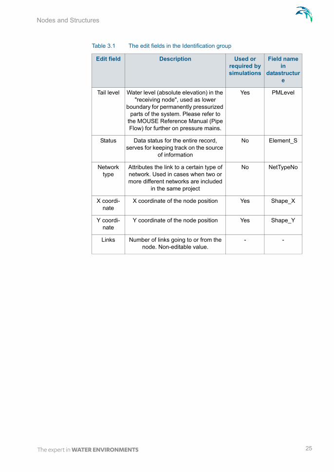
Table 3.1 The edit fields in the Identification group
Edit field Description Used or required by simulations
Field name in
datastructure
Asset ID Reference to an ID used in external data sources
No AssetName
Data source
Reference to an external data source (table ID) where the record has been
imported from
No DataSource
Node ID A unique name for the node. Up to 40 characters (letters, numbers, blank spaces and underscore characters)
Yes MUID
Model Associates the current node to a spec-ified submodel
No SubModelNo
Description User's descriptive information related to the node
No Description
PM Type Definition of the node´s role in the pressure main as the downstream
point of the pressure main’s connec-tion to the network. Manholes and basins can be declared as a “Tail
Node”. Please refer to the MOUSE Reference Manual (Pipe Flow) for fur-
ther on pressure mains.
Yes PMTypeNo
24 MIKE URBAN - © DHI
Nodes and Structures
Tail level Water level (absolute elevation) in the "receiving node", used as lower
boundary for permanently pressurized parts of the system. Please refer to
the MOUSE Reference Manual (Pipe Flow) for further on pressure mains.
Yes PMLevel
Status Data status for the entire record, serves for keeping track on the source
of information
No Element_S
Network type
Attributes the link to a certain type of network. Used in cases when two or more different networks are included
in the same project
No NetTypeNo
X coordi-nate
X coordinate of the node position Yes Shape_X
Y coordi-nate
Y coordinate of the node position Yes Shape_Y
Links Number of links going to or from the node. Non-editable value.
- -
Table 3.1 The edit fields in the Identification group
Edit field Description Used or required by simulations
Field name in
datastructure
25

Hydraulic Network Modeling with MOUSE
3.3.2 MOUSE model data group
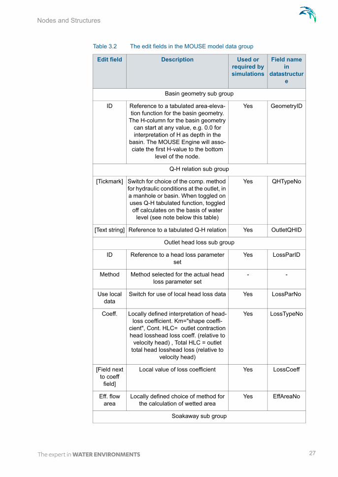
Table 3.2 The edit fields in the MOUSE model data group
Edit field Description Used or required by simulations
Field name in
datastructure
Node type MOUSE Node Types:
1. Manhole - node with shaft and chamber storage
2. Basin
3. Outlet - node where water leaves the system (no storage)
4. Storage node
5. Soakaway
Yes TypeNo
Diameter Diameter of the manhole - not enabled for any other node types
Yes Diameter
Ground level
Ground level of the node Yes GroundLevel
Bottom level
The bottom level of the manhole Yes InvertLevel
Critical level
User defined critical level. Used in result presentations and in the Pipe
Design module
Yes CriticalLevel
[Tickmark] Activates the inlet delimiter function Yes InletCon-trolNo
Max. Inflow Value of maximum possible inflow into the node from runoff
Yes MaxInlet
Cover sub-group
Type Choose among available types:
1. Normal
2. Sealed
3. Spilling
Yes Cover-TypeNo
Buffer pres-sure
Buffer pressure is only active for type = spilling. Equal to the pressure above
the ground level needed to cause spills from the manhole
Yes BufferPres-sure
Spill coeff. Spill coefficient is only active for type = spilling. Controls the spill capacity
Yes SpillCoeff
26 MIKE URBAN - © DHI
Nodes and Structures
Basin geometry sub group
ID Reference to a tabulated area-eleva-tion function for the basin geometry.
The H-column for the basin geometry can start at any value, e.g. 0.0 for interpretation of H as depth in the
basin. The MOUSE Engine will asso-ciate the first H-value to the bottom
level of the node.
Yes GeometryID
Q-H relation sub group
[Tickmark] Switch for choice of the comp. method for hydraulic conditions at the outlet, in a manhole or basin. When toggled on uses Q-H tabulated function, toggled off calculates on the basis of water
level (see note below this table)
Yes QHTypeNo
[Text string] Reference to a tabulated Q-H relation Yes OutletQHID
Outlet head loss sub group
ID Reference to a head loss parameter set
Yes LossParID
Method Method selected for the actual head loss parameter set
- -
Use local data
Switch for use of local head loss data Yes LossParNo
Coeff. Locally defined interpretation of head-loss coefficient. Km="shape coeffi-
cient", Cont. HLC= outlet contraction head losshead loss coeff. (relative to
velocity head) , Total HLC = outlet total head losshead loss (relative to
velocity head)
Yes LossTypeNo
[Field next to coeff
field]
Local value of loss coefficient Yes LossCoeff
Eff. flow area
Locally defined choice of method for the calculation of wetted area
Yes EffAreaNo
Soakaway sub group
Table 3.2 The edit fields in the MOUSE model data group
Edit field Description Used or required by simulations
Field name in
datastructure
27

Hydraulic Network Modeling with MOUSE
3.3.3 Q-H relations for nodes
Specifying a Q-H relation for an outlet controls the flow at the outlet. When specifying a Q-H relation for a manhole or basin the Q-H relation controls infiltration to the node. The Q-H relation specifies the relation between the water level in the manhole (or basin) and the infiltration flow. The flow (Q) value in the Q-H relation should be given as a positive value when water enters the node and a negative value for specifying a loss of water from the network model.
3.3.4 Outlet head loss
If you wish to make changes to the head loss parameter set that you have made a reference to, you can change this by accessing MOUSE|Local Head Losses. The editor is shown in Figure 3.5.
Porosity of fill material
Porosity of filling material Yes Porosity of fill material
Kfs, bottom Conductivity of soil Yes Kfs, bottom
[Tickmark] Activates the bottom conductivity function
Yes
Infiltration method
Method of infiltration Yes Infiltration method
Infiltration rate
Defines the infiltration rate Yes Infiltration rate
Initial water level
Initial water level in soakaway Yes Waterlevel
Table 3.2 The edit fields in the MOUSE model data group
Edit field Description Used or required by simulations
Field name in
datastructure
28 MIKE URBAN - © DHI

Nodes and Structures
Figure 3.5 Outlet head loss editor
3.3.5 Model Concept of Soakaway
Detailed hydraulic modelling of the green solutions can be done by means of the network point node type in MIKE URBAN - named soakaway. The soaka-way can be connected to the pipe network as any other node elements for detailed hydraulic studies. With is implementation in MIKE URBAN the soak-away represents a generic type of LID control as it can represent a number of different WSUD controls. The soakaway can be digitized graphically and it has its own feature layer which can be viewed in the horizontal plan view.
Figure 3.6 Conceptual drawing of a soakaway
A schematic drawing of a soakaway (Bio-retention cell) is illustrated in Figure 3.6. The stormwater drains of the surface and enters the soakaway at
29

Hydraulic Network Modeling with MOUSE
the upper vegetated layer. Then the stormwater infiltrates vertically through the soakaway and infiltrates out of the sides and bottom of the soakaway.
In some cases the soakaway is not connected to any drainage network and captured runoff to the soakaway is infiltrated and in case of extreme rainfall and exceedance of its infiltration and storage capacity storm water is sur-charged to the surface.
In other cases the soakaway is connected to the drainage network by a flow controlled outlet pipe as illustrated in Figure 3.6. During extreme rainfall caus-ing exceedance of its infiltration, storage and outlet flow capacity, the soaka-way also surcharges to the surface.
Figure 3.7 Soakaway concept in MIKE URBAN
A Soakaway will be represented in MIKE URBAN as a node (point) as shown in Figure 3.7.
Since a Soakaway is defined as a node type then the remaining configuration is unlimited in terms of
Inlet pipe(s) + Flow Regulation
Outlet pipe (s) + Flow Regulation
Weirs (s) or Orifice (s)
Connection to the existing drainage system can be configured to match the various types of soakaway installations. Soakaway nodes can i.e. be coupled in series to support the modelling of constructed infiltration trenches.
The soakaway can be added graphically and/or imported from any Asset GIS system hence existing soakaways can be illustrated in the plan view of MIKE URBAN.
The Soakaway node has the following attributes:
30 MIKE URBAN - © DHI

Nodes and Structures
NodeTypeNo = 5 (Soakaway node)
Invert Level
Ground Level
Geometry - defined as basin geometry
CoverType = 2 (Spilling)
Headloss = No Cross Section Changes
The inflow to the Soakaway can be provided as:
Direct Inflow (constant, time series)
Inflow from Rainfall Runoff (Runoff model A, B, C, Unit Hydrograph).
Various infiltration rate options
– No infiltration– Qinf - constant or as time series through boundary condition system – Qinf, side - function of wetted side area. This is calculated by MIKE
1D based on basin geometry– Qinf, bottom - function of bottom area
Saturated hydraulic conductivity [m/s]
Porosity of the soakaway material [ ]
The soakaway is modelled as a regular basin in MIKE URBAN, and it is also MIKE URBAN that calculates the water level based on the inflow (runoff), out-flow to the drainage network (via overflow pipe, weir, orifices etc.) and the infiltration. The soakaway has, unlike a basin, a porous filling material that affects the water level calculations, this is accounted for in the MIKE 1D and the basin geometry is defined as a usual basin geometry description.
The overflow pipe, weir or orifice is modelled in MIKE URBAN. Make sure that the up level of the pipe, weir or orifice is set correctly, and not at the bot-tom of the basin which will be the case if no invert level is specified. If the pipe is placed at the bottom then make sure that flow regulation is applied to the out-going pipe. The inflow pipe is generally not modelled; instead the catch-ment that generates the runoff to the soakaway (e.g. a road section, a roof) is connected directly to the basin via the catchment connection tools in MIKE URBAN.
A new point feature layer has been created to illustrate the soakaway in the plan view and to be used for graphical digitization and graphical connection of soakaway to existing drainage network.
31

Hydraulic Network Modeling with MOUSE
Figure 3.8 Soakaway shown in Feature layer
At the 'Geometry' tab in the dialog the type of node is selected in the Node type combobox and the following attributes are set:
Ground Level
Invert Level
Basin Geometry
Cover Type (Normal, Spilling and Sealed).
The geometry of the soakaway is defined as a standard basin.
Soakaway tab
At the 'Soakaway' tab in the dialog the type of infiltration, porosity and initial water level is selected
The following types of infiltration are available:
No Infiltration
Constant Infiltration
Infiltration
32 MIKE URBAN - © DHI

Nodes and Structures
Figure 3.9 Node Editor
The option 'No Infiltration' is used in cases when the there is no infiltration out of the soakaway. The initial water level can be set.
The 'Constant Infiltration' option provides the functionality of defining a con-stant infiltration rate out of the soakaway. The input required for this option is the Infiltration rate, the porosity of the fill material and the initial water level.
The 'Infiltration' option provides the functionality of having a variation in the infiltration based in the water level in the soakaway. A schematic drawing of the soakaway is provided in Figure 1.5 and Equation 1 describes the water balance of the model. Equation 2 and Equation 3 describe how the infiltration rate is calculated. Parameters and variables are listed and explained and how they are used in MIKE 1D.
33

Hydraulic Network Modeling with MOUSE
Figure 3.10 Schematic of the soakaway model
The 'Infiltration' option is based on the infiltration rate calculated by Equation (3.1) and Equation (3.2):
(3.1)
(3.2)
where is the soakaway porosity and h the calculated water level.
In MIKE 1D the infiltration rate calculated by Equation (3.2) is rewritten to Equation (3.3) to be based on the basin geometry definition in MIKE URBAN as well as to support different hydraulic conductivity at the side and at the bot-tom.
(3.3)
where Kfs,bottom is the field-saturated hydraulic conductivity at the bottom, Kfs,side is the field-saturated hydraulic conductivity at the side, As is the sur-face area and Ac the cross-sectional area.
The infiltration from the bottom can be turned off by a flag. However the infil-tration from both side and bottom can be shut off by setting the field-saturated hydraulic conductivity to zero.
The porosity of the fill material is used to calculate the water level in the soak-away and the initial water level is used to set the initial water level in the soak-away. Table values of hydraulic conductivity, Kfs, for different soil classes are provided in Table 3.3. Within each soil type the hydraulic conductivity varies
hdtd
------1
l w ----------------- Qin t Qf t – Qof t – =
Qf K l w 2h l w+ + =
Qf Kfs bottom As h 0= Kfs side 2Ac 2VolAc
---------+ +=
34 MIKE URBAN - © DHI

Pipes and Canals
significant why it is important to the measure the hydraulic conductivity at the site.
3.4 Pipes and Canals
Figure 3.11 Pipes and Canals editor
Table 3.3 Hydraulic conductivity for different soil classes
Soil classification Hydraulic Conductivity [m/s]
Gravel 0.001 to 0.1
Sand 10-5 to 10-2
Silt 10-9 to 10-5
Clay Below 10-9 to 10-2
“Moræneler” 10-10 to 10-6
35

Hydraulic Network Modeling with MOUSE
A link is specified as a conduit between two nodes. A link is considered as either a straight line or a drawn polyline between two nodes and per default is assumed to connect the adjacent nodes at bottom levels. Pipes permanently running under pressure are specified by setting the tickmark in “Pressure main”. Please refer to the MOUSE Reference Manual (Pipe Flow) for further on pressure mains.
The respective node bottom levels are displayed in the grey areas of the “UpLevel” and “DwLevel” fields by selecting “Recompute” when clicking the “Advanced” button.
In case of a step-wise connection (but not allowed below node bottom level), the elevations of both the upstream and downstream connection must be specified in the editable “UpLevel” and “DwLevel” fields.
Specification of nodes as 'upstream' and 'downstream' does not have any impact on the computations, apart that positive flow is considered from upstream to downstream. Therefore, it is recommended to specify the upstream and downstream in the direction of predominant flows. The specifi-cation of ‘upstream’ and ‘downstream’ can be swapped by selecting “Swap nodes” when clicking on the “Advanced” button.
Depending on the selected type, a link may take the form of one of the 'stand-ard' pipes (Circular, Rectangular, O Shaped, Egg-Shaped), or any closed or open cross section shape (CRS) and Natural Channels. The CRS and Natu-ral Channels are defined in the CRS and Topography Editors.
Standard pipes are defined by diameter (or cross section width and height for non-circular pipes), the geometry of special cross sections is as mentioned specified under the cross section editor. In this dialog, only the reference to the CRS ID.
For natural channels a topography, defined in the Topography editor, is spec-ified. The topography is specified with a series of CRS, where the first is placed in chainage 0. The chainage of the last CRS defines the length of the topography. If the length of the topography is shorter than the computed length for the link (or user specified length if specified) the last cross section will be used for the remaining part of the natural channel. And vice versa, if the length of the topography is longer than the link length only the topography specified until the computed length (or user specified length) will be used, the CRS at the end of the link may be an interpolation from two CRS. When the topography length differs from the computed length (or the user defined length if specified) a warning will be issued. It is possible to define an optional maximum length, dx between to h-points between two CRS. I.e. the distance between two chainages is 235 m and the max dx = 150 m, then MOUSE will add an h-point at the middle between the two CRS at 117.5 m.
A link is characterised by material, which determines the Manning friction coefficient (Manning), the Colebrook White coefficient (Equivalent roughness)
36 MIKE URBAN - © DHI

Pipes and Canals
or Hazen-Williams coefficient. It is optional to use either the default rough-ness values for specific materials or local values.
Specification of the different kind of materials and roughness coefficients is done through the ‘MOUSE | Materials’ Editor
Figure 3.12 Materials Editor
The length of a link is calculated from the shape of the line in MIKE URBAN. The length is displayed in the 'Length_C' field, but is not updated until the 'Recompute' command is executing (from the ‘Advanced’ button). If a user defined length is specified this will overwrite the calculated one during simula-tion.
3.4.1 Identification group
Table 3.4 The edit fields in the Identification group
Edit field Description Used or required by simulations
Field name in
datastructure
Asset ID Reference to an ID used in external data sources
No AssetName
Data source
Reference to an external data source (table ID) where the record has been
imported from
No DataSource
37

Hydraulic Network Modeling with MOUSE
3.4.2 Geometrical properties
Link ID A unique name for the node. Up to 40 characters (letters, numbers, blank spaces and underscore characters)
Yes MUID
Status Data status for the entire record, serves for keeping track on the source
of information
No Element_S
Description User's descriptive information related to the link
No Description
Network type
Attributes the link to a certain type of network. Used in cases when two or more different networks are included
in the same project
No NetTypeNo
From node Upstream Node Yes MUID
To node Downstream Node Yes MUID
Pressure main
Defines a link as pressure main. A link connected to a manhole or basin, can only constitute a pressure main if the manhole/basin is declared to be “tail node”. Please refer to the MOUSE
Reference Manual (Pipe Flow) for fur-ther on pressure mains.
No PMApprNo
Table 3.5
Edt field Description Used or required by simulations
Field name in datastructure
Shape Shape of pipe Yes TypeNo
Size Nominel size of pipe (diameter of cir-cular pipe, height of Egg-shape pipe
and width for O-shaped)
Yes, if Shape = Circular, Egg-Shape
and O-Shaped
Diameter
Table 3.4 The edit fields in the Identification group
Edit field Description Used or required by simulations
Field name in
datastructure
38 MIKE URBAN - © DHI

Pipes and Canals
3.4.3 Hydraulic friction losses
Width Width of rectangular shape Yes, if Shape = Rectangu-
lar
Width
Height Height of rectangular shape Yes, if Shape = Rectangu-
lar
Height
CRS ID ID of cross section Yes, if shape = CRS
CrsID
Topography ID of topography Yes, if Shape = natural channel
Topogra-phyID
Max Dx Max distance between gridpoints Yes, if Shape = natural channel
Maxdx
Length Length of link Yes Length
UpLevel Upstream invert level of link Yes UpLevel
DwLevel Downstream invert level of link Yes DwLevel
Table 3.6
Edit field Description Used or required by simulations
Field name in datastructure
Material Material of link Yes MaterialID
Formula-tion
Formula for calculation of the friction loss (Manning Explicit, Manning
Implicit, Colebrook White, Hazen-Wil-liams)
Yes FricTypeNo
Use local data
Determines if roughness values from the material are overwritten by local
values
Yes FricNo
Manning Manning roughness value Yes, if ‘Man-ning Explicit’ or ‘Manning Implicit’ is chosen
Manning
Table 3.5
Edt field Description Used or required by simulations
Field name in datastructure
39

Hydraulic Network Modeling with MOUSE
3.4.4 Miscellaneous
The ‘Regulation’ button provides access to inserting a regulation in the selected link. This regulation does not require the Control module. The regu-lation can be either a maximum discharge as a function of the water level in a user specified node (Ctrl. Node A) or a maximum discharge as a function of the water level difference between two user specified nodes (Ctrl. Node A and Ctrl. Node B).
Figure 3.13 Links regulation dialog
The ‘Additional’ button provides access to more advanced options for a link such as specifying a depth-variable Manning number.
Eq. rough-ness
Equivalent roughness Yes, if ‘Cole-brook White’ formulation is
chosen
Rough
H-W coef Hazen-Williams roughness coefficient Yes, if ‘Hazen-Wil-
liams’ is cho-sen
HWCoef
Table 3.6
Edit field Description Used or required by simulations
Field name in datastructure
40 MIKE URBAN - © DHI

Weirs
3.5 Weirs
A weir is actually a functional relation, which connects two nodes of a MOUSE network (two-directional flow and submerged flow possible), or is associated with only one node (free flow 'out of the system'). The latter case is achieved if the 'To' field is left empty.
In the real world a weir may be located in a manhole or a similar construction which you normally would define as a node in the model configuration. The numerical solutions for the flow equations, however, need a model configura-tion with two nodes where the weir is defined as the connection between the nodes. The weir will then be placed between the two nodes as the flow con-nection.
It is possible to define several weirs between the same two nodes if this is required. This is similar to the possibility of having more than one pipe as the link between nodes. The generation of the computational grid shown in Figure 3.15 for the orifice is also applied for pumps, weirs and valves. The numerical solution of the flow equations will depend on the selected device. Please refer to the reference manual on more on this.
It is recommended not to place the two nodes in the same spot, instead place the nodes a short distance apart. The reason is that the node head loss com-putation will have a component from change of flow direction. If the two nodes surrounding the device are placed exactly at the same location then the com-putational engine cannot determine the direction of the flow from the coordi-nates of the nodes and a default direction will be applied. This may unintentionally introduce a change in direction and therefore also an unex-pected head loss.
By using a small displacement of the nodes the change in flow direction will be determined based on the coordinates and angles between the connected pipes. Therefore consider carefully the placement of the nodes with respect to the actual construction.
41

Hydraulic Network Modeling with MOUSE
Figure 3.14 Weirs editor
A weir is characterised by the computational method, weir type, crest level, crest width, and orientation. If the Q-H relation is specified, only the crestlevel and a DataSetID are specified. With the built-in weir formula, the results are affected by the specified parameters. The weir type can be selected among 'Rectangular', ‘V-notch’, ‘Trapezoidal’, ‘Irregular’and ‘Long weirs’. For ‘Rec-tangular’ and ‘Long Weirs’ the ‘Weir formula’ option is used. For the other weir types the Q-H relation must be used.
Orientation ('degrees') plays an important role (as long as the head loss coef-ficient is undefined), since depending on the specified orientation, kinetic energy of the flow is included (90o) or is not included (0o) in calculations of the weir flows.
The dimensionless head loss coefficient is optional. If the coefficient is speci-fied, it will overwrite the default and change the computation mode (so that the effect of ‘orientation’ will not be included) during the simulation.
Weirs are per default static (No Control) but can be controlled through Real Time Control (RTC). Clicking on the “RTC” button to the right gives quick access to the RTC specification dialog.
There are no limitations on the number of weirs specified at one location.
42 MIKE URBAN - © DHI

Weirs
3.5.1 Identification and connectivity
Table 3.7
Edit field Description Used or required by simulations
Field name in datastructure
Asset IDReference to an ID used in external data sources
No AssetName
Data source
Reference to an external data source (table ID) where the record has been imported from
No DataSource
Weir IDA unique name for the weir. Up to 40 characters (letters, numbers, blank spaces and underscore characters)
Yes MUID
StatusData status for the entire record, serves for keeping track on the source of information
No Element_S
Location ID of Node where Weir is located Yes MUID
ToID of Node where Weir is discharging to. If field left empty, then water is dis-charging out of the system
Yes MUID
Network type
Attributes the weir to a certain type of network. Used in cases when two or more different networks are included in the same project
No NetTypeNo
Weir type Specification of type of weir Yes TypeNo
DescriptionUser's descriptive information related to the weir
No Description
43

Hydraulic Network Modeling with MOUSE
3.5.2 Model data
3.6 Orifices
An orifice is actually a functional relation, which connects two nodes of a MOUSE network or is associated with only one node (free flow 'out of the system'). The latter case is achieved if the 'To' field is left empty.
Table 3.8
Edit field Description Used or required by simulations
Field name in datastructure
Comp type Selection of computation Method Yes MethodNo
FlapFlap indicating a flap-gate built-in weir (i.e. no return flow possible)
Yes FlapNo
Oper. mode No control or RTC controllable weir YesCon-trolTypeNo
OrientationWeir orientation relative to the main flow direction. “0” is Side weir, “90” is a transversal weir
Yes, if dis-charge coeff. is not speci-fied
AngleNo
Crest level Crest level of weir Yes CrestLevel
Discharge coeff.
Discharge coefficientYes, if weir formula is chosen
Coeff
Crest width Width of rectangular weirYes, if weir formula is chosen
CrestWidth
Q-H table Reference to tabulated Q-H funtionYes, if Q-H is chosen
QHID
Source Channel
The ID of the source or the upstream channel of the weir
Yes, if frag-mented is chosen
SourceLinkID
Destina-tion Chan-nel
The ID of the destination or the down-stream channel of the weir
Yes, if frag-mented is chosen
Destination-LinkID
Weir Crest Geometry
Reference to tabulated variation of the weir crest along the weir
Yes WeirCrestID
44 MIKE URBAN - © DHI

Orifices
In the real world a flow restriction in the form of an orifice may be located in a manhole or a similar construction which you normally would define as a node in the model configuration. The numerical solutions for the flow equations, however, need a model configuration with two nodes where the orifice is defined as the connection between the nodes. The orifice will then be placed between the two nodes as the flow connection.
Figure 3.15 The difference between real world orifice and model configuration of ori-fice
It is possible to define several orifices between the same two nodes if this is required. This is similar to the possibility of having more than one pipe as the link between nodes. The generation of the computational grid shown in Figure 3.15 for the orifice is also applied for pumps, weirs and valves. The numerical solution of the flow equations will depend on the selected device. Please refer to the reference manual on more on this.
It is recommended not to place the two nodes in the same spot, instead place the nodes a short distance apart. The reason is that the node head loss com-putation will have a component from change of flow direction. If the two nodes surrounding the device are placed exactly at the same location then the com-putational engine cannot determine the direction of the flow from the coordi-nates of the nodes and a default direction will be applied. This may unintentionally introduce a change in direction and therefore also an unex-pected head loss.
By using a small displacement of the nodes the change in flow direction will be determined based on the coordinates and angles between the connected
45

Hydraulic Network Modeling with MOUSE
pipes. Therefore consider carefully the placement of the nodes with respect to the actual construction.
An orifice is specified by a type; circular, CRS or rectangular, and the corre-sponding diameter, height and width.
A discharge coefficient can be specified (default = 1.0) and a flap gate (or non-return valve) can be specified.
Orifices are per default static (No Control) but an orifice can be controlled through Real Time Control (RTC). Clicking on the “RTC” button to the right gives quick access to the RTC specification dialog.
Figure 3.16 Orifice editor
46 MIKE URBAN - © DHI

Orifices
3.6.1 Identification and connectivity
3.6.2 Model data
Table 3.9
Edit field Description Used or required by simulations
Field name in datastructure
Asset ID Reference to an ID used in external data sources
No AssetName
Data source
Reference to an external data source (table ID) where the record has been imported from
No DataSource
Orifice ID A unique name for the orifice. Up to 40 characters (letters, numbers, blank spaces and underscore characters)
Yes MUID
Status Data status for the entire record, serves for keeping track on the source of information
No Element_S
Location ID of Node where orifice is located Yes MUID
To ID of Node where orifice is discharg-ing to. If field left empty, then water is discharging out of the system
Yes MUID
Network type
Attributes the link to a certain type of network. Used in cases when two or more different networks are included in the same project
No NetTypeNo
DescriptionUser's descriptive information related to the orifice
No Description
Table 3.10
Edit field Description Used or required by simulations
Field name in datastructure
Type Type of orifice according to shape Yes TypeNo
Flap Flap indicating a flap-gate built-in (i.e. no return flow possible)
Yes FlapNo
47

Hydraulic Network Modeling with MOUSE
3.6.3 Defining a gate or a weir in an orifice
The orifice itself is just an opening with a static shape. In real constructions orifices are often equipped with a controlled gate or weir which can be used in real time control for regulating the flow through the orifice. The gate device will move from the top of the orifice opening and downwards until the orifice is fully closed. The weir moves from the bottom of the orifice upwards and closes fully when the weir crest reaches the top of the orifice opening (see Figure 3.17 for an illustration). It is possible to apply both types of movable devices in the computations. In both cases the device is "added" to a defined orifice. This is done from the Controllable Devices dialog (MOUSE|Con-trol|Controllable Devices). See more on this in section 9.8.
Oper. modeNo control or RTC controllable orifice
Yes Con-trolTypeNo
Discharge coeff
Calibration coefficient. Value = 1 results in the flow as determined by
orifice algorithm
Yes Dis-chargeCoeff
Invert level Absolute elevation of the orifice invert Yes InvertLevel
Height Height of rectangular orifice Yes Height
Width Width of rectangular orifice Yes Width
Diameter Diameter of circular orifice Yes Diameter
CRS ID Reference of a cross-section ID for irregularly-shaped orifice
Yes, if CRS type is cho-
sen
CrsID
Table 3.10
Edit field Description Used or required by simulations
Field name in datastructure
48 MIKE URBAN - © DHI

Stormwater Inlets
Figure 3.17 Examples on a rectangular orifice with a gate and a weir
3.7 Stormwater Inlets
The connections between pipe systems and overland flow networks to simu-late the capture capacity (and surcharge) of side inlet pits and grates can be approximated in MOUSE using a combination of orifices and weir geometry. However, a method has been developed to incorporate the geometry of the inlet structure (Curb Inlet or Lintel) via a new MOUSE element which allows user input of the empirical relationship governing the structure capacity.
A typical Curb Inlet/grate configuration is shown below. Flow into the pit chamber is via both a grate and side weir (operates as an orifice for deeper flow depths).
Figure 3.18 A typical curb inlet configuration
49

Hydraulic Network Modeling with MOUSE
Standard curves have been developed in Australia for "ON-GRADE" type (using a Qapproach/Qcapture relationship where flow can bypass the structure) and "SAG" type (using a Depth/Q relationship at locations/low points where water collects). However the formulation with MOUSE allows for non-specific and user defined relationships. An example of the empirical curves devel-oped for the ON-GRADE type is shown below, with the flow captured repre-sented as a proportion of the approach flow, and varying with approach slope.
Figure 3.19 Example of empirical curves for On-Grade type
3.7.1 Curb Inlet (Lintel)
A Curb Inlet (Lintel) is a connection between two nodes of a MOUSE network (two-directional flow and submerged flow possible), describing the transfer of flow at a grate or inlet from an overland flow network to the sub-surface pipe network. The Curb Inlet dialog is accessed via the “MOUSE | Stormwater Inlets | Curb Inlets” menu.
There are two types of Curb Inlet:
SAG Type, where the connection node on the overland flow network is located at a sag or low point where water will collect. Transfer capacity of the connection is specified as a DQ-relation (tabular data type).
ON-GRADE Type, where flow in the overland flow network can continue past the connection node. Transfer capacity of the connection is depend-ent on the slope of the overland flow network, and specified as a Capture ID (collective of QQ-relations defining the capture rate as a proportion of approach flow).
50 MIKE URBAN - © DHI

Stormwater Inlets
Figure 3.20 The Curb Inlet data dialog (SAG Type)
Figure 3.21 The Curb Inlet data dialog (On-Grade Type)
User defined parameters in the Curb Inlet dialog include:
51

Hydraulic Network Modeling with MOUSE
Invert level (m) defining the point at which spilling starts (similar to weir crest level). The user is shown a system calculated invert level which is the same as the invert of the connection node in the overland flow net-work. As with weir flow, a crest level at least 0.01 m higher than the con-nection node invert level is recommended for initial condition stability.
Freeboard (m), defining a critical water level (Invert - Freeboard) at the connection node in the pipe network below which the defined DQ and QQ-relations apply. For submerged and reverse flow (surcharge), the transfer capacity of the connection reverts to a standard orifice relation-ship.
Slope (%), representing the slope of the steepest link in the overland flow network entering the connection node (only applies to ON-GRADE Type). The system calculated slope is used in the calculation unless a user defined slope is specified.
Blockage factor (%) which can be used to account for debris blockage at the grate/inlet. This linear factor is applied to the tabular data sets defin-ing the transfer capacity of the connection.
Number of Curb Inlets, allowing multiple curb inlets of the same specified geometry (transfer capacity) applied at the same location within a single connection.
Default rectangular orifice geometry, applies to those flow cases (sub-merged and reverse flow) were the defined DQ and QQ-relations do not apply. This generally applies when water levels at the connection node in the pipe network exceed the critical level defined by the Freeboard, including reverse flow (surcharge).
There are no limitations on the number of curb inlets specified at one location; however, the connectivity must be ‘From’ a node in the overland flow network ‘To’ a node in the pipe network, for correct automatic calculation of slope. Note: Link slopes must be calculated in the link dialog for automatic calcula-tion of slope to operate.
3.7.2 On-grade Capture
The On-grade Capture dialog allows the user to group together QQ-relations (tabular data) that comprise a single On-grade Curb Inlet geometry (similar in function to the Topography dialog). As the transfer capacity for an On-grade Curb Inlet is dependent on the slope in the overland flow network, a number of QQ-relations can apply.
52 MIKE URBAN - © DHI

Stormwater Inlets
Figure 3.22 The On-Grade Capture data dialog (On-Grade Type)
For calculated or user defined slopes in the Curb Inlet dialog that are outside the range of slopes specified in the On-grade Capture dialog, the closest slope curve will be used. For intermediate calculated or user defined slopes (lying between slope curves in the On-grade Capture dialog), linear interpola-tion is applied.
In the case of an On-grade Curb Inlet capacity that is not dependent on slope of the overland flow network, the user needs to define the On-grade Capture with a single QQ-relation. Note: In this case, the calculated or user defined slope in the Curb Inlet dialog for ON-GRADE Type will be ignored.
3.7.3 Capacity curves
Two curve types specified in the tabular data (MOUSE|Curves & Relations) can be used with the two different types of Curb Inlets.
Capacity Curve, DQ (depth/discharge relation specified in the Curb Inlets dialog)
Capacity Curve, QQ (Qapproach,Qcapture relation specified in the On-grade capture dialog).
The DQ relation specifies the depth based capacity curve for a SAG Type Curb Inlet. Values must be monotonously increasing in depth and discharge and starting at (0,0). For depths in excess of the maximum value specified in the last row of the table, the last corresponding discharge value is used.
The QQ relation specifies the relationship between approach flow in the over-land flow network (Qapp) and the captured flow at the connection node for an ON-GRADE Type Curb Inlet (Qcap). Values must be monotonously increasing and starting at (0,0). For approach discharges in excess of the maximum
53

Hydraulic Network Modeling with MOUSE
value specified in the last row of the table, the last corresponding capture dis-charge value is used.
3.8 Pumps
A pump is actually a functional relation, which connects two nodes of a MOUSE network or is associated with only one node (free flow 'out of the system'). The latter case is achieved if the 'To' field is left empty. In this case it is also possible to let the water pumped out of the system enter a 2D model (in the case of coupling MIKE URBAN to MIKE 21, i.e. MIKE FLOOD). This is done by setting the tickmark in ‘Coupling to 2D overland flow’.
In the real world a pump may be located in a manhole or a similar construc-tion which you normally would define as a node in the model configuration. The numerical solutions for the flow equations, however, need a model con-figuration with two nodes where the pump is defined as the connection between the nodes. The pump will then be placed between the two nodes as the flow connection.
It is possible to define several pumps between the same two nodes if this is required. This is similar to the possibility of having more than one pipe as the link between nodes. The generation of the computational grid shown in Figure 3.15 for the orifice is also applied for pumps, weirs and valves. The numerical solution of the flow equations will depend on the selected device. Please refer to the reference manual on more on this.
It is recommended not to place the two nodes in the same spot, instead place the nodes a short distance apart. The reason is that the node head loss com-putation will have a component from change of flow direction. If the two nodes surrounding the device are placed exactly at the same location then the com-putational engine cannot determine the direction of the flow from the coordi-nates of the nodes and a default direction will be applied. This may unintentionally introduce a change in direction and therefore also an unex-pected head loss.
By using a small displacement of the nodes the change in flow direction will be determined based on the coordinates and angles between the connected pipes. Therefore consider carefully the placement of the nodes with respect to the actual construction. For pumps the distance between the nodes will often be larger.
3.8.1 Pump types
Several pump types can be specified in MIKE URBAN.
54 MIKE URBAN - © DHI

Pumps
Constant flow pumps
This is the simplest way of modeling pumps. In this case the pump will dis-charge the same constant flow Q at any time when the pump is switched on. Eventually with the variation as defined during acceleration or deceleration periods.
When specifying a constant flow pump, set the Speed to ‘Constant’ and choose ‘Constant’ in the Cap. curve type field and type in the constant flow in the Constant flow field.
Notice: 'Constant flow' pump is different from 'Constant speed' pump. The later may have varying discharge.
Constant speed pumps
When defining pumps in MIKE URBAN models for sewer and drainage sys-tems it will most commonly be pumps with a pump curve of type "Q, dH". The actual pump discharge Q will be a function of the actual pressure difference dH between the pump wet well and the receiving point in the model. The pump curves for this type of pumps will in general be as shown in the figure below.
Figure 3.23 Typical example of pump curve
Pump curves are defined in MIKE URBAN by tabulating the curve (see more in section 5). This can be done by selecting representative points on the pump curve as shown in the next figure. Information about pump curves are typically provide by the manufacturer of the pumps.
55

Hydraulic Network Modeling with MOUSE
Figure 3.24 Tabulating the curve
When a pump curve is tabulated like this and used in the simulations exe-cuted with the MOUSE Engine, then the pump is allowed to operate within the range of the dH values in the table. At any time during the simulation the MOUSE Engine will compute the actual dH and determine the corresponding Q value from the table, resulting in the actual duty point position for the pump.
As a standard feature the MOUSE Engine will stop the simulation with an error message if the hydrodynamic conditions result in an actual dH value outside the range of the pump curve table.
Variable speed pumps
When applying variable speed pumps the manufacturer typically provides a set of pump curves describing the pump capacity at various percentages of maximum rotation speed or maximum power input. You may have a set of curves available as show in the figure below.
Figure 3.25 Pump curves at various percentages of maximum rotation speed or maximum power input
It is also found that variable speed pumps cannot be regulated over the full range between 0% and 100%. Instead the regulation may be in the range of 70% to 100% as indicated in the figure above. Search for specific information available for the pumps applied at the pumping stations being modeled.
56 MIKE URBAN - © DHI

Pumps
For simplicity in the modeling the actual method of varying the pump capacity is not considered. It is not directly related to the actual number of rotations per minute (RPM) or the actual electrical power input. In the modeling we only consider the pump capacity as varying between a pump curve corre-sponding to the minimum speed and a pump curve corresponding to the max-imum speed.
For variable speed pumps the two pump curves are defined as 'RPMmin' and 'RPMmax' pump curves. For constant speed pumps only the 'RPMmax' pump curve is applied.
Figure 3.26 The RPMmax and RPMmin pump curves
When the MOUSE simulation is executed it is the standard condition that the simulation will stop and give an error message if the conditions exceed the range for the dH value in the pump curve table. This applies both for the 'RPMmax' and the 'RPMmin' pump curve.
Operation of variable speed pumpsIf the 'Speed' selection field is set to 'Variable' and the 'Oper. Mode' field is set to 'Wet Well Set Point' a value for the wet well set point is entered.
When a variable speed pump is in operation during the simulation with the MOUSE Engine the duty point will move between the two pump curves depending on the actual conditions. The actual flow is determined by using a PID function which will attempt to control the water level at the wet well to stay at the specified set point value.
The discharge Q determined by the PID function and the dH found by the actual hydraulic conditions defines the duty point. This may vary in the area between the two pump curves.
57

Hydraulic Network Modeling with MOUSE
Figure 3.27
Eventually the conditions may result in the duty point ending up on one of the pump curves. If the PID regulation sets the discharge Q to a value higher than the limitation by the 'RPMmax' pump curve at the given dH condition, then the discharge will be defined by the pump curve. As a consequence the water level in the wet well will rise above the defined set-point value.
Figure 3.28
If the inflow to the pumping station is low, then the operation of the pump may result in an actual duty point located at the 'RPMmin' pump curve. In this case the water level at the wet well will drop below the defined set-point value. Eventually the water level will reach the stop level defined for the pump and the operation is switched off
58 MIKE URBAN - © DHI

Pumps
Figure 3.29
More detailed output information may be added to the standard result file for variable speed pumps. Please refer to the documentation on the DHIAPP.INI file found in the “DHIAPP INI and ADP Files Reference Manual”.
Registration of 'dry stops' of pumpsThe hydrodynamic network simulation provides a simulation summary report at the end of the computation. The summary for the pumps will show the number of pump starts during the simulation and if the individual pumps have been forced to stop due to lack of water in the pump wet well.
There can be various reasons for situations where pumps are running dry. When this happens in the model simulation it indicates a mismatch in the configuration. E.g. too small wet well volume, errors in the applied pump capacity curves or deceleration times.
Figure 3.30 Summary reveals dry stops during simulation
Pumps will be switched off when the water level drops to the defined stop level. But the pump flow continues during the specified deceleration period by a linear decrease to zero flow. During this time interval the water level in wet well may eventually drop to the bottom of the wet well during a single time step. In this situation the MOUSE Engine will force an immediate 'dry stop' of the pump discharge.
59

Hydraulic Network Modeling with MOUSE
The 'Pumps - Discharge' section is only output to the summary report if 'pumps' has been selected in the summary selection dialog (found on the Simulation dialog).
Figure 3.31 Pumps editor
A pump is characterised by the 'Start Level' and 'Stop Level', an offset, accel-eration and deceleration time and a capacity curve. The capacity curve is specified in the Curves and Relations dialog. The capacity curve can be specified as a 'Capacity Curve QH' relation (for screw pumps) or as 'Capacity Curve QdH' relation (for differential head pumps), where 'H' is the absolute water level in the pump's wet well (at 'Location'), and 'dH' is the water level difference between the 'To' and the 'Location' nodes. A pump type with a 'Capacity Curve QH' relation is named a screw pump, while a pump type with a 'dH-Q' relation is named a differential head pump.
If an offset is specified this will be added to the capacity curve relation.
60 MIKE URBAN - © DHI

Pumps
Pumps are per default static (No Control) but can be controlled through Real Time Control (RTC). Clicking on the “RTC” button to the right gives quick access to the RTC specification dialog.
3.8.2 Identification and connectivity
Table 3.11
Edit field Description Used or required by simulations
Field name in datastructure
Asset ID Reference to an ID used in external data sources
No AssetName
Data source
Reference to an external data source (table ID) where the record has been imported from
No DataSource
Pump ID A unique name for the pump. Up to 40 characters (letters, numbers, blank spaces and underscore characters)
Yes MUID
Location ID of Node where pump is located Yes MUID
To ID of Node where Pump is pumping to.
Yes MUID
Status Data status for the entire record, serves for keeping track on the source of information
No Element_S
Network type
Attributes the pump to a certain type of network. Used in cases when two or more different networks are included in the same project
No NetTypeNo
Speed Selection between constant and varia-ble speed pumps. Only variable speed
pumps can be used for PID control
Yes SpeedNo
Description User's descriptive information related to the pump
No Description
61

Hydraulic Network Modeling with MOUSE
3.8.3 Model data
3.9 Valves
A valve is a functional relation which connects two nodes of a MOUSE net-work.
Table 3.12
Edit field Description Used or required by simulations
Field name in datastructure
Oper. mode Switch between “normal” (i.e. ON/OFF at fixed level) and RTC operation.
“Wet-well set point” is a special RTC control, which is accessible also with-
out RTC add-on module
Yes Con-trolTypeNo
Cap. curve type
Type of capacity curve. Type 1 is applicable for archimed Screw, type 2
for all rotodynamic pumps
Yes CapTypeNo
Start level Water level in pump sump which trig-gers the pump to start
Yes StartLevel
Stop level Water level in pump sump which trig-gers the pump to stop
Yes StopLevel
Acc. time Pump acceleration time. Used to dampen sudden increase of flow at
the pumps START events
Yes AccTime
Dec. time Pump decceleration time. Used to dampen sudden decrease of flow at
the pumps STOP events
Yes DecTime
Offset Offset of the capacity curve. Applies to Q-H types, which may be specified
relative to different datums
Yes. if Q-H type
Offset1
Offset Offset of minimum capacity curve. Applies only for variable speed pumps
Yes, if varia-ble speed
pump
Offset2
Wet Well set-point
Absolute water level in the pump sump (i.e. wet well) which the pump is
supposed to maintain
Yes WetWellSet-Point
QMaxSetID Capacity curve for the nominal (max) rotation speed
Yes QMaxSetID
QMinSetID Capacity curve for the minimum speed. Applies only for variable speed
pumps
Yes QMinSetID
62 MIKE URBAN - © DHI

Valves
Figure 3.32 Valve dialog
In the real world a valve may be located in a manhole or a similar construc-tion which you normally would define as a node in the model configuration. The numerical solutions for the flow equations, however, need a model con-figuration with two nodes where the valve is defined as the connection between the nodes. The valve will then be placed between the two nodes as the flow connection.
It is possible to define several valves between the same two nodes if this is required. This is similar to the possibility of having more than one pipe as the link between nodes. The generation of the computational grid shown in Figure 3.15 for the orifice is also applied for pumps, weirs and valves. The numerical solution of the flow equations will depend on the selected device. Please refer to the reference manual on more on this.
It is recommended not to place the two nodes in the same spot, instead place the nodes a short distance apart. The reason is that the node head loss com-putation will have a component from change of flow direction. If the two nodes surrounding the device are placed exactly at the same location then the com-putational engine cannot determine the direction of the flow from the coordi-nates of the nodes and a default direction will be applied. This may unintentionally introduce a change in direction and therefore also an unex-pected head loss.
By using a small displacement of the nodes the change in flow direction will be determined based on the coordinates and angles between the connected
63

Hydraulic Network Modeling with MOUSE
pipes. Therefore consider carefully the placement of the nodes with respect to the actual construction.
A valve is specified by a diameter, flow area (by default calculated on the basis of the diameter, but it is possible to overwrite this value) and an invert level.
It is possible to specify a valve to be a non-return valve and thereby prevent-ing flow in the negative flow direction. A rating curve is specified to define the relation between the valve opening (%) and resistance (k). The rating curve is specified under “MOUSE|Curves & Relations”.
The valve is by default static, in which case the valve opening must be speci-fied. It is also possible to define a valve to be the RTC controlled and then the valve opening will be controlled by any specified control rules.
Table 3.13 Identification and connectivity edit fields of the MIKE URBAN valve edi-tor.
Edit field Description Used or required by simulations
Field name in data struc-
ture
Asset ID Reference to an ID used in external data sources
No AssetName
Valve ID A unique name for the valve. Up to 40 characters (letters, numbers, blank spaces and underscore characters)
Yes MUID
Location ID of Node where valve is located Yes FROMNODE
To ID of Node where valve is discharging to
Yes TONODE
Description User’s descriptive information related to the valve
No Description
Data source
Reference to an external data source (table ID) where the record has been
imported from
No DataSource
Status Data status for the entire record, serves for keeping track on the source
of information
No Elements
64 MIKE URBAN - © DHI

Valves
Table 3.14 Geometrical and hydraulic properties, edit fields of the MIKE URBAN valve editor
Network Type
Attributes the valve to a certain type of network. Used in case where two or more different networks are included
in the same project
No NetTypeNo
Valve Type Specification of type of valve, this information is not used in the simula-
tion engine
No TypeNo
Table 3.15
Edit field Description Used or required by simulations
Field name in data struc-
ture
Comp type Selection of computation Method. Yes MethodNo
Oper.modeNo control or RTC controllable valve
Yes Con-trolTypeNo
Non Return Indicating a flap-gate built-in valve (i.e. no return flow possible)
Yes FlapNo
Rating Curve
Reference to the tabulated k-opening function
Yes RatingCur-veID
Diameter The default value of the area (the field “Flow Area”) is calculated on the
assumption of a circular valve, with the diameter specified in this field.
Furthermore, the transition to a pres-surized valve is defined by the invert
level plus the diameter.
Yes Diameter
Flow Area A user specified flow area overwrites the default valve area computed on the basis of a circular cross section.
Yes Area
Edit field Description Used or required by simulations
Field name in data struc-
ture
65

Hydraulic Network Modeling with MOUSE
3.10 CRS & Topography
The CRS and Topograpy editors allow the definition of the conduit cross-sec-tions and natural streams topographies, according to the following:
CRS editor: Open and closed Cross sections. The X, Z types are appro-priate for irregular cross sections, while H, W are best for symmetric cross sections.
Topography: The "Channel Topography" dialog is an editor for MOUSE topography data. A topography is made up from a number of cross sec-tions,specified in the cross section editor.
The CRS and Topography Editors are reached by selecting MOUSE | CRS & Topography.
Figure 3.33 The CRS editor
Cross sections are classified in seven types: three of them are closed cross sections, and four of them are open cross sections. Each of the types has
Invert Level The invert level defines the minimum water level, which generates flow
through the valve
yes InvertLevel
Valve Opening
Defines the opening of the valve in percentages (value between 0 and 100). For an RTC controlled valve,
this value is not applied, the opening is controlled by the MIKE URBAN
build in RTC algorithm
Yes Opening
Table 3.15
Edit field Description Used or required by simulations
Field name in data struc-
ture
66 MIKE URBAN - © DHI

CRS & Topography
three sub-types, defined by the way how the CRS geometry is described. Thus, the following CRS types are supported:
X, Z open: The CRS geometry is described by points defined by co-ordi-nate pairs (x, z), where 'x' is a horizontal axis, and 'z' a vertical axis. The points are specified in a counter-clockwise direction.
X, Z closed: The CRS geometry is described by points defined by co-ordinate pairs (x, z), where 'x' is a horizontal axis, and 'z' a vertical axis. The points are specified in a counter-clockwise direction. The first and last points are connected to close the cross section.
H, W open: The CRS geometry is described by pairs (h, w), where 'h' is relative height, and 'w' is the corresponding cross section width. The pairs are specified in an upward direction.
H, W closed: The CRS geometry is described by pairs (h, w), where 'h' is relative height, and 'w' is the corresponding cross section width. The pairs are specified in an upward direction. The last specified (h, w) pair defines the top of the closed cross section.
Processed open: The CRS geometry is described directly through their hydraulic parameters; Length (L), Width (W), cross section area (A) and hydraulic radius (R). For this type of CRS a graph is not available.
Processed closed: The CRS geometry is described directly through their hydraulic parameters; Length (L), Width (W), cross section area (A) and hydraulic radius (R). For this type of CRS a graph is not available.
X-Z-R-M open: The CRS geometry is described by points defined by co-ordinate pairs (x, z), where 'x' is a horizontal axis, 'z' a vertical axis, the relative resistance (R) and the marker (M). The points are specified in a counter-clockwise direction.
This cross section type allows to specify open channel systems to have varia-ble roughness across a cross section (common in urban and drainage stud-ies).
A series of lateral resistance factors can hence be specified for the cross sec-tion. The markers (see Figure 3.34) are used for splitting the cross section into parallel channels defined by the markers. The marker (1) and the marker (3) define where the cross section is ‘cut off’, i.e. outside of these markers the cross section will not be taken into account. If marker (1) and (3) are not specified the entire cross section will be used. Marker (2) is not used for MOUSE simulations. Marker (8) and (9) indicate the left and right channel banks respectively. The markers are used for splitting the cross section into three parallel channels. Thus the reach of the left flood plain is given by mark-ers (1) and (8), the reach of the main channel is defined by markers (8) and (9) and finally the right flood plain is defined through markers (9) and (3). The calculation of the hydraulic parameters is carried out for each of the three channels.
67

Hydraulic Network Modeling with MOUSE
Figure 3.34 The marker options for the cross section type X-Z-R-M.
The X, Z types are appropriate for irregular cross sections, while H, W are best for symmetric cross sections.
For X,Z and H,W closed cross section types, MOUSE automatically provides the Preissmann slot, in order to facilitate the flow computations in pressurised conditions.
Figure 3.35 The Topography Editor
A topography is made up from a number of cross sections (specified in the cross section editor), each combined with the corresponding chainage, bot-tom level and three optional parameters: The Manning number at the top of the cross section, the Manning number at the bottom of the cross section and the Manning's number variation exponent. These three parameters allow for a non-linear variation of the Manning number as a function of the water depth in the cross section. If the fields for specification of the parameters are left empty MOUSE will use the Manning's numbers specified for friction loss under 'MOUSE Materials'.
68 MIKE URBAN - © DHI

Emptying Storage Nodes
The 'Chainage' is the location for which the CRS is valid and 'Bottom Level' is the elevation of the CRS at the specific chainage. MOUSE will interpolate between each of the inserted CRS according to chainage. A CRS must always be specified at chainage = 0.0. If the last CRS is specified at a chain-age lower than the length of the pipe the last CRS will be extrapolated to the remainder of the link.
3.11 Emptying Storage Nodes
Storage nodes are dimensionless elements used for a controlled routing of the flows outside the MOUSE network. They are typically used for simulating the partial return of surcharged water into the network in case of urban flood-ing.
Storage nodes are defined only by their name (ID-string), a receiving node, a control node and Emptying function (QH-relation).
Storage nodes are not connected to the MOUSE network by links, which is the case with all other types of nodes.
Water arrives into a storage node over a weir or a pump. This process is con-trolled by the actual hydraulic situation in the system and the weirs or pumps capacities. Weirs and pumps behave in this case as if they discharge "out of the system". The volume of water that can be stored in a storage node is unlimited.
Return of water from storage basins back into the MOUSE network is con-trolled by the emptying functions specified in the dialog "Emptying Storage Nodes". An emptying function is actually a Q-H function, where 'Q' is the flow from the storage node into a 'receiving node', and 'H' is the water level in a 'control node'. The flow according to the emptying function is possible only until the storage node is completely empty.
Table 3.16
Edit field Description Used or required by simulations
Field name in data struc-
ture
Node ID Identifier of a storage node Yes NodeID
Receiving node
Receiving node for the flow from a storage node
Yes RecNodeID
Control node
Identifier of a node for the flows from the storage node
YesContrNodeID
Emptying function
Reference to tabulated emptying func-tion
YesEmptFunctID
69

Hydraulic Network Modeling with MOUSE
70 MIKE URBAN - © DHI

Terms and Concepts
4 Rainfall-Runoff Modelling with MOUSE
4.1 Terms and Concepts
MOUSE provides a versatile set of tools and computational models aimed at modelling surface storm runoff and infiltration on urban and semi-rural catch-ments. As a result, user can quickly prepare a precipitation-runoff model set-up of desired level of detail (in terms of spatial discretization and in terms of input data) and utilize the computed runoff as a load of the collection network.
This Chapter provides a comprehensive guideline for the preparation of the MOUSE hydrological models and execution of the hydrological computations.
Modelling of urban storm runoff and infiltration in MOUSE requires under-standing of the information requirements and the involved processes. This understanding is supported by the illustration in Figure 1-1.
The user must be aware that runoff computation and its subsequent use as a network load are, in principle two distinct steps in the modeling process.
Accordingly, the runoff modeling (Step 1) engages the following:
MIKE URBAN catchments
Optionally (only if network computations will follow), definition of the catchment connection, i.e. specification of the point of runoff inflow into the network.
Definition of the hydrological models
Precipitation (optionally, temperature and evapo-transpiration)
Runoff computations
Upon execution of the runoff computation, the runoff is typically used as a hydraulic load of the collection network (Step 2). This requires further steps:
Declaration of the computed runoff as a network hydraulic load.
Execution of the network computation
Furthermore, an important part of successful modeling is related to the model calibration and verification, which must ensure that the computed results fit reasonably well with the flow observations. The calibration and verification are important engineering activities in the modeling process, and a due atten-tion to them must be paid.
71

Rainfall-Runoff Modelling with MOUSE
Figure 4.1 Illustrated flow of information in hydrological modeling
4.1.1 MIKE URBAN Catchments
In the context of hydrological modeling, MIKE URBAN catchments are treated as hydrological units where storm runoff and infiltration (RDI) are gen-erated on the basis of a single set of model parameters and input data. In fact, MIKE URBAN catchments represent the level of spatial discretization of the hydrological model.
The nature of MIKE URBAN catchments as geographical features, their crea-tion, editing and management has been described in full detail in a separate chapter "MIKE URBAN Catchments". Here, only the aspects of relevance for the hydrological modeling will be repeated and further elaborated.
Catchments are essential for any hydrological model. In MIKE URBAN, the geographical extent of a catchment is determined by the catchment polygon
72 MIKE URBAN - © DHI

Terms and Concepts
perimeter. MIKE URBAN provides upon user request the total catchment area.
In some cases, geographical boundaries of a catchment do not coincide with the actual drainage area. E.g. a catchment extent may be defined on a basis of some administrative division, while the drainage network is present only in some parts of the catchment. In such cases, user may specify "Drainage area", which would simply overwrite the actual catchment area in all hydro-logical computations.
4.1.2 Connecting Catchments to the Network
In order to transfer the runoff generated on the catchment surfaces into the collection network, the MIKE URBAN MOUSE model must include the infor-mation about the connection of the catchment outlet to the collection network. One or multiple catchments can be connected to one node.
Details about the principles and methods for catchment connections can be found in the chapter 13.4.
The information about the catchments connections is written in the MOUSE runoff result file (*.CRF), which can be utilized by the MOUSE pipe flow model.
4.1.3 Hydrological Models
Hydrological models for urban catchments include two distinct classes of models:
Surface runoff model: These are the most common type in urban runoff analysis. The common characteristic of all the models in this class is that only surface runoff is computed. This implies discontinuous runoff hydro-graphs where flow starts as a result of rainfall and ceased back to zero again after the end of rainfall. As such, these models are suitable for rel-atively densely urbanized catchments with dominant amount of runoff generated on impervious surfaces, and for single-event analyses (e.g. design rainfall of certain recurrence interval). These models fail to pro-vide realistic results in dominantly rural catchments and for long-term analyses involving multi-event rainfall series.
73

Rainfall-Runoff Modelling with MOUSE
Continuous hydrological models: These models treat the precipitation volume balance without any truncation, through more or less complex concepts. As a result, the generated runoff includes both the overland and sub-surface runoff components. Due to longer time scales involved, the runoff hydrographs appear practically continuous. An important prop-erty of continuous hydrological models is "hydrological memory", i.e. the ability to simulate the catchment reaction to certain rainfall dependent to previous rainfalls. This type of model is essential for any long-term analy-sis and for dominantly rural catchments. On the other hand, these mod-els are usually incapable of simulating extremely fast response of heavily impermeable urban catchments.
MIKE URBAN MOUSE includes a series of surface runoff models and one continuous hydrological model. The surface runoff models available are:
Time-Area Method (A)
Kinematic Wave (B)
Linear Reservoir (C1 and C2)
Unit Hydrograph Method (UHM)
The continuous hydrological model included is MOUSE RDI.
Any of these models can be used on its own, or in a combination of one sur-face runoff and MOUSE RDI.
However, combining different models for individual catchments in one runoff computation is NOT possible.
Detailed description of the models is available in following paragraphs and in the technical reference documentation.
4.1.4 Creating Hydrological Models for a Catchment
Database records containing MIKE URBAN catchments do NOT include the information related to hydrological modeling. Such information is stored in separate tables - one table for each model. MIKE URBAN maintains the hydrological model tables automatically, i.e. new records are added and obsolete records deleted along with the catchment records.
Each time a catchment is inserted a record is also inserted under the hydrol-ogy tabs. Then the user can add hydrology data for each of the runoff meth-ods available. See e.g. Figure 4.2.
74 MIKE URBAN - © DHI

Time-Area Method (A)
Figure 4.2 Choosing which runoff model records to insert
4.2 Time-Area Method (A)
The Time-Area Method (MOUSE model A) is a simple surface runoff model with minimum data requirements. The runoff computation is based on a sim-ple treatment of hydrological losses and the runoff routing by the so called time-area curve. Details on technical background can be found in the techni-cal reference documentation.
4.2.1 Model Data
The model data are stored in the database table msm_HmodA.
75

Rainfall-Runoff Modelling with MOUSE
Figure 4.3 The Time-Area Model Editor (MOUSE|Runoff Models|Time-Area (A))
A full overview of the editor fields and corresponding database attributes is provided in the Table 4.1.
Table 4.1 Overview of the Time-Area Database Attributes (Table ‘msm_HModA’)
Edit field Description Used or required by simulations
Field name in datastructure
CatchmentID Unique catchment identifier
Yes CatchmentID
Catchment Area Displays the actual model area (total area or drainage
area)
Yes(calculated, read-
only)
-
76 MIKE URBAN - © DHI

Time-Area Method (A)
4.2.2 Parameter Sets
The Time-Area model uses several parameters. For practical reasons, these parameters have been grouped in parameter sets, which, in turn, can be associated with certain catchment. By these means the entire model setup can be established with a very small amount of information, while still allow-ing for full spatial variation of model parameters for individual catchments through the application of local values.
New parameter sets can be inserted and values of individual parameters can be edited in the "Parameters Time-Area" editor. This can be activated at MOUSE|Runoff Models|Parameters Time-Area.
Impervious Area Impervious catch-ment area, as per-cent of the actual
model area
Yes ImpArea
Parameter Set Reference to a set of model parame-ters to be used for the current catch-
ment
Yes ParAID
Use Local Param-eters
Allows for use of individual parame-
ters locally
Optional LocalNo
Reduction Factor Local value of the hydrological reduc-
tion factor
Optional Rfactor
Time of Concentra-tion
Local value of the concentration time
Optional ConcTime
Initial Loss Local value of the initial loss
Optional Iloss
Time-Area Curve/Coefficient
radio buttons
Local switch for use of predefined
tabulated T-A curves or analyti-
cally computed T-A relation
Optional CoeffNo
Time Area Curve Locally selected predefined T-A
curve
Optional ACurveID
Time-Area Coeffi-cient
Local value of the analytical T-A
curve coefficient
Optional TACoeffID
Table 4.1 Overview of the Time-Area Database Attributes (Table ‘msm_HModA’)
Edit field Description Used or required by simulations
Field name in datastructure
77
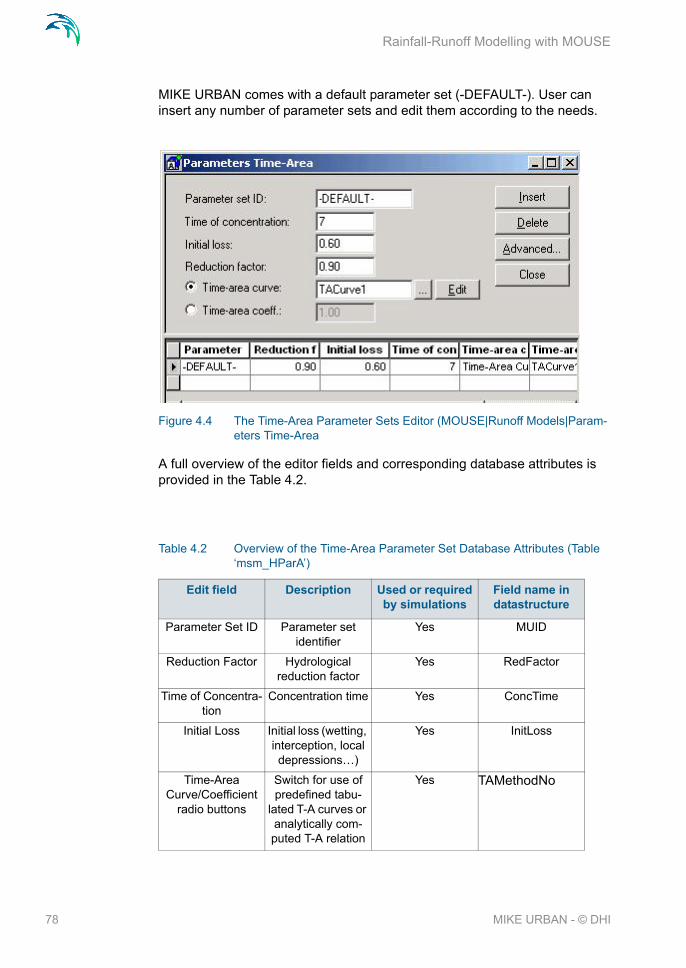
Rainfall-Runoff Modelling with MOUSE
MIKE URBAN comes with a default parameter set (-DEFAULT-). User can insert any number of parameter sets and edit them according to the needs.
Figure 4.4 The Time-Area Parameter Sets Editor (MOUSE|Runoff Models|Param-eters Time-Area
A full overview of the editor fields and corresponding database attributes is provided in the Table 4.2.
Table 4.2 Overview of the Time-Area Parameter Set Database Attributes (Table ‘msm_HParA’)
Edit field Description Used or required by simulations
Field name in datastructure
Parameter Set ID Parameter set identifier
Yes MUID
Reduction Factor Hydrological reduction factor
Yes RedFactor
Time of Concentra-tion
Concentration time Yes ConcTime
Initial Loss Initial loss (wetting, interception, local depressions…)
Yes InitLoss
Time-Area Curve/Coefficient
radio buttons
Switch for use of predefined tabu-
lated T-A curves or analytically com-puted T-A relation
Yes TAMethodNo
78 MIKE URBAN - © DHI

Time-Area Method (A)
4.2.3 Time-Area Curve Editor
The Time-Area model uses (except if analytical curve is applied) predefined tabulated time-area curves. A Time-Area curve represents the contributing part of the catchment surface as function of time. Implicitly, Time-Area curve accounts for the shape of the catchment in relation to outlet point.
MIKE URBAN comes with three defaults time-area curves TACurve1, TACurve2 and TACurve3, applicable for rectangular, divergent and conver-gent catchment, respectively (see the figures below).
Figure 4.5 Three default time-area curves
You can define any number of custom time-area curves. These can be inserted and edited in the editor for the curves and relations (MOUSE|Curves&Relations). Each Time-area table must start with a pair of values (0,0) and must end with a pair of values representing the whole (per default, MIKE URBAN maintains T-A curves in percent (%), i.e. the last pair of values in the table must be (100,100).
Time Area Curve Predefined T-A curve ID
Optional, alter-nates with TACoeff
TACurveID
Time-Area Coeffi-cient
Value of the analyt-ical T-A curve
coefficient
Optional, alter-nates with TACur-
veID
TACoeff
Table 4.2 Overview of the Time-Area Parameter Set Database Attributes (Table ‘msm_HParA’)
Edit field Description Used or required by simulations
Field name in datastructure
79

Rainfall-Runoff Modelling with MOUSE
Figure 4.6 The Curves&Relations editor with one correct user defined time-area curve
4.3 Kinematic Wave (B)
The Kinematic Wave (MOUSE model B) is a surface runoff model with mod-erate data requirements. The runoff computation is based on a comprehen-sive treatment of hydrological losses (including infiltration) and the runoff routing by the kinematic wave (Manning) formula. Details on technical back-ground can be found in the technical reference documentation.
4.3.1 Model Data
The model data are stored in the database table msm_HmodB.
80 MIKE URBAN - © DHI

Kinematic Wave (B)
Figure 4.7 The Kinematic Wave Model Editor (MOUSE|Runoff Models|Kinematic Wave (B)
A full overview of the editor fields and corresponding database attributes is provided in the Table 4.3.
Table 4.3 Overview of the Kinematic Wave Database Attributes (Table ‘msm_H-ModB)
Edit field Description Used or required by simulations
Field name in datastructure
CatchmentID Unique catchment identifier
Yes CatchmentID
Catchment Area Displays the actual model area (total area or drainage
area)
Yes, (calculated, read-only)
-
81

Rainfall-Runoff Modelling with MOUSE
4.3.2 Parameter Sets
The Kinematic Wave model uses relatively large number of parameters. For practical reasons, these parameters have been grouped in parameter sets, which, in turn, can be associated with certain catchment. By these means the entire model setup can be established with a very small amount of informa-tion, while still allowing for full spatial variation of model parameters for indi-vidual catchments through the application of local values.
New parameter sets can be inserted and values of individual parameters can be edited in the "Parameters Kinematic Wave" editor. This can be activated at MOUSE|Runoff Models|Parameters Kinematic Wave.
MIKE URBAN comes with a default parameter set (-DEFAULT-). User can insert any number of parameter sets and edit them according to the needs.
Length Characteristic length of the catch-
ment
Yes Length
Slope Representative slope of the catch-
ment
Yes Slope
Area (five fields) Fraction of the actual model area for each surface
category
Yes AISteep, AIFlat, APSmall, APMe-dium, APLarge
Parameter Set Reference to a set of model parame-ters to be used for the current catch-
ment
Yes ParBID
Use Local Param-eters
Allows for use of individual parame-
ters locally
Optional LocalNo
Manning number (five fields)
Local value of the Manning number
for various types of catchment sur-
faces
Optional MISteep, MIFlat, MPSmall, MPMe-dium,MPLarge
Table 4.3 Overview of the Kinematic Wave Database Attributes (Table ‘msm_H-ModB)
Edit field Description Used or required by simulations
Field name in datastructure
82 MIKE URBAN - © DHI

Kinematic Wave (B)
Figure 4.8 The Kinematic Wave Parameter Sets Editor (MOUSE|Runoff Mod-els|Parameters Kinematic Wave)
A full overview of the editor fields and corresponding database attributes is provided in the Table 4.4.
Table 4.4 Overview of the Kinematic Wave Parameter Set Database Attributes (Table ‘msm_HParB’
Edit field Description Used or required by simulations
Field name in datastructure
Parameter Set ID Parameter set identifier
Yes MUID
Wetting loss (five fields)
Wetting loss on various types of
surfaces
Yes WetSteep, Wet-Flat, WetSmall, WetMedium, WetLarge
Storage loss (four fields)
Storage loss on various types of
surfaces
Yes StorageFlat, Stor-ageSmall, Stor-
ageMedium, StorgaeLarge
Maximum Infiltra-tion Capacity (three fields)
Maximum Infiltra-tion capacity on various types of
surfaces
Yes InfMaxSmall, Inf-MaxMedium, Inf-
MaxLarge
83

Rainfall-Runoff Modelling with MOUSE
4.4 Linear Reservoir (C1 and C2)
The Linear Reservoir (MOUSE model C) is a surface runoff model with mini-mum data requirements. The runoff computation is based on a comprehen-sive treatment of hydrological losses (including infiltration) and the runoff routing by the linear reservoir principle. Details on technical background can be found in the technical reference documentation.
MIKE URBAN includes this model in two versions: C1 and C2. These are var-iants of the same model, and are used as national standards in the Nether-lands and in France, respectively.
4.4.1 Model Data
The model data are stored in the database table msm_HmodC.
Minimum Infiltra-tion Capacity (three fields)
Minimum Infiltra-tion capacity on various types of
surfaces
Yes InfMinSmall, Inf-MinMedium, Inf-
MinLarge
Horton Exponent Wet Conditions
(three fields)
Horton Exponent for wet conditions
on various types of surfaces
Yes InfExpWetSmall, InfExpWetMe-dium, InfExpWet-Large
Horton Exponent Dry Conditions (three fields)
Horton Exponent for dry conditions
on various types of surfaces
Yes InfExpDrySmall, InfExpDryMe-dium, InfExpDry-Large
Manning number (five fields)
Manning number for various types of
catchment sur-faces
Yes ManningSteep, ManningFlat, ManningSmall, ManningMe-dium, Mannin-gLarge
Table 4.4 Overview of the Kinematic Wave Parameter Set Database Attributes (Table ‘msm_HParB’
Edit field Description Used or required by simulations
Field name in datastructure
84 MIKE URBAN - © DHI

Linear Reservoir (C1 and C2)
Figure 4.9 The Linear Reservoir Model Editor (MOUSE|Runoff Models|Linear Res-ervoir (C)), set up for the work with model C1 (Dutch)
85

Rainfall-Runoff Modelling with MOUSE
Figure 4.10 The Linear Reservoir Model Editor (MOUSE|Runoff Models|Linear Res-ervoir (C)), set up for the work with model C2 (French)
A full overview of the editor fields and corresponding database attributes is provided in the Table 4.5.
Table 4.5 Overview of the Linear Reservoir Database Attributes (Table ‘msm_H-ModC’)
Edit field Description Used or required by simulations
Field name in datastructure
CatchmentID Unique catchment identifier
Yes CatchmentID
Catchment Area Displays the actual model area (total area or drainage
area)
Yes, (calculated, read-only)
-
86 MIKE URBAN - © DHI

Linear Reservoir (C1 and C2)
4.4.2 Parameter Sets
The Linear Reservoir model uses a number of parameters. For practical rea-sons, these parameters have been grouped in parameter sets, which, in turn, can be associated with certain catchment. By these means the entire model setup can be established with a very small amount of information, while still
C1/C2 Toggle for editor setting for model
C1 and C2, respectively
Yes -
Length Characteristic length of the catch-
ment
Optional, model C2 only
Length
Slope Representative slope of the catch-
ment
Optional, model C2 only
Slope
Impervious Area Impervious area as a fraction of the
actual model area
Optional, model C2 only
C2Area
Contributing Area Contributing area as a fraction of the actual model area
Optional, model C1 only
C1Area
Parameter Set Reference to a set of model parame-ters to be used for the current catch-
ment
Yes ParCID
Use Local Param-eters
Allows for use of individual parame-
ters locally
Optional LocalNo
Reduction Factor Local value of the hydrological reduc-
tion factor
Optional, model C2 only
RedFactor
Lag Time Local value of the lag time
Optional, model C2 only
LagTime
Time Constant Local value of the time constant
Optional, model C1 only
TimeConst
Initial Loss Local value of the initial loss
Optional, model C2 only
Iloss
Table 4.5 Overview of the Linear Reservoir Database Attributes (Table ‘msm_H-ModC’)
Edit field Description Used or required by simulations
Field name in datastructure
87

Rainfall-Runoff Modelling with MOUSE
allowing for full spatial variation of model parameters for individual catch-ments through the application of local values.
New parameter sets can be inserted and values of individual parameters can be edited in the "Parameters Linear Reservoir" editor. This can be activated at MOUSE|Runoff Models|Parameters Linear Reservoir.
MIKE URBAN comes with a default parameter set (-DEFAULT-). User can insert any number of parameter sets and edit them according to the needs.
Figure 4.11 The Linear Reservoir Parameter Sets Editor (MOUSE|Runoff Mod-els|Parameters Linear Reservoir) - Dutch version
Figure 4.12 The Linear Reservoir Parameter Sets Editor (MOUSE|Runoff Mod-els|Parameters Linear Reservoir) - French version
A full overview of the editor fields and corresponding database attributes is provided in the Table 4.6.
88 MIKE URBAN - © DHI

Unit Hydrograph Method (UHM)
4.5 Unit Hydrograph Method (UHM)
The Unit Hydrograph Method (MOUSE UHM) is a simple surface linear runoff model which can be used to derive hydrographs for any amount of excess precipitation. The runoff computation includes a comprehensive treatment of hydrological losses (i.e. calculation of excessive precipitation) and the runoff routing through creation of a composite hydrograph. Details on technical background can be found in the technical reference documentation.
The model data are stored in the database table msm_HModUHM.
Table 4.6 Overview of the Linear Reservoir Parameter Set Database Attributes (Table ‘msm_HParC’)
Edit field Description Used or required by simulations
Field name in datastructure
Parameter Set ID Parameter set identifier
Yes MUID
C1/C2 Toggle for editor setting for model
C1 and C2, respectively
Yes -
Reduction Factor Local value of the hydrological reduc-
tion factor
Optional, model C2 only
RFactor
Lag Time Local value of the lag time
Optional, model C2 only
LagTime
Time Constant Local value of the time constant
Optional, model C1 only
CTime
Initial Loss Local value of the initial loss
Optional, model C2 only
Iloss
Infiltration Toggle for switch-ing ON and OFF
calculation of infil-tration
Yes InfitrNo
Horton´s infiltra-tion capacity (two
fields)
Minimum and max-imum Infiltration
capacity
Optional, if infiltra-tion included
MaxCap, MinCap
Horton´s time con-stants
Infiltration time constant for wet
and dry conditions
Yes WetCond, Dry-Cond
89

Rainfall-Runoff Modelling with MOUSE
Figure 4.13 The Unit Hydroghraph Model Editor (MOUSE|Runoff Models|UHM)
A full overview of the editor fields and corresponding database attributes is provided in the Table 4.7.
Table 4.7 Overview of the UHM Database Attributes (Atble ‘msm_HModUHM’)
Edit field Description Used or required by simulations
Field name in datastructure
CatchmentID Unique catchment identifier
Yes CatchID
Catchment Area Displays the actual model area (total area or drainage
area)
Yes, (calculated, read-only)
-
Area Adjustment Factor
Relative size of contributing area
Yes AreaFactor
90 MIKE URBAN - © DHI

Unit Hydrograph Method (UHM)
Hydrograph Method for hydro-graph computation
Yes MethodNo
Peaking factor Hydrograph peak factor
Optional, method SUH Standard only
Cp
Slope Representative catchment slope
Optional, method SUH Alameda only
SuhSlope
Loss Model Method for com-puting hydrologi-
cal losses
Yes LossModelNo
Initial Loss Initial loss Optional, "con-stant loss" method
only
InitLoss
Constant Loss Constant Loss Optional, "con-stant loss" method
only
ConstLoss
Runoff Coefficient Runoff Coefficient Optional, "propor-tional loss" method
only
RunoffCoeff
Curve Number Standard hydro-graph curve num-
ber
Optional, "SCS Method" and "SCS Generalized" only
CurveNum
Initial AMC Antecedent Mois-ture Condition
Optional, "SCS Method" only
AMC
Initial Abstraction Depth
Initial Abstrac-tion Depth
Optional, "SCS generalized" only
InitAbstractDepth
Lag Time Method for lag time
Yes LagTimeMethodNo
Lag Time User-specified lag time
Optional, "User specified" lag time
method only
LagTime
Hydraulic Lengt Hydraulic length of the catchment
Optional, "CSC Formula" lag time
method only
HydraulicLength
LT Slope Average catch-ment slope
Optional, "CSC Formula" lag time
method only
Slope
LT Curve Number CSC Curve num-ber used for com-
puting lag time
Optional, "CSC Formula" lag time
method only
LagCurveNum
Table 4.7 Overview of the UHM Database Attributes (Atble ‘msm_HModUHM’)
Edit field Description Used or required by simulations
Field name in datastructure
91

Rainfall-Runoff Modelling with MOUSE
4.6 Additional Flow and RDI
Continuous runoff from MIKE URBAN catchments can be modelled at two distinct levels: either as a simple specification of a constant additional flow or as a MOUSE RDI computation.
The later option involves a continuous hydrological model MOUSE Rainfall Dependent Infiltration (RDI). RDI provides detailed, continuous modeling of the complete land phase of the hydrologic cycle, providing support for urban, rural, and mixed catchments analyses. Precipitation is routed through four dif-ferent types of storage: snow, surface, unsaturated zone ("root-zone") and ground water. This enables continuous modeling of the runoff processes, which is particularly useful when long- term hydraulic and pollution load effects are analyzed.
Instead of performing hydrological load analysis of the sewer system only for short periods of high intensity rainstorms, a continuous, long-term analysis is applied to look at periods of both wet and dry weather, as well as inflows and infiltration to the sewer network. This provides a more accurate picture of actual loads on treatment plants and combined sewer overflows.
When studying the real flow conditions in sewer systems, flow peaks during rain events are often found to exceed the values that can be attributed to the contribution from participating impervious areas. This is a consequence of the phenomenon, usually named Rainfall Induced Infiltration. This differs from the Rainfall Induced Inflow by the fact that it does not depend only on the actual
L Length of the main stream from outlet
to the divide
Optional, "SUH Standard " lag time
method only
SuhL
Lc Length of the main stream from the
outlet to the point closest to the
catchment centroid
Optional, "SUH Standard" lag time
method only
SuhLc
Ct Watershed (catch-ment) coefficient
Optional, "SUH Standard" lag time
method only
Ct
Stream Slope Average Overland Slope
Optional, "SUH Alameda" lag time
method only
StreamSlope
Basin factor Basin Factor Optional, "SUH Alameda" lag time
method only
BasFactor
Table 4.7 Overview of the UHM Database Attributes (Atble ‘msm_HModUHM’)
Edit field Description Used or required by simulations
Field name in datastructure
92 MIKE URBAN - © DHI

Additional Flow and RDI
precipitation, but is heavily affected by the actual hydrological situation, i.e. the "memory" from earlier hydrological events. For a certain rainfall event, the increase in flow will therefore differ, depending on hydrological events during the previous period. The Rainfall Induced Infiltration is also distinguished by a slow flow response, which takes place during several days after the rainfall event.
From a hydrological point of view, parts of the infiltration behave in the same way as the inflow. Therefore, classification of total hydrological loads to infil-tration and inflow is not suitable for modeling approach. Rather, to describe appropriately the constitutive components of flow hydrographs, distinguished by their hydrological behaviour, the following concept is used instead:
FRC - Fast Response Component: comprises the rain induced inflow and fast infiltration component;
SRC - Slow Response Component: comprises slow infiltration compo-nent.
Distinctive for the FRC component is that it is not influenced by the previous hydrological situation, i.e. high or low soil moisture content. It occurs as a direct consequence of a rainfall. The FRC component consists of the inflow to the sewer system and the fast flow component of the infiltration, not depend-ent on previous hydrological conditions.
On the other hand, characteristic of the SRC component is that it is highly dependent on the previous hydrological conditions and usually responses slowly to a rainfall. The SRC component consists of the rest of the precipita-tion-induced infiltration and dry weather infiltration/inflow.
When combined with any of the MOUSE surface runoff models, MOUSE RDI provides a platform for accurate and reliable computation of urban runoff, lib-erated from the limitations inherent to "standard" urban runoff modeling.
Figure 4.14 shows an example illustrating the influence of previous hydrolog-ical conditions for the two components and their response to a rainfall.
93

Rainfall-Runoff Modelling with MOUSE
Figure 4.14 Different catchment response under the same rainfall, due to different soil moisture conditions at the beginning of the rainfall
Figure 4.15 Schematics of the RDI Model
94 MIKE URBAN - © DHI

Additional Flow and RDI
4.6.1 Model Data
The model data for additional catchment flow and RDI are stored in the data-base table msm_HmodCRC.
Figure 4.16 The Additional Flow and RDI Model Editor (MOUSE|Runoff Mod-els|Additional Flow and RDI
A full overview of the editor fields and corresponding database attributes is provided in the Table 4.8.
95
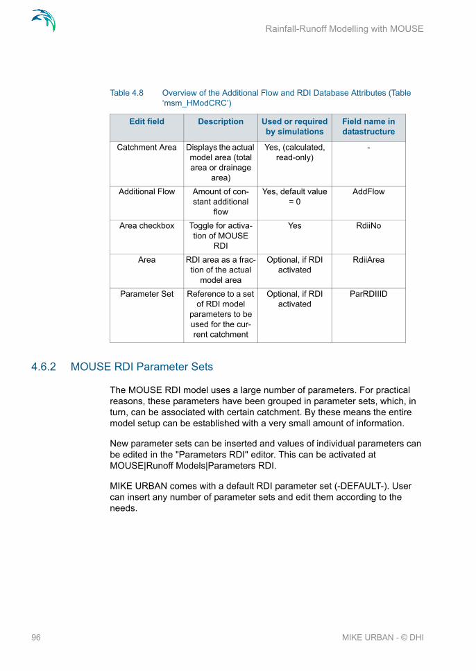
Rainfall-Runoff Modelling with MOUSE
4.6.2 MOUSE RDI Parameter Sets
The MOUSE RDI model uses a large number of parameters. For practical reasons, these parameters have been grouped in parameter sets, which, in turn, can be associated with certain catchment. By these means the entire model setup can be established with a very small amount of information.
New parameter sets can be inserted and values of individual parameters can be edited in the "Parameters RDI" editor. This can be activated at MOUSE|Runoff Models|Parameters RDI.
MIKE URBAN comes with a default RDI parameter set (-DEFAULT-). User can insert any number of parameter sets and edit them according to the needs.
Table 4.8 Overview of the Additional Flow and RDI Database Attributes (Table ‘msm_HModCRC’)
Edit field Description Used or required by simulations
Field name in datastructure
Catchment Area Displays the actual model area (total area or drainage
area)
Yes, (calculated, read-only)
-
Additional Flow Amount of con-stant additional
flow
Yes, default value = 0
AddFlow
Area checkbox Toggle for activa-tion of MOUSE
RDI
Yes RdiiNo
Area RDI area as a frac-tion of the actual
model area
Optional, if RDI activated
RdiiArea
Parameter Set Reference to a set of RDI model
parameters to be used for the cur-rent catchment
Optional, if RDI activated
ParRDIIID
96 MIKE URBAN - © DHI
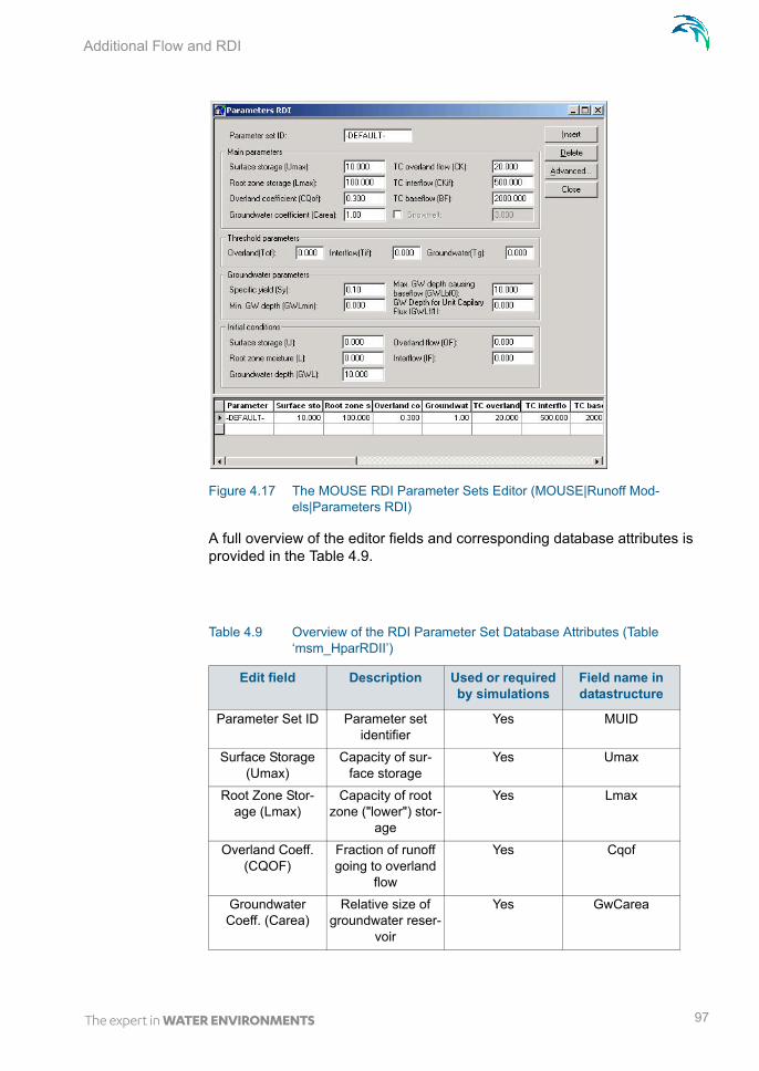
Additional Flow and RDI
Figure 4.17 The MOUSE RDI Parameter Sets Editor (MOUSE|Runoff Mod-els|Parameters RDI)
A full overview of the editor fields and corresponding database attributes is provided in the Table 4.9.
Table 4.9 Overview of the RDI Parameter Set Database Attributes (Table ‘msm_HparRDII’)
Edit field Description Used or required by simulations
Field name in datastructure
Parameter Set ID Parameter set identifier
Yes MUID
Surface Storage (Umax)
Capacity of sur-face storage
Yes Umax
Root Zone Stor-age (Lmax)
Capacity of root zone ("lower") stor-
age
Yes Lmax
Overland Coeff. (CQOF)
Fraction of runoff going to overland
flow
Yes Cqof
Groundwater Coeff. (Carea)
Relative size of groundwater reser-
voir
Yes GwCarea
97

Rainfall-Runoff Modelling with MOUSE
TC Overland Flow Time constant for overland runoff
component
Yes Ck
TC Interflow Time constant for interflow runoff
component
Yes Ckif
TC baseflow Time constant for baseflow runoff
component
Yes Ckbf
Snowmelt check-box
Switch for activa-tion of the snow
storage/snowmelt processes
Yes SnowmeltNo
Snowmelt Snowmelt coeffi-cient
Optional, if snow-melt activated
SnowmeltC
Overland flow threshold (Tof)
Fraction of sur-face storage
capacity at which overland flow
starts
Yes Tof
Interflow threshold (Tif)
Fraction of sur-face storage
capacity at which interflow starts
Yes Tif
Baseflow threshold (Tg)
Fraction of sur-face storage
capacity at which ground water
recharge starts
Yes Tg
Specific Yield Specific yield of the groundwater
reservoir (porosity)
Yes GwSy
Min. GW Depth Top of the ground-water storage
(depth from sur-face)
Yes Gwlmin
Max GW Depth Bottom of the groundwater stor-age (depth from
surface)
Yes Gwlbf0
GW Depth for Unit Capillary Flux
Groundwater depth causing unit
capillary flux
Yes Gwlfl1
Table 4.9 Overview of the RDI Parameter Set Database Attributes (Table ‘msm_HparRDII’)
Edit field Description Used or required by simulations
Field name in datastructure
98 MIKE URBAN - © DHI

Rainfall Data and Other Meteorological Variables - Boundary Conditions for Hydrological models
4.7 Rainfall Data and Other Meteorological Variables - Boundary Conditions for Hydrological models
Any precipitation-runoff model is "driven" by the specified precipitation (rainfall) data. Rainfall data are usually provided as time series - either in the form of accumulated rainfall depths or as average rain-fall intensities. In some cases, the rainfall can be given in a simple form as a "block rain" with constant intensity over the entire simula-tion period.
MOUSE RDI also uses air temperature (used for snowmelt process) and potential evapo-transpiration data. Air temperatures are given as time series of instantaneous values. Potential evapo-transpira-tion is provided as time series of accumulated evapo-transpiration (e.g. on monthly basis). Equally as rainfall, both air temperature and potential evapo-transpiration can be specified as constant for the entire simulation period.
MIKE URBAN MOUSE can utilize time series data stored in DHI pro-prietary format DFS0. Please refer to Chapter 4 for importing, reviewing and editing of time series data.
All three categories of meteorological variables act as boundary conditions for the hydrological model and as such must be specified through the
Initial Surface Stor-age
Water depth in the surface storage at the simulation start
Yes InitU
Initial root zone moisture
Moisture contents in the root zone at the simulation start
Yes InitL
Initial Groundwa-ter Depth
Groundwater depth at the simu-
lation start
Yes InitGw
Initial Interflow Interflow intensity at the simulation
start
Yes InitIf
Initial Overland Flow
Overland flow intensity at the simulation start
Yes InitOf
Table 4.9 Overview of the RDI Parameter Set Database Attributes (Table ‘msm_HparRDII’)
Edit field Description Used or required by simulations
Field name in datastructure
99

Rainfall-Runoff Modelling with MOUSE
MOUSE model boundary system (MOUSE|Boundary Condition|Catchment Loads). As with any other boundary condition, this is done in two distinct steps:
1. Declaration of a catchment boundary (rainfall, air temperature or evapo-transpiration) and its relation to the catchments
A new boundary is inserted by "Insert" button on the "Catchment Loads and meteorological items" editor (MOUSE|Boundary Condi-tion|Catchment Loads). It is recommended to replace the default load identifier by a clearly descriptive string, which undoubtedly defines the actual contents of the boundary (e.g. Rainfall_26-Nov-04).
The current boundary will apply to the catchments according to the specified "Connection Type": All, List or Individual. If "All" is selected, the data source' (e.g. rain gauge or meteorological sta-tion) co-ordinates can optionally be specified.
The co-ordinates are of relevance only in cases where two or more boundaries of the same type have been specified with connection type "All": Instead of applying the boundary condition to the entire model, the system will apply the specified boundary conditions using the principle of geographical proximity to the catchment's centrepoint.
Some data sources (e.g. dfs0 time series) include the information about the data source co-ordinates. By activating the data source
100 MIKE URBAN - © DHI

Rainfall Data and Other Meteorological Variables - Boundary Conditions for Hydrological models
co-ordinates group on this dialog, the specified co-ordinates would overwrite the original co-ordinates from the time series file.
If the connection type is set to "List" or "Individual", the current bound-ary condition will be applied to the specified catchment(s) inde-pendently on the existence of co-ordinate information.
Figure 4.18 The "Catchment Loads…" editor with a rainfall boundary condition applied for all catchments in the model. The co-ordinates specified under the "Data Source Location" represent the rain gauge location
At this point, the declared catchment boundary is just a "placeholder" for the actual rainfall data. These have to be specified in the second step.
2. Specification of the load items
Upon completed declaration of the catchment boundary, user must add the actual "substance" to it. This is done through the specification of "items" asso-ciated with the current boundary. Each catchment boundary condition must include at least one item. By the nature of the meteorological boundaries, they can include only the "default" item types.
The items can be created and edited in the "Boundary Items" editor. This can be open by "Items" button on the "Catchment Loads…" editor (recom-mended), or through the menu at MOUSE|Boundary Conditions|Items.
If opened from the "Boundary Loads…" editor, the "Boundary Items" editor displays only the items associated with the current boundary. Initially, for a newly declared boundary, the list of items will be empty. A new item is created by the "Insert" button.
101

Rainfall-Runoff Modelling with MOUSE
For any item of the catchment meteorological boundary "Temporal Variation" can specified either as "Constant" or as "Time series/Result File". If "Con-stant" is selected, user must specify the constant value. If "Time series" is selected, user must select "DFS0" a source type. The actual DFS0 file to be applied ("Path") can be specified by typing the file name (and a full path if the file is NOT located in the project directory) or by the help of file browser.
Per default, the specified boundary will be applied throughout the entire dura-tion of the simulation or during the period covered by the time series. Option-ally, the user can limit the temporal validity of the specified file to any period within the DFS0 file's duration, by specifying the temporal validity. For the rest of the simulation period, the boundary conditions must be "extended" by some other time series or constant value. This is achieved by inserting and specifying another boundary item.
A full reference on the functionality of the MOUSE boundary system is availa-ble in Chapter 6.
4.8 Running the Runoff Computations
Upon the definition of model data for all catchments, defining the catchment connections (if the computed runoff is to be loaded into the network model) and the definition of the boundary conditions, the model is ready for the runoff computation.
The computation is set-up and initiated from the MOUSE Computation dialog (Simulation|Run MOUSE) - see Chapter 7 for full detail).
On the "General" TAB, the user must specify the essential information about the simulation (see example in Figure 4.19), and the runoff-specific parame-ters on the "Runoff parameters" TAB (see example in Figure 4.20).
102 MIKE URBAN - © DHI

Running the Runoff Computations
Figure 4.19 The "MOUSE Computation dialog (Simulation|Run MOUSE), with gen-eral computation parameters
103

Rainfall-Runoff Modelling with MOUSE
Figure 4.20 The "MOUSE Computation dialog (Simulation|Run MOUSE), with run-off-specific (T-A Curve) computation parameters
4.9 MOUSE RDI - Guidelines for application
4.9.1 Choice of calculation time step
When calculating with MOUSE RDI, time steps are given separately for the Surface Runoff Model and for the rain dependent infiltration part.
The RDI calculation can often be performed with a relatively long time step (several hours), while calculation with the Surface Runoff Model is typically performed with a time step in order of value of several minutes.
The time step for Surface Runoff computations is primarily concerned about the sufficient resolution of the runoff process in time.
Generally, the RDI simulation time step should be chosen in accordance with the resolution of precipitation data, e.g. a time step of 24 hours could be suit-able if only daily precipitation data is available. However, in case when pre-cipitation data with high resolution of e.g. few minutes are available, the RDI time step should be chosen in accordance with the response of the discharge
104 MIKE URBAN - © DHI

MOUSE RDI - Guidelines for application
when raining. E.g., an RDI time step of 2 - 4 hours should be chosen, if the time constant CKOF is given a value of 8 hours.
To minimize the calculation time as well as the size of the result files the RDI calculations are performed according to the following principle:
The RDI simulation is carried out continuously for the whole period specified. On the contrary, the Surface Runoff simulation is carried-out only when rain-ing. Thus, the start time for the Surface Runoff calculation is set as the start time for rain hydrograph. The Surface Runoff calculation continues until all the surface runoff hydrographs are regressed.
4.9.2 The RDI hotstart
There is a HOTSTART facility for MOUSE RDI, i.e. the initial conditions for the various storages can be automatically taken from a former result file, at a simulation start time.
The structure and contents of the result file used as a HOTSTART file requires that the time series in the boundary connection start at least for the maximum specified concentration time Tc earlier than the start time for the HOTSTART is specified. This is required for the correct reconstruction of the surface runoff component (FRC).
4.9.3 The RDI result files
Two result files are generated by a MOUSE RDI calculation. These are:
*.CRF file, containing maximum five time series for each sub-catchment, namely:
– discharge, calculated with the Surface Runoff Model (the FRC com-ponent),
– discharge, calculated with the RDI model (the SRC component),– total discharge,– variation of water content in the surface storage for the Surface Run-
off Model,– variation of water content in the snow storage for the Surface Runoff
Model.The *.CRF file is used as input data for a MOUSE Hydrodynamic calculation.
*.NOF file (optional), containing detailed information about the processes treated by a RDI- model, e.g.:
– different flow components in the RDI model,– variation of water content in the different storage in the RDI model.
The *.NOF file is used for calibration of the SRC component and for RDI hot-start.
105

Rainfall-Runoff Modelling with MOUSE
In the *.CRF file the time series are saved with two various intervals, the shorter one for the periods when the Surface Runoff Model is used, and a larger one in the remaining periods. In the *.NOF file the time series are saved with the larger time interval, which is equal to the time step used for the RDI calculation.
4.9.4 MOUSE RDI Validation
Some of the parameters in MOUSE RDI (here meaning both for the rain dependent inflow and the infiltration part) are related to actual physical data. However, the final choice of parameter values must be based upon a compar-ison with historical measured discharges, since a number of the parameters have an empirical character.
The available period of the measured discharge data and its resolution in time are of major importance for the credibility of the obtained parameter val-ues. Ideally, for a good accuracy, a 3-5 years long time series of measured discharge data with daily values is required for the calibration of the RDI parameters. Several months long time series with higher resolution, i.e. min-utes or hours, depending on the size of the area, are needed for the calibra-tion of the surface runoff model. Measured time series with shorter duration are also useful, although not securing optimal parameter values. In such case it is important that the time series represents different hydrological situations, i.e. typical wet period or dry period.
An exact correspondence between simulations and measurements can how-ever not be expected and for areas where precipitation data of worse quality is used a less accurate calibration result must be accepted. In this case it may be preferable to recall the purpose of the actual model application and concentrate on calibrating yearly volumes, flow peaks or base flows, depend-ing on what kind of analysis is to be performed with the model.
It must be remembered that MOUSE RDI calculates the precipitation-depend-ent flow component. When comparing with measured discharge data the total measured discharge therefore has to be reduced with the flow components not being precipitation dependent, e.g. foul flow.
MOUSE RDI calculates the total generated discharge from a catchment, i.e. overflow within the sub-catchment will also be included in the calculated dis-charge. Therefore, when comparing with measured peak flows and con-trolling the water balance (total volume) this has to be taken into consideration.
In principle, the model validation is concerned about comparison of the com-puted and measured hydrographs. As there are almost an infinite number of possibilities to describe level of agreement between two hydrographs, it is recommended to establish some validation criteria, i.e. a measure for accu-racy of the model, relevant for current application. There are several types of criteria, such as numeric criteria based on single values (e.g. peak discharge,
106 MIKE URBAN - © DHI

MOUSE RDI - Guidelines for application
volume, etc.), or more complex numeric criteria based on statistical analysis of the computed and calculated time series. Also, there are different types of "visual" criteria, based on visual inspection, e.g. comparison of graphic pres-entations of the calculated and measured duration curves. An important issue is to find the most appropriate criteria for the intended application of the model
The choice of criteria is important since it may affect the final choice of parameter values and by that the behaviour of the calibrated model. Numeri-cal criteria are, however, limited and therefore a visual comparison between the hydrographs is indispensable.
MOUSE supports visual comparison of the calculated time series with any time series of the same type contained in the time series database. E.g., when validating the model, the calculated discharge can be plotted on the same graph with the measured discharge and compared.
In the present version of MOUSE RDI there is no automatic calculation or evaluation of specific numeric validation criteria as mentioned above. If appropriate, analysis of that type can be conducted so that the calculated time series are exported to a spreadsheet or some other program for further processing and comparison with measured time series.
In the example related to the illustrations, overflow occurs within the model area. MOUSE RDI can not describe this kind of processes, which compli-cates the choice of validation criteria.
Surface runoff model
When simulating storm sewer systems or fully combined systems, usually a good estimation of the area drained-off by the FRC component (impervious areas etc.) can be obtained from physical data (maps etc.). The final model verification of a FRC should however be based upon comparison with meas-ured discharges during rainfall.
To separate the Afrc component (Surface Runoff Model) and the fast part of the SRC component (Surface Runoff Component in RDI), measured dis-charge data with fairly high resolution in time (hours) is required.
For calibration of the parameters describing the response of the discharge (e.g. tc and TAtype for model A, or M, L and S for model B), a very high reso-lution in time is usually required, minutes to hours.
General hydrological model - RDI
It is not possible to determine the RDI parameters from geophysical measure-ments, since most of the parameters are of empirical nature. It is therefore necessary that measured discharge from the studied area is available, so that the RDI parameters can be determined by comparison between simu-lated and measured discharge through the calibration procedure.
107

Rainfall-Runoff Modelling with MOUSE
The introductory calibration is performed visually by comparing simulated and measured discharge. The final optimization of the parameters is thereafter performed preferably using different numeric and graphical criteria.
The effects of changing each particular parameter are discussed below. Also, the most suitable hydrological periods for calibrating certain parameters are identified, which implies that a certain parameter affects the model behaviour more during periods with specific hydrological conditions. Usually, effects will also be obtained during other periods, why these should also be studied when adjusting a parameter.
The parameters are discussed in the preferable order of adjustment. How-ever, it may be necessary to return to the previous calibration step, as well as repeating the whole process several times. It is recommended, especially for less experienced users, that only one parameter is changed at a time (i.e. for each calculation), so that the effect of the adjustment will appear clearly.
Sometimes, however, the effect of changing one parameter is not sufficient. Then, several parameters controlling similar phenomena can be adjusted together.
In some other cases, undesired secondary effects can be obtained when adjusting certain model parameter. These effects can often be eliminated by simultaneously adjusting other parameters, which do not influence the desired effects, but reduce secondary effects induced by the first parameter.
The following sequence of action is recommended:
The first step in the RDI calibration is usually to adjust the water balance in the system, i.e. the accuracy between the calculated and measured total volume during the observed period. This is done by correcting the proportion of area, Asrc. An increase of Asrc proportionally increases every flow component at each time step.
The total volume generally also contains the runoff from impervious areas (Surface Runoff Model) - see Chapter 4.
Next, the overland flow coefficient CQOF is adjusted to obtain a correct distribution of volume between overland flow (peak flows) and baseflow. This is done after wet periods and preferably for a period with low evapo-ration.
A reduction of CQOF reduces the overland flow and increases the infil-tration, i.e. induces increase in the baseflow.
The measured flow peaks generally also contain the runoff from imper-vious areas (Surface Runoff Model).
108 MIKE URBAN - © DHI

MOUSE RDI - Guidelines for application
CKBF is adjusted against the response of the baseflow, i.e. the build-up and regression of the baseflow. Adjustment against the built-up of base-flow is done during and after wet periods with low evaporation. Adjust-ment against regression is done during the start of dry periods with high evaporation, preferably when baseflow is the only flow component.
An adjustment of CKBF does not influence the size of the discharged volume studied for a longer period, but displaces the volumes in time.
CKOF is adjusted against the response, i.e. the shape of the peak flows. This is done during periods with heavy rainfall, preferably after a wet period.
The measured flow peaks generally also contain the runoff from imper-vious areas (Surface Runoff Model).
A reduction of Umax reduces the actual evapo-transpiration, the process responsible for reduced discharges during period with high potential evaporation. The effect of reducing Umax will be largest for periods preceded by a wet period. Additionally, an increased overland flow is obtained, as well as more water transported to the groundwater storage resulting in an delayed effect of increased baseflow, because of the long response time of baseflow.
An important behaviour of the RDI model is that the surface storage must be filled-up before overland flow and infiltration, respectively, occur. Therefore, during dry periods with high potential evaporation, Umax can be estimated from how much rainfall is required for filling-up the surface storage, i.e. generating overland flow. The same methodol-ogy can also be used for the periods with low potential evaporation, but only if the rain event is preceded by a long dry period.
CKIF is adjusted against the response of interflow during periods with low potential evaporation. A reduction of CKIF will result in a small increase in volume during these periods.
The relative water content in the unsaturated zone (i.e. root-zone), L/Lmax controls several of the different water transports in the RDI model. Since the storage capacity, Lmax, influences the velocity of the filling of L towards Lmax, Lmax is adjusted during periods of heavy filling of the root zone storage. This usually occurs during periods with low potential evaporation preferably in combination with a wet period.
A reduction of Lmax increases the discharge, but it may decrease a lit-tle during period with very high potential evaporation.
The threshold values indicate at which relative water content in the root zone, L/Lmax, overland flow, interflow and baseflow respectively will be generated. Therefore, the threshold values can be estimated from the time of filling the root zone storage when each flow component starts dis-charging.
109

Rainfall-Runoff Modelling with MOUSE
The threshold values have no effect during periods when the root zone storage is full, L = Lmax.
An increased threshold value reduces the discharge during dry periods and in the beginning of wet periods, i.e. periods with low relative water content in the root zone storage.
TG is adjusted during periods with heavy filling of the root zone stor-age, preferably in combination with low potential evaporation and preceded by a dry period. TG is therefore an important parameter for adjusting the increase of the groundwater level in the beginning of wet periods.
TOF is adjusted after a dry period at events with heavy filling of the root zone storage. For example adjustment can be done for events where even larger rainfall volumes does not generate overland flow.
TIF is adjusted after a dry period when filling of the root zone storage, preferably in combination with low potential evaporation. However, TIF is one of the less important parameters.
The degree-day-coefficient, Csnow can be estimated from analysis of the relation between temperature, water content in the snow storage and measured discharge. When temperature is below zero, the precipitation is stored in the snow storage. When temperature is above zero the con-tent in the snow storage is emptied into the surface storage, where the velocity of emptying is controlled by Csnow. An increase of Csnow increases the emptying procedure.
This process should be addressed now and then during the whole cali-bration procedure. Otherwise, there is a risk that a snow-melting phe-nomenon is attempted to be described through adjusting other parameters.
The Carea coefficient establishes the ratio of groundwater catchment and surface catchment (per default, the two surfaces are equal). By changing the ratio, the ratio between the baseflow and other runoff com-ponents is correspondingly changed.
The default values of the remaining RDI parameters: Sy (specific yield of the groundwater reservoir), GWLmin (minimum groundwater depth), GWLBF0 (maximum groundwater depth causing baseflow) and GWL-FL1 (groundwater depth for unit capillary flux) are adjusted only in exceptional cases. Therefore, these parameters have been included into the RDI parameter set dialog in a separate "box". The effects of changing the default values should be well understood prior to adjust-ment.
Figure 8 shows an example of the build-up of the snow cover, followed by the snow-melting process. The calculated and measured flow reac-tions during the same period are shown. The example is from the treat-
110 MIKE URBAN - © DHI

MOUSE RDI - Guidelines for application
ment plant at Duvbacken, Gävle, Sweden. Considering the complexity of the snow melting process within urban areas, a fairly good descrip-tion was obtained with the RDI model.
Since the variation of water contents in the surface and root zone stor-age controls many of the other processes, they should be studied con-tinuously throughout the calibration procedure. Figure 9 shows an example of the variation of water content in the surface storage, root zone storage and groundwater storage. The example comes from the catchment of Rya treatment plant, Göteborg, Sweden. It appears that the root zone storage is emptied only during the summer period, because the evaporation during the rest of the year is almost non-existent. Discharge from the groundwater storage exists continuously all year around. Drawing of the surface storage is faster during sum-mer period since the evaporation is high, and is therefore the dominat-ing effect on the surface storage. During periods with low evaporation, drawing of the surface storage is controlled by the given time constant for interflow, CKIF.
The example also shows that filling of the root zone and groundwater storage only occurs when the surface storage is completely filled, i.e. when precipitation has filled-up the surface storage. A larger surface storage, i.e. a larger Umax, will therefore imply that this happens more rarely and at a smaller extent, allowing a larger part of the precipitation to evaporate.
A smaller root zone storage, i.e. a smaller Lmax, would have led to an increased relative variation in the storage. Furthermore, the actual evaporation will decrease in case of smaller root zone storage, because less water is available for the vegetation to draw water for transpiration, mainly during summer period.
Monthly and yearly values for the different processes, e.g. precipitation volume, real evaporation and total discharge, are written to an ASCII file, NAMSTAT.TXT after every RDI calculation. It is recommended that the content of this file is studied now and then during the calibration procedure.
4.9.5 Overflow within the model area
In those cases when overflow occurs in the studied model area, e.g. when simulating the discharge to the treatment plant, this has to be considered when calibrating the peak flows during rainfall. MOUSE RDI calculates the total generated discharge in the catchment area and is therefore not able to describe hydraulic processes like e.g. over-flow ("loss of water"). Calibration of parameters affecting the volume in the peak flows should therefore be performed for rain events, when overflow is unlikely to occur. Model parameters affecting the response
111

Rainfall-Runoff Modelling with MOUSE
of the discharge, for rain events when overflow occur, can be calibrated against the peak flows base or width.
A well-calibrated MOUSE RDI model can therefore be used for a rough estimation of overflow volume by studying the difference between cal-culated and measured discharge for heavy peak flows. The credibility for such estimation is however strongly affected by the quality of meas-ured precipitation and discharge time series.
4.9.6 Non-precipitation dependent flow components
MOUSE RDI calculates the precipitation dependent flow component. Therefore, both for calibration and validation, other flow components should be treated outside MOUSE RDI.
Examples of non-precipitation dependent flow components are foul flow and sea-water leaking into the sewer system.
The foul flow is preferably estimated through daily values from pro-duced water volumes weighted with yearly charged water volumes. This will however only give a rough estimation, why departure from this methodology may be necessary, e.g. for areas where a large amount of freshwater is used for irrigation.
The amount of leaking sea-water is preferably estimated through an iterative procedure between MOUSE RDI calculation and studies of the difference between the calculated and measured discharge. Only a rough estimation can be achieved, why less accurate calibration results may have to be accepted.
Specially, during the calibration procedure it is very important that non-hydrological errors generally are kept at the lowest level possible in the flow series used. Otherwise, there is a risk of hydrological interpreta-tions of these errors, the error transmitting in the model and increasing when simulating extreme hydrological situations. A typical example is a rough resolution in time for the foul flow component. The method described above should give a description sufficiently correct for most cases.
4.10 Using the Computed Runoff as Network Hydraulic Load
The computed runoff is frequently applied as a hydraulic load to the collection network. This is achieved through the MOUSE boundary system (MOUSE|Boundary Condition|Network Loads). As with any other network load, this is done in two distinct steps:
112 MIKE URBAN - © DHI

Using the Computed Runoff as Network Hydraulic Load
1. Declaration of the network load and its connectivity to the network
A new network load is inserted by "Insert" button on the "Network Loads" edi-tor (MOUSE|Boundary Condition|Network Loads). It is recommended to replace the default load identifier by a clearly descriptive string, which undoubtedly defines the actual contents of the load (e.g. Runoff_event 26-Nov-04).
Concerning the network connectivity of the storm runoff, the option "Defined by Catchment Connections" must be selected. This selection means that the model will utilize the catchment connection information from the runoff result file (*.CRF) used. I.e. no explicit declaration of the runoff connection point is needed.
Figure 4.21 The "Network Loads" editor with runoff defined as a load. "Defined by catchment connections" implies that the MOUSE runoff result file (*.CRF) will be used as a source of connection information
At this point, the declared network load is just a "placeholder" for the actual data. These have to be specified in the second step.
2. Specification of the load items
Upon completed declaration of the network load, user must add the actual "substance" to it. This is done through the specification of "items" associated with the current load. Per default, each load must include the "flow item". This carries the information about the actual water amount and its temporal varia-tion. Optionally, items containing similar information about pollutants, sedi-ments or water temperature associated with this load may be added.
113

Rainfall-Runoff Modelling with MOUSE
The items can be created and edited in the "Boundary Items" editor. This can be open by "Items" button on the "Network Loads" editor (recommended), or through the menu at MOUSE|Boundary Conditions|Items.
If opened from the "Network Loads" editor, the "Boundary Items" editor dis-plays only the items associated with the current load. Initially, for a newly declared load, the list of items will be empty.
"Insert" creates a new item. Automatically, each new item is categorized as "Default", i.e. as flow item. If the current MOUSE model includes any pollut-ants of sediments, user may change the item type to be "Pollutant" or "Sedi-ment". In any case, at least one flow item must be present on the list.
For the default item, "Temporal Variation" is specified as "Time series/Result File". In the "Time series" group, "MOUSE" (i.e. MOUSE result file) is selected as data source type. The actual file to be applied ("Path") can be specified by typing the file name (and a full path if the file is NOT located in the project directory) or by the help of file browser.
Per default, the specified runoff result file will load the network throughout its entire duration, corresponding to the runoff computation Start and End times. Optionally, the user can limit the temporal validity of the specified file to any period within the file's duration, by specifying the temporal validity. For the rest of the simulation period, the network can be loaded by some other runoff result file. This is achieved by inserting and specifying another flow item.
A full reference on the functionality of the MOUSE boundary system is availa-ble in the Chapter 6.
4.11 Low Impact Development (LID)
Water sensitive urban design (WSUD) represents an approach to land devel-opment (or re-development) that works with nature to manage storm water as close to its source as possible, it is known also as Low Impact Development (LID).
Low Impact Development employs principles such as preserving and recreat-ing natural landscape features, minimizing effective imperviousness to create functional and appealing site drainage that treat storm water as a resource rather than a waste product.
Many practices have been used to adhere to these principles such as bio-retention facilities, rain gardens, vegetated rooftops, rainwater tanks, and per-meable pavements. By implementing LID principles and practices, storm water can be managed in a way that reduces the impact of impervious built-up areas and supports the natural movement of water within an urban eco-system or catchment.
114 MIKE URBAN - © DHI

Low Impact Development (LID)
Applied on a broad scale, LID can maintain or restore a catchment's hydro-logic and ecological functions. LID has been characterized as a sustainable storm water practice.
The ability to assess the benefit of the LID practices installed in urban catch-ments is required by Water Utilities and other stakeholders responsible for the urban drainage. Essential part of this requirement is ability to model the vari-ous LID practices at both hydrological screening level and at a detailed hydraulic level in order to evaluate the effect of installing LID practices as parts of a storm water drainage system.
This document describes the implementation and development of model sup-port of various LID structures in MIKE URBAN.
The modelling of LID practices is divided into 2 main approaches:
Modelling of LID at screening level - catchment-based approach
Detailed hydraulic modelling of individual LID structures - drainage net-work based approach. This method will provide the user with the option of detailed modelling of individual LID structures connected hydraulically to the storm water pipe network. This approach is based on the concept of soakaway node explained in section 3.3.5 Model Concept of Soakaway (p. 29).
In this document, the MIKE URBAN implementation of the screening level - the catchment-based approach - is explained.
The catchment-based methods implemented in MIKE URBAN are dominantly based on research published by US EPA, adapted appropriately to the MIKE URBAN modelling concept of urban hydrology. In US, the term Low Impact Development Systems (LIDS) is used for WSUD and the LID concept pro-vides the users with an overall method for evaluating the various LIDS con-trols such as bio-retention cells, rain gardens, green roofs, infiltration trenches, permeable pavements, rain barrels / rainwater tanks and vegetative swales.
A user-defined number of LIDS controls can be deployed and assessed for each individual catchment. This catchment-based approach is used to size the required infiltration or rainwater harvest by subtraction of flow from the calculated runoff within each catchment.
Please be aware that modelling of LID practices in MIKE URBAN is allowed for the Kinematic Wave runoff model (Model B) and runs with the MIKE 1D engine, exclusively.
4.11.1 LID Controls
LID Controls are low impact development structures designed to capture or reduce surface runoff from the collecting area by means of a combination of
115

Rainfall-Runoff Modelling with MOUSE
detention, infiltration and evapotranspiration. Low Impact Development con-trols are conceptual objects that are not displayed on the map visualization of the urban catchment model. Once deployed, they are considered as proper-ties of a given sub-catchment. MIKE URBAN can model seven types of LID controls:
1. Bio Retention Cells
2. Infiltration Trenches
3. Porous Pavement
4. Rain Barrels
5. Vegetative Swales
6. Rain Garden
7. Green Roof
Bio-retention cells, infiltration trenches, and porous pavement systems can all be supplied with optional underdrain systems in their gravel storage beds to convey storage runoff off the site rather than infiltrate it all. They can also have an impermeable floor of liner that prevents any infiltration into the native soil from occurring. Infiltration trenches and porous pavement systems can also be subject to a decrease in hydraulic conductivity over time due to clog-ging.
While some LID practices can also provide important pollutant reduction, the current LIDS implementation in MIKE URBAN can only be used to model the LIDS’ quantitative hydrologic performance.
Bio Retention Cells
Bio-retention Cells are terrain depressions that comprise selected types of vegetation, resistant to the extended periods of high moisture and extreme levels of nutrient concentrations (Nitrogen and Phosphorus) found in storm water runoff, grown in an engineered soil mixture sited above a gravel drain-age bed. They provide storage, infiltration and evaporation of both direct rain-fall and runoff captured from the collecting area surrounding the cell. Rain gardens, street planters, and green roofs are all different types of bio-reten-tion cells.
The different structural layers of this feature are presented in Figure 4.22. There are one or several relevant hydrological processes associated with each layer.
In the surface occur surface storage, surface infiltration, the collecting area run-on, surface evaporation and overflow.
In the soil layer occur percolation (vertical water movement to the storage layer), evapotranspiration (loss due to the plant root action) and storage in the soil's voids.
116 MIKE URBAN - © DHI

Low Impact Development (LID)
In the storage layer, storm water provided by the percolation through the soil layer is detained in the storage layer's voids. Infiltration (leakage) to the native soil through the storage bottom, controlled by the characteristics of the surrounding soil, restores the storage capacity.
An optional underdrain may be included to empty the storage. The underd-rain is activated (with the specified capacity) when the water level in the stor-age reached the offset level.
Figure 4.22 Bio retention cell structure layers
Infiltration Trenches
Infiltration Trenches are storage cells filled with gravel that capture runoff from upstream impervious areas. They provide storage capacity and the pos-sibility for captured runoff to infiltrate the soil underneath.
In Figure 4.23 a schematic drawing of the infiltration trench structure is pre-sented. This type of LID control includes surface, storage and, optionally, underdrain.
The processes simulated for the infiltration trench are similar as for the bio-retention cell, except for the missing soil layer: storm water from the surface enters the storage directly, i.e. without detention in the soil layer.
Figure 4.23 Infiltration trench structure layers
117

Rainfall-Runoff Modelling with MOUSE
Porous Pavement
Porous Pavement systems are excavated areas filled with gravel and paved over with a porous concrete or asphalt mix. Porous pavements are imple-mented in places where surface has to provide a firm support for vehicle traf-fic, such as streets and parking lots.
Normally, all rainfall will immediately pass through the pavement into the gravel storage layer below it where it can infiltrate at natural rates into the site´s native soil.
In Figure 4.24 it is sketched the porous pavement structure comprehending surface, pavement material, storage and underdrain.
Essentially, hydraulic functionality of the porous pavement is similar to that of the bio-retention cell, except that the soil layer (and vegetation) are replaced by some porous asphalt or concrete.
Some types of porous pavements may be subject to clogging by fine sedi-ment particles, which reduces their infiltration capacity.
Figure 4.24 Porous Pavement structure layers
Rain Barrels
Rain Barrels are containers that collect roof runoff during storm events and can either release or re-use the rain water during dry periods.
A rain barrel includes storage (with total porosity, i.e. empty volume) and underdrain.
The processes simulated include water detention in the storage, overflow and drainage (i.e. storage recovery). The action of the underdrain is timed: it can be specified the time offset between the end of rain and the drain activation.
118 MIKE URBAN - © DHI

Low Impact Development (LID)
This feature allows for the simulation of rainwater re-use for garden watering, which normally takes place several hours or days after the rain has stopped.
A conceptual sketch of a rain barrel is presented in Figure 4.25.
Figure 4.25 Rain Barrel
Vegetative Swales
Vegetative Swales are waterways or depressed areas with sloping sides cov-ered with grass and other vegetation. They slow down the conveyance of col-lected runoff and allow it more time to infiltrate to inherent soil beneath it. The only relevant layers regarding vegetative swales are surface and surrounding soil.
Figure 4.26 Vegetative Swale layer structure
Rain Garden
Rain Garden, as a simplified form of bio-retention cell is a garden, which takes advantage of rainfall and storm water runoff in its design, simultane-ously contributing to the reduction of runoff volume and pollutants released from the site. Typically, it is designed as a small garden with selected types of
119

Rainfall-Runoff Modelling with MOUSE
vegetation, resistant to the extended periods of high moisture and extreme levels of nutrient concentrations (Nitrogen and Phosphorus) found in storm water runoff.
The different layers comprising rain gardens are presented in Figure 4.27. These include surface and soil layer
In the surface occur surface storage, surface infiltration, the collecting area run-on, surface evaporation and overflow.
In the soil layer occur storage in the soil's voids, evapotranspiration (loss due to the plant root action) and infiltration (leakage) to the native surrounding soil through the bottom. The infiltration is controlled by the characteristics of the surrounding soil.
Figure 4.27 Rain garden process layers
Green Roof
Green Roofs are structural components that reduce the negative effects of urbanization on water quality and rainfall runoff by absorbing or detaining, and by filtering runoff. They are built of a planted lightweight soil media and a drainage layer.
Green Roofs may be designed with intensive or extensive vegetation cover. Intensive green roofs are heavy, with soil media layer larger than 15 cm. Extensive green roofs may include a soil layer as thin as 3 cm, which governs the choice of vegetative cover.
Green roofs are equipped with a drainage layer named drainage mat, placed beneath the soil media. The purpose of the drain mat is to conduct the sur-plus water percolated through the soil layer from the roof to the drainage sys-tem.
120 MIKE URBAN - © DHI

Low Impact Development (LID)
Figure 4.28 Green roof process layers
4.11.2 The LID Controls Editor
The MIKE URBAN LID Controls editor organizes the data input for the differ-ent layers and functional elements of Low Impact Development structures. The input data is organized into following group and tabs:
Identification: This group provides for the unique identification of the specified LID control and the definition of its type. Each individual LID Control is generic and is specified per unit-area. As such, it can be repli-cated and placed in any sub-catchment of the study area (deployed), with different actual sizes and in any number of instances.
Tabs: Surface, Soil, Pavement, Storage, Drain and Drainage Mat. These tabs represent different layers and functional elements defining the struc-ture of the LID control. The properties of each layer and functional ele-ment, which constitute the actual LID control type, are entered in these tabs. Only the actually relevant data fields for the current LID control type are activated and available for the data input.
Figure 4.29 through Figure 4.34 illustrate the six tabs containing the data for various functional elements of the LID structure. Table 4.10 and Table 4.11 provide a full reference for the attributes of the msm_LIDControl database table.
121

Rainfall-Runoff Modelling with MOUSE
Figure 4.29 The MIKE URBAN LID Control Editor - Surface Tab
Figure 4.30 The MIKE URBAN LID Control Editor - Soil Tab
122 MIKE URBAN - © DHI

Low Impact Development (LID)
Figure 4.31 The MIKE URBAN LID Control Editor - Pavement Tab
Figure 4.32 The MIKE URBAN LID Control Editor - Storage Tab
123

Rainfall-Runoff Modelling with MOUSE
Figure 4.33 The MIKE URBAN LID Control Editor - Drain Tab
Figure 4.34 The MIKE URBAN LID Control Editor - Drainage Mat Tab
124 MIKE URBAN - © DHI

Low Impact Development (LID)
Identification
Table 4.10 The LID Control Identification Group
Edit field Description Used or required by simulations
Field name in data structure
LID Control ID ID of low impact devel-opment, LID
Yes MUID
LID Type Type of LID1:Bio Retention Cell2:Porous Pavement3:Infiltration trench4:Rain Barrel5: Vegetative Swale6:Rain Garden7:Green Roof
Yes LIDTypeNo
125

Rainfall-Runoff Modelling with MOUSE
LID Control data Specification
Table 4.11 The LID data specification
Tab/Edit field Description Used or required by simulations
Field name in data structure
Surface/Storage Depth
When confining walls or berms are present, this is the maximum depth to which water can pond above the surface before overflow occurs. For LIDs that experience ponding it is the height of any surface depression storage. For swales, it is the height of its trapezoidal cross section.
Yes If LIDTypeNo = (1,2,3,5)
StorHt
Surface/Vegetative Cover
The fraction of the storage area above the surface that is filled with vegetation (0 = no vegetation, 1 = no storage available). NOTE: for infiltration trench, vegetative cover is typically non-existent
Yes If LIDTypeNo = (1,2,3,5)
VegFrac
Surface/Surface Rough-ness
Manning´s n or M (used in combination with surface slope and width) for routing of over-flow from the surface of bio-retention cell, rain garden, infiltration trench, porous pavement and for flow routing in vegetative swale (see Table 4.12 for typical values). If specified zero (for all types except vegetative swale), no routing of the overflow is applied
Yes If LIDTypeNo = (1,2,3,5 and 6)
Rough
Surface/Surface Slope
Slope (used in combination with surface roughness and width) for routing of overflow from the surface of bio-retention cell, rain gar-den, infiltration trench, porous pavement and for flow routing in vegetative swale. If speci-fied zero (for all types except vegetative swale), no routing of the overflow is applied
Yes If LIDTypeNo = (1,2,3,5 and 6)
Slope
Surface/Swale Side Slope
Slope (run over rise) of the sidewalls of a vegetative swale´s cross section. Used for the calculation of the stored volume and wet-ted width. This value is ignored for other types of LIDs
Yes If LID-TypeNo=5
Xslope
Soil/Thickness
Thickness of the soil layer. Typical values range from 450 to 900 mm for rain gardens, street planters and other types of land-based bio-retention units, but only 75 to 150 mm for green roofs
Yes If LIDTypeNo = (1, 6, 7)
SThick
Soil/Porosity
Volume of pore space relative to total volume of soil (as a fraction)
Yes If LIDTypeNo = (1, 6, 7)
Por
126 MIKE URBAN - © DHI

Low Impact Development (LID)
Soil/Field Capacity
Volume of pore water relative to total volume held in the soil after excess water has drained away and the rate of downward movement has decreased (as a fraction). Vertical perco-lation of water through the soil occurs only when field capacity level is reached or exceeded.
Yes If LIDTypeNo = (1, 6, 7)
FC
Soil/Wilting Point
Volume of pore water relative to total volume for a well-dried soil where only bound water remains (as a fraction). The moisture content of the soil cannot fall below this limit and wilt-ing point cannot be higher than the Field Capacity level.
Yes If LIDTypeNo = (1, 6, 7)
WP
Soil/Infiltration capacity
The rate of water moving from surface into the soil. It is characteristics of the surface and the uppermost soil layer (equivalent to Hor-ton´s initial infiltration capacity). Infiltration takes place at all times during a rain event and after, as long as there is water available as rainfall, as run on or as water stored in the surface.
Yes If LIDTypeNo = (1, 6, 7)
InfiltrationCapac-ity
Soil/Leakage capac-ity
The rate of water leaving the soil layer into storage. It is characteristic of the soil layer. Leakage starts when soil storage exceeds field capacity, continues at all times while soil storage is above the field capacity.
Yes If LIDTypeNo = (1, 6, 7) AND FlowMethod = 1 (capacity based))
LeakageCapac-ity
Soil/Conductivity
Hydraulic conductivity for the fully saturated soil. This is equivalent to leakage capacity
Yes If LIDTypeNo = (1, 6, 7) AND FlowMethod = 2 (conductivity based))
Ksat
Soil/Conductivity slope
Slope of the curve of log (conductivity) versus soil moisture content (dimensionless). Typical values range from 5 for sands to 15 for silty clay
Yes If LIDTypeNo = (1, 6, 7) AND FlowMethod = 2 (conductivity based)
Kcoeff
Soil/Suction Head
The average value of soil capillary suction along the wetting front. This is the same parameter as used in the Green-Ampt infiltra-tion model
Yes If LIDTypeNo = (1, 6, 7) AND FlowMethod = 2 (conductivity based)
Suct
Pavement/Thickness
Thickness of the pavement. Typical values are 100 to 150 mm
Yes If LIDTypeNo = 2
PThick
Table 4.11 The LID data specification
Tab/Edit field Description Used or required by simulations
Field name in data structure
127

Rainfall-Runoff Modelling with MOUSE
Pavement/Porosity
The ratio (expressed as a fraction) of the vol-ume of the pores or interstices of a material to the total volume of the pavement. Typical values range from 0.11 to 0.17 for pavementsNote that porosity = void ratio / (1 + void ratio).
Yes If LIDTypeNo =2
Pvratio
Pavement/Impervious Sur-face
Ratio of impervious paver material to total area for modular systems; 0 for continuous porous pavement systems
Yes If LIDTypeNo = 2
FracImp
Pavement/Permeability
Permeability of concrete or asphalt used in continuous systems or hydraulic conductivity of the fill material (gravel or sand) used in modular systems. Permeability of new porous concrete or asphalt is high (>2450 mm/h), but over time the fine particles in the runoff tend to clog the pavement, reducing the permeability of the structure.
Yes If LIDTypeNo = 2
Perm
Pavement/Clogging Factor
Voids that are clogged due to fine particles accumulation, as a fraction of total voids area. Use a value of 0 to ignore clogging. Max. value = 1.
Yes IfLIDTypeNo = 2
PVClog
Storage/Height
The height of the storage layer in case of bio retention cell, porous pavement and infiltra-tion trench; the height of a rain barrel (mm or inches). Crushed stone and gravel layers are usually 150 to 450 mm thick while rain barrels vary in height from 600 mm upwards.
Yes If LIDTypeNo = (1,2,3,4)
Height
Storage/Porosity
The ratio of the volume of the pores or inter-stices of a material to the total volume of the layer. Typical values range from 0.30 to 0.45 for gravel beds. Note thatporosity = void ratio / (1 +void ratio).
Yes If LIDTypeNo = (1,2,3)
Svratio
Storage/Conductivity
The maximum rate at which water infiltrates to the surrounding soil through the bottom of the freshly constructed storage layer.
Yes If LIDTypeNo = (1, 2, 3)
Filt
Storage/Clogging Factor
Volume of voids that are clogged due to fine particles accumulation. Use a value of 0 to ignore clogging.
Yes If LIDTypeNo = (1,2,3)
SVclog
Drain/Capacity
Coefficient C that determines the rate of flow through the underdrain as a function of height of stored water above the drain bottom.
Yes If LIDTypeNo = (1,2,3,4)
Coeff
Drain/Exponent
Exponent n that determines the rate of flow through the underdrain as a function of height of stored water above the drain height.
Yes If LIDTypeNo = (1,2,3,4)
Expon
Table 4.11 The LID data specification
Tab/Edit field Description Used or required by simulations
Field name in data structure
128 MIKE URBAN - © DHI

Low Impact Development (LID)
In Table 4.12 are presented examples of Manning' values (M) for different types of surfaces. Table 4.13 shows hydraulic conductivity properties for vari-ous porous media.
Drain/Offset Height
Height of any underdrain piping above the bottom of a storage layer or rain barrel
Yes If LIDTypeNo = (1,2,3,4)
Offset
Drain/Delay
The number of dry weather hours that must elapse before the drain in a rain barrel is acti-vated
Yes If LIDTypeNo = 4
Delay
Drainage Mat/Thickness
The thickness of the mat or plate. It typically ranges between 25 to 50 mm
Yes If LIDTypeNo = 7
DMThick
Void Fraction The ratio of void volume to total volume in the mat. It typically ranges from 0.5 to 0.6
Yes If LIDTypeNo = 7
DMVFraction
Roughness Manning´s number, used to compute the hori-zontal flow rate of drained water through the mat. In absence of standard product specifi-cations provided by manufacturers, the roughness must be estimated. Usage of n-values from 0.1 to 0.4 (M = 2.5 - 10) is suggested.
Yes If LIDTypeNo = 7
DMRough
Table 4.12 Manning´s M of surface for porous pavement or vegetative swale a
Surface type Manning M
Smooth asphalt 91
Smooth concrete 83
Ordinary concrete lining 77
Good wood 71
Brick with cement mortar 71
Vitrified clay 67
Cast Iron 67
Corrugated metal pipes 42
Cement rubble surface 42
Fallow soils (no residue) 20
Cultivated soils 50 to 20
Residue cover < 20% 17
Residue cover > 20% 6
Range (natural) 8
Short, prairie 7
Dense 4
Table 4.11 The LID data specification
Tab/Edit field Description Used or required by simulations
Field name in data structure
129

Rainfall-Runoff Modelling with MOUSE
4.11.3 LID Deployment
The LID Controls are assigned to a catchment by means of the LID deploy-ment editor. In this editor, it is possible to specify the size (i.e. area) of the individual control, the size of the catchment´s impervious area that is fun-neled into it and the number of the current LID control units.
The size properties can be specified either directly as surface area, or as a percentage of the catchment's area. The specified total collecting area must not exceed the size of the catchment's impervious area.
Furthermore, level of initial saturation and routing width for overland flow can be specified.
The input data is organized into following groups:
Identification and Connectivity
LID Deployment Properties
Bermuda grass 2
Woods 10
Light underbrush 2,5
Dense underbrush 1,25
a.Source: McCuen, R. et al. (1996), Hydrology, FHWA-SA-96-067,Federal Highway Administration, Washington, DC
Table 4.13 Hydraulic conductivity and porosity of unconsolidated porous media a
a. Source: Freeze, R.A., and Cherry, J.A., (1979), Groundwater, Prentice-Hall, Englewood Cliffs, NJ
Material Hydraulic conductivity K (cm/s) Porosity (%)
Gravel 10-1 - 102 25 - 40
Sand 10-5 - 1 25 - 40
Silt 10-7 – 10-3 35 - 50
Clay 10-9 – 10-5 40 - 70
Table 4.12 Manning´s M of surface for porous pavement or vegetative swale a
Surface type Manning M
130 MIKE URBAN - © DHI

Low Impact Development (LID)
Figure 4.35 MIKE 1D LID deployment editor
Identification and Connectivity
Each deployed control LID is linked to "LID Deployment MUID". I.e. each deployment represents a LID control deployed on a single catchment in a specified number of units. For each LID deployment, a result file can be gen-erated, containing time series of relevant variables (fluxes and storages). This result file is in the dfs0 time series format.
A full reference of the attributes related to LID deployment in shown in Table 4.14 and Table 4.15.
Table 4.14 The LID Deployment Identification and Connectivity Group
Edit Field Description Used or required by simulations
Field name in data structure
MU ID MIKE URBAN ID Yes MUID
Catchment ID Identification of the catchment
Yes CatchID
LID Control ID Identification of the LID control to be deployed
Yes LidID
131

Rainfall-Runoff Modelling with MOUSE
The possibility of excluding a control is handled by the "Include" checkbox. By default, this checkbox is un-checked.
LID Deployment Properties
The LID deployment result file
Optionally, for each LID control deployment, a dfs0 time series file can be cre-ated. This file includes time series of relevant variables inside the LID control in terms of inflow, flow between layers, storage levels in various layers and output from the control to the native soil.
Table 4.15 The LID Deployment Properties
Edit Field Description Used or required by simulations
Field name in data structure
Number of units
Number of replicate LID units deployed within the catchment
Yes ReplicateNum-ber
Area of unit The surface area of each replicate LID unit Yes UnitArea
Unit area pct The surface area of each replicate LID unit, expressed as a percentage of the total catch-ment area
Yes (not if the Area of unit is defined)
UnitAreaPer-cent
Collecting area A LID practice is connected to a tributary area whose runoff is treated by the unit. This area includes the LID practice area itself..
Yes CollectingArea
Collecting area pct
The tributary area connected to the LID unit presented as a percentage of the catchment
Yes (not if the Col-lecting area is defined)
Collectin-gAreaPercent
Initial satura-tion
For Bio-Retention Cells, rain gardens, and green roofs this is the degree to which the unit´s soil is initially filled with water (0% satu-ration corresponds to the wilting point mois-ture.
Yes InitSat
Width The width of the outflow face of each identical LID unit (meter or feet). This parameter is applied for all control units that use overland flow to transport surface runoff off the unit, being these roofs, pavement, trenches, and swales for the other control types this parame-ter can be set as 0
Yes (for porous pavement, swales, roofs and trenches)
Width
Result File Checkbox for creating a result file specific for the current deployment (dfs0 file). A further detailed description of this file is presented in the Result File section
Yes RptFileNo
File name The name of an optional file where detailed time series for the LID are presented as dfs0 result file
Yes RptFileName
132 MIKE URBAN - © DHI
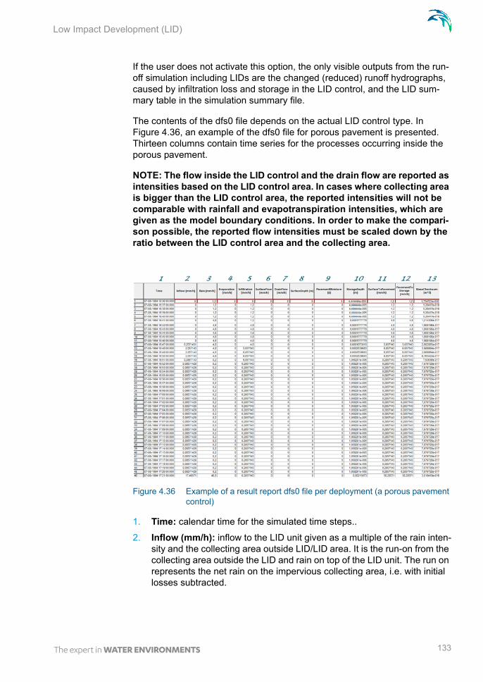
Low Impact Development (LID)
If the user does not activate this option, the only visible outputs from the run-off simulation including LIDs are the changed (reduced) runoff hydrographs, caused by infiltration loss and storage in the LID control, and the LID sum-mary table in the simulation summary file.
The contents of the dfs0 file depends on the actual LID control type. In Figure 4.36, an example of the dfs0 file for porous pavement is presented. Thirteen columns contain time series for the processes occurring inside the porous pavement.
NOTE: The flow inside the LID control and the drain flow are reported as intensities based on the LID control area. In cases where collecting area is bigger than the LID control area, the reported intensities will not be comparable with rainfall and evapotranspiration intensities, which are given as the model boundary conditions. In order to make the compari-son possible, the reported flow intensities must be scaled down by the ratio between the LID control area and the collecting area.
Figure 4.36 Example of a result report dfs0 file per deployment (a porous pavement control)
1. Time: calendar time for the simulated time steps..
2. Inflow (mm/h): inflow to the LID unit given as a multiple of the rain inten-sity and the collecting area outside LID/LID area. It is the run-on from the collecting area outside the LID and rain on top of the LID unit. The run on represents the net rain on the impervious collecting area, i.e. with initial losses subtracted.
133

Rainfall-Runoff Modelling with MOUSE
3. Rain (mm/h): input rain for the catchment containing the LID control unit. This rain loads the LID area directly.
4. Evaporation (mm/h): this is a given parameter specified by the user by means of boundary conditions valid for the catchment as well as for the LID unit.
5. Infiltration (mm/h): infiltration from the LID unit to the surrounding native soil.
6. Surface flow (mm/h): surface water flow. Represents overland flow for vegetative swale; overflow for other LID controls
7. Drain flow (mm/h): water flow through the drain.
8. Surface depth (m): accumulated water on the surface expressed as the water height on the surface. Maximum value is the specified surface stor-age height.
9. Soil moisture (): presented as a fraction, relative to the total volume of the soil layer. Corresponds to the water that is held in the spaces between soil particles. Maximum soil moisture (i.e. full saturation) is equivalent to the specified soil porosity.
10. Pavement moisture(): presented as a fraction, relative to the total vol-ume of the porous pavement layer. Corresponds to the water that is held in the pavement's voids. Maximum pavement moisture (i.e. full satura-tion) is equivalent to the specified pavement porosity.
11. Storage depth (m): accumulated water in the storage layer expressed as the water height in the storage. Maximum value is the storage height.
12. Surface to soil (mm/h): infiltration from the surface layer to the soil layer expressed in mm/h.
13. Surface to pavement (mm/h): infiltration from the surface layer to the pavement layer expressed in mm/h.
14. Soil to storage (mm/h): ): flow from the soil layer to the storage layer expressed in mm/h.
15. Pavement to storage (mm/h): flow from the pavement layer to the stor-age layer mm/h.
16. MassChecksum (m3): regards to the error check in the mass water bal-ance per time step computed, a low value in the order of 1*E-015 indi-cates an accurate internal flow estimation.
The LID Simulation Summary
The LID simulation summary is provided as part of the overall simulation summary html file. The summary table reports the volume balance for each LID deployment (see example in Figure 4.37).
134 MIKE URBAN - © DHI

Low Impact Development (LID)
Figure 4.37 Example of a LID simulation summary
135

Rainfall-Runoff Modelling with MOUSE
136 MIKE URBAN - © DHI

Inserting New Time Series
4 Time Series
Time series can represent both input and result time series. Examples of input time series are e.g. rain event, a varying water level at an outlet etc.
These input time series can be entered in MIKE URBAN through the time series editor. Time series in the time series editor are saved in dfs0 format. In the time series editor it is possible so save several time series with the same time axis in different time series items, these various items are then saved in one time series object. When using the time series as tidal variations of e.g. a specific load in the simulation, reference to the individual time series items within the time series objects are made.
4.1 Inserting New Time Series
When inserting a new time series (TS) go to Edit|Time Series. This will bring up the dialog shown in Figure 4.1. It is normally not expected that a massive TS data input would be done ‘manually’ by typing data. If the data are already available in a digital format, they can readily be imported into MIKE URBAN as described later in this section.
Figure 4.1 The empty time series dialog
If the data are to be typed in anyway, the TS data input starts by specifying the basic TS properties: number of values, start date and time, time interval between successive values (assuming a uniform time resolution of the TS) etc. When data are imported it may also be desirable to change some of the properties, please refer to the example later in this section.
In order to set the properties for the time series object:
Right-click on the TS object
71

Time Series
Choose ‘TSObject Properties’ on the local menu
Figure 4.2 Right-click on the TS object to get to the local dialog
After specifying the properties for the TS object, you can now continue to specify the properties for the TS items. One item is per default already availa-ble.
A new TS item is created this way:
Right-click on the TS object
Choose ‘New Item’ on the local menu
4.1.1 Properties of time series object
The properties of the time series object can be set in the dialog seen in Figure 4.3. A description of the input fields is found in Table 4.1.
Figure 4.3 The TSObject Properties dialog
72 MIKE URBAN - © DHI

Inserting New Time Series
Table 4.1 The TSObject properties
Field Description
Title Title of the time series object
Auto Conversion of Delete Values
When tick mark is set then the values that are in ‘Delete Value’ will be converted on the fly if the unit specified in
the ‘EUM Unit’ field is changed. Only conversion between units of the same type can be done. If the tick
mark is not set then it is possible to change the unit with-out the delete value typed in being converted.
Delete Value Threshold for values that are so small that they should be disregarded.
Nr Days in Year If a time step of months is used, the number of days is used to compute the number of days in a month. Other-
wise not used
TS Data Type Not relevant
73

Time Series
Time Type A time definition can be equidistant, meaning that the time values difference between consecutive Timesteps is constant through the entire time or non-equidistant, meaning that the time values dif-ference between consecutive Timesteps is not constant through the entire time. Besides these two classifications, a time definition can be Calen-dar type, meaning that the time values are speci-fied as dates or Relative type, meaning that time values are specified as numbers.
Equidistant_Calendar - time values difference between consecutive Timesteps is constant through the entire time and time values are speci-fied as dates
Non_Equidistant_Calendar - time values differ-ence between consecutive Timesteps is not con-stant through the entire time and time values are specified as dates.
Equidistant_Relative - time values difference between consecutive Timesteps is constant through the entire time and time values are speci-fied as doubles.
Non_Equidistant_Relative- time values differ-ence between consecutive Timesteps is not con-stant through the entire time and time values are specified as doubles.
Undefined_Time - time type is not specified
Auto Conversion of Time Values
When tick mark is set then the values specified in the timer series will be converted on the fly if the unit speci-fied in the ‘EUM Unit’ field is changed. Only conversion between units of the same type can be done. If the tick
mark is not set then it is possible to change the unit with-out the delete value typed in being converted.
EUM Unit The unit applied for the time axis
Start Time Specifies the start of the time series within the TS object
End Time Specifies the end of the time series within the TS object
Nr TimeSteps Specifies the number of time steps within the TS object. This number needs to be larger than 0.
Table 4.1 The TSObject properties
Field Description
74 MIKE URBAN - © DHI

Inserting New Time Series
4.1.2 Properties of time series item
The properties of the time series item can be set in the dialog seen in Figure 4.4. A description of the input fields is found in Table 4.2.
Figure 4.4 The TSItem Properties dialog
Time Step Value Specifies the time step value within the TS object. If you specify the time steps in the fields in the ‘TimeStep Infor-mation’ group box then the time step value will be com-
puted automatically in the unit specified in the ‘EUM Unit’ field.
Year, Month, Day, Hour, Minute, Sec-
ond
Specification of time step. If e.g. a time step of 1 day and 1 hour is appropriate then type ‘1’ in the ‘Day’ field and
‘1’ in the ’Hour’ field
Table 4.1 The TSObject properties
Field Description
75

Time Series
Table 4.2 The TSItem properties
Field Description
Item Name Name of the item
Data Type Type_Float: 4 byte floating point number, Type_Double: 8 byte floating point number , Type_Char: 1 byte signed integer char, Type_Int: 4 byte signed integer int, Type_Unsigned: 4 byte unsigned integer, Type_Short: 2 byte signed integer short Type_Unsigned_Short: 2 byte unsigned integer
When writing dfs0 files please remember that most of the applications that deal with this file types use always and exclusively Type_Float.
76 MIKE URBAN - © DHI

Inserting New Time Series
Value Type Instantaneous: means that the values are repre-sentative at one precise instant.
Accumulated: means that the values are repre-sentative of one successive accumulation over the time and always relative to the start of the event to register values from. For example, the rainfall accumulated over the year if we have monthly rain-fall values.
Step_Accumulated: means that values are repre-sentative of an accumulation over a Timestep. For example, rainfall is a step-accumulated value in the following context. Let’s say that we start measuring rainfall at 10:00:00. At 11:00:00 someone looks at tipping bucket and registers the value of 10 and then empties the tipping bucket. At 12:00:00 the same process but with a value of 15 and so on. So, in a timeseries we shall have the value 10 at Time-step 11:00:00 and the value 15 at Timestep 12:00:00 and so on. Values represent the timespan between the previous Timestep and the current Timestep
Mean_Step_Accumulated: means that values are representative of an average accumulation per Timestep. Picking the previous example, a mean step accumulated type could be used to register the average rainfall per 15 minutes. Which would be 2.5 (we are working now with 15 minutes and registering in 1 hour Timestep) for 11:00:00 and 3.75 for 12:00:00 and so on. Values represent the timespan between the previous Timestep and the current Timestep
Reverse_Mean_Step_Accumulated: is equal to Mean_Step_Accumulated type, but values repre-sent the timespan between the current Timestep and the next Timestep. Used for forecasting pur-poses.
Table 4.2 The TSItem properties
Field Description
77

Time Series
4.1.3 Time series plot properties
The properties on the time series plot can be accessed by right-clicking on the plot. The local menu see in Figure 4.5. If you have more than one TS object you need to select the relevant TS object before the TS belonging to this object are displayed on the plot.
Auto Conversion of Data Values
If tick mark is set then the values that are entered will be converted on the fly if the unit specified in the ‘Unit’ field is changed. Only conversion between units of the same
type can be done. If the tick mark is not set then it is possible to change the unit without the values typed in
being converted.
Item Type The type of time series that is entered. E.g.if you choose Water Level the units in the ‘Unit’ field will only display
units that are relevant for that type of time series. If ‘undefined’ is chosen all the units displayed in ‘Unit’ will
not be filtered but will display all possible units.
Unit Displays units relevant for the time series type chosen in ‘Unit’
x,y The x and y co-ordinates used to connect a time series of rainfall, evaporation and temperature to a catchment.If x and y co-ordinates are specified in the "Catchment
loads and meterological... " dialog- then these co-ordinates will overwrite the coordinates typed in with the
time series.
z, Alpha, Phi, Theta
Not used in MIKE URBAN
Table 4.2 The TSItem properties
Field Description
78 MIKE URBAN - © DHI

Inserting New Time Series
Figure 4.5 Local menu on the TS plot
Properties Allows to change properties on the x-axis, y-axis and text annotations, e.g. display and placement of legends.
Graphic SettingsAllows to change the display of the graphs, e.g. line thickness, line colour, line type (solid, dotted etc.).
FontAllows to change the font used for the title, legends and the axis.
Zoom in, Zoom Out, Zoom to Selected Item, Next Zoom, Previous ZoomAllows to access various zoom functionality.
Draw Time Axis Label, Draw Left Axis Label, Draw Right Axis Label, Draw Left Legend Label, Draw Right Legend LabelControls the settings of the axis and legends related to the axis.
Draw Grid, Draw Title, Draw Units, Show TooltipsControls the display of the grid, title, units and tooltips.
Use Secondary AxisToggles the secondary axis on/off.
Copy to Clipboard, Save to MetaFile, Save to PicFileAllows to copy the plot to the clipboard as well as saving to either MetaFile or PicFile.
79

Time Series
Mode
Delete Points
When this mode is selected, when the mouse pointer is near a data value, the pointer becomes a rubber and clicking on the left button of the mouse, deletes the data value. The data value is not really deleted from the data set but its value is set to delete value.
Figure 4.6 Delete points mode
Move Points
When the mouse pointer is near a data value, the mouse pointer becomes a moving cross and you can move the data value by moving the mouse while keeping the left button of the mouse down (drag). Before the data value drag begins, the data value is selected. When moving data values, if the selected item is also being shown in a Timeseries Tabular, the correspondent cell value in Timeseries Tabular changes accordingly.
Figure 4.7 Move points mode
Select Points
When clicking in a data value that data value is selected. The current Time-step is set to the selected data value timestep. A red square around the data value appears and the correspondent cell in the Timeseries Tabular (if the selected item is also being shown in a Timeseries Tabular) is selected
80 MIKE URBAN - © DHI

Inserting New Time Series
Figure 4.8 Select points mode
Set Bookmarks
When the mouse pointer is near a data value not bookmarked, the pointer becomes a pushpin. Clicking on the left button of the mouse bookmarks the data value.
Figure 4.9 Set bookmarks mode
Clear Bookmarks
When the mouse pointer is near a bookmarked data value, the pointer becomes a rubber. Clicking on the left button of the mouse removes the book-mark for the data value
Figure 4.10 Clear bookmarks mode
Add Lines, Delete Lines, Move Lines
Allows to add, delete and move a vertical line. If the TS is a result time series the placement of the line is synchronized with the horizontal and longitudinal
81

Time Series
profile plot, e.g. if you place the line at a specific time, the horizontal plot (if it displays results layers) will display the results for the same time.
4.2 Example: How to enter a rain time series
So the procedure is:
1. Go to Edit|Time Series
2. Right-click on the ‘Untitled’ and choose TSObject Properties, see Figure 4.11
Figure 4.11 Right-Click to set the properties for the time series
3. On the dialog that comes up your are able to specify the various proper-ties. The properties for this specific example are seen in Figure 4.12.
In this example we are specifying that the rain starts at the 1st of November 2004, that we would like 20 time steps that are a minute apart.
82 MIKE URBAN - © DHI

Example: How to enter a rain time series
Figure 4.12 Example of TSbject Properties
4. And then it will look like seen in Figure 4.13
Figure 4.13 Example of how it looks after specifying the TSObject Properties
83
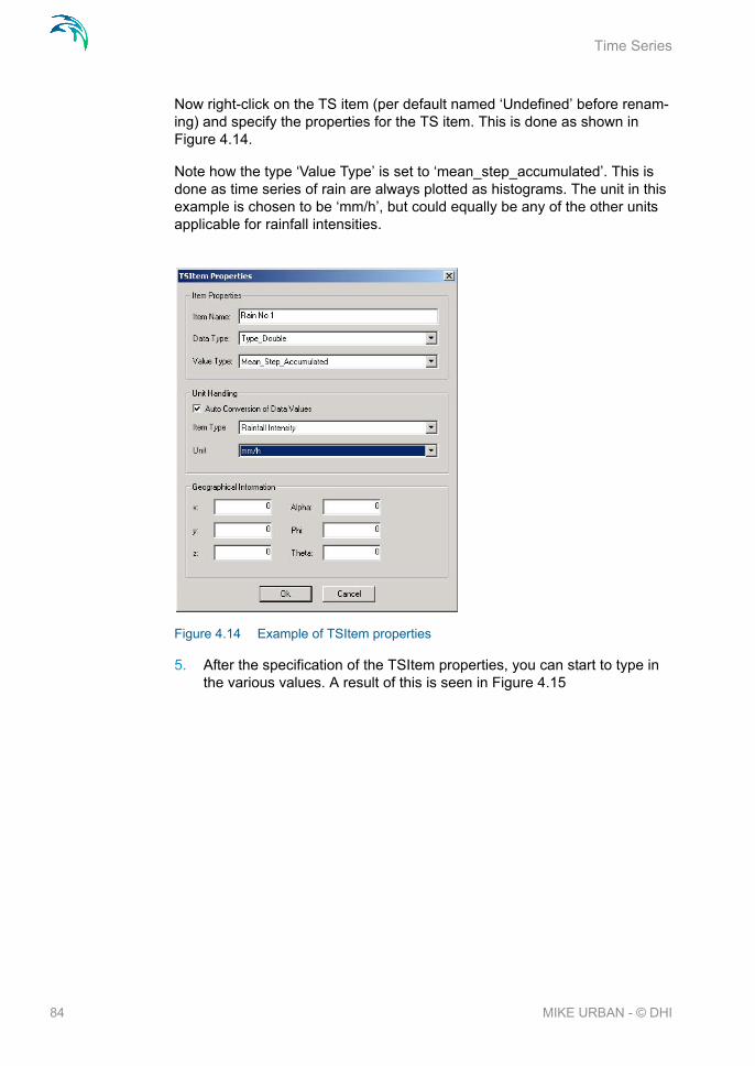
Time Series
Now right-click on the TS item (per default named ‘Undefined’ before renam-ing) and specify the properties for the TS item. This is done as shown in Figure 4.14.
Note how the type ‘Value Type’ is set to ‘mean_step_accumulated’. This is done as time series of rain are always plotted as histograms. The unit in this example is chosen to be ‘mm/h’, but could equally be any of the other units applicable for rainfall intensities.
Figure 4.14 Example of TSItem properties
5. After the specification of the TSItem properties, you can start to type in the various values. A result of this is seen in Figure 4.15
84 MIKE URBAN - © DHI

Example: How to Import a Time Series from Excel
Figure 4.15 Example of how the rainfall is displayed after typing in the values
4.3 Example: How to Import a Time Series from Excel
Assume that you have two time series in Excel that look as seen in Figure 4.16.
Figure 4.16 The TS used in the example
1. Go to Edit|Time Series
2. Choose File|Open
3. On the dialog that comes up choose between available bridges for time series, see e.g. Figure 4.17
85

Time Series
Figure 4.17 Time Series Bridge Selection dialog
4. Choose the ‘Excel Timeseries Bridge’ and press ‘OK’
5. The dialog seen in Figure 4.18 appears
Figure 4.18 Dialog for specifying the import from Excel and ASCII files
6. Now you need to specify how data should be interpreted, e.g. is data a rainfall in mm - or an intensity. First, choose the file and then specify how time should be interpreted. In this case the time and date column is
86 MIKE URBAN - © DHI

Example: How to Import a Time Series from Excel
found in one column. Hence the time description tab page will look as seen in Figure 4.19.
Figure 4.19 The time description for the excel file in this example
7. In this example both time series are rainfall depth measured in mm. The values are mean step accumulated values (see previous section). As the first row in the Excel sheet is used for descriptive headings, data will firs start in row two. All this is then specified on the data description tab page, see Figure 4.20.
87

Time Series
Figure 4.20 The data description for the excel file in this example
8. Then go to the Preview tab page. Here you can see how your time series is interpreted before you import the data into MIKE URBAN. If an error has been made on the previous pages, e.g. you have specified that data will start in row one instead of row two you will now receive an error mes-sage and data cannot be previewed. You can now choose to either import the data straight ahead or to save a template file first that you can reuse when importing data of the same format.
9. The result of the import then looks like seen in Figure 4.21.
Figure 4.21 The TS after import
88 MIKE URBAN - © DHI

Example: How to Import a Time Series from Excel
10. The save the data in the native storage format used in MIKE URBAN for time series, i.e. the dfs0 format. This is done from the file menu of the time series dialog. See Figure 4.22.
Figure 4.22 Saving data into the dfs0 format
You can change the properties for the display of the time series. See Figure 4.23.
Figure 4.23 In the plot the graphic settings have also been changed to make it eas-ier to see the difference.
89

Time Series
90 MIKE URBAN - © DHI

Introduction
5 Curves and Relations
5.1 Introduction
In MOUSE|Curves and Relations (Figure 5.1) a number of tabular data used in other data dialogs are specified.
There are a number of different types of tabular data:
Capacity Curve QH (used for Pumps)
Capacity Curve QdH (used for Pumps)
Pump Acceleration Curve (used for Pumps)
Regulation Qmax(H)
Regulation Qmax(dH)
QH Relation (when specifying a QH relation for a node)
Time-Area Curve (used in Time Area runoff model)
Removal Efficiency (used for the efficiency curve for removal weirs)
Basin Geometry (used for Basins)
Valve Rating Curve (used for Valves)
DQ Relation (used for Curb Inlets)
QQ Relation (used for Curb Inlets)
Capacity Curve QdH & Power
Undefined (used for surface runoff pollutants - SRC, FRC and TOT data-set)
91

Curves and Relations
Figure 5.1 Curves & Relations dialog
5.1.1 Capacity curves
It is possible to define two different capacity curves - both used for specifying pump operation. The capacity curve can be specified either as a 'Capacity Curve QH' relation (for screw pumps) or as 'Capacity Curve QdH' relation (for differential head pumps), where 'H' is the absolute water level in the pump's wet well (at 'Location'), and 'dH' is the water level difference between the 'To' and the 'Location' nodes. A pump type with a 'Capacity Curve QH' relation is named a screw pump, while a pump type with a 'Capacity Curve Q-dH' rela-tion is named a differential head pump.
If an offset is specified this will be added to the capacity curve relation.
Please also note that you can specify a pump capacity curve with the energy consumption as well - for more on this type please refer to section 5.1.10.
5.1.2 Pump acceleration curves
Pumps can be RTC controlled. For those that are PID controlled, the acceler-ation of a pump can be specified as dependent on the actual flow. This pump acceleration curve is then specified as a number of ‘Q, dQ/dt’ data sets.
92 MIKE URBAN - © DHI

Introduction
5.1.3 Regulation curves Qmax(H) and Qmax(dH)
The regulation curves Qmax(H) and Qmax(dH) are used in the regulation of the maximum discharge in links. The regulation can be either a maximum dis-charge as a function of the water level in user specified node or a maximum discharge as a function of the water level difference between two user speci-fied nodes. Please refer to section 3.4.43.4 for regulation in links.
5.1.4 QH relation
QH relations can be used for various types of manholes, outlets, basins and storage nodes.
Manholes, Basins
When using a QH relation in either a manhole or a basin it is possible to spec-ify an infiltration (Q) based on the water level in the manhole/basin.
Outlets
Using a QH relation in an outlet means that you specify the discharge out of the outlet based on the water level in the outlet.
Storage node
Return of water from storage basins back into the MOUSE network is speci-fied in the dialog "Emptying Storage Nodes". An emptying function is a QH relation, where 'Q' is the flow from the storage node into a 'receiving node', and 'H' is the water level in a 'control node'. The flow according to the empty-ing function is possible only until the storage node is completely empty.
5.1.5 Time-Area curve
The Time-Area curve is used in the Time-Area runoff model (see section 4.2). A Time-Area curve represents the contributing part of the catchment surface as function of time.
MIKE URBAN comes with three defaults time-area curves TACurve1, TACurve2 and TACurve3, applicable for rectangular, divergent and conver-gent catchment, respectively (see more in 5.1.5).
You can define any number of custom time-area curves. Each Time-area table must start with a pair of values (0,0) and must end with a pair of values representing the whole (per default, MIKE URBAN maintains T-A curves in percent (%), i.e. the last pair of values in the table must be (100,100)).
93
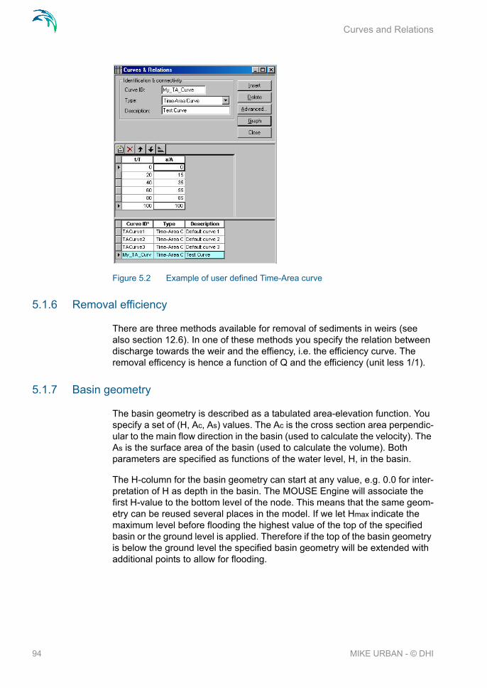
Curves and Relations
Figure 5.2 Example of user defined Time-Area curve
5.1.6 Removal efficiency
There are three methods available for removal of sediments in weirs (see also section 12.6). In one of these methods you specify the relation between discharge towards the weir and the effiency, i.e. the efficiency curve. The removal efficency is hence a function of Q and the efficiency (unit less 1/1).
5.1.7 Basin geometry
The basin geometry is described as a tabulated area-elevation function. You specify a set of (H, Ac, As) values. The Ac is the cross section area perpendic-ular to the main flow direction in the basin (used to calculate the velocity). The As is the surface area of the basin (used to calculate the volume). Both parameters are specified as functions of the water level, H, in the basin.
The H-column for the basin geometry can start at any value, e.g. 0.0 for inter-pretation of H as depth in the basin. The MOUSE Engine will associate the first H-value to the bottom level of the node. This means that the same geom-etry can be reused several places in the model. If we let Hmax indicate the maximum level before flooding the highest value of the top of the specified basin or the ground level is applied. Therefore if the top of the basin geometry is below the ground level the specified basin geometry will be extended with additional points to allow for flooding.
94 MIKE URBAN - © DHI

Introduction
5.1.8 Valve rating curve
A valve is a functional relation which connects two nodes of a MOUSE net-work.
A rating curve is specified to define the relation between the valve opening (%) and resistance (k).
5.1.9 DQ and QQ relations
Two curve types can be specified for the two different types of Curb Inlets (see 3.7):
Capacity Curve, DQ (depth/discharge relation specified in the Curb Inlets dialog)
Capacity Curve, QQ (Qapproach,Qcapture relation specified in the On-grade capture dialog).
The DQ relation specifies the depth based capacity curve for a SAG Type Curb Inlet. Values must be monotonously increasing in depth and discharge and starting at (0,0). For depths in excess of the maximum value specified in the last row of the table, the last corresponding discharge value is used.
The QQ relation specifies the relationship between approach flow in the over-land flow network (Qapp) and the captured flow at the connection node for an ON-GRADE Type Curb Inlet (Qcap). Values must be monotonously increasing and starting at (0,0). For approach discharges in excess of the maximum value specified in the last row of the table, the last corresponding capture dis-charge value is used.
5.1.10 Capacity curve QdH & Power
If you have the knowledge of the power consumption of the pump at various pump levels it is possible to add this to the pump capacity curve by using the ‘QdH & Power’ capacity curve (see Figure 5.3).
95

Curves and Relations
Figure 5.3 Pump capacity curve including power consumption
After the simulation with a ‘QdH & Power’ the summary will contain informa-tion on the power consumption during the simulation period.
Figure 5.4 Snapshot from the html-summary with example of output when using the QdH & Power capacity curve
5.1.11 Undefined type
The undefined type is used for surface runoff pollutants - SRC, FRC and TOT dataset.
The concentrations of a given pollutant can be given for each specific catch-ment. For one catchment it is possible to give a concentration on the slow runoff component (SRC) and the fast runoff component (FRC) or override these settings stating a concentration for the total runoff (TOT). Instead of
96 MIKE URBAN - © DHI

Introduction
fixed concentrations it is possible to state a name of a tabular data set (the undefined type). The tabular data set should then hold a table with concentra-tions versus normalised flow, i.e. the runoff divided by the total catchment area. See more in section 12.7.
97

Curves and Relations
98 MIKE URBAN - © DHI

6 Boundary Conditions
In broad terms, a model boundary condition can be defined as an external interference, which forces the behaviour of the computed variables within the model domain.
A great part of the boundary conditions represent various types of water loads (rainfall, infiltration, wastewater…). The main characteristic of these "load" boundary conditions is that they contain a "transport medium" - water. Water can transport other material (dissolved pollutants, oxygen, sediments), heat (temperature) and organisms (bacteria and para-sites), as well as vari-ous other properties, such as pH, conductivity, turbidity, etc. Properties of "water load" boundary conditions (expressed as concentrations, mass flow, temperature, etc.) are also, in strict terms, boundary conditions for e.g. pollu-tion transport model (Advection-Dispersion). However, these are not treated as separate boundary conditions, but items inseparably associated with the water loads. E.g. a lateral inflow is a water load boundary condition for the hydrodynamic process in the network (defined as discharge item), while the temperature, concentration, etc. associated to this particular inflow are speci-fied as pollutant items of that “load” boundary condition. Effectively, pollutant items of that “load” boundary conditions to the AD process in the network.
Boundary conditions other than water loads are "simple" in a sense that they are fully defined by the boundary condition variable itself, i.e. no additional item is possible to be associated with them. These are water levels, air tem-perature, evapo-transpiration, etc.
In the following the terminology used is:
Boundary condition: it is defined by its type and model connectivity MOUSE distinguishes three groups of boundary conditions:
Catchment Loads and Meteorological Boundary Conditions
Network Loads
External Water Levels
Boundary item: per definition, it is a property inseparably associated with a boundary condition. A boundary item is fully defined by its type, temporal variation and quantity/quality. Through the link to a boundary condition to which it belongs, connection of a boundary item to a model is ensured.
The variable which defines a boundary condition is a default item of the boundary condition.
The structure of boundary conditions and relations between boundary condi-tions and associated items can best be illustrated by a tree-like structure, similar to archive directories and files.
99

Boundary Conditions
On the top level, there are three groups of boundary conditions (see fig-ure….below). Each of these three groups is served by a separate editor, described in full detail further below.
Depending on the model, individual boundary conditions may be added.
Figure 6.1 Basic frame of MOUSE Boundary Conditions with three groups
6.1 Catchment Boundary Condition
Types of variables associated with catchment boundary conditions are:
Air temperature
Evapo-transpiration
Rainfall
Flow - including WQ, sediment and temperature properties
An example illustrating the catchment boundary conditions is presented in below figure
Figure 6.2 The Catchment Boundary Conditions - Example
Any number of each boundary conditions types can be specified.
In this example, the model includes four catchment boundary conditions:
100 MIKE URBAN - © DHI

Catchment Boundary Condition
"Air Temperature" is a boundary condition of the type "air temperature", and always has a temperature (constant or a time series) associated as a default item. This type of boundary condition is used for snow melt calculations.
"Evapo-Transpiration" is a boundary condition of the type "evapo-transpira-tion ", and always has potential evapo-transpiration (constant or a time series) associated as a default item. This type of boundary is used for RDI hydrological calculations.The dfs0 file needs to be of the type ‘Evapo-Transpi-ration’. Delete values will be considered equal to 0.0.
"Rainfall" is a boundary condition of the type "rainfall", and always has rainfall (constant or a time series) associated as a default item. This type of boundary is used for precipitation-runoff hydrological calculations. Association of WQ properties (e.g. temperature, acidity, etc.) with rainfall is not supported. When using a time series the dfs0-file needs to be one of the following Item Types: ‘Rainfall Intensity’, ‘Rainfall’ or ‘Rainfall Depth’. Delete values will be consid-ered equal to 0.0.
"Water Load.Resident DWF" is a boundary condition of the type "catchment load", and always has discharge (constant, cyclic or a time series) associated as a default item. This type of boundary represents various kinds of hydraulic loads, such as area-based or PE-based dry weather loads, area-based infil-tration, etc. The discharge can be associated with any pollutant, sediment or temperature item (constant, cyclic or a time series). In the example above, the default item (Resident WW flow) is associated with pollutants BOD, NH4 and Temperature.
Note that the first three boundary conditions are used by a runoff-precipitation model, while the water load boundary condition can either be appended to the computed runoff (only flow) or passed directly to the network connected to the catchments.
6.1.1 Visualization of catchment boundaries
The catchment loads are visualized by toogling the display of ‘MOUSE Catchment Boundaries’ on in the TOC.
101

Boundary Conditions
Figure 6.3 MOUSE Catchment Boundaries
The following items can be toggled on/off under ‘MOUSE Catchment Bound-aries’ in the TOC:
MOUSE Rain Gauges (represents the rain gauges, as defined by the ‘Data source location’)
MOUSE Rainfall (shows catchments with a catchment load of type ‘Rain-fall’)
MOUSE Catchment Rainfall (shows catchments with a catchment load of type ‘Catchment Discharge’)
MOUSE Air Temperature (shows catchments with a catchment load of type ‘Air Temperature’)
MOUSE Evapo-Transpiration (shows catchments with a catchment load of type ‘Evapo-Transpiration’)
Figure 6.4 Example of the visualization of catchment boundaries
102 MIKE URBAN - © DHI

Network Boundary Conditions
6.2 Network Boundary Conditions
Types of variables associated with MOUSE network (i.e node/grid point) boundary conditions are:
Water level
Flow (discharge) - incl. WQ and sediment properties
The discharge boundary conditions are termed as "Network Loads". An example illustrating the network loads is presented (see illustration below)
Figure 6.5 MOUSE Network Loads - Example
Network Loads represent all kinds of hydraulic loads, such as DWF point-inflows, individual lateral inflows, infiltration, storm runoff, etc. This type of boundary condition always has discharge (constant, cyclic or a time series) associated as a default item. The discharge can be associated with any pol-lutant, sediment or temperature item (constant, cyclic or a time series).
Any number of network loads can be specified, independently on the location point.
In this example, the model includes three network loads:
"Water Load.Industrial DWF" represent some industrial loads. In the example above, the default item (Resident WW flow) is associated with pollutants BOD and NH4 and with Temperature.
"Water Load.Storm Runoff" represent calculated storm runoff loads. Note that in the example above, two default items are specified, each covering different time period. The default items (i.e. storm runoff itself) are associated with temperature and pollutants BOD and NH4.
"Catchment Water Load.Resident DWF" is an example of a special type of network load definition. It is actually only a reference to already existing
103
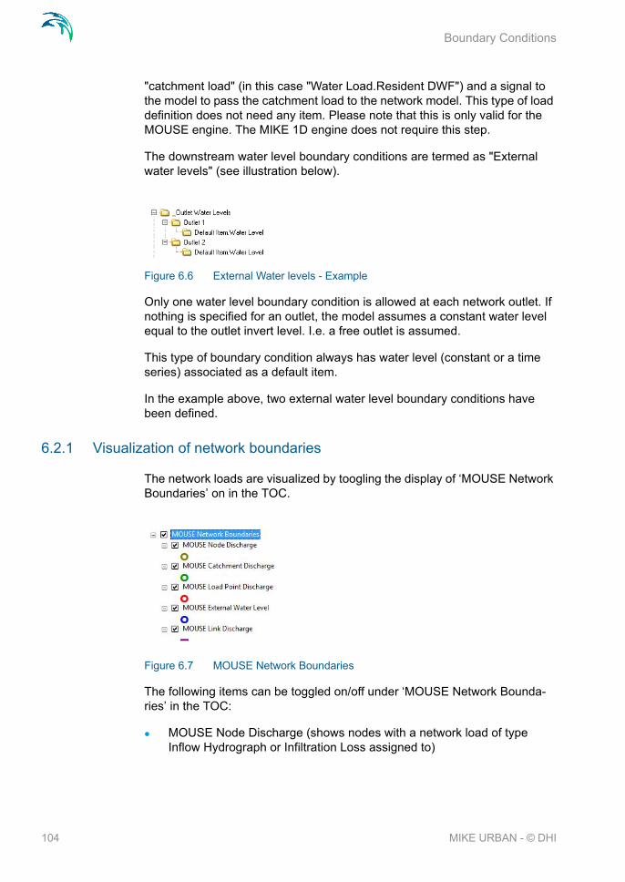
Boundary Conditions
"catchment load" (in this case "Water Load.Resident DWF") and a signal to the model to pass the catchment load to the network model. This type of load definition does not need any item. Please note that this is only valid for the MOUSE engine. The MIKE 1D engine does not require this step.
The downstream water level boundary conditions are termed as "External water levels" (see illustration below).
Figure 6.6 External Water levels - Example
Only one water level boundary condition is allowed at each network outlet. If nothing is specified for an outlet, the model assumes a constant water level equal to the outlet invert level. I.e. a free outlet is assumed.
This type of boundary condition always has water level (constant or a time series) associated as a default item.
In the example above, two external water level boundary conditions have been defined.
6.2.1 Visualization of network boundaries
The network loads are visualized by toogling the display of ‘MOUSE Network Boundaries’ on in the TOC.
Figure 6.7 MOUSE Network Boundaries
The following items can be toggled on/off under ‘MOUSE Network Bounda-ries’ in the TOC:
MOUSE Node Discharge (shows nodes with a network load of type Inflow Hydrograph or Infiltration Loss assigned to)
104 MIKE URBAN - © DHI

Boundary Condition Editors
MOUSE Catchment Discharge (reflects the network load using a Catch-ment Load. In this specific case, the boundary condition will be displayed even if no Boundary Item is created)
MOUSE Load Point Discharge (shows the nodes that have a Load point assigned)
MOUSE External Water Level (shows the outlets that have an External Water Level assigned as a boundary condition)
MOUSE Link Discharge (shows links with a network load of type Inflow Hydrograph or Infiltration Loss assigned to)
Figure 6.8 Example of the visualization of network boundaries
6.3 Boundary Condition Editors
Three editors are available for specifying boundary conditions corresponding to three boundary condition groups and one common editor for boundary items:
Catchments Loads and Meteorological Items
Network Loads
External Water levels
Common for all three editors is the specification of the Boundary condition identifier and controlling if the specified boundary is actually applied to the model or not (per default, each new boundary condition is applied).
To sort the different loads (catchment loads, network loads and external water levels) in each editor, use the right click option "Sort" on top of the "Boundary ID" column. Double clicking on the column will display all boundaries condi-tions loaded in the database indistinctly of the editor type where the user is positioned.
Additionally, there is a common editor for boundary items.
105

Boundary Conditions
6.3.1 Catchments Loads and Meteorological Items Editor
Figure 6.9 The catchment loads editor
The following describes how to define an boundary condition for a catchment.
As the first action after inserting a new boundary conditions, a proper name (ID) must be specified. We recommend that you use a descriptive ID.
Next, a type of boundary connection is selected, among Rainfall, Air tempera-ture, Evapo-transpiration and Catchment Discharge. For the first three types, co-ordinates of a data source (e.g. raingauge) may be specified (Data Source location). The co-ordinates are used for the simulation of spatially distributed rainfall (snowmelt, evapo-transpiration), in cases when the data file itself (i.e. time series file) does not contain this information. Checking the "Data source Location" overrides the coordinates from the TS file.
The "Connection Type" determines the mode of identification of the catch-ments for which this boundary condition applies. "Individual" applies for a sin-gle catchment, and requires a specification of the catchment ID. "List" applies for a set of catchments, contained in the catchment selection file (*.CSE or *.MUS). "All" applies to all catchments. In case of two or more meteorological boundary conditions of the same type specified, the co-ordinate information is used to distribute the boundaries accordingly. This latter only applies when the "Connection Type" is set to "All". It is only possible to have one rain used as a boundary condition per catchment.
106 MIKE URBAN - © DHI

Boundary Condition Editors
To sort the different loads use the right click option "Sort" on top of the "Boundary ID" column. Double clicking on the column will display all bounda-ries conditions loaded in the database.
6.3.2 Network Loads Editor
Figure 6.10 The network loads editor
The following describes how to define an boundary condition for the network. This could e.g. be a discharge entering a manhole or pipe infiltration.
As the first action after inserting a new boundary condition, a proper name (ID) must be specified. We recommend that you use a descriptive ID.
The "Connection Type" determines the mode of definition of the network loca-tion(s) to which this boundary applies. "Individual" applies for a single node or pipe, and requires a specification of the Node ID or Link ID.
If a load is connected to a link, it will be uniformly distributed over all computa-tional grid H-points along the link.
"List" applies for a set of node or links, contained in the selection files (*.NSE, LSE or *.MUS). "Defined by Catchment Connections" applies to the storm runoff loads from MOUSE *.CRF file.
For a node - either an inflow hydrograph can be specified or an infiltration boundary can be specified. If the 'Infiltration' option is chosen the boundary items page allows to specify a positive or negative rate. So either infiltration to
107

Boundary Conditions
the node or loss of water from the node to the surrounding ground can be used.
The loss can be defined for any type of node, but it is primarily intended for use with basins or nodes with geometry representing small ponds. The infil-tration can be defined as a constant rate (velocity) which is multiplied by the actual wet area in the node. Note that the rate value should be given as a negative value for specifying a loss of water from the network model. Apply-ing a positive value will result in water being added to the node.
Check-box "Distribute" is of relevance for network loads connected to a list of nodes or links. If checked, the specified load will be uniformly distributed over the listed nodes or links. Otherwise, each location specified in the list will receive the specified load.
"Geo-coded" applies for point-loads (typically DWF) geo-coded to the net-work nodes. User can select which one of the geo-coded load categories applies for this boundary condition.
Please note that when you use the boundary type “Defined by catchment” and afterwards specify a time series ID in the boundary items dialog then this item is always used regardless of type (water, component) or extension (dfs0, CRF). If you have not specified a time series ID then the catchment name will be used. This is only applicable for the boundary type “Defined by catchment” for other types the time series ID is always used.
To sort the different loads use the right click option "Sort" on top of the "Boundary ID" column. Double clicking on the column will display all bounda-ries conditions loaded in the database.
6.3.3 External Water Levels Editor
This editor is dedicated to specification of external water levels interacting with the collection system.
108 MIKE URBAN - © DHI

Boundary Condition Editors
Figure 6.11 External water levels editor
In addition to the specification of the boundary condition ID and the location (outlet), user can define an open boundary here (relevant for pollution trans-port simulations).
To sort the different loads use the right click option "Sort" on top of the "Boundary ID" column. Double clicking on the column will display all bounda-ries conditions loaded in the database.
6.3.4 Boundary Items Editor
Boundary item editor allows for a full definition of a boundary item in terms of type, temporal variation, quantity/quality and temporal validity
109

Boundary Conditions
Figure 6.12 The Boundary Items Editor
The 'Boundary Items' editor has been designed to operate in conjunction with the three boundary condition editors. When open simultaneously with one of these, this editor displays only the boundary items associated with the cur-rently active boundary condition. Otherwise, displays all boundary items.
'Boundary Items' editor allows for a full definition of a boundary item in terms of type, temporal variation, quantity/quality and temporal validity.
A new boundary item is created by pressing "Insert". The new item is auto-matically associated with the currently active boundary condition and is appended to the list of associated items. Alternatively, already existing item can be re-used and associates it with the currently active boundary. "Re-use Item" actually makes a copy of a selected item and adds it on the list of items for the current boundary condition. By these means user can assign the same item (e.g. concentration of some pollutant in wastewater) to many boundary conditions quickly.
A new item can also be inserted while none of the boundary condition dialogs is open. In that case, user must "manually" connect the item to a boundary condition. There is no automatic control over the match between the bound-ary condition type and the actual item definition, so due care is needed.
Each new item is set as "default". For some types of boundary conditions, this can be changed to "Pollutant" or Sediment". In the later case, a pollutant component or a sediment fraction must be selected from the respective lists. The pollutant items can be defined in terms of concentrations or loads.
110 MIKE URBAN - © DHI

Examples
The scaling factor determines the fraction of the specified load which is actu-ally loaded into the model. Per default, the scaling factor is set to 1.
Temporal variationsTemporal variation of boundary items may take one of the following forms:
Constant - any boundary item can be defined as a constant
Cyclic (Diurnal) - all hydraulic loads items can be defined as diurnal
Time series
A constant boundary item is the simplest form of boundary. In case of large constant network loads, the HD model may display some stability problems. This can be avoided by allowing a gradual increase of the load over a speci-fied start-up time.
Cyclic (diurnal) boundary items are typically associated with wastewater loads. Cyclic loads may be quantified in several ways: as area-based or per-son equivalent-based loads (associated with catchment loads), as average load or geo-coded loads (associated with network loads).
Time series may come from various sources, including previous MOUSE result file (this latter option includes MOUSE files CRF, SMR and PMR).
Temporal validityEach boundary item may be specified with limited temporal validity.
Per default, each item is considered valid during the entire simulation period. Indeed, in case of TS items, the validity is also limited by the length of TS.
If multiple items are specified they may all be with default temporal validity (i.e. over the entire simulation period), or with overlapping validity periods (e.g. when mixing de-fault and limited validity) or with periods with missing coverage.
6.4 Examples
In the following paragraphs some examples on setting up boundary condi-tions are shown step-by-step
6.4.1 How to add a varying water level at an outlet?
This boundary condition falls into the category 'External Water Levels'. The definition involves the specification of a boundary condition itself and the water level (default) item.
Enter Edit mode: Go to Edit|Start Editing
111

Boundary Conditions
Go to MOUSE|Boundary Conditions|External Water Levels
Press Insert button
Boundary ID is then given automatically (hint: you can change this ID if you wish to)
Choose the list button next to the location field (hint: you can also type in the Location directly - note that you can only add External Water Levels to MOUSE outlets)
Select the outlet from the list press OK button (hint: you can just double-click)
Press the Items button to open the Boundary items dialog to connect the time variation for the water level. Note that the Boundary ID is automatically filled in on the Boundary items dialog.
After having pressed Insert an item ID will automatically be given (hint: you can change this ID if you wish to)
Now the temporal variation can be specified:
Choose “Time Series/Result File” in order to specify an irregular varying water level. This activates the Time Series part of the editor
Choose DFS0 as the Source Type, click the list button next to the Path field and choose the dfs0 file with the water level (item ID is only neces-sary to fill out if the dfs0 file contains more than one item, i.e. time series)
After completing this, the time-varying water level has been successfully added to the outlet.
6.4.2 How to add infiltration in a pipe?
This boundary condition falls into the category 'Network Loads'. The definition involves the specification of a boundary condition itself and the infiltration item.
Enter Edit mode: Go to Edit|Start Editing
Go to MOUSE|Boundary Conditions|Network Loads
Press Insert button
Boundary ID is then given automatically (hint: you can change this ID if you wish to)
Choose the connection type to ‘Individual’ and set the radio button in ‘Pipe ID’
Select the pipe from the list and press OK button (hint: you can just dou-ble-click)
112 MIKE URBAN - © DHI

Examples
Press the Items button to open the Boundary items dialog to add the infiltra-tion value. Note that the Boundary ID is automatically filled in on the Bound-ary items dialog.
After having pressed Insert an item ID will automatically be given (hint: you can change this ID if you wish to)
Now the infiltration can be specified. In this case we choose a constant infil-tration:
Choose “Constant” in order to specify a constant infiltration. This acti-vates the ‘Constant’ part of the editor
Type in an infiltration value in the active field. The value is provided as an inflow per length unit of the pipe and is hence also kept constant along the pipe.
After completing this, the constant infiltration to the pipe has been success-fully added.
6.4.3 How to add a rainfall as a boundary condition to the catchments?
This boundary condition falls into the category 'Catchment Loads And Mete-orological Items'. The definition involves the specification of a boundary con-dition itself and the rainfall (default) item.
Enter Edit mode: Go to Edit|Start Editing
Go to MOUSE|Boundary Conditions|Catchment Loads
Press Insert button
ID is then given automatically (hint: you can change this ID if you wish to)
Set Type = Rainfall
Set Connection type, choose = All (All = all catchments, List = a group of catchments, Individual = a single catchment)
Note: Now a rainfall is assigned to all catchments. By checkmarking the data source location field you can specify where the rain gauge is placed
Press the Items button to open the "Items" editor.
Press Insert button on the Boundary Items dialog to insert a rainfall item
After having pressed Insert an item ID will automatically be given (hint: you can change this ID if you wish to)
Now the temporal variation can be specified:
Choose Time Series/Result File in order to choose a time series for the rain event
This activates the Time Series part of the dialog
113

Boundary Conditions
Choose DFS0 as the Source Type, and select the dfs0 file with the rain event (item ID is only necessary to fill out if the dfs0 file contains more than one item, i.e. time series)
Now the rain event has successfully been connected to the catchments!
6.4.4 How to add a discharge to a node?
This boundary condition falls into the category 'Network Loads'. The definition involves the specification of a boundary condition itself and the discharge (default) item.
Enter Edit mode: Go to Edit|Start Editing
Go to MOUSE|Boundary Conditions|Network Loads
Press Insert
A Load ID is automatically assigned (you can change this)
Set the Connection type to 'Individual'
Choose the relevant Node ID
Now press the Items button. This will open the Boundary Items dialog where the discharge variation can be specified
Press Insert button on the Boundary Items dialog. The Boundary ID field is automatically filled in by the current boundary ID. This ensures a bond between the Boundary condition and this item.
After having pressed Insert an item ID will automatically be given (hint: you can change this ID if you wish to)
Specify that the load type is 'Other'. This will insure a correct categorisa-tion of this load in the simulation summary statistics and in the job-list generation for LTS simulations.
Now the temporal variation can be specified:
Choose Time Series/Result File in order to specify a irregular varying discharge (note: constant as well as cyclic variation can also be chosen)
This activates the Time Series part
Choose DFS0 as the Source Type, click next to the Path field and choose the dfs0 file with the water level (item ID is only necessary to fill out if the dfs0 file contains more than one item, i.e. time series)
Now the discharge is successfully connected to your node!
114 MIKE URBAN - © DHI

Examples
6.4.5 How to add runoff results as input for the network computation?
The runoff results are treated as network loads in MIKE URBAN, and can be specified following the same principle as any other load (see the example above). Alternatively, a 'shortcut' specification can be used.
The 'standard' definition of runoff input to the network model is described in the following example. Further below, the "shortcut" hint is provided.
Enter Edit mode: Go to Edit|Start Editing
Go to MOUSE|Boundary Conditions|Network Loads
Press Insert
A Load ID is automatically assigned (you can change this)
Set the Connection type to 'Defined by catchment connection'. No further specification of the location is required, since this is controlled by the catchment connections.
The specification of the load type will allow the computation to take into account where the load came from initially - and hence also report this in e.g. the summary after the simulation
Now press the Items button. This will open the Boundary Items dialog where the runoff result file to be used can be specified
Press Insert button on the Boundary Items dialog. The Boundary ID field is automatically filled in by the current boundary ID. This ensures a bond between the Boundary condition and this item.
After having pressed Insert an item ID will automatically be given (hint: you can change this ID if you wish to).
Specify that the load type is 'Storm Runoff'. This will insure a correct cat-egorisation of this load in the simulation summary statistics and in the job-list generation for LTS simulations.
Now the temporal variation can be specified.
Choose Time Series/Result File in order to choose the result file from the catchment simulation
This activates the Time Series part of the dialog
Choose MOUSE as the Source Type, click the list button next to the Path field and select the *.CRF file containing the results from the runoff computation.
Now the runoff results are used as input for the network computation!
Alternatively, a 'shortcut' definition can be used. On the MOUSE Computa-tions dialog ('Network Parameters') user can checkmark the 'Runoff' in the Runoff Input group, and select the runoff file from the list. The effect of this
115

Boundary Conditions
specification is identical as if the runoff input is specified through the bound-ary conditions dialogs. Please note, that this way it is NOT possible to assign any water quality properties to the runoff input. If this is required, the bound-ary conditions editors must me used.
6.4.6 How do I add DWF in my network dependent on number of inhabitants?
Please note that the steps are different depending on your choice of numeri-cal engine (MOUSE or MIKE1D).
The PE-based and catchment area-based DWF fall into the category of catchment loads. This is because both the input parameters and the results of the computation are catchment-related. However, in most applications, this load is supposed to be passed into the network through the catchment con-nection points. The following example describes the entire definition process.
The overall procedure involves the following major steps:
Define the diurnal patterns (note: not a part of this tutorial)
Define the catchment load. Note that inhabitants (PEs) are associated with catchments, so the DWF load which they generate is also associ-ated with catchments
Define the boundary item for the catchment DWF load
This step only applies for the MOUSE engine (for the MIKE 1D engine this step can be skipped): Define a network load and declare it as a "car-rier" of the catchment load defined previously. This allows for a direct passage of the catchment load into the network. The water is loaded into the network at the catchment connection points. Note that for this load no item definition is required.
The detailed steps:
Enter Edit mode: Go to Edit|Start Editing
Go to MOUSE|Boundary Conditions|Catchment Loads
Press Insert button
ID is then given automatically (hint: you can change this ID if you wish to)
Set Type = Catchment Discharge
Set Connection type, choose = Individual (All = all catchments, List = a group of catchments, Individual = a single catchment)
Choose the list button next to the Individual field and select the catch-ment (hint: you can also type in the catchment ID directly)
The Catchment load and its connectivity to the catchment(s) is specified. The following step is the definition of the boundary item, i.e. temporal variation, quantity and temporal validity of the load.
116 MIKE URBAN - © DHI

Examples
Press the Items button. This opens the Items editor.
Press Insert button on the Boundary Items dialog
Note that the boundary ID is automatically filled in on the Boundary items dia-log.
After having pressed Insert an item ID will automatically be given (hint: you can change this ID if you wish to)
The scaling factor and item type are per default set properly, so no action is required. Now the temporal variation can be specified:
Choose "Cyclic" in order to specify a diurnal load variation. This activates the Cyclic part of the dialog.
Select a predefined pattern from the list.
Specify the Method as "PE Based". This indicates that the DWF contribu-tion is computed taking the number of inhabitants PE on the catchment into account
Specify the water amount per PE/day
Note: "Average" means that an average diurnal value will be used (taken from the field 'Value'), while 'Area based' will compute the total flow taking the catchment area into account.
This completes a full definition of the catchment DWF load based on PEs. The remaining step (which is only needed in case of using the MOUSE engine) is to allow this load be directly applied to the network model.
Go to MOUSE|Boundary Conditions|Network Loads
Press Insert
A Load ID is automatically assigned (you can change this)
Set the tickmark in 'Catchment Load' and select the boundary ID from the list for the catchment load just created.
The specification of the 'Load Type' will allow the computation to take into account where the load came from initially - and hence also report this in e.g. the summary after the simulation.
6.4.7 How to attach a pollutant concentration to a network load?
Attaching a pollutant concentration involves adding a pollutant item to already existing network load.
Enter Edit mode: Go to Edit|Start Editing
Go to MOUSE|Boundary Conditions|Network Loads
Scroll through the list of loads and place cursor on the wanted load record.
117

Boundary Conditions
Press the 'Items' button. This will open the Boundary Items dialog where items associated with the actual load will be displayed. There will be at least one discharge item and, possibly, some pollutant and sediment items.
Press Insert button on the Boundary Items dialog. The Boundary ID field is automatically filled in by the current boundary ID. This ensures a bond between the Boundary condition and the new item.
After having pressed Insert an item ID will automatically be given (hint: you should change this ID in order to be able to identify it easier)
Specify the new item type as 'Pollutant'. This will activate the part of the editor where a pollutant must be selected from the list. Note that pollutant can be specified as concentration (i.e. mass per unit volume of water) or as load (i.e. mass per unit of time). This specification is not effective for the cases where actual pollutant data include the information of actual unit (e.g. dfs0 time series).
Now the temporal variation can be specified. Note that specification of cyclic variation in a combination with "concentration" affects the mass balance, i.e. the simulated pollutant mass changes with changes in cyclic pattern. This must be compensated by appropriate adjustment of the pol-lutant concentration.
Now a pollutant (concentration or load) has been successfully connected to your network load!
6.5 Repetitive Profile Editors
The 'Repetitive Profile Editors' can be used for generating dimensionless, cyclic time series ('repetitive profiles') with a fixed time resolution of one hour. E.g., it can be applied for defining diurnal profiles that can describe the Dry Weather Flow (DWF) from a specific catchment. An unlimited number of repetitive profiles can be applied to different groups of catchments in order to reflect that e.g. an industrial area will have a different DWF flow description than a rural or residential area. The DWF may, however, also vary according to the time of week or year and holidays.
The 'Repetitive Profile Editor' consists of four sections:
Diurnal Patterns- used for specifying the diurnal patterns
Profiles Calendar - used for specifying when the diurnal patterns are to be used
Cyclic Profiles - used for coupling of individual diurnal patterns with pro-files calendar definition
Special Days - used for specifying days that are to be considered as exceptions to the calendar (e.g. the 1st of January).
118 MIKE URBAN - © DHI

Diurnal Patterns
6.6 Diurnal Patterns
A diurnal pattern consists of the 'PatternID', a DeltaT [min] and the non-dimensional coefficients. The dimensionless coefficients may be given any appropriate value, as long as their relative size reflects the diurnal variation. Prior entering the multiplier coefficients, the DelataT is set for the pattern and clicking on ‘Distribute’ fills the two time columns with the appropriate numbers of values for having a daily pattern.
Figure 6.13 Diurnal Pattern Editor
An unlimited number of diurnal patterns can be entered. E.g. one for week-days and one for weekends, but also one for weekdays belonging to one group of catchments and one for weekdays belonging to a different group of catchments. Clicking on ‘Graph’ gives a graphical display of the profile.
6.7 Profiles Calendar
The purpose of the profiles calendar is to specify when the diurnal patterns are to be applied, e.g. only during the summer, only in February, only on weekdays, only on each first in the month, etc.
Three checkboxes 'Week Days', 'Dates' and 'Months' are available for the activation of three different, mutually inclusive modes of the calendar defini-tion. This means that if any day is to be included in the current calendar defi-nition, it must be included in all three definition modes. If any of the definition modes is not activated (i.e. the checkbox not ticked), it does not affect the cal-endar definition. If only a calendar's ID is given, but no tick marks are set, the diurnal pattern that the profiles calendar is assigned to would be uncondition-ally used.
119

Boundary Conditions
Figure 6.14 Profiles Calendar Editor
6.8 Cyclic Profiles
A 'Cyclic Profile' (defined by its 'Profile ID' string max 40.characters) links the diurnal pattern with the relevant calendar definitions.
Each pattern can contain an arbitrary number of profile-calendar links. For inserting a new link, use the "Insert new line" icon. For deleting a selected link use the "Delete selected line" icon. If the calendar definitions for two or more links are covering the same period, the links positioned highest on the list will have the highest priority. In other words, the definition given by some link cov-ers only the days which are not included into any of the higher positioned links. In order to control the priorities, it is possible to change the order of sets in the pattern with the "Move line up" and "Move line down" icons.
For each pattern the 'Interpolation' method is chosen to either 'Linear Interpo-lation' or 'No Interpolation'. The 'Linear Interpolation' performs a linear inter-polation between the values given in the diurnal profile while the 'No Interpolation' will apply a step function. For use with DWF, the 'Linear Interpo-lation’ is recommended
120 MIKE URBAN - © DHI

Special Days
Figure 6.15 Cyclic Profiles Editor
6.9 Special Days
The 'Special days' is used for the specification of individual days that should be considered differently than it is given by the profiles calendar.
E.g. the 1st of January each year (the New year holiday) even though it comes every year on a different day of the week could be coupled with the diurnal profile of e.g. Sunday, since the diurnal pattern of a holiday matches better with Sunday than by any other week day.
The special days are divided in two categories: Special days that are to be considered every year and special days that are only considered once (Unique date). An example of this could be the Easter holiday which will not be on the same date every year.
121

Boundary Conditions
Figure 6.16 Special Days Editor
122 MIKE URBAN - © DHI

The General Simulation Settings
7 MOUSE Simulations
MOUSE simulations may be started from ‘Simulation | Run MOUSE’. Simula-tion options for MOUSE are also defined here.
The editor is split into following five tabsheets:
General
Runoff parameters
Network parameters
Network Summary
2D overland parameters
The ‘Simulation ID’ and ‘Scenario ID’ are found on all four tabsheets as a common reference.
7.1 The General Simulation Settings
On the General page the following can e.g. be specified:
Name of simulation (equal to the name of the result file)
Simulation period
Simulation type
The General page includes a button in the upper right ‘corner’ that allows to copy simulation settings (to be re-used in another simulation, e.g. for another scenario).
123

MOUSE Simulations
Figure 7.1 The MOUSE Simulation General Editor dialog
Edit fields on the General pageA full overview of the editor fields and corresponding database attributes is provided in the Table 7.1.
Table 7.1 Overview of the general simulation settings (Table ‘msm_Project’)
Edit field Description Used or required by simulations
Field name in datastructure
Simulation ID
ID of simulation - user speci-fied. ID will be reflected in the
name of project and result files
Yes MUID
Scenario ID ID of selected Scenario - Acti-vating scenario is done in the
Scenario Manager dialog
Yes ScenarioID
Runoff/Net-work radio
buttons
Switch for starting runoff, net-work or network combined with
2D simulation
Yes Computation-TypeNo
124 MIKE URBAN - © DHI

The General Simulation Settings
‘Info’ buttonThe ‘Info’ button opens a dialog containing:
1. Start and end time of the simulation similar to the values found under max time
2. Start and end time of a hotstart file (if specified) (Table: msm_Project, Attribute: PRFHotstartFileName)
Figure 7.2 Example of the dialog that comes up, when pressing the ‘Info’ button
‘Set max. time’ buttonThe ‘Set max. time’ button will set the maximum simulation time by filling in the start time and the end time of the simulation. The start time of a simulation is considered the latest start time of all boundaries. Likewise the end time for the simulation is considered the earliest end time of all boundaries.
Each boundary contains a number of items which can cover different parts of the simulation.
If a validity is specified for an item this specifies the start and end time. If a validity is not specified only items specified as timeseries have a start and end time. If either a constant or cyclic value is given without validity the item is not included in the evaluation.
Simulation Description
User’s descriptive information No Description
Start Start date and time for the sim-ulation
Yes ComputationBe-gin
Duration Allows to specify the duration of the simulaion. Entering the
duration will automatically fill in the end date and time of the
simulation. If the start and end time are specified the duration
will be filled automatically
Optional (will be automatically
filled)
-
End End date and time for the sim-ulation
Yes ComputationEnd
Table 7.1 Overview of the general simulation settings (Table ‘msm_Project’)
Edit field Description Used or required by simulations
Field name in datastructure
125

MOUSE Simulations
7.1.1 Choice of numerical engine
For each simulation you can choose to use either the classic MOUSE engine or the MIKE 1D engine. Please refer to seperate documentation on the differ-ence between these two engines and the possibilities provided with them.
It is important to note that when running the numerical engine of you choice you need to keep the input for the simulation within the same numerical engine. I.e. when using results from a runoff simulation as input to a pipe flow simulation then both the runoff and the pipeflow simulation needs to be done with the same numerical engine. If runoff result file is computed with e.g. the MOUSE engine and you try to use it as input for MIKE 1D pipeflow simulation you will hence get an error message. You can, however, create a number of simulation records and then choose to have some done with MOUSE and some with MIKE 1D.
The MIKE 1D result files all have the same extension (*res1d), while the MOUSE result files have different extensions based on simulation type. Sev-eral places you will hence see both result types appear as a filter for file types you can choose between:
Computation dialog - RDII hotstart file. The filter says: "Hotstart Files (*.nof, *.res1d)
Computation dialog - runoff input. The filter says: "Runoff Files (*.crf, *.res1d)
Computation dialog - hotstart file. The filter says: "Hotstart files (*.prf, res1d)"
Boundary Items - result file/time series. Both MOUSE Result Files and res1d files can be used
LTS initial conditions - hotstart file. The filter says: "Hotstart Files (*.prf, res1d)"
7.1.2 Hotstart files
What is hot start?Hot start is a facility that enables application of initial conditions for a simula-tion, other than the default initial conditions, i.e. empty network and uniform concentrations of pollutants in the pipe flow model, or initial values of hydro-logical state variables in the RDII hydrological model.
What is a hot start file?The hot start initial conditions represent the state of the system as recorded in a previously generated result file at a specified time - the so-called hot start file.
Relevant information from a hot start file for a network simulation includes:
126 MIKE URBAN - © DHI

The General Simulation Settings
Water levels and pollutants' concentrations in each node of the system;
Water levels, discharges and pollutants' concentrations in all grid points of the network;
Pumps, weirs, orifices (gates) and valves flows and pollutants concentra-tions in these flows;
Position of controllable weirs, gates and valves (if RTC is applied).
For the RDII model, relevant information in the hot start file includes all rele-vant hydrological state variables, such as surface storage, groundwater depth, etc.
A hot start file for a network simulation must be generated with exactly the same model setup as the model used in a hot start simulation run. A result file used as a hot start file must be a complete ("standard") result file. I.e. user-specified result file with reduced contents cannot be used as a hot start file.
Why and when is hot start relevant?Hot start files can be used for the following purposes:
To avoid potential numerical instabilities that occasionally take place under Dynamic Wave computations during the initial phase of the simula-tion.
To create a realistic initial conditions for a productive simulation. This typ-ically implies levying a set of constant base flows (for a natural channel network) or a set of dry weather sanitary flows (for a sewer network) over some startup period of time. The resulting hot start file from this run is then used to initialize a subsequent run where the inflows of real interest are imposed.
To divide long continuous simulations into shorter simulation periods. Here are the initial conditions for each subsequent simulation period set as the end of the previous simulation period.
Specification of the hot start Hot start options are set in the Simulation dialog (runoff parameters tab and network parameters tab)
For the RDII runoff model, the only parameter is the Hot start Filename. The system automatically detects the values of the relevant variables at the simu-lation start time and initiates the actual simulation run accordingly.
For the pipe flow model, the following parameters are needed:
Hot start Filename: This is the name of an existing result file from which initial conditions for the simulation will be loaded.
Hot start Date and Time: The date and time at which the initial conditions are taken from the hot start file. The hot start time must be within the hot start file time coverage.
127

MOUSE Simulations
AD Hotstart (checkbox): If checked, the AD model is initiated from the AD hot start file (with identical file name as the HD hot start file), at the date and time specified. Otherwise, AD model is initiated uniformly by the specified initial values for the AD components .
If the Hot Start Filename specified is identical with the current simulation result file name (concatenated by simulation MUID, ScenarioID and the extension .PRF),
The results of the current simulation will be appended to the hot start file, starting at the simulation start time. In this case, hot start date and time are ignored, as the simulation hot starts at the simulation start time. Any informa-tion in the hot start file beyond the simulation start date and time (the actual hot start date and time) will be lost. This part of the file will be replaced by the new simulation results.
7.1.3 Export to remote simulation
It is possible to run computations on a remote computer via the DHI Remote Simulation Console (see the DHI Remote Simulation documentation for details).
Before running a Remote Simulation, an engine specific input file must be created. These engine specific input files have the extension *.m1dx for MIKE 1D and *.mex for MOUSE.
To create an engine specific input file, open the ‘General’ tab of the ‘Compu-tation’ dialog and click ‘Advanced’ . This opens a menu where there is an option called ‘Export to Remote Simulation’:
128 MIKE URBAN - © DHI
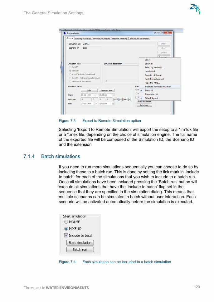
The General Simulation Settings
Figure 7.3 Export to Remote Simulation option
Selecting ‘Export to Remote Simulation’ will export the setup to a *.m1dx file or a *.mex file, depending on the choice of simulation engine. The full name of the exported file will be composed of the Simulation ID, the Scenario ID and the extension.
7.1.4 Batch simulations
If you need to run more simulations sequentially you can choose to do so by including these to a batch run. This is done by setting the tick mark in ‘Include to batch’ for each of the simulations that you wish to include to a batch run. Once all simulations have been included pressing the ‘Batch run’ button will execute all simulations that have the ‘include to batch’ flag set in the sequence that they are specified in the simulation dialog. This means that multiple scenarios can be simulated in batch without user interaction. Each scenario will be activated automatically before the simulation is executed.
Figure 7.4 Each simulation can be included to a batch simulation
129

MOUSE Simulations
7.2 The Runoff Simulation Settings
On the Runoff parameters page the following can e.g. be specified:
Name of simulation (equal to the name of the result file)
Simulation type
Simulation description
Simulation period
Start simulation
Figure 7.5 The MOUSE Simulation Runoff Editor Dialog
130 MIKE URBAN - © DHI

The Runoff Simulation Settings
Table 7.2 The Simulation Runoff Identification
Edit field Description Used or required by simulations
Field name in datastructure
Simulation ID
ID of simulation - user speci-fied. ID will be reflected in the
name of project and result files
Yes MUID
Scenario ID ID of selected Scenario - Acti-vating scenario is done in the
Scenario Manager dialog
Yes ScenarioID
Model Type Selection among available run-off models and combinations:
T-A Curve (A), Kinematic Wave (B), Model C1, Model C2, RDI
(solo), RDI + B, UHM
Yes RunoffModel-TypeNo
Fixed time step
Yes, for runoff models A, B and
UHM
DtFixedSec
Time step dry weather
Time step during dry periods Yes, for runoff model C1 and
C2
DtDryPeriodSec
Time step wet weather
Time step during wet periods Yes, for runoff model C1 and
C2
DtWetPeriodSec
Time step FRC
RDII Fast Runoff Compone-nent time step
Yes for RDI + either model A or B for the fast runoff compo-
nent
RDIIDtFRCSec
Time step SRC
RDII Slow Runoff Component time step
Yes, when RDI modeling is
selected
RDIIDtSRCSec
Additional parameters -
checkbox
If this checkbox is set to true an file for the runoff simulation
can be chosen.
Optional ADPRunoff-FileNo
Surface quality (SRQ)
checkbox
Flag for including the surface quality process in the simula-
tion
Optional SRQComputa-tionNo
131

MOUSE Simulations
7.3 The Network Simulation Settings
The Network page is organized into following groups:
Identification of simulation
Simulation mode
LTS Job list
Runoff Input
Dynamic simulation
Hot Start
Processes
Results
RDII hot start check-
box
If this checkbox is set to true a hotstart file for the RDII part
can be chosen.
Optional RDIIHotStartNo
Overwrite checkbox
Flag which controls if existing runoff result files can be over-
written by a new one created in this simulation under the same
name.
Optional
Table 7.2 The Simulation Runoff Identification
Edit field Description Used or required by simulations
Field name in datastructure
132 MIKE URBAN - © DHI

The Network Simulation Settings
Figure 7.6 The MOUSE Simulation Network Editor Dialog
Table 7.3 The Simulation Network Identification
Edit field Description Used or required by simulations
Field name in datastructure
Simulation ID
ID of simulation - user speci-fied. ID will be reflected in the
name of project and result files
Yes MUID
Scenario ID ID of selected Scenario - Acti-vating scenario is done in the
Scenario Manager dialog
Yes ScenarioID
Simulation mode - radio buttons ‘Nor-
mal’ and ‘LTS’
Choice between Normal (“one event”) simulation or LTS
(Long Term Simulation) simu-lation
Yes Computation-ModeNo
133
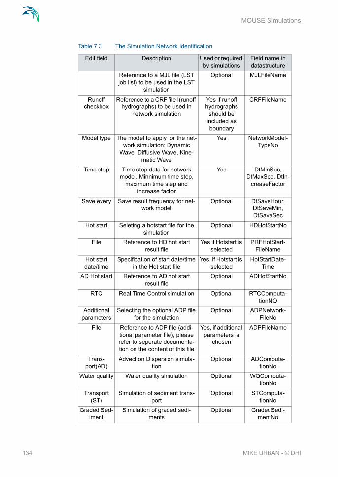
MOUSE Simulations
Reference to a MJL file (LST job list) to be used in the LST
simulation
Optional MJLFileName
Runoff checkbox
Reference to a CRF file I(runoff hydrographs) to be used in
network simulation
Yes if runoff hydrographs
should be included as boundary
CRFFileName
Model type The model to apply for the net-work simulation: Dynamic
Wave, Diffusive Wave, Kine-matic Wave
Yes NetworkModel-TypeNo
Time step Time step data for network model. Minnimum time step,
maximum time step and increase factor
Yes DtMinSec, DtMaxSec, DtIn-
creaseFactor
Save every Save result frequency for net-work model
Optional DtSaveHour, DtSaveMin, DtSaveSec
Hot start Seleting a hotstart file for the simulation
Optional HDHotStartNo
File Reference to HD hot start result file
Yes if Hotstart is selected
PRFHotStart-FileName
Hot start date/time
Specification of start date/time in the Hot start file
Yes, if Hotstart is selected
HotStartDate-Time
AD Hot start Reference to AD hot start result file
Optional ADHotStartNo
RTC Real Time Control simulation Optional RTCComputa-tionNO
Additional parameters
Selecting the optional ADP file for the simulation
Optional ADPNetwork-FileNo
File Reference to ADP file (addi-tional parameter file), please refer to seperate documenta-tion on the content of this file
Yes, if additional parameters is
chosen
ADPFileName
Trans-port(AD)
Advection Dispersion simula-tion
Optional ADComputa-tionNo
Water quality Water quality simulation Optional WQComputa-tionNo
Transport (ST)
Simulation of sediment trans-port
Optional STComputa-tionNo
Graded Sed-iment
Simulation of graded sedi-ments
Optional GradedSedi-mentNo
Table 7.3 The Simulation Network Identification
Edit field Description Used or required by simulations
Field name in datastructure
134 MIKE URBAN - © DHI

The Summary Simulation Settings
For the 2D overland parameters, please refer to separate chapter on this.
The additional parameter file (the ADP-file) is a separate file with additional settings for the simulation. Please refer to the seperate documentation on this file for further information.
7.4 The Summary Simulation Settings
On the Summary page you specify content of the summary after a MOUSE engine simulation. The MIKE 1D engine produces a different summary. The Summary page is organized into following groups:
Identification of simulation
Tables with min, max and accumulated values for
Summary of input data
Use selection to reduce summary tables
Standard Standard result file Optional StandardRe-sultNo
User-speci-fied
User specified result file Optional UserSpecifie-dResultNo
File Reference to result selection file
Yes, if User-specified is cho-
sen
RSFDataID
Overwrite Overwrite existing result file Optional NAllowOwer-writeNo
LTS Statis-tices
Calculation of LTS statistics Optional LTSStatisticsNo
2D Results Definition of 2D outputs Yes, if Network + 2D overland simulation is
chosen
-
Table 7.3 The Simulation Network Identification
Edit field Description Used or required by simulations
Field name in datastructure
135

MOUSE Simulations
Figure 7.7 The MOUSE Simulation Summary Editor Dialog
Table 7.4 The Simulation Summary identification
Edit field Description Used or required by simulations
Field name in datastructure
Simulation ID
ID of simulation - user speci-fied. ID will be reflected in the
name of project and result files
Yes MUID
Scenario ID ID of selected Scenario - Acti-vating scenario is done in the
Scenario Manager dialog
Yes ScenarioID
Nodes Tables with min, max and accumulated values will be included in the summary if
checkbox is true.
Optional Summa-ryNodeNo
136 MIKE URBAN - © DHI

The Summary Simulation Settings
Weirs & orfices
Tables with min, max and accumulated values will be included in the summary if
checkbox is true.
Optional Summary-WeirNo
Pumps Tables with min, max and accumulated values will be included in the summary if
checkbox is true.
Optional Summary-PumpNo
Links Tables with min, max and accumulated values will be included in the summary if
checkbox is true.
Optional SummaryLinkNo
Grid points, water levels
Tables with min, max and accumulated values will be included in the summary if
checkbox is true.
Optional SummaryLin-kLevelNo
Grid points, discharge
Tables with min, max and accumulated values will be included in the summary if
checkbox is true.
Optional SummaryLink-DischargeNo
Links, veloc-ity
Tables with min, max and accumulated values will be included in the summary if
checkbox is true.
Optional Summa-ryLinkVelocityNo
Summary of input data,
Links
Tables with min, max and accumulated values will be included in the summary if
checkbox is true.
Optional SummaryLinkIn-putNo
Node selec-tion file
checkbox
Tables with min, max and accumulated values will be included in the summary if
checkbox is true.
Optional NodeSelec-tionNo
Node selec-tion file
Tables with min, max and accumulated values will be included in the summary if
checkbox is true.
Yes, if NodeSe-lectionNo = True
NodeSelection-Name
Link selec-tion file
checkbox
Tables with min, max and accumulated values will be included in the summary if
checkbox is true.
Optional LinkSelectionNo
Link selec-tion file
Tables with min, max and accumulated values will be included in the summary if
checkbox is true.
Yes, if LinkSe-lectionNo = True
LinkSelection-Name
Table 7.4 The Simulation Summary identification
Edit field Description Used or required by simulations
Field name in datastructure
137

MOUSE Simulations
7.5 The 2D Overland Parameters
This tab page specifies the parameters used when setting up a combined pipe flow and overland flow simulation. Please refer to the chapter on 2D Overland Flow for more on these settings.
7.6 MOUSE Result Selections
It is possible to control the output from a MOUSE pipe flow simulation by defining a user specified result file. A user specified result file contains only the simulated time series according to the specification.
The definition of an user specified result selection contents is achieved through MIKE URBAN menu option "Simulation | MOUSE Result selec-tions…"
Figure 7.8 Network Result Selection Editor
By ticking the 'Save volume data' checkbox, data regarding mass balance in the system will be saved in the result file. If ticked, 'Save time step data' will save information about the used time steps in the simulation.
It is possible to save data in a time period that does not necessarily cover the whole period of the simulation. Make sure that the interval specified by 'start' and 'end' dates is at least partly covered by the simulation period. Saving fre-quency specified for the 'Reduced' result file is not dependent on the time interval chosen for the complete result file, if such a file has been specified.
Results can be saved from four categories; Nodes, Pipes, Weirs, Orifices and Pumps. Consequently, the result save specification is divided into four sepa-
138 MIKE URBAN - © DHI

MOUSE Result Selections
rate tables. By pressing the appropriate button a specific editor can be accessed.
It should be noted that if a set of nodes is selected, and the selection (from the horizontal plot or from the selection file) is loaded into the pumps or weirs list, only nodes where pumps or weirs do actually exist would turn up on the list.
In cases where several pumps or weirs are associated with one node, the results will be saved for all these pumps or weirs.
Presence of a certain item on the list is not sufficient for it to be included into the user specified result file. This is first ensured after a result type is chosen e.g. water level. In figure Figure 7.9 is displayed the Editor for ‘Nodes result selections’
Figure 7.9 Nodes Result Selection Editor
The 'Mark List' option helps clearing or checking all items on the displayed list. If a queried list is displayed, 'Mark List' will operate only on the currently displayed list. The remaining part of the list will retain earlier settings.
When a result selection file has been specified then it is activated in the ‘Run MOUSE | Network parameters’ editor by selecting the Selection ID in the ‘Results’group in the field labeled ‘Contents:’ - see Figure 7.10
139

MOUSE Simulations
Figure 7.10 Selection of ‘Selection_1’ - result selection file
140 MIKE URBAN - © DHI

Introduction
8 2D Overland Flow
8.1 Introduction
Surface flooding can be simulated with MIKE URBAN using the following two approaches:
1. Combined 1D and 2D model: The flow in the subsurface pipes is simu-lated using the MOUSE 1D engine and the overland flow is simulated using the MIKE 21 2D overland flow model. This combination of models is called MIKE FLOOD. The main input required for the 2D overland flow model is a digital elevation model. Based on this, the 2D model is capa-ble of simulating overland flow paths and velocities. The main advan-tages of using this approach are:
– Leads to more reliable and more accurate modelling– Requires less engineering judgement– Requires less engineering hours– Provides better result visualization
The main disadvantage of this approach is the longer simulation run times.
2. Two-layer 1D model: The flow in subsurface pipes as well as the over-land flow are both simulated using the MOUSE 1D engine in MIKE URBAN. This approach requires that the overland flow paths (streets, etc.) are known or estimated beforehand and each flow path is then defined as an open channel in MIKE URBAN. Flow exchange between the pipes and the overland channels is accounted for using MIKE URBAN model components, such as weirs, orifices or curb inlets. The engineering time and judgement required in order to predefine the over-land flow paths can be substantial, and this is one of the main disadvan-tages of this approach. It also adds uncertainties and inaccuracies to the modelling, as the model will only allow overland flow to take place along paths anticipated by the modeller. The main advantages of this approach is shorter simulation run times.
The remaining part of this chapter explains how to apply the combined 1D and 2D modelling approach.
8.2 Input Required - Overview
The main input required for combined 1D and 2D flow modelling is the follow-ing:
1. A working pipe flow model.
2. A digital elevation model (DEM). MIKE URBAN 2D currently accepts DEMs specified as raster data sets which have to be stored in ESRI Grid
141

2D Overland Flow
format or DEMs provided in the .dfs2 file format. The latter is the DHI file format for raster data sets.
3. A number of couplings between the 1D model and the 2D model. Such couplings are connections between the two models allowing for exchange of water between the two model domains. Couplings can, for example, represent manholes or curb inlets.
8.3 Input Required - Details
This section of the manual describes the details of the steps it takes to define a 2D overland flow model and to combine it with an existing 1D pipe flow model.
8.3.1 Choosing 2D model
Select MOUSE | 2D Overland Flow | 2D Model Settings ... to open the dialog shown in Figure 8.1.
The underlying 2D overland flow model, MIKE 21, offers the following differ-ent types of 2D model solvers:
1. Single Grid using a rectangular cell solver. The 2D model area is covered by square calculation cells.
2. Single Grid using a rectangular multi-cell solver. Again, the 2D model area is covered by a grid of square calculation cells. This is referred to as the coarse grid. Each coarse grid cell is further subdivided into N by N cells called the fine grid. N is an integer number - the ratio between the linear cell dimension of the coarse and the fine grid.
3. MIKE 21 Flood Screening Tool (FST) is designed for inland flooding applications. By means of FST the user can run 2D overland flood simu-lations faster than the regular MIKE 21 overland flow simulations. The Flood Screening Tool (FST) provides a simple hydrodynamic solver for computations regarding inland flooding, is based on MIKE 21 Flow Model but uses simpler equations with some parameters from MIKE 21 Flow Model being excluded. In FST solver the convective terms are omit-ted from the model, the viscous terms are omitted in the governing equa-tions, and the influence of wind, atmospheric pressure variation, Coriolis and wave radiation stresses cannot be included.
For further information on the pros and cons of each of the 2D solvers, please refer to the MIKE 21 documentation. For more information regarding the equations employed in MIKE 21 FST please consult MIKE 21 Flow Model & MIKE 21 Flood Screening Tool Hydrodynamic Module - Scientific Documen-tation.
142 MIKE URBAN - © DHI

Input Required - Details
Figure 8.1 Selection of DEM and 2D model area
Flood Screening Tool in MIKE URBAN
In MIKE URBAN the Flood Screening Tool is included in the 2D overland flow editor. In the editor it is possible to enable FST by selecting this module radio button in the "DEM and 2D model area" tab, see Figure 8.1.
Enabling MIKE 21 Flood Screening Tool automatically disable the Eddy Vis-cosity settings which are consequently greyed out in the "2D model settings", see Figure 8.2.
Some advantages of FST compared to MIKE URBAN Flood is that it allows to run faster simulations and requires less information than normal MIKE URBAN Flood simulations.
143

2D Overland Flow
Figure 8.2 2D model settings while selecting FST.
8.3.2 Adding the DEM to the map view
The DEM to be applied is loaded to the map view using the Insert Layer but-ton in the Layer Management toolbar or by choosing Insert Layer in Back-ground Layers within the TOC. Both these options will accept DEM raster data stored in ESRI Grid format or in DHI dfs2 format. Depending on your GIS installation other raster formats could be available.
8.3.3 Defining the 2D model domain and the resolution
The following steps should be followed:
1. Select the desired raster layer as the DEM to be applied in the model.
2. Enter the X- and Y-coordinates for the lower left hand and upper right hand corner of the rectangular area to be modelled with the 2D model. Instead of manually entering the coordinates the buttons ‘Digitize rectan-gle’, ‘Set as extent of data set’ or ‘Set as extent of raster’ can be used to
144 MIKE URBAN - © DHI
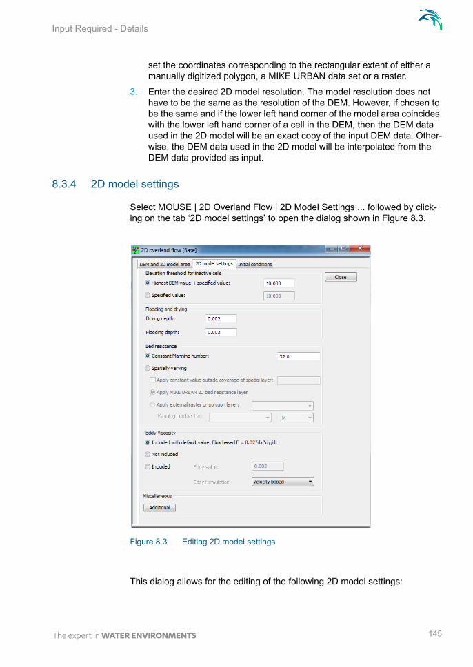
Input Required - Details
set the coordinates corresponding to the rectangular extent of either a manually digitized polygon, a MIKE URBAN data set or a raster.
3. Enter the desired 2D model resolution. The model resolution does not have to be the same as the resolution of the DEM. However, if chosen to be the same and if the lower left hand corner of the model area coincides with the lower left hand corner of a cell in the DEM, then the DEM data used in the 2D model will be an exact copy of the input DEM data. Other-wise, the DEM data used in the 2D model will be interpolated from the DEM data provided as input.
8.3.4 2D model settings
Select MOUSE | 2D Overland Flow | 2D Model Settings ... followed by click-ing on the tab ‘2D model settings’ to open the dialog shown in Figure 8.3.
Figure 8.3 Editing 2D model settings
This dialog allows for the editing of the following 2D model settings:
145

2D Overland Flow
Elevation threshold for inactive cells. The threshold value is applied for two purposes:
– The threshold value for inactive cells is the DEM elevation above which flooding is assumed not to take place. For overland flow simu-lations, the threshold value is often set equal to the highest DEM value within the model area. However, if significant parts of the DEM within the model area are at high elevations, which will never get flooded, a lower value can be specified for the threshold value. Any calculation cell in the 2D model area with an elevation higher than the threshold value will remain dry (called true land in MIKE 21 ter-minology) throughout the simulation.
– The first row/column of cells along the perimeter of the 2D model area DEM data will automatically be assigned the elevation thresh-old value as elevation. The only exception from this is where 2D boundaries are defined. See 8.3.9 for further details. The value will also be assigned to empty cells or areas of empty cells adjacent to the first row/column of cells along the perimeter.
Flooding and drying. For 2D overland flow simulations, flooding and drying is an important mechanism as it reduces the simulation runtime by not having to spend computational efforts on simulating flows in dry cells. The drying and flooding depths are used for deciding when to exclude and to reintroduce cells in the computations. The drying depth must be less than the flooding depth.
Bed resistance. The bed resistance coefficient in terms of the Manning (M) number (m1/3/s) can be specified as a constant value applied throughout the 2D model area or as spatially varying for which two options are available:
– Apply the MIKE URBAN 2D resistance layer: This is a polygon layer stored in the MIKE URBAN database. See 8.3.7 for further details on working with the 2D resistance layer in MIKE URBAN.
– Apply external raster or polygon layer: If data on spatially varying Manning number is available either as a raster layer or as a polygon layer then the raster/polygon can be referenced and used directly after inserting the data to the map view as a background layer.
In both cases a raster data set with the same extent and resolution as the 2D model will automatically be interpolated from the specified poly-gon or raster data. If these data do not cover the entire 2D model area MIKE URBAN will apply the specified constant value outside the cover-age if the option “Apply constant value outside the coverage of the spa-tial layer” is selected. If coverage is incomplete and the option is not selected an error message will appear at the time of starting the simu-lation.
146 MIKE URBAN - © DHI

Input Required - Details
Eddy viscosity. The eddy viscosity influences how eddies are simulated as a result of spatial velocity or flux gradients. Higher values of the eddy viscosity may also dampen numerical instabilities, and increasing the eddy viscosity is thus sometimes used as a method for stabilizing mod-els. The eddy viscosity can be specified in three ways:
– It can be included in terms of an automatically calculated, flux based value equal to 0.2.x.y/t, where x and y are the model cell size and t is the simulation time step.
– It can be excluded.– It can be included as a user defined value, using either a flux based
or velocity based equation. Miscellaneous. Read Section 8.3.9.
8.3.5 2D initial conditions
Select MOUSE | 2D Overland Flow | 2D Model Settings … followed by click-ing on the tab ‘Initial Conditions’ to open the dialog shown in Figure 8.4
Figure 8.4 Specification of initial conditions for the 2D model
The initial water level (water surface elevation) applied in the 2D model can be specified as a constant value applied throughout the 2D model area or as spatially varying for which two options are available:
147

2D Overland Flow
1. Apply the MIKE URBAN 2D initial conditions layer: This is a polygon layer stored in the MIKE URBAN database. See 8.3.6 for further details on working with the 2D initial conditions layer in MIKE URBAN.
2. Apply external raster or polygon layer: If data on spatially varying initial water level is available either as a raster layer or as a polygon layer then the raster/polygon can be referenced and used directly after inserting the data to the map view as a background layer.
In both cases a raster data set with the same extent and resolution as the 2D model will automatically be interpolated from the specified polygon or raster data. If these data do not cover the entire 2D model area MIKE URBAN will apply the specified constant value outside the coverage if the option “Apply constant value outside the coverage of the spatial layer” is selected. If cover-age is incomplete and the option is not selected an error message will appear at the time of starting the simulation.
The specified initial water level (spatially constant or varying) will only apply to 2D cells with a ground elevation less than the initial water level. 2D cells with higher ground elevation will initially be dry.
8.3.6 2D initial condition polygon layer
Spatially varying initial conditions for the 2D model are supported in two ways:
1. Using the polygons stored in the MIKE URBAN database and
2. Using external raster or polygon data.
The choice between these options is done in the Initial Conditions tab page on MOUSE | 2D Overland Flow | 2D Model Settings ... This section explains how to work with the 2D initial condition polygons stored in the MIKE URBAN database.
The form and grid view dialog for the table holding the polygons opens when choosing MOUSE | 2D Overland Flow | 2D Initial Conditions … as shown in Figure 8.5.
148 MIKE URBAN - © DHI

Input Required - Details
Figure 8.5 Form and grid view for 2D Initial Conditions dialog
Initial condition polygons typically apply to areas such as lakes, ponds or strips of coastal waters located within the 2D model and which each have a more or less horizontal water surface initially.
If an area is covered by two or more polygons a priority can be specified for each polygon. The polygon with the highest priority (lowest numerical value) will be used in the simulation. If the priority is unspecified the polygon will have the lowest priority.
Similar to catchment polygons the initial condition polygons can be inserted and edited graphically with the Feature Edit toolbar.
Table 8.1 shows a full overview of the editor fields:
Table 8.1 Editor fields in form and grid view for 2D Initial Conditions dialog
Edit field Description Used or required by simulation
Field name in data structure
2D Condition ID Name or ID of area No MUID
149

2D Overland Flow
8.3.7 2D bed resistance polygon layer
Spatially varying bed resistance for the 2D model are supported in two ways:
1. Using the polygons stored in the MIKE URBAN database and
2. using external raster or polygon data.
The choice between these options is done in the 2D Model Settings tab page on MOUSE | 2D Overland Flow | 2D Model Settings ... This section explains how to work with the 2D bed resistance polygons stored in the MIKE URBAN database.
The form and grid view dialog for the table holding the polygons opens when choosing MOUSE | 2D Overland Flow | 2D Bed Resistance … as shown in Figure 8.6.
Initial Water Level Initial 2D water level in the poly-gon area
Yes InitialWaterLevel
Priority if overlap Used to prioritise between polygons with an overlap-ping area. Low numerical value represents high priority.
Yes Priority
Table 8.1 Editor fields in form and grid view for 2D Initial Conditions dialog
Edit field Description Used or required by simulation
Field name in data structure
150 MIKE URBAN - © DHI

Input Required - Details
Figure 8.6 Form and grid view for 2D Bed Resistance dialog
Bed resistance polygons are applied to represent land use or other ground surface classification with a strong relation to bed resistance. The polygon table is typically populated by importing land use polygons for instance from a number of Shape files each holding multiple polygons with the same land use. The description field in the table can be used to store the land use and thereby, with the selection and field calculator tools, ease bulk changes of the bed resistance for all polygons of the same land use.
If an area is covered by two or more polygons a priority can be specified for each polygon. The polygon with the highest priority (lowest numerical value) will be used in the simulation. If the priority is unspecified the polygon will have the lowest priority.
Similar to catchment polygons the bed resistance polygons can be inserted and edited graphically with the Feature Edit toolbar.
Table 8.2 shows a full overview of the editor fields:
151

2D Overland Flow
8.3.8 2D boundaries
By default the 2D model has a closed boundary and water will not enter or leave the 2D model area across the perimeter of the 2D model areas. How-ever, it is possible to define the following types of 2D boundaries:
Rain: This applies in cases where rainfall should enter each 2D compu-tational cell at each time step. Both constant rain and rain with spatial and temporal variation are supported. Rain directly on 2D cells is used as an alternative to using one of the rainfall-runoff models in MIKE URBAN.
Water level: This applies to a stretch of the perimeter of the 2D model area and is typically applied where the 2D model perimeter crosses a larger water body such as a lake or the sea where the water level is known (constant or time varying). However, a water level boundary can also be applied as a free outlet allowing water to leave the 2D model area rather than backing up against the closed boundary.
Discharge: This applies to a stretch of the perimeter of the 2D model area and is typically applied where the 2D model perimeter crosses a river or similar where the discharge is known (constant or time varying).
Table 8.2 Editor fields in form and grid view for 2D Bed Resistance dialog
Edit field Description Used or required by simulation
Field name in data structure
Bed Resistance ID Name or ID of area No MUID
Manning number Manning number applied as bed resistance within the polygon
Yes ManningNO
Priority if overlap Used to prioritise between polygons with an overlap-ping area. Low numerical value represents high priority.
Yes Priority
Description Description, land use or other classi-fication of the ground surface within the polygon
No Description
152 MIKE URBAN - © DHI

Input Required - Details
Boundaries for the 2D model is defined with the form and grid view which opens when selecting MOUSE | 2D Overland Flow | 2D Boundaries ... , see Figure 8.7.
Figure 8.7 Form and grid view for 2D boundaries dialog. The arrow points to the graphical line showing the location of the boundary
There are three primary choices to make for each boundary:
1. Type: Choose between rain, water level and discharge
2. Location: This only applies for water level and discharge boundaries. The location of the boundary is defined by the x- and y-coordinate of the start and end point. The coordinates can either be typed in or defined by pointing and clicking at the start and end locations in the map view. The latter is done with the arrow-button shown to the right of the x-y edit fields. When clicking one of the arrow-buttons the 2D boundary dialog will disappear and the user is supposed to point and click at the intended start or end location (and the dialog will then reappear). MIKE URBAN will automatically snap to the nearest corner of a 2D cell along the perim-eter of the 2D model, and the x- and y-coordinate of the snapped point will appear in the disabled X and Y edit fields named “Boundary end
153

2D Overland Flow
points”. If the user manually types in the coordinates then snapping will occur when choosing Advanced | Recompute, when the boundary is shown on the map or when a simulation is run. The location of 2D bound-aries can be visualized in the map view by means of a red line between the snapped boundary end points. See Figure 8.7.
3. Value: The value of the boundary condition can be defined as constant or time varying with a .dfs0 file. Rain boundaries can additionally have a spatial variation in which case the data has to be provided in a .dfs2 file.
The discharge boundary is to be specified with positive numbers for flow in the same direction as the X and Y axis. This means that flow into the model area on the northern and eastern boundaries has to be specified as a nega-tive number.
It should further be noted that 2D boundary files (dfs0 and dfs2) should be specified as floats and with an equidistant calendar axis see Chapter 4 ‘Time Series’ for configuration. For a rainfall boundary the item type should be set to “Rainfall rate” and must only include one item in the file. For a spatially var-ying rain specified with a dfs2 file the file must have the same number of cells and cell size as the DEM.
Table 8.3 Editor fields in form and grid view for 2D Boundaries dialog
Edit field Description Used or required by simulation
Field name in data structure
2D Boundary ID Name or ID of boundary
No MUID
User defined end points
X- and Y- coordi-nate of the user defined start and end point of the boundary.
Does not apply for rainfall.
No BCStartX
BCStartY
BCEndX
BCEndY
Boundary end points
X- and Y- coordi-nate of the snapped start and end point of the boundary.
Does not apply for rainfall.
Yes BCStartX_C
BCStartY_C
BCEndX_C
BCEndY_C
Temporal variation Choice of constant or temporal varia-tion of boundary data.
Yes VariationNo
154 MIKE URBAN - © DHI

Input Required - Details
8.3.9 Automatic model adjustments along water level and discharge boundaries
Adjustment of DEM
Along the 2D model perimeter the ground elevation in the first row/column of 2D cells is automatically raised to a high elevation (elevation threshold for active cells) to ensure zero flow across the perimeter. However, this does not apply along stretches where a 2D water level or discharge boundary is defined. Instead, the ground elevation is lowered automatically to ensure suit-able numerics of the simulation at the boundary, because a boundary must be wet all the time. By default the lowering is 0.5 meter and it applies to the first two rows/columns parallel to the 2D boundary. All 2D cells are lowered to the same value which equals the lowering value subtracted from the lowest cell in the first non-adjusted row/column (by default the 3rd) along the 2D boundary. The lowering and the width of the indentation can be adjusted by clicking the “Additional” button in MOUSE | 2D Overland Flow | 2D Model Set-tings ... Figure 8.8 shows an example of how the DEM is adjusted along a boundary.
Source type Choice of spatially constant or varying boundary data.
Yes BridgeTypeNo
Path Name and path of file with boundary data.
Yes TSConnection
Time series ID Name of selected item in boundary data file.
Yes TimeSeriesName
Data type Type of selected item in boundary data file.
Yes DataTypeName
Table 8.3 Editor fields in form and grid view for 2D Boundaries dialog
Edit field Description Used or required by simulation
Field name in data structure
155

2D Overland Flow
Figure 8.8 Example of automatic DEM adjustment along an open 2D boundary spanning 10 2D cells. In each 2D cell the original DEM (upper) and adjusted DEM (lower) is shown
Adjustment of initial conditions
The lowered indentation explained above must be wet initially and MIKE URBAN ensures that by automatically adjusting the initial conditions such that the indentation is initially filled with water. This requires a spatially vary-ing initial condition which is automatically generated by MIKE URBAN. Hence, although a constant initial water level is selected in MOUSE | 2D Overland Flow | 2D Model Settings ... then the 2D initial conditions that are actually applied will be spatially varying if there any open boundaries are defined. The user specified value will still be applied for the entire model area where an adjustment of the DEM has not occurred.
8.3.10 Defining couplings
Defining the couplings between the pipe flow model and the 2D overland flow model involves the following steps:
1. Selection of the pipe flow components to be coupled. These are typically mostly manholes, but it is also possible to establish couplings for basins, weirs, pumps and outlets.
2. Selection of the specific calculation cells in the 2D overland flow model, which the selected pipe flow model components should be coupled to. This selection of 2D cells is done automatically based on number of cells or a search radius (see coupling parameters below for details).
3. For manholes and basins a flow formula is applied for calculating the exchange of flow between the pipe flow model and the overland flow model. The preferred flow formula and the associated parameters have to be selected.
156 MIKE URBAN - © DHI

Input Required - Details
Figure 8.9 Sub-menu for 2D Overland Land Tools
The following set of tools found in the sub-menu MOUSE|2D Overland Tools (see Figure 8.9) are available for defining the couplings:
Coupling parametersSelecting this will open the dialog shown in Figure 8.10.
When coupling a pipe model node to the 2D model, a coupling area covering the spatial extent of the 2D cells involved in the coupling has to be defined. The coupling area will automatically be defined by the tool "Couple nodes". The selection in this dialog defines how many 2D model cells the coupling area will span. There are two choices. 1) Either a squared coupling area with the width/height as the specified number of cells. 2) A coupling area defined by all 2D cells within the specified search radius from the node in question. If no 2D cells will have a cell centre within the specified coupling area, then the 2D cell containing the node in question will be selected as the coupling area.
157

2D Overland Flow
Figure 8.10 Dialog for parameters for the 2D overland flow tools
Couple nodesThis tool applies to manholes, basins and outlets that are not already coupled. If any nodes are selected the tool will apply only to those selected nodes - otherwise to all. Once a node is coupled the following will happen:
– The node will be marked as coupled and it will show-up as such in the tab ‘2D Overland’ in the dialog MOUSE|Nodes.
– A coupling area polygon will be defined and an entry will be added to the table ‘Coupled 2D Areas’. If selected for drawing the coupling area will show up in the map view.
– A line between the node and the centre of the coupling area will be defined and an entry will be added to the table ‘Coupled 2D Connec-tions’. If selected for drawing the connection line will show up in the map view.
Figure 8.11 shows an example of three nodes which have been cou-pled to respectively a single 2D cell, to 3x3 2D cells and to the 2D cells within a circular search radius.
Once a coupling area has been defined automatically, its shape and location can be manually edited using the tools in the Feature Edit tool-bar.
158 MIKE URBAN - © DHI

Input Required - Details
Figure 8.11 Nodes coupled to varying numbers of 2D cells
Un-coupled nodesIf any coupled nodes are selected this tool will apply only to those - oth-erwise to all coupled nodes. The tool will un-couple nodes by taking the following actions:
– The node will be marked as un-coupled and show-up as such in the tab ‘2D Overland’ in the dialog MOUSE|Nodes.
– The associated coupling area polygon will be deleted.– The associated coupling connection will be deleted.
Show coupled 2D cellsThis tool will select all coupling area polygons in the table “Coupled 2D Areas”. If any nodes are selected, the tool will only select the coupling area polygons associated to the selected nodes.
Show all coupled nodesThis tool will select all coupled nodes.
Show ground level and DEM differencesIf any coupled nodes are selected, this tool will apply only to those - oth-erwise to all coupled nodes. This tool will calculate the difference between the ground level in each node and the elevation in the raster layer selected as the DEM. The differences will be added to the map view as a point layer.
Show MIKE 21 j,kMostly there is no reason to be concerned about the so-called j and k coordinates in MIKE 21. These are the horizontal and vertical indices of the 2D cells in the MIKE 21 model grid. The cell in the lower left hand corner of the 2D model area is defined as (j,k)=(0,0).
After clicking this menu item, the MIKE 21 j,k coordinates at the posi-tion of the cursor, when pointing in the map view, will appear in the sta-tus bar alongside with the X,Y coordinates and the map scale. See Figure 8.12.
159

2D Overland Flow
Figure 8.12 Showing MIKE 21 j,k coordinates in status bar
Zoom to MIKE 21 j,kThis tool will prompt the user for a j,k coordinate set and subsequently the map view will zoom to the specified location with a zoom level such that approximately 10x10 2D cells are visible.
8.3.11 Flow parameters at manholes and basins
Urban sewer network models can be coupled to MIKE 21 two dimensional models to simulate urban flood patterns in MIKE FLOOD, the unidimensional model can now be simulated using the MIKE 1D engine whilst the 2D model can be run using the MIKE 21 engine.
Once a manhole or basin has been coupled, the node attribute ‘Coupling to 2D Overland’ will be selected. See Figure 8.13. On this tab the user can set various parameters for how the exchange flow between the pipe flow model and the overland flow model is calculated. For more information, please refer to MIKE FLOOD User Manual.
160 MIKE URBAN - © DHI

Input Required - Details
Figure 8.13 2D Overland flow tab in the nodes dialog
Max flowThis parameters gives an upper limit to the discharge that can flow through the link. If the discharge calculated from the flow equation exceeds this value, then the discharge is reduced to this value.
Qdh factorA parameter indicating the water level at which the calculated discharge should be surpressed. May be used for stabilizing setups where the instability is caused by a small difference in the water level in the two coupled models. The suppression is calculated as the water level differ-ence divided by the Qdh factor to the power of 2.
161

2D Overland Flow
Calculation method
The exchange flow between the 1D and 2D models may be calculated using 4 different methods:
– Orifice equation: The flow is governed by a standard orifice equa-tion.
– Weir equation: The flow is described through a weir equation.– Exponential function: The flow is governed by a simple exponential
function.– Curb Inlet: The flow between MIKE URBAN and MIKE 21 is trans-
ferred at a grate or inlet from a surface overland flow network to the sub-surface pipe network. The transfer capacity of the connection is specified as a DQ-relation (tabular data type). When water is transferred to the surface from the sewer pipe net-work the flow is calculated with the orifice equation
Depending on the calculation method used, additional information is required.
Inlet areaThe inlet area is only used when applying the orifice equation for describ-ing the flow exchange between the 1D model and the 2D model. The greater the cross sectional area the greater the conveyance capacity of the coupling. This parameter corresponds physically to the area of the manhole cover. For a manhole the inlet area used in the calculation will be the smallest value of the specified inlet area and the inlet area calcu-lated from the manhole diameter. For a basin the specified inlet area will always be used.
Orifice coefficientThe orifice coefficient is a non-dimensional factor that may be used to scale the orifice flow.
Crest widthThe crest width is used when the flow exchange is described through a weir equation. The weir crest should typically be the circumference of the manhole cover.
Scaling factorThis factor is only applicable if the simple exponential expression is used to describe the flow exchange. The scaling factor has a linear effect on the discharge. Thus, an increase in this value will generate a larger flow for a certain water level difference between the 1D and 2D model.
ExponentOnly applicable if the simple exponential expression is used to describe the flow exchange. An increase in the exponent factor has a strong impact on the discharge. An increase in this value will generate a larger flow for a specific water level difference between the 1D and 2D model.
162 MIKE URBAN - © DHI

Input Required - Details
FreeboardThe freeboard (see Figure 8.14) defines a critical water level (Invert level- Freeboard) at the connection node in the pipe network below which the defined DQ relation apply. For submerged and reverse flow (surcharge), the transfer capacity of the connection reverts to a standard orifice relationship.
Figure 8.14 Freeboard detail in a Curb Inlet
The freeboard describes the distance (depth) from the Grade Invert Level to the Critical Water Level (i.e. Freeboard = Grade Invert Level - Critical Water Level). The Critical Water Level is the level above which the basin is consid-ered to be 'drowned' such that the DQ relationship for transferring water from the surface to the node no longer applies. For submerged and reverse flow conditions the exchange of water across the coupling reverts to a standard orifice equation.
Capacity curve DQ RelationThe DQ relation specifies the depth based capacity curve for the curb inlet. Values must be monotonously increasing in depth and discharge starting at (0,0). For depths in excess of the maximum value specified in the last row of the table, the last corresponding discharge is used. Posi-tive discharge is considered flow from MIKE 21 into MIKE URBAN (over-land to sewer network).
163

2D Overland Flow
8.3.12 Outlets
An outlet coupled to the 2D overland flow model does not require other parameters than the definition of the coupling area itself. The average water levels in the 2D cells to which the coupling is made will then be applied as a water level boundary. The same algorithm will apply as when a water level boundary is specified in an outlet in the pipe flow model. This will result in an outflow through the outlet (positive or negative) which will correspondingly apply as a point inflow (positive or negative) distributed to the 2D cells in the coupling area. For more information, please refer to MIKE FLOOD User Man-ual.
8.3.13 Pumps and weirs
A pump or a weir can be coupled to the 2D model if the To-node is not defined. When coupled to the 2D model, the weir/pump discharge will be added to the 2D model as a point inflow distributed to the 2D cells in the cou-pling area. The pump/weir discharge will always be independent of the water level in the 2D model and the flow direction in weir/pump couplings will always be from pipe flow model to 2D model. For more information, please refer to MIKE FLOOD User Manual.
8.4 Running the Combined 1D and 2D Simulations
8.4.1 Setting the simulation type and requesting 2D results
To run the combined pipe flow and overland flow simulation three issues needs to be addressed in the simulation dialog as shown in Figure 8.15. Firstly, the simulation type needs to be "Network + 2D overland". Secondly, the time step in the 2D model and the request for output from the 2D model have to be defined in the dialog "2D Overland Results" as shown in Figure 8.16. This dialog can be opened from the "2D Results" button located in the "Network parameters" tab.
164 MIKE URBAN - © DHI

Running the Combined 1D and 2D Simulations
Figure 8.15 2D Overland flow options in the computation dialog
165

2D Overland Flow
Figure 8.16 Selection of time step and request for output in 2D model
In the tab ‘2D Overland Results’ the 2D time step is specified. The request for output is specified as a single 2D output file with maximum flood depth and in the table below, a number of output files with the flood depth at multiple time steps through the simulation. For the latter the following has to be specified for each requested result file:
166 MIKE URBAN - © DHI

Running the Combined 1D and 2D Simulations
Table 8.4 Specifying the content for the result files
Item name Explanation
Type The choice between the following output files both containing multiple time steps:
Flood maps: A 2D output file in .dfs2 raster format.
Time series: A time series output file in .dfs0 format.
Model area This is only enabled for flood map output files. The user can choose be-tween:
Model area: The output file will then cover the full 2D model area.
Selected area: The output file will then cover only a sub-region of the full 2D model area. The sub-region is a rectan-gle defined by the following two set of X,Y coordinates:
X0, Y0
X1, Y1
Type = Flood Maps: Only enabled if the model area is cho-sen as selected area. The lower left and upper right corners of the sub-region from which 2D output will be generated is defined by the two coordinate sets (X0, Y0) and (X1, Y1)
Type = Time series: Results are saved from the location (X0, Y0). (X1, Y1) is not used and thus disabled.
Period Two choices are available:
Simulation period: Output will be saved for the entire simula-tion period
Used defined; User wants output to be saved for a period shorter than the simulation period. The period is specified in the following two items
Start
End
Only enabled if the Period is selected as User Defined. Start and End is the date and time for desired period for saving results
NoSteps An integer value specifying the number of time steps at which results are saved
FileName Name of the result file to be saved. The file name cannot be changed by the user.
Title User specified title which is saved as header information in the result file
Depth, Level, Velocity & Flux
Option for saving water depth, level (water surface eleva-tion), velocity and flux (P, Q) respectively
167

2D Overland Flow
The standard MIKE 21 results (H,P,Q) will be generated when Depth and Flux are chosen. If you would like more information on the result type flux (P and Q), you can check the MIKE 21 documentation.
8.4.2 Starting simulation
After pushing the button Start Simulation in the dialog shown in Figure 8.15 MIKE URBAN data will be exported as for a regular MOUSE simulation. Fol-lowing that export, the MIKE FLOOD simulation progress window shown in Figure 8.17 will appear.
Figure 8.17 Simulation progress window for MIKE FLOOD
8.5 Visualising Simulation Results
The result files generated by the 2D overland flow simulations are time series saved in .dfs0 files and raster data saved in .dfs2 files with water depth or velocities. 2D results in time series files are shown as any other time series file. This section explains how to visualize results in .dfs2 files.
The .dfs2 raster files may contain a single time step or multiple time steps. The former is the case for files containing the maximum flood extend. Such should be added as a raster layer to the map view using the Insert Layer but-ton in the Layer Management toolbar. Dfs2 files with multiple time steps are visualized as explained in the following.
In the main menu bar, choose Model Result > Load Results > Overland Results in order to select the 2D overland result file. This will add information about the file content to the MIKE URBAN session, but as .dfs2 files are potentially very large the data from the individual time steps are not loaded to memory. Thus, nothing will be added to the TOC or the map view when a
168 MIKE URBAN - © DHI

Visualising Simulation Results
.dfs2 files is selected. There are three ways to subsequently visualize the content of a .dfs2 file:
1. As a raster layer in the map view. To do so, select Model Results > Add Results Layer. Subsequently, select the desired.dfs2 file and data type which then will be added to the TOC and map view. The map view will show data from the time step selected with the Animation toolbar. See Figure 8.18.
2. As a time series plot extracted at a particular location. To do so, in the Simulation toolbar click on the Time Series button and then select the desired .dfs2 file and data type. Subsequently, move the cursor to the location in the map view from where a time series should be extracted from the .dfs2 file. See Figure 8.18.
3. As a water surface elevation line in a longitudinal profile view. To do so, firstly a longitudinal profile view should be opened. In here right-click and choose Properties. In the Properties dialog the Raster tab allows for add-ing raster data to the profile view. See Figure 8.19.
Figure 8.18 2D flood results shown as raster data and time series
169
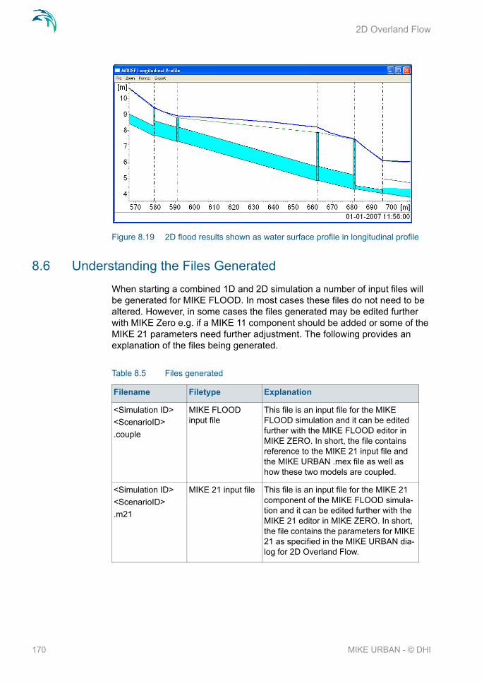
2D Overland Flow
Figure 8.19 2D flood results shown as water surface profile in longitudinal profile
8.6 Understanding the Files Generated
When starting a combined 1D and 2D simulation a number of input files will be generated for MIKE FLOOD. In most cases these files do not need to be altered. However, in some cases the files generated may be edited further with MIKE Zero e.g. if a MIKE 11 component should be added or some of the MIKE 21 parameters need further adjustment. The following provides an explanation of the files being generated.
Table 8.5 Files generated
Filename Filetype Explanation
<Simulation ID>
<ScenarioID>
.couple
MIKE FLOOD input file
This file is an input file for the MIKE FLOOD simulation and it can be edited further with the MIKE FLOOD editor in MIKE ZERO. In short, the file contains reference to the MIKE 21 input file and the MIKE URBAN .mex file as well as how these two models are coupled.
<Simulation ID>
<ScenarioID>
.m21
MIKE 21 input file This file is an input file for the MIKE 21 component of the MIKE FLOOD simula-tion and it can be edited further with the MIKE 21 editor in MIKE ZERO. In short, the file contains the parameters for MIKE 21 as specified in the MIKE URBAN dia-log for 2D Overland Flow.
170 MIKE URBAN - © DHI

Understanding the Files Generated
<Simulation ID>
<ScenarioID>
Coarse
.dfs2
Raster file in dfs2 format
This file contains the DEM data for the 2D model area selected. Data in the file is extracted from the original DEM speci-fied in MIKE URBAN at the requested model resolution.
<Simulation ID>
<ScenarioID>
Fine
.dfs2
Raster file in dfs2 format
This file contains the DEM data for the 2D model area selected. This file is only generated if the Multi Cell 2D model has been chosen. Data in the file is extracted from the original DEM specified in MIKE URBAN at the requested model resolu-tion divided by the fine/coarse ratio.
<Simulation ID>
<Scenario ID>
InitialCondi-tions.dfs2
Raster file in dfs2 format
This file contains spatially varying 2D ini-tial conditions.
<Simulation ID>
<Scenario ID>
Bed_Resist.dfs2
Raster file in dfs2 format
This file contains spatially varying 2D bed resistance
Table 8.5 Files generated
Filename Filetype Explanation
171

2D Overland Flow
172 MIKE URBAN - © DHI

RTC in Urban Drainage and Sewer Systems
9 MOUSE Control module
The MOUSE Control module features advanced Real-Time Control (RTC) simulation capabilities for urban drainage and sewer systems. It permits description of various controllable devices and makes the definition of com-plex operational logic for interdependent regulators fully transparent and time efficient. The following controllable devices can be specified:
Pump
Weir
Orifice with gate
Orifice with weir
Valve
The devices may be specified as settings or PID-controlled, with control function selection based on a global system analysis. Each regulator or pump operates under the control logic encapsulated into a set of simple logical rules and control functions. The system allows a schematised definition of any form and size of decision tree, featuring logical operators AND, OR, NOT and NOR, in any combination.
The process of selecting an appropriate control function under the current operational situations relies on the evaluation of system state conditions including measurable and derived hydraulic and WQ variables (e.g. water level, flow, pollutant concentration, level difference), device status (e.g. gate blade position, pump ON/OFF) and the current control function.
The control functions range from the simplest constants for the operational variables (e.g. constant weir crest setting or constant flow set-point) to dynamic controlled variables, set in a continuous functional relation with any of the measurable variables in the system (e.g. CSO discharge set-point as a function of flow concentration or a pump START/STOP levels as functions of water level at strategic location in the system).
9.1 RTC in Urban Drainage and Sewer Systems
Real time control (RTC) is an active control and operation of flow regulators based on real-time information about the system state.
RTC is feasible where it proves that flexible redistribution of water in space and time contributes to the fulfilment of the specified operational objectives, based on economically and technically sound solutions. Accordingly, applica-tion of RTC to urban drainage and sewer systems may be relevant:
where the system has substantial transport, storage or treatment capac-ity which is not effectively used under passive system operation;
173

MOUSE Control module
where typical rainfall patterns over the catchment area exhibit high degrees of spatial variability resulting in some parts of the system becoming overloaded whilst others are under utilised;
where the urban wastewater system includes treatment processes whose performance is amenable to active, short term control;
where the assimilative capacity of the receiving waters is variable over time.
Usually, RTC is implemented as an integral part of a rehabilitation/upgrade scheme also involving significant civil upgrading works to increase the trans-port, treatment or assimilative capacity of the urban wastewater system. In such circumstances, the role of RTC is to optimise the operation of both the new and the existing facilities, thereby maximising the benefit in performance terms. Where the overall objective is to achieve compliance with specified performance targets, RTC serves to minimise the scale and extent of the nec-essary works.
9.2 Architecture of RTC Systems
An RTC system includes monitors/sensors, which generate measurement values characterising states of the system. To be useful for RTC, the meas-urements must be available with the relatively insignificant time lag (delay). The sensors must be accurate and reliable.
The active control is performed by regulators - controllable movable devices (weirs, gates and valves) and pumps. Regulators may take various forms and sizes, and the regulation may be continuous within the functional range, step-wise, or discontinuous (e.g. ON/OFF, OPEN/CLOSED). The regulators may be powered mechanically, hydraulically or pneumatically.
Controllers on the basis of a pre-programmed operational strategy determine the regulator movements (the control actions). The operational strategy may consist of two parts: the control action(s) and, if more control actions are specified, the control logic (conditions), responsible for the selection of an appropriate control action. A control action establishes a relation between a control variable and a controlled variable. A controlled variable can be a regulator setting (e.g. gate position, pump START/STOP level) or some of the flow variables (e.g. water level, flow).
In the latter case, the control decisions are derived by evaluating (comparing) the current value of the controlled flow variable and the pre-defined set-point value. The control algorithm is based on the numerical solution of the “contin-uous control problem” equation and is usually termed as PID (Proportional-Integral-Differential) control. The actuation signal for the regulator is gener-ated by a PID controller, which usually appears as part of the operational strategy programmed in a Programmable Logical Controller (PLC).
174 MIKE URBAN - © DHI

Architecture of RTC Systems
Selection of a controlled variable is, however, subject to limits set by the vari-able’s “controllability”. Therefore, a controlled variable is usually selected among the flow variables (flow, water level), preferably in the vicinity of the regulator. As a controlled variable becomes more distant from the regulator, it becomes more difficult to control, due to time lags, diffusion and uncontrolla-ble interference. Control of relatively distant controlled variables is difficult and often cannot give satisfactory results.
When a regulator setting is used as a controlled variable, the control algo-rithm is reduced to an explicit functional relation between the control variable and the regulator setting, which controls the system response indirectly. This is much simpler than PID control, but in turn, the control results are in many cases inherently inexact and only a rough flow control can be achieved. This type of control is most suitable for regulators of the ON/OFF (or OPEN/CLOSE) type, while the application to continuously controllable regu-lators should be carefully considered.
If the operational strategy is based on conditions local to the regulated device (for example the ON/OFF-control of a pump based on the water level in a wet well) it is called local control. A PLC receives signals (measurements) from local sensors and sends the control decisions (actuation signals) to the regu-lators. The usual situation for a sewer system is to have a number of local controllers associated with pumps.
If the operational logic is based on global conditions, it is then called global control. In such a situation, a global controller is required. A global control-ler is a computer program that makes the overall system state analysis in real time and provides additional input to the local controllers, which overrides or supplements the local logic with e.g. actuator signals, or by modified set-point values.
Additional component needed is then a data transmission system (UHF radio, leased or dialled telephone lines, GSM, etc.) to transfer data between sensors, controllers and the global controller. In connection with the global controller function, an RTC system is usually equipped with the data man-agement and storage facilities (data bases) and the user interface. This is usually termed as SCADA (Supervisory Control And Data Acquisition) sys-tem.
The global control can be extended also to include forecast data in addition to real-time data, which is then called predictive RTC. The most comprehen-sive way to obtain forecast data is to include a model in the control system. Predictive control brings additional benefits in relatively inert systems, i.e. where the response time of an operational variable is long compared to the change of relevant disturbance (external input or control action).
175

MOUSE Control module
9.3 MOUSE Control vs. Real Life
MOUSE RTC simulates reactive local and global RTC systems in urban drainage and sewer networks. The software implementation is inherently a conceptualisation of real life, of which the user must be fully aware. Some conceptualisations applied in MOUSE RTC are listed below.
The program does not distinguish explicitly between local and global RTC. Per default, all elements of a modelled RTC system are assumed available for global control.
Sensors are specified as operational devices with definition of sensor type and position in the MOUSE network. Sensors with multiple function-ality must be specified individually.
When devices (weirs, gates and pumps) are specified as controllable in the MOUSE interface, a number of additional physical parameters about the behaviour of the structure is required to describe e.g. the allowed change rates for the state of the structure.
The actual controllers are not specified explicitly as physical devices, but their function (i.e. operational logic as a combination of operational con-ditions and control actions) is associated with the respective devices.
MOUSE RTC uses sampling and actuation (control loop) frequency iden-tical to the simulation time step.
Sensor readings are simulated as perfectly accurate and with 100% availability.
Low-level logic of the pump START/STOP operation is built into the pro-gram and is controlled by the START and STOP levels.
The PID control algorithm is built into the program and is controlled by the PID constants and by factors for weighting the terms of the numerical solution of the control equation.
9.4 Sensors
A sensor is a physical device positioned somewhere in the system, which provides information of the actual value of a monitored variable. A sensor can only monitor one variable – if more variables are measured at the same local-ity a corresponding number of sensors has to be described.
176 MIKE URBAN - © DHI

Logical Conditions
Figure 9.1 The sensor dialog
Sensor IDEach sensor needs a unique ID, which can be used to access the sensor information from other dialogs.
TypeThe type of the sensor defines which variable the sensor measures.
Location Type and LocationDepending on the sensor type, there could be one or more location types. Accordingly, the actual location can be specified be selecting from the com-prehensive list.
ComponentFor the "Concentration" sensor type, a measured WQ component must be specified.
9.5 Logical Conditions
A logical condition stands as a frame which demarcates the boundaries of a certain operational situation in the controlled system. This frame consists of an arbitrary number of independent logical tests on the various operational variables, where the relation of the actual value (or state) of the variable (pro-vided by a sensor) is tested against the specified threshold (limit) value (or state). The individual tests are evaluated as “TRUE” or “FALSE”, with the out-come depending on the actual variable value (or state), the threshold and the specified operator.
177

MOUSE Control module
A logical condition is evaluated as "TRUE", only if all of its constitutive tests are evaluated as "TRUE". If only one of the tests is "FALSE", the logical con-dition is rejected.
Figure 9.2 Conditions Editor
Condition IDEach Logical Condition needs a unique ID, which can be used to access the logical condition information from other dialogs.
For each of the tests included in a logical condition the following should be specified.
Type and IDThe type and identification of the variable which should be evaluated. Depending on the type, it might be necessary with two IDs –e.g. for the eval-uation of difference between two sensor values.
For the type "Diff of 2 Sensor Values" the sensors specified under ID1 and ID2 must be of the same type and sensors measuring either level, discharge or concentration.
For the type "Sum of 2 Sensor Values" the sensors specified under ID1 and ID2 must both be sensors measuring discharge.
For the type "Change In Sensor Value" the sensor specified under ID1 must be a sensor measuring level. The threshold will correspond to a speed of change (dH/dt).
For the type "Accumulated Value" the sensor specified under ID1 must be a sensor measuring mass flux.
178 MIKE URBAN - © DHI

Control Actions
Operator and LimitThis part of a test defines the condition which must be fulfilled for the test to be evaluated as "TRUE". In cases with the tested continuous variables, it consists of an algebraic operator (< or >) and a limit value. In cases of logical evaluation (e.g. pump ON/OFF), the test is defined simply by setting the desired device state as "TRUE" or "FALSE"
9.6 Control Actions
A control action is a functional relation between input from one or two sensors and the set-point or the setting for the controlled device.
Figure 9.3 Control Actions Editor
Action IDEach control action needs a unique ID, which can be used to access the actions from other dialogs.
For each of the actions the following should be specified.
Device Type and Action TypeThese two fields hold the information about the applicability of the action (device type) and which type of control it describes. The devices which can be controlled are pumps weirs and gates, and each of these types can be controlled directly or by a PID control.
179

MOUSE Control module
If a direct control is used, the action specifies information of START- and STOP levels for pumps, or of the wanted position for gates or weirs. If a PID-control is applied, the action specifies a set-point (flow or level) anywhere in the system.
Setpoint SensorFor actions of PID-type, it must be specified where in the system the set-point is located. For this purpose a Sensor ID must be specified.
Input Type and Input SensorThe type and identification of the parameter which should be evaluated. Depending on the type it might be necessary with two sensor IDs –e.g. if the flow is regulated as a function of the difference between two level sensor val-ues. If the "Constant" type is selected, a constant value is specified, instead of the sensor(s) and the action.
Input and Output ValuesThe functional relation between the actual input value (sensor reading or a combination of two sensors) and the set-point value (or setting). The tabu-lated values are linearly interpolated.
9.7 PID parameter sets
MOUSE RTC includes the possibilities for PID-control of weirs, gates, pumps and valves. Independently on the choice of the controlled variable, the PID algorithm adjusts the settings of the regulator (or outputs in case of pumps), according to the current error between the specified set-point and the actual value of the controlled variable. The following settings/outputs can be used as means of flow control:
Weirs: weir crest level setting
Gates: level of the bottom lip of the gate setting
Pumps: pump discharge
Valves: opening of the valve
Note: When using a weir as a PID regulator, the weir crest level will not be used. On the other hand, the START and STOP levels for pumps will be used to start a PID-controlled pump.
The following types of controlled variables/set-points are available:
H, water level in a node.
Q, flow in a pipe.
180 MIKE URBAN - © DHI

PID parameter sets
Figure 9.4 PID Parameter Sets
PID IDEach set of PID parameter sets is identified with a unique ID which can be used to access the information from other dialogs.
Proportionality Factor, Integration Time and Derivation TimeThese are the 3 main parameters for the PID control.
Alpha-1, Alpha-2 and Alpha-3Weighting factors for time level n, n-1 and n-2.
9.7.1 Calibration of the PID constants
Tuning of the PID constants (Ti, Td and Kd) is not a straightforward task. Understanding of the theoretical background and the numerical solution of the control equation would be beneficial in this process. The following may be used as an elementary guideline.
Typical values of the PID constants and weighting factorsTi: 300 sec.
Td: 0.8 sec.
K:Pumps and gates:
-setpoint downstream:1.0
-setpoint upstream:-1.0
Weirs
-setpoint downstream:-1.0
-setpoint upstream:1.0
1.0
181

MOUSE Control module
Gates and weirs:0.7
Pumps:1.0
1.0
NOTE: The sign on the K-factor is very important - if it is wrong it will cause the control function not to work at all since the device will typically move to one of the extreme positions and stay there till the end of the simulation.
Figure 9.5, Figure 9.6 and Figure 9.7 show examples of how the actual varia-ble (flow or water level) can fluctuate around the set-point as consequence of various choices of the PID constants. Each figure has three different graphs depending on whether the constant is too high, too low or adequate.
Figure 9.5 Fluctuations around the set point depending on the size of the propor-tionality factor, K
182 MIKE URBAN - © DHI

Controllable Devices
Figure 9.6 Fluctuations around the set point depending on the size of the deriva-tion time, TD.
Figure 9.7 Fluctuations around the set point depending on the size of the integra-tion time, Ti
9.8 Controllable Devices
In this dialog the operational control logic for controllable devices is specified. The control is specified as a set of rules, linking the logical conditions and the control actions. The rules are evaluated sequentially following the rules list sequence.
183

MOUSE Control module
Figure 9.8 Dialog for controllable devices
Device Type and Device IDDevice Type and ID identifies the device which should be controlled. The device types available are 'Pump', 'Weir', 'Orifice with gate’, ‘Orifice with weir’ and 'Valve' (see Figure 9.9). The three devices 'Pump, 'Weir' and 'Valve' require that you have defined the devices first in the relevant dialogs for pumps, weirs or valves.
For 'Orifice with gate' and 'Orifice with weir' you need to define an orifice first. Then the 'Controllable devices' dialog is used for adding either a movable gate or a movable weir to the orifice.
For 'Orifice with weir' you only need to make the selection in this dialog. You should not add the weir in the 'Weir' dialog (please refer later section on the difference between an ‘ordinary’ weir and a weir in a orifice).
Figure 9.9 The different device types
When the 'Device type' has been selected the specific parameters for the configuration of the device can be entered. For this purpose the dialog has
184 MIKE URBAN - © DHI

Controllable Devices
three separate sections. The section to the left covers pumps while the sec-tion to the right covers valves.The center section covers three different device types: 'Weir', 'Orifice with gate' and 'Orifice with weir'. See Figure 9.10.
Figure 9.10 Input for the various device types differs
If e.g. the device type is 'Weir' then you have access to the 'Weir ID' field for selecting the weir to be controlled.
For the device types 'Orifice with gate' and 'Orifice with weir' you will have access to the 'Orifice ID' field where you can select the orifice for which you want to add either a gate or a weir as defined by the device type selection.
The input for each for these types is described in later sections.
Control Type and PID-ID
Once the device type is specified the control type needs to be specified. The control type of the controlled devices can be either direct setting, PID-control of set-point or no control. If PID-control is used a set of PID-parameters should be selected by the PID-ID.
185

MOUSE Control module
9.8.1 Pumps
Figure 9.11 Dialog with control data specific for pumps
Max Start LevelThe maximum START level for the pump. If exceeded, the pump is uncondi-tionally switched ON.
Min Stop LevelThe minimum STOP level for the pump. If a lower level occurs, the pump is unconditionally switched OFF.
Min time Pump ONThe minimum time the pump has to be ON before it can stop.
Min time Pump OFFThe minimum time the pump has to be OFF before it can start again.
Acceleration Curve (for PID control only)For PID-controls, the acceleration of the pump can be specified as dependent on the actual flow. The acceleration curve is specified in tabular data and referred to by the ID of the data set.
186 MIKE URBAN - © DHI

Controllable Devices
9.8.2 Weirs
Figure 9.12 Dialog with control data specific for weirs
Max LevelThe maximum elevation of the movable weir crest.
Min LevelThe minimum elevation of the movable weir crest.
The fixed weir crest level is not used for a RTC weir.
Max Speed UpThe maximum velocity for movement of the weir in upward direction.
Max Speed DownThe maximum velocity for movement of the weir in downward direction.
9.8.3 Orifices with weirs and gates
If the device type is either ‘Orifice with gate’ or ‘Orifice with weir’ the mid-sec-tion of the dialog becomes active.
187

MOUSE Control module
Figure 9.13 Dialog with control data specific for orifices
Max LevelThe maximum elevation of the movable gate/weir.
Min LevelThe minimum elevation of the movable gate/weir.
Max Speed UpThe maximum velocity for movement of the gate/weir in upward direction.
Max Speed DownThe maximum velocity for movement of the gate/weir in downward direction.
9.8.4 Difference between weir and orifice with weir
It is possible to define weirs in two different ways. Either through the 'Weir' dialog alone which we will refer to as an 'ordinary weir'. The second way is to use the combination of an orifice and the controllable device type 'Orifice with weir'.
188 MIKE URBAN - © DHI

Controllable Devices
Figure 9.14 Difference between a ordinary weir and an orifice with a weir.
The main difference is that the 'Orifice with weir' can close the orifice com-pletely while the ordinary weir is always open upwards. It has no ceiling and in principle the flow can always pass over the weir if the water level is higher than the weir crest level.
For the 'Orifice with weir' once the weir is fully closing the orifice then no flow will pass the weir even if the water level is above the crest level.
189

MOUSE Control module
9.8.5 Valves
Figure 9.15 Dialog with control data specific for valves
Max OpeningThe maximum opening of the valve in percentage.
Min OpeningThe minimum opening of the valve in percentage.
Max SpeedThe maximum velocity for movement of the valve in percentages/sec.
9.8.6 Control rules
Any number of rules can be specified to control the device. The statements are evaluated sequentially starting from the top. This means that appropriate sequence of rules is essential for the achievement of the desired control logic. Evaluation of a logical condition belonging to a rule as "TRUE", leads to the selection of the specified control action. If a logical conditions is "FALSE", the evaluation proceeds to the next rule on the list.
If no logical condition is specified, the rule is unconditionally evaluated as "TRUE". This implies that the last rule in the sequence must not include any
190 MIKE URBAN - © DHI

MOUSE Control Computations
logical conditions in order to ensure a selection of a "default" control action if all specified conditions are found "FALSE".
The blocking time ensures that a certain rule is applied for a minimum period. This means that the system is locked to certain rule in a period equal to the blocking period after it was activated.
When specifying the rules a few constraints should be notified:
All control actions used to control a specific device must be of the same func-tion type – corresponding to the specified Device Type and Control Type.
For PID-control, all control actions must refer to the same set-point sensor – change of the set-point sensor during simulation is not allowed
For time dependent control (Input sensor of type “Time since start of simula-tion”) only ONE rule can be specified. The menu allows more functions to be inserted, but only the first one will be used during the simulation.
When starting a simulation, the system checks if these conditions are fulfilled and in the case of any violation, the simulation will not start.
9.9 MOUSE Control Computations
A MOUSE Control computation is started from the usual simulation dialog and will be performed if the checkbox “RTC” is marked, see Figure 9.16.
191

MOUSE Control module
Figure 9.16 The control simulation is activated on the network parameters tab page
9.10 User Written Control
MOUSE supports User Written Control (UWC) for advanced RTC control of the system. This gives the user the possibility of controlling almost all aspects of MOUSE each time step and thereby implementing advanced control strat-egies in the system. UWC is only recommended for the advanced computer user since it involves programming experience. The currently supported lan-guage is Delphi the procedures and functions can however be called from any programming language including Visual Basic, C++ and others that sup-port generating DLLs.
The user can execute code at 3 different steps in the code. The Initialization step is for executing code opening, preparing or reading files needed in the simulation. The Time step is the step in which the control strategies are run. The End step is the step in which files opened in the Initialization step can be
192 MIKE URBAN - © DHI

User Written Control
closed. The three steps are defined under the mouse604.exe Simulation | Options dialog, where a filename and a procedure name are specified for each step under UWC. The compiled DLL with the UWC must be located in the same folder as the mouse_hd.dll file.
There are currently over 140 different procedures and functions exported from MOUSE ranging from setting PID constants runtime to retrieving the flow in a specific grid point in a link. Using the methods require the user to include the MOUSEDLL.pas file into the DLL Delphi project. An example of the use of this is listed below.
library Test;
uses
SysUtils,
Classes,
MOUSEDLL; // <- Important
{$R *.res}
var
OutFile : TextFile;
procedure InitStep;
begin
AssignFile(OutFile, 'C:\MOUSEOutput.txt');
Rewrite(OutFile);
end;
procedure TimeStep;
var
NodeLevelString : String;
193

MOUSE Control module
MOUSETimeString : String;
begin
NodeLevelString := Floattostr(GetNodeLevel('Node_11'));
MOUSETimeString := FormatDateTime('YYYY-MM-DD hh:mm:ss', MOUSE-Time);
Writeln(OutFile, NodeLevelString+' '+MOUSETimeString);
end;
procedure EndStep;
begin
CloseFile(OutFile);
end;
exports
InitStep,
TimeStep,
EndStep;
end.
Figure 9.17 Options dialog of the simulation launcher
194 MIKE URBAN - © DHI

User Written Control
The example above simply writes the water level in a node and the corre-sponding time to a file, but the possibilities are endless.
The next example is the RTCExample provided in the installation where the actual control is handled from UWC. The RTC control in the UND file is not changed for this, which means the UWC RTC overrides the RTC in the UND. This provides a way of overriding standard RTC in e.g. emergency situations in the network. Alternatively the UWC RTC can be used alone. In this case the Control Functions and Logical Conditions are not needed for the Con-trolled Devices, since the actual control is handled externally. In addition to this, the control type number for the 3 PID controlled devices is changed to 5. This change is done using a text editor.
library RTCExample;
uses
SysUtils,
Classes,
MOUSEDLL;
{$R *.res}
procedure TimeStep;
var LevelA, Level02, Level12, Level22,
SetPoint1, Measured1, SetPoint2, Measured2, SetPoint3, Measured3,
StartLevel, StopLevel, GatePosition, WeirPosition : Double;
begin
LevelA := GetSensorValue('Level_A');
Level02 := GetSensorValue('Level_02');
Level12 := GetSensorValue('Level_12');
Level22 := GetSensorValue('Level_22');
195

MOUSE Control module
//Pump_2_3
SetPoint1 := -0.6*LevelA+67;
SetPumpPIDSetpoint('Pump_2_3', SetPoint1);
Measured1 := Level02;
SetPumpPIDMeasurement('Pump_2_3', Measured1);
//Weir_12_3
SetPoint2 := -0.6*LevelA+67;
SetWeirPIDSetpoint('Weir_12_3', SetPoint2);
Measured2 := Level12;
SetWeirPIDMeasurement('Weir_12_3', Measured2);
//Orifice_22_3
SetPoint3 := -0.6*LevelA+67;
SetGatePIDSetpoint('Orifice_22_3', SetPoint3);
Measured3 := Level22;
SetGatePIDMeasurement('Orifice_22_3', Measured3);
//Pump_2a_3
StartLevel := LevelA+0.2;
StopLevel := LevelA;
SetPumpStartLevel('Pump_2a_3', StartLevel);
SetPumpStopLevel('Pump_2a_3', StopLevel);
//Weir_12a_3
WeirPosition := LevelA;
SetWeirPosition('Weir_12a_3', WeirPosition);
196 MIKE URBAN - © DHI

User Written Control
//Orifice_22a_3
GatePosition := LevelA;
SetGatePosition('Orifice_22a_3', GatePosition);
end;
exports
TimeStep;
begin
end.
A documentation of the different procedures and functions can be found in the MOUSEDLL.pas file. DHI does not provide support in the Delphi Pro-gramming language. We are however open to suggestions on improving and adding functionality to this
197

MOUSE Control module
198 MIKE URBAN - © DHI

10 Long term statistics
The Long Term Statistics (LTS) allows that a MOUSE network model with intermittent hydrological inputs can be set up for a time-efficient long-term simulation, covering a long, continuous historical period and the computation of relevant statistics for the operational variables of interest. LTS features an easy way to convert a usual MOUSE simulation covering a long historical period into a discontinuous series of relevant events feasible for the simula-tion, and to define various event-based and annual statistics for the selected parameters.
Based on the specified criteria, the system automatically selects the periods for dynamic pipe flow simulations during wet weather. This reduces the simu-lation time significantly, while preserving the accuracy in the simulation of rel-evant dynamic effects in the system - CSOs, surcharges, etc. For example, by running successive LTS simulations with the existing drainage system configuration and the planned upgrade, impacts of the planned investments (e.g. new sewers, retention tanks, control schemes) on the system perfor-mance can be reliably tested and evaluated based on the computed opera-tional statistics. This allows the user to develop the optimal rehabilitation / upgrade strategy, e.g. for satisfying the requirements of environmental regu-lations.
Statistics on maximum water levels, discharges from weirs, etc., generated by simulating long continuous periods subject to impact of. recorded historical rainfalls, is a specific form of results from numerical simulation models par-ticularly useful for the evaluation of the simulated system functionality. Statis-tics can be used to compare the effects of various mitigation measures in the planned rehabilitation process, the performance of various control strategies, the cost-benefit efficiency of the planned investments, as well as to determine whether the functionality of the sewer system is compliant with legislative requirements.
Functionality of urban drainage systems is often subject to requirements like:
Flooding on terrain must not happen more than once every T years.
Flooding of basements must not happen more than once every T years.
Discharge from CSO weirs to receiving waters must not happen more than n times per year.
Total volume from CSOs must not exceed a certain threshold amount per year.
Etc.
LTS is able to answer these and similar questions and thereby appears as an essential simulation tool for a reliable assessment of system performance.
199

Long term statistics
Statistics on some operational parameters are only reliable if the simulated number of more or less independent events is sufficiently large, i.e. if the sim-ulated historical period is sufficiently long. This, in turn, may imply very long simulation times (if 'normal' computing hardware is applied) and thereby spoil the feasibility of the analysis.
However, use of dynamic simulation for the hydraulic and pollution transport analysis of drainage networks is only beneficial in periods of high-flow dynamics. Otherwise, simpler and much faster simulation tools can be used with a similar level of accuracy. Since high-flow dynamics in urban drainage networks are normally associated with rainfall events, the dynamically simu-lated periods can be reduced to the wet periods, i.e. to only a few percent of the certain historical period.
The fundamental principle behind the LTS concept is therefore the ability to reduce the simulation time without losing significant information. LTS is able, based on the user-specified criteria, to eliminate the irrelevant periods from the simulated series, and to limit the dynamic simulations to a series of dis-connected events, instead of the entire simulation period
10.1 Data Input
10.1.1 Job list
For the purpose of isolating the intervals relevant for dynamic simulation, LTS generates a job list on the basis of system information, the knowledge of time series for dry weather flow (i.e. wastewater), rainfall and other loads and the set of specified 'Job-List Criteria'. The simulation jobs from the list, limited by the simulation start time end the simulation stop time, may optionally be sub-ject to further evaluation by a set of 'Runtime Criteria' during the simulation. Runtime Criteria are founded on the evaluation of the operational variables within the network itself which can potentially extend the simulations beyond the time intervals defined in the job list. Since the 'runtime criteria' are evalu-ated during the simulation, it is not possible to determine the exact duration of the dynamic simulation in advance.
Upon its creation, the job list can be edited, so that the actual start time and date and the estimated stop time for the individual jobs may be modified according to specific requirements
10.1.2 Job list criteria
Job list criteria are used to select the intervals which (at least) should be cal-culated with the hydrodynamic model during a computation with LTS.
200 MIKE URBAN - © DHI

Data Input
The job list criteria represent actually various thresholds for the system load-ing, which are used to evaluate if the state of the system is within or outside the "dynamic" conditions. There are separate START criteria, which deter-mine the start dates and times for the dynamic simulations, and a single STOP criterion, which is used for the estimation of the ending dates and times for dynamic simulations.
The START criteria are evaluated against the loading time series - dry weather flow, rainfall events, etc., for the system as a whole, for a part of the system, or for an individual sub-catchment. A number of START criteria can be defined, and if at least one of them is fulfilled, a certain "event" will be included into the job list.
The STOP criterion includes a threshold for the total load for the entire sys-tem, and an additional time condition which extends the simulation for the specified time after the loading has fallen below the threshold. The objective of the STOP criterion is to delimit the dynamic simulation, but without a poten-tial loss of important information due to the time offset between the loads and effects in the sewer network.
Figure 10.1 Job list criteria dialog
201

Long term statistics
Table 10.1
Edit field Description Used or required by simulation
Field name in data struc-
ture
StartCriteri-aID
Identifier Yes MUID
StartCriteri-aType
Controls the type of criterion to be specified - in this version only “Total Inflow” can be selected
Yes ConditionNo
StartCriteri-aLocation-Type
For the criteria of type ‘Total Inflow’, it must be specified for which part of the system the inflow must be evaluated. ‘Location type’ can be either ‘General’ (the whole system) or ‘Individual’ (a single node).
Yes LocationNo
StartCriteri-aLocation
For the types ‘List’ and ‘Individual’, additional information must be specified in the ‘Location’ field. For the ‘List’, a node selection file (*NSE) must be specified. For the ‘Individual’ a single node name must be types or selected from the node list.
Yes, except Loca-
tionNo=1 (General)
LocationID
StartCriteri-aThreshold
Defines the threshold that must be exceeded in order to evaluate the job start criterion as true.
Yes StartValue
StartCriteri-onDuration
Criteria of type ‘Total Inflow’ can optionally be extended by specify-ing the duration of a continous period in which the threshold must be exceeded in order to evaluate the criterion as true. The default duration is zero.
Yes StartTime
StopCriteri-onThresh-old
Defines the lower threshold that must be achieved in order to eval-uate the job stop criterion as true
Yes StopValue
StopCriteri-onDuration
Specifies the duration of a con-tinous period in which the stopping threshold must be fulfilled in order to evaluate the stop criterion as true. The default duration is zero
Yes StopTime
202 MIKE URBAN - © DHI

Data Input
10.1.3 Initial conditions for simulated events
Appropriate initial conditions for the individual jobs are essential for achieving realistic statistics in hydrodynamic LTS simulations.
LTS provides two different methods for initializing the system. The system can either be initialized in an empty state before each job (default behaviour), or a set of hotstart files can be provided. If the latter option is used, then the specific hotstart file used for a job is selected based on the inflow to the sys-tem at the start of the job. A detailed description of the method is presented below.
If the first option is selected (empty initial system), then the pipe system is emptied of water before each job in the LTS job list is started. Water levels in outlets will still be extended backward into the system similar to a 'normal' simulation without hotstart files (see MOUSE Pipe Flow reference manual). This option is valid only for storm drainage systems where there is no water in the system during dry periods. It is not recommended to use this option in any other situation.
If a set of hotstart files is provided, then each hotstart file must be provided with an inflow interval. This interval is the "validity interval", meaning that the specified hotstart file is valid (the file will be used) for all jobs in the job list where the inflow to the network at the beginning of the job is in that interval. Note that the inflow to the system when selecting a hotstart file is calculated from inflows to the system that are marked "runoff" or "other". Inflows marked as "dry weather flow" (DWF) are excluded from the total inflow when select-ing a hotstart file. Inflow from the rainfall runoff simulation is considered "run-off" and therefore included in the total inflow calculation.
If the total inflow to the system at the beginning of job is outside all the validity intervals provided for the hotstart files, then the system will be initialized with empty pipes before the job is started.
In order to take daily variations in inflow into account, the time-of-day at which the values from the hotstart file should be used is set equal to the time-of-day when the job starts. The date however, is provided by the user. This means that care must be taken to eliminate the filling phase in the beginning of the hotstart files. This is achieved by running simulation that produce the hotstart files over two or more days before the date provided as hotstart date. It also means that the hotstart file must cover a period of at least 24 hours. If all 24 hours of the hotstart date are not covered by the hotstart file, then the simula-tion might fail.
This method of using the starting time of the job to account for daily variations has the drawback that weekly and seasonal variations cannot be taken into account.
203

Long term statistics
Figure 10.2 Initial conditions dialog
Table 10.2 The input on the initial conditions dialog
Edit field Description Used or required by simulation
Field name in data struc-
ture
Empty sys-tem / Use Hotstart
Radio buttons for the selection of the initial conditions mode
Yes
Total inflow interval -From
Defines a lower threshold for inter-vals for total inflow (excluding DWF) which is used at the start of each job in the job list to evaluate what hotstart parameters to use.
Yes, if Hot-start
InitFrom
Total inflow interval - To
Defines an upper threshold for intervals for total inflow (excluding DWF) which is used at the start of each job in the job list to evaluate what the hotstart parameters to use
Yes, if Hot-start
InitTo
204 MIKE URBAN - © DHI

Data Input
10.1.4 Generating job list
On the basis of user-specified Job List criteria, the simulation input files, the simulation period (specified in the Start Computation dialog) and optionally, the initiation hot start files, a job list is automatically created.
The simulation periods for individual events represent the minimum simula-tion time, which may be extended in run-time according to the fulfilment of run-time criteria.
The job list is written into an ASCII file (*.MJL, written in the 'PFS' format), which contains all relevant information about input files for the simulation, definition of the time periods to be simulated (for the individual jobs), and optionally information about the hot start files and hotstart date/time. An example of a job list file is presented in Figure 10.3
Hotstart file Specifies a hotstart file to be used for the system initialization in asso-ciation with the specified range of total inflows (excluding DWF) detected at the beginning of cer-tain job.
Yes, if Hot-start
HotStartFile-Name
Date Specifies the date in the hotstart file to be used in the search for the hotstart conditions associated with the specified range of total inflows (excluding DWF) detected at the beginning of certain job.
Yes, If Hot-start
InitDate
Table 10.2 The input on the initial conditions dialog
Edit field Description Used or required by simulation
Field name in data struc-
ture
205

Long term statistics
Figure 10.3 Example of a job list file
10.1.5 Edit job list
Optionally, the job list file can be edited before starting the LTS calculation. There is no dedicated dialog available for editing the job list.. Instead, Win-dows Notepad is used. Alternatively, any ASCII editor can be used. When editing the job list before starting the computation it is also possible to change the minimum and maximum default time step for each job. Per default, each job has assigned the same minimum and maximum time step, according to the global definition. This ca be changed by editing the values for Dt_MaxSec and Dt_MinSec (see below).
[SIMULATION_EVENT]
Simulation_start = '1937-06-08 01:19:00'
Simulation_end = '1937-06-08 04:33:00'
Dt_MaxSec = 60
Dt_MinSec = 10
EndSect // SIMULATION_EVENT
10.1.6 Runtime stop criteria
Run-time Stop Criteria are evaluated during computations in order to deter-mine the earliest time at which the simulation can be stopped without losing important information, i.e. in the closing phase of the simulated event. The evaluation of run-time stop criteria for the currently simulated event starts immediately after the preliminary event end (determined according to the job list) has been reached. The simulation continues as long as the runtime stop conditions are not fulfilled.
206 MIKE URBAN - © DHI

Data Input
A number of independent Stop Criteria can be specified. They are evaluated through an Evaluation matrix.
Figure 10.4 The runtime stop criteria dialog
Run-Time Stop Criteria Evaluation Matrix
Figure 10.5 The run time stop criteria maxtrix dialog
At every time step during computation (but only after the end time in the job list), each criterion is subject to logical evaluation as an element of an evalua-tion matrix. The evaluation matrix consists of an arbitrary number of lines,
207

Long term statistics
each containing up to five individual criteria. Each line of the evaluation matrix represents a combination of criteria which have to be fulfilled simultaneously (i.e. criteria are linked with the logical operator AND) if the combination is to be evaluated as TRUE and the simulation stopped.
If one line has been evaluated as FALSE, the evaluation algorithm jumps to the next line. This means that the successive lines are connected by the logi-cal operator OR. The process continues until one line has been evaluated as TRUE (the simulation stops).
If none of the lines has been evaluated as TRUE, the simulation continues for one time step. Then, a new evaluation cycle is initiated and the entire evalua-tion repeats.
If no evaluation matrix is specified, periods specified in the job list will be sim-ulated exactly, i.e. no runtime criteria will be evaluated.
Table 10.3
Edit field Description Used or required by simulation
Field name in data struc-
ture
ID Each criterion is identified with a unique indentifier, which is used as a reference in the evaluation matrix.
Yes MUID
Type Controls the type of criterion to be specified - either total outflow, dif-ference in inflow and outflow, total volume stored in the system, or fill-ing degree in the system.
Yes ConditionNo
Location For the ‘List’, a node selection file (*.NSE) must be specified. For the ‘Individual’, a single node name must be types or selected fro the node list.
Yes LocationNo
208 MIKE URBAN - © DHI

LTS Computations
The specified runtime criteria are saved in the MOUSE LTS (*.MTF) file.
10.2 LTS Computations
Running an LTS computation (based on a job list) is usually beneficial if the total simulation period is long and the model is heavy. This
Threshold The residual value of the variable defined by the ‘Type’ that must be achieved in order to evaluate the criterion as true
Yes StopValue
Duration A period in which the parameter value must be below the threshold in order to evaluate the criterion as true.
Yes StopTime
Table 10.3
Edit field Description Used or required by simulation
Field name in data struc-
ture
209

Long term statistics
has a potential of speeding up the simulation significantly, without the loss of vital information.
A LTS discontinuous computation is started from the usual Computa-tion|Run MOUSE dialog and will be performed if the simulation mode is set to 'LTS'.
Figure 10.6
Switching the simulation mode to 'LTS' opens a new part of the dialog, includ-ing fields for selecting, generating and editing a job list file.
Prior to the computation, a job list must be generated. Several different job lists can be generated and the appropriate one selected from the list.
210 MIKE URBAN - © DHI

Result Files
While generating a job list, MOUSE scans the boundary inputs, and evalu-ates the job list start criteria in order to identify the events to be simulated. Each event is preliminarily delimited by the evaluation of the stop criterion.
Simultaneously, total loads (excluding DWF) at the simulation start for each event are determined, and the appropriate initialization file is selected. Please note that MOUSE LTS engine only handles a unique AD component. If sev-eral AD components are specified then MIKE 1D engine has to be used.
When using a job list in a LTS simulation, the specified simulation period may include the entire job list or only a small fraction - ultimately only a single event. This feature opens the possibility to use the same job list through dif-ferent phases of the project - initially using only individual events for test sim-ulations (or in the calibration process), and later extending the simulation to the entire job list. The advantage of using the job list instead of an "ordinary" continuous mode simulation is access to useful statistics available only with MOUSE LTS.
10.3 Result Files
A MOUSE LTS simulation generates the same types of result files as a nor-mal MOUSE simulation ('standard' and 'user-specified'). Due to usually very long simulation periods, attention must be paid to keeping the size of the result files within reasonable limits. The standard MOUSE result file (*.PRF), where most of the computed time series are saved, becomes practically too large in long-term simulations, if the saving frequency is high. On the other hand, too coarse time resolution in a result file might make the saved results useless. Consequently, for simulations covering long periods, a user-speci-fied result file will usually be of major interest.
10.3.1 User-Specified result files
The user-specified result file contains only selected time series of particular interest. This makes it especially practical for keeping the long-term results sufficiently resolved, and the standard result file may often be completely abandoned. Detailed information on the specification of the contents of user-specified result files is provided in the Chapter entitled ‘MOUSE Simulations’.
The specification of the contents of the user-specified result file for hydraulic variables (i.e. *.PRF file) applies also for the results of pollution transport model (AD), i.e. defines the user-specified *.TRF file. This practically means that at the specified locations, all computed water quality variables will be saved. Selective saving of AD variables can be further controlled through the DHIAPP.INI file, located in MIKE URBAN/Bin directory (section MouseTRAP, see below).
[MouseTRAP]
211

Long term statistics
PRINT_WEIR_AD=1
PRINT_PUMP_AD=1
PRINT_NODE_AD=1
PRINT_GRID_AD=1
PRINT_GRID_MASS_AD=1
PRINT_MASS_BALANCE_AD=1
If the parameter value is changed to 0 (zero), then the item will not be written in the result file.
10.3.2 Statistics result file
When running any simulation over a longer period, focus of interest is usually turned to the operational statistics rather than to the raw time series. There-fore, MOUSE LTS provides an option to save an additional result file (*.ERF) containing various statistics (event-based and annual) over the individual computed time series and the system performance as the whole.
The statistics are computed according to the specification
The technical background for statistical computations and the process of specifying which statistical results to save are further described below
10.4 Specification of Statistical Result File
MOUSE LTS provides the possibility to generate a series of useful statistical results - events, annual and system statistics - related to the simulated period. Such statistical results are stored in an optional statistical result file (*.ERF). Contents of the statistical result file must be specified prior to a MOUSE LTS simulation. Configuration of the statistics is enabled through the series of Statistic specification dialogs.
It is possible to combine the MOUSE LTS simulations with MOUSE TRAP pollution transport (AD) module. In this way it is possible to estimate loads of pollutants annually or on an event based level.
Global Statistics Parameters - Event definitions
The computation of statistics can be controlled by specifying the minimum time intervals between the two occurrences (dT) in order to consider these as independent. In this sense, statistics on peak values and statistics on accu-mulated values (discharge, duration) can be distinguished.
212 MIKE URBAN - © DHI

Specification of Statistical Result File
The main parameters which control the event definition for various types of statistics are specified in the editor 'Statistics Specification - Global' (see Fig-ure….).
Also, this editor allows for toggling between the annual and monthly statistics and for requesting the statistics on system emissions (flows and pollutants out of the system).
Figure 10.7 Global Statistics Specification
The peak values statistic operates with instantaneous peak values separated by at least dT. If,for instance, in peak value statistics a continuous series of water levels includes 2 peaks within an interval shorter than that specified for Max(H) events, only the larger of the two values will be counted in the peaks statistics. Accumulated discharge and duration statistics is associated with discontinuous variables like pump or weir discharges (i.e. volumes). The sta-tistics are performed on the events delimited with zero flows. Thus, two suc-cessive weir or pump flows are considered as independent only if they are separated by an inactive interval (i.e. with zero flow) of at least the specified length dT. On the contrary, if the two flow occurrences are close to each other, the statistical parameters will be computed from the sum of the two.
For the continuous flow variables (e.g. pipe flow), which in principle never drop to zero within the simulation period, it means practically that the accu-mulated discharge and duration statistics are calculated for the entire length of the simulated event.
Both for peak statistics and for accumulated flow statistics, two events are always considered as independent if the computation has been stopped in between by the specified stop criteria. Thus, specification of a very long dT - longer than any individual event to be simulated, would result in the number of peak values and the number of accumulated discharges and duration cor-responding exactly to the number of simulated events.
The instantaneous extremes or accumulated values for individual events are ranked according to the size. The annual/monthly statistics remain in chrono-logical order.
213
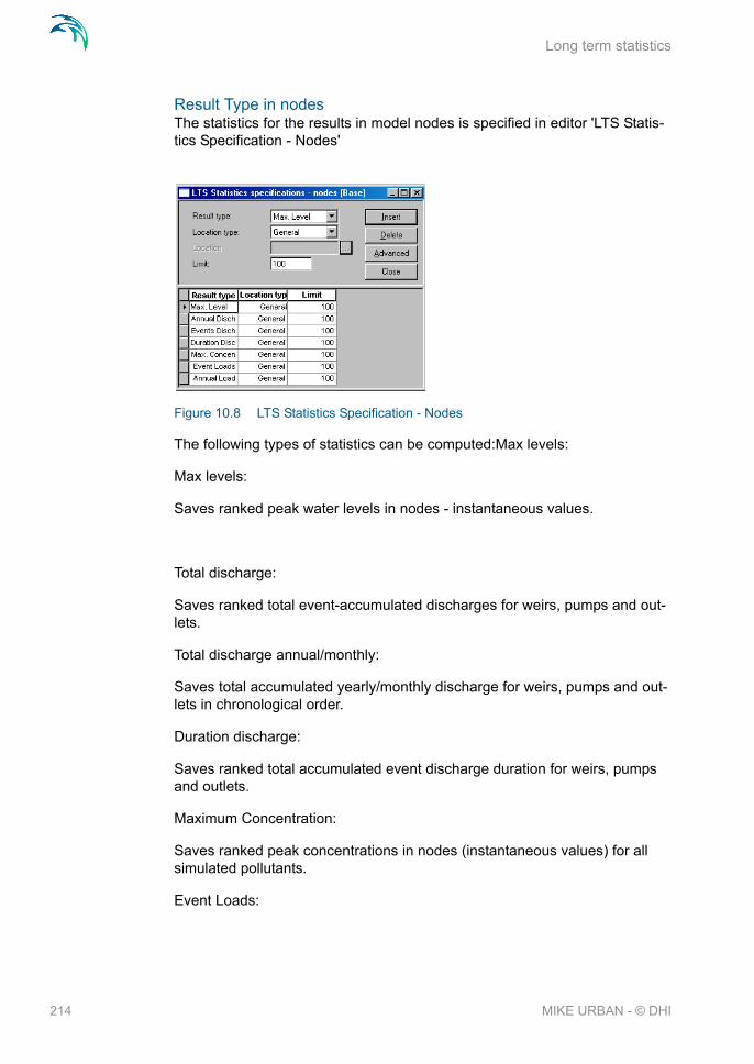
Long term statistics
Result Type in nodesThe statistics for the results in model nodes is specified in editor 'LTS Statis-tics Specification - Nodes'
Figure 10.8 LTS Statistics Specification - Nodes
The following types of statistics can be computed:Max levels:
Max levels:
Saves ranked peak water levels in nodes - instantaneous values.
Total discharge:
Saves ranked total event-accumulated discharges for weirs, pumps and out-lets.
Total discharge annual/monthly:
Saves total accumulated yearly/monthly discharge for weirs, pumps and out-lets in chronological order.
Duration discharge:
Saves ranked total accumulated event discharge duration for weirs, pumps and outlets.
Maximum Concentration:
Saves ranked peak concentrations in nodes (instantaneous values) for all simulated pollutants.
Event Loads:
214 MIKE URBAN - © DHI

Specification of Statistical Result File
Saves ranked total event-accumulated mass flux for weirs, pumps and outlets for all simulated pollutants.
Annual Loads:
Saves total accumulated yearly/monthly mass flux for weirs, pumps and out-lets for all simulated pollutants, in chronological order.
Result Type in linksThe statistics for the results in model links is specified in editor 'LTS Statistics Specification - Links'
Figure 10.9 LTS Statistics Specification - Links
Max levels:
Saves ranked peak water levels in links - instantaneous values.
Max flow:
Saves ranked peak flows in links - instantaneous values.
Max velocity:
Saves ranked peak flow velocity in links - instantaneous values.
Total discharge annual/monthly:
Saves total accumulated yearly/monthly discharge for links in chronological order.
LocationFor all result types it must be specified for which location(s) the desired results are to be saved. Location type can be either 'General' (the whole sys-tem), 'List' (a number of nodes/links specified on NSE/LSE/MUS-file), or 'Indi-vidual' (one node/link name). If 'List' or 'Individual' is selected, the supplementary information of selection file name or node name should be specified.
215

Long term statistics
Additionally, some pre-defined groups can be specified for nodes by selecting type 'All Weirs', 'All Pumps', or 'All Outlets'.
Save TypeFor links, it must be specified where in the link data should be saved. There are four saving possibilities:
Upstream grid point,
Downstream grid point,
Both upstream and downstream grid points,
All grid points.
Max number of events to saveFor some statistics parameters, the number of events during a long MOUSE LTS computation can be very high and the statistics result file size can grow rapidly. Therefore, the statistical computation can be limited to a specified number of highest events, i.e. only the limited number of most significant events is included into the calculation. This is possible if the purpose of statis-tical calculation is to focus on extreme events only. In such a case, all insignif-icant events may be eliminated from the statistics as "irrelevant".
The maximum number of events must be specified within the rand 1-5000.
10.5 LTS Statistics Presentation
LTS Statistics results cannot be presented in MIKE URBAN. This functionality will be added in near future.
In the meantime, presentation facilities in MIKE View result viewing pro-gramme should be used.
216 MIKE URBAN - © DHI

Design Principles
11 Automatic pipe design with MOUSE
The MOUSE Pipe Design Module is a tool, which makes it fast and easy to design pipe diameters for new systems as well as for pipes in existing sys-tems. The basis for the design can be a rough input of a new system with geometric information about where the pipes should be and initial values for diameter and roughness (material) or it can be an existing MOUSE model for a complex system where some pipes should be re-designed.
In both cases the design module will be an excellent help to speed up the process by designing the exact pipe sizes which is needed to fulfil the design criteria and to finally verify that the design system is correctly designed.
However it should be stressed that pipe design is an iterative process, and it is therefor recommended to use the feature on models of moderate size in order to be able to make the necessary number of iterations.
11.1 Design Principles
The design is based on an iterative process, where pipe diameters are changed in order to fulfil the specified design criteria. During each iteration the diameter is kept constant, but the Manning number is changed (increased) during simulation if the criteria is not fulfilled.
In the present version the pipes are always designed from the principle of increasing the diameter until the maximum level upstream in the system is below the design criteria. Thus the module cannot be used to design pipes from downstream criteria.
After end of the simulation the maximum Manning number is used to calcu-late the new diameter which will then be used in next iteration.
This means that after a number of iteration - depending on how good the ini-tial choice of diameters was - the module will stabilise results on the diame-ters needed to fulfil the design criteria.
Each pipe (group) is designed independently of the others, which means that the process can be long if there are many pipes, since changing of one diam-eter can often influence the design of both upstream and downstream pipes.
217

Automatic pipe design with MOUSE
Figure 11.1 Design principle
11.2 Design Input
In the present version input data for the Pipe Design Module are specified in the Additional Parameters File (ADP). In order to activate the design module the simulation is started in the usual way after specification of the ADP file name on the Start Simulation Dialog.
The ADP file can either be written directly in a text editor, e.g. Notepad, or a wizard like tool can be utilized for writing the ADP-file for the design module (see further in 11.2.7). The format of the DESIGN section in the ADP file is as follows:
Table 11.1 The Design section of the ADP file
Keyword No Parameter Description
UNIT_TYPE 1 UNITTYPE Specifies the unit type.
1 - SI, 2 - US
DESIGNRESULT-FILE
1 “RESULTFILE“ File containing the history of the individual diameters. If present at simulation start a continuance of the previous iterations assumed.
DESIGNCON-STANTS
1-6 DC1-DC6 Parameters for internal use. Not mandatory.
218 MIKE URBAN - © DHI

Design Input
MANNINGITEM 1 DESIGNID DesignID is used to identify the actual design group, but has no influence on the simulations.
2 DESIGNTYPE 1 - Fixed invert levels for pipes
2 - Fixed top levels for pipes
3 DESIGNCRITERI-ATYPE
1- Critical levels (specified on node dialog)
2 - Filling degree (value specified as parameter 10 FILLINGDEGREE)
4 DESIGNGR-POUPTYPE
1- Group. All pipes are resized in parallel based on criteria in one node (value specified as parameter 6 UPSTREAMNODE)
2- Individual pipes. Each pipe is designed based on criteria in the immediate upstream node.
5 ELEMENTS LSE-file specifying the group of links to be designed
6 UPSTREAMNODE Upstream node where design crite-ria is evaluated. Only used for DESIGNGROUPTYPE = 1
7 MIN Minimum value of Manning number. Note that extreme low values can cause numerial problems during simulation. It is recommended to use values relatively close to the original value and run a few more iterations instead.
8 MAX Maximum value of Manning num-ber. Note - see above
9 LOWERLIMIT Limit for evaluating the design crite-ria. Specified relative to water level of the design criteria.
10 FILLINGDEGREE Filling degree. Only used for DESIGNCRITERIA = 2.
Diameter Subtar-get [Commer-cial_Pipes]
1 DIAMETER List of commercial diameters. The diameters are not mandatory and should be given in ascending order. For UNIT_TYPE = 1 the unit is mm and for UNIT_TYPE = 2 the unit is inches.
Table 11.1 The Design section of the ADP file
Keyword No Parameter Description
219

Automatic pipe design with MOUSE
11.2.1 Example of an ADP-file
[DESIGN]
DESIGNRESULTFILE = ‘MyOwnResults.txt’
MANNINGITEM = ‘Manning’,1,1,2,’SelectedPipes.lse’,’’, 50, 200, -0.05, 1.0
[Commercial_Pipes]
Diameter = 50
Diameter = 100
Diameter = 200
EndSect // Commercial_Pipes
EndSect // DESIGN
11.2.2 Design Type
There are two design types available for designing pipes – fixed invert levels of pipes and fixed top levels of pipes.
When fixed invert levels are selected the network geometry is updated only with pipe diameters hence all invert levels are kept as in the original setup.
When fixed top levels are selected the top of each pipe is fixed, which means that all invert levels need to be updated according to the new diame-ters. All adjacent pipes are unchanged, hence when a nodes invert level is changed any attached pipe which was previously connected at the invert level of the manhole is now connected above invert of the manhole - at the original invert level of the manhole. A node invert level is never changed to a higher level than for the original setup.
Note: In the present version fixed top levels can only be used for pipes con-nected to manholes in both ends. If either upstream of downstream node is specified as a basin, the pipe will be designed according to the principle of fixed invert levels, regardless of design type. This is necessary in order to accommodate for the complexity of changed basin geometry, weir levels, pump start-/stop levels etc. which will often be present in basin structures.
11.2.3 Design Criteria
220 MIKE URBAN - © DHI

Design Input
The design tool accommodates two types of design criteria – critical levels and filling degree. When the Critical Levels are applied, the pipes will be designed according to the critical level specified in the MOUSE nodes dialog.
The Filling Degree is in this case interpreted as the maximum water level in upstream node compared to the upstream pipe levels. E.g. if the filling degree is set to 0.8 the design criteria will be set as a water level corresponding to the pipe being filled 80% at the design node.
If more than one pipe is connected to the design node the lowest value for all connected pipes is applied in order to ensure that the criteria is fulfilled for all pipes.
11.2.4 Design Group Type
The pipes can be designed either as a group or on individual basis.
If the pipes are designed as a group their sizes will decrease or increase with the same factor in order to obtain the design criteria for one specified upstream node. This means that the pipe sizes will change with same per-centage for all pipes.
When the design acts on individual pipes, each pipe will initially be automat-ically assigned to a design node corresponding to their immediate upstream node. Here the upstream node is defined as the node connected to the high-est end of the pipe from geometric point of view.
If more than one pipe is connected to the same upstream node they will auto-matically be grouped together and thereby maintain their relative sizes.
11.2.5 Lower Limit
During the designing simulation there will be long periods where the water levels are below the design level. In order to avoid that these periods influ-ence too much on the new pipe diameters a lower limit for designing is speci-fied. Hence when the water level is below this limit the design module will not try to resize the current pipe size until the level rises above the limit again.
The limit is defined relative to water level of the design criteria. Thus a nega-tive value indicate a lower limit below the design level and vice versa for a positive value.
221

Automatic pipe design with MOUSE
11.2.6 Commercial Diameters
Through the iterations the pipe design will suggest diameters without taking into account that only some diameters are actually manufactured. Specifying the available pipe diameters can be used to let the module select the most appropriate standard pipe after end of simulation.
The standard pipe diameters should be given in increasing order and in milli-metres (or inches for US-units).
The commercial diameters are an optional input.
11.2.7 Creating the ADP file for the design simulation
The ADP file can either be written directly in a text editor, e.g. Notepad, or a wizardlike tool can be utilized for writting the ADP-file for the design module. This tool can be activated under Tools|User Tools as seen in Figure 11.2.
Figure 11.2 The tool for creating the ADP-file is now located under User Tools
When the tool is launched you are guided step-by-step setting up the ADP-file.
Figure 11.3 Start page of the wizard
222 MIKE URBAN - © DHI

Design Simulation and Output
11.3 Design Simulation and Output
Input data for the Pipe Design Module is specified in the Additional Parame-ters File (ADP). When the design module is in function the simulation is started the usual way (with specification of the ADP file name on the Start Simulation Dialog), but an additional dialog for viewing and editing the design data will be available in parallel to the MOUSE Simulation Launcher.
In the simulation launcher two new item types can be selected from the dialog <Charts>+<Modify>: Designs and Profiles.
Figure 11.4 For changing the charts displayed during simulation go to Charts|Modify
“Designs” are time series plots for the nodes where design criteria has been specified. The default selection will include actual level, critical level and calculated factor of the manning number which is changed dur-ing the simulation
“Profiles” are longitudinal profiles. All profiles which are saved as LPF files can be selected
223

Automatic pipe design with MOUSE
Figure 11.5 After choosing Charts|Modify above dialog displays
During the simulation it will hence be possible to see the results while simu-lated, see Figure 11.6.
Figure 11.6 The results are displayed during the simulation. The critical levels used for the design are clearly marked on the profiles.
224 MIKE URBAN - © DHI

Design Simulation and Output
The additional dialog for pipe design is dominated by a grid with input param-eters and results from the design, and can be used to adjust parameters for the design between the iterations.
The following information is available in the grid:
Below the columns Original, Calculated and Commercial it is possible to press "->New", which will simply copy the column of diameter to the column "New", thus cause them to be used as initial values for next iteration.
Table 11.2 Information found in the grid
ID ID of the pipe
UpStrNodeID ID of the node where design criteria are evaluated
Active “True“ if the pipes should actually be designed - can be used to exclude one or more pipe iterations
Init Factor Initial factor of Manning number for next iteration - val-ues smaller than 1.0 will allow the pipe to decrease in size if necessary, however too small values can cause numerical problems. Values bigger than 1.0 are usu-ally not relevant since it will cause the pipe to increase in size even if it's not necessary. Default is 0.98.
Original Original diameter in mm or inches.
Calculated Calculated diameter in mm or inches - result from last iteration.
%Change Percentage change of diameter in last iteration
Commercial Smallest available commercial diameter which corre-spond to the calculated diameter
New Diameter in mm or inches which will be used as initial value for next iteration. Default is that results from the previous iteration will be used
225

Automatic pipe design with MOUSE
Figure 11.7 The pipe design dialog
Number of reruns can be used to make a number of iterations automatically - default value is 1.
If changes are made in the grid these must be saved in order to be used for the next iteration. Saving can be done by pressing "Apply changes for next iteration", but if data has been changed and a new iteration started, a mes-sage will occur asking if the changes should be used or lost.
Finally there is the possibility to "Create MEX-file With New Diameters" which will change the parameters for the specified elements and create a MEX file. This MEX file can be used to import and update the elements in MIKE URBAN once the optimal set of values has been identified. In order to import and update the elements in the network based on this MEX file you need to go to File|Import/Export and switch to the ‘Use Advanced’ mode. Under the list of pre-defined import jobs you will find the job ‘CS-Update From Pipe Design’. Choosing this option and the MEX file in question (see example in Figure 11.8) will update the elements in your MIKE URBAN model after pressing ‘OK’.
The option "Delete Design File" which will delete results of all the performed iterations and cause the design to start from scratch.
226 MIKE URBAN - © DHI

Design Simulation and Output
Figure 11.8 Choosing to import and update the elements based on the result of the pipe design
227

Automatic pipe design with MOUSE
228 MIKE URBAN - © DHI

Key Features and Application Domain
12 Modelling Water Quality with MOUSE
12.1 Key Features and Application Domain
MOUSE provides several modules for the simulation of and water quality for both urban catchments surfaces and sewer systems. Since pollutants are carried by sediment, sediment transport process and water quality in sewer systems are closely interconnected. This is important for understanding phe-nomena like the first flush effect, which can only be simulated with a descrip-tion of the temporal and spatial distribution of sediment deposits on the catchment surface and in the sewer system. MOUSE can model these com-plex mechanisms using Surface Runoff Quality (SRQ), Pipe Sediment Trans-port (ST), Pipe Advection-Dispersion (AD), and Biological Processes (BP). Output from this, such as pollutant graphs from combined sewer overflows, can then be applied directly to DHI's receiving waters models MIKE 11 and MIKE 21. Using MIKE 11 or MIKE 21 in conjunction with MOUSE allows assessment of water quality for the water bodies receiving these sewer over-flows, such as rivers, streams, lakes and coastal waters.
12.1.1 Surface Runoff Quality (SRQ)
The primary role of the Surface Runoff Quality (SRQ) is to provide a physi-cally-based description of the relevant processes associated with sediments and pollutants due to surface runoff, and then provide surface runoff sedi-ment and pollutant data for the other pipe sewer network sediment transport and water quality modules. The following processes can be accounted for:
Build-up and wash-off of sediment particles on the catchment.
Surface transport of pollutants attached to the sediment particles.
Build-up and wash-out of dissolved pollutants in potholes and stilling basins.
12.1.2 Pipe Sediment Transport (ST)
Sediment deposits can greatly reduce the hydraulic capacity of sewer pipes by restricting their flow area and increasing the bed friction resistance. Pipe Sediment Transport (ST) can be used to account for these problems, by sim-ulating pipe sewer network sediment transport-including deposition and ero-sion from non-uniform (graded) sediments. Contributions from rainstorm wash-off and dry-weather wastewater flow can be included. The ST process runs in conjunction with the dynamic flow routing, thereby simulating dynamic deposition of sediment and providing feedback due to the change in pipe area and resistance caused by sediment deposition. The following issues can be addressed:
229

Modelling Water Quality with MOUSE
Prediction of sediment deposit locations and associated pollutants and metals in the sewer system.
Prediction of reduction in hydraulic capacity due to observed and simu-lated sediment deposits.
Analysis of the sewer system due to modified regulation strategies.
12.1.3 Pipe Advection-Dispersion (AD)
Pipe Advection-Dispersion (AD) simulates the transport of dissolved sub-stances and suspended fine sediments in pipe flow. Conservative materials as well as those that are subject to a linear decay can be simulated. The computed pipe flow discharges, water levels, and cross-sectional flow areas are used in the AD computation. The solution of the advection-dispersion equation is obtained using an implicit, finite-difference scheme which has negligible numerical dispersion. Concentration profiles with very steep fronts can be accurately modeled. The computed results can be displayed as longi-tudinal concentration profiles and pollutant graphs, which could be used at the inflow to a sewage treatment plant or an overflow structure. The AD can be linked to the MOUSE Long Term Statistics modelling capacities to provide long-term simulations of pollutant transport.
The Pipe-Advection module also includes the possibility of simulating water age and blend in percentages between two sources.
12.1.4 Biological Processes (BP)
Biological Processes (BP) works in conjunction with the Advection-Dispersion Module, thereby providing many options for describing the reaction pro-cesses of multi-compound systems, including degradation of organic matter, bacterial fate, exchange of oxygen with the atmosphere and oxygen demand from eroded sewer sediments. This allows realistic analysis of complex phe-nomena related to water quality in sewer systems. BP includes diurnal varia-tion of foul flow discharges and user-specified concentrations of foul flow components. The sediment types included in the interaction with BP are foul flow organic sediments, and fine and course mineral in-pipe sediments origi-nating from catchment runoff, potholes, and stilling basins. BP can account for:
Decay of BOD/COD in bio-film and water phase;
Hydrolysis of suspended matter;
Growth of suspended biomass;
Oxygen consumption from decay of BOD/COD, bio-film, and erosion of sediment;
Re-aeration;
Bacterial fate;
230 MIKE URBAN - © DHI

Key Features and Application Domain
Interaction with sediments for nutrients and metals.
12.1.5 Interaction between water quality modules
The various water quality processes can be used independently or in con-junction, which depends on the level of required sophistication. However, using BP requires a simultaneous run of AD. Interaction between water qual-ity modules shows the individual modules and their connections.
SRQ can be used by itself to study water quality and sediment transport pro-cesses on catchments. The result can be used as input to a river model (MIKE11) or to other water quality modules which deal with processes in the pipe model.
If only dissolved pollutants are of concern, it is sufficient to use the AD-mod-ule, possibly with BP in conjunction.
Finally, if the sediment transport is the only modelling purpose the ST module can be used separately.
Problem types and processes shows which water quality modules should be used for a list of problem types. Figure 12.1 gives an overview of the required modules for different pollutant and sediment types.
Figure 12.1 Interaction between water quality modules
231

Modelling Water Quality with MOUSE
12.2 Surface Runoff Quality (SRQ)
Surface Runoff Quality is used to generate input for the sediment transport, advection-dispersion or water quality computation in the underlying pipe model. The Surface Runoff Quality module consists of three models:
a model for the description of the accumulation (build-up) and wash-off of particles on the catchment surface;
a model for the description of the surface transport of pollutants attached to the sediments;
a model for the description of the build-up and wash-out of dissolved pol-lutants in gully pots.
The Build-up/Wash-off model consists of two sub-models: a model for the description of the accumulation of particles on the catchment and a model for the description of the detachment of particles by rainfall and subsequent rout-ing of the wash-off by the overland flow.
The model works with two sediment fractions, a fine and a coarse, each frac-tion characterised by its mean diameter. The fine fraction typically has a parti-cle size less than 0.1 mm and is limited in supply. On the contrary, the coarse fraction is typically unlimited in supply. Thus, for the coarse fraction, transport capacity is always satisfied and, therefore, the build-up description is only
Table 12.1 Problem types and processes
Type of problem Processes to be used
Single event pollution spill at weirs and pollution loads to treatment plants
Dissolved pollutants
Sediment attached pollut-ants
Sediments
AD, AD/BP
AD/ST, AD/BP/ST
ST
Sedimentation in sewers Uniform sediments
Graded sedimentsST
Pollution of receiving waters from surface catchments & pollution input to pipe system
Sediments
Sediments attached pollut-ants
Dissolved pollutants
SRQ
232 MIKE URBAN - © DHI

Surface Runoff Quality (SRQ)
applicable to the fine sediment fraction to determine the mass available for transport.
The surface sediment transport model is based on the hydrological models available in MOUSE, i.e. the Surface Runoff Model A and the Surface Runoff Model B. In model sediment is routed according to the hydrological descrip-tion in the surface runoff model. Output from the model consists of time series of sediment transport or concentration mass and accumulated mass for each sediment fraction. In addition, a time series of mass of the fine sediment frac-tion on the surface is available. The Sediment and Pollutants model is an optional model, which describes the attachment of pollutants to the sediment. Output from the model consists of time series of mass or concentration and ac-cumulated mass of pollutants attached to the two sediment fractions.
12.2.1 Surface Sediment Data Dialogs
The data for the surface sediment transport calculation is entered and edited through dedicated editors accessible under the 'MOUSE|Water Quality'-menu. The data for the surface sediment model consists of data for the Build-up/Wash-off model, data for the Sediment and Pollutant model and data for the Gully Pot model.
MOUSE| Water Quality| SRQ Main Parameters
The sediment parameters used in the build-up/wash-off computations are specified under 'MOUSE|Water Quality| SRQ Main Parameters.
The parameters for the build-up/wash-off model can be specified in the dialog displayed in the SRQ Main Parameters dialog Figure 12.2.The 'Build Up Method' defines build up method for the fine sediment on the surface. A linear build-up function, or an exponential function, can be chosen.
233
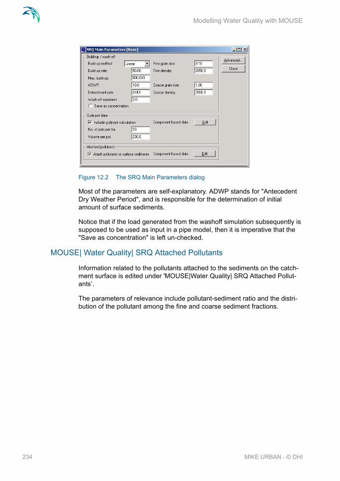
Modelling Water Quality with MOUSE
Figure 12.2 The SRQ Main Parameters dialog
Most of the parameters are self-explanatory. ADWP stands for "Antecedent Dry Weather Period", and is responsible for the determination of initial amount of surface sediments.
Notice that if the load generated from the washoff simulation subsequently is supposed to be used as input in a pipe model, then it is imperative that the "Save as concentration" is left un-checked.
MOUSE| Water Quality| SRQ Attached Pollutants
Information related to the pollutants attached to the sediments on the catch-ment surface is edited under 'MOUSE|Water Quality| SRQ Attached Pollut-ants’.
The parameters of relevance include pollutant-sediment ratio and the distri-bution of the pollutant among the fine and coarse sediment fractions.
234 MIKE URBAN - © DHI

Surface Runoff Quality (SRQ)
Figure 12.3 The SRQ Attached Pollutants dialog
MOUSE| Water Quality| SRQ Gully Pot Data
The data supplied to the Gully pot model facilitate description of the build-up of dissolved pollutants in the gully pots during dry weather and the wash-out of dissolved pollutants from the gully pots during storm events.
Data for description of the build-up of pollutants for each component must be specified. During dry weather flow, the concentration of dissolved pollutants will build-up according to a user-specified linear build-up function, with a max-imum threshold value. During storms, all sediment is routed straight through the gully pots and a simple mixing model is used to mix the incoming water with the gully pot liquor.
The data for the gully pots are specified and edited under 'MOUSE|Water Quality| SRQ Gully Pot Data - see Figure 12.4.
The parameters of relevance include initial concentration, build-up rate and maximum concentration for each of the pollutants
235

Modelling Water Quality with MOUSE
Figure 12.4 The SRQ Gully Pot Data dialog
12.3 Advection-Dispersion (AD)
The Advection-Dispersion model can be used for calculation of the transport of dissolved or suspended substances, age of water, blend in percent between two sources, and for modelling of water temperature variation within the sewer network. The model is based on the one-dimensional transport equations for dissolved material. The equations reflect two transport mecha-nisms: the advective (or convective) transport with the mean flow velocity and the dispersive transport due to concentration gradients in the water. The transport equations are solved by use of an implicit finite difference scheme, which is fully time and space centred, in order to minimize the numerical dis-persion. The main assumptions of the model are:
The considered substance is completely mixed over the cross-sections. This implies that a source/sink term is considered to mix instantaneously over the cross-section;
The substance is conservative or subject to a first order reaction (linear decay);
Fick's diffusion law can be applied, i.e. the dispersive transport is propor-tional to the concentration gradient.
Special considerations have been given to the transport at manholes and other structures. More information on the technical background of the model is given in the ”MOUSE Pollution Transport Reference” manual.
The Advection-Dispersion model requires two types of data: time series of concentrations at the model boundaries and data for full definition of the com-ponents to be modeled, e.g. initial concentrations, dispersion coefficients and decay rates.
236 MIKE URBAN - © DHI

Advection-Dispersion (AD)
12.3.1 Advection-Dispersion Data Dialogs
MOUSE| Water Quality| AD Components
Each of the components (substances) to be included in the Advection-Disper-sion computations must be specified in the is Data dialog, shown in the AD Components dialog, shown in Figure 12.5. The naming of component is absolutely flexible, and no "reserved" or "standard" component names are prescribed.
Please note that when using MOUSE LTS engine only a single AD compo-nent should be specified. If several AD components have to be included in the simulation then use MIKE 1D engine.
Figure 12.5 The AD Components dialog
The specified pollution components can be declared as 'Dissolved', 'Sus-pended', 'Total', 'Bacteria', 'Temperature' ‘Water Age’, ‘Water Blend’ and 'Other'. This categorization is needed for correct handling of units: mass per volume (dissolved, suspended, total, other), counts per volume (bacteria), water age in hours, water blend in %, and degrees (temperature). When working with water-quality model, this categorization is further supplemented with other parameters, in order to apply the components in the WQ model properly. Practically, each of the specified components can be connected to a 'standard' component in the WQ module. By these means the WQ module 'knows' how to treat each component.
For each component, specification of an initial condition and decay coefficient can be specified. The decay coefficient cannot be given for water age and water blend type. If the specification of the initial concentration for a certain component has been omitted, a zero concentration is automatically applied. Water blend concentration must always be given as a number between 0 and 100 percent, and the sum of the two blend components must add up to 100 percent.
237

Modelling Water Quality with MOUSE
Local initial conditions for dissolved or suspended pollutants, water blend, water age and temperature can be specified under 'MOUSE|Water Qual-ity|Conditions Local'., This editor can that be also be accessed directly from the 'AD Components' editor, by pressing the ''Edit'' button.
Figure 12.6 The AD Initial Conditions Local dialog
The initial conditions are specified for individual nodes. The initial conditions in the connected conduits is calculated by linear interpolation of the concen-trations specified in the upstream and downstream nodes.
By defining decay constants, non-conservative components can be specified. For such non-conservative component the concentration is assumed to decay according to the first order expression:
(12.1)
where:
K = the decay coefficient (h-1)
C = the concentration
The decay constant is defined as an uniform decay over the entire model.
The AD model can be run with the components specifications only. In this case all model specific parameters (decay constant, dispersion coefficient, initial concentration) as well as boundary conditions are set to zero.
Please not that the sum of the two blend components must always add up to 100.
dCdt-------- KC=
238 MIKE URBAN - © DHI

Advection-Dispersion (AD)
MOUSE | Water Quality | AD Dispersion
The dispersion coefficient is specified as a function of the flow velocity. The function is given as:
(12.2)
where:
D = the dispersion coefficient (m2/s),
a = the dispersion factor,
u = the flow velocity (m/s),
b = a dimensionless exponent.
If the exponent is set equal to zero, then the dispersion coefficient is constant and independent of the flow velocity. The unit for the dispersion factor will then be m2/s. If the exponent is 1, i.e. the dispersion coefficient is a linear function of the flow velocity, then the unit of the dispersion factor will be meter, and the dispersion factor will in this case be equal to what is generally termed the dispersivity. It is possible to specify values of the minimum and the maximum dispersion coefficients, in order to limit the range of the dispersion coefficient calculated during the simulation.
Figure 12.7 The AD Dispersion dialog
The dispersion coefficient can be given either globally or locally. The global description will be used at all locations except for those pipes where local conditions have been specified in the menu. In the example above the global statement indicates that a constant dispersion coefficient of 2.00 m2/s is applicable, and independent of the flow velocity (the exponent is zero).
For two conduits (see the example below), the dispersion coefficients speci-fied locally, 'overrule' the global specification and prescribe a constant disper-sion coefficient of 4 m2/s.
D aub=
239

Modelling Water Quality with MOUSE
Figure 12.8 The AD Dispersion Local dialog
Advection-Dispersion and Open Boundary Conditions
The main purpose of specifying an open boundary condition is to enable exchange of mass between the MOUSE network and the surroundings (recipient) during the computations. If only inflow takes place at a boundary, then it is not necessary to specify a boundary as an open boundary. Open boundaries are normally located at outlets.
The presence of the open boundaries in the model is declared in the 'MOUSE|Boundary Conditions|External water levels’ (see description of boundary conditions).
A special consideration must be given to the open boundaries in the Advec-tion-Dispersion model. At an open boundary a boundary time series, contain-ing either transport or concentration in the receiving waters must be specified.
If the flow is directed out of the model, the concentrations or transport at the boundary are computed from the concentrations or transport within the model area. In this case the concentration or transport outside the model area is assumed not to influence the conditions in the model area.
If a flow reversal takes place so that flow is directed from the receiving waters into the model area, the specified time series of boundary concentrations or transport are used and assumed to be unaffected by the previous outflow from the model area. A parameter K-mix is used to ensure a smooth transi-tion between the calculated concentration or transport at the boundary before the flow reversal and the specified time series of boundary concentrations. The description of K-mix is given in the "MOUSE Pollution Transport Refer-ence" manual.
240 MIKE URBAN - © DHI

Biological Processes (BP)
12.4 Biological Processes (BP)
This part of MOUSE deals with the transport and transformation of a number of chemical compounds and biological constituents found in sewer systems. These constituents are first of all organic material measured as biological or chemical oxygen demand (BOD and COD respectively), which can affect the oxygen content of the water. Other compounds are the nutrients (ammonia and phosphate), the heavy metals and various other organic or inorganic pol-lutants including bacteria from human and animal wastes.
The determinants that can be analyzed using BP are:
BOD/COD (organic matter) and oxygen
Ammonia and phosphate
Heavy metals
Bacteria : Total and Faecal Coliform and Streptococci
Pollutants attached to sediments
The BP-module is coupled to the AD-module. This means that while the AD-module simulates the transport process, the BP-module deals with the simul-taneous transforming processes of the com-pounds in the sewer. The AD-module is running in parallel to the BP-module when the WQ-module is acti-vated.
The BP module has been constructed to be as flexible as possible. This has resulted in a structure where the determinants mentioned above can be stud-ied individually or rather in the groups indicated above.
12.4.1 Biological Processes Dialog (MOUSE|Water Quality|WQ Process Model)
The determinants included in BP are distributed in 6 groups as shown in the menu.
Group 1 includes the aspects of the classical BOD/DO problem, e.g. the deg-radation of organic material and subsequent consumption of oxygen. The oxygen demand can be specified as BOD or as COD. The processes included in the simulation of these parameters are the degradation of organic material and the resulting oxygen consumption and the reaeration of oxygen.
Group 2 includes nutrients relevant for sewer systems, e.g. the reduced form of nitrogen - ammonia/ammonium and phosphate. The nutrients are modeled as conservative substances.
Group 3 is the heavy metals. The model does not a priori determines which metals to be included. This is defined by the user. The Heavy metals are modeled similarly to the nutrients, e.g. as conservative substances.
241

Modelling Water Quality with MOUSE
Group 4 is bacteria arising from human and animal wastes. Three groups of bacteria can be modeled: faecal coliform, total coliform and streptococci. The coliform bacteria are assumed to be subject to a decay (death) that depends on the temperature.
Group 5 and 6 are facilities for specifying the parameters needed when pol-lutants are modeled as sediment attached. This can be any pollutant (BOD, heavy metals etc).
The processes are described theoretically in the "MOUSE Biological Pro-cesses Reference" manual. Here, a general explanation of the processes and inventory of the required input parameters are given in connection to the discussion about relevant data forms.
The determinants included in this group is the BOD/COD and dissolved oxy-gen. The BOD is modeled as two fractions: the dissolved and readily degra-dable BOD and the suspended BOD that is degraded slower and of which a part is the heterotrophic bacteria responsible for the degradation of a part of the dissolved BOD. The dissolved BOD can also in some cases besides the degradation by the bacteria, be degraded in a biofilm at the inside of the sewer pipe and at the water surface.
242 MIKE URBAN - © DHI

Biological Processes (BP)
Figure 12.9 The processes included in the modelling of BOD/COD - dissolved oxy-gen problems in sewer pipes modeled with MOUSE
The general parameters for the BOD/COD - DO processes are inserted through the data dialog shown dialog in the WQ Process model dialog.
243

Modelling Water Quality with MOUSE
Figure 12.10 The WQ Process model dialog
The reaeration is a relevant process in cases of non-full flow in the pipes. An empirical expression based on measurements in sewer pipes is provided to simulate the reaeration process. The reaeration rate is modeled as a function of the flow velocity, the mean hydraulic water depth and the pipe slope. The reaeration rate is also dependent on the temperature expresses by an Arrhe-nius temperature coefficient. The reaeration constant is calculated at 20°C and adjusted to the actual temperature by means of the temperature coeffi-cient.
The constants in this expression can be changed by the user (totally three constants). Besides these constants a temperature coefficient can be speci-fied.
The Group 4 of determinants is the bacteria that can be faecal and total coli-form bacteria and streptococci. Most pathogenic microorganisms are usually unable to multiply or survive for extensive periods in the aquatic environment. Sedimentation, starvation, pH changes, temperature plus competition with and predation by other naturally occurring microorganisms are factors involved in the decay of pathogenic bacteria in the marine environment.
244 MIKE URBAN - © DHI

Water quality (MIKE ECO Lab)
Escherichia coli (E. coli) is one of the dominant species in faeces from human and warm-blooded animals. The organism itself is normally considered non-pathogenic, but is very often used as indicator organism for faecal pollution and hence a potential of real pathogenic organisms (e.g. other bacteria and vira). Infections obtained from bathing waters are most often caused by vira, protozoas, Shigella and Campylobacter.
Enteric bacteria die-off can be modeled very well by a first order decay reac-tion. However, the die-off constant or decay rate is highly variable due to interaction by environmental factors on bacterial die-off. The main factors are suspected to be: light, temperature and salinity variations. In sewers, the only relevant factor among these to include is the temperature. Other less impor-tant factors are, e.g. predation,sedimentation and the amount of available nutrients.
For each bacteria group, a first order decay rate at 20ºC has to be specified together with a temperature coefficient.
12.5 Water quality (MIKE ECO Lab)
Hydrodynamic and advection-dispersion (transport) simulations can be cou-pled with MIKE ECO Lab for efficient and versatile simulation of water quality processes in sewer systems. This option opens for practically unlimited range of processes to be simulated, as long as these can be described by a consist-ent model.
MIKE ECO Lab is a highly flexible and open framework for formulation of water quality models. MIKE ECO Lab utilises a concept of templates where water quality models are defined transparently: Complete contents of the pre-defined templates supplied by the MU installation is accessible for review and can be modified without any need to involve the software vendor. Also, com-pletely new templates can be developed by the user.
The MIKE URBAN installation includes two pre-defined water quality tem-plates that can be applied “as is” - or they can be adjusted by the user to con-form to the specific project requirements.
A MIKE ECO Lab template is as ASCII file which can be accessed and edited by the MIKE ECO Lab editor. Note that MIKE ECO Lab is part of MIKE Zero and it is necessary install MIKE Zero and acquire a license for MIKE ECO Lab in order to use MIKE ECO Lab with MIKE URBAN.
Please consult the MIKE Zero ECO Lab documentation on how to create or modify model templates, i.e. how to work with the MIKE ECO Lab editor.
Please also note that MIKE ECO Lab couplings are only possible with the MIKE 1D engine. The older MOUSE engine does not support MIKE ECO Lab couplings.
245

Modelling Water Quality with MOUSE
MIKE ECO Lab implementation in MIKE URBAN is limited to coupling the existing MIKE ECO Lab templates for MIKE URBAN with the hydrodynamic and transport model and to editing the MIKE ECO Lab model constants dur-ing calibration.
A simulation job with the coupled HD/AD and MIKE ECO Lab model is set up and launched from within MIKE URBAN in a usual way.
MIKE ECO Lab in MIKE URBAN is supported by a set of four MIKE ECO Lab editors in MIKE URBAN:
Templates and Assignments
State Variables
Forcings
Constants
These four editors and the database tables behind them are described below.
12.5.1 MIKE ECO Lab Templates and Assignments
This editor is used for loading (import) MIKE ECO Lab templates into MIKE URBAN and assigning them to the model elements – nodes and links. The data for this editor is stored in the msm_EcoLabTemplate MU database table.
Before importing a template, a new table record must be created by <Insert> button. Then, the wanted template is browsed and selected. Actual loading of the selected template is done by clicking on <Import> button. The import scans the template and extracts information about state variables, forcings, and constants, and loads it into the respective tables. Contents of these ta-bles is described in the following three sub-sections.
A template can be assigned to the entire model (i.e. to all points where HD/AD calculation is performed or to an arbitrary sub-set. A sub-set is defined by a MIKE URBAN Selection file (*.mus) or as an individual element (a node or a link).
Note that there can only be one MIKE ECO Lab template on a node or link. If a template is used for All, then a template on a single or multiple nodes/links will override the template on all elements.
If a specific template should be connected to both nodes and links, it is nec-essary to create a selection file (*.mus) file to link the desired features to the msm_EcoLabTemplate table to the same template but connected to nodes and links respectively.
The "Apply" check box can be used to disable a template.
246 MIKE URBAN - © DHI
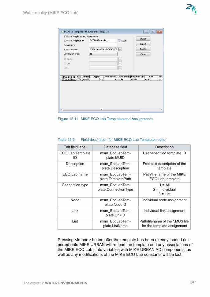
Water quality (MIKE ECO Lab)
Figure 12.11 MIKE ECO Lab Templates and Assignments
Pressing <Import> button after the template has been already loaded (im-ported) into MIKE URBAN will re-load the template and any associations of the MIKE ECO Lab state variables with MIKE URBAN AD components, as well as any modifications of the MIKE ECO Lab constants will be lost.
Table 12.2 Field description for MIKE ECO Lab Templates editor
Edit field label Database field Description
ECO Lab Template ID
msm_EcoLabTem-plate.MUID
User-specified template ID
Description msm_EcoLabTem-plate.Description
Free text description of the template
ECO Lab name msm_EcoLabTem-plate.TemplatePath
Path/filename of the MIKE ECO Lab template
Connection type msm_EcoLabTem-plate.ConnectionType
1 = All2 = Indiviidual
3 = List
Node msm_EcoLabTem-plate.NodeID
Individual node assignment
Link msm_EcoLabTem-plate.LinkID
Individual link assignment
List msm_EcoLabTem-plate.ListName
Path/filename of the *.MUS file for the template assignment
247

Modelling Water Quality with MOUSE
12.5.2 MIKE ECO Lab State Variables
This editor is used for coupling MIKE URBAN AD components to MIKE ECO Lab state variables and for possible reconciliation of differences in units used in MIKE URBAN and in MIKE ECO Lab, respectively. The data for this editor is stored in the msm_EcoLab.Component MU database table.
In MIKE URBAN database table msm_ADComponent there should be an entry for every MIKE ECO Lab state variable defined in the MIKE ECO Lab template. This means that all MIKE ECO Lab state variables are subject to both AD transport mechanisms and to MIKE ECO Lab transformations.
AD components must be specified by the user. These AD components must represent exactly the same constituents as those in the MIKE ECO Lab tem-plate, but their names can be freely defined. The specified initial values for the AD components will be applied in the computation. Initial (default) values for the MIKE ECO Lab state variables defined in the template will be ignored.
The import operation described in the MIKE ECO Lab Templates and Assign-ments section will automatically create the required entries in this table. The user must couple each of these MIKE ECO Lab state variables (components) to the relevant AD component.
The "Conversion Factor" entry (default value 1, i.e. no conversion) can be set different from 1.0 if the units for the AD components and MIKE ECO Lab state variables are different. Please note that the AD components require a specific unit while MIKE ECO Lab does not require a specific unit for a specific com-ponent type.
Figure 12.12 MIKE ECO Lab State Variables
248 MIKE URBAN - © DHI

Water quality (MIKE ECO Lab)
Please note that the only active fields in this editor are those for coupling the MU AD components with MIKE ECO Lab state variables, and for specification of the conversion factor. The remaining fields are read-only.
<Insert> and <Delete> buttons have a functionality limited to very special applications. Inserting a new state variable in Mike Urban will have no effect whatsoever on the functionality of the MIKE ECO Lab template, as it will not be linked to any processes. On the other hand, deleting a state variable would destroy the MIKE ECO Lab template functionality, with unpredictable consequences.
12.5.3 MIKE ECO Lab Forcings
Forcings are external variables associated with computational points (i.e. are spatially fixed), constant or variable in time, which affect some of the pro-cesses on the state variables.
Forcings can be “Built-In” or “User Defined”. “Built-In” means that forcings are provided by the hydraulic model through coupling with MIKE ECO Lab. “User De-fined” forcings must be provided by the user, either as constant values or as time series (dfs0 file name and item in the file).
This editor is used for setting the User Defined forcings associated with the loaded MIKE ECO Lab templates. Built-In forcings are also imported into
Table 12.3 Field description for MIKE ECO Lab State Variables editor
Edit field label Database field Description
Component ID msm_EcoLabCompo-nent.ComponentID
MIKE ECO Lab state variable identifier
MIKE ECO Lab Template
msm_EcoLabCompo-nent.TempID
MIKE URBAN name of the template the component
belongs to
AD Component ID msm_EcoLabCompo-nent.ADComponentID
MU AD component which is coupled to the MIKE ECO Lab
state variable
ECO Lab Unit msm_EcoLabCompo-nent.EcoLabUnit
Unit for the MIKE ECO Lab state variable, as defined in the
template
MU Unit msm_EcoLabCompo-nent.MUUnit
Unit for the MU AD Compo-nent, as defined in the AD
model setup
Conversion factor msm_EcoLabCompo-nent.ConvFactor
Conversion factor for possible units conversion between MU
and MIKE ECO Lab
249

Modelling Water Quality with MOUSE
MIKE URBAN, but specification of their values as constants or time series would not have any effect on the MIKE ECO Lab computations.
The data table in MIKE URBAN database containing MIKE ECO Lab forcings is msm_EcoLabForcing. The database records are created automatically dur-ing the template import. The table contains as many forcings as there are in the MIKE ECO Lab template.
Figure 12.13 MIKE ECO Lab Forcings
Table 12.4 Field description for MIKE ECO Lab Forcings editor
Edit field label Database field Description
Forcing ID msm_EcoLabForcing.Forc-ingID
MIKE ECO Lab forcing identi-fier
MIKE ECO Lab Template
msm_EcoLabForcing.Tem-pID
MIKE URBAN name of the template the forcing belongs to
ECO Lab Unit msm_EcoLabForcing.Eco-LabUnit
Unit for the MIKE ECO Lab forcing, as defined in the tem-
plate
Value msm_EcoLabForc-ing.DefaultValue
Constant value for the forcing
File msm_EcoLabForcing.File-Name
Path/filename for dfs0 time series file containing forcing
TS data
Item msm_EcoLabForcing.Item-Label
dfs0 item reference
250 MIKE URBAN - © DHI

Water quality (MIKE ECO Lab)
Please note that the only active fields are those for the specification of the forcing’s constant value or the reference to dfs0 TS file. The remaining fields are read-only.
<Insert> and <Delete> buttons have a functionality limited to very special applications. Inserting a new forcing in Mike Urban will have no effect what-soever on the functionality of the MIKE ECO Lab template, as it will not be linked to any processes. On the other hand, deleting a forcing would destroy the MIKE ECO Lab template functionality, with unpredictable consequences.
12.5.4 MIKE ECO Lab Constants
This editor is used for setting the values of constants used in the MIKE ECO Lab template, typically in relation to the model calibration.
The data table in MIKE URBAN database containing MIKE ECO Lab con-stants is msm_EcoLabCoeff. The database records are created automatically during the template import. The table contains as many constants as there are in the MIKE ECO Lab template.
Figure 12.14 MIKE ECO Lab Constants
251

Modelling Water Quality with MOUSE
Please note that the only active field in the one containing the constant value. The remaining fields are read-only.
<Insert> and <Delete> buttons have a functionality limited to very special applications. Inserting a new constant in Mike Urban will have no effect what-soever on the functionality of the MIKE ECO Lab template, as it will not be linked to any processes. On the other hand, deleting a constant would destroy the MIKE ECO Lab template functionality, with unpredictable conse-quences.
12.5.5 Running MIKE ECO Lab simulation
To run a MIKE ECO Lab simulation, the network model must be prepared in consistency with the MIKE ECO Lab template which is to be simulated. This means that it should contain at least those AD components which are to be coupled with MIKE ECO Lab state variables.
Further, the wanted MIKE ECO Lab template should be imported to MIKE URBAN. Possible unit inconsistencies must be considered and resolved by providing proper conversion factors. Values of the constant should be reviewed and modified, as appropriate. User-defined forcings should be specified, either as constants or as time series.
The network simulation with MIKE ECO Lab is activated by checking “Trans-port(AD)” and “ECO Lab” checkboxes, as shown in Figure 12.15. Default integration method (EULER) can be applied in most cases.
The simulation will result in three files containing all the hydrodynamic infor-mation (*.res1d), advection and dispersion results for the state variables (*AD.res1D) and the auxiliary variables, processes and derived outputs included in the MIKE ECO Lab results file (ADEL.res1D).
Table 12.5 Field description for MIKE ECO Lab Constants editor
Edit field label Database field Description
Constant ID msm_EcoLabCoeff.CoeffID MIKE ECO Lab constant iden-tifier
MIKE ECO Lab Template
msm_EcoLabCoeff.Tem-pID
MIKE URBAN name of the template the constant belongs
to
Unit msm_EcoLabCoeff.Unit Unit for the MIKE ECO Lab constant, as defined in the
template
Global Value msm_EcoLabCoeff.Coef-fValue
Value of the constant
252 MIKE URBAN - © DHI

Sediment Transport (ST)
Figure 12.15 MIKE ECO Lab Check
12.6 Sediment Transport (ST)
MOUSE supports the computation of non-cohesive sediment transport by means of four different sediment transport formulae. Each of the sediment transport formulae can be used in any of the sediment transport models avail-able in MOUSE ST. The sediment transport models are of different levels of complexity. The most simple model calculates only the hydraulic resistance from sediment deposits in the pipes and the most complex model is a full morphological model for graded sediment. The sediment transport models and the sediment transport formulae are briefly described below. For more detailed technical outlines of the sediment transport models and the sediment transport formula, refer to the “MOUSE Pollution Transport Reference” man-ual.
12.6.1 The Sediment Transport Models in MOUSE ST
The sediment transport models in MOUSE ST can be divided into two groups:
explicit models,
morphological models.
The main difference between the two model types is that in the explicit mod-els the bed levels are fixed during the simulation. In the morphological mod-els the bed levels / sediment deposits are updated dynamically during the simulation.
The Explicit Sediment Transport Models
In the explicit sediment transport models the bed level is fixed throughout the simulation and the only feed-back from the sediment transport computations to the hydrodynamics is established via the Manning number. The sediment transport capacity is calculated in time and space as an explicit function of the corresponding hydrodynamic flow parameters, i.e. the model calculates a potential sediment transport and no sediment is moved around in the system. The explicit models are in general used to:
investigate the hydraulic capacity in pipes with sediment deposits;
calculation of the sediment transport at locations where the bed levels changes are insignificant during a simulation.
253

Modelling Water Quality with MOUSE
In order to select an explicit sediment transport model, leave the checkbox "Apply Morphological Modeling” on the dialog 'MOUSE | Water Quality | ST Main Parameters' unchecked.
The Morphological Models
The morphological models in MOUSE TRAP ST are:
morphological model for uniform sediment,
morphological model for non-uniform sediment.
In the morphological models the sediment transport continuity equation is solved, based on the corresponding values of the hydrodynamic parameters (i.e. discharge, water levels, etc). The feedback to the hydrodynamic module is established through dynamically changed flow area and flow resistance number.
The morphological model for uniform sediment uses one grain diameter at each point in the sewer system to calculate the sediment transport. In the morphological model for non-uniform sediment it is possible to calculate the sediment transport from a range of grain diameters. For the transport of fine organic particles some of the non-uniform sediment fractions can be chosen to be transported by use of the Advection-Dispersion transport formulation instead of the non-cohesive sediment transport formula, as the transport of particles transported in suspension is better described by used of the advec-tion-dispersion equation. The fractions transported by the advection-disper-sion module are still included in the morphological calculation, but the description of erosion/deposition is changed.
Note, the morphological models require sediment or bed level boundary con-ditions at all inflow boundaries. In order to chose the morphological sediment transport model type, check the checkbox "Apply Morphological Modeling" on the dialog 'MOUSE | Water Quality | ST Main Parameters'.
12.6.2 The Transport Formulae - Short Description
The following four non-cohesive sediment transport formulae are imple-mented in MOUSE TRAP ST:
Engelund - Hansen;
Ackers - White;
Engelund - Fredsøe - Deigaard;
van Rijn.
Short descriptions of the sediment transport formulae are given below. No general guidelines can be given for the preference of one formulation over another, as the applicability of each depends on a number of factors.
254 MIKE URBAN - © DHI

Sediment Transport (ST)
All these formulae demonstrate that the sediment transport is a highly non-linear function of the flow velocity: depending on the formulation, the sedi-ment transport is proportional to the velocity raised to the power from 3 to 5. Hence, the user should be very careful in the description of the hydrodynam-ics in the model setup.
The Ackers-White formulae
The formulae determine directly the total sediment transport. The formulae are semi-empirical, based partly on dimensional analysis and partly on physi-cal arguments.
The Engelund-Hansen formula
The formula determines the total sediment transport directly. It has been derived from consideration of the work done by the flow on the sediment being transported. Originally, the formula was derived for a dune covered bed, but it was found applicable to the upper regimes (plane bed and anti-dunes) as well.
The Engelund-Fredsøe-Deigaard formulae
The formulae calculate the total transport as the sum of the bed load trans-port and the suspended transport. The sediment transport is calculated from the skin friction, i.e. the shear stress acting on the surface of the bed. In this formulae it is possible to describe the development of sand dunes in pipes and hence include the resulting friction into the computations. The total bed resistance is then calculated as the sum of a contribution from the skin friction acting on the dune and an expansion loss behind the dune.
The van Rijn formulae
In the van Rijn sediment transport formulae the sediment transport is divided into bed load and suspended load. The bed load is calculated from the salta-tion height, the particle velocity and the bed load concentration. The bed load computations follow the approach of Bagnold (1973), which assumes that the motion of the bed load particles is dominated by the gravity forces. When the bed shear velocity exceeds the fall velocity sediment is transported in sus-pension.
The suspended load is calculated as the depth integration of the local con-centration and flow velocity. The method uses the reference concentration computed from the bed load transport. The formula has been verified for par-ticles in the range 200 - 2000 mm. The verification based on 600 data sets, showed that 77% of the predicted bed load rates were within 0.5 and 2 times the observed values, van Rijn (1984a). The verification for the suspended load, using 800 data sets showed that 76% of the predicted values were within 0.5 and 2 times the observed values, van Rijn (1984b).
255

Modelling Water Quality with MOUSE
12.6.3 The Flow Resistance in Sewer Systems with Sediment Deposits
The hydraulic resistance in the sewer originates from the pipe wall and from the sediment deposits on the bottom of the sewer. The resistance from the sediment deposits consists of two contributions, one part originates from the grain friction and the other part originates from the expansion loss behind the bed forms. The dimensions of the bed forms are determined by the sediment transport and the flow, the resistance from the bed forms can be described through sediment transport formulae.
The average shear stress in a pipe with sediment deposits is calculated from the Einstein side-wall elimination procedure. The calculation is based on the pipe roughness and the bed shear stress calculated from the sediment deposits.
12.6.4 Sediment Transport Data Dialogs
The data dialogs under the Menu option "MOUSE|Water Quality" contain input parameters to the sediment transport model - MOUSE ST. The data are e.g. sediment grain diameter, relative density of the sediment, critical bed shear stress, type of sediment transport model, etc.
MOUSE | Water Quality | ST Main Parameters
Figure 12.16 ST Main Parameters dialog
256 MIKE URBAN - © DHI

Sediment Transport (ST)
Selection of the sediment transport formulae and type of model takes place in the Data Dialog "MOUSE| Water Quality| ST Main Parameters".
In a case when it has been chosen to calculate the bed shear stress during the simulation, the updated values will be used in the hydraulic computations. This implies that the Manning number specified for the bed may vary during the simulation. A detailed description of how the shear stress is calculated is given in the “MOUSE Pollution Transport Reference” manual. If it has been chosen to update the bed level then a morphological model is run during the simulation. Hence, boundary conditions in terms of time series of sediment transport, bed levels and/or available fraction percentages, must be specified at every point where inflow occurs in the sewer network. If it has been chosen not to update the bed level, then an explicit sediment transport model is run during the simulation and boundary conditions for sediment transport are not required. The results of an explicit sediment transport calculation represent the potential sediment transport.
Additional parameters to the sediment transport modeling are also specified in this dialog. Default values are supplied automatically for all parameters, but as these parameters are very important for the calculation of the sediment transport, this menu must be edited before a sediment transport calculation can be carried out.
The various model parameters represent the following:
Relative Density of the sediment, (density of the mineral sediment, rela-tive to water)
Porosity, (sediment porosity)
Theta critical, (the critical Shields' parameter)
Relative Density of fine sediment (AD), (density of the fine sediment con-taining organic material, relative to water)
The default values of computation parameters are typical values, but the actual values of viscosity, density and porosity should be substituted as appropriate. The parameter Theta critical should not be altered unless the user is familiar with the consequences. For a more detailed description of these parameters refer to the related equations in the “MOUSE Pollution Transport Reference” manual.
The initial depth of the sediment deposits, the bed shear stress caused by the sediment deposits and variation of the critical bed shear stress as a function of the initial sediment depth.
The depth of the initial sediment deposits should be specified relative to the bottom level of the pipe.
The bed shear stress from the sediment deposits can be specified in three ways:
257

Modelling Water Quality with MOUSE
the bed shear stress is calculated from the local mean grain diameter according to:
(12.3)
where d is the mean grain diameter,
the bed shear stress is the Manning's M taken from the dialog.
If “Computed” is selected then the software computes an equivalent rough-ness from the sediment grain size.
The variation of the critical bed shear stress can be given as a function of the initial sediment depth as long as only erosion occurs. If deposition occurs, the critical bed shear stress is set equal to the Shields critical bed shear stress. This value of the critical bed shear stress will be used as long as the depth of the sediment deposit is larger than the maximum depth to which the initial sediment deposit has been eroded.
This can be summarized in the following expression:
If the actual sediment depth > maximum eroded sediment depth then
(12.4)
else
(12.5)
where:
bot = the critical bed shear stress at the bottom of the pipe,
bot = the critical bed shear stress at top of the initial sediment deposit,
ysediment = the actual depth of the sediment deposit,
yinitial depth = the initial depth of the sediment deposit.
MOUSE| Water Quality | ST Sediment Fractions
The grain diameter may be specified for nodes in the network. In the links connecting two nodes with different specified grain diameters, the grain sizes are linearly interpolated.
M 25,4
2,5d 1 6-----------------------=
c c Shields=
C bot top bot– ysediment
yinitialdepth
--------------------------
EXP
+=
258 MIKE URBAN - © DHI

Sediment Transport (ST)
Figure 12.17 ST Sediment Fractions dialog
This dialog allows for the specification of the input data required for the simu-lation of graded sediment transport and sediment sorting.
The bed material is represented by two layers, an active layer overlying an inactive, passive layer. Each layer is divided into an equal number of frac-tions. A mean grain size for each fraction and the percentage distribution for both layers must be specified. The sum of the initial percentages for all the layers must equal 100 %. The model assumes that the initial division between active and passive layer is 50-50 %. If the fall velocity is specified to zero, then it will be calculated by the program. The equations used for the fall velocity calculation are given in the “MOUSE Pollution Transport Reference” manual.
The 'Transport Mode' combo-box allows for the choice whether the sediment fraction is transported with ordinary non-cohesive sediment transport formu-lations, or the fraction is transported by the Advection-Dispersion formula-tions. The transport of fine organic sediment fractions is better described by use of an Advection-Dispersion transport formulation instead of the non-cohesive sediment transport formulae. If it has been selected to transport the fraction with the Advection-Dispersion model then the critical shear stress for deposition cd, the critical shear stress for erosion ce and the erodibility coef-ficient must be specified. The morphological changes resulting from the sedi-ments transported by the Advection-Dispersion formulations are still included in the calculation of the bed level, but the changes in bed levels are now cal-culated from source/sink terms. For further information, refer to the “MOUSE Pollution Transport Reference” manual.
MOUSE | Water Quality | ST Initial Sediment Depth Local
The initial sediment depth can be specified either locally or globally, globally it is done on “MOUSE| Water Quality| Main Parameters”.
259

Modelling Water Quality with MOUSE
Figure 12.18 ST Initial Sediment Depth Local
MOUSE| Water Quality| ST Sediment Removal Basins
Sediments can be removed from nodes (tanks, basins) according to the for-mula:
(12.6)
where:
E = efficiency
Ws = setting velocity
n = removal coefficient
Q = flow into basin
A = surface area of the basin
The calculated efficiency multiplied with the inflowing sediment transport gives the amount of the sediment retained in the structure. There is no updat-ing of the bed level in the structure.
E 1 1Ws
nx Q A ------------------------+
n–
–=
260 MIKE URBAN - © DHI

Sediment Transport (ST)
Figure 12.19 ST Removal Basins dialog
MOUSE | Water Quality| ST Sediment Removal Weirs
There are three methods available for removal of sediments in weirs.
Constant efficiency factor.
User-specified relation between efficiency and discharge towards the weir.
Efficiency as a function of fall velocity and velocity of the approaching flow.
Depending on which type of weirs is selected (central weir or vortex separa-tor), different default values of constants which are used in a reversed normal distribution curve will be given.
261

Modelling Water Quality with MOUSE
Figure 12.20 ST Removal Weirs dialog
12.6.5 Boundary Conditions for the Sediment Transport Model
Boundary conditions for the ST module can be specified via sediment trans-port results from a surface calculation (.SMR-file) and/or via the boundary connection system. It is possible to connect sediment loads or concentrations to nodes in this system either as time series, constant values or cyclic pat-terns. Boundary conditions must be specified at all inflow points in the sedi-ment transport model. Hence, if a water level at an outlet results in inflow to the model, a boundary condition must be specified at this location for the morphological model. An appropriate boundary condition at such a location will often be to specify the sediment transport equal to zero.
Computation with Sediment Transport model
A ST simulation is started from the MOUSE Pipe Flow Computation Dialog. Both the explicit and the morphological sediment transport model run in paral-lel with the hydrodynamic model.
The main limitations to the time step in the sediment transport calculation are the boundary conditions. Both the hydrodynamic and the morphological boundary conditions should be well resolved. Finally the calculated changes in the bed level should be sufficiently small in order not to generate instabili-ties in the hydrodynamic calculations.
Notice that additional functionality for the ST module may be available through input data in the DHIAPP.ini or additional parameter file (*.adp).
262 MIKE URBAN - © DHI

Storm Water Quality
12.7 Storm Water Quality
The MOUSE Stormwater Quality modelling features provide possibilities in conjunction with MOUSE AD for modelling transport of pollutants from sur-face water and through the pipe network. The module adds functionality to MOUSE focusing on wash off and transport of suspended sediments, heavy metals and dissolved pollutants from surface water and infiltration. Addition-ally, the module allows modeling of "Treatment nodes". These are typically stormwater ponds, small wetlands, infiltration and retention basins.
Although the module is aimed at stormwater applications it can easily be applied for combined sewer systems. For combined systems dry weather concentrations can be described. This enables modelling of spatially and time varying distribution of pollutants concentrations in domestic sewage.
12.7.1 Assigning concentrations of pollutants to runoff and infiltrations
It is possible to assign variable concentrations to the runoff and infiltration for each pollutant component specified in the MU CS Pollution Transport mod-ule.
The functionality is aimed at modelling the pollutant loads from runoff and infiltration water and is implemented in all the runoff models of the MOUSE engine.
The concentrations of a given pollutant can be given for each specific catch-ment. For one catchment it is possible to give a concentration on the slow runoff component (SRC) and the fast runoff component (FRC) or override these settings stating a concentration for the total runoff (TOT). Instead of fixed concentrations it is possible to state a name of a tabular data set. The tabular data set should then hold a table with concentrations versus normal-ised flow, i.e. the runoff divided by the total catchment area.
263
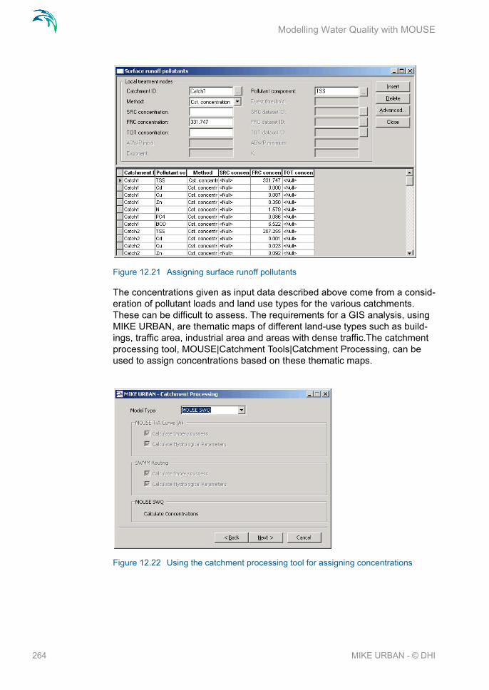
Modelling Water Quality with MOUSE
Figure 12.21 Assigning surface runoff pollutants
The concentrations given as input data described above come from a consid-eration of pollutant loads and land use types for the various catchments. These can be difficult to assess. The requirements for a GIS analysis, using MIKE URBAN, are thematic maps of different land-use types such as build-ings, traffic area, industrial area and areas with dense traffic.The catchment processing tool, MOUSE|Catchment Tools|Catchment Processing, can be used to assign concentrations based on these thematic maps.
Figure 12.22 Using the catchment processing tool for assigning concentrations
264 MIKE URBAN - © DHI

Storm Water Quality
Concentrations for different pollutants are assigned to the various land-use types and are combined with the sub-catchments. Typical pollutant concen-trations are provided in Table 12.6.
Table 12.6 Concentration for various pollutants
Pollutant Normal conc.
Low conc. High conc. Baseflow conc.
Unit
TSS 100 30 400 5 mg/l
Cd 0.5 0.15 1.5 0.005 g/l
Cu 30 15 100 5 g/l
Zn 130 50 400 10 g/l
Tot-N 1.8 0.6 3.5 0.2 mg/l
PO4 100 25 300 0.01 g/l
BOD 0.075*TSS 0.075*TSS 0.075*TSS 0.075*TSS mg/l
Table 12.7 The edit fields for the surface runoff pollutants dialog
Edit field Description
Catchment ID The ID of the catchment. It is recommeended to add pollutants only to catchments with a
surface runoff areas
Pollutant compo-nent
The ID name of the pollutant component in the AD model
Method Method = Cst concentration (method 1), Table concentration (method 2), EMC formula
(method 3)For all methods values in the fields for total
concentrations (TOT) overrides settings speci-fied for SRC and FRC.
SRC concentration Constant concentration value for the slow run-off component. Only used in RDI models.
FRC concentration Constant concentration value for the fast run-off component. This is also the component
used in the model A, B, C and UHM.
TOT concentration Constant concentration value for the total run-off component. Can be used in all models.
SRC dataset ID Only applied with method 2. ID identifier for the tabular dataset applied to the slow runoff com-
ponent.
FRC dataset ID Only applied with method 2. ID identifier for the tabular data set applied to the fast runoff com-
ponent
265

Modelling Water Quality with MOUSE
Cst. concentration (method 1)
The specified constant values of concentrations are assigned to the runoff and infiltration water.
Table concentration (method 2)
The concentration is based on a lookup in a set of tabular data given in the MOUSE menu system for tabular data, MOUSE|Curves & Relations. The run-off discharge divided with the total catchment area is the value from which the concentration is determined, i.e. c(t) = f( Q(t)/Atot ). Values are interpolated linearly between datasets. The tabular data editor in MOUSE is missing the Conc. vs. Q/A datatype. Data should be entered as an “Undefined” table type. The first column should hold flow/total catchment area values and the second column, concentrations.
Please verify the columns for Q/A and concentration.
EMC formula (method 3)
The event mean concentration (EMC) is computed based on the following formula.
(12.7)
As site mean concentration (SMC) is taken the specified constant concentra-tion value (FRC Concentration). The K-factor and the "exponent" is given as
TOT dataset ID Only applied with method 2. ID identifier for the tabular data set applied to the total runoff com-
ponent
K Only applied with method 3. K factor used in the formula.
Event threshold Threshold that defines when a runoff event starts and stops. Events with flows less than
the treshold are seen as dry weather when cal-culating the antcendent dry weather period
(ADWP)
ADWP initial The initial ADWP used before the first runoff event is detected in the data.
ADWP minimum If the duration between two events is smaller than the ADWP minimum then the two events
are perceived as only one event.
Exponent Only applied with method 3. Exponent used in the formula.
Table 12.7 The edit fields for the surface runoff pollutants dialog
Edit field Description
EMC SMC K ADWP onentexp =
266 MIKE URBAN - © DHI
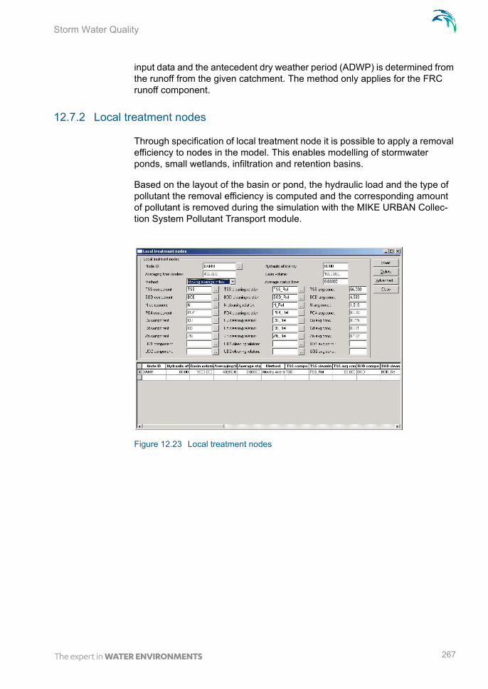
Storm Water Quality
input data and the antecedent dry weather period (ADWP) is determined from the runoff from the given catchment. The method only applies for the FRC runoff component.
12.7.2 Local treatment nodes
Through specification of local treatment node it is possible to apply a removal efficiency to nodes in the model. This enables modelling of stormwater ponds, small wetlands, infiltration and retention basins.
Based on the layout of the basin or pond, the hydraulic load and the type of pollutant the removal efficiency is computed and the corresponding amount of pollutant is removed during the simulation with the MIKE URBAN Collec-tion System Pollutant Transport module.
Figure 12.23 Local treatment nodes
267

Modelling Water Quality with MOUSE
Table 12.8 The edit fields for local treatment nodes
Edit field Description
Node ID The node ID that acts as a local treatment node. Typically basins, but not required.
Hydraulic effi-ciency
The hydraulic efficiency is determined on basis of the shape and layout of the pond. The following figures and table shows a num-ber of examples that can help to determine the hydraulic coefficient. When decided on the basin type that resembles the one that needs modelling the hydraulic efficiency can be interpreted from the table below. The val-ues have been obtained from numerical sim-ulations with the 2D model MIKE 21, which is recommended if high accuracy is of impor-tance.
Basin volume Basin volume used for the computation. If a nega-tive value, e.g. -1 is stated, then the volume is
computed from the geometry given.
268 MIKE URBAN - © DHI

Storm Water Quality
Figure 12.24 Various ponds and basins
The treatment node relations are used from the treatment relationships, see Figure 12.25.
Average time win-dow
In connection with the computation of the removal efficiency the average inflow to the basin is used. The average is computed as a moving average
with a time window equal to the average time win-dow. As default this is set to 43200 minutes (one
month).
Method The volume load is defined as the average flow divided with the basin volume. If Aver-age Method is 1 then the volume load is com-puted as the initial AvgFlow parameter divided by BasinVol, i.e. no moving average is computed. If AvgMethod is 2 then it is the moving average that is divided by BasinVol
Average start up flow
Until the average window is filled up with real model data the average start up is used as an ini-
tial value.
xxx component ID identifier of the attaining pollutant component in MOUSE AD.
xxx cleaning rela-tion
The final removal efficiency is computed based on a polynomium. The nine coefficients for this
are given in the local treatment coefficients.
xxx average con-centration
The computed removal efficiency is adjusted based on the level of the incoming average con-centration to the node. The average concentra-tion is computed the same way as the average flow and is using the same average time and
average method.
Table 12.8 The edit fields for local treatment nodes
Edit field Description
269

Modelling Water Quality with MOUSE
Figure 12.25 Local treatment relationship
Table 12.9 Proportions of the basins or ponds
Type Length [m] Width [m] Depth [m]
G1 300 60 1
G2 132 132 0.5, 1 and 2
G3 200 114 1
G4 188 96 0.5, 1 and 2
G5 132 132 1
G6 144 124 1
G7 236 76 1
Table 12.10 Edit fields for local treatment relationships
Edit field
Relationship ID for the relation
A1-3, B1-3, C1-3 Coefficients used in the polynomium
Low concentration Typical low concentration of incoming pollutants to the treatment node
High concentration Typical high concentration of incoming pollutants to the treatment node
Normal concentra-tion
Typical normal concentration of incoming pollut-ants to the treatment node
Factor low conc Correction factor for changing the computed removal efficiency over the time period of average
time is equal to the low concentration
270 MIKE URBAN - © DHI

Storm Water Quality
For average concentrations which are somewhere in between the sets of data given for low, normal and high, the correction factor is linearly interpo-lated. Typical correction factors are given in below table.
The polynomium for calculating the removal efficiency in % is stated as
(12.8)
Facor normal conc Correction factor for changing the computed removal efficiency over the time period of average
time is equal to the normal concentration
Factor hi conc Correction factor for changing the computed removal efficiency over the time period of average
time is equal to the high concentration
Table 12.11 Typical correction factors
Pollutant TSS BOD Ntot PO4 Cu Cd Zn
Low conc 0.7 1.0 2.2 1.1 0.6 0.5 0.6
Normal conc 1.0 1.0 1.0 1.0 1.0 1.0 1.0
High conc 1.1 0.9 0.4 0.6 1.6 1.4 1.7
Table 12.12 Hydraulic efficiency corresponding to basin G1-G7
Type Hydraulic efficiency
G1 0.93
G2 0.3
G3 0.96
G4 0.58
G5 0.52
G6 0.39
G7 0.69
Table 12.10 Edit fields for local treatment relationships
Edit field
R A1h2 B1H C1+ + q2 A2h2 B2H C2+ + q2 A3h2 B3H C3+ + q2+ +=
where
h:hydraulic efficiency (%)
q:volume load 0.001 m3 h m3
271

Modelling Water Quality with MOUSE
Figure 12.26 The coefficients for a number of pollutants have been determined through MIKE 21 simulations
In order to avoid unrealistic results a number of bounds have been set:
Removal efficiency must be between 1 and 95%
Volume load must be between 2.5 e-3 and 30 e-3 ([m3/ h]/m3)
Hydraulic efficiency must be between 30% and 90%
To sum up the methodology, for each treatment node and for each pollutant:
1. The hydraulic efficiency is determined based on the size and shape of the basin.
2. The volume load is determined as average flow divide with the basin vol-ume.
3. The removal efficiency is calculated based on the volume load, hydraulic efficiency and the pollutant relation given by the nine coefficients.
G2, 2 m depth 0.17
G2, 0.5 m depth 0.37
G4, 2 m depth 0.34
G4, 0.5 m depth 0.7
Table 12.12 Hydraulic efficiency corresponding to basin G1-G7
Type Hydraulic efficiency
272 MIKE URBAN - © DHI

Storm Water Quality
4. The average pollutant concentration is determined.
5. The removal efficiency is computed and adjusted with the correction fac-tor.
6. The removed load for the current time step is computed and subtracted in the MU CS Pollution Transport module.
273

Modelling Water Quality with MOUSE
274 MIKE URBAN - © DHI

MIKE URBAN CS - SWMM
User Guide
275

276 MIKE URBAN - © DHI

Terms and Concept
13 Hydraulic Network Modelling with SWMM
13.1 Terms and Concept
SWMM allows for the hydrodynamic simulation of flows and water levels in urban storm drainage and wastewater collection networks, thus providing an accurate information about the network functionality under a variety of bound-ary conditions. The hydrodynamic simulations can be extended with pollution and water-quality simulations. The model can also be enhanced by the vari-ety of real-time control functions. The simulations can be carried out for single events.
This Chapter provides a comprehensive guideline for the preparation of the basic SWMM hydrodynamic simulation models. Modelling of network hydro-dynamics in SWMM requires understanding of the information requirements. On the other hand, detailed knowledge of the computational theory is not essential.
The modelling process consists of the following distinct steps:
Definition of the network data
Specification of the boundary conditions
Adjustment of the computation parameters and running the simulations
Result analysis.
Furthermore, an important part of successful modelling is related to the model calibration and verification, which must ensure that the computed results fit reasonably well with the flow observations. These are important engineering activities in the modelling process.
A SWMM network within MIKE URBAN can be defined in one of the following ways. Please note that MIKE URBAN supports the EPA SWMM5 format (if you have a SWMM44 model you can locate conversion tools on the US EPA website).
Import of external data (e.g. GIS) into MIKE URBAN CS SWMM network
Copying network data from MIKE URBAN CS Asset network into MIKE URBAN CS SWMM network
Copying network data from MIKE URBAN CS MOUSE network into MIKE URBAN CS SWMM network
Graphical data digitalisation and manual data typing within MIKE URBAN
The last option is frequently used in a combination with one of the previous options as means for achieving a full consistency of the SWMM model.
277

Hydraulic Network Modelling with SWMM
The following paragraphs provide a comprehensive information on the SWMM network data model and the associated editors.
A SWMM model consists of the following elements:
Nodes
Conduits
Orifices
Pumps
Weirs
Outlets
13.2 Nodes
Nodes are hydraulic elements such as Junctions, Outfalls, Storage Units and Flow Dividers used in modelling a CS SWMM storm and sewer collec-tion system.
Junctions are defined as conveyance system nodes where links join together. Physically they can represent the confluence of natural surface channels, manholes in a sewer system, or pipe connection fittings. External inflows can enter the system at junctions. Excess water at a junction can become partially pressurized during surcharge events and can either be lost from the system or be allowed to pond atop the junction and subsequently drain back through it.
Outfalls are defined as terminal nodes of the conveyance system and used to define final downstream boundaries under Dynamic Wave flow routing. For other types of flow routing they behave as a junction. Only one link can be incident on an outfall node.
Storage Units are defined as conveyance system nodes that provide storage volume. Physically they could represent something as small as a catchbasin or as large as a lake. They are allowed to have any shape as described by a function or table of surface area versus height.
Flow Dividers are defined as conveyance system nodes used to split the total flow between exactly to two outflow conduits in a prescribed manner. Flow dividers are only active under Uniform or Kinematic Wave routing and are treated as simple junctions under Dynamic Wave routing.
The CS SWMM Nodes editor organizes the related input data for the hydrau-lic elements into the following groups:
Identification and Connectivity - General identification and location informa-tion
278 MIKE URBAN - © DHI

Nodes
Geometrical and Hydraulic Properties - Model related data
Junction - Geometry information
Storage Unit - Geometry information
Outfall - Outfall information
Flow Divider - Flow Divider information
Figure 13.1 The CS SWMM Nodes Editor
Identification and Connectivity
Table 13.1 The Nodes Identification and Connectivity Group
Edit field Description Used or required by simulations
Field name in datastructure
Asset ID Id in the asset network No AssetName
Junction ID Id of the node Yes MUID
Tag Optional label used to identify or catagorize the junction
No Tag
X Coordi-nate
X coordinate Yes
Y Coordi-nate
Y coordinate Yes
Data source Reference to an external data source from which the record
has been imported from
No DataSource
Status Status according to user speci-fied list
No Element_S
279

Hydraulic Network Modelling with SWMM
Geometrical and Hydraulic Properties
Junction
Figure 13.2 The CS SWMM Nodes - Junction Editor
Network type
Network type describes the type of network i.e Stormwater, Combined or separate. The list
of network types can be extended by user. Network
type can be specified for each hydraulic element.
No NetTypeNo
Links No
Description User's descriptive information related to the node
No Description
Table 13.2 The Nodes Geometrical and Hydraulic Properties Group
Edit field Description Used or required by simulations
Field name in datastructure
Junction Type
Definition of node as either Junction, Storage Unit, Outfall
or Flow Divider
Yes TypeNo
Table 13.1 The Nodes Identification and Connectivity Group
Edit field Description Used or required by simulations
Field name in datastructure
280 MIKE URBAN - © DHI

Nodes
Storage Unit
The geometry of a Storage Unit can be defined by a Functional geometry or a Tabular geometry description. As an example a Storage Unit whose cross-sectional area remains constant with depth (e.g. a cylinder or cube) can be described by using a FUNCTIONAL geometry type whose coefficient equals the cross-sectional area and whose exponent is 0.
Table 13.3 The Nodes Junction
Edit field Description Used or required by simulations
Field name in datastructure
Ponded Area
Area occupied by ponded water atop the junction after flooding occurs. If the Allow Ponding analysis option is
turned on, a non-zero value of this parameter will allow
ponded water to be stored and subsequently returned to the
conveyance system when capacity exists. Default is,
allow ponding is not turned on.
No Apond
Invert Level Invert elevation of the node Yes Einv
Max Depth Maximum depth of node (i.e. from invert to ground surface)
Yes Dmax
Inital Depth Initial depth of water at the node at the start of the simula-
tion
No D0
Surch. Depth
Additional depth of water beyond the maximum depth
that is allowed before the junc-tion floods. This parameter can
be used to model Bolted / Sealed manholes
No Dsur
281

Hydraulic Network Modelling with SWMM
Figure 13.3 The CS SWMM Nodes - Storage Unit Editor
Table 13.4 The Nodes Storage Unit
Edit field Description Used or required by simulations
Field name in datastructure
Geometry Type
Definition of the type of geom-etry description of the Storage Unit (Functional or Tabular)
Yes GeomTypeNo
Coefficient Coefficient for the Functional relationship between storage
depth and surface area
Yes, if Func-tional is chosen
GeomCoeff
Exponent Exponent for the Functional relationship between storage
depth and surface area
Yes, if Func-tional is chosen
GeomExponent
Constant Constant value for the Func-tional relationship between storage depth and surface
area
Yes, if Func-tional is chosen
GeomConst
Evaporation Fraction of potential evapora-tion realized
No Fevap
Geometry ID ID of the Tabular geometrical description. The geometry is specified relative to the invert level. This ensures reusability of the geometry for different Storage Units with different
inverts
Yes if Tabular is chosen
GeomID
Infiltration Option to apply optional Green-Ampt infiltration param-eters so that the storage unit can serve as an infiltration
basin
Yes StorageInfiltra-tionNo
282 MIKE URBAN - © DHI

Nodes
Outfall
Definition of an outfall in an urban drainage network is optional for uniform flow (UF) and Kinematic Wave (KW) routing. However when applying Dynamic Wave routing at least one outfall in the urban drainage system must be defined. It is possible to select between five types of outfalls, FREE, NOR-MAL, FIXED, TIDAL and TIMESERIES.
FREE outfall bases the outfall stage on the smaller of the critical and nor-mal depths of flow in the connecting conduit.
NORMAL outfall uses just the normal depth of flow.
FIXED outfall uses a constant water elevation at all times.
TIDAL outfall has outfall stage varying in a repeating fashion over a tidal period.
TIMESERIES outfall allows the outfall stage varying in any specified manner over time.
Suction Head
Average value of soil capillary suction along wetting front
Yes, if Infiltra-tion is chosen
StorageSuction-Head
Conductivity Soil saturated hydraulic con-ductivity
Yes, if Infiltra-tion is chosen
StorageConduc-tivity
Initial Deficit Fraction of soil volume that is initially dry
Yes, if Infiltra-tion is chosen
StorageInitial-Deficit
Table 13.4 The Nodes Storage Unit
Edit field Description Used or required by simulations
Field name in datastructure
283

Hydraulic Network Modelling with SWMM
Figure 13.4 The CS SWMM Nodes - Outfall Editor
Flow Divider
Three different types of dividers can be specified for each divider node
OVERFLOW divider, all flow above the non-diverted conduits full flow depth is diverted
CUTOFF divider, all flow above the cutoff level is diverted.
TABULAR divider, a curve is supplied that specifies the amount of diverted flow to total flow.
Table 13.5 The Nodes Outfall
Edit field Description Used or required by simulations
Field name in datastructure
Outfall Type If Node Type is selected to Outfall then type of Tide Gate
must be selected
Yes FlapGate-TypeNo
Tidal Curve Outfall stage as a function of hour of day over a complete tidal cycle. Curve is specified
in Tabular Data
Yes if Tide Gate is of type TIDAL
TideGateID
Outfall Time Series
Outfall stage variation over time. Time series specified in
Time Series
Yes if Tide Gate is of type TIME-
SERIES
TideGateTSID
Fixed Stage Fixed position of Tide Gate Yes if Tide Gate is of type FIXED
FixedStage
Tide Gate If TideGate (FlapGate) present then backwater is prevented.
No FlapGateNo
284 MIKE URBAN - © DHI

Nodes
WEIR divider the diverted flow is linearly proportional to the total flow in excess of some minimum flow
Figure 13.5 The CS SWMM Nodes - Flow DIvider Editor
Table 13.6 The Flow Divider
Edit field Description Used or required by simulations
Field name in datastructure
Type Divider Type of Divider is selected to either Overflow, Cutoff, Tabu-
lar, or Weir
Yes, if Junction Type is a Flow
Divider
DividerTypeNo
Divided To The ID of the link that receives the diverted flow
Yes LinkID
Cut Off Flow Cutoff flow value used for a Cutoff divider
Yes, if Type Divider is Cutoff
CutoffFlow
Divided Flow Series
ID of diversion flow series for a Tabular divider
Yes, if Type Divider is Tabu-
lar
DivertedFlowID
Min Flow Minimum flow at which diver-sion continues for a Weir
divider
Yes, if Type Divider is Weir
DivertedMin-Flow
Max Depth Maximum depth above invert at which proportional diversion
continues for a Weir divider
Yes, if Type Divider is Weir
DivertedMax-Depth
Div Coeff Coefficient which determines what fraction between the min and max flow the diverted flow will be given the fraction that current water depth is of the max. depth for a Weir divider
Yes, if Type Divider is Weir
DivertionCoeff
285

Hydraulic Network Modelling with SWMM
13.3 Conduits
Conduits are pipes or channels that move water from one node (Junctions, Storage Units, Flow Dividers and Outfalls) to another node in the drainage system. Their cross-sectional shapes can be selected from a variety of stand-ard open and closed geometries. Irregular natural cross-section shapes are also supported.
The Conduits editor organizes the related input data into the following groups:
Identification and Connectivity - General identification and location infor-mation
Geometrical and Hydraulic Properties - Model related data
Conduit Geometry - Geometry information
Hydraulic Losses - Model Headlosses
Miscellaneous
Figure 13.6 The CS SWMM Conduits Editor
Identification and Connectivity
286 MIKE URBAN - © DHI

Conduits
Geometrical and Hydraulic Properties
Table 13.7 The Conduits Identification and Connectivity Group
Edit field Description Used or required by simulations
Field name in datastructure
Asset ID Id in the asset network No AssetName
Link ID Id of the Link Yes MUID
Tag Optional label used to identify or catagorize the junction
No Tag
Inlet Node ID Upstream Node Yes
Outlet Node ID
Downstream Node Yes
Data source Reference to an external data source from which the record
has been imported from
No DataSource
Status Status accoording to user specified list
No Element_S
Network type
Network type describes the type of network i.e Stormwater, Combined or separate. The list
of network types can be extended by user. Network
type can be specified for each hydraulic element.
No NetTypeNo
Description User's descriptive information related to the node
No Description
Table 13.8 The Conduits Geometrical and Hydraulic Properties
Edit field Description Used or required by simulations
Field name in data-structure
Conduit Geometry
Conduit Shape Cross section shape
Yes ShapeTypeNo
Length Length of conduit Yes Length
Geom. Depth Depth or Diameter of conduit
Yes all shapes except IRREGU-
LAR shape
Depth
Sediment Depth Sediment depth in conduit
Yes, if CIRCULAR shape
SedimentDepth
287

Hydraulic Network Modelling with SWMM
Bottom Width Width of bottom Yes, if MODBAS-KETHANDLE
shape
BottomWidth
Top Width Width of top Yes, if RECT_-CLOSED,
RECT_OPEN,TRAPEZOIDAL,TRIANGULAR,
ARCH,PARABOLIC,
POWER,RECT_TRIANGU-
LAR, andRECT_ROUND
shapes
TopWidth
Bottom Radius Radius of bottom Yes, if RECT_ROUND
shape
BottomRadius
Transect ID ID of Transect ID which is defined in
Transects
Yes, if IRREGU-LAR
TransectID
Inlet Invert Offset heigth of upstream end of
conduit above the invert elevation of its upstream node
InletInvert
Outlet Invert Offset heigth of downstream end of conduit above the invert elevation of
its downstream node
OutletInvert
Left Side Slope Left side slope of trapez
Yes, if TRAPEZOI-DAL shape
LeftSideSlope
Right Side Slope Right side slope of trapez
Yes if TRAPEZOI-DAL shape
RightSideSlope
Exponent Exponent in power function for
describing the shape
Yes, if POWER Exponent
Triangle Height Height of triangular shape
Yes, if RECT_TRI-ANGULAR shape
TriangleHeight
Table 13.8 The Conduits Geometrical and Hydraulic Properties
Edit field Description Used or required by simulations
Field name in data-structure
288 MIKE URBAN - © DHI

Orifices
Minor losses are only computed for the DW, Dynamic wave routing option. The minor losses are computed as K*v2/2g.
13.4 Orifices
Orifices are openings in the wall of a manhole junction or storage unit used to model outlet and diversion structures in drainage systems. Orifices belong to the group of Link components connecting two nodes. An orifice can have either a circular or rectangular shape, be located either at the bottom or along the side of the upstream node, and have a flap gate to prevent backflow.
Barrels A conduit can have a multiple number of barrels mean-
ing that it consists of a multiple num-
ber of parallel pipes of equal size, slope and
roughness. Default value is 1.
Yes Barrels
Hydraulic Losses
Roughness Manning, n-value for the conduit
Yes Roughness
Entry Loss Coeff Entry Loss coeffi-cient (using
entrance velocity)
No EntryLossCoeff
Average Loss Coeff
Average loss coef-ficient (using aver-
age velocity in conduit)
No AvgLossCoeff
Exit Loss Coeff Exit loss coefficient (using exit velocity)
No ExitLossCoeff
Miscellaneous
Initial Flow Flow in conduit at start of simulation
No InitialFlow
Flap Gate Flapgate prevents backwater flow.
Default is No (not present)
No FlapGateNo
Max Flow Maximum flow allowed
Yes MaxFlow
Culvert Code Culvert type code Yes
Table 13.8 The Conduits Geometrical and Hydraulic Properties
Edit field Description Used or required by simulations
Field name in data-structure
289

Hydraulic Network Modelling with SWMM
Orifices attached to storage units are active under all types of flow routing. Those attached to other types of nodes are active only under Dynamic Wave flow routing, otherwise the flow through them is zero. The flow through an ori-fice is computed based on the area of its opening, its discharge coefficient, and the head difference across the orifice. The area of an orifice's opening can be controlled dynamically through user-defined control rules.
The Orifices editor organizes the related input data into the following groups:
Identification and Connectivity - General identification and location infor-mation
Geometrical and Hydraulic Properties - Model related data
Orifices Geometry - Geometry information
Hydraulic Properties - Model Headlosses
Figure 13.7 The CS SWMM Orifices Editor
Identification and Connectivity
Table 13.9 The Orifices Identification and Connectivity Group
Edit field Description Used or required by simulations
Field name in datastructure
Asset ID Id in the asset network No AssetName
Orifice ID Id of the Orifice Yes MUID
Tag Optional label used to identify or catagorize the junction
No Tag
Location Node location of orifice Yes
290 MIKE URBAN - © DHI

Orifices
Geometrical and Hydraulic Properties
To Discharge to Node Yes
Data source Reference to an external data source from which the record
has been imported from
No DataSource
Status Status accoording to user specified list
No Element_S
Network type
Network type describes the type of network i.e Stormwater, Combined or separate. The list
of network types can be extended by user. Network
type can be specified for each hydraulic element.
No NetTypeNo
Description User's descriptive information related to the node
No Description
Table 13.10 The Orifices Geometrical and Hydraulic Properties
Edit field Description Used or required by simulations
Field name in data-structure
Orifices Geometry
Orifice Type Type of orifice, SIDE or BOTTOM
Yes TypeNo
Orifice Shape The geometry of the orifice opening,
CIRCULAR or RECT_CLOSED
Yes ShapeTypeNo
Height Height/Diameter of shape
Yes Height
Width Width of RECT_-CLOSED shape
Yes, if Orifice shape is RECT_-
CLOSED
Width
Crest Height Offset height of ori-fice’s bottom from invert of upstream
node
Yes (if Orifice Type is BOTTOM then
Crest Height is set zero in SWMM
engine)
CrestHeight
Hydraulic Properties
Table 13.9 The Orifices Identification and Connectivity Group
Edit field Description Used or required by simulations
Field name in datastructure
291

Hydraulic Network Modelling with SWMM
13.5 Pumps
Pumps are drainage system links used to lift water to higher elevations. The relation between a pump's flow rate and conditions at its end nodes is described by a pump curve. MIKE URBAN CS SWMM represents a pump as a link connecting two nodes, where the pump itself is placed at the upstream node.
The Pumps editor organizes the related input data into the following groups:
Identification and Connectivity - General identification and location infor-mation
Pump Properties - Model related data
Figure 13.8 The CS SWMM Pumps Editor
Discharge Coeff Discharge coeffi-cient
Yes DischargeCoeff
Flap gate Flapgate prevents reverse flow
through the ori-fice, default is No
No FlapGateNo
Table 13.10 The Orifices Geometrical and Hydraulic Properties
Edit field Description Used or required by simulations
Field name in data-structure
292 MIKE URBAN - © DHI

Pumps
Identification and Connectivity
Pump Properties
Table 13.11 The Pumps Identification and Connectivity Group
Edit field Description Used or required by simulations
Field name in datastructure
Asset ID Id in the asset network No AssetName
Pump ID Id of the Pump Yes MUID
Tag Optional label used to identify or catagorize the junction
No Tag
Location Location of Pump Yes
To Receiving Node Yes
Data source Reference to an external data source from which the record
has been imported from
No DataSource
Status Status accoording to user specified list
No Element_S
Network type
Network type describes the type of network i.e Stormwater, Combined or separate. The list
of network types can be extended by user. Network
type can be specified for each hydraulic element.
No NetTypeNo
Description User's descriptive information related to the node
No Description
Table 13.12 The Pumps Properties Group
Edit field Description Used or required by simulations
Field name in data-structure
Pump Curve ID Reference to a Pump curve
defined as one of the four possible
pump curve types in Tabular Data
(Curves).
Yes PumpCurveID
Initial Status The initial status is On
No InitialStatusNo
293

Hydraulic Network Modelling with SWMM
For each individual pump a pump curve must be defined. Pump curves are defined in Tabular Data (Curves). Following four different types of pump curves are supported:
Type1 - an off-line pump with a wet well where flow increases incremen-tally with wet well volume
Type2 - an in-line pump where flow increases incrementally with node depth
Type3 - an in-line pump where flow varies continuously with head differ-ence between the inlet and outlet nodes
Type4 - a variable speed in-line pump where flow varies continuously with node depth
The on/off status of pumps can be controlled dynamically through user-defined Control Rules.
13.6 Weirs
Weirs, like orifices, are used to model outlet and diversion structures in a drainage system. Weirs are typically located in a chamber of a manhole, along the side of a channel, or along the top of a storage unit. MIKE URBAN CS SWMM represents a weir as a link connecting two nodes, where the weir itself is placed at the upstream node. A flap gate can be included to prevent backflow.
The Weir editor organizes the related input data into the following groups:
Identification and Connectivity - General identification and location infor-mation
Geometrical and Hydraulic Properties - Model related data
Weir Geometry - Geometry information
Hydraulic Properties
294 MIKE URBAN - © DHI

Weirs
Figure 13.9 The CS SWMM Weir Editor
Identification and Connectivity
Table 13.13 The Weir Identification and Connectivity Group
Edit field Description Used or required by simulations
Field name in datastructure
Asset ID Id in the asset network No AssetName
Weir ID Id of the Weir Yes MUID
Tag Optional label used to identify or catagorize the junction
No Tag
Location Node location of Weir Yes
To Receiving Node Yes
Data source Reference to an external data source from which the record
has been imported from
No DataSource
Status Status accoording to user specified list
No Element_S
295
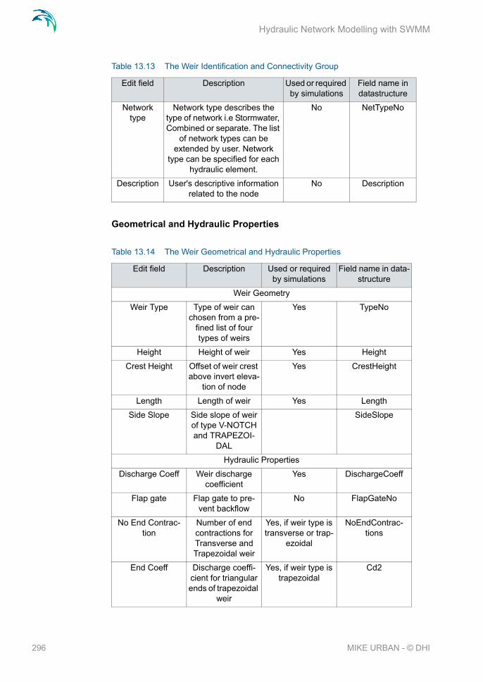
Hydraulic Network Modelling with SWMM
Geometrical and Hydraulic Properties
Network type
Network type describes the type of network i.e Stormwater, Combined or separate. The list
of network types can be extended by user. Network
type can be specified for each hydraulic element.
No NetTypeNo
Description User's descriptive information related to the node
No Description
Table 13.14 The Weir Geometrical and Hydraulic Properties
Edit field Description Used or required by simulations
Field name in data-structure
Weir Geometry
Weir Type Type of weir can chosen from a pre-
fined list of four types of weirs
Yes TypeNo
Height Height of weir Yes Height
Crest Height Offset of weir crest above invert eleva-
tion of node
Yes CrestHeight
Length Length of weir Yes Length
Side Slope Side slope of weir of type V-NOTCH and TRAPEZOI-
DAL
SideSlope
Hydraulic Properties
Discharge Coeff Weir discharge coefficient
Yes DischargeCoeff
Flap gate Flap gate to pre-vent backflow
No FlapGateNo
No End Contrac-tion
Number of end contractions for Transverse and Trapezoidal weir
Yes, if weir type is transverse or trap-
ezoidal
NoEndContrac-tions
End Coeff Discharge coeffi-cient for triangular ends of trapezoidal
weir
Yes, if weir type is trapezoidal
Cd2
Table 13.13 The Weir Identification and Connectivity Group
Edit field Description Used or required by simulations
Field name in datastructure
296 MIKE URBAN - © DHI

Outlets
Four varieties of weirs (Weir Type) are available, each with a slightly different formula for computing flow as a function of area, discharge coefficient and head difference across the weir:
Transverse (rectangular shape)
Sideflow (rectangular shape)
V-notch (triangular shape)
Trapezoidal (trapezoidal shape)
Weirs attached to storage units are active under all types of flow routing. Those attached to other types of nodes are active only under Dynamic Wave flow routing, otherwise the flow through them is zero.
The height of the weir crest above the inlet node invert can be controlled dynamically through user-defined Control Rules. This feature can be used to model RTC controlled Weirs and inflatable dams.
13.7 Outlets
Outlets are flow control devices which are typically used to control outflows from storage units. They are used to model special flow-head relations that cannot be characterized by either orifices or weirs. MIKE URBAN CS SWMM represents an Outlet as a link connecting two nodes, where the outlet itself is placed at the upstream node.
Outlets attached to storage units are active under all types of flow routing. Those attached to other types of nodes are active only under Dynamic Wave flow routing, otherwise the flow through them is zero.
The Outlet editor organizes the related input data into the following groups:
Identification and Connectivity - General identification and location infor-mation
Geometrical and Hydraulic Properties - Model related data
Outlet Geometry - Geometry information
Hydraulic Properties
297

Hydraulic Network Modelling with SWMM
Figure 13.10 The CS SWMM Outlets Editor
Identification and Connectivity
Table 13.15 The Outlets Identification and Connectivity
Edit field Description Used or required by simulations
Field name in datastructure
Asset ID Id in the asset network No AssetName
Outlet ID Id of the Outlet Yes MUID
Tag Optional label used to identify or catagorize the junction
No Tag
Location Node location of Outlet Yes
To Recieving Node Yes
Data source Reference to an external data source from which the record
has been imported from
No DataSource
Status Status accoording to user specified list
No Element_S
Network type
Network type describes the type of network i.e Stormwater, Combined or separate. The list
of network types can be extended by user. Network
type can be specified for each hydraulic element.
No NetTypeNo
Description User's descriptive information related to the node
No Description
298 MIKE URBAN - © DHI

Transects
Geometrical and Hydraulic Properties
An outlet can have a flap gate which restricts flow to only one direction and prevents backwater flow.
The flow through an outlet is determined by a user-supplied function or table of flow versus head difference across the outlet (Q-curve ID). This flow can be controlled dynamically through user-defined Control Rules.
13.8 Transects
Transects refer to the geometric data that describe how bottom elevation var-ies with horizontal distance over the cross section of a natural channel or irregular-shaped conduit. The figure below displays an example of a transect for a natural channel.
Table 13.16 The Outlets Geometrical and Hydraulic Properties
Edit field Description Used or required by simulations
Field name in datastructure
Outlet Geometry
Outlet Type
Outlet Type, 1=TABUAR/DEPTH,2 = TABULAR/HEAD
3 = FUNCIONAL /DEPTH4 = FUNCTIONAL / HEAD
Yes TypeNo
Height Minimum water depth at upstream node of outflow to
occur
Yes Height
Hydraulic Properties
Coeffi-cient
Coefficient of power function that relates outflow to head across the outlet fir a Func-
tional outlet
Yes, if Outlet Type is Functional
Qcoeff
Q-curve ID
ID of rating curve with outflow rate as a function of head
across the outlet for a tabular outlet
Yes if Outlet Type is Tabular
QcurveID
Exponent Exponent of power function that relates outflow to head across the outlet fir a Func-
tional outlet
Yes, if Outlet Type is Functional
Qexpon
Flap Gate
Flap gate Yes FlapGateNo
299

Hydraulic Network Modelling with SWMM
Figure 13.11 Definition of the Transect cross-sectional data
Each transect are given an unique ID. When a IRREGULAR shape is chosen as the shape type for a conduit then a reference to one of the user defined Transects must be made for representing the crossectional shape.
The SWMM engine converts these data into tables of area, top width, and hydraulic radius versus channel depth. In addition, as shown in the figure above, each Transect can have a left and right overbank section whose Man-ning's roughness can be different from that of the main channel. This feature can provide more realistic estimates of channel conveyance under high flow conditions.
The Transects editor organizes the related input data into the following groups:
Identification and Connectivity - General identification and location infor-mation
Geometrical and Hydraulic Properties - Model related data
Transect Geometry - Geometry information
Manning, n - Roughness for Channel and Overbanks
300 MIKE URBAN - © DHI

Transects
Figure 13.12 The SWMM Transects Editor Dialog
The above Transect can be viewed graphically by clicking on the Graph but-ton
Figure 13.13 Graphically display of the transect
301
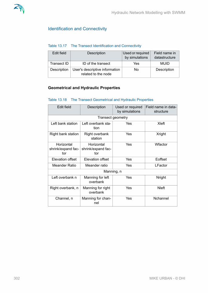
Hydraulic Network Modelling with SWMM
Identification and Connectivity
Geometrical and Hydraulic Properties
Table 13.17 The Transect Identification and Connectivity
Edit field Description Used or required by simulations
Field name in datastructure
Transect ID ID of the transect Yes MUID
Description User's descriptive information related to the node
No Description
Table 13.18 The Transect Geometrical and Hydraulic Properties
Edit field Description Used or required by simulations
Field name in data-structure
Transect geometry
Left bank station Left overbank sta-tion
Yes Xleft
Right bank station Right overbank station
Yes Xright
Horizontal shrink/expand fac-
tor
Horizontal shrink/expand fac-
tor
Yes Wfactor
Elevation offset Elevation offset Yes Eoffset
Meander Ratio Meander ratio Yes LFactor
Manning, n
Left overbank n Manning for left overbank
Yes Nright
Right overbank, n Manning for right overbank
Yes Nleft
Channel, n Manning for chan-nel
Yes Nchannel
302 MIKE URBAN - © DHI

Tabular Data (Curves)
Cross-sectional data, (Station, Elevation)
13.9 Tabular Data (Curves)
Tabular Data (Curves) are used to describe a functional relationship between two quantities. Following types of curves are available:
Storage - defines the geometry of a Storage Unit node by describing the variation of surface area as a function of water depth
Diversion - defines how the diverted outflow from a Flow Divider node is related to the total inflow.
Tidal - defines how the stage at an Outfall node varies by the hour of the day.
Rating - relates flow through an Outlet link to the head difference across the outlet
Pump - relates flow through a Pump link to the depth or volume at the upstream node or to the head delivered by the pump. Following four types of Pump relations are available
Table 13.19 The Transect Cross-sectional data
Edit field Description Used or required by simulations
Field name in data-structure
Station Station, distance of the crosssection
station from some fixed reference
Yes Station
Elevation Elevation of the channel bottom at
a cross-section station relative to some fixed rela-tive reference
Yes Elevation
303

Hydraulic Network Modelling with SWMM
Type 1 - an off-line pump with a wet well where flow increases incrementally with the available wet well volume.
Type 2 - an in-line pump where flow increases incrementally with inlet node depth.
304 MIKE URBAN - © DHI

Tabular Data (Curves)
Type 3 - an in-line pump where flow varies continuously with head difference between the inlet and outlet nodes.
Type 4 - a variable speed in-line pump where flow varies contin-uously with inlet node depth.
The Tabular Data (Curves) editor organizes the related input data into the fol-lowing groups:
Identification and Connectivity - General identification and location infor-mation
305

Hydraulic Network Modelling with SWMM
Figure 13.14 The SWMM Tabular Data (Curves) dialog
Identification and Connectivity
Tabular data in Grid
Table 13.20 The Tabular Data (Curves) Identification and Connectivity
Edit field Description Used or required by simulations
Field name in datastructure
Curve ID ID of the Curve Yes MUID
Type Type of Curve Yes TypeNo
Description User's descriptive information related to the node
No Description
Table 13.21 The Tabular data values
Edit field Description Used or required by simulations
Field name in data-structure
‘Value1’ Value1, depended on Type of curve (Depth, Inflow, Hour, Volume,
Head)
Yes Value1
‘Value2’ Value2, depended on Type of curve (Area, Outflow, Stage, Flow)
Yes Value2
306 MIKE URBAN - © DHI

Controls
13.10 Controls
Controls is used to determine pumps and regulators will be controlled based on simulation time or conditions at specific nodes and links.
The Controls editor organizes the related input data into the following groups:
SWMM control rules - Identification and Connectivity
The control rules are specified in a upper grid
Figure 13.15 The SWMM Controls Editor Dialog
SWMM control rules
Table 13.22 The SWMM control rules Group
Edit field Description Used or required by simulations
Field name in datastructure
Rule ID ID of the specific rule Yes MUID
Priority Priority of the rule Yes Priority
Description User's descriptive information related to the node
No Description
307

Hydraulic Network Modelling with SWMM
Please note there can only be either a Condition or an Action in one line.
Table 13.23 The upper grid Group
Edit field Description Used or required by simulations
Field name in datastructure
TypeNo Condition or Action Yes TypeNo
OperatorNo IF, AND, OR, THEN, ELSE Yes Operators
CObjectNo Node, Link, Pump, Orifice, Weir or Simulation
Yes CObjectNo
CId ID of the object Yes CId
CAttributeNo Depth, Head, Inflow, Flow, Set-ting, Time, Date, Clocktime
Yes CAttributeNo
CRelationNo =, <, >, <>, <=,>= Yes CRelationNo
AObjectNo Node, Link, Pump, Orifice, Weir or Simulation
Yes AObjectNo
AId ID of the object Yes AId
AAttributeNo Node, Link, Pump, Orifice, Weir or Simulation
Yes AAttributeNo
RValue Value Yes RValue
308 MIKE URBAN - © DHI

Terms and Concepts
14 Hydrological Modelling with SWMM
14.1 Terms and Concepts
Various hydrological processes that produce runoff from urban areas can be modelled by SWMM. These include:
time-varying rainfall
evaporation of standing surface water
snow accumulation and melting
rainfall interception in depression storage
infiltration of rainfall into upper soil layers
percolation of infiltrated water into groundwater layers
interflow between groundwater and the conveyance system
nonlinear reservoir routing of overland flow
Spatial variability in all of these processes is achieved by dividing a study area into a smaller collection of homogeneous areas. In the literature different terms are used for describing the delineation of large study areas into smaller sub-areas each containing its own fraction of pervious and impervious areas.
Following terminology for the delineation of areas is widely used in North America
Basin
Sub-basin
Watershed/Sewershed
Catchment
Throughout this documentation the term Catchments will be used as term for the smallest hydrological unit of land.
Overland flow can be routed between catchments or to load points of a drain-age conveyance system.
14.2 Catchments
Catchments are hydrological units of land whose topography cause surface runoff to drain to a single point. The user is responsible for the delineation of a watershed/sewershed into a compatible number of catchments, and for identifying the outlet point of each catchment. Outlet points can be either nodes of the conveyance system or other catchments.
Catchments can be divided into pervious and impervious sub-areas. Surface runoff can infiltrate into the upper soil zone of the pervious sub-area, but not
309

Hydrological Modelling with SWMM
through the impervious sub-area. Impervious areas are themselves divided into two sub-areas - one that contains depression storage and another that does not. A portion of the runoff flow from one sub-area in a catchment can be routed to the other sub-area, or both sub-areas can drain to the catchment outlet.
The CS SWMM Catchments Editor organizes the related input data for the catchment into the following groups. The catchment data in the Catchment Editor is shared by CS models:
General information
Physical Properties
Location
Figure 14.1 The SWMM Catchments Editor
310 MIKE URBAN - © DHI

Catchments
Description of the input fields for catchments
Location
Physical Properties
Table 14.1 The Catchment table
Edit field Description Used or required by simulations
Field name in datastructure
Catchment ID
Id in the catchment Yes MUID
Status Status according to user speci-fied list
No Element_S
Type Type which describes the type of catchment. The list of catch-ment types is user sepcified.
No NetTypeNo
Table 14.2 The Catchment Location Group
Edit field Description Used or required by simulations
Field name in datastructure
System User defined list No SystemID
Sub-system User defined list No SubSystemID
X-coordinate X - coordinate of center of catchment
No X
Y-coordinate Y - coordinate of center of catchment
No Y
Table 14.3 The Catchment Physical Properties Group
Edit field Description Used or required by simulations
Field name in datastructure
Total area Total area of polygon Yes Area_C
Drainage area
User defined catchment area - overwrites Total area
No Area
Max. level Catchment max. level, can be calculated from DEM by GIS
function
No MaxLevel
Min. level Catchment min. level, can be calculated from DEM by GIS
function
No MinLevel
311

Hydrological Modelling with SWMM
General Information
14.3 Surface Routing
The concept of the surface runoff used by CS SWMM is illustrated in the fig-ure below. Each catchment surface is treated as a nonlinear reservoir. Inflow comes from precipitation and upstream catchments. There are several out-flows, including infiltration, evaporation, and surface runoff.
The capacity of this "reservoir" is the maximum depression storage, which is the maximum surface storage provided by ponding, surface wetting, and interception.
Surface runoff per unit area, Q, occurs only when the depth of water in the "reservoir" exceeds the maximum depression storage, dp, in which case the outflow is given by Manning's equation (Kinematic Wave).
Figure 14.2 Nonlinear Reservoir Concept
Depth of water over the catchment is continuously updated with time by solv-ing numerically a water balance equation over the catchment.
The CS SWMM Routing Editor organizes the related input data for the catch-ment concerning the surface runoff into following groups:
Identification and Connectivity
Table 14.4 The Catchment General Information Group
Edit field Description Used or required by simulations
Field name in datastructure
Description Descriptive user field No Description
312 MIKE URBAN - © DHI

Surface Routing
Hydrology and Hydraulic Properties
313

Hydrological Modelling with SWMM
Identification and Connectivity
Hydrology and Hydraulic Properties
Table 14.5 The Routing Identification and Connectivity Group
Edit field Description Used or required by simulations
Field name in datastructure
Catchment ID
ID of the Catchment Yes CatchID
Load Point ID
ID of Node that receives the surface runoff
Yes, If Route-ToNo is OUT-
LET
OutletNodeID
Outlet Catchment
ID
ID of Catchment that receives the surface runoff
Yes, If RoutToNo is IMPERV or
PERV
OutletCatch-mentID
Tag Optional label used to identify or categorize the junction
No Tag
Description User's descriptive information related to the node
No Description
Raingage ID ID of Rain Gauge containing the precipitation used for this
catchment
Yes RaingageID
Table 14.6 The Routing Hydrology and Hydraulic Properties Group
Edit field Description Used or required by simulations
Field name in datastructure
Width Width of catchment Yes Width
Ground Slope
Ground slope of catchment in percentage
Yes Slope
Impervious-ness
Impervious part of the catch-ment area in percentage
Yes Impervious
Imperv. Manning
Manning Number for the Impervious part of the area
Yes NImperv
Pervious Manning
Manning Number for the Pervi-ous part of the area
Yes NPerv
Imperv. d. Storage
Size of Impervious Depression Storage
Yes DImperv
Perv. d. Stor-age
Size of Pervious Depression Storage
Yes DPerv
%DCIA w/o d. storage
Percent of the impervious area with no depression storage
Yes ImpervPctZero
314 MIKE URBAN - © DHI

Infiltration
14.4 Infiltration
Infiltration is the process of rainfall penetrating the ground surface into the soil over the pervious areas of catchments. CS SWMM supports three choices for modelling infiltration:
Horton's EquationThis method is based on empirical observations showing that infiltration decreases exponentially from an initial maximum rate to some minimum rate over the course of a long rainfall event. Input parameters required by this method include the maximum and minimum infiltration rates, a decay coeffi-cient that describes how fast the rate decreases over time, and a regenera-tion constant that describes the restoration of infiltration rate during dry periods.
Green-Ampt MethodThis method for modelling infiltration assumes that a sharp wetting front exists in the soil column, separating soil with some initial moisture content below from saturated soil above. The input parameters required are the initial moisture deficit of the soil, the soil's hydraulic conductivity, and the suction head at the wetting front.
Curve Number MethodThis approach is adopted from the NRCS (SCS) Curve Number method for estimating runoff. It assumes that the total infiltration capacity of a soil can be found from the soil's tabulated Curve Number. During a rain event this capac-ity is depleted as a function of cumulative rainfall and remaining capacity. The input parameters for this method are the curve number, the soil's hydraulic conductivity (used to estimate a minimum separation time for distinct rain events), and a regeneration constant that describes the restoration of infiltra-tion capacity during dry periods.
Only one of the above infiltration methods can be used in one simulation - the option for which method is used is set in Run SWMM5, tabsheet RUNOFF.
The CS SWMM Infiltration Editor organizes the related input data for these three infiltration approaches into following groups:
Subarea routing
Where does the surface rout-ing go to
Yes RouteToNo
Curb length Total length of Curbs in the catchment. Only used when
pollutant buildup is normalized to curb length
No CurbLength
Table 14.6 The Routing Hydrology and Hydraulic Properties Group
Edit field Description Used or required by simulations
Field name in datastructure
315
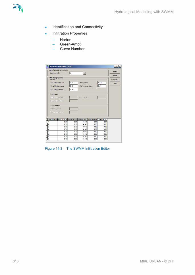
Hydrological Modelling with SWMM
Identification and Connectivity
Infiltration Properties
– Horton– Green-Ampt– Curve Number
Figure 14.3 The SWMM Infiltration Editor
316 MIKE URBAN - © DHI

RDII
Identification and Connectivity
Infiltration Properties
14.5 RDII
Rainfall Dependent Inflow/Infiltration (RDII) - These are stormwater flows that enter sanitary or combined sewers due to "inflow" from direct connections of downspouts, sump pumps, foundation drains, etc. as well as "infiltration" of
Table 14.7 The Infiltration Identification and Connectivity Group
Edit field Description Used or required by simulations
Field name in datastructure
Catchment ID
ID of the Catchment Yes CatchID
Table 14.8 The Infiltration Properties Group
Edit field Description Used or required by simulations
Field name in datastructure
Horton
Max infiltra-tion rate
Max Infiltration Rate Yes MaxRate
Min infiltra-tion rate
Min Infiltration Rate Yes MinRate
Max infiltra-tion vol.
Max Infiltration Volume Yes MaxInFil
Decay rate Decay Rate Yes DecayRate
DWF regen-eration
DWF regeneration factor Yes HRegen
Green-Ampt
Soil capil-lary suction
Soil Capillary Suction Yes Suction
Initial soil moisture
Inital saturated soil moisture Yes InitDef
Conductivity Soil saturated hydraulic con-ductivity
Yes Conduct
Curve Number
Curve Num-ber
Curve No Yes RunoffCN
DWF regn-eration
DWF regeneration factor Yes CRegen
317

Hydrological Modelling with SWMM
subsurface water through cracked pipes, leaky joints, poor manhole connec-tions, etc.
RDII can be computed for a given rainfall record based on set of triangular unit hydrographs (UH) that determine a short-term, intermediate-term, and long-term inflow response for each interval of rainfall. Each unit hydrograph is defined by three parameters:
R: the fraction of rainfall volume that enters the sewer system
T: the time from the onset of rainfall to the peak of the UH in hour
K: the ratio of time to recession of the UH to the time to peak
Figure 14.4 RTK - concept
A CS SWMM RDII Hydrograph can contain up to 12 sets of unit hydrographs (one for each month of the year), and each set can consist of up to 3 individ-ual hydrographs (for short-term, intermediate-term, and long-term responses, respectively).
The CS SWMM RDII Hydrographs Editor organizes the related input data for the RDII Unit Hydrograph approach into following groups:
Identification and Connectivity
Tabular Data
318 MIKE URBAN - © DHI

RDII
Figure 14.5 The SWMM RDII Hydrographs Editor
319

Hydrological Modelling with SWMM
Identification and Connectivity
Tabular Data
Table 14.9 The Identification and Connectivity Group
Edit field Description Used or required by simulations
Field name in datastructure
Hydrograph ID
ID of the RDII Hydrograph (UH Group)
Yes MUID
Raingage ID ID of the Raingage Yes RaingageID
Description User descriptive text No Description
Table 14.10 The Tabular Data Group
Edit field Description Used or required by simulations
Field name in datastructure
MonthNo Individual Months or all months Yes MonthNo
R1 The fraction of rainfall volume that enters the sewer system
Yes R1
T1 The time from the onset of rainfall to the peak of the UH in
hour
Yes T1
K1 The ratio of time to recession of the UH to the time to peak
Yes K1
R2 The fraction of rainfall volume that enters the sewer system
Yes R2
T2 The time from the onset of rainfall to the peak of the UH in
hour
Yes T2
K2 The ratio of time to recession of the UH to the time to peak
Yes K2
R3 The fraction of rainfall volume that enters the sewer system
Yes R3
T3 The time from the onset of rainfall to the peak of the UH in
hour
Yes T3
K3 The ratio of time to recession of the UH to the time to peak
Yes K3
IA_Max1 Short term maximum depth Yes IA_Max1
IA_Rec1 Short term recovery rate Yes IA_Rec1
IA_Init1 Short term initial depth Yes IA_Init1
IA_Max2 Medium term maximum depth Yes IA_Max2
IA_Rec2 Medium term recovery rate Yes IA_Rec2
320 MIKE URBAN - © DHI

RDII
After defining the RDII Hydrographs it is necessary to connect them to a node of the conveyance system and the area of the surrounding sewershed that contributes RDII flow. This done by the CS SWMM RDII Editor which organ-izes the related data into following groups:
Identification and Connectivity
Contributing RDII area
Figure 14.6 The SWMM RDII Editor
Identification and Connectivity
IA_Init2 Medium term initial depth Yes IA_Init2
IA_Max3 Long term maximum depth Yes IA_Max3
IA_Rec3 Long term recovery rate Yes IA_Rec3
IA_Init3 Long term initial depth Yes IA_Init3
Table 14.11 The Identification and Connectivity Group
Edit field Description Used or required by simulations
Field name in datastructure
RDII ID ID of the RDII Yes MUID
Load To ID of Node which recieves RDII
Yes NodeID
Table 14.10 The Tabular Data Group
Edit field Description Used or required by simulations
Field name in datastructure
321

Hydrological Modelling with SWMM
Contributing RDII Area
14.6 Aquifers
Aquifers are sub-surface groundwater areas used to model the vertical move-ment of water infiltrating from the catchments which lie above them. They also permit the infiltration of groundwater into the conveyance system, or exfiltration of surface water from the conveyance system, depending on the hydraulic gradient that exists. The same aquifer object can be shared by sev-eral catchments.
Aquifers are represented using two zones - an unsaturated zone and a satu-rated zone. Their behaviour is characterized using such parameters as soil porosity, hydraulic conductivity, evapotranspiration depth, bottom elevation, and loss rate to deep groundwater. In addition, the initial water table elevation and initial moisture content of the unsaturated zone must be supplied.
Aquifers are connected to catchments and to nodes of the conveyance sys-tem through the CS SWMM Groundwater Editor.
The CS SWMM Aquifer Editor organizes the related input data for the Aquifer into following groups:
Identification and Connectivity
Aquifer Properties
Hydrograph ID
ID of Hydrograph defined in the CS RDII Hydrographs Edi-
tor
Yes HydrographID
Description User descriptive text No Description
Table 14.12 The Contributing RDII Area Group
Edit field Description Used or required by simulations
Field name in datastructure
Sewershed area
Area that contributes with RDII inflow
Yes SewerArea
Table 14.11 The Identification and Connectivity Group
Edit field Description Used or required by simulations
Field name in datastructure
322 MIKE URBAN - © DHI

Aquifers
Figure 14.7 The SWMM Aquifer Editor
Identification and Connectivity
Aquifer Properties
Table 14.13 The Identification and Connectivity Group
Edit field Description Used or required by simulations
Field name in datastructure
Aquifer ID ID of the Aquifer Yes MUID
Table 14.14 The Aquifer Properties Group
Edit field Description Used or required by simulations
Field name in datastructure
Porosity Soil porosity (fraction) Yes Por
Wilting Point Soil wilting point (fraction) Yes WP
Field Capac-ity
Soil field capacity (fraction) Yes FC
Conductiv-ity, K
Saturated hydraulic conductiv-ity
Yes K
Slope of Conductivity
Slope of hydraulic conductivity versus moisture content curve
Yes Kslope
Slope of soil tension
Slope of soil tension versus moisture content curve
Yes Yslope
Fraction of total evap.
Fraction of total evaporation available for evapotranspira-
tion
Yes UEF
323

Hydrological Modelling with SWMM
14.7 Groundwater
A sketch of the two-zone groundwater model that is used in EPA SWMM is shown in Figure 14.8. The upper zone is unsaturated at a varying moisture content of q. The lower zone is saturated and therefore its moisture content is fixed at the soil porosity h. The fluxes shown in the figure, expressed as vol-ume per unit area per unit time, consist of the following:
fI infiltration from the surface
fEU evapotranspiration from the upper zone which is a fixed fraction of the un-used surface evaporation
fU percolation from the upper to lower zone which depends on the upper zone moisture content q and depth dU
fEL evapotranspiration from the lower zone, which is a function of the depth of the upper zone dU
fL percolation from the lower zone to deep groundwater which depends on the lower zone depth dL
fG lateral groundwater interflow to the conveyance network which depends on the lower zone depth dL as well as depths in the receiving channel or node.
Max Depth Maximum depth into lower sat-urated zone over which evapo-
transpiration can occur
Yes LED
Rate of per-colation
Rate of percolation from satu-rated zone to deep groundwa-
ter when water table is at ground surface
Yes GWR
Aquifer Ele-vation
Elevation of the bottom of the aquifer
Yes BE
Water table elevation
Water table elevation at the start of simulation
Yes WTE
UMC Unsaturated zone moisture content at the start of simula-
tion
Yes UMC
Table 14.14 The Aquifer Properties Group
Edit field Description Used or required by simulations
Field name in datastructure
324 MIKE URBAN - © DHI

Groundwater
Figure 14.8 Goundwater Modelling Concept
After computing the water fluxes that exist at a given point in time, a mass balance is written for the change in water volume stored in each zone so that a new water table depth and unsaturated zone moisture content can be com-puted for the next time step.
The CS SWMM Groundwater Editor organizes the related input data for the Groundwater into following groups:
Identification and Connectivity
Groundwater Properties
Figure 14.9 The SWMM Groundwater Editor
Identification and Connectivity
325
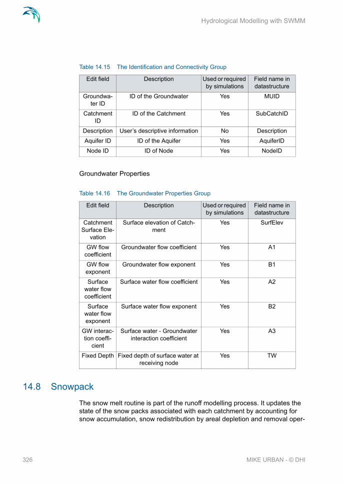
Hydrological Modelling with SWMM
Groundwater Properties
14.8 Snowpack
The snow melt routine is part of the runoff modelling process. It updates the state of the snow packs associated with each catchment by accounting for snow accumulation, snow redistribution by areal depletion and removal oper-
Table 14.15 The Identification and Connectivity Group
Edit field Description Used or required by simulations
Field name in datastructure
Groundwa-ter ID
ID of the Groundwater Yes MUID
Catchment ID
ID of the Catchment Yes SubCatchID
Description User’s descriptive information No Description
Aquifer ID ID of the Aquifer Yes AquiferID
Node ID ID of Node Yes NodeID
Table 14.16 The Groundwater Properties Group
Edit field Description Used or required by simulations
Field name in datastructure
Catchment Surface Ele-
vation
Surface elevation of Catch-ment
Yes SurfElev
GW flow coefficient
Groundwater flow coefficient Yes A1
GW flow exponent
Groundwater flow exponent Yes B1
Surface water flow coefficient
Surface water flow coefficient Yes A2
Surface water flow exponent
Surface water flow exponent Yes B2
GW interac-tion coeffi-
cient
Surface water - Groundwater interaction coefficient
Yes A3
Fixed Depth Fixed depth of surface water at receiving node
Yes TW
326 MIKE URBAN - © DHI

Snowpack
ations, and snow melt via heat budget accounting. Any snow melt coming off the pack is treated as an additional rainfall input into the runoff process.
At each runoff time step the following computations are made:
1. Air temperature and melt coefficients are updated according to the calen-dar date.
2. Any precipitation that falls as snow is added to the snow pack.
3. Any excess snow depth on the plowable area of the pack is redistributed according to the removal parameters established for the pack.
4. Areal coverages of snow on the impervious and pervious areas of the pack are reduced according to the Areal Depletion Curves defined for the study area.
5. The amount of snow in the pack that melts to liquid water is found using:
a heat budget equation for periods with rainfall, where melt rate increases with increasing air temperature, wind speed, and rainfall inten-sity
a degree-day equation for periods with no rainfall, where melt rate equals the product of a melt coefficient and the difference between the air tem-perature and the pack's base melt temperature.
6. If no melting occurs, the pack temperature is adjusted up or down based on the product of the difference between current and past air temperatures and an adjusted melt coefficient. If melting occurs, the temperature of the pack is increased by the equivalent heat content of the melted snow, up to the base melt temperature. Any remaining melt liquid beyond this is available to runoff from the pack.
7. The available snow melt is then reduced by the amount of free water hold-ing capacity remaining in the pack. The remaining melt is treated the same as a direct rainfall input onto the catchment.
The CS SWMM Snowpack Editor and the CS SWMM Climatology Editor (described in next chapter) contains the above information required for char-acterizing the modelling of the snowfall and snow melt processes. The CS SWMM Snowpack Editor organizes the data into following groups
Identification and Connectivity
SnowPack Properties
327
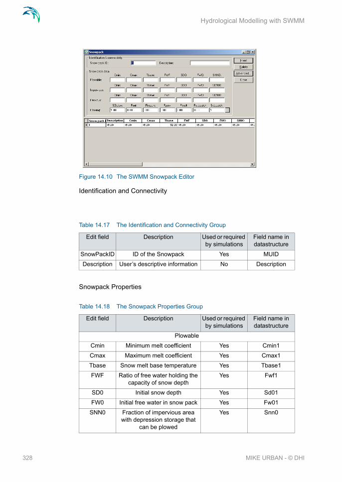
Hydrological Modelling with SWMM
Figure 14.10 The SWMM Snowpack Editor
Identification and Connectivity
Snowpack Properties
Table 14.17 The Identification and Connectivity Group
Edit field Description Used or required by simulations
Field name in datastructure
SnowPackID ID of the Snowpack Yes MUID
Description User’s descriptive information No Description
Table 14.18 The Snowpack Properties Group
Edit field Description Used or required by simulations
Field name in datastructure
Plowable
Cmin Minimum melt coefficient Yes Cmin1
Cmax Maximum melt coefficient Yes Cmax1
Tbase Snow melt base temperature Yes Tbase1
FWF Ratio of free water holding the capacity of snow depth
Yes Fwf1
SD0 Initial snow depth Yes Sd01
FW0 Initial free water in snow pack Yes Fw01
SNN0 Fraction of impervious area with depression storage that
can be plowed
Yes Snn0
328 MIKE URBAN - © DHI

Snowpack
Impervious
Cmin Minimum melt coefficient Yes Cmin1
Cmax Maximum melt coefficient Yes Cmax1
Tbase Snow melt base temperature Yes Tbase1
FWF Ratio of free water holding the capacity of snow depth
Yes Fwf1
SD0 Initial snow depth Yes Sd01
FW0 Initial free water in snow pack Yes Fw01
SD100 Snow depth above which there is 100% cover
Yes SD1002
Pervious
Cmin Minimum melt coefficient Yes Cmin1
Cmax Maximum melt coefficient Yes Cmax1
Tbase Snow melt base temperature Yes Tbase1
FWF Ratio of free water holding the capacity of snow depth
Yes Fwf1
SD0 Initial snow depth Yes Sd01
FW0 Initial free water in snow pack Yes Fw01
SD100 Snow depth above which there is 100% cover
Yes SD1003
Plowing
SDplow Depth of snow on plowable area at which redistribution
through plowing occurs
Yes SDplow
Fout Fraction of excess snow on plowable area transferred out
of watershed
Yes Fout
Fimperv Fraction of excess snow on plowable area transferred to impervious area by plowing
Yes Fimperv
Fperv Fraction of excess snow on plowable area transferred to
pervious area by plowing
Yes Fperv
Fimelt Fraction of excess snow on plowable area converted into
imeediate melt
Yes Fimelt
Table 14.18 The Snowpack Properties Group
Edit field Description Used or required by simulations
Field name in datastructure
329

Hydrological Modelling with SWMM
14.9 Climatology
Climate-related variables used for computing runoff and snow melt are grouped in the Climatology object:
Temperature
Evaporation
Wind Speed
Snow Melt
Areal Depletion
Temperature data are used when simulating snowfall and snow melt pro-cesses during runoff calculations. If these processes are not being simulated then no temperature data are needed.
Temperature data can be supplied from one of the following sources:
a user-supplied time series of point values (values at intermediate times are found by interpolation)
a NCDC 3200 or 3210 climatological file containing daily minimum and maximum values (SWMM fits a sinusoidal curve through these values depending on the day of the year).
For user-supplied time series, temperatures are in degrees F for US units and degrees C for metric units. Note that the NCDC climatological file can also be used to supply evaporation and wind speed as well.
Evaporation can occur for standing water on catchment surfaces, for subsur-face water in groundwater aquifers, and from water held in storage units. Evaporation rates can be stated as:
a single constant value
a set of monthly average values
a user-supplied time series of daily values
daily values read from a NCDC climatological file
Fsubcatch Fraction of excess snow on plowable area transferred to
pervious area in another catch-ment
Yes Fsubcatch
Subcatch ID of catchment recieving the Fsubcatch fraction of trans-
ferred snow
Yes SubcatchID
Table 14.18 The Snowpack Properties Group
Edit field Description Used or required by simulations
Field name in datastructure
330 MIKE URBAN - © DHI

Climatology
If a NCDC file is used then a set of monthly pan coefficients should also be supplied to convert the pan evaporation data to free-water-surface values.
Wind speed is an optional climatological variable that is only used for snow melt calculations. There can be use either a set of monthly average speeds or wind speed data contained in the same NCDC climatological file used for daily min/max temperatures.
Snow melt parameters are climatological variables that apply across the entire model area when simulating snowfall and snow melt. They include:
the temperature at which precipitation falls as snow
heat exchange properties of the snow surface
study area elevation, latitude, and longitude correction
For additional information of the Snow fall and Snow melt processes please consult the chapter Snowpack.
Areal Depletion refers to the tendency of snow to melt non-uniformly over the surface of a catchment. As the melting process proceeds, the area cov-ered by snow is reduced. This behaviour can be described by an Areal Depletion Curve. It plots the fraction of total area that remains snow covered against the ratio of the actual snow depth to the depth at which there is 100% snow cover. A typical ADC for a natural area is shown below.
Two such curves can be supplied, one for impervious areas and another for pervious areas.
The CS SWMM Climatology Editor organizes these data into following tab-sheets and groups:
Temperature Tabsheet
Evaporation Tabsheet
Wind Speed Tabsheet
331

Hydrological Modelling with SWMM
Snow melt Tabsheet
Areal Depletion Tabsheet
Temperature data
Figure 14.11 The SWMM Climatology | Temperature Editor
Evaporation Data
Table 14.19 The Climatology | Temperature Tabsheet
Edit field Description Used or required by simulations
Field name in datastructure
Radio Button Types No TypeNo
No data TypeNo=1, No temperature data
Yes if TypeNo = 1
Time series ID
TypeNo=2, Temperature data read from Time Series
Yes if TypeNo = 2
TimeSeriesID
Climatologi-cal file
(NCDC)
TypeNo=3, Temperature data read from NCDC file
Yes if TypeNo = 3
Filename
Start date TypeNo=3, Start date for read-ing from NCDC data file
Yes if TypeNo = 3
Start
332 MIKE URBAN - © DHI

Climatology
Figure 14.12 The SWMM Climatology | Evaporation Editor
Table 14.20 The Climatology | Evaporation Tabsheet
Edit field Description Used or required by simulations
Field name in datastructure
Radio button types. Yes TypeNo
Climatologi-cal file
(NCDC) selection at temperature
file
Evaporation data are read from the NCDC data file which is
specified on the Temperature Tabsheet
Yes, if TypeNo = 4
Filename
Constant Value
Evaporation is set to constant value
Yes if TypeNo = 1
ConstVale
Jan Monthly evaporation data for January entered by user
Yes if TypeNo = 2
Value1
Feb Monthly evaporation data for February entered by user
Yes if TypeNo = 2
Value2
Mar Monthly evaporation data for March entered by user
Yes if TypeNo = 2
Value3
Apr Monthly evaporation data for April entered by user
Yes if TypeNo = 2
Value4
May Monthly evaporation data for May entered by user
Yes if TypeNo = 2
Value5
June Monthly evaporation data for June entered by user
Yes if TypeNo = 2
Value6
July Monthly evaporation data for July entered by user
Yes if TypeNo = 2
Value7
Aug Monthly evaporation data for August entered by user
Yes if TypeNo = 2
Value8
333

Hydrological Modelling with SWMM
Sept Monthly evaporation data for September entered by user
Yes if TypeNo = 2
Value9
Oct Monthly evaporation data for October entered by user
Yes if TypeNo = 2
Value10
Nov Monthly evaporation data for November entered by user
Yes if TypeNo = 2
Value11
Dec Monthly evaporation data for December entered by user
Yes if TypeNo = 2
Value12
Time series ID
Evaporation data read from Time Series
Yes if TypeNo = 3
TimeSeriesID
Jan Evaporation data for January read from NCDC file
Yes if TypeNo = 4
Pan1
Feb Evaporation data for February read from NCDC file
Yes if TypeNo = 4
Pan2
Mar Evaporation data for March read from NCDC file
Yes if TypeNo = 4
Pan3
Apr Evaporation data for April read from NCDC file
Yes if TypeNo = 4
Pan4
May Evaporation data for May read from NCDC file
Yes if TypeNo = 4
Pan5
June Evaporation data for June read from NCDC file
Yes if TypeNo = 4
Pan6
July Evaporation data for July read from NCDC file
Yes if TypeNo = 4
Pan7
Aug Evaporation data for August read from NCDC file
Yes if TypeNo = 4
Pan8
Sept Evaporation data for Septem-ber read from NCDC file
Yes if TypeNo = 4
Pan9
Oct Evaporation data for October read from NCDC file
Yes if TypeNo = 4
Pan10
Nov Evaporation data for Novem-ber read from NCDC file
Yes if TypeNo = 4
Pan11
Dec Evaporation data for Decem-ber read from NCDC file
Yes if TypeNo = 4
Pan12
Computed from temper-atures in the climate files
Evaporation calculated based on temperature in the tempera-
ture file
Yes if TypeNo = 5
Defined at tem-perature tab in climatology dia-
log
Table 14.20 The Climatology | Evaporation Tabsheet
Edit field Description Used or required by simulations
Field name in datastructure
334 MIKE URBAN - © DHI
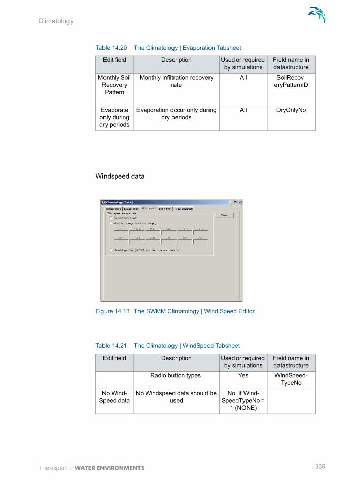
Climatology
Windspeed data
Figure 14.13 The SWMM Climatology | Wind Speed Editor
Monthly Soil Recovery Pattern
Monthly infiltration recovery rate
All SoilRecov-eryPatternID
Evaporate only during dry periods
Evaporation occur only during dry periods
All DryOnlyNo
Table 14.21 The Climatology | WindSpeed Tabsheet
Edit field Description Used or required by simulations
Field name in datastructure
Radio button types. Yes WindSpeed-TypeNo
No Wind-Speed data
No Windspeed data should be used
No, if Wind-SpeedTypeNo =
1 (NONE)
Table 14.20 The Climatology | Evaporation Tabsheet
Edit field Description Used or required by simulations
Field name in datastructure
335

Hydrological Modelling with SWMM
Snowmelt data
Climatologi-cal file
(NCDC) selection at temperature
file
WindSpeed data are read from the NCDC data file which is
specified on the Temperature Tabsheet
Yes, if Wind-SpeedTypeNo =
3 (FILE)
FileName
Jan Monthly evaporation data for January entered by user
Yes, if Wind-SpeedTypeNo 2
Value1
Feb Monthly evaporation data for February entered by user
Yes, if Wind-SpeedTypeNo 2
Value2
Mar Monthly evaporation data for March entered by user
Yes, if Wind-SpeedTypeNo 2
Value3
Apr Monthly evaporation data for April entered by user
Yes, if Wind-SpeedTypeNo 2
Value4
May Monthly evaporation data for May entered by user
Yes, if Wind-SpeedTypeNo 2
Value5
June Monthly evaporation data for June entered by user
Yes, if Wind-SpeedTypeNo 2
Value6
July Monthly evaporation data for July entered by user
Yes, if Wind-SpeedTypeNo 2
Value7
Aug Monthly evaporation data for August entered by user
Yes, if Wind-SpeedTypeNo 2
Value8
Sept Monthly evaporation data for September entered by user
Yes, if Wind-SpeedTypeNo 2
Value9
Oct Monthly evaporation data for October entered by user
Yes, if Wind-SpeedTypeNo 2
Value10
Nov Monthly evaporation data for November entered by user
Yes, if Wind-SpeedTypeNo 2
Value11
Dec Monthly evaporation data for December entered by user
Yes, if Wind-SpeedTypeNo 2
Value12
Table 14.21 The Climatology | WindSpeed Tabsheet
Edit field Description Used or required by simulations
Field name in datastructure
336 MIKE URBAN - © DHI

Climatology
Figure 14.14 The SWMM Climatology | Snow Melt Editor
Table 14.22 The Climatology | Snowmelt Tabsheet
Edit field Description Used or required by simulations
Field name in datastructure
Dividing temperature
between snow and
rain (degrees F)
Temperature below which pre-cipitation falls as snow
Yes SnowTemp
ATI Weight This parameter reflects to what degree heat transfer within a snow pack during non-melt
periods is affected by prior air temperatures. Smaller values reflect a thicker surface layer
of snow which result in reduced rates of heat transfer. Values must be between 0 and
1.The default value is 0.5.
Yes Atiwt
Negative melt ratio
This is the ratio of the heat transfer coefficient of a snow pack during non-melt condi-tions to the coefficient during melt conditions. It must be a
number between 0 and 1. The default value is 0.6.
Yes Rnm
337
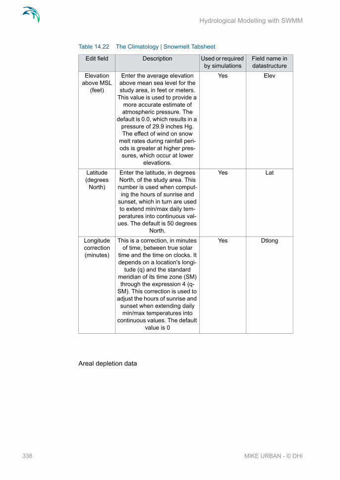
Hydrological Modelling with SWMM
Areal depletion data
Elevation above MSL
(feet)
Enter the average elevation above mean sea level for the study area, in feet or meters.
This value is used to provide a more accurate estimate of atmospheric pressure. The
default is 0.0, which results in a pressure of 29.9 inches Hg. The effect of wind on snow
melt rates during rainfall peri-ods is greater at higher pres-sures, which occur at lower
elevations.
Yes Elev
Latitude (degrees
North)
Enter the latitude, in degrees North, of the study area. This number is used when comput-ing the hours of sunrise and
sunset, which in turn are used to extend min/max daily tem-peratures into continuous val-ues. The default is 50 degrees
North.
Yes Lat
Longitude correction (minutes)
This is a correction, in minutes of time, between true solar
time and the time on clocks. It depends on a location's longi-
tude (q) and the standard meridian of its time zone (SM) through the expression 4 (q-
SM). This correction is used to adjust the hours of sunrise and sunset when extending daily min/max temperatures into
continuous values. The default value is 0
Yes Dtlong
Table 14.22 The Climatology | Snowmelt Tabsheet
Edit field Description Used or required by simulations
Field name in datastructure
338 MIKE URBAN - © DHI

Climatology
Figure 14.15 The SWMM Climatology | Areal Depletion Editor
Table 14.23 The Climatology | Areal depletion Tabsheet
Edit field Description Used or required by simulations
Field name in datastructure
Imervious
0.0 Fraction of impervious area covered by snow at interval
[0.0-0.1]
Yes AdcImPerv0
0.1 Fraction of impervious area covered by snow at interval
]0.1-0.2]
Yes AdcImPerv1
0.2 Fraction of impervious area covered by snow at interval
]0.2-0.3]
Yes AdcImPerv2
0.3 Fraction of impervious area covered by snow at interval
]0.3-0.4]
Yes AdcImPerv3
0.4 Fraction of impervious area covered by snow at interval
]0.4-0.5]
Yes AdcImPerv4
0.5 Fraction of impervious area covered by snow at interval
]0.5-0.6]
Yes AdcImPerv5
0.6 Fraction of impervious area covered by snow at interval
]0.6-0.7]
Yes AdcImPerv6
0.7 Fraction of impervious area covered by snow at interval
]0.7-0.8]
Yes AdcImPerv7
339

Hydrological Modelling with SWMM
14.10 Coverage
The CS SWMM Coverage Editor organizes the related input data for the cov-erage into following groups:
0.8 Fraction of impervious area covered by snow at interval
]0.8-0.9]
Yes AdcImPerv8
0.9 Fraction of impervious area covered by snow at interval
]0.9-1.0]
Yes AdcImPerv9
Pervious
0.0 Fraction of pervious area cov-ered by snow at interval [0.0-
0.1]
Yes AdcPerv0
0.1 Fraction of pervious area cov-ered by snow at interval ]0.1-
0.2]
Yes AdcPerv1
0.2 Fraction of pervious area cov-ered by snow at interval ]0.2-
0.3]
Yes AdcPerv2
0.3 Fraction of pervious area cov-ered by snow at interval ]0.3-
0.4]
Yes AdcPerv3
0.4 Fraction of pervious area cov-ered by snow at interval ]0.4-
0.5]
Yes AdcPerv4
0.5 Fraction of pervious area cov-ered by snow at interval ]0.5-
0.6]
Yes AdcPerv5
0.6 Fraction of pervious area cov-ered by snow at interval ]0.6-
0.7]
Yes AdcPerv6
0.7 Fraction of pervious area cov-ered by snow at interval ]0.7-
0.8]
Yes AdcPerv7
0.8 Fraction of pervious area cov-ered by snow at interval ]0.8-
0.9]
Yes AdcPerv8
0.9 Fraction of pervious area cov-ered by snow at interval ]0.9-
1.0]
Yes AdcPerv9
Table 14.23 The Climatology | Areal depletion Tabsheet
Edit field Description Used or required by simulations
Field name in datastructure
340 MIKE URBAN - © DHI

LID Controls
Identification and Connectivity
Landuse Coverage
Figure 14.16 The SWMM Coverage Editor Dialog
Identification and Connectivity
Landuse coverage
14.11 LID Controls
LID Controls are low impact development practices designed to capture sur-face runoff and provide some combination of detention, infiltration, and evap-otranspiration to it.
Table 14.24 The Coverage Identification and Connectivity Group
Edit field Description Used or required by simulations
Field name in datastructure
CoverageID ID of Coverage Yes MUID
Catchments ID of Catchment Yes SubCatchID
LanduseID ID of Landuse Yes LandUseID
Table 14.25 The Landuse Coverage Group
Edit field Description Used or required by simulations
Field name in datastructure
Percentage Percentage of the catchment area covered by this type of
landuse
Yes Percentage
341

Hydrological Modelling with SWMM
They are considered as properties of a given sub catchment, similar to how Aquifers and Snow Packs are treated. SWMM can explicitly model five differ-ent generic types of LID controls:
Bio-retention Cells
Bio-retention Cells are depressions that contain vegetation grown in an engi-neered soil mixture placed above a gravel drainage bed. They provide stor-age, infiltration and evaporation of both direct rainfall and runoff captured from surrounding areas. Rain gardens, street planters, and green roofs are all variations of bio-retention cells.
Infiltration Trenches
Infiltration Trenches are narrow ditches filled with gravel that intercept runoff from upslope impervious areas. They provide storage volume and additional time for captured runoff to infiltrate the native soil below.
Continuous Porous Pavement
Continuous Porous Pavement systems are excavated areas filled with gravel and paved over with a porous concrete or asphalt mix. Normally all rainfall will immediately pass through the pavement into the gravel storage layer below it where it can infiltrate at natural rates into the site's native soil. Block Paver systems consist of impervious paver blocks placed on a sand or pea gravel bed with a gravel storage layer below. Rainfall is captured in the open spaces between the blocks and conveyed to the storage zone and native soil below.
Rain Barrels
Rain Barrels (or Cisterns) are containers that collect roof runoff during storm events and can either release or re-use the rainwater during dry periods.
Vegetative Swales
Vegetative Swales are channels or depressed areas with sloping sides cov-ered with grass and other vegetation. They slow down the conveyance of col-lected runoff and allow it more time to infiltrate the native soil beneath it.
Bio-retention cells, infiltration trenches, and porous pavement systems can all contain optional underdrain systems in their gravel storage beds to convey captured runoff off of the site rather than letting it all infiltrate. They can also have an impermeable floor or liner that prevents any infiltration into the native soil from occurring. Infiltration trenches and porous pavement systems can also be subjected to a decrease in hydraulic conductivity over time due to clogging.
Although some LID practices can also provide significant pollutant reduction benefits, at this time SWMM only models their hydrologic performance
342 MIKE URBAN - © DHI

LID Controls
The CS SWMM LID Controls Editor organizes the data input for the different types of LID practices. The input data is organized into following group and tabs:
Identification
Tabs: Surface, Soil, Pavement, Storage and Drain
Figure 14.17 The CS SWMM LID Controls Editor - Surface
Figure 14.18 The CS SWMM LID Controls Editor - Soil
343

Hydrological Modelling with SWMM
Figure 14.19 The CS SWMM LID Controls Editor - Pavement
Figure 14.20 The CS SWMM LID Controls Editor - Storage
344 MIKE URBAN - © DHI

LID Controls
Figure 14.21 The CS SWMM LID Controls Editor - Drain
Identification
Table 14.26 The LID Controls Identification Group
Edit field Description Used or required by simulations
Field name in datastructure
LID Control ID
ID of Low Impact Design, LID Yes MUID
LID Type Type of LID1: Bio Retention Cell2: Porous Pavement3: Infiltration Trench
4: Rain Barrel5: Vegetatvie Swale
Yes LIDTypeNo
345

Hydrological Modelling with SWMM
LID control data specification
Table 14.27 The LID data specification
Edit field Description Used or required by simulations
Field name in datastructure
Storage Depth
When confining walls or berms are present this is the maxi-
mum depth to which water can pond above the surface of the unit before overflow occurs (in inches or mm). For LIDs that experience overland flow it is
the height of any surface depression storage. For
swales, it is the height of its trapezoidal cross section.
Yes If LID-TypeNo = (1,2,3,5)
StorHt
Vegetative Cover Frac-
tion
The fraction of the storage area above the surface that is
filled with vegetation
Yes If LID-TypeNo = (1,2,3,5)
VegFrac
Surface Roughness
Manning's n for overland flow over the surface of porous pavement or a vegetative
swale (see this table for sug-gested values). Use 0 for other
types of LIDs.
Yes If LID-TypeNo = (1,2,3,5)
Rough
Surface Slope
Slope of porous pavement sur-face or vegetative swale (per-cent). Use 0 for other types of
LIDs
Yes If LID-TypeNo = (1,2,3,5)
Slope
Swale Side Slope
Slope (run over rise) of the side walls of a vegetative
swale's cross section. This value is ignored for other types
of LIDs
Yes If LID-TypeNo = 5
Xslope
Thickness The thickness of the soil layer (inches or mm). Typical values
range from 18 to 36 inches (450 to 900 mm) for rain gar-
dens, street planters and other types of land-based bio-reten-
tion units, but only 3 to 6 inches (75 to 150 mm) for
green roofs.
Yes If LID-TypeNo = 1
SThick
Porosity The volume of pore space rela-tive to total volume of soil (as a
fraction).
Yes If LID-TypeNo = 1
Por
346 MIKE URBAN - © DHI

LID Controls
Field Capac-ity
Volume of pore water relative to total volume after the soil
has been allowed to drain fully (as a fraction). Below this level,
vertical drainage of water through the soil layer does not
occur.
Yes If LID-TypeNo = 1
FC
Wilting Point Volume of pore water relative to total volume for a well dried soil where only bound water remains (as a fraction). The moisture content of the soil cannot fall below this limit.
Yes If LID-TypeNo = 1
WP
Conductivity Hydraulic conductivity for the fully saturated soil (in/hr or
mm/hr)
Yes If LID-TypeNo = 1
Ksat
Conductivity Slope
Slope of the curve of log(con-ductivity) versus soil moisture content (dimensionless). Typi-
cal values range from 5 for sands to 15 for silty clay
Yes If LID-TypeNo = 1
Kcoeff
Suction Head
The average value of soil capil-lary suction along the wetting front (inches or mm). This is
the same parameter as used in the Green-Ampt infiltration
model
Yes If LID-TypeNo = 1
Suct
Thickness The thickness of the pavement layer (inches or mm). Typical values are 4 to 6 inches (100
to 150 mm)
Yes If LID-TypeNo = 2
PThick
Void Ratio The volume of void space rela-tive to the volume of solids in the pavement for continuous systems or for the fill material
used in modular systems. Typi-cal values for pavements are
0.12 to 0.21. Note that porosity = void ratio / (1 + void ratio).
Yes If LID-TypeNo = 2
PVratio
Impervious Surface
Ratio of impervious paver material to total area for modu-lar systems; 0 for continuous porous pavement systems
Yes If LID-TypeNo = 2
FracImp
Table 14.27 The LID data specification
Edit field Description Used or required by simulations
Field name in datastructure
347

Hydrological Modelling with SWMM
Permeability Permeability of the concrete or asphalt used in continuous
systems or hydraulic conduc-tivity of the fill material (gravel or sand) used in modular sys-tems (in/hr or mm/hr). The per-
meability of new porous concrete or asphalt is very high
(e.g., hundreds of in/hr) but can drop off over time due to
clogging by fine particulates in the runoff
Yes If LID-TypeNo = 2
Perm
Clogging Factor
Number of pavement layer void volumes of runoff treated it takes to completely clog the pavement. Use a value of 0 to ignore clogging. Clogging pro-gressively reduces the pave-ment's permeability in direct proportion to the cumulative
volume of runoff treated.
Yes If LID-TypeNo = 2
PVclog
Height This is the height of a rain bar-rel or thickness of a gravel
layer (inches or mm). Crushed stone and gravel layers are
typically 6 to 18 inches (150 to 450 mm) thick while single
family home rain barrels range in height from 24 to 36 inches
(600 to 900 mm).
Yes If LID-TypeNo = (1,2,3,4)
Height
Void Ratio The volume of void space rela-tive to the volume of solids in
the layer. Typical values range from 0.5 to 0.75 for gravel
beds. Note that porosity = void ratio / (1 + void ratio).
Yes If LID-TypeNo = (1,2,3)
SVratio
Conductivity The maximum rate at which water can flow out the bottom of the layer after it is first con-
structed (in/hr or mm/hr).
Yes If LID-TypeNo = (1,2,3)
Filt
Clogging Factor
Total volume of treated runoff it takes to completely clog the
bottom of the layer divided by the void volume of the layer
Yes If LID-TypeNo = (1,2,3)
SVclog
Apply Yes DrainNo
Table 14.27 The LID data specification
Edit field Description Used or required by simulations
Field name in datastructure
348 MIKE URBAN - © DHI

LID Deployment
14.12 LID Deployment
In the CS SWMM LID Deployment Editor the LID controls are deployed to individual catchments. The type of LID control and number are defined as well as the properties for each LID control. The input data is organized into following groups:
Identification and Connectivity
LID Properties
Coefficient Coefficient C and exponent n that determines the rate of flow
through the underdrain as a function of height of stored
water above the drain height.
Yes If LID-TypeNo = (1,2,3,4)
Coeff
Exponent Coefficient C and exponent n that determines the rate of flow
through the underdrain as a function of height of stored
water above the drain height.
Yes If LID-TypeNo = (1,2,3,4)
Expon
Offset Height
Height of any underdrain pip-ing above the bottom of a stor-age layer or rain barrel (inches
or mm).
Yes If LID-TypeNo = (1,2,3,4)
Offset
Delay The number of dry weather hours that must elapse before the drain line in a rain barrel is opened (the line is assumed to be closed once rainfall begins).
Yes If LID-TypeNo = 4
Delay
Table 14.27 The LID data specification
Edit field Description Used or required by simulations
Field name in datastructure
349
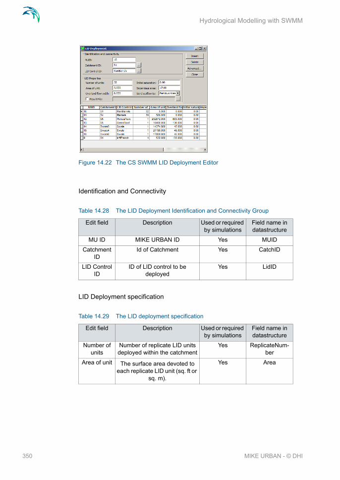
Hydrological Modelling with SWMM
Figure 14.22 The CS SWMM LID Deployment Editor
Identification and Connectivity
LID Deployment specification
Table 14.28 The LID Deployment Identification and Connectivity Group
Edit field Description Used or required by simulations
Field name in datastructure
MU ID MIKE URBAN ID Yes MUID
Catchment ID
Id of Catchment Yes CatchID
LID Control ID
ID of LID control to be deployed
Yes LidID
Table 14.29 The LID deployment specification
Edit field Description Used or required by simulations
Field name in datastructure
Number of units
Number of replicate LID units deployed within the catchment
Yes ReplicateNum-ber
Area of unit The surface area devoted to each replicate LID unit (sq. ft or
sq. m).
Yes Area
350 MIKE URBAN - © DHI

LID Deployment
Overland flow width
The width of the outflow face of each identical LID unit (in ft or
m). This parameter only applies to LID processes such as Porous Pavement and Veg-etative Swales that use over-land flow to convey surface
runoff off of the unit. (The other LID processes, such as Bio-
Retention Cells and Infiltration Trenches simply spill any
excess captured runoff over their berms.)
Yes Width
Initial satura-tion
For Bio-Retention Cells this is the degree to which the unit's soil is initially filled with water
(0 % saturation corresponds to the wilting point moisture con-tent, 100 % saturation has the moisture content equal to the porosity). The storage zone beneath the soil zone of the cell is assumed to be com-
pletely dry. For other types of LIDs it corresponds to the
degree to which their storage zone is initially filled with water
Yes InitSat
Impervious Area
The percent of the impervious portion of the subcatchment's non-LID area whose runoff is treated by the LID practice.
(E.g., if rain barrels are used to capture roof runoff and roofs represent 60% of the impervi-ous area, then the impervious area treated is 60%). If the LID unit treats only direct rainfall,
such as with a green roof, then this value should be 0. If the LID takes up the entire sub-catchment then this field is
ignored.
Yes FromImp
Table 14.29 The LID deployment specification
Edit field Description Used or required by simulations
Field name in datastructure
351

Hydrological Modelling with SWMM
Send flow to Select this option if the outflow from the LID is returned onto the subcatchment's pervious area rather than going to the
subcatchment's outlet. An example of where this might apply is a rain barrel whose
contents are used to irrigate a lawn area. This field is ignored if the LID takes up the entire
subcatchment.
Yes ToPervNo
Result File Report file option Yes RptFileNo
Filename The name of an optional file where detailed time series
results for the LID will be writ-ten
Yes RptFileName
Table 14.29 The LID deployment specification
Edit field Description Used or required by simulations
Field name in datastructure
352 MIKE URBAN - © DHI

15 Time Series and Boundary Conditions in SWMM
Time Series representing rainfall, evaporation, water stages etc. are impor-tant values to model simulations. The time series normally originate from field measurements. The term ‘Boundary Condition’ is used to described the load-ing of these different timeseries to the model.
Visualization of boundary conditions
The boundary conditions can be visualized on the map. Figure 15.1 shows how where you can toggle the visualization on/off in the TOC. Boundary con-ditions are per default unchecked (one exception: catchment connections) and not displayed in the horizontal view but they can be activated at any time during the project.
To be displayed, boundary conditions must be applied and contain at least one ‘Boundary Item’.
Changes in the ‘Boundary Conditions’ dialogs are not immediately displayed in the horizontal view. In order to display the changes, make sure to save your edits and to regenerate the relevant layers. This is done by right-clicking on the layer that needs to be updated and then choosing the ‘Regenerate’ option.
Figure 15.1 SWMM Boundaries
The boundaries that can be seen on the map are explained in below.
SWMM5 Inflow shows the nodes with an inflow load
SWMM5 Dry Weather Flow shows nodes where dry weather flow has been assigned
353

Time Series and Boundary Conditions in SWMM
SWMM5 Outfall shows outfalls where a water level has been assigned. The boundary condition will only be displayed if the Outfall type is set to one of the following type: Fixed (3), Tidal (4) or Timeseries (5).
SWMM5 Catchment Connection shows the link between the center of the catchment and the node it is connected to
SWMM5 Raingauge to Catchment displays the link between the rain-gauge and the center of the catchment when a raingauge is specified in the Routing dialog
SWMM5 Catchment to Catchment displays the link between the centers of two connected catchments
SWMM5 Rainfall shows the catchments where a raingauge has been assigned (this one is similar to the SWMM5 Raingauge to Catchment but will show all catchments where a raingauge has been assigned to)
An example on how this may look is shown in Figure 15.2.
Figure 15.2 Example of the visualization of boundary conditions
15.1 Time Series
Time Series can be user specified or originate from external measured data of i.e. rainfall, evaporation, inflows to nodes of the drainage system, and water stage at outfall boundary nodes.
The SWMM engine supports two time series formats. Time series values can either be in date / time / value format or in time / value format, where each entry is separated by one or more spaces or tab characters.
354 MIKE URBAN - © DHI

Time Series
For the date / time / value format which is the only format supported in MIKE URBAN interface, dates are entered as month/day/year (e.g., 7/21/2004) and times as 24-hour military time (e.g., 8:30 pm is 20:30).
For the time / value format, times are entered as hours since simulation start. If the time / value format has been used outside MIKE URBAN interface, then it is converted during import to the date / time /value format given the start of simulation date as initial start date.
Following types of time series can be defined:
Temperature data
Evaporation data
Rainfall data
Water stage at outfall nodes
External inflow hydrographs at drainage system nodes
External inflow pollutographs at drainage system nodes.
The CS SWMM Time Series editor organizes the related input data for the dif-ferent timeseries into the following groups:
Identification and Connectivity - General identification and location infor-mation
Figure 15.3 The SWMM Time Series Editor
355

Time Series and Boundary Conditions in SWMM
Identification and Connectivity
15.2 Time Patterns
Time Patterns are used to described cyclic behaviour of any timeseries. Fol-lowing four different types of patterns can be supplied
Monthly
Daily
Hourly
Weekend
The CS SWMM Time Patterns editor organizes the related input data for the different time patterns into the following groups:
Identification and Connectivity - General identification and location infor-mation
Pattern types - definition of each pattern.
Table 15.1 The Time Series Identification and Connectivity Group
Edit field Description Used or required by simulations
Field name in datastructure
Time Series ID
ID of Time Series Yes MUID
Type Type of Time Series (Rainfall, Temperature, Inflow Hydro-graph, Evaporation, Outfall Stage and Pollutographs)
Yes TypeNo
Time Series options
Use either external time series file or enter time series values
directly
Yes TimeSeri-esTypeNo
External-Time-
SeriesID
External time series id Yes if TimeSeri-esTypeNo = 1
ExternalTime-SeriesID
Description User’s descriptive information No Description
356 MIKE URBAN - © DHI

Time Patterns
Figure 15.4 The SWMM Pattern Editor
Identification and Connectivity
Time Pattern Data
Table 15.2 The Time Patterns Identification and Connectivity Group
Edit field Description Used or required by simulations
Field name in datastructure
Pattern ID ID of Pattern Yes MUID
Type Type of pattern (Monthly, Daily, Hourly, Weekend)
Yes TypeNo
Description User’s descriptive information No Description
Table 15.3 The Time Pattern data
Edit field Description Used or required by simulations
Field name in datastructure
Jan Pattern value for January Yes, if Monthly Mdr1
Feb Pattern value for February Yes, if Monthly Mdr2
Mar Pattern value for March Yes, if Monthly Mdr3
357

Time Series and Boundary Conditions in SWMM
Apr Pattern value for April Yes, if Monthly Mdr4
May Pattern value for May Yes, if Monthly Mdr5
Jun Pattern value for June Yes, if Monthly Mdr6
Jul Pattern value for July Yes, if Monthly Mdr7
Aug Pattern value for August Yes, if Monthly Mdr8
Sep Pattern value for September Yes, if Monthly Mdr9
Oct Pattern value for October Yes, if Monthly Mdr10
Nov Pattern value for November Yes, if Monthly Mdr11
Dec Pattern value for December Yes, if Monthly Mdr12
Mon Pattern value for Monday Yes, if Daily Day1
Tue Pattern value for Tuesday Yes, if Daily Day2
Wed Pattern value for Wednesday Yes, if Daily Day3
Thu Pattern value for Thursday Yes, if Daily Day4
Fri Pattern value for Friday Yes, if Daily Day5
Sat Pattern value for Saturday Yes, if Daily Day6
Sun Pattern value for Sunday Yes, if Daily Day7
12 Pattern value for 12AM week Yes, if Hourly AM12
01 Pattern value for 01AM week Yes, if Hourly AM1
02 Pattern value for 02AM week Yes, if Hourly AM2
03 Pattern value for 03AM week Yes, if Hourly AM3
04 Pattern value for 04AM week Yes, if Hourly AM4
05 Pattern value for 05AM week Yes, if Hourly AM5
06 Pattern value for 06AM week Yes, if Hourly AM6
07 Pattern value for 07AM week Yes, if Hourly AM7
08 Pattern value for 08AM week Yes, if Hourly AM8
09 Pattern value for 09AM week Yes, if Hourly AM9
10 Pattern value for 10AM week Yes, if Hourly AM10
11 Pattern value for 11AM week Yes, if Hourly AM11
12 Pattern value for 12PM week Yes, if Hourly PM12
01 Pattern value for 01PM week Yes, if Hourly PM1
02 Pattern value for 02PM week Yes, if Hourly PM2
03 Pattern value for 03PM week Yes, if Hourly PM3
04 Pattern value for 04PM week Yes, if Hourly PM4
05 Pattern value for 05PM week Yes, if Hourly PM5
06 Pattern value for 06PM week Yes, if Hourly PM6
07 Pattern value for 07PM week Yes, if Hourly PM7
Table 15.3 The Time Pattern data
Edit field Description Used or required by simulations
Field name in datastructure
358 MIKE URBAN - © DHI

Time Patterns
08 Pattern value for 08PM week Yes, if Hourly PM8
09 Pattern value for 09PM week Yes, if Hourly PM9
10 Pattern value for 10PM week Yes, if Hourly PM10
11 Pattern value for 11PM week Yes, if Hourly PM11
12 Pattern value for 12AM week-end
Yes, if Weekend AMW12
01 Pattern value for 01AM week-end
Yes, if Weekend AMW1
02 Pattern value for 02AM week-end
Yes, if Weekend AMW2
03 Pattern value for 03AM week-end
Yes, if Weekend AMW3
04 Pattern value for 04AM week-end
Yes, if Weekend AMW4
05 Pattern value for 05AM week-end
Yes, if Weekend AMW5
06 Pattern value for 06AM week-end
Yes, if Weekend AMW6
07 Pattern value for 07AM week-end
Yes, if Weekend AMW7
08 Pattern value for 08AM week-end
Yes, if Weekend AMW8
09 Pattern value for 09AM week-end
Yes, if Weekend AMW9
10 Pattern value for 10AM week-end
Yes, if Weekend AMW10
11 Pattern value for 11AM week-end
Yes, if Weekend AMW11
12 Pattern value for 12PM week-end
Yes, if Weekend PMW12
01 Pattern value for 01PM week-end
Yes, if Weekend PMW1
02 Pattern value for 02PM week-end
Yes, if Weekend PMW2
03 Pattern value for 03PM week-end
Yes, if Weekend PMW3
04 Pattern value for 04PM week-end
Yes, if Weekend PMW4
05 Pattern value for 05PM week-end
Yes, if Weekend PMW5
Table 15.3 The Time Pattern data
Edit field Description Used or required by simulations
Field name in datastructure
359

Time Series and Boundary Conditions in SWMM
15.3 Raingauges
Rain Gauges supply precipitation data for one or more catchments in a study area. The rainfall data can be either a user-defined time series (specified in Time Series as Type Rainfall) or come from an external file.
Several different popular rainfall file formats currently in use are supported, as well as a standard user-defined format. These are:
DSI-3240 and related formats which record hourly rainfall at U.S. National Weather Service (NWS) and Federal Aviation Agency stations, available online from the National Climatic Data Center (NCDC) at www.ncdc.noaa.gov/oa/ncdc.html.
DSI-3260 and related formats which record fifteen minute rainfall at NWS stations, also available online from NCDC.
HLY03 and HLY21 formats for hourly rainfall at Canadian stations, avail-able online from Environment Canada at www.climate.weatherof-fice.ec.gc.ca.
FIF21 format for fifteen minute rainfall at Canadian stations, also availa-ble online from Environment Canada.
a standard user-prepared format where each line of the file contains the station ID, year, month, day, hour, minute, and non-zero precipitation reading, all separated by one or more spaces. An excerpt from the user-prepared format might look as follows:
06 Pattern value for 06PM week-end
Yes, if Weekend PMW6
07 Pattern value for 07PM week-end
Yes, if Weekend PMW7
08 Pattern value for 08PM week-end
Yes, if Weekend PMW8
09 Pattern value for 09PM week-end
Yes, if Weekend PMW9
10 Pattern value for 10PM week-end
Yes, if Weekend PMW10
11 Pattern value for 11PM week-end
Yes, if Weekend PMW11
Table 15.3 The Time Pattern data
Edit field Description Used or required by simulations
Field name in datastructure
360 MIKE URBAN - © DHI

Raingauges
STA01 2004 6 12 00 00 0.12
STA01 2004 6 12 01 00 0.04
STA01 2004 6 22 16 00 0.07
When a rain gauge is designated as receiving its rainfall data from a file, the user must supply the name of the file and the name of the recording station referenced in the file.
For the standard user-prepared format, the rainfall type (e.g., intensity or vol-ume), recording time interval, and depth units must also be supplied as rain gauge properties. For the other file types these properties are defined by their respective file format and are automatically recognized by SWMM.
The CS SWMM Raingauges editor organizes the related input data for the rainfall data into the following groups:
Identification and Connectivity - General identification and location infor-mation
Raingauge properties
Figure 15.5 The SWMM Raingauge Editor
361
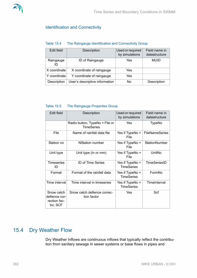
Time Series and Boundary Conditions in SWMM
Identification and Connectivity
15.4 Dry Weather Flow
Dry Weather Inflows are continuous inflows that typically reflect the contribu-tion from sanitary sewage in sewer systems or base flows in pipes and
Table 15.4 The Raingauge Identification and Connectivity Group
Edit field Description Used or required by simulations
Field name in datastructure
Raingauge ID
ID of Raingauge Yes MUID
X coordinate X coordinate of raingauge Yes
Y coordinate Y coordinate of raingauge Yes
Description User’s descriptive information No Description
Table 15.5 The Raingauge Properties Group
Edit field Description Used or required by simulations
Field name in datastructure
Radio button, TypeNo = File or TimeSeries
Yes TypeNo
File Name of rainfall data file Yes if TypeNo = File
FileNameSeries
Station no NStation number Yes if TypeNo = File
StationNumber
Unit type Unit type (in or mm) Yes if TypeNo = File
UnitNo
Timeseries ID
ID of Time Series Yes if TypeNo = TimeSeries
TimeSeriesID
Format Format of the rainfall data Yes if TypeNo = TimeSeries
FormNo
Time interval Time interval in timeseries Yes if TypeNo = TimeSeries
TimeInterval
Snow catch defience cor-rection fac-
tor, SCF
Snow catch defience correc-tion factor
Yes Scf
362 MIKE URBAN - © DHI

Dry Weather Flow
stream channels. They are represented by an average inflow rate that can be periodically adjusted on a monthly, daily, and hourly basis by applying Time Patterns multipliers to this average value.
The CS SWMM Dry Weather Flow editor organizes the related input data for each dry weather inflow into the following groups:
Identification and Connectivity - General identification and location infor-mation
Flow data - flow data and specification of pattern
Pollutant attached to flow - upper grid in dialog
Figure 15.6 The SWMM Dry Weather Flow Editor
Identification and Connectivity
Table 15.6 The Dry Weather Flow Identification and Connectivity Group
Edit field Description Used or required by simulations
Field name in datastructure
DWF ID ID Dry Weather Flow Yes MUID
Load To ID of Node ID for DWF load Yes NodeID
Pollutant attached
Pollutant attached to dry weather flow
Yes PollutNo
Description User’s descriptive information No Description
363

Time Series and Boundary Conditions in SWMM
15.5 Inflow
Direct Inflows are user-defined time series of inflows added directly into a node. They can be used to perform flow and water quality routing in the absence of any runoff computations (as in a study area where no catchments
Table 15.7 The Dry Weather Flow Data Group
Edit field Description Used or required by simulations
Field name in datastructure
Average Flow
Average flow value of DWF Yes FlowValue
Monthly ID of Pattern of Monthly type No PatternMonthID
Daily ID of Pattern of Daily type No PatternWeekID
Week hourly ID of Pattern of Hourly type No PatternWeek-HourlyID
Weekend hourly
ID of Pattern of Weekend type No PatternWeek-endHourlyID
Table 15.8 The Pollutant Data in upper grid attached to dry weather flow
Edit field Description Used or required by simulations
Field name in datastructure
PollutantID ID of Pollutant Yes, if pollutant attached
PollutantID
BValue Base value of pollutant Yes, if pollutant attached
BValue
Monthly ID of Pattern of Monthly type Yes, if pollutant attached
PatternMonthID
Daily ID of Pattern of Daily type Yes, if pollutant attached
PatternWeekID
Week hourly ID of Pattern of Hourly type Yes, if pollutant attached
PatternWeek-HourlyID
Weekend hourly
ID of Pattern of Weekend type Yes, if pollutant attached
PatternWeek-endHourlyID
364 MIKE URBAN - © DHI

Inflow
are defined). A pollutant component can only be defined as inflow to the sys-tem if it is attached to a flow component.
The CS SWMM Inflow editor organizes the related input data for each inflow into the following groups:
Identification and Connectivity - General identification and location infor-mation
Pollutant attached to flow - upper grid in dialog
Figure 15.7 The SWMM Inflow Editor
Identification and Connectivity
Table 15.9 The Inflow Identification and Connectivity Group
Edit field Description Used or required by simulations
Field name in datastructure
Inflow to ID of node where inflow should be loaded to
Yes NodeID
Time series ID
ID of flow time series Yes FlowSeriesID
Pollutant Pollutant attached to flow Yes PollutNo
Base Flow Base flow Yes BaseFlowValue
Scale Factor Scaling factor multiplied to the time series value
Yes ScaleFlowFac-tor
Pattern ID Baseline pattern multiplied to the baseline value
Yes BaselinePat-ternID
Description User’s descriptive information No Description
365

Time Series and Boundary Conditions in SWMM
Table 15.10 The Dry Weather Flow Data Group
Edit field Description Used or required by simulations
Field name in datastructure
PollutantID ID of pollutant Yes, if pollutant attached to flow
PollutantID
Pollut-SeriesID
ID of pollutograph Yes, if pollutant attached to flow
PollutSeriesID
FormatNo Format (MASS, CONCEN) Yes, if pollutant attached to flow
FormatNo
ConvFactor Conversion factor Yes, if pollutant attached to flow
ConvFactor
366 MIKE URBAN - © DHI

The General Simulation Settings
16 Project Options and Simulations in SWMM
The project and simulations options for SWMM are defined in the ‘Simulation | Run SWMM5’.
The CS-SWMM Run SWMM5 editor is split into following four tabsheets:
General
Runoff
Network
Summary
16.1 The General Simulation Settings
The General page is organized into following groups:
Identification and Connectivity
Simulation Period
Start Simulation
Units Selection (main unit group saved to file for engine simulation)
Figure 16.1 The SWMM Simulation General Editor dialog
367

Project Options and Simulations in SWMM
Identification and Connectivity
Simulation Period
Table 16.1 The Simulation, General Identification and Connectivity Group
Edit field Description Used or required by simulations
Field name in data structure
Simulation ID
ID of simulation - user speci-fied. ID will be reflected in the
name of project and result files
Yes MUID
Scenario ID ID of selected Scenario - Acti-vating scenario is done in the
Scenario Manager dialog
Yes ActiveJob
Description User’s descriptive information No Description
Table 16.2 The Simulation, General Simulation Period Group
Edit field Description Used or required by simulations
Field name in data structure
Start Analy-sis on
Start analysis date / time Yes StartDate + StartTime
End Analysis on
End analysis date / time Yes EndDate + End-Time
Sweeping Start
Start sweeping date Yes SweepStartDate
Sweeping End
End sweeping date Yes SweepEndDate
Start Report-ing
Start reporting date / time Yes ReportStartDate + ReportStart-
Time
Reporting time step
Saving time step to report Yes ReportStep
368 MIKE URBAN - © DHI

The Runoff Simulation Settings
Start Simulation
Units selection
16.2 The Runoff Simulation Settings
The Runoff page is organized into following groups:
Identification and Connectivity
Infiltration Method
Runoff time steps
Runoff interface files
Table 16.3 The Simulation, General Start Simulation Group
Edit field Description Used or required by simulations
Field name in data structure
Single Run Initiate simulation
Rainfall/Run-off
Include Rainfall / Runoff Yes IncludeRainfall-RunoffNo
Snow Melt Include Snow Melt Yes IncludeSnow-MeltNo
Groundwater Include Groundwater Yes InlcudeGround-waterNo
Flow Rout-ing
Include Flow Routing Yes IncludeFlow-RoutingNo
Water Qual-ity
Include Water Quality Yes IncludeWater-QualityNo
Table 16.4 The Simulation, General Units selection Group
Edit field Description Used or required by simulations
Field name in data structure
Units Selec-tion
Selection of main Unit for sav-ing to SWMM5 engine
Yes UnitNo
369

Project Options and Simulations in SWMM
Figure 16.2 The SWMM Simulation Runoff Editor Dialog
Identification and Connectivity
Infiltration Method
Table 16.5 The Simulation Runoff Identification and Connectivity Group
Edit field Description Used or required by simulations
Field name in data structure
Simulation ID
ID of simulation - user speci-fied. ID will be reflected in the
name of project and result files
Yes MUID
Scenario ID ID of selected Scenario - Acti-vating scenario is done in the
Scenario Manager dialog
Yes ActiveJob
Table 16.6 The Simulation, Runoff Infiltration Method Group
Edit field Description Used or required by simulations
Field name in data structure
Horton Horton Infiltration method No Infiltration-TypeNo
Green ampt Green ampt Infiltration method No Infiltration-TypeNo
Curve Num-ber
SCS Hydrology - or curve number method
No Infiltration-TypeNo
370 MIKE URBAN - © DHI

The Runoff Simulation Settings
Runoff Time Steps
Runoff Interface Files
Table 16.7 The Simulation, Runoff Time Steps Group
Edit field Description Used or required by simulations
Field name in data structure
Wet Weather Time step length used to com-pute runoff from catchments
Yes WetStep
Dry Weather Time step length used for run-off computations (consisting
essentially of pollutant buildup) during periods when there is
no rainfall and no ponded water at junctions.
Yes DryStep
Antecedent dry days
The number of days with no rainfall prior to start of the sim-
ulation.
Yes DryDays
Table 16.8 The Simulation, Runoff Interface Files Group
Edit field Description Used or required by simulations
Field name in data structure
Rainfall data Include Rainfall data file No RainfallFileNo
Use/Save Optional to read information from already created Rainfall
file or create a Rainfall file
Yes if Rainfall-FileNo is true
RainfallFileUs-eSaveNo
Rainfall-Name
Rainfall file name No RainfallFile-Name
Save Runoff data
Save to runoff file (RunoffUs-eSaveNo = Save)
No RunoffFileNo
RunoffFile-Name
Runoff file name Yes if Runoff-FileNo is true
RunoffFileName
Save RDII Save to RDII file (RDIIFileUs-eSaveNo = Save)
No RDIIFileNo
RDIIFile-Name
Save to RDII file name Yes if RDII FileNo is true
RDIIFileName
371

Project Options and Simulations in SWMM
16.3 The Network Simulation Settings
The Network page is organized into following groups:
Identification and Connectivity
Routing simulation
Dynamic wave options
Routing interface files
Figure 16.3 The SWMM Simulation Network Editor Dialog
Identification and Connectivity
Table 16.9 The Simulation, Network Identification and Connectivity Group
Edit field Description Used or required by simulations
Field name in data structure
Simulation ID
ID of simulation - user speci-fied. ID will be reflected in the
name of project and result files
Yes MUID
Scenario ID ID of selected Scenario - Acti-vating scenario is done in the
Scenario Manager dialog
Yes ActiveJob
372 MIKE URBAN - © DHI

The Network Simulation Settings
Routing Simulation
Dynamic Wave Options
Table 16.10 The Simulation, Network Routing Simulation Group
Edit field Description Used or required by simulations
Field name in data structure
Model Type Steady State, Kinematic Wave or Dynamic Wave
Yes FlowRoutingNo
Time Step Routing timestep for simulation Yes RoutingStep
Table 16.11 The Simulation, Network Dynamic Wave Options Group
Edit field Description Used or required by simulations
Field name in data structure
Inertial Terms
Indicates how initial terms in the St. Venants momentum
equation will be handled
Yes InitialDamp-ingNo
Safety Fac-tor
This is a safety factor, between 10 and 200%, which is applied
to variable time step com-puted from the Courant crite-rion. If Safety Factor is set to 0.0 then the variable timestep
option is not used
Yes VariableStep
Allow Pond-ing
Allows flow to pond at the sur-face during node surcharge for re-entering the network when hydraulic capacity is regained. The size of the surface area for ponding is a input parameter
supplied for the individual junc-tion
Yes AllowPondingNo
Time Step This is a time step, in seconds, used to artificially lengthen
conduits so that they meet the Courant stability criterion under
full-flow conditions (i.e., the travel time of a wave will not be smaller than the specified con-duit lengthening time step). As this value is decreased, fewer conduits will require lengthen-ing. A value of 0 means that no
conduits will be lengthened.
Yes Lengthening-Step
373

Project Options and Simulations in SWMM
Routing Interface Files
Minimum Slope
When this option is non-zero then the computed slope of a conduit can not be below this
value
Yes Mini-mumPipeSlope
Surface Area
Minimum area of a junction. If 0 is entered a default value of 4ft (12.566 square ft) is used
Yes MinSurfArea
Compatibility Indicates which version of SWMM’s dynamic wave solu-tion methods should be used, SWMM5, SWMM 4 or SWMM
3
Yes CompatibilityNo
Surface area This is a minimum surface area used at nodes when com-puting changes in water depth. If 0 is entered, then the default
value of 12.566 ft2 (i.e., the area of a 4-ft diameter man-
hole) is used
Yes MinSurfArea
Table 16.12 The Simulation Network Routing Interface Files Group
Edit field Description Used or required by simulations
Field name in data structure
HotStart data
Start date and time for HotStart No HotStartFileNo
Use/Save Optional to read information from already created HotStart
file or create a HotStart file
No HotStartFileUs-eSaveNo
HotStartFile-Name
HotStart file name No HotStartFile-Name
Inflow Include inflow No InflowFileNo
InflowFile-Name
Inflow filename Yes if Inflow-FileNo = True
InflowFileName
Outflow Save outflow No OutFlowFileNo
OutFlowFile-Name
Save outflow to filename Yes if Outflow-FileNo = True
OutFlowFile-Name
Use RDII data
Include RDII file No RDIIFileNo
Table 16.11 The Simulation, Network Dynamic Wave Options Group
Edit field Description Used or required by simulations
Field name in data structure
374 MIKE URBAN - © DHI

The Summary Simulation Settings
16.4 The Summary Simulation Settings
The Summary page is organized into following groups:
Identification and Connectivity
Summary Specification
Sub catchment Summary
Nodes Summary
Links Summary
Figure 16.4 The SWMM Simulation Summary Editor Dialog
RDIIFile-Name
RDII filename Yes if RDIIFile-NameNo = True
RDIIFileName
Use Runoff data
Include Runoff file No RunoffFileNo
RunoffFile-Name
Runoff filename No RunoffFileName
Table 16.12 The Simulation Network Routing Interface Files Group
Edit field Description Used or required by simulations
Field name in data structure
375

Project Options and Simulations in SWMM
Identification and Connectivity
Summary Specifications
Table 16.13 The Simulation, Summary Identification and Connectivity Group
Edit field Description Used or required by simulations
Field name in data structure
Simulation ID
ID of simulation - user speci-fied. ID will be reflected in the
name of project and result files
Yes MUID
Scenario ID ID of selected Scenario - Acti-vating scenario is done in the
Scenario Manager dialog
Yes ActiveJob
Table 16.14 The Simulation, Summary Specifications Group
Edit field Description Used or required by simulations
Field name in data structure
Input data Specifies whether or not sum-mary of the input data should
be provided in the output report. The default is No.
No InputNo
Flow Statis-tics
Specifies whether or not sum-mary flowstatistics should be reported or not. The default is
Yes.
No FlowStatsNo
Continuity Check
Specifies whether or not sum-mary of continuity checks
should be reported or not. The default is Yes.
No ContinuityNo
Control action
Specifies whether or not sum-mary of control actions taken during simulation should be
listed or not. The default is No.
No ControlsNo
376 MIKE URBAN - © DHI

The Summary Simulation Settings
Subcatchment Summary
Node Summary
Link Summary
Table 16.15 The Simulation, Summary Subcatchment Summary Group
Edit field Description Used or required by simulations
Field name in data structure
All, None or List of catch-
ment
All. None, List of catchments Yes CatchmentsNo
Catchments-FileName
Filename. A selection file *.mus is expected
Yes, if Catch-mentsNo = List of Catchments
CatchmentsFile-Name
Table 16.16 The Simulation, Summary Node Summary Group
Edit field Description Used or required by simulations
Field name in data structure
All, None or List of nodes
All. None, List of nodes Yes NodesNo
NodesFile-Name
Filename. A selection file *.mus is expected
Yes, if NodesNo = List of Nodes
NodesFileName
Table 16.17 The Simulation, Summary Link Summary Group
Edit field Description Used or required by simulations
Field name in data structure
All, None or List of Links
All. None, List of Links Yes LinksNo
LinksFile-Name
Filename. A selection file *.mus is expected
Yes, if LinksNo = List of Links
LinksFileName
377

Project Options and Simulations in SWMM
378 MIKE URBAN - © DHI

Terms and Concepts
17 Water Quality Modelling with SWMM
17.1 Terms and Concepts
MIKE URBAN CS SWMM models both the quantity and quality of runoff gen-erated within each catchment, and the flow rate, flow depth, and quality of water in each pipe and channel during a simulation period comprised of mul-tiple time steps.
Water quality routing within conduit links assumes that the conduit behaves as a continuously stirred tank reactor (CSTR). Although a plug flow reactor assumption might be more realistic, the differences will be small if the travel time through the conduit is on the same order as the routing time step. The concentration of a constituent exiting the conduit at the end of a time step is found by integrating the conservation of mass equation, using average values for quantities that might change over the time step such as flow rate and con-duit volume.
Water quality modelling within storage unit nodes follows the same approach used for conduits. For other types of nodes that have no volume, the quality of water exiting the node is simply the mixture concentration of all water entering the node.
The production and fate of pollutant loads associated with this runoff is also modelled. The following processes can be modelled for any number of user-defined water quality constituents:
dry-weather pollutant buildup over different land uses
pollutant washoff from each land use during storm events
direct contribution of rainfall deposition
reduction in dry-weather buildup due to street cleaning
reduction in washoff load due to BMPs
entry of dry weather sanitary flows and user-specified external inflows at any point in the conveyance system
routing of water quality constituents through the pipe/channel network
reduction in constituent concentration through treatment at junction nodes or in storage units.
17.2 Land Uses
Land Uses are categories of activities or land surface characteristics that are assigned to catchment areas. Examples of land use activities are residential, commercial, industrial, and undeveloped. Land surface characteristics might
379

Water Quality Modelling with SWMM
include roof tops, lawns, paved roads, undisturbed soils, etc. Land uses are used solely to allow spatial variation in pollutant buildup and washoff rates.
There is a complete freedom in defining land uses and assigning them to catchment areas. One approach is to assign a mix of land uses to each catchment, in which case all land uses in the catchment will have the same pervious/impervious characteristics. If this is not appropriate then it is possi-ble to create catchments that have just a single land use classification along with a set of pervious/impervious characteristics that reflects the classifica-tion.
The following processes can be associated with each land use category:
Pollutant Buildup
Pollutant Washoff
Street Cleaning
The CS SWMM Land Use editor organizes the related input data for the land uses into the following groups:
Identification and Connectivity - General identification and location infor-mation
Land Use Properties - Land Use related data
Figure 17.1 The SWMM Land Uses Editor
380 MIKE URBAN - © DHI

Buildup
Identification and Connectivity
Land Use Properties
17.3 Buildup
Pollutant Buildup that accumulates over a category of Land Use is described by either a mass per unit of catchment area or per unit of curb length. The amount of buildup as a function of days of dry weather can be computed using one of the following functions:
Power Function
Pollutant buildup (B) accumulates proportional to time (t) raised to some power, until a maximum limit is achieved,
(17.1)
where C1 = maximum buildup possible (mass per unit of area or curb length), C2 = buildup rate constant, and C3 = time exponent.
Exponential Function
Table 17.1 The Land Use Identification and Connectivity Group
Edit field Description Used or required by simulations
Field name in datastructure
Landuse ID ID of Land Use Yes MUID
Description User’s descriptive information No Description
Table 17.2 The Land Use Properties Group
Edit field Description Used or required by simulations
Field name in datastructure
Sweep Inter-val
Days between sweeping Yes SweepInterval
Availability Fraction of pollutant buildup available for removal by street
sweeping
Yes Availability
LastSweep Days since last sweeping at start of the simulation
Yes LastSweep
B Min C1 C2tC3 =
381

Water Quality Modelling with SWMM
Buildup follows an exponential growth curve that approaches a maximum limit asymptotically,
(17.2)
where C1 = maximum buildup possible (mass per unit of area or curb length) and C2 = buildup rate constant (1/days).
Saturation Function
Buildup begins at a linear rate which proceeds to decline constantly over time until a saturation value is reached,
(17.3)
where C1 = maximum buildup possible (mass per unit area or curb length) and C2 = half-saturation constant (days to reach half of the maximum buildup).
The CS SWMM Buildup Editor organizes the related input data for the pollut-ant buildup into the following groups:
Identification and Connectivity - General identification and location infor-mation
Buildup Properties - Buildup related data
Figure 17.2 The SWMM Buildup Editor
B C1 1 eC2– t
– =
BC1t
C2 t+--------------=
382 MIKE URBAN - © DHI

Washoff
Identification and Connectivity
Buildup Properties
17.4 Washoff
Pollutant Washoff from a given land use category during wet weather periods can be described in one of the following ways:
Exponential Washoff
Table 17.3 The Buildup Identification and Connectivity Group
Edit field Description Used or required by simulations
Field name in datastructure
BuildUp ID ID of Buildup Yes MUID
Pollutant ID ID of Pollutant Yes PollutantID
Landuse ID ID of Landuse Yes LanduseID
Table 17.4 The Buildup Properties Group
Edit field Description Used or required by simulations
Field name in datastructure
Function Function Type (Power, Expo-nential and Saturated)
Yes FuncTypeNo
C1 Coefficient Yes C1
C2 Coefficient Yes, if Function is Power or Exponential
C2
C3 Coefficient Yes, if Function is Power or Sat-
uration
C3
Normalizer Normalizer to Area or to Curb Length
Yes NormalizerNo
Scaling Fac-tor
A scaling factor used to adjust buildup rates listed in the time
series
Yes, if Function is external time
series
C2_Scalingfac-tor
Time Series ID
Time series containing buildup rates
Yes, if Function is external time
series
ExternalTime-SeriesID
383
Water Quality Modelling with SWMM
The washoff load (W) in units of mass per hour is proportional to the product of runoff raised to some power and to the amount of buildup remaining, i.e.,
(17.4)
where C1 = washoff coefficient, C2 = washoff exponent, q = runoff rate per unit area (inches/hour or mm/hour), and B = pollutant buildup in mass (lbs or kg) per unit area or curb length. Washoff mass units are the same as used to express the pollutant's concentration (milligrams, micrograms, or counts).
Rating Curve Washoff
The rate of washoff W in mass per second is proportional to the runoff rate raised to some power, i.e.,
(17.5)
where C1 = washoff coefficient, C2 = washoff exponent, and Q = runoff rate in user-specified flow units.
Event Mean Concentration
This is a special case of Rating Curve Washoff where the exponent is 1.0 and the coefficient C1 represents the concentration of any and all runoff in mass per liter (the conversion between user-specified flow units used for runoff and liters is handled internally by SWMM).
Note that in each case buildup is continuously deplenished as washoff pro-ceeds, and washoff ceases when there is no more buildup available.
Washoff loads for a given pollutant and land use category can be reduced by a fixed percentage by specifying a BMP Removal Efficiency which reflects the effectiveness of any BMP controls associated with the land use.
The CS SWMM Buildup Editor organizes the related input data for the pollut-ant washoff into the following groups:
Identification and Connectivity - General identification and location infor-mation
Washoff Properties - Washoff related data
W C1qC2B=
W C1QC2=
384 MIKE URBAN - © DHI
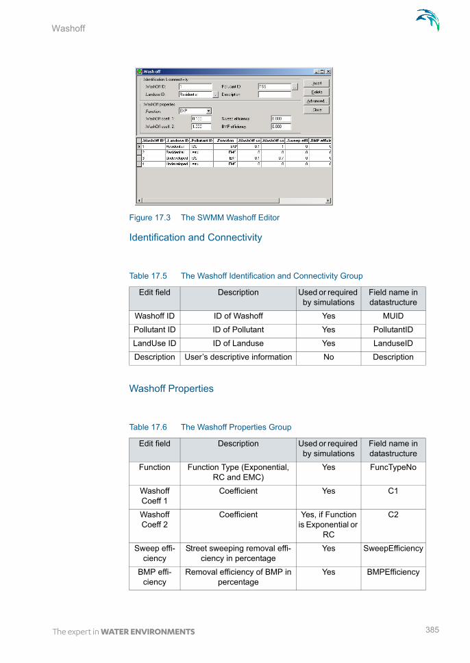
Washoff
Figure 17.3 The SWMM Washoff Editor
Identification and Connectivity
Washoff Properties
Table 17.5 The Washoff Identification and Connectivity Group
Edit field Description Used or required by simulations
Field name in datastructure
Washoff ID ID of Washoff Yes MUID
Pollutant ID ID of Pollutant Yes PollutantID
LandUse ID ID of Landuse Yes LanduseID
Description User’s descriptive information No Description
Table 17.6 The Washoff Properties Group
Edit field Description Used or required by simulations
Field name in datastructure
Function Function Type (Exponential, RC and EMC)
Yes FuncTypeNo
Washoff Coeff 1
Coefficient Yes C1
Washoff Coeff 2
Coefficient Yes, if Function is Exponential or
RC
C2
Sweep effi-ciency
Street sweeping removal effi-ciency in percentage
Yes SweepEfficiency
BMP effi-ciency
Removal efficiency of BMP in percentage
Yes BMPEfficiency
385

Water Quality Modelling with SWMM
17.5 Loading
Input loadings of pollutants from external and dry weather inflows are sup-plied through time series data associated with particular nodes of the collec-tion system.The definition of the boundary connection of external timeseries to a node is done in the CS SWMM Loading Editor.
The CS SWMM Loading Editor organizes the related data for setting up the boundary connection of the pollutant inflow timeseries to the model into the following groups:
Identification and Connectivity - General identification and location infor-mation
Loading Properties - Initial Buildup data
Figure 17.4 The SWMM Loading Editor dialog
Identification and Connectivity
Table 17.7 The Loading Identification and Connectivity Group
Edit field Description Used or required by simulations
Field name in datastructure
Loading ID ID of Loadpoint (Node) Yes MUID
Catchment ID
ID of Catchment Yes CatchID
Pollutant ID ID of Pollutant Yes PollutantID
Description User’s descriptive information No Description
386 MIKE URBAN - © DHI

Pollutant
Loading Properties
17.6 Pollutant
The generation, inflow and fate of any number of user-specified pollutants can be modelled. Concentrations in rainfall, in groundwater, in inflow/infiltra-tion is modelled.
There can be used following different units for the individual user defined pol-lutant units (milligrams/liter, micrograms/liter, or counts/liter)
Co-pollutants can also be modelled. For example, pollutant X can have a co-pollutant Y, meaning that the runoff concentration of X will have some fixed fraction of the runoff concentration of Y added to it.
The pollutant buildup and washoff on catchment areas are determined by the Land Uses assigned to those areas.
The CS SWMM Pollutant Editor organizes the related input data for the pol-lutants into the following groups:
Identification and Connectivity - General identification and location infor-mation
Pollutant Properties - Pollutant related data
Table 17.8 The Loading Properties Group
Edit field Description Used or required by simulations
Field name in datastructure
Initial buildup
Initial buildup of pollutant Yes InitBuildUp
387

Water Quality Modelling with SWMM
Figure 17.5 The SWMM Pollutant Editor
Identification and Connectivity
Pollutant Properties
Table 17.9 The Pollutant Identification and Connectivity Group
Edit field Description Used or required by simulations
Field name in datastructure
Pollutant ID ID of Pollutant Yes MUID
Description User’s descriptive information No Description
Table 17.10 The Pollutant Properties Group
Edit field Description Used or required by simulations
Field name in datastructure
Unit Selec-tion
Unit selection of pollutant Yes TypeNo
Concentra-tion in rain
Concentration of pollutant in rain
Yes Crain
Concentra-tion in GW
Concentration of pollutant in groundwater
Yes Cgw
Concentra-tion I/I
Concentration of pollutant in I/I Yes Cii
First order decay coeff
First order decay coefficient Yes Kdecay
Co-pollutant ID of the co-pollutant Yes CoPollut
Co-pollutant fraction
Fraction of co-pollutant Yes CoFract
388 MIKE URBAN - © DHI

Local Treatments
17.7 Local Treatments
Removal of pollutants contained in the flow into a node can be modelled by assigning a set of treatment functions to the node. Treatment functions can be any well-formed mathematical expression involving:
pollutant concentrations at the node's inlet (use the pollutant name to represent a concentration)
removals of other pollutants (use R_ prepended to the pollutant name to represent removal)
process variables which include:
FLOW for flow rate into node (user's flow units)
DEPTH for water depth above node invert (ft or m)
AREA for node surface area (ft2 or m2)
DT for routing time step (sec)
HRT for hydraulic residence time (hours)
The result of the treatment function can be either a concentration (denoted by the letter C) or a fractional removal (denoted by R).
For example, a first-order decay expression for BOD exiting from a storage node might be:
(17.6)
while having the removal of some trace pollutant be proportional to the removal of total suspended solids (TSS) would be written as:
(17.7)
The CS SWMM Treatment Editor organizes the related input data for the local treatment into the following groups:
Identification and Connectivity - General identification and location infor-mation
Buildup dur-ing snowfall
Buildup during snowfall. Yes if buildup only occurs during
snowfall, no otherwise
Yes SnowFlag
Concentra-tion dwf
Concentration of pollutant in DWF
Yes Cdwf
Table 17.10 The Pollutant Properties Group
Edit field Description Used or required by simulations
Field name in datastructure
C BOD e 0,05– HRT=
R 0,75 R_TSS=
389

Water Quality Modelling with SWMM
Local Treatment Properties - Treatment function
Figure 17.6 The SWMM Treatment Editor dialog
Identification and Connectivity
Treatment Properties
Table 17.11 The Pollutant Identification and Connectivity Group
Edit field Description Used or required by simulations
Field name in datastructure
Node ID ID of Node where local treat-ment is performed
Yes MUID
Pollutant ID ID of pollutant Yes PollutantID
Description User’s descriptive information No Description
Table 17.12 The Treatment Properties Group
Edit field Description Used or required by simulations
Field name in datastructure
Function Function expressing the treat-ment result in terms of pollut-ant concentrations, pollutant removals, and other standard
variables.
Yes Function
390 MIKE URBAN - © DHI

INDEX
457

Index
BBasin geometry . . . . . . . . . . . . . 157Biological Processes . . . . . . . . . . 296
CCapacity Curve . . . . . . . . . . . . . 157Conduits . . . . . . . . . . . . . . . . 352Control action . . . . . . . . . . . . . . 245Controllable devices . . . . . . . . . . 251Cross sections . . . . . . . . . . . . . 66
FFlooding . . . . . . . . . . . . . . . . 207Flow Dividers . . . . . . . . . . . . . . 344FST . . . . . . . . . . . . . . . . . . . 208
HHydrological models . . . . . . . . . . 73
IInlet . . . . . . . . . . . . . . . . . . . 49
JJob list . . . . . . . . . . . . . . . . . 266Junctions . . . . . . . . . . . . . . . . 344
KKinematic Wave . . . . . . . . . . . . 80
LLinear Reservoir . . . . . . . . . . . . 84Long Term Statistics . . . . . . . . . . 265
NNodes and Structures . . . . . . . . . 22
OOrifice . . . . . . . . . . . . . . . . . . 44Outfalls . . . . . . . . . . . . . . . . . 344
PPID . . . . . . . . . . . . . . . . . . . 246Pipe Design . . . . . . . . . . . . . . . 283Pipes and Canals . . . . . . . . . . . . 36Pump . . . . . . . . . . . . . . . . . . 54
QQH Relation . . . . . . . . . . . . . . . 157
RRDI . . . . . . . . . . . . . . . . . . . .92
SSediment transport . . . . . . . . . . . 295Sensor . . . . . . . . . . . . . . . . . 242Soakaway. . . . . . . . . . . . . . . . .29Storage Units . . . . . . . . . . . . . . 344
TTime series . . . . . . . . . . . . . . . 137Time-Area Curve . . . . . . . . . . . . 157Time-Area Method . . . . . . . . . . . .75
UUnit Hydrograph Method . . . . . . . . .89
WWeirs . . . . . . . . . . . . . . . . . . .41
458 MIKE URBAN - © DHI


![[Mike Davis] Planet of Slums(Book ZZ org)](https://img.pdfslide.net/doc/110x75/632066d5069357aa45062ed0/mike-davis-planet-of-slumsbook-zz-org.jpg)


