Minima of interannual sea-level variabilityin the Indian Ocean

D. Shankara, S. G. Aparnaa, J. P. McCrearyb, I. Suresha, S. Neetua, F. Durandc,S. S. C. Shenoia, M. A. Al Saafania,d

aNational Institute of Oceanography, Dona Paula, Goa 403 004, India.bSOEST, University of Hawaii, Honolulu, Hawaii, USA.

cIRD, LEGOS, UMR5566 CNRS-CNES-IRD-UPS, 14 Avenue Edouard Belin, 31400 Toulouse,France.

dDepartment of Earth and Environmental Sciences, Faculty of Science Sana’a University, Yemen.

Abstract

Wavelet analysis of altimeter sea level in the Indian Ocean shows regions of high

variability (maxima) and low variability (minima) at all time scales. At interan-

nual time scales, i.e., at periods of 17 months or more, minima are seen at several

places: in the central equatorial Indian Ocean; in the Arabian Sea along the south

and west coasts of India and Sri Lanka, along the northern boundary, in the Gulf

of Aden, and in patches along the coast of Oman; and in the Bay of Bengal along

the east coasts of Sri Lanka and India south of ∼ 10◦N, and in the southern bay

east of the Sri Lanka thermal dome. We investigate the cause of these interannual

minima using a linear, continuously stratified numerical model, which is able to

simulate the observed minima. We separate the forcing into a set of processes:

direct forcing by winds in the interior ocean, forcing by winds blowing along con-

tinental boundaries, and forcing by Rossby waves generated by the reflection of

equatorial Kelvin waves at the eastern boundary. At interannual periods, min-

ima (maxima) of interannual variability occur where the direct wind forcing and

reflected Rossby waves interfere destructively (constructively). At interannual pe-

Preprint submitted to Elsevier September 27, 2009

Author version: Progress in Oceanography 84 (2010) 225–241

An edited version of this paper was published by Elsevier. Copyright [2010]

riods within the tropics, the adjustment time scale of the system is less than that

of the forcing, leading to a quasi-steady balance, a property that distinguishes the

interannual minima from those at annual and semiannual time scales. Idealised

solutions show that the presence of India forces the minimum along the Indian

west coast, and that it extends around the perimeter of the Arabian Sea into the

Gulf of Aden.

2

1. Introduction

1.1. Background

During the past decade, there has been remarkable progress in observing and

understanding interannual variability in the Indian Ocean. This progress was trig-

gered by advances in satellite technology and the occurrence of an intense Indian

Ocean Dipole/Zonal Mode (IODZM; also called the Indian Ocean Dipole or In-

dian Ocean Zonal Mode) during 1997, a climatic event associated with anomalous

easterlies along the equator and both cool sea-surface temperature (SST) and low

sea level in the eastern equatorial Indian Ocean (EEIO) (Murtugudde et al., 1998;

Saji et al., 1999; Webster et al., 1999; Murtugudde and Busalacchi, 1999; Mur-

tugudde et al., 2000). Since that time, the impacts of both IODZM and El Nino

and the Southern Oscillation (ENSO) on Indian Ocean SST and circulation have

been studied extensively, and there is evidence that interannual SST anomalies in

the Indian Ocean feedback to affect winds and rainfall locally and remotely. See

Yamagata et al. (2004), Annamalai and Murtugudde (2004), Chang et al. (2006),

and Schott et al. (2009) for reviews of this progress.

Sea-level variability has been particularly useful for describing and under-

standing ENSO, IODZM, and other phenomena because of the information it pro-

vides about ocean dynamics. Sakova et al. (2006) used TOPEX/Poseidon data to

show the existence of large sea-level signals in five frequency bands (semiannual,

annual, 18–20 months, 3 years, and 4–6 years), the bands “being separated by

substantial spectral gaps.” Figure 1 shows the variability in the semiannual, an-

nual, 17–20 months, and 3-year bands. (The 4–6-year band is not resolved well in

the short altimeter record.) Interestingly, regions of both high and low variability

are evident in all the panels. Although the magnitude of variability varies through

3

the interannual period range from 17 months to over 3 years, the spatial patterns

for these interannual bands are similar (Figure 1; see also Figure 5 of Sakova et al.

(2006)). The structures of these high- and low-variability regions in the 17–20-

month and 3-year bands, however, differ markedly from those for the annual and

semiannual periods, pointing toward the importance of different processes acting

at the three time scales: interannual, annual, and semiannual.

Baroclinic waves are more apparent in the north Indian Ocean than they are in

the other oceans owing to its tropical location, its small size, and the seasonal forc-

ing by the monsoon winds. The presence of baroclinic waves, which have received

considerable attention in the literature (see, for example, the review by Schott and

McCreary, 2001) implies that changes in sea level can be forced at a given loca-

tion by winds blowing elsewhere earlier in the season. This phenomenon, called

remote forcing, “merges the equatorial Indian Ocean, the Arabian Sea, and the

Bay of Bengal into a single dynamical entity” (Shankar et al., 2002). These waves

are evident at time scales from intraseasonal to interannual.

One of the first descriptions of the basin-scale, baroclinic waves in the IO,

based on the relatively coarse Geosat data, revealed the presence of annual Rossby

waves outside the equatorial waveguide in both hemispheres (Perigaud and Delecluse,

1992a). Such westward-propagating Rossby waves were subsequently observed

in altimeter sea level, radiating from the eastern boundaries of the Bay of Bengal

(Perigaud and Delecluse, 1993; Vinayachandran et al., 1999) and the Arabian Sea

(Shankar and Shetye, 1997; Brandt et al., 2002; Shankar et al., 2004; AlSaafani

et al., 2007), and in the south Indian Ocean (Perigaud and Delecluse, 1993; Fu and

Smith, 1996). The existence of annual Rossby waves has since been confirmed

even in expendable bathythermograph (XBT) data (Masumoto and Meyers, 1998)

4

and in a climatology (Levitus, 1982) of hydrographic data (Unnikrishnan et al.,

1997). Such Rossby waves, as well as coastal and equatorial Kelvin waves, also

appear prominently in model simulations (Lighthill, 1969; McCreary et al., 1993;

Schott and McCreary, 2001; Shankar et al., 2002).

In the equatorial waveguide, the semiannual signal is also strong in the eastern

and western ocean (Knox, 1976; Luyten and Roemmich, 1982; Reverdin, 1987),

there being a minimum-variability region in between (Figure 1).

Model studies show that this strong semiannual signal is due to constructive

interference of incident (directly forced by the wind) and reflected waves (Blanc

and Boulanger, 2001) for the second baroclinic mode (Jensen, 1993; Clarke and

Liu, 1993; Han et al., 1999). Also playing a role in enhancing the semiannual

signal are the different spatial structures of the annual and semiannual winds,

resonance with the semiannual wind, and shear flow in the mixed layer of the

EEIO (Han et al., 1999).

At interannual time scales, Rossby-wave propagation in the tropical south In-

dian Ocean is evident even in Geosat data (Perigaud and Delecluse, 1992b). These

interannual Rossby waves are prominent in altimeter (Fu and Smith, 1996) and

XBT (Masumoto and Meyers, 1998) data and in model simulations (Perigaud and

Delecluse, 1992b; Masumoto and Meyers, 1998). Particularly prominent is the in-

terannual Rossby wave in the south Indian Ocean (Masumoto and Meyers, 1998)

associated with ENSO (e. g. Schott et al., 2009).

1.2. Present research

In this paper, we investigate the processes that lead to an interannual sea-

level pattern like that in the top panels of Figure 1. Although the pattern involves

both maxima and minima of variability, we focus on the latter. The maxima have

5

received considerable attention in the literature. An example is the maximum in

the EEIO, which is associated with IODZM events (see, for example, reviews

by Yamagata et al., 2004; Annamalai and Murtugudde, 2004; Chang et al., 2006;

Schott et al., 2009); this maximum is also prominent in spatial maps of 18–20-

month and 3-year variability (Sakova et al., 2006). The minima, however, are

surprising, given the prevalence of remotely forced waves that can spread signals

throughout the basin. They are therefore more indicative of basic physics than are

the maxima.

Our approach is to identify prominent features of the interannual response in

sea-level observations (Section 2), to assess the contributions of directly-forced

and boundary-wave responses using a numerical ocean model (Section 3), and

to illustrate basic dynamics by obtaining solutions to a simplified version of the

model that allows for an analytic solution (Section 4). Section 5 concludes the

paper.

We emphasize here that the term “interannual variability” designates the vari-

ability that remains after a time series is low-pass filtered to retain frequencies

lower than the annual. Thus, short-term interannual (ENSO, IODZM) events,

prominent aspects of which (e.g., SST anomalies) typically last less than a year,

appear as low-frequency (2–6 year) signals in our analyses, a potential confusion

of time scales. On the other hand, sea-level variations associated with such events

involve the off-equatorial propagation of Rossby waves and so do adjust at in-

terannual time scales. Hence, in summary, we consider interannual variability in

frequency space rather than considering it to be a result of events that occur every

few years.

We find that minima, i. e., regions of low interannual variability, occur pri-

6

marily from the destructive interference between the directly-forced response and

boundary-reflected waves. In addition, their horizontal structure is similar at peri-

ods of 17 months or longer, a property that can be understood in terms of simple

physics: Essentially, these periods are longer than the adjustment time of the trop-

ical Indian Ocean, so that the ocean is nearly adjusted to a quasi-steady state.

2. Observational analyses

2.1. Data2.1.1. AVISO sea level

Our primary data set is the gridded sea-level product from AVISO (AVISO,

1996, hereafter referred to as AVISO) for the period 1993–2004, from which sea-

level anomalies (SLAs) are computed relative to the 7-year mean from 1993–

1999. The AVISO product merges data from several altimeters to produce a

weekly gridded field on a 0.33◦ × 0.33◦ Mercator projection grid (Ducet et al.,

2000), the merged data set having smaller mapping errors and better spatial cov-

erage than a data set based on any one satellite (Ducet et al., 2000; Volkov, 2005).

Comparison with the recently processed MAP (Margins Altimetry Project) data

(Vignudelli et al., 2000) shows that the gridded data product has problems near

coasts, but it is accurate offshore (Durand et al., 2008, 2009).

2.1.2. Spatial and temporal sampling

To facilitate comparison with the numerical simulations reported in Section 3,

we used the regridding tool in Ferret (Hankin et al., 2006) to remap the AVISO

SLA onto the model’s 0.5◦×0.5◦ grid. We considered sampling intervals of both

one week and one month. As may be expected (DeMoortel et al., 2004), the

magnitudes of the wavelet transforms (discussed next) based on the two sampling

7

intervals differ somewhat, but their spatial patterns are essentially the same. In the

rest of this paper, then, we report analyses of monthly records.

2.1.3. Wavelet analysis

To show how spatial patterns of the response vary with frequency, we sub-

jected the data to a wavelet analysis using a Morlet wavelet as the basis function.

The advantage of a wavelet transform over a traditional Fast Fourier Transform

(FFT) analysis is that it also provides the variation of structures with time. Given

the considerable interannual variability even within the limited duration of the al-

timeter record (see, for example, the wavelet spectrum of the 20◦C isotherm in

Figure 2 of Sakova et al. (2006)), the wavelet transform yields more information

than is available from an FFT analysis. The maps of wavelet power in Figure 1

are averaged over 1993–2004 for the semiannual, annual, 17–20-month, and 3-

year period bands, defined by averages over 5.8–6.9 months, 9.8–13.9 months,

16.5–19.7 months, and 33.0–39.3 months, respectively. These maps show the

variability of sea level at the given periods.

2.2. Results2.2.1. Regions of high variability

Consistent with the spectral-density plots of Sakova et al. (2006) (their Fig-

ure 5), wavelet power for the 17–20-months and 3-year bands (top panels of Fig-

ure 1) shows maxima in the tropical south Indian Ocean between 5–10◦S, in the

eastern equatorial Indian Ocean off Sumatra and Java, and in the Somali-Current

region. There are weaker maxima in the northwestern (∼ 15◦N) and southwestern

(∼ 8◦N) Bay of Bengal, both regions being thermal domes where the thermocline

is shallow (Shetye et al., 1996; Vinayachandran and Yamagata, 1998).

8

2.2.2. Regions of low variability

The most prominent minimum occurs in the central equatorial Indian Ocean

(CEIO) between the relative maxima in the EEIO and western equatorial Indian

Ocean (WEIO; top panels of Figure 1). Extending southeastward from this CEIO

minimum is a minimum “tongue” separating the maxima off Sumatra and the

tropical south Indian Ocean between 5–10◦S. A longitude-period section along

the equator shows that minima occur in the CEIO at all periods greater than the

annual (top panel of Figure 2), from a period around 17 months to over 3 years

(the highest period resolved by the data set).

The CEIO minimum is contiguous to the minima south of Sri Lanka and along

the Indian west coast. The latter region broadens to the north, where it spreads

almost halfway across the northern Arabian Sea and extends along the northern

boundary of the Arabian Sea. There are also minima in the Gulf of Aden and along

the Somali coast; they are separated from each other and from the minimum in

the northern Arabian Sea by maxima that occur off Oman and northern Somalia.

These maxima occur in regions of high eddy activity, two examples being the

Great Whirl and the Socotra Eddy (Schott and McCreary, 2001), and the high

interannual variability of the eddy field accounts for the distinct maxima seen in

the wavelet analysis (Figure 1).

The minimum south of Sri Lanka also extends along the east coast of India into

the Bay of Bengal to about 13◦N. To its east is a relative maximum in the regime

of the Sri Lanka dome (Vinayachandran and Yamagata, 1998); farther east is a

broad minimum that spreads across most of the southern Bay of Bengal. To the

north of this southern-bay minimum is a maximum that covers much of the central

bay. The minimum in the southern bay, however, extends into the northcentral bay

9

as an anticlockwise semicircular arc that bounds the central-bay maximum on its

east and north. Finally, along the perimeter of the northern Bay of Bengal, there

is a maximum hugging the coasts of Myanmar (Burma), Bangladesh, and India

north of about 13◦N.

2.2.3. Time series

We filtered the sea-level data with a low-pass filter, using a third-order Butter-

worth filter with a cutoff period of 18 months. Figure 3 plots the resulting time

series at 8 locations, indicated by numbers in Figure 1, in the basin. In regions

of maximum variability (locations 2, 5, and 7), sea level has a higher range than

at minimum locations (locations 1, 3, 4, 6, and 8), but the range was low even in

some maximum locations during some years. For example, in the maximum off

Somalia (location 2) and in the thermal domes (location 5), the range decreased

after 2000. In contrast, in regions of variability minima, the range of sea level was

low throughout the record. That the variability is low at all times in the minimum

locations is the essential difference between them and the maximum locations.

This difference is clearly seen in a wavelet analysis of the altimeter sea level (Fig-

ure 4) at these locations: At all periods greater than the annual, variability is low

at minimum locations throughout the record, although there is a variation in the

wavelet power with both period and time. In maximum locations, wavelet power

shows higher temporal variation.

2.2.4. Summary

Despite noise in the form of patches of high and low interannual variability,

regions of minimal variability are as distinct as those of maximal variability re-

ported earlier (Sakova et al., 2006). Although the altimeter record is too short to

determine if similar minima exist at longer periods, their existence at all resolved

10

periodicities greater than the annual, their persistence throughout the duration of

the record (Figures 3 and 4), and their spatial connectedness suggests that the

phenomenon is an intrinsic feature of all Indian-Ocean sea-level variability at suf-

ficiently long periods. In the rest of this paper, we seek to determine the cause of

these minima.

3. Numerical solutions

In this section, we first describe our ocean model, also providing justifications

for its linearity and that it is only wind-driven (Section 3.1). Then, we report our

main run, comparing it with observations (Section 3.2), and commenting on the

model’s limitations (Section 3.3). We then separate our main run into several parts

(process solutions), noting that only two processes are important at periods greater

than the annual, and that minima occur when these two processes tend to interfere

destructively (Section 3.4). We conclude with a discussion of the model results at

periods higher than those resolved by the altimeter data (Section 3.5).

3.1. Ocean model

A useful tool for understanding the wind-driven oceanic response is the lin-

ear, continuously stratified (LCS) model described next. It has already been used

to investigate a variety of Indian-Ocean phenomena. For example, it was used

to study the dynamics of the East India Coastal Current (EICC) (Shankar et al.,

1996; McCreary et al., 1996), the West India Coastal Current (WICC) (Shankar

and Shetye, 1997; Nethery and Shankar, 2007), and the impact of the Indonesian

Throughflow on Indian Ocean circulations (McCreary et al., 1986, 2007). Here,

we present a brief overview of the model. Additional details can be found else-

where (McCreary, 1980, 1981; Shankar et al., 1996; McCreary et al., 1996). The

11

model is limited in several ways, namely, it is only wind-forced, is linear, and has

a flat bottom. We begin with a discussion of why we feel these limitations are not

serious problems.

3.1.1. Justification

Non-tidal sea-level variations can result from atmospheric pressure, buoyancy

fluxes, and wind forcing (Patullo et al., 1955). At interannual time scales, varia-

tions in atmospheric pressure can be ignored (see Section 6.1 in Shankar (1998),

downloadable from http://hdl.handle.net/2264/24). Han and Webster (2002) con-

sidered the impact of buoyancy fluxes on interannual sea level in the Bay of Ben-

gal, concluding that variability of river discharge has a negligible impact along

the east coast of India, but that variability of precipitation over the Bay of Bengal

is important. When the freshwater fluxes are high (low), steric sea level will rise

(fall), leading to high variability in regions affected by (variability in) freshwater

fluxes. Hence, freshwater fluxes are more relevant for sea-level-variability max-

ima. This effect, however, can be expected to be limited to the regions of high

precipitation and to regions where low-salinity water is advected (Han and Web-

ster, 2002; Shankar and Shetye, 1999, 2001; Shankar, 2000). Hence, in order to

explain the existence of the interannual-sea-level-variability minima in the CEIO

and along the boundaries of the Arabian Sea and Bay of Bengal, we can restrict

our attention to the effect of wind forcing.

As noted by Shankar and Shetye (1997) and Shankar et al. (2002), much of

the response in the Indian Ocean can be understood in terms of linear dynamics,

significant nonlinearities being restricted to the Somali-Current regime. Another

significant nonlinearity is related to regions of strong upwelling, one of them lying

off Somalia and the other off Oman. The simulations of Shankar and Shetye

12

(1997) and Shankar et al. (2002) show, however, that the upwelling off the Indian

west coast is explicable by linear wave theory.

To represent solutions as expansions in vertical normal modes (see below),

the LCS model must have a flat bottom, thereby excluding continental-shelf pro-

cesses. As can be seen from the wavelet analysis in Figure 1, however, the minima

exist on the shelf, off the shelf, and in the open ocean, implying the lack of rele-

vance of shelf physics for their existence.

3.1.2. Equations

The equations of motion of the LCS model are linearized about a state of

rest, with a background Brunt-Vaisala frequency, Nb(z), given by the profile of

Moore and McCreary (1990). There is vertical mixing with coefficients of the

form ν = A/N2b and A = 1.3× 10−4 cm2/s, wind is introduced into the ocean as

a body force of the form Z(z) = θ(z+H)/H, where H = 50 m, and the ocean

bottom is assumed flat with a depth D= 4000 m.

Let q be either u, v, or p. Then, q can be written

q(x,y,z, t) =N

∑n=1qn(x,y, t)ψn(z), (1)

where the set of functions ψn(z) are the vertical (barotropic and baroclinic) modes

of the system that satisfy the eigenfunction equation,(

ψnzN2b

)z=−

1c2n

ψn, (2)

subject to the boundary conditions ψnz(0) = ψnz(−D) = 0 and normalized so that

ψn(0) = 1. The eigenvalues cn are the Kelvin-wave speeds for mode n. The

summation in (1) should extend to ∞, but in practice it must be truncated at a

finite value N. In the present study, we use choose N = 10, and most of the

13

response is captured by the first two modes. The summation begins at n = 1,

thereby neglecting the barotropic (n = 0) response; as in McCreary et al. (1996),

the barotropic impact on sea level is weak in comparison to the baroclinic response

in our wind-driven solutions.

The resulting set of equations for the expansion coefficients is

unt − f vn+1ρpnx = Fn−

(Ac2n

)un+νh∇2un−δun,

vnt + f un+1ρpny = Gn−

(Ac2n

)vn+νh∇2vn,

1c2npnt +unx+ vny =−

(Ac2n

)pn−

δc2npn,

(3)

where Fn = τxZn/Hn, Gn = τyZn/Hn, Hn =R 0−Dψ2ndz, and Zn =

R 0−DZ(z)ψn(z)dz.

The coefficient Zn/Hn determines how strongly mode n is coupled to the wind.

The horizontal mixing coefficient νh = 5×107 cm2 s−1, which is large enough to

ensure numerical stability (McCreary et al., 1996). Some test solutions include a

damper δ(x,y) in the EEIO (x > 92.75◦E, −7.5◦S < y < 7.5◦N), which absorbs

incoming equatorial Kelvin waves as well as the Rossby waves that reflect from

the eastern boundary (McCreary et al., 1996). Following McCreary et al. (1996),

δ has a maximum value of cn/(1.5Δx) (where Δx is the zonal grid spacing) in this

region, and decreases linearly to zero within 5◦ of its western edge and within

2◦ of its northern and southern edges. The advantage of equations (3) is that

the original, three-dimensional (x, y, and z) set of equations are reduced to two

dimensions (x and y).

3.1.3. Basin geometry, boundary conditions, and forcing

Solutions are found for a realistic basin geometry north of 29◦S, with continen-

tal boundaries lying roughly along the 200 m isobath. The grid used is Arakawa-C

14

with a uniform spacing of 0.5◦. The basin shape north of 10◦S is shown in Fig-

ure 5, and the entire basin is provided in McCreary et al. (1993). For most of our

solutions, closed, no-slip conditions

un = vn = 0 (4)

are applied along continental boundaries, the exceptions being two of our process

solutions that use alternate conditions (Equations (5) below). With these closed

boundary conditions, the Indonesian passages are always closed so that there is

no Indonesian Throughflow in any of our solutions.

The model ocean is forced by monthlywinds from the NCEP/NCAR (National

Centers for Environmental Prediction/National Center for Atmospheric Research)

reanalyses (Kalnay et al., 1996). It is spun up from a state of rest starting on 1

January 1948, and model output from 1993–2004 is used for comparison with the

altimeter sea level.

3.2. Main run

Our main run (Solution MR) is the solution obtained using boundary condi-

tions (4) along all continental boundaries and without the equatorial damper, i. e.,

δ(x,y) = 0. As for the altimeter data, we carried out a wavelet analysis of the

model sea level to obtain time-averaged plots of wavelet power. Figure 2 (bot-

tom panel) shows wavelet power along the equator as a function of period, and

Figure 5 (top left panel) presents the spatial map of wavelet power at the 3-year

period; the map for the 17–20-month period is similar to that for the 3-year period.

3.2.1. Maps of interannual wavelet power

Solution MR (top left panel of Figure 5) reproduces all the prominent maxima

and minima in the altimeter data at the 3-year period (Figure 1), the most obvious

15

model/data difference being the smoothness of the solution, which is expected

because the model is linear. The solution simulates the observed minima in the

CEIO, along the eastern and northern boundaries of the Arabian Sea, in the Gulf

of Aden, along the southeast coast of India and Sri Lanka, and in the southern

Bay of Bengal. In addition, it also simulates a narrow minimum along the Omani

coast, not apparent in the observations. Finally, note that there is a maximum

in the region of the thermal domes in the southwestern Bay of Bengal, as in the

altimeter sea level; also, as in the observations, the maximum in the regime of the

Sri Lanka dome in the southwestern bay separates the coastal minimum and the

open-ocean minimum in the southern bay.

3.2.2. Time series

As for the altimeter sea level, we filter model sea level with a low-pass third-

order Butterworth filter with a cutoff period of 18 months. In regions not influ-

enced by river discharge or high rainfall (like the northern Bay of Bengal: not

shown), the model sub-annual variability is similar to that observed (Figure 3).

3.3. Model limitations3.3.1. Minimum tongue southeast of the CEIO

The altimeter data show a striking minimum tongue extending southeastward

from the CEIO (Figure 1), but the model solution merely hints at its existence,

the tongue being very weak in the model and its connection to the CEIO not as

evident (Figure 5). A detailed analysis of this model lacuna is beyond the scope

of our paper, but three possible causes come to mind. First, the region south of the

equator is the regime of the South Equatorial Counter Current (SECC) (see, for

example, Schott and McCreary, 2001), which does not reverse with season. The

SECC flows eastward, opposing the westward propagating Rossby wave. Non-

16

linear interaction between the current and the wave, a process not included in the

LCS model, may interfere with the Rossby wave. Second, the model has a closed

eastern boundary and therefore does not include the impact of the Indonesian

Throughflow; the consequences of this boundary forcing are unclear. Third, the

forcing used is the winds from the NCEP/NCAR reanalysis; it is possible that the

forcing is inaccurate.

3.3.2. Coast of Oman

The minimum along the northern boundary of the Arabian Sea extends coun-

terclockwise along the coast of Oman (Figure 5). In the observations, however,

there is no such continuous minimum along the Omani coast, the minima there

appearing instead as distinct patches (Figure 1). The observations conducted off

the Omani coast during the US JGOFS (Joint Global Ocean Flux Study) program

showed that the offshore flow occurs in squirts and jets at a few capes like Ras al

Hadd, where the Ras al Hadd Jet (Bohm et al., 1999) veers off the coast, trans-

porting the cool, upwelled waters into the interior of the basin. Minima occur

in the vicinity of these capes, being separated by relative maxima; the variabil-

ity, however, is generally weaker along the Omani coast than farther offshore or

southward off Somalia (Figure 1). This difference is to be expected because the

model is linear and jets like the Ras al Hadd Jet are nonlinear phenomena (see the

discussion in Section 4.5 in Schott and McCreary, 2001). Notwithstanding this

difference, it is evident that the interannual variability of even these nonlinear jets

is connected to, and determined by, that of the linear western boundary current of

whose instability they are a manifestation.

17

3.3.3. Freshwater flux into northern bay

The model solution (Figure 5) reproduces the maximum observed along the

perimeter of the northern bay, counterclockwise from the east coast of Myan-

mar to about 13◦N along the Indian east coast (Figure 1). This coastally trapped

maximum, which implies a relative minimum offshore in the northcentral bay

(Figures 1 and 5), is due to the counterclockwise propagation of Kelvin waves

along the perimeter of the bay (Potemra et al., 1991; Yu et al., 1991). Neverthe-

less, though the wind-forced model seems to explain the existence of the maxi-

mum along the perimeter of the northern bay, we cannot rule out the possible role

of freshwater flux in the region. Zonal winds over the equatorial Indian Ocean

(Clarke and Liu, 1994) and Ekman pumping in the interior bay (Han and Web-

ster, 2002) have been invoked to explain the interannual variability observed in

tide-gauge sea level along the Indian east coast. A different hypothesis was pro-

posed by Shankar and Shetye (1999), who found a strong correlation between

rainfall over India and sea-level variability along the Indian west coast on inter-

annual and interdecadal time scales: Shankar and Shetye (1999) linked the low-

frequency variability of sea level to the rainfall over India, with the large-scale

coastal currents and the cross-shore gradient of salinity playing an intermediate

role. Though the numerical simulations of Han and Webster (2002) suggest that

interannual variability in river influx is not as important as interannual variability

of winds for the sea level along the Indian east coast, Han and Webster (2002) did

find that interannual variability in rainfall over the Bay of Bengal is an important

cause of the interannual variability of sea level. The impact of freshwater flux,

whose major source due to rivers lies in the northern bay (Shetye, 1993) and ma-

jor source due to rainfall lies in the northeastern bay (Xie and Arkin, 1999), is felt

18

primarily in the regions near the source and in the regions to which this freshwa-

ter is advected. One major pathway for advection of freshwater from the northern

bay is the east coast of India (Wyrtki, 1971; Shetye et al., 1996; Shenoi et al.,

1999; Han et al., 2001; Durand et al., 2007; Kurian and Vinayachandran, 2007)

and another pathway is along the west coast of Myanmar (Jensen, 2003). These,

the northern, northeastern, and northwestern boundaries of the bay, are precisely

the regions in which the maximum occurs, implying that both wind forcing and

freshwater flux may be important causes of this maximum (and therefore indi-

rectly of the relative minimum to its south in the northcentral bay). Indeed, that

this maximum is stronger on the shelf of this region than on the continental slope

(Figure 1) suggests an important role for freshwater flux.

3.4. Process solutions

The above limitations notwithstanding, the model solution is in remarkable

agreement with the observations. Therefore, because the model is linear, it is pos-

sible to separate the total response into a set of process solutions, each driven by a

different forcing mechanism. As we shall see, sea-level minima can then be gen-

erated by destructive interference between two or more of the process solutions.

3.4.1. Directly-forced and boundary-wave responses

We split the total response into contributions from three sources: 1) direct

forcing by winds in the interior ocean; 2) forcing by coastal winds blowing along

continental boundaries; and 3) Rossby waves generated by the reflection of equa-

torially trapped Kelvin waves at the Sumatra coast. Similar separations have been

carried out earlier for the Bay of Bengal (Shankar et al., 1996; McCreary et al.,

1996) and for the monsoon currents (Shankar et al., 2002).

19

Figures 6 and 7 illustrates the two components of the wind forcing, providing

plots of wavelet power along basin boundaries (process 2) and in the ocean inte-

rior (process 1), respectively. Figure 6 provides a distance-period plot of wavelet

power for zonal winds along the equator and the alongshore component of the

winds along the continental boundary of the northern Indian Ocean. At the annual

period, power stands out in the WEIO and CEIO and almost the entire boundary

of the north Indian Ocean. In contrast, at the semiannual period, the wind field

is strong only in the CEIO, and the coastal winds are weak except off Oman in

the regime of the Findlater Jet (Findlater, 1969). At interannual periods (∼ 2–

5 years), the forcing is associated primarily with ENSO and IODZM, consisting

of easterlies along the equator and southeasterlies in the southeastern tropical In-

dian Ocean. Interannual forcing at periods resolved in the altimeter observations

(≤ 3 years) is strong only in the CEIO (68–96◦E, 10◦S–8◦N).

Figure 7 plots the Ekman-pumping velocity, wek = (1/ρ)curl (τ/ f ), for the

3-year period. Ekman pumping is strong at the 3-year period, and much of it is

associated with the meridional weakening of the equatorial easterlies away from

the equator. Such interannual variability in Ekman pumping during IODZM and

ENSO events has been discussed by several authors (Ashok et al., 2004; Yu et al.,

2005; Rao and Behera, 2005); see Schott et al. (2009) for a recent review.

3.4.2. Methodology

To separate the contributions from each of these forcings, we obtain three

test solutions (TS). The first solution (Solution TS1) is like MR, but includes the

equatorial damper δ. The difference, MR−TS1 (Solution EQ), then illustrates

the effects of remote forcing only by the reflection of equatorial Kelvin waves off

Sumatra (process 3). It also includes the effect of direct wind forcing within the

20

region covered by δ, but this effect is not large because interannual wind forcing

is weak there (Figure 6).

The second solution (Solution TS2) is like MR, except that boundary condi-

tions (4) are replaced by

un = nnn ··· vvvn =−nnn ··· kkk×Fnf

,

vn = kkk×nnn ··· vvvn = 0,(5)

where nnn is a unit vector normal to the boundary, kkk is a unit vector directed upward,

vvvn = (un,vn), un and vn are velocity components perpendicular and parallel to the

boundary, and FFFn = (Fn,Gn). The unit vector nnn points out of the Bay of Ben-

gal (inshore) along its eastern and northeastern margins, into the bay (offshore)

along its northern and western margins, out of the sea (inshore) along the south-

ern boundaries of India and Sri Lanka and along their west coast (eastern Arabian

Sea), and into the sea (offshore) along the northern and western boundaries of the

Arabian Sea (Shankar et al., 2002). According to (5), Ekman drift is allowed to

pass through continental boundaries north of 3.5◦N. The difference, MR−TS2

(Solution CST), then illustrates only the effects of forcing by coastal alongshore

winds in the northern Indian Ocean (process 2). (Solution CST is equivalent to

Process AW of Shankar et al. (2002).)

The third process solution (Solution INT) includes both δ and boundary con-

ditions (5), eliminating effects of both reflection off Sumatra and of alongshore

winds in the north Indian Ocean. This solution (process 1) therefore shows the

effects of direct forcing by winds in the interior ocean, including the generation

of Kelvin waves in the equatorial ocean and of Rossby waves. It also includes

the equatorial Kelvin wave generated by the reflection of the Rossby wave at the

21

western boundary of the basin. Though this reflection is not part of the directly

forced response, we often use the term “directly forced” to refer to this process

solution (INT). Note that INT = MR - EQ - CST, a statement that MR is in fact

equal to the sum of the three process solutions.

3.4.3. Results

Figure 5 plots wavelet power from Solutions EQ (top right panel), CST (mid-

dle left panel), and INT (middle right panel). Since the alongshore winds are

weak at a period of 3 years (Figure 6), the response to these winds (Solution CST)

is negligible in comparison to the impact of the other two processes. Solution

EQ is essentially driven by the sea-level signal at the eastern equatorial boundary.

Coastal Kelvin waves spread the equatorial response poleward along the eastern

boundary, so that sea level is essentially constant along it. Since there is no forcing

for Solution EQ in the interior ocean, the eastern-coastal response then extends

into the interior ocean via Rossby-wave propagation, weakening away from the

EEIO owing to the equatorial damper δ and vertical mixing (the terms propor-

tional to A/c2n in (3)). In contrast, Solution INT is forced throughout the interior

ocean by Ekman pumping and has little or no response along the eastern boundary,

since almost all of that response is being absorbed into EQ. It has a more complex

structure than does Solution EQ, which is determined by the eastern-boundary sea

level.

Figure 3 also plots low-pass-filtered time series for Solutions EQ and INT.

It is evident that minima (maxima) occur at locations where the two solutions

interfere destructively (constructively), tending to cancel (enhance) each other.

Cancellation of EQ and INT occurs, for example, in the CEIO. Since the spatial

variation of EQ is small (Figure 5), it is essentially the spatial variation of INT

22

that determines the location of the minima. In the EEIO, the interannual wind

forcing is weak, leading to a dominance of EQ over INT and a strong sea-level

response there. In the WEIO, although EQ and INT tend to counterbalance each

other, the EQ response is slightly weaker than in the EEIO owing to damping, and

the local wind forcing is just a little stronger, producing a stronger net sea-level

response (and stronger variability) in theWEIO in comparison to CEIO. A similar

cancellation of EQ and INT holds for all the minima (Figure 3).

3.5. Longer periods

The discussion so far has been restricted to a period of 3 years or less because

the short altimeter record precludes an analysis of higher periodicities; periods

greater than 3 years fall outside the cone of influence of the wavelet power spec-

trum (Figure 4).

Our simulations, however, extend from 1948–2004 and can resolve periods up

to 10 years. These simulations show that the model response is practically the

same over the period range from 17–20 months to about 6 years (Figure 8; figure

not shown for 6 years). The similarities are striking, but there are subtle differ-

ences with period, the differences being most notable in the southwestern Bay

of Bengal, in the regime of the thermal domes (Vinayachandran and Yamagata,

1998). An examination of the process solutions (not shown) shows that these dif-

ferences arise as a consequence of differences in Solution INT, the EQ response

changing much less with period.

At a period of 10 years, however, the minimum in the central Indian Ocean

shifts southwestward and is centered at 5◦S (Figure 8). There is still a minimum

in the CEIO relative to the maximum in the EEIO (compare the two bottom panels

in Figure 9), but the variability in the vicinity of the equator is greater than that

23

to the southwest. The minima along the eastern and northern boundaries of the

Arabian Sea still exist, as do the minima along the coast of Oman and the Gulf of

Aden, along the southwestern boundary of the Bay of Bengal, and to the east of

the thermal dome (Figure 8).

Thus, the explanation for the existence of the minima holds at higher periods

too: it is the cancellation of Solutions INT and EQ that causes the minima (bottom

panels of Figure 8). At the 10-year period, however, there are some differences to

be noted. First, the structure of the wind forcing is different. The zonal wind at

the equator is no longer confined to the CEIO and the alongshore winds are not

negligible, unlike for the period range 17 months to 6 years (Figure 6). Hence,

the destructive interference is a 3-way cancellation in regions affected by Solution

CST. Second, as a consequence of the alongshore winds being stronger, the zonal

variation of Ekman pumping at this period, though still much weaker than at the

annual period, is much greater than at any other interannual period (Figure 7).

This zonal variation of the INT forcing leads to changes in the spatial structure of

the interannual-variability maxima and minima in comparison to the interannual

period band from 17–20 months to 6 years.

We do not, however, have basin-wide sea-level data to decide if these features

are realistic. At the 10-year period, the model minimum at 5◦S also contains an

uncertainty arising from the closed boundary in the east, this closed boundary

precluding exchange of mass between the Indian and Pacific Oceans via the In-

donesian Throughflow, and therefore also precluding the impact of the interannual

variability associated with it on the interannual variability of sea level in the south

Indian Ocean.

24

4. Basic dynamics

In Section 3, we have shown that minima at a broad range of interannual time

scales result from destructive interference between the directly forced (INT) and

reflected-Rossby-wave (EQ) responses. Here, we use an idealized version of the

numerical model to demonstrate that they are an aspect of the quasi-steady (near-

equilibrium) response of the ocean, which is approximately valid in the tropics at

interannual time scales.

We begin with a general discussion of quasi-stationarity (Section 4.1), then

report an analytic solution for a quasi-steady approximation to the LCS model

(Section 4.2), and then present idealized numerical solutions (Section 4.3) that

bridge the gap between the analytic solution and the realistic numerical solutions

presented in Section 3. The section concludes with a discussion of the eastern-

boundary pressure field (Section 4.4).

4.1. Quasi-steady response4.1.1. Period independence

The minima occur at all time scales greater than about 17 months and at all

these interannual periods, the mechanism is the same: there is destructive inter-

ference between the directly-forced and reflected-wave responses. Furthermore,

as long as the wind forcing patterns are similar for different interannual periods

(Section 3.5), the patterns of the response are also similar. Thus, the mechanism is

independent of period as long as it is greater than the annual, suggesting a quasi-

steady balance at interannual periods.

4.1.2. Contributions from individual modes

Minima are present in the CEIO for both the first-mode and second-mode re-

sponses, but the second-mode minimum is a little stronger (weaker variability)

25

(bottom panels of Figure 5). This lack of sensitivity to the vertical modenumber

distinguishes the model response at interannual periods from that at the annual

or semiannual periods, for which the first- and second-mode responses are very

different, there being a resonant response of the equatorial Indian Ocean for the

second mode (Jensen, 1993; Clarke and Liu, 1993; Han et al., 1999; Blanc and

Boulanger, 2001). As modenumber increases, however, the damping term A/c2nbecomes important and the interannual response is no longer independent of mod-

enumber; at these higher modes, however, the ocean couples much more weakly

to the wind than do the first two modes, and therefore it is primarily the first two

modes that determine the overall model response, as in McCreary et al. (1996).

That the response is independent of modenumber also suggests a quasi-steady

balance.

4.1.3. Basin adjustment time scale

In the LCS model, baroclinic waves for the first and second modes take just

a few months to cross the basin. For the first mode, the equatorial Kelvin wave

takes just one month to cross and the lowest-meridional-mode Rossby wave takes

3 months (Blanc and Boulanger, 2001); for the second mode, the waves take about

twice as long (Shankar et al., 1996), implying an equatorial adjustment time scale

of about 8 months. Rossby-wave speeds slow appreciably with latitude (∼ y−2),

and at, say, 20◦N, they take 15 and 38 months to cross the basin for the first and

second modes. At interannual periods and within the tropics, then, the forcing

time scale is longer than the adjustment time scale of the system. Therefore,

circulations in the tropical ocean can be assumed to respond in a quasi-steady

fashion to the slowly varying (interannual) forcing. (See Section 4.4 for a more

detailed discussion of this quasi-steady assumption.)

26

4.2. Analytic solution4.2.1. The analytic model

The equations of motion of our idealized model are a simplified form of (3)

without time derivatives and most mixing terms, the former restriction being the

“quasi-steady” assumption. The equations are

− f v+ px = F+ν2uyy,

f u+ py = ν2vxx,

ux+ vy = 0,

(6)

where, for convenience, subscripts n are dropped and the factor of ρ is absorbed

into the pressure. We formally retain the terms ν2vxx and ν2uyy, allowing for the

existence of frictional western, northern, and southern boundary currents; how-

ever, we assume that ν2 is very small (tends to zero) so that the widths of the

boundary currents are negligible and the interior ocean adjusts to the inviscid,

Sverdrup balance.

The ocean basin is a rectangular domain extending latitudinally from ys =

20◦S to yn = 20◦N and longitudinally from xw = 50◦E to xe = 100◦E, and India is

represented by a line segment along x = x1 = 75◦E from y1 = 6◦N to 20◦N. (The

northern boundary of this domain is chosen to coincide with that of the Bay of

Bengal in the numerical model.) With India thus represented, the basin is divided

into three regions: the “interior Indian Ocean” (y< 6◦N), the Bay of Bengal (x>

x1, y≥ 6◦N), and the Arabian Sea (x< x1, y≥ 6◦N).

For simplicity, we assume that τx = τoY (y), so that the wind is x-independent.

Such a form for the wind forcing is suggested by the interannual wind field (Fig-

ure 6). The forcing for the model is then F = τo (Zn/Hn)Y (y)≡ FoY (y).

27

4.2.2. Solution

The flow field is most easily obtained in terms of the streamfunction ψ defined

by

v= ψx, u=−ψy. (7)

It follows from (6) that ψx =−Fy/β, yielding

ψ =−Foβ

(x− xe)Yy (8a)

for the interior Indian Ocean and Bay of Bengal, and

ψAS =−Foβ

(x− x1)Yy (8b)

for the Arabian Sea, both integrations subject to the boundary condition that ψ = 0

along the eastern boundary of their specific region. Note that there is a jump in

ψ along the southern boundary of the Arabian Sea (y = 6◦N); thus, at y = 6◦N,

there is a δ-function zonal jet, which would be broadened in a model with interior

mixing. In addition, values of ψ and ψAS just offshore from the western, northern,

and southern boundaries (i. e., along x = x+w , x = x+1 , y = y−n , and y = y+s ) are

generally not zero, so that δ-function boundary currents are present there as well.

The pressure fields in the interior Indian Ocean and Bay of Bengal are found

by integrating the first of equations (6) from xe and using (8a), yielding

p= pe−Fo (xe− x) (Y − yYy) , (9a)

where pe is an as yet unspecified pressure along the eastern boundary. Note that,

because the mixing term ν2vxx is assumed negligible, the second of equations (6)

requires that pe is constant everywhere along the boundary. Similarly, the pressure

in the Arabian Sea is

pAS = p11−Fo (x1− x) (Y − yYy) , (9b)

28

where p11 = p1(y1), defined next in (10), is the pressure at the tip of India (x= x1,

y= y1) and, by the second of equations (6), all along its west coast.

The pressures along the western boundaries can be obtained without actually

solving for the boundary-current structures (meridional and zonal Munk layers),

by integrating the first of equations (6) across their respective regions so that the

zonal integral of ψx vanishes (since ψ = 0 along all boundaries). The pressure

along the east coast of India (p1) is then

p1(y) = pe−Fo (xe− x1)Y (y), (10)

and that along the western boundary of the basin (pw) is

pw(y) =

⎧⎪⎨⎪⎩p11−Fo (x1− xw)Y (y), y≥ 6◦N,

pe−Fo (xe− xw)Y (y), y< 6◦N.

(11)

Note that pw is continuous at y1 = 6◦N, since p11 = p1(y1). Similarly, the pres-

sures along the northern (pn) and southern (ps) boundaries, obtained by integrat-

ing the first of equations (6) with v= 0 across their respective basins, are

pn(x) =

⎧⎪⎨⎪⎩

pe− (xe− x)FoY (yn), x> x1,

p11− (x1− x)FoY (yn), x< x1,(12)

and

ps(x) = pe− (xe− x)FoY (ys). (13)

As for the streamfunction field, there are generally pressure jumps offshore from

the western, northern, and southern boundaries, indicative of boundary currents.

It remains to specify pe. Suppose the wind is switched on and that initially

pressure is zero everywhere. Since the basin is closed and western boundary re-

gions are negligibly narrow, it follows from (6) that interior pressure is conserved

29

in the domain at all times. In equilibrium, then,ZZ

A

pdxdy+ZZ

A ′

(pAS− p) dxdy= 0, (14)

where A is the area of the entire basin and A ′ is the area of the Arabian Sea.

Constraint (14) provides the additional condition necessary to determine pe. With

the aid of (9), (14) gives

AFope = (xe− xw)2

Z yn

ysY dy+(xe− x1)(x1− xw)

[(yn−2y1)Y (y1)−2

Z yn

y1Y dy

],

(15)

where we use the identity that Y − yYy = 2Y − (yY )y.

4.2.3. Example

To illustrate the solution, we assume that

Y (y) =12

(1+ cos

πyL

)θ(L−|y|), (16)

where θ is a step function and L= 20◦, implying a zonally invariant Ekman pump-

ing field in the interior ocean. A comparison with the wind forcing along the

equator and the Ekman pumping field at the 3-year period (Figure 6) suggests that

this approximation is a reasonable representation of the structure of the observed

interannual wind field. With this choice for Y ,

pe = ΔxL

Δy

{1+

14

[(ynL−2y1L

)Y (y1)−

2L

Z L

y1Y dy

]}= 0.96ΔxFo, (17)

where Δx= xe− x1 = x1− xw and Δy= (yn− ys)/2.

Figure 10 plots the resulting interior ψ, sea-level d = p/g, and |d| fields for

a single mode n with Zn = 1, Hn = H, and τo = 0.22 dyn cm−2. The value used

for τo is the maximum (over the 57-year period 1948–2004) amplitude of the low-

pass-filtered wind at equator in the region 75–90◦E,). In order that the analytic

30

solution compares better with the numerical solutions found in Section 4.3, we

decrease the eastern-boundary pressure to pe = 0.5ΔxFo. (A discussion on this

choice of pe follows in Section 4.4.) South of the equator, the circulation consists

of a large gyre that extends across the basin, with eastward flow near the equa-

tor and westward flow farther to the south (top-left panel of Figure 10), the two

branches closed by a northward western boundary current along xw. Analogous

gyres, but rotating opposite to the south-Indian-Ocean gyre, exist in the Bay of

Bengal and Arabian Sea; both gyres are closed by southward western boundary

currents. There is a discontinuity in ψ and in p west of India along 6◦N, corre-

sponding to a westward current from the bay that crosses the Arabian Sea; at the

western boundary, it bends southward and then eastward just north of the equator

to return to the bay.

Because τo > 0, d slopes down everywhere from east to west in the latitude

band of the wind, which covers the entire domain (|y| ≤ 20◦; top-right panel of

Figure 10). Sea level is zero along the black curve, and the |d| map illustrates the

regions of minimum d centered about the line. Similar to the variability maps for

the numerical solution and altimeter data, minima stand out in the southwest Bay

of Bengal, in the CEIO, and near the eastern and northern coasts of the Arabian

Sea. The latter features are a direct consequence of the presence of India, since

without India the solution in the Arabian Sea is a mirror image of that in the

southern hemisphere (bottom-right panel of Figure 10). Note that the ψ and d

fields would reverse for τo < 0, but the minima, as represented by |d|, would

remain.

31

4.3. Numerical analogs

To bridge the gap between the analytic solution and the numerical solutions

forced by realistic winds, we obtained four solutions to the numerical model of

Section 3. Each is forced by an idealized wind field with the meridional structure

(16) that varies sinusoidally in time with a 3-year period. The four solutions differ

in the basin geometry and in the zonal structure of the wind (Solution 4).

4.3.1. Rectangular basin

Solution 1 uses the same rectangular domain as for the analytic model with

India represented by a strip (top-left panel of Figure 11) and x-independent forc-

ing. Wavelet power for the numerical solution is similar to that for sea level in the

analytic solution, there being a minimum in the CEIO and the southwestern bay.

The structure of the CEIO minimum, with its two lobes, is that of an equatorial

Rossby wave. A steady-state forcing in this numerical model produces a response

(not shown) similar to the analytic solution, but the former is smoother owing to

the presence of lateral mixing.

Solution 2 is like Solution 1, but without the strip representing India (top-right

panel of Figure 11). As expected, there is now a maximum in the eastern Arabian

Sea to the north of the CEIO minimum, just as in the southern hemisphere. Most

striking is the impact of India on the interannual variability in the Arabian Sea

north of 6◦N, the latitude of the southern tip of India. In the absence of India, the

maximum in the northern bay extends across the basin to the west.

Hence, the minima in the northern and northwestern Arabian Sea are due to

the presence of India, which permits communication via coastal Kelvin waves be-

tween the western boundary of the Bay of Bengal and the eastern boundary of

the Arabian Sea. The sea-level response at the southern tip of the Indian sub-

32

continent spreads essentially instantaneously (in comparison to interannual time

scales) along the west coast of India. This adjustment is implicit in equations (9b)

and (10) in the analytic model and in the model of Clarke and Liu (1994), who

used tide-gauge data to study interannual, wind-forced sea-level variability along

the Indian coast. The resulting minimum at the northeastern corner of the Arabian

Sea leads to a minimum along the northern boundary of the Arabian Sea. This

minimum provides a sharp contrast to the northern Bay of Bengal, which shows

a maximum because it is similarly connected via Kelvin waves (Potemra et al.,

1991; Yu et al., 1991; McCreary et al., 1993, 1996) to the maximum in the eastern

Bay of Bengal and EEIO.

4.3.2. Realistic basin geometry

Solution 3 uses the same basin geometry as in Section 3, but has the same

idealised forcing as for Solutions 1 and 2. The resulting wavelet power is shown

in the bottom-left panel of Figure 11. As for Solution 1, the minimum off the

Indian west coast spreads along the northern boundary of the Arabian Sea, and as

for the numerical simulations forced by realistic winds (Figure 5), this minimum

extends counterclockwise along the coast of Oman and into the Gulf of Aden. The

southern limit of this minimum is marked by the maximum off Somalia. Hence,

the minimum in the Gulf of Aden also owes its existence to the presence of India.

In the southern Bay of Bengal, the analytic solution (Figure 10) and the nu-

merical simulation with idealized winds (Figure 11) differ from the numerical

simulation with realistic winds (Figure 5). The simpler solutions produce a mini-

mum in the regime of the Sri Lanka dome and a relative maximum near the south-

western boundary and to the east of the dome, which is opposite to the variability

seen in the observations (Figure 1) and numerical simulations with realistic winds

33

(Figure 5). The cause of this difference lies in the wind forcing: the wind field in

this region is more complex than the idealized, zonally invariant wind field, there

being a zonal variation in Ekman pumping across the southern Bay of Bengal

(Figure 7).

Apart from this difference in the southern bay, Solution 3 differs in two key re-

spects from the solution forced by the NCEP winds (Figure 5). First, the minimum

in the CEIO appears as two distinct lobes on either side of the equator instead of

a single, big patch centered on the equator. Second, the minimum off the Indian

west coast is separated from the coast by a relative maximum. To determine the

impact of the zonal structure of τo on the structure of the response, we restricted

the wind forcing to the longitude band in which the observed the observed, 3-year-

period, zonal wind is strong. Hence, Solution 4 is similar to Solution 3, except

that the zonal extent of the idealized wind was restricted to 75–90◦E and tapered

nonlinearly to zero at 40◦E and 100◦E. This change in forcing decreases the sep-

aration between the two lobes of the CEIO minimum and tends to eliminate the

separation of the west-coast minimum from the coast (bottom-left panel of Fig-

ure 11), demonstrating that the zonal structure of the zonal wind has a significant

impact on the oceanic response at interannual periods, as had been noted earlier

(Han et al., 1999) for the annual and semiannual periods.

4.4. Eastern-boundary pressure pe

A key variable in the analytic model is the eastern-boundary pressure, pe,

which represents the reflected Rossby wave of the numerical analog. As noted in

Section 4.2, the analytic solution that compares best with its numerical analogs

requires a lower value of pe than predicted by (17). Several factors contribute to

this difference.

34

4.4.1. Lack of quasi-stationarity

The most important factor is that, even at interannual time scales, the response

is still not in a quasi-steady state. As discussed in Section 4.1, a measure of the

adjustment time for the tropical circulation is the time taken for Rossby waves to

travel across the basin. Outside the tropics, however, it takes first- and second-

mode Rossby waves much longer to cross the basin. Near the southern boundary

of the basin (29◦S), for example, it takes them 9 and 23 years respectively to cross

the basin, and the quasi-steady-state approximation no longer holds at periods

of 3–6 years. Furthermore, the above times represent only the minimum adjust-

ment times, as the approach to a final steady state requires multiple reflections of

Rossby waves and equatorially trapped Kelvin waves. Thus, although the struc-

ture of the tropical currents is quasi-steady, the value pe is not because it requires

basin-wide adjustments of the mass field.

4.4.2. Damping

The numerical model also includes damping (A/c2n), implying that mass (or

pressure) is not strictly conserved in spite of the basin being closed. It is the low-

order modes, however, that dominate the surface pressure field in our solutions,

and damping for them is weak. Hence, although damping will impact pe to some

degree, its effects are weak.

4.4.3. Slanted eastern boundary

Another complication occurs in the numerical solutions forced by idealized

(zonally invariant) winds and found in realistic basins. In that case, the zonal

winds have an alongshore component along the eastern boundary, and so pe varies

with latitude, thereby influencing the basin-wide mass balance.

35

4.4.4. Southern-boundary condition

Finally, we note that the southern boundary is open in the real Indian Ocean,

and hence the area integral of pressure (mass) is not conserved. In this case, the

value of pressure at the southwest corner of the basin (tip of Africa) is determined

externally, which we can, without loss of generality, assume is zero. In steady

state, there can be no net mass flow into or out of the basin. Since there is no

Ekman flow across the southern boundary because Y (y) = 0 at ys, there can be no

net geostrophic flow there either, and it follows that pe = 0. It follows that the

only way that pe �= 0 is in a transient situation, that is, pe is not quasi-steady.

5. Discussion

We have shown that a simple explanation ties together the several minima in

interannual sea-level variability seen in the equatorial and north Indian Ocean:

the minima are a result of the quasi-steady balance that prevails when the wind

varies sufficiently slowly. Specifically at interannual periods and in the tropics, the

adjustment time scale of the basin is sufficiently smaller than the forcing period

for the quasi-steady approximation to become viable. In support of this idea, the

horizontal structures of our interannual (periods from 17–20 months to∼ 6 years)

solutions are nearly independent of period and, for the low-order vertical modes,

for which mixing is weak, also of vertical modenumber, (Section 4.1). Minima

exist wherever the quasi–steady, Sverdrup-balanced circulation (Solution INT)

cancels the response to the reflection of equatorial Kelvin waves from the eastern

boundary (Solution EQ). Furthermore, a key element of the interannual variability

in the Arabian Sea is the existence of India, which has a major impact on the

response in most of the basin; in particular, it accounts for the minimum that

36

extends around the perimeter of the Arabian Sea from the west coast of India to

Oman.

It is noteworthy that the spatial structures of the wind forcing at interannual

periods are also similar (Figure 6). Hence, even though it is possible to sepa-

rate the 18–20-month and 3-year bands in a spectrum (Sakova et al., 2006), they

appear to be part of the same, broad-band, interannual-period variability of the

sea-level field. At its high-period limit, the band merges into the periodicities

associated with ENSO and IODZM. At its low-period limit (∼17–20 months),

the band already shows a striking difference in both forcing (Figure 6) and sea-

level response from the annual period (compare top right and bottom left panels

of Figure 1). Sakova et al. (2006) note that their spectral analysis did not show a

quasi-biennial periodicity, but it is likely that the period range from 17 months to

about 3 years is part of this phenomenon.

It has been almost four decades since the coarsely-sampled, bimonthly, hy-

drographic data from the International Indian Ocean Expedition (Wyrtki, 1971)

conducted during the 1960s and the seminal work of Lighthill (1969) stamped

time-dependence as a basic characteristic of the north Indian Ocean. That was also

the beginning of the satellite era. It is ironic that it has taken the high-resolution

temporal and spatial sampling of the altimeter to enable a viable quasi-steady the-

ory that yields insights into the low-frequency variability of the Indian Ocean.

The dynamics invoked here is simple, but should be extendable to other basins for

which the interannual wind field can be approximated by a similar function. We

are currently looking at the Pacific Ocean: a similar minimum exists in the central

equatorial Pacific.

Given the strong correlation between sea level and thermocline depth (or depth

37

of a given, say 25◦C, isotherm), it follows that low variability of sea level cor-

responds to a low variability of the thermocline. Regions of high thermocline

variability, like the EEIO (IODZM) or the “thermocline ridge” (Annamalai et al.,

2005) in the southwest Indian Ocean around 10◦S, have been shown to play a role

in the climate of the region. In both these regions, the altimeter data and model

showed maxima of interannual sea-level variability (Figure 5). The variability of

the thermocline is also important for biogeochemistry. What, then, is the implica-

tion, if any, of these minima, where interannual sea-level variability is low at all

times? Are these minima only a beautiful dynamical curiosity, or do they have a

larger impact?

Acknowledgments

D. Shankar, M. Aparna, I. Suresh, S. Neetu, and S. S. C. Shenoi acknowledge

support from the Council of Scientific and Industrial Research (CSIR) under the

Supra-Institutional Project and from the Ministry of Earth Sciences (New Delhi,

India). J. P. McCreary acknowledges support from NIO under the Adjunct Scien-

tist Scheme of CSIR during 2007–2009, and also acknowledges support from the

Japan Agency for Ocean and Earth Science and Technology (JAMSTEC), the Na-

tional Aeronautics and Space administration (NASA), and the National Oceanic

and Atmospheric Administration (NOAA) through their sponsorship of the IPRC.

M. A. Al Saafani acknowledges support from the Government of Yemen and the

facilities provided by the National Institute of Oceanography, Goa. F. Durand ac-

knowledges support from IRD/LEGOS, France. Weiqing Han provided the results

of her simulations from the work of Han and Webster (2002). The wavelet soft-

ware was downloaded from http://paos.colorado.edu. Ferret was used for analysis

38

and graphics. All computations were done on the SGI cluster in NIO. This is NIO

contribution xxxx, SOEST contribution yyyy, and IPRC contribution 636.

References

AlSaafani, M. A., Shenoi, S. S. C., Shankar, D., Aparna, M., Kurian, J., Durand,

F., Vinayachandran, P. N., 2007. Westward movement of eddies into the Gulf of

Aden from the Arabian Sea. Journal of Geophysical Research 112, 3141–3155.

Annamalai, H., Murtugudde, R., 2004. Role of Indian Ocean in regional climate

variability. Geophysical monograph 147, 213–246.

Annamalai, H., Xie, S. P., McCreary, J. P., Murtugudde, R., 2005. Impact of Indian

Ocean sea surface temperature on developing El Nino. Journal of Climate 18,

302–319.

Ashok, K., Guan, Z., Saji, N. H., Yamagata, T., 2004. Individual and combined

influences of ENSO and the Indian Ocean Dipole on the Indian Summer Mon-

soon. Journal of Climate 17, 3141–3155.

AVISO, 1996. AVISO User Handbook: Merged TOPEX/Poseidon Products.

Toulouse, France.

Blanc, J. L. L., Boulanger, J. P., 2001. Propagation and reflection of long equato-

rial waves in the Indian Ocean from TOPEX/Poseidon data during 1993–1998.

Climate Dynamics 17, 547–557.

Bohm, E., Morrison, J. M., Manghnani, V., Kim, H., Flagg, C., 1999. Remotely

sensed and acoustic doppler current profiler observations of the Ras al Hadd

Jet. Deep-Sea Research II 46, 1531–1549.

39

Brandt, P., Stramma, L., Schott, F., Fischer, J., M.Dengler, Quadfasel, D., 2002.

Annual Rossby waves in the Arabian Sea from TOPEX/Poseidon altimeter and

in situ data. Deep-Sea Research II 49, 1197–1210.

Chang, P., Yamagata, T., Schopf, P., Behera, S. K., Carton, J., Kessler, W. S., Mey-

ers, G., Qu, T., Schott, F., Shetye, S. R., Xie, S. P., 2006. Climate fluctuations

of tropical coupled systems — the role of ocean dynamics. Journal of Climate

19, 5122–5174.

Clarke, A. J., Liu, X., 1993. Observations and dynamics of semiannual and annual

sea levels. Journal of Physical Oceanography 23, 386–399.

Clarke, A. J., Liu, X., 1994. Interannual sea level in the northern and eastern

Indian Ocean. Journal of Physical Oceanography 24, 1224–1235.

DeMoortel, I., Munday, S. A., Hood, A. W., 2004. Wavelet analysis: The effect of

varying basic wavelet parameters. Solar Physics 222, 203–228.

Ducet, N., Traon, P. Y. L., Reverdin, G., 2000. Global high-resolution mapping of

ocean circulation from the combination of T/P and ERS-1/2. Journal of Geo-

physical Research 105, 19477–19498.

Durand, F., Shankar, D., Birol, F., Shenoi, S. S. C., 2008. Estimating boundary

currents from satellite altimetry: A case study for the east coast of India. Journal

of Oceanography 64, 831–845.

Durand, F., Shankar, D., Birol, F., Shenoi, S. S. C., 2009. Spatio-temporal struc-

ture of the east india coastal current from satellite altimetry. Journal of Geo-

physical Research, in Press.

40

Durand, F., Shankar, D., Montegu, C. D., Shenoi, S. S. C., Blanke, B., Madec, G.,

2007. Modeling the barrier-layer formation in the southeastern Arabian Sea.

Journal of Climate 20, 2109–2120.

Findlater, J., 1969. A major low-level air current near the Indian Ocean during the

northern summer. Quarterly Journal of the Royal Meteorological Society 95,

362–380.

Fu, L. L., Smith, R. D., 1996. Global ocean circulation from satellite altimetry and

high-resolution computer simulation. Bulletin of the American Meteorological

Society 77, 2625–2636.

Han, W., McCreary, J. P., Anderson, D. L. T., Mariano, A. J., 1999. On the dy-

namics of the eastward surface jets in the equatorial Indian Ocean. Journal of

Physical Oceanography 29, 2191–2209.

Han, W., McCreary, J. P., Kohler, K. E., 2001. Influence of precipitation minus

evaporation and Bay of Bengal rivers on dynamics, thermodynamics, and mixed

layer physics in the upper Indian Ocean. Journal of Geophysical Research 106,

6895–6916.

Han, W., Webster, P. J., 2002. Forcing mechanisms of sea-level interannual vari-

ability in the Bay of Bengal. Journal of Physical Oceanography 23, 216–239.

Hankin, S., Callahan, J., Manke, A., O’Brien, K., Li, J., 2006. Ferret User Guide.

PMEL, NOAA, U.S.A.

Jensen, T. G., 1993. Equatorial variability and resonance in a wind-driven Indian

Ocean model. Journal of Geophysical Research 98, 22533–22552.

41

Jensen, T. G., 2003. Cross-equatorial pathways of salt and tracers from the north-

ern Indian Ocean: Modelling results. Deep-Sea Research II 50, 2111–2127.

Kalnay, E., Kanamitsu, M., Kistler, R., Collins, W., Deaven, D., Gandin, L.,

Iredell, M., Saha, S., White, G., Woollen, J., Zhu, Y., Chelliah, M., Ebisuzaki,

W., Higgins, W., Janowiak, J., Mo, K. C., Ropelewski, C., Wang, J., Leetmaa,

A., Reynolds, R., Jenne, R., Joseph, D., 1996. The NCEP/NCAR 40-year re-

analysis project. Bulltien of American Meterological Society 77, 437–471.

Knox, R. A., 1976. On a long series of the Indian Ocean equatorial currents near

Addu Atoll. Deep-Sea Research 23, 211–221.

Kurian, J., Vinayachandran, P. N., 2007. Mechanisms of formation of Arabian Sea

mini warm pool in a high-resolution OGCM. Journal of Geophysical Research

112.

Levitus, S., 1982. Climatological atlas of the world ocean. NOAA Professional

Paper 13, 173 pp., U.S. Government Printing Office, Washington D.C.

Lighthill, M. J., 1969. Dynamic response of the Indian Ocean to onset of the south-

west monsoon. Philosophical Transactions of the Royal Society of London 265,

45–92.

Luyten, J. R., Roemmich, D. H., 1982. Equatorial currents at semiannual period

in the Indian Ocean. Journal of Physical Oceanograhy 12, 406–413.

Masumoto, Y., Meyers, G., 1998. Forced Rossby waves in the southern tropical

Indian Ocean. Journal of Geophysical Research 103, 27589–27602.

42

McCreary, J. P., 1980. Modelling wind-driven ocean circulation. Technical Re-

port, Univ of Hawaii 80, 64pp.

McCreary, J. P., 1981. A linear stratified ocean model of the Equatorial Undercur-

rent. Philosophical Transactions of the Royal Society of London 298, 603–635.

McCreary, J. P., Han, W., Shankar, D., Shetye, S. R., 1996. Dynamics of the East

India Coastal Current, 2. Numerical solutions. Journal of Geophysical Research

101, 13993–14010.

McCreary, J. P., Kundu, P. K., Molinary, R. L., 1993. A numerical investigation of

the dynamics, thermodynamics and mixed layer processes in the Indian Ocean.

Progress in Oceanography 31, 181–224.

McCreary, J. P., Miyama, T., Furue, R., Jensen, T., Kang, H. W., Bang, B., Qu, T.,

2007. Interactions between the Indonesian Throughflow and circulations in the

Indian and Pacific Oceans. Progress in Oceanography 75, 70–114.

McCreary, J. P., Shetye, S. R., Kundu, P. K., 1986. Thermohaline forcing of east-

ern boundary currents: with application to the circulation off the west coast of

Australia. Journal of Marine Research 44, 71–92.

Moore, D. W., McCreary, J. P., 1990. Excitation of intermediate–frequency equa-

torial waves at a western boundary: with application to observations from the

western Indian Ocean. Journal of Geophysical Research 96, 2515–2534.

Murtugudde, R., Busalacchi, A., 1999. Interannual variability of the dynamics and

thermodynamics of the tropical Indian Ocean. Journal of Climate 12, 2300–

2326.

43

Murtugudde, R., Busalacchi, J., Beauchamp, J., 1998. Seasonal to interannual ef-

fects of the Indonesian Throughflow on the tropical Indo-Pacific basin. Journal

of Geophysical Research 103, 21425–21441.

Murtugudde, R., McCreary, J. P., Busalacchi, J., 2000. Oceanic processes associ-

ated with anomalous events in the Indian Ocean with relevance to 1997–1998.

Journal of Geophysical Research 105, 3295–3306.

Nethery, D., Shankar, D., 2007. Vertical propagation of baroclinic Kelvin waves

along the west coast of India. Journal of Earth System Science 116, 331–339.

Patullo, J., Munk, W., Revelle, R., Strong, E., 1955. The seasonal oscillation in

sea level. Journal of Marine Research 14, 88–156.

Perigaud, C., Delecluse, P., 1992a. Annual sea level variations in the southern

tropical Indian Ocean from Geosat and shallow-water simulations. Journal of

Geophysical Research 97, 20169–20178.

Perigaud, C., Delecluse, P., 1992b. Low-frequency sea level variations in the

indian ocean from geosat altimeter and shallow-water simulations. Trends in

Physical Oceanography 1, 85–110.

Perigaud, C., Delecluse, P., 1993. Interannual sea level variations in the tropical

Indian Ocean from Geosat and shallow-water simulations. Journal of Physical

Oceanography 23, 1916–1934.

Potemra, J. T., Luther, M. E., O’Brien, J. J., 1991. The seasonal circulation of

the upper ocean in the Bay of Bengal. Journal of Geophysical Research 96,

12667–12683.

44

Rao, A. S., Behera, S. K., 2005. Subsurface influence on SST in the tropical Indian

Ocean: Structure and interannual variability. Dynamics of Atmospheres and

Oceans 39, 103–135.

Reverdin, G., 1987. The upper equatorial Indian Ocean: The climatological sea-

sonal cycle. Journal of Physical Oceanography 17, 903–927.

Saji, N. H., Goswami, B. N., Vinayachandran, P. N., Yamagata, T., 1999. A dipole

mode in the tropical Indian Ocean. Nature 401, 360–363.

Sakova, I. V., Meyers, G., Coleman, R., 2006. Interannual variability in the Indian

Ocean using altimeter and IX1-expendable bathy- thermograph (XBT) data:

Does the 18-month signal exist? Geophysical Research Letters 33, 10.1029.

Schott, F. A., McCreary, J. P., 2001. The monsoon circulation of the Indian Ocean.

Progress in Oceanography 51, 1–123.

Schott, F. A., Xie, S. P., McCreary, J. P., 2009. Indian Ocean circulation and

climate variability. Reviews of Geophysics 47, doi:10.1029/2007RG000245.

Shankar, D., 1998. Low-frequency variability of sea level along the coast of India.

Ph.D. thesis, Goa University, Goa, India.

Shankar, D., 2000. Seasonal cycle of sea level and currents along the coast of

India. Current Science 78, 279–288.

Shankar, D., Gopalakrishna, V. V., Shenoi, S. S. C., Durand, F., Shetye, S. R.,

Rajan, C. K., Johnson, Z., Araligidad, N., Michael, G. S., 2004. Observational

evidence for westward propagation of temperature inversions in the southeast-

ern Arabian Sea. Geophysical Research Letters 31, 1–4.

45

Shankar, D., McCreary, J. P., Han, W., Shetye, S. R., 1996. Dynamics of the East

India Coastal Current, 1. Analytic solutions forced by interior Ekman pump-

ing and local alongshore winds. Journal of Geophysical Research 101, 13975–

13991.

Shankar, D., Shetye, S. R., 1997. On the dynamics of the Lakshadweep high and

low in the southeastern Arabian Sea. Journal of Geophysical Research 102,

12551–12562.

Shankar, D., Shetye, S. R., 1999. Are interdecadal sea level changes along the

Indian coast influenced by variability of monsoon rainfall? Journal of Geo-

physical Research 104, 26031–26042.

Shankar, D., Shetye, S. R., 2001. Why is mean sea level along the Indian coast

higher in the Bay of Bengal than in the Arabian Sea? Geophysical Research

Letters 28, 563–565.

Shankar, D., Vinayachandran, P., Unnikrishnan, A. S., 2002. The monsoon cur-

rents in the north Indian Ocean. Progress in Oceanography 52, 63–120.

Shenoi, S. S. C., Shankar, D., Shetye, S. R., 1999. On the sea surface tempera-

ture high in the Lakshadweep Sea before the onset of the southwest monsoon.

Journal of Geophysical Research 104, 15703–15712.

Shetye, S. R., 1993. The movement and implications of the Ganges-Bramhaputra

runoff on entering the Bay of Bengal. Current Science 64, 32—38.

Shetye, S. R., Gouveia, A. D., Shankar, D., Shenoi, S. S. C., Vinayachandran,

P. N., Sundar, D., Michael, G. S., Nampoothiri, G., 1996. Hydrography and

46

circulation in the western Bay of Bengal during the northeast monsoon. Journal

of Geophysical Research 101, 14011–14025.

Sindhu, B., Suresh, I., Unnikrishnan, A. S., Bhatkar, N. V., Neetu, S., Michael,

G. S., 2007. Improved bathymetric datasets for the shallow water regions in the

Indian Ocean. Journal of Earth System Science 116, 261–274.

Unnikrishnan, A. S., Kumar, S. P., Navelkar, G. S., 1997. Large-scale processes

in the upper layers of the Indian Ocean inferred from temperature climatology.

Journal of Marine Research 55, 93–115.

Vignudelli, S., Cipollini, P., Astraldi, M., Gasparini, G. P., Manzella, G., 2000. In-

tegrated use of altimeter and in situ data for understanding the water exchanges

between the Tyrrhenian and Ligurian seas. Journal of Geophysical Research

105, 19649–19663.

Vinayachandran, P. V., Masumoto, Y., Mikawa, T., Yamagata, T., 1999. Intrusion

of the Southwest Monsoon Current into the Bay of Bengal. Journal of Geophys-

ical Research 104, 11077–11085.

Vinayachandran, P. V., Yamagata, T., 1998. Monsoon response of the sea around

Sri Lanka: Generation of thermal domes and anticyclonic vortices. Journal of

Physical Oceanography 28, 1946–1960.

Volkov, D. L., 2005. Interannual variability of the altimetry-derived eddy field

and surface circulation in the extra tropical north Atlantic Ocean in 1993–2001.

Journal of Physical Oceanography 35, 405–426.

47

Webster, P. J., Moore, A. M., Loschnigg, J. P., Leben, R. R., 1999. Coupled ocean-

atmosphere dynamics in the Indian Ocean during 1997-98. Nature 401, 356–

360.

Wyrtki, K., 1971. Oceanographic Atlas of the International Indian Ocean Expedi-

tion. National Science Foundation, Washington, D.C., 531 pp.

Xie, P., Arkin, P. A., 1999. Global precipitation: A 17-year monthly analysis

based on gauge observations, satellite estimates, and numerical model outputs.

Bullitein of American Meteorological Soceity 78, 2539–2558.

Yamagata, T., Behera, S. K., Luo, J. J., Masson, S., Jury, M. R., Rao, S. A., 2004.

Coupled ocean-atmosphere variability in the tropical Indian Ocean. Geophysi-

cal monograph 147, 189–212.

Yu, L., O’Brien, J. J., Yang, J., 1991. On the remote forcing of the circulation in

the Bay of Bengal. Journal of Geophysical Research 96, 20449–20454.

Yu, L., Xiang, B., Liu, L., Liu, N., 2005. Understanding the origins of interan-

nual thermocline variations in the tropical Indian Ocean. Geophysical Research

Letters 32, 1–4.

48

Figure Captions

Figure 1: Wavelet power (cm2), averaged over 1993–2004, based on the

monthly altimeter time series.The wavelet analysis is done for each grid point

and the time-averaged wavelet power, which is representative of the variability

for the chosen period or frequency band, is contoured. The three panels show the

wavelet power for the 3-year (top left), 17–20 month (top right), annual (bottom

left), and semiannual (bottom right) periods. The dashed lines show the position

of the 200 m isobath based on the data set of Sindhu et al. (2007). Sea-level

time series and wavelet power for selected locations, marked on the top panel, are

shown in Figures 3 and 4. The wavelet power scale is logarithmic with base 2.

Wavelet amplitude above 9 cm2 is contoured in black at an interval of 1 cm2.

Figure 2: Longitude-period section of time-averaged wavelet power (cm2) of

altimeter sea level (top) and model sea level (bottom) along the equator. Note the

minima in the CEIO at semiannual and interannual periods. The wavelet power

scale is logarithmic with base 2; also plotted on a logarithmic scale is the period

(ordinate). Wavelet amplitude above 6 cm2 is contoured in black at an interval of

1 cm2.

Figure 3: Low-pass-filtered sea level (cm) for the eight locations indicated in

Figures 1 and 5. Shown are altimeter sea level (thick grey curve), model MR sea

level (thin black curve), and the sea level due to Solutions EQ (dotted curve) and

INT (dashed curve). The three numbers at the top left corner of each panel gives

the location of the station: longitude (◦ E), latitude (◦ N; negative for southern

hemisphere), and location number in parenthesis; see Figure 1

Figure 4: Wavelet power (cm2) of the monthly altimeter sea level at some

locations. Note that the wavelet power scale is logarithmic with base 2; also

49

plotted on a logarithmic scale is the period (ordinate). For the locations on a map,

see Figure 1. Wavelet amplitude above 7 cm2 is contoured in black at an interval

of 1 cm2. The three numbers at the top left corner of each panel gives the location

of the station: longitude (◦ E), latitude (◦ N; negative for southern hemisphere),

and location number in parenthesis; see Figure 1

Figure 5: Wavelet power (cm2) at the 3–year period, averaged over 1993–

2004, for the model main run (MR; top left) and Solutions EQ (top right), CST

(middle left), and INT (middle right). Sea-level time series and wavelet power for

selected locations, marked in all panels, are shown in Figures 3 and 9. The bot-

tom panels show the MR response for the first (left) and second (right) baroclinic

modes. Wavelet amplitude above 6 cm2 is contoured in black at an interval of 1

cm2. Note that the colour scale is different for the model wavelet in this figure

and the observed wavelet in Figure 1.

Figure 6: Wavelet power (cm2 s−2) of the wind forcing. Longitude-period

section of time-averaged wavelet power of zonal wind along the equator and

alongshore winds for the continental boundaries of the north Indian Ocean. The

abscissa starts at the western boundary of the EIO and extends along the equator

till the eastern boundary; it then turns counterclockwise to follow the coast of the

Bay of Bengal and then the coast of the Arabian Sea till it reaches the starting

point at the western boundary of the EIO. The regions marked are as follows. EQ:

Equatorial IO; EB: eastern boundary of the bay; NB: northern boundary of the

bay; WB: western boundary of the bay; EA: eastern boundary of the Arabian Sea;

NA: northern boundary of the Arabian Sea; NWA: northwestern boundary of the

Arabian Sea (coast of Oman and Gulf of Aden) till the tip at the horn of Africa;

SC: Somali coast.

50

Figure 7: Wavelet power (cm2 s−2) at the annual (top left), 17–20 month

(top right), 3–year (bottom left), and 10–year (bottom right) periods for Ekman

pumping. The NCEP wind data for 1958–2004 were used for the wavelet analysis.

Wavelet amplitude above 10 cm2 s−2 is contoured in black at an interval of 2

cm2 s−2.

Figure 8: Wavelet power (cm2) for the model sea level at annual (top left),

17–20 month (top right), 3-year (middle left), and 10-year (middle right) peri-

ods. The wavelet power for Solutions EQ (bottom left) and INT (bottom right)

are also shown for the 10-year period. All these wavelet power spectra were esti-

mated using the model response for 1958–2004. Wavelet amplitude above 9 cm2

is contoured in black at an interval of 1 cm2.

Figure 9Wavelet power (cm2) of the low-pass-filtered model sea level at some

locations. Note that the wavelet power scale is logarithmic with base 2; also

plotted on a logarithmic scale is the period (ordinate). For the locations on a map,

see Figure 5. Wavelet amplitude above 6 cm2 is contoured in black at an interval

of 1 cm2.The three numbers at the top left corner of each panel gives the location

of the station: longitude (◦ E), latitude (◦ N; negative for southern hemisphere),

and location number in parenthesis; see Figure 1.

Figure 10: Streamfunction [ψ (cm2 s−1); top left], sea level [d (cm); top

right], and absolute value of sea level (|d|; bottom left) are shown for the analytic

solution with India represented by a strip north of 6◦N at 75◦E. The solution (sea

level d) without the India strip is also shown (bottom right). The absolute value

(|d|) is an analog of the interannual-sea-level-variability in the numerical solution

and the pattern can be compared with that of the wavelet analysis.

Figure 11: Wavelet power (cm2) at the 3-year period for the sea level response

51

in the numerical model forced by the idealized wind field given by Equation (16).

The top panels show the wavelet power for a rectangular basin, as in the analytic

model, with India (left) and without India (right). The bottom panels show the

response for a realistic basin geometry (as in Figure 5). The bottom left panel

shows the response to a zonally invariant τ0, as in the analytic model (Figure 10) or

for the simulations with the rectangular basin (top panels). The bottom right panel

shows the response to a τ0 that was restricted to the CEIO. For this simulation, τ0

was constant in 75–90◦E and was tapered nonlinearly to zero at 40◦E and 100◦E.

52

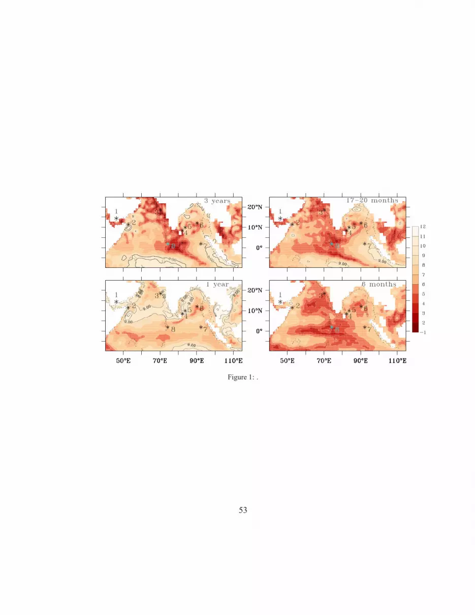
Figure 1: .

53

Figure 2: .

54

Figure 3: .

55

Figure 4: .

56

Figure 5: .

57

Figure 6: .

58

Figure 7: .

59

Figure 8: .

60

Figure 9: .

61

Figure 10: .

62

Figure 11: .

63