Embed Size (px)
Citation preview
International Journal of Information and Management Sciences
22 (2011), 1-25
Minimum Disparity Inference Based on Tangent Disparities
Chanseok Park and Ayanendranath Basu
Clemson University and Indian Statistical Institute
Abstract
This paper introduces the new family of “tangent disparities” based on the tangent func-
tion and considers robust inference based on it. The properties of the resulting inference
procedures are studied. The estimators are asymptotically efficient with asymptotic break-
down points of 1/2 at the model. The corresponding tests are equivalent to the likelihood
ratio test under the null. Numerical studies substantiate the theory developed and compare
the performance of the methods with those based on the Hellinger distance.
Keywords: Tangent disparity, efficiency, breakdown point, robustness, residual adjust-
ment function.
1. Introduction
Let FΘ = {Fθ : θ ∈ Θ ⊂ Rp} be a parametric class of distributions modeling the
true distribution G. Assume that G ∈ G, the class of all distributions having probability
density functions (pdf’s) with respect to a dominating measure. The model FΘ is also
assumed to be a subclass of G. We aim to develop robust inference procedures about
θ, without suffering a corresponding loss in efficiency typically suffered by M -estimators
(Hampel, Ronchetti, Rousseeuw and Stahel [9]).
Among others, Beran [5], Tamura and Boos [22], and Simpson [19, 20] demonstrated
that the simultaneous goals of asymptotic efficiency and robustness can be achieved by
using inference procedures based on the Hellinger distance (HD). Lindsay [12] generalized
the earlier work based on the HD to a general class of disparities generating estimators
that are both robust and first order efficient for discrete models. A disparity is a measure
of discrepancy between a nonparametric density estimator obtained from the data and
the model density. In this paper we develop and investigate the properties of the inference
procedures resulting from a new subclass of disparities based on the tangent function.
This branch of minimum distance estimation actually dates further back. Csiszar [6]
and Ali and Silvey [2] had earlier characterized this class of divergences independently.
Pardo [14] has provided an excellent account of such divergences. However Beran [5]
seems to be the first to point out the robustness applications of such distances. Lindsay
2 CHANSEOK PARK AND AYANENDRANATH BASU
[12] studied the geometry of these distances and identified the general structure which
leads to the robust behavior of the corresponding minimum distance estimators.
The rest of the paper is organized as follows: Section 2 contains a review of minimum
disparity inference. Section 3 develops the class of the tangent disparities, and Section 4
studies asymptotic efficiency of the minimum disparity estimators. Section 5 gives a
breakdown point analysis. Section 6 discusses robust tests of hypotheses. Numerical
illustrations and concluding remarks are given in Sections 7 and 8 respectively.
2. Minimum Disparity Estimation
For the parametric setup of Section 1, let X1,X2, . . . ,Xn be a random sample from
the distribution G (with pdf g), and let
gn(x) =1
nhn
n∑
i=1
w
(
x − Xi
hn
)
(1)
define a nonparametric density estimator of g, where w is a smooth family of kernel
functions with bandwidth hn. For discrete models, we will, without loss of generality, let
the sample space be {0, 1, 2, . . .} and take gn to be the empirical density function, where
gn(x) is the relative frequency of the value x in the sample. Define the Pearson residual
at a point x as
δ(x) =gn(x) − fθ(x)
fθ(x).
Let C(·) be a real-valued, thrice differentiable convex function on [−1,∞) with C(0) = 0.
Lindsay [12] constructed the disparity ρC between gn and fθ defined as
ρC(gn, fθ) =
∫
C(
δ)
fθ, (2)
the integral being with respect to the dominating measure. Under the assumptions on C,
ρC is nonnegative and equals zero if and only if gn ≡ fθ. Examples of disparities include
the likelihood disparity (LD) and the squared HD, defined by LD(g, fθ) =∫
g log (g/fθ)
and HD(g, fθ) =∫
(√
g−√
fθ )2. The LD is a version of the Kullback-Leibler divergence,
and in discrete models is minimized by the maximum likelihood estimator (MLE) of θ.
Let ∇ represent the gradient with respect to θ. For any real valued function u(x) we
will let u′(x) and u′′(x) denote its first and second derivatives with respect to x. Mini-
mization of the disparity ρC(gn, fθ) over θ ∈ Θ gives the minimum disparity estimator
corresponding to the function C. The HD produces the minimum Hellinger distance esti-
mator (MHDE). Under differentiability of the model, the minimum disparity estimating
equation becomes
−∇ρC =
∫
A(δ)∇fθ = 0, (3)
where A(δ) ≡ (δ + 1)C ′(δ) − C(δ). The function A(δ) is increasing on [−1,∞); with-
out affecting the estimating properties of the disparity ρC , it can be redefined to satisfy
MINIMUM DISPARITY INFERENCE 3
A(0) = 0 and A′(0) = 1. This standardized function A(δ) is called the residual adjust-
ment function (RAF) of the disparity. As the estimating equations in (3) are otherwise
equivalent, the form of the RAF determines the specific properties of the estimator like
how strongly the large outlying observations (manifesting themselves as large positive
values of δ) are downweighted. The RAF of the LD and the HD are given respectively
by A(δ) = δ and A(δ) = 2[√
δ + 1− 1]. The curvature A2 = A′′(0) of the RAF measures
how fast the function curves down from the line A(δ) = δ at δ = 0. Large negative values
of A2 provide greater downweighting relative to the MLE, while A2 = 0 indicates a form
of second order efficiency (Rao [16, 17]).
3. The Tangent Disparities
We introduce the new family of tangent disparities (TDα) between two densities g
and f indexed by a single parameter α ∈ [0, 1) as:
TDα(g, f) =
∫[
4
απg(x) tan
(
απ
2
g(x) − f(x)
g(x) + f(x)
)
− g(x) + f(x)
]
. (4)
Let (θ) = TDα(g, fθ) and define the TDα estimation functional Tα : G → Θ as Tα(G)
satisfying
(Tα(G)) = inft∈Θ
(t).
In case Tα(G) is multiple-valued, the notation Tα(G) will represent one of the possible
values chosen arbitrarily. The functional Tα(·) is Fisher consistent since Tα(Fθ) = θ for
all α in our range of interest. By the definition above, the minimum tangent disparity
estimator (MTDE) is Tα(Gn), where Gn is the cumulative distribution function (CDF)
of the kernel density estimator gn based on the data.
The C(·) function and RAF for the TDα disparity are given by
C(δ) =4
απ(δ + 1) tan
(
απ
2
δ
δ + 2
)
− δ, (5)
A(δ) = 4
(
δ + 1
δ + 2
)2
sec2
(
απ
2
δ
δ + 2
)
− 1. (6)
The case for α = 0 corresponds to the continuous limit as α → 0. In the TDα family
A′′(0) = (π2α2 − 4)/8, which equals zero only when α = 2/π. With α = 0, TDα is the
symmetric chi-square (SCS) deviance, which is defined as
SCS(g, f) = 2
∫
(g − f)2
g + f,
see Markatou, Basu and Lindsay [13]. In the following we present a couple of useful
mathematical results about the proposed TDα family.
4 CHANSEOK PARK AND AYANENDRANATH BASU
Lemma 1. Let
D(g, f) =4
απg tan
(
απ
2
g − f
g + f
)
− g + f
be the integrand in (4). Then
D(g, f) ≤ D(0, f)I(g ≤ f) + D(g, 0)I(f < g) ≤ D(0, f) + D(g, 0),
where I(·) is the indicator function.
Proof. For fixed f and g ∈ (0, f), look at D(g, f) as a function of g.
∂
∂gD(g, f) =
4
απtan
(
απ
2
g − f
g + f
)
+4gf
(g + f)2sec2
(
απ
2
g − f
g + f
)
− 1.
This can be rewritten as a function of δ = g/f − 1 as
Dg(δ) =4
απtan
(
απ
2
δ
δ + 2
)
+4(δ + 1)
(δ + 2)2sec2
(
απ
2
δ
δ + 2
)
− 1.
It is easily shown that Dg(δ) is increasing in δ ∈ (−1, 0), Dg(0) = 0, and Dg(·) is
continuous at δ = 0. Hence ∂∂gD(g, f) < 0 for ∀g ∈ (0, f). Since D(·, f) is strictly
decreasing for g ∈ (0, f) and right-continuous at g = 0, we have D(g, f) ≤ D(0, f) for
g ∈ (0, f) with the equality only when g = 0. Similarly, D(g, f) ≤ D(g, 0) for f ∈ (0, g).
�
The following theorem is a simple consequence of Lemma 1.
Theorem 2. The TDα family for 0 ≤ α < 1 admits the following boundedness result:
0 ≤ TDα(g, f) ≤ 4
απtan
(απ
2
)
,
where the bound for the case α = 0 is the limit of the quantity in the right hand side as
α → 0. The left equality holds when g ≡ f , and the right equality holds when the supports
of the two densities are disjoint almost everywhere.
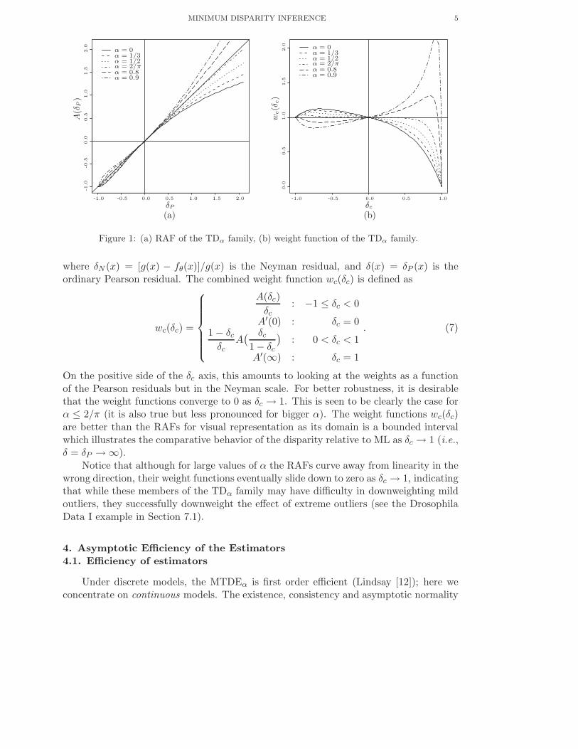
For better visual understanding of the robustness of the TDα disparity procedures,
we graphically present the RAF as well as the combined weight function wc(δc) (Park,
Basu and Lindsay [15]) for this family for different values of α in Figure 1. Notice that
the RAF has a more dampened response to large values of δ (representing the large
outliers) when α is small. The combined weight function wc(δc) represents the relative
impact, A(δ)/δ, of the observation in the estimating equation compared to maximum
likelihood (ML). Here one defines the combined residual δc
δc(x) =
{
δP (x) : g ≤ fθ
δN (x) : g > fθ
MINIMUM DISPARITY INFERENCE 5
Figure 1: (a) RAF of the TDα family, (b) weight function of the TDα family.
where δN (x) = [g(x) − fθ(x)]/g(x) is the Neyman residual, and δ(x) = δP (x) is theordinary Pearson residual. The combined weight function wc(δc) is defined as
wc(δc) =
A(δc)
δc: −1 ≤ δc < 0
A′(0) : δc = 01 − δc
δcA
( δc
1 − δc
)
: 0 < δc < 1
A′(∞) : δc = 1
. (7)
On the positive side of the δc axis, this amounts to looking at the weights as a functionof the Pearson residuals but in the Neyman scale. For better robustness, it is desirablethat the weight functions converge to 0 as δc → 1. This is seen to be clearly the case forα ≤ 2/π (it is also true but less pronounced for bigger α). The weight functions wc(δc)are better than the RAFs for visual representation as its domain is a bounded intervalwhich illustrates the comparative behavior of the disparity relative to ML as δc → 1 (i.e.,δ = δP → ∞).
Notice that although for large values of α the RAFs curve away from linearity in thewrong direction, their weight functions eventually slide down to zero as δc → 1, indicatingthat while these members of the TDα family may have difficulty in downweighting mildoutliers, they successfully downweight the effect of extreme outliers (see the DrosophilaData I example in Section 7.1).
4. Asymptotic Efficiency of the Estimators
4.1. Efficiency of estimators
Under discrete models, the MTDEα is first order efficient (Lindsay [12]); here weconcentrate on continuous models. The existence, consistency and asymptotic normality
6 CHANSEOK PARK AND AYANENDRANATH BASU
of the MTDEα are given by the following results. For the TDα family, C ′(δ), A(δ),
A′(δ)δ and A′′(δ)δ are bounded on [−1,∞). Many of the results presented here are
slight modifications of the proofs of Tamura and Boos [22], Lindsay [12], and Basu,
Sarkar and Vidyashankar [4]. The next theorem is a simple extension of Proposition 1
of Basu, Sarkar and Vidyashankar [4] and the proof is omitted.
Theorem 3. Assume that (a) the parameter space Θ is compact, (b) for θ1 6= θ2,
fθ1(x) 6= fθ2
(x) on a set of positive dominating measure, and (c) fθ(x) is continuous in θ
for almost every x. Then (i) for any G ∈ G, there exists θ ∈ Θ such that Tα(G) = θ, (ii)
TDα(g, fθ) is a continuous function of θ where g is the pdf of G, (iii) for any Fθ∗ ∈ FΘ,
Tα(Fθ∗) = θ∗ is unique for all α ∈ [0, 1).
Remark 1. As in Beran [5], the above result assumes compactness of Θ, but also applies
when Θ can be embedded within a compact set Θ, and the disparity TDα(g, fθ) can be
extended to a continuous function of θ on Θ. For example, in the location-scale family{
fθ(x) =1
σf
(
x − µ
σ
)
: θ = (µ, σ) ∈ (−∞,∞) × (0,∞)
}
, f continuous,
where the parameter space is not compact, (µ, σ) can be reparameterized as β = (β1, β2),
µ = tan(β1), σ = tan(β2), and (β1, β2) ∈ Θ = (−π/2, π/2) × (0, π/2). The disparity
extends as a continuous function on Θ = [−π/2, π/2] × [0, π/2] which is compact, and
the minimum must occur in Θ. Hence the conclusions of Theorem 3 remain valid.
Theorem 4. Let G ∈ G be the true distribution with pdf g. Given a random sample
X1,X2, . . . ,Xn, let the kernel density estimate gn with CDF Gn be as defined in (1).
If Tα(G) is unique, then under the assumptions of Theorem 3 the functional Tα(Gn) is
continuous at Tα(G) in the sense that Tα(Gn) converges to Tα(G) as gn → g in L1.
Proof. Suppose that gn → g in L1. For convenience, denote (θ) = TDα(g, fθ) and
n(θ) = TDα(gn, fθ). We have
|n(t) − (t)| ≤∫
|C(δn) − C(δ)| ft,
where δn = gn/ft − 1 and δ = g/ft − 1. By the mean value theorem, there exists δ∗
satisfying
C(δn) − C(δ) = C ′(δ∗)(δn − δ),
where δ∗ lies between δn and δ. For the TDα family, it is easily seen that |C ′(δ∗)| is
bounded. Denote K = maxδ |C ′(δ)|. Then we have
|n(t) − (t)| ≤ K
∫
|gn − g| for all t ∈ Θ.
Hence we have
supt
∣
∣n(t) − (t)∣
∣ → 0, (8)
MINIMUM DISPARITY INFERENCE 7
as gn → g in L1. Let θn = arg inft n(t) and θ = arg inft (t). If (θ) ≥ n(θn), then
(θ)− n(θn) ≤ (θn) − n(θn), and if n(θn) ≥ (θ), then n(θn) − (θ) ≤ n(θ)− (θ).
Thus
|n(θn) − (θ)| ≤ |n(θn) − (θn)| + |n(θ) − (θ)| ≤ 2 supt
|n(t) − (t)| , (9)
which implies n(θn) → (θ) as gn → g in L1. Using (8) and (9), we obtain
limn→∞
(θn) = (θ). (10)
Then we only have to show that θn → θ as n → ∞. If θn 6→ θ, compactness of Θ ensures
existence of a subsequence {θm} ⊂ {θn} such that θm → θ∗ 6= θ, implying (θm) → (θ∗)
by continuity of (·). By (10), (θ∗) = (θ), which contradicts the uniqueness assumption
of θ = Tα(G). �
Thus under the conditions of Theorem 4, θn = Tα(Gn) is a consistent estimator of
the best fitting best fitting parameter Tα(G) whenever gn → g in L1. When G = Fθ
belongs to the specified model, θn is consistent for θ.
In practice, one may use the bandwidth hn = cnsn where sn is a robust scale es-
timator based on the data and cn is a sequence of positive constants. This gives the
automatic kernel density estimator (Devroye and Gyorfi [8]) of the form
gn(x) =1
ncnsn
n∑
i=1
w
(
x − Xi
cnsn
)
. (11)
In this case, sufficient conditions under which gn → g in L1 are that cn → 0, ncn → ∞and
√n(sn − s) is bounded almost surely, where s is a finite, positive constant.
Remark 2. Suppose that it is difficult to find a compact embedding Θ such that the
disparity extends continuously to all the points of Θ. In such cases, a result of Simpson
([19], Theorem 1) may be applied to show that the existence and continuity results above
still remain valid for the class G∗ of distributions, where any G ∈ G∗ satisfies
infθ∈Θ\Θ∗
TDα(g, fθ) > TDα(g, fθ∗)
for some compact Θ∗ ⊂ Θ and θ∗ ∈ Θ∗. Formally, suppose that fθ(x) is continuous in
θ for each x. Then, for each G ∈ G∗, (i) Tα(G) exists, and (ii) if Tα(G) is unique, then
the condition gn → g in L1 implies that Tα(Gn) → Tα(G) as n → ∞. In particular, if
conditions (b) and (c) of Theorem 3 hold and the parametric family satisfies
inft∈Θ\Θ∗
TDα(fθ, ft) > 0
for some compact Θ∗ ⊂ Θ, then gn → fθ in L1 implies that Tα(Gn) → θ as n → ∞.
Next we introduce some notation. Let uθ(x) = ∇ log fθ(x) be the p-dimensional
vector of ML score function, and let ∇2fθ(x) denote the p × p matrix of second partial
8 CHANSEOK PARK AND AYANENDRANATH BASU
derivatives of fθ. We will denote by uiθ(x) and ∇ijfθ(x) the i-th element of uθ(x) and
(i, j)-th element of ∇2fθ(x) respectively. Then
I(θ) ≡∫
uθuTθ fθ
is the Fisher information matrix, where the superscript T denotes transpose. For deriving
asymptotic normality of the MTDEα we will assume that fθ(x) is twice continuously
differentiable with respect to θ, and TDα(·, fθ) is twice differentiable with respect to θ
under the integral sign. For the latter one, sufficient conditions are: for any θ ∈ Θ, there
exists ǫ > 0, and functions Kiθ(x), Lij
θ (x) and M ijθ (x), i, j = 1, . . . , p, such that for θ†
satisfying ‖θ − θ†‖ < ǫ (‖ · ‖ being the Euclidean norm),
(I) |uiθ†
fθ†(x)| < Kiθ(x),
∫
Kiθ < ∞, i = 1, 2, . . . , p;
(II) |∇ijfθ†(x)| < Lijθ (x),
∫
Lijθ < ∞, i, j = 1, . . . , p;
(III) |uiθ†
(x)ujθ†
(x)fθ†(x)| < M ijθ (x),
∫
M ijθ < ∞, i, j = 1, . . . , p.
Theorem 5. Suppose G = Fθ0, g = fθ0
, Gn and gn are as defined in Theorem 4. Let
{φn} denote any sequence of estimators such that φn = θ0 + op(1), {αn} any sequence
of positive real numbers going to ∞, and IB the indicator function for the set B. In
addition to the conditions (I) – (III) above, assume the following:
(a)∫
|∇ijfφn−∇ijfθ0
| = op(1) and∫
|uiφn
ujφn
fφn− ui
θ0uj
θ0fθ0
| = op(1), i, j = 1, . . . , p,
for all {φn} defined above.
(b)∫
uiθ0
(x+a)ujθ0
(x+a)fθ0(x)dx →
∫
uiθ0
(x)ujθ0
(x)fθ0(x)dx as |a| → 0, i, j = 1, . . . , p,
and the matrix I(θ0) is finite (element-wise).
(c) The kernel w(·) is a density which is symmetric about 0, square integrable, and
twice continuously differentiable with compact support S. The bandwidth hn satisfies
hn → 0, n1/2hn → ∞, and n1/2h4n → 0 as n → ∞.
(d) lim supn→∞
supy∈An
∫
|∇ijfθ0(x+y)uθ0
(x)|dx < ∞ for i, j = 1, . . . , p, where An = {y : y =
hnz, z ∈ S}.
(e) n supt∈S P (|X1 − hnt| > αn) → 0 as n → ∞, for all {αn} defined above.
(f) (n1/2hn)−1∫
∣
∣uθ0I|x|≤αn
∣
∣ → 0, for all {αn} defined above.
(g) sup|x|≤αnsupt∈S{fθ0
(x + hnt)/fθ0(x)} = O(1), for all {αn} defined above.
Then,√
n(
Tα(Gn) − Tα(G))
converges in distribution to N(0, I−1(θ0)).
MINIMUM DISPARITY INFERENCE 9
The proof is given in the Appendix. Condition (a) is a simple continuity condition
at the model stating that the second derivative of fθ with respect to θ is L1-continuous
and Eθ[uiθu
jθ] is continuous in θ. This condition is satisfied by the distributions of the
exponential family. Condition (b) is satisfied if uiθ0
(x) is uniformly continuous in x on
compact sets. Condition (c) represents the key restriction on the bandwidth. Conditions
(e)–(g) have been used and discussed by Tamura and Boos ([22], Theorem 4.1)
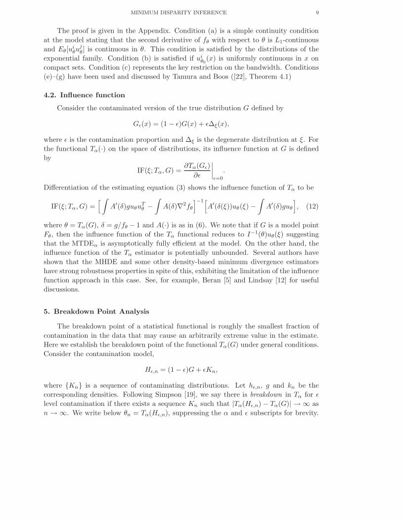
4.2. Influence function
Consider the contaminated version of the true distribution G defined by
Gǫ(x) = (1 − ǫ)G(x) + ǫ∆ξ(x),
where ǫ is the contamination proportion and ∆ξ is the degenerate distribution at ξ. For
the functional Tα(·) on the space of distributions, its influence function at G is defined
by
IF(ξ;Tα, G) =∂Tα(Gǫ)
∂ǫ
∣
∣
∣
∣
ǫ=0
.
Differentiation of the estimating equation (3) shows the influence function of Tα to be
IF(ξ;Tα, G) =[
∫
A′(δ)guθuTθ −
∫
A(δ)∇2fθ
]−1[
A′(δ(ξ))uθ(ξ) −∫
A′(δ)guθ
]
, (12)
where θ = Tα(G), δ = g/fθ − 1 and A(·) is as in (6). We note that if G is a model point
Fθ, then the influence function of the Tα functional reduces to I−1(θ)uθ(ξ) suggesting
that the MTDEα is asymptotically fully efficient at the model. On the other hand, the
influence function of the Tα estimator is potentially unbounded. Several authors have
shown that the MHDE and some other density-based minimum divergence estimators
have strong robustness properties in spite of this, exhibiting the limitation of the influence
function approach in this case. See, for example, Beran [5] and Lindsay [12] for useful
discussions.
5. Breakdown Point Analysis
The breakdown point of a statistical functional is roughly the smallest fraction of
contamination in the data that may cause an arbitrarily extreme value in the estimate.
Here we establish the breakdown point of the functional Tα(G) under general conditions.
Consider the contamination model,
Hǫ,n = (1 − ǫ)G + ǫKn,
where {Kn} is a sequence of contaminating distributions. Let hǫ,n, g and kn be the
corresponding densities. Following Simpson [19], we say there is breakdown in Tα for ǫ
level contamination if there exists a sequence Kn such that |Tα(Hǫ,n) − Tα(G)| → ∞ as
n → ∞. We write below θn = Tα(Hǫ,n), suppressing the α and ǫ subscripts for brevity.
10 CHANSEOK PARK AND AYANENDRANATH BASU
We assume the following conditions for the breakdown point analysis. The conditions
reflect the intuitively worst possible choice of the contamination, and the expected be-
havior or the functional when breakdown does and does not occur respectively. The
proof of the theorem is in the appendix.
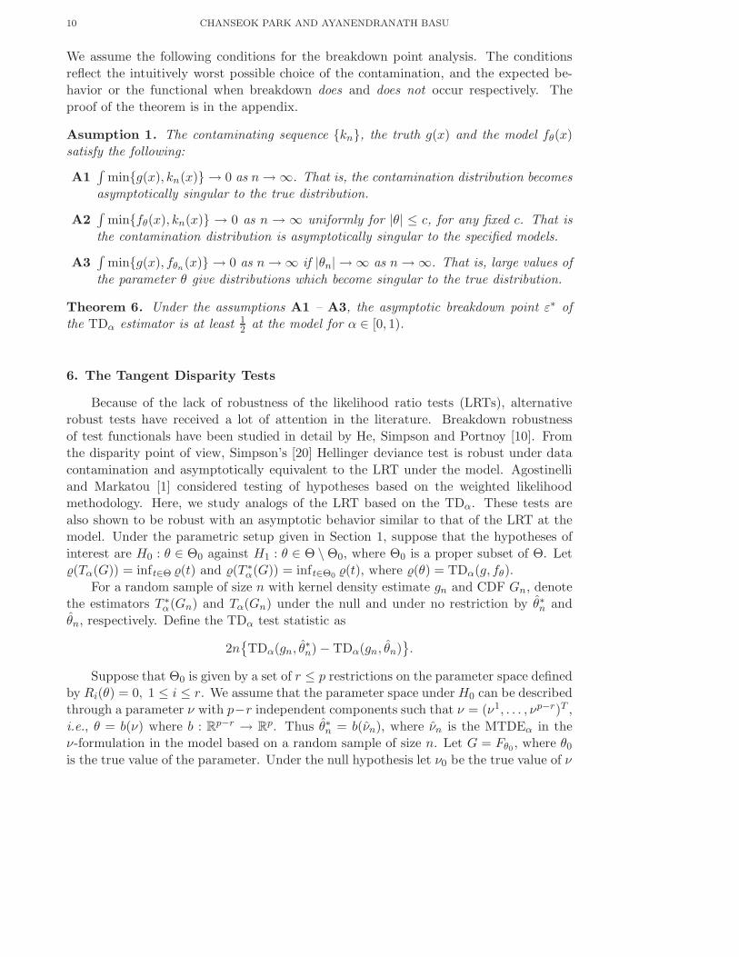
Asumption 1. The contaminating sequence {kn}, the truth g(x) and the model fθ(x)
satisfy the following:
A1∫
min{g(x), kn(x)} → 0 as n → ∞. That is, the contamination distribution becomes
asymptotically singular to the true distribution.
A2∫
min{fθ(x), kn(x)} → 0 as n → ∞ uniformly for |θ| ≤ c, for any fixed c. That is
the contamination distribution is asymptotically singular to the specified models.
A3∫
min{g(x), fθn(x)} → 0 as n → ∞ if |θn| → ∞ as n → ∞. That is, large values of
the parameter θ give distributions which become singular to the true distribution.
Theorem 6. Under the assumptions A1 – A3, the asymptotic breakdown point ε∗ of
the TDα estimator is at least 12 at the model for α ∈ [0, 1).
6. The Tangent Disparity Tests
Because of the lack of robustness of the likelihood ratio tests (LRTs), alternative
robust tests have received a lot of attention in the literature. Breakdown robustness
of test functionals have been studied in detail by He, Simpson and Portnoy [10]. From
the disparity point of view, Simpson’s [20] Hellinger deviance test is robust under data
contamination and asymptotically equivalent to the LRT under the model. Agostinelli
and Markatou [1] considered testing of hypotheses based on the weighted likelihood
methodology. Here, we study analogs of the LRT based on the TDα. These tests are
also shown to be robust with an asymptotic behavior similar to that of the LRT at the
model. Under the parametric setup given in Section 1, suppose that the hypotheses of
interest are H0 : θ ∈ Θ0 against H1 : θ ∈ Θ \ Θ0, where Θ0 is a proper subset of Θ. Let
(Tα(G)) = inft∈Θ (t) and (T ∗α(G)) = inft∈Θ0
(t), where (θ) = TDα(g, fθ).
For a random sample of size n with kernel density estimate gn and CDF Gn, denote
the estimators T ∗α(Gn) and Tα(Gn) under the null and under no restriction by θ∗n and
θn, respectively. Define the TDα test statistic as
2n{
TDα(gn, θ∗n) − TDα(gn, θn)}
.
Suppose that Θ0 is given by a set of r ≤ p restrictions on the parameter space defined
by Ri(θ) = 0, 1 ≤ i ≤ r. We assume that the parameter space under H0 can be described
through a parameter ν with p−r independent components such that ν = (ν1, . . . , νp−r)T ,
i.e., θ = b(ν) where b : Rp−r → R
p. Thus θ∗n = b(νn), where νn is the MTDEα in the
ν-formulation in the model based on a random sample of size n. Let G = Fθ0, where θ0
is the true value of the parameter. Under the null hypothesis let ν0 be the true value of ν
MINIMUM DISPARITY INFERENCE 11
parameter. From the arguments of Section 4 it follows that, under H0, νn is a consistent
estimator of ν0 and θ∗n is a consistent estimator of θ0. Define Dν = [∂bi/∂νj ]p×(p−r). Let
J(ν0) denote the information matrix under the ν-formulation, while I(θ0) denotes that
under no restrictions. The LRT has the form
LRT = 2{
n∑
i=1
log fθML(Xi) −
n∑
i=1
log fθ∗ML
(Xi)}
,
where θML and θ∗ML represent the MLEs of θ under no restrictions and under H0, respec-
tively. Asymptotically the statistic LRT has a χ2(r) distribution under H0. The following
theorem is proved in the Appendix which establishes the asymptotic distribution of the
TDα statistic under the null hypothesis.
Theorem 7. Under the conditions of Theorem 5, 2n{
TDα(gn, fθ∗n
) − TDα(gn, fθn)}
−LRT = op(1).
7. Examples and Simulations
7.1. Examples
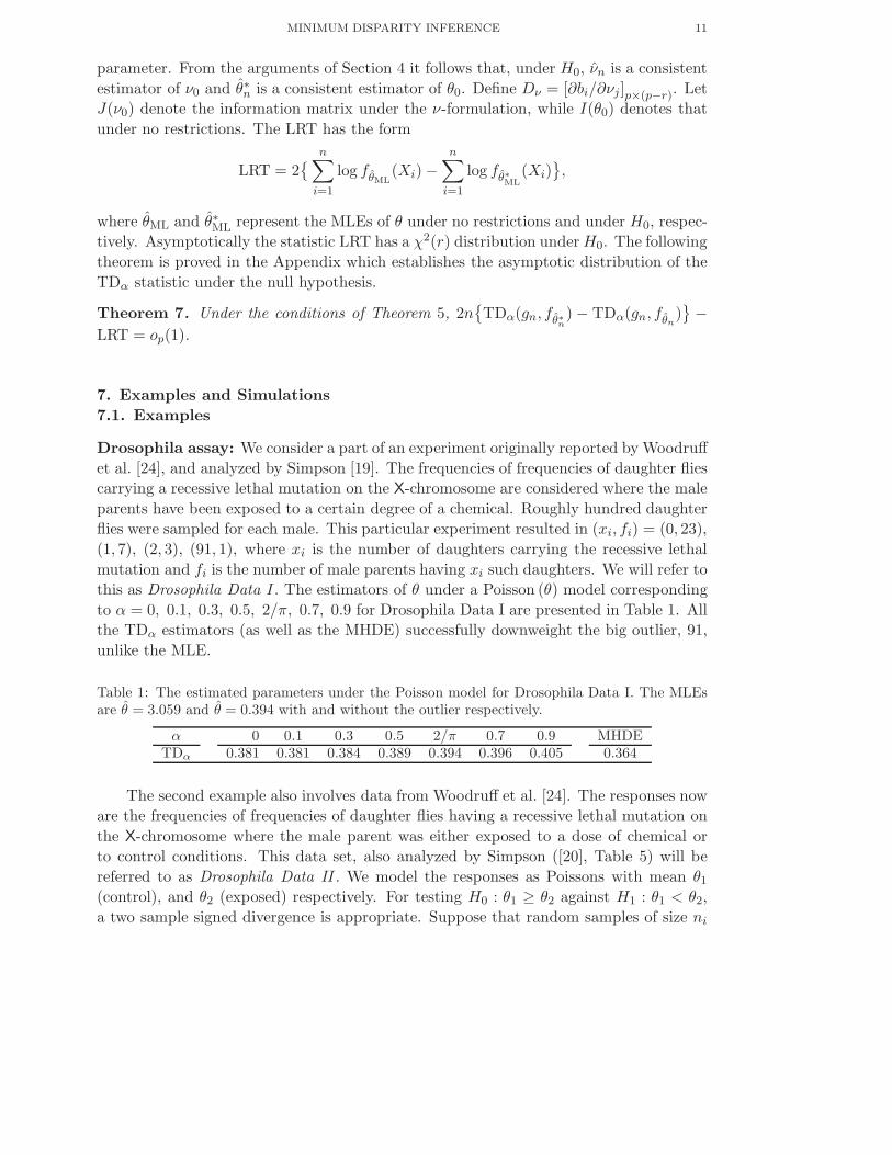
Drosophila assay: We consider a part of an experiment originally reported by Woodruff
et al. [24], and analyzed by Simpson [19]. The frequencies of frequencies of daughter flies
carrying a recessive lethal mutation on the X-chromosome are considered where the male
parents have been exposed to a certain degree of a chemical. Roughly hundred daughter
flies were sampled for each male. This particular experiment resulted in (xi, fi) = (0, 23),
(1, 7), (2, 3), (91, 1), where xi is the number of daughters carrying the recessive lethal
mutation and fi is the number of male parents having xi such daughters. We will refer to
this as Drosophila Data I . The estimators of θ under a Poisson (θ) model corresponding
to α = 0, 0.1, 0.3, 0.5, 2/π, 0.7, 0.9 for Drosophila Data I are presented in Table 1. All
the TDα estimators (as well as the MHDE) successfully downweight the big outlier, 91,
unlike the MLE.
Table 1: The estimated parameters under the Poisson model for Drosophila Data I. The MLEsare θ = 3.059 and θ = 0.394 with and without the outlier respectively.
α 0 0.1 0.3 0.5 2/π 0.7 0.9 MHDETDα 0.381 0.381 0.384 0.389 0.394 0.396 0.405 0.364
The second example also involves data from Woodruff et al. [24]. The responses now
are the frequencies of frequencies of daughter flies having a recessive lethal mutation on
the X-chromosome where the male parent was either exposed to a dose of chemical or
to control conditions. This data set, also analyzed by Simpson ([20], Table 5) will be
referred to as Drosophila Data II . We model the responses as Poissons with mean θ1
(control), and θ2 (exposed) respectively. For testing H0 : θ1 ≥ θ2 against H1 : θ1 < θ2,
a two sample signed divergence is appropriate. Suppose that random samples of size ni
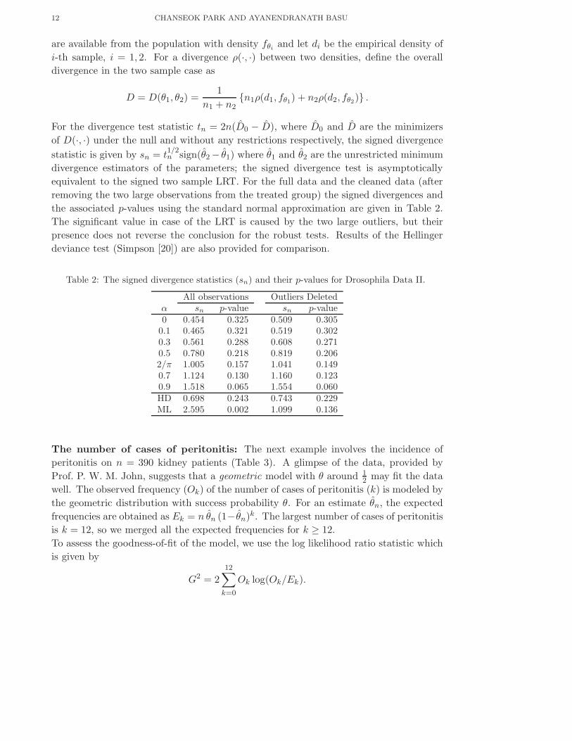
12 CHANSEOK PARK AND AYANENDRANATH BASU
are available from the population with density fθiand let di be the empirical density of
i-th sample, i = 1, 2. For a divergence ρ(·, ·) between two densities, define the overall
divergence in the two sample case as
D = D(θ1, θ2) =1
n1 + n2{n1ρ(d1, fθ1
) + n2ρ(d2, fθ2)} .
For the divergence test statistic tn = 2n(D0 − D), where D0 and D are the minimizers
of D(·, ·) under the null and without any restrictions respectively, the signed divergence
statistic is given by sn = t1/2n sign(θ2 − θ1) where θ1 and θ2 are the unrestricted minimum
divergence estimators of the parameters; the signed divergence test is asymptotically
equivalent to the signed two sample LRT. For the full data and the cleaned data (after
removing the two large observations from the treated group) the signed divergences and
the associated p-values using the standard normal approximation are given in Table 2.
The significant value in case of the LRT is caused by the two large outliers, but their
presence does not reverse the conclusion for the robust tests. Results of the Hellinger
deviance test (Simpson [20]) are also provided for comparison.
Table 2: The signed divergence statistics (sn) and their p-values for Drosophila Data II.
All observations Outliers Deletedα sn p-value sn p-value0 0.454 0.325 0.509 0.305
0.1 0.465 0.321 0.519 0.3020.3 0.561 0.288 0.608 0.2710.5 0.780 0.218 0.819 0.2062/π 1.005 0.157 1.041 0.1490.7 1.124 0.130 1.160 0.1230.9 1.518 0.065 1.554 0.060HD 0.698 0.243 0.743 0.229ML 2.595 0.002 1.099 0.136
The number of cases of peritonitis: The next example involves the incidence of
peritonitis on n = 390 kidney patients (Table 3). A glimpse of the data, provided by
Prof. P. W. M. John, suggests that a geometric model with θ around 12 may fit the data
well. The observed frequency (Ok) of the number of cases of peritonitis (k) is modeled by
the geometric distribution with success probability θ. For an estimate θn, the expected
frequencies are obtained as Ek = n θn (1−θn)k. The largest number of cases of peritonitis
is k = 12, so we merged all the expected frequencies for k ≥ 12.
To assess the goodness-of-fit of the model, we use the log likelihood ratio statistic which
is given by
G2 = 2
12∑
k=0
Ok log(Ok/Ek).
MINIMUM DISPARITY INFERENCE 13
Table 3: The observed frequencies (Ok) of the number of cases (k) of peritonitis for each of 390kidney patients and the expected frequencies under different methods with the goodness-of-fitlikelihood ratio statistics (G2).
k 0 1 2 3 4 5 6 7 8 9 10 11 12+ G2
Ok 199 94 46 23 17 4 4 1 0 0 1 0 1 —α TDα
0 197.8 97.5 48.0 23.7 11.7 5.7 2.8 1.4 0.7 0.3 0.2 0.1 0.1 10.90.1 197.8 97.5 48.1 23.7 11.7 5.8 2.8 1.4 0.7 0.3 0.2 0.1 0.1 10.90.3 197.4 97.5 48.2 23.8 11.7 5.8 2.9 1.4 0.7 0.3 0.2 0.1 0.1 10.80.5 196.4 97.5 48.4 24.0 11.9 5.9 2.9 1.5 0.7 0.4 0.2 0.1 0.1 10.62/π 195.3 97.5 48.7 24.3 12.1 6.1 3.0 1.5 0.8 0.4 0.2 0.1 0.1 10.50.7 194.4 97.5 48.9 24.5 12.3 6.2 3.1 1.5 0.8 0.4 0.2 0.1 0.1 10.50.9 188.8 97.4 50.2 25.9 13.4 6.9 3.6 1.8 0.9 0.5 0.3 0.1 0.1 10.8HD 199.1 97.5 47.7 23.4 11.4 5.6 2.7 1.3 0.7 0.3 0.2 0.1 0.1 11.1ML 193.5 97.5 49.1 24.7 12.5 6.3 3.2 1.6 0.8 0.4 0.2 0.1 0.1 10.4
In this example the fit provided by the MLE is excellent. The two marginally large
observations at 10 and 12 have little impact since the sample size is so large. Notice that
the fit provided by most of the robust estimates is almost equally good (last column,
Table 3) and clearly better than the HD. The example demonstrates that the proposed
methods can work almost as well as the ML method when the model provides good fit
to the data.
Determinations of the parallax of the sun: We consider Short’s data (Stigler [21],
Data Set 2) for the determination of the parallax of the sun, the angle subtended by the
earth’s radius, as if viewed and measured from the surface of the sun. From this angle
and available knowledge of the physical dimensions of the earth, the mean distance from
earth to sun could be easily determined. For our estimation we have used the kernel
density defined in (11), with the Epanechnikov kernel (w(x) = (3/4)(1 − x2), if |x| < 1,
and w(x) = 0, otherwise). Following Devroye and Gyorfi ([8], pp. 107-108), the mean L1
criterion with the Epanechnikov kernel and Gaussian pdf f leads to a bandwidth of the
form
hn = (15e)1/5(π/32)1/10σ n−1/5 = 1.66σ n−1/5,
where σ is the standard deviation. As the standard deviation is not specified, one can
use hn = 1.66 σ n−1/5, where σ = MAD = median(|Xi − median(Xi)|)/0.674.
Table 4: Fits of a normal N(µ, σ2) to the Short’s data using the maximum likelihood (ML),maximum likelihood without outlier (ML-O), and minimum TDα estimation.
α 0 0.1 0.3 0.5 2/π 0.7 0.9 ML-O ML HDµ 8.378 8.378 8.376 8.377 8.525 8.541 8.280 8.541 8.378 8.386
TDσ 0.335 0.335 0.339 0.350 0.555 0.571 0.971 0.552 0.846 0.352
14 CHANSEOK PARK AND AYANENDRANATH BASU
•• ••• ••• • ••• ••• ••5 6 7 8 9 10
0.0
0.2
0.4
0.6
0.8
1.0
1.2
TDα=0.5
MLKernel density
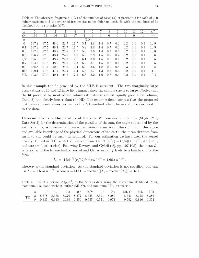
Figure 2: Density estimates for Short’s 1763 determinations of the parallax of the sun in Dataset 2 (Stigler [21]).’
For the Short’s data, Table 4 gives the values of the minimum TDα estimates of µ and σ
for various values of α under the normal model, the MHDEs, as well as the MLEs for all
the observations and that after deleting the outlier, 5.76. Figure 2 shows the fit for the
kernel density estimate and the normal densities by ML and TDα=0.5 estimators. Notice
that the estimates are highly robust for small values of α. Most of them downweight the
other remaining moderate outliers also, and hence provide a smaller scale than ML-O.
Measurements of the passages of the light: We next consider Newcomb’s light
speed data (Stigler [21]). For the data, Table 5 gives the values of the TDα estimate of µ
and σ for various values of α under the normal model, the MHDEs, as well as the MLEs
for the full data (ML), and that after deleting −44, and −2, the two obvious outliers
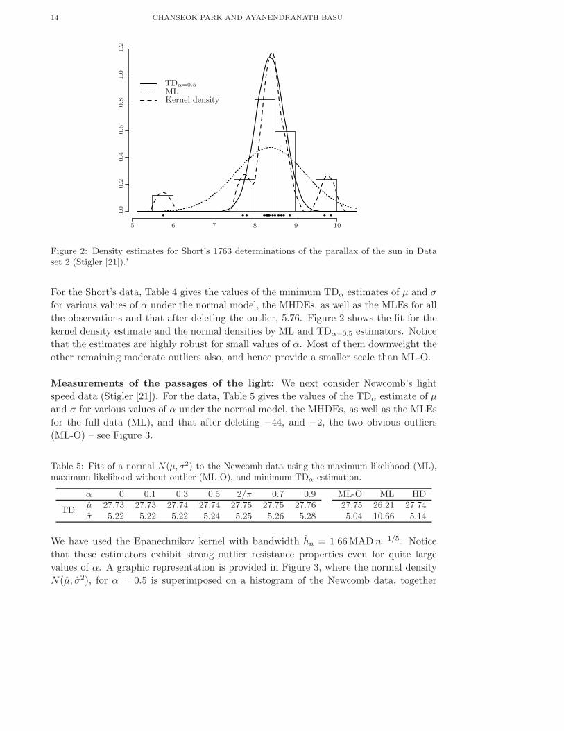
(ML-O) – see Figure 3.
Table 5: Fits of a normal N(µ, σ2) to the Newcomb data using the maximum likelihood (ML),maximum likelihood without outlier (ML-O), and minimum TDα estimation.
α 0 0.1 0.3 0.5 2/π 0.7 0.9 ML-O ML HDµ 27.73 27.73 27.74 27.74 27.75 27.75 27.76 27.75 26.21 27.74
TDσ 5.22 5.22 5.22 5.24 5.25 5.26 5.28 5.04 10.66 5.14
We have used the Epanechnikov kernel with bandwidth hn = 1.66MAD n−1/5. Notice
that these estimators exhibit strong outlier resistance properties even for quite large
values of α. A graphic representation is provided in Figure 3, where the normal density
N(µ, σ2), for α = 0.5 is superimposed on a histogram of the Newcomb data, together
MINIMUM DISPARITY INFERENCE 15
•• •••••• •• • •• •• • •• •• • • ••• • •• •• ••• • •••• ••• ••• ••• • •• •••• ••• • ••• •0-40
0.0
2
-20
0.0
4
20
0.0
6
40
0.0
80.0
TDα=0.5
MLKernel density
Figure 3: Density estimates for the Newcomb data
with the N(µML, σ2ML) density and the kernel density estimate. For the robust method,
the normal density fits the main body of the histogram quite well.
Telephone-line faults: Welch [23] presented a data set from an experiment to test a
method of reducing faults on telephone lines. This data set was previously analyzed by
using the HD (Simpson [20]). For the Telephone-line faults data, the ordered differences
between the inverse test rates and the inverse control rates are given in Table 6. In
Table 7 are given the values of the TDα estimate of µ and σ for various values of α under
the normal model, the MHDEs, as well as the MLEs for the full data (ML), and those
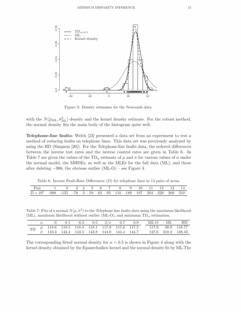
after deleting −988, the obvious outlier (ML-O) – see Figure 4.
Table 6: Inverse Fault-Rate Differences (D) for telephone lines in 14 pairs of areas.
Pair 1 2 3 4 5 6 7 8 9 10 11 12 13 14D × 105 -988 -135 -78 3 59 83 93 110 189 197 204 229 269 310
Table 7: Fits of a normal N(µ, σ2) to the Telephone line faults data using the maximum likelihood(ML), maximum likelihood without outlier (ML-O), and minimum TDα estimation.
α 0 0.1 0.3 0.5 2/π 0.7 0.9 ML-O ML HDµ 118.6 118.5 118.4 118.1 117.9 117.6 117.5 117.9 38.9 116.77
TDσ 143.3 143.4 143.5 143.8 144.0 144.4 144.7 127.6 310.2 138.43
The corresponding fitted normal density for α = 0.5 is shown in Figure 4 along with the
kernel density obtained by the Epanechnikov kernel and the normal density fit by ML.The
16 CHANSEOK PARK AND AYANENDRANATH BASU
• • • • •••• •••• • •0
0.0
-1000 -500 500
0.0
005
0.0
010
0.0
015
0.0
020
0.0
025
TDα=0.5
MLKernel density
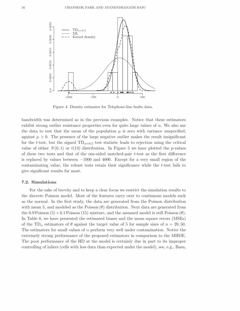
Figure 4: Density estimates for Telephone-line faults data.
bandwidth was determined as in the previous examples. Notice that these estimators
exhibit strong outlier resistance properties even for quite large values of α. We also use
the data to test that the mean of the population µ is zero with variance unspecified,
against µ > 0. The presence of the large negative outlier makes the result insignificant
for the t-test, but the signed TDα=0.5 test statistic leads to rejection using the critical
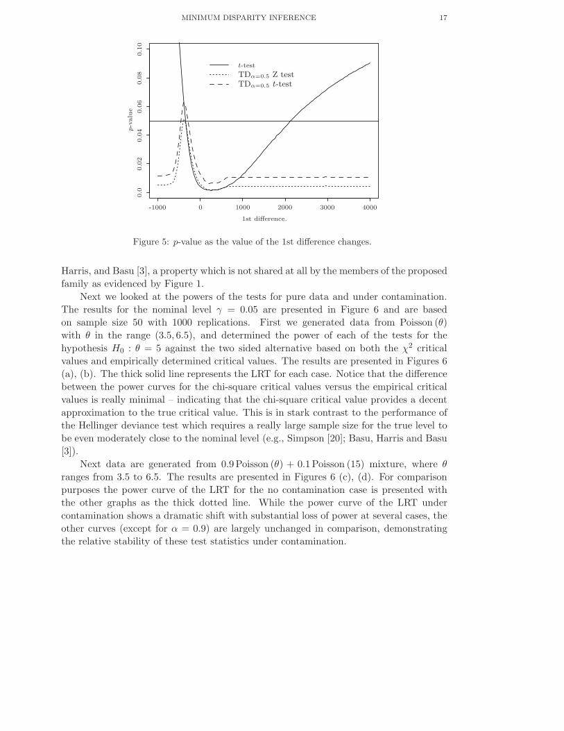
value of either N(0, 1) or t(13) distribution. In Figure 5 we have plotted the p-values
of these two tests and that of the one-sided matched-pair t-test as the first difference
is replaced by values between −1000 and 4000. Except for a very small region of the
contaminating value, the robust tests retain their significance while the t-test fails to
give significant results for most.
7.2. Simulations
For the sake of brevity and to keep a clear focus we restrict the simulation results to
the discrete Poisson model. Most of the features carry over to continuous models such
as the normal. In the first study, the data are generated from the Poisson distribution
with mean 5, and modeled as the Poisson (θ) distribution. Next data are generated from
the 0.9Poisson (5)+ 0.1Poisson (15) mixture, and the assumed model is still Poisson (θ).
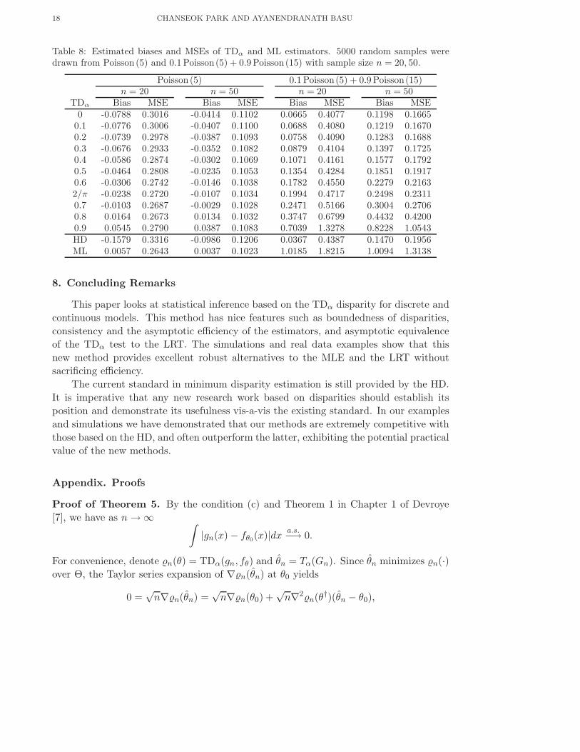
In Table 8, we have presented the estimated biases and the mean square errors (MSEs)
of the TDα estimators of θ against the target value of 5 for sample sizes of n = 20, 50.
The estimators for small values of α perform very well under contamination. Notice the
extremely strong performance of the proposed estimators in comparison to the MHDE.
The poor performance of the HD at the model is certainly due in part to its improper
controlling of inliers (cells with less data than expected under the model), see, e.g., Basu,
MINIMUM DISPARITY INFERENCE 17
0
0.0
20.0
40.0
60.0
80.0
-1000 1000 2000 3000 4000
0.1
0
TDα=0.5 Z testTDα=0.5 t-test
t-test
p-v
alu
e
1st difference.
Figure 5: p-value as the value of the 1st difference changes.
Harris, and Basu [3], a property which is not shared at all by the members of the proposed
family as evidenced by Figure 1.
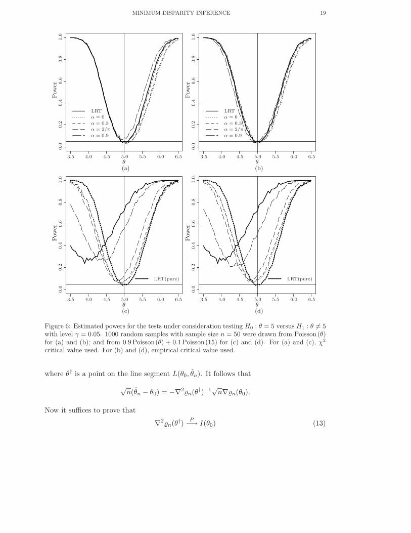
Next we looked at the powers of the tests for pure data and under contamination.
The results for the nominal level γ = 0.05 are presented in Figure 6 and are based
on sample size 50 with 1000 replications. First we generated data from Poisson (θ)
with θ in the range (3.5, 6.5), and determined the power of each of the tests for the
hypothesis H0 : θ = 5 against the two sided alternative based on both the χ2 critical
values and empirically determined critical values. The results are presented in Figures 6
(a), (b). The thick solid line represents the LRT for each case. Notice that the difference
between the power curves for the chi-square critical values versus the empirical critical
values is really minimal – indicating that the chi-square critical value provides a decent
approximation to the true critical value. This is in stark contrast to the performance of
the Hellinger deviance test which requires a really large sample size for the true level to
be even moderately close to the nominal level (e.g., Simpson [20]; Basu, Harris and Basu
[3]).
Next data are generated from 0.9Poisson (θ) + 0.1Poisson (15) mixture, where θ
ranges from 3.5 to 6.5. The results are presented in Figures 6 (c), (d). For comparison
purposes the power curve of the LRT for the no contamination case is presented with
the other graphs as the thick dotted line. While the power curve of the LRT under
contamination shows a dramatic shift with substantial loss of power at several cases, the
other curves (except for α = 0.9) are largely unchanged in comparison, demonstrating
the relative stability of these test statistics under contamination.
18 CHANSEOK PARK AND AYANENDRANATH BASU
Table 8: Estimated biases and MSEs of TDα and ML estimators. 5000 random samples weredrawn from Poisson (5) and 0.1 Poisson(5) + 0.9 Poisson(15) with sample size n = 20, 50.
Poisson (5) 0.1 Poisson(5) + 0.9 Poisson(15)n = 20 n = 50 n = 20 n = 50
TDα Bias MSE Bias MSE Bias MSE Bias MSE0 -0.0788 0.3016 -0.0414 0.1102 0.0665 0.4077 0.1198 0.1665
0.1 -0.0776 0.3006 -0.0407 0.1100 0.0688 0.4080 0.1219 0.16700.2 -0.0739 0.2978 -0.0387 0.1093 0.0758 0.4090 0.1283 0.16880.3 -0.0676 0.2933 -0.0352 0.1082 0.0879 0.4104 0.1397 0.17250.4 -0.0586 0.2874 -0.0302 0.1069 0.1071 0.4161 0.1577 0.17920.5 -0.0464 0.2808 -0.0235 0.1053 0.1354 0.4284 0.1851 0.19170.6 -0.0306 0.2742 -0.0146 0.1038 0.1782 0.4550 0.2279 0.21632/π -0.0238 0.2720 -0.0107 0.1034 0.1994 0.4717 0.2498 0.23110.7 -0.0103 0.2687 -0.0029 0.1028 0.2471 0.5166 0.3004 0.27060.8 0.0164 0.2673 0.0134 0.1032 0.3747 0.6799 0.4432 0.42000.9 0.0545 0.2790 0.0387 0.1083 0.7039 1.3278 0.8228 1.0543HD -0.1579 0.3316 -0.0986 0.1206 0.0367 0.4387 0.1470 0.1956ML 0.0057 0.2643 0.0037 0.1023 1.0185 1.8215 1.0094 1.3138
8. Concluding Remarks
This paper looks at statistical inference based on the TDα disparity for discrete and
continuous models. This method has nice features such as boundedness of disparities,
consistency and the asymptotic efficiency of the estimators, and asymptotic equivalence
of the TDα test to the LRT. The simulations and real data examples show that this
new method provides excellent robust alternatives to the MLE and the LRT without
sacrificing efficiency.
The current standard in minimum disparity estimation is still provided by the HD.
It is imperative that any new research work based on disparities should establish its
position and demonstrate its usefulness vis-a-vis the existing standard. In our examples
and simulations we have demonstrated that our methods are extremely competitive with
those based on the HD, and often outperform the latter, exhibiting the potential practical
value of the new methods.
Appendix. Proofs
Proof of Theorem 5. By the condition (c) and Theorem 1 in Chapter 1 of Devroye
[7], we have as n → ∞∫
|gn(x) − fθ0(x)|dx
a.s.−→ 0.
For convenience, denote n(θ) = TDα(gn, fθ) and θn = Tα(Gn). Since θn minimizes n(·)over Θ, the Taylor series expansion of ∇n(θn) at θ0 yields
0 =√
n∇n(θn) =√
n∇n(θ0) +√
n∇2n(θ†)(θn − θ0),
MINIMUM DISPARITY INFERENCE 19
0.0
0.0
0.0
0.0
0.2
0.2
0.2
0.2
0.4
0.4
0.4
0.4
0.5
0.6
0.6
0.6
0.6
0.8
0.8
0.8
0.8
1.0
1.0
1.0
1.0
3.53.5
3.53.5
4.04.0
4.04.0
4.54.5
4.54.5
5.05.0
5.05.0
5.55.5
5.55.5
6.06.0
6.06.0
6.56.5
6.56.5
θθ
θθ
Pow
er
Pow
er
Pow
er
Pow
er
LRTLRT
LRT(pure)LRT(pure)
α = 0α = 0
α = 0.3α = 0.3
α = 2/πα = 2/π
α = 0.9α = 0.9
(a) (b)
(c) (d)
Figure 6: Estimated powers for the tests under consideration testing H0 : θ = 5 versus H1 : θ 6= 5with level γ = 0.05. 1000 random samples with sample size n = 50 were drawn from Poisson (θ)for (a) and (b); and from 0.9 Poisson(θ) + 0.1 Poisson(15) for (c) and (d). For (a) and (c), χ2
critical value used. For (b) and (d), empirical critical value used.
where θ† is a point on the line segment L(θ0, θn). It follows that
√n(θn − θ0) = −∇2n(θ†)−1√n∇n(θ0).
Now it suffices to prove that
∇2n(θ†)P−→ I(θ0) (13)
20 CHANSEOK PARK AND AYANENDRANATH BASU
and
−√
n∇n(θ0)D−→ N(0, I(θ0)). (14)
First we prove (13). Let δn(θ) = gn/fθ − 1. Differentiating with respect to θ, we
have
∇2n(θ) = −∫
A(δn)∇2fθ +
∫
A′(δn)(δn + 1)uθuTθ fθ
It is easily seen that |A(δ)| and |A′(δ)(δ + 1)| are bounded for all δ. Let us denote
B1 = supδ |A(δ)| and B2 = supδ |A′(δ)(δ + 1)|. It follows from assumption (a) that as
n → ∞∣
∣
∣
∫
A(δn(θ†))(∇2fθ† −∇2fθ0)∣
∣
∣≤ B1
∫
|∇2fθ† −∇2fθ0| P−→ 0, (15)
and∣
∣
∣
∫
A′(δn(θ†)){
δn(θ†) + 1}
(uθ†uTθ†fθ† − uθ0
uTθ0
fθ0)∣
∣
∣≤ B2
∫
|uθ†uTθ†fθ† − uθ0
uTθ0
fθ0| P−→ 0.
(16)
Since A(0) = 0 and δn(θ†) → 0 as n → ∞, using the dominated convergence theorem we
have∫
A(δn(θ†))∇2fθ0
P−→ 0,
and hence by (15)∫
A(δn(θ†))∇2fθ†P−→ 0.
Using assumption (b), A′(0) = 1 and δn(θ†) → 0 as n → ∞, we have∫
A′(δn(θ†)){
δn(θ†) + 1}
uθ0uT
θ0fθ0
P−→∫
uθ0uT
θ0fθ0
,
by the dominated convergence theorem and hence by (16)∫
A′(δn(θ†)){
δn(θ†) + 1}
uθ†uTθ†fθ†
P−→∫
uθ0uT
θ0fθ0
.
Therefore we have (13).
Next we prove (14). Note that
−√
n∇n(θ0) =√
n
∫
A(δn(θ0))∇fθ0,
and from the equations (3.12) and (3.13) of Beran [5],
√n
∫
δn(θ0)∇fθ0=
√n
∫
(gn − fθ0)uθ0
D−→ N(0, I(θ0)).
Therefore, it is enough to prove that
∣
∣
∣
√n
∫
{
A(δn(θ0)) − δn(θ0)}
∇fθ0
∣
∣
∣
P−→ 0. (17)
MINIMUM DISPARITY INFERENCE 21
It can be shown that A′(δ) and A′′(δ)(δ + 1) are bounded. Thus using Lemma 25 of
Lindsay [12], we have a finite B such that∣
∣A(r2 − 1) − (r2 − 1)∣
∣ ≤ B × (r − 1)2 for all
r ≥ 0. Evidently we have∣
∣
∣A(δn(θ0)) − δn(θ0)
∣
∣
∣=
∣
∣
∣A
(
(√
gn/fθ0)2 − 1
)
−[
(√
gn/fθ0)2 − 1
]
∣
∣
∣
≤ B × (√
gn/fθ0− 1
)2.
Using this and (17), we have
∣
∣
∣
√n
∫
{
A(δn(θ0)) − δn(θ0)}
∇fθ0
∣
∣
∣≤ B
√n
∫
(√gn −
√
fθ0
)2|uθ0|.
Using the inequality (a − b)2 ≤ (a − c)2 + (b − c)2, we have
√n
∫
(√gn −
√
fθ0
)2|uθ0| ≤ T1 + T2,
where T1 =√
n∫ (√
gn −√
Egn(X))2|uθ0
| and T2 =√
n∫ (√
fθ0−
√
Egn(X))2|uθ0
|.The term T1 represents the Hellinger deviation of the estimator Gn from its mean and its
convergence to zero in probability has been established by Tamura and Boos [22] using
conditions (e), (f) and (g). The term T2 represents the bias in the Hellinger metric and
its convergence to zero in probability follows from conditions (c) and (d). This completes
the proof. �
Proof of Theorem 6. Let θn be the minimizer of TDα(hǫ,n, fθ). Given a level of
contamination ǫ, if possible, breakdown occurs, that is there exists a sequence {Kn}such that |θn| → ∞ where θn = Tα(Hǫ,n). Then
TDα(hǫ,n, fθn) =
∫
An
D(hǫ,n(x), fθn(x)) +
∫
Acn
D(hǫ,n(x), fθn(x)),
where An = {x : g(x) > max(kn(x), fθn(x))} and D(·, ·) is as in Lemma 1. From A1,
∫
Ankn(x) → 0, and from A3,
∫
Anfθn
(x) → 0 as n → ∞. Similarly from A1 and
A3,∫
Acn
g(x) → 0 as n → ∞. Thus under g(·), the set Acn converges to a set of zero
probability, while under kn(·) and fθn(·), the set An converges to a set of zero probability.
Thus on An, D(hǫ,n(x), fθn(x)) → D((1 − ǫ)g(x), 0) as n → ∞ and
∣
∣
∣
∫
An
D(hǫ,n(x), fθn(x)) −
∫
D((1 − ǫ)g(x), 0)∣
∣
∣→ 0
by dominated convergence theorem. Notice that∫
D((1 − ǫ)g(x), 0) =
∫
D((1 − ǫ)g(x), 0) = (1 − ǫ)
[
4
απtan
(απ
2
)
− 1
]
.
Similarly we have∣
∣
∣
∫
Acn
D(hǫ,n(x), fθn(x)) −
∫
D(ǫkn(x), fθn(x))
∣
∣
∣→ 0.
22 CHANSEOK PARK AND AYANENDRANATH BASU
Notice that∫
D(ǫkn(x), fθn(x)) ≥ C(ǫ − 1) by Jensen’s inequality. It follows that
lim infn→∞
TDα(hǫ,n, fθn) ≥ C(ǫ − 1) + (1 − ǫ)
[
4
απtan
(απ
2
)
− 1
]
= a1(ǫ),
(say). We will have a contradiction to our assumption that {kn} is a sequence for which
breakdown occurs if we can show that there exists a constant value θ∗ in the parameter
space such that for the same sequence {kn},
lim supn→∞
TDα(hǫ,n, fθ∗) < a1(ǫ) (18)
as then the {θn} sequence above could not minimize TDα for every n. We will show
that this is true for all ǫ < 1/2 under the model where θ∗ is the minimizer of∫
D((1 −ǫ)g(x), fθ(x)). Using analogous techniques, assumptions A1, A2, and Lemma 1 we
obtain, for any fixed θ,
limn→∞
TDα(hǫ,n, fθ) = ǫ
[
4
απtan
(απ
2
)
− 1
]
+
∫
D((1 − ǫ)g(x), fθ(x))
≥ ǫ
[
4
απtan
(απ
2
)
− 1
]
+ infθ
∫
D((1 − ǫ)g(x), fθ(x)). (19)
with equality for θ = θ∗. Let a2(ǫ) = ǫ[
4απ tan
(
απ2
)
− 1]
+∫
D((1 − ǫ)g(x), fθ∗(x)).
Notice from (19) that among all fixed θ the divergence TDα(hǫ,n, fθ) is minimized in the
limit by θ∗.
If g(·) = fθt(·), that is the true distribution belongs to the model,
∫
D((1− ǫ)fθt(x),
fθt(x)) = C(−ǫ) which is also the lower bound (over θ ∈ Θ) for
∫
D((1− ǫ)fθt(x), fθ(x)).
Thus in this case θ∗ = θt, and from (19),
limn→∞
TDα(hǫ,n, fθ) = C(−ǫ) + ǫ
[
4
απtan
(απ
2
)
− 1
]
(20)
As a result asymptotically there is no breakdown for ǫ level contamination when a3(ǫ) <
a1(ǫ), where a3(ǫ) is the right hand sides of equation (20). Note that a1(ǫ) and a3(ǫ)
are strictly decreasing and increasing respectively in ǫ, and a1(1/2) = a3(1/2), so that
asymptotically there is no breakdown and lim supn→∞ |Tα(Hǫ,n)| < ∞ for ǫ < 1/2. �
Proof of Theorem 7. Denote n(θ) = TDα(gn, fθ) and θn = Tα(Gn). By a Taylor
series expansion at θn, we have
n(θ∗n) = n(θn) + ∇n(θn)T (θ∗n − θn) +1
2(θ∗n − θn)T∇2n(θ†)(θ∗n − θn),
where θ† is a point on the line segment L(θn, θ∗n). Using ∇n(θn) = 0, it follows that
2n{
n(θ∗n)−n(θn)}
= n(θ∗n−θn)T I(θ0)(θ∗n−θn)+n(θ∗n−θn)T {∇2n(θ†)−I(θ0)}(θ∗n−θn).
(21)
MINIMUM DISPARITY INFERENCE 23
Now we show that, under H0
√n(θML − θ∗ML) =
√n(θ − θ∗) + op(1), (22)
√n(θML − θ∗ML) = Op(1),
√n(θn − θ∗n) = Op(1), (23)
∇2n(θ†) − I(θ0) = op(1). (24)
From the theory of maximum likelihood inference we know that
√n(θML − θ0) = I−1(θ0)
√n
[
1
n
n∑
i=1
uθ0(Xi)
]
+ op(1). (25)
Using ∇n(θn) = 0 and a Taylor expansion of ∇n(θ) at θ0, we have
√n(θn − θ0) =
{
∇2n(θ‡)}−1{ −
√n∇n(θ0)
}
where θ‡ is a point on the line segment L(θ0, θn). By (13), we get ∇2n(θ‡) = I(θ0)+op(1)
and from (17)
−√
n∇n(θ0) =√
n
∫
gnuθ0+ op(1) =
√n
[
1
n
n∑
i=1
uθ0(Xi)
]
+ op(1),
where the second equality above follows from the proof of Theorem 4 in Beran [5].
Therefore,√
n(θn − θ0) = I−1(θ0)√
n
[
1
n
n∑
i=1
uθ0(Xi)
]
+ op(1). (26)
Now by (25) and (26) we have
√n(θML − θn) = op(1) (27)
and √n(θML − θ0)
D−→ N(0, I−1(θ0)), (28)
√n(θn − θ0)
D−→ N(0, I−1(θ0)). (29)
Likewise, under H0, it can be shown that
√n(θ∗ML − θ∗n) = op(1) (30)
and √n(θ∗ML − θ0)
D−→ N(0,Dν0J−1(ν0)D
Tν0
), (31)
√n(θ∗n − θ0)
D−→ N(0,Dν0J−1(ν0)D
Tν0
). (32)
By (27) and (30) it follows that
√n(θML − θ∗ML) =
√n(θn − θ∗n) + op(1),
24 CHANSEOK PARK AND AYANENDRANATH BASU
which is equation (22). Note that equation (23) follows from the use of (28) together
with (31), and (29) together with (32). Equation (24) follows from (13). Using (22), we
have
n(θ∗n − θn)T I(θ0)(θ∗n − θn) = n(θ∗ML − θML)T I(θ0)(θ
∗ML − θML) + op(1). (33)
Therefore, by (21), (23), (24) and (33) we have
2n{
n(θ∗n) − n(θn)}
= n(θ∗ML − θML)T I(θ0)(θ∗ML − θML) + op(1).
Thus the result follows that from the proof of Theorem 4.4.4 of Serfling [18] where it is
shown that, under the null hypothesis
n(θ∗ML − θML)T I(θ0)(θ∗ML − θML)
D−→ χ2(r). �
References
[1] Agostinelli, C. and Markatou, M., Tests of hypotheses based on the weighted likelihood methodology,
Statistica Sinica, Vol.11, pp.499-514, 2001.
[2] Ali, S. M. and Silvey, S. D., A general class of coefficients of divergence of one distribution from
another, Journal of the Royal Statistical Society B, Vol.28, pp.131-142, 1966.
[3] Basu, A., Harris, I. R., and Basu, S., Tests of hypotheses in discrete models based on the penalized
Hellinger distance, Statistics and Probability Letters, Vol.27, pp.367-373, 1996.
[4] Basu, A., Sarkar, S., and Vidyashankar, A. N., Minimum negative exponential disparity estimation
in parametric models, Journal of Statistical Planning and Inference, Vol.58, pp.349-370, 1997.
[5] Beran, R. J., Minimum Hellinger distance estimates for parametric models, Annals of Statistics,Vol.5, pp.445-463, 1977.
[6] Csiszar, I., Eine informations theoretische Ungleichung und ihre Anwendung auf den Beweis der
Ergodizitat von Markoffschen Ketten, Publ. Math. Inst. Hungar. Acad. Sci., Vol.3, pp.85-107, 1963.
[7] Devroye, L., A Course in Density Estimation, Birkhauser, Boston, 1987.
[8] Devroye, L. and Gyorfi, L., Nonparametric Density Estimation: The L1 View, Wiley, 1985.
[9] Hampel, F. R., Ronchetti, E., Rousseeuw, P. J., and Stahel, W., Robust Statistics: The ApproachBased on Influence Functions, John Wiley & Sons, New York, 1986.
[10] He, X., Simpson, D. G., and Portnoy, S. L., Breakdown robustness of tests, Journal of the American
Statistical Association, Vol.85, pp.446-452, 1990.
[11] Jones, M. C., Marron, J. S., and Sheather, S. J., A brief survey of bandwidth selection for density
estimation, Journal of the American Statistical Association, Vol.91, pp.401-407, 1996.
[12] Lindsay, B. G., Efficiency versus robustness: The case for minimum Hellinger distance and related
methods, Annals of Statistics, Vol.22, pp.1081-1114, 1994.
[13] Markatou, M., Basu, A., and Lindsay, B. G., Weighted likelihood equations with bootstrap root search,Journal of the American Statistical Association, Vol.93, pp.740-750, 1998.
[14] Pardo, L., Statistical Inference based on Divergences, CRC/Chapman-Hall, 2006.
[15] Park, C., Basu, A., and Lindsay, B. G., The residual adjustment function and weighted likelihood:
A graphical interpretation of robustness of minimum disparity estimators, Computational Statisticsand Data Analysis, Vol.39, pp.21-33, 2002.
[16] Rao, C. R., Asymptotic efficiency and limiting information, In Proc. Fourth Berkeley Symp., Vol. 1,pp.531-546, Berkeley. University of California Press, 1961.
[17] Rao, C. R., Efficient estimates and optimum inference procedures in large samples (with discussion),Journal of the Royal Statistical Society B, Vol.24, pp.46-72, 1962.
MINIMUM DISPARITY INFERENCE 25
[18] Serfling, R. J., Approximation Theorems of Mathematical Statistics, John Wiley & Sons, New York,
1980.
[19] Simpson, D. G., Minimum Hellinger distance estimation for the analysis of count data, Journal of
the American Statistical Association, Vol.82, pp.802-807, 1987.
[20] Simpson, D. G., Hellinger deviance test: efficiency, breakdown points, and examples, Journal of the
American Statistical Association, Vol.84, pp.107-113, 1989.
[21] Stigler, S. M., Do robust estimators work with real data? Annals of Statistics, Vol.5, pp.1055-1098,
1977.
[22] Tamura, R. N. and Boos, D. D., Minimum Hellinger distance estimation for multivariate location
and covariance, Journal of the American Statistical Association, Vol.81, pp.223-229, 1986.
[23] Welch, W. J., Rerandomizing the median in matched-pairs designs, Biometrika, Vol.74, pp.609-614,
1987.
[24] Woodruff, R. C., Mason, J. M., Valencia, R., and Zimmering, A., Chemical mutagenesis testing
in drosophila – I: Comparison of positive and negative control data for sex-linked recessive lethal
mutations and reciprocal translocations in three laboratories, Environmental Mutagenesis, Vol.6,pp.189-202, 1984.
Department of Mathematical Sciences, Clemson University, Clemson, SC 29634, USA.
E-mail: [email protected]
Major area(s): Applied statistics, Quality and reliability engineering, Robust inference.
Bayesian and Interdisciplinary Research Unit, Indian Statistical Institute, 203 B. T. Road, Kolkata 700
108, India.
E-mail: [email protected]
Major area(s): Minimum distance inference, Robust statistical methods, Discrete data.
(Received March 2011; accepted March 2011)


