DOT-HS-807-082

DOT-TSC-NHTSA-87-1 A Statistical Analysis ofthe Effects of a UniformMinimum Drinking Age

Paul Hoxie

David Skinner

Transportation Systems CenterCambridge, MA 02142

April 1987ReprintOctober 1988

Final Report

This document is available to the publicthrough the National Technical InformationService, Springfield, Virginia 22161.

oUS Department of Transportation

National Highway Traffic SafetyAdministration

Office of Research and DevelopmentNational Center for Statistics and AnalysisWashington, DC 20590

NOTICE

This document is disseminated under the sponsorship of the Department ofTransportation in the interest of information exchange. The United StatesGovernment assumes no liability for its contents or use thereof.

NOTICE

The United States Government does not endorse products of manufacturers.Trade or manufacturers' names appear herein solely because they are considered essential to the object of this report.

I. Report No.

DOT-HS-807-082

Government Accession No

4. Title and Subtitle

A STATISTICAL ANALYSIS OF THE EFFECTS

OF A UNIFORM MINIMUM DRINKING AGE

7. Author(s)

Paul Hoxie and David Skinner

Performing Organization Name and AddressU.S. Department of TransportationResearch and Special Programs AdministrationTransportation Systems CenterCambridge, MA 02142

12. Sponsoring Agency Name and Address

U.S. Department of TransportationNational Highway Traffic Safety AdministrationOffice of Research and DevelopmentWashington, DC 20590

15 Supplementary Notes

16 Abstract

Technical Report Documentation PageRecipient's Catalog No.

5. Report Date

April 1987Reprint

October 1988

Performing Organization Code

DTS-45

8. Performing Organization Report No

DOT-TSC-NHTSA-87-1

10. Work Unit No. (TRAIS)

HS770/S7009

11. Contractor Grant No.

13. Type of Report and Period Covered

Final ReportJanuary 1975-December 1985

14 Sponsoring Agency Code

NRD-31

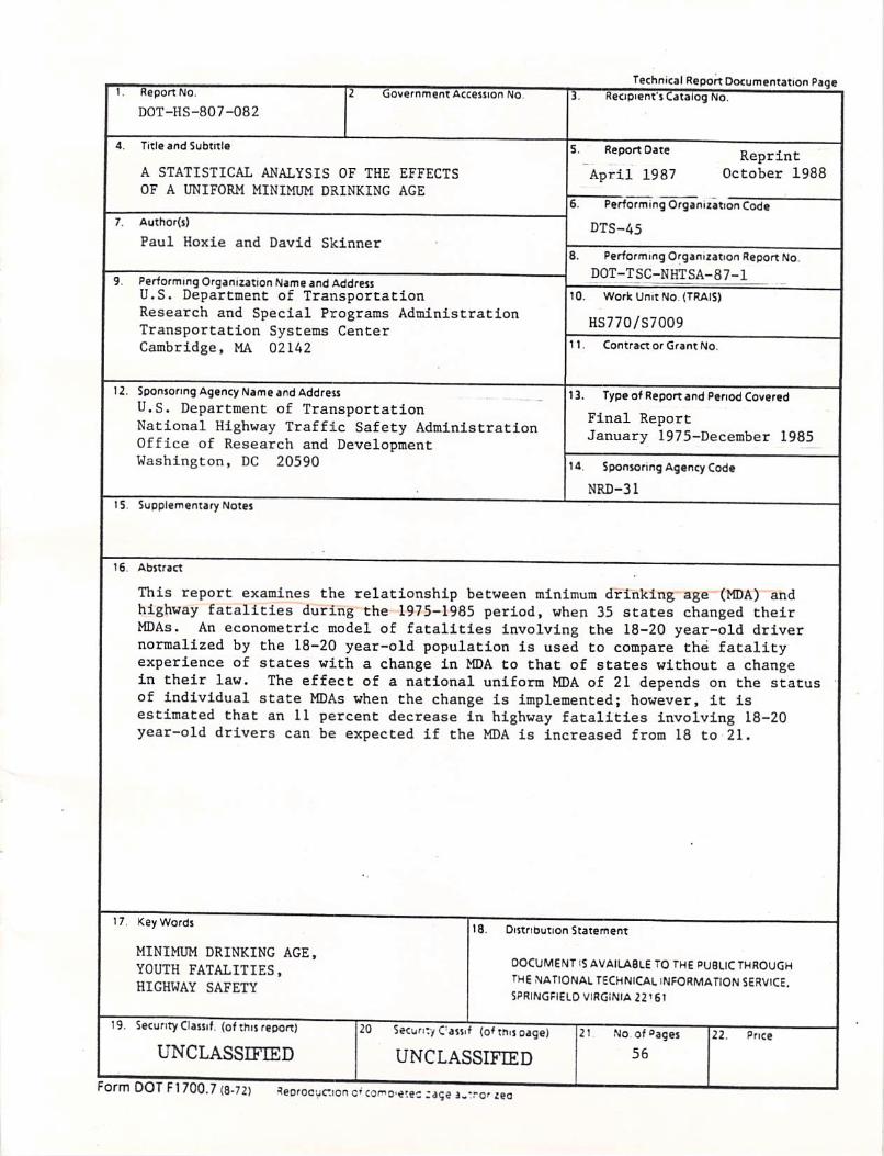
This report examines the relationship between minimum drinking age (MDA) andhighway fatalities during the 1975-1985 period, when 35 states changed theirMDAs. An econometric model of fatalities involving the 18-20 year-old drivernormalized by the 18-20 year-old population is used to compare the fatalityexperience of states with a change in MDA to that of states without a changein their law. The effect of a national uniform MDA of 21 depends on the statusof individual state MDAs when the change is implemented; however, it isestimated that an 11 percent decrease in highway fatalities involving 18-20year-old drivers can be expected if the MDA is increased from 18 to 21.

17. Keywords

MINIMUM DRINKING AGE,YOUTH FATALITIES,HIGHWAY SAFETY

19. Security Classif (of this report)

UNCLASSIFIED

18. Distnoution Statement

DOCUMENT IS AVAILABLE TOTHE PUBLIC THROUGHTHE NATIONAL TECHNICAL INFORMATION SERVICE.SPRINGFIELD VIRGINIA 22'61

20 Security C'assif (o'trusoage)

UNCLASSIFIED

21. No of "ages

56

22. Price

Form DOT F1 700.7 (8-72) Reorocyoon o< como-ewa :age i.tror *ea

PREFACE

This study examines the experience of states which have changed their minimum

drinking age during the 1975 to 1984 period and from this information develops an

estimate of the effect of a uniform minimum drinking age of 21 on highway fatalities in

the United States.

The work was performed by the U.S. Department of Transportation, Research and

Special Programs Administration, Transportation Systems Center, Cambridge,

Massachusetts under sponsorship of the U.S. Department of Transportation, National

Highway Traffic Safety Administration, Office of Research and Development,

Washington, DC.

The authors are grateful to James Hedlund, Chief of the Mathematical Analysis Divison

of NHTSA's Center for Statistics and Analysis for suggesting and sponsoring the study

and for the many valuable suggestions to improve it. The authors are also thankful for

the suggestions made by E. Donald Sussman of TSC in his reviews of the work and to

Robin Barnes for the tireless typing support which made the many drafts of the report

possible.

iii

METRICCONVERSIONFACTORS

-=s ApproximateCominlonstoMetricMutum

SymbolWhenYouKnowMultiplybyToFindSymbol~^•—

LENGTH

inInch**•24centlmatartcm

ItIMI90centimeter*cm

v<«yards04metersm

mlmilM14kilometerskm

In*squareinch**

AREA

squarecentimeters 64cm*It*squaretest048squaremeter*m*

vd»•quartyards04squaremeter*m*mi*squaremile*24squarekilometerskm*

•era*04hectaresha

$MASS(weight)

MeuMM28grams8bpoundi0.48kilogramskg

•hOfttOAS04tonnest

(2000161

up

VOLUME

teaspoons6millilitersml

Huplablaspoon*16mttlilltsrsnil

flotfluidounces30millilitersml

ecupi044liters1

Ptpints0.47liters1

qtquant046liters1

0*1gallons34liters1

ft*eubklau043cubicmetersmlyd*cubicyard)0.76cubicmetersm*

TEMPERATURE(exact)

»FFahrenheit6/BtetterCelsius•C

temperaturesubtracting321

tempereture

"lIn.»344cm(saacdyl.Forotharexactconversion*andmoradatalltabtoisaaNBSMisc.PubLaee.Unit*olWeightandMeasures.Prka$2.2&SOCatalogNo.cistoago.

ISB.

—E

-=s-

Inchai—s

-23

-22

-21

-18

-18

-17

-18

-16

-14

-13

-12

-II

-10

-8

-3

-2

-1

ApproximiuConversionsfromMetricMature*

SymbolWhanYouKnowMultiplybyToFindSymbol

LENGTH

m

m

km

cm*m*km*ha

s

kgt

I

i

I

m»m»

mlUlmeterscentlmaiers

maters

0440.43.31.104

AREA

lastyard*

squarecentimeter*0.16squeremeter*14squareyard*squarekilometer*0.4squaremusthectaresllOjOOOm*I24

kilogramstonne*11000kgl

milliliterstitan

liter*

mar*

cubicmeters

cubicmeters

MASS(weight)

0436

241.1

VOLUME

043

XI148

048

38

14

shorttons

fluidounce*

pint*quarts

cubiclast

cubicyards

TEMPERATURE(exact)

Celsiustsmpereture

«F-400

|IJI.I-40

"C

I"T20

8/fi(thanadd321

Fahrenheittempereture

32140

-lU-i

88.680I120

I.1I.IIIII20

T40

37

VH-h160

in

ft

ydmi

In*yd*mr*

II01

pt

qtonit*

»F

•F312

1602001IJI.II.I

100

°c

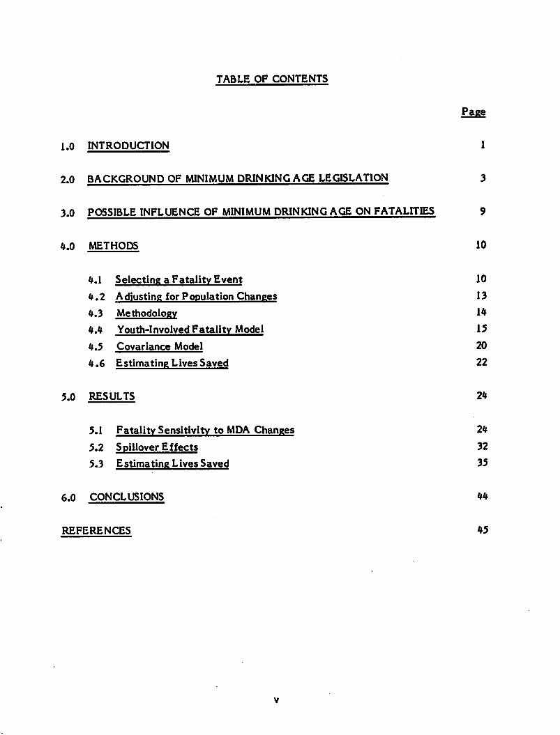
TABLE OF CONTENTS

Page

1.0 INTRODUCTION 1

2.0 BACKGROUND OF MINIMUM DRINKING AGE LEGISLATION 3

3.0 POSSIBLE INFLUENCE OF MINIMUM DRINKING AGE ON FATALITIES 9

4.0 METHODS 10

4.1 Selecting a Fatality Event 10

4.2 Adjusting for Population Changes 13

4.3 Methodology 14

4.4 Youth-Involved Fatality Model 15

4.5 Covariance Model 20

4.6 Estimating Lives Saved 22

5.0 RESULTS 24

5.1 Fatality Sensitivity to MDA Changes 24

5.2 Spillover Effects 32

5.3 Estimating Lives Saved 35

6.0 CONCLUSIONS 44

REFERENCES 45

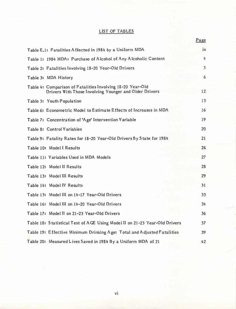
LIST OF TABLES

Page

Table E.l: Fatalities Affected in 1984 by a Uniform MDA ix

Table 1: 1984 MDA: Purchase of Alcohol of Any Alcoholic Content 4

Table 2: Fatalities Involving 18-20 Year-Old Drivers 5

Table 3: MDA History 6

Tabled: Comparison of Fatalities Involving 18-20 Year-OldDrivers With Those Involving Younger and Older Drivers 12

Tabled: Youth Population 13

Table 6: Econometric Model to Estimate Effects of Increases in MDA 16

Table 7: Concentration of 'Age' Intervention Variable 19

Table 8: Control Variables 20

Table 9: Fatality Rates for 18-20 Year-Old Drivers By State for 1984 21

Table 10: Model I Results 26

Table 11: Variables Used in MDA Models 27

Table 12: Model II Results 28

Table 13: Model III Results 29

Table 14: Model IV Results 31

Table 15: Model III on 14-17 Year-Old Drivers 33

Table 16: Model III on 14-20 Year-Old Drivers 34

Table 17: Model II on 21-23 Year-Old Drivers 36

Table 18: Statistical Test of AGE Using Model II on 21-23 Year-Old Drivers 37

Table 19: Effective Minimum Drinking Age: Total and Adjusted Fatalities 39

Table 20: Measured Lives Saved in 1984 By a Uniform MDA of 21 42

vi

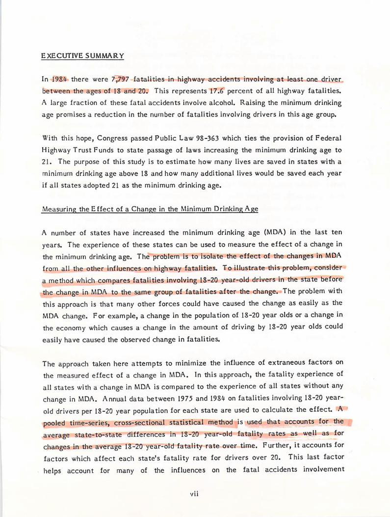
EXECUTIVE SUMMARY

In 1984 there were 7,797 fatalities in highway accidents involving at least one driver

between the ages of 18 and 20. This represents 17.6 percent of all highway fatalities.

A large fraction of these fatal accidents involve alcohol. Raising the minimum drinking

age promises a reduction in the number of fatalities involving drivers in this age group.

With this hope, Congress passed Public Law 98-363 which ties the provision of Federal

Highway Trust Funds to state passage of laws increasing the minimum drinking age to

21. The purpose of this study is to estimate how many lives are saved in states with a

minimum drinking age above 18 and how many additional lives would be saved each year

if all states adopted 21 as the minimum drinking age.

Measuring the Effect of a Change in the Minimum Drinking Age

A number of states have increased the minimum drinking age (MDA) in the last ten

years. The experience of these states can be used to measure the effect of a change in

the minimum drinking age. The problem is to isolate the effect of the changes in MDA

from all the other influences on highway fatalities. To illustrate this problem, consider

a method which compares fatalities involving 18-20 year-old drivers in the state beforethe change in MDA to the same group of fatalities after the change. The problem with

this approach is that many other forces could have caused the change as easily as the

MDA change. For example, a change in the population of 18-20 year olds or a change inthe economy which causes a change in the amount of driving by 18-20 year olds could

easily have caused the observed change in fatalities.

The approach taken here attempts to minimize the influence of extraneous factors onthe measured effect of a change in MDA. In this approach, the fatality experience of

all states with a change in MDA is compared to the experience of all states without anychange in MDA. Annual data between 1975 and 1984 on fatalities involving 18-20 year-old drivers per 18-20 year population for each state are used to calculate the effect. Apooled time-series, cross-sectional statistical method is used that accounts for theaverage state-to-state differences in 18-20 year-old fatality rates as well as forchanges in the average 18-20 year-old fatality rate over time. Further, it accounts forfactors which affect each state's fatality rate for drivers over 20. This last factor

helps account for many of the influences on the fatal accidents involvement

vii

rate of the 18-20 year-old drivers. In summary, the approach goes to great lengths toisolate the effect of changes in MDA from the numerous other factors which influencethe fatality involvement rate of 18-20 year olds.

Identifying the Affected Drivers

In order to estimate the national effect of changes in MDA, from the reduction in

fatalities involving affected drivers, we need to know how many 18-20 year-old driverswould be affected by the law change. This depends on the state drinking age laws in1984. 3,292 of the 7,797 fatalities involving drivers in the 18-20 age group occurred instates where the MDA is already 21. No reduction in fatalities can be expected in these

states. Of the remaining 4,505 fatalities, 399 occurred in states where the minimum

drinking age is 20. If 18 year olds, 19 year olds and 20 year olds were each involved in

one-third of these fatal accidents, then we could expect a change in the minimum

drinking age from 20 to 21 to affect only about one-third of the 399 fatalities, 133,

because only the fatalities involving 20 year-old drivers would be affected.

Similar reasoning leads us to estimate that two-thirds of the 3,065 fatalities involving

drivers in the 18-20 age group in states with a current MDA of 19 might be affected by

a change in the drinking age from 19 to 21. This represents 2,043 fatalities. In the

remaining states, where the MDA is currently 18, all of the 1,041 fatalities could be

affected. These calculations are summarized in Table E.l along with complimentary

calculations of the fatalities affected by a hypothetical change in MDA to 18. The

change in MDA to 18 is used to measure how many lives are already being saved by

MDAs above 18.

Table E.l distinguishes between legal MDA and effective MDA. This distinction

reflects the fact that states often permit people who can legally drink under the

existing law to continue to drink under the new law. So, if a state changed its MDAfrom 18 to 21 on January 1, 1983 and this "grandfather" clause was included in the new

law, then at the beginning of 1984, 19 and 20 year olds could still drink in that state,but fewer and fewer 19 year olds could drink in the state as the year progressed. Whenthe law changing the MDA takes effect on a date other than January 1, an additionaladjustment is needed in the number of fatalities under each age group to reflect partialyears.

via

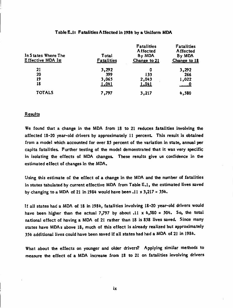
Table E.l: Fatalities Affected in 1984 by a Uniform MDA

In S tates Where TheEffective MDA Is;

21

20

19

18

TOTALS

Results

TotalFatalities

FatalitiesAffectedBy MDA

Change to 21

FatalitiesAffectedBy MDA

Change to 18

3,292 0 3,292399 133 266

3,065 2,043 1,0221.041 1.041 0

7,797 3,217 4,580

We found that a change in the MDA from 18 to 21 reduces fatalities involving the

affected 18-20 year-old drivers by approximately 11 percent. This result is obtained

from a model which accounted for over 85 percent of the variation in state, annual per

capita fatalities. Further testing of the model demonstrated that it was very specific

in isolating the effects of MDA changes. These results give us confidence in the

estimated effect of changes in the MDA.

Using this estimate of the effect of a change in the MDA and the number of fatalities

in states tabulated by current effective MDA from Table E.l, the estimated lives saved

by changing to a MDA of 21 in 1984 would have been .11 x 3,217 = 354.

If all states had a MDA of 18 in 1984, fatalities involving 18-20 year-old drivers would

have been higher than the actual 7,797 by about .11 x 4,580 = 504. So, the totalnational effect of having a MDA of 21 rather than 18 is 858 lives saved. Since manystates have MDAs above 18, much of this effect is already realized but approximately

354 additional lives could have been saved if all states had had a MDA of 21 in 1984.

What about the effects on younger and older drivers? Applying similar methods tomeasure the effect of a MDA increase from 18 to 21 on fatalities involving drivers

ix

between 14 and 18 years old revealed a slight reduction in fatalities but the measured

effect was not statistically significant.

The results for older drivers were similar. A slight decrease in fatalities involving 21-

23 year-old drivers was revealed, but again this effect was not statistically significant.Only two states had enough experience with a change in drinking age to 21 to be used incalculating this effect, further experience of other states might reveal a reliableeffect.

If all states had responded to the Federal Government's suggestion by passing lawswhich set the MDA at 21, an additional 354 lives could have been saved in 1984.

Further, PL 98-363 by penalizing states with MDAs below 21, ensures that the 1984

estimate of 504 lives saved (due to MDAs above 18) will not decrease. The 858 lives

which are saved as a result of a change in MDA from 18 to 21 represent 1.9 percent of

all highway fatalities in 1984.

1.0 INTRODUCTION

PL 98-363 authorized the Secretary of Transportation to withhold Highway Trust Funds

from any state allowing purchase or public consumption of any alcoholic beverage by a

person less than 21 years old. The law applies to funds apportioned to states in fiscal

year 1987. It is intended to influence all states not currently at the compliance age to

raise their Minimum Drinking Age (MDA) to 21 years old. The purpose of this study is

to assess the effect a national, uniform MDA of 21 years old would have on total

highway fatalities. That is, how many lives would be saved if those states which do not

presently have a 21 year-old MDA, increased the MDA to that level? We focus on the

effect of the uniform MDA on highway fatalities for two reasons. First, alcohol is

involved in approximately one-half of all fatal highway accidents, so changes in the

MDA are likely to have a significant effect on highway fatalities. Second, the Fatal

Accident Reporting Systems (FARS) provides a high-quality, consistent series of fatal

highway accident data from 1975 onward. This data permits analyses which would not

be workable with the less complete and less consistent data series on all highway

accidents. The study does not assess all the benefits which would result from a uniform

MDA of 21. A uniform MDA will reduce non-fatal as well as fatal highway accidents.

The injury and property damage associated with the highway accidents avoided by

increasing the MDA to 21 is a substantial benefit. In assessing the total benefits of a

uniform MDA of 21, these other benefits must be added to the decrease in fatalities

which is measured in this study.

The methodology used to estimate the effect of a national, uniform MDA of 21 isdivided into two components. The first uses cross-section, time-series econometric

models to estimate the percentage change in fatalities expected to result from

increases in MDA. The second identifies the current MDA in all states so that the

population affected by a uniform MDA can be determined. The estimated nationaleffect of a uniform MDA applies the empirically estimated percentage change in

fatalities to the affected population.

Obviously, if fatalities are not very sensitive to the MDA because young drivers can

still obtain alcohol easily or if the states with most of the highway fatalities already

have a MDA near or at 21 years old, then the uniform MDA will have a small national

impact upon fatalities. But, if fatalities are very sensitive to MDA changes and many

high fatality states have low MDAs, then a sizable impact could occur.

This study was supported by Mathematical Analysis Division (MAD) of NHTSA's

National Center for Statistics and Analysis (NCSA). MAD suggested the topic and the

FARS data used in the analysis are collected and maintained by NCSA.

Chapter 2.0 presents a brief history of MDA legislation. Chapter 3.0 discusses how the

legislation might influence state highway fatality levels. Chapter 4.0 presents the

methods used in this study to estimate the effect of a uniform MDA of 21 years old.

Chapter 5.0 presents the results of our analysis; Chapter 6.0 our conclusions.

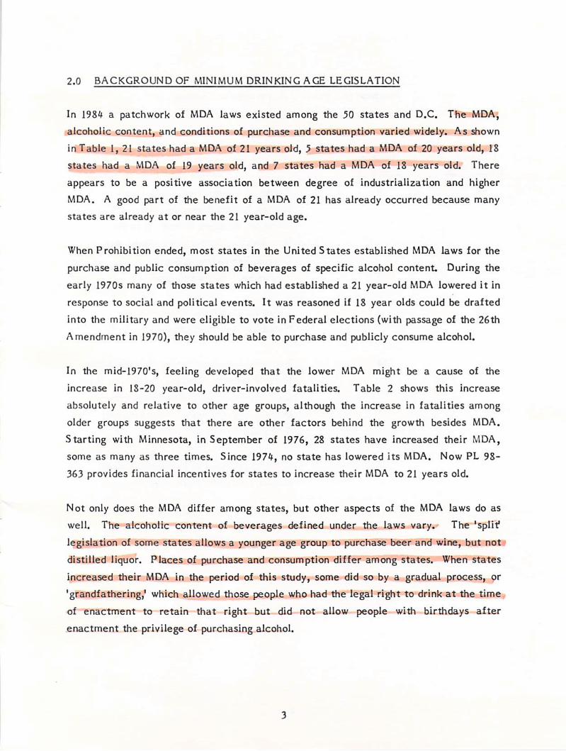
2.0 BACKGROUND OF MINIMUM DRINKING AGE LEGISLATION

In 1984 a patchwork of MDA laws existed among the 50 states and D.C. The MDA,

alcoholic content, and conditions of purchase and consumption varied widely. As shown

in Table 1,21 states had a MDA of 21 years old, 5 states had a MDA of 20 years old, 18

states had a MDA of 19 years old, and 7 states had a MDA of 18 years old. There

appears to be a positive association between degree of industrialization and higher

MDA. A good part of the benefit of a MDA of 21 has already occurred because many

states are already at or near the 21 year-old age.

When Prohibition ended, most states in the United States established MDA laws for the

purchase and public consumption of beverages of specific alcohol content. During the

early 1970s many of those states which had established a 21 year-old MDA lowered it in

response to social and political events. It was reasoned if 18 year olds could be drafted

into the military and were eligible to vote in Federal elections (with passage of the 26th

Amendment in 1970), they should be able to purchase and publicly consume alcohol.

In the mid-1970's, feeling developed that the lower MDA might be a cause of the

increase in 18-20 year-old, driver-involved fatalities. Table 2 shows this increase

absolutely and relative to other age groups, although the increase in fatalities among

older groups suggests that there are other factors behind the growth besides MDA.

Starting with Minnesota, in September of 1976, 28 states have increased their MDA,

some as many as three times. Since 1974, no state has lowered its MDA. Now PL 98-

363 provides financial incentives for states to increase their MDA to 21 years old.

Not only does the MDA differ among states, but other aspects of the MDA laws do as

well. The alcoholic content of beverages defined under the laws vary. The 'split1

legislation of some states allows a younger age group to purchase beer and wine, but not

distilled liquor. Places of purchase and consumption differ among states. When states

increased their MDA in the period of this study, some did so by a gradual process, or

'grandfathering,1 which allowed those people who had the legal right to drink at the time

of enactment to retain that right but did not allow people with birthdays after

enactment the privilege of purchasing alcohol.

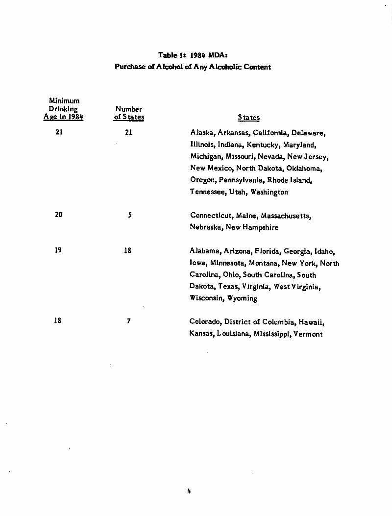
Table 1: 1984 MDA:

Purchase of Alcohol of Any Alcoholic Content

Minimum

Drinking NumberAge in 1984 of States States

21 21 Alaska, Arkansas, California, Delaware,

Illinois, Indiana, Kentucky, Maryland,

Michigan, Missouri, Nevada, New Jersey,

New Mexico, North Dakota, Oklahoma,

Oregon, Pennsylvania, Rhode Island,

Tennessee, Utah, Washington

20 5 Connecticut, Maine, Massachusetts,

Nebraska, New Hampshire

19 18 Alabama, Arizona, Florida, Georgia, Idaho,Iowa, Minnesota, Montana, New York, North

Carolina, Ohio, South Carolina, South

Dakota, Texas, Virginia, West Virginia,

Wisconsin, Wyoming

18 7 Colorado, District of Columbia, Hawaii,Kansas, Louisiana, Mississippi, Vermont

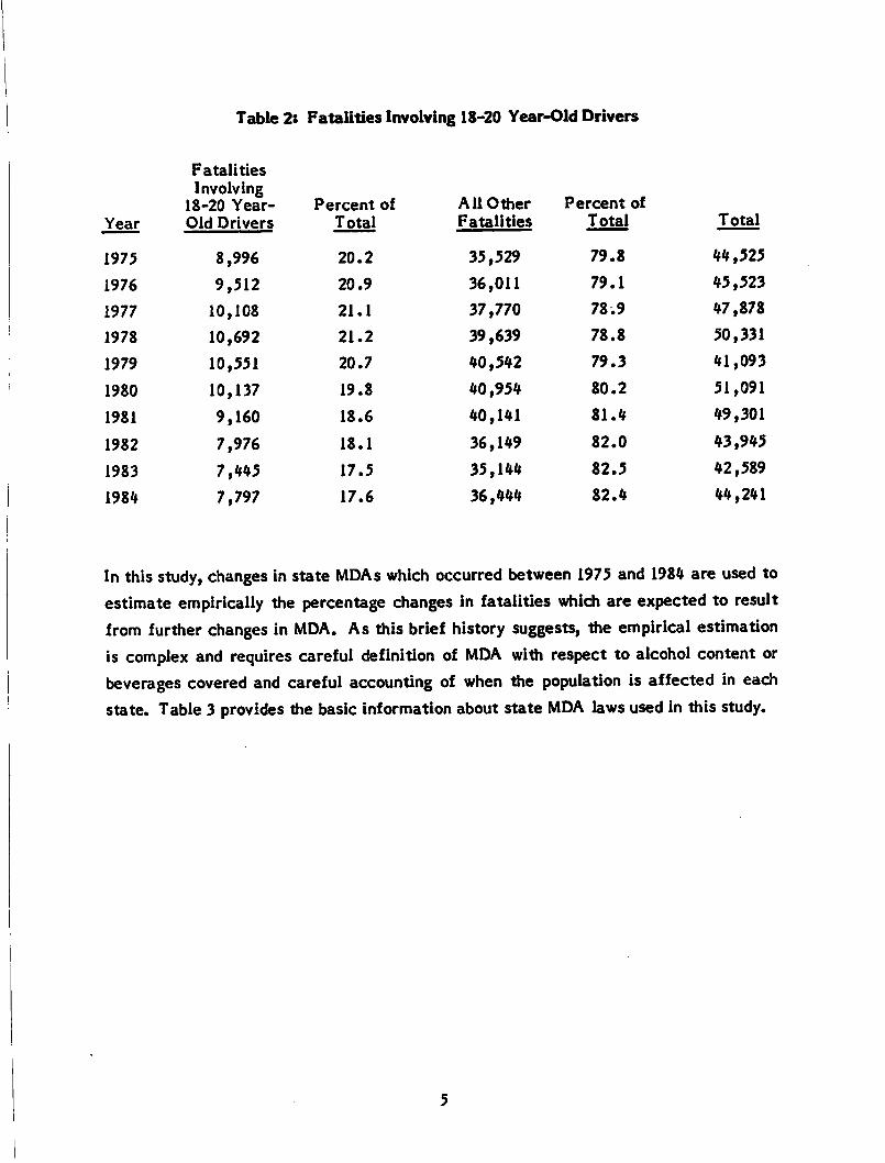
Table 2: Fatalities Involving 18-20 Year-Old Drivers

Year

FatalitiesInvolving

18-20 Year-Old Drivers

Percent of

Total

AllOther

Fatalities

Percent of

Total Total

1975 8,996 20.2 35,529 79.8 44,525

1976 9,512 20.9 36,011 79.1 45,523

1977 10,108 21.1 37,770 78.9 47,878

1978 10,692 21.2 39,639 78.8 50,331

1979 10,551 20.7 40,542 79.3 41,093

1980 10,137 19.8 40,954 80.2 51,091

1981 9,160 18.6 40,141 81.4 49,301

1982 7,976 18.1 36,149 82.0 43,945

1983 7,445 17.5 35,144 82.5 42,589

1984 7,797 17.6 36,444 82.4 44,241

In this study, changes in state MDAs which occurred between 1975 and 1984 are used toestimate empirically the percentage changes in fatalities which are expected to resultfrom further changes in MDA. As this brief history suggests, the empirical estimationis complex and requires careful definition of MDA with respect to alcohol content orbeverages covered and careful accounting of when the population is affected in eachstate. Table 3 provides the basic information about state MDA laws used in this study.

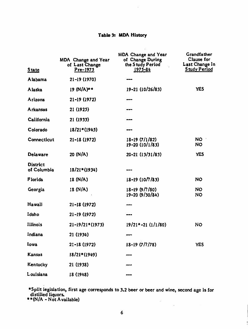
Table 3: MDA History

State

MDA Change and Yearof Last Change

Pre-1975

MDA Change and Yearof Change Duringthe Study Period

1975-84

Grandfather

Clause forLast Change InStudy Period

Alabama 21-19 (1970) —

Alaska 19 (N/A)*» 19-21 (10/26/83) YES

Arizona 21-19 (1972) —

Arkansas 21 (1925) —

California 21 (1933) —

Colorado 18/21»(1945) —

Connecticut 21-18 (1972) 18-19 (7/1/82)19-20 (10/1/83)

NO

NO

Delaware 20 (N/A) 20-21 (13/31/83) YES

District

of Columbia 18/21*(1934) —-

Florida 18 (N/A) 18-19 (10/7/83) NO

Georgia 18 (N/A) 18-19 (9/?/80)19-20 (9/30/84)

NO

NO

Hawaii 21-18 (1972) —

Idaho 21-19 (1972) —

Illinois 21-19/21*0973) 19/21*-21 (1/1/80) NO

Indiana 21 (1934) —

Iowa 21-18 (1972) 18-19 (7/?/78) YES

Kansas 18/21*(1949) —

Kentucky 21 (1938) —

Louisiana 18 (1948) ___

♦Split legislation, first age corresponds to 3.2 beer or beer and wine, second age is fordistilled liquors.

**(N/A -NotAvailable)

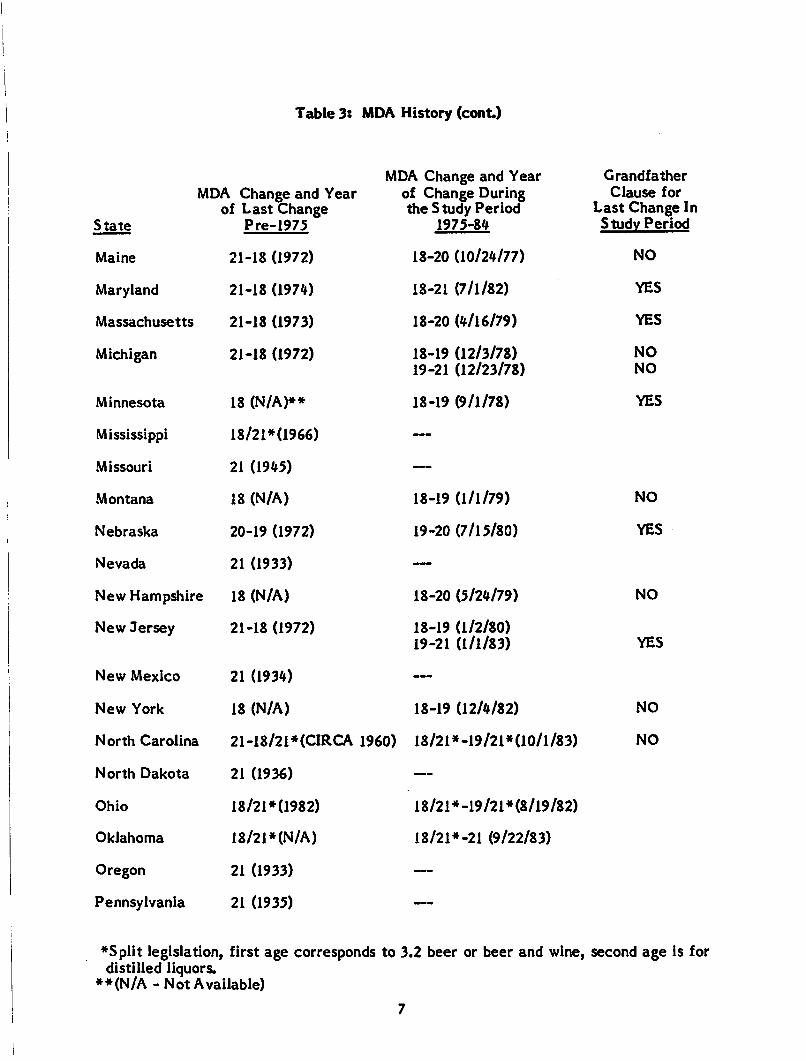
Table 3: MIDA History (cont.)

MDA Change and Year Grandfather

MDA Change and Yearof Last Change

State Pre-1975

of Change Duringthe Study Period

1975-84

Clause forLast Change IStudy Period

Maine 21-18 (1972) 18-20 (10/24/77) NO

Maryland 21-18 (1974) 18-21 (7/1/82) YES

Massachusetts 21-18 (1973) 18-20 (4/16/79) YES

Michigan 21-18 (1972) 18-19 (12/3/78)19-21 (12/23/78)

NO

NO

Minnesota 18 (N/A)** 18-19 (9/1/78) YES

Mississippi 18/21*(1966) —

Missouri 21 (1945) —

Montana 18 (N/A) 18-19 (1/1/79) NO

Nebraska 20-19 (1972) 19-20 (7/15/80) YES

Nevada 21 (1933) —

New Hampshire 18 (N/A) 18-20 (5/24/79) NO

New Jersey 21-18 (1972) 18-19 (1/2/80)19-21 (1/1/83) YES

New Mexico 21 (1934) —

New York 18 (N/A) 18-19 (12/4/82) NO

North Carolina 21-18/2i*(CIRCA I960) 18/21*-19/21*(10/l/83) NO

North Dakota 21 (1936) —

Ohio 18/21*0982) 18/21*-19/21*(8/l9/82)

Oklahoma 18/21*(N/A) 18/21*-21 (9/22/83)

Oregon 21 (1933) —

Pennsylvania 21 (1935) —-

♦Split legislation, first age corresponds to 3.2 beer or beer and wine, second age is fordistilled liquors.

**(N/A-Not Available)

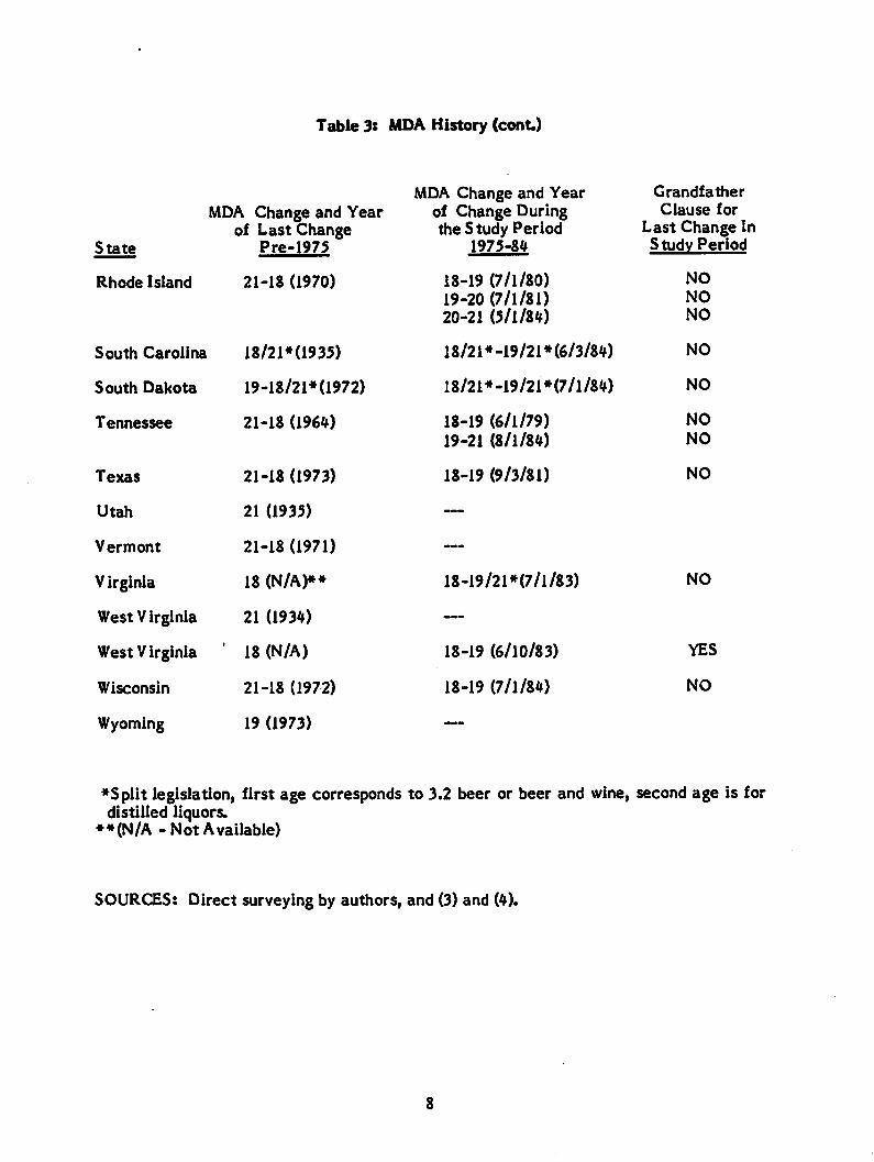
Table 3: MDA History (cont.)

MDA Change and Year

State

MDA Change and Yearof Last Change

Pre-1975

of Change Duringthe Study Period

1975-84

Rhode Island 21-18 (1970) 18-19 (7/1/80)19-20 (7/1/81)20-21 (5/1/84)

South Carolina 18/21*0935) 18/21*-19/21* (6/3/84)

South Dakota 19-18/21*0972) 18/21*-19/21*(7/l/84)

Tennessee 21-18 (1964) 18-19 (6/1/79)19-21 (8/1/84)

Texas 21-18 (1973) 18-19 (9/3/81)

Utah 21 (1935) —

Vermont 21-18 (1971) —

Virginia 18 (N/A)** 18-19/21*(7/l/83)

West Virginia 21 (1934) —

West Virginia ' 18 (N/A) 18-19 (6/10/83)

Wisconsin 21-18 (1972) 18-19 (7/1/84)

Wyoming 19 (1973) —

Grandfather

Clause forLast Change InStudy Period

NO

NO

NO

NO

NO

NO

NO

NO

NO

YES

NO

♦Split legislation, first age corresponds to 3.2 beer or beer and wine, second age is fordistilled liquors.

**(N/A-Not Available)

SOURCES: Direct surveying by authors, and (3) and (4).

3.0 POSSIBLE INFLUENCE OF MINIMUM DRINKING AGE ON FATALITIES

The recent increases in MDA were legislated in the belief that a higher drinking agewould reduce youth-involved highway fatalities because reduced alcohol consumptionamong this group would reduce drunk driving. Increases in MDA will not eliminate

alcohol consumption altogether among affected youth because the tendency toexperiment and use alcohol is strong and alcohol can be obtained illegally in severalways. The hope is that the law will convey the potential dangers of alcohol, reducepeer pressure to drink, and eliminate the serving of alcohol at social occasions. For

those in this age group who still want to drink, MDA laws will raise the cost ofobtaining alcohol in terms of both time and money. It will be necessary to search more,pay premiums for illegal sales, and travel greater distances. The increase in cost shouldreduce consumption and possibly induce more judicious use. Not only shouldconsumption be reduced, but dangerous drinking/driving patterns such as 'bar-hopping,'driving soon after consumption, and many drunk drivers interacting at once as barsclose should be reduced.

MDA laws have been criticized, however. Some people object to the abridgment of the

rights of youth and the placing of taboos which may make drinking all the more

intriguing. Others describe situations under which MDA laws may act as an unfavorable

influence on highway fatalities even if alcohol consumption is reduced. They point to

the substitution of drinking in cars (turning 'cars into bars') for on-premise drinking

under supervision, the substitution of higher potency liquors for beers, more intense

drinking per drinking occasion, and border crossings (creation of 'fatality alleys').

One other view is held on the MDA issue although maybe not in the extreme in which itis sometimes stated. The view is that alcohol is present in a high percentage of youth-

related fatalities — maybe 60 percent —but it is not the primary cause of thesefatalities. Rather it is only a symptom of the real cause -- risk-taking behavior.Hence, by this view, MDA laws will not affect youth-related fatalities.

We take the position in this study that it is difficult to reason about how MDA lawsactually work let alone quantify the result. It is likely that there is anet effect fromthe factors mentioned which impact youth who are simultaneously learning to drink anddrive. Because it is difficult to reason about the effects of MDA legislation in order toforecast future results, we measure the results empirically.

4.0 METHODS

Changes in MDA that have occurred in the 1975-1984 period are used to gauge thesensitivity of youth-involved highway fatalities to changes in MDA. An econometricmodel of fatalities involving an 18-20 year-old driver normalized by the population ofthat age is developed. Independent variables believed to influence the fatality rate aretested empirically. The model uses cross-sectional observations for each of the 50states and the District of Columbia over a ten-year period, 1975-1984, forming a pooledcross-section, time-series model estimation. All of the data available in the FARS database at the time of this study are used in the estimation. One of the independentvariables used in the model is a MDA intervention variable which specifies, for eachstate, the time and characteristics of any MDA change during the study period. It isthe coefficient of this variable which is the statistical estimate of the sensitivity ofyouth-involved fatalities to MDA increases. The sensitivity is then applied to the MDAstatus in each state In 1984 to estimate how many lives could have been saved if each

state had had a MDA of 21 years old. The lives affected in 1984 are taken as anestimate of what would happen if all states adopt a uniform MDA of 21 years old.

4.1 Selecting a Fatality Event

Up to this point, we have described the fatalities affected by MDA law increases as

'youth-involved fatalities' or by the longer phrase 'fatalities involving an 18-20 year-old

driver.' In this subsection, we give a precise definition to these terms, show what their

relationship is to other fatalities and, most importantly, discuss the reasons for their

selection.

Since the primary purpose of this study is to determine the effect of a national, uniformMDA on the total number of fatalities in the United States in a year, a fatality measureis needed which is sensitive to any changes resulting from the MDA change and whichcan be used to estimate the full national effect Because we plan to estimate theeffect of the MDA change empirically, we do not need to know that eliminating alcoholwould eliminate the fatal accident. All we need to know is that there is achance that achange in MDA would alter the conditions which led to the fatal accident

Ideally, the fatalities in accidents where an 18-20 year-old driver had apositive bloodalcohol level would be used to estimate the effect. However, driver blood alcohol level

10

is not reliably reported in FARS; and increases in the MDA would be likely to

correspond to increases in reporting. Further, since increases in reporting can only

increase the number of reported fatal accidents involving alcohol, basing the analysis on

fatalities in alcohol-involved accidents involving 18-20 year-old drivers is likely to

produce misleading results. Without using direct evidence on alcohol involvement,

there is a trade-off between having a fatality measure which can adequately be

translated into a total impact, and a measure which is sensitive and logically related to

prospective MDA effects.

As an example of this trade-off, consider single-vehicle, nighttime, male fatalities

which are often used as a surrogate or proxy for alcohol-related fatalities. Single-

vehicle, nighttime fatalities involving male 18-20 year-old drivers should be very

sensitive to changes in MDA. However, a MDA change will affect many more highway

accidents than these. So, this measure has little utility in measuring the total effect of

a national uniform MDA of 21 years old.

At the other extreme, if all highway fatalities were used as the dependent variable,

another problem is created. The statistical estimation will not properly detect the

effects of MDA increases because too much variation exists for the fatalities which are

conceptually different from those affected by MDA. This variation can swamp any

effects of MDA increases.

In this study, we have tried to choose a fatality series that is sensitive to MDA

increases yet permits the full effect of a MDA on highway fatalities in the United

States to be measured. We have selected fatalities in all accidents which involve an 18-

20 year-old driver. As Table 4 shows, these fatalities were 17.6 percent of all highwayfatalities in the United States for 1984. Table 4 also shows the per capita fatality rate

and a comparison to the rates of the two adjacent age cohorts. (Notice that these

fatality rates are not measured in the usual way, and since they measure all fatalities in

accidents involving a driver in the age group, the fatalities involving 18-20 and 21-23

year-old drivers are not mutually exclusive.)

11

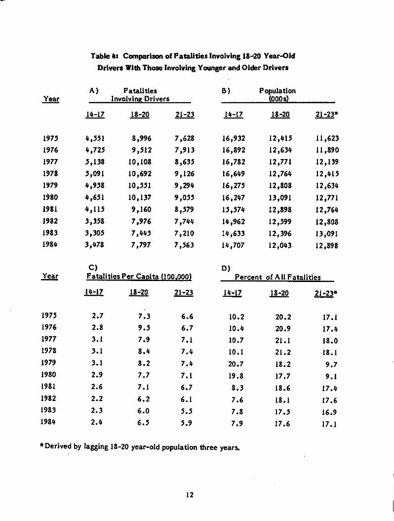
Table 4: Comparison of Fatalities Involving 18-20 Year-Old

Drivers With Those Involving Younger and Older Drivers

Year

A) Fatalities

Involving DriversB) Population

(000 s)

14-17 18-20 21-23 14-17 18-20 21-23*

1975 4,551 8,996 7,628 16,932 12,415 11,623

1976 4,725 9,512 7,913 16,892 12,634 11,890

1977 5,138 10,108 8,635 16,782 12,771 12,139

1978 5,091 10,692 9,126 16,649 12,764 12,415

1979 4,958 10,551 9,294 16,275 12,808 12,634

1980 4,651 10,137 9,055 16,247 13,091 12,771

1981 4,115 9,160 8,579 15,574 12,898 12,764

1982 3,358 7,976 7,744 14,962 12,599 12,808

1983 3,305 7,445 7,210 14,633 12,396 13,091

1984 3,478 7,797 7,563 14,707 12,043 12,898

Year

C)Fatalities Per Capita (100.000)

D)Percent of All Fatalities

14-17 18-20 21-23 14-17 18-20 21-23*

1975 2.7 7.3 6.6 10.2 20.2 17.1

1976 2.8 9.5 6.7 10.4 20.9 17.4

1977 3.1 7.9 7.1 10.7 21.1 18.0

1978 3.1 8.4 7.4 10.1 21.2 18.1

1979 3.1 8.2 7.4 20.7 18.2 9.7

1980 2.9 7.7 7.1 19.8 17.7 9.1

1981 2.6 7.1 6.7 8.3 18.6 17.4

1982 2.2 6.2 6.1 7.6 18.1 17.6

1983 2.3 6.0 5.5 7.8 17.5 16.9

1984 2.4 6.5 5.9 7.9 17.6 17.1

♦Derived by lagging 18-20 year-old population three years.

12

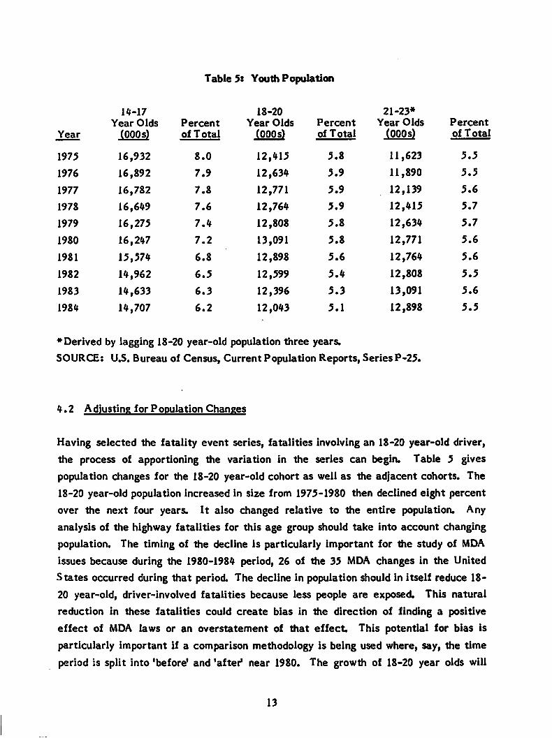
Table 5: Youth Population

Year

14-17

Year Olds

(000 s)Percentof Total

18-20

Year Olds(000s)

Percent

of Total

21-23*Year Olds

(000 s)Percentof Total

1975 16,932 8.0 12,415 5.8 11,623 5.5

1976 16,892 7.9 12,634 5.9 11,890 5.5

1977 16,782 7.8 12,771 5.9 12,139 5.6

1978 16,649 7.6 12,764 5.9 12,415 5.7

1979 16,275 7.4 12,808 5.8 12,634 5.7

1980 16,247 7.2 13,091 5.8 12,771 5.6

1981 15,574 6.8 12,898 5.6 12,764 5.6

1982 14,962 6.5 12,599 5.4 12,808 5.5

1983 14,633 6.3 12,396 5.3 13,091 5.6

1984 14,707 6.2 12,043 5.1 12,898 5.5

♦Derived by lagging 18-20 year-old population three years.

SOURCE: U3. Bureau of Census, Current Population Reports, Series P-25.

4.2 Adjusting for Population Changes

Having selected the fatality event series, fatalities involving an 18-20 year-old driver,

the process of apportioning the variation in the series can begin. Table 5 gives

population changes for the 18-20 year-old cohort as well as the adjacent cohorts. The

18-20 year-old population increased in size from 1975-1980 then declined eight percent

over the next four years. It also changed relative to the entire population. Any

analysis of the highway fatalities for this age group should take into account changing

population. The timing of the decline is particularly important for the study of MDA

issues because during the 1980-1984 period, 26 of the 35 MDA changes in the United

States occurred during that period. The decline in population should in itself reduce 18-

20 year-old, driver-involved fatalities because less people are exposed. This natural

reduction in these fatalities could create bias in the direction of finding a positive

effect of MDA laws or an overstatement of that effect This potential for bias is

particularly important if a comparison methodology is being used where, say, the time

period is split into 'before' and 'after1 near 1980. The growth of 18-20 year olds will

13

tend to increase fatalities in the pre-1980 period while it will tend to decrease

fatalities in the after period, making the comparison biased in the direction of finding

positive MDA effects.

Since this study uses state level data, the consideration of population is doubly

important because within the aggregate 18-20 year-old population trend that peaks in1980 are specific state population shifts. Some states are gaining population whileothers are losing. Further, there are large population differences among states which

affect the fatality levels for the state for all age groups.

In this study, we have controlled for the effects of population by dividing fatalities

involving an 18-20 year-old driver by the population of that age group. By normalizing

a per capita fatality rate is formed. The per capita fatality rate is used as the

dependent variable in a multiple regression model with other variables, many also in

rate form, serving as independent variables.

Two other measures of exposure to highway accidents would have been used to

normalize fatalities if they were available. The number of miles driven by 18-20 year-

old drivers would be ideal. However, it is not tabulated by driver age and state. The

closest variable available is total vehicle miles travelled (VMT) for all drivers. The

other measure is the number of 18-20 year-old registered drivers. It would be

somewhat better than population as a normalizing factor because the proportion of 18-

20 year olds which drive varies among states. Data on licensed drivers by age and state

is only approximated for several states and therefore may give misleading results.

4.3 Methodology

To determine the sensitivity of fatalities to increases in the MDA, an econometric

model is constructed using pooled cross-section, time-series data. The model measures

the effect of changes in MDA while controlling for other factors which affect fatalities

(such as economic activity). Annual fatality rates for each state and the District of

Columbia represent the units of observation of the dependent variable. These 51 cross-

sectional units are observed over a ten-year period, 1975-1984. 1984 is the last year of

full reporting in FARS which was available at the time of this study. The ten years of

cross-sectional values provide 510 observations on which to construct a model of the

effect of MDA changes. The independent variables are state observations of economic

14

activity, driving activity, beer consumption, and other factors which theoretically

should affect 18-20 year-old, driver-involved fatalities.

Construction of a pooled cross-section, time-series econometric model draws upon the

methodologies of intervention analysis and panel studies. Panel studies are

characterized by a relatively large cross-sectional number of units compared to the

number of times the set is observed. A large number of cross-sectional units allows for

an adequate statistical sample to be built up after only a few years of time. The quick

achievement of a significant sample allows for the timely evaluation of an activity

affecting the 'panel,' a feature which is desirable for studying MDA issues. A rich body

of literature exists, especially from sociology and political science, on methodologies

for use in panel studies (see Reference 5). Detailed statistical procedures have also

been developed for panel studies, especially techniques for dealing with the complicated

regression error structures mat some of these models have. Work has also been done in

developing the methodology for intervention analyses. Thought must be given to

spliting the sample at some point before and after, and to controls for standardizing the

before and after period.

Using a pooled cross-section, time-series model has several advantages over the usual

method of comparing a 'before' and 'after* MDA period:

o staggered intervention (not all states change at the same time) can be

modeled;

o explicit control and identification can be given to other factors which affect

fatalities;

o use of all information available will provide for efficient estimation; and

o prediction of actual fatality levels for a state is possible as well as

percentage impact

4.4 Youth-Involved Fatality Model

The pooled cross-section, time-series econometric model used to test the sensitivity of

fatalities to increases in MDA is shown in Table 6. The dependent variable is a fatality

rate, the number of fatalities involving 18-20 year-old drivers for each state divided by

the population of that age group for the state. Thus, a fatality rate is formed for each

state and D.C. for each of ten years over the period, 1975-1984. The natural logarithm

is taken of this rate as it is for all other variables except the MDA intervention

15

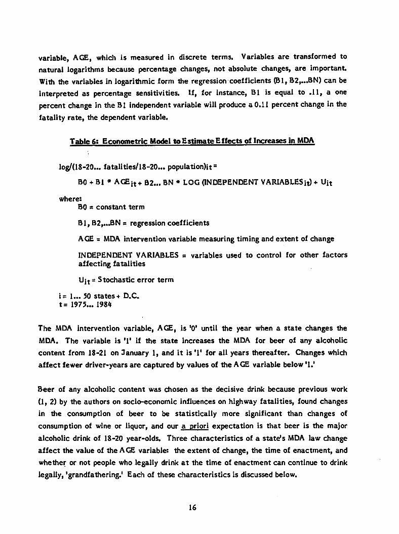
variable, AGE, which is measured in discrete terms. Variables are transformed tonatural logarithms because percentage changes, not absolute changes, are importantWith the variables in logarithmic form the regression coefficients (Bl, B2,...BN) can beinterpreted as percentage sensitivities. If, for instance, Bl is equal to .11, a onepercent change in the Bl independent variable will produce a 0.11 percent change in thefatality rate, the dependent variable.

Table 6: Econometric Model to Estimate Effects of Increases in MDA

log/(18-20... fatalities/18-20... population)it =

BO + Bl * AGEit+ B2... BN * LOG (INDEPENDENT VARIABLES it) + Uit

where:

BO = constant term

Bl, B2,...BN = regression coefficients

AGE = MDA intervention variable measuring timing and extent of change

INDEPENDENT VARIABLES = variables used to control for other factorsaffecting fatalities

Ujt = Stochastic error term

i= 1... 50 states + D.C.

t= 1975... 1984

The MDA intervention variable, AGE, is '0' until the year when a state changes the

MDA. The variable is '1' if the state increases the MDA for beer of any alcoholic

content from 18-21 on January 1, and it is '1' for all years thereafter. Changes which

affect fewer driver-years are captured by values of the AGE variable below '1.'

Beer of any alcoholic content was chosen as the decisive drink because previous work

(1, 2) by the authors on socio-economic influences on highway fatalities, found changes

in the consumption of beer to be statistically more significant than changes of

consumption of wine or liquor, and our a priori expectation is that beer is the major

alcoholic drink of 18-20 year-olds. Three characteristics of a state's MDA law change

affect the value of the AGE variable: the extent of change, the time of enactment, and

whether or not people who legally drink at the time of enactment can continue to drink

legally, 'grandfathering.' Each of these characteristics is discussed below.

16

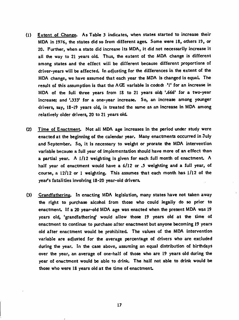
(1) Extent of Change. As Table 3 indicates, when states started to increase their

MDA in 1976, the states did so from different ages. Some were 18, others 19, or

20. Further, when a state did increase its MDA, it did not necessarily increase it

all the way to 21 years old. Thus, the extent of the MDA change is different

among states and the effect will be different because different proportions of

driver-years will be affected. In adjusting for the differences in the extent of the

MDA change, we have assumed that each year the MDA is changed is equal. The

result of this assumption is that the AGE variable is coded: T for an increase in

MDA of the full three years from 18 to 21 years old; '.666' for a two-year

increase; and '.333' for a one-year increase. So, an increase among younger

drivers, say, 18-19 years old, is treated the same as an increase In MDA among

relatively older drivers, 20 to 21 years old.

(2) Time of Enactment Not all MDA age increases in the period under study were

enacted at the beginning of the calendar year. Many enactments occurred in Julyand September. So, it is necessary to weight or prorate the MDA intervention

variable because a full year of implementation should have more of an effect than

a partial year. A 1/12 weighting is given for each full month of enactment A

half year of enactment would have a 6/12 or .5 weighting and a full year, of

course, a 12/12 or 1 weighting. This assumes that each month has 1/12 of theyear's fatalities involving 18-20 year-old drivers.

(3) Grandfathering. In enacting MDA legislation, many states have not taken away

the right to purchase alcohol from those who could legally do so prior to

enactment If a 20 year-old MDA age was enacted when the present MDA was 19

years old, 'grandfathering* would allow those 19 years old at the time of

enactment to continue to purchase after enactment but anyone becoming 19 years

old after enactment would be prohibited. The values of the MDA intervention

variable are adjusted for the average percentage of drivers who are excluded

during the year. In the case above, assuming an equal distribution of birthdays

over the year, an average of one-half of those who are 19 years old during the

year of enactment would be able to drink. The half not able to drink would be

those who were 18 years old at the time of enactment

17

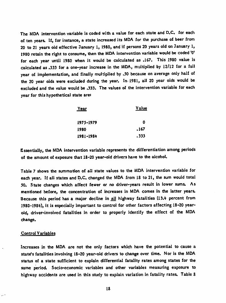
The MDA intervention variable is coded with a value for each state and D.C. for each

of ten years. If, for instance, a state increased its MDA for the purchase of beer from20 to 21 years old effective January 1, 1980, and if persons 20 years old on January 1,1980 retain the right to consume, then the MDA intervention variable would be coded '0'for each year until 1980 when it would be calculated as .167. This 1980 value iscalculated as .333 for a one-year increase in the MDA, multiplied by 12/12 for a fullyear of implementation, and finally multiplied by .50 because on average only half ofthe 20 year olds were excluded during the year. In 1981, all 20 year olds would beexcluded and the value would be .333. The values of the intervention variable for each

year for this hypothetical state are:

Year Value

1975-1979 0

1980 .167

1981-1984 .333

Essentially, the MDA intervention variable represents the differentiation among periodsof the amount of exposure that 18-20 year-old drivers have to the alcohol.

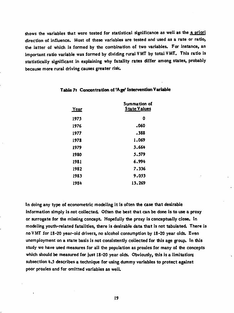
Table 7 shows the summation of all state values to the MDA intervention variable for

each year. If all states and D.C. changed the MDA from 18 to 21, the sum would total50. State changes which affect fewer or no driver-years result in lower sums. Asmentioned before, the concentration of increases in MDA comes in the latter years.

Because this period has a major decline in all highway fatalities (13.4 percent from1980-1984), it is especially important to control for other factors affecting 18-20 year-

old, driver-involved fatalities in order to properly identify the effect of the MDA

change.

Control Variables

Increases in the MDA are not the only factors which have the potential to cause a

state's fatalities involving 18-20 year-old drivers to change over time. Nor is the MDAstatus of a state sufficient to explain differential fatality rates among states for the

same period. Socio-economic variables and other variables measuring exposure to

highway accidents are used in this study to explain variation in fatality rates. Table 8

18

shows the variables that were tested for statistical significance as well as the a prioridirection of influence. Most of these variables are tested and used as a rate or ratio,

the latter of which is formed by the combination of two variables. For instance, animportant ratio variable was formed by dividing rural VMT by total VMT. This ratio Isstatistically significant in explaining why fatality rates differ among states, probablybecause more rural driving causes greater risk.

Table 7: Concentration of 'Age* Intervention Variable

Summation ofYear State Values

1975 0

1976 .060

1977 .388

1978 1.069

1979 3.664

1980 5.579

1981 6.994

1982 7.336

1983 9.053

1984 13.269

In doing any type of econometric modeling it is often the case that desirable

information simply is not collected. Often the best that can be done is to use a proxy

or surrogate for the missing concept Hopefully the proxy is conceptually close. In

modeling youth-related fatalities, there is desirable data that is not tabulated. There is

no VMT for 18-20 year-old drivers, no alcohol consumption by 18-20 year olds. Even

unemployment on a state basis is not consistently collected for this age group. In this

study we have used measures for all the population as proxies for many of the concepts

which should be measured for just 18-20 year olds. Obviously, this is a limitation;

subsection 4.5 describes a technique for using dummy variables to protect against

poor proxies and for omitted variables as well.

19

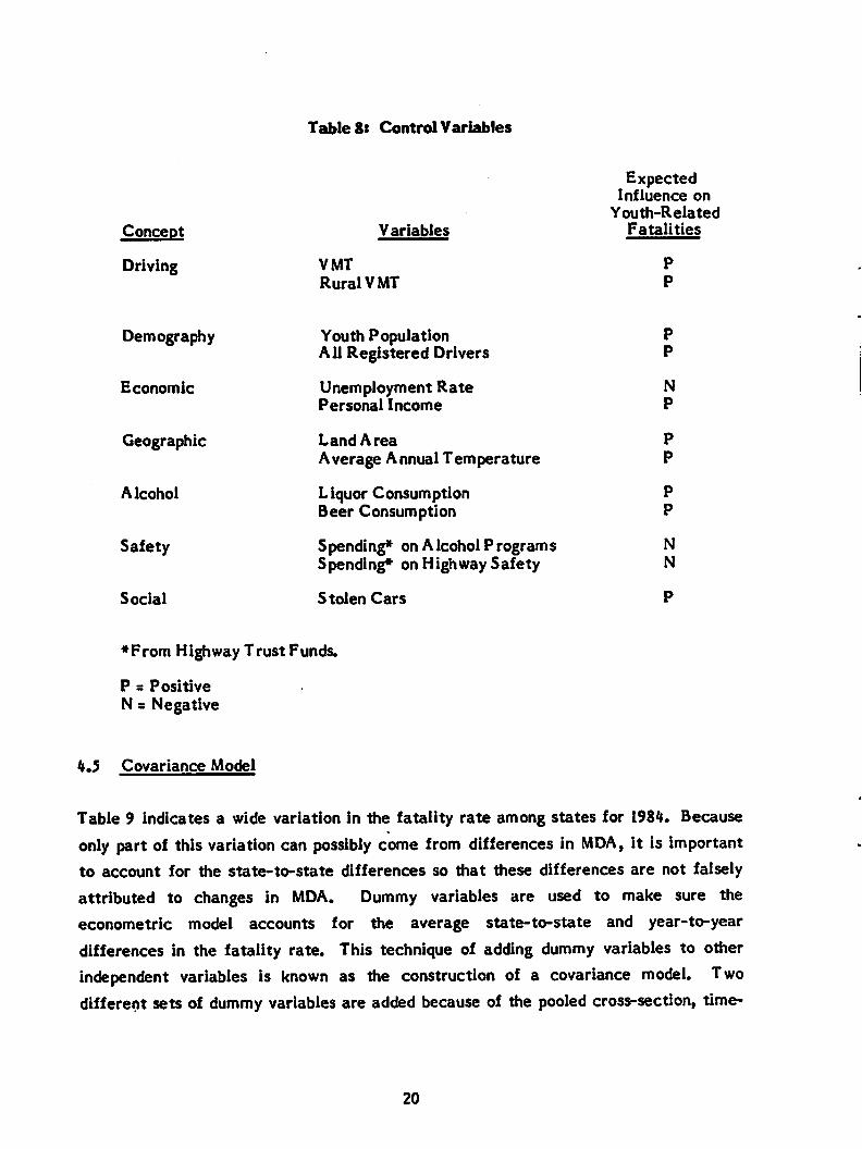
Concept

Driving

Demography

Economic

Geographic

Alcohol

Safety

Social

TableS: Control Variables

ExpectedInfluence on

Youth-RelatedVariables Fatalities

VMT P

Rural VMT P

Youth Population P

All Registered Drivers P

Unemployment Rate N

Personal Income P

Land Area P

Average Annual Temperature P

Liquor Consumption P

Beer Consumption P

S pending* on A Icohol Programs N

Spending* on Highway Safety N

Stolen Cars

*From Highway Trust Funds.

P = Positive

N s Negative

4.5 Covariance Model

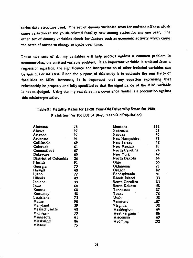
Table 9 indicates a wide variation in the fatality rate among states for 1984. Because

only part of this variation can possibly come from differences in MDA, it is importantto account for the state-to-state differences so that these differences are not falsely

attributed to changes in MDA. Dummy variables are used to make sure the

econometric model accounts for the average state-to-state and year-to-year

differences in the fatality rate. This technique of adding dummy variables to otherindependent variables is known as the construction of a covariance model. Twodifferent sets of dummy variables are added because of the pooled cross-section, time-

20

series data structure used. One set of dummy variables tests for omitted effects whichcause variation in the youth-related fatality rate among states for any one year. Theother set of dummy variables check for factors such as economic activity which cause

the rates of states to change or cycle over time.

These two sets of dummy variables will help protect against a common problem ineconometrics, the omitted variable problem. If an important variable Is omitted from aregression equation, the significance and interpretation of other included variables canbe spurious or inflated. Since the purpose of this study is to estimate the sensitivity offatalities to MDA increases, it is important that any equation expressing thatrelationship be properly and fully specified so that the significance of the MDA variableis not misjudged. Using dummy variables in a covariance model is a precaution against

this misinterpretation.

Table 9: Fatality Rates for 18-20 Year-Old Drivers By State for 1984

(Fatalities Per 100,000 of 18-20 Year-Old Population)

Alabama 78

Alaska 97

Arizona 97

A rkansas 91

California 69Colorado 61Connecticut 67

Delaware 63District of Columbia 26

Florida 91

GeorgiaHawaii

7540

Idaho 77

Illinois 49

Indiana 55Iowa 64Kansas 68KentuckyLouisiana

58

73

Maine 90

MarylandMassachusetts

3948

MichiganMinnesota

59

61MississippiMissouri

86

75

21

Montana 132

Nebraska 53

Nevada 70

New HampshireNew JerseyNew Mexico

71

42

89

North Carolina 74

New York 42

North Dakota 64

Ohio 55Oklahoma 71OregonPennsylvaniaRhode Island

82

51

33

South Carolina 83South Dakota 58Tennessee 87Texas 76

Utah 58Vermont 107

VirginiaWashingtonWest VirginiaWisconsin

58

64

86

69

Wyoming 132

4.6 Estimating Lives Saved

Using econometric models with proper controls provides an estimate of the percent

change in fatalities resulting from increases in MDA. This estimation is the first stage

in determining the number of lives saved if all states enact a MDA of 21 years old. In

this study we use a series of steps to calculate lives saved. These lives saved are

determined within the framework of what would have happened to highway fatality

levels in 1984 had the MDA changed in specific states. Fatality savings can be

calculated for any prior year or for any future year using the methodology of this

study. To calculate the effect In a future year, it is necessary to make assumptions and

forecasts about many of the variables in the model. We selected 1984 as the year

to compute lives saved so that it would not be necessary to make projections of higher

variables in the model. Inferences can be made about fatalities in future years from

the 1984 calculations.

Lives saved in 1984 are calculated from two perspectives. First, how many lives were

saved because the states already had MDAs above 18 years old in 1984, and, second,

how many additional lives would have been saved if all states had increased their MDA

to 21 years old in 1984?

In order to determine how many lives have been and could be saved within this

framework, it is necessary to calculate the existing 'effective' MDA for each state in

1984. A state's MDA may.have legally increased, say, to 20 years old, but for most of

the year 19 year olds could still legally consume alcohol because the law was

grandfathered and/or because the law was passed late in the year. If increases in MDA

reduce fatalities, then, all other things being equal, this state should have comparable

fatality count than a state having a MDA of 20 years old throughout the year. The

'effective' MDA accounts for these considerations so that the fatalities in each state

can be classified consistently as to the MDA conditions under which 1984 fatality levels

actually occurred.

An example makes this clearer. In 1984, 245 people died in accidents involving 18-20

year-old drivers in Georgia. The legal age to purchase beer in Georgia was increased to

20 years old on September 30, 1984. It had been 19 years old. For most of the year,

22

Georgia's MDA was 19 years old. However, for one-quarter of the year (September 30-December 31), 19 year olds would not have been affected by a hypothetical change inMDA to 21 years old because they were affected by the actual law change in Georgia.Since we want to use driver-years as a proxy for accidents, we want to count one-fourthof the one-third of all 18-20 year-old driver-years which are 19 year olds as not beingaffected by the hypothetical MDA change. So, 1/4 x 1/3 = 1/12 of the 245 Georgiafatalities should be classified as not affected (like a state with a MDA of 21), and 11/12

should be classified as affected as a state with a MDA of 19 years old. While this

calculation is rather involved, particularly for states which grandfathered changes, it is

essential to accurately account for likely effects of changes in the MDA.

23

5.0 RESULTS

This section reports the results of estimating the sensitivity of fatalities to increases

in MDA fatalities and presents the implications of this sensitivity in terms of lives

saved.

5.1 Fatality Sensitivity to MDA Changes

In order to estimate the sensitivity of 18-20 year-old, driver-related fatalities to

increases in MDA during the 1975-84 period, a series of four pooled cross-section, time-

series multiple regression models were constructed. The four models represent steps

taken to find the best estimate of sensitivity and to protect against any spurious

interpretation. In the first few models tested, the protection against omitted variables

is not strong enough. In the last few models tested the protection is probably overdone,

causing a collinearity among included variables.

Table 10 shows the best model that can be constructed without the covariance model

structure using only available socio-economic and activity driving data. It is best in the

sense of having theoretically important variables which are statistically significant and

which explain more of the variation than other models. (Table 11 gives the definitions

of the variables used in this and subsequent models.) The t-statistics for the variables

are given in parentheses directly below the coefficient values. These coefficients are

interpreted as producing a percentage change in the dependent variable, the fatality

rate because the variables are in natural logarithmic form. To insure that undue

influence is not exerted by states with relatively small numbers of fatalities, statistical

estimation is done by Weighted Least Squares (WLS) as well as Ordinary Least Squares

(OLS). In the WLS estimation, fatalities are used to weight the state-year observed.

As indicated by the adjusted R2 (ADJ.R2), Model I explains between 40 to 60 percent ofthe variation in the fatality rate depending upon whether WLS and OLS estimation is

used. The coefficient of the MDA intervention variable, AGE, is -0.19 and -0.26 for

WLS and OLS estimation, respectively. This means that a change in the MDA from 18

to 21 will produce a change in fatalities involving 18-20 year-old drivers of between 19

and 26 percent (depending on method of estimation).

24

Model I, shown in Table 10 (variables defined in Table 11), indicates that fatalitiesinvolving 18-20 year-old drivers are correlated negatively with the unemployment ratewhich was expected from previous studies (1, 2). The consumption of beer is positively

associated with youth-related fatalities as is the percentage of rural VMT. Both theseoutcomes meet a priori expectations. All of the variables in Model 1 are statistically

significant at the one percent level as indicated by the t-statistics.

Many other variables were tried as well as different specifications of the included

variables, but Model I was the 'best* in terms of theoretical expectations, statisticalsignificance (F-value and t-statistics), and fraction of variation explained (ADJ.R2).

Model I does have several drawbacks. First, the different estimating techniques, OLS

and WLS, produce sizeable differences among coefficient values indicating that the

specified model is not stable or robust Second, only about half the variation in

fatalities is explained. Third, though beer consumption affects fatalities involving 18-

20 year-old drivers, it is also affected by the MDA change. So, some of the MDA effect

will be measured in the BEER coefficient Finally, it is not difficult to think of other

variables which, if available, should have been included in Model I. In summary, the

possibility exists that important variables which also affect this group of fatalities have

been left out of the model This omission may bias the coefficients of the variables in

the model including the AGE variable.

To protect against the effects of an omitted variable, dummy variables are used to test

and account for unexplained variation associated with either state or year. One set of

dummy variables is used to test for different fatality rates among states. Since there

are 50 states plus D.C. in the data set, 50 dummy variables are used to differentiate

each of these units from the other. The one remaining unit is contained in part in the

constant term of the regression model. Coding 51 dummy variables would produce

perfect collinearity and econometric estimation would not be possible. To account for

differences in fatality rates over time, a series of nine dummy variables are capable of

distinguishing variations among the ten years of observations. Both these sets of

discretely coded dummy variables (coded '0' or '1') will not of course identify the causes

of the variation. The dummy variables will only account for It However, the technique

of using these variables in the construction of a covariance model is useful for a

situation like the MDA issue where not all explanatory variables are available or known.

25

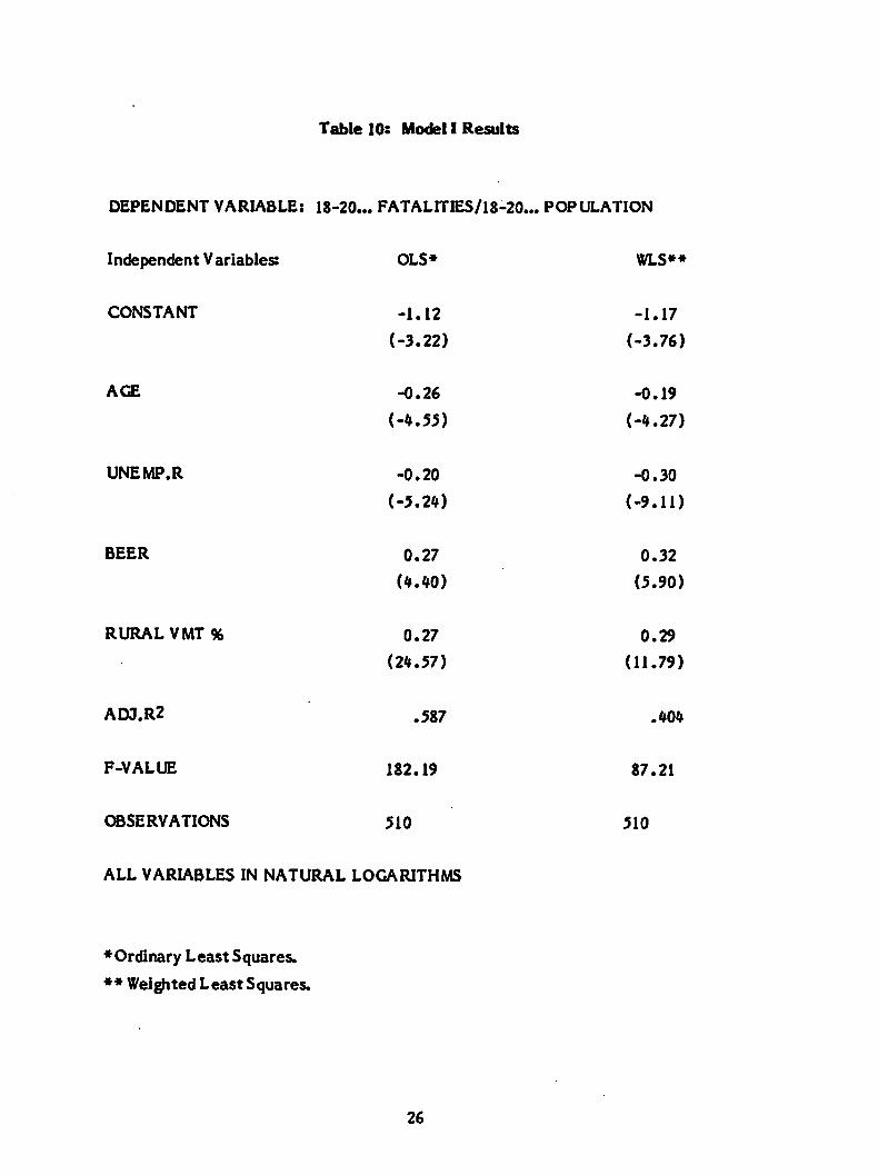
Table 10: Model I Results

DEPENDENT VARIABLE: 18-20... FATALITIES/18-20... POPULATION

Independent Variables: OLS* WLS**

CONSTANT -1.12 -1.17

(-3.22) (-3.76)

AGE -0.26 -0.19

(-4.55) (-4.27)

UNEMP.R -0.20 -0.30

(-5.24) (-9.11)

BEER 0.27 0.32

(4.40) (5.90)

RURAL VMT % 0.27 0.29

(24.57) (11.79)

ADJ.R2 .587 .404

F-VALUE 182.19 87.21

OBSERVATIONS 510 510

ALL VARIABLES IN NATURAL LOGARITHMS

♦OrdinaryLeast Squares.

♦♦ Weighted Least Squares.

26

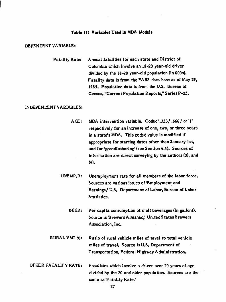
Table 11: Variables Used in MDA Models

DEPENDENT VARIABLE:

Fatality Rate:

INDEPENDENT VARIABLES:

Annual fatalities for each state and District of

Columbia which involve an 18-20 year-old driver

divided by the 18-20 year-old population (in 000s).

Fatality data is from the FARS data base as of May 29,

1985. Population data is from the U.S. Bureau of

Census, "Current Population Reports," Series P-25.

AGE: MDA intervention variable. Coded'.333,' .666,' or '1'

respectively for an increase of one, two, or three years

in a state's MDA. This coded value is modified if

appropriate for starting dates other than January 1st,

and for 'grandfathering* (see Section 4.4). Sources of

information are direct surveying by the authors (3), and

(4).

UNEMP.R: Unemployment rate for all members of the labor force.

Sources are various issues of 'Employment and

Earnings,' U.S. Department of Labor, Bureau of Labor

Statistics.

BEER: Per capita consumption of malt beverages (in gallons).

Source is'Brewers Almanac,' United States Brewers

Association, Inc.

RURAL VMT %:

OTHER FATALITY RATE:

Ratio of rural vehicle miles of tavel to total vehicle

miles of travel Source is U.S. Department of

Transportation, Federal Highway Administration.

Fatalities which involve a driver over 20 years of age

divided by the 20 and older population. Sources are the

same as 'Fatality Rate.'

27

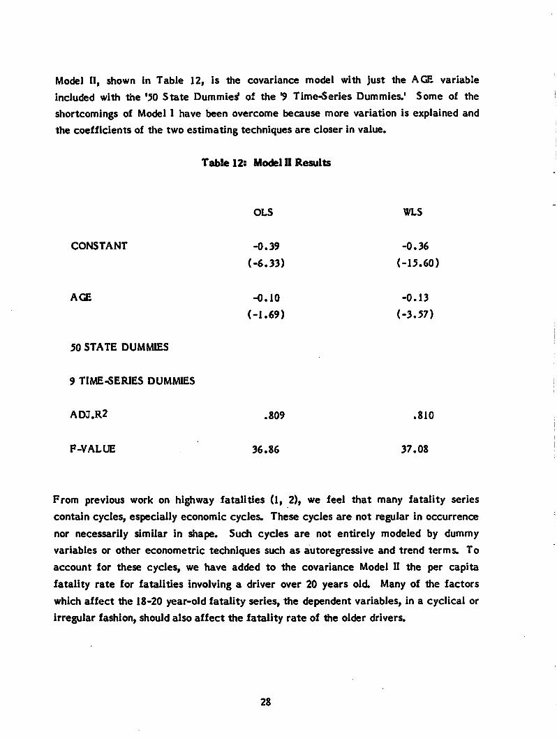
Model II, shown in Table 12, is the covariance model with just the AGE variable

included with the '50 State Dummies' of the "9 Time-Series Dummies.' Some of the

shortcomings of Model I have been overcome because more variation is explained and

the coefficients of the two estimating techniques are closer in value.

Table 12: Model 0 Results

OLS WLS

CONSTANT -0.39 -0.36

(-6.33) (-15.60)

AGE -0.10 -0.13

(-1.69) (-3.57)

50 STATE DUMMIES

9 TIME-SERIES DUMMIES

ADJ.R2 .809 .810

F-VALUE 36.86 37.08

From previous work on highway fatalities (1, 2), we feel that many fatality series

contain cycles, especially economic cycles. These cycles are not regular in occurrence

nor necessarily similar in shape. Such cycles are not entirely modeled by dummy

variables or other econometric techniques such as autoregressive and trend terms. To

account for these cycles, we have added to the covariance Model II the per capita

fatality rate for fatalities involving a driver over 20 years old. Many of tiie factors

which affect the 18-20 year-old fatality series, the dependent variables, in a cyclical or

irregular fashion, should also affect the fatality rate of tiie older drivers.

28

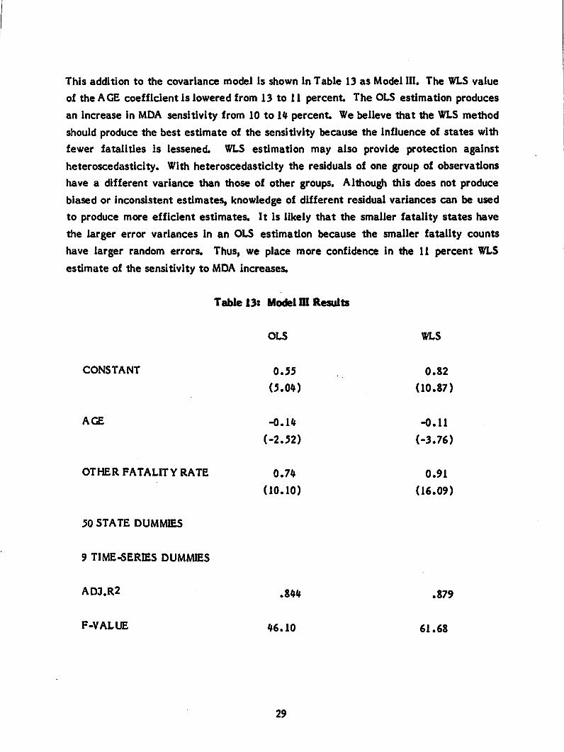
This addition to the covariance model is shown in Table 13 as Model III. The WLS value

of the AGE coefficient is lowered from 13 to 11 percent The OLS estimation produces

an increase in MDA sensitivity from 10 to 14 percent We believe that the WLS method

should produce the best estimate of the sensitivity because the influence of states with

fewer fatalities is lessened. WLS estimation may also provide protection against

heteroscedasticity. With heteroscedasticity the residuals of one group of observations

have a different variance than those of other groups. Although this does not produce

biased or inconsistent estimates, knowledge of different residual variances can be used

to produce more efficient estimates. It is likely that the smaller fatality states have

the larger error variances in an OLS estimation because the smaller fatality counts

have larger random errors. Thus, we place more confidence in the 11 percent WLS

estimate of the sensitivity to MDA increases.

Table 13: Model m Results

OLS WLS

CONSTANT 0.55 0.82

(5.04) (10.87)

AGE -0.14 -0.11

(-2.52) (-3.76)

OTHER FATALITY RATE 0.74 0.91

(10.10) (16.09)

50 STATE DUMMIES

9 TIME-SERIES DUMMIES

ADJ.R2 .844 .879

F-VALUE 46.10 61.68

29

The variables used in Model I and Model III are combined in Model IV (see Table 14).

The unemployment rate for all members of the labor force is not statistically

significant We interpret this to mean that general unemployment does not affect

youth-related fatalities any differently than other fatalities. Any economic effect, as

determined by the unemployment rate, is contained in the older-driver fatality rate.

The ratio of rural VMT to total VMT was not statistically significant. We haveconcluded that in Model I this ratio partly explains why youth-related fatality rates are

different among states for a given year. In the covariance model, the difference among

states is explained more fully by the set of state dummy variables. The per capita beer

consumption variable (BEER), though statistically significant and the expected sign, hasthe same problem identified in Model I. Per capita beer consumption is affected by the

MDA change. So, the effect of the MDA change is underestimated when BEER is also

in the model. Finally, notice that the adjusted R2 of Model IV is almost the same as

Model III. So, the extra variables contained in Model IV contribute almost nothing toour ability to explain variations in annual, state, per capita fatalities involving 18-20year-old drivers.

The best estimate (Model III) of the sensitivity of youth-involved fatalities to changes inMDA is 11 percent Thus, a change in MDA from 18 to 21 would cause an eleven

percent reduction in a state's annual per capita fatalities involving 18 to 20 year-old

drivers. This estimate is determined in Model III which explains about 88 percent of the

variation in this set of annual state fatalities. Obviously, we cannot be certain that the

true effect of such a MDA change is not somewhat higher or lower. We can say that

the true effect of a MDA change from 18 to 21 lies between 5 percent and 17 percentat the 95 percent confidence level.

In any econometric model such as the one that produced the above results, the residuals

of the regression equation, the terms which represent unexplained variation, should

have desirable properties such as randomness, independence, and an approximate normal

distribution. The residuals were not extensively tested for Model III. However, two

common deficiencies of the residuals were considered. As mentioned above, the

problem of heteroscedasticity would be reduced by WLS estimation, and by the

logarithmically transformed data in the model. First-order autocorrelation of the

residuals was found not to be a problem in the model.

30

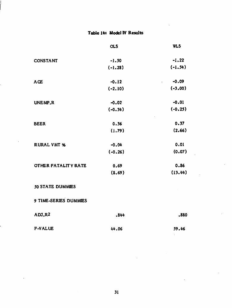
Table 14: Model IV Results

CONSTANT

AGE

UNEMP.R

BEER

RURALVMT%

OTHER FATALITY RATE

50 STATE DUMMIES

9 TIME-SERIES DUMMIES

ADJ.R2

F-VALUE

OLS

-1.50

(-1.28)

-0.12

(-2.10)

-0.02

(-0.34)

0.36

(1.79)

-0.04

(-0.26)

0.69

(8.69)

.844

44.06

31

WLS

-1.22

(-1.54)

-0.09

(-3.00)

-0.01

(-0.25)

0.37

(2.66)

0.01

(0.07)

0.86

(13.44)

.880

59.46

5.2 Spillover Effects

MDA law increases were found to reduce fatalities involving 18-20 year-old drivers.

Before calculating the lives saved by MDA laws, we wish to consider a related issue.

Does the effect spillover and effect other age groups? The models previously developed

are flexible enough to test for a spillover effect.

Model III is used to test if fatalities involving 14-17 year-old drivers have changed

significantly after MDA increases. The theory is that these younger drivers will also

reduce their alcohol consumption because the difficulty in obtaining alcohol will be

further increased by the increased MDA. Table 15 gives the results of this test. The

dependent variable has been changed to the fatalities involving this younger group and

the population of the younger group is used to normalize the variable. The MDA

intervention variable, AGE, is not statistically significant. As Table 4 indicates, the

14-17 year-old, driver-involved fatality series is only about 55 percent of the 18-20 year

olds. Hence, there may be more 'noise' in the younger series which makes it difficult to

discern any effect To overcome this, we combined the two series into a fatality rate

involving 14-20 year-old drivers. Table 16 shows the results of this test The AGE

variable is statistically significant The coefficient of the AGE variable indicates a

sensitivity of about seven percent for a full three-year MDA increase. The combined

fatality series is three times as large as the younger series and it contains, of course,

the 18-20 year-old, driver-involved fatalities which have been shown to be sensitive to

MDA changes. However, the coefficient reduction (11 percent to 7 percent) is directly

proportional to the increase in the population covered in the dependent variable. So,

the estimated lives saved using the 18-20 year olds model Is the same as the estimated

lives saved using the 14-20 year olds model. Therefore, none of the lives saved can be

attributed to the effects of the MDA on accidents involving 14-17 year-old drivers.

From this evidence, we conclude that there is no statistical evidence of a spillovereffect from MDA increases to the younger cohort.

It has been argued that even if raising the MDA reduces 18-20 year-old driver-involved

fatalities, there is an increase in fatalities among those slightly older than 21 years old.

It is argued that fatalities are postponed until a time when drivers begin to drink.

Postponing legal drinking will only postpone fatalities because initial experience with

alcohol is particularly dangerous no matter when it occurs. To test this hypothesis, a

dependent variable was constructed for the fatality rate involving 21-23

32

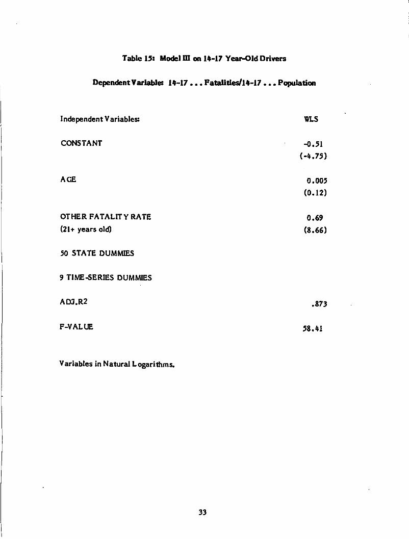
Table 15: Model ffl on 14-17 Year-Old Drivers

DependentVariable: 14-17 ... Fatalities/14-17 ... Population

Independent V ariables: WLS

CONSTANT -0.51

(-4.75)

AGE 0.005

(0.12)

OTHER FATALITY RATE 0.69

(21+ years old) (8.66)

50 STATE DUMMIES

9 TIME-SERIES DUMMIES

ADJ.R2 .873

F-VALUE 58.41

Variables in Natural Logarithms.

33

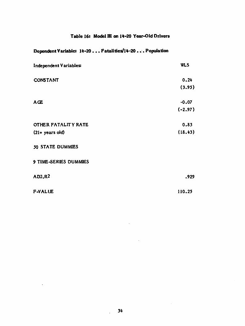
Table 16: Model m on 14-20 Year-Old Drivers

DependentVariable: 14-20 ... Fatalities/14-20... Population

Independent Variables: WLS

CONSTANT 0.24

(3.95)

AGE -0.07

(-2.97)

OTHER FATALITY RATE 0.83

(21+ years old) (18.43)

50 STATE DUMMIES

9 TIME-SERIES DUMMIES

ADJ.R2 .929

F-VALUE 110.25

34

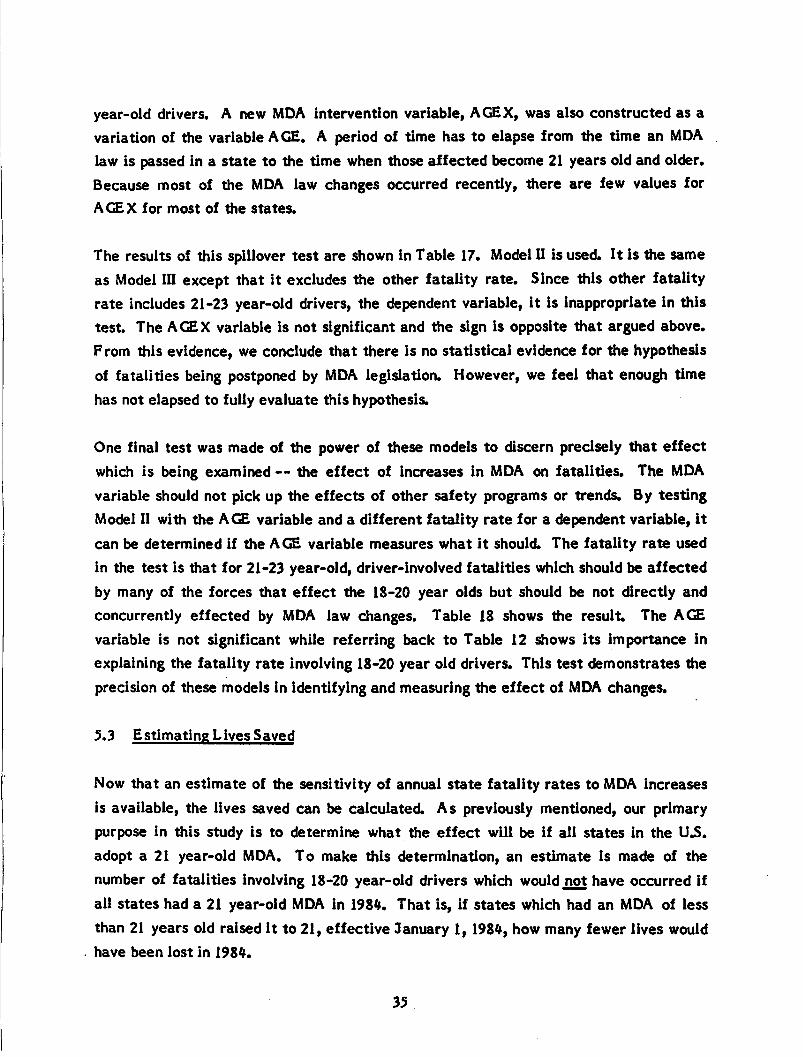
year-old drivers. A new MDA intervention variable, AGEX, was also constructed as a

variation of the variable AGE. A period of time has to elapse from the time an MDA

law is passed in a state to the time when those affected become 21 years old and older.

Because most of the MDA law changes occurred recently, there are few values for

AGEX for most of the states.

The results of this spillover test are shown in Table 17. Model II is used. It is the same

as Model III except that it excludes the other fatality rate. Since this other fatalityrate includes 21-23 year-old drivers, the dependent variable, it is inappropriate in this

test The AGEX variable is not significant and the sign is opposite that argued above.

From this evidence, we conclude that there is no statistical evidence for the hypothesis

of fatalities being postponed by MDA legislation. However, we feel that enough time

has not elapsed to fully evaluate this hypothesis.

One final test was made of the power of these models to discern precisely that effect

which is being examined — the effect of increases in MDA on fatalities. The MDA

variable should not pick up the effects of other safety programs or trends. By testing

Model II with the AGE variable and a different fatality rate for a dependent variable, it

can be determined if the AGE variable measures what it should. The fatality rate used

in the test is that for 21-23 year-old, driver-involved fatalities which should be affected

by many of the forces that effect the 18-20 year olds but should be not directly and

concurrently effected by MDA law changes. Table 18 shows the result The AGE

variable is not significant while referring back to Table 12 shows its importance in

explaining the fatality rate involving 18-20 year old drivers. This test demonstrates the

precision of these models in identifying and measuring the effect of MDA changes.

5.3 Estimating Lives Saved

Now that an estimate of the sensitivity of annual state fatality rates to MDA increases

is available, the lives saved can be calculated. As previously mentioned, our primary

purpose in this study is to determine what the effect will be if all states in the U.S.

adopt a 21 year-old MDA. To make this determination, an estimate is made of the

number of fatalities involving 18-20 year-old drivers which would not have occurred if

ail states had a 21 year-old MDA in 1984. That is, if states which had an MDA of less

than 21 years old raised it to 21, effective January 1, 1984, how many fewer lives would

have been lost in 1984.

35

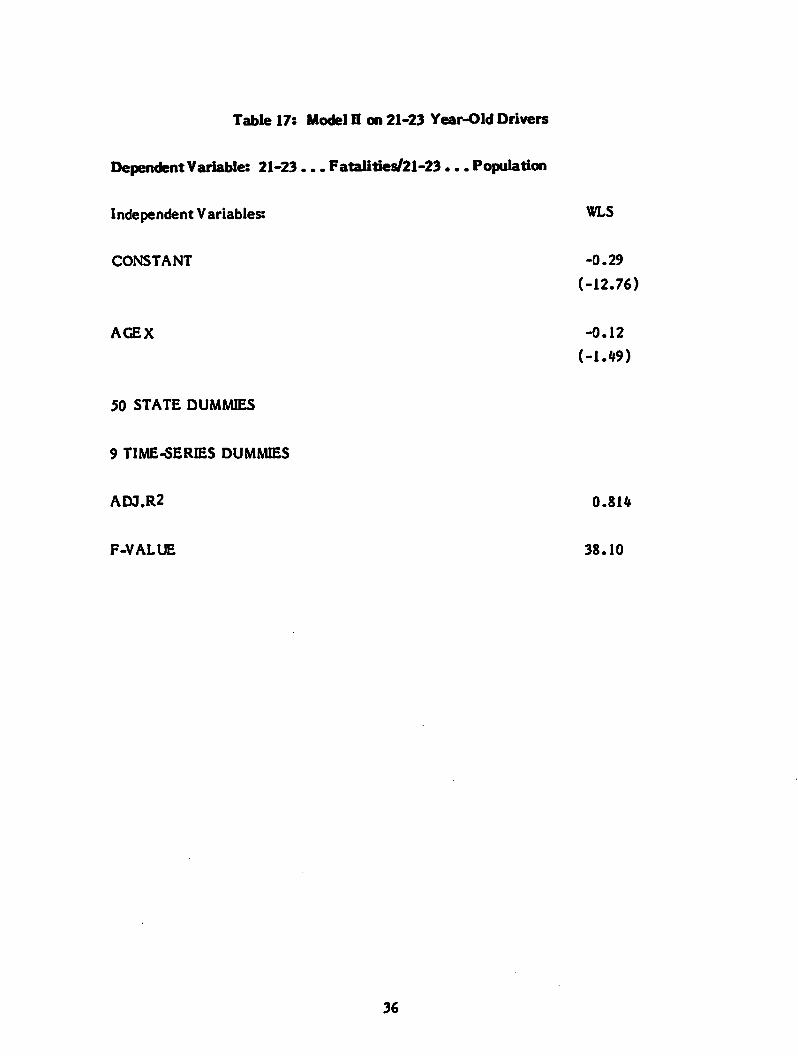
Table 17: Model H on 21-23 Year-Old Drivers

DependentVariable: 21-23... Fatalities/21-23... Population

Independent Variables: WLS

CONSTANT -0.29

(-12.76)

AGEX -0.12

(-1.49)

50 STATE DUMMIES

9 TIME-SERIES DUMMIES

ADJ.R2 0.814

F-VALUE 38.10

36

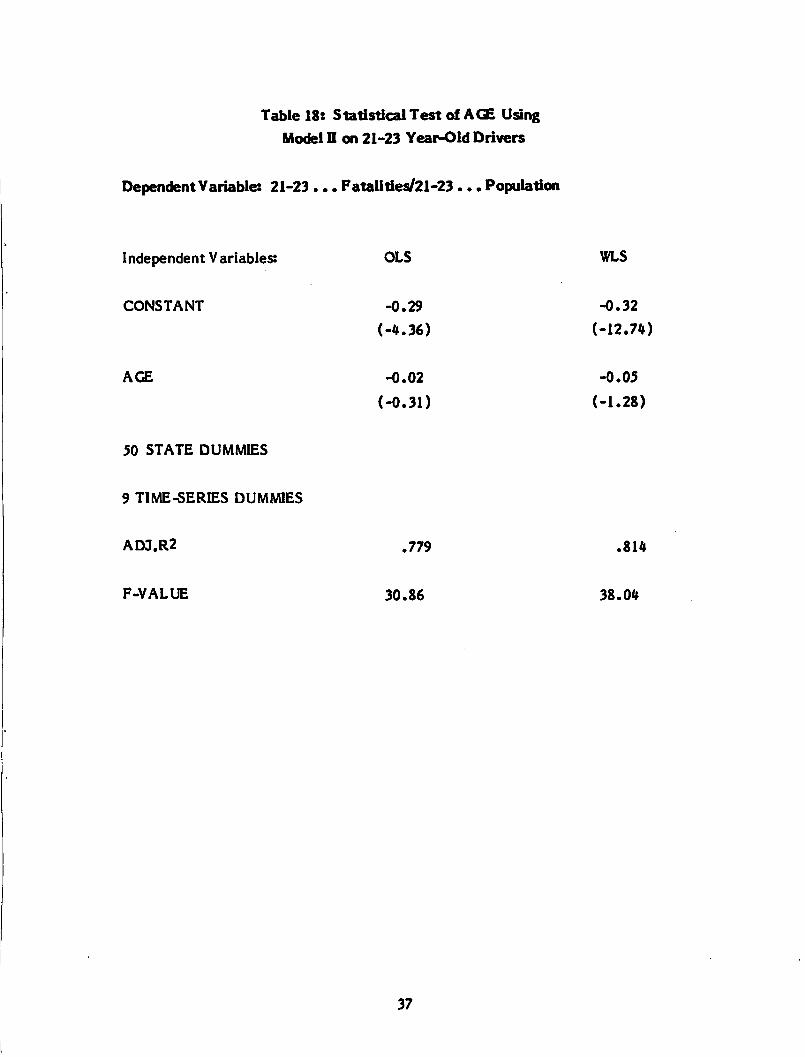
Table 18: Statistical Test of AGE Using

Model H on 21-23 Year-Old Drivers

DependentVariable: 21-23 ... Fatalities/21-23 ... Population

Independent Variables:

CONSTANT

AGE

50 STATE DUMMIES

9 TIME-SERIES DUMMIES

ADJ.R2

F-VALUE

OLS

-0.29

(-4.36)

-0.02

(-0.31)

.779

30.86

37

WLS

-0.32

(-12.74)

-0.05

(-1.28)

.814

38.04

In addition to estimating the lives which might have been saved in 1984, we also

estimate the present effect of MDA laws above 18 years old. By this we mean the

increase in lives lost in 1984 if all states had a MDA of 18.

In the following calculations, -11 percent is used as the sensitivity of fatalities to MDAchanges from 18 to 21. For states with a MDA of 19 years old, the sensitivity would be

.666 of the -11 percent or about -7 percent For states with a MDA of 20 years old, the

sensitivity would be .333 of the -11 percent or about -4 percent In calculating the lives

saved already by any MDA above 18 years old, the different sensitivity changes are

applied to the age groups in reverse because the sensitivity is measured from existing

fatality levels In either direction. That is, +11 percent is used to estimate the effect of

a roll back from 21 to 18 years old; +7 percent for 20 to 18; and +4 percent for 19 to 18.

Before applying these sensitivities to the actual number of 1984 fatalities which

occurred in each state, an adjustment needs to be made for partial MDA effects. For

some of the states, 1984 was a year of transition because new MDA's were established

after the beginning of the year and/or grandfathering was in effect. We have used a

procedure much like that of determining the value of the MDA intervention variable,

AGE. The percentage of the time during the year that a new MDA law was in effect is

used to adjust the number of fatalities in each age group for each state. The

consideration of these partial effects creates fatality counts which can be used with the

appropriate MDA sensitivity percentage to calculate the effects of MDA changes.

Table 19 shows these adjusted fatality totals for states grouped by effective MDA for

1984. The effective MDA aggregation of fatalities is very similar to a summing by

groups of states with the same legal MDA. The only real difference is that for a few

states, the MDA which was in force for most of the year is selected instead of the

present legal MDA. This adjustment groups fatalities for calculating lives saved easily

without distorting the results.

In determining the lives saved from a uniform MDA of 21 in 1984, the number of

fatalities of each age group that would be affected is first calculated. Obviously, none

of the 21 year-old group is affected. Only about one-third of the 18-20 year-old drivers

in states with an effective MDA of 20 will be effected by an increase in MDA to 21.

This sensitivity can be expressed by saying that one-third of the 399 fatalities, or 133

fatalities, should be reduced by the 11 percent to determine the benefits to this group.

38

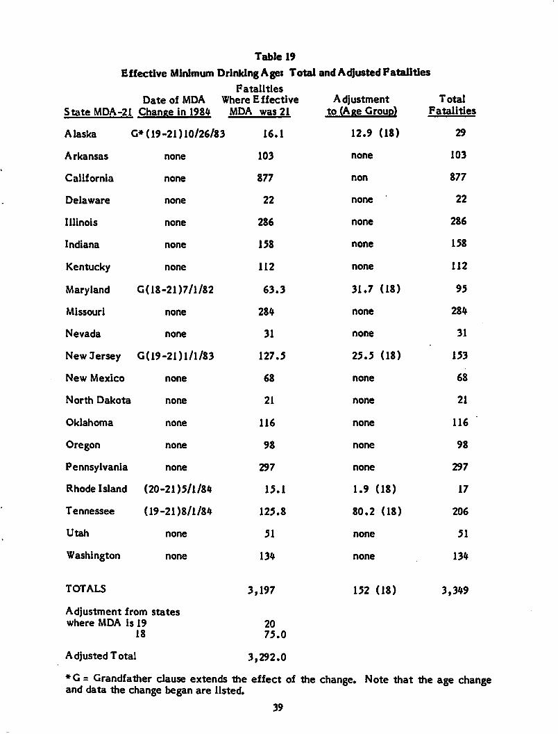
Table 19

Effective Minimum DrinkingAge: Total and Adjusted FatalitiesFatalities

State MDA-21

Date of MDA Where EffectiveChange in 1984 MDA was 21

Adjustmentto (Age Group)

TotalFatalities

Alaska '3» (19-21)10/26/83 16.1 12.9 (18) 29

Arkansas none 103 none 103

California none 877 non 877

Delaware none 22 none 22

Illinois none 286 none 286

Indiana none 158 none 158

Kentucky none 112 none 112

Maryland G(18-21)7/l/82 63.3 31.7 (18) 95

Missouri none 284 none 284

Nevada none 31 none 31

New Jersey G(19-21)l/l/83 127.5 25.5 (18) 153

New Mexico none 68 none 68

North Dakota none 21 none 21

Oklahoma none 116 none 116

Oregon none 98 none 98

Pennsylvania none 297 none 297

Rhode Island (20-21)5/1/84 15.1 1.9 (18) 17

Tennessee (19-21)8/1/84 125.8 80.2 (18) 206

Utah none 51 none 51

Washington none 134 none 134

TOTALS

Adjustment from stateswhere MDA is 19

18

Adjusted Total

3,197

2075.0

3,292.0

152 (18) 3,349

♦G = Grandfather clause extends the effect of the change. Note that the age changeand data the change began are listed.

39

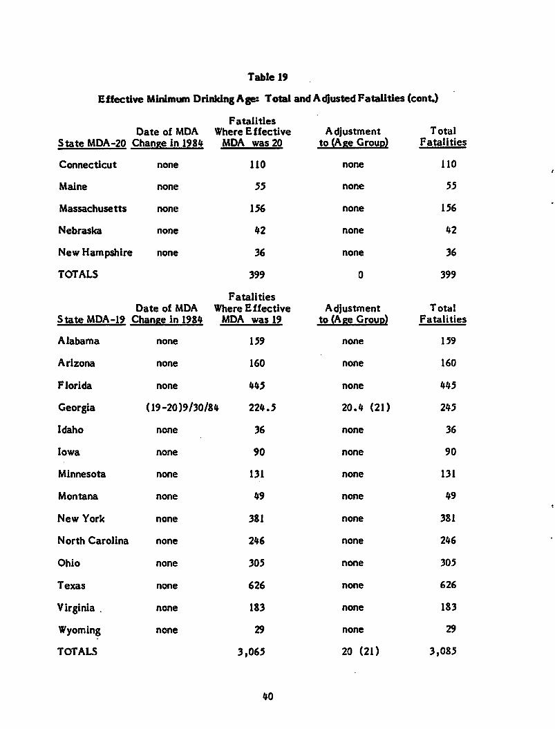
Table 19

Effective Minimum Drinking Age: Total and Adjusted Fatalities (cont)

State MDA-20

Date of MDA

Change in 1984

FatalitiesWhere Effective

MDA was 20

Adjustmentto (Age Group)

Total

Fatalities

Connecticut none 110 none 110

Maine none 55 none 55

Massachusetts none 156 none 156

Nebraska none 42 none 42

New Hampshire none 36 none 36

TOTALS 399 0 399

State MDA-19

Date of MDA

Change in 1984

FatalitiesWhere Effective

MDA was 19Adjustment

to (Age Group)Total

Fatalities

Alabama none 159 none 159

Arizona none 160 none 160

Florida none 445 none 445

Georgia (19-20)9/30/84 224.5 20.4 (21) 245

Idaho none 36 none 36

Iowa none 90 none 90

Minnesota none 131 none 131

Montana none 49 none 49

New York none 381 none 381

North Carolina none 246 none 246

Ohio none 305 none 305

Texas none 626 none 626

Virginia . none 183 none 183

Wyoming none 29 none 29

TOTALS 3,065 20 (21) 3,085

40

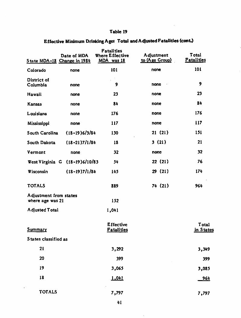
Table 19

Effective Minimum Drinking Age: Total and AdjustedFatalities(cont)

State MDA-18

FatalitiesDate of MDA Where Effective

Change in 1984 MDA was 18

Adjustmentto (Age Group)

TotalFatalities

Colorado none 101 none 101

District of

Columbia none 9 none 9

Hawaii none 23 none 23

Kansas none 84 none 84

Louisiana none 176 none 176

Mississippi none 117 none 117

South Carolina (18-19)6/3/84 130 21 (21) 151

South Dakota (18-21)7/1/84 18 3 (21) 21

Vermont none 32 none 32

West Virginia G (18-19)6/10/83 54 22 (21) 76

Wisconsin (18-19)7/1/84 145 29 (21) 174

TOTALS 889

Adjustment from stateswhere age was 21 152

Adjusted Total 1,041

SummaryEffectiveFatalities

States classified as

21 3,292

20 399

19 3,065

18 1,041

TOTALS 7,797

41

74 (21) 964

Totalin States

3,349

399

3,085

964

7,797

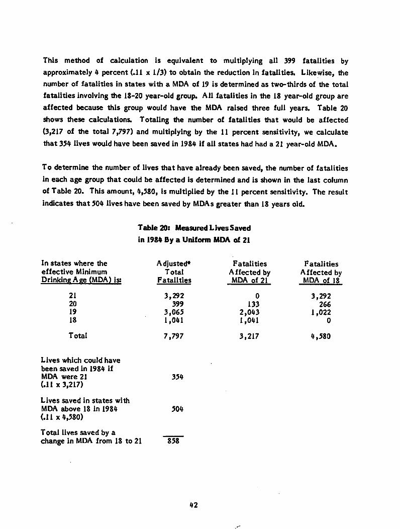
This method of calculation is equivalent to multiplying all 399 fatalities by

approximately 4 percent (.11 x 1/3) to obtain the reduction in fatalities. Likewise, thenumber of fatalities in states with a MDA of 19 is determined as two-thirds of the total

fatalities involving the 18-20 year-old group. AH fatalities in the 18 year-old group are

affected because this group would have the MDA raised three full years. Table 20

shows these calculations. Totaling the number of fatalities that would be affected

(3,217 of the total 7,797) and multiplying by the 11 percent sensitivity, we calculate

that 354 lives would have been saved in 1984 if all states had had a 21 year-old MDA.

To determine the number of lives that have already been saved, the number of fatalities

in each age group that could be affected is determined and is shown in the last column

of Table 20. This amount, 4,580, is multiplied by the 11 percent sensitivity. The result

indicates that 504 lives have been saved by MDAs greater than 18 years old.

Table 20: Measured Lives Saved

in 1984 By a Uniform MDA of 21

In states where the

effective MinimumDrinking Age (MDA) is:

21

20

19

18

Total

Lives which could have

been saved in 1984 ifMDA were 21(.11 x 3,217)

Lives saved in states with

MDA above 18 in 1984(.11 x 4,580)

Total lives saved by achange in MDA from 18 to 21

Adjusted*Total

Fatalities

3,292399

3,0651,041

7,797

354

504

858

42

Fatalities

Affected byMDA of 21

0

133

2,0431,041

3,217

Fatalities

Affected byMDA of 18

3,292266

1,0220

4,580

Altogether, it is concluded that 858 (354 plus 504) lives would be saved by a MDAchange from 18 to 21 years old in all states. The 354 lives that would be saved bypresently increasing the MDA to 21 years old in the states with MDAs below 21 in 1984represents 4.5 percent of the 7,797 youth-related fatalities and slightly less than one.percent of all fatalities.

43

6.0 CONCLUSIONS

A pooled cross-section, time-series econometric model was used to develop an estimate

of the effect of uniform MDA of 21 on highway fatalities in the United States. The

models of state per capita annual fatalities involving 18-20 year-old drivers explain

more than 85 percent of the variation in fatality rates. The measure of the state MDA

changes is selective and precise in isolating the effect of MDA changes. We feel

confident that we have not credited MDA changes for changes in fatalities caused by

other factors.

The best estimate of the effect of a change in MDA from 18 to 21 on highway fatalities

involving 18-20 year-old drivers is 11 percent That is, we expect highway fatalities

involving 18-20 year-old drivers to decline by 11 percent if the MDA is increased from

18 to 21. In states where the MDA is already above 18, we expect the change in

fatalities to be smaller because fewer drivers are affected by the change. In states

where the current MDA is 19, we expect only two-thirds of this change in fatalities

when the MDA is changed to 21. Similarly, states with a MDA of 20 are expected to

experience only one-third of the change in fatalities by increasing the MDA to 21.

Obviously, the total effect of a uniform MDA of 21 in the United States depends on the

status of state MDA laws when the change goes into effect In this study, we calculate

the total United States effect based on what actually took place in 1984. In that year,

7,797 highway fatalities involved drivers in the 18-20 age group. Based on the MDA

laws in effect in the states where these fatalities occurred, we estimate that 354 lives

would have been saved if those states with MDAs less than 21 in 1984 had raised their

MDA to 21.

Finally, we estimate that 504 lives were saved in 1984 because many states had MDAs

above 18.

44

REFERENCES

1. Hoxie, Paul, David Skinner, and George H.K. Wang, "Socio-Economic Influences on

Highway Fatalities: An Empirical Investigation," U.S. Department of

Transportation, Transportation Systems Center, DOT-HS-806 525, a staff study.

2. Hoxie, Paul and David Skinner, "A Statistical Analysis of Socio-Economic

Influences on Three Groups of High Risk Fatalities," U.S. Department of

Transportation, Transportation Systems Center, FR-45-U-NHT-86-06, a staff

study.

3. Wagenaar, Alexander C, Alcohol. Young Drivers, and Traffic Accidents.

Lexington Books, D.C. Heath and Company, Lexington, MA, 1983.

4. The Liquor Handbook, 1984 (and previous issues).

5. Greenberg, D.F. and R.C. Kessler, Linear Panel Analysis: Models of Quantitative

Change. Academic Press, New York, 1981.

50 copies *5ll&

US

Dep

artm

ent

of

Tra

nsp

ort

atio

n

Resea

rch

an

dS

pecia

lP

rog

ram

sA

dm

inis

tra

tio

n

Ken

da

llS

qu

are

Ca

mb

rid

ge

Ma

ssa

chu

sett

s0

2U

?

Off

icia

lB

usi

ness

Pen

all

ylo

iP

riva

teU

seJ3

00

Po

cla

g*

an

dF

ees

Pa

idR

ese

arc

ha

nd

Sp

ecia

lP

rogr

am*

Ad

min

istr

ati

on

DO

T5

13