arX

iv:1

409.

2695

v1 [

mat

h.C

O]

9 S

ep 2

014

MINIMUM FAULT-TOLERANT, LOCAL AND STRONG METRIC

DIMENSION OF GRAPHS

MUHAMMAD SALMAN, IMRAN JAVAID∗, MUHAMMAD ANWAR CHAUDHRY

Abstract. In this paper, we consider three similar optimization problems: the

fault-tolerant metric dimension problem, the local metric dimension problem and

the strong metric dimension problem. These problems have applications in many

diverse areas, including network discovery and verification, robot navigation and

chemistry, etc. We give integer linear programming formulations of the fault-

tolerant metric dimension problem and the local metric dimension problem. Also,

we study local metric dimension and strong metric dimension of two convex poly-

topes Sn and Un.

1. Introduction.

The metric dimension problem was introduced independently by Slater [30] and

Harary and Melter [12]. Roughly speaking, the metric dimension of an undirected

and connected graph G is the minimum cardinality of a subset W of vertex set of

G with the property that all the vertices of G are uniquely determined by their

shortest distances to the vertices in W . The metric dimension problem has been

widely investigated. Since the complete survey of all the applications and results is

out of scope of this paper, only some applications and recent results are revealed.

The metric dimension arises in many diverse areas, including telecommunications

[3], connected joints in graphs and chemistry [8], the robot navigation [19] and ge-

ographical routing protocols [22], etc. In the area of telecommunication, especially

interesting in the metric dimension problem application to network discovery and

verification [3]. Due to its fast dynamic, distributed growth process, it is hard to

obtain an accurate map of the global network. A common way to obtain such maps

is to make certain local measurements at a small subset of the nodes, and then to

combine them in order to discover the actual graph. Each of these measurements

is potentially quite costly. It is thus a natural objective to minimize the number

of measurements, which still discover the whole graph. That is, to determine the

metric dimension of the graph. In [3], simple greedy strategies were used in a simula-

tion with various types of randomly generated graphs. The results of the simulation

Key words and phrases. resolving set, fault-tolerant resolving set, local resolving set, strong

resolving set, ILP formulations, convex polytopes.

2010 Mathematics Subject Classification: 05C12∗ Corresponding author: ijavaidbzu@gmail.com.

1

were presented as two dimensional diagrams displaying the average number of mea-

surements (cardinality of a resolving set) as a function of the degree of a particular

graph class.

An application of the metric dimension problem in chemistry is described in [8].

The structure of a chemical compound can be represented as a labeled graph where

the vertex and edge labels specify the atoms and bond types, respectively. Under the

traditional view, it can be determine whether any two compounds in the collection

share the same functional property at a particular position. These positions simply

reflect uniquely defined atoms (vertices) of the substructure (common subgraph).

It is important to find smallest number of these positions which is functionally

equivalent to the metric dimension of the given graph. This observation can be used

in drug discovery when it is to be determined whether the features of a compound

are responsible for its pharmacological activity. For more details see [8].

An other interesting application of the metric dimension problem arises in robot

navigation [19]. Suppose that a robot is navigating in a space modeled by a graph

and wants to know its current position. It can send a signal to find out how far it is

form each among a set of fixed landmarks. The problem of computing the minimum

number of landmarks and their positions such that the robot can always uniquely

determine its location is equivalent to the metric dimension problem.

Now, we formally state the metric dimension problem as follows: Given a simple

connected graph G with vertex set V (G) and edge set E(G). Let d(u, v) denotes

the distance between vertices u and v, i.e, the length of a shortest u − v path. A

vertex w of G resolves the vertices u and v in G if d(u, w) 6= d(v, w). A subset

W = {w1, w2, . . . , wk} of V (G) is a resolving set of G if every two distinct vertices

of G are resolved by some vertex of G. A metric basis of G is a resolving set of

the minimum cardinality. The metric dimension of G, denoted by β(G), is the

cardinality of its metric basis.

Metric dimension of several interesting classes of graphs have been investigated:

Grassmann graphs [1], Johnson and Kneser graph [2], cartesian product of graphs

[5], Cayley digraphs [11], convex plytopes [14], generalized Petersen graphs [16, 17],

Cayley graphs [18], silicate networks [23], circulant graphs [28]. It also has been

shown that some infinite graphs have infinite metric dimension [4].

Elements of metric bases were referred to as censors in an application given in [7].

If one of the censors does not work properly, we will not have enough information to

deal with the intruder (fire, thief, etc). In order to overcome this kind of problems,

concept of fault-tolerant metric dimension was introduced by Hernando et al. [13].

Fault-tolerant resolving set provide correct information even when one of the censors

is not working. Roughly speaking, a resolving set is said to be fault-tolerant if the

removal of any element from it keeps it resolving. Formally, a resolving set W of a

graph G is said to be fault-tolerant if W \{w} is also a resolving set of G, for each w

2

inW . The fault-tolerant metric dimension (FTMD) of G is the minimum cardinality

of a fault-tolerant resolving set, denoted by β ′(G). A fault-tolerant resolving set of

cardinality β ′(G) is called a fault-tolerant metric basis (FTMB) of G.

A more common problem in graph theory concerns distinguishing every two neigh-

bors in a graph G by means of some coloring rather than distinguishing all the

vertices of G by graph coloring. Since distinguishing all the vertices of a connected

graph G has been studied with the aid of distances in G. This suggests the topic

of using distances to distinguish the two vertices in each pair of neighbors only, and

thus Okamoto et al. [26] introduced the local metric dimension problem, defined as

follows: A subset W of vertex set of a connected graph G is called a local resolving

set of G if every two adjacent vertices of G are resolved by some element of W . A

local metric basis of G is a local resolving set of the minimum cardinality. The local

metric dimension of G, denoted by lmd(G), is the cardinality of its local metric ba-

sis. Note that each resolving set of G is vertex-distinguishing (since it resolves every

two vertices of G), and each local resolving set is neighbor-distinguishing (since it

resolves every two adjacent vertices of G). Thus every resolving set is also a local

resolving set of G, so if G is a non-trivial connected graph of order n, then

1 ≤ lmd(G) ≤ β(G) ≤ n− 1. (1)

The strong metric dimension problem was introduced by Sebo and Tannier [29] and

further investigated by Oellermann and Peters-Fransen [27]. Recently, the strong

metric dimension of distance hereditary graphs has been studied by May and Oeller-

mann [24]. This concept is defined as follows: A vertex w strongly resolves two

distinct vertices u and v of G if u belongs to a shortest v−w path or v belongs to a

shortest u − w path, i.e., d(v, w) = d(v, u) + d(u, w) or d(u, w) = d(u, v) + d(v, w).

A subset S of V (G) is a strong resolving set of G if every two distinct vertices of G

are strongly resolved by some vertex of S. A strong metric basis of G is a strong

resolving set of the minimum cardinality. The strong metric dimension of G, de-

noted by sdim(G), is the cardinality of its strong metric basis. It is easy to see that

if a vertex w strongly resolves vertices u and v, then w also resolves these vertices.

Hence every strong resolving set is a resolving set and β(G) ≤ sdim(G).

To determine whether a given set W ⊆ V (G) is a local (strong) resolving set of G,

W needs only to be verified for the vertices in V (G) \W since every vertex w ∈ W

is the only vertex of G whose distance from w is 0.

The metric dimension of convex polytopes Sn, Tn and Un, which are combinations

of two graphs of convex polytopes, has been studied in [14]. Also the strong metric

dimension of Tn has been studied in [20]. In this paper, we study the minimal local

resolving sets and strong resolving sets of the convex polytopes Sn and Un. We prove3

that for all n ≥ 3, lmd(Un) = 2 and for all n ≥ 3,

lmd(Sn) =

{

2, if n is odd,

3, if n is even,

while the strong metric dimension of both families of convex polytopes Sn and Un

depends on n.

The paper is organized as follows: In section 2, we give integer linear program-

ming formulations of the fault-tolerant metric dimension problem and the local

metric dimension problem. In section 3 and 4, we get explicit expressions for

lmd(Sn), sdim(Sn), lmd(Un) and sdim(Un). In what follows, the indices after n

will be taken modulo n.

2. Mathematical Programming Formulations

As described in [10], it is useful to represent problems of extremal graph theory

as integer linear programming (ILP) problems in order to use the different well-

known optimization techniques. Following that idea, two integer linear programming

formulations of the metric dimension problem were proposed by Chartrand et al. in

2000 [8], and Currie and Oellermann in 2001 [9]. Recently, in 2012, Mladenovic et al.

[25] proposed a new mathematical programming formulation of the metric dimension

problem with new objective function which (instead of minimizing the cardinality

of a resolving set) minimized the number of pairs of vertices from G that are not

resolved by vertices of a set with a given cardinality. So the difficulty that arises

when solving the plateaux problem, i.e., problems with a large number of solutions

with the same objective function values, vanishes with the new objective function.

The integer linear programming formulation of the strong metric dimension problem

was proposed by Kratica et al. in 2012 [20]. To our knowledge, the following ILP

formulations of the FTMD problem and the local metric dimension problem are

new.

2.1. Fault-Tolerant Metric Dimension Problem. The following result was proved

by Javaid et al. in [15].

Lemma 2.1. [15] A resolving set W of a graph G is fault-tolerant if and only if

every pair of vertices in G is resolved by at least two elements of W .

Thus, we have the following remark:

Remark 2.2. Any pair (u, v) of distinct vertices of a connected graph G is said

to be fault-tolerantly resolved in G if for two distinct vertices x, y of G, we have

d(u, x) 6= d(v, x) and d(u, y) 6= d(v, y).

Given a simple connected undirected graph G = (V (G), E(G)), where V (G) =

{1, 2, . . . , n} and |E(G)| = m. It is easy to determine the length d(u, v) of a shortest4

u − v path for all u, v ∈ V (G) using any shortest path algorithm. The coefficient

matrix A is defined as follows:

A(u,v),(i,j) =

{

1, d(u, i) 6= d(v, i) and d(u, j) 6= d(v, j),

0, d(u, i) = d(v, i) and d(u, j) = d(v, j), (2)

where 1 ≤ u < v ≤ n, 1 ≤ i < j ≤ n. Variable xi described by (3) determines

whether vertex i belongs to a fault-tolerant resolving set W or not. Similarly, yijdetermines whether both i, j are in W .

xi =

{

1, i ∈ W,

0, i 6∈ W. (3)

yij =

{

1, i, j ∈ W,

0, otherwise. (4)

The ILP model of the FTMD problem can now be formulated as:

Minimze f(x1, x2, . . . , xn) =n

∑

k=1

xk (5)

subject to:

n−1∑

i=1

n∑

j=i+1

A(u,v),(i,j) yij ≥ 1, 1 ≤ u < v ≤ n, (6)

yij ≤1

2xi +

1

2xj , 1 ≤ i < j ≤ n, (7)

yij ≥ xi + xj − 1, 1 ≤ i < j ≤ n, (8)

yij ∈ {0, 1}, xk ∈ {0, 1}, 1 ≤ i < j ≤ n, 1 ≤ k ≤ n. (9)

Note that, the ILP model (5)-(9) has n +(

n

2

)

variables and 3(

n

2

)

linear constraints.

The following proposition shows that each feasible solution of (6)-(9) defines a fault-

tolerant resolving set of G and vice-versa.

Proposition 2.3. W is a fault-tolerant resolving set of G if and only if constraints

(6)-(9) are satisfied.

Proof. (⇒) Suppose that W is a fault-tolerant resolving set of G. Then for each

u, v ∈ V (G), u 6= v, there exist i, j ∈ W (i.e., yij = 1), i 6= j, such that d(u, i) 6=

d(v, i) and d(u, j) 6= d(v, j). Without loss of generality, we may assume that u < v

and i < j. It follows that A(u,v),(i,j) = 1, and consequently constraints (6) are

satisfied. Constraints (7)-(9) are obviously satisfied since i, j ∈ W implies that

xi = xj = yij = 1.

(⇐) According to (3), W = {i ∈ {1, 2, . . . , n} | xi = 1}. For all i, j ∈ W , from (8)

and (9) it follows that yij = 1 because yij ≥ xi+xj−1 = 1 and by (9), yij is a binary

variable. If i or j is not in W , then constraints (7) imply that yij ≤12xi +

12xj ≤

12.

5

Since yij is a binary variable, it follows that yij = 0. Therefore, yij = 1 if and

only if i, j ∈ W . If constraints (6) are satisfied, then for each 1 ≤ u < v ≤ n,

there exist i, j ∈ {1, . . . , n}, i < j, such that A(u,v),(i,j)yij ≥ 1, which implies that

yij = 1 (i.e., i, j ∈ W ) and A(u,v),(i,j) = 1 (i.e., d(u, i) 6= d(v, i) and d(u, j) 6= d(v, j)).

It follows that the set W is a fault-tolerant resolving set of G. �

Remark 2.4. The ILP formulation of the FTMD problem generally looks like the

ILP formulation of the minimum doubly resolving set (MDRS) problem proposed

by Kratica et al. [21]. But the difference is in finding the entries A(u,v),(i,j) of the

coefficient matrix A. For instance, if G = P4 : 1, 2, 3, 4 (path on four vertices).

Then in the case of MDRS problem, A(1,2),(3,4) = 0 (by the definition of the coefficient

matrix given in [21]), where as in the case of FTRS problem, A(1,2),(3,4) = 1.

2.2. Local Metric Dimension Problem. Let u be a vertex of a graph G. The

open neighborhood of u is N(u) = {v ∈ V (G) | v is adjacent with u in G} and the

closed neighborhood of u is N [u] = N(u) ∪ {u}. Now, from the definition of local

resolving set, we have the following proposition:

Proposition 2.5. A subset W of V (G) of a non-trivial connected graph G is local

resolving set if and only if for all u ∈ V (G) and for each v ∈ N(u), d(u, w) 6= d(v, w)

for some w ∈ W .

Proof. (⇒) Suppose that W is a local resolving set of G. Then by definition, for

any two adjacent vertices u and v in G, i.e., for all u ∈ V (G) and for each v ∈ N(u),

there exists a vertex w in W such that d(u, w) 6= d(v, w).

(⇐) If for all u ∈ V (G) and for each v ∈ N(u), d(u, w) 6= d(v, w) for some w ∈ W ,

then every two adjacent vertices are resolved by some vertex w of W , which implies

that W is a local resolving set of G. �

Given a simple connected undirected graph G = (V (G), E(G)), where V (G) =

{1, 2, . . . , n} and |E(G)| = m. It is easy to determine the length d(u, v) of a shortest

u − v path for all u, v ∈ V (G) using any shortest path algorithm. The coefficient

matrix A is defined as follows:

A(u,v),i =

{

1, d(u, i) 6= d(v, i),

0, d(u, i) = d(v, i), (10)

where 1 ≤ u ≤ n, 1 ≤ i ≤ n and v ∈ N(u) with v > u.

Variable xi described by (11) determines whether vertex i belongs to a local

resolving set W or not.

xi =

{

1, i ∈ W,

0, i 6∈ W. (11)6

The ILP model of the local metric dimension problem can now be formulated as:

Minimze f(x1, x2, . . . , xn) =

n∑

i=1

xi (12)

subject to:n

∑

i=1

A(u,v),i xi ≥ 1, 1 ≤ u ≤ n and v ∈ N(u) with v > u, (13)

xi ∈ {0, 1}, 1 ≤ i ≤ n. (14)

Note that, the ILP model (12)-(14) has n variables and m linear constraints. The

following proposition shows that each feasible solution of (13) and (14) defines a

local resolving set of G and vice-versa.

Proposition 2.6. W is a local resolving set of G if and only if constraints (13) and

(14) are satisfied.

Proof. (⇒) Suppose that W is a local resolving set of G. Then by Proposition 2.5,

for all u ∈ V (G) and for each v ∈ N(u), there exists a vertex i in W (i.e., xi = 1)

such that d(u, i) 6= d(v, i). It follows that A(u,v),i = 1, and consequently constraints

(13) are satisfied. Constraints (14) are obviously satisfies by the definition of variable

xi.

(⇐) According to (11), W = {i ∈ {1, 2, . . . , n} | xi = 1}. If constraints (13) are

satisfied, then for all u ∈ V (G) and for each v ∈ N(u) with v > u, there exists

i ∈ {1, 2, . . . , n} such that A(u,v),i xi ≥ 1. This implies that xi = 1 (i.e., i ∈ W ) and

A(u,v),i = 1 (i.e., d(u, i) 6= d(v, i)). It follows, by Proposition 2.5, that W is a local

resolving set of G. �

3. Convex Polytopes Sn

The convex polytopes Sn, n ≥ 3, [14] (see Figure 1) consists of 2n 3-sided faces,

2n 4-sided faces and a pair of n-sided faces obtained by the combination of a convex

polytope Rn and a prism Dn having vertex and edge sets as:

V (Sn) = {ai, bi, ci, di | 1 ≤ i ≤ n},

E(Sn) = {aiai+1, bibi+1, cici+1, didi+1, ai+1bi, aibi, bici, cidi | 1 ≤ i ≤ n}.

The metric dimension of Sn was studied in [14]. In this section, we show that

lmd(Sn) = 2 when n is odd and lmd(Sn) = 3 when n is even. Moreover, we show

that sdim(Sn) = n when n is odd and sdim(Sn) =3n2

when n is even. The main

results of this section are the following:

Theorem 3.1. For any convex polytope Sn, n ≥ 3, we have

lmd(Sn) =

{

2, if n is odd,

3, if n is even.

7

dn

an-1

bn-1

bn-2

c1

c3

c2

dn-2

dn-1

d3

d1

d2

bnb1

cn

b3

ana2

a3

b2

cn-1

cn-2

a1

Figure 1. The graph of convex polytope Sn

Theorem 3.2. For any convex polytope Sn, n ≥ 3, we have

sdim(Sn) =

{

n, if n is odd,3n2, if n is even.

For each fixed i ∈ {a, b, c, d}, let Ci denotes the cycle induced by the vertices

i1, i2, . . . , in in Sn. Next we prove the several lemmas which support the proofs of

Theorem 3.1 and Theorem 3.2.

Lemma 3.3. For n = 2k, k ≥ 2, if lmd(Sn) = 2, then any local metric basis of Sn

does not contain both the vertices of the same cycle Ci, i ∈ {a, b, c, d}.

Proof. Suppose contrarily that W = {u, v} be a local matric basis of Sn with u, v ∈

V (Ci), i ∈ {a, b, c, d}. Then for fixed i ∈ {a, b, c, d}, there is no loss of generality in

assuming that u = i1 and v = ij , 2 ≤ j ≤ n. This gives that for any two adjacent

vertices x and y of Sn such that

x, y ∈

{

N [a1], when 2 ≤ j ≤ k + 1,

N [a2], when k + 2 ≤ j ≤ n,

we have d(x, w) = d(y, w) for all w ∈ W , a contradiction to the fact that lmd(Sn) =

2. �

Lemma 3.4. For n = 2k, k ≥ 2, if lmd(Sn) = 2, then any local metric basis W of

Sn does not has the property that W contains one vertex from Ci and the other one

from Cj (j 6= i), where i, j ∈ {a, b, c, d}.

Proof. Suppose contrarily that W = {u, v} be a local matric basis of Sn with

u ∈ V (Ci) and v ∈ V (Cj) (j 6= i), i, j ∈ {a, b, c, d}. Then we have the follow-

ing three cases:

8

Case 1: When u ∈ Ca and v ∈ Ci, i ∈ {b, c, d}. Without loss of generality, we

assume that u = a1 and v = ij , 1 ≤ j ≤ n. Then for 1 ≤ j ≤ k, there

exists a vertex bj+k in N [aj+k] such that d(aj+k, w) = d(bj+k, w) for all

w ∈ W , a contradiction. Also for k + 1 ≤ j ≤ n, there exists a vertex

aj−k+1 in N [bj−k] such that d(aj−k+1, w) = d(bj−k, w) for all w ∈ W , a

contradiction.

Case 2: When u ∈ Cb and v ∈ Ci, i ∈ {c, d}. Without loss of generality, we

assume that u = b1 and v = ij , 1 ≤ j ≤ n. Then there exist two vertices

x and y in N [u] such that d(x, w) = d(y, w) for all w ∈ W , a contradiction.

Case 3: When u ∈ Cc and v ∈ Cd. Without loss of generality, we assume that

u = c1 and v = dj, 1 ≤ j ≤ n. Then there exist two vertices x and y in

N [u] such that d(x, w) = d(y, w) for all w ∈ W , a contradiction. �

Lemma 3.5. For n = 2k + 1, k ≥ 2, W = {a1, ak+1} is a local resolving set of Sn.

Proof. We show that for all u = ij ∈ V (Sn), i ∈ {a, b, c, d}, 1 ≤ j ≤ n, and for each

v ∈ N(u), d(u, a1) − d(v, a1) 6= 0 or d(u, ak+1) − d(v, ak+1) 6= 0. Then Proposition

2.5 will concludes that the set {a1, ak+1} is a local resolving set of Sn. First note

that, if u = a1 or u = ak+1, then for each v ∈ N(u), d(u, u) = 0 6= 1 = d(v, u).

Further, note that

d(aj, a1) =

{

j − 1, 1 ≤ j ≤ k + 1,

2k − j + 2, k + 2 ≤ j ≤ 2k + 1,

d(bj , a1) =

{

j, 1 ≤ j ≤ k,

2k − j + 2, k + 1 ≤ j ≤ 2k + 1,

d(cj, a1) =

{

j + 1, 1 ≤ j ≤ k,

2k − j + 3, k + 1 ≤ j ≤ 2k + 1,

d(dj, a1) =

{

j + 2, 1 ≤ j ≤ k,

2k − j + 4, k + 1 ≤ j ≤ 2k + 1,

d(aj, ak+1) =

{

k − j + 1, 1 ≤ j ≤ k + 1,

j − k − 1, k + 2 ≤ j ≤ 2k + 1,

d(bj , ak+1) =

{

k − j + 1, 1 ≤ j ≤ k,

j − k, k + 1 ≤ j ≤ 2k + 1,

d(cj, ak+1) =

{

k − j + 2, 1 ≤ j ≤ k,

j − k + 1, k + 1 ≤ j ≤ 2k + 1,

d(dj, ak+1) =

{

k − j + 3, 1 ≤ j ≤ k,

j − k + 2, k + 1 ≤ j ≤ 2k + 1.

Now, according to the above listed distances, the following four cases conclude the

proof.

9

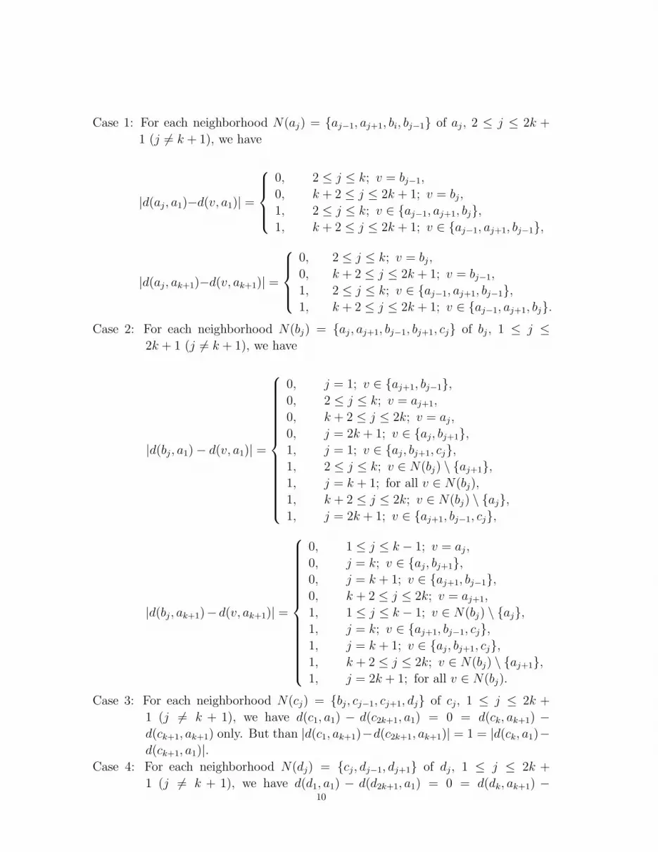
Case 1: For each neighborhood N(aj) = {aj−1, aj+1, bi, bj−1} of aj , 2 ≤ j ≤ 2k +

1 (j 6= k + 1), we have

|d(aj, a1)−d(v, a1)| =

0, 2 ≤ j ≤ k; v = bj−1,

0, k + 2 ≤ j ≤ 2k + 1; v = bj ,

1, 2 ≤ j ≤ k; v ∈ {aj−1, aj+1, bj},

1, k + 2 ≤ j ≤ 2k + 1; v ∈ {aj−1, aj+1, bj−1},

|d(aj, ak+1)−d(v, ak+1)| =

0, 2 ≤ j ≤ k; v = bj ,

0, k + 2 ≤ j ≤ 2k + 1; v = bj−1,

1, 2 ≤ j ≤ k; v ∈ {aj−1, aj+1, bj−1},

1, k + 2 ≤ j ≤ 2k + 1; v ∈ {aj−1, aj+1, bj}.

Case 2: For each neighborhood N(bj) = {aj , aj+1, bj−1, bj+1, cj} of bj , 1 ≤ j ≤

2k + 1 (j 6= k + 1), we have

|d(bj , a1)− d(v, a1)| =

0, j = 1; v ∈ {aj+1, bj−1},

0, 2 ≤ j ≤ k; v = aj+1,

0, k + 2 ≤ j ≤ 2k; v = aj ,

0, j = 2k + 1; v ∈ {aj, bj+1},

1, j = 1; v ∈ {aj, bj+1, cj},

1, 2 ≤ j ≤ k; v ∈ N(bj) \ {aj+1},

1, j = k + 1; for all v ∈ N(bj),

1, k + 2 ≤ j ≤ 2k; v ∈ N(bj) \ {aj},

1, j = 2k + 1; v ∈ {aj+1, bj−1, cj},

|d(bj, ak+1)− d(v, ak+1)| =

0, 1 ≤ j ≤ k − 1; v = aj ,

0, j = k; v ∈ {aj, bj+1},

0, j = k + 1; v ∈ {aj+1, bj−1},

0, k + 2 ≤ j ≤ 2k; v = aj+1,

1, 1 ≤ j ≤ k − 1; v ∈ N(bj) \ {aj},

1, j = k; v ∈ {aj+1, bj−1, cj},

1, j = k + 1; v ∈ {aj, bj+1, cj},

1, k + 2 ≤ j ≤ 2k; v ∈ N(bj) \ {aj+1},

1, j = 2k + 1; for all v ∈ N(bj).

Case 3: For each neighborhood N(cj) = {bj, cj−1, cj+1, dj} of cj, 1 ≤ j ≤ 2k +

1 (j 6= k + 1), we have d(c1, a1) − d(c2k+1, a1) = 0 = d(ck, ak+1) −

d(ck+1, ak+1) only. But than |d(c1, ak+1)−d(c2k+1, ak+1)| = 1 = |d(ck, a1)−

d(ck+1, a1)|.

Case 4: For each neighborhood N(dj) = {cj, dj−1, dj+1} of dj, 1 ≤ j ≤ 2k +

1 (j 6= k + 1), we have d(d1, a1) − d(d2k+1, a1) = 0 = d(dk, ak+1) −10

d(dk+1, ak+1) only. But than |d(d1, ak+1)−d(d2k+1, ak+1)| = 1 = |d(dk, a1)−

d(dk+1, a1)|. �

For a vertex v in G, the eccentricity, ecc(v), is the maximum distance between v

and any other vertex of G. The diameter of G, denoted by diam(G), is the maximum

eccentricity of a vertex v in G. The following lemma and two properties, proved by

Kratica et al. [20], will be used in the sequel.

Lemma 3.6. [20] Let u, v ∈ V (G), u 6= v, and

(i) d(w, v) ≤ d(u, v) for each w ∈ N(u) and

(ii) d(u, w) ≤ d(u, v) for each w ∈ N(v).

Then there does not exist vertex x ∈ V (G), x 6= u, v, that strongly resolves the

vertices u and v.

Property 3.7. [20] If S is a strong resolving resolving set of G, then for every two

distinct vertices u, v ∈ V (G) which satisfy conditions (i) and (ii) of Lemma 3.6, we

have u ∈ S or v ∈ S.

Property 3.8. [20] If S is a strong resolving resolving set of G, then for every two

distinct vertices u, v ∈ V (G) such that d(u, v) = diam(G), we have u ∈ S or v ∈ S.

Lemma 3.9. For n = 2k + 1, k ≥ 1, if S is a strong resolving set of Sn, then

|S| ≥ n.

Proof. Let us consider the pair (ai, di+k) of vertices of Sn for i = 1, 2, . . . , n. Then

it is easy to see that d(ai, di+k) = k+3. Since diam(Sn) = k+3 so according to the

Property 3.8, ai ∈ S or di+k ∈ S for all i = 1, 2 . . . , n. Therefore |S| ≥ n. �

Lemma 3.10. For n = 2k + 1, k ≥ 1, the subset {di | i = 1, 2, . . . , n} of V (Sn) is

a strong resolving set of Sn.

Proof. Let us prove that for each i = 1, 2, . . . , n, the vertex di strongly resolves the

pairs (ci, aj), (ci, bj), (ci, cj)(i 6=j), (bi, aj), (bi, bj)(i 6=j) and (ai, aj)(j 6=i,i+1,...,i+k), where j =

1, 2, . . . , n. It is easy to see that d(di, ci) = 1, d(di, bi) = 2 = d(di, ci) + 1 and

d(bj , ci) = d(cj, di) =

{

j − i− 1, i ≤ j ≤ i+ k,

n− j + i+ 1, i+ k + 1 ≤ j ≤ i+ n− 1.

Note that

(i) d(cj, ci) = d(cj, di)−1,

⇒ d(di, cj) = d(ci, cj)+1 = d(di, ci)+d(ci, cj). (15)

(ii) d(bj , di) = d(cj, di)+1 = d(bj, ci)+d(ci, di),

⇒ d(di, bj) = d(di, ci)+d(ci, bj). (16)

(iii) d(bj , bi) = d(bj , ci)−1,11

so equation (16) becomes

d(di, bj) = d(di, ci)+d(bi, bj)+1 = d(di, bi)+d(bi, bj). (17)

Equations (15), (16) and (17) conclude that the pairs (ci, cj), (ci, bj) and (bi, bj) are

strongly resolved by di.

Now, consider the following shortest paths between di and ai+k+1:

• P1 : di, ci, bi, ai, ai−1, ai−2, . . . , ai+k+2, ai+k+1;

• P2 : di, ci, bi, ai+1, ai+2, . . . , ai+k, ai+k+1.

Then one can easily see that for j = i, i + k + 1, i + k + 2, . . . , i + n − 1, the pairs

(ci, aj), (bi, aj) and the pair (ai, aj), j 6= i, i+1, i+2, . . . , i+k, are strongly resolved

by di according to the shortest di − aj path P1 which contains the vertices ai, bi, ci;

and for j = i+ 1, i+ 2, . . . , i+ k, the pairs (ci, aj) and (bi, aj) are strongly resolved

by di according to the shortest di− aj path P2 which contains the vertices bi and ci.

Finally, the remaining pairs (ai, aj), j = i+1, i+2, . . . , i+k, are strongly resolved

by di+k because of the shortest di+k−ai path di+k, ci+k, bi+k, ai+k, ai+k−1, . . . , ai+1, ai,

which contains the vertex aj . �

Lemma 3.11. For n = 2k, k ≥ 2, if S is a strong resolving set of Sn, then |S| ≥ 3n2.

Proof. Consider the pair (bi, di+k) of vertices of Sn for i = 1, 2, . . . , n. Then d(ai, di+k)

= k+ 2. As diam(Sn) = k + 2, so according to the Property 3.8, bi ∈ S or di+k ∈ S

for all i = 1, 2 . . . , n. Moreover, the vertices in pair (ai, ai+k), i = 1, 2, . . . , k, satisfy

both the conditions of Lemma 3.6. So according to the Property 3.7, ai ∈ S or

ai+k ∈ S for all i = 1, 2 . . . , k. Therefore |S| ≥ n+ k = 3n2. �

Lemma 3.12. For n = 2k, k ≥ 2, the subset {di, ai′ | i = 1, 2, . . . , n; i′ =

1, 2, . . . , k} of V (Sn) is a strong resolving set of Sn.

Proof. First we prove that for each i = 1, 2, . . . , n, the vertex di strongly resolves the

pairs (ci, bj), (ci, cj)(i 6=j), (bi, bj)(i 6=j) for all j = 1, 2 . . . , n and the pairs (ci, aj), (bi, aj)

for j = k + 1, k + 2, . . . , n. To this end, we consider the following shortest paths:

• P1 : di, ci, ci+1, . . . , ci+k−1, ci+k;

• P2 : di, ci, ci−1, ci−2, . . . , ci+k+1, ci+k;

• P3 : di, ci, bi, bi+1, . . . , bi+k−1, bi+k;

• P4 : di, ci, bi, bi−1, bi−2, . . . , bi+k+1, bi+k;

• P5 : di, ci, bi, ai+1, . . . , ai+k−1, ai+k;

• P6 : di, ci, bi, ai, ai−1, ai−2, . . . , ai+k+2, ai+k+1.

Note that, each above mentioned pair is strongly resolved by di because of the

existence of a shortest di − vj path (v ∈ {a, b, c}) as shown in Table 1.

Moreover, according to the path P6 between di and ai+k+1, each pair (al, am) is

also strongly resolved by di, where i + k + 1 ≤ l, m ≤ i + n − 1 (l 6= m). Finally,

each pair (ai+k, aj), j = i + k + 1, i + k + 2, . . . , i + n − 1, is strongly resolved by

ai+k−1 because of the shortest ai+k−1 − aj path ai+k−1, ai+k, . . . , aj, which contains

the vertex ai+k. �

12

pair for i+ 1 ≤ j ≤ i+ k for j = i, i− 1, i− 2, . . . , i+ k + 1

(ci, cj) v = c, P1 contains ci v = c, P2 contains ci(bi, bj), (ci, bj) v = b, P3 contains bi, ci v = b, P4 contains bi, ci(bi, aj), (ci, aj) v = a, P5 contains bi, ci v = a, P6 contains bi, ci

Table 1. Shortest di − vj paths (v ∈ {a, b, c})

Proof of Theorem 3.1. We have the following two cases:

Case 1: n is even. Since lmd(G) ≤ β(G), by equation (1), and β(Sn) = 3 [14]

so lmd(Sn) ≤ 3. For the lower bound, if we suppose that a subset {u, v}

of V (Sn) is a local resolving set of Sn. Then either both u and v belong

to the same cycle Ci, i ∈ {a, b, c, d} (but, it is not possible according to

Lemma 3.3), or u and v belong to the different cycles Ci and Cj, respectively,

where i, j ∈ {a, b, c, d}, (i 6= j) (but, it is not possible according to Lemma

3.4). Hence, no two vertices of Sn form a local resolving set of Sn. Therefore

lmd(Sn) ≥ 3.

Case 2: n is odd. As lmd(G) = 1 if and only if G is a bipartite graph [26] and Sn

is not a bipartite graph, so Lemma 3.5 concludes that lmd(Sn) = 2. �

Proof of Theorem 3.2. When n is odd, then Lemma 3.9 and Lemma 3.10 conclude

the proof; and when n is even, then Lemma 3.11 and Lemma 3.12 conclude the

proof. �

4. Convex Polytopes Un

The convex polytopes Un, n ≥ 3, [14] (Figure 2) consists of n 4-sided faces, 2n

5-sided faces and a pair of n-sided faces obtained by the combination of a convex

polytope Dn and a prism Dn having vertex and edge sets as:

V (Un) = {ai, bi, ci, di, ei | 1 ≤ i ≤ n},

E(Un) = {aiai+1, bibi+1, eiei+1, aibi, bici, cidi, diei, ci+1di | 1 ≤ i ≤ n}.

The metric dimension of Un was studied in [14]. In this section, we show that

lmd(Un) = 2 for all n ≥ 3. Moreover, we show that sdim(Un) = 2n when n is

odd and sdim(Un) = 5n2

when n is even. The main results of this section are the

following:

Theorem 4.1. For any convex polytope Un, n ≥ 3, we have lmd(Un) = 2.

Theorem 4.2. For any convex polytope Un, n ≥ 3, we have

sdim(Un) =

{

2n, if n is odd,5n2, if n is even.

13

dn

an-1

bn-1

bn-2

c1

c3

c2

dn-2

dn-1

d3

d1

d2

bn

b1

cn

b3

ana2

a3

b2

cn-1

cn-2

a1

a4

b4c4

e1

e2

en

e3

en-1

en-2

an-2

Figure 2. The graph of convex polytope Un

Let Vi = {ij | j = 1, 2, . . . , n}, i ∈ {a, b, c, d, e} be mutually disjoint subsets of

V (Un). Now, we prove several lemmas which support the proofs of Theorem 4.1 and

Theorem 4.2.

Lemma 4.3. For n = 2k + 1, k ≥ 1, W = {a1, ak+1} is a local resolving set of Un.

Proof. One can easily see that the list of distances (given below) of each element of

the set Vi, i ∈ {a, b, c, d, e}, with a1 and ak+1 concludes that for each u ∈ N(ij), 1 ≤

j ≤ 2k+1, either d(u, a1) 6= d(ij, a1) or d(u, ak+1) 6= d(ij , ak+1), and hance the subset

{a1, ak+1} of V (Un) is a local resolving set of Un, by Proposition 2.5.

d(aj, al) =

j − 1, 1 ≤ j ≤ k + 1; l = 1,

2k − j + 2, k + 2 ≤ j ≤ 2k + 1; l = 1,

k − j + 1, 1 ≤ j ≤ k + 1; l = k + 1,

j − k − 1, k + 2 ≤ j ≤ 2k + 1; l = k + 1,

d(bj , al) =

j, 1 ≤ j ≤ k + 1; l = 1,

2k − j + 3, k + 2 ≤ j ≤ 2k + 1; l = 1,

k − j + 2, 1 ≤ j ≤ k + 1; l = k + 1,

j − k, k + 2 ≤ j ≤ 2k + 1; l = k + 1,

d(cj, al) =

j + 1, 1 ≤ j ≤ k + 1; l = 1,

2k − j + 4, k + 2 ≤ j ≤ 2k + 1; l = 1,

k − j + 3, 1 ≤ j ≤ k + 1; l = k + 1,

j − k + 1, k + 2 ≤ j ≤ 2k + 1; l = k + 1,14

d(dj, al) =

j + 2, 1 ≤ j ≤ k + 1; l = 1,

2k − j + 4, k + 2 ≤ j ≤ 2k + 1; l = 1,

k − j + 3, 1 ≤ j ≤ k + 1; l = k + 1,

j − k + 2, k + 2 ≤ j ≤ 2k + 1; l = k + 1,

d(ej, al) =

j + 3, 1 ≤ j ≤ k + 1; l = 1,

2k − j + 5, k + 2 ≤ j ≤ 2k + 1; l = 1,

k − j + 4, 1 ≤ j ≤ k + 1; l = k + 1,

j − k + 3, k + 2 ≤ j ≤ 2k + 1; l = k + 1.

�

Lemma 4.4. For n = 2k, k ≥ 2, W = {c1, v} is a local resolving set of Un, where

v =

e1, when k = 2,

c2, when k = 3,

d4, when k = 4,

ck, when k ≥ 5.

Proof. It is easy to see that the sets {c1, e1}, {c1, c2} and {c1, d4} are local resolving

sets for U2, U3 and U4, respectively. For k ≥ 5, first we give the list of distances of

each vertex of Un with c1 and v = ck.

d(aj, cl) =

j + 1, 1 ≤ j ≤ k; l = 1,

2k − j + 3, k + 1 ≤ j ≤ 2k; l = 1,

k − j + 2, 1 ≤ j ≤ k; l = k,

j − k + 2, k + 1 ≤ j ≤ 2k; l = k,

d(bj , cl) = d(aj, cj)−1, 1 ≤ j ≤ 2k; for both l = 1, k,

d(cj, cl) =

d(bj , cl)− 1, j = 1; l = 1,

d(bj , cl), j = 2, 2k; l = 1,

d(bj , cl) + 1, j = 1, 2, 2k; l = k,

d(bj , cl) + 1, 3 ≤ j ≤ k − 2; l = 1, k,

d(bj , cl) + 1, j = k − 1, k, k + 1; l = 1,

d(bj , cl), j = k − 1, k + 1, 5; l = k,

d(bj , cl) + 1, k + 2 ≤ j ≤ 2k − 1; l = 1, k,

d(bj , cl)− 1, j = k; l = k.

d(dj, cl) =

d(cj, cl) + 1, 1 ≤ j ≤ k; l = 1,

d(cj, cl), k + 1 ≤ j ≤ 2k − 2; l = 1,

d(cj, cl)− 1, j = 2k − 1, 2k; l = 1,

d(cj, cl)− 1, j = k − 2, k − 1; l = k,

d(cj, cl), 1 ≤ j ≤ k − 3 ∧ j = 2k; l = k,

d(cj, cl) + 1, k ≤ j ≤ 2k − 1; l = k,15

for i ≤ j ≤ i+ k for i+ k ≤ j ≤ i+ n− 1

ai, bi, bi+1, . . . , bj bj+1, bj+2, . . . , bi−1, bi, aiai, bi, bi+1, . . . , bj, cj , dj dj, cj+1, bj+1, bj+2, . . . , bi−1, bi, ai

ai, bi, bi+1, . . . , bj , cj, dj, ej ej , dj, cj+1, bj+1, bj+2, . . . , bi−1, bi, ai

Table 2. Shortest ai − vj paths (v ∈ {b, d, e})

d(ej, cl) =

d(dj, cl) + 1, j = 1, 2k; l = 1,

d(dj, cl), j = 2, 2k − 1; l = 1,

d(dj, cl)− 1, 3 ≤ j ≤ 2k − 2; l = 1,

d(dj, cl)− 1, 1 ≤ j ≤ k − 3 ∧ k + 2 ≤ j ≤ 2k; l = k,

d(dj, cl), j = k − 2, k + 1; l = k,

d(dj, cl) + 1, j = k − 1, k; l = k,

Now, it can be easily seen that for each u ∈ N(ij), 1 ≤ j ≤ 2k + 1, either

d(u, c1) 6= d(ij , c1) or d(u, v) 6= d(ij , v), and hance, by Proposition 2.5, the subset

{c1, ck} of V (Un) is a local resolving set of Un. �

Lemma 4.5. For n = 2k + 1, k ≥ 1, if S is a strong resolving set of Un, then

|S| ≥ 2n.

Proof. Consider the pair (ai, ei+k), i = 1, 2, . . . , n, of vertices of Un. Then it is easy

to see that d(ai, ei+k) = k + 4. As diam(Un) = k + 4, so according to the Property

3.8, ai ∈ S or ei+k ∈ S for all i = 1, 2, . . . , n. Further, the vertices in the pair

(ci, di+k), i = 1, 2, . . . , n satisfy both the conditions of Lemma 3.6, so according to

the Property 3.7, ci ∈ S or di+k ∈ S for all i = 1, 2, . . . , n. Therefore |S| ≥ 2n. �

Lemma 4.6. For n = 2k+1, k ≥ 1, the subset {ai, ci | i = 1, 2, . . . , n} of V (Un) is

a strong resolving set of Un.

Proof. First we prove that for each i = 1, 2, . . . , n, the vertex ai strongly resolves

the pairs (bi, bj), (bi, dj) and (bi, ej) for all j = 1, 2 . . . , n. For this, let us consider

the shortest ai − vj paths shown in Table 2, where v ∈ {b, d, e}.

Then each pair (bi, bj), (bi, dj) and (bi, ej) is strongly resolved by ai because bibelongs to each shortest ai − vj path listed in Table 2, where v ∈ {b, d, e}.

Moreover, we note that each pair (di, dj), (di, ej) and (ei, ej) is strongly resolved

by ci (1 ≤ i ≤ n) for j = i, i + 1, . . . , i + k, and strongly resolved by ci+1 for

j = i + k + 1, . . . , i + n − 1, because of the following shortest ci − vj and ci+1 − vjpaths (v ∈ {d, e}), which contains the vertices di and ei:

• ci, di, ci+1, di+1;

• di+n−1, ci, di, ci+1;

• ci, di, ei, ei+1, . . . , ej, j = i, i+ 1, . . . , i+ k;

• ci, di, ei, ei+1, . . . , ej, dj, j = i+ 2, i+ 3, . . . , i+ k;16

• ej , ej+1, . . . , ei, di, ci+1, j = i+ k + 1, . . . , i+ n− 1;

• dj, ej , ej+1, . . . , ei, di, ci+1, j = i+ k + 1, . . . , i+ n− 2. �

Lemma 4.7. For n = 2k, k ≥ 2, if S is a strong resolving set of Un, then |S| ≥ 5n2.

Proof. Consider the pair (ai, ei+k), i = 1, 2, . . . , n, of vertices of Un. Then d(ai, ei+k) =

k + 3. Since diam(Un) = k + 3 so according to the Property 3.8, ai ∈ S or ei+k ∈ S

for all i = 1, 2, . . . , n. Moreover, the vertices in the pairs (ci, di+2) and (dj, dj+k),

1 ≤ i ≤ n, 1 ≤ j ≤ k, satisfy both the conditions of Lemma 3.6, so according to the

Property 3.7, ci ∈ S or di+2 ∈ S for all i = 1, 2, . . . , n and dj ∈ S or dj+k ∈ S for all

j = 1, 2, . . . , k. Therefore |S| ≥ n + n+ k = 5n2. �

Lemma 4.8. For n = 2k, k ≥ 2, the subset {ai, ci, di′ | i = 1, 2, . . . , n; i′ =

1, 2, . . . , k} of V (Un) is a strong resolving set of Un.

Proof. First we prove that for each i = 1, 2, . . . , n, the vertex ai strongly resolves the

pairs (bi, bj), (bi, ej), 1 ≤ j ≤ n, and the pair (bi, dj) for all j = k+1, k+2 . . . , n. For

this, let us consider the shortest ai − vj paths shown in Table 3, where v ∈ {b, d, e}.

Then each pair (bi, bj), (bi, dj) and (bi, ej) is strongly resolved by ai because bi belongs

to each shortest ai − vj path listed in Table 3, where v ∈ {b, d, e}.

Now, consider the following shortest paths:

• ci, di, ci+1, di+1, i = k + 1, k + 2, . . . , n;

• di+n−1, ci, di, ci+1, i = k + 1, k + 2, . . . , n;

• ci, di, ei, ei+1, . . . , ej, j = i, i+ 1, . . . , i+ k − 1;

• ci, di, ei, ei+1, . . . , ej, dj, i = k+1, k+2, . . . , n−1; j = i+1, i+2, . . . , i+n−1;

• ej , ej+1, . . . , ei, di, ci+1, j = i+ k + 1, . . . , i+ n− 1;

• dj, ej , ej+1, . . . , ei, di, ci+1, i = k + 1, k + 2, . . . , n; j = i+ k + 1, . . . , i+ n;

• di, ei, ei+1, . . . , ei+k, i = 1, 2, . . . , k;

• ci, di, ei, ei+1, . . . , ej, dj, i = k + 1, k + 2, . . . , n; j = i, i+ 1, . . . , i+ k − 1;

• di+k, ei+k, ei+k+1, . . . , ei−1, ei, di, i = k + 1, k + 2, . . . , n.

Then it is easy to see that the pairs (di, dj); k + 1 ≤ i ≤ n − 1, i + 1 ≤ j ≤ n,

(di, ej); k + 1 ≤ i ≤ n, i ≤ j ≤ i + k − 1, (ei, ej); 1 ≤ i ≤ n, i+ 1,≤ j ≤ i + k − 1

are strongly resolved by ci; the pairs (di, ej); k + 1 ≤ i ≤ n − 1, i + k + 1 ≤ j ≤

i + n − 1, (ei, ej); 1 ≤ i ≤ n, i + k + 1 ≤ j ≤ i + n − 1 are strongly resolved by

ci+1; the pair (di, ei+k); k + 1 ≤ i ≤ n is strongly resolved by di+k; and the pair

(ei, ei+k); 1 ≤ i ≤ k is strongly resolved by di, because the above listed shortest

ci− vj , ci+1− vj ; v ∈ {d, e}, di− ei+k and di+k − di paths contains the vertices di, eiand ei+k.

�

Proof of Theorem 4.1. As lmd(G) = 1 if and only if G is a bipartite graph [26] and

Un is not a bipartite graph, so Lemma 4.3 and Lemma 4.4 conclude that lmd(Un) =

2. �

17

for i ≤ j ≤ i+ k − 1 for i+ k ≤ j ≤ i+ n− 1

ai, bi, bi+1, . . . , bj bj+1, bj+2, . . . , bi−1, bi, aiai, bi, bi+1, . . . , bj, cj , dj dj, cj+1, bj+1, bj+2, . . . , bi−1, bi, ai

ai, bi, bi+1, . . . , bj , cj, dj, ej ej , dj, cj+1, bj+1, bj+2, . . . , bi−1, bi, ai

Table 3. Shortest ai − vj paths (v ∈ {b, d, e})

Proof of Theorem 4.2. When n is odd, then Lemma 4.5 and Lemma 4.6 conclude

the proof; and when n is even, then Lemma 4.7 and Lemma 4.8 conclude the

proof. �

References

[1] R. Bailey, P. Cameron, Basie size, metric dimension and other invariants of groups and

graphs, Bull. of London Math. Soc. 43(2011) 209-242.

[2] R. Bailey, K. Meagher, On the metric dimension of grassmann graphs, Technical Reports

2011, arXiv: 1010.4495.

[3] Z. Beerloiva, F. Eberhard, T. Erlebach. A. Hall, M. Hoffmann, M. Mihalak, L. Ram, Network

discovery and verification. IEEEE J. Selected Area in Commun. 24(2006) 2168-2181.

[4] J. Caceres, C. Hernando, M. Mora, I. M. Pelayoe, M. L. Puertas, On the metric dimension

of infinite graphs, Elect. Notes in Disc. Math. 35(2009) 15-20.

[5] J. Caceres, C. Hernando, M. Mora, I. M. Pelayoe, M. L. Puertas, C. Seara, D. R. Wood, On

the metric dimension of cartesian products of graphs, SIAM J. Disc. Math. 21(2007) 423-441.

[6] G. Chappell, J. Gimbel, C. Hartman, Bounds on the metric and partition dimension of a

graph, Ars Combin. 88(2008) 349-366.

[7] G. Chartrand, P. Zhang, The theory and applications of resolvability in graphs: A survey,

Congr. Numer. 160(2003) 47-68.

[8] G. Chartrand, L. Eroh, M. A. Johnson, O. R. Oellermann, Resolvability in graphs and the

metric dimension of a graph, Disc. Appl. Math. 105(2000) 99-113.

[9] J. Currie, O. Oellermann, The metric dimension and metric independence of a graph, J.

Combin. Math. Combin. Comput. 39(2001) 157-167.

[10] D. Cvetkovic, P. Hansen, V. Kovacevic-Vujcic, On some interconnections between combina-

torial optimization and extremal hraph theory, Yugosal. J. Oper. Res. 14(2)(2004) 147-154.

[11] M. Fehr, S. Gosselin, O. Oellermann, The metric dimension of Cayley digraphs, Disc. Math.

306(2006) 31-41.

[12] F. Harary, R. A. Melter, On the metric dimension of a graph, Ars. Combin. 2(1976) 191-195.

[13] C. Hernando, M. Mora, P. J. Slater, D. R. Wood, Fault-Tolerant metric dimension of graphs,

Proc. Internat. Conf. Convexity in Discrete Structures, Ramanujan Math. Society Lecture

Notes, 5(2008) 81-85.

[14] M. Imran. S. U. H. Bokary, A. Baig, On families of convex polytopes with constant metric

dimension, Comp. Math. Appl. 60(2010) 2629-2638.

[15] I. Javaid, M. Salman, M. A. Chaudhry, S. Shokat, Fault-Tolerance in Resolvability, Util.

Math. 80(2009) 263-275.

[16] I. Javaid, M. T. Rahim, K. Ali, Families of regular graphs with constant metric dimension,

Util. Math. 75(2008) 21-33.18

[17] I. Javaid, M. Salman, M. A. Chaudary, S. A. Aleem, On the metric dimension of generlized

Petersen graphs, Quaestiones Mathematicae, in press.

[18] I. Javaid, M. N. Azhar M. Salman, Metric dimension and determining number of Cayley

graphs, World Applied Sciences Journal, in press.

[19] S. Khuller, B. Raghavachari, A. Rosenfeld, Landmarks in graphs, Disc. Appl. Math. 70(1996)

217-229.

[20] J. Kratica, V. Kovacevic-Vujcic, M. Cangalovic, M. Stojanovic. Minimal doubly resolving sets

and the strong metric dimension of some convex polytopes, Appl. Math. Comp. 218(2012)

9790-9801.

[21] J. Kratica, M. Cangalovic, V. Kovacevic-Vujcic, Computing minimal doubly resolving sets

of graphs, Comp. Oper. Res. 36(2009) 2149-2159.

[22] K. Liu, N. Abu-Ghazaleh, Virtual coordinate back tracking for void travarsal in geographic

routing, Lecture Notes Comp. Sci. 4104(2006) 46-59.

[23] P. Manuel, I. Rajasingh, Minimum metric dimension of silicate networks, Ars. Combin.

98(2011) 501-510.

[24] T. May, O. Oellermann, The strong dimension of distance hereditary graphs, J. Combin.

Math. Combin. Comput. 76(2011) 59-73.

[25] N. Mladenovic, J. Kratica, V. Kovacevic-Vujcic, M. Cangalovic, Variable neighborhood

search for metric dimension and minimal doubly resolving set problems, Europ. J. Oper.

Res. 220(2012) 328-337.

[26] F. Okamoto, L. Crosse, B. Phinezy, P. Zhang, Kalamazoo, The local metric dimension of

graphs, Mathematica Bohemica 135(3)(2010) 239-255.

[27] O. Oellermann, J. Peters-Fransen, The strong metric dimension of graphs and digraphs, Disc.

Appl. Math. 155(2007) 356-364.

[28] M. Salman, I. Javaid, M. A. Chaudhry, Resolvability in circulant graphs, Acta. Math. Sinica

Englich Series 28(9)(2012) 1851-1864.

[29] A. Sebo, E. Tannier, On metric generators of graphs, Math. Oper. Res. 29(2)(2004) 383-393.

[30] P. J. Slater, Leaves of trees, Cong. Numer. 14(1975) 549-559.

Centre for Advanced Studies in Pure and Applied Mathematics, Bahauddin Za-

kariya University Multan, Pakistan.

E-Mail: {solo33, ijavaidbzu}@gmail.com, chaudhry@bzu.edu.pk

19