Embed Size (px)
Citation preview
JOURNAL OF SPATIAL INFORMATION SCIENCE
Number 6 (2013), pp. 1–42 doi:10.5311/JOSIS.2013.6.94
RESEARCH ARTICLE
Mining sensor datasets withspatiotemporal neighborhoods
Michael P. McGuire1, Vandana P. Janeja2, and AryyaGangopadhyay2
1Department of Computer and Information Sciences, Towson University, USA2Information Systems Department,University of Maryland, Baltimore County, USA
Received: June 28, 2012; returned: October 8, 2012; revised: December 7, 2012; accepted: December 11, 2012.
Abstract: Many spatiotemporal data mining methods are dependent on how relationshipsbetween a spatiotemporal unit and its neighbors are defined. These relationships are oftentermed the neighborhood of a spatiotemporal object. The focus of this paper is the dis-covery of spatiotemporal neighborhoods to find automatically spatiotemporal sub-regionsin a sensor dataset. This research is motivated by the need to characterize large sensordatasets like those found in oceanographic and meteorological research. The approach pre-sented in this paper finds spatiotemporal neighborhoods in sensor datasets by combiningan agglomerative method to create temporal intervals and a graph-based method to findspatial neighborhoods within each temporal interval. These methods were tested on real-world datasets including (a) sea surface temperature data from the Tropical AtmosphericOcean Project (TAO) array in the Equatorial Pacific Ocean and (b) NEXRAD precipitationdata from the Hydro-NEXRAD system. The results were evaluated based on known pat-terns of the phenomenon being measured. Furthermore, the results were quantified byperforming hypothesis testing to establish the statistical significance using Monte Carlosimulations. The approach was also compared with existing approaches using validationmetrics namely spatial autocorrelation and temporal interval dissimilarity. The results ofthese experiments show that our approach indeed identifies highly refined spatiotemporalneighborhoods.
Keywords: spatiotemporal patterns, data mining, sensors, spatial neighborhoods, spatialclustering, discretization, change detection, spatial autocorrelation
c© by the author(s) Licensed under Creative Commons Attribution 3.0 License CC©
2 MICHAEL P. MCGUIRE, JANEJA, GANGOPADHYAY
1 Introduction
Spatiotemporal data from automatic sensing devices has become prevalent in many do-mains such as climatology, hydrology, transportation planning, and environmental scienceand we are currently experiencing a deluge of spatiotemporal data collected at increasinglynumerous locations and fine temporal granularities. In the context of this paper, a sensor isdefined as a device that automatically measures a physical quantity over time at a location.Finding spatiotemporal patterns in large sensor datasets helps identify physical processesgoverning the phenomenon being measured. As the data grows over time, spatiotempo-ral patterns become more difficult to analyze. Another challenge in spatiotemporal datamining is to identify the proper method for neighborhood generation. The spatiotemporalneighborhood is particularly important because it is used to define relationships between aspatiotemporal unit and its neighbors and many spatiotemporal data mining methods aredependent on how the neighborhood is defined [56]. This paper focuses on the discoveryof spatiotemporal neighborhoods where, in space, the neighborhood is generally a set oflocations that are proximal and have similar characteristics. In time, a neighborhood is aset of time periods that are similar for either a single location or set of locations. Our notionof a spatiotemporal neighborhood is distinct from the traditional notions since we considerboth a spatial characterization as well as a temporal characterization of neighborhoods.
t1 t2 t3
s1 s2 s3
s4s5 s6 s7
s8s9 s10
s11 s12 s13 s14
s1 s2 s3
s4s5 s6 s7
s8s9 s10
s11 s12 s13 s14
s1 s2 s3
s4s5 s6 s7
s8s9 s10
s11 s12 s13 s14
spatial sub-regions
temporal sub-regions
Figure 1: Spatiotemporal sub-regions
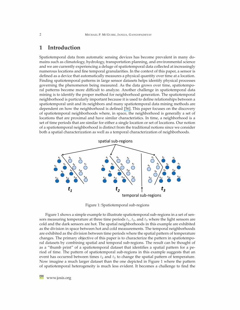
Figure 1 shows a simple example to illustrate spatiotemporal sub-regions in a set of sen-sors measuring temperature at three time periods t1, t2, and t3 where the light sensors arecold and the dark sensors are hot. The spatial neighborhoods in this example are exhibitedas the division in space between hot and cold measurements. The temporal neighborhoodsare exhibited as the division between time periods where the spatial pattern of temperaturechanges. The primary objective of this paper is to characterize the pattern in spatiotempo-ral datasets by combining spatial and temporal sub-regions. The result can be thought ofas a “thumb print” of a spatiotemporal dataset that identifies a spatial pattern for a pe-riod of time. The pattern of spatiotemporal sub-regions in this example suggests that anevent has occurred between times t2 and t3 to change the spatial pattern of temperature.Now imagine a much larger dataset than the one depicted in Figure 1 where the patternof spatiotemporal heterogeneity is much less evident. It becomes a challenge to find the
www.josis.org
MINING SENSOR DATASETS WITH SPATIOTEMPORAL NEIGHBORHOODS 3
pattern of changing spatiotemporal sub-regions and therefore approaches are needed toautomatically uncover these patterns in large sensor datasets.
This paper proposes an approach to identify spatiotemporal neighborhoods to find theinherent pattern of spatiotemporal sub-regions in the data. The resulting characterizationof spatiotemporal data can be seen as a key step to knowledge discovery in a numberof domains including climatology, hydrology, transportation planning, and environmentalscience because it provides an automated way to find the homogeneous sub-regions inspace and time in the dataset. The resulting regions can then be used in the identificationand characterization of events. The following presents a motivating example in the domainof climatology:
1.1 Motivating Example
El Nino events are characterized by anomalously warm sea surface temperatures (SST)in the Equatorial Pacific Ocean and can have important implications for global weatherconditions [47]. The TAO/TRITON array [46] consists of sensors installed on buoys posi-tioned in the equatorial region of the Pacific Ocean. The sensors collect a wide range ofmeteorological and oceanographic measurements. SST measurements are reported everyfive minutes. Over time, this results in a massive dynamic spatiotemporal dataset. Thisdata played an integral part in characterizing the 1997–98 El Nino [38] and are currentlybeing used to initialize models for El Nino prediction. There have been a number of stud-ies which assimilate meteorological and oceanographic data to offer a description of thephenomena associated with the events of the 1982–83 El Nino [5, 49] and the 1997–1998 ElNino [38]. These analyses show a particular importance in the spatiotemporal patterns ofSST anomalies that characterize El Nino events. Understanding these patterns can lead tonew knowledge about the global climate and in turn can assist in predicting local weatherpatterns such as drought and flooding.
As a use case, consider the perspective of a climatologist analyzing the SST data overtime. The aim might be to find regions, boundaries, and outliers in the dataset; critical timeperiods where changes in these regions occur; and relations between these global patternsand local weather conditions. In the current mode of analysis, daily anomalies are typicallycalculated using a combination of in situ and satellite measurements where the degree ofthe anomaly is based on the difference between the current SST analysis value and SSTmonthly climatology. This method finds global outliers at coarse spatial and temporal res-olutions, in the order of 1 day [51]. Instead, a climatologist might prefer to develop a moredetailed spatiotemporal characterization of SST by using data from the TAO/TRITON net-work. To begin this analysis, the climatologist must first be able to characterize the evolu-tion of El Nino events by finding distinct points in time where the pattern of SST changes.
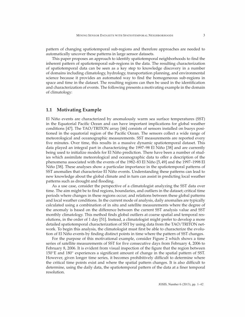
For the purpose of this motivational example, consider Figure 2 which shows a timeseries of satellite measurements of SST for five consecutive days from February 4, 2006 toFebruary 8, 2006. It is evident from visual inspection of the figure that the region between150◦E and 180◦ experiences a significant amount of change in the spatial pattern of SST.However, given longer time series, it becomes prohibitively difficult to determine wherethe critical time points exist and where the spatial pattern changes. It is also difficult todetermine, using the daily data, the spatiotemporal pattern of the data at a finer temporalresolution.
JOSIS, Number 6 (2013), pp. 1–42
4 MICHAEL P. MCGUIRE, JANEJA, GANGOPADHYAY
Longitude
Figure 2: A time series of daily SST between the dates of 2/4/2006 and 2/8/2006 mea-sured by the NOAA AVHRR satellite. The black dots in the figure represent the SST sen-sors of the TAO/Triton Array. The region between 150◦E and 180◦ experiences a significantamount of change. Figure created using the IRI/LDEO Climate Data Library (http:�iridl.ldeo.columbia.edu/).
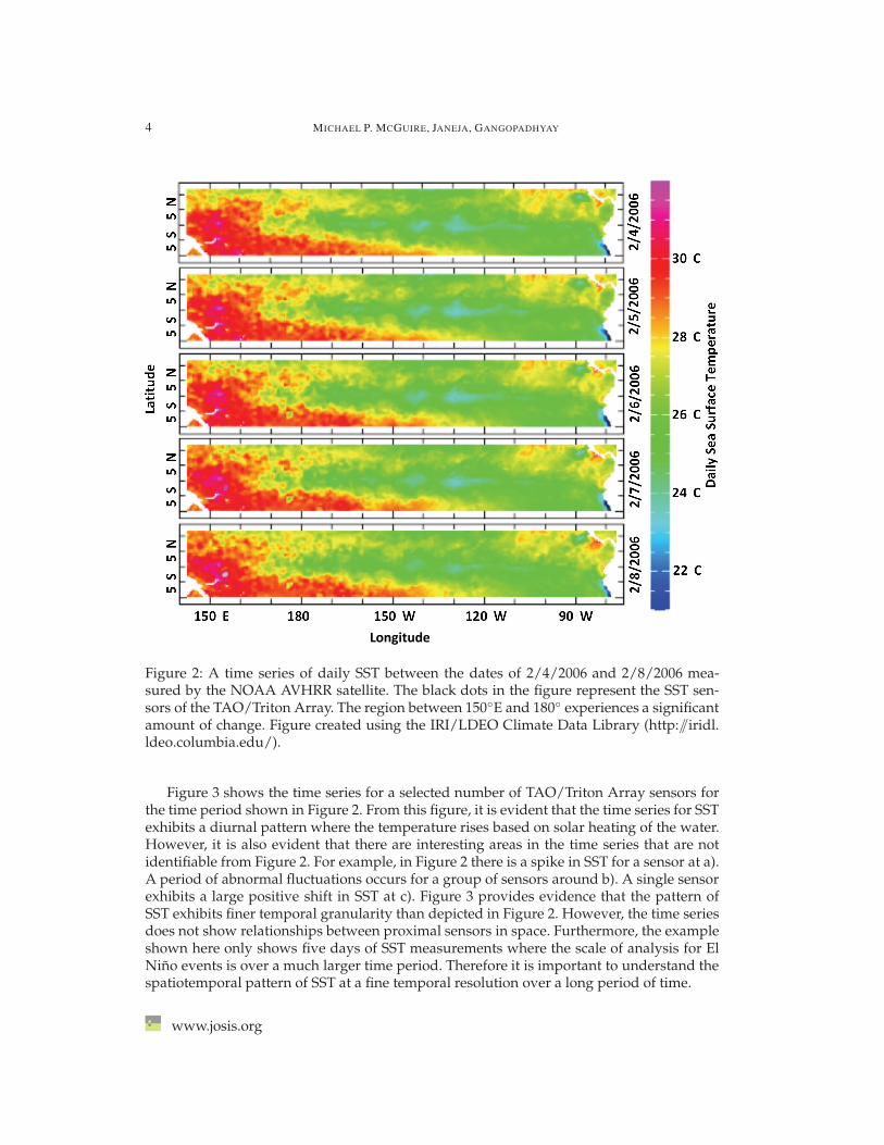
Figure 3 shows the time series for a selected number of TAO/Triton Array sensors forthe time period shown in Figure 2. From this figure, it is evident that the time series for SSTexhibits a diurnal pattern where the temperature rises based on solar heating of the water.However, it is also evident that there are interesting areas in the time series that are notidentifiable from Figure 2. For example, in Figure 2 there is a spike in SST for a sensor at a).A period of abnormal fluctuations occurs for a group of sensors around b). A single sensorexhibits a large positive shift in SST at c). Figure 3 provides evidence that the pattern ofSST exhibits finer temporal granularity than depicted in Figure 2. However, the time seriesdoes not show relationships between proximal sensors in space. Furthermore, the exampleshown here only shows five days of SST measurements where the scale of analysis for ElNino events is over a much larger time period. Therefore it is important to understand thespatiotemporal pattern of SST at a fine temporal resolution over a long period of time.
www.josis.org

MINING SENSOR DATASETS WITH SPATIOTEMPORAL NEIGHBORHOODS 5
2/4/2006 2/5/2006 2/6/2006 2/7/2006 2/8/200623
24
25
26
27
28
29
30
31
32
a)
b)
c)
Date
Tem
pera
ture
(°C
)
Figure 3: Time series of measurements for the SST sensors shown in Figure 2.
This use case presents a number of challenges. The first challenge is to find proximalsensors in the TAO/Triton network that have similar SST measurements in a particular timeframe. To make the analysis more efficient, the climatologist would like to automaticallyfind areas in the data where changes to the spatiotemporal patterns are most likely to occurand focus the analysis on finding anomalies in these areas. For example, by finding theseareas, the climatologist could then pinpoint time periods where exploration of the satellitedata might prove to be fruitful. Furthermore, finding these areas can lead to the discoveryof events that shape the spatiotemporal pattern of SST. If these events can be identified inadvance, they can be used in the prediction of global weather conditions such as localizeddrought and flooding. In short, the climatologist is in need of a mechanism that allowsfor the spatiotemporal characterization of the natural boundaries in space and time in thesensor network.
The approach to spatiotemporal neighborhoods presented in this paper first determinesadjacent spatial nodes then applies an agglomerative method to create temporal inter-vals for multiple sensors based on spatial relationships between adjacent sensors. Then, agraph-based method is used to create spatial neighborhoods for each interval. The combi-nation of the temporal intervals and spatial neighborhoods results in spatiotemporal neigh-borhoods.
The rest of the paper is organized as follows. Related research is discussed in Section2. Section 3 provides the objectives and preliminaries for the discovery of spatiotemporalneighborhoods. Section 4 discusses the approach and algorithms as well as validation met-rics. Detailed experimental results are discussed in Section 5. Finally, Section 7 offers someconcluding remarks.
JOSIS, Number 6 (2013), pp. 1–42
6 MICHAEL P. MCGUIRE, JANEJA, GANGOPADHYAY
2 Related work and contributions
Related works relevant to this research are situated in the areas of spatial neighborhooddiscovery, time series segmentation, and spatiotemporal pattern discovery.
2.1 Spatial neighborhoods
The model used to determine the neighborhood of a spatial object is a critical step in spatialand spatiotemporal statistical analysis [8]. Spatial neighborhood formation has been iden-tified as a critical challenge in future research in spatial data mining and is a key aspectto spatial data mining techniques [56]. This is never more true than in the case of spatialoutlier detection. For example, the issue of graph-based spatial outlier detection using asingle attribute has been addressed in [57]. Their definition of a neighborhood is similarto the neighborhood graph [10], which is primarily based on spatial relationships. How-ever the process of selecting the spatial predicates and identifying the spatial relationshipcan be an intricate process in itself. Another approach generates neighborhoods using acombination of distance and semantic relationships [2]. In general the neighborhoods inthese approaches have crisp boundaries and do not take the measurements from the spa-tial objects into account for the generation of the neighborhoods. The approach presentedin this paper extends the crisp neighborhood by using a measure of connectivity strengthto assign a degree of membership of spatial nodes to a particular neighborhood. Further-more, this approach uses the measurements taken at the spatial nodes to initialize neighborrelationships and the number of neighborhoods are not known a priori.
Spatial neighborhood discovery can also be formulated as a spatial clustering problem.Most of the existing clustering methods for spatial data either cluster spatial data aloneor treat attributes as another dimension along with spatial dimensions. The approach pre-sented in this paper treats the spatial dimension separately from attribute dimensions inthe dataset therefore generating neighborhoods that are constrained by the spatial dimen-sion and defined by the parameter being measured. There have been many applicationsof various types of clustering algorithms on spatial data [20]. Clustering methods are typ-ically categorized as partitioning-based, hierarchical, density-based, grid-based, or graph-based methods. Partitioning-based methods typically group objects in the data based ona distance from the closest cluster center. Partitioning methods include k-means [35], k-medoids [27], CLARANS [42], and affinity propagation [13].
Hierarchical methods introduced in [23] form a dendrogram of clustered objects by re-cursively splitting the dataset. Popular hierarchical clustering methods include BIRCH [62],AGNES [27], and CURE [18]. Density-based clustering methods such as DBSCAN [11]and OPTICS [3], instead of simply using distance between objects, form clusters in denseregions of points in the data. Grid-based clustering methods such as STING [60] andWaveCluster [55], allocate all data points into a grid structure and clustering is formedby agglomerations of grid cells. Finally, graph-based methods model the data using agraph structure and clusters are typically formed by using graph partitioning methods[12, 25, 26, 34, 61]. Most closely related to our work is the work on using a Delaunay tri-angulation for the clustering of spatial objects. In [25] the Delaunay triangulation is usedto cluster spatial points based on the connectivity of the triangulation after applying anedge cut based on a spatial distance threshold. In [34] a Delaunay triangulation is used forclustering and boundary detection in spatial datasets. The work presented in this paper
www.josis.org
MINING SENSOR DATASETS WITH SPATIOTEMPORAL NEIGHBORHOODS 7
builds on this approach. However, instead of applying an edge cut based on a spatial dis-tance threshold, we perform edge cuts based on the difference between the measurementsat connected spatial nodes.
2.2 Time series segmentation
The concept of a temporal neighborhood is most closely related to the literature focused ontime series segmentation. The methods presented in this paper focus on finding temporalintervals across a number of time series taken at a number of spatial locations. Moreover,this is the first approach to delineate temporal intervals that are based on relationshipsbetween adjacent spatial nodes. The existing literature primarily focuses on approximat-ing a time series, and do not result in a set of discrete temporal intervals. Furthermore, theliterature has largely focused on segmentation of a single time series. To the authors’ knowl-edge, there is no existing approach that discretizes multiple time series in a spatiotemporaldataset. Numerous algorithms [1,4,21,29,32] have been written to segment time series. Oneof the most common solutions to this problem applies a piecewise linear approximation us-ing dynamic programming [4]. Three common algorithms for time series segmentation arethe bottom-up, top-down, and sliding window algorithms [29]. Another approach, globaliterative replacement (GIR), uses a greedy algorithm to gradually move break points tomore optimal positions [21]. Abonyi et al. (2003) [1] offer a method to segment time seriesbased on fuzzy clustering. In this approach, principal component analysis (PCA) modelsare used to test the homogeneity of the resulting segments. Most recently [32] developed amethod to segment time series using polynomial degrees with regressor-based costs.
2.3 Spatiotemporal pattern discovery
This paper also has a number of commonalities with literature in spatiotemporal data min-ing. Many of these approaches first perform a spatial characterization of the data thenfind the temporal pattern. The work presented in this paper sets itself apart from thisliterature by first finding temporal intervals in the dataset. Also, a novel aspect of thisresearch is the idea of combining temporal intervals with spatial neighborhoods to findspatiotemporal neighborhoods. A number of works discover spatiotemporal patterns insensor data [6, 15, 16, 30, 40, 57]. In [57] a simple definition of a spatiotemporal neighbor-hood is introduced as two or more nodes in a graph that are connected during a certainpoint in time. Graphs can be used to represent spatiotemporal features for the purposes ofdata mining. Time-expanded graphs were developed for the purpose of road traffic con-trol to model traffic flows and solve flow problems on a network over time [30]. Buildingon this approach, George and Shekhar devised the time-aggregated graph, defined as agraph where at each node, a time series exists that represents the presence of the node atany period in time [16]. Spatiotemporal sensor graphs (STSG) [15] extend the concept oftime-aggregated graphs to model spatiotemporal patterns in sensor networks. The STSGapproach includes not only a time series for the representation of nodes but also for therepresentation of edges in the graph. This allows for the network which connects nodes toalso be dynamic. Chan et al. [6] also uses a graph representation to mine spatiotemporalpatterns. In this approach, clustering for spatiotemporal analysis of graphs (cSTAG) is usedto mine spatiotemporal patterns in emerging graphs.
JOSIS, Number 6 (2013), pp. 1–42
8 MICHAEL P. MCGUIRE, JANEJA, GANGOPADHYAY
There have been a number of approaches to spatiotemporal clustering. In [50] a selforganizing map (SOM) neural network is used to find spatiotemporal regions of precipita-tion data. Another approach improves spatiotemporal clustering by extending the distancemeasure traditionally used in most clustering algorithms to be a function of the positionhistory of the spatiotemporal objects in the dataset [52]. In [54] a weighted kernel k-meansalgorithm is proposed to account for problems with nonlinear separability in spatiotem-poral data. In [33] a tight clustering algorithm is presented where the clustering is basedon a measure of process similarity. While this approach does account for spatiotemporalaspects of the data, it provides a global clustering for an entire time series and therefore,does not uncover changing patterns over time. A number of approaches are focused onfinding dense areas or clusters in moving object databases. For example, in [59] spatiotem-poral association rules are used to find stationary and high-traffic regions in object mobilitydatabases. In [24] a combination of density-based clustering and time slices are used to findclusters of moving objects in trajectory databases. Finally, in [19] a grid-based technique isused to find dense groups of moving objects across time.
2.4 Contribution of this work
The primary contribution of this paper is the discovery of neighborhood for spatiotemporaldata, which is a critical challenge in spatiotemporal statistical analysis [8] and spatiotem-poral data mining [56]. The approach presented in this paper discretizes temporal intervalsand discovers spatial neighborhoods within each temporal interval to form spatiotempo-ral neighborhoods. This notion of a spatiotemporal neighborhood is unique because theformation of these neighborhoods is based on both a spatial characterization as well as atemporal characterization. Also, there has yet to be an approach to spatiotemporal neigh-borhoods that is based on the ability to track relationships between spatial locations overtime. Furthermore, experiments were performed on real world datasets on SST and precip-itation data with promising results in finding distinct temporal interval and spatial neigh-borhoods in both datasets. The specific contributions of this research are as follows:
Temporal intervals Temporal intervals embody the concept of neighborhoods in time.One major contribution is the discovery of unequal width or unequal frequency intervalsthat are robust in the presence of outliers. Furthermore, this is the first approach to temporalintervals that is based on the relationships of measurements taken at adjacent spatial nodes.Lastly, the efficacy of the interval discovery method is demonstrated on very large realworld sensor datasets from the TAO/TRITON Array [46] and Hydro-NEXRAD system[31].
Spatiotemporal neighborhoods The spatiotemporal neighborhood method finds group-ings of locations in terms of the spatial distribution of measurements based on their re-lationships with neighboring locations. The spatiotemporal neighborhood approach pre-sented in this paper is conceptually similar to clustering approaches which use a graph cre-ated by a Delaunay triangulation [25,34]. However, no existing approach combines tempo-ral intervals with spatial neighborhoods to form spatiotemporal neighborhoods. Further-more, the approach presented in this paper can accommodate for spatial nodes that areirregularly distributed as well as spatial nodes that are distributed in the form of a grid.
www.josis.org

MINING SENSOR DATASETS WITH SPATIOTEMPORAL NEIGHBORHOODS 9
Validation The approaches presented in this paper are validated by using both estab-lished metrics as well as new measures for comparison with alternative approaches. TheMoran’s I statistic, a standard measure of spatial autocorrelation, is used to validate thequality of the spatial contiguity represented by the spatiotemporal neighborhoods. Thebetween interval dissimilarity (bid) measures the quality of a set of temporal intervals bycalculating the dissimilarity of adjacent intervals. This metric is used to compare our re-sults with other established approaches. The significance of our results is then tested usingMonte Carlo simulation.
3 Objectives and preliminaries
In most real-world sensor deployments, a heterogeneous pattern of spatial and temporaldependence exists based on the physical properties of the process being measured. Withthis in mind, finding the how this pattern is expressed by the formation of homogeneousspatiotemporal sub-regions in the data can lead to the discovery of distinct spatiotemporalsub-regions in the dataset. Considering the motivational example of climatology, findingthese naturally occurring boundaries can lead to a better characterization of El Nino eventswhich in turn can lead to the discovery of new impacts on global weather patterns. In Fig-ure 4, the spatial pattern can be determined by grouping the locations into regions based onthe measurements taken at each time period. Conversely, the temporal pattern can be de-termined by grouping the time periods based on the measurements taken at each locations.The goal of spatiotemporal neighborhoods (STN) is to find the spatial and temporal pat-terns in a dataset by first delineating temporal intervals in a spatiotemporal dataset acrossall locations, then, for each interval, to determine the spatial pattern in terms of groupingsof similar spatial nodes. The specific objectives of STN are as follows:
• Find the temporal pattern for a set of spatial nodes S and temporal measurements Tby dividing the time series for a set of spatial nodes and temporal measurements intoa set of unequal width temporal intervals.
• Find the spatial pattern for a set of spatial nodes S and temporal measurements T byfinding the spatial neighborhoods for each temporal interval resulting in spatiotem-poral intervals where the number of neighborhoods is not known a priori.
3.1 Sensor datasets: Spatial nodes and temporal measurements
Conceptually, sensor deployments consist of a set of spatial nodes distributed in Euclideanspace where each spatial node is associated with a set of measurements taken over time.More formally we consider the following input:
• Let S represent a set of spatial nodes where S = {s1, ..., sn} and each si ∈ S has a setof coordinates in 2D Euclidean space (six, siy).
• Each si ∈ S also has a set of spatial neighbors SNi ⊂ S that are defined by a spatialrelationship sr such that given two spatial nodes (sp, sq) ∈ S a spatial relationshipsr(sp, sq) exists if there is either a distance, direction or topological relationship be-tween them.
• Each si ∈ S has a set of measurements that are taken for a set of time periods Ti ={ti1, . . . , tim} where ti1 < ti2 < · · · < tim. A time period is defined as any individualtij ∈ Ti.
JOSIS, Number 6 (2013), pp. 1–42
10 MICHAEL P. MCGUIRE, JANEJA, GANGOPADHYAY
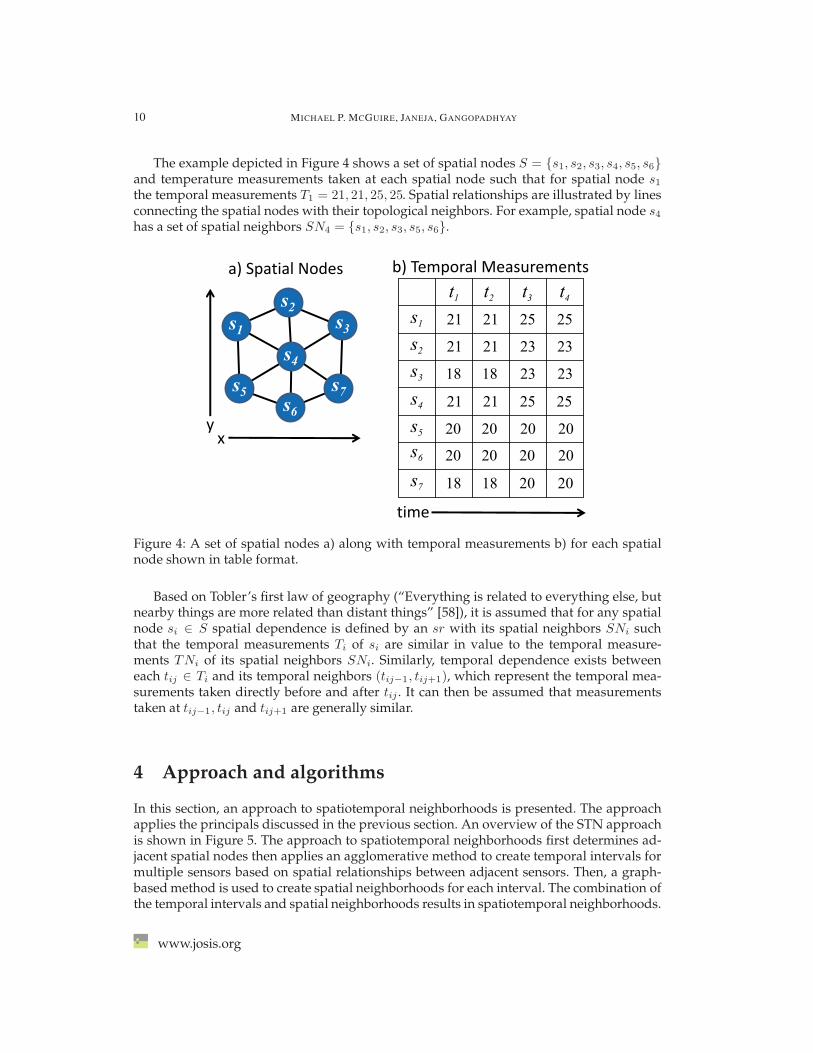
The example depicted in Figure 4 shows a set of spatial nodes S = {s1, s2, s3, s4, s5, s6}and temperature measurements taken at each spatial node such that for spatial node s1the temporal measurements T1 = 21, 21, 25, 25. Spatial relationships are illustrated by linesconnecting the spatial nodes with their topological neighbors. For example, spatial node s4has a set of spatial neighbors SN4 = {s1, s2, s3, s5, s6}.
s4
s1s2
s3
s5 s7s6
a) Spatial Nodes
x
b) Temporal Measurements
y
time
t2 t3 t4t1s1s2s3s4s5s6s7
21 21 25 25
21 21 23 23
21 21 25 25
18 18 23 23
18 18 20 20
20 2020 20
20 2020 20
Figure 4: A set of spatial nodes a) along with temporal measurements b) for each spatialnode shown in table format.
Based on Tobler’s first law of geography (“Everything is related to everything else, butnearby things are more related than distant things” [58]), it is assumed that for any spatialnode si ∈ S spatial dependence is defined by an sr with its spatial neighbors SNi suchthat the temporal measurements Ti of si are similar in value to the temporal measure-ments TNi of its spatial neighbors SNi. Similarly, temporal dependence exists betweeneach tij ∈ Ti and its temporal neighbors (tij−1, tij+1), which represent the temporal mea-surements taken directly before and after tij . It can then be assumed that measurementstaken at tij−1, tij and tij+1 are generally similar.
4 Approach and algorithms
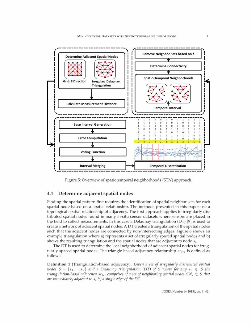
In this section, an approach to spatiotemporal neighborhoods is presented. The approachapplies the principals discussed in the previous section. An overview of the STN approachis shown in Figure 5. The approach to spatiotemporal neighborhoods first determines ad-jacent spatial nodes then applies an agglomerative method to create temporal intervals formultiple sensors based on spatial relationships between adjacent sensors. Then, a graph-based method is used to create spatial neighborhoods for each interval. The combination ofthe temporal intervals and spatial neighborhoods results in spatiotemporal neighborhoods.
www.josis.org
MINING SENSOR DATASETS WITH SPATIOTEMPORAL NEIGHBORHOODS 11
Determine Adjacent Spatial Nodes
Spatio-Temporal Neighborhoods
Temporal Interval
Grid: 8 Direction Irregular: Delaunay Triangulation
Calculate Measurement Distance
Remove Neighbor Sets based on λ
Determine Connectivity
Base Interval Generation
Error Computation
Voting Function
Interval Merging Temporal Discretization
1 1 1 0 0 0 0 0 1 1 1 11 1 1 1 0 0 0 0 0 1 1 11 1 0 0 0 0 0 0 0 1 1 10 0 0 0 0 0 1 1 1 1 1 11 1 1 1 0 0 0 0 0 1 1 10 0 0 0 1 1 1 1 1 0 0 01 0 0 0 1 1 1 0 0 0 0 05 4 3 2 2 2 3 2 3 5 5 5
Figure 5: Overview of spatiotemporal neighborhoods (STN) approach.
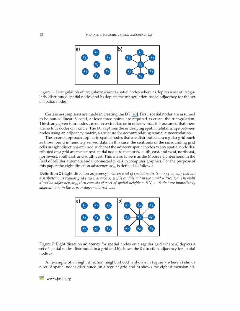
4.1 Determine adjacent spatial nodes
Finding the spatial pattern first requires the identification of spatial neighbor sets for eachspatial node based on a spatial relationship. The methods presented in this paper use atopological spatial relationship of adjacency. The first approach applies to irregularly dis-tributed spatial nodes found in many in-situ sensor datasets where sensors are placed inthe field to collect measurements. In this case a Delaunay triangulation (DT) [9] is used tocreate a network of adjacent spatial nodes. A DT creates a triangulation of the spatial nodessuch that the adjacent nodes are connected by non-intersecting edges. Figure 6 shows anexample triangulation where a) represents a set of irregularly spaced spatial nodes and b)shows the resulting triangulation and the spatial nodes that are adjacent to node s4.
The DT is used to determine the local neighborhood of adjacent spatial nodes for irreg-ularly spaced spatial nodes. The triangle-based adjacency relationship srtri is defined asfollows:
Definition 1 (Triangulation-based adjacency). Given a set of irregularly distributed spatialnodes S = {s1, ..., sn} and a Delaunay triangulation (DT) of S where for any si ∈ S thetriangulation-based adjacency srtri comprises of a set of neighboring spatial nodes SNi ⊂ S thatare immediately adjacent to si by a single edge of the DT.
JOSIS, Number 6 (2013), pp. 1–42
12 MICHAEL P. MCGUIRE, JANEJA, GANGOPADHYAY
s4
s1s2
s3
s5 s7s6
a) b)
s4
s1s2
s3
s5 s7s6
Figure 6: Triangulation of irregularly spaced spatial nodes where a) depicts a set of irregu-larly distributed spatial nodes and b) depicts the triangulation-based adjacency for the setof spatial nodes.
Certain assumptions are made in creating the DT [48]. First, spatial nodes are assumedto be non-collinear. Second, at least three points are required to create the triangulation.Third, any given four nodes are non-co-circular, or in other words, it is assumed that thereare no four nodes on a circle. The DT captures the underlying spatial relationships betweennodes using an adjacency matrix, a structure for accommodating spatial autocorrelation.
The second approach applies to spatial nodes that are distributed as a regular grid, suchas those found in remotely sensed data. In this case, the centroids of the surrounding gridcells in eight directions are used such that the adjacent spatial nodes to any spatial node dis-tributed on a grid are the nearest spatial nodes to the north, south, east, and west, northeast,northwest, southeast, and southwest. This is also known as the Moore neighborhood in thefield of cellular automata and 8-connected pixels in computer graphics. For the purpose ofthis paper, the eight direction adjacency srd8 is defined as follows:
Definition 2 (Eight direction adjacency). Given a set of spatial nodes S = {s1, ..., sn} that aredistributed on a regular grid such that each si ∈ S is equidistant in the x and y direction. The eightdirection adjacency srd8 then consists of a set of spatial neighbors SNi ⊂ S that are immediatelyadjacent to si in the x, y, or diagonal directions.
s4
s1 s2 s3
s5
s7
s6
a) b)
s8 s9
s4
s1 s2 s3
s5
s7
s6
s8 s9
Figure 7: Eight direction adjacency for spatial nodes on a regular grid where a) depicts aset of spatial nodes distributed in a grid and b) shows the 8-direction adjacency for spatialnode s5.
An example of an eight direction neighborhood is shown in Figure 7 where a) showsa set of spatial nodes distributed on a regular grid and b) shows the eight dimension ad-
www.josis.org
MINING SENSOR DATASETS WITH SPATIOTEMPORAL NEIGHBORHOODS 13
jacency for node s5. In the case of irregularly distributed spatial nodes, the triangulation-based spatial adjacency is used. Alternatively, in the case of spatial nodes distributed ona grid, the 8 direction spatial adjacency is used. We also use the concept of measurementdistance md in this step because md is used in the next step to create temporal intervals.
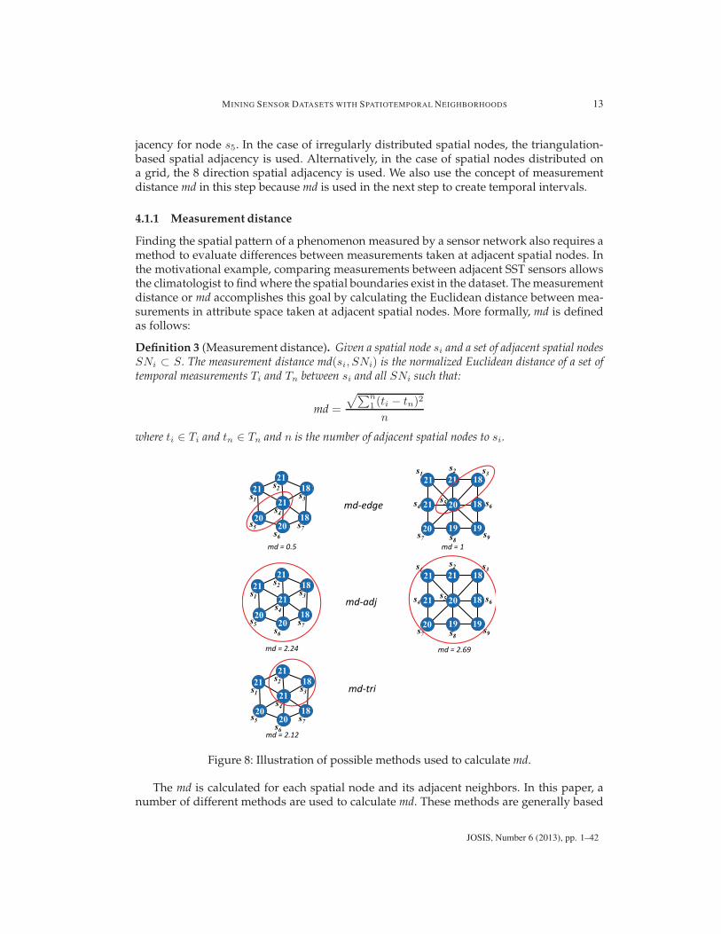
4.1.1 Measurement distance
Finding the spatial pattern of a phenomenon measured by a sensor network also requires amethod to evaluate differences between measurements taken at adjacent spatial nodes. Inthe motivational example, comparing measurements between adjacent SST sensors allowsthe climatologist to find where the spatial boundaries exist in the dataset. The measurementdistance or md accomplishes this goal by calculating the Euclidean distance between mea-surements in attribute space taken at adjacent spatial nodes. More formally, md is definedas follows:
Definition 3 (Measurement distance). Given a spatial node si and a set of adjacent spatial nodesSNi ⊂ S. The measurement distance md(si, SNi) is the normalized Euclidean distance of a set oftemporal measurements Ti and Tn between si and all SNi such that:
md =
√∑n1 (ti − tn)2
n
where ti ∈ Ti and tn ∈ Tn and n is the number of adjacent spatial nodes to si.
s4
s1s2
s3
s5 s7s6
2121
1821
2020
18
s4
s1s2
s3
s5 s7s6
2121
1821
2020
18
s4
s1s2
s3
s5 s7s6
2121
1821
2020
18
s4
s1 s2 s3
s5
s7
s6
s8 s9
18
18
1919
20
2121
21
20
s4
s1 s2 s3
s5
s7
s6
s8 s9
18
18
1919
20
2121
21
20
md-edge
md-adj
md-tri
md = 0.5 md = 1
md = 2.24 md = 2.69
md = 2.12
Figure 8: Illustration of possible methods used to calculate md.
The md is calculated for each spatial node and its adjacent neighbors. In this paper, anumber of different methods are used to calculate md. These methods are generally based
JOSIS, Number 6 (2013), pp. 1–42
14 MICHAEL P. MCGUIRE, JANEJA, GANGOPADHYAY
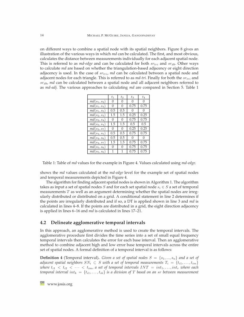
on different ways to combine a spatial node with its spatial neighbors. Figure 8 gives anillustration of the various ways in which md can be calculated. The first, and most obvious,calculates the distance between measurements individually for each adjacent spatial node.This is referred to as md-edge and can be calculated for both srtri and srd8. Other waysto calculate md are based on whether the triangulation-based adjacency or eight directionadjacency is used. In the case of srtri, md can be calculated between a spatial node andadjacent nodes for each triangle. This is referred to as md-tri. Finally for both the srtri andsrd8, md can be calculated between a spatial node and all adjacent neighbors referred toas md-adj. The various approaches to calculating md are compared in Section 5. Table 1
t1 t2 t3 t4md(s1, s2) 0 0 0 0md(s1, s4) 0 0 0.75 0.75md(s1, s5) 0.5 0.5 0 0md(s2, s3) 1.5 1.5 0.25 0.25md(s2, s4) 0 0 0.75 0.75md(s3, s4) 1.5 1.5 0.5 0.5md(s3, s7) 0 0 0.25 0.25md(s4, s5) 0.5 0.5 0.75 0.75md(s4, s6) 0.5 0.5 0 0md(s4, s7) 1.5 1.5 0.75 0.75md(s5, s6) 0 0 0.75 0.75md(s5, s6) 1 1 0.75 0.75
Table 1: Table of md values for the example in Figure 4. Values calculated using md-edge.
shows the md values calculated at the md-edge level for the example set of spatial nodesand temporal measurements depicted in Figure 4.
The algorithm for finding adjacent spatial nodes is shown in Algorithm 1. The algorithmtakes as input a set of spatial nodes S and for each set spatial node si ∈ S a set of temporalmeasurements T as well as an argument determining whether the spatial nodes are irreg-ularly distributed or distributed on a grid. A conditional statement in line 2 determines ifthe points are irregularly distributed and if so, a DT is applied shown in line 3 and md iscalculated in lines 4–8. If the points are distributed in a grid, the eight direction adjacencyis applied in lines 6–16 and md is calculated in lines 17–21.
4.2 Delineate agglomerative temporal intervals
In this approach, an agglomerative method is used to create the temporal intervals. Theagglomerative procedure first divides the time series into a set of small equal frequencytemporal intervals then calculates the error for each base interval. Then an agglomerativemethod to combine adjacent high and low error base temporal intervals across the entireset of spatial nodes. A formal definition of a temporal interval is as follows:
Definition 4 (Temporal interval). Given a set of spatial nodes S = {s1, ..., sn} and a set ofadjacent spatial neighbors SNi ⊂ S with a set of temporal measurements Ti = {ti1, . . . , tim}where ti1 < ti2 < · · · < tim, a set of temporal intervals INT = int1, . . . , intr where eachtemporal interval intk = {ti1, . . . , tik} is a division of T based on an sr between measurement
www.josis.org
MINING SENSOR DATASETS WITH SPATIOTEMPORAL NEIGHBORHOODS 15
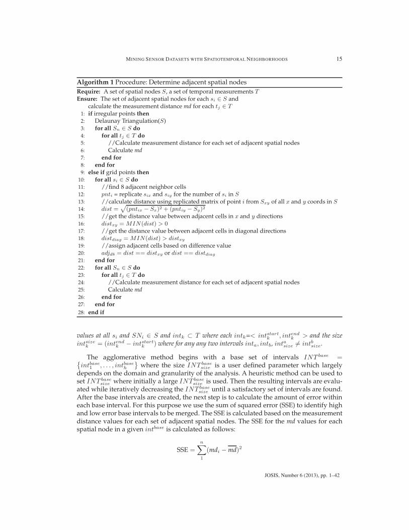
Algorithm 1 Procedure: Determine adjacent spatial nodesRequire: A set of spatial nodes S, a set of temporal measurements TEnsure: The set of adjacent spatial nodes for each si ∈ S and
calculate the measurement distance md for each tj ∈ T1: if irregular points then2: Delaunay Triangulation(S)3: for all Sn ∈ S do4: for all tj ∈ T do5: //Calculate measurement distance for each set of adjacent spatial nodes6: Calculate md7: end for8: end for9: else if grid points then
10: for all si ∈ S do11: //find 8 adjacent neighbor cells12: pnti = replicate six and siy for the number of si in S13: //calculate distance using replicated matrix of point i from Sxy of all x and y coords in S14: dist =
√(pntix − Sx)2 + (pntiy − Sy)2
15: //get the distance value between adjacent cells in x and y directions16: distxy = MIN(dist) > 017: //get the distance value between adjacent cells in diagonal directions18: distdiag = MIN(dist) > distxy19: //assign adjacent cells based on difference value20: adjd8 = dist == distxy or dist == distdiag21: end for22: for all Sn ∈ S do23: for all tj ∈ T do24: //Calculate measurement distance for each set of adjacent spatial nodes25: Calculate md26: end for27: end for28: end if
values at all si and SNi ∈ S and intk ⊂ T where each intk=< intstartk , intendk > and the sizeintsizek = (intendk − intstartk ) where for any any two intervals inta, intb, intasize �= intbsize.
The agglomerative method begins with a base set of intervals INT base ={intbase1 , . . . , intbaseh
}where the size INT base
size is a user defined parameter which largelydepends on the domain and granularity of the analysis. A heuristic method can be used toset INT base
size where initially a large INT basesize is used. Then the resulting intervals are evalu-
ated while iteratively decreasing the INT basesize until a satisfactory set of intervals are found.
After the base intervals are created, the next step is to calculate the amount of error withineach base interval. For this purpose we use the sum of squared error (SSE) to identify highand low error base intervals to be merged. The SSE is calculated based on the measurementdistance values for each set of adjacent spatial nodes. The SSE for the md values for eachspatial node in a given intbase is calculated as follows:
SSE =
n∑
1
(mdi − md)2
JOSIS, Number 6 (2013), pp. 1–42
16 MICHAEL P. MCGUIRE, JANEJA, GANGOPADHYAY
where n is the number of spatial nodes, dist is the Euclidean distance, and md is the meanof all values within a base interval.
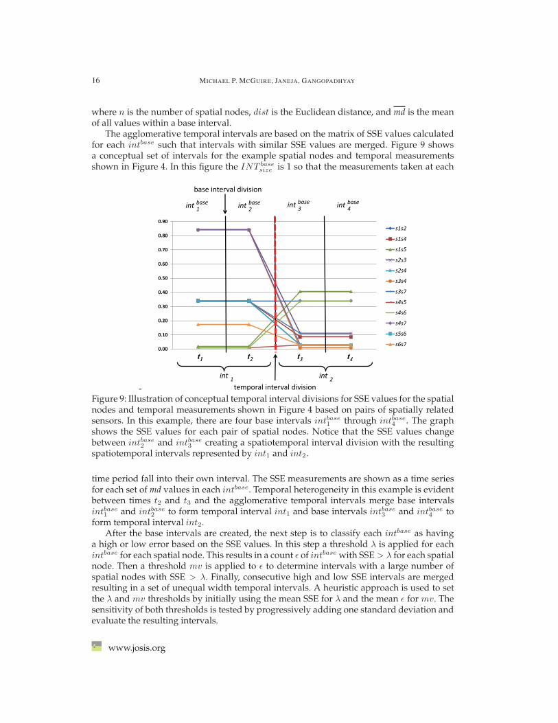
The agglomerative temporal intervals are based on the matrix of SSE values calculatedfor each intbase such that intervals with similar SSE values are merged. Figure 9 showsa conceptual set of intervals for the example spatial nodes and temporal measurementsshown in Figure 4. In this figure the INT base
size is 1 so that the measurements taken at each
-
0.00
0.10
0.20
0.30
0.40
0.50
0.60
0.70
0.80
0.90
int base1 int base2 int base3 int base4
base interval division
temporal interval divisionint 1 int 2
t1 t2 t3 t4
s1s2
s1s4
s1s5
s2s3
s2s4
s3s4
s3s7
s4s5
s4s6
s4s7
s5s6
s6s7
Figure 9: Illustration of conceptual temporal interval divisions for SSE values for the spatialnodes and temporal measurements shown in Figure 4 based on pairs of spatially relatedsensors. In this example, there are four base intervals intbase1 through intbase4 . The graphshows the SSE values for each pair of spatial nodes. Notice that the SSE values changebetween intbase2 and intbase3 creating a spatiotemporal interval division with the resultingspatiotemporal intervals represented by int1 and int2.
time period fall into their own interval. The SSE measurements are shown as a time seriesfor each set of md values in each intbase. Temporal heterogeneity in this example is evidentbetween times t2 and t3 and the agglomerative temporal intervals merge base intervalsintbase1 and intbase2 to form temporal interval int1 and base intervals intbase3 and intbase4 toform temporal interval int2.
After the base intervals are created, the next step is to classify each intbase as havinga high or low error based on the SSE values. In this step a threshold λ is applied for eachintbase for each spatial node. This results in a count ε of intbase with SSE > λ for each spatialnode. Then a threshold mv is applied to ε to determine intervals with a large number ofspatial nodes with SSE > λ. Finally, consecutive high and low SSE intervals are mergedresulting in a set of unequal width temporal intervals. A heuristic approach is used to setthe λ and mv thresholds by initially using the mean SSE for λ and the mean ε for mv. Thesensitivity of both thresholds is tested by progressively adding one standard deviation andevaluate the resulting intervals.
www.josis.org

MINING SENSOR DATASETS WITH SPATIOTEMPORAL NEIGHBORHOODS 17
The algorithm for delineating temporal intervals is shown in Algorithm 2. The algo-rithm takes as input a set of spatial nodes S and a set of temporal measurements T for allsi ∈ S, a base interval size INT base
size , an error threshold λ, and a voting function thresholdmv. In lines 1–8 the base temporal intervals are created and the SSE is calculated for eachinterval. The voting function is applied in lines 9–21 where ε is calculated for each intbasein lines 10–14 and the mv threshold and interval merging are applied in lines 15–21.
Algorithm 2 Procedure: Delineate temporal intervalsRequire: a set of spatial nodes S, a set of temporal measurements T ,
a base interval size INT basesize , a SSE threshold λ,
and a voting threshold mvEnsure: temporal intervals for S and T based on intbasesize ,λ, and mv
1: //Create base temporal intervals and calculate SSE2: Interval Start = 13: Interval End = Interval Start + intbasesize
4: while Interval Start < count(tj ∈ T ) do5: CALCULATE SSE6: Interval Start = Interval End + 17: Interval End = Interval Start + intbasesize
8: end while9: //Apply Voting Function
10: for all intk ∈ INTbase do11: ε = 112: for all si ∈ S do13: if SSE > λ then14: ε = ε+ 115: end if16: end for17: //Apply mv threshold and merge intervals18: if ε > mv and εold < mv then19: Output Interval Start, Interval End20: else if ε < mv and εold > mv then21: Output Interval Start, Interval End22: εold = ε23: end if24: end for
4.3 Spatiotemporal neighborhood discovery
Once the temporal intervals are discovered the spatial pattern can be explored further byfinding groupings of similar spatial nodes for a particular temporal interval. The spatialgroupings combined with the temporal interval configuration discussed above is termedthe spatiotemporal neighborhood and represents a set of divisions in time and space whereboundaries occur in a spatiotemporal dataset. With this in mind, the spatiotemporal neigh-borhoods allow the climatologist to first identify an event, then analyze the spatial patternof SST before and after the event. More formally, a spatiotemporal neighborhood is definedas follows:
JOSIS, Number 6 (2013), pp. 1–42
18 MICHAEL P. MCGUIRE, JANEJA, GANGOPADHYAY
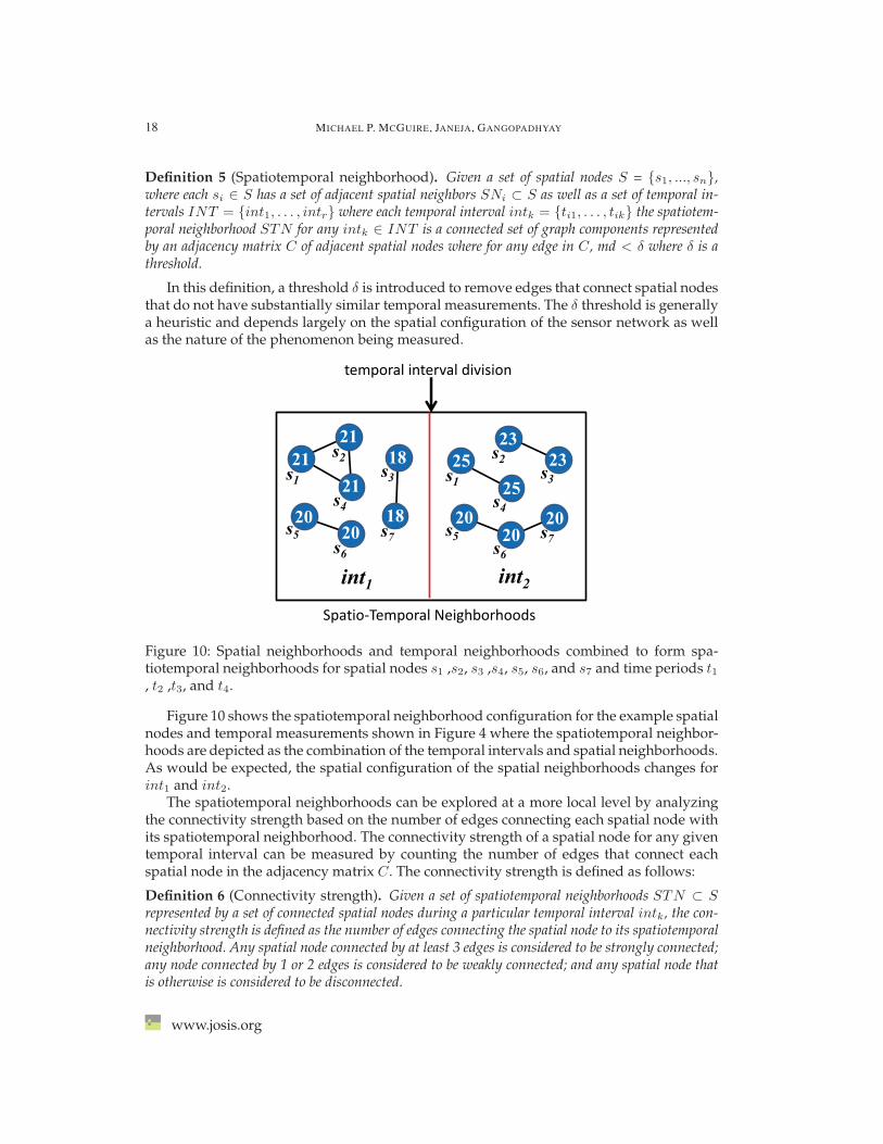
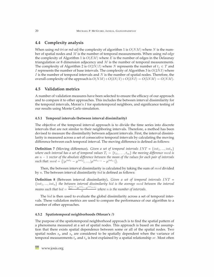
Definition 5 (Spatiotemporal neighborhood). Given a set of spatial nodes S = {s1, ..., sn},where each si ∈ S has a set of adjacent spatial neighbors SNi ⊂ S as well as a set of temporal in-tervals INT = {int1, . . . , intr} where each temporal interval intk = {ti1, . . . , tik} the spatiotem-poral neighborhood STN for any intk ∈ INT is a connected set of graph components representedby an adjacency matrix C of adjacent spatial nodes where for any edge in C, md < δ where δ is athreshold.
In this definition, a threshold δ is introduced to remove edges that connect spatial nodesthat do not have substantially similar temporal measurements. The δ threshold is generallya heuristic and depends largely on the spatial configuration of the sensor network as wellas the nature of the phenomenon being measured.
s4
s1s2
s3
s5 s7s6
int2int1
s4
s1s2
s3
s5 s7s6
2121
1821
2020
18
2523
2325
2020
20
Spatio-Temporal Neighborhoods
temporal interval division
Figure 10: Spatial neighborhoods and temporal neighborhoods combined to form spa-tiotemporal neighborhoods for spatial nodes s1 ,s2, s3 ,s4, s5, s6, and s7 and time periods t1, t2 ,t3, and t4.
Figure 10 shows the spatiotemporal neighborhood configuration for the example spatialnodes and temporal measurements shown in Figure 4 where the spatiotemporal neighbor-hoods are depicted as the combination of the temporal intervals and spatial neighborhoods.As would be expected, the spatial configuration of the spatial neighborhoods changes forint1 and int2.
The spatiotemporal neighborhoods can be explored at a more local level by analyzingthe connectivity strength based on the number of edges connecting each spatial node withits spatiotemporal neighborhood. The connectivity strength of a spatial node for any giventemporal interval can be measured by counting the number of edges that connect eachspatial node in the adjacency matrix C. The connectivity strength is defined as follows:
Definition 6 (Connectivity strength). Given a set of spatiotemporal neighborhoods STN ⊂ Srepresented by a set of connected spatial nodes during a particular temporal interval intk, the con-nectivity strength is defined as the number of edges connecting the spatial node to its spatiotemporalneighborhood. Any spatial node connected by at least 3 edges is considered to be strongly connected;any node connected by 1 or 2 edges is considered to be weakly connected; and any spatial node thatis otherwise is considered to be disconnected.
www.josis.org

MINING SENSOR DATASETS WITH SPATIOTEMPORAL NEIGHBORHOODS 19
For the example shown in Figure 10 all the spatial nodes are weakly connected becauseno spatial node is connected by at least 3 edges. Also, there are no completely disconnectednodes. This suggests that a high level of spatial heterogeneity exists for both intervals inthe spatial process represented in this figure.
The algorithm for discovering spatiotemporal neighborhoods is presented in Algorithm3. The algorithm takes as input a set of spatial nodes S and for each si ∈ S a set of temporalmeasurements T and a set of adjacent spatial nodes SNi, a set of temporal intervals INT ,and a measurement distance threshold δ. The md is calculated in lines 3–5. The λ thresholdis applied in lines 6–8. The resulting set of spatial neighbors are added to the adjacencymatrix C in lines 9–11.
Algorithm 3 Procedure: Discover spatiotemporal neighborhoodsRequire: a set of spatial nodesS, a set of temporal
measurements T , a set of adjacent spatial nodes SN , a set oftemporal intervals INT , a measurement distance threshold δ
Ensure: Spatiotemporal neighborhoods for S and T for eachinterval INT based on threshold δ
1: //discover spatiotemporal neighborhoods2: for all intk ∈ INT do3: for all SN ∈ S do4: //calculate measurement distance for each SN5: Calculate md6: end for7: //incrementally remove neighbor sets based on δ8: while MAX(adjmd) > δ do9: SPN = Sn < max(adjmd)
10: end while//create adjacency matrix C11: for all si ∈ SN do12: Add to C13: end for14: end for
4.3.1 Order Invariance of Approach
The STN algorithm is order invariant in that it will result in the same spatial neighborhoodsregardless of the starting spatial node. The following offers a formal proof of this property:
Theorem 1. For a set of spatial nodes S, Algorithm 3 will result in the same set of spatial neigh-borhoods regardless of the starting spatial node.
Proof. The property of order invariance is proven by contradiction. Assume to the con-trary that given a set of spatial nodes S and two spatial nodes sp and sq ∈ S that producetwo spatial graphs sgp and sgq each with a set of edges and nodes 〈ep, np〉 and 〈eq, nq〉respectively that result in two sets of spatial neighborhoods SPNp = {spnp
1, . . . , spnpl }
and SPNq = {spnq1, . . . , spn
ql } derived from each graph. Because both the 8 direction and
triangulation adjacencies produce a connected graph where every spatial node s ∈ S isconnected to every other spatial node s ∈ S via a path p ⊂ e, the resulting set of edgesand nodes 〈ep, np〉 = 〈eq, nq〉 and therefore, sgp = sgq and SPNp = SPNq contradicting ourassumption.
JOSIS, Number 6 (2013), pp. 1–42
20 MICHAEL P. MCGUIRE, JANEJA, GANGOPADHYAY
4.4 Complexity analysis
When using md-tri or md-adj the complexity of algorithm 1 is O(NM) where N is the num-ber of spatial nodes and M is the number of temporal measurements. When using md-edgethe complexity of Algorithm 1 is O(EM) where E is the number of edges in the Delaunaytriangulation or 8 dimension adjacency and M is the number of temporal measurements.The complexity of Algorithm 2 is O(2N/I) where N represents the number of tj ∈ T andI represents the number of base intervals. The complexity of Algorithm 3 is O(2NI) whereI is the number of temporal intervals and N is the number of spatial nodes. Therefore, theoverall complexity of the approach is O(NM)+O(2N/I)+O(2NI) = O(5NM) = O(NM).
4.5 Validation metrics
A number of validation measures have been selected to ensure the efficacy of our approachand to compare it to other approaches. This includes the between interval dissimilarity forthe temporal intervals, Moran’s I for spatiotemporal neighbors, and significance testing ofour results using Monte Carlo simulation.
4.5.1 Temporal intervals (between interval dissimilarity)
The objective of the temporal interval approach is to divide the time series into discreteintervals that are not similar to their neighboring intervals. Therefore, a method has beendevised to measure the dissimilarity between adjacent intervals. First, the interval dissimi-larity is measured across a set of consecutive temporal intervals by calculating the movingdifference between each temporal interval. The moving difference is defined as follows:
Definition 7 (Moving difference). Given a set of temporal intervals INT = {int1, ..., intn}where each interval has a set of temporal values Ti = {ti1, . . . , tin} the moving difference mvd isan n − 1 vector of the absolute difference between the mean of the values for each pair of intervalssuch that: mvd =
{|μint1 − μint2 |, ..., |μintn−1 − μintn |}.
Then, the between interval dissimilarity is calculated by taking the sum of mvd dividedby n. The between interval dissimilarity bid is defined as follows:
Definition 8 (Between interval dissimilarity). Given a set of temporal intervals INT ={int1, ..., intn} the between interval dissimilarity bid is the average mvd between the interval
means such that bid =∑n−1
i |µinti−µinti+1 |n where n is the number of intervals.
The bid is then used to evaluate the global dissimilarity across a set of temporal inter-vals. These validation metrics are used to compare the performance of our algorithm to anumber of other approaches.
4.5.2 Spatiotemporal neighborhoods (Moran’s I)
The purpose of the spatiotemporal neighborhood approach is to find the spatial pattern ofa phenomena measured at a set of spatial nodes. This approach is based on the assump-tion that there exists spatial dependence between some or all of the spatial nodes. Twospatial nodes sp and sq are considered to be spatially dependent when the variance oftemporal measurements tp and tq is best explained by a spatial relationship sr. Most often
www.josis.org
MINING SENSOR DATASETS WITH SPATIOTEMPORAL NEIGHBORHOODS 21
there exist distinct regions of spatially dependent nodes. For example, given a set of spatialnodes S and two subsets of spatial nodes represented by spatial neighborhoods STN1 andSTN2 ⊂ S the pattern is heterogeneous if the spatial dependence of the nodes in STN1 isdistinct from the spatial dependence of the nodes in STN2. This heterogeneous pattern canbe caused by regions in the underlying geographical process. For example, in the SST datathere are regions of warm and cool water in the Pacific Ocean that form a heterogeneouspattern.
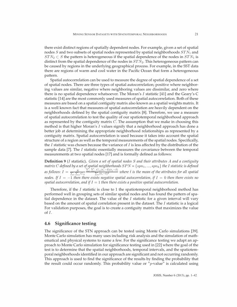
Spatial autocorrelation can be used to measure the degree of spatial dependence of a setof spatial nodes. There are three types of spatial autocorrelation; positive where neighbor-ing values are similar, negative where neighboring values are dissimilar, and zero wherethere is no spatial dependence whatsoever. The Moran’s I statistic [41] and the Geary’s Cstatistic [14] are the most commonly used measures of spatial autocorrelation. Both of thesemeasures are based on a spatial contiguity matrix also known as a spatial weights matrix. Itis a well known fact that measures of spatial autocorrelation are heavily dependent on theneighborhoods defined by the spatial contiguity matrix [8]. Therefore, we use a measureof spatial autocorrelation to test the quality of our spatiotemporal neighborhood approachas represented by the contiguity matrix C. The assumption that we make in choosing thismethod is that higher Moran’s I values signify that a neighborhood approach has done abetter job at determining the appropriate neighborhood relationships as represented by acontiguity matrix. Spatial autocorrelation is used because it takes into account the spatialstructure of a region as well as the temporal measurements of the spatial nodes. Specifically,the I statistic was chosen because the variance of I is less affected by the distribution of thesample data [7]. The I statistic essentially measures the covariance between the temporalmeasurements at two spatial nodes [17] and is formally defined as follows:
Definition 9 (I statistic). Given a set of spatial nodes S and their attributes A and a contiguitymatrix C defined by a set of spatial neighborhoods SPN = {spn1, ..., spnk} the I statistic is definedas follows: I = N∑
i
∑j Cij
∑i
∑j Cij(ti−t)(tj−t)∑
i(ti−t)2 where t is the mean of the attributes for all spatialnodes. If I = −1 then there exists negative spatial autocorrelation, if I = 0 then there exists nospatial autocorrelation, and if I = 1 then there exists a positive spatial autocorrelation.
Therefore, if the I statistic is close to 1 the spatiotemporal neighborhood method hasperformed well in grouping sets of similar spatial nodes and has found the pattern of spa-tial dependence in the dataset. The value of the I statistic for a given interval will varybased on the amount of spatial correlation present in the dataset. The I statistic is a logicalFor validation purposes, the goal is to create a contiguity matrix that maximizes the valueof I .
4.6 Significance testing
The significance of the STN approach can be tested using Monte Carlo simulations [39].Monte Carlo simulation has many uses including risk analysis and the simulation of math-ematical and physical systems to name a few. For the significance testing we adapt an ap-proach to Monte Carlo simulation for significance testing used in [22] where the goal of thetest is to determine that the spatial neighborhoods, temporal intervals, and the spatiotem-poral neighborhoods identified in our approach are significant and not occurring randomly.This approach is used to find the significance of the results by finding the probability thatthe result could occur randomly. This probability value or “p-value” is calculated using
JOSIS, Number 6 (2013), pp. 1–42
22 MICHAEL P. MCGUIRE, JANEJA, GANGOPADHYAY
Monte Carlo simulation. In this case the data is randomized and the algorithm is run andvalidation metrics are calculated on the randomized dataset for a large number of simu-lations. For each component the null hypothesis H0 states that the results are random andthe alternative hypothesis HA states that the resulting temporal intervals validated by thebetween interval dissimilarity bidO and spatiotemporal neighborhoods validated by the Istatistic I0 are not random.
In every case described above the actual measures IO and bidO are calculated and MonteCarlo simulation measures Ir or bidr are calculated for each iteration where the subscriptr represents the iteration. The measures for all simulations are sorted in descending order.Then, where the measures IO and bidO fall in this ranking, determines the p-value by cal-culating the ranking divided by the number of simulations. In all cases a p-value of < 0.05(5%) is significant in that it is within the 95% confidence interval and therefore, the nullhypothesis H0 is rejected.
5 Experimental results
In this section the results of experiments are presented where the spatiotemporal neigh-borhood approach is tested on real-world datasets including SST data for the equatorialPacific Ocean and precipitation data for a watershed in Baltimore, Maryland, USA. The ap-proaches were qualitatively validated empirically by providing ground-truth validationsthat show how finding the spatiotemporal neighborhoods in a dataset can lead to the dis-covery of interesting events. The approaches were also quantitatively compared with otherapproaches using the Moran’s I and bid validation metrics along with the results of thesignificance testing using Monte Carlo simulation. The final part of this section discussesexperiments to test the scalability of the approach.
5.1 Datasets
Experiments were performed on two datasets. The following provides a detailed descrip-tion of the datasets.
SST data SST data was retrieved from the TAO Project data delivery website [46]. Highresolution data (10 minute average) was downloaded for the entire year of 2006. This con-sisted of data from 55 sensors, 13 of which were missing an extensive number of timeperiods, and 42 had a full record for the year and had no-data values where measurementswere missing. Therefore, 42 sensors that had a full record were used in the experiment. Thedataset consisted of 52,563 temporal measurements for each spatial node resulting in a totalof 2,207,646 data points.
Precipitation data Precipitation data was retrieved from the Hydro-NEXRAD system[31]. The data was in grid format where each grid cell maps directly to a NEXRAD cell.For the purpose of these experiments, the center of each grid cell is treated as an individualsensor.
The data was extracted for the Gwynns Falls Watershed which lies to the west of Bal-timore, Maryland, USA. The dataset consisted of 198 grid cells and 33,492 temporal mea-surements for each spatial node resulting in a total of 6,631,416 data points.
www.josis.org
MINING SENSOR DATASETS WITH SPATIOTEMPORAL NEIGHBORHOODS 23
5.2 Setting thresholds
The spatiotemporal neighborhoods require a number of thresholds to be set at initializa-tion. For this experiment we used a number of heuristic based approaches to set the thresh-olds. The temporal intervals require a base interval size INT base
size . For this threshold a largeINT base
size is first chosen and iteratively decreased until a satisfactory discretization is found.The λ and mv thresholds are initialized with the mean SSE and mean ε respectively. Thesensitivity of both thresholds is tested by progressively adding one standard deviation. Theresulting intervals are visually inspected at each step until a satisfactory set of intervals isfound. A similar approach is taken for the δ threshold applied to md in the spatiotemporalneighborhood step where the sensitivity of the threshold is tested by adding one standarddeviation to the mean md for all spatial nodes. The results are then visually inspected ateach step until satisfactory neighborhoods are found.
5.3 Temporal intervals
In this section the results for the discovery of temporal intervals are presented. This sectionbegins with a presentation of the empirical results for the SST and precipitation data. Thenthe temporal interval approach with a other approaches including piecewise linear repre-sentation and equal width temporal intervals followed by the results of the significancetesting using Monte Carlo simulations.
5.3.1 Knowledge discovery in temporal intervals
Temporal intervals were found for both the SST data and the precipitation data.
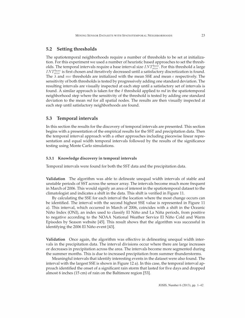
Validation The algorithm was able to delineate unequal width intervals of stable andunstable periods of SST across the sensor array. The intervals become much more frequentin March of 2006. This would signify an area of interest in the spatiotemporal dataset to theclimatologist and indicates a shift in the data. This shift is verified in Figure 11.
By calculating the SSE for each interval the location where the most change occurs canbe identified. The interval with the second highest SSE value is represented in Figure 11a). This interval, which occurred in March of 2006, coincides with a shift in the OceanicNino Index (ONI), an index used to classify El Nino and La Nina periods, from positiveto negative according to the NOAA National Weather Service El Nino Cold and WarmEpisodes by Season website [45]. This result shows that the algorithm was successful inidentifying the 2006 El Nino event [43].
Validation Once again, the algorithm was effective in delineating unequal width inter-vals in the precipitation data. The interval divisions occur where there are large increasesor decreases in precipitation across the area. The intervals become more segmented duringthe summer months. This is due to increased precipitation from summer thunderstorms.
Meaningful intervals that identify interesting events in the dataset were also found. Theinterval with the largest SSE is shown in Figure 12 a). In this case, the temporal interval ap-proach identified the onset of a significant rain storm that lasted for five days and droppedalmost 6 inches (15 cm) of rain on the Baltimore region [53].
JOSIS, Number 6 (2013), pp. 1–42
24 MICHAEL P. MCGUIRE, JANEJA, GANGOPADHYAY
Jan. Feb. Mar. Apr.
35
30
25
20
15
Sea
Sur
face
Tem
pera
ture
(C
) a)
Figure 11: Temporal interval with greatest SSE for SST data where a) shows the location ofthe interval division.
Jan. Feb. Mar. Apr. May June July Aug. Sep. Oct. Nov. Dec.
25
20
15
10
5
Pre
cipi
tatio
n (m
m.)
a)
5
Figure 12: Temporal Interval with greatest SSE for precipitation data where a) shows thelocation of the interval division.
5.3.2 Comparison of temporal intervals to other approaches
The quality of the temporal intervals was compared using the between interval dissimilar-ity measure with equal width temporal intervals and piecewise linear representation. Timeseries data is often segmented using equally sized bins. We compare our method with anequal width binning of the time series to prove the need for unequal-width intervals todiscretize spatiotemporal data. Equal width temporal intervals were created by dividingthe time series into equally sized bins. We also compare our approach with a time seriessegmentation method that results in unequally sized bins. Piecewise linear approximationis a commonly used method for representing a complex time series in a given number ofsegments where the time series is approximated using a given number of linear segments.The resulting segments are then used to represent a high-level discretization of a time se-
www.josis.org
MINING SENSOR DATASETS WITH SPATIOTEMPORAL NEIGHBORHOODS 25
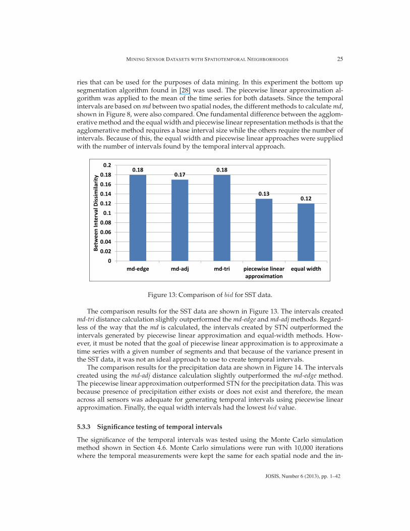
ries that can be used for the purposes of data mining. In this experiment the bottom upsegmentation algorithm found in [28] was used. The piecewise linear approximation al-gorithm was applied to the mean of the time series for both datasets. Since the temporalintervals are based on md between two spatial nodes, the different methods to calculate md,shown in Figure 8, were also compared. One fundamental difference between the agglom-erative method and the equal width and piecewise linear representation methods is that theagglomerative method requires a base interval size while the others require the number ofintervals. Because of this, the equal width and piecewise linear approaches were suppliedwith the number of intervals found by the temporal interval approach.
0.180.17
0.18
0.130.12
00.020.040.060.08
0.10.120.140.160.18
0.2
md-edge md-adj md-tri piecewise linearapproximation
equal width
Betw
een
Inte
rval
Dis
sim
ilarit
y
Figure 13: Comparison of bid for SST data.
The comparison results for the SST data are shown in Figure 13. The intervals createdmd-tri distance calculation slightly outperformed the md-edge and md-adj methods. Regard-less of the way that the md is calculated, the intervals created by STN outperformed theintervals generated by piecewise linear approximation and equal-width methods. How-ever, it must be noted that the goal of piecewise linear approximation is to approximate atime series with a given number of segments and that because of the variance present inthe SST data, it was not an ideal approach to use to create temporal intervals.
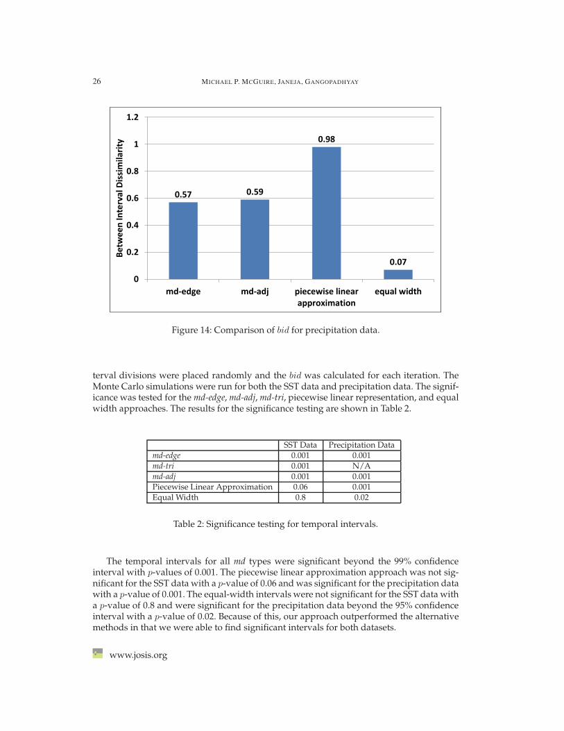
The comparison results for the precipitation data are shown in Figure 14. The intervalscreated using the md-adj distance calculation slightly outperformed the md-edge method.The piecewise linear approximation outperformed STN for the precipitation data. This wasbecause presence of precipitation either exists or does not exist and therefore, the meanacross all sensors was adequate for generating temporal intervals using piecewise linearapproximation. Finally, the equal width intervals had the lowest bid value.
5.3.3 Significance testing of temporal intervals
The significance of the temporal intervals was tested using the Monte Carlo simulationmethod shown in Section 4.6. Monte Carlo simulations were run with 10,000 iterationswhere the temporal measurements were kept the same for each spatial node and the in-
JOSIS, Number 6 (2013), pp. 1–42
26 MICHAEL P. MCGUIRE, JANEJA, GANGOPADHYAY
0.57 0.59
0.98
0.07
0
0.2
0.4
0.6
0.8
1
1.2
md-edge md-adj piecewise linearapproximation
equal width
Betw
een
Inte
rval
Dis
sim
ilarit
y
Figure 14: Comparison of bid for precipitation data.
terval divisions were placed randomly and the bid was calculated for each iteration. TheMonte Carlo simulations were run for both the SST data and precipitation data. The signif-icance was tested for the md-edge, md-adj, md-tri, piecewise linear representation, and equalwidth approaches. The results for the significance testing are shown in Table 2.
SST Data Precipitation Datamd-edge 0.001 0.001md-tri 0.001 N/Amd-adj 0.001 0.001Piecewise Linear Approximation 0.06 0.001Equal Width 0.8 0.02
Table 2: Significance testing for temporal intervals.
The temporal intervals for all md types were significant beyond the 99% confidenceinterval with p-values of 0.001. The piecewise linear approximation approach was not sig-nificant for the SST data with a p-value of 0.06 and was significant for the precipitation datawith a p-value of 0.001. The equal-width intervals were not significant for the SST data witha p-value of 0.8 and were significant for the precipitation data beyond the 95% confidenceinterval with a p-value of 0.02. Because of this, our approach outperformed the alternativemethods in that we were able to find significant intervals for both datasets.
www.josis.org
MINING SENSOR DATASETS WITH SPATIOTEMPORAL NEIGHBORHOODS 27
5.4 Spatiotemporal neighborhoods
In this section the results for spatiotemporal neighborhood discovery are presented for theSST and precipitation datasets. The empirical results for the experiments are presented.Then the STN approach is compared to a method that uses a fully connected graph [36].Finally the significance of the STN approach is tested across the set of temporal intervals.
5.4.1 Knowledge discovery in spatiotemporal neighborhoods
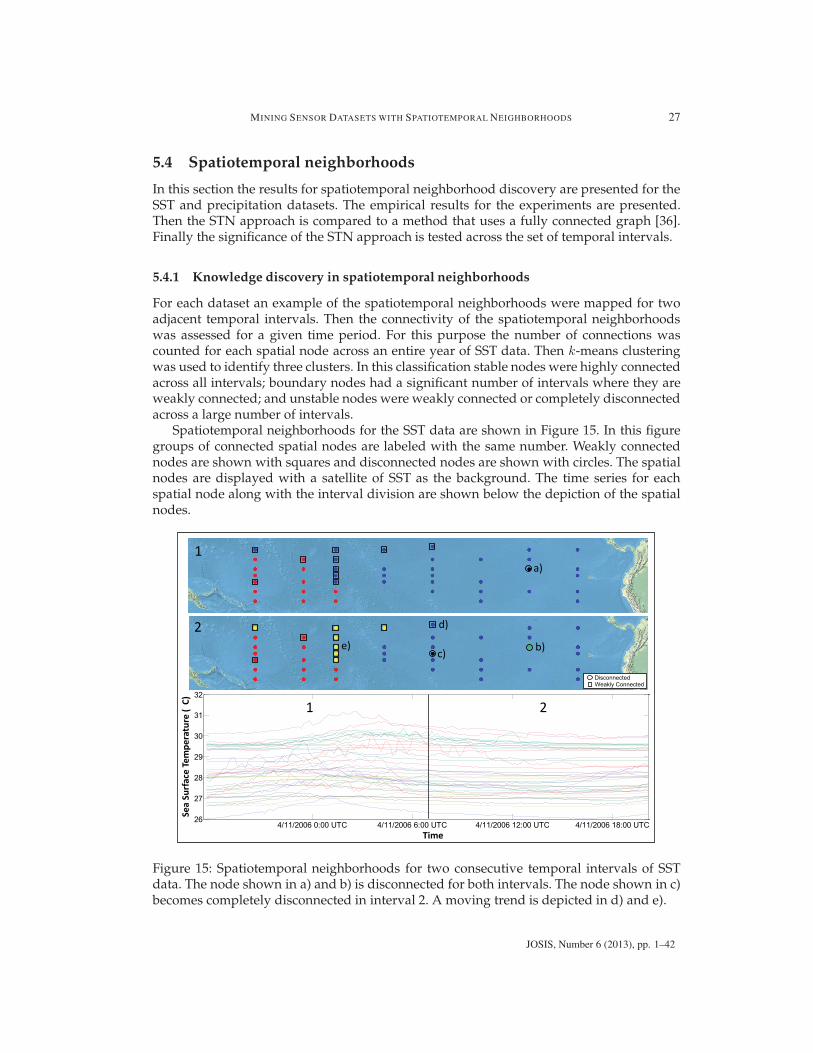
For each dataset an example of the spatiotemporal neighborhoods were mapped for twoadjacent temporal intervals. Then the connectivity of the spatiotemporal neighborhoodswas assessed for a given time period. For this purpose the number of connections wascounted for each spatial node across an entire year of SST data. Then k-means clusteringwas used to identify three clusters. In this classification stable nodes were highly connectedacross all intervals; boundary nodes had a significant number of intervals where they areweakly connected; and unstable nodes were weakly connected or completely disconnectedacross a large number of intervals.
Spatiotemporal neighborhoods for the SST data are shown in Figure 15. In this figuregroups of connected spatial nodes are labeled with the same number. Weakly connectednodes are shown with squares and disconnected nodes are shown with circles. The spatialnodes are displayed with a satellite of SST as the background. The time series for eachspatial node along with the interval division are shown below the depiction of the spatialnodes.
4/11/2006 0:00 UTC 4/11/2006 6:00 UTC 4/11/2006 12:00 UTC 4/11/2006 18:00 UTC26
27
28
29
30
31
32
1 2
1
2
a)
b)c)
d)
e)
Sea
Surf
ace
Tem
pera
ture
(C)
Time
DisconnectedWeakly Connected
Figure 15: Spatiotemporal neighborhoods for two consecutive temporal intervals of SSTdata. The node shown in a) and b) is disconnected for both intervals. The node shown in c)becomes completely disconnected in interval 2. A moving trend is depicted in d) and e).
JOSIS, Number 6 (2013), pp. 1–42
28 MICHAEL P. MCGUIRE, JANEJA, GANGOPADHYAY
Validation The algorithm was able to find the pattern of SST as validated by the satelliteimagery. Figure 15 a) depicts a completely disconnected spatial node. This is due to coldwater that typically travels west along the equator. This spatial node is disconnected in 15b). The cold water continues to travel westward in 15 c), where a node that was previouslyweakly connected in interval 1 is disconnected in interval 2. Figure 15 d) indicates anotherlocation where a moving trend is detected. In this scenario, a new neighborhood is createdin Figure 15 e) and spreads north and eastward.
Figure 16: Pattern of stability for one year of SST data. a) and e) disconnected nodes; b)boundary nodes; c) and d) instability caused by cold water traveling west along the equa-tor; e) instability caused by warm water coming from the southwest.
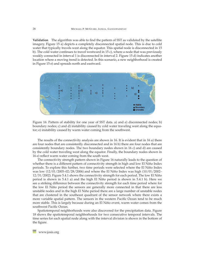
The results of the connectivity analysis are shown in 16. It is evident that in 16 a) thereare four nodes that are consistently disconnected and in 16 b) there are four nodes that areconsistently boundary nodes. The two boundary nodes shown in 16 c) and d) are causedby the cold water traveling west along the equator. Finally, the boundary nodes shown in16 e) reflect warm water coming from the south west.
The connectivity strength pattern shown in Figure 16 naturally leads to the question ofwhether there is a different pattern of connectivity strength in high and low El Nino Indexperiods. To explore this further, two time periods were selected where the El Nino Indexwas low (12/01/2005–02/28/2006) and where the El Nino Index was high (10/01/2002–12/31/2002). Figure 5.4.1 shows the connectivity strength for each period. The low El Ninoperiod is shown in 5.4.1 a) and the high El Nino period is shown in 5.4.1 b). Here wesee a striking difference between the connectivity strength for each time period where forthe low El Nino period the sensors are generally more connected in that there are lessunstable nodes and in the high El Nino period there are a large number of unstable nodesthat are clustered in the southeast quadrant of the sensor network where there exists amore variable spatial pattern. The sensors in the western Pacific Ocean tend to be muchmore stable. This is largely because during an El Nino event, warm water comes from thesouthwest Pacific Ocean.
Spatiotemporal neighborhoods were also discovered for the precipitation data. Figure18 shows the spatiotemporal neighborhoods for two consecutive temporal intervals. Thetime series for each spatial node along with the interval division is shown in the bottom ofthe figure.
www.josis.org

MINING SENSOR DATASETS WITH SPATIOTEMPORAL NEIGHBORHOODS 29
(a) Low El Nino Index period 12/01/2005–02/28/2006
(b) High El Nino Index period 10/01/2002–12/31/2002
Figure 17: Connectivity strength for high and low El Nino periods.
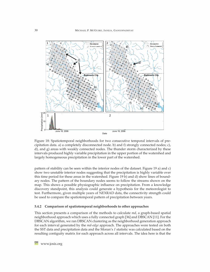
Validation The algorithm was effective in finding spatiotemporal neighborhoods in theprecipitation data. The interval shown in Figure 18 characterizes a heavy precipitationevent while in Figure 18-2 there is light precipitation. Figure 18 a) shows a completelydisconnected node. Figure 18 b) shows a large neighborhood of strongly connected node.Figure 18 c) shows three areas where there are weakly connected nodes. The pattern shownhere can be used to characterize precipitation for this particular temporal interval. Figures18 a) and c) represent areas of highly variable precipitation where there exists a large gra-dient suggesting a locally heavy downpour. Figure 18 b) represents an area with low vari-ability which indicates a homogeneous region of precipitation. In interval 2 in Figure 18,d) and f) show areas with strong connectivity while Figure 18 e) and g) show areas withweak connectivity. For this particular interval, these disconnected areas represent locallyheavy precipitation cells caused by local thunderstorms. This result can be used to char-acterize this precipitation event represented by interval 1: the upper part of the watershedhas a highly variable pattern of precipitation and the lower part of the watershed is largelyhomogeneous.
Figure 19 shows the results of the connectivity analysis for the entire year of precipita-tion data. It is evident that there is some spatial instability caused by the spatial configu-ration of the dataset in terms of unstable nodes occurring along the outside boundary. A
JOSIS, Number 6 (2013), pp. 1–42
30 MICHAEL P. MCGUIRE, JANEJA, GANGOPADHYAY
June 18, 2006 June 19, 20060
10
20
a)
b)
c)
d)
e)
f)
g)
1 2
1 2Pr
ecip
itatio
n (m
m)
Date
Figure 18: Spatiotemporal neighborhoods for two consecutive temporal intervals of pre-cipitation data. a) a completely disconnected node. b) and f) strongly connected nodes; c),d), and g) areas with weakly connected nodes. The thunder storm characterized by theseintervals produced highly variable precipitation in the upper portion of the watershed andlargely homogeneous precipitation in the lower part of the watershed.
pattern of stability can be seen within the interior nodes of the dataset. Figure 19 a) and c)show two unstable interior nodes suggesting that the precipitation is highly variable overthis time period for these areas in the watershed. Figure 19 b) and d) show lines of bound-ary nodes. The pattern of the boundary nodes seems to follow the streams shown on themap. This shows a possible physiographic influence on precipitation. From a knowledgediscovery standpoint, this analysis could generate a hypothesis for the meteorologist totest. Furthermore, given multiple years of NEXRAD data, the connectivity strength couldbe used to compare the spatiotemporal pattern of precipitation between years.
5.4.2 Comparison of spatiotemporal neighborhoods to other approaches
This section presents a comparison of the methods to calculate md, a graph-based spatialneighborhood approach which uses a fully connected graph [36] and DBSCAN [11]. For theDBSCAN algorithm, we ran DBSCAN clustering as the neighborhood generation approachfor each interval generated by the md-edge approach. The approaches were tested on boththe SST data and precipitation data and the Moran’s I statistic was calculated based on theresulting contiguity matrix for each approach across all intervals. The idea here is that the
www.josis.org
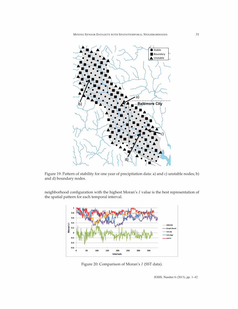
MINING SENSOR DATASETS WITH SPATIOTEMPORAL NEIGHBORHOODS 31
b)
c)
d)
a)
StableBoundaryUnstable
Figure 19: Pattern of stability for one year of precipitation data: a) and c) unstable nodes; b)and d) boundary nodes.
neighborhood configuration with the highest Moran’s I value is the best representation ofthe spatial pattern for each temporal interval.
-0.6
-0.4
-0.2
0
0.2
0.4
0.6
0.8
1
0 50 100 150 200 250 300 350
Mor
an's
I
Intervals
DBSCAN
Graph-Based
md-adj
md-edge
md-tri
Figure 20: Comparison of Moran’s I (SST data).
JOSIS, Number 6 (2013), pp. 1–42
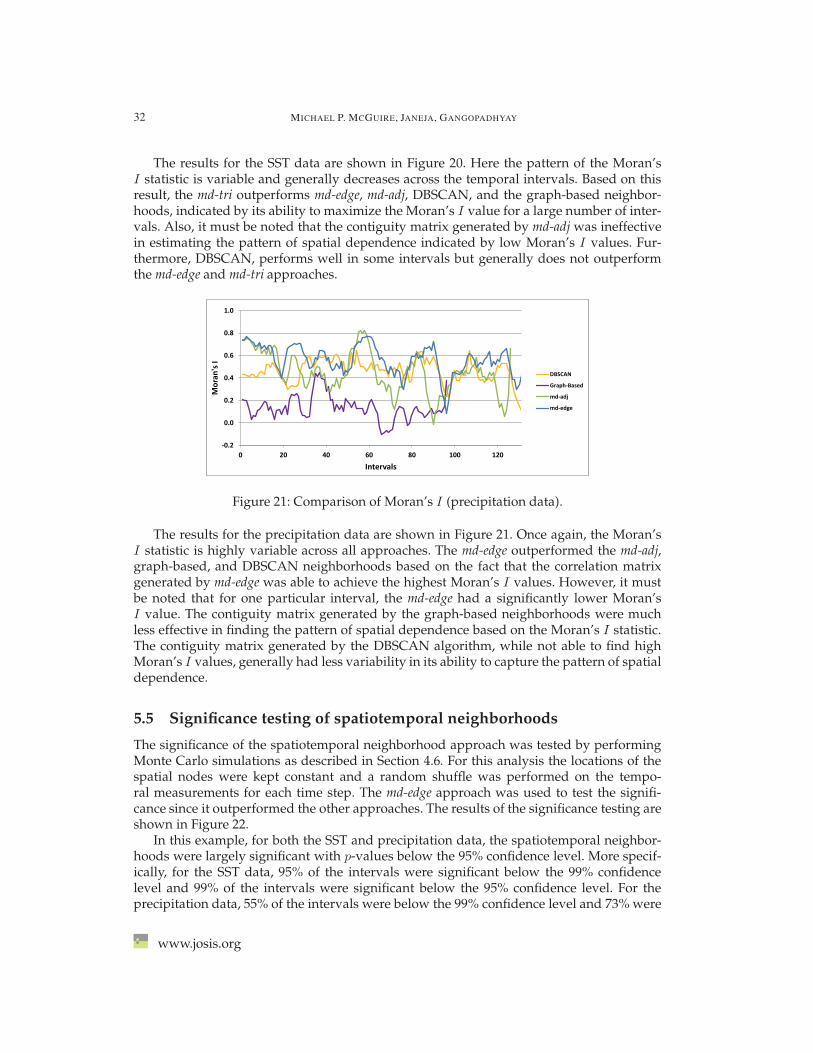
32 MICHAEL P. MCGUIRE, JANEJA, GANGOPADHYAY
The results for the SST data are shown in Figure 20. Here the pattern of the Moran’sI statistic is variable and generally decreases across the temporal intervals. Based on thisresult, the md-tri outperforms md-edge, md-adj, DBSCAN, and the graph-based neighbor-hoods, indicated by its ability to maximize the Moran’s I value for a large number of inter-vals. Also, it must be noted that the contiguity matrix generated by md-adj was ineffectivein estimating the pattern of spatial dependence indicated by low Moran’s I values. Fur-thermore, DBSCAN, performs well in some intervals but generally does not outperformthe md-edge and md-tri approaches.
-0.2
0.0
0.2
0.4
0.6
0.8
1.0
0 20 40 60 80 100 120
Mor
an's
I
Intervals
DBSCAN
Graph-Based
md-adj
md-edge
Figure 21: Comparison of Moran’s I (precipitation data).
The results for the precipitation data are shown in Figure 21. Once again, the Moran’sI statistic is highly variable across all approaches. The md-edge outperformed the md-adj,graph-based, and DBSCAN neighborhoods based on the fact that the correlation matrixgenerated by md-edge was able to achieve the highest Moran’s I values. However, it mustbe noted that for one particular interval, the md-edge had a significantly lower Moran’sI value. The contiguity matrix generated by the graph-based neighborhoods were muchless effective in finding the pattern of spatial dependence based on the Moran’s I statistic.The contiguity matrix generated by the DBSCAN algorithm, while not able to find highMoran’s I values, generally had less variability in its ability to capture the pattern of spatialdependence.
5.5 Significance testing of spatiotemporal neighborhoods
The significance of the spatiotemporal neighborhood approach was tested by performingMonte Carlo simulations as described in Section 4.6. For this analysis the locations of thespatial nodes were kept constant and a random shuffle was performed on the tempo-ral measurements for each time step. The md-edge approach was used to test the signifi-cance since it outperformed the other approaches. The results of the significance testing areshown in Figure 22.
In this example, for both the SST and precipitation data, the spatiotemporal neighbor-hoods were largely significant with p-values below the 95% confidence level. More specif-ically, for the SST data, 95% of the intervals were significant below the 99% confidencelevel and 99% of the intervals were significant below the 95% confidence level. For theprecipitation data, 55% of the intervals were below the 99% confidence level and 73% were
www.josis.org
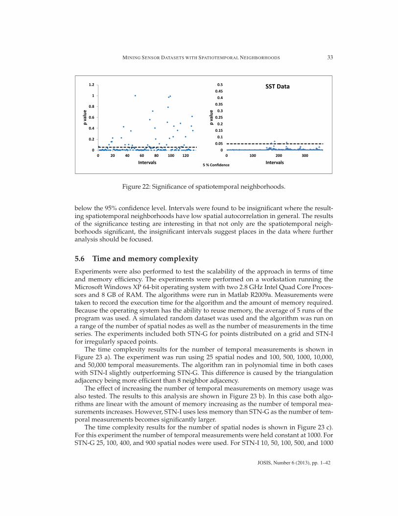
MINING SENSOR DATASETS WITH SPATIOTEMPORAL NEIGHBORHOODS 33
0
0.2
0.4
0.6
0.8
1
1.2
0 20 40 60 80 100 120
p va
lue
Intervals
00.05
0.10.15
0.20.25
0.30.35
0.40.45
0.5
0 100 200 300
p va
lue
Intervals95 % Confidence
SST Data
Figure 22: Significance of spatiotemporal neighborhoods.
below the 95% confidence level. Intervals were found to be insignificant where the result-ing spatiotemporal neighborhoods have low spatial autocorrelation in general. The resultsof the significance testing are interesting in that not only are the spatiotemporal neigh-borhoods significant, the insignificant intervals suggest places in the data where furtheranalysis should be focused.
5.6 Time and memory complexity
Experiments were also performed to test the scalability of the approach in terms of timeand memory efficiency. The experiments were performed on a workstation running theMicrosoft Windows XP 64-bit operating system with two 2.8 GHz Intel Quad Core Proces-sors and 8 GB of RAM. The algorithms were run in Matlab R2009a. Measurements weretaken to record the execution time for the algorithm and the amount of memory required.Because the operating system has the ability to reuse memory, the average of 5 runs of theprogram was used. A simulated random dataset was used and the algorithm was run ona range of the number of spatial nodes as well as the number of measurements in the timeseries. The experiments included both STN-G for points distributed on a grid and STN-Ifor irregularly spaced points.
The time complexity results for the number of temporal measurements is shown inFigure 23 a). The experiment was run using 25 spatial nodes and 100, 500, 1000, 10,000,and 50,000 temporal measurements. The algorithm ran in polynomial time in both caseswith STN-I slightly outperforming STN-G. This difference is caused by the triangulationadjacency being more efficient than 8 neighbor adjacency.
The effect of increasing the number of temporal measurements on memory usage wasalso tested. The results to this analysis are shown in Figure 23 b). In this case both algo-rithms are linear with the amount of memory increasing as the number of temporal mea-surements increases. However, STN-I uses less memory than STN-G as the number of tem-poral measurements becomes significantly larger.
The time complexity results for the number of spatial nodes is shown in Figure 23 c).For this experiment the number of temporal measurements were held constant at 1000. ForSTN-G 25, 100, 400, and 900 spatial nodes were used. For STN-I 10, 50, 100, 500, and 1000
JOSIS, Number 6 (2013), pp. 1–42
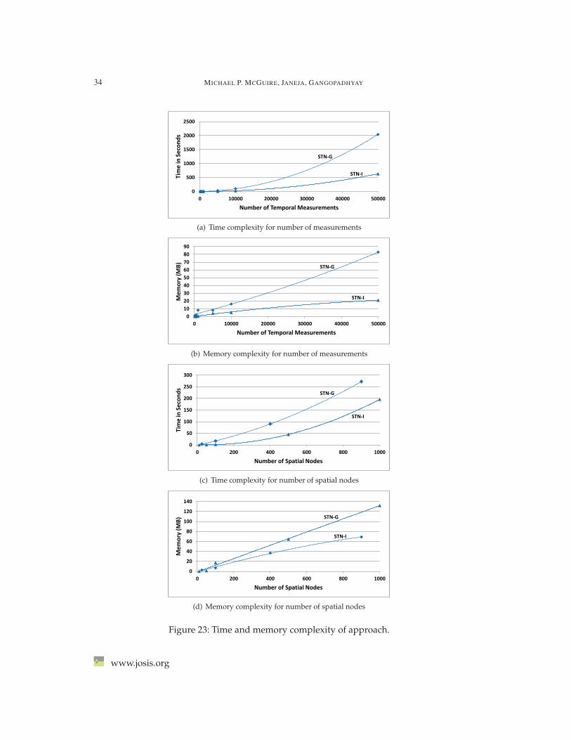
34 MICHAEL P. MCGUIRE, JANEJA, GANGOPADHYAY
0
500
1000
1500
2000
2500
0 10000 20000 30000 40000 50000
Tim
e in
Sec
onds
Number of Temporal Measurements
STN-G
STN-I
(a) Time complexity for number of measurements
STN-G
STN-I
0102030405060708090
0 10000 20000 30000 40000 50000
Mem
ory
(MB)
Number of Temporal Measurements
(b) Memory complexity for number of measurements
STN-G
STN-I
0
50
100
150
200
250
300
0 200 400 600 800 1000
Tim
e in
Sec
onds
Number of Spatial Nodes
(c) Time complexity for number of spatial nodes
STN-G
STN-I
0
20
40
60
80
100
120
140
0 200 400 600 800 1000
Mem
ory
(MB)
Number of Spatial Nodes
(d) Memory complexity for number of spatial nodes
Figure 23: Time and memory complexity of approach.
www.josis.org
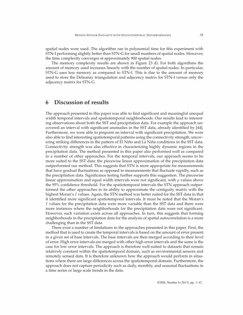
MINING SENSOR DATASETS WITH SPATIOTEMPORAL NEIGHBORHOODS 35
spatial nodes were used. The algorithm ran in polynomial time for this experiment withSTN-I performing slightly better than STN-G for small numbers of spatial nodes. However,the time complexity converges at approximately 900 spatial nodes.
The memory complexity results are shown in Figure 23 d). For both algorithms theamount of memory used increases linearly with the number of spatial nodes. In particular,STN-G uses less memory as compared to STN-I. This is due to the amount of memoryused to store the Delaunay triangulation and adjacency matrix for STN-I versus only theadjacency matrix for STN-G.
6 Discussion of results
The approach presented in this paper was able to find significant and meaningful unequalwidth temporal intervals and spatiotemporal neighborhoods. Our results lead to interest-ing observations about both the SST and precipitation data. For example the approach un-covered an interval with significant anomalies in the SST data, already identified by [44].Furthermore, we were able to pinpoint an interval with significant precipitation. We werealso able to find interesting spatiotemporal patterns using the connectivity strength, uncov-ering striking differences in the pattern of El Nino and La Nina conditions in the SST data.Connectivity strength was also effective in characterizing highly dynamic regions in theprecipitation data. The method presented in this paper also performed well as comparedto a number of other approaches. For the temporal intervals, our approach seems to bemore suited to the SST data: the piecewise linear approximation of the precipitation dataoutperformed our method. This suggests that STN is more appropriate for measurementsthat have gradual fluctuations as opposed to measurements that fluctuate rapidly, such asthe precipitation data. Significance testing further supports this suggestion. The piecewiselinear approximation and equal width intervals were not significant, with p values abovethe 95% confidence threshold. For the spatiotemporal intervals the STN approach outper-formed the other approaches in its ability to approximate the contiguity matrix with thehighest Moran’s I values. Again, the STN method was better suited for the SST data in thatit identified more significant spatiotemporal intervals. It must be noted that the Moran’sI values for the precipitation data were more variable than the SST data and there weremore instances where the neighborhoods for the precipitation data were not significant.However, such variation exists across all approaches. In turn, this suggests that formingneighborhoods in the precipitation data for the analysis of spatial autocorrelation is a morechallenging than in the SST data.
There exist a number of limitations to the approaches presented in this paper. First, themethod that is used to create the temporal intervals is based on the amount of error presentin a given set of base intervals. The base intervals are then merged according to their levelof error. High error intervals are merged with other high error intervals and the same is thecase for low error intervals. The approach is therefore well-suited to datasets that remainrelatively constant within the spatiotemporal domain, such as environmental sensors andremotely sensed data. It is therefore unknown how the approach would perform in situa-tions where there are large differences across the spatiotemporal domain. Furthermore, theapproach does not capture periodicity such as daily, monthly, and seasonal fluctuations ina time series or large scale trends in the data.
JOSIS, Number 6 (2013), pp. 1–42
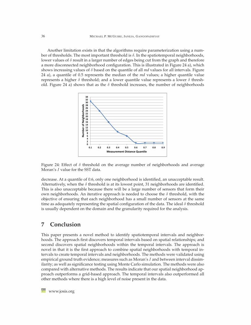
36 MICHAEL P. MCGUIRE, JANEJA, GANGOPADHYAY
Another limitation exists in that the algorithms require parameterization using a num-ber of thresholds. The most important threshold is δ. In the spatiotemporal neighborhoods,lower values of δ result in a larger number of edges being cut from the graph and thereforea more disconnected neighborhood configuration. This is illustrated in Figure 24 a), whichshows increasing values of δ based on the quantile of all md values for all intervals. Figure24 a), a quantile of 0.5 represents the median of the md values; a higher quantile valuerepresents a higher δ threshold; and a lower quantile value represents a lower δ thresh-old. Figure 24 a) shows that as the δ threshold increases, the number of neighborhoods
02468
10121416182022242628303234
0.1 0.2 0.3 0.4 0.5 0.6 0.7 0.8 0.9
Num
ber o
f Nei
ghbo
rhoo
ds
Measurement Distance Quantile
Figure 24: Effect of δ threshold on the average number of neighborhoods and averageMoran’s I value for the SST data.
decrease. At a quantile of 0.6, only one neighborhood is identified, an unacceptable result.Alternatively, when the δ threshold is at its lowest point, 31 neighborhoods are identified.This is also unacceptable because there will be a large number of sensors that form theirown neighborhoods. An iterative approach is needed to choose the δ threshold, with theobjective of ensuring that each neighborhood has a small number of sensors at the sametime as adequately representing the spatial configuration of the data. The ideal δ thresholdis usually dependent on the domain and the granularity required for the analysis.
7 Conclusion
This paper presents a novel method to identify spatiotemporal intervals and neighbor-hoods. The approach first discovers temporal intervals based on spatial relationships; andsecond discovers spatial neighborhoods within the temporal intervals. The approach isnovel in that it is the first approach to combine spatial neighborhoods with temporal in-tervals to create temporal intervals and neighborhoods. The methods were validated usingempirical ground truth evidence; measures such as Moran’s I and between interval dissim-ilarity; as well as significance testing using Monte Carlo simulation. The methods were alsocompared with alternative methods. The results indicate that our spatial neighborhood ap-proach outperforms a grid-based approach. The temporal intervals also outperformed allother methods where there is a high level of noise present in the data.
www.josis.org
MINING SENSOR DATASETS WITH SPATIOTEMPORAL NEIGHBORHOODS 37
There are a number of areas where this work can be extended. The temporal intervalscould be extended to include more properties of the time series, such as noise and period-icity and long term trends. A logical extension to this approach would be to include func-tionality to detect return frequencies and trends in the base intervals and to use this infor-mation to detect periodic and long-term trends in the data. For such an extension, a multi-resolution approach might be more suitable [37]. Another approach that has been recentlyproposed uses a combination of temporal and spatial autocorrelation to find spatiotem-poral outliers [63]. This approach shows promising results in outlier and event detection.A similar approach using spatiotemporal autocorrelation could be used to find periodicand long-term trends in the data. Another direction for extension of this work would beto include a method to differentiate between interval divisions caused by malfunctioningsensors versus those caused by naturally occurring events. Lastly, the method presented inthis paper is based on the analysis of a single attribute over space and time. This approachcould be extended to deal with multiple attributes in a spatiotemporal dataset simply byadapting the md calculation, based on the Euclidean distance, to multiple attributes.
Acknowledgments
This work has been funded in part by the United States National Oceanic and AtmosphericAdministration Grants NA06OAR4310243, NA07OAR4170518, and NA10OAR310220. Thestatements, findings, conclusions, and recommendations are those of the authors and donot necessarily reflect the views of the National Oceanic and Atmospheric Administrationor the Department of Commerce. This work was also partially supported by the FDRCgrant of Towson University.
References
[1] ABONYI, J., FEIL, B., NEMETH, S., AND ARVA, P. Fuzzy clustering basedsegmentation of time-series. In Proc. 5th International Symposium on IntelligentData Analysis (IDA) (2003), M. R. Berthold, H.-J. Lenz, E. Bradley, R. Kruse,and C. Borgelt, Eds., Lecture Notes in Computer Science, Springer, pp. 275–285.doi:10.1007/978-3-540-45231-7 26.
[2] ADAM, N. R., JANEJA, V. P., AND ATLURI, V. Neighborhood based detection ofanomalies in high dimensional spatio-temporal sensor datasets. In Proc. ACM Sym-posium on Applied Computing (SAC) (2004), pp. 576–583. doi:10.1145/967900.968020.
[3] ANKERST, M., BREUNIG, M., KRIEGEL, H., AND SANDER, J. OPTICS: Ordering pointsto identify the clustering structure. In Proc. ACM SIGMOD International Conference onManagement of Data (1999), ACM Press, pp. 49–60. doi:10.1145/304182.304187.
[4] BELLMAN, R., AND ROTH, R. Curve fitting by segmented straight lines.Journal of the American Statistical Association 64, 327 (1969), 1079–1084.doi:10.1080/01621459.1969.10501038.
[5] CANE, M. Oceanographic events during El Nino. Science 222, 4629 (1983), 1189–1195.doi:10.1126/science.222.4629.1189.
JOSIS, Number 6 (2013), pp. 1–42
38 MICHAEL P. MCGUIRE, JANEJA, GANGOPADHYAY
[6] CHAN, J., BAILEY, J., AND LECKIE, C. Discovering and summarising regionsof correlated spatio-temporal change in evolving graphs. In Proc. 6th IEEE In-ternational Conference on Data Mining (2006), IEEE Computer Society, pp. 361–365.doi:10.1109/ICDMW.2006.61.
[7] CLIFF, A. D., AND ORD, J. K. Spatial Autocorrelation. Pion, London, 1973.doi:10.2307/143144.
[8] CRESSIE, N., AND WIKLE, C. Statistics for spatio-temporal data. Wiley, Hoboken, NJ,2011.
[9] DELAUNAY, B. Sur la sphere vide. Bulletin of Academy of Sciences of the USSR, 6 (1934),793–800.
[10] ESTER, M., KRIEGEL, H., AND SANDER, J. Spatial data mining: A database approach.In 5th International Symposium on Advances in Spatial Databases (1997), Springer, pp. 47–66. doi:10.1007/3-540-63238-7 24.
[11] ESTER, M., KRIEGEL, H., SANDER, J., AND XU, X. A density-based algorithm for dis-covering clusters in large spatial databases with noise. In Proc. 2nd International Con-ference on Knowledge Discovery and Data Mining (1996), pp. 226–231. doi:10.1.1.121.9220.
[12] FLAKE, G., TARJAN, R., AND TSIOUTSIOULIKLIS, K. Graph clustering and minimumcut trees. Internet Mathematics 1, 4 (2004), 385–408.
[13] FREY, B., AND DUECK, D. Clustering by passing messages between data points. Sci-ence 315, 5814 (2007), 972–976. doi:10.1126/science.1136800.
[14] GEARY, R. The contiguity ratio and statistical mapping. The Incorporated Statistician(1954), 115–145. doi:10.2307/2986645.
[15] GEORGE, B., KANG, J., AND SHEKHAR, S. Spatio-temporal sensor graphs (STSG): Asensor model for the discovery of spatio-temporal patterns. In Proc. First InternationalWorkshop on Knowledge Discovery from Sensor Data (2007). doi:10.3233/IDA-2009-0376.
[16] GEORGE, B., AND SHEKHAR, S. Time-aggregated graphs for modelingspatio-temporal networks. Lecture Notes in Computer Science 4231 (2006), 85.doi:10.1007/11908883 12.
[17] GOODCHILD, M. F. Spatial Autocorrelation. Geo Books, Norwich, UK, 1986.
[18] GUHA, S., RASTOGI, R., AND SHIM, K. Cure: An efficient clustering algorithm forlarge databases. Information Systems 26, 1 (2001), 35–58. doi:10.1145/276304.276312.
[19] HADJIELEFTHERIOU, M., KOLLIOS, G., GUNOPULOS, D., AND TSOTRAS, V. On-linediscovery of dense areas in spatio-temporal databases. Lecture Notes in Computer Sci-ence (2003), 306–324. doi:10.1.1.7.2606.
[20] HAN, J., M. K., AND TUNG, A. K. H. Spatial clustering methods in data mining: Asurvey. In Geographic Data Mining and Knowledge Discovery. Taylor and Francis, Lon-don, UK, 2001, ch. 1, pp. 1–29.
www.josis.org
MINING SENSOR DATASETS WITH SPATIOTEMPORAL NEIGHBORHOODS 39
[21] HIMBERG, J., KORPIAHO, K., MANNILA, H., TIKANMAKI, J., AND TOIVO-NEN, H. Time series segmentation for context recognition in mobile devices.In Proc. International Conference on Data Mining (ICDM) (2001), pp. 203–210.doi:10.1109/ICDM.2001.989520.
[22] JANEJA, V., AND ATLURI, V. Random walks to identify anomalous free-form spatialscan windows. IEEE Transactions on Knowledge and Data Engineering 20, 10 (2008), 1378–1392.
[23] JOHNSON, S. Hierarchical clustering schemes. Psychometrika 32, 3 (1967), 241–254.doi:10.1007/BF02289588.
[24] KALNIS, P., MAMOULIS, N., AND BAKIRAS, S. On discovering moving clustersin spatio-temporal data. In Proc. Advances in Spatial and Temporal Databases (2005),C. Medeiros, M. Egenhofer, and E. Bertino, Eds., vol. 3633 of Lecture Notes in ComputerScience, pp. 364–381.
[25] KANG, I.-S., KIM, T.-W., AND LI, K.-J. A spatial data mining method by Delaunaytriangulation. In Proc. 5th ACM International Workshop on Advances in Geographic Infor-mation Systems (1997), ACM, pp. 35–39. doi:10.1145/267825.267836.
[26] KARYPIS, G., HAN, E.-H., AND KUMAR, V. Chameleon: Hierarchical clustering usingdynamic modeling. Computer 32, 8 (1999), 68–75. doi:10.1109/2.781637.
[27] KAUFMAN, L., AND ROUSSEEUW, P. Finding Groups in Data. Wiley, New York, 1990.
[28] KEOGH, E., CHU, S., HART, D., AND PAZZANI, M. An online algorithm for seg-menting time series. In Proc. IEEE International Conference on Data Mining (2001), IEEEComputer Society, pp. 289–296. doi:10.1109/ICDM.2001.989531.
[29] KEOGH, E., AND SMYTH, P. A probabilistic approach to fast pattern matching in timeseries databases. In Proc. 3rd International Conference on Knowledge Discovery and DataMining (KDD) (1997), pp. 24–30.
[30] KOHLER, E., LANGKAU, K., AND SKUTELLA, M. Time-expanded graphs for flow-dependent transit times. In Proc. 10th Annual European Symposium on Algorithms (ESA)(2002), vol. 2, Springer, pp. 599–611.
[31] KRAJEWSKI, W. F., KRUGER, A., SMITH, J. A., BAECK, M. L., DOMASZCZYNSKI, P.,GOSKA, R., SEO, B., CUNHA, L., GUNYON, C., VILLARINI, G., AND NTELEKOS, A.Hydro-NEXRAD: A community resource for future research on improving rainfall-rainfall estimation and hydrologic applications. In AGU Fall Meeting Abstracts (Dec.2007).
[32] LEMIRE, D. A better alternative to piecewise linear time series segmentation. In Proc.7th SIAM International Conference on Data Mining (2007).
[33] LIN, F., XIE, K., SONG, G., AND WU, T. A novel spatio-temporal clustering approachby process similarity. In Proc. 6th International Conference on Fuzzy Systems and Knowl-edge Discovery (FSKD) (2009), vol. 5, pp. 150–154. doi:10.1109/FSKD.2009.584.
JOSIS, Number 6 (2013), pp. 1–42
40 MICHAEL P. MCGUIRE, JANEJA, GANGOPADHYAY
[34] LIU, D., NOSOVSKIY, G. V., AND SOURINA, O. Effective clustering and boundarydetection algorithm based on delaunay triangulation. Pattern Recognition Letters 29, 9(2008), 1261–1273. doi:10.1016/j.patrec.2008.01.028.
[35] MACQUEEN, J. Some methods for classification and analysis of multivariate observa-tions. In Proc. 5th Berkeley Symposium on Mathematical Statistics and Probability (1967),vol. 1, pp. 281–297.
[36] MCGUIRE, M., JANEJA, V., AND GANGOPADHYAY, A. Spatiotemporal neighborhooddiscovery for sensor data. Lecture Notes in Computer Science 5840 (2010), 203–225.doi:10.1007/978-3-642-12519-5 12.
[37] MCGUIRE, M., JANEJA, V., AND GANGOPADHYAY, A. Characterizing sensor datasetswith multi-granular spatio-temporal intervals. In Proc. 19th ACM SIGSPATIAL In-ternational Conference on Advances in Geographic Information Systems (2011), ACM.doi:10.1145/2F2093973.2094045.
[38] MCPHADEN, M. Genesis and evolution of the 1997–98 el nino. Science 283 (1999),950–954. doi:10.1126/science.283.5404.950.
[39] METROPOLIS, N., AND ULAM, S. The Monte Carlo method. Journal of the AmericanStatistical Association (1949), 335–341. doi:10.1080/01621459.1949.10483310.
[40] MOHAMMADI, S., JANEJA, V., AND GANGOPADHYAY, A. Discretized spatio-temporalscan window. In Proc. 9th SIAM International Conference on Data Mining (2009).
[41] MORAN, P. The interpretation of statistical maps. Journal of the Royal Statistical SocietyB 10, 2 (1948), 245–251.
[42] NG, R., AND HAN, J. CLARANS: A method for clustering objects for spatial datamining. IEEE Transactions on Knowledge and Data Engineering 14, 5 (2002), 1003–1016.doi:10.1109/TKDE.2002.1033770.
[43] NOAA, NATIONAL OCEANIC AND ATMOSPHERIC ADMINISTRATION. State of theClimate: El Nino/Southern Oscillation Analysis for Annual 2006. http:�www.ncdc.noaa.gov/sotc/enso/2006/13, December 2006. Accessed 11 February 2013.
[44] NOAA, NATIONAL OCEANIC AND ATMOSPHERIC ADMINISTRATION. State of theClimate El Nino/Southern Oscillation Analysis November 2006. http:�www.ncdc.noaa.gov/sotc/?report=enso&year=2006&month=11&submitted=Get+Report, 2006.Accessed 11 February 2013.
[45] NOAA, NATIONAL OCEANIC AND ATMOSPHERIC ADMINISTRATION. Cold andwarm episodes by season. http:�www.cpc.noaa.gov/products/analysis monitoring/ensostuff/ensoyears.shtml, 2009. Accessed 11 February 2013.
[46] NOAA, NATIONAL OCEANIC AND ATMOSPHERIC ADMINISTRATION. Tropical atmo-sphere ocean project. http:�www.pmel.noaa.gov/tao/jsdisplay/, 2009. Accessed 11February 2013.
[47] NOAA, NATIONAL OCEANIC AND ATMOSPHERIC ADMINISTRATION. El NinoTheme Page. http:�www.pmel.noaa.gov/tao/elnino/el-nino-story.html, 2010. Ac-cessed 11 February 2013.
www.josis.org
MINING SENSOR DATASETS WITH SPATIOTEMPORAL NEIGHBORHOODS 41
[48] OKABE, A., BOOTS, B., SUGIHARA, K., AND CHIU., S. Spatial Tessellations: Conceptsand Applications of Voronoi Diagrams. Wiley, 2000.
[49] RASMUSSON, E., AND WALLACE, J. Meteorological aspects of the El Nino/SouthernOscillation. Science 222, 4629 (1983), 1195–1202. doi:10.1126/science.222.4629.1195.
[50] RELJIN, I., RELJIN D, B., AND JOVANOVIC, G. Clustering and mapping spatial-temporal datasets using som neural networks. Journal of Automatic Control 13, 1 (2003),55–60.
[51] REYNOLDS, R., SMITH, T., LIU, C., CHELTON, D., CASEY, K., AND SCHLAX, M. Dailyhigh-resolution-blended analyses for sea surface temperature. Journal of Climate 20, 22(2007), 5473–5496. doi:10.1175/2007JCLI1824.1.
[52] ROSSWOG, J. GHOSE, K. Detecting and tracking spatio-temporal clusters with adap-tive history filtering. In Proc. IEEE International Conference on Data Mining Workshops(ICDMW) (2008), pp. 448–457. doi:10.1109/ICDMW.2008.93.
[53] ROYLANCE, F. Maryland weather blog. http:�weblogs.marylandweather.com, 2006.Accessed 11 February 2013.
[54] SAP, M.N.M. AWAN, A. Finding spatio-temporal patterns in climate data using clus-tering. In Proc. International Conference on Cyberworlds (2005). doi:10.1109/CW.2005.45.
[55] SHEIKHOLESLAMI, G., CHATTERJEE, S., AND ZHANG, A. WaveCluster: A multi-resolution clustering approach for very large spatial databases. In Proc. 24rd Inter-national Conference on Very Large Data Bases (1998), pp. 428–439.
[56] SHEKHAR, S., EVANS, M., KANG, J., AND MOHAN, P. Identifying patterns in spatialinformation: A survey of methods. Wiley Interdisciplinary Reviews: Data Mining andKnowledge Discovery 1, 3 (2011), 193–214. doi:10.1002/widm.25.
[57] SHEKHAR, S., LU, C., AND ZHANG, P. Detecting graph-based spatial outliers: Al-gorithms and applications (a summary of results). In Proc. 7th ACM SIGKDD In-ternational Conference on Knowledge Discovery and Data Mining (2001), pp. 371–376.doi:10.1145/502512.502567.
[58] TOBLER, W. A computer movie simulating urban growth in the Detroit region. Eco-nomic Geography 46 (1970), 234–240.
[59] VERHEIN, F., AND CHAWLA, S. Mining spatio-temporal patterns in objectmobility databases. Data Mining and Knowledge Discovery 16, 1 (2008), 5–38.doi:10.1007/s10618-007-0079-5.
[60] WANG, W., YANG, J., AND MUNTZ, R. STING: A Statistical Information Grid Approachto Spatial Data Mining. Morgan Kaufmann, San Francisco, CA, 1997.
[61] ZABIH, R., AND KOLMOGOROV, V. Spatially coherent clustering using graph cuts. InProc. IEEE Computer Society Conference on Computer Vision and Pattern Recognition (LosAlamitos, CA, 2004), vol. 2, IEEE Computer Society, pp. 437–444.
JOSIS, Number 6 (2013), pp. 1–42

42 MICHAEL P. MCGUIRE, JANEJA, GANGOPADHYAY
[62] ZHANG, T., RAMAKRISHNAN, R., AND LIVNY, M. BIRCH: An efficient data clus-tering method for very large databases. In Proc. ACM SIGMOD International Con-ference on Management of Data (1996), ACM Press New York, NY, USA, pp. 103–114.doi:10.1.1.152.7115.
[63] ZHANG, Y., HAMM, N., MERATNIA, N., STEIN, A., VAN DE VOORT, M., ANDHAVINGA, P. Statistics-based outlier detection for wireless sensor networks.International Journal of Geographical Information Science 26, 8 (2012), 1373–1392.doi:10.1080/13658816.2012.654493.
www.josis.org


