Embed Size (px)
Citation preview
MIPAS Level 2 ATBD
Prog. Doc. N.: IFAC_GA_2007_12_SC
Issue: 7.1 Revision: FINAL
Date: 07/01/2020 Page 1 of 124
High level algorithm definition and
physical and mathematical optimisations
MIPAS Level 2 Algorithm Theoretical Baseline Document
(MIPAS Level 2 ATBD)
7 January 2020
Issue 7 Rev. 1
(Compliant with ORM Version 8.22)
Delivery of the study:
Support to MIPAS Level 2 processor verification and validation - Phase F
upgrade of the delivery of the original studies:
“Support to MIPAS Level 2 Product Validation” and
"Development of an Optimised Algorithm for Routine P, T and VMR Retrieval from MIPAS
Limb Emission Spectra"
Prepared by:
Name Institute
B. Carli IFAC-CNR, Firenze, Italy
M. Carlotti University of Bologna, Italy
S. Ceccherini IFAC-CNR, Firenze, Italy
M. Höpfner KIT, Karlsruhe, Germany
P. Raspollini IFAC-CNR, Firenze, Italy
M. Ridolfi University of Bologna, Italy
L. Sgheri IAC-CNR, Firenze, Italy
MIPAS Level 2 ATBD
Prog. Doc. N.: IFAC_GA_2007_12_SC
Issue: 7.1 Revision: FINAL
Date: 07/01/2020 Page 2 of 124
TABLE OF CONTENTS
1 - INTRODUCTION 7
1.1 Changes from Issue 2A to Issue 3 of the present document 8
1.2 Changes from Issue 3 to Issue 4 of the present document 8
1.3 Changes from Issue 4 to Issue 5 of the present document 9
1.4 Changes from Issue 5 to Issue 6 of the present document 9
1.5 Changes from Issue 6 to Issue 7 of the present document 9
2 - OBJECTIVES OF THE TECHNICAL NOTE 10
3 - CRITERIA FOR THE OPTIMISATION 10
4 - THE INVERSE (OR RETRIEVAL) PROBLEM 11
4.1 Mathematical conventions 11
4.2 Theoretical background 12 4.2.1 The direct problem 12 4.2.2 The Gauss Newton method 13 4.2.3 The Levenberg-Marquardt method 15 4.2.4 Review of the possible convergence criteria 16 4.2.5 Use of external (a-priori) information in the inversion model 17 4.2.6 Use of the optimal estimation, for inclusion of LOS engineering information (LEI) in p,T retrieval 18 4.2.7 Covariance matrix and averaging kernels of the LM solution 21
4.3 The global fit analysis 23
4.4 The forward model 23 4.4.1 The radiative transfer 24 4.4.2 Convolution with the AILS 27 4.4.3 Convolution with the FOV 27 4.4.4 Instrumental continuum 28 4.4.5 Summary of required variables 28
4.5 Calculation of the VCM of the measurements 29 4.5.1 Operations performed on the interferogram to obtain the apodised spectrum 29 4.5.2 Computation of the VCM relating to a single microwindow 31 4.5.3 Computation of the inverse of the VCM 33
4.6 Calculation of the Jacobian matrix K of the simulations 34
4.7 Generalised inverse 35
4.8 Variance-covariance matrix of tangent height corrections 35
4.9 Tangent heights correction based on ECMWF data 37
5 - SCIENTIFIC ASPECTS AND PHYSICAL OPTIMISATIONS 39
5.1 Choice between retrieval of profiles at fixed levels and at tangent altitude levels 39
MIPAS Level 2 ATBD
Prog. Doc. N.: IFAC_GA_2007_12_SC
Issue: 7.1 Revision: FINAL
Date: 07/01/2020 Page 3 of 124
5.1.1 Retrieval at tangent altitude and interpolation between retrieved values 39 5.1.2 Retrieval at fixed levels 40 5.1.3 Discussion of the problem 40 5.1.4 Conclusions 41
5.2 Use of a-priori information 41 5.2.1 - Precision improvement 41 5.2.2 - Systematic errors 42 5.2.3 - Hydrostatic equilibrium and LOS Engineering information 43
5.3 Latitudinal variability 44 5.3.1 Angular spread of the limb measurements 44 5.3.2 Latitudinal temperature gradients 45 5.3.3 Modeling the latitudinal variability with a horizontal gradient 45
5.4 Earth model and gravity 48 5.4.1 Earth model 48 5.4.2 Gravity 48
5.5 Ray tracing and atmospheric refraction 50 5.5.1 Refraction model 52
5.6 Line shape modeling 52 5.6.1 Numerical calculation of the Voigt profile 53 5.6.2 Approximation of the Voigt profile by the Lorentz function 54 5.6.3 -factors in the case of CO2 and H2O 54
5.7 Line-mixing 55
5.8 Pressure shift 55
5.9 Implementation of Non-LTE effects 56
5.10 Self broadening 56
5.11 Continuum 57 5.11.1 Instrumental continuum 57 5.11.2 Near continuum 57 5.11.3 Far continuum 57
5.12 Interpolation of the profiles in the forward / retrieval model 59
5.13 Interpolation of the “retrieved” profiles to a user-defined grid 60
5.14 Optimized algorithm for construction of initial guess profiles and gradients 62 5.14.1 Initial guess pressure, temperature and VMR profiles, and their horizontal gradients 62 5.14.2 Initial guess continuum profiles 63
5.15 Profiles regularization 63 5.15.1 The error consistency (EC) method 63 5.15.2 The Iterative Variable Strength (IVS) regularization method 67
5.16 Cloud filtering 70
6 - MATHEMATICAL OPTIMISATIONS 72
6.1 Radiative Transfer integral and use of Curtis-Godson mean values 72 6.1.1 Layering of the atmosphere 75
6.2 Secant law approximation for the calculation of Curtis-Godson quantities and definition of paths (not
used in the ORM v.8) 77
MIPAS Level 2 ATBD
Prog. Doc. N.: IFAC_GA_2007_12_SC
Issue: 7.1 Revision: FINAL
Date: 07/01/2020 Page 4 of 124
6.2.2 Sequence of the operations 81
6.3 Interpolation of cross sections for different geometries 82
6.4 Calculation of the spectrum: spherical symmetries (not used in the ORM v.8) 83
6.5 Use of interpolation for the calculation of Planck function 84
6.6 Finite instrument field of view. 85
6.7 Analytical derivatives 89 6.7.1 General considerations 89 6.7.2 Derivative with respect to the volume mixing ratio 91 6.7.3 Derivative with respect to temperature 92 6.7.4 Derivative with respect to the atmospheric continuum 93 6.7.5 Derivative with respect to the tangent pressure 93 6.7.6 Independence of retrieved variables 94 6.7.7 New choice of continuum variables in the MIPAS processor starting from V.7.0. 94
6.8 Convergence criteria 96
6.9 Pre-calculation of line shapes 97
6.10 Different grids during the cross-section calculation 98
6.11 Cross-section look-up tables 98
6.12 Variable frequency grids for radiative transfer computation 99
REFERENCES 100
APPENDIX A: DETERMINATION OF THE VCM OF ENGINEERING TANGENT
HEIGHTS IN MIPAS 103
APPENDIX B: EVALUATION OF RETRIEVAL ERROR COMPONENTS AND TOTAL
ERROR BUDGET 112
APPENDIX C: GENERATION OF MW DATABASES AND OCCUPATION MATRICES114
APPENDIX D: GENERATION OF LUTS AND IRREGULAR FREQUENCY GRIDS (IG)116
APPENDIX E: GENERATION OF MW-DEDICATED SPECTRAL LINELISTS 117
APPENDIX F: MIPAS OBSERVATION MODES 121
MIPAS Level 2 ATBD
Prog. Doc. N.: IFAC_GA_2007_12_SC
Issue: 7.1 Revision: FINAL
Date: 07/01/2020 Page 5 of 124
ACRONYMS LIST
AILS Apodised Instrument Line Shape
ATBD Algorithm Theoretical Baseline Document
ATMOS Atmospheric Trace MOlecule Spectroscopy experiment
BAe British Aerospace
CKD Clough-Kneizys-Davies
CPU Central Processing Unit
EC Error Consistency
ECMWF European Centre for Medium-range Weather Forecasts
ENVISAT ENVironment SATellite
ESA European Space Agency
FM Forward Model
FOV Field Of View
FR Full Resolution measurements acquired by MIPAS in the
first two years of operations (2002 – 2004)
FTS Fourier Transform Spectrometer
FWHM Full Width at Half Maximum
GN Gauss Newton (minimization method)
HITRAN HIgh-resolution TRANsmission molecular absorption
database
HWHM Half Width at Half Maximum
IAPTs Implemented Atmospheric Pressures and Temperatures,
IFOV Instantaneous Field Of View
IG Irregular Grid
ILS Instrument Line Shape
IMK Institut für Meteorologie und Klimaforschung
IVS Iterative Variable Strength (regularization method)
LEI LOS Engineering Information
LM Levenberg-Marquardt (minimization method)
LOS Line Of Sight
LS Lower Stratosphere
LSF Least Squares Fit
LTE Local Thermal Equilibrium
MIPAS Level 2 ATBD
Prog. Doc. N.: IFAC_GA_2007_12_SC
Issue: 7.1 Revision: FINAL
Date: 07/01/2020 Page 6 of 124
LUT Look Up Table
MIPAS Michelson Interferometer for Passive Atmospheric
Sounding
ML2PP MIPAS Level 2 Processor Prototype
MPD Maximum Path Difference
MW spectral MicroWindow
NESR Noise Equivalent Spectral Radiance
NLSF Non-linear Least Squares Fit
NLTE, Non-LTE Non Local Thermal Equilibrium
NRT Near Real Time
OFM Optimized Forward Model
OR Optimized Resolution measurements acquired by MIPAS
from January 2005 to April 2012
ORM Optimised Retrieval Model
PDS Payload Data Segment
POEM Polar Orbit Earth Mission
REC Residuals and Errors Correlation analysis
RFM Reference Forward Model
RMS Root Mean Square
SVD Singular Value Decomposition
TA Tangent Altitude
UTLS Upper Troposphere / Lower Stratosphere
VCM Variance Covariance Matrix
VMR Volume Mixing Ratio
VS Variable Strength (regularization method)
ZFPD Zero-Filled Path Difference
ZPD Zero Path Difference
MIPAS Level 2 ATBD
Prog. Doc. N.: IFAC_GA_2007_12_SC
Issue: 7.1 Revision: FINAL
Date: 07/01/2020 Page 7 of 124
1 - Introduction
MIPAS (Michelson Interferometer for Passive Atmospheric Sounding) is an ESA developed
instrument that operated on board of the ENVISAT satellite launched on a polar orbit on March 1st,
2002, as part of the first Polar Orbit Earth Observation Mission program (POEM-1). MIPAS measured
the atmospheric limb-emission spectrum in the middle infrared (670 – 2410 cm-1) from April 2002
until 8 April 2012, i.e. the day in which the contact with ENVISAT was lost. The first measurement
acquired by MIPAS dates back to 24 March 2002. Starting from July 2002 nearly continuous
measurements were acquired during the first two years of operations. In this mission phase, most of
the measurements were acquired with a spectral resolution of 0.025 cm-1, in the nominal scanning
mode, consisting of 17 sweeps per limb scan, with tangent heights ranging from 6 to 68 km and steps
of 3 km from 6 to 42 km, of 5 km from 42 to 52 km and of 8 km from 52 to 68 km. In this period only
few measurements were acquired using the so called “special modes”. The measurements relating to
the first two years (2002 – 2004) of operations are referred to as Full-Resolution (FR) measurements.
Due to problems with the mirror driver of the interferometer, MIPAS measurements were discontinued
at the end of March of 2004. In January 2005 MIPAS operations were resumed with a reduced
maximum interferometric optical path difference (corresponding to a lower spectral resolution of
0.0625 cm-1 instead of the original 0.025 cm-1) and with a finer vertical sampling step of the limb
measurements. These measurements acquired from January 2005 onward are referred to as Optimized
Resolution (OR) measurements. Several new special measurement modes were devised for this mission
phase and a significant fraction of measurements was actually acquired in this configuration. Appendix
F includes a detailed description of the measurement modes employed during the whole MIPAS
mission.
The raw interferograms acquired by MIPAS are transformed into geo-located and radiometrically
calibrated spectral radiances by the Level 1b processing chain. Subsequently, the Level 2 processor
inverts the calibrated radiances to infer the vertical distribution profiles of numerous trace gases and
atmospheric state variables.
Starting from 1995, in the frame of the ESA project "Development of an Optimised Algorithm for
Routine P, T and VMR Retrievals from MIPAS Limb Emission Spectra" a scientific code referred to
as the Optimized Retrieval Model (ORM) was developed for near real time (NRT) Level 2 analysis of
MIPAS. The code was developed by optimizing the accuracy of the Level 2 products, with the
limitations owing to the strong computing time constraint set by the needs of NRT processing. The
results of the study were used by industry as an input for the development of a prototype for the Level
2 code, the so called ML2PP. In turn, the algorithms of the ML2PP were re-coded by a second industrial
contractor and implemented in the ENVISAT payload data segment (PDS). MIPAS Level 2 products
up to Version 5.x were generated by the ENVISAT PDS Level 2 processor. In the time frame from
2002 to 2004, MIPAS measurements were processed by ESA both Near-Real Time (NRT) and,
subsequently, off-line (OFL) with the same PDS processor, but using different auxiliary data to get
more accurate results at the expenses of an increased computing time. MIPAS Level 2 products
Versions 6.x and 7.x were generated by ESA, using the ML2PP. The final reprocessing of MIPAS data,
Version 8, was obtained using directly the ORM Version 8. This last version of the ORM differs
significantly as compared to the older versions: the original NRT computing time requirements do not
hold for this version, allowing the implementation of much more sophisticated and accurate algorithms.
Moreover, while the earliest ESA Level 2 processor versions were able to handle only nominal mode
MIPAS measurements, ORM version 8 is able to handle all measurement modes. The processing of
the modes including tangent heights above 75 km is however limited to the sweeps with tangent
altitudes lower than this bound. This choice prevents the assumption of Local Thermodynamic
Equilibrium (LTE), still present in the ORM v8, from introducing too large model errors in the
simulated radiances.

MIPAS Level 2 ATBD
Prog. Doc. N.: IFAC_GA_2007_12_SC
Issue: 7.1 Revision: FINAL
Date: 07/01/2020 Page 8 of 124
Using a pre-defined set of auxiliary data, the ORM v8 processor retrieves from MIPAS limb radiances
the pressure at the tangent points of the limb measurements and the vertical profiles of temperature and
of Volume Mixing Ratio (VMR) of the following atmospheric constituents: H2O, O3, HNO3, CH4,
N2O, NO2, F11, F12, N2O5, ClONO2, F22, F14, COF2, CCl4, HCN, C2H2, CH3Cl, COCl2, C2H6, OCS,
HDO.
The present document describes the theoretical baseline of the algorithms implemented in the ORM
Version 8. Physical and mathematical optimizations that were implemented in former ORM versions
and are no longer used in Version 8 are still described in this document for future records. In these
cases, however, the title of the related section is extended with the remark “not used in ORM v8”.
1.1 Changes from Issue 2A to Issue 3 of the present document
The main changes consist in the introduction of new sections regarding the description of items that
previously were either described in sparse memorandums and small notes or not described at all.
Namely, the following new sections have been introduced:
Sect. 5.13: Interpolation of the retrieved profiles to a user-defined grid,
Sect. 5.14: Optimized algorithm for construction of initial guess profiles (including generation of
continuum profiles described in sub-sect 5.14.1),
Sect. 5.15: Profiles regularization
Appendix A: Determination of the VCM of the engineering tangent heights in MIPAS,
Appendix B: Evaluation of retrieval error components and total error budget (includes pT error
propagation approach),
Appendix C: Algorithm for generation of MW databases and occupation matrices,
Appendix D: Algorithm for generation of LUTs and irregular frequency grids,
Appendix E: Algorithm for generation MW-dedicated spectral linelists.
Furthermore, Sect. 4.5 regarding the calculation of the VCM of the measurements was strongly
modified in order to be consistent with baseline modifications. A new sub-section, 4.5.3, describing
the method used to calculate the inverse of the VCM of the measurements was introduced. This sub-
section replaces the old Sect. 6.13 (now removed).
Additional sparse modifications were introduced in order to remove obsolete statements and make the
document in line with the current status of the study.
1.2 Changes from Issue 3 to Issue 4 of the present document
The main change consists in the update of the section 5.15 describing the regularization adopted, that
was modified as a consequence of the change of the observation scenario after January 2005.
Additional sparse modifications were introduced in order to remove obsolete statements and make the
document in line with the current status of the study.
A notation change concerning adopted symbols for the used variables and parameters has been
performed.
Some mismatchings have been corrected.
Introduction has been updated and modified according to changes occurred in instrument
measurement mode.
MIPAS Level 2 ATBD
Prog. Doc. N.: IFAC_GA_2007_12_SC
Issue: 7.1 Revision: FINAL
Date: 07/01/2020 Page 9 of 124
Appendix C has been updated; a figure reporting a summary of the total error for the profiles retrieved
from measurements acquired after January 2005 has been introduced.
Appendix F with the description of the MIPAS observation modes has been introduced.
A list of the used acronyms has been added together with a list of the main quantities with the
adopted symbols.
1.3 Changes from Issue 4 to Issue 5 of the present document
Document modified in order to be compliant with ORM_ABC_PDS_V2.01 and IPF V. 6.0. In
particular:
Section 1, Introduction: adapted for compliance with the current study status.
Sect. 4.2.3 new information included about the Levenberg-Marquardt method.
Sect.s 4.2.4 and 6.8, new convergence criteria included.
Sect. 4.2.7 new section regarding the calculation of covariance matrix and averaging kernels
of the Levenberg-Marquardt solution.
Beyond these main modifications, the whole document has been revised to remove or update
outdated sentences.
1.4 Changes from Issue 5 to Issue 6 of the present document
Document modified in order to comply with ORM_ABC_PDS_V3.0 / ML2PP V7.0. The main
algorithm updates from ML2PP V6.0 to V7.0 concern the following areas:
a) The implementation of a self-adapting altitude-dependent regularization scheme that is very
effective also when applied to the most difficult profiles, such as the H2O VMR, that show strong
variations across the altitude retrieval range.
b) Implementation of a change in continuum retrieval variables. The new selected variables make the
retrieval more stable, and permit to reach a deeper minimum of the cost function optimized in the
inversion.
The new implemented features are described in sections:
5.16 The Iterative Variable Strength (IVS) regularization method.
6.7.7 New choice of continuum variables in the MIPAS processor starting from V.7.0.
A few minor additional changes are spread throughout the whole document, as necessary to keep it
aligned with the current status of the activities.
1.5 Changes from Issue 6 to Issue 7 of the present document
We describe the algorithms that are new in the ORM v8.22 as compared to the previous processor
version (ORM_ABC_PDS_V3.0 / ML2PP V7.0). Note that at high level, the algorithms implemented
in the ORM versions 8.0 and 8.22 do not differ, thus in this document we simply refer to ORM v.8,
while alle the considerations made here apply also to ORM v.8.22. The present issue of the document
includes modifications to pre-existing Sections as well as some new Sections. For future memory, we
keep in the document also the description of some optimizations that were particularly important in
the previous processor versions and that are no longer used in the ORM v8. In these cases, we
explicitly mention “not used in the ORM v.8” in the related Section title and, at the end of the Section
itself, we explain why the optimization is no longer used in the ORM v.8.
MIPAS Level 2 ATBD
Prog. Doc. N.: IFAC_GA_2007_12_SC
Issue: 7.1 Revision: FINAL
Date: 07/01/2020 Page 10 of 124
2 - Objectives of the technical note
The main objective of the present document is to provide a description of the equations implemented
in the ORM algorithm. Whenever several options are possible for implementation, we outline the
individual options and, for each of them, we assess advantages and disadvantages. We also provide a
rationale for the choice of the preferred option for implementation in the code and identify a strategy
for its validation.
For a further high-level description of the algorithms implemented in the Level 2 scientific code of
MIPAS, the reader should also refer to the following published papers: Ridolfi et al. (2000), Raspollini
et al. (2006), Ceccherini et al. (2007, 2010), Raspollini et al. (2013), Ridolfi and Sgheri (2009, 2011,
2013, 2014).
3 - Criteria for the optimisation
In the implementation of the ORM code, the requirements that were considered with highest priority
are due to:
characteristics of input data,
scientific requirements of output data,
correctness of the atmospheric model,
correctness of the instrument model,
numerical accuracy,
robustness in presence of erroneous observational data,
reduced computing time.
The main difficulty was due to the last requirement, which, in presence of the others, imposed the
search for physical and mathematical optimisations.
For the development of the initial ORM versions, some choices have been made on a purely theoretical
basis. Subsequently, tests performed with real data have in some cases consolidated the results of
theoretical tests, and in some other cases have suggested a different approach.
In the initial ORM code develpments, the ESA acceptance criterion, and therefore our choices, were
based on the combined development of the ORM, an Optimised Forward Model (OFM) and a
Reference Forward Model (RFM).
Retrievals with the ORM from spectra simulated with the OFM and the RFM, with and without
measurement noise, allow the identification of errors due to:
1. measurement,
2. convergence or minimization,
3. approximations in the forward model, due to the optimisations.
Tests performed with different computing accuracy and with different profile discretizations allow
assess, respectively:
4. the numerical accuracy
5. and the smoothing error.
The acceptance criterion required the ORM to limit errors 2. and 3. so that the overall error budget
including errors from 1. to 5. as well as systematic error, is kept below the following requirements:
MIPAS Level 2 ATBD
Prog. Doc. N.: IFAC_GA_2007_12_SC
Issue: 7.1 Revision: FINAL
Date: 07/01/2020 Page 11 of 124
3% error in tangent pressure retrieval,
2 K error in temperature retrieval,
5% error in VMR retrievals,
in the tangent altitude range 8 - 53 km.
These were the requirements established at the beginning of the study in absence of specific indications
regarding the ultimate accuracy attainable from MIPAS measurements. However, test retrievals
performed later have shown that the above requirements cannot be met in the whole altitude range
explored by the MIPAS scan and for all the constituents retrieved by the ESA Level 2 processor.
The problem of assessing the ultimate retrieval accuracy attainable from MIPAS measurements has
been tackled in the framework of the study for the selection of optimized spectral intervals
(microwindows, MW) for MIPAS retrievals (see Appendix C and Bennett et al.,(1999)).
An acceptance test for the code, on the basis of actual retrieval error has been performed by using the
complete OFM/ORM chain as well as the reference spectra generated by the RFM.
In general, the strategy adopted to operate a choice for implementation in the code has been the
following one:
since an altitude error is directly connected to a pressure error, which in turn corresponds also to a
VMR error, whenever an approximation corresponds to an altitude error the approximation is
accepted if the error is less than 0.15 km (corresponding to a 2% pressure error). Actually, this is
not a very conservative criterion but it is still satisfactory because it is applied only for the evaluation
of approximations to model the instrument Field-Of-View (FOV) and line self-broadening.
If the approximation does not correspond to an altitude error, the approximation is accepted on the
basis of the radiance error it generates. Random error components must be smaller than the NESR
(Noise Equivalent Spectral Radiance), systematic errors must be smaller than NESR divided by the
square root of the multiplicity of the effect. If individual approximations behave as either random
or systematic errors can only be assessed by the full retrieval process. An educated compromise is
made by using an acceptance threshold equal to NESR/4.
In Sect. 4 we summarize the mathematics of the inverse problem. Sect. 5 is dedicated to the scientific
aspects that affect the atmospheric and the instrument model and to the corresponding physical
optimisations. Sect. 6 is dedicated to the choices related to the implementation of the calculations in
the computing software and to the corresponding mathematical optimisations.
4 - The inverse (or retrieval) problem
4.1 Mathematical conventions
The mathematical conventions used in the present technical note are herewith summarised.
The functions may have the following attributes:
Qualifiers: are given only as subscripts (or as superscript if subscript is not possible) and consist of
a note that helps to distinguish the different functions (e.g. the Variance Covariance matrix S of
different quantities) or the same function at different levels of the calculation (e.g. the iteration
MIPAS Level 2 ATBD
Prog. Doc. N.: IFAC_GA_2007_12_SC
Issue: 7.1 Revision: FINAL
Date: 07/01/2020 Page 12 of 124
number of a retrieved quantity). Parentheses are used to separate the qualifier from the other
mathematical operations that can be confused with the qualifiers (e.g. to separate qualifiers from
transpose or inversion operation).
The variables of the functions can appear either as a subscript or as arguments. In order to provide
a representation consistent with the convention of matrices and vectors, whenever possible, the
variables relative to which the variability of the function is explicitly sampled within the code are
shown as a subscript, while variables relative to which a dependence only exists implicitly in the
equations are shown as arguments.
When dealing with matrices and vectors, bold symbols are used.
The operation of convolution is indicated with an asterisk.
4.2 Theoretical background
The problem of retrieving the altitude distribution of a physical or chemical quantity from limb-
scanning observations of the atmosphere, drops within the general class of problems that require the
fitting of a theoretical physical / mathematical model (or Forward Model, FM), that describes the
behaviour of a given system, to a set of observations of the system itself. The theoretical model
describes the system through a set of parameters (or the so called state vector x) so that the retrieval
procedure consists in the search for the set of values of the parameters x that produce the "best"
simulation of the observations. The most commonly adopted criterion to accomplish the objective is
the minimisation of a cost function, referred to as the 2(x) function. In the Least Squares Fit (LSF)
approach, 2(x) is defined as the summation of the squared error-weighted differences between
observations and simulations. When the forward model does not depend linearly on the unknown
parameters the problem is called Non-linear Least Squares Fit (NLSF). In this case, the minimum of
2(x) cannot be found directly, by using a solution formula, and a numerical iterative minimization
method must be used instead. Several methods exist for the NLSF, the one selected for our purposes is
the Gauss Newton (GN) method modified according to the Levenberg-Marquardt (LM) criterion (see
Levenberg, 1944 and Marquardt, 1963). In the literature, this method is considered the most effective
and robust in all the cases in which the calculation of the forward model implies a significant
computational effort. The method requires also the computation of the forward model Jacobian,
however, this additional effort is usually over-compensated by the extremely fast convergence rate of
the method (very few iterations required) and by its accuracy in finding the local minimum of 2(x). In
order to provide the framework of the subsequent discussion, the general mathematical formulation of
the problem is herewith briefly reviewed. The formalism adopted here is described with full details in
Carlotti and Carli, (1994). A more general and comprehensive monography on inverse methods for
atmospheric sounding is included in Rodgers, (2000), with a slightly different formalism.
4.2.1 The direct problem
The spectral radiance reaching the spectrometer can be modelled, by means of the radiative transfer
equation (described in Sect. 4.6), as a function S = S(b, x(z)) of the observational parameters b and of
the vertical distribution profile x(z) of the atmospheric quantity to be retrieved (z being the altitude
coordinate). The function S(b,x(z)) is called forward model. Since the radiative transfer does not
represent a linear transformation, the problem of deriving the distribution x(z) from the observed values
of S cannot be solved through the analytical inversion of the radiative transfer equation.
MIPAS Level 2 ATBD
Prog. Doc. N.: IFAC_GA_2007_12_SC
Issue: 7.1 Revision: FINAL
Date: 07/01/2020 Page 13 of 124
A linear transformation connecting S and x(z) can be obtained by operating a first-order Taylor
expansion of the radiative transfer equation, around an assumed profile x z . In the hypothesis that
x z is close enough to the true profile to drop in a linear behaviour of the function S, the Taylor
expansion can be truncated to the first term to obtain:
x z =x z
S( , x z ) S , x z =S , x z x z x z , z
x z
bb b (4.2.1)
Note that the profile x(z) here is considered as a continuous function. Equation (4.2.1) can be written
as:
0
= K , x z S x z dz
b b (4.2.2)
where:
( )=S , x z -S , x z S b b b (4.2.3)
x z =x z
S , x zK( , x)
x z
bb (4.2.4)
x z x zx z . (4.2.5)
Equation (4.2.2) is an integral equation that represents a linear transformation of the unknown Δx(z)
leading to the observations ΔS(b) by way of the kernel K( , x)b .
4.2.2 The Gauss Newton method
In the case of practical calculations, the mathematical entities defined in Sect. 4.2.1 are represented by
discrete values. Actually, we will deal with a finite number (M) of observations and a finite number
(N) of values to represent, in a vector x(z), the altitude distribution of the unknown quantities (these N
values will be denoted as "parameters" from now on).
As a consequence, the integral operator of Eq. (4.2.2) becomes a summation and the equation itself can
be expressed in matrix notation as:
ΔS = K Δx (4.2.6)
In equation (4.2.6):
ΔS is a column vector of dimension M. The entry mj of ΔS is the difference between observation j
and the corresponding simulation calculated using the assumed profile x z (Eq. 4.2.3).
MIPAS Level 2 ATBD
Prog. Doc. N.: IFAC_GA_2007_12_SC
Issue: 7.1 Revision: FINAL
Date: 07/01/2020 Page 14 of 124
K is a matrix (the Jacobian of the forward model) of M rows and N columns. The entry kij of K is
the derivative of forward model simulation i with respect to element j of parameter vector x (Eq.
4.2.4)
Δx is a column vector of dimension N. The entry (Δx)i of Δx is the correction to be applied to the
assumed value of parameter x z in order to obtain its correct value x z . The goal of the retrieval
is the determination of this vector.
The problem is therefore that of the search for a "solution matrix" G (of N rows and M columns) that,
multiplied by vector ΔS provides Δx.
If the vector ΔS is characterised by the variance-covariance matrix (VCM) Sm (square matrixx of
dimension M), the 2 function which must be minimised is defined as:
χ2 = ΔST(Sm)-1ΔS (4.2.7)
and matrix G is equal to:
1 1 ( ) T
m m
T 1G K S K K S . (4.2.8)
The superscript “T” denotes the transpose and the superscript “-1” denotes the matrix inverse, if the
inverse of Sm does not exist, its generalised inverse can be used instead (see Kalman (1976) and Sect.
4.7). If the unknown quantities are suitably chosen, matrix 1( )m
TK S K is not singular, thought it might
be ill-conditioned.
If the absolute minimum of the 2 function is found and Sm is a correct estimate of the measurement
errors, the quantity defined by equation (4.2.7) has expectation value equal to (M - N) and a standard
deviation equal to NM . The value of the quantity NM
2 (the so called normalized or reduced
chi-square) provides therefore a good estimate of the quality of the fit. Values of NM
2 significantly
deviating from unity, indicate the presence of incorrect assumptions in the retrieval.
The unknown vector Δx is then computed as:
Δx = G ΔS (4.2.9)
and the new estimate of the parameters as:
ex z =x z ( )x z (4.2.10)
The errors associated with the solution to the inversion procedure can be characterised by the variance-
covariance matrix (Sx) of x(z) given by:
-1
T T T -1
x m mS = GS G = K S K (4.2.11)
Matrix Sx permits to estimate how the experimental random errors map into the uncertainty of the
retrieved parameters. Actually, the square roots of the diagonal elements of Sx measure the root mean
square (r.m.s.) error of the corresponding parameter. The off-diagonal element sij of matrix Sx,
MIPAS Level 2 ATBD
Prog. Doc. N.: IFAC_GA_2007_12_SC
Issue: 7.1 Revision: FINAL
Date: 07/01/2020 Page 15 of 124
normalised to the square root of the product of the two diagonal elements sii and sjj, provides the
correlation coefficient between parameters i and j.
If the hypothesis of linearity made in Sect. 4.2.1 about the behaviour of function S is satisfied, Eq.
(4.2.10) provides the result of the retrieval process. If the hypothesis is not satisfied, the minimum of
the 2 function has not been reached but only a step has been done towards the minimum and the vector
x(z) computed by Eq. (4.2.10) represents a better estimate of the parameters with respect to x z . In
this case the whole procedure must be reiterated starting from the new estimate of the parameters which
is used to produce a new Jacobian K. Convergence criteria are therefore needed in order to establish
when the minimum of the 2 function has been approached with sufficient accuracy to stop the
iterations.
4.2.3 The Levenberg-Marquardt method
The Levenberg-Marquardt (LM) method introduces a modification to the procedure described in the
previous sub-section. This modification permits to achieve the convergence also in the case of strongly
non-linear problems. The LM method consists in modifying matrix 1( )m
TK S K before using it in (4.2.8)
for the calculation of G. The modification consists in amplifying the diagonal elements of matrix 1( )m
TA K S K according to:
1 1( ( ) ) ( ( ) ) 1T T
m ii m ii M K S K K S K (4.2.12)
where M is a positive scalar with the effect of damping the norm of the correction vector Δx , thus
reducing the risk of projecting the parameters vector far away from the local linearity region. The
modification (4.2.12) also rotates the correction vector Δx, from the GN direction towards the direction
of 2 , thus increasing the chance of obtaining a smaller
2 with the updated parameters vector.
The algorithm proceeds as follows:
1. calculate the 2 function and matrix A for the initial values of the parameters,
2. set M to a initial "small" value (e.g. 0.001) and modify A according to Eq. (4.2.12),
3. calculate the new estimate of the parameters for the current choice of M using equation (4.2.9),
4. calculate the new value of 2 using equation (4.2.7),
5. if 2 calculated at step 4 is greater than that calculated at step 1, then increase M by an appropriate
factor (e.g. 10) and repeat from step 3 (micro iteration),
6. if 2 calculated at step 4 is smaller than that calculated at step 1, then decrease M by an appropriate
factor (e.g. 10), adopt the new set of parameters to compute a new matrix A and proceed to step 3
(macro iteration).
The (macro) iterations are stopped when a pre-defined convergence criterion is fulfilled. An advantage
of using the LM method is that the calculation of the Jacobian matrix can be avoided in the micro-
iterations. For the development of the ORM code, however, since most operational retrievals do not to
deal with a strongly non-linear problem and since the calculation of the Jacobian matrix is faster when
performed within the forward model, simultaneously with the calculation of the limb-radiances, the
ORM is optimized for a Gauss Newton loop (macro-iteration), i.e. the Jacobian matrix is computed
also in the micro-iterations loops.
MIPAS Level 2 ATBD
Prog. Doc. N.: IFAC_GA_2007_12_SC
Issue: 7.1 Revision: FINAL
Date: 07/01/2020 Page 16 of 124
As a “side effect” the LM modification (4.2.12) improves the conditioning of matrix A and introduces
a regularizing effect that is mostly lost during the iterations, whenever sufficient information on the
retrieved parameters in present in the observations. This feature permits to avoid the risk of introducing
biases in the solution. More details on the regularizing effect of the LM method can be found in Doicu
et al. (2010). The behaviour of the LM method is critically reviewed and compared to the Tikhonov
regularization with constant strength in Ridolfi et al. (2011). For a deeper understanding of the
regularizing LM method we still recommend Ridolfi et al. (2011) and especially all the pertinent
references cited therein.
4.2.4 Review of the possible convergence criteria
Here we review several conditions which can be considered for the definition of a convergence
criterion.
1. The relative variation of the 2 function obtained in the present iteration with respect to the previous
iteration is less than a given threshold t1 i.e.:
12
212
)(
)()(t
iter
iteriter
x
xx
(4.2.14)
where iter is the current iteration index.
2. The maximum correction to be applied to the parameters for the next iteration is below a fixed
threshold t2 i.e.:
2
1
j)(
)()(Max t
j
iter
j
iter
j
iter
x
xx (4.2.15)
different thresholds can be eventually used for the different types of parameters (T, p, and VMR).
The absolute variations of the parameters can also be considered instead of the relative variations,
whenever an absolute accuracy requirement is present for a parameter (as for the case of
temperature). Auxiliary parameters, such as continuum and instrumental offset, that are retrieved to
improve the quality of the inversion should not be included in this check.
3. Since the expression (4.2.15) is singular whenever a parameter is equal to zero, an alternative
formula which can be considered is:
T -1iter 1 iter 1
2
3
iter iter
iter tN
xx x S x x (4.2.15bis)
Here 2 represents the normalized chi-square, testing the compatibility of xiter with xiter-1 within the
error described by the covariance matrix iterxS . The quantity
2f roughly represents the
average distance between of xiter and xiter-1 measured as a fraction of the error bar iterxS . Unless a
secondary minimum of the cost function has been approached, f measures also the convergence
error. This consideration can be used to set the threshold t3 on the basis of the maximum acceptable
MIPAS Level 2 ATBD
Prog. Doc. N.: IFAC_GA_2007_12_SC
Issue: 7.1 Revision: FINAL
Date: 07/01/2020 Page 17 of 124
convergence error. For example, if we require the convergence error to be smaller than 1/10 of the
error due to measurement noise, then we should select 2
3 1/10 0.01t . The reason that
discouraged using (4.2.15bis) since the very beginning of the ORM development, is that iterxS
does not really represent the noise error of the solution when the retrieval is far from convergence.
The experience gained in retrievals from real data, however, showed that the inter-iteration changes
of xS are usually marginal and (4.2.15bis) can be generally used with satisfaction.
4. The difference between the real 2 and the chi-square computed in the linear approximation
(2
LIN ) is less than a fixed threshold t3:
2 2
42
( ) ( )
( )
iter iter
LIN
itert
x x
x (4.2.16)
where 2
LIN is computed using the expression:
SmS ΔKG1SΔKG1 12 T (4.2.17)
4. The iteration index has reached a maximum allowed value (t4):
iter t4 (4.2.18)
The choice of the most appropriate logical combination of the above conditions (which provides the
convergence criterion) is discussed in the section of mathematical optimisations (see Sect. 6.8).
4.2.5 Use of external (a-priori) information in the inversion model
When some a-priori information on the retrieved parameters is available from sources external to the
MIPAS interferometer, the error of retrieved parameters can be improved by including this information
in the retrieval process. Assuming the a-priori information to consist both of an estimate xA of the state
vector and of its variance covariance matrix SA, the combination of the retrieved vector with the
externally provided vector xA can be made, after the convergence has been reached, by using the
following Bayesian formula (of the weighted average):
1
1 1 1 1 x
oe x A x S A Ax S S S GΔ S x (4.2.19)
Introducing the explicit expressions of G and Sx given respectively by equations (4.2.8) and (4.2.11),
equation (4.2.19) becomes:
1
1 1 1 1 1 T T
oe A
m A m S x Ax K S K S K S Δ S x S x (4.2.20)
This is the so called “optimal estimation” or “Maximum A-posteriori Probability, MAP) formula (see
Rodgers (1976) and Rodgers (2000)). Eq. (4.2.20) can be used also at each retrieval iteration step, in
place of eq. (4.2.9), to derive the new estimate of the unknowns. When equation (4.2.20) is used in the
MIPAS Level 2 ATBD
Prog. Doc. N.: IFAC_GA_2007_12_SC
Issue: 7.1 Revision: FINAL
Date: 07/01/2020 Page 18 of 124
iterations of the retrieval, the a-priori estimate of the retrieved parameters provides information on the
unknown quantities also at the altitudes where the measurements may contain only poor information.
In this case the retrieval process is more stable (see also Sect. 5.2).
However, when using equation (4.2.20) in the retrieval iterations, the external information and the
retrieval information are mixed during the minimisation process and therefore they cannot be
individually accessed at any time. This prevents to easily estimate the correction and the bias
introduced by the a-priori information on the retrieved quantities.
The decision on whether to use equation (4.2.20) during the retrieval iterations or to use (4.2.9) during
the retrieval and (4.2.20) after the convergence has been reached, chiefly depends on the type of a-
priori information we are dealing with. In the cases in which the used a-priori information is expected
not to bias the results of the retrieval (e.g. in the cases in which independent a-priori estimates are
available for different retrievals), equation (4.2.20) can be profitably used during the retrieval
iterations.
Further advantages and disadvantages of the use of a-priori information are described as a scientific
aspect in Sect. 5.2.
4.2.6 Use of the optimal estimation, for inclusion of LOS engineering information (LEI) in p,T
retrieval
Engineering LOS data are updated at each scan and therefore constitute an effective and independent
source of information which can be routinely used in p,T retrievals and does not bias the retrieved
profiles. In this case it is really worth to use formula (4.2.20) at each iteration step and let the LOS
information to help the convergence of the retrieval. In this case the a-priori information does not
provide directly an estimate of the unknowns of the retrieval, but a measurement of a quantity related
to the unknowns by way of the hydrostatic equilibrium law.
The engineering information on the pointing consists of a vector z containing the tangent height
increments between the sweeps of the current scan and of a VCM Vz estimating the actual error of the
vector z . The components of the vector z are defined as:
11
121
swswsw NNN zzz
zzz
(4.2.21)
where swN is the number of sweeps of the considered scan. If we define the vector ΔS1 as:
ΔS1=z- tgz (4.2.22)
where tgz is the vector of the differences between the tangent altitudes at the current iteration; instead
of equation (4.2.6) we have a couple of equations defining the retrieval problem:
ΔS = K Δx
(4.2.23) ΔS,L = KL Δx,L
where the matrix KL is the jacobian that links the differences between tangent altitudes with the vector
of the unknowns. This matrix has to be re-computed at each retrieval iteration (as matrix K); the recipe
for the calculation of this matrix is given in Sect. 4.2.6.1. The 2 function to be minimised becomes:
MIPAS Level 2 ATBD
Prog. Doc. N.: IFAC_GA_2007_12_SC
Issue: 7.1 Revision: FINAL
Date: 07/01/2020 Page 19 of 124
2 1 1
1 1
T T S m S S z SΔ S Δ Δ S Δ (4.2.24)
and the vector x,LΔ which minimises this 2 is given by:
1
1 1 1 1
1
T T
T T
x,L m L z L m S L z SΔ K S K K S K K S Δ K S Δ (4.2.25)
Therefore, if we define matrices A, B, and BL as:
1 1
1
1
T T
T
T
m L z L
m
L L z
A K S K K S K
B K S
B K S
(4.2.26)
equation (4.2.25) becomes:
1
1L
x,L S SΔ A BΔ B Δ (4.2.27)
In the linear regime, this equation provides the solution of the retrieval problem. At each retrieval
iteration the retrieval program has to compute matrices K, KL, A, B and BL, then, since LM algorithm
is used, matrix A has to be modified accordingly to equation (4.2.13) and afterwards used in equation
(4.2.27) in order to derive y .
In this approach, the equation which defines the linear chi-square 2
LIN is:
2 1 1
1
TT
LIN m S x S x S1 L x1 z S L x1Δ KΔ S Δ KΔ Δ K Δ S Δ K Δ (4.2.28)
this is the equation to be used instead of equation (4.2.17).
4.2.6.1 Calculation of the jacobian matrix KL of the engineering tangent altitudes (TA)
Let’s explicitly write the second component of equation (4.2.23):
Δ𝒛 = Δ𝒛𝑡𝑔 + 𝐊𝐋Δ𝐱 (4.2.29)
It is clear from this relation that the component i,j of KL is:
j
iL
x
zji
),(K with i=1, ..., swN -1 and j=1, ..., topI (4.2.30)
where topI is the total number of fitted parameters in the current retrieval.
Now, being xpT the vector of the unknowns of p,T retrieval, it is composed as follows:
The first swN elements represent the tangent pressures,
The elements from swN +1 up to 2* swN represent the tangent temperatures,
MIPAS Level 2 ATBD
Prog. Doc. N.: IFAC_GA_2007_12_SC
Issue: 7.1 Revision: FINAL
Date: 07/01/2020 Page 20 of 124
The elements from 2* swN +1 up to topI represent atmospheric continuum and instrumental offset
parameters.
Since engineering tangent altitudes do not depend on continuum and offset parameters KL(i,j)=0 for
i=1, .., swN -1 and j=2* swN +1, ..., topI .
On the other hand, the engineering tangent altitudes are connected with tangent pressures and tangent
temperatures through hydrostatic equilibrium law.
The transformation which leads to z starting from P,T is defined by the hydrostatic equilibrium:
1 ..., 1,=for P
Pln
2
TT 11
sw
i
i
I
iii Niz
(4.2.31)
where P and T indicate, as usual, pressure and temperature and i is equal to:
R
Mzgi ),(0 (4.2.32)
where g0 is the acceleration of gravity at the mean altitude of the layer 2/1 ii zzz and latitude
s ; M is the air mass and R the gas constant. If the altitudes are measured in km and T in Kelvin, we
get M/R = 3.483676.
The jacobian matrix J1 associated with the transformation (4.2.31) is a ( swN -1; 2 swN ) matrix
containing the derivatives:
swswsw
Nj
i
swsw
j
i
NNjN iT
zji
NjN iP
zji
sw
2 ..., 1,+= and 1..., 1,= for ),(
..., 1,= and 1..., 1,= for ),(
1
1
J
J
(4.2.33)
Therefore, deriving equations (4.2.31) we obtain:
ij
i
ij
i
iiji P
1
P
1
2
TT),( 1
1
11J
for i = 1, ... swN -1 and j = 1, ... swN
(4.2.34)
iNjiNj
i
iSWswji
1
11
P
Pln
2
1),(J
for i = 1, ... swN -1 and j = swN +1, ...2 swN
where the function is defined as:
FALSE = [arg] if 0
TRUE= [arg] if 1arg (4.2.35)
Considering that the original vector of the unknowns of p,T retrieval contains also continuum and offset
parameters, matrix KL can be obtained by extending matrix J1 with as many columns as required to
MIPAS Level 2 ATBD
Prog. Doc. N.: IFAC_GA_2007_12_SC
Issue: 7.1 Revision: FINAL
Date: 07/01/2020 Page 21 of 124
reach the dimension ( swN -1; topI ). As mentioned earlier, these extra columns contain only zeroes due
to the fact that the tangent altitudes do not depend on continuum and offset parameters.
For what concerns the variance-covariance matrix Sz of MIPAS tangent heights required for the
implementation of the equations reported in Sect. 4.2.6, this matrix is derived using a simple algorithm
based on MIPAS pointing specifications. This algorithm is described in Appendix A.
4.2.7 Covariance matrix and averaging kernels of the LM solution
The covariance matrix (VCM) and the averaging kernels (AKs, Rodgers, 2000) are diagnostic tools
commonly used to characterize the solution of the retrieval. In particular, the VCM describes the
mapping of the measurement noise error onto the solution, while the AKs describe the response of the
system (instrument and retrieval algorithm) to infinitesimal variations in the true atmospheric state,
hence characterizes the vertical resolution of the retrieved profiles. Three different algorithms are
implemented in the ORM to calculate VCM and AKs of the LM solution. The three methods represent
different levels of sophistication and are selectable via a switch.
Method 1): VCM and AKs of the LM solution, in the GN approximation.
If matrix 1( )m
TK S K of Eq. (4.2.12) is well-conditioned (for the inversion involved in Eq. (4.2.8)) and
if the iterative process converges within the machine numerical precision, then the LM solution
coincides with the GN solution, therefore its VCM ( xS ) and AK ( xA ) are calculated as (see Rodgers
(2000)):
1 1( )m
T
xS K S K
(4.2.36)
xA I
(4.2.37)
where I is the identity matrix of dimension equal to the number of elements in the state vector x.
Method 2): VCM and AKs of the LM solution, in the single-iteration approximation.
If matrix 1( )m
TK S K of Eq. (4.2.12) is ill-conditioned and / or the retrieval iterations are stopped by
some physically meaningful criterion before the exact numerical convergence is reached, then the
expressions (4.2.36) and (4.2.37) may be a rough approximation, as the LM and the GN solutions do
differ. In this case the LM damping term must be taken into account. The LM solution LMx at the last
iteration can be written as:
1
1 1
LM ( )T T
i m M m i
x x K S K D K S y f x (4.2.38)
where ix is the state vector estimate at the second-last iteration, y the observations vector with VCM
mS , f the forward model and K its Jacobian evaluated at ix . We also introduced 1diag T
m
D K S K ,
where the symbol diag[...] indicates a diagonal matrix with diagonal elements equal to those of the
matrix reported within the squared brackets [...]. If we assume ix to be independent of y (single
iteration approximation), for the VCM and AKs of the LM solution we easily get:
1 1
1 1 1T T T
m M m m M
xS K S K D K S K K S K D (4.2.39)
MIPAS Level 2 ATBD
Prog. Doc. N.: IFAC_GA_2007_12_SC
Issue: 7.1 Revision: FINAL
Date: 07/01/2020 Page 22 of 124
1
1 1T T
m M m
xA K S K D K S K (4.2.40)
Method 3): VCM and AKs of the LM solution, taking into account the whole minimization path.
The limiting approximations of methods 1) and 2) illustrated above can be avoided with a
mathematical trick. We start by rewriting the generic form of the iterative Eq.(4.2.38) as:
1
1 1
+1 ( ) ( )T T
i i i m i i i i m i i i i
x x K S K D K S y f x x G y f x (4.2.41)
here we explicitly added a subscript i to all quantities depending on the iteration count i, and we
introduced the gain matrix:
1
1 1T T
i i m i i i i m
G K S K D K S (4.2.42)
If we introduce the iteration-dependent matrix iT as:
i j
i jkk
xT
y (4.2.43)
and we assume the retrieval is stopped (by some meaningful criterion) at iteration 1i r , then
formally, the VCM and the AK of the LM solution can be written as:
T
r y rxS T S T (4.2.44)
r rr r
x
x x yA T K
x y x (4.2.45)
Matrices Ti can be calculated as the derivative of Eq. (4.2.41) with respect to y. Neglecting the
derivatives of Ki with respect to xi (hypothesis already exploited in the Gauss-Netwon approach
itself), and consequently with respect to y, we get:
1i i i i i T T G I K T (4.2.46)
Rearranging Eq. (4.2.46) and considering that the initial guess x0 does not depend on the
observations y, we obtain the following recursive formula for the matrices Ti:
𝐓𝑖+1 = 𝐆𝑖 + (𝐈 − 𝐆𝑖𝐊𝑖)𝐓𝑖 with 𝐓0 = 𝟎 (4.2.47)
Equation (4.2.47) for i=0,1, …, r-1 determines Tr. This matrix is then used in Eq.s (4.2.44) and
(4.2.45) to provide the VCM and the AK of the solution xr.
Eqs. (4.2.44) and (4.2.45) show that both the VCM and the AK depend on Tr which, in turn, as
shown by Eq. (4.2.47), depends on the path in the parameter space followed by the minimization
procedure, from the initial guess to the solution. Note that, if an iteration step is done with i = 0
(Gauss-Newton iteration) from Eq. (4.2.42) we get GiKi=I and from Eq. (4.2.47) it follows that Tr
is independent of the steps performed before the considered iteration. Therefore, we can say that a
Gauss-Netwon iteration resets the memory of the path followed before that iteration.
This last method 3) was first introduced in Ceccherini and Ridolfi (2010), it does not use hypotheses
such as well-conditioned inversion, exact numerical convergence or single-iteration retrieval,
therefore in general it is far more accurate than the more usual methods 1) and 2) described earlier.
The relative accuracy of methods 1) 2) and 3) is critically reviewed and tested in Ceccherini and
Ridolfi (2010).
MIPAS Level 2 ATBD
Prog. Doc. N.: IFAC_GA_2007_12_SC
Issue: 7.1 Revision: FINAL
Date: 07/01/2020 Page 23 of 124
4.3 The global fit analysis
In the global-fit introduced by Carlotti, (1988), the whole altitude profile is retrieved from
simultaneous analysis of all the selected limb-scanning measurements. The retrieval is based on the
least-squares criterion and looks for a solution profile that has a number p of degrees of freedom smaller
than or equal to the number of the observed data points. In practice the profile is retrieved at p discrete
altitudes and at intermediate altitudes an interpolated value is used.
In this approach, the vector SΔ that appears in Eq. (4.2.9) is the difference between all the selected
observations and the corresponding simulations (all the spectral intervals and all the limb-scanning
measurements are included in this vector, eventually also a-priori information can be included).
The unknown vector Δx may contain a different variable depending on the retrieval we are performing,
in general it is, however, an altitude dependent distribution which is sampled at a number of discrete
altitudes as well as some spectroscopic and instrumental parameters (e.g. atmospheric continuum).
The use of the LM method for the minimisation of the 2 function requires the computation of the
quantities that appear in the equations (4.2.8) and (4.2.9), namely:
simulations for all the limb-scanning measurements and all the selected microwindows,
the variance covariance matrix Sy of the observations,
the Jacobian K of the forward model
The simulation of the observed spectra is made using the forward model described in Sect. 4.4.
The variance covariance matrix related to the apodised spectral data (observations) is derived starting
from noise levels, apodisation function and zero filling information, using the algorithm described in
Sect. 4.5.
The Jacobian matrix containing the derivatives of the simulated spectra with respect to the unknown
parameters is computed as described in Sect. 4.6.
4.4 The forward model
The task of the forward model is the simulation of the spectra measured by the instrument in the
case of known atmospheric composition. Therefore, this model consists of:
1. the simulation of the radiative transfer through the Earth’s atmosphere for an ideal instrument, with
infinitesimal field of view (FOV), infinite spectral resolution and no distortions in the line-shape.
2. the convolution of this spectrum with the apodised instrument line shape (AILS) to obtain the
apodised spectrum which includes line shape distortions.
3. the convolution with the FOV of the instrument.
Note that while step 1. provides a model of the atmospheric signal entering the instrument, steps 2. and
3. simulate instrument effects. Not all the instrumental effects are however simulated in the forward
model, since the retrieval is performed from calibrated spectra, instrument responsivity and phase
errors are corrected in Level 1b processing. The AILS which includes the effects of finite spectral
resolution, instrument line-shape distortions and apodization is provided by Level 1b processing.
MIPAS Level 2 ATBD
Prog. Doc. N.: IFAC_GA_2007_12_SC
Issue: 7.1 Revision: FINAL
Date: 07/01/2020 Page 24 of 124
4.4.1 The radiative transfer
In order to obtain the spectral radiance ),( gzS (i.e. the intensity as a function of the wavenumber )
for the different limb geometries (denoted by the tangent altitude zg of the observation g), the following
radiative transfer integral has to be calculated:
1
),())(,(),(bs
ggg sdsTBzS (4.4.1)
Where:
= wavenumber
zg = tangent altitude of the optical path g
sg = co-ordinate along the line of sight (LOS) belonging to
the optical path with the tangent altitude zg
S(,zg) = spectral intensity
T(sg) = temperature along the Line of Sight
B(,T) = source function
(,sg) = transmission between the point sg on the LOS and the observer located at s0.
This quantity depends on the atmospheric composition, pressure and
temperature through the co-ordinate s.
b = indicator for the farthest point that contributes to the signal
Under the assumption of local thermodynamic equilibrium (LTE), and in the absence of scattering (e.g.
from cloud particles), B(,T) is the Planck function:
1exp
2),(
32
TK
hc
hcTB
B
(4.4.2)
with h = Planck’s constant
c = speed of the light in vacuum
KB = Boltzmann’s constant
The transmission can be expressed as a function of sg:
gs
s
g dsssks
0
')'()',(exp),( (4.4.3)
with )(
)()(
gB
g
gsTK
sps = number density of the air
p(sg) = pressure
and the weighted absorption cross section:
MIPAS Level 2 ATBD
Prog. Doc. N.: IFAC_GA_2007_12_SC
Issue: 7.1 Revision: FINAL
Date: 07/01/2020 Page 25 of 124
msN
m
g
VMR
mgmg sxsksk1
)(),(),( (4.4.4)
where Nms = number of different molecular species that absorb in the
spectral region under consideration
)( g
VMR
m sx = volume mixing ratio (VMR) of the species m at the point sg
km(,sg) = absorption cross sections of the chemical species m
In the retrieval model the atmospheric continuum emission is taken into account as an additional
species with VMR = 1 and the corresponding cross section is fitted as a function of altitude and
microwindow (see Sect. 5.11.3). For the continuum calculation in the self standing forward model the
cross sections are taken from a look up table and the real VMR of the continuum species is used (see
Sect. 5.11.3).
Equation (4.4.1) can now be written as:
bg
bg
s
s
ggggg
s
s
g
g
g
gg
dssssksTB
dsds
sdsTBsS
0
0
),()(),())(,(=
),())(,(),(
(4.4.5)
In order to determine the integral (4.4.5) two basic steps are necessary:
the ray tracing, i.e. the determination of the optical path sg and, consequently, the temperature T(sg),
the pressure p(sg) and the volume mixing ratio xVMRm(sg) along the LOS and
the calculation of the absorption cross sections km(,sg)
Ray tracing
The line of sight in the atmosphere is determined by the position and the viewing direction of the
instrument, and by atmospheric refraction. The refractive index of air depends mainly on pressure,
temperature and water vapour content, therefore it is a function of the position within the atmosphere.
An assessment of a few ray-tracing and air refraction models is presented in Sect. 5.5.
Absorption cross section calculation
The absorption cross section of one molecular species m as a function of temperature and pressure is
given by the following sum over all lines of the species:
lines
l
lm
A
lmlmm pTATLpTk1
,,, ),,()(),,( (4.4.6)
where Lm,l (T) = line strength of line l of species m
m,l = central wavenumber of line l of species m
MIPAS Level 2 ATBD
Prog. Doc. N.: IFAC_GA_2007_12_SC
Issue: 7.1 Revision: FINAL
Date: 07/01/2020 Page 26 of 124
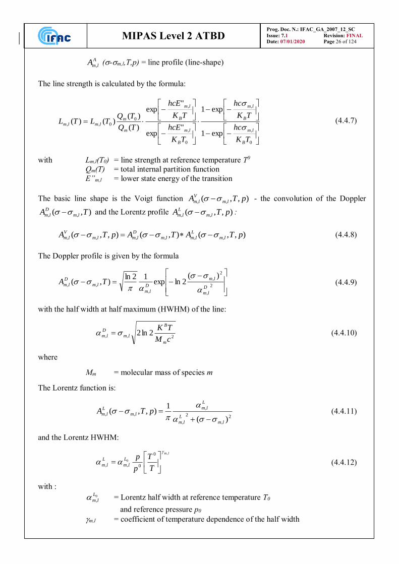
A
lmA , (-m,l,T,p) = line profile (line-shape)
The line strength is calculated by the formula:
0
,
,
0
,
,
0
0,,
exp1
exp1
"exp
"exp
)(
)()()(
TK
hc
TK
hc
TK
hcE
TK
hcE
TQ
TQTLTL
B
lm
B
lm
B
lm
B
lm
m
m
lmlm
(4.4.7)
with Lm,l(T0) = line strength at reference temperature T0
Qm(T) = total internal partition function
E”m,l = lower state energy of the transition
The basic line shape is the Voigt function ),,( ,, pTA lm
V
lm - the convolution of the Doppler
),( ,, TA lm
D
lm and the Lorentz profile ),,( ,, pTA lm
L
lm :
),,(),(),,( ,,,,,, pTATApTA lm
L
lmlm
D
lmlm
V
lm (4.4.8)
The Doppler profile is given by the formula
2
,
2
,
,
,,
)(2lnexp
12ln),(
D
lm
lm
D
lm
lm
D
lm TA
(4.4.9)
with the half width at half maximum (HWHM) of the line:
2,, 2ln2
cM
TK
m
B
lm
D
lm (4.4.10)
where
Mm = molecular mass of species m
The Lorentz function is:
2
,
2
,
,
,,
)(
1),,(
lm
L
lm
L
lm
lm
L
lm pTA
(4.4.11)
and the Lorentz HWHM:
lm
T
T
p
pL
lm
L
lm
,
0
0
0,,
(4.4.12)
with :
0
,
L
lm = Lorentz half width at reference temperature T0
and reference pressure p0
m,l = coefficient of temperature dependence of the half width
MIPAS Level 2 ATBD
Prog. Doc. N.: IFAC_GA_2007_12_SC
Issue: 7.1 Revision: FINAL
Date: 07/01/2020 Page 27 of 124
Using the substitutions:
D
lm
lm
lmx,
,
, 2ln
(4.4.13)
and
D
lm
L
lm
lmy,
,
, 2ln
(4.4.14)
the Voigt function can be rewritten as:
),(12ln
),,( ,,
,
,, lmlmD
lm
lm
V
lm yxKpTA
(4.4.15)
with:
dt
ytx
eyyxK
lmlm
tlm
lmlm 2
,
2
,
,
,,)(
),(
2
(4.4.16)
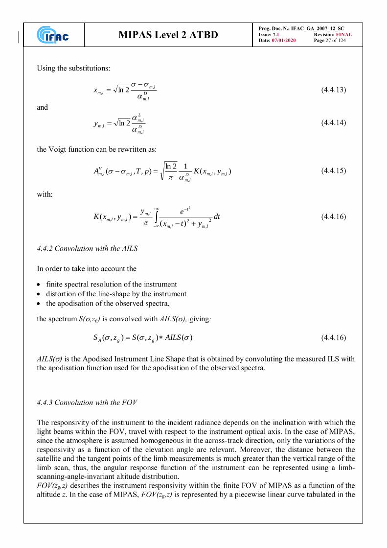
4.4.2 Convolution with the AILS
In order to take into account the
finite spectral resolution of the instrument
distortion of the line-shape by the instrument
the apodisation of the observed spectra,
the spectrum S(,zg) is convolved with AILS(), giving:
)(),(),( AILSzSzS ggA (4.4.16)
AILS() is the Apodised Instrument Line Shape that is obtained by convoluting the measured ILS with
the apodisation function used for the apodisation of the observed spectra.
4.4.3 Convolution with the FOV
The responsivity of the instrument to the incident radiance depends on the inclination with which the
light beams within the FOV, travel with respect to the instrument optical axis. In the case of MIPAS,
since the atmosphere is assumed homogeneous in the across-track direction, only the variations of the
responsivity as a function of the elevation angle are relevant. Moreover, the distance between the
satellite and the tangent points of the limb measurements is much greater than the vertical range of the
limb scan, thus, the angular response function of the instrument can be represented using a limb-
scanning-angle-invariant altitude distribution.
FOV(zg,z) describes the instrument responsivity within the finite FOV of MIPAS as a function of the
altitude z. In the case of MIPAS, FOV(zg,z) is represented by a piecewise linear curve tabulated in the
MIPAS Level 2 ATBD
Prog. Doc. N.: IFAC_GA_2007_12_SC
Issue: 7.1 Revision: FINAL
Date: 07/01/2020 Page 28 of 124
input files. For the simulation of the spectrum affected by the finite FOV (SFA(,zg)) the following
convolution is calculated:
),(),(),( zzFOVzSzS gAgFA (4.4.17)
4.4.4 Instrumental continuum
For the simulation of the instrumental continuum an additional (microwindow dependent and sweep
independent) term is added to ),( gF zS . This term is fitted in the retrieval program.
4.4.5 Summary of required variables
For the atmospheric model:
pressure along the line of sight g p(sg)
temperature along the line of sight g T(sg)
volume mixing ratio along the line of sight g xVMR(sg)
For the ray tracing:
altitude and viewing direction of the instrument or
tangent altitude (in case of homogeneously layered and spherical atmosphere) zg
For the cross section calculation:
central wavenumber of transition l of species m m,l
reference line strength of transition l of species m Lm,l(T0)
lower state energy of transition l of species m E”m,l
total internal partition function of species m Qm(T)
molecular mass of species m Mm
reference Lorentz half width of transition l of species m 0
,
L
lm
coefficient of temperature dependence of the half width m,l
For the AILS convolution:
apodised instrument line shape AILS()
For the FOV convolution:
field of view function FOV(zg,z)
Note: The forward model implemented in the ORM processor (Sect. 4.4) is not designed to simulate
limb emission radiances when scattering and absorption processes are relevant, as in the presence of
MIPAS Level 2 ATBD
Prog. Doc. N.: IFAC_GA_2007_12_SC
Issue: 7.1 Revision: FINAL
Date: 07/01/2020 Page 29 of 124
clouds. For this reason, MIPAS spectral radiance measurements are filtered out for the presence of
clouds before Level 2 processing. The cloud-filtering algorithm employed in the ORM pre-processing
stage is described in Sect. 5.17.
4.5 Calculation of the VCM of the measurements
The variance covariance matrix (VCM) of the residuals Sm, used in Eq. (4.2.24), is in principle given
by the summation of the VCM of the observations Sy and the VCM of the forward model SFM :
FMym SSS (4.5.1)
However, since:
the amplitude of the forward model error is not accurately known;
correlations between forward model errors are difficult to quantify
in the retrieval algorithm we choose to use Sm = Sy. The entity of the forward model errors is evaluated
by analyzing the behaviour of the 2 - test for the different microwindows, at the different altitudes. In
particular, the obtained 2 - test is compared with its expected value as determined on the basis of the
total error evaluated by the so called “Residuals and Error Correlation (= REC)" analysis (see Piccolo
et al. (2001)).
Herewith we describe how the VCM of the observations Sy is derived.
Even if the points of the interferograms measured by MIPAS are sampled independently of each other
(no correlation between the measurements), the spectral data are affected by correlation. The
correlation arises from the data processing performed on the interferogram (e.g. apodisation).
For this reason the noise levels provided by Level 1B processing do not fully characterise the
measurement errors and the computation of a complete VCM Sy of the spectrum S() is needed.
In Section 4.5.1 we describe the operations performed on the interferogram in order to obtain the
apodised spectrum. On the basis of these operations, in Sect. 4.5.2 we describe how the variance
covariance matrix Sy of the observations ise derived. Finally, in Sect. 4.5.3 the procedure used to invert
Sy is described.
4.5.1 Operations performed on the interferogram to obtain the apodised spectrum
The standard MIPAS interferogram is a double-sided interferogram obtained with a nominal maximum
optical path difference (MPD) of +/- 20 cm in the FR measurements and +/- 8 cm in the OR
measurements. The apodised spectrum )(ˆ S is obtained by subsequently performing the following
operations on the interferogram:
1. Zero-filling
During Level 1B processing, in order to exploit the fast Fourier Transform algorithm, the number
of points of the interferogram is made equal to a power of 2 by extending the interferogram with
zeroes from the MPD to the Zero-Filled Path Difference (ZFPD).
The measured interferogram is therefore equal to an interferogram with maximum path difference
ZFPD, multiplied by a boxcar function (d) defined as:
MIPAS Level 2 ATBD
Prog. Doc. N.: IFAC_GA_2007_12_SC
Issue: 7.1 Revision: FINAL
Date: 07/01/2020 Page 30 of 124
MPD],MPD[when 0
]MPD,MPD[when 1
d
ddMPD
(MPD = Max. Path Difference) (4.5.2)
2. Fourier Transformation (FT)
Let us call )(NAHRS the spectrum obtained from the measured (and zero-filled) interferogram
and )(HRS the spectrum that would have been obtained from the interferogram with maximum
path difference ZFPD. )(NAHRS , )(HRS and )]([ FT dMPD are all given in the sampling grid
ZFPD
2
1 .
Since the FT of the product of two functions is equal to the convolution of the FT’s of the two
functions, we obtain:
)]([ FT)()( dMPD HRNAHR SS . (4.5.3)
3. Re-sampling at the fixed grid Since a pre-defined and constant grid is required by the ORM for its optimisations, the spectrum
is re-sampled at a fixed grid D
2
1cm 025.0 1- , with D equal to 20 cm (
-1 10.0625 cm
2 D
, with D equal to 8 cm for the OR measurements). The performed
operation can be written as:
dFT ZFPD *NAHRNA SS , (4.5.4)
where )(NAS is calculated at the fixed grid D
2
1 .
In this case the operation (4.5.4) is not a classical convolution among quantities that are defined
on the same grid (e.g. Eq. (4.5.3)), but is a re-sampling process which changes the grid spacing
from ZFPD2
1 of NAHRS to
D2
1of NAS .
This operation does not introduce correlation between the spectral points only if MPD D.
If DMPD the result of (4.5.4) is equal to the FT of a ±20 cm (±8 cm for OR) interferogram.
If DMPD the result of (4.5.4) is equal to the zero-filling to 20 cm (8 cm for OR) path difference
of an interferogram with path difference MPD, therefore the spectral points are correlated to each
other.
The NESR values given in the Level 1B product are computed after this re-sampling step.
4. Apodisation
The apodised spectrum )(ˆ S is obtained by convolving the spectrum )(NAS with the apodisation
function ap(), sampled at D
2
1 .
apNASS *ˆ (4.5.5)
MIPAS Level 2 ATBD
Prog. Doc. N.: IFAC_GA_2007_12_SC
Issue: 7.1 Revision: FINAL
Date: 07/01/2020 Page 31 of 124
4.5.2 Computation of the VCM relating to a single microwindow
In the case of MIPAS data the microwindows are usually well separated and it is reasonable to assume
as uncorrelated the spectral data points belonging to different microwindows. As a consequence, the
variance covariance matrix of the spectrum Sy is a block-diagonal matrix with as many blocks as many
microwindows are processed, and the dimension of each block is equal to the number of spectral points
in the corresponding microwindow. We assume that different points of the microwindow are
characterised by the same error, but different microwindows can have different errors. In this section
we derive the relationship that applies to each block and for simplicity with Sy we refer to a single
block rather than to the full VCM of the observations.
The correlation between different spectral points of the microwindow is due to the apodisation process
and to the zero-filling that is present in the case of MPD < D.
If DMPD , only the apodisation is a cause of correlation and the VCM Sy of the apodised spectrum
)(ˆ S can be computed from the VCM SNA associated with NAS , (SNA is a diagonal matrix since the
spectral points of NAS are uncorrelated) and from the Jacobian J of the transformation (4.5.5):
T T
y NA NAS JS J S JJ (4.5.6)
In Eq. (4.5.6) the order of the operations has been changed because SNA is a diagonal matrix and all the
diagonal elements are equal. The diagonal values are equal to (NESR)2, where NESR is the quantity
calculated after operation 3 of Sect. 4.5.1.
The calculation of matrix J is straightforward. From the explicit expression of the convolution (4.5.5):
j
japNASS )()()(ˆiji (4.5.7)
it follows that the entry i,k of matrix J is equal to:
)(, kiapki J (4.5.8)
and the variance covariance matrix Sycan be computed as:
2 2
, , i,( ) ( )T
y i k k j ap k ap j ki jk
NESR NESR S J J . (4.5.9)
If DMPD also the effect of zero-filling must be taken into account. Furthermore, the mathematics
is more difficult because zero-filling introduces a correlation between the spectral points of )(NAS
(Eq. (4.5.4)) and the measurement error of this spectrum is characterised by a VCM SNA, with off-
diagonal elements different from zero.
The apodised spectrum S of a measurement made with MPD<D is given by:
*ˆMPDNASS (4.5.10)
where MPD is the apodisation function that is used in the case of a zero-filled spectrum. In the
interferogram domain the FT of MPD is a function that applies the selected apodisation rule between
zero and MPD and is zero-filled between MPD and D.
As in the case of Eq. (4.5.6), Sy is obtained from the following equation :
MIPAS Level 2 ATBD
Prog. Doc. N.: IFAC_GA_2007_12_SC
Issue: 7.1 Revision: FINAL
Date: 07/01/2020 Page 32 of 124
TJSJS NAy (4.5.11)
where in this case J is the Jacobian of the apodisation with MPD and SNA is the VCM of the zero
filled spectrum and has off-diagonal elements different from zero. Therefore, we know the diagonal
elements of this matrix, which are equal to the NESR calculated in Level 1B, but further calculations
must be performed in order to determine the off-diagonal elements.
A few simple considerations allow us to overcome this difficulty.
The spectrum SNA() measured with maximum path difference MPD can be expressed as a function of
the spectrum SNAD() measured with maximum path difference D :
dFTSS MPD
NADNA * (4.5.12)
and SNA can be computed as a function of SNAD using the following expression:
TNA NADS FS F , (4.5.13)
where F is the Jacobian matrix associated with the transformation (4.5.12).
Since SNAD is a diagonal matrix
Tx x T
NAS F IF FF , (4.5.14)
where I is the identity matrix and x is the value of each diagonal element of SNAD (also in this case it
is assumed that the spectral data in the same microwindow are affected by the same error).
From Eq. (4.5.14), the diagonal elements of SNA are equal to:
( )ii
f x NAS ; (4.5.15)
where f is a “continuous representation” of the columns of the matrix F. Using the Parseval
theorem we get:
D
MPDdddd
Df
D
MPDMPD 0
2''
1 , (4.5.16)
and since 2
iiNESRNAS , from Eq. (4.5.15) and Eq. (4.5.16) we obtain :
2NESRMPD
Dx (4.5.17)
The result obtained with Eq. (4.5.17) implies that the measurement of the NESR, even if it does not
fully determine SNA, can be used to fully determine SNAD.
Therefore, we can express S as a function of NADS . From Eq. (4.5.10) and Eq. (4.5.12) we obtain:
MIPAS Level 2 ATBD
Prog. Doc. N.: IFAC_GA_2007_12_SC
Issue: 7.1 Revision: FINAL
Date: 07/01/2020 Page 33 of 124
** MPD
MPD
NAD dFTSS (4.5.18)
and since from the definition of the apodisation function it follows that
* MPDMPD
MPD dFT , it results :
* MPDNADSS (4.5.19)
This expression is analogous to Eq. (4.5.5), where SNA() has been replaced by SNAD() and the
apodisation function has been replaced with the apodisation function related to MPD. Using this
expression the calculations of the VCM related to S() requires the following calculation:
T T
y x x T
NADS JS J J IJ JJ (4.5.20)
and from Eq. (4.5.17) it follows that
2( ) T
y
DNESR
MPDS JJ (4.5.21)
The result is similar to the one found for MPD D with the exception of the extra term MPD
D. Besides,
since the apodisation function contains 0 values between MPD and D, TJJ and Sy are singular matrices.
4.5.3 Computation of the inverse of the VCM
In the ORM the inverse of matrix Sy is required. If Sy is a block-diagonal matrix, also (Sy)-1 is a block-
diagonal matrix and is made of blocks equal to the inverse of the blocks of Sy.
As stated earlier, when MPD < D the “ranks” of the blocks are smaller than their dimension. This fact
would be evident in the case in which the VCM is calculated in a sufficiently broad spectral range.
However, in the ORM, where microwindows are used and correlations are calculated in a limited
spectral range, the truncations make the determinant different from zero even if the number of
independent pieces of information is less than the dimension of the matrix and the singularity of the
matrix is not always automatically detected. The problem can be solved by modifying the routine that
inverts the VCM: the VCM is inverted with the Singular Value Decomposition method (see Section.
4.7) also when the determinant is different from zero and the smallest eigenvalues are set equal to 0.
The number of the eigenvalues set to 0 is given by the number of dependent points in the spectrum (
(1-MPD/D)*n1, where n1 is the dimension of the matrix (equal to the number of the sampling points
of the microwindow included in the fit).
This issue is further complicated by the use of a selected set of spectral points for the retrieval
(microwindows with masked points, see Appendix C). When a subset of points is used for the retrieval
the blocks of Sy are made by a corresponding subset of lines and columns. By reducing the dimension
of the block the ratio between the rank and the dimension of the block is altered. The selection of a
fraction of eigenvalues provides an useful conservative criterion.
MIPAS Level 2 ATBD
Prog. Doc. N.: IFAC_GA_2007_12_SC
Issue: 7.1 Revision: FINAL
Date: 07/01/2020 Page 34 of 124
4.6 Calculation of the Jacobian matrix K of the simulations
The use of Gauss-Newton algorithm for the minimisation of the 2 function requires the computation
of the Jacobian matrix K of the simulations. The element of indexes i,j of this matrix is defined by the
following relationship:
xxj
i
jix
xFK
~
,
)(
(4.6.1)
where Fi is the spectrum simulated with the Forward Model, and xj is the j-th component of the vector
x containing the unknowns of the problem. The vector x of the unknown parameters may contain the
following groups of the parameters:
pressures at the tangent points,
temperatures at tangent altitudes,
VMR of one or more gases at tangent altitudes
continuum at tangent altitudes, for the central frequencies of the microwindows used for the
retrieval,
instrumental continuum (i.e. additive term to the spectrum that is assumed as constant varying the
observation geometry and function of the microwindow),
Notes regarding Version 8 of the ORM:
ORM v.8 includes the so called Multi-Target Retrieval (MTR) functionality. Although not
exploited in the standard Level 2 retrievals, this functionality allows the simultaneous retrieval
of tangent pressure, temperature and VMR profiles of one or more atmospheric constituents.
This functionality is particularly important for the retrieval of gases that contribute to the limb
emission spectrum only with very weak features which, at the MIPAS spectral resolution,
ovelap with lines of other gases that are also not retrievable with high precision. In this case, to
minimize (and properly account for) the interference error, the best approach is the
simultaneous retrieval of all the gases that contribute to the selected spectral region. This
approach was used e.g. by Valeri et al. 2016 to retrieve for the first time the Phosgene (COCl2)
vertical profile from MIPAS observations.
The ORM v.8 includes the capability to retrievethe VMR of the HDO isotopologue. Since this
is the only isotopologue retrieved in the standard MIPAS ESA Level 2 inversions, there is no
specific algorithm implemented in the ORM v.8 to retrieve generic isotopic ratios or their
deviation from the standard natural ratio assumed in the HITRAN spectroscopic database to
scale the line intensities. In the ORM auxiliary data files, HDO is actually handled as a
“separate” gas, with its own specific molecule code, line parameters and VMR profile different
from those of the other H2O isotopologues. Despite of that, like in HITRAN, also in the MIPAS
spectroscopic database the HDO line intensities are scaled by the HDO natural isotopic
abundance so that, whenever HDO is not retrieved, it is possible to use a single H2O VMR
profile in the forward model calculations. This choice implies that, internally, for the HDO
retrieval the ORM still uses the H2O VMR profile as initial guess (and a-priori, see Sect. 5.2)
for HDO. After completion of the retrieval, however, the HDO profile is multiplied by the
natural isotopic abundance assumed in the spectroscopic database and is reported in the output
files with the correct units (ppmv).
The derivatives of the forward model are computed in correspondence of a vector x containing:
the initial guess of the unknown parameters in the first iteration step,
MIPAS Level 2 ATBD
Prog. Doc. N.: IFAC_GA_2007_12_SC
Issue: 7.1 Revision: FINAL
Date: 07/01/2020 Page 35 of 124
the new guess of the parameters in the subsequent iterations.
These derivatives can be computed either numerically or analytically. In general, the numerical
approach requires an extra call to the forward model for the computation of each partial derivative,
while in the analytical approach the calculation of the derivatives can be performed in parallel with the
calculation of the spectrum.
Tests have shown that:
the derivatives with respect to tangent pressure, VMR, continuum cross-sections, and instrumental
continuum can be computed analytically using only minor approximations.
the derivatives with respect to tangent temperature cannot computed analytically without
introducing approximations that significantly degrade the accuracy.
The formulas to be used for the analytical calculation of the above derivatives are strictly linked to the
mathematical optimisations used for the implementation of the atmospheric model into the program.
These formulas are described in Sect. 6.7.
4.7 Generalised inverse
Even if a detailed description of the formulas needed for the calculation of the generalised inverse
matrix can be found in Kalman (1976), it is however useful to recall here a simple method that can be
used for the computation of the generalised inverse of a symmetric matrix. This algorithm (the
truncated singular value decomposition method) is used in the ORM to invert the matrices Sm and
)( 1KSK m
T appearing in equation (4.2.8). In the case in which these matrices are non-singular the
method provides the exact inverse matrix.
Let’s call C a symmetric matrix of dimension ‘r’. It is possible to find a base of ‘r’ independent
eigenvectors of C. If SC is the matrix whose columns are the eigenvectors of C, matrix C can then be
written in the form:
T C CC S wS (4.7.1)
where w is a diagonal matrix containing the eigenvalues of C. The inverse matrix of C is then:
1 1 T C CC S w S (4.7.2)
The appearance of singularities in C is detected by the presence of eigenvalues close to zero in w. In
this case the singularities can be eliminated by imposing 1/wi = 0 whenever wi0.
This procedure corresponds to the calculation of the generalised inverse matrix of C.
4.8 Variance-covariance matrix of tangent height corrections
In p,T retrieval the retrieved quantities are pressures at the tangent points and the temperatures
corresponding to tangent pressures. In an atmosphere in hydrostatic equilibrium, after p,T retrieval is
completed, it is always possible to derive from these two quantities an estimate of the differences
between the tangent altitudes of two contiguous sweeps. Besides, if one of the tangent altitudes
provided by engineering measurements is assumed as perfectly known, an estimate of all the tangent
altitudes can be easily obtained. The differences between the tangent altitudes obtained from p,T
MIPAS Level 2 ATBD
Prog. Doc. N.: IFAC_GA_2007_12_SC
Issue: 7.1 Revision: FINAL
Date: 07/01/2020 Page 36 of 124
retrieval and the corresponding engineering estimates of the tangent altitudes constitute the so called
vector of ‘tangent heights corrections’. Purpose of this section is to define the algorithm for the
calculation of the VCM of this vector.
Let’s assume that the analysed scan consists of NSW sweeps and that the tangent altitude z(NSW) of the
lowest sweep is perfectly known. The corrections iz to the engineering tangent altitudes are defined
as:
ENG
i
RET
ii zzz (4.8.1)
where RET
iz are the tangent altitudes derived from p,T retrieval and ENG
iz the engineering estimates of
the tangent altitudes; the index i ranges from 1 to NSW -1. It is important to appreciate that the error on
iz that is given in its VCM, is not intended as the error on the difference contained in equation (4.8.1),
which is complicated by the fact that both estimates of the tangent altitude are affected by an error and
the two errors are not independent. The error on z is intended as the error which should be attributed
to the retrieved tangent altitude when this quantity is reconstructed by adding the correction z to the
reference levels provided by the engineering tangent altitudes.
By using hydrostatic equilibrium law and the tangent altitude of the lowest sweep, RET
iz (i = 1, …,
NSW-1) can be expressed as:
swN
ij j
j
M
jj
SW
RET
iP
P
K
TTNzz
1 1
1log
2)( (4.8.2)
where, as usual, jT and jP are respectively temperature and pressure at tangent altitude RET
jz and
KM=M/g with M = air mass and g = acceleration of gravity.
Therefore, the tangent altitude corrections can be expressed as a function of jT and jP by substituting
equation (4.8.2) in (4.8.1):
1,...,1log21 1
1
SWENG
j
N
ij j
j
M
jj
i NizP
P
K
TTz
SW
(4.8.3)
where ENG
iz are defined as:
SWENG
j
ENG
j
ENG
i Njzzz ,...,21 (4.8.4)
Now, equation (4.8.3) allows the evaluation of the variance-covariance matrix SHC of the heights
corrections iz starting from the variance-covariance matrix (Sx) of the retrieved values of pressure
and temperature (see Eq. (4.2.11) in Sect. 4.2.2, this matrix is directly provided by the retrieval
algorithm). The transformation which links SHC and Sx is:
THC D x DS K S K (4.8.5)
where DK is the jacobian matrix connecting iz with iT and iP . The elements of DK are the
derivatives:
MIPAS Level 2 ATBD
Prog. Doc. N.: IFAC_GA_2007_12_SC
Issue: 7.1 Revision: FINAL
Date: 07/01/2020 Page 37 of 124
j
i
P
zji
)(),( DK with i = 1, …, NSW -1 and j = 1, …, NSW
and (4.8.6)
j
iSW
T
zjNi
)(),( DK with i = 1, …, NSW -1 and j = 1, …, NSW
these expressions can be easily evaluated by deriving Eq. (4.8.3) with respect to pressure and
temperature. We obtain:
swN
ij j
jh
j
jhjj
h
i
PPK
TT
P
z
1 1
1,,1
2
)(
with i = 1, …, NSW -1 and h = 1, …, NSW
and (4.8.7)
swN
ij j
j
hjhj
h
i
P
P
KT
z
1 1
,1, log2
1)(
with i = 1, …, NSW -1 and h = 1, …, NSW
Summarising, the steps to be carried-out for the calculation of the variance-covariance matrix SHC are:
calculation of the jacobian matrix KD by using equations (4.8.7),
transformation of the variance-covariance matrix Sx of the retrieved pressures and temperatures, by
using equation (4.8.5).
4.9 Tangent heights correction based on ECMWF data
MIPAS limb emission measurements are very sensitive to pressure at the tangent point. For this reason,
tangent pressures are retrieved by the Level 2 processor with a precision reaching a few percents. The
retrieved pressures and temperatures are fed onto the hydrostatic equilibrium equation to derive tangent
height increments with a precision better than 100 m. Despite this relatively high precision of the
retrieved tangent height increments, the absolute values of tangent heights remain uncertain, due to the
intrinsic lack of sensitivity of the limb measurements to the geometrical altitude of the tangent points,
when pressure is considered an independent variable. At each pT retrieval iteration, tangent heights are
re-calculated by adding the tangent height increments to the lowest tangent height of the scan, which
is assumed to be known from engineering pointing data. The absolute accuracy of engineering pointing
data, however, can be as poor as 1 km, according to the specifications (see Appendix A).
To improve the accuracy of the absolute tangent heights of each MIPAS scan, we apply to the retrieved
tangent altitudes a common vertical shift, calculated on the basis of the nearest ECMWF profiles
matching in space and time the considered MIPAS scan. The vertical shift is calculated as follows: we
consider the retrieved tangent pressures and altitudes of the three lowest sweeps of the processed scan.
Using log(p) interpolation, we find the three ECMWF altitudes that correspond to the retrieved tangent
pressures of the lowest three sweeps. We compute the average difference between these three altitudes
and the three lowest retrieved tangent heights. We finally shift all the tangent heights of the scan by
adding to them this average difference.
Validations against correlative independent measurements have confirmed that this a-posteriori
correction of the altitude scale of MIPAS profiles is very effective in reducing the discrepancies
between MIPAS and correlative measurements. As an example, Fig. 4.9.1 (courtesy of Daan Hubert,
BIRA-IASB) shows the median bias between MIPAS retrieved profile altitudes and altitudes obtained
from co-located radiosonde measurements for matching pressures. Top plots refer to the Full
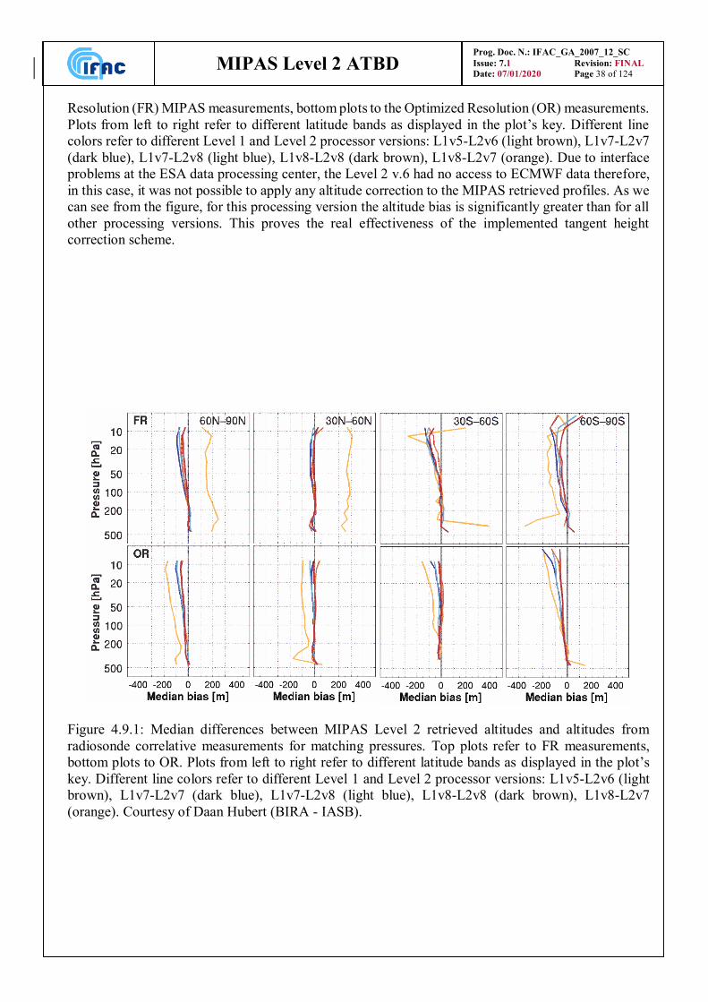
MIPAS Level 2 ATBD
Prog. Doc. N.: IFAC_GA_2007_12_SC
Issue: 7.1 Revision: FINAL
Date: 07/01/2020 Page 38 of 124
Resolution (FR) MIPAS measurements, bottom plots to the Optimized Resolution (OR) measurements.
Plots from left to right refer to different latitude bands as displayed in the plot’s key. Different line
colors refer to different Level 1 and Level 2 processor versions: L1v5-L2v6 (light brown), L1v7-L2v7
(dark blue), L1v7-L2v8 (light blue), L1v8-L2v8 (dark brown), L1v8-L2v7 (orange). Due to interface
problems at the ESA data processing center, the Level 2 v.6 had no access to ECMWF data therefore,
in this case, it was not possible to apply any altitude correction to the MIPAS retrieved profiles. As we
can see from the figure, for this processing version the altitude bias is significantly greater than for all
other processing versions. This proves the real effectiveness of the implemented tangent height
correction scheme.
Figure 4.9.1: Median differences between MIPAS Level 2 retrieved altitudes and altitudes from
radiosonde correlative measurements for matching pressures. Top plots refer to FR measurements,
bottom plots to OR. Plots from left to right refer to different latitude bands as displayed in the plot’s
key. Different line colors refer to different Level 1 and Level 2 processor versions: L1v5-L2v6 (light
brown), L1v7-L2v7 (dark blue), L1v7-L2v8 (light blue), L1v8-L2v8 (dark brown), L1v8-L2v7
(orange). Courtesy of Daan Hubert (BIRA - IASB).
MIPAS Level 2 ATBD
Prog. Doc. N.: IFAC_GA_2007_12_SC
Issue: 7.1 Revision: FINAL
Date: 07/01/2020 Page 39 of 124
5 - Scientific aspects and physical optimisations
In this section the baselines for the choice of the implementation of specific physical aspects and
optimisations into the code are discussed. This discussion includes the following items:
explanation of the physical effects
possible physical models for the description of these effects
options for the implementation into the code
optimisations: improved algorithms, simplifications, items to be neglected
choices for the implementation
accuracy of baselines
The discussed aspects are:
1. Retrieval grid: retrieval of the unknowns at fixed levels or at tangent altitudes
2. Use of a-priori information
3. Latitudinal variability of atmospheric parameters
4. Model of the earth and calculation of the gravity
5. Ray tracing: refraction model and determination of the optical path
6. Line shape
7. Line mixing
8. Pressure shift
9. Non local thermodynamic equilibrium (NLTE)
10.Self broadening
11.Continuum: instrumental, near, far
12.Interpolation of the profiles
5.1 Choice between retrieval of profiles at fixed levels and at tangent altitude levels
In the case of the onion peeling method, the retrieved values of VMR can only be determined at the
pressure levels that correspond to the tangent altitude of the limb scanning sequence. In the case of
global fit this constraint does not exist and other discrete levels can be used. Since in Level 3 data
processing global maps on pressure surfaces are produced, an interesting possibility offered by global
fit is that of using fixed pressure levels which will in general be different from the tangent altitude
levels.
5.1.1 Retrieval at tangent altitude and interpolation between retrieved values
If the pressure levels at which the retrieval is performed are the ones identified by the observation
geometries of the limb scanning sequence they may not correspond to those needed by the user. In this
case an interpolation can be applied and, as it is shown in Carli (1995), the equations that fully
characterise the interpolated values of the profiles assess that, even if a reduced statistic error applies
to the profile at the interpolated altitude levels, the vertical resolution of the measurement is degraded.
Numerical tests have shown that between two retrieved values the measurement error has a minimum
while the width of the averaging kernel (see e.g. Rodgers (1976)) has a maximum (i.e. the interpolation
changes the trade-off between vertical resolution and precision in favour of the latter). Interpolation of
retrieved values provides therefore a variable trade-off between precision and vertical resolution of the
MIPAS Level 2 ATBD
Prog. Doc. N.: IFAC_GA_2007_12_SC
Issue: 7.1 Revision: FINAL
Date: 07/01/2020 Page 40 of 124
measurement. Alternative interpolation schemes to be applied to retrieved profiles have been studied
in Carli et al., (2001). One of the methods proposed in this reference is discussed in Sect. 5.13.
5.1.2 Retrieval at fixed levels
If the data utilisation requires VMR at fixed levels (for instance in level 3 data processing global maps
on pressure surfaces are produced) an alternative could be that of retrieving the VMR directly at the
required fixed levels. The quality of the retrieval performed at fixed levels should be assessed with
appropriate tests, but it is reasonable to expect that in general it provides larger noise and a more
uniform vertical resolution.
5.1.3 Discussion of the problem
The basic problem that is behind the different trade-off between precision and vertical resolution of the
profile retrieved with the two approaches can be explained by the Nyquist theorem. This theorem states
that in order to measure a periodic variation of a distribution, the distribution must be sampled with
steps at least as small as half the period of the variation. If the maxima and the minima of the variation
coincide with the sampling points (detection of the cosine variation) a sampling step equal to half of
the period is sufficient to detect the signal. A sampling step equal to a quarter of the period is needed
in order to detect a variation with any phase (detection of both the cosine and the sine components).
According to the Nyquist theorem, we have that:
the vertical resolution of the retrieved profiles coincides (if no a-priori information and/or external
constraints are explicitly used in the inversion) with the vertical sampling step of the sounding if the
retrieval is performed at tangent altitudes levels
the vertical resolution of the retrieved profiles cannot be equal to the vertical resolution of the
sounding if the retrieval is performed at intermediate levels.
Therefore, if the offset introduced by the pointing system, between wanted and implemented tangent
altitudes causes a sounding of the atmosphere at tangent altitudes located in between the fixed levels
required by the user, it is impossible to obtain at the fixed levels the maximum vertical resolution. This
result, which is based on the implicit assumption that the weighting functions of limb sounding
observations peak at the tangent altitudes, may have a partial exception if the difference between
weighting functions at different frequencies and in different microwindows provides some information
at intermediate altitudes. However, the exploitation of this second order information is bound to cause
a major increase of the measurement error.
The choice is therefore between:
1. retrieval at tangent altitude levels followed by interpolation for determination of VMR at required
levels: this procedure makes the best use of the data when no interpolation is used. If interpolation
is used, the vertical resolution of the measurement depends upon the offset between retrieved and
interpolated points. Up to a factor of two of loss in vertical resolution can be encountered.
2. retrieval at fixed pressure levels: this option has not been adequately tested, it is expected to provide
retrievals at roughly (T dependence) constant vertical resolution, but the noise depends upon the
offset between wanted and implemented tangent altitudes. A very large increase of noise can be
encountered and it is not easy to quantify this increase.
The first option is the one with fewer risks. The second option is simpler from the conceptual point of
view. The two options imply a different implementation of level 2 data analysis and a significant
MIPAS Level 2 ATBD
Prog. Doc. N.: IFAC_GA_2007_12_SC
Issue: 7.1 Revision: FINAL
Date: 07/01/2020 Page 41 of 124
compromise in scientific requirements, but from the code point of view there is no strong reasons in
favour of any of the two.
5.1.4 Conclusions
The following strategy has been assumed for the development of Level 2 scientific code:
for the level 2 retrieval algorithm we have adopted the option of the retrieval at tangent altitudes
levels eventually followed by interpolation. The reason for this choice is that at the time of the code
development we could not afford the unknowns of the other option.
Some flexibility is maintained in the code in order not to prevent the implementation of the
alternative approach in subsequent versions, in case it is recommended by retrieval studies.
The trade-off between vertical resolution and precision and the alternative of retrieving the profiles
either at tangent altitude levels or at fixed (user-defined) levels have been fully addressed in a
quantitative study carried-out in a parallel ESA contract (12055/96/NL/CN). We therefore refer to the
final report of that study for a quantitative assessment of the topics described in the present section. In
any case, no explicit recommendation for a retrieval at fixed levels emerged from the mentioned study.
5.2 Use of a-priori information
The use of information provided by sources different from the spectroscopic measurements can
increase the overall information content (equal to retrieval information plus extra information) and
improve the quality of the retrieved profiles. This possibility is source of both, improvements and
concern because, if on one hand it can lead to a positive result in the case of marginal precision in the
retrieval, on the other hand it can become a cosmetic exercise which hides serious systematic errors.
These two aspects of external information will be discussed in the next two sections.
5.2.1 - Precision improvement
The exploitation of external information is worthwhile only if it leads to a significant precision
improvement. In order to understand the entity of the improvement, the mathematics of the
combination of information is herewith briefly recalled.
It is well known that if two independent measurements x1 and x2 exist of a scalar quantity x, the two
measurements can be combined by way of their r.m.s. errors 1 and 2 leading to the new estimate:
)()(= 2
2
21
2
1
12
2
2
1 xxqc
(5.2.1)
with an error:
21
2
2
2
1
c (5.2.2)
We know that in this case the error of the new estimate:
is reduced by a factor 21 when the two measurements have the same error,
is practically equal to the error of the best measurement when a large difference exists between the
two errors.
MIPAS Level 2 ATBD
Prog. Doc. N.: IFAC_GA_2007_12_SC
Issue: 7.1 Revision: FINAL
Date: 07/01/2020 Page 42 of 124
In practice, combining information from different measurements brings no advantage when the
measurements have different quality.
A similar error combination can be made in the case in which the measured quantity is a vector x. The
weighted combination xc of the two measurements x1 and x2 having respectively the variance-
covariance matrices 1xS and
2xS is equal to:
1
1 1 1 1
1 2 1 1 2 2
C x x x xx S S S x S x (5.2.3)
and has a variance-covariance matrix equal to
1
1 1
1 2
xC x xS S S (5.2.4)
The similarity of respectively expressions (5.2.1), (5.2.2) and (5.2.3), (5.2.4) may suggest that also
similar properties apply, and it is not worthwhile to combine two measurements if their errors are very
different.
In our case this would imply that if the external information is better than the retrieved information we
do not need the limb scanning measurements and if the external information is worse than the retrieved
information we do not need to waste efforts combining the two. However, the situation is not so simple
in the case of measurements of vectors and the considerations made for scalar quantities do not fully
apply.
Limb scanning observations often provide very good measurements with low errors at some altitudes,
and undetermined measurements with large errors at other altitudes. An approximate estimate, which
may be available from either statistical studies or models, of course does not directly add information
where good measurements have been retrieved, but can reduce significantly the errors where the
retrieved measurements are undetermined. Since a correlation exists between measurements at
different altitudes, the reduction of the errors at some altitudes may lead to a reduction of all the errors.
This explains why in the case of combination of vectors the errors may be reduced more than what is
expected on the basis of the quadratic combination.
In Carlotti et al. (1995) some numerical tests were performed showing that a significant improvement
is possible by using a-priori knowledge such as that which can be obtained from either the previous
measurement or statistical seasonal and geographical maps.
The use of external information can, therefore, be very profitable and should be seriously considered
as part of the retrieval strategy.
5.2.2 - Systematic errors
A concern about the combination of the retrieved information with an a-priori estimate of the profile
is that whenever the same a-priori information is used for several profiles, the error budget of each
profile contains both a random and a systematic component (the first due to the measurement and the
second due to the constant a-priori information).
Usually it is a good rule to list separately random and systematic errors in order to avoid mistakes in
the subsequent operations. In fact in the case of averages random errors are reduced and systematic
errors remain constant, while in the case of differences, systematic errors cancel and random errors
increase. If we want to maintain this separation between random and systematic errors it is necessary,
therefore, to make retrievals without a-priori information (our primary output) and combine externally
provided profiles with the retrieved profiles only optionally.
MIPAS Level 2 ATBD
Prog. Doc. N.: IFAC_GA_2007_12_SC
Issue: 7.1 Revision: FINAL
Date: 07/01/2020 Page 43 of 124
The different approach of using a-priori information routinely, during the retrieval iterations, can be
adopted when the a-priori information has a random character.
5.2.3 - Hydrostatic equilibrium and LOS Engineering information
In the case of p, T retrieval an external information is also provided by the hydrostatic equilibrium.
This information is a relationship between the unknowns and another measurement (provided by the
engineering data) rather than a constant a-priori estimate and implies therefore different choices.
Hydrostatic equilibrium is a condition that applies to an ideal atmosphere which is perfectly stratified.
The integrated form of the equation that describes this condition is:
n
i
i
i
n zT
gR
Mpp
0
0
1exp (5.2.5)
where the notations are:
pn pressure at a given altitude,
po pressure at the reference altitude,
M average molecular weight of the atmosphere,
R universal gas constant,
Ti temperature of the atmospheric layer i,
iz thickness of the atmospheric layer i.
Now, since equation (5.2.5) is a relationship between T, 0ppn and iz increments, the measurements
of pressure and temperature at tangent altitude obtained from the spectroscopic observations, can be
used to get an estimate of the differences iz between the tangent altitudes of the sweeps in the same
limb-scanning sequence. Another estimate of the differences between tangent altitudes is provided by
the engineering measurements. The two estimates are then combined using equation (5.2.3) and the
variance covariance matrix of the new estimate is computed using (5.2.4). The variance covariance
matrix related to the engineering pointing that is needed for the above operations is an input of p, T
retrieval program. The mathematics required by this operation is discussed with further details in Sect.
4.2.6.
Note that in this approach, only the differences between tangent altitudes and not the absolute pointing
altitudes are improved by the retrieval process. In fact, when pressure is a fitted quantity, the sensitivity
of radiative transfer to the tangent altitude of the measurement is very weak and it is not possible to
retrieve any of the tangent altitudes of the limb-scanning sequence.
Baselines:
Engineering LOS data is routinely used in p,T retrieval by exploiting the constraint provided by
hydrostatic equilibrium, as explained in the above section.
The ORM version 8 includes the possibility to perform the inversions using also the Optimal Estimation
(or the Maximum A-Posteriori) method (Rodgers, 2000). With a user selectable switch, it is possible
to enable the use of a-prori estimates and error covariance matrices for selected sets of retrieval
parameters. In practice this option is used only for the retrieval of the VMR of gases that contribute to
MIPAS radiances the with very weak spectral features as compared to the measurement noise. As
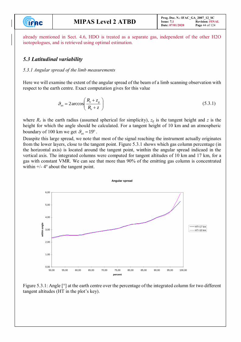
MIPAS Level 2 ATBD
Prog. Doc. N.: IFAC_GA_2007_12_SC
Issue: 7.1 Revision: FINAL
Date: 07/01/2020 Page 44 of 124
already mentioned in Sect. 4.6, HDO is treated as a separate gas, independent of the other H2O
isotopologues, and is retrieved using optimal estimation.
5.3 Latitudinal variability
5.3.1 Angular spread of the limb measurements
Here we will examine the extent of the angular spread of the beam of a limb scanning observation with
respect to the earth centre. Exact computation gives for this value
zR
zR
e
ge
as arccos2 (5.3.1)
where Re is the earth radius (assumed spherical for simplicity), zg is the tangent height and z is the
height for which the angle should be calculated. For a tangent height of 10 km and an atmospheric
boundary of 100 km we get 19as .
Deaspite this large spread, we note that most of the signal reaching the instrument actually originates
from the lower layers, close to the tangent point. Figure 5.3.1 shows which gas column percentage (in
the horizontal axis) is located around the tangent point, winthin the angular spread indicaed in the
vertical axis. The integrated columns were computed for tangent altitudes of 10 km and 17 km, for a
gas with constant VMR. We can see that more than 90% of the emitting gas column is concentrated
within +/- 4o about the tangent point.
Figure 5.3.1: Angle [°] at the earth centre over the percentage of the integrated column for two different
tangent altitudes (HT in the plot’s key).
Angular spread
0,00
1,00
2,00
3,00
4,00
5,00
6,00
50,00 55,00 60,00 65,00 70,00 75,00 80,00 85,00 90,00 95,00 100,00
percent
wit
hin
an
gle
HT=17 km
HT=10 km
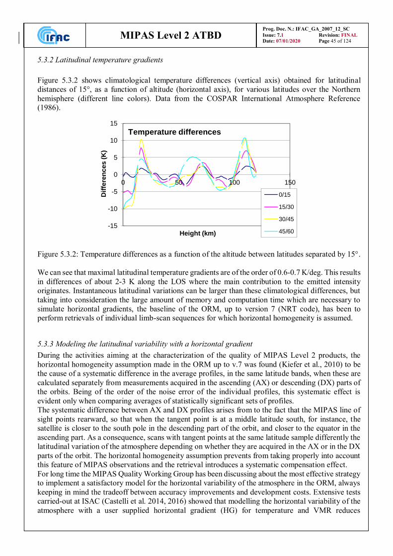
MIPAS Level 2 ATBD
Prog. Doc. N.: IFAC_GA_2007_12_SC
Issue: 7.1 Revision: FINAL
Date: 07/01/2020 Page 45 of 124
5.3.2 Latitudinal temperature gradients
Figure 5.3.2 shows climatological temperature differences (vertical axis) obtained for latitudinal
distances of 15°, as a function of altitude (horizontal axis), for various latitudes over the Northern
hemisphere (different line colors). Data from the COSPAR International Atmosphere Reference
(1986).
Figure 5.3.2: Temperature differences as a function of the altitude between latitudes separated by 15.
We can see that maximal latitudinal temperature gradients are of the order of 0.6-0.7 K/deg. This results
in differences of about 2-3 K along the LOS where the main contribution to the emitted intensity
originates. Instantaneous latitudinal variations can be larger than these climatological differences, but
taking into consideration the large amount of memory and computation time which are necessary to
simulate horizontal gradients, the baseline of the ORM, up to version 7 (NRT code), has been to
perform retrievals of individual limb-scan sequences for which horizontal homogeneity is assumed.
5.3.3 Modeling the latitudinal variability with a horizontal gradient
During the activities aiming at the characterization of the quality of MIPAS Level 2 products, the
horizontal homogeneity assumption made in the ORM up to v.7 was found (Kiefer et al., 2010) to be
the cause of a systematic difference in the average profiles, in the same latitude bands, when these are
calculated separately from measurements acquired in the ascending (AX) or descending (DX) parts of
the orbits. Being of the order of the noise error of the individual profiles, this systematic effect is
evident only when comparing averages of statistically significant sets of profiles.
The systematic difference between AX and DX profiles arises from to the fact that the MIPAS line of
sight points rearward, so that when the tangent point is at a middle latitude south, for instance, the
satellite is closer to the south pole in the descending part of the orbit, and closer to the equator in the
ascending part. As a consequence, scans with tangent points at the same latitude sample differently the
latitudinal variation of the atmosphere depending on whether they are acquired in the AX or in the DX
parts of the orbit. The horizontal homogeneity assumption prevents from taking properly into account
this feature of MIPAS observations and the retrieval introduces a systematic compensation effect.
For long time the MIPAS Quality Working Group has been discussing about the most effective strategy
to implement a satisfactory model for the horizontal variability of the atmosphere in the ORM, always
keeping in mind the tradeoff between accuracy improvements and development costs. Extensive tests
carried-out at ISAC (Castelli et al. 2014, 2016) showed that modelling the horizontal variability of the
atmosphere with a user supplied horizontal gradient (HG) for temperature and VMR reduces
-15
-10
-5
0
5
10
15
0 50 100 150
Dif
fere
nces (
K)
Height (km)
Temperature differences
0/15
15/30
30/45
45/60
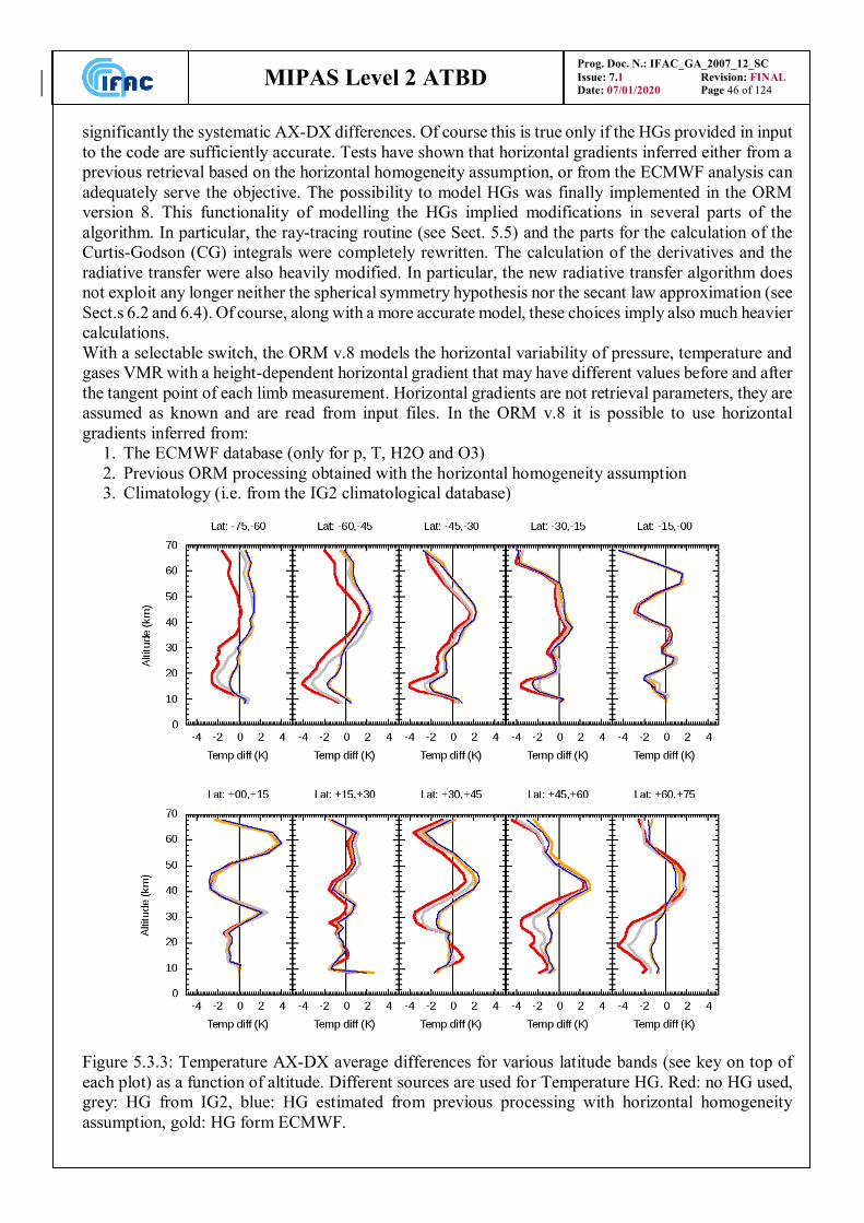
MIPAS Level 2 ATBD
Prog. Doc. N.: IFAC_GA_2007_12_SC
Issue: 7.1 Revision: FINAL
Date: 07/01/2020 Page 46 of 124
significantly the systematic AX-DX differences. Of course this is true only if the HGs provided in input
to the code are sufficiently accurate. Tests have shown that horizontal gradients inferred either from a
previous retrieval based on the horizontal homogeneity assumption, or from the ECMWF analysis can
adequately serve the objective. The possibility to model HGs was finally implemented in the ORM
version 8. This functionality of modelling the HGs implied modifications in several parts of the
algorithm. In particular, the ray-tracing routine (see Sect. 5.5) and the parts for the calculation of the
Curtis-Godson (CG) integrals were completely rewritten. The calculation of the derivatives and the
radiative transfer were also heavily modified. In particular, the new radiative transfer algorithm does
not exploit any longer neither the spherical symmetry hypothesis nor the secant law approximation (see
Sect.s 6.2 and 6.4). Of course, along with a more accurate model, these choices imply also much heavier
calculations.
With a selectable switch, the ORM v.8 models the horizontal variability of pressure, temperature and
gases VMR with a height-dependent horizontal gradient that may have different values before and after
the tangent point of each limb measurement. Horizontal gradients are not retrieval parameters, they are
assumed as known and are read from input files. In the ORM v.8 it is possible to use horizontal
gradients inferred from:
1. The ECMWF database (only for p, T, H2O and O3)
2. Previous ORM processing obtained with the horizontal homogeneity assumption
3. Climatology (i.e. from the IG2 climatological database)
Figure 5.3.3: Temperature AX-DX average differences for various latitude bands (see key on top of
each plot) as a function of altitude. Different sources are used for Temperature HG. Red: no HG used,
grey: HG from IG2, blue: HG estimated from previous processing with horizontal homogeneity
assumption, gold: HG form ECMWF.
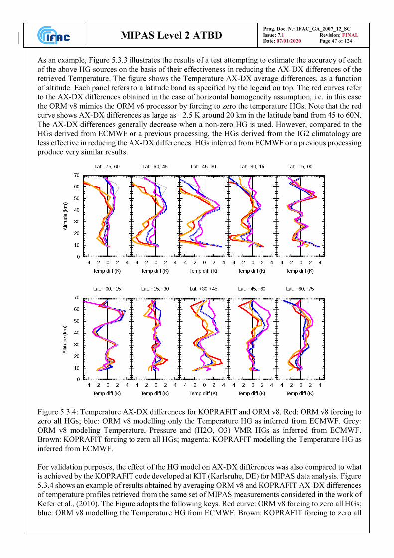
MIPAS Level 2 ATBD
Prog. Doc. N.: IFAC_GA_2007_12_SC
Issue: 7.1 Revision: FINAL
Date: 07/01/2020 Page 47 of 124
As an example, Figure 5.3.3 illustrates the results of a test attempting to estimate the accuracy of each
of the above HG sources on the basis of their effectiveness in reducing the AX-DX differences of the
retrieved Temperature. The figure shows the Temperature AX-DX average differences, as a function
of altitude. Each panel refers to a latitude band as specified by the legend on top. The red curves refer
to the AX-DX differences obtained in the case of horizontal homogeneity assumption, i.e. in this case
the ORM v8 mimics the ORM v6 processor by forcing to zero the temperature HGs. Note that the red
curve shows AX-DX differences as large as −2.5 K around 20 km in the latitude band from 45 to 60N.
The AX-DX differences generally decrease when a non-zero HG is used. However, compared to the
HGs derived from ECMWF or a previous processing, the HGs derived from the IG2 climatology are
less effective in reducing the AX-DX differences. HGs inferred from ECMWF or a previous processing
produce very similar results.
Figure 5.3.4: Temperature AX-DX differences for KOPRAFIT and ORM v8. Red: ORM v8 forcing to
zero all HGs; blue: ORM v8 modelling only the Temperature HG as inferred from ECMWF. Grey:
ORM v8 modeling Temperature, Pressure and (H2O, O3) VMR HGs as inferred from ECMWF.
Brown: KOPRAFIT forcing to zero all HGs; magenta: KOPRAFIT modelling the Temperature HG as
inferred from ECMWF.
For validation purposes, the effect of the HG model on AX-DX differences was also compared to what
is achieved by the KOPRAFIT code developed at KIT (Karlsruhe, DE) for MIPAS data analysis. Figure
5.3.4 shows an example of results obtained by averaging ORM v8 and KOPRAFIT AX-DX differences
of temperature profiles retrieved from the same set of MIPAS measurements considered in the work of
Kefer et al., (2010). The Figure adopts the following keys. Red curve: ORM v8 forcing to zero all HGs;
blue: ORM v8 modelling the Temperature HG from ECMWF. Brown: KOPRAFIT forcing to zero all
MIPAS Level 2 ATBD
Prog. Doc. N.: IFAC_GA_2007_12_SC
Issue: 7.1 Revision: FINAL
Date: 07/01/2020 Page 48 of 124
HGs; pink: KOPRAFIT modelling the Temperature HG from ECMWF. From the figure it is evident
that both KOPRAFIT and the ORM v8 achieve very similar AX-DX differences both when the
Temperature HG is modelled and when the atmosphere is assumed horizontally homogeneous.
Details of implementation of the HG model in the ORM v.8 are described in Sgheri and Ridolfi (2018).
The results of validation, and assessment tests are presented in Ridolfi et al. (2017).
5.4 Earth model and gravity
5.4.1 Earth model
For the earth shape the simplified WGS84 model has been adopted. This model simulates the earth as
an ellipsoid with the half-major axis a = 6378.137 km and the half-minor axis b = 6356.752 km. From
the WGS84 model, also the local radius of curvature is derived.
5.4.2 Gravity
For the calculation of the gravity as a function of altitude and latitude a formula taken from Clarmann
(1986) has been adopted. The acceleration of gravity at the sea level (identified by the WGS84
ellipsoid), as a function of geodetic latitude can be computed using the following empirical formula
which includes the centrifugal effect:
)]2(cos0.0000059 + )cos(20.0026373 - [1 80616.9 2
0 g (5.4.1)
Since the centrifugal component of g0 has a different dependence on the altitude as compared to the
gravitational component, it is then necessary to separate the two components in order to properly insert
in g0 the dependence on the altitude. Let us define:
segR
fgg 2
22
0 cos + (5.4.2)
where gg is the gravitational component and does not contain the centrifugal effect; is the angular
speed of the earth and is equal to:
41.00273790/sec./day 86400
2 (5.4.3)
the factor 1.002737904 is the star time rotation factor which takes into account the motion of the earth
along the orbit. Furthermore, the meaning of Re and f is explained in Fig. 5.3 and they are computed
using the following formulas:
ssena
b
af
2
2
2
11
(5.4.4)

MIPAS Level 2 ATBD
Prog. Doc. N.: IFAC_GA_2007_12_SC
Issue: 7.1 Revision: FINAL
Date: 07/01/2020 Page 49 of 124
2
2
222 cos
se senf
a
bfR (5.4.5)
where a and b are respectively the equatorial and the polar radii of the Earth.
The dependence on the altitude is then included in g:
s
ee
e
R
zff
zR
R
22
2
g cosg=g (5.4.4)
In the above equation, z is the altitude of the considered point with respect to the sea level.
The results provided by equation (5.4.4) have been compared with the values of the gravity provided
by other models (see e.g. List (1963), Stern (1960), Defense (1987)): the observed relative differences
are always smaller than 2*10-4.
Fig. 5.3: Earth model
R e
s s
Re
e
MIPAS Level 2 ATBD
Prog. Doc. N.: IFAC_GA_2007_12_SC
Issue: 7.1 Revision: FINAL
Date: 07/01/2020 Page 50 of 124
5.5 Ray tracing and atmospheric refraction
In the ORM versions older than v8, the atmosphere is modelled with concentrical spherical shells
assumed homogeneous in composition and physical state. Within this assumption, the ray tracing is
computed by applying Snell’s law at the boundaries of homogeneous shells. In the ORM v8 the
atmospheric composition and physical state are allowed to change as a function of both altitude and
polar coordinate (i.e. horizontally), therefore the ray-tracing has been updated to allow also for this
new modelling capability. Various ray-tracing methods were considered for implementation in the
ORM version 8. In Ridolfi and Sgheri (2014), these methods are reviewed and evaluated with respect
to their accuracy and computational demands. Here we summarize the results of the study.
The propagation path of electromagnetic rays through an inhomogeneous medium is governed by the
eikonal equation (Born and Wolf, 1975):
|∇𝜙(𝒙)|2 = 𝑛2(𝒙) (5.5.1)
where x is the position vector, n(x) the refractive index and 𝜙(𝒙) is the so called eikonal function. This
equation can be derived directly from the first-order Maxwell equations or from the second-order wave
equations for either the electric or the magnetic field. The only simplifying assumption used in this
derivation is that n(x) varies slowly with respect to the wavelength of the electromagnetic field. Of
course, for the propagation of mid-infrared radiation in the Earth's atmosphere, this hypothesis is
verified with extremely high accuracy. The surfaces 𝜙(𝒙) = 𝑐𝑜𝑛𝑠𝑡𝑎𝑛𝑡 are the geometrical wave
fronts. Therefore, the ray direction is parallel to ∇𝜙(𝒙). Let p(s) be the ray path, parametrized with the
arc parameter s. We can write
𝑑𝐩(𝑠)
𝑑𝑠=
∇𝜙(𝐩(𝑠))
|∇𝜙(𝐩(𝑠))| (5.5.2)
After some algebraic manipulation, using Eq. (5.5.1) we get the differential form of the light rays
equation (Born and Wolf, 1975):
𝑑
𝑑𝑠(𝑛(𝐩(𝑠))
𝑑(𝐩(𝑠))
𝑑𝑠) = ∇𝑛(𝐩(𝑠)) (5.5.3)
This is a vectorial second-order differential equation that permits one to derive the full ray path across
an inhomogeneous medium, if n(x) and the boundary conditions are known. From this equation, several
ray-tracing methods can be derived with different tradeoffs between accuracy and computational speed.
In Ridolfi and Sgheri (2014), the following three ray-tracing methods are compared and assessed:
direct numerical solution of Eq. (5.5.3)
tangential displacement method (Hase and Hoepfner, 1999),
iterative Snell's law (Thayer 1967, Hobiger et al. 2008),
In Thayer's implementation of Snell's law, the atmosphere is assumed horizontally homogeneous. This
implementation is one of the fastest ray-tracing methods, however, if the horizontal variability of the
atmosphere is taken into account, this method is not adequate. For horizontally varying atmosphere,
the level lines of n(x) do not coincide with the altitude levels. Thus, in the Thayer implementation, the
calculation of the refraction angle with Snell's law is based on a wrong hypothesis. From test
calculations we found that in several synthetic but realistic atmospheric conditions, with strong
horizontal gradients of pressure and temperature, the method produces a wrong ray path, partly
following Earth's curvature. In Hobiger et al. (2008), a refined approach of Thayer's method is
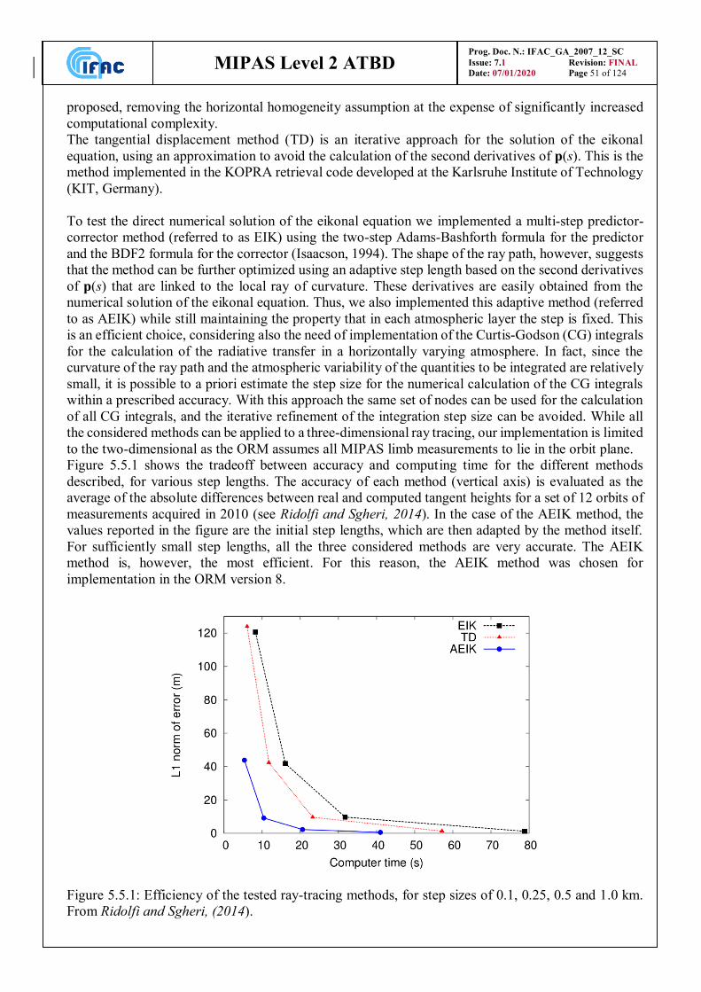
MIPAS Level 2 ATBD
Prog. Doc. N.: IFAC_GA_2007_12_SC
Issue: 7.1 Revision: FINAL
Date: 07/01/2020 Page 51 of 124
proposed, removing the horizontal homogeneity assumption at the expense of significantly increased
computational complexity.
The tangential displacement method (TD) is an iterative approach for the solution of the eikonal
equation, using an approximation to avoid the calculation of the second derivatives of p(s). This is the
method implemented in the KOPRA retrieval code developed at the Karlsruhe Institute of Technology
(KIT, Germany).
To test the direct numerical solution of the eikonal equation we implemented a multi-step predictor-
corrector method (referred to as EIK) using the two-step Adams-Bashforth formula for the predictor
and the BDF2 formula for the corrector (Isaacson, 1994). The shape of the ray path, however, suggests
that the method can be further optimized using an adaptive step length based on the second derivatives
of p(s) that are linked to the local ray of curvature. These derivatives are easily obtained from the
numerical solution of the eikonal equation. Thus, we also implemented this adaptive method (referred
to as AEIK) while still maintaining the property that in each atmospheric layer the step is fixed. This
is an efficient choice, considering also the need of implementation of the Curtis-Godson (CG) integrals
for the calculation of the radiative transfer in a horizontally varying atmosphere. In fact, since the
curvature of the ray path and the atmospheric variability of the quantities to be integrated are relatively
small, it is possible to a priori estimate the step size for the numerical calculation of the CG integrals
within a prescribed accuracy. With this approach the same set of nodes can be used for the calculation
of all CG integrals, and the iterative refinement of the integration step size can be avoided. While all
the considered methods can be applied to a three-dimensional ray tracing, our implementation is limited
to the two-dimensional as the ORM assumes all MIPAS limb measurements to lie in the orbit plane.
Figure 5.5.1 shows the tradeoff between accuracy and computing time for the different methods
described, for various step lengths. The accuracy of each method (vertical axis) is evaluated as the
average of the absolute differences between real and computed tangent heights for a set of 12 orbits of
measurements acquired in 2010 (see Ridolfi and Sgheri, 2014). In the case of the AEIK method, the
values reported in the figure are the initial step lengths, which are then adapted by the method itself.
For sufficiently small step lengths, all the three considered methods are very accurate. The AEIK
method is, however, the most efficient. For this reason, the AEIK method was chosen for
implementation in the ORM version 8.
Figure 5.5.1: Efficiency of the tested ray-tracing methods, for step sizes of 0.1, 0.25, 0.5 and 1.0 km.
From Ridolfi and Sgheri, (2014).
MIPAS Level 2 ATBD
Prog. Doc. N.: IFAC_GA_2007_12_SC
Issue: 7.1 Revision: FINAL
Date: 07/01/2020 Page 52 of 124
5.5.1 Refraction model
In the study of Ridolfi and Sgheri (2014), three refraction models of the air are reviewed and evaluated.
Namely:
the Barrel–Sears formula (Barrel and Sears, 1939),
the simplified Edlén formula (Edlén, 1966),
the Ciddor formula (Ciddor, 1996).
The Barrel–Sears empirical formula has been used for long time in atmospheric infrared applications.
The version we implemented for testing purposes is:
(𝑛 − 1) × 106 = (77.48 +0.44
𝜆2 +0.007
𝜆4 )𝑝
𝑇− (12.79 −
0.14
𝜆2 )𝑝𝑤
𝑇 (5.5.4)
where p is the total air pressure expressed in hPa, T is the temperature in Kelvin, λ the wavelength in
μm and pw is the water vapor partial pressure in hPa.
The simplified Edlén’s formula is the model implemented in the ORM code up to version 7. The
formula is:
𝑛 − 1 = 𝑐0 ⋅𝑇0
𝑝0⋅
𝑝
𝑇 (5.5.5)
with the constants p0 = 1013.25 hPa, T0 = 288.16 K and c0 = 0.000272632. This formula clearly does
not model the dependence of the refraction on the wavelength and the water vapor amount.
Ciddor’s formula models the refractive index as a function of wavelength, pressure, temperature, water
vapor and carbon dioxide content. The formula was originally tested with experimental data extending
only up to 1.7 μm; however, the work of Mathar (2004) suggests that its accuracy should be on the
order of 10-6 also up to 25 μm, i.e., over the whole spectral region covered by MIPAS observations
(4.1-14.9 μm). We implemented Ciddor’s formula following the original paper of Ciddor, (1996).
The differences implied by the three considered refraction models in the calculation of the tangent
heights of the limb measurements is actually very small as compared to the accuracy required (of the
order of 50 – 100 m). Test computations show that Edlén’s and Ciddor’s models are in very good
agreement, producing tangent heights that, on average, differ by less than 30 cm. The Barrel Sears
model produces tangent heights differing by less than 2.5 m as compared to those calculated using the
Ciddor’s formula. According to these results, there is no strong preference for the implementation of
one specific refraction model in the ORM. As a baseline for implementation in the ORM Version 8 the
Ciddor formula was chosen, as it is considered the most accurate by Young, (2011). As a backup option,
should the water and / or CO2 profiles be unavailable, the ORM v.8 uses Edlén’s formula.
5.6 Line shape modeling
The line shape function which has to be modelled appropriately inside the forward model is the Voigt
profile (equation 4.4.15), equal to the convolution of the Doppler profile caused by the velocity of the
molecules and the Lorentz profile induced by collisions. While the Doppler function is the correct
description of the physical effect of Doppler shift, the Lorentz profile is an approximation that is valid
if:
MIPAS Level 2 ATBD
Prog. Doc. N.: IFAC_GA_2007_12_SC
Issue: 7.1 Revision: FINAL
Date: 07/01/2020 Page 53 of 124
the spectral region under consideration is not far from the line centre and
the distance from other lines of the molecule is so large that the line can be considered as isolated
The first assumption fails if we try to model lines far away from the centre. Two important examples
for this are the sub-Lorentzian shape of the line wings of CO2, or the super- and sub-Lorentzian
behaviour of H2O. These effects are normally modelled by introducing a (experimentally determined)
-factor into the line-wing description (see 5.6.3).
The second assumption causes major problems in the modelling of Q-branches since the lines are very
close to each other and molecular collisions lead to an intensity transfer between the transitions. This
effect is called line-mixing (see also 5.7).
5.6.1 Numerical calculation of the Voigt profile
Since the convolution integral of the Voigt profile cannot be evaluated in an analytical form it has to
be calculated numerically. In order to fulfil this task several algorithms were developed and compared
(e.g. Schreier, 1992) with regard to speed and accuracy, especially for the application in line-by-line
models. Due to the recommendations of the latter intercomparison and our own tests regarding
computation time of different approaches (see Table 5.1) it was decided to use the algorithm described
by Humlicek (1982). This routine calculates a rational approximation (with a relative accuracy of
10-4) of the complex probability function:
),(),(de2
1e)(0
22
yxiLyxKti
zw ww
z
tzH
(5.6.1)
with:
iyxz
Kw(x,y) is the convolution integral of the Voigt function from equation (4.4.15).
Method Relative run time
Humlicek (Humlicek, 1982) 1
AFGL (Clough et al., 1981) 1.2
Drayson (Drayson, 1976) 3.0
Table 5.1: Run time comparison between different approaches for the calculation of the Voigt lineshape.
As a baseline Humlicek (1982) has been implemented in the scientific code. A more sophisticated and
optimised version of the Humlicek algorithm has been developed at IMK by M.Kuntz (priv. com.).
However, the algorithm currently implemented in the scientific code will not be upgraded because, as
it will be shown in Sect. 6.11, the final baseline of MIPAS Level 2 processor for operational retrievals
is to compute cross-sections using compressed Look-Up Tables (LUTs).
MIPAS Level 2 ATBD
Prog. Doc. N.: IFAC_GA_2007_12_SC
Issue: 7.1 Revision: FINAL
Date: 07/01/2020 Page 54 of 124
5.6.2 Approximation of the Voigt profile by the Lorentz function
Since the calculation of the Voigt function is much more time consuming than the Lorentz function it
is reasonable to use the Voigt shape only near the line centre where the differences between both are
relatively large. Outside this region the Lorentz line shape can be used. The criterion that can be used
for the application of the different functions is the relative error as a function of the distance from the
centre in multiples of the Doppler half width D. The maximum relative errors are:
Table 5.2: The maximum (y 0 in eq. 4.4.15) relative error between the Voigt and the Lorentz function as a function of the difference from the line centre.
Besides, test calculations using the 30D boundary for 6 selected pT microwindows showed maximum
differences in the order of NESR/120. In these cases the time saving was 60% with respect to the
calculation with the Voigt-profile.
The baseline is to use the Voigt profile only within 30 Doppler half-widths from the line centre. A less
conservative transition can be considered if further computing time saving is found to be necessary.
5.6.3 -factors in the case of CO2 and H2O
In order to describe the sub-Lorentzian behaviour of the CO2 lines -factors were experimentally
determined e.g. by Cousin et al. (1985) for the CO2 3 band head at 4.3 m. These factors start from
unity at the line centre and remain 1 until 0.5-5 cm-1 distance (temperature dependent). Afterwards they
decay exponentially.
The -factor for H2O represents the super-Lorentzian behaviour of water vapour until some 100 -1cm
from the line centre and the sub-Lorentzian shape beyond this (Clough et al., 1989).
Since the -factors are equal to 1 up to some wavenumbers from the line centre, we can disregard them
inside one microwindow. On the other hand the factors are considered for those lines which contribute
as near continuum (see Sect. 5.11.2) to the radiation inside the microwindow.
Distance from the
line centre Relative error
(Lorentz-Voigt)/
Voigt
10 D -1.5%
20 D -0.37%
30 D -0.17%
40 D -0.10%
50 D -0.06%
MIPAS Level 2 ATBD
Prog. Doc. N.: IFAC_GA_2007_12_SC
Issue: 7.1 Revision: FINAL
Date: 07/01/2020 Page 55 of 124
5.7 Line-mixing
Line mixing, known also as line interference, line coupling, collision narrowing, Q-branch collapse,
corresponds to the deviation of the measured line shape from the Lorentzian function (generally in
regions with dense rotational structures, but effects in microwindows of transparency in vibration-
rotation bands have been observed as well).
For practical calculations the suggested line shape (Rosenkranz, 1975) is:
22
Im
1,
L
llll
ll
L
ll
pA
(5.7.1)
with the first order coupling coefficient:
'
'
)'('
'2ll
ll
lll l
ll
d
d
(5.7.2)
is the (frequency dependent) relaxation matrix, with diagonal elements determining the shape of
uncoupled lines ( L
lll Re , the Lorentz half widths) and the lineshifts ( ll Im ), and off-diagonal
elements responsible for non additive effects (line mixing) when the lines overlap, and ld is the reduced
matrix of the dipole moment.
The Rosenkranz expression for the line shape is easily convoluted with the Doppler function. The
modified Voigt function resulting from this convolution may be written in terms of the real (Kw(x,y))
and imaginary parts (Lw(x,y)) of the complex error function w(z) which are calculated by the Humlicek
algorithm (equation 5.6.1):
),(),(12ln
)( llwlllwD
l
l
V
l yxLpYyxKA LM
(5.7.3)
The baseline for Level 2 processor up to IPF version 5.0 has been not to use Q-branches where line-
mixing is known to have strong effects. These spectral regions were avoided with an appropriate choice
of the microwindows, so that line mixing does not need to be simulated. Starting from Level 2 processor
IPF version 6, the line-mixing model of Niro et al., (2007) has been implemented in the algorithm that
computes off-line the cross-section lookup tables (see Appendix D).
5.8 Pressure shift
Beside the line mixing effect, equation (5.7.1) contains the pressure shift in the form of the term
ll Im which is proportional to the atmospheric pressure p. Since at the time of the ORM
development pressure shift data were available only for CH4 and for CO2 above 2300 cm-1 (in the
HITRAN96 data base) pressure shift was not coded in the forward model within the ORM. Pressure-
shift is however modelled in the calculation of cross-section LUTs. Therefore, when LUTs are enabled,
pressure-shift is correctly modelled by the forward model internal to the ORM.
MIPAS Level 2 ATBD
Prog. Doc. N.: IFAC_GA_2007_12_SC
Issue: 7.1 Revision: FINAL
Date: 07/01/2020 Page 56 of 124
5.9 Implementation of Non-LTE effects
The recommendation arising from the final report of Non-LTE study (Bologna, January 23, 1996) is
that no inclusion of externally provided vibrational temperatures for target transitions is needed in
operational processing. The impact of Non-LTE effects in p, T and VMR retrievals is reduced by using
an appropriate selection of microwindows. The capability of handling NLTE is therefore not
implemented in the OFM / ORM.
5.10 Self broadening
The Lorentz half width from equation (4.6.12) includes both, foreign fL0 and self broadened
sL0
components:
iLVMRiLVMRiL sf
xx,,, 000 )1( (5.10.1)
With the volume mixing ratio xVMR.
The relative error which is done when neglecting the self broadening is 1,,VMR 00 iLiL
fs
x . Table
5.3 gives the maximum errors of the half width when assuming maximum values for xVMR and
maximum values for the quotient of self and foreign broadened half widths.
Gas Max.
iLiLfs ,, 00 Max. xVMR
(8-50 km)
[ppmv]
Max. error
[%]
CO2 1.3 360 0.011
O3 1.3 7 0.0002
H2O 10
5 (average)
700 (tropical)
200 (mid-latitude)
0.7
0.08 (average/mid-lat.)
CH4 1.3 1.7 0.00005
N2O not in HITRAN92 - -
HNO3 not in HITRAN92 - -
Table 5.3: Maximum errors in the Lorentz half width when neglecting the self-broadening. Data was taken from HITRAN92
considering the entire range 685-2410 cm-1
From Table 5.3 it is evident, that the self-broadening is negligible for all target species except water
vapour in the tropical troposphere where maximum errors of about 0.7% can occur. However, this
maximum error corresponds (through the Lorentz line shape formulation) directly to a pressure error
of 0.7% which is one third of our acceptance criteria for approximations (2%, see chapter 3). Therefore
our baseline is to disregard the self-broadening in all cases. Self broadening is modelled in the
algorithm that computes cross-section LUTs. Therefore, when LUTs are enabled, self-broadening is
correctly modelled by the forward model internal to the ORM.

MIPAS Level 2 ATBD
Prog. Doc. N.: IFAC_GA_2007_12_SC
Issue: 7.1 Revision: FINAL
Date: 07/01/2020 Page 57 of 124
5.11 Continuum
Three different effects contribute as a continuum to the spectral emission in a given microwindow:
the instrumental continuum
the near continuum
the far continuum
First we discuss these effects and their origin, then we discuss how they can be simulated on the light
of the objectives of this study. For their simulation by the forward model it is necessary to distinguish
between the self standing forward model and the model included in the retrieval code.
5.11.1 Instrumental continuum
This continuum contribution is caused by the instrument itself. Its effect on the spectrum is a pure
additive offset. The reasons for an instrumental continuum are manifold - e.g. self emission of the
instrument, scattering of light into the instrument, or 3rd order non-linearity of the detectors. These
distortions are corrected during the calibration in the Level 1b data processing but specifications
indicate that the residual instrumental continuum averaged over the spectral range of the microwindow
can be larger than the measurement noise. Therefore, the retrieval must be able to model the remaining
radiometric errors. The simulation of the instrumental continuum can be performed by adding a
wavenumber dependent offset to the spectrum.
The baselines are:
for the self-standing forward model to disregard this effect since this program should only simulate
atmospheric contributions.
for the retrieval to assume that the instrumental offset does not vary with changing limb scan angles
and fit for each microwindow only one instrumental continuum offset value.
5.11.2 Near continuum
This contribution to the intensity inside a microwindow is caused by nearby emission lines of
atmospheric gases. Therefore, the simulation of this effect has to be performed during the calculation
of the absorption cross sections. The different possibilities for its calculation are:
1. explicit calculation of the wings of the lines at each fine-grid point inside the microwindow (see
5.6).
2. calculation only at three grid points inside the microwindow and parabolic interpolation in between
For the simulation of the near continuum the ORM uses a switch stored in the MW-specific
spectroscopic database files. These files include, for each spectral line, a parameter indicating whether
the line is to be calculated explicitly at each spectral grid point in the MW (option 1) or can be
calculated only at three spectral grid points and interpolated at the remaining grid points. Baseline is
to use option 2. The same option is used for both self standing and retrieval forward model.
5.11.3 Far continuum
This term includes all continuum-like contributions which are not included in the previous two
definitions. These are e.g. the line wings of lines farther than 25 cm-1 from the current wavenumber
(the most important contribution here is from H2O), the pressure broadened bands of O2 at 1550 cm-1
MIPAS Level 2 ATBD
Prog. Doc. N.: IFAC_GA_2007_12_SC
Issue: 7.1 Revision: FINAL
Date: 07/01/2020 Page 58 of 124
and N2 at 2350 cm-1 and the absorption by aerosols. For this continuum we have to distinguish between
the self standing forward model and the forward model implemented into the retrieval code.
Self standing forward model:
The self standing forward model must produce realistic simulations of the atmospheric spectra that
include the continuum. We decided to use the same continuum as in FASCOD (Clough et al., 1989).
The water continuum is described in Clough et al. (1989). Herein the continuum cross section
)(2 OHcontk is given by the sum of the far line wings using the Van Vleck and Huber line shape function
which is modified in order to fit the experimental data of Burch and Alt (1984):
)(
),(),(),(),(2/tanh2
tanh)(22
2
inesl
lOHllOHl
Bll
l
B
contff
TKhc
S
TK
hck OH
(5.11.1)
where:
1-
22cm 25 if
)(
1),(
l
l
L
l
L
llf
(5.11.2)
1-
22cm 25 if
25
1),(
l
L
l
L
llf
(5.11.3)
and ),(2 lOH is the -factors of water.
For the implementation into the forward model the following equation is used:
),(1),(2
tanh)( 000 22
2 TCxTCTk
hck fOHsOHB
cont OH
(5.11.4)
),(0 TC s and ),(0 TC f are the continuum absorption parameters for the self and the foreign
broadening at the reference number density 0. is the actual air density. To determine the temperature
dependence of the self broadening values, exponential interpolation between the tabulated parameters
)K 260,(0 sC and )296K,(0 sC is performed. For the foreign broadening )296K,(0 fC is used for
all temperatures. The interpolation in frequency is performed linearly.
This continuum description includes only contributions of lines farther than 25 cm-1 from the line
centre. Since the self standing forward model will use the spectroscopic database which uses various
selection criteria for the lines, not all water lines within 25 cm-1 may be considered.
However, tests have shown that the error due to this fact is less than 0.175NESR (and in most cases
much less than this). Because this is presumably smaller than the absolute accuracy of the continuum
model and because the self-standing forward model is not required to describe the continuum with very
high accuracy, our baseline is to use selected water lines from the spectroscopic database. If higher
accuracy is needed, the missing water lines can be added to the data-base.
The N2 continuum is parameterised, temperature independently, every 5 cm-1 between 2020 and 2800
cm-1 for a reference number density 0. In order to calculate it for the actual pressure and temperature
it has to be multiplied by the ratio 0 , where is the actual number density, and linearly interpolated
to the wavenumber. For a details on the implemented N2 continuum model, please refer to Lafferty at
al., (1996).
MIPAS Level 2 ATBD
Prog. Doc. N.: IFAC_GA_2007_12_SC
Issue: 7.1 Revision: FINAL
Date: 07/01/2020 Page 59 of 124
The O2 continuum is given in the form of three parameters (one strength and two for the temperature
correction) from 1395-1760 cm-1. For a detailed description of the adopted model of O2 continuum,
please refer to the paper of Thibault et al., (1997).
Forward model in the retrieval:
The forward model in the retrieval code simulates the far-continuum using a MW- and altitude-
dependent cross-section KMW(z). The transmission of each atmospheric layer ownig to the gases is
multiplied by 𝜉MW(𝑧) = exp(−𝐾MW(𝑧) ⋅ 𝐶𝐴𝐼𝑅(𝑧)) where 𝐶𝐴𝐼𝑅(𝑧) is the total air column of the
atmospheric layer at altitude z. A profile 𝜉MW(𝑧) is retreived for each MW, in the altitude range where
the MW is used, possibly limited to the top altitude bound for continuum retrieval, that is supplied by
the user in the settings file (tipycally 30 km). In order to limit the number of retrieved parameters /
profiles, the retrieval algorithm offers the possibility to apply some constraints to the retrieved 𝜉MW(𝑧)
profiles.
For each microwindow and each altitude, the frequency range Δ𝜈 is defined in which the continuum is
expected to vary linearly with frequency. This frequency range is used to establish the constraints
between retrieved continuum profiles. Particularly, if the distance between the centers of two (or more)
selected MWs is less than a fraction f of Δ𝜈, the MWs are considered to be in ‘tight contiguity’ and
they share the same retrieved continuum profile 𝜉MW(𝑧). If a set of MWs is located in a frequency
interval whose width is less than Δ𝜈, continuum profiles 𝜉MW(𝑧) are retrieved for the MWs at the edges
of the set and continuum is obtained via linear interpolation for the MWs in between. The MWs within
this type of set are said in ‘loose contiguity’.
The most recent versions of the algorithm for automated selection of spectral microwindows
(MWMAKE, see Appendix C and Bennett et al., 1999) use the fitted atmospheric continuum
parameters to compensate for various systematic error sources that introduce in the spectrum a
continuum-like effect. This baseline implies that currently, the fitted “continuum” parameters have lost
their physical meaning. Therefore, while in principle in the ORM it is still possible to apply the above
mentioned constraints, in routine retrievals these are not applied. Continuum constraints are disabled
by setting to a very small value the continuum linearity range Δ𝜈.
Note that, in the first versions of the MIPAS Level 2 processor (up to Version 5.0) the baseline was to
retrieve vertical profiles of continuum cross-sections KMW(z). Starting from Version 6.0, the baseline
has changed to the retrieval of 𝜉MW(𝑧) profiles. According to the results of the studies of Ridolfi and
Sgheri, (2013), this new baseline makes the retrieval better conditioned and improves the stability.
5.12 Interpolation of the profiles in the forward / retrieval model
Since both initial guess and retrieved profiles are often represented on a grid much coarser ( 3km)
than the grid used for the discretization of the atmosphere ( 1km, for the radiative transfer calculation),
a set of interpolation rules must be established for the various types of profiles.
Pressure and temperature profiles are always constrained to fulfil the hydrostatic equilibrium equation.
Tests have shown that, using any of the atmospheric standard models, neglecting the temperature
gradient leads to negligible errors when layers thinner than 6 km are adopted and the temperature in
the middle of the layer is used as the representative temperature of the layer.
When the altitude is the independent variable, it is common to consider the temperature and the VMR
profiles as varying linearly with altitude, and pressure as varying accordingly to the hydrostatic
MIPAS Level 2 ATBD
Prog. Doc. N.: IFAC_GA_2007_12_SC
Issue: 7.1 Revision: FINAL
Date: 07/01/2020 Page 60 of 124
equilibrium law (i.e. exponentially with the altitude if the temperature is assumed locally constant for
the calculation of pressure).
Now, since in our case the independent variable is pressure, the most appropriate interpolation rule is
linear interpolation for both temperature and VMR profiles in log(P). The baseline is therefore to use
type of interpolation for temperature and VMR profiles whenever an interpolation is required.
Regarding continuum cross-section profiles: whenever an interpolation is required, since the
continuum emission behaves as the square of pressure (Clough et al., 1989), and since the fitted
continuum cross-section profiles are multiplied by the air column (proportional to pressure) in order to
obtain continuum emission, it is then reasonable to interpolate continuum profiles linearly in pressure.
5.13 Interpolation of the “retrieved” profiles to a user-defined grid
5.13.1 Description of the problem
The baseline of the Level 2 scientific processor is to retrieve the target profiles in correspondence of
the tangent pressures. However, the users of MIPAS products may need to resample the retrieved
profiles to a user-defined set of pressures. The problem arises therefore of providing a recommended
interpolation scheme consistent with the Level 2 algorithm assumptions.
The first possibility is to recommend the use of the same set of interpolation rules used in the retrieval
processor (see Sect. 5.12). However, considering that Level 2 profiles have been derived from limb-
scanning measurements, the a-posteriori interpolation process should generate profiles that, when
provided in input to the forward model, reproduce the simulated spectra calculated in the retrieval at
convergence. Therefore, considering that the simulated limb-radiances strongly depend on the total
column amounts above the tangent point, the interpolation scheme should conserve the total column.
In other words, the column calculated for the interpolated points should be equal, within some pre-
defined tolerance, to the column obtained with the original data profile.
We recall that the vertical column of a gas, above a particular altitude rz1 is defined as
1
( )
( )
rulatm
VMR
gas
rz
p zCol Const x dz
T z (5.13.1)
where rulatm is the altitude of the upper boundary of the atmosphere and VMR
gasx , p(z) and T(z) are the
gas VMR, pressure and temperature respectively.
The quantities VMR
gasx , p(z) and T(z) are measured for a discrete altitude grid, thus, in order to have a
realistic result we must calculate the total column as the sum of partial columns between the altitudes
of this grid. In turn these partial columns can be calculated interpolating the pressure, temperature and
VMR profiles between the two edge altitudes: linear interpolation is used for Temperature and VMR,
and exponential interpolation for the pressure.
Therefore, the problem of the interpolation of the VMR profiles becomes one of finding an appropriate
transformation of the VMR profile that fulfils the constraint of an unchanged vertical column.
5.13.2 Strategy
The strategy adopted consists of constructing a new grid of VMR points and to impose a one-to-one
correspondence of partial columns with the original profile. By finding the VMR values that satisfy
this condition, a profile is identified at the new grid points. The latter will be different of the one
obtained with a classical interpolation rule.
MIPAS Level 2 ATBD
Prog. Doc. N.: IFAC_GA_2007_12_SC
Issue: 7.1 Revision: FINAL
Date: 07/01/2020 Page 61 of 124
A ‘classical’ interpolation law is defined in order to identify from the discrete output of the ORM a
continuous representation of the atmosphere. For each value of the independent variable (pressure), the
corresponding altitude and temperature can be obtained by means of hydrostatic equilibrium equation,
assuming a linear dependence of temperature on altitude. In turn, the VMR values at each user-defined
altitude can be obtained by linear interpolation between the two nearest retrieved values.
On the basis of this continuous representation, partial columns and total columns can be defined with
respect to both the retrieval grid and the user defined grid in the following way:
1. First partial columns are calculated on the retrieval-grid
2. Then the VMR values are calculated at the user-defined grid using linear interpolation with the
altitude.
3. Then the partial columns at the retrieval-grid are calculated following a spline that joins the user-
defined grid points only.
4. We then vary the VMR values at the user-defined grid until the difference between the partial
columns of the new profile and of the original profile are minimum. By definition, the resulting
profile has the property of keeping unmodified the vertical column.
The variation of the VMR values on the user-defined grid are calculated using a non-linear least-
squares fitting procedure. The quantities to be fitted are the partial columns on the retrieval grid. The
parameters to be fitted are the VMR values at the pressure levels of the user-defined grid. The fitting
method is the Gauss-Newton method: if XV is a vector containing the difference between the observed
partial columns and the calculated partial columns, then the correction CV to be applied to the values
of the VMR at the user-grid to minimise this difference is given by:
XVVCV G (5.13.2)
where 1
1 1T T
V v col v v colG K S K K S and Kv is the Jacobian matrix and Scol is the Variance Covariance
Matrix (VCM) of the measured columns.
Since the values of the partial columns are numbers that change by several orders of magnitude from
the highest altitude to the lowest, instead of fitting their values we fit the logarithm of their values. So
Scol becomes the VCM of the logarithm of the partial columns Slog(col).
An output of the retrieval code is the VCM of the measured columns col(i) at the various tangent
altitudes i. To get the VCM of the logarithm of the columns we apply the following transformation:
col ,
log(col) ,
i j
i j col i col j
SS (5.13.3)
The errors associated with the solution of the fit are given by the square roots of the diagonal elements
of the VCM of the solution (S) given by:
1
1
log(col)
T
v vS K S K (5.13.4)
After solving equation (5.13.2), the VMR profile on the user-defined grid will be given by the new
vector xVMRint:
xVMRint=xVMRlinint+ CV (5.13.5)
MIPAS Level 2 ATBD
Prog. Doc. N.: IFAC_GA_2007_12_SC
Issue: 7.1 Revision: FINAL
Date: 07/01/2020 Page 62 of 124
The fitting procedure is repeated until the sum of the squares of the differences between the new
columns and the measured ones doesn’t change of more than 1%. In the ORM code the retrieved profile
above the highest fitted altitude is obtained by scaling the initial-guess profile of the same quantity
used for the highest fitted point. The same procedure has to be applied to the interpolated points above
the highest fitted altitude or to the highest point of the user-defined grid if it happens to be below the
highest fitted altitude.
The errors associated with the new VMR values are characterised by the variance-covariance matrix S
provided by equation (5.13.4).
5.14 Optimized algorithm for construction of initial guess profiles and gradients
The scientific version of this function was implemented only in the ORM v.8. Earlier ORM versions
had no access to operational data from the European Centre for Medium-range Weather Forecast
(ECMWF), therefore this function was only implemented in the so called “framework” module of the
industrial Level 2 processor. Furthermore, the construction of the initial guess profiles requires
knowledge of the profiles retrieved from the “previous scan” in the orbit and, at the beginning of the
development, the ORM had the capability of handling only individual scans.
For the analysis of a given limb scan of measurements, the ORM needs the vertical profiles and
horizontal gradients of the following quantities:
1. Pressure and temperature,
2. VMR of retrieved and non-retrieved (or assumed) gases contributing to the MWs used in the
retrievals to be performed.
3. Continuum vertical profiles for the microwindows used in the retrievals to be performed.
The profiles can be used in the different retrievals either as a first guess of the profiles that are going
to be retrieved or as assumed profiles of the atmospheric model (profiles of interfering species and p,T
profiles in the case of VMR retrievals). Horizontal gradients are assumed (not retrieved) in the forward
model computations.
5.14.1 Initial guess pressure, temperature and VMR profiles, and their horizontal gradients
The ORM v.8 builds the initial guess / assumed profiles and horizontal gradients of Pressure,
Temperature and VMR on the basis of input files. These files are built by the ORM pre-processing
stage, starting from the following sources:
- IG2: the IG2 climatological profile database (Remedios et al., 2007)
- ORM: profile retrieved by the ORM from the current scan being processed, e.g. pT and H2O
profiles already retrieved from the current scan
- ADJ: profiles retrieved by the ORM from the scan adjacent to the current scan.
- NET: profiles retrieved by the ORM in a previous processing of the current orbit of
measurements.
- ECM: ECMWF profiles (p, T, H2O and O3 profiles) obtained by inerpolationg to time and geo-
location of the current scan the ECMWF analysis profiles.
In the ORM, the above profile sources are prioritized according to a list provided by the user in the
settings file. Intial profiles and gradients are then computed by the ORM pre-processing module for
each scan, using first the highest priority sources available, then eventually extending them in altitude,
MIPAS Level 2 ATBD
Prog. Doc. N.: IFAC_GA_2007_12_SC
Issue: 7.1 Revision: FINAL
Date: 07/01/2020 Page 63 of 124
with profiles and horizontal gradients from lower priority sources, so as to cover the whole 0 – 120 km
vertical range that is adopted for the IG2 profiles.
From the ORM settings file it is possible to require the profiles arising from a specific gas retrieval not
to contribute to building the initial guess / assumed profiles for the subsequent retrievals. This option
is especially useful for gas profiles retrieved with extremely low signal to noise ratio, large error bars
and, possibly, large oscillations. Test retrievals have shown that in these cases the use of IG2
climatological profiles as initial guess makes the retrieval generally more stable and improves the
quality of the results. Full details of the algorithm employed by the ORM v.8 to build initial guess /
assumed profiles are described in Sgheri, (2017).
5.14.2 Initial guess continuum profiles
The initial guess continuum profiles used by the retrieval algorithm are purely climatological profiles.
Retrieved continuum profiles are not considered for the generation of the initial guess as they suffer of
very large uncertainties (and also because retrieved continuum parameters, being used also to
compensate for continuum-like error sources, may be very different from scan to scan).
Climatological continuum profiles are generated on the basis of a simple algorithm that, starting from
given profiles of pressure, temperature and water vapor, calculates profiles of water vapor cross-
sections in correspondence of the central frequencies of the considered microwindows. Water vapor
continuum cross-sections are calculated using the CKD v.2.4 model (Clough, (1989)). The continuum
of other species like CO2, N2, O2, aerosols etc. is not considered in this algorithm because we have
found that in the presence of large uncertainties on the continuum emission, it is by far preferred to use
initial guess profiles that underestimate the real continuum. In fact, an overestimated initial guess
continuum easily leads to a very opaque atmosphere in which the line of sight may not be able to
penetrate. In these conditions the fitting procedure may be unable to recover the correct continuum
emission.
5.15 Profiles regularization
In the nominal observation mode adopted after January 2005, a MIPAS limb-scan consists of 27 spectra
that look at tangent altitudes from 7 to 72 km, with 1.5 km steps from 7 to 22 km, 2 km steps from 22
to 32 km, 3 km steps from 32 to 47 km, 4 km steps from 47 to 63 km and 4.5 km steps from 63 to 72
km. The signal measured by the instrument is obtained with an instantaneous field of view (IFOV)
equal to 3x30 km2 (vertical height times across-track width). Since the step of the measurement grid is
for some altitudes smaller than the vertical IFOV, contiguous limb scanning views have overlapping
IFOVs. This situation, combined with the choice of using a retrieval grid that matches the measurement
grid, determines an ill-conditioning of the inversion and the need for a regularization in order to avoid
instabilities in the retrieved profiles. The ORM adopts a Tikhonov-Twomey regularization scheme
(Tikhonov, 1963), whose strength can be established (depending on the features of the retrieved profile)
using two alternative approaches: the error consistency (EC) method of Ceccherini, (2005), or the
Iterative Variable Strength (IVS) method proposed by Ridolfi and Sgheri, (2009). These two methods
are herewith briefly described.
5.15.1 The error consistency (EC) method
The Tikhonov regularized solution of the retrieval problem can be obtained by minimizing the
following cost function (see e. g. Rodgers (2000)):
MIPAS Level 2 ATBD
Prog. Doc. N.: IFAC_GA_2007_12_SC
Issue: 7.1 Revision: FINAL
Date: 07/01/2020 Page 64 of 124
a
T
aRy
Tf xxRxxxFySxFyx
1 (5.15.1)
where x is the vector representing the profile to be determined, y is the measurement vector, Sy is the
VCM describing the errors of y, F(x) is the forward model, R is a positive parameter characterizing
the strength of the regularization, xa is an a priori estimate of the state vector and R is a regularization
matrix. The cost function f(x) contains two terms: the first term is the ``chi-square'' that measures how
well the forward model calculated in x is able to reproduce the measurements within their errors, and
the second term measures how well the retrieved profile follows some feature of xa determined by the
regularization matrix. In our case, where R=L1TL1 with L1 equal to the discrete first derivative operator,
the vertical increments of the retrieved profile are constrained to follow those of xa. If xa is a smooth
profile, the L1 operator provides a smoothing of the retrieved profile while reducing the negative
correlations between vertically adjacent values introduced by the fact that contiguous limb views have
overlapping IFOVs.
The minimum of f(x) may be searched iteratively using the Gauss-Newton method, that provides the
following expression of x at each iteration:
aRR RxxSRSx xx ˆ1
ˆ
11
ˆ (5.15.2)
where x is the non-regularized state vector, i.e. the solution obtained when only the first term of f(x)
is minimized and x
Sˆ, is its VCM. This is an unconventional expression of the solution that will be
useful for the subsequent considerations and that can be reduced to the conventional expression
recalling that:
0y
T
y
T
0 xFySKKSKxx ˆˆˆ 111 (5.15.3)
11
ˆ
KSKS y
T
x (5.15.4)
0x being the initial guess of the iteration and K the Jacobian matrix of F(x) calculated in 0x .
The solution of Eq. (5.15.2) is characterized by the following averaging kernel matrix (AKM)
(Rodgers, 2000):
1
ˆ
11
ˆ
xxx SRSA R
AKM (5.15.5)
and by the following VCM:
11
ˆ
1
ˆ
11
ˆ
RSSRSS xxxx RR . (5.15.6)
To determine the regularization strength, the EC method (Ceccherini, 2005) can be applied. It is based
on the requirement that the difference between the regularized and the non-regularized profiles
weighted with the inverse of the VCM of the regularized profile must be equal to the number nR of
points of the profile:
Rx
Tn
xxSxx ˆˆ 1. (5.15.7)
MIPAS Level 2 ATBD
Prog. Doc. N.: IFAC_GA_2007_12_SC
Issue: 7.1 Revision: FINAL
Date: 07/01/2020 Page 65 of 124
A simplified interpretation of Eq. (5.15.7) is obtained in the case that xS is a diagonal matrix (even if
this never occurs for atmospheric profiles retrieved from remote sensing measurements). In this case
the differences between the regularized and the non-regularized profiles must be on average equal to
the errors of the regularized profile (measured by the square root of the diagonal elements of xS ).
Substituting in Eq. (5.15.7) x from Eq. (5.15.2) and xS from Eq. (5.15.6), with straightforward
calculations the following value for R is obtained:
xxRRSxx
x ˆˆ ˆ
a
T
a
RR
n . (5.15.8)
In Eq. (5.15.8) the xS ˆ , which measures the random errors due to the mapping of random radiometric
noise into the retrieved profile, is used instead of the VCM of the total retrieval errors. In this way the
error components due to forward model errors are neglected in the regularization process. This choice
is based on the consideration that these components are usually characterized by a positive correlation
between values contiguous in altitude, and therefore, the regularization does not need to account for
them.
The application of this method to the MIPAS retrieval code has to take into account the following
considerations. The Gauss-Newton iterative method is successful only in the case of a sufficiently weak
non-linearity of the forward model. In the case of strong non-linearities some iterations of the
iterative method can lead to an increase rather than to a decrease of the residuals. For this reason in the
ORM a modification of the Gauss-Newton method, the Levenberg-Marquardt technique (Levenberg,
1944; Marquardt, 1963), is used. This latter modifies Eqs. (5.15.3) and (5.15.4) into:
0y
T
y
T
0 xFySKMKSKxx ˆˆˆ 111
reg (5.15.9)
11111
ˆ
MKSKKSKMKSKS y
T
y
T
y
T
x regreg (5.15.10)
where M is a matrix that in the ORM is diagonal, with the diagonal elements equal to those of the
matrix KSK y
T 1 and reg is a parameter that, during the retrieval iterations, is increased or decreased
depending on whether the chi-square function increases or decreases while the atmospheric state is
upgraded from 0x to x only when the chi-square function decreases. Accordingly, the AKM is not an
identity matrix, as in the pure Gauss-Newton approach, but it is equal to:
KSKMKSKA1
y
T1
y
T
x
1
ˆ reg
AKM (5.15.11)
Some tests on MIPAS measurements have confirmed that, because of the high non-linearity of the
problem, the pure Gauss-Newton iteration often produces an increased chi-square value. The
Levenberg-Marquardt method is needed to determine the minimum of the chi-square, and this need is
not abated by the use of the Tikhonov regularization. For this reason we decided to use both the
Levenberg-Marquardt method and the Tikhonov regularization.
Recalling that the objective of the Levenberg-Marquardt method is to reach the minimum of the chi-
square and the objective of the Tikhonov regularization is to limit the oscillations of the retrieved
profile, it is convenient to exploit Eq. (5.15.2) which calculates the regularized profile from the non-
regularized one and to perform the two operations sequentially. First the chi-square function is
minimized using the Levenberg-Marquardt method by means of the iterative application of Eq.
MIPAS Level 2 ATBD
Prog. Doc. N.: IFAC_GA_2007_12_SC
Issue: 7.1 Revision: FINAL
Date: 07/01/2020 Page 66 of 124
(5.15.9), secondly, when convergence has been reached, an a-posteriori regularization defined by Eq.
(5.15.2), with x and xS ˆ given by the Eqs. (5.15.9-5.15.10) at the last iteration of the minimization
process, is applied. This procedure is different from the commonly used procedure that performs the
regularization at each iteration step. The two procedures produce similar performances in terms of
vertical resolution and retrieval errors and the adopted strategy has the advantage of lighter calculations
that is important for operational retrievals.
The strength of the regularization can be determined by means of the EC method using Eq. (5.15.8).
The VCM of the regularized profile is given by Eq. (5.15.6) and the AKM is obtained by calculating
the derivative of x (provided by Eq. (5.15.2)) with respect to the atmospheric true state, taking into
account that the derivative of x with respect to the atmospheric true state is (by definition) AKM
xA ˆ :
AKM
R
AKM
x xxx ASRSA ˆ
1
ˆ
11
ˆ
(5.15.12)
where AKM
xA ˆ is provided by Eq. (5.15.11) calculated at the last iteration of the minimization process.
The methods described so far have a limitation in the case of H2O whose VMR values change several
order of magnitude within a single profile. In fact in this case the procedure regularizes the profile only
in the altitude regions where the VMR is large (because in this region the absolute error is the largest),
and does not regularize the profile where the VMR is small. This problem can be overcome considering
the logarithm of the profile in the place of the profile, in this case the regularization method uses the
relative errors (instead of the absolute errors) to choose where to regularise the profile. Since the
relative errors are expected to be more constant along the profile, a more uniform regularisation is
expected.
In this case the regularisation must be applied to the profile of the logarithm of water vapour VMR.
When the cost function of equation (5.15.1) is defined for the logarithm of the profile, solution (5.15.2)
becomes:
aRR xRxSRSx xx logˆloglog1
ˆlog
11
ˆlog
(5.15.13)
where:
ji
ji
ji xx ˆˆ
,ˆ
,ˆlog
x
x
SS (5.15.14)
From Eq. (5.15.13) it follows that:
11
ˆlog
1
ˆlog
11
ˆloglog
RSSRSS xxxx RR (5.15.15)
The regularised profile is obtained by means of the exponential function:
aRR xRxSRSxx xx logˆlogexplogexp1
ˆlog
11
ˆlog
(5.15.16)
and is characterized by the following VCM and AKM:
jijiRRji xx,
11
ˆlog
1
ˆlog
11
ˆlog,
RSSRSS xxx
x (5.15.17)
AKMAKM
xx CAA ˆ (5.15.18)
MIPAS Level 2 ATBD
Prog. Doc. N.: IFAC_GA_2007_12_SC
Issue: 7.1 Revision: FINAL
Date: 07/01/2020 Page 67 of 124
where C is defined by:
j
i
jiRjix
x
ˆ,
1
ˆlog
11
ˆlog,
xx SRSC (5.15.19)
The value of the regularization parameter R can be determined applying the EC method to the
logarithm of the profile:
R
Tn
xxSxx xˆloglogˆloglog
1
log (5.15.20)
Substituting the equations (5.15.13) and (5.15.15) in equation (5.15.20) we find an analytical solution
for the regularization parameter R
xxRRSxx x
ˆloglogˆloglog ˆlog
a
T
a
RR
n
Remark: application to real data of the method presented above, in which the logarithm of the H2O
VMR is regularized with the EC approach, has been found to be critical. The criticality arises from the
large error bars (< 100%) that sometimes are encountered, in localized altitude ranges (just above the
tropopause), in the H2O profiles. In fact, too large error bars imply the failure of the linearity hypothesis
used above, for the calculation of the VCM of the logarithm of the VMR profile. For this reason H2O
profile regularization has been disabled in the ESA IPF version 6.0 retrievals. The IPF/ML2PP version
7 implements a more sophisticated approach for the selection of the regularization strength, the so
called “Iterative Variable Strength” (IVS) method.
5.15.2 The Iterative Variable Strength (IVS) regularization method
Due to the above mentioned problems with the EC regularization method, in Ridolfi and Sgheri,
(2009) we proposed the VS (variable strength) regularization scheme, a self-adapting and altitude-
dependent approach that detects whether the actual observations contain information about small-
scale profile features, and determines the strength of the regularization accordingly. While
representing an optimal solution, this method has two drawbacks. First, the method relies on an
external minimization routine that needs to be carefully tuned to obtain optimal performances.
Second, the computational requirements of the method, and specifically of the optimization routine,
lead to an increase of the retrieval time of more than 20%. This extra computing load was considered
unacceptable by ESA for the MIPAS ground processor. For this reason we explored the possibility
to simplify the VS method, with the aim of reducing its computational cost while preserving the
good performances. Therefore we proposed the IVS (iterative variable strength) method, an
alternative to the VS scheme. The IVS, while based on the same rationale of the VS, does not use
any minimization routine, so that the implementation is easier and the additional computational
effort required amounts only to about 1.5% of the total retrieval time.
Tikhonov regularization is often used to improve the conditioning of atmospheric profile inversion.
Smoother profiles are obtained by penalizing the oscillating solutions in the inversion formula. Let
y = f(x) be the forward problem, where y is the m-dimensional vector of the observations with error
covariance matrix Sy, f is the forward model, function of the n-dimensional atmospheric state vector
x, whose components represent the unknown profile at altitudes z = zj , j = 1, …, n. The Tikhonov
solution is the state vector xt minimizing the following cost function:
MIPAS Level 2 ATBD
Prog. Doc. N.: IFAC_GA_2007_12_SC
Issue: 7.1 Revision: FINAL
Date: 07/01/2020 Page 68 of 124
2 1( ) ( )T T T
y s s y f x S y f x x x L L x x
The first term of the right side of (5.16.1) is referred to as 2 and represents the cost function
minimized in the least-squares (LS) approach. The vector xs is an a-priori estimate of the solution.
Since it is usually not easy to have reliable a-priori estimates of the solution we always take xs = 0,
L is a h x n matrix operator, usually approximating a linear combination of the i-th order vertical
derivatives (i = 0, 1, 2). The h x h matrix is diagonal, positive semi-definite and drives the strength
of the regularization. Note that normally h < n. The standard scalar Tikhonov regularization is
obtained when I . Several methods may be used to select the regularization strength through
the amplitude of . The IVS method determines a profile of as the result of an optimization
process. In the ORM v.8 we apply the regularization a-prsteriori after the convergence of the
minimization sequence. As reported in Ceccherini et al. (2007) and in Ridolfi and Sgheri (2009),
this choice improves the convergence rate. In other words, we first find the minimum of the 2
using the Levenberg-Marquardt (LM) approach:
1
1 1 1
1 diag[ ] ( )T T T
k k y y y k
x x K S K K S K K S y f x
Let k be the iteration count at convergence, thus xOE = xk+1 is the unregularized solution. Let AOE be
the averaging kernel of xOE and SOE its measurement error covariance matrix. Within the ORM AOE
and SOE can be calculated with alternative algorithms of different sophistication as explained in
Ceccherini et al.(2007) and Ceccherini and Ridolfi (2010). The theory explained hereafter does not
depend on the method used to infer AOE and SOE. We can compute the last iterate as the minimizer
of (5.16.1) that includes also the regularization term. Thus the regularized solution x is given by:
1
1 1 1diag[ ] ( )T T T T T
k y y y k k
x x K S K K S K L L K S y f x L Lx
If we set:
1
1 1 1 1diag[ ] diag[ ]T T T T T
y y y y
D K S K K S K L L K S K K S K
Then, after a few algebraic manipulations and using (5.16.2), (5.16.3) can be re-written as:
OE x Dx
the averaging kernel A and the covariance matrix S of x can be written as:
OE A DA (5.16.6)
T
OE S DS D (5.16.7)
To determine the regularization strength the IVS method proceeds as follows. We define a -
profile ( )z on a vertical grid so fine that we can consider it a continuous function. We start with a
large (0)( ) MAXz constant profile and decrease it iteratively until the following requirements are
fullled:
MIPAS Level 2 ATBD
Prog. Doc. N.: IFAC_GA_2007_12_SC
Issue: 7.1 Revision: FINAL
Date: 07/01/2020 Page 69 of 124
1T
l l
OE OE OE ew n
x x S x x
l
j r jv w z x with j = 1, ..., n
Where l is the iteration count, lx is the regularized solution calculated from (5.16.5) using
( )( )l
jj jz for j=1, ..., h. l
jv x is the vertical resolution calculated at altitude jz as the
FWHM of the averaging kernels (5.16.6). Condition (5.16.8) ensures that, on average, the
regularized profile lays within a fraction we of the error bars of the unregularized profile. Condition
(5.16.9) guarantees that at any altitude jz in the retrieval range the vertical resolution is kept smaller
than a multiple factor wr of the vertical step jz of the retrieval grid. we and wr are user-selectable
parameters. Fix a threshold MIN Let 1,...,J n the set of indeces of the altitudes jz for which
(0)( )j MINz and:
l
OE e OEj jjjw S x x or (5.16.10)
l
j r jv w z x
If the requirements (5.16.8) and (5.16.9) are not met J is not empty and we decrease
( )l
z The
decreased profile 1
( )l
z
is calculated as:
1( ) , , ( )
l l
j j j
j J
z T z z z
Where T is the triangular shaped function defined as:
- +
-
+
1 if < or > ,
1, , if 0,
1 if 0 ,
j j j
z z
rT z z r z z
rr z z
and 0 < r < 1, , 0 are constants. Note that 1 1
( ) ( )l l
z z
if and only if
,j j j jz z z for some j J . The parameter r drives the speed of the attenuation of the
-profile, in our implementation we used r = 0.99. Furthermore we set 3j j jz z
3j j jz z
on the basis of the following considerations. The x profile is obtained from xOE via the formula
(5.16.5). For any standard choice of L, TL L is at most a pentadiagonal matrix. In our case we use
L = L2 (the discrete second derivative operator), therefore TL L is pentadiagonal. Moreover the
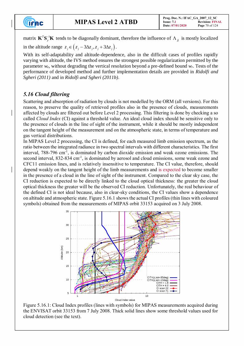
MIPAS Level 2 ATBD
Prog. Doc. N.: IFAC_GA_2007_12_SC
Issue: 7.1 Revision: FINAL
Date: 07/01/2020 Page 70 of 124
matrix 1T
y
K S K tends to be diagonally dominant, therefore the influence of jj is mostly localized
in the altitude range 3 , 3j j j j jz z z z z .
With its self-adaptability and altitude-dependence, also in the difficult cases of profiles rapidly
varying with altitude, the IVS method ensures the strongest possible regularization permitted by the
parameter we, without degrading the vertical resolution beyond a pre-defined bound wr. Tests of the
performance of developed method and further implementation details are provided in Ridolfi and
Sgheri (2011) and in Ridolfi and Sgheri (2011b).
5.16 Cloud filtering
Scattering and absorption of radiation by clouds is not modelled by the ORM (all versions). For this
reason, to preserve the quality of retrieved profiles also in the presence of clouds, measurements
affected by clouds are filtered out before Level 2 processing. This filtering is done by checking a so
called Cloud Index (CI) against a threshold value. An ideal cloud index should be sensitive only to
the presence of clouds in the line of sight of the instrument, while it should be mostly independent
on the tangent height of the measurement and on the atmospheric state, in terms of temperature and
gas vertical distributions.
In MIPAS Level 2 processing, the CI is defined, for each measured limb emission spectrum, as the
ratio between the integrated radiance in two spectral intervals with different characteristics. The first
interval, 788-796 cm-1, is dominated by carbon dioxide emission and weak ozone emissions. The
second interval, 832-834 cm-1, is dominated by aerosol and cloud emissions, some weak ozone and
CFC11 emission lines, and is relatively insensitive to temperature. The CI value, therefore, should
depend weakly on the tangent height of the limb measurements and is expected to become smaller
in the presence of a cloud in the line of sight of the instrument. Compared to the clear sky case, the
CI reduction is expected to be directly linked to the cloud optical thickness: the greater the cloud
optical thickness the greater will be the observed CI reduction. Unfortunately, the real behaviour of
the defined CI is not ideal because, also in clear-sky conditions, the CI values show a dependence
on altitude and atmospheric state. Figure 5.16.1 shows the actual CI profiles (thin lines with coloured
symbols) obtained from the measurements of MIPAS orbit 33153 acquired on 3 July 2008.
Figure 5.16.1: Cloud Index profiles (lines with symbols) for MIPAS measurements acquired during
the ENVISAT orbit 33153 from 7 July 2008. Thick solid lines show some threshold values used for
cloud detection (see the text).
MIPAS Level 2 ATBD
Prog. Doc. N.: IFAC_GA_2007_12_SC
Issue: 7.1 Revision: FINAL
Date: 07/01/2020 Page 71 of 124
The bulk of clustered CI profiles shown in Fig. 5.16.1 corresponds to clear-sky conditions.
Particularly, the thick red line with symbols represents the CI profile of scan 22 that apparently
corresponds to clear-sky, and is going down to 6 km tangent height. The thick (dark) blue line with
symbols represents the CI profile of scan 71 acquired at Antarctic latitudes. This CI profile shows a
marked reduction already at 23 km tangent height, corresponding to a Polar Stratospheric Cloud
(PSC) entering the FOV of the instrument. In general, we see that the CI values change significantly
with the tangent height of the measurements. Moreover, above 25 or 30 km, the measurement noise
has a significant impact on the cloud index calculation. These features make it hard to detect clouds
by comparing the CI with a single threshold independent of altitude.
The thick vertical black line shown in Fig. 5.16.1 represents the (height independent) CI-threshold
of 1.8 used for cloud detection in MIPAS Level 2 processings up to Version 7. With this choice,
several sweeps affected by high-clouds (namely PSCs) are classified as clear-sky and used in the
retrievals, causing outliers in the retrieved VMR profiles, especially of H2O, NO2 and N2O5. In a
first attempt we tried to solve the problem by using the more conservative CI-threshold of 4 (thick
vertical brown line in Fig. 5.16.1), already adopted at KIT (Karlsruhe) for the scientific KOPRAFIT
retrievals. This choice mostly solves the problem of undetected high clouds, however, many clear
sky measurements with tangent heights below 10 km are erroneously flagged as cloudy. In the ORM
version 8, altitude- and latitude- dependent CI-threshold profiles are employed. The used CI-
threshold profiles are obtained multiplying by 0.8 the profiles established by Reinhold Spang in the
so called “MIPAS clouds” study (ESA contract no. 400011677/16/NL/LvH, lead by the
Forschungszentrum Juelich GmbH). Figure 5.16.1 shows two specific CI-threshold profiles used by
the ORM v.8 at the two latitudes of 85°S (thick blue line) and 10°S (thick magenta line). As we can
see, these altitude- and latitude- dependent CI-thresholds permit to avoid high-clouds and, at the
same time, do not represent a too conservative filter for the lowest measurements of the MIPAS
scan.

MIPAS Level 2 ATBD
Prog. Doc. N.: IFAC_GA_2007_12_SC
Issue: 7.1 Revision: FINAL
Date: 07/01/2020 Page 72 of 124
6 - Mathematical Optimisations
In this section we describe the different mathematical optimisations implemented in the optimised
forward-retrieval model (OFM/ORM): in particular, the advantages and disadvantages of the different
options are reviewed and the preferred option is identified.
The parameters defining the different optimisations, like parameters dealing with layering, have been
determined on the basis of intercomparisons with the RFM.
These are the guidelines used in the search for possible mathematical optimisations:
Research of feasibility of performing analytically integrals and derivatives.
When this is not possible, in case of numerical integrals, minimisation of the number of the intervals
over which complex expression are evaluated.
In case of very time consuming calculations, study of feasibility of using pre-tabulated data and
interpolation schemes.
Research and exploitation of the symmetries that can reduce the number of calculations.
Study of the possibility of storing quantities that are used more than once.
Whenever possible, for each of the implemented optimisations we identify:
physical aspect
different options for modelling it
selected choice
reason for choice
how the optimisation is implemented into the program
performed validations
Since the calculation of the synthetic spectra and of their Jacobian matrix used in the LM algorithm are
by far the most time consuming parts of the retrieval code, the optimisations concern mainly the
forward model and its interfaces with the retrieval module.
6.1 Radiative Transfer integral and use of Curtis-Godson mean values
Forward model consists essentially of the calculation of Radiative Transfer integral (eq. (4.4.5)), a
curvilinear integral along the line of sight. Optimising the forward model means to optimise the
calculation of this integral. An analytical expression of absorption cross-sections as a function of
pressure and temperature is not available, so the integral must be solved numerically, using a
discretisation, i.e. by calculating the individual elementary contributions and summing them up. This
implies that atmosphere has to be segmented or “discretized”. Two main optimisations can be
implemented:
the first refers to the type of segmentation: since spectra corresponding to different lines of sight
have to be calculated, a segmentation that can be used to simulate all the limb views of a scan avoids
to repeat several times the same calculations;
the second refers to the length of the segments and consequently to the number of segments to be
considered: the coarser is the segmentation the faster is the forward model.
MIPAS Level 2 ATBD
Prog. Doc. N.: IFAC_GA_2007_12_SC
Issue: 7.1 Revision: FINAL
Date: 07/01/2020 Page 73 of 124
In this section we describe two different methods for building the segmentation, as well as different
possibilities to calculate the contribution of individual segments (or paths) to the whole integral.
Integration variable
If the arc parameter s, i.e. the co-ordinate along the line of sight, is used as integration variable, the
optical path is subdivided into intervals of equal length, so that the jump in altitude, at each increment
of s decreases when approaching the tangent point: in this way the atmosphere is sampled with greater
detail near the tangent point, from where most of the signal originates. The disadvantage of this method
is that a different segmentation is necessary for each limb view, thus the results from one limb view
cannot be used for the others.
On the contrary, if the altitude z is used as integration variable, the atmosphere can be divided in a pre-
defined number of layers, that are valid for the calculation of all limb views. This layering can be
critical near the tangent altitude if the layering is not sufficiently fine, but it has an important advantage:
the same layering can be used for the calculation of all limb views of the scan, allowing to save a great
amount of calculations if the atmosphere is assumed horizontally homogeneous. As it will be clear
from the following sections, this characteristic looses its importance when the layers are not considered
homogeneous and a latitudinal gradient is introduced. Despite of this loss, for continuity with the earlier
ORM versions, also the ORM v.8 adopts a vertical layering of the atmosphere.
The atmosphere is subdivided in a set of layers, whose thickness is defined according to the criteria
discussed in section 6.1.1.
Layers versus levels in the discretisation of the unknown profiles
The unknown profiles (temperature and VMR) must be represented by discrete values corresponding
to a finite set of altitudes. The altitude distribution that corresponds to these discrete values can be
obtained either with the layer approach (the profile is constant between contiguous altitudes) or with
the level approach (the profile changes linearly between contiguous altitudes). The level approach has
been chosen as baseline for OFM / ORM algorithms: the reason for this choice is simply that, from the
physics point of view, continuous profiles are always considered more realistic than step-like profiles.
Planarity of MIPAS observations and polar angle
In the ORM v.8, all MIPAS measured limb scans of a given orbit are assumed to lay in the orbit plane.
This is not exactly true in the Polar regions where the instrument pointing azimuth angle is usually
slightly steered from the rear-looking direction to the side-looking direction, in order to cover higher
latitudes that otherwise would not be covered due to the orbit inclination. In the studies related to the
GEOFIT development (Carlotti et al, 2001), however, this assumption was proven to introduce
negligibly small inaccuracies. The planarity hypothesis permits to use a 2-dimensional ray-tracing
instead of a 3-dimensional one, thus each point of the instrument line of sight is identified by only two
coordinates: its altitude z (or equivalently its distance r from the Earth’s center) and the polar angle 𝜃,
measured starting from the tangent point of the considered sweep.
Calculation of the transmission of each path in a layer
In order to compute the radiative transfer integral, the transmission of each path within the layers must
be computed. Two options have been analysed for this purpose.
The first option consists in using interpolated cross-sections from the values computed at the
boundaries of the layer: this method requires layers thinner than 1km, because of the critical
dependence of cross-sections on temperature and pressure. With this method, analytical calculation of
the radiative transfer integral is possible only in the absence of refraction. Using the refraction model
illustrated in Sect. 5.5 prevents the analytical integration and makes this approach much less attractive.
MIPAS Level 2 ATBD
Prog. Doc. N.: IFAC_GA_2007_12_SC
Issue: 7.1 Revision: FINAL
Date: 07/01/2020 Page 74 of 124
The second option consists in the calculation of path transmission by computing the cross-sections at
some values of pressure and temperature representative of the layer. These quantities can be either the
mean pressure and temperature of the layer, or the Curtis-Godson (CG) equivalent values. These latter
allow using a coarser atmospheric layering as they are gas-density weighted averages computed along
the ray path within each layer. Namely, the CG Equivalent pressures and temperatures are given by:
l
l
l
l
z
z
gVMR
m
z
z
gVMR
m
e
glm
dzdz
dszTzpzx
dzdz
dszTzpzxzp
p
1
1
,,,,
,,,,,
,,
, (6.1.1)
l
l
l
l
z
z
gVMR
m
z
z
gVMR
m
e
glm
dzdz
dszTzpzx
dzdz
dszTzpzxzT
T
1
1
,,,,
,,,,,
,,
(6.1.2)
Where: z is the altitude, lz and 1lz are the heights of the layer boundaries, 𝜃 is the polar angle,
),( zxVMR
m is the VMR of the m-th gas, sg is the line of sight dependent on geometry, ),(),,( zTzp
is the air number density. The normalisation factor of these expressions is the gas column glmC ,, for
the considered path:
l
l
z
z
gVMR
mglm dzdz
dszTzpzxC
1
,,,,,, . (6.1.3)
Integrals (6.1.1), (6.1.2), (6.1.3) are solved taking into account refraction, that impacts the term dsg/dz
(see section 5.5). We have verified that, as expected, using CG pressures and temperatures, instead of
mean values, allows for a coarser stratification of the atmosphere. A complication of this method is
that, in principle, the CG equivalent pressures and temperatures are specific for each gas and each ray-
path within the layers. In particular, their dependence on the gas (that is useful when calculating the
analytical derivatives with respect to the VMR) implies that cross-sections for all the gases need to be
stored into the computer RAM memory (see Sect. 6.2.2), thus requiring a large amount of memory. On
the contrary, the use of mean temperature and pressure, that do not depend neither on the molecules
nor on the geometry, requires a finer layering and consequently more computing time.
We have to underline that the calculation of CG equivalent pressures and temperatures, as well as gas
columns, is not a time consuming part of forward model calculation, and no optimisation effort is
worthwhile.
Using equivalent pressure and temperature, the transmission of the path l relating to the limb
geometry g, due to all the gases, is given by:
MIPAS Level 2 ATBD
Prog. Doc. N.: IFAC_GA_2007_12_SC
Issue: 7.1 Revision: FINAL
Date: 07/01/2020 Page 75 of 124
m
glm
e
gl
e
glgl
m
z
z
gVMR
m
e
gl
e
glgl
m
z
z
gVMR
mgl
CTpk
dzdz
dszTzpzxTpk
dzdz
dszTzpzxzTzpk
l
l
l
l
,,,,,,
,,,,
,,
,exp
,,,,,exp
,,,,,,,exp
1
1
(6.1.4)
Using this result, expression (4.4.5) can be rewritten as:
N
l
l
j
gjgl
e
glg zTBS1
1
1
,,,,
main
,, 1 (6.1.5)
N represents the number of paths defined by the intersection of the line of sight with the levels used for
atmospheric layering. N is equal to twice the number of layers minus one. The source function B , that
has to be calculated for each frequency of the considered microwindow and each layer, does not depend
on the gas, while the equivalent temperature of the layer is gas-dependent.
If the retrieval of a single gas VMR or of Temperature is carried-out, we can assume each selected
microwindow as characterised mainly by emission lines of the gas being retrieved or of CO2 in the case
of Temperature retrieval. Non-retrieved gases may be assumed to contribute very little to the total
spectrum of the MWs. Therefore, we choose to calculate the source function at the CG temperature of
the main (retrieved) gas contributing to the spectrum in the considered microwindows.
If the VMR profiles of several gases are retrieved simultaneously or, if pT retrieval is simoultaneous
with the retrieval of one or more gases, several gases may contribute significantly to the spectrum of
each considered MW in the retrieval. In this case the ORM v.8 offers two alternative possibilities
selectable via a setting parameter:
1. Calculation of the Planck function at the CG temperature of air (obtained assuming a constant
VMR in Eq. 6.1.2), or
2. Calculation of the Planck function at a temperature obtained as the weighted average of the
CG temperatures of the gases contributing to the spectrum in the considered MWs. The weights
being provided by the inverse of the VMRs of the individual gases.
Currently, ESA Level 2 processings do not exploit the Multi-Target Retrieval functionality of the ORM
v.8. For this reason, no tests have been carried-out so far to decide which of the two approaches 1. or
2. is the most accurate.
6.1.1 Layering of the atmosphere
On the basis of the above choices, the atmosphere is modelled using layers whose boundaries are
marked by levels at fixed pressure. Within the levels the temperature and the VMR profiles are assumed
to vary linearly with the altitude, while the behaviour of pressure profile is assumed exponential with
altitude. Pressure and temperature profiles obey to the hydrostatic equilibrium law. Either altitude or
pressure can be considered the independent variable at this stage, provided that we use the correct
interpolation rules for dependent variables. While setting-up the layering of the atmosphere the chosen
independent variable is the altitude; this is because the visual inspection of the generated levels is
easier. The algorithm which builds the levels proceeds as follows:
MIPAS Level 2 ATBD
Prog. Doc. N.: IFAC_GA_2007_12_SC
Issue: 7.1 Revision: FINAL
Date: 07/01/2020 Page 76 of 124
Step 1:
A set of levels corresponding to the tangent altitudes of the spectra we want to simulate is set-up;
radiative transfer calculation is indeed simpler if the tangent altitudes are at the boundary of one
layer. Since we want to take into account the FOV effect using interpolation of the spectra in the
altitude domain (see Sect. 6.6), not only the spectra whose tangent altitudes correspond to
measurements have to be simulated, but ‘extra’ spectra are needed as well. In the case of p,T
retrieval, the simulated spectra are the ones corresponding to the measurements, plus one extra
spectrum located below the lowest measurement and one extra spectrum located above the highest
measurement. The distance between the tangent altitude of each extra spectrum and the tangent
altitude of the nearby measurement is kept equal to half of the FOV width.
Tests have shown that the explained set of simulations does not allow performing an accurate
interpolation of the spectra when the VMR of the main gas of the retrieval has a large gradient as at
low altitudes in the case of H2O, (see Sect. 6.6). In these cases further intermediate simulations are
included in the set.
Step 2:
Each couple of adjacent levels generated at step 1 is considered. We check whether, moving from
one level to the other, the following two conditions are satisfied:
1. the variation of the temperature is below a fixed threshold. Two different thresholds are used
depending on the altitude of the first considered level, a more conservative threshold is used at
low altitudes.
2. The variation of the Voigt half-width of a reference line is below a fixed threshold.
If both these conditions are satisfied then we consider the next couple of levels generated at step 1
and redo checks 1 and 2. If one or both the above conditions are not satisfied, then we insert new
evenly-spaced levels within the couple of considered levels, until conditions 1 and 2 are satisfied
for all the new sub-levels.
After this step is completed, it turns out that the altitude range in which the tangent altitudes of the
simulated geometries lie, is sub-divided into layers of suitable thickness, whose boundaries are
marked by the levels.
Step 3:
Above the tangent altitude of the highest simulated spectrum a set of levels is determined which
divide the atmosphere into layers for the radiative transfer calculation.
Starting from the tangent altitude of the highest simulated spectrum, (*) a user-defined guess increment Δz is used to build next level, then, conditions 1. and 2. (used at
the previous step) are checked and:
if the two conditions are both satisfied then the guess level is accepted and the algorithm proceeds
to (*)
else, the guess increment Δz is reduced using an appropriate factor and the conditions 1. and 2.
are checked again.
It is clear that after this procedure the maximum allowed thickness of the layers is equal to the initial
value of Δz that is controlled by the user.
The new levels are added to those obtained in step 2.
The user-defined parameters that control the layering of the atmosphere are subject of tuning:
because of the speed requirements, in operational conditions, the parameters that allow a more
coarse layering without significantly affecting the accuracy of the computed spectra have to be
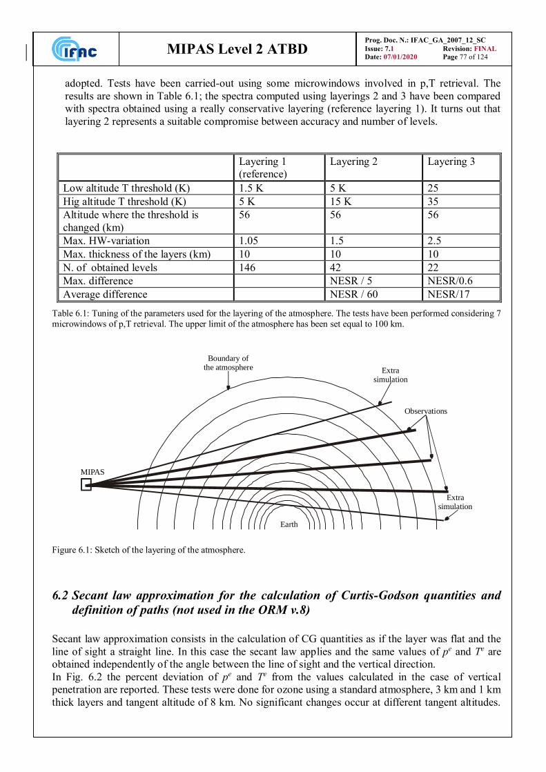
MIPAS Level 2 ATBD
Prog. Doc. N.: IFAC_GA_2007_12_SC
Issue: 7.1 Revision: FINAL
Date: 07/01/2020 Page 77 of 124
adopted. Tests have been carried-out using some microwindows involved in p,T retrieval. The
results are shown in Table 6.1; the spectra computed using layerings 2 and 3 have been compared
with spectra obtained using a really conservative layering (reference layering 1). It turns out that
layering 2 represents a suitable compromise between accuracy and number of levels.
Layering 1
(reference)
Layering 2 Layering 3
Low altitude T threshold (K) 1.5 K 5 K 25
Hig altitude T threshold (K) 5 K 15 K 35
Altitude where the threshold is
changed (km)
56 56 56
Max. HW-variation 1.05 1.5 2.5
Max. thickness of the layers (km) 10 10 10
N. of obtained levels 146 42 22
Max. difference NESR / 5 NESR/0.6
Average difference NESR / 60 NESR/17
Table 6.1: Tuning of the parameters used for the layering of the atmosphere. The tests have been performed considering 7
microwindows of p,T retrieval. The upper limit of the atmosphere has been set equal to 100 km.
Extrasimulation
Extrasimulation
Observations
Boundary ofthe atmosphere
Earth
MIPAS
Figure 6.1: Sketch of the layering of the atmosphere.
6.2 Secant law approximation for the calculation of Curtis-Godson quantities and
definition of paths (not used in the ORM v.8)
Secant law approximation consists in the calculation of CG quantities as if the layer was flat and the
line of sight a straight line. In this case the secant law applies and the same values of pe and Te are
obtained independently of the angle between the line of sight and the vertical direction.
In Fig. 6.2 the percent deviation of pe and Te from the values calculated in the case of vertical
penetration are reported. These tests were done for ozone using a standard atmosphere, 3 km and 1 km
thick layers and tangent altitude of 8 km. No significant changes occur at different tangent altitudes.
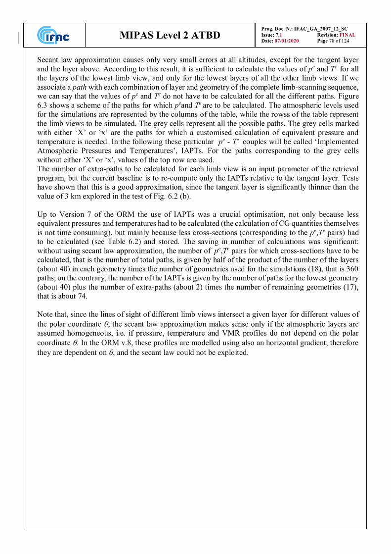
MIPAS Level 2 ATBD
Prog. Doc. N.: IFAC_GA_2007_12_SC
Issue: 7.1 Revision: FINAL
Date: 07/01/2020 Page 78 of 124
Secant law approximation causes only very small errors at all altitudes, except for the tangent layer
and the layer above. According to this result, it is sufficient to calculate the values of pe and Te for all
the layers of the lowest limb view, and only for the lowest layers of all the other limb views. If we
associate a path with each combination of layer and geometry of the complete limb-scanning sequence,
we can say that the values of pe and Te do not have to be calculated for all the different paths. Figure
6.3 shows a scheme of the paths for which peand Te are to be calculated. The atmospheric levels used
for the simulations are represented by the columns of the table, while the rowss of the table represent
the limb views to be simulated. The grey cells represent all the possible paths. The grey cells marked
with either ‘X’ or ‘x’ are the paths for which a customised calculation of equivalent pressure and
temperature is needed. In the following these particular pe - Te couples will be called ‘Implemented
Atmospheric Pressures and Temperatures’, IAPTs. For the paths corresponding to the grey cells
without either ‘X’ or ‘x’, values of the top row are used.
The number of extra-paths to be calculated for each limb view is an input parameter of the retrieval
program, but the current baseline is to re-compute only the IAPTs relative to the tangent layer. Tests
have shown that this is a good approximation, since the tangent layer is significantly thinner than the
value of 3 km explored in the test of Fig. 6.2 (b).
Up to Version 7 of the ORM the use of IAPTs was a crucial optimisation, not only because less
equivalent pressures and temperatures had to be calculated (the calculation of CG quantities themselves
is not time consuming), but mainly because less cross-sections (corresponding to the pe,Te pairs) had
to be calculated (see Table 6.2) and stored. The saving in number of calculations was significant:
without using secant law approximation, the number of pe,Te pairs for which cross-sections have to be
calculated, that is the number of total paths, is given by half of the product of the number of the layers
(about 40) in each geometry times the number of geometries used for the simulations (18), that is 360
paths; on the contrary, the number of the IAPTs is given by the number of paths for the lowest geometry
(about 40) plus the number of extra-paths (about 2) times the number of remaining geometries (17),
that is about 74.
Note that, since the lines of sight of different limb views intersect a given layer for different values of
the polar coordinate , the secant law approximation makes sense only if the atmospheric layers are
assumed homogeneous, i.e. if pressure, temperature and VMR profiles do not depend on the polar
coordinate . In the ORM v.8, these profiles are modelled using also an horizontal gradient, therefore
they are dependent on , and the secant law could not be exploited.
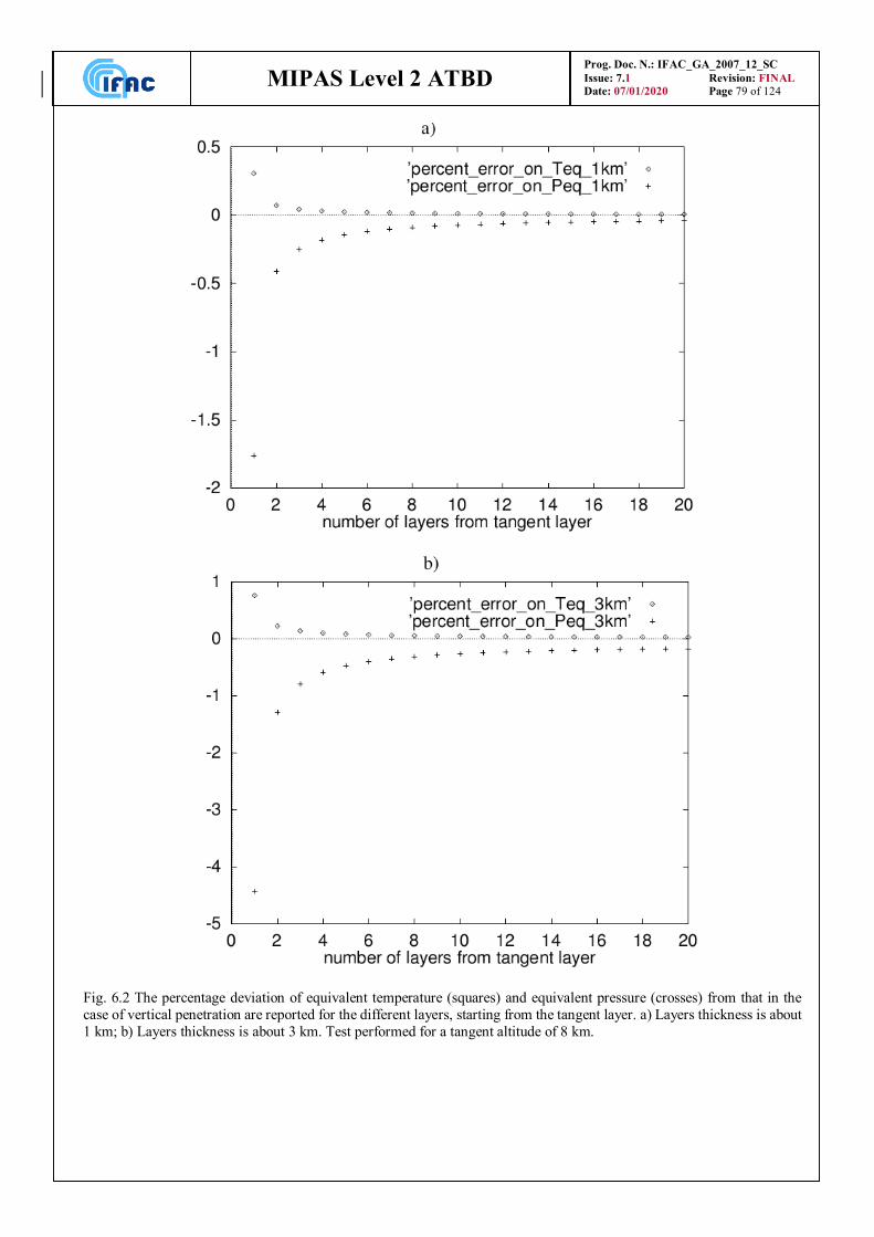
MIPAS Level 2 ATBD
Prog. Doc. N.: IFAC_GA_2007_12_SC
Issue: 7.1 Revision: FINAL
Date: 07/01/2020 Page 79 of 124
Fig. 6.2 The percentage deviation of equivalent temperature (squares) and equivalent pressure (crosses) from that in the
case of vertical penetration are reported for the different layers, starting from the tangent layer. a) Layers thickness is about
1 km; b) Layers thickness is about 3 km. Test performed for a tangent altitude of 8 km.
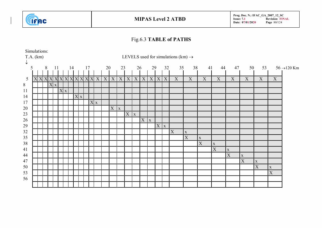
Prog. Doc. N.: IFAC_GA_2007_12_SC
Issue: 7.1 Revision: FINAL
Date: 07/01/2020 Page 80/124 MIPAS Level 2 ATBD
Fig.6.3 TABLE of PATHS
Simulations:
T.A. (km) LEVELS used for simulations (km)
5 8 11 14 17 20 23 26 29 32 35 38 41 44 47 50 53 56 120 Km
5 X X X X X X X X X X X X X X X X X X X X X X X X X X X X X X
8 X x
11 X x
14 X x
17 X x
20 X x
23 X x
26 X x
29 X x
32 X x
35 X x
38 X x
41 X x
44 X x
47 X x
50 X x
53 X
56
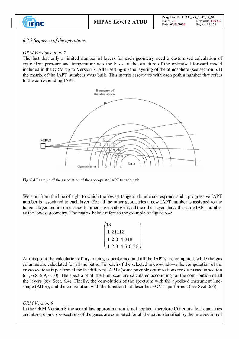
Prog. Doc. N.: IFAC_GA_2007_12_SC
Issue: 7.1 Revision: FINAL
Date: 07/01/2020 Page n. 81/124 MIPAS Level 2 ATBD
6.2.2 Sequence of the operations
ORM Versions up to 7
The fact that only a limited number of layers for each geometry need a customised calculation of
equivalent pressure and temperature was the basis of the structure of the optimised forward model
included in the ORM up to Version 7. After setting-up the layering of the atmosphere (see section 6.1)
the matrix of the IAPT numbers wass built. This matrix associates with each path a number that refers
to the corresponding IAPT.
Fig. 6.4 Example of the association of the appropriate IAPT to each path.
We start from the line of sight to which the lowest tangent altitude corresponds and a progressive IAPT
number is associated to each layer. For all the other geometries a new IAPT number is assigned to the
tangent layer and in some cases to others layers above it, all the other layers have the same IAPT number
as the lowest geometry. The matrix below refers to the example of figure 6.4:
8
7
6
10
5
9
4
4
12
3
3
11
2
2
2
1
1
1
13
At this point the calculation of ray-tracing is performed and all the IAPTs are computed, while the gas
columns are calculated for all the paths. For each of the selected microwindows the computation of the
cross-sections is performed for the different IAPTs (some possible optimisations are discussed in section
6.3, 6.8, 6.9, 6.10). The spectra of all the limb scan are calculated accounting for the contribution of all
the layers (see Sect. 6.4). Finally, the convolution of the spectrum with the apodised instrument line-
shape (AILS), and the convolution with the function that describes FOV is performed (see Sect. 6.6).
ORM Version 8
In the ORM Version 8 the secant law approximation is not applied, therefore CG equivalent quantities
and absorption cross-sections of the gases are computed for all the paths identified by the intersection of
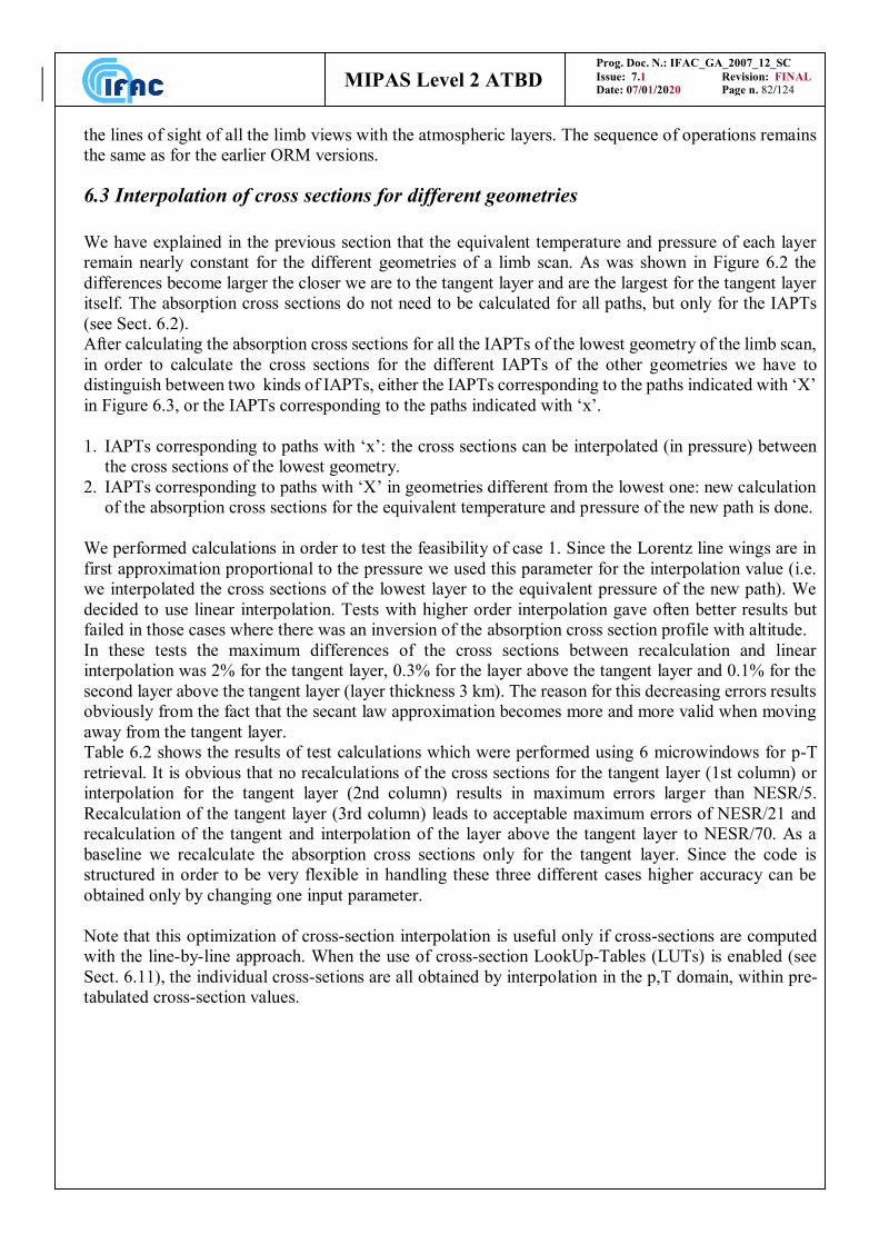
Prog. Doc. N.: IFAC_GA_2007_12_SC
Issue: 7.1 Revision: FINAL
Date: 07/01/2020 Page n. 82/124 MIPAS Level 2 ATBD
the lines of sight of all the limb views with the atmospheric layers. The sequence of operations remains
the same as for the earlier ORM versions.
6.3 Interpolation of cross sections for different geometries
We have explained in the previous section that the equivalent temperature and pressure of each layer
remain nearly constant for the different geometries of a limb scan. As was shown in Figure 6.2 the
differences become larger the closer we are to the tangent layer and are the largest for the tangent layer
itself. The absorption cross sections do not need to be calculated for all paths, but only for the IAPTs
(see Sect. 6.2).
After calculating the absorption cross sections for all the IAPTs of the lowest geometry of the limb scan,
in order to calculate the cross sections for the different IAPTs of the other geometries we have to
distinguish between two kinds of IAPTs, either the IAPTs corresponding to the paths indicated with ‘X’
in Figure 6.3, or the IAPTs corresponding to the paths indicated with ‘x’.
1. IAPTs corresponding to paths with ‘x’: the cross sections can be interpolated (in pressure) between
the cross sections of the lowest geometry.
2. IAPTs corresponding to paths with ‘X’ in geometries different from the lowest one: new calculation
of the absorption cross sections for the equivalent temperature and pressure of the new path is done.
We performed calculations in order to test the feasibility of case 1. Since the Lorentz line wings are in
first approximation proportional to the pressure we used this parameter for the interpolation value (i.e.
we interpolated the cross sections of the lowest layer to the equivalent pressure of the new path). We
decided to use linear interpolation. Tests with higher order interpolation gave often better results but
failed in those cases where there was an inversion of the absorption cross section profile with altitude.
In these tests the maximum differences of the cross sections between recalculation and linear
interpolation was 2% for the tangent layer, 0.3% for the layer above the tangent layer and 0.1% for the
second layer above the tangent layer (layer thickness 3 km). The reason for this decreasing errors results
obviously from the fact that the secant law approximation becomes more and more valid when moving
away from the tangent layer.
Table 6.2 shows the results of test calculations which were performed using 6 microwindows for p-T
retrieval. It is obvious that no recalculations of the cross sections for the tangent layer (1st column) or
interpolation for the tangent layer (2nd column) results in maximum errors larger than NESR/5.
Recalculation of the tangent layer (3rd column) leads to acceptable maximum errors of NESR/21 and
recalculation of the tangent and interpolation of the layer above the tangent layer to NESR/70. As a
baseline we recalculate the absorption cross sections only for the tangent layer. Since the code is
structured in order to be very flexible in handling these three different cases higher accuracy can be
obtained only by changing one input parameter.
Note that this optimization of cross-section interpolation is useful only if cross-sections are computed
with the line-by-line approach. When the use of cross-section LookUp-Tables (LUTs) is enabled (see
Sect. 6.11), the individual cross-setions are all obtained by interpolation in the p,T domain, within pre-
tabulated cross-section values.
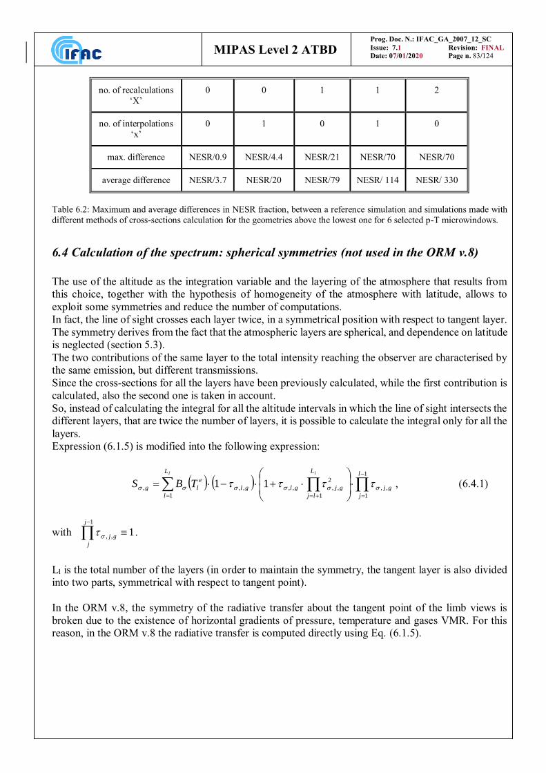
Prog. Doc. N.: IFAC_GA_2007_12_SC
Issue: 7.1 Revision: FINAL
Date: 07/01/2020 Page n. 83/124 MIPAS Level 2 ATBD
no. of recalculations
‘X’
0 0 1 1 2
no. of interpolations
‘x’
0 1 0 1 0
max. difference NESR/0.9 NESR/4.4 NESR/21 NESR/70 NESR/70
average difference NESR/3.7 NESR/20 NESR/79 NESR/ 114 NESR/ 330
Table 6.2: Maximum and average differences in NESR fraction, between a reference simulation and simulations made with
different methods of cross-sections calculation for the geometries above the lowest one for 6 selected p-T microwindows.
6.4 Calculation of the spectrum: spherical symmetries (not used in the ORM v.8)
The use of the altitude as the integration variable and the layering of the atmosphere that results from
this choice, together with the hypothesis of homogeneity of the atmosphere with latitude, allows to
exploit some symmetries and reduce the number of computations.
In fact, the line of sight crosses each layer twice, in a symmetrical position with respect to tangent layer.
The symmetry derives from the fact that the atmospheric layers are spherical, and dependence on latitude
is neglected (section 5.3).
The two contributions of the same layer to the total intensity reaching the observer are characterised by
the same emission, but different transmissions.
Since the cross-sections for all the layers have been previously calculated, while the first contribution is
calculated, also the second one is taken in account.
So, instead of calculating the integral for all the altitude intervals in which the line of sight intersects the
different layers, that are twice the number of layers, it is possible to calculate the integral only for all the
layers.
Expression (6.1.5) is modified into the following expression:
l lL
l
l
j
gj
L
lj
gjglgl
e
lg TBS1
1
1
,,
1
2
,,,,,,, 11 , (6.4.1)
with 11
,, j
j
gj .
Ll is the total number of the layers (in order to maintain the symmetry, the tangent layer is also divided
into two parts, symmetrical with respect to tangent point).
In the ORM v.8, the symmetry of the radiative transfer about the tangent point of the limb views is
broken due to the existence of horizontal gradients of pressure, temperature and gases VMR. For this
reason, in the ORM v.8 the radiative transfer is computed directly using Eq. (6.1.5).
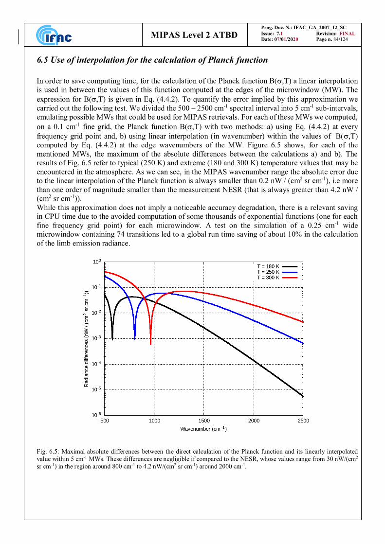
Prog. Doc. N.: IFAC_GA_2007_12_SC
Issue: 7.1 Revision: FINAL
Date: 07/01/2020 Page n. 84/124 MIPAS Level 2 ATBD
6.5 Use of interpolation for the calculation of Planck function
In order to save computing time, for the calculation of the Planck function B(,T) a linear interpolation
is used in between the values of this function computed at the edges of the microwindow (MW). The
expression for B(,T) is given in Eq. (4.4.2). To quantify the error implied by this approximation we
carried out the following test. We divided the 500 – 2500 cm-1 spectral interval into 5 cm-1 sub-intervals,
emulating possible MWs that could be used for MIPAS retrievals. For each of these MWs we computed,
on a 0.1 cm-1 fine grid, the Planck function B(,T) with two methods: a) using Eq. (4.4.2) at every
frequency grid point and, b) using linear interpolation (in wavenumber) within the values of B(,T)
computed by Eq. (4.4.2) at the edge wavenumbers of the MW. Figure 6.5 shows, for each of the
mentioned MWs, the maximum of the absolute differences between the calculations a) and b). The
results of Fig. 6.5 refer to typical (250 K) and extreme (180 and 300 K) temperature values that may be
encountered in the atmosphere. As we can see, in the MIPAS wavenumber range the absolute error due
to the linear interpolation of the Planck function is always smaller than 0.2 nW / (cm2 sr cm-1), i.e more
than one order of magnitude smaller than the measurement NESR (that is always greater than 4.2 nW /
(cm2 sr cm-1)).
While this approximation does not imply a noticeable accuracy degradation, there is a relevant saving
in CPU time due to the avoided computation of some thousands of exponential functions (one for each
fine frequency grid point) for each microwindow. A test on the simulation of a 0.25 cm-1 wide
microwindow containing 74 transitions led to a global run time saving of about 10% in the calculation
of the limb emission radiance.
Fig. 6.5: Maximal absolute differences between the direct calculation of the Planck function and its linearly interpolated
value within 5 cm-1 MWs. These differences are negligible if compared to the NESR, whose values range from 30 nW/(cm2
sr cm-1) in the region around 800 cm-1 to 4.2 nW/(cm2 sr cm-1) around 2000 cm-1.
Prog. Doc. N.: IFAC_GA_2007_12_SC
Issue: 7.1 Revision: FINAL
Date: 07/01/2020 Page n. 85/124 MIPAS Level 2 ATBD
6.6 Finite instrument field of view.
The problem of finite field of view is a consequence of the fact that:
the input diaphragm of the interferometer has non-zero angular size;
light from an extended source crosses it;
this source is characterised by a vertical exponential energy distribution.
These factors have two main effects: a modification in the ILS and a modification in the ‘effective’
tangent altitude of the spectrum.
The change of the ILS in the specific case of MIPAS rectangular aperture, with a vertical exponential
energy distribution across it, have been analysed by L. Debouille and G. Roland (1995): they found that
the use of a rectangular aperture creates a small asymmetry in the ILS, but even the strongest exponential
energy distribution across the field of view does not significantly modify the ILS with respect to that
calculated in the case of homogenous source.
The other effect is that the exponential distribution introduces a non-negligible difference between the
geometrical tangent altitude, defined by the centre of the input diaphragm, and the ‘spectral tangent
height’, that is the position, along the vertical scale, of the mean emitted signal.
Delbouille and Roland (1995) found that corrections (dependent on the molecule) up to nearly 1 km
have to be applied to tangent altitude when the rate of change of the emission is of the order of a factor
three per kilometre.
We have verified that, at least at low tangent altitudes, neglecting the field of view effect implies an error
in the spectrum larger than NESR.
The antenna pattern of the field of view provided by ESA was initially represented by a spread in the
altitude domain FOV(z), independent on the tangent height of the considered sweep, and with the shape
of a trapezium with the greater base of about 4 km and the smaller base of about 3 km. Ground
characterization measurements on the MIPAS flight module indicated, however, that the MIPAS FOV
can be more adequately represented using a piecewise linear shape. A tabulated piecewise distribution
is in fact the FOV representation presently adopted in the ORM/OFM.
According to these arguments, the effect of field of view can be taken into account in two different ways:
by using an equivalent observation geometry,
by performing, for each spectral frequency, the convolution between the spectrum and the antenna
pattern (Sect. 4.4.3):
, , ,FA g A gS z S p z FOV z z . (6.6.1)
Since the equivalent observation geometry is strongly dependent on the molecule, the second option has
been chosen.
The standard method used is, therefore, to perform a numerical convolution with the FOV function after
repeating forward model calculations for a number of lines of sight that span a user-defined vertical
range around the tangent altitude of the sweep to be simulated.
In order to reduce the number of computations, the following optimisations have been implemented:
convolution of the high resolution spectra with the apodised instrument line shape, before taking into
account FOV effects, in order to operate FOV convolution in the coarse frequency grid, instead of
the fine grid.
interpolation of the spectra calculated at the tangent pressures to determine the dependence of the
spectra as a function of altitude; the result is used to perform an analytical convolution.
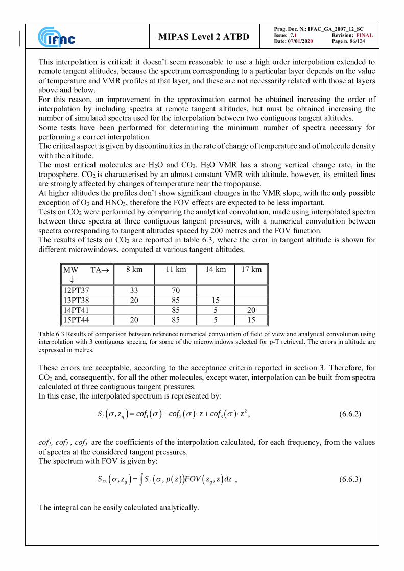
Prog. Doc. N.: IFAC_GA_2007_12_SC
Issue: 7.1 Revision: FINAL
Date: 07/01/2020 Page n. 86/124 MIPAS Level 2 ATBD
This interpolation is critical: it doesn’t seem reasonable to use a high order interpolation extended to
remote tangent altitudes, because the spectrum corresponding to a particular layer depends on the value
of temperature and VMR profiles at that layer, and these are not necessarily related with those at layers
above and below.
For this reason, an improvement in the approximation cannot be obtained increasing the order of
interpolation by including spectra at remote tangent altitudes, but must be obtained increasing the
number of simulated spectra used for the interpolation between two contiguous tangent altitudes.
Some tests have been performed for determining the minimum number of spectra necessary for
performing a correct interpolation.
The critical aspect is given by discontinuities in the rate of change of temperature and of molecule density
with the altitude.
The most critical molecules are H2O and CO2. H2O VMR has a strong vertical change rate, in the
troposphere. CO2 is characterised by an almost constant VMR with altitude, however, its emitted lines
are strongly affected by changes of temperature near the tropopause.
At higher altitudes the profiles don’t show significant changes in the VMR slope, with the only possible
exception of O3 and HNO3, therefore the FOV effects are expected to be less important.
Tests on CO2 were performed by comparing the analytical convolution, made using interpolated spectra
between three spectra at three contiguous tangent pressures, with a numerical convolution between
spectra corresponding to tangent altitudes spaced by 200 metres and the FOV function.
The results of tests on CO2 are reported in table 6.3, where the error in tangent altitude is shown for
different microwindows, computed at various tangent altitudes.
MW TA
8 km 11 km 14 km 17 km
12PT37 33 70
13PT38 20 85 15
14PT41 85 5 20
15PT44 20 85 5 15
Table 6.3 Results of comparison between reference numerical convolution of field of view and analytical convolution using
interpolation with 3 contiguous spectra, for some of the microwindows selected for p-T retrieval. The errors in altitude are
expressed in metres.
These errors are acceptable, according to the acceptance criteria reported in section 3. Therefore, for
CO2 and, consequently, for all the other molecules, except water, interpolation can be built from spectra
calculated at three contiguous tangent pressures.
In this case, the interpolated spectrum is represented by:
2
1 2 3,I gS z cof cof z cof z , (6.6.2)
cof1, cof2 , cof3 are the coefficients of the interpolation calculated, for each frequency, from the values
of spectra at the considered tangent pressures.
The spectrum with FOV is given by:
, , ,FA Ig gS z S p z FOV z z dz , (6.6.3)
The integral can be easily calculated analytically.
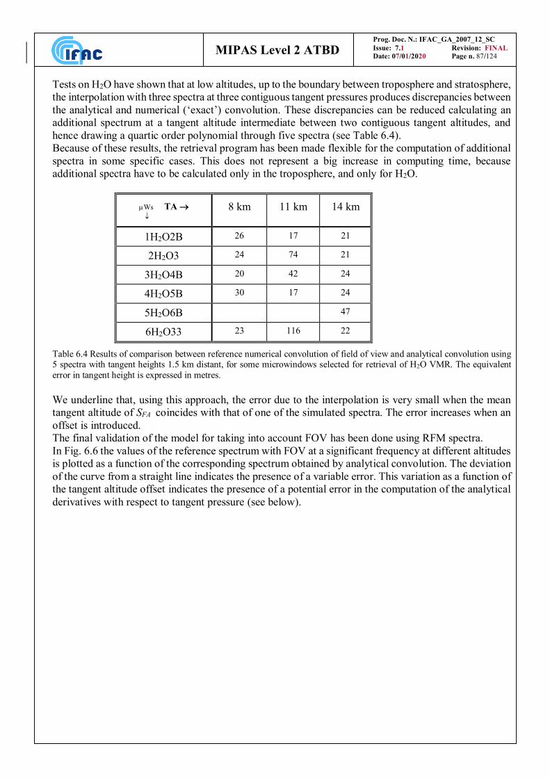
Prog. Doc. N.: IFAC_GA_2007_12_SC
Issue: 7.1 Revision: FINAL
Date: 07/01/2020 Page n. 87/124 MIPAS Level 2 ATBD
Tests on H2O have shown that at low altitudes, up to the boundary between troposphere and stratosphere,
the interpolation with three spectra at three contiguous tangent pressures produces discrepancies between
the analytical and numerical (‘exact’) convolution. These discrepancies can be reduced calculating an
additional spectrum at a tangent altitude intermediate between two contiguous tangent altitudes, and
hence drawing a quartic order polynomial through five spectra (see Table 6.4).
Because of these results, the retrieval program has been made flexible for the computation of additional
spectra in some specific cases. This does not represent a big increase in computing time, because
additional spectra have to be calculated only in the troposphere, and only for H2O.
Ws TA
8 km 11 km 14 km
1H2O2B 26 17 21
2H2O3 24 74 21
3H2O4B 20 42 24
4H2O5B 30 17 24
5H2O6B 47
6H2O33 23 116 22
Table 6.4 Results of comparison between reference numerical convolution of field of view and analytical convolution using 5 spectra with tangent heights 1.5 km distant, for some microwindows selected for retrieval of H2O VMR. The equivalent
error in tangent height is expressed in metres.
We underline that, using this approach, the error due to the interpolation is very small when the mean
tangent altitude of SFA coincides with that of one of the simulated spectra. The error increases when an
offset is introduced.
The final validation of the model for taking into account FOV has been done using RFM spectra.
In Fig. 6.6 the values of the reference spectrum with FOV at a significant frequency at different altitudes
is plotted as a function of the corresponding spectrum obtained by analytical convolution. The deviation
of the curve from a straight line indicates the presence of a variable error. This variation as a function of
the tangent altitude offset indicates the presence of a potential error in the computation of the analytical
derivatives with respect to tangent pressure (see below).
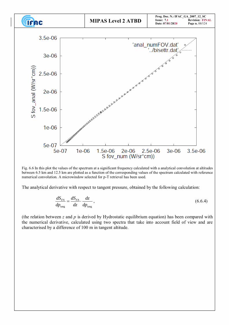
Prog. Doc. N.: IFAC_GA_2007_12_SC
Issue: 7.1 Revision: FINAL
Date: 07/01/2020 Page n. 88/124 MIPAS Level 2 ATBD
Fig. 6.6 In this plot the values of the spectrum at a significant frequency calculated with a analytical convolution at altitudes
between 6.5 km and 12.5 km are plotted as a function of the corresponding values of the spectrum calculated with reference
numerical convolution. A microwindow selected for p-T retrieval has been used.
The analytical derivative with respect to tangent pressure, obtained by the following calculation:
tang tang
FA FAdS dS dz
dp dz dp , (6.6.4)
(the relation between z and p is derived by Hydrostatic equilibrium equation) has been compared with
the numerical derivative, calculated using two spectra that take into account field of view and are
characterised by a difference of 100 m in tangent altitude.
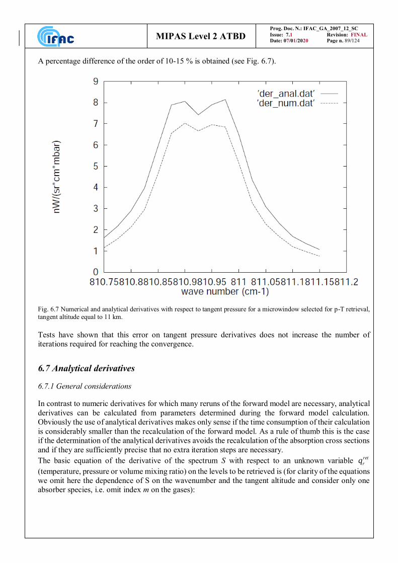
Prog. Doc. N.: IFAC_GA_2007_12_SC
Issue: 7.1 Revision: FINAL
Date: 07/01/2020 Page n. 89/124 MIPAS Level 2 ATBD
A percentage difference of the order of 10-15 % is obtained (see Fig. 6.7).
Fig. 6.7 Numerical and analytical derivatives with respect to tangent pressure for a microwindow selected for p-T retrieval,
tangent altitude equal to 11 km.
Tests have shown that this error on tangent pressure derivatives does not increase the number of
iterations required for reaching the convergence.
6.7 Analytical derivatives
6.7.1 General considerations
In contrast to numeric derivatives for which many reruns of the forward model are necessary, analytical
derivatives can be calculated from parameters determined during the forward model calculation.
Obviously the use of analytical derivatives makes only sense if the time consumption of their calculation
is considerably smaller than the recalculation of the forward model. As a rule of thumb this is the case
if the determination of the analytical derivatives avoids the recalculation of the absorption cross sections
and if they are sufficiently precise that no extra iteration steps are necessary.
The basic equation of the derivative of the spectrum S with respect to an unknown variable ret
rq
(temperature, pressure or volume mixing ratio) on the levels to be retrieved is (for clarity of the equations
we omit here the dependence of S on the wavenumber and the tangent altitude and consider only one
absorber species, i.e. omit index m on the gases):
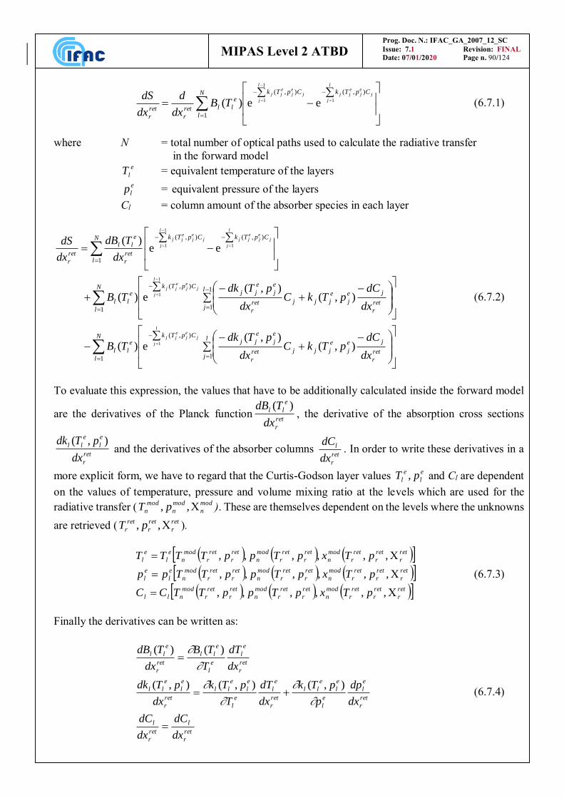
Prog. Doc. N.: IFAC_GA_2007_12_SC
Issue: 7.1 Revision: FINAL
Date: 07/01/2020 Page n. 90/124 MIPAS Level 2 ATBD
N
l
CpTkCpTke
llret
r
ret
r
l
j
jej
ejj
l
j
jej
ejj
TBdx
d
dx
dS
1
),(),(
1
1
1 ee)( (6.7.1)
where N = total number of optical paths used to calculate the radiative transfer
in the forward model
e
lT = equivalent temperature of the layers
e
lp = equivalent pressure of the layers
Cl = column amount of the absorber species in each layer
N
l
l
jret
r
je
j
e
jjjret
r
e
j
e
jjCpTk
e
ll
N
l
l
jret
r
je
j
e
jjjret
r
e
j
e
jjCpTk
e
ll
N
l
CpTkCpTk
ret
r
e
ll
ret
r
dx
dCpTkC
dx
pTdkTB
dx
dCpTkC
dx
pTdkTB
dx
TdB
dx
dS
l
j
jej
ejj
l
j
jej
ejj
l
j
jej
ejj
l
j
jej
ejj
1 1
),(
1
1
1
),(
1
),(),(
),(),(
e)(
),(),(
e)(
ee)(
1
1
1
1
1
1
(6.7.2)
To evaluate this expression, the values that have to be additionally calculated inside the forward model
are the derivatives of the Planck functionret
r
e
ll
dx
TdB )(, the derivative of the absorption cross sections
ret
r
e
l
e
ll
dx
pTdk ),( and the derivatives of the absorber columns
ret
r
l
dx
dC. In order to write these derivatives in a
more explicit form, we have to regard that the Curtis-Godson layer values e
l
e
l pT , and Cl are dependent
on the values of temperature, pressure and volume mixing ratio at the levels which are used for the
radiative transfer (mod
n
mod
n
mod
n pT ,, ). These are themselves dependent on the levels where the unknowns
are retrieved (ret
r
ret
r
ret
r pT ,, ).
ret
r
ret
r
ret
r
mod
n
ret
r
ret
r
mod
n
ret
r
ret
r
mod
nll
ret
r
ret
r
ret
r
mod
n
ret
r
ret
r
mod
n
ret
r
ret
r
mod
n
e
l
e
l
ret
r
ret
r
ret
r
mod
n
ret
r
ret
r
mod
n
ret
r
ret
r
mod
n
e
l
e
l
pTxpTppTTCC
pTxpTppTTpp
pTxpTppTTTT
,,,,,,
,,,,,,
,,,,,,
(6.7.3)
Finally the derivatives can be written as:
ret
r
l
ret
r
l
ret
r
e
l
e
l
e
l
e
ll
ret
r
e
l
e
l
e
l
e
ll
ret
r
e
l
e
ll
ret
r
e
l
e
l
e
ll
ret
r
e
ll
dx
dC
dx
dC
dx
dp
p
pTk
dx
dT
T
pTk
dx
pTdk
dx
dT
T
TB
dx
TdB
),(),(),(
)()(
(6.7.4)
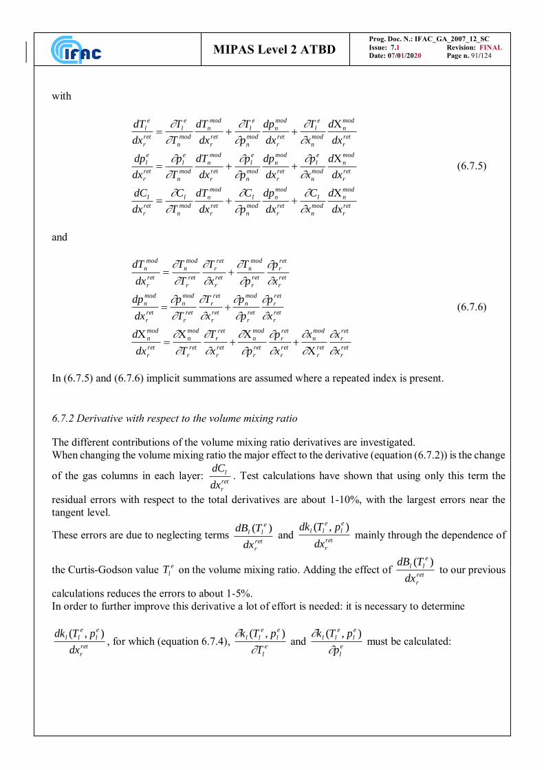
Prog. Doc. N.: IFAC_GA_2007_12_SC
Issue: 7.1 Revision: FINAL
Date: 07/01/2020 Page n. 91/124 MIPAS Level 2 ATBD
with
ret
r
mod
n
mod
n
l
ret
r
mod
n
mod
n
l
ret
r
mod
n
mod
n
l
ret
r
l
ret
r
mod
n
mod
n
e
l
ret
r
mod
n
mod
n
e
l
ret
r
mod
n
mod
n
e
l
ret
r
e
l
ret
r
mod
n
mod
n
e
l
ret
r
mod
n
mod
n
e
l
ret
r
mod
n
mod
n
e
l
ret
r
e
l
dx
d
x
C
dx
dp
p
C
dx
dT
T
C
dx
dC
dx
d
x
p
dx
dp
p
p
dx
dT
T
p
dx
dp
dx
d
x
T
dx
dp
p
T
dx
dT
T
T
dx
dT
(6.7.5)
and
ret
r
ret
r
ret
r
mod
n
ret
r
ret
r
ret
r
mod
n
ret
r
ret
r
ret
r
mod
n
ret
r
mod
n
ret
r
ret
r
ret
r
mod
n
ret
r
ret
r
ret
r
mod
n
ret
r
mod
n
ret
r
ret
r
ret
r
mod
n
ret
r
ret
r
ret
r
mod
n
ret
r
mod
n
x
xx
x
p
px
T
Tdx
d
x
p
p
p
x
T
T
p
dx
dp
x
p
p
T
x
T
T
T
dx
dT
(6.7.6)
In (6.7.5) and (6.7.6) implicit summations are assumed where a repeated index is present.
6.7.2 Derivative with respect to the volume mixing ratio
The different contributions of the volume mixing ratio derivatives are investigated.
When changing the volume mixing ratio the major effect to the derivative (equation (6.7.2)) is the change
of the gas columns in each layer: ret
r
l
dx
dC. Test calculations have shown that using only this term the
residual errors with respect to the total derivatives are about 1-10%, with the largest errors near the
tangent level.
These errors are due to neglecting terms ret
r
e
ll
dx
TdB )( and
ret
r
e
l
e
ll
dx
pTdk ),( mainly through the dependence of
the Curtis-Godson value e
lT on the volume mixing ratio. Adding the effect of ret
r
e
ll
dx
TdB )( to our previous
calculations reduces the errors to about 1-5%.
In order to further improve this derivative a lot of effort is needed: it is necessary to determine
ret
r
e
l
e
ll
dx
pTdk ),(, for which (equation 6.7.4),
e
l
e
l
e
ll
T
pTk
),( and
e
l
e
l
e
ll
p
pTk
),( must be calculated:
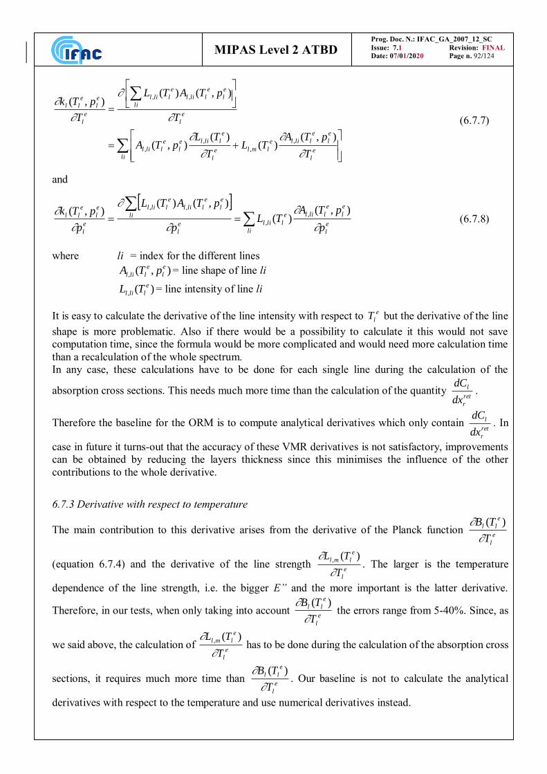
Prog. Doc. N.: IFAC_GA_2007_12_SC
Issue: 7.1 Revision: FINAL
Date: 07/01/2020 Page n. 92/124 MIPAS Level 2 ATBD
lie
l
e
l
e
llile
lmle
l
e
llile
l
e
llil
e
l
li
e
l
e
llil
e
llil
e
l
e
l
e
ll
T
pTATL
T
TLpTA
T
pTATL
T
pTk
),()(
)(),(
),()(),(
,
,
,
,
,,
(6.7.7)
and
lie
l
e
l
e
llile
llile
l
li
e
l
e
llil
e
llil
e
l
e
l
e
ll
p
pTATL
p
pTATL
p
pTk
),()(
),()(),( ,
,
,,
(6.7.8)
where li = index for the different lines
),(,
e
l
e
llil pTA = line shape of line li
)(,
e
llil TL = line intensity of line li
It is easy to calculate the derivative of the line intensity with respect to e
lT but the derivative of the line
shape is more problematic. Also if there would be a possibility to calculate it this would not save
computation time, since the formula would be more complicated and would need more calculation time
than a recalculation of the whole spectrum.
In any case, these calculations have to be done for each single line during the calculation of the
absorption cross sections. This needs much more time than the calculation of the quantity ret
r
l
dx
dC.
Therefore the baseline for the ORM is to compute analytical derivatives which only contain ret
r
l
dx
dC. In
case in future it turns-out that the accuracy of these VMR derivatives is not satisfactory, improvements
can be obtained by reducing the layers thickness since this minimises the influence of the other
contributions to the whole derivative.
6.7.3 Derivative with respect to temperature
The main contribution to this derivative arises from the derivative of the Planck function e
l
e
ll
T
TB
)(
(equation 6.7.4) and the derivative of the line strength e
l
e
lml
T
TL
)(,. The larger is the temperature
dependence of the line strength, i.e. the bigger E” and the more important is the latter derivative.
Therefore, in our tests, when only taking into account e
l
e
ll
T
TB
)( the errors range from 5-40%. Since, as
we said above, the calculation of e
l
e
lml
T
TL
)(, has to be done during the calculation of the absorption cross
sections, it requires much more time than e
l
e
ll
T
TB
)(. Our baseline is not to calculate the analytical
derivatives with respect to the temperature and use numerical derivatives instead.
Prog. Doc. N.: IFAC_GA_2007_12_SC
Issue: 7.1 Revision: FINAL
Date: 07/01/2020 Page n. 93/124 MIPAS Level 2 ATBD
However, the numerical derivatives are implemented in an optimised form (i.e. the calculation of spectra
with the ‘T-perturbed’ profiles is parallel to the one with the ‘original’ profile), and not by just recalling
the forward model.
6.7.4 Derivative with respect to the atmospheric continuum
The derivative with respect to the atmospheric continuum can be easily calculated since the continuum
is taken into account as an absorption cross section which is multiplied by the air column of each path.
The Curtis-Godson temperatures, pressures, or the total air column do not change when varying the
continuum cross sections. Equation 6.7.1 can be written as:
N
l
CkCke
llretcont
r
retcont
r
l
j
airj
econtj
l
j
airj
econtj
TBdk
d
dk
dS
1,,
1
,1
1
,
ee)( (6.7.9)
and for 6.7.2 follows:
N
l
l
j
l
j
air
jretcont
r
econt
jCk
air
jretcont
r
econt
jCk
e
llretcont
r
Cdk
dkC
dk
dkTB
dk
dSl
j
airj
econtj
l
j
airj
econtj
1
1
1 1,
,
,
,
,
1
,1
1
,
ee)(
(6.7.10)
econt
lk , are the continuum absorption cross sections of the forward model layers and are therefore
dependent on the forward model levels (modcont
nk ,) which are themselves dependent on the levels where
the continuum has to be retrieved (retcont
rk ,):
retcont
r
modcont
n
modcont
n
econt
l
retcont
r
econt
l
k
k
k
k
dk
dk,
,
,
,
,
,
(6.7.11)
The baseline is to use these analytical derivatives.
6.7.5 Derivative with respect to the tangent pressure
The main effects of this derivative result from the change of the column, the change of the line shape
and the change of the temperature with the tangent pressure. For the modelling of the change of the line
shape it is necessary to do calculations in the domain of the absorption cross sections which are very
time consuming. Therefore, we decided not to calculate this derivative as given by the formulas above,
but to determine it during the convolution with the FOV-function. The spectrum ),( pSFA is calculated
for the field of view function FOV centred at the tangent pressure. Since the convolution with the FOV
is an analytical expression, its derivative with respect to the central pressure of the FOV can be easily
obtained.
Our baseline is to use this kind of analytical derivatives for the calculation of the derivatives with respect
to the tangent pressure.
Prog. Doc. N.: IFAC_GA_2007_12_SC
Issue: 7.1 Revision: FINAL
Date: 07/01/2020 Page n. 94/124 MIPAS Level 2 ATBD
6.7.6 Independence of retrieved variables
The Jacobian matrix (equation 4.2.6) contains the partial derivatives of the spectrum with respect to the
parameters. Therefore, while performing the calculation of the derivatives, one has to take care that
either they are partial (if parameters are dependent) or that the parameters are independent (
jiparameterparameter ji ,0 ), so that the partial derivatives are equal to the total ones.
This assumption is clearly fulfilled for the volume mixing ratio retrieval where the parameters are the
volume mixing ratios and the continuum cross sections at the tangent levels and the instrumental offset.
During the p-T retrieval one has to be more careful since (due to the optimised calculation of the tangent
pressure derivatives, cf. 6.7.5) varying the tangent pressure implies also a change of the tangent
temperature and of the atmospheric continuum on the tangent levels. This difficulty disappears when we
define for each iteration cycle as the fitted parameters the new tangent pressure and the temperature and
continuum cross sections at the tangent pressures of the previous iteration. In a subsequent step the new
temperatures and continuum cross sections at the previous tangent pressures are interpolated to the new
tangent pressures.
6.7.7 New choice of continuum variables in the MIPAS processor starting from V.7.0.
The radiative transfer is a first order differential equation; the solutions are written using exponentials.
By combining the emission and absorption phenomena the spectrum is a linear combination of
exponentials. The retrieval variables, both for the continuum and the VMR, are located in the
exponents of the exponentials. Let 1, ,l N be the paths defined by the intersections of a given
line-of-sight with the defined atmospheric layers. The spectrum reaching the instrument may be
written as
1
, ,
1 1
( ) ( , )(1 )N l
e
l l j
l j
S B T
(6.7.12)
where ,l is the transmittance through the path l at frequency . The transmittance of the path l has
the following expression:
, , , , ,exp ( , ) exp ( , )e e e e
l m l l l m m l l l mm mk p T c k p T c (6.7.13)
where m is the gas index, ,mk is the cross-section of that gas at frequency , which depends only
on the equivalent pressure e
lp and temperature of that layer. Finally ,l mc is the gas column in the in
the path, which depends on the gas VMR ( )mx z in the following way:
, ( ) ( ) ( )l m ml
dsc x z z z dz
dz . (6.7.14)
Here z is the altitude, ( )z is the density and /ds dz is the linear element along the line of sight. In
the case of the continuum m c we have ( ) 1cx z , so the columns ,l cc may be explicitely calculated
from the pressure and the temperature of the atmosphere and the knowledge of the line of sight.
On the other hand, the unknowns are the cross-section vertical profile. Being a continuum, within
each MW, the cross-section does not depend on the frequency. ORM_SDC versions earlier than 3.0
use the cross-sections ( )i ik k z at tangent altitudes iz , 1, ,i n as retrieval variables. The cross
Prog. Doc. N.: IFAC_GA_2007_12_SC
Issue: 7.1 Revision: FINAL
Date: 07/01/2020 Page n. 95/124 MIPAS Level 2 ATBD
section in a given path l is then represented by calculating the average pressure of the path, and
interpolating linearly in pressure between the tangent altitudes above and below the layer l. In
formulas, if ( )i l is the index of the tangent altitude above the path l:
( ) 1 ( )l l i l l i lk a k b k , (6.7.15)
where la , lb are positive constants belonging to the [0,1] interval.
While being physically sound, the retrieval of a linear combination of exponentials from their
exponents is unstable, we refer to Transtrum et al. (2011) for details. The following example shows
the problems linked with the fit of the exponents: it can be readily seen that, given the model function 1 2( , ) t tf t e e it is almost impossible to identify the parameters 1 and 2 given the
experimental values of ( , )jf t , even for moderately large values of t.
The standard methods to treat this situation, which is called a sloppy model, is to modify the
minimization method, adjusting the step-length according to some recipe which involves the cost
function. At each step, a unidimensional search is therefore necessary along the direction predicted
by the descent method (be it the gradient method, or the Gauss-Newton method as in the case of the
ORM). This is unacceptable in our case, because this would imply many forward model evaluations,
which is very costly in terms of time for the atmospheric model.
As an alternative solution, we changed the retrieval variables in order to eliminate the exponential
dependence. Instead of using the ik from Eq. (6.7.15) we use the new variables
exp( )i ik C (6.7.16)
Where C is a constant. Then the transmission of the continuum of the path l
, ( ) 1 ( ) ,exp ( )l c l i l l i l l ca k b k c (6.7.17)
becomes
, ,/ /
, ( ) 1 ( )l l c l l ca c C b c C
l c i l i l (6.7.18)
By choosing a constant ,l cC c for all the paths l, we ensure that the exponents in (6.7.18) are positive
and less than 1. We choose 2510C .
There are two consequences of this choice. First, the dependence of the ,l c on the j is of polynomial
type. Second, while the permitted values for the jk were [0, ) , the new variables vary in the [0,1]
interval. Note that the value 0jk (full transparency) in the old variables corresponds to 1j in
the new variables. Analogously the value jk (complete opacity) in the old variables corresponds
to 0j in the new variables.
The only two non-vanishing derivatives of the ,l c with respect to the new retrieval variables are:
, ,
1, , , ,
( ) 1 ( )
( ) 1 ( ) 1
l l c l l ca c b c
l c l c l c l cC Cl i l i l l
i l i l
c ca a
C C
(6.7.19)
Prog. Doc. N.: IFAC_GA_2007_12_SC
Issue: 7.1 Revision: FINAL
Date: 07/01/2020 Page n. 96/124 MIPAS Level 2 ATBD
and
, ,
1, , , ,
( ) 1 ( )
( ) ( )
l l c l l ca c b c
l c l c l c l cC Cl i l i l l
i l i l
c cb b
C C
. (6.7.20)
The ORM calculates the derivatives of the spectrum with respect to the continuum variables by
summing the contributions coming from each path l, and applying the chain rule:
,
,
l c
lj l c j
S S
k k
(6.7.21)
To use the new retrieval variables, we have simply to substitute the last term, thus getting
,
,
l c
lj l c j
S S
(6.7.22)
With this new approach the retrieval variables for the continuum are better identifiable, so that the
retrieval is more stable. In this way the regularizing effect of the LM method can be kept weaker.
With this approach we were able to reduce the initial value of the LM damping for the continuum
variables by a factor of 10.
Tests with real MIPAS observations show that a more stable retrieval is obtained with these new
variables. As a consequence, we obtain a reduction in the number of iterations, a smaller minimum
of the cost function, and slightly less oscillating profiles. The same modification can be applied also
to the VMR retrieval variables. Our tests show, however, that (at least in the present formulation)
there is no real advantage connected with this additional change. Further details on this modification
can be found in Ridolfi and Sgheri (2012) and in Ridolfi and Sgheri (2013).
6.8 Convergence criteria
In Sect. 4.2.4 four possible conditions have been considered for the definition of reached convergence.
After several otpimizations based on the analysis of real measurements, the convergence criteria used
by the ORM are organized as follows. Let 1 2 3 4 5 6, , , , , t t t t t t be user-defined, tuned, numerical thresholds.
The retrieval is stopped at a macro-iteration “it” if at least one of the following conditions is fulfilled:
1. Is 2 2 2
LIN 1( ) ( ) / ( )it it it t and 2
6( )it t ?
2. Is 2 2 2
2( ) ( 1) / ( )it it it t and 2
6( )it t ?
3. Only in pT retrieval. Is the maximum relative variation of tangent pressure wrt the previous
iteration less than t3 and is the maximum variation of temperature wrt the previous iteration less
than t4 ?
4. Only in VMR retrieval. Is the maximum relative variation of VMR wrt the previous iteration less
than t3 ?
5. Is 1/ 2
1
1 x, 1 5/T
it it it it it n t
x x S x x ? Where xit is the retrieved profile at iteration it, n its
number points and x,itS the estimate of its covariance matrix at the same iteration, i.e.:
Prog. Doc. N.: IFAC_GA_2007_12_SC
Issue: 7.1 Revision: FINAL
Date: 07/01/2020 Page n. 97/124 MIPAS Level 2 ATBD
1
1
x,
T
it it y it
S K S K .
6. Is it < itmax ? where itmax is the maximum number of allowed iterations.
Condition 6. has no physical rationale, it is only used to limit the computation time and, in normal
conditions, it should never be fulfilled. If a retrieval is stopped due to this condition being fulfilled, then
the retrieval is said “non-converging” and the corresponding output profile is flagged as invalid.
Conditions from 2. to 5. are more or less equivalent and aim at establishing whether the retrieved profile
is changing too little (compared to its error bars) from one iteration to the next, it that case additional
iterations would not be worth. When the thresholds ti are properly tuned, these conditions all ensure that
the convergence error is smaller than a suitable fraction of the error due to measurement noise.
Condition 2. checks the relative difference between the actual chi-square and the chi-square evaluated
with a linear expansion of the forward model about the current estimate of the state vector. A small value
of this difference indicates that the forward model behaves almost linearly, therefore with the current
iteration we should have already reached the minimum of the chi-square function.
If the final 2 is less than t6 the retrieved profile is flagged “good” and it is used either as initial guess
or as assumed profile in the subsequent retrievals. An exception to this rule is for pT values used in VMR
retrievals. VMR retrievals must use pT values retrieved from the same scan, also if pT retrieval
terminated with 2
6t . Conditions 1. and 2. are checked only when 2
6( )it t because we
encountered scans with a large 2 not changing from one iteration to the next. As a consequence the
first part of conditions 2. and 3. could be fulfilled even with such a large 2 . A check on these scans
revealed that applying further iterations would reduce the 2 under the t6 threshold.
A comment to the adopted strategy could be that the above conditions could be erroneously triggered
when still far away from the minimum of the 2 function, due to occasionally large values of the LM
damping parameter M . While in principle this event can occur, we verified that in practice it is very
rare (few retrievals over thousands). Of course these occurrences can be detected by checking the final
value of M of the retrieval. When the final M is greater than a pre-defined threshold the related profile
can be discarded. The thresholds to be used are currently included in the “readme” file accompanying
ESA Level 2 products.
Some investigations based on the ESA Level 2 processor IPF v.6, showed that the convergence error
achieved with the used convergence thresholds is, on average, of the order of 1/10 of the error due to
measurement noise. The results of these investigations can be found in Ridolfi et al. (2011). A document
reporting the most recent tests for the selection of the above mentioned criteria is Ridolfi and Sgheri
(2011).
6.9 Pre-calculation of line shapes
This item concerns the line shape calculation in the case of HNO3 lines. Since a lot of lines have to be
taken into consideration in HNO3 microwindows this is a very time consuming part of the VMR-retrieval
process. In order to optimise this calculation, we can use the fact that in the HITRAN data base the HNO3
lines have the same Lorentz half width and the same coefficient of the temperature dependence (equation
4.4.12). Therefore, it is not necessary to calculate the line shape (equation 4.4.15) for each HNO3 line,
this can be calculated for a single line, at the beginning of the cross section calculation for a new path
(peq,Teq pair) and used for all other HNO3 lines of the microwindow. For each transition the pre-
calculated line shape is then centred at the central line frequency and interpolated to the wavenumber
Prog. Doc. N.: IFAC_GA_2007_12_SC
Issue: 7.1 Revision: FINAL
Date: 07/01/2020 Page n. 98/124 MIPAS Level 2 ATBD
grid of the microwindow. This interpolation is performed linearly. The resulting error was determined
by test calculations. The maximum difference between exact calculation and use of the interpolated pre-
calculated line shape was NESR/88. Due to this small value of the introduced error and to the time saving
of 66%, our baseline is to use the pre-calculated HNO3 line-shapes. Of course, this optimisation is not
used when cross-sections are computed from pre-calculated LUTs.
6.10 Different grids during the cross-section calculation
For the calculation of the radiative transfer, absorption cross-sections are required at each grid point of
the fine frequency grid at which also the radiative transfer is calculated. Tests have shown that a
reasonable and conservative value for the step between two fine grid points can be 510-4 cm-1. This
value, which can in principle be optimised in terms of faster computations, as been adopted as baseline.
This results in 4000 points for a 2 cm-1 microwindow where cross sections for each transition have to be
calculated. Therefore, the run time is directly proportional to the number of grid points. In order to reduce
the number of grid points during the calculation of cross sections two methods are used even by accurate
line-by-line codes (e.g. Edwards, 1991; Gordley, 1994):
1. far off the line centre the frequency grid can be coarser than near the centre.
2. the grid can be proportional to the half-width of the line, i.e. it can be dependent on the pressure of
the layer for which the cross-sections have to be calculated.
These two methods have been implemented into the subroutine for the line-by-line calculation of cross
section in the following way: in addition to the constant general fine grid ( gf =510-4 cm-1) two grids,
the local coarse ( lc ) and the local fine grid ( lf ), are defined for each path where the cross sections
are calculated. The grid distances are multiple integers of each other:
mnmn
mn lflcgflf
1 , 1 and ,,with
, (6.11.1)
m, which determines the local coarse grid, is a tunable parameter.
n is the nearest positive integer value so that mm DL
lf , where mm DL , are the Lorentz
and the Doppler half width of the target gas transition with the largest intensity, and is a second
optimisation parameter that determines the period of the local fine grid.
The third parameter defines the distance mm DL of the transition between local fine and
local coarse grid from the line centre.
After the calculation of the cross sections for all lines of the microwindow both grids are linearly
interpolated to the general fine grid. Run time tests with this implementation showed a considerable time
saving for the calculation of the absorption cross sections of more than 50%. Again, also this
optimisation is used only when absorption cross-sections are computed with the line-by-line approach,
it is not exploited when cross-sections are computed from pre-calculated LUTs.
6.11 Cross-section look-up tables
The use of pre-computed look-up tables (LUTs) is an alternative method to the explicit line-by-line
calculation of absorption cross sections (equation 4.4.6). The basic idea of this method is to pre-calculate
Prog. Doc. N.: IFAC_GA_2007_12_SC
Issue: 7.1 Revision: FINAL
Date: 07/01/2020 Page n. 99/124 MIPAS Level 2 ATBD
for each frequency grid point the absorption cross sections of each gas for a set of different pressures
and temperatures within the range of the atmospheric variability. These data are stored in files which are
read at the beginning of each retrieval. Then they are interpolated to the equivalent pressure and
temperature of the atmospheric paths (peq, Teq pairs). Since the frequency grid in which the cross sections
have to be calculated is rather fine (510-4 cm-1, see Sect. 6.10) the amount of data is large.
In order to reduce the amount of data contained in the look-up tables and their reading time, a
compression procedure has been studied at University of Oxford (see Morris (1997)). The algorithm
used to build compressed look-up tables and procedure for the decompression are based on the matrix
singular value decomposition applied to the cross-sections and is described in Strow et al., (1998).
Since version 2.3, the ORM code is able to handle these compressed look-up tables, including cases in
which the look-up tables are available only for a sub-set of the operational microwindows and / or for a
sub-set of the gases contributing to the emission in each microwindow.
The importance of time savings obtained using LUTs instead of line-by-line calculations depends very
much on the considered retrieval. Largest savings are obtained in the case of HNO3 retrieval (38%
reduction of forward model runtime), less significant savings (15% reduction of forward model runtime)
are obtained in the cases of O3 and CH4. In other cases the use of compressed LUTs provides no time
savings (N2O) or an increase of computing time like in p,T and H2O retrievals.
LUTs represent a very efficient optimisation only when irregular frequency grids (see Sect. 6.12) are
used in combination.
6.12 Variable frequency grids for radiative transfer computation
Limb radiance spectra contain spectral features on a range of scales varying from the narrow, isolated,
Doppler-broadened line centers at high altitudes, to wide, overlapping, Lorentz-broadened line wings
from low altitudes.
Therefore, a minimum subset of spectral grid points (irregular grid) can be determined that are sufficient
to reconstruct full radiance spectra, applicable over a range of tangent altitudes and atmospheres. Full
radiative transfer calculations are then only required for this subset of points, the remaining fine grid
points are obtained using a pre-determined interpolation scheme. The irregular grid is a function of the
microwindow boundaries, the chosen interpolation scheme and the spectral convolution by the
Instrument Line Shape.
Typically, it is found that only 5-10 % of the full resolution grid is required for reconstruction of the
spectra. When combined with the Look-Up Tables, this also means that absorption cross-section only
has to be reconstructed at the same fraction of grid points resulting in even more efficient optimization.
On the other hand, the use of irregular grids does not reduce the computation time of the algorithm for
line-by-line evaluation of the cross-section. This algorithm in fact already uses its own internal, line-
specific, irregular grid (see Sect. 6.10) and takes little advantage from the externally provided optimized
grids.
The ORM code is able to exploit externally provided, microwindow-specific irregular grids. Due to the
very significant time savings obtained with the combined use of LUTs and irregular grids (a factor of 10
in the computing time required for the full retrieval chain) and to the small size of the introduced
inaccuracies (< NESR / 10 in spectral radiances), the ORM baseline is to use both LUTs and irregular
grids in operational retrievals.
Both LUTs (see Sect. 6.11) and irregular grids optimized for MIPAS microwindows are currently
calculated by a dedicated algorithm developed at Oxford University (see Morris, (1997) and Wells,
(1997)). A summary description of this algorithm is reported in Appendix D.
Prog. Doc. N.: IFAC_GA_2007_12_SC
Issue: 7.1 Revision: FINAL
Date: 07/01/2020 Page n. 100/124 MIPAS Level 2 ATBD
References
Barrell, H. and Sears, J. E.: The refraction and dispersion of air for the visible spectrum, Philos. T. Roy. Soc. A, 238, 1–62,
1939.
Bennett, V. L., A. Dudhia and C. D. Rodgers, Microwindow Selection for MIPAS using Information Content, ESAMS'99
Proceedings, 18-22 January 1999, Noordwijk, NL.
Born, M., E. Wolf, ‘Principles of Optics’, Oxford, Pergamon Press, 5th edition, 1975.
Carli, B.,’Document on the choice between retrieval of profile at fixed levels and at tangent altitude levels‘, Action item from
24th MIPAS SAG Meeting of 15 November 1995, 4 December 1995.
Carli, B., B.M.Dinelli, P.Raspollini, M.Ridolfi, ‘Discrete representation and resampling in the case of limb-sounding
measurements’, Appl. Optics, Vol. 40, No. 8, p. 1261-1268, (2001).
Carlotti M., ‘Global-fit approach to the analysis of limb-scanning atmospheric measurements’, Appl. Optics, 27, 3250-3254,
(1988).
Carlotti, M., B.Carli, ‘Approach to the design and data analysis of limb-scanning atmospheric measurements’, Appl. Optics,
33, 15, 3237-3249, (1994)
Carlotti, M., G. Paruolo, F. Alboni, B. Carli, F. Mencaraglia, M. Ridolfi, ‘Determination of atmospheric pressure and
temperature distributions from MIPAS limb emission line spectra’, ESA contract report No. 142956, 1995.
Carlotti, M., B.M.Dinelli, P.Raspollini, M.Ridolfi, ‘Geo-fit approach to the analysis of satellite limb-scanning
measurements’, Appl. Optics, Vol. 40, No. 12, p. 1872 – 1875, (April 2001).
Castelli E., Marco Ridolfi, Massimo Carlotti, Michael Kiefer, Bjorn-Martin Sinnhuber, Investigations on horizontal
inhomogeneities issue: Outcome of WP 9000, Tech. Note output of WP9000 of the study Support to MIPAS L2 product
validation, Issue 1.0, 22 February 2014.
Castelli, E., Ridolfi, M., Carlotti, M., Sinnhuber, B.-M., Kirner, O., and Dinelli, B. M.: Errors induced by different
approximations in handling horizontal atmospheric inhomogeneities in MIPAS/ENVISAT retrievals, Atmos. Meas. Tech.,
doi:10.5194/amt-2016-68, 2016.
S. Ceccherini, ‘Analytical determination of the regularization parameter in the retrieval of atmospheric vertical profiles’,
Optics Letters, 30, 2554-2556, (2005).
S. Ceccherini, C. Belotti, B. Carli, P. Raspollini and M. Ridolfi, ‘Technical Note: Regularization performances with the error consistency method in the case of retrieved atmospheric profiles’, Atmos. Chem. Phys., 7, 1435-1440, (2007).
S. Ceccherini and M. Ridolfi, Technical Note: Variance-covariance matrix and averaging kernels for the Levenberg-
Marquardt solution of the retrieval of atmospheric vertical profiles, Atmos. Chem. Phys., 10, 3131-3139 (2010).
Ciddor, P. E.: Refractive index of air: new equations for the visible and near infrared, Appl. Optics, 35, 1566–1573, 1996.
Clarmann T., ‘Untersuchungen zur Strahldichteberechnung mit Linie - für - Linie - Computerprogrammen’, Diplomarbeit für Meteorologie, Universität München, Meteorologisches Institut, 1986.
Clough, S. A., F. X. Kneizys, L. S. Rothman, and W. O. Gallery, ‘Atmopspheric spectral transmission and radiance:
FASCOD1B’, SPIE 277, 152-166, 1981.
Clough, S. A., F. X. Kneizys and R. W. Davies, ‘Line shape and the water vapor continuum’, Atmospheric Research, 23
229-241, 1989.
Cousin, C., R. Le Doucen, C. Boulet, and A. Henry, ’Temperature dependence of the absorption in the region beyond the 4.3
m band head of CO2. 2: N2 and O2 broadening’, Appl. Opt., 24, 3899-3907, 1985.
Defense Mapping Agency, ‘WGS84 Ellipsoidal Gravity Formula and Gravity Anomaly Conversion Equations’: DMA
Aerospace Center, St. Louis p. 10.
Delbouille, L., G. Roland, ‘Assessement of finite field-of-view effects on MIPAS ILS & Review of resolution enhancement
techniques’, Answer to ESA NTO/ME/1573.
Dinelli, B.M., E.Battistini, B.Carli, 'MIPAS-B2 data analysis' TN-ISM-0002, (2000).
Doicu, A., Trautmann, T. and Schreier, F., Numerical regularization for atmospheric inverse problems (Springer, Berlin,
2010).
Drayson, S. R., ‘Rapid computation of the Voigt profile’, J Quant. Spectr. Radiat. Transfer, 16, 611-614, 1976.
Dudhia, P. E. Morris and R. J. Wells, Acceleration of Radiative Transfer Calculations ESAMS'99 Proceedings, 18-22 January
1999, Noordwijk, NL.
Dudhia, A., 'MIPAS ultimate retrieval accuracy', final report, 19 June 2000 (a).
Dudhia, A., 'MIPAS ultimate retrieval accuracy' appendix to the final report, 7 December 2000 (b).
Prog. Doc. N.: IFAC_GA_2007_12_SC
Issue: 7.1 Revision: FINAL
Date: 07/01/2020 Page n. 101/124 MIPAS Level 2 ATBD
Dudhia, A., 'Latitude-dependence of MIPAS microwindow selection', report of task 5.7 of the CCN5 of the ESA contract
11717/95/NL/CN, 12 February 2001.
Edlén, B.: The refractive index of air, Metrologia, 2, 71–80, 1966.
Edwards, D. P., ‘GENLN2 a general line-by-line atmospheric transmittance and radiance model’ Version 3.0 Description
and Users Guide, 1992.
Flaud, J.-M., C.Piccolo, B.Carli, 'Update A of the spectroscopic Database for MIPAS', TN-LPM-IROE-01, draft, (May 2001).
Gordley, L. L., B. T. Marshall, D. A.. Chu, LINEPAK: algorithms for modelling spectral transmittance and radiance’, J
Quant. Spectr. Radiat. Transfer, 52, 563-580, 1994.
Hase, F. and Höpfner, M.: Atmospheric ray path modeling for radiative transfer algorithms, Appl. Optics, 38, 3129–3133,
doi:10.1364/AO.38.003129, 1999.
Hobiger, T., Ichikawa, R., Koyama, Y., and Kondo, T.: Fast and accurate ray-tracing algorithms for real-time space geodetic
applications using numerical weather models, J. Geophys. Res., 113, D20302, doi:10.1029/2008JD010503, 2008.
Hollweg, H.D., V.S. Kostsov, G. Schlussel, P. Schlussel, Y.M. Timofeyev, Interaction at MM and Optical Frequencies, ESA
Interim Report Contract 10603/93/NL/NB, 1994.
Humlicek, J., ‘Optimized computation of the Voigt and complex probability functions’, J. Quant. Spectr. Radiat. Transfer, 27,
437-444, 1982.
Isaacson, E.: Analysis of Numerical Methods, Courier Dover Publications, 1994.
Kiefer, M., Arnone, E., Dudhia, A., Carlotti, M., Castelli, E., von Clarmann, T., Dinelli, B. M., Kleinert, A., Linden, A., Milz,
M., Papandrea, E., and Stiller, G.: Impact of temperature field inhomogeneities on the retrieval of atmospheric species from
MIPAS IR limb emission spectra, Atmos. Meas. Tech., 3, 1487-1507, doi:10.5194amt-3-1487-2010, 2010.
Lafferty, W..J., A.M.Solodov, A.Weber, W.B.Olson, J.-M.Hartmann: ‘Infrared collision-induced absorption by N2 near 4.3
m for atmospheric applications: measurements and empirical modelling’, Appl. Opt., 35, 5911-5917, (1996).
Levenberg, K.: A method for the solution of certain problems in least squares, Quart. Appl. Math., 2, 164-168, 1944.
List R. J. ed.: Smithsonian Meteorological Tables, Sixth Revised Edition, Washington, D.C., 1963.
Marquardt D. W.: An algorithm for the least-squares estimation of nonlinear parameters, SIAM J. Appl. Math., 11, 431-
441, 1963.
Mathar, R. J.: Calculated refractivity of water vapor and moist air in the atmospheric window at 10 μm, Appl. Optics, 43,
928–932, 2004.
Morris P., ‘Generation of compressed cross-section look-up tables for NRT MIPAS retrievals’, ESA report PO-TN-OXF-
GS-0011, (1997).
F. Niro, G. Brizzi, M. Carlotti, E. Papandrea, and M. Ridolfi, Precision improvements in the geo-fit retrieval of pressure
and temperature from MIPAS limb observations by modeling CO2 line-mixing. Journal of Quantitative Spectroscopy and
Radiative Transfer, 103(1), 14-26, (2007).
C. Piccolo, M. Prosperi, M. Ridolfi, V. Tenna, ‘Level 2 Algorithm Characterization and Validation Plan’, prog. doc. n. TN-
IROE-GS0101, (2001).
Press, W. H., S. A. Teukolsky, W. T. Wetterling, B. P. Flannerly: ‘Numerical Recipes in Fortran’, Second Edition Cambridge University Press 1992.
P. Raspollini, C. Belotti, A. Burgess, B. Carli, M. Carlotti, S. Ceccherini, B. M. Dinelli, A. Dudhia, J.-M. Flaud, B. Funke,
M. Hoepfner, M. Lopez-Puertas, V. Payne, C. Piccolo, J. J. Remedios, M. Ridolfi and R. Spang, ‘MIPAS level 2 operational
analysis’, Atmos. Chem. Phys., 6, 5605-5630, 2006
P.Raspollini and M.Ridolfi, ‘Mapping of Temperature and Line-of-Sight Errors in Constituent Retrievals for MIPAS /
ENVISAT Measurements’, Atmospheric Environment, Vol. 34, Nos. 29 – 30, p. 5329 – 5336 (2000).
Raspollini, P., Carli, B., Carlotti, M., Ceccherini, S., Dehn, A., Dinelli, B. M., Dudhia, A., Flaud, J.-M., López-Puertas, M.,
Niro, F., Remedios, J. J., Ridolfi, M., Sembhi, H., Sgheri, L., and von Clarmann, T.: Ten years of MIPAS measurements with
ESA Level 2 processor V6 – Part I: retrieval algorithm and diagnostics of the products, Atmos. Meas. Tech. Discuss., 6,
461-518, doi:10.5194/amtd-6-461-2013, (2013).
Remedios, J. J., Leigh, R. J., Waterfall, A. M., Moore, D. P., Sembhi, H., Parkes, I., Greenhough, J., Chipperfield, M. P., and Hauglustaine, D.: MIPAS reference atmospheres and comparisons to V4.61/V4.62 MIPAS level 2 geophysical data sets,
Atmos. Chem. Phys. Discuss., 7, 9973–10017, https://doi.org/10.5194/acpd-7-9973-2007, 2007.
Ridolfi M., B.Carli, M.Carlotti, T.v.Clarmann, B.M.Dinelli, A.Dudhia, J.-M.Flaud, M.Hoepfner, P.E.Morris, P.Raspollini,
G.Stiller, R.J.Wells, ‘Optimized forward model and retrieval scheme for MIPAS near-real-time data processing’ Appl. Optics,
Vol. 39, No. 8, p. 1323 – 1340 (10 March 2000).

Prog. Doc. N.: IFAC_GA_2007_12_SC
Issue: 7.1 Revision: FINAL
Date: 07/01/2020 Page n. 102/124 MIPAS Level 2 ATBD
Ridolfi, M. and Sgheri, L.: A self-adapting and altitude-dependent regularization method for atmospheric profile retrievals,
Atmos. Chem. Phys., 9, 1883-1897, (2009).
Ridolfi, M., Carli, B., Carlotti, M., Ceccherini, S., Dinelli, B.M., Raspollini, P. and Sgheri, L.: Diagnostics and convergence
in the ORM and GEOFIT Levenberg-Marquardt retrievals - rebuttal report -, Technical Note, Issue 1, October 2011.
Ridolfi, M. And Sgheri, L., Improvement of the ORM convergence criteria: test of performance and implementation
details, Technical Note, May 2011.
Ridolfi, M. and Sgheri, L.: Iterative Variable Strength (IVS) regularization for MIPAS retrievals, Technical Note, 7 July
2011.
Ridolfi, M. and Sgheri, L.: Iterative approach to self-adapting and altitude-dependent regularization for atmospheric profile
retrievals, Opt Express 19, 26696-26709 (2011).
Ridolfi, M. and Sgheri, L.: New retrieval variables for the continuum profile, July 2012 (technical note).
Ridolfi, M. and Sgheri, L.: On the choice of retrieval variables in the inversion of remotely sensed atmospheric
measurements, Optics Express, 21(9), 11465 - 11474, (2013).
Ridolfi, M. and Sgheri, L., Characterization of model errors in the calculation of tangent heights for atmospheric infrared
limb measurements, Atmospheric Measurement Techniques, 7(12), 4117 - 4122, (2014).
Ridolfi, M., Sgheri, L., Cartelli, E., Dinelli, B.-M., Technical note: testing the horizontal gradient model implemented in the
ORM v8, delivery of the study “Support to MIPAS Level 2 processor verification and validation - Phase F”, 23 May 2017.
Rodgers C. D. ‘Retrieval of Atmospheric Temperature and Composition from Remote Measurements of Thermal Radiation’,
Reviews of Geophysics and Space Physics, Vol. 14 N. 4, p.609, 1976.
Rodgers C. D., ‘Inverse Methods for Atmospheric Sounding: Theory and Practice’, Series on Atmospheric, Oceanic and
Planetary Physics – Vol. 2, World Scientific, (2000).
Rosenkranz, P. W., ‘Shape of the 5 mm oxygen band in the Atmosphere’, IEEE Trans. Antennas Propag. 23, 498-506, 1975.
Schreier, F., ‘The Voigt and complex error function: a comparison of computational methods’, J Quant. Spectr. Radiat.
Transfer, 48, 743-762, 1992.
Sgheri, L. and Ridolfi, M., Tech Note: Implementation of the Horizontal Gradients in the ORM V8, delivery of the study
“Support to MIPAS Level 2 processor verification and validation - Phase F”, Issue 1.0, 19 April 2018.
Sterne T. E. ‘An Introduction to Celestial Mechanics’, Interscience publishers Ltd, London, 1960.
Strow, L.L., Motteler H.E., Benson R.G., Hannon S.E. and De Souza-Machado S. ‘Fast Computation of monochromatic
infrared atmospheric transmittances using compressed look-up tables’. J. Quant. Spectrosc. Radiat. Transfer, 59, p481-493,
(1998).
Thayer, G. D.: A rapid and accurate ray tracing algorithm for a horizontally stratified atmosphere, Radio Sci., 1, 249–252,
1967.
Thibault, F., V.Menoux, R.Le Doucen, L.Rosenmann, J.-M.Hartmann, Ch.Boulet: ‘Infrared collision-induced absorption by
O2 near 6.4 m for atmospheric applications: measurements and empirical modelling’, Appl. Opt., 36, 563-567, (1997).
Tikhonov, A., ‘On the solution of incorrectly stated problems and a method of regularization’, Dokl. Acad. Nauk. SSSR,
151, 501-504, 1963.
Transtrum M.K., Machta B.B. and Sethna J.P.: Geometry of nonlinear least squares with applications to sloppy models
and optimization, Phys. Rev. E, 83, 036701, 2011.
Turner, D. S., ‘Absorption coefficient estimation using a two-dimensional interpolation procedure’, J. Quant. Spectrosc.
Radiat. Transfer, 55, 633-637, 1995.
Young, A. T.: Refractivity of air, available at: http://mintaka.sdsu.edu/GF/explain/atmos_refr/air_refr.html (last access: 22
August 2019), 2011.
Valeri, M., Carlotti, M., Flaud, J.-M., Raspollini, P., Ridolfi, M., and Dinelli, B. M.: Phosgene in the UTLS: seasonal and latitudinal variations from MIPAS observations, Atmos. Meas. Tech., 9, 4655-4663, 2016.
Wells, R., ‘Generation of optimized spectral grids’, Technical report for ESA study 11886/96/NL/GS, document: PO-TN-
OXF-GS-0010, (14th July 1997).
Prog. Doc. N.: IFAC_GA_2007_12_SC
Issue: 7.1 Revision: FINAL
Date: 07/01/2020 Page n. 103/124 MIPAS Level 2 ATBD
Appendix A: Determination of the VCM of engineering tangent heights in MIPAS
Based on a memorandum prepared by M. Ridolfi and B. Carli, (22 July 1999)
A1. Introduction
The ORM code uses engineering pointing information in p,T retrieval. This information is included in
the retrieval using the optimal estimation method, therefore also a realistic variance-covariance matrix
(VCM) is needed for a proper weighting of engineering data by the inversion algorithm (see Sect. 4.2.6).
Since the MIPAS pointing system is characterized only by very general engineering specifications, some
assumptions must be made and an algorithm must be set up to build a realistic VCM of the engineering
tangent altitudes, starting from the specified pointing performance. In this Appendix we present the
algorithm used by the ORM for this purpose.
A2. MIPAS pointing performance
The VCM of pointing is built on the basis of some pieces of information provided by British Aerospace
(BAe) which is responsible for the platform and for compiling the pointing budgets. BAe reports MIPAS
pointing stability for 4.0 and 75 s time intervals for the three satellite axes (x-axis being the most critical
for MIPAS pointing accuracy). x-axis stability, in terms of tangent altitude, is:
230 m for 4 s stability
660 m for 75 s stability
BAe provides also the total pointing accuracy:
2000 m is the total accuracy
The reported values have a confidence level of 95.4%, meaning that the above values are not exceeded
in 95.4% of the cases. The errors are not purely gaussian because they include e.g. linear drifts due to
temporary unavailability of the stars used by the satellite star sensors. However, in order to exploit the
formalism of the statistics, we will consider these errors as gaussian with standard deviation equal to
half of the above reported figures (Note: we are assuming that the stability provided by BAe is an
excursion from an average value, a quarter should be used if the provided value is a peak-to-peak
excursion).
BAe informs also that for time intervals between 4 and 75 s no analyses have been made, however in
these cases, the best approximation is to linearly interpolate between the above reported figures. This
approximation will not be exploited in the proposed algorithm because it does not provide realistic
stability figures for time intervals much shorter than 4s and much longer than 75s. In Sect.A3 a more
sophisticated interpolation scheme is proposed.
Another assumption we will use in the following is about the speed of MIPAS interferometer. We
assume that MIPAS will be always operated at a 5 cm/s speed independently of the adopted spectral
resolution. Furthermore we will assume the ‘turn-around’ time, i.e. the time required for speed inversion
and positioning of the limb-scanning mirror, to be equal to 0.45 s. Scans with altitude step greater than
10 km characterized by a turn-around time greater than 0.45 s will not be considered here. In this
hypothesis, the time t required for measuring a sweep with resolution identified by MPD is given by:
sscm
cmMPDt s 45.0
/5
)(
Prog. Doc. N.: IFAC_GA_2007_12_SC
Issue: 7.1 Revision: FINAL
Date: 07/01/2020 Page n. 104/124 MIPAS Level 2 ATBD
A3. Algorithm
From the above figures, the total pointing error ( tot 1000 m) can be intended as absolute error of the
individual tangent heights, while the stability specifications can be exploited (as it will be explained) to
derive the correlations between tangent heights.
Let’s calculate explicitly the correlation kic , between two generic tangent heights zi and zk, assuming
that they have been measured at times ti and tk. The general expression of the correlation provides:
2
1
1
2
1
2
1,
)()(
)()(
N
j
kk
N
j
ii
N
j
kkii
ki
zjzzjz
zjzzjz
c (A1)
where iz is given by:
N
j
ii
N
jzz
1
)( (A2)
and the index j ranges over an hypothetical set of N measurements of the tangent heights zi and zk with
i,k =1, 2, …, LSN ( LSN = number of sweeps in the considered limb-scanning (LS) sequence).
Let’s indicate:
iii zjzj )()( (A3)
)( ji is the error on )( jzi in the sense that it is the deviation of )( jzi from its ‘true’ value which is
represented by the average of equation (A2).
If the two tangent heights zi and zk have been measured at times ti and tk such that ki ttt , their
errors cannot differ too much due to the stability specifications of the pointing. In particular we will
have:
)()()( jjj tik (A4)
where )( jt is a random term with standard deviation t . In order to calculate t from the
specified short- and long- term stability we will use the following function:
ttott exp1 (A5)
with and constants determined imposing sst 44 and sst 7575 , where s4 = 115 m
and s75 = 330 m are the standard deviations associated respectively to the 4s and to the 75 s specified
stability. Please note that, as it is logically required, expression (A5) provides 0t for t 0 and
tott for t . The behavior of t as a function of t is plotted in Fig.A1.
Prog. Doc. N.: IFAC_GA_2007_12_SC
Issue: 7.1 Revision: FINAL
Date: 07/01/2020 Page n. 105/124 MIPAS Level 2 ATBD
The standard deviation of k (equation (A3)) can be expressed as:
N
jt
N
j
titot
N
jt
N
j
ti
N
j
i
N
j
ti
N
jk
jN
jjN
jN
jjN
jN
jjN
jN
1
2
1
2
1
2
11
2
1
2
1
2
)(1
)()(2
)(1
)()(2
)(1
)()(1
)(1
(A6)
Now, since k must have standard deviation equal to tot , from equation (A6) we get:
N
jt
N
j
ti jjj
1
2
1
)(2
1)()( (A7)
Substituting expressions (A3) and (A7) in (A1) we obtain:
2
2
2
1
2
2
1,
21
2
)(
1
)(
tot
t
tot
N
jt
tot
N
j
tii
kiN
j
N
jjj
c
(A8)
where in the second step we have used:
N
jN
j
i
tot
1
2
2
(A9)
Considering that:
222ttt
(A10)
and that, from heuristic considerations, it should be:
22222 22ttottotttot
(A11)
equation (A8) becomes:
2
2
, 1
tot
tkic
(A12)
From a more qualitative point of view, this very simple result can also be justified as follows. The tangent
height zk has two error components: the first component ( 1 ) is linked to the measurement of the
Prog. Doc. N.: IFAC_GA_2007_12_SC
Issue: 7.1 Revision: FINAL
Date: 07/01/2020 Page n. 106/124 MIPAS Level 2 ATBD
neighboring tangent height zi, the second component t does not depend on previous measurements.
The two components must satisfy:
tott
21
2 (A13)
since the error associated to zi is tot , the correlation between tangent heights zi and zk is by definition:
2
2221
, 1
tot
t
tot
ttot
totkic
(A14)
where the value for 1 has been extracted from equation (A13).
Equation (A12), together with expression (A5) provides the tool for calculating the correlation between
two generic tangent heights zi and zk. This tool can be exploited for computing the VCM S of the tangent
heights whose elements si,k are given by:
kitotki cs ,
2
, (A15)
The VCM Vz relating to the differences between tangent heights (whose inverse is used by the ORM)
can be obtained through the transformation:
T zS J SJ (A16)
where JΔ is the jacobian matrix that represents the linear transformation leading from tangent heights to
differences between tangent heights. If we indicate with iii zzz 1 , the jacobian JΔ contains the
derivatives:
casesother in the 0
1 if 1
if 1
,ki
ki
z
zJ
k
i
ki (A17)
with i = 1, …, LSN -1 and k = 1, …, LSN .
A4. Software module
A very simple software module has been implemented that computes the VCMs S and Sz of MIPAS
pointing system using the explained algorithm. Beside the parameters defining pointing performances
described in Sect.A2, the only inputs of this tool are the max. path difference and the number of sweeps
of the limb-scanning sequence for which we want to calculate the VCM of pointings. The outputs of this
program are:
correlation matrix of tangent heights
VCM of tangent heights
correlation matrix of differences between tangent heights
errors on differences between tangent heights
VCM of differences between tangent heights
inverse of VCM of differences between tangent heights
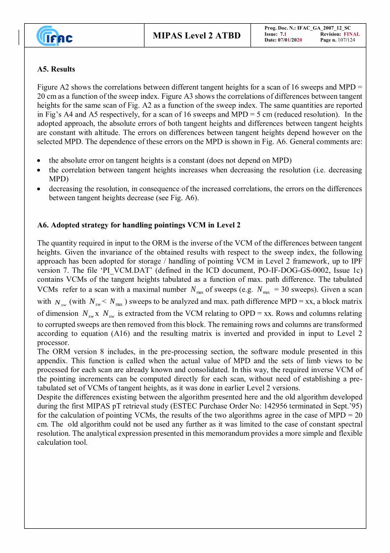
Prog. Doc. N.: IFAC_GA_2007_12_SC
Issue: 7.1 Revision: FINAL
Date: 07/01/2020 Page n. 107/124 MIPAS Level 2 ATBD
A5. Results
Figure A2 shows the correlations between different tangent heights for a scan of 16 sweeps and MPD =
20 cm as a function of the sweep index. Figure A3 shows the correlations of differences between tangent
heights for the same scan of Fig. A2 as a function of the sweep index. The same quantities are reported
in Fig’s A4 and A5 respectively, for a scan of 16 sweeps and MPD = 5 cm (reduced resolution). In the
adopted approach, the absolute errors of both tangent heights and differences between tangent heights
are constant with altitude. The errors on differences between tangent heights depend however on the
selected MPD. The dependence of these errors on the MPD is shown in Fig. A6. General comments are:
the absolute error on tangent heights is a constant (does not depend on MPD)
the correlation between tangent heights increases when decreasing the resolution (i.e. decreasing
MPD)
decreasing the resolution, in consequence of the increased correlations, the errors on the differences
between tangent heights decrease (see Fig. A6).
A6. Adopted strategy for handling pointings VCM in Level 2
The quantity required in input to the ORM is the inverse of the VCM of the differences between tangent
heights. Given the invariance of the obtained results with respect to the sweep index, the following
approach has been adopted for storage / handling of pointing VCM in Level 2 framework, up to IPF
version 7. The file ‘PI_VCM.DAT’ (defined in the ICD document, PO-IF-DOG-GS-0002, Issue 1c)
contains VCMs of the tangent heights tabulated as a function of max. path difference. The tabulated
VCMs refer to a scan with a maximal number maxN of sweeps (e.g. maxN = 30 sweeps). Given a scan
with swN (with swN < maxN ) sweeps to be analyzed and max. path difference MPD = xx, a block matrix
of dimension swN x swN is extracted from the VCM relating to OPD = xx. Rows and columns relating
to corrupted sweeps are then removed from this block. The remaining rows and columns are transformed
according to equation (A16) and the resulting matrix is inverted and provided in input to Level 2
processor.
The ORM version 8 includes, in the pre-processing section, the software module presented in this
appendix. This function is called when the actual value of MPD and the sets of limb views to be
processed for each scan are already known and consolidated. In this way, the required inverse VCM of
the pointing increments can be computed directly for each scan, without need of establishing a pre-
tabulated set of VCMs of tangent heights, as it was done in earlier Level 2 versions.
Despite the differences existing between the algorithm presented here and the old algorithm developed
during the first MIPAS pT retrieval study (ESTEC Purchase Order No: 142956 terminated in Sept.’95)
for the calculation of pointing VCMs, the results of the two algorithms agree in the case of MPD = 20
cm. The old algorithm could not be used any further as it was limited to the case of constant spectral
resolution. The analytical expression presented in this memorandum provides a more simple and flexible
calculation tool.
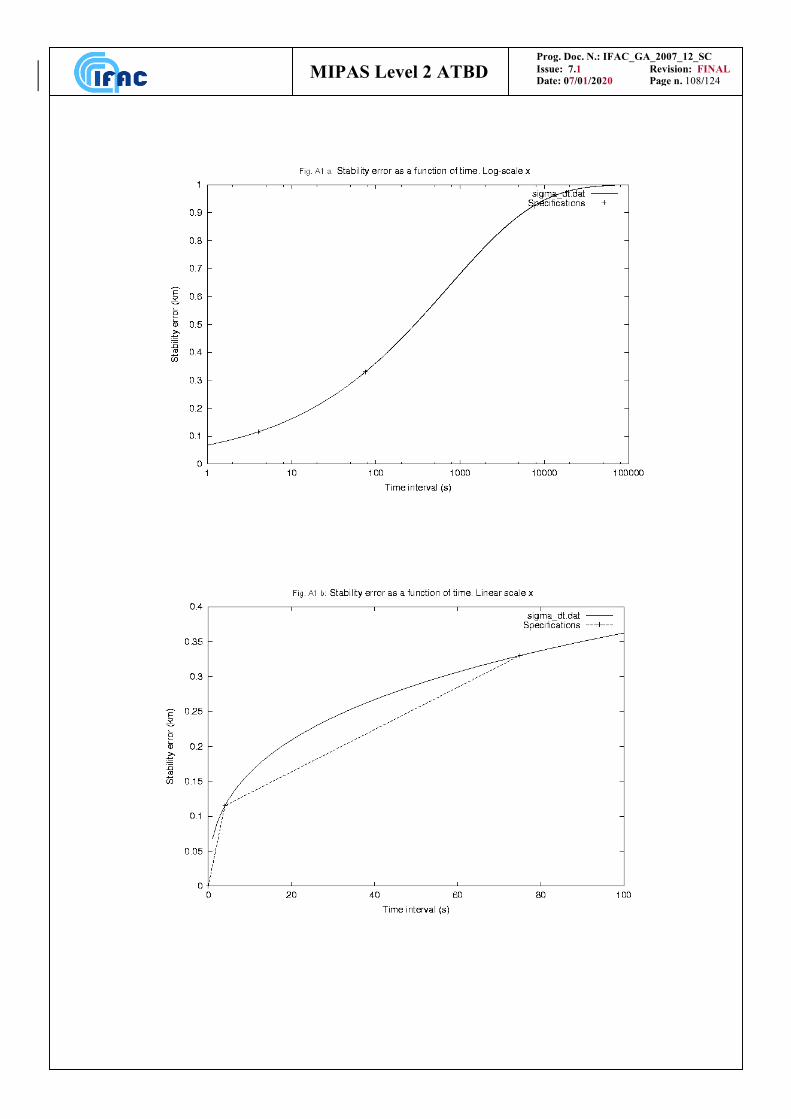
Prog. Doc. N.: IFAC_GA_2007_12_SC
Issue: 7.1 Revision: FINAL
Date: 07/01/2020 Page n. 108/124 MIPAS Level 2 ATBD
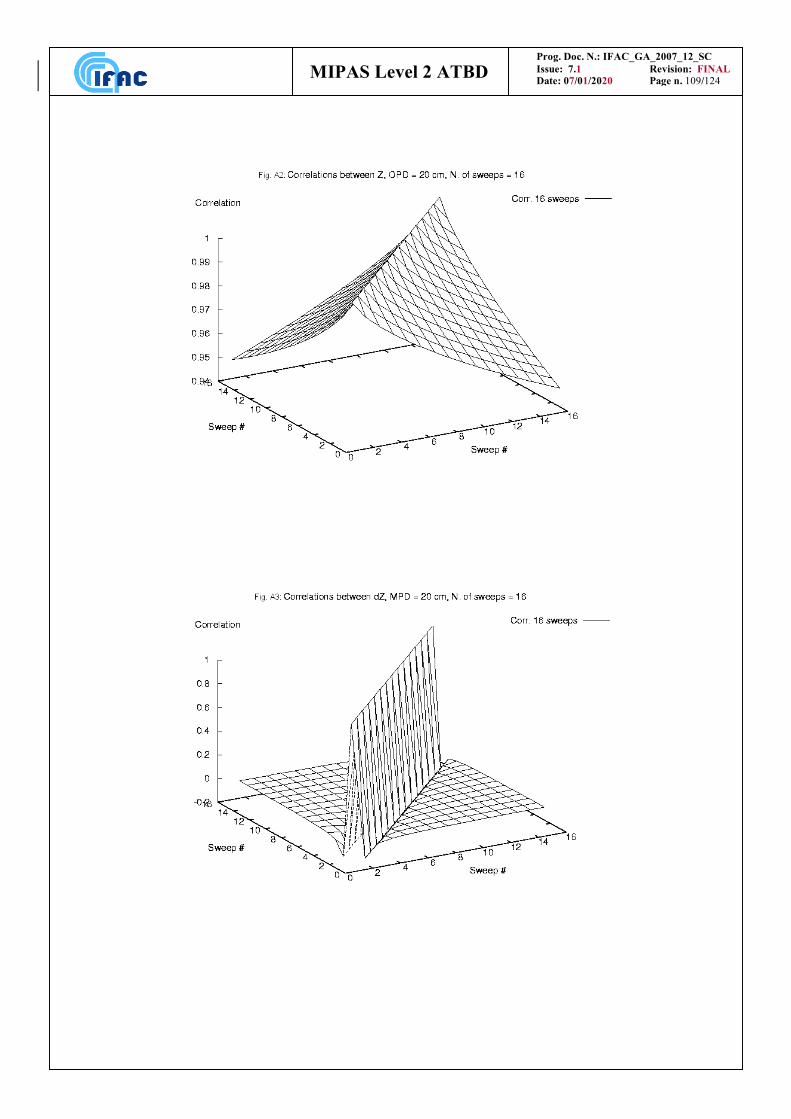
Prog. Doc. N.: IFAC_GA_2007_12_SC
Issue: 7.1 Revision: FINAL
Date: 07/01/2020 Page n. 109/124 MIPAS Level 2 ATBD
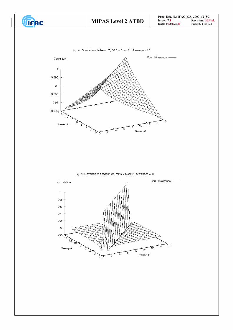
Prog. Doc. N.: IFAC_GA_2007_12_SC
Issue: 7.1 Revision: FINAL
Date: 07/01/2020 Page n. 110/124 MIPAS Level 2 ATBD
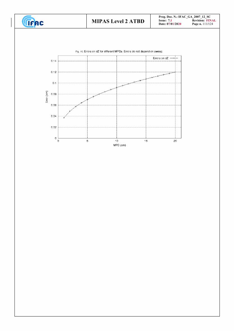
Prog. Doc. N.: IFAC_GA_2007_12_SC
Issue: 7.1 Revision: FINAL
Date: 07/01/2020 Page n. 111/124 MIPAS Level 2 ATBD

Prog. Doc. N.: IFAC_GA_2007_12_SC
Issue: 7.1 Revision: FINAL
Date: 07/01/2020 Page n. 112/124 MIPAS Level 2 ATBD
Appendix B: Evaluation of retrieval error components and total error budget
The recommendations arising from the 30th MIPAS Scientific Advisory Group meeting (ESTEC, 25th
and 26th June 1998) regarding total retrieval error (see SAG minutes MIN-MIPAS-0030), can be
summarized by the following statements:
the random error affecting the retrieved profiles has two components:
The first random component is due to measurement noise. This component is evaluated as part of
the inversion procedure (Gauss-Newton method) by the retrieval program. The ORM output files
already contain the retrieved profile(s) variance-covariance matrix obtained from measurement
noise (derived in Level 1b processing) without scaling by the actual 2 of the fit. This variance-
covariance matrix is included in Level 2 products.
The second random component of profiles error is due to pressure and temperature error
propagation in VMR retrievals. This component is evaluated, on-line, by a function implemented
in Level 2 processor and is also included in Level 2 products.
Systematic error on the retrieved profiles has several components:
Contaminants: this error component is due to imperfect assumption of the contaminant profiles
in the forward model.
Horizontal homogeneity error: due to horizontal homogeneity assumption in the forward model
(this error component is applicable only to Level 2 products version 7 and older)
Spectroscopic errors: are due to errors in spectroscopic data used by the forward model.
Instrumental errors. Due to imperfect (frequency and intensity) calibration of the observed
spectra, imperfect knowledge of the ILS (and of the FOV).
Model errors. These are purely systematic errors biasing the simulated observations. For the
moment only errors arising from neglecting Non-LTE and using LUTs and IGs in the forward
model are expected to belong to this group.
Systematic errors in contaminant profiles, model assumptions, horizontal homogeneity, and instrument
may have some ‘random’ character in the sense that, in principle, their value may vary from retrieval to
retrieval. For this reason, the rule with which they combine may vary as a function of the application.
This prevents the calculation of a total error budget valid in general.
The evaluation of the total systematic errors affecting the retrieved profiles is not a task of the Level 2
processor. A database has been developed at Oxford University containing systematic error profiles
relating to Temperature and VMR profiles retrieved by the Level 2 processor. The database can be freely
accessed from this link: http://eodg.atm.ox.ac.uk/MIPAS/err/ .
The retrieval error due to the mapping of the measurement noise into the solution of the retrieval is
described by the random error covariance matrix included in the Level 2 products, calculated as
described in Sect. 4.2.7.
Here below we describe how the Level 2 processor computes the random error component on the
retrieved VMR profiles due to the propagation of the random error on the retrieved tangent pressures
and temperature profile.
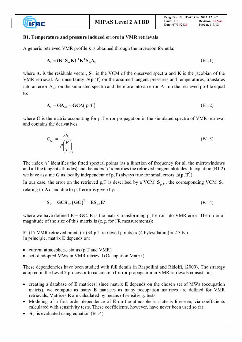
Prog. Doc. N.: IFAC_GA_2007_12_SC
Issue: 7.1 Revision: FINAL
Date: 07/01/2020 Page n. 113/124 MIPAS Level 2 ATBD
B1. Temperature and pressure induced errors in VMR retrievals
A generic retrieved VMR profile x is obtained through the inversion formula:
1( )x m m S
T TΔ K S K K S Δ (B1.1)
where Δs is the residuals vector, Sm is the VCM of the observed spectra and K is the jacobian of the
VMR retrieval. An uncertainty Tp , on the assumed tangent pressures and temperatures, translates
into an error S on the simulated spectra and therefore into an error x on the retrieved profile equal
to:
,p T x SΔ GΔ GC (B1.2)
where C is the matrix accounting for p,T error propagation in the simulated spectra of VMR retrieval
and contains the derivatives:
j
i
ji
T
P
SC
, (B1.3)
The index ‘i’ identifies the fitted spectral points (as a function of frequency for all the microwindows
and all the tangent altitudes) and the index ‘j’ identifies the retrieved tangent altitudes. In equation (B1.2)
we have assume G as locally independent of p,T (always true for small errors Tp , ).
In our case, the error on the retrieved p,T is described by a VCM ,p TS , the corresponding VCM 'xS
relating to Δx and due to p,T error is given by:
' , ,x p T p T
T T
S GCS GC ES E (B1.4)
where we have defined E = GC. E is the matrix transforming p,T error into VMR error. The order of
magnitude of the size of this matrix is (e.g. for FR measurements):
E: (17 VMR retrieved points) x (34 p,T retrieved points) x (4 bytes/datum) 2.3 Kb
In principle, matrix E depends on:
current atmospheric status (p,T and VMR)
set of adopted MWs in VMR retrieval (Occupation Matrix)
These dependencies have been studied with full details in Raspollini and Ridolfi, (2000). The strategy
adopted in the Level 2 processor to calculate pT error propagation in VMR retrievals consists in:
creating a database of E matrices: since matrix E depends on the chosen set of MWs (occupation
matrix), we compute as many E matrices as many occupation matrices are defined for VMR
retrievals. Matrices E are calculated by means of sensitivity tests.
Modeling of a first order dependence of E on the atmospheric state is foreseen, via coefficients
calculated with sensitivity tests. These coefficients, however, have never been used so far.
'xS is evaluated using equation (B1.4).
Prog. Doc. N.: IFAC_GA_2007_12_SC
Issue: 7.1 Revision: FINAL
Date: 07/01/2020 Page n. 114/124 MIPAS Level 2 ATBD
Appendix C: Generation of MW Databases and Occupation matrices
Microwindow selection is performed by an algorithm which simulates the propagation of random and
systematic errors through the retrieval and attempts to maximise the information content (Bennett et
al, 1999). The information content of a microwindow increases as the "log" of the determinant of the
total covariance decreases, total covariance being the sum of the random and various systematic error
covariances. Broadly speaking, 1 `bit' of information is equivalent to a factor 2 reduction in the
uncertainty at one profile altitude.
Microwindows are created by first selecting a number of single measurements, identified by location
in the spectral and tangent altitude grids, as starting points. Adjacent measurements are added to each
until the information content no longer improves or the maximum width of 3 cm-1 is reached. The
best of these trial microwindows is selected, the retrieval covariance modified, and the process
repeated for a new set of measurements as starting points. The procedure of growing microwindows
also allows for measurements within microwindows to be `masked', i.e., excluded from the retrieval.
This usually applies to measurements where the associated systematic errors such as the uncertainty
in modelling a contaminant, outweigh any benefit in the reduction of the random error when
considering the total covariance.
Initially, a set of typically 10 microwindows, or 10000 measurements (whichever occurs first) is
selected based on the assumption that spectra for all MIPAS bands are available. Further
microwindows are then selected to maximise information retrieved in situations where data from
different bands may be unavailable. This set of 20-30 microwindows constitutes the database.
Occupation matrices represent subsets of microwindows to be used under different retrieval
circumstances, and these are constructed using the same approach: selecting the microwindows from
the database (rather than growing new microwindows) in the sequence which maximises the retrieved
information. A number of these OMs are pre-computed, corresponding to different band-
availabilities, and associated with each of these is a single figure-of-merit representing the
information content.
Further details of the algorithm used to grow optimised spectral microwindows are included in
Dudhia, (2000 a), Dudhia, (2000 b) and in Dudhia, (2001).
From the above description it is clear that a side product of this algorithm is the total error affecting
the retrieved profiles as a function of altitude. By operating the algorithm without constraints limiting
the maximum number of observations included in the analysis, it is possible to obtain ultimate
accuracy figures for the parameters retrieved from MIPAS measurements.
For each of the measurement scenarios of the two mission phases (FR and OR, see Appendix F) and
each target retrieval parameter, an occupation matrix has been established. The various error
components evaluated by the algorithm illustrated above are shown in the following web page
maintained at the University of Oxford: http://eodg.atm.ox.ac.uk/MIPAS/err/ .
Figures C1 and C2 show, for the highest priority retrieval parameters and the two mission phases, the
ultimate retrieval accuracy. The estimation of the retrieval accuracy for the profiles of the Optimized
Resolution (OR) part of the mission (after January 2005) does not take into account the regularization
applied. This is because the regularization strength is self-adapting and, therefore, changes on the
basis of the actual atmospheric state. As a consequence, the accuracy reported in Fig. C2 should be
regarded as an upper bound for the actual profile accuracy.
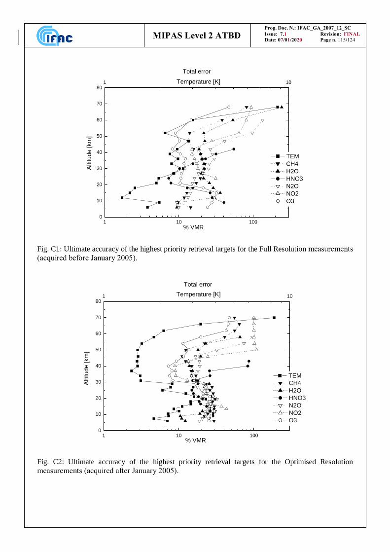
Prog. Doc. N.: IFAC_GA_2007_12_SC
Issue: 7.1 Revision: FINAL
Date: 07/01/2020 Page n. 115/124 MIPAS Level 2 ATBD
0
10
20
30
40
50
60
70
80
1 10 100
1 10
% VMR
Altitu
de
[km
]
CH4
H2O
HNO3
N2O
NO2
O3
Total error
Temperature [K]
TEM
Fig. C1: Ultimate accuracy of the highest priority retrieval targets for the Full Resolution measurements
(acquired before January 2005).
0
10
20
30
40
50
60
70
80
1 10 100
1 10
% VMR
Altitu
de
[km
]
CH4
H2O
HNO3
N2O
NO2
O3
Total error
Temperature [K]
TEM
Fig. C2: Ultimate accuracy of the highest priority retrieval targets for the Optimised Resolution
measurements (acquired after January 2005).

Prog. Doc. N.: IFAC_GA_2007_12_SC
Issue: 7.1 Revision: FINAL
Date: 07/01/2020 Page n. 116/124 MIPAS Level 2 ATBD
Appendix D: Generation of LUTs and Irregular frequency Grids (IG)
The creation of lookup tables and the irregular grids for spectral calculations is a process consisting of
four stages (Dudhia et al, 1999).
The first stage is to determine the significant absorbers for each microwindow. The maximum radiance
for all potential absorbers is assessed considering atmospheres containing just that absorber in isolation
with its maximum concentration. Any absorber contributing more than 10% of the NESR is considered
significant and added to the absorber list for the microwindow.
The second stage is to establish the tabulation axis increments in temperature and ln[pressure] for the
absorber look-up tables. Large tables (i.e., small axis increments) of monochromatic absorption
coefficient are initially created for all microwindow absorbers. MIPAS radiances are modelled for three
different atmospheres (representing nominal, minimum and maximum absorber concentrations) using
these tables and compared with line-by-line calculations for the same cases. The tabulation axis
increments are iteratively increased for each absorber until the maximum discrepancy reaches NESR/30.
The third stage is to perform the singular value decomposition (SVD) of these tables. Initially, each
absorber table is SVD-compressed, retaining 30 singular values. MIPAS radiances are modelled using
the SVD-compressed tables for the three atmospheres as in the previous stage, and compared with the
same line-by-line calculations. The number of singular values for each absorber table is iteratively
reduced until the maximum discrepancy reaches NESR/15.
The fourth stage is to determine the irregular grid for spectral integration. This starts with the MIPAS
radiances calculated with the SVD-compressed LUTs in the previous stage, which are determined on a
regular fine grid (0.0005 cm-1 spacing) prior to the AILS convolution. Grid points are then selectively
removed until the maximum discrepancy compared to a line-by-line on the full spectral grid reaches
NESR/10.
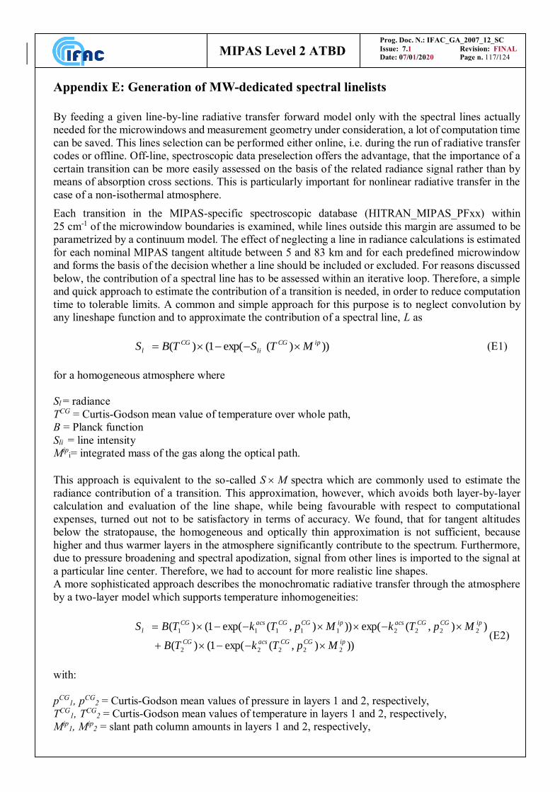
Prog. Doc. N.: IFAC_GA_2007_12_SC
Issue: 7.1 Revision: FINAL
Date: 07/01/2020 Page n. 117/124 MIPAS Level 2 ATBD
Appendix E: Generation of MW-dedicated spectral linelists
By feeding a given line-by-line radiative transfer forward model only with the spectral lines actually
needed for the microwindows and measurement geometry under consideration, a lot of computation time
can be saved. This lines selection can be performed either online, i.e. during the run of radiative transfer
codes or offline. Off-line, spectroscopic data preselection offers the advantage, that the importance of a
certain transition can be more easily assessed on the basis of the related radiance signal rather than by
means of absorption cross sections. This is particularly important for nonlinear radiative transfer in the
case of a non-isothermal atmosphere.
Each transition in the MIPAS-specific spectroscopic database (HITRAN_MIPAS_PFxx) within
25 cm-1 of the microwindow boundaries is examined, while lines outside this margin are assumed to be
parametrized by a continuum model. The effect of neglecting a line in radiance calculations is estimated
for each nominal MIPAS tangent altitude between 5 and 83 km and for each predefined microwindow
and forms the basis of the decision whether a line should be included or excluded. For reasons discussed
below, the contribution of a spectral line has to be assessed within an iterative loop. Therefore, a simple
and quick approach to estimate the contribution of a transition is needed, in order to reduce computation
time to tolerable limits. A common and simple approach for this purpose is to neglect convolution by
any lineshape function and to approximate the contribution of a spectral line, L as
)))(exp(1()( ipCG
li
CG
l MTSTBS (E1)
for a homogeneous atmosphere where
Sl = radiance
TCG = Curtis-Godson mean value of temperature over whole path,
B = Planck function
Sli = line intensity
Mipi= integrated mass of the gas along the optical path.
This approach is equivalent to the so-called S M spectra which are commonly used to estimate the
radiance contribution of a transition. This approximation, however, which avoids both layer-by-layer
calculation and evaluation of the line shape, while being favourable with respect to computational
expenses, turned out not to be satisfactory in terms of accuracy. We found, that for tangent altitudes
below the stratopause, the homogeneous and optically thin approximation is not sufficient, because
higher and thus warmer layers in the atmosphere significantly contribute to the spectrum. Furthermore,
due to pressure broadening and spectral apodization, signal from other lines is imported to the signal at
a particular line center. Therefore, we had to account for more realistic line shapes.
A more sophisticated approach describes the monochromatic radiative transfer through the atmosphere
by a two-layer model which supports temperature inhomogeneities:
))),(exp(1()(
)),(exp())),(exp(1()(
22222
222211111
ipCGCGacsCG
ipCGCGacsipCGCGacsCG
l
MpTkTB
MpTkMpTkTBS
(E2)
with:
pCG1, p
CG2 = Curtis-Godson mean values of pressure in layers 1 and 2, respectively,
TCG1, T
CG2 = Curtis-Godson mean values of temperature in layers 1 and 2, respectively,
Mip1, M
ip2 = slant path column amounts in layers 1 and 2, respectively,
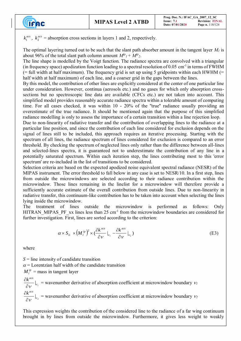
Prog. Doc. N.: IFAC_GA_2007_12_SC
Issue: 7.1 Revision: FINAL
Date: 07/01/2020 Page n. 118/124 MIPAS Level 2 ATBD
acsk1 ,, acsk2 = absorption cross sections in layers 1 and 2, respectively.
The optimal layering turned out to be such that the slant path absorber amount in the tangent layer M1 is
about 96% of the total slant path column amount Mip1 + Mip
2.
The line shape is modelled by the Voigt function. The radiance spectra are convolved with a triangular
(in frequency space) apodization function leading to a spectral resolution of 0.05 cm-1 in terms of FWHM
(= full width at half maximum). The frequency grid is set up using 5 gridpoints within each HWHM (=
half width at half maximum) of each line, and a coarser grid in the gaps between the lines.
By this model, the contribution of other lines are explicitly considered at the center of one particular line
under consideration. However, continua (aerosols etc.) and no gases for which only absorption cross-
sections but no spectroscopic line data are available (CFCs etc.) are not taken into account. This
simplified model provides reasonably accurate radiance spectra within a tolerable amount of computing
time. For all cases checked, it was within 10 - 20% of the ''true'' radiance usually providing an
overestimate of the true radiance. It should be mentioned again that the purpose of this simplified
radiance modelling is only to assess the importance of a certain transition within a line rejection loop.
Due to non-linearity of radiative transfer and the contribution of overlapping lines to the radiance at a
particular line position, and since the contribution of each line considered for exclusion depends on the
signal of lines still to be included, this approach requires an iterative processing. Starting with the
spectrum of all lines, the radiance spectrum of lines considered for exclusion is compared to an error
threshold. By checking the spectrum of neglected lines only rather than the difference between all-lines
and selected-lines spectra, it is guaranteed not to underestimate the contribution of any line in a
potentially saturated spectrum. Within each iteration step, the lines contributing most to this 'error
spectrum' are re-included in the list of transitions to be considered.
Selection criteria are based on the expected apodized noise equivalent spectral radiance (NESR) of the
MIPAS instrument. The error threshold to fall below in any case is set to NESR/10. In a first step, lines
from outside the microwindows are selected according to their radiance contribution within the
microwindow. Those lines remaining in the linelist for a microwindow will therefore provide a
sufficiently accurate estimate of the overall contribution from outside lines. Due to non-linearity in
radiative transfer, this continuum-like contribution has to be taken into account when selecting the lines
lying inside the microwindow.
The treatment of lines outside the microwindow is performed as follows: Only
HITRAN_MIPAS_PF_xx lines less than 25 cm-1 from the microwindow boundaries are considered for
further investigation. First, lines are sorted according to the criterion:
)||(21
2
acsacsip
lli
kkMS (E3)
where
S = line intensity of candidate transition
= Lorentzian half width of the candidate transition ip
lM = mass in tangent layer
1|
acsk = wavenumber derivative of absorption coefficient at microwindow boundary 1
2|
acsk = wavenumber derivative of absorption coefficient at microwindow boundary 2
This expression weights the contribution of the considered line to the radiance of a far wing continuum
brought in by lines from outside the microwindow. Furthermore, it gives less weight to weakly
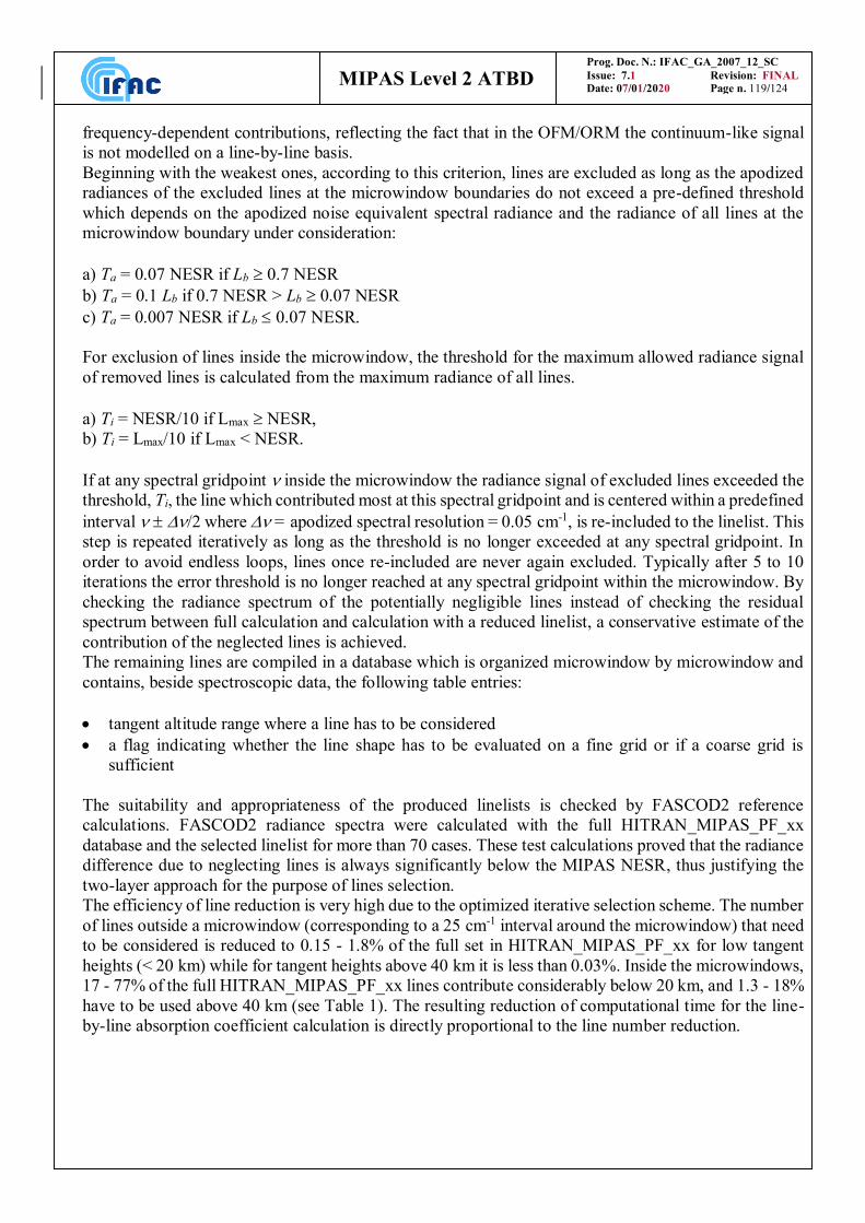
Prog. Doc. N.: IFAC_GA_2007_12_SC
Issue: 7.1 Revision: FINAL
Date: 07/01/2020 Page n. 119/124 MIPAS Level 2 ATBD
frequency-dependent contributions, reflecting the fact that in the OFM/ORM the continuum-like signal
is not modelled on a line-by-line basis.
Beginning with the weakest ones, according to this criterion, lines are excluded as long as the apodized
radiances of the excluded lines at the microwindow boundaries do not exceed a pre-defined threshold
which depends on the apodized noise equivalent spectral radiance and the radiance of all lines at the
microwindow boundary under consideration:
a) Ta = 0.07 NESR if Lb 0.7 NESR
b) Ta = 0.1 Lb if 0.7 NESR > Lb 0.07 NESR
c) Ta = 0.007 NESR if Lb 0.07 NESR.
For exclusion of lines inside the microwindow, the threshold for the maximum allowed radiance signal
of removed lines is calculated from the maximum radiance of all lines.
a) Ti = NESR/10 if Lmax NESR,
b) Ti = Lmax/10 if Lmax < NESR.
If at any spectral gridpoint inside the microwindow the radiance signal of excluded lines exceeded the
threshold, Ti, the line which contributed most at this spectral gridpoint and is centered within a predefined
interval /2 where = apodized spectral resolution = 0.05 cm-1, is re-included to the linelist. This
step is repeated iteratively as long as the threshold is no longer exceeded at any spectral gridpoint. In
order to avoid endless loops, lines once re-included are never again excluded. Typically after 5 to 10
iterations the error threshold is no longer reached at any spectral gridpoint within the microwindow. By
checking the radiance spectrum of the potentially negligible lines instead of checking the residual
spectrum between full calculation and calculation with a reduced linelist, a conservative estimate of the
contribution of the neglected lines is achieved.
The remaining lines are compiled in a database which is organized microwindow by microwindow and
contains, beside spectroscopic data, the following table entries:
tangent altitude range where a line has to be considered
a flag indicating whether the line shape has to be evaluated on a fine grid or if a coarse grid is
sufficient
The suitability and appropriateness of the produced linelists is checked by FASCOD2 reference
calculations. FASCOD2 radiance spectra were calculated with the full HITRAN_MIPAS_PF_xx
database and the selected linelist for more than 70 cases. These test calculations proved that the radiance
difference due to neglecting lines is always significantly below the MIPAS NESR, thus justifying the
two-layer approach for the purpose of lines selection.
The efficiency of line reduction is very high due to the optimized iterative selection scheme. The number
of lines outside a microwindow (corresponding to a 25 cm-1 interval around the microwindow) that need
to be considered is reduced to 0.15 - 1.8% of the full set in HITRAN_MIPAS_PF_xx for low tangent
heights (< 20 km) while for tangent heights above 40 km it is less than 0.03%. Inside the microwindows,
17 - 77% of the full HITRAN_MIPAS_PF_xx lines contribute considerably below 20 km, and 1.3 - 18%
have to be used above 40 km (see Table 1). The resulting reduction of computational time for the line-
by-line absorption coefficient calculation is directly proportional to the line number reduction.
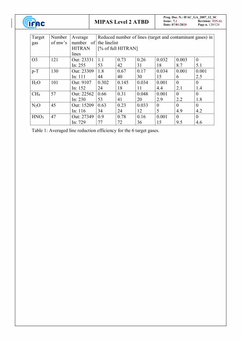
Prog. Doc. N.: IFAC_GA_2007_12_SC
Issue: 7.1 Revision: FINAL
Date: 07/01/2020 Page n. 120/124 MIPAS Level 2 ATBD
Target
gas
Number
of mw’s
Average
number of
HITRAN
lines
Reduced number of lines (target and contaminant gases) in
the linelist
[% of full HITRAN]
O3 121 Out: 23331
In: 255
1.1
53
0.73
42
0.26
31
0.032
18
0.003
8.7
0
5.1
p-T 130 Out: 23309
In: 111
1.8
44
0.67
40
0.17
30
0.034
15
0.001
6
0.001
2.5
H2O 101 Out: 9107
In: 152
0.302
24
0.145
18
0.034
11
0.001
4.4
0
2.1
0
1.4
CH4 57 Out: 22562
In: 230
0.66
53
0.31
41
0.048
20
0.001
2.9
0
2.2
0
1.8
N2O 45 Out: 15209
In: 116
0.63
34
0.23
24
0.033
12
0
5
0
4.9
0
4.2
HNO3 47 Out: 27349
In: 729
0.9
77
0.78
72
0.16
36
0.001
15
0
9.5
0
4.6
Table 1: Averaged line reduction efficiency for the 6 target gases.
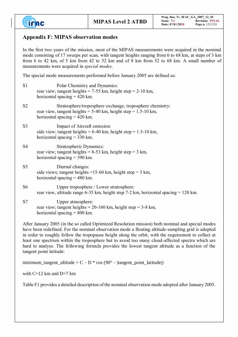
Prog. Doc. N.: IFAC_GA_2007_12_SC
Issue: 7.1 Revision: FINAL
Date: 07/01/2020 Page n. 121/124 MIPAS Level 2 ATBD
Appendix F: MIPAS observation modes
In the first two years of the mission, most of the MIPAS measurements were acquired in the nominal
mode consisting of 17 sweeps per scan, with tangent heights ranging from 6 to 68 km, at steps of 3 km
from 6 to 42 km, of 5 km from 42 to 52 km and of 8 km from 52 to 68 km. A small number of
measurements were acquired in special modes.
The special mode measurements performed before January 2005 are defined as:
S1 Polar Chemistry and Dynamics:
rear view; tangent heights = 7-55 km, height step = 2-10 km,
horizontal spacing = 420 km.
S2 Stratosphere/troposphere exchange, troposphere chemistry:
rear view, tangent heights = 5-40 km, height step = 1.5-10 km,
horizontal spacing = 420 km.
S3 Impact of Aircraft emission:
side view; tangent heights = 6-40 km, height step = 1.5-10 km,
horizontal spacing = 330 km.
S4 Stratospheric Dynamics:
rear view; tangent heights = 8-53 km, height step = 3 km,
horizontal spacing = 390 km.
S5 Diurnal changes:
side views; tangent heights =15-60 km, height step = 3 km,
horizontal spacing = 480 km.
S6 Upper troposphere / Lower stratosphere:
rear view, altitude range 6-35 km, height step 7-2 km, horizontal spacing = 120 km.
S7 Upper atmosphere:
rear view; tangent heights = 20-160 km, height step = 3-8 km,
horizontal spacing = 800 km.
After January 2005 (in the so called Optimized Resolution mission) both nominal and special modes
have been redefined. For the nominal observation mode a floating altitude-sampling grid is adopted
in order to roughly follow the tropopause height along the orbit, with the requirement to collect at
least one spectrum within the troposphere but to avoid too many cloud-affected spectra which are
hard to analyse. The following formula provides the lowest tangent altitude as a function of the
tangent point latitude:
minimum_tangent_altitude = C – D * cos (90° – |tangent_point_latitude|)
with C=12 km and D=7 km
Table F1 provides a detailed description of the nominal observation mode adopted after January 2005.
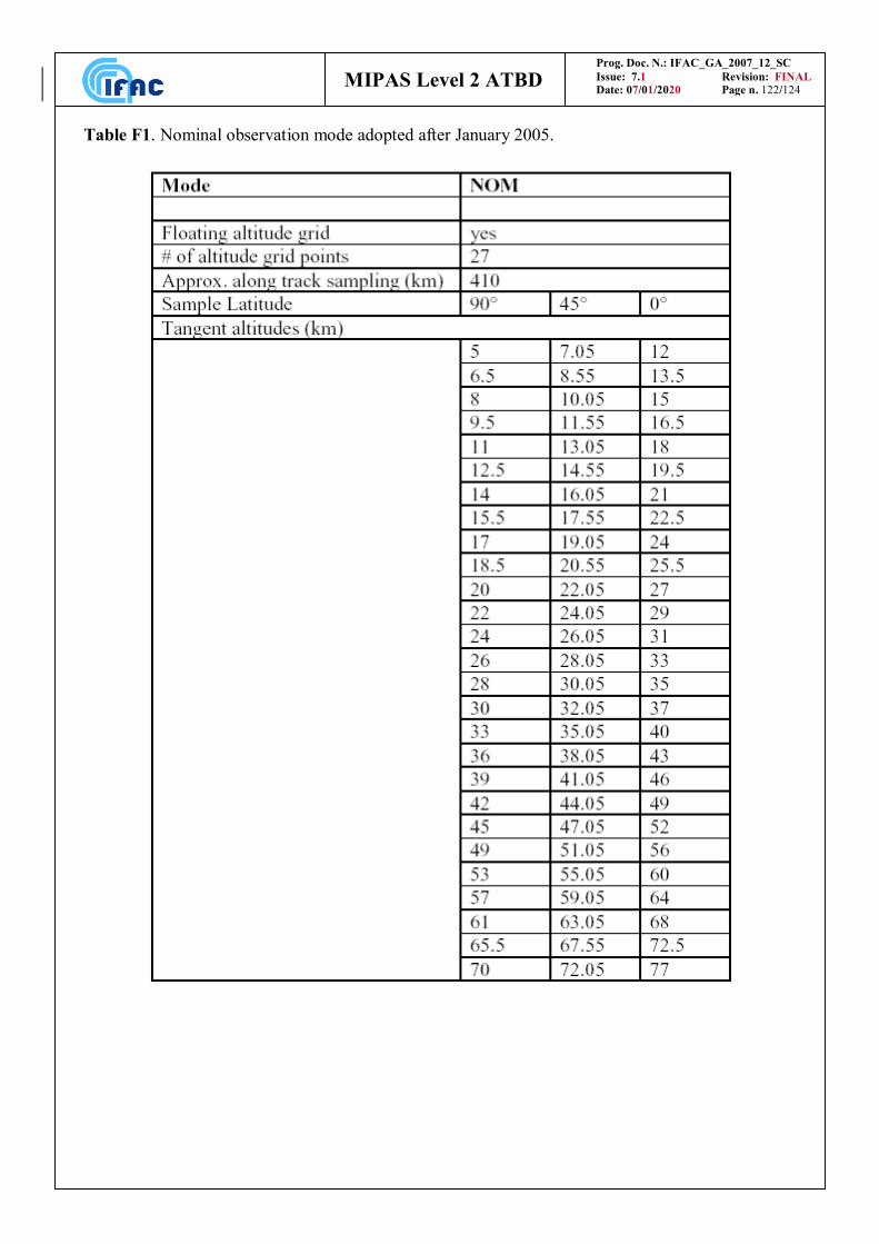
Prog. Doc. N.: IFAC_GA_2007_12_SC
Issue: 7.1 Revision: FINAL
Date: 07/01/2020 Page n. 122/124 MIPAS Level 2 ATBD
Table F1. Nominal observation mode adopted after January 2005.

Prog. Doc. N.: IFAC_GA_2007_12_SC
Issue: 7.1 Revision: FINAL
Date: 07/01/2020 Page n. 123/124 MIPAS Level 2 ATBD
The special mode measurements defined for the mission phase after January 2005:
UTLS-1 Upper Troposphere Lower Stratosphere (primary UTLS mode)
UTLS-2 Upper Troposphere Lower Stratosphere (Test mode for 2-D retrievals)
MA Middle Atmosphere
NLC Middle/Upper atmosphere in summer (Noctilucent clouds)
UA Upper Atmosphere
AE Aircraft Emissions
For the UTLS-1 mode a floating altitude-sampling grid is adopted, according to the following formula
which provides the lowest tangent altitude as a function of the tangent point latitude:
minimum_tangent_altitude = A + B * cos (2*tangent_point_latitude)
with A=8.5 km and B=3 km
Table F2 provides a detailed description of the special observation modes adopted after January 2005.
A schematic summary of MIPAS measurement modes, as well as the related “mission plan”
documents are available at the following web-pages maintained by A.Dudhia at University of Oxford:
FR modes: http://www.atm.ox.ac.uk/group/mipas/frmodes.html (years 2002-2004)
OR modes: http://www.atm.ox.ac.uk/group/mipas/rrmodes.html (years 2005 - onward)
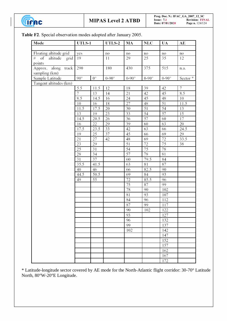
Prog. Doc. N.: IFAC_GA_2007_12_SC
Issue: 7.1 Revision: FINAL
Date: 07/01/2020 Page n. 124/124 MIPAS Level 2 ATBD
Table F2. Special observation modes adopted after January 2005.
* Latitude-longitude sector covered by AE mode for the North-Atlantic flight corridor: 30-70° Latitude
North, 80°W-20°E Longitude.


